Economics of Agricultural Biotechnology in Crop Protection in ...
291
Economics of Agricultural Biotechnology in Crop Protection in Developing Countries – The Case of Bt-Cotton in Shandong Province, China Diemuth E. Pemsl A Publication of the Pesticide Policy Project Hannover, May 2006 Special Issue Publication Series, No. 11
-
Upload
khangminh22 -
Category
Documents
-
view
1 -
download
0
Transcript of Economics of Agricultural Biotechnology in Crop Protection in ...
Economics of Agricultural Biotechnology in Crop Protection in Developing Countries –
The Case of Bt-Cotton in Shandong Province, China
Diemuth E . Pems l
A Publication of the Pesticide Policy Project
Hannover, May 2006 Special Issue Publication Series, No. 11
Pesticide Policy Project Publication Series Special Issue No. 11, May, 2006
Development and Agricultural Economics Faculty of Economics and Management
University of Hannover, Germany
Economics of Agricultural Biotechnology in Crop Protection in Developing Countries –
The Case of Bt-Cotton in Shandong Province, China
Doctoral Dissertation at the Faculty of Economics and Management
University of Hannover, 2005
Editor of the Pesticide Policy Project Publication Series:
Prof. Dr. H. Waibel Development and Agricultural Economics Faculty of Economics and Management University of Hannover Königsworther Platz 1 30167 Hannover Germany
Tel.: +49 - (0)511 - 762 - 2666 Fax: +49 - (0)511 - 762 - 2667 E-Mail: [email protected]
All rights reserved by the author.
Publication of the Institute of Development and Agricultural Economics, Königsworther Platz 1, 30167 Hannover, Germany
Printing: Uni Druck Hannover, 30419 Hannover, Germany
ISBN: 3-934373-12-7

“Genetic modification is, I would suggest, a uniquely polarizing issue.
I can't think of another subject - with the possible exception of macro-
economic theory - where intelligent and concerned people can look at the
same set of facts and come up with such divergent conclusions.”
Richard Black (BBC) – 16 September 2004

Preface
The debate on the need and value of genetically modified crops, and their contributions, especially to developing countries continues to be highly controversial. Some scientists and policy makers have high expectations regarding the potential of biotechnology in agriculture to increase productivity and to help reduce poverty. On the other hand, biotechnology is subject to an often emotional public debate regarding the risks of this technology for human health and biodiversity.
China is a particularly interesting case because it is so far the only developing country that has rapidly introduced Bt cotton on a large scale. The economic studies that have been carried out found that insect resistant transgenic varieties reduce chemical pesticides and diminish crop losses caused by pests. These studies have relied on data from farmer surveys comparing adopters and non-adopters of the technology. The research of Diemuth E. Pemsl makes a unique contribution to the existing literature. Her analysis is based on a careful case study with some 150 farmers in Shandong province. She has spent considerable time in the field and collected her data in a participatory manner. Different from most of the other economic studies, the classic impact assessment approach, i.e. to compare farmers’ performance with and without the new technology was not possible in her case because Bt cotton varieties had become widely used in the province. Therefore, in her econometric analysis, she used a toxicity index as measure of Bt thus advancing the traditional approach of using a dummy variable.
The findings presented in this book are very significant in two regards: First, they show that it can be very insightful to rely on several methodologies to assess the profitability of new technologies. Second, impact assessment of Bt cotton is not only useful immediately after its introduction but especially after farmers have gained some experience with the new varieties. Then, many of the constraints become observable under real world conditions. As this case study clearly demonstrates, institutional conditions govern the success of a new technology. Undoubtedly, the research of Diemuth E. Pemsl not only has generated several important messages relevant for plant protection experts and policy makers but it has also raised a new set of questions that call for more intensive research jointly conducted by economists and biological scientists.
Hermann Waibel Development and Agricultural Economics Faculty of Economics and Management University of Hannover

Acknowledgements
I could not have completed this thesis without the generous and far-reaching support of a large number of individuals. First of all, I would like to thank the 150 farmers in Linqing who participated in the case study and recorded all cotton production inputs over a whole season with great accuracy and perseverance. They willingly answered my many questions and welcomed me with lasting hospitality (see Appendix 25 for a list of names).
The Chinese counterpart for the study was the National Agro-Technical Extension and Service Centre (NATESC), within the Ministry of Agriculture in Beijing and I am grateful to Prof. Piao Yongfan and Dr. Yang Puyun for providing valuable expertise and support. Mr. Wu Lifeng deserves much credit for help in accessing secondary data and for translation. Numerous staff of the Plant Protection Stations in Jinan and Linqing, represented by Mr. Lu Zengquan and Mr. Tian Ru Yi helped in organizational matters and facilitated the fieldwork and my stay in China. Fēi cháng găn xiè nĭ men! Mrs. Li Hong Hua worked hard and was a dedicated interpreter and assistant in arranging the fieldwork. She did a wonderful job.
My foremost appreciation and gratitude goes to my supervisor Prof. Dr. Hermann Waibel who provided me with the opportunity to conduct this study and gave support and invaluable advice during the entire project. Working with him has always been tremendously inspiring and motivating.
I am thankful to Prof. Dr. David Zilbermann (UC Berkeley, USA) for valuable comments on the draft of this thesis and his willingness to be an external reviewer for my dissertation. Prof. Dr. Wu Kongming and Dr. Zhang Yongjun from the Chinese Academy of Agricultural Sciences (CAAS, Beijing, China) facilitated and conducted the laboratory analysis of bollworm moths and cotton leaf samples. I thank them for their support. I am indebted to Prof. Dr. Andrew P. Gutierrez (UC Berkeley, USA) for his conceptual advice on the experiments, his support for the modeling part, and for hosting me while I was in Berkeley. I greatly benefited from the discussions on the stochastic frontier model with Dr. Timo Kuosmanen and Dr. Justus Wesseler (Wageningen University, The Netherlands). I am grateful for the helpful comments on the draft of the thesis from Dr Graham Dalton. I highly appreciate the continuous interest shown in the research by Dr. Peter Ooi and Dr. Peter Kenmore of the Food and Agriculture Organization (FAO) of the United Nations and gratefully acknowledge the financial support that was provided by FAO for the fieldwork. Special thanks go to Thongporn Tongruksawattana for the sometimes exasperating task of editing the final manuscript.
Finally, I thank my colleagues for helpful discussions and shared breaks, and my family, and friends, and especially Christian for their peace, love, and understanding.

Contents
List of Tables ......................................................................... xii List of Figures ....................................................................... xiv List of Boxes .......................................................................... xv List of Appendices ................................................................. xvi Acronyms ............................................................................. xvii Notations .............................................................................. xix Zusammenfassung .................................................................. xx Abstract .............................................................................. xxiii 摘要 ...................................................................................... xxv
1 Introduction ........................................................................ 1
1.1 Introduction and background ................................................................ 1 1.2 Objectives of the research .................................................................... 2 1.3 Organization of the thesis ..................................................................... 7
2 Biotechnology in agriculture ............................................. 10
2.1 Global status of agricultural biotechnology......................................... 10 2.1.1 History and current status of agricultural biotechnology........... 10 2.1.2 The example of insect resistant Bt-cotton ................................ 13
2.2 Issues in the debate of agricultural biotechnology.............................. 19 2.2.1 Potential costs and benefits...................................................... 19 2.2.2 Agricultural biotechnology and developing countries ............... 25
2.3 Development of agricultural biotechnology in China .......................... 32 2.3.1 History and development .......................................................... 33 2.3.2 Regulatory framework and biotechnology policy ...................... 36 2.3.3 Environmental impact and consumer acceptance.................... 41
2.4 Summary ............................................................................................ 42 3 Impact assessment of agricultural biotechnology:
review of methods and studies .......................................... 44
3.1 Methods to measure costs and benefits of agricultural biotechnology44 3.2 Literature review of recent economic studies on Bt-cotton................. 53
3.2.1 Bt-cotton in India....................................................................... 55 3.2.2 Bt-cotton in China ..................................................................... 58
3.3 Summary ............................................................................................ 61
x
4 Theoretical concepts for economic analysis of Bt-cotton .. 63
4.1 Productivity assessment of input factors ............................................ 63 4.1.1 Neoclassical production functions and damage control ........... 64 4.1.2 Production frontiers and the measurement of efficiency .......... 69
4.2 Implications of risk and uncertainty..................................................... 74 4.2.1 Decision-making under uncertainty .......................................... 75 4.2.2 Pest control and production risk ............................................... 79
4.3 Ecological economics and bio-economics.......................................... 82 4.4 Research hypotheses and methods ................................................... 85
4.4.1 Research hypotheses ............................................................... 85 4.4.2 Conceptual framework and methods used in the study............ 86
5 Procedure and methodology of data collection ................. 89
5.1 Pre-test and orientation phase in 2001............................................... 89 5.1.1 Purpose and outline of the 2001 study ..................................... 89 5.1.2 Overview of findings ................................................................. 90
5.2 Conceptualization and framework of the 2002 survey........................ 98 5.3 Characterization of the study location............................................... 101 5.4 Data collection methods ................................................................... 104
5.4.1 Farm-level interviews.............................................................. 105 5.4.2 Season-long monitoring.......................................................... 106 5.4.3 Experiments and testing of leaf tissue and bollworm larvae... 106 5.4.4 Expert survey and secondary data ......................................... 109
6 Descriptive analysis of Bt-cotton production in Linqing... 110
6.1 Farming system analysis .................................................................. 110 6.1.1 Farm characteristics and production system .......................... 110 6.1.2 Economic indicators for main crops........................................ 114
6.2 Analysis of Bt-cotton production ....................................................... 117 6.2.1 Production of Bt-cotton ........................................................... 117 6.2.2 Pesticide use in Bt-cotton production ..................................... 122 6.2.3 Farmers’ perception of pest infestation in Bt-cotton ............... 128 6.2.4 Institutional problems in technology implementation .............. 131
6.3 Summary .......................................................................................... 138
xi
7 Productivity analysis of Bt-cotton .................................... 140
7.1 Estimation of production and insecticide use function...................... 140 7.1.1 Methodology of production function estimation ...................... 140 7.1.2 Data and variables for the regression analysis....................... 144 7.1.3 Productivity estimates of Bt-toxin and insecticides................. 146
7.2 Semi-parametric estimation of the damage control function ............ 156 7.2.1 Methodology of efficiency analysis ......................................... 156 7.2.2 Data and variables for the semi-parametric model................. 164 7.2.3 Results of the semi-parametric model .................................... 166
7.3 Summary .......................................................................................... 170 8 Modeling crop protection strategies in cotton .................. 172
8.1 Partial budgeting model of pest control ............................................ 172 8.1.1 Methodology and structure of the simulation model ............... 172 8.1.2 Expert survey to validate assumptions ................................... 178 8.1.3 Model assumptions and limitations......................................... 185 8.1.4 Simulation results and discussion .......................................... 190
8.2 Bio-economic model ......................................................................... 196 8.2.1 Methodology for the bio-economic model............................... 196 8.2.2 Description of control strategies ............................................. 200 8.2.3 Modelling results and discussion............................................ 203
8.3 Summary .......................................................................................... 212 9 Conclusion and recommendations ................................... 215
9.1 Discussion of findings ....................................................................... 215 9.2 Recommendations for further research ............................................ 219 9.3 Conclusion and outlook .................................................................... 220
10 Summary .......................................................................... 222
References........................................................................... 228 Appendix ............................................................................. 242
xii
List of Tables
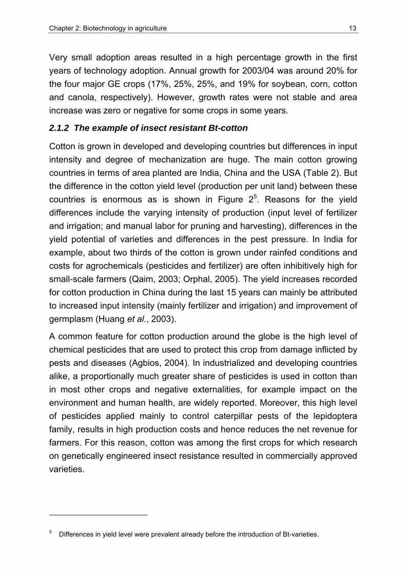
Table 1: Total agricultural and GE crop acreage in 2004 by country ............................. 12
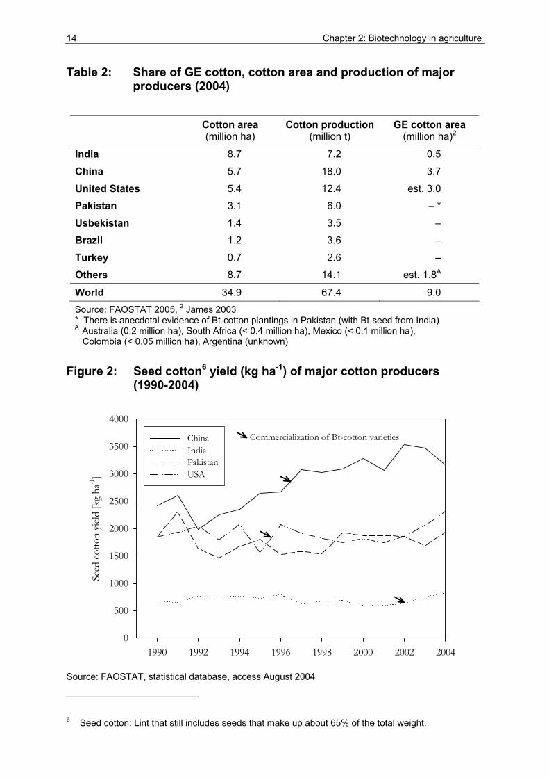
Table 2: Share of GE cotton, cotton area and production of major producers (2004).... 14
Table 3: Regulatory approvals of Bt-cotton.................................................................... 16
Table 4: Overview of costs and benefits related to agricultural biotechnology............... 20
Table 5: Changes in policies towards GE crops in China .............................................. 37
Table 6: Potential costs and benefits of growing Bt-cotton varieties .............................. 52
Table 7: Recent studies on the impact of Bt-cotton in developing countries.................. 54
Table 8: Performance difference (% change) of Bt and conventional cotton varieties... 58
Table 9: Findings of the impact studies of Bt-cotton in China ........................................ 60
Table 10: Classification of methods for the assessment of Bt-cotton varieties ................ 87
Table 11: Demographics and landholdings of sampled HH (2001).................................. 91
Table 12: Characteristics of maize and wheat production in the study area (2001)......... 95
Table 13: Characteristics of cotton production in the study area (2001) .......................... 95
Table 14: Pesticide use and toxicity of products according to WHO classification .......... 96
Table 15: Characteristics of the five survey villages ...................................................... 103
Table 16: Measurement problems of pesticide use and monitoring response ............... 105
Table 17: Demographics and landholdings of sampled households (2002)................... 112
Table 18: Sales and own consumption of wheat and maize .......................................... 112
Table 19: Production indicators for maize by village...................................................... 115
Table 20: Production indicators for wheat by village...................................................... 115
Table 21: Production indicators for Bt-cotton ................................................................. 120
Table 22: Seed price, on-farm propagation and share of Monsanto varieties................ 121
Table 23: Pesticide use in Bt-cotton production (amount of formulated products)......... 123
Table 24: Toxicity of pesticides used in Bt-cotton production ........................................ 124
Table 25: Pesticide poisoning in Bt-cotton production in 2002....................................... 126
Table 26: Results of cotton leaf tissue testing on Bt-toxin concentration ....................... 134
Table 27: Production indicators of farmers grouped by type of seed............................. 134
Table 28: Bt-toxin concentration in leaf tissue* and production data ............................. 136
Table 29: Mean and standard deviation of variables used in the model ........................ 144
Table 30: Overview of the binary variables (0, 1) used in the model ............................. 146
Table 31: Estimated coefficients for insecticide use function (N = 144)......................... 147
Table 32: Estimated parameters for the cotton production function (CD and different damage control function specifications), N = 144 .......................................... 149
Table 33: Parameter estimates for different exponential damage function types .......... 151
Table 34: Derived marginal physical product of insecticides and Bt-toxin ..................... 152
xiii
Table 35: Coefficients for the simultaneous estimation (using 3SLS) of insecticide use and production function (exponential damage function), N = 144 ........... 155
Table 36: Input and output indicators of Bt-cotton production........................................ 165
Table 37: Efficiency scores for Bt-cotton production by village ...................................... 166
Table 38: Results of the truncated linear regression I.................................................... 168
Table 39: Results of the truncated linear regression II................................................... 169
Table 40: Overview of the costs and benefits of different control strategies .................. 174
Table 41: Expert assessment of pest-free potential cotton yield and potential bollworm damage under different control strategies........................ 180
Table 42: Chemical control of CBW and potential yield loss by CBW generation.......... 180
Table 43: Expert assessment of damage inflicted by other pests and timing of occurrence in relation to CBW damage.......................................................... 182
Table 44: Expert assessment of farm-level costs of cotton production inputs ............... 184
Table 45: Model assumptions on the timing of pest pressure ........................................ 187
Table 46: Probability distributions of stochastic parameters in the model...................... 189
Table 47: Standardized beta-coefficients from the linear regression of generated data (Bt-strategies)........................................................................ 193
Table 48: Standardized beta-coefficients from the linear regression of generated data (insecticide based strategies)................................................ 193
Table 49: Overview of potential CBW control strategies ................................................ 201
Table 50: Average yield (t ha-1) for the different control strategies................................. 204
Table 51: Linear regression results for different levels of ecosystem disruption............ 205
Table 52: Linear regression results for all levels of ecosystem disruption ..................... 206
Table 53: Fitted distributions of yield outcome for the different strategies ..................... 208
Table 54: Standardized beta-coefficients from the linear regression of generated data on net revenue of the control strategies................................ 210
xiv
List of Figures
Figure 1: Annual growth rate (%) of global area planted to GE crops (1996-2004) ..... 12
Figure 2: Seed cotton yield (kg ha-1) of major cotton producers (1990-2004) ............. 14
Figure 3: Conceptual model for the economic assessment of Bt-cotton ...................... 24
Figure 4: Technological change and the total product curve........................................ 46
Figure 5: Economic surplus model and (distribution of) gains from technical change.. 48
Figure 6: Net revenue of Bt and non-Bt-cotton production in China............................. 59
Figure 7: Effect of insecticide use on yield (with and without Bt-variety)...................... 66
Figure 8: Combined effect of insecticide use and Bt-toxin concentration I................... 67
Figure 9: Combined effect of pesticide use and Bt-toxin concentration II .................... 68
Figure 10: A cross section of individual firm observations in the input-output q space .. 70
Figure 11: Technical and allocative efficiency from input and output orientation ........... 71
Figure 12: Deterministic and stochastic frontier production function .............................. 73
Figure 13: A decision tree for pest management in cotton production ........................... 76
Figure 14: Risk attitudes and related shape of the utility function .................................. 78
Figure 15: Distribution of net returns of different crop protection technologies .............. 81
Figure 16: Scheme of sequential decision-making in pest management ....................... 81
Figure 17: Sampling for the 2001 household survey in Shandong Province .................. 90
Figure 18: Cropping calendar for main crops in the survey region................................. 92
Figure 19: Adoption of Bt-cotton varieties in the 2001 sample by county....................... 92
Figure 20: Shares of cotton (%) on total agricultural land by county .............................. 93
Figure 21: Variability in seed price (US$ kg-1) by county................................................ 98
Figure 22: Distribution of cotton yield within the sample and normal distribution ........... 99
Figure 23: Scheme of the integrated data collection framework................................... 100
Figure 24: Chinese cotton production by province (% of total), 1995 - 2000 averages 102
Figure 25: Chinese cotton production 1992 – 2003, by province ................................. 102
Figure 26: Number of female cotton bollworm moths (Linqing 1990-2002).................. 104
Figure 27: Share of cotton (%) on total farm land, by village........................................ 113
Figure 28: Distribution of stated yield (t ha-1) and fitted normal distribution curve........ 118
Figure 29: Adoption of Bt-cotton varieties in the 2002 sample ..................................... 118
Figure 30: Proportion of saved seeds and cotton seed price in the sample................. 120
Figure 31: Insecticides and CBW-specific sprays compared to total pesticide use...... 123
Figure 32: Insecticide applications of farmers in the sample (by village) against the CBW and light trap moth counts (pest pressure) in 2002............................ 125
Figure 33: Change in the number of pesticide applications in Bt-cotton....................... 127
Figure 34: Perception of pest infestation in Bt-cotton in 2002 (% of farmers) .............. 129
Figure 35: Ranking of cotton pests for the 2002 season (% of farmers) ...................... 129
Figure 36: Perception of pest changes since Bt-cotton adoption (% of farmers).......... 130
xv
Figure 37: Bt-toxin concentration in cotton leaf tissue.................................................. 133
Figure 38: Cumulative distribution of Bt-toxin concentration in monitored plots ........... 135
Figure 39: Correlation between toxin concentration and insecticide use...................... 137
Figure 40: Marginal value product of insecticides (different specification) ................... 153
Figure 41: Crop loss due to pest damage at different levels of insecticide use............ 154
Figure 42: Relationship of probability density function (PDF) to cumulative distribution function (CDF)........................................................................... 176
Figure 43: Structure of the stochastic partial budgeting model of control benefits ....... 178
Figure 44: Simulation results of budgeting model (all IPM strategies).......................... 190
Figure 45: Simulation results of budgeting model (high quality Bt)............................... 191
Figure 46: Simulation results of budgeting model (low quality Bt) ................................ 191
Figure 47: Simulation results of budgeting model (higher CBW pest pressure) ........... 194
Figure 48: Simulation results of budgeting model (lower CBW pest pressure) ............ 194
Figure 49: Structure of the bio-economic model........................................................... 199
Figure 50: Correlation of yield outcomes for baseline and strategies........................... 203
Figure 51: Yield (t ha-1) of the biological model for the different control strategies....... 205
Figure 52: Simulation results of bio-economic model, 0.75 disruption ......................... 209
Figure 53: Simulation results of bio-economic model, 0.5 disruption ........................... 209
Figure 54: Simulation results of bio-economic model, 0 disruption .............................. 211
List of Boxes
Box 1: Empirical and methodological challenges to assess the impact of Bt-cotton ...... 4
Box 2: The “high-dose/refuge” resistance management strategy................................. 18
Box 3: Testing of Bt-toxin level in leaf tissues ............................................................ 107
Box 4: Bioassay of bollworm larvae............................................................................ 107
Box 5: Cotton growth experiment ............................................................................... 108
Box 6: Description of the semi-parametric estimation procedure ............................... 162
Box 7: Underlying assumptions for the stochastic budgeting model .......................... 188
Box 8: Findings of the cotton growth experiment, Linqing County, 2002 ................... 197
xvi
List of Appendices
Appendix 1: Map of China (with cotton areas) and location of the 2002 study site...... 243
Appendix 2: Global status of transgenic crops, 1996-2003.......................................... 244
Appendix 3: Overview of biotechnology regulations issued in China (1990-2004) ...... 245
Appendix 4: Major government agencies and institutions in the sector of agricultural biotechnology in China (responsibilities as of 2002) ................................ 246
Appendix 5: Overview of field trials and approval for agricultural biotechnology applications in China in 1999 ................................................................... 247
Appendix 6: Approval of GE cotton varieties by the Biosafety Committee................... 248
Appendix 7: Milestones in the evolution of sciences and biotechnology...................... 250
Appendix 8: Main cotton pests and cultivated crops in the study region...................... 251
Appendix 9: Production inputs for cotton...................................................................... 251
Appendix 10: Climatic data for the 2002 season and long-term averages (Linqing)...... 252
Appendix 11: Cotton bollworm (Helicoverpa armigera H.) larvae and adult moth.......... 253
Appendix 12: Resistance of cotton bollworm to Cry1Ac Protein in Linqing (2002) ........ 254
Appendix 13: Dose responses of CryIA(c) protein inhibiting development of H. armigera larvae into 3rd instars ............................................................ 255
Appendix 14: Analysis of Bt-toxin concentration in cotton leaf tissue ............................ 255
Appendix 15: Design of the cotton growth experiment................................................... 257
Appendix 16: Light trap catches of cotton bollworm moths (Linqing 2000-2002).......... 258
Appendix 17: Timing of 2002 insecticide applications against CBW by sample farmers and CBW pest pressure in the area (moth counts) ..................... 258
Appendix 18: Dry weight development (by functional part) and bud and boll counts of non-Bt-plants recorded in the cotton growth experiment...................... 259
Appendix 19: Dry weight development (by functional part) and bud and boll counts of Bt-plants recorded in the cotton growth experiment............................. 260
Appendix 20: Dry weight development of Bt and non-Bt plants (by functional part) as simulated with the cotton-ecosystems model ...................................... 261
Appendix 21: Goodness of fit for the underlying normal distributions of cotton yield (based on biological model generated yield figures) ................................ 262
Appendix 22: Correlation of variables used in the estimation of the production function ................................................................................... 263
Appendix 23: Pesticide applications against cotton bollworm ........................................ 264
Appendix 24: List of Chinese experts consulted for the model assumptions ................. 264
Appendix 25: List of farmers participating in the season long monitoring ...................... 265

xvii
Acronyms
3SLS Three stage least squares BC Biosafety Committee Bt Bacillus thuringiensis CAAS Chinese Academy of Agricultural Sciences CBW Cotton Bollworm CCAP Chinese Center for Agricultural Policy CD Cobb-Douglas CDF Cumulative Distribution Function CE Certainty Equivalent CpTI Cowpea Trypsin Inhibitor DEA Data Envelopment Analysis DGP Data Generating Process DNA Deoxyribonucleic Acid ED Ecosystem Disruption EMS Efficiency Measurement System EU European Union EV Expected Value FAO Food and Agricultural Organization of the United Nations FFS Farmer Field School FSD First-Degree Stochastic Dominance GE Genetically Engineered GLS Generalized Least-Squares Estimation GME Generalized Maximum Entropy GMM Generalized Method of Moments Estimation GMO Genetically Modified Organism GURT Genetic Use Restriction Technology ha Hectare HH Household ibid Ibidem (Latin: at the same place) IC Inhibiting Concentration IFPRI International Food Policy Research Institute IPM Integrated Pest Management IPR Intellectual Property Rights kg Kilogram
xviii
LD Lethal Dose MAHYCO Maharashtra Hybrid Seed Company MLE Maximum Likelihood Estimator MoA Ministry of Agriculture MoH Ministry of Health MPP Marginal Physical Product N Sample size NATESC National Agro-Technical Extension and Service Centre NGO Non-Governmental Organization OLS Ordinary Least-Square Estimation pd Personday (1 pd = 8 working hours) PDF Probability Density Function PIC Prior Informed Consent PPS Plant Protection Station R Risk Premium R&D Research and Development RMB Ren Min Bi = Yuan ¥, Chin. Currency, US$1 = RMB ¥ 8.36 RMS Resistance Management Strategy RR Round-up Ready (trade name for herbicide resistant varieties) S&T Science and Technology S1 – S7 CBW control strategies 1 – 7 SD Standard Deviation SEPA State Environmental Protection Authority SEU Subjective Expected Utility SSD Second-Degree Stochastic Dominance t Metric Ton TC Technical Change UN United Nations US$ United States of America Dollar USA United States of America V1 – V5 Villages 1 – 5 that were included in the survey WHO World Health Organization WTO World Trade Organization
xix
Notations
AYLj Total avoided yield loss of strategy j Ci Control costs of strategy j Eji Effectiveness of pest control of strategy j for pest i G Damage control function Li Pest pressure of pest i μ Mean value NRj Net revenue of strategy j pY Cotton output price r Interest rate (per month) σ Standard deviation
εσ Standard error
ˆεσ Estimated standard error
t Points in time (respective month) T Time span of one cotton season (number months) θ (Inverse) efficiency
*θ (Inverse) efficiency estimator *θ Bootstrap estimation of efficiency
ˆBCθ Bias corrected efficiency estimator
θ% Pseudo efficiency
U(a) Utility function y Yield (output) for production function y% Pseudo output
Y0 Potential pest free yield Yj Yield under control strategy j YB Baseline yield (realized cotton yield without external control) z Damage agents
Dix Vector of direct inputs vector (for example labor, capital)
Pix Vector of damage control inputs (for example Bt-toxin,
insecticides)
1Px Damage control input Bt-toxin concentration
2Px Damage control input insecticide use
xx
Zusammenfassung
Der Einsatz genetisch veränderter Pflanzen, die eine Resistenz gegen bestimmte Insekten aufweisen, eröffnet zusätzliche Möglichkeiten im Bereich des Pflanzenschutzes. Bei der ökonomischen Bewertung dieser neuen Technologien gibt es jedoch eine Reihe von empirischen und methodischen Herausforderungen.
Die vorliegende Arbeit stellt eine detaillierte Fallstudie der Produktion von Bt-Baumwolle1 im Nordosten Chinas dar. Die Zielsetzung der Forschung ist eine Bewertung der Faktorproduktivität und Wirtschaftlichkeit der insektenresistenten Bt-Baumwollsorten. Darüber hinaus soll ein methodischer Beitrag zur Weiterentwicklung der Bewertung der Kosten und Nutzen des Einsatzes von Biotechnologie im Pflanzenschutz auf der Ebene der Produzenten insbesondere in Entwicklungsländern geleistet werden.
Die Datenerhebung für die Arbeit fand von März bis Oktober 2002 in Linqing County, einem Hauptanbaugebiet von Baumwolle in der Provinz Shandong in China statt. 150 Bauern aus fünf Dörfern führten über eine Baumwollsaison Protokoll über alle eingesetzten Produktionsmittel in der Baumwollproduktion. Diese Aufzeichnungen wurden in zweiwöchigem Rhythmus zusammen mit den Bauern überprüft und dann eingesammelt. Zusätzlich wurden mit jedem Haushalt drei Interviews geführt, in denen Informationen zu der Ressourcenausstattung des Haushalts, zur Anbaupraxis anderer Feldfrüchte sowie zur subjektiven Einschätzung der Veränderungen von Schädlings- und Nützlings-populationen und zur Vorteilhaftigkeit von transgenen Sorten abgefragt wurden. Weiterer Bestandteil der integrierten Datenerhebung war ein Wachstumsversuch einer konventionellen und einer Bt-Baumwollsorte. Die Ergebnisse des Versuches dienen der Anpassung eines bestehenden Baumwoll-Ökosystem-Modells an die Bedingungen in der Untersuchungs-region. Ferner wurden Blattproben von Baumwollpflanzen aller Felder der befragten Bauern auf den Gehalt an Bt-Toxin untersucht und Raupen des Baumwollkapselwurms auf eventuelle Resistenz gegen das Toxin getestet.
Alle befragten Bauern kultivierten im Jahr 2002 nur Bt-Baumwollsorten. Trotzdem war die Anzahl der Pestizidspritzungen hoch und die verwendeten
1 Bt-Sorten enthalten ein Gen des Bodenbakteriums Bacillus thuringiensis, das die Produktion eines für einige Insekten aus der Familie der Lepidopteren und Coleopteren toxischen Proteins auslöst.
xxi
Mittel waren fast ausschließlich Insektizide. Obwohl nur Bt-Baumwolle angepflanzt wurde, erachteten die Bauern den Kapselwurm noch immer als einen der Hauptschädlinge in dieser Kultur. Im Jahr 2002 erfolgte knapp ein Drittel aller Spritzungen gegen diesen Schädling.
Die Bewertung der Faktorproduktivität der Bt-Sorten erfolgt durch die Schätzung der Produktionsfunktions. Hierbei wurde die besondere Rolle von Insektiziden und Bt-Sorten als Schadensvermeidungsvariablen berücksichtigt. Während in bisherigen Untersuchungen die Eigenschaft Bt-Sorte stets als binäre Variable geschätzt wurde, stehen für diese Studie die quantitativen Toxinkonzentrationswerte der Blattanalysen zur Verfügung. Die geschätzten Parameter für Bt-Toxin und Insektizideinsatz waren nicht signifikant (mit Ausnahme der exponentiellen Spezifizierung), so dass gefolgert werden kann, dass diese Produktionsmittel nur einen begrenzten Beitrag zum erzielten Baumwollertrag leisten. Die Grenzwertprodukte von Insektiziden zeigten außerdem, dass, gemessen am Faktorpreis, der Einsatz dieser Mittel deutlich über dem ökonomisch optimalen Niveau liegt. Als nächstes wurde deshalb die Produktionseffizienz mit Hilfe einer Stochastic Frontier Analyse bestimmt. Der errechnete Ineffizienzwert wurde als abhängige Variable mit Hilfe einer Regression verschiedener Schadensvermeidungsvariablen erklärt. Hierbei wurden in der Regression Interaktionsterme aus der Intensität des Schädlingsbefalls (in den Stufen gering, normal, schwer) und der Pflanzenschutzmaßnahme gebildet, so dass die Faktorproduktivität unterschiedliche Werte für verschiedene Befallsstärken annehmen konnte. Die Ergebnisse zeigen, dass Bt-Sorten eine höhere Produktivität aufweisen, wenn der Befallsdruck gering ist, während die Produktivität der Insektizide bei höherem Befallsdruck steigt. Die meisten der geschätzten Parameter waren jedoch nicht statistisch signifikant.
Das Produktionssystem im Untersuchungsgebiet ist gekennzeichnet durch Schwankungen im Ertragniveau und dem Schaderregerbefall auf Grund von Klimaschwankungen, Marktrisiko, sowie Unsicherheit im Bezug auf die Qualität der verwendeten Produktionsmittel. Um unter diesen Umständen verschiedene Strategien zur Kontrolle des Baumwollkapselwurms zu beurteilen, wurde ein stochastisches Modell zur Darstellung der Kosten und Leistungen der Bekämpfung erstellt. Die verwendeten Häufigkeitsverteilungen für die erklärenden Variablen basieren auf den Ergebnissen einer Expertenbefragung mit chinesischen Wissenschaftlern sowie den Resultaten
xxii
der Fallstudie. Der Nettonutzen der Bekämpfung schwankt für alle untersuchten Strategien erheblich. Die Verwendung von Saatgut mit geringerer Qualität und zusätzlichen Insektizidausbringungen und die Schädlingsbekämpfung ausschließlich mit Insektiziden unter Verwendung einer konventionellen (nicht insektenresistenten) Baumwollsorte waren nach dem Kriterium der stochastischen Dominanz ersten Grades vorteilhafter als der Einsatz von Bt-Saatgut hoher Qualität (mit der Option ergänzender Spritzungen).
Das stochastische Simulationsmodel wurde durch die Einbeziehung eines biologischen Ökosystemmodells erweitert, welches die Nützlings- und Schädlingspopulationen und das Pflanzenwachstum, basierend auf den Klimavariablen Strahlung und Temperatur, simuliert und auch die Interaktionen innerhalb des Ökosystems berücksichtigt. Die vom Ökosystemmodell simulierten Ertragsdaten für die verschiedenen Bekämpfungsstrategien wurden dann als Grundlage für eine erneute stochastische Simulation des Nutzens verwendet. Die Ergebnisse zeigen, dass die Nützlingspopulation erheblichen Einfluss auf die Produktivität von Schädlingsbekämpfungsvariablen hat. So hängt die Produktivität von Bt-Sorten und Insektiziden wesentlich vom Zustand des Ökosystems und der natürlichen Kontrollfunktion der Nützlinge ab. Eine Störung dieses Gleichgewichtes führt zu einem Anstieg in der Faktorproduktivität von Pflanzenschutzmassnahmen.
Die wichtigste Schlussfolgerung aus der Fallstudie ist, dass eine integrierte Vorgehensweise mit ökonomischen und ökologischen Kriterien wichtige Erkenntnisse für die Produktivität von Bt-Baumwollsorten unter Praxisbedingungen liefert. Für ein besseres Verständnis der einzelbetrieblichen Auswirkungen der Einführung von Bt-Baumwolle ist es besonders wichtig, die existierende Unsicherheit in den erklärenden Variablen zu berücksichtigen, sowie ökologische Prozesse, die wesentlich zum Produktionsergebnis beitragen, mit einzubeziehen. Darüber hinaus zeigt die Studie die Bedeutung von institutionellen Rahmenbedingungen als Voraussetzung für die Ausschöpfung des Nutzenpotenzials von grüner Biotechnologie in Entwicklungsländern.
xxiii
Abstract
The use of genetically engineered crop varieties has recently become one option to prevent pest damage. However, some methodological and empirical challenges arise when assessing the impact of biotechnology solutions in the field of crop protection. This thesis provides an in-depth case study of the application of Bt-cotton2 in North East China. The objective of the thesis is to assess the contribution of the insect resistance trait in Bt-varieties to the productivity and profitability of small-scale cotton cultivation. Concurrently, the research aims at advancing the methodology used to assess costs and benefits of biotechnology in crop protection at the production level.
Data were collected in 2002 (March - October) in Linqing County, a major cotton growing area of Shandong Province and comprise a season-long monitoring of Bt-cotton production with 150 farmers from five villages, and three complementary household interviews. A cotton growth experiment was conducted to adapt an ecosystems model to the study site. In addition, cotton leaf samples from each field were analyzed for Bt-toxin concentration, and bollworm larvae were sampled in farmers’ fields to assess the resistance level of pests against Bt-toxin. All farmers in the case study were growing Bt-cotton varieties in 2002. Nevertheless, they sprayed high amounts of chemical pesticides that were almost entirely insecticides. A majority of respondents still considered the cotton bollworm as a major pest despite the shift to Bt-varieties and nearly one third of all sprays in cotton targeted this pest. There was a large variation in the cotton seed price and substantial variation in Bt-toxin concentration, indicating that the quality of Bt-seed is subject to uncertainty. Some leaf samples contained very low levels of Bt-toxin and the incidence of substandard levels of Bt-toxin was higher for samples from less costly seed.
A production function following the damage control concept was estimated to assess the productivity of Bt-cotton. While previous analyses captured the Bt-trait in a dummy variable, the continuous measures of Bt-toxin concentration were used for this assessment. The estimated coefficients for Bt-toxin were not statistically significant and those for insecticides were only statistically
2 Bt-crops are genetically engineered to carry a gene from the soil bacterium Bacillus thuringiensis. This gene encodes for a toxin that is lethal for certain insects (mainly Lepidoptera and Coleoptera family). The modified Bt-crops also express this toxin and hence are resistant against some pests.
xxiv
significant for the exponential specifications. These results suggest that the contribution of these inputs to yield may be limited.
The marginal value products of insecticides reveal a drastic overuse of this input at the current input price level. Inefficiency of production was assessed using the stochastic frontier concept. Inefficiency scores were then regressed on the damage control inputs. Including the severity of infestation as a slope dummy allowed for varying factor productivity dependent on the level of pest pressure. Results indicate that Bt-toxin has higher productivity when pest pressure is low while insecticides have a higher productivity when pest pressure is high. Most of the coefficients were not significant. Variation in yield and pest pressure due to climatic changes, market risk, and uncertainty about input quality are characteristics of local production systems. A stochastic partial budgeting model was used to assess the performance of different control strategies for the cotton bollworm. The probability distributions of explaining variables were generated based on an expert survey and the results of the case study. Net revenue of bollworm control varied substantially for all strategies. The use of low quality Bt-cotton seed with additional sprays, and non-Bt cotton combined with an IPM strategy were superior by the criteria of first-degree stochastic dominance to the use of high quality Bt-cotton seed. As a next step, a biological model was used to simulate cotton yield for different control strategies. The model simulates the populations of pests and natural enemies and plant growth while accounting for the impact of control interventions especially on the activity of natural enemies. Model-generated cotton yield was used as input for the stochastic budgeting model. The results indicate that the activity of natural enemies is decisive for the productivity of pest control inputs. The productivity of Bt-varieties and insecticides depends crucially on the ecosystem disruption level and increases greatly if natural enemy activity is disturbed.
The key conclusion of the study is that productivity assessment of Bt-cotton varieties benefits from a broader framework that combines ecological and economic indicators. To better understand farm-level implications of Bt-cotton introduction in developing countries it is important to capture the inherent uncertainty that exists in key variables, and integrate the ecological processes that largely determine technology performance. Moreover, a technology introduction without enabling institutions that assure proper use of the technology can considerably limit the benefits.
xxv
摘要
近年来,采用转基因农作物品种已成为预防病虫危害的一种选择。然而,在评
估生物技术解决方案在农作物保护领域的影响时,仍然存在一些研究方法和经
验上的挑战。
本论文对中国东北部地区的Bt棉1应用进行了深入的个案研究。其目的是评估在
小规模的棉花栽培模式下,Bt棉的抗虫性对棉花产量和收益的影响。与此同时
,本研究还希望能改进在农作物保护领域中进行生物技术成本效益分析的研究
方法。
用于本研究的数据是于2002年(3月至10月)在临清县调查收集的,该
县是中国山东省主要棉区之一。当时,就Bt棉生产对分布于5个村庄的150
个农户进行了全生育期的跟踪调查,并辅以三次入户访问。为了在该地区拟合
一个生态系统模型,我们做了一个棉花生长实验。另外,我们从每一地块采集
了棉叶样本以分析其中的Bt毒素含量,还在农田中采集了棉铃虫幼虫以测定其
对Bt毒素的抗性。
本研究调查的所有农民在2002年栽培的都是Bt棉品种。然而,他们仍然喷
洒了大剂量的化学农药,且基本上都是杀虫剂。尽管改种了Bt棉,绝大多数接
受调查的农民仍然认为棉铃虫是主要害虫,所用农药的近三分之一是用于防治
这种害虫。棉种价格的巨大差异和棉叶中Bt毒素含量的明显不同说明了Bt棉种
的质量没有保障。有些棉叶样本中Bt毒素含量很低,这种情况在低价棉种样本
中的发生机率较高。
本研究使用了一个基于危害控制概念的生产模型来评估Bt棉的产量效应。以前
的研究使用虚变量(dummy variable) 代表Bt棉,本研究则使用Bt毒素含量这
个连续变量。Bt毒素含量前的系数在统计学上没有参考价值,杀虫剂前的系数
只在指数模型中有参考价值。上述结果说明,这些投入对产量的贡献可能是有
限的。
杀虫剂的边际价值产品说明在当前价格水平下存在严重的过量使用这种投入的
问题。本研究采用随机可能曲线来评估这种生产的低效性。低效程度和虫害防
治投入之间存在显著的回归关系。用斜变量(slope dummy)
xxvi
代表虫害发生程度,建立不同投入品增产效应对病虫害发生程度的回归。结果
说明,当虫害发生轻时,Bt毒素有较大的增产作用,而虫害发生重时,杀虫剂
有较大的增产作用。然而,绝大多数系数没有参考价值。
在开展本研究的地区,棉花产量和虫害发生程度常常随气候条件、市场风险和
生产投入质量的不确定性而变化。本研究采用了一个随机部分预算模型来评估
不同措施防治棉铃虫的效果。我们根据专家咨询和案例研究的结果确定了解释
变量的概率分布。不同措施防治棉铃虫的纯收益差别很大。根据一级随机优势
判断,质量较差的Bt棉种和较多的农药配合使用以及常规棉和IPM技术配合使用
的效果优于单一的质量较好的Bt棉种的使用效果。本研究还采用了一个生物学
模型来模拟不同防治措施下的棉花产量。在研究防治措施的影响特别是对天敌
行为的影响时,该模型模拟了有害生物和天敌种群动态以及作物生长情况。这
一模型产生的棉花产量被用于模拟随机预算模型。结果显示,天敌的活动情况
对虫害防治投入的产量效应具有至关重要的影响。Bt棉的种类和杀虫剂的有效
性在很大程度上依赖于生态系统的破坏情况,尤其当天敌行为受到严重干扰时
会大大增加。
本研究最重要的结论是,Bt棉的产量效应取决于一系列生态和经济学方面的因
素。为了更好地理解在发展中国家引入Bt棉对农民的影响,非常有必要:
(i)注意主要变量固有的不确定性,和(ii)综合考虑各种在很大程度上决定技术效
应的生态过程。另外,采用新技术时,如果不能充分发挥那些指导技术使用的
机构的作用,这将严重制约该技术效应的发挥。
1 In t roduct ion
1.1 Introduction and background
Application of biotechnology in agriculture sometimes referred to as the gene revolution offers remarkable possibilities from a natural science point of view. However, there are a number of open questions with regard to the assessment of costs and benefits as well as the institutional conditions that are required if these new technologies are implemented.
The area planted to genetically engineered (GE) crops worldwide has continuously increased since first commercial approvals were given in the mid 1990s. Still, on a global scale only a tiny share of some 1 - 2% of total agricultural land is now planted to GE crops, although this share is much higher for some crops. Globally, approximately 60% of all soybeans and 30% of cotton were genetically modified in 2004 (James, 2004). Today, around one third of the transgenic crops are grown in the developing world. Although only three developing countries (Argentina, Brazil and China) have large-scale plantings of GE crops, the expectations that are raised for the alleviation of poverty and hunger due to adoption of agricultural biotechnology applications are far reaching. Insect resistant crop varieties that can withstand major pests, for example, could prevent pest-inflicted crop damage either completely without or with reduced application of chemical pesticides. An increase in yields and a reduction in production costs, labor input, human health impairment and environmental pollution would not only boost farm income but could have additional external benefits. Drought-resistant varieties could enable farming on marginal lands and save scarce water resources, and added nutritional traits in food crops such as in golden rice3 could remedy vitamin and nutrient deficiencies and in this way prevent illnesses and even untimely death, especially of poor people.
Although these are promising prospects and some technologies are already available (for example insect resistant plants) most others still have to be
3 Golden rice refers to GE varieties producing beta-carotene, a substance that the body can convert to vitamin A. The trait was named after the yellow grain colour due to the beta-carotene level. Golden rice aims at curing vitamin A deficiency that in severe cases can cause blindness; less severe deficiencies weaken the immune system, increasing the risk of infections such as measles and malaria. Varieties are still under testing and there is on-going debate about this technology.
2 Chapter 1: Introduction
developed and/or tested. Private companies conduct most of the research and development (R&D) in the field of agricultural biotechnology and thus product development is primarily focused on the needs of solvent customers – mainly in the developed countries. In fact, three quarters of the area planted with GE crops in 2004 were covered with herbicide-resistant soybean and corn varieties that have little direct impact on poverty eradication and enhanced food security.
The central question with regard to the application of agricultural biotechnology in developing countries is hence will it help the poor? under the current institutional settings (Peters, 2000). Undoubtedly, improvement in the situation of developing countries is most needed because despite the achievements of the green revolution and continued economic development in many countries, an estimated 2.8 billion people still live below or close to the poverty line of US$2 per person per day (World Bank, 2003). Moreover, around the world, a large proportion of the poor is engaged in the agricultural sector (as farmers or farm laborers) and the rural and urban poor may potentially benefit from productivity increases in farming and a subsequent reduction in food prices. Although politicians prefer easy, prompt and complete solutions to a problem, causes of hunger are multifaceted and there is wide agreement in the scientific community that the use of agricultural biotechnology alone cannot solve the food security and poverty problem and that institutions play a pivotal role (de Janvry et al., 2005). Agricultural biotechnology has been introduced in some regions and the question of whether to release genetically modified crop varieties in more countries in Asia, South America and Africa is currently being debated. Careful case-by-case economic assessment of costs and benefits can be an important decision-making tool in answering this question.
1.2 Objectives of the research
The principal motivation for economic analysis is based on the fact that resources are scarce and hence should be used in a way that the best possible outcome is achieved. Assessing the impact of agricultural biotechnology on agricultural productivity which is a precondition for an impact on poverty and food insecurity is important for this very reason.
Chapter 1: Introduction 3
This thesis is an in-depth case study of the application of Bt-cotton in China, which is among the first and major adopters of GE crops in the developing world. The aim of the thesis is to advance the methodology used to assess the costs and benefits of biotechnology at the production level. The research problem therefore is to assess the productivity impact of agricultural biotechnology and more specifically the contribution of the insect resistance trait in Bt-cotton varieties to the productivity and profitability of small-scale cotton cultivation in North China. China was selected for the case study because it was the first developing country with major plantings of Bt-cotton. In 2002, an estimated 2.8 million hectares or about 60% of the national cotton area, were planted to Bt-varieties (James, 2003). The Bt-technology was introduced in 1997 so the findings are not an early assessment but show the situation in the field after some five years’ experience with the technology and adjustment of the system.
When assessing the impact of Bt-cotton or other biotechnology solutions in crop protection, a number of challenges arise. Methodological and empirical challenges for the assessment of Bt-cotton are listed in Box 1 and the major ones are discussed in greater detail in the following text as background to the specific objectives of the thesis. If assessment is carried out ex ante prior to the introduction of the technology or at an early stage of technology implementation only surrogates for farm-level production data (field trial information or experiment findings) are available. Impact assessment that relies on such information normally does not give a good picture of the actual on-farm effects (Kalaitzandonakes, 2003b). Moreover, scale and long-term effects may be still unknown at the time of assessment. This does not apply to the farm-level impact assessment of Bt-cotton in China because the technology was introduced in 1997 and has been practiced by farmers for years. The main empirical challenge for ex post impact assessment is the collection of accurate input (especially for pesticides) and output (yield) information from small-scale farmers.
According to the findings of previous studies (Pray et al., 2001; Qaim, 2003) the lion’s share of farm-level benefits from adopting Bt-varieties is a reduction in insecticide use and related production, labor and health costs.
4 Chapter 1: Introduction
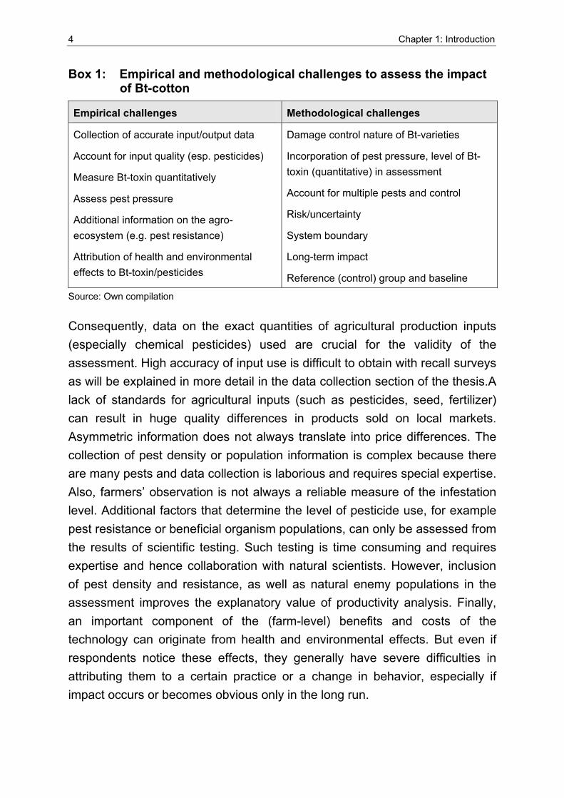
Box 1: Empirical and methodological challenges to assess the impact of Bt-cotton
Empirical challenges Methodological challenges
Collection of accurate input/output data
Account for input quality (esp. pesticides)
Measure Bt-toxin quantitatively
Assess pest pressure
Additional information on the agro-ecosystem (e.g. pest resistance)
Attribution of health and environmental effects to Bt-toxin/pesticides
Damage control nature of Bt-varieties
Incorporation of pest pressure, level of Bt-toxin (quantitative) in assessment
Account for multiple pests and control
Risk/uncertainty
System boundary
Long-term impact
Reference (control) group and baseline
Source: Own compilation
Consequently, data on the exact quantities of agricultural production inputs (especially chemical pesticides) used are crucial for the validity of the assessment. High accuracy of input use is difficult to obtain with recall surveys as will be explained in more detail in the data collection section of the thesis.A lack of standards for agricultural inputs (such as pesticides, seed, fertilizer) can result in huge quality differences in products sold on local markets. Asymmetric information does not always translate into price differences. The collection of pest density or population information is complex because there are many pests and data collection is laborious and requires special expertise. Also, farmers’ observation is not always a reliable measure of the infestation level. Additional factors that determine the level of pesticide use, for example pest resistance or beneficial organism populations, can only be assessed from the results of scientific testing. Such testing is time consuming and requires expertise and hence collaboration with natural scientists. However, inclusion of pest density and resistance, as well as natural enemy populations in the assessment improves the explanatory value of productivity analysis. Finally, an important component of the (farm-level) benefits and costs of the technology can originate from health and environmental effects. But even if respondents notice these effects, they generally have severe difficulties in attributing them to a certain practice or a change in behavior, especially if impact occurs or becomes obvious only in the long run.
Chapter 1: Introduction 5
The prime methodological challenge to assessing the productivity effect of Bt-cotton is to adequately capture the damage control nature of the Bt-trait. Lichtenberg and Zilberman (1986) provided a general specification for a damage control function in-built in the production function for chemical pesticides. In principle this methodology can be applied to the case of Bt-cotton. Possible extensions of the approach could relate to the quantitative measurement of the Bt-trait and its prophylactic nature, situations with multiple pests, application of other control agents (pesticides and natural enemies) in addition to using a Bt-variety, and the severity of pest pressure.
The impact of biotechnology solutions is subject to a considerable degree of uncertainty due to natural fluctuations in the biotic and abiotic environment (climate, pest pressure, availability of irrigation) so that a data set with information from only one or a few years is insufficient for general impact conclusions. Deterministic models might misrepresent actual conditions and hence, economic methodology needs to account for this uncertainty and results should be presented as probabilistic rather than rigid values such as a single cost-benefit-ratio or a single marginal value product. Also, the wider agro-ecosystem impacts should be considered to adequately capture all features of the technology. This requires a multi-disciplinary approach in which socio-economic, social, and ecological effects are evaluated and hence the choice of an appropriate measure is more complicated (Alston et al., 2000). Finally, it is not only difficult to measure long-term effects like resistance build-up or ecosystem changes but it is also complex to incorporate them in the assessment. It can be expected that the results of static impact assessment from an initial adoption period or pilot areas will be higher than those acquired after several years of adoption. Thus, net benefits can be overestimated if conclusions are drawn from an early adoption phase (Zadoks and Waibel, 2000).
If all these empirical and methodological aspects of evaluating the farm-level impact of Bt-cotton have been considered, the last hurdle is the question of a valid control group and the attribution of the effect to the technology or intervention in question. To establish a causal relationship and avoid attribution errors when assessing a new technology, with and without scenarios are needed in addition to the before and after comparison (Fleischer et al., 1999; Maredia et al., 2000).
6 Chapter 1: Introduction
This means that relevant information should be recorded prior to and after technology implementation for adopters and non-adopters, respectively to account for changes over time and changes due to technology adoption (Casley and Lury, 1982). Because farmers are not randomly assigned to the groups of adopters or non-adopters but make the decision themselves, self-selection as a source of bias is highly relevant in the adoption of new technologies (Greene, 2003) and should be accounted for (Fernandez-Cornejo and McBride, 2000).
Moreover, the counterfactual for the benefit assessment of a new technology should be the next best option. In the case of Bt-cotton in China, it seems questionable to select conventional chemical plant protection with overuse of chemical pesticides and incidence of pest resistance against most active ingredients (Wu et al., 1997) as the reference scenario. Comparing a new technology (Bt-trait) with a depreciated technology (chemical pesticides) as control group means considering different points in the technology life cycle. Benefits are generally highest in the early adoption phase of a pest control strategy, while scale and long-term negative effects and diminishing effectiveness of the control due to resistance cause a decrease in control benefits over time. So a technology that is in use already for some decades, such as the use of chemical pesticides can be considered depreciated.
The outline of the major challenges in the assessment of Bt-cotton shows the complexity of the problem. This thesis especially addresses the challenges of accurate data collection by using a strict monitoring protocol of production inputs and practices of smallholder farmers rather than relying on information obtained from recall surveys. Also, the laboratory testing of leaf tissue allows the inclusion of the Bt-trait as a quantitative variable in the analysis. From the methodological challenges listed above, the damage control nature of Bt-varieties is taken into account in the productivity assessment. The fact that most of the explanatory variables are uncertain is accounted for by applying stochastic frontier and stochastic budgeting approaches. Finally, a bio-economic model accounts for additional ecosystem aspects such as the impact of the respective control on natural enemies and the interaction of pest and natural enemy populations. The consideration of such ecosystem variables aims at a better systems understanding and an improved assessment of control interventions.
Chapter 1: Introduction 7
The case study of Bt-cotton production and the subsequent analysis focuses on the assessment of farm-level impact. Technology externalities or impact on other levels, or equity issues that arise from technology introduction are not considered.
Subject to the problem background and the general research question outlined above, the specific objectives are to:
• specify data requirements for assessment of plant protection technologies,
• assess short-term productivity effects of adopting Bt-cotton varieties,
• extend the concept of damage-control functions in productivity analysis of Bt-cotton by including biological models and
• contribute to the development of a methodology for assessing economic benefits of GE crop varieties that are used for plant protection.
The approaches applied in the analysis aim at capturing different aspects of the Bt-cotton technology since “dealing with the many facets of biotechnology, however, often points out the limits of economic analysis and, hopefully, provides an incentive to expand the limits of our discipline” (Gaisford et al., 2001). The application of different complementary approaches to assess short-term productivity enables a discussion of the validity and plausibility of the results and the strengths and weaknesses of the respective approaches This allows an enhanced understanding of the nature of the Bt-technology and the complex system in question.
1.3 Organization of the thesis
Chapter 2 presents current status and recent developments in the diffusion of agricultural biotechnology on a global scale. After a short introduction of the Bt-technology, potential risks and benefits of agricultural biotechnology are briefly summarized. Some more thoughts and challenges related to special features and potential of introducing agricultural biotechnology in developing countries are provided. The expectations and promises made are huge, while impact assessment under the conditions of these countries is even more challenging than under developed country conditions. The chapter closes with an in-depth review of the history and current status of agricultural biotechnology research and adoption in China. A review of available methods used to assess the impact of agricultural biotechnology and a brief discussion of the major limitations is given in Chapter 3.
8 Chapter 1: Introduction
The overview is followed by a literature review of recent economic studies that analyze the impact of Bt-cotton in developing countries. This presentation of the state of the art is the entry point for the selection of methods used in this study and highlights the strengths and weaknesses of the different approaches commonly adopted. Theoretical economic concepts relevant for the assessment of productivity of damage control agents in agricultural production systems are introduced in Chapter 4. The chapter starts with the application of neoclassical production theory for the special features of the Bt-technology. Some general considerations on the incorporation of uncertainty are provided and finally ecological economics is introduced as an interdisciplinary approach that provides the basis for the bio-economic model. Based on this theoretical framework the formal research hypotheses are formulated. In Chapter 5 the study location and the data collection procedure are described. A three-month pre-test phase with a smaller household survey was conducted before the data collection for the main study to identify key issues and constraints and select the study area.
Chapter 6 gives in-depth insight to the situation at the study site and relevant local institutions, and shows the style and status of implementation and the characteristics of technology adoption for the location. In Chapter 7, the short-term productivity impact of Bt-cotton varieties is assessed – firstly with an estimated production function and secondly by applying the concept of stochastic frontiers. Both econometric analyses use data generated in the farm-level interviews, the season-long monitoring of production inputs and additional testing (cotton tissue and bollworm larvae). To capture the uncertainty inherent in major determining variables, a partial stochastic budgeting model is introduced in Chapter 8. An expert survey with Chinese scientists, mainly from the field of plant protection, was conducted to validate the assumptions for the model. Outcomes of the stochastic budgeting model are cumulative distribution functions of net revenue of different pest management strategies that can be compared using the criteria of stochastic dominance. To account for the complexity of the biological-ecological system not captured within purely econometric approaches, a bio-economic model is implemented. For this purpose an existing cotton-growth model that simulates the dynamics of pests and beneficials and plant growth was adapted and validated for the research location and combined with a stochastic budgeting model.
Chapter 1: Introduction 9
Outputs of this bio-economic model are the cumulative distribution functions of the net revenue of different control strategies. The thesis closes with a discussion of results obtained and an examination of strengths and weaknesses of the approaches used in the study (Chapter 9). Conclusions and recommendations for further research are derived from the findings. Chapter 10 is an executive summary of the work.
2 B io technology in agr icu l ture
This chapter describes the status and development of agricultural biotechnology on a global scale and in more detail for the special case of China. After a short introduction to the history and characteristics of the Bt-technology the main issues and concerns that are generally raised in the debate of agricultural biotechnology are briefly summarized. The aim is to enable a better understanding of the different categories of agricultural biotechnology impact. The following section deals with the role that agricultural biotechnology has or can have in developing countries. This is important because expectations and promises regarding the potential to reduce poverty and contribute to food security are enormous and the situation in developing countries in many respects differs from the conditions in the developed world. The chapter closes with a review of the history, current status and regulatory framework of agricultural biotechnology in China.
2.1 Global status of agricultural biotechnology
2.1.1 History and current status of agricultural biotechnology
Biotechnology has been defined as “any technique that uses living organisms, or substances from those organisms, to make or modify a product, to improve plants or animals, or to develop microorganisms for specific uses” (OTA, 1989). This definition is broad enough to cover both, traditional biotechnology applications, for example the commercial use of microbes for brewing and biological control, as well as modern biotechnology that comprises the more complex methods of genetic engineering of plants and animals (Persley, 1991). Throughout this thesis, the term biotechnology is used for the latter type of biotechnology applications, mainly recombinant DNA technologies (where genes of plants or animals are inserted into agricultural crops to obtain transgenic plants with favorable traits such as insect resistance). Appendix 7 provides a summary of the history and evolution of biotechnology research. The debate over agricultural biotechnology by far exceeds the discussions about any other new technology in agriculture. While proponents stress the potential to increase food security (especially relevant for developing countries) and achieve a reduction in production costs and use of chemical pesticides while at the same time increasing crop yields, opponents point to issues mainly regarding food safety, the environmental impact, corporate control of agriculture, and ethical concerns (Nelson, 2001).
Chapter 2: Biotechnology in agriculture 11
The first commercial release of a genetically engineered (GE) crop took place in China in 1988, when a virus-resistant variety of tobacco was approved for planting (Pray, 1999). But this variety was later banned because tobacco companies feared a negative consumer response. In 1994 a delayed ripening tomato (FlavrSavr®) obtained approval for commercial use in the USA (James and Krattiger, 1996). Since that time, the area planted with transgenic varieties has increased, reaching an estimated global area of 81 million hectares by the year 2004 (James, 2004). To date, genetically modified crops are grown in 18 countries and cover an estimated 1.6% of the global agricultural area but reach considerably higher shares for certain crops (Table 1). The five most important countries in terms of GE adoption, namely the USA (59% of the global GE area), Argentina (20%), Brazil (6%), Canada (6%), and China (5%) together accounted for 96% of the global GE acreage in 2004 (James, 2004). In Argentina and Brazil soybeans are the only transgenic crop while the GE area in China is almost entirely Bt-cotton. China is the only developing country that has introduced Bt-cotton on a large scale, with some 66% of the total cotton area planted with Bt-varieties in 2004 (James, 2004). India, the country with the largest cotton area, gave approval for commercial use of Bt-cotton varieties only recently (in the 2002 season).
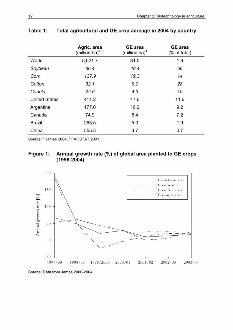
The main traits of genetically modified plants grown in 2004 were herbicide resistance (72% of the total global GE area) and insect resistance (19%) or a combination of both (9%). Larger scale commercial applications only include four main crops, namely soybean, corn, cotton, and canola (Table 1). Herbicide resistant soybeans account for by far the largest part of total GE adoption. Appendix 2 provides an overview of the development of GE area, crops and traits by country and globally as well as adoption shares for the main crops4. The annual growth rate of the area planted to the different GE crops is depicted in Figure 1.
4 It needs to be stressed that the presented adoption figures reported are estimates only. These
may be fairly reliable for developed countries (e.g. USA) since sales of transgenic seed or company information on royalties can be used. Estimation of adoption figures for developing countries is more difficult and numbers are prone to errors. Unapproved planting of GE varieties (e.g. soybean in Brazil or GE trees in China) is not accounted for. At the same time seeds may be labelled GE but actually are not e.g. counterfeit Bt-cotton in China and India.
12 Chapter 2: Biotechnology in agriculture
Table 1: Total agricultural and GE crop acreage in 2004 by country
Agric. area (million ha)1, 2
GE area (million ha)1
GE area (% of total)
World 5,021.7 81.0 1.6 Soybean 86.4 48.4 56 Corn 137.9 19.3 14 Cotton 32.1 9.0 28 Canola 22.6 4.3 19 United States 411.2 47.6 11.6 Argentina 177.0 16.2 9.2 Canada 74.9 5.4 7.2 Brazil 263.5 5.0 1.9 China 555.3 3.7 0.7
Source: 1 James 2004, 2 FAOSTAT 2003
Figure 1: Annual growth rate (%) of global area planted to GE crops (1996-2004)
1997/98 1998/99 1999/2000 2000/01 2001/02 2002/03 2003/04
Ann
ual g
row
th ra
te [%
]
-50
0
50
100
150
200
GE soybean areaGE corn areaGE cotton areaGE canola area
Source: Data from James 2000-2004
Chapter 2: Biotechnology in agriculture 13
Very small adoption areas resulted in a high percentage growth in the first years of technology adoption. Annual growth for 2003/04 was around 20% for the four major GE crops (17%, 25%, 25%, and 19% for soybean, corn, cotton and canola, respectively). However, growth rates were not stable and area increase was zero or negative for some crops in some years.
2.1.2 The example of insect resistant Bt-cotton
Cotton is grown in developed and developing countries but differences in input intensity and degree of mechanization are huge. The main cotton growing countries in terms of area planted are India, China and the USA (Table 2). But the difference in the cotton yield level (production per unit land) between these countries is enormous as is shown in Figure 25. Reasons for the yield differences include the varying intensity of production (input level of fertilizer and irrigation; and manual labor for pruning and harvesting), differences in the yield potential of varieties and differences in the pest pressure. In India for example, about two thirds of the cotton is grown under rainfed conditions and costs for agrochemicals (pesticides and fertilizer) are often inhibitively high for small-scale farmers (Qaim, 2003; Orphal, 2005). The yield increases recorded for cotton production in China during the last 15 years can mainly be attributed to increased input intensity (mainly fertilizer and irrigation) and improvement of germplasm (Huang et al., 2003).
A common feature for cotton production around the globe is the high level of chemical pesticides that are used to protect this crop from damage inflicted by pests and diseases (Agbios, 2004). In industrialized and developing countries alike, a proportionally much greater share of pesticides is used in cotton than in most other crops and negative externalities, for example impact on the environment and human health, are widely reported. Moreover, this high level of pesticides applied mainly to control caterpillar pests of the lepidoptera family, results in high production costs and hence reduces the net revenue for farmers. For this reason, cotton was among the first crops for which research on genetically engineered insect resistance resulted in commercially approved varieties.
5 Differences in yield level were prevalent already before the introduction of Bt-varieties.
14 Chapter 2: Biotechnology in agriculture
Table 2: Share of GE cotton, cotton area and production of major producers (2004)
Cotton area (million ha)
Cotton production (million t)
GE cotton area (million ha)2
India 8.7 7.2 0.5
China 5.7 18.0 3.7
United States 5.4 12.4 est. 3.0
Pakistan 3.1 6.0 – *
Usbekistan 1.4 3.5 –
Brazil 1.2 3.6 –
Turkey 0.7 2.6 –
Others 8.7 14.1 est. 1.8A
World 34.9 67.4 9.0 Source: FAOSTAT 2005, 2 James 2003 * There is anecdotal evidence of Bt-cotton plantings in Pakistan (with Bt-seed from India) A Australia (0.2 million ha), South Africa (< 0.4 million ha), Mexico (< 0.1 million ha), Colombia (< 0.05 million ha), Argentina (unknown)
Figure 2: Seed cotton6 yield (kg ha-1) of major cotton producers (1990-2004)
1990 1992 1994 1996 1998 2000 2002 2004
Seed
cot
ton
yield
[kg
ha-1
]
0
500
1000
1500
2000
2500
3000
3500
4000
ChinaIndiaPakistanUSA
Commercialization of Bt-cotton varieties
Source: FAOSTAT, statistical database, access August 2004
6 Seed cotton: Lint that still includes seeds that make up about 65% of the total weight.
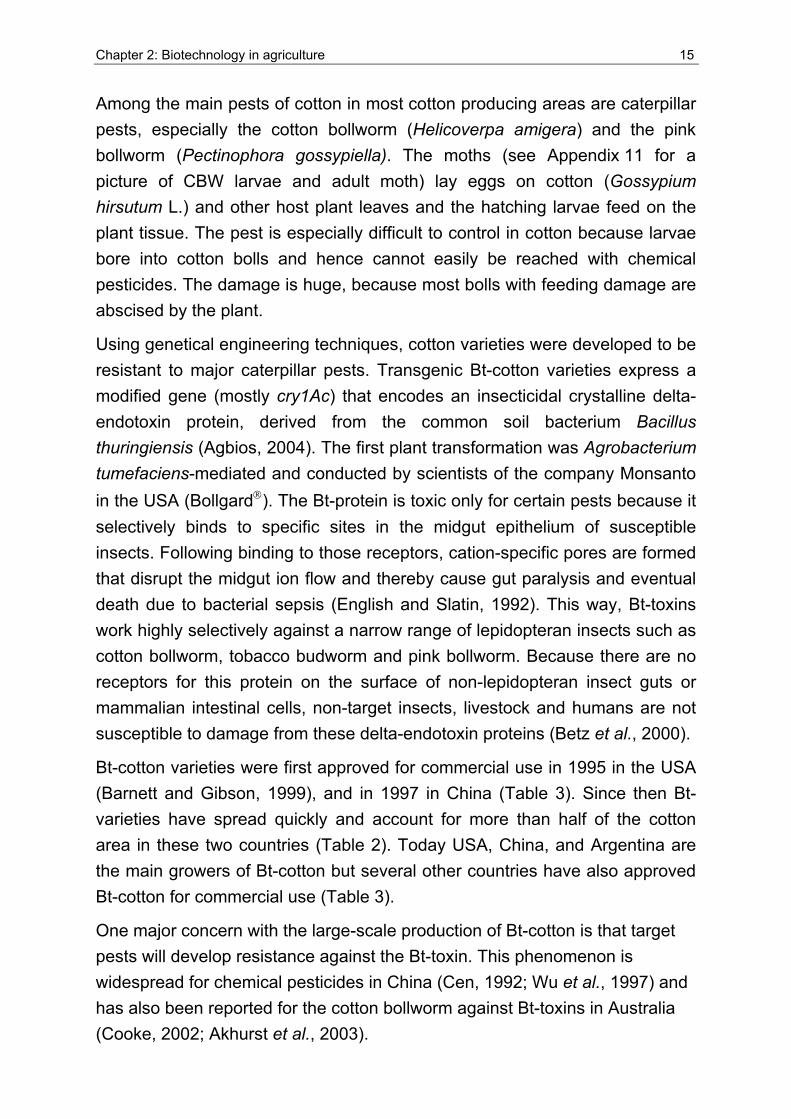
Chapter 2: Biotechnology in agriculture 15
Among the main pests of cotton in most cotton producing areas are caterpillar pests, especially the cotton bollworm (Helicoverpa amigera) and the pink bollworm (Pectinophora gossypiella). The moths (see Appendix 11 for a picture of CBW larvae and adult moth) lay eggs on cotton (Gossypium hirsutum L.) and other host plant leaves and the hatching larvae feed on the plant tissue. The pest is especially difficult to control in cotton because larvae bore into cotton bolls and hence cannot easily be reached with chemical pesticides. The damage is huge, because most bolls with feeding damage are abscised by the plant.
Using genetical engineering techniques, cotton varieties were developed to be resistant to major caterpillar pests. Transgenic Bt-cotton varieties express a modified gene (mostly cry1Ac) that encodes an insecticidal crystalline delta-endotoxin protein, derived from the common soil bacterium Bacillus thuringiensis (Agbios, 2004). The first plant transformation was Agrobacterium tumefaciens-mediated and conducted by scientists of the company Monsanto in the USA (Bollgard®). The Bt-protein is toxic only for certain pests because it selectively binds to specific sites in the midgut epithelium of susceptible insects. Following binding to those receptors, cation-specific pores are formed that disrupt the midgut ion flow and thereby cause gut paralysis and eventual death due to bacterial sepsis (English and Slatin, 1992). This way, Bt-toxins work highly selectively against a narrow range of lepidopteran insects such as cotton bollworm, tobacco budworm and pink bollworm. Because there are no receptors for this protein on the surface of non-lepidopteran insect guts or mammalian intestinal cells, non-target insects, livestock and humans are not susceptible to damage from these delta-endotoxin proteins (Betz et al., 2000).
Bt-cotton varieties were first approved for commercial use in 1995 in the USA (Barnett and Gibson, 1999), and in 1997 in China (Table 3). Since then Bt-varieties have spread quickly and account for more than half of the cotton area in these two countries (Table 2). Today USA, China, and Argentina are the main growers of Bt-cotton but several other countries have also approved Bt-cotton for commercial use (Table 3).
One major concern with the large-scale production of Bt-cotton is that target pests will develop resistance against the Bt-toxin. This phenomenon is widespread for chemical pesticides in China (Cen, 1992; Wu et al., 1997) and has also been reported for the cotton bollworm against Bt-toxins in Australia (Cooke, 2002; Akhurst et al., 2003).
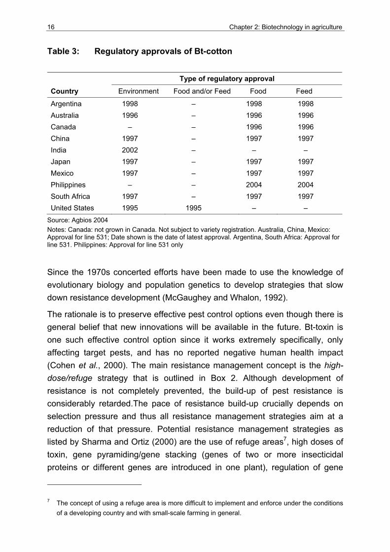
16 Chapter 2: Biotechnology in agriculture
Table 3: Regulatory approvals of Bt-cotton
Type of regulatory approval
Country Environment Food and/or Feed Food Feed
Argentina 1998 – 1998 1998 Australia 1996 – 1996 1996 Canada – – 1996 1996 China 1997 – 1997 1997 India 2002 – – – Japan 1997 – 1997 1997 Mexico 1997 – 1997 1997 Philippines – – 2004 2004 South Africa 1997 – 1997 1997 United States 1995 1995 – –
Source: Agbios 2004 Notes: Canada: not grown in Canada. Not subject to variety registration. Australia, China, Mexico: Approval for line 531; Date shown is the date of latest approval. Argentina, South Africa: Approval for line 531. Philippines: Approval for line 531 only
Since the 1970s concerted efforts have been made to use the knowledge of evolutionary biology and population genetics to develop strategies that slow down resistance development (McGaughey and Whalon, 1992).
The rationale is to preserve effective pest control options even though there is general belief that new innovations will be available in the future. Bt-toxin is one such effective control option since it works extremely specifically, only affecting target pests, and has no reported negative human health impact (Cohen et al., 2000). The main resistance management concept is the high-dose/refuge strategy that is outlined in Box 2. Although development of resistance is not completely prevented, the build-up of pest resistance is considerably retarded.The pace of resistance build-up crucially depends on selection pressure and thus all resistance management strategies aim at a reduction of that pressure. Potential resistance management strategies as listed by Sharma and Ortiz (2000) are the use of refuge areas7, high doses of toxin, gene pyramiding/gene stacking (genes of two or more insecticidal proteins or different genes are introduced in one plant), regulation of gene
7 The concept of using a refuge area is more difficult to implement and enforce under the conditions of a developing country and with small-scale farming in general.
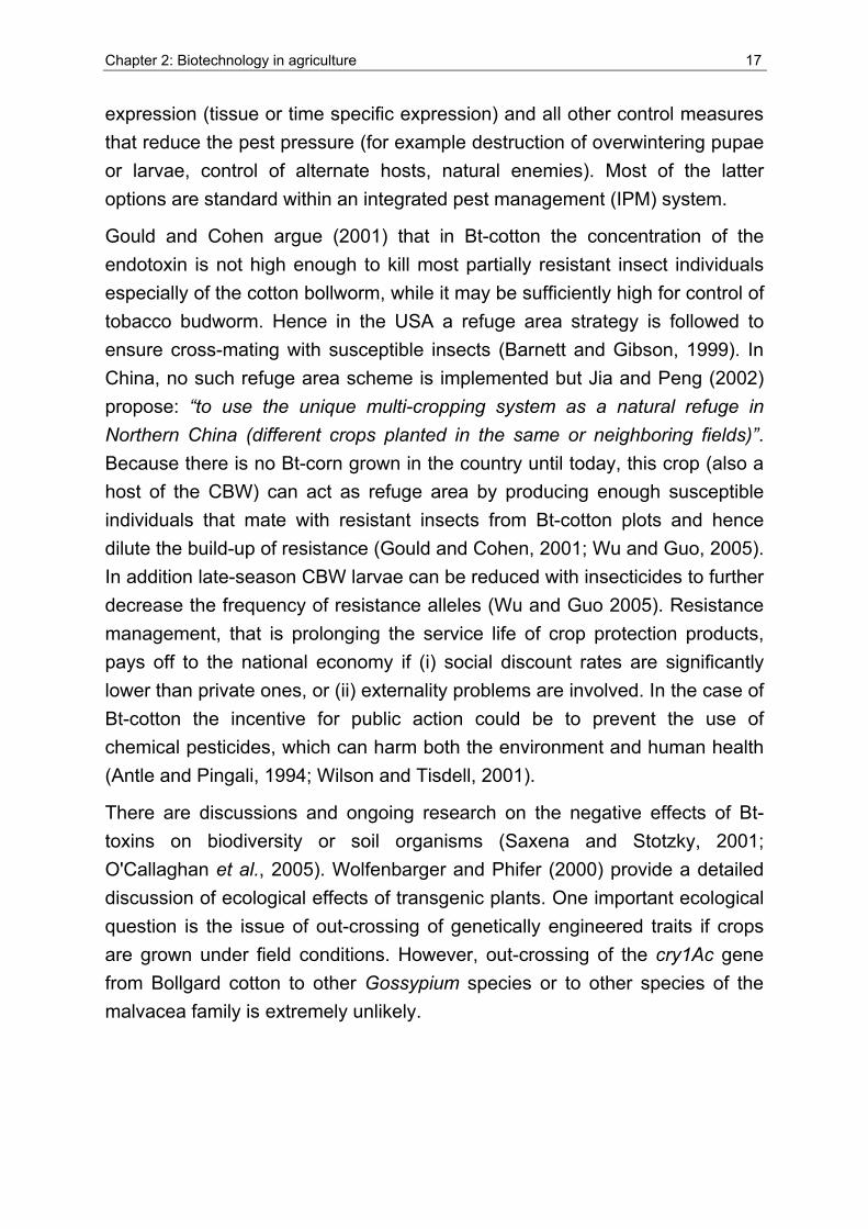
Chapter 2: Biotechnology in agriculture 17
expression (tissue or time specific expression) and all other control measures that reduce the pest pressure (for example destruction of overwintering pupae or larvae, control of alternate hosts, natural enemies). Most of the latter options are standard within an integrated pest management (IPM) system.
Gould and Cohen argue (2001) that in Bt-cotton the concentration of the endotoxin is not high enough to kill most partially resistant insect individuals especially of the cotton bollworm, while it may be sufficiently high for control of tobacco budworm. Hence in the USA a refuge area strategy is followed to ensure cross-mating with susceptible insects (Barnett and Gibson, 1999). In China, no such refuge area scheme is implemented but Jia and Peng (2002) propose: “to use the unique multi-cropping system as a natural refuge in Northern China (different crops planted in the same or neighboring fields)”. Because there is no Bt-corn grown in the country until today, this crop (also a host of the CBW) can act as refuge area by producing enough susceptible individuals that mate with resistant insects from Bt-cotton plots and hence dilute the build-up of resistance (Gould and Cohen, 2001; Wu and Guo, 2005). In addition late-season CBW larvae can be reduced with insecticides to further decrease the frequency of resistance alleles (Wu and Guo 2005). Resistance management, that is prolonging the service life of crop protection products, pays off to the national economy if (i) social discount rates are significantly lower than private ones, or (ii) externality problems are involved. In the case of Bt-cotton the incentive for public action could be to prevent the use of chemical pesticides, which can harm both the environment and human health (Antle and Pingali, 1994; Wilson and Tisdell, 2001).
There are discussions and ongoing research on the negative effects of Bt-toxins on biodiversity or soil organisms (Saxena and Stotzky, 2001; O'Callaghan et al., 2005). Wolfenbarger and Phifer (2000) provide a detailed discussion of ecological effects of transgenic plants. One important ecological question is the issue of out-crossing of genetically engineered traits if crops are grown under field conditions. However, out-crossing of the cry1Ac gene from Bollgard cotton to other Gossypium species or to other species of the malvacea family is extremely unlikely.
18 Chapter 2: Biotechnology in agriculture
Box 2: The “high-dose/refuge” resistance management strategy
Percival (1999) provides the following reasons: (1) cotton is generally self-pollinating, but can be cross-pollinating if suitable insect pollinators (bees) are present; (2) cultivated cotton is an allotetraploid and incompatible with cultivated or wild diploid cotton species; therefore, it cannot cross and produce fertile offspring; (3) although out-crossing to wild allotetraploid Gossypium species can occur, commercial cotton production generally does not occur in the same geographical locations as the wild relatives; and (4) there are no identified non-cotton plants that are sexually compatible with cultivated cotton. A crossing of the Bt-trait into other cultivated cotton varieties is possible, but is not regarded as a concern because no adverse environmental impact is expected (Mehetre, 1992). The question of how stable the insect resistance trait is when Bt-cotton is propagated on-farm for several generations is not yet fully answered.
The offspring of SS*RR matings are RS, and therefore will not survive when they feed on high-dose Bt plants. Which spatial arrangement of refuge plants is best depends on the biology of the pest. Mixtures of Bt and non-Bt plants within fields can be established by sowing seed mixtures or by planting rows of refuge plants within fields of Bt-plants. Within-field mixtures are not the best type of refuge for insects that move between plants during development. This is because some of the insects will feed on Bt and non-Bt plants, thereby “diluting“ the high-dose concentration in Bt plants.
The dose-response lines indicate mortality of three insect genotypes at increasing concentrations of an insecticidal toxin. The dotted line indicates the concentration required for a “high dose”. S allele con-ferring susceptibility; R allele resistance
Source: Adapted from Cohen et al. (2000)
To understand how the high-dose/refuge strategy works, it is necessary to examine the genetic basis of resistance. In many cases, resistance to an insecticide is caused by a mutation in one gene of an insect. If there are two possible forms of the gene (alleles), R (mutant allele, conferring resistance) and S (normal allele, susceptibility), and each insect has two copies of the gene, then there are three possible genetic types (genotypes) of insects: SS, RS, and RR. The figure illustrates the response of each genotype to increasing concentrations of an insecticide. The response of RS insects to the insecticide is intermediate between that of the SS and RR insects, but is more similar to that of the SS insects, indicating that the R allele is partially recessive. To implement the high dose/refuge strategy, it is necessary to have a concentra-tion of toxin in the Bt cultivar that is high enough to kill almost all of the RS insects (indicated by the dotted line). „Refuges“ are non-Bt crop plants that serve to maintain Bt-susceptible insects in the population. Refuges can consist of fields planted with non-Bt plants or non-Bt plants within Bt fields. The large number of insects with the SS genotype that survive on the refuge plants are then available to mate with the small number of RR insects that survive on the Bt plants.
Chapter 2: Biotechnology in agriculture 19
2.2 Issues in the debate of agricultural biotechnology
This section briefly discusses the major risks and benefits of agricultural biotechnology and gives some information on the legislation and regulation of biotechnology applications, as well as related trade and equity implications. Special emphasis is given to the impact of the technology in the context of developing countries. The ethical reasoning about whether or not human kind should embark on biotechnology at all is not considered in this study.
2.2.1 Potential costs and benefits
The scientific and political discussion on potential costs (or risks in the definition of adverse outcomes) and benefits of agricultural biotechnology is still ongoing. This is not surprising since the first applications of the technology became available only a couple of years ago (see Section 2.1). The debate is further fueled by the considerable interest that different stakeholders (industry, scientists, NGOs) have in the topic and the ethical component of the subject in question. This section lists a number of anticipated benefits and risks of agricultural biotechnology that are issues of debate. However, aim of this overview is not to provide evidence or to conclude on the magnitude of these effects. An overview of existing economic studies on the impact of agricultural biotechnology under a range of conditions (especially in developing countries) is provided in Chapter 3.
The use of biotechnology in the field of agriculture could contribute in the following four main areas (Krimsky and Wrubel, 1996):
• yield gains through resistance to environmental stresses,
• cost savings for labor and production inputs,
• higher quality food and value added products, and
• environmentally benign methods of managing weeds and insect pests.
This list indicates that the expected impact can be environmental and economic as well as of socio-political nature. The same categories are valid for the anticipated risks. Here the three main areas are human health, environmental impact and ethical questions that emanate from existing value systems within a society and which can not be solved with additional research or information (Lele, 2003). A more specific overview of the main benefits and costs that are anticipated is presented in Table 4.
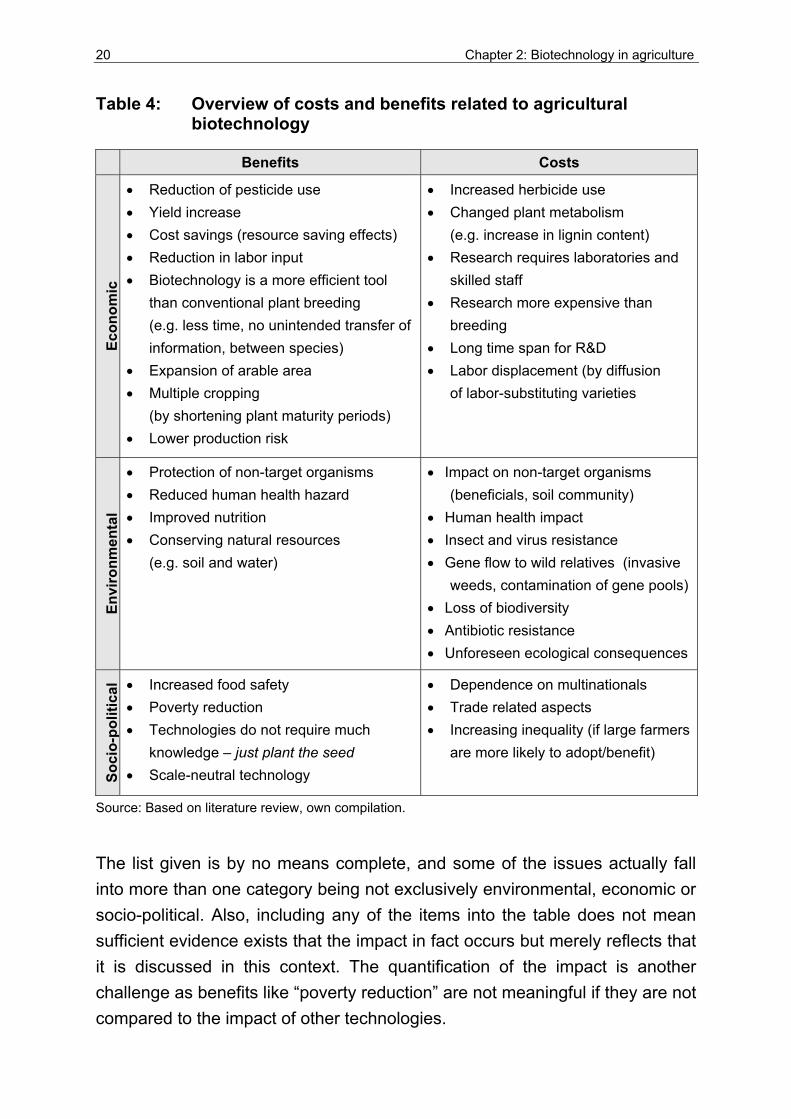
20 Chapter 2: Biotechnology in agriculture
Table 4: Overview of costs and benefits related to agricultural biotechnology
Benefits Costs
Econ
omic
• Reduction of pesticide use • Yield increase • Cost savings (resource saving effects) • Reduction in labor input • Biotechnology is a more efficient tool
than conventional plant breeding (e.g. less time, no unintended transfer of information, between species)
• Expansion of arable area • Multiple cropping
(by shortening plant maturity periods) • Lower production risk
• Increased herbicide use • Changed plant metabolism
(e.g. increase in lignin content) • Research requires laboratories and
skilled staff • Research more expensive than
breeding • Long time span for R&D • Labor displacement (by diffusion
of labor-substituting varieties
Envi
ronm
enta
l
• Protection of non-target organisms • Reduced human health hazard • Improved nutrition • Conserving natural resources
(e.g. soil and water)
• Impact on non-target organisms (beneficials, soil community)
• Human health impact • Insect and virus resistance • Gene flow to wild relatives (invasive
weeds, contamination of gene pools) • Loss of biodiversity • Antibiotic resistance • Unforeseen ecological consequences
Soci
o-po
litic
al • Increased food safety
• Poverty reduction • Technologies do not require much
knowledge – just plant the seed • Scale-neutral technology
• Dependence on multinationals • Trade related aspects • Increasing inequality (if large farmers
are more likely to adopt/benefit)
Source: Based on literature review, own compilation.
The list given is by no means complete, and some of the issues actually fall into more than one category being not exclusively environmental, economic or socio-political. Also, including any of the items into the table does not mean sufficient evidence exists that the impact in fact occurs but merely reflects that it is discussed in this context. The quantification of the impact is another challenge as benefits like “poverty reduction” are not meaningful if they are not compared to the impact of other technologies.
Chapter 2: Biotechnology in agriculture 21
The methodology to quantify the effects deserves a more in-depth discussion and is dealt with in the third chapter, while environmental and socio-political consequences are touched on without a detailed review. In the following text, the most important aspects from each of the impact categories will be briefly highlighted.
The environmental and human impacts of biotechnology are generally referred to as biosafety, with the Convention on Biological Diversity (1993) and the Cartagena Protocol on Biosafety8 (2003) as the main international agreements on biosafety (Sampath, 2004). In most developed countries, the set up of a regulatory framework for biosafety of GE crops started as early as in the mid 1980s, whereas most developing countries started the regulatory process only in recent years (Nap et al., 2003). There is a fundamental distinction in the perception of GMOs and hence the way of regulating GE products. Some countries (for example USA; Canada, Australia, New Zealand) decided to implement product-based regulations following the principle of substantial equivalence that presumes that food made from genetically engineered crops does not differ in any substantial way from food derived with traditional breeding methods (Sheldon, 2002).
Under the concept of substantial equivalence, the baseline for any risk assessment of GE crops is the impact of the corresponding non-GE crop. Following this reasoning there is also no explicit right to know about the production process for consumers and hence labeling of GE products or foods made from GE crops is not considered necessary if the product is not substantially different (no different nutritional properties, or allergens not normally present).
In contrast, other countries (mainly within the EU) argue that the process of producing GE crops and foods is different and hence the resulting products should be considered as novel foods (Kydd et al., 2000). Because inherent risks (especially in the long-run) might exist and are not known, the precautionary principle should be applied in order to ensure that adverse effects of GE products on human health and the environment are avoided 8 The protocol is a supplement to the UN “Convention on Biological Diversity”. It was adopted in
January 2000 and opened for signatures in May of the same year. The Protocol entered into force on 11 September 2003, ninety days after receipt of the 50th instrument of ratification and concerns the international transfer of living modified organisms with the two centerpieces being the “precautionary approach” and the requirement of “prior informed consent (PIC)”. Also see the web page of the “Convention on Biological Diversity” under http://www.biodiv.org/default.aspx.
22 Chapter 2: Biotechnology in agriculture
(Sheldon, 2002). Following the precautionary principle means, that “release of GMOs into the environment or the commercial marketing of GE foods (should not be permitted) until there is extensive evidence that they will not cause harm to humans, animals and the environment” (ibid). This reasoning in general goes along with the request of traceability of GE products and labeling of food containing GE ingredients to enable that consumers make a free choice. One of the key questions that the regulation of biosafety of GMOs is facing is “when is safe sufficiently safe?” (Nap et al., 2003).
Essential differences in the set up of biosafety frameworks, as outlined above, bear high potential for international trade disputes over GE crops and products because “exporters of GE crops, the USA in particular have a significant interest in ensuring market access for both current and future generations of bio-engineered crops” (Sheldon, 2002)9. The World Trade Organization (WTO) is a likely forum for this kind of international trade dispute and in cases that look similar on first sight, for example the EU’s ban of hormone-treated beef (challenged by the USA and Canada) or the import of Mexican tuna (caught with dolphin-harming methods) to the USA. The WTO finally ruled in these cases setting major legal precedence (ibid). Recently the United States10 brought a formal complaint before the WTO, claiming that the de facto moratorium of the EU is violating international trade agreements in blocking imports of agricultural produce (USDA, 2003). Although it is unlikely that the WTO will interfere in the institutional structure of the regulatory process of its member countries (regulations for testing and adoption of GMOs), since GATT article XX explicitly recognizes the right of countries to develop policies that protect human, plant and animal health, it would be concerned if specific aspects of GMO regulation were trade distorting (Sheldon, 2002).
Conflicts like import restrictions would fall under the WTO Sanitary and Phytosanitary (SPS) and/or the Technical Barriers to Trade (TBT) Agreements and the key issue in any such dispute would be the question of whether GMO
9 This predicted potential became reality when the USA together with other countries filed a
complaint against the EU in early 2003. This matter is still pending but most likely initialised the recent changes in the EU policy towards GMOs (e.g. EU allowed imports of a GM maize) and the formal end of the five-year moratorium.
10 The complaint was also filed by Argentina, Canada, Egypt, Australia, New Zealand, Mexico, Chile, Colombia, El Salvador, Honduras, Peru and Uruguay.
Chapter 2: Biotechnology in agriculture 23
and conventional products are sufficiently different or do fall under the definition of like goods11 (ibid).
Some consider the first commercial approvals of GE corn in September 200412 as the end of the moratorium and see a shift in the official position of the EU towards GMOs as a response to the trade complaint. The outcome of the filed complaint against the EU is expected to be important also for developing countries, like China and some countries in Africa, that have a high incentive for strategic behavior to secure export markets for GE free crops and products if such a position is accepted under WTO ruling. On the other hand, Cohen and Paarlberg (2004) stress that an efficient regulatory framework is necessary to foster investments in biotechnology from development agencies, as well as the public and private sector. Such a framework needs to cover and well co-ordinate not only biosafety aspects of genetically modified crops, but, in addition among others, the protection of intellectual property rights (IPR) of plant varieties (prescribed for example as minimum statement under the WTO and related agreements), regulations of biodiversity as well as issues of food safety and labeling (Sampath, 2004).
Another important and controversial issue that is related to the regulation of GE crops is the question of legal liability (Nap et al., 2003; Sampath, 2004). If non-GE crops are produced parallel to GE crops, out-crossing of genetic information is a problem that could either be interpreted as an infringement of intellectual property rights from the point of view of the firm that holds a patent on the GE variety (as practiced in the USA) or as contamination of the (potentially higher priced) non-GE crop from the view point of the non-GE crop producer (for example current German law). Again, different ways of handling the liability aspect are possible: holding either the GE crop producer responsible for any damage caused from his crop or requiring the non-GE
11 This definition is further complicated if not only scientific but in addition ethical, cultural and religious reasons form the ground for restrictions or bans.
12 BRUSSELS, Sept 8 2004 (Reuters) - The EU approved on Wednesday the first genetically modified (GMO) seeds for planting that may be sold across the 25-nation bloc. … The EU executive authorised 17 different seed strains of maize engineered by U.S. biotech giant Monsanto <MON.N> from a parent crop that won approval for growing just before the EU began its biotech ban in 1998 that lasted nearly six years. … Before Wednesday's decision, the 17 seeds only had national authorisations issued by France and Spain. This meant that only farmers in those countries were able to buy and plant the seeds. Under an established legal procedure, once an EU state gives the green light for a seed to be sold on its territory -- and assuming all EU legislation is complied with -- the Commission is obliged to extend that authorization onto an EU-wide basis.
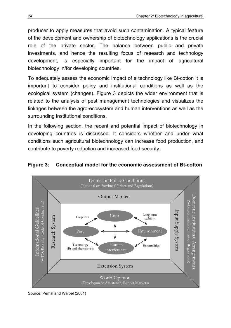
24 Chapter 2: Biotechnology in agriculture
producer to apply measures that avoid such contamination. A typical feature of the development and ownership of biotechnology applications is the crucial role of the private sector. The balance between public and private investments, and hence the resulting focus of research and technology development, is especially important for the impact of agricultural biotechnology in/for developing countries.
To adequately assess the economic impact of a technology like Bt-cotton it is important to consider policy and institutional conditions as well as the ecological system (changes). Figure 3 depicts the wider environment that is related to the analysis of pest management technologies and visualizes the linkages between the agro-ecosystem and human interventions as well as the surrounding institutional conditions.
In the following section, the recent and potential impact of biotechnology in developing countries is discussed. It considers whether and under what conditions such agricultural biotechnology can increase food production, and contribute to poverty reduction and increased food security.
Figure 3: Conceptual model for the economic assessment of Bt-cotton
Output Markets
Domestic Policy Conditions (National or Provincial Prices and Regulations)
Rese
arch
Sys
tem
Input Supply System
Extension System
Inte
rnat
iona
l Gui
delin
es
(WTO
, Bio
safty
, Cod
e of
Con
duct
etc
.)
World Opinion (Development Assistance, Export Markets)
Dom
estic Institutional Arrangem
ents (Subsidies, E
nforcement of Regulations)
Pest
Crop
Environment
Human interference
Crop loss Long term
stability
ExternalitiesTechnology (Bt and alternatives)
Source: Pemsl and Waibel (2001)
Chapter 2: Biotechnology in agriculture 25
2.2.2 Agricultural biotechnology and developing countries
The main challenges that developing countries are facing today are poverty and food insecurity of a large population share, caused and aggravated by increasing environmental degradation (Lele, 2003). Since many of the world’s poor depend on agriculture (either directly as farmers or as hired laborers employed in agriculture or indirectly via the prices of staple foods for all food purchasing consumers) the question of whether biotechnology can help to improve agriculture in developing countries is of great importance.
In 2003 a share of close to 30% or about 20 million hectares of the total area planted to GE crops was grown in developing countries (James, 2003). But up until now, some commercial GE products in only a few countries make up this share13. These figures show that until now biotechnology has had no or only limited impact in most developing countries. Lele (2003) states that the major reasons for the so far hesitant response of developing countries towards agricultural biotechnology are considerations of trade policy and consumer preferences as well as anticipated environmental risks. Cohen and Paarlberg (2002) argue that besides the most frequently used explanations (weak local scientific and research capacities, intellectual property rights constraints and concerns with biological and food safety), the most potent explanation for the slow uptake of agricultural biotechnology in developing countries is the fear of loosing export markets, mainly in Europe and Japan if GE crops should be adopted. Despite the current modest status of agricultural biotechnology in the developing world, there is ongoing debate about the potential of these technologies to contribute to the reduction of poverty and hunger and enhanced food security (Altieri and Rosset, 1999; McGloughlin, 1999; Qaim and Virchow, 2000; Lipton, 2001; Zilberman et al., 2004). The remainder of this chapter gives a brief overview of the potential contribution of biotechnology in developing countries, followed by a discussion of major challenges and necessary conditions or (policy) measures that are prerequisites to realize this potential.
13 Kent (2004) gives a list of countries and respective GE crops: Argentina (herbicide tolerant (RR) soybean, Bt-corn and -cotton), Brazil (RR soybean), South Africa (RR soybean, Bt-corn and -cotton), Philippines (Bt-corn), China (Bt-cotton, several other applications), Indonesia and India (Bt-cotton).
26 Chapter 2: Biotechnology in agriculture
The three general levels in which impact can occur are (1) the field of (agricultural) research and development, (2) the farm or production level and (3) society as a whole. One major potential of biotechnology is the field of genomics14 that provides molecular tools to accelerate the pace and improve the precision of conventional breeding, hence reducing breeding costs (Byerlee and Fischer, 2002). There is however dispute over whether there really is a reduction in costs and development time if all research and development costs and the time that is required for safety testing of products is considered (Cox, 2002).
Biotechnology tools enable gene transfer not only within but also between species. The possibility to create plants (or animals) with entirely new traits widens the scope of conventional breeding. This way genes/traits once identified and analyzed can rather easily be transferred into new crops or locally adapted varieties. But fundamental research in this field is both time-consuming and costly, and requires high investments in laboratories and considerable human capital, thus largely increasing the fixed costs. This situation has led to a steady development of agricultural biotechnology research especially in relatively large countries with well-established infrastructure for research where the human and financial resources allocated to biotechnology research and development (R&D) are relatively high (Cohen et al., 2004). Poorer countries in sub-Sahara Africa or South Asia are left behind.
Most (especially smaller) developing countries do not have the capacity to invest in this field and it is unlikely that they will be able to afford it in the near future. Only China has significant numbers of qualified national research staff and relevant public research in the field of biotechnology (Huang et al., 2002b). This can be a problem in terms of the impact for developing countries since, different from the green revolution in the 1960s and 1970s where public agricultural research centers were the main players, research in the field of biotechnology is dominated by the private sector (Altieri and Rosset, 1999).
14 Definition of genomics: “The research strategy that uses molecular characterization and cloning of
whole genomes to understand the structure, function and evolution of genes and to answer fundamental biological questions.” Source: FAO Glossary of Biotechnology for Food and Agriculture, Access: 17th December 2004, http://www.fao.org/biotech/index_glossary.asp?lang=en
Chapter 2: Biotechnology in agriculture 27
Mergers in the last decade reduced the number of firms so that today only a few internationally operating companies own most of the patents in the field and fund the lion’s share of agricultural biotechnology research (see Pray and Naseem, 2003). A situation of such high market concentration with only few dominating firms could depress the rate of progress due to a lack of competition (Qaim and Virchow, 2000).
For many technologies that could help farmers in developing countries, there is little economic incentive for private research and development since the markets for such products are small or non-existent (Kydd et al., 2000). Pray and Naseem (2003) conclude that “it is clear that the private sector will not develop many of the traits or new varieties needed by the poor“. This led to the term orphan crops for (staple food) crops grown by small-scale farmers, that are unlikely to receive any research attention if the public sector does not step into the scene (Serageldin, 1999). Even in cases where a large potential market for a certain technology exists the private sector might not be willing to invest if institutional conditions are unfavorable (Kent, 2004). Examples are the sales of Bt-cotton seed in China or herbicide resistant (RR) soybean varieties in Argentina, where only a minor share of the seeds is certified and intellectual property rights (IPR) are weak or frequently infringed due to lack of enforcement.
From a legal point of view, Article 27 of the WTO’s 1994 Trade Related Aspects of Intellectual Property (TRIPS) agreement specifically excludes countries from any obligation to provide legislation related to patenting life forms (Kydd et al., 2000). This means that developing countries do not have to recognize patents in this area. Although zero enforcement of IPRs can be an optimal strategy for governments of developing countries to maximize the adoption of a technology and maintain international competitiveness of national producers (Giannakas, 2002), weak IPR protection is on the other hand a strong disincentive for private companies to invest (Lele, 2003). The application of genetic use restriction technologies (GURTs)15 by crop innovators could increase the rate of innovation in the private sector, triggering
15 An example for GURTs is the so-called terminator gene that prevents plants from producing fertile seeds, meaning farmers would have to buy new seeds, rather than saving part of their harvest to plant next year's crop. The patent holding company Monsanto announced that the technology would never be commercialised (after it had faced enormous worldwide opposition).
28 Chapter 2: Biotechnology in agriculture
increased growth at the technological frontier (Goeschl and Swanson, 2000). Nevertheless, application of GURTs could have a negative impact on the diffusion of innovations and in addition might further increase the gap between rich and poor farmers. Publicly funded and operated research and development, together with different concepts of public-private partnership and participatory research that better accounts for the needs of farmers, is hence regarded as essential for the future impact of agricultural biotechnology, especially in developing countries (Pray and Naseem, 2003).
To date the agricultural biotechnology applications in developing countries are nearly exclusively the planting of herbicide and insect resistant varieties of corn, cotton and canola, and these are principally labor-saving technologies. Drought or saline tolerant varieties or major yield increases in staple food crops and nutritional improvement that tackle the primary constraints of poor farmers remain an unrealized potential for the time being (Scoones, 2002). Pray and Naseem (2003) find in their analysis that “first generation research of private firms did not concentrate on the crops, traits and countries needed to make a difference for the poor”. In contrast to the first generation of GE crops (mainly input saving traits like pest-resistance) the second generation of biotechnology products in agriculture relate to improved output characteristics, for example changes in the content and composition of crops that create value downstream from production (Ruttan, 1999). Applications of such (nutritional) traits that are currently under development or testing include golden rice that is genetically engineered to produce beta-carotene, a substance that the body can convert to Vitamin A and iron-fortified vegetable crops (Kydd et al., 2000). Since first generation technologies are simple to use and do not require changes in the farming practices these could be of great importance to the developing countries, while for the second generation traits lower adoption rates are predicted due to uncertain benefits and need for more complex marketing arrangements (Ameden and Zilberman, 2005).
If crop varieties with relevance to the poor in developing countries were created and distributed, the following direct and indirect effects occur. As potential direct effects of agricultural biotechnology de Janvry et al. (2005) list a rise in the welfare of the poor due to “increased production for home consumption, more nutritious foods, higher gross revenues …, lower production costs, lower yield risks, lower exposure to unhealthy chemicals, and improved natural resource management”.
Chapter 2: Biotechnology in agriculture 29
Indirect effects resulting from the adoption of agricultural biotechnologies, that could also help to reduce poverty, are changes in “the price of food for net buyers, employment and wages in the agricultural sector as well as in other sectors of economic activity through production, consumption expenditures, and savings linkages with agriculture, lower costs of agricultural raw materials, lower nominal wages for employers (as a consequence of lower food prices), and foreign exchange contribution of agriculture to overall national economic growth” (ibid). Whether the impact of direct or indirect effects will dominate depends on the share of rural landless and urban poor in relation to poor farmers.
A major argument why agricultural biotechnology is needed in the developing countries reads that new traits (like insect resistance or higher yields) could lead to higher yield of food crops and hence increased food production and so a reduction of food insecurity and poverty. However, yields in most developing countries are so low that substantial yield gains could be realized with higher levels or a more efficient use of technical inputs (such as fertilizer, soil and crop management) in conventional varieties.
Even more important, the concept of food entitlement introduced by Sen (1981) illustrated that food security is not (exclusively) bound to the availability and supply of food at the global level, but rather defined as access (at the individual household level) to sufficient food. This shift in emphasis is also reflected in the more recent food security definition: “access by all people at all times to enough food for an active healthy life” that was first used by the World Bank (1986). Serageldin (1999) put it the other way round citing a Vision 2020 IFPRI report and states that the food security problem is not solved merely by increasing food production, but producing enough food is a necessary though not sufficient criterion for food security. He stresses that for the next green revolution policy changes, investments in rural health and education, rural infrastructure (including roads and credit availability) and high-quality research (with biotechnology having an increasing role) will be needed.
An additional aspect of food security and poverty besides the (average) yield level are fluctuations in the production outcome since crop failure means hardship, especially for subsistence and small-scale farmers (Gould and Cohen, 2001). The question therefore is whether agricultural biotechnology products can (help to) decrease yield variability.
30 Chapter 2: Biotechnology in agriculture
Evidence suggests that strongly improving one trait can have an adverse impact on the stability of the organism (for example the frail race horse). Consequently the variation in crop yields determines the suitability of the product for small-scale farmers. An example for a biotechnology product where extreme yield fluctuations are reported is the use of Bt-cotton varieties in India16. Effective resistance management can also contribute to the longevity of cultivars and traits and hence stable yields, though enforcement can be difficult or impossible under developing country conditions.
To summarize the points raised above, although agricultural biotechnology may have good potential to contribute to productivity increase in developing countries, it is by no means a silver bullet or panacea and there are major constraints and challenges (Gould and Cohen, 2001; Lele, 2003; Evenson, 2004). Though Lele (2003) states that “the challenge for developing countries thus seems to be how to manage the risks associated with biotechnology, not whether to deploy it …” Peters (2000) concludes that the major question is not “can biotechnology help the poor” but rather “will biotechnology help the poor” and what general set-up is necessary to solve or circumvent related problems. Gould and Cohen (2001) argue that “giving farmers the right kind of seeds can never ensure food security, but giving them the wrong kind of seeds always can make things worse”. This stresses the need to address food insecurity and poverty within a broader development framework (including basic needs like health and education and other welfare dimensions like empowerment, equity, and rights) and not only focusing on agricultural productivity increases.
As pointed out by de Janvry et al. (2005) the impact of biotechnology will depend on “the ability to put in place the necessary public and private institutions for the generation, transfer, delivery, regulation, and adoption of bio-technological innovations favorable to poverty reduction. Since weak institutional development is an integral feature of under-development, and a pro-poor bias in developing country institutions has been notably lacking, this poses particular difficulties in achieving success that need to be pro-actively addressed”. If agricultural biotechnology is to contribute to improved food security then poverty relevant traits need to be developed, transferred and delivered, and finally adopted by smallholders. 16 Bt-cotton was only recently introduced but initial reports show huge benefits under certain
conditions and crop failure under different conditions. (Morse et al., 2005; Qwaim, 2003; Qayum and Sakkhari, 2002).
Chapter 2: Biotechnology in agriculture 31
To ensure the development and delivery of such products, the public sector role, private-public partnerships and increased research capacity in developing countries and engagement in final product development are crucial (Pingali and Traxler, 2002). Private sector activities can be triggered by set-up and enforcement of IPRs and transparent regulatory and biosafety frameworks that do not require excessive testing and so raise prices for product approval (Kent, 2004). Mechanisms like an international clearing-house (Graff and Zilberman, 2001) or information networks aim at making intellectual property generated by universities and government research institutes more readily available (Pray and Naseem, 2003). Donations of traits or technologies from the private sector for public research projects, in fields where commercial markets do not exist or markets can be segregated, can contribute to product development and an increased poverty relevance of agricultural biotechnology (Qaim and Virchow, 2000; Spillane, 2001).
At the same time conventional plant breeding and research on alternative agriculture should be continued to improve the varieties available as the basis for gene transfer and provide technologies for integrated approaches (Kydd et al., 2000). Public sector research should focus on crops and traits not addressed by the private sector as the hopes of directing adoption and benefits of agricultural biotechnology to resource-poor farmers lie largely with the strengthening of public capacity for research, transfer and delivery of products (Byerlee and Fischer, 2002).
In a recent survey of the current status of research in 15 developing countries, Cohen (2005) found that though GE research trends are positive, only very few products have been released into pre-commercial testing or into use. This is among other factors attributed to the overall isolation of public research institutes, and few opportunities to use proprietary genetic resources. According to the findings “public-private partnerships in plant biotechnology are very rare, even at international research centers” and no South-to-South collaboration was forged (Cohen, 2005). Furthermore, the author stresses that regulatory approval is more difficult for novel, locally developed products as compared to commercial GE crops that have been approved already in an industrialized country. Pricing strategies and enforcement of IPRs can be influenced by national governments to promote the adoption of new technologies by poor farmers.
32 Chapter 2: Biotechnology in agriculture
Social constraints can impede the adoption of biotechnology so the technology needs to be incorporated into local practices and farmers’ management skills may need to be improved (Stone, 2004). In addition to the GE crops, institutional conditions like (input) markets and quality standards are crucial for the realization of benefits. This is highly relevant also for seed markets because the genetic quality is especially difficult to assess for the farmer, and information about the identity of the variety is necessary for optimal crop management (Tripp, 2001). A proper resistance management scheme to maintain the susceptibility of pests should be implemented together with technology introduction to make the benefits of new technologies sustainable.
Finally the question remains, considering all the issues raised above, whether other technological advances (for example agro-ecological farming practices like integrated pest management, improved farming systems, increase of technical inputs, and targeted traditional breeding) may be more appropriate than biotechnology to enhance small-holder incomes. Other approaches for income gains like investment in irrigation, human capital, and improved property rights are available and are potentially cheaper and faster (de Janvry et al., 2005). On an aggregate level, changes in the system of subsidies and tariffs practiced by developed countries may have a far higher impact on agricultural production in developing countries. In conclusion, many problems that developing countries are facing are not amenable to technological solutions and hence agricultural biotechnology and technical tools can only be one in a wider set of (policy) measures.
2.3 Development of agricultural biotechnology in China
China is a special case for several reasons. First, most research on agricultural biotechnology is conducted with public funds (Cohen et al., 2004) and a public research system exists that is competitive with private research conducted by multinational companies. Second, the government linked the issue of agricultural biotechnology to higher-level policy goals and the provision of public goods such as economic development, food security, poverty reduction, and protection of the environment (Huang and Wang, 2003; Yang, 2003). Third, modern biotechnology not only offers a potential niche in the global knowledge economy for China but in addition “appeals to a particularly Chinese commitment to modernization and faith in the power of
Chapter 2: Biotechnology in agriculture 33
science and technology” (Keeley, 2003). Events in recent Chinese history as well as the political system determine China’s attitude and policy towards biotechnology. In this chapter an introduction and summary of main facts regarding the history and status of agricultural biotechnology in China is presented.
2.3.1 History and development
Severe famines in China in the late 1950s and early 1960s stimulated the establishment of a strong national state-run agricultural research and extension system with the major aim of modernizing agriculture and ensuring food self-sufficiency and food security (Song, 1999). Even though reforms since the 1970s at least partly liberalized the state control, the Chinese government still holds significant control in many aspects and continues a technology-driven agricultural development policy (Song, 1999; Yang, 2003).
Research in the field of agricultural biotechnology in China started as early as the mid 1980s and the first product that was released was a virus-resistant tobacco variety (1988) making China the first country in the world where a genetically modified crop was commercially grown (Pray, 1999). According to James (1997) virus-resistant tobacco occupied an area of 1.6 million hectares in China in 1996 before the crop was banned when customers (mainly the USA based tobacco company Philip Morris) stopped using the GE tobacco for cigarettes production due to anticipated consumer concerns (Huang et al., 2002b). Broader efforts in the research and development of transgenic crops started in 1986 when the Chinese Government launched the 863 Program to support progress in high-tech research fields, including biotechnology (Huang and Wang, 2003). Supported by these special subsidies, research on insect resistant cotton began in 1991 and in 1997 the Guokang variety (with combined resistance mechanism)17 developed by scientists at the Chinese Academy of Agricultural Sciences (CAAS) was patented and approved for commercial use in four Chinese provinces (Song, 1999).
At about the same time the USA-based company Monsanto received commercial approval for its Bollgard® cotton for Hebei province through a joint venture named JiDai established between the Provincial Government Seed Company, and Monsanto and Delta & Pine Land (Song, 1999).
17 The varieties contain a gene for the expression of Bt-toxin and cowpea trypsin inhibitor (CpTI).
34 Chapter 2: Biotechnology in agriculture
Being partly government owned, JiDai had access to the entire government seed system, extension service, and marketing system with local government officials and extension workers functioning as salespersons (Song, 1999) and hence the market share of its varieties increased rapidly. The area planted to transgenic cotton has since then increased rapidly, reaching an estimated acreage of 3.7 million hectares in 2004 (James, 2004); more than 60% of the total cotton plantings in China. Since in China commercial approval of biotechnology products is granted to individual provinces, diffusion shows a distinct regional distribution. For example, Bt-cotton has spread quickly in North and East China (adoption rates of close to 100% in Shandong and Hebei Province) while in some provinces in Southern China these varieties are not grown at all or to a much lesser extent. Up until 2002, some 18 transgenic cotton varieties with resistance to the cotton bollworm were developed and released by Chinese institutions and another five varieties from the company Monsanto had been approved for commercialization (Huang and Wang, 2002). As of 2004 Bt-cotton is approved for commercial use in nine provinces18 (see Appendix 6 for details), namely in Anhui since 1997, Hebei 1997, Henan 1999, Hubei 1997, Jiangsu 1999, Liaoning 1999, Shandong 1997, Shanxi 1997, and Xinjiang 1999.
Cotton is a priority crop for biotechnology R&D because of its importance in terms of area sown and its contribution to the textile industry and trade (China produces about 25% of the world’s cotton)19 and its historic importance in obtaining foreign exchange (Fang and Babcock, 2003). As well, the large amounts of pesticides used to produce the crop resulted in high farm-level production costs (Huang and Wang, 2002), negative externalities to the environment and human health. In addition, target pests developed resistance against the main active ingredients of frequently used chemical pesticides (Wu et al., 1997; Huang and Wang, 2002; Wu et al., 2005).
Though Bt-cotton is the only GE crop that is commercially grown on a large scale in China biotechnology research is also conducted on rice, wheat, maize, soybean, some vegetable crops, ornamental flowers and trees (Yang, 2003).
18 The term “province” in this context also refers to autonomous regions (e.g. Xinjiang). 19 Source: Data from FAS, Production Estimates and Crop Assessment Division, cited in the 2004
USDA agricultural production statistics, available under http://www.usda.gov/nass/pubs/pubs.htm.
Chapter 2: Biotechnology in agriculture 35
Research efforts focus on insect and disease resistance with more than 90% of field trials targeting these traits and more recently on quality improvement and resistance against adverse abiotic conditions like drought resistance. In industrialized countries the focus is different with 45% of trials aiming at herbicide tolerance and improved product quality and only 19% of the field trials targeting insect resistance (Huang et al., 2002b). This is in line with the claim that research in China is concerned with biotechnology applications and crops not covered by privately funded research in the industrialized countries and geared to the local conditions (Keeley, 2003).
Today, China has the largest biotechnology capacity outside the USA, with a large list of genetically modified plant technologies in testing and trials20 and an estimated total public investment in plant biotechnology of some US$40 million in the year 2000 (Huang and Wang, 2002). Chinese research investments in biotechnology increased with an annual growth rate of about 30% in the period from 1986 to 2002 (Huang and Wang, 2002) and the Chinese government stated plans to further boost public spending in this field. Huang and Wang (2003) report that the “total investment under the 10th Five-year Plan (2001-2005) is targeted to be four times the total amount spent on agricultural biotechnology in the past 15 years (1985 - 2000)” accounting for about one-fourth of global public spending on agricultural biotechnology. Jia and Peng (2002) state that in China in 501 cases the field trials stage for crop biotechnology was reached between March 1997 and February 2002 and 59 applications were granted commercial approval in this time (see Appendix 5 for a list of crops and traits).
Despite the policy support, broad scope and good funding of research in the sector of agricultural biotechnology, the government is reluctant when it comes to commercial approval and release of genetically modified crops (Huang et al., 2002b). This is especially true for food crops and manifests in the pending decision on whether or not to release genetically engineered (Bt-) rice. Reasons for this gap between research investments and commercial approval of GE crops are public concerns about biosafety, acceptance of GE produce on export markets in Europe and Japan, and a “close the door for Western agribiotech firms until domestic products can compete effectively”
20 For example, Chinese scientists were e.g. the first to publish a sequence of the rice genome. (Yu et al., 2002).
36 Chapter 2: Biotechnology in agriculture
strategy (Macilwain, 2003). The regulatory basis for this wait and see approach of the Chinese government and further potential reasons and issues in the decision-making on policy in the field of agricultural biotechnology are discussed in the following sections.
2.3.2 Regulatory framework and biotechnology policy
This section gives a brief overview of the main laws and regulations that were issued in the field of agricultural biotechnology in China. A summary of these regulations and an overview of the major institutions and their respective functions in the regulatory process are provided in Appendix 3 and 4.
In the early period of biotechnology application China’s policies were regarded as promotional and more or less solely focused on embracing the benefits of the new technology (Paarlberg, 2000; Huang et al., 2001). This attitude was expressed in subsidies for research and an absence of laws and regulations concerning the biosafety and health aspects of agricultural biotechnology (see Table 5). It was only in 2001 that the State Council decreed a new regulation on the safety administration of agricultural GMOs (Huang and Wang, 2002) and in early 2002 the Ministry of Agriculture (MoA) issued three administration regulations on biosafety management, trade, and labeling of GE farm products21. In the National Biosafety Framework that was formulated in 1998 and 1999, general policy principles are outlined that require equal consideration of the development of biotechnology and biosafety, application of a precautionary approach, the integration of central supervision with sectoral administration, science as underlying basis for biotechnology administration as well as active participation in international cooperation for biosafety (Yang, 2003). China took the first step in terms of international cooperation when signing the Cartagena Protocol on Biosafety but until today has not ratified the protocol though it announced in February 2004 that it would soon do so.
The current status of China’s regulatory system, however, looks different from the early promotional approach. Table 5 visualises the most important areas of change in Chinese policy towards GE crops. Stricter regulations were issued in the fields of trade, biosafety and most strikingly food safety and
21 See Marchant et al. (2002), Huang and Wang (2003) or Keeley (2003a; 2003b) for a detailed description of China’s biosafety regulations and Foreign Agricultural Service (2002) for an English translation of the full text of the three regulations that were issued in 2002.
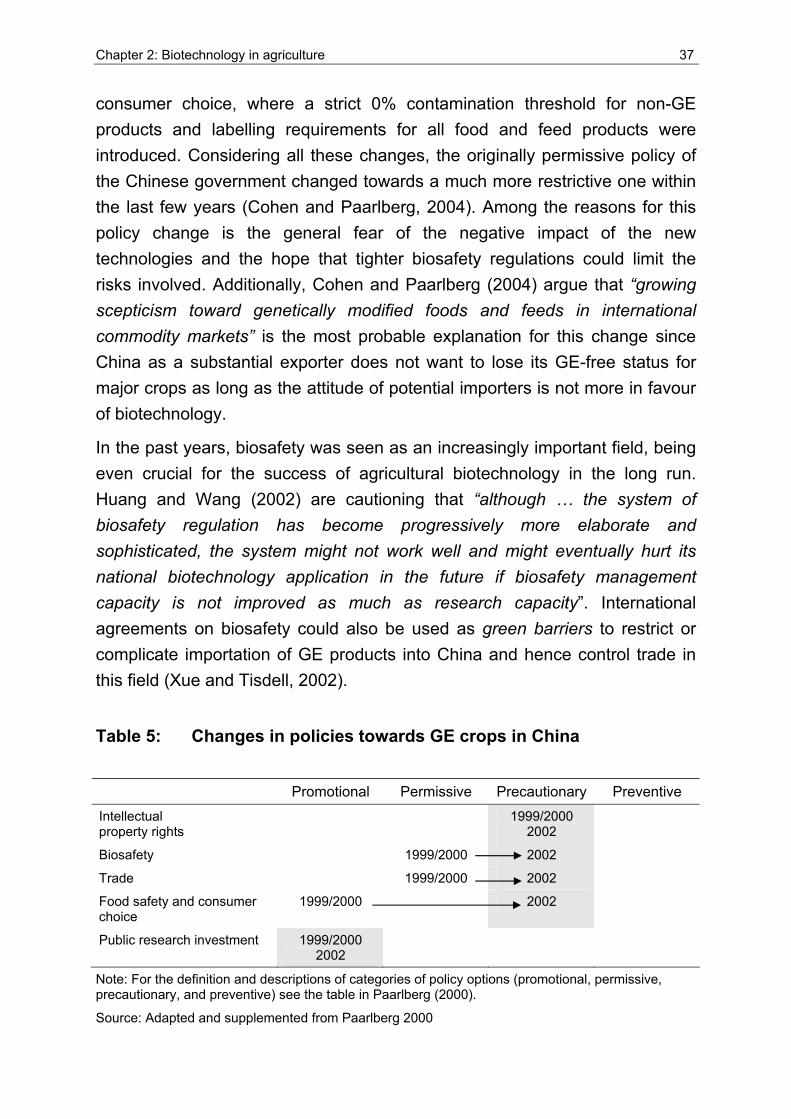
Chapter 2: Biotechnology in agriculture 37
consumer choice, where a strict 0% contamination threshold for non-GE products and labelling requirements for all food and feed products were introduced. Considering all these changes, the originally permissive policy of the Chinese government changed towards a much more restrictive one within the last few years (Cohen and Paarlberg, 2004). Among the reasons for this policy change is the general fear of the negative impact of the new technologies and the hope that tighter biosafety regulations could limit the risks involved. Additionally, Cohen and Paarlberg (2004) argue that “growing scepticism toward genetically modified foods and feeds in international commodity markets” is the most probable explanation for this change since China as a substantial exporter does not want to lose its GE-free status for major crops as long as the attitude of potential importers is not more in favour of biotechnology.
In the past years, biosafety was seen as an increasingly important field, being even crucial for the success of agricultural biotechnology in the long run. Huang and Wang (2002) are cautioning that “although … the system of biosafety regulation has become progressively more elaborate and sophisticated, the system might not work well and might eventually hurt its national biotechnology application in the future if biosafety management capacity is not improved as much as research capacity”. International agreements on biosafety could also be used as green barriers to restrict or complicate importation of GE products into China and hence control trade in this field (Xue and Tisdell, 2002).
Table 5: Changes in policies towards GE crops in China
Promotional Permissive Precautionary Preventive Intellectual property rights 1999/2000
2002
Biosafety 1999/2000 2002
Trade 1999/2000 2002
Food safety and consumer choice
1999/2000 2002
Public research investment 1999/2000 2002
Note: For the definition and descriptions of categories of policy options (promotional, permissive, precautionary, and preventive) see the table in Paarlberg (2000).
Source: Adapted and supplemented from Paarlberg 2000
38 Chapter 2: Biotechnology in agriculture
Besides the more technical question how to best implement biotechnology and limit potential costs and risks, Chinese policy towards agricultural biotechnology is determined by a power struggle between different institutions. The agencies that are involved in the regulation of agricultural GMOs have diverging interests and are competing for influence in setting laws and policies in this strategically important field.
Newell (2003) stresses the “importance of seeing states not as theoretically bound and homogenous entities, but rather as complex configurations of competing political and bureaucratic units” but concludes that in the case of China, there nevertheless seems to be a “consensus in favor of the precautionary principle as a guide to risk-based decision-making” (ibid).
The main players and their responsibilities are listed in Appendix 4. The Ministry of Agriculture (MoA) and the State Environmental Protection Authority (SEPA) are the two main institutions competing for the power to regulate agricultural biotechnology. Huang and Wang (2002) analyse the institutional settings of agricultural GMO biosafety management in China and conclude that the MoA has more power than its counterparts in other countries, for example the USA or EU. According to the authors, the State Council established this arrangement because the MoA is believed to have the best expertise in agriculture and agricultural GMOs and in addition is also already in charge of pesticide use and related environmental effects. In addition, the Ministry of Agriculture according to Cohen and Paarlberg (2004) is a suitable institution to represent farmers’ interests in the regulatory decision-making. However, this setting might result in an under-weighing of the environmental risks of GMOs and bears the additional danger of conflicting interests since the MoA’s primary responsibility is agricultural production, and many biotechnology applications were in fact developed (and marketed) by MoA’s own research and extension system (Huang and Wang, 2002).
Another player is the National Agricultural GMO Biosafety Committee22 (BC) that was established in 1997 under the MoA as a ministry-level institution and upgraded in June 2002 to national-level status (Huang and Wang, 2002). 22 The BC’s 56 members, all technical experts (scientists from different disciplines or part of the
agricultural administration), nominated by the MoA work part-time for the Committee. The BC meets twice a year and evaluates biosafety assessment applications related to experimental research, field trials, environmental release, and commercialisation of agricultural GMOs (Huang and Wang, 2002).
Chapter 2: Biotechnology in agriculture 39
The committee is highly respected and plays a crucial role within the biosafety decision-making process by advising the Biosafety Office on the approval of applications. A potential drawback of the Chinese regulatory system is that it relies heavily on the expertise of few individuals (mainly scientists involved in biotechnology research that are considered experts in the field) and a few key people are very influential and powerful. Those individuals may have considerable interest of their own in the issue at stake, for example to sustain the funding of their research work or to earn money if they own or work for a company that would sell the seed/technology if commercial approval would be granted (Keeley, 2003).
Cases in point are the Chinese policy and regulations regarding the activities and role of foreign companies/multinationals in the biotechnology sector. In the early period, foreign firms could only operate in the form of joint ventures with local firms and only certain local state-owned enterprises were allowed to sell the seed of major field crops (Pray, 1999). In recent years regulations where tightened even further so that foreign investment in agricultural biotechnology is severely restricted. In April 2002 three state commissions jointly issued a Guideline List of Foreign Investment, which declares GMOs as a “prohibited area for foreign investment” (Huang and Wang, 2003). Though this new guideline does not affect the existing joint ventures, it hinders further foreign investment in the field. The main purpose of this restriction is to leave time for national enterprises to catch up and occupy market shares (Keeley, 2003; Newell, 2003) hence the backing of an infant industry. Huang and Wang (2003) also refer to the perception of policy makers, as “there are risks associated with reliance on imported technologies to guarantee national food security”. However, this is in contradiction to the policy changes that Pray (1999) suggests, namely “(1) allowing the private sector to play a larger role in seed and chemical distribution, (2) stronger intellectual property rights, such as including plants in patents and enforcement of existing legislation, and (3) a transparent approval process for new plant varieties and transgenic plants”.
Yang (2003) concludes that although biotechnology is of crucial importance, Chinese GMO regulations are currently not well coordinated among the responsible agencies and the process of regulation and safety assessment should be more transparent to the public. She argues that this is especially true in the field of trade, where “foreign exporters may need to apply to both the MoA and MoH separately for GMO safety certificates” (Yang, 2003).
40 Chapter 2: Biotechnology in agriculture
This process may hinder trade and there is already a formal request by USA trade officials that China should have one single agency similar to the Food and Drug Administration (FDA) in the USA that would deal with all approvals (Newell, 2003).
The political and international trade dimension of biosafety regulations for GE crops is of great importance. When China, which entered the WTO in December 2001, issued its first biosafety administration in early 2002, it caused a trade dispute on the importation of GE soybean from the USA to China (with China being the world’s largest importer and the USA being the largest exporter of soybean and 81% of the soybean grown in the USA being transgenic). Marchant et al. (2002) argue that “these implementing regulations explicitly implied that China could potentially use these rules to delay, reduce, and control imports of biotech commodities into China”. When the regulation was issued, soybean imports were seriously affected until China allowed temporary import certificates and in that way responded to political pressure from the USA. The outcome of the “recent WTO complaint filed by the United States and cooperating countries against the EU’ Moratorium on Biotech Foods and Crops will surely have a significant impact on China’s future implementation of its biotech regulations” (Marchant et al., 2002).
The Chinese government is managing multinational companies in China by restricting them to joint-venture models (where the foreign partner is not allowed to have a majority share), limiting options of breeding programmes in China and “granting plant variety protection on a strategic basis” (Keeley, 2003). This is a logical conclusion when on the one hand a Regulation on the Protection of New Varieties of Plants and a Seed Law were issued in 1999 and 2000, respectively, but cotton (the only GE crop currently on the market) is not included in the variety protection list.
In an interview with a Monsanto employee23 the problem of counterfeit seed was stressed as a severe limitation to the company’s activities in China and as the main reason not to introduce any new technologies in the near future unless the protection of intellectual property rights and the enforcement thereof was changed significantly. Keeley (2003) summarizes and cites from personal interviews: “Monsanto, for example, complain that they are presented as having sales in official statistics in provinces where they are not
23 Personal communication, Beijing, 14th November 2001.
Chapter 2: Biotechnology in agriculture 41
formally even allowed to sell. In Hebei province – Monsanto’s biggest success story and a province where Bt-cotton may be as much as 99 per cent – one Monsanto manager put the breakdown for the cotton grown as: ’15 per cent Monsanto, 15 per cent Biocentury 24, 30 per cent farmer saved seed, 30 per cent counterfeit, 10 per cent others’.” Huang and Wang (2003) point out the same problem and state that half of the GE cotton grown is not officially approved at all. Newell (2003) reports that Bt-cotton was widely grown (an estimated 40% of cotton area) in the Yangtze River valley before approval and Pray and Naseem (2003) also point to enforcement problems and state that most cotton seed was produced by farmers or small companies or institutes without biosafety approval or royalty payments. This problem of enforcement of existing regulations sheds serious doubts on the effectiveness of any biosafety measures and in addition is a strong disincentive for private companies to invest and act in this field.
Despite the challenges listed above, China is still seen as a large, if not the largest potential market by many multinational companies (Newell, 2003).
2.3.3 Environmental impact and consumer acceptance
The debate on the potential adverse environmental impact of GE crops in China grew after Greenpeace published the report “A summary of research on the environmental impact of Bt-cotton in China” (Xue, 2002). The author collected and analyzed laboratory experiments and field research results on the environmental impact of Bt-cotton conducted by high-ranking Chinese scientists. Based on that data, the author concludes that there are significant negative impacts of Bt-cotton on the environment.
The main negative effects according to him are a decrease in parasitic natural enemies and diversity indices, while secondary pests increased (Xue, 2002). Moreover, he stresses the potential of resistance build-up of target pests against the toxin and the lack of suitable resistance management measures, as well as the reduced control of bollworm by Bt-varieties late in the season (ibid). Some of the scientists who conducted the biosafety research, were not informed prior to the publication of the report and dissociated themselves from the conclusions drawn or report diverging conclusions (Jia and Peng, 2002).
24 Biocentury is a private sector company that was formed by state research institutes in 1998.
Biocentury markets the Chinese cotton varieties that contain the gene developed by the Biotechnology Research Institute in the Chinese Academy of Agricultural Sciences, Beijing.
42 Chapter 2: Biotechnology in agriculture
This ambiguous use of scientific data and results gives evidence of the difficult position that researchers have in the controversial discussion of the impact of biotechnology. In the past, as consequence of the political system, public opinion and the attitude of Chinese consumers towards agricultural biotechnology was of minor importance and not a significant factor in policy making. But this may change with increasing liberalization and continuation of the opening-up strategy of the Chinese government.
A couple of consumer surveys were conducted more recently, among those the study of Lin et al. (2004) that was undertaken in five provinces in China in 2002 with 1,100 respondents. The main findings are briefly summarized below. First, in line with previous studies that are cited in that paper, it was confirmed that the majority of urban Chinese consumers have “favorable or neutral attitudes towards biotech food” while only some 10% opposed it (Lin et al., 2004). The authors found that consumers would be even more supportive if biotech food were offered at a 10% price discount. Some 20% of the consumers would not be willing to purchase biotech food regardless of a price discount. Chinese consumers have very limited knowledge on biotechnology and the (government controlled) mass media was stated as main source of information on this issue. These findings are in line with previous studies (Li et al., 2002).
Findings of such consumer surveys stress the political dimension of agricultural biotechnology and it becomes clear that the conflicting interests of major players shape and determine how the issue is addressed in China (and most other countries). This may indicate that in the future the role of civil society will increase, and consumer and farmer associations are likely to have a stake in agricultural biotechnology that differs from the interest of researchers and companies.
2.4 Summary
This chapter provided an overview of the status of agricultural biotechnology on a global level and especially in developing countries. In 2004 only 1.6% of the global agricultural area was planted with genetically engineered crops, mainly corn, soybean, cotton, and canola that are resistant to herbicides or certain insect pests. Among the main challenges that biotechnology applications are facing are biosafety regulations, trade issues and sustainability and equity questions.
Chapter 2: Biotechnology in agriculture 43
Great expectations are raised regarding the potential of agricultural biotechnology, primarily the claim that this technology can reduce poverty and solve the food security problem in the developing countries. But the nature of the technologies that have been implemented until now suggests that the contribution of agricultural biotechnology to solve these problems is limited. The realization of the potential benefits in the future crucially depends on the role of the public sector in research and development of products. The role and interaction of the private and public sectors in the development and dissemination of agricultural biotechnology will determine the extent to which so called orphan crops and traits most needed by the poor are tackled. It is unlikely that agricultural biotechnology will reduce poverty and food security if the private sector continues to dominate the scene. Also, many of the problems that the poor in developing countries are facing are not amenable to purely technical solutions but require a broader set of measures (including education, health care and infrastructure).
An in-depth analysis of the development and status of agricultural biotechnology in China shows that this country is special in several ways. First, it is one of the few developing countries with a substantial area planted to GE crops (some 60% of the nation’s cotton area is planted to Bt-varieties). Second, the Chinese government heavily invests in public research in the field of agricultural biotechnology and actively influences the direction of research and in this way is creating a counterbalance to the private sector.
The next chapter briefly introduces general concepts associated with measuring the costs and benefits of agricultural biotechnology and highlights the advantages and limitations of each approach.
3 Impact assessment o f agr icu l tura l b io technology: rev iew of methods and s tud ies
This chapter first reviews the methodology used to assess the impact of biotechnology applications in agriculture at different levels (farm-household or national economy). The second part of the chapter provides a brief literature review of economic impact analyses of Bt-cotton with a focus on the impact in developing countries. The applied methods and findings of these recent studies are presented and discussed. Each method has particular advantages and limitations and selection of either one leads to specific data requirements, and different scopes and levels of conclusions that can be drawn from the results. This provides the entry point for the set-up of a conceptual framework and the selection of methods for this study that are presented in Chapters 4 and 5.
3.1 Methods to measure costs and benefits of agricultural biotechnology
Scatasta and Wesseler (2004) introduce a general framework for the analysis of economic impact of GE crops consisting of a social welfare function that is maximized by the government. In their framework three distinct levels for the analysis of agricultural biotechnology are identified: (1) social welfare, (2) producer welfare, and (3) consumer welfare. For the analysis of impact on these levels, different economic models and methods can be applied. The two most commonly used approaches are the estimation of a production function and the application of equilibrium displacement models. Other impact studies of GE crops use a comparison of average input and output information on an aggregate level (Benbrook, 2004). This methodology only leads to valid results if adopters and non-adopters are not different in other regards25. In the case studies on the impact of agricultural biotechnology conducted by Giannessi et al. in the USA (2002) and in Europe (2003) potential impact was quantified in terms of changes in production costs, changes in quantity and value of crop production, and changes in the amount of pesticides used.
25 For the example of herbicide and insect resistant varieties, Benbrook found higher use levels of pesticides for adopters after several years of adoption. Carpenter and Gianessi (2001) argue that this comparison is not valid since most likely the adopters of such technologies experience above average pest pressure and so naturally have above average input use of pesticides.
Chapter 3: Impact assessment of agricultural biotechnology: review of methods and studies 45
Secondary data, scientific publications, and official statistics were collected and interviews with involved scientists conducted to back up the assumptions on the potential impact. Evaluation was conducted for individual states where the technology was developed, the target crop was grown on a large scale or the specific pest problem was widespread and severe.
The following text introduces the methods that are commonly used for impact assessment of GE crops. Results of impact assessment of agricultural biotechnology are not unambiguous and findings of some studies are discussed in a brief literature review in the second part of this chapter.
Production function framework: Increased profitability of production is due to a reduction in production costs and/or higher levels of output or better quality of output using the same input level26. The technical relationship between inputs and outputs of a production process is described by a production function (Coelli et al., 1998). Agricultural production functions are often assumed to have a Cobb-Douglas form (CD) and are estimated for a set of input and output data. The estimated production function can be used to calculate the productivity of a specific input using the partial derivative of the function. Use of a Cobb-Douglas production function has the major advantages that coefficients can be directly interpreted as elasticities, with coefficients summing up to 1, the function is relatively easy to handle, and the shape suits the overall expectation of the causal relation of diminishing marginal products of individual inputs (Heady and Dillon, 1961).
Figure 4 graphically depicts the relation between one input (given that all other inputs are fixed, ceteris paribus) and the production outcome. The adoption of a GE variety can be regarded as technical change (TC) 27 since, for example, reduced input of irrigation water is required for a drought resistant crop variety to obtain ceteris paribus the same level of yield.
26 Increase of profitability could also occur due to higher prices of output but those are exogenous and the producer cannot influence them (in a competitive market).
27 Nelson and Bullock (2001) define technical change as “change in the production process that results in fewer or less expensive resources needed to produce the same amount of product or enhanced characteristics of the product.” They list the following main categories of TC: (1) increase of biological maximum yield (2) increase of economical optimum yield (3) input-switching TC (4) quality enhancing TC (5) risk reducing TC.
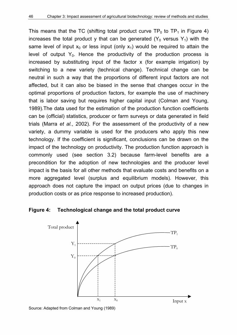
46 Chapter 3: Impact assessment of agricultural biotechnology: review of methods and studies
This means that the TC (shifting total product curve TP0 to TP1 in Figure 4) increases the total product y that can be generated (Y0 versus Y1) with the same level of input x0 or less input (only x1) would be required to attain the level of output Y0. Hence the productivity of the production process is increased by substituting input of the factor x (for example irrigation) by switching to a new variety (technical change). Technical change can be neutral in such a way that the proportions of different input factors are not affected, but it can also be biased in the sense that changes occur in the optimal proportions of production factors, for example the use of machinery that is labor saving but requires higher capital input (Colman and Young, 1989).The data used for the estimation of the production function coefficients can be (official) statistics, producer or farm surveys or data generated in field trials (Marra et al., 2002). For the assessment of the productivity of a new variety, a dummy variable is used for the producers who apply this new technology. If the coefficient is significant, conclusions can be drawn on the impact of the technology on productivity. The production function approach is commonly used (see section 3.2) because farm-level benefits are a precondition for the adoption of new technologies and the producer level impact is the basis for all other methods that evaluate costs and benefits on a more aggregated level (surplus and equilibrium models). However, this approach does not capture the impact on output prices (due to changes in production costs or as price response to increased production).
Figure 4: Technological change and the total product curve
Input x
Total product TP1
TP0 Y1
Y0
x0 x1
Source: Adapted from Colman and Young (1989)
Chapter 3: Impact assessment of agricultural biotechnology: review of methods and studies 47
Such price changes can (positively or negatively) influence the benefits of producers and consumers of the product. The approach also does not account for equity issues or questions about the distribution of costs/benefits of the technology within society.
Economic surplus models: Economists often use the (perfect) market model to measure the aggregated impact of TC in agriculture (Alston et al., 1995; Traxler et al., 2003b; Wesseler, 2003; Scatasta and Wesseler, 2004). Economic surplus models combine the main elements of production theory and consumer behavior (Colman and Young, 1989) to measure the impact on social welfare. Neoclassical theory predicts that technical change ceteris paribus leads to a gain in net social welfare (Gaisford et al., 2001).
The impact of TC and the distribution of gains can be illustrated using the simple market model depicted in Figure 5. Following Alston et al. (1995) the total consumer surplus from the use of the goods equals the triangular area FaP0 that is the area beneath the demand curve D less the costs of the consumed goods. In the same way the triangular area P0aI0 that is the total revenue less total costs of production (area under the supply curve S0) equals the total producer surplus. The total economic surplus is the sum of producer and consumer surplus (Alston et al., 1995). Assuming that the adoption of first generation agricultural biotechnology products (varieties with input-traits) increases crop yields or reduces input costs, this technical change would reduce production costs and hence cause a shift of the supply curve S to the right from S0 to S1. This supply shift results (under the conditions of perfect and competitive markets) in a reduction of the equilibrium price P from P0 to P1 (Gaisford et al., 2001). Consumers do benefit from price and quantity effects (consuming more goods at a lower price) and producers sell more goods but prices have decreased.
The changes in consumer and producer surplus can be measured as changes in the surplus areas described above. The change in consumer welfare resulting from the supply shift S0 to S1 is represented by the area P0abP1 and the change in producer welfare similarly by the area P1bI1 - P0aI0 (Alston et al., 1995).
Using this basic partial equilibrium model, the total impact of a technological change as well as the rent distribution of benefits (how much of the benefits go to producers and consumers, respectively) can be calculated.
48 Chapter 3: Impact assessment of agricultural biotechnology: review of methods and studies
Since most innovations in the field of agriculture are developed by the private sector and technology innovators tend to be monopolists, a share of the rent will go to the innovator of the technology.
Moschini and Lapan (1997) extended the basic economic surplus model to account for intellectual property rights of technology innovators. This approach to include monopolist profits in the model was taken up by subsequent studies (Falck-Zepeda et al., 1999).
The economic surplus approach also has some limitations and inherent problems when it is used for impact assessment of agricultural biotechnology. Although models can be adjusted to represent open or closed, large or small and competitive or non-competitive economies, some problems remain. First of all, the assumption that demand and supply curves are linear eases the calculation of surplus areas but does not necessarily depict the real shape of the curves28. Probably the most crucial issue in the use of partial equilibrium models is the magnitude and nature of the assumed supply shift.
Figure 5: Economic surplus model and (distribution of) gains from technical change
Q uantity
P rice
a
S 0
S 1
D
b
cd
e
Q 0 Q 10
I0
I1
P 0 P 1
F
Source: Adapted from Alston et al. (1995)
28 Linear demand functions that are often used in empirical studies cannot be derived from the consumer utility functions that are typically used in theoretical studies (Scatasta and Wesseler 2004).
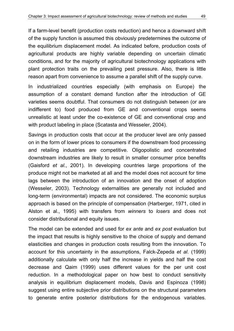
Chapter 3: Impact assessment of agricultural biotechnology: review of methods and studies 49
If a farm-level benefit (production costs reduction) and hence a downward shift of the supply function is assumed this obviously predetermines the outcome of the equilibrium displacement model. As indicated before, production costs of agricultural products are highly variable depending on uncertain climatic conditions, and for the majority of agricultural biotechnology applications with plant protection traits on the prevailing pest pressure. Also, there is little reason apart from convenience to assume a parallel shift of the supply curve.
In industrialized countries especially (with emphasis on Europe) the assumption of a constant demand function after the introduction of GE varieties seems doubtful. That consumers do not distinguish between (or are indifferent to) food produced from GE and conventional crops seems unrealistic at least under the co-existence of GE and conventional crop and with product labeling in place (Scatasta and Wesseler, 2004).
Savings in production costs that occur at the producer level are only passed on in the form of lower prices to consumers if the downstream food processing and retailing industries are competitive. Oligopolistic and concentrated downstream industries are likely to result in smaller consumer price benefits (Gaisford et al., 2001). In developing countries large proportions of the produce might not be marketed at all and the model does not account for time lags between the introduction of an innovation and the onset of adoption (Wesseler, 2003). Technology externalities are generally not included and long-term (environmental) impacts are not considered. The economic surplus approach is based on the principle of compensation (Harberger, 1971, cited in Alston et al., 1995) with transfers from winners to losers and does not consider distributional and equity issues.
The model can be extended and used for ex ante and ex post evaluation but the impact that results is highly sensitive to the choice of supply and demand elasticities and changes in production costs resulting from the innovation. To account for this uncertainty in the assumptions, Falck-Zepeda et al. (1999) additionally calculate with only half the increase in yields and half the cost decrease and Qaim (1999) uses different values for the per unit cost reduction. In a methodological paper on how best to conduct sensitivity analysis in equilibrium displacement models, Davis and Espinoza (1998) suggest using entire subjective prior distributions on the structural parameters to generate entire posterior distributions for the endogenous variables.
50 Chapter 3: Impact assessment of agricultural biotechnology: review of methods and studies
Measures of central tendency and higher moments can give information that helps to better judge the results of economic surplus models (ibid).
Real option and option value approaches: Benefits and costs associated with the release of genetically engineered crops into the environment are highly uncertain and in addition some of the benefits and costs are irreversible29 (Wesseler, 2003). Nevertheless, decision-makers have to implicitly or explicitly weigh and compare related costs and benefits and decide on the release of transgenic crops without perfect knowledge. As a basis for such ex ante decisions the real option approach that originates from financial markets is an alternative that extends the economic surplus model introduced in the previous section (Dixit and Pindyck, 1994). Real option approaches can be used as the decision basis when the options are to release GE crops now or wait and hence to structure regulatory decision-making. Morel et al. (2003) show how this structure can be linked to the precautionary principle. Uncertainty of costs and benefits of transgenic crops was mentioned and described in length in previous chapters. Irreversibility in general refers to impact (benefits or costs) that continues or occurs even if the action has stopped (or the technology is disadopted). Examples for irreversibility with regard to the introduction of GE crops are on the cost side: resistance build-up of target pests, non-target impact and outcrossing to wild relatives; and on the benefit side: reduced environmental and health impairments due to a reduction in pesticide use (Wesseler, 2003; Demont et al., 2004b). The basic assumption for the option approach is that decisions should not be based solely on the net present value criterion but must include irreversibility and the possibility of delaying in order to adequately depict the real situation (Dixit and Pindyck, 1994). Hence the decision rule is modified towards “invest when the value of a unit of capital exceeds the purchase and installation cost by an amount equal to the value of keeping the investment option alive” (ibid). This accounts for the option (but not obligation) to invest at a later time that is exercised (or killed) when irreversible investments are taken since this means giving up the possibility of waiting for new information. For empirical applications of the approach in the field of agricultural biotechnology and details on methodology and procedure see Demont (2004a; 2004b), Wesseler (2003), Scatasta and Wesseler (2004), and Morel et al. (2003).
29 Irreversible costs are sunk costs that cannot be recovered (Dixit and Pindyck 1994).
Chapter 3: Impact assessment of agricultural biotechnology: review of methods and studies 51
Based on the results, the decision can be not to release a transgenic crop (in a specific region) at a certain time but it does include the possibility that release is only postponed and may take place later, indicating flexibility (Demont et al., 2004a).
Although Scatasta and Wesseler (2004) point to the theoretical advantages of the model they admit that some problems exist in the empirical application of the approach. As an extension of the economic surplus model, some of the limitations inherent in this approach remain when using option values. The estimation of the net reversible benefits is based on the same assumptions as in the surplus model and so the same criticism applies. Also, for the supply shift it is assumed that conventional and transgenic products are homogenous – which might not actually be the case. Finally, the uncertainty included in the analysis relates to the income or gross margin of producers, not to the action of adopting a transgenic crop (Scatasta and Wesseler, 2004).
As outlined in the previous review, first generation agricultural biotechnology products (herbicide and insect resistant plant varieties) can be regarded as input-saving TC. Technical change typically provides increased financial returns to the adopter, otherwise commercial operators would not switch to the new technology (Nelson and Bullock, 2001). Hence, technology adoption is determined by private profitability, and impact assessment of farm-level consequences only determines how much a new technology increases returns. Farm-level decisions to adopt a technology involve only private costs and benefits but do not include any external effects that may be generated by this choice. This means that a wider scope of assessment is needed whenever the consequences of a new technology have an impact beyond the producer level. Moreover, the ex ante impact assessment of research is of interest in order to find out if a technology should be released and what the consequences for large-scale adoption would be. For these studies assumptions (based on expert opinion or data generated in experiments or trials) for the likely outcomes of technology adoption can be used. Ex ante assessment is especially relevant if technologies or choices are mutually exclusive and difficult or costly to revert. In such a situation decision-makers need the information which technology generates the highest benefits a priori.
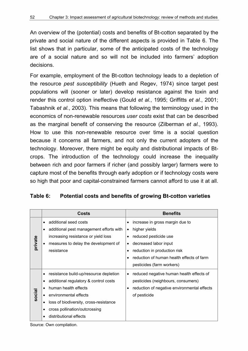
52 Chapter 3: Impact assessment of agricultural biotechnology: review of methods and studies
An overview of the (potential) costs and benefits of Bt-cotton separated by the private and social nature of the different aspects is provided in Table 6. The list shows that in particular, some of the anticipated costs of the technology are of a social nature and so will not be included into farmers’ adoption decisions.
For example, employment of the Bt-cotton technology leads to a depletion of the resource pest susceptibility (Hueth and Regev, 1974) since target pest populations will (sooner or later) develop resistance against the toxin and render this control option ineffective (Gould et al., 1995; Griffitts et al., 2001; Tabashnik et al., 2003). This means that following the terminology used in the economics of non-renewable resources user costs exist that can be described as the marginal benefit of conserving the resource (Zilberman et al., 1993). How to use this non-renewable resource over time is a social question because it concerns all farmers, and not only the current adopters of the technology. Moreover, there might be equity and distributional impacts of Bt-crops. The introduction of the technology could increase the inequality between rich and poor farmers if richer (and possibly larger) farmers were to capture most of the benefits through early adoption or if technology costs were so high that poor and capital-constrained farmers cannot afford to use it at all.
Table 6: Potential costs and benefits of growing Bt-cotton varieties
Costs Benefits
priv
ate
• additional seed costs
• additional pest management efforts with
increasing resistance or yield loss
• measures to delay the development of
resistance
• increase in gross margin due to
• higher yields
• reduced pesticide use
• decreased labor input
• reduction in production risk
• reduction of human health effects of farm
pesticides (farm workers)
soci
al
• resistance build-up/resource depletion
• additional regulatory & control costs
• human health effects
• environmental effects
• loss of biodiversity, cross-resistance
• cross pollination/outcrossing
• distributional effects
• reduced negative human health effects of
pesticides (neighbours, consumers)
• reduction of negative environmental effects
of pesticide
Source: Own compilation.
Chapter 3: Impact assessment of agricultural biotechnology: review of methods and studies 53
Assessing the impact of agricultural biotechnology is inherently difficult because of the entanglement of different technologies, and uneven distribution of technology impacts over time (Kalaitzandonakes, 2003a). Measurement is complex as impact can occur as direct and indirect effects, short-term output, medium term results, and long-term consequences (Guijt, 1998). A complete impact assessment should also include a monetary evaluation of non-market effects.
To capture the full impact of the technology, economic and non-economic measures can be applied (Alston et al., 2000).Despite these difficulties, impact assessment of agricultural biotechnology is very important in view of the continued political discussion and the implications that the introduction of a presumably irreversible technology carries.
3.2 Literature review of recent economic studies on Bt-cotton
In this section recent economic studies analyzing the impact of Bt-cotton are presented and findings and conclusions are compared and discussed. The review is restricted to assessments of Bt-cotton under the conditions of developing countries. Based on the lessons learned from these previous studies and identified needs for further research, the conceptual framework and methodology for this study is developed.
Cotton is the most widely studied of all genetically engineered crops. There is a multitude of evaluations based on experimental and on-farm testing in the USA where the technology was first introduced (Falck-Zepeda et al., 2001) and some more recent studies that concentrate on the impact of the technology in the developing world. Table 7 lists peer-reviewed studies assessing the impact of Bt-cotton in different countries and regions in the developing world (mainly South East Asia and Africa) using different methodological approaches for the analysis. All studies but the China case with repeated surveys were conducted in an initial phase of technology introduction and mostly farm-level survey data from only one or two years were used for the analysis. The ex ante studies are based on cost and benefit assumptions derived from experiments or trials and rely heavily on the set-up and purpose of the testing as well as additional expert opinion or advice for the remaining assumptions.
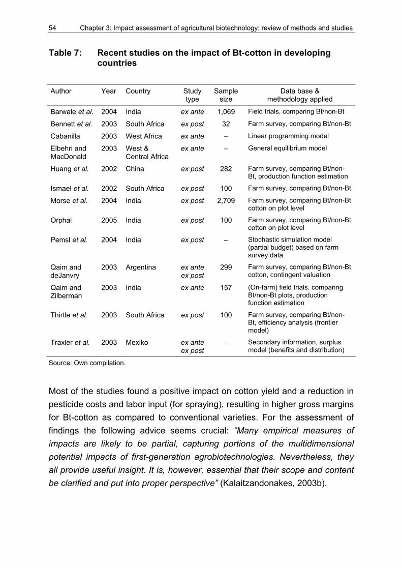
54 Chapter 3: Impact assessment of agricultural biotechnology: review of methods and studies
Table 7: Recent studies on the impact of Bt-cotton in developing countries
Author Year Country Study type
Sample size
Data base & methodology applied
Barwale et al. 2004 India ex ante 1,069 Field trials, comparing Bt/non-Bt
Bennett et al. 2003 South Africa ex post 32 Farm survey, comparing Bt/non-Bt
Cabanilla 2003 West Africa ex ante – Linear programming model
Elbehri and MacDonald
2003 West & Central Africa
ex ante – General equilibrium model
Huang et al. 2002 China ex post 282 Farm survey, comparing Bt/non-Bt, production function estimation
Ismael et al. 2002 South Africa ex post 100 Farm survey, comparing Bt/non-Bt
Morse et al. 2004 India ex post 2,709 Farm survey, comparing Bt/non-Bt cotton on plot level
Orphal 2005 India ex post 100 Farm survey, comparing Bt/non-Bt cotton on plot level
Pemsl et al. 2004 India ex post – Stochastic simulation model (partial budget) based on farm survey data
Qaim and deJanvry
2003 Argentina ex anteex post
299 Farm survey, comparing Bt/non-Bt cotton, contingent valuation
Qaim and Zilberman
2003 India ex ante 157 (On-farm) field trials, comparing Bt/non-Bt plots, production function estimation
Thirtle et al. 2003 South Africa ex post 100 Farm survey, comparing Bt/non-Bt, efficiency analysis (frontier model)
Traxler et al. 2003 Mexiko ex anteex post
– Secondary information, surplus model (benefits and distribution)
Source: Own compilation.
Most of the studies found a positive impact on cotton yield and a reduction in pesticide costs and labor input (for spraying), resulting in higher gross margins for Bt-cotton as compared to conventional varieties. For the assessment of findings the following advice seems crucial: “Many empirical measures of impacts are likely to be partial, capturing portions of the multidimensional potential impacts of first-generation agrobiotechnologies. Nevertheless, they all provide useful insight. It is, however, essential that their scope and content be clarified and put into proper perspective” (Kalaitzandonakes, 2003b).
Chapter 3: Impact assessment of agricultural biotechnology: review of methods and studies 55
It would be impractical to present all these studies, but an overview of the impact of Bt-cotton in India and China is provided. India was selected because the cotton area in that country is large and so impact is potentially high.
In addition, study results from diverse locations over several years and resulting from different procedures are available. The discussion in this section is especially concerned with the different results obtained and possible methodological and empirical reasons for such divergence in findings. The case of China is the starting point for the design and analysis of this case study and the findings obtained here can be compared to the results of the previous studies. Until now only one economic impact study (or activities by one team of researchers) was conducted to assess the impact of Bt-cotton introduction in China. The focus of the discussion lies on the empirical challenges, the methodology applied and some potential areas in which an alternative procedure might be worthwhile.
3.2.1 Bt-cotton in India
India has the largest cotton production area (around a quarter of the global cotton area) but yield levels are generally low (see Figure 2). One reason for the low productivity is a lack of water, as only about one third of the total cotton area is irrigated while most cotton is produced under rain-fed conditions (Choudhary and Laroia, 2001). According to Mohanty et al. (2002) limited supply of quality seed and poor management practices are additional reasons for low actual yields, although hybrid varieties account for about 70% of the cultivated cotton (Choudhary and Laroia, 2001). Even though cotton consumes nearly half of the total amount of insecticides used in India while only accounting for some 5% of the cropped area, substantial pest-related losses are reported (ibid). Bt-cotton varieties were only recently introduced in the country in 200230 and by 2004 covered an estimated 6% of the national cotton area (James, 2004).
However, a rapid adoption of the technology similar to the one in China may occur, and a recent economic study (Qaim, 2003) projects the area of Bt-cotton in India to rise to 5 million hectares or 60% of the nation’s 8.7 million
30 MAHYCO (Maharashtra Hybrid Seed Company) produced hybrid Bt-cotton varieties that are back-crosses of Monsantoa’s Bt-varieties with local varieties. After several years of field testing and political debate three varieties (Mech 12, Mech 164 and Mech 184) obtained commercial approval in March 2002 for Central and South India (Scoones, 2003).
56 Chapter 3: Impact assessment of agricultural biotechnology: review of methods and studies
hectares cotton area by 2005. However, reports on the performance of Bt-varieties in India are ambiguous and results of economic studies vary to a notable degree.
The brief literature review in this section presents some of the findings and highlights some differences in the approaches used. Table 8 shows the results of some current economic studies on the impact of Bt-cotton adoption in India. The findings from Barwale et al. (2004) titled study 1 in the table are based on field trial results from 1,069 farmers. The authors found on average 61% yield increase (42 – 72% for the different states that were included with lowest values for Gujarat and Andhra Pradesh and highest figures for Madhya Pradesh). At the same time the number of pesticide applications is on average 1.9 sprays less in Bt-cotton as compared to non-Bt cotton. The authors also calculate the economic benefit of growing Bt-cotton varieties. However, the substantial additional costs for purchasing Bt-cotton seed (see Table 8) are ignored in their benefit assessment. The revenue from using a Bt-variety (value of additional yield and cost savings due to less pesticides) amounts to 77% of the profit on average according to their findings. In order to calculate the change in profits the additional seed costs (not available in this case) need to be deducted. The study by Qaim and Zilberman (2003) is based on farmer-managed field trials initiated by the company MAHYCO and additional information that was collected from 157 of the participating farmers in three Indian states. The trials demonstrate an 80% higher yield from the Bt-varieties and 39% lower control costs and gross margins, Bt-varieties had 287% higher seed costs but due to much higher yields and cost savings for pesticides 426% higher gross margin results as compared to conventional varieties. These results are based on the assumption that quality and output price are identical for Bt- and non-Bt cotton (which is not necessarily the case as highlighted in the discussion of study 3) and the increase in production does not impact the cotton price.
The authors acknowledge that the findings may not represent real on-farm conditions because of the trial character of plantings, and further stress that the 2001 season was characterized by extreme cotton bollworm pressure. Consequently the cultivation practices may not be congruent with farmers’ practice (for example why do farmers not apply more pesticides in non-Bt plots?) and benefits overestimated.
Chapter 3: Impact assessment of agricultural biotechnology: review of methods and studies 57
In a survey of 100 cotton farmers in Karnataka state in the 2002 season Orphal (2005) found large differences in the performance of Bt-cotton dependent on whether or not the plot was irrigated. Only under irrigated conditions were Bt-yields slightly higher as compared to conventional varieties, and pesticide application numbers are low for non-Bt-cotton already (only 2 and 2.3 sprays for irrigated and non-irrigated, respectively). Although for the irrigated plots she found a reduction in pest control costs and an increase in yield, high additional seed costs resulted in only 24% profit gain when using Bt-varieties. For the rainfed production, profit for Bt-cotton is even lower compared to conventional varieties. One of the main driving forces of these outcomes is a difference in the cotton lint quality and consequently a price difference between Bt- and non-Bt cotton varieties. In the region long staple varieties are used, producing higher quality lint than the new Bt-varieties. According to price information collected from traders the maximum price for cotton in Dharwad in 2002 was nearly 30% lower for Bt-varieties while minimum prices were about the same.
These findings are the basis for a partial budgeting simulation model used to assess the profitability of Bt-cotton in Karnataka (Pemsl et al., 2004). The study findings of Orphal (2005) are used to fit probability distributions to the stochastic parameters and then a simulation using Monte Carlo techniques generates the cumulative distributions of net revenues of planting Bt- and non-Bt cotton. Results show that under non-irrigated conditions there is a 40% chance that net revenues of Bt-cotton are negative, and under irrigated conditions the probability of net revenues below zero is still around 25%. The simulation results depend on the difference in output prices and on the severity and probability of bollworm damage.
A study by Morse et al. (2005) analyzing data from 7,793 plots for the 2002 season and 1,577 for the 2003 season found that although seed costs for Bt are much higher (Table 8), a reduction in pest control costs and a yield increase resulted in higher profits for Bt-cotton production.
Despite this overall increase in gross margin for Bt plots, the authors found variations among the three included sub-regions of Maharashtra state, with gross margin increases ranging from 14 to 92% in 2002 and 45 to 101% in 2003. In addition to the studies cited, there are a number of reports on the (economic) performance of Bt-cotton conducted by Indian scientists and institutions.
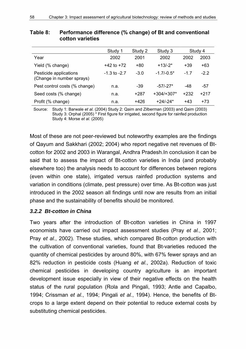
58 Chapter 3: Impact assessment of agricultural biotechnology: review of methods and studies
Table 8: Performance difference (% change) of Bt and conventional cotton varieties
Study 1 Study 2 Study 3 Study 4 Year 2002 2001 2002 2002 2003
Yield (% change) +42 to +72 +80 +13/-2* +39 +63
Pesticide applications (Change in number sprays)
-1.3 to -2.7 -3.0 -1.7/-0.5* -1.7 -2.2
Pest control costs (% change) n.a. -39 -57/-27* -48 -57
Seed costs (% change) n.a. +287 +304/+307* +232 +217
Profit (% change) n.a. +426 +24/-24* +43 +73 Source: Study 1: Barwale et al. (2004) Study 2: Qaim and Zilberman (2003) and Qaim (2003)
Study 3: Orphal (2005) * First figure for irrigated, second figure for rainfed production Study 4: Morse et al. (2005)
Most of these are not peer-reviewed but noteworthy examples are the findings of Qayum and Sakkhari (2002; 2004) who report negative net revenues of Bt-cotton for 2002 and 2003 in Warangal, Andhra Pradesh.In conclusion it can be said that to assess the impact of Bt-cotton varieties in India (and probably elsewhere too) the analysis needs to account for differences between regions (even within one state), irrigated versus rainfed production systems and variation in conditions (climate, pest pressure) over time. As Bt-cotton was just introduced in the 2002 season all findings until now are results from an initial phase and the sustainability of benefits should be monitored.
3.2.2 Bt-cotton in China
Two years after the introduction of Bt-cotton varieties in China in 1997 economists have carried out impact assessment studies (Pray et al., 2001; Pray et al., 2002). These studies, which compared Bt-cotton production with the cultivation of conventional varieties, found that Bt-varieties reduced the quantity of chemical pesticides by around 80%, with 67% fewer sprays and an 82% reduction in pesticide costs (Huang et al., 2002a). Reduction of toxic chemical pesticides in developing country agriculture is an important development issue especially in view of their negative effects on the health status of the rural population (Rola and Pingali, 1993; Antle and Capalbo, 1994; Crissman et al., 1994; Pingali et al., 1994). Hence, the benefits of Bt-crops to a large extent depend on their potential to reduce external costs by substituting chemical pesticides.
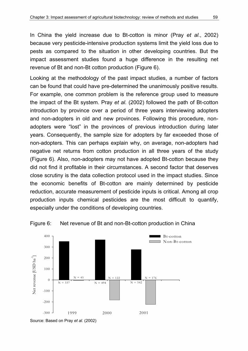
Chapter 3: Impact assessment of agricultural biotechnology: review of methods and studies 59
In China the yield increase due to Bt-cotton is minor (Pray et al., 2002) because very pesticide-intensive production systems limit the yield loss due to pests as compared to the situation in other developing countries. But the impact assessment studies found a huge difference in the resulting net revenue of Bt and non-Bt cotton production (Figure 6).
Looking at the methodology of the past impact studies, a number of factors can be found that could have pre-determined the unanimously positive results. For example, one common problem is the reference group used to measure the impact of the Bt system. Pray et al. (2002) followed the path of Bt-cotton introduction by province over a period of three years interviewing adopters and non-adopters in old and new provinces. Following this procedure, non-adopters were “lost” in the provinces of previous introduction during later years. Consequently, the sample size for adopters by far exceeded those of non-adopters. This can perhaps explain why, on average, non-adopters had negative net returns from cotton production in all three years of the study (Figure 6). Also, non-adopters may not have adopted Bt-cotton because they did not find it profitable in their circumstances. A second factor that deserves close scrutiny is the data collection protocol used in the impact studies. Since the economic benefits of Bt-cotton are mainly determined by pesticide reduction, accurate measurement of pesticide inputs is critical. Among all crop production inputs chemical pesticides are the most difficult to quantify, especially under the conditions of developing countries.
Figure 6: Net revenue of Bt and non-Bt-cotton production in China
Net
reve
nue
[USD
ha-1
]
-300
-200
-100
0
100
200
300
400 Bt-cottonNon-Bt-cotton
1999 2000 2001
N = 337
N = 45
N = 494N = 122
N = 542N = 176
Source: Based on Pray et al. (2002)
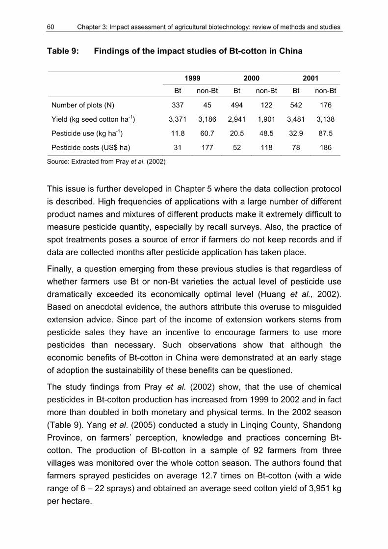
60 Chapter 3: Impact assessment of agricultural biotechnology: review of methods and studies
Table 9: Findings of the impact studies of Bt-cotton in China
1999 2000 2001
Bt non-Bt Bt non-Bt Bt non-Bt
Number of plots (N) 337 45 494 122 542 176
Yield (kg seed cotton ha-1) 3,371 3,186 2,941 1,901 3,481 3,138
Pesticide use (kg ha-1) 11.8 60.7 20.5 48.5 32.9 87.5
Pesticide costs (US$ ha) 31 177 52 118 78 186
Source: Extracted from Pray et al. (2002)
This issue is further developed in Chapter 5 where the data collection protocol is described. High frequencies of applications with a large number of different product names and mixtures of different products make it extremely difficult to measure pesticide quantity, especially by recall surveys. Also, the practice of spot treatments poses a source of error if farmers do not keep records and if data are collected months after pesticide application has taken place.
Finally, a question emerging from these previous studies is that regardless of whether farmers use Bt or non-Bt varieties the actual level of pesticide use dramatically exceeded its economically optimal level (Huang et al., 2002). Based on anecdotal evidence, the authors attribute this overuse to misguided extension advice. Since part of the income of extension workers stems from pesticide sales they have an incentive to encourage farmers to use more pesticides than necessary. Such observations show that although the economic benefits of Bt-cotton in China were demonstrated at an early stage of adoption the sustainability of these benefits can be questioned.
The study findings from Pray et al. (2002) show, that the use of chemical pesticides in Bt-cotton production has increased from 1999 to 2002 and in fact more than doubled in both monetary and physical terms. In the 2002 season (Table 9). Yang et al. (2005) conducted a study in Linqing County, Shandong Province, on farmers’ perception, knowledge and practices concerning Bt-cotton. The production of Bt-cotton in a sample of 92 farmers from three villages was monitored over the whole cotton season. The authors found that farmers sprayed pesticides on average 12.7 times on Bt-cotton (with a wide range of 6 – 22 sprays) and obtained an average seed cotton yield of 3,951 kg per hectare.
Chapter 3: Impact assessment of agricultural biotechnology: review of methods and studies 61
Farmers spent US$111.8 per hectare of cotton on pesticides and realized average gross margins of US$947. These results are generally in line with the findings of the case study presented in Chapter 6. A majority of 60% of the surveyed farmers stated that the cotton bollworm is still a problem in Bt-cotton production and 37% of farmers spray pesticides immediately when they find CBW larvae in the Bt-cotton field. In this data set, no control (farmers growing non-Bt cotton) is included because all farmers in Shandong Province have grown Bt-cotton since around 2000/2001.
3.3 Summary
The chapter reviewed the most common methods used to assess the impact of agricultural biotechnology. The relevant levels for the analysis are producer, consumer and social welfare and the two most commonly used approaches are the estimation of production functions and equilibrium displacement models. Both methods have some limitations with regard to the measurement of the impact of agricultural biotechnology. The measurement of impact of agricultural biotechnology is complex as impact can be of private and public nature; occur as direct and indirect effects, short-term output, medium term results, and long-term consequences. Despite the difficulties, impact assessment of agricultural biotechnology is very important in view of the continued political discussion and the implications that introduction of a presumably irreversible technology carries.
The second part of the chapter gave a brief literature review of recent studies that assess the economic impact of Bt-cotton in developing countries. Major issues in the assessment of Bt-cotton under Indian conditions are performance differences between (sub-) regions and among production systems with or without irrigation. Also, conditions (climate, pest pressure, price) vary over the years and accordingly results of an impact assessment that relies on data from only one or a few years cannot be generalized. Though reports on the performance of Bt-cotton in India are ambiguous, most of the impact assessment studies that are published in (economic) journals state high benefits31.
31 Scott (2003) analyses the scientific discourse and controversy on genetically modified crops and argues for “further inquiries into institutional reform in academic science to help contain conflict with cooperation”. This comment does not of course only apply to the case of India.
62 Chapter 3: Impact assessment of agricultural biotechnology: review of methods and studies
A review of the existing impact assessment study in China reveals some empirical and methodological drawbacks.The major challenges are identification of a suitable control group and accurate measurement of agricultural inputs especially pesticides under the conditions of small-scale farmers. This is especially relevant because benefits of the Bt-cotton technology in China mainly come from a reduction in production costs (and not so much from increases in yields) and even in Bt-cotton the level of chemical pesticide use is very high.
Based on the review of available methods and recent impact assessment studies it can be concluded that though a general methodology is available, there are unresolved issues in the assessment of agricultural biotechnology. In this study, the main focus is on the analysis of farm-level productivity of Bt-cotton varieties. Hence, the estimation of a production function is the most suitable method. Surplus models rely on assumptions of productivity effects and are thus not only more aggregate but also can be considered as subsequent step in the analysis. The option value approach is not suitable for this analysis, because Bt-cotton varieties had been released in China already and the assessment is ex post rather than ex ante. In-depth farm-level case studies are scarce, especially under developing country conditions. This work aims at an in-depth analysis of the productivity impact of Bt-cotton and attempts to include the impact of uncertainty and some of the impact of the technology on the agro-ecosystem. The next chapter starts with the theoretical concepts and then describes the framework for the analysis.
4 Theore t ica l concepts for economic ana lys is o f Bt -cot ton
In performing an economic analysis and productivity assessment of pest control agents such as chemical pesticides or Bt-varieties, different theoretical concepts can be applied. As outlined in the previous chapter the farm-level impact of a new technology largely determines the overall welfare effect, and assessing the productivity effect of Bt-varieties is the basis for all further and aggregated analysis. This chapter introduces relevant neoclassical production theory, including the concept of production functions with an in-built damage control function. The complementary approach of measuring efficiency with a frontier function is briefly presented in the following section. The rationale that production inefficiency might be attributed to differences in the pest management of individual farms is presented. The performance of Bt-varieties in crop protection is not deterministic but depends on a number of stochastic variables. To adequately capture these effects it is essential to include risk and uncertainty in the analysis. Moreover, the adoption of a crop protection strategy has an impact on the wider agro-ecosystem and in addition could cause externalities and other long-term effects. Hence, some relevant concepts of ecological economics are summarized in the next section. This leads to a more interdisciplinary approach in tackling the research question by setting up a bio-economic model. In the last section of the chapter the research hypotheses are derived and the methods used in the analytical part of the study are outlined.
4.1 Productivity assessment of input factors
Production economics in general is concerned with the question of what to produce and how to best allocate scarce available resources in order to maximize overall welfare (Samuelson and Nordhaus, 1998). The challenge to find the optimal combination of resources and the optimal input level of a certain production input is as important for a small-scale farmer as it is for a large industrial firm. Neoclassical production theory relies on a set of assumptions. The key assumptions as outlined by Beattie and Taylor (1993) are that (1) inputs and outputs are homogenous (no quality differences), (2) only one production cycle is covered, and the production process is mono-periodic, (3) behavior of agents is profit maximizing, and (4) product and factor prices, as well as the production function, are known with certainty.
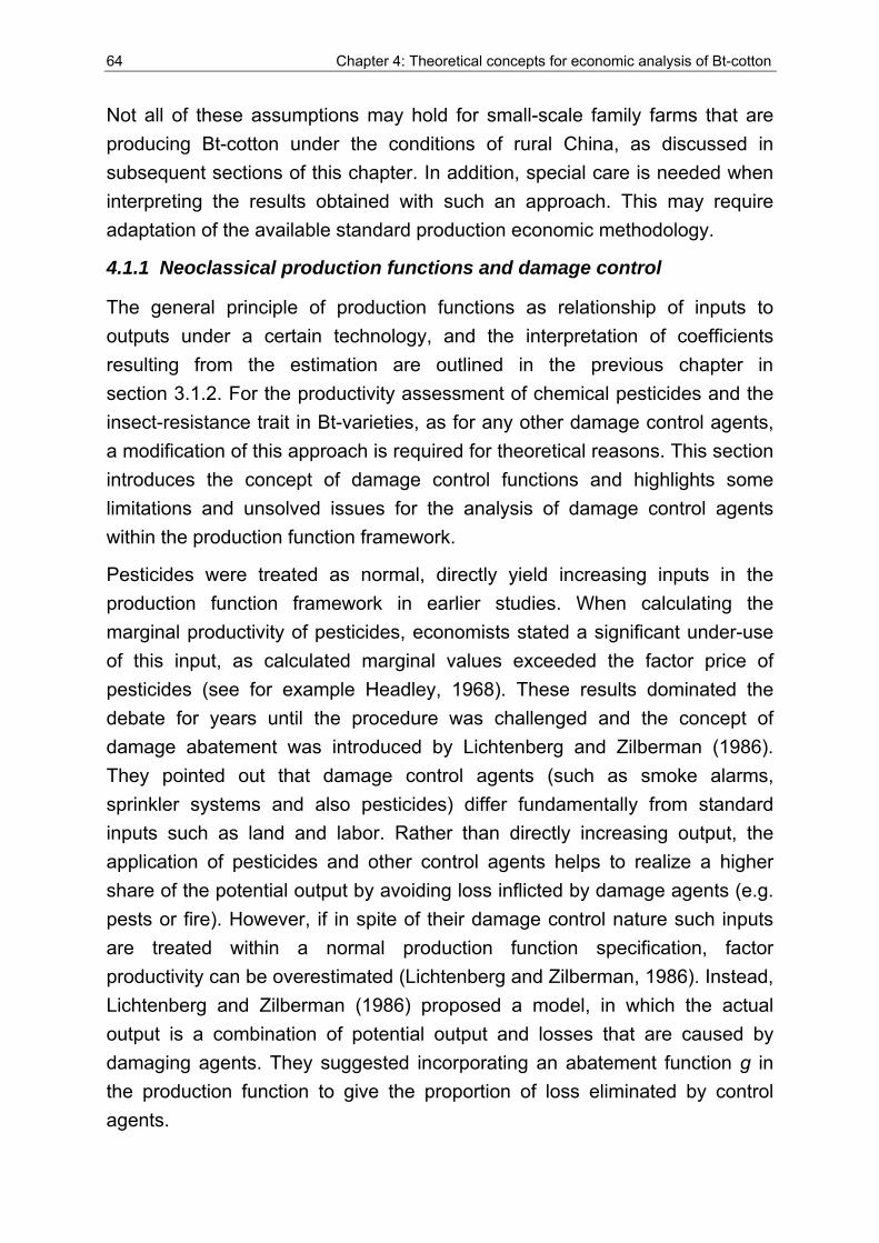
64 Chapter 4: Theoretical concepts for economic analysis of Bt-cotton
Not all of these assumptions may hold for small-scale family farms that are producing Bt-cotton under the conditions of rural China, as discussed in subsequent sections of this chapter. In addition, special care is needed when interpreting the results obtained with such an approach. This may require adaptation of the available standard production economic methodology.
4.1.1 Neoclassical production functions and damage control
The general principle of production functions as relationship of inputs to outputs under a certain technology, and the interpretation of coefficients resulting from the estimation are outlined in the previous chapter in section 3.1.2. For the productivity assessment of chemical pesticides and the insect-resistance trait in Bt-varieties, as for any other damage control agents, a modification of this approach is required for theoretical reasons. This section introduces the concept of damage control functions and highlights some limitations and unsolved issues for the analysis of damage control agents within the production function framework.
Pesticides were treated as normal, directly yield increasing inputs in the production function framework in earlier studies. When calculating the marginal productivity of pesticides, economists stated a significant under-use of this input, as calculated marginal values exceeded the factor price of pesticides (see for example Headley, 1968). These results dominated the debate for years until the procedure was challenged and the concept of damage abatement was introduced by Lichtenberg and Zilberman (1986). They pointed out that damage control agents (such as smoke alarms, sprinkler systems and also pesticides) differ fundamentally from standard inputs such as land and labor. Rather than directly increasing output, the application of pesticides and other control agents helps to realize a higher share of the potential output by avoiding loss inflicted by damage agents (e.g. pests or fire). However, if in spite of their damage control nature such inputs are treated within a normal production function specification, factor productivity can be overestimated (Lichtenberg and Zilberman, 1986). Instead, Lichtenberg and Zilberman (1986) proposed a model, in which the actual output is a combination of potential output and losses that are caused by damaging agents. They suggested incorporating an abatement function g in the production function to give the proportion of loss eliminated by control agents.
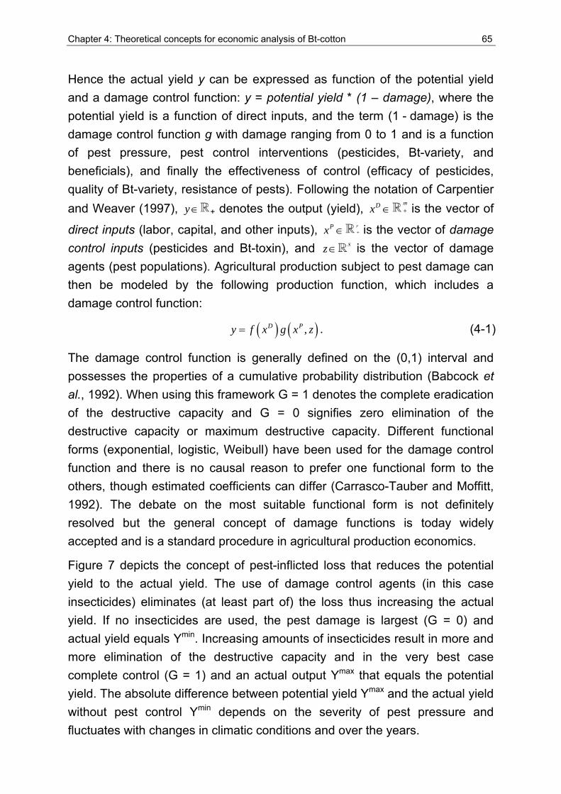
Chapter 4: Theoretical concepts for economic analysis of Bt-cotton 65
Hence the actual yield y can be expressed as function of the potential yield and a damage control function: y = potential yield * (1 – damage), where the potential yield is a function of direct inputs, and the term (1 - damage) is the damage control function g with damage ranging from 0 to 1 and is a function of pest pressure, pest control interventions (pesticides, Bt-variety, and beneficials), and finally the effectiveness of control (efficacy of pesticides, quality of Bt-variety, resistance of pests). Following the notation of Carpentier and Weaver (1997), y∈ + denotes the output (yield), Dx ∈ is the vector of
direct inputs (labor, capital, and other inputs), Px ∈ is the vector of damage control inputs (pesticides and Bt-toxin), and z∈ is the vector of damage agents (pest populations). Agricultural production subject to pest damage can then be modeled by the following production function, which includes a damage control function:
( ) ( ),D Py f x g x z= . (4-1)
The damage control function is generally defined on the (0,1) interval and possesses the properties of a cumulative probability distribution (Babcock et al., 1992). When using this framework G = 1 denotes the complete eradication of the destructive capacity and G = 0 signifies zero elimination of the destructive capacity or maximum destructive capacity. Different functional forms (exponential, logistic, Weibull) have been used for the damage control function and there is no causal reason to prefer one functional form to the others, though estimated coefficients can differ (Carrasco-Tauber and Moffitt, 1992). The debate on the most suitable functional form is not definitely resolved but the general concept of damage functions is today widely accepted and is a standard procedure in agricultural production economics.
Figure 7 depicts the concept of pest-inflicted loss that reduces the potential yield to the actual yield. The use of damage control agents (in this case insecticides) eliminates (at least part of) the loss thus increasing the actual yield. If no insecticides are used, the pest damage is largest (G = 0) and actual yield equals Ymin. Increasing amounts of insecticides result in more and more elimination of the destructive capacity and in the very best case complete control (G = 1) and an actual output Ymax that equals the potential yield. The absolute difference between potential yield Ymax and the actual yield without pest control Ymin depends on the severity of pest pressure and fluctuates with changes in climatic conditions and over the years.
66 Chapter 4: Theoretical concepts for economic analysis of Bt-cotton
Figure 7: Effect of insecticide use on yield (with and without Bt-variety)
Yield
Insecticide input
Ymax
Y1 (Bt)
Y1
Insecticide productivity curve with Bt-variety
Insecticide productivity curve without Bt-variety
0 X1
Ymin (Bt)
Ymin
Damage control of Bt-variety
Ymax = Maximum attainable yield Ymin (Bt) = Minimum yield under the worst
pest attack (with Bt-variety)
Ymin = Minimum yield under the worst
pest attack (without Bt-variety)
G = 1
GBt= 0
G = 0
X2
Source: Adapted from Ajayi (1999)
If now in addition to the use of chemical insecticides a Bt-variety (that is also a damage control agent) is planted, the minimum yield Ymin that is realized without insecticide use increases to Ymin (Bt). In this case the effect of the different control agents is additive and consequently less insecticides need to be applied to eliminate all damage if a Bt-variety is grown. At the same time, the use of a Bt-variety leads to a reduction of the economically optimal input level of chemical insecticides (in Figure 7 from X1 to X2).
The presentation in Figure 7 assumes that the control agent Bt-variety is a binary variable that is either used or not, and has a fixed control impact (upwards shift of the minimum yield Ymin ). Alternatively, especially since under the conditions of developing countries huge fluctuations in the quality of agricultural inputs can occur, the Bt-trait can be perceived as a continuous variable by measuring the actual toxin concentration. In this case, the substitution relationship between chemical insecticides and Bt-toxin could be described as depicted in Figure 8. Either, a high concentration of toxin or a high input level of chemical insecticides would eliminate all pest pressure even in the absence of the other damage control agent.
Chapter 4: Theoretical concepts for economic analysis of Bt-cotton 67
Figure 8: Combined effect of insecticide use and Bt-toxin concentration I
Yiel
d
Insecticide use
B t tox in concen tration
Y m ax
Y m in
Source: Own presentation
Moreover, a combination of both inputs would have the same effect and the optimal input level for both control agents (and the rate of factor substitution), could be determined based on the marginal productivity (yield loss that is prevented by the last unit of the factor) and the respective factor prices (Debertin, 1986).This builds on the assumption that the CBW as the main target pest of the Bt-toxin is the only damage agent in cotton production and hence a perfect substitution exists between Bt-toxin and insecticides. Under field conditions however, a number of different pests cause yield damage and only some are controlled by the Bt-toxin. Hence Figure 9 may better represent the actual substitution relationship of Bt-toxin and insecticides. Bt-toxin can only control the damage caused by bollworm pests, while chemical insecticides in addition eliminate damage from other insect pests. The floors in the graph that represent the minimum yield (without pest control) and maximum yield (with full elimination of pest damage) as well as the share of CBW and other pests, are again uncertain.
The continuous measurement of the control agent Bt-toxin generally solves the issue of variation in input quality, although the concentration varies over the season and so more than one measurement may be needed. The quantification of insecticide use is probably even more difficult. Amounts of formulated product applied and insecticide costs are not very good measures for this control input since the effectiveness largely depends on the efficacy of the product itself, the match of product and pest and the timing and realization of the application, as well as the climatic conditions (temperature, rain).
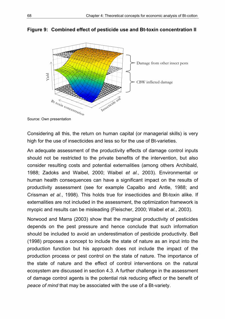
68 Chapter 4: Theoretical concepts for economic analysis of Bt-cotton
Figure 9: Combined effect of pesticide use and Bt-toxin concentration II
Insectici
de useBt toxin concentration
Yiel
d
Source: Own presentation
Considering all this, the return on human capital (or managerial skills) is very high for the use of insecticides and less so for the use of Bt-varieties.
An adequate assessment of the productivity effects of damage control inputs should not be restricted to the private benefits of the intervention, but also consider resulting costs and potential externalities (among others Archibald, 1988; Zadoks and Waibel, 2000; Waibel et al., 2003). Environmental or human health consequences can have a significant impact on the results of productivity assessment (see for example Capalbo and Antle, 1988; and Crissman et al., 1998). This holds true for insecticides and Bt-toxin alike. If externalities are not included in the assessment, the optimization framework is myopic and results can be misleading (Fleischer, 2000; Waibel et al., 2003).
Norwood and Marra (2003) show that the marginal productivity of pesticides depends on the pest pressure and hence conclude that such information should be included to avoid an underestimation of pesticide productivity. Bell (1998) proposes a concept to include the state of nature as an input into the production function but his approach does not include the impact of the production process or pest control on the state of nature. The importance of the state of nature and the effect of control interventions on the natural ecosystem are discussed in section 4.3. A further challenge in the assessment of damage control agents is the potential risk reducing effect or the benefit of peace of mind that may be associated with the use of a Bt-variety.
CBW inflicted damage
Damage from other insect pests
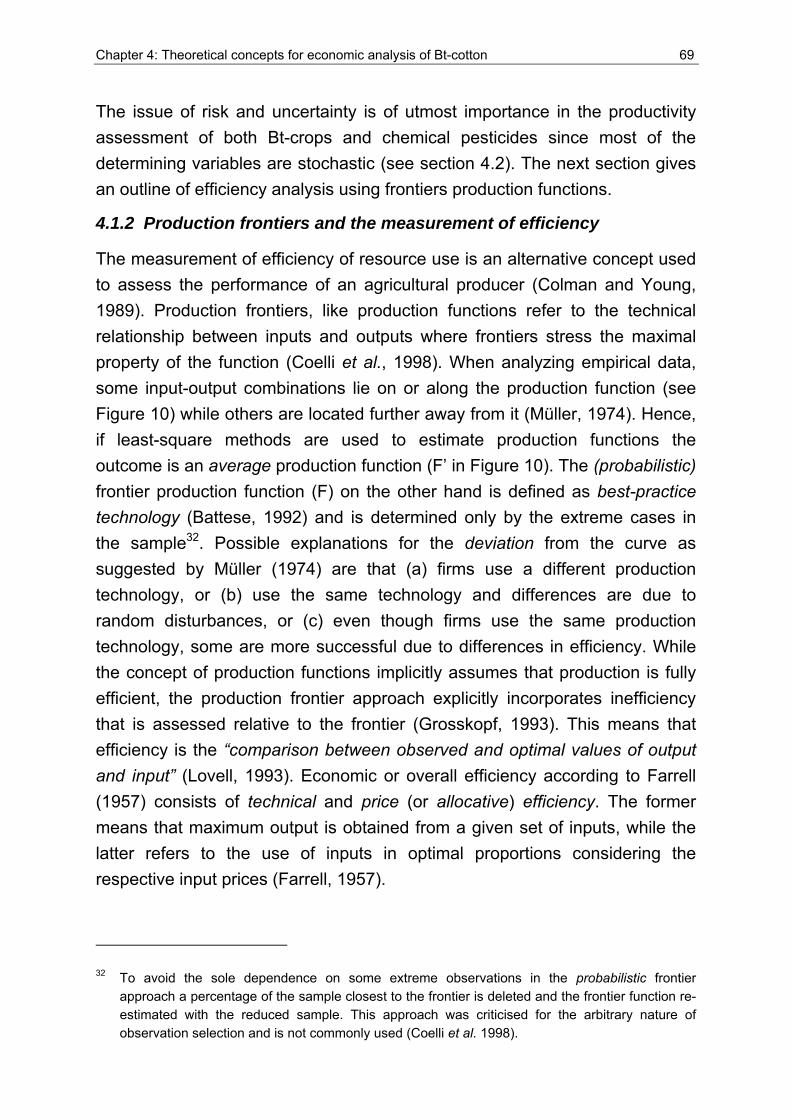
Chapter 4: Theoretical concepts for economic analysis of Bt-cotton 69
The issue of risk and uncertainty is of utmost importance in the productivity assessment of both Bt-crops and chemical pesticides since most of the determining variables are stochastic (see section 4.2). The next section gives an outline of efficiency analysis using frontiers production functions.
4.1.2 Production frontiers and the measurement of efficiency
The measurement of efficiency of resource use is an alternative concept used to assess the performance of an agricultural producer (Colman and Young, 1989). Production frontiers, like production functions refer to the technical relationship between inputs and outputs where frontiers stress the maximal property of the function (Coelli et al., 1998). When analyzing empirical data, some input-output combinations lie on or along the production function (see Figure 10) while others are located further away from it (Müller, 1974). Hence, if least-square methods are used to estimate production functions the outcome is an average production function (F’ in Figure 10). The (probabilistic) frontier production function (F) on the other hand is defined as best-practice technology (Battese, 1992) and is determined only by the extreme cases in the sample32. Possible explanations for the deviation from the curve as suggested by Müller (1974) are that (a) firms use a different production technology, or (b) use the same technology and differences are due to random disturbances, or (c) even though firms use the same production technology, some are more successful due to differences in efficiency. While the concept of production functions implicitly assumes that production is fully efficient, the production frontier approach explicitly incorporates inefficiency that is assessed relative to the frontier (Grosskopf, 1993). This means that efficiency is the “comparison between observed and optimal values of output and input” (Lovell, 1993). Economic or overall efficiency according to Farrell (1957) consists of technical and price (or allocative) efficiency. The former means that maximum output is obtained from a given set of inputs, while the latter refers to the use of inputs in optimal proportions considering the respective input prices (Farrell, 1957).
32 To avoid the sole dependence on some extreme observations in the probabilistic frontier approach a percentage of the sample closest to the frontier is deleted and the frontier function re-estimated with the reduced sample. This approach was criticised for the arbitrary nature of observation selection and is not commonly used (Coelli et al. 1998).
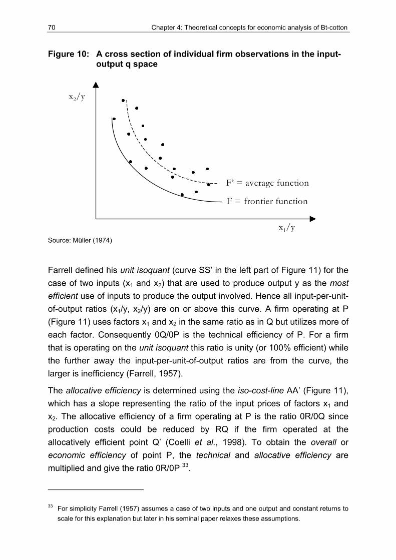
70 Chapter 4: Theoretical concepts for economic analysis of Bt-cotton
Figure 10: A cross section of individual firm observations in the input-output q space
x2/y
x1/y
F = frontier function
F’ = average function
Source: Müller (1974)
Farrell defined his unit isoquant (curve SS’ in the left part of Figure 11) for the case of two inputs (x1 and x2) that are used to produce output y as the most efficient use of inputs to produce the output involved. Hence all input-per-unit-of-output ratios (x1/y, x2/y) are on or above this curve. A firm operating at P (Figure 11) uses factors x1 and x2 in the same ratio as in Q but utilizes more of each factor. Consequently 0Q/0P is the technical efficiency of P. For a firm that is operating on the unit isoquant this ratio is unity (or 100% efficient) while the further away the input-per-unit-of-output ratios are from the curve, the larger is inefficiency (Farrell, 1957).
The allocative efficiency is determined using the iso-cost-line AA’ (Figure 11), which has a slope representing the ratio of the input prices of factors x1 and x2. The allocative efficiency of a firm operating at P is the ratio 0R/0Q since production costs could be reduced by RQ if the firm operated at the allocatively efficient point Q’ (Coelli et al., 1998). To obtain the overall or economic efficiency of point P, the technical and allocative efficiency are multiplied and give the ratio 0R/0P 33.
33 For simplicity Farrell (1957) assumes a case of two inputs and one output and constant returns to scale for this explanation but later in his seminal paper relaxes these assumptions.
Chapter 4: Theoretical concepts for economic analysis of Bt-cotton 71
Figure 11: Technical and allocative efficiency from input and output orientation
x2 /y
x1 /y
A
0 A’
R
Q
Q’
P
S Input orientation
S’
x2 /y
x1 /y
Z
0 Z’ D’
F B’
C
DOutput orientation
B
Source: Farrell et al. (1957) and Coelli et al. (1998)
Alternatively to the input orientation where input quantities are reduced while still obtaining a given level of output, the problem can also be phrased from the output perspective in a way such that output can be increased without altering input quantities (Färe et al., 1994)34. Technical and allocative efficiency for the output-orientated measures (right part, Figure 11) are 0F/0B and 0B/0C, respectively, and are obtained by analogy with the input orientation outlined above. Economic efficiency for the output orientation is again defined as the product of the former two measures, technical and allocative efficiency, and hence reads 0F/0C (Coelli et al., 1998).
To estimate the unknown production frontier representing the fully efficient firm from sample data Farrell (1957) suggests the use of either a nonparametric piece-wise-linear technology or a parametric function. This resulted in the development of two principal methods used to estimate production frontiers, namely the data envelopment analysis (DEA) approach that constructs a surface (frontier) over the data using linear programming methods and the stochastic frontier approach that is based on econometric methods (Lovell, 1993). If quantities and prices are available, economic efficiency can be calculated using the frontier as reference and decomposed into technical and allocative efficiency (Lovell, 1993).
34 Färe et al. (1994) give a good introduction of this methodology and in-depth explanation of input
and output based efficiency measure.
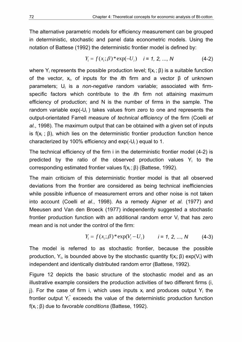
72 Chapter 4: Theoretical concepts for economic analysis of Bt-cotton
The alternative parametric models for efficiency measurement can be grouped in deterministic, stochastic and panel data econometric models. Using the notation of Battese (1992) the deterministic frontier model is defined by:
( ; )*exp( )i i iY f x Uβ= − i = 1, 2, ..., N (4-2)
where Yi represents the possible production level; f(xi ; β) is a suitable function of the vector, xi, of inputs for the ith firm and a vector β of unknown parameters; Ui is a non-negative random variable; associated with firm-specific factors which contribute to the ith firm not attaining maximum efficiency of production; and N is the number of firms in the sample. The random variable exp(-Ui ) takes values from zero to one and represents the output-orientated Farrell measure of technical efficiency of the firm (Coelli et al., 1998). The maximum output that can be obtained with a given set of inputs is f(xi ; β), which lies on the deterministic frontier production function hence characterized by 100% efficiency and exp(-Ui ) equal to 1.
The technical efficiency of the firm i in the deterministic frontier model (4-2) is predicted by the ratio of the observed production values Yi to the corresponding estimated frontier values f(xi ; β) (Battese, 1992).
The main criticism of this deterministic frontier model is that all observed deviations from the frontier are considered as being technical inefficiencies while possible influence of measurement errors and other noise is not taken into account (Coelli et al., 1998). As a remedy Aigner et al. (1977) and Meeusen and Van den Broeck (1977) independently suggested a stochastic frontier production function with an additional random error Vi that has zero mean and is not under the control of the firm:
( ; )*exp( )i i i iY f x V Uβ= − i = 1, 2, ..., N (4-3)
The model is referred to as stochastic frontier, because the possible production, Yi, is bounded above by the stochastic quantity f(xi; β) exp(Vi) with independent and identically distributed random error (Battese, 1992).
Figure 12 depicts the basic structure of the stochastic model and as an illustrative example considers the production activities of two different firms (i, j). For the case of firm i, which uses inputs xi and produces output Yi the frontier output Yi
* exceeds the value of the deterministic production function f(xi ; β) due to favorable conditions (Battese, 1992).
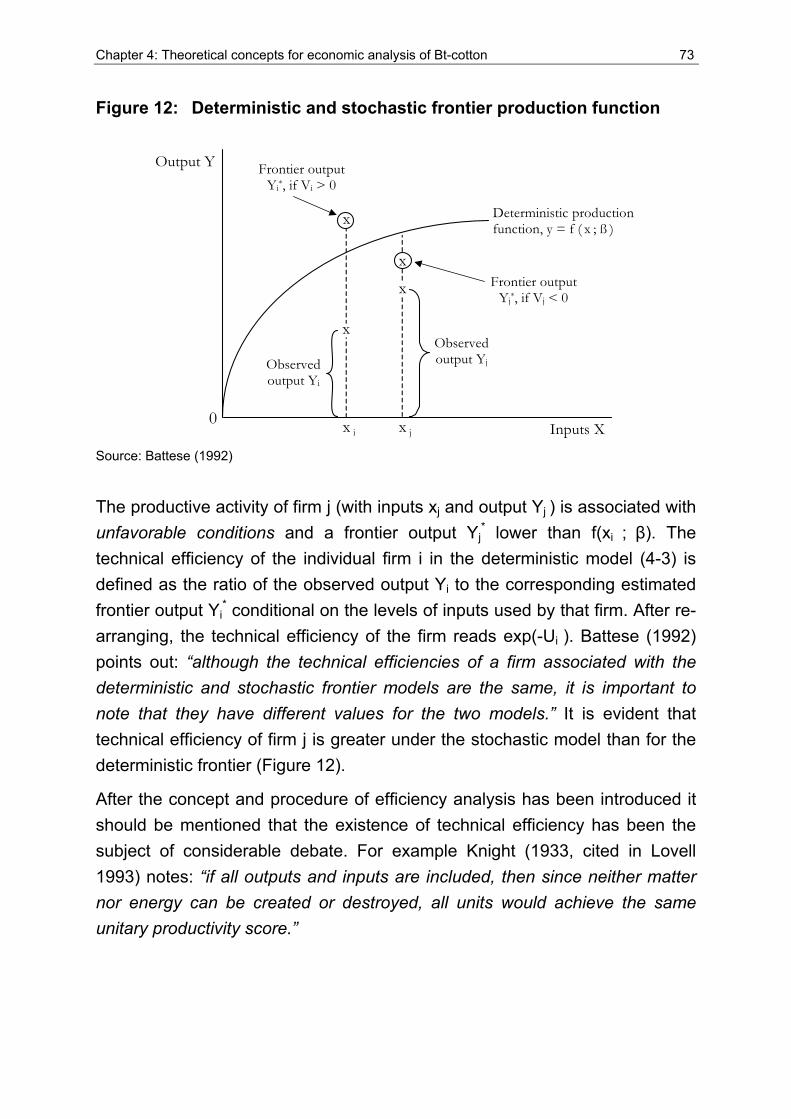
Chapter 4: Theoretical concepts for economic analysis of Bt-cotton 73
Figure 12: Deterministic and stochastic frontier production function
Output Y
Inputs X 0 x i x j
Deterministic production function, y = f ( x ; ß )
x
x
x
x
Observed output Yi
Observed output Yj
Frontier output Yj*, if Vj < 0
Frontier output Yi*, if Vi > 0
Source: Battese (1992)
The productive activity of firm j (with inputs xj and output Yj ) is associated with unfavorable conditions and a frontier output Yj
* lower than f(xi ; β). The technical efficiency of the individual firm i in the deterministic model (4-3) is defined as the ratio of the observed output Yi to the corresponding estimated frontier output Yi
* conditional on the levels of inputs used by that firm. After re-arranging, the technical efficiency of the firm reads exp(-Ui ). Battese (1992) points out: “although the technical efficiencies of a firm associated with the deterministic and stochastic frontier models are the same, it is important to note that they have different values for the two models.” It is evident that technical efficiency of firm j is greater under the stochastic model than for the deterministic frontier (Figure 12).
After the concept and procedure of efficiency analysis has been introduced it should be mentioned that the existence of technical efficiency has been the subject of considerable debate. For example Knight (1933, cited in Lovell 1993) notes: “if all outputs and inputs are included, then since neither matter nor energy can be created or destroyed, all units would achieve the same unitary productivity score.”
74 Chapter 4: Theoretical concepts for economic analysis of Bt-cotton
Consequently, measured inefficiency may just reflect the failure to incorporate the relevant variables and should disappear except for random disturbances once all inputs are taken into account (Battese, 1992). One example for such an input variable is the level of information and knowledge. Müller (1974) argues that these non-physical inputs influence a firm’s ability to use the available resources and their exclusion hence is a misspecification of the model. He uses a sample of dairy farms in California to show that differences in information obtained by managers can explain productivity differences. Such findings very likely also apply to the analysis of crop protection measures, which require substantial knowledge and managerial capability in terms of product selection and timing as well as implementation of the control intervention. Moreover, the observed inefficiency may be due to inaccurate measurement of inputs (Colman and Young, 1989). Contrary to the assumption in production theory that inputs are homogenous, quality differences generally exist (land and labor quality for example) but may be difficult to record. However, despite these criticisms the estimation of technical efficiency may provide useful insights and can help to compare the performance of different firms
4.2 Implications of risk and uncertainty
Risk is an inevitable feature of agriculture and the issue has received a lot of attention in the economics of pest control in the last decades (see Pannell, 1991). The main sources for risk in agriculture can be categorized as (1) production uncertainty due to (unpredictable) environmental variation (climatic changes influencing crop yield and level of pest pressure, hence the production function is stochastic), (2) price uncertainty (due to the inherent volatility of agricultural markets), and (3) technological uncertainty (due to the evolution of production technology that makes quasi-fixed past investments obsolete, and finally (4) policy or institutional uncertainty due to (changes in) government interventions (Just and Pope, 2001). Hardaker et al. (1997) further define human or personal risk as being part of the business risk and financial risk. A commonly used definition is that “risk is imperfect knowledge where the probabilities of the possible outcomes are known, and uncertainty exists when these probabilities are not known” (Hardaker et al., 1997).

Chapter 4: Theoretical concepts for economic analysis of Bt-cotton 75
The authors argue, however, that this definition is not a useful distinction, since probabilities are seldom objectively known and in most cases the decision-maker has subjective beliefs about (outcome) distributions (Antle, 1988). Risk can be perceived as the chance of negative outcomes like injury or loss, and Debertin (1986) describes risk (with known outcomes and probabilities) and uncertainty (without such knowledge) as two extremes of a continuum. Though the terms risk and uncertainty are often used interchangeably, following Robison and Barry (1987, cited in Just and Pope, 2001) uncertainty describes the environment in which economic decisions are made while risk refers to economically relevant implications of uncertainty.
4.2.1 Decision-making under uncertainty
Decision analysis deals with the rationalization of choice in a situation with uncertainty. Pest management in cotton production is an example for such a decision problem. A decision tree (Figure 13) can represent the problem. The graph contains two kinds of forks, namely decision nodes, where the branches indicate alternative choices, and event nodes, where the branches show alternative events or states. The decision tree plotted in Figure 13 shows only some of the decision and event nodes that characterize cotton pest management. At the very end of each of the branches is the outcome (net revenue) of the respective control strategy. Each branch that sprouts from an event node has to carry a probability of occurrence to allow a rational decision. These probabilities can be a subjective assessment of the probabilities for different outcomes (such as pest pressure level or climatic conditions). Such subjective probabilities can be elicited directly or by using a reference lottery (Hardaker et al., 1997). A fork can of course also lead into three or more branches (consider for example the choice of pesticide products, variety selection, or output prices that constitute a continuous variable). According to Just and Pope (2001) “weather and pests are continuous inputs that affect the crop growth throughout the entire growing season.” This means that as in the example of the decision tree for cotton production, risk can be sequential (Upton, 1996) and there may not only be uncertainty on the probability of outcomes but outcomes themselves may be unknown.
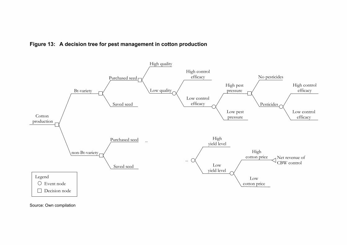
Figure 13: A decision tree for pest management in cotton production
Cotton production
High controlefficacy
Saved seedLow pestpressure
PesticidesLow control
efficacy
High pestpressure
High quality
Purchased seed
non-Bt-variety
Bt-variety
Saved seed
Purchased seed
Low quality
No pesticides
Highyield level
Net revenue of CBW control
High control efficacy
Low control efficacy
Lowyield level
...
Highcotton price
Lowcotton price
Legend Event node Decision node
...
Source: Own compilation
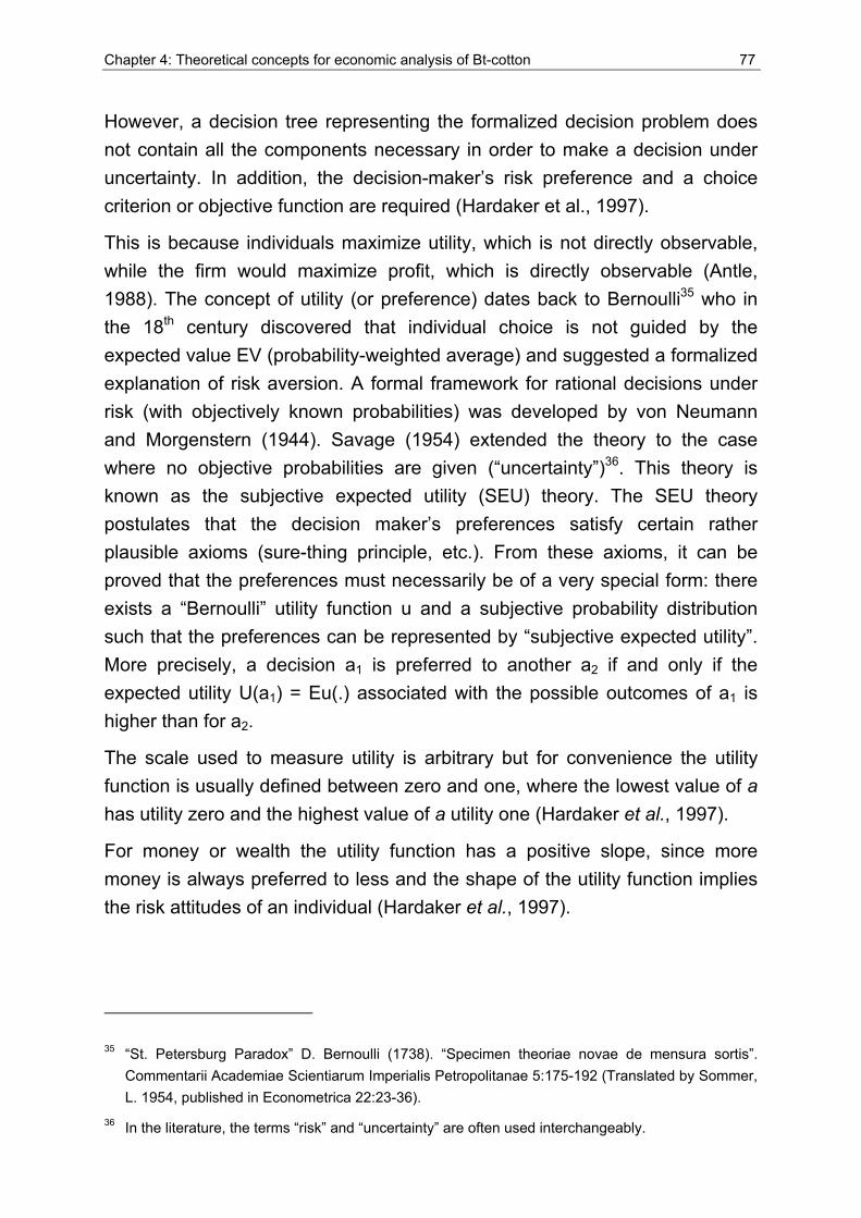
Chapter 4: Theoretical concepts for economic analysis of Bt-cotton 77
However, a decision tree representing the formalized decision problem does not contain all the components necessary in order to make a decision under uncertainty. In addition, the decision-maker’s risk preference and a choice criterion or objective function are required (Hardaker et al., 1997).
This is because individuals maximize utility, which is not directly observable, while the firm would maximize profit, which is directly observable (Antle, 1988). The concept of utility (or preference) dates back to Bernoulli35 who in the 18th century discovered that individual choice is not guided by the expected value EV (probability-weighted average) and suggested a formalized explanation of risk aversion. A formal framework for rational decisions under risk (with objectively known probabilities) was developed by von Neumann and Morgenstern (1944). Savage (1954) extended the theory to the case where no objective probabilities are given (“uncertainty”)36. This theory is known as the subjective expected utility (SEU) theory. The SEU theory postulates that the decision maker’s preferences satisfy certain rather plausible axioms (sure-thing principle, etc.). From these axioms, it can be proved that the preferences must necessarily be of a very special form: there exists a “Bernoulli” utility function u and a subjective probability distribution such that the preferences can be represented by “subjective expected utility”. More precisely, a decision a1 is preferred to another a2 if and only if the expected utility U(a1) = Eu(.) associated with the possible outcomes of a1 is higher than for a2.
The scale used to measure utility is arbitrary but for convenience the utility function is usually defined between zero and one, where the lowest value of a has utility zero and the highest value of a utility one (Hardaker et al., 1997).
For money or wealth the utility function has a positive slope, since more money is always preferred to less and the shape of the utility function implies the risk attitudes of an individual (Hardaker et al., 1997).
35 “St. Petersburg Paradox” D. Bernoulli (1738). “Specimen theoriae novae de mensura sortis”. Commentarii Academiae Scientiarum Imperialis Petropolitanae 5:175-192 (Translated by Sommer, L. 1954, published in Econometrica 22:23-36).
36 In the literature, the terms “risk” and “uncertainty” are often used interchangeably.
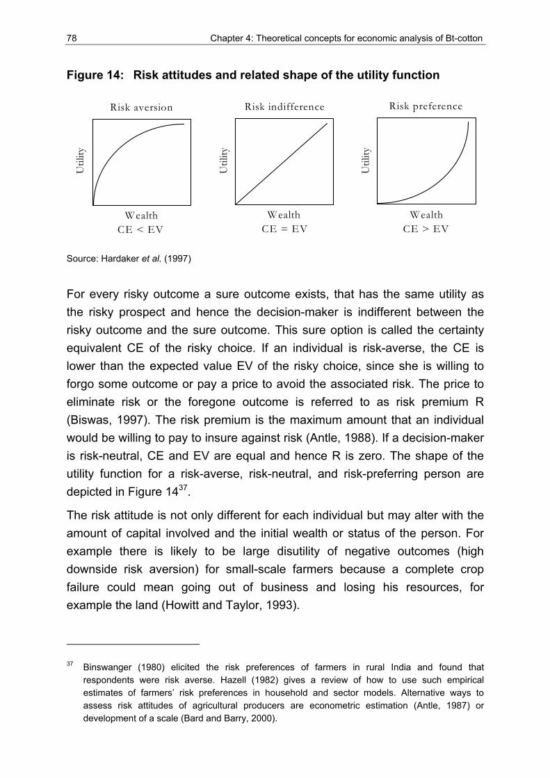
78 Chapter 4: Theoretical concepts for economic analysis of Bt-cotton
Figure 14: Risk attitudes and related shape of the utility function
Wealth Wealth Wealth
Util
ity
Risk aversion Risk indifference Risk preference
CE < EV CE = EV CE > EV
Util
ity
Util
ity
Source: Hardaker et al. (1997)
For every risky outcome a sure outcome exists, that has the same utility as the risky prospect and hence the decision-maker is indifferent between the risky outcome and the sure outcome. This sure option is called the certainty equivalent CE of the risky choice. If an individual is risk-averse, the CE is lower than the expected value EV of the risky choice, since she is willing to forgo some outcome or pay a price to avoid the associated risk. The price to eliminate risk or the foregone outcome is referred to as risk premium R (Biswas, 1997). The risk premium is the maximum amount that an individual would be willing to pay to insure against risk (Antle, 1988). If a decision-maker is risk-neutral, CE and EV are equal and hence R is zero. The shape of the utility function for a risk-averse, risk-neutral, and risk-preferring person are depicted in Figure 1437.
The risk attitude is not only different for each individual but may alter with the amount of capital involved and the initial wealth or status of the person. For example there is likely to be large disutility of negative outcomes (high downside risk aversion) for small-scale farmers because a complete crop failure could mean going out of business and losing his resources, for example the land (Howitt and Taylor, 1993).
37 Binswanger (1980) elicited the risk preferences of farmers in rural India and found that respondents were risk averse. Hazell (1982) gives a review of how to use such empirical estimates of farmers’ risk preferences in household and sector models. Alternative ways to assess risk attitudes of agricultural producers are econometric estimation (Antle, 1987) or development of a scale (Bard and Barry, 2000).
Chapter 4: Theoretical concepts for economic analysis of Bt-cotton 79
This would most likely lead to poverty and hunger for the family. Consequently the strategy with the highest utility for such a decision-maker will be a safety first or maximin38 approach and the maximization of the net return is subject to the constraint that a probability of some event, for example a negative net revenue, does not exceed a pre-specified level or income does not fall below the level that is required to meet basic needs (Hazell, 1982).
Kahneman and Tversky (1979) found that respondents weight losses substantially more than commensurate gains. This implies that the utility function of individuals is different for gain and loss situations. An empirical testing of their prospect theory applied to the field of pest management has yet to be conducted.
4.2.2 Pest control and production risk
In this section the effect that risk has on pest control decisions and the impact of pest control interventions on production risk are discussed. Excessive pesticide use is typically accompanied by a surplus of marginal costs over the expected value of the marginal product and could be interpreted within the utility concept as a risk premium that risk-averse farmers pay (Antle, 1988).
However, the empirical evidence of the risk impact of pesticides is mixed. Pannell (1990) found that risk reduced the level of herbicide use of risk-neutral decision-makers because uncertainty decreases the marginal productivity of herbicides and hence the optimal use level. He concludes that the effect that risk has on pest control decisions is mainly due to risk aversion of the decision-maker or impact on expected profit (Pannell, 1991). Figure 15 depicts the potential impact of a control intervention39. The control could impact the first order moment by a change in mean yield or profit as illustrated by a shift from outcome distribution d1 to d3 with respective mean values NR1 and NR3. The decision-maker would value such an impact irrespective of her risk attitudes.
38 Following the safety first or maximin approach means to select the choice with the highest outcome under the worst conditions (maximisation of the minimum return).
39 The figure depicts only scenarios in which the control intervention leads to an improvement of the
situation. Negative returns (net costs) to pest control are not considered for this illustrative
example.
80 Chapter 4: Theoretical concepts for economic analysis of Bt-cotton
Another potential impact is a change in higher order moments, for example a reduction in the variability of outcomes without a change in the mean value (depicted as change from d1 to d2 with equal mean NR1). Changes in higher order moments will only affect utility if the decision-maker is risk-averse (Hurley and Babcock, 2003). The same authors define an input as risk reducing “if a risk-averse firm will use more of it than a risk-neutral firm”. In their empirical study on the adoption of Bt-corn that protects against the European corn borer, Hurley and Babcock (2003) found that risk-averse producers were less likely to adopt the technology compared to risk-neutral producers. However, based on the density function of yield from conventional and Bt-corn it becomes obvious that it would be misleading to describe the technology as risk increasing. Although total variability is increased according to their findings the Bt-technology reduced the probability of low yields while increasing the probability of achieving high yields. This shows that the variance of yield alone is not necessarily an appropriate measure of risk. None-the-less it needs to be cautioned that the decision criterion for the farmer is more likely to be the profit or net revenue than the realized crop yield.
Horowitz and Lichtenberg (1994) explore the conditions under which pesticides increase or decrease profit risk and find that the impact on risk largely depends on the principal source of risk. According to their findings pesticides are risk reducing when pest populations are the uncertain factor, while they will likely be risk increasing if, for example, crop growth is random. They state that the work of Feder (1979) that largely contributed to the view that pesticides are risk-reducing, only accounts for randomness in the pest population, the damage per pest and the pesticide effectiveness while ignoring important other sources of uncertainty such as potential output and prices. Pannell (1991) acknowledges that the impact of risk attitudes on pest management decisions also depends on the framing of the decision problem. If a simple binary decision rule don’t treat or treat at the recommended dose is used, pest management decisions are more likely to be insensitive to risk aversion, while considering continuous dosage rates would increase the sensitivity of decisions to changes in risk aversion (ibid).
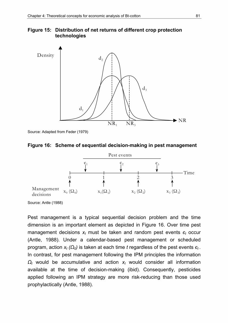
Chapter 4: Theoretical concepts for economic analysis of Bt-cotton 81
Figure 15: Distribution of net returns of different crop protection technologies
Density
NR NR3 NR1
d2
d1
d3
Source: Adapted from Feder (1979)
Figure 16: Scheme of sequential decision-making in pest management
Time0 1 2 3
Management decisions
Pest eventsє1 є2 є3
x0 (Ω0) x1(Ω1) x2 (Ω2) x3 (Ω3)
Source: Antle (1988)
Pest management is a typical sequential decision problem and the time dimension is an important element as depicted in Figure 16. Over time pest management decisions xt must be taken and random pest events єt occur (Antle, 1988). Under a calendar-based pest management or scheduled program, action xt (Ω0) is taken at each time t regardless of the pest events єt . In contrast, for pest management following the IPM principles the information Ωt would be accumulative and action xt would consider all information available at the time of decision-making (ibid). Consequently, pesticides applied following an IPM strategy are more risk-reducing than those used prophylactically (Antle, 1988).
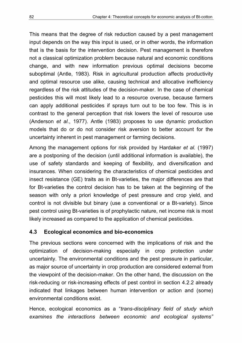
82 Chapter 4: Theoretical concepts for economic analysis of Bt-cotton
This means that the degree of risk reduction caused by a pest management input depends on the way this input is used, or in other words, the information that is the basis for the intervention decision. Pest management is therefore not a classical optimization problem because natural and economic conditions change, and with new information previous optimal decisions become suboptimal (Antle, 1983). Risk in agricultural production affects productivity and optimal resource use alike, causing technical and allocative inefficiency regardless of the risk attitudes of the decision-maker. In the case of chemical pesticides this will most likely lead to a resource overuse, because farmers can apply additional pesticides if sprays turn out to be too few. This is in contrast to the general perception that risk lowers the level of resource use (Anderson et al., 1977). Antle (1983) proposes to use dynamic production models that do or do not consider risk aversion to better account for the uncertainty inherent in pest management or farming decisions.
Among the management options for risk provided by Hardaker et al. (1997) are a postponing of the decision (until additional information is available), the use of safety standards and keeping of flexibility, and diversification and insurances. When considering the characteristics of chemical pesticides and insect resistance (GE) traits as in Bt-varieties, the major differences are that for Bt-varieties the control decision has to be taken at the beginning of the season with only a priori knowledge of pest pressure and crop yield, and control is not divisible but binary (use a conventional or a Bt-variety). Since pest control using Bt-varieties is of prophylactic nature, net income risk is most likely increased as compared to the application of chemical pesticides.
4.3 Ecological economics and bio-economics
The previous sections were concerned with the implications of risk and the optimization of decision-making especially in crop protection under uncertainty. The environmental conditions and the pest pressure in particular, as major source of uncertainty in crop production are considered external from the viewpoint of the decision-maker. On the other hand, the discussion on the risk-reducing or risk-increasing effects of pest control in section 4.2.2 already indicated that linkages between human intervention or action and (some) environmental conditions exist.
Hence, ecological economics as a “trans-disciplinary field of study which examines the interactions between economic and ecological systems”
Chapter 4: Theoretical concepts for economic analysis of Bt-cotton 83
(Edwards-Jones et al., 2000) could offer additional insights for the analysis. The methodology applied in ecological economics is not restricted to one discipline but integrates different fields to account for the complexity of the analyzed systems (Tisdell, 1993). Research in this field primarily relies on principles from natural sciences, particularly thermodynamics and ecology (Perman et al., 1996). To symbolize the earth as closed sphere of human activity, Boulding (1966) used the simile of a spaceship (spaceship earth) that is a closed system, carrying a certain stock of resources or inputs and only having a limited storage capacity for waste. He suggests two strategies to handle this situation: (i) minimize the throughput of material in the economy, and (ii) ensure efficient use of throughput.
A comparable approach, assuming that economic systems are embedded within a wider set of environmental conditions, was developed by Georgescu-Roegen (1987), who focused on the energy flows and the implications of the laws of thermodynamic to human economic activity. The second thermodynamic law40 states that the level of disorder would continuously increase until a closed system finally reaches a stationary state at the highest level of disorder. However, both authors recognize that the earth is not a completely closed system because solar radiation provides steady influx of energy.
Based on the assumption that human kind operates in a (quasi) closed system, the broad subject matter and the central problem that is the focus of research in ecological economics is sustainability. Pezzey (1997) distinguishes between:
sustainable (if MAXt tU U≤ always),
sustained (if 0tU ≥& always), and
survivable (if SURtU U> always) development,
40 “The two fundamental laws of thermodynamic state the following: (1) Matter and energy themselves are neither created nor destroyed. In a closed system, the total amount of energy and matter remains constant. (2) In any thermodynamic process (any physical activity of any kind), the entropy of the system either remains the same or increases. Entropy is a measure of the level of organization or structuring of material and energy; high-entropy states are disordered, low-entropy ones are well ordered.” (Edwards-Jones et al., 2000)
84 Chapter 4: Theoretical concepts for economic analysis of Bt-cotton
where tU is the utility level at time t, tU& is the rate of change of utility at time t, MAXtU is the maximum utility which can be held constant infinitely from time t
onwards, given production opportunities available at time t, and SURU the minimum utility level consistent with survival of the given population. These aspects are implicitly captured in the following definition: “Sustainable development is development that meets the needs of the present without compromising the ability of future generations to meet their own needs.” that was provided by the World Commission on Environment and Development (1987).
The terms sustainability and sustainable development have come into popular use within the last decades indicating at least increased awareness of the conservation of resources and the long-term benefits of humanity (Perman et al., 1996). Turning this into the question of how we should behave with respect to future generations shows that the sustainability concept involves (a certain degree of) ethics.
The integrated goals41 of resource management from an ecological economics perspective are economic efficiency (allocation), ecological sustainability (scale), and social fairness (distribution). The first goal relates to positive economic questions and analyses, while the latter two require valuation and thus are of normative character.
Most people would readily agree that sustainability is a desirable concept; and the phrase is currently omnipresent at the policy level and in the agenda of the development organizations. Why then, is achieving this goal so difficult? – There are three major biases against sustainability, namely the common ownership of resource stocks (referred to as tragedy of the commons), future discounting, and the effects of uncertainty (Clark, 1991). Pannell (2003), for example, identifies uncertainty as a major limitation to the adoption of sustainable farming systems such as land conservation and partly attributes the limited adoption to market failure. All the biases listed also apply to the field of agricultural pest management. The susceptibility of target pests to the control intervention can be considered as common property resource (Hueth and Regev, 1974), negative externalities of pest control often occur off-side
41 Listed by R. Costanza in his plenary presentation at the 8th Biennial Conference of the International Society for Ecological Economics (ISEE), July 11-14, 2004, Montreal.
Chapter 4: Theoretical concepts for economic analysis of Bt-cotton 85
and off-time (resistance build-up and long-term health effects), and important elements of the production system and hence of pest management are subject to considerable uncertainty (yield, pest pressure, prices).
Moreover, pest management can be considered as substitution for environmental services such as predator populations functioning as natural enemies and a high degree of interaction between the ecosystem and the control intervention can be expected. To depict these interactions, methods to link biological and economic models such as bio-economic modelling are available. Ecological economics’ principles suggest that bio-economic models are useful tools to capture the dynamics of a system with biological and economic components and can be used to identify optimal use patterns of renewable resources (such as fish stocks or timber). Such models are positive economic methods that describe what will happen (under different scenarios) and what would be the most efficient way to use the resource (Clark, 1990). The integration of biological processes and economic models can give essential insights and capture dynamics not accounted for in purely econometric models (Dovers et al., 2003).
4.4 Research hypotheses and methods
The quantitative methods applied in the analytical part of the thesis aim at providing answers to the research question of how the insect resistance trait in Bt-cotton varieties contributes to the productivity and profitability of small-scale cotton cultivation in North China. Following on from the discussion of the general problem in Chapter 2 and the relevant economic concepts and theory in Chapters 3 and 4, the research hypotheses are derived in this section. The conceptual framework for the analysis starts with the typology of the methods applied. Subsequently, a description of the analytical procedure selected to economically assess the use of Bt-cotton in the study area is provided.
4.4.1 Research hypotheses
As outlined in Chapters 2 and 3, the economic assessment of the impact of agricultural biotechnology is not straightforward but complex, mainly due to the different categories of costs and benefits, uncertainty of outcomes, and the existence of externalities and long-term effects. However, in the literature, assessment is mainly conducted using econometric methods.
86 Chapter 4: Theoretical concepts for economic analysis of Bt-cotton
These generally do not account for the characteristics of the Bt-technology and the agro-ecosystem. Challenging the standard econometric assessment methods, the following research hypotheses are identified: (1) the institutional conditions and market failure determine the success of technology implementation and can limit the realization of benefits, especially under the conditions of developing countries, (2) the specification of the econometric model influences the results of the assessment, (3) uncertainty is an essential element of agro-ecosystems and incorporating risk in the analysis provides additional in-sight into the performance of the Bt-cotton technology, and (4) an interdisciplinary approach, that in addition to farm level performance data, considers the underlying biological and ecological processes, has a higher explanatory value.
4.4.2 Conceptual framework and methods used in the study
A principal typology of economic models distinguishes between positive and normative approaches. Positive methods do not ex ante postulate a specific behaviour but use empirical data to test hypotheses, while normative methods require some value judgement or assumptions. To analyse the impact of using a Bt-cotton variety, different positive and normative methods can be applied. The approaches followed in the study are all primal but corresponding dual approaches exist that consider the input and output prices rather than the quantities. The analytical framework for the assessment can be either static or dynamic to account for long-term effects and optimisation of resource use over time. Finally, methods can be categorized as either deterministic – assuming a fixed causal effect of an action, or stochastic – accounting for variation in the outcomes.
Table 10 groups the methods used in the study into the two categories positive/normative and deterministic/stochastic approaches. The study uses both positive and normative models to analyse the productivity effect of Bt-cotton varieties. The selected approaches are static in nature covering deterministic and stochastic methods. The first analysis step (Chapter 7) is the econometric estimation of a production function that belongs to the positive approaches.
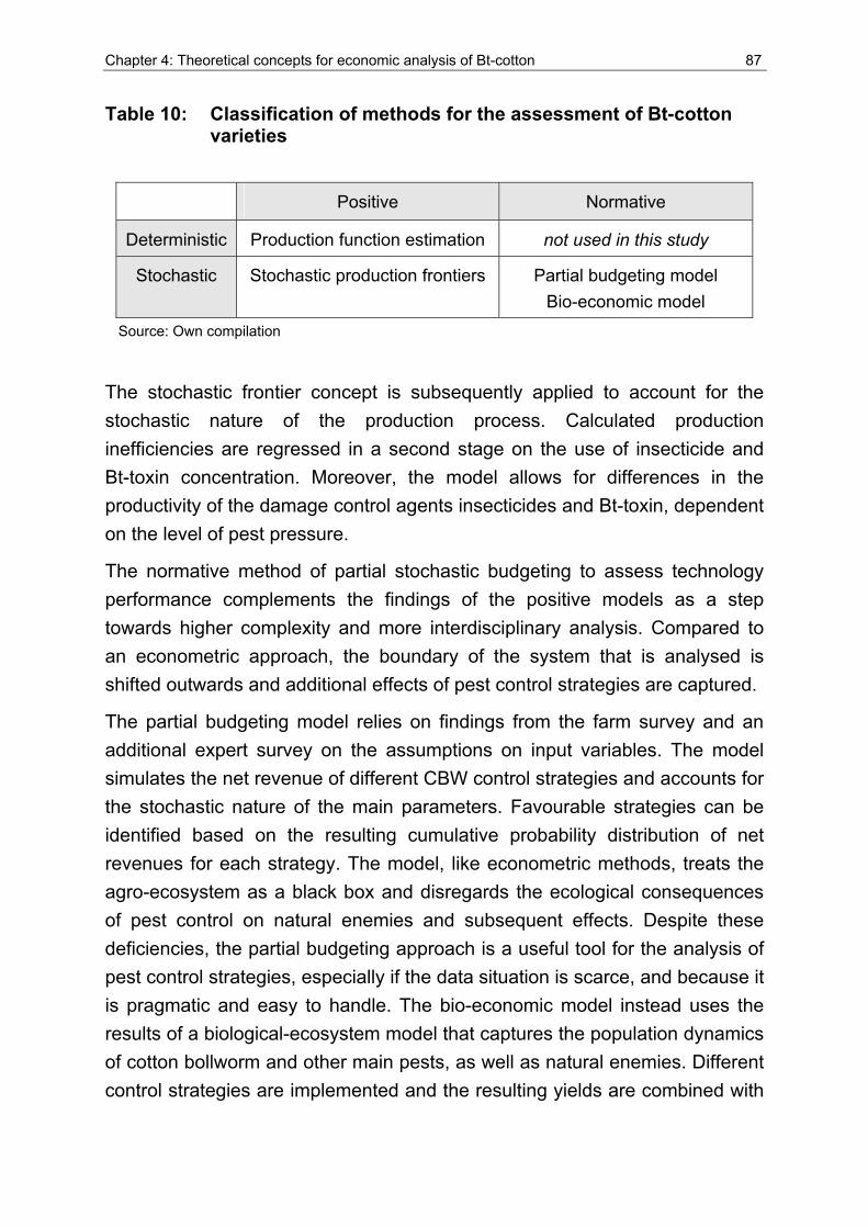
Chapter 4: Theoretical concepts for economic analysis of Bt-cotton 87
Table 10: Classification of methods for the assessment of Bt-cotton varieties
Positive Normative
Deterministic Production function estimation not used in this study
Stochastic Stochastic production frontiers Partial budgeting model Bio-economic model
Source: Own compilation
The stochastic frontier concept is subsequently applied to account for the stochastic nature of the production process. Calculated production inefficiencies are regressed in a second stage on the use of insecticide and Bt-toxin concentration. Moreover, the model allows for differences in the productivity of the damage control agents insecticides and Bt-toxin, dependent on the level of pest pressure.
The normative method of partial stochastic budgeting to assess technology performance complements the findings of the positive models as a step towards higher complexity and more interdisciplinary analysis. Compared to an econometric approach, the boundary of the system that is analysed is shifted outwards and additional effects of pest control strategies are captured.
The partial budgeting model relies on findings from the farm survey and an additional expert survey on the assumptions on input variables. The model simulates the net revenue of different CBW control strategies and accounts for the stochastic nature of the main parameters. Favourable strategies can be identified based on the resulting cumulative probability distribution of net revenues for each strategy. The model, like econometric methods, treats the agro-ecosystem as a black box and disregards the ecological consequences of pest control on natural enemies and subsequent effects. Despite these deficiencies, the partial budgeting approach is a useful tool for the analysis of pest control strategies, especially if the data situation is scarce, and because it is pragmatic and easy to handle. The bio-economic model instead uses the results of a biological-ecosystem model that captures the population dynamics of cotton bollworm and other main pests, as well as natural enemies. Different control strategies are implemented and the resulting yields are combined with
88 Chapter 4: Theoretical concepts for economic analysis of Bt-cotton
price and cost information in the economic model to obtain net revenue estimates for each of the strategies.
The four different analysis methods applied are complementary in the sense that they cover different aspects of the research problem and comprise increasing complexity and integration.
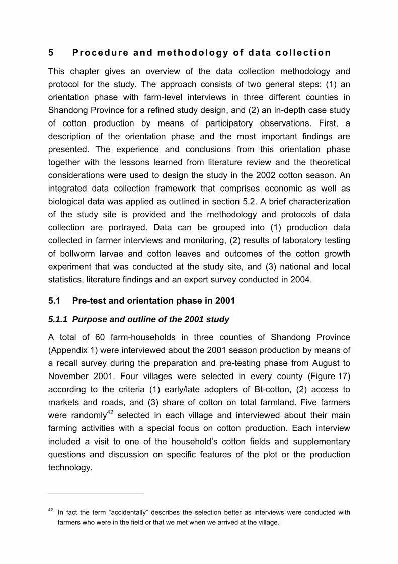
5 Procedure and methodology o f da ta co l lec t ion
This chapter gives an overview of the data collection methodology and protocol for the study. The approach consists of two general steps: (1) an orientation phase with farm-level interviews in three different counties in Shandong Province for a refined study design, and (2) an in-depth case study of cotton production by means of participatory observations. First, a description of the orientation phase and the most important findings are presented. The experience and conclusions from this orientation phase together with the lessons learned from literature review and the theoretical considerations were used to design the study in the 2002 cotton season. An integrated data collection framework that comprises economic as well as biological data was applied as outlined in section 5.2. A brief characterization of the study site is provided and the methodology and protocols of data collection are portrayed. Data can be grouped into (1) production data collected in farmer interviews and monitoring, (2) results of laboratory testing of bollworm larvae and cotton leaves and outcomes of the cotton growth experiment that was conducted at the study site, and (3) national and local statistics, literature findings and an expert survey conducted in 2004.
5.1 Pre-test and orientation phase in 2001
5.1.1 Purpose and outline of the 2001 study
A total of 60 farm-households in three counties of Shandong Province (Appendix 1) were interviewed about the 2001 season production by means of a recall survey during the preparation and pre-testing phase from August to November 2001. Four villages were selected in every county (Figure 17) according to the criteria (1) early/late adopters of Bt-cotton, (2) access to markets and roads, and (3) share of cotton on total farmland. Five farmers were randomly42 selected in each village and interviewed about their main farming activities with a special focus on cotton production. Each interview included a visit to one of the household’s cotton fields and supplementary questions and discussion on specific features of the plot or the production technology.
42 In fact the term “accidentally” describes the selection better as interviews were conducted with farmers who were in the field or that we met when we arrived at the village.
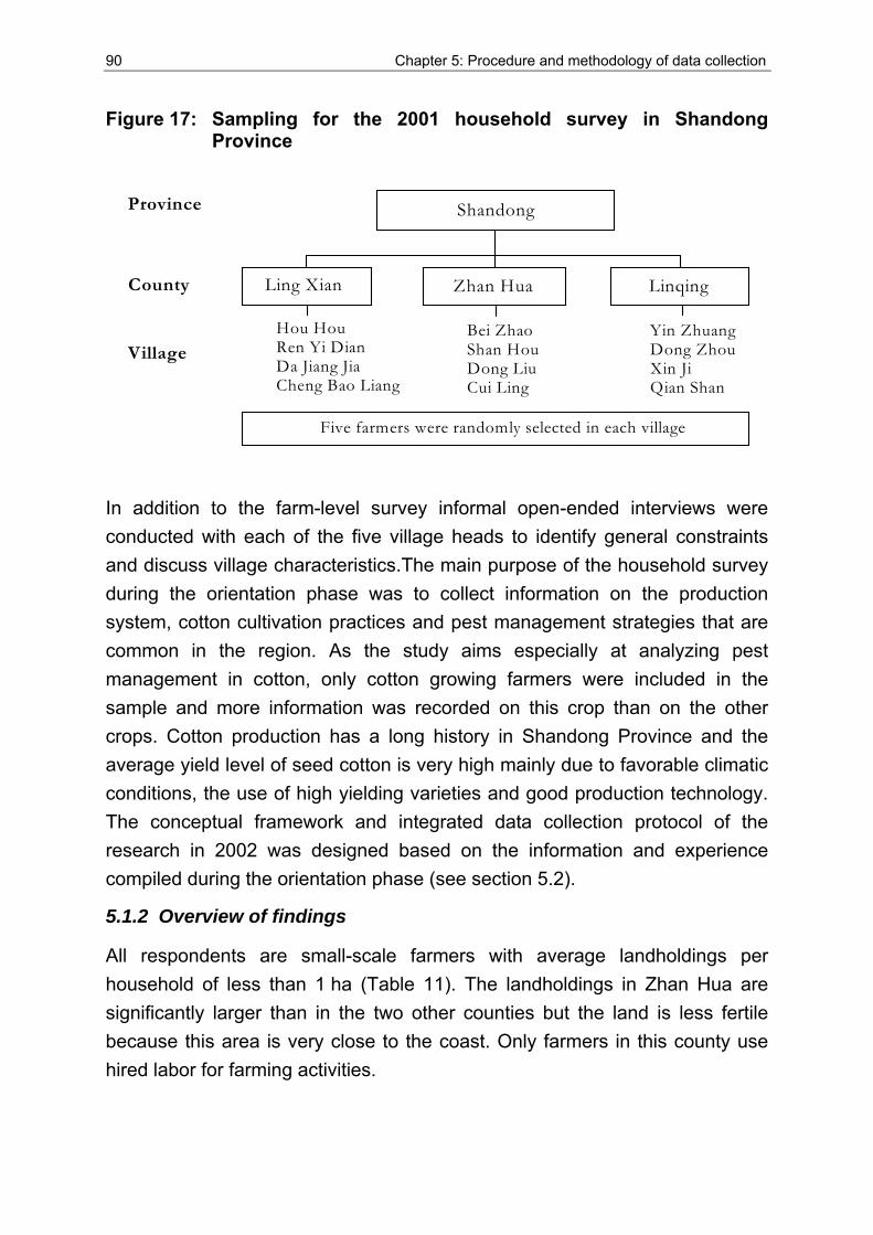
90 Chapter 5: Procedure and methodology of data collection
Figure 17: Sampling for the 2001 household survey in Shandong Province
Shandong
Ling Xian Zhan Hua Linqing
Hou Hou Ren Yi Dian Da Jiang Jia Cheng Bao Liang
Bei Zhao Shan Hou Dong Liu Cui Ling
Yin Zhuang Dong Zhou Xin Ji Qian Shan Five farmers were randomly selected in each village
County
Village
Province
In addition to the farm-level survey informal open-ended interviews were conducted with each of the five village heads to identify general constraints and discuss village characteristics.The main purpose of the household survey during the orientation phase was to collect information on the production system, cotton cultivation practices and pest management strategies that are common in the region. As the study aims especially at analyzing pest management in cotton, only cotton growing farmers were included in the sample and more information was recorded on this crop than on the other crops. Cotton production has a long history in Shandong Province and the average yield level of seed cotton is very high mainly due to favorable climatic conditions, the use of high yielding varieties and good production technology. The conceptual framework and integrated data collection protocol of the research in 2002 was designed based on the information and experience compiled during the orientation phase (see section 5.2).
5.1.2 Overview of findings
All respondents are small-scale farmers with average landholdings per household of less than 1 ha (Table 11). The landholdings in Zhan Hua are significantly larger than in the two other counties but the land is less fertile because this area is very close to the coast. Only farmers in this county use hired labor for farming activities.
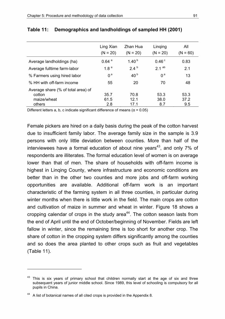
Chapter 5: Procedure and methodology of data collection 91
Table 11: Demographics and landholdings of sampled HH (2001)
Ling Xian (N = 20)
Zhan Hua (N = 20)
Linqing (N = 20)
All (N = 60)
Average landholdings (ha) 0.64 a 1.40 b 0.46 c 0.83
Average fulltime farm-labor 1.8 a 2.4 b 2.1 ab 2.1
% Farmers using hired labor 0 a 40 b 0 a 13
% HH with off-farm income 55 20 70 48
Average share (% of total area) of cotton 35.7 70.8 53.3 53.3 maize/wheat 61.5 12.1 38.0 37.2 others 2.8 17.1 8.7 9.5
Different letters a, b, c indicate significant difference of means (α = 0.05)
Female pickers are hired on a daily basis during the peak of the cotton harvest due to insufficient family labor. The average family size in the sample is 3.9 persons with only little deviation between counties. More than half of the interviewees have a formal education of about nine years43, and only 7% of respondents are illiterates. The formal education level of women is on average lower than that of men. The share of households with off-farm income is highest in Linqing County, where infrastructure and economic conditions are better than in the other two counties and more jobs and off-farm working opportunities are available. Additional off-farm work is an important characteristic of the farming system in all three counties, in particular during winter months when there is little work in the field. The main crops are cotton and cultivation of maize in summer and wheat in winter. Figure 18 shows a cropping calendar of crops in the study area44. The cotton season lasts from the end of April until the end of October/beginning of November. Fields are left fallow in winter, since the remaining time is too short for another crop. The share of cotton in the cropping system differs significantly among the counties and so does the area planted to other crops such as fruit and vegetables (Table 11).
43 This is six years of primary school that children normally start at the age of six and three subsequent years of junior middle school. Since 1989, this level of schooling is compulsory for all pupils in China.
44 A list of botanical names of all cited crops is provided in the Appendix 8.
92 Chapter 5: Procedure and methodology of data collection
Figure 18: Cropping calendar for main crops in the survey region
J MF A JM J A S N D
Cotton
MaizeWheat Wheat
Soybean
Watermelon
O
Figure 19: Adoption of Bt-cotton varieties in the 2001 sample by county
1995 1996 1997 1998 1999 2000 2001
Ado
ptio
n of
Bt-c
otto
n [c
umul
ativ
e %
]
0
20
40
60
80
100
Ling XianZhan Hua Linqing
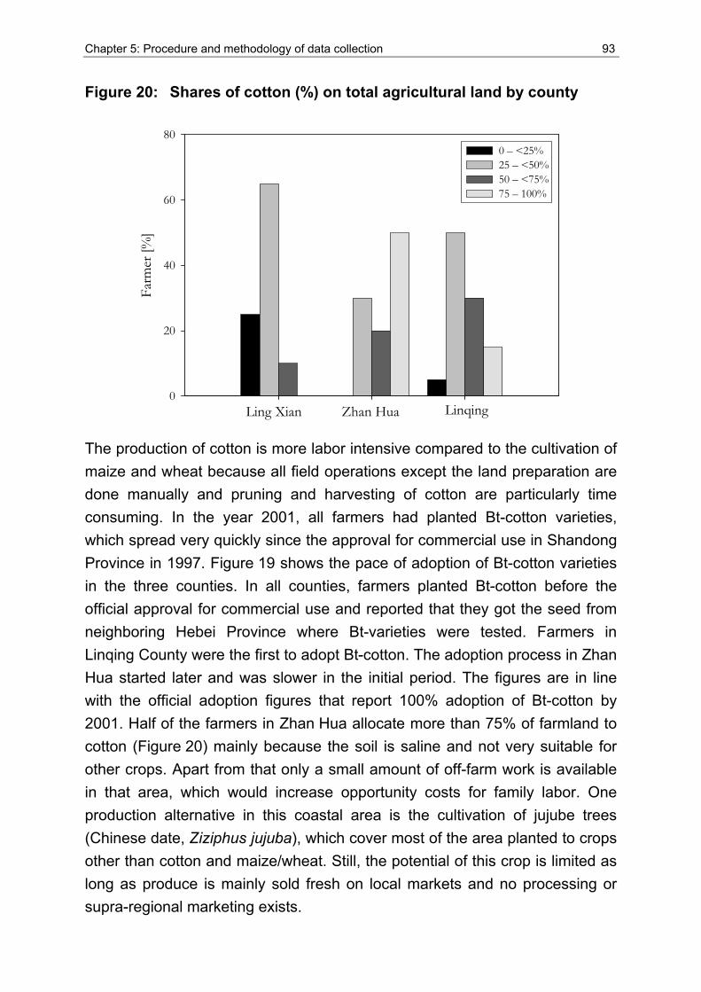
Chapter 5: Procedure and methodology of data collection 93
Figure 20: Shares of cotton (%) on total agricultural land by county
Farm
er [%
]
0
20
40
60
800 – <25%25 – <50%50 – <75%75 – 100%
Ling Xian Zhan Hua Linqing
The production of cotton is more labor intensive compared to the cultivation of maize and wheat because all field operations except the land preparation are done manually and pruning and harvesting of cotton are particularly time consuming. In the year 2001, all farmers had planted Bt-cotton varieties, which spread very quickly since the approval for commercial use in Shandong Province in 1997. Figure 19 shows the pace of adoption of Bt-cotton varieties in the three counties. In all counties, farmers planted Bt-cotton before the official approval for commercial use and reported that they got the seed from neighboring Hebei Province where Bt-varieties were tested. Farmers in Linqing County were the first to adopt Bt-cotton. The adoption process in Zhan Hua started later and was slower in the initial period. The figures are in line with the official adoption figures that report 100% adoption of Bt-cotton by 2001. Half of the farmers in Zhan Hua allocate more than 75% of farmland to cotton (Figure 20) mainly because the soil is saline and not very suitable for other crops. Apart from that only a small amount of off-farm work is available in that area, which would increase opportunity costs for family labor. One production alternative in this coastal area is the cultivation of jujube trees (Chinese date, Ziziphus jujuba), which cover most of the area planted to crops other than cotton and maize/wheat. Still, the potential of this crop is limited as long as produce is mainly sold fresh on local markets and no processing or supra-regional marketing exists.
94 Chapter 5: Procedure and methodology of data collection
Farming systems are more diverse in Ling Xian and Linqing where farmers grow a larger variety of crops and off-farm work is much more common. Most farmers in these two counties grow only 25 – 50% cotton. The main characteristics of the production system are the crop portfolio, the share of off-farm work, and animal husbandry. Livestock is an important component of the farming system in Ling Xian while only a few farmers in the other two counties keep animals. With the exception of some farmers who are running chicken farms only a few animals are kept in those two counties. Cattle and donkeys are used for transportation and land preparation, and most farmers raise chickens for home consumption of meat and eggs.
Some key economic indicators of wheat and maize are presented in Table 12 and those of cotton in Table 13. Production of maize in summer and wheat during winter on the same plot is the most common alternative to cotton production. Cultivation of maize and wheat is less labor intensive and less demanding in terms of pesticide use than the growing of cotton. The maize harvest is used to raise animals or is sold on the market. Crop residues can also be used to feed animals and hence are stored during the winter months. The labor input for wheat is very low because machines are used for the main activities (land preparation, sowing, and reaping) and returns to labor are much higher than for cotton. Wheat produce is used for own consumption and any surplus is sold on the market. In this area, wheat (bread, noodles) is a staple crop.
Some farmers also sell wheat straw as raw material for paper production but prices for straw are very low. The use of pesticides in wheat is lower than in maize with on average only 1.5 sprays, and fewer farmers use herbicides due to the high weed competitiveness of this crop (Table 12). Costs of family labor are not included for the computation of the gross margins. Instead, the returns to family labor are calculated and can be compared among the three counties although employment opportunities and wage rates differ. Cotton is the most important cash crop for farmers in the survey area and the gross margin of cotton (Table 13) is slightly higher than the sum of the gross margins of the alternative land use option to cultivate a maize/wheat crop (Table 12).
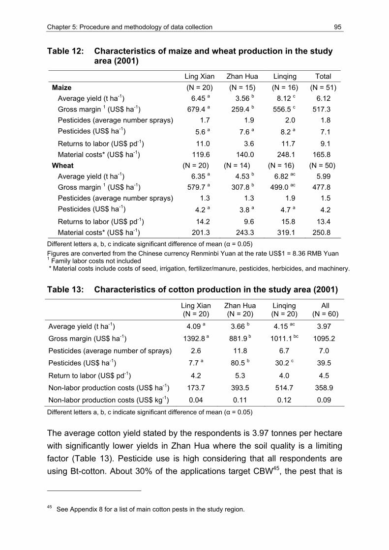
Chapter 5: Procedure and methodology of data collection 95
Table 12: Characteristics of maize and wheat production in the study area (2001)
Ling Xian Zhan Hua Linqing Total Maize (N = 20) (N = 15) (N = 16) (N = 51)
Average yield (t ha-1) 6.45 a 3.56 b 8.12 c 6.12 Gross margin 1 (US$ ha-1) 679.4 a 259.4 b 556.5 c 517.3 Pesticides (average number sprays) 1.7 1.9 2.0 1.8 Pesticides (US$ ha-1) 5.6 a 7.6 a 8.2 a 7.1 Returns to labor (US$ pd-1) 11.0 3.6 11.7 9.1 Material costs* (US$ ha-1) 119.6 140.0 248.1 165.8
Wheat (N = 20) (N = 14) (N = 16) (N = 50) Average yield (t ha-1) 6.35 a 4.53 b 6.82 ac 5.99 Gross margin 1 (US$ ha-1) 579.7 a 307.8 b 499.0 ac 477.8 Pesticides (average number sprays) 1.3 1.3 1.9 1.5 Pesticides (US$ ha-1) 4.2 a 3.8 a 4.7 a 4.2 Returns to labor (US$ pd-1) 14.2 9.6 15.8 13.4 Material costs* (US$ ha-1) 201.3 243.3 319.1 250.8
Different letters a, b, c indicate significant difference of mean (α = 0.05) Figures are converted from the Chinese currency Renminbi Yuan at the rate US$1 = 8.36 RMB Yuan 1 Family labor costs not included * Material costs include costs of seed, irrigation, fertilizer/manure, pesticides, herbicides, and machinery.
Table 13: Characteristics of cotton production in the study area (2001)
Ling Xian (N = 20)
Zhan Hua (N = 20)
Linqing (N = 20)
All (N = 60)
Average yield (t ha-1) 4.09 a 3.66 b 4.15 ac 3.97
Gross margin (US$ ha-1) 1392.8 a 881.9 b 1011.1 bc 1095.2
Pesticides (average number of sprays) 2.6 11.8 6.7 7.0
Pesticides (US$ ha-1) 7.7 a 80.5 b 30.2 c 39.5
Return to labor (US$ pd-1) 4.2 5.3 4.0 4.5
Non-labor production costs (US$ ha-1) 173.7 393.5 514.7 358.9
Non-labor production costs (US$ kg-1) 0.04 0.11 0.12 0.09 Different letters a, b, c indicate significant difference of mean (α = 0.05)
The average cotton yield stated by the respondents is 3.97 tonnes per hectare with significantly lower yields in Zhan Hua where the soil quality is a limiting factor (Table 13). Pesticide use is high considering that all respondents are using Bt-cotton. About 30% of the applications target CBW45, the pest that is
45 See Appendix 8 for a list of main cotton pests in the study region.
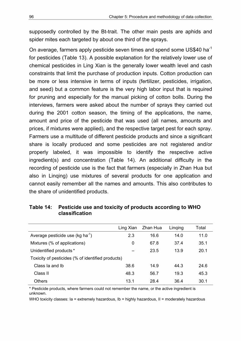
96 Chapter 5: Procedure and methodology of data collection
supposedly controlled by the Bt-trait. The other main pests are aphids and spider mites each targeted by about one third of the sprays.
On average, farmers apply pesticide seven times and spend some US$40 ha-1 for pesticides (Table 13). A possible explanation for the relatively lower use of chemical pesticides in Ling Xian is the generally lower wealth level and cash constraints that limit the purchase of production inputs. Cotton production can be more or less intensive in terms of inputs (fertilizer, pesticides, irrigation, and seed) but a common feature is the very high labor input that is required for pruning and especially for the manual picking of cotton bolls. During the interviews, farmers were asked about the number of sprays they carried out during the 2001 cotton season, the timing of the applications, the name, amount and price of the pesticide that was used (all names, amounts and prices, if mixtures were applied), and the respective target pest for each spray. Farmers use a multitude of different pesticide products and since a significant share is locally produced and some pesticides are not registered and/or properly labeled, it was impossible to identify the respective active ingredient(s) and concentration (Table 14). An additional difficulty in the recording of pesticide use is the fact that farmers (especially in Zhan Hua but also in Linqing) use mixtures of several products for one application and cannot easily remember all the names and amounts. This also contributes to the share of unidentified products.
Table 14: Pesticide use and toxicity of products according to WHO classification
Ling Xian Zhan Hua Linqing Total
Average pesticide use (kg ha-1) 2.3 16.6 14.0 11.0
Mixtures (% of applications) 0 67.8 37.4 35.1
Unidentified products * – 23.5 13.9 20.1
Toxicity of pesticides (% of identified products)
Class Ia and Ib 38.6 14.9 44.3 24.6
Class II 48.3 56.7 19.3 45.3
Others 13.1 28.4 36.4 30.1 * Pesticide products, where farmers could not remember the name, or the active ingredient is unknown. WHO toxicity classes: Ia = extremely hazardous, Ib = highly hazardous, II = moderately hazardous
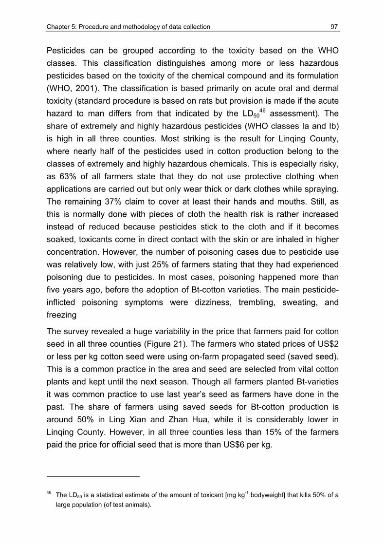
Chapter 5: Procedure and methodology of data collection 97
Pesticides can be grouped according to the toxicity based on the WHO classes. This classification distinguishes among more or less hazardous pesticides based on the toxicity of the chemical compound and its formulation (WHO, 2001). The classification is based primarily on acute oral and dermal toxicity (standard procedure is based on rats but provision is made if the acute hazard to man differs from that indicated by the LD50
46 assessment). The share of extremely and highly hazardous pesticides (WHO classes Ia and Ib) is high in all three counties. Most striking is the result for Linqing County, where nearly half of the pesticides used in cotton production belong to the classes of extremely and highly hazardous chemicals. This is especially risky, as 63% of all farmers state that they do not use protective clothing when applications are carried out but only wear thick or dark clothes while spraying. The remaining 37% claim to cover at least their hands and mouths. Still, as this is normally done with pieces of cloth the health risk is rather increased instead of reduced because pesticides stick to the cloth and if it becomes soaked, toxicants come in direct contact with the skin or are inhaled in higher concentration. However, the number of poisoning cases due to pesticide use was relatively low, with just 25% of farmers stating that they had experienced poisoning due to pesticides. In most cases, poisoning happened more than five years ago, before the adoption of Bt-cotton varieties. The main pesticide-inflicted poisoning symptoms were dizziness, trembling, sweating, and freezing
The survey revealed a huge variability in the price that farmers paid for cotton seed in all three counties (Figure 21). The farmers who stated prices of US$2 or less per kg cotton seed were using on-farm propagated seed (saved seed). This is a common practice in the area and seed are selected from vital cotton plants and kept until the next season. Though all farmers planted Bt-varieties it was common practice to use last year’s seed as farmers have done in the past. The share of farmers using saved seeds for Bt-cotton production is around 50% in Ling Xian and Zhan Hua, while it is considerably lower in Linqing County. However, in all three counties less than 15% of the farmers paid the price for official seed that is more than US$6 per kg.
46 The LD50 is a statistical estimate of the amount of toxicant [mg kg-1 bodyweight] that kills 50% of a large population (of test animals).
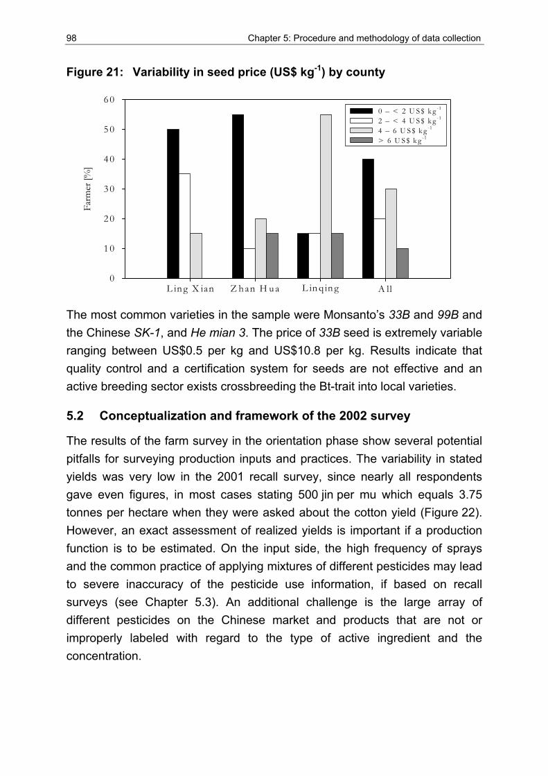
98 Chapter 5: Procedure and methodology of data collection
Figure 21: Variability in seed price (US$ kg-1) by county
Farm
er [%
]
0
1 0
2 0
3 0
4 0
5 0
6 0
L in g X ian Z h an H u a L in q in g A ll
0 – < 2 U S $ k g -1
2 – < 4 U S $ k g -1
4 – 6 U S $ k g -1
> 6 U S $ k g -1
The most common varieties in the sample were Monsanto’s 33B and 99B and the Chinese SK-1, and He mian 3. The price of 33B seed is extremely variable ranging between US$0.5 per kg and US$10.8 per kg. Results indicate that quality control and a certification system for seeds are not effective and an active breeding sector exists crossbreeding the Bt-trait into local varieties.
5.2 Conceptualization and framework of the 2002 survey
The results of the farm survey in the orientation phase show several potential pitfalls for surveying production inputs and practices. The variability in stated yields was very low in the 2001 recall survey, since nearly all respondents gave even figures, in most cases stating 500 jin per mu which equals 3.75 tonnes per hectare when they were asked about the cotton yield (Figure 22). However, an exact assessment of realized yields is important if a production function is to be estimated. On the input side, the high frequency of sprays and the common practice of applying mixtures of different pesticides may lead to severe inaccuracy of the pesticide use information, if based on recall surveys (see Chapter 5.3). An additional challenge is the large array of different pesticides on the Chinese market and products that are not or improperly labeled with regard to the type of active ingredient and the concentration.
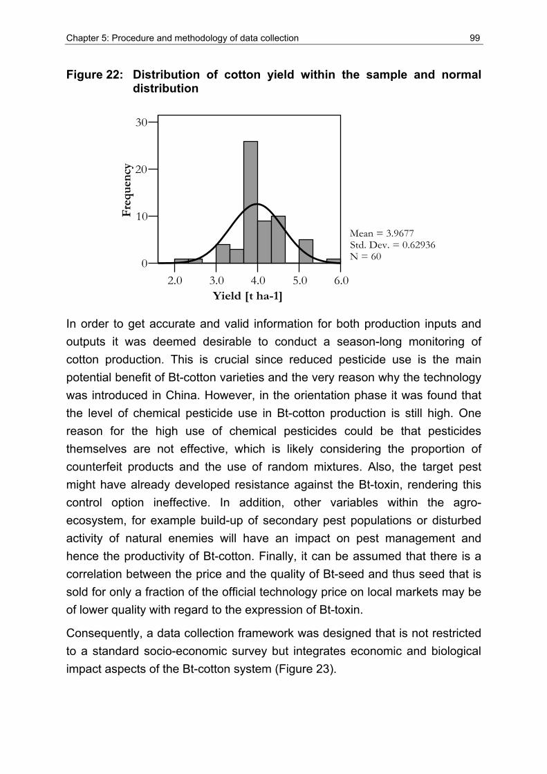
Chapter 5: Procedure and methodology of data collection 99
Figure 22: Distribution of cotton yield within the sample and normal distribution
2.0 3.0 4.0 5.0 6.0Yield [t ha-1]
0
10
20
30F
requ
ency
Mean = 3.9677Std. Dev. = 0.62936N = 60
In order to get accurate and valid information for both production inputs and outputs it was deemed desirable to conduct a season-long monitoring of cotton production. This is crucial since reduced pesticide use is the main potential benefit of Bt-cotton varieties and the very reason why the technology was introduced in China. However, in the orientation phase it was found that the level of chemical pesticide use in Bt-cotton production is still high. One reason for the high use of chemical pesticides could be that pesticides themselves are not effective, which is likely considering the proportion of counterfeit products and the use of random mixtures. Also, the target pest might have already developed resistance against the Bt-toxin, rendering this control option ineffective. In addition, other variables within the agro-ecosystem, for example build-up of secondary pest populations or disturbed activity of natural enemies will have an impact on pest management and hence the productivity of Bt-cotton. Finally, it can be assumed that there is a correlation between the price and the quality of Bt-seed and thus seed that is sold for only a fraction of the official technology price on local markets may be of lower quality with regard to the expression of Bt-toxin.
Consequently, a data collection framework was designed that is not restricted to a standard socio-economic survey but integrates economic and biological impact aspects of the Bt-cotton system (Figure 23).
100 Chapter 5: Procedure and methodology of data collection
Figure 23: Scheme of the integrated data collection framework
POLICY ENVIRONMENTECOLOGICAL ENVIRONMENT
FARM HOUSEHOLD MARKET AGRO-ECOSYSTEM
HH demographics Farming system Production practices Knowledge/perception
Resistance of pests Pest pressure Bt-trait Plant growth Natural enemies
Input prices Output prices Quality standards
Farmer interviews Production monitoring
Interviews Testing
Experiments, Testing Expert survey
INTEGRATED DATA COLLECTION FRAMEWORK
Source: Own compilation
Data comprises information collected in farm-level interviews and in a season-long monitoring of production inputs and output of Bt-cotton. Complementary information not only on the price but also on the quality of inputs is crucial. Ecological variables need to be considered for an in-depth case study of Bt-cotton production in addition to the farm-level production data. Such information can only be captured through experiments and requires collaboration with natural scientists. Data collection methods are described in section 5.4.
Based on the results of the orientation phase, Linqing was selected for the in-depth study in 2002. Linqing best represents the conditions of the Yellow River Plain cotton area as alternative cropping options are available and the cropping system is diverse.
The region has a long tradition of cotton cultivation and its farmers were among the early adopters of Bt-varieties. This means they have some five years of experience now in growing Bt-cotton and it can be expected that they have optimized the system and possibly that some long-term impact had already occurred.
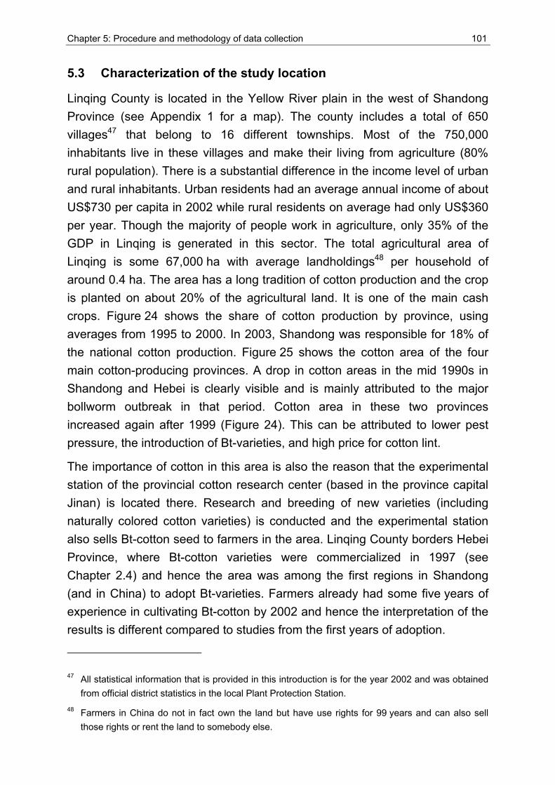
Chapter 5: Procedure and methodology of data collection 101
5.3 Characterization of the study location
Linqing County is located in the Yellow River plain in the west of Shandong Province (see Appendix 1 for a map). The county includes a total of 650 villages47 that belong to 16 different townships. Most of the 750,000 inhabitants live in these villages and make their living from agriculture (80% rural population). There is a substantial difference in the income level of urban and rural inhabitants. Urban residents had an average annual income of about US$730 per capita in 2002 while rural residents on average had only US$360 per year. Though the majority of people work in agriculture, only 35% of the GDP in Linqing is generated in this sector. The total agricultural area of Linqing is some 67,000 ha with average landholdings48 per household of around 0.4 ha. The area has a long tradition of cotton production and the crop is planted on about 20% of the agricultural land. It is one of the main cash crops. Figure 24 shows the share of cotton production by province, using averages from 1995 to 2000. In 2003, Shandong was responsible for 18% of the national cotton production. Figure 25 shows the cotton area of the four main cotton-producing provinces. A drop in cotton areas in the mid 1990s in Shandong and Hebei is clearly visible and is mainly attributed to the major bollworm outbreak in that period. Cotton area in these two provinces increased again after 1999 (Figure 24). This can be attributed to lower pest pressure, the introduction of Bt-varieties, and high price for cotton lint.
The importance of cotton in this area is also the reason that the experimental station of the provincial cotton research center (based in the province capital Jinan) is located there. Research and breeding of new varieties (including naturally colored cotton varieties) is conducted and the experimental station also sells Bt-cotton seed to farmers in the area. Linqing County borders Hebei Province, where Bt-cotton varieties were commercialized in 1997 (see Chapter 2.4) and hence the area was among the first regions in Shandong (and in China) to adopt Bt-varieties. Farmers already had some five years of experience in cultivating Bt-cotton by 2002 and hence the interpretation of the results is different compared to studies from the first years of adoption.
47 All statistical information that is provided in this introduction is for the year 2002 and was obtained from official district statistics in the local Plant Protection Station.
48 Farmers in China do not in fact own the land but have use rights for 99 years and can also sell those rights or rent the land to somebody else.
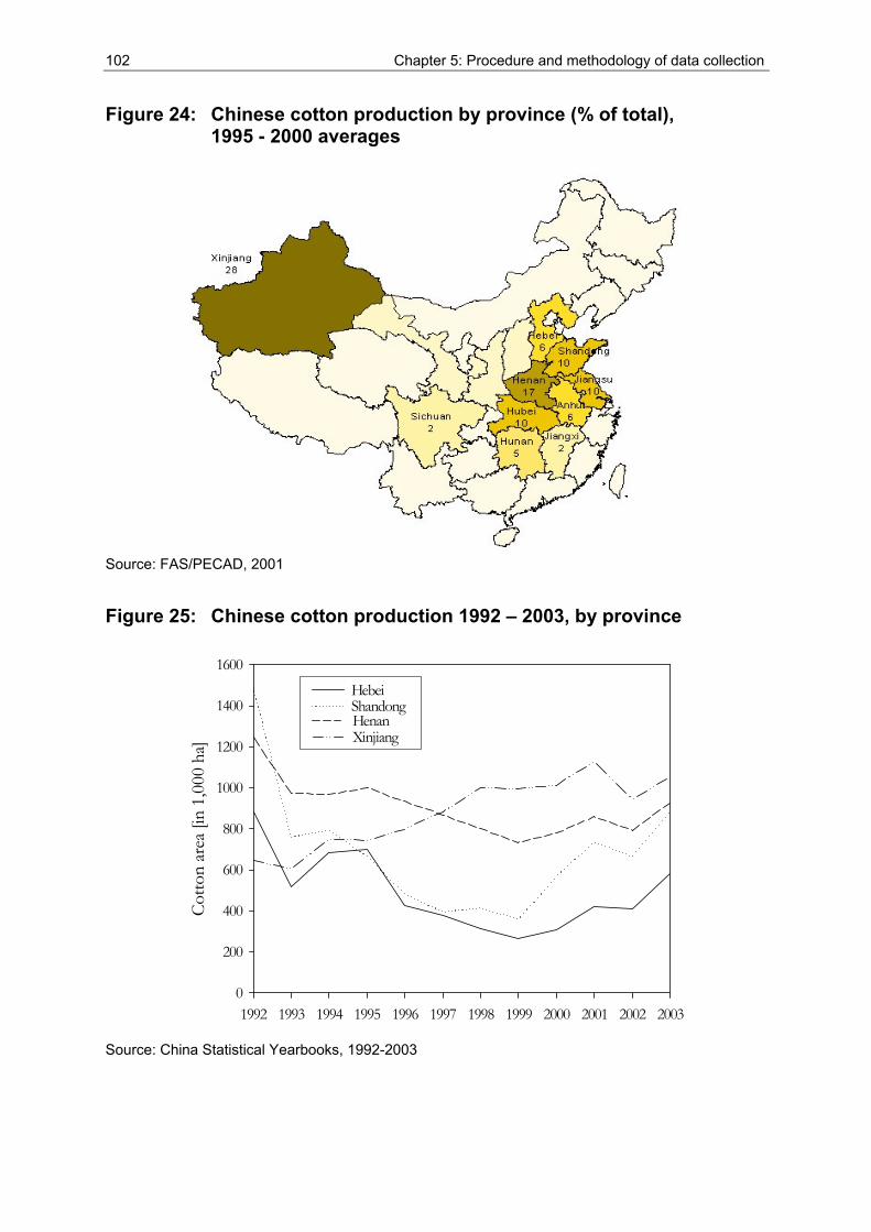
102 Chapter 5: Procedure and methodology of data collection
Figure 24: Chinese cotton production by province (% of total), 1995 - 2000 averages
Source: FAS/PECAD, 2001
Figure 25: Chinese cotton production 1992 – 2003, by province
1992 1993 1994 1995 1996 1997 1998 1999 2000 2001 2002 2003
Cotto
n ar
ea [i
n 1,
000
ha]
0
200
400
600
800
1000
1200
1400
1600
HebeiShandongHenanXinjiang
Source: China Statistical Yearbooks, 1992-2003
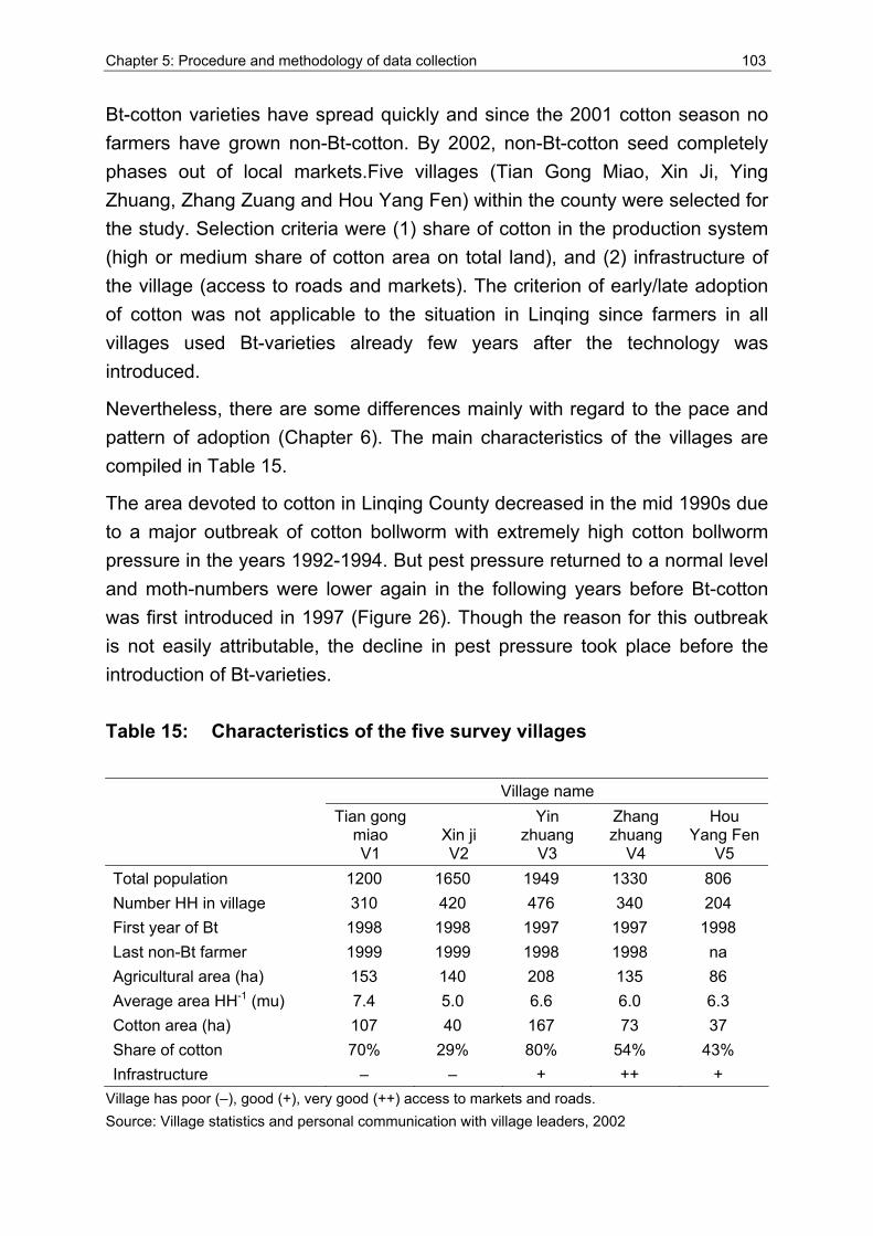
Chapter 5: Procedure and methodology of data collection 103
Bt-cotton varieties have spread quickly and since the 2001 cotton season no farmers have grown non-Bt-cotton. By 2002, non-Bt-cotton seed completely phases out of local markets.Five villages (Tian Gong Miao, Xin Ji, Ying Zhuang, Zhang Zuang and Hou Yang Fen) within the county were selected for the study. Selection criteria were (1) share of cotton in the production system (high or medium share of cotton area on total land), and (2) infrastructure of the village (access to roads and markets). The criterion of early/late adoption of cotton was not applicable to the situation in Linqing since farmers in all villages used Bt-varieties already few years after the technology was introduced.
Nevertheless, there are some differences mainly with regard to the pace and pattern of adoption (Chapter 6). The main characteristics of the villages are compiled in Table 15.
The area devoted to cotton in Linqing County decreased in the mid 1990s due to a major outbreak of cotton bollworm with extremely high cotton bollworm pressure in the years 1992-1994. But pest pressure returned to a normal level and moth-numbers were lower again in the following years before Bt-cotton was first introduced in 1997 (Figure 26). Though the reason for this outbreak is not easily attributable, the decline in pest pressure took place before the introduction of Bt-varieties.
Table 15: Characteristics of the five survey villages
Village name Tian gong
miao V1
Xin ji V2
Yin zhuang
V3
Zhang zhuang
V4
Hou Yang Fen
V5 Total population 1200 1650 1949 1330 806 Number HH in village 310 420 476 340 204 First year of Bt 1998 1998 1997 1997 1998 Last non-Bt farmer 1999 1999 1998 1998 na Agricultural area (ha) 153 140 208 135 86 Average area HH-1 (mu) 7.4 5.0 6.6 6.0 6.3 Cotton area (ha) 107 40 167 73 37 Share of cotton 70% 29% 80% 54% 43% Infrastructure – – + ++ +
Village has poor (–), good (+), very good (++) access to markets and roads. Source: Village statistics and personal communication with village leaders, 2002
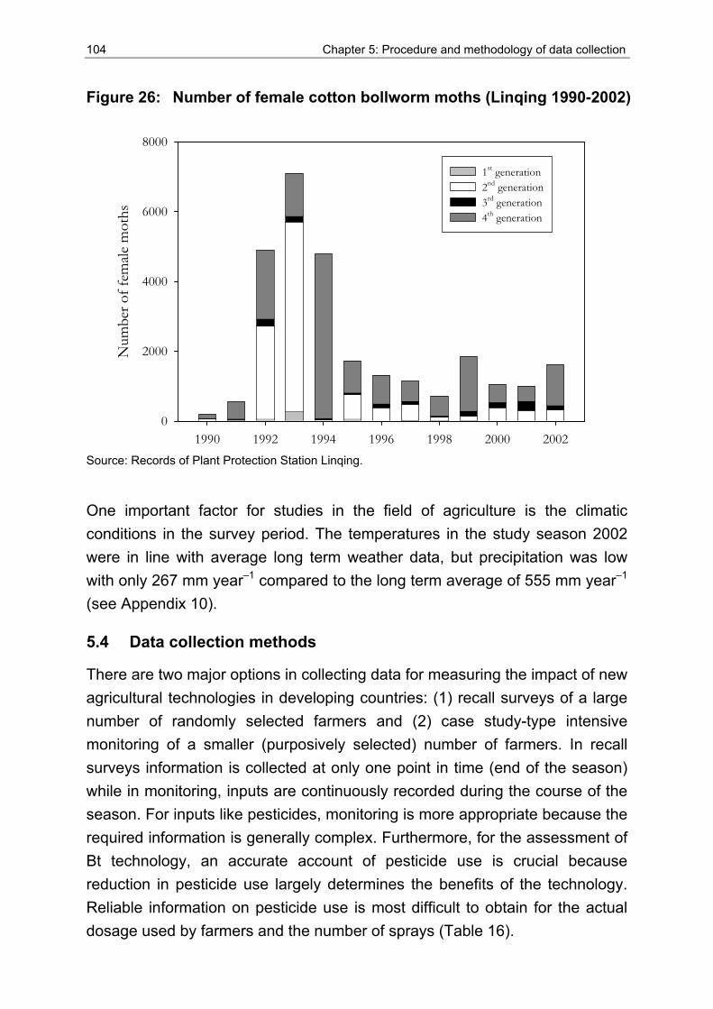
104 Chapter 5: Procedure and methodology of data collection
Figure 26: Number of female cotton bollworm moths (Linqing 1990-2002)
1990 1992 1994 1996 1998 2000 2002
Num
ber o
f fem
ale m
oths
0
2000
4000
6000
8000
1st generation2nd generation3rd generation4th generation
Source: Records of Plant Protection Station Linqing.
One important factor for studies in the field of agriculture is the climatic conditions in the survey period. The temperatures in the study season 2002 were in line with average long term weather data, but precipitation was low with only 267 mm year–1 compared to the long term average of 555 mm year–1 (see Appendix 10).
5.4 Data collection methods
There are two major options in collecting data for measuring the impact of new agricultural technologies in developing countries: (1) recall surveys of a large number of randomly selected farmers and (2) case study-type intensive monitoring of a smaller (purposively selected) number of farmers. In recall surveys information is collected at only one point in time (end of the season) while in monitoring, inputs are continuously recorded during the course of the season. For inputs like pesticides, monitoring is more appropriate because the required information is generally complex. Furthermore, for the assessment of Bt technology, an accurate account of pesticide use is crucial because reduction in pesticide use largely determines the benefits of the technology. Reliable information on pesticide use is most difficult to obtain for the actual dosage used by farmers and the number of sprays (Table 16).
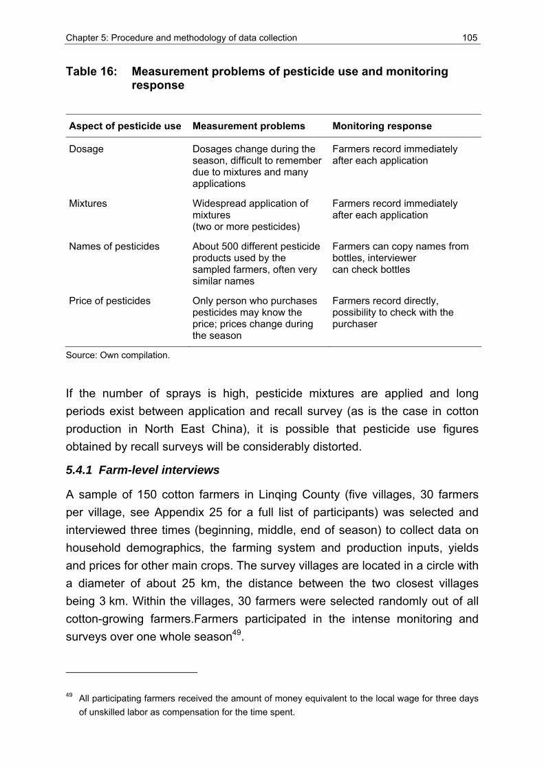
Chapter 5: Procedure and methodology of data collection 105
Table 16: Measurement problems of pesticide use and monitoring response
Aspect of pesticide use Measurement problems Monitoring response
Dosage Dosages change during the season, difficult to remember due to mixtures and many applications
Farmers record immediately after each application
Mixtures Widespread application of mixtures (two or more pesticides)
Farmers record immediately after each application
Names of pesticides About 500 different pesticide products used by the sampled farmers, often very similar names
Farmers can copy names from bottles, interviewer can check bottles
Price of pesticides Only person who purchases pesticides may know the price; prices change during the season
Farmers record directly, possibility to check with the purchaser
Source: Own compilation.
If the number of sprays is high, pesticide mixtures are applied and long periods exist between application and recall survey (as is the case in cotton production in North East China), it is possible that pesticide use figures obtained by recall surveys will be considerably distorted.
5.4.1 Farm-level interviews
A sample of 150 cotton farmers in Linqing County (five villages, 30 farmers per village, see Appendix 25 for a full list of participants) was selected and interviewed three times (beginning, middle, end of season) to collect data on household demographics, the farming system and production inputs, yields and prices for other main crops. The survey villages are located in a circle with a diameter of about 25 km, the distance between the two closest villages being 3 km. Within the villages, 30 farmers were selected randomly out of all cotton-growing farmers.Farmers participated in the intense monitoring and surveys over one whole season49.
49 All participating farmers received the amount of money equivalent to the local wage for three days of unskilled labor as compensation for the time spent.
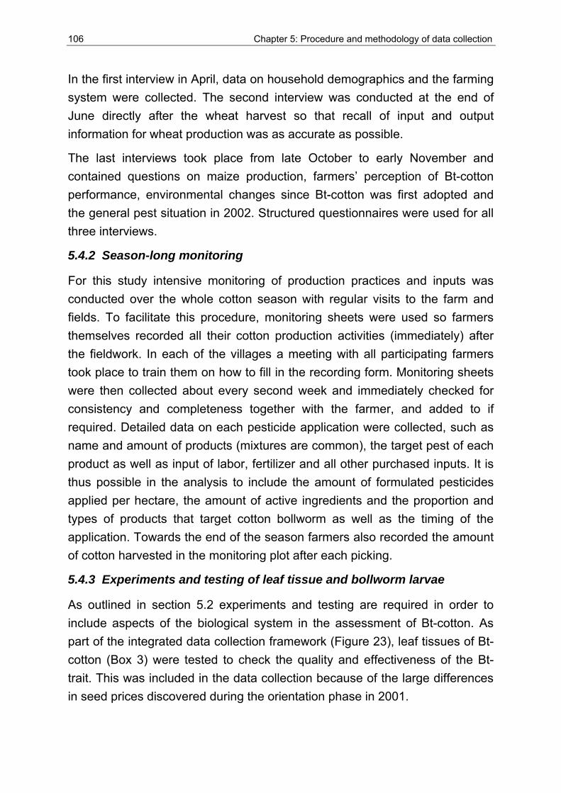
106 Chapter 5: Procedure and methodology of data collection
In the first interview in April, data on household demographics and the farming system were collected. The second interview was conducted at the end of June directly after the wheat harvest so that recall of input and output information for wheat production was as accurate as possible.
The last interviews took place from late October to early November and contained questions on maize production, farmers’ perception of Bt-cotton performance, environmental changes since Bt-cotton was first adopted and the general pest situation in 2002. Structured questionnaires were used for all three interviews.
5.4.2 Season-long monitoring
For this study intensive monitoring of production practices and inputs was conducted over the whole cotton season with regular visits to the farm and fields. To facilitate this procedure, monitoring sheets were used so farmers themselves recorded all their cotton production activities (immediately) after the fieldwork. In each of the villages a meeting with all participating farmers took place to train them on how to fill in the recording form. Monitoring sheets were then collected about every second week and immediately checked for consistency and completeness together with the farmer, and added to if required. Detailed data on each pesticide application were collected, such as name and amount of products (mixtures are common), the target pest of each product as well as input of labor, fertilizer and all other purchased inputs. It is thus possible in the analysis to include the amount of formulated pesticides applied per hectare, the amount of active ingredients and the proportion and types of products that target cotton bollworm as well as the timing of the application. Towards the end of the season farmers also recorded the amount of cotton harvested in the monitoring plot after each picking.
5.4.3 Experiments and testing of leaf tissue and bollworm larvae
As outlined in section 5.2 experiments and testing are required in order to include aspects of the biological system in the assessment of Bt-cotton. As part of the integrated data collection framework (Figure 23), leaf tissues of Bt-cotton (Box 3) were tested to check the quality and effectiveness of the Bt-trait. This was included in the data collection because of the large differences in seed prices discovered during the orientation phase in 2001.
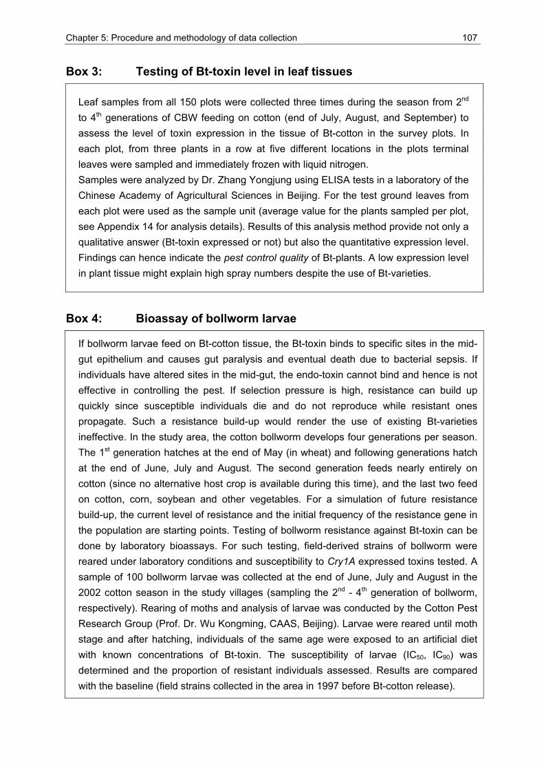
Chapter 5: Procedure and methodology of data collection 107
Box 3: Testing of Bt-toxin level in leaf tissues
Leaf samples from all 150 plots were collected three times during the season from 2nd to 4th generations of CBW feeding on cotton (end of July, August, and September) to assess the level of toxin expression in the tissue of Bt-cotton in the survey plots. In each plot, from three plants in a row at five different locations in the plots terminal leaves were sampled and immediately frozen with liquid nitrogen. Samples were analyzed by Dr. Zhang Yongjung using ELISA tests in a laboratory of the Chinese Academy of Agricultural Sciences in Beijing. For the test ground leaves from each plot were used as the sample unit (average value for the plants sampled per plot, see Appendix 14 for analysis details). Results of this analysis method provide not only a qualitative answer (Bt-toxin expressed or not) but also the quantitative expression level. Findings can hence indicate the pest control quality of Bt-plants. A low expression level in plant tissue might explain high spray numbers despite the use of Bt-varieties.
Box 4: Bioassay of bollworm larvae
If bollworm larvae feed on Bt-cotton tissue, the Bt-toxin binds to specific sites in the mid-gut epithelium and causes gut paralysis and eventual death due to bacterial sepsis. If individuals have altered sites in the mid-gut, the endo-toxin cannot bind and hence is not effective in controlling the pest. If selection pressure is high, resistance can build up quickly since susceptible individuals die and do not reproduce while resistant ones propagate. Such a resistance build-up would render the use of existing Bt-varieties ineffective. In the study area, the cotton bollworm develops four generations per season. The 1st generation hatches at the end of May (in wheat) and following generations hatch at the end of June, July and August. The second generation feeds nearly entirely on cotton (since no alternative host crop is available during this time), and the last two feed on cotton, corn, soybean and other vegetables. For a simulation of future resistance build-up, the current level of resistance and the initial frequency of the resistance gene in the population are starting points. Testing of bollworm resistance against Bt-toxin can be done by laboratory bioassays. For such testing, field-derived strains of bollworm were reared under laboratory conditions and susceptibility to Cry1A expressed toxins tested. A sample of 100 bollworm larvae was collected at the end of June, July and August in the 2002 cotton season in the study villages (sampling the 2nd - 4th generation of bollworm, respectively). Rearing of moths and analysis of larvae was conducted by the Cotton Pest Research Group (Prof. Dr. Wu Kongming, CAAS, Beijing). Larvae were reared until moth stage and after hatching, individuals of the same age were exposed to an artificial diet with known concentrations of Bt-toxin. The susceptibility of larvae (IC50, IC90) was determined and the proportion of resistant individuals assessed. Results are compared with the baseline (field strains collected in the area in 1997 before Bt-cotton release).
108 Chapter 5: Procedure and methodology of data collection
The effectiveness of the Bt-trait in addition depends on the susceptibility of target pest populations. Resistance build-up of target pests as an evolutionary response to control interventions was discussed in Chapter 2. For this study, bollworm larvae were collected in the survey fields at different times and analyzed with regard to susceptibility to the Bt-toxin (Box 4).Finally, a cotton growth experiment with Bt- and non-Bt-cotton was conducted at the study site in 2002. This experiment aimed at generating data that could be used to calibrate an existing ecosystem-model to the local conditions. The experiment is described in more detail in Box 5 and the design of the planting, as well as all inputs and outputs, is provided in Appendix 15. Although the author conducted the sampling for the bioassay of larvae and the leaf tissue testing as well as the cotton growth experiment, this integrated data collection framework was only possible due to the expertise and effort of collaborating partners.
Box 5: Cotton growth experiment
The objective of the experiment was to generate data that could be used to calibrate an existing model that simulates cotton – pest – environment interaction (Gutierrez et al., 1991a; Gutierrez et al., 1991b; Gutierrez et al., 2005; Gutierrez and Ponsard, 2005) to the conditions of North China. In the experiment a Bt-cotton variety that is widely used (33B, Monsanto) and a non-Bt-cotton variety (Zhong mian 12) with comparable growth and yield characteristics that was common in the region before Bt-cotton was introduced, were planted. Destructive sampling of cotton plants was carried out in weekly intervals to collect all the data needed to calibrate the plant growth model. Each sampling included the measurement/recording of the following plant growth indicators:
number and location (node number) of all squares and bolls node of the first and all following lateral branches number of fruits with damage (holes) from cotton bollworm
Applying this procedure the plant was entirely mapped. Finally, sample plants were separated into stem, leaves, roots and fruit section and the dry weight of each category was measured from germination to maturity (weekly sampling from May - September). The number of plants that were sampled every week was n = 5 (with three replicates) for each variety; an experimental field of around 1,200 m2 was used (see Appendix 15 for design). While mapping the plants, the presence of eggs and larvae of pests was recorded. Data on abiotic factors (temperature, solar radiation, wind and precipitation) on a daily basis for the year 2002, close to the experimental plot were obtained from the surveillance station of the Climate Bureau in the county. In addition, climate records of the last ten years were collected to compare the 2002 data with the long-term average.
Chapter 5: Procedure and methodology of data collection 109
5.4.4 Expert survey and secondary data
A questionnaire was designed and translated into Chinese in late 2004 and sent to 34 experts, mainly from the field of plant protection. Questions were asked about the potential cotton yield, the severity of damage from different pests, time of pest occurrence and differences between Bt- and non-Bt cotton production. The aim of this expert survey was the generation and validation of assumptions for the stochastic budgeting model. The results of the 15 filled questionnaires that were returned are summarized in Chapter 8.1.2. The Plant Protection Station and the Meteorological Station in Linqing County kindly provided data and statistics on the pest pressure and climate history in the area and on active ingredients of registered pesticide products. Additional information sources were the China Statistical Yearbooks and published literature on this topic.
6 Descr ip t ive ana lys is o f Bt -cot ton product ion in L inq ing
This chapter presents the results of a descriptive analysis of the in-depth case study that was conducted in Linqing County in 2002. The main purpose is to give a detailed description of the situation in the field and an overview of the production system. The basis for the analysis is the information collected in the household survey and the production monitoring that was conducted with 150 respondents in five villages.
The first section gives an introduction of the farming system in general. This includes information on the farm characteristics and main farming activities (namely the cropping of wheat and maize). The cotton production practices of surveyed farmers are described in detail in section 6.2, which includes an in-depth analysis of production inputs, especially of chemical pesticides and related household-level human health impairments. Then a summary of farmers’ perception of Bt-cotton characteristics and performance, as well as observed changes in the agro-ecosystem, is provided.
The last section points to some institutional problems in the implementation of the Bt-cotton technology in the study area that can hinder full realization of the potential benefits. The data from the production survey and results of testing and experiments are the basis for the subsequent econometric and modeling approaches.
6.1 Farming system analysis
This section provides a brief overview of the farming system prevalent in the study area. Farm characteristics and major farming activities are analyzed and economic indicators for the production of the two major crops maize and wheat are presented. The analysis reveals significant differences among the villages that were included in the survey. The main distinctions and possible reasons are outlined in the text.
6.1.1 Farm characteristics and production system
The farm households in the sample hold on average only 0.58 ha of agricultural land with areas ranging from 0.51 to 0.78 ha for the different villages (Table 17).
Chapter 6: Descriptive analysis of Bt-cotton production in Linqing 111
Renting of land in addition to owned plots is common in V350 where 50% of the respondents rented land, but less so in the other villages (3 – 23% of farmers). The family size is 4.2 persons on average for the total sample and is not significantly different among the villages. Out of this number 1.8 to 2.1 family members work fulltime on the farm. The majority of the surveyed households (75%) had additional income from off-farm sources. Off-farm work was equally common in all five villages but the extent in terms of number of days worked and its share of total household income varies (Table 17).
Average annual household income ranges from about US$1,400 - 2,000. This is in line with the district level statistics and (just) above the commonly used poverty line of US$1 per person per day. For the total sample some 30% of the household income is from off-farm activities (ranging from 25 to 44% for the different villages). In some cases, household members (male and female) had full-time off-farm jobs (being workers in a factory or teachers) but in most cases the male members of the family work off-farm on a day-to-day basis during the winter months and devote most time to farming. The income figures are based on recall data for off-farm income and income from other crops and livestock51.
It is possible that the income figures presented underestimate actual household income, because respondents had difficulties in remembering all sales activities or small off-farm jobs. Also, children or other relatives may occasionally provide financial support to the household. Although there is a high diversification of income sources, households mainly rely on agricultural activities. The main farming activities in the region are the production of cotton, wheat, and maize as well as the cultivation of vegetables and fruits (especially in V5). Performance of the cotton crop determines the farm income to a large degree as cotton contributes 22 – 52% of total income in the five villages (Table 17).
50 Throughout this chapter the following village numbers (V) are used for brevity: Tian Gong Miao (V1), Xin Ji (V2), Ying Zhuang (V3), Zhang Zhuang (V4), and Hou Yang Fen (V5). N = 30 per village.
51 Value of crops (other than cotton, wheat and maize) and livestock used for own consumption is not included. Costs for agricultural inputs for sold farm-products are already deducted.
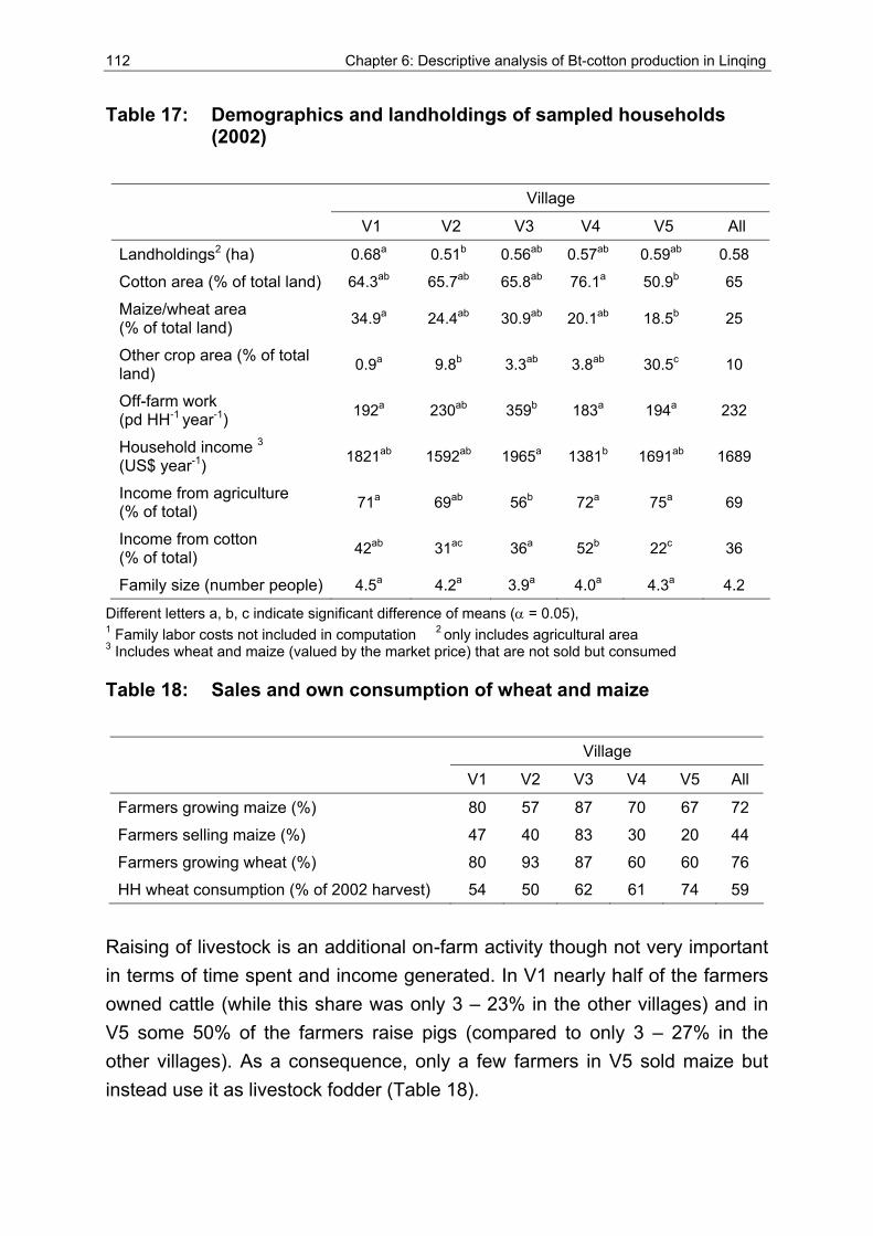
112 Chapter 6: Descriptive analysis of Bt-cotton production in Linqing
Table 17: Demographics and landholdings of sampled households (2002)
Different letters a, b, c indicate significant difference of means (α = 0.05), 1 Family labor costs not included in computation 2 only includes agricultural area 3 Includes wheat and maize (valued by the market price) that are not sold but consumed Table 18: Sales and own consumption of wheat and maize
Village
V1 V2 V3 V4 V5 All
Farmers growing maize (%) 80 57 87 70 67 72
Farmers selling maize (%) 47 40 83 30 20 44
Farmers growing wheat (%) 80 93 87 60 60 76
HH wheat consumption (% of 2002 harvest) 54 50 62 61 74 59
Raising of livestock is an additional on-farm activity though not very important in terms of time spent and income generated. In V1 nearly half of the farmers owned cattle (while this share was only 3 – 23% in the other villages) and in V5 some 50% of the farmers raise pigs (compared to only 3 – 27% in the other villages). As a consequence, only a few farmers in V5 sold maize but instead use it as livestock fodder (Table 18).
Village
V1 V2 V3 V4 V5 All
Landholdings2 (ha) 0.68a 0.51b 0.56ab 0.57ab 0.59ab 0.58
Cotton area (% of total land) 64.3ab 65.7ab 65.8ab 76.1a 50.9b 65
Maize/wheat area (% of total land) 34.9a 24.4ab 30.9ab 20.1ab 18.5b 25
Other crop area (% of total land) 0.9a 9.8b 3.3ab 3.8ab 30.5c 10
Off-farm work (pd HH-1 year-1) 192a 230ab 359b 183a 194a 232
Household income 3
(US$ year-1) 1821ab 1592ab 1965a 1381b 1691ab 1689
Income from agriculture (% of total) 71a 69ab 56b 72a 75a 69
Income from cotton (% of total) 42ab 31ac 36a 52b 22c 36
Family size (number people) 4.5a 4.2a 3.9a 4.0a 4.3a 4.2
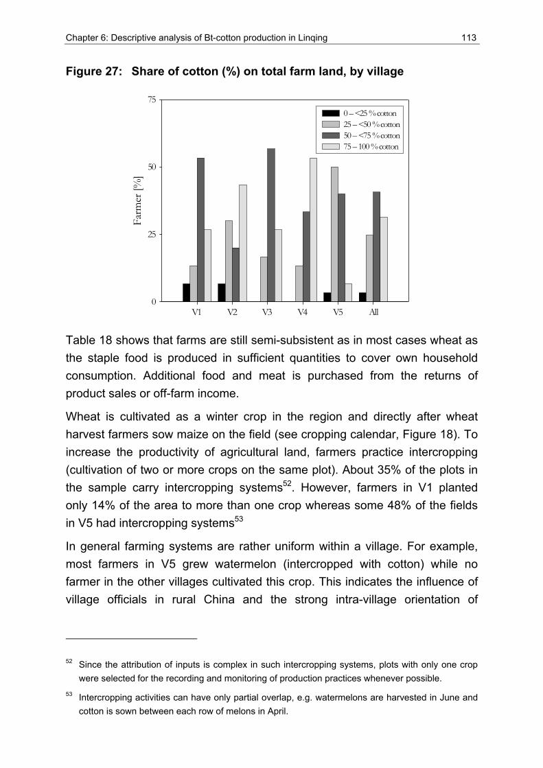
Chapter 6: Descriptive analysis of Bt-cotton production in Linqing 113
Figure 27: Share of cotton (%) on total farm land, by village
Farm
er [%
]
0
25
50
75
V1 V2 V3 V4 AllV5
0 – <25 % cotton25 – <50 % cotton50 – <75 % cotton75 – 100 % cotton
Table 18 shows that farms are still semi-subsistent as in most cases wheat as the staple food is produced in sufficient quantities to cover own household consumption. Additional food and meat is purchased from the returns of product sales or off-farm income.
Wheat is cultivated as a winter crop in the region and directly after wheat harvest farmers sow maize on the field (see cropping calendar, Figure 18). To increase the productivity of agricultural land, farmers practice intercropping (cultivation of two or more crops on the same plot). About 35% of the plots in the sample carry intercropping systems52. However, farmers in V1 planted only 14% of the area to more than one crop whereas some 48% of the fields in V5 had intercropping systems53
In general farming systems are rather uniform within a village. For example, most farmers in V5 grew watermelon (intercropped with cotton) while no farmer in the other villages cultivated this crop. This indicates the influence of village officials in rural China and the strong intra-village orientation of
52 Since the attribution of inputs is complex in such intercropping systems, plots with only one crop were selected for the recording and monitoring of production practices whenever possible.
53 Intercropping activities can have only partial overlap, e.g. watermelons are harvested in June and cotton is sown between each row of melons in April.
114 Chapter 6: Descriptive analysis of Bt-cotton production in Linqing
farmers. Moreover, there are positive (scale) effects if farmers specialize in the same activity
The area planted with cotton ranged from 51 – 77% of total landholdings in the five villages. Figure 27 shows the distribution of cotton share on total landholdings and is distinctive for each of the villages. While a majority of farmers in V2 and V4 have very high shares of cotton in the farming system, farmers in V5 allocated less land to the production of cotton but were growing more fruits (mainly watermelon and apples).
From 2001 to 2002 there was on average a slight increase (5%) of the cotton area in the sample. Farmers in V2 increased cotton area by 30% while there were slight area reductions in V1 and V4. As the main reason for increased cotton area, respondents in V2 stated the advice of village leaders and the introduction of a new cotton variety, while in the other villages the high cotton price was the most important motivation for area increases. For reductions in cotton area, farmers mainly stated a lack of water and routine crop rotation as reasons.
The main problem in farming in the study area as perceived by the respondents is a lack of water (stated by some 30% of the respondents, mainly in V1 and V3), crop pests and diseases (around 13% of respondents, evenly in all villages) and insufficient family labor (11% of farmers, mainly in V5, where labor intensive vegetable crops are grown).
6.1.2 Economic indicators for main crops
Cotton is clearly the major crop in the region cultivated on 65% of the agricultural land, while the combination of wheat (in winter) and maize (in summer) covers around one quarter of the area. This section provides key economic indicators for wheat and maize production of sampled households in the 2002 season.
Wheat produced is mainly used for household consumption and maize is mainly used as fodder for livestock. Surplus wheat is usually stored and maize surplus sold for cash income. For the 2002 season, the sum of the gross margins of maize and wheat is US$1,070 per hectare compared to a gross margin of US$1,114 per hectare from growing cotton (Tables 19 to 21). Output prices for agricultural products fluctuate over the year (lowest prices after harvest) and hence farmers do not sell the entire crop immediately after harvesting but store at least a part for sale later in the season.
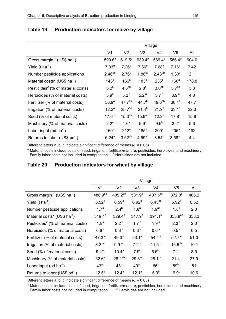
Chapter 6: Descriptive analysis of Bt-cotton production in Linqing 115
Table 19: Production indicators for maize by village
Village
V1 V2 V3 V4 V5 All
Gross margin 1 (US$ ha-1) 599.6a 619.5a 639.4a 569.4a 586.4a 604.0
Yield (t ha-1) 7.03a 7.26a 7.86a 7.68a 7.16a 7.42
Number pesticide applications 2.46ab 2.76a 1.88bc 2.43ab 1.30c 2.1
Material costs* (US$ ha-1) 143a 166a 183a 235b 168a 178.8
Pesticides2 (% of material costs) 5.2a 4.6ab 2.8b 3.0ab 3.7ab 3.8
Herbicides (% of material costs) 5.9a 5.2 a 5.2 a 3.7 a 3.9 a 4.8
Fertilizer (% of material costs) 56.9a 47.7ab 44.7b 49.6ab 38.4b 47.7
Irrigation (% of material costs) 12.2a 25.7bc 21.4b 21.9b 33.1c 22.3
Seed (% of material costs) 17.6 a 15.3ab 15.9ab 12.3b 17.8a 15.8
Machinery (% of material costs) 2.2a 1.6a 9.9b 9.6b 3.2a 5.6
Labor input (pd ha-1) 160a 212a 185a 209a 205a 192
Returns to labor (US$ pd-1) 6.24a 3.62ab 4.59ab 3.54b 3.58ab 4.4
Different letters a, b, c indicate significant difference of means (α = 0.05) * Material costs include costs of seed, irrigation, fertilizer/manure, pesticides, herbicides, and machinery. 1 Family labor costs not included in computation 2 Herbicides are not included Table 20: Production indicators for wheat by village
Village
V1 V2 V3 V4 V5 All
Gross margin 1 (US$ ha-1) 486.9ab 485.2ab 531.9a 407.5bc 372.8c 466.2
Yield (t ha-1) 6.52a 6.59a 6.92a 6.43ab 5.92b 6.52
Number pesticide applications 1.7a 2.4b 1.8a 1.9ab 1.8a 2.0
Material costs* (US$ ha-1) 319.4a 329.4a 317.9a 391.1b 353.9ab 338.3
Pesticides2 (% of material costs) 1.8a 2.2 a 1.7 a 1.9 a 2.3 a 2.0
Herbicides (% of material costs) 0.6 a 0.3 a 0.3 a 0.6 a 0.5 a 0.5
Fertilizer (% of material costs) 47.3 a 49.0 a 53.1a 54.4 a 52.7 a 51.0
Irrigation (% of material costs) 8.2 ac 9.9 ac 7.2 a 11.5 c 15.6 b 10.1
Seed (% of material costs) 9.4ac 10.4a 7.9c 6.5bc 7.2c 8.5
Machinery (% of material costs) 32.6a 28.2ab 29.8ac 25.1bc 21.4b 27.9
Labor input (pd ha-1) 43ac 43a 49ac 66b 59bc 51
Returns to labor (US$ pd-1) 12.5a 12.4a 12.1a 6.9b 6.9b 10.6
Different letters a, b, c indicate significant difference of means (α = 0.05) * Material costs include costs of seed, irrigation, fertilizer/manure, pesticides, herbicides, and machinery. 1 Family labor costs not included in computation 2 Herbicides are not included
116 Chapter 6: Descriptive analysis of Bt-cotton production in Linqing
For the computation of gross margins average prices are used. Average prices for wheat and maize in 2002 were US$0.119 per kg and US$0.105 per kg, respectively. Production of wheat and maize is less labor intensive compared to cotton and returns to labor are higher. For maize, returns to family labor is US$4.4 per personday on average but with immense differences among the villages. Differences are mainly due to variation in the material input and labor used for irrigation. In V1 irrigation expenditures (pump fuel, water fees) account for only 12% of the material costs and labor input is lower than in the other villages (though not statistically significant). Harvesting maize is very labor intensive as cobs are picked from the plants, peeled at the field and later the grains are removed manually from the cob before drying and storage. The labor required for these tasks largely depends on the yield level further explaining the lower labor figures in V1 where yield level is lowest. Still, returns to labor are well above the local wage level for unskilled labor (US$1.2 – 1.8 per personday).
The lion’s share of material costs in maize production is spent for fertilizer (50%) and conduct irrigation (22%) while the share of pesticides is only minor (Table 19). The lack of rain in 2002 (Appendix 10) might have caused lower yields and/or higher costs for irrigation and hence lower gross margins for the summer crops (cotton and maize) as compared to other years. Seed costs for maize represent a relatively high proportion of total material costs because all farmers are using hybrid varieties and hence purchase new seed every year because yields decline dramatically if seed is kept and used for the following season. Sowing and harvesting in wheat production are done with rented machines, resulting in high machinery costs (nearly 30% of material costs) and high total material costs (Table 20). Wheat production requires lower labor input, on average 51 personday per hectare and the returns to family labor from wheat production are on average US$10.6 per personday. This is far above the local wage level for unskilled labor and also much higher than the returns to labor for other crops (maize and cotton). Again, there are huge differences between villages and returns to labor from wheat production in V1 are almost double those in V4. This results from differences in material costs and labor use due to particular village conditions (mainly availability of water for irrigation). Similarly to the situation in maize production, fertilizer makes up the lion’s share of material costs (51% on average). Irrigation is relatively less important during the cooler winter months. Seed costs are also lower since
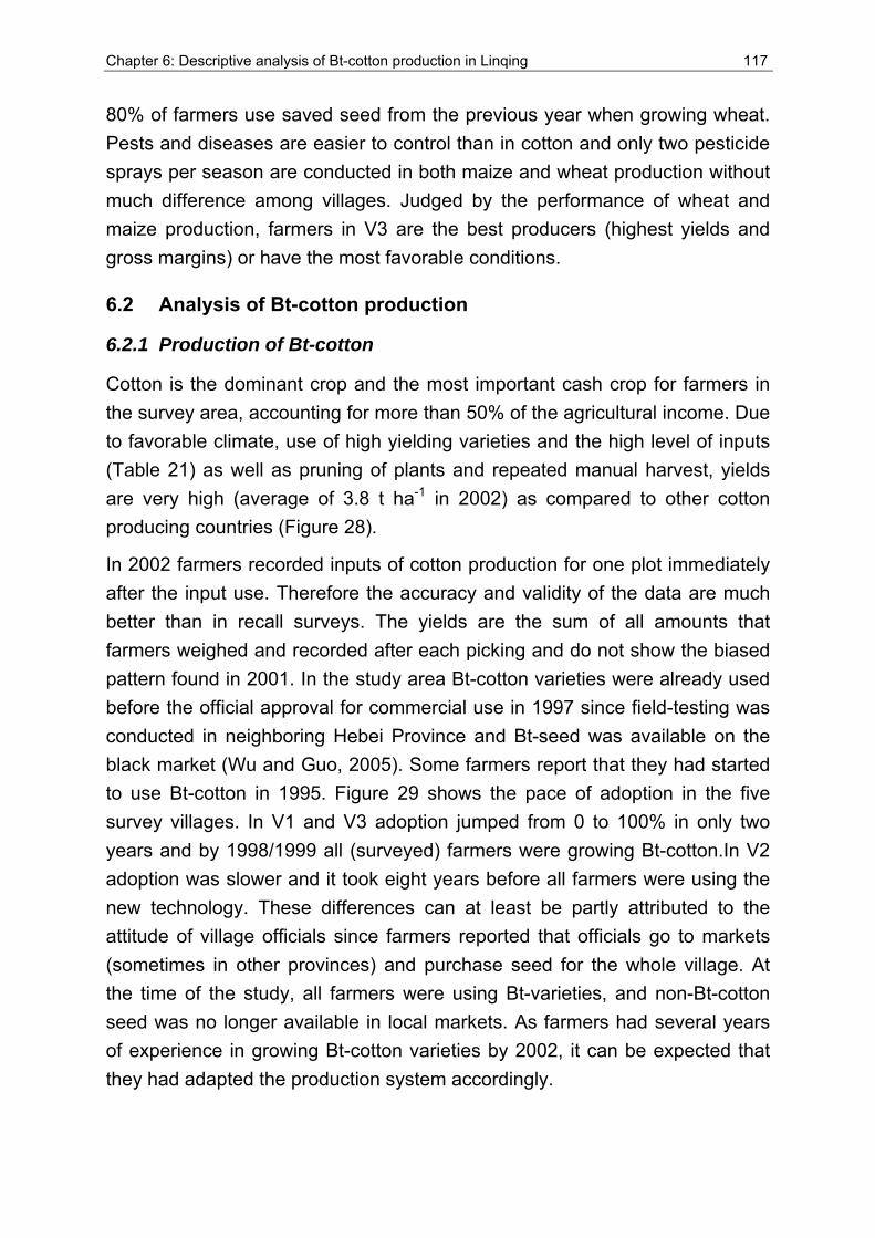
Chapter 6: Descriptive analysis of Bt-cotton production in Linqing 117
80% of farmers use saved seed from the previous year when growing wheat. Pests and diseases are easier to control than in cotton and only two pesticide sprays per season are conducted in both maize and wheat production without much difference among villages. Judged by the performance of wheat and maize production, farmers in V3 are the best producers (highest yields and gross margins) or have the most favorable conditions.
6.2 Analysis of Bt-cotton production
6.2.1 Production of Bt-cotton
Cotton is the dominant crop and the most important cash crop for farmers in the survey area, accounting for more than 50% of the agricultural income. Due to favorable climate, use of high yielding varieties and the high level of inputs (Table 21) as well as pruning of plants and repeated manual harvest, yields are very high (average of 3.8 t ha-1 in 2002) as compared to other cotton producing countries (Figure 28).
In 2002 farmers recorded inputs of cotton production for one plot immediately after the input use. Therefore the accuracy and validity of the data are much better than in recall surveys. The yields are the sum of all amounts that farmers weighed and recorded after each picking and do not show the biased pattern found in 2001. In the study area Bt-cotton varieties were already used before the official approval for commercial use in 1997 since field-testing was conducted in neighboring Hebei Province and Bt-seed was available on the black market (Wu and Guo, 2005). Some farmers report that they had started to use Bt-cotton in 1995. Figure 29 shows the pace of adoption in the five survey villages. In V1 and V3 adoption jumped from 0 to 100% in only two years and by 1998/1999 all (surveyed) farmers were growing Bt-cotton.In V2 adoption was slower and it took eight years before all farmers were using the new technology. These differences can at least be partly attributed to the attitude of village officials since farmers reported that officials go to markets (sometimes in other provinces) and purchase seed for the whole village. At the time of the study, all farmers were using Bt-varieties, and non-Bt-cotton seed was no longer available in local markets. As farmers had several years of experience in growing Bt-cotton varieties by 2002, it can be expected that they had adapted the production system accordingly.
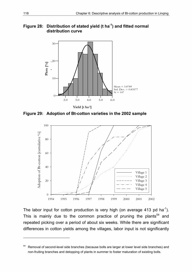
118 Chapter 6: Descriptive analysis of Bt-cotton production in Linqing
Figure 28: Distribution of stated yield (t ha-1) and fitted normal distribution curve
2.0 3.0 4.0 5.0 6.00
10
20
30
qy
Mean = 3.8789Std. Dev. = 0.83577N = 147
Figure 29: Adoption of Bt-cotton varieties in the 2002 sample
1994 1995 1996 1997 1998 1999 2000 2001 2002
Ado
ptio
n of
Bt-c
otto
n [c
umul
ativ
e %
]
0
20
40
60
80
100
Village 1Village 2Village 3Village 4Village 5
The labor input for cotton production is very high (on average 413 pd ha-1). This is mainly due to the common practice of pruning the plants54 and repeated picking over a period of about six weeks. While there are significant differences in cotton yields among the villages, labor input is not significantly
54 Removal of second-level side branches (because bolls are larger at lower level side branches) and non-fruiting branches and detopping of plants in summer to foster maturation of existing bolls.
Yield [t ha-1]
Plo
ts [
%]
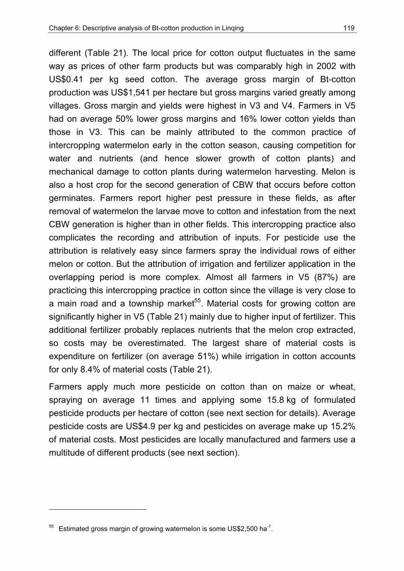
Chapter 6: Descriptive analysis of Bt-cotton production in Linqing 119
different (Table 21). The local price for cotton output fluctuates in the same way as prices of other farm products but was comparably high in 2002 with US$0.41 per kg seed cotton. The average gross margin of Bt-cotton production was US$1,541 per hectare but gross margins varied greatly among villages. Gross margin and yields were highest in V3 and V4. Farmers in V5 had on average 50% lower gross margins and 16% lower cotton yields than those in V3. This can be mainly attributed to the common practice of intercropping watermelon early in the cotton season, causing competition for water and nutrients (and hence slower growth of cotton plants) and mechanical damage to cotton plants during watermelon harvesting. Melon is also a host crop for the second generation of CBW that occurs before cotton germinates. Farmers report higher pest pressure in these fields, as after removal of watermelon the larvae move to cotton and infestation from the next CBW generation is higher than in other fields. This intercropping practice also complicates the recording and attribution of inputs. For pesticide use the attribution is relatively easy since farmers spray the individual rows of either melon or cotton. But the attribution of irrigation and fertilizer application in the overlapping period is more complex. Almost all farmers in V5 (87%) are practicing this intercropping practice in cotton since the village is very close to a main road and a township market55. Material costs for growing cotton are significantly higher in V5 (Table 21) mainly due to higher input of fertilizer. This additional fertilizer probably replaces nutrients that the melon crop extracted, so costs may be overestimated. The largest share of material costs is expenditure on fertilizer (on average 51%) while irrigation in cotton accounts for only 8.4% of material costs (Table 21).
Farmers apply much more pesticide on cotton than on maize or wheat, spraying on average 11 times and applying some 15.8 kg of formulated pesticide products per hectare of cotton (see next section for details). Average pesticide costs are US$4.9 per kg and pesticides on average make up 15.2% of material costs. Most pesticides are locally manufactured and farmers use a multitude of different products (see next section).
55 Estimated gross margin of growing watermelon is some US$2,500 ha-1.
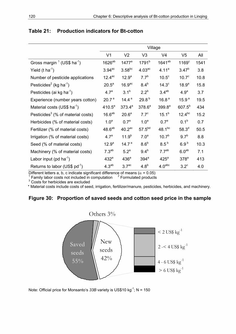
120 Chapter 6: Descriptive analysis of Bt-cotton production in Linqing
Table 21: Production indicators for Bt-cotton
Village
V1 V2 V3 V4 V5 All
Gross margin 1 (US$ ha-1) 1626ab 1477a 1791b 1641ab 1169c 1541
Yield (t ha-1) 3.94ac 3.58bc 4.03ac 4.11a 3.47b 3.8
Number of pesticide applications 12.4ac 12.9a 7.7b 10.5c 10.7c 10.8
Pesticides2 (kg ha-1) 20.5a 16.9ac 8.4b 14.3c 18.9a 15.8
Pesticides (ai kg ha-1) 4.7a 3.1b 2.2b 3.4ab 4.9a 3.7
Experience (number years cotton) 20.7 a 14.4 a 29.8 b 16.8 a 15.9 a 19.5
Material costs (US$ ha-1) 410.5a 373.4a 378.6a 399.8a 607.5b 434
Pesticides3 (% of material costs) 16.6ab 20.6a 7.7c 15.1b 12.4bc 15.2
Herbicides (% of material costs) 1.0a 0.7a 1.0a 0.7a 0.1b 0.7
Fertilizer (% of material costs) 48.6ab 40.2ac 57.5bd 48.1bc 58.3d 50.5
Irrigation (% of material costs) 4.7a 11.9b 7.0a 10.7b 9.7b 8.8
Seed (% of material costs) 12.9a 14.7 a 8.6b 8.5 b 6.9 b 10.3
Machinery (% of material costs) 7.3ab 5.2a 9.4b 7.7ab 6.0ab 7.1
Labor input (pd ha-1) 432a 436a 394a 425a 378a 413
Returns to labor (US$ pd-1) 4.3ab 3.7ac 4.8b 4.0abc 3.2c 4.0 Different letters a, b, c indicate significant difference of means (α = 0.05) 1 Family labor costs not included in computation 2 Formulated products 3 Costs for herbicides are excluded * Material costs include costs of seed, irrigation, fertilizer/manure, pesticides, herbicides, and machinery. Figure 30: Proportion of saved seeds and cotton seed price in the sample
> 6 US$ kg-1
New seeds42%
Others 3%
Saved seeds55% 4 - 6 US$ kg-1
< 2 US$ kg-1
2 -< 4 US$ kg-1
Note: Official price for Monsanto‘s 33B variety is US$10 kg-1; N = 150
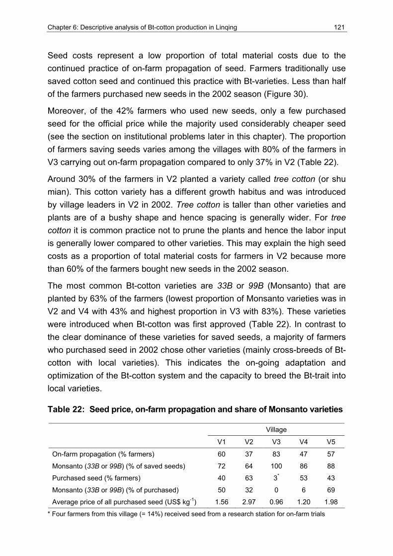
Chapter 6: Descriptive analysis of Bt-cotton production in Linqing 121
Seed costs represent a low proportion of total material costs due to the continued practice of on-farm propagation of seed. Farmers traditionally use saved cotton seed and continued this practice with Bt-varieties. Less than half of the farmers purchased new seeds in the 2002 season (Figure 30).
Moreover, of the 42% farmers who used new seeds, only a few purchased seed for the official price while the majority used considerably cheaper seed (see the section on institutional problems later in this chapter). The proportion of farmers saving seeds varies among the villages with 80% of the farmers in V3 carrying out on-farm propagation compared to only 37% in V2 (Table 22).
Around 30% of the farmers in V2 planted a variety called tree cotton (or shu mian). This cotton variety has a different growth habitus and was introduced by village leaders in V2 in 2002. Tree cotton is taller than other varieties and plants are of a bushy shape and hence spacing is generally wider. For tree cotton it is common practice not to prune the plants and hence the labor input is generally lower compared to other varieties. This may explain the high seed costs as a proportion of total material costs for farmers in V2 because more than 60% of the farmers bought new seeds in the 2002 season.
The most common Bt-cotton varieties are 33B or 99B (Monsanto) that are planted by 63% of the farmers (lowest proportion of Monsanto varieties was in V2 and V4 with 43% and highest proportion in V3 with 83%). These varieties were introduced when Bt-cotton was first approved (Table 22). In contrast to the clear dominance of these varieties for saved seeds, a majority of farmers who purchased seed in 2002 chose other varieties (mainly cross-breeds of Bt-cotton with local varieties). This indicates the on-going adaptation and optimization of the Bt-cotton system and the capacity to breed the Bt-trait into local varieties.
Table 22: Seed price, on-farm propagation and share of Monsanto varieties
Village
V1 V2 V3 V4 V5
On-farm propagation (% farmers) 60 37 83 47 57
Monsanto (33B or 99B) (% of saved seeds) 72 64 100 86 88
Purchased seed (% farmers) 40 63 3* 53 43
Monsanto (33B or 99B) (% of purchased) 50 32 0 6 69
Average price of all purchased seed (US$ kg-1) 1.56 2.97 0.96 1.20 1.98
* Four farmers from this village (= 14%) received seed from a research station for on-farm trials
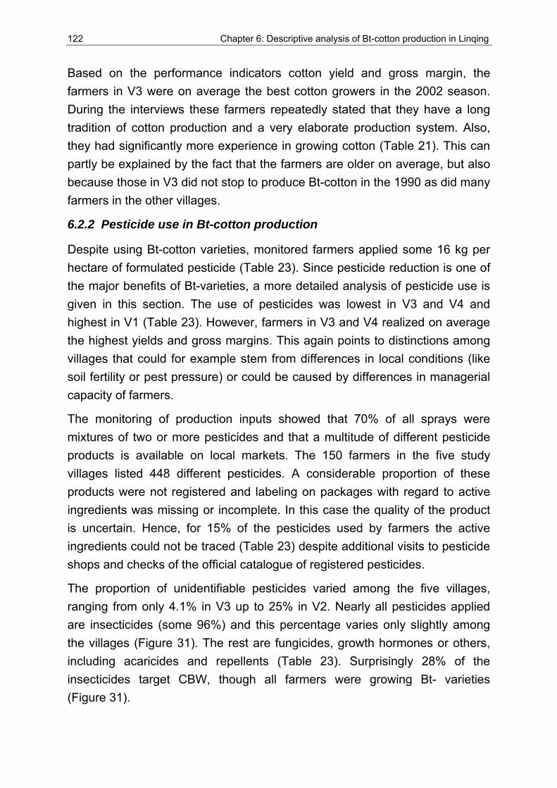
122 Chapter 6: Descriptive analysis of Bt-cotton production in Linqing
Based on the performance indicators cotton yield and gross margin, the farmers in V3 were on average the best cotton growers in the 2002 season. During the interviews these farmers repeatedly stated that they have a long tradition of cotton production and a very elaborate production system. Also, they had significantly more experience in growing cotton (Table 21). This can partly be explained by the fact that the farmers are older on average, but also because those in V3 did not stop to produce Bt-cotton in the 1990 as did many farmers in the other villages.
6.2.2 Pesticide use in Bt-cotton production
Despite using Bt-cotton varieties, monitored farmers applied some 16 kg per hectare of formulated pesticide (Table 23). Since pesticide reduction is one of the major benefits of Bt-varieties, a more detailed analysis of pesticide use is given in this section. The use of pesticides was lowest in V3 and V4 and highest in V1 (Table 23). However, farmers in V3 and V4 realized on average the highest yields and gross margins. This again points to distinctions among villages that could for example stem from differences in local conditions (like soil fertility or pest pressure) or could be caused by differences in managerial capacity of farmers.
The monitoring of production inputs showed that 70% of all sprays were mixtures of two or more pesticides and that a multitude of different pesticide products is available on local markets. The 150 farmers in the five study villages listed 448 different pesticides. A considerable proportion of these products were not registered and labeling on packages with regard to active ingredients was missing or incomplete. In this case the quality of the product is uncertain. Hence, for 15% of the pesticides used by farmers the active ingredients could not be traced (Table 23) despite additional visits to pesticide shops and checks of the official catalogue of registered pesticides.
The proportion of unidentifiable pesticides varied among the five villages, ranging from only 4.1% in V3 up to 25% in V2. Nearly all pesticides applied are insecticides (some 96%) and this percentage varies only slightly among the villages (Figure 31). The rest are fungicides, growth hormones or others, including acaricides and repellents (Table 23). Surprisingly 28% of the insecticides target CBW, though all farmers were growing Bt- varieties (Figure 31).
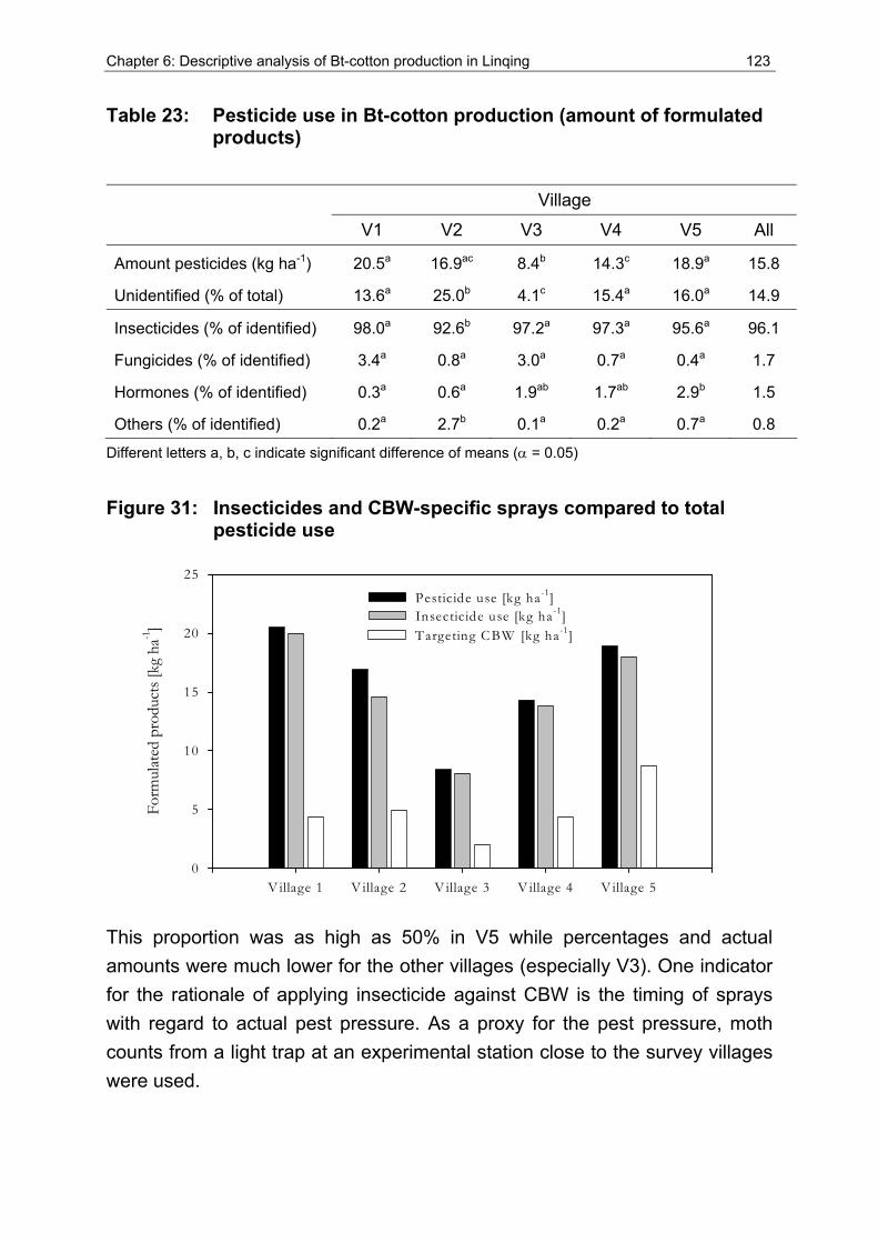
Chapter 6: Descriptive analysis of Bt-cotton production in Linqing 123
Table 23: Pesticide use in Bt-cotton production (amount of formulated products)
Village V1 V2 V3 V4 V5 All
Amount pesticides (kg ha-1) 20.5a 16.9ac 8.4b 14.3c 18.9a 15.8
Unidentified (% of total) 13.6a 25.0b 4.1c 15.4a 16.0a 14.9
Insecticides (% of identified) 98.0a 92.6b 97.2a 97.3a 95.6a 96.1
Fungicides (% of identified) 3.4a 0.8a 3.0a 0.7a 0.4a 1.7
Hormones (% of identified) 0.3a 0.6a 1.9ab 1.7ab 2.9b 1.5
Others (% of identified) 0.2a 2.7b 0.1a 0.2a 0.7a 0.8
Different letters a, b, c indicate significant difference of means (α = 0.05)
Figure 31: Insecticides and CBW-specific sprays compared to total
pesticide use
V illage 1 V illage 2 V illage 3 V illage 4 V illage 5
Form
ulat
ed p
rodu
cts [
kg h
a-1]
0
5
10
15
20
25
Pesticide use [kg ha-1]Insecticide use [kg ha-1]Targeting C BW [kg ha-1]
This proportion was as high as 50% in V5 while percentages and actual amounts were much lower for the other villages (especially V3). One indicator for the rationale of applying insecticide against CBW is the timing of sprays with regard to actual pest pressure. As a proxy for the pest pressure, moth counts from a light trap at an experimental station close to the survey villages were used.
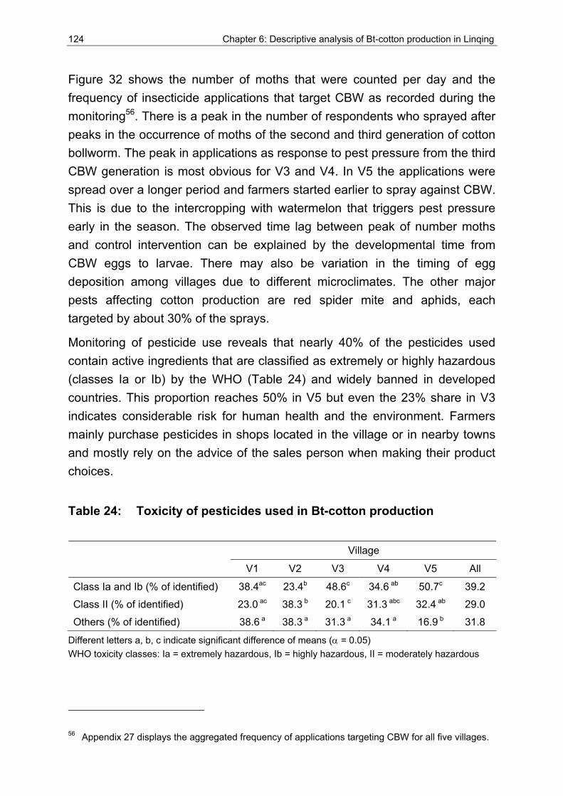
124 Chapter 6: Descriptive analysis of Bt-cotton production in Linqing
Figure 32 shows the number of moths that were counted per day and the frequency of insecticide applications that target CBW as recorded during the monitoring56. There is a peak in the number of respondents who sprayed after peaks in the occurrence of moths of the second and third generation of cotton bollworm. The peak in applications as response to pest pressure from the third CBW generation is most obvious for V3 and V4. In V5 the applications were spread over a longer period and farmers started earlier to spray against CBW. This is due to the intercropping with watermelon that triggers pest pressure early in the season. The observed time lag between peak of number moths and control intervention can be explained by the developmental time from CBW eggs to larvae. There may also be variation in the timing of egg deposition among villages due to different microclimates. The other major pests affecting cotton production are red spider mite and aphids, each targeted by about 30% of the sprays.
Monitoring of pesticide use reveals that nearly 40% of the pesticides used contain active ingredients that are classified as extremely or highly hazardous (classes Ia or Ib) by the WHO (Table 24) and widely banned in developed countries. This proportion reaches 50% in V5 but even the 23% share in V3 indicates considerable risk for human health and the environment. Farmers mainly purchase pesticides in shops located in the village or in nearby towns and mostly rely on the advice of the sales person when making their product choices.
Table 24: Toxicity of pesticides used in Bt-cotton production
Village V1 V2 V3 V4 V5 All
Class Ia and Ib (% of identified) 38.4ac 23.4b 48.6c 34.6 ab 50.7c 39.2
Class II (% of identified) 23.0 ac 38.3 b 20.1 c 31.3 abc 32.4 ab 29.0
Others (% of identified) 38.6 a 38.3 a 31.3 a 34.1 a 16.9 b 31.8
Different letters a, b, c indicate significant difference of means (α = 0.05) WHO toxicity classes: Ia = extremely hazardous, Ib = highly hazardous, II = moderately hazardous
56 Appendix 27 displays the aggregated frequency of applications targeting CBW for all five villages.
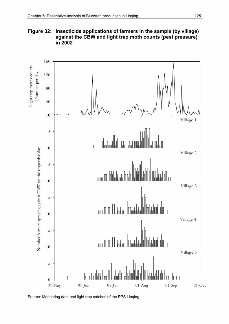
Chapter 6: Descriptive analysis of Bt-cotton production in Linqing 125
Figure 32: Insecticide applications of farmers in the sample (by village) against the CBW and light trap moth counts (pest pressure) in 2002
0
5
10
Num
ber f
arm
ers s
pray
ing
again
st C
BW o
n th
e re
spec
tive
day
0
5
10
0
5
10
Village 1
Village 2
Village 3
0
5
10
01-May 01-Jun 01-Jul 01-Aug 01-Sep 01-Oct0
5
10
Village 4
Village 5
Ligh
t tro
p m
oths
cou
nts
[Num
ber p
er d
ay]
0
40
80
120
160
Source: Monitoring data and light trop catches of the PPS Linqing
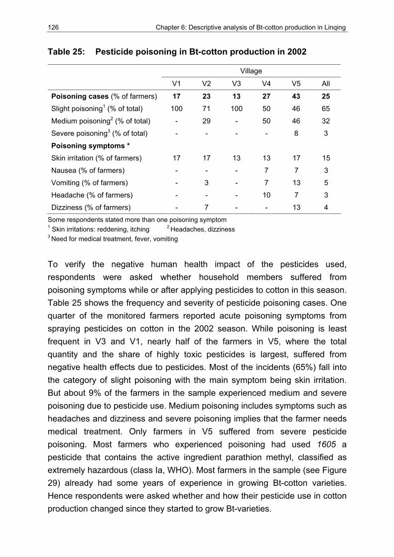
126 Chapter 6: Descriptive analysis of Bt-cotton production in Linqing
Table 25: Pesticide poisoning in Bt-cotton production in 2002
Village
V1 V2 V3 V4 V5 All
Poisoning cases (% of farmers) 17 23 13 27 43 25 Slight poisoning1 (% of total) 100 71 100 50 46 65
Medium poisoning2 (% of total) - 29 - 50 46 32
Severe poisoning3 (% of total) - - - - 8 3
Poisoning symptoms * Skin irritation (% of farmers) 17 17 13 13 17 15
Nausea (% of farmers) - - - 7 7 3
Vomiting (% of farmers) - 3 - 7 13 5
Headache (% of farmers) - - - 10 7 3
Dizziness (% of farmers) - 7 - - 13 4 Some respondents stated more than one poisoning symptom 1 Skin irritations: reddening, itching 2 Headaches, dizziness 3 Need for medical treatment, fever, vomiting
To verify the negative human health impact of the pesticides used, respondents were asked whether household members suffered from poisoning symptoms while or after applying pesticides to cotton in this season. Table 25 shows the frequency and severity of pesticide poisoning cases. One quarter of the monitored farmers reported acute poisoning symptoms from spraying pesticides on cotton in the 2002 season. While poisoning is least frequent in V3 and V1, nearly half of the farmers in V5, where the total quantity and the share of highly toxic pesticides is largest, suffered from negative health effects due to pesticides. Most of the incidents (65%) fall into the category of slight poisoning with the main symptom being skin irritation. But about 9% of the farmers in the sample experienced medium and severe poisoning due to pesticide use. Medium poisoning includes symptoms such as headaches and dizziness and severe poisoning implies that the farmer needs medical treatment. Only farmers in V5 suffered from severe pesticide poisoning. Most farmers who experienced poisoning had used 1605 a pesticide that contains the active ingredient parathion methyl, classified as extremely hazardous (class Ia, WHO). Most farmers in the sample (see Figure 29) already had some years of experience in growing Bt-cotton varieties. Hence respondents were asked whether and how their pesticide use in cotton production changed since they started to grow Bt-varieties.
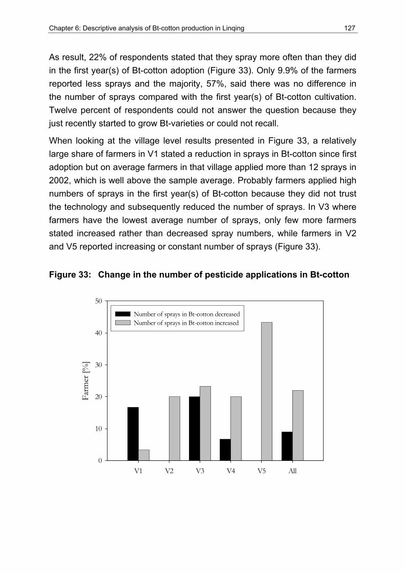
Chapter 6: Descriptive analysis of Bt-cotton production in Linqing 127
As result, 22% of respondents stated that they spray more often than they did in the first year(s) of Bt-cotton adoption (Figure 33). Only 9.9% of the farmers reported less sprays and the majority, 57%, said there was no difference in the number of sprays compared with the first year(s) of Bt-cotton cultivation. Twelve percent of respondents could not answer the question because they just recently started to grow Bt-varieties or could not recall.
When looking at the village level results presented in Figure 33, a relatively large share of farmers in V1 stated a reduction in sprays in Bt-cotton since first adoption but on average farmers in that village applied more than 12 sprays in 2002, which is well above the sample average. Probably farmers applied high numbers of sprays in the first year(s) of Bt-cotton because they did not trust the technology and subsequently reduced the number of sprays. In V3 where farmers have the lowest average number of sprays, only few more farmers stated increased rather than decreased spray numbers, while farmers in V2 and V5 reported increasing or constant number of sprays (Figure 33).
Figure 33: Change in the number of pesticide applications in Bt-cotton
V1 V2 V3 V4 V5 All
Farm
er [%
]
0
10
20
30
40
50
Number of sprays in Bt-cotton decreasedNumber of sprays in Bt-cotton increased
128 Chapter 6: Descriptive analysis of Bt-cotton production in Linqing
One potential reason for an increase in the number of pesticide applications is the development of resistance against the Bt-toxin in CBW populations. Testing of the resistance level of CBW in the study area was conducted by means of a bioassay (see Appendix 12 and 13 for details of the testing and the findings). The outcome of the laboratory testing shows no significant difference between the levels of resistance against Bt-toxins of larvae collected in the study area in 2002 and larvae from a strain reared in the laboratory since 1997. This means that the high amount of chemical pesticides that farmers in the sample applied is not a reaction to resistance build-up of target pests against Bt-toxin. Another possible reason for an increase in the number of sprays is the development of secondary pests, and that is analyzed in the next section.
6.2.3 Farmers’ perception of pest infestation in Bt-cotton
When discussing the pesticide use that was recorded by farmers for Bt-cotton production in the 2002 season it is important to consider the prevailing pest situation. CBW, aphid and spider mite are the major pests in cotton in the regions and national statistics show that those pests (if uncontrolled) cause considerable damage to cotton production57. Farmers were asked to give an assessment of the pest situation in the 2002 cotton season, separately for the three main pests (spider mite, CBW, and aphid) and for the overall pest infestation (including all cotton insect pests). The proportions of respondents who considered 2002 as having low and high overall pest infestation are nearly equal. However, the majority of farmers replied that pest infestation of spider mite was higher in the 2002 season than in normal years, and the incidence of CBW and aphids was lower than usual (Figure 34). When asked for a ranking of cotton pests in the 2002 season farmers stated spider mite was the most important pest followed by CBW and aphid. Despite growing Bt-cotton varieties, more than 60% of the farmers still considered cotton bollworm as the second most important cotton pest (Figure 35). This perception, and the high level of insecticide use, implies that the introduction of Bt-varieties did not entirely solve the CBW problem.
57 Professional Statistics of Plant Protection, Beijing, China, from the National Agro-technical Extension and Service Center (NATESC).
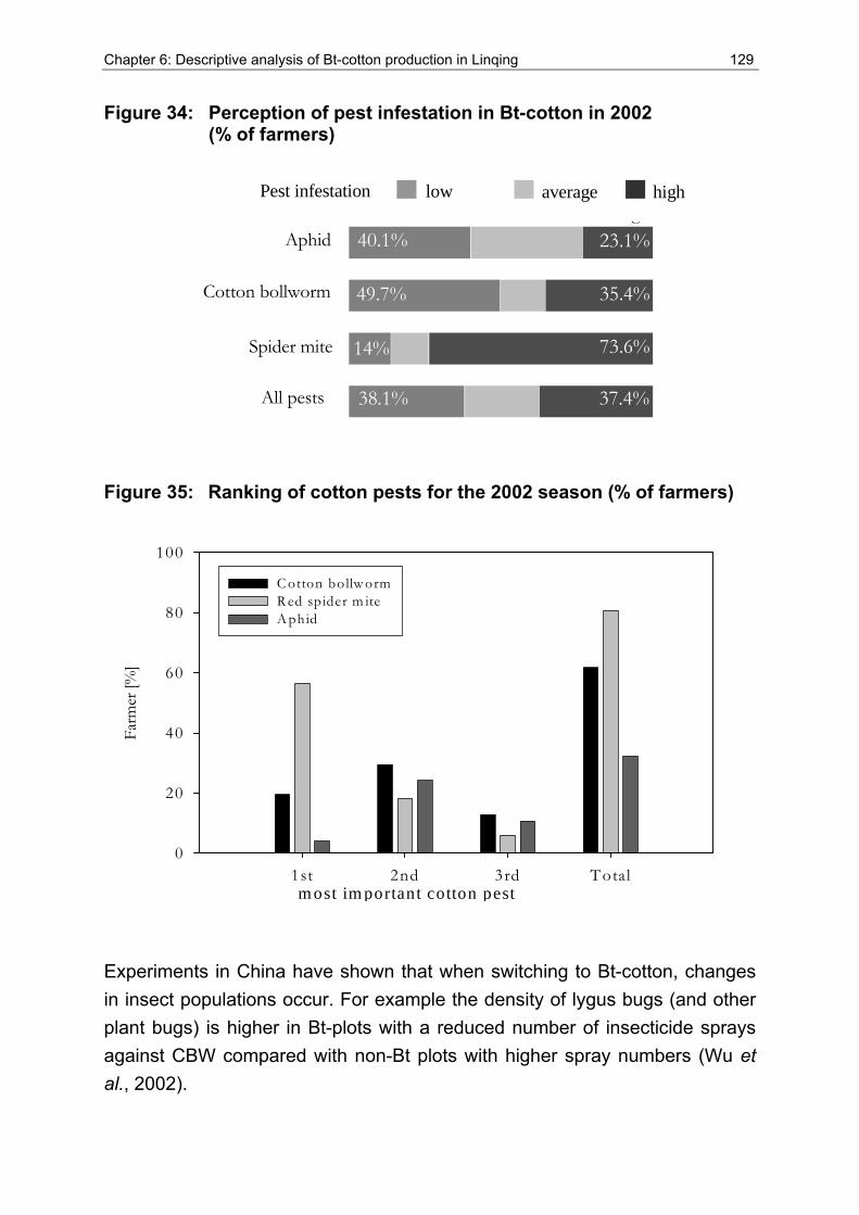
Chapter 6: Descriptive analysis of Bt-cotton production in Linqing 129
Figure 34: Perception of pest infestation in Bt-cotton in 2002 (% of farmers)
Pest infestation low average high g
Cotton bollworm
73 . 6%
37 . 4%
35 . 4%
23 . 1%
49 . 7%
40 . 1%
38 . 1%
14%
All pests
Spider mite
Aphid
Figure 35: Ranking of cotton pests for the 2002 season (% of farmers)
1st 2nd 3rd Total
Farm
er [%
]
0
20
40
60
80
100
C otton bollw ormR ed spider m iteA phid
m ost im portant cotton pest
Experiments in China have shown that when switching to Bt-cotton, changes in insect populations occur. For example the density of lygus bugs (and other plant bugs) is higher in Bt-plots with a reduced number of insecticide sprays against CBW compared with non-Bt plots with higher spray numbers (Wu et al., 2002).
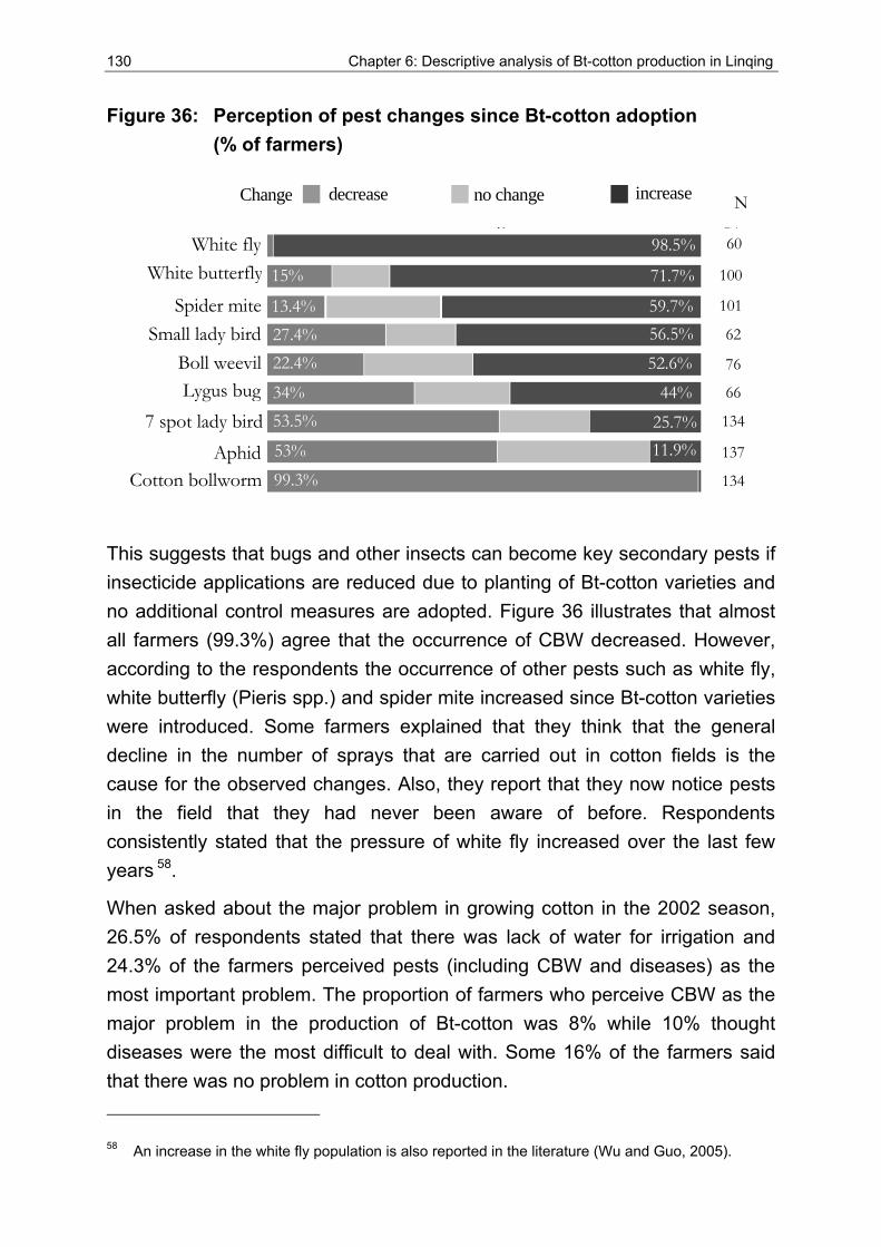
130 Chapter 6: Descriptive analysis of Bt-cotton production in Linqing
Figure 36: Perception of pest changes since Bt-cotton adoption (% of farmers)
Change decrease no change increase
60
100
101
62
76
66
134
137
134
Spider mite 59.7%
White fly 98.5%
Cotton bollworm 99.3%
7 spot lady bird 53.5%
Aphid 53%
Lygus bug 44%
Small lady bird 56.5% Boll weevil 52.6%
71.7% White butterfly
g N
11.9% 25.7%
34%
22.4% 27.4% 13.4%
15%
This suggests that bugs and other insects can become key secondary pests if insecticide applications are reduced due to planting of Bt-cotton varieties and no additional control measures are adopted. Figure 36 illustrates that almost all farmers (99.3%) agree that the occurrence of CBW decreased. However, according to the respondents the occurrence of other pests such as white fly, white butterfly (Pieris spp.) and spider mite increased since Bt-cotton varieties were introduced. Some farmers explained that they think that the general decline in the number of sprays that are carried out in cotton fields is the cause for the observed changes. Also, they report that they now notice pests in the field that they had never been aware of before. Respondents consistently stated that the pressure of white fly increased over the last few years 58.
When asked about the major problem in growing cotton in the 2002 season, 26.5% of respondents stated that there was lack of water for irrigation and 24.3% of the farmers perceived pests (including CBW and diseases) as the most important problem. The proportion of farmers who perceive CBW as the major problem in the production of Bt-cotton was 8% while 10% thought diseases were the most difficult to deal with. Some 16% of the farmers said that there was no problem in cotton production.
58 An increase in the white fly population is also reported in the literature (Wu and Guo, 2005).
N
Chapter 6: Descriptive analysis of Bt-cotton production in Linqing 131
Regarding future plans and the intentions to change the area of cotton, 51% of all farmers pointed out that they were planning to increase the area planted to cotton in the next season. Only 12% of the surveyed farmers planned a reduction of cotton area, while 37% wanted to keep the cotton area constant. There are slight differences among villages with more farmers in V1, V2, and V5 planning an increase of the cotton area in the 2003 season. The main determinants for the decision to change the area planted with cotton was the cotton price and availability of family labor and irrigation water. Households in V3 had the highest number of off-farm workdays so that labor was more limiting than in the other villages. In addition, the significantly higher level of experience shows that in the sample, farmers in this village were older and hence do not plan to increase the area of labor-intensive cotton production. In V4 the share of cotton in the production system is already very high (76.1%), which might explain the decision to not further increase the cotton area.
6.2.4 Institutional problems in technology implementation
The case study presented above shows that the usage level of chemical insecticides in Bt-cotton production was high and one third of the sprays still targeted the CBW, which should be controlled by the Bt-trait. Also, farmers perceived CBW as the second most important pest in cotton despite the use of Bt-varieties. When asked how current Bt-varieties could be improved the most common reply (32.2% of farmers) was that varieties should possess (higher) resistance against cotton diseases. Ranking second and stated by 28.2% of the farmers is the request that Bt-varieties should better control the CBW. Again there are significant differences among the villages, as only 10% and 13% of farmers in V1 and V3, respectively, request better CBW control of Bt-varieties while this share is 33% in V5, 37% in V4 and 47% in V2.
One potential reason for the high insecticide use level would be resistance of bollworms against the Bt-toxin, but this was not (yet) observed in the area (see bioassay of bollworm larvae in Appendix 12 and 13). Another factor that could explain high use of insecticides and the request that Bt-cotton should better control the CBW is the quality and hence effectiveness of Bt-varieties. Different Bt-varieties are available, with striking differences in price. Bt-cotton seed can be purchased for less than US$2 per kg (official price around US$10 per kg) and different qualities are on sale even for the Monsanto varieties, indicating that counterfeit products exist.
132 Chapter 6: Descriptive analysis of Bt-cotton production in Linqing
This situation in local seed markets suggests that institutional problems may hamper full realization of benefits from the Bt-technology. Also, most farmers continue on-farm propagation when using Bt-varieties.
To determine the concentration of Bt-toxin as an indicator of the effectiveness of Bt-varieties, tissue testing of cotton leaves was carried out. Three samples were collected from each of the 150 monitored farmer plots at three different times and flash-frozen immediately. The results of the laboratory testing of leaves show a high variation of toxin concentration among samples.
Figure 37 displays the results of Bt-toxin concentration in the August and September samples in the form of a histogram. As standard or control, leaf tissue was simultaneously sampled from the cotton growth experiment (Monsanto’s 33B as Bt-variety and Zhong mian 12 as non-Bt-variety). The respective toxin concentrations are 683 and 618 ng toxin g-1 fresh leaf for the Bt-samples in August and September, respectively, while all non-Bt-samples had zero toxin content. There is a significant number of samples with toxin concentration below the standard (certified Bt-seed) established in the cotton growth experiment. In the August sample 81% of the sample had lower toxin concentration than the standard, while this was the case of 57% of the samples in September59. Table 26 provides mean values and minimum and maximum toxin concentrations measured by villages60. Even though toxin concentrations vary depending on the time of sampling and the respective plant part (Greenplate, 1999; Adamcyzk et al., 2001a; 2001b), and there is only a slight correlation between the results of the August and September samples, the high variation in the results indicates a quality problem of the Bt-cotton seed that is planted in the area.
One important question is whether there is general uncertainty about the quality of the seed (in terms of Bt-toxin expression) or whether cheaper seed is of lower quality and has lower toxin concentrations. The first would be equivalent to a market failure for the Bt-trait while the latter indicates a general institutional problem with quality control of agricultural inputs.
59 A possible reason is better crop management, as the toxin concentration depends not only on the plant part and the physiological age of the tissue but also on the nutritional state and general strength of the plant that is determined among other factors by irrigation and fertilization.
60 The results of the July sample are not presented and not used for further analysis since the samples were not completely frozen any more, when they reached the laboratory in Beijing.
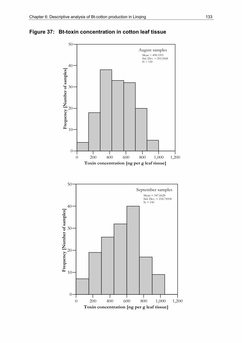
Chapter 6: Descriptive analysis of Bt-cotton production in Linqing 133
Figure 37: Bt-toxin concentration in cotton leaf tissue
0 200 400 600 800 1,000 1,200Toxin concentration [ng per g leaf tissue]
0
10
20
30
40
50
Fre
quen
cy [
Num
ber
of s
ampl
es]
Mean = 498.1593Std. Dev. = 203.2668N = 150
August samples
0 200 400 600 800 1,000 1,200Toxin concentration [ng per g leaf tissue]
0
10
20
30
40
50
Fre
quen
cy [
Num
ber
of s
ampl
es]
Mean = 547.6628Std. Dev. = 234.74104N = 150
September samples
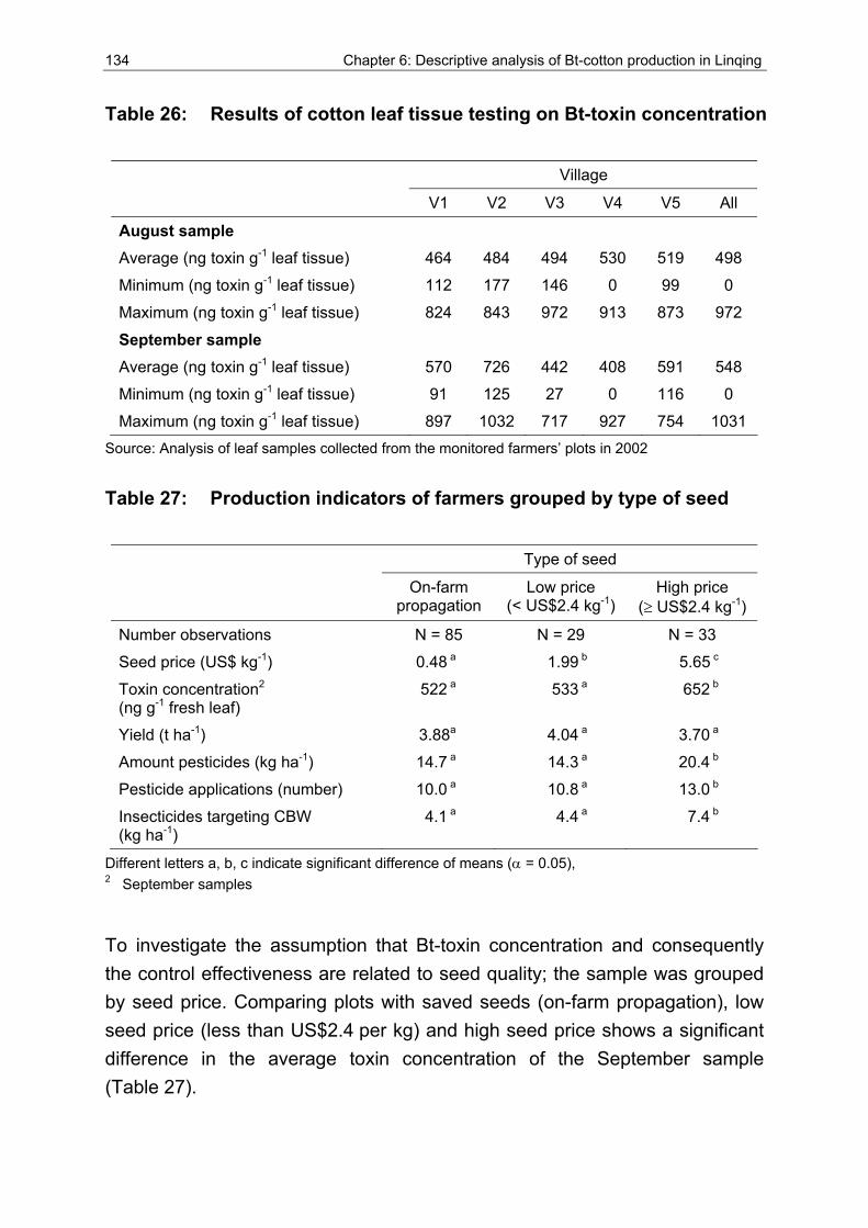
134 Chapter 6: Descriptive analysis of Bt-cotton production in Linqing
Table 26: Results of cotton leaf tissue testing on Bt-toxin concentration
Village
V1 V2 V3 V4 V5 All
August sample Average (ng toxin g-1 leaf tissue) 464 484 494 530 519 498
Minimum (ng toxin g-1 leaf tissue) 112 177 146 0 99 0
Maximum (ng toxin g-1 leaf tissue) 824 843 972 913 873 972
September sample
Average (ng toxin g-1 leaf tissue) 570 726 442 408 591 548
Minimum (ng toxin g-1 leaf tissue) 91 125 27 0 116 0
Maximum (ng toxin g-1 leaf tissue) 897 1032 717 927 754 1031 Source: Analysis of leaf samples collected from the monitored farmers’ plots in 2002
Table 27: Production indicators of farmers grouped by type of seed
Type of seed
On-farm propagation
Low price (< US$2.4 kg-1)
High price (≥ US$2.4 kg-1)
Number observations N = 85 N = 29 N = 33
Seed price (US$ kg-1) 0.48 a 1.99 b 5.65 c
Toxin concentration2 (ng g-1 fresh leaf)
522 a 533 a 652 b
Yield (t ha-1) 3.88a 4.04 a 3.70 a
Amount pesticides (kg ha-1) 14.7 a 14.3 a 20.4 b
Pesticide applications (number) 10.0 a 10.8 a 13.0 b
Insecticides targeting CBW (kg ha-1)
4.1 a 4.4 a 7.4 b
Different letters a, b, c indicate significant difference of means (α = 0.05), 2 September samples
To investigate the assumption that Bt-toxin concentration and consequently the control effectiveness are related to seed quality; the sample was grouped by seed price. Comparing plots with saved seeds (on-farm propagation), low seed price (less than US$2.4 per kg) and high seed price shows a significant difference in the average toxin concentration of the September sample (Table 27).
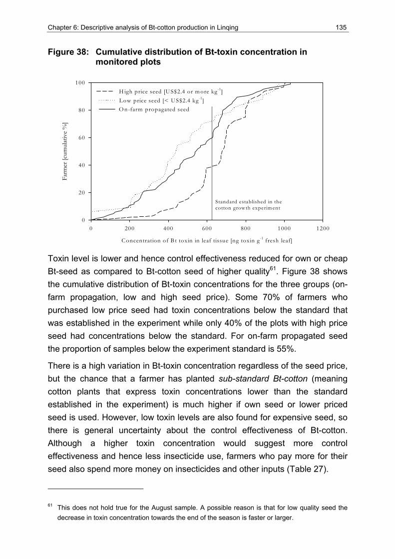
Chapter 6: Descriptive analysis of Bt-cotton production in Linqing 135
Figure 38: Cumulative distribution of Bt-toxin concentration in monitored plots
Concentration of B t toxin in leaf tissue [ng toxin g-1 fresh leaf]
0 200 400 600 800 1000 1200
Farm
er [c
umul
ativ
e %
]
0
20
40
60
80
100
O n-farm propagated seedLow price seed [< US$2.4 kg-1]H igh price seed [U S$2.4 or m ore kg-1]
Standard established in thecotton growth experim ent
Toxin level is lower and hence control effectiveness reduced for own or cheap Bt-seed as compared to Bt-cotton seed of higher quality61. Figure 38 shows the cumulative distribution of Bt-toxin concentrations for the three groups (on-farm propagation, low and high seed price). Some 70% of farmers who purchased low price seed had toxin concentrations below the standard that was established in the experiment while only 40% of the plots with high price seed had concentrations below the standard. For on-farm propagated seed the proportion of samples below the experiment standard is 55%.
There is a high variation in Bt-toxin concentration regardless of the seed price, but the chance that a farmer has planted sub-standard Bt-cotton (meaning cotton plants that express toxin concentrations lower than the standard established in the experiment) is much higher if own seed or lower priced seed is used. However, low toxin levels are also found for expensive seed, so there is general uncertainty about the control effectiveness of Bt-cotton. Although a higher toxin concentration would suggest more control effectiveness and hence less insecticide use, farmers who pay more for their seed also spend more money on insecticides and other inputs (Table 27).
61 This does not hold true for the August sample. A possible reason is that for low quality seed the decrease in toxin concentration towards the end of the season is faster or larger.
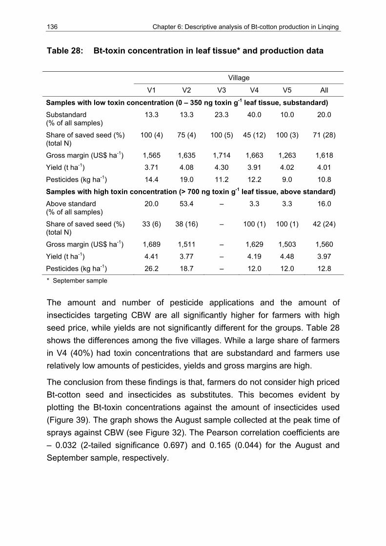
136 Chapter 6: Descriptive analysis of Bt-cotton production in Linqing
Table 28: Bt-toxin concentration in leaf tissue* and production data
Village
V1 V2 V3 V4 V5 All
Samples with low toxin concentration (0 – 350 ng toxin g-1 leaf tissue, substandard) Substandard (% of all samples)
13.3 13.3 23.3 40.0 10.0 20.0
Share of saved seed (%) (total N)
100 (4) 75 (4) 100 (5) 45 (12) 100 (3) 71 (28)
Gross margin (US$ ha-1) 1,565 1,635 1,714 1,663 1,263 1,618
Yield (t ha-1) 3.71 4.08 4.30 3.91 4.02 4.01
Pesticides (kg ha-1) 14.4 19.0 11.2 12.2 9.0 10.8
Samples with high toxin concentration (> 700 ng toxin g-1 leaf tissue, above standard) Above standard (% of all samples)
20.0 53.4 – 3.3 3.3 16.0
Share of saved seed (%) (total N)
33 (6) 38 (16) – 100 (1) 100 (1) 42 (24)
Gross margin (US$ ha-1) 1,689 1,511 – 1,629 1,503 1,560
Yield (t ha-1) 4.41 3.77 – 4.19 4.48 3.97
Pesticides (kg ha-1) 26.2 18.7 – 12.0 12.0 12.8 * September sample
The amount and number of pesticide applications and the amount of insecticides targeting CBW are all significantly higher for farmers with high seed price, while yields are not significantly different for the groups. Table 28 shows the differences among the five villages. While a large share of farmers in V4 (40%) had toxin concentrations that are substandard and farmers use relatively low amounts of pesticides, yields and gross margins are high.
The conclusion from these findings is that, farmers do not consider high priced Bt-cotton seed and insecticides as substitutes. This becomes evident by plotting the Bt-toxin concentrations against the amount of insecticides used (Figure 39). The graph shows the August sample collected at the peak time of sprays against CBW (see Figure 32). The Pearson correlation coefficients are – 0.032 (2-tailed significance 0.697) and 0.165 (0.044) for the August and September sample, respectively.
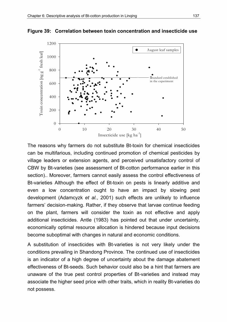
Chapter 6: Descriptive analysis of Bt-cotton production in Linqing 137
Figure 39: Correlation between toxin concentration and insecticide use
Insecticide use [kg ha-1]0 10 20 30 40 50
Toxi
n co
ncen
tratio
n [n
g g-1
fres
h lea
f]
0
200
400
600
800
1000
1200August leaf samples
Standard established in the experiment
The reasons why farmers do not substitute Bt-toxin for chemical insecticides can be multifarious, including continued promotion of chemical pesticides by village leaders or extension agents, and perceived unsatisfactory control of CBW by Bt-varieties (see assessment of Bt-cotton performance earlier in this section).. Moreover, farmers cannot easily assess the control effectiveness of Bt-varieties Although the effect of Bt-toxin on pests is linearly additive and even a low concentration ought to have an impact by slowing pest development (Adamcyzk et al., 2001) such effects are unlikely to influence farmers’ decision-making. Rather, if they observe that larvae continue feeding on the plant, farmers will consider the toxin as not effective and apply additional insecticides. Antle (1983) has pointed out that under uncertainty, economically optimal resource allocation is hindered because input decisions become suboptimal with changes in natural and economic conditions.
A substitution of insecticides with Bt-varieties is not very likely under the conditions prevailing in Shandong Province. The continued use of insecticides is an indicator of a high degree of uncertainty about the damage abatement effectiveness of Bt-seeds. Such behavior could also be a hint that farmers are unaware of the true pest control properties of Bt-varieties and instead may associate the higher seed price with other traits, which in reality Bt-varieties do not possess.
138 Chapter 6: Descriptive analysis of Bt-cotton production in Linqing
Based on the case study findings presented in this chapter the introduction of Bt-cotton varieties did not (entirely) solve the CBW problem for farmers and even less so did it solve the pest problem in general.
6.3 Summary
Linqing County, located in the west of Shandong Province was selected as the study location. This decision was based on the findings of an orientation phase that was conducted in 2001 to facilitate the conception and design of the case study. In 2002 an in-depth survey of cotton production was carried out with 150 small-scale farmers from five different villages, all growing Bt-cotton. The monitoring of cotton production was supplemented with household interviews, a cotton growth experiment and testing of cotton leaf tissue and CBW larvae.
Cotton is the major crop in the area and the main source of cash income for farmers. Farmers in the sample allocated some 60% of farmland to cotton production and derived about 40% of total household income from this crop. Other income sources are the production of wheat and maize, growing of fruit and vegetables, livestock husbandry and supplementary off-farm work (especially during winter months). Cotton is produced with high intensity, especially in terms of labor use and input of agro-chemicals. Even though farmers were growing Bt-varieties they sprayed on average 11 times and applied some 16 kg of formulated pesticides per hectare of cotton. The cotton bollworm (the pest that Bt-varieties are supposed to control) was still perceived as the second most important cotton pest and targeted by some 30% of all insecticides applied.
Testing of the susceptibility of CBW caterpillars revealed that the local strains do not show an increased level of resistance against the Bt-toxin. Therefore, pest resistance is not the reason for the high insecticide use. Most farmers sow on-farm propagated seed and those who purchased cotton seed spend on average much less than the official price for the certified Bt-cotton seed. Therefore, leaf tissue was analyzed to quantify the Bt-toxin concentration that indicates the effectiveness of Bt-related pest control. Laboratory testing revealed that Bt-toxin concentrations vary significantly in the samples and some 20% of samples have toxin concentrations less than half of the level found in the certified Monsanto seed that was used in the experiment.
Chapter 6: Descriptive analysis of Bt-cotton production in Linqing 139
The main reason for this quality problem in Bt-cotton is the lack of control and standards in the market for seed. The large number of different pesticide products and lack of registration and labeling indicate similar problems in this field.
A major precondition and challenges for the impact of agricultural biotechnology in developing countries according to de Janvry et al. (2005) is to put in place the necessary public and private institutions (Chapter 2). The survey and experimental findings presented in this chapter raise some doubt as to whether the implementation of Bt-cotton in China is carried out with the necessary supportive institutions and follows a stepwise evaluation approach. Based on the findings of Huang et al. (2002) it can be concluded that the performance of Bt-cotton is deteriorating with the on-going time and adoption scale. This case study reveals that ecosystem changes (development of secondary pests) and equally important institutional problems reduce the benefits that can be found during the initial phase of technology introduction.
The information presented in this chapter is the basis for the subsequent modeling and econometric approaches.
7 Product iv i ty ana lys is o f B t -cot ton
In this chapter the empirical evidence for the impact of Bt-cotton varieties on insecticide use and productivity of cotton production is investigated. The special features and difficulties when assessing the productivity of production inputs that are damage control agents were introduced and outlined in Chapter 4. Chapters 5 and 6 gave a detailed description of the available data and the detailed case study of Bt-cotton production in China several years after the first introduction of the technology. This chapter presents the econometric productivity assessment of the damage control agents insecticides and Bt-toxin. Two different econometric approaches are followed. The first part of the chapter deals with the application of the damage control function concept. A distinctive feature of the methodology adopted in this research is that quantitative measurements of toxin concentration were specified as a continuous variable. This represents an advancement over the dummy variable approach (Bt- or non-Bt) used by previous studies. Different functional forms of the damage control function are compared.
In the second section a complementary positive method for productivity analysis is proposed. The two-stage semi-parametric method does not depend on the specification of the functional form of the production technology, and allows for changes in productivity based on the level of pest pressure.
7.1 Estimation of production and insecticide use function
7.1.1 Methodology of production function estimation
One possibility for assessing the input substitution and productivity effects of Bt-cotton as pest control agents is to apply the damage control framework of Lichtenberg and Zilberman (1986). In previous studies (Huang et al., 2002a; Qaim and Zilberman, 2003) the effect of the Bt-variety was captured in a variety dummy using data from Bt- and non-Bt-cotton farmers or fields. The problem with this approach is that such a variety dummy may also include non-pest control effects if other factors cannot be adequately controlled. In this analysis the Bt-toxin concentration is included as a continuous variable in the damage control function.
Assuming a Cobb-Douglas type production function with an integrated damage control function the cotton yield y can be described as:
Chapter 7: Productivity analysis of Bt-cotton 141
01
( ) * ( )i
nD Pi
i
Y a x G xβ γ
=
⎡ ⎤= ⎢ ⎥
⎣ ⎦∏ (7-1)
where Dix , i=1, 2, …, n, are explanatory variables (independent production
inputs such as labor, fertilizer and farmer- and location-specific factors), βi are the respective coefficients to be estimated and Px is a vector of damage
control agents within the damage control function G. Following Carrasco-Tauber and Moffitt (1992) who refer to a working paper by Babcock, Lichtenberg and Zilberman, the parameter restriction γ = 1 was imposed on (7-1) to facilitate the estimation.
Different functional forms can be assumed for the damage control function G(xP) and specification can be crucial for the parameter results (Carrasco-Tauber and Moffitt, 1992; Fox and Weersink, 1995; Ajayi, 1999). Since up until now there is no consensus on which specification best suits the purpose, different functional forms were used and parameter estimates compared afterwards. With the introduction of Bt-varieties there are two major damage control agents in cotton production, namely insecticides and Bt toxin62 that correspond with the main sources of damage in cotton in North China: cotton bollworm and other insect pests (aphid and spider mite). If the control measures were explicitly aimed at abating potential damage from only one source (for example only cotton bollworm) the form of the abatement function used by Babcock et al. (1992) could be applied even in the case of more than one source of damage. But since in the case of insecticide use all insect pests, including cotton bollworm, are affected due to the broad-spectrum nature of most products, a division of control efforts according to separate sources of damage is not possible.
Hence, a specification that sums up all damage abatement inputs was adopted because it is assumed that insecticides and Bt-toxin are substitutes. The following general functional forms are used for the damage control function:
Exponential: G (xP) = 1 – exp (- λ1 1Px - λ2 2
Px - λ3 1Px 2
Px ) (7-2)
Logistic: G (xP) = (1 + exp (µ- σ1 1Px - σ 2 2
Px - σ 3 1Px 2
Px )) – 1 (7-3)
142 Chapter 7: Productivity analysis of Bt-cotton
Weibull: G (xP) = 1 – exp (-( 1Px )c1 – ( 2
Px )c2 – ( 1Px 2
Px )c3) (7-4)
where 1Px is the Bt-toxin concentration in leaf tissue (ng toxin g-1 fresh leaf), 2
Px
the amount of chemical insecticides (kg ha-1), and 1 2P Px x an interaction term for
both control agents. The coefficients λ1- λ3, σ1 - σ3, µ, and c1 - c3 are to be estimated. For the estimation of the parameters the logarithmic form of the production function is used and an error term ε is added to the equation. The respective equations read:
Pure Cobb-Douglas: 1 1
( ) ( ) ( ) ( )n m
D Pi i j i
i jLog Y Log a Log x Log xβ δ ε
= =
= + + +∑ ∑
With damage control function: 1
( ) ( ) ( ) ( ( ))n
D Pi i
iLog Y Log a Log x Log G xβ ε
=
= + + +∑
where Y is the cotton yield (output), a the intercept, Dix are direct inputs, and
Pjx the damage control agents as defined above. The respective parameter
vectors β, δ, λ, σ, c, and parameters a and µ must be estimated by non-linear regression methods because the abatement function is nonlinear. The estimated coefficients of the production function can be used to compute the marginal product of production inputs. For the direct inputs in the Cobb-Douglas type of function, the coefficients βi directly estimate the elasticity of the input D
ix (Debertin, 1986):
Di
i Di
xYY x
β ∂= ∗
∂ (7-5)
Re-arranging (7-5) the marginal product of input Dix can be expressed as:
iD Di i
Y Yx x
β∂=
∂ (7-6)
Since this study is focusing on the productivity of crop protection inputs, the marginal product of insecticides and Bt-toxin is of special interest. (7-6) can be used to compute the marginal product of Bt-toxin and insecticides in the Cobb-Douglas specification.
62 Of course a range of cultural practices could also be considered as damage control factors but due to the dominance of pesticides and Bt these factors are ignored in the analysis.
Chapter 7: Productivity analysis of Bt-cotton 143
Computing the elasticities of damage abatement variables that are part of the damage function ( )PG x works analogously to the marginal product of direct
inputs.
The marginal product of damage control agent Pjx can be expressed as:
( )
( )
Pj
P P Pj j j
G xY Yx G x x
∂∂= ∗
∂ ∂ (7-7)
In this general form of the marginal productivity the term ( )PjG x can be
substituted with the alternative specifications of the damage function that are given above63. The marginal product (MP) for 1
Px (Bt-toxin) for the exponential
form of the damage function hence reads:
1 3 2 1 1 2 2 3 1 21
1 1 1 2 2 3 1 2
( ) exp( )( )1 exp( )
P P P P PP
P P P P P
Y x x x x xYMP xx x x x x
λ λ λ λ λλ λ λ
∗ + ∗ − − −∂= =∂ − − − −
(7-8)
The marginal productivity of 2Px (insecticides) can be derived analogously
using the respective partial derivation.
A problem in estimating production functions, including pest control variables, is that regressors (independent, explanatory variables) are correlated with the production function error term ε (see also Huang et al., 2002a) because unobserved factors like the climate may results in both high input levels of insecticides and low yields. However, if regressors are correlated with the error term, parameter estimates of ordinary least squares (OLS) procedures are biased and the results inconsistent (Johnston and DiNardo, 1997). To overcome the problem of correlation between insecticide use and the error term of the production function, an iterative three stage least square (3SLS) procedure using instrumental variables to estimate the predicted value of insecticide use can be applied (Wooldridge, 2002). Thus, the insecticide use function (with the dependent variable ‘amount of insecticides’) and the production function with the damage control function (dependent variable ‘log yield’) were estimated simultaneously.
For the computation of the parameters of the insecticide use and production function the procedures PROC MODEL and PROC REG of the software
63 The parameter γ is restricted to equal 1 for the equations presented.
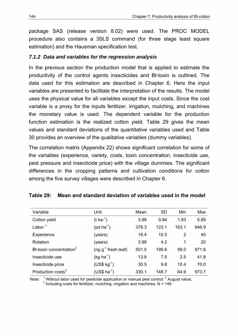
144 Chapter 7: Productivity analysis of Bt-cotton
package SAS (release version 8.02) were used. The PROC MODEL procedure also contains a 3SLS command (for three stage least square estimation) and the Hausman specification test.
7.1.2 Data and variables for the regression analysis
In the previous section the production model that is applied to estimate the productivity of the control agents insecticides and Bt-toxin is outlined. The data used for this estimation are described in Chapter 6. Here the input variables are presented to facilitate the interpretation of the results. The model uses the physical value for all variables except the input costs. Since the cost variable is a proxy for the inputs fertilizer, irrigation, mulching, and machines the monetary value is used. The dependent variable for the production function estimation is the realized cotton yield. Table 29 gives the mean values and standard deviations of the quantitative variables used and Table 30 provides an overview of the qualitative variables (dummy variables).
The correlation matrix (Appendix 22) shows significant correlation for some of the variables (experience, variety, costs, toxin concentration, insecticide use, pest pressure and insecticide price) with the village dummies. The significant differences in the cropping patterns and cultivation conditions for cotton among the five survey villages were described in Chapter 6.
Table 29: Mean and standard deviation of variables used in the model
Variable Unit Mean SD Min Max
Cotton yield (t ha-1) 3.88 0.84 1.83 5.89
Labor 1 (pd ha-1) 378.3 123.1 163.1 946.9
Experience (years) 19.4 10.5 2 45
Rotation (years) 3.99 4.2 1 20
Bt-toxin concentration2 (ng g-1 fresh leaf) 501.5 199.8 99.0 971.6
Insecticide use (kg ha-1) 13.8 7.5 2.5 41.8
Insecticide price (US$ kg-1) 30.5 9.8 10.4 70.0
Production costs3 (US$ ha-1) 330.1 148.7 64.9 973.7 Note: 1 Without labor used for pesticide application or manual pest control; 2 August value;
3 Including costs for fertilizer, mulching, irrigation and machines, N = 149
Chapter 7: Productivity analysis of Bt-cotton 145
Village dummies are included in the analysis to control for unobserved village-specific influences, as the observed variables may not capture all the differences in cultivation practices and (environmental) conditions.
The dependent variable Y is the seed cotton yield in tonnes that is harvested per hectare. Labor input is defined as the number of persondays of labor that are used to produce and harvest one hectare of cotton64. The labor used for pesticide applications and other pest control measures is excluded. Farmers recorded the time spent in hours and these were converted to persondays assuming that a personday equals eight hours of work. The time that it takes to reach the field and return is normally included in the figures. The variable experience states the number of years the farmer has been producing cotton (this does not necessarily mean continuous production of cotton). Additional experience generally improves the performance, but many years of experience characterize older farmers who might work more slowly or have less strength. The rotation variable stands for the number of continuous years of cotton cultivation on the plot and is an indicator for soil-born pests and diseases, and decreasing soil fertility.
However, farmers in V3 who have a very large share of cotton in the production system, plant cotton on the same plot for a long time (up to 20 years) and stated that there is no reduction in yield. The toxin variable is the Bt-toxin concentration in the plant expressed in nanograms of toxin per gram of fresh cotton leaf tissue in the August sample. Interpolated insecticide figures were used for the insecticide variable because some of the pesticides could not be identified with regard to active ingredient and pesticide type. The insecticide use is measured in kilograms of formulated product per hectare. The insecticide price is expressed in US$ per kg of formulated product (farmer average) and is assumed to reflect differences in the quality of the products applied. More expensive products may be of higher quality and have a better control effectiveness than less costly products.
64 The labor input is not separated into work of males and females because most tasks in cotton production are gender specific anyway. For example, men mainly do the land preparation and spraying of pesticides. But pruning and harvesting, the most labor consuming tasks, are done equally by men and women. However, there is no indication that a difference exists in the labor productivity of men and women. Children rarely work in the fields, as schooling is compulsory in China.
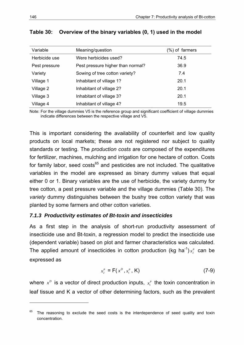
146 Chapter 7: Productivity analysis of Bt-cotton
Table 30: Overview of the binary variables (0, 1) used in the model
Variable Meaning/question (%) of farmers
Herbicide use Were herbicides used? 74.5
Pest pressure Pest pressure higher than normal? 36.9
Variety Sowing of tree cotton variety? 7.4
Village 1 Inhabitant of village 1? 20.1
Village 2 Inhabitant of village 2? 20.1
Village 3 Inhabitant of village 3? 20.1
Village 4 Inhabitant of village 4? 19.5 Note: For the village dummies V5 is the reference group and significant coefficient of village dummies
indicate differences between the respective village and V5.
This is important considering the availability of counterfeit and low quality products on local markets; these are not registered nor subject to quality standards or testing. The production costs are composed of the expenditures for fertilizer, machines, mulching and irrigation for one hectare of cotton. Costs for family labor, seed costs65 and pesticides are not included. The qualitative variables in the model are expressed as binary dummy values that equal either 0 or 1. Binary variables are the use of herbicide, the variety dummy for tree cotton, a pest pressure variable and the village dummies (Table 30). The variety dummy distinguishes between the bushy tree cotton variety that was planted by some farmers and other cotton varieties.
7.1.3 Productivity estimates of Bt-toxin and insecticides
As a first step in the analysis of short-run productivity assessment of insecticide use and Bt-toxin, a regression model to predict the insecticide use (dependent variable) based on plot and farmer characteristics was calculated. The applied amount of insecticides in cotton production (kg ha-1) 2
Px can be
expressed as
2Px = F( Dx , 1
Px , K) (7-9)
where Dx is a vector of direct production inputs, 1Px the toxin concentration in
leaf tissue and K a vector of other determining factors, such as the prevalent
65 The reasoning to exclude the seed costs is the interdependence of seed quality and toxin concentration.
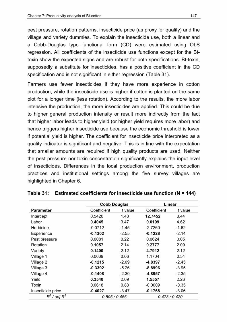
Chapter 7: Productivity analysis of Bt-cotton 147
pest pressure, rotation patterns, insecticide price (as proxy for quality) and the village and variety dummies. To explain the insecticide use, both a linear and a Cobb-Douglas type functional form (CD) were estimated using OLS regression. All coefficients of the insecticide use functions except for the Bt-toxin show the expected signs and are robust for both specifications. Bt-toxin, supposedly a substitute for insecticides, has a positive coefficient in the CD specification and is not significant in either regression (Table 31).
Farmers use fewer insecticides if they have more experience in cotton production, while the insecticide use is higher if cotton is planted on the same plot for a longer time (less rotation). According to the results, the more labor intensive the production, the more insecticides are applied. This could be due to higher general production intensity or result more indirectly from the fact that higher labor leads to higher yield (or higher yield requires more labor) and hence triggers higher insecticide use because the economic threshold is lower if potential yield is higher. The coefficient for insecticide price interpreted as a quality indicator is significant and negative. This is in line with the expectation that smaller amounts are required if high quality products are used. Neither the pest pressure nor toxin concentration significantly explains the input level of insecticides. Differences in the local production environment, production practices and institutional settings among the five survey villages are highlighted in Chapter 6. Table 31: Estimated coefficients for insecticide use function (N = 144)
Cobb Douglas Linear
Parameter Coefficient t value Coefficient t value Intercept 0.5420 1.43 12.7452 3.44 Labor 0.4045 3.47 0.0199 4.62 Herbicide -0.0712 -1.45 -2.7260 -1.62 Experience -0.1302 -2.55 -0.1228 -2.14 Pest pressure 0.0081 0.22 0.0624 0.05 Rotation 0.1057 2.14 0.2777 2.09 Variety 0.1400 2.12 4.7912 2.12 Village 1 0.0039 0.06 1.1704 0.54 Village 2 -0.1215 -2.09 -4.8397 -2.45 Village 3 -0.3392 -5.26 -8.8996 -3.95 Village 4 -0.1408 -2.30 -4.8957 -2.35 Yield 0.3540 2.09 1.5557 2.26 Toxin 0.0618 0.83 -0.0009 -0.35 Insecticide price -0.4027 -3.47 -0.1768 -3.06
R2 / adj R2 0.506 / 0.456 0.473 / 0.420
148 Chapter 7: Productivity analysis of Bt-cotton
In the insecticide use function, the coefficients for V2 to V4 are negative and significant, indicating significantly lower insecticide use as compared to V566.
As a next step in the analysis the production function with the dependent variable yield (kg ha-1) is estimated. For the production function a CD specification and three different functional forms for the damage function (Exponential, Weibull and Logistic) are used (see section 7.1.1). The parameter estimates of the non-linear ordinary least square (OLS) regression are summarized in Table 32. The coefficients of all the direct production inputs conform to prior expectations and are robust over the different functional forms of the damage control function. Results indicate that higher input of labor and more cost intensive production result in higher cotton output while longer periods of cotton cultivation on the same plot lead to a significant reduction in output.
The control costs do not include the costs for cotton seed as the findings of the leaf testing presented in Chapter 6 imply a difference in toxin concentration between the low price and high price seeds. Although there was no significant correlation between the seed costs and the toxin concentration or the use of insecticides, those costs were not included. However, the seed costs may also capture variety specifics such as the potential yield for a variety and are a quality indicator, for example in terms of germination rate.
For all specifications the pest pressure dummy is negative and statistically significant. The rationale to include the pest pressure dummy in the production function part is that the regression on insecticide use showed no significance and there is also no correlation between the perceived pest pressure and the toxin concentration and the insecticide use. Hence this variable can be interpreted as the remaining pest damage that farmers could not control rather than a pest pressure variable. All four village dummy coefficients have a positive sign indicating that yields are higher in V1 – V4 compared to V5, although only the coefficient for V3 is statistically significant. The control agents insecticides and toxin are not significant with the one exception of the insecticide coefficient within the exponential damage function specification.
66 Estimation of the insecticide use and production function was also conducted without data from V5. Results did not change substantially so the analysis was continued with the full data set.
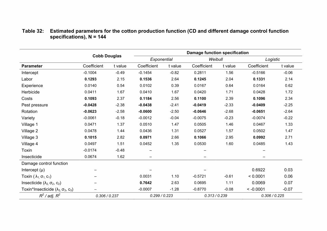
Table 32: Estimated parameters for the cotton production function (CD and different damage control function specifications), N = 144
Damage function specification
Cobb Douglas Exponential Weibull Logistic
Parameter Coefficient t value Coefficient t value Coefficient t value Coefficient t value Intercept -0.1004 -0.49 -0.1454 -0.82 0.2811 1.56 -0.5166 -0.06
Labor 0.1293 2.15 0.1536 2.64 0.1245 2.04 0.1331 2.14
Experience 0.0140 0.54 0.0102 0.39 0.0167 0.64 0.0164 0.62
Herbicide 0.0411 1.67 0.0410 1.67 0.0420 1.71 0.0428 1.72
Costs 0.1093 2.37 0.1184 2.56 0.1100 2.39 0.1096 2.34
Pest pressure -0.0428 -2.38 -0.0438 -2.41 -0.0419 -2.33 -0.0409 -2.25
Rotation -0.0623 -2.58 -0.0600 -2.50 -0.0646 -2.68 -0.0651 -2.64
Variety -0.0061 -0.18 -0.0012 -0.04 -0.0075 -0.23 -0.0074 -0.22
Village 1 0.0471 1.37 0.0510 1.47 0.0505 1.46 0.0467 1.33
Village 2 0.0478 1.44 0.0436 1.31 0.0527 1.57 0.0502 1.47
Village 3 0.1015 2.82 0.0971 2.66 0.1066 2.95 0.0992 2.71
Village 4 0.0497 1.51 0.0452 1.35 0.0530 1.60 0.0485 1.43
Toxin -0.0174 -0.48 – – –
Insecticide 0.0674 1.62 – – –
Damage control function Intercept (μ) – – – 0.6922 0.03 Toxin ( λ1, σ1, c1) – 0.0031 1.10 -0.5721 -0.61 < 0.0001 0.06 Insecticide (λ2, σ2, c2) – 0.7642 2.63 0.0695 1.11 0.0069 0.07 Toxin*Insecticide (λ3, σ3, c3) – -0.0007 -1.28 -0.8770 -0.08 < -0.0001 -0.07
R2 / adj. R2 0.306 / 0.237 0.299 / 0.223 0.313 / 0.239 0.306 / 0.225
150 Chapter 7: Productivity analysis of Bt-cotton
This leads to the conclusion that neither Bt-toxin nor use of insecticides significantly increases cotton yield at the study site. Based on the regression results none of the specifications is to be preferred to the others since coefficient estimates are very similar and the overall fit of the models does not vary much. To further explore the impact of different specifications of the damage function, three additional models with slightly different exponential specifications were estimated. The aim of these regressions is to find the best fit to the empirical data before continuing with the computation of the marginal productivity of control agents. The exponential damage function specification was selected because that is the only functional form where any of the damage control agents returns a statistically significant coefficient estimate. A fixed term λ0 is introduced in specifications (7-10) and (7-11) while the specification in (7-12) only contains terms for toxin and insecticides and no interaction term of the two.
Exponential 2: G ( Px ) = 1 – exp (-λ0 - λ1 1Px - λ2 2
Px ) (7-10)
Exponential 3: G ( Px ) = 1 – exp (-λ0 - λ1 1Px - λ2 2
Px - λ3 1Px 2
Px ) (7-11)
Exponential 4: G ( Px ) = 1 – exp (-λ1 1Px - λ2 2
Px ) (7-12)
The fixed term in the damage function can be interpreted as natural control (for example the activity and pest reducing capacity of natural enemies in the cotton field) that exists irrespective of the input of external control inputs. Results of the additional regressions are compiled in Table 33. Introduction of the fixed term λ0 increases the fit of the model compared to the initial specifiation. While the fixed term is significant, the interaction term in specification (7-11) is not and hence this specification does not respresent an improvement as compared to (7-10). However, the difference in the outcome of these two specifications is minor. Specification (7-12) shows the poorest fit and is hence not discussed further. None of the additional exponential specification shows statistically significant coefficients for Bt-toxin or insecticide use (Table 33). The parameter estimates for all the direct inputs in the production function are nearly unchanged and the same set of explanatory variables is statistically significant as compared to the initial specification displayed in Table 32.
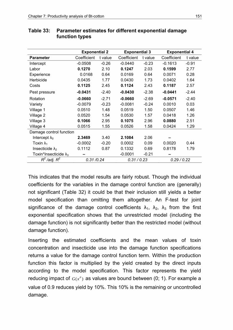
Chapter 7: Productivity analysis of Bt-cotton 151
Table 33: Parameter estimates for different exponential damage function types
Exponential 2 Exponential 3 Exponential 4 Parameter Coefficient t value Coefficient t value Coefficient t value Intercept -0.0508 -0.26 -0.0440 -0.23 -0.1613 -0.91 Labor 0.1270 2.10 0.1247 2.03 0.1599 2.77 Experience 0.0168 0.64 0.0169 0.64 0.0071 0.28 Herbicide 0.0435 1.77 0.0430 1.73 0.0402 1.64 Costs 0.1125 2.45 0.1124 2.43 0.1187 2.57 Pest pressure -0.0431 -2.40 -0.0430 -2.38 -0.0441 -2.44 Rotation -0.0660 -2.71 -0.0660 -2.69 -0.0571 -2.40 Variety -0.0079 -0.23 -0.0081 -0.24 0.0010 0.03 Village 1 0.0510 1.48 0.0519 1.50 0.0507 1.46 Village 2 0.0520 1.54 0.0530 1.57 0.0418 1.26 Village 3 0.1066 2.95 0.1075 2.96 0.0880 2.51 Village 4 0.0515 1.55 0.0526 1.58 0.0424 1.29 Damage control function
Intercept λ0 2.3469 3.40 2.1084 2.06 – Toxin λ1 -0.0002 -0.20 0.0002 0.09 0.0020 0.44 Insecticide λ2 0.1112 0.87 0.1332 0.69 0.8178 1.79 Toxin*Insecticide λ3 – -0.0001 -0.21 –
R2 /adj. R2 0.31 /0.24 0.31 / 0.23 0.29 / 0.22
This indicates that the model results are fairly robust. Though the individual coefficients for the variables in the damage control function are (generally) not significant (Table 32) it could be that their inclusion still yields a better model specification than omitting them altogether. An F-test for joint significance of the damage control coefficients λ1, λ2, λ3 from the first exponential specification shows that the unrestricted model (including the damage function) is not significantly better than the restricted model (without damage function).
Inserting the estimated coefficients and the mean values of toxin concentration and insecticide use into the damage function specifications returns a value for the damage control function term. Within the production function this factor is multiplied by the yield created by the direct inputs according to the model specification. This factor represents the yield reducing impact of ( )PG x as values are bound between (0; 1). For example a
value of 0.9 reduces yield by 10%. This 10% is the remaining or uncontrolled damage.
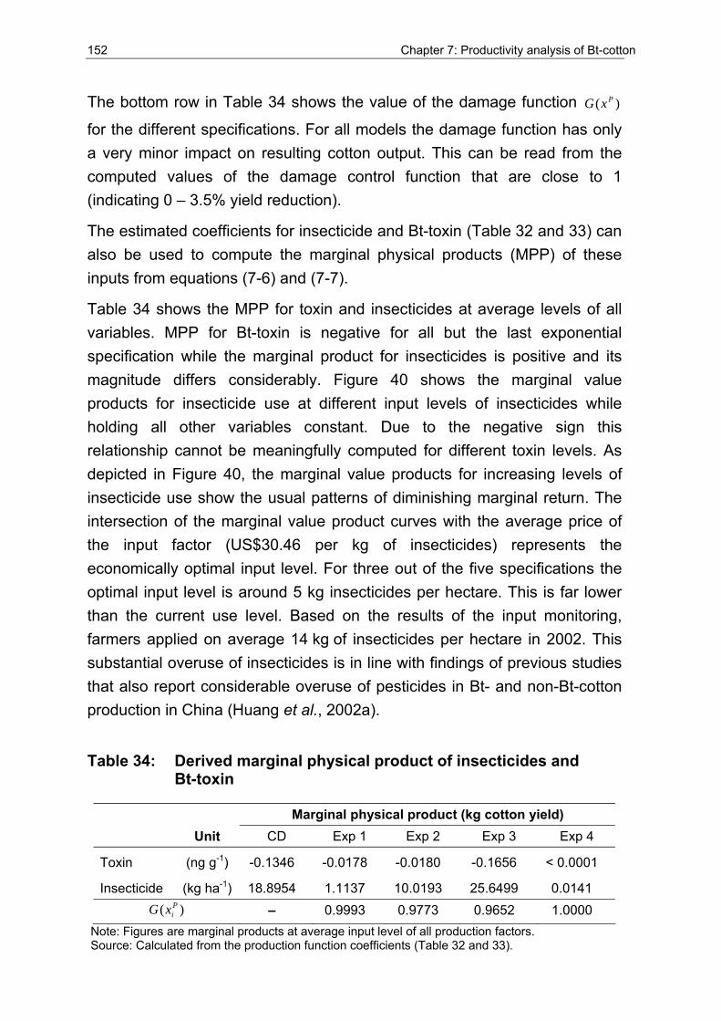
152 Chapter 7: Productivity analysis of Bt-cotton
The bottom row in Table 34 shows the value of the damage function ( )PG x
for the different specifications. For all models the damage function has only a very minor impact on resulting cotton output. This can be read from the computed values of the damage control function that are close to 1 (indicating 0 – 3.5% yield reduction).
The estimated coefficients for insecticide and Bt-toxin (Table 32 and 33) can also be used to compute the marginal physical products (MPP) of these inputs from equations (7-6) and (7-7).
Table 34 shows the MPP for toxin and insecticides at average levels of all variables. MPP for Bt-toxin is negative for all but the last exponential specification while the marginal product for insecticides is positive and its magnitude differs considerably. Figure 40 shows the marginal value products for insecticide use at different input levels of insecticides while holding all other variables constant. Due to the negative sign this relationship cannot be meaningfully computed for different toxin levels. As depicted in Figure 40, the marginal value products for increasing levels of insecticide use show the usual patterns of diminishing marginal return. The intersection of the marginal value product curves with the average price of the input factor (US$30.46 per kg of insecticides) represents the economically optimal input level. For three out of the five specifications the optimal input level is around 5 kg insecticides per hectare. This is far lower than the current use level. Based on the results of the input monitoring, farmers applied on average 14 kg of insecticides per hectare in 2002. This substantial overuse of insecticides is in line with findings of previous studies that also report considerable overuse of pesticides in Bt- and non-Bt-cotton production in China (Huang et al., 2002a).
Table 34: Derived marginal physical product of insecticides and Bt-toxin
Marginal physical product (kg cotton yield) Unit CD Exp 1 Exp 2 Exp 3 Exp 4
Toxin (ng g-1) -0.1346 -0.0178 -0.0180 -0.1656 < 0.0001
Insecticide (kg ha-1) 18.8954 1.1137 10.0193 25.6499 0.0141 ( )P
iG x – 0.9993 0.9773 0.9652 1.0000 Note: Figures are marginal products at average input level of all production factors. Source: Calculated from the production function coefficients (Table 32 and 33).
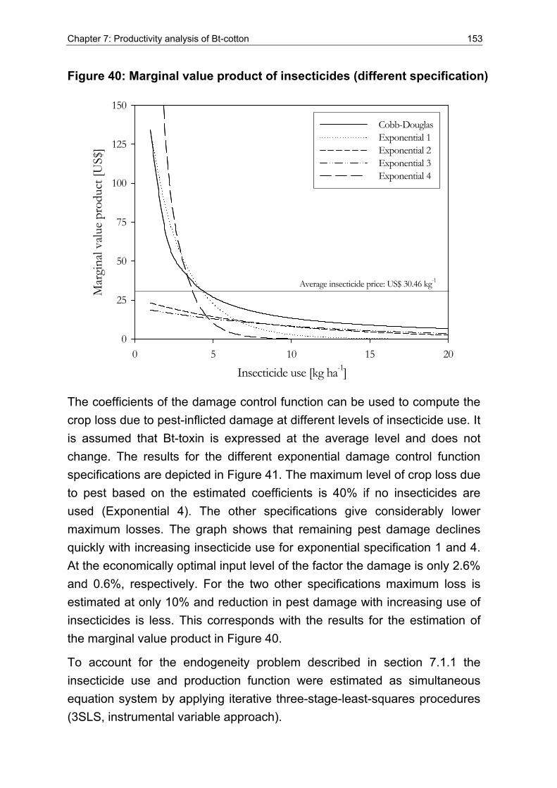
Chapter 7: Productivity analysis of Bt-cotton 153
Figure 40: Marginal value product of insecticides (different specification)
Insecticide use [kg ha-1]0 5 10 15 20
Mar
gina
l valu
e pr
oduc
t [U
S$]
0
25
50
75
100
125
150
Cobb-DouglasExponential 1Exponential 2Exponential 3Exponential 4
Average insecticide price: US$ 30.46 kg-1
The coefficients of the damage control function can be used to compute the crop loss due to pest-inflicted damage at different levels of insecticide use. It is assumed that Bt-toxin is expressed at the average level and does not change. The results for the different exponential damage control function specifications are depicted in Figure 41. The maximum level of crop loss due to pest based on the estimated coefficients is 40% if no insecticides are used (Exponential 4). The other specifications give considerably lower maximum losses. The graph shows that remaining pest damage declines quickly with increasing insecticide use for exponential specification 1 and 4. At the economically optimal input level of the factor the damage is only 2.6% and 0.6%, respectively. For the two other specifications maximum loss is estimated at only 10% and reduction in pest damage with increasing use of insecticides is less. This corresponds with the results for the estimation of the marginal value product in Figure 40.
To account for the endogeneity problem described in section 7.1.1 the insecticide use and production function were estimated as simultaneous equation system by applying iterative three-stage-least-squares procedures (3SLS, instrumental variable approach).
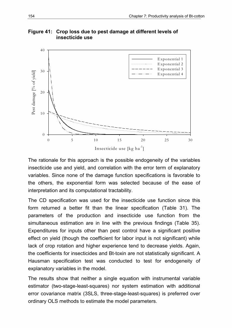
154 Chapter 7: Productivity analysis of Bt-cotton
Figure 41: Crop loss due to pest damage at different levels of insecticide use
Insecticide use [kg ha-1]
0 5 10 15 20 25 30
Pest
dam
age
[% o
f yiel
d]
0
10
20
30
40
Exponential 1Exponential 2Exponential 3Exponential 4
The rationale for this approach is the possible endogeneity of the variables insecticide use and yield, and correlation with the error term of explanatory variables. Since none of the damage function specifications is favorable to the others, the exponential form was selected because of the ease of interpretation and its computational tractability.
The CD specification was used for the insecticide use function since this form returned a better fit than the linear specification (Table 31). The parameters of the production and insecticide use function from the simultaneous estimation are in line with the previous findings (Table 35). Expenditures for inputs other than pest control have a significant positive effect on yield (though the coefficient for labor input is not significant) while lack of crop rotation and higher experience tend to decrease yields. Again, the coefficients for insecticides and Bt-toxin are not statistically significant. A Hausman specification test was conducted to test for endogeneity of explanatory variables in the model.
The results show that neither a single equation with instrumental variable estimator (two-stage-least-squares) nor system estimation with additional error covariance matrix (3SLS, three-stage-least-squares) is preferred over ordinary OLS methods to estimate the model parameters.
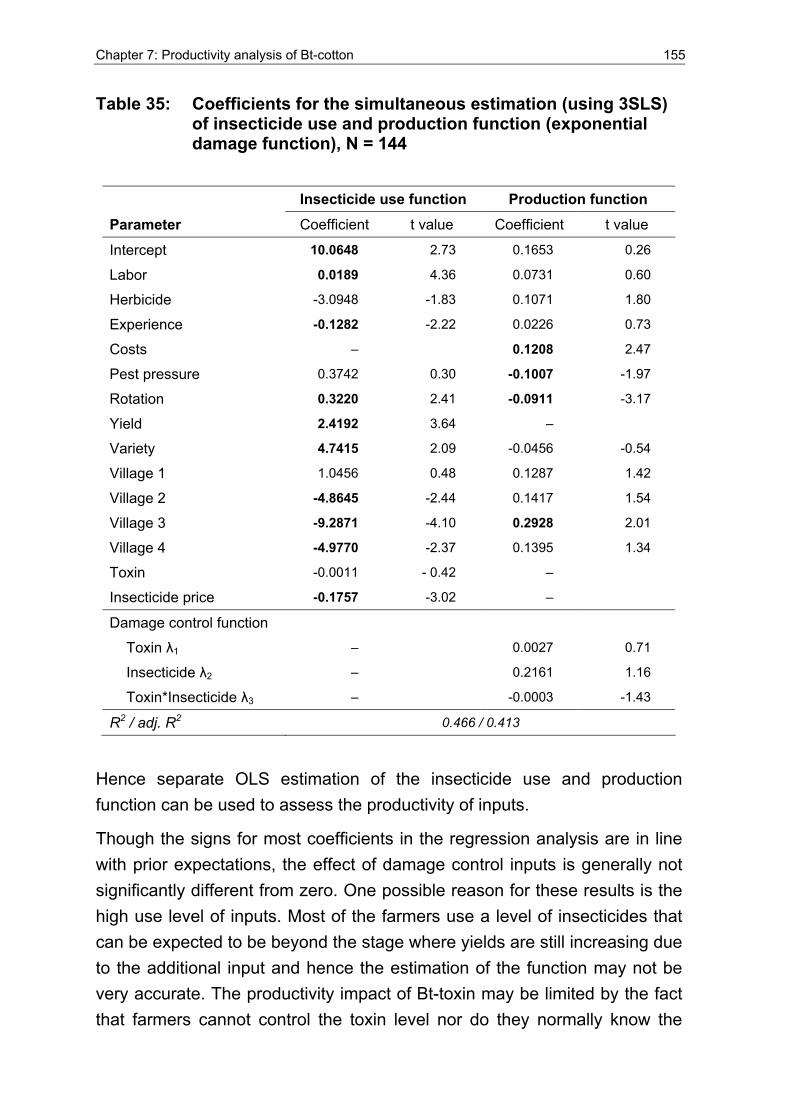
Chapter 7: Productivity analysis of Bt-cotton 155
Table 35: Coefficients for the simultaneous estimation (using 3SLS) of insecticide use and production function (exponential damage function), N = 144
Insecticide use function Production function
Parameter Coefficient t value Coefficient t value
Intercept 10.0648 2.73 0.1653 0.26
Labor 0.0189 4.36 0.0731 0.60
Herbicide -3.0948 -1.83 0.1071 1.80
Experience -0.1282 -2.22 0.0226 0.73
Costs – 0.1208 2.47
Pest pressure 0.3742 0.30 -0.1007 -1.97
Rotation 0.3220 2.41 -0.0911 -3.17
Yield 2.4192 3.64 –
Variety 4.7415 2.09 -0.0456 -0.54
Village 1 1.0456 0.48 0.1287 1.42
Village 2 -4.8645 -2.44 0.1417 1.54
Village 3 -9.2871 -4.10 0.2928 2.01
Village 4 -4.9770 -2.37 0.1395 1.34
Toxin -0.0011 - 0.42 –
Insecticide price -0.1757 -3.02 –
Damage control function
Toxin λ1 – 0.0027 0.71
Insecticide λ2 – 0.2161 1.16
Toxin*Insecticide λ3 – -0.0003 -1.43
R2 / adj. R2 0.466 / 0.413
Hence separate OLS estimation of the insecticide use and production function can be used to assess the productivity of inputs.
Though the signs for most coefficients in the regression analysis are in line with prior expectations, the effect of damage control inputs is generally not significantly different from zero. One possible reason for these results is the high use level of inputs. Most of the farmers use a level of insecticides that can be expected to be beyond the stage where yields are still increasing due to the additional input and hence the estimation of the function may not be very accurate. The productivity impact of Bt-toxin may be limited by the fact that farmers cannot control the toxin level nor do they normally know the
156 Chapter 7: Productivity analysis of Bt-cotton
toxin level and so do not adjust the use of other (substitute) inputs such as insecticides. Moreover, the input of insecticides is so high that the toxin concentration does not produce an additional impact. The substantial overuse of insecticides can possibly be explained by the large uncertainty about the quality and effectiveness of production inputs (Bt-seed and insecticides, see Chapter 6) and the willingness to rather spend more money on these inputs rather than to risk pest-inflicted damage. Hence the results seem plausible although they contradict other studies that found significant effects of the Bt-dummy and the applied pesticide quantity on cotton yield (Huang et al., 2002a; Qaim and Zilberman, 2003).Following on from the estimation of production functions, an alternative empirical approach to productivity analysis of damage control agents, which does not depend on the specification of the functional form of the production technology, is applied next.
7.2 Semi-parametric estimation of the damage control function
7.2.1 Methodology of efficiency analysis
In empirical research, the production function f and the damage control function g are unknown, and must be estimated from the data. The usual approach is to assume a certain parametric functional form, and then estimate the unknown parameters by using least squares or maximum likelihood techniques. An important question in the productivity assessment of damage control agents is the specification of the functional form of the production function. Unfortunately, there are no ex ante theoretical economic, technical, or biological reasons to prefer one functional form over another. In addition, the results are often sensitive to the specification of functional form in the sense that different specifications yield contradictory marginal value products for damage control inputs (Carrasco-Tauber and Moffitt, 1992; Fox and Weersink, 1995). The results of section 7.1 illustrated the specification dependence of productivity results for the damage control agents. To avoid this problem a general framework can be used for estimating the damage control function in a semi-parametric fashion.
The two-stage semi-parametric approach presented combines the attractive features of both the nonparametric and parametric techniques: the minimal assumptions of the nonparametric techniques and the specificity of the parametric techniques. This type of semi-parametric approach is widely
Chapter 7: Productivity analysis of Bt-cotton 157
applied in productivity and efficiency analysis and is used here to assess the productivity of damage control in cotton production.
Adhering to the distinction between yield increasing and damage controlling inputs following Lichtenberg and Zilbermann (1986), the analysis is partitioned into two stages. In the first stage, efficiency of the direct, yield increasing inputs relative to the best practice in the sample, estimated by the nonparametric data envelopment analysis (DEA) method is measured. The rationale for using a nonparametric technique in the first stage is to avoid imposing a certain functional form on the direct yield increasing inputs. The resulting efficiency indices include systematic effects of pest pressure, damage control inputs, and potential differences in farmers’ skills as well as random effects such as weather conditions. In the second stage, the average productivity impact of damage control inputs is estimated by means of parametric regression techniques to investigate whether differences in damage control activities explain efficiency differences. The rationale for resorting to parametric techniques in stage two lies in the possibility of summarizing the productivity impacts of the damage control inputs of interest into a single coefficient (or elasticity), which is not possible in the fully nonparametric approaches. The two-stage procedure is outlined below:
Stage one: Reorganizing expression (4-1), the damage control function can be written as
( , ) / ( )P Dg x z y f x= (7-13)
Note that the damage control inputs Px are confined to the left hand side, while direct inputs Dx are now confined to the right hand side of this equation. The strategy is to first estimate the right hand side of the expression, and then use the estimated values as the dependent variable in the estimation of the damage control function. The right hand side of (7-13) is the reciprocal of the Farrell output efficiency measure: the ratio of the maximum output obtainable with the given inputs to the actual output. The Farrell efficiency multiplier can be interpreted as the yield-increase potential that could be accomplished with the present inputs if the farm could operate in the same way as the most efficient farms in the sample.
158 Chapter 7: Productivity analysis of Bt-cotton
Efficiency differences across farms can arise from numerous factors, including differences in soil-quality, microclimate, and the quality of production factors, in addition to operational and managerial skills.
The literature of productive efficiency analysis puts forward a large body of both parametric and nonparametric techniques for estimating Farrell efficiency. The advantage of the nonparametric approach, also known as activity analysis or DEA, is that it does not require any prior assumptions about the functional form of the production function or the distribution function of inefficiencies. The drawback of the basic nonparametric models is that they can be sensitive to data errors and other stochastic noise, which are not explicitly modeled (Coelli et al., 1998). The parametric approaches (Bauer, 1990) usually do model the stochastic noise explicitly. However, this comes at the cost of making prior assumptions about the functional form of the production function and the distribution of inefficiencies. Even if these parametric assumptions are “correct”, the parametric models need not necessarily perform any better than the basic nonparametric techniques in a cross-sectional setting (Coelli et al., 1998; Ondrich and Ruggiero, 2001). In fact, the nonparametric techniques perform reasonably well under ideal conditions for the parametric techniques, and they are expected to be much more robust to violations of these conditions. In addition, the problem with stochastic noise can be dealt with in the more sophisticated models (Varian, 1985). All these are strong arguments to follow the nonparametric route.
The activity analysis approach does not impose any parametric functional form on the production function f. Rather the estimation is based on standard properties of technology such as monotonicity (= free disposability), convexity, and assumptions about returns to scale. Following the so-called minimum extrapolation principle (Banker et al., 1984), the production possibility set is approximated by the smallest subset of the input-output space that contains all observed production vectors and satisfies the maintained production assumptions. If monotonicity, convexity and constant returns to scale in direct inputs67 are assumed, estimates of Farrell efficiency of farm k (with input vector xk and output yk) can be
67 The assumptions of constant returns to scale and convexity are easy to relax (Kousmanen 2001).
Chapter 7: Productivity analysis of Bt-cotton 159
calculated as the optimal solution to the following linear programming problem:
,
1
1
max
. .
0.
n
k i ii
nD Dk i i
i
i
s t
y y
x x
θ λθ
θ λ
λ
λ
=
=
≤
≥
≥
∑
∑
(7-14)
The variables iλ represent intensity weights that are used for forming
convex combinations of the sample farms. The scalar θ that is to be maximized is the inverse of the Farrell efficiency measure. If the assumed production assumptions hold, the resulting optimal solution *θ is a consistent estimate of ( ) /Df x y (Banker, 1993; Simar and Wilson, 2000).
Therefore, (the vector of) inverses *1/θ can be used as consistent nonparametric estimates for the unknown Farrell efficiencies / ( )Dy f x on the right-hand-side of (7-13).
Stage two: Having estimated the dependent variable *1/θ , the next step is to estimate the damage control function g from (7-13). Specifically, the following regression equation needs to be estimated:
*1/θ = ( , )Pg x z ε+ (7-15)
where the left-hand-side Farrell efficiencies are obtained as the optimal solution to (7-14). There are four fundamental challenges to the approach, as pointed out by Simar and Wilson (2003). Firstly, the true Farrell efficiency
/ ( )Dy f x is not observed directly, but only its empirical estimates *1/θ . The efficiency estimate of one farm is dependent on the input-output values and hence efficiencies of other farms, that is, these empirical estimates are serially correlated. Secondly, the empirical efficiency estimates are calculated based on a sample of farms, which typically excludes some efficient production possibilities that are feasible but not observed in the sample. This implies that the empirical efficiency estimates are overestimated. Thirdly, the output also depends on the level of damage control inputs and damage agents, which are not taken into account in the
160 Chapter 7: Productivity analysis of Bt-cotton
first stage efficiency estimation. This implies that the error term ε must be correlated with the damage control inputs Px and the damage agents z. Fourthly, the domain of the efficiency ratios / ( )Dy f x and *1/θ is restricted to the interval (0,1), which should be taken into account in the estimation.
To simultaneously address these challenges Simar and Wilson (2003) propose a procedure that in the first stage estimates Farrell efficiency in the nonparametric fashion using (7-14), and in the second stage estimates regression equation (7-15) using truncated regression.68
Both stages are complemented with bootstrap simulation, in order to eliminate the sampling bias and to allow for consistent statistical inference. The two-stage double-bootstrap algorithm is described in detail in Box 6.
In the present context, it is also worth noting that the double-bootstrap procedure approach does allow for interaction between direct inputs and the damage control function. If the damage agents are dependent on the levels of direct inputs, then the error term of regression equation (7-15) is dependent on damage agents and damage control inputs. While this dependence would be a problem for most regression techniques, the correlation between the explanatory variables and the error term is a prime motive for applying the double-bootstrap approach in the first place.
For the specification of the regression function, a linear damage control function is applied. This specification enables interpretation of the slope coefficients of damage control inputs as the average marginal products of these inputs. The main interest is in estimating the average marginal product that summarizes the contribution of an input in a single number, and not so much the empirical fit. However, the linear functional form as such is too simplistic for the purpose, because it assumes the marginal product of an input is constant over the entire domain of the damage control function. Bearing in mind that the main argument for differentiating between damage control inputs and ordinary yield increasing inputs is that the level of potential damage influences the former inputs, a functional form is needed that allows the slope coefficients (or marginal product) to vary across
68 Simar and Wilson (2003) favor truncated regression over censored regression, because the former is consistent with their model assumptions about the data generating process.
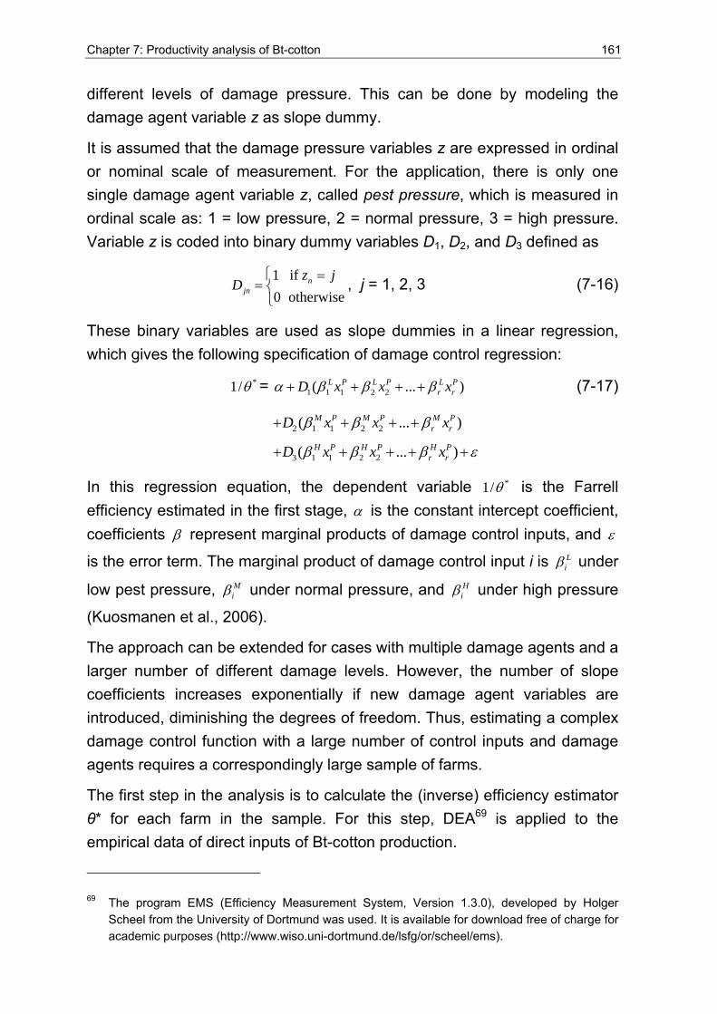
Chapter 7: Productivity analysis of Bt-cotton 161
different levels of damage pressure. This can be done by modeling the damage agent variable z as slope dummy.
It is assumed that the damage pressure variables z are expressed in ordinal or nominal scale of measurement. For the application, there is only one single damage agent variable z, called pest pressure, which is measured in ordinal scale as: 1 = low pressure, 2 = normal pressure, 3 = high pressure. Variable z is coded into binary dummy variables D1, D2, and D3 defined as
1 if 0 otherwise
njn
z jD
⎧ == ⎨⎩
, j = 1, 2, 3 (7-16)
These binary variables are used as slope dummies in a linear regression, which gives the following specification of damage control regression:
*1/θ = 1 1 1 2 2( ... )α β β β+ + + +L P L P L Pr rD x x x (7-17)
2 1 1 2 2
3 1 1 2 2
( ... )
( ... )
M P M P M Pr r
H P H P H Pr r
D x x x
D x x x
β β β
β β β ε
+ + + +
+ + + + +
In this regression equation, the dependent variable *1/θ is the Farrell efficiency estimated in the first stage, α is the constant intercept coefficient, coefficients β represent marginal products of damage control inputs, and ε
is the error term. The marginal product of damage control input i is β Li under
low pest pressure, β Mi under normal pressure, and β H
i under high pressure
(Kuosmanen et al., 2006).
The approach can be extended for cases with multiple damage agents and a larger number of different damage levels. However, the number of slope coefficients increases exponentially if new damage agent variables are introduced, diminishing the degrees of freedom. Thus, estimating a complex damage control function with a large number of control inputs and damage agents requires a correspondingly large sample of farms.
The first step in the analysis is to calculate the (inverse) efficiency estimator θ* for each farm in the sample. For this step, DEA69 is applied to the empirical data of direct inputs of Bt-cotton production.
69 The program EMS (Efficiency Measurement System, Version 1.3.0), developed by Holger Scheel from the University of Dortmund was used. It is available for download free of charge for academic purposes (http://www.wiso.uni-dortmund.de/lsfg/or/scheel/ems).
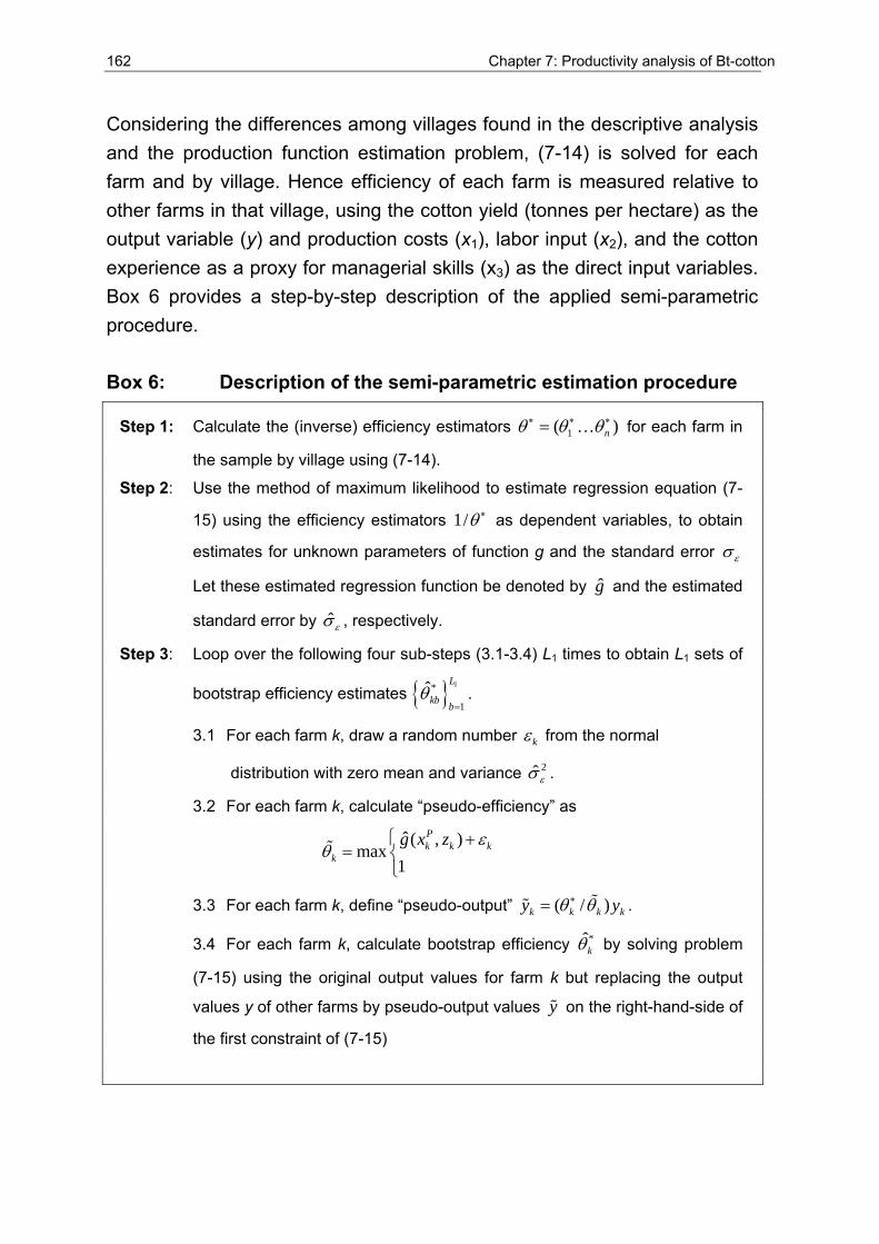
162 Chapter 7: Productivity analysis of Bt-cotton
Considering the differences among villages found in the descriptive analysis and the production function estimation problem, (7-14) is solved for each farm and by village. Hence efficiency of each farm is measured relative to other farms in that village, using the cotton yield (tonnes per hectare) as the output variable (y) and production costs (x1), labor input (x2), and the cotton experience as a proxy for managerial skills (x3) as the direct input variables. Box 6 provides a step-by-step description of the applied semi-parametric procedure.
Box 6: Description of the semi-parametric estimation procedure
Step 1: Calculate the (inverse) efficiency estimators 1( )nθ θ θ∗ ∗ ∗= K for each farm in
the sample by village using (7-14). Step 2: Use the method of maximum likelihood to estimate regression equation (7-
15) using the efficiency estimators 1/θ ∗ as dependent variables, to obtain
estimates for unknown parameters of function g and the standard error εσ
Let these estimated regression function be denoted by g and the estimated
standard error by ˆεσ , respectively.
Step 3: Loop over the following four sub-steps (3.1-3.4) L1 times to obtain L1 sets of
bootstrap efficiency estimates 1*
1ˆ L
kb bθ
=.
3.1 For each farm k, draw a random number kε from the normal
distribution with zero mean and variance 2ˆεσ .
3.2 For each farm k, calculate “pseudo-efficiency” as
ˆ ( , )
max1
Pk k k
kg x z ε
θ⎧ +
= ⎨⎩
%
3.3 For each farm k, define “pseudo-output” ( / )k k k ky yθ θ∗= %% .
3.4 For each farm k, calculate bootstrap efficiency *kθ by solving problem
(7-15) using the original output values for farm k but replacing the output
values y of other farms by pseudo-output values y% on the right-hand-side of
the first constraint of (7-15)
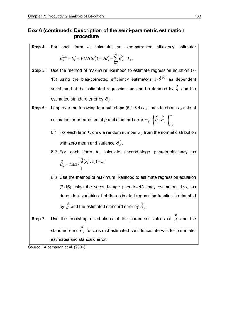
Chapter 7: Productivity analysis of Bt-cotton 163
Box 6 (continued): Description of the semi-parametric estimation procedure
Step 4: For each farm k, calculate the bias-corrected efficiency estimator
1* * * *
11
ˆ ˆ( ) 2 /L
BCk k k k kb
bBIAS Lθ θ θ θ θ
=
= − = −∑ .
Step 5: Use the method of maximum likelihood to estimate regression equation (7-
15) using the bias-corrected efficiency estimators ˆ1/ BCθ as dependent
variables. Let the estimated regression function be denoted by ˆg and the
estimated standard error by ˆεσ .
Step 6: Loop over the following four sub-steps (6.1-6.4) L2 times to obtain L2 sets of
estimates for parameters of g and standard error εσ : 2
1
ˆ ˆˆ ˆˆ ˆ,L
b bb
g εσ=
6.1 For each farm k, draw a random number kε from the normal distribution
with zero mean and variance 2ˆεσ .
6.2 For each farm k, calculate second-stage pseudo-efficiency as
ˆ ( , )max1
Pk k k
kg x z εθ
⎧ +⎪= ⎨⎪⎩
%%
6.3 Use the method of maximum likelihood to estimate regression equation
(7-15) using the second-stage pseudo-efficiency estimators 1/ kθ%% as
dependent variables. Let the estimated regression function be denoted
by ˆg and the estimated standard error by
ˆεσ .
Step 7: Use the bootstrap distributions of the parameter values of ˆg and the
standard error ˆεσ to construct estimated confidence intervals for parameter
estimates and standard error.
Source: Kuosmanen et al. (2006)
164 Chapter 7: Productivity analysis of Bt-cotton
7.2.2 Data and variables for the semi-parametric model
The input data for the semi-parametric model are described in detail in Chapters 6, and variables are largely congruent with the set used in the analysis in Chapter 7.1. However, a slightly different set of data was used for the model. The employed sample size is smaller (N = 131)70 because the data from the sub-sample of 11 households that were cultivating tree cotton is excluded. The rationale for this restricted sample is the difference in the production practices for this variety (wider plant spacing, different level of production inputs such as labor) as compared to the other varieties. This difference may disturb the efficiency estimation in the first step of the analysis. The key values of each of these variables for this set of data are listed in Table 36.The seed cotton yield is the dependent variable y and the direct inputs for the first stage of the model are the use of labor, the experience of the farmer and the production costs. Labor input does not include the labor used for the application of pesticides nor for other pest control measures. The production costs are in US$ per hectare and include expenses for seed71, mulching, fertilizer and irrigation and hence are a proxy for other direct inputs used. The use of insecticides and the Bt-toxin concentration as well as manual control of pests, crop rotation and the pest knowledge of the farmer are the damage control inputs for the model. The two additional damage control inputs that were not included for analysis so far are the labor for manual pest control in persondays per hectare and a score for the pest knowledge. The knowledge score is an indicator for the awareness and comprehension a farmer has on pest management issues. The score is generated by summing up the number of insect pests the farmer can name and briefly describe (not including the three main pests spider mite, cotton bollworm, and aphids) and the number of natural enemies he or she is aware of. Introducing such a knowledge score in the model assumes that increasing awareness and comprehension can (at least partly) substitute other damage control inputs.
70 Only the 144 households where all the information is available were included (see Tables 31) and the 11 farmers growing tree cotton were excluded limiting the sample size to 131.
71 Costs for seed were included since there was no correlation between the seed costs and the toxin concentration or the insecticide use. Though the seed price may also indicate quality with regard to Bt-toxin concentration (see Chapter 6), the amount of seed used and hence seed costs are considered important for the estimation of production efficiency.
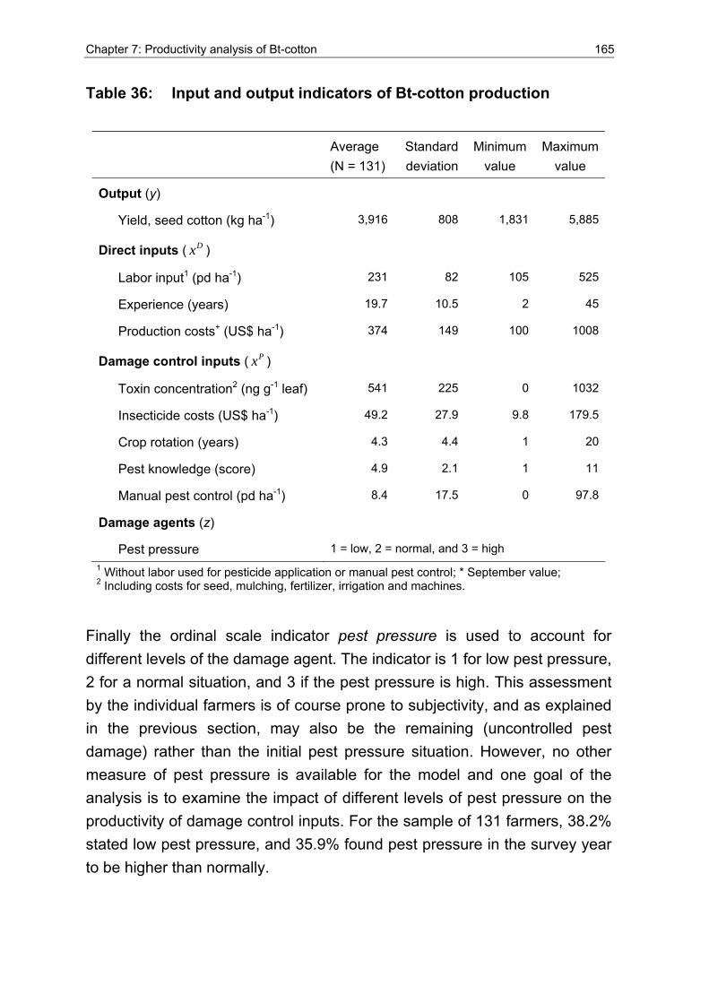
Chapter 7: Productivity analysis of Bt-cotton 165
Table 36: Input and output indicators of Bt-cotton production
Average (N = 131)
Standard deviation
Minimum value
Maximumvalue
Output (y)
Yield, seed cotton (kg ha-1) 3,916 808 1,831 5,885
Direct inputs ( Dx )
Labor input1 (pd ha-1) 231 82 105 525
Experience (years) 19.7 10.5 2 45
Production costs+ (US$ ha-1) 374 149 100 1008
Damage control inputs ( Px )
Toxin concentration2 (ng g-1 leaf) 541 225 0 1032
Insecticide costs (US$ ha-1) 49.2 27.9 9.8 179.5
Crop rotation (years) 4.3 4.4 1 20
Pest knowledge (score) 4.9 2.1 1 11
Manual pest control (pd ha-1) 8.4 17.5 0 97.8
Damage agents (z)
Pest pressure 1 = low, 2 = normal, and 3 = high 1 Without labor used for pesticide application or manual pest control; * September value; 2 Including costs for seed, mulching, fertilizer, irrigation and machines.
Finally the ordinal scale indicator pest pressure is used to account for different levels of the damage agent. The indicator is 1 for low pest pressure, 2 for a normal situation, and 3 if the pest pressure is high. This assessment by the individual farmers is of course prone to subjectivity, and as explained in the previous section, may also be the remaining (uncontrolled pest damage) rather than the initial pest pressure situation. However, no other measure of pest pressure is available for the model and one goal of the analysis is to examine the impact of different levels of pest pressure on the productivity of damage control inputs. For the sample of 131 farmers, 38.2% stated low pest pressure, and 35.9% found pest pressure in the survey year to be higher than normally.
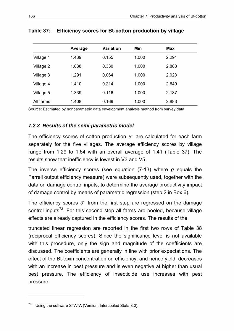
166 Chapter 7: Productivity analysis of Bt-cotton
Table 37: Efficiency scores for Bt-cotton production by village
Average Variation Min Max
Village 1 1.439 0.155 1.000 2.291
Village 2 1.638 0.330 1.000 2.883
Village 3 1.291 0.064 1.000 2.023
Village 4 1.410 0.214 1.000 2.649
Village 5 1.339 0.116 1.000 2.187
All farms 1.408 0.169 1.000 2.883
Source: Estimated by nonparametric data envelopment analysis method from survey data
7.2.3 Results of the semi-parametric model
The efficiency scores of cotton production θ ∗ are calculated for each farm separately for the five villages. The average efficiency scores by village range from 1.29 to 1.64 with an overall average of 1.41 (Table 37). The results show that inefficiency is lowest in V3 and V5.
The inverse efficiency scores (see equation (7-13) where g equals the Farrell output efficiency measure) were subsequently used, together with the data on damage control inputs, to determine the average productivity impact of damage control by means of parametric regression (step 2 in Box 6).
The efficiency scores θ ∗ from the first step are regressed on the damage control inputs72. For this second step all farms are pooled, because village effects are already captured in the efficiency scores. The results of the
truncated linear regression are reported in the first two rows of Table 38 (reciprocal efficiency scores). Since the significance level is not available with this procedure, only the sign and magnitude of the coefficients are discussed. The coefficients are generally in line with prior expectations. The effect of the Bt-toxin concentration on efficiency, and hence yield, decreases with an increase in pest pressure and is even negative at higher than usual pest pressure. The efficiency of insecticide use increases with pest pressure.
72 Using the software STATA (Version: Intercooled Stata 8.0).
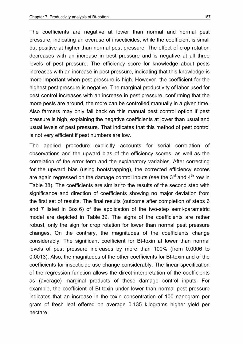
Chapter 7: Productivity analysis of Bt-cotton 167
The coefficients are negative at lower than normal and normal pest pressure, indicating an overuse of insecticides, while the coefficient is small but positive at higher than normal pest pressure. The effect of crop rotation decreases with an increase in pest pressure and is negative at all three levels of pest pressure. The efficiency score for knowledge about pests increases with an increase in pest pressure, indicating that this knowledge is more important when pest pressure is high. However, the coefficient for the highest pest pressure is negative. The marginal productivity of labor used for pest control increases with an increase in pest pressure, confirming that the more pests are around, the more can be controlled manually in a given time. Also farmers may only fall back on this manual pest control option if pest pressure is high, explaining the negative coefficients at lower than usual and usual levels of pest pressure. That indicates that this method of pest control is not very efficient if pest numbers are low.
The applied procedure explicitly accounts for serial correlation of observations and the upward bias of the efficiency scores, as well as the correlation of the error term and the explanatory variables. After correcting for the upward bias (using bootstrapping), the corrected efficiency scores are again regressed on the damage control inputs (see the 3rd and 4th row in Table 38). The coefficients are similar to the results of the second step with significance and direction of coefficients showing no major deviation from the first set of results. The final results (outcome after completion of steps 6 and 7 listed in Box 6) of the application of the two-step semi-parametric model are depicted in Table 39. The signs of the coefficients are rather robust, only the sign for crop rotation for lower than normal pest pressure changes. On the contrary, the magnitudes of the coefficients change considerably. The significant coefficient for Bt-toxin at lower than normal levels of pest pressure increases by more than 100% (from 0.0006 to 0.0013). Also, the magnitudes of the other coefficients for Bt-toxin and of the coefficients for insecticide use change considerably. The linear specification of the regression function allows the direct interpretation of the coefficients as (average) marginal products of these damage control inputs. For example, the coefficient of Bt-toxin under lower than normal pest pressure indicates that an increase in the toxin concentration of 100 nanogram per gram of fresh leaf offered on average 0.135 kilograms higher yield per hectare.
168 Chapter 7: Productivity analysis of Bt-cotton
Table 38: Results of the truncated linear regression I
Reciprocal efficiency scores
Bias-corrected efficiency scores
Coefficient Standard error Coefficient Standard error Bt-toxin 1 0.000779 0.0003 0.000622 0.0002 Bt-toxin 2 -0.000010 0.0004 0.000017 0.0002 Bt-toxin 3 -0.000357 0.0002 -0.000262 0.0001 Insecticide 1 -0.005740 0.0025 -0.004174 0.0014 Insecticide 2 -0.003889 0.0024 -0.002940 0.0014 Insecticide 3 0.001032 0.0022 0.000374 0.0012 Crop rotation 1 -0.006289 0.0127 -0.002033 0.0075 Crop rotation 2 -0.003283 0.0139 -0.001982 0.0082 Crop rotation 3 -0.030228 0.0208 -0.016093 0.0124 Pest knowledge 1 -0.010167 0.0285 -0.017176 0.0161 Pest knowledge 2 0.029802 0.0382 0.019160 0.0218 Pest knowledge 3 -0.004920 0.0243 -0.004928 0.0142 Labor 1 -0.004738 0.0037 -0.003416 0.0022 Labor 2 -0.005861 0.0032 -0.004235 0.0019 Labor 3 0.002110 0.0033 0.001546 0.0020 Constant 1.097583 0.1809 0.911471 0.0893 Log likelihood: 75.7 78.9
N = 131, truncated regression: lower limit: 0, upper limit: 1 Note: Reciprocal efficiency scores and bias-corrected efficiency scores as dependent variables.
The important new component of Table 39 is that statistical significance tests are now available. Several of the coefficients for Bt-toxin, the insecticide costs and labor are statistically significant at the five percent level. The negligible impact of Bt-toxin at higher pest pressure is hardly surprising in the present sample of farms, which use high quantities of insecticides that may eliminate the pests the Bt-toxin should control for. A comparison of the marginal productivities between the applied approaches shows lower and mostly significant values for the Bt-toxin under the semi-parametric approach. This suggests that previous studies on the productivity of Bt-cotton using a conventional production function estimation (Huang et al., 2002a; Qaim, 2003; Thirtle et al., 2003) may overstate the benefits of the technology.
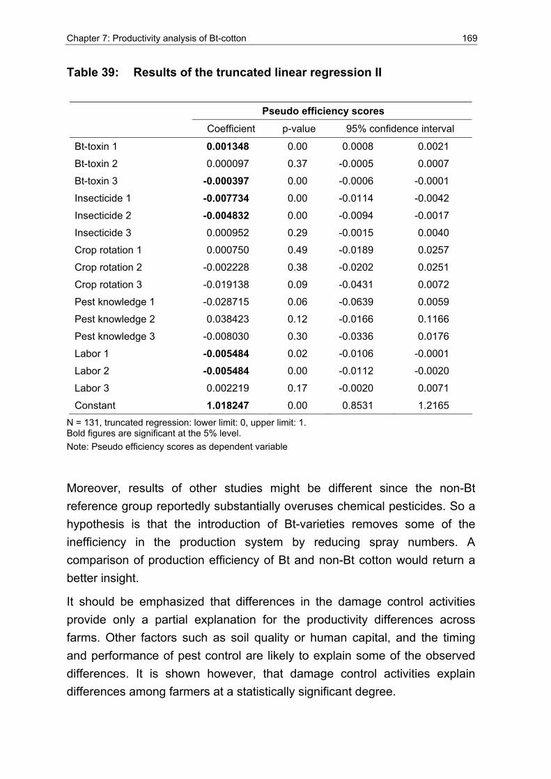
Chapter 7: Productivity analysis of Bt-cotton 169
Table 39: Results of the truncated linear regression II
Pseudo efficiency scores
Coefficient p-value 95% confidence interval
Bt-toxin 1 0.001348 0.00 0.0008 0.0021
Bt-toxin 2 0.000097 0.37 -0.0005 0.0007
Bt-toxin 3 -0.000397 0.00 -0.0006 -0.0001
Insecticide 1 -0.007734 0.00 -0.0114 -0.0042
Insecticide 2 -0.004832 0.00 -0.0094 -0.0017
Insecticide 3 0.000952 0.29 -0.0015 0.0040
Crop rotation 1 0.000750 0.49 -0.0189 0.0257
Crop rotation 2 -0.002228 0.38 -0.0202 0.0251
Crop rotation 3 -0.019138 0.09 -0.0431 0.0072
Pest knowledge 1 -0.028715 0.06 -0.0639 0.0059
Pest knowledge 2 0.038423 0.12 -0.0166 0.1166
Pest knowledge 3 -0.008030 0.30 -0.0336 0.0176
Labor 1 -0.005484 0.02 -0.0106 -0.0001
Labor 2 -0.005484 0.00 -0.0112 -0.0020
Labor 3 0.002219 0.17 -0.0020 0.0071
Constant 1.018247 0.00 0.8531 1.2165 N = 131, truncated regression: lower limit: 0, upper limit: 1. Bold figures are significant at the 5% level. Note: Pseudo efficiency scores as dependent variable
Moreover, results of other studies might be different since the non-Bt reference group reportedly substantially overuses chemical pesticides. So a hypothesis is that the introduction of Bt-varieties removes some of the inefficiency in the production system by reducing spray numbers. A comparison of production efficiency of Bt and non-Bt cotton would return a better insight.
It should be emphasized that differences in the damage control activities provide only a partial explanation for the productivity differences across farms. Other factors such as soil quality or human capital, and the timing and performance of pest control are likely to explain some of the observed differences. It is shown however, that damage control activities explain differences among farmers at a statistically significant degree.
170 Chapter 7: Productivity analysis of Bt-cotton
The introduction of the slope dummies for the pest pressure variable confirmed that the productivity of damage control inputs varies with changes in the level of damage agents.
7.3 Summary
The chapter presented the analysis of short-term productivity of Bt-toxin and insecticides and other damage control variables. In section 7.1 an insecticide use function and a production function for Bt-cotton were estimated. For the estimation of the production function a damage control function was included and different specifications of the damage control function were tested.
The estimation of the insecticide use function shows that in accordance with prior expectations higher input of labor, higher yield levels, and less rotation significantly increase the use of insecticides. The significance of the village dummy variables indicates differences among the villages. As expected, longer experience in cotton production and higher quality insecticides (higher product price) result in lower use of insecticides. However, the level of Bt-toxin is not significant, indicating that farmers do not substitute insecticides with Bt-toxin. For the production function estimation there is only little difference between the functional specifications (pure Cobb-Douglas, and with damage control function with exponential, logistic or Weibull form). For all specifications the direct inputs labor and production costs significantly increase the cotton yield while longer rotation and higher pest pressure lead to lower yield outcomes. The significance for the village dummy coefficient for V3 indicates that farmers in this village realize higher cotton yields. The coefficient for Bt-toxin is not significant in any of the specifications. Higher use of insecticides has a significant yield-increasing effect only for the exponential damage control function.
The marginal physical product of insecticides varies for the different functional forms, but is positive for all estimated functions. A graph with the marginal value product of insecticides at different input levels shows that the economically optimal use level is much lower as the actual use level and hence this factor is substantially overused. The marginal product for Bt-toxin is negative for all but one specification and computation of marginal productivity is hence not meaningful.
Chapter 7: Productivity analysis of Bt-cotton 171
In section 7.2 a two stage semi-parametric approach to estimate the marginal productivity of chemical insecticides and Bt-toxin was presented. While commonly results for marginal productivity of pesticides or Bt-toxin depend on the specification of the damage control function and the production function, the semi-parametric approach provides results independent of the functional form of the production function.
Moreover, correcting for (1) serial correlation and (2) correlation of the error term as well as (3) bias in the dependent variable changes the coefficients considerably (more than 100% for those that are statistically significant at the five percent level).
The pest pressure variable is used as a slope dummy to allow for differences in productivity of variables for different levels of pest pressure. Results show that factor productivity of control inputs depends on the actual level of the damage agent. The results obtained differ from the outcome of the previous damage control function estimates where neither the use of insecticides (in most cases) nor the concentration of Bt-toxin led to significant coefficients in the regression. In the semi-parametric approach, the level of Bt-toxin concentration in leaf tissue, the use of chemical insecticides and pest control by manual labor explain at least part of the variation in the dependent efficiency index.
8 Model ing crop protec t ion s t ra teg ies in cot ton
8.1 Partial budgeting model of pest control
The production function estimation and the semi-parametric bootstrapping analysis from the previous chapter analyze the productivity effect of using Bt-cotton varieties under the small-scale conditions in the study area. However, neither approach captures important characteristics of the agro-ecosystem they intend to describe. Among those characteristics are the complexity of interactions between plant and ecosystem and the impact of control interventions on this system, as well as the uncertainty in the main determining variables. This uncertainty becomes evident in the fluctuation of cotton yield, pest pressure (due to climatic conditions), input and output prices, and the effectiveness of the applied control measures. The data used for analysis, as in most other studies of this kind, depicts the situation for only one year and for a limited number of observations. Thus, results and conclusions cannot be generalized but apply only to the specific time and location of the survey. Furthermore, with coverage of Bt-cotton varieties of about 100% in the study area, no counterfactual or control group of farmers growing non-Bt cotton exists that can readily be used for a comparison. Other weaknesses of the productivity approaches are endogeneity problems and likely measurement errors, and difficulties such as varying quality of inputs and non-physical variables like knowledge and information.
Stochastic partial budgeting models, like the one presented in this chapter, are a complementary approach to assess the farm-level performance of a new technology such as Bt-cotton. One major advantage of such models is that it is possible to account for the stochastic nature of the main variables and compare alternative strategies and scenarios that cannot readily be found in the study area.
8.1.1 Methodology and structure of the simulation model
The use of Bt-cotton varieties is a new option in cotton bollworm control that can (at least partially) substitute insecticide treatments against this major pest. Comparing the planting of a Bt-variety and the application of chemical insecticides to control the pest (or a combination of both) requires the identification of the distinct properties of each of the control measures. One important distinction is that Bt-crops provide a prophylactic pest control
Chapter 8: Modeling crop protection strategies in cotton 173
treatment in which the control decision is made at the beginning of the season when farmers do not yet know the severity of bollworm attack. Hence, the embodiment of traits in the seed prevents partial or sequential adoption of pest control and changes the structure of production costs. The variable costs for pest control become seasonal fixed costs if insect or virus resistant varieties are planted, increasing the net risk and the liquidity requirements for farmers. Depending on the severity of pest pressure and prevailing prices, this form of preventive pest management can yield negative net revenues if pest pressure or crop yield is low, since farmers cannot adjust their pest management strategy to actual conditions (see Pemsl et al., 2004 for an empirical example). Insecticides, on the other hand, can be applied in response to actual pest pressure and with regard to the potential yield level73.
An economic assessment of pest control can be performed in the context of a partial budget analysis by calculating the net revenue of different bollworm control methods (Herdt et al., 1984). For such a partial budgeting model, the main factors that determine the net revenue NRj of bollworm control strategy j are the monetary value of the avoided yield loss (calculated using the potential pest free yield Y0 , the pest pressure L0 , the effectiveness of pest control Ej and the cotton output price pY) and the related control costs Cj of the strategy j. The following equation shows how the net revenue NRj is composed
(8-1)
Such a simple model can illustrate the profitability of different control options as demonstrated for the use of Bt-cotton varieties, compared to a control strategy using insecticides to control CBW in Karnataka state in India (Pemsl et al., 2004). Table 40 gives an overview of benefits and costs of the two major CBW control options, namely the use of a Bt-cotton variety and the application of chemical insecticides. The main difference from the model presented in (8-1) is the additional benefit of the insecticides strategy from the reduction of other insect pests. This benefit results because cotton farmers in the Yellow River area in China use broad-spectrum insecticides to control the cotton bollworm and these are not very target-specific, making them effective against most insects in the field. The other main insect pests are aphids, red
73 This implies that pest damage destroys a certain percentage of the yield and hence the absolute benefit of a pesticide application would be larger for higher yield levels.
[ ] jYjj CpLYELYNR −∗−−−−= )1(*))1(*1(* 0000
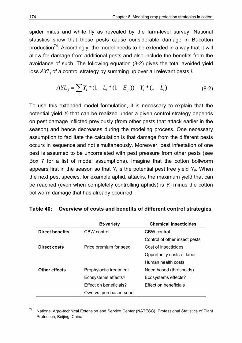
174 Chapter 8: Modeling crop protection strategies in cotton
spider mites and white fly as revealed by the farm-level survey. National statistics show that those pests cause considerable damage in Bt-cotton production74. Accordingly, the model needs to be extended in a way that it will allow for damage from additional pests and also include the benefits from the avoidance of such. The following equation (8-2) gives the total avoided yield loss AYLj of a control strategy by summing up over all relevant pests i.
(8-2)
To use this extended model formulation, it is necessary to explain that the potential yield Yi that can be realized under a given control strategy depends on pest damage inflicted previously (from other pests that attack earlier in the season) and hence decreases during the modeling process. One necessary assumption to facilitate the calculation is that damage from the different pests occurs in sequence and not simultaneously. Moreover, pest infestation of one pest is assumed to be uncorrelated with pest pressure from other pests (see Box 7 for a list of model assumptions). Imagine that the cotton bollworm appears first in the season so that Yi is the potential pest free yield Y0. When the next pest species, for example aphid, attacks, the maximum yield that can be reached (even when completely controlling aphids) is Y0 minus the cotton bollworm damage that has already occurred.
Table 40: Overview of costs and benefits of different control strategies
Bt-variety Chemical insecticides
Direct benefits CBW control CBW control
Control of other insect pests
Direct costs Price premium for seed
Cost of insecticides
Opportunity costs of labor
Human health costs
Other effects Prophylactic treatment
Ecosystems effects?
Effect on beneficials?
Own vs. purchased seed
Need based (thresholds)
Ecosystems effects?
Effect on beneficials
74 National Agro-technical Extension and Service Center (NATESC). Professional Statistics of Plant Protection, Beijing, China.
∑ −−−−=i
iijiiij LYELYAYL )1(*))1(*1(*
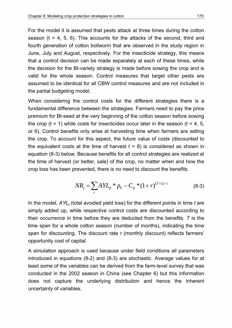
Chapter 8: Modeling crop protection strategies in cotton 175
For the model it is assumed that pests attack at three times during the cotton season (t = 4, 5, 6). This accounts for the attacks of the second, third and fourth generation of cotton bollworm that are observed in the study region in June, July and August, respectively. For the insecticide strategy, this means that a control decision can be made separately at each of these times, while the decision for the Bt-variety strategy is made before sowing the crop and is valid for the whole season. Control measures that target other pests are assumed to be identical for all CBW control measures and are not included in the partial budgeting model.
When considering the control costs for the different strategies there is a fundamental difference between the strategies. Farmers need to pay the price premium for Bt-seed at the very beginning of the cotton season before sowing the crop (t = 1) while costs for insecticides occur later in the season (t = 4, 5, or 6). Control benefits only arise at harvesting time when farmers are selling the crop. To account for this aspect, the future value of costs (discounted to the equivalent costs at the time of harvest t = 8) is considered as shown in equation (8-3) below. Because benefits for all control strategies are realized at the time of harvest (or better, sale) of the crop, no matter when and how the crop loss has been prevented, there is no need to discount the benefits.
(8-3)
In the model, AYLj (total avoided yield loss) for the different points in time t are simply added up, while respective control costs are discounted according to their occurrence in time before they are deducted from the benefits. T is the time span for a whole cotton season (number of months), indicating the time span for discounting. The discount rate r (monthly discount) reflects farmers’ opportunity cost of capital.
A simulation approach is used because under field conditions all parameters introduced in equations (8-2) and (8-3) are stochastic. Average values for at least some of the variables can be derived from the farm-level survey that was conducted in the 2002 season in China (see Chapter 6) but this information does not capture the underlying distribution and hence the inherent uncertainty of variables.
∑ −++−=t
tTjtYjtj rCpAYLNR )1()1(**
176 Chapter 8: Modeling crop protection strategies in cotton
Figure 42: Relationship of probability density function (PDF) to cumulative distribution function (CDF)
CDF
f(x)
F(x)
X
X
m
m
a
a
x
x
b
b
A
A
Source: Hardaker et al. (1997)
If such a probability distribution is known, stochastic parameters can be drawn using Monte Carlo simulation. Monte Carlo techniques are therefore appropriate tools for integrating relevant observations especially in situations where the data situation is sparse (Anderson et al., 1977).
With a high number of replicates, such sampling re-creates the distribution because more samples are drawn in areas of high occurrence within the distribution (Hardaker et al., 1997). In the budgeting model, each set of generated values is used to calculate the net revenue of the respective bollworm control strategies. From all resulting values NRj of each strategy a cumulative distribution function (CDF) is generated. Figure 42 shows the relationship between a probability density function (PDF) and a CDF. The CDF or F(X) of a random variable X gives the probability that it takes a value lower or equal to a specified numerical value x0 so that ( ) ( )0 0F X x P X x= = ≤
Chapter 8: Modeling crop protection strategies in cotton 177
(Gujarati, 2003). These CDFs of the net revenue of different control strategies can be compared by applying the criteria of first-degree stochastic dominance (FSD) and second-degree stochastic dominance (SSD). The criterion for first-degree stochastic dominance (8-4) is that all values of x (net revenues) of control method one (Bt-variety) are lower or equal than those of a different method two (pesticides) with at least one strong inequality (Hardaker et al., 1997). This criterion corresponds to the shift of the probability density function as described in section 4.2.2 and all decision-makers irrespective of their risk attitudes would prefer the strategy that is first-degree stochastic dominant.
( ) ( )xFxF PBt ≤ (8-4)
In second-degree stochastic dominance (8-5) the Bt strategy (Bt) will be preferable to the pesticide strategy (P) if the area under FBt is less than the area under FP, for all values of x* (Moschini and Hennessy, 2001). The SSD refers to a reduction in the variability of outcomes and will only increase utility if the decision-maker is risk-averse. Based on these two criteria the different control strategies can be ranked and the probability of a negative net revenue of control can be directly read from the graph.
dxxFFdxxFFx
PP
x
BtBt )()(**
∫∫∞−∞−
=≤= (8-5)
Figure 43 depicts the structure of the simulation model and shows the process of iterated drawing of replications. All input variables for the model (listed in the grey box on the left-hand side of the figure) are generated using Monte Carlo sampling. These figures are used to calculate the resulting yield when applying a certain control strategy (summing up for the different pests and the different points in time) and under a scenario without control.
The difference between those two values multiplied by the output price is the benefit of the respective control strategy. Deduction of the control costs from this benefit figure gives the net revenue of the control. This procedure is repeated for a large number of replications so that finally a cumulative distribution of the net revenues of the distinct control strategies can be derived.
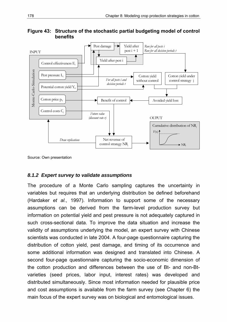
178 Chapter 8: Modeling crop protection strategies in cotton
Figure 43: Structure of the stochastic partial budgeting model of control benefits
Cotton yield under control strategy j
Avoided yield loss
Net revenue of control strategy NRj
Cumulative distribution of NRj
Mon
te-C
arlo
-Sim
ulat
ion
F(x)
NRj
Pest pressure Li
Control effectiveness Ei
Cotton price pY
Control costs Cj
Draw replications
Run for all decision periods t
Benefit of control
Future value (discount rate r)
Cotton yield without control
Potential cotton yield Y0
For all pests i and decision periods t
Run for all pests i
Yield after pest i
Yield after pest i + 1
Pest damageINPUT
OUPUT
Source: Own presentation
8.1.2 Expert survey to validate assumptions
The procedure of a Monte Carlo sampling captures the uncertainty in variables but requires that an underlying distribution be defined beforehand (Hardaker et al., 1997). Information to support some of the necessary assumptions can be derived from the farm-level production survey but information on potential yield and pest pressure is not adequately captured in such cross-sectional data. To improve the data situation and increase the validity of assumptions underlying the model, an expert survey with Chinese scientists was conducted in late 2004. A four-page questionnaire capturing the distribution of cotton yield, pest damage, and timing of its occurrence and some additional information was designed and translated into Chinese. A second four-page questionnaire capturing the socio-economic dimension of the cotton production and differences between the use of Bt- and non-Bt-varieties (seed prices, labor input, interest rates) was developed and distributed simultaneously. Since most information needed for plausible price and cost assumptions is available from the farm survey (see Chapter 6) the main focus of the expert survey was on biological and entomological issues.
Chapter 8: Modeling crop protection strategies in cotton 179
The questionnaire, together with a cover letter that explained the purpose of the survey and the way results would be used was sent out via email in late October/early November. Recipients of the questionnaire were 26 Chinese cotton experts mainly from the field of plant protection and eight experts with a socio-economic background who all have experience in the field of Bt-cotton production in the case study region. By the end of December the experts had filled and returned 11 biological questionnaires and four socio-economic questionnaires (see Appendix 24 for respondents’ names and affiliation). The following section gives an overview of the results of the expert survey.
The assumptions that are derived from the findings and experience of the 2002 case study and experiments and the expert consultation are presented in section 8.1.3. To ease the understanding and the quantification of the probability distribution of the stochastic variables, a triangular form of the underlying probability distribution was assumed for all variables in question. Triangular distributions are characterized by a minimum, mode and maximum value, which correspond to the situation of a very bad, a normal and a very good year in terms of production conditions. All experts agreed that there is considerable uncertainty in the production process as shown by the divergence of stated minimum and maximum values for all concerned variables. Table 41 shows the expert assessment of the potential (pest free) Bt-cotton yield that varies considerably from a minimum of about 2.2 tonnes per hectare to a maximum of more than 5 tonnes per hectare depending on the prevailing climatic conditions. Only three of the experts think that there is a difference in the potential pest-free yield between Bt- and non Bt-cotton varieties (all stating a higher yield for the non-Bt-cotton varieties) and hence the yield assumptions for non-Bt-cotton are not listed separately. However, five respondents out of eight stated that there is generally a difference in the lint quality between Bt and non-Bt-varieties because the proportion of seed is higher in Bt-varieties. At the same time, three of the experts stated that Bt-cotton varieties require higher input of (potash) fertilizer to obtain the same level of yield as compared to non Bt-varieties. The expected damage from cotton bollworm (CBW) shows major fluctuation between years and for the different control options according to the surveyed experts (Table 41).
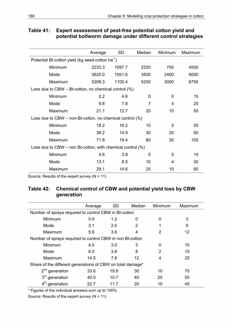
180 Chapter 8: Modeling crop protection strategies in cotton
Table 41: Expert assessment of pest-free potential cotton yield and potential bollworm damage under different control strategies
Average SD Median Minimum Maximum
Potential Bt-cotton yield (kg seed-cotton ha-1)
Minimum 2233.3 1097.7 2250 750 4500
Mode 3825.0 1051.6 3500 2400 6000
Maximum 5208.3 1100.4 5250 3000 6750
Loss due to CBW – Bt-cotton, no chemical control (%)
Minimum 2.2 4.6 0 0 15
Mode 9.8 7.8 7 4 25
Maximum 21.1 12.7 20 10 50
Loss due to CBW – non-Bt-cotton, no chemical control (%)
Minimum 18.2 16.2 15 0 50
Mode 38.2 14.9 30 20 60
Maximum 71.8 19.4 80 30 100
Loss due to CBW – non Bt-cotton, with chemical control (%)
Minimum 4.6 3.9 5 0 10
Mode 13.1 8.5 10 4 30
Maximum 29.1 14.6 25 10 60 Source: Results of the expert survey (N = 11) Table 42: Chemical control of CBW and potential yield loss by CBW
generation
Average SD Median Minimum Maximum Number of sprays required to control CBW in Bt-cotton
Minimum 0.9 1.2 0 0 3 Mode 3.1 2.0 2 1 6 Maximum 5.8 3.6 4 2 12
Number of sprays required to control CBW in non Bt-cotton Minimum 4.0 3.0 3 0 10 Mode 8.0 3.8 8 2 15 Maximum 14.5 7.6 12 4 25
Share of the different generations of CBW on total damage* 2nd generation 33.6 19.8 30 10 70 3rd generation 40.0 10.7 40 20 55 4th generation 22.7 11.7 20 10 45
* Figures of the individual answers sum up to 100%. Source: Results of the expert survey (N = 11)
Chapter 8: Modeling crop protection strategies in cotton 181
For the use of Bt-varieties without additional chemical control the experts anticipate a yield loss due to CBW of up to 21% for a situation of high pest pressure. For the baseline scenario without any control (planting a non-Bt-cotton variety and not applying insecticides) yield losses of 18 to 72% are expected, while the application of chemical insecticides, according to expert opinion, can reduce losses from CBW in non-Bt-cotton to less than 30% even in the worst case (see Table 41). Though application of chemical insecticides is one pest management option, all but one expert feel that resistance of pests against the active ingredients of major insecticides is a problem for the chemical control of cotton bollworm (and other pests). When asked about how many applications (number of sprays) of chemical insecticides are necessary to control the cotton bollworm, the respondents estimate a need of one to six sprays in Bt-cotton and two to 15 sprays in non-Bt-cotton, depending on the prevailing pest infestation (Table 42). According to their judgement, the 3rd generation of cotton bollworm is most damaging to the cotton crop and destroys on average 40% of the potential yield while the 2nd and 4th generation cause comparably less damage. The experts’ opinion on the severity of damage from other pests (aphids, spider mite and white fly) and the timing of the harm in relation to the damage from cotton bollworm is given in Table 43. According to the respondents, all three pests can cause considerable damage to the cotton crop.
The timing of the damage from different pests follows a distinct pattern based on the specific population dynamics and life cycles, with damage from aphids occurring rather early in the season and white fly damage late in the season. Three of the experts believe that the damage inflicted by different pests is correlated in a way such that high pest pressure for one pest occurs together with high infestation of the others, while six experts do not see such a correlation. In addition to the three main pests found in the farmer survey, eight experts stated that plant bugs are a significant problem in cotton production.
The perception of the effectiveness of late season sprays to reduce the overwintering bollworm population is ambiguous, with some respondents stating that there is the potential of reducing next season´s pest pressure while others see no effect or even suspect a disruption of beneficial insects and hence a negative effect of late season control. All experts agree that there is a danger of resistance build-up of CBW against the Bt-toxin.
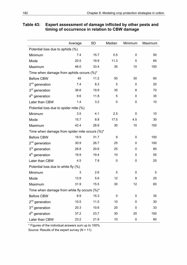
182 Chapter 8: Modeling crop protection strategies in cotton
Table 43: Expert assessment of damage inflicted by other pests and timing of occurrence in relation to CBW damage
Average SD Median Minimum Maximum
Potential loss due to aphids (%)
Minimum 7.4 15.7 0.5 0 50
Mode 20.5 19.9 11.3 5 65
Maximum 46.0 33.4 35 10 100
Time when damage from aphids occurs (%)*
Before CBW 45 11.2 50 30 60
2nd generation 7.4 8.3 5 0 20
3rd generation 36.6 19.9 35 8 70
4th generation 9.6 11.8 5 0 35
Later than CBW 1.4 3.2 0 0 10
Potential loss due to spider mite (%)
Minimum 3.5 4.1 2.5 0 10
Mode 15.7 8.8 17.5 4.5 30
Maximum 42.4 28.9 30 10 100
Time when damage from spider mite occurs (%)*
Before CBW 19.9 31.7 9 0 100
2nd generation 30.9 26.7 25 0 100
3rd generation 26.8 20.6 25 0 60
4th generation 16.9 19.4 10 0 55
Later than CBW 4.5 7.9 0 0 25
Potential loss due to white fly (%)
Minimum 3 2.6 5 0 5
Mode 13.9 5.6 12 8 25
Maximum 31.9 15.5 30 12 60
Time when damage from white fly occurs (%)*
Before CBW 8.9 15.3 0 0 35
2nd generation 10.5 11.5 10 0 30
3rd generation 20.3 10.6 20 0 33
4th generation 37.2 23.7 30 20 100
Later than CBW 23.2 21.9 10 0 60
* Figures of the individual answers sum up to 100%. Source: Results of the expert survey (N = 11)
Chapter 8: Modeling crop protection strategies in cotton 183
The expected time that it will take until the bollworm population shows such resistance varies from a minimum of two years to a maximum of 20 years. The average lies around eight years but most experts acknowledge that the pace of resistance development largely depends on the resistance management scheme that is followed, so that such estimates are very difficult.
For the socio-economic variables that enter the simulation model most of the information needed to make plausible assumptions is available from the farm-survey in the case study. Though only few experts participated, some of the replies from experts with an economic background are helpful complements or provide additional confirmation of the case study results. The response of the experts confirms the wide range of seed prices for Bt-varieties that were found in the farm-survey in Linqing County. According to the prices indicated by the respondents, Bt-seed that is not more expensive than non-Bt-cotton seed is available on local markets and there is generally a huge variation in the price for Bt-seed (Table 44). The experts estimated lower seed rates for high priced seed and a higher seed rate for farmers’ seed (due to an expected lower germination rate). All experts have noted that pesticide applications are conducted by family members and not by hired labor. The labor requirements for one application of pesticides increase as the cotton crop grows larger over the season. The experts all agree that the opportunity costs for family labor are highest in June, the harvesting time for wheat and planting time for maize, and lowest in July when few agricultural tasks are waiting to be done (Table 44). In terms of cotton output, three of the four experts say that there is no difference in the quality of lint and the sales price of Bt- and non-Bt-cotton produce. All experts perceive that there are human health costs associated with the exposure of persons to chemical insecticides but the valuation of this risk is different. While one expert estimates the minimum to be zero, the highest maximum value (US$24 per personday of exposure) lies far above the average maximum of US$9 that is given in Table 44. According to the opinion of the respondents, local credits are not in general easily available but they stated that there is no difference in the interest rate for such credits over the year and the interest rates stated are in the range of 4 – 10% per year. All experts agree that planting of Bt-varieties will not be regulated in the sense that only a certain share of the area can be used for Bt-varieties and a non-Bt-cotton refuge will become mandatory as a measure of resistance management.
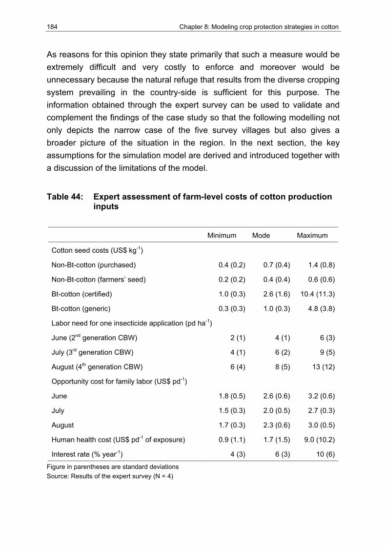
184 Chapter 8: Modeling crop protection strategies in cotton
As reasons for this opinion they state primarily that such a measure would be extremely difficult and very costly to enforce and moreover would be unnecessary because the natural refuge that results from the diverse cropping system prevailing in the country-side is sufficient for this purpose. The information obtained through the expert survey can be used to validate and complement the findings of the case study so that the following modelling not only depicts the narrow case of the five survey villages but also gives a broader picture of the situation in the region. In the next section, the key assumptions for the simulation model are derived and introduced together with a discussion of the limitations of the model.
Table 44: Expert assessment of farm-level costs of cotton production inputs
Minimum Mode Maximum
Cotton seed costs (US$ kg-1)
Non-Bt-cotton (purchased) 0.4 (0.2) 0.7 (0.4) 1.4 (0.8)
Non-Bt-cotton (farmers’ seed) 0.2 (0.2) 0.4 (0.4) 0.6 (0.6)
Bt-cotton (certified) 1.0 (0.3) 2.6 (1.6) 10.4 (11.3)
Bt-cotton (generic) 0.3 (0.3) 1.0 (0.3) 4.8 (3.8)
Labor need for one insecticide application (pd ha-1)
June (2nd generation CBW) 2 (1) 4 (1) 6 (3)
July (3rd generation CBW) 4 (1) 6 (2) 9 (5)
August (4th generation CBW) 6 (4) 8 (5) 13 (12)
Opportunity cost for family labor (US$ pd-1)
June 1.8 (0.5) 2.6 (0.6) 3.2 (0.6)
July 1.5 (0.3) 2.0 (0.5) 2.7 (0.3)
August 1.7 (0.3) 2.3 (0.6) 3.0 (0.5)
Human health cost (US$ pd-1 of exposure) 0.9 (1.1) 1.7 (1.5) 9.0 (10.2)
Interest rate (% year-1) 4 (3) 6 (3) 10 (6)
Figure in parentheses are standard deviations Source: Results of the expert survey (N = 4)
Chapter 8: Modeling crop protection strategies in cotton 185
8.1.3 Model assumptions and limitations
Running the stochastic budgeting model outlined above requires a set of assumptions. First, a definition of CBW control strategies to be compared with the simulation model is needed. A set of further general assumptions for the model is formulated (see Box 7) and the probability distributions for the input variables are defined based on the results of the expert survey and the production monitoring data (Table 46).
In the case of Shandong Province in China, the counterfactual strategy for the use of Bt-cotton varieties is the application of chemical insecticides to control the cotton bollworm. Based on the findings of the farm-survey (see Chapter 6), two different options for Bt-cotton seed are assumed. The analysis of the price and toxin information of Bt-cotton revealed that cross-breeding of local varieties with Bt-varieties, the sale of second generation Bt-seed or in general product adulteration (all these can be considered low quality seed) can lead to lower toxin concentration and hence lower effectiveness of CBW control and/or a higher probability of failure to control the pest. At the same time, a control strategy using Bt-seed of lower quality is cheaper. According to the results of the farm-level survey a large proportion of the farmers in the study area use such low quality and low priced seed. Hence, a low-quality Bt-cotton strategy is included in the simulation model and compared to the strategy of buying more expensive seed.
In addition to the choice of seed (high and low quality Bt-seed or non-Bt variety) different levels of insecticides can be applied as part of the control strategy. Sprays can be applied either calendar-based or need-based (in the latter case, insecticides are only used in Bt-cotton when pest pressure is extreme or the Bt-trait fails to protect the crop). One frequently used decision model for the question whether or not to apply pesticides is the economic threshold. The economic threshold concept uses the pest density or the potential crop loss to decide on the use of a pesticide or other control measures (Carlson and Wetzstein, 1993). The economic threshold is defined as the “minimum pest density that must be present before the marginal value of the crop saved will equal the marginal cost of treatment” (ibid). Antle (1988) defines the economic threshold as “the level of pest population at which the private benefits of pesticide use outweigh the costs”.
186 Chapter 8: Modeling crop protection strategies in cotton
The damage from a certain level of pest infestation, the value of the crop saved and treatment costs or expected values thereof are required to assess this threshold. The threshold problem can be further divided into the optimal time to treat and the type/dosage of treatment to take (Hall and Norgaard, 1973).
In the model, insecticide use according to the economic threshold concept is labeled as integrated pest management (IPM). The cost of the insecticide strategy is the sum of costs for insecticides, the opportunity costs of family labor used for spraying, and related human health costs. Cost for the Bt-strategies is the price premium for the Bt-seed. The decision to apply insecticides is made separately for the different generations of cotton bollworm but the decision to plant a Bt-variety applies for the whole season. Additional general assumptions for the modeling process are listed in Box 7.
For most stochastic input variables an underlying triangular probability distribution is assumed because such distributions can easily be described by key values (minimum, mode or most likely, maximum). These key values are relatively easy to obtain from the expert assessment. For the calculation of the future value of control costs, a discount rate of 0.5% per month (equivalent to about 6% per year) is used. For costs of the impairment of human health due to exposure to chemical insecticides while spraying, the conservative assumption of such costs equaling the value of insecticides applied is made following the results of Pingali et al. (1994), and Rola and Pingali (1993). If more than one application of insecticides is used or the control strategy includes a combination of Bt-control and chemical insecticides, the control effectiveness of the separate measures is added multiplicatively. Following the specification in (8-1) the potential pest damage is multiplied with a second term (1 - control effectiveness). For example, two insecticide applications each with 40% control effectiveness together reduce the pest damage by 64% (2 * E - E2). Such a decreasing marginal return on insecticide use fits in with actual field observations and production economic principles. A 10% higher yield is assumed for non-Bt-cotton since experts stated that Bt-varieties require higher input levels of fertilizer, have lower potential yield and worse lint quality with a higher ratio of seed to lint.
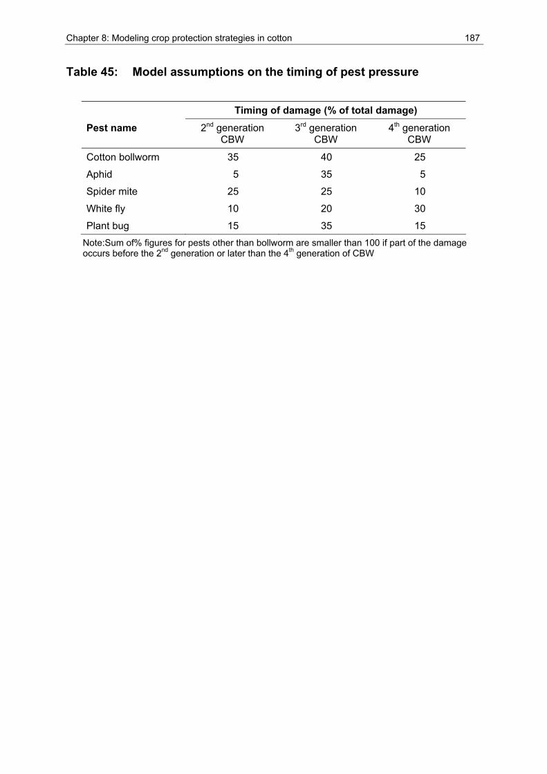
Chapter 8: Modeling crop protection strategies in cotton 187
Table 45: Model assumptions on the timing of pest pressure
Timing of damage (% of total damage)
Pest name 2nd generation CBW
3rd generation CBW
4th generation CBW
Cotton bollworm 35 40 25
Aphid 5 35 5
Spider mite 25 25 10
White fly 10 20 30
Plant bug 15 35 15 Note:Sum of% figures for pests other than bollworm are smaller than 100 if part of the damage occurs before the 2nd generation or later than the 4th generation of CBW
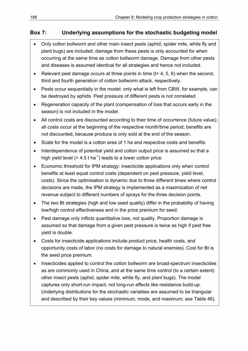
188 Chapter 8: Modeling crop protection strategies in cotton
Box 7: Underlying assumptions for the stochastic budgeting model
• Only cotton bollworm and other main insect pests (aphid, spider mite, white fly and plant bugs) are included; damage from these pests is only accounted for when occurring at the same time as cotton bollworm damage. Damage from other pests and diseases is assumed identical for all strategies and hence not included.
• Relevant pest damage occurs at three points in time (t= 4, 5, 6) when the second, third and fourth generation of cotton bollworm attack, respectively.
• Pests occur sequentially in the model: only what is left from CBW, for example, can be destroyed by aphids. Pest pressure of different pests is not correlated.
• Regeneration capacity of the plant (compensation of loss that occurs early in the season) is not included in the model.
• All control costs are discounted according to their time of occurrence (future value); all costs occur at the beginning of the respective month/time period; benefits are not discounted, because produce is only sold at the end of the season.
• Scale for the model is a cotton area of 1 ha and respective costs and benefits
• Interdependence of potential yield and cotton output price is assumed so that a high yield level (> 4.5 t ha-1) leads to a lower cotton price.
• Economic threshold for IPM strategy: insecticide applications only when control benefits at least equal control costs (dependent on pest pressure, yield level, costs). Since the optimisation is dynamic due to three different times where control decisions are made, the IPM strategy is implemented as a maximization of net revenue subject to different numbers of sprays for the three decision points.
• The two Bt strategies (high and low seed quality) differ in the probability of having low/high control effectiveness and in the price premium for seed.
• Pest damage only inflicts quantitative loss, not quality. Proportion damage is assumed so that damage from a given pest pressure is twice as high if pest free yield is double.
• Costs for insecticide applications include product price, health costs, and opportunity costs of labor (no costs for damage to natural enemies). Cost for Bt is the seed price premium.
• Insecticides applied to control the cotton bollworm are broad-spectrum insecticides as are commonly used in China, and at the same time control (to a certain extent) other insect pests (aphid, spider mite, white fly, and plant bugs). The model captures only short-run impact, not long-run effects like resistance build-up. Underlying distributions for the stochastic variables are assumed to be triangular and described by their key values (minimum, mode, and maximum; see Table 46).
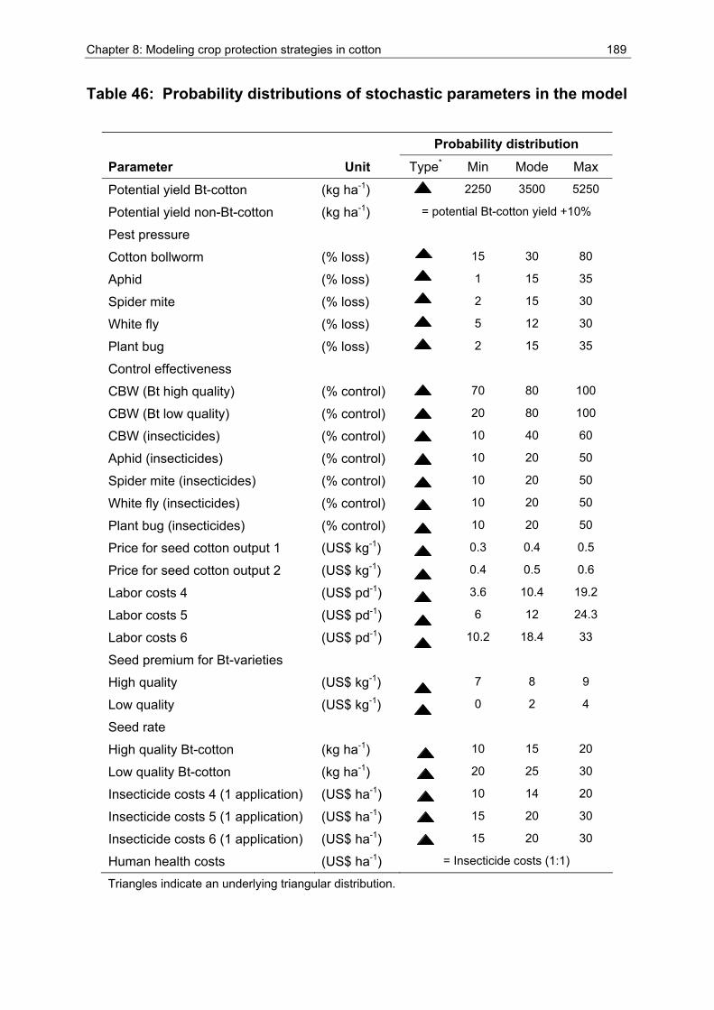
Chapter 8: Modeling crop protection strategies in cotton 189
Table 46: Probability distributions of stochastic parameters in the model
Probability distribution
Parameter Unit Type* Min Mode Max
Potential yield Bt-cotton (kg ha-1) 2250 3500 5250
Potential yield non-Bt-cotton (kg ha-1) = potential Bt-cotton yield +10%
Pest pressure
Cotton bollworm (% loss) 15 30 80
Aphid (% loss) 1 15 35
Spider mite (% loss) 2 15 30
White fly (% loss) 5 12 30
Plant bug (% loss) 2 15 35
Control effectiveness
CBW (Bt high quality) (% control) 70 80 100
CBW (Bt low quality) (% control) 20 80 100
CBW (insecticides) (% control) 10 40 60
Aphid (insecticides) (% control) 10 20 50
Spider mite (insecticides) (% control) 10 20 50
White fly (insecticides) (% control) 10 20 50
Plant bug (insecticides) (% control) 10 20 50
Price for seed cotton output 1 (US$ kg-1) 0.3 0.4 0.5
Price for seed cotton output 2 (US$ kg-1) 0.4 0.5 0.6
Labor costs 4 (US$ pd-1) 3.6 10.4 19.2
Labor costs 5 (US$ pd-1) 6 12 24.3
Labor costs 6 (US$ pd-1) 10.2 18.4 33
Seed premium for Bt-varieties
High quality (US$ kg-1) 7 8 9
Low quality (US$ kg-1) 0 2 4
Seed rate
High quality Bt-cotton (kg ha-1) 10 15 20
Low quality Bt-cotton (kg ha-1) 20 25 30
Insecticide costs 4 (1 application) (US$ ha-1) 10 14 20
Insecticide costs 5 (1 application) (US$ ha-1) 15 20 30
Insecticide costs 6 (1 application) (US$ ha-1) 15 20 30
Human health costs (US$ ha-1) = Insecticide costs (1:1)
Triangles indicate an underlying triangular distribution.
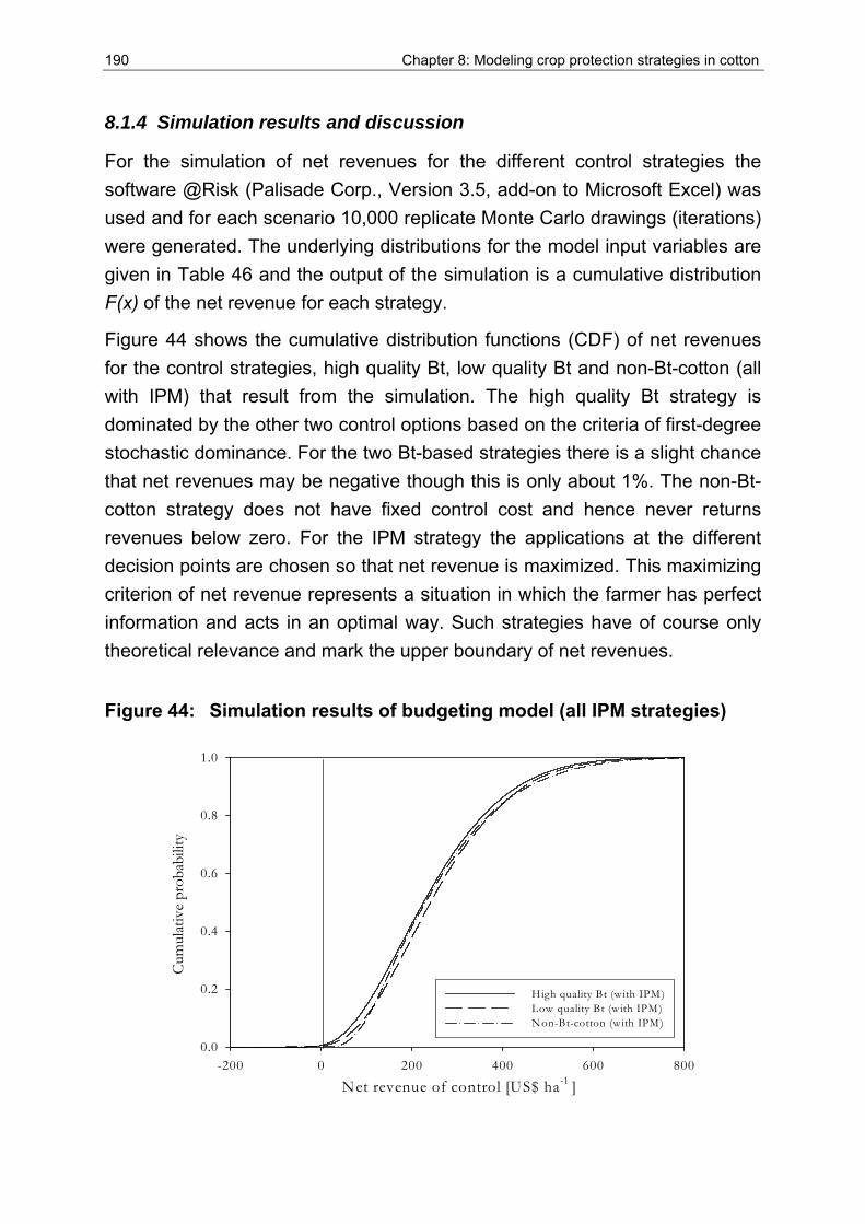
190 Chapter 8: Modeling crop protection strategies in cotton
8.1.4 Simulation results and discussion
For the simulation of net revenues for the different control strategies the software @Risk (Palisade Corp., Version 3.5, add-on to Microsoft Excel) was used and for each scenario 10,000 replicate Monte Carlo drawings (iterations) were generated. The underlying distributions for the model input variables are given in Table 46 and the output of the simulation is a cumulative distribution F(x) of the net revenue for each strategy.
Figure 44 shows the cumulative distribution functions (CDF) of net revenues for the control strategies, high quality Bt, low quality Bt and non-Bt-cotton (all with IPM) that result from the simulation. The high quality Bt strategy is dominated by the other two control options based on the criteria of first-degree stochastic dominance. For the two Bt-based strategies there is a slight chance that net revenues may be negative though this is only about 1%. The non-Bt-cotton strategy does not have fixed control cost and hence never returns revenues below zero. For the IPM strategy the applications at the different decision points are chosen so that net revenue is maximized. This maximizing criterion of net revenue represents a situation in which the farmer has perfect information and acts in an optimal way. Such strategies have of course only theoretical relevance and mark the upper boundary of net revenues.
Figure 44: Simulation results of budgeting model (all IPM strategies)
Net revenue of control [US$ ha-1 ]-200 0 200 400 600 800
Cum
ulat
ive
prob
abili
ty
0.0
0.2
0.4
0.6
0.8
1.0
High quality Bt (with IPM)Low quality Bt (with IPM)Non-Bt-cotton (with IPM)
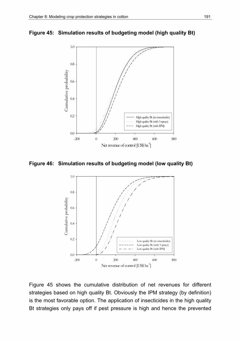
Chapter 8: Modeling crop protection strategies in cotton 191
Figure 45: Simulation results of budgeting model (high quality Bt)
Net revenue of control [US$ ha-1]-200 0 200 400 600 800
Cum
ulat
ive
prob
abili
ty
0.0
0.2
0.4
0.6
0.8
1.0
High quality Bt (no insecticides)High quality Bt (with 3 sprays)High quality Bt (with IPM)
Figure 46: Simulation results of budgeting model (low quality Bt)
Net revenue of control [US$ ha-1]-200 0 200 400 600 800
Cum
ulat
ive
prob
abili
ty
0.0
0.2
0.4
0.6
0.8
1.0
Low quality Bt (no insecticides)Low quality Bt (with 3 sprays)Low quality Bt (with IPM)
Figure 45 shows the cumulative distribution of net revenues for different strategies based on high quality Bt. Obviously the IPM strategy (by definition) is the most favorable option. The application of insecticides in the high quality Bt strategies only pays off if pest pressure is high and hence the prevented
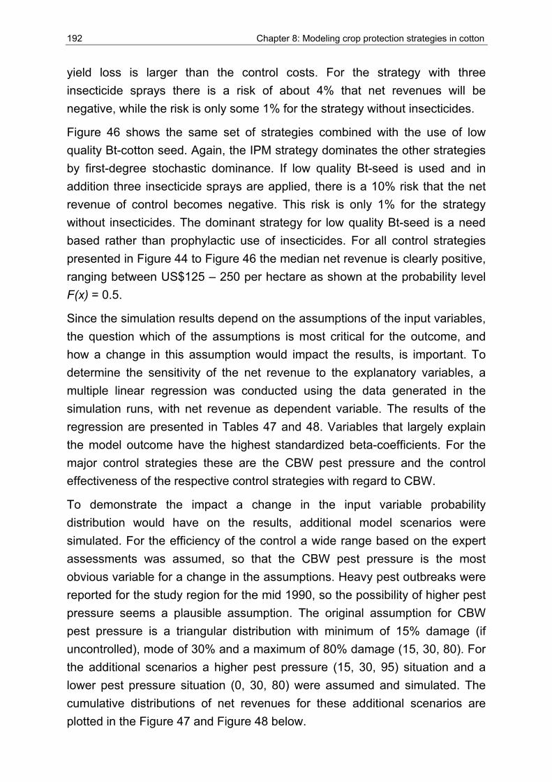
192 Chapter 8: Modeling crop protection strategies in cotton
yield loss is larger than the control costs. For the strategy with three insecticide sprays there is a risk of about 4% that net revenues will be negative, while the risk is only some 1% for the strategy without insecticides.
Figure 46 shows the same set of strategies combined with the use of low quality Bt-cotton seed. Again, the IPM strategy dominates the other strategies by first-degree stochastic dominance. If low quality Bt-seed is used and in addition three insecticide sprays are applied, there is a 10% risk that the net revenue of control becomes negative. This risk is only 1% for the strategy without insecticides. The dominant strategy for low quality Bt-seed is a need based rather than prophylactic use of insecticides. For all control strategies presented in Figure 44 to Figure 46 the median net revenue is clearly positive, ranging between US$125 – 250 per hectare as shown at the probability level F(x) = 0.5.
Since the simulation results depend on the assumptions of the input variables, the question which of the assumptions is most critical for the outcome, and how a change in this assumption would impact the results, is important. To determine the sensitivity of the net revenue to the explanatory variables, a multiple linear regression was conducted using the data generated in the simulation runs, with net revenue as dependent variable. The results of the regression are presented in Tables 47 and 48. Variables that largely explain the model outcome have the highest standardized beta-coefficients. For the major control strategies these are the CBW pest pressure and the control effectiveness of the respective control strategies with regard to CBW.
To demonstrate the impact a change in the input variable probability distribution would have on the results, additional model scenarios were simulated. For the efficiency of the control a wide range based on the expert assessments was assumed, so that the CBW pest pressure is the most obvious variable for a change in the assumptions. Heavy pest outbreaks were reported for the study region for the mid 1990, so the possibility of higher pest pressure seems a plausible assumption. The original assumption for CBW pest pressure is a triangular distribution with minimum of 15% damage (if uncontrolled), mode of 30% and a maximum of 80% damage (15, 30, 80). For the additional scenarios a higher pest pressure (15, 30, 95) situation and a lower pest pressure situation (0, 30, 80) were assumed and simulated. The cumulative distributions of net revenues for these additional scenarios are plotted in the Figure 47 and Figure 48 below.
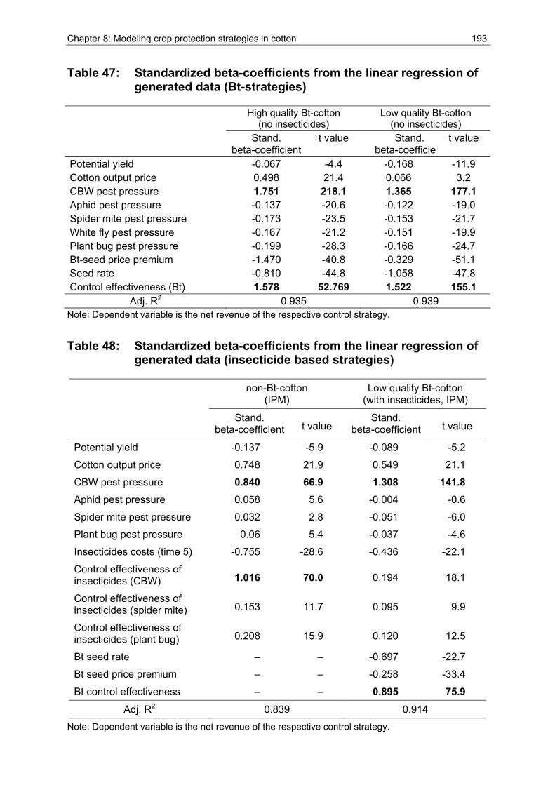
Chapter 8: Modeling crop protection strategies in cotton 193
Table 47: Standardized beta-coefficients from the linear regression of generated data (Bt-strategies)
High quality Bt-cotton (no insecticides)
Low quality Bt-cotton (no insecticides)
Stand. beta-coefficient
t value Stand. beta-coefficie
t value
Potential yield -0.067 -4.4 -0.168 -11.9 Cotton output price 0.498 21.4 0.066 3.2 CBW pest pressure 1.751 218.1 1.365 177.1 Aphid pest pressure -0.137 -20.6 -0.122 -19.0 Spider mite pest pressure -0.173 -23.5 -0.153 -21.7 White fly pest pressure -0.167 -21.2 -0.151 -19.9 Plant bug pest pressure -0.199 -28.3 -0.166 -24.7 Bt-seed price premium -1.470 -40.8 -0.329 -51.1 Seed rate -0.810 -44.8 -1.058 -47.8 Control effectiveness (Bt) 1.578 52.769 1.522 155.1
Adj. R2 0.935 0.939 Note: Dependent variable is the net revenue of the respective control strategy.
Table 48: Standardized beta-coefficients from the linear regression of generated data (insecticide based strategies)
non-Bt-cotton (IPM)
Low quality Bt-cotton (with insecticides, IPM)
Stand. beta-coefficient t value
Stand. beta-coefficient t value
Potential yield -0.137 -5.9 -0.089 -5.2
Cotton output price 0.748 21.9 0.549 21.1
CBW pest pressure 0.840 66.9 1.308 141.8 Aphid pest pressure 0.058 5.6 -0.004 -0.6
Spider mite pest pressure 0.032 2.8 -0.051 -6.0
Plant bug pest pressure 0.06 5.4 -0.037 -4.6
Insecticides costs (time 5) -0.755 -28.6 -0.436 -22.1
Control effectiveness of insecticides (CBW) 1.016 70.0 0.194 18.1
Control effectiveness of insecticides (spider mite) 0.153 11.7 0.095 9.9
Control effectiveness of insecticides (plant bug) 0.208 15.9 0.120 12.5
Bt seed rate – – -0.697 -22.7
Bt seed price premium – – -0.258 -33.4
Bt control effectiveness – – 0.895 75.9 Adj. R2 0.839 0.914
Note: Dependent variable is the net revenue of the respective control strategy.
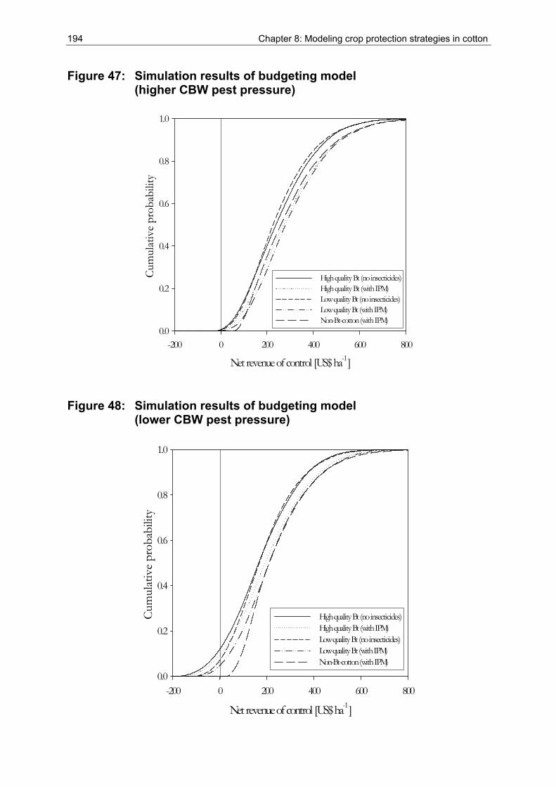
194 Chapter 8: Modeling crop protection strategies in cotton
Figure 47: Simulation results of budgeting model (higher CBW pest pressure)
Net revenue of control [US$ ha-1 ]-200 0 200 400 600 800
Cum
ulat
ive
prob
abili
ty
0.0
0.2
0.4
0.6
0.8
1.0
High quality Bt (no insecticides)High quality Bt (with IPM)Low quality Bt (no insecticides)Low quality Bt (with IPM)Non-Bt-cotton (with IPM)
Figure 48: Simulation results of budgeting model (lower CBW pest pressure)
Net revenue of control [US$ ha-1 ]-200 0 200 400 600 800
Cum
ulat
ive
prob
abili
ty
0.0
0.2
0.4
0.6
0.8
1.0
High quality Bt (no insecticides)High quality Bt (with IPM)Low quality Bt (no insecticides)Low quality Bt (with IPM)Non-Bt-cotton (with IPM)
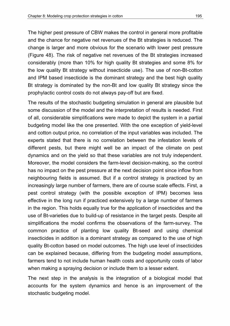
Chapter 8: Modeling crop protection strategies in cotton 195
The higher pest pressure of CBW makes the control in general more profitable and the chance for negative net revenues of the Bt strategies is reduced. The change is larger and more obvious for the scenario with lower pest pressure (Figure 48). The risk of negative net revenues of the Bt strategies increased considerably (more than 10% for high quality Bt strategies and some 8% for the low quality Bt strategy without insecticide use). The use of non-Bt-cotton and IPM based insecticide is the dominant strategy and the best high quality Bt strategy is dominated by the non-Bt and low quality Bt strategy since the prophylactic control costs do not always pay-off but are fixed.
The results of the stochastic budgeting simulation in general are plausible but some discussion of the model and the interpretation of results is needed. First of all, considerable simplifications were made to depict the system in a partial budgeting model like the one presented. With the one exception of yield-level and cotton output price, no correlation of the input variables was included. The experts stated that there is no correlation between the infestation levels of different pests, but there might well be an impact of the climate on pest dynamics and on the yield so that these variables are not truly independent. Moreover, the model considers the farm-level decision-making, so the control has no impact on the pest pressure at the next decision point since inflow from neighbouring fields is assumed. But if a control strategy is practiced by an increasingly large number of farmers, there are of course scale effects. First, a pest control strategy (with the possible exception of IPM) becomes less effective in the long run if practiced extensively by a large number of farmers in the region. This holds equally true for the application of insecticides and the use of Bt-varieties due to build-up of resistance in the target pests. Despite all simplifications the model confirms the observations of the farm-survey. The common practice of planting low quality Bt-seed and using chemical insecticides in addition is a dominant strategy as compared to the use of high quality Bt-cotton based on model outcomes. The high use level of insecticides can be explained because, differing from the budgeting model assumptions, farmers tend to not include human health costs and opportunity costs of labor when making a spraying decision or include them to a lesser extent.
The next step in the analysis is the integration of a biological model that accounts for the system dynamics and hence is an improvement of the stochastic budgeting model.
196 Chapter 8: Modeling crop protection strategies in cotton
8.2 Bio-economic model
The simulation of the net revenues of different cotton bollworm control strategies in the previous section shows the impact of uncertainty on the effects and benefits of the control. However, the assumptions regarding the pest pressure and resulting yield levels rely solely on the expert assessment without considering any of the underlying system processes. To incorporate these aspects of crop protection strategies, a physiologically based age-mass structured model of cotton and major pests and natural enemies was combined with the economic part of the model. The biological model part simulates the dynamics of the agro-ecosystem and the impact of interventions on system components, especially natural enemy populations. This biological model was adapted for the study location in North China based on the findings of the cotton growth experiment and additional climatic information, and simulates the cotton yield for the different control strategies. Accepting the black box character of the biological model that is not described here in detail, resulting yield outcomes can be used as input for an adapted version of the partial budgeting model presented in the previous section.
8.2.1 Methodology for the bio-economic model
The bio-economic model (see Figure 49 for the model structure) consists of two distinct parts. (1) A biological-ecosystem model that simulates the mass dynamics of the cotton plant, as well as pest and natural enemy populations and related interactions. Different control interventions can be implemented in this model and the simulated output is the resulting cotton yield for the respective control strategies. (2) The economic part of the model is an adapted version of the partial budgeting model presented in the previous section, using the yield figures generated by the biological-ecosystem model as well as the control costs and the cotton price as inputs to assess the benefits of the different control strategies.
The biological-ecosystem model was originally developed for the conditions of cotton production in California, USA (Gutierrez et al., 1975) but subsequently adapted to other locations for example tropical Brazil (Gutierrez et al., 1991a; Gutierrez et al., 1991b). The latest version of this biological-ecosystem model (Ponsard et al., 2002; Gutierrez et al., 2005; Gutierrez and Ponsard, 2005)
Chapter 8: Modeling crop protection strategies in cotton 197
was calibrated to match the conditions of the study location in North China75. For the adaptation of the model to the local conditions, a cotton-growth experiment was conducted at the study site during the 2002 cotton season (see Box 8). The data collected in this experiment and additional climatic information were the basis for the adaptation process of the biological model.
Box 8: Findings of the cotton growth experiment, Linqing County, 2002
The cotton growth experiment was carried out to collect data for calibrating and
adapting the existing cotton-ecosystem-model, which quantifies the influence of biotic
and abiotic factors that determine the cotton yield. Appendix 15 shows the design of
the cotton growth experiment that was located close to the study villages. The plant
mapping and boll counts were analyzed and used for the calibration of the model
described in section 8.2.
Information on plant dry weight obtained in the experiment is presented in Appendix 18
and Appendix 19. The scaling of development based on day degrees (DD) corrects for
the later sowing of the non-Bt-cotton plots. The lower yields and the delayed fruiting in
the non-Bt-cotton plots are due to damage from CBW.
The adapted cotton-ecosystem-model simulates the dry matter developments for Bt
and non-Bt cotton (see Appendix 20). The simulation is congruent with the measured
dry weights that were obtained in the experiment. The curves are smooth, since values
were generated on a day-to-day basis instead of the weekly measurement intervals of
the experiment. Moreover, the experiment measured different plants (destructively) so
that some variation exists between the characteristics of individual plants while the
model simulates continuous dry matter.
The adapted model is then used to simulate the resulting cotton yield output if different
CBW control strategies were implemented. A problem with this kind of experiment is
that the surrounding ecosystem is distorted due to pesticide application in such a way
that pest pressure is high and few natural enemies exist. A small no-spray plot located
in the middle of heavily sprayed fields is hence not adequately representing the
situation without sprays since a huge inflow of pest individuals from neighboring plots
can be expected, and the non-sprayed area is too small for a stable population of
natural enemies. For an ideal experiment a large unsprayed area would be set up and
sample plots located in the middle of this undisturbed environment.
75 This part of the analysis was only possible because of the generous collaboration and the efforts of Prof. A. Gutierrez (University of California at Berkeley) and his team.
198 Chapter 8: Modeling crop protection strategies in cotton
After successful adaptation the biological-ecosystem model gives a good reproduction of the empirical results of the experiment (Appendix 20).
The ecological model simulates the mass (and number) dynamics of the cotton plant, pests and natural enemies. The model is founded on the physiologically-based metabolic pool model approach. For the simulation of plant growth, daily photosynthetic rates (production of dry matter in grams) are computed and depend on the weather conditions (light, temperature, soil water status, nitrogen levels) and the plant states (among others leaf area and leaf age, and plant density). The photosynthate is allocated to the different plant subunits in priority order of respiration: fruit if present, then vegetative growth in the order leaf, stem, root and reserves (Gutierrez et al., 1991b). The population dynamics of the cotton bollworm are also physiologically based and also determined by the weather conditions and the developmental stage of the pest. The biological model integrates the effects of weather and soil factors on the plant and hence on pests, and the effects of natural enemies on pests and of pests on the plant. The determinants of the yield are hence the climatic conditions, the degree of ecological disturbance of the system, the amount of chemical insecticides used and the (quality of the) Bt-toxin.
Different strategies to control the cotton bollworm (Bt-variety and/or insecticides) are then implemented in the adapted model (see next section for details of the strategies). For each strategy 20 simulation runs with stochastic climatic conditions are conducted. These runs represent 20 consecutive years in which only the genotypes of the larvae enter the next year, and year-to-year survival and build-up of pest pressure or resistance is not allowed for. Insecticide applications act directly and have a negative impact on natural enemies that disturbs the system and leads to pest resurgence and secondary pest outbreaks. Bt-toxin acts indirectly by affecting natural enemy efficacy when they feed on Bt-intoxicated prey (Ponsard et al., 2002). The difference in the outcome results from the changes in the climatic data that enters the model as random divergence of up to ± 10% from the climatic conditions recorded in the survey year. These climate variations cause differences in plant growth and pest and natural enemy population dynamics. For the simulation it is assumed that all agronomic factors (such as fertilizer and irrigation) are constant and none limiting. The resulting yield output figures for each of the control strategies are used to derive a distribution of yield outcomes for the respective strategy.
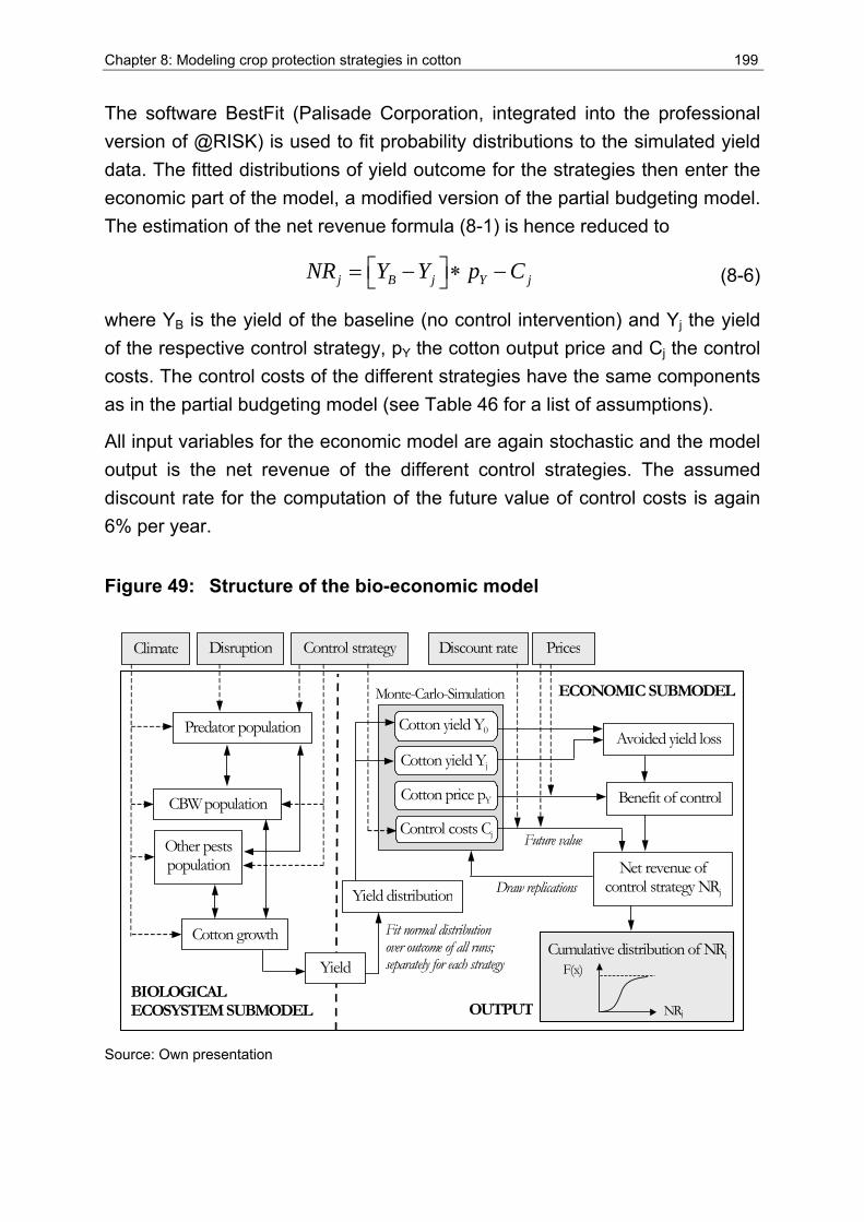
Chapter 8: Modeling crop protection strategies in cotton 199
The software BestFit (Palisade Corporation, integrated into the professional version of @RISK) is used to fit probability distributions to the simulated yield data. The fitted distributions of yield outcome for the strategies then enter the economic part of the model, a modified version of the partial budgeting model. The estimation of the net revenue formula (8-1) is hence reduced to
j B j Y jNR Y Y p C⎡ ⎤= − ∗ −⎣ ⎦ (8-6)
where YB is the yield of the baseline (no control intervention) and Yj the yield of the respective control strategy, pY the cotton output price and Cj the control costs. The control costs of the different strategies have the same components as in the partial budgeting model (see Table 46 for a list of assumptions).
All input variables for the economic model are again stochastic and the model output is the net revenue of the different control strategies. The assumed discount rate for the computation of the future value of control costs is again 6% per year.
Figure 49: Structure of the bio-economic model
Avoided yield loss
Net revenue of control strategy NRj
Cumulative distribution of NRj
Monte-Carlo-Simulation
F(x)
NRj
Draw replications
Benefit of control
Future value
Cotton yield Y0
Cotton yield Yj
Cotton price pY
Control costs Cj
Cotton growth
CBW population
Other pests population
Predator population
Control strategyClimate Disruption Discount rate Prices
BIOLOGICAL ECOSYSTEM SUBMODEL
ECONOMIC SUBMODEL
Yield
Fit normal distribution over outcome of all runs; separately for each strategy
Yield distribution
OUTPUT
Source: Own presentation
200 Chapter 8: Modeling crop protection strategies in cotton
Human health costs equivalent to the costs of insecticide products are included in the control costs. The structure of the adjusted partial budgeting model is depicted in Figure 49. The overall rationale and simulation procedure is analogous to the partial budgeting model outlined in section 8.1.1.
The impact of the control interventions that was previously part of the stochastic budgeting model is now implemented and takes place within the biological model. The advantage of this procedure is that the outcome of the biological model accounts for the system dynamics and not only impact on the target pest and secondary pests, but includes the effect on natural enemies and all interactions between plants and insect populations.
8.2.2 Description of control strategies
The control strategies that are included in the biological model are a combination of the seed choice and an insecticide treatment level. For the choice of seed the farmer in general has three options: purchase high quality Bt-seed, opt for low quality Bt-seed or choose a non-Bt cotton variety. The special case of on-farm propagation of seed in general falls into one of the three categories above though probably the farmer can be even less sure about the quality of the seed compared to purchased seed if using a Bt-variety. Following the findings from the case study, where a testing of the leaf toxin concentration revealed that lower priced seeds bear a higher chance of low control effectiveness, the seed choice has an impact on the resulting control of the Bt-variety. At the same time the lower quality seed can be obtained for a considerably lower price. The condition that lower quality seed has a higher chance of poor control of the cotton bollworm was modeled via the variable Bt-susceptibility in the biological model. For the high quality seed the scalar is assumed to be 0.95 while this figure is only 0.75 for the low quality Bt-seed. At the same time, a higher seed rate is assumed if farmers use lower quality Bt-seed or non-Bt-seed because the germination rate is lower and farmers use more seed to avoid missing plants in the field (see Table 46).
The three different choices for cotton seed are combined with one of the three different intensities of chemical control of the cotton bollworm. Based on the survey findings, a level of six insecticide applications against the cotton bollworm is common practice in the study area (= farmers’ practices). The sprays are implemented on a calendar basis from mid June to the end of
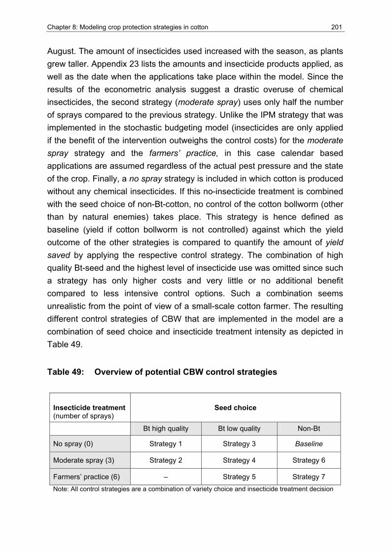
Chapter 8: Modeling crop protection strategies in cotton 201
August. The amount of insecticides used increased with the season, as plants grew taller. Appendix 23 lists the amounts and insecticide products applied, as well as the date when the applications take place within the model. Since the results of the econometric analysis suggest a drastic overuse of chemical insecticides, the second strategy (moderate spray) uses only half the number of sprays compared to the previous strategy. Unlike the IPM strategy that was implemented in the stochastic budgeting model (insecticides are only applied if the benefit of the intervention outweighs the control costs) for the moderate spray strategy and the farmers’ practice, in this case calendar based applications are assumed regardless of the actual pest pressure and the state of the crop. Finally, a no spray strategy is included in which cotton is produced without any chemical insecticides. If this no-insecticide treatment is combined with the seed choice of non-Bt-cotton, no control of the cotton bollworm (other than by natural enemies) takes place. This strategy is hence defined as baseline (yield if cotton bollworm is not controlled) against which the yield outcome of the other strategies is compared to quantify the amount of yield saved by applying the respective control strategy. The combination of high quality Bt-seed and the highest level of insecticide use was omitted since such a strategy has only higher costs and very little or no additional benefit compared to less intensive control options. Such a combination seems unrealistic from the point of view of a small-scale cotton farmer. The resulting different control strategies of CBW that are implemented in the model are a combination of seed choice and insecticide treatment intensity as depicted in Table 49.
Table 49: Overview of potential CBW control strategies
Insecticide treatment (number of sprays)
Seed choice
Bt high quality Bt low quality Non-Bt
No spray (0) Strategy 1 Strategy 3 Baseline
Moderate spray (3) Strategy 2 Strategy 4 Strategy 6
Farmers’ practice (6) – Strategy 5 Strategy 7 Note: All control strategies are a combination of variety choice and insecticide treatment decision
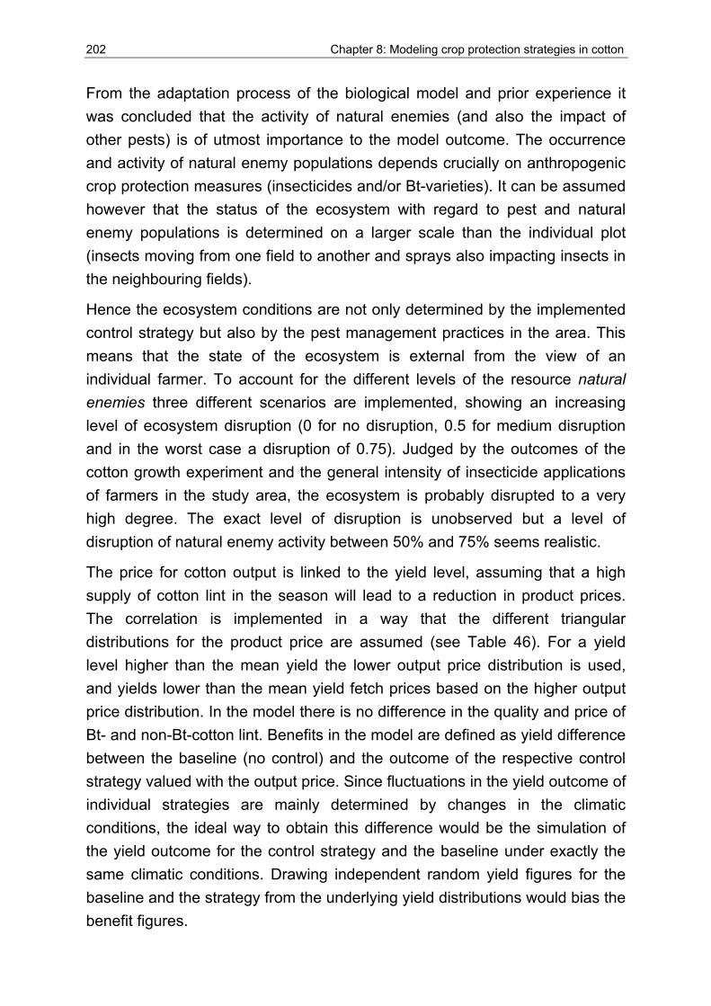
202 Chapter 8: Modeling crop protection strategies in cotton
From the adaptation process of the biological model and prior experience it was concluded that the activity of natural enemies (and also the impact of other pests) is of utmost importance to the model outcome. The occurrence and activity of natural enemy populations depends crucially on anthropogenic crop protection measures (insecticides and/or Bt-varieties). It can be assumed however that the status of the ecosystem with regard to pest and natural enemy populations is determined on a larger scale than the individual plot (insects moving from one field to another and sprays also impacting insects in the neighbouring fields).
Hence the ecosystem conditions are not only determined by the implemented control strategy but also by the pest management practices in the area. This means that the state of the ecosystem is external from the view of an individual farmer. To account for the different levels of the resource natural enemies three different scenarios are implemented, showing an increasing level of ecosystem disruption (0 for no disruption, 0.5 for medium disruption and in the worst case a disruption of 0.75). Judged by the outcomes of the cotton growth experiment and the general intensity of insecticide applications of farmers in the study area, the ecosystem is probably disrupted to a very high degree. The exact level of disruption is unobserved but a level of disruption of natural enemy activity between 50% and 75% seems realistic.
The price for cotton output is linked to the yield level, assuming that a high supply of cotton lint in the season will lead to a reduction in product prices. The correlation is implemented in a way that the different triangular distributions for the product price are assumed (see Table 46). For a yield level higher than the mean yield the lower output price distribution is used, and yields lower than the mean yield fetch prices based on the higher output price distribution. In the model there is no difference in the quality and price of Bt- and non-Bt-cotton lint. Benefits in the model are defined as yield difference between the baseline (no control) and the outcome of the respective control strategy valued with the output price. Since fluctuations in the yield outcome of individual strategies are mainly determined by changes in the climatic conditions, the ideal way to obtain this difference would be the simulation of the yield outcome for the control strategy and the baseline under exactly the same climatic conditions. Drawing independent random yield figures for the baseline and the strategy from the underlying yield distributions would bias the benefit figures.
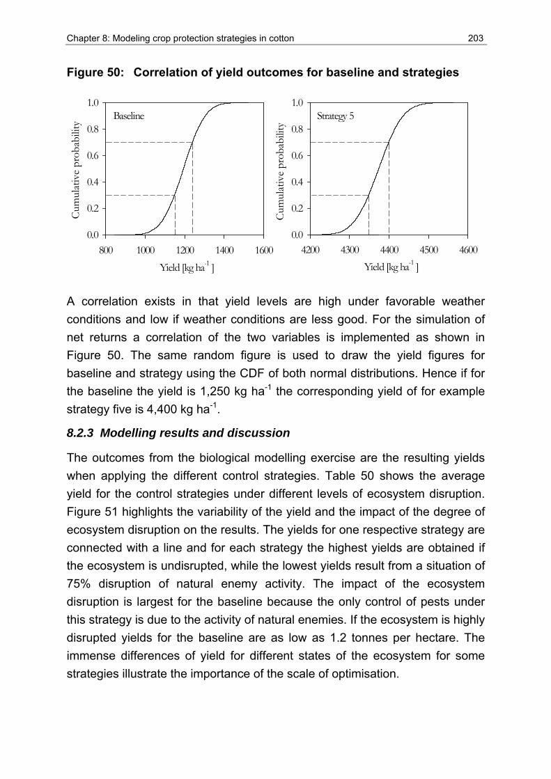
Chapter 8: Modeling crop protection strategies in cotton 203
Figure 50: Correlation of yield outcomes for baseline and strategies
Yield [kg ha-1 ]800 1000 1200 1400 1600
Cum
ulat
ive
prob
abili
ty
0.0
0.2
0.4
0.6
0.8
1.0
Yield [kg ha-1 ]4200 4300 4400 4500 4600
Cum
ulat
ive
prob
abili
ty
0.0
0.2
0.4
0.6
0.8
1.0Baseline Strategy 5
A correlation exists in that yield levels are high under favorable weather conditions and low if weather conditions are less good. For the simulation of net returns a correlation of the two variables is implemented as shown in Figure 50. The same random figure is used to draw the yield figures for baseline and strategy using the CDF of both normal distributions. Hence if for the baseline the yield is 1,250 kg ha-1 the corresponding yield of for example strategy five is 4,400 kg ha-1.
8.2.3 Modelling results and discussion
The outcomes from the biological modelling exercise are the resulting yields when applying the different control strategies. Table 50 shows the average yield for the control strategies under different levels of ecosystem disruption. Figure 51 highlights the variability of the yield and the impact of the degree of ecosystem disruption on the results. The yields for one respective strategy are connected with a line and for each strategy the highest yields are obtained if the ecosystem is undisrupted, while the lowest yields result from a situation of 75% disruption of natural enemy activity. The impact of the ecosystem disruption is largest for the baseline because the only control of pests under this strategy is due to the activity of natural enemies. If the ecosystem is highly disrupted yields for the baseline are as low as 1.2 tonnes per hectare. The immense differences of yield for different states of the ecosystem for some strategies illustrate the importance of the scale of optimisation.
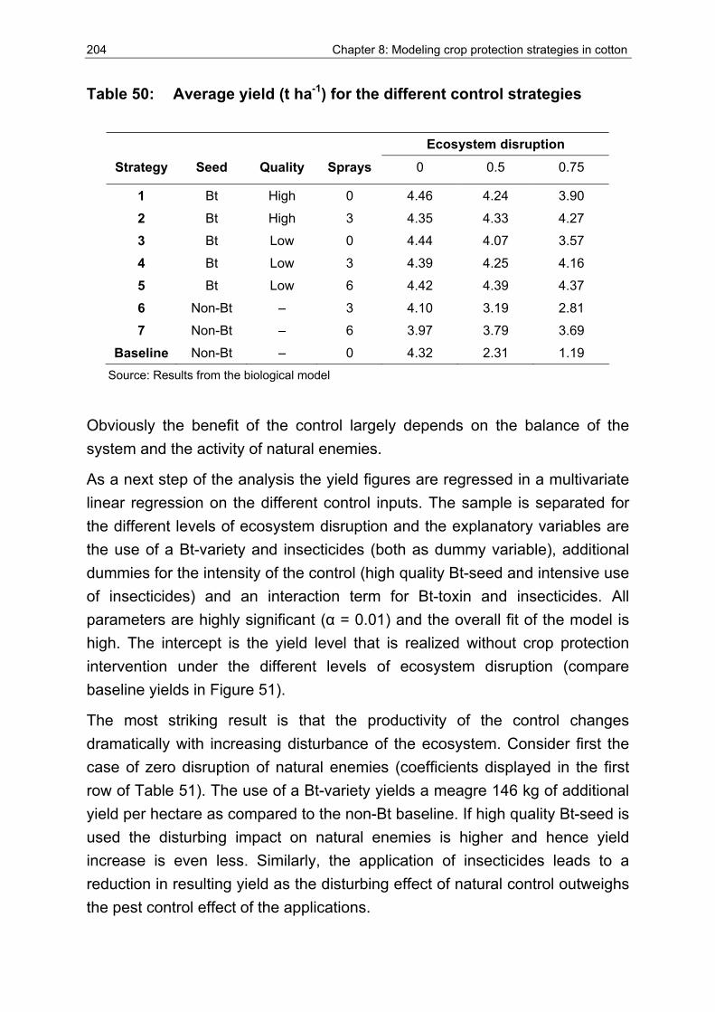
204 Chapter 8: Modeling crop protection strategies in cotton
Table 50: Average yield (t ha-1) for the different control strategies
Ecosystem disruption
Strategy Seed Quality Sprays 0 0.5 0.75
1 Bt High 0 4.46 4.24 3.90
2 Bt High 3 4.35 4.33 4.27
3 Bt Low 0 4.44 4.07 3.57
4 Bt Low 3 4.39 4.25 4.16
5 Bt Low 6 4.42 4.39 4.37
6 Non-Bt – 3 4.10 3.19 2.81
7 Non-Bt – 6 3.97 3.79 3.69
Baseline Non-Bt – 0 4.32 2.31 1.19 Source: Results from the biological model
Obviously the benefit of the control largely depends on the balance of the system and the activity of natural enemies.
As a next step of the analysis the yield figures are regressed in a multivariate linear regression on the different control inputs. The sample is separated for the different levels of ecosystem disruption and the explanatory variables are the use of a Bt-variety and insecticides (both as dummy variable), additional dummies for the intensity of the control (high quality Bt-seed and intensive use of insecticides) and an interaction term for Bt-toxin and insecticides. All parameters are highly significant (α = 0.01) and the overall fit of the model is high. The intercept is the yield level that is realized without crop protection intervention under the different levels of ecosystem disruption (compare baseline yields in Figure 51).
The most striking result is that the productivity of the control changes dramatically with increasing disturbance of the ecosystem. Consider first the case of zero disruption of natural enemies (coefficients displayed in the first row of Table 51). The use of a Bt-variety yields a meagre 146 kg of additional yield per hectare as compared to the non-Bt baseline. If high quality Bt-seed is used the disturbing impact on natural enemies is higher and hence yield increase is even less. Similarly, the application of insecticides leads to a reduction in resulting yield as the disturbing effect of natural control outweighs the pest control effect of the applications.
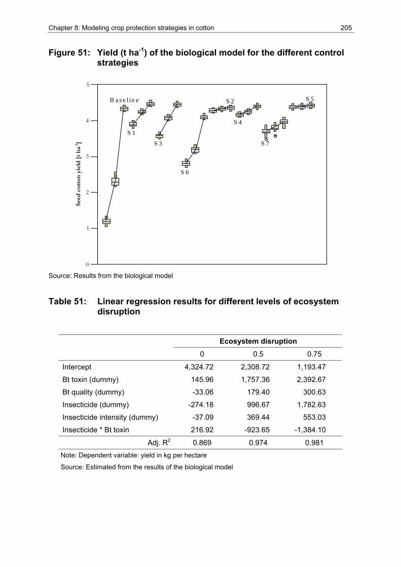
Chapter 8: Modeling crop protection strategies in cotton 205
Figure 51: Yield (t ha-1) of the biological model for the different control strategies
0
1
2
3
4
5 Se
ed c
otto
n y
ield
[t
ha-1
]
B a s e l in e
S 1
S 3
S 5
S 7
S 6
S 4
S 2
Source: Results from the biological model
Table 51: Linear regression results for different levels of ecosystem disruption
Ecosystem disruption
0 0.5 0.75
Intercept 4,324.72 2,308.72 1,193.47
Bt toxin (dummy) 145.96 1,757.36 2,392.67
Bt quality (dummy) -33.06 179.40 300.63
Insecticide (dummy) -274.18 996.67 1,782.63
Insecticide intensity (dummy) -37.09 369.44 553.03
Insecticide * Bt toxin 216.92 -923.65 -1,384.10
Adj. R2 0.869 0.974 0.981 Note: Dependent variable: yield in kg per hectare
Source: Estimated from the results of the biological model
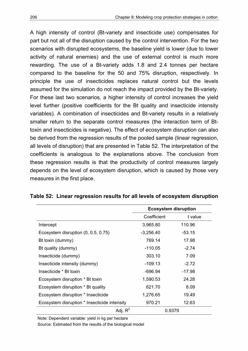
206 Chapter 8: Modeling crop protection strategies in cotton
A high intensity of control (Bt-variety and insecticide use) compensates for part but not all of the disruption caused by the control intervention. For the two scenarios with disrupted ecosystems, the baseline yield is lower (due to lower activity of natural enemies) and the use of external control is much more rewarding. The use of a Bt-variety adds 1.8 and 2.4 tonnes per hectare compared to the baseline for the 50 and 75% disruption, respectively. In principle the use of insecticides replaces natural control but the levels assumed for the simulation do not reach the impact provided by the Bt-variety. For these last two scenarios, a higher intensity of control increases the yield level further (positive coefficients for the Bt quality and insecticide intensity variables). A combination of insecticides and Bt-variety results in a relatively smaller return to the separate control measures (the interaction term of Bt-toxin and insecticides is negative). The effect of ecosystem disruption can also be derived from the regression results of the pooled sample (linear regression, all levels of disruption) that are presented in Table 52. The interpretation of the coefficients is analogous to the explanations above. The conclusion from these regression results is that the productivity of control measures largely depends on the level of ecosystem disruption, which is caused by those very measures in the first place.
Table 52: Linear regression results for all levels of ecosystem disruption
Ecosystem disruption
Coefficient t value
Intercept 3,965.80 110.96
Ecosystem disruption (0, 0.5, 0.75) -3,256.40 -53.15
Bt toxin (dummy) 769.14 17.98
Bt quality (dummy) -110.05 -2.74
Insecticide (dummy) 303.10 7.09
Insecticide intensity (dummy) -109.13 -2.72
Insecticide * Bt toxin -696.94 -17.98
Ecosystem disruption * Bt toxin 1,590.53 24.28
Ecosystem disruption * Bt quality 621.70 8.09
Ecosystem disruption * Insecticide 1,276.65 19.49
Ecosystem disruption * Insecticide intensity 970.21 12.63
Adj. R2 0.9379 Note: Dependent variable: yield in kg per hectare Source: Estimated from the results of the biological model
Chapter 8: Modeling crop protection strategies in cotton 207
These results confirm much older findings (see for example Falcon et al., 1968; Ehler et al., 1974; Eveleens et al., 1974) that the use of pesticides (and analogous planting of Bt-varieties) offers a remedy for a problem that is created by the pesticide use itself and would not otherwise exist. Consequently, the productivity of such damage control inputs is overestimated if the no control scenario in a disrupted system is used as the baseline for the assessment rather than the undisrupted situation. The results and conclusions outlined above use the cotton yield as performance indicator for the impact assessment of the control measures. For an assessment of the economic performance of the different strategies, output prices and control costs have to be included. Therefore the yield figures of the biological model are used as input for a stochastic budgeting model. Based on the simulated yield outcomes for the different control strategies, distribution functions are derived that enter the economic part of the model. The most obvious and commonly used distribution form for yield figures is a normal distribution.
To generate normal distributions the parameters μ and σ are estimated using a Maximum Likelihood Estimator (MLE) so that the resulting function is the closest match to the data (Vose, 1996; PALISADE, 2000). The results are presented in Table 52 for the highly disturbed scenario (75% disruption) and in Appendix 21 for all levels of disruption. The appendix table also gives indicators of the goodness-of-fit (Chi-Square, Kolmogorov-Smirinov, Anderson-Darling statistics) of estimated normal distributions. The estimated normal distribution functions mostly have a good fit in the middle of the distribution (Kolmogorov-Smirinov) and at the distribution tails (Anderson-Darling). However, the chi-square statistics show that most of the yield data sets are not very well described by a normal distribution. This can be attributed to the relatively few data points (only 20 per set) that were available. Even though for some of the yield data sets other distributional forms (such as log logistic) would have a better fit, the normal distribution function was selected for all sets to make the procedure transparent and not superimpose additional assumptions. The correlated yield distributions are then implemented as inputs in the budgeting model. Results of the subsequent Monte Carlo simulations of net revenues for different control strategies are presented in Figures 52 – 54. In accordance with the yield outcomes from the biological model, the net revenue of control measures depends strongly on the status of the ecosystem (level of disruption).
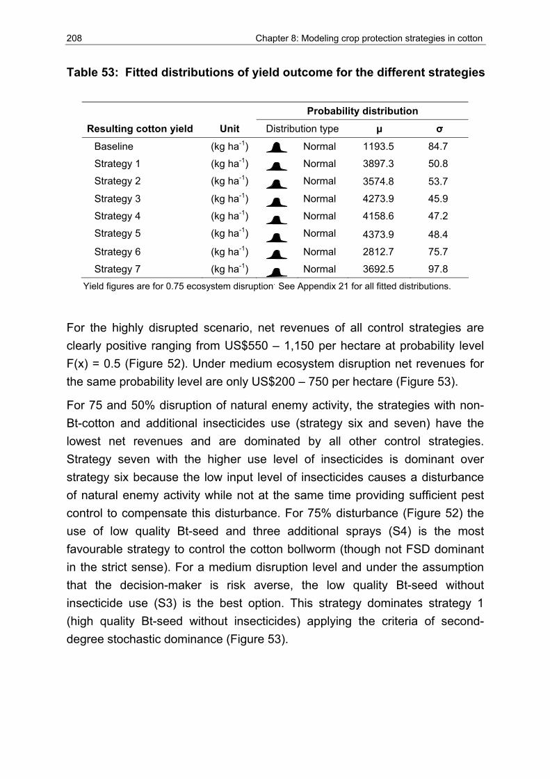
208 Chapter 8: Modeling crop protection strategies in cotton
Table 53: Fitted distributions of yield outcome for the different strategies
Probability distribution
Resulting cotton yield Unit Distribution type μ σ
Baseline (kg ha-1) Normal 1193.5 84.7
Strategy 1 (kg ha-1) Normal 3897.3 50.8
Strategy 2 (kg ha-1) Normal 3574.8 53.7
Strategy 3 (kg ha-1) Normal 4273.9 45.9
Strategy 4 (kg ha-1) Normal 4158.6 47.2
Strategy 5 (kg ha-1) Normal 4373.9 48.4
Strategy 6 (kg ha-1) Normal 2812.7 75.7
Strategy 7 (kg ha-1) Normal 3692.5 97.8 Yield figures are for 0.75 ecosystem disruption. See Appendix 21 for all fitted distributions.
For the highly disrupted scenario, net revenues of all control strategies are clearly positive ranging from US$550 – 1,150 per hectare at probability level F(x) = 0.5 (Figure 52). Under medium ecosystem disruption net revenues for the same probability level are only US$200 – 750 per hectare (Figure 53).
For 75 and 50% disruption of natural enemy activity, the strategies with non-Bt-cotton and additional insecticides use (strategy six and seven) have the lowest net revenues and are dominated by all other control strategies. Strategy seven with the higher use level of insecticides is dominant over strategy six because the low input level of insecticides causes a disturbance of natural enemy activity while not at the same time providing sufficient pest control to compensate this disturbance. For 75% disturbance (Figure 52) the use of low quality Bt-seed and three additional sprays (S4) is the most favourable strategy to control the cotton bollworm (though not FSD dominant in the strict sense). For a medium disruption level and under the assumption that the decision-maker is risk averse, the low quality Bt-seed without insecticide use (S3) is the best option. This strategy dominates strategy 1 (high quality Bt-seed without insecticides) applying the criteria of second-degree stochastic dominance (Figure 53).
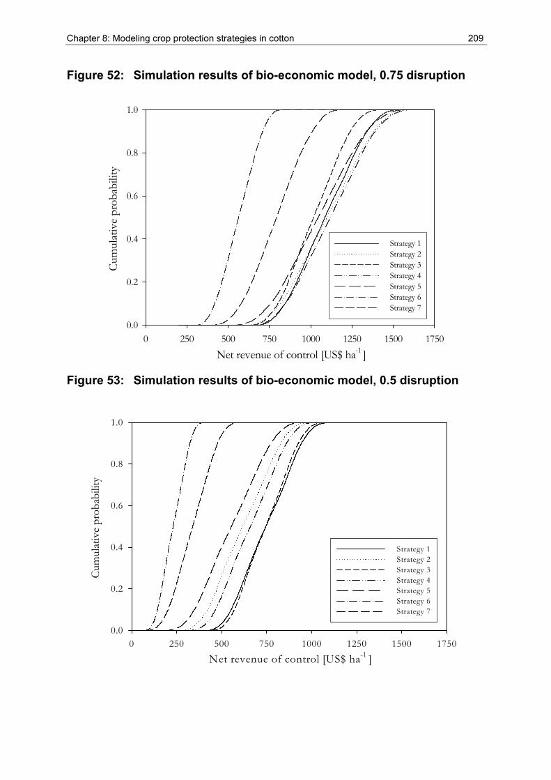
Chapter 8: Modeling crop protection strategies in cotton 209
Figure 52: Simulation results of bio-economic model, 0.75 disruption
Net revenue of control [US$ ha-1 ]0 250 500 750 1000 1250 1500 1750
Cum
ulat
ive
prob
abili
ty
0.0
0.2
0.4
0.6
0.8
1.0
Strategy 1Strategy 2Strategy 3Strategy 4Strategy 5Strategy 6Strategy 7
Figure 53: Simulation results of bio-economic model, 0.5 disruption
Net revenue of control [US$ ha-1 ]0 250 500 750 1000 1250 1500 1750
Cum
ulat
ive
prob
abili
ty
0.0
0.2
0.4
0.6
0.8
1.0
Strategy 1Strategy 2Strategy 3Strategy 4Strategy 5Strategy 6Strategy 7
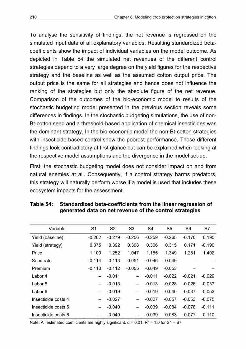
210 Chapter 8: Modeling crop protection strategies in cotton
To analyse the sensitivity of findings, the net revenue is regressed on the simulated input data of all explanatory variables. Resulting standardized beta-coefficients show the impact of individual variables on the model outcome. As depicted in Table 54 the simulated net revenues of the different control strategies depend to a very large degree on the yield figures for the respective strategy and the baseline as well as the assumed cotton output price. The output price is the same for all strategies and hence does not influence the ranking of the strategies but only the absolute figure of the net revenue. Comparison of the outcomes of the bio-economic model to results of the stochastic budgeting model presented in the previous section reveals some differences in findings. In the stochastic budgeting simulations, the use of non-Bt-cotton seed and a threshold-based application of chemical insecticides was the dominant strategy. In the bio-economic model the non-Bt-cotton strategies with insecticide-based control show the poorest performance. These different findings look contradictory at first glance but can be explained when looking at the respective model assumptions and the divergence in the model set-up.
First, the stochastic budgeting model does not consider impact on and from natural enemies at all. Consequently, if a control strategy harms predators, this strategy will naturally perform worse if a model is used that includes these ecosystem impacts for the assessment.
Table 54: Standardized beta-coefficients from the linear regression of generated data on net revenue of the control strategies
Variable S1 S2 S3 S4 S5 S6 S7
Yield (baseline) -0.262 -0.279 -0.256 -0.259 -0.265 -0.170 0.190
Yield (strategy) 0.375 0.392 0.308 0.306 0.315 0.171 -0.190
Price 1.109 1.252 1.047 1.185 1.349 1.281 1.402
Seed rate -0.114 -0.113 -0.051 -0.046 -0.049 – –
Premium -0.113 -0.112 -0.055 -0.049 -0.053 – –
Labor 4 – -0.011 – -0.011 -0.022 -0.021 -0.029
Labor 5 – -0.013 – -0.013 -0.028 -0.026 -0.037
Labor 6 – -0.019 – -0.019 -0.040 -0.037 -0.053
Insecticide costs 4 – -0.027 – -0.027 -0.057 -0.053 -0.075
Insecticide costs 5 – -0.040 – -0.039 -0.084 -0.078 -0.111
Insecticide costs 6 – -0.040 – -0.039 -0.083 -0.077 -0.110Note: All estimated coefficients are highly significant, α = 0.01, R2 = 1.0 for S1 – S7
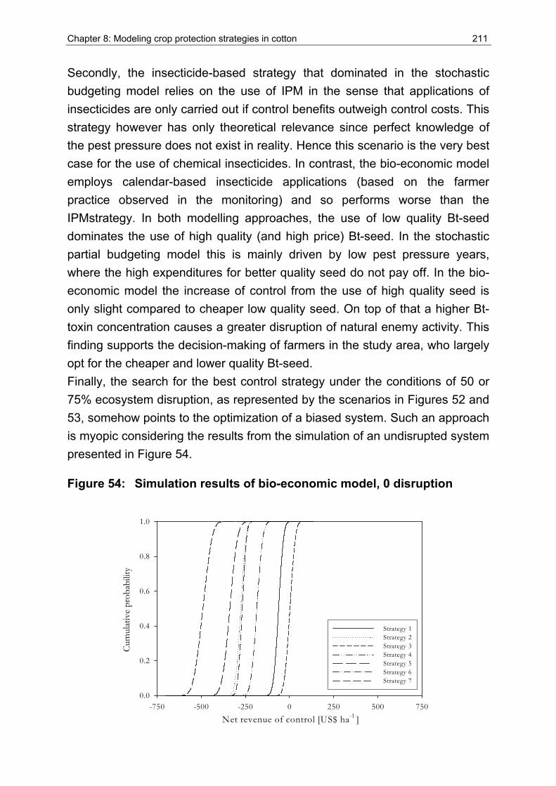
Chapter 8: Modeling crop protection strategies in cotton 211
Secondly, the insecticide-based strategy that dominated in the stochastic budgeting model relies on the use of IPM in the sense that applications of insecticides are only carried out if control benefits outweigh control costs. This strategy however has only theoretical relevance since perfect knowledge of the pest pressure does not exist in reality. Hence this scenario is the very best case for the use of chemical insecticides. In contrast, the bio-economic model employs calendar-based insecticide applications (based on the farmer practice observed in the monitoring) and so performs worse than the IPMstrategy. In both modelling approaches, the use of low quality Bt-seed dominates the use of high quality (and high price) Bt-seed. In the stochastic partial budgeting model this is mainly driven by low pest pressure years, where the high expenditures for better quality seed do not pay off. In the bio-economic model the increase of control from the use of high quality seed is only slight compared to cheaper low quality seed. On top of that a higher Bt-toxin concentration causes a greater disruption of natural enemy activity. This finding supports the decision-making of farmers in the study area, who largely opt for the cheaper and lower quality Bt-seed. Finally, the search for the best control strategy under the conditions of 50 or 75% ecosystem disruption, as represented by the scenarios in Figures 52 and 53, somehow points to the optimization of a biased system. Such an approach is myopic considering the results from the simulation of an undisrupted system presented in Figure 54.
Figure 54: Simulation results of bio-economic model, 0 disruption
Net revenue of control [US$ ha-1 ]-750 -500 -250 0 250 500 750
Cum
ulat
ive
prob
abili
ty
0.0
0.2
0.4
0.6
0.8
1.0
Strategy 1Strategy 2Strategy 3Strategy 4Strategy 5Strategy 6Strategy 7
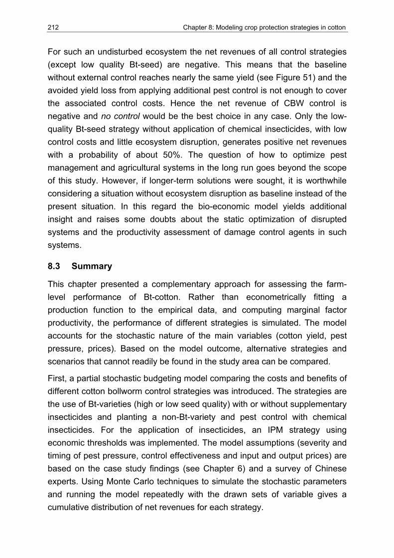
212 Chapter 8: Modeling crop protection strategies in cotton
For such an undisturbed ecosystem the net revenues of all control strategies (except low quality Bt-seed) are negative. This means that the baseline without external control reaches nearly the same yield (see Figure 51) and the avoided yield loss from applying additional pest control is not enough to cover the associated control costs. Hence the net revenue of CBW control is negative and no control would be the best choice in any case. Only the low-quality Bt-seed strategy without application of chemical insecticides, with low control costs and little ecosystem disruption, generates positive net revenues with a probability of about 50%. The question of how to optimize pest management and agricultural systems in the long run goes beyond the scope of this study. However, if longer-term solutions were sought, it is worthwhile considering a situation without ecosystem disruption as baseline instead of the present situation. In this regard the bio-economic model yields additional insight and raises some doubts about the static optimization of disrupted systems and the productivity assessment of damage control agents in such systems.
8.3 Summary
This chapter presented a complementary approach for assessing the farm-level performance of Bt-cotton. Rather than econometrically fitting a production function to the empirical data, and computing marginal factor productivity, the performance of different strategies is simulated. The model accounts for the stochastic nature of the main variables (cotton yield, pest pressure, prices). Based on the model outcome, alternative strategies and scenarios that cannot readily be found in the study area can be compared.
First, a partial stochastic budgeting model comparing the costs and benefits of different cotton bollworm control strategies was introduced. The strategies are the use of Bt-varieties (high or low seed quality) with or without supplementary insecticides and planting a non-Bt-variety and pest control with chemical insecticides. For the application of insecticides, an IPM strategy using economic thresholds was implemented. The model assumptions (severity and timing of pest pressure, control effectiveness and input and output prices) are based on the case study findings (see Chapter 6) and a survey of Chinese experts. Using Monte Carlo techniques to simulate the stochastic parameters and running the model repeatedly with the drawn sets of variable gives a cumulative distribution of net revenues for each strategy.
Chapter 8: Modeling crop protection strategies in cotton 213
Results show that the use of non-Bt-cotton combined with an IPM use of insecticides is the dominant strategy. All strategies that use Bt-seed yield negative net revenues if pest pressure is low (because control costs are fixed and cannot be adapted to the actual pest pressure or yield level). This is also the reason why the low quality (and cheaper) Bt-seed performs better than the high quality seed. The insecticides strategy with non-Bt-cotton based on economic thresholds always gives positive net revenues (since control only takes place when it pays off by definition).
As a next step a bio-economic model was introduced in the second part of the chapter. This consists of a biological model that simulates the mass and number dynamics of plant growth and pest and predator populations, and an economic part that uses the yield figures of the biological model to compute net revenues of different strategies. For the biological model three different levels of ecosystem disruption as a measure of reduced natural enemy activity are assumed. The situation in the study area with intensive use of chemical pesticides and Bt-varieties is highly disturbed, with disruption levels between 50 and 75%.
Then, the yield outcomes generated by the biological model are regressed on the different control inputs (dummies for Bt-varieties, insecticide use, Bt-quality, high insecticide use intensity and the interaction of Bt-toxin and insecticides). Results show the impact of the ecosystem disruption on the baseline yield with only natural control (without additional external pest control) and the productivity of control measures. The baseline yield in an undisrupted system is only a little lower than yield outcome under intensive pest control (Bt-variety and sprays). For a highly disrupted system baseline yields are dramatically lower. The higher intensity of control (high quality seed or higher number of insecticide applications) gives only comparably low yield increases. Most strikingly, the productivity of both Bt-varieties and insecticides crucially depends on the disruption level of the ecosystem and increases considerably if natural enemy activity is disturbed. This implies that at least part of the productivity of pest control is only a solution for a homemade problem. A recent overview of the evolution of cotton pest management in China acknowledges that control interventions amplify pest problems in the past by triggering resistance build-up and disrupting natural enemy populations (Wu and Guo, 2005).
214 Chapter 8: Modeling crop protection strategies in cotton
If normal distributions are fitted to the yield outcomes of the biological model for the different control strategies (under the different disruption scenarios) these can be used as input for an adapted version of the stochastic budgeting model. Using Monte Carlo simulation gives cumulative distributions for the net revenues for the different control strategies. Diverging from the previous results, the purely insecticide-based strategies perform poorly since calendar-based sprays are assumed rather than an IPM strategy, and ecosystem disruption from insecticides is severe.
The low quality seed Bt-cotton strategies perform better than the high quality options because costs are less and ecosystem disruption is reduced for lower toxin concentrations. The most important result however is the impact of the ecosystem disruption, rather than the ranking of the strategies. Under the highly disrupted scenarios, pest control yields positive net revenues while in an undisrupted environment a no control strategy is the best option. Findings confirm the importance of including ecosystem aspects into the assessment of damage control agents to avoid bias and overestimation of productivity effects.
9 Conc lus ion and recommendat ions
9.1 Discussion of findings
The objective of this study was to (i) assess the contribution of the insect resistance trait in Bt-cotton varieties to the productivity and profitability of small-scale cotton cultivation in Linqing County, China, and (ii) advance the methodology used to assess the costs and benefits of biotechnology in crop protection at the production level.
The case study findings show that despite the introduction and exclusive use of Bt-varieties, farmers in the study area used high levels of chemical pesticides. The average input level of insecticides, which make up the lion’s share of pesticides used, recorded in the production monitoring was well above the economically optimal level as computed from the estimated marginal productivity of this factor. This is in line with results of Huang et al. (2002a), who also found substantial overuse of pesticides in Bt-cotton production in North East China. The authors state that the extent of pesticide promotion may be an important factor in explaining this overuse. About one third of the insecticides used in Bt-cotton production still targeted cotton bollworm according to respondents. A possible explanation for this continued reliance on chemical insecticides, despite shifting to Bt-varieties, may be a lack of effectiveness of insecticides or insufficient control of target pests by Bt-cotton. Moreover, farmers may have decision criteria other than profit maximization that are not captured when calculating optimal factor input levels. If farmers were loss averse or had an extreme perception of potential CBW damage, the costs of pesticides could be considered as a risk premium76.
Testing of bollworm larvae collected at the study site showed that as of 2002 there was no resistance-build up against the Bt-toxin in target pest populations. But the analysis of cotton leaf samples confirmed a quality problem in Bt-varieties that was already indicated by substantial variation in seed prices and the multitude of different Bt-seed available in local markets.
The toxin concentration varied widely but plants from less costly seed showed higher probabilities of low toxin concentrations. However, samples from high
76 See Chapter 4 for a discussion of the risk reducing effects of chemical pesticides.
216 Chapter 9: Conclusion and recommendations
priced seed also expressed low levels of Bt-toxin, so that the effectiveness of the Bt-trait is uncertain from the farmer’s point of view at the time of purchase and also later in the season. Lack of quality standards and quality control for agricultural inputs increases the uncertainty about input factors and results in economically inefficient factor use. Consequently, substitution of Bt-toxin for insecticides is severely limited because farmers cannot directly observe the toxin concentration.
For the case study it can be concluded that the introduction of Bt-varieties did not entirely solve the cotton bollworm problem since most of the farmers still perceive CBW as the second most important cotton pest. Even less so did it solve the pest problems in cotton in general as the number of pesticide sprays remains high and farmers even stated that spray numbers (mainly targeting secondary pests) have increased compared to the time when Bt-cotton was first introduced. Although the economic benefits of Bt-cotton in China were demonstrated at an early stage of technology adoption (Pray et al., 2001), the sustainability of these benefits can be questioned.
Hypothesis 1 was that institutional conditions and market failure determine the success of technology implementation and can limit the realization of benefits, especially under the conditions in developing countries. In the case study, the lack of standards and quality control of agricultural inputs increases uncertainty for farmers and in particular leads to inefficiency in factor use and resource allocation. Deficiency of supportive institutions may explain why an introduction of Bt-cotton varieties did not (satisfactorily) solve the pest (and pesticide) problem. The situation reminds of the lessons learned from the introduction of integrated pest management that shows high benefits in experiments and pilot projects, but farm-level benefits can be considerably limited by institutional as well as socio-economic and technical constraints (Beckmann and Wesseler, 2003). Thus the prevailing institutional conditions are crucial to the realization of potential benefits of new technologies, especially those aiming at pesticide use reduction.
Results of the production function estimation showed the expected direction of coefficients for the directly yield increasing production factors labor, capital and variables like crop rotation and experience. However, the concentration of Bt-toxin had no significant effect on the realized yield. In addition, the coefficients for Bt-toxin indicate a negative relationship between its concentration and the resulting cotton yield.
Chapter 9: Conclusion and recommendations 217
The coefficient for insecticides was significant for only one exponential specification. These results support hypothesis 2, which stated that the specification of the econometric model used influences the results of the assessment.
The results of the semi-parametric approach used to assess the factor productivity of damage control inputs showed that the level of pest infestation has an impact on the performance of inputs such as Bt-toxin and insecticides. Some of the coefficients of Bt-toxin and insecticides are significant but the impact of those factors on cotton yield outcome is very small. The results of the two approaches correspond well since both models show that the impact of Bt-toxin and insecticide use is minor. Moreover, directions of coefficients for the damage control inputs are not always conclusive. One possible explanation is the overall high use of insecticides. Since all farmers are considerably overusing insecticides, an additional unit at average input level may in fact not yield additional benefits. The strength of these econometric approaches is the sole reliance on empirical findings, not requiring additional assumptions about any part of the system. The relatively small explanatory power of the two econometric approaches, however, is an indication that pure econometric approaches do not sufficiently cover all the essential variables and characteristics of complex production systems. In the context of China and other developing countries, there is evidence that the quality of farming inputs varies considerably due to lack of quality standards and control and even product adulteration. The fact that the control of pests depends not only on the amount of control agents used, but also on other factors (the timeliness and accuracy of control, climatic conditions, the match of damage agent and control applied) further challenges productivity analysis of agricultural production.
To include the uncertainty inherent in most of the explanatory variables, a stochastic budgeting model was used. A survey conducted with Chinese researchers and scientists confirmed the stochastic nature of most underlying variables. Model outcome showed that the performance of crop protection strategies is largely determined by the prevailing conditions and fluctuates over a wide range. For the control strategies that used Bt-varieties, net revenue of bollworm control was sometimes even negative under certain circumstances.
218 Chapter 9: Conclusion and recommendations
Summarizing the results, those strategies that performed better were less costly and more flexible in terms of adjustment of the control towards the actual conditions (curative rather than prophylactic control). The strategy using high priced Bt-seed was dominated, according to first-degree stochastic dominance, by the other options, due to the high fixed costs that occurred irrespective of actual pest damage and realized yield level. Strategies such as the use of Bt-varieties could have the additional positive effect of greatly and rather immediately reducing the pest pressure of CBW. However, this is not the case for the diverse cropping system in China, where other host crops are available for the target pest and hence pest pressure is maintained. The model findings confirm hypothesis 3 that uncertainty is an essential element of agro-ecosystems and incorporating risk in the analysis yields additional insight into the performance of Bt-cotton. A major limitation of the stochastic budgeting model presented is the reliance on assumptions and the simplification of underlying system processes. This can be overcome by integrating an ecosystems model that captures the dynamics and interactions of plant growth, pest and natural enemy populations. The resulting bio-economic model also accounts for the impact of natural enemies and the effect of control interventions on this natural resource. The results of this modeling part reveal the substantial impact that the system characteristic disturbance level of natural enemies has on the productivity of external control interventions.
In answer to hypothesis 4, clearly, an interdisciplinary approach that, in addition to farm-level performance data, considers the underlying biological and ecological processes has increased the explanatory value. Inclusion of ecosystem and factor market aspects advances the methodology used to assess the costs and benefits of new technologies in crop protection at the production level. The thesis tackled a number of the empirical and methodological challenges that arise when assessing the impact of biotechnology applications in crop protection. If additional factors were to be included in the analysis, the explanatory power of the model and the validity of results will most likely increase further. The following section lists some of the remaining aspects and challenges that warrant further research.
Chapter 9: Conclusion and recommendations 219
9.2 Recommendations for further research
The experience and results from the recall survey during the orientation phase and the season-long production monitoring show that the data collection protocol is of utmost importance in assuring the validity of input data of small-scale farming in developing countries. Impact assessment of plant protection technologies requires accurate data that is extremely difficult to obtain by means of recall surveys, especially for pesticide use.
The analysis of the case study findings of Bt-cotton production showed significant differences in production practices and performance among the five villages that were included in the survey. The differences could be due to variation in microclimate or resource availability (soil fertility or access to irrigation water) or varying human capacity or managerial skills of farmers that is more likely to diffuse within villages. To reduce the impact of village level effects on the assessment of technology performance, a higher number of villages could be included.
The performance of plant protection interventions largely depends on the level of pest infestation, as demonstrated in the econometric analysis by differences in estimated coefficients for damage control inputs at different pest pressure levels. Future studies could include improved measures of actual pest pressure and at the same time further enhance the proxies for pest control interventions. The results of this case study show that quality differences in inputs such as Bt-seed can only be captured if a proxy such as the toxin concentration is measured as a continuous variable. Corresponding indicators for chemical pesticides exist and could be applied. One more important aspect of crop protection technologies is the role of human capital. There is substantial return to human capital for pest control that relies on pesticides where the product choice and application method (including the timing) is crucial for the control impact. Whereas for technologies such as Bt-crops, it is claimed that all that farmers need to do is plant the seed. However, there are indications of the emergence of secondary pests, and a sustainable use of the technology requires proper resistance-management. Hence, more research on the complementarity of integrated pest management and Bt-varieties is needed.
220 Chapter 9: Conclusion and recommendations
For a more in-depth analysis of the system, the long-term dynamic effects of a pest control technology (such as a possible resistance build-up) can be included in bio-economic modeling. Also, further research could extend the analysis to multi-period models to include dynamic aspects of the ecosystem. Analysis of the productivity impact of different control strategies in the long run and accounting for related externalities may give additional insight into the performance of different crop protection strategies. The findings of the bio-economic model applied in this study show the fundamental impact of ecosystem disturbance variables captured as the activity level of natural enemies. The linkage of ecological and economic models widens the scope of the analysis and can lead to more realistic assessments of technology impact.
To highlight this fact the quote “dealing with the many facets of biotechnology, however, often points out the limits of economic analysis and, hopefully, provides an incentive to expand the limits of our discipline” (Gaisford et al., 2001) shall be repeated.
9.3 Conclusion and outlook
The key conclusion of the study is that productivity assessment of Bt-cotton varieties benefits from a broader framework that combines ecological and economic indicators. To better understand the farm-level implications of Bt-cotton introduction in developing countries, it is important to (i) capture the inherent uncertainty that exists in key variables, and (ii) integrate ecological processes that largely determine technology performance in the analysis. In addition to the ecological impact of the technology in question, the institutional environment is an important determinant of the resulting benefits. As pointed out by de Janvry et al. (2005), it is a major precondition and challenge for the effective implementation of agricultural biotechnology in developing countries to put in place the necessary public and private institutions. The introduction of such technologies without enabling institutions that assure proper use of the technologies can limit the benefits considerably. The survey and experimental findings presented in this thesis indicate that the implementation of Bt-cotton in China was carried out without the necessary supportive institutions and a stepwise evaluation. To the contrary, the technology was introduced very rapidly without prior implementation and/or enforcement of a set of clear rules and standards.
Chapter 9: Conclusion and recommendations 221
Although a technical fix is often the focus of attention, biotechnology alone, like previous technologies in this field, is very unlikely to ultimately solve (plant protection) problems. The need for the introduction of transgenic cotton expressing insecticidal genes other than Cry1Ac and CpIT for future pest management was recently emphasized by Wu and Guo (2005). However, the results of this case study show the importance of considering causes and possible remedies for market failure in agricultural input markets and the need to dissolve institutional constraints before introducing additional GE crops in China. These lessons learned should also be considered before the introduction of biotechnology to other developing countries with similar conditions.
The impact of the commercialization of other Bt-crops in China goes beyond the farm-level impact of the technology. Corn, for example, is reportedly the major refuge area for CBW and thus ensures that large enough populations of susceptible larvae can dilute a potential resistance build-up. The rapid spread of Bt-cotton has illustrated that such technologies cannot easily be limited regionally, and even less be withdrawn once released. Undoubtedly will the stance of China in the debate on genetically engineered (food) crops have global ramifications, as the country is one of the largest agricultural producers and importers worldwide.
10 Summary
The use of genetically engineered crop varieties has recently become an option for pest control, particularly for crops with high levels of pesticide use. However, a number of methodological and empirical challenges arise when assessing the impact of biotechnology solutions in crop protection, especially in developing countries. Major empirical challenges are the collection of accurate input and output data, and variability in the quality of agricultural inputs. Principal methodological challenges are due to the special damage control nature of pest control inputs, the uncertainty in most explanatory variables, and the interdependence of ecosystem variables and control inputs. The objective of this thesis is to assess the contribution of the insect resistance trait in Bt-varieties77 to the productivity and profitability of small-scale cotton cultivation in Linqing County, China. Concurrently, the research aims at advancing the methodology used to assess the costs and benefits of biotechnology in crop protection at the production level.
The main genetically engineered (GE) crops are corn, soybean, cotton and canola that are resistant to herbicides and/or certain insect pests. Though GE varieties made up some 56% of the global soybean area in 2004, only 1.6% of the total global agricultural area was planted with GE crops. China is one of the few developing countries with a substantial area planted to GE crops (some 60% of the nation’s cotton area was planted to Bt-varieties in 2002). Different from the situation in most other countries, the Chinese government invests heavily in public research in the field of agricultural biotechnology and actively influences the direction of research.
This thesis provides an in-depth case study of the application of Bt-cotton in North East China. Season-long monitoring (March – October) of Bt-cotton production was conducted with a sample of 150 farmers in five villages in Linqing County in the 2002 cotton season. Farm-level interviews conducted with 60 cotton-growing farmers in three different counties of Shandong Province at the end of the 2001 cotton season revealed that farmers had severe difficulties in recalling quantities of chemical pesticides and other
77 Bt-varieties are genetically engineered to carry a gene from the soil bacterium Bacillus thuringiensis. This gene encodes for a toxin that is lethal for certain insects (mainly Lepidoptera and Coleoptera species). The modified Bt-crops also express this toxin and hence are resistant against some pests.
Chapter 10: Summary 223
production inputs. Consequently, farm households were visited biweekly and three additional interviews were conducted on household demographics, knowledge and perception of Bt-cotton, and the production of other crops during the input monitoring in 2002. Moreover, the survey in 2001 revealed the necessity for an integrated data collection framework to capture certain aspects of the ecological and policy environment, in addition to the farm-level information. A cotton growth experiment with Bt- and non-Bt-plots was carried out as part of the integrated approach in the 2002 season to adapt a biological ecosystems model to the conditions at the study site. In addition, cotton leaf samples from each monitored field were analyzed with regard to Bt-toxin concentration, and bollworm larvae were sampled in farmers’ fields to assess the resistance level against Bt-toxin.
A review of available methods as well as results of impact studies of Bt-cotton, particularly from developing countries, disclosed unresolved issues in the assessment of agricultural biotechnology. The following principal issues were addressed in this study: (1) the prevailing institutional conditions that determine and potentially limit technology success, (2) the consequences of different specifications of econometric models to assess the productivity of damage control inputs, (3) uncertainty as an essential element of the agro-ecosystem, and (4) the use of interdisciplinary approaches that consider the underlying biological and ecological processes in addition to farm level performance.
The framework for the analysis consists of three main parts, representing increasing levels of complexity in the analysis. First, a descriptive analysis of the case study on Bt-cotton production in Linqing County provides insight into the production practices and highlights some of the problems of the technology under local conditions. Second is an econometric analysis of the short-term productivity of the Bt-toxin and other damage control variables such as insecticides. Third, the farm-level performance of different pest control strategies in Bt-cotton is simulated using a partial stochastic budgeting model. The model accounts for the stochastic nature of the main variables and is extended to a bio-economic model by incorporating an ecosystems model.
Cotton is the major crop in the study area and the main source of cash income for farmers. The crop is produced with high intensity, especially in terms of labor use and input of agro-chemicals. Even though farmers are growing Bt-varieties, they sprayed on average 11 times and applied some 16 kg of
224 Chapter 10: Summary
formulated pesticides per hectare of cotton per season. Such high levels of pesticide use pose a considerable human health risk. The cotton bollworm (CBW, the pest that Bt-varieties are supposed to control) is still perceived as the second most important cotton pest and targeted by some 30% of all insecticides applied. Testing of the susceptibility of CBW caterpillars revealed that the local strains do not show an increased level of resistance against the Bt-toxin. Therefore, pest resistance was not a reason for the high insecticide use. It was common in the region to use saved cotton seed (on-farm propagation) and some 55% of the farmers continue this practice when planting Bt-varieties. Those who purchased cotton seed paid on average far less than the price for certified Bt-cotton seed. Leaf tissue was analyzed to quantify the Bt-toxin concentration, indicating the effectiveness of Bt-related pest control. Laboratory testing revealed that Bt-toxin concentrations vary significantly in the samples and some samples have very low toxin concentrations. The main reason for this quality problem in Bt-cotton is a lack of control and standards in the market for seed. The large number of pesticide products that are not registered and improperly labeled (or not labeled at all) suggests similar quality problems. The case study reveals that institutional problems and ecosystem changes (development of secondary pests) reduce the farm-level benefits of the Bt-technology.
To assess the short-term productivity of Bt-toxin, a Cobb-Douglas type production function with an inbuilt damage control function (different specifications) was estimated using yield as dependent variable. Instead of a dummy variable, the continuous measures of Bt-toxin concentration were used. Results of the production function estimation are robust with only little variation in the coefficients of varying functional specifications. For all functions, the direct inputs labor and material costs increase the cotton yield while longer rotation and higher pest pressure lead to lower yield. The coefficient for farmers in village 3 is also significant, indicating differences among the villages. The coefficient for Bt-toxin is not significant and in fact shows a negative sign in some of the specifications, implying lower actual yields for higher toxin concentration. Higher use of insecticides has a significant yield-increasing effect only for the exponential damage control function. The marginal product of insecticides varies for the different functional forms, but is positive for all estimated functions.
Chapter 10: Summary 225
The marginal value product of insecticides calculated at different input levels shows that the economically optimal use level is only about five kilograms per hectare. This is less than one third of the amount currently applied to Bt-cotton by farmers in the study region. Thus, chemical insecticides are severely overused from a production economic view. The marginal product for the Bt-toxin is negative for all but one exponential specification.
A two stage semi-parametric approach is used as complementary method to assess the factor productivity of the Bt-trait. The pest pressure variable is implemented as a slope dummy and thus allows for varying factor productivity dependent on the level of pest infestation. Results show that the factor productivity of control inputs depends on the actual level of the damage agent such that Bt-toxin had higher productivity when pest pressure was low while insecticides had higher productivity when pest pressure was high. The results obtained differ from the outcome of the previous damage control function estimates where neither the use of insecticides (in most cases) nor the concentration of Bt-toxin led to significant coefficients in the regression. A comparison of the marginal productivities between the two approaches shows that most of the coefficients for Bt-toxin are significant in the semi-parametric approach. The level of Bt-toxin concentration in leaf tissue, the use of chemical insecticides, and pest control by manual labor explain at least part of the variation in the dependent efficiency index. The actual damage control effect of the inputs is only partly captured by the explanatory variables. This can be attributed to the variability in the quality of farming inputs caused by possible product adulteration and a lack of quality standards and control. Productivity analysis of pest control inputs using econometric methods remains a challenge because the control effect does not only depend on the amount of control agents used, but also on the timeliness and accuracy of control, the climatic conditions, and the match of damage agent and control applied. Varying yield and pest pressure due to climatic changes, market risk and uncertainty about the quality of inputs are characteristics of the local cotton production system. A stochastic budgeting model was used to assess the performance of different control strategies for the cotton bollworm. The model accounts for the stochastic nature of the main variables (cotton yield, pest pressure, and prices). The different control strategies are the use of Bt-varieties (high or low seed quality) or non-Bt-varieties with or without supplementary insecticides.
226 Chapter 10: Summary
The probability distributions of explaining variables were generated based on an expert survey of Chinese scientists and the findings of the case study. Cumulative distributions of net revenues for each strategy result from using Monte Carlo techniques to simulate the stochastic parameters, and running the model repeatedly with the drawn sets of variables. The results show that the use of non-Bt-cotton combined with judicious use of chemical insecticides and low quality Bt-seed dominate the high quality (and more expensive) Bt-cotton strategy. All strategies using Bt-seed result in negative net revenues if pest pressure is low because control costs are fixed and cannot be adapted to the actual pest pressure or yield level. This is also why low quality and less costly Bt-seed perform better than the high quality seed.
The presented bio-economic model consists of (i) a biological model that simulates plant growth and populations of pests and predators, including relevant interactions, and (ii) an economic budgeting part that uses the model-generated cotton yields to compute net revenues of different CBW control strategies. For the biological model, different levels of natural enemy activity are assumed as a measure of ecosystem disruption. At the study site the activity of natural enemies is reduced (disturbed situation) due to intensive use of chemical pesticides and Bt-varieties. Regressing the model-generated cotton yield on the control inputs shows that the baseline yield (without control) in an undisrupted system is only a little lower than yield outcome under intensive pest control (Bt-variety and sprays), while for a disrupted system, baseline yield is dramatically lower. A higher intensity of control results in only small yield increases. The productivity of Bt-varieties and insecticides depends crucially on the ecosystem disruption level and increases largely if natural enemy activity is disturbed. This implies that the productivity of pest control depends on prior ecosystem interventions, which often were misguided. In contrast to the results of the stochastic budgeting model, the non-Bt cotton strategy performs poorly in the analysis using the bio-economic model, because chemical insecticides can cause severe disruption of the ecosystem and calendar-based sprays rather than a need-based strategy are assumed. The low quality Bt-seed strategies perform better than the high quality options because costs are lower and ecosystem disruption is less for lower toxin concentrations. The most important result, however, is the impact of the ecosystem disruption rather than the ranking of the strategies.
Chapter 10: Summary 227
Pest control yields positive net revenues under the highly disrupted scenarios, while a no control strategy is the most favourable option in an undisrupted environment. The findings stress the necessity to include ecosystem variables in the assessment of damage control agents to avoid bias and overestimation of productivity effects.
The key conclusion of the study is that productivity assessment of Bt-cotton varieties benefits from a broader framework that combines ecological and economic indicators. To better understand the farm-level implications of Bt-cotton introduction in developing countries it is important to (i) capture the inherent uncertainty that exists in key variables, and (ii) integrate the ecological processes that largely determine technology performance in the analysis. Moreover, introducing the technology without enabling institutions that assure proper use of the technology can considerably limit the benefits.
References
Adamcyzk, J. J., D. D. Hardee, L. C. Adams and D. V. Sumerford, 2001. "Correlating differences in larval survival and development of bollworm (Lepidoptera: Noctuidae) and fall armyworm (Lepidoptera: Noctuidae) to differential expression of Cry1A (c) sigma-endotoxin in various plant parts among commercial cultivars of transgenic Bacillus thuringiensis cotton." Journal of Economic Entomology 94(1): 284-290.
Adamczyk, J. J., L. C. Adams and D. D. Hardee, 2001. "Field efficacy and seasonal expression profiles for terminal leaves of single and double Bacillus thuringiensis toxin cotton genotypes." Journal of Economic Entomology 94(6): 1589-1593.
Agbios. (2004). GM Database. www.agbios.com. Date of access: 15.10.2004.
Aigner, D. J., C. A. K. Lovell and P. Schmidt, 1977. "Formulation and estimation of stochastic frontier production function models." Journal of Econometrics 6: 21-37.
Ajayi, O. O. C., 1999. Pesticide use practices, productivity and farmers' health: the case of cotton-rice systems in Côte d'Ivoire, West Africa. Hannover, Pesticide Policy Project. 172 pp.
Akhurst, R. J., W. James, L. Bird and C. Beard, 2003. "Resistance to the Cry1Ac endotoxin of Bacillus thuringiensis in the cotton bollworm, Helicoverpa amigera (Lepidoptera: Noctuidae)." Journal of Economic Entomology 96(4): 1290-1299.
Alston, J. M., C. Chan-Kang, M. C. Marra, P. G. Pardey and T. J. Wyatt, 2000. A meta-analysis of rates of return to agricultural R&D. Washington, IFPRI. Research Report No.113. 148 pp.
Alston, J. M., G. W. Norton and P. G. Pardey, 1995. Science under scarcity - principles and practice for agricultural research evaluation and priority setting. Ithaca, Cornell University Press. 585 pp.
Altieri, M. A. and P. Rosset, 1999. "Ten reasons why biotechnology will not ensure food security, protect the environment and reduce poverty in the developing world." AgBioForum 2(3&4): 155-162.
Ameden, H., M. Qaim and D. Zilberman, 2005. Adoption of biotechnology in developing countries. pp. 329-357. In: J. Cooper, L.M. Lipper and D. Zilberman (Eds.), Agricultural Biodiversity and Biotechnology in Economic Development, Natural Resource Management and Policy Vol. 27, Springer, New York. 499 pp.
Anderson, J. R., J. L. Dillon and J. B. Hardaker, 1977. Production under risk. Ames, Iowa, Iowa State University Press. 344 pp.
Antle, J. M., 1983. "Incorporating risk in production analysis." American Journal of Agricultural Economics 65(5): 1099-1106.
Antle, J. M., 1987. "Econometric estimation of producers' risk attitudes." American Journal of Agricultural Economics 69: 509-522.
Antle, J. M., 1988. Pesticide policy, production risk, and producer welfare - an econometric approach to applied welfare economics. Washington, Resources for the Future (RFF). 134 pp.
Antle, J. M. and S. M. Capalbo, 1994. "Pesticides, productivity, and farmer health: implications for regulatory policy and agricultural research." American Journal of Agricultural Economics 76(1994): 598-602.
Antle, J. M. and P. L. Pingali, 1994. "Pesticides, productivity, and farmer health: a Philippine case study." American Journal of Agricultural Economics 76: 418-430.
References 229
Archibald, S. O., 1988. Incorporating externalities into agricultural productivity analysis. pp 366-393. In: S. M. Capalbo and J. M. Antle (Eds.), Agricultural Productivity - Measurement and Explanation. Resources for the Future (RFF), Washington, D. C. 404 pp.
Babcock, B. A., E. Lichtenberg and D. Zilberman, 1992. "Impact of damage control and quality of output: estimating pest control effectiveness." American Journal of Agricultural Economics 74: 163-172.
Banker, R. D., 1993. "Maximum likelihood, consistency and data envelopment analysis: a statistical foundation." Management Science 39: 1265-1273.
Banker, R. D., A. Charnes and W. W. Cooper, 1984. "Some models for estimating technical and scale inefficiencies in data envelopment analysis." Management Science 30: 1078-1092.
Bard, S. K. and P. J. Barry, 2000. "Developing a scale for assessing risk attitudes of agricultural decision makers." International Food and Agribusiness Management Review 3: 9-25.
Barnett, B. J. and B. O. Gibson, 1999." Economic challenges of transgenic crops: the case of Bt cotton." Journal of Economic Issues 33(3): 647-659.
Barwale, R. B., V. R. Gadwal, U. Zehr and B. Zehr, 2004. "Prospects for Bt cotton technology in India." AgBioForum 7(1&2): 23-26.
Battese, G. E., 1992. "Frontier production functions and technical efficiency: a survey of empirical applications in agricultural economics." Agricultural Economics 7: 185-208.
Bauer, P. W., 1990. "Recent developments in the econometric estimation of frontiers." Journal of Econometrics 46: 39-56.
Beattie, B. R. and C. R. Taylor, 1993. The economics of production. Malabar, Florida, Krieger Publishing Company. 258 pp.
Beckmann, V. and J. Wesseler, 2003. "How labour organization may affect technology adoption: an analytical framework analysing the case of integrated pest management." Environment and Development Economics 8: 437-450.
Bell, F. W., 1998. "The state of nature as an input into the production function." Journal of Economic Research 3: 1-20.
Benbrook, C. M., 2004. Impacts of genetically engineered crops on pesticide use in the United States: the first nine years, BioTech InfoNet. Technical Paper No. 7. 42 pp.
Bennett, R., T. J. Buthelezi, Y. Ismael and S. Morse, 2003. "Bt cotton, pesticides, labour and health: A case study of smallholder farmers in the Makhathini Flats, Republic of South Africa." Outlook on Agriculture 32(2): 123-128.
Betz, F. S., B. G. Hammond and R. L. Fuchs, 2000. "Safety and advantages of Bacillus thuringiensis-protected plants to control insect pests." Regulatory Toxicology and Pharmacology 32(2): 156-173.
Binswanger, H. P., 1980. "Attitudes towards risk: experimental measurement in rural India." American Journal of Agricultural Economics 62(3): 395-407.
Biswas, T., 1997. Decision making under uncertainty. London, MacMillan Press. 215 pp.
Boulding, K. E., 1966. The economics of the coming spaceship Earth. pp 3-14. In: H. Jarrett (Ed.) Environmental Quality in a Growing Economy. Baltimore, Resources for the Future/John Hopkins University Press. 189 pp.
Byerlee, D. and K. Fischer, 2002. "Accessing modern science: policy and institutional options for agricultural biotechnology in developing countries."World Development 30(6), 931-948.
230 References
Cabanilla, L. S., T. Abdoulaye and J. H. Sanders, 2003. Economic cost of non-adoption of Bt cotton in West Africa: with special reference to Mali. Paper presented at the 7th International ICABR Conference on "Public Goods and Public Policy for Agricultural Biotechnology", June 29 to July 3, Ravello, Italy.
Capalbo, S. M. and J. M. Antle, 1988. Agricultural productivity - measurement and explanation. Washington, Resources for the Future. 404 pp.
Carlson, G. A. and M. E. Wetzstein, 1993. Pesticides and pest management. pp 268-318. In: G. Carlson, D. Zilberman and J. A. Miranowski (Eds.), Agricultural and Environmental Resource Economics. New York, Oxford University Press. 544 pp.
Carpenter, J. E. and L. P. Gianessi, 2001. Agricultural biotechnology: updated benefit estimates. Washington, National Center for Food and Agricultural Policy. 46 pp.
Carpentier, A. and R. D. Weaver, 1997. "Damage control productivity: why econometrics matters." American Journal of Agricultural Economics 79: 47-61.
Carrasco-Tauber, C. and L. J. Moffitt, 1992. "Damage control econometrics: functional specification and pesticide productivity." American Journal of Agricultural Economics 74: 158-162.
Casley, D. J. and D. A. Lury, 1982. Monitoring and evaluation of agriculture and rural development projects. Baltimore, The John Hopkins University Press. 145 pp.
Cen, W., 1992. "Investigation on the resistance level of the cotton bollworm Heliothis armigera to four kinds of pyrethroid pesticides in China in 1991." Resistance Pest Managment Newsletter 4: 17-21.
Choudhary, B. and G. Laroia, 2001. "Technological developments and cotton production in India and China." Current Science 80(8): 925-932.
Clark, C. W., 1990. Mathematical Bioeconomics. New York, John Wiley & Sons, Inc. 386 pp.
Clark, C. W., 1991. Economics biases against sustainable development. pp 319-330. In: R. Costanza (Ed.), Ecological Economics: The Science and Management of Sustainability. New York, Columbia Press. 525 pp.
Coelli, T., D. S. P. Rao and G. E. Battese, 1998. An introduction to efficiency and productivity analysis. Boston, Kluwer Academis Publisher. 275 pp.
Cohen, J., 2005. "Poorer nations turn to publicly developed GM crops." Nature Biotechnology 23(1): 27-33.
Cohen, J., J. Komen and J. B. Falck-Zepeda, 2004. National agricultural biotechnology research capacity in developing countries. Rome, Agricultural and Development Economics Division, FAO. ESA Working Paper No. 04_14. 20 pp.
Cohen, J. and R. L. Paarlberg, 2002. "Explaining restricted approval and availability of GM crops in developing countries." AgBiotechNet 4: 1-6.
Cohen, J. and R. L. Paarlberg, 2004. "Unlocking crop biotechnology in developing countries - a report from the field." World Development 32(9): 1563-1577.
Cohen, M. B., F. Gould and J. S. Bentur, 2000. "Bt rice: practical steps to sustainable use." International Rice Research News 25.2: 4-10.
Colman, D. and T. Young, 1989. Principles of agricultural economics - markets and prices in less developed countries. Cambridge, Cambridge University Press. 323 pp.
Cooke, L. R., 2002. "Evidence of shift in susceptibility of Bacillus thuringiensis delta-endotoxin Cry1Ac in Australia Helicoverpa armigera (Lepidoptera: Noctuidae)." Resistance Pest Managment Newsletter 11(2): 44-48.
Cox, T. S., 2002. "The mirage of genetic engineering." American Journal of Alternative Agriculture 17(1): 1-3.
References 231
Crissman, C. C., J. M. Antle and S. M. Capalbo, Eds., 1998. Economic, environmental, and health tradeoffs in agriculture: Pesticides and the sustainability of Andean potato production. Natural Resource Management and Policy. Dordrecth, Kluwer Academic Publishers. 281 pp.
Crissman, C. C., D. C. Cole and F. Carpio, 1994. "Pesticide use and farm worker health in Ecuadorian potato production." American Journal of Agricultural Economics 76(1994): 593-597.
Davis, G. C. and M. C. Espinoza, 1998. "A unified approach to sensitivity analysis in equilibrium displacement models." American Journal of Agricultural Economics 80: 868-879.
de Janvry, A., G. Graff, E. Sadoulet and D. Zilberman, 2005. Technological change in agriculture and poverty reduction: the potential role of biotechnology. Chapter 18. In: J. Cooper, L.M. Lipper and D. Zilberman (Eds.), Agricultural Biodiversity and Biotechnology in Economic Development, Natural Resource Management and Policy Vol. 27, Springer, New York. 499 pp.
Debertin, D. L., 1986. Agricultural production economics. New York, Macmillan Publishing Company. 366 pp.
Demont, M., J. Wesseler and E. Tollens, 2004a. "Biodiversity versus transgenic sugar beet: the one euro question." European Review of Agricultural Economics 31(1): 1-18.
Demont, M., J. Wesseler and E. Tollens, 2004b. Irreversible costs and benefits of transgenic crops: What are they? Chapter 8a, pp. 113 - 122. In: J. Wesseler (Ed.), Environmental costs and benefits of transgenic crops. Dordrecht, Kluwer Academic Publisher, 280 pp.
Dixit, A. and R. S. Pindyck, 1994. Investment under uncertainty. Princeton, Princeton University Press. 476 pp.
Dovers, S., D. I. Stern and M. D. Young (Eds.) 2003. New dimensions in ecological economics - Integrated approaches to people and nature. Cheltenham, UK, Edward Elgar. 215 pp.
Edwards-Jones, G., B. Davies and S. Hussain, 2000. Ecological economics - an introduction. Oxford, Blackwell Science. 266 pp.
Ehler, L. E., K. G. Eveleens and R. Van den Bosch, 1974. "An evaluation of some natural enemies of cabbage looper in cotton in California." Environmental Entomology 2: 1009-1015.
Elbehri, A. and S. MacDonald, 2003. "Transgenic cotton and crop productivity: A general equilibrium analysis for West and Central Africa." World Development 32(12): 2049-2064.
English, L. and S. L. Slatin, 1992. "Mode of action of delta-endotoxin from Bacillusthuringiensis: a comparison with other bacterial toxins." Insect Biochemistry and Molecular Biology 22(1): 1-7.
Eveleens, K. G., R. Van den Bosch and L. E. Ehler, 1974. "Secondary outbreak introduction of beet army-worm by experimental insecticide application in cotton in California." Environmental Entomology 2: 497-503.
Evenson, R. E., 2004. "GMOs: prospects for productivity increase in developing countries." Journal of Agricultural & Food Industrial Organization 2, Article 2.
Falck-Zepeda, J. B., G. Traxler and R. G. Nelson, 1999. Rent creation and distribution from the first three years of planting Bt cotton. Ithaka, NY, ISAAA, 18 pp.
Falck-Zepeda, J. B., G. Traxler and R. G. Nelson, 2001. Cotton GMO adoption and private profitability. pp. 47-58. In: G. C. Nelson (Ed.), Genetically modified organisms in agriculture - Economics and politics. London, Academic Press. 344 pp.
232 References
Falcon, L. A., R. Van den Bosch, C. A. Ferris, L. K. Stromert, L. K. Etzel, R. E. Stinner and T. F. Leigh, 1968. "A comparison of season-long cotton pest-control programs in California during 1966." Journal of Economic Entomology 61: 633-642.
Fang, C. and B. A. Babcock, 2003. China's cotton policy and the impact of China's WTO accession and Bt cotton adoption on the Chinese and U.S. cotton sectors. Ames, Iowa, Center for Agricultural and Rural Development. Working Paper No. 03-WP-322. 28pp.
Färe, R., S. Grosskopf and C. A. K. Lovell, 1994. Production frontiers. Cambridge, Cambridge University Press. 296 pp.
Farrell, M. J., 1957. "The measurement of productive efficiency." Journal of the Royal Statistical Society Series A CXX(Part III): 253-281.
Feder, G., 1979. "Pesticides, information, and pest management under uncertainty." American Journal of Agricultural Economics 61: 97-103.
Fernandez-Cornejo, J. and W. D. McBride, 2000. Genetically engineered crops for pest management in U.S. agriculture: Farm-level effects. Washington, U.S. Department of Agriculture. Agricultural Economic Report Np. 786. 20 pp.
Fleischer, G., 2000. "Resource costs of pesticide use in Germany - The case of Atrazine." Agrarwirtschaft 49(11): 379-387.
Fleischer, G., F. Jungbluth, H. Waibel and J. C. Zadoks, 1999. A field practitioner's guide to economic evaluation of IPM. Hannover, University of Hannover. Pesticide Policy Publication Series No. 9. 78 pp.
Foreign Agricultural Service, 2002. China, People's Republic of, Food and Agricultural Import Regulations and Standards, Ag GMO Implementation Measures 2002 (GAIN Report). Washington, DC, United States Department of Agriculture. No. 17.
Fox, G. and A. Weersink, 1995. "Damage Control and Increasing Returns."American Journal of Agricultural Economics 77: 33-39.
Gaisford, J. D., J. E. Hobbs, W. A. Kerr, N. Perdikis and M. D. Plunkett, 2001. The economics of biotechnology. Cheltenham, UK, Edward Elgar. 246 pp.
Georgescu-Roegen, N., 1987. The Entropy Law and the economic Process in Retrospect - Deutsche Erstübersetzung durch das IÖW mit Geleitworten von Eberhard K. Seifert und Anhängen. Berlin, Institut für Ökologische Wirtschaftsforschung. Schriftenreihe des IÖW No. 5/87. 65 pp.
Gianessi, L. P., S. Sankula and N. Reigner, 2003. Plant biotechnology: potential impact for improving pest management in European agriculture: a summary of three case studies, NCFAP. 12 pp.
Gianessi, L. P., C. S. Silvers, S. Sankula and J. E. Carpenter, 2002. Plant biotechnology: current and potential impact for improving pest management In US agriculture: an analysis of 40 case studies, NCFAP. 75 pp.
Giannakas, K., 2002. "Infringment of intellectual property rights: causes and consequences." Amer. J. Agr. Econ 84(2): 482-494.
Goeschl, T. and T. Swanson, 2000. "Genetic use restriction technologies and the diffusion of yield gains to developing countries." Journal of International Development 12: 1159-1178.
Gould, F., A. Anderson, A. Reynolds, L. Bumgarner and W. Moar, 1995. "Selection and Genetic Analysis of a Heliothis virescens strain with High levels of Resistance to Bacillus thuringiensis Toxins." Journal of Economic Entomology 88(6): 1545-1559.
Gould, F. and M. B. Cohen, 2001. Sustainable use of genetically modified crops in developing countries. pp. 139 -146. In: G. J. Persley and M. M. Lantin (Eds.), Agricultural Biotechnology and the Poor, CGIAR. 235 pp.
References 233
Graff, G. and D. Zilberman, 2001. "An intellectual property clearinghouse for agricultural biotechnology." Nature Biotechnology 19, 2003: 1179-1180.
Greene, W., 2003. Econometric analysis. Upper Saddle River, Prentice Hall. 1026 pp.
Greenplate, J. T., 1999. "Quantification of Bacillus thuringiensis Insect Control Protein Cry1Ac over Time in Bollgard Cotton Fruit and Terminals." J Econ Entomol 92(6): 1377-1383.
Griffitts, J. S., J. L. Whitacre, D. E. Stevens and R. V. Aroian, 2001. "Bt Toxin Resistance from Loss of a Putative Carbohydrate-Modifying Enzyme." Science 293(3 August): 860-864.
Grosskopf, S., 1993. Efficiency and productivity. pp 160-194. In: H. O. Fried, C. A. K. Lovell and S. S. Schmidt (Eds.), The measurement of productive efficiency. Oxford, Oxford University Press. 440 pp.
Guijt, I., 1998. Participatory monitoring and impact assessment of sustainable agricultural initiatives, SARL. Discussion Paper No. 1. 112 pp.
Gujarati, D. N., 2003. Basic Econometrics. New York, McGraw-Hill International Editions. 1002 pp.
Gutierrez, A. P., J. J. Adamcyzk and S. Ponsard, 2005. "Physiologically based demographics of Bt cotton - pest interactions: II. Temporal refuges, natural enemy interaction." Ecological Modelling 191:360-382.
Gutierrez, A. P., W. J. Dos Santos, M. A. Pizzamiglio, A. M. Villacorta, C. K. Ellis, C. A. P. Fernandes and I. Tutida, 1991a. "Modelling the Interaction of Cotton and the Cotton Boll Weevil. II Bollweevil (Anthonomus Grandis) in Brazil." Journal of Applied Ecology 28: 398-418.
Gutierrez, A. P., W. J. Dos Santos, A. M. Villacorta, M. A. Pizzamiglio, C. K. Ellis, L. H. Carvalho and N. D. Stone, 1991b. "Modelling the Interaction of Cotton and the Cotton Boll Weevil. I. A Comparison of Growth and Development of Cotton Varieties." Journal of Applied Ecology 28: 371-397.
Gutierrez, A. P., L. A. Falcon, W. Loew, P. A. Leipzig and R. Van den Bosch, 1975. "An analysis of cotton production in California: a model for Acala cotton and the effects of defoliators on its yield." Environmental Entomology 4(1): 125-136.
Gutierrez, A. P. and S. Ponsard, 2005. "Physiologically based demographics of Bt cotton - pest interactions: I. Pink bollworm resistance, refuges and risk." Ecological Modelling 191:364-359.
Hall, D. C. and R. B. Norgaard, 1973. "On the timing and application of pesticides." Amer. J. Agr. Econ 55: 198-201.
Harberger, A. C., 1971. "Three basic postulates for applied welfare economics: an interpretive essay." Journal of Economic Literature 9(3): 785-797.
Hardaker, J. B., R. B. M. Huirne and J. R. Anderson, 1997. Coping with Risk in Agriculture. Wallington, CAB International. 274 pp.
Hazell, P. B. R., 1982. "Application of risk preference estimates in firm-household and agricultural sector models." American Journal of Agricultural Economics 64(2): 384-390.
Headley, J. C., 1968. "Estimating the Productivity of Agricultural Pesticides." American Journal of Agricultural Economics 50: 13-23.
Heady, E. O. and J. L. Dillon, 1961. Agricultural Production Functions. Ames, Iowa State University Press. 667 pp.
Herdt, R. W., L. L. Castillo and S. K. Jayasuriya, 1984. The economics of insect control on rice in the Philippines. pp 41-56. In: Judicious and efficient use of insecticides on rice. Los Banos, Philippines, International Rice Research Institute.
234 References
Horowitz, J. K. and E. Lichtenberg, 1994. "Risk-reducing and risk-increasing effects of pesticides." Journal of Agricultural Economics 45(1): 82-89.
Howitt, R. E. and C. R. Taylor, 1993. Some microeconomics of agricultural resource use. pp 28-68. In: G. Carlson, D. Zilberman and J. A. Miranowski (Eds.), Agricultural and Environmental Resource Economics. New York, Oxford University Press. 544 pp.
Huang, J., R. Hu, C. E. Pray, F. Qiao and S. Rozelle, 2003. "Biotechnology as an Alternative to Chemical Pesticides: A Case Study of Bt Cotton in China." Agricultural Economics 29(1): 55-67.
Huang, J., R. Hu, S. Rozelle, F. Qiao and C. E. Pray, 2002a. "Transgenic varieties and productivity of smallholder cotton farmers in China." The Australian Journal of Agricultural and Resource Economics 46(3): 367-387.
Huang, J., S. Rozelle, C. Pray and Q. Wang, 2002b. "Plant Biotechnology in China." Science 295: 674-677.
Huang, J. and Q. Wang, 2002. "Agricultural biotechnology development and policy in China." AgBioForum 5(4):122-135.
Huang, J. and Q. Wang, 2003. Biotechnology policy and regulation in China. Brighton, Institute of Development Studies. IDS Working Paper No. 195. 21 pp.
Huang, J., Q. Wang, Y. Zhang and J. Falck-Zepeda, 2001. Agricultural biotechnology research indicators: China. Beijing, China, Chinese Center for Agricultural Policy (CCAP). Working Paper No. 01-E3. 42 pp.
Hueth, D. and U. Regev, 1974. "Optimal agricultural pest management with increasing pest resistance." American Journal of Agricultural Economics 56: 543-553.
Hurley, T., M. and B. A. Babcock, 2003. Valuing pest control: How much is due to risk aversion? pp 132-144. In: B. A. Babcock, R. W. Fraser and J. N. Lekakis (Eds.), Risk Management and the Environment: Agriculture in Perspective, Kluwer Academic Publisher.224 pp.
Ismael, Y., R. Bennett and S. Morse, 2002. "Benefits from Bt cotton use by smallholder farmers in South Africa." AgBioForum 5(1): 1-5.
James, C., 1997. Global status of transgenic crops in 1997. Ithaca, NY. ISAAA Briefs No. 5. 30 pp.
James, C., 2000. Global review of commercialized transgenic crops: 2000. Ithaca, NY. ISAAA Briefs No. 23. 110 pp.
James, C., 2002. Global status of commercialized transgenic crops: 2002. Ithaca, ISAAA. ISAAA Briefs No. 27.
James, C., 2003. Global review of commercialized transgenic crops: 2003. Ithaca, ISAAA. ISAAA Briefs No. 30.
James, C., 2004. Global status of commercialized biotech/GM crops: 2004. Ithaca, ISAAA. ISAAA Briefs No. 32.
James, C. and A. F. Krattiger, 1996. Global review of the field testing and commercialisation of transgenic plants, 1986 to 1995: the first decade of crop biotechnology. Ithaca, NY. ISAAA Briefs No. 1. 31 pp.
Jia, S. and Y. Peng, 2002. "GMO biosafety research in China." Environmental Biosafety 1: 5-8.
Johnston, J. and J. DiNardo, 1997. Econometric methods. New York, McGraw-Hill. 531 pp.
Just, R. E. and R. D. Pope, 2001. The agricultural producer: theory and statistical measurement. pp 629-741. In: B. Gardner and G. Rausser (Eds.), Handbook of Agricultural Economics. Amsterdam, North-Holland. 1A Agricultural Production. 741 pp.
References 235
Kahneman, D. and A. Tversky, 1979. "Prospect theory: an analysis of decision under risk." Econometrica 47(2): 263-291.
Kalaitzandonakes, N., (Ed.). 2003a. The economic and environmental impacts of Agbiotech - A global perspective. New York, Kluwer Academic/Plenum Publishers. 336 pp.
Kalaitzandonakes, N., 2003b. Introduction. pp 1-18. In: N. Kalaitzandonakes (Ed.), The economic and environmental impacts of Agbiotech - A global perspective. New York, Kluwer Academic/Plenum Publishers. 336 pp.
Keeley, J., 2003a. The biotech developmental state? Investigating the Chinese gene revolution. Brighton, Institute of Development Studies. IDS Working Paper No. 207. 54 pp.
Keeley, J., 2003b. Regulating biotechnology in China: the politics of biosafety. Brighton, Sussex, Institute of Development Studies. IDS Working Paper No. 208. 45 pp.
Kent, L., 2004. "What's the holdup? Addressing constraints to the use of plant biotechnology in developing countries." AgBioForum 7(1&2): 63-69.
Krimsky, S. and R. Wrubel, 1996. Agricultural biotechnology and the environment - Science, policy, and social issues. Urbana, University of Illinois Press. 294 pp.
Kuosmanen, T., 2001. "DEA with efficiency classification preserving conditional convexity." European Journal of Operational Research 132: 83-99.
Kuosmanen, T., D. Pemsl and J. Wesseler, 2006. "Specification and estimation of production functions involving damage control inputs: a two-stage, semi-parametric approach" American Journal of Agricultural Economics 88: 499-511.
Kydd, J., J. Haddock, J. Mansfield, C. Ainsworth and A. Buckwell, 2000. "Genetically Modified Organisms: Major Issues and Policy Responses for Developing Countries." Journal of International Development 12: 1133-1145.
Lele, U., 2003. "Biotechnology: Opportunities and Challenges for Developing Countries." American Journal of Agricultural Economics 85(5): 1119-1125.
Li, Q., K. R. Curtis, J. J. McCluskey and T. I. Wahl, 2002. "Consumer attitudes toward genetically modified foods in Beijing, China." AgBioForum 5(4): 145-152.
Lichtenberg, E. and D. Zilberman, 1986. "The econometrics of damage control: why specification matters." American Journal of Agricultural Economics 68(May 1986): 261-273.
Lin, W., A. Somwaru, F. Tuan, J. Huang and J. Bai, 2004. Consumer attitudes toward biotech foods in China. Paper presented and the 8th ICABR Conference on Agricultural Biotechnology: "International Trade and Domestic Production", Ravello, Italy.
Lipton, M., 2001. Reviving Global Poverty Reduction: What Role for Genetically Modified Plants?" Journal of International Development 13: 823-846.
Lovell, C. A. K., 1993. Production frontiers and productive efficiency. In: H. O. Fried, C. A. K. Lovell and S. S. Schmidt (Eds.), The measurement of productive efficiency. New York, Oxford University Press. pp 3-67.
Macilwain, C., 2003. "Against the grain." Nature 422: 111-112.
Marchant, M. A., C. Fang and B. Song, 2002. "Issues on adoption, import regulations, and policies for Biotech commodities in China with a focus on soybeans." AgBioForum 5(4): 167-174.
Maredia, M., D. Byerlee and J. R. Anderson, 2000. Ex-post evaluation of Economic impacts of Agricultural Research Programs: A tour of good practice. Paper presented to the Workshop on “The Future of Impact Assessment in CGIAR: Needs, Constraints, and Options”, Standing Panel on Impact Assessment (SPIA) of the Technical Advisory Committee, Rome, May 3-5, Rome. 39 pp.
236 References
Marra, M. C., P. G. Pardey and J. M. Alston, 2002. The payoffs to agricultural biotechnology: an assessment of the evidence. Washington DC, IFPRI. EPTD Discussion Paper No. 87. 49 pp.
McGaughey, W. H. and M. E. Whalon, 1992. "Managing Insect Resistance to Bacillus thuringiensis Toxins." Science 258: 1451-1455.
McGloughlin, M., 1999. "Ten Reasons Why Biotechnology Will Be Important To The Developing World." AgBioForum 2(3&4): 163-174.
Meeusen, W. and J. Van den Broeck, 1977. "Efficiency estimation from Cobb-Douglas production functions with composed error." International Economic Review 18(435-444).
Mehetre, S. S., 1992. "Natural crossing in cotton (Gossypium Sp.): Its significance in maintaining variety purity and production of hybrid seed using male sterile lines." Journal of Cotton Research and Development 6(2): 73-97.
Mohanty, S., C. Fang and J. Chaudhary, 2002. Assessing the competitiveness of Indian cotton production: a policy analysis matrix approach, Center for Agricultural and Rural Development, Iowa State University. Working Paper No. 02-WP 301.17 pp.
Morel, B., R. S. Farrow, F. Wu and E. A. Casman, 2003. Pesticide resistance, the precautionary principle, and the regulation of Bt corn. pp 184-213. In: R. Laxminarayan (Ed.), Battling Resistance to Antibiotics and Pesticides - An Economic Approach. Washington, Resources for the Future. 320 pp.
Morse, S., R. M. Bennett and Y. Ismael, 2005. "Genetically modified insect resistance in cotton: some farm level economic impacts in India." Crop Protection 24(5): 433-440.
Moschini, G. and D. Hennessy, 2001. Uncertainty, risk aversion, and risk management for agricultural producers. pp 87-153. In: B. Gardner and G. Rausser (Eds.), Handbook of Agricultural Economics. Amsterdam, North-Holland. 1A Agricultural Production. 741 pp.
Moschini, G. and H. Lapan, 1997. "Intellectual property rights and the welfare effects on agricultural R&D." American Journal of Agricultural Economics 79: 1229-1242.
Müller, J., 1974. "On sources of measured technical efficiency: the impact of information." American Journal of Agricultural Economics 56(4): 730-738.
Nap, J.-P., P. L. J. Metz, M. Escaler and A. Conner, 2003. "The release of genetically modified crops into the environment." The Plant Journal 33: 1-18.
Nelson, G. C., 2001. Introduction. pp 3-6. In: G. C. Nelson (Ed.), Genetically modified organisms in agriculture: Economics and politics. San Diego, Academic Press. 344 pp.
Nelson, G. C. and D. S. Bullock, 2001. The economics of technology adoption. pp 15-20. In: G. C. Nelson (Ed.), Genetically modified organisms in agriculture: Economics and politics. San Diego, Academic Press. 344 pp.
Newell, P., 2003. Domesticating global policy on GMOs: comparing India and China. Brighton, Institute of Development Studies. IDS Working Paper No. 206. 53 pp.
Norwood, F. B. and M. C. Marra, 2003. "Pesticide productivity: of bugs and biases." Journal of Agricultural and Resource Economics 28(3): 596-610.
O'Callaghan, M., T. R. Glare, E. P. J. Burgess and L. A. Malone, 2005. "Effects of plants genetically modified for insect resistance on nontartet organisms." Annual Review of Entomology 50: 271-292.
Ondrich, J. and J. Ruggiero, 2001. "Efficiency measurement in the stochastic frontier model." European Journal of Operational Research 129: 434-442.
Orphal, J., 2005. Comparative analysis of the economics of Bt and non-Bt cotton production. Pesticide Policy Project Publication Series Special Issue No. 8. Hannover, University of Hannover.53 pp
References 237
OTA, 1989. New developments in biotechnology: patenting life. Washington DC, US Government Printing Office. Special Report No. OTA-BA-370.
Paarlberg, R. L., 2000. Governing the GM Crop Revolution - Policy Choices for Developing Countries. Washington, IFPRI. Food, Agriculture, and the Environment Discussion Papert No. 33. 36 pp.
PALISADE, 2000. Guide to using @risk - Advanced risk analysis for spreadsheets. Newfield, New York, Palisade Corporation. 474 pp.
Pannell, D. J., 1990. "Responses to risk in weed control decisions." Journal of Agricultural Economics 41: 391-403.
Pannell, D. J., 1991. "Pests and pesticides, risk and risk aversion." Agricultural Economics 5: 361-383.
Pannell, D. J., 2003. Uncertainty and adoption of sustainable farming systems. pp 67-81. In: B. A. Babcock, R. W. Fraser and J. N. Lekakis (Eds.), Risk management and the environment: agriculture in perspective, Kluwer Academic Publisher. 220 pp.
Pemsl, D. and H. Waibel, 2001. Grüne Biotechnologie - Ausweg oder Sackgasse? Ökonomische Bewertung ist notwendig. (Biotechnology in Agriculture - economic assessment is necessary). Uni-Magazin Hannover. 3/4: 42-45.
Pemsl, D., H. Waibel and J. Orphal, 2004. "A methodology to assess the profitability of Bt-cotton: case study results from the state of Karnataka, India." Crop Protection 23(12): 1249-1257.
Percival, A. E., J. F. Wendel and J. M. Stewart, 1999. Taxonomy and Germplasm Resources. pp 33-63. In: C.W. Smith and J.T. Cothren (Eds.), Cotton - Origin, History, Technology, and Production, John Wiley and Sons. 850 pp.
Perman, R., Y. Ma and J. McGilvray, 1996. Natural Resources & Environmental Economics. New York, Longman. 396 pp.
Persley, G. J., 1991. Beyond Mendel's garden: biotechnology in the service of world agriculture. Wallingford, CABI. 155 pp.
Peters, C. J., 2000. "Genetic engineering in agriculture: who stands to benefit?" Journal of Agricultural and Environmental Ethics 13: 313-327.
Pezzey, J. C. V., 1997. "Sustainability constraints versus "opimality" versus intertemporal concern, and axioms versus data." Land Economics 93(4): 448-466.
Pingali, P. L., C. B. Marquez and F. G. Palis, 1994. Pesticide and Philippine rice farmer health: a medical and economic analysis. American Journal of Agricultural Economics 76(1994): 587-592.
Pingali, P. L. and G. Traxler, 2002. "Changing locus of agricultural research: will the poor benefit from biotechnology and privatization trends?" Food Policy 27: 223-238.
Ponsard, S., A. P. Gutierrez and N. J. Mills, 2002. "Effect of Bt-toxin (Cry1Ac) in Transgenic Cotton on the Adult Longevity of Four Heteropteran Predators." Entomological Society of America 31(6): 197-1205.
Pray, C., 1999. "Public and private collaboration on plant biotechnology in China." AgBioForum 2(1): 48-53.
Pray, C. and A. Naseem, 2003. Biotechnology R&D: policy options to ensure access and benefits for the poor. Rome, FAO. ESA Working Paper No. 03-08. 37 pp.
Pray, C. E., J. Huang, R. Hu and S. Rozelle, 2002. "Five years of Bt cotton in China - the benefits continue." The Plant Journal 31(4): 423-430.
Pray, C. E., D. Ma, J. Huang and F. Qiao, 2001. "Impact of Bt cotton in China." World Development 29(5): 813-825.
238 References
Qaim, M., 1999. "Potential benefits of agricultural biotechnology: an example from the Mexican potato sector." Review of Agricultural Economics 21(2): 390-408.
Qaim, M., 2003. "Bt cotton in India: field trial results and economic projections." World Development 31(12): 2115-2127.
Qaim, M. and A. de Janvry, 2003. "Genetically modified crops, corporate pricing strategies, and farmers' adoption: the case of Bt cotton in Argentina." Amer. J. Agr. Econ 85(4): 814-828.
Qaim, M. and D. Virchow, 2000. "The role of biotechnology for global food security." Agrarwirtschaft 49(9/10): 348-355.
Qaim, M. and D. Zilberman, 2003. "Yield effects of genetically modified crops in developing countries." Science 299: 900-902.
Qayum, A. and K. Sakkhari, 2002. Did Bt cotton save farmers in Warangal? Hyderabad, Deccan Development Society. 26-54 pp.
Qayum, A. and K. Sakkhari, 2004. Did Bt cotton fail again in 2003-2004? A season long study of the performance of Bt cotton in Andhra Pradesh, India., Deccan Development Society. 24 pp.
Rola, A. C. and P. L. Pingali, 1993. Pesticides, rice productivity, and farmers' health - an economic assessment. Manila, Philippines, IRRI. 100 pp.
Ruttan, V. W., 1999. "Biotechnology and agriculture: a skeptical perspective." AgBioForum 2(1): 54-60.
Sampath, P. G., 2004. Agricultural biotechnology: issues for biosafety governance in Asian countries. Maastricht, United Nations University, Institute for New Technologies. Discussion Paper Series No. 2004-13. 38 pp.
Samuelson, P. A. and W. D. Nordhaus, 1998. Economics. Boston, McGraw-Hill. 781 pp.
Savage, L. J., 1954. The Foundations of Statistics. New York, Wiley Publications in Statistics. 376 pp.
Saxena, D. and G. Stotzky, 2001. "Fate and effects of the insecticidal toxins from Bacillus thuringiensis." ISB News May 2001. 4 pp.
Scatasta, S. and J. Wesseler, 2004. A critical assessment of methods for analysis of environmental and economic cost and benefits of genetically modified crops in a survey of existing literature. Paper presented at 8th ICABR Conference on Agricultural Biotechnology: "International Trade and Domestic Production", Ravello, Italy.
Scoones, I., 2002. Agricultural biotechnology and food security: exploring the debate. Brighton, Institute of Development Studies. IDS Working Paper No. 145. 39 pp.
Scoones, I., 2003. Regulatory manoeuvres: the Bt controversy in India. Brighton, Institute of Development Studies. IDS Working Paper No. 197. 44 pp.
Scott, D., 2003. "Science and the consequences of mistrust: lessons from the recent GM controversies." Journal of Agricultural and Environmental Ethics 16: 569-582.
Sen, A., 1981. Poverty and Famines: An Essay on Entitlement and Deprivation. Oxford, Clarendon Press. 257 pp.
Serageldin, I., 1999. "Biotechnology and Food Security in the 21st Century." Science 285: 387-389.
Sharma, H. C. and R. Ortiz, 2000. "Transgenics, pest management, and the environment." Current Science 79(4): 421-437.
Sheldon, I. M., 2002. "Regulation of biotechnology: will we ever trade "freely" in GMOs?" European Journal of Agricultural Economics 29(1): 155-176.
References 239
Simar, L. and P. W. Wilson, 2000. "Statistical inference in nonparametric frontier models: the state of the art." Journal of Productivity Analysis 13: 49-78.
Simar, L. and P. W. Wilson, 2003. Estimation and inference in two-stage, semi-parametric models of production processes. Louvain, Université Catholique de Louvain. Discussion Paper No. 0307. 36 pp.
Sims, S. R. and S. A. Berberich, 1996. "Bacillus thuringiensis Cry1A protein levels in raw and processed seed of transgenic cotton: determination using insect bioassay and ELISA." Journal of Economic Entomology 89(1): 247-251.
Song, Y., 1999. "Introduction of transgenic cotton in China." Biotechnology and Development Monitor 37: 14-17.
Spillane, C., 2001. Agricultural biotechnology and developing countries: proprietary knowledge and diffusion benefits. pp 67-136. In: T. Swanson (Ed.), Biotechnology, Agriculture and the Developing World: The Distributional Implications of Technological Change. Cheltenham, Edward Elgar. 296 pp.
Stone, G. D., 2004. "Social constraints on crop biotechnology in developing countries." AgBioForum 7(1&2): 76-79.
Tabashnik, B. E., Y. Carrière, T. J. Dennehy, S. Morin, M. S. Sisterson, R. T. Roush, A. M. Shelton and J.-Z. Zhao, 2003. "Insect resistance to transgenic Bt crops: lessons from the laboratory and field." J Econ Entomol 96(4): 1031-1038.
Thirtle, C., L. Beyers, Y. Ismael and J. Piesse, 2003. "Can GM-technology help the poor? The impact of Bt cotton in Makhathini Flats, KwaZulu-Natal." World Development 31(4): 717-732.
Tisdell, C., 1993. Environmental economics: policies for environmental management and sustainable development. Hants, Edgar Elgar. 259 pp.
Traxler, G. S., S. Godoy-Avila, J. B. Falck-Zepeda and J. J. Espinoza-Arellano, 2003a. Transgenic cotton in Mexico: a case study of the Comarca Lagunera. In: N. Kalaitzandonakes (Ed. The Economic and Environmental Impacts of Agbiotech - A Global Perspective. New York, Kluwer Academic/Plenum Publisher. pp 183-202.
Traxler, G. S., S. Godoy-Avila, J. B. Falck-Zepeda and J. J. Espinoza-Arellano, 2003b. Transgenic cotton in Mexico: economic and environmental impacts. In: N. Kalaitzandonakes (Ed. The economic and environmental impacts of first generation biotechnologies. New York, Kluwer Academic/Plenum Publisher. pp 183-202.
Tripp, R., 2001. "Can biotechnology reach the poor? The adequacy of information and seed delivery." Food Policy 26: 249-264.
Upton, M., 1996. The economics of tropical farming systems. Cambridge, Cambridge. 374 pp.
USDA. (2003). U.S. and cooperating countries file WTO case against EU moratorium on biotech foods and crops. http://www.usda.gov/news/releases/2003/05/0156.htm. Date of access: 13. September 2003,
Varian, H. R., 1985."Nonparametric analysis of optimizing behavior with measurement error." Journal of Econometrics 30: 445-458.
von Neumann, J. and O. Morgenstern, 1944. Theory of Games and Economic Behavior. Princeton, Princeton University Press. 642 pp.
Vose, D., 1996. Quantitative risk analysis: a guide to Monte Carlo simulation modelling. Chichester, John Wiley & Sons. 328 pp.
Waibel, H., J. C. Zadoks and G. Fleischer, 2003. What can we learn from the Economics of Pesticides? Impact Assessment of Genetically Modified Plants. pp 137-157. In: R. Laxminarayan (Ed.), Battling Resistance to Antibiotics and Pesticides - An Economic Approach. Washington, Resources for the Future. 320 pp.
240 References
WCED (World Commission on Environment and Development), 1987. Our common future. New York, United Nations.
Wesseler, J., 2003. Resistance economics of transgenic crops under uncertainty. pp 214-237. In: R. Laxminarayan (Ed.), Battling Resistance to Antibiotics and Pesticides - An Economic Approach. Washington, Resources for the Future. 320 pp.
WHO, 2001. The WHO recommended classification of pesticides by hazard, World Health Organisation. 60 pp.
WHO, 2002. The WHO recommended classification of pesticides by hazard and guidelines to classification 2000 - 2002, World Health Organisation. 60 pp.
Wilson, C. and C. Tisdell, 2001. "Why farmers continue to use pesticides despite environmental, health and sustainability costs." Ecological Economics 39: 449-462.
Wolfenbarger, L. L. and P. R. Phifer, 2000. "The ecological risks and benefits of genetically engineered plants." Science 290: 2088-2093.
Wooldridge, J. M., 2002. Econometric analysis of cross section and panel data. Cambridge, MIT Press. 752 pp.
World Bank, 1986. Poverty and hunger. Washington, World Bank. Policy Study No. 69.
World Bank, 2003. World Development Report 2003: Sustainable Development in a Dynamic World: Transforming Institutions, Growth, and Quality of Life. Washington, World Bank. World Development Report 2003. 272 pp.
Wu, K. and Y. Guo, 2005. "The evolution of cotton pest management practices in China." Annual Review of Entomology 50: 1-29.
Wu, K., W. Li, H. Feng and Y. Guo, 2002. "Seasonal abundance of the mirids Lygus lucorum and Adelphocoris spp. (Hemiptera: Miridae) on Bt cotton in northern China." Crop Protection 21: 997-1002.
Wu, K., G. Liang and Y. Guo, 1997. "Phoxim Resistance in Helicoverpa armigera in China." Journal of Economic Entomology 90(4): 868-872.
Wu, K., W. Mu, G. Liang and Y. Guo, 2005. "Regional reversion of insecticide resistance in Helicoverpa armigera (Lepidoptera: Noctuidae) is associated with the use of Bt cotton in northern China." Pest Management Science 61:491-498.
Xue, D., 2002. A summary of research on the environmental impact of Bt cotton in China, Greenpeace. 25 pp.
Xue, D. and C. Tisdell, 2002. "Global trade in GM food and the Cartagena protocol on biosafety: consequences for China." Journal of Agricultural and Environmental Ethics 15: 337-356.
Yang, P., M. Iles, S. Yan and F. Jolliffe, 2005. "Farmers' knowledge, perceptions and practices in transgenic Bt cotton in small producer systems in Northern China." Crop Protection 24(3): 229-239.
Yang, W., 2003. "Regulation of genetically modified organisms in China." RECIEL 12(1): 99-108.
Yu, J., S. Hu, J. Wang, G. K. S. Wong, S. Li and B. Liu, 2002. "A draft sequence of the rice genome (Oryza sativa L. ssp Indica)." Science 296: 79-108.
Zadoks, J. C. and H. Waibel, 2000. "From pesticides to genetically modified plants: history, economics and politics." Netherlands Journal of Agricultural Science 48(2):125-149.
Zilberman, D., G. Graff, H. Ameden and M. Qaim, 2004. "Agricultural biotechnology: productivity, biodiversity, and intellectual property rights." Journal of Agricultural & Food Industrial Organization 2(3), Article 3.
References 241
Zilberman, D., M. E. Wetzstein and M. C. Marra, 1993. The economics of nonrenewable and renewable resources. pp 69-141. In: G. Carlson, D. Zilberman and J. A. Miranowski (Eds.), Agricultural and Environmental Resource Economics. New York, Oxford University Press. 544 pp.
242 Appendix
Appendix
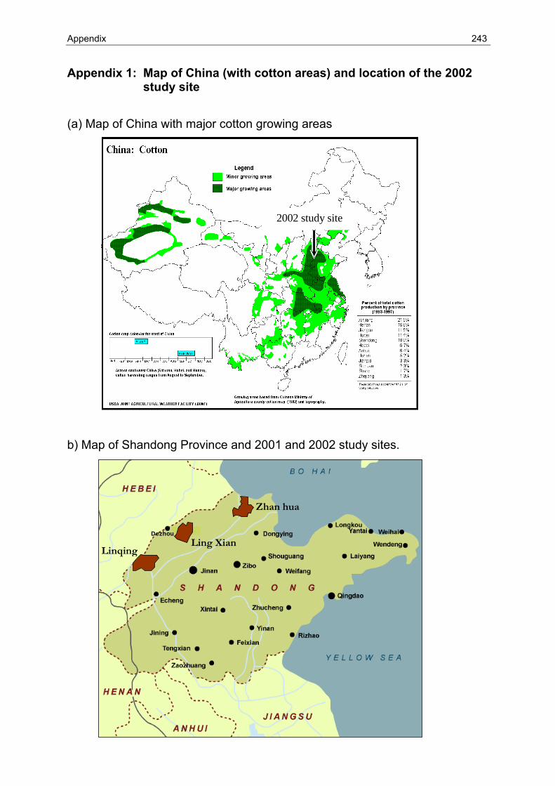
Appendix 243
Appendix 1: Map of China (with cotton areas) and location of the 2002 study site
(a) Map of China with major cotton growing areas
b) Map of Shandong Province and 2001 and 2002 study sites.
2002 study site
Zhan hua
Ling Xian Linqing
Dezhou
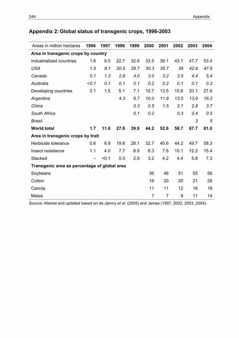
244 Appendix
Appendix 2: Global status of transgenic crops, 1996-2003
Areas in million hectares 1996 1997 1998 1999 2000 2001 2002 2003 2004
Area in transgenic crops by country Industrialized countries 1.6 9.5 22.7 32.8 33.5 39.1 43.1 47.7 53.4
USA 1.5 8.1 20.5 28.7 30.3 35.7 39 42.8 47.6
Canada 0.1 1.3 2.8 4.0 3.0 3.2 3.5 4.4 5.4
Australia <0.1 0.1 0.1 0.1 0.2 0.2 0.1 0.1 0.2
Developing countries 0.1 1.5 5.1 7.1 10.7 13.5 15.6 20.1 27.6
Argentina 4.3 6.7 10.0 11.8 13.5 13.9 16.2
China 0.3 0.5 1.5 2.1 2.8 3.7
South Africa 0.1 0.2 0.3 0.4 0.5
Brasil 3 5
World total 1.7 11.0 27.8 39.9 44.2 52.6 58.7 67.7 81.0Area in transgenic crops by trait Herbicide tolerance 0.6 6.9 19.8 28.1 32.7 40.6 44.2 49.7 58.3
Insect resistance 1.1 4.0 7.7 8.9 8.3 7.8 10.1 12.2 15.4
Stacked – <0.1 0.3 2.9 3.2 4.2 4.4 5.8 7.3
Transgenic area as percentage of global area Soybeans 36 46 51 55 56
Cotton 16 20 20 21 28
Canola 11 11 12 16 19
Maize 7 7 9 11 14Source: Altered and updated based on de Janvry et al. (2005) and James (1997, 2002, 2003, 2004).
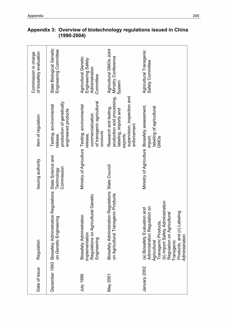
Appendix 245
Appendix 3: Overview of biotechnology regulations issued in China (1990-2004)
Com
mis
sion
in c
harg
e
of b
iosa
fety
eva
luat
ion
Sta
te B
iolo
gica
l Gen
etic
E
ngin
eerin
g C
omm
ittee
Agr
icul
tura
l Gen
etic
E
ngin
eerin
g S
afet
y
Adm
inis
tratio
n C
omm
ittee
Agr
icul
tura
l GM
Os
Join
t M
inis
try C
onfe
renc
e S
yste
m
Agr
icul
tura
l Tra
nsge
nic
S
afet
y C
omm
ittee
Item
of r
egul
atio
n
Tes
ting,
env
ironm
enta
l re
leas
e,
pro
duct
ion
of g
enet
ical
ly
eng
inee
red
prod
ucts
Tes
ting,
env
ironm
enta
l re
leas
e,
com
mer
cial
izat
ion
o
f tra
nsge
nic
agric
ultu
ral
pro
duct
s
Res
earc
h an
d te
stin
g,
pro
duct
ion
and
proc
essi
ng,
labe
ling,
impo
rts a
nd
expo
rts,
sup
ervi
sion
, ins
pect
ion
and
e
nfor
cem
ent
Bio
safe
ty a
sses
smen
t, im
port,
la
belin
g of
agr
icul
tura
l G
MO
s
Issu
ing
auth
ority
Sta
te S
cien
ce a
nd
Tec
hnol
ogy
C
omm
issi
on
Min
istry
of A
gric
ultu
re
Sta
te C
ounc
il
Min
istry
of A
gric
ultu
re
Reg
ulat
ion
Bio
safe
ty A
dmin
istra
tion
Reg
ulat
ions
o
n G
enet
ic E
ngin
eerin
g
Bio
safe
ty A
dmin
istra
tion
Impl
emen
tatio
n R
egul
atio
ns o
n A
gric
ultu
ral G
enet
ic
Eng
inee
ring
Bio
safe
ty A
dmin
istra
tion
Reg
ulat
ions
o
n A
gric
ultu
ral T
rans
geni
c P
rodu
cts
(a) B
iosa
fety
Eva
luat
ion
and
Adm
inis
tratio
n R
egul
atio
n on
A
gric
ultu
ral
Tra
nsge
nic
Pro
duct
s,
(b) I
mpo
rt S
afet
y A
dmin
istra
tion
R
egul
atio
n on
Agr
icul
tura
l Tr
ansg
enic
P
rodu
cts,
and
(c) L
abel
ing
Adm
inis
tratio
n
Dat
e of
issu
e
Dec
embe
r 199
3
Jul
y 19
96
May
200
1
Jan
uary
200
2
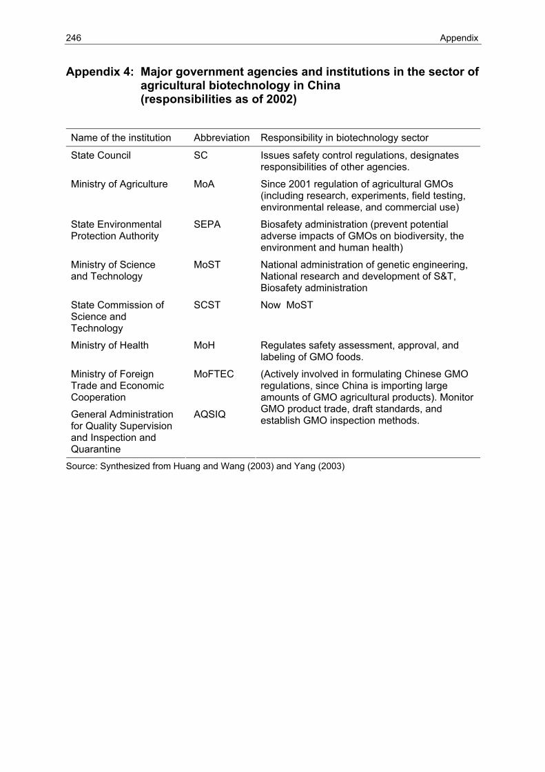
246 Appendix
Appendix 4: Major government agencies and institutions in the sector of agricultural biotechnology in China (responsibilities as of 2002)
Name of the institution Abbreviation Responsibility in biotechnology sector
State Council SC Issues safety control regulations, designates responsibilities of other agencies.
Ministry of Agriculture MoA Since 2001 regulation of agricultural GMOs (including research, experiments, field testing, environmental release, and commercial use)
State Environmental Protection Authority
SEPA Biosafety administration (prevent potential adverse impacts of GMOs on biodiversity, the environment and human health)
Ministry of Science and Technology
MoST National administration of genetic engineering, National research and development of S&T, Biosafety administration
State Commission of Science and Technology
SCST Now MoST
Ministry of Health MoH Regulates safety assessment, approval, and labeling of GMO foods.
Ministry of Foreign Trade and Economic Cooperation
MoFTEC
General Administration for Quality Supervision and Inspection and Quarantine
AQSIQ
(Actively involved in formulating Chinese GMO regulations, since China is importing large amounts of GMO agricultural products). Monitor GMO product trade, draft standards, and establish GMO inspection methods.
Source: Synthesized from Huang and Wang (2003) and Yang (2003)
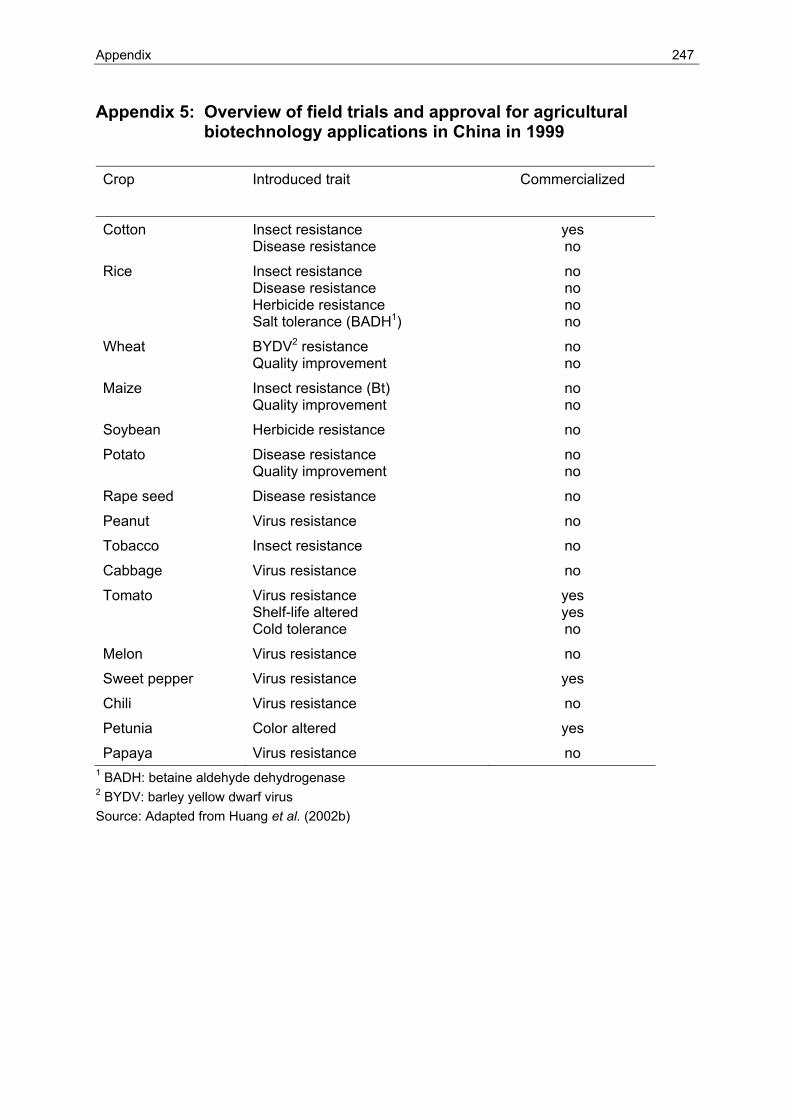
Appendix 247
Appendix 5: Overview of field trials and approval for agricultural biotechnology applications in China in 1999
Crop
Introduced trait Commercialized
Cotton Insect resistance Disease resistance
yes no
Rice Insect resistance Disease resistance Herbicide resistance Salt tolerance (BADH1)
no no no no
Wheat BYDV2 resistance Quality improvement
no no
Maize Insect resistance (Bt) Quality improvement
no no
Soybean Herbicide resistance no
Potato Disease resistance Quality improvement
no no
Rape seed Disease resistance no
Peanut Virus resistance no
Tobacco Insect resistance no
Cabbage Virus resistance no
Tomato Virus resistance Shelf-life altered Cold tolerance
yes yes no
Melon Virus resistance no
Sweet pepper Virus resistance yes
Chili Virus resistance no
Petunia Color altered yes
Papaya Virus resistance no 1 BADH: betaine aldehyde dehydrogenase 2 BYDV: barley yellow dwarf virus Source: Adapted from Huang et al. (2002b)
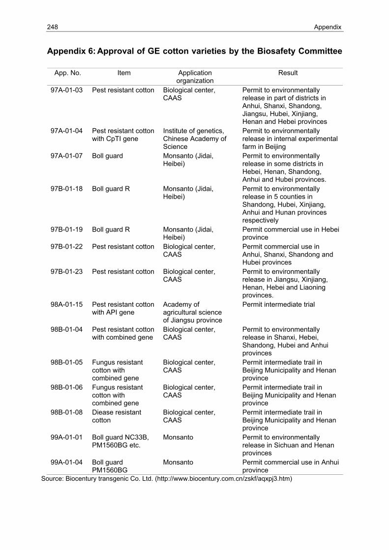
248 Appendix
Appendix 6: Approval of GE cotton varieties by the Biosafety Committee
App. No. Item Application organization
Result
97A-01-03 Pest resistant cotton Biological center, CAAS
Permit to environmentally release in part of districts in Anhui, Shanxi, Shandong, Jiangsu, Hubei, Xinjiang, Henan and Hebei provinces
97A-01-04 Pest resistant cotton with CpTI gene
Institute of genetics, Chinese Academy of Science
Permit to environmentally release in internal experimental farm in Beijing
97A-01-07 Boll guard Monsanto (Jidai, Heibei)
Permit to environmentally release in some districts in Hebei, Henan, Shandong, Anhui and Hubei provinces.
97B-01-18 Boll guard R Monsanto (Jidai, Heibei)
Permit to environmentally release in 5 counties in Shandong, Hubei, Xinjiang, Anhui and Hunan provinces respectively
97B-01-19 Boll guard R Monsanto (Jidai, Heibei)
Permit commercial use in Hebei province
97B-01-22 Pest resistant cotton Biological center, CAAS
Permit commercial use in Anhui, Shanxi, Shandong and Hubei provinces
97B-01-23 Pest resistant cotton Biological center, CAAS
Permit to environmentally release in Jiangsu, Xinjiang, Henan, Hebei and Liaoning provinces.
98A-01-15 Pest resistant cotton with API gene
Academy of agricultural science of Jiangsu province
Permit intermediate trial
98B-01-04 Pest resistant cotton with combined gene
Biological center, CAAS
Permit to environmentally release in Shanxi, Hebei, Shandong, Hubei and Anhui provinces
98B-01-05 Fungus resistant cotton with combined gene
Biological center, CAAS
Permit intermediate trail in Beijing Municipality and Henan province
98B-01-06 Fungus resistant cotton with combined gene
Biological center, CAAS
Permit intermediate trail in Beijing Municipality and Henan province
98B-01-08 Diease resistant cotton
Biological center, CAAS
Permit intermediate trail in Beijing Municipality and Henan province
99A-01-01 Boll guard NC33B, PM1560BG etc.
Monsanto Permit to environmentally release in Sichuan and Henan provinces
99A-01-04 Boll guard PM1560BG
Monsanto Permit commercial use in Anhui province
Source: Biocentury transgenic Co. Ltd. (http://www.biocentury.com.cn/zskf/aqxpj3.htm)
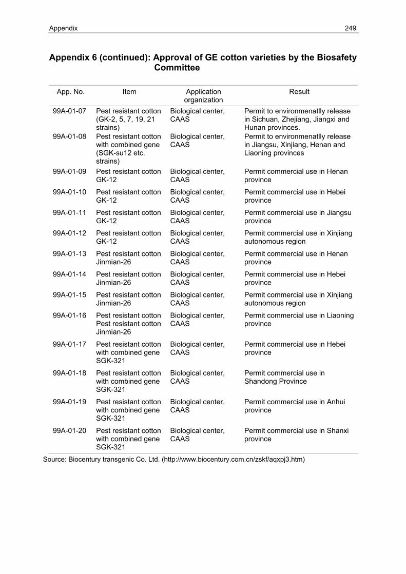
Appendix 249
Appendix 6 (continued): Approval of GE cotton varieties by the Biosafety Committee
App. No. Item Application organization
Result
99A-01-07 Pest resistant cotton (GK-2, 5, 7, 19, 21 strains)
Biological center, CAAS
Permit to environmenatlly release in Sichuan, Zhejiang, Jiangxi and Hunan provinces.
99A-01-08 Pest resistant cotton with combined gene (SGK-su12 etc. strains)
Biological center, CAAS
Permit to environmenatlly release in Jiangsu, Xinjiang, Henan and Liaoning provinces
99A-01-09 Pest resistant cotton GK-12
Biological center, CAAS
Permit commercial use in Henan province
99A-01-10 Pest resistant cotton GK-12
Biological center, CAAS
Permit commercial use in Hebei province
99A-01-11 Pest resistant cotton GK-12
Biological center, CAAS
Permit commercial use in Jiangsu province
99A-01-12 Pest resistant cotton GK-12
Biological center, CAAS
Permit commercial use in Xinjiang autonomous region
99A-01-13 Pest resistant cotton Jinmian-26
Biological center, CAAS
Permit commercial use in Henan province
99A-01-14 Pest resistant cotton Jinmian-26
Biological center, CAAS
Permit commercial use in Hebei province
99A-01-15 Pest resistant cotton Jinmian-26
Biological center, CAAS
Permit commercial use in Xinjiang autonomous region
99A-01-16 Pest resistant cotton Pest resistant cotton Jinmian-26
Biological center, CAAS
Permit commercial use in Liaoning province
99A-01-17 Pest resistant cotton with combined gene SGK-321
Biological center, CAAS
Permit commercial use in Hebei province
99A-01-18 Pest resistant cotton with combined gene SGK-321
Biological center, CAAS
Permit commercial use in Shandong Province
99A-01-19 Pest resistant cotton with combined gene SGK-321
Biological center, CAAS
Permit commercial use in Anhui province
99A-01-20 Pest resistant cotton with combined gene SGK-321
Biological center, CAAS
Permit commercial use in Shanxi province
Source: Biocentury transgenic Co. Ltd. (http://www.biocentury.com.cn/zskf/aqxpj3.htm)
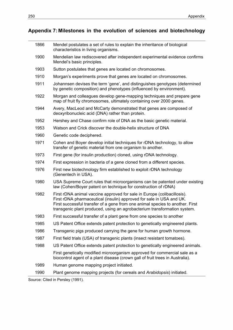
250 Appendix
Appendix 7: Milestones in the evolution of sciences and biotechnology
1866 Mendel postulates a set of rules to explain the inheritance of biological characteristics in living organisms.
1900 Mendelian law rediscovered after independent experimental evidence confirms Mendel’s basic principles.
1903 Sutton postulates that genes are located on chromosomes.
1910 Morgan’s experiments prove that genes are located on chromosomes.
1911 Johannsen devises the term ‘gene’, and distinguishes genotypes (determined by genetic composition) and phenotypes (influenced by environment).
1922 Morgan and colleagues develop gene-mapping techniques and prepare gene map of fruit fly chromosomes, ultimately containing over 2000 genes.
1944 Avery, MacLeod and McCarty demonstrated that genes are composed of deoxyribonucleic acid (DNA) rather than protein.
1952 Hershey and Chase confirm role of DNA as the basic genetic material.
1953 Watson and Crick discover the double-helix structure of DNA
1960 Genetic code deciphered.
1971 Cohen and Boyer develop initial techniques for rDNA technology, to allow transfer of genetic material from one organism to another.
1973 First gene (for insulin production) cloned, using rDNA technology.
1974 First expression in bacteria of a gene cloned from a different species.
1976 First new biotechnology firm established to exploit rDNA technology (Genentech in USA).
1980 USA Supreme Court rules that microorganisms can be patented under existing law (Cohen/Boyer patent on technique for construction of rDNA)
1982 First rDNA animal vaccine approved for sale in Europe (colibacillosis). First rDNA pharmaceutical (insulin) approved for sale in USA and UK. First successful transfer of a gene from one animal species to another. First transgenic plant produced, using an agrobacterium transformation system.
1983 First successful transfer of a plant gene from one species to another
1985 US Patent Office extends patent protection to genetically engineered plants.
1986 Transgenic pigs produced carrying the gene for human growth hormone.
1987 First field trials (USA) of transgenic plants (insect resistant tomatoes).
1988 US Patent Office extends patent protection to genetically engineered animals.
First genetically modified microorganism approved for commercial sale as a biocontrol agent of a plant disease (crown gall of fruit trees in Australia).
1989 Human genome mapping project initiated.
1990 Plant genome mapping projects (for cereals and Arabidopsis) initiated. Source: Cited in Persley (1991).
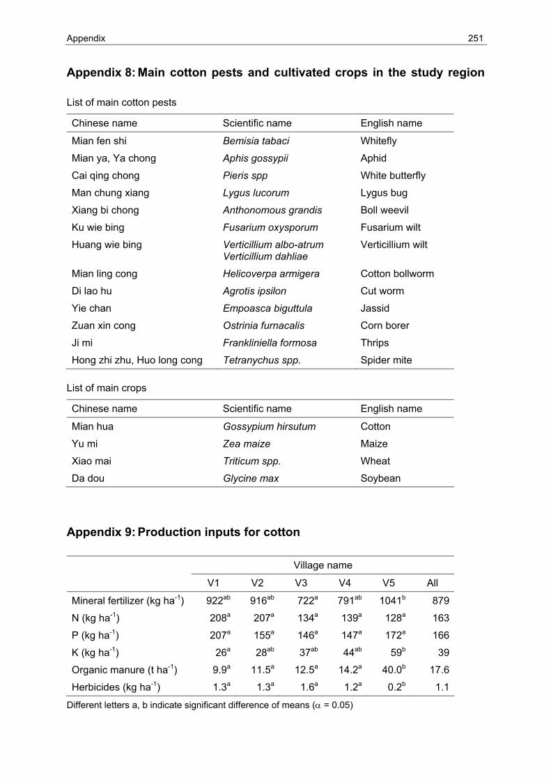
Appendix 251
Appendix 8: Main cotton pests and cultivated crops in the study region
List of main cotton pests
Chinese name Scientific name English name
Mian fen shi Bemisia tabaci Whitefly
Mian ya, Ya chong Aphis gossypii Aphid
Cai qing chong Pieris spp White butterfly
Man chung xiang Lygus lucorum Lygus bug
Xiang bi chong Anthonomous grandis Boll weevil
Ku wie bing Fusarium oxysporum Fusarium wilt
Huang wie bing Verticillium albo-atrum Verticillium dahliae
Verticillium wilt
Mian ling cong Helicoverpa armigera Cotton bollworm
Di lao hu Agrotis ipsilon Cut worm
Yie chan Empoasca biguttula Jassid
Zuan xin cong Ostrinia furnacalis Corn borer
Ji mi Frankliniella formosa Thrips
Hong zhi zhu, Huo long cong Tetranychus spp. Spider mite List of main crops
Chinese name Scientific name English name
Mian hua Gossypium hirsutum Cotton
Yu mi Zea maize Maize
Xiao mai Triticum spp. Wheat
Da dou Glycine max Soybean
Appendix 9: Production inputs for cotton
Village name
V1 V2 V3 V4 V5 All
Mineral fertilizer (kg ha-1) 922ab 916ab 722a 791ab 1041b 879
N (kg ha-1) 208a 207a 134a 139a 128a 163
P (kg ha-1) 207a 155a 146a 147a 172a 166
K (kg ha-1) 26a 28ab 37ab 44ab 59b 39
Organic manure (t ha-1) 9.9a 11.5a 12.5a 14.2a 40.0b 17.6
Herbicides (kg ha-1) 1.3a 1.3a 1.6a 1.2a 0.2b 1.1
Different letters a, b indicate significant difference of means (α = 0.05)
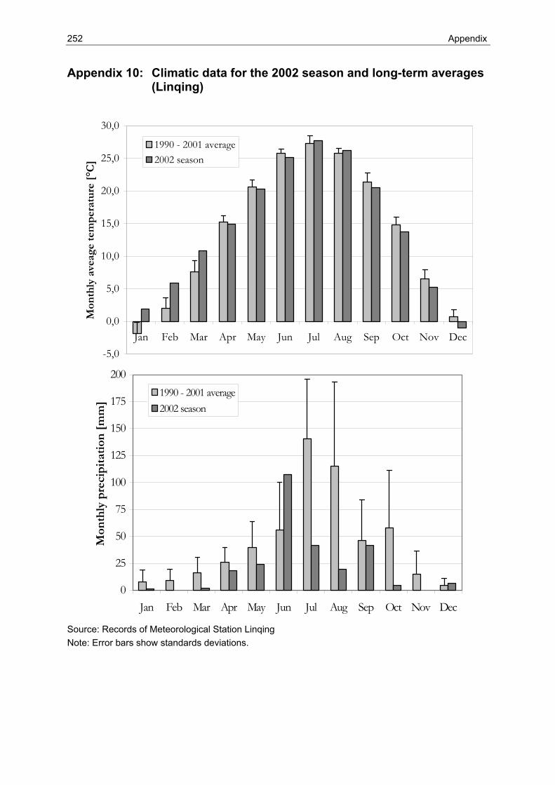
252 Appendix
Appendix 10: Climatic data for the 2002 season and long-term averages (Linqing)
-5,0
0,0
5,0
10,0
15,0
20,0
25,0
30,0
Jan Feb Mar Apr May Jun Jul Aug Sep Oct Nov Dec
Mon
thly
ave
age
tem
per
atu
re [
°C]
1990 - 2001 average2002 season
0
25
50
75
100
125
150
175
200
Jan Feb Mar Apr May Jun Jul Aug Sep Oct Nov Dec
Mon
thly
pre
cip
itat
ion
[m
m]
1990 - 2001 average2002 season
Source: Records of Meteorological Station Linqing Note: Error bars show standards deviations.
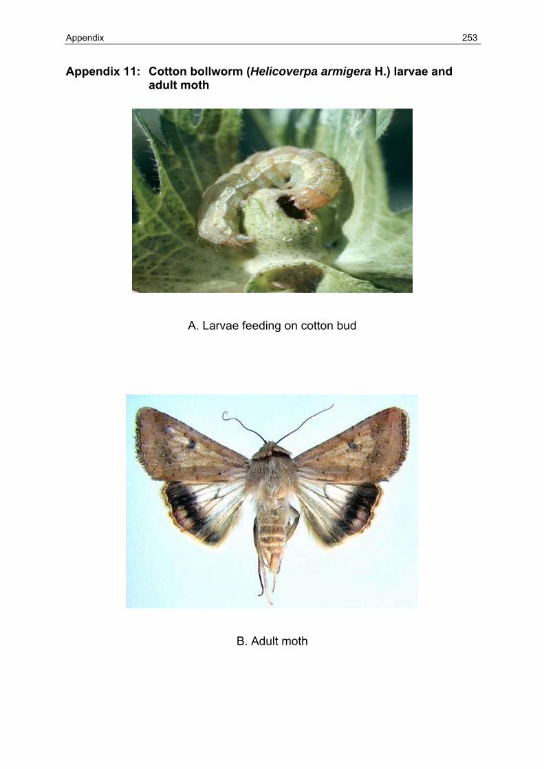
Appendix 253
Appendix 11: Cotton bollworm (Helicoverpa armigera H.) larvae and adult moth
A. Larvae feeding on cotton bud
B. Adult moth
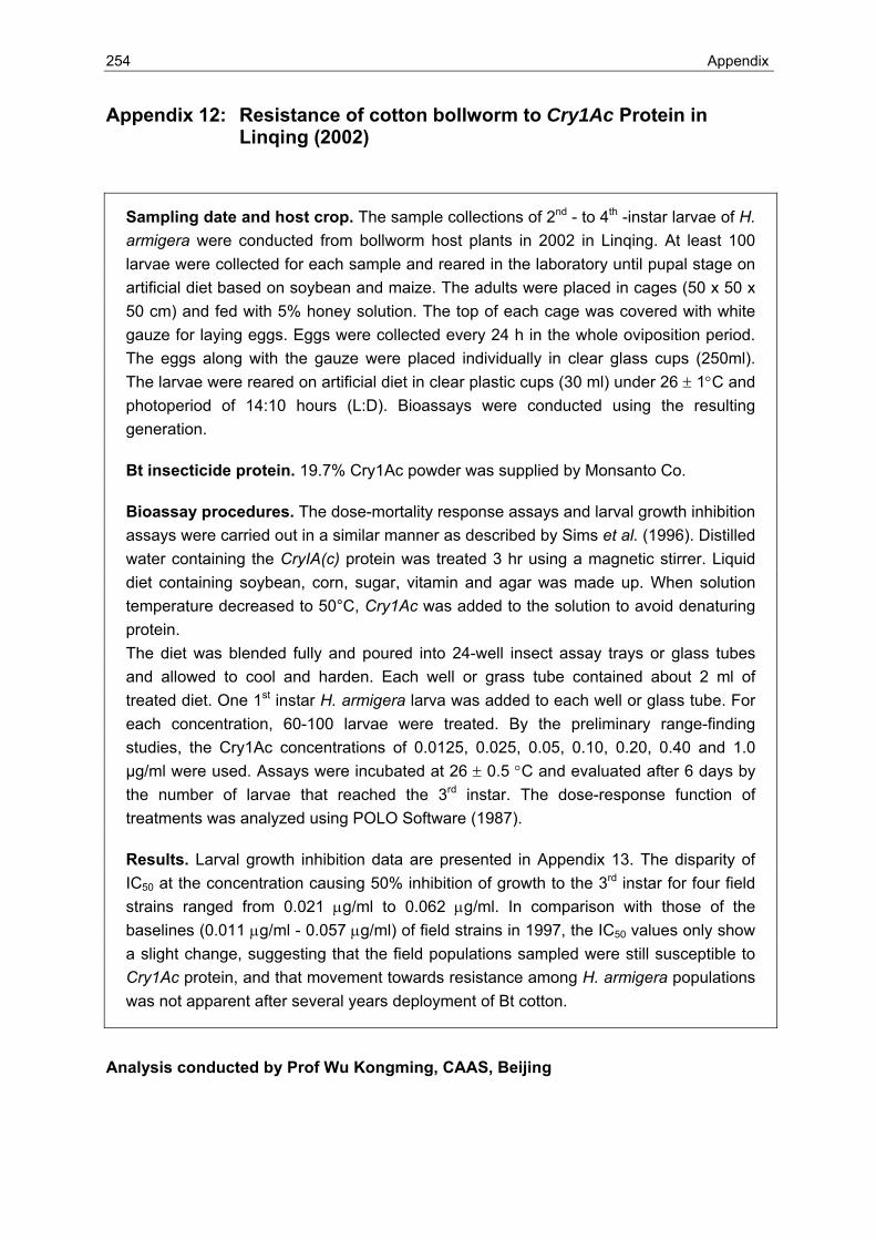
254 Appendix
Appendix 12: Resistance of cotton bollworm to Cry1Ac Protein in Linqing (2002)
Sampling date and host crop. The sample collections of 2nd - to 4th -instar larvae of H. armigera were conducted from bollworm host plants in 2002 in Linqing. At least 100 larvae were collected for each sample and reared in the laboratory until pupal stage on artificial diet based on soybean and maize. The adults were placed in cages (50 x 50 x 50 cm) and fed with 5% honey solution. The top of each cage was covered with white gauze for laying eggs. Eggs were collected every 24 h in the whole oviposition period. The eggs along with the gauze were placed individually in clear glass cups (250ml). The larvae were reared on artificial diet in clear plastic cups (30 ml) under 26 ± 1°C and photoperiod of 14:10 hours (L:D). Bioassays were conducted using the resulting generation.
Bt insecticide protein. 19.7% Cry1Ac powder was supplied by Monsanto Co.
Bioassay procedures. The dose-mortality response assays and larval growth inhibition assays were carried out in a similar manner as described by Sims et al. (1996). Distilled water containing the CryIA(c) protein was treated 3 hr using a magnetic stirrer. Liquid diet containing soybean, corn, sugar, vitamin and agar was made up. When solution temperature decreased to 50°C, Cry1Ac was added to the solution to avoid denaturing protein. The diet was blended fully and poured into 24-well insect assay trays or glass tubes and allowed to cool and harden. Each well or grass tube contained about 2 ml of treated diet. One 1st instar H. armigera larva was added to each well or glass tube. For each concentration, 60-100 larvae were treated. By the preliminary range-finding studies, the Cry1Ac concentrations of 0.0125, 0.025, 0.05, 0.10, 0.20, 0.40 and 1.0 μg/ml were used. Assays were incubated at 26 ± 0.5 °C and evaluated after 6 days by the number of larvae that reached the 3rd instar. The dose-response function of treatments was analyzed using POLO Software (1987).
Results. Larval growth inhibition data are presented in Appendix 13. The disparity of IC50 at the concentration causing 50% inhibition of growth to the 3rd instar for four field strains ranged from 0.021 μg/ml to 0.062 μg/ml. In comparison with those of the baselines (0.011 μg/ml - 0.057 μg/ml) of field strains in 1997, the IC50 values only show a slight change, suggesting that the field populations sampled were still susceptible to Cry1Ac protein, and that movement towards resistance among H. armigera populations was not apparent after several years deployment of Bt cotton.
Analysis conducted by Prof Wu Kongming, CAAS, Beijing
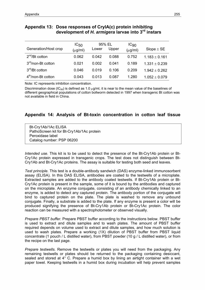
Appendix 255
Appendix 13: Dose responses of CryIA(c) protein inhibiting development of H. armigera larvae into 3rd instars
Generation/Host crop
IC50 (μg/ml)
95% EL Lower Upper
IC90 (μg/ml)
Slope ± SE
2nd/Bt cotton 0.062 0.042 0.088 0.752 1.183 ± 0.161
3rd/non-Bt cotton 0.021 0.002 0.041 0.189 1.331 ± 0.239
3rd/Bt cotton 0.046 0.019 0.106 0.209 1.942 ± 0.262
4th/non-Bt cotton 0.043 0.013 0.087 1.280 1.052 ± 0.079 Note: IC represents inhibition concentration. Discrimination dose (IC99) is defined as 1.0 μg/ml, it is near to the mean value of the baselines of different geographical populations of cotton bollworm detected in 1997 when transgenic Bt cotton was not available in field in China.
Appendix 14: Analysis of Bt-toxin concentration in cotton leaf tissue
Bt-Cry1Ab/1Ac ELISA PathoScreen kit for Bt-Cry1Ab/1Ac protein Peroxidase label Catalog number: PSP 06200
Intended use. This kit is to be used to detect the presence of the Bt-Cry1Ab protein or Bt-Cry1Ac protein expressed in transgenic crops. The test does not distinguish between Bt-Cry1Ab and Bt-Cry1Ac proteins. The assay is suitable for testing both seed and leaves. Test principle. This test is a double-antibody sandwich (DAS) enzyme-linked immunosorbent assay (ELISA). In this DAS ELISA, antibodies are coated to the testwells of a microplate. Extracted samples are added to the antibody coated testwells. If Bt-Cry1Ab protein or Bt-Cry1Ac protein is present in the sample, some of it is bound by the antibodies and captured on the microplate. An enzyme conjugate, consisting of an antibody chemically linked to an enzyme, is added to detect any captured protein. The antibody portion of the conjugate will bind to captured protein on the plate. The plate is washed to remove any unbound conjugate. Finally, a substrate is added to the plate. If any enzyme is present a color will be produced signifying the presence of Bt-Cry1Ab protein or Bt-Cry1Ac protein. The color reaction can be measured with a spectrophotometer or observed visually. Prepare PBST buffer. Prepare PBST buffer according to the instructions below. PBST buffer is used to extract and dilute samples and to wash plates. The amount of PBST buffer required depends on volume used to extract and dilute samples, and how much solution is used to wash plates. Prepare a working (1X) dilution of PBST buffer from PBST liquid concentrate (1 pouch / L distilled water), from PBST powder (10 g / L distilled water), or from the recipe on the last page. Prepare testwells. Remove the testwells or plates you will need from the packaging. Any remaining testwells or plates should be returned to the packaging containing desiccant, sealed and stored at 4° C. Prepare a humid box by lining an airtight container with a wet paper towel. Keeping testwells in a humid box during incubation will help prevent samples
256 Appendix
from evaporating. Make a copy of the loading diagram and record the locations of your samples and controls. Prepare samples. For leaf samples you can use Agdia's sample extraction bags (catalog no. ACC 00930), a mortar and pestle, or other grinding devices to help extract samples. Wash and rinse grinding equipment thoroughly between samples. Grind leaf samples and dilute extracts with PBST buffer to a ratio of 1:10 (w/v). Prepare controls. Reconstitute the bottle of lyophilized positive control and negative control with 2 ml PBST buffer. Make control aliquots. After preparing the positive and negative control, divide them into aliquots, each sufficient for one use. Dispense aliquots into tubes that can be securely capped. If you will be using a control in one well each time you run the test, prepare 120 µl aliquots. Control aliquots must be stored frozen (-20° C freezer or household freezer). Do not thaw until just before use. At the time of each test run, remove from storage only the aliquots that will be used. Allow the tubes to thaw and mix the contents thoroughly. At the time you add sample extracts to testwells, add the same volume of negative and positive control to the appropriate control wells. Do not refreeze controls. Test procedure 1. Add enzyme conjugate. Dispense 100 µl of enzyme conjugate per well. 2. Dispense samples/controls. Following your loading diagram, dispense 100 µl of each prepared sample into the appropriate testwells of the ELISA plate. Add 100 µl of each positive and negative control into the appropriate testwell. 3. Incubate plate. Set the plate inside a humid box and incubate 2 hours at room temperature or overnight in the refrigerator (4° C). 4. Wash plate. When the incubation with the sample is complete, wash the plate. While squeezing the long sides of the frame to hold the strips in place, use a quick flipping motion to empty the contents of the wells into a sink or waste container. Fill all the wells to overflowing with 1X PBST wash buffer, then quickly empty them again. Repeat 6-7 times. If using an automatic plate washer please be sure that the machine is at the appropriate settings for washing flat bottom plates. 5. Soak plate. Fill each well with 1X PBST wash buffer and allow to sit for at least 1 minute. Empty the wells with a quick flipping motion. Then hold the frame upside down and tap firmly on a folded paper towel to remove the remaining drops of buffer from the wells. 6. Add substrate solution. Dispense 100 µl of the TMB substrate solution into each well of the plate. Set plate aside and wait for color development. 7. Measure color. Color will develop between 5 and 15 minutes. Measure the optical density of the testwells on a plate reader at 650 nm or visually. Wells in which a blue color develops indicate positive results. Wells which remain clear or very light blue indicate negative results. If either control well does not show the appropriate color, disregard results. Optional: Add stop solution. At the end of the 15 minute incubation with TMB substrate, add 50 µl of 3M sulfuric acid to each testwell. Measure the optical density of the testwells on a plate reader at 450 nm.
PBST wash buffer recipe. Dissolve in distilled water to 1000 ml:
Sodium chloride 8.0 g Sodium phosphate, dibasic (anhydrous) 1.15 g Potassium phosphate, monobasic (anhydrous) 0.2 g Potassium chloride 0.2 g Tween-20 0.5 g
Adjust pH to 7.4 Source: Agdia product documentation, www.agdia.com
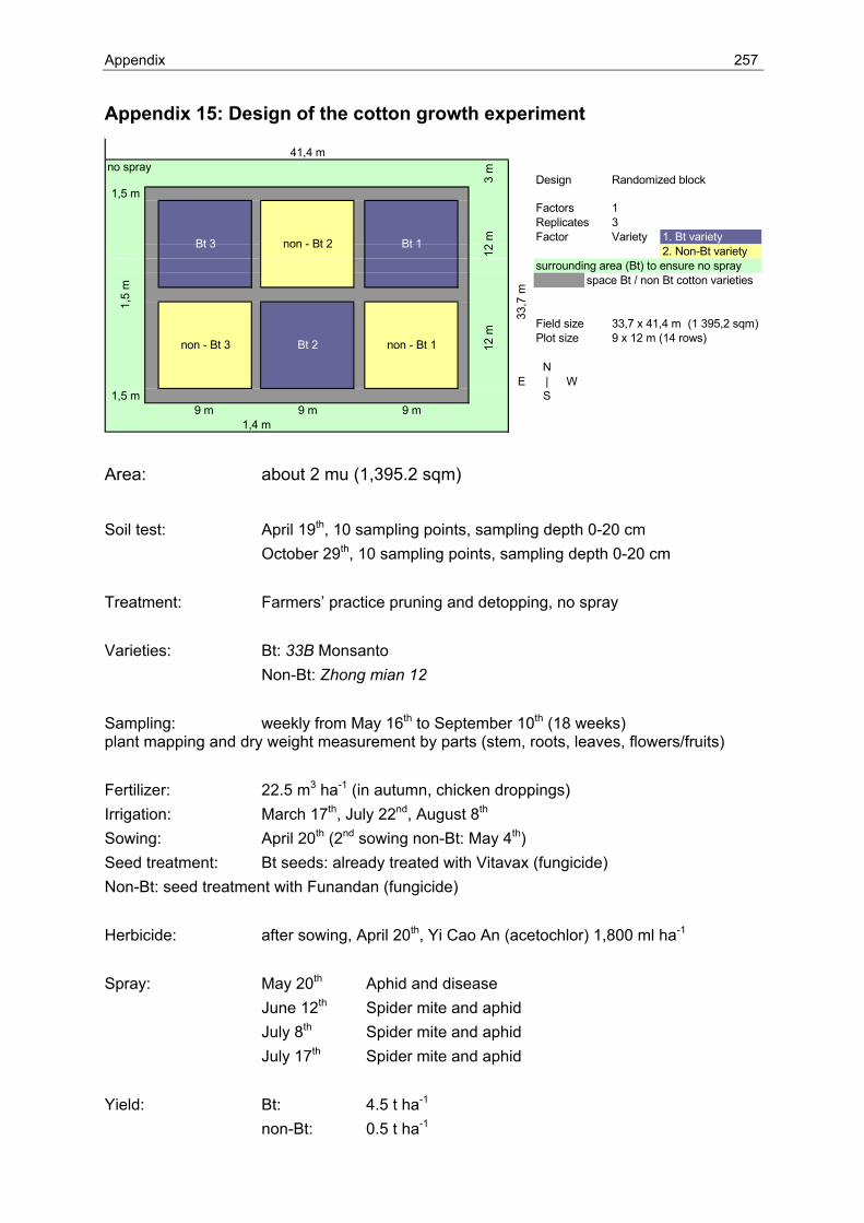
Appendix 257
41,4 mno spray
Design Randomized block1,5 m
Factors 1Replicates 3Factor Variety 1. Bt variety
2. Non-Bt varietysurrounding area (Bt) to ensure no spray
space Bt / non Bt cotton varieties
Field size 33,7 x 41,4 m (1 395,2 sqm)Plot size 9 x 12 m (14 rows)
NE | W
1,5 m S9 m 9 m 9 m
33,7
m
1,5
m
3 m
non - Bt 2 Bt 1
12 m
12 m
non - Bt 1Bt 2
Bt 3
non - Bt 3
1,4 m
Appendix 15: Design of the cotton growth experiment
Area: about 2 mu (1,395.2 sqm) Soil test: April 19th, 10 sampling points, sampling depth 0-20 cm October 29th, 10 sampling points, sampling depth 0-20 cm Treatment: Farmers’ practice pruning and detopping, no spray Varieties: Bt: 33B Monsanto Non-Bt: Zhong mian 12 Sampling: weekly from May 16th to September 10th (18 weeks) plant mapping and dry weight measurement by parts (stem, roots, leaves, flowers/fruits) Fertilizer: 22.5 m3 ha-1 (in autumn, chicken droppings) Irrigation: March 17th, July 22nd, August 8th Sowing: April 20th (2nd sowing non-Bt: May 4th) Seed treatment: Bt seeds: already treated with Vitavax (fungicide) Non-Bt: seed treatment with Funandan (fungicide) Herbicide: after sowing, April 20th, Yi Cao An (acetochlor) 1,800 ml ha-1 Spray: May 20th Aphid and disease June 12th Spider mite and aphid July 8th Spider mite and aphid July 17th Spider mite and aphid Yield: Bt: 4.5 t ha-1 non-Bt: 0.5 t ha-1
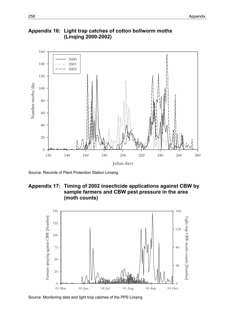
258 Appendix
Appendix 16: Light trap catches of cotton bollworm moths (Linqing 2000-2002)
2002 DD vs y2002
Julian days
120 140 160 180 200 220 240 260 280
Num
ber m
oths
/day
0
20
40
60
80
100
120
140
160
2000 2001 2002
Source: Records of Plant Protection Station Linqing.
Appendix 17: Timing of 2002 insecticide applications against CBW by sample farmers and CBW pest pressure in the area (moth counts)
01-May 01-Jun 01-Jul 01-Aug 01-Sep 01-Oct
Farm
ers s
pray
ing
again
st C
BW [N
umbe
r]
0
25
50
75
100
125
150
Light trap CBW m
oths counts [Num
ber]
0
40
80
120
160
Source: Monitoring data and light trop catches of the PPS Linqing
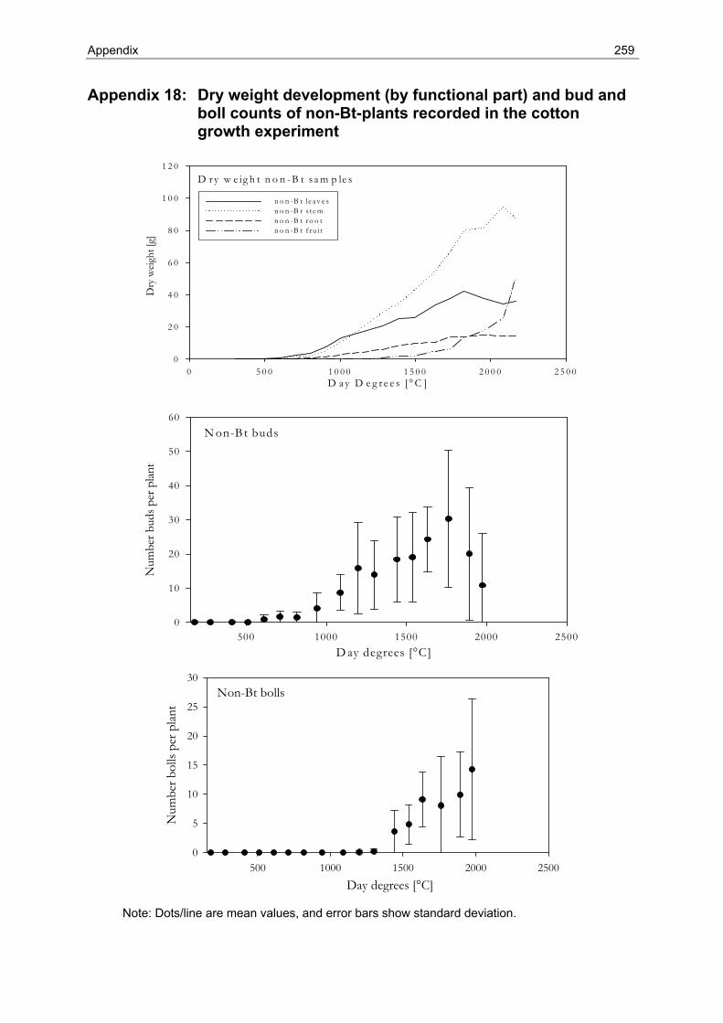
Appendix 259
Appendix 18: Dry weight development (by functional part) and bud and boll counts of non-Bt-plants recorded in the cotton growth experiment
D ry w e ig h t n o n -B t s a m p le s
D a y D e g r e e s [ ° C ]0 5 0 0 1 0 0 0 1 5 0 0 2 0 0 0 2 5 0 0
Dry
weig
ht [g
]
0
2 0
4 0
6 0
8 0
1 0 0
1 2 0
n o n -B t le a v e sn o n -B t s t e mn o n -B t ro o tn o n -B t f r u it
N on-Bt buds
D ay degrees [°C]500 1000 1500 2000 2500
Num
ber b
uds p
er p
lant
0
10
20
30
40
50
60
Non-Bt bolls
Day degrees [°C]500 1000 1500 2000 2500
Num
ber b
olls
per p
lant
0
5
10
15
20
25
30
Note: Dots/line are mean values, and error bars show standard deviation.
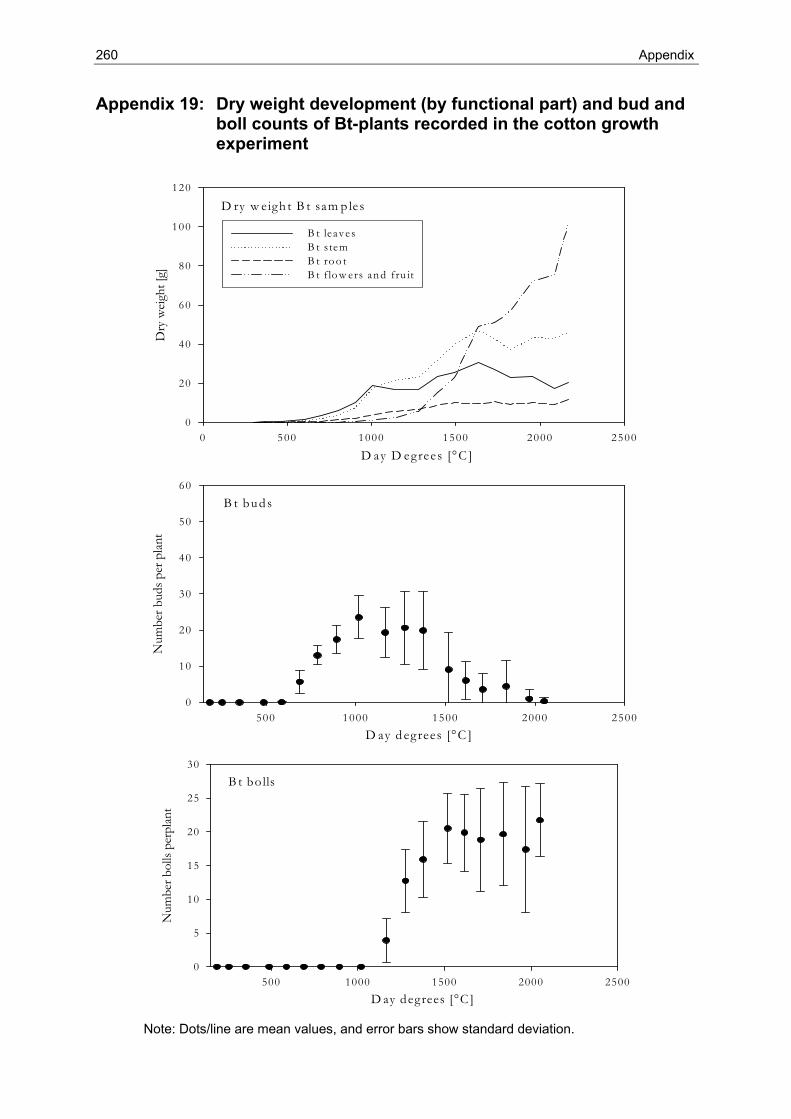
260 Appendix
Appendix 19: Dry weight development (by functional part) and bud and boll counts of Bt-plants recorded in the cotton growth experiment
D ry w e igh t B t sam p les
D ay D egrees [°C ]0 500 1000 1500 2000 2500
Dry
wei
ght [
g]
0
20
40
60
80
100
120
B t leaves B t s tem B t ro o t B t f lo w ers an d fru it
B t buds
D ay degrees [°C ]500 1000 1500 2000 2500
Num
ber b
uds p
er p
lant
0
10
20
30
40
50
60
B t bolls
D ay degrees [°C ]500 1000 1500 2000 2500
Num
ber b
olls
perp
lant
0
5
10
15
20
25
30
Note: Dots/line are mean values, and error bars show standard deviation.
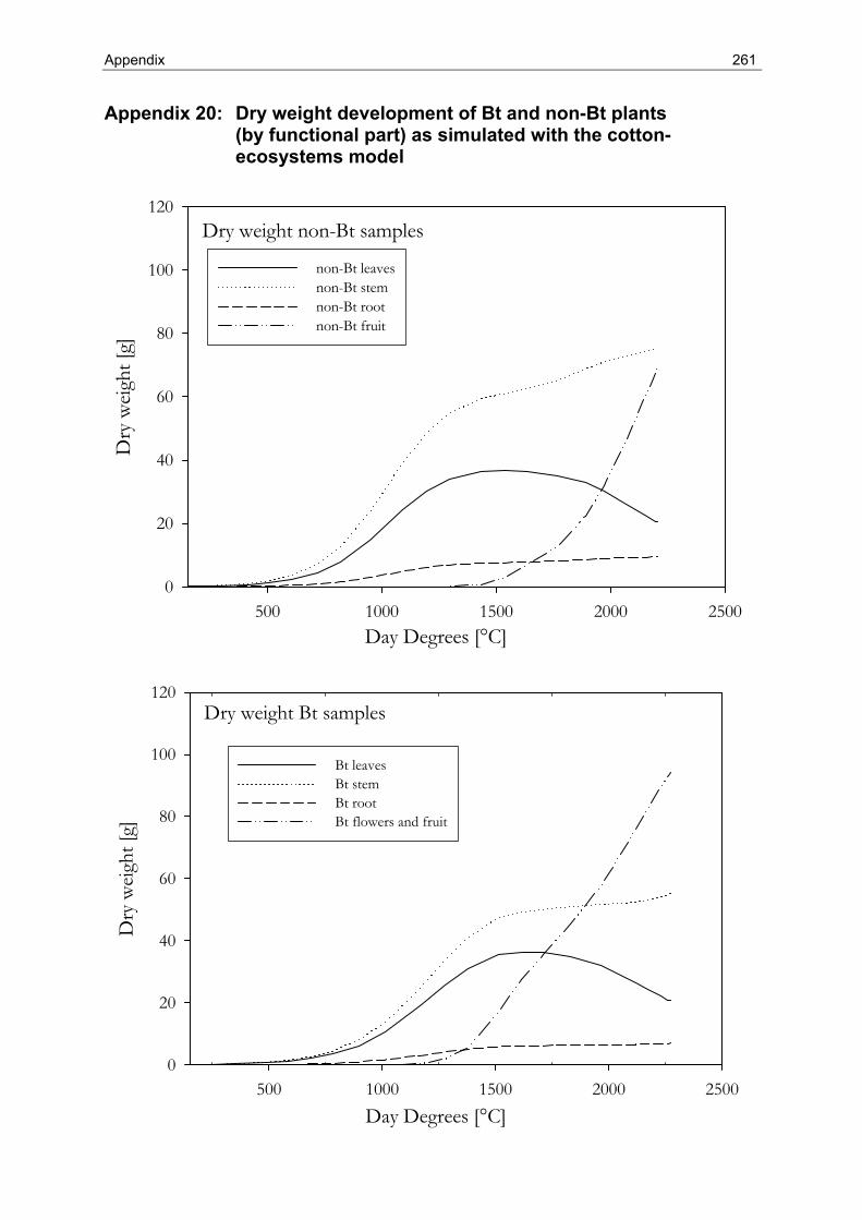
Appendix 261
Appendix 20: Dry weight development of Bt and non-Bt plants (by functional part) as simulated with the cotton- ecosystems model
Dry weight non-Bt samples
Day Degrees [°C]500 1000 1500 2000 2500
Dry
weig
ht [g
]
0
20
40
60
80
100
120
non-Bt leavesnon-Bt stemnon-Bt rootnon-Bt fruit
Dry weight Bt samples
Day Degrees [°C]500 1000 1500 2000 2500
Dry
weig
ht [g
]
0
20
40
60
80
100
120
Bt leaves Bt stem Bt root Bt flowers and fruit
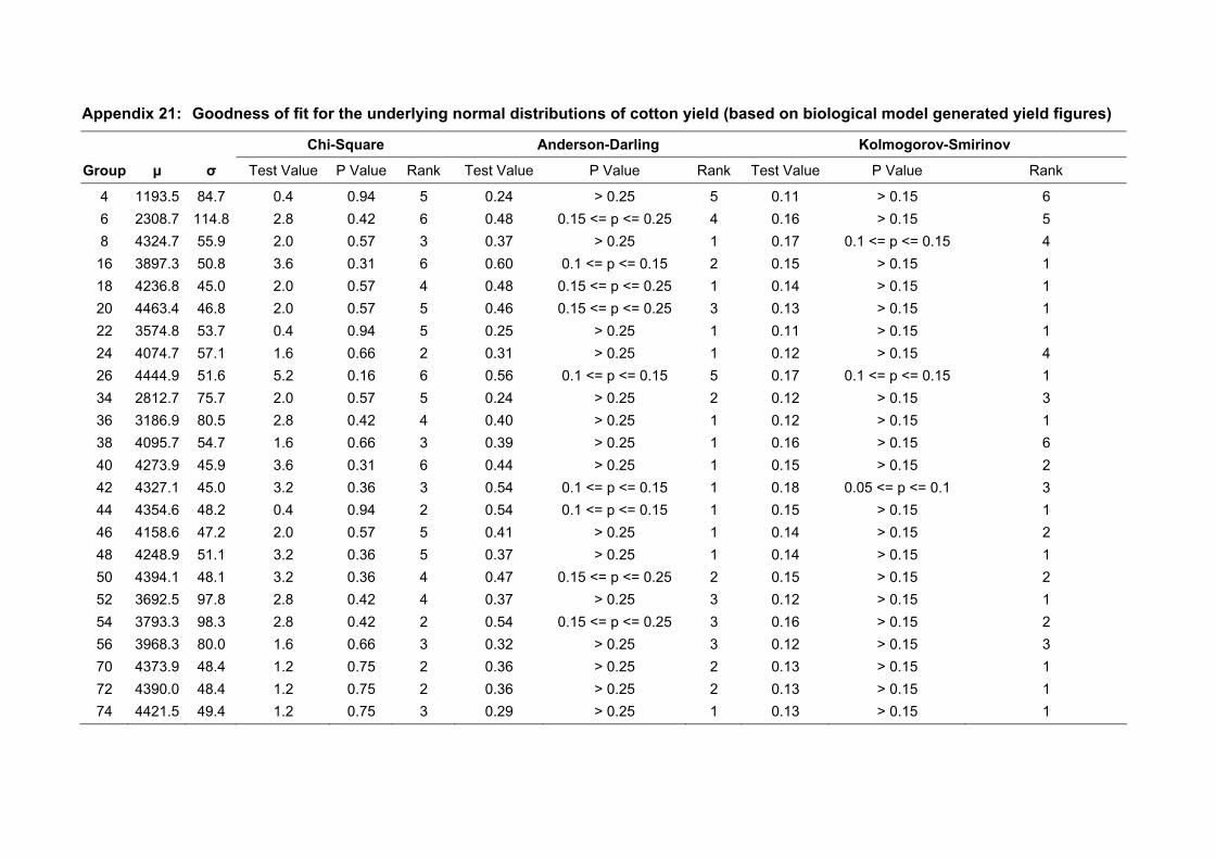
Appendix 21: Goodness of fit for the underlying normal distributions of cotton yield (based on biological model generated yield figures)
Chi-Square Anderson-Darling Kolmogorov-Smirinov
Group μ σ Test Value P Value Rank Test Value P Value Rank Test Value P Value Rank
4 1193.5 84.7 0.4 0.94 5 0.24 > 0.25 5 0.11 > 0.15 6 6 2308.7 114.8 2.8 0.42 6 0.48 0.15 <= p <= 0.25 4 0.16 > 0.15 5 8 4324.7 55.9 2.0 0.57 3 0.37 > 0.25 1 0.17 0.1 <= p <= 0.15 4 16 3897.3 50.8 3.6 0.31 6 0.60 0.1 <= p <= 0.15 2 0.15 > 0.15 1 18 4236.8 45.0 2.0 0.57 4 0.48 0.15 <= p <= 0.25 1 0.14 > 0.15 1 20 4463.4 46.8 2.0 0.57 5 0.46 0.15 <= p <= 0.25 3 0.13 > 0.15 1 22 3574.8 53.7 0.4 0.94 5 0.25 > 0.25 1 0.11 > 0.15 1 24 4074.7 57.1 1.6 0.66 2 0.31 > 0.25 1 0.12 > 0.15 4 26 4444.9 51.6 5.2 0.16 6 0.56 0.1 <= p <= 0.15 5 0.17 0.1 <= p <= 0.15 1 34 2812.7 75.7 2.0 0.57 5 0.24 > 0.25 2 0.12 > 0.15 3 36 3186.9 80.5 2.8 0.42 4 0.40 > 0.25 1 0.12 > 0.15 1 38 4095.7 54.7 1.6 0.66 3 0.39 > 0.25 1 0.16 > 0.15 6 40 4273.9 45.9 3.6 0.31 6 0.44 > 0.25 1 0.15 > 0.15 2 42 4327.1 45.0 3.2 0.36 3 0.54 0.1 <= p <= 0.15 1 0.18 0.05 <= p <= 0.1 3 44 4354.6 48.2 0.4 0.94 2 0.54 0.1 <= p <= 0.15 1 0.15 > 0.15 1 46 4158.6 47.2 2.0 0.57 5 0.41 > 0.25 1 0.14 > 0.15 2 48 4248.9 51.1 3.2 0.36 5 0.37 > 0.25 1 0.14 > 0.15 1 50 4394.1 48.1 3.2 0.36 4 0.47 0.15 <= p <= 0.25 2 0.15 > 0.15 2 52 3692.5 97.8 2.8 0.42 4 0.37 > 0.25 3 0.12 > 0.15 1 54 3793.3 98.3 2.8 0.42 2 0.54 0.15 <= p <= 0.25 3 0.16 > 0.15 2 56 3968.3 80.0 1.6 0.66 3 0.32 > 0.25 3 0.12 > 0.15 3 70 4373.9 48.4 1.2 0.75 2 0.36 > 0.25 2 0.13 > 0.15 1 72 4390.0 48.4 1.2 0.75 2 0.36 > 0.25 2 0.13 > 0.15 1 74 4421.5 49.4 1.2 0.75 3 0.29 > 0.25 1 0.13 > 0.15 1
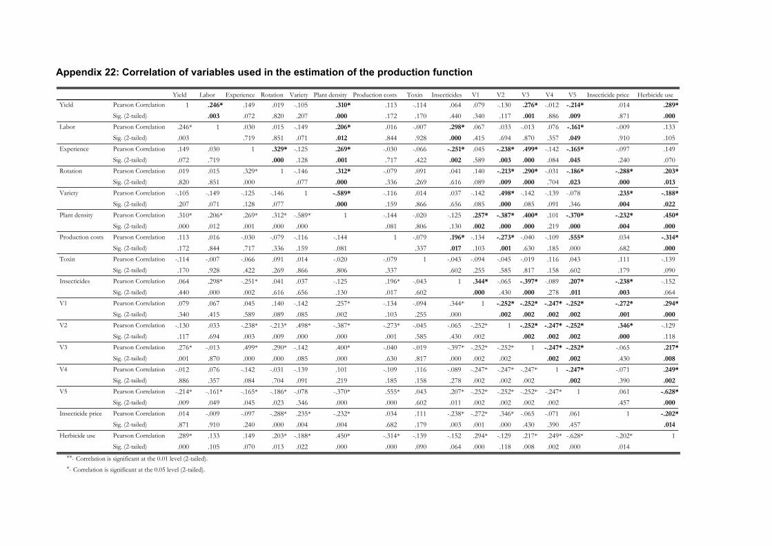
Appendix 22: Correlation of variables used in the estimation of the production function
1 .246* .149 .019 -.105 .310* .113 -.114 .064 .079 -.130 .276* -.012 -.214* .014 .289*
.003 .072 .820 .207 .000 .172 .170 .440 .340 .117 .001 .886 .009 .871 .000
.246** 1 .030 .015 -.149 .206* .016 -.007 .298* .067 .033 -.013 .076 -.161* -.009 .133
.003 .719 .851 .071 .012 .844 .928 .000 .415 .694 .870 .357 .049 .910 .105
.149 .030 1 .329** -.125 .269* -.030 -.066 -.251* .045 -.238* .499* -.142 -.165* -.097 .149
.072 .719 .000 .128 .001 .717 .422 .002 .589 .003 .000 .084 .045 .240 .070
.019 .015 .329** 1 -.146 .312* -.079 .091 .041 .140 -.213* .290* -.031 -.186* -.288* .203*
.820 .851 .000 .077 .000 .336 .269 .616 .089 .009 .000 .704 .023 .000 .013
-.105 -.149 -.125 -.146 1 -.589* -.116 .014 .037 -.142 .498* -.142 -.139 -.078 .235* -.188*
.207 .071 .128 .077 .000 .159 .866 .656 .085 .000 .085 .091 .346 .004 .022
.310** .206* .269** .312** -.589** 1 -.144 -.020 -.125 .257** -.387* .400* .101 -.370* -.232* .450*
.000 .012 .001 .000 .000 .081 .806 .130 .002 .000 .000 .219 .000 .004 .000
.113 .016 -.030 -.079 -.116 -.144 1 -.079 .196* -.134 -.273* -.040 -.109 .555* .034 -.314*
.172 .844 .717 .336 .159 .081 .337 .017 .103 .001 .630 .185 .000 .682 .000
-.114 -.007 -.066 .091 .014 -.020 -.079 1 -.043 -.094 -.045 -.019 .116 .043 .111 -.139.170 .928 .422 .269 .866 .806 .337 .602 .255 .585 .817 .158 .602 .179 .090.064 .298** -.251** .041 .037 -.125 .196* -.043 1 .344** -.065 -.397* -.089 .207* -.238* -.152.440 .000 .002 .616 .656 .130 .017 .602 .000 .430 .000 .278 .011 .003 .064.079 .067 .045 .140 -.142 .257** -.134 -.094 .344** 1 -.252* -.252* -.247* -.252* -.272* .294*
.340 .415 .589 .089 .085 .002 .103 .255 .000 .002 .002 .002 .002 .001 .000
-.130 .033 -.238** -.213** .498** -.387** -.273** -.045 -.065 -.252** 1 -.252* -.247* -.252* .346* -.129.117 .694 .003 .009 .000 .000 .001 .585 .430 .002 .002 .002 .002 .000 .118.276** -.013 .499** .290** -.142 .400** -.040 -.019 -.397** -.252** -.252** 1 -.247* -.252* -.065 .217*
.001 .870 .000 .000 .085 .000 .630 .817 .000 .002 .002 .002 .002 .430 .008
-.012 .076 -.142 -.031 -.139 .101 -.109 .116 -.089 -.247** -.247** -.247** 1 -.247* -.071 .249*
.886 .357 .084 .704 .091 .219 .185 .158 .278 .002 .002 .002 .002 .390 .002
-.214** -.161* -.165* -.186* -.078 -.370** .555** .043 .207* -.252** -.252** -.252** -.247** 1 .061 -.628*
.009 .049 .045 .023 .346 .000 .000 .602 .011 .002 .002 .002 .002 .457 .000
.014 -.009 -.097 -.288** .235** -.232** .034 .111 -.238** -.272** .346** -.065 -.071 .061 1 -.202*
.871 .910 .240 .000 .004 .004 .682 .179 .003 .001 .000 .430 .390 .457 .014
.289** .133 .149 .203* -.188* .450** -.314** -.139 -.152 .294** -.129 .217** .249** -.628** -.202* 1
.000 .105 .070 .013 .022 .000 .000 .090 .064 .000 .118 .008 .002 .000 .014
Pearson Correlation
Sig. (2-tailed)
Pearson Correlation
Sig. (2-tailed)
Pearson Correlation
Sig. (2-tailed)
Pearson Correlation
Sig. (2-tailed)
Pearson Correlation
Sig. (2-tailed)
Pearson Correlation
Sig. (2-tailed)
Pearson Correlation
Sig. (2-tailed)
Pearson Correlation
Sig. (2-tailed)
Pearson Correlation
Sig. (2-tailed)
Pearson Correlation
Sig. (2-tailed)
Pearson Correlation
Sig. (2-tailed)
Pearson Correlation
Sig. (2-tailed)
Pearson Correlation
Sig. (2-tailed)
Pearson Correlation
Sig. (2-tailed)
Pearson Correlation
Sig. (2-tailed)
Pearson Correlation
Sig. (2-tailed)
Yield
Labor
Experience
Rotation
Variety
Plant density
Production costs
Toxin
Insecticides
V1
V2
V3
V4
V5
Insecticide price
Herbicide use
Yield Labor Experience Rotation Variety Plant density Production costs Toxin Insecticides V1 V2 V3 V4 V5 Insecticide price Herbicide use
Correlation is significant at the 0.01 level (2-tailed).**.
Correlation is significant at the 0.05 level (2-tailed).*.
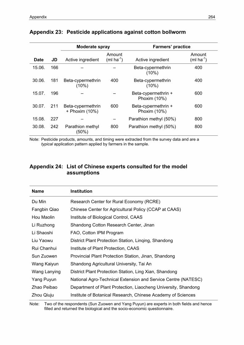
Appendix 264
Appendix 23: Pesticide applications against cotton bollworm
Moderate spray Farmers’ practice
Date
JD
Active ingredient
Amount (ml ha-1)
Active ingredient
Amount (ml ha-1)
15.06. 166 – – Beta-cypermethrin (10%)
400
30.06. 181 Beta-cypermethrin (10%)
400 Beta-cypermethrin (10%)
400
15.07. 196 – – Beta-cypermethrin + Phoxim (10%)
600
30.07. 211 Beta-cypermethrin + Phoxim (10%)
600 Beta-cypermethrin + Phoxim (10%)
600
15.08. 227 – – Parathion methyl (50%) 800
30.08. 242 Parathion methyl (50%)
800 Parathion methyl (50%) 800
Note: Pesticide products, amounts, and timing were extracted from the survey data and are a typical application pattern applied by farmers in the sample.
Appendix 24: List of Chinese experts consulted for the model assumptions
Name Institution
Du Min Research Center for Rural Economy (RCRE)
Fangbin Qiao Chinese Center for Agricultural Policy (CCAP at CAAS)
Hou Maolin Institute of Biological Control, CAAS
Li Ruzhong Shandong Cotton Research Center, Jinan
Li Shaoshi FAO, Cotton IPM Program
Liu Yaowu District Plant Protection Station, Linqing, Shandong
Rui Chanhui Institute of Plant Protection, CAAS
Sun Zuowen Provincial Plant Protection Station, Jinan, Shandong
Wang Kaiyun Shandong Agricultural University, Tai An
Wang Lanying District Plant Protection Station, Ling Xian, Shandong
Yang Puyun National Agro-Technical Extension and Service Centre (NATESC)
Zhao Peibao Department of Plant Protection, Liaocheng University, Shandong
Zhou Qiuju Institute of Botanical Research, Chinese Academy of Sciences
Note: Two of the respondents (Sun Zuowen and Yang Puyun) are experts in both fields and hence filled and returned the biological and the socio-economic questionnaire.
265 Appendix
Appendix 25: List of farmers participating in the season long monitoring
Village – Tian Gong Miao
Gao Hong Chun Gao Hong Xiang He Ying Xiang He Zai Xiang Jiang Guang Hua Jiang Guang Jun Jiang Guang Ling Jiang Guang Shan Jiang Guang Wu Jiang Guang Xi Jiang Guang Xu Jiang Guang Zhen Jiang Wen Jie Jiang Wen Chun Jiang Wen Feng Jiang Zhen Bo Jiang Zhen Jie Li Zhan Cai Li Zhan You Wang Feng Xin Wang Jiang Lin Wang Xi An Wang Xi Hu Wang Xi Yu Wang Yi Feng Wang Yu Cheng Wang Ze Hua Wang Zhan Hai Wang Zhan Wen Yin Wan Hua
Village – Xin Ji
Hao Gui Ling Hao Gui Sheng Li Bao Sheng Li Chen Hai Li Jun Hai Li Ke Cai Li Ke He Li Lan Wen Li Lan Wu Li Shang Hai Li Shi Chun Li Shi Feng Li Shi Wen Li Shi Xian Li Shi Xin Li Shi Yu Li Shu Ling Liu Xi Fa Liu Yan Sheng Ma Jia Bao Shi Feng Hua Sun Jia Rui Wang Bao Shan Wang Bao Sheng Wang Cheng Long Wang Shi Fu Wang Yan Tang Wang Zhao Xiang Xue Gui Qing Zheng Pei Hua
Village – Yin Zhuang
Chen Jin Long Du Huai He Du Xi Ping Ge Yue Hai Ge Yue Huan Li Hong Lou Li Ji Cheng Li Ji Ming Li Ji Shan Li Ji Wen Liu Guang Yi Liu Guang Zhi Liu Xing Ming Liu Zhen Feng Pi Gui Ping Wang Feng Er Wang Shi Guang Wang Shi Hai Wang Shi Lin Wang Shu Zhi Wang Wei Jiang Wang Wei Tang Wang Wei Yang Wang You Bing Wang You Ming Xing Xian Zhou Xing Xiou Xin Yang Fu Gui Zhang Jin Lu Zhang Jin Tang
Village – Zhang Zhuang
Chen Fu Fang Hu Ke Yi Hu Pei Dong Hu Pei Qiang Hu Pei Xian Hu Pei Zhu Hu Wen Bo Hu Wen Zhou Li Ju Lan Liu Ai Peng Liu Ai Xiang Liu Ming Shan Liu Yu Shan Lü Yu Zhen Ma Chang Xin Ma Jin Hua Song Xian Ping Sun Shu Lin Sun Shu Wen Wang Cheng Ye Wang Feng Lian Wang Shou Xiang Wang Shou Yin Wang Wu Fang Wang Xiu Zhen Wang Yin Fu Wang Yu Bao Xia Jin Lan Xu Zhen Sheng Zhang Xi Yan
Village – Hou Yang Fen
Li Zhi Rui Lu Xing Wu Lu Yue Kun Mu Chang He Peng Xin Sheng Wang Dong Quan Wang Guo Quan Wang Ji Chen Wang Ji Jun Wang Jia Zhong Wang Jin Po Wang Qin Quan Wang Shi Chun Wang Shi Feng Wang Shi Fu Wang Shi Guang Wang Shi Hu Wang Shi Qiao Wang Shi Xing Wang Shi You Wang Xiang Quan Wang Xiu Ling Wang Yin Quan Wang Yue Quan Yang Ben Feng Yang Ben Hui Yang Ben Qiang Yang Ben Ru Yang Ben Shan Yang Wei Min