Joint tracking and identification algorithms for multisensor data

A. Farina, P. Lombard0 and M. Marsella

Abstract: The paper describes an algorithm to jointly form a track and assign an identity flag to a target on the basis of measurements provided by a suite of sensors: surveillance radar, high resolution radar and electronic support measures. The algorithm is built around Bayes’ inference and Kalinan filters with the interacting multiple model. The improved performance in the track formation and identity estimation, which accrues by the joint tracking and identification algorithm, is evaluated by Monte Carlo simulation and compared to the performance of filters that process the data provided by each single sensor. The joint tracking and identification algorithm plays an important role in modem surveillance systems with non-cooperative target recognition capabilities.

List of acronyms and symbols

ATC EM ESM HRR IMM LRR MAP NCTR RCS c n, w no PT

x h zk

A i 1

n 0 Q E Wx, m , P )

Y

air traffic control electromagnetic elcctronic support measures high resolution radar interacting multiple model low rcsolution radar maximum a posteriori probability non-cooperative target recognition radar cross-section target type process and measurement noise vectors number of target types manoeuvre transition probability matrix state vector measurement vector emission state transition probability matrix likelihood function mode probability innovation process confusion matrix aspect angle of target set of all emitters Gaussian function, calculated at x, with mean m and covariance matrix P

tB IEE, 2002 IEE Pmceedings online no. 20020790

Dol: I O . 1049lip-nn:20020790 Paper first received 28th January and in revised form 4th Octoher 2002 A. Farina i s with the Radar & Technology Division, Alcnia Marconi Systcms, Via Tiburtina Km. 12.400, 00131 Rome, Italy P. Lomhvrdo is with Dept. InfoCom, University of Rome ‘La Sapienza’, Via Eudossiana IS, 00184 Rome. Italy

M. Manclla i s with Space Enginccnng S.p.A., Via dei FJciio 91, 00155 Rome, Italy

IEE Pm.-Rudor Sonar Navig., liol 14Y. No. 6, Decmdrr ZOO2

1. Introduction

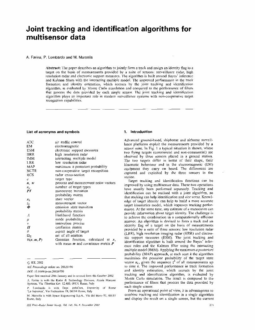
Advanced ground-based, shipbome and airbome surveil- lance platforms exploit the measurements provided by a sensor suite. In Fig. 1 a typical situation is shown, where two flying targets (commercial and non-commercial) are observed by three sensors placed in a ground station. The two targets differ in terms of their shape, their kinematic behaviour and in the electromagnetic (EM) equipment they carry on board. The differences are captured and exploited by the three sensors in the station.

Target tracking and identification functions can be improved by using multisensor data. These two operations have usually been performed separately. Tracking and identification can be realised with a joint algorithm, so that tracking can help identification and vice vtxsu. Knowl- edge of target identity can help to build a more accurate target kinematics model, which improves tracking perfor- mance. At the same time, any estimate of a manoeuvre can provide information about target identity. The challenge is to achieve the combination in a computationally efficient manner. An algorithm is devised to form a track and an identity flag of a target on the basis of measurements provided by a suite of three sensors: low resolution radar (LRR), high resolution imaging radar (HRR) and clectro- nic support measures (ESM). The joint tracking and identification algorithm is built around the Bayes’ infer- ence rules and the Kalman filter using the interacting multiple model (IMM). Applying the maximum aposteriori probability (MAP) approach, at each scan k thc algorithm niaximises the posterior probability of the target state vector x k , given the sequence zk of all measurements up to time k. The improved performance in track formation and identity estimation, which accrues by the joint tracking and identification algorithm, is evaluated by Monte Carlo simulation. The result is compared to the performance of filters that process the data provided by each single sensor.

From an operational point of view, it is advantageous to combine tracking and identification in a single algorithm and display the result on a single screen, but the current

27 1

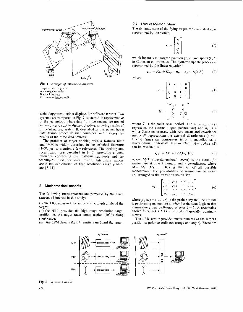
Fig. 1 Targel mined sig~nals: A - ndvigalion radar B - tracking radar C - communication radio

Erotnple of ,nrrlrisensor. platform

technology uses distinct displays for different sensors. Two systems are compared in Fig. 2: system A is representative of the technology where data from the sensors are treated separately and sent to distinct displays, showing results of differcnt nature; system B, described in this paper, has a data fusion procedure that combincs and displays the results of the three data sources.

The problem of target tracking with a Kalman filter and IMM is widely described in the technical literature

2.7 Low resolution radar The dynamic state of the flying target, at time instant k, is represented by the vector:

x,= [;j which includes the target's position (x, y ) , and speed (+, j) in Cartesian co-ordinates. The dynamic update process is represented by the linear equation:

( 2 ) -q+, = Fx, + Cu, + nk, up - R(0, N ) where

F =

c =

identification are described in [4-61, providing a g o o d reference concerning the mathematical tools and the techniques used for data fusion. Interesting papers about the exploitation of high resolution range profiles are [7-1 I].

O O l T 0 0 0 1

L _I

where T is the radar scan period. The term uL. in ( 2 ) represents the external input (manoeuvre) and nr is a white Gaussian process, with zero mcan and covariance matrix N , representing the external disturbances (turbu- lences). Since the manoeuvre input is modelled as a discrete-time, finite-state Markov chain, the update (2)

[1-3], just to mention a few references. The tracking and can De rewritten as

2 Mathematical models

The following measurements are provided by the three sensors of interest in this study:

(i) the LRR measures the range and azimuth angle of the target; (ii) the HRR provides the high range resolution target profile, i.e. the target radar cross section (RCS) along slant range; (iii) the E S M detects the E M emitters on board the target.

xk+I = Fx, + GM,(k) + n, ( 5 )

where M,<k) (two-dimensional vector) is the actual j th manoeuvre at time k along x and y co-ordinates, where M= {MI, M2,. . ., M y } is the set of all possible manoeuvres. The probabilities of manoeuvre transition are arranged in the transition matrix PT

PT =

PI.1 P1.2 " ' PI.,- P2.1 Pz.2 " ' P2,r 1 (6) . . . . . . . . . . . .

~vslem A

LP,., Pr .2 ' . ' P7.r 1 where pji (i. j = 1, . . . , r ) is thc probability that thc aircraft is performing manoeuvre number i at the scan k, given that manoeuvre j was performed at scan k ~ I . A reasonable choice is to set PT as a strongly diagonally dominant matrix.

The LRR sensor provides measurements of the target's position in polar co-ordinates (range and angle). These are

then converted into Cartesian co-ordinates. The measure- ment process is modelled as

zk = Hxi + wk (71 where

":[I 0 0 1 0 O O 0 1

and wk is the measurement Gaussian distributed noise with zero mean and a suitable covariance matrix W ( [ I], p. 155). Under mild conditions this conversion is unbiased.

2.2 High resolution radar The HRR sensor provides measurements of the along- range target profile. The profilc is a one-dimensional EM image of the target and is stored as a time-dependent signal or, in sampled form, as a vector. Identity information is achieved by comparing the received high resolution data with the data collected in an archive. Measuring high resolution data is not a perfect process. There are two error sources: the system thermal noise and the speckle. The speckle is a multiplicative noise (with standard devia- tion equal to the signal mean value), and is much stronger than thennal noise. It is a frequent problem when obser- ving a target with short waves (shorter than target's dimensions): the reflected signal is the coherent sum of the contributions from all the elementary scatterers, so there may be constructive or destructive interferences. The signal reflected by the target is

(9) p(t) = s(t) ' x(1)

Specifically, the proposed simplified target model comes from the known characteristics of the imaging of extended objects. The reflected signal p(t) from the target is the product of the average RCS profile s ( f ] (provided by the sequence of point scatterers along range, with their ampli- tude and relative phase), multiplied by a noise-like inter- ference a(t), accounting for the random phase combination typical of the coherent radar. Similar effects could be due to multihonnce, masking, glint, typical of scintillating portions of the target. We call this term speckle, reminis- cent of the SAR (synthetic aperture radar) nomenclature, even if it has, in this context. a broader meaning. The received signal is:

r(t) = p(t) + n(t)

whcrc n(t] is the additive Gaussian-distributed white ther- mal noise. Usually, the speckle is reduced by averaging a number of range profiles taken within a suitably small viewing angle. The signal-to-noise power ratio (SNR), defined as the power of the whole target signal along range divided by the power of noise, is a quality parameter of the target range profile.

2.3 ESM sensor The status of each of the emitters carried on board the target is modelled with a two-state Markov chain (on-off) with a matrix of transition probabilities:

(10)

The ESM may receive many sequences of pulses from several radio frequency sources; it de-interleaves the pulses and clusters them in different classes. The sensor is affected by errors due to a not perfect de-interleaving

iEE Pmc -Rodor Sonor Noiig.. Phi. 149. No. 6, December- 2002

operation. The errors are represented by the confusion probability matrix IL

where Si is the generic set of emitters carried by an aircraft type and h is the number of possible subsets of carried emitters, including the empty set; ifthere are three different emitters, h=8. The generic element of matrix n is the probability of wrong interpretation between the sets of emitters Si and 3, with i, j = I, 2 , . . . , h . The rationale of this model is described in [4-61.

3 Separate estimation algorithms

There are three estimation algorithms, each one pertinent to a single sensor. In this Section the three separate algorithms are studied and their performances are analysed.

3. I Low resolution radar The sequence of (x, .v) measurements at successive radar scans can be processed to implement tracking and identification.

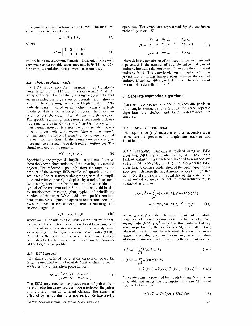
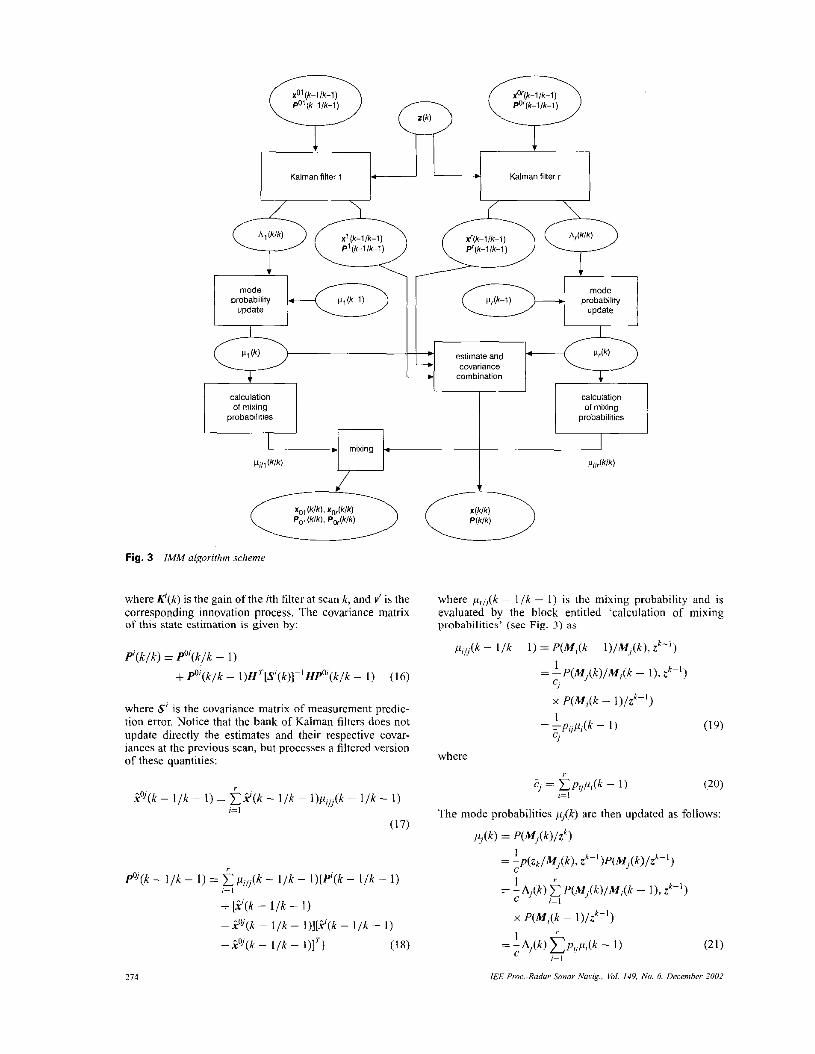
3.7.7 Tracking: Tracking is realised using an IMM algorithm. IMM is a fully adaptive algorithm, based on a bank of Kalman filters, each one matched to a manoeuvre in the set M= { M I , M 2 , . . . , M,}. Fig. 3 depicts the IMM algorithm. A concise explanation of the main equations is now given. Because the target motion process is modelled as in (9, the a posferiori probability of the state vy to r xk at instant k, given the set of measurements z , is evaluated as follows:

p(xk/zk) = k p ( x k / M , ( k ) , zk)p(M,(k) /zkf j= I

= C p ( x k / M j ( k I . ZL-: z '- ' )P,(~) (13) j = I

where zk and zh are the kth measurement and the whole sequence of radar measurements up to the kth scan, respectively. P(Mi ( k ] / z k ) = p j ( k ) is the mode probability (i.c. the probability that manoeuvre M, is actually taking place at time k). Thus the estimated state and the covar- iance matrix values are given by the weighted combination of the estimates obtained by assuming thc different models:

P ( k / k ) = C @)lf"(k/k) j = I

+ [ i j ( k / k ) - i ( k / k ) ] [ i j ( k / k ) - i ( k / k ) ] T l (146)

The state estimate provided by the ith Kalman filter at time k is obtained under the assumption that the ith model applies to the target:

i . ' ( k / k ) = i"o'(k/k) +K'(k)r,'(k) (15)

273

of mixing probabilities

Fig. 3 IMM algurirhm scheme

of mixing probabilities

where K'(k) is the gain of the ith filter at scan k, and V I is the corresponding innovation process. The covariance matrix of this state estimation is given by:

P(k /k ) = po'(k/k - 1)

+ P"(k/k - I ) H r [ S ' ( k ) ] ~ ' H P " ' ( k / k - I ) (16)

where S' is the covariance matrix of measurement predic- tion error. Notice that thc bank of Kalman filters does not update directly the estimates and their respective covar- iances at the previous scan, but processes a filtered version of these quantities:

i%'(k - I / k ~ I ) F i i ' ( k - l / k - I)piil(k ~ I / k - 1) ,=I

(17)

PoJ(k - I / k - I ) = i p , / , ( k - I / k - I)(P'(k - I / k - 1) c = I

+ [ 2 ( k - I / k - 1)

~ ioJ(k ~ I / k - l)][.?(k - I / k - I )

-P"J(k ~ I / k - I)]') (18)

274

where pzl j (k ~ l / k - 1) is the mixing probability and is evaluated by the block entitled 'calculation of mixing probabilities' (see Fig. 3 ) as

prij(k - I / k ~ 1) = P ( M , ( k ~ l ) / M , ( k ) , z k - ' ) 1

ci = ,P(MJ(k) /M,( :k - I ) , z")

where

where

and A,(k) is the likelihood ofjth Kalman's filter at time k :

A,(k) = p(zk/M,(k). z"')

=p(zk/Mj(k),.?''(k - I l k - I), Pnj(k - I / k - I ) )

= K [ x ~ ; i ' [k /k - I,.C"'(k - I/k - I)];

S'[k. p'(k - I/k - I)]] (23)

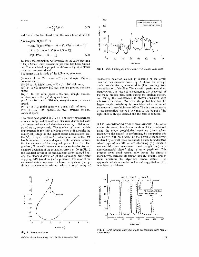
To study the estimation performance of the IMM tracking filter, a Monte Carlo simulation program has been carried out. The simulated target path is shown in Fig. 4; a planar case has been cousidered. The target path is made of the following segments:

( i ) scans I to 29: speed=70m/s, straight motion, constant speed; (ii) 30 to 5 3 : initial speed=70m/s, 180" right turn; (iii) 54 to 60: speed = 880 m/s, straight motion, constant speed; (iv) 61 to 70: initial speed=880m/s, straight motion, accelerations -10 m/s2 along each axis; (v) 71 to 76: speed=3IOm/s, straight motion, constant speed; (vi) 77 to 1 I O : initial speed =310m/s, 180" left turn; (vii) I I I to 130: speed = 760 m/s, straight motion, constant speed.

The radar scan period is T=4 s. The radar measurement errors in range and azimuth are Gaussian distributed with zero mean and standard deviation values u,? = 100 m and u,, = 2 mrad, respectively. The number of target models implemented in the IMM are three per co-ordinate axis; the numerical values of the h pothesised accelerations are: 0 m/s2, 10 m/s2, -10 m/s{ furthermore, the matrix PT has been selected almost diagonal with numerical entrics for the elements of the diagonal greater than 0.9. The number of Monte Carlo runs used to determine the bias and standard deviation of the estimation crrors is 100. In Fig. 5 the standard deviation of measurement error (dashed line) and the standard deviation of the estimation error after applying IMM (solid line) are represented. The error of the estimated state components is lower everywhere (except during manoeuvre transitions, where a small delay of

37

-6

-7 4 -2 6 8

x. m (.io4)

Fig. 4 Target trajcclnv

IEE Proc.-Rador Sonor ,Vavig., Yo1 14Y, No. 6, December N U 2

estimation error measurement error E 250

0 0 20 40 60 80 100 120 140

radar scan

IMM trucking olgon'ihnz error (100 Monte Carlo rms) Fig. 5

manoeuvre detection causes an increase of the error) than the measuremcnt error. Fig. 6 shows the average mode probabilities p, introduced in (13), resulting from the application of the filter. The aircraft is performing three manoeuvres. The result is encouraging, the behaviour of the mode probabilities, both during the straight motion, and during the manoeuvres, is always consistent with intuitive expectation. Moreover, the probability that the largest mode probability is coincident wi$?he actual manoeuvre is very high (over 95%). This is a cyhsequence of the appropriate choice of PT matrix: the output of the right filter is always selected and the error is reduced.

3.1.2 Identification from motion model: The infor- mation for target identification with an LRR is achieved using the mode probabilities: once we know which manoeuvre the aircraft is performing, by comparing this manoeuvre with an archive of the possible manoeuvres (ordered by aircraft type), we should be able to understand which type of aircraft we are observing (e.g. either a commercial (slow manoeuvre, most straight line) or a non-commercial aircraft (high g tums possible)). This process gives good results only during the aircraft's manoeuvres, because all aircraft can fly straight, and in these situations the algorithm cannot decide. This approach, which is similar to the one suggested in [13], is obtained as follows.

man. 3

80 100 120 140

radar *can

Fig. 6 IMM tracking algorithm mode pmhabilities (100 Monte Carlo rim)

275

Evaluate the probability of target type

P(c = UJZk) (24)

(i.c. the probability that, at time k, aircraft type c is ui). By applying Bayes' theorem we have

where no is the number of possible target types.

(Le. P(c=ui)= Iln,, Vi), the probability becomes Assuming no prior information about target type

(26) ' h = z p ( z /c = a0

where S is the normalisation constant:

JL 6 = C p ( z h / c = a;) (27)

j= I

The key of the identification algorithm is the likelihood p(zh /c=ui ) . Assuming the measurement error w (see (7)) to be Gaussian distributed and white, its samples are uncorrelated and then the distributions of the single obser- vations will be mutually independent. Thus the likelihood can be written as follows:

k

!,,=I

h p ( z le = ai) = n p(z , , izm-l , = (28)

The advantage is that, once we use the IMM algorithm for tracking, all the quantities needed by identification algo- rithm are already available (see (21) and (23)):

"0)

,=I

x ~ ( u ( m ) = ~ $ m ) / z ' " + ' . c = i )

p(z,Jzn'-', c = a,) = Cp(z*/U("l ) = M j m ) , z"'-l, c = i )

where A;(m) and pi(m) have the same meaning as in (23) and (21), and the index i (i= 1, 2, . . . , no) denotes the ith target type. The number of possible manoeuvres r(i) depends on target type; the dynamical models chosen for the targets can be different, consequently, the numbers of possible manoeuvres can also be different from target to target.

By substituting (29) in (28) and exploiting (19), we get the tinal formula to use in (26):

h h p ( z /c = a,) = n p(z,"/z"'-l, c = u,)

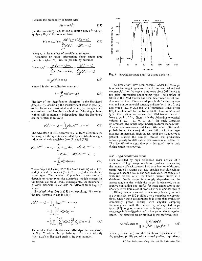
The results of identification via IMM algorithm arc shown in Fig. 7 where the probability of correct identity P(c=ai/zS is displayed against the scan number.

216

radar scan

Fig. 7 Idenrrficurion using LRR (100 Munrr Carlo rims)

The simulations have been executed under the assump- tion that two target types are possible: commercial and not commercial, thus the curve value starts from 50%, there is not prior information about target type. The number of filters in the IMM tracker has been determined as follows. Assume that three filters are adopted both for the commer- cial and not commercial targets; indicate by {-ac, 0, uc} and with {-a, , , 0, ant} the set of numerical values of the target accelerations for the two aircraft. Because the actual type of aircraft is not known, the IMM tracker needs to have a bank of five filters with the following numerical values: {-uric, -ac, 0, a,, a,,, 1 for each Cartesian co-ordinate. The actual target undergoes three manoeuvres. As soon as a manoeuvre is detected (the value of the mode probability p i increases), the probability of target type assumes immediately high values, until the manoeuvre is present. During the straight motion the probability returns quickly to 50% until a new manoeuvre is detected. This identification algorithm provides good results only during target manoeuvres.

3.2 High resolution radar Data collected by high resolution radar consist of a sequence of high range resolution profiles representing the intensity of backscattered field as a function of distance (more refined systems can also provide two-dimensional images). Once the profile has been extracted, we compare it with the profiles of all the known aircraft stored in a database. Profile shape is strongly dependent on the aspect angle under which the target is observed, so an archive containing one profile for each target type is not enough. If we store a set of profiles with an angular step of 1 O , 180.n,, comparisons will be necessary (usually aircraft are symmetric: so 180 profiles give a complete representa- tion). Under these assumptions it is clear that evaluation complexity grows linearly with angular sampling frequency and with the number n, of expected target types [12]. A good comparison technique Is thus crucial to success in identitication and in increasing the processing speed. The classical scalar product is the preferred tool:

/

where f ( t ) and g(t) are the functions representative of the received profile and of the stored profile, respectively.

IEE Pmc.-Kodaiur so nu^ Navig.. 6;. I4Y. No. 6, Decenther 2OlJ.1

50

range. m "7%- azimuth, deg .-

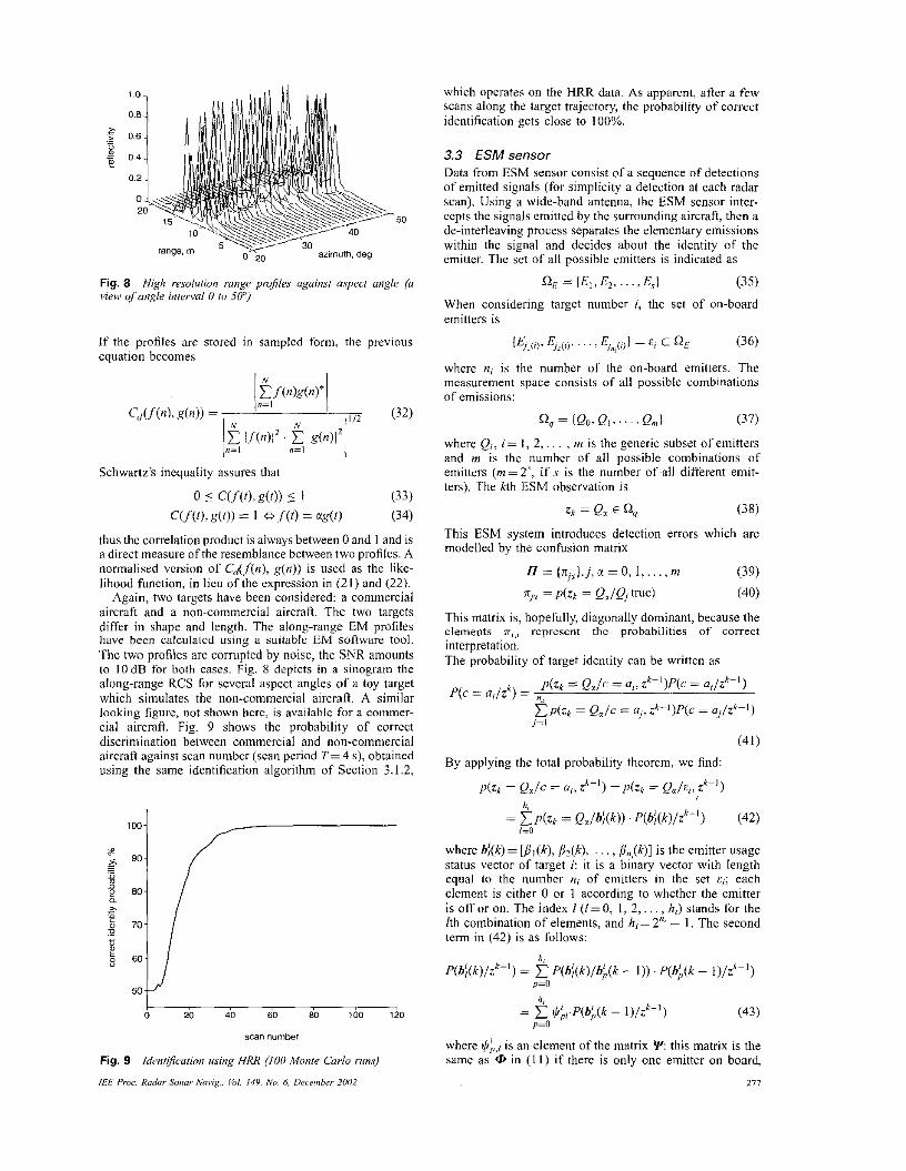
Fig. 8 v i m qf mgle imerval 0 m 500)

High resolution range pr.ofiles against uspect ungle (a

If the profiles are stored in samplcd form, the previous equation becomes

!+*I G ( f ( n ) , g(n)) = 112 ( 3 2 ) I F ?I=[ if(n)l2 . ?l=l E lg(.)l'l

Schwartz's inequality assures that

0 5 c(f(0. A t ) ) 5 1 (33) (34) cw) , g(o) = I a. f (o = W(O

thus the correlation product is always between 0 and 1 and is a direct measure ofthe resemblance between two profiles. A normalised vcrsion of CJ,f(n), g(n)) is used as the like- lihood function, in lieu of the expression in (21) and (22).

Again, two targets have been considered: a commercial aircraft and a non-commercial aircraft. The two targets differ in shape and length. The along-range EM profiles have bccn calculatcd using a suitable EM software tool. The two profiles are corrupted by noise, the SNR amounts to lOdB for both cases. Fig. 8 depicts in a sinogram the along-range RCS for several aspect angles of a toy target which simulates the non-commercial aircraft. A similar looking figure, not shown here, is available for a commer- cial aircraft. Fig. 9 shows the probability of correct discrimination between commercial and non-commercial aircrafi against scan number (scan period T= 4 s) , obtained using the same identification algorithm of Section 3.1.2,

0 20 i o 60 i o *bo iio

scannumber

Fig. 9 Idml$cficurion using HRR (I00 Manre Carlo rrm)

/€E Pruc.-Rodor. Sarior Novig.. el. /4Y. h'o. 6. Dccrrnber 2002

which operates on the HRR data. As apparcnt, after a few scans along the targct trajectory, the probability of correct identification gets close to 100%.

3.3 ESM sensor Data from ESM sensor consist of a sequence of detections of emitted signals (for simplicity a detection at each radar scan). Using a wide-band antenna, the ESM sensor inter- cepts thc signals emitted by the surrounding aircraft, then a de-interleaving process separates the elementary emissions within the signal and decides about the identity of the emitter. The set of all possible emitters is indicated as

QE = { E , , 4. . . . ,Es) (35) When considering targct number i , the set of on-board emitters is

[E,,(;). Ej2(zj . . . . 1 Ejnj(zjl = 8, c Q E (36)

where n, is the number of the on-board emitters. The measurement space consists of all possible combinations of emissions:

Q, = [Qo, Qi,. . . , Q n , l (37)

where Q;, i = 1, 2 , . . . , m is the generic subset of emitters and m is the number of all possible combinatinns of emitters ( m = 2 ' , if s is the number of.all different emit- ters). The kth ESM observation is

ZI Q, E Q, (38)

This ESM system introduces detection errors which are modelled by the confusion matrix

L ' = { n j J , j , x = O , l , . . . , m (39) Zjz = P(Zk = Q,/Qj true) (40)

This matrix is, hopefully, diagonally dominant, because the dements z,,~ represcnt the probabilities of correct interpretation. The probability of target identity can be written as

- p(zk = Q,/c = a,, zk-')P(c = ai /zk- l ) P(c = U i / Z ) - nr

C p ( z k = Q,/c = a/, zk--')P(c = aj/zk-I) j= I

(41) By applying the total probability theorem, we find:

p(zk = Q,/c = a,, z k - l ) =p(zk = Q , z / ~ i , zk - ' )

= C p ( z k = Q,/b;(k)) . P(b;(k)/z"') (42)

where b;(k) = [Ol(k), p2(k), . . . , 0,8,(k)] is the emitter usage status vector of target i : it is a binary vector with length equal to the number n, of emitters in the set c,; each element is either 0 or 1 according to whether the emitter is off or on. The index I ( I = 0, I, 2, . . . , h,) stands for the Ith combination of elements, and h;=2"* - 1. The second term in (42) is as follows:

P(b;(k) / zk- l ) =

/a,

;=0

h ,

p=0 P(bj(k)/bi(k - 1)) . P(b;>(k - 1)/zk-')

where is an element of the matrix 'E this matrix is the same as @ in (11) if there is only one emitter on hoard

277

50 Y 0 20 40 60 80 100 120 140

scan number

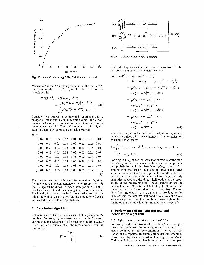
Fig. 10 Iderztrfication rising ESM (I00 Monte Curb mm)

-0.87 0.03 0.03 0.03 0.01 0.01 0.01 0.01 0.03 0.84 0.03 0.03 0.02 0.02 0.02 0.01

0.03 0.03 0.03 0.84 0.02 0.02 0.02 0.01 0.03 0.03 0.84 0.03 0.02 0.02 0.02 0.01

0.02 0.03 0.03 0.03 0.78 0.03 0.03 0.05

0.02 0.03 0.03 0.03 0.03 0.78 0.03 0.05 0.02 0.03 0.03 0.03 0.03 0.03 0.78 0.05

-0.01 0.03 0.03 0.03 0.05 0.05 0.05 0.75 i

Fig. 11 Scheme o/duta fusion olgorithm

Under the hypothesis that the measurements from all the sensors arc mutually independent, we have:

k P(c = a,/Zk) = P(c = U i / Z l , . . . , zk) k- I = P(c = ai/a,,h. . . . , Z>V.k. ZI . . , , ,ak- l )

x P(c = u,/af-l,. . . ,&-I)

x p ( ~ , ~ . ~ / c = a;.

x ~ ( c = a,/zf-I, . . . , & I )

= -p(zl ,k/c = a;. zf-1) x . . .

x P(z,V.klc = a;> zk-9 x P(c = a; /zk- ' ) (47)

I 6 = -p(a I .K. . . . . zNv.k/c = ai, zf-1, . . . , &I)

1 6

= - p ( ~ ~ , ~ / e = a;, at- ' ) x . . .

1 6

where P(c =a,/& is the probability that, at time k, aircraft type c is a; , given all the measurements. The normalisation constant 6 is given by

6 = ""

[p(z l .k /c = a,. zi-1) x " ' xp(z,v,k/c = a/. z:;l)

x P(c = a 1 / P ) ] (48)

j = I

Looking at (47), it can be seen that correct classification probability at the current scan is the update of the preced- ing probability with the likelihood p ( ~ ; . ~ / c = a,, z"'), coming from the sensors. It is straightforward that, after an initialisation (if there are n , possible aircraft models, at the first scan all probabilities are set to Iln,) , the only quantities needed are the three likelihoods and the prob- ability at the preceding scan. These likelihoods are the ones defined in (26), (32) and (41). Fig. I I shows all the stages of the data fusion algorithm. Using (26) , (32) and (41), from the data zLKK, zHRR and zEsM provided by the three sensors, the identity likelihood LI.RR, LHRR and LBsM are evaluated. Equation (47) combines these likelihoods to finally obtain the joint identity probability P(c =a;/&).

5 identification algorithm

5.1 Operation under normal conditions Following the theory introduced in Section 4, it is straight- forward to implement the joint algorithm based on partial results obtained by the three algorithms: the partial like- lihood of the separate algorithms are taken and combined in (47) scan by scan, as illustrated in Fig. I I . A Monte Carlo simulation program has been carried out to compare

IK.5 Pmr.~Rulrr- Sonar. vuv vi^.. h/. i49, No 6. December 2002

Performance of the joint tracking and

the identification and tracking performance of the three separate algorithms (described in Sections 3.1, 3.2 and 3.3, respectively) and of the data fusion algorithm (Section 4). A highly manoeuvring non-commercial target has been gcnerated in this scenario, whose trajectory is similar to the one depicted in Fig. 4. The target along-range profile is reported in Fig. 8, the EM emission is characterised as in Section 3.3. The purpose of the simulation exercise is to track the target motion and classify the target under analysis as commercial aircraft or non-commercial aircraft.

Fig. 12 displays the probability of correct identification of the three separate algorithms and of the data fusion algorithm against sensor scan number; all the three sensors have the same scan period. Note that IMM tracker, which processes the LRR data, has a bank of five filters; the tracker does not know u priori the target type. The rate of increase of the probability obtained with the joint algorithm (solid line) is very high and stable, especially when compared with the results of the separate algorithms (lion-solid curves). The target identity is reliable and available in less than ten radar scans. An interesting aspect of the joint algorithm is that i t can be extended to any number of sensors by just adding appropriate factors to the product in (47).

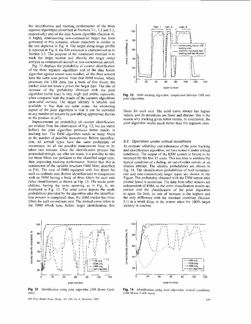
Improvements on probability of correct identification are evident from the observation of Fig. 12, hut (as stated before) the joint algorithm produccs better results in tracking too. The IMM algorithm needs as many filters as the number of possible manoeuvres. Before identifica- tion, all aircraft types have the same probability of occurrence, so all the possible manocuvres have to be taken into account. Once the identification process has proceeded enough, say atter ten scans, it is possible to take out those filters not pertinent to the identified target type, thus improving tracking performance. Notice that this is reminiscent of the variable structure IMM filter, described i n [14]. The case of IMM equipped with five filters for each co-ordinate axis (before identification) in comparison with an IMM having a bank of three lilters for each axis (after identification) is shown in Fig. 13. The mode proh- abilities, having the same meaning as in Fig. 6, are displayed in Fig. 13. The solid curve depicts the mode probabilities provided by the algorithm after the identifica- tion process is complcted; thus, the IMM tracker has three filters for each co-ordinate axis. The dashed curve refers to the IMM which runs, before target identification. five

100-

80 -

60 ~

40-

20-

0 -

man. 1 man. 2 man.3 .-. .- .- . . . .

: , ;I _ _ _ manoeuueng status. LRR : I tracbng only :I - manoeuvring statu^. ioint

tracking and identillcation

t , I I I t

\

I # \

, I I : , I I

, , ; , ; I t ; ,

L--.,_. ._- J -. - - 0 20 40 60 80 100 120 140

scan number

Fig. 13 joint algorithms

IMM trucking algo>or-ilhm, contparism between LRR und

filters for each axis. The solid curve always has higher values, and its transitions are faster and sharper: this is the reason why tracking gives better results. In conclusion, the joint algorithm works much better than the separate ones.

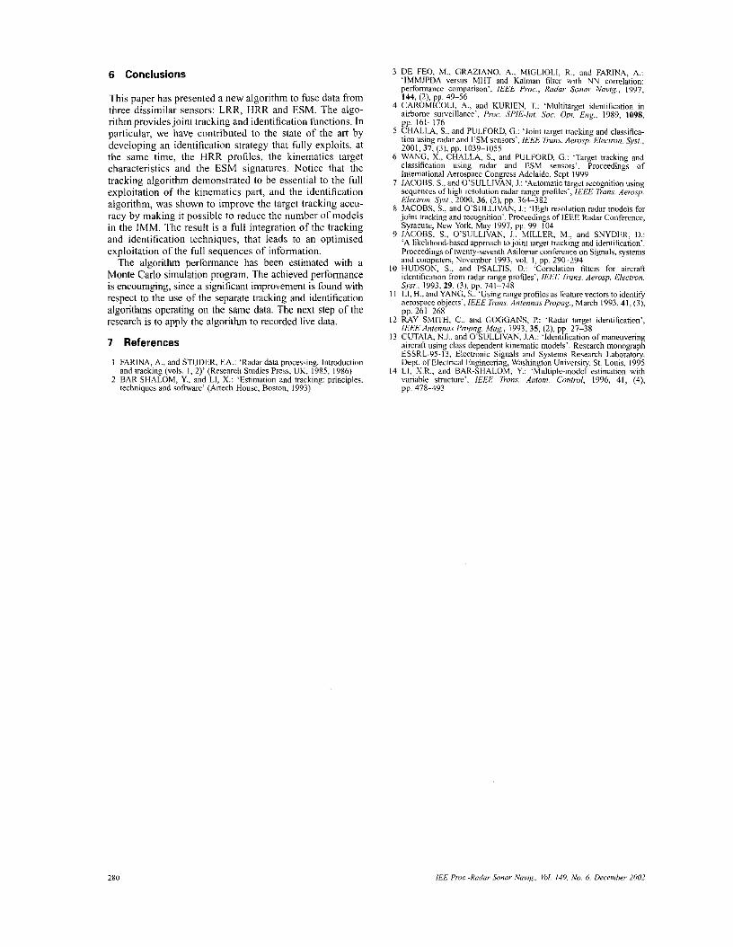
5.2 Operation under critical conditions To evaluate reliability and robustness of the joint tracking and identification algorithm, we have tested it under critical conditions. The output of the ESM system is forced to be incorrect for the first 15 scans. This test tries to emulate the typical condition o f a fading, an out-of-order sensor, or an elusion attempt. The identity probabilities are shown in Fig. 14. The identification probabilities of both (commer- cial and non-commercial) target types are shown in the Figure. The probability obtained with the ESM sensor only (dotted lines) is erroneous. The data from other sensors are indcpendent of ESM, so the other classification results are correct and the classification of the joint algorithm is again the best; its rate of increase is the highest and the only difference with the standard condition (Section 5.1) is a small delay in the instant when the 100% target identity is reached.

1 0 20 40 60 80 100 120

scan number

Fig. 14 (IOU Monte C d o rrms)

Identification using joirzl algor-ithm, critical cutiditions

279

6 Conclusions

This paper has presented a new algorithm to fuse data from three dissimilar sensors: LRR, HRR and ESM. The algo- rithmprovidesjoint tracking and identification functions. In particular, we have contributed to the state of the art by developing an identification strategy that fully exploits, at the same time, the HRR profiles, the kinematics target characteristics and the ESM signatures. Notice that the tracking algorithm demonstrated to be essential to the full exploitation of the kinematics part, and the identification algorithm, was shown to improve the target tracking accu- racy by making it possible to reduce the number of models in the IMM. The result is a full integration of the tracking and identification techniques, that leads to an optimised exploitation of the full sequences of information.

The algorithm performance has been estimated with a Monte Carlo simulation program. The achieved performance is encouraging, since a significant improvement is found with respect to the use of the separate tracking and identification algorithms operating on the same data. The next step of the rescarch is to apply the algorithm to recorded live data.

7 References

I FARINA, A,, and STUDER, F A 'Radar data processing. Introduction and tracking (vols. I, 2)' (Research Studies Press, UK. 1985, 1986)

2 BAR-SHALOM, Y., and LI, X.: 'Estimation and tracking: principles. techniques and software' (Anech House, Boston, 1993)

3

10

I I

I 2

13

14

DE FEO, M., CRAZIANO, A.. MIGLIOLI, R., and FARINA, A,: 'IMMJPDA versus MllT and K a h n filter with NN canelation: performuacc comparison', IEEE Proc., Rador Sonar- Navig.. 1997, ,Ad 17, "- AO-qA .-~, ,,p. ~, l"

CAROMICOLI, A., and KURIEN, T.: 'Multirarget identification in airborne sumillmce', Pmc. SPIE-I,II. Soc. Opr. Eng., 1989, 1098, pp. 161-176 CHALLA, S., and PULFORD, G.: 'Joint target tracking and classifica- tion using radar and ESM sensors', IEEE fi-uas. Aerosp. Eleciro,i. S ~ X I . , mi 17 11) I O V - ~ ~ F F - - - - , - ., ,-,, rr ."_, WANG, X.. CHALLA, S., and PULFORD. G.: 'Target tracking and classification wine radar and ESM sensors'~ Proccedinm of -- ~~

~ ~ ~ ~ ~ ~ ~ ~~. International Aerospace Congrcss Adelaide. Sept i999 JACOBS. S.. and O'SULLIVAN, J.: 'Automatic target recognition using sequences of high rCSolution radar range profiles', IEEE Pans. A e m s p Eleclwn. S~.TI., 2000, 36, ( 2 ) , pp. 364-382 JACOBS, S., and O'SULLIVAN, J.: 'High resolution radar models for ioint trackine and iccoenition'. Procsrdinrs o f IEEE Radar Confcrcnce.

~~ ~~~ ~~

and camp&% Novimbmbur 1993, "01. I . pp. 290-294 HUDSON. S., and PSALTIS. D.: 'Correlation filtcn for aircraft identification from radar range profiles', IEEE Tron.~. Aemsp. Elrcnnn. S w t . 1993. 29. 13). DD 741-748 i l , H . . and YANb,'S.?Using mnge protiles as feature V ~ C I D R to identify aeraspacc objects', IEEE k n s . AntennasPqmg., March 1993.41, (3). nn 7hIL76R ~~. _..I RAY SMITH, C.. and COCGANS, P.: 'Radar target identification'. IEEEAnlrsrm Pmpog. h4ug.. 1993, 35, (2) , pp. 27-38 CUTAIA, N.J.. and OSULLIVAN. J.A.: 'Identification of maneuverhe aircraft using class dependent kinematic models'. Research monorrdpE

vanable structure'. IEEE 7mn.s. Aulon,. Control. 1996. 41. (41. pp. 478-493

280 IEE PIUC -Radar Sonar " J i g . . bb/. 1.19, Nu. 6. Decnnher- 21102