Joint Program in Oceanography/ Applied Ocean Science and ...
347
2010-05 DOCTORAL DISSERTATION by Jacob R. Waldbauer February 2010 Molecular Biogeochemistry of Modern and Ancient Marine Microbes MIT/WHOI Joint Program in Oceanography/ Applied Ocean Science and Engineering Massachusetts Institute of Technology Woods Hole Oceanographic Institution
-
Upload
khangminh22 -
Category
Documents
-
view
0 -
download
0
Transcript of Joint Program in Oceanography/ Applied Ocean Science and ...

2010-05
DOCTORAL DISSERTATION
by
Jacob R. Waldbauer
February 2010
Molecular Biogeochemistry of Modern andAncient Marine Microbes
MIT/WHOI
Joint Programin Oceanography/
Applied Ocean Scienceand Engineering
Massachusetts Institute of Technology
Woods Hole Oceanographic Institution
MITIWHOI
2010-05
Molecular Biogeochemiat:ry at Modern and Ancient Marine Microbe.
by
Jacob R. Waldbauer
Massachusetts Institute of TechnologyCambridge, Massachusetts 02139
'nd
Woods Hole Oceanographic InstitutionWoods Hole, Massachusetts 02543
February 2010
DOCTORAL DISSERTATION
Funding was provided by the National Science Foundation, the Office of Naval Research NationalDefense Science & Engineering Graduate Fellowship. National Science Foundation Graduate ReseS.feh
Fellowship. NASA Exobiology Program and Astrobiology Institute Awards, AgouroD InstituteGeobiology Award, Gordon and Betty Moore Foundation Marine Microbiology Award 495, Department
of Energy Awards, and the Woods Hole Oceanographic Institution Academic Programs Office.
Reproduction in whole or in part is permitted for any purpose of the United States Government. Thisthesis should be cited as: Jacob R. Waldbauer, 2010. Molecular Biogeochemistry of Modern and Ancient
Marine Microbes. Ph.D. Thesis. MlT/WHOI, 2010-05.
Approved for pu.blication; distribution u.nlimited.
Approved for Distribution:
Daniel]. Repeta, Interim Chair
Department of Marine Chemistry and Geochemistry
Ed BoyleMIT Director ofJoint Program
,~~-James A. Yoder
WHOI Dean of Graduate Studies
MOLECUl.AR BIOGEOCIIEMISTRV OF MODERN AND ANCIENT MARINE MICROBES
by
Jacob Richard Waldbauer
A.B .. Dartmouth College, 2001
Submined in partial fulfillment of the requirements for the degree of
Doctor of Philosophyat the
MASSACHUSETTS INSTITUTE OF TECHNOLOGYand the
WOODS HOLE OCEANOGRAPHIC INSTITUTION
February 20 I0
02010 Jacob R. Waldbauer. All rights reserved.
The author hereby grant's (0 MIT and WHOI pennission to reproduce and to distribute publiclypaper and electronic copies of this thesis document in whole or in part in any medium now known
or hereafter cr ted.
Signawre of Author:._--:--:--:__--:--:::-_'l-_,-,--"c--:--:=:...--:--:__--:--:--:_--:_Joint Program in Ocean graphy/Applied Ocean Science and Engineering
January 8, 20 I0
Roger E. SummonsChair, Joint Committee for Chemical Oceanography
_ _ ?t"-~~Accepted by: ~
Certified bY; -"~::::::~~~ev~JtJL~::=====:::-c-:--:-Sallie W. Chisholm
Lee and Geraldine Martin Professor of Environmental StudiesProfessor of Civil and Environmental Engineering and of Biology___7 ~ ....~ The,i,Supervisor
~ Roger E. Summon'Professor of Earth, Atmospheric and Planetary Sciences
Thesis Supervisor

2
Molecular Biogeochemistry of Modern and Ancient Marine Microbes
by
Jacob Richard Waldbauer
Submitted to the Joint Program in Oceanography/Applied Ocean Science and Engineering in partial fulfillment of the requirements for the degree of
Doctor of Philosophy in Chemical Oceanography
Abstract Biological activity has shaped the surface of the earth in numerous ways, but life’s most pervasive and persistent global impact has been the secular oxidation of the surface environment. Through primary production – the biochemical reduction of carbon dioxide to synthesize biomass – large amounts of oxidants such as molecular oxygen, sulfate and ferric iron have accumulated in the ocean, atmosphere and crust, fundamentally altering the chemical environment of the earth’s surface. This thesis addresses aspects of the role of marine microorganisms in driving this process. In the first section of the thesis, biomarkers (hydrocarbon molecular fossils) are used to investigate the early history of microbial diversity and biogeochemistry. Molecular fossils from the Transvaal Supergroup, South Africa, document the presence in the oceans of a diverse microbiota, including eukaryotes, as well as oxygenic photosynthesis and aerobic biochemistry, by ca. 2.7Ga. Experimental study of the oxygen requirements of steroid biosynthesis suggests that sterane biomarkers in late Archean rocks are consistent with the persistence of microaerobic surface ocean environments long before the initial oxygenation of the atmosphere. In the second part, using Prochlorococcus (a marine cyanobacterium that is the most abundant primary producer on earth today) as a model system, we explored how microbes use the limited nutrient resources available in the marine environment to make the protein catalysts that enable primary production. Quantification of the Prochlorococcus proteome over the diel cell-division cycle reveals that protein abundances are distinct from transcript-level dynamics, and that small temporal shifts in enzyme levels can redirect metabolic fluxes. This thesis illustrates how molecular techniques can contribute to a systems-level understanding of biogeochemical processes, which will aid in reconstructing the past of, and predicting future change in, earth surface environments. Thesis supervisor: Sallie W. Chisholm Title: Lee and Geraldine Martin Professor of Environmental Studies Professor of Civil and Environmental Engineering and of Biology
Thesis supervisor: Roger E. Summons Title: Professor of Earth, Atmospheric and Planetary Sciences
3
ACKNOWLEDGMENTS
I have incurred many debts of gratitude and appreciation over the course of this work. None are greater than those to my advisors, Penny Chisholm and Roger Summons, who allowed and enabled me to pursue such a wide range of scientific interests and offered their help and advice every step of the way. I have been very lucky to have had the chance to learn so much during my Ph.D., and none of that would have been possible without their guidance and support. I have also had the great fortune to know and work with all the members of the Chisholm and Summons labs, who have made this an enjoyable and rewarding place to be. I am especially grateful to Laura Sherman for her skill and dedication in analyzing biomarkers in the late Archean cores – it was truly getting blood from a stone. I was lucky to collaborate with Sébastien Rodrigue, whose expertise and collegiality made the diel experiment even more fruitful than I could have hoped. Many others, including Matt Sullivan, Anne Thompson, Alex Bradley, Gordon Love, Rex Malmstrom, Libusha Kelly, Luke Thompson, Jason Bragg and Adam Rivers, shared advice, ideas, reagents, humor and beer. Thanks as well to Carolyn Colonero, Allison Coe, Marcia Osburne, Alla Skorokhod, Mary Elliff and Deborah Fullerton for the wonderful job they have done in keeping the labs running. Early in my graduate career, John Hayes generously shared his time and insights into the mysteries of the carbon cycle. Our discussions shaped my view of the earth system and the role of life within it. I am also thankful for both the scientific opportunities and warm hospitality offered to me by Dianne Newman and her lab. Paula Welander, Alexa Price-Whelan, Alex Poulain and Lars Dietrich patiently taught me anaerobic culturing and microelectrode techniques. Further scientific support came from many quarters. My thesis committee members, Liz Kujawinski and Mak Saito, offered guidance and helpful feedback. Melissa Soule managed the FTMS facility at WHOI, and the proteomics dataset would not have been collected without her help. Bryan Krastins and David Sarracino provided invaluable bench training. David Shtyenberg at ISB enabled much of the proteomics data analysis. The Agouron Griqualand Drilling Project and core sampling were coordinated by Andy Knoll, Nic Beukes and Joe Kirschvink, and Alex Birch and Francis McDonald oversaw the difficult clean drilling operation.
A special community is assembled around the Joint Program, EAPS and the Parsons Lab. The EAPS and APO staff, including Ronni Schwartz, Valerie Caron, Julia Westwater, Carol Sprague and especially Marsha Gomes, were unfailingly knowledgeable and helpful. Vicki Murphy kept me employed, funded, and, on some days, sane. Numerous friends – Elizabeth Tuckerman, Frédéric Chagnon, Sora Kim, Alyson Santoro, Seth Newsome, Alison Cohen, Nurit Bloom, Virginia Rich, Tracy Mincer, Janelle Thompson, Gajan Sivandran and Rebecca Giannotti, to name only a few – shared good times and laughter. The Klepac-Ceraj clan, Vanja, Ivan, Zara and Mirta, became treasured family; hvala lijepa. Ray Gilliar, Quang Truong, Adam Bisig and Jeff Kinkaid have provided a welcome yearly diversion at the annual conference.
4

My parents have helped, supported, and inspired me in innumerable ways through the years, for which I will always be grateful.
The second sentence wasn’t true. My greatest debt is to Maureen. Thank you. THIS WORK WAS SUPPORTED BY THE FOLLOWING FUNDING SOURCES: Office of Naval Research National Defense Science & Engineering Graduate Fellowship
(to JRW) National Science Foundation Graduate Research Fellowship (to JRW) NASA Exobiology Program Award NNG05GN62G (to RES) NASA Astrobiology Institute Award NNA08CN84A (to RES) National Science Foundation Award EAR0418619 (to RES) Agouron Institute Geobiology Award AI-GB4.02.3Extn06.2bMIT (to RES) Gordon and Betty Moore Foundation Marine Microbiology Award 495 (to SWC) National Science Foundation Award OCE0425602 (to SWC) National Science Foundation Award EF0424599 (to SWC) Department of Energy Award DE-FG02-07ER64506 (to SWC) Department of Energy Award DE-FG02-08ER64516 (to SWC)
5

6
TABLE OF CONTENTS
CHAPTER 1: Introduction 9
CHAPTER 2: Late Archean molecular fossils from the Transvaal Supergroup record the antiquity of microbial diversity and aerobiosis
Waldbauer et al. (2009) Precambrian Research 169:28-47. 21
CHAPTER 3: Microaerobic steroid biosynthesis and the molecular fossil record of Archean life 43
CHAPTER 4: A multilevel view of gene expression and regulation in the diel cell cycle of Prochlorococcus 71
CHAPTER 5: Biogeochemical insights from Prochlorococcus systems biology 167
CHAPTER 6: Conclusions and Future Directions 209
APPENDIX A: Use of stable isotope labeled cells to identify active grazers of picocyanobacteria in ocean surface waters
Frias-Lopez et al. (2009) Environ Microbiol 11: 512-525. 215 APPENDIX B: Improved methods for isolating and validating indigenous biomarkers in Precambrian rocks
Sherman et al. (2007) Org Geochem 38:1987-2000. 245 APPENDIX C: Proteorhodopsin photosystem gene expression enables photophosphorylation in a heterologous host
Martínez et al. (2007) PNAS 104:5590-5595. 261 APPENDIX D: The Geological Succession of Primary Producers in the Oceans
Knoll et al. (2007) In The Evolution of Primary Producers in the Sea, Falkowski and Knoll, eds. Academic Press, p.133-163. 269
APPENDIX E: The carbon cycle and associated redox processes through time Hayes & Waldbauer (2006) Phil Trans Roy Soc B 361:931-950. 303
APPENDIX F: Steroids, triterpenoids and molecular oxygen Summons et al. (2006) Phil Trans Roy Soc B 361:951-968. 325
7

8

CHAPTER ONE
Introduction
9

10
Introduction The coevolution of life and earth surface environments is central to the history and
functioning of our planet. Life and its habitats coevolve through a wide array of
reciprocal interactions, constantly applying pressures to and driving changes in one
another. Only life evolves in a Darwinian sense and has a distinct mechanism for
heritable transmission of information. But the impact of biology on the geochemistry of
the oceans, atmosphere and crust is so pervasive that the present distributions of even
inorganic chemicals are inexplicable without acknowledging life’s influence. When the
changes in geochemical distributions over time, evident in the rock record, are taken into
account, biology’s role appears even more central.
The most enduring and globally significant change that life has driven over the course of
earth history has been the progressive oxidation of the surface environment. As a result
of biological activity, particularly photosynthesis, oxidizing power has been continuously
exported by the carbon cycle and has accumulated in reservoirs such as molecular
oxygen, sulfate, and ferric iron. This process has increased redox disequilibrium between
the surface environment (including the atmosphere, oceans and upper crust) and the
deeper solid earth, with broad consequences for the cycling of nearly all elements.
Progressive oxidation has also been a defining control on the ecological distribution of
microbes and on the biogeochemistry that results from their activities.
HOW DID LIFE OXIDIZE THE EARTH’S SURFACE?
The secular oxidation of the surface environment has been driven in large part by primary
production. Life, of course, does not create or destroy electrons; “secular oxidation”
means the redistribution of reducing equivalents, principally from a variety of electron-
donating species to carbon. (The only recognized process that truly changes the redox
state of the planet as a whole is the escape of hydrogen to space, which, while in itself a
11
purely physical phenomenon, has also been strongly influenced by biology (Catling et al.,
2001).) In the process, oxidized species such as O2, Fe(III) and SO42- accumulate, while
carbon undergoes net reduction. It is in molecular action of the biochemical machinery
of autotrophy that the sum total of this redistribution takes place. The other various and
complex components of the carbon cycle – respiration, burial, weathering, subduction
and so on – act to reverse autotrophs’ accomplishments and make the net redistribution
only a tiny fraction of the gross.
The planetary-scale workings of the carbon cycle as a whole have determined the rate of
secular oxidation. But what controls the gross rate of autotrophic transfer of electrons
from donors to carbon? Most basically, this process requires a source of carbon and a
suitable source of reducing power. Carbon has generally not been a limiting nutrient for
primary production over earth history, as attested by the consistent 13C depletion of
sedimentary organic carbon below that of marine carbonates, which suggests that
enzymatic discrimination between C isotopes has generally been expressed (in contrast,
for example, to the situation for S isotopes (Canfield, 2001). Notable exceptions include
photosynthesis by some terrestrial and aquatic C3 plants in the modern, low-CO2
atmosphere (Wullschleger, 1993) and certain geochemically extraordinary habitats such
as the Lost City hydrothermal system (Bradley et al., 2009). The former is a geologically
recent phenomenon of the late Cenozoic, while the latter is a spatially-constrained
phenomenon. During the “snowball earth” episodes of the Neoproterozoic, marine
primary producers may also have been limited by some combination of carbon- and light-
starvation due to permanent sea ice cover, which may have influenced the evolution of
carbon concentrating mechanisms (Riding, 2006). For the vast majority of times and
places in earth history, though, autotrophs in sunlit aquatic habitats have not been carbon-
limited.
Primary electron donors have a greater potential to limit primary production, though
whether they have truly done so on a global scale is unclear. Supplies of reductants such
12
as sulfide, ferrous iron and molecular hydrogen are ultimately dependent on volcanism
and rock weathering and hardly ever approach the availability of inorganic carbon. The
invention of oxygenic photosynthesis, which uses water as an electron donor, might have
relieved reductant limitation; if it did, oxygenic primary producers ought to have
proliferated rapidly. Water is in unlimited supply in aquatic environments, and has only
become growth-limiting in geologically-recent periods as vascular plants have colonized
drier parts of the land surface. Examining the pace and character of the global ecological
succession from anoxygenic to oxygenic primary production would tell us much about
the limitations faced, and the adaptive strategies employed, by photoautotrophs.
WHEN – AND HOW QUICKLY – DID OXYGENIC PHOTOSYNTHESIS ARISE?
Knowing when life developed the ability to produce O2 would provide a valuable
landmark for reconstructions of biological diversity and environmental conditions over
earth history. In particular, assessing the relative timing of the origin of oxygenic
photosynthesis and the oxygenation of various parts of the surface environment (the
atmosphere, surface and deep oceans, pore waters, etc.) would lend insight into the
pacing and feedbacks involved in coevolutionary processes. Chapters 2 and 3 of this
thesis address the timing and biogeochemical consequences of the evolution of oxygenic
photosynthesis using biomarkers – hydrocarbon molecular fossils of membrane lipids
produced by microorganisms and preserved in sedimentary rocks.
Chapter 2 presents findings of a molecular fossil investigation of late Archean marine
sedimentary rocks from the Transvaal Supergroup, South Africa dating from ca. 2.67-
2.46Ga. Previous molecular fossil studies had been carried out on rocks of similar age
from Western Australia (Brocks et al., 1999; Brocks et al., 2003; Eigenbrode et al.,
2008), and documented a diverse microbiota, including the oldest molecular evidence for
oxygenic cyanobacteria. However, those findings have remained controversial
(Rasmussen et al., 2008), due in part to the rock samples having been recovered many
13
years earlier as part of a resource-exploration drilling project, and thus potentially
compromised by hydrocarbon contamination during core recovery and/or storage. The
work presented here is the first to have been conducted on freshly-extracted core material
that had been drilled without the usual hydrocarbon lubricants for the express purpose of
organic geochemical investigation. Furthermore, exceptional care was taken and novel
analytical methods developed (described in Appendix B) to ensure that syngenetic
molecular fossils were not compromised or overprinted with exogenous contaminants.
To the first-order question, is there reliable evidence of oxygenic photosynthesis in
late Archean sedimentary rocks?, the answer is clearly affirmative. Multiple types of
molecular fossils found in the Transvaal rocks are indicative of both the presence of
cyanobacteria and the utilization of molecular oxygen by other microorganisms in the
community. This result, in accord with other recently-described lines of evidence (Anbar
et al., 2007; Bosak et al., 2009; Frei et al., 2009), suggests that oxygen production was
occurring in some marine ecosystems at least 250-300 million years before the first signs
of widespread atmospheric oxygenation. Beyond aerobiosis, what types of organisms
and metabolisms were present in the ocean before the oxygenation of the
atmosphere? The molecular fossil record documents a broad taxonomic range of
microbes – including Eubacteria, Archaea, and Eukaryotes – implying that the three
Domains of cellular life had all originated by the late Archean. The broader evidence for
active biogeochemical cycling of most elements also suggests that much of higher-level
microbial diversification had taken place by this time.
Chapter 3 of this thesis addresses the biogeochemical implications of one class of
molecular fossils: the steranes. These hydrocarbons are the diagenetic products of
steroids, and finding them in late Archean rocks is particularly significant because steroid
biosynthesis requires molecular oxygen. Thus their presence in marine sediments of this
era implies that dissolved O2 was available in biochemically significant concentrations in
at least some parts of the ocean. Simultaneously, multiple geochemical proxies suggest
14
an atmosphere with an O2 content <10-6 of the present level until ca. 2.4Ga. Are
prevailing interpretations of the molecular fossil and geochemical proxies for
oxygenation mutually inconsistent? To answer this question, we investigated the
oxygen requirements of de novo steroid biosynthesis. By growing the facultatively
anaerobic eukaryote Saccharomyces cerevisiae under well-defined, microaerobic
conditions and tracking the incorporation of isotopically-labeled carbon into sterols, we
found that steroid biosynthesis is enabled by oxygen concentrations as low as nanomolar.
Using constraints from Precambrian atmospheric evolution models, we show that such
microaerobic regions of the surface ocean could have been persistent features long before
the oxygenation of the atmosphere.
Taken together, these results contribute to understanding of the nature and tempo of
biogeochemical change in the early Precambrian. Rather than the evolution of
cyanobacteria suddenly relieving global reductant limitation and driving rapid
oxygenation of the atmosphere and oceans, the process appears to have been much more
gradual. The origination of cyanobacteria (along with most other high-level microbial
diversity) before 2.7Ga was followed by a extended period of close coexistence between
oxygenic and anoxygenic primary producers (Johnston et al., 2009).
HOW DO PRIMARY PRODUCERS USE NUTRIENTS?
If carbon has not been growth limiting until perhaps the late Cenozoic, and reductants
have not been limiting even since before the invention of oxygenic photosynthesis (and
certainly not afterwards), what has limited primary production over most of earth history?
With both reactants (inorganic carbon and electron donors) in abundant supply but the
inherent kinetics terribly slow, the rate of reaction is limited by the availability and
activity of catalyst. Life provides catalysts for autotrophy in the form of protein-based
enzymes. These enzymes are made of nitrogen-rich amino acids, are encoded and
expressed by phosphate-rich nucleic acids, and require a wide variety of metals as
15
cofactors. Thus the kinetic limitation of the gross rate of carbon fixation is also limitation
by nutrients.
The second part of this thesis explores how a particular marine primary producer,
Prochlorococcus, utilizes nutrients to make the biochemicals it needs to grow. A
cyanobacterium abundant in the tropical and subtropical epipelagic ocean,
Prochlorococcus contributes significantly to global primary production while living in
one of the most nutrient-deplete habitats on earth (Partensky et al., 1999; Coleman and
Chisholm, 2007). How it accomplishes this feat is intriguing from a metabolic
biochemistry standpoint and central to our understanding of the functioning of nutrient
limited ecosystems in the past and present.
The time scale of this investigation is rather shorter than the geologic spans considered in
Chapters 2 and 3: we focus on the dynamics of gene expression over the 24-hour diel
cycle, to which cell division in Prochlorococcus is closely synchronized (Vaulot et al.,
1995). Chapter 4 presents results of a proteomic, transcriptomic and regulatory
investigation of the diel cell cycle. In particular, we sought to address the question, what
are the differences in, and controls on, gene expression patterns between mRNA and
proteins during the diel cell cycle? We found that temporal variations in protein
abundance are substantially smaller than the oscillations in their respective transcripts
(Zinser et al., 2009). Physiologically-essential shifts in metabolic fluxes occurring over
the diel cycle appear to be driven by fairly small changes in the relative abundance of
enzymes. This includes central pathways of carbon fixation and respiration, suggesting
that Prochlorococcus’ role as a primary producer hinges on precise control of a metabolic
network poised near a flux balancing point.
The whole-cell, quantitative portrait of gene expression generated in this experiment also
enabled us to ask, which proteins constitute the greatest proportion of the proteome,
and is the composition of the proteome strongly remodeled over the diel cycle?
16
Given the phototrophic lifestyle of Prochlorococcus, we might expect that the cells bear a
quite distinct complement of enzymes in the light and dark periods of the day. Somewhat
surprisingly, we found that the overall composition of the proteome, as gauged by the
fractional abundance of various gene products, remained generally constant. The set of
highly abundant proteins included expected enzymes involved in photosynthesis, C
fixation, nutrient acquisition and cell growth, but also some unexpected oxidative-stress
and biosynthetic systems. There did not appear to be evidence for large-scale
redistributions of cellular resources (at least in terms of protein) to different metabolic
systems over the course of the day-night cycle. Since many, if not most, physiological
processes in Prochlorococcus are temporally variable to some extent, the stability of its
proteome composition underlines the well-tuned nature of cellular metabolic networks.
Chapter 5 presents a model of Prochlorococcus cellular composition based on this
systems-level view of metabolism and gene product abundances. To provide initial
bounds on problem, we asked, how are the major elemental complements of
Prochlorococcus cells apportioned among various pools of biochemicals? Using a
combination of experimental and genomic data, we calculated carbon, nitrogen and
phosphorus distributions among the major biochemical constituents of a hypothetical
Prochlorococcus cell. From these budgets we infer that almost half of cellular P is in the
chromosome, that cells contain only a few hundred ribosomes, and that protein copy
numbers probably span about four orders of magnitude.
We then used these cellular elemental and biochemical budgets to inform two outstanding
questions regarding the ecology and evolution of Prochlorococcus. First, is genome
streamlining in Prochlorococcus primarily driven by adaptation to nutrient
limitation? The small, A+T-rich genomes, especially of high-light-adapted strains, have
been proposed to result from selection for lowered nutrient requirements (Dufresne et al.,
2005; Partensky and Garczarek, 2010). Instead, we found that the effects of genome
streamlining on cellular nutrient budgets were likely marginal, and some of the more
17
significant nutrient economies actually oppose the streamlining trend. It seems more
plausible that a combination of genetic- and population-level processes are responsible
for many of the large-scale features of genome evolution in marine picocyanobacteria.
Second, how might stochasticity in gene expression affect the growth of
Prochlorococcus cells? As small, nutrient-poor cells with low-integer number of copies
of most gene products, Prochlorococcus could be susceptible to strong stochastic effects
in expressing its genes, which could lead to metabolic and phenotypic instability (Raj and
van Oudenaarden, 2008). However, the slow translation rate in Prochlorococcus would
act to damp expression noise at the protein level, and we develop a hypothesis for the
potential of stochastic effects to indirectly limit the growth of small cells.
REFERENCES
Anbar, AD, Y Duan, TW Lyons, GL Arnold, B Kendall, RA Creaser, AJ Kaufman, GW Gordon, C Scott, J Garvin, and R Buick. 2007. A whiff of oxygen before the great oxidation event? Science 317, no. 5846: 1903–1906.
Bosak, T, B Liang, MS Sim, and AP Petroff. 2009. Morphological record of oxygenic photosynthesis in conical stromatolites. Proc Natl Acad Sci USA 106, no. 27: 10939–10943.
Bradley, AS, JM Hayes, and RE Summons. 2009. Extraordinary 13C enrichment of diether lipids at the Lost City Hydrothermal Field indicates a carbon-limited ecosystem. Geochimica et Cosmochimica Acta 73, 102-118.
Brocks, JJ, GA Logan, R Buick, and RE Summons. 1999. Archean molecular fossils and the early rise of eukaryotes. Science 285, no. 5430: 1033–1036.
Brocks, JJ, R Buick, RE Summons, and GA Logan. 2003. A reconstruction of Archean biological diversity based on molecular fossils from the 2.78 to 2.45 billion-year-old Mount Bruce Supergroup, Hamersley Basin, Western Australia. Geochimica et Cosmochimica Acta 67, no. 22: 4321–4335.
Canfield, DE. 2001. Biogeochemistry of sulfur isotopes. Reviews in Mineralogy & Geochemistry 43, 607-636.
Catling, DC, KJ Zahnle, and C McKay. 2001. Biogenic methane, hydrogen escape, and the irreversible oxidation of early Earth. Science 293, no. 5531: 839–843.
Coleman, ML, and SW Chisholm. 2007. Code and context: Prochlorococcus as a model for cross-scale biology. Trends Microbiol 15, no. 9: 398–407.
Dufresne, A, L Garczarek, and F Partensky. 2005. Accelerated evolution associated with genome reduction in a free-living prokaryote. Genome Biol 6, no. 2:
Eigenbrode, JL, KH Freeman, and RE Summons. 2008. Methylhopane biomarker hydrocarbons in Hamersley Province sediments provide evidence for Neoarchean aerobiosis. Earth and Planetary Science Letters 273, no. 3-4: 323–331.
18
Frei, R, C Gaucher, SW Poulton, and DE Canfield. 2009. Fluctuations in Precambrian atmospheric oxygenation recorded by chromium isotopes. Nature 461, no. 7261: 250–253.
Johnston, D, F Wolfe-Simon, A Pearson, and AH Knoll. 2009. Anoxygenic photosynthesis modulated Proterozoic oxygen and sustained Earth's middle age. Proceedings of the National Academy of Sciences
Partensky, F, and L Garczarek. 2010. Prochlorococcus: Advantages and Limits of Minimalism. Annual Review of Marine Science 2, 211-237.
Partensky, F, WR Hess, and D Vaulot. 1999. Prochlorococcus, a marine photosynthetic prokaryote of global significance. Microbiol Mol Biol Rev 63, no. 1: 106–127.
Raj, A, and A van Oudenaarden. 2008. Nature, nurture, or chance: stochastic gene expression and its consequences. Cell 135, no. 2: 216–226.
Rasmussen, B, IR Fletcher, JJ Brocks, and MR Kilburn. 2008. Reassessing the first appearance of eukaryotes and cyanobacteria. Nature 455, 1101-1104.
Riding, R. 2006. Cyanobacterial calcification, carbon diodixe concentrating mechanisms, and Proterozoic-Cambrian changes in atmospheric composition. Geobiology 4, 299-316.
Vaulot, D, D Marie, RJ Olson, and SW Chisholm. 1995. Growth of Prochlorococcus, a Photosynthetic Prokaryote, in the Equatorial Pacific Ocean. Science 268, no. 5216: 1480-1482.
Wullschleger, SD. 1993. Biochemical limitations to carbon assimilation in C3 plants -- a retrospective analysis of the A/Ci curves from 109 species. Journal of Experimental Botany 44, 907-920.
Zinser, ER, D Lindell, ZI Johnson, ME Futschik, C Steglich, ML Coleman, MA Wright, T Rector, R Steen, N McNulty, LR Thompson, and SW Chisholm. 2009. Choreography of the transcriptome, photophysiology, and cell cycle of a minimal photoautotroph, Prochlorococcus. PLoS ONE 4, no. 4: e5135.
19

20
CHAPTER TWO
Late Archean molecular fossils from the Transvaal Supergroup record the antiquity of microbial diversity and aerobiosis
Jacob R. Waldbauer, Laura S. Sherman, Dawn Y. Sumner and
Roger E. Summons
Reprinted with permission from Precambrian Research © 2009 Elsevier B.V. Waldbauer, J.R., Sherman, L.S., Sumner, D.Y. and Summons, R.E. (2009) Late Archean molecular fossils from the Transvaal Supergroup record the antiquity of microbial diversity and aerobiosis. Precambrian Research 169: 28-47.
21

22
Precambrian Research 169 (2009) 28–47
Contents lists available at ScienceDirect
Precambrian Research
journa l homepage: www.e lsev ier .com/ locate /precamres
Late Archean molecular fossils from the Transvaal Supergroup record theantiquity of microbial diversity and aerobiosis
Jacob R. Waldbauera, Laura S. Shermanb,1, Dawn Y. Sumnerc, Roger E. Summonsb,!
a Joint Program in Chemical Oceanography, Massachusetts Institute of Technology and Woods Hole Oceanographic Institution, Cambridge, MA 02139, United Statesb Department of Earth, Atmospheric, and Planetary Sciences, Massachusetts Institute of Technology, Cambridge, MA 02139, United Statesc Department of Geology, University of California, Davis, CA 95616, United States
a r t i c l e i n f o
Article history:Received 5 July 2007Received in revised form 21 December 2007Accepted 23 October 2008
Keywords:BiomarkerArcheanMolecular fossilOxygenSteraneTriterpaneTransvaal
a b s t r a c t
Cores recovered during the Agouron Griqualand Drilling Project contain over 2500 m of well-preservedlate Archean Transvaal Supergroup sediments, dating from ca. 2.67 to 2.46 Ga. Bitumen extracts of thesestrata were obtained using clean drilling, sampling and analysis protocols that avoided overprinting syn-genetic molecular fossil signatures with contaminant hydrocarbons. Comparisons of biomarker contentsin stratigraphically correlated intervals from diverse lithofacies in two boreholes separated by 24 km, aswell as across a "2 Gyr unconformity, provide compelling support for their syngenetic nature. The suiteof molecular fossils identified in the late Archean bitumens includes hopanes attributable to bacteria,potentially including cyanobacteria and methanotrophs, and steranes of eukaryotic origin. This molecu-lar fossil record supports an origin in the Archean Eon of the three Domains of cellular life, as well as ofoxygenic photosynthesis and the anabolic use of O2.
© 2009 Elsevier B.V. All rights reserved.
1. Introduction
Widely accepted evidence for an active microbial biosphereduring the Archean Eon (3.8–2.5 Ga) includes physically preservedobjects, such as microfossils and stromatolites, and a range of chem-ical, isotopic and geologic signatures of biogeochemical processes(Schopf and Walter, 1983; Knoll, 2003; Schopf, 2006). Shales bear-ing abundant organic matter attest to vigorous primary productionin marine ecosystems by the middle Archean, and biotic activitymay have also played a role in deposition of the massive iron forma-tions of the period (Cloud and Licari, 1968; Cloud, 1973). Althoughthere is little doubt that life had established itself throughout muchof the oceans no later than ca. 3.4 Ga (Allwood et al., 2006), there isscant information about what types of organisms were present inArchean marine environments, or what sorts of metabolic processesthey relied on.
While there are numerous reports of microfossils in Archeansediments (Schopf, 2006), it is generally agreed that morphologycannot consistently document the phylogenetic affinities or phys-iological capabilities of Archean microbes. Several sets of criteriafor judging the biogenicity of microstructures have been proposed(Schopf, 2006). Archean stromatolites are also controversial bio-
! Corresponding author.E-mail address: [email protected] (R.E. Summons).
1 Present address: Department of Geological Sciences, University of Michigan, AnnArbor, MI 48109, United States.
genic remains (Walter et al., 1980; Walter, 1983; Grotzinger andRothman, 1996; Hofmann et al., 1999). Their occurrence and diversemorphologies tend to be associated with shallow water deposi-tional settings (Allwood et al., 2006), and some authors attributeparticular deposits to microbes capable of oxygenic (Buick, 1992;Altermann et al., 2006) or anoxygenic (Bosak et al., 2007) photo-synthesis.
Chemical and isotopic traces of Archean life are widespreadand may sometimes be directly associated with particular micro-fossils (House et al., 2000). Sulfur isotopic data provide indirectevidence for the early evolution of sulfate reduction (Shen et al.,2001; Shen and Buick, 2004). Carbon isotopes of total organiccarbon in Archean rocks provide more general information aboutbiogeochemical processes such as carbon assimilation, methano-genesis, methanotrophy and aerobiosis (Hayes, 1983; Eigenbrodeand Freeman, 2006). This sedimentary organic matter is the directgeological legacy of microbial activity and, if it is of sufficiently lowthermal grade, there is potential for a far more detailed evaluationof the microbiota present at the time of deposition using particu-lar kinds of hydrocarbons, or biomarkers, preserved therein (Brocksand Summons, 2003).
Fossil biomarkers are chemically stable molecules that derivefrom the carbon skeletons of precursor lipids. Biomarkers becomeincorporated into sediments, either freely as bitumen or boundinto macromolecular organic matter (kerogen), where they may bepreserved for billions of years (Eglinton et al., 1964; Brocks et al.,1999, 2003b). Where these compounds occur intact and uncontam-
0301-9268/$ – see front matter © 2009 Elsevier B.V. All rights reserved.doi:10.1016/j.precamres.2008.10.011
23
J.R. Waldbauer et al. / Precambrian Research 169 (2009) 28–47 29
inated, they represent a direct avenue for ancient organisms to leaveidentifiable traces of themselves in the fossil record. In contrast tobulk chemical and isotopic data, which only carry circumstantialevidence of the metabolic attributes of their sources, biomarkerscan carry specific information about the identities and physiologiesof organisms because they were, in their original state, function-ing components of living cells. In their preserved state, they havechemical structures derived from the original biomolecules throughreasonably well-known pathways of diagenetic alteration (Peterset al., 2005). Most paleobiologically informative biomarkers arestructurally related to steroids, triterpenoids and photosyntheticpigments of various types (Ourisson and Albrecht, 1992; Brocks andSummons, 2003; Volkman, 2005).
For a biomarker extracted from a rock to be considered a molecu-lar fossil, we must be able to assess its syngeneity: that is, to discernwhether or not a particular molecule derives from the original inputof organic matter to a sediment. There are two principal routes fornon-syngenetic biomarker hydrocarbons to be introduced into sed-imentary rocks. First, under certain conditions, hydrocarbons canbe widely mobile in sedimentary basins, so bitumen (operationallydefined as the solvent-extractable portion of the organic matter) ina particular rock can potentially include material that has migratedbetween hydraulically connected strata of very different ages. Thisphenomenon is central to the accumulation of massive bitumendeposits – for example, oil reservoirs – in many petroleum systems.Second, human activity has suffused much of the surface envi-ronment with petroleum-derived hydrocarbons, rendering outcropsamples of bitumen-poor, thermally mature Precambrian rocksunsuitable for biomarker analysis. The heavy weathering experi-enced by most Archean terrains and their low bitumen contentsmean that surface exposures are generally compromised. Samplingthe subsurface by drilling affords long stretches of pristine stratig-raphy, but necessitates contact of the core samples with drillingequipment and fluids. The trace quantities of biomarker moleculesextractable from even the best-preserved Archean strata meanthat attention to the possibility of even low-level contamination isessential to establishing a genuine molecular fossil record (Shermanet al., 2007).
To date there have been few detailed studies of biomarkers fromArchean deposits. Two in recent years (Brocks, 2001; Eigenbrode,2004) focused on biomarker analysis of resource-exploration coresdrilled in the ca. 2.7–2.5 Ga Hamersley Basin, Western Australia.In both cases the syngeneity of the proposed Archean hydrocar-bons was carefully assessed, although the approaches and methodsdiffered. Both authors referred to the geological isolation of thebasin, the structural integrity of the sediments studied and theabsence of younger petroleum source rocks from the HamersleyBasin as valid reasons for discounting contamination from hydro-carbons migrated long distances from adjacent petroleum-pronebasins. Brocks (2001) established that the identified HamersleyBasin hydrocarbons were associated with kerogenous shales, thatthey were at concentrations significantly above procedural blanksand that they showed maturity patterns, especially in respect toaromatic steroids, adamantanes and polyaromatic hydrocarbons,that were consistent with the prehnite-pumpellyite to lower green-schist metamorphic grade of the host rocks. He also showed thatthere was significant stratigraphic variation in biomarker composi-tions, that the biomarkers showed typical Precambrian patterns andthat inappropriate compounds (e.g. plant terpanes) were not evi-dent. Brocks et al. (2003a) concluded that the biomarkers from theHamersley and Fortescue groups were ‘probably syngenetic withtheir Archean host rock’ although they could not absolutely ruleout anthropogenic hydrocarbon contamination introduced duringdrilling, transport and storage of the cores.
Eigenbrode (2004) examined samples representing a wider suiteof lithologies (and, therefore, paleoenvironments) and reached sim-
ilar findings for those wells that were analyzed in common withBrocks (2001). Eigenbrode detected significant dispersion in the!13C values of kerogen that was interpreted in the context ofdifferent paleoevironmental settings and a secular trend towardincreasing apparent oxygenation of shallow water environments(Eigenbrode and Freeman, 2006). Further, it was shown that somebiomarker ratios were strongly correlated to the !13C values ofassociated kerogens or to dolomite abundance, supporting a syn-genetic relationship with host sediments (Eigenbrode, 2004, 2008;Eigenbrode et al., 2008).
Another approach to molecular analysis of Precambrian organicmatter is the study of hydrocarbons trapped in fluid inclusions.Hydrocarbon-bearing fluid inclusions in Proterozoic rocks fromAustralia (Dutkiewicz et al., 2003a,b, 2004; Volk et al., 2003;George et al., 2008), Gabon (Dutkiewicz et al., 2007) and Canada(Dutkiewicz et al., 2006) dating as far back as >2.2 Ga haveyielded suites of biomarker compounds including steroids andtriterpenoids. Fluid inclusions present unique bitumen trappingconditions, including high fluid pressures and the absence of clayminerals, and the opportunity to assess the inclusion entrapment inthe context of the alteration history of the host rock. Fluid inclusionanalysis has provided insight into both the molecular fossil recordof Precambrian life and the chemical behavior of biomarker hydro-carbons at high temperatures and pressures (George et al., 2008).
In this study, we examined the characteristics of organic mat-ter in two cores (GKF01 and GKP01) drilled as part of the AgouronGriqualand Drilling Project with the express purpose of obtainingfresh, minimally contaminated late Archean sediments for sedi-mentological, geochemical and paleontological analyses (Beukes etal., 2004; Schröder et al., 2006; Sumner and Beukes, 2006). Impor-tantly, these cores represent some of the first to be recovered fromlate Archean strata using protocols specifically designed to mini-mize potential for organic contamination throughout the drilling,handling and storage process. Given the extremely low quantitiesof extractable hydrocarbons in even the best-preserved Archeansediments, minimization of contamination is essential to avoidoverprinting the indigenous organic signatures. A detailed discus-sion of these measures and the biomarker analysis methods usedin this work is presented elsewhere (Sherman et al., 2007). Herewe report the results of analysis of Archean biomarkers and corre-lations of their patterns across the same formations in two coresdrilled 24 km apart.
2. Geological context
The Transvaal Supergroup consists of a mixed siliciclastic-carbonate ramp that grades upward into an extensive carbonateplatform overlain by banded iron formation. It was deposited onthe Kaapvaal Craton between 2670 and 2460 Ma (Armstrong et al.,1991; Barton et al., 1994; Walraven and Martini, 1995; Sumner andBowring, 1996). The platform is up to 2 km thick, with predomi-nantly peritidal facies in the north and east and mostly deeper faciesto the south and west. Platform, slope and basinal sediments arepreserved between Griquatown and Prieska (Beukes, 1987; Sumnerand Beukes, 2006).
Two scientific cores, Agouron Institute cores GKP01 and GKF01(hereafter referred to as GKP and GKF), were drilled through slopefacies to provide geochemically fresh samples. The two cores arecorrelated to each other with 14 tie lines using volcanic and impactspherule layers, shale geochemistry, and distinctive facies distribu-tions (Schröder et al., 2006). They are correlated to the shallowerplatform with five time lines using impact spherule layers andsequence stratigraphy (Sumner et al., unpublished). Water depthsrepresented in the cores range from wave base to hundreds ofmeters, with GKP comprised of generally deeper-water facies thanGKF.
24
30 J.R. Waldbauer et al. / Precambrian Research 169 (2009) 28–47
Depositional facies in the cores are well preserved. Most ofthe platform experienced sub-greenschist grade metamorphism atmost (Button, 1973; Miyano and Beukes, 1984). However, super-gene alteration during late fluid flow produced local Pb–Zn, fluorite,and gold deposits along fluid flow paths (Martini, 1976; Clay, 1986;Duane et al., 1991, 2004; Tyler and Tyler, 1996) and caused dolomiti-zation along the platform margin, including rocks in GKP and GKF.Fluid flow was driven by the ca. 2 Ga Kheis orogeny to the west(Beukes and Smit, 1987; Duane and Kruger, 1991), and this eventprobably produced the peak alteration temperatures experiencedby these rocks (Duane et al., 2004).
3. Methods
3.1. Sample selection and correlation
Samples were chosen to both span the full stratigraphictime represented by the cores and to represent the breadth oflithofacies. Sampling also focused on collecting temporally equiv-alent samples from the two cores, utilizing detailed inter-corestratigraphic correlations (Schröder et al., 2006; Sumner et al.,unpublished). This sampling approach produced pairs of sam-ples that can be used to compare biomarker preservation andcomposition in temporally equivalent but environmentally dis-tinct samples. The depths of the samples analyzed, as well astheir formations, rock types and correlations, are indicated inTable 1. Detailed images of the full lengths of the cores andstratigraphic columns are available as part of the Agouron-Griqualand Paleoproterozoic Drilling Project Online Database athttp://general.uj.ac.za/agouron/index.aspx. After recovery, coreswere stored in aluminum trays and samples selected for biomarkeranalysis were wrapped in two layers of precombusted aluminumfoil.
3.2. Materials
Solvents (hexane, dichloromethane, and methanol) used in sam-ple extraction and equipment cleaning were high purity grade(OmniSolv, EMD Chemicals). De-ionized (DI) water and hydrochlo-ric acid (HCl) used to process samples were extracted five timeswith dichloromethane (DCM). Glassware, aluminum foil, silica gel,and glass wool were combusted at 550 #C for 8 h and quartz sand(Accusand, Unimin Corp.) was combusted at 850 #C for 12 h priorto use. Metal tools used to process samples were cleaned with DIwater and then rinsed five times with methanol, DCM, and hexane.Crushing tools (described below) were cleaned of particulates withcombusted quartz sand and then ultrasonicated for 30 min each inmethanol and DCM.
3.3. Sample preparation
Quarter core samples (mostly 1⁄4 NQ, 47.6 mm diameter) wereapproximately 20–50 cm in length and 50–200 g in weight. Theywere processed in batches of six with at least one procedural sandblank per batch. Through a series of experiments (Sherman etal., 2007), we found that foreign, less mature organic matter waspresent on the outsides of the cores and that this component couldnot be removed simply by ultrasonication in organic solvents. As aresult, we found it necessary to remove the outer 3–5 mm of eachexposed surface of the core pieces. Samples were cut using a sec-tioning saw with a water lubricated diamond-edged blade (UKAM).DCM-extracted water was used to lubricate the saw blade. Betweensamples, the saw was washed with DI water and the blade waswashed and ultrasonicated in methanol and DCM. After cutting,the inner core pieces were ultrasonicated in DCM-cleaned water,
methanol, and DCM to further clean their outer surfaces. The sam-ples were then crushed to <5 mm pieces using a stainless steelmortar and pestle. These pieces were then ground to a fine powder(sub-140 mesh) in a SPEX 8510 Shatterbox using a stainless steelpuck mill that was modeled after a SPEX 8507 mill (Sherman et al.,2007).
3.4. Extraction and fractionation
Each powdered sample (40–90 g) was divided into 60 ml vials("15 g per vial) and 25–30 ml of DCM was added to each vial.The vials were then ultrasonicated for 30 min and the extractionsolvent decanted after allowing the rock powder to settle. Thisprocess was repeated twice and the solvent from the three extrac-tions was pooled. These total bitumen extracts were filtered inwide-bore columns over "3 cm of silica gel and then treated withacid-activated copper to remove elemental sulfur. The extracts wereseparated into saturated, aromatic, and polar fractions by liquid col-umn chromatography in glass pipette columns packed with "8 cmof silica gel. Saturated hydrocarbons were eluted with hexane (3/8column volume), aromatic hydrocarbons with hexane:DCM (4:1(v/v); 4 column volumes), and polars with DCM:methanol (7:3(v/v); 4 column volumes).
3.5. Preparation of bitumen II
After the samples were extracted as described above, a sub-set of powders were demineralized by acidification. About 30 g ofeach sample was placed into aqua regia- and solvent-cleaned Teflontubes ("12 g per tube). Acids were then added to the samples andallowed to react as follows: 6N DCM-extracted HCl for 24–48 h(to remove carbonates), 48% HF for at least 72 h (to dissolve sili-cates), and 6N DCM-extracted HCl again for 24 h (to remove fluorideprecipitates). The samples were then washed several times in DCM-extracted water. The resulting powders were re-extracted followingthe procedures described above and were analyzed as “bitumen II.”
3.6. GC–MS and GC–MS–MS (MRM) analyses
The saturated and aromatic hydrocarbon fractions were thengently dried under a stream of nitrogen to a volume of roughly80 "l. 10 ng of D4 (d4-C29-###-ethlycholestane; Chiron Laborato-ries, Inc.) and 1 "g of aiC22 (3-methylheneicosane, 99+% purity;ULTRA Scientific) was added to the saturated fraction and 413 ng ofD14 (d14-para-terphenyl, 98 atom% deuterium; Cambridge IsotopeLaboratories, Inc.) was added to the aromatic fraction as internalstandards.
The saturated and aromatic hydrocarbon fractions were ana-lyzed by gas chromatography–mass spectrometry (GC–MS) in fullscan mode and by selected ion monitoring respectively. Biomarkeranalyses of the saturated fraction were conducted by metastablereaction monitoring GC–MS (GC–MS–MS or MRM). Each of theseanalyses was conducted on a Micromass AutoSpec Ultima equippedwith an Agilent 6890N gas chromatograph. The GC was fitted witha DB-1 fused silica capillary column (60 m $ 0.25 mm i.d., 0.25 "mfilm thickness; J&W Scientific) and used He as the carrier gas. Dur-ing each analysis, the GC ramped from 60 to 150 #C at 10 #C/min,then at 3 #C/min to 315 #C, which was held for 24 min. The AutoSpecsource was operated in EI-mode at 250 #C, 70 eV ionization energy,and 8 kV accelerating voltage. Full scan analyses were conductedover a mass range of 50–600 Da at a rate of 0.8 s/decade with a 0.2 sinter-scan delay. Data were acquired and processed using MassLynx4.0 (Micromass Ltd.). Compounds were quantified based on manualpeak integration and comparison to the internal standards (usingm/z = 85 for full scan analyses).
25
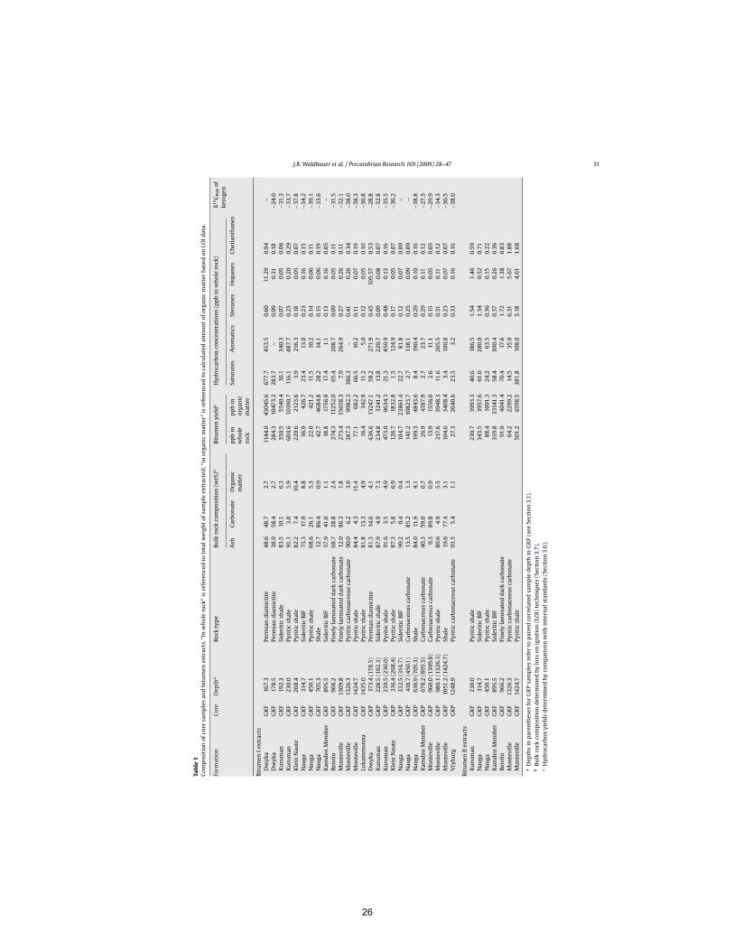
J.R. Waldbauer et al. / Precambrian Research 169 (2009) 28–47 31
Tabl
e1
Com
posi
tion
ofco
resa
mpl
esan
dbi
tum
enex
trac
ts.“
Inw
hole
rock
”is
refe
renc
edto
tota
lwei
ghto
fsam
ple
extr
acte
d;“i
nor
gani
cm
atte
r”is
refe
renc
edto
calc
ulat
edam
ount
ofor
gani
cm
atte
rba
sed
onLO
Idat
a.
Form
atio
nCo
reD
epth
aRo
ckty
peBu
lkro
ckco
mpo
siti
on(w
t%)b
Bitu
men
yiel
dcH
ydro
carb
onco
ncen
trat
ions
(ppb
inw
hole
rock
)!13
C PD
Bof
kero
gen
Ash
Carb
onat
eO
rgan
icm
atte
rpp
bin
who
lero
ck
ppb
inor
gani
cm
atte
r
Satu
rate
sA
rom
atic
sSt
eran
esH
opan
esCh
eila
ntha
nes
Bitu
men
Iext
ract
sD
wyk
aG
KF
167.
3Pe
rmia
ndi
amic
tite
48.6
48.7
2.7
1144
.043
045.
667
7.7
453.
50.
6011
.29
0.94
–D
wyk
aG
KF
178.
5Pe
rmia
ndi
amic
tite
38.9
58.4
2.7
284.
310
473.
228
3.7
–0.
090.
310.
18%
24.0
Kuru
man
GK
F19
2.3
Side
riti
csh
ale
83.5
10.1
6.3
350.
555
40.4
10.1
340.
30.
070.
050.
06%
31.3
Kuru
man
GK
F23
0.0
Pyri
tic
shal
e91
.13.
05.
960
4.6
1019
0.7
116.
148
7.7
0.25
0.20
0.29
%33
.7K
lein
Nau
teG
KF
268.
4Py
riti
csh
ale
82.2
7.4
10.4
220.
621
23.6
3.9
216.
30.
180.
050.
07%
37.8
Nau
gaG
KF
314.
7Si
deri
tic
BIF
73.3
17.9
8.8
36.9
426.
723
.413
.00.
230.
160.
15%
34.2
Nau
gaG
KF
450.
1Py
riti
csh
ale
68.6
26.1
5.3
22.0
421.
211
.510
.20.
140.
060.
11%
39.1
Nau
gaG
KF
705.
3Sh
ale
12.7
86.4
0.9
42.7
4684
.828
.214
.10.
150.
060.
19%
33.6
Kam
den
Mem
ber
GK
F89
5.5
Side
riti
cBI
F57
.941
.01.
118
.817
56.9
17.4
1.1
0.13
0.16
0.05
–Re
ivilo
GK
F96
6.2
Fine
lyla
min
ated
dark
carb
onat
e68
.728
.82.
427
4.3
1125
2.0
65.4
208.
70.
090.
050.
11%
31.5
Mon
tevi
lleG
KF
1309
.8Fi
nely
lam
inat
edda
rkca
rbon
ate
12.0
86.3
1.8
273.
415
658.
37.
926
4.9
0.27
0.26
0.11
%32
.1M
onte
ville
GK
F13
26.3
Pyri
tic
carb
onac
eous
carb
onat
e90
.06.
23.
938
7.3
9982
.338
6.3
–0.
410.
260.
34%
38.0
Mon
tevi
lleG
KF
1424
.7Py
riti
csh
ale
84.4
4.3
11.4
77.1
682.
266
.510
.20.
110.
070.
19%
38.3
Loka
mm
onna
GK
F14
35.0
Pyri
tic
shal
e81
.813
.34.
916
.434
2.9
11.2
5.0
0.12
0.05
0.10
%36
.8D
wyk
aG
KP
173.
4(1
78.5
)Pe
rmia
ndi
amic
tite
81.3
14.6
4.1
436.
613
247.
158
.227
1.9
0.45
105.
570.
53%
28.8
Kuru
man
GK
P22
8.5
(192
.3)
Side
riti
csh
ale
87.9
4.9
7.3
234.
832
41.2
13.8
220.
70.
090.
080.
07%
32.8
Kuru
man
GK
P23
9.5
(230
.0)
Pyri
tic
shal
e91
.63.
54.
947
3.0
9634
.321
.345
0.9
0.48
0.13
0.16
%35
.5K
lein
Nau
teG
KP
316.
4(2
68.4
)Py
riti
csh
ale
87.3
5.8
6.9
126.
718
32.8
1.5
124.
90.
170.
050.
07%
36.2
Nau
gaG
KP
332.
5(3
14.7
)Si
deri
tic
BIF
99.2
0.4
0.4
104.
723
861.
422
.781
.80.
120.
070.
09–
Nau
gaG
KP
418.
7(4
50.1
)Ca
rbon
aceo
usca
rbon
ate
13.5
85.2
1.3
141.
210
823.
72.
713
8.1
0.25
0.09
0.09
–N
auga
GK
P63
6.9
(705
.3)
Shal
e84
.011
.94.
119
9.3
4843
.68.
419
0.4
0.29
0.10
0.16
%38
.8K
amde
nM
embe
rG
KP
678.
2(8
95.5
)Ca
rbon
aceo
usca
rbon
ate
40.3
59.0
0.7
26.9
4187
.92.
723
.70.
290.
110.
12%
27.5
Mon
tevi
lleG
KP
960.
0(1
309.
8)Ca
rbon
aceo
usca
rbon
ate
9.3
89.8
0.9
13.9
1556
.02.
611
.10.
150.
050.
05%
29.9
Mon
tevi
lleG
KP
980.
1(1
326.
3)Py
riti
csh
ale
89.6
4.9
5.5
217.
639
48.3
11.6
205.
50.
310.
110.
12%
34.3
Mon
tevi
lleG
KP
1051
.2(1
424.
7)Sh
ale
19.6
77.4
3.1
104.
634
08.4
3.4
100.
80.
230.
070.
07%
36.5
Vry
burg
GK
P12
48.9
Pyri
tic
carb
onac
eous
carb
onat
e93
.55.
41.
127
.326
40.6
23.5
3.2
0.33
0.16
0.16
%38
.0
Bitu
men
IIex
trac
tsKu
rum
anG
KF
230.
0Py
riti
csh
ale
230.
739
93.3
40.6
186.
51.
541.
460.
59N
auga
GK
F31
4.7
Side
riti
cBI
F34
3.5
3957
.661
.028
0.0
1.34
0.52
0.71
Nau
gaG
KF
450.
1Py
riti
csh
ale
88.4
1691
.324
.263
.50.
360.
150.
22K
amde
nM
embe
rG
KF
895.
5Si
deri
tic
BIF
359.
833
141.
358
.430
0.4
0.37
0.26
0.36
Reiv
iloG
KF
966.
2Fi
nely
lam
inat
edda
rkca
rbon
ate
91.9
4041
.470
.417
.61.
721.
380.
83M
onte
ville
GK
F13
26.3
Pyri
tic
carb
onac
eous
carb
onat
e64
.222
99.2
14.5
35.9
6.31
5.67
1.88
Mon
tevi
lleG
KF
1424
.7Py
riti
csh
ale
501.
245
98.5
381.
810
8.0
5.18
4.61
1.68
aD
epth
sin
pare
nthe
ses
for
GK
Psa
mpl
esre
fer
topa
ired
corr
elat
edsa
mpl
ede
pth
inG
KF
(see
Sect
ion
3.1)
.b
Bulk
rock
com
posi
tion
dete
rmin
edby
loss
onig
niti
on(L
OI)
tech
niqu
es(S
ecti
on3.
7).
cH
ydro
carb
onyi
elds
dete
rmin
edby
com
pari
son
wit
hin
tern
alst
anda
rds
(Sec
tion
3.6)
.
26
32 J.R. Waldbauer et al. / Precambrian Research 169 (2009) 28–47
3.7. Bulk composition by LOI
Bulk weight percent organic matter, weight percent carbon-ate, and weight percent ash of each sample was estimated usingloss on ignition (LOI) techniques. 300–400 mg of rock powder wasweighed into a small ceramic crucible and combusted in a Barn-stead/Thermolyne 30400 furnace at 550 #C for 4 h. Once cool, thepowders were weighed, and mass loss at this step taken as theorganic matter content. The powders were then re-combusted at950 #C for 2 h, and the further mass loss taken as weight percentcarbonate. Material remaining after the final combustion (primarilysilicate, oxide and sulfide minerals) was considered ash.
3.8. EA-IRMS analyses
Rock powders for kerogen isotope measurements were firstdemineralized using 6N HCl and 48% HF as described above. Afterthis treatment, 1N HNO3 was added to the samples to dissolvesulfide minerals. The largely demineralized powders were thendried and weighed in triplicate into tin cups (0.5–0.8 mg each). Car-bon isotopic compositions were determined using a Fisons (CarloErba) NA 1500 elemental analyzer fitted with a Costech Zero BlankAutosampler and coupled to a Thermo Finnigan Delta Plus XP iso-tope ratio mass spectrometer.
4. Composition of Archean organic matter
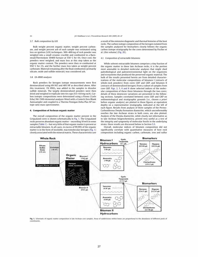
The overall composition of the organic matter present in theGriqualand cores is shown schematically in Fig. 1. The Griqualandrocks preserve abundant organic matter – exceeding 10 wt% in somesamples (Table 1) – but very little of that organic matter is present asextractable bitumen. In all cases, in excess of 99.99% of the organicmatter is in the form of insoluble, macromolecular kerogen (Fig. 1)closely associated with the mineral matrix. These characteristics are
a result of the extensive diagenetic and thermal histories of the hostrocks. The carbon isotope composition of the kerogen isolated fromthe samples analyzed for biomarkers closely follows the organiccarbon isotope stratigraphy for the cores determined by Fischer etal. (this volume) (Fig. 2E).
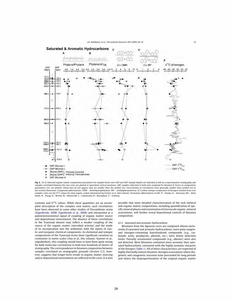
4.1. Composition of extractable bitumens
While solvent-extractable bitumen comprises a tiny fraction ofthe organic matter in these late Archean rocks, it is the portionmost amenable to detailed molecular analyses that might shedpaleobiological and paleoenvironmental light on the organismsand ecosystems that produced the preserved organic material. Thebulk of the results presented herein are from detailed character-izations of the molecular compositions of bitumen I (extracts ofwhole-rock powders) from cores GKF and GKP, and bitumen II(extracts of demineralized kerogen) from a subset of samples fromcore GKF. Figs. 2, 5, 6 and 8 show selected indices of the molec-ular composition of these three bitumens through the two cores;details of these downcore variations are presented in the follow-ing sections. Samples correlated between cores GKF and GKP onsedimentological and stratigraphic grounds (i.e., chosen a prioribefore organic analysis) are plotted in those figures at equivalentdepths on a representative stratigraphy, indicated at the left ofeach figure. Results from analysis of three samples of the Permo-Carboniferous Dwyka formation diamictite, which unconformablyoverlies the late Archean strata in both cores, are also plotted.Analysis of the Dwyka diamictite, while clearly not informative asto late Archean biogeochemistry, proved very useful as a test ofthe integrity and syngeneity of molecular fossils in the underlyingstrata; these results are discussed below in Section 5.5.
Overall, molecular indices of bitumen composition did notsignificantly correlate with quantitative measures of host rockcomposition including organic carbon, carbonate, iron and sulfur
Fig. 1. Schematic of organic matter composition in late Archean core samples. Areas of subdivisions within boxes are proportional to the abundance of different pools ofconstituents.
27
J.R. Waldbauer et al. / Precambrian Research 169 (2009) 28–47 33
Fig. 2. (A–E) Selected organic matter composition parameters for samples from cores GKF and GKP. Sample depths are indicated at left on a representative stratigraphy andsamples correlated between the two cores are plotted at equivalent vertical positions. GKF samples indicated in bold were analyzed for bitumen II. Errors in compositionparameters (2!) are plotted; where bars do not appear, they are smaller than the symbol size. Uncertainties in correlations were generally smaller than symbol size inthe vertical dimension. Compound abbreviations: DMN – dimethylnaphthalene, MP – methylphenanthrene. (E) Carbon isotope composition of kerogen isolated from coresamples. Lines are the !13C values for total organic carbon determined by Fischer et al. (this volume). Formation abbreviations at left: D – Dwyka, K – Kuruman, KN – KleinNaute, N – Nauga, R – Reivilo, M – Monteville, L – Lokamonna, B – Boomplaas, V – Vryburg.
contents and !13C values. While these quantities are an incom-plete description of the complex rock matrix, such correlationshave been observed in some other studies of Precambrian strata(Eigenbrode, 2008; Eigenbrode et al., 2008) and interpreted as apaleoenvironmental signal of coupling of organic matter sourceand depositional environment. The absence of these correlationsin the Transvaal dataset may reflect a weaker coupling of thesource of the organic matter (microbial activity) and the modeof its incorporation into the sediments with the inputs of clas-tic and inorganic chemical components. As elemental and isotopiccompositions of the Transvaal strata show significant variation oncentimeter to meter scales (Ono et al., this volume; Sumner et al.,unpublished), this coupling would have to have been quite strongfor bulk-molecular correlations to hold over hundreds of meters ofstratigraphy. The correspondence in bitumen composition betweensamples correlated on stratigraphic grounds (Section 5.3), how-ever, suggests that longer-term trends in organic matter sourcingand/or depositional environment are reflected in the cores. It is also
possible that more detailed characterization of the rock mineraland organic matrix compositions, including quantification of spe-cific mineral phases and examination of microscale organic-mineralassociations, will further reveal depositional controls of bitumencomposition.
4.1.1. Saturated and aromatic hydrocarbonsBitumens from the Agouron cores are composed almost exclu-
sively of saturated and aromatic hydrocarbons; more polar oxygen-and nitrogen-containing functionalized compounds (e.g., car-boxylic acids, porphyrins, phenols, etc.) were below detectionlimits. Partially unsaturated compounds (e.g., alkenes) were alsonot detected. Most bitumens contained more aromatic than satu-rated hydrocarbons, consistent with the highly aromatic characterof the kerogen (Table 1). All of these characteristics are expected ofhighly thermally mature bitumen–kerogen associations where dia-genetic and catagenetic reactions have proceeded for long periodsand where the disproportionation of the original organic matter
28
34 J.R. Waldbauer et al. / Precambrian Research 169 (2009) 28–47
into disordered, aromatised carbon and light hydrocarbons is near-ing completion.
Saturated hydrocarbon fractions extracted from these sed-iments are dominated by straight-chain n-alkanes, with acondensate-like carbon-number distribution peaking between C11
and C20. The acyclic isoprenoids pristane and phytane, generallyconsidered to be the products of diagenesis of the side-chain ofchlorophyll, were detected in all samples. The pristane/phytaneratios of the late Archean bitumens are low (0.4–1.5; Fig. 2A),which is consistent with (though not necessarily indicative of)
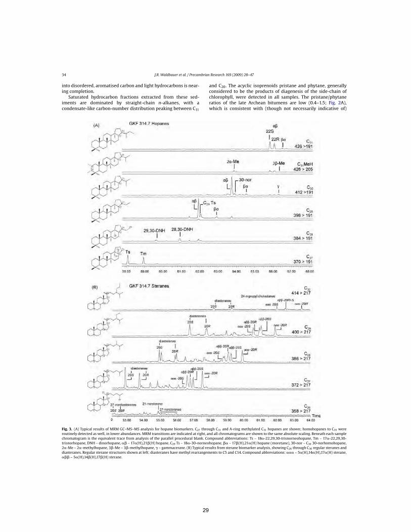
Fig. 3. (A) Typical results of MRM GC–MS–MS analysis for hopane biomarkers. C27 through C31 and A-ring methylated C31 hopanes are shown; homohopanes to C35 wereroutinely detected as well, in lower abundances. MRM transitions are indicated at right, and all chromatograms are shown to the same absolute scaling. Beneath each samplechromatogram is the equivalent trace from analysis of the parallel procedural blank. Compound abbreviations: Ts – 18#-22,29,30-trisnorneohopane, Tm – 17#-22,29,30-trisnorhopane, DNH – dinorhopane, #$ – 17#(H),21$(H) hopane, C29 Ts – 18#-30-norneohopane, $# – 17$(H),21#(H) hopane (moretane), 30-nor – C30 30-norhomohopane,2#-Me – 2#-methylhopane, 3$-Me – 3$-methylhopane, % – gammacerane. (B) Typical results from sterane biomarker analysis, showing C26 through C30 regular steranes anddiasteranes. Regular sterane structures shown at left; diasteranes have methyl rearrangements to C5 and C14. Compound abbreviations: ### – 5#(H),14#(H),17#(H) sterane,#$$ – 5#(H),14$(H),17$(H) sterane.
29
J.R. Waldbauer et al. / Precambrian Research 169 (2009) 28–47 35
Table 2Sample-to-blank (S/B) ratios for biomarker compounds, shown as averages across analyses of bitumen I extracts from Transvaal Supergroup samples (n = 23). Where a peakcorresponding a given isomer was not identified in the analysis of a procedural blank, a baseline noise peak of equivalent retention time was integrated to reflect the detectionlimit of the mass spectrometer during that analytical session.
Hopanes Average S/B Cheilanthanes/terpanes Average S/B Steranes Average S/B
C27 hopane Ts 7.3 C19 #$ tricyclic 17.7 C26 27-nordiasterane $# 20S 7.3C27 hopane Tm 16.0 C20 #$ tricyclic 13.4 C26 27-nordiasterane $# 20R 6.3C28 29,30-dinorhopane 5.6 C21 #$ tricyclic 4.9 C26 21-norsterane 16.4C28 28,30-dinorhopane 22.9 C22 #$ tricyclic 2.9 C26 27-norsterane ### 20S 4.9C29 #$ hopane 9.3 C23 #$ tricyclic 4.6 C26 27-norsterane #$$ 20R 7.3C29 Ts 35.2 C24 #$ tricyclic 5.0 C26 27-norsterane #$$ 20S 3.8C29 $# hopane (moretane) 27.3 C25 #$ tricyclic 22R 6.2 C26 27-norsterane ### 20R 8.8C30 #$ hopane 13.5 C25 #$ tricyclic 22S 5.7 C27 diasterane $# 20S 36.8C30 30-norhopane 11.2 C26 #$ tricyclic 22R 18.0 C27 diasterane $# 20R 45.8C30 $# hopane 18.7 C26 #$ tricyclic 22S 35.1 C27 sterane ### 20S 21.4C31 2#-methylhopane 25.9 C24 tetracyclic 9.8 C27 sterane #$$ 20R 26.4C31 #$ hopane 22S 64.4 C30 gammacerane 5.3 C27 sterane #$$ 20S 32.0C31 #$ hopane 22R 59.2 C27 sterane ### 20R 21.0C32 #$ hopane 22S 27.2 C28 diasterane $# 20S 29.3C32 #$ hopane 22R 14.2 C28 diasterane $# 20R 31.8C33 #$ hopane 22S 19.6 C28 sterane ### 20S 14.9C33 #$ hopane 22R 25.5 C28 sterane #$$ 20R 18.8C34 #$ hopane 22S 14.6 C28 sterane #$$ 20S 10.6C34 #$ hopane 22R 7.6 C28 sterane ### 20R 18.5C35 #$ hopane 22S 7.5 C29 diasterane $# 20S 23.4C35 #$ hopane 22R 5.6 C29 diasterane $# 20R 29.6
C29 sterane ### 20S 34.5C29 sterane #$$ 20R 21.3C29 sterane #$$ 20S 18.1C29 sterane ### 20R 15.7C30 diasterane $# 20S 8.3C30 diasterane $# 20R 5.6C30 24-n-propyl sterane ### 20S 7.6C30 24-n-propyl sterane #$$ 20R+20S 9.9C30 24-n-propyl sterane ### 20R 6.0
deposition in a saline, anoxic environment. The aromatic frac-tions (as analyzed by SIM-GC–MS) are composed primarily oflow-molecular weight polycyclic aromatic hydrocarbons (PAH;naphthalene and phenanthrene) and their alkylated homologues.Larger PAHs, including fluoranthene, pyrene and (in some sam-ples) perylene were detected at much lower abundances. Thesubstitution patterns of dimethylnaphthalenes and methylphenan-threnes showed dominance of the thermodynamically favored$-isomers over the more sterically hindered #-isomers (Fig. 2C andD).
The preponderance of low-molecular weight compounds in theTransvaal Supergroup bitumens also means that that they are verysusceptible to evaporation during extraction and analysis. Thisapplies particularly to n-alkanes <C14 and naphthalenes and mayhave affected the apparent bitumen yields, which can be consideredlower limits for in situ concentrations. With the possible excep-tion of chlorophyll-derived pristane and phytane, little can be saidabout the specific biological sources of these simpler hydrocarbonsor their precursors.
4.2. Biomarkers
Though they represent only a small proportion of the bitu-men extracts (Fig. 1), the cyclic terpenoids – hopanes, steranesand cheilanthanes – are the most information-rich molecules withregard to interpretations of the paleobiological source of the organicmatter and its diagenetic history. These molecules are unam-biguously biogenic; the hopanoids and steroids, in particular, arewell-characterized as the biosynthetic products of the enzymaticcyclization of squalene and oxidosqualene, respectively (Rohmeret al., 1984; Ourisson et al., 1987; Summons et al., 2006; Fischerand Pearson, 2007), which enables a more informed interpretationof these compounds as molecular fossils. Typical results of MRMGC–MS–MS biomarker analysis of a saturated hydrocarbon frac-
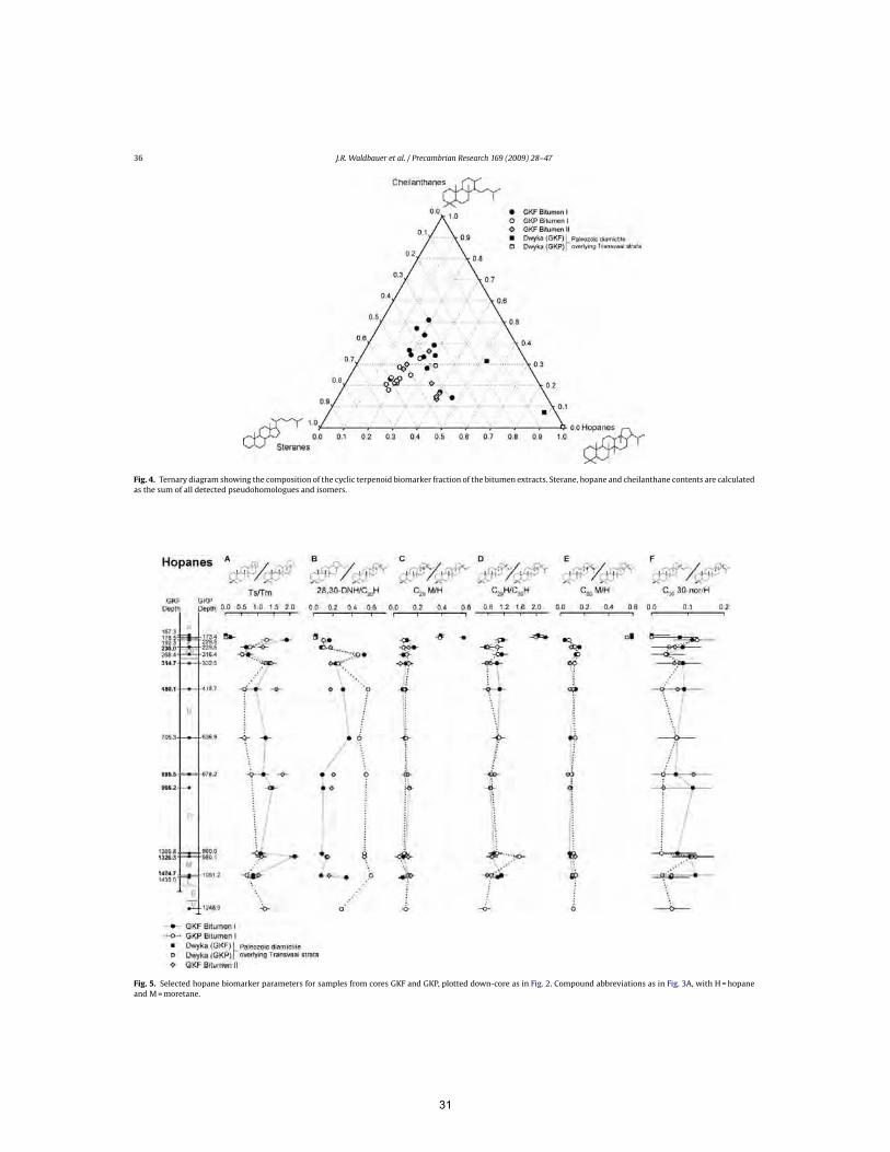
tion from a bitumen extract is shown in Fig. 3. These classes ofcyclic terpenoids were present at ppb to sub-ppb levels (Table 1),with concentrations of individual compounds at the parts per tril-lion level by weight. Despite these extremely low yields, a broaddiversity of biomarker structures could be consistently detected inbitumen extracts over the full depth of Archean strata intersectedby both cores. Analytical sample-to-blank ratios (i.e., amount of agiven compound detected in a core sample compared to that inthe parallel procedural blank) for biomarker compounds are listedin Table 2. For many compounds, the ‘blank’ reflects the detectionlimit of the mass spectrometer (baseline noise above which a peakmust rise) rather than the identified presence of a compound in theprocedural sand blank. The relative contributions of hopanes, ster-anes and cheilanthanes to the total biomarker content are shown inFig. 4. The three types are present in roughly equal abundance, witha slight preference for steranes that may or may not be significantwith regard to the source and/or diagenesis of the organic matter(see Section 6.2).
4.2.1. HopanesSeveral series of hopanes with 27–35 carbon atoms were
detected in all bitumens (Fig. 3A). These include: 17#(H),21$(H)-hopanes; 2#- and 3$-methylhopanes; 17$(H),21#(H)-hopanes(moretanes); and several rearranged and norhopanes (Fig. 3A).Average sample-to-blank ratios generally exceeded 10 for theprincipal C27–C31 isomers (Table 2). The stratigraphic distribu-tions of selected hopane isomers are shown in Fig. 5. The isomerdistributions of the hopanes show predominance of the more ther-modynamically stable forms, consistent with the high thermalmaturity of the Transvaal host rocks. In particular, all the lateArchean bitumens show high Ts/Tm ratios (>0.5; Fig. 5A) and lowmoretane/hopane ratios – approaching the thermodynamic end-point of 0.05 – in the C29 and C30 homologues (Fig. 5C and E). Theseindices of high maturity are consistent between bitumens I and II
30
36 J.R. Waldbauer et al. / Precambrian Research 169 (2009) 28–47
Fig. 4. Ternary diagram showing the composition of the cyclic terpenoid biomarker fraction of the bitumen extracts. Sterane, hopane and cheilanthane contents are calculatedas the sum of all detected pseudohomologues and isomers.
Fig. 5. Selected hopane biomarker parameters for samples from cores GKF and GKP, plotted down-core as in Fig. 2. Compound abbreviations as in Fig. 3A, with H = hopaneand M = moretane.
31
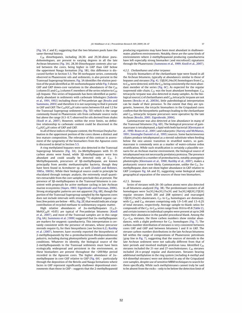
J.R. Waldbauer et al. / Precambrian Research 169 (2009) 28–47 37
(Fig. 5A, C and E), suggesting that the two bitumen pools have thesame thermal history.
C28 dinorhopanes, including 28,30- and 29,30-dinor pseu-dohomologues, are present to varying degrees in all the lateArchean bitumens (Fig. 3A). 28,30-Dinorhopane contents also var-ied between the cores, being higher in GKP than GKF belowthe uppermost Nauga formation (Fig. 5B); this difference is dis-cussed further in Section 5.3. The 30-norhopane series, commonlyobserved in Phanerozoic oils and sediments, is also present in theTransvaal Supergroup bitumens. Fig. 3A identifies the elution posi-tion of the peak identified as 30-norhomohopane while Fig. 5 showsGKF and GKP down-core variations in the abundances of the C29(column D) and C30 (column F) members of the series relative to C30#$-hopane. This series of hopanoids has been identified as partic-ularly abundant in sediments with carbonate lithologies (Subrotoet al., 1991, 1992) including those of Precambrian age (Brocks andSummons, 2003) and therefore it is not surprising to find it presentin GKF and GKP. The C29H/C30H ratio varies between 0.8 and 1.2 forthe Transvaal Supergroup sediments (Fig. 5D) which is the rangecommonly found in Phanerozoic oils from carbonate source rocksbut above the range (0.3–0.7) observed for oils derived from shales(Knoll et al., 2007). However, within the error limits, no defini-tive relationship to carbonate content could be discerned in theC29H/C30H ratios of GKP and GKF.
In all of these indices of hopane content, the Permian Dwyka For-mation in the uppermost portion of the cores shows a distinct andless mature composition. The relevance of this contrast in assess-ment of the syngeneity of the biomarkers from the Agouron coresis discussed in detail in Section 5.5.
A-ring methylated hopanes were also detected in the TransvaalSupergroup bitumens (Fig. 3A). 2#-Methylhopanes with 31–35carbon atoms were found, while 3$-methylhopanes were lessabundant and could usually be detected only at C31. 3-Methylhopanoids, precursors of 3$-methylhopane, are knownprincipally from aerobic methanotrophic bacteria, though theyhave been found in Acetobacter sp. as well (Zundel and Rohmer,1985a, 1985b). While their biological source could in principle beelucidated through isotopic analysis, the extremely small quanti-ties extractable from the core samples preclude this at present. Thepresence of 3$-methylhopanes in the Transvaal bitumens is con-sistent with proposals for active methane cycling in late Archeanmarine ecosystems (Hayes, 1983; Eigenbrode and Freeman, 2006).Strong stratigraphic patterns are not apparent (Fig. 6B), though theportion of the Transvaal Supergroup sampled by the Agouron coresdoes not include intervals with strongly 13C-depleted organic car-bon (few points are below%40‰; Fig. 2E) that would indicate a largecontribution of recycled methane to sedimentary organic matter.
High relative abundances of 2#-methylhopanes (C312-MeH/C30H >0.05) are typical of Precambrian bitumens (Knollet al., 2007), and most of the Transvaal samples are in this range(Fig. 6A). Summons et al. (1999) suggested that 2#-methylhopanesare markers for oxygenic cyanobacteria. This interpretation is cer-tainly consistent with the presence of steranes, whose precursorsteroids require O2 for their biosynthesis (see Section 6.2). Rashbyet al. (2007), however, have recently reported the biosynthesis of2-methylhopanoids by the #-proteobacterium Rhodopseudomonaspalustris, including during photosynthetic growth under anaerobicconditions. Whatever its identity, the biological source of the2-methylhopanoids to the Transvaal sediments must have beenecologically widespread and persistent in the environment, asthese biomarkers are present throughout the >200 Myr periodrecorded in the Agouron cores. The higher abundance of 2#-methylhopane in core GKF relative to GKP (Fig. 6A) – particularlythrough the deposition of the Reivilo and Nauga formations wherefacies in GKF represent significantly shallower depositional envi-ronments than those in GKP – suggests that the 2-methylhopanoid
producing organisms may have been most abundant in shallower-water, platform environments. Notably, these are the same kinds ofenvironments where 2-methylhopanoid producing cyanobacteriahave left especially strong biomarker (and microfossil) signaturesthrough the Phanerozoic (Summons et al., 1999; Knoll et al., 2007).
4.2.2. Cheilanthanes and other terpanesTricyclic biomarkers of the cheilanthane type were found in all
the Archean bitumens, typically at abundances similar to those ofhopanes and steranes (Fig. 4). 13$(H),14#(H) homologues from C19to C26 were detected, with the C23 being consistently the most abun-dant member of the series (Fig. 6C). As expected for the regularisoprenoid side-chain, C22 was the least abundant homologue. C24tetracyclic terpane was also detected in many samples. As the bio-logical source(s) of cheilanthanes and C24 tetracyclic terpane are notknown (Brocks et al., 2003b), little paleobiological interpretationcan be made of their presence. To the extent that they are syn-genetic, however, the tricyclic biomarkers in the Griqualand coresconfirm that the biosynthetic pathways leading to the cheilanthaneand C24 tetracyclic terpane precursors were operative by the lateArchean (Brocks, 2001; Eigenbrode, 2004).
Gammacerane was also detected at low abundance in many ofthe Transvaal bitumens (Fig. 6D). The biological precursor of gam-macerane is tetrahymanol, a lipid with both bacterial (Kleemann etal., 1990; Bravo et al., 2001) and eukaryotic (Harvey and McManus,1991; Sinninghe Damsté et al., 1995) sources. Some bacteriovorousciliates produce tetrahymanol as a steroid substitute when feedingbelow the oxic–anoxic transition in stratified waters, so gam-macerane is commonly seen as a marker of water-column redoxstratification. While such stratification is certainly a plausible sce-nario for an Archean marine environment, the biological source oftetrahymanol was not necessarily predatory protozoa. The presenceof tetrahymanol in a number of proteobacteria, notably anoxygenicphototrophs (Kleemann et al., 1990; Rashby et al., 2007), makes aprokaryotic source more likely. Gammacerane, unlike the C31 2#-methylhopane, does not show higher abundance in GKF relative toGKP (compare Fig. 6A and D), suggesting some biological and/orgeographical separation of the sources of those two biomarkers.
4.2.3. SteranesSeries of steranes with 26–30 carbon atoms were also detected
in all bitumens analyzed (Fig. 3B). The predominant isomers of allhomologues were 5#(H),14#(H),17#(H) and 5#(H),14$(H),17$(H)regular steranes (both 20S and 20R epimers) and rearranged13$(H),17#(H)-diasteranes. C27 to C29 homologues are dominant,with C26 and C30 steranes comprising only 1.9–5.4% and 1.5–6.2%of total steranes, respectively. Average sample-to-blank ratios forcompounds of the C27 to C29 series range from 10.6 to 45.8 (Table 2),and certain isomers in individual samples were present at up to 248times their abundance in the parallel procedural blank. Among theC27–C29 steranes, the three carbon numbers show similar abun-dances, with a slight preference for C27 homologues (Fig. 7). Thecarbon-number distribution of steranes is very consistent betweencores GKF and GKP and between bitumens I and II in GKF. Thesterane carbon-number distributions in the late Archean bitumensfall within the range of compositions of Phanerozoic petroleum(gray line in Fig. 7), suggesting that the sources of steroids to thelate Archean sediment were not radically different from that oflater periods and involved multiple protistan taxa. Identified C26steranes included the 21-nor and 27-norcholestanes. C30 steranesincluded 24-n-propyl regular and diasteranes. Steranes bearingadditional methylation in the ring system (including 4-methyl and4,4-dimethyl steranes) were not detected in any of the Griqualandcore samples, despite use of sensitive MRM techniques to search forthem specifically. While such methylsteranes cannot truly be saidto be absent from the rocks – only to be below the detection limit of
32
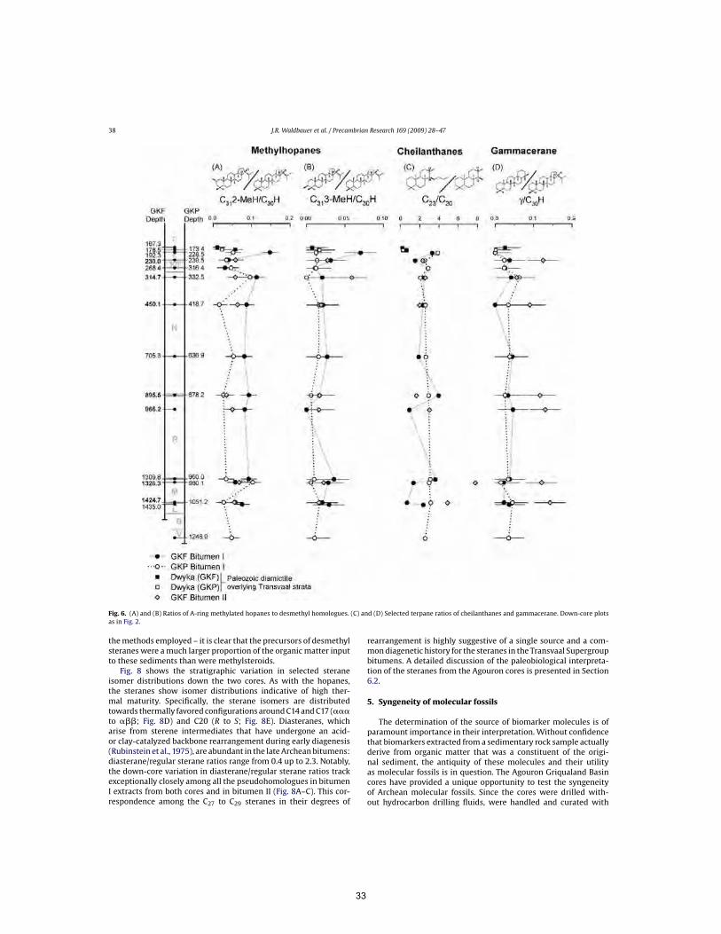
38 J.R. Waldbauer et al. / Precambrian Research 169 (2009) 28–47
Fig. 6. (A) and (B) Ratios of A-ring methylated hopanes to desmethyl homologues. (C) and (D) Selected terpane ratios of cheilanthanes and gammacerane. Down-core plotsas in Fig. 2.
the methods employed – it is clear that the precursors of desmethylsteranes were a much larger proportion of the organic matter inputto these sediments than were methylsteroids.
Fig. 8 shows the stratigraphic variation in selected steraneisomer distributions down the two cores. As with the hopanes,the steranes show isomer distributions indicative of high ther-mal maturity. Specifically, the sterane isomers are distributedtowards thermally favored configurations around C14 and C17 (###to #$$; Fig. 8D) and C20 (R to S; Fig. 8E). Diasteranes, whicharise from sterene intermediates that have undergone an acid-or clay-catalyzed backbone rearrangement during early diagenesis(Rubinstein et al., 1975), are abundant in the late Archean bitumens:diasterane/regular sterane ratios range from 0.4 up to 2.3. Notably,the down-core variation in diasterane/regular sterane ratios trackexceptionally closely among all the pseudohomologues in bitumenI extracts from both cores and in bitumen II (Fig. 8A–C). This cor-respondence among the C27 to C29 steranes in their degrees of
rearrangement is highly suggestive of a single source and a com-mon diagenetic history for the steranes in the Transvaal Supergroupbitumens. A detailed discussion of the paleobiological interpreta-tion of the steranes from the Agouron cores is presented in Section6.2.
5. Syngeneity of molecular fossils
The determination of the source of biomarker molecules is ofparamount importance in their interpretation. Without confidencethat biomarkers extracted from a sedimentary rock sample actuallyderive from organic matter that was a constituent of the origi-nal sediment, the antiquity of these molecules and their utilityas molecular fossils is in question. The Agouron Griqualand Basincores have provided a unique opportunity to test the syngeneityof Archean molecular fossils. Since the cores were drilled with-out hydrocarbon drilling fluids, were handled and curated with
33
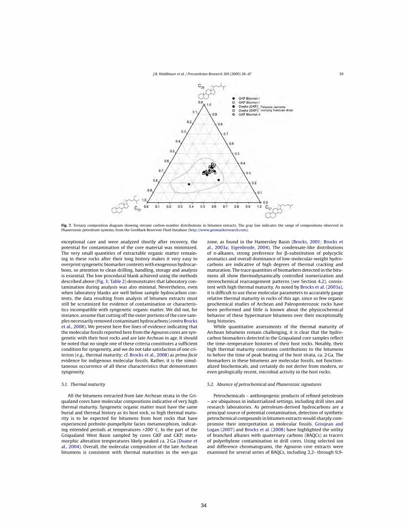
J.R. Waldbauer et al. / Precambrian Research 169 (2009) 28–47 39
Fig. 7. Ternary composition diagram showing sterane carbon-number distributions in bitumen extracts. The gray line indicates the range of compositions observed inPhanerozoic petroleum systems, from the GeoMark Reservoir Fluid Database (http://www.geomarkresearch.com).
exceptional care and were analyzed shortly after recovery, thepotential for contamination of the core material was minimized.The very small quantities of extractable organic matter remain-ing in these rocks after their long history makes it very easy tooverprint syngenetic biomarker contents with exogenous hydrocar-bons, so attention to clean drilling, handling, storage and analysisis essential. The low procedural blank achieved using the methodsdescribed above (Fig. 3; Table 2) demonstrates that laboratory con-tamination during analysis was also minimal. Nevertheless, evenwhen laboratory blanks are well below sample hydrocarbon con-tents, the data resulting from analysis of bitumen extracts muststill be scrutinized for evidence of contamination or characteris-tics incompatible with syngenetic organic matter. We did not, forinstance, assume that cutting off the outer portions of the core sam-ples necessarily removed contaminant hydrocarbons (contra Brockset al., 2008). We present here five lines of evidence indicating thatthe molecular fossils reported here from the Agouron cores are syn-genetic with their host rocks and are late Archean in age. It shouldbe noted that no single one of these criteria constitutes a sufficientcondition for syngeneity, and we do not take satisfaction of one cri-terion (e.g., thermal maturity; cf. Brocks et al., 2008) as prima facieevidence for indigenous molecular fossils. Rather, it is the simul-taneous occurrence of all these characteristics that demonstratessyngeneity.
5.1. Thermal maturity
All the bitumens extracted from late Archean strata in the Gri-qualand cores have molecular compositions indicative of very highthermal maturity. Syngenetic organic matter must have the sameburial and thermal history as its host rock, so high thermal matu-rity is to be expected for bitumens from host rocks that haveexperienced prehnite-pumpellyite facies metamorphism, indicat-ing extended periods at temperatures >200 #C. In the part of theGriqualand West Basin sampled by cores GKF and GKP, meta-morphic alteration temperatures likely peaked ca. 2 Ga (Duane etal., 2004). Overall, the molecular composition of the late Archeanbitumens is consistent with thermal maturities in the wet-gas
zone, as found in the Hamersley Basin (Brocks, 2001; Brocks etal., 2003a; Eigenbrode, 2004). The condensate-like distributionsof n-alkanes, strong preference for $-substitution of polycyclicaromatics and overall dominance of low-molecular-weight hydro-carbons are indicative of high degrees of thermal cracking andmaturation. The trace quantities of biomarkers detected in the bitu-mens all show thermodynamically controlled isomerization andstereochemical rearrangement patterns (see Section 4.2), consis-tent with high thermal maturity. As noted by Brocks et al. (2003a),it is difficult to use these molecular parameters to accurately gaugerelative thermal maturity in rocks of this age, since so few organicgeochemical studies of Archean and Paleoproterozoic rocks havebeen performed and little is known about the physicochemicalbehavior of these hypermature bitumens over their exceptionallylong histories.
While quantitative assessments of the thermal maturity ofArchean bitumens remain challenging, it is clear that the hydro-carbon biomarkers detected in the Griqualand core samples reflectthe time–temperature histories of their host rocks. Notably, theirhigh thermal maturity constrains contributions to the bitumensto before the time of peak heating of the host strata, ca. 2 Ga. Thebiomarkers in these bitumens are molecular fossils, not function-alized biochemicals, and certainly do not derive from modern, oreven geologically recent, microbial activity in the host rocks.
5.2. Absence of petrochemical and Phanerozoic signatures
Petrochemicals – anthropogenic products of refined petroleum– are ubiquitous in industrialized settings, including drill sites andresearch laboratories. As petroleum-derived hydrocarbons are aprincipal source of potential contamination, detection of syntheticpetrochemical compounds in bitumen extracts would sharply com-promise their interpretation as molecular fossils. Grosjean andLogan (2007) and Brocks et al. (2008) have highlighted the utilityof branched alkanes with quaternary carbons (BAQCs) as tracersof polyethylene contamination in drill cores. Using selected ionand difference chromatograms, the Agouron core extracts wereexamined for several series of BAQCs, including 2,2- through 9,9-
34

40 J.R. Waldbauer et al. / Precambrian Research 169 (2009) 28–47
Fig. 8. Selected sterane biomarker parameters for samples from cores GKF and GKP, plotted down-core as in Fig. 2. Compound abbreviations as in Fig. 3B.
dimethyl, -diethyl and mixed alkyl (e.g., ethyl-, methyl-; butyl-,ethyl-) alkanes. No signals indicative of the presence of BAQCs weredetected. The absence of this one class of contaminants does notexclude the possibility of other forms of contamination, but lendssome confidence that core storage and handling conditions did notintroduce high levels of exogenous petrochemicals into the sam-ples.
Syngenetic organic matter from Precambrian rocks should alsobe devoid of biomarkers known only from later-evolving organisms.The largest class of these characteristically Phanerozoic biomarkersare the wide variety of polyterpenoid compounds synthesized byvascular plants. No fossils of plant terpenoids could be identifiedin the late Archean bitumens, despite specific investigation whenpotential signals of their presence were detected. In one instance,this investigation led to detection of an additional series of biomark-ers.
MRM-GC–MS–MS analysis of a number of core extracts showeda small, partly resolved doublet peak in the m/z 412 > 191 reactionchromatogram for a compound eluting just before C30 hopane at thetime expected for oleanane, a diagnostic marker for angiosperms(indicated with an asterisk in Fig. 9A). Oleanane is abundant inthe sedimentary record only from the late Cretaceous onwards
(Moldowan et al., 1994) so its presence in the Transvaal Supergroupbitumens would be clear evidence of contamination by youngerhydrocarbons. Identification based solely on the m/z 412 > 191 tran-sition is insufficient, however, since oleanane is known to co-elutewith other triterpenoids including members of the 25-norhopaneseries, as shown by Dzou et al. (1999). 25-norhopanes are generallyconsidered to be the products of microbial degradation of hopanes(Volkman et al., 1983; Peters et al., 1996), and, owing to the removalof the C10 methyl group, give a strong m/z 177 fragment ion.
We thus re-examined the samples with the potential oleananepeak by measuring a series of M+ > 177 transitions, and comparedthe results with analysis of a biodegraded crude oil from theLlanos Basin of Colombia that contains abundant 25-norhopanes(Fig. 9A). Inspection of the trace for the 412 > 177 transition revealedthe presence of two peaks at the retention times of the C3025-norhomohopanes (22S + R). Note the inversion of the relativecontributions of the 22S and 22R epimers between the 412 > 191and 412 > 177 traces, observed in both the oil and core samples.Examination of other MRM transitions indicated the presence ofC29 25-norhopane and C28 25,30-dinorhopane as well (Fig. 9B)confirming the presence of a pseudohomologous series of thesebiomarkers. In fact, the series of 25-norhopanes appeared to be
35
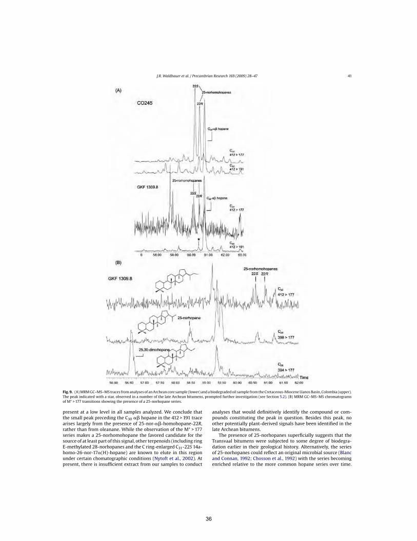
J.R. Waldbauer et al. / Precambrian Research 169 (2009) 28–47 41
Fig. 9. (A) MRM GC–MS–MS traces from analyses of an Archean core sample (lower) and a biodegraded oil sample from the Cretaceous-Miocene Llanos Basin, Colombia (upper).The peak indicated with a star, observed in a number of the late Archean bitumens, prompted further investigation (see Section 5.2). (B) MRM GC–MS–MS chromatogramsof M+ > 177 transitions showing the presence of a 25-norhopane series.
present at a low level in all samples analyzed. We conclude thatthe small peak preceding the C30 #$ hopane in the 412 > 191 tracearises largely from the presence of 25-nor-#$-homohopane-22R,rather than from oleanane. While the observation of the M+ > 177series makes a 25-norhomohopane the favored candidate for thesource of at least part of this signal, other terpenoids (including ringE-methylated 28-norhopanes and the C ring-enlarged C31-22S 14a-homo-26-nor-17#(H)-hopane) are known to elute in this regionunder certain chomatographic conditions (Nytoft et al., 2002). Atpresent, there is insufficient extract from our samples to conduct
analyses that would definitively identify the compound or com-pounds constituting the peak in question. Besides this peak, noother potentially plant-derived signals have been identified in thelate Archean bitumens.
The presence of 25-norhopanes superficially suggests that theTransvaal bitumens were subjected to some degree of biodegra-dation earlier in their geological history. Alternatively, the seriesof 25-norhopanes could reflect an original microbial source (Blancand Connan, 1992; Chosson et al., 1992) with the series becomingenriched relative to the more common hopane series over time.
36
42 J.R. Waldbauer et al. / Precambrian Research 169 (2009) 28–47
In the present case, the origins of the 25-norhopanes cannot beascribed; they may derive from original microbial input or fromearlier in situ biodegradation or, possibly, they are somewhat morethermodynamically stable and resistant to cracking.
Beyond the absence of diagnostic markers of later-evolvingorganisms, the biomarker composition of the late Archean bitu-mens would be very unusual if detected in a Phanerozoic setting.For example, the Transvaal Supergroup bitumens have relativelylarge amounts of C28 steranes (30–40% of total C27–29; Fig. 7), whichare typically <25% of the total in Paleozoic oils (Grantham andWakefield, 1988; Knoll et al., 2007). Mesozoic and younger bitu-mens contain more C28 steranes, owing to the rise to ecologicalprominence of the chlorophyll c-containing phytoplankton (Knollet al., 2007), but also usually contain plant markers (especiallyoleanane in Cretaceous and younger systems) and/or abundantdinosteranes, none of which were detected here. The high rela-tive abundance 2-methylhopane, exceeding 10% of C30 hopane ina number samples of various lithologies (Fig. 6A), is also a signa-ture more typical of Precambrian deposits than Phanerozoic ones(Knoll et al., 2007). Taken together, the constellation of biomarkersseen in the Transvaal Supergroup bitumens is inconsistent with asource of Phanerozoic age. It is thus difficult – merely on composi-tional grounds – to construct a scenario by which the bitumen in theTransvaal strata could have migrated from a much younger source.
5.3. Correlation between cores GKF and GKP
An important aspect of the Agouron Griqualand drilling project,unique among Precambian Earth-history drilling efforts, is therecovery of long intervals of correlated stratigraphy from geo-graphically distant parts of a single depositional system. CoresGKF and GKP, drilled 24 km apart, are well correlated over muchof their lengths, representing ca. 200 million years of depositionof the Transvaal Supergroup. The basis for these correlations anddetailed discussion of the depositional environment are presentedelsewhere (Schröder et al., 2006; Sumner et al., unpublished).These correlated sections provide a singular opportunity to lookfor chemostratigraphic patterns in biomarker contents. The lateArchean bitumens, while of a uniformly high maturity, do exhibitenough compositional heterogeneity that variations along thestratigraphy are potentially informative.
When the molecular composition of bitumens from GKF andGKP are compared down-core, the stratigraphic correspondencein biomarker variation is striking. The values of many biomarkerparameters from samples correlated on sedimentological groundsplot nearly on top of one another, even as they vary betweenstrata by amounts significantly greater than the analytical preci-sion (Figs. 2, 5 and 8). The correspondence is particularly notable inthe upper sections of the core over the Kuruman, Klein Naute, anduppermost Nauga formations, where $/# dimethylnaphthalene(Fig. 2C), Ts/Tm (Fig. 5A), 28,30-dinorhopane/C30 hopane (Fig. 5B),C30 30-norhopane/hopane (Fig. 5F) and each of C27–C29 diaster-ane/regular sterane (Fig. 8A–C) ratios all track exceptionally closelyover more than 100 m of stratigraphy. The two cores sample sim-ilar deepwater depositional environments through this interval,and so likely had similar organic matter inputs, and the litholo-gies of the host rocks are similar, creating similar physicochemicalenvironments for diagenesis. While one expects similar biomarkersignatures from similar depositional settings with similar organic-matter sources, finding such correspondence preserved over 2.5billion years in trace quantities of molecular fossils is remarkable.
In the lower portion of the cores, from the Nauga Formationdown to the lowermost correlated samples in the Monteville,there is more inter-core variation and the bitumen compositionsof the two cores diverge in certain respects. The lower parts ofthe cores represent less similar depositional settings, with GKF
comprising relatively more marginal and GKP more basinal facies.However, nowhere do we detect gross compositional differencesthat suggest radically different sources of organic matter to thesites of the two cores, and a number of biomarker ratios (e.g.,Fig. 5C–E, Fig. 8E) do correlate, albeit within a small range of varia-tion comparable to the analytical precision. Some parameters (e.g.,Figs. 2C and D, 5F, and 8D and F) show apparently uncorrelatedvariation around a constant mean. A few consistent differences,however, can be discerned between the lower sections of GKF andGKP, and these may be related to their relative positions on theplatform margin.
Below the upper Nauga, GKP has lower diasterane/regularsterane ratios (Fig. 8A–C), higher relative amounts of 28,30-dinorhopane (Fig. 5B) and lower Ts/Tm ratios (Fig. 5A) than GKF. C29Ts/hopane ratios, analogous to Ts/Tm, show similar behavior (datanot shown). This is in spite of similar patterns of other hopanes (C29and C30 moretane/hopane; Fig. 5C and E) and steranes (#$$/###and 20S/20R; Fig. 8D and E) in a majority of samples. Several com-positional differences are also apparent: GKP has relatively moresteranes (at the expense of cheilanthanes; Fig. 4), higher relativeC28 sterane content (Fig. 7) and less 2#-methylhopane (Fig. 6A)than GKF and less variable ratios of some cheilanthanes such asC23/C20 (Fig. 6C). These differences, while not large, suggest thatthere may have been a cross-platform gradient in microbial com-munity composition and, more tentatively, that sedimentary redoxconditions at the location of GKP may have been more reducing, upuntil partway through the deposition of the Nauga Formation.
The consistency down-core of the differences in C27–C29 diaster-ane and 28,30-DNH (Fig. 5B) contents between GKF and GKP areparticularly striking and, perhaps, record a subtle sedimentary orenvironmental distinction that decreased over the time of plat-form deposition. The biomarker 28,30-DNH is typically abundantin highly reducing environments (Grantham et al., 1980; Peters etal., 2005). However, in the case of immature Miocene California Bor-derland sediments, where the whole sedimentary section recordsa reducing paleoenvironment, the abundance of 28,30-DNH rela-tive to the total hopane content is inversely correlated with thecontent of clay minerals (Brincat and Abbott, 2001) whose pres-ence should promote the formation of diasteranes. In accord withthis pattern, below the uppermost Nauga Formation the relativecontents of diasteranes and Ts in GKF increase compared to thecorrelated intervals in GKP while 28,30-DNH is relatively moreabundant in GKP.
The observed chemostratigraphic relationships between corre-lated samples in GKF and GKP provide compelling evidence forsyngeneity. The bed-to-bed correlation is especially close in thedeepwater facies in the upper "350 m of each core, and the lowerportions show compositional differences that may reflect theirrelative positions on the Campbellrand Platform margin. Theserelationships can only arise when the organic contents of rocksare depositionally controlled and not subsequently overprinted byhydrocarbon migration or anthropogenic contamination.
5.4. Composition of bitumens I and II
To further test the syngeneity of the Archean bitumens, sevensamples from core GKF (which had already been solvent extractedto prepare bitumen I) were treated with acids (HCl and HF) todissolve and disaggregate much of the mineral matter and werethen re-extracted to yield a fraction termed bitumen II (see Sec-tion 3.5). In contrast to bitumen I (the bitumen extractable fromwhole-rock powder), bitumen II represents material that was notsolvent-accessible in situ or even after mechanical crushing. Whileits precise microscale distribution is unclear, bitumen II is certainlymore closely associated with the kerogen and mineral matricesof the rock than is bitumen I. Additionally, since contaminants
37
J.R. Waldbauer et al. / Precambrian Research 169 (2009) 28–47 43
(anthropogenic or migrated) are necessarily mobile, they are morelikely to be found in the more solvent-accessible bitumen I. Hence,where bitumen I and II extracts from the same rock show sim-ilar compositions, they are likely derived from syn-depositionalorganic matter, with the caveat that bitumen II may be enrichedin compounds produced by mineral-surface-catalyzed diageneticreactions and derived from maturing kerogen.
The compositions of bitumens I and II from the GKF core sam-ples appear similar in many respects. Yields of the two bitumensare in the same tens-to-hundreds of ppb range (Table 1); there isnot a very much larger quantity of solvent-extractable bitumen lib-erated by acid demineralization. The gross molecular compositionof the two bitumens is the same, dominated by low-molecular-weight saturated and aromatic hydrocarbons (Fig. 1). Bitumen IIcontains cyclic terpenoid biomarkers at slightly higher concentra-tions than bitumen I (Table 1). The carbon-number distributions ofsteranes (Fig. 7), hopanes (Fig. 5D) and cheilanthanes (Fig. 6C) fullyoverlap between bitumens I and II, and moretanes and norhopanesshow very similar relative abundances (Fig. 5B–D and F), consistentwith the biomarkers in the two pools of organic matter deriv-ing from the same source. Crucially, the thermal maturities of thetwo bitumens inferred from the biomarker isomer distributionsare equivalent—an essential and characteristic quality of syngeneticorganic matter. Evidence for equivalent thermal maturities includessimilar values in bitumen I and II extracts for: hopanoid Ts/Tm ratios(Fig. 5A) and extent of $#-to-#$ isomerization around C17 and C21for C29 and C30 homologues (moretane/hopane; Fig. 5C and E), aswell as ratios of C27–29 #$$ to ### steranes (Fig. 8D) and epimer-izaton around C20 (Fig. 8E). The down-core variability for several ofthese indices tracks closely between bitumens I and II as well; thisis good evidence that organic matter source and depositional envi-ronment, rather than later overprinting by contaminants, controlsdifferences in bitumen composition between strata. Taken together,the consistent similarities in molecular composition, thermal matu-rity and patterns of stratigraphic variation between bitumens I andII are strong evidence for syngeneity.
Furthermore, the compositional differences between the twobitumen extracts are in fact of the kind one might expect in com-paring pools of organic matter that have the same source, but aremore- versus less-closely matrix-associated in the same rock. Oneexample is the higher diasterane/regular sterane ratios in bitumen IIthan bitumen I, especially in the upper "1000 m of core GKF, abovethe Monteville formation (Fig. 8A–C). Diasteranes are thought tobe generated from sterenes by concerted methyl-rearrangementreactions that are catalyzed by acidic sites on clay minerals suchas montmorillonite and illite (Rubinstein et al., 1975; Sieskind etal., 1979; van Kaam-Peters et al., 1998). Hence, the more closelymineral-associated bitumen II, having greater access to clays in therock matrix, would plausibly be enriched in diasteranes relative tobitumen I. The two samples from the Monteville formation, how-ever, show nearly identical diasterane/regular sterane ratios. Thismay be related to a distinct clay mineralogy or style of organicsedimentation in the Monteville; in any event, it points towarddepositional control of organic matter composition and diagenesis.As noted above in comparing between GKF and GKP, these down-core patterns are consistent in bitumens I and II between C27, C28and C29 (dia)steranes. Both similarities and contrasts in molecularcomposition between bitumens I and II indicate the hydrocarbons’derivation from syn-depositional organic matter.
5.5. Contrasting composition of overlying Dwyka diamictite
One unintended – but unexpectedly useful – aspect of theGriqualand drilling was the intersection (in both the GKF andGKP boreholes) of the Dwyka Formation, a Permo-Carboniferousdiamictite that was deposited over a large portion of southern
Africa (Visser, 1989). This Phanerozoic glacial deposit overlies thelate Archean Transvaal sedimentary sequence above a 2-billion-year unconformity with the Kuruman Formation. While not thetarget of the Agouron drilling project, the Dwyka was intersected inthe two cores to depths approaching 200 m, well below the mod-ern weathering horizon. The recovery of unweathered Phanerozoicsedimentary rock in the same borehole provides another oppor-tunity to test the syngeneity of the Archean bitumens, since theorganic matter in the Dwyka has very different sources and thermalhistory from the Transvaal sediments, yet the core samples wereall exposed to the same drilling equipment, handling and storageconditions, and chemical analyses. Pervasive contamination duringdrilling and analysis would obliterate the contrast that should beapparent across the Dwyka/Kuruman unconformity. On the otherhand, if the very different character of the Dwyka organic matterwere observed in analyses of the Griqualand cores, this would bestrong evidence that anthropogenic contamination did not over-print syngenetic organic signatures in the core samples.
By nearly every metric of molecular composition, the Dwykasamples from the Griqualand cores are, in fact, distinct from the lateArchean rocks directly below. Both saturate and aromatic hydrocar-bon fractions show differences, including higher pristane/phytaneand lower phytane/n-C18 ratios (Fig. 2A and B), strong even-over-odd alkane preferences in the GKF Dwyka samples, and much highercontents of thermodynamically disfavored #-substituted dimethyl-naphthalenes and methylphenanthrenes (Fig. 2C and D). Bitumenfrom the Dwyka also contains less thermally stable molecules, suchas anthracene (Smith et al., 1995), that are not detected in theTransvaal.
The contrast is especially clear in cyclic biomarker contents,which uniformly indicate a significant difference in source and ther-mal history across the unconformity. The biomarkers in two Dwykasamples are strongly hopane-dominated, while the third is less sobut still outside the range of the Archean samples (Fig. 4). Organicmatter from the Dwyka appears rather heterogeneous, which isexpected in a clastic glaciogenic deposit. Consistent with this depo-sitional setting, the studied core samples contained numerouslarge, irregularly shaped clasts with dissimilar lithologies, indi-cating multiple sedimentary sources. The sterane carbon-numberdistributions of the Archean samples define a small field in Fig. 7,while those of the Dwyka vary much more widely, with the GKPsample plotting just on the edge of the Archean field and the twoGKF samples completely distinct from it. Their relatively low con-tent of C28 steranes is also a typically Paleozoic signature. Evenmore striking are the sharp contrasts in biomarker maturity param-eters across as little as 15 m of stratigraphy, shown in Figs. 5 and 8.By every measure, the organic matter in the Dwyka is far lessthermally mature than the Archean sedimentary rocks just a fewmeters below. Evidence includes: much lower Ts/Tm and higher$#/#$ hopane ratios (Fig. 5A, C and D), lower diasterane/regularsterane and lower sterane #$$/### ratios (Fig. 8A–D), and thedetection in the Dwyka of thermodynamically less-stable isomers,such as 17$-hopanes, which are absent from the Transvaal rocks.Carbon-number distributions of hopanes (Fig. 5D) and cheilan-thanes (Fig. 6C) are also distinct.
Clearly, the sharp compositional and maturity contrastsbetween the Dwyka and the underlying late Archean rocks arepreserved in both cores. These contrasts constitute an original,unconformity-related relationship and the process of recoveringand analyzing the core material has not compromised this sig-nal. The distinct and immature composition of the Dwyka organicmatter also precludes it from being the source of the bitumens inthe Transvaal strata. The detection of this demonstrably syngeneticcharacteristic of the organic matter in both GKF and GKP cores pro-vides additional strong evidence that the biomarkers in the lateArchean bitumens are not contaminants.
38
44 J.R. Waldbauer et al. / Precambrian Research 169 (2009) 28–47
6. Discussion
6.1. Late Archean molecular fossils and the antiquity of microbialdiversity
Taken together, we find the evidence for the syngenetic natureof the Transvaal bitumens (Section 5) to be compelling. As they aresyngenetic, and thus late Archean in age, the bitumens constitutea molecular fossil record of microbial activity during the deposi-tion of the Transvaal Supergroup. The Transvaal sediments, likemany Precambrian sequences, bear a number of signs of microbialinvolvement in their deposition. Numerous sedimentary texturescan be attributed to microbial activity (Schröder et al., this volume)and large amounts of organic matter with textures and isotopiccompositions consistent with a biogenic origin are present (Fis-cher et al., this volume), so there is no doubt that vigorous marineecosystems were functioning widely by the late Archean, if notmuch earlier. A molecular fossil record aids our understanding ofthis period by contributing information about the specific identi-ties and physiologies of the microorganisms active in late Archeanoceans.
The late Archean molecular fossil record from this study and oth-ers of early Precambrian rocks (Brocks et al., 2003b; Eigenbrode,2004; Dutkiewicz et al., 2006) is the most specific evidence atpresent for the antiquity of the three principal Domains of cellu-lar life: the Bacteria, Eukarya and Archaea. The hopanoid fossilsdetected throughout the Griqualand cores are bacterial in origin;in extant organisms extended C35 hopanoids are exclusive to bac-teria (Rohmer et al., 1984), and it is virtually certain that the bulkof other hopanoids in late Archean bitumens are bacterial (ratherthan eukaryotic) as well. The fossil steroids detected in late Archeanrocks have been more controversial, and their interpretation asmolecular fossils is discussed in detail below (Section 6.2). Weconsider the suite of steranes present in the Transvaal bitumensfrom these cores to be strong evidence for the presence of eukary-otes in late Archean coastal oceans. In contrast to another report(Ventura et al., 2007), molecular fossils specifically diagnostic forthe Archaea, such as mid-chain cyclized or head-to-head-linked >C20 isoprenoids, were not detected. These extended isoprenoids,even if they were initially present, are unlikely to have survived thelong thermal and diagenetic history that the Transvaal Supergrouphas experienced. The finding of characteristic fossils of the othertwo Domains, however, makes the presence of at least stem-grouparchaea by the late Archean a likely scenario. Indirect geochemi-cal evidence for widespread methanogenesis even earlier in Earthhistory (Hayes, 1983) is further support for Archean archaea. Theconsensus emerging from multiple, independent molecular fos-sil studies of the late Archean rock record supports the presenceof members of all three Domains by at least 2.7 billion yearsago.
Below Domain level, few molecular fossils have been detectedthat carry taxonomic specificity. Possible exceptions include theA-ring methylated hopanes where 2#-methylhopanes are provi-sionally indicative of cyanobacterial primary productivity whilethe 3$-methylhopanes are likely proteobacterial and possibly frommethanotrophic %-proteobacteria. Gammacerane (fossil tetrahy-manol), while known to originate from some ciliates, is alsoprobably proteobacterial.
6.2. Interpretation of late Archean steranes
Perhaps the most contentious claim to arise from molecularfossil analysis of late Archean organic matter has been the inter-pretation of steranes as indicative of the presence of eukaryotesin marine environments as far back as 2.7 Ga (Brocks et al., 1999,2003b). These molecular fossils are almost a billion years older than
the earliest convincingly eukaryotic body fossils (Knoll et al., 2007)although a recent report offers evidence for an earlier appearance(Zang, 2007). The presence of steranes in Archean sediments sug-gests (though does not require) that cardinal events in eukaryoticevolution took place very early in Earth history. Furthermore, sincesteroid biosynthesis requires molecular oxygen, the presence of fos-sil steranes in late Archean rocks implies that O2 was available in atleast some aquatic ecosystems several hundred million years beforethe first geological and geochemical evidence for persistent atmo-spheric O2, ca. 2.4 Ga (Holland, 2006; Summons et al., 2006). Sincethe only environmentally significant source of O2 is oxygenic pho-tosynthesis, fossil steranes also imply that oxygenic photosynthesisarose long before the Paleoproterozoic appearance of atmosphericO2.
This set of interpretations of Archean steranes has been ques-tioned on several grounds. First, the syngeneity of the sterane fossilshas been doubted. The evidence presented herein (Section 5) for thesyngeneity of Archean molecular fossils, including steranes, is, inour opinion, the strongest yet. We have demonstrated stratigraphicand compositional relationships in cleanly recovered drill-coresamples that are inconsistent with anthropogenic or geologicallyrecent contamination. Second, some (Raymond and Blankenship,2004; Kopp et al., 2005) have proposed that steroid biosynthesismight have been conducted by an ancestral, anaerobic pathwaythat was subsequently “replaced” by the modern, O2-dependentroute. These proposals have been addressed in detail by Summonset al. (2006); we will not repeat that discussion here, except to saythat we do not consider the arguments for a hypothetical anaero-bic steroid biosynthetic pathway to be convincing. Evidence for theantiquity of the known aerobic pathway is robust, and its operationduring the late Archean remains the most probable and parsimo-nious explanation for the presence of steranes in rocks of that age.
A third objection has been that a very few bacteria do producesteroids de novo (Bird et al., 1971; Bode et al., 2003; Pearson et al.,2003) and so the steranes in Archean rocks could have a prokaryoticsource (Cavalier-Smith, 2006). Aspects of the phylogenetic distri-bution of steroid biosynthesis among the bacteria and the genesinvolved are discussed by Summons et al. (2006). It has been noted(Brocks and Summons, 2003; Volkman, 2005) that no prokaryote isknown to be able to produce the C28 and C29 24-alkyl steroid struc-tures detected in abundance in the late Archean rocks. Additionally,the majority of prokaryotic steroids are 4-methyl and 4,4-dimethyl,resulting from the typically abbreviated steroid biosynthetic path-ways of these few bacteria. A dominance of 4-methyl steroids wasfound in the Mesoproterozic (1.64 Ga) Barney Creek Formation,likely deposited under strongly euxinic conditions and reflectingminimal eukaryotic activity in highly sulfidic waters (Brocks et al.,2005). As noted above, 4-methyl steranes were not observed in theGriqualand core material, despite efforts taken specifically to detectthem, suggesting that 4-desmethyl (i.e., more typically eukaryotic)steroids were a much larger component of the sedimentary organicmatter.
To these biosynthetic considerations, analysis of the twoAgouron cores adds an ecological dimension: steranes with all thehallmarks of syngenetic molecular fossils are found consistentlyover more than 2500 m of core that stratigraphically representdepositional environments from shallow marine to deep slope. Thesource organisms for the fossil steranes must therefore have hada broad ecological distribution in the coastal ocean and have con-tributed substantially to organic matter input to sediments oversuch a range of conditions. The source organisms must also havemaintained that ecological distribution and organic matter pro-duction throughout the "200 million years of geological historyrepresented in the cores. None of the known bacterial steroid pro-ducers has such an ecological distribution or prominence in thefossil record. Arguments for a prokaryotic origin for fossil steranes
39
J.R. Waldbauer et al. / Precambrian Research 169 (2009) 28–47 45
must account for both biosynthetic and ecological discrepanciesbetween the established biology of steroid-producing bacteria andthe fossil record, or else postulate extinct biochemistries and ecolo-gies for putative marine steroid producing bacteria for which allother evidence has been lost.
The range of sterane skeletons observed suggests that a num-ber of different steroid synthesis pathways were operative in thiscoastal marine environment, at the very least with regard to side-chain alkylation. The carbon-number distributions (C27/C28/C29;Fig. 7) of steranes in the late Archean bitumens are suggestive ofthe simultaneous presence of multiple protistan sources. In theabsence of a more continuous Precambrian body and molecularfossil record, it is premature to interpret these carbon-numberpatterns in terms of the predominance of particular protistangroups, as has been done successfully over much of the Phanero-zoic (Grantham and Wakefield, 1988; McCaffrey et al., 1994; Holbaet al., 1998; Knoll et al., 2007). We cannot say definitively whetherthese eukaryotes were photo- or heterotrophic – which would puta constraint on the timing of primary plastid endosymbiosis – assteroid synthesis appears to have been present in the last commonancestor of all extant eukaryotes (Summons et al., 2006). What-ever the metabolic modes of their producers, the finding of steranesthroughout the Transvaal Supergroup strata attests to a broad eco-logical distribution and persistence of the source organisms. Nosterane fossils are found that cannot be attributed to recognizedextant biosynthetic pathways, nor are there ‘orphan’ moleculesindicative of extinct steroid biochemistry. Remarkably, much ofsteroid biosynthesis – at least with regard to ring-system forma-tion and side-chain modification – appears to have been operativeby at least 2.6 Ga.
It seems unlikely that the relative amounts of biomarker classes– such as sterane/hopane ratios – could be used to infer relativecontributions to sedimentary organic matter or community abun-dance of groups of organisms, such as eukaryotes versus bacteria,in these ancient and overmature bitumens. On organic geochemi-cal grounds, not enough is known about the relative stabilities ofdifferent biomarker structures once such high degrees of thermalmaturity and extreme ages are reached, and small differences willbecome magnified over very long alteration histories. On biosyn-thetic grounds, while the vast majority of free-living eukaryotesproduce steroids, only an unquantified minority of bacteria makehopanoids, and this proportion is almost certainly not constantover different environmental conditions or Earth history. The ster-anes detected in the Transvaal Supergroup bitumens indicate thepresence of eukaryotes, but do not necessarily assign to them anyspecific ecological prominence.
In summation, the steranes detected throughout the Griqua-land cores have all the hallmarks of syngenetic molecular fossilsof eukaryotes. Their isomeric distributions are fully consistent withthe high thermal maturity expected of this ancient organic mat-ter. Their stratigraphic distribution, particularly their correlationbetween two separate boreholes and sharp maturity contrast withoverlying rocks, is a geochemical signature difficult to reconcilewith scenarios of contamination by younger migrated hydrocar-bons or during drilling and analysis. The sterane structures detectedin the Archean bitumens are typical of those produced by eukary-otes, unknown (or at best highly atypical) among prokaryotes, andoccur over a range of paleoenvironments inconsistent with presentknowledge of the ecology of steroid-producing bacteria. Currentunderstanding of the chemistry of steroid biosynthesis suggeststhat molecular oxygen is absolutely required, especially for produc-tion of the 4,14-desmethyl steranes that dominate the late Archean(and most younger) bitumens (Summons et al., 2006). Hence, thismolecular fossil record provides simultaneous evidence for thethree Domains of life, oxygenic photosynthesis and the anabolicuse of O2.
7. Conclusions
The Agouron Griqualand drilling project has recovered relativelywell-preserved organic-rich strata from the Transvaal Supergroup,and has done so without overprinting syngenetic molecular fos-sil signatures with contaminant hydrocarbons. These drill coreshave enabled stratigraphic comparisons of biomarker contents thatsupport their syngenetic nature. The suite of molecular fossils iden-tified in the late Archean bitumens includes hopanes attributable tobacteria, potentially including cyanobacteria and methanotrophs,and steranes almost certainly of eukaryotic origin. This work isin accord with other reports (Brocks, 2001; Brocks et al., 2003b;Eigenbrode, 2004; Dutkiewicz et al., 2006) of early Precambrianmolecular fossils and extends those findings to the Kaapvaal cra-ton.
What, we might ask, would constitute yet stronger evidence formicrobial (including eukaryotic) diversity in the Archean? There isalways the hope that some sort of Lagerstätte might yet be found,a trove of spectacularly well preserved fossils – morphologicalor molecular – of Archean microbes. Hope of such finds rests oncontinued exploration of the Archean rock record. The Agouron Gri-qualand drilling project and other Earth-history drilling efforts havehighlighted the value of extending such exploration to the subsur-face. Beyond the perhaps faint hope of finding a pocket of lightlyaltered, thermally immature Archean sediment, drilling projectsrecover long stretches of continuous stratigraphy, unavailable inoutcrop, that allow multiproxy geochemical records such as theones presented in this volume to be constructed from materialwhose provenance is controlled.
The Archean paleobiological record, incomplete and problem-atic as it is, is beginning to yield a picture of the early phases ofevolutionary history. An emerging finding is that much of cellu-lar biochemistry, including diverse metabolic pathways of electrontransport, photosynthesis, carbon fixation, nutrient assimilationand lipid biosynthesis, appears to have arisen very early in Earthhistory. The Archean might be viewed as the cardinal epoch ofbiochemical innovation, resulting in most of the molecular toolkiton which a wide spectrum of biological form and function wouldeventually be based. This possibility makes understanding of theArchean surface environment – the physicochemical context inwhich this innovation took place – all the more essential.
Acknowledgements
We thank the Agouron Institute and members of the GriqualandDrilling Project team for provision of the cores. Alex Birch oversawthe clean drilling operation and Francis McDonald provided fieldsupport. We are especially grateful to Nic Beukes and Joe Kirschvinkfor discussions of geologic context and for sampling logistics, andto Gordon Love for discussions of biomarker analyses. Fundingsupport for this work came from the NASA Exobiology Program(Grants NNG05GN62G and NNG04GJ13G), NSF (EAR0418619) andthe Agouron Institute. JRW receives support through an NDSEG Fel-lowship from the Office of Naval Research and a Graduate ResearchFellowship from the National Science Foundation. John Zumbergeof GeoMark Research provided crude oil samples used as referencematerials. Carolyn Colonero provided laboratory assistance, partic-ularly in the maintenance and operation of the mass spectrometers.Thanks to Andrew Knoll for helpful comments, and to reviewersSimon George and Roger Buick for suggestions that improved themanuscript.
References
Allwood, A.C., Walter, M.R., Kamber, B.S., Marshall, C.P., Burch, I.W., 2006. Stromato-lite reef from the Early Archaean era of Australia. Nature 441, 714–718.
40
46 J.R. Waldbauer et al. / Precambrian Research 169 (2009) 28–47
Altermann, W., Kazmierczak, J., Oren, A., Wright, D.T., 2006. Cyanobacterial calcifi-cation and its rock-building potential during 3.5 billion years of Earth history.Geobiology 4, 147–166.
Armstrong, R.A., Compston, W., Retief, E.A., Williams, I.S., Welke, H.J., 1991. Zirconion microprobe studies bearing on the age and evolution of the Witwatersrandtriad. Precambrian Research 53, 243–266.
Barton, E.S., Altermann, W., Williams, I.S., Smith, C.B., 1994. U–Pb zircon age for a tuffin the Campbell Group, Griqualand West Sequence, South Africa: implicationsfor Early Proterozoic rock accumulation rates. Geology 22, 343–346.
Beukes, N.J., 1987. Facies relations, depositional environments and diagenesis ina major Early Proterozoic stromatolitic carbonate platform to basin sequence,Campbellrand Subgroup, Transvaal Supergroup, Southern Africa. SedimentaryGeology 54, 1–46.
Beukes, N.J., Smit, C.A., 1987. New evidence for thrusting in Griqualand West, SouthAfrica: Implications for stratigraphy and the age of red beds. South African Jour-nal of Geology 90, 378–394.
Beukes, N.J., Evans, D.A.D., Grotzinger, J.P., Kirschvink, J.L., Knoll, A.H., Sumner,D.Y., 2004. Multidisciplinary study of the precambrian biosphere and surficialoxygenation, Kaapvaal Craton, South Africa: the Agouron Cores. InternationalJournal of Astrobiology 3 (Suppl. 1), 15.
Bird, C.W., Lynch, J.M., Pirt, F.J., et al., 1971. Steroids and squalene in Methylococcuscapsulatus grown on methane. Nature 230, 473–474.
Blanc, P., Connan, J., 1992. Origin and occurrence of 25-norhopanes: a statisticalstudy. Organic Geochemistry 18, 813–828.
Bode, H.B., Zeggel, B., Silakowski, B., Wenzel, S.C., Reichenbach, H., Muller, R., 2003.Steroid biosynthesis in prokaryotes: identification of myxobacterial steroids andcloning of the first bacterial 2,3(S)-oxidosqualene cyclase from the myxobac-terium Stigmatella aurantiaca. Molecular Microbiology 47, 471–481.
Bosak, T., Greene, S.E., Newman, D.K., 2007. A likely role for anoxygenic photosyn-thetic microbes in the formation of ancient stromatolites. Geobiology 5, 119–126.
Bravo, J.M., Perzl, M., Hartner, T., Kannenberg, E.L., Rohmer, M., 2001. Novelmethylated triterpenoids of the gammacerane series from the nitrogen-fixingbacterium Bradyrhizobium japonicum USDA 110. European Journal of Biochem-istry 268, 1323–1331.
Brincat, D., Abbott, G.D., 2001. Some aspects of the molecular biogeochemistry oflaminated and massive rocks from the Naples Beach Section (Santa Barbara-Ventura Basin). In: Isaacs, C.M., Rullkotter, J. (Eds.), The Monterey Formation:From Rocks to Molecules. Columbia University Press, New York, pp. 140–149.
Brocks, J.J., 2001. Molecular fossils in Archean rocks. Ph.D. Thesis. Sydney University,Sydney, Australia.
Brocks, J.J., Summons, R.E., 2003. Sedimentary hydrocarbons, biomarkers for earlylife. In: Holland, H., Turekian, K.K. (Eds.), Treatise on Geochemistry. Pergamon,Oxford, pp. 63–115.
Brocks, J.J., Logan, G.A., Buick, R., Summons, R.E., 1999. Archean molecular fossils andthe early rise of Eukaryotes. Science 285, 1033–1036.
Brocks, J.J., Buick, R., Logan, G.A., Summons, R.E., 2003a. Composition and syngeneityof molecular fossils from the 2.78 to 2.45 billion-year-old Mount Bruce Super-group, Pilbara Craton, Western Australia. Geochimica et Cosmochimica Acta 67,4289–4319.
Brocks, J.J., Buick, R., Summons, R.E., Logan, G.A., 2003b. A reconstruction of Archeanbiological diversity based on molecular fossils from the 2.78 to 2.45 billion-year-old Mount Bruce Supergroup, Hamersley Basin, Western Australia. Geochimicaet Cosmochimica Acta 67, 4321–4335.
Brocks, J.J., Love, G.D., Summons, R.E., Knoll, A.H., Logan, G.A., Bowden, S.A., 2005.Biomarker evidence for green and purple sulphur bacteria in a stratified Palaeo-proterozoic sea. Nature 437, 866–870.
Brocks, J.J., Grosjean, E., Logan, G.A., 2008. Assessing biomarker syngeneity usingbranched alkanes with quaternary carbon (BAQCs) and other plastic contami-nants. Geochimica et Cosmochimica Acta 72, 871–888.
Buick, R., 1992. The antiquity of oxygenic photosynthesis: evidence from stromato-lites in sulphate-deficient Archaean lakes. Science 255, 74–77.
Button, A., 1973. The stratigraphic history of the Malmani dolomite in the eastern andnorth-eastern Transvaal. Transactions of the Geological Society of South Africa76, 229–247.
Cavalier-Smith, T., 2006. Rooting the tree of life by transition analyses. Biology Direct1, doi:10.1186/1745-6150-1-19.
Chosson, P., Connan, J., Dessort, D., Lanau, C., 1992. In vitro biodegradation of steranesand terpanes: A clue to understanding geological situations. In: Moldowan, J.M.,Albrecht, P., Philp, R.P. (Eds.), Biological Markers in Sediments and Petroleum.Prentice Hall, Englewood Cliffs, NJ, pp. 320–349.
Clay, A.N., 1986. The stratigraphy of the Malmani Dolomite Subgroup in the Car-letonville area, Transvaal: genetic implications for lead–zinc mineralization. In:Anhaeusser, C.R., Maske, S. (Eds.), Mineral Deposits of Southern Africa. GeologicalSociety of South Africa, Johannesburg, pp. 853–860.
Cloud, P., 1973. Paleoecological significance of the banded iron-formation. EconomicGeology 68, 1135–1143.
Cloud, P., Licari, G.R., 1968. Microbiotas of the banded iron formations. PNAS 61,779–786.
Duane, M.J., Kruger, F.J., 1991. Geochronological evidence for tectonically driven brinemigration during the early Proterozoic Kheis Orogeny of southern Africa. Geo-physical Research Letters 18, 975–978.
Duane, M.J., Kruger, F.J., Roberts, P.J., Smith, G.B., 1991. Pb and Sr isotope and origin ofProterozoic base metal (fluorite) and gold deposits, Transvaal Sequence, SouthAfrica. Economic Geology 86, 1491–1505.
Duane, M.J., Kruger, F.J., Turner, A.M., Whitelaw, H.T., Coetzee, H., Verhagen, B.T., 2004.The timing and isotopic character of regional hydrothermal alteration and asso-
ciated epigenetic mineralization in the western sector of the Kaapvaal Craton(South Africa). Journal of African Earth Sciences 38, 461–476.
Dutkiewicz, A., Ridley, J., Buick, R., 2003a. Oil-bearing CO2–CH4–H2O fluid inclusions:oil survival since the Palaeoproterozoic after high temperature entrapment.Chemical Geology 194, 51–79.
Dutkiewicz, A., Volk, H., Ridley, J., George, S.C., 2003b. Biomarkers, brines, and oil inthe Mesoproterozoic, Roper Superbasin, Australia. Geology 31 (11), 981–984.
Dutkiewicz, A., Volk, H., Ridley, J., George, S.C., 2004. Geochemistry of oil in fluidinclusions in a middle Proterozoic igneous intrusion: implications for the sourceof hydrocarbons in crystalline rocks. Organic Geochemistry 35 (8), 937–957.
Dutkiewicz, A., Volk, H., George, S.C., Ridley, J., Buick, R., 2006. Biomarkers fromHuronian oil-bearing fluid inclusions: an uncontaminated record of life beforethe Great Oxidation Event. Geology 34, 437–440.
Dutkiewicz, A., George, S.C., Mossman, D.J., Ridley, J., Volk, H., 2007. Oil and itsbiomarkers associated with the Palaeoproterozoic Oklo natural fission reactors,Gabon. Chemical Geology 244, 130–154.
Dzou, L., Holba, A.G., Ramon, J., Moldowan, J.M., Zinniker, D., 1999. Application of newditerpane biomarkers to source, biodegradation and mixing effects on CentralLlanos Basin oils, Colombia. Organic Geochemistry 30, 515–534.
Eglinton, G., Scott, P.M., Besky, T., Burlingame, A.L., Calvin, M., 1964. Hydrocarbonsfrom a one-billion-year-old sediment. Science 145, 263–264.
Eigenbrode, J.L., 2004. Late Archean Microbial Ecology: an integration of molecular,isotopic and lithological studies. Ph.D Thesis. The Pennsylvania State University,State College, PA.
Eigenbrode, J.L., 2008. Fossil lipids for life-detection: a case study from the earlyearth record. Space Science Reviews, doi:10.1007/s11214-007-9252-9.
Eigenbrode, J.L., Freeman, K.H., 2006. Late Archean rise of aerobic microbial ecosys-tems. PNAS 103 (43), 15759–15764.
Eigenbrode, J.L., Freeman, K.H., Summons, R.E., 2008. Methylhopane biomarkerhydrocarbons in Hamersley Province sediments provide evidence forNeoarchean aerobiosis. Earth and Planetary Science Letters 273, 323–331.
Fischer, W.W., Pearson, A., 2007. Hypotheses for the origin and early evolution oftriterpenoid cyclases. Geobiology 5, 19–34.
George, S.C., Volk, H., Dutkiewicz, A., Ridley, J., Buick, R., 2008. Preservation of hydro-carbons and biomarkers in oil trapped inside fluid inclusions for >2 billion years.Geochimica et Cosmochimica Acta 72, 844–870.
Grantham, P.J., Wakefield, L.L., 1988. Variations in the sterane carbon number dis-tributions of marine source rock derived crude oils through geological time.Organic Geochemistry 12, 61–73.
Grantham, P.J., Posthuma, J., DeGroot, K., 1980. Variation and significance of the C27and C28 triterpane content of a North Sea core and various North Sea crude oils.In: Douglas, A.G., Maxwell, J.R. (Eds.), Advances in Organic Geochemistry 1979.Pergamon Press, New York, pp. 29–38.
Grosjean, E., Logan, G.A., 2007. Incorporation of organic contaminants into geochem-ical samples and an assessment of potential sources: examples from GeoscienceAustralia marine survey S282. Organic Geochemistry 38, 853–869.
Grotzinger, J.P., Rothman, D.H., 1996. An abiotic model for stromatolite morphogen-esis. Nature 383, 423–425.
Harvey, H.R., McManus, G.B., 1991. Marine ciliates as a widespread source of tetrahy-manol and hopan-3$-ol in sediments. Geochimica et Cosmochimica Acta 55,3387–3390.
Hayes, J.M., 1983. Geochemical evidence bearing on the origin of aerobiosis, a specu-lative hypothesis. In: Schopf, J.W. (Ed.), Earth’s Earliest Biosphere: Its Origin andEvolution. Princeton University Press, Princeton, NJ, pp. 291–301.
Hofmann, H., Grey, K., Hickman, A., Thorpe, R., 1999. Origin of 3.45 Ga coniformstromatolites in Warrawoona Group, Western Australia. Geological Society ofAmerica Bulletin 111, 1256–1262.
Holba, A.G., Dzou, L.I.P., Masterson, W.D., Hughes, W.B., Huizinga, B.J., Singletary, M.S.,Moldowan, J.M., Mello, M.R., Tegelaar, E., 1998. Application of 24-norcholestanesfor constraining source age of petroleum. Organic Geochemistry 29, 1269–1283.
Holland, H.D., 2006. The oxygenation of the atmosphere and oceans. PhilosophicalTransactions of the Royal Society B 361, 903–915.
House, C.H., Schopf, J.W., McKeegan, K.D., Coath, C.D., Harrison, T.M., Stetter, K.O.,2000. Carbon isotopic composition of individual Precambrian microfossils. Geol-ogy 28, 707–710.
Kleemann, G., Poralla, K., Englert, G., Kjøsen, H., Liaaen-Jensen, S., Neunlist, S.,Rohmer, M., 1990. Tetrahymanol from the phototrophic bacteriaum Rhodopseu-domonas palustris: first report of a gammacerane triterpene from a prokaryote.Journal of General Microbiology 136, 2551–2553.
Knoll, A.H., 2003. Life on a young planet. Princeton University Press, Princeton, NJ.Knoll, A.H., Summons, R.E., Waldbauer, J.R., Zumberge, J., 2007. The geological suc-
cession of primary producers in the oceans. In: Falkowski, P., Knoll, A.H. (Eds.),The Evolution of Primary Producers in the Sea. Academic Press, Boston, pp. 133–163.
Kopp, R.E., Kirschvink, J.L., Hilburn, I.A., Nash, C.Z., 2005. The Paleoproterozoicsnowball Earth: a climate disaster triggered by the evolution of oxygenic photo-synthesis. PNAS 102, 11131–11136.
Martini, J.E.J., 1976. The fluorite deposits in the Dolomite Series of the Marico District,Transvaal, South Africa. Economic Geology 71, 625–635.
McCaffrey, M.A., Moldowan, J.M., Lipton, P.A., Summons, R.E., Peters, K.E., Jeganathan,A., Watt, D.S., 1994. Paleoenvironmental implications of novel C30 steranes in Pre-cambrian to Cenozoic Age petroleum and bitumen. Geochimica et CosmochimicaActa 58, 529–532.
Miyano, T., Beukes, N.J., 1984. Phase relations of stilpnomelane, ferri-annite, andriebeckite in very low-grade metamorphosed iron-formations. Transactions ofthe Geological Society of South Africa 87, 111–124.
41
J.R. Waldbauer et al. / Precambrian Research 169 (2009) 28–47 47
Moldowan, J.M., Dahl, J., Huizinga, B.J., Fago, F.J., Hickey, L.J., Peakman, T.M., Tay-lor, D.W., 1994. The molecular fossil record of oleanane and its relation toangiosperms. Science 265, 768–771.
Nytoft, H.P., Bojesen-Koefoed, J.A., Christiansen, F.G., Fowler, M.G., 2002. Oleananeor lupane? Reappraisal of the presence of oleanane in Cretaceous-Tertiary oilsand sediments. Organic Geochemistry 33, 1225–1240.
Ourisson, G., Albrecht, P., 1992. Geohopanoids: the most abundant natural productson Earth? Accounts of Chemical Research 25, 298–402.
Ourisson, G., Rohmer, M., Poralla, K., 1987. Prokaryotic Hopanoids and other Polyter-penoid Sterol Surrogates. Annual Review of Microbiology 41, 301–333.
Pearson, A., Budin, M., Brocks, J.J., 2003. Phylogenetic and biochemical evi-dence for sterol synthesis in the bacterium Gemmata obscuriglobus. PNAS 100,15352–15357.
Peters, K.E., Moldowan, J.M., McCaffrey, M.A., Fago, F.J., 1996. Selective biodegrada-tion of extended hopanes to 25-norhopanes in petroleum reservoirs: insightsfrom molecular mechanics. Organic Geochemistry 24, 765–783.
Peters, K.E., Walters, C.C., Moldowan, J.M., 2005. The Biomarker Guide, Second Edi-tion. Cambridge University Press, Cambridge, UK.
Rashby, S.E., Sessions, A.L., Summons, R.E., Newman, D.K., 2007. Biosynthesisof 2-methylbacteriohopanepolyols by an anoxygenic phototroph. PNAS 104,15099–15104.
Raymond, J., Blankenship, R.E., 2004. Biosynthetic pathways, gene replacement andthe antiquity of life. Geobiology 2, 199–203.
Rohmer, M., Bouvier-Nave, P., Ourisson, G., 1984. Distribution of Hopanoid Triter-penes in Prokaryotes. Journal of General Microbiology 130, 1137–1150.
Rubinstein, I., Sieskind, O., Albrecht, P., 1975. Rearranged steranes in a shale:occurrence and simulated formation. Journal of the Chemical Society, PerkinTransaction I, 1833–1836.
Schopf, J.W., 2006. Fossil evidence of Archaean life. Philosophical Transactions of theRoyal Society B 361, 869–885.
Schopf, J.W., Walter, M.R., 1983. Archean microfossils—new evidence of ancientmicrobes. In: Schopf, J.W. (Ed.), Earth’s earliest biosphere: Its origin and evo-lution. Princeton University Press, Princeton, NJ, pp. 214–239.
Schröder, S., Lacassi, J.P., Beukes, N.J., 2006. Stratigraphic and geochemical frameworkof the Agouron drill cores, Transvaal Supergroup (Neoarchean-Paleoproterozoic,South Africa). South African Journal of Geology 109, 23–54.
Shen, Y., Buick, R., 2004. The antiquity of microbial sulfate reduction. Earth ScienceReviews 64, 243–272.
Shen, Y., Buick, R., Canfield, D.E., 2001. Isotopic evidence for microbial sulphatereduction in the early Archaean era. Nature 410, 77–81.
Sherman, L.S., Walbauer, J.R., Summons, R.E., 2007. Improved methods for isolatingand validating indigenous biomarkers in Precambrian rocks. Organic Geochem-istry 38, 1987–2000.
Sieskind, O., Joly, G., Albrecht, P., 1979. Simulation of the geochemical transformationof sterols: superacid effects of clay minerals. Geochimica et Cosmochimica Acta43, 1675–1679.
Sinninghe Damsté, J.S., Kenig, F., Koopmans, M.P., Koster, J., Schouten, S., Hayes, J.M.,de Leeuw, J.W., 1995. Evidence for gammacerane as an indicator of water columnstratification. Geochimica et Cosmochimica Acta 59, 1895–1900.
Smith, J.W., George, S.C., Batts, B.D., 1995. The geosynthesis of alkylaromatics.Organic Geochemistry 23, 71–80.
Subroto, E.A., Alexander, R., Kagi, R.I., 1991. 30-Norhopanes: their occurrence insediments and crude oils. Chemical Geology 93, 179–192.
Subroto, E.A., Alexander, R., Pranjoto, U., Kagi, R.I., 1992. The use of 30-norhopaneseries, a novel carbonate marker, in source rock to crude oil correlation in theNorth Sumatra basin. In: Proceedings of the Indonesian Petroleum Association21st Annual Convention, pp. 145–163.
Summons, R.E., Jahnke, L.L., Hope, J.M., Logan, G.A., 1999. 2-Methylhopanoids asbiomarkers for cyanobacterial oxygenic photosynthesis. Nature 400, 554–556.
Summons, R.E., Bradley, A.S., Jahnke, L.L., Waldbauer, J.R., 2006. Steroids, triter-penoids and molecular oxygen. Philosophical Transactions of the Royal SocietyB 361, 951–968.
Sumner, D.Y., Beukes, N.J., 2006. Sequence stratigraphic development of theNeoarchean Transvaal carbonate platform, Kaapvaal Craton, South Africa. SouthAfrican Journal of Geology 109, 11–22.
Sumner, D.Y., Bowring, S.A., 1996. U–Pb geochronologic constraints on deposition ofthe Campbellrand Subgroup, Transvaal Supergroup, South Africa. PrecambrianResearch 79, 25–35.
Tyler, R., Tyler, N., 1996. Stratigraphic and structural controls on gold mineraliza-tion in the Pilgrim’s Rest goldfield, eastern Transvaal, South Africa. PrecambrianResearch 79, 141–169.
van Kaam-Peters, H.M.E., Koster, J., va der Gaast, S.J., Dekker, M., de Leeuw, J.W.,Sinninghe Damsté, J.S., 1998. The effect of clay minerals on diasterane/steraneratios. Geochimica et Cosmochimica Acta 62, 2923–2929.
Ventura, G.T., Kenig, F., Reddy, C.M., Schieber, J., Frysinger, G.S., Nelson, R.K., Dinel, E.,Gaines, R.B., Schaeffer, P., 2007. Molecular evidence of Late Archean archaea andthe presence of a subsurface hydrothermal biosphere. PNAS 104, 14260–14265.
Visser, J.N.J., 1989. The Permo-Carboniferous Dwyka Formation of Southern Africa:deposition by a predominantly subpolar marine ice sheet. Palaeogeography,Palaeoclimatology, Palaeoecology 70, 377–391.
Volk, H., Dutkiewicz, A., George, S.C., Ridley, J., 2003. Oil migration in the MiddleProterozoic Roper Superbasin, Australia: evidence from oil inclusions and theirgeochemistries. Journal of Geochemical Exploration 78–79, 437–441.
Volkman, J.K., 2005. Sterols and other triterpenoids: source specificity and evolutionof biosynthetic pathways. Organic Geochemistry 36, 139–159.
Volkman, J.K., Alexander, R., Kagi, R.I., Woodhouse, G.W., 1983. Demethylatedhopanes in crude oils and their applications in petroleum geochemistry.Geochimica et Cosmochimica Acta 47, 785–794.
Walraven, F., Martini, J., 1995. Zircon Pb-evaporation age determinations of theOak Tree Formation, Chuniespoort Group, Transvaal Sequence: implications forTransvaal-Griqualand West basin correlations. South African Journal of Geology98, 58–67.
Walter, M.R., 1983. Archean stromatolites: evidence of Earth’s earliest benthos. In:Schopf, J.W. (Ed.), Earth’s earliest biosphere. Princeton University Press, Prince-ton, NJ, pp. 187–213.
Walter, M.R., Buick, R., Dunlop, J.S.R., 1980. Stromatolites 3,400–3,500 Myr old fromthe North Pole area, Western Australia. Nature 284, 443–445.
Zang, W.-L., 2007. Deposition and deformation of late Archaean sediments andpreservation of microfossils in the Harris Greenstone Domain, Gawler Craton,South Australia. Precambrian Research 156, 107–124.
Zundel, M., Rohmer, M., 1985a. Hopanoids of the methylotrophic bacteria Methy-lococcus capsulatus and Methylomonas sp. as possible presursors of C29 and C30hopanoid chemical fossils. FEMS Microbiology Letters 28, 61–64.
Zundel, M., Rohmer, M., 1985b. Prokaryotic triterpenoids. 1. 3!-Methylhopanoidsfrom Acetobacter sp. and Methylococcus capsulatus. European Journal of Biochem-istry 150, 23–27.
42
CHAPTER THREE
Microaerobic steroid biosynthesis and the molecular fossil record of Archean life
Jacob R. Waldbauer, Dianne K. Newman and Roger E. Summons
43

44
Microaerobic steroid biosynthesis and the molecular fossil record
of Archean life
Jacob R. Waldbauer, Dianne K. Newman, and Roger E. Summons
The power of molecular oxygen to drive many crucial biogeochemical reactions, from respiration to weathering, makes reconstructing the history of its production and accumulation a first-order question for understanding earth’s evolution. Among the various geochemical proxies for the presence of oxygen in the environment, molecular fossils present a record of O2 where it was first produced and consumed by biology, in sunlit aquatic habitats. As steroid biosynthesis requires molecular oxygen, fossil steranes have been key to inferences about aerobiosis in the early Precambrian, but better quantitative constraints on the oxygen requirement of this biochemistry would clarify these molecular fossils’ implications for environmental conditions at the time of their production. Here we demonstrate that steroid biosynthesis is a microaerobic process, enabled by dissolved oxygen concentrations in the nanomolar range. We also present evidence that microaerobic marine environments were likely to have been widespread and persistent for long periods of time prior to the earliest geologic evidence for atmospheric oxygen. 1. GEOCHEMICAL RECORDS OF OXIDATION, OXYGENATION AND EVOLUTION
Over the course of earth’s history, life has left one particularly indelible mark: the surface
of the planet is far more oxidized than it would be without biological activity. Life has
done this by transferring electrons from a number of donors (notably oxygen, sulfur and
iron) to carbon, for the purpose of producing the organic carbon that is the stuff of
biomass. In doing so, life has effected a net reduction of carbon and caused oxidized
waste products, including molecular oxygen, sulfate, and ferric iron, to accumulate in the
atmosphere, oceans and upper crust to much higher levels than would be present
otherwise. This net export of oxidizing power by the carbon cycle has gone on more or
less continuously since at least the mid-Archean (ca. 3.5Ga; Ga = billion years ago), and
represents a biologically-driven, unidirectional change in the state of the earth system.
In quantitative terms, molecular oxygen is actually the smallest of these pools of
accumulated oxidants. At present, the oxygen in the atmosphere and dissolved in the
45
oceans amounts to only about 10% of the oxidizing power represented by sulfate, and
only 2-3% of that represented by the excess ferric iron in the crust over the proportion in
the mantle (Hayes and Waldbauer, 2006). Of course, since oxygen is the most powerful
of those three oxidants, sulfate and ferric iron can be produced (either biotically or
abiotically) from sulfide and ferrous iron, using O2 as the oxidant. Hence much of the
SO42- and Fe(III) in the modern world also stems from oxygenic primary production. But
the relatively small size of the molecular oxygen pool highlights the distinction between
oxidation – the net transfer of electrons from inorganic species to carbon – and
oxygenation – the accumulation of O2 in the atmosphere-ocean system. The two are
undoubtedly closely linked, but have not necessarily proceeded apace. In particular,
secular oxidation is a global process involving redox transformations between a wide
range of species, where reservoir effects and geophysical processes come into play and a
number of important fluxes are poorly constrained. Oxygenation, on the other hand, is
(at least conceptually) simpler: the abundance of O2 at a given time represents the
integration of a long-term source-sink balance, of which the source is biological and the
sink is geochemical.
1.1 The emergence of oxygenic photosynthesis: wildfire or slow burn?
Because molecular oxygen is a biological product, its influence on biogeochemistry has a
start date: the evolution of water-splitting, oxygenic photosynthesis. This biochemistry
was apparently invented exactly once, by an ancestor of the cyanobacteria, when type I
and type II photosystems were combined with a unique cofactor, the oxygen evolving
center. The specifics of how oxygenic photosynthesis came to be are not fully clear and
remain the subject of active investigation and debate (Allen and Martin, 2007). In
geochemical terms, our ability to infer the history of the influence of biological activity
on the redox state of the earth’s surface would be greatly aided by knowledge of this start
date.
46
The geologic record, helpfully, does provide some evidence of a minimum age for
oxygenic photosynthesis. An ensemble of geological and geochemical evidence for
atmospheric oxygenation, which has come to be known as the “Great Oxidation Event”,
points to the period ca. 2.40-2.45Ga as the time when O2 became a persistent and
geochemically significant component of the atmosphere, which it has remained ever
since. The suite of observed geochemical signals and their prevailing interpretations
have recently been reviewed (Catling and Claire, 2005; Buick, 2008; Sessions et al.,
2009); suffice it here to say that ca. 2.45Ga stands as a minimum age by which oxygenic
photosynthesis must have arisen. The basic question, then, is: does the Great Oxidation
Event (GOE) actually document the evolution of oxygenic photosynthesis, or is the
process significantly older? In other words, was the spread of oxygenic photoautotrophs
a wildfire or a slow burn?
The appearance of the GOE ensemble in the geologic record could be taken as prima
facie evidence of the dawn of oxygenic photosynthesis, an interpretation to which, with
amendments, some authors hold (Kopp et al., 2005; Kirschvink and Kopp, 2008). It is
important to keep in mind, however, the distinction between the accumulation of O2 in
the atmosphere and its production by microorganisms in aquatic environments. The
latter is necessary but not sufficient for the former; the oxygenation of the atmosphere
depends on the integrated imbalance between sources and sinks of oxygen. The
interpretation of the GOE as marking the origin of oxygenesis requires that this balance
have been upset rapidly by vigorous O2 production, overwhelming the capacity of
existing sinks.
The source term for atmospheric oxygen in the early Precambrian is relatively simple: net
primary production (photosynthesis in excess of local aerobic respiration) drives
supersaturation of O2 in surface waters, which results in a sea-to-air flux of oxygen.
(Throughout, we will refer to oxygen production in marine environments, since it is
marine sedimentary sequences that bear geochemical records of oxygenation. This does
47

not, however, exclude the possibility that lacustrine or other freshwater environments
contributed to the oxygen flux – there is simply very little geological record of such
environments from the early Precambrian.) The sink or loss term, on the other hand, is
rather complicated: a wide variety of geochemical pathways exist for oxygen reduction,
involving many atmospheric and mineral reaction partners. Fortunately, the loss of
molecular oxygen from the Archean atmosphere has been the subject of several recent,
detailed modeling studies (Pavlov and Kasting, 2002; Claire et al., 2006; Goldblatt et al.,
2006; Zahnle et al., 2006), which provide valuable constraints on how the composition of
the atmosphere might evolve given a biogenic O2 flux.
The scenario of rapid spread of newly-evolved oxygenic photoautotrophs triggering the
GOE is predicated on the idea that, prior to ca. 2.45Ga, marine primary producers were
strongly and globally limited by the availability of reductant. If iron- and sulfide- and
hydrogen-oxidizing autotrophs were limited only by supplies of their respective
reductants, and not by any other factor, then the cyanobacteria’s newly-developed ability
to use water as a reductant for carbon fixation would have given them a profound
ecological advantage. This assumption, however, is quite a strong one. It requires that
all other growth substrates (including phosphate, fixed nitrogen, trace metals and light) be
in plentiful supply, and be underexploited by anoxygenic primary producers, presumably
because of their reductant limitation. This notion contradicts the tendency of ecosystems
towards co-limitation, where overabundance of one substrate relative to another drives its
preferential exploitation until multiple forms of limitation occur simultaneously.
Anoxygenic autotrophs are not necessarily less efficient at nutrient or light harvesting
than cyanobacteria, and were well-adapted to their respective environments.
Cyanobacteria had to ‘shoulder aside’ and gradually outcompete these prior inhabitants in
order to occupy their sunlit habitats. In doing so, they had the distinct advantage of never
facing reductant limitation and producing a metabolic waste product that was deleterious
to their competitors. But it is a strong and, in our view, unsupported assumption to posit
that this global-scale process of ecological succession occurred in a geologic eyeblink.
48
The concept of a rapid takeover of global primary production by oxygenic
photoautotrophs at 2.4Ga is also at odds with longer-term geologic records. For all the
geologic evidence of the appearance of atmospheric oxygenation at that time, there is
relatively little evidence of large-scale oxidation. The period is not marked by unusually
large deposits of organic carbon, and the only perturbations to the isotopic compositions
of sedimentary carbon reservoirs come later, closer to 2.1Ga, and are more plausibly
related to changes in global patterns in diagenesis than to enhanced organic carbon burial
(Hayes and Waldbauer, 2006). These patterns are inconsistent with the notion that there
were large excesses of nutrients just waiting to be unlocked and rapidly consumed by
water-splitting primary producers. The persistence of deep-water anoxia and coexistence
of oxygenic and anoxygenic primary producers in marine settings for another nearly two
billion years (Johnston et al., 2009), until the latest Neoproterozoic, is further evidence of
the gradual nature of the succession in oceanic primary production.
And there is also another good reason to doubt that the GOE indicators immediately
recorded the emergence of oxygenic photosynthesis: other proxies for molecular oxygen
document its production and consumption long before its accumulation in the
atmosphere. The next section discusses the distinctions between what is recorded by the
various geochemical proxies for oxygenation.
1.2 Proxies for oxygenation
Most of what we know about the history of the oxygenation of the surface environment
comes from geologic and geochemical proxies that are sensitive to the involvement of O2
in weathering processes and/or atmospheric chemistry. The ensemble of ‘classic’ GOE
indicators fall into this category: oxidized paleosols record oxic chemical weathering
directly, detrital redox-sensitive minerals such as pyrite, siderite and uraninite record
erosion and anoxic fluvial transport, and the sharp termination of mass-independent
49

fractionation of S isotopes that cemented the GOE paradigm documents a change in
atmospheric chemistry brought on by oxygenation. A number of other oxygen proxies
track the mobility, speciation and/or isotopic fractionation of redox-sensitive metals,
including Mo, Re (Anbar et al., 2007), U (Coogan, 2009), Cr (Frei et al., 2009) and Fe
(Reinhard et al., 2009), and also test the involvement of oxygen in weathering, transport
and sedimentation processes.
For signals to be recorded in these geologic and geochemical proxies, oxygen must have
already accumulated in the atmosphere to some extent and persisted there for a
geologically-significant period of time. As noted in the previous section, there are
reasons to question the assumption that signals would necessarily appear in these proxies
promptly after the evolution of oxygenic photosynthesis. They are at somewhat of a
remove – separated by considerations of transport and source-sink balances – from the
biology of oxygen production. Ideally, we could find a direct proxy for the oxygenic
biochemistry itself; unfortunately, the molecular components of the water-splitting
apparatus do not leave identifiable fossil remains. The body fossil record of early
Precambrian microbes is also very poor, and even those microstructures accepted as
biogenic do not reliably inform taxonomic or physiological identifications.
A remarkable recent finding suggests what may be some of the most immediate fossil
evidence yet for oxygenic photosynthetic microbes. Bosak et al. (2009) examined the
conical structures built by some filamentous cyanobacteria, which are plausible
analogues for types of stromatolites seen in the Archean rock record. They observed that
oxygenic photosynthesis by these organisms resulted in the formation of oxygen bubbles,
which accumulated near the tips of the cones. Spherical features similar to bubbles are
also seen enclosed by mat laminae in the crests of some late Archean stromatolites,
beginning about 2.7Ga, and Bosak et al. (2009) detail why these features are likely
signatures of oxygenic photosynthesis. If so, they are very nearly “fossil oxygen”.
50
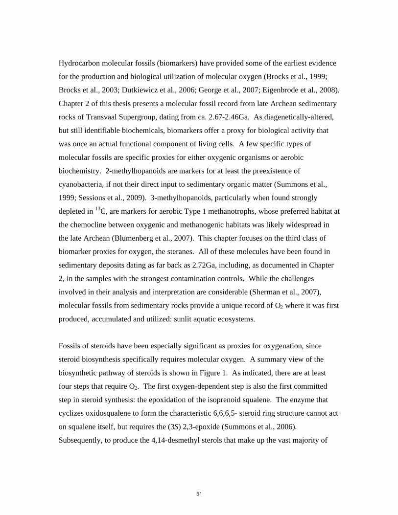
Hydrocarbon molecular fossils (biomarkers) have provided some of the earliest evidence
for the production and biological utilization of molecular oxygen (Brocks et al., 1999;
Brocks et al., 2003; Dutkiewicz et al., 2006; George et al., 2007; Eigenbrode et al., 2008).
Chapter 2 of this thesis presents a molecular fossil record from late Archean sedimentary
rocks of Transvaal Supergroup, dating from ca. 2.67-2.46Ga. As diagenetically-altered,
but still identifiable biochemicals, biomarkers offer a proxy for biological activity that
was once an actual functional component of living cells. A few specific types of
molecular fossils are specific proxies for either oxygenic organisms or aerobic
biochemistry. 2-methylhopanoids are markers for at least the preexistence of
cyanobacteria, if not their direct input to sedimentary organic matter (Summons et al.,
1999; Sessions et al., 2009). 3-methylhopanoids, particularly when found strongly
depleted in 13C, are markers for aerobic Type 1 methanotrophs, whose preferred habitat at
the chemocline between oxygenic and methanogenic habitats was likely widespread in
the late Archean (Blumenberg et al., 2007). This chapter focuses on the third class of
biomarker proxies for oxygen, the steranes. All of these molecules have been found in
sedimentary deposits dating as far back as 2.72Ga, including, as documented in Chapter
2, in the samples with the strongest contamination controls. While the challenges
involved in their analysis and interpretation are considerable (Sherman et al., 2007),
molecular fossils from sedimentary rocks provide a unique record of O2 where it was first
produced, accumulated and utilized: sunlit aquatic ecosystems.
Fossils of steroids have been especially significant as proxies for oxygenation, since
steroid biosynthesis specifically requires molecular oxygen. A summary view of the
biosynthetic pathway of steroids is shown in Figure 1. As indicated, there are at least
four steps that require O2. The first oxygen-dependent step is also the first committed
step in steroid synthesis: the epoxidation of the isoprenoid squalene. The enzyme that
cyclizes oxidosqualene to form the characteristic 6,6,6,5- steroid ring structure cannot act
on squalene itself, but requires the (3S) 2,3-epoxide (Summons et al., 2006).
Subsequently, to produce the 4,14-desmethyl sterols that make up the vast majority of
51
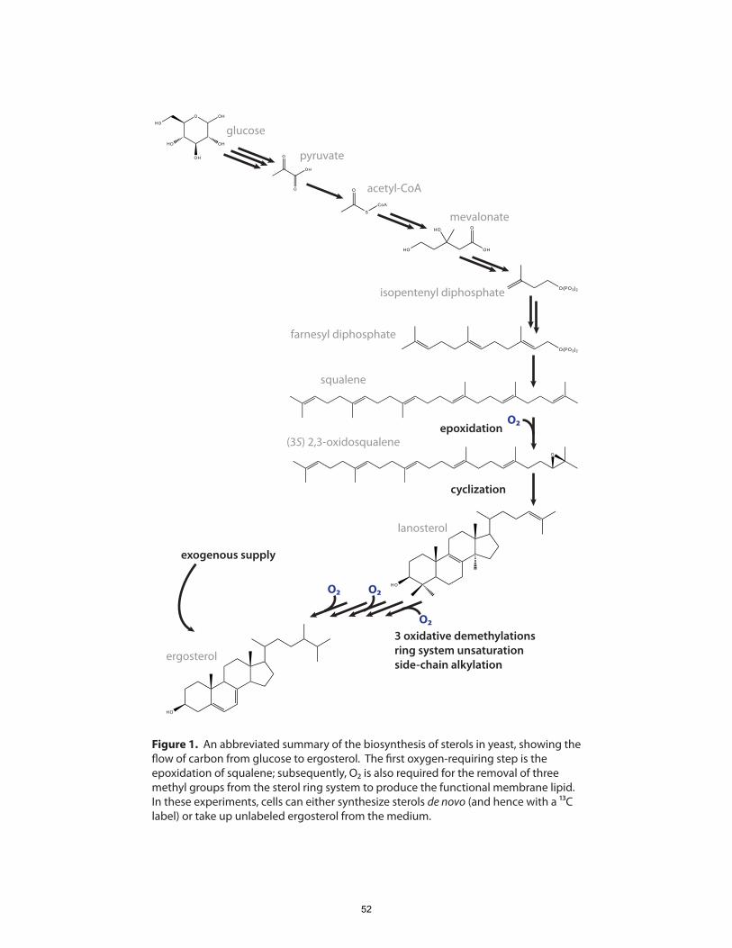
OH
OH
OH
HO
OHO
glucose
O
O
OH
O
SCoA
HO
HO O
OH
O(PO3)2
O(PO3)2
O
HO
HO
pyruvate
acetyl-CoA
mevalonate
isopentenyl diphosphate
farnesyl diphosphate
squalene
(3S) 2,3-oxidosqualene
lanosterol
ergosterol
O2epoxidation
cyclization
O2 O2
O23 oxidative demethylationsring system unsaturationside-chain alkylation
exogenous supply
Figure 1. An abbreviated summary of the biosynthesis of sterols in yeast, showing the �ow of carbon from glucose to ergosterol. The �rst oxygen-requiring step is the epoxidation of squalene; subsequently, O2 is also required for the removal of three methyl groups from the sterol ring system to produce the functional membrane lipid. In these experiments, cells can either synthesize sterols de novo (and hence with a 13C label) or take up unlabeled ergosterol from the medium.
52
both membrane lipids and molecular fossils, nine more molecules of O2 are necessary to
effect three oxidative demethylation reactions. The synthesis of some steroids (e.g.,
cholesterol) requires yet more oxygen to introduce unsaturations into the carbon skeleton.
Steroid biosynthesis is highly evolutionarily conserved, and was present in the last
common ancestral lineage of all extant eukaryotes (Summons et al., 2006; Desmond and
Gribaldo 2009).
Steranes – defunctionalized, saturated, diagenetically altered fossil steroids – have been
detected in sedimentary rocks as old as 2.72Ga, roughly 300 million years before the
GOE. The presence of steranes in rocks of this age implies that some molecular oxygen
was available in the marine environments that produced the organic matter preserved in
late Archean sediments. The implication is that the integrated source-sink imbalance for
atmospheric oxygen remained very small for hundreds of millions of years after the
evolutionary origin of oxygenic photosynthesis, keeping atmospheric O2 somewhere
below 10-6 of its modern level. At present, however, constraints on the environmental
oxygen concentration that enables steroid biosynthesis are limited: Jahnke and Klein
(1983) reported an apparent oxygen Km (half-saturation content) for squalene epoxidase
of 4.3µM, and Rogers and Stewart reported apparent O2 Km values for ergosterol contents
in yeast of 0.5µM (Rogers and Stewart, 1973b) and “0.3µM or less” (Rogers and Stewart,
1973a). The former is an in vitro measure of a crude preparation of a single part of the
pathway, while the latter reflects a physiological response (cellular sterol levels) rather
than biosynthesis itself; nor have these experiments been repeated in the years since.
Hence it is difficult to assess the consistency between interpretations of the biomarker
record and reconstructions of Archean biogeochemistry and atmospheric evolution. The
experiments presented in this chapter seek to provide constraints on the oxygen
requirement of sterol biosynthesis that more directly apply to the interpretation of the
molecular fossil record.
53
To directly assay the oxygen requirements of steroid biosynthesis, we adopted an isotopic
labeling strategy. Yeast (S. cerevisiae) was chosen as a test organism because it is a
facultatively anaerobic eukaryote, able to grow at any oxygen concentration. Yeast cells
were grown in a defined minimal medium containing 13C-glucose and unlabeled (12C-)
ergosterol. Since steroid biosynthesis requires molecular oxygen, the cells are obligately
auxotrophic for steroids under anaerobic conditions, and take up the supplied (unlabeled)
ergosterol. Under aerobic conditions, however, steroids are made de novo from carbon
substrates, and so acquire the 13C label from glucose. By analyzing the cells’ lipid
complements using mass spectrometry, we could examine the incorporation of 13C into
specific compounds, including sterols. Our goal was to determine the lowest dissolved
oxygen concentration that would enable de novo steroid synthesis.
2. EXPERIMENTAL METHODS
2.1 Microaerobic growth experiments
2.1.1 Culture conditions and sampling
Saccharomyces cerevisiae (strain D273-10B, ATCC) cells were grown in a defined
minimal medium containing 4g/l uniformly-labeled 13C6-glucose (99%, Cambridge
Isotope), supplemented with 10mg/l ergosterol (Alfa Aesar) and 0.5ml/l Tween 80
(polyoxyethylene sorbitan monooleate). The Tween 80 provided a source of unsaturated
fatty acids, which yeast also require molecular oxygen to produce. The medium was also
amended with 1ml/l FG-10 (Dow Chemical), a polydimethylsiloxane-based surfactant, as
an antifoaming agent. Cultures were maintained in an anaerobic chamber (Coy) in an
atmosphere of 5% hydrogen, 15% CO2 and <1ppm O2. For microaerobic growth, 6ml of
late log-phase culture (OD600 ~ 0.8) was inoculated into 300ml of media in a bubbler
bottle with the headspace exhausted to external vacuum. Dissolved oxygen concentration
in the media was controlled by vigorous bubbling with O2:N2 mixtures (5-5000ppm O2,
Airgas). Cells were grown with bubbling and stirring for 12-16h, until an OD600 of 0.2
54
was reached. The cells were then harvested by vacuum filtration in the anaerobic
chamber onto a precombusted GF/F filter (Whatman). Filters were placed into glass
centrifuge tubes filled with 19ml of Bligh-Dyer extraction solvent (10:5:4
chloroform:methanol:water; Bligh and Dyer, 1959) that had been pre-equilibrated with
the anaerobic atmosphere, and incubated in the anaerobic chamber overnight to ensure
complete enzyme deactivation prior to oxygen exposure.
2.2.2 Dissolved O2 measurements
Oxygen concentration in the cultures during microaerobic growth was measured by two
methods: a colorimetric assay based on Rhodazine-D (Chemetrics) and a novel type of
microelectrode with a polarizable front guard (Unisense). The Rhodazine-D test, based
on a proprietary redox-sensitive chromophore, is convenient and inexpensive, but is
limited in sensitivity to dissolved oxygen concentrations above approximately 300nM. It
is also susceptible to interferences from Fe(III) and Cu(II), and higher concentrations of
suspended particulates (such as cells) can require prefiltration, potentially limiting
accuracy. The recently-developed STOX (Switchable Trace Oxygen) electrode
(Revsbech et al., 2009) allows in situ electrochemical detection of O2 down to
concentrations as low as 5-10nM (equivalent to equlibrium at 25ºC and 1atm with an
atmosphere containing 4-8ppmv O2).
2.2 Lipid analysis
2.2.1 Lipid extraction/derivitisation
Tubes containing filters and solvent were removed from the anaerobic chamber and
ultrasonicated for 20 minutes. Tubes were then centrifuged for 5 minutes at 1000×g, the
supernatant decanted (first extract) and 19ml Bligh-Dyer solvent added again. After a
second ultrasonication and centrifugation, the second extract was pooled with the first,
and 10ml water and 10ml chloroform added to induce phase separation. Phase separation
continued overnight at -20˚C, after which the upper phase and interfacial debris were
55
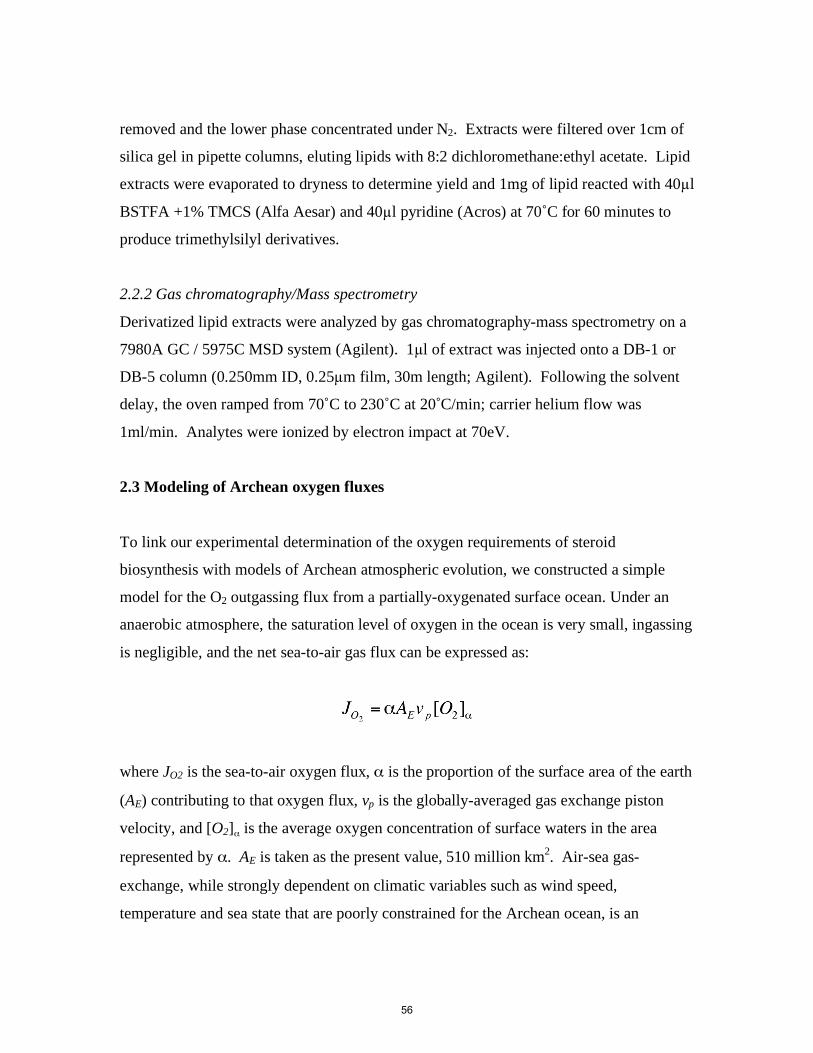
removed and the lower phase concentrated under N2. Extracts were filtered over 1cm of
silica gel in pipette columns, eluting lipids with 8:2 dichloromethane:ethyl acetate. Lipid
extracts were evaporated to dryness to determine yield and 1mg of lipid reacted with 40µl
BSTFA +1% TMCS (Alfa Aesar) and 40µl pyridine (Acros) at 70˚C for 60 minutes to
produce trimethylsilyl derivatives.
2.2.2 Gas chromatography/Mass spectrometry
Derivatized lipid extracts were analyzed by gas chromatography-mass spectrometry on a
7980A GC / 5975C MSD system (Agilent). 1µl of extract was injected onto a DB-1 or
DB-5 column (0.250mm ID, 0.25µm film, 30m length; Agilent). Following the solvent
delay, the oven ramped from 70˚C to 230˚C at 20˚C/min; carrier helium flow was
1ml/min. Analytes were ionized by electron impact at 70eV.
2.3 Modeling of Archean oxygen fluxes
To link our experimental determination of the oxygen requirements of steroid
biosynthesis with models of Archean atmospheric evolution, we constructed a simple
model for the O2 outgassing flux from a partially-oxygenated surface ocean. Under an
anaerobic atmosphere, the saturation level of oxygen in the ocean is very small, ingassing
is negligible, and the net sea-to-air gas flux can be expressed as:
where JO2 is the sea-to-air oxygen flux, α is the proportion of the surface area of the earth
(AE) contributing to that oxygen flux, vp is the globally-averaged gas exchange piston
velocity, and [O2]α is the average oxygen concentration of surface waters in the area
represented by α. AE is taken as the present value, 510 million km2. Air-sea gas-
exchange, while strongly dependent on climatic variables such as wind speed,
temperature and sea state that are poorly constrained for the Archean ocean, is an
56
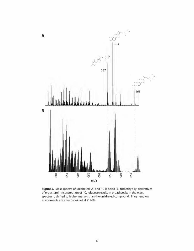
O
Si
+
+
468
+
363
337
Figure 2. Mass spectra of unlabeled (A) and 13C-labeled (B) trimethylsilyl derivatives of ergosterol. Incorporation of 13C6-glucose results in broad peaks in the mass spectrum, shifted to higher masses than the unlabeled compound. Fragment ion assignments are after Brooks et al. (1968).
300
400
350
450
250
200
150
100
m/z
A
B
57
essentially physical process likely to have been more or less constant over time. Here we
utilize the modern, long-term global average value of 16cm/h of Glover et al. (2007). We
note that vp is unlikely to vary by more than an order of magnitude, while the modeled
range of interest of JO2 and [O2]α span roughly four orders of magnitude, so overall the
model is not expected to be highly sensitive to the precise physics of gas exchange.
3. RESULTS: STEROID BIOSYNTHESIS IS A MICROAEROBIC PROCESS
3.1 The oxygen requirements of steroid biosynthesis
The incorporation of the 13C label from glucose produced a distinct shift in the
appearance of lipid mass spectra (Fig. 2). 13C-labeled compounds showed large peaks in
the mass spectra, shifted up the mass scale relative to peaks in the spectra of unlabeled
compounds. These distinct spectra provide an unambiguous signal of de novo lipid
biosynthesis.
The carbon-13 label was incorporated into squalene – the last steroid synthesis
intermediate reachable in the absence of O2 – in all conditions (Fig. 3). Under anaerobic
conditions, no lanosterol was detected, and only unlabeled ergosterol (taken up from the
medium) was present. This is the pattern expected if steroid synthesis is not operative,
and is entirely consistent with the oxygen dependence of sterol biosynthesis. Once
oxygen was provided to the culture by bubbling, however, labeled steroids were produced
de novo. In the presence of oxygen, lanosterol is synthesized and bears the 13C label, and
labeled ergosterol is also present.
Surprisingly, even the lowest oxygen concentration tested to date – estimated at 7nM –
appears to support steroid biosynthesis. This is a remarkably low oxygen level to enable
what has been thought of as a classically aerobic biochemistry. It should be noted,
however, that this result has yet to be duplicated in a replicate experiment, and that the
58
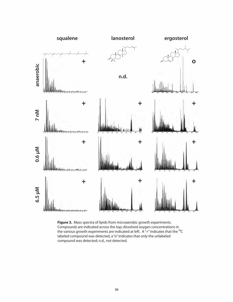
squalene
HO
lanosterol
HO
ergosterol
n.d.
anae
robi
c7
nM0.
6 µM
6.5
µM
+
+
+
+
+
+
+ +
+
+
o
Figure 3. Mass spectra of lipids from microaerobic growth experiments. Compounds are indicated across the top; dissolved oxygen concentrations in the various growth experiments are indicated at left. A “+” indicates that the 13C labeled compound was detected, a “o” indicates that only the unlabeled compound was detected; n.d., not detected.
59
oxygen concentration is only an estimate, based on the calculated solubility and the
composition of the gas mixture as certified by the manufacturer. At the time this
experiment was performed, we did not have access to the new STOX electrode, and so
had no way of directly measuring such low O2 concentrations. This experiment will be
repeated in the very near future, with the dissolved oxygen monitored electrochemically.
With those caveats in mind, we provisionally interpret these results as a useful, perhaps
even conservative, lower bound for the oxygen requirement for steroid synthesis. While
yeast is certainly an incomplete model for the unknown diversity of eukaryotic organisms
in the Archean ocean, the fact that a modern organism can perform this biochemistry at
such low oxygen concentrations suggests that early eukaryotes, adapted to chronic O2
scarcity, likely could as well. Notably, steroid biosynthesis is possible well below the
Pasteur point of 1% PAL (~2µM O2), above which fermentation is inhibited. The Pasteur
point has sometimes been misinterpreted as a switching point between aerobic and
anaerobic metabolism (Rutten, 1970; Goldblatt et al., 2006). Along with recent results
suggesting microaerobic respiration in E. coli (Stolper et al., 2009), this experiment
shows that there is a geochemically-significant range of dissolved O2 concentrations
below the Pasteur point that enable aerobic biochemistry.
The exceptionally low oxygen levels enabling steroid synthesis also highlight the close
connection between steroid biochemistry and oxygen sensing, metabolism and defense
(Galea and Brown, 2009). Studies of industrial fermentations have documented that,
during aeration pulses, the first aerobic biochemistry to become active is steroid
synthesis, not respiration (Rosenfeld et al., 2003). In our experiment, de novo steroid
synthesis occurred despite an abundant supply of exogenous sterols in the growth
medium. It would appear that sterol homeostasis is one of the most sensitive oxygen-
detecting systems in biology, which is consistent with its emergence in microaerobic
aquatic settings, well before the oxygenation of the atmosphere.
60
3.2 Oxygenation of the Archean surface ocean
Our results demonstrate that steroid biosynthesis is possible in microaerobic
environments, which has significant implications for the biogeochemical interpretation of
steranes in the fossil record. The fossil steranes in late Archean sedimentary rocks can be
interpreted as evidence for microaerobic conditions in a portion of the marine water
column in an otherwise anaerobic world. Is this interpretation of the molecular fossil
record consistent with other geochemical evidence for the evolution of atmospheric
oxygen levels? In particular, could microaerobic regions of the surface ocean have
supplied the O2 fluxes called for by current models of Precambrian atmospheric
evolution? To answer this question, we constructed a simple model of global air-sea gas
exchange and used it to predict the mixed-layer supersaturation of dissolved oxygen
implied by given values of the O2 flux to the atmosphere (Sec. 2.3).
The results of this model, shown in Figure 4, indicate that microaerobic ocean surface
environments capable of supporting steroid biosynthesis are entirely consistent with –
even required by – models of Archean atmospheric evolution. To provide the oxygen
outgassing fluxes called for in the models of Pavlov and Kasting (2002) and Zahnle et al.
(2006), that the average supersaturation in ocean regions contributing to sea-to-air
oxygen outgassing would be in the range of 0.1-1µM. This is 10-100 times our
experimental determination of the concentration required for sterol biosynthesis. These
models show how such an oxygen flux can persist for hundreds of millions of years
without causing oxygenation of the atmosphere to the extent that would ‘trip’ the
geologic and geochemical proxies whose signals appear at or near the GOE. Even if the
total flux were an order of magnitude less than the lower limit considered by Zahnle et al.
(2006), if it were concentrated in high-productivity hotspots (“oxygen oases”), the local
oxygen concentration was likely to have been high enough to allow steroids to be made.
It is important to recognize that no threshold value of sea-to-air O2 flux requires that the
atmosphere become oxygenated; so long as the oxygen is accompanied by inputs of
61
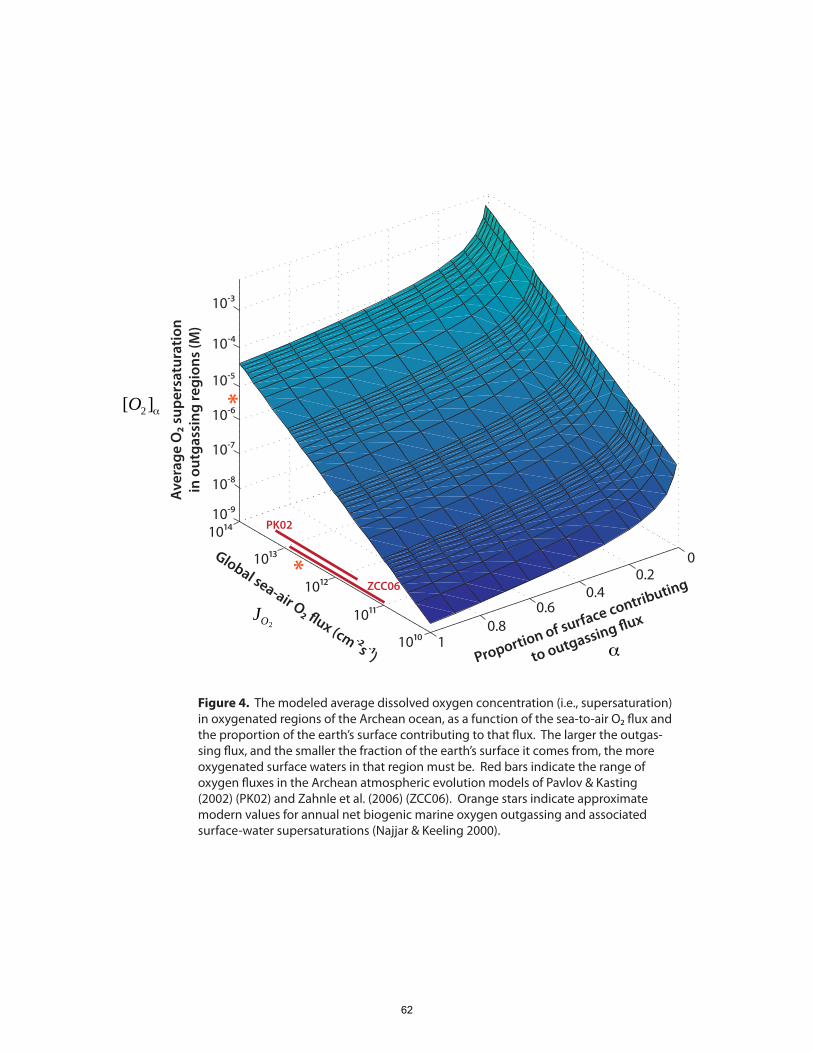
00.2
0.40.6
0.811010
1011
1012
1013
101410-9
10-3
10-4
10-5
10-6
10-7
10-8
[O2]α
JO2
α
Global sea-air O2 �ux (cm-2s-1)
Aver
age
O2 s
uper
satu
ratio
nin
out
gass
ing
regi
ons
(M)
Proportion of surface contributing
to outgassing �ux
Figure 4. The modeled average dissolved oxygen concentration (i.e., supersaturation) in oxygenated regions of the Archean ocean, as a function of the sea-to-air O2 �ux and the proportion of the earth’s surface contributing to that �ux. The larger the outgas-sing �ux, and the smaller the fraction of the earth’s surface it comes from, the more oxygenated surface waters in that region must be. Red bars indicate the range of oxygen �uxes in the Archean atmospheric evolution models of Pavlov & Kasting (2002) (PK02) and Zahnle et al. (2006) (ZCC06). Orange stars indicate approximate modern values for annual net biogenic marine oxygen outgassing and associated surface-water supersaturations (Najjar & Keeling 2000).
*
*
PK02
ZCC06
62
sufficient reductant, even the modern O2 flux could coexist with an anaerobic atmosphere
(Claire et al., 2006; Goldblatt et al., 2006; Zahnle et al., 2006).
The biogeochemical distribution of oxygen in the Archean ocean likely resembled (in
general terms) that of biogenic trace gases in the modern ocean, such as dimethylsulfide
(DMS). In fact, the parallels between Archean oxygen and modern DMS are striking:
both have biological sources in the upper water column, vanishingly small atmospheric
concentrations and atmospheric lifetimes of hours to days (Kettle et al., 1999; Kloster et
al., 2007). Oxygen in the Archean ocean probably had rather heterogeneous geographic
and seasonal distributions, as DMS does today. Moreover, in both cases, some degree of
supersaturation of the surface ocean is persistent over long time scales (a phenomenon
also seen with some abiogenic gases, such as 222Rn) and biologically relevant.
The past O2 content of the surface ocean cannot be inferred accurately from atmospheric
O2 levels alone, nor should its concentration be assumed to have been homogeneous.
This is especially true when considering biochemical processes, since, as steroid
biosynthesis exemplifies, micromolar-scale deviations from saturation are highly
significant. Hence, the geologic record of atmospheric O2 does not directly constrain the
evolutionary history of aerobic biochemistries, as has sometimes been assumed
(Goldblatt et al., 2006; de Duve, 2007). While the oxygenation of the ocean may seem
trivial compared to that of the atmosphere (the ocean contains only about 0.5% of the O2
in the modern world), the ocean has played a pivotal role as a source region for oxygen
production.
4. A BRIEF PORTRAIT OF LIFE & GEOCHEMISTRY IN THE LATE ARCHEAN
The support from molecular (e.g., Chapter 2), morphological (Bosak et al., 2009) and
newer geochemical (Frei et al., 2009) proxies for microaerobic surface ocean
environments as far back as 2.7Ga adds new features to the picture of Archean
63
biogeochemistry. A cartoon representation of a late Archean coastal ocean environment
and some of the biogeochemical processes that went on there is shown in Figure 5. A
wide variety of microbial metabolisms were probably present, in an ecosystem every bit
as spatially structured as those of the Phanerozoic. Microaerobic regions where
cyanobacteria were burgeoning primary producers provided an outgassing flux of O2 to
the atmosphere. While most gross primary production was likely locally aerobically
respired (as it is today), any net export of organic from microaerobic zones was, in a low-
Fe(III), low-sulfate ocean, most likely subject to methanogenic diagenesis. Where the
methane so produced met the fringes of the oxygenated zones, aerobic methanotrophy
would have been active and formed another sink for O2. The biogenic gases that escaped
the photosynthesis-respiration-methanogenesis-methanotrophy loop in the water column
and evaded to the atmosphere would have provided a stoichiometric 2:1 flux of
oxygen:methane that, in the absence of an ozone shield, would have undergone rapid
photochemical recombination (Claire et al., 2006). Catling et al. (2001) have noted that
the small, steady leak of methane out of this atmospheric process – due to hydrogen
escape to space – may have been essential to the eventual oxygenation of the atmosphere.
Meanwhile, hydrothermal supplies of reductants (including H2 produced by
serpentinization of basaltic crust (Hayes and Waldbauer, 2006)) fueled various
phototrophic and chemotrophic metabolisms, both at the periphery of microaerobic zones
and distant from them. A fruitful direction for future research will be to examine how
and when shifts from dominantly anoxygenic to dominantly oxygenic primary
productivity occurred, a process that, as discussed above, was probably gradual and
spatially heterogeneous.
The biodiversity implied by this range of biogeochemical processes is considerable, and
implies that much of microbial metabolism and that many, if not most, of the major
taxonomic lineages had appeared by the late Archean. The molecular fossil record
provides specific evidence for bacteria and eukaryotes (Chapter 2), methanogenesis
implies the presence of archaea, and the active biogeochemical cycles evident in the
64
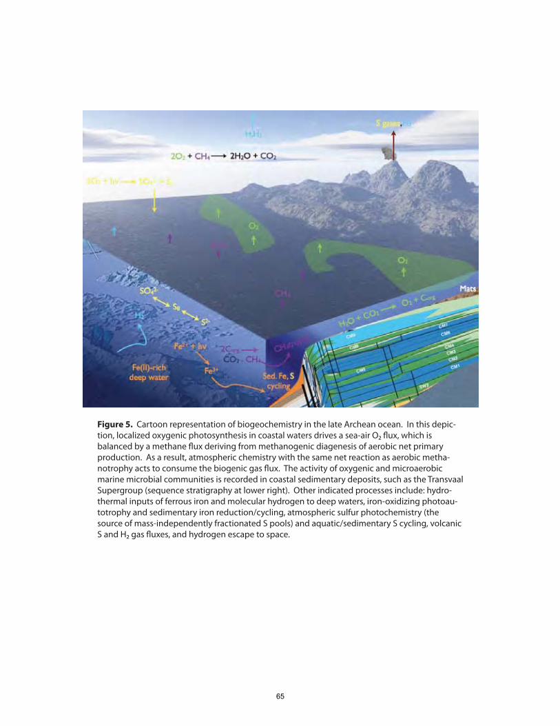
Figure 5. Cartoon representation of biogeochemistry in the late Archean ocean. In this depic-tion, localized oxygenic photosynthesis in coastal waters drives a sea-air O2 �ux, which is balanced by a methane �ux deriving from methanogenic diagenesis of aerobic net primary production. As a result, atmospheric chemistry with the same net reaction as aerobic metha-notrophy acts to consume the biogenic gas �ux. The activity of oxygenic and microaerobic marine microbial communities is recorded in coastal sedimentary deposits, such as the Transvaal Supergroup (sequence stratigraphy at lower right). Other indicated processes include: hydro-thermal inputs of ferrous iron and molecular hydrogen to deep waters, iron-oxidizing photoau-totrophy and sedimentary iron reduction/cycling, atmospheric sulfur photochemistry (the source of mass-independently fractionated S pools) and aquatic/sedimentary S cycling, volcanic S and H2 gas �uxes, and hydrogen escape to space.
65
geologic record suggest that life was widely diversified. It seems that the majority of key
biochemical networks, including energy-generating and biosynthetic pathways, were
operative by the late Archean. Studies such as this one are showing that some classically
aerobic biochemical pathways, including some characteristic of eukaryotic biology, are
operative under the very low dissolved oxygen concentrations that may have been
widespread and persistent during the late Archean.
It should be noted that the production of sterols does not strictly entail an oxygenated
water column. It could be argued that the oxygen used to synthesize sterols in the
Archean ocean was actually produced by the eukaryotes themselves, and that their
presence in sedimentary organic matter reflects only the intracellular availability of O2.
A remarkable example of eukaryotes maintaining intracellular O2 while living in anoxic
environments was recently described by Esteban et al. (2009), who found that certain
freshwater ciliates living just below an oxic-anoxic transition zone sequester still-active
chloroplasts from algal prey in order to provide an oxygen supply for aerobic
biochemistry. But while solely intracellular O2 is a conceivable explanation for sterol
production in isolation, all eukaryotic photosynthesis is ultimately ‘borrowed’ from
cyanobacteria, through either endosymbiosis or kleptoplasty as described by Esteban et
al. (2009). Hence the presence of photosynthetic eukaryotes of any sort would mean that
oxygenic cyanobacteria had already emerged, and thus more probable that oxygenation of
the water column was underway to some extent.
Accurate reconstruction of the history of oxygen in the atmosphere and oceans and
evolution of the organisms and biochemistry responsible for its production are central to
understanding the reciprocal interactions between life and environments. The
demonstration here that steroid biosynthesis is possible under microaerobic (but not
anaerobic) conditions provides new context for the interpretation of the biomarker record
and inferences about ocean biogeochemistry. The assumption that an anaerobic
atmosphere means an anaerobic ocean is misleading, as biologically-sustained deviations
66
from physical equilibria are common and important today and were in the distant past as
well. Reconstructions of microbial evolution, often framed in the context of global, long-
term trends, should keep in mind the heterogeneity of natural environments.
ACKNOWLEDGEMENTS
We are grateful to Alexa Price-Whelan and Paula Welander for guidance with anaerobic culturing techniques, Lars Dietrich for help with microelectrode measurements, and Maureen Coleman for discussions. This work was supported by grants from the Agouron Institute and the NASA Astrobiology Institute to RES, and by an Office of Naval Research NDSEG Fellowship and an NSF Graduate Research Fellowship to JRW. REFERENCES Allen, JF, and W Martin. 2007. Evolutionary biology: out of thin air. Nature 445, no.
7128: 610–612. Anbar, AD, Y Duan, TW Lyons, GL Arnold, B Kendall, RA Creaser, AJ Kaufman, GW
Gordon, C Scott, J Garvin, and R Buick. 2007. A whiff of oxygen before the great oxidation event? Science 317, no. 5846: 1903–1906.
Bligh, EG, and WJ Dyer. 1959. A rapid method of total lipid extraction and purification. Canadian Journal of Physiology and Pharmacology 37, 911-917.
Blumenberg, M, R Seifert, and W Michaelis. 2007. Aerobic methanotrophy in the oxic--anoxic transition zone of the Black Sea water column. Organic Geochemistry 38, no. 1: 84–91.
Bosak, T, B Liang, MS Sim, and AP Petroff. 2009. Morphological record of oxygenic photosynthesis in conical stromatolites. Proc Natl Acad Sci USA 106, no. 27: 10939–10943.
Brocks, JJ, GA Logan, R Buick, and RE Summons. 1999. Archean molecular fossils and the early rise of eukaryotes. Science 285, no. 5430: 1033–1036.
Brocks, JJ, R Buick, RE Summons, and GA Logan. 2003. A reconstruction of Archean biological diversity based on molecular fossils from the 2.78 to 2.45 billion-year-old Mount Bruce Supergroup, Hamersley Basin, Western Australia. Geochimica et Cosmochimica Acta 67, no. 22: 4321–4335.
Brooks, CJW, ES Horning and JS Young. 1968. Characterization of Sterols by Gas Chromatography-Mass Spectrometry of the Trimethylsilyl Ethers. Lipids 3, no. 5: 391-402.
Buick, R. 2008. When did oxygenic photosynthesis evolve? Philosophical Transactions of the Royal Society B: Biological Sciences 363, no. 1504: 2731.
Catling, DC, KJ Zahnle, and C McKay. 2001. Biogenic methane, hydrogen escape, and the irreversible oxidation of early Earth. Science 293, no. 5531: 839–843.
67
Catling, DC, and MW Claire. 2005. How Earth's atmosphere evolved to an oxic state: a status report. Earth and Planetary Science Letters 237, no. 1-2: 1–20.
Claire, MW, DC Catling, and KJ Zahnle. 2006. Biogeochemical modelling of the rise in atmospheric oxygen. Geobiology 4, no. 4: 239.
Coogan, L. 2009. Did natural reactors form as a consequence of the emergence of oxygenic photosynthesis during the Archean? GSAT 19, no. 10: 4–10.
de Duve, C. 2007. The origin of eukaryotes: a reappraisal. Nature Reviews Genetics 8, no. 5: 395–403.
Desmond, E and S Gribaldo. 2009. Phylogenomics of Sterol Synthesis: Insights into the Origin, Evolution, and Diversity of a Key Eukaryotic Feature. Genome Biology and Evolution 1, no. 1: 364-381.
Dutkiewicz, A, H Volk, SC George, J Ridley, and R Buick. 2006. Biomarkers from Huronian oil-bearing fluid inclusions: an uncontaminated record of life before the Great Oxidation Event. Geology 34, no. 6: 437.
Eigenbrode, JL, KH Freeman, and RE Summons. 2008. Methylhopane biomarker hydrocarbons in Hamersley Province sediments provide evidence for Neoarchean aerobiosis. Earth and Planetary Science Letters 273, no. 3-4: 323–331.
Esteban, GF, BJ Finlay, and KJ Clarke. 2009. Sequestered organelles sustain aerobic microbial life in anoxic environments. Environmental Microbiology 11, no. 2: 544–550.
Frei, R, C Gaucher, SW Poulton, and DE Canfield. 2009. Fluctuations in Precambrian atmospheric oxygenation recorded by chromium isotopes. Nature 461, no. 7261: 250–253.
Galea, AM, and AJ Brown. 2009. Special relationship between sterols and oxygen: Were sterols an adaptation to aerobic life? Free Radical Biology and Medicine 47, no. 6: 880–889.
George, SC, H Volk, A Dutkiewicz, J Ridley, and R Buick. 2007. Preservation of hydrocarbons and biomarkers in oil trapped inside fluid inclusions for> 2 billion years. Geochimica et Cosmochimica Acta
Glover, DM, NM Frew, and SJ McCue. 2007. Air--sea gas transfer velocity estimates from the Jason-1 and TOPEX altimeters: prospects for a long-term global time series. Journal of Marine Systems 66, no. 1-4: 173–181.
Goldblatt, C, TM Lenton, and AJ Watson. 2006. Bistability of atmospheric oxygen and the Great Oxidation. Nature 443, no. 7112: 683–686.
Hayes, JM, and JR Waldbauer. 2006. The carbon cycle and associated redox processes through time. Philos Trans R Soc Lond, B, Biol Sci 361, no. 1470: 931–950.
Jahnke, L, and HP Klein. 1983. Oxygen requirements for formation and activity of the squalene epoxidase in Saccharomyces cerevisiae. J Bacteriol 155, no. 2: 488–492.
Johnston, D, F Wolfe-Simon, A Pearson, and AH Knoll. 2009. Anoxygenic photosynthesis modulated Proterozoic oxygen and sustained Earth's middle age. Proceedings of the National Academy of Sciences
Kettle, AJ, MO Andreae, D Amouroux, TW Andreae, TS Bates, H Berresheim, H Bingemer, R Boniforti, MAJ Curran, and GR DiTullio. 1999. A global database of sea surface dimethylsulfide (DMS) measurements and a procedure to predict
68
sea surface DMS as a function of latitude, longitude, and month. Global Biogeochemical Cycles 13, no. 2:
Kirschvink, JL, and RE Kopp. 2008. Palaeoproterozoic ice houses and the evolution of oxygen-mediating enzymes: the case for a late origin of photosystem II. Philosophical Transactions of the Royal Society B: Biological Sciences 363, no. 1504: 2755.
Kloster, S, KD Six, J Feichter, E Maier-Reimer, E Roeckner, P Wetzel, P Stier, and M Esch. 2007. Response of dimethylsulfide (DMS) in the ocean and atmosphere to global warming. Journal of Geophysical Research-Biogeosciences 112, no. G3: G03005.
Kopp, RE, JL Kirschvink, IA Hilburn, and CZ Nash. 2005. The Paleoproterozoic snowball Earth: a climate disaster triggered by the evolution of oxygenic photosynthesis. Proc Natl Acad Sci USA 102, no. 32: 11131–11136.
Najjar, RG, and RF Keeling. 2000. Mean annual cycle of the air-sea oxygen flux: A global view. Glob Biogeochem Cycles 14, no. 2: 573-584.
Pavlov, AA, and JF Kasting. 2002. Mass-independent fractionation of sulfur isotopes in Archean sediments: strong evidence for an anoxic Archean atmosphere. Astrobiology 2, no. 1: 27–41.
Reinhard, CT, R Raiswell, C Scott, AD Anbar, and TW Lyons. 2009. A Late Archean Sulfidic Sea Stimulated by Early Oxidative Weathering of the Continents. Science 326, no. 5953: 713–716.
Revsbech, NP, LH Larsen, J Gundersen, T Dalsgaard, O Ulloa, and B Thamdrup. 2009. Determination of ultra-low oxygen concentrations in oxygen minimum zones by the STOX sensor. Limnol. Oceanogr. Methods 7, 371–381.
Rogers, PJ, and P Stewart. 1973a. Mitochondrial and peroxisomal contributions to the energy metabolism of Saccharomyces cervisiae in continuous culture. Journal of General Microbiology 79, 205–217.
Rogers, PJ, and PR Stewart. 1973b. Respiratory development in Saccharomyces cerevisiae grown at controlled oxygen tension. J Bacteriol 115, no. 1: 88–97.
Rosenfeld, E, B Beauvoit, B Blondin, and J-M Salmon. 2003. Oxygen consumption by anaerobic Saccharomyces cerevisiae under enological conditions: effect on fermentation kinetics. Appl Environ Microbiol 69, no. 1: 113–121.
Rutten, MG. 1970. The history of atmospheric oxygen. Space Life Sciences 2, 5–17. Sessions, AL, DM Doughty, PV Welander, RE Summons, and DK Newman. 2009. The
continuing puzzle of the great oxidation event. Curr Biol 19, no. 14: R567–74. Sherman, LS, JR Waldbauer, and RE Summons. 2007. Improved methods for isolating
and validating indigenous biomarkers in Precambrian rocks. Organic Geochemistry 38, no. 12: 1987–2000.
Stolper, D, N Revsbech, and DE Canfield. 2009. Growth of E. coli at nanomolar concentrations of oxygen. American Geophysical Union Annual Meeting Abstracts.
Summons, RE, LL Jahnke, JM Hope, and GA Logan. 1999. 2-Methylhopanoids as biomarkers for cyanobacterial oxygenic photosynthesis. Nature 400, no. 6744: 554–557.
69

Summons, RE, AS Bradley, LL Jahnke, and JR Waldbauer. 2006. Steroids, triterpenoids and molecular oxygen. Philosophical Transactions B 361, no. 1470: 951.
Zahnle, K, M Claire, and D Catling. 2006. The loss of mass-independent fractionation in sulfur due to a Palaeoproterozoic collapse of atmospheric methane. Geobiology 4, no. 4: 271–283.
70
CHAPTER FOUR
A multilevel view of gene expression and regulation in the Prochlorococcus diel cell cycle
Jacob R. Waldbauer, Sébastien Rodrigue, Maureen L. Coleman,
and Sallie W. Chisholm
71

72
A multilevel view of gene expression and regulation in the diel cell cycle
of Prochlorococcus
Jacob R. Waldbauer, Sébastien Rodrigue, Maureen L. Coleman and Sallie W. Chisholm
The cell division cycle of Prochlorococcus populations is tightly coupled to the diel cycle of light and darkness, with chromosome replication in the late afternoon being followed by cellular fission after sunset. Experiments in culture have shown that the mRNA-level expression profiles of most genes also have a diel rhythm. Here we quantify the abundance and periodicity of the Prochlorococcus proteome over a diel cycle and compare transcript-level and protein-level expression patterns. Strong diel oscillations in transcript abundance are broadly damped at the protein level, and temporal offsets between the two suggest that posttranslational regulatory mechanisms are important in determining the abundance dynamics of a number of proteins. The overall composition of the proteome is quite stable over the diel cycle, with some proteins consistently among the most abundant in the cell at all times of day. The small changes in protein abundance that accompany significant changes in central metabolic activities imply that Prochlorococcus biochemical networks may be poised near balance points that allow for redirection of metabolic fluxes with relatively small changes in the abundance of their components.
1. INTRODUCTION: THE IMPORTANCE OF THE DIEL CYCLE TO LIFE IN THE
SUBTROPICAL EPIPELAGIC
The twenty-four hour alternation of light and darkness caused by the earth’s rotation is
one of the strongest periodicities imposed on natural systems. Since the sun is the
ultimate source of nearly all energy input to ecosystems, its diurnal motion has dramatic
consequences for the activity of surface-dwelling organisms ranging from bacteria to
humans. This is especially true for phototrophs, whose physiology is directly tied to solar
energy utilization. In the ocean, the great majority of photosynthesis is carried out by
microbes, whose small body sizes require them to closely balance metabolic demands of
growth with the availability of light energy. In the low-latitude epipelagic where
Prochlorococcus is a dominant primary producer, the diel cycle is one of the main time-
varying properties of the ecosystem.
73
As the most abundant photosynthetic organism on earth and the base of the food web in
vast areas of the open ocean, Prochlorococcus is a central player in marine
biogeochemistry. Shortly after its discovery and initial characterization in the late 1980s,
a remarkable property of Prochlorococcus populations was observed: their growth is
clearly synchronized to the diel cycle. Fortuitously, the tool used to discover and identify
Prochlorococcus in the ocean, flow cytometry, is also ideal for assessing cell cycling, and
utilization of DNA-binding fluorescent dyes allowed the cell cycle progression of natural
communities to be tracked quantitatively. A well-conserved pattern emerged: cells
replicate their DNA in the afternoon and divide from around sunset into the evening
(Vaulot et al., 1995). With generally one cell division per day (though see Shalapyonok
et al., 1998), this synchronization results in well-defined B-, C- and D-phases equivalent
to the G1, S and G2+M phases, respectively, of eukaryotic cells (Wang and Levin, 2009).
The diel cell cycle of Prochlorococcus has one additional characteristic that has enabled
its detailed investigation: it can be reproduced in laboratory culture. Principal cell cycle
parameters of axenic cultures maintained on a light-dark cycle, including growth rate and
the length of DNA synthesis and cell division phases, are similar to those observed in
field populations – suggesting that the biology occurring in the laboratory is at least a
first-order representation of what occurs in nature. A number of studies have explored
aspects of the Prochlorococcus diel cell cycle using a variety of experimental
arrangements, and have added insights into changes in photophysiology (Bruyant et al.,
2005) and optical properties (Claustre et al., 2002) as well as in the expression of selected
photosynthesis- (Garczarek et al., 2001) and cell cycle-related (Holtzendorff et al., 2001)
genes.
A further intriguing aspect of diel cell cycling in Prochlorococcus is the absence of the
kind of true circadian clock that has been documented in other cyanobacteria. Typical
cyanobacterial circadian clock systems are comprised of three proteins, KaiA, KaiB and
KaiC. The molecular basis of the clock is a 24-hour oscillation in the phosphorylation
74
state of KaiC, with KaiA promoting phosphorylation and KaiB promoting
dephosphorylation. All sequenced Prochlorococcus strains, however, lack a homologue
of KaiA. Holtzendorff et al. (2008) have demonstrated that the diel coordination of
growth and associated expression oscillations damp rapidly (at least in terms of their
population averages) when cultures are shifted to continuous light, implying that the
Prochlorococcus timing system relies on external cues during each photoperiod.
Recently, Axmann et al. (2009) showed that the KaiC of Prochlorococcus MED4 is
hyperphosphorylated by default, apparently enabling the KaiBC-only system to oscillate.
It may be that a streamlined, less robust timing mechanism is sufficient for
Prochlorococcus because it inhabits the low-latitude open ocean, and therefore
experiences smaller seasonal changes in day length than phototrophs at higher latitudes or
those in freshwater settings where shading by vegetation or sediment is more likely
(Axmann et al., 2009; Mullineaux and Stanewsky, 2009).
The most comprehensive molecular picture of the Prochlorococcus diel cell cycle to date
has come from the work of Zinser et al. (2009), who used microarrays to track gene
expression genome-wide with 2-hour resolution over two consecutive diel periods in
axenic cultures of Prochlorococcus MED4. This study found that 82% of transcripts of
protein-coding genes had a detectable circadian oscillation of expression. The high
proportion of transcripts cycling with 24 hour periodicity suggests that the diel cycle
could be seen as the ‘master regulator’ of Prochlorococcus gene expression – though
how this regulation is effected is unclear. The MED4 genome encodes only a small
number of the complement of regulatory systems typically found in bacteria (Mary and
Vaulot, 2003; Vogel et al., 2003; Kielbasa et al., 2007). Small RNAs, including antisense
transcripts, likely play important regulatory roles (Steglich et al., 2008; Richter et al.,
2010).
In light of these previous findings, the experiment described here was designed to address
two key aspects of the diel cell cycle in Prochlorococcus. One is the regulatory
75
underpinnings of the observed transcriptional program. The small complement of
regulatory systems in MED4 makes a genome-wide analysis of the dynamics of the
transcriptional regulatory network feasible. Using a combination of 5’- and 3’-RACE
(Rapid Amplification of cDNA Ends) and ChIP-Seq (Chromatin Immunoprecipitation
and Sequencing) techniques, the binding sites and DNA association patterns of
transcription factors can be mapped over the diel cycle. This work is in progress and will
be presented elsewhere (Rodrigue et al., in prep.). This chapter presents the second focus
of the diel growth experiment: the relationship between gene expression at the transcript
and protein levels.
The central dogma of molecular biology holds that gene sequence information in cells
generally flows from DNA to RNA to protein. While this specifies the topology of the
chemical network involved in gene expression, it leaves open the question of the relative
abundances of gene products. It is clear that the relative abundance of a gene at the RNA
level is not readily predictable from its abundance at the DNA level: two genes each
present at a single copy in the genome can be transcribed at very different rates. The
same is true for the translation of RNA into protein. Transcript abundance, while
undoubtedly a major factor influencing protein level, does not fully determine, predict or
explain it. The observed abundance of a gene product reflects the dynamic balance
between production (by transcription or translation) and degradation, hence the
motivation to complement the mRNA-level picture of diel cyclic gene expression in
Prochlorococcus with a protein-level one.
In biogeochemical terms, to understand how organisms effect molecular transformations
in the environment, protein quantification is essential. Proteins are the catalysts for many
biogeochemically-significant reactions, and themselves represent a large proportion of
the nutrient requirements of microbial cells. Large-scale gene expression measurements
are coming to the fore as assays of the activities and physiological states of microbial
communities, including investigations of the diel cycle in marine surface waters
76
(Poretsky et al., 2009). If protein and transcript levels diverge, however, the mRNA-level
view of biological activity may be misleading. It is therefore increasingly important to
quantify the relationships between gene products at multiple biological levels, so that
accurate inferences about community function can be drawn from biochemical
measurements.
We also sought to address the relationship between the proportional cellular abundances
of mRNAs and proteins. Previous microarray analyses (Zinser et al., 2009) have
accurately resolved relative changes in mRNA-level gene expression (that is, changes in
the abundance of a given transcript over time), but, due to widely varying hybridization
efficiencies and the potential for saturation of the microarray signal (Levicky and
Horgan, 2005), it has been difficult to compare the abundance of different gene products
at a given time. The use of parallel RNA-sequencing and mass spectrometry to measure
transcript and protein abundance, respectively, allow comparison of abundances between
gene products. Hence we obtain a first view of the rank-abundance structure of
Prochlorococcus gene products at the transcript and protein levels and how it changes
over the diel cell cycle. The relationships between transcript and protein abundance are
an important component of systems-level understanding of cellular functions and the
biogeochemistry they participate in.
2. EXPERIMENTAL METHODS & TECHNICAL DISCUSSION
2.1 Diel growth experiment
2.1.1 Culture conditions
Axenic Prochlorococcus MED4 was grown in duplicate batches in 30L acid-cleaned
polycarbonate carboys (Nalgene) in a modified I-66LL illuminated incubator (Percival
Scientific), depicted in Figure 1A. The illumination in the incubator was controlled by
custom PID-controlled dimmer circuitry and programmed to match a diel irradiance
77
0
50
100
150
200
250
0:00 2:00 4:00 6:00 8:00 10:00 12:00 14:00 16:00 18:00 20:00 22:00 0:00
time
light
inte
nsity
(µE
/ m2 s
)
ProgrammedMeasured
A
B
Figure 1. A Photograph of Prochlorococcus MED4 batch cultures in sunbox incubator. B Programmedand measured irradiance curves for the sunbox. Programmed curve derived from data from theHawaii Ocean Time-series (HOT) station ALOHA.
sunr
ise
05:3
0
suns
et 1
8:30
78
curve from the Hawaii Ocean Time-series station ALOHA, as shown in Figure 1B.
Temperature in the incubator was maintained at 24˚C. Each culture was stirred
continuously by a large teflon-coated magnetic stir bar. Prior to inoculation of the large-
volume batch cultures for this experiment, the culture had been maintained for several
months in the same incubator to ensure synchronization to the light-dark cycle. The
culture medium was a modified version of Pro99 (Moore et al., 2007) based on Vineyard
Sound seawater (collected at Woods Hole, MA) and pH-buffered with 10mM HEPES
and 6mM sodium bicarbonate. Starting culture volume for the diel growth experiment
was 20L. Separately, Prochlorococcus MED4 labeled with 15N were prepared by
growing cells from the same axenic strain used in the diel growth experiment on Pro99
medium in continuous light, where the ammonium chloride that is the sole fixed N source
in the medium was >99% 15NH4Cl (Cambridge Isotope). A 1L culture was grown to late-
exponential phase and harvested by centrifugation as described below, with samples
preserved for flow cytometry to provide accurate cell counts of the pellets.
2.1.2 Sampling
During the diel growth experiment, samples were taken every two hours over a 26 hour
span, beginning at local midnight, resulting in 14 total timepoints. At each timepoint,
500ml samples of each culture were withdrawn using spigots mounted at the bottom of
the carboys and dispensed in to 2×250ml centrifuge bottles (Nalgene). For sampling
during dark and low-light periods, a low-power green lamp was used to provide indirect
work light. Additionally, five 1ml samples of the culture were preserved with 0.125%
glutaraldehyde (Tousimis) in cryovials (Nunc) for flow cytometric determination of cell
density and growth cycling. Large-volume samples were centrifuged at 16,000×g for 10
minutes in an Avanti J-10 centrifuge (Beckman Coulter). After pipetting off the
supernatant, the two pellets from each culture were resuspended, combined in a 15ml
conical tube (VWR), and the volume brought to 5ml with Pro99 media. Duplicate 10µl
aliquots of the resuspended concentrate were diluted 1:100 with 0.125% glutaraldehyde
in Pro99 in for flow cytometric analysis to ensure precise and accurate determination of
79
cell counts in the sample pellets. The remainder of the concentrate was then split into
2×2ml and 4×0.25ml aliquots in 2ml microcentrifuge tubes (Sarstedt), the former for
RNA-sequencing and the latter for proteomics. These aliquots were then centrifuged for
6 minutes at 14,000×g in a 5418 centrifuge (Eppendorf). The supernatant was then
removed and preserved with 5µl 25% glutaraldehyde in cryovials for flow cytometric
counting to assess pelleting efficiency. Cell pellets and flow cytometry samples were
kept frozen at -80˚C until analysis.
2.1.3 Flow cytometry
Cell counts and cell cycle were analyzed using an InFlux flow cytometer (Cytopeia).
Glutaraldehyde-fixed samples were diluted in filtered sterile seawater to appropriate
concentrations. Light scatter and fluorescence signals were detected using a 488nm
excitation beam, triggering on forward (small-angle) light scatter and counting cells on
the basis of scatter characteristics and chlorophyll fluorescence. Cell cycle analysis was
performed using SYBR Green (Invitrogen) to stain DNA. Flow cytometry data were
analyzed using FlowJo (TreeStar).
2.2 Proteomics sample preparation
2.2.1 Protein extraction
Prochlorococcus cell pellets were resuspended in 2× LDS buffer (Invitrogen) with 10mM
dithiothreitol (DTT), vortexed, and incubated in a heat block at 95˚C for 20 minutes.
They were subsequently vortexed again and incubated at 37˚C for 60 minutes. After
cooling to room temperature, iodoacetamide (0.5M in 100mM NH4HCO3) was added to a
concentration of 45mM and incubated at room temperature in the dark for 60 minutes to
alkylate cysteine residues. DTT (2M) was then added to a concentration of 45mM
(assumed to be 10mM after quenching of residual iodoacetamide). Volumes of
extraction buffer and reduction/alkylation reagents were chosen to result in a final
concentration of 1×10⁹ extracted cells/50µl. Extract from sample pellets was then mixed
80
1:1 by cell numbers (established previously by flow cytometry) with extract from an
identically and simultaneously processed 15N-labeled cell pellet.
2.2.2 SDS-PAGE
Extract from up to 1×10⁹ total cells was loaded per lane into 10-lane, 10cm×1.5mm 10%
SDS-PAGE gels (NuPAGE, Invitrogen) with MOPS running buffer (Invitrogen). Gels
were run at 50mA per gel with water cooling to 25˚C in a vertical format (SE260,
Hoefer) for 90 minutes. Benchmark protein ladder (Invitrogen) was used as a molecular
weight standard. After electrophoresis, gels were removed from their cases and fixed in
50% ethanol/7.5% acetic acid overnight on an orbital shaker. They were then rehydrated
in Milli-Q water for 30 minutes before staining with SimplyBlue coomassie stain
(Invitrogen). Gels were imaged on a flatbed scanner prior to slicing with a razor blade
into ~1mm cubes. Eight separate molecular weight fractions were prepared for each
timepoint. The fastest-running component of the extract (the bottom-most band, rich in
chlorophyll as evidenced by its green color during electrophoresis) was excised and not
included in further processing. The gel slices were transferred to 1.5ml microcentrifuge
tubes (Axygen) and destained by shaking for 4 hours in 50% ethanol/7.5% acetic acid at
37˚C. The destain solution was then changed and the gel pieces returned to the
incubator/shaker overnight.
2.2.3 Trypsin digestion
The destained gel pieces were washed five times: twice alternating acetonitrile/50mM
ammonium bicarbonate for 20 minutes each, then a final acetonitrile wash until fully
dehydrated. The acetonitrile was then removed and the dry pieces chilled on ice.
Sequencing grade modified porcine trypsin (Promega) was diluted in 10% acetonitrile in
50mM ammonium bicarbonate and chilled on ice. Sufficient trypsin solution was added
to the sample tubes to cover the gel pieces (~100-200µl/tube), and the incubation
continued on ice until the gel pieces were clear. The tubes were then incubated for 24
81
hours at 37˚C, at which point 200µl of 10% acetonitrile in 50mM ammonium bicarbonate
was added and incubated for a further 24 hours at 37˚C.
2.2.4 Peptide extraction
After incubation with trypsin for 48 hours, the liquid from the digestion tubes was
transferred to a new set of 1.5ml microcentrifuge tubes, which were kept at 4˚C. 200µl of
10% acetonitrile in 50mM ammonium bicarbonate was added to the pieces and incubated
for 1 hour at 37˚C before being pooled with the initial extract. This process was repeated
once more with 10% acetonitrile in 50mM ammonium bicarbonate and then twice with
50% acetonitrile in 0.1% formic acid; total extract volume was ~1ml. Extracts were
frozen solid at -80˚C before being concentrated in a vacuum centrifuge for 4-5 hours at
30˚C. The dried extracts were then resuspended in 500µl of 5% acetonitrile in 0.25%
formic acid, vortexed vigorously, and centrifuged for 10 minutes at 14,000×g to pellet
residual gel fragements and debris. The supernatant was removed, frozen solid at -80˚C
and finally concentrated by vacuum centrifuge for ~2 hours at 30˚C.
2.3 LC-MS/MS analysis
2.3.1 Liquid chromatography/nanoelectrospray ionization
Frozen, dried peptide fractions (8 per timepoint) were resuspended in 10µl of 5%
acetonitrile in 0.25% formic acid and transferred to a 384-well plate (Nunc). 6µl of each
sample was injected via qualitative µl pickup with a MicroAS autosampler
(Thermo/Spark Holland) fitted with a 10µl sample loop. Mobile phase was delivered by
a Surveyor LC pump (Thermo) fitted with a backpressure regulator (P-880, Upchurch)
and a fixed-T flow splitter (ratio ~90:1). Peptides were loaded onto a reversed-phase
capillary LC column (Hypersil Gold C18, 0.18×100mm, 3µm×175Å particles, Thermo).
The mobile phase system for the LC consisted of 0.1% formic acid in water (buffer A)
and 0.1% formic acid in acteonitrile (B). Solvents for LC-MS were HPLC grade
(Burdick & Jackson). Peptides were eluted with a gradient of 5% to 37.5% B over 105
82
minutes, followed by a ramp to 100% B and washing for 25 minutes, then 40 minutes re-
equilibration with 5% B. Column flow rate was 1.3µl/min, and total LC cycle time was
180 minutes. The LC system was interfaced to the mass spectrometer through an
TriVersa Nanomate nanospray source/fraction collector (Advion). Post-column flow
split between the nanospray chip and the collector mandrel was 1:2, resulting in a flow of
~400nl/min to the chip. The spray chip was operated at a voltage of 1.6-1.8kV, and spray
current was monitored to ensure ionization stability.
2.3.2 Mass spectrometry
Mass spectral data was acquired on a LTQ-FT Ultra (Thermo) in a data-dependent
manner. Each full scan in the ICR cell (profile mode, m/z 300-1600, resolution 100,000)
was followed by 4 CID MS/MS scans on selected precursors in the linear ion trap.
Dynamic exclusion was enabled, with repeat count set to 2 and exclusion duration 30
seconds. Singly charged ions, ions whose charge state could not be assigned, and
common contaminant ions were excluded from MS/MS precursor selection. The LTQ-
FT ion optics were tuned on a mixture of angiotensin (Calbiochem) and bradykinin
(Genscript) for best sensitivity and transmission of peptide ions.
2.3.3 Peptide/protein identification
Mass spectral data acquired by Xcalibur (v. 2.0, Thermo .RAW format) was converted to
mzXML format with ReAdW (v. 4.3.1). Peptide-spectrum matching was done against a
database consisting of the Prochlorococcus MED4 genome (Rocap et al., 2003), its
reversed complement, and a set of common contaminant proteins including porcine
trypsin and human keratins. Three MS/MS database search algoriths were employed:
X!Tandem (v. TORNADO, Craig and Beavis, 2004; with the k-score plugin, MacLean et
al., 2006), MyriMatch (v. 060509, Tabb et al., 2007) and OMSSA (v. 2.1.7, Geer et al.,
2004). For all search engines, semi-tryptic searches were conducted with two missed
cleavages allowed. Amino acid modfications included static carbamidomethylated
cysteine, variably oxidized methionine, and variable formation of pyro-glutamine, -
83

glutamate or -carbamidomethylcysteine on the N-termini of peptides. For OMSSA
searching, a concatenated DTA file (.odta format) was first produced from each mzXML
file using mzXML2Search, and spectra were then searched on the Darwin computing
cluster at MIT. Output from the 3 search engines was converted (if necessary) to
pepXML format and a Perl script used to unify their formats. Each pepXML file was
then processed with PeptideProphet (Keller et al., 2002) to assign probabilities to each
peptide identification; peptides longer than 6 amino acids were considered, and accurate
mass information was used. The peptide identifications in the 24 pepXML files from
each timepoint (8 gel slices × 3 search engines) were merged using iProphet (Shteynberg
et al., in prep; all models enabled). A Perl script was used to reindex the merged
pepXML file, to ensure that each peptide ID had a unique index value. Peptide
identifications were then assigned to proteins by ProteinProphet (Nesvizhskii et al., 2003)
using Occam’s razor logic, and requiring a minimum PeptideProphet score of 0.05 to
filter out the weakest spectrum IDs. Further filtering based on an arbitrary
ProteinProphet score cutoff was not necessary at this point (except to exclude those with
scores of 0.00), as the false discovery rate (FDR) was already acceptably low: 33 decoy
proteins were identified among 1021 MED4 proteins, for a nominal dataset-wide protein-
identification FDR of 3.2% (Supplementary Fig. 2). If only proteins identified at 2 or
more timepoints are considered, the FDR was 1.6% (14 decoys among 873 MED4
proteins). As discussed below (Sec. 2.4.1), the process of constructing expression
timecourses eliminated all decoy data, resulting in a protein-ID FDR in the time-series
data of <0.2%.
2.4 Protein timecourse quantification
2.4.1 Isotope-labeling-based quantification
The method of quantification used here to construct timecourses of protein abundance
over the diel sampling period is based on the use of isotopically-labeled internal
standards. Metabolic isotope labeling, here using 15N, affords an internal standard for
84
virtually every peptide observed in the sample. Mixing the samples taken at each diel
sampling timepoint with aliquots of identical 15N-labeled cells at the earliest stage of
protein extraction minimizes the effect of subsequent experimental biases (protein
extraction yields, peptide ionization efficiencies, etc.) on the observed abundance ratio.
Accurate cell counts ensure that the 14N/15N mixing ratio was near 1:1. Analysis of
quantitative proteomics data using 15N-labeling does present challenges, however, not the
least of which is the variable mass difference between sample and standard. Details of
the method used to construct timecourses of protein abundance over the diel cycle is
described below.
MS1 peaks corresponding to 15N-labeled versions of identified MED4 peptides were
matched to their unlabeled, coeluting partners by ASAPRatio (Li et al., 2003), and the
abundance ratios of the 15N- versus 14N-peaks were computed. A window of 0.05 m/z
was used for integration, background correction was set to zero, multiple charge states
were used for quantification, and peakgroup pairs were constrained to the same elution
time range. ASAPRatio estimates an integrated intensity error for each peak by the
difference between the integrated raw intensity and the integrated area under a fitted peak
generated by a Savitzky-Golay smoothing filter; this error was used to calculate a
coefficient of variation (CV) for each individual peakgroup ratio. The set of quantified
peakgroup ratios for the entire dataset was extracted from the protXML files for each
timepoint, and a data matrix constructed and subsequent analyses performed in
MATLAB (MathWorks). Redundant values for the same physical LC-MS feature were
removed by requiring a 5% integrated intensity difference for duplicate, identical ratio
values for a given peptide at a given timepoint. The total dataset comprised isotope ratios
for 95,542 unique peakgroup pairs – here referred to as “peaks” for brevity, but actually
representing in excess of 500,000 distinct LC-MS features, including both 14N- and 15N-
partners and 13C-isotopologues for each peptide across multiple charge states.
85
The set of unique peak ratios was then filtered to remove peaks with a ratio CV greater
than 41%, corresponding to the 80th percentile in CV ranking. These high-CV peaks are
generally of low intensity and/or poor peak shape, making them more prone to
quantification errors. The remaining data were then log2-transformed, and the peak ratios
were adjusted to compensate for slight variations away from 1:1 in the mixing ratio of 14N- and 15N-protein at different timepoints. This was done by finding the median of the
log2-peak ratios between -1 and 1 for each timepoint, and subtracting that value from
each peak ratio at that timepoint. This normalization procedure ensures that the peak
ratio distributions for each timepoint have a common median (i.e., 0 on a logarithmic
scale) and that timecourse variations for indivdual proteins are not due to systematic
biases in the overall dataset.
Protein-level expression timecourses were constructed from the peak-level data in the
following manner: for a given protein, if four or more peaks were found at eight or more
timepoints, those timepoints were included in the timecourse. If a timecourse could not
be constructed with those criteria, the threshold number of peaks required for that protein
was sequentially lowered (to 3, 2, or 1) until 8 or more timepoints were included. This
approach was chosen to maximize the quality of the extracted timecourses for data-rich
proteins, but to also allow timecourses to be constructed for proteins consistently detected
at low levels. For timepoints with at least 4 peaks, the set of peak ratios was tested for
outliers using a variation of the integrated inconsistent rate (IIR) method (Hsiao et al.,
2009), with an IIR cutoff value of 1.81.
Protein expression ratios were calculated from the peak-level data at each timepoint by
maximum likelihood estimation of the parameters of a lognormal fit to the data, taking
the mean of the lognormal distribution as the protein ratio. The uncertainty in the ratio
was taken as the upper and lower 95% confidence limits calculated from an unbiased
estimate of the standard error of the mean (Gurland and Tripathi, 1971). Thus the
protein-level uncertainty is given by: ±(1.96cNs)/(N0.5), where s is the standard deviation
86
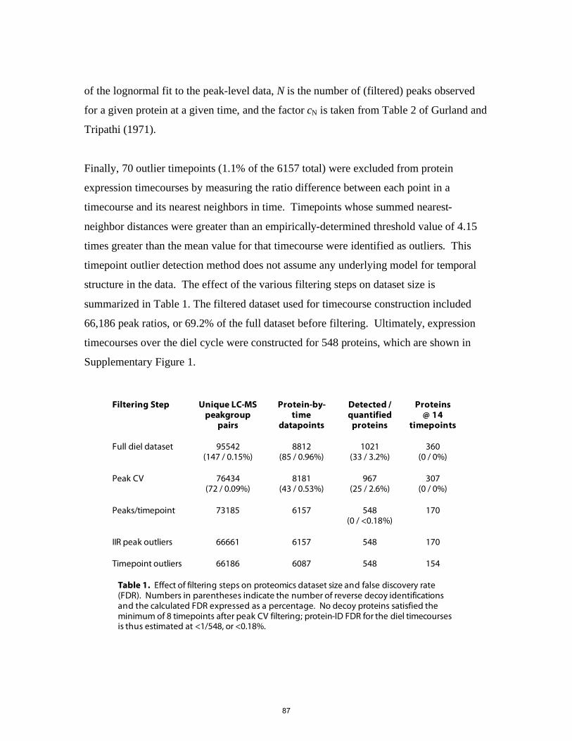
of the lognormal fit to the peak-level data, N is the number of (filtered) peaks observed
for a given protein at a given time, and the factor cN is taken from Table 2 of Gurland and
Tripathi (1971).
Finally, 70 outlier timepoints (1.1% of the 6157 total) were excluded from protein
expression timecourses by measuring the ratio difference between each point in a
timecourse and its nearest neighbors in time. Timepoints whose summed nearest-
neighbor distances were greater than an empirically-determined threshold value of 4.15
times greater than the mean value for that timecourse were identified as outliers. This
timepoint outlier detection method does not assume any underlying model for temporal
structure in the data. The effect of the various filtering steps on dataset size is
summarized in Table 1. The filtered dataset used for timecourse construction included
66,186 peak ratios, or 69.2% of the full dataset before filtering. Ultimately, expression
timecourses over the diel cycle were constructed for 548 proteins, which are shown in
Supplementary Figure 1.
Filtering Step Unique LC-MS peakgroup
pairs
Protein-by-time
datapoints
Detected / quantified
proteins
Proteins @ 14
timepoints
Full diel dataset 95542 (147 / 0.15%)
8812 (85 / 0.96%)
1021 (33 / 3.2%)
360 (0 / 0%)
Peak CV 76434 (72 / 0.09%)
8181 (43 / 0.53%)
967 (25 / 2.6%)
307 (0 / 0%)
Peaks/timepoint 73185 6157 548 (0 / <0.18%)
170
IIR peak outliers 66661 6157 548 170
Timepoint outliers 66186 6087 548 154
Table 1. Effect of filtering steps on proteomics dataset size and false discovery rate (FDR). Numbers in parentheses indicate the number of reverse decoy identifications and the calculated FDR expressed as a percentage. No decoy proteins satisfied the minimum of 8 timepoints after peak CV filtering; protein-ID FDR for the diel timecourses is thus estimated at <1/548, or <0.18%.
87
Table 1 also shows the effect of data filtering on the false discovery rate (FDR). As
noted above, the FDR for protein identification in the full dataset was 3.2% (33/1021),
but decoys amounted to only <1% of the protein-by-time datapoints, and even less
(0.15%) of the total number of peaks. In the unfiltered dataset, the greatest number of
timepoints at which any one decoy protein was identified was 9, and the majority (19/33)
were found at only one timepoint (Supplementary Fig. 2). Filtering on the basis of 14N/15N ratio CV eliminated more than half of the decoy peaks, as expected if most of
them are spurious identifications of features without a true isotopic partner of appropriate
mass difference. After peak CV filtering, no decoy protein was found at more than 5
timepoints; hence no decoys passed the 8-timepoint requirement for timecourse
construction. Thus, at least on the basis of decoy hits, the estimated protein-ID FDR for
the timecourse data is bounded at <0.18% (<1/548).
2.4.2 Analysis of diel expression cycling
Analysis of the temporal cycling of protein expression followed an approach based on
that outlined by Futschik and Herzel (2008). For the 548 proteins quantified over the diel
timecourse, any missing timepoint values were imputed using k-nearest neighbors
(Troyanskaya et al., 2001), with the missing data inferred as the weighted average of the
two closest timepoints by Euclidean distance in expression profile. The imputed data
were used solely for the purpose of assessing the significance of expression cycling. The
protein timecourses were then standardized to mean = 0 and standard deviation = 1. Two
tests were then applied to identify proteins whose expression cycled over the diel.
First, Fourier scores were caluclated for all timecourses on the basis of a 24-hour cell
cycle, as in Zinser et al. (2009). To assess the significance of a given Fourier score value,
a background distribution of scores from 1000 simulated first-order autoregressive
(AR(1)) timecourses was generated for each protein, using autoregression coefficients
and white noise distributions derived from the protein timecourse. Futschik and Herzel
(2008) have shown that an AR(1) background model is a more stringent and specific test
88
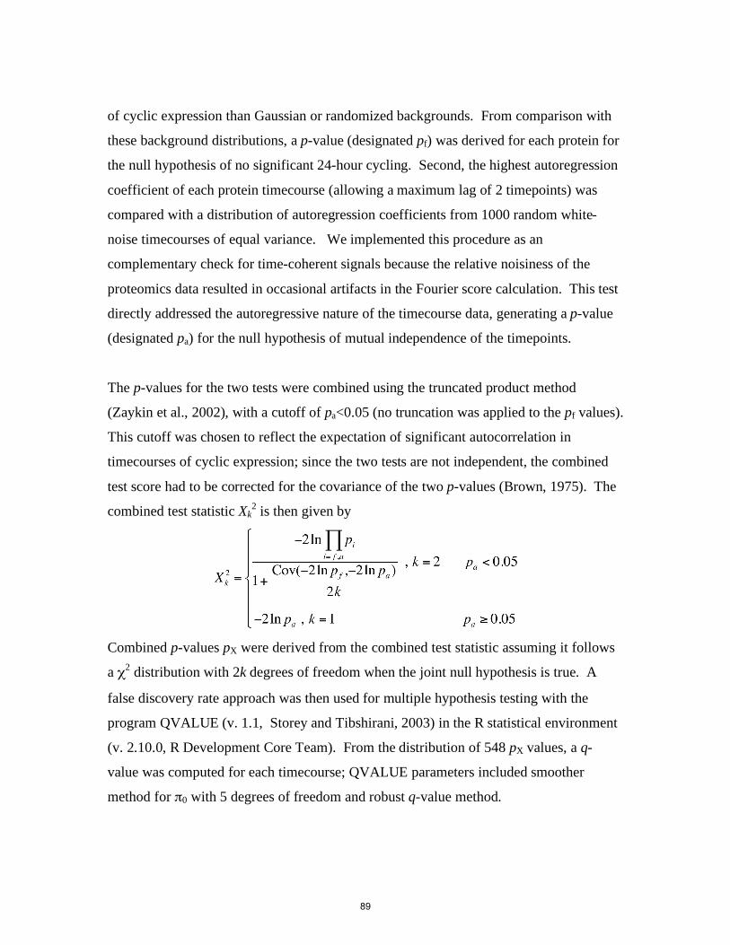
of cyclic expression than Gaussian or randomized backgrounds. From comparison with
these background distributions, a p-value (designated pf) was derived for each protein for
the null hypothesis of no significant 24-hour cycling. Second, the highest autoregression
coefficient of each protein timecourse (allowing a maximum lag of 2 timepoints) was
compared with a distribution of autoregression coefficients from 1000 random white-
noise timecourses of equal variance. We implemented this procedure as an
complementary check for time-coherent signals because the relative noisiness of the
proteomics data resulted in occasional artifacts in the Fourier score calculation. This test
directly addressed the autoregressive nature of the timecourse data, generating a p-value
(designated pa) for the null hypothesis of mutual independence of the timepoints.
The p-values for the two tests were combined using the truncated product method
(Zaykin et al., 2002), with a cutoff of pa<0.05 (no truncation was applied to the pf values).
This cutoff was chosen to reflect the expectation of significant autocorrelation in
timecourses of cyclic expression; since the two tests are not independent, the combined
test score had to be corrected for the covariance of the two p-values (Brown, 1975). The
combined test statistic Xk2 is then given by
Combined p-values pX were derived from the combined test statistic assuming it follows
a χ2 distribution with 2k degrees of freedom when the joint null hypothesis is true. A
false discovery rate approach was then used for multiple hypothesis testing with the
program QVALUE (v. 1.1, Storey and Tibshirani, 2003) in the R statistical environment
(v. 2.10.0, R Development Core Team). From the distribution of 548 pX values, a q-
value was computed for each timecourse; QVALUE parameters included smoother
method for π0 with 5 degrees of freedom and robust q-value method.
89
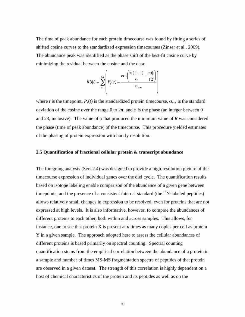
The time of peak abundance for each protein timecourse was found by fitting a series of
shifted cosine curves to the standardized expression timecourses (Zinser et al., 2009).
The abundance peak was identified as the phase shift of the best-fit cosine curve by
minimizing the residual between the cosine and the data:
where t is the timepoint, Ps(t) is the standardized protein timecourse, σcos is the standard
deviation of the cosine over the range 0 to 2π, and φ is the phase (an integer between 0
and 23, inclusive). The value of φ that produced the minimum value of R was considered
the phase (time of peak abundance) of the timecourse. This procedure yielded estimates
of the phasing of protein expression with hourly resolution.
2.5 Quantification of fractional cellular protein & transcript abundance
The foregoing analysis (Sec. 2.4) was designed to provide a high-resolution picture of the
timecourse expression of individual genes over the diel cycle. The quantification results
based on isotope labeling enable comparison of the abundance of a given gene between
timepoints, and the presence of a consistent internal standard (the 15N-labeled peptides)
allows relatively small changes in expression to be resolved, even for proteins that are not
expressed at high levels. It is also informative, however, to compare the abundances of
different proteins to each other, both within and across samples. This allows, for
instance, one to see that protein X is present at n times as many copies per cell as protein
Y in a given sample. The approach adopted here to assess the cellular abundances of
different proteins is based primarily on spectral counting. Spectral counting
quantification stems from the empirical correlation between the abundance of a protein in
a sample and number of times MS-MS fragmentation spectra of peptides of that protein
are observed in a given dataset. The strength of this correlation is highly dependent on a
host of chemical characteristics of the protein and its peptides as well as on the
90
particulars of the analytical setup used to collect the mass spectral data. The utility of
spectral counting as a mode of quantification is greatly enhanced by computational
modeling of, and correction for, these experimental biases (Mallick et al., 2007). In this
work, we used a computational approach to spectral counting termed APEX (Lu et al.,
2007; Vogel and Marcotte, 2008) for Absolute Protein Expression.
The term “absolute abundance” is somewhat problematic. What spectral-counting
techniques such as APEX calculate is in fact the fraction of the total amount of protein
detected in a sample comprised by any one gene product. Thus it is still a form of
relative quantification, though it is protein X relative to protein Y in sample A, as
opposed to protein X in sample A relative to protein X in sample B. The latter is the kind
of quantification obtained by isotope labeling methods. Spectral counting methods can
be (and often are) used successfully for intersample comparisons of protein abundance,
particularly for the more abundant components of the proteome (Hendrickson et al.,
2006). Here we use spectral counts for protein-to-protein relative abundance
measurements. These can be converted to nominally “absolute” units if the total amount
of protein in the cell is known; for example, if the APEX score of a protein is 0.005,
meaning it comprises 0.5% of all (detected) protein, and there are 500,000 protein
molecules in the cell (estimated from cellular N content, amino acid analysis, or
colorimetric assays such as the Bradford, Lowry or BCA), we could say that there are
2500 copies of that protein in the average cell in that sample. However, APEX is blind to
all the non-detected proteins, which are generally numerous and, as noted in Section
3.5.1, not necessarily of low cellular abundance. This is what makes spectral-count-
based “absolute” quantification qualitatively different from the use of synthetic,
absolutely-quantified peptide standards: the latter affords a measurement of the molar
abundance of one molecular species irrespective of the presence of others, and is thus
truly absolute. Since APEX has an inherently limited analytical window, we chose not to
convert its fractional abundance results to quasi-absolute, copies-per-cell values, as those
will inevitably be overestimates of the true cellular abundance.
91
With those caveats in mind, however, protein-to-protein relative comparisons remain
valuable. To perform this analysis, the set of MS2 spectra at each of the 14 diel
timepoints identified as belonging to peptides of Prochlorococcus MED4 proteins were
analyzed using the APEX Quantitative Proteomics Tool (v. 1.0.0, Braisted et al., 2008).
The Random Forest classifier was trained on a merged set of data from the 06:00, 12:00,
18:00 and 24:00 timepoints, using a set of 50 proteins observed in all 14 timepoints and
the same protein database used for peptide identification. All peptide properties were
used by the classifier, with a minimum peptide length of 6 amino acids and 2 missed
cleavages allowed. After training and generation of Oi values, APEX scores were
generated for each timepoint. All data were normalized such that the APEX scores for
proteins observed at a given timepoint sum to one. Hence the APEX score for each
protein is equivalent to its fraction of the total (detected) cellular protein at a given
timepoint.
We also compared the results of the APEX quantification to the simple, MS1-based,
label-free “absolute” quantification method of Silva et al. (2006). The Silva et al. (2006)
method (hereinafter referred to as “Top3”) is based on an empirical observation of the
correlation between protein abundance and the average of the MS1 intensities of the three
peptides belonging to that protein giving the largest MS1 peaks. Here we limited the
application of the Top3 method to proteins where 10 or more unique peptides were
detected, as was the case for the results of Silva et al. (2006). The Top3 abundance
values were normalized in the same way as the APEX scores, i.e., as a proportion of the
total at a given timepoint. Top3-based abundances were thus generated for 1799 (20%)
of the 8812 protein-by-time datapoints in the full diel dataset. A comparison between
APEX and Top3 abundance values is shown in Supplementary Figure 3. The correlation
coefficient between the results of the two quantification methods is 0.59 over two orders
of magnitude in predicted abundance, indicating broad agreement. Similar results were
obtained by Malmström et al. (2009) in their quantification of the Leptospira interrogans
92
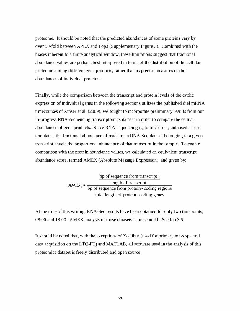
proteome. It should be noted that the predicted abundances of some proteins vary by
over 50-fold between APEX and Top3 (Supplementary Figure 3). Combined with the
biases inherent to a finite analytical window, these limitations suggest that fractional
abundance values are perhaps best interpreted in terms of the distribution of the cellular
proteome among different gene products, rather than as precise measures of the
abundances of individual proteins.
Finally, while the comparison between the transcript and protein levels of the cyclic
expression of individual genes in the following sections utilizes the published diel mRNA
timecourses of Zinser et al. (2009), we sought to incorporate preliminary results from our
in-progress RNA-sequencing transcriptomics dataset in order to compare the celluar
abundances of gene products. Since RNA-sequencing is, to first order, unbiased across
templates, the fractional abundance of reads in an RNA-Seq dataset belonging to a given
transcript equals the proportional abundance of that transcript in the sample. To enable
comparison with the protein abundance values, we calculated an equivalent transcript
abundance score, termed AMEX (Absolute Message Expression), and given by:
!
AMEXi =
bp of sequence from transcript ilength of transcript i
bp of sequence from protein - coding regionstotal length of protein - coding genes
At the time of this writing, RNA-Seq results have been obtained for only two timepoints,
08:00 and 18:00. AMEX analysis of those datasets is presented in Section 3.5.
It should be noted that, with the exceptions of Xcalibur (used for primary mass spectral
data acquisition on the LTQ-FT) and MATLAB, all software used in the analysis of this
proteomics dataset is freely distributed and open source.
93
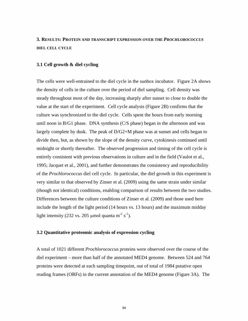
3. RESULTS: PROTEIN AND TRANSCRIPT EXPRESSION OVER THE PROCHLOROCOCCUS
DIEL CELL CYCLE
3.1 Cell growth & diel cycling
The cells were well-entrained to the diel cycle in the sunbox incubator. Figure 2A shows
the density of cells in the culture over the period of diel sampling. Cell density was
steady throughout most of the day, increasing sharply after sunset to close to double the
value at the start of the experiment. Cell cycle analysis (Figure 2B) confirms that the
culture was synchronized to the diel cycle. Cells spent the hours from early morning
until noon in B/G1 phase. DNA synthesis (C/S phase) began in the afternoon and was
largely complete by dusk. The peak of D/G2+M phase was at sunset and cells began to
divide then, but, as shown by the slope of the density curve, cytokinesis continued until
midnight or shortly thereafter. The observed progression and timing of the cell cycle is
entirely consistent with previous observations in culture and in the field (Vaulot et al.,
1995; Jacquet et al., 2001), and further demonstrates the consistency and reproducibility
of the Prochlorococcus diel cell cycle. In particular, the diel growth in this experiment is
very similar to that observed by Zinser et al. (2009) using the same strain under similar
(though not identical) conditions, enabling comparison of results between the two studies.
Differences between the culture conditions of Zinser et al. (2009) and those used here
include the length of the light period (14 hours vs. 13 hours) and the maximum midday
light intensity (232 vs. 205 µmol quanta m-2 s-1).
3.2 Quantitative proteomic analysis of expression cycling
A total of 1021 different Prochlorococcus proteins were observed over the course of the
diel experiment – more than half of the annotated MED4 genome. Between 524 and 764
proteins were detected at each sampling timepoint, out of total of 1984 putative open
reading frames (ORFs) in the current annotation of the MED4 genome (Figure 3A). The
94
0
10
20
30
40
50
60
70
80
90
100
12:00 16:00 20:00 24:00
time
% o
f cel
ls
B / G1C / SD / G2+M
00:00 04:00 08:00
5
6
7
8
9
10
11
12
13
14
Cells
/ml i
n cu
lture
(×10
7)
12:00 16:00 20:00 24:0000:00 04:00 08:00
time
A
B
Figure 2. A Cell density in the culture over the timecourse of the experiment, as counted by�ow cytometry. Density was essentially constant between sunrise and sunset, and increased after dark as cells began cytokinesis. Cell density doubled over the course of the experiment, meaning >90% of cells divided. B Proportion of cells in the 3 phases of the cell cycle, measuredby DNA staining and �ow cytometry. DNA replication began in the afternoon and was largelycomplete by dusk, when cell division began. The times of experimental sunrise and sunset(05:30 and 18:30, respectively), are indicated by symbols.
95
average coverage (i.e., proportion of amino acid positions represented in observed
peptides) of detected proteins was 25.1%, with a mean of 6.8 unique peptides per protein.
Since a primary goal of this study is to quantify protein expression over time, consistent
observation of a set of proteins across all (or at least a majority of) timepoints is critical.
Figure 3B shows the number of timepoints at which each observed protein was detected.
Of the 1021 total detected proteins, 584 were found in at least 8 timepoints, and 360 were
detected in all 14 timepoints. The regularly-observed proteins actually constitute the
majority of the dataset, since they exhibit the greatest number of detected peptides and
LC-MS peaks. These consistently-observed proteins are the group we will focus on in
examining expression patterns over the diel. The proteins observed at only a few
timepoints are very likely genuine observations (having passed through the same
identification and validation process), but little can be said about their expression
timecourses; there are not, for example, clear-cut instances of catching only the peak of a
protein’s expression in just a few successive timepoints. The great majority of these
infrequently-observed proteins are detected sporadically over the diel, consistent with
them being expressed at relatively low levels and hovering on the edge of the analytical
window.
In the current MED4 genome annotation, there are 963 ORFs for which no peptides were
detected at any of the diel timepoints. Some of these genes are essential to critical cell
functions and were undoubtedly expressed during this experiment; their absence reflects
the widely varying detectability of different proteins in LC-MS-based proteomics.
Examples of such genes include subunits of photosystems I and II and the cytochrome b6f
complex, and several nucleotide biosynthesis enzymes. A majority the undetected
proteins, however, are short and/or hypothetical ORFs that may or may not actually
produce proteins. Of the 963 undetected ORFs, 53% (512) are annotated as
“hypothetical” or “conserved hypothetical”, which is significantly higher than the 25% of
detected proteins bearing those annotations. Peptides from 252 hypothetical ORFs were
96
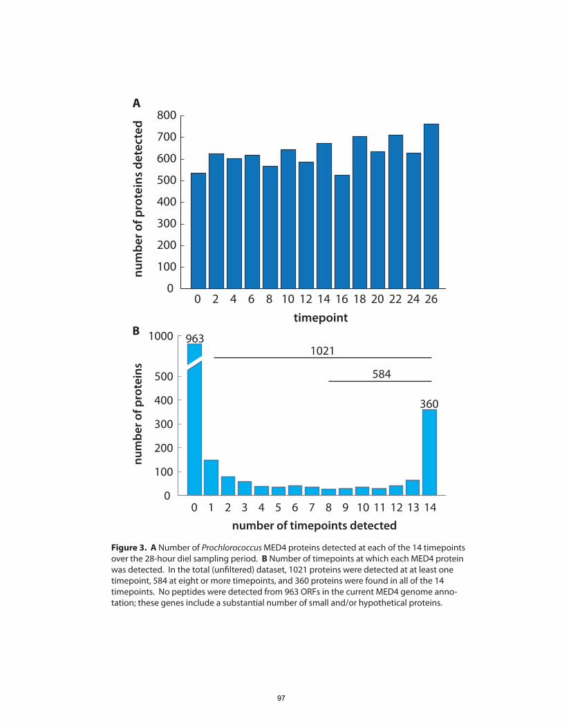
0 2 4 6 8 10 12 14 16 18 20 22 24 260
100
200
300
400
500
600
700
800
timepoint
num
ber o
f pro
tein
s de
tect
ed
A
0 1 2 3 4 5 6 7 8 9 10 11 12 13 140
100
200
300
400
500
1000
number of timepoints detected
num
ber o
f pro
tein
s
360
963
584
1021
B
Figure 3. A Number of Prochlorococcus MED4 proteins detected at each of the 14 timepointsover the 28-hour diel sampling period. B Number of timepoints at which each MED4 proteinwas detected. In the total (un�ltered) dataset, 1021 proteins were detected at at least onetimepoint, 584 at eight or more timepoints, and 360 proteins were found in all of the 14 timepoints. No peptides were detected from 963 ORFs in the current MED4 genome anno-tation; these genes include a substantial number of small and/or hypothetical proteins.
97
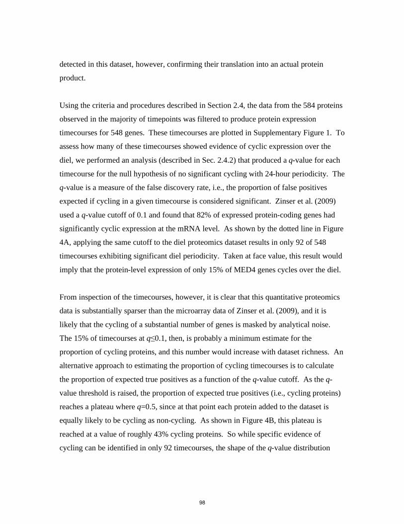
detected in this dataset, however, confirming their translation into an actual protein
product.
Using the criteria and procedures described in Section 2.4, the data from the 584 proteins
observed in the majority of timepoints was filtered to produce protein expression
timecourses for 548 genes. These timecourses are plotted in Supplementary Figure 1. To
assess how many of these timecourses showed evidence of cyclic expression over the
diel, we performed an analysis (described in Sec. 2.4.2) that produced a q-value for each
timecourse for the null hypothesis of no significant cycling with 24-hour periodicity. The
q-value is a measure of the false discovery rate, i.e., the proportion of false positives
expected if cycling in a given timecourse is considered significant. Zinser et al. (2009)
used a q-value cutoff of 0.1 and found that 82% of expressed protein-coding genes had
significantly cyclic expression at the mRNA level. As shown by the dotted line in Figure
4A, applying the same cutoff to the diel proteomics dataset results in only 92 of 548
timecourses exhibiting significant diel periodicity. Taken at face value, this result would
imply that the protein-level expression of only 15% of MED4 genes cycles over the diel.
From inspection of the timecourses, however, it is clear that this quantitative proteomics
data is substantially sparser than the microarray data of Zinser et al. (2009), and it is
likely that the cycling of a substantial number of genes is masked by analytical noise.
The 15% of timecourses at q≤0.1, then, is probably a minimum estimate for the
proportion of cycling proteins, and this number would increase with dataset richness. An
alternative approach to estimating the proportion of cycling timecourses is to calculate
the proportion of expected true positives as a function of the q-value cutoff. As the q-
value threshold is raised, the proportion of expected true positives (i.e., cycling proteins)
reaches a plateau where q=0.5, since at that point each protein added to the dataset is
equally likely to be cycling as non-cycling. As shown in Figure 4B, this plateau is
reached at a value of roughly 43% cycling proteins. So while specific evidence of
cycling can be identified in only 92 timecourses, the shape of the q-value distribution
98
0
100
200
300
400
500
600
0.00 0.10 0.20 0.30 0.40 0.50 0.60
q-value cuto�
num
ber o
f sig
ni�c
antly
cyc
ling
prot
eins
0
5
10
15
20
25
30
35
40
45
50
0 100 200 300 400 500 600
timecourses considered (lowest highest q-value)
% p
rote
ins
cycl
ing
A
B
Figure 4. Results of analysis of diel cycling of protein timecourses. A Number of proteins consid-ered to be signi�cantly cycling with 24-hour periodicity, as a function of q-value, a measure of the false discovery rate. Insets show examples of protein timecourses with low (HimA, q=0.04) and high (SqdB, q=0.46) q-values. At the chosen cuto� of 0.1 (shown by the dotted line and equivalent to that used by Zinser et al. (2009)), 92 proteins show signi�cant cycling. Note that the number of cycling proteins is not very sensitive to q-value in the range 0.09-0.15. B An estimate of the proportion of expected cycling proteins, calculated from proportion of expected true positives (i.e., cycling proteins). As more timecourses are considered, the expected proportion of cycling proteins plateaus near 43%, once the q-value reaches 0.5. So while clear evidence of cycling can be seen in only 15% of individual protein timecourses, the shape of the q-value distribution suggests that up to 43% may have some diel periodicity.
0 10 20−0.4
−0.2
0
PMED4_18751 SqdB
0.46
0 10 20
0.10.20.30.40.5
PMED4_14891 HimA
0.04
99
suggests that almost half of proteins could be cycling – though it does not specify the
members of that group, nor the parameters (e.g., phase, amplitude) of their cycling. This
result, while hardly robust in itself, is generally consistent with an estimate of the
proportion of cycling genes derived from the temporal distribution of peak protein
abundances (see Sec. 3.3.3).
It should be noted that mass spectrometry-based proteomics data in general is much
sparser in terms of coverage and redundant observations of gene product abundance than
microarray or massively parallel RNA-sequencing is. Large-scale comparisons of gene
expression patterns at different biological levels using different methodologies must be
mindful of the relative richness and biases of various datasets. In the next section, we
focus on the relationship between mRNA and protein expression for genes where the
cycling (or lack thereof) is well-resolved at both levels.
3.3 Relationships of mRNA and protein expression cycles
Beyond simply characterizing the Prochlorococcus proteome, a key aim of this study is
to illuminate the dynamic relationship between gene product abundances at the transcript
and protein levels. Here we compare protein expression timecourses with the mRNA-
level results of Zinser et al. (2009). It is important to recognize that certain aspects of the
two experiments limit how precisely they can be intercompared. In particular, the
photoperiod in the work of Zinser et al. (2009) was 14 hours, an hour longer than in this
experiment, and the sampling points in the two studies were shifted relative to their
respective dusk and dawn. While there may be some quantitative differences in detail, we
expect the mRNA-protein relationships outlined below to remain qualitatively the same.
In the near future, a complete diel transcriptome from this experiment will be available
(Rodrigue et al., in prep), allowing direct and precise comparisons of simultaneous
transcript and protein abundance measurements. Analysis of the transcriptome samples is
100
currently underway; to date, RNA-Seq libraries have been sequenced for two timepoints
from this experiment, 08:00 and 18:00. While data from just two timepoints is
insufficient to assess transcript expression cycling, analysis of this data is presented in
Sec. 3.4 in the context of cellular gene product abundances.
3.3.1 Temporal patterns of transcript & protein abundance
Three examples of the types of mRNA-protein cycling relationships observed in the
Prochlorococcus diel cell cycle are shown in Figure 5. The first is exemplified by nrdJ,
encoding the ribonucleotide reductase that converts ribonucleotides to
deoxyribonucleotides by removing the 2’-hydroxyl of ribose, which is an essential step in
DNA synthesis. This gene shows what might be considered the ‘expected’ relationship
between transcript and protein abundance dynamics: the protein abundance tracks the
transcript abundance quite closely, showing the same amplitude of variation and perhaps
a slight temporal lag. Both mRNA and protein vary in abundance by about 10-fold over
the diel cycle. The timing of peak abundance also makes intuitive sense: the abundance
of nrdJ gene products increases through C/S phase, when cells are replicating their
chromosomes and thus require deoxyribonucleotides, and declines thereafter. nrdJ, then,
is likely an example of gene whose expression is dominated by transcriptional regulation.
It turns out, however, that this apparently straightforward relationship between transcript
and protein is the exception rather than the rule.
A more widely observed pattern is exemplified by rbcL, the large subunit of the principal
carbon fixation enzyme Rubisco (Figure 5B and E). In this case, the abundance
oscillation over the diel is 35 times stronger at the transcript level (46-fold change) than
at the protein level (1.3-fold). We hypothesize that, in this case, the mRNA-level
variability in expression is strongly damped by posttranscriptional processes.
Nevertheless, the small-amplitude diel cycle in RbcL protein abundance was well-
resolved (Fig. 5B, inset), and it shows a peak in the early afternoon – a time when rbcL
transcript abundance is declining from its peak near sunrise. So in this case, mRNA and
101
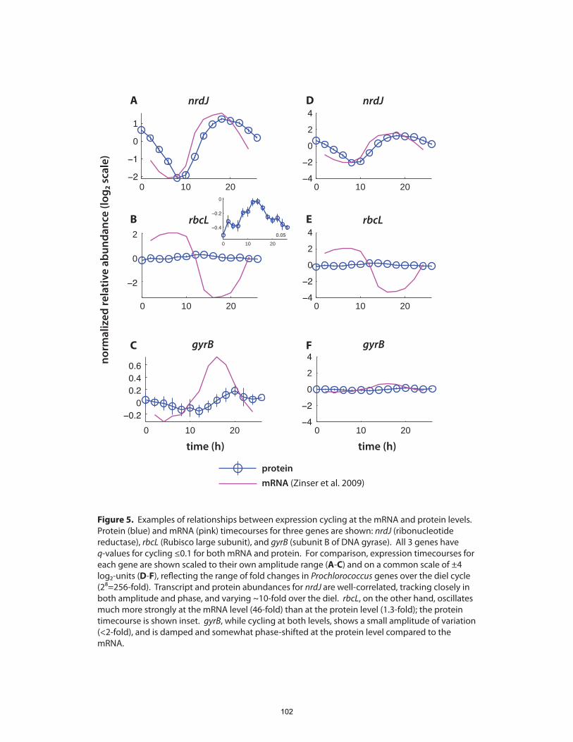
0 10 20
−2
0
2rbcL
0 10 20−2
−1
0
1
nrdJ
0 10 20−0.2
00.20.40.6
gyrB
0 10 20−4
−2
0
24
rbcL
0 10 20−4
−2
0
2
4nrdJ
0 10 20−4
−2
0
24
gyrB
norm
aliz
ed re
lativ
e ab
unda
nce
(log2
sca
le)
proteinmRNA (Zinser et al. 2009)
time (h) time (h)
A
B
C
D
E
F
Figure 5. Examples of relationships between expression cycling at the mRNA and protein levels. Protein (blue) and mRNA (pink) timecourses for three genes are shown: nrdJ (ribonucleotide reductase), rbcL (Rubisco large subunit), and gyrB (subunit B of DNA gyrase). All 3 genes have q-values for cycling ≤0.1 for both mRNA and protein. For comparison, expression timecourses for each gene are shown scaled to their own amplitude range (A-C) and on a common scale of ±4 log2-units (D-F), re�ecting the range of fold changes in Prochlorococcus genes over the diel cycle (28=256-fold). Transcript and protein abundances for nrdJ are well-correlated, tracking closely in both amplitude and phase, and varying ~10-fold over the diel. rbcL, on the other hand, oscillates much more strongly at the mRNA level (46-fold) than at the protein level (1.3-fold); the protein timecourse is shown inset. gyrB, while cycling at both levels, shows a small amplitude of variation (<2-fold), and is damped and somewhat phase-shifted at the protein level compared to the mRNA.
0 10 20
−0.4
−0.2
0
0.05
102
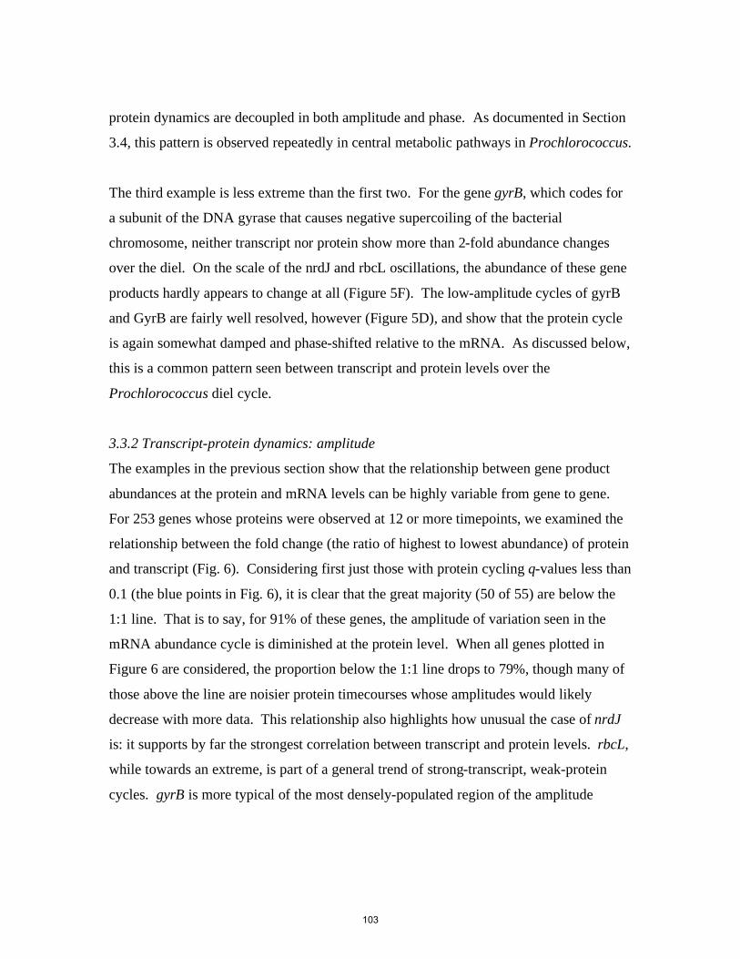
protein dynamics are decoupled in both amplitude and phase. As documented in Section
3.4, this pattern is observed repeatedly in central metabolic pathways in Prochlorococcus.
The third example is less extreme than the first two. For the gene gyrB, which codes for
a subunit of the DNA gyrase that causes negative supercoiling of the bacterial
chromosome, neither transcript nor protein show more than 2-fold abundance changes
over the diel. On the scale of the nrdJ and rbcL oscillations, the abundance of these gene
products hardly appears to change at all (Figure 5F). The low-amplitude cycles of gyrB
and GyrB are fairly well resolved, however (Figure 5D), and show that the protein cycle
is again somewhat damped and phase-shifted relative to the mRNA. As discussed below,
this is a common pattern seen between transcript and protein levels over the
Prochlorococcus diel cycle.
3.3.2 Transcript-protein dynamics: amplitude
The examples in the previous section show that the relationship between gene product
abundances at the protein and mRNA levels can be highly variable from gene to gene.
For 253 genes whose proteins were observed at 12 or more timepoints, we examined the
relationship between the fold change (the ratio of highest to lowest abundance) of protein
and transcript (Fig. 6). Considering first just those with protein cycling q-values less than
0.1 (the blue points in Fig. 6), it is clear that the great majority (50 of 55) are below the
1:1 line. That is to say, for 91% of these genes, the amplitude of variation seen in the
mRNA abundance cycle is diminished at the protein level. When all genes plotted in
Figure 6 are considered, the proportion below the 1:1 line drops to 79%, though many of
those above the line are noisier protein timecourses whose amplitudes would likely
decrease with more data. This relationship also highlights how unusual the case of nrdJ
is: it supports by far the strongest correlation between transcript and protein levels. rbcL,
while towards an extreme, is part of a general trend of strong-transcript, weak-protein
cycles. gyrB is more typical of the most densely-populated region of the amplitude
103
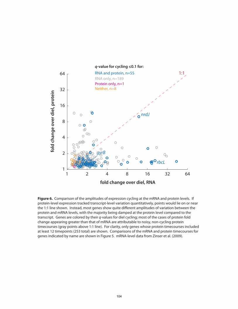
1 2 4 8 16 32 641
2
4
8
16
32
64
fold change over diel, RNA
fold
cha
nge
over
die
l, pr
otei
n
RNA and protein, n=55RNA only, n=189Protein only, n=1Neither, n=8
q-value for cycling ≤0.1 for:
1:1
Figure 6. Comparison of the amplitudes of expression cycling at the mRNA and protein levels. Ifprotein-level expression tracked transcript-level variation quantitatively, points would lie on or nearthe 1:1 line shown. Instead, most genes show quite di�erent amplitudes of variation between theprotein and mRNA levels, with the majority being damped at the protein level compared to thetranscript. Genes are colored by their q-values for diel cycling; most of the cases of protein foldchange appearing greater than that of mRNA are attributable to noisy, non-cycling protein timecourses (gray points above 1:1 line). For clarity, only genes whose protein timecourses included at least 12 timepoints (253 total) are shown. Comparisons of the mRNA and protein timecourses for genes indicated by name are shown in Figure 5. mRNA-level data from Zinser et al. (2009).
nrdJ
rbcL
gyrB
104
space. Overall, the comparison of expression fold-changes suggests that mRNA-level
variations are broadly damped at the protein level.
The methods used here to detect cyclic protein expression (metabolic isotope labeling,
Fourier scoring with false discovery rates; see Sec. 2.4) can confidently detect protein
abundance oscillations even when the amplitude is less than 2-fold – as it is for most
observed proteins (Figure 6). When protein abundances are tracked over time with
sufficient temporal resolution, small variations that would be impossible to resolve in 2-
sample comparisons become apparent and interpretable. If we had simply contrasted
protein abundances at, say, sunrise and sunset or midday and midnight, few differences
would be significant. It would appear that the protein abundance variations that
accompany (and underlie) the light-dark entrained cell cycle of Prochlorococcus are
generally of a smaller magnitude than those observed in typical laboratory gene
expression experiments involving strong, systemic perturbations such as acute nutrient
starvation, temperature shock or toxin exposure.
3.3.3 Transcript-protein dynamics: phase
Besides the amplitude or magnitude of abundance changes, the phase of expression
cycles (i.e., the timing of the peaks and troughs in abundance) can also vary between the
mRNA and protein levels. If transcriptional control were dominant, we might expect to
see a small, more or less consistent lag between the peaks of transcript and protein
abundance, simply due to the finite speed of translation – much as observed for nrdJ
(Figure 5A). As shown in Figure 7, however, the protein abundance cycles observed in
this experiment show a wide range of phase relationships with their respective transcripts.
A substantial number do plot slightly above and to the left of the 1:1 “in phase” diagonal,
which is where proteins lagging their transcripts would fall, though the range of lags in
that group spans 1-8 hours. This is many times longer than the half-life of
Prochlorococcus mRNA molecules (which averages 2.4 minutes; Steglich et al., in prep)
and, even given the slow translation rates in Prochlorococcus (see Chapter 5), it is
105
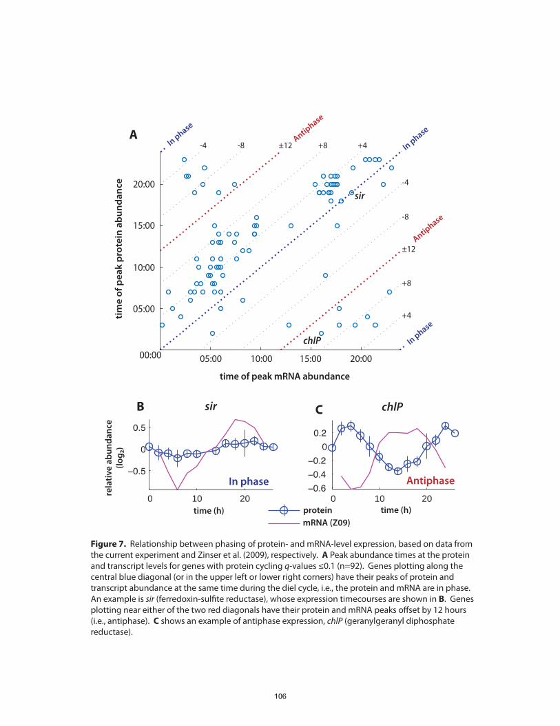
rela
tive
abun
danc
e(lo
g2)
05:00 10:00 15:00 20:0000:00
05:00
10:00
15:00
20:00
time of peak mRNA abundance
tim
e of
pea
k pr
otei
n ab
unda
nce
+4+8±12-4 -8
+4
+8
±12
-4
-8
In phase
Antiphase
Antiphase
In phase
In phase
chlP
sir
A
0 10 20
−0.5
0
0.5
sir
time (h)
In phase
B
0 10 20−0.6−0.4−0.2
00.2
chlP
time (h)
Antiphase
C
proteinmRNA (Z09)
Figure 7. Relationship between phasing of protein- and mRNA-level expression, based on data from the current experiment and Zinser et al. (2009), respectively. A Peak abundance times at the protein and transcript levels for genes with protein cycling q-values ≤0.1 (n=92). Genes plotting along the central blue diagonal (or in the upper left or lower right corners) have their peaks of protein and transcript abundance at the same time during the diel cycle, i.e., the protein and mRNA are in phase. An example is sir (ferredoxin-sul�te reductase), whose expression timecourses are shown in B. Genes plotting near either of the two red diagonals have their protein and mRNA peaks o�set by 12 hours (i.e., antiphase). C shows an example of antiphase expression, chlP (geranylgeranyl diphosphate reductase).
106
difficult to see how transcript abundance variations would take, say, 6 hours (a quarter of
the cell cycle) to be transmitted to the protein level. Assessment of the significance of
these smaller phase offsets will await the transcriptome timecourses from the current
experiment.
There are, however, a number of genes (e.g., chlP, Fig. 7C) for which the phasing of
mRNA and protein abundance are clearly divergent and involve posttranscriptional, and
probably posttranslational, processes. It is conceivable that for these genes, protein
degradation is also strongly cyclic, and this imposes another time-varying driver on
protein abundance. If protein degradation and transcript abundance both cycle with
sufficient amplitude and with different phases, the observed timecourse of protein
abundance would represent the sum of these two oscillating source and sink terms. Why
certain proteins would be subject to this mode of regulation remains a question for future
investigation.
Zinser et al. (2009) found that a majority of Prochlorococcus transcripts peak in
abundance near sunrise and sunset. A two-peaked distribution of peak abundance times
was also found in the protein timecourses from this experiment (Figure 8). Consistent
with the peaks in the abundance of transcripts, the peaks in the protein phase distribution
follow shortly after sunrise and sunset. The histograms in Figure 8 also provide an way
to estimate the proportion of non-cycling genes. If no genes were significantly cycling,
the distribution of phases would be random, and the histogram should look flat, with the
same number of genes ‘peaking’ at each timepoint. Viewed in this way, the sunrise and
sunset peaks sit on top of a flat, ‘background’ distribution of roughly 12 proteins per
timepoint. If those 288 (12 proteins × 24 timepoints) are considered non-cycling, then
the predicted proportion of cycling proteins is 47%, similar to the 43% estimated from
the shape of the q-value distribution, above.
107

0
5
10
15
20
25
30
35
40
45
50
00:0
0
06:0
0
12:0
0
18:0
0
time of peak abundance
num
ber o
f pro
tein
s
0
20
40
60
80
100
120
140
160
time of peak abundance
num
ber o
f tra
nscr
ipts
00:0
0
06:0
0
12:0
0
18:0
0
A
B
Figure 8. Histograms of times of peak expression with hourly resolution for (A) proteins in the current experiment and (B) transcripts in the diel microarray experiment of Zinser et al. (2009). Both distributions show peaks near sunrise and sunset, whose times during the two experimentsare indicated by symbols. Note that the photoperiod is one hour longer in B than in A. The white dotted line in the upper panel represents a hypothetical null distribution of non-cycling proteins, approximately 12 per timepoint.
108

3.4 Diel balance of carbon metabolism in Prochlorococcus
One of the most important cellular functions in Prochlorococcus, and arguably the most
important with regard to its role in ocean biogeochemistry, is carbon fixation. The
immediate incorporation of CO2 into organic matter is catalyzed by Rubisco, but this is
just one reaction in a central carbon metabolic network that involves both reductive (C-
fixing) and oxidative (C-respiring) pathways. Two components of this metabolic
network, the Calvin cycle and the pentose phosphate pathway, can be viewed as a
superpathway of two intersecting cycles working in opposite directions (Fig. 9A). In
essence, the reductive portion (the Calvin cycle) trades energy (ATP) and reducing power
(NADPH) for fixed carbon, while the oxidative portion (the pentose phosphate pathway)
trades fixed carbon for reducing power. During the day, photosynthesis can replenish the
ATP and NADPH consumed by the Calvin cycle, allowing net fixation of carbon. At
night, reserves of fixed carbon stored as glycogen are consumed and NADPH is
regenerated.
Proper regulation of the intersection of these two cycles is essential. To illustrate why,
consider what happens if the metabolic flux is allowed to run around the outside of the
superpathway: chemistry accomplished in one part of the cycle is undone in another, with
no net result except the waste of 3 molecules of ATP. It is the balance of fluxes through
the intersection of the reductive and oxidative portions that determines whether net
carbon fixation or respiration occurs.
The expression of the genes coding for enzymes of central carbon metabolism was
discussed in detail by Zinser et al. (2009). They found that transcripts for components of
the reductive and shared portions of the network were most abundant near sunrise, while
those for the oxidative section were highest near sunset. The amplitude of expression
variation was particularly strong for the initial C-fixing enzymes of the Calvin cycle,
Rubisco and phosphoglycerate kinase.
109
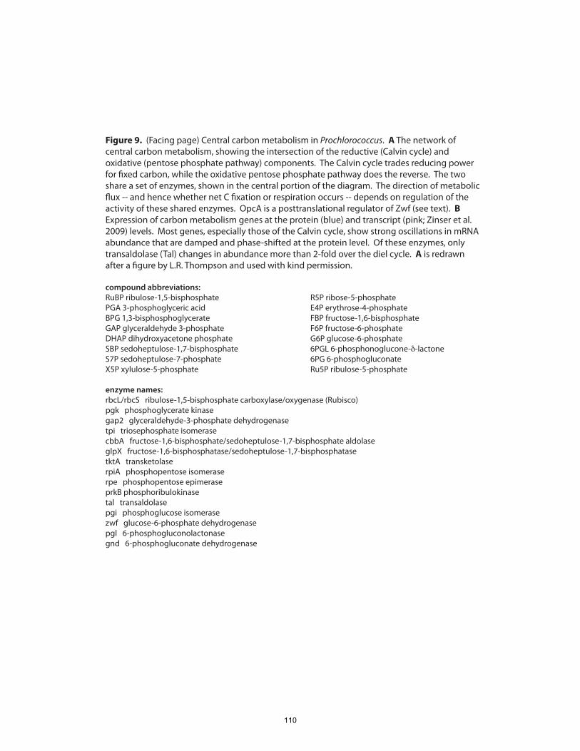
Figure 9. (Facing page) Central carbon metabolism in Prochlorococcus. A The network of central carbon metabolism, showing the intersection of the reductive (Calvin cycle) and oxidative (pentose phosphate pathway) components. The Calvin cycle trades reducing power for �xed carbon, while the oxidative pentose phosphate pathway does the reverse. The two share a set of enzymes, shown in the central portion of the diagram. The direction of metabolic �ux -- and hence whether net C �xation or respiration occurs -- depends on regulation of the activity of these shared enzymes. OpcA is a posttranslational regulator of Zwf (see text). B Expression of carbon metabolism genes at the protein (blue) and transcript (pink; Zinser et al. 2009) levels. Most genes, especially those of the Calvin cycle, show strong oscillations in mRNA abundance that are damped and phase-shifted at the protein level. Of these enzymes, only transaldolase (Tal) changes in abundance more than 2-fold over the diel cycle. A is redrawn after a �gure by L.R. Thompson and used with kind permission.
compound abbreviations:RuBP ribulose-1,5-bisphosphate R5P ribose-5-phosphatePGA 3-phosphoglyceric acid E4P erythrose-4-phosphateBPG 1,3-bisphosphoglycerate FBP fructose-1,6-bisphosphateGAP glyceraldehyde 3-phosphate F6P fructose-6-phosphateDHAP dihydroxyacetone phosphate G6P glucose-6-phosphateSBP sedoheptulose-1,7-bisphosphate 6PGL 6-phosphonoglucone-δ-lactoneS7P sedoheptulose-7-phosphate 6PG 6-phosphogluconateX5P xylulose-5-phosphate Ru5P ribulose-5-phosphate
enzyme names:rbcL/rbcS ribulose-1,5-bisphosphate carboxylase/oxygenase (Rubisco)pgk phosphoglycerate kinasegap2 glyceraldehyde-3-phosphate dehydrogenasetpi triosephosphate isomerasecbbA fructose-1,6-bisphosphate/sedoheptulose-1,7-bisphosphate aldolaseglpX fructose-1,6-bisphosphatase/sedoheptulose-1,7-bisphosphatasetktA transketolaserpiA phosphopentose isomeraserpe phosphopentose epimeraseprkB phosphoribulokinasetal transaldolasepgi phosphoglucose isomerasezwf glucose-6-phosphate dehydrogenasepgl 6-phosphogluconolactonasegnd 6-phosphogluconate dehydrogenase
110
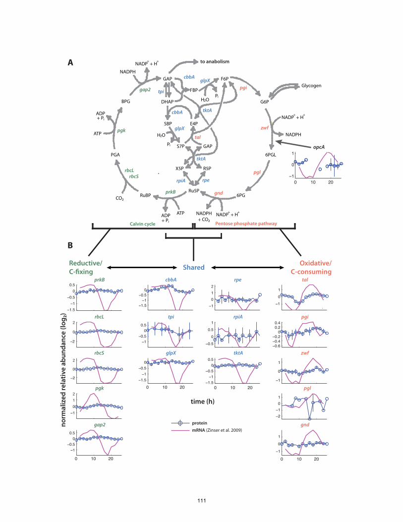
−1.5−1
−0.50
cbbA
−1.5−1
−0.50
0.5prkB
−1−0.5
00.5
tpi
0 10 20−1
0
1
gnd
−2−101
pgl
−101
tal
−2
0
2rbcL
−2
0
2rbcS
−1012
pgk
−1−0.5
00.5
gap2
−1.5−1
−0.50
glpX
−1012
rpe
−0.50
0.51
rpiA
−1.5−1
−0.50
0.5tktA
−0.6−0.4−0.2
00.20.4
pgi
−1
0
1
zwf
Reductive/C-�xing
Oxidative/C-consumingShared
0 10 200 10 20
0 10 20
time (h)
norm
aliz
ed re
lativ
e ab
unda
nce
(log2
)
Calvin cycle Pentose phosphate pathway
Ru5PRuBP
PGA
BPG
GAP
6PG
6PGL
G6P
F6P
DHAP
FBP
SBP
S7P
X5P
GAP
E4P
R5P
ATPADP NADPH+ CO2
CO2
ATP
ADP
NADP + H
NADPH
H2OPi
H2O
Pi
NADPH
Glycogen
+ +
+ Pi
+ Pi
NADP + H+ +
NADP + H+ +
prkB
rbcLrbcS
pgk
gap2
cbbA
cbbA
tpi
glpX
glpX
rperpiA
tktA
tktA
tal
pgi
zwf
pgl
gnd
proteinmRNA (Zinser et al. 2009)
A
B
to anabolism
0 10 20−1
0
1opcA
111
The results shown in Figure 9B add new insights to our understanding of carbon
metabolism and fixation by Prochlorococcus. The large-amplitude oscillation of
expression at the mRNA level, especially for genes in the reductive/Calvin cycle portion
of the pathway, is strongly damped at the protein level. The abundances of central
carbon metabolism enzymes show only small variations over the diel cycle. If these
small changes are sufficient to alter the balance of fluxes through the central intersection
– as they apparently are – this implies that this metabolic network is poised near a kind of
balancing point. The many-fold changes in transcript levels observed by Zinser et al.
(2009) do not result in wholesale redistribution of protein abundances between the
oxidative and reductive portions of the cycle, but rather nudge the network to one side or
the other of the flux balance point.
Notably, the only one of these central carbon metabolism enzymes to show more than 2-
fold changes in abundance is transaldolase (tal), which is also the only component of the
central intersection to act solely in the oxidative direction. These data suggest that the
abundance of the transaldolase protein is a key parameter regulating the direction of flux
through central carbon metabolism. The lower abundance of transaldolase during the
morning hours may be just enough to constrict flux through the oxidative pentose
phosphate pathway, promoting carbon fixation. The importance of transaldolase levels
has previously been inferred from the presence of genes encoding transaldolase in
cyanophage genomes and the production of proteins from those genes during phage
infection (L.R. Thompson et al., in prep).
Zinser et al. (2009) also raised the possibility of posttranslational regulation of carbon
metabolism. In particular, the PrkB/Gap2-binding inhibitor CP12 and the allosteric Zwf
effector OpcA were suggested to promote flux through the oxidative pathway at
nighttime. CP12 was not observed in our proteomics dataset; it is quite small (74aa) and
would not remain bound to its regulatory targets under the denaturing conditions used to
112
prepare the samples. OpcA, though, was observed, and almost exclusively during the
dark timepoints (Figure 9A). While it is difficult to quantify its cycling amplitude since it
dropped out of the analytical window for much of the day, OpcA is clearly significantly
more abundant at night, when it likely promotes flux through the oxidative portion of the
pathway. The observed constancy of the abundances of enzymes such as Zwf reinforces
the importance of the role of these regulatory proteins in modulating fluxes through
metabolic pathways.
The relatively constant abundance of Calvin cycle enzymes also helps explain a
somewhat puzzling observation in the experiment of Zinser et al. (2009). They noted
that, at night, the maximal light-saturated rate of carbon fixation drops to only 2- to 3-
fold below its daytime peak (c.f. Figure 3B of Zinser et al., 2009). This is surprising
given that Rubisco shows a more than 40-fold change in transcript abundance over the
diel, and other enzymes in the C-reduction pathway cycle by 4-10 fold at the mRNA level
(Fig. 9B). It is now clear that the troughs in transcript abundance for Calvin cycle genes
at the sunset do not result in low levels of their respective proteins during the night.
Nighttime abundances of Calvin cycle proteins are only ~40% below their daytime peaks;
the remaining 10-25% drop in C fixation capacity between day and night is likely due to
the more oxidized state of the cellular metabolite pool in the dark (L.R. Thompson et al.,
in prep). Central carbon metabolism in Prochlorococcus is clearly both a
biogeochemically important pathway and one that needs to be understood at multiple
levels of gene expression and regulation.
3.5 Cellular gene product abundances over the diel cycle
3.5.1 Correlation of fractional transcript and protein abundance
The use of the APEX (Absolute Protein Expression) technique (Lu et al., 2007), and an
equivalent measure of transcript abundance, here termed AMEX (Absolute Message
Expression), allows us to express gene product abundances in fractional terms – that is, as
113

a percent of the total amount of protein detected at any one timepoint. The basis for these
metrics and the caveats to their interpretation are discussed in more detail in Sec. 2.5;
suffice it here to note that the APEX/AMEX abundances represent fractions of detected
gene products – since the amount of detected protein or mRNA is always less than the
total, such measurements will overestimate true cellular abundances to some degree.
This problem is significantly more acute at the protein level, since many fewer gene
products are represented in the proteomics datasets (27-39%) than in the RNA-Seq
libraries (89-92%). With these experimental limitations in mind, however, we can gain
biological insights from comparisons of fractional gene product abundances.
We analyzed the relationship between fractional abundances at the protein and transcript
levels, for the two timepoints (08:00 and 18:00) for which mRNA sequencing has been
performed to date (Fig. 10). The correlation between the two is quite low: mRNA
abundance explains only 8-18% of the variance in protein abundance. While it is
perhaps surprising that transcript and protein abundances should be so decoupled, similar
results have been obtained from protein-transcript comparisons in a variety of organisms,
including yeast (Gygi et al., 1999; Foss et al., 2007; Garcia-Martinez and Gonzalez-
Candelas, 2007; Tuller et al., 2007; Ingolia et al., 2009), E. coli (Ishihama et al., 2008),
Streptomyces (Jayapal et al., 2008), Desulfovibrio (Nie et al., 2006), mouse (Huttlin et al.,
2009) and human (Gry et al., 2009). The loose connection between mRNA and protein
abundances is a theme emerging from multiple studies, and an important one if we are to
quantify molecular interactions between microbes and their environments.
It should also be noted that the genes whose protein products were not detected were not
necessarily rare at the transcript level. The gray points along the x-axes in Figure 10
show the fractional abundances of transcripts for which no peptides were detected, some
of which rank among the most abundant transcripts in the cell at a given timepoint.
While some of these are transcripts of hypothetical ORFs that may actually not be
translated, some of them are genes that encode important cellular functions and their
114
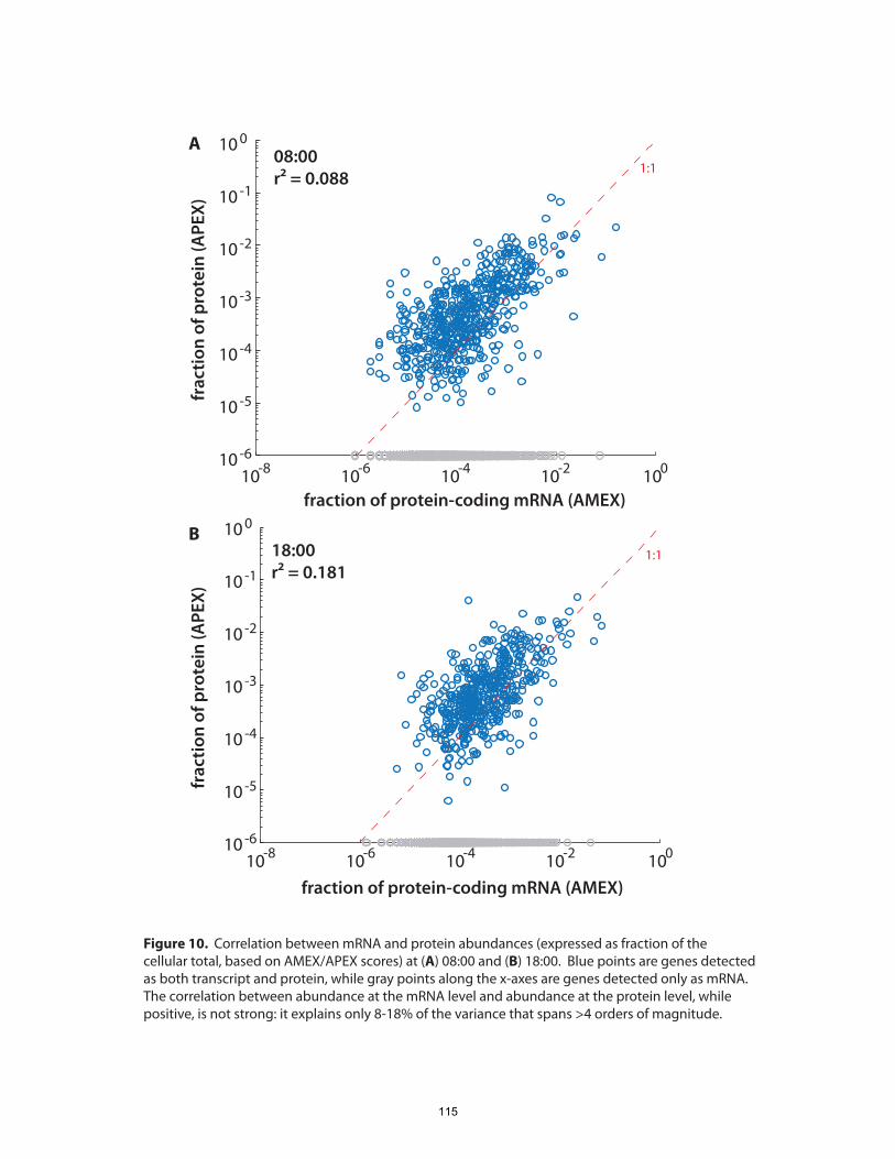
10-8 10-6 10-4 10-2 10010 -6
10 -5
10 -4
10 -3
10 -2
10 -1
10 008:00r2 = 0.088
fraction of protein-coding mRNA (AMEX)
frac
tion
of p
rote
in (A
PEX)
1:1
A
10-8 10-6 10-4 10-2 10010 -6
10 -5
10 -4
10 -3
10 -2
10 -1
10 0
fraction of protein-coding mRNA (AMEX)
frac
tion
of p
rote
in (A
PEX)
18:00r2 = 0.181
1:1B
Figure 10. Correlation between mRNA and protein abundances (expressed as fraction of the cellular total, based on AMEX/APEX scores) at (A) 08:00 and (B) 18:00. Blue points are genes detected as both transcript and protein, while gray points along the x-axes are genes detected only as mRNA. The correlation between abundance at the mRNA level and abundance at the protein level, whilepositive, is not strong: it explains only 8-18% of the variance that spans >4 orders of magnitude.
115
absence is due to the limited size and experimental biases of the proteomic dataset. The
possibility that a number of relatively abundant protein products are outside the analytical
window reinforces the approximate nature of fractional abundance measurements.
3.5.2 Stability of proteome composition over the diel cycle
One very useful question that gene product fractional abundance measurements allow us
to address is to what extent cellular resources are redistributed among different parts of
metabolism over the diel cycle. Are, for example, photosynthesis proteins a major
portion of the cellular proteome during the day, but then degraded and hardly present in
the cell at night? Does the diel cycle involve large-scale sifts of amino acids among
proteins involved in different cellular processes? As documented in Section 3.4, enzymes
of the Calvin cycle are still present in the cell at night, at more than half of their daytime
abundance, even though Prochlorococcus respires carbon at night rather than fixing it. A
proteome-wide view of fractional abundance changes over the diel is shown in Figure
11A, as the correlations between abundance profiles at three timepoints: 06:00 (just after
sunrise), 08:00, and 18:00 (just before sunset). If a large proportion of the proteome were
being redistributed among different sets of proteins over time, we would expect the
contrast between sunrise and sunset to be significantly greater than that between
successive timepoints. This is not borne out by the observations: the fractional
abundance of proteins at 06:00 correlates equally well with abundances at 08:00 as with
those at 18:00. The correlation between 06:00 and 18:00 is actually slightly higher than
that between 06:00 and 08:00, due primarily to closer correspondence in a few high-
abundance proteins. There does not appear to be evidence of major remodeling of the
proteome over the diel cycle.
A yet broader picture of proteome stability over the diel is revealed by the matrix of
pairwise correlations between fractional abundances at all timepoints (Fig. 11B). Each
set of APEX values was compared to every other, with the aim of gauging whether
protein abundances correlate better between nearby timepoints than between distant ones.
116
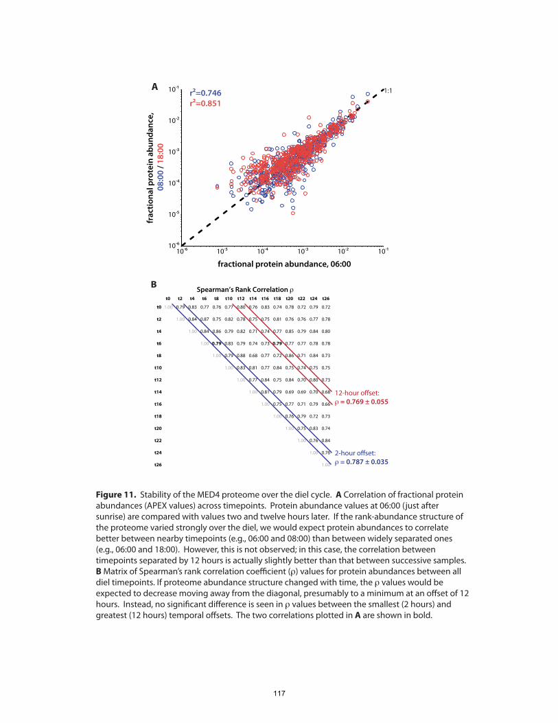
10-6
10-5
10-4
10-3
10-2
10-1
10-6 10-5 10-4 10-3 10-2 10-1
fractional protein abundance, 06:00
frac
tiona
l pro
tein
abu
ndan
ce,
08:
00 /
18:0
0
t0 t2 t4 t6 t8 t10 t12 t14 t16 t18 t20 t22 t24 t26
t0 1.00 0.79 0.83 0.77 0.76 0.77 0.80 0.76 0.83 0.74 0.78 0.72 0.79 0.72
t2 1.00 0.84 0.87 0.75 0.82 0.78 0.75 0.75 0.81 0.76 0.76 0.77 0.78
t4 1.00 0.84 0.86 0.79 0.82 0.71 0.74 0.77 0.85 0.79 0.84 0.80
t6 1.00 0.79 0.83 0.79 0.74 0.73 0.79 0.77 0.77 0.78 0.78
t8 1.00 0.79 0.88 0.68 0.77 0.72 0.86 0.71 0.84 0.73
t10 1.00 0.83 0.81 0.77 0.84 0.75 0.74 0.75 0.75
t12 1.00 0.77 0.84 0.75 0.84 0.70 0.80 0.73
t14 1.00 0.81 0.79 0.69 0.69 0.70 0.68
t16 1.00 0.75 0.77 0.71 0.79 0.66
t18 1.00 0.76 0.79 0.72 0.73
t20 1.00 0.75 0.83 0.74
t22 1.00 0.76 0.84
t24 1.00 0.76
t26 1.00
12-hour offset:ρ = 0.769 ± 0.055
2-hour offset:ρ = 0.787 ± 0.035
Spearman’s Rank Correlation ρ
r2=0.746r2=0.851
1:1A
B
Figure 11. Stability of the MED4 proteome over the diel cycle. A Correlation of fractional protein abundances (APEX values) across timepoints. Protein abundance values at 06:00 (just after sunrise) are compared with values two and twelve hours later. If the rank-abundance structure of the proteome varied strongly over the diel, we would expect protein abundances to correlate better between nearby timepoints (e.g., 06:00 and 08:00) than between widely separated ones (e.g., 06:00 and 18:00). However, this is not observed; in this case, the correlation between timepoints separated by 12 hours is actually slightly better than that between successive samples. B Matrix of Spearman’s rank correlation coe�cient (ρ) values for protein abundances between all diel timepoints. If proteome abundance structure changed with time, the ρ values would be expected to decrease moving away from the diagonal, presumably to a minimum at an o�set of 12 hours. Instead, no signi�cant di�erence is seen in ρ values between the smallest (2 hours) and greatest (12 hours) temporal o�sets. The two correlations plotted in A are shown in bold.
117

Spearman’s rank correlation (ρ; simply the standard Pearson’s r calculated on ranks) was
used here to avoid weighting the highest-abundance proteins too heavily and maintain a
proteome-wide measure of correspondence. Using ρ, the two correlations shown in
Figure 11A give the same coefficient. This matrix of correlations allows us to assess the
similarity in proteome composition as a function of temporal offsets between timepoints.
If proteome composition varied systematically over the diel cycle, the ρ values should
decrease away from the main diagonal to a minimum where the offset is 12 hours. In
fact, however, the ρ values at 12-hour offsets are not significantly lower than those at 2-
hour offsets (one-tailed t-test, p=0.19). This data strongly suggests that the overall
composition of the Prochlorococcus proteome remains stable over the diel cycle.
3.5.3 Cellular functions of abundant proteins
The stability of proteome composition means that a particular set of proteins are
consistently the most abundant in the cell. One enumeration of this set is listed in Table
2, where all 51 proteins with average fractional abundance over the diel cycle of 0.005 or
greater are grouped by function. To illustrate the consistency of protein abundance,
consider that these 51 proteins occupy 92% (656/714) of the spots in the combined top-51
abundance rankings of the 14 timepoints. The biochemical functions of many of the
abundant proteins are ones expected from Prochlorococcus: carbon fixation,
photosynthesis, ATP synthesis and nutrient uptake. Necessary cellular functions such as
protein folding (chaperonins), nucleotide metabolism, fatty acid biosynthesis, cell
division (FtsZ) and translation (TufA) are also represented. Notably, the most abundant
central carbon metabolism proteins are predominantly those involved in the Calvin cycle;
none of the oxidative pentose phosphate pathway-specific proteins appear (the most
abundant of these, transaldolase, has an average APEX score of 0.0024).
A few biochemical systems appear in the list of abundant proteins that have not to date
been the subject of detailed investigation in Prochlorococcus. Two components of the
thioredoxin system, TrxA and AhpC, are highly abundant. Thioredoxin (TrxA) is a
118
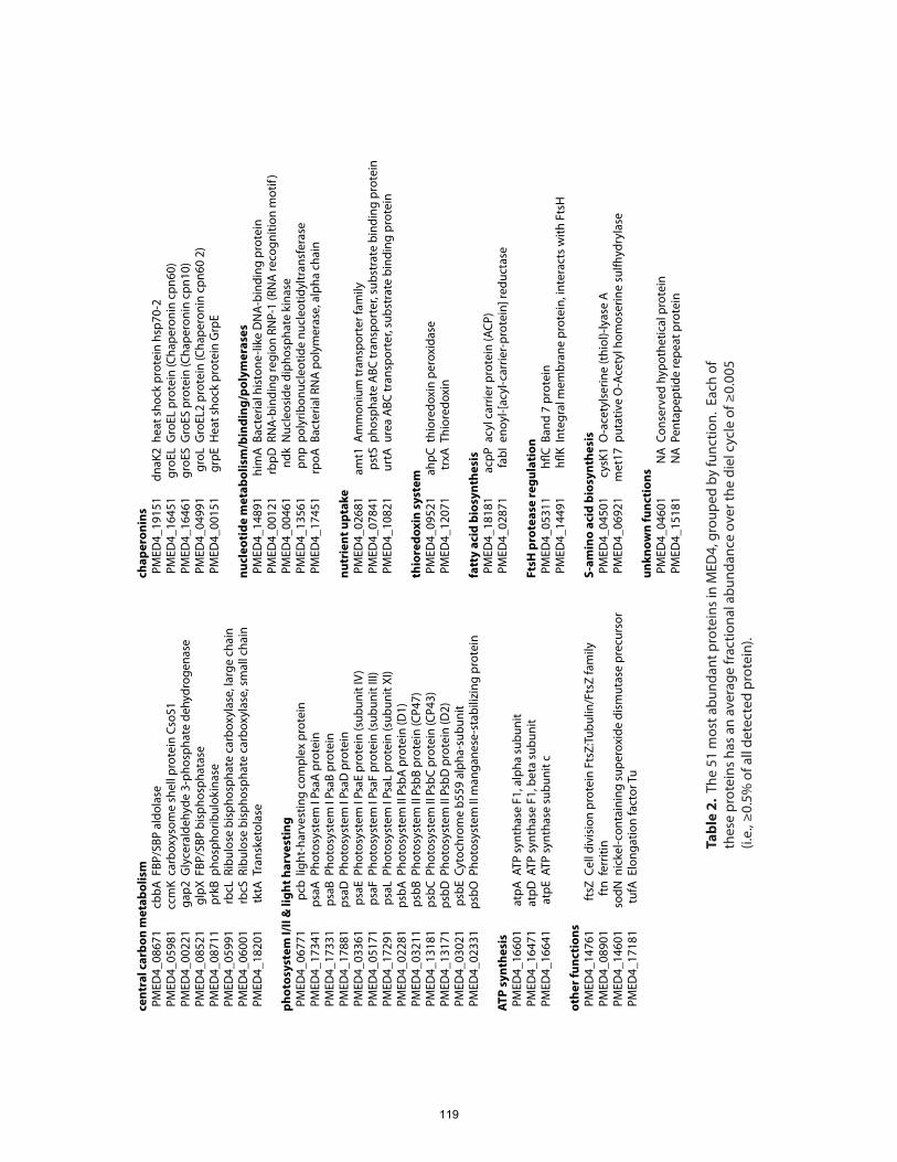
cent
ral c
arbo
n m
etab
olis
mPM
ED4_
0867
1cb
bAFB
P/SB
P al
dola
se
PMED
4_05
981
ccm
Kca
rbox
ysom
e sh
ell p
rote
in C
soS1
PM
ED4_
0022
1ga
p2G
lyce
rald
ehyd
e 3-
phos
phat
e de
hydr
ogen
ase
PMED
4_08
521
glpX
FBP/
SBP
bisp
hosp
hata
se
PMED
4_08
711
prkB
phos
phor
ibul
okin
ase
PMED
4_05
991
rbcL
Ribu
lose
bis
phos
phat
e ca
rbox
ylas
e, la
rge
chai
n PM
ED4_
0600
1rb
cSRi
bulo
se b
isph
osph
ate
carb
oxyl
ase,
sm
all c
hain
PM
ED4_
1820
1tk
tATr
ansk
etol
ase
phot
osys
tem
I/II
& li
ght h
arve
stin
gPM
ED4_
0677
1pc
blig
ht-h
arve
stin
g co
mpl
ex p
rote
in
PMED
4_17
341
psaA
Phot
osys
tem
I Ps
aA p
rote
in
PMED
4_17
331
psaB
Phot
osys
tem
I Ps
aB p
rote
in
PMED
4_17
881
psaD
Phot
osys
tem
I Ps
aD p
rote
in
PMED
4_03
361
psaE
Phot
osys
tem
I Ps
aE p
rote
in (s
ubun
it IV
) PM
ED4_
0517
1ps
aFPh
otos
yste
m I
PsaF
pro
tein
(sub
unit
III)
PMED
4_17
291
psaL
Phot
osys
tem
I Ps
aL p
rote
in (s
ubun
it XI
) PM
ED4_
0228
1ps
bAPh
otos
yste
m II
Psb
A p
rote
in (D
1)
PMED
4_03
211
psbB
Phot
osys
tem
II P
sbB
prot
ein
(CP4
7)
PMED
4_13
181
psbC
Phot
osys
tem
II P
sbC
prot
ein
(CP4
3)
PMED
4_13
171
psbD
Phot
osys
tem
II P
sbD
pro
tein
(D2)
PM
ED4_
0302
1ps
bECy
toch
rom
e b5
59 a
lpha
-sub
unit
PMED
4_02
331
psbO
Phot
osys
tem
II m
anga
nese
-sta
biliz
ing
prot
ein
ATP
synt
hesi
sPM
ED4_
1660
1at
pAAT
P sy
ntha
se F
1, a
lpha
sub
unit
PMED
4_16
471
atpD
ATP
synt
hase
F1,
bet
a su
buni
t PM
ED4_
1664
1at
pEAT
P sy
ntha
se s
ubun
it c
othe
r fun
ctio
nsPM
ED4_
1476
1ft
sZCe
ll di
visi
on p
rote
in F
tsZ:
Tubu
lin/F
tsZ
fam
ily
PMED
4_08
901
ftn
ferr
itin
PMED
4_14
601
sodN
nick
el-c
onta
inin
g su
pero
xide
dis
mut
ase
prec
urso
r PM
ED4_
1718
1tu
fAEl
onga
tion
fact
or T
u
chap
eron
ins
PMED
4_19
151
dnaK
2he
at s
hock
pro
tein
hsp
70-2
PM
ED4_
1645
1gr
oEL
Gro
EL p
rote
in (C
hape
roni
n cp
n60)
PM
ED4_
1646
1gr
oES
Gro
ES p
rote
in (C
hape
roni
n cp
n10)
PM
ED4_
0499
1gr
oLG
roEL
2 pr
otei
n (C
hape
roni
n cp
n60
2)
PMED
4_00
151
grpE
Hea
t sho
ck p
rote
in G
rpE
nucl
eoti
de m
etab
olis
m/b
indi
ng/p
olym
eras
esPM
ED4_
1489
1hi
mA
Bact
eria
l his
tone
-like
DN
A-b
indi
ng p
rote
in
PMED
4_00
121
rbpD
RNA
-bin
ding
regi
on R
NP-
1 (R
NA
reco
gniti
on m
otif
) PM
ED4_
0046
1nd
kN
ucle
osid
e di
phos
phat
e ki
nase
PM
ED4_
1356
1pn
ppo
lyrib
onuc
leot
ide
nucl
eotid
yltr
ansf
eras
e PM
ED4_
1745
1rp
oABa
cter
ial R
NA
pol
ymer
ase,
alp
ha c
hain
nutr
ient
upt
ake
PMED
4_02
681
amt1
Am
mon
ium
tran
spor
ter f
amily
PM
ED4_
0784
1ps
tSph
osph
ate
ABC
tran
spor
ter,
subs
trat
e bi
ndin
g pr
otei
n PM
ED4_
1082
1ur
tAur
ea A
BC tr
ansp
orte
r, su
bstr
ate
bind
ing
prot
ein
thio
redo
xin
syst
emPM
ED4_
0952
1ah
pCth
iore
doxi
n pe
roxi
dase
PM
ED4_
1207
1tr
xATh
iore
doxi
n
fatt
y ac
id b
iosy
nthe
sis
PMED
4_18
181
acpP
acyl
car
rier p
rote
in (A
CP)
PMED
4_02
871
fabI
enoy
l-[ac
yl-c
arrie
r-pr
otei
n] re
duct
ase
FtsH
pro
teas
e re
gula
tion
PMED
4_05
311
h�C
Band
7 p
rote
in
PMED
4_14
491
h�K
Inte
gral
mem
bran
e pr
otei
n, in
tera
cts
with
Fts
H
S-am
ino
acid
bio
synt
hesi
sPM
ED4_
0450
1cy
sK1
O-a
cety
lser
ine
(thi
ol)-l
yase
A
PMED
4_06
921
met
17pu
tativ
e O
-Ace
tyl h
omos
erin
e su
lfhyd
ryla
se
unkn
own
func
tion
sPM
ED4_
0460
1N
ACo
nser
ved
hypo
thet
ical
pro
tein
PM
ED4_
1518
1N
APe
ntap
eptid
e re
peat
pro
tein
Tabl
e 2.
The
51
mos
t abu
ndan
t pro
tein
s in
MED
4, g
roup
ed b
y fu
nctio
n. E
ach
of
thes
e pr
otei
ns h
as a
n av
erag
e fr
actio
nal a
bund
ance
ove
r the
die
l cyc
le o
f ≥0.
005
(i.e.
, ≥0.
5% o
f all
dete
cted
pro
tein
).
119
redox-active protein that interacts with a wide range of enzymes involved in
photosynthesis (Schurmann and Buchanan, 2008). Thioredoxin peroxidase (AhpC) is an
inorganic and alkylperoxide detoxifying enzyme (Parsonage et al., 2008) that uses
thioredoxin as an electron donor; since Prochlorococcus lacks genes for catalase and
heme peroxidases, it likely relies on this thioredoxin-based system to deal with peroxides
that are an inevitable byproduct of its oxygenic metabolism. This may be especially true
in axenic culture conditions (such as the current experiment), as it has been shown that
one of the key “helper” roles of heterotrophic bacteria in co-culture with
Prochlorococcus is as peroxide scavengers (Morris et al., 2008). Nickel-containing
superoxide dismutase was also one of the most abundant proteins, consistent with the
notion that these dense (~108 cells/ml), axenic cultures of Prochlorococcus are
oxidatively stressful environments for the cells.
Another surprise is the abundance of two enzymes, CysK1 and Met17, involved in the
biosynthesis of the sulfur-containing amino acids, cysteine and methionine. These two
enzymes catalyze the same step in their respective pathways: the insertion of sulfide
(from assimilatory sulfate reduction) into O-acetyl(homo)serine. This is unexpected
because Cys and Met are two of the least-common amino acids in the MED4 proteome
(20th- and 17th-most abundant, respectively; see Chapter 5). Moreover, conditions known
to promote high expression of these genes, such as sulfur limitation (Wirtz et al., 2004),
seem unlikely in a sulfate-rich medium like seawater. The high abundance of these
proteins is therefore puzzling. It may be that the MED4 alleles of these two enzymes are
catalytically slow, necessitating high abundances even to provide the small required
supply of Cys and Met. It is also possible that Prochlorococcus is especially sensitive to
sulfide, and the abundance of these enzymes ensures that H2S produced by assimilatory
sulfate reduction is quickly utilized for its intended biosynthetic purpose and does not
build up in the cytosol.
120
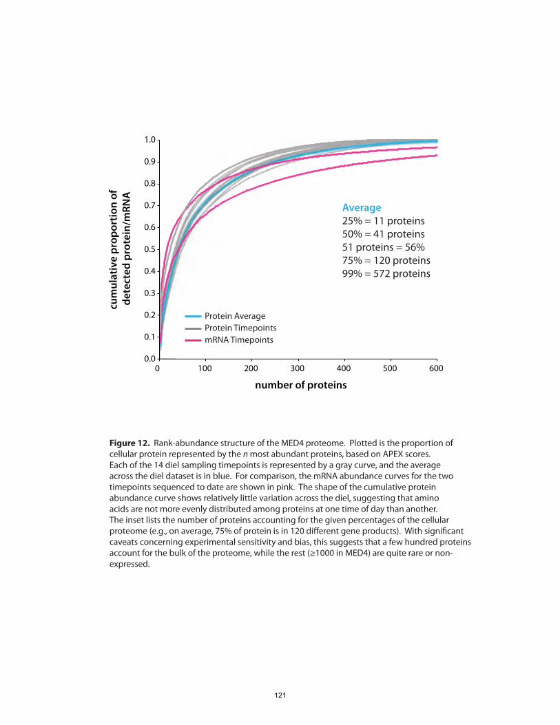
number of proteins
cum
ulat
ive
prop
ortio
n of
de
tect
ed p
rote
in/m
RNA
Average25% = 11 proteins50% = 41 proteins51 proteins = 56%75% = 120 proteins99% = 572 proteins
0.0
0.1
0.2
0.3
0.4
0.5
0.6
0.7
0.8
0.9
1.0
0 100 200 300 400 500 600
Figure 12. Rank-abundance structure of the MED4 proteome. Plotted is the proportion ofcellular protein represented by the n most abundant proteins, based on APEX scores.Each of the 14 diel sampling timepoints is represented by a gray curve, and the averageacross the diel dataset is in blue. For comparison, the mRNA abundance curves for the twotimepoints sequenced to date are shown in pink. The shape of the cumulative protein abundance curve shows relatively little variation across the diel, suggesting that amino acids are not more evenly distributed among proteins at one time of day than another. The inset lists the number of proteins accounting for the given percentages of the cellular proteome (e.g., on average, 75% of protein is in 120 di�erent gene products). With signi�cant caveats concerning experimental sensitivity and bias, this suggests that a few hundred proteinsaccount for the bulk of the proteome, while the rest (≥1000 in MED4) are quite rare or non-expressed.
Protein AverageProtein TimepointsmRNA Timepoints
121
3.5.4 Rank-abundance structure of the proteome
Finally, fractional abundance measurements can provide an estimate of how concentrated
a cell’s total complement of proteins are in the most abundant gene products. Figure 12
shows the rank-cumulative abundance structure for the MED4 proteome as measured
over the diel cycle. The 51 most abundant proteins discussed in the previous section
make up, on average, 56% of the total amount of detected protein. The shapes of the
rank-abundance curves for the various timepoints (gray lines) do not vary dramatically,
further evidence that the overall composition of the proteome is generally stable over the
diel cycle. 99% of the detected protein is accounted for by roughly 572 proteins; taken at
face value, this implies that the products of all other gene (a total of 1356 ORFs) sum to
≤1% of cellular protein. As discussed above, however, fractional abundance estimates
are blind to undetected proteins, which are not necessarily rare. By comparison, the
higher-coverage transcriptomics datasets (pink lines in Figure 12) suggest that the top
600 gene products make up ~90% of the total. While the estimates are uncertain at this
point, these data do point towards a “long tail” of gene product abundance, with over
1000 gene products accounting for perhaps ~10-20% of the cellular total. Similar “long
tails” have been observed in other biological systems, including human plasma
(Anderson and Anderson, 2002). These distributions illustrate the enormous expansion
in the dynamic range of gene product abundance between DNA and protein.
4. CONCLUSIONS
A principal finding of this study is that the strong diel periodicity in the expression of
many Prochlorococcus genes at the mRNA level (Zinser et al., 2009) is substantially
damped at the protein level. While Zinser et al. (2009) found that 82% of transcripts of
protein-coding genes exhibit a diel abundance cycle, we estimate that only 15-47% of
proteins cycle significantly over the diel. While mass-spectrometry based proteomics
data is not as rich as microarrays or RNA-sequencing as a probe of gene expression, it is
clear that, for 80-90% of genes, the amplitude of oscillation in gene product abundance is
122
lower at the protein level than at the mRNA level. Additionally, for many proteins the
timing of peak abundance is quite different from – or even opposite to – the maximum in
transcript abundance, and these offsets are highly variable from gene to gene. Hence the
temporal dynamics of protein expression cannot be directly extrapolated from transcript
abundance timecourses. Our results show that substantial decoupling of transcript and
protein abundances occurs even in a small, ‘simple’ organism like Prochlorococcus that
has streamlined metabolism and regulatory systems.
We have also established that the overall composition of the proteome, in terms of
proportional protein abundance, is quite stable over the diel cycle. Proteins that are
highly abundant in the cell remain so around the clock, not being degraded down to low
levels and then re-synthesized. Thus in proteomic terms, Prochlorococcus is not a
“phototroph by day, heterotroph by night”; the protein machinery for its photoautotrophic
lifestyle is present in the cells in the dark, and the enzymes used for respiration at night
are present during the day as well. The fact that Prochlorococcus actually does perform
net C fixation during the day and net respiration at night suggests that its metabolic
networks are poised near a flux balance point. Relatively small changes in the abundance
of enzymes at key points in the network, likely combined with other forms of
posttranslational regulation, can redirect metabolic fluxes to match cellular demands and
environmental conditions. This picture of metabolism reflects the evolutionary
refinement of microbial physiology, whereby fluxes through a complex biochemical
network are modulated by small, targeted shifts rather than system-wide remodeling.
Since most proteins change so little in abundance over the diel cycle, the few that do
oscillate strongly stand out. In particular, ribonucleotide reductase (NrdJ) changes more
than 10-fold in abundance between morning and late afternoon. This variation is
certainly coherent with NrdJ’s role in DNA synthesis, which occurs between noon and
sunset. But other cell-cycle-specific proteins do not oscillate nearly so strongly; FtsZ and
MreB, for example, vary only 1.3-fold. Why the large cycle in NrdJ? It may be that the
123
presence of ribonucleotide reductase in the cytosol outside of C/S phase is deleterious; at
other times, the main goal of nucleotide synthesis is RNA, and having material diverted
to DNA may be substantially counterproductive. But the presence of nrdJ in phage
genomes (L.R. Thompson et al., in prep) offers another hypothesis: the low abundance of
NrdJ outside of the DNA synthesis may be a mode of defense against phage infection.
When a bacteriophage infects a host cell, it shuts down translation of the host genome
and begins expressing its own using the host’s machinery. Thus, to make progeny, the
phage is dependent on the presence of DNA-synthesis enzymes (notably NrdJ) in the host
cell at the time of infection. If infection occurs when NrdJ protein levels are low (as they
are in the morning), phage infection may stall for want of deoxyribonucleotides to copy
the phage genome. In this scenario, the presence of ribonucleotide reductase genes in the
majority of sequenced cyanophage genomes (Sullivan et al., 2005; Sullivan et al., in
press) is a strategy adopted by phage to circumvent dependence on host NrdJ by encoding
their own copy and expressing it during infection.
The results of this experiment also have implications for how inferences can be drawn
between lab- and field-based datasets, and what sorts of techniques might be most useful
as assays of conditions and microbial activities in natural environments. First, it appears
that growth in dense, axenic culture imposes particular oxidative stress on
Prochlorococcus cells. Assessing the true biochemistry and regulation of the response of
Prochlorococcus to reactive oxygen species under oceanic conditions is therefore likely
to be challenging, since the cell densities currently required to produce sufficient material
for some kinds of molecular analyses (as well as the absence of exogenous reductants
produced by other members of the community) are a source of oxidative stress. Second,
if measurements of gene product abundances are to be used as reporters of the
physiological activities of, and environmental stresses felt by, organisms in natural
settings, then a multilevel, systems view of gene expression and regulation is warranted.
This experiment exemplifies how the dynamics of protein abundance can be very
different in both timing and magnitude from those of transcripts, yet for a variety of
124
methodological reasons (such as the ability to selectively amplify a gene of interest), it is
often desirable to assay gene expression at the transcript level. Given the findings
presented here, and similar results emerging from systems biology more generally (Beyer
et al., 2004; Nie et al., 2007), we suggest that complementing transcript-level
measurements with information from other biological metrics (be they proteins,
metabolites, activity assays, etc.) will often be valuable for drawing accurate
biogeochemical inferences.
The quantitative concordance between levels of biological organization (transcriptome,
proteome, metabolism) is likely to be greatest in concerted responses to acute stresses
(Halbeisen and Gerber, 2009). The majority of laboratory gene expression studies test
such responses, as the contrast between stress and control conditions is distinct and
produces strong experimental signals. With the exception of studies of specific
perturbation events, however, observations of natural populations are generally not
studies of acute stress responses. When we look at a microbial community in its natural
habitat, we are seeing a group of organisms that have necessarily adapted to that
environment over many generations. When we contrast two environments that differ in,
for example, availability of a particular nutrient, the adaptation involved is to a chronic
stressor, and is not the same as the kind of acute nutrient limitation that is often imposed
in the laboratory. The longest-running experimental evolution study, the E. coli Long-
term Evolution Experiment (Barrick et al., 2009), has tracked populations over 40,000
generations, and most steady-state culture studies (e.g., in chemostats) are much shorter.
Prochlorococcus has undergone roughly 40,000 generations just since the year 1900,
while living in an ocean undergoing both natural and anthropogenic change on a
continuum of timescales ranging from decadal to geologic. Experimental nutrient
limitation in culture can help identify important genes and functions (e.g., Martiny and
Coleman et al., 2006), but the quantitative dynamics of that response are distinct from
those involved in long-term adaptation. The laboratory study presented here attempts to
approximate, however imperfectly, the quotidian activities of Prochlorococcus over its
125
natural, unstressed diel growth cycle. In taking a multilevel view of gene expression and
metabolic regulation, we hope to contribute to bridging the gap between laboratory and
environmental characterizations of microbial roles in biogeochemistry.
ACKNOWLEDGEMENTS
We are grateful to Luke Thompson for discussions of carbon metabolism and permission to reproduce Figure 9A, Anne Thompson for assistance with sampling during the diel growth experiment, Bryan Krastins for advice on proteomics sample preparation, and to David Shteynberg and Matt Chambers for help with proteomics data analysis. LC-MS data were collected at the Fourier-Transform Mass Spectrometry Facility at the Woods Hole Oceanographic Institution; we thank Facility Manager Melissa Soule for guidance and technical support. This work was supported by grants from the Department of Energy Genomics:GtL program, the NSF Center for Microbial Oceanography: Research and Education, and the Gordon and Betty Moore Foundation to SWC, and by an Office of Naval Research NDSEG Fellowship and an NSF Graduate Research Fellowship to JRW.
REFERENCES
Anderson, NL, and NG Anderson. 2002. The Human Plasma Proteome: History, Character, and Diagnostic Prospects. Mol Cell Proteomics 1: 845-867.
Axmann, IM, U Duhring, L Seeliger, A Arnold, JT Vanselow, A Kramer, and A Wilde. 2009. Biochemical Evidence for a Timing Mechanism in Prochlorococcus. J Bacteriol 191, no. 17: 5342–5347.
Barrick, JE, DS Yu, SH Yoon, H Jeong, TK Oh, D Schneider, RE Lenski, and JF Kim. 2009. Genome evolution and adaptation in a long-term experiment with Escherichia coli. Nature 461:1243-1247.
Beyer, A, J Hollunder, H-P Nasheuer and T Wilhelm. 2004. Post-transcriptional Expression Regulation in the Yeast Saccharomyces cerevisiae on a Genomic Scale. Mol Cell Proteomics 3: 1083-1092.
Braisted, JC, S Kuntumalla, C Vogel, EM Marcotte, AR Rodrigues, R Wang, S-T Huang, ES Ferlanti, AI Saeed, RD Fleischmann, SN Peterson, and R Pieper. 2008. The APEX Quantitative Proteomics Tool: generating protein quantitation estimates from LC-MS/MS proteomics results. BMC Bioinformatics 9, 529.
Brown, MB. 1975. 400: A Method for Combining Non-Independent, One-Sided Tests of Significance. Biometrics 31, no. 4: 987–992.
Bruyant, F, M Babin, B Genty, O Prasil, MJ Behrenfeld, H Claustre, A Bricaud, L Garczarek, J Holtzendorff, and M Koblizek. 2005. Diel variations in the photosynthetic parameters of Prochlorococcus strain PCC 9511: Combined effects of light and cell cycle. Limnology and Oceanography 50, no. 3: 850–863.
126

Claustre, H, A Bricaud, M Babin, F Bruyant, L Guillou, FL Gall, D Marie, and F Partensky. 2002. Diel variations in Prochlorococcus optical properties. Limnology and Oceanography 1637–1647.
Craig, R, and RC Beavis. 2004. TANDEM: matching proteins with tandem mass spectra. Bioinformatics 20, no. 9: 1466–1467.
Foss, EJ, D Radulovic, SA Shaffer, DM Ruderfer, A Bedalov, DR Goodlett, and L Kruglyak. 2007. Genetic basis of proteome variation in yeast. Nature Genetics 39, no. 11: 1369–1375.
Futschik, ME, and H Herzel. 2008. Are we overestimating the number of cell-cycling genes? The impact of background models on time-series analysis. Bioinformatics 24, no. 8: 1063.
Garcia-Martinez, J, and F Gonzalez-Candelas. 2007. Common gene expression strategies revealed by genome-wide analysis in yeast. Genome Biology
Garczarek, L, F Partensky, H Irlbacher, J Holtzendorff, M Babin, I Mary, JC Thomas, and WR Hess. 2001. Differential expression of antenna and core genes in Prochlorococcus PCC 9511 (Oxyphotobacteria) grown under a modulated light-dark cycle. Environmental Microbiology 3, no. 3: 168–175.
Geer, LY, SP Markey, JA Kowalak, L Wagner, M Xu, DM Maynard, X Yang, W Shi, and SH Bryant. 2004. Open mass spectrometry search algorithm. J Proteome Res 3, no. 5: 958–964.
Gry, M, R Rimini, S Stromberg, A Asplund, F Ponten, M Uhlen, and P Nilsson. 2009. Correlations between RNA and protein expression profiles in 23 human cell lines. BMC Genomics 10, 365.
Gurland, J, and RC Tripathi. 1971. A simple approximation for unbiased estimation of the standard deviation. American Statistician 30–32.
Gygi, SP, Y Rochon, BR Franza, and R Aebersold. 1999. Correlation between protein and mRNA abundance in yeast. Mol Cell Biol 19, no. 3: 1720–1730.
Halbeisen, R, and A Gerber. 2009. Stress-Dependent Coordination of Transcriptome and Translatome in Yeast. PLoS Biol 7, no. 5: e105.
Hendrickson, EL, Q Xia, T Wang, JA Leigh, and M Hackett. 2006. Comparison of spectral counting and metabolic stable isotope labeling for use with quantitative microbial proteomics. The Analyst 131, no. 12: 1335–1341.
Holtzendorff, J, F Partensky, S Jacquet, F Bruyant, D Marie, L Garczarek, I Mary, D Vaulot, and WR Hess. 2001. Diel expression of cell cycle-related genes in synchronized cultures of Prochlorococcus sp. strain PCC 9511. J Bacteriol 183, no. 3: 915–920.
Holtzendorff, J, F Partensky, D Mella, J-F Lennon, H WR, and L Garczarek. 2008. Genome streamlining results in loss of robustness of the circadian clock in the marine cyanobacterium Prochlorococcus marinus PCC9511. Journal of Biological Rhythms 23, 187-199.
Hsiao, C, H Chen, K Furuse, and N Ohbo. 2009. Figure and Ground: A Complete Approach to Outlier Detection. AIP Conference Proceedings
Huttlin, EL, X Chen, GA Barrett-Wilt, AD Hegeman, RB Halberg, AC Harms, MA Newton, WF Dove, and MR Sussman. 2009. Discovery and validation of colonic
127
tumor-associated proteins via metabolic labeling and stable isotopic dilution. Proc Natl Acad Sci USA 106, no. 40: 17235–17240.
Ingolia, NT, S Ghaemmaghami, JRS Newman, and JS Weissman. 2009. Genome-Wide Analysis in Vivo of Translation with Nucleotide Resolution Using Ribosome Profiling. Science 324, no. 5924: 218–223.
Ishihama, Y, T Schmidt, J Rappsilber, M Mann, FU Hartl, MJ Kerner, and D Frishman. 2008. Protein abundance profiling of the Escherichia coli cytosol. BMC Genomics 9, 102.
Jacquet, S, F Partensky, D Marie, R Casotti, and D Vaulot. 2001. Cell cycle regulation by light in Prochlorococcus strains. Appl Environ Microbiol 67, no. 2: 782–790.
Jayapal, KP, RJ Philp, Y-J Kok, MGS Yap, DH Sherman, TJ Griffin, and W-S Hu. 2008. Uncovering genes with divergent mRNA-protein dynamics in Streptomyces coelicolor. PLoS ONE 3, no. 5: e2097.
Keller, A, AI Nesvizhskii, E Kolker, and R Aebersold. 2002. Empirical statistical model to estimate the accuracy of peptide identifications made by MS/MS and database search. Anal Chem 74, no. 20: 5383–5392.
Kielbasa, SM, H Herzel, and IM Axmann. 2007. Regulatory elements of marine cyanobacteria. Genome Informatics 18, 1–11.
Levicky, R and A Horgan. 2005. Physicochemical perspectives on DNA microarray and biosensor technologies. Trends Biotechnol 23, no. 3: 143-149.
Li, X-J, H Zhang, JA Ranish, and R Aebersold. 2003. Automated statistical analysis of protein abundance ratios from data generated by stable-isotope dilution and tandem mass spectrometry. Anal Chem 75, no. 23: 6648–6657.
Lu, P, C Vogel, R Wang, X Yao, and EM Marcotte. 2007. Absolute protein expression profiling estimates the relative contributions of transcriptional and translational regulation. Nat Biotechnol 25, no. 1: 117–124.
MacLean, B, JK Eng, RC Beavis, and M McIntosh. 2006. General framework for developing and evaluating database scoring algorithms using the TANDEM search engine. Bioinformatics 22, no. 22: 2830–2832.
Mallick, P, M Schirle, SS Chen, MR Flory, H Lee, D Martin, J Ranish, B Raught, R Schmitt, T Werner, B Kuster, and R Aebersold. 2007. Computational prediction of proteotypic peptides for quantitative proteomics. Nat Biotechnol 25, no. 1: 125–131.
Malmström, J, M Beck, A Schmidt, V Lange, EW Deutsch and R Aebersold. 2009. Proteome-wide cellular protein concentrations of the human pathogen Leptospira interrogans. Nature 460: 762-765.
Martiny, AC, ML Coleman, and SW Chisholm. 2006. Phosphate acquisition genes in Prochlorococcus ecotypes: evidence for genome-wide adaptation. PNAS 103, no. 33: 12552-12557.
Mary, I, and D Vaulot. 2003. Two-component systems in Prochlorococcus MED4: genomic analysis and differential expression under stress. FEMS Microbiol Lett 226, no. 1: 135-144.
128
Moore, LR, A Coe, ER Zinser, MA Saito, MB Sullivan, D Lindell, K Frois-Moniz, J Waterbury, and SW Chisholm. 2007. Culturing the marine cyanobacterium Prochlorococcus. Limnology and Oceanography: Methods 5, 353–362.
Morris, JJ, R Kirkegaard, MJ Szul, ZI Johnson, and ER Zinser. 2008. Facilitation of Robust Growth of Prochlorococcus Colonies and Dilute Liquid Cultures by "Helper" Heterotrophic Bacteria. Appl Environ Microbiol 74, no. 14: 4530–4534.
Mullineaux, CW, and R Stanewsky. 2009. The Rolex and the Hourglass: a Simplified Circadian Clock in Prochlorococcus? J Bacteriol 191, no. 17: 5333–5335.
Nesvizhskii, AI, A Keller, E Kolker, and R Aebersold. 2003. A statistical model for identifying proteins by tandem mass spectrometry. Anal Chem 75, no. 17: 4646–4658.
Nie, L, G Wu and W Zhang. 2006. Correlation between mRNA and protein abundance in Desulfovibrio vulgaris: A multiple regression to identify sources of variations. Biochem Biophys Res Comm 339: 603–610.
Nie, L, G Wu, DE Culley, JCM Scholten and W Zhang. 2007. Integrative Analysis of Transcriptomic and Proteomic Data: Challenges, Solutions and Applications. Crit Rev Biotechnol 27:63–75.
Parsonage, D, PA Karplus, and LB Poole. 2008. Substrate specificity and redox potential of AhpC, a bacterial peroxiredoxin. Proc Natl Acad Sci USA 105, no. 24: 8209–8214.
Poretsky, RS, I Hewson, S Sun, AE Allen, JP Zehr, and MA Moran. 2009. Comparative day/night metatranscriptomic analysis of microbial communities in the North Pacific subtropical gyre. Environmental Microbiology 11, no. 6: 1358–1375.
Richter, AS, C Schleberger, R Backofen and C Steglich. 2010. Seed-based INTARNA prediction combined with GFP-reporter system identifies mRNA targets of the small RNA Yfr1. Bioinformatics 26, no. 1: 1-5.
Rocap, G, FW Larimer, J Lamerdin, S Malfatti, P Chain, NA Ahlgren, A Arellano, ML Coleman, L Hauser, WR Hess, ZI Johnson, M Land, D Lindell, AF Post, W Regala, M Shah, SL Shaw, C Steglich, MB Sullivan, CS Ting, AC Tolonen, EA Webb, ER Zinser, and SW Chisholm. 2003. Genome divergence in two Prochlorococcus ecotypes reflects oceanic niche differentiation. Nature 424, no. 6952: 1042-1047.
Schurmann, P, and BB Buchanan. 2008. The ferredoxin thioredoxin system of oxygenic photosynthesis. Antioxidants & Redox Signaling 10, no. 7: 1235–1274.
Silva, JC, MV Gorenstein, G-Z Li, JPC Vissers, and SJ Geromanos. 2006. Absolute quantification of proteins by LCMSE: a virtue of parallel MS acquisition. Mol Cell Proteomics 5, no. 1: 144–156.
Shalapyonok, A, RJ Olson and LS Shalapyonok. 1998. Ultradian Growth in Prochlorococcus spp. Appl Env Micr 64, no. 3: 1066-1069.
Steglich, C, ME Futschik, D Lindell, B Voss, SW Chisholm and WR Hess. 2008. The Challenge of Regulation in a Minimal Photoautotroph: Non-Coding RNAs in Prochlorococcus. PLoS Genet 4, no. 8: e1000173.
Storey, JD, and R Tibshirani. 2003. Statistical significance for genomewide studies. Proc Natl Acad Sci USA 100, no. 16: 9440–9445.
129
Sullivan, MB, ML Coleman, P Weigele, F Rohwer, and SW Chisholm. 2005. Three Prochlorococcus cyanophage genomes: signature features and ecological interpretations. PLoS Biol 3, no. 5: e144.
Sullivan, MB, KH Huang, JC Ignacio-Espinoza, A Berlin, L Kelly, PR Weigele, AS DeFrancesco, SE Kern, LR Thompson, S Young, C Yandava, R Fu, B Krastins, M Chase, D Sarracino, MS Osburne, MR Henn and SW Chisholm. In press. Genomic analysis of oceanic cyanobacterial myoviruses compared to T4-like myoviruses from diverse hosts and environments. Env Microbiol.
Tabb, DL, CG Fernando, and MC Chambers. 2007. MyriMatch: highly accurate tandem mass spectral peptide identification by multivariate hypergeometric analysis. J Proteome Res 6, no. 2: 654–661.
Troyanskaya, O, M Cantor, G Sherlock, P Brown, T Hastie, R Tibshirani, D Botstein, and RB Altman. 2001. Missing value estimation methods for DNA microarrays. Bioinformatics 17, no. 6: 520–525.
Tuller, T, M Kupiec, and E Ruppin. 2007. Determinants of protein abundance and translation efficiency in S. cerevisiae. PLoS Comput Biol 3, no. 12: e248.
Vaulot, D, D Marie, R Olson, and S Chisholm. 1995. Growth of Prochlorococcus, a Photosynthetic Prokaryote, in the Equatorial Pacific Ocean. Science 268, no. 5216: 1480–1482.
Vogel, C, and EM Marcotte. 2008. Calculating absolute and relative protein abundance from mass spectrometry-based protein expression data. Nat Protoc 3, no. 9: 1444–1451.
Vogel, J, IM Axmann, H Herzel, and WR Hess. 2003. Experimental and computational analysis of transcriptional start sites in the cyanobacterium Prochlorococcus MED4. Nucleic Acids Res 31, no. 11: 2890-2899.
Wang, JD, and PA Levin. 2009. Metabolism, cell growth and the bacterial cell cycle. Nat Rev Microbiol 7, no. 11: 822–827.
Wirtz, M, M Droux, and R Hell. 2004. O-acetylserine (thiol) lyase: an enigmatic enzyme of plant cysteine biosynthesis revisited in Arabidopsis thaliana. J Exp Bot 55, no. 404: 1785–1798.
Zaykin, DV, LA Zhivotovsky, PH Westfall, and BS Weir. 2002. Truncated product method for combining P-values. Genet Epidemiol 22, no. 2: 170–185.
Zinser, ER, D Lindell, ZI Johnson, ME Futschik, C Steglich, ML Coleman, MA Wright, T Rector, R Steen, N McNulty, LR Thompson, and SW Chisholm. 2009. Choreography of the transcriptome, photophysiology, and cell cycle of a minimal photoautotroph, Prochlorococcus. PLoS ONE 4, no. 4: e5135.
130

131

Supplementary Figure 1. Timecourses for 548 proteins quanti�ed over the diel cycle in Prochlorococcus MED4. For each protein, relative abundance is shown on a log2 scale. Protein-level abundance at each timepoint was calculated as the mean of a lognormal �t to the �ltered peak-level 14N/15N abundance ratios, and error bars indicate 95% con�dence intervals based on an unbiased estimate of the standard error of that mean (Sec. 2.4.1). Titles indicate the gene locus and name, where applicable. In the lower right corner of each timecourse panel is the q-value calculated for the signi�cance of diel cycling (Sec. 2.4.2).
132
0 10 20−0.6
−0.4
−0.2
0
0.2
PMED4_00001 dnaN
0.36
0 10 200
0.5
1
PMED4_00021 purL
0.16
0 10 20
0
5
10
PMED4_00031 purF
0.20
0 10 20
0
2
4
PMED4_00041
0.53
0 10 20−1
0
1
PMED4_00071
0.39
0 10 20
−0.8−0.6−0.4−0.2
00.2
PMED4_00091 ftsY
0.09
0 10 20
−0.4
−0.2
0
PMED4_00121
0.53
0 10 20
−0.2
0
0.2
0.4PMED4_00151 grpE
0.24
0 10 20
−0.5
0
0.5
PMED4_00161 dnaJ
0.17
0 10 20
−0.6
−0.4
−0.2
0
0.2
PMED4_00191
0.39
0 10 200.1
0.2
0.3
0.4
0.5PMED4_00221 gap2
0.07
0 10 20
0
2
4
6
PMED4_00241
0.34
0 10 20−0.8−0.6−0.4−0.2
00.2
PMED4_00261 accB
0.56
0 10 20
0
2
4
PMED4_00281
0.56
0 10 20
−1
0
1
2PMED4_00311
0.41
0 10 20
−0.5
0
0.5
PMED4_00341 DHSS
0.20
0 10 20
−1
−0.5
0
PMED4_00361 guaA
0.46
0 10 20
−1
0
1
PMED4_00441 alaS
0.28
133
0 10 20
0.2
0.3
0.4
0.5
0.6
PMED4_00461 ndk
0.06
0 10 20
−0.2
0
0.2
0.4
PMED4_00481 gatB
0.33
0 10 20
−1
0
1
2
3
PMED4_00551
0.15
0 10 20
−1
−0.5
0
PMED4_00601
0.12
0 10 20
−0.5
0
0.5
1
1.5PMED4_00621 accC
0.48
0 10 20
−1
0
1
2
PMED4_00651
0.44
0 10 20
−1
−0.5
0
0.5
PMED4_00671
0.54
0 10 20
0
0.5
1PMED4_00701 def
0.15
0 10 20
−0.5
0
0.5
PMED4_00741 sufC
0.56
0 10 20
−1
−0.5
0
0.5
PMED4_00771
0.04
0 10 20
0.10.20.30.40.5
PMED4_00791 pgm
0.15
0 10 20−1.2
−1−0.8−0.6−0.4−0.2
PMED4_00821 bcp
0.49
0 10 20
−1
−0.5
0
0.5
PMED4_00841 cysH
0.26
0 10 20
−1
−0.5
0
0.5
PMED4_00881
0.49
0 10 20
−1.5
−1
−0.5
0
PMED4_00951
0.43
0 10 20
−0.6
−0.4
−0.2
0
0.2
0.4PMED4_01011
0.21
0 10 20
−202468
PMED4_01021
0.56
0 10 20
0
0.5
1
1.5
PMED4_01061
0.56
134

0 10 202
4
6
8
PMED4_01101
0.54
0 10 20
−1
0
1
2
PMED4_01161
0.15
0 10 20−2
0
2
4
PMED4_01211 crtQ
0.33
0 10 20−0.5
0
0.5
1
1.5PMED4_01291 cysK2
0.34
0 10 20−1
0
1
2
3
PMED4_01301
0.26
0 10 20
−1
−0.5
0
0.5
1PMED4_01341 rpaA
0.50
0 10 20
−0.5
0
0.5
1
1.5
PMED4_01381
0.06
0 10 20
−0.2
0
0.2
PMED4_01401 rpaB
0.09
0 10 20
−2
0
2
4
6
PMED4_01431 fabD
0.41
0 10 20−0.5
0
0.5
1
PMED4_01481
0.09
0 10 20
−0.6−0.4−0.2
00.20.4
PMED4_01491 crtB,pys
0.43
0 10 20−2
0
2
4
6
8
PMED4_01501 pds
0.54
0 10 20
−0.8−0.6−0.4−0.2
00.20.4
PMED4_01511
0.28
0 10 20
−1
−0.5
0
PMED4_01531 rbcR
0.52
0 10 20
0
1
2
PMED4_01561 ndhD
0.39
0 10 20
−0.5
0
0.5
PMED4_01591 metF
0.37
0 10 20−0.5
0
0.5
PMED4_01601 csgD
0.28
0 10 20
−2
−1
0
1
PMED4_01651 ndhI
0.35
135
0 10 20
−2
−1
0
1
PMED4_01661 ndhA
0.57
0 10 20−0.8
−0.6
−0.4
PMED4_01671 gltA
0.19
0 10 20
−1
0
1
2
PMED4_01701 trpB
0.40
0 10 20−3
−2
−1
0
1
PMED4_01721 cysC
0.15
0 10 20
−0.5
0
0.5
1
PMED4_01741 chlM
0.56
0 10 20
−0.4
−0.2
0
PMED4_01751
0.09
0 10 20
−0.5
0
0.5
1
1.5
PMED4_01781 ndhH
0.50
0 10 20−1.4−1.2
−1−0.8−0.6−0.4−0.2
PMED4_01841 gshB
0.18
0 10 20−0.5
0
0.5
1
PMED4_01931 argS
0.25
0 10 20
0
2
4PMED4_01941 nadC
0.25
0 10 20
−1
0
1
PMED4_01951 thdF
0.20
0 10 20
0.2
0.4
0.6
PMED4_02011 pgk
0.04
0 10 20−0.2
0
0.2
PMED4_02071 rplL
0.50
0 10 20
−0.5
0
0.5PMED4_02081 rplJ
0.35
0 10 20
0
0.2
0.4
0.6
PMED4_02091 rplA
0.57
0 10 20
0
0.2
0.4
PMED4_02101 rplK
0.54
0 10 20
0
0.2
0.4
PMED4_02111 nusG
0.41
0 10 20
−0.5
0
0.5
1
PMED4_02131 clpB2
0.56
136
0 10 20
−0.4−0.3−0.2−0.1
0
PMED4_02141 eno
0.16
0 10 20
−2
−1
0
1
PMED4_02151
0.44
0 10 20
−0.8
−0.6
−0.4
−0.2
PMED4_02171 trxB
0.15
0 10 20−0.8−0.6−0.4−0.2
00.20.4
PMED4_02201
0.05
0 10 20
−1
−0.5
0
0.5
1
PMED4_02211 hemB
0.42
0 10 20−1
0
1
2
PMED4_02281 psbA
0.20
0 10 20
0
2
4PMED4_02291 aroC
0.17
0 10 20
0
0.1
0.2
PMED4_02311 ftsH2
0.05
0 10 20−0.5
0
0.5
PMED4_02321 cysD
0.07
0 10 20
−0.2
−0.1
0
0.1
0.2
PMED4_02331 psbO
0.04
0 10 20
−0.5
0
0.5
PMED4_02401 gatC
0.26
0 10 20
−0.2
0
0.2
PMED4_02431 ileS
0.13
0 10 20
0
0.2
0.4
0.6
PMED4_02481 thy1
0.41
0 10 20
−0.5
0
0.5
PMED4_02491 dcd
0.05
0 10 20
−1
0
1
PMED4_02561 psbH
0.43
0 10 20
−0.5
0
0.5
PMED4_02591
0.39
0 10 20
−0.2
0
0.2
0.4
0.6
PMED4_02631 glyA
0.14
0 10 20
−1
−0.5
0
PMED4_02681 amt1
0.48
137
0 10 20
0
2
4
6
PMED4_02701
0.39
0 10 20−0.8−0.6−0.4−0.2
00.2
PMED4_02711 purH
0.56
0 10 20
0
1
2
3PMED4_02721
0.42
0 10 20
0
1
2
3
PMED4_02781
0.53
0 10 20
0
1
2
3
PMED4_02791
0.48
0 10 20
−4
−2
0
PMED4_02801 pyrE
0.44
0 10 20
−0.8
−0.6
−0.4
−0.2
0PMED4_02861 hisB
0.24
0 10 20−0.2
−0.1
0
0.1
0.2PMED4_02871 fabI
0.09
0 10 20
−1
0
1
2
PMED4_02931 chlD
0.23
0 10 20
−0.6
−0.4
−0.2
0
PMED4_02941
0.28
0 10 20
0
1
2PMED4_02971 ndhJ
0.15
0 10 20−2
0
2
4
6PMED4_02981 ndhK
0.49
0 10 20−1
−0.5
0
PMED4_03001 rub
0.16
0 10 20−0.5
0
0.5
PMED4_03011
0.15
0 10 20
−0.6
−0.4
−0.2
0
PMED4_03021 psbE
0.46
0 10 20
−0.4
−0.3
−0.2
−0.1
0
PMED4_03041 psbL
0.21
0 10 20−0.6
−0.4
−0.2
0PMED4_03051 psbJ
0.31
0 10 20
−1
0
1
2
3
PMED4_03061
0.09
138
0 10 20
0
0.2
0.4
PMED4_03171 metK
0.31
0 10 20
0
0.2
0.4
0.6
0.8PMED4_03181 rps1a, rpsA1
0.07
0 10 20−1
−0.5
0
0.5
1
PMED4_03211 psbB
0.43
0 10 20
−0.6
−0.5
−0.4
−0.3
−0.2
PMED4_03251 sua5
0.37
0 10 20
−2
−1
0
PMED4_03271 minE
0.45
0 10 20
−1
−0.5
0
PMED4_03281 minD
0.33
0 10 20−0.5
0
0.5
PMED4_03311 ctpA
0.49
0 10 20
0
0.5
1
1.5
2PMED4_03321 petB
0.22
0 10 20
−1.5
−1
−0.5
0
PMED4_03341
0.40
0 10 20−0.3
−0.2
−0.1
0
0.1
PMED4_03361 psaE
0.33
0 10 20
−2
0
2
4
PMED4_03371
0.09
0 10 20−0.5
0
0.5
PMED4_03501
0.06
0 10 20
4
5
6
7
PMED4_03811
0.24
0 10 20
0.4
0.6
0.8
1PMED4_03911
0.15
0 10 20
0
1
2
3
PMED4_03941
0.56
0 10 20
−0.5
0
0.5
PMED4_04031
0.27
0 10 20
−1.5
−1
−0.5PMED4_04061 cynS
0.15
0 10 20
0
0.5
1
PMED4_04111
0.15
139
0 10 20
0
2
4
PMED4_04231 spnII−interrupted−C
0.33
0 10 20
−1
0
1
2PMED4_04411 lrtA
0.07
0 10 20
−1
−0.8
−0.6
−0.4
PMED4_04441
0.27
0 10 20
−0.2
0
0.2
PMED4_04481 pdhC
0.56
0 10 20
−0.4
−0.2
0
PMED4_04501 cysK1
0.16
0 10 20
−0.2
0
0.2
0.4
PMED4_04531 rpsD
0.24
0 10 20−0.8
−0.6
−0.4
−0.2
0
PMED4_04601
0.13
0 10 20
0
1
2
3
PMED4_04641 lepA
0.19
0 10 20
−0.8−0.6−0.4−0.2
00.2
PMED4_04771 hisF
0.38
0 10 20
−4
−2
0
2PMED4_04821 ndhB
0.23
0 10 20−0.5
0
0.5
1
PMED4_04831 topA
0.36
0 10 20
−0.55
−0.5
−0.45
−0.4
−0.35
PMED4_04991 groL
0.39
0 10 20
−0.6
−0.4
−0.2
0
0.2
PMED4_05011 fabG
0.41
0 10 20
0
1
2
PMED4_05051 ppx
0.40
0 10 20
−0.3
−0.2
−0.1
0
PMED4_05061
0.34
0 10 200.2
0.4
0.6
0.8
PMED4_05091 petA
0.26
0 10 20
−0.5
0
0.5
1
PMED4_05101 petC
0.20
0 10 200
1
2
3
4
PMED4_05141
0.20
140
0 10 20
−0.4
−0.2
0
PMED4_05171 psaF
0.23
0 10 20
−2
−1
0
1
PMED4_05211 gltX
0.36
0 10 20
0
2
4
PMED4_05221
0.46
0 10 20
−0.5
0
0.5
PMED4_05231 rplS
0.06
0 10 200.2
0.4
0.6
0.8
1
PMED4_05251 map
0.56
0 10 20
−0.8
−0.6
−0.4
−0.2
0
0.2PMED4_05281
0.29
0 10 20
−2
−1.5
−1
−0.5
PMED4_05291
0.20
0 10 20−0.4
−0.3
−0.2
−0.1
PMED4_05311 hflC
0.04
0 10 20−0.2
0
0.2
PMED4_05321 hemL
0.46
0 10 20
0
1
2
PMED4_05351
0.35
0 10 20
−1.5
−1
−0.5
0
PMED4_05391
0.31
0 10 20
−1
0
1
2
3
PMED4_05421 cxp
0.24
0 10 20−0.8
−0.6
−0.4
−0.2
0
PMED4_05431
0.36
0 10 20−0.4
−0.2
0
0.2
PMED4_05441 hemC
0.40
0 10 200.5
1
1.5
PMED4_05451
0.22
0 10 20−1
0
1
2
PMED4_05481 argB
0.56
0 10 20
−1
−0.5
0
PMED4_05551 purA
0.34
0 10 20
−0.20
0.20.40.60.8
PMED4_05561 psb27
0.07
141
0 10 200.2
0.4
0.6
0.8
1
PMED4_05571 proS
0.29
0 10 20
0
1
2
PMED4_05641 gpmB
0.33
0 10 20
−0.5
0
0.5
PMED4_05681 tal
0.04
0 10 20
−0.5
0
0.5
PMED4_05701 frr
0.15
0 10 20−0.4
−0.2
0
0.2
0.4PMED4_05711 pyrH
0.31
0 10 20−0.2
0
0.2
PMED4_05751 ilvH
0.15
0 10 20
−0.4
−0.2
0
0.2
PMED4_05791 rps1b, rpsA2, nbp1
0.24
0 10 20
−0.5
0
0.5
1
PMED4_05801
0.46
0 10 20
0.4
0.6
0.8
1
PMED4_05811
0.04
0 10 20
−1
−0.8
−0.6
−0.4
−0.2
PMED4_05831 accA
0.49
0 10 20
−1
0
1
2
3PMED4_05851 folE
0.27
0 10 20−1.5
−1
−0.5
0
0.5PMED4_05911 por, pcr
0.49
0 10 20
1.5
2
2.5PMED4_05921 chlL
0.05
0 10 20
0
0.5
1
PMED4_05931 chlB
0.06
0 10 20
0
1
2
3
4
PMED4_05941 chlN
0.30
0 10 20
−0.4
−0.2
0
0.2PMED4_05981 ccmK
0.05
0 10 20
−0.4
−0.2
0PMED4_05991 rbcL
0.05
0 10 20−0.6
−0.4
−0.2
0
PMED4_06001 rbcS
0.05
142
0 10 20−0.4
−0.2
0
0.2
PMED4_06011 csoS2
0.04
0 10 20
−1
−0.5
0
PMED4_06021 csoS3
0.53
0 10 20−0.8−0.6−0.4−0.2
00.2
PMED4_06071 tdcF
0.42
0 10 20
−0.4
−0.2
0
0.2
0.4
PMED4_06091 hisG
0.24
0 10 20
−1
0
1
2
3PMED4_06251
0.06
0 10 20
−2
0
2
4
PMED4_06261
0.34
0 10 20
−1
−0.5
0PMED4_06271 hisI
0.16
0 10 20
−1
0
1
PMED4_06291 clpB
0.08
0 10 20−2
−1
0
1
2
PMED4_06301 petE
0.53
0 10 20
−0.2
0
0.2
0.4PMED4_06321 hemE
0.05
0 10 20
−0.5
0
0.5
PMED4_06331 glgB
0.24
0 10 20
−1
0
1
PMED4_06391 proA
0.22
0 10 20
−1
0
1
2
PMED4_06441 thrB
0.42
0 10 20
−0.5
0
0.5PMED4_06461 thrS
0.19
0 10 20−0.5
0
0.5
PMED4_06471 trpS
0.53
0 10 20
−0.5
0
0.5
PMED4_06481
0.08
0 10 20
−0.5
0
0.5
PMED4_06501
0.35
0 10 20−1
0
1
PMED4_06531
0.22
143
0 10 20
0
0.2
0.4PMED4_06571 menB
0.54
0 10 20
−2
−1
0
1
2
PMED4_06581 glgA
0.35
0 10 20
−1
−0.5
0
0.5PMED4_06631
0.48
0 10 20
−0.2
0
0.2
0.4PMED4_06671 sds
0.28
0 10 20
0
0.1
0.2
0.3
0.4
PMED4_06681 acs
0.08
0 10 20
0
2
4
6
PMED4_06721 hisS
0.33
0 10 20
−0.5
0
0.5
PMED4_06771 pcb
0.19
0 10 20
0
0.5
1
PMED4_06911
0.36
0 10 20
−0.4
−0.3
−0.2
−0.1
PMED4_06921 MET17
0.05
0 10 20
0
1
2
PMED4_07151
0.41
0 10 20
−2
−1
0
PMED4_07171 nrdJ
0.04
0 10 20
−1
−0.5
0
0.5
PMED4_07191 prfC
0.22
0 10 20
0
2
4
6PMED4_07291
0.30
0 10 20
−1
−0.5
0
0.5
1
PMED4_07301 aspC
0.21
0 10 20
0
1
2
3PMED4_07321 gcpE
0.22
0 10 20−0.4
−0.2
0
0.2
PMED4_07381 aroB
0.39
0 10 20
−0.8
−0.6
−0.4
−0.2
0PMED4_07501
0.21
0 10 20
−1
−0.5
0
0.5
1
PMED4_07631
0.56
144
0 10 20
−0.5
−0.4
−0.3
−0.2
PMED4_07841
0.24
0 10 20−2
−1
0
PMED4_07871 gap1
0.06
0 10 20−0.6
−0.4
−0.2
0
0.2PMED4_07981
0.39
0 10 20
0
2
4
6
8
PMED4_07991 pstC
0.56
0 10 20
−0.2
0
0.2PMED4_08091
0.14
0 10 20
−0.4
−0.2
0
PMED4_08181
0.27
0 10 20
0
0.2
0.4
0.6
PMED4_08261
0.36
0 10 20
0.2
0.4
0.6
0.8
PMED4_08271
0.25
0 10 20
0.2
0.4
0.6PMED4_08281
0.06
0 10 20
0
0.1
0.2
0.3
PMED4_08381 rpsB
0.06
0 10 20−0.4
−0.2
0
PMED4_08391 tsf
0.49
0 10 20
−0.2
0
0.2
0.4
PMED4_08431 sir
0.04
0 10 20
−2
−1
0
1PMED4_08441 glyS
0.49
0 10 20−0.6
−0.4
−0.2
0
PMED4_08451 chlP
0.04
0 10 20
−0.2
0
0.2
0.4
PMED4_08471 typA
0.45
0 10 20
−0.8
−0.7
−0.6
−0.5
PMED4_08491
0.56
0 10 20
0
1
2
PMED4_08511 rpe
0.28
0 10 20
−0.4
−0.2
0
PMED4_08521 glpX
0.43
145
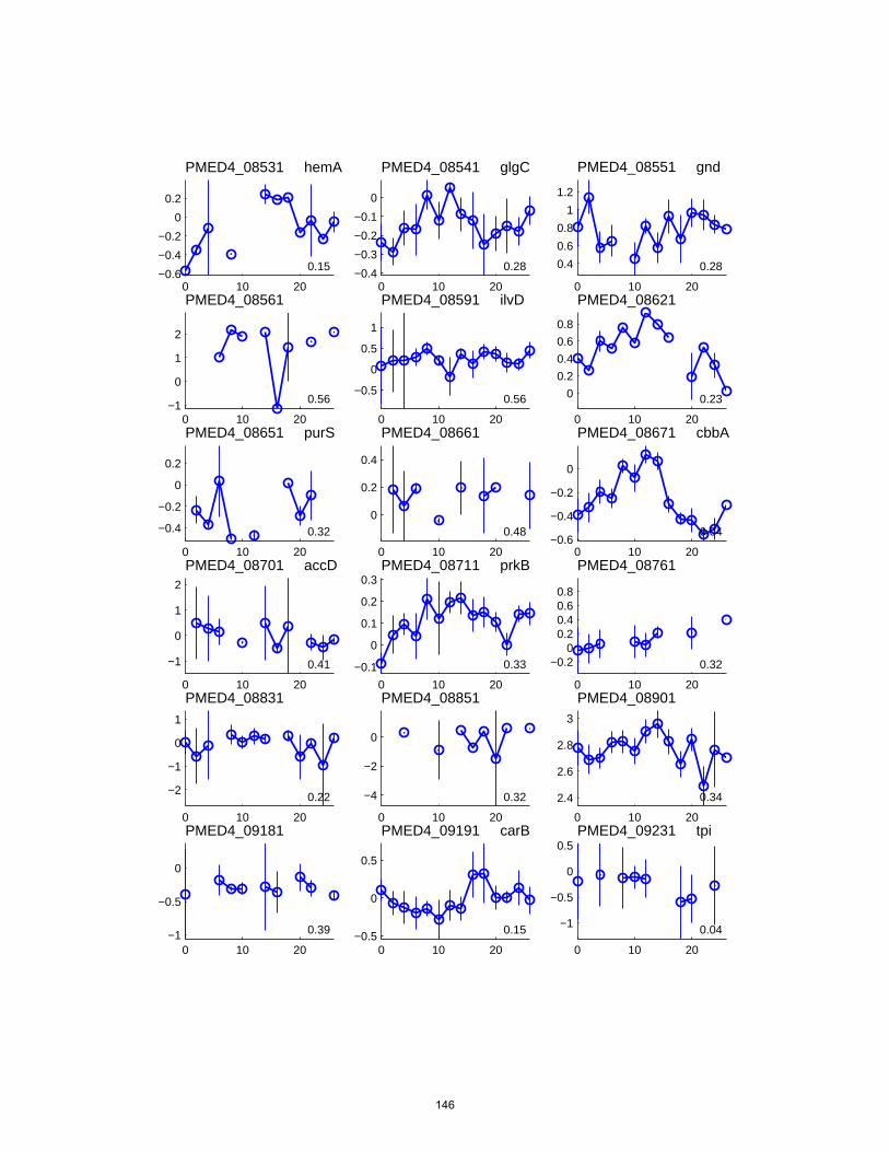
0 10 20−0.6
−0.4
−0.2
0
0.2
PMED4_08531 hemA
0.15
0 10 20−0.4
−0.3
−0.2
−0.1
0
PMED4_08541 glgC
0.28
0 10 20
0.4
0.6
0.8
1
1.2
PMED4_08551 gnd
0.28
0 10 20−1
0
1
2
PMED4_08561
0.56
0 10 20
−0.5
0
0.5
1
PMED4_08591 ilvD
0.56
0 10 20
0
0.2
0.4
0.6
0.8
PMED4_08621
0.23
0 10 20
−0.4
−0.2
0
0.2
PMED4_08651 purS
0.32
0 10 20
0
0.2
0.4
PMED4_08661
0.48
0 10 20−0.6
−0.4
−0.2
0
PMED4_08671 cbbA
0.04
0 10 20
−1
0
1
2
PMED4_08701 accD
0.41
0 10 20
−0.1
0
0.1
0.2
0.3PMED4_08711 prkB
0.33
0 10 20
−0.20
0.20.40.60.8
PMED4_08761
0.32
0 10 20
−2
−1
0
1
PMED4_08831
0.22
0 10 20
−4
−2
0
PMED4_08851
0.32
0 10 20
2.4
2.6
2.8
3
PMED4_08901
0.34
0 10 20−1
−0.5
0
PMED4_09181
0.39
0 10 20−0.5
0
0.5
PMED4_09191 carB
0.15
0 10 20
−1
−0.5
0
0.5PMED4_09231 tpi
0.04
146
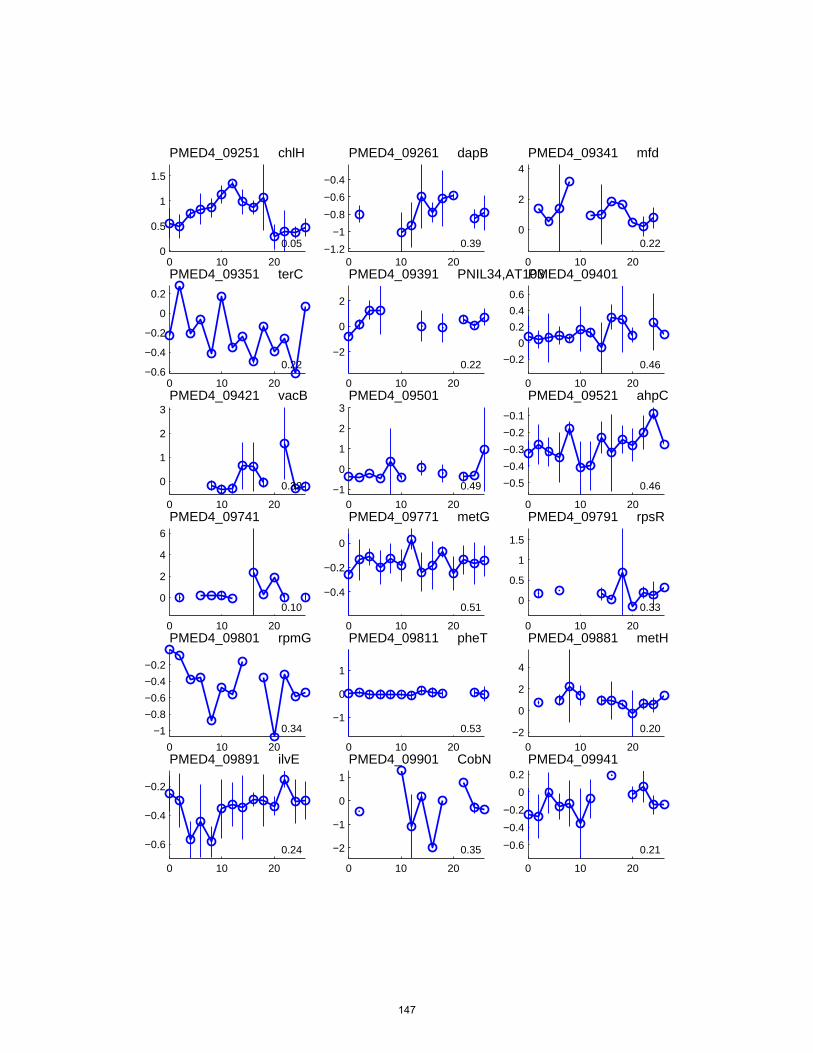
0 10 200
0.5
1
1.5
PMED4_09251 chlH
0.05
0 10 20−1.2
−1
−0.8
−0.6
−0.4
PMED4_09261 dapB
0.39
0 10 20
0
2
4PMED4_09341 mfd
0.22
0 10 20−0.6
−0.4
−0.2
0
0.2
PMED4_09351 terC
0.22
0 10 20
−2
0
2
PMED4_09391 PNIL34,AT103
0.22
0 10 20
−0.2
0
0.2
0.4
0.6
PMED4_09401
0.46
0 10 20
0
1
2
3PMED4_09421 vacB
0.32
0 10 20−1
0
1
2
3PMED4_09501
0.49
0 10 20
−0.5
−0.4
−0.3
−0.2
−0.1
PMED4_09521 ahpC
0.46
0 10 20
0
2
4
6
PMED4_09741
0.10
0 10 20
−0.4
−0.2
0
PMED4_09771 metG
0.51
0 10 20
0
0.5
1
1.5
PMED4_09791 rpsR
0.33
0 10 20
−1
−0.8
−0.6
−0.4
−0.2
PMED4_09801 rpmG
0.34
0 10 20
−1
0
1
PMED4_09811 pheT
0.53
0 10 20−2
0
2
4
PMED4_09881 metH
0.20
0 10 20
−0.6
−0.4
−0.2
PMED4_09891 ilvE
0.24
0 10 20
−2
−1
0
1
PMED4_09901 CobN
0.35
0 10 20
−0.6
−0.4
−0.2
0
0.2PMED4_09941
0.21
147
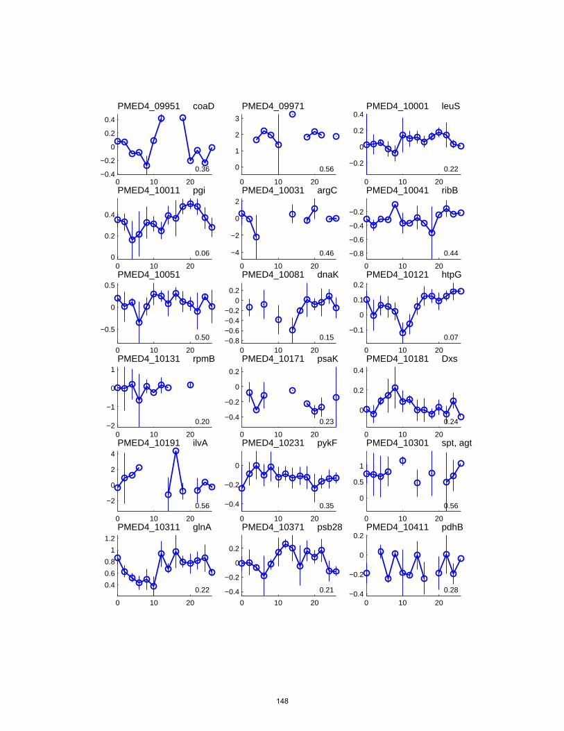
0 10 20−0.4
−0.2
0
0.2
0.4
PMED4_09951 coaD
0.36
0 10 20
0
1
2
3
PMED4_09971
0.56
0 10 20
−0.2
0
0.2
0.4PMED4_10001 leuS
0.22
0 10 200
0.2
0.4
PMED4_10011 pgi
0.06
0 10 20
−4
−2
0
2
PMED4_10031 argC
0.46
0 10 20
−0.8
−0.6
−0.4
−0.2
PMED4_10041 ribB
0.44
0 10 20
−0.5
0
0.5PMED4_10051
0.50
0 10 20−0.8−0.6−0.4−0.2
00.2
PMED4_10081 dnaK
0.15
0 10 20
−0.1
0
0.1
0.2PMED4_10121 htpG
0.07
0 10 20−2
−1
0
1PMED4_10131 rpmB
0.20
0 10 20
−0.4
−0.2
0
0.2
PMED4_10171 psaK
0.23
0 10 20
0
0.2
0.4
PMED4_10181 Dxs
0.24
0 10 20
−2
0
2
4PMED4_10191 ilvA
0.56
0 10 20
−0.4
−0.2
0
PMED4_10231 pykF
0.35
0 10 20
0
0.5
1
PMED4_10301 spt, agt
0.56
0 10 20
0.4
0.6
0.8
1
1.2
PMED4_10311 glnA
0.22
0 10 20
−0.4
−0.2
0
0.2
PMED4_10371 psb28
0.21
0 10 20−0.4
−0.2
0
0.2PMED4_10411 pdhB
0.28
148
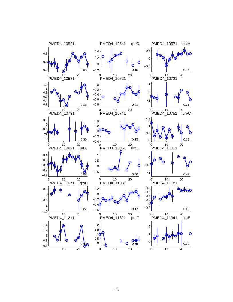
0 10 20
0.2
0.4
0.6
PMED4_10521
0.08
0 10 20
−0.2
0
0.2
0.4
PMED4_10541 rpsO
0.10
0 10 20
−0.5
0
0.5
PMED4_10571 gatA
0.16
0 10 20
0.20.40.60.8
11.2
PMED4_10581
0.15
0 10 20
−0.8
−0.6
−0.4
−0.2
0
PMED4_10621
0.21
0 10 20
−1
0
1
PMED4_10721
0.31
0 10 20
−1.5
−1
−0.5
0
0.5
PMED4_10731
0.36
0 10 20−0.4
−0.2
0
0.2
0.4
PMED4_10741
0.15
0 10 20
0
0.5
1
1.5
PMED4_10751 ureC
0.23
0 10 20−0.8
−0.7
−0.6
−0.5
−0.4
PMED4_10821 urtA
0.07
0 10 20
−0.5
0
0.5
1
PMED4_10861 urtE
0.56
0 10 20
−1
−0.5
0
PMED4_11011
0.44
0 10 20−1.5
−1
−0.5
0
0.5
PMED4_11071 rpsU
0.27
0 10 20−0.6
−0.4
−0.2
0
0.2
PMED4_11081
0.17
0 10 20
−0.20
0.20.40.60.8
PMED4_11181
0.06
0 10 200.6
0.8
1
1.2
1.4
PMED4_11211
0.49
0 10 20
0
0.5
1
1.5
2
PMED4_11321 purT
0.35
0 10 20
0
1
2
PMED4_11341 btuE
0.32
149
0 10 20
−0.6
−0.4
−0.2
0PMED4_11351
0.35
0 10 20
−0.6
−0.4
−0.2
0PMED4_11741
0.35
0 10 20
0
1
2
3
4
PMED4_11751 lraI
0.49
0 10 20
−0.2
0
0.2
PMED4_11761
0.30
0 10 200
0.5
1
PMED4_11871
0.33
0 10 20
−0.6
−0.4
−0.2
PMED4_12011 chlI
0.07
0 10 20
−0.4
−0.3
−0.2
−0.1
PMED4_12071 trxA
0.18
0 10 20
−0.5
0
0.5PMED4_12081 guaB
0.41
0 10 20
−0.4
−0.2
0
PMED4_12091 gyrA
0.43
0 10 20
−0.8
−0.6
−0.4
−0.2
0
PMED4_12121 leuA
0.14
0 10 20
−1
0
1
2
3
PMED4_12151 folD
0.15
0 10 20
−0.6−0.4−0.2
00.20.4
PMED4_12161 ispA
0.16
0 10 20
−0.5
0
0.5
PMED4_12191
0.15
0 10 20
−0.20
0.20.40.60.8
PMED4_12201 zwf
0.15
0 10 20
0.1
0.2
0.3
PMED4_12211 petH
0.15
0 10 20
−0.5
0
0.5
1
1.5
PMED4_12251
0.56
0 10 20
−0.5
0
0.5
PMED4_12261 prsA
0.15
0 10 20
−2
0
2
4
PMED4_12301 cad
0.20
150
0 10 20
0.2
0.3
0.4
PMED4_12341 clpC
0.05
0 10 20
0
0.5
1
1.5
2
PMED4_12361 lysA
0.17
0 10 20
0
1
2
3
PMED4_12431 recR
0.56
0 10 20
−2
−1
0
1PMED4_12441 psbP
0.10
0 10 20
0
2
4
6
PMED4_12471 srmB
0.06
0 10 20
0
1
2
PMED4_12521
0.20
0 10 20
−2
−1
0
1
2
PMED4_12531 pdxJ
0.43
0 10 20
−0.2
0
0.2
0.4
PMED4_12551
0.35
0 10 20
−0.4
−0.3
−0.2
−0.1PMED4_12571
0.43
0 10 20
−0.6
−0.4
−0.2
0
PMED4_12591
0.05
0 10 20
0
2
4
6
PMED4_12611 crtH
0.28
0 10 20
0
2
4
PMED4_12981 polA
0.07
0 10 20
01234
PMED4_13001 dxr
0.56
0 10 20
−1
0
1
PMED4_13031 pntB
0.16
0 10 20−1.2
−1
−0.8
−0.6
PMED4_13051 pntA
0.04
0 10 20
−0.5
0
0.5
PMED4_13111 ycf39
0.32
0 10 20
−0.6
−0.4
−0.2
0
PMED4_13141 ilvN
0.20
0 10 20−1
0
1
PMED4_13161
0.51
151
0 10 20
−0.8−0.6−0.4−0.2
00.2
PMED4_13171 psbD
0.06
0 10 20
−1
−0.5
0
0.5PMED4_13181 psbC
0.33
0 10 20
−5.6
−5.4
−5.2
−5
−4.8
PMED4_13281 afuA
0.17
0 10 20
−1
−0.5
0
0.5
PMED4_13291 glyQ
0.09
0 10 20−1.5
−1
−0.5
0
PMED4_13301
0.24
0 10 20
−0.5
0
0.5
1
PMED4_13311
0.55
0 10 20
−1.5
−1
−0.5
PMED4_13361 isiB
0.54
0 10 20
0.2
0.4
0.6
0.8
1
PMED4_13451 sppA
0.15
0 10 20
−0.5
0
0.5
PMED4_13471
0.43
0 10 20
0
2
4
PMED4_13501
0.21
0 10 20
−0.6
−0.4
−0.2
0
0.2PMED4_13511 yidC
0.15
0 10 20
0
2
4
PMED4_13521
0.33
0 10 20
−0.8−0.6−0.4−0.2
00.2
PMED4_13531 serS
0.28
0 10 20
−0.5
0
0.5PMED4_13551 rpsN
0.16
0 10 20
0
0.05
0.1
0.15
PMED4_13561 pnp
0.30
0 10 20
0
2
4
PMED4_13651
0.35
0 10 20
−1
−0.5
0
PMED4_13691 ddhA, rfbF
0.43
0 10 20
−0.5
0
0.5
PMED4_13701
0.57
152
0 10 20−4
−2
0
2
PMED4_13731 gmd
0.56
0 10 20
−2
0
2
PMED4_13751
0.41
0 10 20−0.5
0
0.5
1
PMED4_13771
0.15
0 10 20
0
2
4
6PMED4_13781
0.52
0 10 20−2
−1
0
1
PMED4_13821 gmhA
0.21
0 10 20−1
−0.5
0
0.5
PMED4_13831 rfaE
0.05
0 10 20−0.8−0.6−0.4−0.2
00.20.4
PMED4_13841
0.07
0 10 20
−2
−1
0
1
PMED4_13891 gumB
0.17
0 10 20
−0.4
−0.2
0
0.2
PMED4_13901
0.44
0 10 20
−0.2
0
0.2
0.4
PMED4_13941
0.44
0 10 20
0
0.2
0.4
0.6
PMED4_13951
0.20
0 10 20
−0.5
0
0.5
PMED4_13961
0.31
0 10 20
−0.6
−0.4
−0.2
PMED4_13971
0.46
0 10 20−0.4
−0.2
0
0.2
PMED4_13991 adhC
0.49
0 10 20−0.5
0
0.5
PMED4_14001
0.40
0 10 20
−0.6
−0.4
−0.2
0
0.2
PMED4_14011
0.33
0 10 20
−0.5
0
0.5
PMED4_14041 hetA
0.41
0 10 20
0
2
4
PMED4_14051
0.31
153
0 10 20
−0.6
−0.4
−0.2
0
PMED4_14111
0.50
0 10 20
−0.5
0
0.5
PMED4_14121
0.41
0 10 20
0
2
4
6
PMED4_14231
0.53
0 10 20
−0.4
−0.2
0
PMED4_14241
0.25
0 10 20
−0.5
0
0.5PMED4_14251
0.57
0 10 20−1.5
−1
−0.5
0
0.5
PMED4_14271 ugd
0.48
0 10 20
0
2
4PMED4_14291 argF
0.24
0 10 20
−0.4
−0.3
−0.2
−0.1
0
PMED4_14301
0.22
0 10 20
−1.5
−1
−0.5
0
0.5
PMED4_14321
0.25
0 10 20−0.5
0
0.5
PMED4_14351
0.56
0 10 20
0
0.5
1
1.5PMED4_14361 pheS
0.37
0 10 20
−1.2
−1
−0.8
−0.6
−0.4
PMED4_14451
0.46
0 10 20
−1
0
1PMED4_14491
0.46
0 10 200.4
0.6
0.8
PMED4_14501 phoH
0.20
0 10 20
0
0.2
0.4
0.6
0.8
PMED4_14511 rpsP
0.28
0 10 20−0.5
0
0.5
PMED4_14521 ffh
0.20
0 10 20
0
0.2
0.4
PMED4_14531
0.07
0 10 20−1
−0.5
0
PMED4_14541 acoA
0.33
154
0 10 20−0.2
0
0.2
0.4
0.6
PMED4_14591
0.50
0 10 20
1.1
1.2
1.3
1.4
1.5
PMED4_14601
0.17
0 10 20−0.6
−0.4
−0.2
0
0.2
PMED4_14631 trpC
0.41
0 10 20
−0.6
−0.4
−0.2
0
0.2
PMED4_14641 lpd
0.09
0 10 20
−0.2
0
0.2
PMED4_14761 ftsZ
0.04
0 10 20
−0.5
0
0.5
PMED4_14771 panB
0.17
0 10 20−0.5
0
0.5
PMED4_14791
0.47
0 10 20
−0.2
0
0.2
PMED4_14801
0.34
0 10 20−0.6
−0.4
−0.2
0
0.2
PMED4_14811
0.17
0 10 20
−0.4
−0.2
0
PMED4_14821 ilvC
0.34
0 10 20
0.1
0.2
0.3
0.4
0.5
PMED4_14891 himA
0.04
0 10 20
−0.3
−0.2
−0.1
0
0.1
PMED4_14931
0.41
0 10 20
−0.5
0
0.5
PMED4_14941
0.38
0 10 20
−0.2
0
0.2
0.4
0.6PMED4_14981
0.20
0 10 20
−0.5
0
0.5
PMED4_15001 pepB
0.44
0 10 20
−1
−0.5
0
0.5PMED4_15031 lpxA
0.28
0 10 20
0
2
4
PMED4_15041 fabZ
0.28
0 10 20
−0.3
−0.2
−0.1
0
PMED4_15061
0.13
155
0 10 20
0
1
2
3
PMED4_15091 nblS
0.33
0 10 20
−1.5
−1
−0.5
0
0.5PMED4_15101 kaiC
0.43
0 10 20−0.6
−0.4
−0.2
0
PMED4_15111 kaiB
0.48
0 10 20
0
1
2
3
PMED4_15121 rplU
0.30
0 10 20
−1
0
1
2
3PMED4_15131 rpmA
0.46
0 10 20
−0.2
−0.1
0
0.1
0.2
PMED4_15181
0.04
0 10 20
−1
−0.5
0
0.5PMED4_15221 serA
0.38
0 10 20
−1
0
1
2
PMED4_15581
0.09
0 10 20
−1.4
−1.2
−1
−0.8
PMED4_16171
0.24
0 10 20
−1
−0.5
0
0.5
1
PMED4_16211
0.45
0 10 20
0
1
2
3PMED4_16391 rpoZ
0.43
0 10 20
0
2
4
6PMED4_16411 pyrR
0.33
0 10 20
−1
0
1
2PMED4_16431 gpmI
0.22
0 10 20
−0.3
−0.2
−0.1
0
PMED4_16451 groEL
0.07
0 10 20
−0.4
−0.2
0
0.2
PMED4_16461 groES
0.09
0 10 200.3
0.4
0.5
0.6
PMED4_16471 atpD
0.05
0 10 20−1.5
−1
−0.5
0
0.5
PMED4_16481 atpC
0.13
0 10 20
0
0.2
0.4
PMED4_16491
0.40
156
0 10 20
0.2
0.4
0.6
0.8
PMED4_16591 atpC
0.33
0 10 200.3
0.4
0.5
0.6
PMED4_16601 atpA
0.08
0 10 200.2
0.4
0.6
0.8
1
PMED4_16611 atpH
0.16
0 10 20
−0.20
0.20.40.60.8
PMED4_16621 atpF
0.56
0 10 20
0.2
0.4
0.6
0.8
PMED4_16631 atpG
0.34
0 10 20−1
−0.5
0
0.5
PMED4_16641 atpE
0.07
0 10 20
−1
−0.8
−0.6
−0.4
PMED4_16721 glnB
0.09
0 10 20
0
1
2
PMED4_16741 purB
0.37
0 10 20
−1
0
1
PMED4_16761
0.54
0 10 20
0
1
2
PMED4_16811 BioA
0.15
0 10 20
−0.5
0
0.5
1PMED4_16891
0.07
0 10 200
0.1
0.2
PMED4_16931 rpoC2
0.26
0 10 20
−0.1
0
0.1
0.2PMED4_16941 rpoC1
0.50
0 10 20
0.05
0.1
0.15
0.2
0.25
PMED4_16951 rpoB
0.09
0 10 200
0.2
0.4
0.6PMED4_16971 rpsT
0.38
0 10 20
−2
0
2
PMED4_16981 hisD
0.39
0 10 20−0.5
0
0.5
1PMED4_16991 rpiA
0.24
0 10 20
−0.3
−0.2
−0.1
0
PMED4_17021 nusA
0.05
157
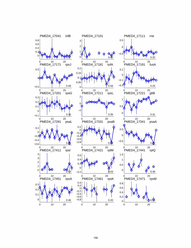
0 10 20
0
0.2
0.4
0.6
0.8
PMED4_17041 infB
0.57
0 10 20
0
1
2
3
PMED4_17101
0.40
0 10 20
−0.5
0
0.5
PMED4_17111 rne
0.32
0 10 20−0.5
0
0.5
PMED4_17171 rpsJ
0.49
0 10 200
0.05
0.1
0.15
0.2
PMED4_17181 tufA
0.56
0 10 20
−0.2
−0.1
0
0.1
PMED4_17191 fusA
0.25
0 10 20−0.1
0
0.1
0.2
0.3
PMED4_17201 rpsG
0.16
0 10 20
−2
0
2PMED4_17211 rpsL
0.35
0 10 20
0
0.5
1
PMED4_17221 gltB
0.31
0 10 20−0.6
−0.4
−0.2
0
0.2
PMED4_17291 psaL
0.07
0 10 20
−0.8−0.6−0.4−0.2
00.2
PMED4_17331 psaB
0.34
0 10 20
−0.5
0
0.5
PMED4_17341 psaA
0.37
0 10 20
0
1
2
3
4
PMED4_17411 rpsI
0.53
0 10 20
−0.2
0
0.2
0.4
0.6
PMED4_17421 rplM
0.53
0 10 20
0
0.5
1
1.5
PMED4_17441 rplQ
0.46
0 10 20
0
0.1
0.2
0.3
PMED4_17451 rpoA
0.36
0 10 20
−0.8−0.6−0.4−0.2
00.20.4
PMED4_17461 rpsK
0.20
0 10 200
0.2
0.4
0.6
0.8
PMED4_17471 rpsM
0.24
158
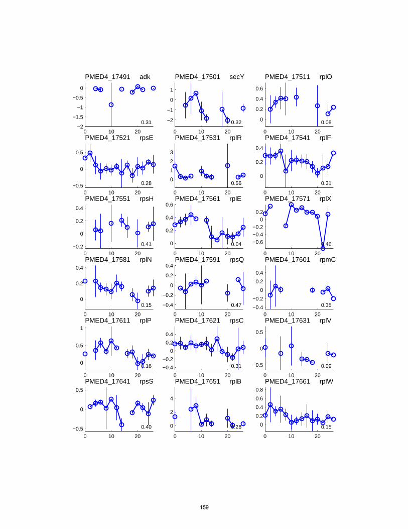
0 10 20−2
−1.5
−1
−0.5
0
PMED4_17491 adk
0.31
0 10 20
−2
−1
0
1
PMED4_17501 secY
0.32
0 10 20
0
0.2
0.4
0.6
PMED4_17511 rplO
0.08
0 10 20−0.5
0
0.5
PMED4_17521 rpsE
0.28
0 10 20
0
1
2
3
PMED4_17531 rplR
0.56
0 10 20
0
0.2
0.4
PMED4_17541 rplF
0.31
0 10 20−0.2
0
0.2
0.4
PMED4_17551 rpsH
0.41
0 10 20
0
0.2
0.4
0.6PMED4_17561 rplE
0.04
0 10 20
−0.6−0.4−0.2
00.2
PMED4_17571 rplX
0.46
0 10 20
0
0.2
0.4
PMED4_17581 rplN
0.15
0 10 20
−0.4
−0.2
0
0.2
0.4PMED4_17591 rpsQ
0.47
0 10 20−0.4
−0.2
0
0.2
0.4
PMED4_17601 rpmC
0.35
0 10 20
0
0.5
1PMED4_17611 rplP
0.16
0 10 20
−0.4
−0.2
0
0.2
0.4
PMED4_17621 rpsC
0.31
0 10 20
−0.5
0
0.5
PMED4_17631 rplV
0.09
0 10 20−0.5
0
0.5
PMED4_17641 rpsS
0.40
0 10 20
0
2
4
PMED4_17651 rplB
0.28
0 10 20
0
0.2
0.4
0.6
0.8
PMED4_17661 rplW
0.15
159
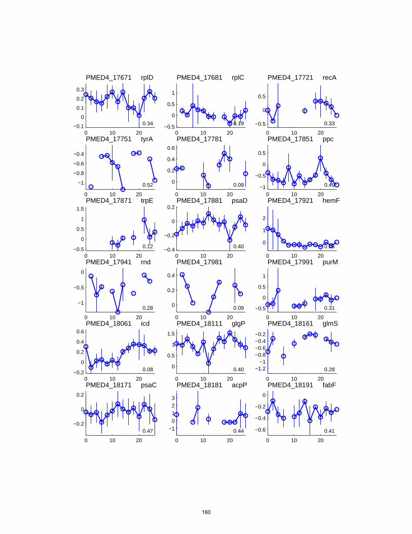
0 10 20−0.1
0
0.1
0.2
0.3
PMED4_17671 rplD
0.34
0 10 20−0.5
0
0.5
1
PMED4_17681 rplC
0.19
0 10 20
−0.5
0
0.5
PMED4_17721 recA
0.33
0 10 20
−1
−0.8
−0.6
−0.4
PMED4_17751 tyrA
0.52
0 10 20
0
0.2
0.4
0.6
PMED4_17781
0.09
0 10 20−1
−0.5
0
0.5
PMED4_17851 ppc
0.49
0 10 20−0.5
0
0.5
1
1.5
PMED4_17871 trpE
0.12
0 10 20−0.4
−0.2
0
0.2PMED4_17881 psaD
0.40
0 10 20
0
1
2
PMED4_17921 hemF
0.05
0 10 20
−1
−0.5
0
PMED4_17941 rnd
0.28
0 10 20
0
0.2
0.4
PMED4_17981
0.09
0 10 20
−0.5
0
0.5
1
PMED4_17991 purM
0.31
0 10 20−0.2
0
0.2
0.4
0.6PMED4_18061 icd
0.08
0 10 20
0
0.5
1
1.5
PMED4_18111 glgP
0.40
0 10 20
−1.2−1
−0.8−0.6−0.4−0.2
PMED4_18161 glmS
0.28
0 10 20
−0.2
0
0.2
PMED4_18171 psaC
0.47
0 10 20
−10123
PMED4_18181 acpP
0.44
0 10 20
−0.6
−0.4
−0.2
0
PMED4_18191 fabF
0.41
160

0 10 20
−0.1
0
0.1
0.2
PMED4_18201 tktA
0.43
0 10 20−1
−0.5
0
0.5
PMED4_18211 thiC
0.04
0 10 20
−0.5
0
0.5
1
PMED4_18281 lysS
0.22
0 10 20
0
0.2
0.4
PMED4_18291
0.14
0 10 20
−0.4
−0.2
0
PMED4_18321 mreB
0.04
0 10 20
−2
−1
0
1
PMED4_18331 ssb
0.24
0 10 20
0.6
0.8
1
PMED4_18351 sam1
0.16
0 10 20
−0.8
−0.6
−0.4
−0.2
0
PMED4_18401 mgtE
0.49
0 10 20
−0.3
−0.2
−0.1
0
0.1
PMED4_18441 gyrB
0.04
0 10 20
0
2
4
6PMED4_18461 infC
0.56
0 10 20
−1.5
−1
−0.5
0
0.5
PMED4_18471
0.46
0 10 20
−0.5
0
0.5
PMED4_18481 cysE
0.35
0 10 20
0.20.30.40.50.6
PMED4_18491 secA
0.24
0 10 20−0.2
0
0.2
0.4
0.6PMED4_18531 ribH
0.49
0 10 20
−1
−0.5
0
PMED4_18581 lysC
0.55
0 10 20−2
−1.8
−1.6
−1.4
−1.2
PMED4_18601
0.32
0 10 20
0
1
2
3
PMED4_18611 mesJ
0.34
0 10 20−0.5
0
0.5
PMED4_18621
0.34
161
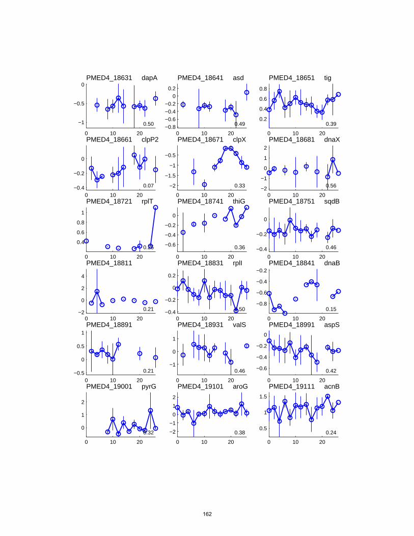
0 10 20
−1
−0.5
0PMED4_18631 dapA
0.50
0 10 20−0.8−0.6−0.4−0.2
00.2
PMED4_18641 asd
0.49
0 10 20
0.2
0.4
0.6
0.8
PMED4_18651 tig
0.39
0 10 20−0.4
−0.2
0
PMED4_18661 clpP2
0.07
0 10 20
−2
−1.5
−1
−0.5
PMED4_18671 clpX
0.33
0 10 20−2
−1
0
1
2
PMED4_18681 dnaX
0.56
0 10 20
0.4
0.6
0.8
1
PMED4_18721 rplT
0.25
0 10 20
−0.6
−0.4
−0.2
0
PMED4_18741 thiG
0.36
0 10 20−0.4
−0.2
0
PMED4_18751 sqdB
0.46
0 10 20−2
0
2
4
PMED4_18811
0.21
0 10 20−0.4
−0.2
0
0.2
PMED4_18831 rplI
0.50
0 10 20
−0.8
−0.6
−0.4
−0.2PMED4_18841 dnaB
0.15
0 10 20−0.5
0
0.5
1PMED4_18891
0.21
0 10 20
−1
0
1
PMED4_18931 valS
0.46
0 10 20
−0.6
−0.4
−0.2
0
PMED4_18991 aspS
0.42
0 10 20
0
1
2
PMED4_19001 pyrG
0.32
0 10 20
−2
−1
0
1
2
PMED4_19101 aroG
0.38
0 10 20
0.5
1
1.5
PMED4_19111 acnB
0.24
162
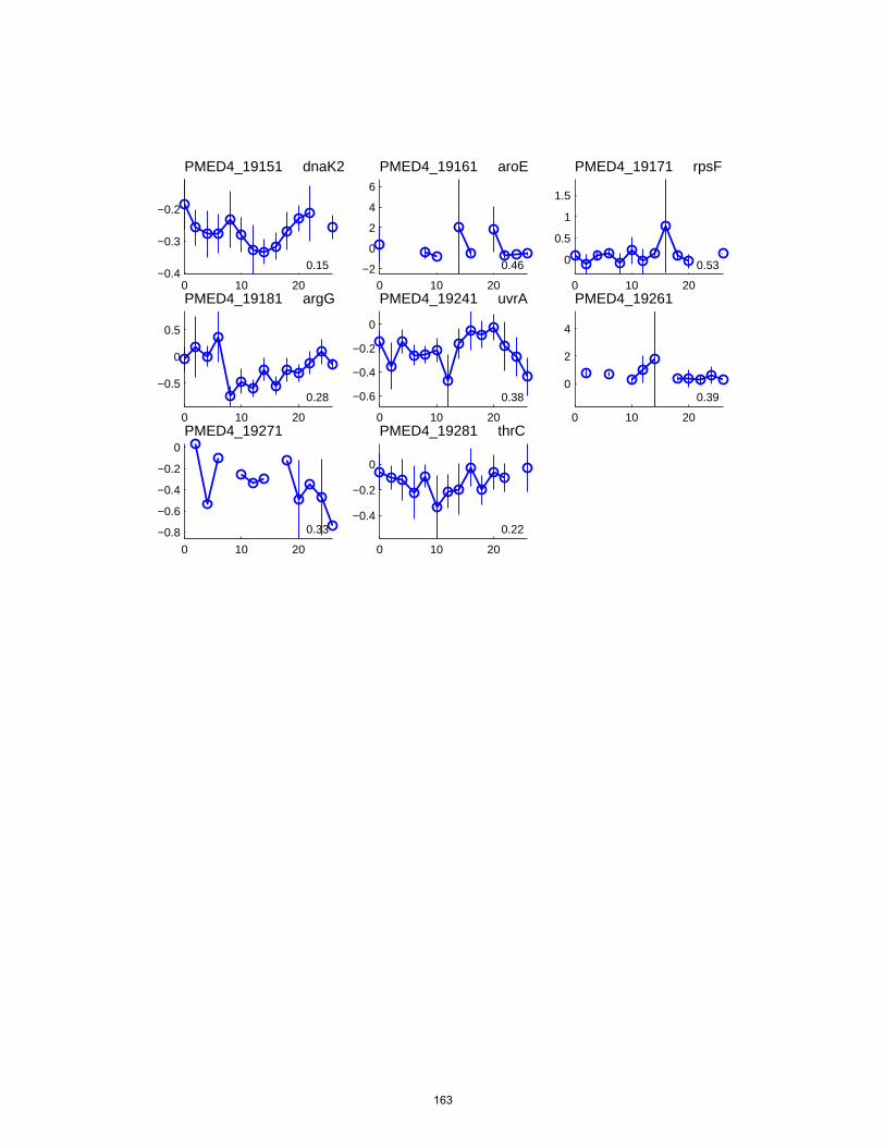
0 10 20−0.4
−0.3
−0.2
PMED4_19151 dnaK2
0.15
0 10 20−2
0
2
4
6
PMED4_19161 aroE
0.46
0 10 20
0
0.5
1
1.5
PMED4_19171 rpsF
0.53
0 10 20
−0.5
0
0.5
PMED4_19181 argG
0.28
0 10 20
−0.6
−0.4
−0.2
0
PMED4_19241 uvrA
0.38
0 10 20
0
2
4
PMED4_19261
0.39
0 10 20
−0.8
−0.6
−0.4
−0.2
0PMED4_19271
0.33
0 10 20
−0.4
−0.2
0
PMED4_19281 thrC
0.22
163
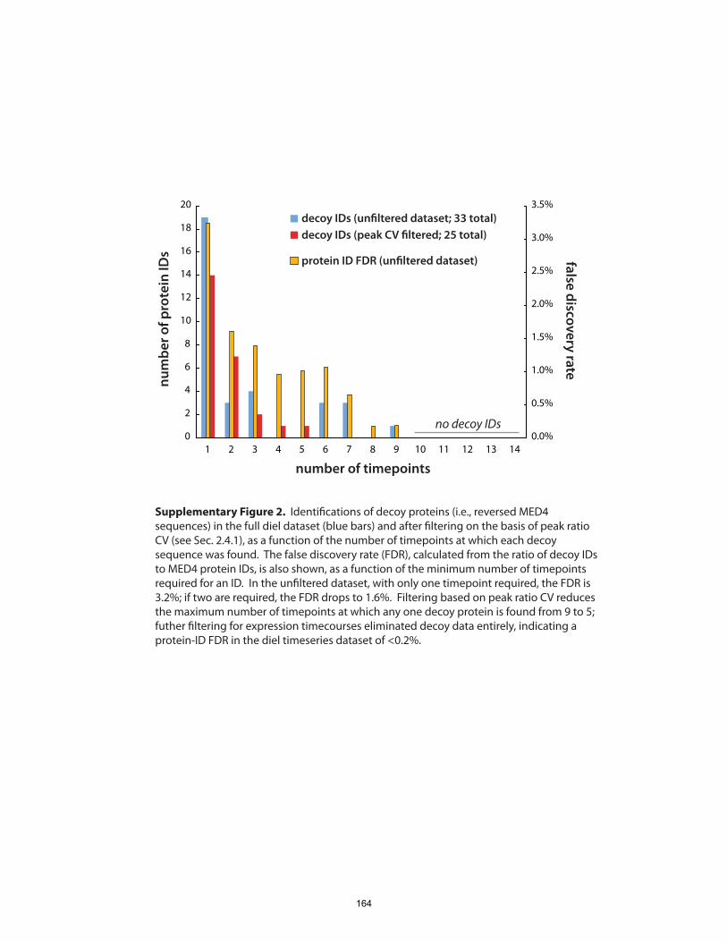
Supplementary Figure 2. Identi�cations of decoy proteins (i.e., reversed MED4 sequences) in the full diel dataset (blue bars) and after �ltering on the basis of peak ratio CV (see Sec. 2.4.1), as a function of the number of timepoints at which each decoy sequence was found. The false discovery rate (FDR), calculated from the ratio of decoy IDs to MED4 protein IDs, is also shown, as a function of the minimum number of timepoints required for an ID. In the un�ltered dataset, with only one timepoint required, the FDR is 3.2%; if two are required, the FDR drops to 1.6%. Filtering based on peak ratio CV reduces the maximum number of timepoints at which any one decoy protein is found from 9 to 5; futher �ltering for expression timecourses eliminated decoy data entirely, indicating a protein-ID FDR in the diel timeseries dataset of <0.2%.
0
2
4
6
8
10
12
14
16
18
20
1 2 3 4 5 6 7 8 9 10 11 12 13 140.0%
0.5%
1.0%
1.5%
2.0%
2.5%
3.0%
3.5%
number of timepoints
num
ber o
f pro
tein
IDs false discovery rate
decoy IDs (un�ltered dataset; 33 total)decoy IDs (peak CV �ltered; 25 total)
protein ID FDR (un�ltered dataset)
no decoy IDs
164
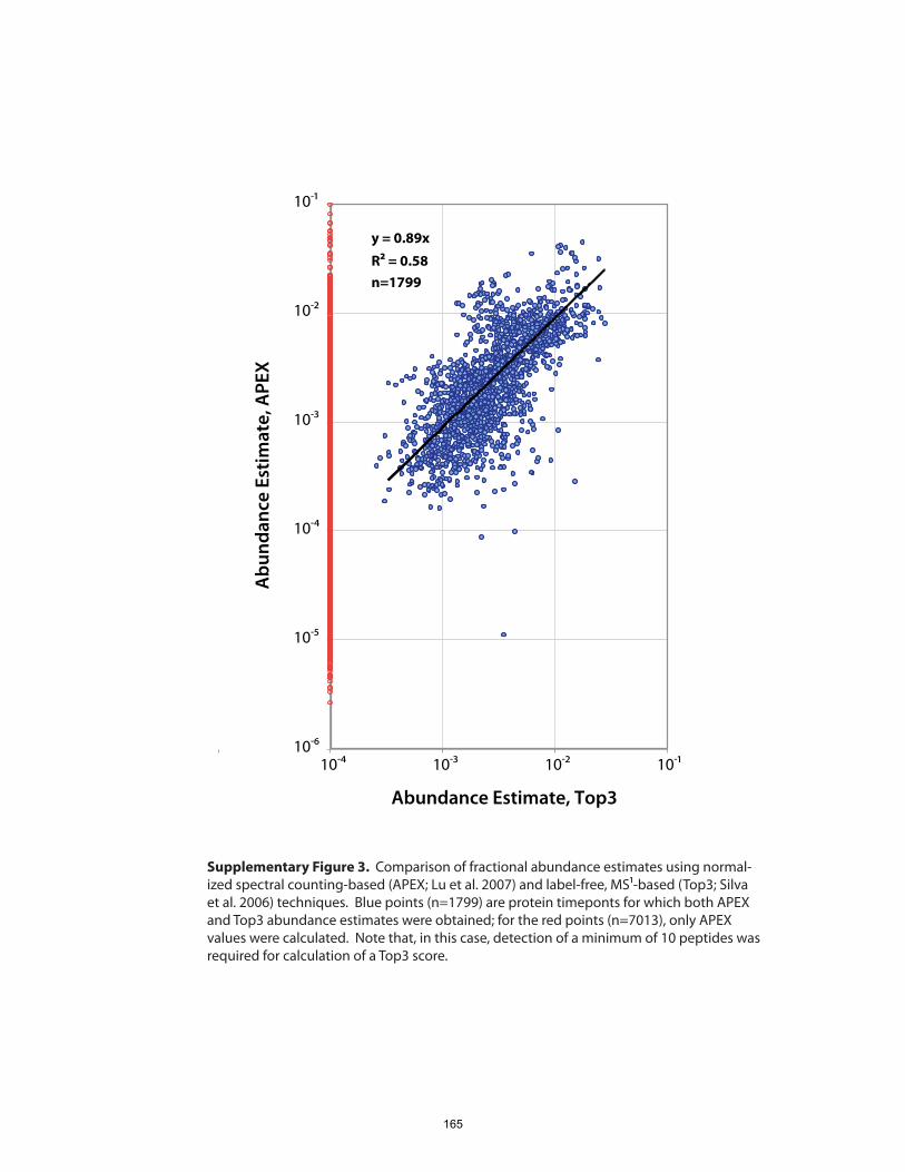
y = 0.89x
R2 = 0.58n=1799
10-6
10-5
10-4
10-3
10-2
10-1
10-4 10-3 10-2 10-1
Abundance Estimate, Top3
Abu
ndan
ce E
stim
ate,
APE
X
Supplementary Figure 3. Comparison of fractional abundance estimates using normal-ized spectral counting-based (APEX; Lu et al. 2007) and label-free, MS1-based (Top3; Silva et al. 2006) techniques. Blue points (n=1799) are protein timeponts for which both APEX and Top3 abundance estimates were obtained; for the red points (n=7013), only APEX values were calculated. Note that, in this case, detection of a minimum of 10 peptides was required for calculation of a Top3 score.
165

166
CHAPTER FIVE
Biogeochemical insights from Prochlorococcus systems biology
Jacob R. Waldbauer and Sallie W. Chisholm
167

168
Biogeochemical insights from Prochlorococcus systems biology
Jacob R. Waldbauer and Sallie W. Chisholm
In order to see cells as biogeochemical agents and incorporate cellular metabolism into a systems-level view of natural environments, an understanding of organisms’ molecular composition is fundamental. Specifying molecular composition – albeit largely in a laboratory context – has emerged as a basic goal of systems biology en route to an integrated view of cellular function. The tools developed for systems biology with mainly biomedical or biotechnological goals in mind have been increasingly turned to address questions in biogeochemistry and environmental science. Chapter 4 presented an example of using such tools, including microarrays, proteomics and RNA-sequencing, to assess the inventories and dynamics of gene products in Prochlorococcus. In this chapter, we take a holistic view of the molecular composition of Prochlorococcus cells, first modeling how elemental budgets are apportioned among major pools of biochemicals, and then addressing how cellular molecular composition informs hypotheses concerning genome evolution and stochastic gene expression effects. We propose that genome streamlining in Prochlorococcus is unlikely to be driven primarily by adaptation to oligotrophic conditions, and that noise in gene expression may play an ecological role in limiting the growth rates of very small cells. 1. ELEMENTAL AND BIOCHEMICAL BUDGETS FOR PROCHLOROCOCCUS CELLS
We consider first the major elemental (carbon, nitrogen, phosphorus) budgets of a
‘hypothetical’ high-light Prochlorococcus cell. Our goal is to provide a first-order
accounting of biochemical components, on the basis of available experimental and
genomic data. We focus on the B/G1 period of the cell cycle, when the cell has a single
copy of its chromosome (Wang and Levin, 2009); for Prochlorococcus, this period
extends from approximately midnight to mid-afternoon each day. Populations will
naturally show variation around the values presented, and that variation is itself likely to
be interesting and ecologically relevant. The calculations and assumptions involved in
deriving these values are described in the following section.
169
1.1 Budgeting calculations
1.1.1 Elemental stoichiometry
Several studies have presented measurements of the elemental composition of
Prochlorococcus cells (Bertilsson et al., 2003; Heldal et al., 2003; Fu et al., 2007) and
provide a basis for major-element budgets. These papers report a range of elemental
contents and C:N:P stoichiometries for Prochlorococcus cells. Here we treat the C:N
ratio as an independent variable, and allow it to range over the span reported in the
literature (5.7-9.9). We further take the cellular P content to be 13 amol, which, as
discussed further below, represents the majority of results reported in all three studies. At
a given C:N ratio, then, the C:P ratio is chosen so that the cellular carbon budget (detailed
below) closes (i.e., such that the cellular C content equals the sum of the constituent
biochemicals). The resultant modeled elemental contents and C:N:P ratios are shown in
Figures 1 and 2, plotted along with the literature values. The elemental budgets for three
cases (I, II and III; indicated in Figs. 1 and 2) that span the range of modeled
stoichiometries are included in Table 1; the assumptions and calculations behind these
budgets are detailed in Sections 1.1.2-1.1.4, and the results are discussed in Section 1.2.
The method for constructing cellular elemental budgets used here was designed to
produce self-consistent, closed budgets, so that the distribution of C, N and P among
biochemical pools can be meaningfully interpreted. As shown in Figures 1 and 2, no
single set of elemental contents or ratios can encompass all of the literature data, which in
any case represent differing strains, media, culture conditions and growth rates. It is also
not generally possible to close budgets based on a fixed stoichiometry without including
‘mystery pool’ of biochemicals of arbitrary composition and size, chosen solely to
account for material stipulated by the stoichiometry. Including such a chemically ill-
defined component of the cells renders the proportional demands of major constituents
such as protein and RNA much less interpretable. The modeled cellular C and N contents
do match the experimental values quite well (Figure 1A). The choice was made to fix the
170

0
1
2
3
4
5
6
0.0 0.1 0.2 0.3 0.4 0.5 0.6 0.7 0.8
N content (fmol/cell)
C co
nten
t (fm
ol/c
ell)
ModelHeldal et al. 2003Bertilsson et al. 2003Fu et al. 2007
0
1
2
3
4
5
6
0 0.005 0.01 0.015 0.02 0.025 0.03 0.035 0.04P content (fmol/cell)
C co
nten
t (fm
ol/c
ell)
0.0
0.1
0.2
0.3
0.4
0.5
0.6
0.7
0.8
0 0.005 0.01 0.015 0.02 0.025 0.03 0.035 0.04
P content (fmol/cell)
N c
onte
nt (f
mol
/cel
l)
A
B
C
-P
-P
-P
Figure 1. Cellular contents of carbon, nitrogen and phosphorus, from literature reports and as modeled here. The phosphorus-limited measurement by Bertilsson et al. (2003) (the only data from nutrient-limited culture) is indicated by the -P. The content values for the three model cases summarized in Table 1 (I, II, III) are indicated by circled symbols.
IIIII
I
III
II
I
III
II
I
171
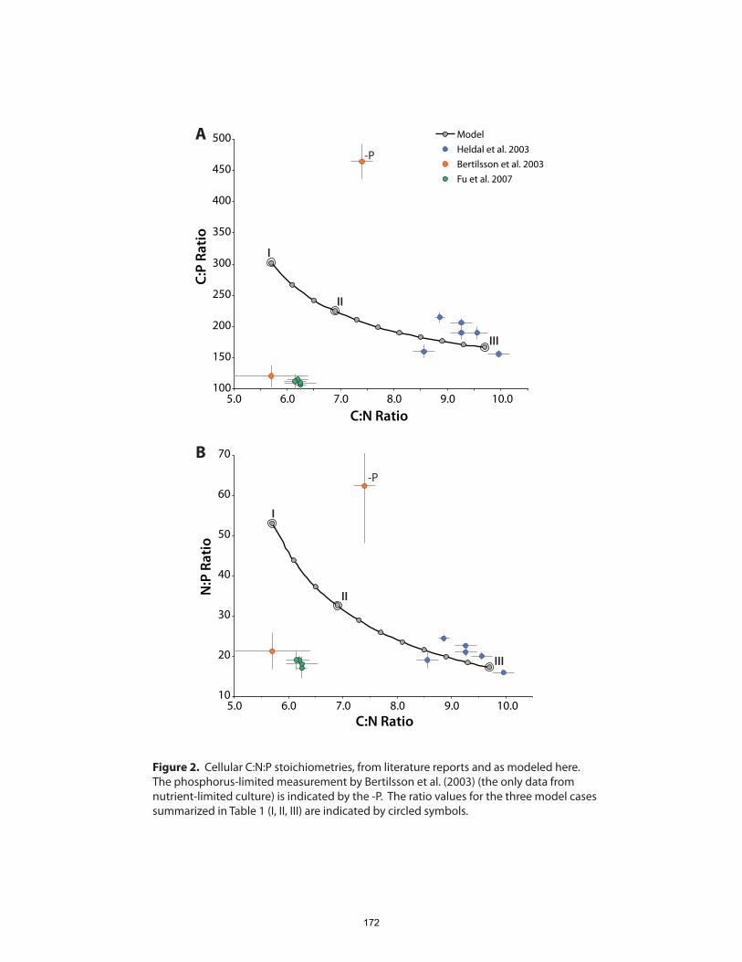
C:P
Rati
o
ModelHeldal et al. 2003Bertilsson et al. 2003Fu et al. 2007
N:P
Rat
io
C:N Ratio
10
20
30
40
50
60
70
5.0 6.0 7.0 8.0 9.0 10.0
-P
C:N Ratio
100
150
200
250
300
350
400
450
500
5.0 6.0 7.0 8.0 9.0 10.0
-P
B
A
Figure 2. Cellular C:N:P stoichiometries, from literature reports and as modeled here. The phosphorus-limited measurement by Bertilsson et al. (2003) (the only data from nutrient-limited culture) is indicated by the -P. The ratio values for the three model cases summarized in Table 1 (I, II, III) are indicated by circled symbols.
I
II
III
I
II
III
172
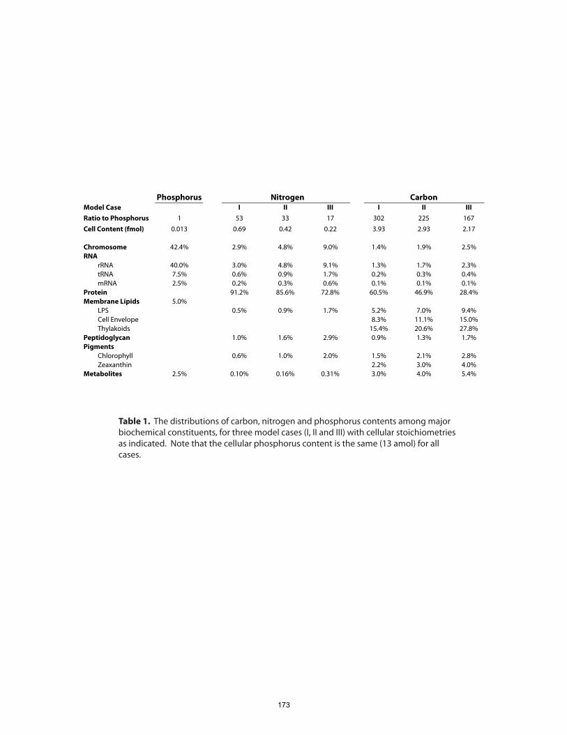
Phosphorus Nitrogen CarbonI II III I II III
Ratio to Phosphorus 1 53 33 17 302 225 167Cell Content (fmol) 0.013 0.69 0.42 0.22 3.93 2.93 2.17
Chromosome 42.4% 2.9% 4.8% 9.0% 1.4% 1.9% 2.5%RNA
rRNA 40.0% 3.0% 4.8% 9.1% 1.3% 1.7% 2.3%tRNA 7.5% 0.6% 0.9% 1.7% 0.2% 0.3% 0.4%mRNA 2.5% 0.2% 0.3% 0.6% 0.1% 0.1% 0.1%
Protein 91.2% 85.6% 72.8% 60.5% 46.9% 28.4%Membrane Lipids 5.0%
LPS 0.5% 0.9% 1.7% 5.2% 7.0% 9.4%Cell Envelope 8.3% 11.1% 15.0%Thylakoids 15.4% 20.6% 27.8%
Peptidoglycan 1.0% 1.6% 2.9% 0.9% 1.3% 1.7%Pigments
Chlorophyll 0.6% 1.0% 2.0% 1.5% 2.1% 2.8%Zeaxanthin 2.2% 3.0% 4.0%
Metabolites 2.5% 0.10% 0.16% 0.31% 3.0% 4.0% 5.4%
Table 1. The distributions of carbon, nitrogen and phosphorus contents among major biochemical constituents, for three model cases (I, II and III) with cellular stoichiometries as indicated. Note that the cellular phosphorus content is the same (13 amol) for all cases.
Model Case
173
cellular P content at 13 amol because values in that range appear in all three studies and it
appears to approximate a lower limit of P content in Prochlorococcus (Figure 1B and C).
We are less interested here in precisely modeling exponential growth under optimum,
nutrient-replete conditions than in assessing how a cell can be built with the small
nutrient complements likely to prevail in oligotrophic habitats. In our judgment, the sole
measurement of Prochlorococcus cellular elemental stoichiometry under nutrient-limited
conditions (that of Bertilsson et al., 2003, indicated in Figures 1 and 2), is quite relevant
to real oceanic conditions and should be given due consideration. The C:N:P
stoichiometries that result from this model approach those found by Heldal et al. (2003)
at higher C:N ratios, and C:P and N:P ratios rise as C:N drops (Figure 2).
These broad uncertainties in cellular elemental composition mean that the biochemical
budgets outlined here should be considered flexible. Certainly, a more precisely
constrained composition would be required for detailed systems modeling, such as flux
balance analysis. Nevertheless, the kinds of budgeting calculations described here can
readily accommodate a range of stoichiometries, and hopefully future data (especially
from field samples) will better constrain the C:N:P ranges most relevant to oceanic
conditions.
1.1.2 Phosphorus budget
Phosphorus is present in Prochlorococcus as a component of several types of
biochemicals: nucleic acid polymers (DNA and RNA), phospholipids, and small
molecule metabolites. The amount in the chromosome can be calculated exactly from the
genome size (1.66Mbp). Phospholipids are rather rare in Prochlorococcus compared to
most other microbes likely as an adaptation to chronic P scarcity (Van Mooy et al., 2006).
We calculate the total number of lipid molecules in the cell by assuming a typical
geometry for Prochlorococcus: the cell envelope (outer membrane, murein layer and
inner membrane) is set at 0.6µm in diameter. Within the cell are two complete, spherical
thylakoid membranes averaging 0.5µm in diameter (compare Fig. 1A-D of Ting et al.,
174
2007) – for geometric simplicity, we neglect the small ‘hairpin’ region where each
membrane wraps around itself to enclose the lumen. Thus the inner and outer cell
membranes comprise 4 leaflets (2 bilayers), while the thylakoids comprise 8 leaflets (4
bilayers), and we assume a membrane area of 0.55nm2 per lipid molecule (Lopez
Cascales et al., 1996) and that lipids constitute 80% of total membrane area (Nikaido,
1996). Hence our hypothetical cell contains about 14 million lipid molecules, 2% of
which are assumed to be phosphatidylglycerol (Van Mooy et al., 2006). Little data exists
on metabolites or their concentrations in Prochlorococcus; here we assume a cytosolic
concentration of 1mM for nucleotide triphosphates (e.g., ATP, GTP), probably the most
abundant P-containing metabolites (Bennett et al., 2009). Finally, all of the 13 amol P
complement not accounted for by DNA, lipids and metabolites is assumed to be RNA,
thereby closing the cellular phosphorus budget. Total RNA is assumed to be 80% rRNA,
15% tRNA and 5% mRNA (Bremer and Dennis, 2008).
1.1.3 Nitrogen budget
Nitrogen in DNA is again calculated exactly from the genome size and base composition
(30.8% G+C). Nitrogen in RNA is calculated from the RNA P content, with an RNA
N:P ratio of 3.8:1 derived from MED4 RNA sequences. To calculate the N in
metabolites, we assume that the metabolite pool is dominated by compatible solutes at a
concentration of 0.1M (Bennett et al., 2009). The compatible solute pool is taken to be
comprised of sucrose / glucosylglycerate / glutamate in a 10:5:1 stoichiometric ratio
(Klähn et al., 2009); hence metabolite N reflects cytosolic glutamate. Nitrogen in
chlorophyll is based on a chlorophyll content of 1 fg/cell, an average of literature values
that range from 0.3-5 fg/cell (Morel et al., 1993; Moore and Chisholm, 1999; Claustre et
al., 2002). The amount in peptidoglycan is again calculated from the cell geometry,
assuming a cell-wall area of 2 nm2 per disaccharide unit (Vollmer and Holtje, 2004), and
an N content of 7 atoms/unit. Nitrogen in lipopolysaccharide (LPS) is also calculated
from membrane area, assuming a membrane area of 0.202 nm2 per fatty acid chain in
LPS. LPS structure was assumed to be the same as that reported by Snyder et al. (2009)
175
for strains of marine Synechococcus, with two nitrogen atoms and four fatty acid chains
per unit, resulting in roughly 1.1 million LPS units per cell. Finally, all remaining
nitrogen is assumed to be in protein, thereby closing the N budget. The number of amino
acids in the cell can be calculated from the average nitrogen content of 1.310 N per
residue, derived from the composition of the MED4 proteome as measured over the diel
cycle (see Sec. 2).
1.1.4 Carbon budget
Carbon in DNA is calculated from genome size and base composition. Carbon in RNA is
calculated from P content, with an RNA C:P ratio of 9.5:1. Metabolite C is calculated
based on the same assumptions about compatible osmolytes made in the nitrogen budget.
Chlorophyll C is again based on 1 fg Chl/cell, and zeaxanthin C is based on a Zea:Chl
ratio of 1.25 (wt/wt; Claustre et al., 2002). Protein C is calculated from the cellular
amino acid content, with an average residue composition of 5.075 C per amino acid,
based on protein sequences. Lipid carbon is based on the measurements of Van Mooy et
al. (2006), which suggest an average C content of 39.7 atoms per lipid molecule. Based
on the cell geometry calculations described above, there are approximately 20 million
lipid molecules in our hypothetical Prochlorococcus cell. This is, however, probably the
most uncertain component of the cellular carbon budget, as membrane geometry and lipid
composition are likely to vary strongly with growth rate, light intensity and temperature.
1.2 Budgeting results
Three scenarios of C:N:P stoichiometry span the modeled range: cases I (302:53:1), II
(225:33:1), and III (167:17:1). Case III is likely most analogous to exponential growth in
culture under nutrient-replete conditions. Case I reflects extreme phosphorus limitation,
akin to the results of Bertilsson et al. (2003), and possibly applicable to exceptionally P-
poor oceanic regions such as the Sargasso Sea (Ammerman et al., 2003) or eastern
Mediterranean (Thingstad et al., 2005), though whether the high cell contents of C and N
176

suggested by the model would actually obtain in such situations is uncertain. Case II is
probably the most relevant for the majority of conditions encountered by
Prochlorococcus in oligotrophic marine habitats. The range presented here should not be
construed to necessarily encompass the whole range of possible compositions of
Prochlorococcus cells in the world’s oceans. In particular, should a cell operate with a
phosphorus quota substantially larger or smaller than 13 amol, a number of budgetary
aspects could be qualitatively different. However, as discussed in the next section, the P
quota can hardly be much smaller, and given that most of the elemental stoichiometry
data is from P-replete cultures, it seems unlikely to be very much larger. Just how ‘hard-
wired’ the phosphorus quota is into a given strain of Prochlorococcus remains an
intriguing and important question.
1.2.1 Phosphorus economy
The P budget of our hypothetical Prochlorococcus cell illustrates the “phosphorus
economy” (Coleman and Chisholm, 2007) of small cells adapted to nutrient-poor
environments. Note that the phosphorus budget is the same for cases I, II and III, since
the cellular P content is fixed in this model. More than 40% of the cellular P quota is
devoted to the ‘fixed cost’ of the chromosome. This makes the fact that most
Prochlorococcus cells contain a substantial number of rare flexible genes (i.e., genes
present in some but not all Prochlorococcus strains; Kettler et al., 2007) in their genomes
– likely recently acquired and only occasionally with adaptive value – all the more telling
of the importance of continuous gene exchange to microbial ecology and evolution
(Coleman and Chisholm, submitted). We discuss the relationship between genome size,
composition and nutrient budgets in detail in Section 2, below.
The amount of P in rRNA (5.2 amol) is sufficient to build 598 ribosomes. This is quite a
small number; by comparison, log-phase E. coli cells have between 8,000 and 73,000
ribosomes, depending on growth rate (Bremer and Dennis, 2008). Similarly, the number
of Prochlorococcus tRNA molecules predicted from the budget (7,866), is 10- to 100-
177
fold lower than E. coli (74,000-680,000; Bremer and Dennis, 2008). The predicted
amount of mRNA is also quite small: just 200kb (compared to 1.0-4.3Mb in E. coli;
Bremer and Dennis, 2008), which allows only about 12% of the genome to be transcribed
at any given time. Together, the DNA to encode genes and the RNA to express them
account for over 90% of the cellular phosphorus budget. To a first approximation,
Prochlorococcus uses any acquired P for nucleic acids – about half for DNA, half for
RNA.
The other two phosphorus-containing classes of biochemicals, phospholipids and
metabolites, are relatively minor in the cellular P budget. The low phospholipid content
of picocyanobacteria, especially Prochlorococcus (~2 mol%), has recently been explored
in detail by Van Mooy et al. (2006; 2009). Interestingly, Prochlorococcus does not seem
to upregulate phospholipid biosynthesis even when grown in P-replete conditions (Van
Mooy et al., 2006). This is in stark contrast to other bacteria: marine heterotrophs contain
>80% phospholipids (Van Mooy et al., 2006), while E. coli uses phospholipids almost
exclusively (Cronan and Rock, 2008). The amount of phosphorus in metabolites, on the
other hand, is more uncertain. Little metabolome-wide quantitative data exists for
bacteria, and none in Prochlorococcus; the estimates here are based on the recent
comprehensive study by Bennett et al. (2009) in E. coli. It has recently been shown that
sucrose is the major compatible solute in Prochlorococcus cells, with glucosylglycerate
taking the place of glutamate as the second-most abundant metabolite under N-limiting
conditions (Klähn et al., 2009). While glucosylglycerate contains neither P nor N, it is
synthesized from relatively P-rich precursors (ADP-glucose and 3-phosphoglycerate),
suggesting that the glycosylglycerate / glutamate exchange may also be a P/N
substitution.
1.2.2 Nitrogen
The great majority of cellular nitrogen – 80 to 90% – is in protein (Figure 3A), in accord
with findings for other phytoplankton and bacteria generally (Falkowski and Raven,
178
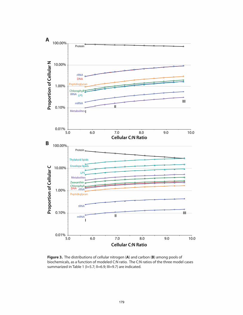
Prop
ortio
n of
Cel
lula
r N
0.01%
0.10%
1.00%
10.00%
100.00%
5.0 6.0 7.0 8.0 9.0 10.0Cellular C:N Ratio
Protein
DNArRNA
tRNA
mRNA
Metabolites
Chlorophyll
Peptidoglycan
LPS
Prop
ortio
n of
Cel
lula
r C
0.01%
0.10%
1.00%
10.00%
100.00%
5.0 6.0 7.0 8.0 9.0 10.0
Cellular C:N Ratio
Protein
rRNA
tRNA
mRNA
Metabolites
Chlorophyll
Peptidoglycan
Zeaxanthin
Envelope lipids
Thylakoid lipids
LPS
DNA
A
B
Figure 3. The distributions of cellular nitrogen (A) and carbon (B) among pools of biochemicals, as a function of modeled C:N ratio. The C:N ratios of the three model cases summarized in Table 1 (I=5.7; II=6.9; III=9.7) are indicated.
III
III
III
III
179
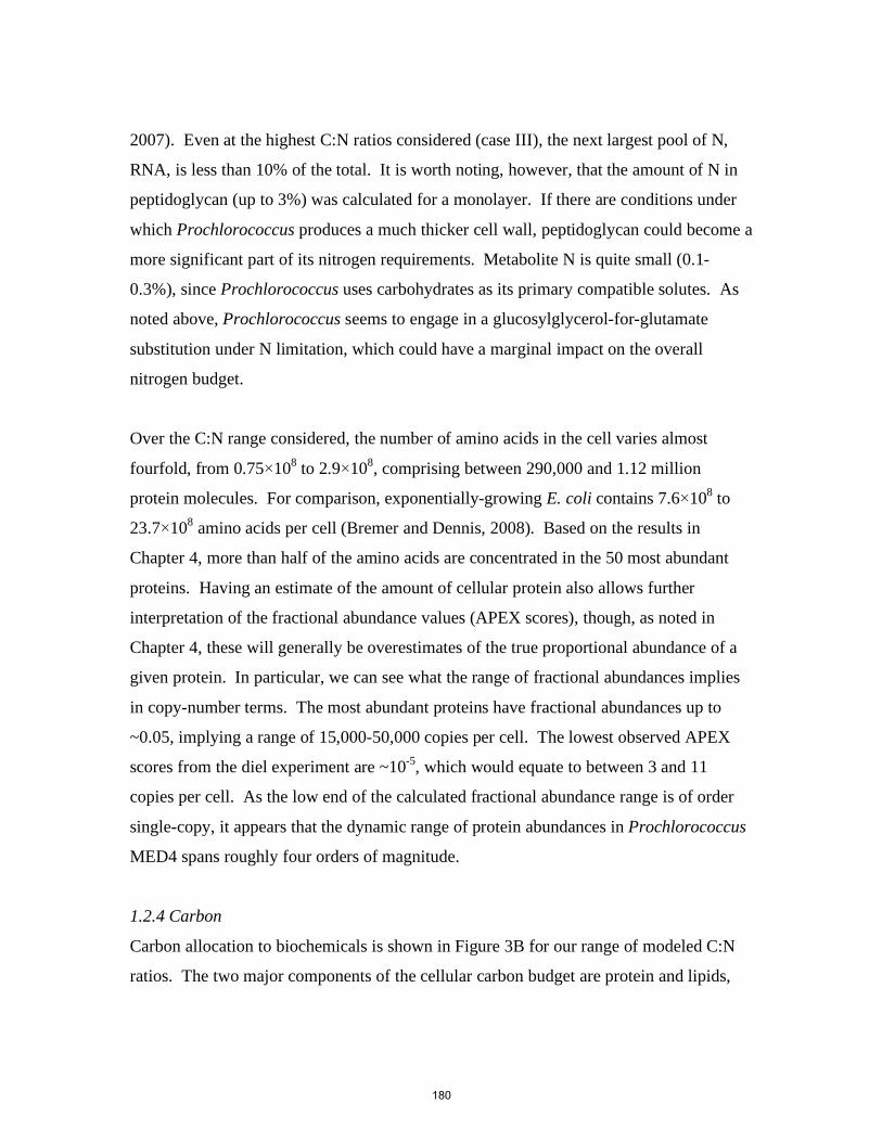
2007). Even at the highest C:N ratios considered (case III), the next largest pool of N,
RNA, is less than 10% of the total. It is worth noting, however, that the amount of N in
peptidoglycan (up to 3%) was calculated for a monolayer. If there are conditions under
which Prochlorococcus produces a much thicker cell wall, peptidoglycan could become a
more significant part of its nitrogen requirements. Metabolite N is quite small (0.1-
0.3%), since Prochlorococcus uses carbohydrates as its primary compatible solutes. As
noted above, Prochlorococcus seems to engage in a glucosylglycerol-for-glutamate
substitution under N limitation, which could have a marginal impact on the overall
nitrogen budget.
Over the C:N range considered, the number of amino acids in the cell varies almost
fourfold, from 0.75×10⁸ to 2.9×10⁸, comprising between 290,000 and 1.12 million
protein molecules. For comparison, exponentially-growing E. coli contains 7.6×10⁸ to
23.7×10⁸ amino acids per cell (Bremer and Dennis, 2008). Based on the results in
Chapter 4, more than half of the amino acids are concentrated in the 50 most abundant
proteins. Having an estimate of the amount of cellular protein also allows further
interpretation of the fractional abundance values (APEX scores), though, as noted in
Chapter 4, these will generally be overestimates of the true proportional abundance of a
given protein. In particular, we can see what the range of fractional abundances implies
in copy-number terms. The most abundant proteins have fractional abundances up to
~0.05, implying a range of 15,000-50,000 copies per cell. The lowest observed APEX
scores from the diel experiment are ~10-5, which would equate to between 3 and 11
copies per cell. As the low end of the calculated fractional abundance range is of order
single-copy, it appears that the dynamic range of protein abundances in Prochlorococcus
MED4 spans roughly four orders of magnitude.
1.2.4 Carbon
Carbon allocation to biochemicals is shown in Figure 3B for our range of modeled C:N
ratios. The two major components of the cellular carbon budget are protein and lipids,
180
and the largest effect of shifting elemental stoichiometry is on the relative amounts of C
in the two pools. In case I, there is twice as much carbon in protein as in the lipids, while
in case III, the proportions are reversed (nearly twice as much in lipids as in protein).
Most cells probably divide net photosynthate approximately equally between the two,
which is typical for phytoplankton (Falkowski and Raven, 2007). This budget does not
include a specific amount of stored carbon, likely to be in the form of glycogen or other
polysaccharides, which is produced during the day and catabolized at night (Chapter 4
and Zinser et al., 2009) and could constitute a substantial proportion of the cellular C
budget early in the dark period. Other components of the carbon budget are small,
amounting to no more than 5% individually and 15% collectively, but should not be
disregarded. Metabolites, in particular, might comprise only 3-5% of cellular carbon, but
this is probably the pool of cellular biochemicals that is turning over at the highest rate,
as well as that most likely to exchange with the extracellular medium and thereby impact
water-column chemistry.
These elemental and biochemical budgets provide a useful baseline for considering how
gene expression and nutrient utilization can influence one another. In the following
sections, we explore two aspects of this interplay:
• To what extent adaptation to oligotrophic conditions might drive genome
streamlining in Prochlorococcus
• How these small cells with limited pools of biochemicals cope with stochastic
effects in gene expression
2. IMPACT OF GENOME STREAMLINING ON CELLULAR NUTRIENT BUDGETS
2.1 Genome streamlining: occurrence and hypotheses
The cellular biochemical budgets in Section 1 enable us to assess the effect of genome
streamlining in Prochlorococcus on its nutrient requirements. It has been suggested that
181
the loss of genes and decrease in genomic G+C content evident along the evolutionary
grade from Synechococcus through low-light Prochlorococcus to high-light
Prochlorococcus (Figure 4) reflects specialization for growth in oligotrophic habitats
(Dufresne et al., 2005; Partensky and Garczarek, 2010). Other small marine bacteria,
notably the abundant Pelagibacter/SAR11 α-proteobacteria, also have small, A+T-rich
genomes, and a similar nutrient-economy rationale has been proposed to explain this
(Giovannoni et al., 2005), though the evolutionary context is not well characterized in
these cases. One hypothesis (Wilhelm et al., 2007) holds that nutrient limitation places
these bacteria are under strong selective pressure to excise any ‘extraneous’ DNA whose
expression is not essential or immediately advantageous.
Small, A+T-rich genomes are not, however, limited to bacteria from nutrient-poor
environments (nor are all oligotroph genomes compact and G+C-poor). Instead, the
majority of such genomes are found in parasites (Dagan et al., 2006), for whom the
explanation for genome streamlining is quite different. For parasites, the stable, nutrient-
rich environment of the host renders many cellular functions (especially biosynthetic
ones) superfluous, thereby relaxing selective pressure to maintain those functions and
allowing drift to eventually eliminate genes from the genome. So in one case, genome
streamlining is proposed to be the result of strong selective pressures from the
environment, while in the other, streamlining results from weakening of environmental
selective pressure. These scenarios are not necessarily contradictory and both could be
true; it would, however, be an unusual example of convergent evolution for these
opposing causes to produce the same effect.
Using the cellular elemental and biochemical budgets developed above, we can quantify
the relative impact of genome size reduction and base composition changes on nutrient
requirements. We consider the changes in genome composition between
Prochlorococcus MIT9313 and MED4, namely a reduction in genome size by 750kbp
and a drop in G+C content from 50.7% to 30.8% (Fig. 4). The effects on nutrient budgets
182
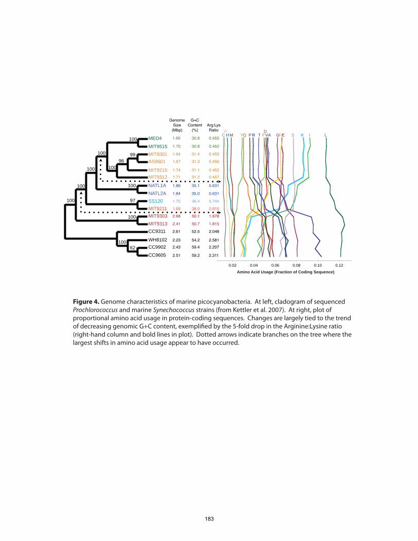
0.00 0.02 0.04 0.06 0.08 0.10 0.12 0.14
CW
H M YQ P R T FDVA GNE S K I L
Amino Acid Usage (Fraction of Coding Sequence)
Figure 4. Genome characteristics of marine picocyanobacteria. At left, cladogram of sequencedProchlorococcus and marine Synechococcus strains (from Kettler et al. 2007). At right, plot of proportional amino acid usage in protein-coding sequences. Changes are largely tied to the trend of decreasing genomic G+C content, exempli�ed by the 5-fold drop in the Arginine:Lysine ratio (right-hand column and bold lines in plot). Dotted arrows indicate branches on the tree where the largest shifts in amino acid usage appear to have occurred.
MED4
MIT9515MIT9301AS9601
MIT9215MIT9312
NATL1ANATL2ASS120MIT9211MIT9303MIT9313CC9311
WH8102CC9902
CC9605
100
99
100
97
100
10062
100
100
100
100
10096
183
are calculated relative to the cellular compositions in Section 1, which is for a high-light
adapted, MED4-like cell. The intent here is not to compare nutrient requirements of
MIT9313- and MED4-type cells, but rather to gauge the additional burden that carrying a
MIT9313-like genome would have imposed on a MED4-like cell.
2.2 Consequences for nutrient requirements
The larger genome, of course, requires more phosphorus to duplicate. An additional
750kbp would increase the size of the MED4 genome by 45%. The net increase in the
cellular P requirement for just the extra DNA would be 19.1%. Assuming these
additional genes were expressed at the same average level as the rest of the genome, the
additional mRNA would add 1.1% to the phosphorus quota. Hence the total P savings
from the smaller, high-light genome amounts to roughly 20.2% of the cellular phosphorus
budget – in total, an amount likely visible to selection under P-limiting conditions.
However, DNA is lost from bacterial genomes in fragments much smaller than 750kbp –
perhaps only a few tens of bases at a time – and the incremental effect of each loss is
much smaller and less likely to be selected for. Bragg and Wagner (2009) have shown
how single-atom changes in gene composition can be adaptive under nutrient limitation,
if the selective pressure is strong enough. Quantifying this selective pressure would
require knowledge of the effective population size of Prochlorococcus (i.e., the size of a
subpopulation bearing the same degree of neutral genetic varation as the total
population), which is difficult to ascertain for bacteria generally (Fraser et al., 2007). The
global census population is of order 1027 cells (Partensky et al., 1999), though the
effective population size could be many orders of magnitude smaller. The potential
exists for a huge effective population size to select for even small chromosomal changes
in Prochlorococcus. As discussed below, however, there are multiple lines of evidence
from high-light isolate genomes that suggest that ‘extraneous’ DNA is not always rapidly
excised from cells.
184
The effects of genome streamlining on the cellular nitrogen budget are more equivocal.
750,000 base pairs of DNA amounts to 1.2-3.7% of the cellular N budget. The effect of
the decrease in G+C content is even smaller – if the MED4 genome were 50.7% G+C,
the cellular N requirement would increase by only 0.1-0.2%. Because of a bias in the
genetic code that associates G+C-rich codons with N-rich amino acids, a decrease in
genomic G+C will also produce a lower-N proteome. This can be clearly seen in the
trend in the Arg:Lys ratio along the evolutionary grade, which decreases fivefold from
~2.3 in Synechococcus to 0.45 in high-light Prochlorococcus (Fig. 4). Arginine and
lysine are both basic amino acids, and can often substitute for one another in proteins.
Since arginine has 4 nitrogens to lysine’s two, and Arg is encoded by more G+C-rich
codons (CGx, AGA, AGG) than Lys (AAA, AAG), a single transition mutation could
save the cell 3 nitrogen atoms. If the MED4 genome coded for amino acids at the same
relative frequency as MIT9313, its proteome would be predicted to be richer in nitrogen
by 0.031 N per amino acid. For the cell compositions outlined in Section 1, this would
increase the N budget by 1.8-2.1%. Hence the total potential nitrogen savings associated
with genome streamlining in MED4 amount to 3.4-5.7% of the cellular N requirement.
As in the case of phosphorus, each small, incremental change in genome composition
would have to be visible to selection – which could be plausible, given the potentially
huge effective population size of Prochlorococcus, and would be influenced by the
expression level of each protein. Nitrogen savings in highly-expressed proteins will have
a proportionally larger impact on the cellular N budget, and therefore be more likely to be
selected under N limitation. The calculation of fractional protein abundances based on
the data presented in Chapter 4 equips us to address this question. Figure 5 shows three
views of the amino acid composition of the proteome: the average of coding sequences in
the genome (also plotted in Figure 4), the proteome composition suggested by the
fractional abundance measurements (i.e., the average of sequences of detected proteins,
weighted by APEX scores), and the average of sequences of the 51 most abundant
proteins in MED4 (i.e., those with highest average APEX scores over the diel cycle; see
185
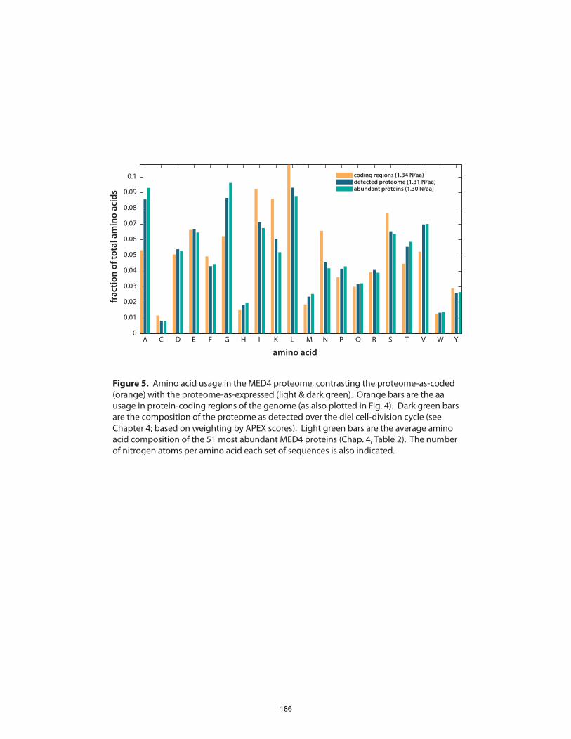
A C D E F G H I K L M N P Q R S T V W Y0
0.01
0.02
0.03
0.04
0.05
0.06
0.07
0.08
0.09
0.1
frac
tion
of to
tal a
min
o ac
ids
coding regions (1.34 N/aa)detected proteome (1.31 N/aa)abundant proteins (1.30 N/aa)
amino acid
Figure 5. Amino acid usage in the MED4 proteome, contrasting the proteome-as-coded (orange) with the proteome-as-expressed (light & dark green). Orange bars are the aa usage in protein-coding regions of the genome (as also plotted in Fig. 4). Dark green bars are the composition of the proteome as detected over the diel cell-division cycle (see Chapter 4; based on weighting by APEX scores). Light green bars are the average amino acid composition of the 51 most abundant MED4 proteins (Chap. 4, Table 2). The number of nitrogen atoms per amino acid each set of sequences is also indicated.
186
Chapter 4). The proteome-as-expressed is indeed lower in nitrogen than the proteome-as-
coded, to the tune of 0.03 N per amino acid (1.34 vs. 1.31), or 2.4%. The most abundant
proteins are even slightly lower in N content. This suggests that the sequences of highly-
expressed proteins have in fact been selected to limit N demand.
Does the genome streamlining process explain the relative nitrogen efficiency of highly-
expressed proteins? Surprisingly, the answer seems to be no. The abundant proteins in
MED4 are not endmembers or extreme examples of the evolutionary compositional
trends illustrated in Figure 4. Rather, the low N content of abundant proteins stems
primarily from less usage of two N-rich amino acids (Lys and Asp), whose genomic
frequency increases towards the high-light clade (Fig. 4), in favor of more usage of three
N-poor residues (Ala, Gly and Val) whose frequency decreases along the trend. Since A,
G and V are encoded by G+C-rich codons (GCx, GGx and GTx, respectively), the G+C
content of the 50 most highly-expressed genes is actually higher than the genome as a
whole (38.9% vs. 30.8%). In other words, highly-expressed proteins show economy of N
usage despite the overall effect of genome streamlining, not because of it. Whatever the
evolutionary process driving genome streamlining, it does not appear to be closely linked
to reducing cellular demand for nitrogen.
2.3 Streamlining in the light of evolution
Viewed in a broader evolutionary context, the case for genome streamlining in
Prochlorococcus as being driven primarily by adaptation to nutrient scarcity is tenuous.
The two kinds of genomic changes – size reduction and G+C loss – are uncoupled in the
evolutionary history of Prochlorococcus. From the phylogenetic tree in Figure 4 it would
at first appear that, rather than being a gradual, continuous process, there was a single
episode of genome size reduction in Prochlorococcus, along the branch between the
MIT9313/MIT9303 divergence and all other strains. With more careful consideration of
the histories of individual gene families, a different picture emerges: the Synechococcus-
187
like size of the MIT9313/MIT9303 genomes is not due to retention of nearly all genes
from a Prochlorococcus/Synechococcus ancestor, but rather substantial gene gain within
that lineage (Kettler et al., 2007) – implying that genome size reduction actually occurred
in the Prochlorococcus common ancestor. The slightly enlarged genomes of the NATL
strains – bigger than either the more basal or distal groups in the tree – also reflects
lineage-specific gene acquisition. Moreover, none of these patterns correlates at all with
the distributions of phosphorus-stress related genes among Prochlorococcus strains. As
shown by Martiny and Coleman et al. (2006), closely-related isolates with similar
genome sizes often bear radically different complements of P acquisition and utilization
genes. As noted by Coleman and Chisholm (2007), adaptation to phosphorus availability
appears to occur on a very different evolutionary scale from changes in genome size.
Drops in G+C content, and the associated changes in amino acid usage, also have a
phylogenetic distribution distinct from the pattern of genome size reduction. These
appear to be concentrated in two places on the evolutionary tree: between
MIT9313/MIT9303 and other Prochlorococcus, and between the NATL strains and the
ancestor of the high-light adapted group (Figure 4). If G+C content changes were
primarily influenced by nitrogen availability while genome size reduction is a
phosphorus-saving measure, it is unclear how the two should become so decoupled over
evolutionary timescales.
Most significantly, there is increasing evidence that, even under the strongest forms of P-
limitation, cells bear a significant number of genes that have little or no immediate
adaptive value. In high-light Prochlorococcus isolates, roughly 10% of the genome
consists of hypervariable regions, and the size of these regions is uncorrelated with the
distribution of phosphate-adaptation genes. If genome size were linked to adaptation to P
limitation, we would expect strains with larger complements of P-acquisition genes to
have smaller genomes, but no such correlation is observed among strains sequenced to
date. The hypervariable 10% of the genome represents approximately 4.5% of the
188
cellular P budget that could be considered the cell’s ‘investment’ in gene exchange.
Metagenomic sequence data from the HOT and BATS ocean time-series stations also
provides evidence that adaptation to strong P limitation at BATS has not produced a
decrease in genome size. If genome size reduction were a strategy to adapt to nutrient
limitation, we would expect many genes to be less abundant at the more strongly P-
limited site. In fact, the opposite pattern is observed: core genes (i.e., those shared by all
sequenced Prochlorococcus strains; Kettler et al., 2007) show indistinguishable per-cell
abundance distributions at HOT and BATS, and of the 29 flexible genes that are
differentially abundant, 26 are actually more abundant at BATS than HOT (Coleman and
Chisholm, submitted).
If nutrient-utilization efficiency fails to account for the evolution of small, A+T-rich
genomes in Prochlorococcus, what processes offer a more satisfactory explanation?
Partensky and Garczarek (2010) discuss the loss of several DNA-repair genes within the
Prochlorococcus lineage, and note that the inactivation of these systems is likely to
increase the rate of G:C-to-A:T mutations. These authors also point out, however, that
gene losses are not clearly linked to high mutation rates, as that should result in the
presence of numerous inactivated pseudogenes, which are nearly absent in
Prochlorococcus genomes. Quantification of mutation rates in various Prochlorococcus
ecotypes would be highly valuable in assessing the role of DNA repair in genome
streamlining.
With regard to gene loss, Lynch (2006) has suggested that the presence of nonfunctional
DNA in bacterial genomes is opposed by selection because of the mutational burden it
introduces. For example, a mutation in a 5’ untranslated region could introduce an
alternative start site for its associated ORF, with deleterious consequences. The strength
of the selection that opposes the maintenance of such sequences is proportional to the
effective population size, which as noted above, is difficult to discern at present. In
organisms such as Prochlorococcus, it would appear that not only nonfunctional DNA,
189

but also coding regions have been excised. This may be tied to reductions in cell size and
metabolic simplification: as overall expression levels drop, some genes enter a ‘gray
zone’ between functional and nonfunctional DNA. A gene that is no longer (or not yet)
expressed may be a waste of a couple of thousand phosphorus atoms, but its much greater
burden is as a neighbor to genes that do need to be expressed efficiently and need a well-
ordered chromosomal neighborhood to do so. This ‘use it or lose it’ notion of genome
streamlining is also more consistent with the clustering of recently-acquired genes in
hypervariable islands (Coleman et al., 2006), as islands could serve as genomic ‘holding
pens’ that allow active gene exchange without undue disruption of expression of the rest
of the chromosome. Ultimately, genome streamlining in Prochlorococcus (and other
marine bacteria) may well be tied to oligotrophic conditions – but through overall
reductions in gene expression (as noted in Section 1, the major nutrient demand on the
cell) rather than selection on the composition of DNA per se. Furthermore, this scenario
unifies the root causes of genome streamlining in parasitic and oligotrophic bacteria, as
both could stem from genetic disuse. Much remains to be explored regarding the
evolutionary trajectories of Prochlorococcus genomes, and multiple driving forces are
likely to be at work. Nevertheless, the ability of population-genomic processes to explain
genome characteristics of a wide variety of organisms inhabiting many different habitats
(Lynch, 2006) offers promise for a deeper understanding of microbial evolution.
3. STOCHASTIC GENE EXPRESSION EFFECTS AND THE ECOLOGICAL CONSEQUENCES OF
NOISE
3.1 The nature of noise
The expression of genes by cells is a stochastic phenomenon. Gene expression is
stochastic in that fluctuations in gene product abundances, both in a particular cell over
time and between nominally identical cells at a given time, are governed by processes,
such as macromolecular diffusion, that are random and can only be described statistically
190
(Kærn et al., 2005; Larson et al., 2009). Note that this does not mean that expression
levels as typically considered – as population or steady-state averages – are random or
non-deterministic. Regulatory mechanisms clearly control the averages and central
tendencies; it is in the variance and high-frequency dynamics that stochastic effects
become significant. For individual cells, however, long-term or population averages are
irrelevant, and stochasticity can have a major impact on how a cell goes about
accomplishing a physiological programme such as cell division.
To illustrate this idea, consider the abundance of a given gene’s transcript in a
hypothetical Prochlorococcus cell. As noted above (Section 1.2.1), only about 12% of
the cell’s genome is transcribed at any given time, so the mean transcript abundance
(averaged across all genes and cells) is 0.12 copies/cell. Of course, transcripts only exist
in integer copy numbers, so this result is more meaningfully interpreted along the lines
of, “A given cell contains a copy of a given transcript about 12% of the time,” or, “A
given transcript is present in about 12% of cells in a population at any given time.” In
reality, there is a wide range of average transcript abundances (spanning four orders of
magnitude, according to the AMEX results in Chapter 4), so some transcripts are
probably found in most cells most of the time (average abundances at or above 1), while
others are very rare (~0.001 copies/cell). Nevertheless, the fact that the average
transcript abundance is significantly less than 1 copy/cell means that each individual
transcription event (i.e., each mRNA molecule produced) usually causes a huge
proportional change in the abundance of that gene product in the cell. Since transcription
is a stochastic process, the low average abundance of transcripts in Prochlorococcus cells
mean that the actual number of copies of a particular mRNA molecule in a given cell will
be subject to strong and unpredictable fluctuations over time. As a cell tries to perform
more or less of a certain metabolic process (e.g., in response to changing light availability
over the diel cycle) by changing the expression of a related gene, it must cope with the
random noise imposed by stochastic effects on the gene product abundance is it
attempting to regulate.
191
The small size, limited chemical complements and low absolute gene expression levels of
Prochlorococcus cells could have significant implications for their physiological
functioning. In particular, small cells might ‘sample’ the range of physiological states
(phenotypes) available to them in a more discrete fashion than larger cells do, because the
pools of biochemicals that enable those different states are smaller and thus integer
changes in copy numbers of gene products are proportionally more significant. This
‘granularity’ in gene product abundance makes small cells especially susceptible to
stochastic effects in gene expression. Stochasticity can give rise to phenotypic variability
even within an isogenic population, with various aspects of cell physiology and
metabolism varying around a population mean (Longo and Hasty, 2006). In large
populations, then, rare phenotypes are more likely to arise and have an ecological, and
potentially evolutionary, impact. Nutrient scarcity can also exacerbate stochastic effects,
particularly for autotrophic organisms, since gene products (mRNA and proteins) and
gene expression machinery (especially ribosomes) are the most nutrient-intensive
biochemicals in the cell. Prochlorococcus, as one of the smallest and most abundant
free-living bacteria and an inhabitant of exceptionally nutrient-poor habitats, appears to
be in the ‘perfect storm’ of stochastic gene expression effects. Here we develop a
hypothesis for how Prochlorococcus – and small cells in general – might cope with
expression noise, which suggests that modulating these effects could be an important
constraint on these organisms’ physiology and ecology.
Stochastic effects in gene expression (also termed ‘noise’) have been of interest for a
number of years, and a variety of experimental and theoretical studies have been
published. The significance of stochastic effects in processes such as determination of
cell fate (Losick and Desplan, 2008) and responses to environmental perturbations (Acar
et al., 2008) been demonstrated. The exploration of stochastic effects in
Prochlorococcus, however, is hindered by the lack of genetic tools that would enable the
kind of single-cell studies that have elucidated similar phenomena in other microbes.
192
Fluorescent protein fusions have been especially powerful tools for visualizing stochastic
effects, and allow detection by flow cytometry (Newman et al., 2006). Transfer of a
GFP-containing plasmid into (and its expression by) one Prochlorococcus strain has been
acheived (Tolonen et al., 2006), but expressed fusions to native proteins have yet to be
demonstrated. While direct experimental investigation of noisiness in Prochlorococcus
gene expression awaits further developments, the cellular biochemical budgets outlined
in the first section allow us to bound the problem and generate some useful hypotheses
for how such effects might be manifested.
3.2 Bounding the noisiness of Prochlorococcus
We consider two different scenarios for gene expression noise, depending on the noise
source: a “Poisson” scenario, where expression noise is dominated by the random births
and deaths of mRNA molecules, and a “Telegraph” scenario, where noise is dominated
by random promoter binding events (Kaufmann and van Oudenaarden, 2007). The
Poisson scenario is a one-state model in that the probability of transcription is constant
with time. The Telegraph scenario is a two-state model, since transcription is dependent
on promoter binding, which is itself stochastic. While the Poisson model has generally
been considered to sufficiently explain observations of expression fluctuations in bacteria
(Raj and van Oudenaarden, 2008), there is some evidence for the transcriptional bursting
implied by the Telegraph model (Golding and Cox, 2006), so here we consider both
possibilities. The equations describing mRNA and protein noise under the two scenarios
are given in Table 2 (Kaufmann and van Oudenaarden, 2007), and we introduce the ratio
of the noise at the mRNA and protein levels, designated H2.
A description of each of the noise parameters, and their values for Prochlorococcus near
the upper and lower limits of environmentally-observed growth rates (Veldhuis et al.,
2005), are given in Table 3. Where required, values from the budgets in Section 1 of this
chapter were taken, using case II. Note that because of the way gene product abundances
193
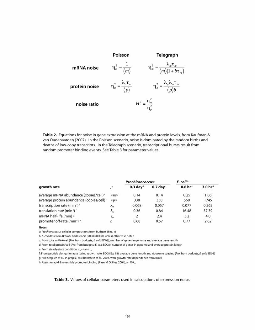
Prochlorococcus a E. coli b
growth rate μ 0.3 day-1 0.7 day-1 0.6 hr-1 3.0 hr-1
average mRNA abundance (copies/cell) c <m> 0.14 0.14 0.25 1.06average protein abundance (copies/cell) d <p> 338 338 560 1745transcription rate (min-1) e
m 0.068 0.057 0.077 0.262translation rate (min-1) f
p 0.36 0.84 16.48 57.39mRNA half-life (min) g
m 2 2.4 3.2 4.0promoter o -rate (min-1) h b 0.68 0.57 0.77 2.62
Notesa: Prochlorococcus cellular compositions from budgets (Sec. 1)b: E. coli data from Bremer and Dennis (2008) (BD08), unless otherwise notedc: From total mRNA/cell (Pro: from budgets; E. coli: BD08), number of genes in genome and average gene lengthd: From total protein/cell (Pro: from budgets; E. coli: BD08), number of genes in genome and average protein lengthe: From steady-state condition, m=<m>/ m
f: From peptide elongation rate (using growth rate; BD08 Eq. 18), average gene length and ribosome spacing (Pro: from budgets, E. coli: BD08)g: Pro: Steglich et al., in prep; E. coli: Bernstein et al., 2004, with growth-rate dependence from BD08h: Assume rapid & reversible promoter binding (Raser & O'Shea 2004), b=10 m
ηm2 =
1m
ηm2 =
λmτm
m 1+ bτm( )
ηp2 =
λpτm
pηp
2 =λpλmτm
p b
H 2 =ηm
2
ηp2
mRNA noise
protein noise
noise ratio
Poisson Telegraph
Table 3. Values of cellular parameters used in calculations of expression noise.
Table 2. Equations for noise in gene expression at the mRNA and protein levels, from Kaufman & van Oudenaarden (2007). In the Poisson scenario, noise is dominated by the random births and deaths of low-copy transcripts. In the Telegraph scenario, transcriptional bursts result from random promoter binding events. See Table 3 for parameter values.
194
and rates are calculated here, stochastic effects for Prochlorococcus are independent of
cell stoichiometry at a given growth rate. This is certainly a simplification, and in real
settings there are likely tradeoffs between growth, noise and budgets that are important to
environmental adaptation. To help put the Prochlorococcus results in context, values of
the same parameters for E. coli growing at two different rates are also shown (Table 3).
As expected from its slower growth and lower ribosome content, the translation rate in
Prochlorococcus is substantially lower than in E. coli.
Under both the Poisson and Telegraph scenarios, gene expression is noisier in
Prochlorococcus than E. coli at the mRNA level, but less noisy at the protein level (Table
4). For both organisms, noise scales inversely with growth rate, principally due to the
larger pools of gene products and expression components in the faster-growing cells.
Stochastic effects due to mRNA fluctuations (the Poisson scenario) are larger than those
predicted for promoter noise (the Telegraph scenario), though this is contingent on
promoter kinetics that likely vary widely between individual genes.
A key prediction of this model is that gene expression in Prochlorococcus is much
noisier at the mRNA level – probably by a factor of over a thousand – than at the protein
level. Values of the mRNA:protein noise ratio (H2 value) in Prochlorococcus range from
near 700 in the Telegraph promoter-noise scenario at fast growth rates to over 3000 in the
Poisson scenario at slow growth rates. By comparison, the noise ratios in E. coli range
from ~6 up to only 43. The main factors contributing to the high noise ratio in
Prochlorococcus are the small numbers of transcripts and slow translation rate. This
results in fewer proteins being produced per transcript, limiting the effects of translational
bursting. In fact, the model presented here implies that many transcripts in
Prochlorococcus may go untranslated, essentially for want of an available ribosome.
Since transcription (and therefore transcript degradation) is not slowed to nearly the same
degree as translation, a sizeable proportion of transcripts might be recycled before a
ribosome binds to them. While ‘wasteful’ to a certain extent, Prochlorococcus invests
195

Prochlorococcus E. coligrowth rate μ 0.3 day-1 0.7 day-1 0.6 hr-1 3.0 hr-1
Poisson scenariomRNA noise m
2 7.35 7.35 4.07 0.95protein noise p
2 0.0021 0.0060 0.0942 0.1326Noise ratio 2 3453 1233 43 7.1
Telegraph scenariomRNA noise m
2 0.424 0.424 0.289 0.087protein noise p
2 0.0002 0.0006 0.0094 0.0133Noise ratio 2 1990 711 30.7 6.5
Table 4. Results of expression noise modeling, using equations and values from Tables 2 and 3. Under both noise scenarios and over the full range of growth rates, gene expression in Prochlorococ-cus is noisier at the mRNA level but less noisy at the protein level than in E. coli. Protein noise is e�ectively damped by the slow translation rate in Prochlorococcus.
196
only a relatively small proportion of nutrients in mRNA. High mRNA turnover could be
energy-intensive, but if the phenotypic consequences of protein-level noise are severe
enough, it may be worthwhile to express genes in a manner that damps stochastic
fluctuations in protein abundances.
If protein-level expression noise is in fact a constraint on cellular metabolism, the
equations in Table 2 outline several potential strategies for dealing with it. Perhaps most
straightforward is to increase <p> -- that is, to make larger pools of proteins. This, of
course, requires greater nutrient supplies and larger cells, and would be ecologically
disadvantageous in an oligotrophic marine habitat. Another strategy is to decrease
mRNA half-life (smaller τm). Prochlorococcus has quite short mRNA half-lives
(Steglich et al., submitted), but it seems likely that this strategy can only be taken so far,
as half-lives would become too short for mRNAs to be translated at all. The third option
is to slow down protein synthesis (smaller λp) – which can be taken as far as the
ecological consequences of the concomitant slowdown in cell growth can be tolerated.
The damping of protein noise by slow translation (in the sense of low protein yield per
transcript molecule, not necessarily due to “slow ribosomes”) may be a substantial factor
in the low, fixed cell division rate of Prochlorococcus.
It is interesting, then, that Prochlorococcus makes relatively little use the first noise-
damping option – making more protein and bigger cells – even when nutrients are
abundant. It is clear that some “facultatively copiotrophic” (or conversely, “facultatively
oligotrophic”) microbes can tune cellular protein abundances, sizes and growth rates to
the prevailing nutrient regimes, making smaller, slow-growing cells under oligotrophic
conditions and larger, faster-growing ones when nutrients are replete. It may be that
nutrient enrichments to epipelagic waters are infrequent enough that Prochlorococcus
lost the genetic machinery to speed growth under meso- to eutrophic conditions through
disuse, as described in the previous section. Not all open-ocean microbes have lost these
abilities, however (Martin and Macleod, 1984), suggesting that the putatively large
197
effective population size of Prochlorococcus may have driven it further down the path of
genome streamlining.
The relative lifetimes of proteins and transcripts may also be crucial to expression noise.
Steglich et al. (submitted) have shown that mRNA half-lives in Prochlorococcus are
relatively short, and the timecourse expression results presented in Chapter 4 suggest
(though do not require) that protein lifetimes are relatively long. This τp/τm ratio figures
prominently in several more recent models of stochastic gene expression. In the models
of Pedraza and Paulsson (2008) and Shahrezaei and Swain (2008), which treat bursting
effects explicitly in a temporal framework, the contribution of mRNA noise to
stochasticity at the protein level is modulated by τp/τm. In fact (cf. Pedraza and Paulsson,
2008, Eq. 1 and 2; Shahrezaei and Swain, 2008, Eq. 21), in the case where τp >> τm, as
may well be the case for Prochlorococcus, protein noise in these models simplifies to
1/<p>, the inherent small-number lower limit. Temporally-resolved proteomics
measurements, akin to those presented in Chapter 4, should allow gene-product lifetime
experiments analogous to that of Steglich et al. to be performed at the protein level,
providing a global view of τp/τm ratios for Prochlorococcus genes. This combination of
transcript and protein half-life measurements would test whether the combination of
long-lived proteins and rapid mRNA turnover contributes to noise reduction, and how
this effect varies among different genes.
3.3 The growth costs of noise, or, You can’t just shrink a Ferrari
The low translation rate that contributes to limiting protein-level expression noise in
Prochlorococcus goes hand-in-hand with relatively slow cell growth. Slow growth may
be a general feature of very small cells, if low translation rates are a common strategy to
damp protein noise and stabilize metabolism. To apply an automotive metaphor, in small
cells, the ‘engine’ of transcription is running fast, producing (and degrading) mRNA at
rates comparable to faster-growing cells, but the ‘transmission’ of translation is in low
198
gear, producing the ‘torque’ required to control the cell division program at the expense
of slowing protein production. In this scenario, small cells grow slowly for the same
reason a moped can’t go 60 mph up a steep hill: the small engine can only generate so
much torque with the largest gear that will fit on the frame. As with motor vehicles, there
may be a size-speed tradeoff in cells: initial increases in size produce speed (growth rate)
gains, as a more powerful drivetrain (expression machinery) can be accommodated by the
frame. But eventually, an optimum power:weight ratio is reached, maximizing speed, as
exemplified by racecars or E. coli. Above this optimum size, top speed/maximum growth
rate declines (for bigger ‘vehicles’, e.g., cargo trucks, or large protists such as
dinoflagellates) as the chassis accommodates heavier and heavier loads.
There is biological evidence for the growth rate-cell mass relationship on both sides of
this proposed optimum. In E. coli, growth rate increases proportionally to cell mass up to
a maximum of a 20 minute doubling time at a mass of 1.02 pg (Bremer and Dennis,
2008). Interestingly, this positive correlation between cell size and growth rate is the
opposite of the relationship proposed from some compilations of phytoplankton growth
rates, which have been fit with a (mass)-1/4 trend (Finkel et al., 2009); it should be noted
that positive correlations between cell size and growth rate have been also observed for
some phytoplankton (Costello and Chisholm, 1981). A negative correlation between
growth and size in larger organisms has been justified theoretically in the context of the
metabolic theory of ecology (Brown et al., 2004). So one hypothesis, shown
diagrammatically in Figure 6, might be that rapidly-growing bacteria such as E. coli are
perched at an optimum at the border between metabolically-dominated and
stochastically-dominated growth regimes. In this view, the increase in growth rate gained
by alleviating metabolic burdens in smaller cells is counterbalanced by the challenge of
speeding up a transcriptional program whose smaller pools of gene products are more
susceptible to stochastic effects. Testing this hypothesis would require intercalibration of
growth rate-cell size relationships across a broad range of taxa (especially small, slow-
199

log
grow
th ra
te
log cell mass
E. coli
Prochlorococcus
Metabolic e�ects dominateStochastic
e�ects dominate
~3/hr
~1pg
Larger phytoplankton
Figure 6. Schematic of hypothesized relationship between cell mass and growth rate. At low cell mass, small pools of gene products result in large stochastic e�ects in gene expression; slow growth is suggested as one way to damp these e�ects at the protein level and thereby maintain metabolic/phenotypic stability. For larger cells, stochastic e�ects are small and growth rates are limited primarily by metabolic considerations . Fast-growing bacteria such as E. coli are proposed to live at the borderbetween the two growth-limitation regimes.
200
growing bacteria and archaea), which is challenging (Finkel et al., 2009). But one can’t
simply shrink down a Ferrari and expect it to still go as fast.
While stochastic gene expression effects might be observable in the laboratory (though
not yet in Prochlorococcus) and at least partially predictable on theoretical grounds, it is
less clear how consequential they are for organismal physiology and even less clear for
ecology. Experimental studies to date have shown that increased stochasticity can
provide an advantage when environmental conditions fluctuate. With the notable
exception of the diel cycle (Chapter 4), the tropical/subtropical open-ocean habitat of
Prochlorococcus is generally considered one of the more stable environments on earth.
Physical and chemical conditions in the upper water column of subtropical gyres change
relatively slowly, and seasonality is weak. In recent years, however, increasing attention
has been paid to smaller-scale variability that may be highly relevant for microbial
physiology. Even in the well-mixed upper open ocean, eddies and aeolian deposition
events produce substantial changes in nutrient availability over scales of 102-105 m and
days to weeks. Perhaps more importantly over longer time scales, even conditions that
appear stable using conventional, ‘bulk’ oceanographic measurements are increasingly
appreciated as highly heterogeneous on the spatial scales of individual microbial cells
(Seymour et al., 2004; Mitchell et al., 2008). Microscale events such as the formation
and dissipation of nutrient patches or the aggregation and sinking of rare, large particles
are occurring constantly and represent environmental fluctuations from the perspective of
individual cells. The ecological (and ultimately evolutionary) consequences of stochastic
gene expression in planktonic marine microbes may well be tied to the exploitation of
microscale, transient features in the water column.
4. CONCLUSIONS AND FUTURE DIRECTIONS
This chapter presents a simple model for the molecular composition of hypothetical high-
light Prochlorococcus cells, based on available experimental and genomic data.
201
Budgeting of cellular contents of carbon, nitrogen and phosphorus reveals that almost
half of cellular P is contained in the chromosome, leaving enough for only about 600
ribosomes and the transcription of 10-15% of the genome. 70-90% of cellular N is in
protein, and copy numbers of individual proteins range up to perhaps 50,000 copies per
cell. We suggest that genome streamlining is unlikely to be driven primarily by
adaptation to oligotrophic conditions, and hypothesize that population-level evolutionary
processes are more likely to explain genome evolution in Prochlorococcus.
Consideration of cell composition in light of stochastic effects in gene expression yields a
prediction that transcript levels in Prochlorococcus cells are likely to be very noisy, but
that noise is strongly damped at the protein level due to slow translation. Slow
translation is concomitant with slow growth, and we propose a hypothesis for growth
limitation of small cells by the need to limit the metabolic and phenotypic influence of
stochastic gene expression.
There is a large gulf in microbial biogeochemistry between the rapidly-expanding
inventory of microbial diversity and knowledge of the molecular composition of
microbial communities. A very few organisms, notably E. coli and S. cerevisiae, have
been the subject of extensive quantitative investigation. While these lab models are of
limited environmental relevance in themselves, they have provided essential data on the
molecular organization of universal biological structures, such as ribosomes and
membranes. Armed with such parameters, and with some basic information about cell
size and elemental composition – and a sequenced genome – one can actually constrain
the molecular makeup of any microorganism to a reasonably informative degree. For a
cultivable organism like Prochlorococcus, more physiological and biochemical data are
available, enabling greater refinement of a cell composition model. Any natural
microbial population is comprised of a wide variety of organisms, ranging in
characterization from undiscovered to cultivated, and in-depth investigation of the
properties of each and every relevant microbial type is unfeasible. A more viable goal is
to build conceptual framework to ‘bootstrap’ the information about the composition of
202
better-characterized organisms into inferences about less well-known members of the
community.
Ultimately, we would like to be able to use data from high-throughput, culture-
independent techniques as inputs to biogeochemical models of microbial communities.
Such techniques are already available to measure some aspects of cellular composition:
flow cytometry, for example, can count cells and detect a variety of pigments, and with
the right sort of dye or probe can assay for a huge range of properties, and can examine
thousands of cells per second. Nucleic acid sequence information, of course, is now a
readily observed property of any microbial system, and can even be obtained from single,
uncultivated cells (Rodrigue and Malmstrom et al., 2009). Chemical imaging methods
such as SIMS (secondary ion mass spectrometry) and X-ray microanalysis are
increasingly used to examine the makeup of microbial cells, and high-speed cell sorting
and microfluidic devices promise new ways of preparing environmental samples for
molecular analysis. The real benefit of a compositional view of cells will come in
integrating information from these disparate technologies, identifying key unknowns for
further investigation, and feeding into process models of microbial activity and its
biogeochemical consequences. Biogeochemistry that is informed by systems biology
will undoubtedly afford deeper insights into the structure, function and coevolution of
earth’s life and environments.
ACKNOWLEDGEMENTS
We are grateful to Maureen Coleman for discussions of genome evolution and expression dynamics and for analysis of amino acid utilization patterns, and to Jason Bragg and Chris Kempes for discussions of interactions between organismal stoichiometry, metabolism and growth. This work was supported by grants from the Department of Energy Genomics:GtL program, the NSF Center for Microbial Oceanography: Research and Education, and the Gordon and Betty Moore Foundation to SWC, and by an Office of Naval Research NDSEG Fellowship and an NSF Graduate Research Fellowship to JRW.
203
REFERENCES Acar, M, JT Mettetal, and A van Oudenaarden. 2008. Stochastic switching as a survival
strategy in fluctuating environments. Nat Genet 40, no. 4: 471–475. Ammerman, JW, RR Hood, DA Case, and JB Cotner. 2003. Phosphorus deficiency in the
Atlantic: an emerging paradigm in oceanography. Eos, Transactions American Geophysical Union 84, no. 18: 165.
Bennett, BD, EH Kimball, M Gao, R Osterhout, SJV Dien, and JD Rabinowitz. 2009. Absolute metabolite concentrations and implied enzyme active site occupancy in Escherichia coli. Nat Chem Biol 5, no. 8: 593–599.
Bertilsson, S, O Berglund, DM Karl, and SW Chisholm. 2003. Elemental Composition of Marine Prochlorococcus and Synechococcus: Lmplications for the Ecological Stoichiometry of the Sea. Limnology and Oceanography 1721–1731.
Bragg, JG, and A Wagner. 2009. Protein material costs: single atoms can make an evolutionary difference. Trends Genet 25, no. 1: 5–8.
Bremer, H., and P.P. Dennis. 2008. Modulation of chemical composition and other parameters of the cell at different exponential growth rates. In EcoSal -- Escherichia coli and Salmonella typhimurium: Cellular and Molecular Biology, eds. A. Böck, R. Curtiss III, J. B. Kaper, P. D. Karp, F. C. Neidhardt, T. Nyström, J. M. Slauch, C. L. Squires, and D. Ussery, Washington, D.C.: ASM Press.
Brown, JH, JF Gillooly, AP Allen, VM Savage, and GB West. 2004. Toward a metabolic theory of ecology. Ecology 85, no. 7: 1771–1789.
Claustre, H, A Bricaud, M Babin, F Bruyant, L Guillou, FL Gall, D Marie, and F Partensky. 2002. Diel variations in Prochlorococcus optical properties. Limnology and Oceanography 1637–1647.
Coleman, ML, and SW Chisholm. 2007. Code and context: Prochlorococcus as a model for cross-scale biology. Trends Microbiol 15, no. 9: 398–407.
Coleman, ML, MB Sullivan, AC Martiny, C Steglich, K Barry, EF Delong, and SW Chisholm. 2006. Genomic islands and the ecology and evolution of Prochlorococcus. Science 311, no. 5768: 1768–1770.
Costello, JC and SW Chisholm. 1981. The influence of cell size on the growth rate of Thalassiosira weissflogii. Journal of Plankton Research 3, 415-419.
Cronan, J.E., and C.O. Rock. 2008. Biosynthesis of membrane lipids. In EcoSal -- Escherichia coli and Salmonella typhimurium: Cellular and Molecular Biology, eds. A. Böck, R. Curtiss III, J. B. Kaper, P. D. Karp, F. C. Neidhardt, T. Nyström, J. M. Slauch, C. L. Squires, and D. Ussery, Washington, D.C.: ASM Press.
Dagan, T, R Blekhman, and D Graur. 2006. The" domino theory" of gene death: gradual and mass gene extinction events in three lineages of obligate symbiotic bacterial pathogens. Molecular biology and evolution 23, no. 2: 310.
Dufresne, A, L Garczarek, and F Partensky. 2005. Accelerated evolution associated with genome reduction in a free-living prokaryote. Genome Biol 6, no. 2:
Falkowski, P.G., and J.A. Raven. 2007. Aquatic Photosynthesis. Princeton, NJ: Princeton University Press.
204
Finkel, ZV, J Beardall, KJ Flynn, A Quigg, TAV Rees, and JA Raven. 2009. Phytoplankton in a changing world: cell size and elemental stoichiometry. Journal of Plankton Research 1–19.
Fraser, C, WP Hanage, and BG Spratt. 2007. Recombination and the nature of bacterial speciation. Science 315, no. 5811: 476.
Fu, FX, ME Warner, Y Zhang, Y Feng, and DA Hutchins. 2007. Effects of increased temperature and CO2 on photosynthesis, growth, and elemental ratios in marine Synechococcus and Prochlorococcus (cyanobacteria). Journal of Phycology 43, no. 3: 485–496.
Giovannoni, SJ, HJ Tripp, S Givan, M Podar, KL Vergin, D Baptista, L Bibbs, J Eads, TH Richardson, M Noordewier, MS Rappe, JM Short, JC Carrington, and EJ Mathur. 2005. Genome streamlining in a cosmopolitan oceanic bacterium. Science 309, no. 5738: 1242-1245.
Golding, I, and EC Cox. 2006. Physical nature of bacterial cytoplasm. Physical review letters 96, no. 9: 98102.
Heldal, M, DJ Scanlan, S Norl, TF Thingstad, and NH Mann. 2003. Elemental composition of single cells of various strains of marine Prochlorococcus and Synechococcus using X-ray microanalysis. Limnol Oceanogr 48, no. 5: 1732–1743.
Kærn, M, TC Elston, WJ Blake, and JJ Collins. 2005. Stochasticity in gene expression: from theories to phenotypes. Nature Reviews Genetics 6, no. 6: 451–464.
Kaufmann, BB, and A van Oudenaarden. 2007. Stochastic gene expression: from single molecules to the proteome. Curr Opin Genet Dev 17, no. 2: 107–112.
Kettler, G, AC Martiny, K Huang, J Zucker, ML Coleman, S Rodrigue, F Chen, A Lapidus, S Ferriera, J Johnson, C Steglich, GM Church, PM Richardson, and SW Chisholm. 2007. Patterns and Implications of Gene Gain and Loss in the Evolution of Prochlorococcus. PLoS Genet 3, no. 12: e231.
Klähn, S, C Steglich, WR Hess, and M Hagemann. 2009. Glucosylglycerate: a secondary compatible solute common to marine cyanobacteria from nitrogen-poor environments. Environmental Microbiology
Larson, D, R Singer, and D Zenklusen. 2009. A single molecule view of gene expression. Trends in Cell Biology
Longo, D, and J Hasty. 2006. Dynamics of single-cell gene expression. Mol Syst Biol 2, 64.
Lopez Cascales, JJ, JGdl Torre, SJ Marrink, and HJC Berendsen. 1996. Molecular dynamics simulation of a charged biological membrane. J. Chem. Phys 104, no. 7:
Losick, R, and C Desplan. 2008. Stochasticity and cell fate. Science 320, no. 5872: 65–68.
Lynch, M. 2006. Streamlining and simplification of microbial genome architecture. Annu Rev Microbiol 60, 327–349.
Martin, P, and R Macleod. 1984. Observations on the Distinction Between Oligotrophic and Eutrophic Marine Bacteria. Appl Environ Microbiol 47, no. 5: 1017–1022.
205
Martiny, AC, ML Coleman, and SW Chisholm. 2006. Phosphate acquisition genes in Prochlorococcus ecotypes: evidence for genome-wide adaptation. PNAS 103, no. 33: 12552-12557.
Mitchell, JG, H Yamazaki, L Seuront, F Wolk, and H Li. 2008. Phytoplankton patch patterns: Seascape anatomy in a turbulent ocean. Journal of Marine Systems 69, no. 3-4: 247–253.
Moore, LR, and SW Chisholm. 1999. Photophysiology of the marine cyanobacterium Prochlorococcus: ecotypic differences among cultured isolates. Limnology and Oceanography 628–638.
Morel, A, YH Ahn, F Partensky, D Vaulot, and H Claustre. 1993. Prochlorococcus and Synechococcus: A comparative study of their optical properties in relation to their size and pigmentation. Journal of Marine Research 51, no. 3: 617–649.
Newman, JRS, S Ghaemmaghami, J Ihmels, DK Breslow, M Noble, JL DeRisi and JS Weissman. 2006. Single-cell proteomic analysis of S. cerevisiae reveals the architecture of biological noise. Nature 441: 840-846.
Nikaido, H. 1996. Outer Membrane. In Escherichia coli and Salmonella typhimurium: Cellular and Molecular Biology, ed. F. C. Neidhardt, Washington, D.C.: ASM Press.
Partensky, F, and L Garczarek. 2010. Prochlorococcus: Advantages and Limits of Minimalism. Annual Review of Marine Science 2, 211-237.
Partensky, F, WR Hess, and D Vaulot. 1999. Prochlorococcus, a marine photosynthetic prokaryote of global significance. Microbiol Mol Biol Rev 63, no. 1: 106-127.
Pedraza, JM, and J Paulsson. 2008. Effects of molecular memory and bursting on fluctuations in gene expression. Science 319, no. 5861: 339–343.
Raj, A, and A van Oudenaarden. 2008. Nature, nurture, or chance: stochastic gene expression and its consequences. Cell 135, no. 2: 216–226.
Rodrigue, S, RR Malmstrom, AM Berlin, BW Birren, MR Henn, and SW Chisholm. 2009. Whole genome amplification and de novo assembly of single bacterial cells. PLoS ONE 4, no. 9: e6864.
Seymour, JR, JG Mitchell, and L Seuront. 2004. Microscale heterogeneity in the activity of coastal bacterioplankton communities. Aquatic Microbial Ecology 35, no. 1: 1–16.
Shahrezaei, V, and PS Swain. 2008. Analytical distributions for stochastic gene expression. Proc Natl Acad Sci USA 105, no. 45: 17256–17261.
Snyder, DS, B Brahamsha, P Azadi, and B Palenik. 2009. Structure of Compositionally Simple Lipopolysaccharide from Marine Synechococcus. J Bacteriol 191, no. 17: 5499–5509.
Thingstad, TF, MD Krom, RFC Mantoura, GAF Flaten, S Groom, B Herut, N Kress, CS Law, A Pasternak, P Pitta, S Psarra, F Rassoulzadegan, T Tanaka, A Tselepides, P Wassmann, EMS Woodward, CW Riser, G Zodiatis, and T Zohary. 2005. Nature of phosphorus limitation in the ultraoligotrophic eastern Mediterranean. Science 309, no. 5737: 1068–1071.
Ting, CS, C Hsieh, S Sundararaman, C Mannella, and M Marko. 2007. Cryo-Electron Tomography Reveals the Comparative Three-Dimensional Architecture of
206
Prochlorococcus, a Globally Important Marine Cyanobacterium. J Bacteriol 189, no. 12: 4485–4493.
Tolonen, AC, GB Liszt and WR Hess. 2006. Genetic Manipulation of Prochlorococcus Strain MIT9313: Green Fluorescent Protein Expression from an RSF1010 Plasmid and Tn5 Transposition. Appl Env Microbiol 72, no. 12: 7607-7613.
Van Mooy, BAS, G Rocap, HF Fredricks, CT Evans, and AH Devol. 2006. Sulfolipids dramatically decrease phosphorus demand by picocyanobacteria in oligotrophic marine environments. PNAS 103, no. 23: 8607-8612.
Van Mooy, BAS, H Fredricks, B Pedler, S Dyhrman, D Karl, M Koblizek, M Lomas, T Mincer, L Moore, T Moutin, M Rappe, and E Webb. 2009. Phytoplankton in the ocean use non-phosphorus lipids in response to phosphorus scarcity. Nature
Veldhuis, MJW, KR Timmermans, P Croot, and Bvd Wagt. 2005. Picophytoplankton; a comparative study of their biochemical composition and photosynthetic properties. Journal of Sea Research 53, no. 1-2: 7–24.
Vollmer, W, and J-V Holtje. 2004. The architecture of the murein (peptidoglycan) in gram-negative bacteria: vertical scaffold or horizontal layer(s)? J Bacteriol 186, no. 18: 5978–5987.
Wang, JD, and PA Levin. 2009. Metabolism, cell growth and the bacterial cell cycle. Nat Rev Microbiol 7, no. 11: 822–827.
Wilhelm, LJ, HJ Tripp, S Givan, D Smith, and SJ Giovannoni. 2007. Natural variation in SAR11 marine bacterioplankton genomes inferred from metagenomic data. Biol Direct 2, no. 1: 27.
Zinser, ER, D Lindell, ZI Johnson, ME Futschik, C Steglich, ML Coleman, MA Wright, T Rector, R Steen, N McNulty, LR Thompson, and SW Chisholm. 2009. Choreography of the transcriptome, photophysiology, and cell cycle of a minimal photoautotroph, Prochlorococcus. PLoS ONE 4, no. 4: e5135.
207

208
CHAPTER SIX
Conclusions and Future Directions
209

210

The work presented in this thesis has sought to contribute to understanding of how, when
and why biological activity, especially primary production by oxygenic photoautotrophs,
has driven the secular oxidation of earth’s surface environment. Using a variety of
molecular tools and examining processes at timescales spanning hours to billions of
years, the goal of these studies has been to provide new insights into the biogeochemistry
of marine microbes, both as documented in the rock record from the distant past and
visible in the activities of living organisms. The principal findings include:
• The molecular fossil record bears clear evidence of a diverse microbial
community in the oceans by at least 2.7 billion years ago, including members
of all three domains of life.
• The presence of biomarkers for aerobic biochemistry long before the
oxygenation of the atmosphere is fully consistent with their production in
persistently microaerobic regions of the surface ocean.
• The diel cell cycle of Prochlorococcus and associated shifts in metabolic
fluxes are underlain by small variations in a proteome whose composition is
generally stable, despite strong oscillations in expression at the transcript level.
• The relatively simple cellular and biochemical architecture of Prochlorococcus
enables a compositional budget to be constructed of the sort that can inform
biogeochemical models, as well as guide inferences about the ecological
consequences of genome streamlining and stochastic gene expression in small
cells.
211
FUTURE DIRECTIONS: THE MOLECULAR RECORD OF PRIMARY PRODUCTION AND
OXIDATION
The work presented here has helped to place the late Archean biomarker record on firmer
footing, but much remains to be learned about the molecular fossils contained in the vast
and still-growing archive of material recovered by the Agouron drilling project and other
scientific drilling initiatives. In particular, it would be helpful to characterize and identify
the controls on finer spatial-scale variability in biomarker compositions, and map
correlations with other geochemical proxies in greater detail. While the low extractable
hydrocarbon contents of these overmature rocks make high-resolution measurements
quite challenging, an understanding of such distributions would both lend greater
confidence to the molecular fossils’ syngeneity and likely provide new insights into the
ecological and biogeochemical structure of the microbial community.
The late Archean Hamersley and Transvaal basins, on which much Precambrian
biomarker work has focused, are essentially the end of the line: no older sedimentary
rocks of equivalently low metamorphic grade (such that biogeochemically-informative
molecular fossils are likely to have been preserved) have yet been found. Pushing the
molecular fossil record deeper into the Archean will be a considerable challenge, and
likely contingent on both methodological advances and new subsurface sampling efforts.
But, having jumped as far back as possible, it may be fruitful to turn back towards the
Proterozoic, during which time both the redox structure of the atmosphere and oceans and
the ecology of primary producers underwent repeated reorganizations. Establishing a
more global, continuous molecular fossil record for the Paleo- and Mesoproterozoic will
help to clarify the biogeochemical and evolutionary transitions involved in the long
journey from the late Archean to the dawn of the modern Phanerozoic earth system.
212
FUTURE DIRECTIONS: MOLECULAR NETWORKS IN BIOGEOCHEMISTRY
It is clear that the tools of systems biology can open new windows on biogeochemistry;
the two fields share a desire to unpack the interlocking, nested, overlapping molecular
interactions in complex networks while keeping sight of how those networks produce
first-order emergent phenomena like cell growth and net primary production. Likewise,
biogeochemistry can offer systems biology a framework for understanding the real
environmental conditions that biological systems respond to, where all variables are
continuous rather than binary. Much fruitful cross-fertilization seems possible between
the two fields. For instance, an integrative transcriptomic/proteomic/metabolomic/
biochemical/regulatory investigation of central carbon metabolism in Prochlorococcus
would illustrate the systems-level control of a key physiological process. A not-
insubstantial portion of marine primary production flows through this network, so a more
in-depth understanding of its functioning would also yield biogeochemical and
oceanographic insights.
The development of novel assays for biogeochemically-significant processes that can be
applied to environmental samples is one of the most challenging yet exciting prospects of
this interaction. Taking the tools of systems biology outside would enable a far more
direct view of both the molecular bases of biogeochemistry and of the full range of
adaptive strategies employed by life’s diversity in the face of myriad environmental
pressures that cannot be simulated in the laboratory. The challenges lie in the molecular
complexity of natural materials, where analytes of interest are often a small minority of a
vast number of potentially confounding molecular species. Such technological obstacles
are, to one degree or another, surmountable. The promise of a deeper, richer
understanding of the functioning of earth system, its evolution and our impacts on it, is
too valuable to pass up.
213

214
Appendix A
Use of stable isotope labeled cells to identify active grazers of picocyanobacteria in ocean surface waters
Jorge Frias-Lopez, Anne W. Thompson, Jacob R. Waldbauer and
Sallie W. Chisholm
Reprinted with permission from Environmental Microbiology © 2008 The authors Frias-Lopez, J., Thompson, A.W., Waldbauer, J.R. and Chisholm, S.W. (2009) Use of stable isotope labeled cells to identify active grazers of picocyanobacteria in ocean surface waters. Environmental Microbiology 11: 512-525.
215

216
Use of stable isotope-labelled cells to identify activegrazers of picocyanobacteria in ocean surface watersOnlineOpen: This article is available free online at w w w .blackwell-synergy.com
Jorge Frias-Lopez,1* Anne Thompson,1,2
Jacob Waldbauer1,3 and Sallie W. Chisholm1
1Department of Civil and Environmental Engineering,
Massachusetts Institute of Technology, 15 Vassar
Street, Cambridge, MA 02139, USA.2MIT/Woods Hole Joint Program in Biological
Oceanography, Cambridge, MA 02139, USA.3MIT/Woods Hole Joint Program in Chemical
Oceanography, Cambridge, MA 02139, USA.
Summary
Prochlorococcus and Synechococcus are the twomost abundant marine cyanobacteria. They representa significant fraction of the total primary productionof the world oceans and comprise a major fraction ofthe prey biomass available to phagotrophic protists.Despite relatively rapid growth rates, picocyanobac-terial cell densities in open-ocean surface watersremain fairly constant, implying steady mortality dueto viral infection and consumption by predators.There have been several studies on grazing by spe-cific protists on Prochlorococcus and Synechococ-
cus in culture, and of cell loss rates due to overallgrazing in the field. However, the specific sources ofmortality of these primary producers in the wildremain unknown. Here, we use a modification of theRNA stable isotope probing technique (RNA-SIP),which involves adding labelled cells to natural sea-water, to identify active predators that are specificallyconsuming Prochlorococcus and Synechococcus inthe surface waters of the Pacific Ocean. Four majorgroups were identified as having their 18S rRNAhighly labelled: Prymnesiophyceae (Haptophyta), Dic-tyochophyceae (Stramenopiles), Bolidomonas (Stra-menopiles) and Dinoflagellata (Alveolata). For the firstthree of these, the closest relative of the sequencesidentified was a photosynthetic organism, indicatingthe presence of mixotrophs among picocyanobacte-rial predators. We conclude that the use of RNA-SIP is
a useful method to identity specific predators forpicocyanobacteria in situ, and that the method couldpossibly be used to identify other bacterial predatorsimportant in the microbial food-web.
Introduction
The mechanisms that regulate microbial communities area central issue in ocean ecology. Phagotrophic protistsand viruses are the main sources of mortality for thesemicrobes in oligotrophic environments (Fuhrman andCampbell, 1998; Partensky et al., 1999a) and play animportant role in shaping microbial communities in theocean (so-called ‘top-down’ regulation) (Sherr and Sherr,2002; Pernthaler, 2005). One of the outstanding questionsis precisely how the food-web is structured: which protistseat which microbes?
Grazing activity by eukaryotes is a major factor of bac-terial mortality in the ocean and a major force for shapingmicrobial communities in those environments (Jurgensand Matz, 2002). Heterotrophic nanoflagellates andciliates are considered to be the primary grazers onplanktonic marine bacteria (Sherr et al., 1989; Simek andChrzanowski, 1992; Cho et al., 2000; Sherr and Sherr,2002). In general, grazing by bacterivorous protists uponsuspended bacteria is size selective (Chrzanowski andSímek, 1990; Gonzalez et al., 1990; Simek and Chrza-nowski, 1992; Jürgens and Güde, 1994; Anderson andRivkin, 2001) with most protists grazing preferentially onmedium-sized bacterial cells.
Because Prochlorococcus and Synechococcus numeri-cally dominate the oxygenic phototrophs in ocean waters(Chisholm et al., 1988; Partensky et al., 1999a,b), under-standing their sources of mortality is central to under-standing the structure of the microbial food-web, andthe regulation of marine productivity and nutrient cyclingin the ocean. Laboratory studies using cultured het-erotrophic flagellates and ciliates have shown that theycan survive when fed Prochlorococcus and Synechococ-
cus (Christaki et al., 1999; Guillou et al., 2001) and thatsome feed preferentially on one or the other (Christakiet al., 1999; Guillou et al., 2001). Studies using naturalnanoflagellate populations show that the nanoflagellatecommunity composition shapes the picoautotrophiccommunity structure and, vice versa, the picoautotrophic
Received 7 May, 2008; accepted 13 September, 2008. *Forcorrespondence. E-mail [email protected]; Tel. (+1) 617 253 1771; Fax(+1) 617 324 0336.Re-use of this article is permitted in accordance with the CreativeCommons Deed, Attribution 2.5, which does not permit commercialexploitation.
Environmental Microbiology (2009) 11(2), 512–525 doi:10.1111/j.1462-2920.2008.01793.x
© 2008 The AuthorsJournal compilation © 2008 Society for Applied Microbiology and Blackwell Publishing Ltd
217
community structure favours or inhibits the growth ofsome nanoflagellates groups (Christaki et al., 2005).However, these studies do not address the question of theidentity of the grazers feeding on bacteria.
While rates of grazing-induced mortality of picocyano-bacteria have been measured in situ (Sherr et al., 1987;Hall et al., 1993; Ishii et al., 2002; Massana et al., 2002;Worden and Binder, 2003; An-Yi et al., 2007), the spe-cific identity of the grazers feeding on these cells hasnot been studied. In the present work, we have used amodification of a RNA stable isotope probing technique(RNA-SIP) (Radajewski et al., 2000; Manefield et al.,2002; Lueders et al., 2004) to identify eukaryotic cellsthat consume Prochlorococcus and Synechococcus insurface waters at the Hawaii Ocean Time Series (HOT)station ALOHA. A similar approach had been previouslyused to identify micropredators of Escherichia coli in asample of agricultural soil (Lueders et al., 2006). Theuse of this method avoids problems associated withusing non-active bacteria (González et al., 1990; Landryet al., 1991; del Giorgio et al., 1996; Ishii et al., 2002;Koton-Czaarnecka and Chrost, 2003), and enablesmolecular taxonomic resolution.
Results and discussion
Characterization of the indigenous eukaryotic protist
community
We first characterized the diversity of protists in oursample, collected from the study site, Station ALOHA(Hawaii Ocean Time Series) through the analysis of theindigenous 18S rDNA sequences (Figs 1A and 2 andFig. S1). The community was similar to those reportedfor other oligotrophic surface ocean waters (Countwayet al., 2005; 2007; Not et al., 2007), in terms of first-and second-rank marine protistan and Super-group taxadefined by Adl and colleagues (2005). Alveolates, andspecifically Dinozoa, including novel Alveolate groups Iand II (NAI and NAII), are among the most abundantsequences found. Stramenopiles, including novel MarineStramenopiles (MAST), are also well represented(Figs 1A and 2 and Fig. S1).
Incubation experiments with labelled cultures
To determine which protists from this community mostactively grazed on Prochlorococcus and Synechococ-
cus, 13C- and 15N-labelled cultures of these cyanobacte-ria were added to seawater samples and incubated for1 day, allowing the indigenous community to consumethe labelled cells (see Experimental procedures fordetails). After 24 h, the microbial community was
collected by filtration, RNA was extracted, and ‘heavy’(labelled) and ‘light’ (unlabelled) RNA was separatedby density gradient ultracentrifugation. Density-resolved18S rRNA sequences were amplified, sequenced andanalysed. Sequences from the labelled subfraction(which are enriched in a subset of sequences as theyare physically separated from the bulk community beforesequencing) are interpreted as being derived fromeukaryotic cells that consumed high numbers of labelledProchlorococcus or Synechococcus cells during theincubation. Sequences in the unlabelled RNA fractionrepresent protists that did not graze on the labelled cellsduring the incubation. Because different levels of RNAlabelling are likely to occur depending on what fractionof the diet of a particular grazer consists of Prochloro-
coccus and Synechococcus, we analysed only the mosthighly labelled fractions (Fig. 3).
We recognize that there are, theoretically, a number ofpossible indirect routes for the heavy isotopes to end up inthe 18S rRNA. We analysed these possibilities in detail ina separate section below, and conclude that direct grazingon Prochlorococcus and Synechococcus is the most con-sistent explanation for the incorporation of label into 18SrRNA in our experiments.
Community structure analysis using terminal restriction
fragment length polymorphism (T-RFLP)
Before analysing the sequences of rRNA from thelabelled and unlabelled fractions in detail, we assessedthe quality of the biological replicates and general dif-ferences and similarities among the treatments, usingterminal restriction length polymorphism (T-RFLP) andcluster analysis (GEPAS, http://www.gepas.org) (Doll-hopf et al., 2001). The eukaryotic cells at the onset ofthe experiment (time 0), as well as those that remainedunlabelled after a 24 h incubation (i.e. those that didnot prey on either Prochlorococcus or Synechococcus),cluster together in both replicates (Fig. 4). The similarityof these two groups indicates that there were no signifi-cant changes in the food-web structure in the incubationbottles during the 24 h incubation. More importantly, the18S rRNA sequences containing the Prochlorococcus-derived label and Synechococcus-derived label clus-tered separately from the time 0 and unlabelled rRNAsamples, indicating that we are identifying a specificsubset of the community that is preying upon thesecyanobacteria. Furthermore, the predator sequencesoriginating from addition of Prochlorococcus and Syn-
echococcus did not cluster together, suggesting distinctpredators for these two types of cyanobacteria, consis-tent with observations from laboratory studies (Guillouet al., 2001; Pernthaler, 2005).
Identifying grazers of picocyanobacteria in ocean waters 513
© 2008 The AuthorsJournal compilation © 2008 Society for Applied Microbiology and Blackwell Publishing Ltd, Environmental Microbiology, 11, 512–525
218
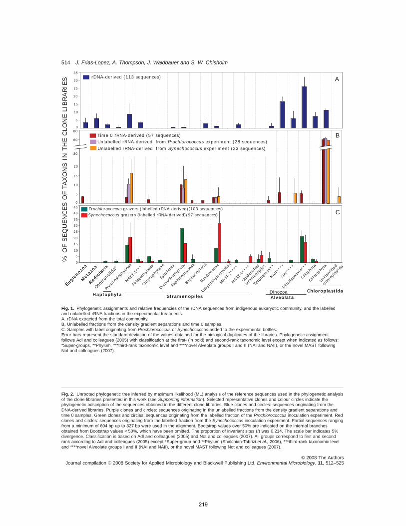
0
5
10
20
30
15
60
800
5
10
15
20
25
30
35
rDNA-derived (113 sequences)
Time 0 rRNA-derived (57 sequences)
Unlabelled rRNA-derived from Prochlorococcus experiment (28 sequences)
Unlabelled rRNA-derived from Synechococcus experiment (23 sequences)
A
B
Haptophyta Stramenopiles
Eugle
nozo
a
Meta
zoa
Rad
iola
ria
Cen
troh
elida*
Prym
nesiop
hyce
ae
MAS
T-1*
**
Pelago
phyc
eae
Chr
ysop
hyce
ae
Synu
lare
s
Dictyoc
hoph
ycea
e
Raph
idop
hyce
ae
Bacilla
riop
hyta
Bolid
omonas
Laby
rint
hylomyc
etes
MAS
T-7*
***
MAS
T-6*
***
Unide
ntified
stra
men
opile
s
Telone
mia**
NAI
I***
*
NAI
****
Ciliop
hora
Chlor
ophy
ta
Alveolata
ChloroplastidaDinoflage
llata**
*
Unide
ntified
chloro
plas
tida
0
5
10
15
20
25
30
35
40
45
Dinozoa
Synechococcus grazers (labelled rRNA-derived)(97 sequences)
Prochlorococcus grazers (labelled rRNA-derived)(103 sequences)
% O
F S
EQ
UEN
CES O
F T
AXO
NS I
N T
HE C
LO
NE L
IBRARIE
S
C
Fig. 1. Phylogenetic assignments and relative frequencies of the rDNA sequences from indigenous eukaryotic community, and the labelledand unlabelled rRNA fractions in the experimental treatments.A. rDNA extracted from the total community.B. Unlabelled fractions from the density gradient separations and time 0 samples.C. Samples with label originating from Prochlorococcus or Synechococcus added to the experimental bottles.Error bars represent the standard deviation of the values obtained for the biological duplicates of the libraries. Phylogenetic assignmentfollows Adl and colleagues (2005) with classification at the first- (in bold) and second-rank taxonomic level except when indicated as follows:*Super-groups, **Phylum, ***third-rank taxonomic level and ****novel Alveolate groups I and II (NAI and NAII), or the novel MAST followingNot and colleagues (2007).
Fig. 2. Unrooted phylogenetic tree inferred by maximum likelihood (ML) analysis of the reference sequences used in the phylogenetic analysisof the clone libraries presented in this work (see Supporting information). Selected representative clones and colour circles indicate thephylogenetic adscription of the sequences obtained in the different clone libraries. Blue clones and circles: sequences originating from theDNA-derived libraries. Purple clones and circles: sequences originating in the unlabelled fractions from the density gradient separations andtime 0 samples. Green clones and circles: sequences originating from the labelled fraction of the Prochlorococcus inoculation experiment. Redclones and circles: sequences originating from the labelled fraction from the Synechococcus inoculation experiment. Partial sequences rangingfrom a minimum of 604 bp up to 827 bp were used in the alignment. Bootstrap values over 50% are indicated on the internal branchesobtained from Bootstrap values < 50%, which have been omitted. The proportion of invariant sites (I) was 0.214. The scale bar indicates 5%divergence. Classification is based on Adl and colleagues (2005) and Not and colleagues (2007). All groups correspond to first and secondrank according to Adl and colleagues (2005) except *Super-group and **Phylum (Shalchian-Tabrizi et al., 2006), ***third-rank taxonomic leveland ****novel Alveolate groups I and II (NAI and NAII), or the novel MAST following Not and colleagues (2007).
514 J. Frias-Lopez, A. Thompson, J. Waldbauer and S. W. Chisholm
© 2008 The AuthorsJournal compilation © 2008 Society for Applied Microbiology and Blackwell Publishing Ltd, Environmental Microbiology, 11, 512–525
219
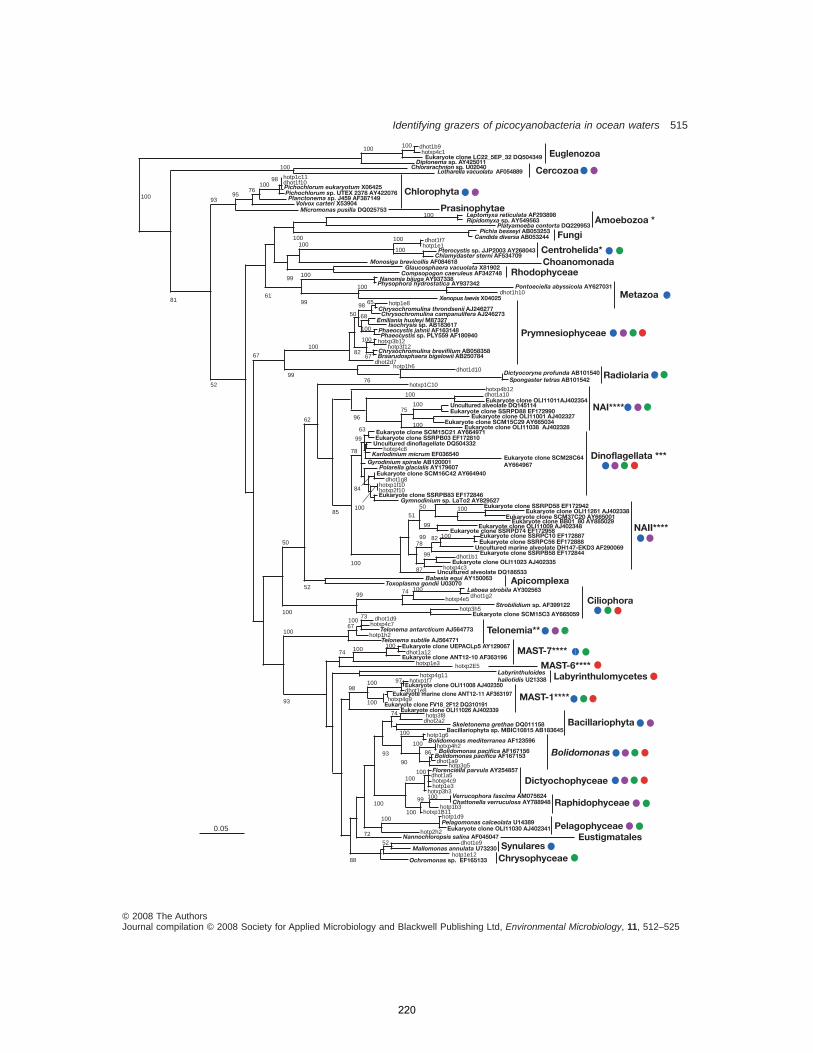
dhot1e952
hotp2h2
hotp1d9100hotxp1B11
hotp1b310099hotxp3h3
hotp1e3hotxp4c9dhot1a5
100
100
hotp3g5dhot1a9
86hotxp4h2
100
100hotp1g6
90
100
93
100
72
88
hotxp4g9dhot1e8
hotxp1f797
100
10098
hotxp2E5hotxp4g11
hotxp1e3
dhot1a1210010074
hotp1h2
hotxp4c7dhot1d973
67
93
100
hotp3h5hotxp4e5 dhot1g2
10074
100
99
hotxp1C10
52
62
100
50
hotp1h6dhot2d7
hotp3f12hotxp3b12
67
100
100
68
hotp1e86598
82
50
100
99
67
dhot1h10100
99
100
hotp1e1dhot1f7
100
100100
99
100
100
61
dhot1f10hotp1c11
100
98100
7695
52
93
81
hotxp4c1dhot1b9100100
100
0.05
Euglenozoa
Cercozoa
Chlorophyta
Fungi
Amoebozoa *
Choanomonada
Centrohelida*
Metazoa
Rhodophyceae
Prymnesiophyceae
dhot1d10Radiolaria
NAI****
hotxp4c3
dhot1b199
10082
87
78
100
99
99
5051
hotxp2f10hotxp1f10
100
dhot1g884
hotxp4c8
63
100
78
99
85
hotxp4b12
100
10075
dhot1a10
96
100
76
Dinoflagellata ***
NAII****
Apicomplexa
Ciliophora
Telonemia**
MAST-7****
LabyrinthulomycetesMAST-6****
hotp3f8dhot2a2
74
MAST-1****
Bacillariophyta
Bolidomonas
Eustigmatales
Dictyochophyceae
Raphidophyceae
Pelagophyceae
Synulareshotp1e12
Chrysophyceae
Eukaryote clone LC22_5EP_32 DQ504349Diplonema sp. AY425011
Lotharella vacuolata AF054889Chlorarachnion sp. U02040
Micromonas pusilla DQ025753 Prasinophytae
Pichochlorum eukaryotum X06425Pichochlorum sp. UTEX 2378 AY422076Planctonema sp. J459 AF387149
Volvox carteri X53904
Ripidomyxa sp. AY549563 Leptomyxa reticulata AF293898
Platyamoeba contorta DQ229953
Candida diversa AB053244Pichia besseyi AB053253
Monosiga brevicollis AF084618Chlamydaster sterni AF534709Pterocystis sp. JJP2003 AY268043
Compsopogon caeruleus AF342748Glaucosphaera vacuolata X81902
Xenopus laevis X04025
Pontoeciella abyssicola AY627031Physophora hydrostatica AY937342Nanomia bijuga AY937338
Phaeocystis sp. PLY559 AF180940Phaeocystis jahnii AF163148
Isochrysis sp. AB183617Emiliania huxleyi M87327
Chrysochromulina campanulifera AJ246273Chrysochromulina throndsenii AJ246277
Braarudosphaera bigelowii AB250784Chrysochromulina brevifilum AB058358
Spongaster tetras AB101542
Dictyocoryne profunda AB101540
Eukaryote clone SCM15C29 AY665034Eukaryote clone OLI11001 AJ402327
Eukaryote clone SSRPD88 EF172990
Eukaryote clone OLI11038 AJ402328
Eukaryote clone OLI11011AJ402354Uncultured alveolate DQ145114
Eukaryote clone SCM15C3 AY665059
Laboea strobila AY302563
Strobilidium sp. AF399122
Eukaryote clone SCM28C64
AY664967
Eukaryote clone SSRPB03 EF172810 Eukaryote clone SCM15C21 AY664971
Uncultured dinoflagellate DQ504332
Karlodinium micrum EF036540
Gyrodinium spirale AB120001
Gymnodinium sp. LaTo2 AY829527Eukaryote clone SSRPB83 EF172846
Eukaryote clone SCM16C42 AY664940 Polarella glacialis AY179607
Eukaryote clone SSRPD58 EF172942
Eukaryote clone SSRPD74 EF172958Eukaryote clone OLI11009 AJ402348
Eukaryote clone OLI11023 AJ402335
Uncultured alveolate DQ186533
Eukaryote clone BB01_80 AY885029Eukaryote clone SCM37C20 AY665001
Eukaryote clone OLI11261 AJ402338
Eukaryote clone SSRPB58 EF172844
Eukaryote clone SSRPC56 EF172888Eukaryote clone SSRPC10 EF172887
Uncultured marine alveolate DH147-EKD3 AF290069
Babesia equi AY150063Toxoplasma gondii U03070
Telonema antarcticum AJ564773
Telonema subtile AJ564771
Eukaryote clone ANT12-10 AF363196
Eukaryote clone UEPACLp5 AY129067
Labyrinthuloides
haliotidis U21338
Eukaryote clone OLI11026 AJ402339
Eukaryote clone OLI11008 AJ402350
Eukaryote clone FV18_2F12 DQ310191
Eukaryote marine clone ANT12-11 AF363197
Bacillariophyta sp. MBIC10815 AB183645Skeletonema grethae DQ011158
Bolidomonas pacifica AF167156
Bolidomonas mediterranea AF123596
Bolidomonas pacifica AF167153
Florenciella parvula AY254857
Chattonella verruculosa AY788948Verrucophora fascima AM075624
Pelagomonas calceolata U14389Eukaryote clone OLI11030 AJ402341
Nannochloropsis salina AF045047
Mallomonas annulata U73230
Ochromonas sp. EF165133
Identifying grazers of picocyanobacteria in ocean waters 515
© 2008 The AuthorsJournal compilation © 2008 Society for Applied Microbiology and Blackwell Publishing Ltd, Environmental Microbiology, 11, 512–525
220
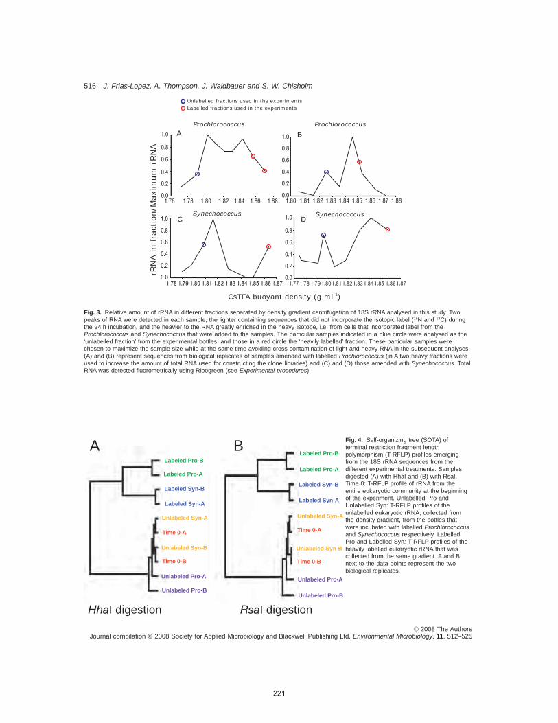
CsTFA buoyant density (g ml-1)
rRN
A in fra
ction/M
axim
um
rRN
A
C D
Prochlorococcus Prochlorococcus
Synechococcus Synechococcus
Labelled fractions used in the experiments
Unlabelled fractions used in the experiments
0.0
0.2
0.4
0.6
0.8
1.0
1.80 1.81 1.82 1.83 1.84 1.85 1.86 1.87 1.88
B
0.0
0.2
0.4
0.6
0.8
1.0
1.76 1.78 1.80 1.82 1.84 1.86 1.88
A
0.0
0.2
0.4
0.6
0.8
1.0
1.78 1.79 1.80 1.81 1.82 1.83 1.84 1.85 1.86 1.870.0
0.2
0.4
0.6
0.8
1.0
1.77 1.78 1.79 1.80 1.81 1.82 1.83 1.84 1.85 1.86 1.87
Fig. 3. Relative amount of rRNA in different fractions separated by density gradient centrifugation of 18S rRNA analysed in this study. Twopeaks of RNA were detected in each sample, the lighter containing sequences that did not incorporate the isotopic label (15N and 13C) duringthe 24 h incubation, and the heavier to the RNA greatly enriched in the heavy isotope, i.e. from cells that incorporated label from theProchlorococcus and Synechococcus that were added to the samples. The particular samples indicated in a blue circle were analysed as the‘unlabelled fraction’ from the experimental bottles, and those in a red circle the ‘heavily labelled’ fraction. These particular samples werechosen to maximize the sample size while at the same time avoiding cross-contamination of light and heavy RNA in the subsequent analyses.(A) and (B) represent sequences from biological replicates of samples amended with labelled Prochlorococcus (in A two heavy fractions wereused to increase the amount of total RNA used for constructing the clone libraries) and (C) and (D) those amended with Synechococcus. TotalRNA was detected fluorometrically using Ribogreen (see Experimental procedures).
Fig. 4. Self-organizing tree (SOTA) ofterminal restriction fragment lengthpolymorphism (T-RFLP) profiles emergingfrom the 18S rRNA sequences from thedifferent experimental treatments. Samplesdigested (A) with HhaI and (B) with RsaI.Time 0: T-RFLP profile of rRNA from theentire eukaryotic community at the beginningof the experiment. Unlabelled Pro andUnlabelled Syn: T-RFLP profiles of theunlabelled eukaryotic rRNA, collected fromthe density gradient, from the bottles thatwere incubated with labelled Prochlorococcus
and Synechococcus respectively. LabelledPro and Labelled Syn: T-RFLP profiles of theheavily labelled eukaryotic rRNA that wascollected from the same gradient. A and Bnext to the data points represent the twobiological replicates.
HhaI digestion
B
RsaI digestion
A Labeled Pro-B
Labeled Pro-A
Labeled Syn-B
Labeled Syn-A
Unlabeled Syn-A
Time 0-A
Time 0-B
Unlabeled Syn-B
Unlabeled Pro-A
Unlabeled Pro-B
Labeled Pro-B
Labeled Pro-A
Labeled Syn-B
Labeled Syn-A
Unlabeled Syn-A
Time 0-A
Time 0-B
Unlabeled Syn-B
Unlabeled Pro-A
Unlabeled Pro-B
516 J. Frias-Lopez, A. Thompson, J. Waldbauer and S. W. Chisholm
© 2008 The AuthorsJournal compilation © 2008 Society for Applied Microbiology and Blackwell Publishing Ltd, Environmental Microbiology, 11, 512–525
221
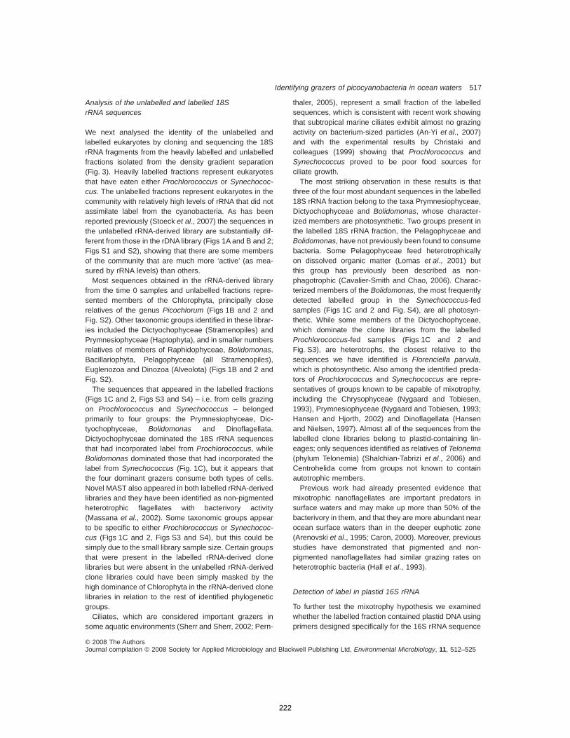
Analysis of the unlabelled and labelled 18S
rRNA sequences
We next analysed the identity of the unlabelled andlabelled eukaryotes by cloning and sequencing the 18SrRNA fragments from the heavily labelled and unlabelledfractions isolated from the density gradient separation(Fig. 3). Heavily labelled fractions represent eukaryotesthat have eaten either Prochlorococcus or Synechococ-
cus. The unlabelled fractions represent eukaryotes in thecommunity with relatively high levels of rRNA that did notassimilate label from the cyanobacteria. As has beenreported previously (Stoeck et al., 2007) the sequences inthe unlabelled rRNA-derived library are substantially dif-ferent from those in the rDNA library (Figs 1A and B and 2;Figs S1 and S2), showing that there are some membersof the community that are much more ‘active’ (as mea-sured by rRNA levels) than others.
Most sequences obtained in the rRNA-derived libraryfrom the time 0 samples and unlabelled fractions repre-sented members of the Chlorophyta, principally closerelatives of the genus Picochlorum (Figs 1B and 2 andFig. S2). Other taxonomic groups identified in these librar-ies included the Dictyochophyceae (Stramenopiles) andPrymnesiophyceae (Haptophyta), and in smaller numbersrelatives of members of Raphidophyceae, Bolidomonas,Bacillariophyta, Pelagophyceae (all Stramenopiles),Euglenozoa and Dinozoa (Alveolota) (Figs 1B and 2 andFig. S2).
The sequences that appeared in the labelled fractions(Figs 1C and 2, Figs S3 and S4) – i.e. from cells grazingon Prochlorococcus and Synechococcus – belongedprimarily to four groups: the Prymnesiophyceae, Dic-tyochophyceae, Bolidomonas and Dinoflagellata.Dictyochophyceae dominated the 18S rRNA sequencesthat had incorporated label from Prochlorococcus, whileBolidomonas dominated those that had incorporated thelabel from Synechococcus (Fig. 1C), but it appears thatthe four dominant grazers consume both types of cells.Novel MAST also appeared in both labelled rRNA-derivedlibraries and they have been identified as non-pigmentedheterotrophic flagellates with bacterivory activity(Massana et al., 2002). Some taxonomic groups appearto be specific to either Prochlorococcus or Synechococ-
cus (Figs 1C and 2, Figs S3 and S4), but this could besimply due to the small library sample size. Certain groupsthat were present in the labelled rRNA-derived clonelibraries but were absent in the unlabelled rRNA-derivedclone libraries could have been simply masked by thehigh dominance of Chlorophyta in the rRNA-derived clonelibraries in relation to the rest of identified phylogeneticgroups.
Ciliates, which are considered important grazers insome aquatic environments (Sherr and Sherr, 2002; Pern-
thaler, 2005), represent a small fraction of the labelledsequences, which is consistent with recent work showingthat subtropical marine ciliates exhibit almost no grazingactivity on bacterium-sized particles (An-Yi et al., 2007)and with the experimental results by Christaki andcolleagues (1999) showing that Prochlorococcus andSynechococcus proved to be poor food sources forciliate growth.
The most striking observation in these results is thatthree of the four most abundant sequences in the labelled18S rRNA fraction belong to the taxa Prymnesiophyceae,Dictyochophyceae and Bolidomonas, whose character-ized members are photosynthetic. Two groups present inthe labelled 18S rRNA fraction, the Pelagophyceae andBolidomonas, have not previously been found to consumebacteria. Some Pelagophyceae feed heterotrophicallyon dissolved organic matter (Lomas et al., 2001) butthis group has previously been described as non-phagotrophic (Cavalier-Smith and Chao, 2006). Charac-terized members of the Bolidomonas, the most frequentlydetected labelled group in the Synechococcus-fedsamples (Figs 1C and 2 and Fig. S4), are all photosyn-thetic. While some members of the Dictyochophyceae,which dominate the clone libraries from the labelledProchlorococcus-fed samples (Figs 1C and 2 andFig. S3), are heterotrophs, the closest relative to thesequences we have identified is Florenciella parvula,which is photosynthetic. Also among the identified preda-tors of Prochlorococcus and Synechococcus are repre-sentatives of groups known to be capable of mixotrophy,including the Chrysophyceae (Nygaard and Tobiesen,1993), Prymnesiophyceae (Nygaard and Tobiesen, 1993;Hansen and Hjorth, 2002) and Dinoflagellata (Hansenand Nielsen, 1997). Almost all of the sequences from thelabelled clone libraries belong to plastid-containing lin-eages; only sequences identified as relatives of Telonema
(phylum Telonemia) (Shalchian-Tabrizi et al., 2006) andCentrohelida come from groups not known to containautotrophic members.
Previous work had already presented evidence thatmixotrophic nanoflagellates are important predators insurface waters and may make up more than 50% of thebacterivory in them, and that they are more abundant nearocean surface waters than in the deeper euphotic zone(Arenovski et al., 1995; Caron, 2000). Moreover, previousstudies have demonstrated that pigmented and non-pigmented nanoflagellates had similar grazing rates onheterotrophic bacteria (Hall et al., 1993).
Detection of label in plastid 16S rRNA
To further test the mixotrophy hypothesis we examinedwhether the labelled fraction contained plastid DNA usingprimers designed specifically for the 16S rRNA sequence
Identifying grazers of picocyanobacteria in ocean waters 517
© 2008 The AuthorsJournal compilation © 2008 Society for Applied Microbiology and Blackwell Publishing Ltd, Environmental Microbiology, 11, 512–525
222
in chloroplast DNA (Table S1). We designed theseprimers specifically to amplify plastid 16S rRNA genes,but not Prochlorococcus and Synechococcus 16S rRNA,since the latter would have dominated our signal. Thismeant we did not recover as many plastid sequences aswe might have if we had used published plastid 16S rRNAprimers (Fuller et al., 2006), but this was an unavoidablelimitation, given the experimental design.
Two of the primer sets for plastid 16S rRNA (primerssets 6 and 15, Table S1) yielded PCR products of theexpected size, and in the case of primer set 15 theproduct was long enough (approximately 650 bp) to besequenced and analysed. Although it is difficult to deter-mine the exact affiliation of these chloroplast sequencesgiven the short length of the amplified PCR product, andthe limited coverage of chloroplast sequences from differ-ent plastid-containing phylogenetic groups in the data-base, the phylogenetic analysis showed that the amplifiedsequences from the labelled fraction were indeed fromchloroplasts (Fig. S5). Furthermore, the phylogeneticanalysis showed that the closest relatives of the chloro-plasts identified in our labelled fraction were related toBolidomonas mediterranea and diatom chloroplasts(Fig. S5). As there are a limited number of chloroplastsequences representing other groups of Stramenopiles inthe databases, and given the short size of the analysedproduct, the exact phylogenetic affiliation of thesesequences is not entirely clear. The key finding, however,is that all of the sequences obtained cluster with chloro-plasts indicating that the heavy label ended up in eukary-otic cells capable of photosynthesis.
Analysis of alternative routes for label incorporation
In this and other types of labelling experiments withnatural populations, the possibility that the isotopic labelmight have been acquired by protists via a route otherthan phagotrophic predation must be considered. Forexample, it is conceivable that the label might havepassed through a dissolved phase, either organic or inor-ganic, and was acquired through non-phagotrophic nutri-ent uptake. Alternatively, the label could have been initiallyacquired by bacterial heterotrophs that were subse-quently grazed by phagotrophs. Below we consider eachof these possibilities in turn, and present evidencethat they do not appear to be playing a role in theseexperiments.
The labelled cyanobacterial biomass could have beentransformed to dissolved inorganic carbon (DIC) throughrespiration, either by the picocyanobacteria themselves orby other heterotrophs. Had a substantial amount of theadded biomass been respired, that labelled carbon wouldhave become broadly available for fixation by all of theautotrophs in the sample, which would then appear in the
labelled fraction. In fact, the most abundant sequences inthe unlabelled rRNA-derived clone libraries – the photo-autotrophic Chlorophyta – were not represented in thelabelled fraction (Figs 1B and C and 2, Figs S2–S4). Thisdemonstrates that no significant quantity of labelled DICwas available for photosynthetic fixation, and passage ofthe label through the dissolved carbonate pool can beexcluded.
Another possibility would be that the initially supplied,isotopically labelled biomass might have entered the dis-solved organic carbon (DOC) pool by exudation, lysis or‘sloppy feeding’ by zooplankton. The latter two mecha-nisms would result in substantial declines in the picocy-anobacterial population during the experiment; however,the concentration of picocyanobacteria did not changedramatically over the 24 h of incubation. In all cases theinitial and final concentration, after 24 h of incubation, ofboth Prochlorococcus and Synechococcus was of 105
cells ml-1, suggesting that mechanisms involving celldeath (including lysis and sloppy feeding) did not releaselarge amounts of biomass into the dissolved phase. Toconsider exudation, we can use the Prochlorococcus
addition experiment as an example. Prochlorococcus
MED4 cells were added to the seawater sample at aconcentration of 1.7 ¥ 105 per ml and typically containabout 60 fg of carbon per cell (Bertilsson et al., 2003). Ifwe imagine that the added Prochlorococcus couldsomehow exude all of their initial labelled carbon as DOC– while suffering no great decline in cell numbers – this isequivalent to the addition of 0.9 mM of 13C-DOC, clearly anupper limit for the potential contribution of the isotopicallylabelled Prochlorococcus to the DOC pool. Typicalsurface total DOC concentrations at station ALOHA,where the samples for this study were taken, are around75 mM, of which 40 mM is likely refractory organic matterthat turns over very slowly (Carlson, 2002). Hence there isroughly 35 mM of labile DOC available for rapid het-erotrophic consumption. Addition of Prochlorococcus-derived 13C-DOC to this could result in a 36 mM pool oflabile DOC with maximum 13C content of 3.5 atom%,which is in turn the upper limit for labelling by DOC con-sumption. Similar considerations limit the 13C content ofDOC in the Synechococcus addition experiments to 10.6atom%.
Next, we consider the extent of labelling of the heavyRNA fractions in our incubation experiments. The differ-ence in buoyant density between heavy and light RNAfractions in these experiments ranged from 0.034 to0.078 g ml-1 (Fig. 3), equal to or exceeding the buoyancydifferences (0.035–0.04 g ml-1) observed by Lueders andcolleagues (2004) for 100% 13C-labelled SSU rRNA. Thislarge difference in buoyant density suggests that theheavy fractions analysed in this experiment were highlylabelled, likely in excess of 90 atom% 13C. This is far
518 J. Frias-Lopez, A. Thompson, J. Waldbauer and S. W. Chisholm
© 2008 The AuthorsJournal compilation © 2008 Society for Applied Microbiology and Blackwell Publishing Ltd, Environmental Microbiology, 11, 512–525
223
greater than the 3–11% possible from DOC consumption,even under the assumption of maximally rapid exudationby the added cyanobacteria. The buoyancy differencesobserved here in excess of the ~0.4 g ml-1 reported byLueders and colleagues (2004) may reflect 15N incorpo-ration and/or differences in centrifugation conditions. Inany event, the heavy RNA in these experiments is muchtoo highly labelled to derive from heterotrophic consump-tion of DOC.
A third, even more mechanistically complicated possi-bility is the direct and specific consumption of picocyano-bacteria by heterotrophic bacteria or the consumption oflabelled DOC exuded by, or otherwise released from,the picocyanobacteria by those heterotrophs. Protistanpredators can then graze on these labelled heterotrophs.If this occurred, the 18S sequences observed in the heavyfraction would reflect grazing activity, though not specifi-cally on Prochlorococcus or Synechococcus. Underthis scenario, a subset of heterotrophic bacteria wouldbecome highly labelled, and their RNA should be found inthe heavy fraction. To address this possibility, we con-structed 16S rRNA clone libraries as described in Experi-
mental procedures. If there had been transfer of labelledorganic matter through heterotrophic bacteria at the levelneeded to fractionate differentially in a CsTFA gradient wewould expect to find 16S rRNA sequences from het-erotrophic bacteria. Forty-three clones from the labelledfractions were sequenced. Seventeen clones came fromthe fraction obtained from the bottles inoculated withlabelled Prochlorococcus MED4 and in all cases thebest BLASTN match for those sequences correspondedto Prochlorococcus marinus. Similarly, 26 clones comingfrom the fraction obtained from the bottles inoculated withlabelled Synechococcus WH8102 and in all cases thebest BLASTN match corresponded to Synechococcus.Additionally, 11 clones coming from the unlabelled fractionfrom the Prochlorococcus experiment were sequencedand 18% of those corresponded to P. marinus, while therest were sequences from heterotrophic bacteria. Theseresults demonstrate that 16S rRNA compositions of thelabelled and unlabelled fractions were indeed distinct, andthat heterotrophic bacteria did not appear to becomehighly labelled over the course of the incubation. We thusconclude that the labelled eukaryotes did not obtain theirlabel indirectly via predation of heterotrophic bacteria.
Conclusions and implications
The reproducibility and internal consistency of theresults obtained in the study indicate that the use ofRNA-SIP for studying the marine microbial food-webs in
situ has tremendous potential. There are a multitude ofvariations on this experimental design that could yieldmany insights into the specific pathways of the flow of
carbon and energy in the marine food-web. These par-ticular results also reveal that a significant fraction ofthe eukaryotes that we identified as grazing specificallyon Prochlorococcus and Synechococcus were likelymixotrophs – i.e. cells that utilize both phototrophy andphagotrophic heterotrophy as a way of obtaining nutri-ents and energy (Raven, 1997; Jones, 2000). While afew studies have provided evidence of the importance ofmixotrophy in marine aquatic environments (Arenovskiet al., 1995; An-Yi et al., 2007; Unrein et al., 2007), thisis the first study to identify marine mixotrophs throughtheir grazing activity on specific prey.
The adoption of mixotrophy as a survival strategy underoligotrophic oceanic conditions might confer a fitnessadvantage for a number of reasons (Raven, 1997). First,phagotrophy may be a way for relatively large eukaryoticcells to acquire inorganic nutrients such as N, P and Fein oligotrophic waters. Arenovski and colleagues (1995)presented experimental evidence of a decrease in theabundance of mixotrophic phototrophs under nutrientenrichment conditions, suggesting that phagotrophy isused under low dissolved nutrient concentrations, condi-tions that are normal in surface oligotrophic water. Withtheir larger surface to volume ratio, picocyanobacteria likeProchlorococcus and Synechococcus likely have anadvantage over larger eukaryotic cells in acquiring dis-solved nutrients. Consuming cyanobacteria may also be away for the larger cells to increase their relative fitness byreducing the abundance of their competitors for nutrients.Mixotrophy has been linked to survival of nanoflagellatesunder nutrient limitation (Unrein et al., 2007) and it hasbeen shown that algal flagellates increase bacterivoryunder phosphate limitation (Nygaard and Tobiesen,1993). Moreover, the metabolic costs of adding phag-otrophic machinery to an otherwise photosyntheticmetabolism may be rather low in comparison with thepotential benefits (Raven, 1997).
Predation by mixotrophs also has implications for ourunderstanding of the population dynamics of marine pico-cyanobacteria. While picocyanobacteria are generally thenumerically dominant phytoplankton in stratified olig-otrophic open-ocean waters, they usually do not bloom(i.e. increase markedly in cell concentrations) in responseto episodic nutrient supplies (Mann and Chisholm, 2000).This behaviour has been explained by concomitantincreases in grazing rates, implying that these grazers areable to respond very quickly to shifts in prey growth andquality. Our identification of mixotrophic predators mayshed further light on this dynamic: eukaryotic mixotrophsdirectly exploit the same episodic supplies of dissolvednutrients as their picocyanobacterial prey, and thus couldgrow faster, through stimulated autotrophy, as nutrientsbecome more abundant. As their populations grow andconsume the available nutrients, they may shift towards
Identifying grazers of picocyanobacteria in ocean waters 519
© 2008 The AuthorsJournal compilation © 2008 Society for Applied Microbiology and Blackwell Publishing Ltd, Environmental Microbiology, 11, 512–525
224
phagotrophy, increasing the mortality rate of cyanobacte-ria, preventing bloom formation even in the face of rapidgrowth rates. This hypothesis is directly testable using theapproach we have described.
As evidence increasingly points towards the mix-otrophic capabilities of both nominally photo- and het-erotrophic organisms it is becoming clear that a sharpdistinction between photosynthetic and predatory lif-estyles is a false dichotomy. It is likely that marine protistsutilize a spectrum of trophic strategies, ranging betweenobligate photoautotrophic and strictly phagotrophic endmembers and occupying nearly all gradations in between(Sanchez-Puerta et al., 2007). Further investigationsregarding other ocean sites and different depths areneeded to confirm the potential importance of mixotrophyas a common metabolic strategy for grazes feeding onpicocyanobacteria.
Experimental procedures
Sampling and incubation conditions
Prochlorococcus MED4 and Synechococcus WH8102 weregrown for 4 days at 19°C under continuous cool white light(16.6 mmol Q m-2 s-1) in artificial seawater medium (Rippkaet al., 2000) amended with 6 mM 13C-sodium bicarbonate and800 mM 15N-ammonium chloride. Cells were harvested bycentrifugation at 8000 g for 15 min and washed twice in unla-belled artificial seawater medium and re-suspended in thesame medium. Cells were counted by flow cytometry to havean estimate of the volume of inoculum to be used in theexperiment, in order to have a final concentration of picocy-anobacteria similar to the concentration found in naturalsamples (approximately 105 cells ml-1). Final isotopic enrich-ment of the cultures was measured by mass spectrometry atUC Davis Stable Isotope Facility using on-line combustion(Europa Integra): atom% 13C for Prochlorococcus MED4 was98.86% and for Synechococcus WH8102 84.20% andatom% 15N for Prochlorococcus MED4 was 61.13% and forSynechococcus WH8102 39.83%. These cultures were thentransported overnight in the dark to the field site for use in thegrazing experiments.
Samples of ocean surface water (3–5 m depth) were col-lected in 500 ml acid cleaned bottles during the month ofMarch 2006 as a part of HOT cruise 179, and inoculated witheither labelled Prochlorococcus MED4 or Synechococcus
WH8102 at a final concentration of 105 cells ml-1. All ship-board incubations were performed in duplicate and analysedindependently. The incubations were set in an on-deck incu-bator, which was constantly re-circulated with surface seawa-ter to maintain temperature. Two samples of 200 ml werecollected at the beginning of the experiment as a control toidentify the initial eukaryotic community. Samples of 250 mlwere collected from the bottles with added labelled Prochlo-
rococcus and Synechococcus after 24 h of incubation. The24 h period allowed enough time for the labelled isotopes tobe incorporated into the nucleic acids of the grazers yetprevented both significant changes in the eukaryotic commu-nity, and potential indirect incorporation of labelled isotopes
that could occur during an extended incubation. All watersamples were filtered through 0.2-mm-pore-size membranesand preserved in RNAlater at -80°C until analysis.
DNA and RNA extraction, gradient fractionation
and cDNA synthesis
RNAlater was removed by washing the filters with cold 70%ethanol. DNA was extracted following Coffroth and col-leagues (1992) protocol. Filters were placed in 0.5 ml ofCTAB (hexadecyltrimethyl ammonium bromide) buffer (1.4 MNaCl, 20 mM EDTA, 100 mM Tris-HCl pH 8.0, 0.2% CTABand 0.2% 2-mercapthoethanol) and the tubes were placed ina mini-bead beater (BioSpec Products, Bartlesville, OK,USA) and vortexed for 2 min at the maximum speed(4800 r.p.m.) to re-suspend the cells. Proteinase K wasadded to a final concentration of 0.1 mg ml-1 and sampleswere incubated at 65°C for 1 h. An equal volume of chloro-form was added, mixed and spun at 14 000 g for 10 min. Theaqueous layer was transferred to a new tube and DNA wasextracted with an equal volume of phenol : chloroform :isoamyl alcohol (25:24:1). Finally, DNA was precipitated byaddition of 2 vols of cold 95% ethanol without addition ofadditional salt. Pellet was washed twice with 70% coldethanol dried and re-suspended in water.
For RNA extraction filters were placed in 100 ml of 10 mMTris-HCl pH 8.0, 4 ml of RNase inhibitor (Ambion, Austin, TX,USA) and 2 ml lysozyme (50 mg ml-1). Samples were incu-bated for 30 min at 37°C. An additional 2 ml of the 50 mg ml-1
lysozyme solution was added and the samples were incu-bated again for 30 min at 37°C. Total RNA was immediatelyextracted by a mirVana RNA isolation kit (Ambion, Austin, TX,USA).
Labelled and unlabelled RNA were separated by densitygradient centrifugation, performed according to the protocolof Lueders and colleagues (2004). Centrifugation media wereprepared by mixing 4.5 ml of a 2 g ml-1 CsTFA stock solution(Amersham Pharmacia Biotech), up to 1 ml of gradient buffer(GB; 0.1 M Tris-HCl pH 8; 0.1 M KCl; 1 mM EDTA) and RNAextracts (up to 500 ng). Additionally, 175 ml of formamide wasadded to centrifugation media to guarantee that RNA wasdenatured. The average density of all prepared gradientswas checked with an AR200 digital refractometer (LeicaMicrosystems), and adjusted by adding small volumes of Cssalt solution or gradient buffer, if necessary. 18S rRNA wasresolved in CsTFA gradients with an average density of1.8316 g ml-1 at 20°C. Quick-Seal Polyallomer tubes, 3.9 ml(Beckmann Instruments), were filled up with centrifugationmedia plus sample, and centrifuged in an Optima TLXultracentrifuge using a TLN100 vertical rotor (BeckmannInstruments). Centrifugation conditions were > 60 h at61 000 r.p.m. (131 000 g).
Centrifuged gradients were fractionated from bottom to topinto 12 equal fractions (~400 ml). A precisely controlled flowrate was achieved by displacing the gradient medium withwater at the top of the tube using a syringe pump (HarvardApparatus). The density of 15 ml from each collected fractionwas determined using an AR200 digital refractometer (LeicaMicrosystems). Total RNA was precipitated with 1 vol. of iso-propanol. Precipitates from gradient fractions were washedonce with 70% ethanol and re-suspended in 25 ml of EB for
520 J. Frias-Lopez, A. Thompson, J. Waldbauer and S. W. Chisholm
© 2008 The AuthorsJournal compilation © 2008 Society for Applied Microbiology and Blackwell Publishing Ltd, Environmental Microbiology, 11, 512–525
225
subsequent determination of total RNA using RiboGreen(Molecular Probes, Invitrogen, Carlsbad, CA, USA) assays.
Primers for 18S rRNA eukaryotic genes were designedusing the Design Probes tool from the ARB software (Ludwiget al., 2004): EukF (5!-GGGTTCGATTCCGGAGAG-3!) EukR(5!-CCGTGTTGAGTCAAATT-3!) (Integrated DNA Technolo-gies Coralville, IA, USA). The database used contained27 887 complete sequences, all of eukaryotic origin. EukFprimer matched 19 378 sequences with 0 mismatches and23 459 sequences with one mismatch. EukR primer matched25 739 sequences with 0 mismatches and 27 447 sequenceswith one mismatch. They were tested in two cultures ofCafeteria, two cultures of Paraphysomonas and one cultureof Dullaniella, given in all cases the expected-size PCRproduct of approximately 830 bp.
Total RNA (0.5–5 ng) from fractions containing highlylabelled and unlabelled RNA was reverse transcribed with thespecific primers using the ThermoScript RT-PCR system(Invitrogen, Carlsbad, CA, USA). Reverse transcription wasperformed for 2 h at 50°C.
PCR reactions were performed using Taq DNA polymerasefrom NEB and primers at 2 mM concentration. After 5 minat 95°C, 35 cycles of denaturation (95°C, 45 s), annealing(52°C, 1 min), elongation (72°C, 1 min) and a final elongationstep (72°C, 10 min) were run in a MJ Research PTC 100Thermal Cycler. PCR products were cleaned up using aQIAquick PCR purification kit (Qiagen, Valencia, CA, USA)and cloned into either TOPO TA cloning vector (Invitrogen,Carlsbad, CA, USA) or pGEM-T cloning vector (Promega,Madison, WI, USA). Inserts were sequenced either atGenaissance Pharmaceuticals (New Haven, CT; now Cogen-ics, MA, USA) using primers for the T7 promoter region or inhouse using the same primer and the BigDye sequencing kit(Applied Biosystems, Foster City, CA, USA) at 1 min dena-turation and 25 cycles of 95°C-30 s, 50°C-20 s, 60°C-4 min,and finally held at 4°C. The reactions were then purified byethanol precipitation and run on an ABI PRISM 3730 (AppliedBiosystems) capillary DNA sequencer.
16S rRNA genes from bacteria present in the heavy frac-tions were cloned and sequenced using universal primers 9F(5!-GAGTTTGATYMTGGCTC) and 1509R (5!-GYTACCTTGTTACGACTT) (Integrated DNA Technologies Coralville, IA,USA). PCR and cloning were performed as described abovebut elongation at 72°C was extended to 2 min. Fragmentswere sequenced using theABI PRISM BigDye Terminator v3.1Cycle Sequencing Kit (Applied Biosystems, Warrington, UK)and primers for the T7 promoter region.
Taxonomic affiliation and phylogenetic analysis
Vector contamination was assessed using VecScreen (http://www.ncbi.nlm.nih.gov/VecScreen/VecScreen.html). On thebasis of the evaluation by the CHECK_CHIMERA program of theRibosomal Database Project (Maidak et al., 2001) onlysequences that showed no evidence for potential chimericgene artefacts were analysed.
Preliminary taxonomic affiliation of the sequences wasdetermined using BLASTN against the GenBank nr database(March 2005). Phylogenetic analysis was based on partialsequences trimmed to the shortest common denominator.A first analysis to confirm the taxonomic affiliation of the
sequences, and have a raw picture of the overall phyloge-netic tree, was performed using ARB software. Sequenceswere aligned against the eukaryotic database (SSRef release90 12.05.2007, SILVA database project http://www.arb-silva.de/ with 27 887 pre-aligned sequences) (Pruesse et al.,2007) in the ARB software version 07.02.20 (Ludwig et al.,2004) and performed using the Fast Alignment tool. Align-ments were edited manually and sequences were added tothe backbone tree using ARB’s ‘Parsimony insertion’ feature.
For maximum likelihood (ML), neighbour joining (NJ)-distance and maximum parsimony (MP) analyses, align-ments were generated using MAFFT (Katoh et al., 2002;2005) and edited manually using Sequence AlignmentEditor v2.0 (http://tree.bio.ed.ac.uk/software/seal/). Maximumparsimony analysis was performed using the ‘fast’ stepwise-addition algorithm in PAUP 4.0b10 (Altivec) with 1000 boot-straps replicates. For each alignment the best DNAsubstitution model was evaluated using MrModeltest 2.2(Nylander, 2004), which ranked General Time Reversible-gamma-Proportion invariant (GTR+g+I) best model in allcases. Maximum likelihood analysis was performed using thesoftware PHYML_v2.4.4 (Guindon and Gascuel, 2003) andGTR as a substitution model with 100 bootstraps replicates.Neighbour joining-distance analysis was performed usingPAUP 4.0b10 (Altivec) using the also GTR as a substitutionmodel, with 1000 bootstraps replicates, and the values ofGamma-shape and proportion of invariable sites estimatedby PHYML. Trees were visualized and plotted using NJPlotv2.1 (Perriere and Gouy, 1996).
T-RFLP analysis
Fluorescently labelled PCR products for the T-RFLP analysiswere generated by the PCR protocol described above, using aFAM-labelled forward primer. PCR products were digestedwith the restriction endonucleases HhaI and RsaI (NewEngland Biolabs, Ipswich, MA, USA). The resulting fluorescentterminal fragments were resolved and analysed at the Roy J.Carver Biotechnology Center (University of Illinois at Urbana-Champaign) using an ABI Prism 3730xl Analyser automatedsequencer, and GeneMapper version 3.7 software.
Clustering of the different T-RFLP profiles was performedusing the Self-Organizing Tree Algorithm (SOTA) from theGEPAS 4.0 (GEPAS website http://www.gepas.org).
Chloroplast 16S rRNA analysis
Labelled fractions from both Prochlorococcus and Synecho-
coccus grazers were tested for the presence of 16S rRNAchloroplast sequences. Specific oligonucleotides againstchloroplast sequences (SSRef release 90 12.05. 2007, SILVAdatabase project http://www.arb-silva.de/) were design usingthe Design Probes tool from the ARB software (Ludwig et al.,2004). Although a total of 16 sets of primers were used in theexperiment (Table S1), only the set of primers 15F (5!-TTAACTCAAGTG GCGGACGG) and 15R (AGTGTTAGTAATAGCCCAGTA) gave a PCR product long enough to besequenced. PCR reactions were performed using Taq DNApolymerase from NEB and primers at 2 mM concentration.After 5 min at 95°C, 40 cycles of denaturation (95°C, 45 s),
Identifying grazers of picocyanobacteria in ocean waters 521
© 2008 The AuthorsJournal compilation © 2008 Society for Applied Microbiology and Blackwell Publishing Ltd, Environmental Microbiology, 11, 512–525
226

annealing (56°C, 1 min), elongation (72°C, 1 min) and a finalelongation step (72°C, 10 min) were run in a MJ ResearchPTC 100 Thermal Cycler. PCR products were clean up usinga QIAquick PCR purification kit (Qiagen, Valencia, CA, USA)and cloned into TOPO TA cloning vector (Invitrogen, Carls-bad, CA, USA) and sequenced as described above.
Nucleotide sequence accession numbers
Ribosomal RNA sequences have been deposited atGenBank/EMBL under Accession Nos EF695076–EF695247and EU499951–EU500232.
Acknowledgements
This research was supported by grants from the NationalScience Foundation Biological Oceanography Program, theGordon and Betty Moore Foundation Marine MicrobiologyProgram and the Department of Energy GTL Program. JacobWaldbauer was supported in part by an NSF Graduate Fel-lowship. We thank Marcia Osborne for helpful discussionsand comments, which improved the manuscript. We alsothank Edward F. DeLong for access to the ABI PRISM3730 (Applied Biosystems) capillary DNA sequencer in hislaboratory.
References
Adl, S.M., Simpson, A.G.B., Farmer, M.A., Andersen, R.A.,Anderson, O.R., Barta, J.R., et al. (2005) The new higherlevel classification of eukaryotes with emphasis on thetaxonomy of protists. J Eukaryot Microbiol 52: 399–451.
Anderson, M.R., and Rivkin, R.B. (2001) Seasonal patterns ingrazing mortality of bacterioplankton in polar oceans: abipolar comparison. Aquat Microb Ecol 25: 195–206.
An-Yi, T., Chiang, K.-P., Chan, Y.-F., Lin, Y.-C., and Chang,J. (2007) Pigmented nanoflagellates in the coastal westernsubtropical Pacific are important grazers on Synechococ-
cus populations. J Plankton Res 29: 71–77.Arenovski, A.L., Lim, E.L., and Caron, D.A. (1995) Mix-
otrophic nanoplankton in oligotrophic surface waters of theSargasso Sea may employ phagotrophy to obtain majornutrients. J Plankton Res 17: 801–820.
Bertilsson, S., Berglund, O., Karl, D.M., and Chisholm, S.W.(2003) Elemental composition of marine Prochlorococcus
and Synechococcus: implications for the ecological stoichi-ometry of the sea. Limnol Oceanogr 48: 1721–1731.
Carlson, C.A. (2002) Production and removal processes.In Biogeochemistry of Marine Dissolved Organic Matter.Hansell, D.A., and Carlson, C.A. (eds). San Diego: Aca-demic Press, pp. 91–151.
Caron, D.A. (2000) Symbiosis and Mixotrophic among
Pelagic Microorganism. New York, USA: Wiley-Liss.Cavalier-Smith, T., and Chao, E.E.Y. (2006) Phylogeny and
megasystematics of phagotrophic heterokonts (kingdomChromista). J Mol Evol 62: 388–420.
Chisholm, S.W., Olson, R.J., Zettler, E.R., Waterbury, J.B.,Goericke, R., and Welschmeyer, N. (1988) A novel free-living prochlorophyte occurs at high cell concentrations inthe oceanic euphotic zone. Nature 334: 340–343.
Cho, B.C., Na, S.C., and Choi, D.H. (2000) Active ingestionof fluorescently labeled bacteria by mesopelagic het-erotrophic nanoflagellates in the East Sea, Korea. Mar Ecol
Prog Ser 206: 23–32.Christaki, U., Jacquet, S., Dolan, J.R., Vaulot, D., and Ras-
soulzadegan, F. (1999) Growth and grazing on Prochloro-
coccus and Synechococcus by two marine ciliates. Limnol
Oceanogr 44: 52–61.Christaki, U., Vazquez-Dominguez, E., Courties, C., and
Lebaron, P. (2005) Grazing impact of different het-erotrophic nanoflagellates on eukaryotic (Ostreococcus
tauri) and prokaryotic picoautotrophs (Prochlorococcus
and Synechococcus). Environ Microbiol 7: 1200–1210.Chrzanowski, T.H., and Símek, K. (1990) Prey-size selection
by freshwater fagellated protozoa. Limnol Oceanogr 35:1424–1436.
Coffroth, M.A., Lasker, H.R., Diamond, M.E., Bruenn, J.A.,and Bermingham, E. (1992) DNA fingerprints of a gorgon-ian coral: a method for detecting clonal structure in a veg-etative species. Mar Biol 114: 317–325.
Countway, P.D., Gast, R.J., Savai, P., and Caron, D.A.(2005) Protistan diversity estimates based on 18S rDNAfrom seawater incubations in the western North Atlantic.J Eukaryot Microbiol 52: 95–106.
Countway, P.D., Gast, R.J., Dennett, M.R., Savai, P., Rose,J.M., and Caron, D.A. (2007) Distinct protistan assem-blages characerize the euphotic zone and deep sea (2500m) of the western North Atlantic (Sargasso Sea and GulfStream). Environ Microbiol 9: 1219–1232.
Dollhopf, S.L., Hashsham, S.A., and Tiedje, J.M. (2001)Interpreting 16S rDNA T-RFLP data: application of self-organizing maps and principal component analysis todescribe community dynamics and convergence. Microb
Ecol 42: 495–505.Fuhrman, J.A., and Campbell, L. (1998) Marine ecology –
microbial microdiversity. Nature 393: 410–411.Fuller, N.J., Campbell, C., Allen, D.J., Pitt, F.D., Zwirglmaierl,
K., Le Gall, F., et al. (2006) Analysis of photosyntheticpicoeukaryote diversity at open ocean sites in the ArabianSea using a PCR biased towards marine algal plastids.Aquat Microb Ecol 43: 79–93.
del Giorgio, P.A., Gasol, J.M., Vaque, D., Mura, P., Agusti, S.,and Duarte, C.M. (1996) Bacterioplankton communitystructure: protists control net production and the proportionof active bacteria in a coastal marine community. Limnol
Oceanogr 41: 1169–1179.Gonzalez, J.M., Sherr, E.B., and Sherr, B.F. (1990) Size-
selective grazing on bacteria by natural assemblages ofestuarine flagellates and ciliates. Appl Environ Microbiol
56: 583–589.González, J.M., Iriberri, J., Egea, L., and Barcina, I. (1990)
Differential rates of digestion of bacteria by freshwater andmarine phagotrophic protozoa. Appl Environ Microbiol 56:1851–1857.
Guillou, L., Jacquet, S., Chretiennot-Dinet, M.J., and Vaulot,D. (2001) Grazing impact of two small heterotrophicflagellates on Prochlorococcus and Synechococcus. Aquat
Microb Ecol 26: 201–207.Guindon, S., and Gascuel, O. (2003) A simple, fast, and
accurate algorithm to estimate large phylogenies bymaximum likelihood. Syst Biol 52: 696–704.
522 J. Frias-Lopez, A. Thompson, J. Waldbauer and S. W. Chisholm
© 2008 The AuthorsJournal compilation © 2008 Society for Applied Microbiology and Blackwell Publishing Ltd, Environmental Microbiology, 11, 512–525
227
Hall, J.A., Barret, D.P., and James, M.R. (1993) The impor-tance of phytoflagellates, heterotrophic flagellate andciliate grazing on bacteria and picophytoplankton sizedprey in a coastal marine environment. J Plankton Res 15:1075–1086.
Hansen, P.J., and Hjorth, M. (2002) Growth and grazingresponses of Chrysochromulina ericina (Prymnesio-phyceae): the role of irradiance, prey concentration andpH. Mar Biol 141: 975–983.
Hansen, P.J., and Nielsen, T.G. (1997) Mixotrophic feedingof Fragilidium subglobosum (Dinophyceae) on threespecies of Ceratium: effects of prey concentration, preyspecies and light intensity. Mar Ecol Prog Ser 147: 187–196.
Ishii, N., Takeda, H., Doi, M., Fuma, S., Miyamoto, K., Yanag-isawa, K., and Kawabata, Z. (2002) A new method usingenhanced green fluorescent protein (EGFP) to determinegrazing rate on live bacterial cells by protists. Limnology 3:47–50.
Jones, R.I. (2000) Mixotrophy in planktonic protists: an over-view. Freshw Biol 45: 219–226.
Jurgens, K., and Matz, C. (2002) Predation as a shapingforce for the phenotypic and genotypic composition ofplanktonic bacteria. Antonie Van Leeuwenhoek 81: 413–434.
Jürgens, K., and Güde, H. (1994) The potential importance ofgrazing-resistant bacteria in planktonic systems. Mar Ecol
Prog Ser 112: 169–188.Katoh, K., Misawa, K., Kuma, K., and Miyata, T. (2002)
MAFFT: a novel method for rapid multiple sequence align-ment based on fast Fourier transform. Nucleic Acids Res
30: 3059–3066.Katoh, K., Kuma, K., Toh, H., and Miyata, T. (2005) MAFFT
version 5: improvement in accuracy of multiple sequencealignment. Nucleic Acids Res 33: 511–518.
Koton-Czaarnecka, M., and Chrost, R.J. (2003) Protozoansprefer large and metabolically active bacteria. Polish J
Environ Studies 12: 325–334.Landry, M.R., Lehner-Fournier, J.M., Sundstrom, J.A., Fager-
ness, V.L., and Selph, K.E. (1991) Discrimination betweenliving and heat-killed prey by a marine zooflagellate, Para-
physomonas vestita (Stokes). J Exp Mar Biol Ecol 146:139.
Lomas, M.W., Glibert, P.M., Clougherty, D.A., Huber, D.R.,Jones, J., Alexander, J., and Haramoto, E. (2001) Elevatedorganic nutrient ratios associated with brown tide algalblooms of Aureococcus anophagefferens (Pelago-phyceae). J Plankton Res 23: 1339–1344.
Ludwig, W., Strunk, O., Westram, R., Richter, L., Meier, H.,Yadhukumar, et al. (2004) ARB: a software environment forsequence data. Nucleic Acids Res 32: 1363–1371.
Lueders, T., Manefield, M., and Friedrich, M.W. (2004)Enhanced sensitivity of DNA- and rRNA-based stableisotope probing by fractionation and quantitative analysisof isopycnic centrifugation gradients. Environ Microbiol 6:73–78.
Lueders, T., Kindler, R., Miltner, A., Friedrich, M.W., andKaestner, M. (2006) Identification of bacterial micropreda-tors distinctively active in a soil microbial food web. Appl
Environ Microbiol 72: 5342–5348.Maidak, B.L., Cole, J.R., Lilburn, T.G., Parker, C.T., Jr,
Saxman, P.R., Farris, R.J., et al. (2001) The RDP-II(Ribosomal Database Project). Nucleic Acids Res 29: 173–174.
Manefield, M., Whiteley, A.S., Griffiths, R.I., and Bailey, M.J.(2002) RNA stable isotope probing, a novel means oflinking microbial community function to phylogeny. Appl
Environ Microbiol 68: 5367–5373.Mann, E.L., and Chisholm, S.W. (2000) Iron limits the cell
division rate of Prochlorococcus in the eastern equatorialPacific. Limnol Oceanogr 45: 1067–1076.
Massana, R., Guillou, L., Diez, B., and Pedros-Alio, C. (2002)Unveiling the organisms behind novel eukaryotic ribosomalDNA sequences from the ocean. Appl Environ Microbiol
68: 4554–4558.Not, F., Gausling, R., Azam, F., Heidelberg, J.F., and
Worden, A.Z. (2007) Vertical distribution of picoeukaryoticdiversity in the Sargasso Sea. Environ Microbiol 9: 1233–1252.
Nylander, J. (2004) MrModeltest v2. Program distributed bythe author. Evolutionary Biology Centre, Upssala Univer-sity.
Nygaard, K., and Tobiesen, A. (1993) Bacterivory in algae –a survival strategy during nutrient limitation. Limnol Ocean-
ogr 38: 273–279.Partensky, F., Hess, W.R., and Vaulot, D. (1999a) Prochlo-
rococcus, a marine photosynthetic prokaryote of globalsignificance. Microbiol Mol Biol Rev 63: 106–127.
Partensky, F., Blanchot, J., and Vaulot, D. (1999b) Differentialdistribution and ecology of Prochlorococcus and Synecho-
coccus in oceanic waters: a review. Bull Inst Océanogr
Monaco Special No. 19: 457–475.Pernthaler, J. (2005) Predation on prokaryotes in the water
column and its ecological implications. Nat Rev Microbiol
3: 537–546.Perriere, G., and Gouy, M. (1996) WWW-Query: an on-line
retrieval system for biological sequence banks. Biochimie
78: 364–369.Pruesse, E., Quast, C., Knittel, K., Fuchs, B.M., Ludwig, W.,
Peplies, J., and Glockner, F.O. (2007) SILVA: a compre-hensive online resource for quality checked and alignedribosomal RNA sequence data compatible with ARB.Nucleic Acids Res 35: 7188–7196.
Radajewski, S., Ineson, P., Parekh, N.R., and Murrell, J.C.(2000) Stable-isotope probing as a tool in microbialecology. Nature 403: 646–649.
Raven, J.A. (1997) Phagotrophy in phototrophs. Limnol
Oceanogr 42: 198–205.Rippka, R., Coursin, T., Hess, W., Lichtle, C., Scanlan, D.J.,
et al. (2000) Prochlorococcus marinus Chisholm et al.
1992 subsp. pastoris subsp. nov. strain PCC 9511, the firstaxenic chlorophyll a2/b2-containing cyanobacterium (Oxy-
photobacteria). Int J Syst Evol Microbiol 50 (Part 5): 1833–1847.
Sanchez-Puerta, M.V., Lippmeier, J.C., Apt, K.E., and Del-wiche, C.F. (2007) Plastid genes in a non-photosyntheticdinoflagellate. Protist 158: 105–117.
Shalchian-Tabrizi, K., Eikrem, W., Klaveness, D., Vaulot, D.,Minge, M.A., Le Gall, F., et al. (2006) Telonemia, a newprotist phylum with affinity to chromist lineages. Proc Biol
Sci 273: 1833–1842.Sherr, B.F., Sherr, E.B., and Fallon, R.D. (1987) Use of
Identifying grazers of picocyanobacteria in ocean waters 523
© 2008 The AuthorsJournal compilation © 2008 Society for Applied Microbiology and Blackwell Publishing Ltd, Environmental Microbiology, 11, 512–525
228
monodispersed, fluorescently labeled bacteria to estimatein situ protozoan bacterivory. Appl Environ Microbiol 53:958–965.
Sherr, E.B., and Sherr, B.F. (2002) Significance of predationby protists in aquatic microbial food webs. Antonie Van
Leeuwenhoek (Int J Gen Mol Microbiol) 81: 293–308.Sherr, E.B., Rassouladegan, F., and Sherr, B.F. (1989) Bac-
terivory by pelagic choreotrichous ciliates in coastal watersof the NW Mediterranean Sea. Mar Ecol Prog Ser 55:235–240.
Simek, K., and Chrzanowski, T.H. (1992) Direct and indirectevidence of size-selective grazing on pelagic bacteria byfreshwater nanoflagellates. Appl Environ Microbiol 58:3715–3720.
Stoeck, T., Zuendorf, A., Breiner, H.W., and Behnke, A.(2007) A molecular approach to identify active microbes inenvironmental eukaryote clone libraries. Microb Ecol 53:328–339.
Unrein, F., Massana, R., Alonso-Saez, L., and Gasol, J.M.(2007) Significant year-round effect of small mixotrophicflagellates on bacterioplankton in an oligotrophic coastalsystem. Limnol Oceanogr 52: 456–469.
Worden, A.Z., and Binder, B.J. (2003) Application of dilutionexperiments for measuring growth and mortality ratesamong Prochlorococcus and Synechococcus populationsin oligotrophic environments. Aquat Microb Ecol 30: 159–174.
Supporting information
Additional Supporting Information may be found in the onlineversion of this article:Fig. S1. Phylogenetic analysis of the sequences derivedfrom the 18S rDNA sequences in the indigenous microbialcommunity. Unrooted phylogenetic tree inferred by maximumlikelihood (ML) analysis. A total of 1090 positions used,including gaps (sequences ranging from a minimum of585 bp up to 893 bp), from an alignment of 203 partialsequences were used. Bootstrap values over 50% are indi-cated on the internal branches obtained from both ML, neigh-bour joining-distance methods (NJ-Dis) and using maximumparsimony (MP) (in the order ML/NJ-Dist/MP). Bootstrapvalues < 50%, or not supported at least in two of the analy-ses, have been omitted. The gamma distribution parameter(a) was estimated at 0.520; and the proportion of invariantsites (I) was 0.015. The scale bar indicates 10% divergence.The sequences from the duplicate biological samples areindicated as (dhot1) and (dhot2). Classification is based onAdl and colleagues (2005) and Not and colleagues (2007). Allgroups correspond to first and second rank according to Adland colleagues (2005) except *Super-group and **Phylum(Shalchian-Tabrizi et al., 2006).Fig. S2. Phylogenetic analysis of the sequences derivedfrom the 18S rDNA sequences in the unlabelled fractionsfrom the experiments (time 0 and blue circles in Fig. 2).Unrooted SSU rRNA-derived library phylogenetic tree ofeukaryotes inferred by maximum likelihood (ML) analysis. Atotal of 1058 positions used, including gaps (sequencesranging from a minimum of 512 bp up to 886 bp), from analignment of 200 partial sequences were used. Bootstrapvalues over 50% are indicated on the internal branches
obtained from both ML, neighbour joining-distance methods(NJ-Dis) and using maximum parsimony (MP) (in the orderML/NJ-Dist/MP). Bootstrap values < 50%, or not supported atleast in two of the analyses, have been omitted. The gammadistribution parameter (a) was estimated at 0.594; and theproportion of invariant sites (I) was 0.000. The scale barindicates 10% divergence. The sequences coming from theduplicate biological samples is indicated as (A) and (B).Clones colour code: dark red: sequences from the time 0sample, representing the metabolically active initial eukary-otic microbial community; purple: sequences from the unla-belled eukaryotic RNA obtained from the samples incubatedwith Prochlorococcus; orange: sequences from the unla-belled fraction from the samples incubated with Synechococ-
cus. Classification is based on Adl and colleagues (2005) andNot and colleagues (2007). All groups correspond to firstand second rank according to Adl and colleagues (2005)except when noted as follows: *Super-group and **Phylum(Shalchian-Tabrizi et al., 2006). ***Unidentified chloroplas-tida, BLAST results gave no clear match and the sequencesdid not cluster clearly with any of the second-rank groupsused in the tree that could indicate the exact affiliation of thesequence.Fig. S3. Phylogenetic analysis of the sequences derivedfrom the labelled 18S rDNA sequences (red circles in Fig. 2)from the experimental bottles amended with labelled Prochlo-
rococcus cells. Unrooted 18S rRNA-derived library phyloge-netic tree of eukaryotes inferred by maximum likelihood (ML)analysis. A total of 1145 positions used, including gaps(sequences ranging from a minimum of 545 bp up to 980 bp),from an alignment of 192 partial sequences were used. Boot-strap values over 50% are indicated on the internal branchesobtained from both ML, neighbour joining-distance methods(NJ-Dis) and using maximum parsimony (MP) (in the orderML/NJ-Dist/MP). Bootstrap values < 50%, or not supported atleast in two of the analyses, have been omitted. The gammadistribution parameter (a) was estimated at 0.512; and theproportion of invariant sites (I) was 0.000. The scale barindicates 10% divergence. The sequences coming from theduplicate biological samples is indicated as (A) and (B). Clas-sification is based on Adl and colleagues (2005) and Not andcolleagues (2007). All groups correspond to first and secondrank according to Adl and colleagues (2005) except whennoted as follows: *Super-group and **Phylum (Shalchian-Tabrizi et al., 2006). ***Unidentified stramenopiles, BLASTresults gave no clear match and the sequences did notcluster clearly with any of the second-rank groups used in thetree that could indicate the exact affiliation of the sequence.Fig. S4. Phylogenetic analysis of the sequences derivedfrom the labelled 18S rDNA sequences (red circles in Fig. 2)from the experimental bottles amended with labelled Syn-
echococcus cells. Unrooted 18S rRNA-derived library phylo-genetic tree of eukaryotes inferred by maximum likelihood(ML) analysis. A total of 1156 positions used, including gaps(sequences ranging from a minimum of 507 bp up to 977 bp),from an alignment of 188 partial sequences were used. Boot-strap values over 50% are indicated on the internal branchesobtained from both ML, neighbour joining-distance methods(NJ-Dis) and using maximum parsimony (MP) (in the orderML/NJ-Dist/MP). Bootstrap values < 50%, or not supported atleast in two of the analyses, have been omitted. The gamma
524 J. Frias-Lopez, A. Thompson, J. Waldbauer and S. W. Chisholm
© 2008 The AuthorsJournal compilation © 2008 Society for Applied Microbiology and Blackwell Publishing Ltd, Environmental Microbiology, 11, 512–525
229
distribution parameter (a) was estimated at 0.543; and theproportion of invariant sites (I) was 0.036. The scale barindicates 10% divergence. The sequences coming from theduplicate biological samples is indicated as (A) and (B). Clas-sification is based on Adl and colleagues (2005) and Not andcolleagues (2007). All groups correspond to first and secondrank according to Adl and colleagues (2005) except whennoted as follows: *Super-group and **Phylum (Shalchian-Tabrizi et al., 2006). ***Unidentified stramenopiles, BLASTresults gave no clear match and the sequences did notcluster clearly with any of the second-rank groups used in thetree that could indicate the exact affiliation of the sequence.Fig. S5. Phylogenetic tree 16S rRNA sequences from chlo-roplasts and bacteria inferred by maximum likelihood (ML)analysis. Blue: cyanobacterial 16S rRNA sequences. Green:sequences originating from the labelled fraction of theProchlorococcus inoculation experiment. Orange: sequencesoriginated from the labelled fraction from the Synechococcus
inoculation experiment. (A) and (B) represent the two biologi-cal replicates in the experiments. A total of 724 positions were
used, including gaps (sequences ranging from a minimumof 358 bp up to 668 bp), from an alignment of 103 partialsequences. Bootstrap values over 50% are indicated on theinternal branches obtained from ML, neighbour joining-distance methods (NJ-Dist) and using maximum parsimony(MP) (in the order ML/NJ-Dist/MP). Bootstrap values < 50%,or not supported at least in two of the analyses, have beenomitted. The proportion of invariant sites (I) was 0.241. Thescale bar indicates 10% divergence. An archaeal sequencewas used as out-group (Sulfolobus acidocaldarius).Table S1. Oligonucleotides used for the amplification of16S rRNA chloroplast genes from different groups definedbased on the ARB tree (SSRef release 90 12.05.2007) forthese group of sequences. F, forward primer. R, reverseprimer.
Please note: Wiley-Blackwell are not responsible for thecontent or functionality of any supporting materials suppliedby the authors. Any queries (other than missing material)should be directed to the corresponding author for the article.
Identifying grazers of picocyanobacteria in ocean waters 525
© 2008 The AuthorsJournal compilation © 2008 Society for Applied Microbiology and Blackwell Publishing Ltd, Environmental Microbiology, 11, 512–525
230
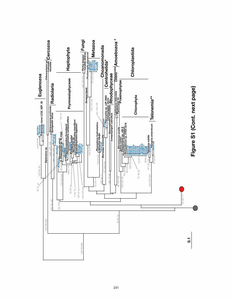
99
dh
ot1
d9
Te
lon
em
a a
nta
rcti
cu
md
ho
t1a
7Te
lon
em
a s
ub
tile
97
dh
ot2
c6
dh
ot1
g6
dh
ot2
h1
1d
ho
t2d
12
dh
ot2
g1
1
85
dh
ot1
c3
dh
ot1
a3
dh
ot1
b6
dh
ot1
b1
0d
ho
t1c
2
74
dh
ot1
d3
dh
ot1
e6
dh
ot1
f10
72
Pic
ho
ch
loru
m s
p.
UT
EX
23
78
Pic
ho
ch
loru
m e
uk
ary
otu
mP
lan
cto
ne
ma
sp
. J
45
-9
10
0
Vo
lvo
x c
art
eri
88
81
10
0
10
0
Co
mp
so
po
go
n c
ae
rule
us
Gla
uc
osp
ha
era
va
cu
ola
ta
94
Ch
lam
yd
aste
r ste
rni
Pte
roc
ysti
s s
p. JJP
-2003
dh
ot1
f7 M
on
osig
a b
revic
ollis
10
0
dh
ot1
a2
Na
no
mia
biju
ga
Ph
yso
ph
ora
hyd
rosta
tic
a
57
dh
ot2
f6d
ho
t1g
10
dh
ot1
h1
0d
ho
t2b
1d
ho
t2c
7P
on
toe
cie
lla
ab
yssic
ola
99
Xen
op
us la
evis
10
0
10
0
10
0
Ca
nd
ida
div
ers
aP
ich
ia b
esse
yi
70
10
0d
ho
t1g
1d
ho
t2b
11
dh
ot1
g3
Bra
aru
do
sp
ha
era
big
elo
wii
Ch
ryso
ch
rom
ulin
a b
revif
ilu
m
10
0
Iso
ch
rysis
sp
.E
milia
nia
hu
xle
yi
10
0
dh
ot2
d7
Ch
ryso
ch
rom
ulin
a c
am
pa
nu
life
raC
hry
so
ch
rom
ulin
a t
hro
nd
se
nii
dh
ot2
b4
95
dh
ot1
c9
Ph
ae
ocysti
s s
p. P
LY
559
Ph
ae
ocysti
s ja
hn
ii
58
82
dh
ot2
c4
99
dh
ot2
g7
10
0
53
dh
ot2
d6
dh
ot1
d1
0S
po
ng
aste
r te
tra
sD
icty
oc
ory
ne
pro
fun
da
10
0
10
01
00
Lo
thare
lla
Ch
lora
rach
nio
n s
p.
10
0D
iplo
ne
ma
sp
.d
ho
t1b
9E
uk
ary
ote
clo
ne
LC
22_5E
P_32
dh
ot2
d3
dh
ot1
h1
10
01
00
0.1
Rip
ido
myxa
sp
.L
ep
tom
yxa
re
tic
ula
taP
laty
am
oe
ba
Eu
gle
no
zo
a
Ce
rco
zo
a
Pry
mn
esio
ph
yc
ea
e
Fu
ng
i
Me
tazo
a
Ch
oa
no
mo
na
da
Rh
od
op
hyc
ea
eA
mo
eb
ozo
a *
Mic
rom
on
as p
usilla
P
rasin
op
hyta
e
Ch
loro
ph
yta
Te
lon
em
ia**
Ra
dio
lari
a
Ha
pto
ph
yta
Ce
ntr
oh
elid
a*
Ch
loro
pla
sti
da
93
10
0
10
0
10
0
10
0
52
10
01
00
10
0
10
0
10
0
10
0
95
10
01
00
95
79
10
01
00
96
86
53
10
0
87
66
55
10
0
97
87
92
60
92
10
0
69
89
99
10
0
10
0
72
67
72
88
78
10
0
83
10
0
66
10
0
84
10
0
95
98
10
09
9
10
0
10
0
10
0
10
01
00
95
10
0
10
0
10
01
00
10
0
10
0
10
01
00
10
01
00
10
09
6
76
91
71
-
-
-
-
--
- -
10
0
--
Fig
ure
S1 (
Co
nt.
ne
xt
pa
ge
)
-
vacu
ola
ta
co
nto
rta
231
La
byri
nth
ulo
ide
s h
alio
tid
is
dh
ot1
d6
Eu
ka
ryo
te c
lon
e O
LI1
1026
Eu
ka
ryo
te c
lon
e O
LI1
1008
dh
ot2
b5
dh
ot1
e8
68
Eu
ka
ryo
te c
lon
e F
V18_2F
12
dh
ot1
f1E
uk
ary
ote
ma
rin
e c
lon
e A
NT
12-1
11
00
92
dh
ot1
a5
Flo
ren
cie
lla
pa
rvu
laC
ha
tto
ne
lla
ve
rru
cu
losa
Ve
rru
co
ph
ora
fa
scim
a1
00
Pe
lag
om
on
as c
alc
eo
lata
Eu
ka
ryo
te c
lon
e O
LI1
1030
10
0
10
0O
ch
rom
on
as s
p.
dh
ot1
e9
Ma
llo
mo
na
s a
nn
ula
ta5
0N
an
no
ch
loro
psis
sa
lin
a
97
dh
ot1
b5
Bo
lid
om
on
as p
acif
ica
AF
167153
dh
ot1
a9
Bo
lid
om
on
as p
acif
ica
AF
167156
10
0
Bo
lid
om
on
as m
ed
ite
rra
ne
a
94
Ske
leto
ne
ma
gre
tha
ed
ho
t2a
2d
ho
t2a
7B
acilla
rio
ph
yta
sp
. M
BIC
10815
99 96
Eu
ka
ryo
te c
lon
e A
NT
12-1
0d
ho
t2e
5E
uk
ary
ote
clo
ne
UE
PA
CL
p5
dh
ot1
a12
62
10
0
94
53
0.1
Ba
cilla
rio
ph
yta
MA
ST-7
Bo
lid
om
on
as E
usti
gm
ata
les
Ch
ryso
ph
yc
ea
eP
ela
go
ph
yc
ea
eR
ap
hid
op
hyc
ea
eD
icty
oc
ho
ph
yc
ea
e
MA
ST-
1
La
byri
nth
ulo
myc
ete
s
Syn
ula
res
Str
am
en
op
ile
s
98
10
0
97
64
10
0
10
0
10
0
10
0
60
99
81
83
99
99
10
01
00
61
95
97
10
01
00
99
10
0
10
01
00
10
0
90
70
10
01
00
54
74
85
72
96
99
97
10
01
00
-
-
Fig
ure
S1
(C
on
t. n
ext
pa
ge
)
232
dhot2g8dhot2f11
dhot1h4Eukaryote clone OLI11261
dhot2e7dhot1h9
Eukaryote clone SCM37C20
100
58
78
dhot2d10Eukaryote clone BB01_80
88
100dhot1e7
Eukaryote clone SSRPD58
95
92 dhot2d4dhot1a6
dhot2b3dhot1b1
Eukaryote clone OLI11023
100
Uncultured alveolate DQ186533dhot1f5dhot2c195
58
100Eukaryote clone SSRPC56Eukaryote clone SSRPC10
Uncultured marine alveolate DH147-EKD3100
dhot1h5dhot1g5Eukaryote clone SSRPB58
85
10066
dhot1h12dhot1h11
Eukaryote clone OLI11009Eukaryote clone SSRPD7495
92
dhot1f4dhot1d1
85
dhot1e5dhot1d5
91
100
dhot1f11Karlodinium micrum
57
dhot2e6dhot2e9
dhot1c8dhot1f8
1
dhot1a11dhot2f8
dhot1g9Uncultured dinoflagellate DQ504332
dhot1d12dhot1e3
dhot1c5Eukaryote clone SSRPB03
dhot2b6dhot1h8
Eukaryote clone SCM15C21dhot2d5
68
dhot2e2dhot2d11
dhot1h3dhot1g11
dhot1g8dhot1e1
100
Eukaryote clone SCM16C42dhot2b10dhot1d4
dhot1b8Eukaryote clone SSRPB83
Gymnodinium sp. LaTo2dhot1h6Polarella glacialis
1
dhot1e10dhot1b11
dhot1c4dhot1a1Gyrodinium spirale
85
Eukaryote clone SCM28C64dhot1c1dhot1d8 dhot2b9
Eukaryote clone OLI11011
dhot1a10100dhot1e12Uncultured alveolate DQ145114
dhot1e2Eukaryote clone SSRPD88
dhot1b12 dhot1f2Eukaryote clone SCM15C29
Eukaryote clone OLI11001
85
71
100
78
Eukaryote clone OLI11038
64
100
93
97
Toxoplasma gondiiBabesia equi
95
dhot1f6dhot1g2dhot1d7dhot1c771 Laboea strobila
dhot2b7Strobilidium sp.
100
100dhot1d11
dhot1b4dhot1b3
Eukaryote clone SCM15C359100
dhot2h3
92
78
82
0.1
Ciliophora
Apicomplexa
Dinoflagellata
NAI
NAII
Dinozoa
82
91
100
100
100
51
100
9997
63
67
96
100
100
100
79
67
100
78
53
7387
52
100
8793
80
98
100
99
66
99
100
63
78
100
100
92
75
70
92
10072
72
96
10073
94
76
70
99
85
92
83
72
73
100
89
8172
78
9991
84 87
100
98
97
100
76
53
59
97
91
100
92
81
64
56
100
Alveolata
-
-
--
-
100 -
-
-
-
-
100
-
Figure S1
233
Ba
cilla
rio
ph
yta
Eu
sti
gm
ata
les
Ch
ryso
ph
yc
ea
e
Mo
no
sig
a b
revic
ollis
10
0
90
10
0
100
Xen
op
us la
evis
Po
nto
ec
iella
ab
yssic
ola
92
10
0
10
0D
iplo
ne
ma
sp
.E
uk
ary
ote
clo
ne
LC
22_5E
P_32
ho
txp
4c
11, t0
-Bh
otx
p4c1, t0
-A
97
99
Eu
gle
no
zo
a
Lo
thare
lla
Ch
lora
rach
nio
n s
p.
Ce
rco
zo
a
Sp
on
ga
ste
r te
tra
sD
icty
oc
ory
ne
pro
fun
da
Ra
dio
lari
aC
an
did
a d
ive
rsa
Pic
hia
be
sse
yi
Fu
ng
i
Na
no
mia
biju
ga
Ph
yso
ph
ora
hyd
rosta
tic
a
Ch
lam
yd
aste
r ste
rni
Pte
rocysti
s s
p. JJP
-2003
Ce
ntr
oh
elid
a*
Co
mp
so
po
go
n c
ae
rule
us
Gla
uco
sp
ha
era
va
cu
ola
ta
Ch
oa
no
mo
na
da
Rh
od
op
hyc
ea
e
Me
tazo
a
10
0
10
0
10
0
10
0
86
10
0
10
0
10
05
3
98
10
0
10
0
89
100
10
0
10
0
10
0
63
99
10
0
10
0
Fig
ure
S2 (
Co
nt.
ne
xt
pa
ge
)
Rip
ido
myxa
sp
.L
ep
tom
yxa
re
ticu
lata
Pla
tya
mo
eb
a c
on
tort
a
Am
oe
bo
zo
a *
ho
txp
4c7, t0
-B
Te
lon
em
a a
nta
rcti
cu
mTe
lon
em
a s
ub
tile
91
Eu
ka
ryo
te c
lon
e A
NT
12-1
0E
uk
ary
ote
clo
ne
UE
PA
CL
p5
La
byri
nth
ulo
ide
s
ha
lio
tid
is1
00
ho
txp
4A
4, syn
-AB
olid
om
on
as m
ed
ite
rra
ne
ah
otp
3g
5,
t0-B
ho
tp3
g2
, t0
-Bh
otx
p2h
7, m
ed
4-B
Bo
lid
om
on
as p
acif
ica
AF
167153
10
0
87
Bo
lid
om
on
as p
acif
ica
AF
167156
99
86
Ba
cilla
rio
ph
yta
sp
.MB
IC10815
80
ho
tp3F
8,
t0-B
Ske
leto
ne
ma
gre
tha
eh
otp
1b
3,
t0-B
Ch
att
on
ella
ve
rru
cu
losa
Ve
rru
co
ph
ora
fa
scim
ah
otp
3g
8,
t0-B
ho
tp7
a1
0,
me
d4
-AF
lore
ncie
lla
pa
rvu
lah
otp
3g
9,
t0-B
ho
tp3
g4
, t0
-Bh
otp
3a
3,
t0-B
ho
txp
4c9, t0
-B1
00
ho
tp7
g4
, syn
-Bh
otx
p4b
3,
syn
-Ah
otp
1D
8, t0
-Ah
otp
7a
6,
me
d4
-Ah
otp
7e
4,
syn
-A
57
10
0
Ma
llo
mo
na
s a
nn
ula
taO
ch
rom
on
as s
p.
10
0
10
0h
otp
2h
2,
t0-A
Pe
lag
om
on
as c
alc
eo
lata
Eu
ka
ryo
te c
lon
e O
LI1
1030
10
0N
an
no
ch
loro
psis
sa
lin
aE
uk
ary
ote
clo
ne
OL
I11008
Eu
ka
ryo
te c
lon
e O
LI1
1026
Eu
ka
ryo
te c
lon
e F
V18_2F
12
Eu
ka
ryo
te m
ari
ne
clo
ne
AN
T12-1
11
00
91
59
ho
tp2
a5
, m
ed
4-B
ho
txp
4b
1,s
yn
-Ah
otx
p2H
4, m
ed
4-A
Ch
ryso
ch
rom
ulin
a t
hro
nd
se
nii
10
0
Ch
ryso
ch
rom
ulin
a c
am
pa
nu
life
ra8
5
86
Em
ilia
nia
hu
xle
yi
Iso
ch
rysis
sp
.h
otp
3F
12
, t0
-BB
raa
rud
osp
ha
era
big
elo
wii
Ch
ryso
ch
rom
ulin
a b
revif
ilu
m
91
98
56
ho
tp7
e1
2,
syn
-Ah
otp
2a
4,
me
d4
-BP
ha
eo
cysti
s s
p. P
LY
559
Ph
ae
ocysti
s ja
hn
ii
10
0
70
ho
tp1b
9,
t0-B
93
84
77
687
6
ho
tp7
g5
, syn
-B
88ho
txp
4b
5,s
yn
-A
80
60
89
10
0
Pry
mn
esio
ph
yc
ea
e
La
byri
nth
ulo
myc
ete
s
Te
lon
em
ia**
MA
ST-7
Bo
lid
om
on
as
Ra
ph
ido
ph
yc
ea
e
Dic
tyo
ch
op
hyc
ea
e
Pe
lag
op
hyc
ea
e
MA
ST-1
Syn
ula
res
Ha
pto
ph
yta
Str
am
en
op
ile
s
55
66
59
10
0
10
0
95
10
0
96
10
09
9
99
96
59 1
00
99
54
93
10
0
89
76
10
0
90
79
72
10
0
68
97
10
0
79
10
0
10
0
10
0
99
93
98
95
10
0
92
89
55
88
54
51
10
0
86
62
92
93 5
8
10
0
71
10
0
62
76
99
98
89
83
61
10
0
99
-
-
-
-
-
-
0.1
-
-
-
vacu
ola
ta
--
-
-
234
Eu
ka
ryo
te c
lon
e S
CM
15
C3
La
bo
ea
str
ob
ilaS
tro
bilid
ium
sp
.B
ab
esia
eq
ui
To
xo
pla
sm
a g
on
dii
ho
txp
4b
12
, syn
-BE
uk
ary
ote
clo
ne
SC
M1
5C
29
Eu
ka
ryo
te c
lon
e O
LI1
1001
Eu
ka
ryo
te c
lon
e S
SR
PD
88
Un
cu
ltu
red
alv
eo
late
DQ
145114
10
0E
uk
ary
ote
clo
ne
OL
I11038
79
Eu
ka
ryo
te c
lon
e O
LI1
1011
98
96
Eu
ka
ryo
te c
lon
e S
CM
28
C6
4h
otx
p4C
8, t0
-BE
uk
ary
ote
clo
ne
SC
M1
5C
21
Eu
ka
ryo
te c
lon
e S
SR
PB
03
Un
cu
ltu
red
din
olf
ag
ella
te D
Q504332
Gym
no
din
ium
sp
. L
aT
o2
Eu
ka
ryo
te c
lon
e S
SR
PB
83
Eu
ka
ryo
te c
lon
e S
CM
16
C4
2P
ola
rella
gla
cia
lis
Gyro
din
ium
sp
ira
leh
otx
p4C
4, t0
-AK
arl
od
iniu
m m
icru
mh
otp
3F
10, t0
-BU
nc
ult
ure
d a
lve
ola
te D
Q186533
ho
txp
4C
2, t0
-AE
uk
ary
ote
clo
ne
SS
RP
D7
4E
uk
ary
ote
clo
ne
OL
I11009
10
0
Eu
ka
ryo
te c
lon
e S
SR
PB
58
Eu
ka
ryo
te c
lon
e S
SR
PC
56
Eu
ka
ryo
te c
lon
e S
SR
PC
10
Un
cu
ltu
red
ma
rin
e a
lve
ola
te D
H1
47
-EK
D3
10
0
ho
txp
4C
5,
t0-A
ho
txp
4C
3,
t0-A
Eu
ka
ryo
te c
lon
e O
LI1
10
23
96
Eu
ka
ryo
te c
lon
e B
B0
1_8
0E
uk
ary
ote
clo
ne
SC
M3
7C
20
Eu
ka
ryo
te c
lon
e O
LI1
12
61
10
0
Eu
ka
ryo
te c
lon
e S
SR
PD
58
88
58
10
0
10
0
65
0.1
Din
ofl
ag
ella
ta
NA
I
Cilio
ph
ora
Ap
ico
mp
lexa
NA
II
Din
ozo
a
99
10
0
73
58
10
07
2
10
0
94
10
0
81
10
0
97
98
96
83
98
76
10
0
99
88
51
97
54
10
0
88
10
0
99
Alv
eo
lata
-
-
10
0
10
0-
Fig
ure
S2
(C
on
t. n
ext
pa
ge
)
235
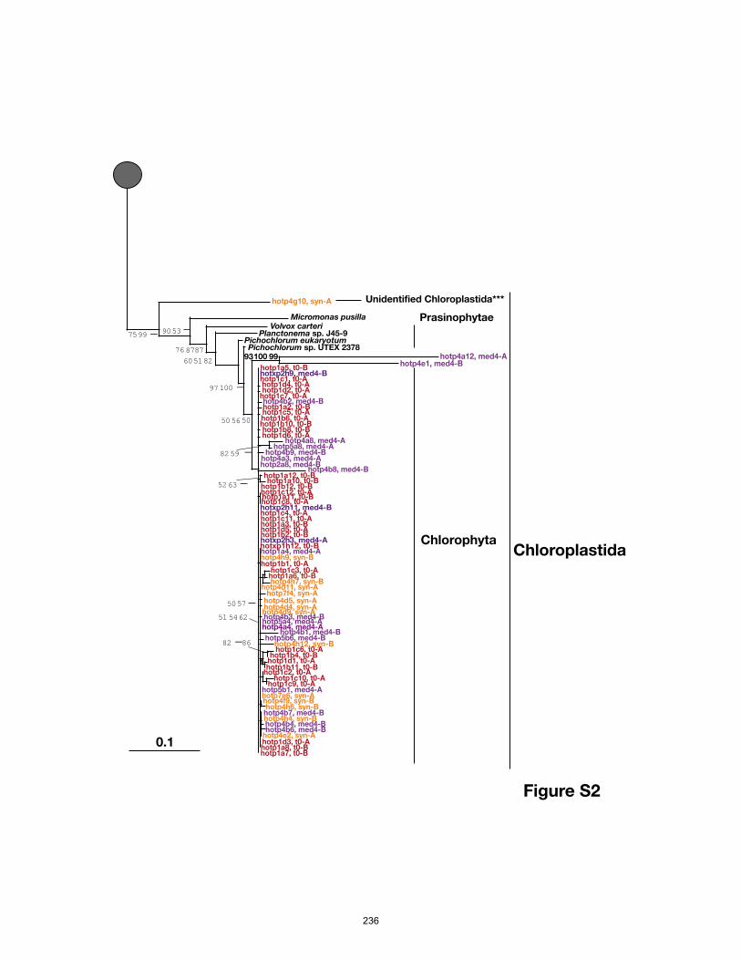
hotp1a7, t0-Bhotp1a8, t0-Bhotp1d3, t0-A hotp4e2, syn-Ahotp4b6, med4-Bhotp4b4, med4-Bhotp4h4, syn-Bhotp4b7, med4-Bhotp4h6, syn-B
hotp4f9, syn-Bhotp7e6, syn-Ahotp5b1, med4-A
hotp1c9, t0-Ahotp1c10, t0-A
hotp1c2, t0-Ahotp1b11, t0-Bhotp1d1, t0-Ahotp1b4, t0-B
hotp1c6, t0-A82 hotp4h12, syn-B
hotp5b6, med4-Bhotp4b1, med4-B
1
hotp4a4, med4-Ahotp5a4, med4-A
51 hotp4b3, med4-Bhotp4d9, syn-A
50 hotp4d4, syn-Ahotp4d5, syn-Ahotp7f4, syn-A
hotp4d11, syn-Ahotp4h7, syn-Bhotp1a6, t0-Bhotp1c3, t0-A
hotp1b1, t0-Ahotp4h9, syn-Bhotp1a4, med4-Ahotxp1h12, t0-Bhotxp2h3, med4-Ahotp1b2, t0-Bhotp1d5, t0-Ahotp1a3, t0-Bhotp1c11, t0-Ahotp1c4, t0-Ahotxp2h11, med4-Bhotp1c8, t0-Ahotp1a11, t0-Bhotp1c12, t0-Ahotp1b12, t0-B
hotp1a10, t0-Bhotp1a12, t0-B
52
hotp4b8, med4-Bhotp2a8, med4-Bhotp4a3, med4-A
hotp4b9, med4-Bhotp5a8, med4-A
hotp4a8, med4-Ahotp1d6, t0-A
82
hotp1b8, t0-Bhotp1b10, t0-Bhotp1b6, t0-Ahotp1c5, t0-Ahotp1a2, t0-Bhotp4b2, med4-B
hotp1c7, t0-Ahotp1d2, t0-Ahotp1d4, t0-Ahotp1c1, t0-Ahotxp2h9, med4-Bhotp1a5, t0-B
hotp4e1, med4-Bhotp4a12, med4-A93
Pichochlorum sp. UTEX 2378
50
Pichochlorum eukaryotumPlanctonema sp. J45-9
97
Volvox carteri
60
76
hotp4g10, syn-A
9075
0.1
Micromonas pusilla
ChlorophytaChloroplastida
9953
87
51
100
56
54
59
57
62
63
99
86
50
82
87100
Prasinophytae
- -
-
-
-
-
-
Figure S2
Unidentified Chloroplastida***
236
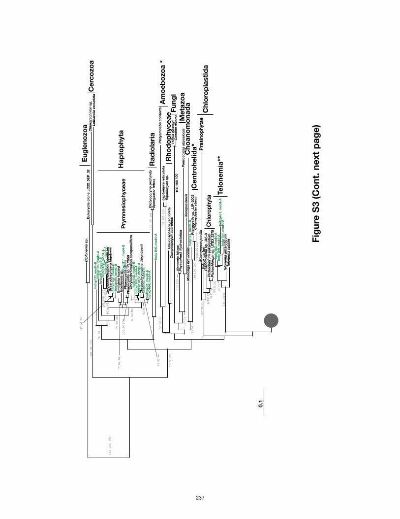
Telo
ne
ma
su
bti
leTe
lon
em
a a
nta
rcti
cu
mh
otp
1h
4, m
ed
4-A
ho
txp
4e
1,
me
d4
-Ah
otp
1h
9, m
ed
4-A
ho
tp1
h2,
me
d4-
A5
0
10
0
Pic
ho
ch
loru
m s
p. U
TE
X 2
378
Pic
ho
ch
loru
m e
uka
ryo
tum
Pla
ncto
ne
ma
sp
. J45-9
10
0
Vo
lvo
x c
art
eri
91
Mic
rom
on
as p
usill
a
84
Ch
lam
yd
aste
r ste
rni
Pte
rocysti
s s
p. JJP
-2003
ho
tp1
e1
, m
ed
4-B
Mo
no
sig
a b
revic
ollis
10
0
Xen
op
us la
evis
Po
nto
ec
iella
ab
yssic
ola
Ph
yso
ph
ora
hyd
rosta
tic
aN
an
om
ia b
iju
ga
99
10
0C
an
did
a d
ive
rsa
Pic
hia
be
sse
yi
67
100
53
57
ho
tp1
h6
, m
ed
4-A
Sp
on
ga
ste
r te
tra
sD
icty
oc
ory
ne
pro
fun
da
10
0h
otx
p4
d4
, m
ed
4-A
ho
txp
4d
1,
me
d4
-Ah
otp
1e
8,
me
d4
-BC
hry
so
ch
rom
ulin
a t
hro
nd
se
nii
ho
txp
1d
12
, m
ed
4-A
ho
txp
1d
8,
me
d4
-Ah
otp
1e
8,
me
d4
-B
97
Ch
ryso
ch
rom
ulin
a c
am
pa
nu
life
raP
ha
eo
cysti
s s
p. P
LY
559
Ph
ae
oc
ysti
s ja
hn
iih
otx
p1
f11
, m
ed
4-B
Iso
ch
rysis
sp
.E
milia
nia
hu
xle
yi
77
ho
txp
4f8
, m
ed
4-B
ho
txp
1g
2,
me
d4
-BB
raa
rud
osp
ha
era
big
elo
wii
Ch
ryso
ch
rom
ulin
a b
revif
ilu
m
87
ho
txp
4e
7,
me
d4
-Ah
otx
p1
b8
, m
ed
4-A
10
0
90
82
ho
txp
4f1
, m
ed
4-B
71
ho
txp
1d
4,
me
d4
-A
73
ho
txp
1f3
, m
ed
4-B
78
Lo
thare
lla v
acu
ola
taC
hlo
rara
ch
nio
n s
p.
10
0E
uk
ary
ote
clo
ne
LC
22_5E
P_32
Dip
lon
em
a s
p.
10
0
Eu
gle
no
zo
aC
erc
ozo
a
Ra
dio
lari
a
Fu
ng
i
Pry
mn
esio
ph
yc
ea
e
Ch
oa
no
mo
na
da
Me
tazo
a
Rip
ido
myxa
sp
.L
ep
tom
yxa
re
ticu
lata
Pla
tya
mo
eb
a c
on
tort
aA
mo
eb
ozo
a *
Co
mp
so
po
go
n c
ae
rule
us
Gla
uco
sp
ha
era
va
cu
ola
taR
ho
do
ph
yc
ea
e
Ce
ntr
oh
elid
a*
Pra
sin
op
hyta
e
Ch
loro
ph
yta
Te
lon
em
ia**
Ha
pto
ph
yta
Ch
loro
pla
sti
da
10
0
100
10
0
10
0
79
78
10
0
59
10
0
59
10
0
10
0
84
62
10
0
96
69
98
87
98
92
90
62
10
01
00
10
0
76
82
55
66
10
01
00
77
71
87
98
61
100
96
10
0
10
0
75
90
62
10
01
00
10
0
10
0
10
01
00
10
01
00
-
-
10
0
-
-
-
-
Fig
ure
S3
(C
on
t. n
ext
pa
ge
)
0.1
-
-
237
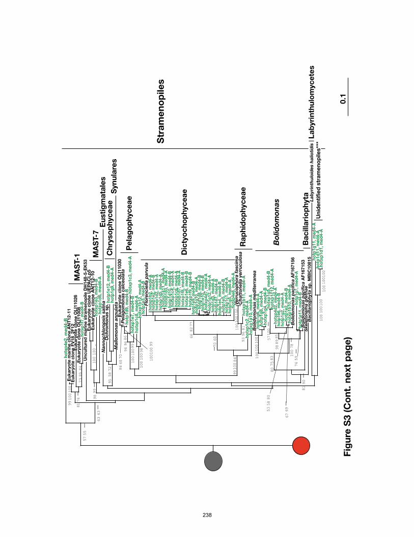
ho
txp
1d
1,
me
d4
-Ah
otp
1d
11
, m
ed
4-A
ho
tp1
g1
1,
me
d4
-A
10
0
La
byri
nth
ulo
ide
s h
alio
tid
is
10
0
Ba
cilla
rio
ph
yta
sp
. M
BIC
10815
81
ho
txp
1a
10
, m
ed
4-A
ho
txp
1b
12, m
ed
4-A
ho
txp
1c
8,
me
d4
-Ah
otx
p1
e7
, m
ed
4-B
ho
txp
1c
3,
me
d4
-Ah
otp
1d
9,
me
d4
-BP
ela
go
mo
na
s c
alc
eo
lata
Eu
ka
ryo
te c
lon
e O
LI1
1030
86
10
0
10
010
0
99
Ma
llo
mo
na
s a
nn
ula
tah
otp
1g
9,
me
d4
-Ah
otp
1e
12
, m
ed
4-B
Och
rom
on
as s
p.
Na
nn
och
loro
psis
sa
lin
a
95
ho
txp
1d
6,
me
d4
-Ah
otx
p1
e3
, m
ed
4-B
Eu
ka
ryo
te c
lon
e A
NT
12-1
0E
uk
ary
ote
clo
ne
UE
PA
CL
p5
10
0Un
cu
ltu
red
ma
rin
e s
tra
me
no
pile
DH
148-5
-EK
53
ho
txp
1f7
, m
ed
4-B
Eu
ka
ryo
te c
lon
e O
LI1
1008
Eu
ka
ryo
te c
lon
e O
LI1
1026
98
Eu
ka
ryo
te c
lon
e F
V18_2F
12
Eu
ka
ryo
te m
ari
ne
clo
ne
AN
T12-1
1
73
99
81
ho
txp
4e2, m
ed
4-B
63
57
MA
ST-1
La
byri
nth
ulo
myc
ete
s
MA
ST-7
Eu
sti
gm
ata
les
Ch
ryso
ph
yc
ea
eS
yn
ula
res
Pe
lag
op
hyc
ea
e
Ske
leto
ne
ma
gre
tha
eB
olid
om
on
as p
acif
ica
AF
167153
ho
tp1
e1
1, m
ed
4-B
ho
tp1
g7, m
ed
4-A
76
Bo
lid
om
on
as p
acif
ica
AF
167156
ho
txp
1b
10, m
ed
4-A
ho
tp1
e2, m
ed
4-B
ho
tp1
g2, m
ed
4-A
ho
tp1
e6, m
ed
4-B
ho
txp
4d
2, m
ed
4-A
67
ho
txp
1c
12
, m
ed
4-A
ho
txp
1g
5,
me
d4
-B5
3
98
ho
txp
1g
4,
me
d4
-Bh
otp
1g
8,
me
d4
-Ah
otp
1g
6,
me
d4
-A
57
Bo
lid
om
on
as m
ed
ite
rra
ne
a
86
10
0
80
Bo
lid
om
on
as
Ba
cilla
rio
ph
yta
ho
txp
1c
2,
me
d4
-Ah
otx
p1
b1
1,
me
d4
-AC
ha
tto
ne
lla
ve
rru
cu
losa
Ve
rru
co
ph
ora
fa
scim
a
Ra
ph
ido
ph
yc
ea
e1
00
ho
txp
4e
8, m
ed
4-A
ho
tp1
g5, m
ed
4-A
ho
txp
1c
1, m
ed
4-A
ho
tp1
e5, m
ed
4-B
ho
tp1
e4, m
ed
4-B
ho
tp1
e7, m
ed
4-B
ho
tp1
g3, m
ed
4-A
ho
tp1
g1
2, m
ed
4-A
ho
txp
4d
7, m
ed
4-A
ho
tp1
e1
0, m
ed
4-B
ho
tp1
d8, m
ed
4-B
ho
tp1
g1
0, m
ed
4-A
ho
tp1
e9, m
ed
4-B
1
ho
txp
1f9
, m
ed
4-B
ho
txp
1e
6, m
ed
4-B
ho
txp
1f8
, m
ed
4-B
ho
txp
1d
7, m
ed
4-A
ho
txp
1c
6, m
ed
4-A
ho
txp
1c
4, m
ed
4-A
ho
tp1
d1
0, m
ed
4-B
ho
txp
1d
3, m
ed
4-A
ho
txp
1a
11, m
ed
4-A
ho
txp
1d
5, m
ed
4-A
ho
txp
1d
2, m
ed
4-A
ho
txp
1e
2, m
ed
4-B
ho
txp
1b
2, m
ed
4-A
Flo
ren
cie
lla
pa
rvu
lah
otp
1e
3, m
ed
4-B
66
Dic
tyo
ch
op
hyc
ea
e
Un
ide
nti
fie
d s
tra
me
no
pile
s**
*Str
am
en
op
ile
s
55
63
90
10
0 75
10
0
10
0
70
82
10
0
10
0
60
10
0
59
58
58
10
0
69
89
76
99
10
01
00
80
85
78
83
10
0
72
70
99
99
96
96
86
10
01
00
96
81
9360
84
77
84
99
98
10
0
10
01
00
10
01
00
-
-
- -
-
-
-
-
--
0.1
Fig
ure
S3
(C
on
t. n
ext
pa
ge
)-
238
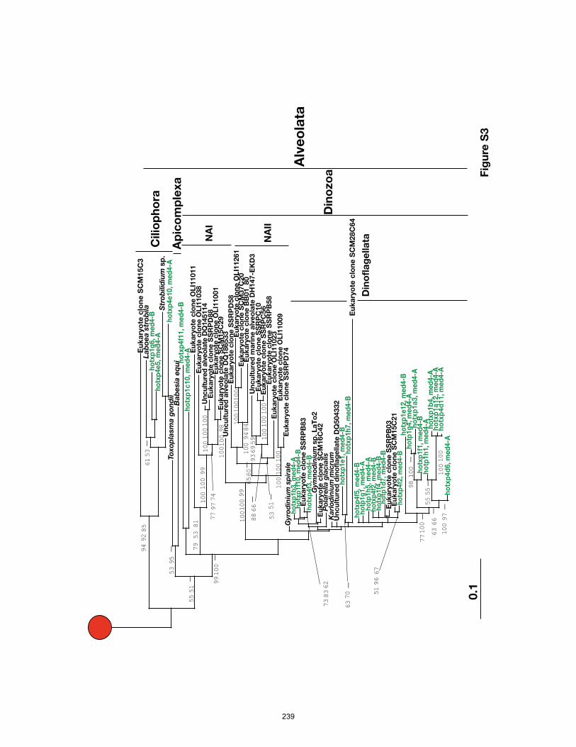
ho
txp
4d
6, m
ed
4-A
ho
txp
4d
11, m
ed
4-A
ho
txp
1a
12, m
ed
4-A
ho
txp
1b
4, m
ed
4-A
ho
tp1
h1, m
ed
4-A
10
0
55
ho
txp
1f1
, m
ed
4-B
ho
txp
1a
3, m
ed
4-A
ho
tp1
g4, m
ed
4-A
98
63
ho
txp
1e
12, m
ed
4-B
10
0
ho
txp
4f2
, m
ed
4-B
Eu
ka
ryo
te c
lon
e S
CM
15
C2
1E
uk
ary
ote
clo
ne
SS
RP
B0
3h
otp
1d
7, m
ed
4-B
ho
txp
1f4
, m
ed
4-B
ho
txp
4f2
, m
ed
4-B
77
51
ho
tp1
h5, m
ed
4-A
ho
tp1
g1, m
ed
4-A
ho
txp
4f5
, m
ed
4-B
Eu
ka
ryo
te c
lon
e S
CM
28
C6
4h
otx
p1
h7
, m
ed
4-B
ho
txp
1e
1, m
ed
4-B
63
Un
cu
ltu
red
din
ofl
ag
ella
te D
Q5
04
33
2K
arl
od
iniu
m m
icru
mP
ola
rella
gla
cia
lis
Eu
ka
ryo
te c
lon
e S
CM
16
C4
2G
ym
no
din
ium
sp
. L
aT
o2
ho
txp
4f3
, m
ed
4-B
Eu
ka
ryo
te c
lon
e S
SR
PB
83
ho
txp
1f1
0, m
ed
4-B
ho
txp
1b
3, m
ed
4-A
Gyro
din
ium
sp
ira
leE
uk
ary
ote
clo
ne
SS
RP
D7
4E
uk
ary
ote
clo
ne
OL
I11
00
9E
uk
ary
ote
clo
ne
OL
I11
02
3E
uk
ary
ote
clo
ne
SS
RP
B5
8E
uk
ary
ote
clo
ne
SS
RP
C5
6E
uk
ary
ote
clo
ne
SS
RP
C1
0U
nc
ult
ure
d m
ari
ne
alv
eo
late
DH
14
7-E
KD
3
10
0
88
Eu
ka
ryo
te c
lon
e B
B0
1_8
0E
uk
ary
ote
clo
ne
SC
M3
7C
20
Eu
ka
ryo
te c
lon
e O
LI1
12
61
10
0E
uk
ary
ote
clo
ne
SS
RP
D5
8
93
53
10
0
65
Un
cu
ltu
red
alv
eo
late
DQ
18
65
33
10
0
Eu
ka
ryo
te c
lon
e S
CM
15
C2
9E
uk
ary
ote
clo
ne
OL
I11
00
1E
uk
ary
ote
clo
ne
SS
RP
D8
8U
ncu
ltu
red
alv
eo
late
DQ
145114
10
0
10
0E
uk
ary
ote
clo
ne
OL
I11
03
8
10
0
Eu
ka
ryo
te c
lon
e O
LI1
10
11
10
0
79
ho
txp
1c
10, m
ed
4-A
ho
txp
4f1
1, m
ed
4-B
53
Ba
be
sia
eq
ui
To
xo
pla
sm
a g
on
dii
ho
txp
4e
10, m
ed
4-A
Str
ob
ilid
ium
sp
. h
otx
p4
e5, m
ed
4-A
ho
txp
1g
6, m
ed
4-B
La
bo
ea
str
ob
ila
99
61
Eu
ka
ryo
te c
lon
e S
CM
15
C3
55
94
Cilio
ph
ora
NA
I
NA
II
Din
ofl
ag
ella
ta
Din
ozo
a
Ap
ico
mp
lexa
92
53
95
10
0
51
53
10
0
10
0
55
66
10
0
97
10
0
10
0
66 51
60 10
0
10
0
83
70
10
0
10
0
Alv
eo
lata
10
0
69
59
99
10
0
10
01
00
94
841
00
98
99
81
77
97
74
62
73
96
67
85
-
-
-
-- -
-- -
-
--
-
-
Fig
ure
S3
0.1
239
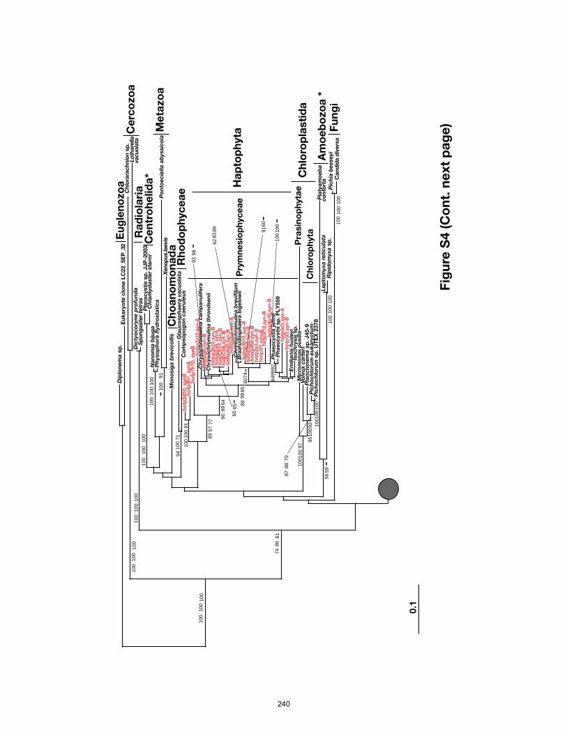
100
Pic
ho
ch
loru
m s
p. U
TE
X 2
378
Pic
ho
ch
loru
m e
uka
ryo
tum
Pla
ncto
ne
ma
sp
. J45-9
100
Vo
lvo
x c
art
eri
87
95
Iso
ch
rysis
sp
.E
milia
nia
hu
xle
yi
ho
tp3f3
,syn
-Bh
otp
3d
1,s
yn
-AP
ha
eo
cysti
s s
p. P
LY
559
Ph
ae
ocysti
s ja
hn
ii84
ho
txp
4g
10,s
yn
-Bh
otp
3f1
2,s
yn
-Bh
otp
3f1
,syn
-Bh
otp
2e3,s
yn
-Bh
otx
p4h
9,s
yn
-B
100
ho
txp
2g
2,s
yn
-Bh
otx
p3b
12,s
yn
-A
91
Bra
aru
do
sp
ha
era
big
elo
wii
Ch
ryso
ch
rom
ulin
a b
revif
ilu
m
8960
ho
txp
2b
5,s
yn
-Ah
otx
p4g
5,s
yn
-Bh
otp
Ch
6,s
yn
-Bh
otp
Ch
11,s
yn
-B
ho
txp
3h
10,s
yn
-B
60
Ch
ryso
ch
rom
ulin
a t
hro
nd
se
nii
62
ho
txp
2g
8,s
yn
-BC
hry
so
ch
rom
ulin
a c
am
pa
nu
life
ra
93h
otx
p2a12,s
yn
-Ah
otp
7h
10, syn
B
90
ho
tp3h
1, syn
Ah
otp
2d
10, syn
B
89
Co
mp
so
po
go
n c
ae
rule
us
Gla
uco
sp
ha
era
va
cu
ola
ta
Mo
no
sig
a b
revic
ollis
Xen
op
us la
evis
Po
nto
ec
iella
ab
yssic
ola
Ph
yso
ph
ora
hyd
rosta
tic
aN
an
om
ia b
iju
ga
100
Ch
lam
yd
aste
r ste
rni
Pte
rocysti
s s
p. JJP
-2003
100
9410
0
100
56
100
Lo
thare
lla
Ch
lora
rach
nio
n s
p.
74
100
Eu
ka
ryo
te c
lon
e L
C22_5E
P_32
Dip
lon
em
a s
p.
100
Eu
gle
no
zo
aC
erc
ozo
aS
po
ng
aste
r te
tra
sD
icty
oc
ory
ne
pro
fun
da
Ra
dio
lari
aC
en
tro
he
lid
a*
Me
tazo
aC
ho
an
om
on
ad
aR
ho
do
ph
yc
ea
e
Pry
mn
esio
ph
yc
ea
e
Mic
rom
on
as p
usilla
P
rasin
op
hyta
e
Ch
loro
ph
yta
Rip
ido
myxa
sp
.L
ep
tom
yxa
re
ticu
lata
Pla
tya
mo
eb
aA
mo
eb
ozo
a *
Ca
nd
ida
div
ers
aP
ich
ia b
esse
yi
Fu
ng
i
Ha
pto
ph
yta
Ch
loro
pla
sti
da
100
100
100 10
0
100
100
100
100
98
9974
10060
83
98
99
57
100
100
100
6186
100
100
59-
100
-91
100
100
100 71
100
100
100
8879
100 9
2
97
64
77
91
89
65-
92
-
65-
- -
0.1
Fig
ure
S4 (
Co
nt.
ne
xt
pa
ge
)
vacu
ola
ta
co
nto
rta
100
ho
txp
2a
9,
syn
A
240
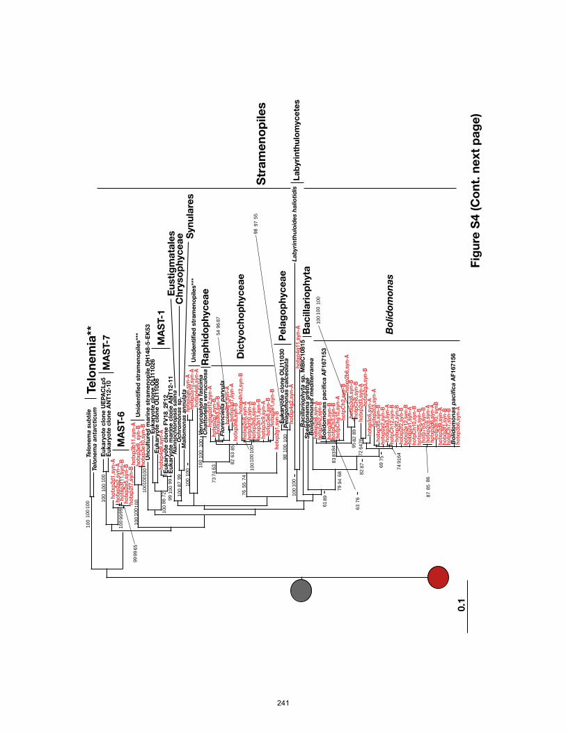
ho
txp
3b
6,s
yn
-AB
olid
om
on
as p
ac
ific
a A
F1
67
15
6h
otp
Ch
7,s
yn
-Bh
otx
p2f1
,syn
-Bh
otx
p2d
9,s
yn
-Ah
otp
3h
10, syn
Bh
otx
p2d
6,s
yn
-Ah
otx
p2c9,s
yn
-Ah
otp
7h
5,s
yn
-B87
ho
txp
2f5
,syn
-Bh
otp
Ch
10,s
yn
-Bh
otx
p2a1,s
yn
-Ah
otx
p2e
12,s
yn
-Bh
otx
p2f2
,syn
-Bh
otx
p3f2
,syn
-Bh
otp
Ch
12,s
yn
-Bh
otx
p3a3,s
yn
-Ah
otx
p2e2,s
yn
-B
74
ho
txp
3f5
,syn
-Bh
otx
p2c3,s
yn
-Ah
otx
p3c6,s
yn
-Aho
txp
2g
3,s
yn
-Bh
otx
p2d
3,s
yn
-A72
ho
tpC
h8,s
yn
-Bh
otx
p3g
8,s
yn
-Bh
otx
p2b
6,s
yn
-A
100
ho
tpC
h2,s
yn
-Bh
otp
Ch
g10,s
yn
-Ah
otp
Ch
3,s
yn
-Bh
otx
p3f8
,syn
-B
95
Bo
lid
om
on
as p
ac
ific
a A
F1
67
15
3h
otx
p4h
2,s
yn
-Bh
otx
p2a4,s
yn
-A
6361
69
83
Bo
lid
om
on
as m
ed
ite
rra
ne
a
82
79
ho
txp
4g
11,s
yn
-Ah
otx
p4g
2,s
yn
-AP
ela
go
mo
na
s c
alc
eo
lata
Eu
ka
ryo
te c
lon
e O
LI1
10
30
98h
otx
p2g
1,s
yn
-Bh
otx
p2e1,s
yn
-Bh
otx
p3e8,s
yn
-Bh
otx
p3c9,s
yn
-Ah
otx
p3h
11,s
yn
-Bh
otx
p3h
5,s
yn
-Bh
otp
3d
10,s
yn
-Ah
otx
p2c8,s
yn
-Ah
otx
p4h
12,s
yn
-Bh
otx
p3h
8,s
yn
-Bh
otx
p3d
7,s
yn
-Ah
otx
p2b
1,s
yn
-AF
lore
nc
iella
pa
rvu
la
100
ho
txp
3h
3,s
yn
-Bh
otx
p2g
7,s
yn
-Bh
otx
p2d
12,s
yn
-A
54
Ch
att
on
ella
ve
rru
cu
losa
Ve
rru
co
ph
ora
fa
scim
a
82100
73
100
76
ho
txp
4g
8,s
yn
-Ah
otx
p2a10,s
yn
-Ah
otx
p2a6,s
yn
-A
100
Ma
llo
mo
na
s a
nn
ula
taO
ch
rom
on
as s
p.
100
Eu
ka
ryo
te m
ari
ne
clo
ne
AN
T1
2-1
1E
uk
ary
ote
clo
ne
FV
18
_2
F1
2h
otx
p4g
9,s
yn
-A
99
Eu
ka
ryo
te c
lon
e O
LI1
10
08
Eu
ka
ryo
te c
lon
e O
LI1
10
26
Un
cu
ltu
red
ma
rin
e s
tra
me
no
pile
DH
14
8-5
-EK
53
h
otx
p3e
10,s
yn
-Bh
otx
p3e9, syn
-Bh
otx
p3b
11,s
yn
-A
100
100
ho
txp
2f7
,syn
-Bh
otx
p2e5,s
yn
-Bh
otx
p3f1
1,s
yn
-Bh
otx
p2a2,s
yn
-Ah
otx
p2d
1,s
yn
-A
99
100
100
Eu
ka
ryo
te c
lon
e A
NT
12
-10
Eu
ka
ryo
te c
lon
e U
EP
AC
Lp
5M
AS
T-7 M
AS
T-1
Na
nn
och
loro
psis
sa
lin
aE
usti
gm
ata
les
Ch
ryso
ph
yc
ea
e Syn
ula
res
Ra
ph
ido
ph
yc
ea
e
Dic
tyo
ch
op
hyc
ea
e
Pe
lag
op
hyc
ea
eL
ab
yri
nth
ulo
ide
s h
alio
tid
isL
ab
yri
nth
ulo
myc
ete
sB
ac
illa
rio
ph
yta
sp
. M
BIC
10
81
5S
ke
leto
ne
ma
gre
tha
eB
ac
illa
rio
ph
yta
Bo
lid
om
on
as
MA
ST-6
Un
ide
nti
fie
d s
tra
me
no
pile
s**
*
Str
am
en
op
ile
s
100
100
100
100
100
97
100
86
87
63
100
94
89
87
75
83
91
6476
85
82
100
9999
9965
100
100
100
100
74 6
3
55 7
4
85
9687
100
100
5598
99
100
99 7
2
100
100
89
84
86
68
76
64
-
-
--
100
Fig
ure
S4
(C
on
t. n
ext
pa
ge
)
0.1
-
-
Un
ide
nti
fie
d s
tra
me
no
pile
s**
*
Te
lon
em
a a
nta
rcti
cu
mTe
lon
em
a s
ub
tile
100
Te
lon
em
ia**
1001
00
241
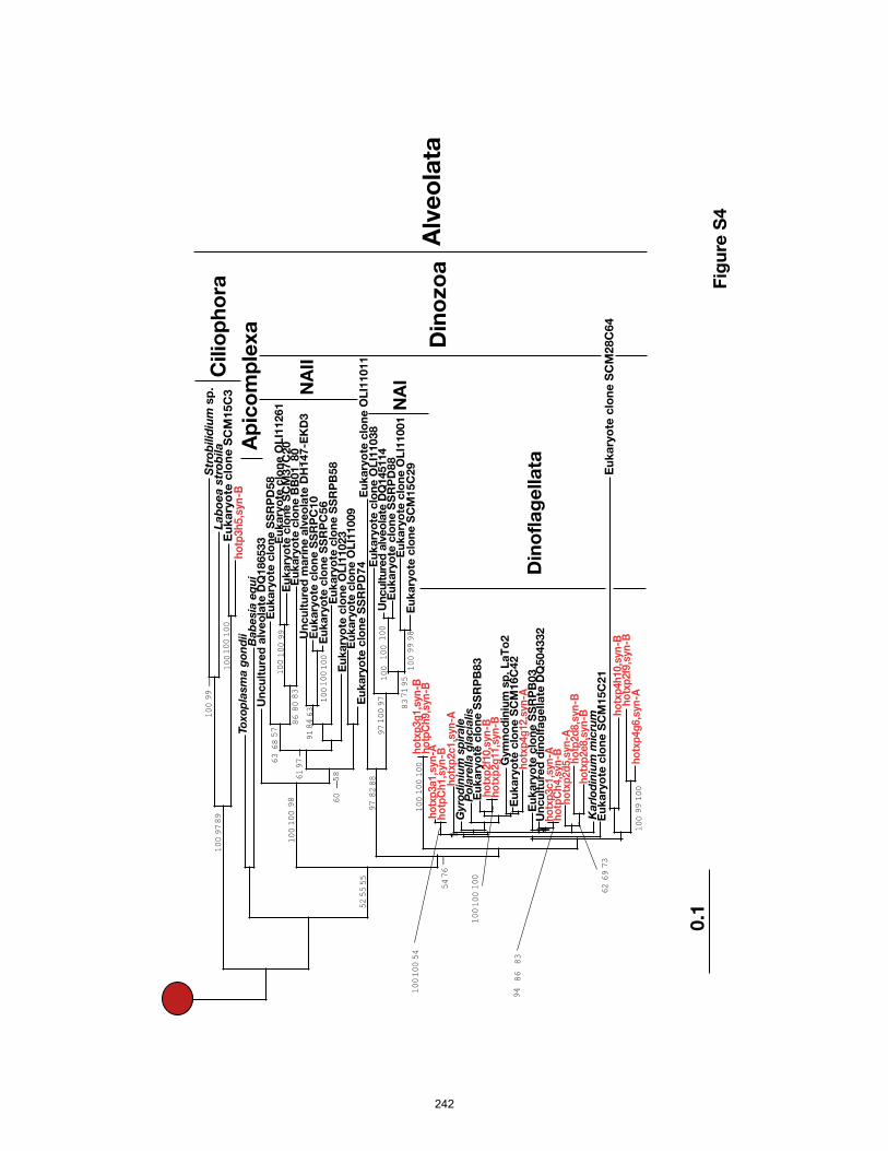
ho
txp
4g
6,s
yn
-Ah
otx
p2f9
,syn
-Bh
otx
p4h
10,s
yn
-BE
uk
ary
ote
clo
ne
SC
M2
8C
64
10
0
62
Eu
ka
ryo
te c
lon
e S
CM
15
C2
1K
arl
od
iniu
m m
icru
mh
otx
p2e8,s
yn
-Bh
otp
2d
8,s
yn
-Bh
otx
p2d
5,s
yn
-Ah
otp
Ch
4,s
yn
-Bh
otx
p3c1,s
yn
-AU
nc
ult
ure
d d
ino
lfa
ge
lla
te D
Q5
04
33
2E
uk
ary
ote
clo
ne
SS
RP
B0
3
1
ho
txp
4g
12,s
yn
-AE
uk
ary
ote
clo
ne
SC
M1
6C
42
Gym
no
din
ium
sp
. L
aT
o2
ho
txp
2g
11,s
yn
-Bh
otx
p2f1
0,s
yn
-BE
uk
ary
ote
clo
ne
SS
RP
B8
3P
ola
rella
gla
cia
lis
Gyro
din
ium
sp
ira
leh
otx
p2c1,s
yn
-A
1
ho
tpC
h1,s
yn
-Bh
otx
p3a1,s
yn
-A
10
0
1
ho
tpC
h9,s
yn
-Bh
otx
p3g
1,s
yn
-B1
00
Eu
ka
ryo
te c
lon
e S
CM
15
C2
9E
uk
ary
ote
clo
ne
OL
I11
00
1E
uk
ary
ote
clo
ne
SS
RP
D8
8U
ncu
ltu
red
alv
eo
late
DQ
145114
10
0
10
0
Eu
ka
ryo
te c
lon
e O
LI1
10
38
83
Eu
ka
ryo
te c
lon
e O
LI1
10
11
97
54
97
Eu
ka
ryo
te c
lon
e S
SR
PD
74
Eu
ka
ryo
te c
lon
e O
LI1
10
09
Eu
ka
ryo
te c
lon
e O
LI1
10
23
Eu
ka
ryo
te c
lon
e S
SR
PB
58
Eu
ka
ryo
te c
lon
e S
SR
PC
56
Eu
ka
ryo
te c
lon
e S
SR
PC
10
Un
cu
ltu
red
ma
rin
e a
lve
ola
te D
H1
47
-EK
D3
86
Eu
ka
ryo
te c
lon
e B
B0
1_8
0E
uk
ary
ote
clo
ne
SC
M3
7C
20
Eu
ka
ryo
te c
lon
e O
LI1
12
61
10
0
Eu
ka
ryo
te c
lon
e S
SR
PD
58
91
63
61
Un
cu
ltu
red
alv
eo
late
DQ
18
65
33
60
52
10
0
Ba
be
sia
eq
ui
To
xo
pla
sm
a g
on
dii
ho
tp3h
5,s
yn
-BE
uk
ary
ote
clo
ne
SC
M1
5C
3L
ab
oe
a s
tro
bila
Str
ob
ilid
ium
sp
. 1
00
10
0C
ilio
ph
ora
Ap
ico
mp
lexa
NA
I
NA
II
Din
ofl
ag
ella
ta
Din
ozo
a
97
55
10
0
76
82
10
01
00
10
01
00
69
10
0
84
10
06
8
97
-
Alv
eo
lata
10
01
00
10
0
99
89
10
01
00
63
99
80
83
57
98
58
-
10
0
99
10
0
54
86
83
94
10
01
00
10
0
55
10
0
99
98
71
95
97
88
- 73
-
Fig
ure
S4
0.1
242
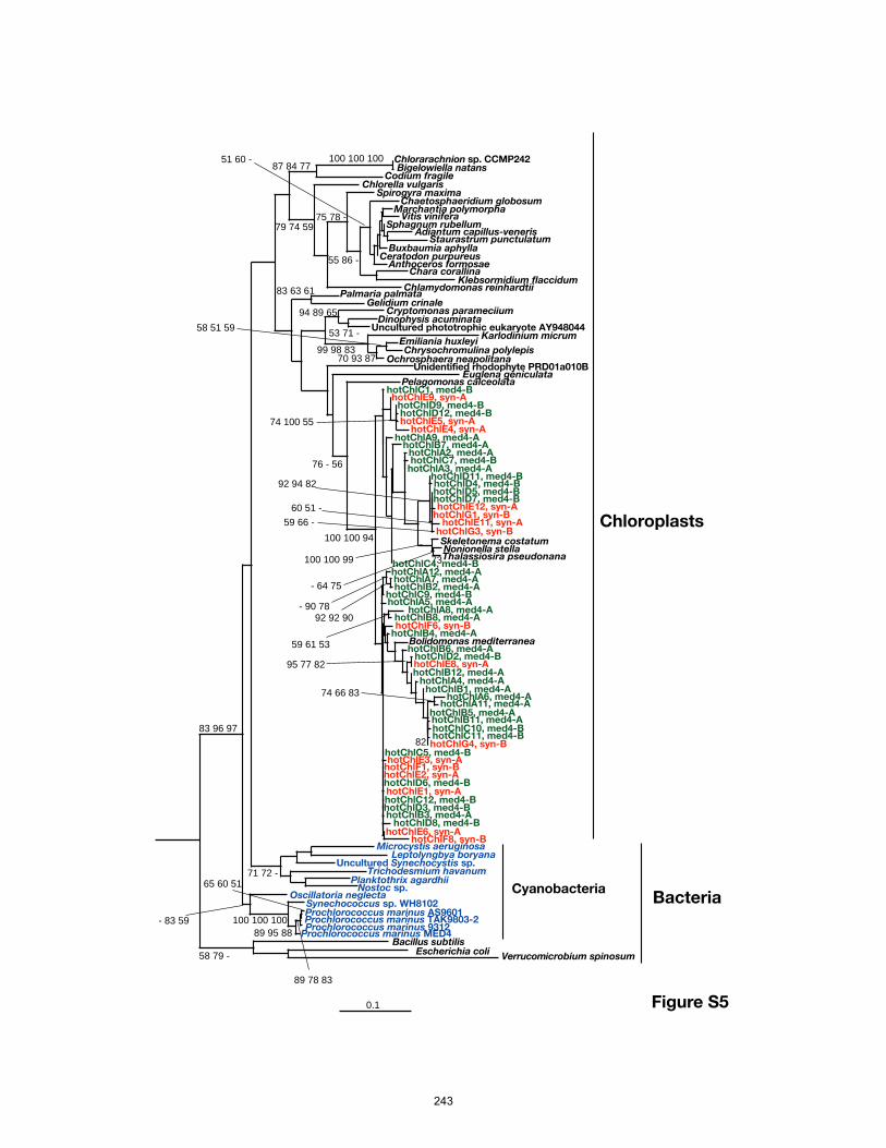
65 60 51
89 78 83
89 95 88100 100 100
82
74 66 83
95 77 82
Bolidomonas mediterranea59 61 53
92 92 90
Thalassiosira pseudonanaNonionella stella
73
60 51 -59 66 -
100 100 99
92 94 82
74 100 55
Pelagomonas calceolata
100 100 94
76 - 56
58 51 59
70 93 87
53 71 -99 98 83
94 89 65
83 63 61
51 60 -
55 86 -
75 78 -
100 100 100
79 74 59
87 84 77
71 72 -
58 79 -
83 96 97
Verrucomicrobium spinosumEscherichia coli
Bacillus subtilisProchlorococcus marinus MED4Prochlorococcus marinus 9312Prochlorococcus marinus TAK9803-2Prochlorococcus marinus AS9601Synechococcus sp. WH8102
Oscillatoria neglectaNostoc sp.
Planktothrix agardhiiTrichodesmium havanum
Microcystis aeruginosaLeptolyngbya boryana
Uncultured Synechocystis sp.
Euglena geniculataUnidentified rhodophyte PRD01a010B
Klebsormidium flaccidum
Chlorarachnion sp. CCMP242Bigelowiella natans
Codium fragileChlorella vulgaris
Spirogyra maximaChaetosphaeridium globosum
Marchantia polymorphaVitis vinifera
Sphagnum rubellumAdiantum capillus-veneris
Staurastrum punctulatum Buxbaumia aphylla
Ceratodon purpureusAnthoceros formosae
Chara corallina
Chlamydomonas reinhardtiiPalmaria palmata
Gelidium crinaleCryptomonas parameciium
Dinophysis acuminataUncultured phototrophic eukaryote AY948044
Karlodinium micrum
Ochrosphaera neapolitanaChrysochromulina polylepis
Emiliania huxleyi
Skeletonema costatum
hotChlE9, syn-AhotChlC1, med4-B
hotChlD9, med4-BhotChlD12, med4-BhotChlE5, syn-A
hotChlE4, syn-AhotChlA9, med4-A
hotChlB7, med4-AhotChlA2, med4-AhotChlC7, med4-B
hotChlA3, med4-AhotChlD11, med4-BhotChlD4, med4-BhotChlD5, med4-BhotChlD7, med4-BhotChlE12, syn-A
hotChlG1, syn-BhotChlE11, syn-A
hotChlG3, syn-B
hotChlC4, med4-BhotChlA12, med4-AhotChlA7, med4-AhotChlB2, med4-A
hotChlC9, med4-BhotChlA5, med4-A
hotChlA8, med4-AhotChlB8, med4-AhotChlF6, syn-B
hotChlB4, med4-A
hotChlB6, med4-AhotChlD2, med4-BhotChlE8, syn-AhotChlB12, med4-A
hotChlA4, med4-AhotChlB1, med4-A
hotChlA6, med4-AhotChlA11, med4-A
hotChlB5, med4-AhotChlB11, med4-AhotChlC10, med4-BhotChlC11, med4-BhotChlG4, syn-B
hotChlC5, med4-BhotChlE3, syn-A
hotChlF1, syn-BhotChlE2, syn-AhotChlD6, med4-BhotChlE1, syn-AhotChlC12, med4-BhotChlD3, med4-BhotChlB3, med4-A
hotChlD8, med4-BhotChlE6, syn-A
hotChlF8, syn-B
CyanobacteriaBacteria
0.1
Chloroplasts
- 64 75
- 90 78
- 83 59
Figure S5
243
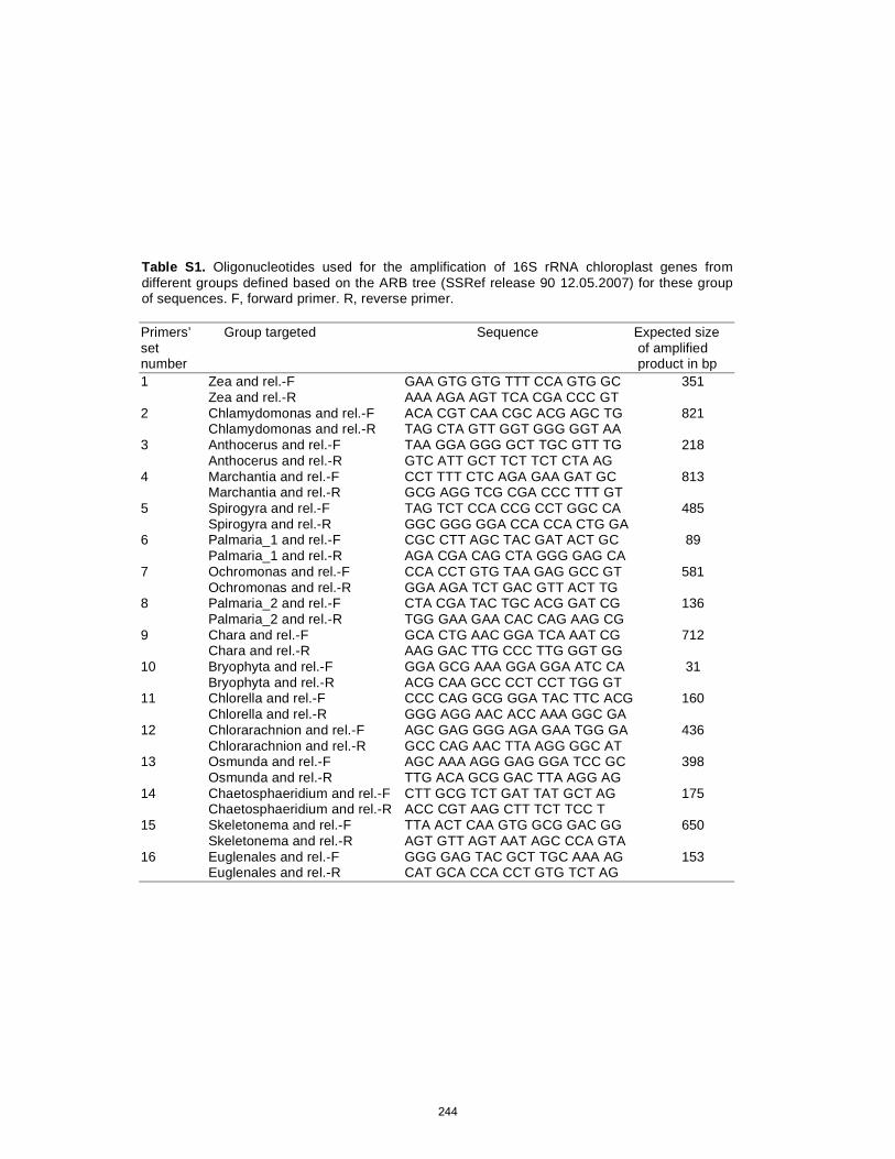
Table S1. Oligonucleotides used for the amplification of 16S rRNA chloroplast genes from different groups defined based on the ARB tree (SSRef release 90 12.05.2007) for these group of sequences. F, forward primer. R, reverse primer.
Primers’ Group targeted Sequence Expected size set of amplified number product in bp 1 Zea and rel.-F GAA GTG GTG TTT CCA GTG GC 351 Zea and rel.-R AAA AGA AGT TCA CGA CCC GT 2 Chlamydomonas and rel.-F ACA CGT CAA CGC ACG AGC TG 821 Chlamydomonas and rel.-R TAG CTA GTT GGT GGG GGT AA 3 Anthocerus and rel.-F TAA GGA GGG GCT TGC GTT TG 218 Anthocerus and rel.-R GTC ATT GCT TCT TCT CTA AG 4 Marchantia and rel.-F CCT TTT CTC AGA GAA GAT GC 813 Marchantia and rel.-R GCG AGG TCG CGA CCC TTT GT 5 Spirogyra and rel.-F TAG TCT CCA CCG CCT GGC CA 485 Spirogyra and rel.-R GGC GGG GGA CCA CCA CTG GA 6 Palmaria_1 and rel.-F CGC CTT AGC TAC GAT ACT GC 89 Palmaria_1 and rel.-R AGA CGA CAG CTA GGG GAG CA 7 Ochromonas and rel.-F CCA CCT GTG TAA GAG GCC GT 581 Ochromonas and rel.-R GGA AGA TCT GAC GTT ACT TG 8 Palmaria_2 and rel.-F CTA CGA TAC TGC ACG GAT CG 136 Palmaria_2 and rel.-R TGG GAA GAA CAC CAG AAG CG 9 Chara and rel.-F GCA CTG AAC GGA TCA AAT CG 712 Chara and rel.-R AAG GAC TTG CCC TTG GGT GG 10 Bryophyta and rel.-F GGA GCG AAA GGA GGA ATC CA 31 Bryophyta and rel.-R ACG CAA GCC CCT CCT TGG GT 11 Chlorella and rel.-F CCC CAG GCG GGA TAC TTC ACG 160 Chlorella and rel.-R GGG AGG AAC ACC AAA GGC GA 12 Chlorarachnion and rel.-F AGC GAG GGG AGA GAA TGG GA 436 Chlorarachnion and rel.-R GCC CAG AAC TTA AGG GGC AT 13 Osmunda and rel.-F AGC AAA AGG GAG GGA TCC GC 398 Osmunda and rel.-R TTG ACA GCG GAC TTA AGG AG 14 Chaetosphaeridium and rel.-F CTT GCG TCT GAT TAT GCT AG 175 Chaetosphaeridium and rel.-R ACC CGT AAG CTT TCT TCC T 15 Skeletonema and rel.-F TTA ACT CAA GTG GCG GAC GG 650 Skeletonema and rel.-R AGT GTT AGT AAT AGC CCA GTA 16 Euglenales and rel.-F GGG GAG TAC GCT TGC AAA AG 153 Euglenales and rel.-R CAT GCA CCA CCT GTG TCT AG
244
Appendix B
Improved methods for isolating and validating indigenous biomarkers in Precambrian rocks
Laura S. Sherman, Jacob R. Waldbauer and Roger E. Summons
Reprinted with permission from Organic Geochemistry © 2007 Elsevier Ltd.
Sherman, L.S., Waldbauer, J.R. and Summons, R.E. (2007) Improved methods for isolating and validating indigenous biomarkers in Precambrian rocks. Organic Geochemistry 38: 1987-2000.
245

246
Improved methods for isolating and validatingindigenous biomarkers in Precambrian rocks
Laura S. Sherman a, Jacob R. Waldbauer b, Roger E. Summons a,*
a Department of Earth, Atmospheric and Planetary Sciences, Massachusetts Institute of Technology, Cambridge, MA 02139, USAb Joint Program in Chemical Oceanography, Massachusetts Institute of Technology and Woods Hole Oceanographic Institution,
Cambridge, MA 02139, USA
Received 24 July 2007; accepted 31 August 2007Available online 14 September 2007
Abstract
Hydrocarbon biomarkers in highly mature Precambrian rocks have the potential to provide important informationabout the diversity ecology, and evolution of early life, but studying them presents special analytical challenges. Extract-able hydrocarbons are present in Archean and most Paleoproterozoic sedimentary rocks in such trace concentration thateven slight contamination from petroleum-derived materials in situ or during drilling, storage, sampling, handling and lab-oratory analysis would compromise the results and, thereby, any consequent inferences. Here we report protocols that wehave developed for the analysis of cores from several recently completed deep-time scientific drilling initiatives. By payingspecial attention to cutting, cleaning, crushing and extraction, it is possible to significantly reduce laboratory blanks toacceptable levels. When these methods are utilized, meaningful variations in the patterns of biomarkers over stratigraphicand lithologic boundaries provide compelling evidence for syngeneity.! 2007 Elsevier Ltd. All rights reserved.
1. Introduction
Molecular fossils of biogenic lipids (i.e., bio-markers) preserved over geologic time in sedimen-tary rocks of low metamorphic grade can be usedto describe ancient microbiota and environmentalconditions (Eglinton et al., 1964; Brocks et al.,1999, 2003b). Because biomarkers are the hydrocar-bon skeletons of biogenic precursor lipids, thosethat are created through known biosynthetic anddiagenetic pathways convey information about theidentity and physiology of their source organisms
(Brocks and Summons, 2003; Brocks and Pearson,2005). Biomarker geochemistry is therefore apotentially powerful tool for establishing the recordof ancient life on Earth and for better understand-ing early microbial evolution. However, the applica-tion of biomarker techniques to highly maturePrecambrian organic matter presents uniquechallenges, requires the use of special methods andnecessitates extraordinary attention to concerns ofcontamination.
Although some Precambrian rocks contain abun-dant amounts of syndepositional organic matter(exceeding 10 wt% in some samples in this study),very little is in the form of extractable bitumen.Over billions of years, even under relatively low
0146-6380/$ - see front matter ! 2007 Elsevier Ltd. All rights reserved.doi:10.1016/j.orggeochem.2007.08.012
* Corresponding author.E-mail address: [email protected] (R.E. Summons).
Available online at www.sciencedirect.com
Organic Geochemistry 38 (2007) 1987–2000
www.elsevier.com/locate/orggeochem
OrganicGeochemistry
247
grade metamorphic conditions, the majority of theorganic constituents of a sediment are incorporatedinto the macromolecular kerogen network (Brocksand Summons, 2003). Because very few hydrocar-bons are present as extractable biomarker molecules(sub-ppb quantities), even low level contaminationintroduced during drilling, sampling, storage, orlaboratory processing may overprint the originalsignatures.
The first purportedly Precambrian biomarkerswere amino acids identified by P.H. Abelson in thelate 1950s (Barghoorn, 1957); numerous studies inthe 1960s subsequently reported finding fatty acids,amino acids, n-alkanes, porphyrins and acyclic iso-prenoids in Precambrian rocks (McKirdy, 1974;Hayes et al., 1983; Imbus and McKirdy, 1993).However, these findings were quickly called intoquestion (Hoering, 1966; Leventhal et al., 1975).Hoering (1966) noted that most high maturityArchean rocks had thermal histories inconsistentwith the preservation of soluble organic molecules.He also detailed numerous sources of contamina-tion, including anthropogenic petroleum products,laboratory equipment and sample storage bags(Hoering, 1966; Hoering, 1967). Furthermore, sub-sequent reports described the potential for youngeroils and drill fluids to penetrate and be preserved inPrecambrian units (Barghoorn et al., 1965; Mei-nschein, 1965; Nagy, 1970; Sanyal et al., 1971).These problems overshadowed Precambrian organicgeochemistry investigations for almost thirty years.
More recent studies, including those by Brocks(2001), Brocks et al. (1999), Brocks and Summons(2003), Eigenbrode (2004) and Dutkiewicz et al.(2006) have re-visited Precambrian organic geo-chemistry with extreme care, in order to assess thesyngeneity of detected molecules. The current studywas undertaken to both gain a better understandingof early microbial evolution and develop a protocolfor sampling, handling, and analyzing high maturityPrecambrian organic matter.
We examined rocks from two cores (GKP01 andGKF01, hereafter GKP and GKF) drilled as part ofthe Agouron Griqualand Drilling Project and rocksfrom one core (ABDP9) drilled as part of the DeepTime Drilling Project of the NASA AstrobiologyDrilling Program. These sedimentary successionscontain some of the earliest evidence of the accumu-lation and cycling of molecular oxygen in surfaceenvironments (Bekker et al., 2004; Anbar et al.,2007; Kaufman et al., 2007). The Agouron coreswere each drilled without the use of hydrocarbon
fluids through more than a kilometer of Archeansediments. The cores intersect platform and slopefacies of the Transvaal Supergroup and were depos-ited on the Kaapvaal Craton of South Africabetween 2670–2460 Ma (Armstrong et al., 1986;Barton et al., 1994; Walraven and Martini, 1995;Sumner and Bowring, 1996). Stratigraphic correla-tions between the two Agouron cores, based onthe presence of volcanic ash beds, spherule layers,flooding surfaces, sequence boundaries and litho-logic marker beds (Schroder et al., 2006), enabledintercomparison of the biomarker contents of corre-lated beds. Core ABDP9 was drilled through thePilbara Craton of western Australia, intersectingiron formations, shales, mixed clastics and carbon-ates. Although drilling di!culties required the useof petroleum-based additives part way through thecoring, the top 200 m were obtained with minimalcontamination. These two drilling projects areamong the first e"orts to recover long stretches ofArchean strata with the express purpose of collect-ing samples for molecular fossil analysis.
2. Methodology: sample collection and processing
The methods were developed for the extractionand analysis of Precambrian hydrocarbons withminimal contamination. The methodology is basedon techniques described by Brocks (2001), Brockset al. (2003a,b) and Eigenbrode (2004), with refine-ments as described. Rationalization of key aspectsof the methods can be found in Section 4.
2.1. Drilling
As described above, the data presented in thisstudy are results of analysis of rock samples fromthe Agouron Griqualand Drilling Project and theDeep Time Drilling Project. Drill cores have severaladvantages over outcrop samples for the purposesof biomarker analysis. The surface exposures ofearly Precambrian terranes are generally heavilyweathered, meaning they have been exposed to cir-culating modern surface water and groundwaterthat carry contaminant lipids and hydrocarbons.Drilling below the modern weathering horizon –which can be tens to hundreds of meters deep –a"ords rock samples that have not been in contactwith fluids in the recent geologic past. Drill coresalso sample long stretches of continuous stratigra-phy, generally much longer intervals than can beaccessed in often sparse surface exposure. Impor-
1988 L.S. Sherman et al. / Organic Geochemistry 38 (2007) 1987–2000
248
tantly, drill cores represent a group of samples takenat one time that have all been subject to the samehandling and storage conditions. This facilitatesstratigraphic comparisons of biomarker contents,which can be valuable both for both assessing thesyngeneity of the extracted hydrocarbons and estab-lishing records of paleoenvironmental change.
While deep core drilling o"ers several keyadvantages in sample recovery for Precambrianbiomarker analysis, other potentially complicatingfactors must be kept in mind. Individual drill coresnecessarily represent a finite amount of materialdeposited at each time interval and cannot be used,as outcrop samples often can, to determine the lat-eral variability of a stratigraphic unit. Because theseprojects are costly and time consuming, it is oftennot practical to drill a series of cores in a small area.A central concern when studying drill cores is thatthe samples will necessarily have come into contactwith drilling equipment and fluids. It is essentialthat the hydrocarbon-based lubricants typicallyused in diamond-bit core drilling be eschewed, ide-ally in favor of pure water as a drilling fluid. Useof water as the sole drilling fluid is di!cult, and gen-erally increases rate of equipment fatigue and fail-ure. Nevertheless, the extremely low quantities ofextractable bitumen in high maturity Precambrianrocks mean that the syngenetic signal can easily beoverprinted by even minimal hydrocarbon contentin the drilling fluid. Any additive or substance tobe put into the borehole should be pre-screenedfor hydrocarbon and biomarker content. Somecommercial products, such as those based on plantoils, are less likely to be confused with indigenousPrecambrian biomarkers because they are com-posed primarily of polar compounds and displayimmature isomer distributions. Other products,advertised as ‘hydrocarbon free’, often containquantities of petroleum-derived biomarkers thatcould compromise trace level analysis. Even forcores drilled under the cleanest practicable condi-tions, we have found that the outer surfaces of corepieces bear signals of low level contamination,necessitating their removal (see Sections 2.3 and4.1).
From hundreds of meters of drill core, only asmall subset of the recovered stratigraphy can befeasibly analyzed. We chose our sub-samples forbiomarker work on the basis of several criteria.Originally, visibly organic-rich strata (primarily finegrained black shales, often with abundant pyrite)were sampled because we expected that they would
yield the most extractable bitumen. Ultimately, wefound little correlation between bitumen yield andwhole rock organic matter content, with more car-bonate-rich beds sometimes having as much extract-able hydrocarbon as shales (Waldbauer et al., 2007).Hence, we consider it useful to sample all lithofaciesintersected in a given core, particularly because con-trasts between siliciclastic and carbonate-dominateddepositional environments are a potentially strongpaleoenvironmental signal (Eigenbrode, 2004). Sim-ilarly, we sampled across formation and sequenceboundaries to explore how changes in sedimentsourcing and deposition might be recorded in bio-marker content.
2.2. Materials
In general, it is important to minimize the num-ber of external surfaces that touch Archean rocksamples. Each surface contacted represents anopportunity for contaminant hydrocarbons to beintroduced into the samples. Surfaces that samplesdo contact are either cleaned exhaustively withorganic solvents or thoroughly combusted. Addi-tionally, materials used to process high maturitysamples are reserved only for these samples andare kept separate from general laboratory supplies.
Laboratory solvents including hexane, dichloro-methane (DCM) and methanol (MeOH) are highpurity and organic free (OmniSolv, EMD Chemi-cals). Prior to use, glassware, glass wool, aluminumfoil and silica gel are combusted at 550 "C (8 h) andquartz sand (Accusand, Unimin Corp.) is com-busted at 850 "C (12 h). De-ionized (DI) water andhydrochloric acid (HCl) used in sample processingare extracted (·5) with DCM. Metal tools used toprocess samples are rinsed with DI water andcleaned (·5 each) with MeOH, DCM and hexane.Crushing tools (see Section 2.3) are scrubbed withcombusted quartz sand, rinsed with DI water andsonicated for 30 min each in MeOH and DCM.
2.3. Sample preparation
Quarter core samples (1/4 NQ size, ! 47.6 mmwhole core diameter) were approximately 50 to200 g in weight and 20 to 50 cm in length. They wereprocessed in batches of six with at least one proce-dural sand blank per set. Samples were labeledaccording to core name and downcore depth inmeters (e.g., GKF 230). We found that foreign con-taminants are present on the outside surfaces of the
L.S. Sherman et al. / Organic Geochemistry 38 (2007) 1987–2000 1989
249
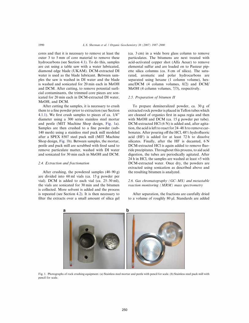
cores and that it is necessary to remove at least theouter 3 to 5 mm of core material to remove thesehydrocarbons (see Section 4.1). To do this, samplesare cut using a table saw with a water lubricated,diamond edge blade (UKAM). DCM-extracted DIwater is used as the blade lubricant. Between sam-ples the saw is washed in DI water and the bladeis washed and sonicated for 20 min each in MeOHand DCM. After cutting, to remove potential surfi-cial contaminants, the trimmed core pieces are son-icated for 20 min each in DCM-extracted DI water,MeOH, and DCM.
After cutting the samples, it is necessary to crushthem to a fine powder prior to extraction (see Section4.1.1). We first crush samples to pieces of ca. 1/4’’diameter using a 300 series stainless steel mortarand pestle (MIT Machine Shop design, Fig. 1a).Samples are then crushed to a fine powder (sub-140 mesh) using a stainless steel puck mill modeledafter a SPEX 8507 steel puck mill (MIT MachineShop design, Fig. 1b). Between samples, the mortar,pestle and puck mill are scrubbed with fired sand toremove particulate matter, washed with DI waterand sonicated for 30 min each in MeOH and DCM.
2.4. Extraction and fractionation
After crushing, the powdered samples (40–90 g)are divided into 60 ml vials (ca. 15 g powder pervial). DCM is added to each vial (ca. 25–30 ml),the vials are sonicated for 30 min and the bitumenis collected. More solvent is added and the processis repeated (see Section 4.2). It is then necessary tofilter the extracts over a small amount of silica gel
(ca. 3 cm) in a wide bore glass column to removeparticulates. The bitumens are next treated withacid-activated copper shot (Alfa Aesar) to removeelemental sulfur and are loaded on to Pasteur pip-ette silica columns (ca. 8 cm of silica). The satu-rated, aromatic and polar hydrocarbons areseparated using hexane (1 column volume), hex-ane/DCM (4 column volumes, 8/2) and DCM/MeOH (4 column volumes, 7/3), respectively.
2.5. Preparation of bitumen II
To prepare demineralized powder, ca. 30 g ofextracted rock powder is placed inTeflon tubeswhichare cleaned of organics first in aqua regia and thenwith MeOH and DCM (ca. 15 g powder per tube).DCM-extracted HCl (6 N) is added and, after agita-tion, the acid is left to react for 24–48 h to remove car-bonates. After pouring o" the HCl, 48% hydrofluoricacid (HF) is added for at least 72 h to dissolvesilicates. Finally, after the HF is decanted, 6 NDCM-extracted HCl is again added to remove fluo-ride precipitates. Throughout this process, to aid aciddigestion, the tubes are periodically agitated. After24 h in HCl, the samples are washed at least ·5 withDCM-extracted water. Once dry, the powders areextracted using sonication as described above andthe resulting bitumen is analyzed.
2.6. Gas chromatography (GC–MS) and metastablereaction monitoring (MRM) mass spectrometry
After separation, the fractions are carefully driedto a volume of roughly 80 ll. Standards are added
Fig. 1. Photographs of rock crushing equipment. (a) Stainless steel mortar and pestle with pencil for scale. (b) Stainless steel puck mill withpencil for scale.
1990 L.S. Sherman et al. / Organic Geochemistry 38 (2007) 1987–2000
250
as follows: 10 ng D4 (D4-aaa-ethylcholestane,Chiron) and 1 lg aiC22 (3-methylheneicosane,99+%, ULTRA Scientific) to the saturated fractionand 413 ng D14 (D14-para-terphenyl, 98 at.% D,Cambridge Isotope) to the aromatic fraction.
The saturated fractions are analyzed using GC–MS in full scan mode and metastable reaction mon-itoring GC–MS (MRM–GC–MS–MS; Table 1). Thearomatic fractions are analyzed using GC–MS withselected ion monitoring. All the analyses are con-ducted with a Micromass AutoSpec Ultima coupledto an Agilent 6890 N gas chromatograph, fitted with
a DB-1 fused silica column (60 m · 0.25 mm i.d.,0.25 lm film thickness, J&W Scientific) and usingHe as carrier gas. The mass spectrometer sourceoperates at 250 "C under electron ionization condi-tions (70 eV) and an accelerating voltage of 8 kV isused. Full scan analyses are conducted over a rangeof m/z 50–600. Peaks are integrated manually andquantified on the basis of comparison to the internalstandards (using m/z 85 from full scan analyses).
3. Typical results
Agouron Archean core samples ranged from 34.1to 95.6 g rock powder and yielded between 0.31 and21.1 lg of bitumen (saturated hydrocarbons andcyclic terpenoid biomarkers). By weight, the bitu-men content ranges from 13.9 to 604.6 ppb wholerock or 0.34 to 23.9 ppm organic matter. All theArchean bitumens yielded broadly similar typesand abundances of hydrocarbons. The compoundclasses detected, and their overall abundances andrelative amounts of rearranged isomers, are charac-teristic of highly thermally mature organic matter.Typical biomarker and saturated hydrocarbonchromatograms from a representative sample(GKF 705.3) are presented in Fig. 2. The Archeanbitumens are comprised almost entirely of saturatedand aromatic hydrocarbons; polar and partiallyunsaturated compounds are below detection limit.The saturated fractions are composed primarily oflow molecular weight n-alkanes with condensate-like carbon number distributions (Fig. 2b). The aro-matic fractions are dominated by low molecularweight polycyclic hydrocarbons and their alkylatedhomologs.
Cyclic terpenoid biomarker compounds are pres-ent in ppb to sub-ppb quantities; cheilanthanes,hopanes and steranes are present at roughly equalabundances. Thermodynamically-favored isomersfrom each of these terpenoid classes are found ingreater relative abundance. Tricyclic biomarkers,including 13b(H), 14a(H) homologs of C19 to C26
cheilanthanes, and a C24 tetracyclic terpane arepresent in all of the samples. Gammacerane is alsofound in low abundance in many of the samples.C27 to C35 hopanes of several series including17a(H), 21b(H)-hopanes, 17b(H), 21a(H)-hopanes(moretanes), 2a- and 3b-methylhopanes, 25- and30-norhopane, and C28 dinorhopanes are present(Fig. 2a). C26 to C30 steranes are also found in everysample, those with 27, 28 and 29 carbons being themost abundant (Fig. 2a). Among these, 5a(H),
Table 1MRM–GC–MS–MS precursor to product transitions
Precursor mass(Da)a
Product mass(Da)a
Biomarkers
262.265 191.179 C19 Tricyclic terpane276.280 191.179 C20 Tricyclic terpane290.296 191.179 C21 Tricyclic terpane304.312 191.179 C22 Tricyclic terpane318.328 191.179 C23 Tricyclic terpane330.328 191.179 C24 Tetracyclic
terpane332.344 191.179 C24 Tricyclic terpane346.359 191.179 C25 Tricyclic terpane360.374 191.179 C26 Tricyclic terpane358.353 217.196 C26 Steranes372.376 217.196 C27 Steranes386.391 217.196 C28 Steranes404.432 221.221 D4 C29 Sterane
b
400.407 217.196 C29 Steranes414.423 217.196 C30 Steranes426.421 205.194 Me–C30 Hopanesc
370.359 191.179 C27 Hopanes440.437 205.194 Me–C31
Homohopanes384.374 191.179 C28 Hopanes454.452 205.194 Me–C32
Homohopanes398.390 191.179 C29 Hopanes468.467 205.194 Me–C33
Homohopanes412.406 191.179 C30 Hopanes482.482 205.194 Me–C34
Homohopanes426.421 191.179 C31 Homohopanes496.496 205.194 Me–C35
Homohopanes440.437 191.179 C32 Homohopanes454.452 191.179 C33 Homohopanes468.467 191.179 C34 Homohopanes482.482 191.179 C35 Homohopanesa Precursor and product mass in Daltons.b ‘‘D4 C29 sterane’’ is the internal standard, D4-aaa-
ethylcholestane.c ‘‘Me–Cx’’ steranes and hopanes are methylated versions of the
indicated compounds.
L.S. Sherman et al. / Organic Geochemistry 38 (2007) 1987–2000 1991
251
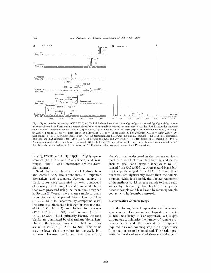
14a(H), 17b(H) and 5a(H), 14b(H), 17b(H) regularsteranes (both 20R and 20S epimers) and rear-ranged 13b(H), 17a(H)-diasteranes are the domi-nant isomers.
Sand blanks are largely free of hydrocarbonsand contain very low abundances of terpenoidbiomarkers and n-alkanes. Average sample toblank ratios were calculated for each compoundclass using the 17 samples and four sand blanksthat were processed using the techniques describedin Section 2. Overall, the average sample to blankratio for cyclic terpenoid biomarkers is 11.58(± 7.77, 1r SD). Separated by compound class,the sample to blank ratio is lower for cheilanthanes(4.88 ± 1.57, 1r SD) and higher for steranes(19.70 ± 15.82, 1r SD) and hopanes (16.38 ±14.10, 1r SD). This is primarily because the sandblanks are dominated by cheilanthane biomarkers.Overall, the average sample to blank ratio forn-alkanes is 3.67 (± 2.81, 1r SD). This valuemay be lower than the values for the cyclic bio-markers because n-alkanes are particularly
abundant and widespread in the modern environ-ment as a result of fossil fuel burning and petro-chemical use. Sand blank alkane yields (n = 4)ranged from 83.7 to 805 ng, whereas sand blank bio-marker yields ranged from 0.93 to 5.18 ng; thesequantities are significantly lower than the samplebitumen yields. It is possible that further refinementof the methods could increase sample to blank ratiovalues by eliminating low levels of carry-overbetween samples and blanks and by reducing samplecontact with hydrocarbon aerosols.
4. Justification of methodology
In developing the techniques described in Section2, we conducted several methodological experimentsto test the e!cacy of our approach. We soughtthroughout to minimize the number of sample pro-cessing steps and the amount of equipmentrequired, as each handling step is an opportunityfor contaminants to be introduced. This section pre-sents the results of several of these methodological
54.00 56.00 58.00 60.00 62.00 64.00Time
00 20.00 25.00 30.00 35.00 40.00 45.00 50.00
!GKF 705.3
m/z = 85
"""-20R
"##-20SDiasteranes
20S 20R
"""-20S
"##-20S
"""-20R
"##-20R
Diasteranes
20S 20R
"##-20R
"""-20S
TsTm
"""-20S
"##-20S
"""-20R
"##-20R
Diasteranes
20S 20R
GKF 705.3
********
*
*
C29 steranes400 > 217
C28 steranes386 > 217
C27 steranes372 > 217
Pr Ph
*
*
C27 hopanes370 > 191
C29 hopanes398 > 191
C30 hopanes412 > 191
#"
"#
#"
"# 30-nor
C29 Ts
Fig. 2. Typical results (from sample GKF 705.3). (a) Typical Archean biomarker traces. C27 to C29 steranes and C27, C29 and C30 hopanetraces are shown. Sand blank chromatograms shown below each sample trace are to the same absolute scaling. Relative retention times areshown in min. Compound abbreviations: C30-ab = 17a(H),21b(H)-hopane; 30-nor = 17a(H),21b(H)-30-norhomohopane; C30-ba = 17b-(H),21a(H)-hopane; C29-ab = 17a(H), 21b(H)-30-norhopane; C29 Ts = 18a(H),21b(H)-30-norneohopane; C29-ba = 17b(H),21a(H)-30-norhopane; Ts = C27 18a-trisnorhopane II; Tm = C27 17a-trisnorhopane; diasteranes (20S and 20R epimers) = 13b(H),17a(H) diasterane;aaa (20S and 20R epimers) = 5a(H),14a(H),17a(H) sterane; abb (20S and 20R epimers) = 5a(H),14b(H),17b(H) sterane. (b) TypicalArchean saturated hydrocarbon trace (from sample GKF 705.3; m/z 85). Internal standard (1 ug 3-methylheneicosane) indicated by ‘‘n’’.Regular n-alkane peaks (C13 to C24) indicated by ‘‘*’’. Compound abbreviations: Pr = pristane; Ph = phytane.
1992 L.S. Sherman et al. / Organic Geochemistry 38 (2007) 1987–2000
252
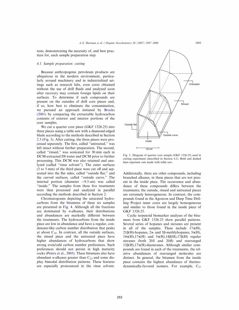
tests, demonstrating the necessity of, and best prac-tices for, each sample preparation step.
4.1. Sample preparation: cutting
Because anthropogenic petroleum products areubiquitous in the modern environment, particu-larly around machinery and in industrialized set-tings such as research labs, even cores obtainedwithout the use of drill fluids and analyzed soonafter recovery may contain foreign lipids on theirsurfaces. To determine if such compounds arepresent on the outsides of drill core pieces and,if so, how best to eliminate the contamination,we pursued an approach initiated by Brocks(2001) by comparing the extractable hydrocarboncontents of exterior and interior portions of thecore samples.
We cut a quarter core piece (GKF 1326.25) intothree pieces using a table saw with a diamond-edgedblade according to the methods described in Section2.3 (Fig. 3). After cutting, the three pieces were pro-cessed separately. The first, called ‘‘untreated,’’ wasleft intact without further preparation. The second,called ‘‘rinsed,’’ was sonicated for 30 min each inDCM-extracted DI water and DCM prior to furtherprocessing. This DCM was also retained and ana-lyzed (called ‘‘rinse solvent’’). The outer surfaces(3 to 5 mm) of the third piece were cut o" and sep-arated into the flat sides, called ‘‘outside flat,’’ andthe curved surfaces, called ‘‘outside curve,’’ Theinternal portion (diameter !9.5 cm) was called‘‘inside.’’ The samples from these five treatmentswere then processed and analyzed in parallelaccording the methods described in Section 2.
Chromatograms depicting the saturated hydro-carbons from the bitumens of these six samplesare presented in Fig. 4. Although all the fractionsare dominated by n-alkanes, their distributionsand abundances are markedly di"erent betweenthe treatments. The hydrocarbons from the insidepiece are low in abundance and have a regular, con-densate-like carbon number distribution that peaksat about C18. In contrast, all the outside surfaces,the rinsed piece and the untreated piece havehigher abundances of hydrocarbons that showstrong even/odd carbon number preferences. Suchpreferences should not persist in high maturityrocks (Peters et al., 2005). These bitumens also haveabundant n-alkanes greater than C22 and some dis-play bimodal distribution patterns. These featuresare especially pronounced in the rinse solvent.
Additionally, there are other compounds, includingbranched alkanes, in these pieces that are not pres-ent in the inside piece. The occurrence and abun-dance of these compounds di"ers between thetreatments; the outside, rinsed and untreated piecesare extremely heterogeneous. In contrast, the com-pounds found in the Agouron and Deep Time Dril-ling Project inner cores are largely homogeneousand similar to those found in the inside piece ofGKF 1326.25.
Cyclic terpenoid biomarker analyses of the bitu-mens from GKF 1326.25 show parallel patterns.Several series of hopanes and steranes are presentin all of the samples. These include 17a(H),21b(H)-hopanes, 2a- and 3b-methlyhopanes, 5a(H),14a(H),17a(H) and 5a(H),14b(H),17b(H) regularsteranes (both 20S and 20R) and rearranged13b(H),17a(H)-diasteranes. Although similar com-pounds are found in each of the treatments, the rel-ative abundances of rearranged molecules aredistinct. In general, the bitumen from the insidepiece contains the highest abundance of thermo-dynamically-favored isomers. For example, C27
Untreated
Rinsed
Inside
Outside flat
Outside curve
10 cm
Fig. 3. Diagram of quarter core sample (GKF 1326.25) used incutting experiment (described in Section 4.1). Bold and dashedlines represent cuts made with table saw.
L.S. Sherman et al. / Organic Geochemistry 38 (2007) 1987–2000 1993
253
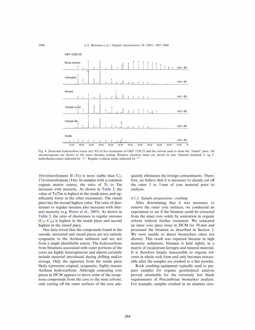
18a-trisnorhopane II (Ts) is more stable than C27
17a-trisnorhopane (Tm). In samples with a commonorganic matter source, the ratio of Ts to Tmincreases with maturity. As shown in Table 2, thevalue of Ts/Tm is highest in the inside piece and sig-nificantly lower in the other treatments. The rinsedpiece has the second highest value. The ratio of dias-teranes to regular steranes also increases with ther-mal maturity (e.g. Peters et al., 2005). As shown inTable 2, the ratio of diasteranes to regular steranes(C27–C29) is highest in the inside piece and secondhighest in the rinsed piece.
Our data reveal that the compounds found in theoutside, untreated and rinsed pieces are not entirelysyngenetic to the Archean sediment and are notfrom a single identifiable source. The hydrocarbonsfrom bitumens associated with outer portions of thecores are highly heterogeneous and almost certainlyinclude material introduced during drilling and/orstorage. Only the signature from the inside piecelikely represents original, syngenetic, highly matureArchean hydrocarbons. Although sonicating corepieces in DCM appears to move some of the exoge-nous compounds from the core to the rinse solvent,only cutting o" the outer surfaces of the core ade-
quately eliminates the foreign contaminants. There-fore, we believe that it is necessary to cleanly cut o"the outer 3 to 5 mm of core material prior toanalysis.
4.1.1. Sample preparation: crushingAfter determining that it was necessary to
remove the outer core surfaces, we conducted anexperiment to see if the bitumen could be extractedfrom the inner core solely by sonication in organicsolvent without further treatment. We sonicatedan inner core piece twice in DCM for 30 min andprocessed the bitumen as described in Section 2.We were unable to detect biomarkers (data notshown). This result was expected because in highmaturity sediments, bitumen is held tightly in amatrix of recalcitrant kerogen and mineral material.It is therefore largely inaccessible to organic sol-vents in whole rock form and only becomes extract-able after the samples are crushed to a fine powder.
Rock crushing equipment typically used to pre-pare samples for organic geochemical analysisproved unsuitable for the extremely low blankrequirements of Precambrian biomarker analysis.For example, samples crushed in an alumnia cera-
15.00 20.00 25.00 30.00 35.00 40.00 45.00 50.00 55.00 60.00 65.00 70.00 75
!
!
!
!
!
!Rinse solvent
Untreated
Rinsed
Outside curve
Outside flat
Inside
GKF 1326.25
m/z = 85
m/z = 85
m/z = 85
m/z = 85
m/z = 85
m/z = 85
***
*
*
*
***
* * * * * * *** * * *
***
*
*
*
**
*
* * * **
* ***** * * * *** *
*
**
*
*
*
**
* * * *** * *
* *****
* * * **
**
*
* ***** * *** **
Fig. 4. Saturated hydrocarbon traces (m/z 85) of five treatments of GKF 1326.25 and the solvent used to clean the ‘‘rinsed’’ piece. Allchromatograms are shown to the same absolute scaling. Relative retention times are shown in min. Internal standard (1 ug 3-methylheneicosane) indicated by ‘‘n’’. Regular n-alkane peaks indicated by ‘‘*’’.
1994 L.S. Sherman et al. / Organic Geochemistry 38 (2007) 1987–2000
254
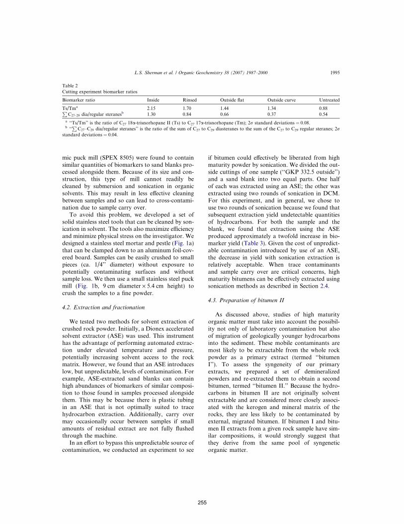
mic puck mill (SPEX 8505) were found to containsimilar quantities of biomarkers to sand blanks pro-cessed alongside them. Because of its size and con-struction, this type of mill cannot readily becleaned by submersion and sonication in organicsolvents. This may result in less e"ective cleaningbetween samples and so can lead to cross-contami-nation due to sample carry over.
To avoid this problem, we developed a set ofsolid stainless steel tools that can be cleaned by son-ication in solvent. The tools also maximize e!ciencyand minimize physical stress on the investigator. Wedesigned a stainless steel mortar and pestle (Fig. 1a)that can be clamped down to an aluminum foil-cov-ered board. Samples can be easily crushed to smallpieces (ca. 1/4’’ diameter) without exposure topotentially contaminating surfaces and withoutsample loss. We then use a small stainless steel puckmill (Fig. 1b, 9 cm diameter · 5.4 cm height) tocrush the samples to a fine powder.
4.2. Extraction and fractionation
We tested two methods for solvent extraction ofcrushed rock powder. Initially, a Dionex acceleratedsolvent extractor (ASE) was used. This instrumenthas the advantage of performing automated extrac-tion under elevated temperature and pressure,potentially increasing solvent access to the rockmatrix. However, we found that an ASE introduceslow, but unpredictable, levels of contamination. Forexample, ASE-extracted sand blanks can containhigh abundances of biomarkers of similar composi-tion to those found in samples processed alongsidethem. This may be because there is plastic tubingin an ASE that is not optimally suited to tracehydrocarbon extraction. Additionally, carry overmay occasionally occur between samples if smallamounts of residual extract are not fully flushedthrough the machine.
In an e"ort to bypass this unpredictable source ofcontamination, we conducted an experiment to see
if bitumen could e"ectively be liberated from highmaturity powder by sonication. We divided the out-side cuttings of one sample (‘‘GKP 332.5 outside’’)and a sand blank into two equal parts. One halfof each was extracted using an ASE; the other wasextracted using two rounds of sonication in DCM.For this experiment, and in general, we chose touse two rounds of sonication because we found thatsubsequent extraction yield undetectable quantitiesof hydrocarbons. For both the sample and theblank, we found that extraction using the ASEproduced approximately a twofold increase in bio-marker yield (Table 3). Given the cost of unpredict-able contamination introduced by use of an ASE,the decrease in yield with sonication extraction isrelatively acceptable. When trace contaminantsand sample carry over are critical concerns, highmaturity bitumens can be e"ectively extracted usingsonication methods as described in Section 2.4.
4.3. Preparation of bitumen II
As discussed above, studies of high maturityorganic matter must take into account the possibil-ity not only of laboratory contamination but alsoof migration of geologically younger hydrocarbonsinto the sediment. These mobile contaminants aremost likely to be extractable from the whole rockpowder as a primary extract (termed ‘‘bitumenI’’). To assess the syngeneity of our primaryextracts, we prepared a set of demineralizedpowders and re-extracted them to obtain a secondbitumen, termed ‘‘bitumen II.’’ Because the hydro-carbons in bitumen II are not originally solventextractable and are considered more closely associ-ated with the kerogen and mineral matrix of therocks, they are less likely to be contaminated byexternal, migrated bitumen. If bitumen I and bitu-men II extracts from a given rock sample have sim-ilar compositions, it would strongly suggest thatthey derive from the same pool of syngeneticorganic matter.
Table 2Cutting experiment biomarker ratios
Biomarker ratio Inside Rinsed Outside flat Outside curve Untreated
Ts/Tma 2.15 1.70 1.44 1.34 0.88PC27–29 dia/regular steranesb 1.30 0.84 0.66 0.37 0.54
a ‘‘Ts/Tm’’ is the ratio of C27 18a-trisnorhopane II (Ts) to C27 17a-trisnorhopane (Tm); 2r standard deviations = 0.08.b ‘‘
PC27–C29 dia/regular steranes’’ is the ratio of the sum of C27 to C29 diasteranes to the sum of the C27 to C29 regular steranes; 2r
standard deviations = 0.04.
L.S. Sherman et al. / Organic Geochemistry 38 (2007) 1987–2000 1995
255
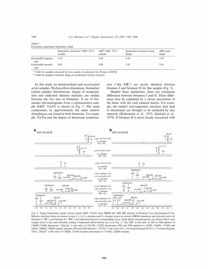
In this study we demineralized and re-extractedseven samples. Hydrocarbon abundance, biomarkercarbon number distributions, degree of isomeriza-tion and indicated thermal maturity are similarbetween the two sets of bitumens. A set of bio-marker chromatograms from a representative sam-ple (GKF 314.65) is shown in Fig. 5. The samecompounds, in approximately the same relativeabundances, are found in both bitumens. For exam-ple, Ts/Tm and the degree of diasterane isomeriza-
tion (‘‘dia S/R’’) are nearly identical betweenbitumen I and bitumen II for this sample (Fig. 5).
Despite these similarities, there are systematicdi"erences between bitumens I and II. These di"er-ences may be explained by a closer association ofthe latter with the rock mineral matrix. For exam-ple, the methyl rearrangement reactions that leadto diasteranes are thought to be catalyzed by clayminerals (Rubenstein et al., 1975; Sieskind et al.,1979). If bitumen II is more closely associated with
Table 3Extraction experiment biomarker yields
Sonication extractiona GKF 332.5outside
ASEb GKF 332.5outside
Sonication extraction sandblank
ASE sandblank
Extractable hopanes(ng)
2.39 5.49 0.50 1.83
Extractable steranes(ng)
4.81 9.08 1.05 2.61
a Yield for samples extracted by two rounds of sonication for 30 min in DCM.b Yield for samples extracted using an accelerated solvent extractor.
53.00 54.00 55.00 56.00 57.00 58.00 59.00 60.00 61.00 62.00 63.00 64.00 3.00 54.00 55.00 56.00 57.00 58.00 59.00 60.00 61.00 62.00 63.00 64.00 6
C27 hopanes370 > 191
C27 steranes372 > 217
C29 hopanes398 > 191
C30 hopanes412 > 191
GKF 314.65 BI GKF 314.65 BII
"""-20R
20S20R
"##-20S
Diasteranes
20S 20R
"""-20S "##-20S"""-20R
"##-20RDiasteranes
20S 20R
"##-20R
"""-20S
"""-20R"##-20R"""-20S
"##-20S
Ts Tm
Diasteranes
#"
"#
#"
"# 30-nor
C29 Ts
"""-20R
20R
"##-20S
Diasteranes
20S20R
"""-20S "##-20S"""-20R
"##-20R
Diasteranes
20S20R
"##-20R
"""-20S
"""-20R"##-20R"##-20S
Ts Tm
#"
"#
"#
C29 Ts
Diasteranes20S
"""-20S
#"
30-nor
dia/reg0.80 1.67
Ts/Tm1.36 1.42
0.10 0.06
0.08 0.08
#"/"#
#"/"#
dia S/R1.65 1.55
C28 steranes386 > 217
dia/reg0.74 2.21dia S/R1.65 1.72
C29 steranes400 > 217
dia/reg0.59 1.41dia S/R1.17 1.37
Fig. 5. Typical biomarker results (from sample GKF 314.65) from MRM–GC–MS–MS analysis of bitumen I (a) and bitumen II (b).Relative retention times are shown in min. C27 to C29 steranes and C27 hopane traces are shown; MRM transitions and relevant ratios forbitumen I (‘‘BI’’) and bitumen II (‘‘BII’’) are indicated between corresponding traces. Sand blank chromatograms are shown below eachsample trace to the same absolute scaling. Compound abbreviations are as in Fig. 2; ‘‘dia S/R’’ is the ratio of 20S to 20R epimers of13b(H),17a(H) diasterane; ‘‘dia/reg’’ is the ratio of 13b (H), 17a(H) diasteranes (20S and 20R epimers) to 5a(H), 14a(H), 17a(H) and5a(H), 14b(H), 17b(H) regular steranes (20S and 20R epimers); ‘‘Ts/Tm’’ is the ratio of C27 18a-trisnorhopane II to C27 17a-trisnorhopane(Tm); ‘‘ba/ab’’ is the ratio of 17b(H), 21a(H) hopane (moretane) to 17a(H), 21b(H) hopane.
1996 L.S. Sherman et al. / Organic Geochemistry 38 (2007) 1987–2000
256
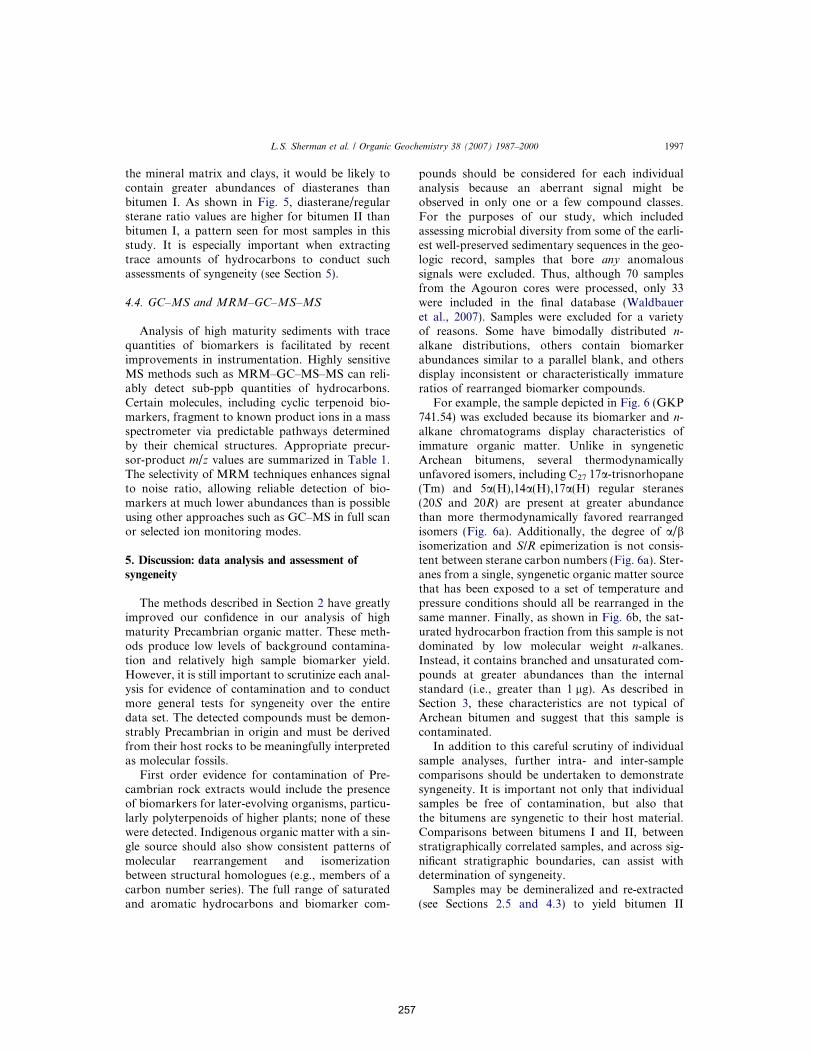
the mineral matrix and clays, it would be likely tocontain greater abundances of diasteranes thanbitumen I. As shown in Fig. 5, diasterane/regularsterane ratio values are higher for bitumen II thanbitumen I, a pattern seen for most samples in thisstudy. It is especially important when extractingtrace amounts of hydrocarbons to conduct suchassessments of syngeneity (see Section 5).
4.4. GC–MS and MRM–GC–MS–MS
Analysis of high maturity sediments with tracequantities of biomarkers is facilitated by recentimprovements in instrumentation. Highly sensitiveMS methods such as MRM–GC–MS–MS can reli-ably detect sub-ppb quantities of hydrocarbons.Certain molecules, including cyclic terpenoid bio-markers, fragment to known product ions in a massspectrometer via predictable pathways determinedby their chemical structures. Appropriate precur-sor-product m/z values are summarized in Table 1.The selectivity of MRM techniques enhances signalto noise ratio, allowing reliable detection of bio-markers at much lower abundances than is possibleusing other approaches such as GC–MS in full scanor selected ion monitoring modes.
5. Discussion: data analysis and assessment ofsyngeneity
The methods described in Section 2 have greatlyimproved our confidence in our analysis of highmaturity Precambrian organic matter. These meth-ods produce low levels of background contamina-tion and relatively high sample biomarker yield.However, it is still important to scrutinize each anal-ysis for evidence of contamination and to conductmore general tests for syngeneity over the entiredata set. The detected compounds must be demon-strably Precambrian in origin and must be derivedfrom their host rocks to be meaningfully interpretedas molecular fossils.
First order evidence for contamination of Pre-cambrian rock extracts would include the presenceof biomarkers for later-evolving organisms, particu-larly polyterpenoids of higher plants; none of thesewere detected. Indigenous organic matter with a sin-gle source should also show consistent patterns ofmolecular rearrangement and isomerizationbetween structural homologues (e.g., members of acarbon number series). The full range of saturatedand aromatic hydrocarbons and biomarker com-
pounds should be considered for each individualanalysis because an aberrant signal might beobserved in only one or a few compound classes.For the purposes of our study, which includedassessing microbial diversity from some of the earli-est well-preserved sedimentary sequences in the geo-logic record, samples that bore any anomaloussignals were excluded. Thus, although 70 samplesfrom the Agouron cores were processed, only 33were included in the final database (Waldbaueret al., 2007). Samples were excluded for a varietyof reasons. Some have bimodally distributed n-alkane distributions, others contain biomarkerabundances similar to a parallel blank, and othersdisplay inconsistent or characteristically immatureratios of rearranged biomarker compounds.
For example, the sample depicted in Fig. 6 (GKP741.54) was excluded because its biomarker and n-alkane chromatograms display characteristics ofimmature organic matter. Unlike in syngeneticArchean bitumens, several thermodynamicallyunfavored isomers, including C27 17a-trisnorhopane(Tm) and 5a(H),14a(H),17a(H) regular steranes(20S and 20R) are present at greater abundancethan more thermodynamically favored rearrangedisomers (Fig. 6a). Additionally, the degree of a/bisomerization and S/R epimerization is not consis-tent between sterane carbon numbers (Fig. 6a). Ster-anes from a single, syngenetic organic matter sourcethat has been exposed to a set of temperature andpressure conditions should all be rearranged in thesame manner. Finally, as shown in Fig. 6b, the sat-urated hydrocarbon fraction from this sample is notdominated by low molecular weight n-alkanes.Instead, it contains branched and unsaturated com-pounds at greater abundances than the internalstandard (i.e., greater than 1 lg). As described inSection 3, these characteristics are not typical ofArchean bitumen and suggest that this sample iscontaminated.
In addition to this careful scrutiny of individualsample analyses, further intra- and inter-samplecomparisons should be undertaken to demonstratesyngeneity. It is important not only that individualsamples be free of contamination, but also thatthe bitumens are syngenetic to their host material.Comparisons between bitumens I and II, betweenstratigraphically correlated samples, and across sig-nificant stratigraphic boundaries, can assist withdetermination of syngeneity.
Samples may be demineralized and re-extracted(see Sections 2.5 and 4.3) to yield bitumen II
L.S. Sherman et al. / Organic Geochemistry 38 (2007) 1987–2000 1997
257
fractions. Because bitumen II represents a pool ofhydrocarbons that was not solvent-accessible inthe crushed rock powder, it is less likely to bea"ected by mobile contaminants than bitumen I.Therefore, for a given sample, if bitumen I is sim-ilar in composition to bitumen II (with predictabledi"erences as described in Section 4.3), it is likelyto be derived from the same pool of syndeposi-tional organic matter instead of from a separatesource.
Comparisons between stratigraphically corre-lated samples from geographically distinct corescan also strongly support claims of syngeneity. Iffeasible, cores drilled at close proximity can be usedto assess the lateral variability along the strike of agiven unit. Such cores also allow for comparison ofdirectly correlated samples, potentially strengthen-ing claims of syngeneity. Given the resources neces-sary to obtain drill core material, it may be di!cultto justify ‘re-sampling’ the same strata; nevertheless,we have found inter-core comparisons to be valu-able tests of syngeneity. For example, in the caseof the Agouron Griqualand Drilling Project, coresGKF and GKP were drilled 24 km apart throughdi"erent but correlatable portions of a depositionalsystem. This allows for the comparison of chemo-stratigraphic patterns and variations between corre-
lated samples through a variety of depositionalsystems. By making such comparisons betweenGKP and GKF, we observed strong correlationsin biomarker content, especially in the deepwaterfacies (Waldbauer et al., 2007). Inter-core correla-tions are strong evidence both for depositional con-trol of organic matter content and the syngeneity ofmolecular fossils.
Comparison of Archean samples to youngerunits across an unconformity may also supportclaims of syngeneity. In cases where Phanerozoicsediments unconformably overlie Precambrianmaterial, a strong geochemical contrast shouldexist. This contrast would be overprinted anddiminished if contaminants were introduced duringdrilling, storage, or handling. The Agouron Drillingproject recovered approximately 200 m of a Permo-Carboniferous diamictite that was deposited directlyon top of the youngest Precambrian unit, creating a2 billion year unconformity (Visser, 1989). Bitumensextracted from this diamictite are in fact geochemi-cally distinct from the underlying Archean material.The younger material is much less thermally matureand substantially more heterogeneous. This clearcontrast provides additional evidence that bitumensextracted from Archean units are in fact syngeneticand were not contaminated either by hydrocarbons
54.00 56.00 58.00 60.00 62.00 15.00 20.00 25.00 30.00 35.00 40.00 45.
!
GKF 741.54
m/z = 85
"""-20R
"##-20SDiasteranes20S
20R
"""-20S
"##-20S
"""-20R"##-20RDiasteranes
20S 20R
"##-20R
"""-20S
TsTm
dia/reg
C27 hopanes370 > 191
C27 steranes372 > 217
"""-20S
"##-20S """-20R"##
"##
"##
"##
-20RDiasteranes
20S 20R
GKF 741.54
***
**
*
*
*
*
*
*
0.34reg S/R 1.28
dia/reg
C28 steranes386 > 217
0.41reg S/R 0.42
dia/reg
C29 steranes400 > 217
0.44reg S/R 2.67
Ts/Tm 0.59
Fig. 6. Example of a potentially contaminated sample (GKF 741.54). Compound abbreviations and symbols are as in Figs. 2 and 5; ‘‘regabb S/R’’ is the ratio of 20S to 20R epimers of 5a(H),14b(H),17b(H) sterane. Relative retention times are shown in min. (a) Biomarkerchromatograms of C27 to C29 steranes and C27 hopanes; sand blank traces are shown below each chromatogram to the same absolutescaling. (b) Chromatogram of saturated hydrocarbon fraction (m/z 85).
1998 L.S. Sherman et al. / Organic Geochemistry 38 (2007) 1987–2000
258
from younger units or from the externalenvironment.
All of the characteristics of each sample and itscorresponding blank should be examined in tandemwith complete data set analyses of syngeneity asdescribed above. Given the low biomarker yieldsfrom Precambrian sediments and the ubiquitousenvironmental presence of petroleum-derivedhydrocarbons, sample contamination can easilyoccur. Throughout data analysis, it remains up tothe investigator to determine the best and most con-sistent course of action – a single set of criteria isunlikely to be applicable to all situations.
6. Conclusions
Key aspects of methods described in this paperwould not have been feasible during the 1960s whenthe organic geochemistry of Precambrian rocks wasfirst studied. Not only did researchers not initiallyrecognize the prevalence of potential contaminants,but also the materials and instrumentation neces-sary to successfully process high maturity sampleswere not available. Materials such as high purityorganic-free solvents were not commercially avail-able and investigators had to distill their own (Hoer-ing, 1967). Pure, isotopically labeled internalstandards were similarly not available. Additionally,instrumentation such as highly sensitive GC–MS–MS was not refined until the 1980s.
The procedures presented take advantage ofthese advances in technology. While we believe thatthe methods are well suited for the analysis of traceamounts of hydrocarbons, as described above, eachdata set should be carefully examined for any evi-dence of contamination or sample carry over.Application of the techniques allows researchers todo now that which was impossible in the mid-20thcentury, that is, study demonstrably Precambrianhigh maturity organic matter to learn about micro-bial evolution and early life on Earth.
Acknowledgements
Funding for this research came from the NSF(EAR0418619), the NASA Exobiology Program(Grant# NNG05GN62G), the Agouron Instituteand the NASA Astrobiology Institute. J.R.W. re-ceives support through an NDSEG Fellowship fromthe O!ce of Naval Research. We would like tothank the Griqualand Project team members, theAgouron Institute and the members of the Deep
Time Drilling Project and the NASA AstrobiologyInstitute for the core samples. We specificallyacknowledge Alex Birch, Francis McDonald, JohnDunlop and Les Bonser for overseeing the core dril-ling and field operations. Thanks go to RogerBuick, Ariel Anbar, Joe Kirschvink and DawnSumner for on-site sample collection and core cura-tion. For design and manufacture of our crushingtools, we would like to thank Andrew Gallant andthe MIT Central Machine Shop. We would also liketo thank Gordon Love for many useful discussionson biomarker analysis, Rick Kayser for lab. assis-tance and Carolyn Colonero for maintaining themass spectrometers. Finally, we thank Kenneth Pe-ters and an anonymous reviewer for thoughtfulcomments.
Associate Editor—K. E. Peters
References
Anbar, A.D., Duan, Y., Lyons, T.W., Arnold, G.L., Kendall, B.,Creaser, R.A., Kaufman, A.J., Gordon, G.W., Scott, C.,Garvin, J., Buick, R., 2007. A whi" of oxygen before theGreat Oxidation Event? Science 317, 1903–1906.
Armstrong, R.A., Compton, W., Retief, E.A., Wilke, N.J., 1986.Ages and isotopic evolution of the Ventersdorp volcanics. In:Geocongress 1986. Geological Society of South Africa, SouthAfrica, pp. 89–92.
Barghoorn, E.S., 1957. Origin of Life. Geological Society ofAmerica Memoir 67, 75–86.
Barghoorn, E.S., Meinschein, W.G., Schopf, J.W., 1965.Paleobiology of a Precambrian shale. Science 148, 461–472.
Barton, E.S., Altermann, W., Williams, I.S., Smith, C.B., 1994.U-Pb zircon age for a tu" in the Campbell Group, GriqualandWest Sequence, South Africa; implications for early Protero-zoic rock accumulation rates. Geology 22, 343–346.
Bekker, A., Holland, H.D., Wang, P.L., Rumble III, D., Stein,H.J., Hannah, J.L., Coetzee, L.L., Beukes, N.J., 2004. Datingthe rise of atmospheric oxygen. Nature 427, 117–120.
Brocks, J.J., 2001. Molecular Fossils in Archean Rocks. SydneyUniversity, Sydney.
Brocks, J.J., Buick, R., Logan, G.A., Summons, R.E., 2003a.Composition and syngeneity of molecular fossils from the2.78 to 2.45 billion-year-old Mount Bruce Supergroup,Pilbara Craton, Western Australia. Geochimica et Cosmo-chimica Acta 67, 4289–4319.
Brocks, J.J., Buick, R., Summons, R.E., Logan, G.A., 2003b. Areconstruction of Archean biological diversity based onmolecular fossils from the 2.78 to 2.45 billion-year-old MountBruce Supergroup, Hamersley Basin, Western Australia.Geochimica et Cosmochimica Acta 67, 4321–4335.
Brocks, J.J., Logan, G.A., Buick, R., Summons, R.E., 1999.Archean molecular fossils and the early rise of eukaryotes.Science 285, 1033–1036.
Brocks, J.J., Pearson, A., 2005. Building the biomarker tree oflife. Review in Mineralogy and Geochemistry 59, 233–258.
L.S. Sherman et al. / Organic Geochemistry 38 (2007) 1987–2000 1999
259
Brocks, J.J., Summons, R.E., 2003. Sedimentary hydrocarbons,biomarkers for early life. In: Holland, H.D., Turekian, K.K.(Eds.), Treatise on Geochemistry. Pergamon, Oxford, pp. 63–115.
Dutkiewicz, A., Volk, H., George, S.C., Ridley, J., Buick, R.,2006. Biomarkers from huronian oil-bearing fluid inclusions:An uncontaminated record of life before the Great OxidationEvent. Geology 34 (6), 437–440.
Eglinton, G., Scott, P.M., Belsky, T., Burlingame, A.L., Calvin,M., 1964. Hydrocarbons from a one-billion-year-old sedi-ment. Science 145, 263–264.
Eigenbrode, J.L., 2004. Late Archean microbial ecology: Anintegration of molecular, isotopic and lithological studies. In:Earth Sciences. The Pennsylvania State University, StateCollege.
Hayes, J.M., Kaplan, I.R., Wedeking, K.W., 1983. Precambrianorganic geochemistry, preservation of the record. In: Schopf,J.W. (Ed.), Earth’s Earliest Biosphere, Its Origin and Evolu-tion. Princeton University Press, Princeton, pp. 93–134.
Hoering, T.C., 1966. Criteria for suitable rocks in Precambrianorganic geochemistry. Carnegie Institution of WashingtonYearbook 65, 365–372.
Hoering, T.C., 1967. The organic geochemistry of Precambrianrocks. In: Abelson, P.H. (Ed.), Researches in Geochemistry,vol. 2. John Wiley, New York, pp. 87–111.
Imbus, S.W., McKirdy, D.M., 1993. Organic geochemistry ofPrecambrian sedimentary rocks. In: Engel, M.H., Macko,S.A. (Eds.), Organic Geochemistry. Plenum Press, New York,pp. 657–684.
Kaufman, A.J., Johnston, D.T., Farquhar, J., Masterson, A.L.,Lyons, T.W., Bates, S., Anbar, A., Arnold, G.L., Garvin, J.,Buick, R., 2007. Late Archean biospheric oxygenation andatmospheric evolution. Science 317, 1900–1903.
Leventhal, J., Suess, S.E., Cloud, P., 1975. Nonprevalence ofbiochemical fossils in kerogen from pre-Phanerozoic sedi-ments. Geology 72, 4706–4710.
McKirdy, D.M., 1974. Organic geochemistry in Precambrianresearch. Precambrian Research 1, 75–137.
Meinschein, W.G., 1965. Soudan Formation: organic extracts ofearly Precambrian rocks. Science 150, 601–605.
Nagy, B., 1970. Porosity and permeability of the earlyPrecambrian Onverwacht chert: Origin of the hydrocar-bon content. Geochimica et Cosmochimica Acta 34,525–526.
Peters, K.E., Walters, C.C., Moldowan, J.M., 2005. The Bio-marker Guide. Cambridge University Press, Cambridge, 1155pp.
Rubenstein, I., Seiskind, O., Albrecht, P., 1975. Rearrangedsteranes in a shale: Occurrence and simulated formation.Journal of the Chemical Society, Perkin Transactions I, 1833–1836.
Sanyal, S.K., Kvenvolden, K.A., Marsden, S.S.J., 1971. Perme-abilities of Precambrian Onverwacht cherts and other lowpermeability rocks. Nature 232, 325–327.
Schroder, S., Lacassi, J.P., Beukes, N.J., 2006. Stratigraphicand geochemical framework of the Agouron drill cores,Transvaal Supergroup (Neoarchean-Paleoproterozoic,South Africa). South African Journal of Geology 109,23–54.
Sieskind, O., Joly, G., Albrecht, P., 1979. Simulation of thegeochemical transformation of sterols: Superacid e!ects ofclay minerals. Geochimica et Cosmochimica Acta 43, 1675–1679.
Sumner, D.Y., Bowring, S.A., 1996. U-Pb geochronologicconstraints on deposition of the Campbellrand Subgroup,Transvaal Supergroup, South Africa. Precambrian Research79, 25–35.
Visser, J.N.J., 1989. The Permo-Carboniferous Dwyka Forma-tion of Southern Africa: Deposition by a predominantlysubpolar marine ice sheet. Palaeogeography, Palaeoclimatol-ogy, Palaeoecology 70, 377–391.
Waldbauer, J.R., Sherman, L.S., Sumner, D.Y., Summons, R.E.,2007. Late Archean molecular fossils from the TransvaalSupergroup record the antiquity of microbial diversity andaerobiosis. Precambrian Research.
Walraven, F., Martini, J., 1995. Zircon Pb-evaporation agedeterminations of the Oak Tree Formation, ChuniespoortGroup, Transvaal Sequence: Implications for Transvaal-Griqualand West basin correlations. South African Journalof Geology 98, 58–67.
2000 L.S. Sherman et al. / Organic Geochemistry 38 (2007) 1987–2000
260
Appendix C
Proteorhodopsin photosystem gene expression enables photophosphorylation in a heterologous host
Asunción Martínez, Alexander S. Bradley, Jacob R. Waldbauer,
Roger E. Summons and Edward F. DeLong
Reprinted with permission from Proceedings of the National Academy of Sciences © 2007 The National Academy of Sciences of the USA Martínez, A., Bradley, A.S., Waldbauer, J.R., Summons, R.E. and DeLong, E.F. (2007) Proteorhodopsin photosystem gene expression enables photophosphorylation in a heterologous host. Proceedings of the National Academy of Sciences 104: 5590-5595.
261

262
Proteorhodopsin photosystem gene expressionenables photophosphorylation in a heterologous hostA. Martinez*, A. S. Bradley†, J. R. Waldbauer‡, R. E. Summons†, and E. F. DeLong*§
*Department of Civil and Environmental Engineering, Division of Biological Engineering, and †Department of Earth, Atmospheric, and Planetary Sciences,Massachusetts Institute of Technology, Cambridge, MA 02139; and ‡Joint Program in Chemical Oceanography, Woods Hole Oceanographic Institutionand Massachusetts Institute of Technology, Cambridge, MA 02139
Edited by W. Ford Doolittle, Dalhousie University, Halifax, NS, Canada, and approved February 9, 2007 (received for review December 22, 2006)
Proteorhodopsins (PRs) are retinal-containing proteins that cata-lyze light-activated proton efflux across the cell membrane. Thesephotoproteins are known to be globally distributed in the ocean’sphotic zone, and they are found in a diverse array of Bacteria andArchaea. Recently, light-enhanced growth rates and yields havebeen reported in at least one PR-containing marine bacterium, butthe physiological basis of light-activated growth stimulation hasnot yet been determined. To describe more fully PR photosystemgenetics and biochemistry, we functionally surveyed a marinepicoplankton large-insert genomic library for recombinant clonesexpressing PR photosystems in vivo. Our screening approach ex-ploited transient increases in vector copy number that significantlyenhanced the sensitivity of phenotypic detection. Two geneticallydistinct recombinants, initially identified by their orange pigmen-tation, expressed a small cluster of genes encoding a completePR-based photosystem. Genetic and biochemical analyses of trans-poson mutants verified the function of gene products in thephotopigment and opsin biosynthetic pathways. Heterologousexpression of six genes, five encoding photopigment biosyntheticproteins and one encoding a PR, generated a fully functional PRphotosystem that enabled photophosphorylation in recombinantEscherichia coli cells exposed to light. Our results demonstrate thata single genetic event can result in the acquisition of phototrophiccapabilities in an otherwise chemoorganotrophic microorganism,and they explain in part the ubiquity of PR photosystems amongdiverse microbial taxa.
photoheterotrophy ! rhodopsin ! lateral gene transfer ! marine !metagenomics
Proteorhodopsins (PRs) are retinal-binding membrane pro-teins belonging to the rhodopsin family. Prokaryotic mem-
bers of this family include photosensors (sensory rhodopsins),transmembrane proton pumps (bacteriorhodopsins, xanthoro-hodopsin, and PRs), and transmembrane chloride pumps (halor-hodopsins). Originally discovered in Archaea, rhodopsins werelater identified in Gammaproteobacteria of the SAR86 groupduring a cultivation-independent genomic survey. Dubbed pro-teorhodopsin, this photoprotein functions as a light-activatedproton pump when expressed in Escherichia coli in the presenceof exogenously added retinal (1). Since then, numerous molec-ular surveys have demonstrated that PR genes are ubiquitous inbacteria inhabiting the ocean’s photic zone (2–9). An estimated13% of bacteria in marine picoplankton populations, as well asa significant fraction of planktonic Euryarchaeota, contain a PRgene (4, 8). In a number of marine bacteria, retinal biosyntheticgenes and PR are genetically linked, and their lateral transferand retention appear to be relatively common events, indicatingthat the photosystem confers a significant fitness advantage (3,4, 7, 10, 11). A recent report of light-stimulated growth in aPR-containing marine flavobacterium supports this hypothesis(11). Despite all of these observations however, the variousspecific functions and physiological roles of diverse marinemicrobial PRs remain to be fully described.
To further characterize PR photosystem structure and func-tion, we directly screened large-insert DNA libraries derivedfrom marine picoplankton for visibly detectable PR-expressingphenotypes. In this report, we describe completely intact PR-based photosystems that can be functionally expressed in E. coli,without addition of exogenous photopigment (e.g., retinal or itsprecursors). Analyses of insertional mutants verified the func-tional annotation of each gene product in the photosystembiosynthetic pathway. We also show that light-activated, PR-catalyzed proton translocation, by the chemiosmotic potential itgenerates, activates photophosphorylation in E. coli.
ResultsScreening a Fosmid Library for in Vivo PR Photosystem Expression.When E. coli expresses a PR apoprotein from an induciblepromoter on a high-copy number plasmid, the cells acquire a redor orange pigmentation in the presence of exogenous all-transretinal (1, 12). Retinal addition is required because E. coli lacksthe ability to biosynthesize retinal or its precursor, !-carotene.Based on these observations, we screened for PR-containingclones on retinal-containing LB agar plating medium, which weexpected would display an orange to red phenotype under theseconditions. To enhance assay sensitivity, we used the copy-control system present in our fosmid vector that allowed acontrolled transition from one copy per cell to multiple (up to100) vector copies upon addition of the inducer L-arabinose (13).
A fosmid library prepared from ocean surface water pico-plankton containing 12,280 clones (!440 Mb of cloned DNA)(14) was screened by using the above approach. Three orangecolonies were identified as potential PR-expressing clones on theLB-retinal-L-arabinose agar plates. All three showed no pigmen-tation in the absence of the high-copy number inducer. Unex-pectedly, these clones also displayed an orange phenotype in theabsence of L-retinal when induced to high copy number. Thesequence of one clone, HF10!19P19, revealed the presence of aPR gene near the fosmid vector junction (see below). Becausethe clones exhibited orange pigmentation in the absence ofexogenous retinal, we expected that they must also be expressingretinal biosynthetic genes. Two clones, HF10!25F10 and
Author contributions: A.M. and E.F.D. designed research; A.M., A.S.B., and J.R.W. per-formed research; A.M., A.S.B., J.R.W., R.E.S., and E.F.D. analyzed data; and A.M. and E.F.D.wrote the paper.
The authors declare no conflict of interest.
This article is a PNAS direct submission.
Abbreviations: CCCP, carbonylcyanide m-chlorophenylhydrazone; DCCD, N,N"-dicyclo-hexylcarbodiimide; FPP, farnesyl diphosphate; GGPP, geranylgeranyl pyrophosphate; IPP,isopentenyl diphosphate; PR, proteorhodopsin.
Data deposition: The sequences reported in this paper have been deposited in the GenBankdatabase [accession nos. EF100190 (HF10!19P19) and EF100191 (HF10!25F10)].§To whom correspondence should be addressed at: Department of Civil and EnvironmentalEngineering, 48-427, Massachusetts Institute of Technology, 15 Vassar Street, Cambridge,MA 02139. E-mail: [email protected].
This article contains supporting information online at www.pnas.org/cgi/content/full/0611470104/DC1.
© 2007 by The National Academy of Sciences of the USA
5590–5595 ! PNAS ! March 27, 2007 ! vol. 104 ! no. 13 www.pnas.org"cgi"doi"10.1073"pnas.0611470104
263
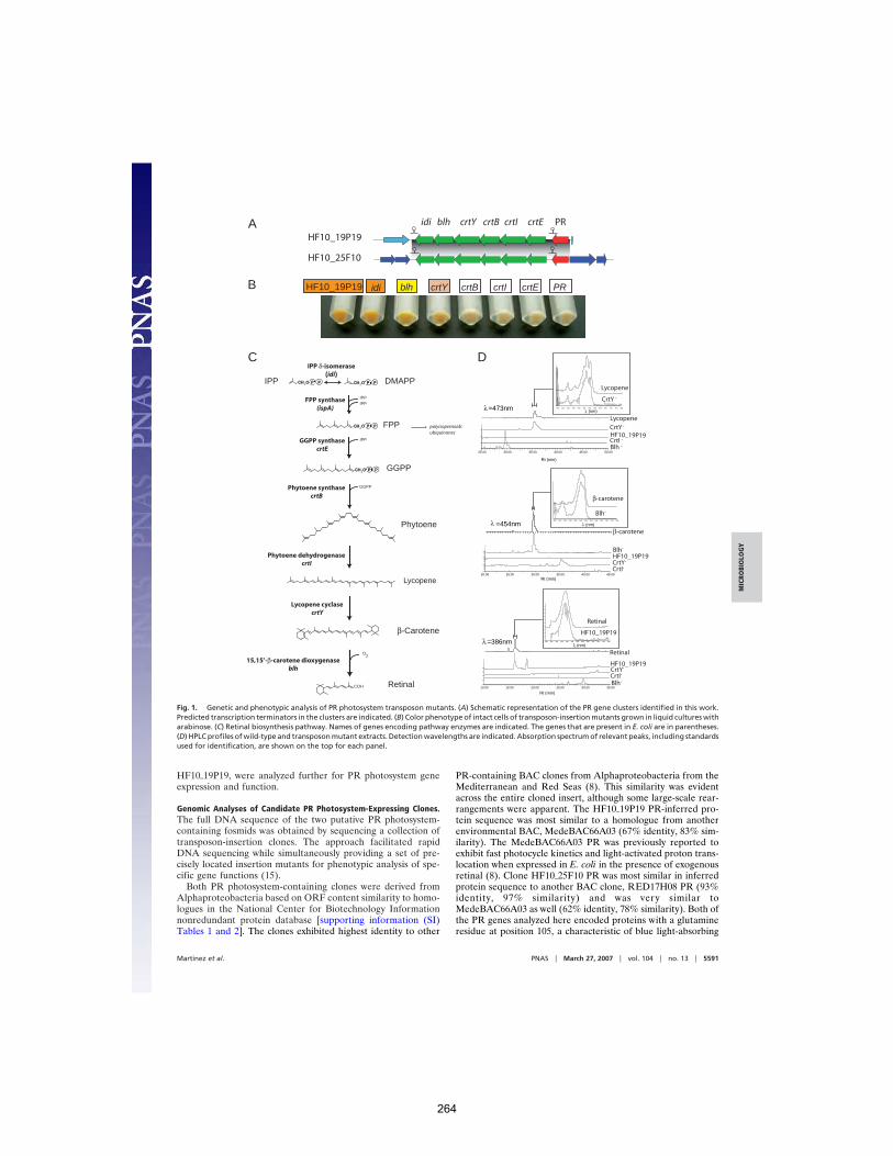
HF10!19P19, were analyzed further for PR photosystem geneexpression and function.
Genomic Analyses of Candidate PR Photosystem-Expressing Clones.The full DNA sequence of the two putative PR photosystem-containing fosmids was obtained by sequencing a collection oftransposon-insertion clones. The approach facilitated rapidDNA sequencing while simultaneously providing a set of pre-cisely located insertion mutants for phenotypic analysis of spe-cific gene functions (15).
Both PR photosystem-containing clones were derived fromAlphaproteobacteria based on ORF content similarity to homo-logues in the National Center for Biotechnology Informationnonredundant protein database [supporting information (SI)Tables 1 and 2]. The clones exhibited highest identity to other
PR-containing BAC clones from Alphaproteobacteria from theMediterranean and Red Seas (8). This similarity was evidentacross the entire cloned insert, although some large-scale rear-rangements were apparent. The HF10!19P19 PR-inferred pro-tein sequence was most similar to a homologue from anotherenvironmental BAC, MedeBAC66A03 (67% identity, 83% sim-ilarity). The MedeBAC66A03 PR was previously reported toexhibit fast photocycle kinetics and light-activated proton trans-location when expressed in E. coli in the presence of exogenousretinal (8). Clone HF10!25F10 PR was most similar in inferredprotein sequence to another BAC clone, RED17H08 PR (93%identity, 97% similarity) and was very similar toMedeBAC66A03 as well (62% identity, 78% similarity). Both ofthe PR genes analyzed here encoded proteins with a glutamineresidue at position 105, a characteristic of blue light-absorbing
00.0500.5400.0400.5300.0300.52
! mn374= nm008057007056006055005054004053003052002
! )mn(
)nim( tR
Lycopene
CrtY -
LycopeneCrtY -
CrtI -HF10_19P19
Blh -GGPP synthase
crtE
Phytoene synthasecrtB
Phytoene dehydrogenasecrtI
Lycopene cyclasecrtY
15,15’-"-carotene dioxygenaseblh
FPP
Phytoene
Lycopene
"-Carotene
COH Retinal
GGPP
IPP
IPP IPP FPP synthase
(ispA)
polyisoprenoidsubiquinones
GGPP2CH O P P P P
2CH O P P P P
DMAPP IPP IPP #-isomerase
(idi)2CH O P P P P 2CH O P P P P
00.5400.0400.5300.0300.5200.02
n008057007056006055005054004053003052002
mn454= ! )mn(
)nim( tR
"-carotene
Blh-
"-carotene
Blh-
CrtY-
CrtI-
HF10_19P19
!
000 0051 0002 0052 0003 53 00.5300.0300.5200.0200.5100.01
mn683= n008057007056006055005054004053003052002
91.2
)mn(
)nim( tR
! !
Retinal
HF10_19P19
HF10_19P19
Retinal
CrtY-
CrtI-
Blh-
PRcrtEcrtIcrtBcrtYblhidi
A
C
B HF10_19P19
HF10_19P19
HF10_25F10
PRidi blh crtY crtB crtI crtE
D
O2
Fig. 1. Genetic and phenotypic analysis of PR photosystem transposon mutants. (A) Schematic representation of the PR gene clusters identified in this work.Predicted transcription terminators in the clusters are indicated. (B) Color phenotype of intact cells of transposon-insertion mutants grown in liquid cultures witharabinose. (C) Retinal biosynthesis pathway. Names of genes encoding pathway enzymes are indicated. The genes that are present in E. coli are in parentheses.(D) HPLC profiles of wild-type and transposon mutant extracts. Detection wavelengths are indicated. Absorption spectrum of relevant peaks, including standardsused for identification, are shown on the top for each panel.
Martinez et al. PNAS ! March 27, 2007 ! vol. 104 ! no. 13 ! 5591
MIC
ROBI
OLO
GY
264
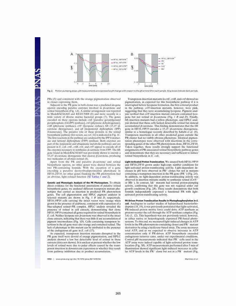
PRs (5) and consistent with the orange pigmentation observedin clones expressing them.
Adjacent to the PR gene in both clones was a predicted six-geneoperon encoding putative enzymes involved in !-carotene andretinal biosynthesis (Fig. 1A). A similar arrangement was reportedin MedeBAC66A03 and RED17H08 (8) and more recently in awide variety of diverse marine bacterial groups (7). The genesencoded on these operons include crtE [putative geranylgeranylpyrophosphate (GGPP) synthase], crtI (phytoene dehydrogenase),crtB (phytoene synthase), crtY (lycopene cyclase), blh (15,15"-!-carotene dioxygenase), and idi [isopentenyl diphosphate (IPP)"-isomerase]. The putative role of these proteins in the retinalbiosynthetic pathway (for review, see ref. 16) is indicated in Fig. 1C.The first reactions in the pathway are catalyzed by the IPP "-isomer-ase and farnesyl diphosphate (FPP) synthase. Both enzymes arepart of the isoprenoid and ubiquinone metabolic pathways and arepresent in E. coli. crtE, crtB, crtI, and crtY appear to encode all ofthe enzymes necessary to synthesize !-carotene from FPP. The blhgene found in MedeBAC66A03 was previously shown to encode a15,15"-!-carotene dioxygenase that cleaves !-carotene, producingtwo molecules of all-trans-retinal (8).
Apart from the PR and putative !-carotene and retinalbiosynthesis operon, no other genes were shared between thetwo PR-containing fosmids. With the exception of a geneencoding a putative deoxyribodipyrimidine photolyase inHF10!25F10, no other genes flanking the PR photosystem hadan obvious, light-related function (SI Tables 1 and 2).
Genetic and Phenotypic Analysis of the PR Photosystem. To obtaindirect evidence for the functional annotations of putative retinalbiosynthesis genes, we analyzed different transposon mutant phe-notypes that carried an insertion in predicted PR photosystemgenes. The cell pigmentation and HPLC pigment analyses inselected mutants are shown in Fig. 1 B and D, respectively.HF10!19P19 cells carrying the intact vector were orange whengrown in the presence of arabinose, consistent with expression of ablue-adapted retinal–PR complex. HPLC analysis revealed thepresence of retinal in cell extracts, demonstrating that cloneHF10!19P19 contained all genes required for retinal biosynthesis inE. coli. Neither lycopene nor !-carotene was observed in the intactclone extracts, indicating that there was little if any accumulation ofpigment intermediates (Fig. 1D). Cells containing transposon in-sertions in the idi gene were also orange and contained retinal. Thelack of phenotype in this mutant can be attributed to the presenceof the endogenous idi gene in E. coli (17).
As expected, transposon insertion mutants disrupted in thePR gene itself were devoid of orange pigmentation, and HPLCanalysis showed a low but detectable level of retinal in theseextracts (data not shown). It is unclear at present whether the lowlevels of retinal were due to polar effects caused by the trans-poson insertion in downstream expression or whether they resultfrom pathway inhibition due to product accumulation.
Transposon-insertion mutants in crtE, crtB, and crtI showed nopigmentation, as expected for this biosynthetic pathway if it isinterrupted before lycopene formation, the first colored productin the pathway. crtY-insertion mutants, however, were pink,suggesting that they were accumulating lycopene. Pigment anal-ysis verified that crtY-insertion mutant extracts contained lyco-pene but not retinal or !-carotene (Fig. 1 B and D). Finally,blh-insertion mutants had a yellow phenotype, and HPLC anal-ysis showed that these cells lacked detectable retinal but insteadaccumulated !-carotene. This finding demonstrates that the blhgene in HF10!19P19 encodes a 15,15"-!-carotene dioxygenase,similar to a homologue recently described by Sabehi et al. (8).Transposon insertions in all other predicted genes outside thePR cluster had no visibly obvious phenotype. Identical pigmen-tation phenotypes were observed with insertions in the corre-sponding genes of the other PR photosystem clone, HF10!25F10.Taken together, these results strongly support the functionalassignments of PR-associated retinal biosynthetic pathway genesand demonstrate that they are necessary and sufficient to induceretinal biosynthesis in E. coli.
Light-Activated Proton Translocation. We assayed both HF10!19P19and HF10!25F10 grown under high-copy number conditions forlight-activated proton-translocating activity. Light-dependent de-creases in pH were observed in PR# clones but not in mutantscontaining a transposon insertion in the PR gene (PR$) (Fig. 2A).In addition, no light-dependent proton-translocating activity wasobserved in insertion mutants unable to synthesize retinal (CrtY$
or Blh$). In contrast, Idi$ mutants had normal proton-pumpingactivity, confirming that this gene was not required under ourgrowth conditions (Fig. 2B). These results demonstrate that bothfosmids independently expressed a functional PR with light-activated proton-translocating activity.
PR-Driven Proton Translocation Results in Photophosphorylation in E.coli. Analogous to earlier studies of haloarchaeal bacteriorho-dopsins (18, 19), it was previously postulated that light-activated,PR-induced proton motive force could drive ATP synthesis asprotons reenter the cell through the ATP synthase complex (Fig.3A) (1, 12). This hypothesis was not previously tested, however,in either native or heterologously expressed PR-based photo-systems. To this end, we measured light-induced changes in ATPlevels in the PR-photosystem-containing clones and PR$ mutantderivatives by using a luciferase-based assay. The assay measurestotal ATP, and so we expected to observe increases in ATPconcentration only if PR-driven ATP biosynthesis exceededendogenous turnover rates, under our experimental conditions.Control pH measurements indicated that PR# cells used in theATP assay were indeed capable of light-activated proton trans-location (Fig. 3B). ATP measurements performed after 5 min ofillumination showed significant light-induced increases in cellu-lar ATP levels in the PR# clone but not in a PR$ mutant (Fig.
-0.3
-0.2
-0.1
0
0 2 4 6 8 100.10
0.00
0 2 4 6
HF10_19P19 PR+
HF10_19P19 PR -
HF10_25F10 PR -HF10_25F10 PR+
time (min)
HF10_19P19 PR+
PR -
IdiCrtY
Blh-0.05
--
-
B
time (min)
A
Fig. 2. Proton-pumping assays. pH measurements are expressed as pH change with respect to the pH at time 0 for each sample. Gray boxes indicate dark periods.
5592 ! www.pnas.org"cgi"doi"10.1073"pnas.0611470104 Martinez et al.
265
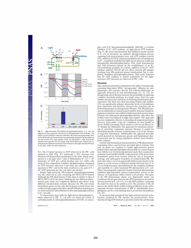
3C). The 0.3-pmol increase in ATP observed in the PR# cellsexposed to light (Fig. 3C) represents a 29% increase overidentical cell preparations maintained in the dark, which corre-sponds to a net gain after 5 min of illumination of !2.2 % 105
molecules of ATP per colony-forming unit (or viable cell)assayed. For comparison, oxidative phosphorylation, measuredby ATP increases observed 5 min after the addition of 0.2%succinate to PR# cells in the dark, resulted in a net gain of 9 %105 ATP molecules per live cell (data not shown).
Similar light-activated, PR-catalyzed photophosphorylationwas also observed in cells containing the HF10!25F10 fosmid.Although the PR photosystem of this clone is similar to that ofHF10!19P19, all of the genes flanking the two different photo-system gene suites are completely different and derive fromdifferent chromosomal contexts. Because the PR and retinalbiosynthetic genes are the only shared genes on both clones, theresults strongly suggest that these specific PR photosystem genesare both necessary and sufficient to drive photophosphorylationin E. coli cells.
To characterize more fully the light-driven photophosphory-lation observed in PR# E. coli cells, we tested the effects ofcarbonylcyanide m-chlorophenylhydrazone (CCCP), an uncou-
pler, and N,N"-dicyclohexylcarbodiimide (DCCD), a covalentinhibitor of H#-ATP synthase, on light-driven ATP synthesis(Fig. 3). We used concentrations that inhibited aerobic growthof E. coli on succinate, an oxidative phosphorylation processrequiring both proton-motive force and ATP synthase activity(20). Addition of CCCP, which permeabilizes the cell membraneto H#, completely abolished the light-driven decrease in pH andsubsequently photophosphorylation. This result demonstratesthat both processes depend on the establishment of an H#
electrochemical gradient. In contrast, addition of the H#-ATPsynthase inhibitor DCCD did not affect external pH changesresulting from PR-catalyzed proton translocation, but it com-pletely abolished photophosphorylation. This result indicatesthat H#-ATP synthase is indeed responsible for the light-activated ATP increases we observed in PR# cells.
DiscussionThe results presented here demonstrate the utility of functionallyscreening large-insert DNA ‘‘metagenomic’’ libraries for newphenotypes and activities directly and without subcloning, anapproach pioneered by soil microbiologists (15, 21, 22). Al-though large-insert libraries increase the probability of capturingcomplete metabolic pathways in a single clone, their low copynumber decreases the sensitivity of detecting heterologous geneexpression. We show here that increasing fosmid copy number(13) can significantly enhance detectable levels of recombinantgene expression and therefore increases the detection rate ofdesired phenotypes in metagenomic libraries. The PR photosys-tem recombinants we characterized could be detected visually bypigment production and exhibited light-dependent proton trans-location and subsequent photophosphorylation, only when thefosmid vector was induced to high copy number. The approachwas not completely effective in detecting all targeted genotypeshowever. Even under ‘‘copy-up’’ conditions, we were unable todetect all PR-containing clones known to exist in our library (4,7). Despite the limitations, this approach for functional screen-ing of microbial community genomic libraries is useful foridentifying specific activities or phenotypes, even in the absenceof sequence information. Additionally, this approach providesuseful material for downstream genetic and biochemical char-acterization and for testing hypotheses derived from bioinfor-matic analyses.
Genetic and biochemical characterization of PR photosystem-containing clones reported here provided direct evidence thatonly six genes are required to enable light-activated protontranslocation and photophosphorylation fully in a heterologoushost. Sabehi et al. (8) demonstrated previously that coexpressionof marine bacterial blh with PR, in the presence of the !-carotenebiosynthetic genes from Erwinia herbicola, led to !-carotenecleavage and subsequent formation of retinal-bound PR. Weshow here that a set of six genetically linked genes known to befound in a wide variety of different marine bacterial taxa (7, 8,11) are both necessary and sufficient for the complete synthesisand assembly of a fully functional PR photoprotein in E. coli.These heterologously expressed marine bacterial photosystemsexhibited light-dependent proton translocation activity in theabsence of exogenously added retinal or !-carotene. One genein the PR photosystem cluster was dispensable under ourconditions: the idi gene that encodes IPP "-isomerase, an activityalready present in E. coli (17), as is the FPP synthase, catalyzingthe next two steps in the pathway (23). The presence of the idigene in the cluster likely enables retinal production in the nativeorganism because isomerization of IPP to dimethylallyl pyro-phosphate can be a rate-limiting step in !-carotene biosynthesis(24, 25).
It was previously postulated that light-activated proton trans-location catalyzed by PR elevates the proton-motive force,thereby driving ATP synthesis as protons reenter the cell through
DCCDDCCD
H+H+
H+
H+
H+ H+H+
H+H+
PR
H+H+
H+H+
H+H+CCCPCCCP
ATPsynthase
ATPADP+Pi
Light
-0.1
0
0.1
0.2
0.3
0.4
0.5
PR PR PR CCCP PR DCCD- + ++
-0.16
-0.12
-0.08
-0.04
0
0.04
0 2 4 6 8 10
time (min)
PR PR CCCPPR DCCD
A
C
B
+
-PR+
+
Fig. 3. Light-activated, PR-enabled photophosphorylation in E. coli. (A)Diagram of the proposed mechanism of PR-dependent ATP synthesis. Theeffects of the inhibitors used are indicated. (B) Proton-pumping assays withHF10!19P19 cells. pH measurements are expressed as the pH change respect tothe pH at time 0 for each sample. CCCP, 25 #M; DCCD, 1 mM. Gray boxesindicate dark periods. (C) ATP assays with HF10!19P19 cells. Results are ex-pressed as the difference between the ATP level in the light and the ATP levelin the dark, &ATP, for each treatment.
Martinez et al. PNAS ! March 27, 2007 ! vol. 104 ! no. 13 ! 5593
MIC
ROBI
OLO
GY
266
the H#-ATP synthase complex (1, 12). Although this capabilityhas been demonstrated for haloarchaeal bacteriorhodopsins (18,19, 26, 27), PR-based photophosphorylation has not been dem-onstrated previously. Our data demonstrate that illumination ofcells expressing a native marine bacterial PR photosystem gen-erates a proton-motive force that does indeed drive cellular ATPsynthesis. Under our experimental conditions, 5 min of illumi-nation resulted in a net gain of 2.2 % 105 ATP molecules per cell.It should be quite possible to utilize the light to biochemicalenergy conversion enabled by the PR photosystem, for biosyn-thetic purposes.
The PR photosystem-catalyzed photophosphorylation describedhere is consistent with a proposed role for PR in marine microbialphotoheterotrophy. A few previous studies were unable to detectlight-enhanced growth rates or yields in PR-containing isolatesgrown in seawater or natural seawater incubations (28, 29). In onerecent report, light stimulation of growth rate or yield in Pelagibacterubique, a ubiquitous PR-containing marine planktonic bacterium,could not be detected. These negative results are somewhat difficultto interpret because natural seawater incubations are by necessitychemically undefined, and preferred growth substrates or otherlimiting nutrients in these experiments were unknown. In contrast,a significant enhancement of both growth rate and yield wasrecently reported in PR-expressing marine flavobacterium (11)albeit a direct link between PR and the light-induced growthstimulation was not conclusively demonstrated. Our direct obser-vation of an intact PR photosystem gene expression and subsequentphotophosphorylation, the recently reported light-enhancedgrowth rates and yields of PR-containing Flavobacteria (11), andthe general ubiquity of PR photosystem genes in diverse microbialtaxa of the ocean’s photic zone (2–9) all strongly support asignificant role for PR-based phototrophy in planktonic marinemicroorganisms.
In different physiological, ecological, phylogenetic, andgenomic contexts, PR activity may benefit cells in a variety ofways, some not directly related to enhanced growth rates oryields. In some bacteria, the H#-ATP synthase functions as anATPase under low respiratory conditions, hydrolyzing ATP anddriving proton efflux to maintain the proton-motive force (30).In the light, PR activity could offset this effect and reverseconditions from ATP consumption to ATP production. PRcontributions to cellular energy metabolism are likely to beparticularly important in starved or substrate-limited cells. Sim-ilar to the situation for some Haloarchaea, which use bacterio-rhodopsin under oxygen-limiting conditions (18, 19, 26, 27), lowrespiratory rates may trigger PR expression or activity in marinebacteria, as well. The PR-generated proton-motive force can alsobe directly coupled to other energy-requiring cellular activities,including flagellar motility or active transport of solutes into orout of the cell (32–34). This phenomenon was recently demon-strated by the coupling of PR activity to flagellar rotation in E.coli (31). Although a sensory function for some PR variants isalso a possibility (10, 35), the PR photosystems described here,and the vast majority of others observed to date (1, 3, 4, 7, 8, 11),are not genetically linked to sensory transducers, the hallmark ofall known sensory rhodopsins. Most all PRs characterized so fartherefore appear to function as light-activated ion pumps.
The marine PR family is remarkably diverse, has a widespreadphylogenetic distribution, and is functional in both ether-linkedphytanyl and ester-linked fatty acid membrane systems of Ar-chaea and Bacteria (4, 7, 10). A recent survey found thatone-third of PR clones examined were colocalized with pho-topigment biosynthetic operons (7). Operon arrangement anddistribution, as well as phylogenetic relationships, suggest thatlateral transfer of PR photosystem genes is relatively commonamong diverse marine microbes (4, 7, 10). The observationsreported here demonstrate that acquisition of just a few genescan lead to functional PR photosystem expression and photo-
phosphorylation. The ability of a single lateral transfer event toconfer phototrophic capabilities likely explains the ecologicaland phylogenetic prevalence of these photosystems in nature. Inprinciple, any microorganism capable of synthesizing FPP (awidespread intermediate in isoprenoid biosynthesis) couldreadily acquire this capability, as we have observed in E. coli.
Apparently, many otherwise chemoorganotrophic microbes inthe ocean’s photic zone have acquired the ability to use light energyto supplement cellular energy metabolism. The broad array ofPR-containing microbes reflects the photosystem’s fundamentalcontribution to cellular bioenergetics, a simplicity and compactnessthat favors PR photosystem lateral mobility, and a remarkableplasticity that enables photoprotein assembly and function in adiversity of phylogenetic groups and cell membrane types. From agenetic, physiological, and ecological perspective, the transitionfrom heterotrophy to PR-enabled photoheterotrophy seems torepresent a relatively small evolutionary step for contemporarymicroorganisms.
Materials and MethodsFosmid Library. The HOT!10m fosmid library screened in thiswork has been described previously (14). It contains DNA froma planktonic sample collected 10 m below the surface at theALOHA station (22°45" N, 158°W) of the Hawaii Ocean Timeseries (HOT) cloned into the copy-controlled pCC1FOS fosmidvector (Epicentre Biotechnologies, Madison, WI). The libraryhost, E. coli EPI300 (Epicentre Biotechnologies), supports thecopy-control option of pCC1FOS.
Screening for PR Expression. High-density colony macroarrays[12,280 clones of the HOT!10m library (ref. 14)] were preparedon a Performa II filter (Genetix Ltd., Boston, MA) by using aQ-PixII robot (Genetix Ltd.). The filter was carefully laid over a22-cm plate containing 250 ml of LB agar supplemented withL-arabinose (0.02%), the copy-up inducer, and all-trans-retinal(20 #M), and the plate was incubated at 37°C for 24 h. The filterswere used to facilitate the visual detection of color against thewhite background. Colonies were inspected visually for theappearance of orange or red color. Fosmid DNA from positiveclones was retransformed into fresh E. coli EPI300 and re-screened as above to verify that the color was conferred by thefosmid. The end DNA sequence of the positive clones wasobtained by using primers T7 and EpiFos5R as describedpreviously (14).
In Vitro Transposition and Full Fosmid Sequencing. Fosmid clones tobe characterized were submitted to random in vitro transposition byusing the EZ-Tn5'kan-2( insertion kit (Epicentre Biotechnolo-gies) according to the manufacturer’s instructions. The transposi-tion reaction was transformed by electroporation into EPI300 cells,and clones containing fosmids with Tn5 insertions were selected inLB chloramphenicol, kanamycin (12 #g/ml and 25 #g/ml, respec-tively). The color phenotype of individual Tn5-insertion clones wasanalyzed on LB plates containing chloramphenicol, kanamycin,and 0.02% L-arabinose as above. DNA sequencing off the Tn5 endswas performed by using KAN-2 FP-1 and KAN-2 RP-1 primers, aBigDye version 3.1 cycle sequencing kit, and ABI Prism 3700 DNAanalyzer (Applied Biosystems, Forest City, CA). The completeDNA sequence was assembled by using Sequencher version 4.5(Gene Codes Corporation, Ann Arbor, MI) and annotated withFGENESB (Softberry, Mount Kisco, NY) and Artemis version 6(The Wellcome Trust Sanger Institute, Cambridge, U.K.).
Carotenoid Extraction. Overnight cultures of the appropriateclones were diluted 1:100 into 50 ml of LB chloramphenicol (12#g/ml) and incubated for 3 h at 37°C with shaking (200 rpm). Atthat point, L-arabinose was added to a 0.02% final concentration,and cultures were incubated for 16 h. Cells were harvested by
5594 ! www.pnas.org"cgi"doi"10.1073"pnas.0611470104 Martinez et al.
267
centrifugation and rinsed twice in salt solution. Cell pellets werekept frozen ($20°C) in the dark. Frozen cells were extracted bysonication (5 min) in a cold 4:1 (vol/vol) mixture of acetone/methanol (OmniSolv; EMD Chemicals, Gibbstown, NJ) with 0.1mM butylated hydroxytoluene added as an antioxidant. Cellswere pelleted by centrifugation, and the supernatant was re-moved and filtered through ashed silica gel (230–400 mesh;EMD Chemicals). Extracts were then concentrated by evapora-tion under dry N2. All extraction steps were performed indarkness or low light to minimize carotenoid photooxidation.
HPLC Analysis. Chromatographic separation and analysis of caro-tenoids by high-performance liquid chromatography (HPLC)adapted a reverse-phase method from Barua and Olson (36). A5-#m Zorbax-ODS C18 column (150 % 4.6 mm) (AgilentTechnologies, Palo Alto, CA) was used at 30°C in a column ovenwith a Waters (Milford, MA) 2795 separations module operatedwith MassLynx 4.0 software. Separation was achieved with alinear gradient at a flow rate of 0.8 ml/min: 100% solvent A to100% B over 20 min followed by isocratic elution with B for anadditional 20 min, where A ) methanol/water (3:1 vol/vol) andB ) methanol/dichloromethane (4:1 vol/vol). The column wasequilibrated after each run with solvent A for 10 min. Thedetector was a Waters 996 photodiode array detector scanningwavelengths from 190 to 800 nm with a resolution of 1.2 nm andsampling rate of one spectrum per s. Carotenoids were identifiedby comparing absorbance spectra and retention times withauthentic standards.
Proton-Pumping Experiments. Clones to be analyzed for proton-pumping activity were streaked on 15-cm LB agar plates con-taining 12 #g/ml chloramphenicol and 0.001% L-arabinose andincubated at 37°C for 48 h. Cells were resuspended in 20 ml ofsalt solution (10 mM NaCl/10 mM MgCl2/100 #M CaCl2, pH7.0),
rinsed twice, and adjusted to an A600 of 0.5–0.7. Two millilitersof cell suspension was placed in an RPC-100 photosyntheticchamber (i-Works, Dover, NH) connected to a 22°C circulatingwater bath. pH was measured by using a Beckman (Fullerton,CA) *360 pH meter equipped with a Futura microelectrode.Light was provided by a 160-watt halogen lamp placed 4 cm fromthe chamber. Irradiance within the chamber was 500–650 #molQ m$2 s$1.
ATP Measurements. Cell suspensions were prepared as above.Three milliliters of cell suspension was placed in 5-ml screw-capglass vials. The vials for the dark samples were wrapped in foil.Ten centimeters of water was used to minimize heat transfer tothe samples. Irradiance under these conditions was 650 #mol Qm$2 s$1. ATP was measured by using a luciferase-based assay(BactTiter Glo, Promega, Madison, WI) as follows. At each timepoint, 5 aliquots (20 #l each) of every sample were dispensed intowhite 96-well assay plates [CoStar (Bethesda, MD) 3917]. Onehundred microliters of BactTiterGlo reagent was added per well,and luminescence was measured after 10 min using a Victor3plate reader (PerkinElmer, Waltham, MA) with a 1-s integrationtime. An ATP standard curve was used to calculate the con-centration of ATP in the samples. For inhibitor experiments, cellsuspensions were incubated in the dark for 20 h in the presenceof 1 mM DCCD or for 2 h in the presence of 25 #M CCCP orthe ethanol vehicle. Succinate was added to a 0.2% final con-centration to measure ATP synthesis from respiration in thedark.
We thank Drew Endy for the use of the luminometer, and Jay McCarrenfor comments on the manuscript. This work was supported by a grantfrom the Gordon and Betty Moore Foundation (to E.F.D.), NationalScience Foundation (NSF) Microbial Observatory award (MCB-0348001), and NSF Science and Technology Center Award EF0424599(to E.F.D.).
1. Beja O, Aravind L, Koonin EV, Suzuki MT, Hadd A, Nguyen LP, JovanovichSB, Gates CM, Feldman RA, Spudich JL, et al. (2000) Science 289:1902–1906.
2. Venter JC, Remington K, Heidelberg JF, Halpern AL, Rusch D, Eisen JA, WuD, Paulsen I, Nelson KE, Nelson W, et al. (2004) Science 304:66–74.
3. de la Torre JR, Christianson LM, Beja O, Suzuki MT, Karl DM, HeidelbergJ, DeLong EF (2003) Proc Natl Acad Sci USA 100:12830–12835.
4. Frigaard N-U, Martinez A, Mincer TJ, DeLong EF (2006) Nature 439:847–850.5. Man D, Wang W, Sabehi G, Aravind L, Post AF, Massana R, Spudich EN,
Spudich JL, Beja O (2003) EMBO J 22:1725–1731.6. Man-Aharonovich D, Sabehi G, Sineshchekov O, Spudich EN, Spudich JL,
Beja O (2004) Photochem Photobiol Sci 3:459–462.7. McCarren J, DeLong EF, Environ Microbiol, in press.8. Sabehi G, Loy A, Jung K-H, Partha R, Spudich JL, Isaacson T, Hirschberg J,
Wagner M, Beja O (2005) PLoS Biol 3:e273.9. Sabehi G, Massana R, Bielawski JP, Rosenberg M, Delong EF, Beja O (2003)
Environ Microbiol 5:842–849.10. Sharma AK, Spudich JL, Doolittle WF (2006) Trends Microbiol 14:463–469.11. Gomez-Consarnau L, Gonzalez JM, Coll-Llado M, Gourdon P, Pascher T,
Neutze R, Pedros-Alio C, Pinhassi J (2007) Nature 445:210–213.12. Beja O, Spudich EN, Spudich JL, Leclerc M, DeLong EF (2001) Nature
411:786–789.13. Wild J, Hradecna Z, Szybalski W (2002) Genome Res 12:1434–1444.14. DeLong EF, Preston CM, Mincer T, Rich V, Hallam SJ, Frigaard N-U,
Martinez A, Sullivan MB, Edwards R, Brito BR, et al. (2006) Science 311:496–503.
15. MacNeil IA, Tiong CL, Minor C, August PR, Grossman TH, Loiacono KA,Lynch BA, Phillips T, Narula S, Sundaramoorthi R, et al. (2001) J Mol MicrobiolBiotechnol 3:301–308.
16. Armstrong GA (1997) Annu Rev Microbiol 51:629–659.17. Hahn FM, Hurlburt AP, Poulter CD (1999) J Bacteriol 181:4499–4504.
18. Danon A, Stoeckenius W (1974) Proc Natl Acad Sci USA 71:1234–1238.19. Oesterhelt D, Stoeckenius W (1973) Proc Natl Acad Sci USA 70:2853–2857.20. Ito M, Ohnishi Y, Itoh S, Nishimura M (1983) J Bacteriol 153:310–315.21. Rondon MR, August PR, Bettermann AD, Brady SF, Grossman TH, Liles MR,
Loiacono KA, Lynch BA, MacNeil IA, Minor C, et al. (2000) Appl EnvironMicrobiol 66:2541–2547.
22. Gillespie DE, Brady SF, Bettermann AD, Cianciotto NP, Liles MR, RondonMR, Clardy J, Goodman RM, Handelsman J (2002) Appl Environ Microbiol68:4301–4306.
23. Fujisaki S, Takahashi I, Hara H, Horiuchi K, Nishino T, Nishimura Y (2005)J Biochem (Tokyo) 137:395–400.
24. Kajiwara S, Fraser PD, Kondo K, Misawa N (1997) Biochem J 324:421–426.25. Sun Z, Cunningham FX, Jr, Gantt E (1998) Proc Natl Acad Sci USA
95:11482–11488.26. Brock TD, Petersen S (1976) Arch Microbiol 109:199–200.27. Hartmann R, Sickinger HD, Oesterhelt D (1980) Proc Natl Acad Sci USA
77:3821–3825.28. Giovannoni SJ, Bibbs L, Cho J-C, Stapels MD, Desiderio R, Vergin KL, Rappe
MS, Laney S, Wilhelm LJ, Tripp HJ, et al. (2005) Nature 438:82–85.29. Schwalbach MS, Brown M, Fuhrman J (2005) Aquatic Microb Ecol 39:235–245.30. Booth IR (1985) Microbiol Rev 49:359–378.31. Walter JM, Greenfield D, Bustamante C, Liphardt V (2007) Proc Natl Acad Sci
USA 104:2408–2412.32. Konings WN (2006) Antonie Van Leeuwenhoek 90:325–342.33. Manson MD, Tedesco P, Berg HC, Harold FM, Van der Drift C (1977) Proc
Natl Acad Sci USA 74:3060–3064.34. Matsura S, Shioi J, Imae Y (1977) FEBS Lett 82:187–190.35. Spudich JL (2006) Trends Microbiol 14:480–487.36. Barua AB, Olson JA (1998) J Chromatog 707:69–79.
Martinez et al. PNAS ! March 27, 2007 ! vol. 104 ! no. 13 ! 5595
MIC
ROBI
OLO
GY
268
Appendix D
The Geological Succession of Primary Producers in the Oceans
Andrew H. Knoll, Roger E. Summons, Jacob R. Waldbauer and John E. Zumberge
Reprinted with permission from The Evolution of Primary Producers in the Sea © 2007 Elsevier Inc. Knoll, A.H., Summons, R.E., Waldbauer, J.R. and Zumberge, J.E. (2007) The Geological Succession of Primary Producers in the Oceans. In The Evolution of Primary Producers in the Sea, P.G. Falkowski and A.H. Knoll, eds. Academic Press, p. 133-163.
269

270
C H A P T E R
8
The Geological Succession of
Primary Producers in the Oceans
ANDREW H. KNOLL, ROGER E. SUMMONS, JACOB R. WALDBAUER, AND JOHN E. ZUMBERGE
I. Records of Primary Producers in Ancient Oceans A. Microfossils B. Molecular Biomarkers
II. The Rise of Modern Phytoplankton A. Fossils and Phylogeny B. Biomarkers and the Rise of Modern Phytoplankton C. Summary of the Rise of Modern Phytoplankton
III. Paleozoic Primary Production A. Microfossils B. Paleozoic Molecular Biomarkers C. Paleozoic Summary
IV. Proterozoic Primary Production A. Prokaryotic Fossils B. Eukaryotic Fossils C. Proterozoic Molecular Biomarkers D. Summary of the Proterozoic Record
V. Archean Oceans VI. Conclusions
A. Directions for Continuing Research References
In the modem oceans, diatoms, dinoflagel- lates, and coccolithophorids play prominent roles in primary production (Falkowski et al. 2004). The biological observation that these groups acquired photosynthesis via endo- symbiosis requires that they were preceded in time by other photoautotrophs. The geologi- cal observation that the three groups rose to
geobiological prominence only in the Mesozoic Era also requires that other primary producers fueled marine ecosystems for most of Earth history. The question, then, is: what did pri- mary production in the oceans look like before the rise of modem phytoplankton groups?
In this chapter, we explore two records of past primary producers: morphological
133
271
134 8. THE GEOLOGICAL SUCCESSION OF PRIMARY PRODUCERS IN THE OCEANS
fossils and molecular biomarkers. Because these two windows on ancient biology are framed by such different patterns of pres- ervational bias and diagenetic selectivity, they are likely to present a common picture of stratigraphic variation only if that view reflects evolutionary history.
I. RECORDS OF PRIMARY PRODUCERS
IN ANCIENT OCEANS
A. Microfossils
Microfossils, preserved as organic cell walls or mineralized tests and scales, record the morphologies and (viewed via transmis- sion electron microscopy) ultrastructures of ancient microorganisms. Such fossils can provide unambiguous records of phyto- plankton in past oceans--diatom frustules, for example--and they commonly occur in large population sizes, with numerous occurrences that permit fine stratigraphic resolution and wide geographic coverage.
Set against this is a number of factors that limit interpretation. Not all photoau- totrophs produce preservable cell walls or scales, and, of those that do, not all gener- ate fossils that are taxonomically diagnos- tic. Thus, although many modern diatoms precipitate robust frustules of silica likely to enter the geologic record, others secrete weakly mineralized shells with a corre- spondingly lower probability of preserva- tion. Similarly, whereas dinoflagellates as a group have left a clear record of dinocysts, many extant species do not produce pre- servable cysts and others form cysts that would not be recognized unambiguously as dinoflagellate in fossil assemblages. (The phylogenetic affinities of fossil dinocysts are established by the presence of an arche- opyle, a distinctive excystment mechanism peculiar to but not universally found within dinoflagellates.) Especially in the early his- tory of a group, character combinations that readily distinguish younger members may not be in place. Thus, stem group diatoms
without well-developed frustules might well leave no morphologic record at all in sediments.
By virtue of their decay-resistant extracel- lular sheaths and envelopes, many cyano- bacteria have a relatively high probability of entering the fossil record, and some ben- thic lineages are both readily preservable and morphologically distinctive (Knoll and Golubic 1992). On the other hand, impor- tant picoplankton such as Prochlorococcus are unlikely to leave recognizable body (or, as it turns out, molecular) fossils. A number of algal clades include good candidates for fos- silization, especially groups with distinctive resting stages (phycomate prasinophytes, dinoflagellates) or mineralized skeletons (diatoms, coccolithophorids, coralline reds, caulerpalean and dasyclad greens). Other primary producers fossilize occasionally but only under unusual depositional or diage- netic circumstances (e.g., Butterfield 2000; Xiao et al. 2002, 2004; Foster and Afonin 2006), and still others rarely if ever produce mor- phologically interpretable fossils.
Diagenesis can obliterate fossils as well as preserve them: organic walls are subject to postdepositional oxidation and miner- alized skeletons may dissolve in under- saturated pore waters. The result is that presence and absence cannot be weighted equally in micropaleontology. The presence of a fossil unambiguously shows that the cell from which it derived lived at a certain time in a particular place, but absence may reflect true absence, low probability of fos- silization, or obfuscating depositional or diagenetic conditions. For older time inter- vals, tectonic destruction of the sedimentary record imposes an additional challenge; in particular, subduction inexorably destroys oceanic crust and the sediments that mantle it, so that deep-sea sediments are common only in Jurassic and younger ocean basins.
B. Molecular Biomarkers
The chemical constituents of biomass pro- duced by living organisms can be incorporated
272
I. RECORDS OF PRIMARY PRODUCERS IN ANCIENT OCEANS 13 5
into sediments and ultimately into sedimen- tary rocks that can survive for billions of years. Where these compounds are preserved in recognizable forms, they represent another opportunity for organisms to leave a trace of themselves in the fossil record. Organic biomarkers are the diagenetically altered remains of the products of cellular biosyn- thesis and may be aptly termed molecular fossils. Most biomarkers are derived from lipids and are potentially stable over bil- lion-year time scales under ideal conditions (Brocks and Summons 2004).
Given the variety of organic compounds produced by cells and the vast quantities of sedimentary organic matter in a rock record that stretches back billions of years, biomar- kers are a potentially rich source of informa- tion concerning the diversity and ecology of ancient communities. However, the process of organic matter incorporation into rocks and its transformation during deep burial imposes some strong constraints on the kinds of information that can be recovered millions of years after the fact. The classes of molecules that contain molecular sequence information, nucleic acids, and most pro- teins, do not survive long in the geologic environment. DNA can survive for at least a few hundred thousand years, especially in reducing environments such as euxinic sed- iments (e.g., Coolen et al. 2004) where het- erotrophy is curtailed by a lack of electron acceptors, but it is not an option where the aim is to look at changes on million-year or longer time scales. Other kinds of biomol- ecules, however, prove remarkably resilient in the rock record.
Any molecule with a hydrocarbon skel- eton has the potential to be preserved over long periods. For the most part, this refers to the hydrocarbon portions of membrane lipids, which are the major constituent of extractable organic matter (bitumen) in sedimentary rocks. Diagenesis quickly strips these compounds of their reactive polar functionalities, and over longer peri- ods causes stereochemical and structural rearrangements, but hydrocarbon skeletons
can remain recognizable as the products of particular biosynthetic pathways on time scales that approach the age of the Earth (e.g., Brocks and Summons 2004; Peters et al. 2005).
The character of the information con- tained in molecular fossils is variable. Some are markers for the presence and, to the extent they can be quantified rela- tive to other inputs, abundance of particu- lar organisms. The taxonomic specificity of such biomarkers ranges from species to domain level. Others are markers for the operation of a particular physiology or bio- synthetic pathway that may have a broad and/or patchy taxonomic distribution. Still other kinds of biomarkers are most strongly associated with specific depositional set- tings, making their presence more indica- tive of paleoenvironmental conditions than of any particular biology. Interpretation of the molecular fossil record depends on our ability to recognize biomarker compounds, link them to biosynthetic precursors, and then make inferences about what the pres- ence of those molecules in the rock record tells us about contemporary biology and geochemistry.
Turning to biomarkers that might estab- lish a molecular fossil record of primary pro- duction in marine settings, several classes of compounds are promising for their com- bination of biochemical and/or taxonomic specificity. Pigments are natural candidates, representing markers of the photosynthetic machinery itself. Input of chlorophyll to sedi- ments can result in several kinds of molecular fossils, including porphyrins and the pristane and phytane skeletons of the chlorophyll side chain (Figure 1). It was the recognition of vanadyl porphyrin as the molecular fossil of chlorophyll that led Alfred Treibs (1936) to make the first compelling chemical argument for the biogenic origin of petroleum. Other pigments, such as carotenoids, are subject to very selective preservation, generally requir- ing the presence of reduced sulfur species; the functional groups that confer many of their biophysical properties and taxonomic
273
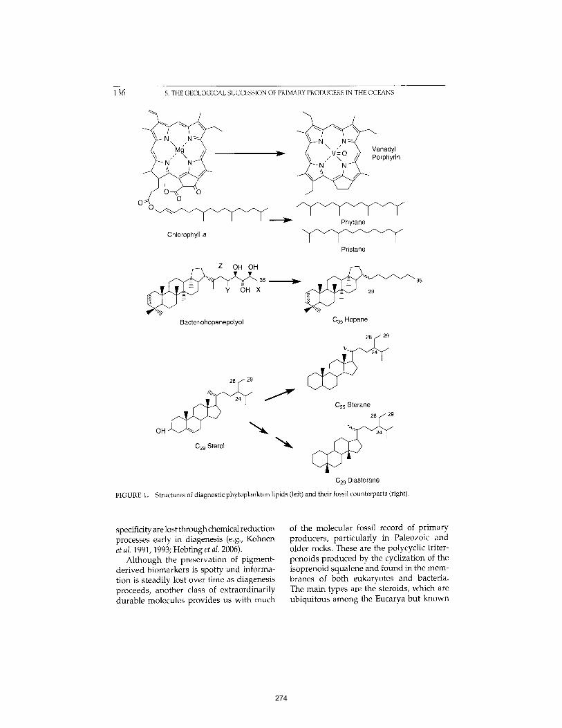
136 8. THE GEOLOGICAL SUCCESSION OF PRIMARY PRODUCERS IN THE OCEANS
O
v
Chlorophyll a
nadyl rphyrin
Phytane
Pristane
Z OH OH
Bacteriohopanepolyol
28(- 29
029 Sterol
~ ~ 35 v
2 9
035 Hopane
029 Sterane
C29 Diasterane
FIGURE 1. Structures of diagnostic phytoplankton lipids (left) and their fossil counterparts (right).
specificity are lost through chemical reduction processes early in diagenesis (e.g., Kohnen et al. 1991, 1993; Hebting et al. 2006).
Although the preservation of pigment- derived biomarkers is spotty and informa- tion is steadily lost over time as diagenesis proceeds, another class of extraordinarily durable molecules provides us with much
of the molecular fossil record of primary producers, particularly in Paleozoic and older rocks. These are the polycyclic triter- penoids produced by the cyclization of the isoprenoid squalene and found in the mem- branes of both eukaryotes and bacteria. The main types are the steroids, which are ubiquitous among the Eucarya but known
274
I. RECORDS OF PRIMARY PRODUCERS IN ANCIENT OCEANS 13 7
from only a very few bacteria, and the hopanoids, including the bacteriohopanep- olyols (BHPs), produced by a wide variety of autotrophic and heterotrophic bacteria. These molecules have the great advan- tages of a durable polycyclic skeleton that is clearly a biological product and a well- characterized diagenetic fate involving a number of rearrangements that provide information about the postburial history of the organic matter. The structures of some commonly used biomarker lipids and their fossil counterparts are shown in Figure 1. Table 1 summarizes current knowledge of the biological affinities of hydrocarbons commonly found in marine sediment sam- pies, excluding biomarkers derived from terrestrial organisms.
Molecular fossils suffer from some of the same limitations as body fossils. Not all ecologically and biogeochemically impor- tant groups leave distinctive molecular fin- gerprints, making them difficult to follow in time. Moreover, the structures of lipids are not nearly as diverse as body fossils; different, often distantly related or physi- ologically disparate organisms can produce similar patterns of lipids. Generally, biomar- kers will reflect an average of inputs to sedi- ments, which can be influenced by factors including bottom water oxygenation, sedi- ment mineralogy, and grain surface area available for sorptive protection (Hedges and Keil 1995). These inputs are attenuated by remineralization of organic matter as it sinks: this reworking is >95% complete by 3000m depth (Martin et al. 1987). The high degree of water-column degradation of organic matter in deep basins means that, even where deep-water sediments survive subduction, they commonly contain little organic matter; hence, the biomarker record of open-ocean primary production is poor. The problem of interpreting absence can be acute, because in biomarker analysis, absence can only be defined in terms of detection limits and, hence, is conditionally dependent upon the analytical technology available.
Much of what is known about the dia- genesis and preservation of biomarkers derives from studies of the origin and com- position of petroleum (e.g., Peters et al. 2005). Petroleum geologists were initially interested in identifying the source rocks from which hydrocarbon accumulations originated. Information on the thermal his- tories of source rocks is also key for mod- eling hydrocarbon generation. Biomarkers provide a way to determine both param- eters through complementary analyses of sedimentary bitumen in source rocks and their derived oil accumulations. Companies serving the petroleum exploration indus- try have developed and maintained data- bases of bitumen and oil composition that can be used to compare oils to bitumen in their source horizons and model the ther- mal histories of petroleum deposits. These databases can be employed as a predictive tool when exploring in frontier regions. An example is the commercial "Oils" database generated by GeoMark Research, which records geochemical analyses of more than 10,000 crude oil samples from every known petroliferous basin on the globe (www.geo- markresearch.com). The "Oils" data com- prise the contents of S, Ni, and V; the carbon isotopic compositions of bulk saturated and aromatic hydrocarbons; and quantitative analysis of approximately 100 individual hydrocarbons, including n-alkanes, acyclic isoprenoids, steroids, and triterpenoids. Abundances of the latter biomarkers, which have been determined using a rigorously reproducible analytical protocol, allow cal- culation of 23 diagnostic molecular ratios that can be used to predict paleoenviron- mental features of an oil's source rock without direct knowledge of the rock itself (Zumberge 1987) or to evaluate hydrocar- bon charge histories from field to basin scales (e.g., Zumberge et al. 2005). Aver- aging of data from numerous oil samples within a well, field, or an entire basin helps to overcome anomalies in individual hydro- carbon samples that reflect differences in maturity and losses from evaporation, water
275
138 8. THE GEOLOGICAL SUCCESSION OF PRIMARY PRODUCERS IN THE OCEANS
TABLE 1. Hydrocarbon biomarkers prevalent in marine sediments and petroleum derived from marine sediments and their known source organisms
Fossil hydrocarbon a Functionalized precursors Established sources b'c References a
C27---C35 bacteriohopanes
2-Methylhopanes
3-Methylhopanes
Aryl isoprenoids, isorenieratane Gammacerane
Tricyclic terpanes, cheilanthanes <C20 acyclic isoprenoids
>C20 acyclic isoprenoids
Cholestane
Ergostane; 24-methylcholestane Stigmastane; 24-ethylcholestane 24-n-Propylcholestane Dinosterane, triaromatic dinosteroids
24-Norcholestane
C20 ' C25 ' and C30 highly branched isoprenoids (HBIs)
C35 bacteriohopanepolyols (BHPs) 2-Methyl-BHP
3-Methyl-BHP
Aromatic carotenoids, e.g., isorenieratene, okenone Tetrahymanol
Unknown
Bacterial and algal chlorophylls archaeol
Glycerol ether lipids; also found as free hydrocarbons Cholesterol and related C27 sterols Erogosterol and related CaB sterols Sitosterol, stigmasterol, and related C29 sterols 24-n-Propylcholesterol Dinosterol, dinostanol
Bacteria although nonspecific Cyanobacteria although also in methanotrophs and other bacteria
Methanotrophs, other proteobacteria Green and purple sulfur bacteria Purple nonsulfur bacteria, some protists Unknown, probably bacteria Photosynthetic bacteria and protists Archaea although nonspecific Archaea although nonspecific Photosynthetic protists, metazoa Photosynthetic protists, prevalent in diatoms Photosynthetic protists, prevalent in chlorophytes Marine chrysophytes Dinoflagellates
24-Norcholesterol and Diatoms related 24-nor sterols Mono- or polyunsaturated Diatoms HBIs
n-C37-C39 alkenones n-C37-C39 alkenones Haptophytes or alkanes
Rohmer et al. 1984 1992 Zundel and Rohmer 1985b, 1985c; Bisseret et al. 1985; Summons et al. 1999 Zundel and Rohmer 19 85a Summons and Powell 1987; Brocks et al. 2005 Ten Haven et al. 1989; Kleemann et al. 1990 Moldowan et al. 1983 Peters et al. 2005
Peters et al. 2005
Volkman 2003
Volkman 2003
Volkman 2003
Moldowan 1984 Summons et al. 1987, 1992; Moldowan and Talyzina 1988 Rampen et al. 2005
Volkman et al. 1994; Belt et al. 2000; Sinninghe Damst6 et al. 2004 Volkman et al. 1980; Marlowe et al. 1984
qn most cases, the connection between the fossil hydrocarbon and organismic source is supported by detection of diagenetic intermediates in sediments.
bExtensive, systematic studies of lipids from microbial cultures are rare. Many lipid-organism relationships remain unknown.
cGenomic sequencing will also help identify the metabolic potential of source organisms to produce preservable compounds; such identificationdepends on (currently incomplete) knowledge of the biosynthetic pathways of biomarker molecules.
qndicative but incomplete list. Reviews that provide extensive citation lists include Brocks and Summons 2004 and Peters et al. 2005.
276
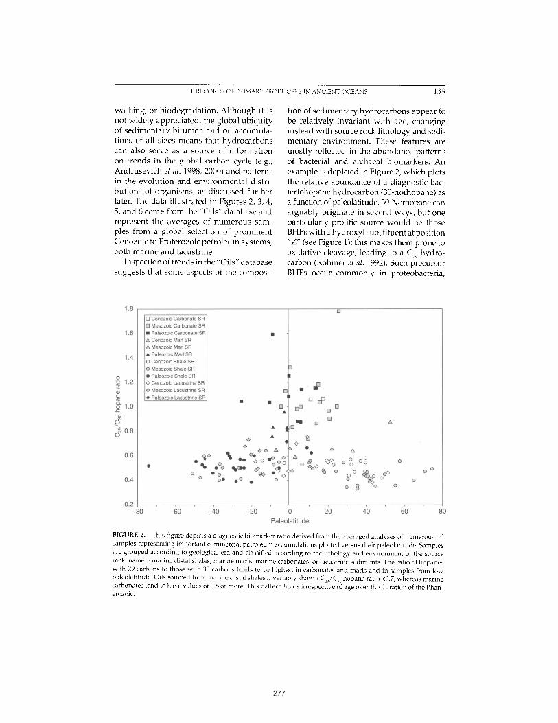
I. RECORDS OF PRIMARY PRODUCERS IN ANCIENT OCEANS 139
washing, or biodegradation. Al though it is not widely appreciated, the global ubiquity of sedimentary bi tumen and oil accumula- tions of all sizes means that hydrocarbons can also serve as a source of information on trends in the global carbon cycle (e.g., Andrusevich et al. 1998, 2000) and patterns in the evolution and environmental distri- butions of organisms, as discussed further later. The data illustrated in Figures 2, 3, 4, 5, and 6 come from the "Oils" database and represent the averages of numerous sam- ples from a global selection of prominent Cenozoic to Proterozoic petroleum systems, both marine and lacustrine.
Inspection of trends in the "Oils" database suggests that some aspects of the composi-
tion of sedimentary hydrocarbons appear to be relatively invariant with age, changing instead with source rock lithology and sedi- mentary environment. These features are mostly reflected in the abundance patterns of bacterial and archaeal biomarkers. An example is depicted in Figure 2, which plots the relative abundance of a diagnostic bac- teriohopane hydrocarbon (30-norhopane) as a function of paleolatitude. 30-Norhopane can arguably originate in several ways, but one particularly prolific source would be those BHPs with a hydroxyl substituent at position "Z" (see Figure 1); this makes them prone to oxidative cleavage, leading to a C29 hydro- carbon (Rohmer et al. 1992). Such precursor BHPs occur commonly in proteobacteria,
1.8
1.6
1.4
O 1.2
c- c'~ o 1.0 ¢.- o o3
o Ob 0.8 0
0.6
0.4
0.2
[ ] Cenozoic Carbonate SR [ ] Mesozoic Carbonate SR • Paleozoic Carbonate SR A Cenozoic Marl SR A Mesozoic Marl SR • Paleozoic Marl SR O Cenozoic Shale SR O Mesozoic Shale SR • Paleozoic Shale SR O Cenozoic Lacustrine SR
Mesozoic Lacustrine SR • Paleozoic Lacustrine SR
!
=
• • []
• [] []
• t D
'--°" :t ;o 0 o ~ o O ~ o 0 0 (~'% ° ° 0 ° o 0
%.o o o oO o • o o ~ ~
O O • 0 O • O 0 0 0
o 8
-80 -60 -40 -20 0 20 40
Paleolatitude 60 80
FIGURE 2. This figure depicts a diagnostic biomarker ratio derived from the averaged analyses of numerous oil samples representing important commercial petroleum accumulations plotted versus their paleolatitude. Samples are grouped according to geological era and classified according to the lithology and environment of the source rock, namely marine distal shales, marine marls, marine carbonates, or lacustrine sediments. The ratio of hopanes with 29 carbons to those with 30 carbons tends to be highest in carbonates and marls and in samples from low paleolatitude. Oils sourced from marine distal shales invariably show a C29/C30 hopane ratio <0.7, whereas marine carbonates tend to have values of 0.8 or more. This pattern holds irrespective of age over the duration of the Phan- erozoic.
277
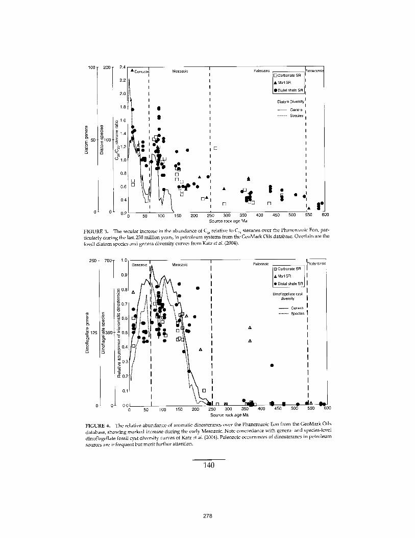
100
+°
~5
200
~ 100 o
~5
0 " 0
~_.4
_>.2
>_.0
1.8
o l . 6
~ 1.4
O 1.0
0.8
0.E
0.,1
0.~,
A I Cenozoi~ Mesozoic
!
s I
i , ' , . I
I , ..
ki tl I o [] A D i ~ iI I Dm [] it ;I I 1~?.l lb°.
V
Paleozoic I I
I
I
I
I
I
I
I
I
I
I
I
i D
I
I
I
01 I
I
I
D&I I
I 1-1 Carbonate SR
A Marl SR
• Distal shale SR
Diatom Diversity
Genera ........ Species
0 50 100 150 200 300 350 400 450 500 Source rock age Ma
:~roterozoic
I
I
I- I ° 550 600
FIGURE 3. The secular increase in the abundance of C28 relative to C29 steranes over the Phanerozoic Eon, par- ticularly during the last 250 million years, in petroleum systems from the GeoMark Oils database. Overlain are the fossil diatom species and genera diversity curves from Katz et al. (2004).
250
Q~ r- Q)
_.m 125 Q~
O r'- ._ a
,oo!
+
__.350-
5
1.0
[1.9
0.8
0.7
0.6
0.5
D / ' 1 0.4 ] I
o.3 j I t ! t
o.a i I
, I
0.1 I I
0.0 - - ~ - | 0 50
I Mesozoic Paleozoic I I
• I • I
i I I
& • I ~ I
• I A I
• I & ~. A t
\ t
i i
• I
~- [] I I , , _
n Carbonate SR
& Marl SR
• Distal shale SR
Din•flagellate cyst diversity
Genera ......... Species
100 150 200 250 300 350-- 400 450 500 550 600 Source rock age Ma
FIGURE 4. The relative abundance of aromatic dinosteranes over the Phanerozoic Eon from the GeoMark Oils database, showing marked increase during the early Mesozoic. Note concordance with genera- and species-level din•flagellate fossil cyst diversity curves of Katz et al. (2004). Paleozoic occurrences of dinosteranes in petroleum sources are infrequent but merit further attention.
140
278
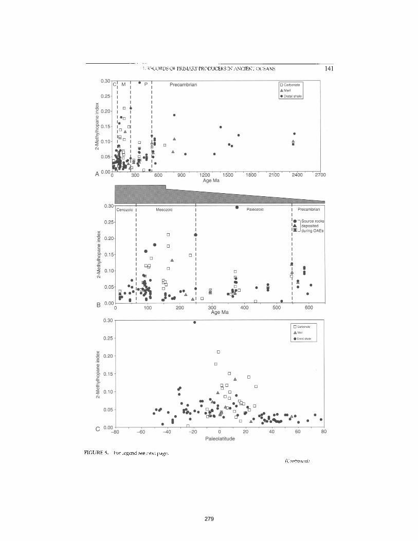
I. RECORDS OF PRIMARY PRODUCERS IN ANCIENT OCEANS 141 0.30 t M i O p t
C I I I Precambr ian
I I I 0.25 I I I
x I I I
I [] ~ n " 0 .~ 0.20 I I I
no D I I • c i o I I Q.
o 0 .15 I DI i .c IDA I I
. c I1~ I ~fl $ 0.10- i [] i J, A & I~ I ~ []
o.0s , ~ , |
A o o o [] on " 0 ' ' 3 0 0 ' ' 6 0 0 ' ' 9 0 0 ' '
O O
12'00 ' ' 15 '00 ' ' 18 '00 ' Age Ma
[ ] Carbonate I
A Marl
• D sta shale
2100 2400 2700
0.30
0.25-
x
'o 0.20- c . _
¢,..
Q. o 0.15 c- >,,
Cenozoic I Mesozoic I w Paleozoic I Precambrian I I I
I I I O ~ Source rocks I I IA | deposited I I I Igl _.; during OAEs I [] • I
I I I
I • [] I I
I • I I
I [] I I
I [] A I I
n ~ n i [] , i O 0.10 []
& u ~ n • ' '- :
0.05 00 I ~, I •
I i . " : " " ' ' I ~ • I •
• ° ° l g i l t A I [ ] B o.oo o i o - , ' ~ , [ ] , , • I
0 100 200 300 400 500 ' 600 Age Ma
0.30
0.25
x 0.20 " o
c . _
c
0.15 O r- > , r -
0.10 &
0.05
C 0.00 - 8 0 - 6 0
[] Carbonate
A, Marl
• Distal shale
[]
A []
S ~D [] • A [] •
OI O~ lid
OoE~3 o [] • ° ° • ° D - - o ° ~o
"" o" r,: . .~ . .~ . ~ , o . . r , . ' - , . . • • [] ,L° o ~ b w • • •
, I-I - 4 0 - 2 0 0 20 40 60 80
Pa le • l a t i t ude
FIGURE 5. For legend see next page.
(Continued)
279
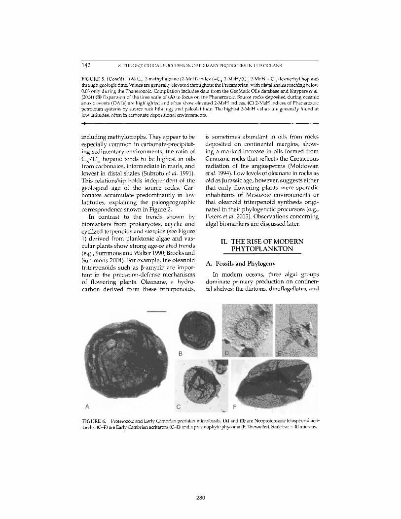
14 2 8. THE GEOLOGICAL SUCCESSION OF PRIMARY PRODUCERS IN THE OCEANS
FIGURE 5. (Cont'd) (A) C30 2-methylhopane (2-MeH) index (=C30 2-MeH/(C30 2-MeH + C30 desmethyl hopane) through geologic time. Values are generally elevated throughout the Precambrian, with distal shales reaching below 0.05 only during the Phanerozoic. Compilation includes data from the GeoMark Oils database and Kuypers et al. (2004) (B) Expansion of the time scale of (A) to focus on the Phanerozoic. Source rocks deposited during oceanic anoxic events (OAEs) are highlighted and often show elevated 2-MeH indices. (C) 2-MeH indices of Phanerozoic petroleum systems by source rock lithology and paleolatitude. The highest 2-MeH values are generally found at low latitudes, often in carbonate depositional environments.
including methylotrophs. They appear to be especially common in carbonate-precipitat- ing sedimentary environments; the ratio of C29/C30 hopane tends to be highest in oils from carbonates, intermediate in marls, and lowest in distal shales (Subroto et al. 1991). This relationship holds independent of the geological age of the source rocks. Car- bonates accumulate predominantly in low latitudes, explaining the paleogeographic correspondence shown in Figure 2.
In contrast to the trends shown by biomarkers from prokaryotes, acyclic and cyclized terpenoids and steroids (see Figure 1) derived from planktonic algae and vas- cular plants show strong age-related trends (e.g., Summons and Walter 1990; Brocks and Summons 2004). For example, the oleanoid triterpenoids such as ~-amyrin are impor- tant in the predation-defense mechanisms of flowering plants. Oleanane, a hydro- carbon derived from these triterpenoids,
is sometimes abundant in oils from rocks deposited on continental margins, show- ing a marked increase in oils formed from Cenozoic rocks that reflects the Cretaceous radiation of the angiosperms (Moldowan et al. 1994). Low levels of oleanane in rocks as old as Jurassic age, however, suggests either that early flowering plants were sporadic inhabitants of Mesozoic environments or that oleanoid triterpenoid synthesis origi- nated in their phylogenetic precursors (e.g., Peters et al. 2005). Observations concerning algal biomarkers are discussed later.
II. THE RISE OF MODERN
P H Y T O P L A N K T O N
A. Fossils and Phylogeny
In modem oceans, three algal groups dominate primary production on continen- tal shelves: the diatoms, dinoflagellates, and
L
A
FIGURE 6. Proterozoic and Early Cambrian protistan microfossils. (A) and (B) are Neoproterozoic leiospherid acri- tarchs; (C-F) are Early Cambrian acritarchs (C-E) and a prasinophyte phycoma (F; Tasmanites). Scale bar = 40 microns.
280
II. THE RISE OF MODERN PHYTOPLANKTON 143
coccolithophorids. As detailed elsewhere in this volume, fossils clearly suggest that these groups all rose to taxonomic and ecological prominence only during the Mesozoic Era (Delwiche, Chapter 10; de Vargas et al., Chapter 12; Kooistra et al., Chapter 11, this volume). Could there have been, however, an earlier "cryptic" evolutionary history for these groups? For example, might nonmineralizing stem group diatoms or haptophytes have been ecologically important but paleontologi- cally uninterpretable in Paleozoic oceans? Might the significance of Paleozoic dinoflagel- lates be obscured by fossils that are abundant and diverse but lack archeopyles?
Several reports claim microfossil evidence for Paleozoic diatoms, dinoflagellates, and haptophytes, but such fossils are rare and subject to alternative interpretation as con- taminants (the mineralized skeletons) or different taxa (organic fossils). Stratigraphic research indicates that the Paleozoic silica cycle differed substantially from that of the Cretaceous and Tertiary periods, with sponges and radiolarians dominating biolog- ical removal of silica from the oceans (Maliva et al. 1989). Similarly, sediments preserved in obducted slices of Paleozoic seafloor at best contain only limited evidence for pelagic car- bonate deposition. Such observations cannot eliminate the possibility that rare diatoms, coccolithophorids, or calcareous dinoflag- ellates lived in Paleozoic oceans, but they clearly indicate that these groups did not perform the biogeochemical roles they have played since the Mesozoic Era.
Complementing this, molecular clock estimates for diatom and coccolithophorid diversification, calibrated by well-preserved fossils, suggest that these groups have no long Paleozoic "prehistory" (de Vargas et al., Chapter 12; Kooistra et al., Chapter 11, this volume). On the other hand, some molec- ular clock analyses suggest divergence times for the plastids in photosynthetic chromalveolates well back into the Protero- zoic (Douzery et al. 2004; Yoon et al. 2004). If these estimates are even broadly cor-
rect, they must be accommodated in one of two ways. Either the molecular clocks date divergence within a closely related group of unicellular red algae that subsequently and individually were incorporated as plastids in chromalveolate algae, or photosynthetic chromalveolates emerged from a single Proterozoic endosymbiosis (Cavalier-Smith 1999) but remained ecologically unimpor- tant or paleontologically unrecognizable until much later.
B. Biomarkers and the Rise of Modern Phytoplankton
The rise to ecological prominence of the three chlorophyll c-containing eukaryotic plankton lineages left several imprints in the molecular fossil record, especially in the distributions of steranes with different side- chain alkylation patterns. A secular increase in the ratio of CaB to C29 steranes (24-methyl- cholestanes versus 24-ethylcholestanes), first noted by Grantham and Wakefield (1988), has been attributed to increasing production by chlorophyll c algae, which dominate CaB sterane input, relative to green algae, which synthesize primarily C29 ster- oids (Volkman 2003). An updated plot of the C28/C29 sterane ratio versus geological age, based on averages from 123 petroleum sys- tems worldwide, is shown in Figure 3 along with data for diatom diversity. The C28/C29 sterane ratio remains below 0.4 in the Neo- proterozoic and, with one exception, below 0.7 through the Paleozoic. Correspond- ing to the diversification of diatoms in the later half of the Mesozoic, there is a rise in the C28/C29 sterane ratio to values as high as 1.8, followed by an apparent drop in the Paleocene and Eocene. Values climb again in the Miocene, accompanying a second rise in the numbers of diatom genera and species.
Other biomarkers show marked increases in abundance in the Cretaceous that also likely reflect diatom radiation. These include 24-norcholestanes (Holba et al. 1998a, b), the so-called highly branched isoprenoids (HBIs; Sinninghe Damst6 et al. 1999a, b; Belt
281
144 8. THE GEOLOGICAL SUCCESSION OF PRIMARY PRODUCERS IN THE OCEANS
et al. 2000; Allard et al. 2001), long-chain diols, and mid-chain hydroxyl methyl- alkanoates (Sinninghe Damst6 et al. 2003). The secular increase in 24-norcholestane abundance (Moldowan et al. 1991; Holba et al. 1998a, b) was observed and linked to the diatom radiation well before a precur- sor sterol was recognized in a culture of the centric diatom Thalassiosira aff. antarctica (Rampen et al. 2005). In fact, in the study of Rampen et al. (2005) only one, that is T. aft. antarctica, of 100 different diatom taxa was found to produce 24-norcholesta-5, 22-dien-3~-ol.
The detail of novel sterol production by diatoms provides an interesting window into the connections among biomarkers, taxonomy, and the physiological roles of lipids. In a recent study of diatom sterols, Suzuki et al. (2005) reported that environ- mental samples of ~ diatoms collected from the North Pacific Ocean and the Bering Sea contained 24-norsterols. Further, samples of the diatom Coscinodiscus marginatus, ini- tially devoid of 24-norcholesterol, contained significant amounts of this and the related steroid 27-nor-24-methylcholesta-5,22-dien- 3~-ol after storage at 3°C for 30 days. These authors attributed the latter change to bac- terial biodegradation. Due to the ubiquity of 24-norsteranes in Mesozoic sediments (Holba et al. 1998a, b), and no other evidence for selective side-chain biodegradation of sterols (biodegrading bacteria are unlikely to select for removal of C26 and C27 of the apparent precursor 24-methylcholesta- 5,22-dien-3~-ol and leave other sterols un- touched), it seems far more likely that there is a direct, as opposed to diagenetic, source for the 24-norsteroids in Sediments. The rarity of 24-norsterols in cultured diatoms (Rampen et al. 2005) more likely reflects the fact that sterol biosynthesis responds to physiological conditions and that laboratory culture conditions have as yet not mimicked the natural conditions, such as low tempera- ture and, perhaps, low light under which 24-norsterols are produced by some dia- toms. The enigma surrounding the origins of
24-norsteroids, and the ultimate detection of 24-norcholesta-5,22-dien-3~-ol by Rampen et al. (2005) in a cold water diatom species, pro- vide a timely reminder that biomarkers not only reflect the presence of particular algal taxa but also reflect the environmental con- ditions under which they thrive. A corollary to this is that cultured organisms might not always produce the same assemblage of lip- ids as their counterparts growing under natu- ral conditions.
The other major class of diatom-specific biomarkers is the HBI. So far as is currently known, the occurrence of HBI is confined to four genera, namely Navicula, Haslea, and Pleurosigma within the pennates, and Rhizosolenia among the centrics (Volkman et al. 1994; Belt et al. 2000; Sinninghe Damst6 et al. 2004). Both molecular phylogeny and fossils indicate that centric diatoms predate pennates (Kooistra et al. 2006). Therefore, the genus Rhizosolenia is considered the likely source of the first recorded fossil HBI at about 91 million years ago (Ma) --which predates recorded fossil tests of Rhizosole- nid diatoms by about 20 million years (Sin- ninghe Damst6 et al. 2004). This discrepancy in timing could reflect incomplete paleon- tological sampling, which systematically underestimates first appearances, HBI syn- thesis by a morphologically distinct stem group relative of the rhizosolenids, or both. Biosynthetic pathways are such a funda- mental characteristic of organisms that they might be detectable through chemical fos- sils before the first classical fossils of a clade are ever recognizable.
Dinosteroid biomarkers, derived from the 4-methylsterols of dinoflagellates (Robinson et al. 1984), show an analogous pattern of secular increase in the Mesozoic, in accord with microfossil evidence for later Trias- sic dinoflagellate radiation. As in the case of diatom HBI, however, several reported occurrences of dinosteranes predate fossil cysts, in some cases by hundreds of millions of years (Summons et al. 1992; Moldowan and Talyzina 1998; Talyzina et al. 2000). These deserve close attention as they may
282
II. THE RISE OF MODERN PHYTOPLANKTON 145
establish a genuine pre-Mesozoic history of dinoflagellates, as predicted by molecular phylogenies and clocks. Some aspects of this putative history are considered further later. In Figure 4, data derived from the "Oils" database show the pattern of secular varia- tion in triaromatic dinosteroid abundances, along with a recent compilation of dinoflag- ellate cyst diversity (Katz et al. 2004).
The third group of modern plankton, the haptophytes, produces distinctive lipids in the form of long-chain (n-C37 to C39), unsatu- rated ketones known as alkenones (Volkman et al. 1980; Marlowe et al. 1984). These can be abundant and easily recognized in Recent and Cenozoic sediments that have not expe- rienced extensive diagenesis, and they form the basis of a widely used paleotempera- ture proxy (Brassell et al. 1986). Their dis- tinctiveness, however, lies in the carbonyl functionality and one to four unsaturations, which are easily reduced and inherently unstable over geological time scales (Prahl et al. 1989). Thus, the oldest reported detec- tion is in Cretaceous sediments (Farrimond et al. 1986), and we would not expect to be able to recognize them in Paleozoic or older rocks.
The molecular and morphological records of eukaryotic predominance in shelf primary production are mirrored by indica- tions of relatively low cyanobacterial contri- butions. Some cyanobacteria are known to biosynthesize BHPs and analogues with an extra methyl group attached to the 2 posi- tion of the A ring (2-MeBHP); the hydro- carbon cores of these molecules provide a potentially useful tracer for cyanobacterial input to sedimentary organic matter (Sum- mons et al. 1999). Apart from a few notable exceptions, values of the 2-methylhopane (2-MeHI) index fraction of hopanoids (methylated at the 2 position relative to their desmethyl counterparts) tend higher in Pro- terozoic samples than they are in Paleozoic and, especially, Jurassic and younger oils (Figure 5A). This is especially true of sam- ples from shales. (Examination of the Phan- erozoic record [Figure 5B] shows that higher
2-MeHI values are found in oils from car- bonate lithologies, formed predominantly at low paleolatitudes [Figure 5C].) The exceptions are associated with widespread anoxia in the oceans (Figure 5B). Kuypers et al. (2004a, b) and Dumitrescu and Brassell (2005) studied biomarkers associated with Cretaceous oceanic anoxic events (OAEs) and found that the relative abundances of 2-methylhopanoids, as measured by the 2- MeHI, were distinctively enhanced, along with nitrogen (N), isotopic evidence for cyanobacterial primary productivity (Kuy- pers et al. 2004b). Mass extinction at the Permian-Triassic boundary is also associ- ated with widespread anoxia in shallow oceans (Wignall and Twitchett 2002). In Fig- ure 5, the two data points for the Permian Triassic transition represent unpublished data from the Perth Basin, Australia, and the boundary stratotype in Meishan, China; in these sections, high 2-MeHI correlate with independent molecular, iron speciation, and sulfur isotopic evidence for intense euxinia (Grice et al. 2005). The highest 2- MeHI value (0.29) recorded in the GeoMark Oils database comes from the Larapin- tine Petroleum System, Australia, which includes oils from the Late Devonian reef complex of the Canning Basin (Edwards et al. 1997) sourced from black shales depos- ited near to Frasnian-Famennian boundary, another event characterized by geological and geochemical evidence for pervasive euxinia (e.g., Bond et al. 2004). The samples from the Cretaceous OAEs, Permian-Trias- sic boundary, and Frasnian-Fammenian shale all contain abundant isorenieratane and aryl isoprenoids derived from the brown pigmented strains of the green sul- fur bacteria (Chlorobiaceae), considered diagnostic for photic zone euxinia (e.g., Summons and Powell 1987; Koopmans et al. 1996; Kuypers et al. 2004a; Grice et al. 2005; van Breugel et al. 2005). Kuypers et al. (2004b) hypothesize that the N cycle was compromised while euxinic conditions prevailed during the Cretaceous OAEs, creating an unusual opportunity for the
283
146 8. THE GEOLOGICAL SUCCESSION OF PRIMARY PRODUCERS IN THE OCEANS
proliferation of N-fixing cyanobacteria. The disparate occurrences described pre- viously suggest a more general correlation between high 2-MeHI and photic zone euxinia, a topic we return to in our discus- sion of Proterozoic primary production.
Although cyanobacteria appear to have been minor contributors to primary produc- tion on most Mesozoic and Cenozoic conti- nental shelves, they remain the dominant phytoplankton in open-ocean, oligotrophic environments today. Whether this is a recent or long-standing situation is difficult to discern given the paucity of the deep- sea sedimentary records and the absence of 2Me-BHP in cyanobacterial picoplankton (Summons, unpublished data).
C. Summary of the Rise of Modern Phytoplankton
Fossils, molecular biomarkers, molecular clocks for individual clades, and the sedi- mentary silica record all tell a consistent story: the modern phytoplankton has Mes- ozoic roots. How we interpret this transfor- mation depends in no small part on what we think came before.
III. PALEOZOIC PRIMARY
P R O D U C T I O N
A. Microfossils
Microfossils of presumptive eukaryo- tic phytoplankton are both abundant and diverse in Paleozoic marine rocks (Figure 6C-F). A number of forms, including Tas- manites, Pterospermella, and Cymatiosphaera, have morphologies and ultrastructures that relate them to prasinophyte phycomata (Tappan 1980). Indeed, in well-studied microfossil assemblages from Lower Cam- brian shales, at least 20% of described morphotaxa and more than half of all indi- vidual fossils are likely prasinophytes (e.g., Volkova et al. 1983; Knoll and Swett 1987; Moczydlowska 1991). Others, with regu- larly distributed processes, tantalizingly
resemble dinocysts, but lack archeopyles. Still other acritarchs (the group name given to closed, organic-walled microfossils of uncertain systematic relationships) (Evitt 1963) do not closely resemble known cysts of modem phytoplankton. Collectively, these microfossils show evidence of marked Cambrian and Ordovician radiations that parallel the two-stage diversification of marine animals (Knoll 1989). For reasons that remain obscure, acritarch diversity drops near the end of the Devonian and remains low for the remainder of the Paleo- zoic Era (Molyneux et al. 1996).
Moldowan and Talyzina (1998) innova- tively attempted to break the phylogenetic impasse regarding Cambrian microfos- sils. Extracts from fossiliferous clays of the Lower Cambrian Lfikati Formation, Esto- nia, contain low abundances of dinoster- ane and 4a-methyl-24-ethylcholestane, both known to originate from the sterols of dinoflagellates (Robinson et al. 1984; Sum- mons et al. 1987). Moldowan and Talyzina (1998) divided the microfossil populations in a L~ikati sample into three groups--tas- manitids (see Figure 6F; interpreted as pra- sinophyte phycomata), a low fluorescence group dominated by leiosphaerid acritarchs (also possible phycomata of prasinophytes like the extant Halosphaera), and a high fluorescence fraction containing abundant process-bearing acritarchs (e.g., see Figure 6D)--and analyzed the sterane content of these subassemblages. The tasmanitid and low fluorescence fractions contained rela- tively abundant C29 steranes but little or no dinoflagellate lipid. In contrast, the high flu- orescence fraction contained relatively high abundances of dinosterane, suggesting that the dominant, process-bearing acritarchs are dinocysts sans archeopyles. It is not clear that sterols play a structural role in cyst walls, making selective adsorption a real possi- bility. Moreover, whereas dinosterane and 4a-methyl-24-ethylcholestane abundances in these samples are relatively high, their concentrations are absolutely low. Thus, the specific attribution of acritarch taxa to
284
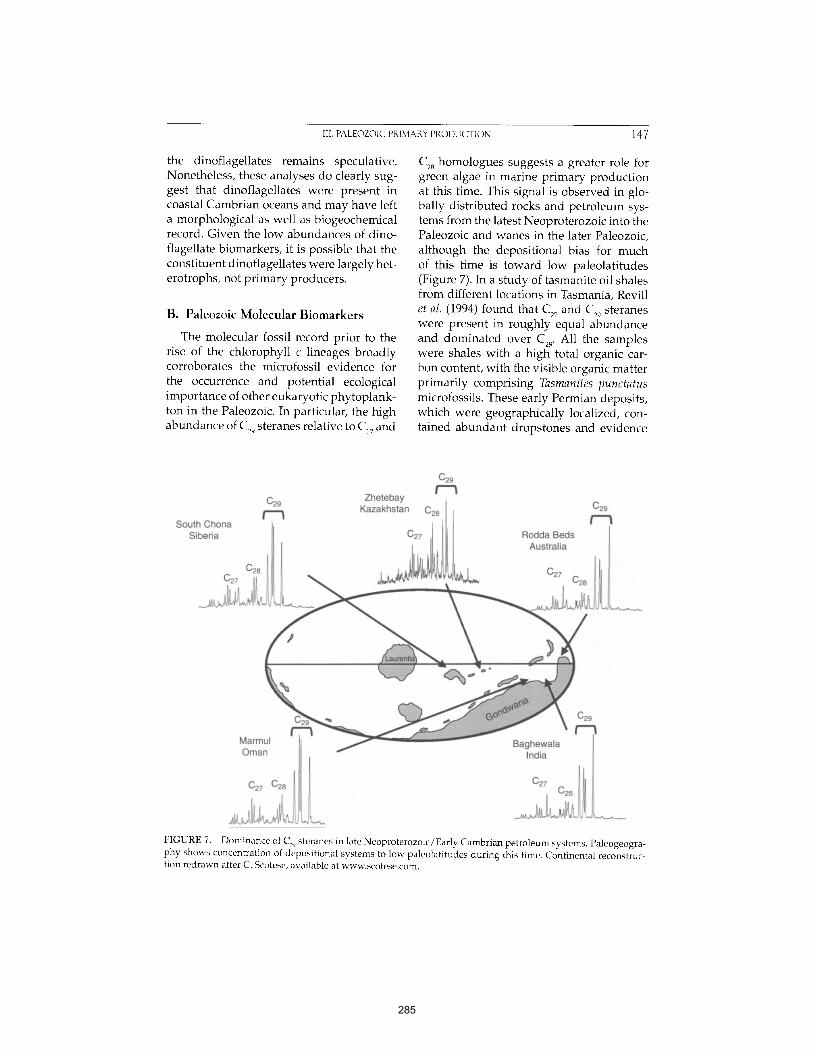
III. PALEOZOIC PRIMARY PRODUCTION 147
the dinoflagellates remains speculative. Nonetheless, these analyses do clearly sug- gest that dinoflagellates were present in coastal Cambrian oceans and may have left a morphological as well as biogeochemical record. Given the low abundances of dino- flagellate biomarkers, it is possible that the constituent dinoflagellates were largely het- erotrophs, not primary producers.
B. Paleozoic Molecular Biomarkers
The molecular fossil record prior to the rise of the chlorophyll c lineages broadly corroborates the microfossil evidence for the occurrence and potential ecological importance of other eukaryotic phytoplank- ton in the Paleozoic. In particular, the high abundance of C29 steranes relative to C27 and
C28 homologues suggests a greater role for green algae in marine primary production at this time. This signal is observed in glo- bally distributed rocks and petroleum sys- tems from the latest Neoproterozoic into the Paleozoic and wanes in the later Paleozoic, although the depositional bias for much of this time is toward low paleolatitudes (Figure 7). In a study of tasmanite oil shales from different locations in Tasmania, Revill et al. (1994) found that C27 and C29 steranes were present in roughly equal abundance and dominated over CaB. All the samples were shales with a high total organic car- bon content, with the visible organic matter primarily comprising Tasmanites punctatus microfossils. These early Permian deposits, which were geographically localized, con- tained abundant dropstones and evidence
029 Kazakhstan 028 I 029
I ~ I South Chona Siberia
028 1 c~7 , iil~
029 t " 3 Zhetebay
Rodda Beds Australia
027 C,
£ " 3 . Marmul q Oman / Baghewala
India . ~
627 028 li
. . . . . . . . . . . . . . . . . . . . . . . . . . . . . . . . . . . . . . . . . . . . . . . . . . . . . . . . . . . . . . . . . . . . . . . . . . . . . . . . . . . . . . . . . . . . . . . . . . . . . . .
FIGURE 7. Dominance of C29 steranes in late Neoproterozoic/Early Cambrian petroleum systems. Paleogeogra- phy shows concentration of depositional systems to low paleolatitudes during this time. Continental reconstruc- tion redrawn after C. Scotese, available at www.scotese.com.
285
148 8. THE GEOLOGICAL SUCCESSION OF PRIMARY PRODUCERS IN THE OCEANS
of low-temperature minerals, which were clearly glacial in origin. Thus, the Tasmanites punctatus may have occupied an ecological niche similar to that occupied by modem sea- ice diatom communities (Revill et al. 1994).
Dinosteranes are generally below detec- tion in the Paleozoic marine sediments and oils that have been examined and reported to date. In contrast, triaromatic dinosteroids have been found in significant abundance in several lower Paleozoic sedimentary rocks and petroleum samples. This speaks to the occurrence of either stem or crown group dinoflagellates in Paleozoic oceans. An additional factor in observed dinoster- ane abundances may be preservational bias. Saturated dinosteroids, dinosteranes, may only be preserved under strongly reducing conditions. A wider search for triaromatic dinosteroids, and authentication of the Paleozoic petroleum data through reanaly- sis and careful checking of pedigrees, may expose a more extensive pattern of occur- rence, and hence, a richer early history for these plankton than is evident from the distribution of fossilized cysts.
fossils, predominantly of calcareous skel- etons, further indicate that red and green algae were ecologically important in the shallow shelf benthos (Wray 1977).
IV. PROTEROZOIC PRIMARY
PRODUCTION
Fossils (whether morphological or molec- ular) are less abundant in Proterozoic rocks than they are in Phanerozoic samples, and Proterozoic sedimentary rocks, themselves, are less abundantly preserved than their younger counterparts. Nonetheless, fossils have been reported from hundreds of Pro- terozoic localities (Mendelson and Schopf 1992), allowing us to recognize at least broad patterns of stratigraphic and paleoenviron- mental distribution. Indeed, Proterozoic micropaleontology has developed to the point where it has become predictive, in the sense that knowledge of age and environ- mental setting permits reasonable predic- tion about the fossil content of a given rock sample (e.g., Knoll et al. 2006).
C. Paleozoic Summary
Biomarker data for oils and some sedi- ments suggest that dinoflagellates existed in Paleozoic oceans, but with few excep- tions, lipids thought to be sourced by dino- flagellates occur in low abundances, raising the question whether Paleozoic dinoflag- ellates functioned to any great extent as primary producers. The same is true of possible stem-group heterokonts. Thus, although Chl a+c phytoplankton may well have existed in Paleozoic oceans, they do not appear to have played anything like the ecological role they have assumed since the Mesozoic Era began. In contrast, microfossil and biomarker molecules both suggest that green algae played a greater role in marine primary production than they have in the past 100 million years, and biomarkers also suggest a significant role for cyanobacterial production on continental shelves. Macro-
A. Prokaryotic Fossils
By the earliest Proterozoic Eon, cyano- bacteria must have been important con- tributors to primary production--there is no other plausible source for the 0 2 that began to accumulate in the atmosphere and surface oceans 2.45-2.32 billion years ago (Ga). Consistent with this observation, it has been appreciated since the early days of Precambrian paleontology that cyano- bacteria-like microfossils are abundant and widespread constituents of Proterozoic fos- sil assemblages (Figure 8; Schopf 1968). Not all cyanobacteria have diagnostic morpholo- gies, but some do and others are likely can- didates for attribution given knowledge of taphonomy (processes of preservation) and depositional environments represented in the record. By mid-Proterozoic times, if not earlier, all major clades of cyanobacteria existed in marine and near-shore terrestrial
286

IV. PROTEROZOIC PRIMARY PRODUCTION 149
. . . . . . . . % i j ............................................................. ~ ii.~ ........... ........... ~i~
FIGURE 8. Cyanobacteria in Proterozoic sedimentary rocks. (A) 700-800-million-year-old endolithic pleur- capsalean fossil. (B) 1500-million-year-old mat building cyanobacterium closely related to modern Entophysalis. (C) 1500-million-year-old short trichome. (D) Spirulina-like fossil in latest Proterozoic (<600Ma) phosphorite. Scale bar = 15 microns in (A-C), and = 25 microns in (D).
environments, including those that differen- tiate akinetes and heterocysts (Tomitani et al. 2006). The best-characterized Proterozoic cyan-obacteria come from early diagenetic chert nodules in carbonate successions (e.g., Schopf 1968; Zhang 1981; Knoll et al. 1991; Sergeev et al. 1995, 2002; Golubic and Seong- Joo 1999). These fossils are largely benthic and largely coastal marine. Stromatolites, however, indicate a much wider distribution of benthic cyanobacteria in the photic zone. (A role for cyanobacteria or of organisms in general is difficult to establish in the precipi- tated stromatolites found in Earth's oldest well-preserved sedimentary successions; however, the likelihood that cyanobacteria were major architects of Proterozoic stroma- tolites that accreted primarily by trapping and binding is high) (Grotzinger and Knoll 1999). Microfossils are less useful for evalu- ating the contributions of cyanobacteria to the phytoplankton of Proterozoic oceans because many were small, nondescript, and likely to settle on the seafloor in places where interpretable preservation was improbable. Given the distribution of planktonic clades
on a phylogenetic tree calibrated by well- documented fossils, however, it is likely that cyanobacteria were important constituents of the phytoplankton in Proterozoic oceans (Sanchez-Baracaldo et al. 2005; Tomitani et al. 2006; see later).
B. Eukaryotic Fossils
Two problems shadow attempts to under- stand the Proterozoic history of photosyn- thetic eukaryotes. Given the polyphyletic evolution of at least simple unicellular and multicellular characters, convergence com- plicates interpretation of many Proterozoic protistan fossils. In addition, given the oft- observed reality that stem group organisms display only a subset of the characters that collectively identify crown group members of clades, early fossils may challenge finer scale systematic attribution, even though they may be unambiguously eukaryotic.
Despite these problems, a small number of fossil populations provide calibration points for eukaryotic phylogenies. Bangi- omorpha pubescens (Butterfield 2000) is a large
287
150 8. THE GEOLOGICAL SUCCESSION OF PRIMARY PRODUCERS IN THE OCEANS
population of multicellular microfossils found in tidal flat deposits of the ca. 1200 Ma Hunting Formation, Arctic Canada. These erect filaments, preserved via rapid burial by carbonate mud and subsequent silicifi- cation, display patterns of thallus organiza- tion, cell division, and cell differentiation that ally them to the bangiophyte red algae. Complementing this, a moderate diversity of cellularly preserved florideophyte red algal thalli occurs in <600 Ma phosphorites of the Ediacaran Doushantuo Formation, China (Xiao et al. 2004). Shifting to another branch of the eukaryotic tree, several taxa of vase shaped microfossils in the ca. 750 Kwagunt Formation, Grand Canyon, Ari- zona, can be related to lobose testate amoe- bae, placing a minimum constraint on the timing of amoebozoan divergence (Porter et al. 2003).
Accepting the presence of red algae by 1200 Ma, one might expect to observe green algal fossils in younger Proterozoic rocks. Several candidate taxa have been described, of which Proterocladus, a branching coeno- cytic thallus organized much like living Cladophora, is most compelling (Butterfield et al. 1994). Palaeovaucheria clavata, described from >1005 +_4Ma shales in Siberia (Her- man 1990), as well as ca. 750-800 Ma shales from Spitsbergen (Butterfield 2004), has a branching filamentous morphology and pattern of reproductive cell differentiation very similar to that of the extant xantho- phyte alga Vaucheria. Kooistra et al. (Chapter 11, this volume) speculate that this similar- ity arose via convergence in a green algal clade; either interpretation places the origin of green algae earlier than 1000 Ma.
Fossils show that eukaryotic photoau- totrophs were present in the benthos no later than the Mesoproterozoic Era (1600- 1000Ma), but what about the phytoplank- ton? Unicellular taxa occur in all three divisions of the Plantae, making it likely that such cells existed by the time that Ban- giomorpha evolved. Of these, however, only the phycomate prasinophytes are likely to have left a tractable fossil record in marine
sedimentary rocks. As noted previously, the three major types of ornamented phy- coma known from living prasinophytes have fossil records that extend backward to the Early Cambrian, but there is lit- tle evidence of earlier origin. In contrast, extant Halosphaera develop smoothly sphe- roidal phycomata that could easily be rep- resented among leiosphaerid acritarchs in Proterozoic rocks (see Figure 6A and B; Tap- pan 1980). Ultrastructural and microchemi- cal studies (e.g., Javaux et al. 2004; Marshall et al. 2005) provide our best opportunity to test this hypothesis.
Chromalveolates may be recorded in a very different way. In 1986, Allison and Hilgert reported small (7-40 ~tm in maximum dimension), apparently siliceous ovoid scales in cherts of the Tindir Group, northwestern Canada, now judged to be >635 and <710Ma (Kaufman et al. 1992). The scales resemble those formed by liv- ing prymnesiophytes and (at a smaller size range) chrysophytes, likely documenting early diversification somewhere within the chromalveolate branch of the eukaryotic tree.
Fossils of any kind are rare in rocks older than about 2000 million years, but unambiguous fossils of eukaryotes occur in shales as old as 1650-1850Ma (Knoll etal. 2006); little is known about their systematic relationships or physiology. Compilations of total diversity (e.g., Knoll 1994; Vidal and Moczydlowska 1997), assemblage diversity (Knoll et al. 2006), and morphospace occupation (Huntley et al. 2006) through time agree that a mod- erate diversity of eukaryotic organisms existed in Mesoproterozoic oceans. By ca. 1200Ma if not earlier, this diversity included photosynthetic eukaryotes. Diver- sity appears to have increased modestly in the Neoproterozoic, but the major radia- tions within preservable seaweed and phytoplankton groups took place only at the end of the Proterozoic Era and dur- ing the ensuing Cambrian and Ordovician Periods (Knoll et al. 2006).
288
IV. PROTEROZOIC PRIMARY PRODUCTION 151
C. Proterozoic Molecular Biomarkers
Rocks containing organic matter amena- ble to biomarker analysis grow increasingly rare as we sample more deeply into the Pro- terozoic, and many of those available have undergone extensive heating such that only the most recalcitrant molecules remain. Nevertheless, a molecular fossil record of primary production is emerging for this long interval of Earth history. A major feature of the record is the high relative abundance of 2-MeHI in organic-rich distal shales throughout the Proterozoic (see Figure 5), which, in conjunction with the microfossil record and geochemical evidence for oxic surface waters in oceans, provides strong evidence for the importance of cyanobacte- rial production. There has been such limited sampling of Paleo- and Mesoproterozoic sediments that it has not been possible to examine these for correlations with lithology, as has been accomplished for the Phanerozoic (see Figure 5C).
Steranes have been reported from a num- ber of Proterozoic successions (e.g., Summons and Walter 1990; Hayes et al. 1992; Dutkie- wicz et al. 2003) and are generally found in low abundance, reflecting at least in part the thermal maturity of their host rocks. These molecular fossils establish the presence of eukaryotes in Proterozoic oceans, but the scarcity of detailed records limits the infer- ences that can be drawn concerning eco- logical role or taxonomic affinities (because group-distinctive markers are generally below detection limits). The geologic record of steroid biosynthesis extends into the Late Archean, several hundred million years before the first recognized protistan fos- sils. However, there continue to be doubts about the syngeneity of these steroids because of the advanced maturity of all the sections studied so far and because of the potential for the bitumens found there to have migrated from younger sequences or to be contaminants from drill and handling (e.g., Brocks et al. 2003a, b). In contrast, the Roper and McArthur Basins of northern
Australia contain rocks of low-to-moderate thermal maturity, more consistent with the probability of finding genuinely syngenetic biomarkers. Given that studies of the Roper and McArthur Basin sediments and oils consistently show the presence of steroids (Summons et al. 1988a, b; Dutkiewicz et al. 2003) along with other evidence for the in situ (Summons et al. 1994) character of the bitumens, there seems little doubt that ster- oid biosynthesis operated as long ago as 1640 Ma. Preservation is a major limitation for both body and molecular fossil records at this point. Nonetheless, sterane abun- dances in rocks of this age appear to be low, independent of maturity level, and do not approach Phanerozoic abundances until the Neoproterozoic Era. Based on a few excep- tionally well-preserved deposits of organic material in Mesoproterozoic shales, there appear to have been times and places where producer communities were very different from those that characterize later periods. Brocks et al. (2005) have reported biomarkers of anaerobic, sulfide-utilizing phototrophs in the carbonate facies of the Barney Creek Formation, Australia, suggesting that eux- inic waters extended well into the photic zone. Molecular markers of eukaryotes and cyanobacteria in those portions of the Barney Creek Formation are exceptionally scarce, raising the possibility that, in at least some environments during the Proterozoic, production by anoxygenic photoautotrophs may have been quantitatively important. In fact, the scarcity of steroids and 2- methylhopanoids in samples with most abundant biomarkers for phototrophic sul- fur bacteria is also consistent with the highly euxinic conditions they require. The extent to which this scenario reflects global versus local conditions awaits further elucidation, but it is consistent with geochemical prox- ies for oceanic redox conditions, observed globally (e.g., Logan et al. 1995; Arnold et al. 2003; Shen et al. 2003; Gellatly and Lyons 2005).
In contrast to the scarcity of suitable organic-rich rocks in the Paleoproterozoic
289
15 2 8. THE GEOLOGICAL SUCCESSION OF PRIMARY PRODUCERS IN THE OCEANS
and Mesoproterozoic successions, the Neo- proterozoic is replete with well-character- ized organic matter in low maturity sections from Australia, North America, Groan (e.g., Grantham et al. 1987) and eastern Sibe- ria (Summons and Powell 1992; see Sum- mons and Walter 1990; Hayes et al. 1992, for reviews). Of particular note are the oldest commercial petroleum accumulations in Siberia and Oman. These late Neoprotero- zoic oils display striking biomarker patterns characterized by particularly abundant steroidal hydrocarbons. Predominance of C29 steranes over other homologues is a fea- ture of oils from the South Oman Salt Basin that has received much attention since it was first reported by Grantham (1986). Examination of Neoproterozoic petroleum samples worldwide suggests that this is a globally significant feature (see Figure 7) that records the rise of green algae to eco- logical prominence. Further, samples that show the strong predominance of C29 ster- anes are also generally characterized by anomalously light carbon isotopic composi- tions, in the range of-33 to -37%0 PDB. It is likely no coincidence that the oldest com- mercial petroleum deposits bear the promi- nent signature of a green algal contribution to petroleum-prone organic matter and that some green algae are known for their capac- ity to biosynthesize decay-resistant aliphatic biopolymers in their cell wall (algaenans; Derenne et al. 1991, 1992; Gelin et al. 1996, 1997, 1999), a likely source of acyclic hydro- carbons in these oils (e.g., H61d et al. 1999).
D. Summary of the Proterozoic Record
Microfossil and biomarker records are consistent in showing that cyanobacte- ria and eukaryotic microorganisms were both present in Proterozoic oceans. Fossils indicate that the primary endosymbiotic event establishing the photosynthetic Plan- tae took place no later than ca. 1200Ma, in broad agreement with molecular clock estimates appropriately ornamented by error estimates (Hackett et al., Chapter 7,
this volume). Thus, eukaryotic algae con- tributed to primary production during at least the last 600 million years of the Proterozoic Era. Yet, preserved biomark- ers are dominated by cyanobacteria and other photosynthetic bacteria, suggesting that eukaryotes played a limited quantita- tive role in primary production. Increas- ing amounts of C29 steranes appear in later Neoproterozoic samples, typified by the high sterane-to-hopane ratios and strong C29 sterane predominances in oils from the South Oman Salt Basin and eastern Siberia (e.g., Grantham 1986; Summons and Powel11992); this suggests that green algae began to play an increasing role in primary production by 600-700 Ma. The timing of this transition is not well constrained but, in Oman, it begins prior to the Marinoan glaciation and extends to the Neoproterozoic-Cambrian boundary (Grosjean et al. 2005, and unpublished data), falsifying the hypothesis that the green algal proliferation was a response to the Acra- man impact event in Australia (McKirdy et al. 2006). In short, algae may have emerged as major contributors to global primary pro- duction only during the late Neoproterozoic to Early Paleozoic interval distinguished by marked increases in fossil diversity.
V. ARCHEAN OCEANS
We evaluate the Archean geobiologi- cal record cautiously, as available data are sparse. Sedimentary rocks are limited in volume, especially for the early Archean, and most surviving strata have been altered by at least moderate metamorphism. Thus, any interpretation must be provisional.
The expectation from both phylogeny and the Proterozoic biogeochemical record is that prokaryotic primary producers are likely to have governed early marine ecosystems. Cyanobacteria have the ecological advantage of obtaining electrons from ubiquitous water molecules, but there is no reason to believe that cyanobacteria were the pri- mordial photoautotrophs (see Blankenship
290
V. ARCHEAN OCEANS 153
et al., Chapter 3, this volume). Indeed, the question of when cyanobacteria, with their coupled photosystems, evolved remains contentious. In an early ocean dominated by anoxygenic photobacteria, the availabil- ity of electron donors (Fe ÷÷, H2, H2S ) would have limited primary production (Kharecha et al. 2005).
The four principal lines of evidence used to contract an evolutionary history of Prot- erozoic oceans apply equally to the Archean record: microfossils, biomarker molecules, sedimentary textures that record microbe/ sediment interactions on the ancient sea- floor (e.g., stromatolites), and stable isotopic signatures (Knoll 2003b). Few microfossils have been reported from Archean cherts and shales. Somewhat poorly preserved fossils occur in latest Archean cherts from South Africa (Lanier 1986; Klein et al. 1987; Alter- mann and Schopf 1995); these could include cyanobacteria, but other alternatives can- not be rejected. More controversial are the nearly 3500Ma carbonaceous microstruc- tures interpreted as bacterial, and possibly cyanobacterial, trichomes by Schopf (1993). Recently, not only their systematic interpre- tation but their fundamental interpretation as biogenic has been called into question (Brasier et al. 2002, 2005, 2006). Debate about these structures continues (e.g., Schopf et al. 2002a, b, in response to Brasier et al. 2002), but few believe that these structures, what- ever their origin, provide phylogenetic or physiological insights into early life.
The stromatolite record is similar. At least 40 occurrences of stromatolites have been reported from Archean rocks (Schopf 2006)~not a lot given that the record is I billion years long. Those younger than about 3000Ma include structures that accreted by the trapping and binding of fine parti- cles; such textures are more or less uni- formly associated with microbial activity. Bedding surfaces on siliciclastic rocks of comparable age similarly include textures attributable to microbial mat communities (Noffke et al. 2006). Older stromatolites are largely precipitated structures whose bio-
genicity is harder to establish. Conoidal forms in ca. 3450Ma rocks from Western Australia (Hofmann et al. 1999; Allwood et al. 2006) and "roll-up structures" (sediment sheets that were ripped up and rolled into a cylinder by currents, suggesting microbi- ally mediated cohesion of poorly lithified laminae) in comparably old rocks from South Africa (Tice and Lowe 2004) may well require biological participation to form, but the taxonomic and physiological nature of the participants remains uncertain (see Tice and Lowe 2006, for an argument that anox- ygenic photobacteria fueled Early Archean mat ecosystems).
No biogeochemically informative organic molecules are known from Early Archean rocks. Late Archean biomarkers have been reported; controversy surrounding their identification and interpretation has two distinct aspects. The first relates to their provenance and whether or not all the organic matter present in ancient sedi- ments is coeval, as recognized by Brocks et al. (2003a, b). This question can best be addres- sed through studies of cores recently drilled and curated under controlled conditions. For example, the Agouron-Griqualand Paleo- proterozoic Drilling Project (AGPDP) and the NASA Astrobiology Institute Drilling Project (ABDP) have recovered fresh cores from South Africa and the Pilbara Craton of Western Australia, respectively, which are being studied for a range of paleobiologic proxies, including analyses of preserved organic matter. One aim of this research is to control or eliminate contamination by hydrocarbons from younger sediments; a second aim is to test for relationships between extractable hydrocarbons and rock properties that could not exist in the case of contamination.
The second aspect of the controversy revolves around the degree to which bio- synthetic pathways may have evolved over long time scales. It is fair to state that there must have been evolution in the structure and function of lipids over geological time. However, key enzymes in the biosynthetic
291
154 8. THE GEOLOGICAL SUCCESSION OF PRIMARY PRODUCERS IN THE OCEANS
pathways leading to sterols (Summons et al. 2006) and other triterpenoids in extant organisms are highly conserved. The known geological record of molecular fossils, espe- cially steranes and triterpanes, is notable for the limited number of structural motifs that are recorded. With a few exceptions, the carbon skeletons are the same as those found in the lipids of extant organisms, and no demonstrably extinct structures have been reported. Furthermore, the patterns of occurrence of sterane and triterpane iso- mers are rigid over billion-year time scales and correlate strongly with environments of deposition, suggesting that diagenetic path- ways connecting functional lipids to their fossil biomarker counterparts are also con- served. We also have evidence, through the occurrence of rearranged steranes (diaster- anes) and unconventional steroids such as the 2-alkyl and 3-alkyl steranes (Summons and Capon 1988,1991; van Kaam-Peters et al. 1998) and their aromatic counterparts (Dahl et al. 1995), that fossil steranes originated from precursors that carried a 3-hydroxyl group and unsaturation in the tetracyclic ring system, as extant sterols do. Thus, there is no evidence for major changes in the known record of chemical fossils that could be attributed to the inception, evolution, or alternative lipid biosynthetic pathways to the 24-alkylated steroids or hopanoids (Kopp et al. 2005). Accordingly, if biomark- ers that have been identified are confirmed to be indigenous to late Archean rocks, this will constitute robust evidence for the pres- ence of algae and bacteria early in Earth his- tory. The fact that molecular oxygen is an absolute requirement for the biosynthesis of algal sterols also implies that oxygenic pho- tosynthesis must have been present at the time (Summons et al. 2006).
The carbon isotopic abundances of Early Archean carbonates and organic matter are comparable to those of younger rocks, indicating fractionation like that impart- ed by Rubisco-based autotrophy. Indeed, C-isotop ic signa tures that are consistent with carbon fixation by Rubisco extend backward
to nearly 3800Ma metamorphosed sediments from southwestern Greenland (Rosing and Frei 2004). The question is whether these sig- natures require such an interpretation. Other biochemical pathways for carbon fixation exist and at least some of them impart iso- topic signatures that are equally consistent with Archean data (e.g., Knoll and Canfield 1998). It has been known for 2 decades that abiotic syntheses of organic matter, like that demonstrated by Miller (1953), fractionate C-isotopes (Chang et al. 1982); the degree of fractionation appears to vary widely as a function of initial conditions. More recently, McCollom and Seewald (2006) have shown that Fischer-Tropsch-type (FTT) synthesis can produce organic compounds depleted in 13C relative to their carbon source to a degree similar to that associated with bio- logical carbon fixation. In these experi- ments, formic acid was reacted with native iron at 250°C and 325 bar, and a series of n-alkanes were produced that were depleted by ~36%o relative to the reactant carbon. This isotopic discrimination is in the range observed for the difference in 813C values of coexisting carbonate minerals and organic matter in some Archean deposits. This find- ing emphasizes the importance of under- standing the depositional context (e.g., sedimentary versus hydrothermal) of this very ancient carbonaceous matter when assessing its biogenicity.
We conclude that the origin of life predates the known record of preserved sedimentary rocks, but the nature of that life--and, in particular, the nature of primary produc- ers in the oceans--remains uncertain. All known geobiological records from Archean rocks are consistent with an early evolution of cyanobacteria, but few if any require such an interpretation (Knoll 2003a). Indeed, Kopp et al. (2005) have hypothesized that cyanobacteria originated only in association with the initial accumulation of free oxygen in the atmosphere, 2320-2450Ma (Holland 2006). Careful geobiological analyses of well-preserved Archean rocks remain a priority for continuing research.
292
VI. CONCLUSIONS 155
VI. CONCLUSIONS
In combination, paleontological and organic geochemical data suggest that the second half of Earth history can be divided into three major eras, with respect to marine photosynthesis. Limited data from Paleo- proterozoic and Mesoproterozoic rocks suggest that cyanobacteria and other pho- tosynthetic bacteria dominated primary production at that time, with anoxygenic photosynthetic bacteria playing an impor- tant role, at least locally, in water masses subtended by a euxinic oxygen-minimum zone. Indeed, available data suggest that cyanobacteria continued as principal pho- toautotrophs well into the Phanerozoic Eon and long after photosynthesis originated in eukaryotic cells. C29 sterane abundances indicate that green algae joined, but did not entirely displace, cyanobacteria as major primary producers during the latest Prot- erozoic and Cambrian; the second phase of primary production history thus initiated persisted until the Mesozoic radiation of modern phytoplankton dominants. Later Triassic oceans may have been the first in which cyanobacteria played a relatively minor role in continental shelf production. (Of course, they remain important today in the open gyre systems little recorded by pre-Jurassic sedimentary rocks.) The degree to which Chl a+c algae partici- pated in Neoproterozoic and Paleozoic marine ecosystems remains unresolved, but if present their role must have been much smaller than it has been during the past 200 million years.
The observation that the oceans have experienced two major shifts over the past billion years in the composition of primary producers, and the corollary that at least some clades emerged as ecologically domi- nant primary producers long after their evolutionary origin, invites discussion of possible drivers. The importance of cyano- bacteria in Proterozoic primary production can be attributed to at least two circum- stances, their early diversification and envi-
ronmental circumstances in Proterozoic oceans. Prior to the proliferation of eukary- otic algae, cyanobacteria would, of course, have had an open playing field, flourishing in oxygenated surface waters from coast- line to mid-ocean gyres, although ceding deeper, at least intermittently euxinic parts of the photic zone to green and purple pho- tosynthetic bacteria. Why, however, does it appear that cyanobacteria continued as dominant features of the photosynthetic biota on continental shelves long after red and green algae entered the oceans? At least in part, the answer may have to do with the nutrient structure of oceans in which, beneath an oxygenated surface layer, the oxygen minimum zone (Brocks et al. 2005), if not the entire deep ocean (Canfield 1998), had a high propensity for developing euxinia. Under these conditions, one would expect little fixed N to resurface during upwelling (Anbar and Knoll 2002; Fennel et al. 2005), providing strong selective advantage for cyanobacteria able to fix N and scavenge low concentrations of fixed N effectively from seawater.
Increasing oxygenation of the oceans during the Neoproterozoic Era (Canfield et al. 2006; Fike et al. 2006) would have begun to alleviate the N budget, as the mid- level waters that source upwelling would have been increasingly likely to remain oxic, limiting denitrification and anammox reactions that strip fixed N from ascend- ing anoxic water masses. More ammonium would have been returned to the surface, and nitrate would have begun to accu- mulate for the first time. In consequence, eukaryotes would have spread more com- pletely across benthic environments and into the phytoplankton, as recorded in the geological record (Knoll et al. 2006).
Dinoflagellates, diatoms, and coccolitho- phorids exhibit many features that collectively account for their ecological success in mod- ern oceans (Delwiche, Chapter 10; de Vargas et al., Chapter 12; Kooistra et al., Chapter 11, this volume). Why, then, do we not see evi- dence for similar success in Paleozoic seas?
293
156 8. THE GEOLOGICAL SUCCESSION OF PRIMARY PRODUCERS IN THE OCEANS
One possibility is that the secondary endosym- bioses that led to these groups took place only at the beginning of the Mesozoic Era or shortly earlier. Such a scenario is consistent with clade- specific molectflar clocks for diatoms and coc- colithophorids but is inconsistent with the hypothesis that secondary endosymbiosis involving red algal photosymbionts occurred only once, in the early history of the chromal- veolates (Hacker et al., Chapter 7, this volume). Regardless of the timing of clade origination, however, we need to consider environmental factors, for the simple reason that it is hard to conceive of biological barriers would have pre- vented secondary endosymbiosis long before the Mesozoic began.
Black shale distributions may provide per- spective on this issue. Multiregional to glo- bally widespread black shales are essentially absent from Cenozoic successions but occur at about seven discrete stratigraphic horizons in the Mesozoic record (Jones and Jenkyns 2001). In contrast, there are at least seven black shale horizons in the Devonian record alone and many more in other parts of the Paleo- zoic, especially the Cambrian and Ordovician (Berry and Wilde 1978). Prior to the dawn of the Cambrian, most shales were carbonaceous (e.g., Knoll and Swett 1990; Abbott and Sweet 2000). If the redox structure of the oceans influ- enced the selective environment of green ver- sus Chl a+c phytoplankton, then it may be that only in Mesozoic oceans did environmental conditions routinely favor the latter. As noted previously, fossils and biomarkers indicate that greens and cyanobacteria transiently re- established themselves as principal primary producers during the Mesozoic OAEs; green sulfurbacteria also proliferated during episodes of photic zone euxinia. Moreover, unlike chro- malveolate photoautotrophs, both green algae and cyanobacteria show a pronounced prefer- ence for ammonium over nitrate in metabo- lism (Litchman, Chapter 16, this volume). Thus, the long-term redox evolution of the oceans may govern the composition of marine primary producers through time.
Whatever their drivers, the two observed transitions in the marine photosynthetic
biota provide an important framework and stimulus for continuing paleobiological investigations of animal evolution. Latest Proterozoic and Cambrian phytoplankton radiation may not simply be a response to animal evolution (e.g., Peterson and Butterfield 2005) but also a driver. Well- documented (Bambach 1993) increases in body size among Mesozoic (versus Paleo- zoic) marine invertebrates may reflect the Mesozoic radiation of larger net plankton, while the so-called Mesozoic Marine Revo- lution among mostly Cretaceous and Ceno- zoic marine animals may specifically reflect the rise to ecological prominence of diatoms (see Finkel, Chapter 15, this volume). Vermeij (1977) first documented the major evo- lutionary changes in skeletonized marine fauna during this interval and ascribed it to a late Mesozoic radiation of predators able to penetrate shells. Bambach (1993), however, argued that the required radia- tion of top predators could only occur as a consequence of increased primary produc- tion and, hence, increase nutrient status in the oceans. Bambach (1993) suggested that evolving angiosperms increased nutrient fluxes to the oceans, and although this likely did occur (see Knoll 2003c), the evolution of a high-quality food source and efficient nutrient transporter in the form of diatoms likely played at least an equal role.
A. Directions for Continuing Research
Over the past decade, both paleontolo- gists and organic geochemists have made inroads into problems of photosynthetic history. Nonetheless, there continue to be more questions than answers. Future research will require more and independ- ent studies of fossils and hydrocarbon dis- tribution on Archean and Proterozoic rocks. However, it will also require phylogenetic, biosynthetic, and functional studies of ster- ols and BHPs (especially 2-Me-BHP) in liv- ing organisms that will increase our ability to interpret ancient records. In comparable fashion, continuing research on Protero-
294
REFERENCES 157
zoic and Paleozoic microfossils will need to stress wall ultrastructure (Arouri et al. 1999, 2000; Talzyina 2000; Javaux et at. 2004) and microchemical analysis (e.g., FTIR, hydropyrolysis, x-ray and, perhaps, Raman spectroscopy; Love et al. 1995; Schopf et al. 2002a, b; Boyce et al. 2003; Marshall et al., 2005) interpreted in light of corresponding analyses of living cells and younger, taxo- nomically unambiguous fossils.
Finally, as noted previously, the evolu- tion of photosynthetic organisms did not take place in a passive or unchanging ocean nor did it occur in an ecological vacuum. Improved understanding of Earth's redox history and the evolutionary record of ani- mals (and land plants) (Falkowski et al. 2004) will provide the framework needed to interpret the evolutionary history of marine photoautotrophs as it continues to emerge.
Acknowledgments
AHK, JW, and RES acknowledge research support from NSF grant 0420592. AHK also acknowledges NSF grant OCE-0084032 (Project EREUVF, P. Falkowski, PI). RES is further supported by NASA Exobiology Program (Grant No. NNG05GN62G), NSF (EAR0418619), and PRF grant (41553-AC2) from the American Chemical Society. JRW receives support from an NDSEG Graduate Fellowship from the Office of Naval Research.
References
Abbott, S.T., and Sweet, I.P. (2000). Tectonic control on third-order sequences in a siliciclastic ramp-style basin: an example from the Roper Superbasin (Mes- oproterozoic), northern Australia. Austral. J. Earth Sci. 47- 637-657.
Allard, W.G., Belt, S.T., Mass6, G., Naumann, R., Robert, J.-M., and Rowland, S. J. (2001). Tetra- unsaturated sesterterpenoids (Haslenes) from Has- lea ostrearia and related species. Phytochemistry 56" 795-800.
Allison, C.W., and Hilgert, J.W. (1986). Scale microfos- sils from the Early Cambrian of northwest Canada. J. Paleontol. 60: 973-1015.
Allwood,A.C.,Walter, M.R., Kamber, B.S., Marshall, C.P., and Burch, I.W. (2006). Stromatolite reef from the
Early Archaean era of Australia. Nature 441: 714- 718.
Altermann, W., and Schopf, J.W. (1995). Microfossils from the Neoarchean Campbell Group, Griqualand West sequence of the Transvaal Supergroup, and their paleoenvironmental and evolutionary implica- tions. Precambrian Res. 75" 65-90.
Anbar, A.D., and Knoll, A.H. (2002). Proterozoic ocean chemistry and evolution: a bioorganic bridge? Science 297" 1137-1142.
Andrusevich, V.E., Engel, M.H., Zumberge, J.E., and Brothers, L.A. (1998). Secular, episodic changes in stable isotopic composition of crude oils. Chem. Geol. 152" 59-72.
Andrusevich, V.E., Engel, M.H., and Zumberge, J.E. (2000). Effects of paleolatitude on the stable carbon iso- tope composition of crude oils. Geology 28." 847-850.
Arnold, G.L., Anbar, A.D., Barling, J., and Lyons, T.W. (2003). Molybdenum isotope evidence for wide- spread anoxia in mid-Proterozoic oceans. Science 304: 87-90.
Arouri, K., Greenwood P.F., and Walter, M.R. (1999). A possible chlorophycean affinity of some Neoprotero- zoic acritarchs. Org. Geochem. 30- 1323-1337.
Arouri, K., Greenwood, P.F., and Walter, M.R. (2000). Biological affinities of Neoproterozoic acritarchs from Australia: microscopic and chemical charac- terisation. Org. Geochem. 31" 75-89.
Bambach, R.K. (1993). Seafood through time---changes in biomass, energetics, and productivity in the marine ecosystem. Paleobiology 19- 372-397.
Belt, S.T., Allard, W.G., Mass6, G., Robert, J.-M., and Rowland S. J. (2000). Highly branched isoprenoids (HBIs): identification of the most common and abun- dant sedimentary isomers. Geochim. Cosmochim. Acta 64" 3839-3851.
Berry, W.B.N., and Wilde, P. (1978). Progressive venti- lation of the oceans--an explanation for the distribu- tion of the Lower Paleozoic Black Shales. Am. J. Sci. 278- 257-275.
Bisseret, P., Zundel, M., and Rohmer, M. (1985). Prok- aryotic triterpenoids. 2. 2B-Methylhopanoids from Methylobacterium organophilum and Nostoc muscorum, a new series of prokaryotic triterpenoids. Eur. J. Bio- chem. 150." 29-34.
Blankenship, R., Sadekar, S., and Raymond, J. (2007). The evolutionary transition from anoxygenic to oxygenic photosynthesis. Evolution of Primary Pro- ducers in the sea. P.G. Falkowski and A.H. Knoll, eds. Boston, Elsevier, pp. 21-35.
Bond, D., Wignall, P.B., and Racki, G. (2004). Extent and duration of marine anoxia during the Fras- nian-Famennian (Late Devonian) mass extinction in Poland, Germany, Austria and France. Geol. Mag. 141: 173-193.
Boyce, C.K., Cody, G.D., Fogel, M.L., Hazen, R.M., and Knoll, A.H. (2003). Chemical evidence for cell wall lignification and the evolution of tracheids in Early Devonian plants. Int. J. Plant Sci. 164: 691-702.
295
158 8. THE GEOLOGICAL SUCCESSION OF PRIMARY PRODUCERS IN THE OCEANS
Brasier, M., McLoughlin, N., Green, O., and Wacey; D. (2006). A fresh look at the fossil evidence for early Archaean cellular life. Phil. Trans. R. Soc. B 361: 887-902.
Brasier, M.D., Green, O.R., Jephcoat, A.R, Kleppe, A.K., van Kranendonk, M.J., Lindsay, J.F., Steele, A., and Grassineau, N.V. (2002). Questioning the evidence for Earth's oldest fossils. Nature 416: 76-81.
Brasier, M.D., Green, O.R., Lindsay, J.F., McLoughlin, N., Steele, A., and Stoakes, C. (2005). Critical test- ing of Earth's oldest putative fossil assemblage from the similar to 3.5 Ga Apex Chert, Chinaman Creek, western Australia. Precambrian Res. 140: 55-102.
Brassell, S.C., Eglinton, G., Marlowe, I.T., Pflaumann, U., and Sarnthein, M. (1986). Molecular stratigraphy: a new tool for climatic assessment. Nature 320:
129-133. Brocks, J.J., Love, G.D., Snape, C.E., Logan, G.A.,
Summons, R.E., and Buick, R. (2003a) Release of bound aromatic hydrocarbons from late Archean and Mesoproterozoic kerogens via hydropyrolysis. Geochim. Cosmochim. Acta 67: 1521-1530.
Brocks, J.J., Love, G.D., Summons, R.E., Knoll, A.H., Logan, G.A., and Bowden, S. (2005). Biomarker evidence for green and purple sulfur bacteria in an intensely stratified Paleoproterozoic ocean. Nature 437: 866-870.
Brocks, J.J., and Summons, R.E. (2004). Sedimentary hydrocarbons, biomarkers for early life. Treatise in Geochemistry. Vol. 8. H.D. Holland and K. Turekian, eds. Amsterdam, Elsevier, pp. 65-115.
Brocks, J.J., Summons, R.E., Logan, G.A., and Buick, R. (2003b). Molecular fossils in Archean rocks II: com- position, thermal maturity and integrity of hydro- carbons extracted from sedimentary rocks of the 2.78 to 2.45 billion years old Mount Bruce Supergroup, Pilbara Craton, Western Australia. Geochim. Cosmo- chim. Acta 67: 4289-4319.
Butterfield, N.J. (2000). Bangiomorpha pubescens n. gen., n. sp.: implications for the evolution of sex, multicel- lularity and the Mesoproterozoic/Neoproterozoic radiation of eukaryotes. Paleobiology 26: 386-404.
Butterfield, N.J. (2004). A vaucheriacean alga from the middle Neoproterozoic of Spitsbergen: implications for the evolution of Proterozoic eukaryotes and the Cambrian explosion. Paleobiology 30: 231-252.
Butterfield, N.J., Knoll, A.H., and Swett, N. (1994). Paleobiology of the Neoproterozoic Svanbergfjellet Formation, Spitsbergen. Fossils Strata 34: 1-84.
Canfield, D.E. (1998). A new model for Proterozoic ocean chemistry. Nature 396: 450-453.
Canfield, D.E., Poulton, S.W., and Narbonne, G.M. (2007) Late Neoproterozoic deep-ocean oxygenation and the rise of animal life. Science 315: 92-95.
Cavalier-Smith, T. (1999). Principles of protein and lipid targeting in secondary symbiogenesis: euglenoid, dinoflagellate, and sporozoan plastid origins and the eukaryote family tree. J. Euk. Microbiol. 46: 347-366.
Chang, S., Des Marais, D., Mack, R., Miller, S.L., and Strathearn, G.E. (1982). Prebiotic organic syntheses
and the origin of life. Earth's Earliest Biosphere: Its Origin and Evolution. J.W. Schopf, ed. Princeton, NJ, Princeton University Press, p. 53-92.
Coolen, M.J.L., Muyzer, G., Rijpstra, W.I.C., Schouten, S., Volkman, J.K., and Sinninghe Damst6, J.S. (2004). Combined DNA and lipid analyses of sediments reveal changes in Holocene haptophyte and diatom populations in an Antarctic lake. Earth Planet. Sci. Lett. 223: 225-239.
Dahl J., MoldowanJ.M., Summons R.E., McCaffrey M.A., Lipton P.A., Watt D.S., and Hope J.M. (1995). Extended 3~-alkyl steranes and 3-alkyl triaromatic steroids in oils and rock extracts. Geochim. Cosmo- chim. Acta 59: 3717-3729.
Delwiche, C.E (2007) The origin and evolution of dino- flagellates. Evolution of Primary Producers in the Sea. P.G. Falkowski and A.H. Knoll, eds. Boston, Elsevier, pp. 195-205.
Derenne, S., Largeau, C., Casadevall, E., Berkaloff, C., and Rousseau, B. (1991).Chemical evidence of kero- gen formation in source rocks and oil shales via selective preservation of thin resistant outer walls of microalgae: origin of ultralaminae. Geochim. Cosmo- chim. Acta 55: 1041-1050.
Derenne, S., Le Berre, F., Largeau, C., Hatcher, P. G., Connan, J., and Raynaud, J.-F. (1992). Formation of ultralaminae in marine kerogens via selective pres- ervation of thin resistant outer walls of microalgae. Org.Geochem. 19: 345-350.
de Vargas, C., Aubrey, M.-P., Probert, I., and Young, J. (2006). Origin and evolution of coccolitho- phores: From coastal hunters to oceanic farmers. Evolution of Primary Producers in the Sea. P.G. Falkowski and A.H. Knoll, eds. Boston, Elsevier, pp. 251-285.
Douzery, E.J.P., Snell, E.A., Bapteste, E., Delsuc, F., and Philippe, H. (2004). The timing of eukaryotic evolution: does a relaxed molecular clock reconcile proteins and fossils? Proc. Nat. Acad. Sci. U S A 101:
15386-15391. Dumitrescu, M., and Brassell, S.C. (2005). Biogeochemi-
cal assessment of sources of organic matter and paleo- productivity during the early Aptian oceanic anoxic event at Shatsky Rise, ODP Leg 198. Org. Geochem. 36:
1002-1022. Dutkiewicz, A., Volk, H., Ridley, J., and George, S.
(2003). Biomarkers, brines, and oil in the Mesopro- terozoic, Roper Superbasin, Australia. Geology 31:
981-984. Edwards, D.S., Summons, R.E., Kennard, J.M.,
Nicoll, R.S., Bradshaw, J., Bradshaw, M., Foster C.B., O'Brien, G.W., and Zumberge, J.E. (1997). Geochemical characterisation of Palaeozoic petro- leum systems in northwestern Australia. Aus- tral. Petrol. Production Explorationists Assoc. J. 37:
351-379. Evitt, W.R. (1963). A discussion and proposals concern-
ing fossil dinoflagellates, hystrichospheres, and acri- tarchs: 2. Proc. Nat. Acad. Sci., U S A 49: 298-302.
296
REFERENCES 159
Farrimond, P., Eglinton, G., and Brassell, S.C. (1986). Alkenones in Cretaceous black shales, Blake-Bahama Basin, western North Atlantic. Org. Geochem. 10: 897-903.
Falkowski, P.G., Katz, M.E., Knoll, A.H., Quigg, A., Raven, J.A., Schofield, O., and Taylor, F.J.R. (2004). The evolution of modern eukaryotic phytoplankton. Science 305: 354-360.
Fennel, K., Follows, M., and Falkowski, P.G. (2005). The co-evolution of the nitrogen, carbon and oxy- gen cycles in the Proterozoic ocean. Am. J. Sci. 305" 526-545.
Fike, D.A., Grotzinger, J.P., Pratt, L.M., and Summons, R.E. (2006). Oxidation of the Ediacaran Ocean. Nature 444: 744-747.
Finkel, Z.V. (2007). Does phytoplankton cell size matter? The evolution of modern marine food webs. Evolution of Primary Producers in the Sea. P.G. Falkowski and A.H. Knoll, eds. Boston, Elsevier, pp. 333-350.
Foster, C.B., and Afonin, S.A. (2006). Syndesmorion gen. nov. A coenobial alga of Chlorococcalean affinity from the continental Permian-Triassic deposits of Dalongkou section, Xinjiang Province, China. Rev. Palaeobot. Palynol. 138: 1-8.
Gelin, F., Boogers, I., Noordeloos, A.A.M., Sinninghe Damst6, J.S., Hatcher, P.G., and de Leeuw, J.W. (1996). Novel, resistant microalgal polyethers: An important sink of organic carbon in the marine envi- ronment? Geochim. Cosmochim. Acta 60" 1275-1280.
Gelin, F., Boogers, I., Noordeloos, A.A.M., Sinninghe Damst6, J.S., Riegman, R., and de Leeuw, J.W. (1997). Resistant biomacromolecules in marine microalgae of the classes Eustigmatophyceae and Chlorophyc- eae: geochemical implications. Org. Geochem. 26" 659-675.
Gelin, F., Volkman, J.K., Largeau, C., Derenne, S., Sin- ninghe Damst6, J.S., and de Leeuw, J. W. (1999). Dis- tribution of aliphatic, nonhydrolyzable biopolymers in marine microalgae. Org. Geochem. 30" 147-159.
Gellatly, A.M., and Lyons, T.M. (2005). Trace sulfate in mid-Proterozoic carbonates and the sulfur isotope record of biospheric evolution. Geochim. Cosmochim. Acta 69" 3813-3829.
Golubic, S., and Seong-Joo, L. (1999). Early cyanobacte- rial fossil record: preservation, palaeoenvironments and identification. Eur. J. Phycot. 34" 339-348.
Grantham, P.J. (1986). The occurrence of unusual C27 and C29 sterane predominances in two types of Oman crude oil. Org. Geochem. 9: 1-10.
Grantham, P.J., Lijmbach, G.W.M., Posthuma, J., Hughes Clarke, M.W., and Willink, R.J. (1987). Origin of crude oils in Oman. J. Petroleum Geol. 11" 61-80.
Grantham, P.J., and Wakefield, L.L. (1988). Variations in the sterane carbon number distributions of marine source rock derived crude oils through geological time. Org. Geochem. 12: 61-73.
Grice, K., Cao, C., Love, G.D., Bottcher, M.E., Twitchett, R.J., Grosjean, E., Summons, R.E.,
Turgeon, S.C., Dunning, W., and Jin, Y. (2005). Photic zone euxinia during the Permian-Triassic superan- oxic event. Science 307: 706-709.
Grosjean, E., Stalvies, C., Love, G.D., Lewis, A.N., Hebting, Y., Fike, D.A., Taylor, P.N., Newall, M.J., Grotzinger, J.P., Farrimond, P., and Summons, R.E. (2005). New oil-source correlations in the South Oman Salt Basin. Organic Geochemistry: Challenges for the 21st Century. 22 IMOG Seville, Spain, Abstract OOS-1.
Grotzinger, J.P., and Knoll, A.H. (1999). Proterozoic stromatolites: evolutionary mileposts or environ- mental dipsticks? Ann. Rev. Earth Planet. Sci. 27" 313-358.
Hackett, J.D., Yoon, H.S., Butterfield, N.J., Sanderson, M.J., and Bhattacharya, D. (2007). Plastid endo- symbiosis: Sources and timing of the major events. Evolution of the Primary Producers in the Sea. P.G. Falkowski and A.H. Knoll, eds. Boston, Elsevier, pp. 109-131.
Hayes, J.M., Summons, R.E., Strauss, H., Des Marais, D.J., and Lambert, I.B. (1992). Proterozoic bio- geochemistry. The Proterozoic Biosphere: A Multi- disciplinary Study. J.W. Schopf and C. Klein, eds. Cambridge, UK, Cambridge University Press, pp. 81-133.
Hebting, Y., Schaeffer, P., Behrens, A., Adam, P., Schmitt, G., Schneckenburger, P., Bernasconi, S. M., andAlbrecht, P. (2006). Biomarker evidence for a major preservation pathway of sedimentary organic carbon. Science 312" 1627-1631.
Hedges, J.I., and Keil, R.G. (1995). Sedimentary organic matter preservation: an assessment and speculative synthesis. Mar. Chem. 49: 81-115.
Herman, N. (1990). Organic World One Billion Years Ago. Nauka, Leningrad.
Hofmann, H.J., Grey, K., Hickman, A. H., and Thorpe, R.I. (1999). Origin of 3.45 Ga coniform stromatolites in Warrawoona Group, Western Australia. Geol. Soc. Am. Bull. 111: 1256-1262.
Holba, A.G., Dzou, L.I.P., Masterson, W.D., Hughes, W.B., Huizinga, B.J., Singletary, M.S., Moldowan, J.M., Mello, M.R., and Tegelaar, E. (1998a). Applica- tion of 24-norcholestanes for constraining source age of petroleum. Org. Geochem. 29: 1269-1283.
Holba, A.G., Tegelaar, E.W., Huizinga, B.J., Moldowan, J.M., Singletary, M.S., McCaffrey, M.A., and Dzou, L.I.P. (1998b). 24-norcholestanes as age-sensitive molecular fossils. Geology 26" 783-786.
H61d, I.M., Schouten, S., Jellema, J., and Sinninghe Damst6, J.S. (1999). Origin of free and bound mid- chain methyl alkanes in oils, bitumens and kero- gens of the marine, Infracambrian Huqf Formation (Oman). Org. Geochem. 30: 1411-1428.
Holland, H.D. (2006). The oxygenation of the atmos- phere and oceans. Phil. Trans. R. Soc. B. 361." 903-915.
Huntley, J.W., Xiao, S.H., and Kowalewski, M. (2006). 1.3 billion years of acritarch history: an empirical morphospace approach. Precambrian Res. 144: 52-68.
297
160 8. THE GEOLOGICAL SUCCESSION OF PRIMARY PRODUCERS IN THE OCEANS
Javaux, E.J., Knoll, A.H., and Walter, M.R. (2004). TEM evidence for eukaryotic diversity in mid-Proterozoic oceans. Geobiology 2: 121-132.
Jones, C.E., and Jenkyns, H.C. (2001). Seawater stron- tium isotopes, oceanic anoxic events, and seafloor hydrothermal activity in the Jurassic and Cretaceous. Am. J. Sci. 301:112-149.
Katz, M.E., Finkel, Z.V., Grzebyk, D., Falkowski, P.G., and Knoll, A.H. (2004). Evolutionary trajectories and biogeochemical impacts of marine eukaryotic phytoplankton. Ann. Rev. Ecol. Syst. 35: 523-556.
Kaufman, A.J., Knoll, A.H., and Awramik, S.M. (1992). Bio- and chemostratigraphic correlation of Neopro- terozoic sedimentary successions: the upper Tindir Group, northwestern Canada as a test case. Geology 20: 181-185.
Kharecha, P., Kasting, J., and Siefert, J. (2005). A cou- pled atmosphere-ecosystem model of the early Archean Earth. Geobiology 3: 53-76.
Kleemann, G., Poralla, K., Englert, G., Kjosen, H., Liaaen-Jensen, S., Neunlist, S., and Rohmer, M. (1990). Tetrahymanol from the phototrophic bac- terium Rhodopseudomonas palustris: first report of a gammacerane triterpene from a prokaryote. J. Gen. Microbiol. 136: 2551-2553.
Klein, C., Beukes, N.J., and Schopf, J.W. (1987). Fila- mentous microfossils in the early Proterozoic Trans- vaal Supergroup~their morphology, significance, and paleoenvironmental setting. Precambrian Res. 36: 81-94.
Knoll, A.H. (1989). Evolution and extinction in marine realm: some constraints imposed by microplankton. Phil. Trans. R. Soc. B 325: 279-290.
Knoll, A.H. (1994). Proterozoic and Early Cambrian protists: evidence for accelerating evolutionary tempo. Proc. Nat. Acad. Sci. U S A 91: 6743-6750.
Knoll, A.H. (2003a). The geological consequences of evolution. Geobiology 1: 3-14.
Knoll, A.H. (2003b). Life on a Young Planet. Princeton, NJ, Princeton University Press.
Knoll, A.H. (2003c). Biomineralization and evolution- ary history. Rev. Mineral. Geochem. 54: 329-356.
Knoll, A.H., and Canfield, D.E. (1998). Isotopic infer- ences on early ecosystems. Paleontol. Soc. Pap. 4: 212-243.
Knoll, A.H., and Golubic, S. (1992). Living and Prot- erozoic cyanobacteria. Early Organic Evolution: Impli- cations for Mineral Energy Resources. M. Schidlowski, S. Golubic, M.M. Kimberley, D.M. McKirdy, and P.A. Trudinger, eds. Berlin, Springer-Verlag, pp. 450-462.
Knoll, A.H., Javaux, E.J., Hewitt, D., and Cohen, P. (2006). Eukaryotic organisms in Proterozoic oceans. Phil. Trans. R. Soc. B 361: 1023-1038.
Knoll, A.H., and Swett, K. (1987). Micropaleontology across the Precambrian-Cambrian boundary in Spitsbergen. J. Paleontol. 61: 898-926.
Knoll, A.H., and Swett, K. (1990). Carbonate deposi- tion during the late Proterozoic era: an example from Spitsbergen. Am. J. Sci. 290-A: 104-132.
Knoll, A.H., Swett, K., and Mark, J. (1991). The Draken Conglomerate Formation: paleobiology of a Protero- zoic tidal flat complex. J. Paleontol. 65: 531-569.
Kohnen, M.E.L., Sinninghe Damst6, J.S., Baas, M., Kock-van Dalen, A.C., and de Leeuw, J.W. (1993). Sulphur-bound steroid and phytane carbon skel- etons in geomacromolecules: implications for the mechanism of incorporation of sulphur into organic matter. Geochim. Cosmochim. Acta 57: 2515- 2528.
Kohnen, M.E.L., Sinninghe Damst6, J.S., and de Leeuw, J.W. (1991). Biases from natural sulphuriza- tion in palaeoenvironmental reconstruction based on hydrocarbon biomarker distributions. Nature 349- 775-778.
Kooistra, W.H.C.F., Gersonde, R., Medlin, L.K., and Mann, D.G. (2007). The origin and evolution of the diatoms: Their adaptation to a planktonic exist- ence. Evolution of Primary Producers in the Sea. P. G. Falkowski and A.H. Knoll, eds. Boston, Elsevier, pp. 207-249.
Koopmans, M.P., Van Kaam-Peters, H.M.E., Schouten, S., de Leeuw, J.W., Sinninghe Damst6, J.S., Koster, J., Kenig, F., and Hartgers, W.A. (1996). Diagenetic and catagenetic products of isorenieratene: molecular indicators for photic zone anoxia: Geochim. Cosmo- chim. Acta 60- 4467--4496.
Kopp, R.E., Kirschvink, J.L., Hilbum, I.A., and Nash, C.Z. (2005). The Paleoproterozoic snowball Earth: a climate disaster triggered by the evolution of oxygenic photosynthesis. Proc. Nat. Acad. Sci. U S A 102" 11131-11136.
Kuypers, M.M.M., Lourens, L.J., Rijpstra, W.I.C., Pancost, R.D., Nijenhuis, I.A., and Sinninghe Damst6, J.S. (2004a). Orbital forcing of organic carbon burial in the proto-North Atlantic during oceanic anoxic event 2. Earth Planet. Sci. Lett. 228: 465-482.
Kuypers, M.M.M., van Breugel, Y., Schouten, S., Erba, E., Sinninghe Damst6, J.S. (2004b). Nz-fixing cyanobac- teria supplied nutrient N for Cretaceous oceanic anoxic events. Geology 32: 853-856.
Lanier, W.P. (1986). Approximate growth rates of Early Proterozoic microstromatolites as deduced by bio- mass productivity. Palaios 1: 525-542.
Litchman, E. (2007). Resource competition and the ecological success of phytoplankton. Evolution of Pri- mary Producers in the Sea. P.G. Falkowski and A.H. Knoll, eds. Boston, Elsevier, pp. 351-375.
Logan, G.A., Hayes, J.M., Hieshima, G.B., and Summons, R.E. (1995). Terminal Proterozoic reor- ganisation of biogeochemical cycles. Nature 376: 53-56.
Love, G.D., Snape, C.E., Carr, A.D., and Houghton, R.C. (1995). Release of covalently-bound alkane biomarkers in high yields from kerogen via catalytic hydropyrolysis. Org. Geochem. 23" 981-986.
Maliva, R., Knoll, A.H., and Siever, R. (1989). Secular change in chert distribution: a reflection of evolving
298
REFERENCES 161
biological participation in the silica cycle. Palaios 4" 519-532.
Marlowe, I.T., Green, J.C., Neal, A.C., Brassell, S.C., Eglinton, G., and Course, P.A. (1984). Long chain (n-C37-C39) alkenones in the Prymnesiophyc- eae. Distribution of alkenones and other lipids and their taxonomic significance. Br. Phycol. J. 19" 203-216.
Marshall, C.P., Javaux, E.J., Knoll, A.H., and Walter, M.R. (2005). Combined micro-Fourier transform infrared (FTIR) spectroscopy and Micro-Raman spectroscopy of Proterozoic acritarchs: a new approach to palaeo- biology. Precambrian Res. 138: 208-224.
Martin, J.H., Knauer, G.A., Karl, D.M., and Broenkow, W.W. (1987). VERTEX: carbon cycling in the north- east Pacific. Deep-Sea Res. 34: 267-285.
McCollom, T.M., and Seewald, J.S. (2006). Carbon iso- tope composition of organic compounds produced by abiotic synthesis under hydrothermal conditions. Earth Planet. Sci. Lett. 243: 74-84.
McKirdy, D.M., Webster, L.J., Arouri, K.R., Grey, K., and Gostin, V.A. (2006). Contrasting sterane signa- tures in Neoproterozoic marine rocks of Australia before and after the Acraman asteroid impact. Org. Geochem. 37: 189-207.
Mendelson, C.V., and Schopf, J.W. (1992). Protero- zoic and selected Early Cambrian microfossils and microfossil-like objects. The Proterozoic Biosphere: A Multidisciplinary Study. J.W. Schopf and C. Klein, eds. Cambridge, UK, Cambridge University Press, pp. 867-951.
Miller, S.L. (1953). A production of amino acids under possible primitive Earth conditions. Science 117: 527-528.
Moczydlowska, M. (1991). Acritarch biostratigraphy of the Lower Cambrian and the Precambrian-Cam- brian boundary in southeast Poland. Fossils Strata 29" 1-127.
Moldowan, J.M. (1984). C30-steranes, novel mark- ers for marine petroleums and sedimentary rocks. Geochim. Cosmochim. Acta 48- 2767-2768.
Moldowan, J.M., Dahl, J.E.P., Huizinga, B.J., Fago, F.J., Hickey, L.J., Peakman, T.M., and Taylor, D.W. (1994). The molecular fossil record of oleanane and its rela- tion to angiosperms. Science 265: 768-771.
Moldowan, J.M., Lee, C.Y., Watt, D.S., Jeganathan, A., Slougui, N.E., and Gallegos, E.J. (1991). Analysis and occurrence of C26-steranes in petroleum and source rocks. Geochim. Cosmochim. Acta 55: 1065-1081.
Moldowan, J.M., Seifert, W.K., and Gallegos, E.J. (1983). Identification of an extended series of tricyclic ter- panes in petroleum. Geochimicha et Cosmochimica Acta 47: 1531-1534.
Moldowan, J.M., and Talyzina, N.M. (1998). Biogeo- chemical evidence for dinoflagellate ancestors in the early Cambrian. Science 281: 1168-1170.
Molyneux, S.G., Le H6riss6, A., and Wicander, R. (1996). Paleozoic phytoplankton. Palynology: Principles and Applications. J. Jansonius and D.C. McGregor, eds.
Tulsa, OK, American Association of Stratigraphic Palynologists Press, pp. 493-529.
Noffke,N.,Eriksson, K.A.,Hazen, R.M.,andSimpson, E.L. (2006). A new window into Early Archean life: microbial mats in Earth's oldest siliciclastic tidal deposits (3.2 Ga Moodies Group, South Africa). Geology 34" 253-256.
Peters, K.E., Walters, C.C., and Moldowan, J.M. (2005). The Biomarker Guide, 2nd ed. Cambridge, UK, Cambridge University Press.
Peterson, K.J., and Butterfield, N.J. (2005). Origin of the Eumetazoa: testing ecological predictions of molecu- lar clocks against the Proterozoic fossil record. Proc. Nat. Acad. Sci. U S A 102: 9547-9552.
Porter, S.M, Meisterfeld, R., and Knoll, A.H. (2003). Vase-shaped microfossils from the Neoprotero- zoic Chuar Group, Grand Canyon: a classification guided by modern testate amoebae. J. Paleontol. 77: 409-429.
Prahl, F.G., de Lange, G.J., Lyle, M., and Sparrow, M.A. (1989). Postdepositional stability of long-chain alkenones under contrasting redox conditions. Nature 341: 434-437.
Rampen, S.W., Schouten, S., Abbas, B., Panoto, F.E., Muyzer, G., Campbell, C.N., Fehling, J., and Sinninghe Damst6, J.S. (2005). The origin of 24- norcholestanes and their use as age-diagnostic biomarkers. Organic Geochemistry: Challenges for the 21st Century. 22 IMOG Seville, Spain, Abstract PBI-10.
Revill, A.T., Volkman, J.K., O'Leary, T., Summons, R.E., Boreham, C.J., Banks, M.R., and Denwer, K. (1994). Depositional setting, hydrocarbon biomark- ers and thermal maturity of tasmanite oil shales from Tasmania, Australia. Geochim. Cosmochim. Acta 58: 3803-3822.
Robinson, N., Eglinton, G., and Brassell, S.C. (1984). Dinoflagellate origin for sedimentary 40t-methylster- oids and 50ffH)-stanols. Nature 308: 439--442.
Rohmer, M., Bisseret, P., and Neunlist, S. (1992). The hopanoids: prokaryotic triterpenoids and precursors of ubiquitous molecular fossils. Biological Markers in Sediments and Petroleum. J.M. Moldowan, P. Albre- cht, and R.P. Philp, eds. New York, Prentice Hall, pp. 1-17.
Rohmer, M., Bouvier-Nave, P., and Ourisson, G. (1984). Distribution of hopanoid triterpenes in prokaryotes. J. Gen. Microbiol. 130- 1137-1150.
Rosing, M.T., and Frei, R. (2004). U-rich Archaean seafloor sediments from Greenlandmindications of >3700 Ma oxygenic photosynthesis. Earth Planet. Sci. Lett. 217" 237-244.
Sanchez-Baracaldo, P., Hayes, P.K., and Blank, C.E. (2005). Morphological and habitat evolution in the Cyanobacteria using a compartmentalization approach. Geobiology 3" 145-165.
Schopf, J.W. (1968). Microflora of the Bitter Springs Formation, Late Precambrian, central Australia. J. Paleontol. 42" 651-688.
299
162 8. THE GEOLOGICAL SUCCESSION OF PRIMARY PRODUCERS IN THE OCEANS
Schopf, J.W. (1993). Microfossils of the early Archean Apex chertmnew evidence of the antiquity of life. Science 260: 640-646.
Schopf, J.W. (2006). Fossil evidence of Archaean life. Phil. Trans. R. Soc. B 361: 869-885.
Schopf, J.W., Kudryavtsev, A.B., Agresti, D.G., Wdowiak, T.J., and Czaja, A.D. (2002a). Laser- Raman imagery of Earth's earliest fossils. Nature 416: 73-76.
Schopf, J.W.,Kudryavtsev, A.B.,Agresti, D.G.,Wdowiak, T.J., and Czaja, A.D. (2002b). Laser-Raman spectros- copy: images of the Earth's earliest fossils? Reply. Nature 420: 477.
Sergeev, V.N., Gerasimenko, L.M., and Zavarzin, G.A. (2002). The Proterozoic history and present state of cyanobacteria. Microbiology 71: 623-637.
Sergeev, V.N., Knoll, A.H., and Grotzinger, J.P. (1995). Paleobiology of the Mesoproterozoic Billyakh Group, northern Siberia. Paleontol. Soc. Mem. 39: 1-37.
Shen, Y., Knoll, A.H., and Walter, M.R. (2003). Evidence for low sulphate and deep water anoxia in a mid- Proterozoic marine basin. Nature 423" 632-635.
Sinninghe Damst6, J.S., Muyzer, G., Abbas, B., Rampen, S.W., Masse, G., Allard, W.G., Belt, S.T., Robert, J.M., Rowland, S.J., Moldowan, J.M., Barbanti, S.M., Fago, F.J., Denisevich, P., Dahl, J., Trindade, L.A.F., and Schouten, S. (2004). The rise of the rhizosolenid diatoms. Science 304: 584-587.
Sinninghe Damst6, J.S., Rampen, S., Rijpstra, W.I.C., Abbas, B., Muyzer, G., and Schouten, S. (2003). A diatomaceous origin for long-chain diols and mid- chain hydroxy methyl alkanoates widely occurring in Quaternary marine sediments: Indicators for high-nutrient conditions. Geochim. Cosmochim. Acta 67: 1339-1348.
Sinninghe Damst6, J.S., Rijpstra, W.I.C., Schouten, S., Peletier, H., van der Maarel, M.J., and Gieskes, W.W.C. (1999a). A C25 highly branched isoprenoid alkene and Cas and C27 n-polyenes in the marine dia- tom Rhizosolenia setigera. Org. Geochem. 30: 95-100.
Sinninghe Damst6, J.S., Schouten, S., Rijpstra, W.I.C., Hopmans, E.C., Peletier, H., Gieskes, W.W.C., and Geenevasen, J.A.J. (1999b). Structural identification of the C25 highly branched isoprenoid pentaene in the marine diatom Rhizosolenia setigera. Org. Geochem. 30: 1581-1583.
Subroto, E.A., Alexander, R., and Kagi, R.I. (1991). 30-Norhopanes: their occurrence in sediments and crude oils. Chem. Geol. 93- 179-192.
Summons, R.E., Bradley, A.S., Jahnke, L.L., and Waldbauer, J.R. (2006). Steroids, triterpenoids and molecular oxygen. Phil. Trans. R. Soc. B 361:951-968
Summons, R.E., Brassell, S.C., Eglinton, G., Evans, E., Horodyski, R.J., Robinson, N., and Ward, D.M. (1988b). Distinctive hydrocarbon biomarkers from fossiliferous sediments of the Late Proterozoic Wal- cott Member, Chuar Group, Grand Canyon, Arizona. Geochim. Cosmochim. Acta 52" 2625-2637.
Summons, R.E., and Capon, R.J. (1988). Fossil ster- anes with unprecedented methylation in ring-A. Geochimicha et Cosmochimica Acta 52: 2733-2736.
Summons, R.E., and Capon, R.J. (1991). Identification and significance of 3-ethyl steranes in sediments and petroleum. Geochim. Cosmochim. Acta 55: 2391-2395.
Summons, R.E.,Jahnke, L.U,Hope,J.M.,andLogan, G.A. (1999). 2-Methylhopanoids as biomarkers for cyano- bacterial oxygenic photosynthesis. Nature 400: 554-557.
Summons, R.E., and Powell, T.G. (1987). Identification of aryl isoprenoids in source rocks and crude oils: biological markers for the green sulphur bacteria. Geochim. Cosmochim. Acta 51" 557-566.
Summons, R.E., and Powell, T.G. (1992). Hydrocar- bon composition of the Late Proterozoic oils of the Siberian Platform: implications for the depositional environment of the source rocks. Early Organic Evo- lution: Implications for Mineral and Energy Resources. M. Schidlowski, S. Golubic, M.M. Kimberley; D.M. McKirdy, and P.A. Trudinger, eds. Berlin, Springer- Verlag, pp. 296-507.
Summons, R.E., Powell, T.G., and Boreham, C.J. (1988a). Petroleum geology and geochemistry of the Middle Proterozoic McArthur Basin, Northern Aus- tralia: III. Composition of extractable hydrocarbons. Geochim. Cosmochim. Acta 52." 1747-1763.
Summons, R.E., Taylor D., and Boreham, C.J. (1994). Geochemical tools for evaluating petroleum gen- eration in Middle Proterozoic sediments of the McArthur Basin, Northern Territory, Australia. Austral. Petroleum Explor. Assoc. J. 34: 692-706.
Summons, R.E., Thomas, J., Maxwell, J.R., and Boreham, C. J. (1992). Secular and environmental constraints on the occurrence of dinosterane in sedi- ments. Geochim. Cosmochim. Acta 56: 2437-2444.
Summons, R.E., Volkman, J.K., and Boreham, C.J. (1987). Dinosterane and other steroidal hydrocar- bons of dinoflagellate origin in sediments and petro- leum. Geochim. Cosmochim. Acta 51- 3075-3082.
Summons, R.E., and Walter M.R. (1990). Molecular fos- sils and microfossils of prokaryotes and protists from Proterozoic sediments. Am. J. Sci. 290-A'. 212-244.
Suzuki, N., Yasuo, N., Nakajo, T., and Shine, H. (2005). Possible origin of 24-norcholesterol in marine envi- ronment. Organic Geochemistry: Challenges for the 21st Century. 22 IMOG Seville, Spain, Abstract OB2-2.
Talyzina, N.M. (2000). Ultrastructure and morphology of Chuaria circularis (Walcott, 1899) Vidal and Ford (1985) from the Neoproterozoic Visingso Group, Sweden. Precambrian Res. 102: 123-134.
Talyzina, N.M., Moldowan, J.M., Johannisson, A., and Fago, EJ. (2000). Affinities of Early Cambrian acritarchs studied by using microscopy; fluorescence flow cytom- etry and biomarkers. Rev. Palaeobot. Palynol. 108: 37-53.
Tappan, H. (1980). The Paleobiology of Plant Protists. San Francisco, Freeman.
300
REFERENCES 163
Ten Haven, H.L., Rohmer, M., Rullkotter, J., and Bisseret, P. (1989). Tetrahymanol, the most likely precursor of gammacerane, occurs ubiquitously in marine sediments. Geochim. Cosmochim. Acta 53" 3073-3079.
Tice, M.M., and Lowe, D.R. (2004). Photosynthetic microbial mats in the 3,416-Myr-old ocean. Nature 431" 549-552.
Tice, M.M., and Lowe, D.R. (2006). Hydrogen-based carbon fixation in the earliest known photosynthetic organisms. Geology 34" 37-40.
Tomitani, A., Knoll, A.H., Cavanaugh, C.M., and Ohno, T. (2006). The evolutionary diversification of cyanobacteria: molecular phylogenetic and paleon- tological perspectives. Proc. Nat. Acad. Sci. U S A 103" 5442-5447.
Treibs, A. (1936). Chlorophyll and hemin derivatives in organic mineral substances. Angew. Chem. 49" 682-686.
van Breugel, Y., Schouten, S., Paetzel, M., Ossebaar, J., Sinninghe Damst6, J.S. (2005). Reconstruction of 813C of chemocline CO2 (aq) in past oceans and lakes using the 813C of fossil isorenieratene. Earth Planet. Sci. Lett. 235: 421-434.
van Kaam-Peters, H.M.E., K6ster, J., van der Gaast, S.J., Dekker, M., de Leeuw, J.W., and Sinninghe Damst6, J.S. (1998). The effect of clay minerals on diasterane/ sterane ratios. Geochim. Cosmochim. Acta 62" 2923-2929.
Vermeij, G.J. (1977). The Mesozoic marine revolu- tion; evidence from snails, predators and grazers. Paleobiology 3" 245-258.
Vidal, G., and Moczydlowska, M. (1997). Biodiversity, speciation, and extinction trends of Proterozoic and Cambrian phytoplankton. Paleobiology 23" 230-246.
Volkman, J.K. (2003). Sterols in microorganisms. Appl. Microbiol. Biotechnol. 60" 496-506.
Volkman, J.K., Barrett, S.M., and Dunstan, G.A. (1994). C25 and C30 highly branched isoprenoid alkanes in laboratory cultures of two marine diatoms. Org. Geo- chem. 21" 407-413.
Volkman, J.K., Eglinton, G., Corner, E.D.S., and Sargent, J.R. (1980). Novel unsaturated straight-chain C37- C39 methyl and ethyl ketones in marine sediments and a coccolithophore Emiliania huxleyi. Advances in Organic Geochemistry 1979. A.G. Douglas and J.R. Maxwell, eds. London, Pergamon, pp. 219-227.
Volkova, N.G., Kirjanov, V.V., Piscun, L.V., Pa~keviciene, L.T., and Jankauskas, T.V. (1983). Plant microfos-
sils. Upper Precambrian and Cambrian Palaeontology of the East European Platform. A. Urbanek and A.Y. Rozanov, eds. Warsaw, Wydawnictwa Geologiczne. pp. 7-46.
Wignall, P.B., and Twitchett, R.J. (2002). Extent, dura- tion and nature of the Permian-Triassic superanoxic event. Geol. Soc. Am. Spec. Paper 356" 395-413.
Wray, J.L. (1977). Calcareous Algae. Amsterdam, Elsevier, Amsterdam.
Xiao, S., Knoll, A.H., Yuan, X., and Pueschel, C.M. (2004). Phosphatized multicellular algae in the Neoproterozoic Doushantuo Formation, China, and the early evolution of florideophyte red algae. Am. J. Bot. 91" 214-227.
Xiao, S., Yuan, X., Steiner, M., and Knoll, A.H. (2002). Macroscopic carbonaceous compressions in a termi- nal Proterozoic shale: a systematic reassessment of the Miaohe biota, South China. J. Paleontol. 76: 345-374.
Yoon, H.S., Hackett, J.D., Ciniglia, C., Pinto, G., and Bhattacharya, D. (2004). A molecular timeline for the origin of photosynthetic eukaryotes. Mol. Biol. Evol. 21" 809-818.
Zhang, Y. (1981). Proterozoic stromatolite microflo- ras of the Gaoyuzhuang Formation (Early Sinian, Riphean), Hebei, China. J. Paleontol. 55" 485-506.
Zumberge, J.E. (1987). Prediction of source rock char- acteristics based on terpane biomarkers in crude oils: a multivariate statistical approach. Geochim. Cosmochim. Acta 51: 1625-1637.
Zumberge, J.E., Russell, J.A., and Reid, S.A. (2005). Charging of Elk Hills reservoirs as determined by oil geochemistry. AAPG Bull. 89" 1347-1371.
Zundel, M., and Rohmer, M. (1985a). Hopanoids of the methylotrophic bacteria Methylococcus capsulatus and Methylomonas sp. as possible precursors of C29 and C30 hopanoid chemical fossils. FEMS Microbiol. Lett. 28" 61-64.
Zundel, M., and Rohmer, M. (1985b). Prokaryotic trit- erpenoids 3. The biosynthesis of 2t~-methylhopa- noids and 3t~-methylhopanoids of Methylobacterium organophilum and Acetobacter pasteurianus ssp. pasteu- rianus. Eur. J. Biochem. 150- 35-39.
Zundel, M., and Rohmer, M. (1985c). Prokaryotic triter- penoids. 1.3[3-Methylhopanoids fromAcetobacter sp. and Methylococcus capsulatus. Eur. J. Biochem. 150" 23-27.
301

302
Appendix E
The carbon cycle and associated redox processes through time
John M. Hayes and Jacob R. Waldbauer
Reprinted with permission from Philosophical Transactions of the Royal Society B © 2006 The authors Hayes, J.M. and Waldbauer, J.R. (2006) The carbon cycle and associated redox processes through time. Philosophical Transactions of the Royal Society B 361: 931-950.
303

304
The carbon cycle and associated redoxprocesses through time
John M. Hayes1,* and Jacob R. Waldbauer2
1Department of Geology and Geophysics, Woods Hole Oceanographic Institution, Woods Hole,MA 02543, USA
2Joint Program in Chemical Oceanography, Woods Hole Oceanographic Institution, and MassachusettsInstitute of Technology, Cambridge, MA 02139, USA
Earth’s biogeochemical cycle of carbon delivers both limestones and organic materials to the crust. Innumerous, biologically catalysed redox reactions, hydrogen, sulphur, iron, and oxygen serveprominently as electron donors and acceptors. The progress of these reactions can be reconstructedfrom records of variations in the abundance of 13C in sedimentary carbonate minerals and organicmaterials. Because the crust is always receiving new CO2 from the mantle and a portion of it is beingreduced by photoautotrophs, the carbon cycle has continuously released oxidizing power. Most of itis represented by Fe3C that has accumulated in the crust or been returned to the mantle viasubduction. Less than 3% of the estimated, integrated production of oxidizing power since 3.8 Gyrago is represented by O2 in the atmosphere and dissolved in seawater. The balance is represented bysulphate. The accumulation of oxidizing power can be estimated from budgets summarizing inputs ofmantle carbon and rates of organic-carbon burial, but levels of O2 are only weakly and indirectlycoupled to those phenomena and thus to carbon-isotopic records. Elevated abundances of 13C incarbonate minerals ca 2.3 Gyr old, in particular, are here interpreted as indicating the importance ofmethanogenic bacteria in sediments rather than increased burial of organic carbon.
Keywords: carbon cycle; carbon isotopes; atmospheric oxygen; methanogenesis;subduction; mantle
Together, biological and geological processes—oxygenic photosynthesis and the burial of organiccarbon—get credit for producing and maintaining theO2 in Earth’s breathable atmosphere. This view of thecarbon cycle as the engine of environmental evolutionis based on sedimentary records. The disappearance ofmass-independent fractionation of the isotopes ofsulphur is the most reliable indicator for the accumu-lation and persistence of traces of O2 in the atmospherebeginning at about 2.4 Gyr ago (Ga) (PO2
R10K5 atm;Pavlov & Kasting 2002; Farquhar & Wing 2003;Bekker et al. 2004). Biomarkers derived from lipidsassociated with cyanobacteria first appear in sedimen-tary rocks with an age of 2.7 Gyr (Summons et al. 1999;Brocks et al. 2003; Eigenbrode 2004). These providestrong evidence for oxygenic photoautotrophy at thattime (i.e. for production of O2 as opposed to itsaccumulation, persistence, and global distribution).Abundances of oxidized and reduced minerals inancient soil profiles and sediments generally indicate atransition from weakly reducing to weakly oxidizingconditions at Earth’s surface soon after 2.47 Ga (Bekkeret al. 2004; Canfield 2005; Catling & Claire 2005).
But what about examining the engine itself?Records of the burial of organic carbon, whichshould be provided by abundances of 13C in
sedimentary carbonates and organic material(Broecker 1970), could indicate the pace and themechanism of oxidation. For events and processesduring the past 500 Myr, carbon-isotopic recordshave been interpreted with considerable success (e.g.Garrels & Lerman 1981; Holland 1984; Berner1991, 2004; Kump & Arthur 1999). The sameapproach has been extended to Precambrian records(e.g. Schidlowski et al. 1975; Hayes 1983, 1994;Knoll et al. 1986; Derry et al. 1992; Karhu &Holland 1996; Halverson et al. 2005), but con-clusions have usually been qualitative rather thanquantitative. The carbon-isotopic record can bedescribed as ‘consistent with’ some postulated eventor process, but understanding of the carbon cyclehas not been complete enough to allow resolution ofuncertainties or elaboration of details.
Two recent findings may change this. First, newevidence (Saal et al. 2002) has led to wide agreement(cf. Resing et al. 2004) on the rate at which C isdelivered to the crust from the mantle at mid-oceanridges. This significant reduction in uncertainties aboutthe input allows a new approach to carbon budgets.Second, a previously overlooked output of carbon fromthe ocean has been recognized and quantified. Whereasearlier concepts limited the outputs to sedimentarycarbonates and organic matter, the new view includes avery large flow of carbon that is taken up during theweathering of seafloor basalts. This changes thestructure of the mass balances. The potential role ofthis production of ‘carbonated basalts’ in the carbon
Phil. Trans. R. Soc. B (2006) 361, 931–950
doi:10.1098/rstb.2006.1840
Published online 8 May 2006
One contribution of 14 to a Discussion Meeting Issue ‘Major steps incell evolution’.
*Author for correspondence ([email protected]).
931 q 2006 The Royal Society
305
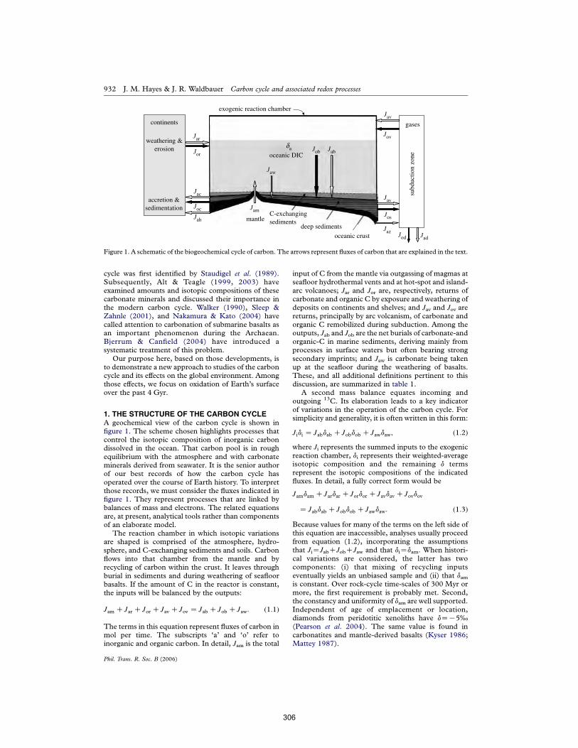
cycle was first identified by Staudigel et al. (1989).Subsequently, Alt & Teagle (1999, 2003) haveexamined amounts and isotopic compositions of thesecarbonate minerals and discussed their importance inthe modern carbon cycle. Walker (1990), Sleep &Zahnle (2001), and Nakamura & Kato (2004) havecalled attention to carbonation of submarine basalts asan important phenomenon during the Archaean.Bjerrum & Canfield (2004) have introduced asystematic treatment of this problem.
Our purpose here, based on those developments, isto demonstrate a new approach to studies of the carboncycle and its effects on the global environment. Amongthose effects, we focus on oxidation of Earth’s surfaceover the past 4 Gyr.
1. THE STRUCTURE OF THE CARBON CYCLEA geochemical view of the carbon cycle is shown infigure 1. The scheme chosen highlights processes thatcontrol the isotopic composition of inorganic carbondissolved in the ocean. That carbon pool is in roughequilibrium with the atmosphere and with carbonateminerals derived from seawater. It is the senior authorof our best records of how the carbon cycle hasoperated over the course of Earth history. To interpretthose records, we must consider the fluxes indicated infigure 1. They represent processes that are linked bybalances of mass and electrons. The related equationsare, at present, analytical tools rather than componentsof an elaborate model.
The reaction chamber in which isotopic variationsare shaped is comprised of the atmosphere, hydro-sphere, and C-exchanging sediments and soils. Carbonflows into that chamber from the mantle and byrecycling of carbon within the crust. It leaves throughburial in sediments and during weathering of seafloorbasalts. If the amount of C in the reactor is constant,the inputs will be balanced by the outputs:
Jam CJar CJor CJav CJov Z Jab CJob CJaw: !1:1"
The terms in this equation represent fluxes of carbon inmol per time. The subscripts ‘a’ and ‘o’ refer toinorganic and organic carbon. In detail, Jam is the total
input of C from the mantle via outgassing of magmas atseafloor hydrothermal vents and at hot-spot and island-arc volcanoes; Jar and Jor are, respectively, returns ofcarbonate and organic C by exposure and weathering ofdeposits on continents and shelves; and Jav and Jov arereturns, principally by arc volcanism, of carbonate andorganic C remobilized during subduction. Among theoutputs, Jab and Job are the net burials of carbonate-andorganic-C in marine sediments, deriving mainly fromprocesses in surface waters but often bearing strongsecondary imprints; and Jaw is carbonate being takenup at the seafloor during the weathering of basalts.These, and all additional definitions pertinent to thisdiscussion, are summarized in table 1.
A second mass balance equates incoming andoutgoing 13C. Its elaboration leads to a key indicatorof variations in the operation of the carbon cycle. Forsimplicity and generality, it is often written in this form:
Jidi Z Jabdab CJobdob CJawdaw; !1:2"
where Ji represents the summed inputs to the exogenicreaction chamber, di represents their weighted-averageisotopic composition and the remaining d termsrepresent the isotopic compositions of the indicatedfluxes. In detail, a fully correct form would be
Jamdam CJardar CJordor CJavdav CJovdov
Z Jabdab CJobdob CJawdaw: !1:3"
Because values for many of the terms on the left side ofthis equation are inaccessible, analyses usually proceedfrom equation (1.2), incorporating the assumptionsthat JiZJabCJobCJaw and that diZdam. When histori-cal variations are considered, the latter has twocomponents: (i) that mixing of recycling inputseventually yields an unbiased sample and (ii) that damis constant. Over rock-cycle time-scales of 300 Myr ormore, the first requirement is probably met. Second,the constancy and uniformity of dam are well supported.Independent of age of emplacement or location,diamonds from peridotitic xenoliths have dZK5‰(Pearson et al. 2004). The same value is found incarbonatites and mantle-derived basalts (Kyser 1986;Mattey 1987).
daoceanic DIC
subd
uctio
n zo
ne
C-exchangingsediments
oceanic crust
Javcontinents
exogenic reaction chamber
Jov
Jas
Jos
Jaz
Jah
Joc
Jac
Jor
Jar
accretion &sedimentation
weathering &erosion
Jam
Jaw
Job Jab
JadJod
gases
mantledeep sediments
Figure 1. A schematic of the biogeochemical cycle of carbon. The arrows represent fluxes of carbon that are explained in the text.
932 J. M. Hayes & J. R. Waldbauer Carbon cycle and associated redox processes
Phil. Trans. R. Soc. B (2006)
306
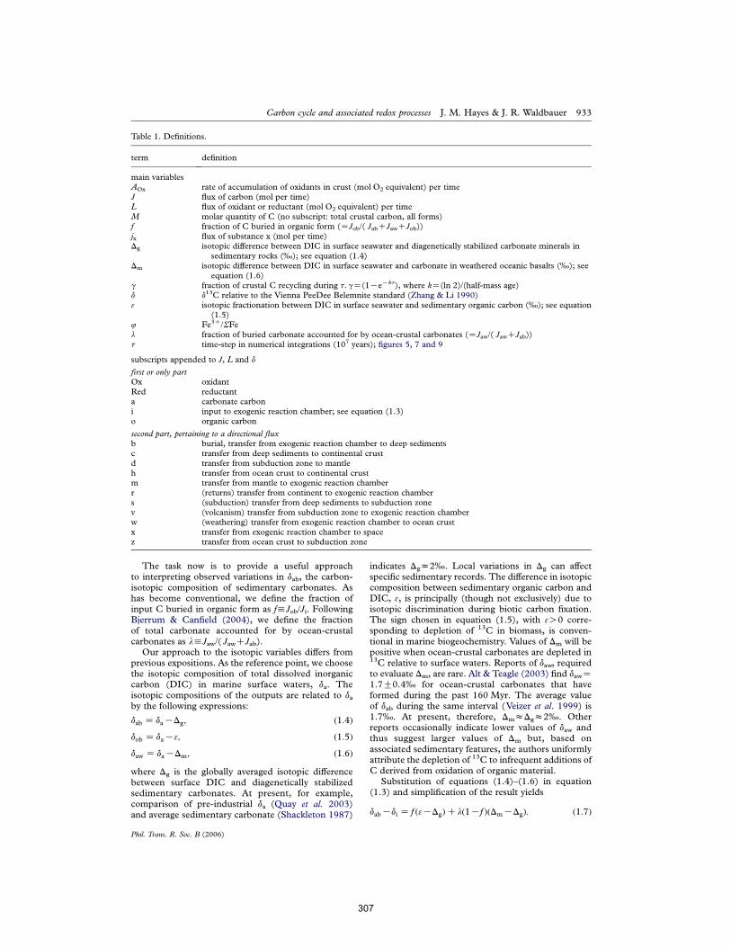
The task now is to provide a useful approachto interpreting observed variations in dab, the carbon-isotopic composition of sedimentary carbonates. Ashas become conventional, we define the fraction ofinput C buried in organic form as fhJob/Ji. FollowingBjerrum & Canfield (2004), we define the fractionof total carbonate accounted for by ocean-crustalcarbonates as lhJaw/( JawCJab).
Our approach to the isotopic variables differs fromprevious expositions. As the reference point, we choosethe isotopic composition of total dissolved inorganiccarbon (DIC) in marine surface waters, da. Theisotopic compositions of the outputs are related to daby the following expressions:
dab Z daKDg; !1:4"dob Z daK3; !1:5"daw Z daKDm; !1:6"
where Dg is the globally averaged isotopic differencebetween surface DIC and diagenetically stabilizedsedimentary carbonates. At present, for example,comparison of pre-industrial da (Quay et al. 2003)and average sedimentary carbonate (Shackleton 1987)
indicates Dgz2‰. Local variations in Dg can affectspecific sedimentary records. The difference in isotopiccomposition between sedimentary organic carbon andDIC, 3, is principally (though not exclusively) due toisotopic discrimination during biotic carbon fixation.The sign chosen in equation (1.5), with 3O0 corre-sponding to depletion of 13C in biomass, is conven-tional in marine biogeochemistry. Values of Dm will bepositive when ocean-crustal carbonates are depleted in13C relative to surface waters. Reports of daw, requiredto evaluate Dm, are rare. Alt & Teagle (2003) find dawZ1.7G0.4‰ for ocean-crustal carbonates that haveformed during the past 160 Myr. The average valueof dab during the same interval (Veizer et al. 1999) is1.7‰. At present, therefore, DmzDgz2‰. Otherreports occasionally indicate lower values of daw andthus suggest larger values of Dm but, based onassociated sedimentary features, the authors uniformlyattribute the depletion of 13C to infrequent additions ofC derived from oxidation of organic material.
Substitution of equations (1.4)–(1.6) in equation(1.3) and simplification of the result yields
dabKdi Z f !3KDg"Cl!1Kf "!DmKDg": !1:7"
Table 1. Definitions.
term definition
main variablesAOx rate of accumulation of oxidants in crust (mol O2 equivalent) per timeJ flux of carbon (mol per time)L flux of oxidant or reductant (mol O2 equivalent) per timeM molar quantity of C (no subscript: total crustal carbon, all forms)f fraction of C buried in organic form (ZJob/( JabCJawCJob))jx flux of substance x (mol per time)Dg isotopic difference between DIC in surface seawater and diagenetically stabilized carbonate minerals in
sedimentary rocks (‰); see equation (1.4)Dm isotopic difference between DIC in surface seawater and carbonate in weathered oceanic basalts (‰); see
equation (1.6)g fraction of crustal C recycling during t.gZ(1KeKkt), where kZ(ln 2)/(half-mass age)d d13C relative to the Vienna PeeDee Belemnite standard (Zhang & Li 1990)3 isotopic fractionation between DIC in surface seawater and sedimentary organic carbon (‰); see equation
(1.5)4 Fe3C/SFel fraction of buried carbonate accounted for by ocean-crustal carbonates (ZJaw/( JawCJab))t time-step in numerical integrations (107 years); figures 5, 7 and 9
subscripts appended to J, L and d
first or only partOx oxidantRed reductanta carbonate carboni input to exogenic reaction chamber; see equation (1.3)o organic carbon
second part, pertaining to a directional fluxb burial, transfer from exogenic reaction chamber to deep sedimentsc transfer from deep sediments to continental crustd transfer from subduction zone to mantleh transfer from ocean crust to continental crustm transfer from mantle to exogenic reaction chamberr (returns) transfer from continent to exogenic reaction chambers (subduction) transfer from deep sediments to subduction zonev (volcanism) transfer from subduction zone to exogenic reaction chamberw (weathering) transfer from exogenic reaction chamber to ocean crustx transfer from exogenic reaction chamber to spacez transfer from ocean crust to subduction zone
Carbon cycle and associated redox processes J. M. Hayes & J. R. Waldbauer 933
Phil. Trans. R. Soc. B (2006)
307
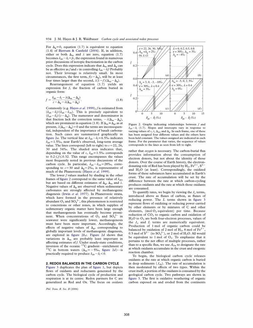
For DgZ0, equation (1.7) is equivalent to equation(1.4) of Bjerrum & Canfield (2004). If, in addition,either or both Dm and l are zero, equation (1.7)becomes dabKdiZf3, the expression found in numerousprior discussions of isotopic fractionation in the carboncycle. Does this expression indicate that Dm and Dg canbe as effective as f and 3 in controlling dabKdi? Probablynot. Their leverage is relatively small. In mostcircumstances, the first term, f(3KDg), will be at leastfour times larger than the second, l(1Kf )(DmKDg).
Rearrangement of equation (1.7) yields anexpression for f, the fraction of carbon buried inorganic form:
f ZdabKdiKl!DmKDg"3KDgKl!DmKDg"
: !1:8"
Commonly (e.g. Hayes et al. 1999), f is estimated from(dabKdi)/(dabKdob). This is precisely equivalent to(dabKdi)/(3KDg). The numerator and denominator inthat fraction lack the correction terms, Kl(DmKDg),which are prominent in equation (1.8). If DmzDg, as atpresent, l(DmKDg)Z0 and the terms are inconsequen-tial, independent of the importance of basalt carbona-tion. Such cases are summarized graphically infigure 2a. The vertical line at dabKdiZ6.5‰ indicatesdabZ1.5‰, near Earth’s observed, long-term averagevalue. The lines correspond (left to right) to 3Z22, 26,30 and 34‰. The shaded area indicates that,depending on the value of 3, dabZ1.5‰ correspondsto 0.2%f%0.32. This range encompasses the valuesmost frequently noted in previous discussions of thecarbon cycle. In particular, dabKdobZ28‰, corre-sponding to 3Z30 and DgZ2‰, is representative ofmuch of the Phanerozoic (Hayes et al. 1999).
The lower f values marked by shading in the otherframes of figure 2 correspond to the same value of dab,but are based on different estimates of Dg, Dm and l.Negative values of Dg are observed when sedimentarycarbonates are strongly affected by methanogenicdiagenesis (Irwin et al. 1977). In Phanerozoic strata,which have formed in the presence of relativelyabundant O2 and SO 2K
4 , this phenomenon is restrictedto concretions or other zones, in which supplies ofsedimentary organic matter have been large enoughthat methanogenesis has eventually become promi-nent. When concentrations of O2 and SO 2K
4 inseawater were significantly lower, methanogenesismust have been more important. Accordingly, theeffects of negative values of Dg, corresponding toglobally important levels of methanogenic diagenesis,are explored in figure 2b,c. Figure 2d shows thatvariations in Dm are probably least important inaffecting estimates of f. Under steady-state conditions,inversion of the oceanic 13C gradient—enrichment of13C in bottom waters (DmZK5‰, figure 2d )—ispractically required to produce dabKdi!0.
2. REDOX BALANCES IN THE CARBON CYCLEFigure 3 duplicates the plan of figure 1, but depictsflows of oxidants and reductants generated by thecarbon cycle. The biological cycle of production andrespiration is at its centre. Redox partners for C aregeneralized as Red and Ox. The focus on oxidants
rather that oxygen is necessary. The carbon-burial fluxprovides information about the consumption ofelectron donors, but not about the identity of thosedonors. Over the course of Earth history, the electron-donating role of Red has been played by H2, Fe
2C, S2K
and H2O (at least). Correspondingly, the oxidizedforms of these substances have accumulated in Earth’scrust. The rate of accumulation will be set by thedifference between the rate at which carbon-cyclingproduces oxidants and the rate at which those oxidantsare consumed.
To quantify rates, we begin by viewing the Jo terms,introduced above as fluxes of carbon, as fluxes ofreducing power. The L terms shown in figure 3represent flows of oxidizing or reducing power carriedby other elements or by mixtures of C and otherelements, (mol O2 equivalent) per time. Becausereduction of CO2 to organic carbon and oxidation ofH2O to O2 are both four-electron processes, values ofthe Jo and L terms are numerically equivalent.Production of 1 mol of organic carbon could bebalanced by oxidation of 2 mol of H2, 8 mol of Fe2C,0.5 mol of S2K (to SO 2K
4 ), or 2 mol of H2O. All wouldbe equivalent to 1 mol of O2. To emphasize that itpertains to the net effect of multiple processes, ratherthan to a specific flux, we use AOx to designate the rateat which oxidants accumulate in the crust and exogenicreaction chamber.
To begin, the biological carbon cycle releasesoxidants at the rate at which organic carbon is buriedin deep sediments ( Job). The rate of accumulation isthen moderated by effects of two types. Within thecrust itself, a portion of the oxidants is consumed by thegeological carbon cycle. Two pathways are shown infigure 3. The first is oxidative weathering of organiccarbon exposed on and eroded from the continents
f
0.0
0.2
0.4
0 10
f
0
0.2
0.4
0 5 10 15
e = 22, 26, 30, 34‰ !m =!g = 2‰0" l "1
l = 0, 0.2, 0.5, 0.8e = 30‰, !m = 3‰!g = –4‰
!g = 3, 0, –3, –10‰
(a) (b)
(c) (d )
e = 30‰, l = 0.4!m = 3‰
!m = –5, 0, 2, 5‰
e = 30‰, l = 0.4!g = 0‰
dab – di (‰) dab – di (‰)5
Figure 2. Graphs indicating relationships between f anddabKdi (1.7). Slopes and intercepts vary in response tovarying values of 3, l, Dm, and Dg. In each frame, one of thesehas been assigned four different values and the others havebeen held constant. The values assigned are indicated in eachframe. For the parameter that varies, the sequence of valuescorresponds to the lines as seen from left to right.
934 J. M. Hayes & J. R. Waldbauer Carbon cycle and associated redox processes
Phil. Trans. R. Soc. B (2006)
308
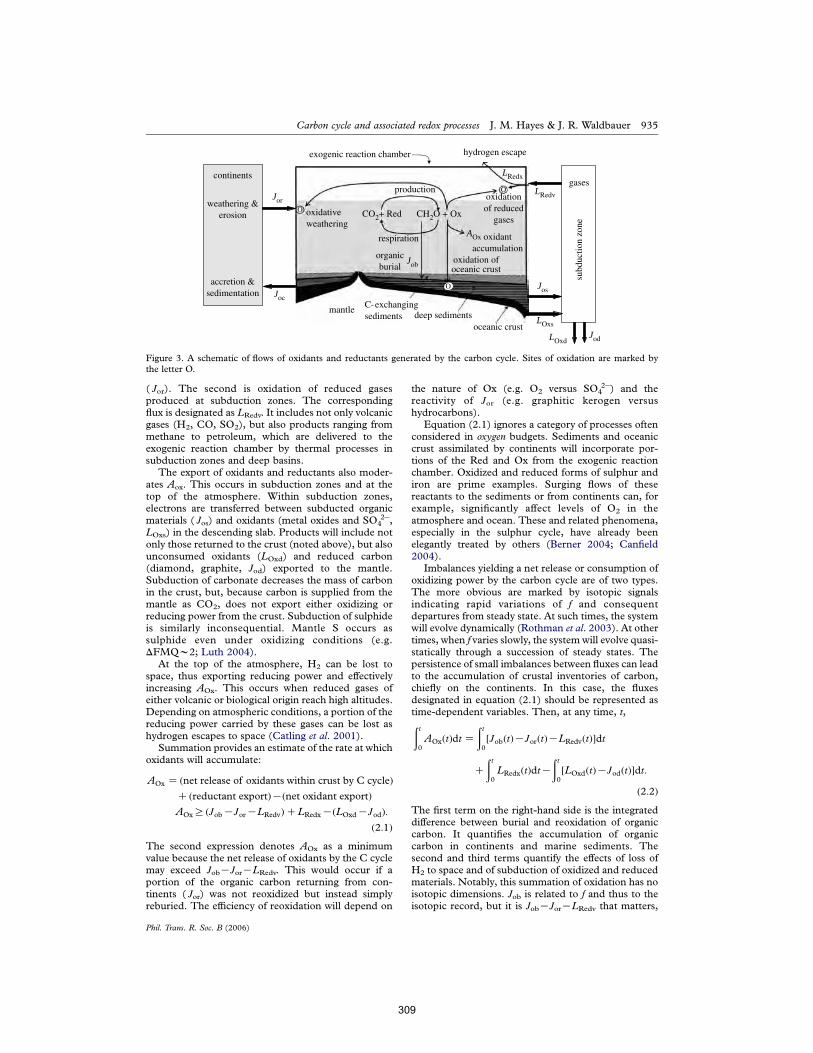
( Jor). The second is oxidation of reduced gasesproduced at subduction zones. The correspondingflux is designated as LRedv. It includes not only volcanicgases (H2, CO, SO2), but also products ranging frommethane to petroleum, which are delivered to theexogenic reaction chamber by thermal processes insubduction zones and deep basins.
The export of oxidants and reductants also moder-ates Aox. This occurs in subduction zones and at thetop of the atmosphere. Within subduction zones,electrons are transferred between subducted organicmaterials ( Jos) and oxidants (metal oxides and SO 2K
4 ,LOxs) in the descending slab. Products will include notonly those returned to the crust (noted above), but alsounconsumed oxidants (LOxd) and reduced carbon(diamond, graphite, Jod) exported to the mantle.Subduction of carbonate decreases the mass of carbonin the crust, but, because carbon is supplied from themantle as CO2, does not export either oxidizing orreducing power from the crust. Subduction of sulphideis similarly inconsequential. Mantle S occurs assulphide even under oxidizing conditions (e.g.DFMQw2; Luth 2004).
At the top of the atmosphere, H2 can be lost tospace, thus exporting reducing power and effectivelyincreasing AOx. This occurs when reduced gases ofeither volcanic or biological origin reach high altitudes.Depending on atmospheric conditions, a portion of thereducing power carried by these gases can be lost ashydrogen escapes to space (Catling et al. 2001).
Summation provides an estimate of the rate at whichoxidants will accumulate:
AOx Z !net release of oxidants within crust by C cycle"C !reductant export"K!net oxidant export"AOxR !JobKJorKLRedv"CLRedxK!LOxdKJod":
!2:1"The second expression denotes AOx as a minimumvalue because the net release of oxidants by the C cyclemay exceed JobKJorKLRedv. This would occur if aportion of the organic carbon returning from con-tinents ( Jor) was not reoxidized but instead simplyreburied. The efficiency of reoxidation will depend on
the nature of Ox (e.g. O2 versus SO 2K4 ) and the
reactivity of Jor (e.g. graphitic kerogen versushydrocarbons).
Equation (2.1) ignores a category of processes oftenconsidered in oxygen budgets. Sediments and oceaniccrust assimilated by continents will incorporate por-tions of the Red and Ox from the exogenic reactionchamber. Oxidized and reduced forms of sulphur andiron are prime examples. Surging flows of thesereactants to the sediments or from continents can, forexample, significantly affect levels of O2 in theatmosphere and ocean. These and related phenomena,especially in the sulphur cycle, have already beenelegantly treated by others (Berner 2004; Canfield2004).
Imbalances yielding a net release or consumption ofoxidizing power by the carbon cycle are of two types.The more obvious are marked by isotopic signalsindicating rapid variations of f and consequentdepartures from steady state. At such times, the systemwill evolve dynamically (Rothman et al. 2003). At othertimes, when f varies slowly, the system will evolve quasi-statically through a succession of steady states. Thepersistence of small imbalances between fluxes can leadto the accumulation of crustal inventories of carbon,chiefly on the continents. In this case, the fluxesdesignated in equation (2.1) should be represented astime-dependent variables. Then, at any time, t,!t
0AOx!t"dt Z
!t
0#Job!t"KJor!t"KLRedv!t"$dt
C
!t
0LRedx!t"dtK
!t
0#LOxd!t"KJod!t"$dt:
!2:2"The first term on the right-hand side is the integrateddifference between burial and reoxidation of organiccarbon. It quantifies the accumulation of organiccarbon in continents and marine sediments. Thesecond and third terms quantify the effects of loss ofH2 to space and of subduction of oxidized and reducedmaterials. Notably, this summation of oxidation has noisotopic dimensions. Job is related to f and thus to theisotopic record, but it is JobKJorKLRedv that matters,
O
subd
uctio
n zo
ne
mantle C-exchangingsediments deep sediments
oceanic crust
continents
O
exogenic reaction chamber
LRedv
JosJoc
Jor
accretion &sedimentation
weathering &erosion
Job
Jod
gases
CO2+ Red CH2O + Ox
AOx
LRedx
oxidativeweathering
respiration
productionoxidationof reduced
gases
oxidantaccumulation
organicburial
oxidation ofoceanic crust
LOxs
LOxd
O
hydrogen escape
Figure 3. A schematic of flows of oxidants and reductants generated by the carbon cycle. Sites of oxidation are marked bythe letter O.
Carbon cycle and associated redox processes J. M. Hayes & J. R. Waldbauer 935
Phil. Trans. R. Soc. B (2006)
309
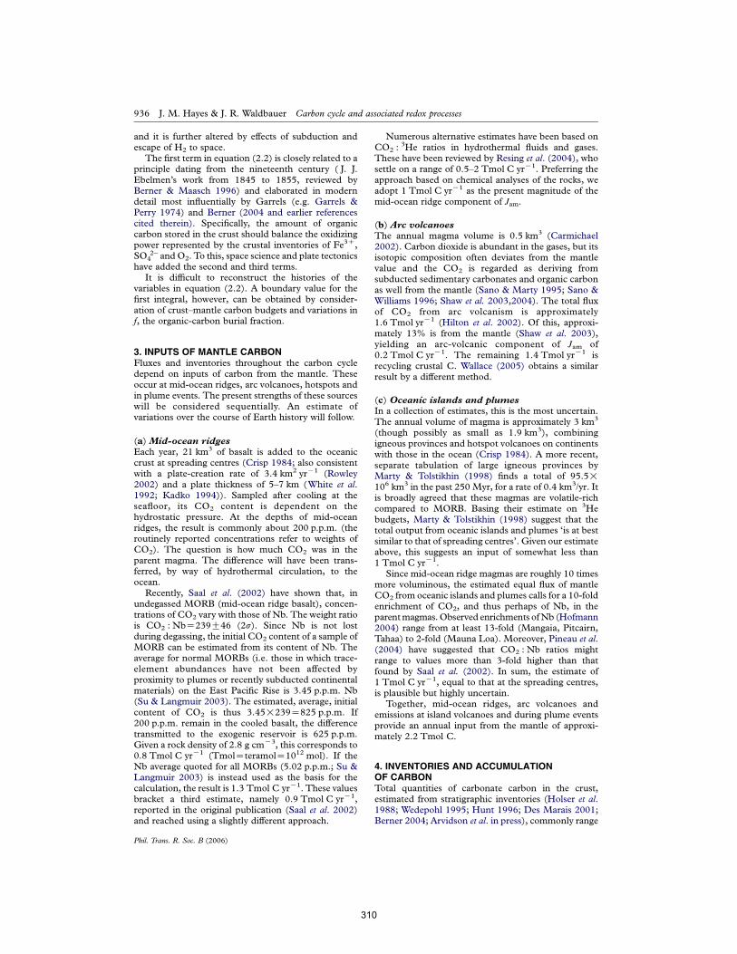
and it is further altered by effects of subduction andescape of H2 to space.
The first term in equation (2.2) is closely related to aprinciple dating from the nineteenth century ( J. J.Ebelmen’s work from 1845 to 1855, reviewed byBerner & Maasch 1996) and elaborated in moderndetail most influentially by Garrels (e.g. Garrels &Perry 1974) and Berner (2004 and earlier referencescited therein). Specifically, the amount of organiccarbon stored in the crust should balance the oxidizingpower represented by the crustal inventories of Fe3C,SO 2K
4 and O2. To this, space science and plate tectonicshave added the second and third terms.
It is difficult to reconstruct the histories of thevariables in equation (2.2). A boundary value for thefirst integral, however, can be obtained by consider-ation of crust–mantle carbon budgets and variations inf, the organic-carbon burial fraction.
3. INPUTS OF MANTLE CARBONFluxes and inventories throughout the carbon cycledepend on inputs of carbon from the mantle. Theseoccur at mid-ocean ridges, arc volcanoes, hotspots andin plume events. The present strengths of these sourceswill be considered sequentially. An estimate ofvariations over the course of Earth history will follow.
(a) Mid-ocean ridgesEach year, 21 km3 of basalt is added to the oceaniccrust at spreading centres (Crisp 1984; also consistentwith a plate-creation rate of 3.4 km2 yrK1 (Rowley2002) and a plate thickness of 5–7 km (White et al.1992; Kadko 1994)). Sampled after cooling at theseafloor, its CO2 content is dependent on thehydrostatic pressure. At the depths of mid-oceanridges, the result is commonly about 200 p.p.m. (theroutinely reported concentrations refer to weights ofCO2). The question is how much CO2 was in theparent magma. The difference will have been trans-ferred, by way of hydrothermal circulation, to theocean.
Recently, Saal et al. (2002) have shown that, inundegassed MORB (mid-ocean ridge basalt), concen-trations of CO2 vary with those of Nb. The weight ratiois CO2 : NbZ239G46 (2s). Since Nb is not lostduring degassing, the initial CO2 content of a sample ofMORB can be estimated from its content of Nb. Theaverage for normal MORBs (i.e. those in which trace-element abundances have not been affected byproximity to plumes or recently subducted continentalmaterials) on the East Pacific Rise is 3.45 p.p.m. Nb(Su & Langmuir 2003). The estimated, average, initialcontent of CO2 is thus 3.45!239Z825 p.p.m. If200 p.p.m. remain in the cooled basalt, the differencetransmitted to the exogenic reservoir is 625 p.p.m.Given a rock density of 2.8 g cmK3, this corresponds to0.8 Tmol C yrK1 (TmolZteramolZ1012 mol). If theNb average quoted for all MORBs (5.02 p.p.m.; Su &Langmuir 2003) is instead used as the basis for thecalculation, the result is 1.3 Tmol C yrK1. These valuesbracket a third estimate, namely 0.9 Tmol C yrK1,reported in the original publication (Saal et al. 2002)and reached using a slightly different approach.
Numerous alternative estimates have been based onCO2 :
3He ratios in hydrothermal fluids and gases.These have been reviewed by Resing et al. (2004), whosettle on a range of 0.5–2 Tmol C yrK1. Preferring theapproach based on chemical analyses of the rocks, weadopt 1 Tmol C yrK1 as the present magnitude of themid-ocean ridge component of Jam.
(b) Arc volcanoesThe annual magma volume is 0.5 km3 (Carmichael2002). Carbon dioxide is abundant in the gases, but itsisotopic composition often deviates from the mantlevalue and the CO2 is regarded as deriving fromsubducted sedimentary carbonates and organic carbonas well from the mantle (Sano & Marty 1995; Sano &Williams 1996; Shaw et al. 2003,2004). The total fluxof CO2 from arc volcanism is approximately1.6 Tmol yrK1 (Hilton et al. 2002). Of this, approxi-mately 13% is from the mantle (Shaw et al. 2003),yielding an arc-volcanic component of Jam of0.2 Tmol C yrK1. The remaining 1.4 Tmol yrK1 isrecycling crustal C. Wallace (2005) obtains a similarresult by a different method.
(c) Oceanic islands and plumesIn a collection of estimates, this is the most uncertain.The annual volume of magma is approximately 3 km3
(though possibly as small as 1.9 km3), combiningigneous provinces and hotspot volcanoes on continentswith those in the ocean (Crisp 1984). A more recent,separate tabulation of large igneous provinces byMarty & Tolstikhin (1998) finds a total of 95.5!106 km3 in the past 250 Myr, for a rate of 0.4 km3/yr. Itis broadly agreed that these magmas are volatile-richcompared to MORB. Basing their estimate on 3Hebudgets, Marty & Tolstikhin (1998) suggest that thetotal output from oceanic islands and plumes ‘is at bestsimilar to that of spreading centres’. Given our estimateabove, this suggests an input of somewhat less than1 Tmol C yrK1.
Since mid-ocean ridge magmas are roughly 10 timesmore voluminous, the estimated equal flux of mantleCO2 from oceanic islands and plumes calls for a 10-foldenrichment of CO2, and thus perhaps of Nb, in theparentmagmas.Observed enrichments ofNb (Hofmann2004) range from at least 13-fold (Mangaia, Pitcairn,Tahaa) to 2-fold (Mauna Loa). Moreover, Pineau et al.(2004) have suggested that CO2 : Nb ratios mightrange to values more than 3-fold higher than thatfound by Saal et al. (2002). In sum, the estimate of1 Tmol C yrK1, equal to that at the spreading centres,is plausible but highly uncertain.
Together, mid-ocean ridges, arc volcanoes andemissions at island volcanoes and during plume eventsprovide an annual input from the mantle of approxi-mately 2.2 Tmol C.
4. INVENTORIES AND ACCUMULATIONOF CARBONTotal quantities of carbonate carbon in the crust,estimated from stratigraphic inventories (Holser et al.1988; Wedepohl 1995; Hunt 1996; Des Marais 2001;Berner 2004; Arvidson et al. in press), commonly range
936 J. M. Hayes & J. R. Waldbauer Carbon cycle and associated redox processes
Phil. Trans. R. Soc. B (2006)
310
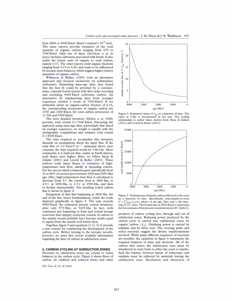
from 2800 to 6500 Emol (EmolZexamolZ1018 mol).The same reports provide estimates of the totalquantity of organic carbon ranging from 675 to1300 Emol. Only one of these (Arvidson et al. inpress) includes carbonate associated with basalt. It alsoyields the lowest ratio of organic to total carbon,namely 0.13. The other reports yield organic fractionsranging from 0.15 to 0.20, and seem to be influencedby isotopic mass balances, which suggest higher relativequantities of organic carbon.
Wilkinson & Walker (1989) took an alternativeapproach and focused exclusively on sedimentarycarbonates. Examining mass-age data, they foundthat the best fit could be provided by a constant-mass, constant-burial system with first-order recyclingand including 9600 Emol carbonate carbon. Analternative fit emphasizing data from youngersequences yielded a result of 7900 Emol. If wearbitrarily adopt an organic-carbon fraction of 0.15,the corresponding inventories of organic carbon are1700 and 1400 Emol, for total carbon inventories of11 300 and 9300 Emol.
The most detailed inventory (Holser et al. 1988)provides total crustal CZ7640 Emol. Favouring theapproach using mass-age data, particularly that basedon younger sequences, we weight it equally with thestratigraphic compilations and estimate total crustalCZ8500 Emol.
The time required to accumulate this inventorydepends on assumptions about the input flux. If thetotal flux of 2.2 Tmol C yrK1 estimated above wereconstant, the time required would be 3.86 Gyr. Morecommonly, it is believed that, earlier in Earth history,such fluxes were higher. Here, we follow Sleep &Zahnle (2001) and Lowell & Keller (2003). Theseauthors scale input fluxes to estimates of high-temperature heat flow, chiefly at spreading centres.For the case in which continents grew episodically from10 to 80% of current area between 3200 and 2500 Myrago (Ma), high-temperature heat flow is calculated todecrease from 9! the current level at 3800 Ma, to4.9! at 3200 Ma, to 2.3! at 2500 Ma, and thento decline exponentially. The resulting scaled carbonflux is shown in figure 4.
Integration of that flux beginning at 3800 Ma, theend of the late, heavy bombardment, yields the totalsdepicted graphically in figure 5. The sum exceeds8500 Emol, the estimated present crustal inventory,after only 575 Myr, at 3225 Ma. In fact, withcontinents just beginning to form and crustal storagereservoirs thus sharply restricted, returns of carbon tothe mantle would probably have become nearly equalto inputs from the mantle well before then.
Together, figure 5 and equations (1.1)–(2.2) providea new context for considering the development of thecarbon cycle. Before turning to the isotopic records,however, we must first review available informationregarding the fates of carbon in subduction zones.
5. CARBON CYCLING AT SUBDUCTION ZONESProcesses in subduction zones are crucial to redoxbalances in the carbon cycle. Figure 6 shows flows ofcarbon (in oxidized and reduced form) and other
products of carbon cycling into, through and out ofsubduction zones. Reducing power produced by thecarbon cycle is carried into subduction zones byorganic carbon ( Jos). Oxidizing power is carried bysulphate and by ferric iron. The crossing paths andredox reactions suggest the diverse transformationsinvolved. While many different sequences of reactionsare possible, the equations in figure 6 summarize therequired balances of mass and electrons. All of thecarbon that enters the subduction zone must betransferred in some form to either the crust or mantle.And the balance between inputs of reductants andoxidants must be reflected by materials leaving thesubduction zone. Resolution and dissection of
age (Myr)01000200030004000
man
tle-t
o-cr
ust f
lux
of C
, Jam
(Tm
ol y
r–1)
0
5
10
15
20
25
Figure 4. Estimated values of Jam as a function of time. Thevalue at 0 Ma is documented in the text. The scalingrelationship at earlier times derives from Sleep & Zahnle(2001) and Lowell & Keller (2003).
age (Myr)01000200030004000
tota
l man
tle-t
o-cr
ust C
(Em
ol)
0
5000
10000
15000
20000
25000
Figure 5. Total amount ofmantle carbon delivered to the crustas a function of time. Specifically, total mantle-to-crustCZ
Pt3800 Jam!t"t, where t is the age, Myr, and t, the time-
step, is 107 years. The broken line at 8500 Emol C representsthe best estimate of the present crustal inventory ofC (table 2).
Carbon cycle and associated redox processes J. M. Hayes & J. R. Waldbauer 937
Phil. Trans. R. Soc. B (2006)
311
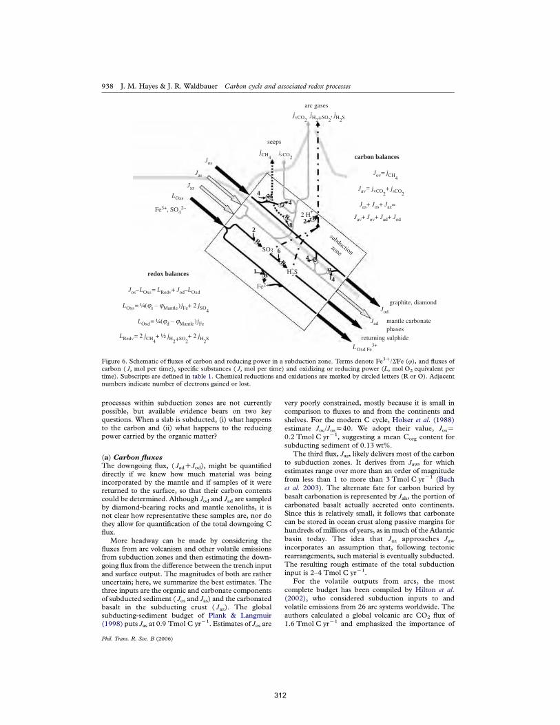
processes within subduction zones are not currentlypossible, but available evidence bears on two keyquestions. When a slab is subducted, (i) what happensto the carbon and (ii) what happens to the reducingpower carried by the organic matter?
(a) Carbon fluxesThe downgoing flux, ( JadCJod), might be quantifieddirectly if we knew how much material was beingincorporated by the mantle and if samples of it werereturned to the surface, so that their carbon contentscould be determined. Although Jod and Jad are sampledby diamond-bearing rocks and mantle xenoliths, it isnot clear how representative these samples are, nor dothey allow for quantification of the total downgoing Cflux.
More headway can be made by considering thefluxes from arc volcanism and other volatile emissionsfrom subduction zones and then estimating the down-going flux from the difference between the trench inputand surface output. The magnitudes of both are ratheruncertain; here, we summarize the best estimates. Thethree inputs are the organic and carbonate componentsof subducted sediment ( Jos and Jas) and the carbonatedbasalt in the subducting crust ( Jaz). The globalsubducting-sediment budget of Plank & Langmuir(1998) puts Jas at 0.9 Tmol C yrK1. Estimates of Jos are
very poorly constrained, mostly because it is small incomparison to fluxes to and from the continents andshelves. For the modern C cycle, Holser et al. (1988)estimate Joc/Josz40. We adopt their value, JosZ0.2 Tmol C yrK1, suggesting a mean Corg content forsubducting sediment of 0.13 wt%.
The third flux, Jaz, likely delivers most of the carbonto subduction zones. It derives from Jaw, for whichestimates range over more than an order of magnitudefrom less than 1 to more than 3 Tmol C yrK1 (Bachet al. 2003). The alternate fate for carbon buried bybasalt carbonation is represented by Jah, the portion ofcarbonated basalt actually accreted onto continents.Since this is relatively small, it follows that carbonatecan be stored in ocean crust along passive margins forhundreds of millions of years, as in much of the Atlanticbasin today. The idea that Jaz approaches Jawincorporates an assumption that, following tectonicrearrangements, such material is eventually subducted.The resulting rough estimate of the total subductioninput is 2–4 Tmol C yrK1.
For the volatile outputs from arcs, the mostcomplete budget has been compiled by Hilton et al.(2002), who considered subduction inputs to andvolatile emissions from 26 arc systems worldwide. Theauthors calculated a global volcanic arc CO2 flux of1.6 Tmol C yrK1 and emphasized the importance of
Jaz
Jas
Jos
Jod
Jad
graphite, diamond
subductionzone
mantle carbonatephases
seeps
arc gases
4
4
8
44
2R
O
RR
O
redox balances
Jos–LOxs= LRedv+ Jod–LOxd
LOxs= !(js – jMantle) jFe+ 2 jSO4
LOxd= !(jd – jMantle) jFe
LRedv= 2 jCH4+ " jH2+SO2
+ 2 jH2S
carbon balances
Jov= jCH4
Jav= jvCO2+ jsCO2
Jas+ Jos+ Jaz=
Jav+ Jov+ Jad+ Jod
jCH4jsCO2
jvCO2 jH2+SO2, jH2S
LOxs
2
LOxd Fe3+
Fe3+, SO42–
SO2 6
H2S1
Fe2+
R
R
2 H+R
R
returning sulphide
Figure 6. Schematic of fluxes of carbon and reducing power in a subduction zone. Terms denote Fe3C/SFe (4), and fluxes ofcarbon ( J, mol per time), specific substances ( J, mol per time) and oxidizing or reducing power (L, mol O2 equivalent pertime). Subscripts are defined in table 1. Chemical reductions and oxidations are marked by circled letters (R or O). Adjacentnumbers indicate number of electrons gained or lost.
938 J. M. Hayes & J. R. Waldbauer Carbon cycle and associated redox processes
Phil. Trans. R. Soc. B (2006)
312
distinguishing between sources of volatiles. For CO2,these are carbonate and organic C in the subductingslab and CO2 in the mantle wedge. Since the mantlecomponent amounts to 0.2 Tmol C yrK1 (notedabove), jvCO2
Z1.4 Tmol C yrK1. The portion due tosubducted carbonates can be estimated from theisotopic composition of the non-mantle component.For all of the arcs, it exceeded the input of sedimentarycarbonate. In all cases but one, inclusion of carbonatedbasalt eliminated the shortfall. Notably, these resultsare at odds with calculated phase equilibria thatindicate carbonated basalts should undergo littledevolatilization along most subduction geotherms(Kerrick & Connolly 2001). The other component ofJav is jsCO2
, emission of CO2 from seeps, especially infore-arc and back-arc regions. This flux is uncon-strained, and may be as large as jvCO2
(Hilton et al.2002). Ingebritsen & Manning (2002) have pointed todiffuse fluid flow through tectonically active crust aspotentially a major flux of subduction-derived volatiles.This degassing pathway may be sufficient to reconcilethe crust–mantle water balance, and could wellconstitute a significant return of slab-derived CO2 tothe crust. Accordingly, Jav is between 1.4 and2.8 Tmol C yrK1.
The other return flux of carbon from subductionzones to the exogenic chamber is Jov, the reducedcarbon from high-and low-temperature seeps, primar-ily CH4. The related geological forms are diverse, andinclude mud volcanoes and seeps associated with gashydrates (Milkov & Etiope 2005; Milkov 2005). Theiroutput of CH4, estimated at 2.1 Tmol yrK1 (Milkov &Etiope 2005), derives from microbial methanogenesisand thermal processes in sediments and sedimentaryrocks, as well as from subducted carbon. Since thecarbon in Jov (ZCH4) has oxidation number equal toK4 and the organic carbon in Jos has oxidation numberequal to zero, redox balance provides the strongerconstraint. If Jos is approximately 0.2 Tmol C yrK1, Jovcannot be larger than 0.1 Tmol C yrK1. Total volcanicand seep fluxes of carbon ( JavCJov) are between 1.5and 2.9 Tmol C yrK1.
From inputs of 2–4 Tmol C yrK1 and recyclingfluxes of 1.5–2.9 Tmol C yrK1, we estimate that thefraction recycled is approximately 0.6. By difference, theflux returning to the mantle is 0.8–1.6 Tmol C yrK1.
(b) Reducing powerAny reduced C sent to the mantle—graphite, diamond,elemental C—leaves oxidant behind in the surfaceenvironment, thus contributing to AOx. It is alsopossible that organic C would be oxidized within thesubduction zone by reaction with sulphate or anoxidized metal, such as Fe3C. When this occurs, doesthe reduction product (Fe2C, for example) become anorganic-carbon proxy that also contributes to AOx? No,the reaction instead amounts to a last-minute reversalof processes within the carbon cycle. Within theexogenic reaction chamber, Fe3C will have beenproduced within the downgoing slab by hydrothermalalteration and by oxidation of Fe2C at the expense ofO2. Or the sulphate will have been produced byprocesses within the carbon cycle. In either case, theoxidizing power will be represented by an equivalent
quantity of organic carbon. For the carbon cycle,therefore, the oxidation of organic carbon by oxidizedmetals or sulphur within subduction zones is afunctional equivalent of biological respiration. Detailsfollow.
If the Fe3C or sulphate is a product of aerobicoxidation, it carries the oxidizing power of O2 producedduring photosynthesis. The same organism thatproduced the O2 produced an equivalent amount oforganic carbon. The oxidation of that organic materialwithin the subduction zone amounts to a reversal of theoverall process.
If the Fe3C was produced at the expense of sulphateduring hydrothermal alteration, that sulphate cansimilarly be traced to photosynthetic O2 and carbon.The chain of chemical events has an additional link, butthe oxidation of organic carbon within the subductionzone is again simply a reversal of the process.
If the sulphate was produced by anaerobic, photo-synthetic bacteria, those organisms will have producedan equivalent amount of organic carbon. The oxidationof that organic material within the subduction zoneamounts to a reversal of the overall process.
Finally, if the Fe3C was produced by serpentiniza-tion, an equivalent quantity of H2 will also have beenproduced and used by microbiota to produce anequivalent amount of organic carbon, either directly,through chemosynthesis, or indirectly, through con-sumption of O2, photosynthetic production of organicmatter, etc. Again, the oxidation of organic C withinthe subduction zone amounts simply to a reversal.
If the subducted organic carbon returned to thesurface as CO2 after reducing an inorganic substance tosome oxidation state lower than that of its input—ifFe3C/SFe in the downgoing slab were driven to valueslower than Fe3C/SFe in unaltered MORB—that wouldcontribute to AOx. Failing that, JodO0 provides theonly route by which processes in subduction zone canyield a net export of oxidizing power by the carboncycle.
In magnitude, Jod is constrained to be less than Jos.Exchange of C between reduced and oxidized pools isnot excluded. Some of the C in Jod might derive fromJas or Jaz. Estimation of Jod requires knowledge of Josand LRedv. The rate of subduction of organic matter, asdiscussed above, is here taken as 0.2 Tmol yrK1,though better estimates are clearly warranted. LRedv
has two components: the reduced gas flux from arcvolcanoes, and the reduced gases from other seeps,represented by jCH4
.The reduced component of the volcanic gas flux
is represented by jH2CSO2and jH2S
. In the presentcontext, the question is how it relates to Jos, thereducing power delivered by subduction of organiccarbon. The hydrogen abundance in volcanic gases isset by redox equilibrium with water, such thatH2 : H2O ratios are maintained near ca 0.01 atmost eruptive temperatures (Giggenbach 1996).Taking the arc magmatic-water flux at 17 Tmol yrK1
(Wallace 2005) results in a hydrogen component of0.17 Tmol yrK1. The SO2 efflux from arcs, some ofwhich may derive from sources other than reductionof subducted sulphate, is of similar magnitude,0.16–0.28 Tmol yrK1 (Halmer et al. 2002; Wallace
Carbon cycle and associated redox processes J. M. Hayes & J. R. Waldbauer 939
Phil. Trans. R. Soc. B (2006)
313
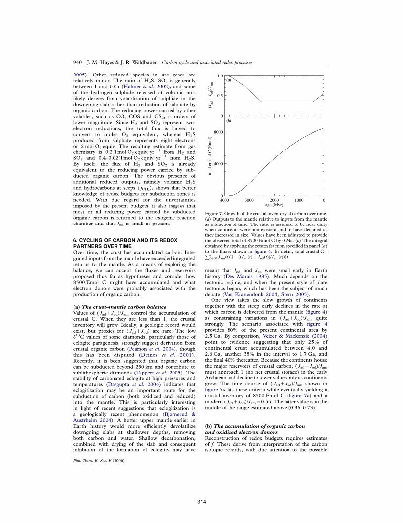
2005). Other reduced species in arc gases arerelatively minor. The ratio of H2S : SO2 is generallybetween 1 and 0.05 (Halmer et al. 2002), and someof the hydrogen sulphide released at volcanic arcslikely derives from volatilization of sulphide in thedowngoing slab rather than reduction of sulphate byorganic carbon. The reducing power carried by othervolatiles, such as CO, COS and CS2, is orders oflower magnitude. Since H2 and SO2 represent two-electron reductions, the total flux is halved toconvert to moles O2 equivalent, whereas H2Sproduced from sulphate represents eight electronsor 2 mol O2 equiv. The resulting estimate from gaschemistry is 0.2 Tmol O2 equiv. yr
K1 from H2 andSO2 and 0.4–0.02 Tmol O2 equiv. yr
K1 from H2S.By itself, the flux of H2 and SO2 is alreadyequivalent to the reducing power carried by sub-ducted organic carbon. The obvious presence ofadditional reduced outputs, namely volcanic H2Sand hydrocarbons at seeps ( jCH4
), shows that betterknowledge of redox budgets for subduction zones isneeded. With due regard for the uncertaintiesimposed by the present budgets, it also suggests thatmost or all reducing power carried by subductedorganic carbon is returned to the exogenic reactionchamber and that Jod is small at present.
6. CYCLING OF CARBON AND ITS REDOXPARTNERS OVER TIMEOver time, the crust has accumulated carbon. Inte-grated inputs from the mantle have exceeded integratedreturns to the mantle. As a means of exploring thebalance, we can accept the fluxes and reservoirsproposed thus far as hypotheses and consider how8500 Emol C might have accumulated and whatelectron donors were probably associated with theproduction of organic carbon.
(a) The crust–mantle carbon balanceValues of ( JadCJod)/Jam control the accumulation ofcrustal C. When they are less than 1, the crustalinventory will grow. Ideally, a geologic record wouldexist, but proxies for ( JadCJod) are rare. The lowd13C values of some diamonds, particularly those ofeclogite paragenesis, strongly suggest derivation fromcrustal organic carbon (Pearson et al. 2004), thoughthis has been disputed (Deines et al. 2001).Recently, it is been suggested that organic carboncan be subducted beyond 250 km and contribute tosublithospheric diamonds (Tappert et al. 2005). Thestability of carbonated eclogite at high pressures andtemperatures (Dasgupta et al. 2004) indicates thateclogitization may be an important route for thesubduction of carbon (both oxidized and reduced)into the mantle. This is particularly interestingin light of recent suggestions that eclogitization isa geologically recent phenomenon (Bjørnerud &Austrheim 2004). A hotter upper mantle earlier inEarth history would more efficiently devolatilizedowngoing slabs at shallower depths, removingboth carbon and water. Shallow decarbonation,combined with drying of the slab and consequentinhibition of the formation of eclogite, may have
meant that Jod and Jad were small early in Earthhistory (Des Marais 1985). Much depends on thetectonic regime, and when the present style of platetectonics began, which has been the subject of muchdebate (Van Kranendonk 2004; Stern 2005).
One view takes the slow growth of continentstogether with the steep early declines in the rate atwhich carbon is delivered from the mantle (figure 4)as constraining variations in ( JadCJod)/Jam quitestrongly. The scenario associated with figure 4provides 80% of the present continental area by2.5 Ga. By comparison, Veizer & Mackenzie (2004)point to evidence suggesting that only 25% ofcontinental crust accumulated between 4.0 and2.6 Ga, another 35% in the interval to 1.7 Ga, andthe final 40% thereafter. Because the continents housethe major reservoirs of crustal carbon, ( JadCJod)/Jammust approach 1 (no net crustal storage) in the earlyArchaean and decline to lower values only as continentsgrow. The time course of ( JadCJod)/Jam shown infigure 7a fits these criteria while eventually yielding acrustal inventory of 8500 Emol C (figure 7b) and amodern ( JadCJod)/JamZ0.55. The latter value is in themiddle of the range estimated above (0.36–0.73).
(b) The accumulation of organic carbonand oxidized electron donorsReconstruction of redox budgets requires estimatesof f. These derive from interpretation of the carbonisotopic records, with due attention to the possible
0
0.5
1.0
age (Myr)01000200030004000
tota
l cru
stal
C (E
mol
)
4000
8000
(a)
(b)
0
(Jad
+ J
od)/
J amFigure 7. Growth of the crustal inventory of carbon over time.(a) Outputs to the mantle relative to inputs from the mantleas a function of time. The ratio is assumed to be near unitywhen continents were non-existent and to have declined asthey increased in size. Values have been adjusted to providethe observed total of 8500 Emol C by 0 Ma. (b) The integralobtained by applying the return fraction specified in panel (a)to the fluxes shown in figure 4. In detail, total crustal CZPt
3800 Jam!t"#1K!!Jad!t"CJod!t""=Jam!t""$t.
940 J. M. Hayes & J. R. Waldbauer Carbon cycle and associated redox processes
Phil. Trans. R. Soc. B (2006)
314
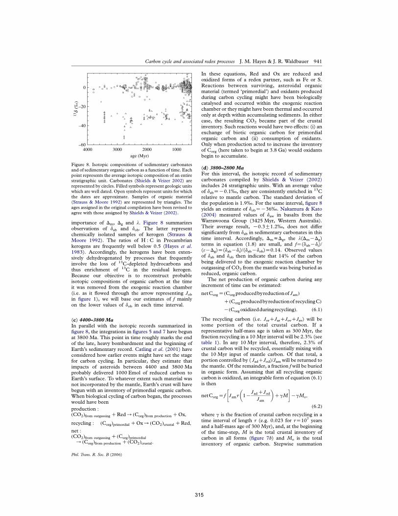
importance of Dm, Dg and l. Figure 8 summarizesobservations of dab and dob. The latter representchemically isolated samples of kerogen (Strauss &Moore 1992). The ratios of H : C in Precambriankerogens are frequently well below 0.5 (Hayes et al.1983). Accordingly, the kerogens have been exten-sively dehydrogenated by processes that frequentlyinvolve the loss of 13C-depleted hydrocarbons andthus enrichment of 13C in the residual kerogen.Because our objective is to reconstruct probableisotopic compositions of organic carbon at the timeit was removed from the exogenic reaction chamber(i.e. as it flowed through the arrow representing Jobin figure 1), we will base our estimates of f mainlyon the lower values of dob in each time interval.
(c) 4400–3800 MaIn parallel with the isotopic records summarized infigure 8, the integrations in figures 5 and 7 have begunat 3800 Ma. This point in time roughly marks the endof the late, heavy bombardment and the beginning ofEarth’s sedimentary record. Catling et al. (2001) haveconsidered how earlier events might have set the stagefor carbon cycling. In particular, they estimate thatimpacts of asteroids between 4400 and 3800 Maprobably delivered 1000 Emol of reduced carbon toEarth’s surface. To whatever extent such material wasnot incorporated by the mantle, Earth’s crust will havebegun with an inventory of primordial organic carbon.When biological cycling of carbon began, the processeswould have been
production :!CO2"from outgassing CRed/ !Corg"from production COx;
recycling : !Corg"primordial COx/ !CO2"crustal CRed;
net :!CO2"from outgassing C !Corg"primordial
/ !Corg"from production C !CO2"crustal:
In these equations, Red and Ox are reduced andoxidized forms of a redox partner, such as Fe or S.Reactions between surviving, asteroidal organicmaterial (termed ‘primordial’) and oxidants producedduring carbon cycling might have been biologicallycatalysed and occurred within the exogenic reactionchamber or they might have been thermal and occurredonly at depth within accumulating sediments. In eithercase, the resulting CO2 became part of the crustalinventory. Such reactions would have two effects: (i) anexchange of biotic organic carbon for primordialorganic carbon and (ii) consumption of oxidants.Only when production acted to increase the inventoryof Corg (here taken to begin at 3.8 Ga) would oxidantsbegin to accumulate.
(d) 3800–2800 MaFor this interval, the isotopic record of sedimentarycarbonates compiled by Shields & Veizer (2002)includes 24 stratigraphic units. With an average valueof dabZK0.1‰, they are consistently enriched in 13Crelative to mantle carbon. The standard deviation ofthe population is 1.9‰. For the same interval, figure 8yields an estimate of dobZK36‰. Nakamura & Kato(2004) measured values of daw in basalts from theWarrawoona Group (3425 Myr, Western Australia).Their average result, K0.3G1.2‰, does not differsignificantly from dab in sedimentary carbonates in thistime interval. Accordingly, DmzDg, the l(DmKDg)terms in equation (1.8) are small, and fZ(dabKdi)/(3KDg)Z(dabKdi)/(dabKdob)Z0.14. Observed valuesof dab and dob then indicate that 14% of the carbonbeing delivered to the exogenic reaction chamber byoutgassing of CO2 from the mantle was being buried asreduced, organic carbon.
The net production of organic carbon during anyincrement of time can be estimated:
netCorgZ!Corg producedbyreductionof Jam"C!Corg producedbyreductionof recyclingC"K!Corg oxidizedduringrecycling": !6:1"
The recycling carbon (i.e. JorCJarCJovCJav) will besome portion of the total crustal carbon. If arepresentative half-mass age is taken as 300 Myr, thefraction recycling in a 10 Myr interval will be 2.3% (seetable 1). In any 10 Myr interval, therefore, 2.3% ofcrustal carbon will be recycled, essentially mixing withthe 10 Myr input of mantle carbon. Of that total, aportion controlled by ( JadCJod)/Jam will be returned tothe mantle. Of the remainder, a fraction f will be buriedin organic form. Assuming that all recycling organiccarbon is oxidized, an integrable form of equation (6.1)is then
netCorgZf Jamt 1KJadCJod
Jam
" #CgM
$ %KgMo;
!6:2"where g is the fraction of crustal carbon recycling in atime interval of length t (e.g. 0.023 for tZ107 yearsand a half-mass age of 300 Myr), and, at the beginningof the time-step, M is the total crustal inventory ofcarbon in all forms (figure 7b) and Mo is the totalinventory of organic carbon. Stepwise summation
age (Myr)1000200030004000
13d
(‰)
–60
–40
–20
0
Figure 8. Isotopic compositions of sedimentary carbonatesand of sedimentary organic carbon as a function of time. Eachpoint represents the average isotopic composition of an entirestratigraphic unit. Carbonates (Shields & Veizer 2002) arerepresented by circles. Filled symbols represent geologic unitswhich are well dated. Open symbols represent units for whichthe dates are approximate. Samples of organic material(Strauss & Moore 1992) are represented by triangles. Theages assigned in the original compilation have been revised toagree with those assigned by Shields & Veizer (2002).
Carbon cycle and associated redox processes J. M. Hayes & J. R. Waldbauer 941
Phil. Trans. R. Soc. B (2006)
315
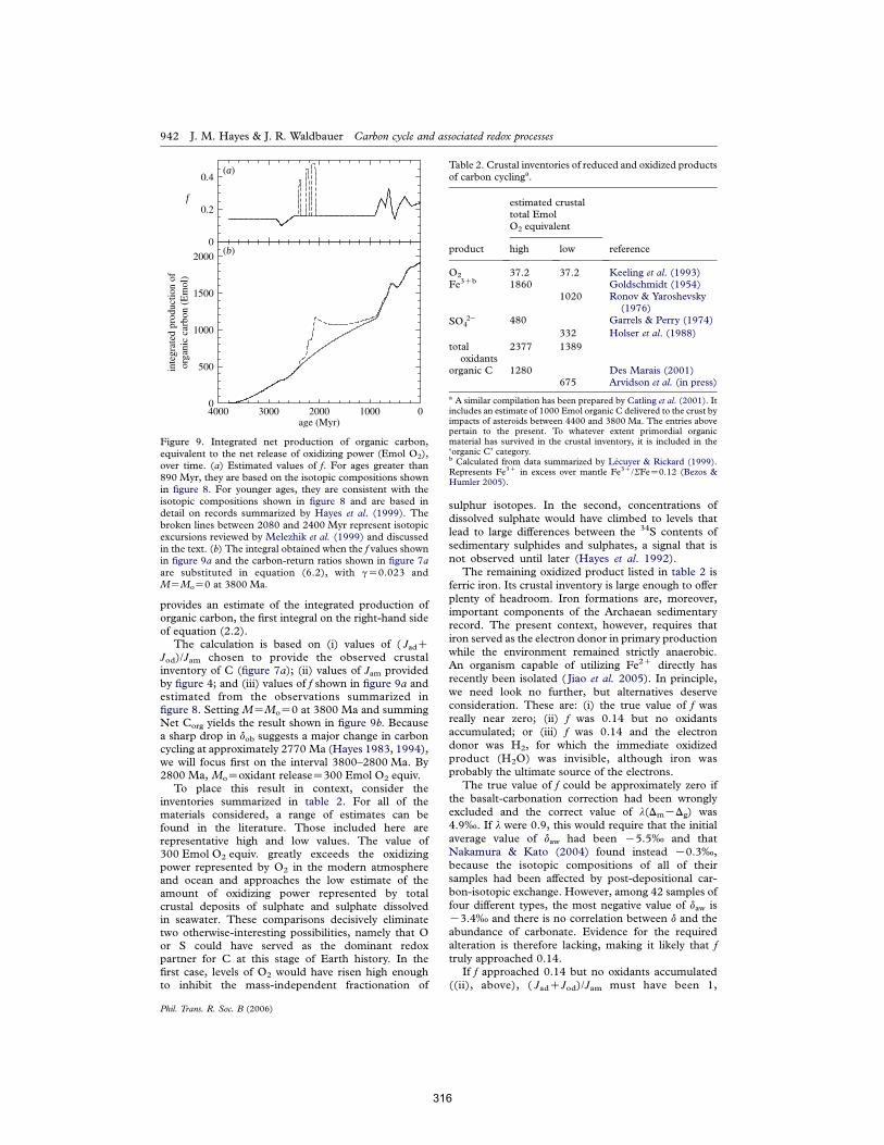
provides an estimate of the integrated production oforganic carbon, the first integral on the right-hand sideof equation (2.2).
The calculation is based on (i) values of ( JadCJod)/Jam chosen to provide the observed crustalinventory of C (figure 7a); (ii) values of Jam providedby figure 4; and (iii) values of f shown in figure 9a andestimated from the observations summarized infigure 8. Setting MZMoZ0 at 3800 Ma and summingNet Corg yields the result shown in figure 9b. Becausea sharp drop in dob suggests a major change in carboncycling at approximately 2770 Ma (Hayes 1983, 1994),we will focus first on the interval 3800–2800 Ma. By2800 Ma, MoZoxidant releaseZ300 Emol O2 equiv.
To place this result in context, consider theinventories summarized in table 2. For all of thematerials considered, a range of estimates can befound in the literature. Those included here arerepresentative high and low values. The value of300 Emol O2 equiv. greatly exceeds the oxidizingpower represented by O2 in the modern atmosphereand ocean and approaches the low estimate of theamount of oxidizing power represented by totalcrustal deposits of sulphate and sulphate dissolvedin seawater. These comparisons decisively eliminatetwo otherwise-interesting possibilities, namely that Oor S could have served as the dominant redoxpartner for C at this stage of Earth history. In thefirst case, levels of O2 would have risen high enoughto inhibit the mass-independent fractionation of
sulphur isotopes. In the second, concentrations ofdissolved sulphate would have climbed to levels thatlead to large differences between the 34S contents ofsedimentary sulphides and sulphates, a signal that isnot observed until later (Hayes et al. 1992).
The remaining oxidized product listed in table 2 isferric iron. Its crustal inventory is large enough to offerplenty of headroom. Iron formations are, moreover,important components of the Archaean sedimentaryrecord. The present context, however, requires thatiron served as the electron donor in primary productionwhile the environment remained strictly anaerobic.An organism capable of utilizing Fe2C directly hasrecently been isolated ( Jiao et al. 2005). In principle,we need look no further, but alternatives deserveconsideration. These are: (i) the true value of f wasreally near zero; (ii) f was 0.14 but no oxidantsaccumulated; or (iii) f was 0.14 and the electrondonor was H2, for which the immediate oxidizedproduct (H2O) was invisible, although iron wasprobably the ultimate source of the electrons.
The true value of f could be approximately zero ifthe basalt-carbonation correction had been wronglyexcluded and the correct value of l(DmKDg) was4.9‰. If l were 0.9, this would require that the initialaverage value of daw had been K5.5‰ and thatNakamura & Kato (2004) found instead K0.3‰,because the isotopic compositions of all of theirsamples had been affected by post-depositional car-bon-isotopic exchange. However, among 42 samples offour different types, the most negative value of daw isK3.4‰ and there is no correlation between d and theabundance of carbonate. Evidence for the requiredalteration is therefore lacking, making it likely that ftruly approached 0.14.
If f approached 0.14 but no oxidants accumulated((ii), above), ( JadCJod)/Jam must have been 1,
Table 2. Crustal inventories of reduced and oxidized productsof carbon cyclinga.
product
estimated crustaltotal EmolO2 equivalent
referencehigh low
O2 37.2 37.2 Keeling et al. (1993)Fe3Cb 1860 Goldschmidt (1954)
1020 Ronov & Yaroshevsky(1976)
SO 2K4 480 Garrels & Perry (1974)
332 Holser et al. (1988)
totaloxidants
2377 1389
organic C 1280 Des Marais (2001)675 Arvidson et al. (in press)
a A similar compilation has been prepared by Catling et al. (2001). Itincludes an estimate of 1000 Emol organic C delivered to the crust byimpacts of asteroids between 4400 and 3800 Ma. The entries abovepertain to the present. To whatever extent primordial organicmaterial has survived in the crustal inventory, it is included in the‘organic C’ category.b Calculated from data summarized by Lecuyer & Rickard (1999).Represents Fe3C in excess over mantle Fe3C/SFeZ0.12 (Bezos &Humler 2005).
age (Myr)01000200030004000
inte
grat
ed p
rodu
ctio
n of
orga
nic
carb
on (E
mol
)
500
1500
0
f
0
0.2
0.4
2000
1000
(a)
(b)
Figure 9. Integrated net production of organic carbon,equivalent to the net release of oxidizing power (Emol O2),over time. (a) Estimated values of f. For ages greater than890 Myr, they are based on the isotopic compositions shownin figure 8. For younger ages, they are consistent with theisotopic compositions shown in figure 8 and are based indetail on records summarized by Hayes et al. (1999). Thebroken lines between 2080 and 2400 Myr represent isotopicexcursions reviewed by Melezhik et al. (1999) and discussedin the text. (b) The integral obtained when the f values shownin figure 9a and the carbon-return ratios shown in figure 7aare substituted in equation (6.2), with gZ0.023 andMZMoZ0 at 3800 Ma.
942 J. M. Hayes & J. R. Waldbauer Carbon cycle and associated redox processes
Phil. Trans. R. Soc. B (2006)
316
indicating rapid and quantitative return of all carbon tothe mantle, even as 3.5 million km2 of continental crust(Lowe 1992) formed prior to 3.2 Ga. Moreover, assubstantial quantities of organic carbon were formingas required by fZ0.14 (and thus Job/JamR0.14), theputatively non-accumulating oxidant, which could notbe either O2 or sulphate and which had to be presentonly at trace levels, was able to reoxidize all of theorganic material completely even as the carbon itselfreturned quantitatively to the mantle. The requiredcombination of circumstances is practically impossible.
The third alternative, in which f was approximately0.14 and H2 served as the electron donor, fits well withmultiple lines of evidence. Anaerobic organismscapable of producing organic material from CO2 andH2 are abundant and include both chemoautotrophs(methanogens, acetogens) and photoautotrophs(photosynthetic bacteria; Tice & Lowe 2004 havealready postulated that such organisms were importantmembers of near-shore microbial communities3.4 Ga). The potential versatility of microbial ecosys-tems based on such organisms is great enough toprovide both producer and consumer assemblages andthus to stabilize carbon cycling and yield globallyconsistent isotopic fractionations. Fermentative con-sumption would remobilize organic C as a mixture ofCO2 and CH4, providing needed greenhouse warming(Kasting & Catling 2003) and setting the stage for theisotopic transient observed at 2.8–2.7 Ga (Hayes1994).
The required net input of H2 would be 600 Emol(Z300 Emol O2 equiv.). Owing to the postulateddeclines in Jam (figure 4) and increases in [1K( JadCJod)/Jam] (equation (6.2)), the required rate would riseonly slowly from 0.5 Tmol yrK1 at 3500 Ma to0.9 Tmol yrK1 at 2800 Ma. If, as is likely, conditionsat the seafloor favoured serpentinization reactions(Sleep et al. 2004), a flux of 0.7 Tmol H2 yr
K1 couldbe provided by alteration of less than 1015 g Mg-rich(komatiitic) basalt per year. The present rate ofgeneration of ocean crust is about 6!1016 g yrK1, sothe requirement poses no problem. In the overallsequence of electron transfers, it is only the immediateoxidized product of carbon fixation (H2O) which is‘invisible’. The reducing power represented by theorganic matter is balanced by Fe3C, which is accumu-lating or being subducted.
To summarize, from both geological and biologicalpoints of view, there are highly plausible mechanismsby which substantial amounts of organic carbon couldbe produced and buried in accord with the isotopicrecords, with complementary releases of oxidizingpower, without any requirement for generation of O2
during the interval 3800–2800 Ga. The most likelyredox partner for C during this interval is Fe, eitherdirectly via phototrophic oxidation of dissolved Fe2C,and/or indirectly, with H2 shuttling electrons fromFe2C in seafloor basalts to phototrophic and chemoau-totrophic producers.
(e) 2800–1800 MaThe next billion years begin with the apparent onset ofoxygenic photosynthesis (Hayes 1983, 1994; Sum-mons et al. 1999), which includes a period during
which the abundance of 13C in sedimentary carbonateswas sometimes markedly enriched (Karhu & Holland1996; Melezhik et al. 1999), and ends with the likelyonset of sulphidic conditions in the deep sea (Canfield1998).
Estimates of f derived from the isotopic recordsprovide scant evidence that the development ofoxygenic photosynthesis, for all its magnificence as abiochemical innovation, provided a significant increasein the net release of oxidizing power. If anything, Jobinitially declined, a feature marked by the notch visibleat 2.8 Ga in figure 9a. By 2500 Ma, f appears to haverisen to 0.16, a value only slightly higher than thatestimated for the early Archaean. At 2450 Ma, whentraces of O2 quench the mass-independent fraction-ation of sulphur isotopes, the estimated minimal totalrelease of oxidizing power by the C cycle is460 Emol O2 equiv. Although uncertainties in thattotal are very large, it is far short of the capacities ofcrustal Fe and S to supply electrons (table 2). Levels ofO2 in the environment would have been sharply limitedby the strength of those sinks.
What, then, happened between 2400 and 2000 Ma?Contents of 13C in carbonates are frequently elevated,occasionally exceeding C10‰ (figure 8). Acceptingthese compositions as representative of the global poolof oceanic DIC would imply a near-trebling of f.Writing three years after Karhu & Holland (1996)published ‘Carbon isotopes and the rise of atmosphericoxygen’, Melezhik et al. (1999) drew on additional datato define three apparently separate pulses of isotopicenrichment. That dissection of the record yields thethree spikes in f that are represented by broken lines infigure 9a (alternative stratigraphic correlations yieldonly two spikes; Bekker et al. 2003). The isotopic signalhas been associated with other lines of geochemicalevidence indicating that the atmosphere becamemore oxidizing at about the same time. The ensemblehas become known as ‘The Great Oxidation Event’(Holland 2002).
One view of the scale of the event is provided by thebroken line in figure 9b. If the isotopic signals representpulses of carbon burial, the integrated production oforganic carbon by 2000 Ma would be 600 Emolgreater. As shown by table 2, that is more than enoughto provide the present inventories of SO 2K
4 and O2. Butthere are problems with interpreting these isotopicvariations in terms of carbon burial.
(i) There is no parallel isotopic enrichment in theorganic carbon, as would be expected if thecarbonate represented the oceanic DIC that wasthe carbon source for primary producers.Karhu & Holland (1996) searched for a signalin the organic-carbon record and found itsabsence ‘rather odd’. If the record were not sofragmentary and noisy (preservation is a muchgreater problem for organic carbon than forcarbonate minerals) that the problem could beset aside (Melezhik et al. 1999), this alone wouldbe fatal to the interpretation.
(ii) Evidence is lacking for the large deposits oforganic carbon that should have formed(Melezhik et al. 1999; Aharon 2005).
Carbon cycle and associated redox processes J. M. Hayes & J. R. Waldbauer 943
Phil. Trans. R. Soc. B (2006)
317
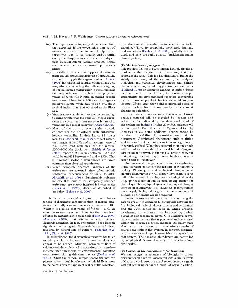
(iii) The sequence of isotopic signals is reversed fromthat expected. If the oxygenation that cut offmass-independent fractionation of sulphur iso-topes was due to an organic-carbon-burialevent, the disappearance of the mass-indepen-dent fractionation of sulphur isotopes shouldnot precede the first carbon-isotopic enrich-ments.
(iv) It is difficult to envision supplies of nutrientsgreat enough to sustain the levels of productivityrequired to supply the organic carbon. Aharon(2005) has discussed supplies of phosphate veryinsightfully, concluding that efficient strippingof P from organic matter prior to burial providesthe only solution. To achieve the projectedvalues of f, the C : P ratio in buried organicmatter would have to be 4000 and the organic-preservation rate would have to be 6.6%, aboutfivefold higher than that observed in the BlackSea.
(v) Stratigraphic correlations are not secure enoughto demonstrate that the various isotopic excur-sions are coeval, and thus necessarily linked tovariations in a global reservoir (Aharon 2005).
(vi) Most of the units displaying the isotopicenrichments are dolostones with substantialisotopic variability. In their list of 12 ‘majorlocalities,’ Melezhik et al. (1999) report within-unit ranges of 3–13‰ and an average range of7‰. Consistent with this, for the interval2350–2000 Ma (inclusive), Shields & Veizer(2002) report 589 d-values between K2.5 andC2.5‰ and 424 betweenC5 andC13‰. Thatis, ‘normal’ isotopic abundances are morecommon than elevated abundances.
(vii) When complete chemical analyses of thecarbonates are reported, they often includesubstantial concentrations of SiO2 (to 40%;Melezhik et al. 1999). Stratigraphic columnsindicate that some of the isotopically enrichedcarbonates are closely interbedded with shales(Buick et al. 1998), others are described as‘nodular’ (Bekker et al. 2003).
The latter features (vi) and (vii) are more charac-teristic of diagenetic carbonates than of marine lime-stones faithfully carrying records of oceanic DIC.When it is recalled that values of 13d to C13‰ arecommon in much younger dolomites that have beenaffected by methanogenic diagenesis (Klein et al. 1999;Mazzullo 2000), that alternative interpretationdemands attention. In fact, attribution of the isotopicsignals to methanogenic diagenesis has already beenfavoured by several sets of authors (Yudovich et al.1991; Dix et al. 1995).
In all likelihood, the diagenetic alternative has failedto win popularity because an alternative does notappear to be needed. Multiple, convergent lines ofevidence—independent of carbon-isotopic signals—indicate that thresholds of environmental oxidationwere crossed during this time interval (Bekker et al.2004). When the carbon-isotopic record fits into thispicture at least roughly, why not include it? Even moreto the point, given the apparent reality of the oxidation,
how else should the carbon-isotopic enrichments beexplained? They are temporally associated, dramaticand numerous (Bekker et al. 2003), globally distrib-uted, and have the right polarity (enrichment ratherthan depletion).
(f ) Mechanisms of oxygenationThe problem lies not in accepting the isotopic signals asmarkers of the oxidation but in assuming that theyrepresent the cause. This is a key distinction. Either thesteady functioning of the carbon cycle catalysedbiological and ecological developments that shiftedthe relative strengths of oxygen sources and sinks(Holland 1978) or dramatic changes in carbon fluxeswere required. If the former, the carbon-isotopicenrichments are environmental reporters comparableto the mass-independent fractionations of sulphurisotopes. If the latter, they point to increased burial oforganic carbon but not necessarily to permanentchanges in oxidation.
Flux-driven changes are subject to reversal. Buriedorganic material will be recycled by erosion andvolcanism. As indicated by the downward trend ofthe broken line in figure 9b after 2000 Ma, oxidants willbe consumed. Even if a rise in O2 were driven byincreases in Job, some additional change would berequired to stabilize the transition and make itpermanent. Geophysical phenomena such as riftingand increased sedimentation can increase Job, but areinherently cyclical. What they accomplish in one epochwill be undone in another. Increased burial of organiccarbon is a half answer. It can push O2 levels higher, butmaintaining them will require some further change, asecond half to the answer.
Unidirectional change, a permanent strengtheningof the source of oxidants, is in the realm of evolutionarybiology. Physiological and ecological changes couldstabilize higher levels of O2. Do they serve as the secondhalf of the answer? If so, they are the biological resultsof geophysical stimuli and we need an explanation forthe linkage. Or are physiological and ecological changesanswers in themselves? If so, advances in oxygenationhave largely biological origins and combinations ofdisparate phenomena are not required.
Kinetic factors are also pertinent. In discussing thecarbon cycle, it is common to distinguish between thefast, biological cycle of photosynthesis and respirationand the slow, geological cycle in which erosion,weathering and volcanism are balanced by carbonburial. In global chemical terms, O2 is a highly reactive,transient intermediate that is produced and consumedwithin the exogenic reaction chamber. Its steady-stateabundance must depend on the relative strengths ofsources and sinks in that system. In contrast, sedimen-tary carbonates and organic materials are outputs fromthat system. Their relative abundances are controlledby geophysical factors that vary over relatively longtime-scales.
(g) Causes of the carbon-isotopic transientWe can suggest a sequence of biologically drivenenvironmental changes, associated with a rise in levelsof O2, that would produce the observed isotopic signalswithout requiring enhanced burial of organic carbon.
944 J. M. Hayes & J. R. Waldbauer Carbon cycle and associated redox processes
Phil. Trans. R. Soc. B (2006)
318
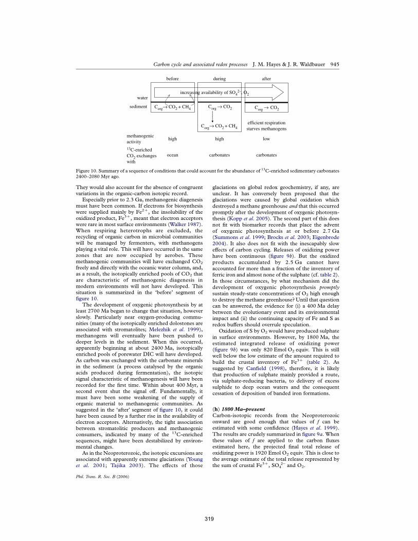
They would also account for the absence of congruentvariations in the organic-carbon isotopic record.
Especially prior to 2.3 Ga, methanogenic diagenesismust have been common. If electrons for biosynthesiswere supplied mainly by Fe2C, the insolubility of theoxidized product, Fe3C, meant that electron acceptorswere rare in most surface environments (Walker 1987).When respiring heterotrophs are excluded, therecycling of organic carbon in microbial communitieswill be managed by fermenters, with methanogensplaying a vital role. This will have occurred in the samezones that are now occupied by aerobes. Thesemethanogenic communities will have exchanged CO2
freely and directly with the oceanic water column, and,as a result, the isotopically enriched pools of CO2 thatare characteristic of methanogenic diagenesis inmodern environments will not have developed. Thissituation is summarized in the ‘before’ segment offigure 10.
The development of oxygenic photosynthesis by atleast 2700 Ma began to change that situation, howeverslowly. Particularly near oxygen-producing commu-nities (many of the isotopically enriched dolostones areassociated with stromatolites; Melezhik et al. 1999),methanogens will eventually have been pushed todeeper levels in the sediment. When this occurred,apparently beginning at about 2400 Ma, isotopicallyenriched pools of porewater DIC will have developed.As carbon was exchanged with the carbonate mineralsin the sediment (a process catalysed by the organicacids produced during fermentation), the isotopicsignal characteristic of methanogenesis will have beenrecorded for the first time. Within about 400 Myr, asecond event shut the signal off. Fundamentally, itmust have been some weakening of the supply oforganic material to methanogenic communities. Assuggested in the ‘after’ segment of figure 10, it couldhave been caused by a further rise in the availability ofelectron acceptors. Alternatively, the tight associationbetween stromatolitic producers and methanogenicconsumers, indicated by many of the 13C-enrichedsequences, might have been destabilized by environ-mental changes.
As in the Neoproterozoic, the isotopic excursions areassociated with apparently extreme glaciations (Younget al. 2001; Tajika 2003). The effects of those
glaciations on global redox geochemistry, if any, areunclear. It has conversely been proposed that theglaciations were caused by global oxidation whichdestroyed a methane greenhouse and that this occurredpromptly after the development of oxygenic photosyn-thesis (Kopp et al. 2005). The second part of this doesnot fit with biomarker records that place the adventof oxygenic photosynthesis at or before 2.7 Ga(Summons et al. 1999; Brocks et al. 2003; Eigenbrode2004). It also does not fit with the inescapably sloweffects of carbon cycling. Releases of oxidizing powerhave been continuous (figure 9b). But the oxidizedproducts accumulated by 2.5 Ga cannot haveaccounted for more than a fraction of the inventory offerric iron and almost none of the sulphate (cf. table 2).In those circumstances, by what mechanism did thedevelopment of oxygenic photosynthesis promptlysustain steady-state concentrations of O2 high enoughto destroy the methane greenhouse? Until that questioncan be answered, the evidence for (i) a 400 Ma delaybetween the evolutionary event and its environmentalimpact and (ii) the continuing capacity of Fe and S asredox buffers should overrule speculation.
Oxidation of S by O2 would have produced sulphatein surface environments. However, by 1800 Ma, theestimated integrated release of oxidizing power(figure 9b) was only 820 Emol O2 equiv. This is stillwell below the low estimate of the amount required tobuild the crustal inventory of Fe3C (table 2). Assuggested by Canfield (1998), therefore, it is likelythat production of sulphate mainly provided a route,via sulphate-reducing bacteria, to delivery of excesssulphide to deep ocean waters and the consequentcessation of deposition of banded iron formations.
(h) 1800 Ma–presentCarbon-isotopic records from the Neoproterozoiconward are good enough that values of f can beestimated with some confidence (Hayes et al. 1999).The results are crudely summarized in figure 9a. Whenthese values of f are applied to the carbon fluxesestimated here, the projected final total release ofoxidizing power is 1920 Emol O2 equiv. This is close tothe average estimate of the total release represented bythe sum of crustal Fe3C, SO 2K
4 and O2.
methanogenicactivity13C-enrichedCO2 exchangeswith
high
before during after
ocean
high
carbonates
low
carbonates
water
sediment Corg CO2 + CH4
Corg CO2 + CH4
Corg CO2 Corg CO2
efficient respirationstarves methanogens
increasing availability of SO42–, O2
Figure 10. Summary of a sequence of conditions that could account for the abundance of 13C-enriched sedimentary carbonates2400–2080 Myr ago.
Carbon cycle and associated redox processes J. M. Hayes & J. R. Waldbauer 945
Phil. Trans. R. Soc. B (2006)
319
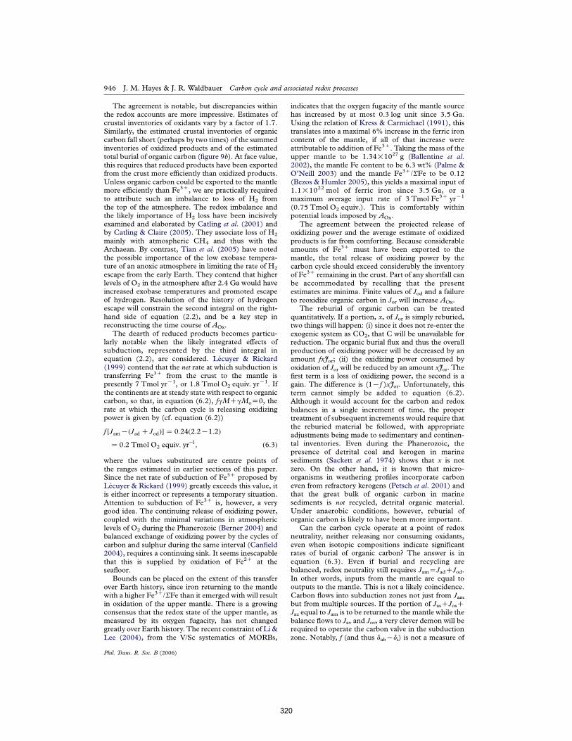
The agreement is notable, but discrepancies withinthe redox accounts are more impressive. Estimates ofcrustal inventories of oxidants vary by a factor of 1.7.Similarly, the estimated crustal inventories of organiccarbon fall short (perhaps by two times) of the summedinventories of oxidized products and of the estimatedtotal burial of organic carbon (figure 9b). At face value,this requires that reduced products have been exportedfrom the crust more efficiently than oxidized products.Unless organic carbon could be exported to the mantlemore efficiently than Fe3C, we are practically requiredto attribute such an imbalance to loss of H2 fromthe top of the atmosphere. The redox imbalance andthe likely importance of H2 loss have been incisivelyexamined and elaborated by Catling et al. (2001) andby Catling & Claire (2005). They associate loss of H2
mainly with atmospheric CH4 and thus with theArchaean. By contrast, Tian et al. (2005) have notedthe possible importance of the low exobase tempera-ture of an anoxic atmosphere in limiting the rate of H2
escape from the early Earth. They contend that higherlevels of O2 in the atmosphere after 2.4 Ga would haveincreased exobase temperatures and promoted escapeof hydrogen. Resolution of the history of hydrogenescape will constrain the second integral on the right-hand side of equation (2.2), and be a key step inreconstructing the time course of AOx.
The dearth of reduced products becomes particu-larly notable when the likely integrated effects ofsubduction, represented by the third integral inequation (2.2), are considered. Lecuyer & Rickard(1999) contend that the net rate at which subduction istransferring Fe3C from the crust to the mantle ispresently 7 Tmol yrK1, or 1.8 Tmol O2 equiv. yr
K1. Ifthe continents are at steady state with respect to organiccarbon, so that, in equation (6.2), fgMCgMoZ0, therate at which the carbon cycle is releasing oxidizingpower is given by (cf. equation (6.2))
f #JamK!Jad CJod"$Z 0:24!2:2K1:2"Z 0:2 Tmol O2 equiv: yr
K1; !6:3"
where the values substituted are centre points ofthe ranges estimated in earlier sections of this paper.Since the net rate of subduction of Fe3C proposed byLecuyer & Rickard (1999) greatly exceeds this value, itis either incorrect or represents a temporary situation.Attention to subduction of Fe3C is, however, a verygood idea. The continuing release of oxidizing power,coupled with the minimal variations in atmosphericlevels of O2 during the Phanerozoic (Berner 2004) andbalanced exchange of oxidizing power by the cycles ofcarbon and sulphur during the same interval (Canfield2004), requires a continuing sink. It seems inescapablethat this is supplied by oxidation of Fe2C at theseafloor.
Bounds can be placed on the extent of this transferover Earth history, since iron returning to the mantlewith a higher Fe3C/SFe than it emerged with will resultin oxidation of the upper mantle. There is a growingconsensus that the redox state of the upper mantle, asmeasured by its oxygen fugacity, has not changedgreatly over Earth history. The recent constraint of Li &Lee (2004), from the V/Sc systematics of MORBs,
indicates that the oxygen fugacity of the mantle sourcehas increased by at most 0.3 log unit since 3.5 Ga.Using the relation of Kress & Carmichael (1991), thistranslates into a maximal 6% increase in the ferric ironcontent of the mantle, if all of that increase wereattributable to addition of Fe3C. Taking the mass of theupper mantle to be 1.34!1027 g (Ballentine et al.2002), the mantle Fe content to be 6.3 wt% (Palme &O’Neill 2003) and the mantle Fe3C/SFe to be 0.12(Bezos & Humler 2005), this yields a maximal input of1.1!1022 mol of ferric iron since 3.5 Ga, or amaximum average input rate of 3 Tmol Fe3C yrK1
(0.75 Tmol O2 equiv.). This is comfortably withinpotential loads imposed by AOx.
The agreement between the projected release ofoxidizing power and the average estimate of oxidizedproducts is far from comforting. Because considerableamounts of Fe3C must have been exported to themantle, the total release of oxidizing power by thecarbon cycle should exceed considerably the inventoryof Fe3C remaining in the crust. Part of any shortfall canbe accommodated by recalling that the presentestimates are minima. Finite values of Jod and a failureto reoxidize organic carbon in Jor will increase AOx.
The reburial of organic carbon can be treatedquantitatively. If a portion, x, of Jor is simply reburied,two things will happen: (i) since it does not re-enter theexogenic system as CO2, that C will be unavailable forreduction. The organic burial flux and thus the overallproduction of oxidizing power will be decreased by anamount fxJor; (ii) the oxidizing power consumed byoxidation of Jor will be reduced by an amount xJor. Thefirst term is a loss of oxidizing power, the second is again. The difference is (1Kf )xJor. Unfortunately, thisterm cannot simply be added to equation (6.2).Although it would account for the carbon and redoxbalances in a single increment of time, the propertreatment of subsequent increments would require thatthe reburied material be followed, with appropriateadjustments being made to sedimentary and continen-tal inventories. Even during the Phanerozoic, thepresence of detrital coal and kerogen in marinesediments (Sackett et al. 1974) shows that x is notzero. On the other hand, it is known that micro-organisms in weathering profiles incorporate carboneven from refractory kerogens (Petsch et al. 2001) andthat the great bulk of organic carbon in marinesediments is not recycled, detrital organic material.Under anaerobic conditions, however, reburial oforganic carbon is likely to have been more important.
Can the carbon cycle operate at a point of redoxneutrality, neither releasing nor consuming oxidants,even when isotopic compositions indicate significantrates of burial of organic carbon? The answer is inequation (6.3). Even if burial and recycling arebalanced, redox neutrality still requires JamZJadCJod.In other words, inputs from the mantle are equal tooutputs to the mantle. This is not a likely coincidence.Carbon flows into subduction zones not just from Jambut from multiple sources. If the portion of JasCJosCJaz equal to Jam is to be returned to the mantle while thebalance flows to Jav and Jov, a very clever demon will berequired to operate the carbon valve in the subductionzone. Notably, f (and thus dabKdi) is not a measure of
946 J. M. Hayes & J. R. Waldbauer Carbon cycle and associated redox processes
Phil. Trans. R. Soc. B (2006)
320
JamK( JadCJod). No particular value of dab can berecognized as indicating redox neutrality. This yieldstwo fundamental insights. First, caution is requiredwhen interpreting the isotopic record in terms of redoxvariations. Second, the conditions required for redoxneutrality are precise and improbable.
7. CONCLUDING REMARKSWe have taken a new approach to mass and redoxbalances involving the C cycle. Its principal strength isa realistic acknowledgement of the importance ofinputs from and outputs to the mantle. This broadercontext has invited consideration of processes that mayotherwise be overlooked or misconstrued. Its weaknessis that our knowledge of some of the key processes ispresently imprecise. We need to learn more aboutinputs of carbon, hydrogen escape and processes insubduction zones to better evaluate each component ofAOx. Even now, however, the resulting uncertainties donot cripple the approach. The key finding is dramatic:the persistence of dab at values near zero rather thanK5‰ can be interpreted only in terms of continuousand substantial releases of oxidizing power by thecarbon cycle. Two points follow.
The oxidation of the crust has beenmore continuousthan episodic. Increases in steady-state levels ofoxidants derive either from combinations of geologicaland biological changes or from biological changesalone. The scientific problem of reconstructing Earth’soxidation is more biological than geochemical.
Continuous sinks for oxidizing power are required,at least since atmospheric levels of O2 stabilized atcurrent levels approximately 550 Ma. Since exchangesof oxidizing power between the carbon and sulphurcycles have been balanced during that same timeinterval, this can have been provided only by theoxidation of iron.
Together, these affect our view of the carbon cycle. Itshould not be seen as the competent and versatilemanager of an electron-transfer market, effortlesslybalancing offers and bids. Instead, it is a wrong-waypassenger on a downgoing escalator. It continuouslyreceives new CO2 from the mantle, relentless suppliesof solar energy and nutrients leached from deposits thathave retained their organic carbon. To hold its place, itmust constantly produce new organic matter. Whiledoing so, it releases oxidants that threaten to reverse itsaccomplishments. The stability of dab is an indicator ofthe success of its evolutionary strategies. The stabilityof PO2
is evidence of an equally competent sink.
The seeds from which the ideas discussed have grown wereplanted when J.M.H. looked out of Alvin’s viewports andobserved the H2-rich waters of the Lost City hydrothermalvent system. The generosity of Deborah Kelley and JeffreyKarson, the co-chief scientists of the Lost City cruise, isgreatly appreciated. Since then, we have benefited fromhelpful and stimulating exchanges with Stan Hart, DonAnderson, David Rowley and Alberto Saal. We are verygrateful for critical reviews of this manuscript provided byDavid Catling and Jennifer Eigenbrode. J.M.H. receivessupport as a member of the Astrobiology team led byS. D’Hondt, University of Rhode Island. J.R.W. is supportedby an NDSEG Graduate Fellowship from the Office of NavalResearch.
REFERENCESAharon, P. 2005 Redox stratification and anoxia of the early
Precambrian oceans: implications for carbon isotopeexcursions and oxidation events. Precambrian Res. 137,207–222.
Alt, J. C. & Teagle, D. A. H. 1999 The uptake of carbonduring alteration of ocean crust. Geochim. Cosmochim.Acta 63, 1527–1535. (doi:10.1016/S0016-7037(99)00123-4)
Alt, J. C. & Teagle, D. A. H. 2003 Hydrothermal alteration ofupper oceanic crust formed at a fast-spreading ridge:mineral, chemical, and isotopic evidence from ODP Site801. Chem. Geol. 201, 191–211. (doi:10.1016/S0009-2541(03)00201-8)
Arvidson, R. S., Mackenzie, F. T. & Guidry, M. In press.MAGic: a Phanerozoic model for the geochemical cyclingof major rock-forming components. Am. J. Sci.
Bach, W., Peucker-Ehrenbrink, B., Hart, S. R. & Blusztajn,J. S. 2003 Geochemistry of hydrothermally altered oceaniccrust: DSDP/ODP Hole 504B—implications for sea-water-crust exchange budgets and Sr- and Pb-isotopicevolution of the mantle. Geochem. Geophys. Geosyst. G3 4,1–29.
Ballentine, C. J., van Keken, P. E., Porcelli, D. &Houri, E. H.2002 Numerical models, geochemistry and the zero-paradox noble-gas mantle. Phil. Trans. R. Soc. A 360,2611–2631. (doi:10.1098/rsta.2002.1083)
Bekker, A., Karhu, J. A., Eriksson, K. A. & Kaufman, A. J.2003 Chemostratigraphy of Paleoproterozoic carbonatesuccessions of the Wyoming Craton: tectonic forcing ofbiogeochemical change? Precambrian Res. 120, 279–325.(doi:10.1016/S0301-9268(02)00164-X)
Bekker, A., Holland, H. D., Wang, P.-L., Rumble III, D.,Stein, H. J., Hannah, J. L., Coetzee, L. L. & Beukes, N. J.2004 Dating the rise of atmospheric oxygen. Nature 427,117–120. (doi:10.1038/nature02260)
Berner, R. A. 1991 A model for atmospheric CO2 overPhanerozoic time. Am. J. Sci. 291, 339–376.
Berner, R. A. 2004 The Phanerozoic carbon cycle. New York,NY: Oxford University Press.
Berner, R. A. & Maasch, K. A. 1996 Chemical weatheringand controls on atmospheric O2 and CO2: fundamentalprinciples were enunciated by J. J. Ebelmen in 1845.Geochim. Cosmochim. Acta 60, 1633–1637. (doi:10.1016/0016-7037(96)00104-4)
Bezos, A. & Humler, E. 2005 The Fe3C/SFe ratios of MORBglasses and their implications for mantle melting.Geochim.Cosmochim. Acta 69, 711–725. (doi:10.1016/j.gca.2004.07.026)
Bjerrum, C. J. & Canfield, D. E. 2004 New insights into theburial history of organic carbon on the early Earth.Geochem. Geophys. Geosyst. 5, 1–9. (doi:10.1029/2004GC000713)
Bjørnerud, M. G. & Austrheim, H. 2004 Inhibited eclogiteformation: the key to the rapid growth of strong andBuoyant Archean continental crust. Geol. Soc. Am. 32,765–768. (doi:10.1130/G20590.1)
Brocks, J. J., Buick, R., Logan, G. A. & Summons, R. E. 2003Composition and syngeneity of molecular fossils fromthe 2.78 to 2.45 billion-year-old Mount Bruce Super-group, Pilbara Craton, Western Australia. Geochim.Cosmochim. Acta 67, 4289–4319. (doi:10.1016/S0016-7037(03)00208-4)
Broecker, W. S. 1970 A boundary condition on the evolutionof atmospheric oxygen. J. Geophys. Res. 75, 3553–3557.
Buick, I. S.,Uken,R.,Gibson,R.L.&Wallmach,T. 1998Highd13C Paleoproterozoic carbonates from the transvaal Super-group, South Africa. Geology 26, 875–878. (doi:10.1130/0091-7613(1998)026!0875:HCPCFTO2.3.CO;2)
Carbon cycle and associated redox processes J. M. Hayes & J. R. Waldbauer 947
Phil. Trans. R. Soc. B (2006)
321
Canfield, D. E. 1998 A new model for Proterozoic oceanchemistry. Nature 396, 450–453. (doi:10.1038/24839)
Canfield, D. E. 2004 The evolution of the earth surface sulfurreservoir. Am. J. Sci. 304, 839–861.
Canfield, D. E. 2005 The early history of atmosphericoxygen: homage to Robert M. Garrels. Annu. Rev. EarthPlanet. Sci. 33, 1–36. (doi:10.1146/annurev.earth.33.092203.122711)
Carmichael, I. S. E. 2002 The ‘andesite aqueduct’ perspec-tives on the evolution of intermediate magmatism in west-central (105–998W) Mexico. Contrib. Mineral. Petrol. 143,641–663.
Catling, D. C. &Claire, M.W. 2005HowEarth’s atmosphereevolved to an oxic state: a status report. Earth Planet. Sci.Lett. 237, 1–20. (doi:10.1016/j.epsl.2005.06.013)
Catling, D. C., Zahnle, K. J. & McKay, C. P. 2001 Biogenicmethane, hydrogen escape, and the irreversible oxidationof the early earth. Science 293, 839–843. (doi:10.1126/science.1061976)
Crisp, J. A. 1984 Rates of magma emplacement and volcanicoutput. J. Volcanol. Geotherm. Res. 20, 177–211. (doi:10.1016/0377-0273(84)90039-8)
Dasgupta, R., Hirschmann, M. & Withers, A. C. 2004 Deepglobal cycling of carbon constrained by the solidus ofanhydrous, carbonated eclogite under upper mantleconditions. Earth Planet. Sci. Lett. 227, 73–85. (doi:10.1016/j.epsl.2004.08.004)
Deines, P., Viljoen, F. &Harris, J. W. 2001 Implications of thecarbon isotope and mineral inclusion record for theformation of diamonds in the mantle underlying a mobilebelt: Venetia, South Africa. Geochim. Cosmochim. Acta 65,813–838. (doi:10.1016/S0016-7037(00)00569-X)
Derry, L. A., Kaufman, A. J. & Jacobsen, S. B. 1992Sedimentary cycling and environmental change in theLate Proterozoic: evidence from stable and radiogenicisotopes. Geochim. Cosmochim. Acta 56, 1317–1329.(doi:10.1016/0016-7037(92)90064-P)
Des Marais, D. J. 1985 Carbon exchange between the mantleand the crust, and its effect upon the atmosphere: todaycompared to Archean time. In The carbon cycle andatmospheric CO2: natural variations Archean to present (ed.E. T. Sundquist & W. S. Broecker), GeophysicalMonograph 32, pp. 602–611. Washington, DC: AmericanGeophysical Union.
Des Marais, D. J. 2001 Isotopic evolution of the biogeo-chemical carbon cycle during the Precambrian. Rev.Mineral. Geochem. 43, 555–578.
Dix, G. R., Thomson, M. L., Longstaffe, F. J. & McNutt,R. H. 1995 Systematic decrease of high delta13C valueswith burial in late Archaean (2.8 Ga) diagenetic dolomite:evidence for methanogenesis from the Crixas GreenstoneBelt, Brazil. Precambrian Res. 70, 253–268. (doi:10.1016/0301-9268(94)00044-R)
Eigenbrode, J. 2004 Late archean microbial ecology: anintegration of molecular, isotopic, and lithologic studies.Ph.D. thesis, Earth Sciences, the Pennsylvania StateUniversity.
Farquhar, J. & Wing, B. A. 2003 Multiple sulfur isotopes andthe evolution of the atmosphere. Earth Planet. Sci. Lett.213, 1–13. (doi:10.1016/S0012-821X(03)00296-6)
Garrels, R. M. & Lerman, A. 1981 Phanerozoic cycles ofsedimentary carbon and sulfur. Geology 78, 4652–4655.
Garrels, R. M. & Perry Jr, E. A. 1974 Cycling of carbon,sulfur, and oxygen through geologic time. Sea 5, 303–336.
Giggenbach, W. F. 1996 Chemical composition of volcanicgases. In Monitoring and mitigation of volcano hazards (ed.S. Scarpa & R. I. Tilling), pp. 221–256. Berlin: Springer.
Goldschmidt, V. M. 1954 Geochemistry. Oxford: ClarendonPress.
Halmer, M. M., Schmincke, H.-U. & Graf, H.-F. 2002 Theannual volcanic gas input into the atmosphere, inparticular into the stratosphere: a global data set for thepast 100 years. J. Volcanol. Geotherm. Res. 115, 511–528.(doi:10.1016/S0377-0273(01)00318-3)
Halverson, G. P., Hoffman, P. F., Schrag, D. P., Maloof, A. C.& Rice, A. H. H. 2005 Toward a Neoproterozoiccomposite carbon-isotope record. Geol. Soc. Am. 117,1181–1207. (doi:10.1130/B25630.1)
Hayes, J. M. 1983 Geochemical evidence bearing on theorigin of aerobiosis, a speculative interpretation. In TheEarth’s earliest biosphere: its origin and evolution (ed. J. W.Schopf), pp. 291–301. Princeton, NJ: Princeton Univer-sity Press.
Hayes, J. M. 1994 Global methanotrophy at the Arche-an–Proterozoic transition. In Early life on Earth. NobelSymposium (ed. S. Bengtson), pp. 220–236. New York,NY: Columbia University Press.
Hayes, J. M., Kaplan, I. R. & Wedeking, K. W. 1983Precambrian organic geochemistry, preservation of therecord. In The Earth’s earliest biosphere: its origin andevolution (ed. J. W. Schopf ), pp. 93–134. Princeton, NJ:Princeton University Press.
Hayes, J. M., Lambert, I. B. & Strauss, H. 1992 The sulfur-isotopic record. In The Proterozoic biosphere, a multi-disciplinary study (ed. J. W. Schopf & C. Klein),pp. 129–132. Cambridge, UK: Cambridge UniversityPress.
Hayes, J. M., Strauss, H. & Kaufman, A. J. 1999 Theabundance of 13C in marine organic matter and isotopicfractionation in the global biogeochemical cycle of carbonduring the past 800 Ma. Chem. Geol. 161, 103–125.(doi:10.1016/S0009-2541(99)00083-2)
Hilton, D. R., Fischer, T. & Marty, B. 2002 Noble gases andvolatile recycling at subduction zones. MSA SpecialVolume: Noble Gasses 47, 319–370.
Hofmann, A. W. 2004 Sampling mantle heterogeneitythrough oceanic basalts: isotopes and trace elements. InTreatise on geochemistry, vol. 2 (ed. H. D. Holland & K. K.Turekian), pp. 61–101. Oxford: Elsevier.
Holland, H. D. 1978 The chemistry of the atmosphere andoceans. New York, NY: Wiley.
Holland, H. D. 1984 The chemical evolution of the atmosphereand oceans. Princeton, NJ: Princeton University Press.
Holland, H. D. 2002 Volcanic gases, black smokers, and thegreat oxidation event. Geochim. Cosmochim. Acta 66,3811–3826. (doi:10.1016/S0016-7037(02)00950-X)
Holser, W. T., Schidlowski, M., MacKenzie, F. T. &Maynard, J. B. 1988 Geochemical cycles of carbon andsulfur. In Chemical cycles in the evolution of the Earth (ed.C. B. Gregor, R. M. Garrels, F. T. Mackenzie & J. B.Maynard), pp. 105–173. New York, NY: Wiley.
Hunt, J. M. 1996 Petroleum geochemistry and geology. NewYork, NY: Freeman.
Ingebritsen, S. E. & Manning, C. E. 2002 Diffuse fluid fluxthrough orogenic belts: implications for the world ocean.Proc. Natl Acad. Sci. USA 99, 9113–9116. (doi:10.1073/pnas.132275699)
Irwin, H., Curtis, C. D. & Coleman, M. L. 1977 Isotopicevidence for source of diagenetic carbonates formedduring burial of organic rich sediments. Nature 269,209–213. (doi:10.1038/269209a0)
Jiao, Y., Kappler, A., Croal, L. R. & Newman, D. K. 2005Isolation and characterization of a genetically tractablephotoautotrophic Fe(II)-oxidizing bacterium, Rhodopseu-domonas palustris strainTIE-1.Appl. Environ.Microbiol. 71,4487–4496. (doi:10.1128/AEM.71.8.4487-4496.2005)
Kadko, D. 1994 An assessment of the effect of chemicalscavenging within hydrothermal plumes upon ocean
948 J. M. Hayes & J. R. Waldbauer Carbon cycle and associated redox processes
Phil. Trans. R. Soc. B (2006)
322
geochemistry. Earth Planet. Sci. Lett. 120, 361–374.(doi:10.1016/0012-821X(93)90250-D)
Karhu, J. A. & Holland, H. D. 1996 Carbon isotopes and therise of atmospheric oxygen. Geology 24, 867–870. (doi:10.1130/0091-7613(1996)024!0867:CIATROO2.3.CO;2)
Kasting, J. F. & Catling, D. 2003 Evolution of a habitableplanet. Annu. Rev. Astron. Astrophys. 41, 429–463.(doi:10.1146/annurev.astro.41.071601.170049)
Keeling, R. F., Najjar, R. P., Bender, M. L. & Tans, P. P. 1993What atmospheric oxygen measurements can tell us aboutthe global carbon cycle. Global Biogeochemical Cycles 7,36–67.
Kerrick, D. M. & Connolly, J. A. D. 2001 Metamorphicdevolatilization of subducted oceanic metabasalts: impli-cations for seismicity, arc magmatism and volatilerecycling. Earth Planet. Sci. Lett. 189, 19–29. (doi:10.1016/S0012-821X(01)00347-8)
Klein, J. S., Mozley, P., Campbell, A. & Cole, R. 1999 Spatialdistribution of carbon and oxygen isotopes in laterallyextensive carbonate-cemented layers: implications for modeof growth and subsurface identification. J. Sediment. Res. 69,184–191.
Knoll, A. H., Hayes, J. M., Kaufman, A. J., Swett, K. &Lambert, I. B. 1986 Secular variation in carbon isotoperatios fromUpper Proterozoic successions of Svalbard andEast Greenland. Nature 321, 832–838. (doi:10.1038/321832a0)
Kopp, R. E., Kirschvink, J. L., Hilburn, I. A. & Nash, C. Z.2005 The Paleoproterozoic snowball Earth: a climatedisaster triggered by the evolution of oxygenic photosyn-thesis. Proc. Natl Acad. Sci. USA 102, 11 131–11 136.(doi:10.1073/pnas.0504878102)
Kress, V. C. & Carmichael, I. S. E. 1991 The compressibilityof silicate liquids containing Fe2O3 and the effect ofcomposition, temperature, oxygen fugacity and pressureon their redox states. Contrib. Mineral. Petrol. 108, 82–92.(doi:10.1007/BF00307328)
Kump,L.R.&Arthur,M.A. 1999 Interpreting carbon-isotopeexcursions: carbonates and organicmatter.Chem.Geol. 161,181–198. (doi:10.1016/S0009-2541(99)00086-8)
Kyser, T. K. 1986 Stable isotope variations in the mantle.Stable isotopes in high temperature geological processes.Rev. Mineral. 16, 141–164.
Lecuyer, C. & Ricard, Y. 1999 Long-term fluxes and budgetof ferric iron: implication for the redox states of the Earth’smantle and atmosphere. Earth Planet. Sci. Lett. 165,197–211. (doi:10.1016/S0012-821X(98)00267-2)
Li, Z.-X. A. & Lee, C.-T. A. 2004 The constancy of uppermantle fO2 through time inferred from V/Sc ratios inbasalts. Earth Planet. Sci. Lett. 228, 483–493. (doi:10.1016/j.epsl.2004.10.006)
Lowe, D. R. 1992Major events in the geological developmentof the Precambrian Earth. In The Proterozoic biosphere (ed.J. W. Schopf & C. Klein), pp. 67–76. Cambridge, UK:Cambridge University Press.
Lowell, R. P. & Keller, S. M. 2003 High-temperature seafloorhydrothermal circulation over geologic time and Archeanbanded iron formations. Geophys. Res. Lett. 30, 1–44.(doi:10.1029/2002GL016536)
Luth, R. W. 2004 Mantle volatiles—distribution andconsequences. In Treatise on geochemistry, vol. 2 (ed.H. D. Holland & K. K. Turekian), pp. 319–361. Oxford:Elsevier.
Marty, B. & Tolstikhin, I. N. 1998 CO2 fluxes from mid-ocean ridges, arcs and plumes. Chem. Geol. 145, 233–248.(doi:10.1016/S0009-2541(97)00145-9)
Mattey, D. P. 1987 Carbon isotopes in the mantle. TerraCognita 7, 31–37.
Mazzullo, S. J. 2000 Organogenic dolomitization in peritidalto deep-sea sediments. J. Sediment. Res. 70, 10–23.
Melezhik, V. A., Fallick, A. E., Medvedev, P. V. &Makarikhin, V. V. 1999 Extreme 13Ccarb enrichment inca. 2.0 Ga magnesite–stromatolite–dolomite–‘red beds’association in a global context: a case for the world-widesignal enhanced by a local environment. Earth Sci. Rev. 48,71–120. (doi:10.1016/S0012-8252(99)00044-6)
Milkov, A. V. 2005 Molecular and stable isotope compo-sitions of natural gas hydrates: a revised global dataset andbasic interpretations in the context of geological settings.Org. Geochem. 36, 681–702. (doi:10.1016/j.orggeochem.2005.01.010)
Milkov, A. V. & Etiope, G. 2005 Global methane emissionthrough mud volcanoes and its past and present impact onthe Earth’s climate—a comment. Int. J. Earth Sci. (Geol.Rundsch.) 94, 490–492. (doi:10.1007/s00531-005-0480-5)
Nakamura, K. & Kato, Y. 2004 Carbonatization of oceaniccrust by the seafloor hydrothermal activity and itssignificance as a CO2 sink in the Early Archean. Geochim.Cosmochim. Acta 68, 4595–4618. (doi:10.1016/j.gca.2004.05.023)
Palme, H. & O’Neill, H. S. C. 2003 Cosmochemicalestimates of mantle composition. In Treatise on geochem-istry, vol. 2 (ed. H. D. Holland & K. K. Turekian),pp. 1–38. Oxford: Elsevier.
Pavlov, A. A. & Kasting, J. F. 2002 Mass-independentfractionation of sulfur isotopes in Archean sediments:strong evidence for an anoxic Archean atmosphere.Astrobiology 2, 27–41. (doi:10.1089/153110702753621321)
Pearson, D. G., Canil, D. & Shirey, S. B. 2004 Mantlesamples included in volcanic rocks: xenoliths and dia-monds. In Treatise on geochemistry, vol. 2 (ed. H. D.Holland & K. K. Turekian), pp. 172–221. Oxford:Elsevier.
Petsch, S. T., Eglinton, T. I. & Edwards, K. J. 2001 14C-Deadliving biomass: evidence for microbial assimilation ofancient organic carbon during shale weathering. Science292, 1127–1131. (doi:10.1126/science.1058332)
Pineau, F., Cartigny, P. & Javoy, M. 2004 Carbon flux andC/Nb ratios in the mantle in ridge context, Eos Trans.AGU, vol. 85, Fall Meet. Suppl., Abstract V31C-1453P.
Plank, T. & Langmuir, C. H. 1998 The chemical compositionof subducting sediment and its consequences for the crustand mantle. Chem. Geol. 145, 325–394. (doi:10.1016/S0009-2541(97)00150-2)
Quay, P., Sonnerup, P., Westby, T., Stutsman, J. &McNichol,A. 2003 Changes in the 13C/12C of dissolved inorganiccarbon in the ocean as a tracer of anthropogenic CO2
uptake. Global Biogeochem. Cycles 17, 1–4. (doi:10.1029/2001GB001817)
Resing, J. A., Lupton, J. E., Feely, R. A. & Lilley, M. D. 2004CO2 and 3He in hydrothermal plumes: implications formid-ocean ridge CO2 flux. Earth Planet. Sci. Lett. 226,449–464. (doi:10.1016/j.epsl.2004.07.028)
Ronov, A. B. & Yaroshevsky, A. A. 1976 A new model for thechemical structure of Earth’s crust. Geochem. Int. 13,89–121.
Rothman, D. H., Hayes, J. M. & Summons, R. E. 2003Dynamics of the Neoproterozoic carbon cycle. Proc. NatlAcad. Sci. USA 100, 8124–8129. (doi:10.1073/pnas.0832439100)
Rowley, D. B. 2002 Rate of plate creation and destruction:180Ma to present. Geol. Soc. Am. Bull. 114, 927–933.(doi:10.1130/0016-7606(2002)114!0927:ROPCADO2.0.CO;2)
Saal, A. E., Hauri, E. H., Langmuir, C. H. & Perfit, M. R.2002 Vapour undersaturation in primitive mid-ocean-ridge basalt and the volatile content of Earth’s uppermantle. Nature 419, 451–446. (doi:10.1038/nature01073)
Carbon cycle and associated redox processes J. M. Hayes & J. R. Waldbauer 949
Phil. Trans. R. Soc. B (2006)
323
Sackett, W. M., Poag, C. W. & Eadie, B. J. 1974 Kerogenrecycling in the Ross Sea, Antarctica. Science 185,1045–1047.
Sano, Y. & Marty, B. 1995 Origin of carbon in fumarolic gasfrom island arcs.Chem. Geol. 119, 265–274. (doi:10.1016/0009-2541(94)00097-R)
Sano,Y.&Williams,S.N.1996Fluxesofmantle andsubductedcarbon along convergent plate boundaries. Geophys. Res.Lett. 23, 2749–2752. (doi:10.1029/96GL02260)
Schidlowski, M., Eichmann, R. & Junge, C. E. 1975Precambrian sedimentary carbonates: carbon and oxygenisotope geochemistry and implications for the terrestrialoxygen budget. Precambrian Res. 2, 1–69. (doi:10.1016/0301-9268(75)90018-2)
Shackleton, N. J. 1987 The carbon isotope record of theCenozoic: history of organic carbon burial and of oxygen inthe ocean and atmosphere. In Marine petroleum source rocks(ed. J. Brooks & A. J. Fleet). Geological Society SpecialPublication No. 26, pp. 423–434. Oxford: Blackwell.
Shaw, A. M., Hilton, D. R., Fischer, T. P., Walker, J. A. &Alvarado, G. E. 2003 Contrasting He–C relationships inNicaragua and Costa Rica: insights into C cycling throughsubduction zones. Earth Planet. Sci. Lett. 214, 499–513.(doi:10.1016/S0012-821X(03)00401-1)
Shaw, A. M., Hilton, D. R., Macpherson, C. G. & Sinton,J. M. 2004 The CO2–He–Ar–H2O systematics of theManus back-arc basin: resolving source composition fromdegassing and contamination effects.Geochim. Cosmochim.Acta 68, 1837–1856. (doi:10.1016/j.gca.2003.10.015)
Shields, G. & Veizer, J. 2002 Precambrian marine carbonateisotope database: version 1.1. Geochem. Geophys. Geosyst.G3 3, 1–12.
Sleep, N. H. & Zahnle, K. 2001 Carbon dioxide cycling andimplications for climate. J. Geophys. Res. 106, 1373–1399.(doi:10.1029/2000JE001247)
Sleep, N. H., Meibom, A., Fridriksson, T., Coleman, R. G. &Bird, D. K. 2004 H2-rich fluids from serpentinization:geochemical and biotic implications. Proc. Natl Acad. SciUSA 101, 12 818–12 823. (doi:10.1073/pnas.0405289101)
Staudigel, H., Hart, S. R., Schmincke, H.-U. & Smith, B. M.1989 Cretaceous ocean crust at DSDP Sites 417 and 418:carbon uptake from weathering versus loss by magmaticoutgassing. Geochim. Cosmochim. Acta 53, 3091–3094.(doi:10.1016/0016-7037(89)90189-0)
Stern, R. J. 2005 Evidence from ophiolites, blueschists, andultrahigh-pressure metamorphic terranes that the modernepisode of subduction tectonics began in Neoproterozoictime.Geol. Soc. Am. 33, 557–560. (doi:10.1130/G21365.1)
Strauss, H. & Moore, T. B. 1992 Abundances and isotopiccompositions of carbon and sulfur species in whole rockand kerogen samples. In The Proterozoic biosphere (ed. J. W.Schopf & C. Klein), pp. 709–798. Cambridge, UK:Cambridge University Press.
Su, Y., & Langmuir, C.H. 2003 Global MORB chemistrycompilation at the segment scale. MS thesis, Departmentof Earth and Environmental Sciences, Columbia Univer-sity, Database available at http://www.petdb.org.
Summons, R. E., Jahnke, L. L., Hope, J. M. & Logan, G. A.1999 2-Methylhopanoids as biomarkers for cyanobacterialoxygenic photosynthesis. Nature 400, 554–557. (doi:10.1038/23005)
Tajika, E. 2003 Faint young sun and the carbon cycle:implications for the Proterozoic global glaciations. EarthPlanet. Sci. Lett. 214, 443–453. (doi:10.1016/S0012-821X(03)00396-0)
Tappert, R., Stachel, T., Harris, J. W., Muehlenbachs, K.,Lugwig, T. & Grey, G. P. 2005 Subducting oceanic crust:the source of deep diamonds. Geol. Soc. Am. Bull. 33,565–568.
Tian, F., Toon, O. B., Pavlov, A. A. & De Sterck, H. 2005A hydrogen-rich early earth atmosphere. Science 308,1014–1017. (doi:10.1126/science.1106983)
Tice, M. M. & Lowe, D. R. 2004 Photosynthetic microbialmats in the 3416-Myr-old ocean. Nature 431, 549–552.(doi:10.1038/nature02888)
Van Kranendonk, M. 2004 Archean tectonics 2004: a review.Precambrian Res. 131, 143–151. (doi:10.1016/j.precamres.2003.12.008)
Veizer, J. & Mackenzie, F. T. 2004 Evolution of sedimentaryrocks. In Treatise on geochemistry, vol. 7 (ed. H. D. Holland& K. K. Turekian), pp. 369–407. Oxford: Elsevier.
Veizer, J. et al. 1999 87Sr/86Sr, and d18O evolution ofPhanerozoic seawater. Chem. Geol. 161, 59–88. (doi:10.1016/S0009-2541(99)00081-9)
Walker, J. C. G. 1987 Was the Archean biosphere upsidedown? Nature 329, 710–712. (doi:10.1038/329710a0)
Walker, J. C. G. 1990 Precambrian evolution of the climatesystem. Palaeogeogr. Palaeoclimatol. Palaeoecol. 82,261–289.
Wallace, P. J. 2005 Volatiles in subduction zone magmas:concentrations and fluxes based on melt inclusion andvolcanic gas data. J. Volcanol. Geotherm. Res. 140,217–240. (doi:10.1016/j.jvolgeores.2004.07.023)
Wedepohl, K. H. 1995 The composition of the continentalcrust. Geochim. Cosmochim. Acta 59, 1217–1232. (doi:10.1016/0016-7037(95)00038-2)
White, R. S., McKenzie, D. P. & O’Nions, R. K. 1992Oceanic crustal thickness from seismic measurements andrare earth element inversions. J. Geophys. Res. 97,683–714.
Wilkinson, B. H. &Walker, J. C. G. 1989 Phanerozoic cyclingof sedimentary carbonate. Am. J. Sci. 289, 525–548.
Young, G. M., Long, D. G. F., Fedo, C. M. & Nesbitt, H. W.2001 Paleoproterozoic Huronian basin: product of aWilson cycle punctuated by glaciations and a meteoriteimpact. Sediment. Geol. 141-142, 233–254. (doi:10.1016/S0037-0738(01)00076-8)
Yudovich, Y. E., Makarikhin, V. V., Medvedev, P. V. &Sukhanov, N. V. 1991 Carbon isotope anomalies incarbonates of the Karelian Complex. Geochem. Int. 28,56–62.
Zhang, Q.-L. & Li, W.-J. 1990 A calibrated measurement ofthe atomic weight of carbon. Chinese Sci. Bull. 35,290–296.
950 J. M. Hayes & J. R. Waldbauer Carbon cycle and associated redox processes
Phil. Trans. R. Soc. B (2006)
324
Appendix F
Steroids, triterpenoids and molecular oxygen
Roger E. Summons, Alexander S. Bradley, Linda L. Jahnke and Jacob R. Waldbauer
Reprinted with permission from Philosophical Transactions of the Royal Society B © 2006 The authors
Summons, R.E., Bradley, A.S., Jahnke, L.L. and Waldbauer, J.R. (2006) Steroids, triterpenoids and molecular oxygen. Philosophical Transactions of the Royal Society B 361: 951-968.
325

326
Steroids, triterpenoids and molecular oxygenRoger E. Summons1,*, Alexander S. Bradley1, Linda L. Jahnke2
and Jacob R. Waldbauer3
1Department of Earth, Atmospheric and Planetary Sciences, Massachusetts Institute of Technology,77 Massachusetts Avenue E34-246, Cambridge, MA 02139-4307, USA
2Planetary Biology Branch, NASA Ames Research Center, Moffett Field, CA 94035, USA3Joint Program in Chemical Oceanography, Woods Hole Oceanographic Institution and MIT,
Cambridge, MA 02139, USA
There is a close connection between modern-day biosynthesis of particular triterpenoid biomarkersand presence of molecular oxygen in the environment. Thus, the detection of steroid and triterpenoidhydrocarbons far back in Earth history has been used to infer the antiquity of oxygenicphotosynthesis. This prompts the question: were these compounds produced similarly in the past?In this paper, we address this question with a review of the current state of knowledge surrounding theoxygen requirement for steroid biosynthesis and phylogenetic patterns in the distribution of steroidand triterpenoid biosynthetic pathways.
The hopanoid and steroid biosynthetic pathways are very highly conserved within the bacterial andeukaryotic domains, respectively. Bacteriohopanepolyols are produced by a wide range of bacteria,and are methylated in significant abundance at the C2 position by oxygen-producing cyanobacteria.On the other hand, sterol biosynthesis is sparsely distributed in distantly related bacterial taxa and thepathways do not produce the wide range of products that characterize eukaryotes. In particular,evidence for sterol biosynthesis by cyanobacteria appears flawed. Our experiments show thatcyanobacterial cultures are easily contaminated by sterol-producing rust fungi, which can beeliminated by treatment with cycloheximide affording sterol-free samples.
Sterols are ubiquitous features of eukaryotic membranes, and it appears likely that the initial stepsin sterol biosynthesis were present in their modern form in the last common ancestor of eukaryotes.Eleven molecules of O2 are required by four enzymes to produce one molecule of cholesterol.Thermodynamic arguments, optimization of function and parsimony all indicate that an ancestralanaerobic pathway is highly unlikely.
The known geological record of molecular fossils, especially steranes and triterpanes, is notable forthe limited number of structural motifs that have been observed. With a few exceptions, the carbonskeletons are the same as those found in the lipids of extant organisms and no demonstrably extinctstructures have been reported. Furthermore, their patterns of occurrence over billion year time-scalescorrelate strongly with environments of deposition. Accordingly, biomarkers are excellent indicatorsof environmental conditions even though the taxonomic affinities of all biomarkers cannot beprecisely specified. Biomarkers are ultimately tied to biochemicals with very specific functionalproperties, and interpretations of the biomarker record will benefit from increased understanding ofthe biological roles of geologically durable molecules.
Keywords: Archaean; biomarker hydrocarbons; steroids; sterols; triterpenoids;hopanes aerobic biosynthesis
1. INTRODUCTION(a) The advent of oxygenic photosynthesis andan oxygen-rich atmosphereThe compositional and evolutionary history of theatmosphere–ocean system may be reconstructed fromthe chemistry and habit of sedimentary minerals, basaltweathering profiles and secular change in stableisotopes, along with numerical modelling and theo-retical considerations (Cloud 1972). According to theparadigm of Cloud, Holland and Walker, oxygen was a
trace component of the early atmosphere and rose,within weakly constrained bounds, to within one-tenthof the present atmospheric level (PAL) by about 540Myr ago (Ma) (Cloud 1972; Walker et al. 1983). It isfurther hypothesized that oxygen played a role in thedeposition of Archaean and Palaeoproterozoic bandediron formations, and that the fluxes of reduced mineralsand volcanic gases into the ocean and atmosphere actedas a buffer to keep atmospheric oxygen concentrationslow for a protracted period. An apparently ‘sudden’development of oxidized soil profiles about 2300 Ma,together with carbon, sulphur and iron isotopicindicators, suggest that the oxygen rise was not uniformbut occurred in a stepwise manner (Holland 1984;Holland & Beukes 1990; Des Marais et al. 1992;
Phil. Trans. R. Soc. B (2006) 361, 951–968
doi:10.1098/rstb.2006.1837
Published online 17 May 2006
One contribution of 14 to a Discussion Meeting Issue ‘Major steps incell evolution’.
*Author for correspondence ([email protected]).
951 q 2006 The Royal Society
327
Karhu &Holland 1996; Rasmussen & Buick 1999; DesMarais 2000; Farquhar et al. 2000a,b; Holland 2002;Rouxel et al. 2005). The ‘step’ which occurred justprior to 2300 Ma was to greater than 10K5 PAL andaccompanied by dramatic environmental changesindicated by large excursions in the d13C content ofmarine carbonates, and possible ‘snowball Earth’events (Kirschvink et al. 2000; Bekker et al. 2004). Asecond very significant rise in the Late Neoproterozoicalso probably took place in stages punctuated bymultiple ice ages with dramatic swings in carbon andsulphur isotopes indicating a radical reorganization ofthe biogeochemical cycles (Hoffman & Schrag 2002;Rothman et al. 2003; Halverson et al. 2005; Hurtgenet al. 2005).
(b) Isotopic and molecular evidence pertainingto timingCarbon and sulphur isotopes, molecular biomarkers,and possibly iron isotopes suggest that the advent ofoxygenic photosynthesis preceded the Early Palaeo-proterozoic ‘Great Oxidation Event’ by 400 Myr ormore. Certain 2-methylhopanoid biomarkers that weassociate with modern-day oxygen-producing cyano-bacteria and steroids that require oxygen-utilizingenzymes for their biosynthesis can be found in rocksas old as 2715 Myr. This is consistent with thenotion that oxygen production from oxygenic photo-synthesis is indeed an ancient process. The inventoryof organic carbon preserved in Middle to LateArchaean black shales and carbonates, indicatingprolific primary productivity in diverse palaeoenvir-onments, is another signal that would be consistentwith an early appearance of oxygenic photosynthesissince electron donors other than water might havebeen limiting in supply and/or spatial distribution inan anaerobic surface ocean (Walker et al. 1983; DesMarais 2000; Rosing & Frei 2004). Molecularhydrogen, a feasible alternative electron donorproduced by sub-sea basalt weathering, was likelyabundant in the deep ocean, available for carbonfixation and possibly for phototrophic carbon fixation(Sleep et al. 2004; Tice & Lowe 2004; Hayes &Waldbauer 2006). Sulphur isotopic data indicate thatsulphate reducing bacteria were active by 2.7 Gyr ago(Ga) which, indirectly, suggest that oxygenic photo-synthesis was extant (Shen et al. 2001; Rouxel et al.2005).
Analyses of hydrocarbons from Fortescue andHamersley group sediments of the Pilbara Craton,western Australia (Brocks et al. 1999; Summons et al.1999; Eigenbrode et al. 2001, 2004; Eigenbrode2004) have uncovered many of the same kinds ofcarbon skeletons that are prevalent in Phanerozoicsediments and petroleum (Peters et al. 2004). Ofparticular interest are the steroid and triterpenoidcarbon skeletons that are apparently derived fromsterols and bacteriohopanepolyols (BHP), respect-ively. The presence of these types of hydrocarbons inLate Archaean sediments, which are considered bymany researchers to be diagnostic for Eukarya andBacteria, has been further used as an evidence forthe antiquity of both of these domains (Brocks et al.1999).
(c) Hopanoid biomarkersIn bacteria, the functional forms of hopanoids areamphiphilic BHP. These comprise a C30 pentacyclictriterpene hydrocarbon skeleton, derived from squa-lene via the enzyme squalene–hopene cyclase, and arelinked via a C–C bond to a C5 sugar moiety derivedfrom ribose. The polar moieties of BHP may beaugmented with sugars, amino acids or other function-alized units. These substituents on BHP evidently servea functional role and also provide a chemical mechan-ism for their preservation in the geological record. Theyfacilitate intermolecular condensation reactions, andcross-linking by reduced sulphur compounds, thatresult in incorporation into kerogen (Wakeham et al.1995). The apolar ring system of hopanoids may bemodified by unsaturation or by addition of an extramethyl group at either position 2 or position 3 locatedin the A-ring. Although oxygen is not required forhopanoid biosynthesis, the vast majority of knownhopanoid producers are aerobic or microaerophilicbacteria (Rohmer et al. 1984). These include thecyanobacteria and a- and b-proteobacteria. Notableexceptions include Geobacter sp. (Fischer et al. 2005)although, logically, there may be manymore obligate orfacultative anaerobes which make BHP, given thatsurveys of bacterial taxa have been limited. Recentstudies have provided molecular isotopic evidence forbiosynthesis of hopanoids in anaerobic environments(Thiel et al. 1999, 2003; Pancost et al. 2000).
Cyanobacteria are presently the only knownbacteria to synthesize abundant 2-methylhopanoidswith an extended polyhydroxylated side chain (i.e.2Me-BHP) (Rohmer et al. 1984; Summons et al.1999). Labelling experiments demonstrate that the2-methyl substituent originates from L-methionine,presumably via S-adenosylmethionine, with preser-vation of all three hydrogens and consistent withmethylation of a D2-hopanoid (Zundel & Rohmer1985). Other details of the biosynthesis and thespecific functions of 2Me-BHP remain to be eluci-dated. Cyanobacteria containing 2Me-BHP are dis-tributed broadly throughout cyanobacterial phylogenyincluding Gloeobacter violaceus (a deeply branchingcyanobacterium lacking thylakoids) and the N2-fixingNostoc spp. (a heterocystous filament-former). Whilemarine cyanobacteria were poorly represented in theinitial survey (Summons et al. 1999), more recentwork does not suggest that 2Me-BHP are widelyrepresented in those marine cyanobacteria that havebeen brought into culture.
(d) Steroid biomarkersSterols are derived from the same squalene precursor ashopanoids but, in marked contrast to BHP, are knownto have an oxygen-dependent biosynthesis beginningwith the formation of the first intermediate, 2,3-oxidosqualene. Enzymes involved in sterol biosynthesisare highly specific in their substrate requirements andthe mechanism by which oxidosqualene cyclase (OSC)converts 2,3-oxidosqualene to either of two protoster-ols, lanosterol or cycloartenol, depends on precisecontrol of multiple intermediates along the cyclizationcascade (Abe et al. 1993; Wendt et al. 1997, 2000). Theunravelling of the intimate details of these exquisitely
952 R. E. Summons and others Steroids, triterpenoids and molecular oxygen
Phil. Trans. R. Soc. B (2006)
328
stereospecific reactions, based on more than 50 yearsconcerted research since the process was postulated(Woodward & Bloch 1953), is considered one of theclassic accomplishments of molecular science.
Sterols are characteristic of all Eukarya. They arenot found in Archaea and the proven occurrences inBacteria are sparsely distributed and yield a limitedarray of products. Methylococcus capsulatus, Gemmataobscuriglobus and some members of the myxobacteriaare proven steroid-producing bacteria (Bird et al. 1971;Kohl et al. 1983; Bode et al. 2003; Pearson et al. 2003;Volkman 2003, 2005).
There are at least 11 original studies and numerousreviews citing sterol occurrence in cyanobacteria.Prominent among these, a crystalline mixture of sterolswas isolated from a culture of Phormidium luridum andidentified by gas chromatography–mass spectrometry(GC–MS) to contain C29D7, C29D5, C29D7,22,C29D5,7,22 and C29D5,22 with minor amounts ofcholesterol (DeSousa & Nes 1968). When it wasconducted, this work stood in marked contrast toearlier studies asserting the absence of sterols fromcyanobacteria (Levin & Bloch 1964) while other, morerecent studies have failed to detect them (Rohmer et al.1979, 1984).
The reports of cyanobacterial sterols apply to ataxonomically diverse range of cultured organismsincluding Spirulina platensis, Nostoc sp. and Calothrixsp. with C29D5, C29D7, C29D5,22 (Paoletti et al. 1976),Anabaena sp. (x3), Nodularia sp. and Nostoc sp. withC29D5, C29D7, C29D5,22, C29D5,7,22, C29:0 andcholesterol (Kohlhase & Pohl 1988), and Anabaenahallensis with C29D5, C28D5, C29:0 (Hai et al. 1996).Lanosterol has been identified in Chlorogloeopsis fritschii(Sallal et al. 1987) and there are numerous reports ofsterols in natural samples such as cyanobacterial mats.
Given the variety of organisms investigated, andapartfrom theC. fritschii results, there is a striking similarity inthe sterols identified aswell as their relative abundances.It has been noted that the strong predominance ofunsaturated C29 sterols—phytosterols—is similar tothat found in green algae and vascular plants.Moreover,of the more than a dozen cyanobacterial genomescompleted to date (ranging from Gloeobacter to Nostoc)none contains genes encoding sterol synthesis enzymes.
(e) Alternative views about oxygen andbiomarkersAn alternate hypothesis concerning the history ofenvironmental oxidation argues for a relatively late(just prior to 2.3 Ga) evolution of cyanobacteria whoseoxygen-producing capability destroyed a methanegreenhouse thereby directly triggering the 2.3–2.2 GaMakganeyene glaciation. It was recently proposed(Kopp et al. 2005) that all the ‘sudden’ indicators ofenvironmental oxidation, such as red bed appearanceand the large attenuation in mass-independent sulphurisotope fractionation around this time period, recordthe inception of oxygenic photosynthesis, and thatthere was essentially no time lag between the origin oforganisms capable of oxygenic photosynthesis and theirrise to ecological dominance and impact on globalgeochemistry.
(f ) The present studyThe validity of biomarker methodologies for drawinginferences about biota and ocean redox in the Archaeanrests upon a number of foundations.
(i) The fossilized lipids, hydrocarbons, reported inArchaean rocks must actually be ‘Archaean’ inage and indigenous to the samples in which theywere found.
(ii) Membrane lipid compositions and biosyntheticpathways must be features of cell biology thatare conserved over evolutionary time, such thatinformation about past life can be drawn fromknowledge of modern organisms.
(iii) The distribution of lipid biosynthetic pathwaysshould be phylogenetically informative, suchthat the presence of particular molecules in therock record provides information about con-temporaneous biodiversity.
These premises all deserve critical appraisal. Theissue of syngeneity has been addressed by Brocks et al.(2003) who concluded that Archaean biomarkers were‘probably syngenetic’ with the host rocks. However,they could not totally exclude bitumen migration fromyounger sediments and, thus, additional research toaddress this point using freshly drilled and carefullycurated drill cores is underway (Buick et al. 2004;Summons et al. 2004).
To address (ii) and (iii) above, we draw on theinventory of protein sequences of key biosyntheticenzymes for fresh insights about the biosyntheticoxygen requirement for sterol synthesis and the statusof sterols as markers that are specific for Eukarya. Wealso investigated the sterol contents of some cyano-bacteria purported to contain them, including theircapacity for biosynthesis. Lastly, we review studies ofthe biosynthesis of 2-methylhopanoids and the phylo-genetic distribution that pertains to oxygen availability.
2. MATERIAL AND METHODS(a) Protein sequence and structure analysis
Protein sequences and structures of sterol synthesis enzymesin various organisms were obtained from databases using thebasic local alignment search tool (Altschul et al. 1997).Except as noted below, sequence and structure data wereretrieved from databases searched through the NationalCenter for Biotechnology Information and Joint GenomeInstitute Web servers. OSC sequences for Acanthamoebacastellanii and Hartmannella vermiformis were retrieved fromthe Protist EST Programme database (http://amoebidia.bcm.umontreal.ca/public/pepdb/welcome.php); for Cyanidioschy-zon merolae from the C. merolae Genome Project (http://merolae.biol.s.u-tokyo.ac.jp/) and for G. obscuriglobus fromthe Institute for Genomic Research (http://www.tigr.org/tdb/ufmg/index.shtml). Sequences were aligned using CLUSTALXand alignments manually edited in GeneDoc, and proteincrystal structures were visualized with Cn3D and RasMol.
(b) Cyanobacterial lipid analysis
(i) Culture conditionsCyanobacteria were grown within an illuminated incubator(12–12 light–dark cycle) with 300 ml of BG-11 or D-mediawith addition of filter-sterilized cycloheximide (100 mg lK1).
Steroids, triterpenoids and molecular oxygen R. E. Summons and others 953
Phil. Trans. R. Soc. B (2006)
329
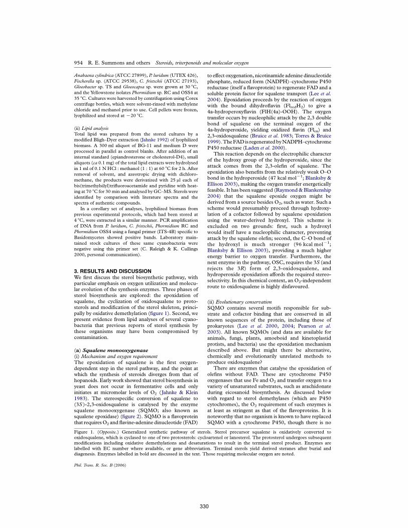
Anabaena cylindrica (ATCC 27899), P. luridum (UTEX 426),Fischerella sp. (ATCC 29538), C. fristschii (ATCC 27193),Gloeobacter sp. TS and Gloeocapsa sp. were grown at 30 8C,and the Yellowstone isolates Phormidium sp. RC and OSS4 at35 8C. Cultures were harvested by centrifugation using Corexcentrifuge bottles, which were solvent-rinsed with methylenechloride and methanol prior to use. Cell pellets were frozen,lyophilized and stored at K20 8C.
(ii) Lipid analysisTotal lipid was prepared from the stored cultures by amodified Bligh–Dyer extraction (Jahnke 1992) of lyophilizedbiomass. A 300 ml aliquot of BG-11 and medium D wereprocessed in parallel as control blanks. After addition of aninternal standard (epiandrosterone or cholesterol-D4), smallaliquots (ca 0.1 mg) of the total lipid extracts were hydrolysedin 1 ml of 0.1 N HCl : methanol (1 : 1) at 60 8C for 2 h. Afterremoval of solvent, and azeotropic drying with dichloro-methane, the products were derivatized with 25 ml each ofbis(trimethylsilyl)trifluoroacetamide and pyridine with heat-ing at 70 8C for 30 min and analysed by GC–MS. Sterols wereidentified by comparison with literature spectra and thespectra of authentic compounds.
In a corollary set of analyses, lyophilized biomass fromprevious experimental protocols, which had been stored at4 8C, were extracted in a similar manner. PCR amplificationof DNA from P. luridum, C. fristschii, Phormidium RC andPhormidium OSS4 using a fungal primer (ITS-4B) specific toBasidomycetes showed positive bands. Laboratory main-tained stock cultures of these same cyanobacteria werenegative using this primer set (C. Raleigh & K. Cullings2000, personal communication).
3. RESULTS AND DISCUSSIONWe first discuss the sterol biosynthetic pathway, withparticular emphasis on oxygen utilization and molecu-lar evolution of the synthesis enzymes. Three phases ofsterol biosynthesis are explored: the epoxidation ofsqualene, the cyclization of oxidosqualene to proto-sterols and modification of the sterol skeleton, princi-pally by oxidative demethylation (figure 1). Second, wepresent evidence from lipid analyses of several cyano-bacteria that previous reports of sterol synthesis bythese organisms may have been compromised bycontamination.
(a) Squalene monooxygenase(i) Mechanism and oxygen requirementThe epoxidation of squalene is the first oxygen-dependent step in the sterol pathway, and the point atwhich the synthesis of steroids diverges from that ofhopanoids. Early work showed that sterol biosynthesis inyeast does not occur in fermentative cells and onlyinitiates at micromolar levels of O2 (Jahnke & Klein1983). The stereospecific conversion of squalene to(3S )-2,3-oxidosqualene is catalysed by the enzymesqualene monooxygenase (SQMO; also known assqualene epoxidase) (figure 2). SQMO is a flavoproteinthat requiresO2 and flavine-adenine dinucleotide (FAD)
to effect oxygenation, nicotinamide adenine dinucleotidephosphate, reduced form (NADPH)–cytochrome P450reductase (itself a flavoprotein) to regenerate FAD and asoluble protein factor for squalene transport (Lee et al.2004). Epoxidation proceeds by the reaction of oxygenwith the bound dihydroflavin (FlredH2) to give a4a-hydroperoxyflavin (FlH(4a)-OOH). The oxygentransfer occurs by nucleophilic attack by the 2,3 doublebond of squalene on the terminal oxygen of the4a-hydroperoxide, yielding oxidized flavin (Flox) and2,3-oxidosqualene (Bruice et al. 1983; Torres & Bruice1999).TheFADis regeneratedbyNADPH–cytochromeP450 reductase (Laden et al. 2000).
This reaction depends on the electrophilic characterof the hydroxy group of the hydroperoxide, since theattack comes from the 2,3-olefin of squalene. Theepoxidation also benefits from the relatively weak O–Obond in the hydroperoxide (47 kcal molK1; Blanksby &Ellison 2003), making the oxygen transfer energeticallyfeasible. It has been suggested (Raymond&Blankenship2004) that the squalene epoxide oxygen might bederived from a source besides O2, such as water. Such ascheme would presumably proceed through hydroxy-lation of a cofactor followed by squalene epoxidationusing the water-derived hydroxyl. This scheme isexcluded on two grounds: first, such a hydroxylwould itself have a nucleophilic character, preventingattack by the squalene olefin; second, the C–O bond ofthe hydroxyl is much stronger (96 kcal molK1;Blanksby & Ellison 2003), providing a much higherenergy barrier to oxygen transfer. Furthermore, thenext enzyme in the pathway, OSC, requires the 3S (andrejects the 3R) form of 2,3-oxidosqualene, andhydroperoxide epoxidation affords the required stereo-selectivity. In this chemical context, an O2-independentroute to oxidosqualene is highly disfavoured.
(ii) Evolutionary conservationSQMO contains several motifs responsible for sub-strate and cofactor binding that are conserved in allknown sequences of the protein, including those ofprokaryotes (Lee et al. 2000, 2004; Pearson et al.2003). All known SQMOs (and data are available foranimals, fungi, plants, amoeboid and kinetoplastidprotists, and bacteria) use the epoxidation mechanismdescribed above. But might there be alternative,chemically and evolutionarily unrelated methods toproduce oxidosqualene?
There are enzymes that catalyse the epoxidation ofolefins without FAD. These are cytochrome P450oxygenases that use Fe and O2 and transfer oxygen to avariety of unsaturated substrates, such as arachidonateduring eicosanoid biosynthesis. As discussed belowwith regard to sterol demethylases (which are P450cytochromes), the O2 requirement of such enzymes isat least as stringent as that of the flavoproteins. It isnoteworthy that no organism is known to have replacedSQMO with a cytochrome P450, though there is no
Figure 1. (Opposite.) Generalized synthetic pathway of sterols. Sterol precursor squalene is oxidatively converted tooxidosqualene, which is cyclased to one of two protosterols: cycloartenol or lanosterol. The protosterol undergoes subsequentmodifications including oxidative demethylations and desaturations to result in the terminal sterol product. Enzymes arelabelled with EC number where available, or gene abbreviation. Terminal sterols yield derived steranes after burial anddiagenesis. Enzymes labelled in bold are discussed in the text. Those requiring molecular oxygen are noted.
954 R. E. Summons and others Steroids, triterpenoids and molecular oxygen
Phil. Trans. R. Soc. B (2006)
330
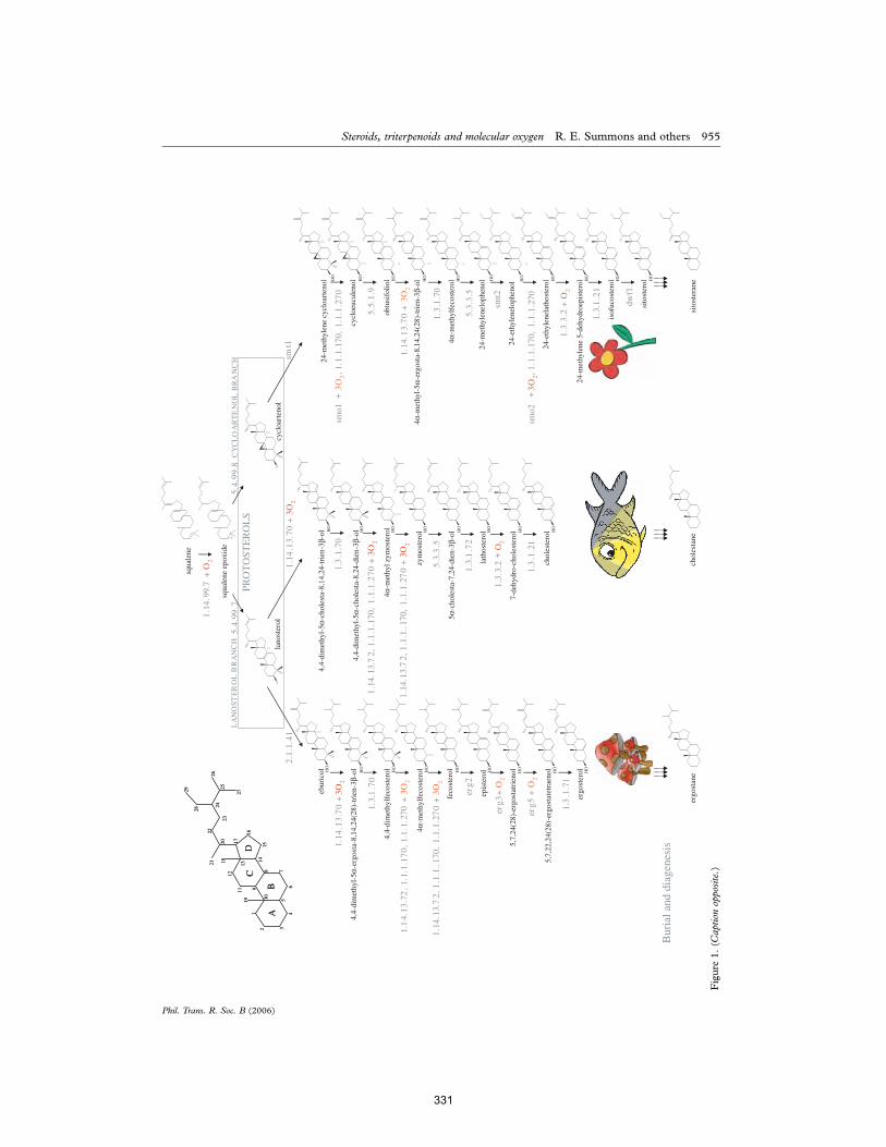
dwf1
HO
5.4.
99.7
O
squa
lene
epo
xide
1.14
.99.
7+
O2
smt1
HO
cycl
oart
enol
4!-m
ethy
l-5!
-erg
osta
-8,1
4,24
(28)
-tri
en-3
"-ol
HO
lano
ster
ol
1.14
.13.
72,
1.1
.1.1
70,
1.1.
1.27
0 +
3O2
1.14
.13.
72,
1.1
.1..
170,
1.1
.1.2
70
+ 3O
2
HO
5.5.
1.9
24-m
ethy
lene
cyc
loar
teno
l
cycl
oeuc
alen
ol
smo1
3 O
2,1
.1.1
.170
, 1.
1.1.
270
obtu
sifo
liol
1.3.
1.70
1.14
.13.
70+
3O2
4!-m
ethy
lfec
oste
rol
5.3.
3.5
24-m
ethy
lene
loph
enol
24-e
thyl
enel
ophe
nol
smt2
smo2
3 O
2, 1
.1.1
.170
, 1.
1.1.
270
1.3.
3.2
+ O
2
1.3.
1.2
1
24-e
thyl
enel
atho
ster
ol
24-m
ethy
lene
5-d
ehyd
roep
iste
rol
isof
ucos
tero
l
sito
ster
ol
CY
CL
OA
RT
EN
OL
BR
AN
CH
sito
ster
ane
chol
esta
ne
5.4.
99.8
2.1.
1.41
feco
ster
ol
erg2
epis
tero
l
erg3
+ O
2
5,7,
24(2
8)-e
rgos
tatr
ieno
l
erg5
+ O
2
1.3
.1.7
1
5,7,
22,2
4(28
)-er
gost
atet
raen
ol
ergo
ster
ol
ergo
stan
e
ebur
icol
5.3.
3.5
4,4-
dim
ethy
l-5!
-cho
lest
a-8,
14,2
4-tr
ien-
3"-o
l
1.3.
3.2
O2
1.3
.1.2
1
1.3
.1.7
0
1.14
.13.
70+
3O2
4,4-
dim
ethy
l-5!
-cho
lest
a-8,
24-d
ien-
3"-o
l
4!-m
ethy
l zym
oste
rol
zym
oste
rol
5!-c
hole
sta-
7,24
-die
n-3"
-ol
1.3.
1.7
2
lath
oste
rol
7-de
hydr
o-ch
oles
tero
l
chol
este
rol
AB
CD
1
2 3
45
6
78
9
10
11
12
13
1415
16
17
18
19
20
2122
2324
25
26
27
28
29
AB
CD
1
2 3
45
6
78
9
10
11
12
13
1415
16
17
18
19
20
2122
2324
25
26
27
28
29
1.14
.13.
70+
3O2
4,4-
dim
ethy
l-5!
-erg
osta
-8,1
4,24
(28)
-tri
en-3
"-ol
4!-m
ethy
lfec
oste
rol
1.3.
1.7
0
1.1
4.13
.72
, 1.1
.1.1
70, 1
.1.1
.270
+ 3
O2
1.14
.13.
72,
1.1
.1..
170,
1.1
.1.2
70
+ 3O
2
Bur
ial a
nd d
iage
nesi
s
PRO
TO
STE
RO
LS
squa
lene
LA
NO
STE
RO
L B
RA
NC
H
4,4-
dim
ethy
lfec
oste
rol
HO
HO
HO HO
HO
HO
HO
HO
HO
HO
HO
HO
HO
HO
HO
HO
HO
HO
HO
HO
HO
HO
HO
HO
HO
HO
+
+ +
Figure
1.(C
aptionopposite.)
Steroids, triterpenoids and molecular oxygen R. E. Summons and others 955
Phil. Trans. R. Soc. B (2006)
331
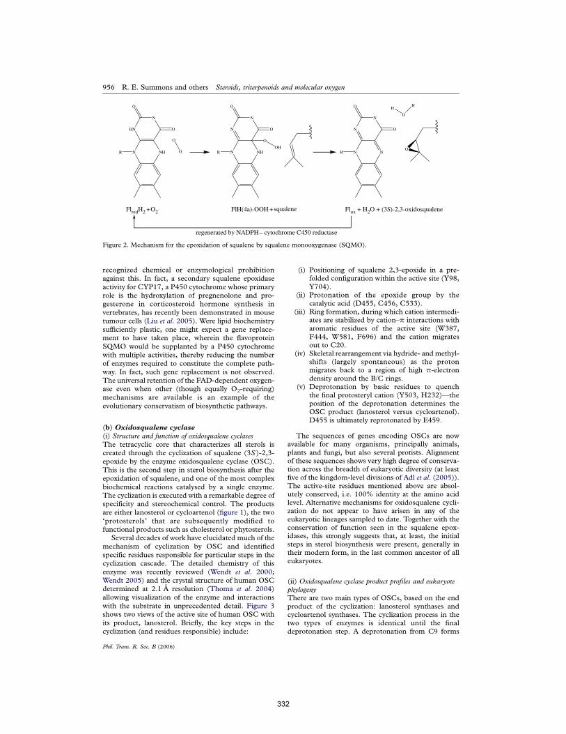
recognized chemical or enzymological prohibitionagainst this. In fact, a secondary squalene epoxidaseactivity for CYP17, a P450 cytochrome whose primaryrole is the hydroxylation of pregnenolone and pro-gesterone in corticosteroid hormone synthesis invertebrates, has recently been demonstrated in mousetumour cells (Liu et al. 2005). Were lipid biochemistrysufficiently plastic, one might expect a gene replace-ment to have taken place, wherein the flavoproteinSQMO would be supplanted by a P450 cytochromewith multiple activities, thereby reducing the numberof enzymes required to constitute the complete path-way. In fact, such gene replacement is not observed.The universal retention of the FAD-dependent oxygen-ase even when other (though equally O2-requiring)mechanisms are available is an example of theevolutionary conservatism of biosynthetic pathways.
(b) Oxidosqualene cyclase(i) Structure and function of oxidosqualene cyclasesThe tetracyclic core that characterizes all sterols iscreated through the cyclization of squalene (3S )-2,3-epoxide by the enzyme oxidosqualene cyclase (OSC).This is the second step in sterol biosynthesis after theepoxidation of squalene, and one of the most complexbiochemical reactions catalysed by a single enzyme.The cyclization is executed with a remarkable degree ofspecificity and stereochemical control. The productsare either lanosterol or cycloartenol (figure 1), the two‘protosterols’ that are subsequently modified tofunctional products such as cholesterol or phytosterols.
Several decades of work have elucidated much of themechanism of cyclization by OSC and identifiedspecific residues responsible for particular steps in thecyclization cascade. The detailed chemistry of thisenzyme was recently reviewed (Wendt et al. 2000;Wendt 2005) and the crystal structure of human OSCdetermined at 2.1 A resolution (Thoma et al. 2004)allowing visualization of the enzyme and interactionswith the substrate in unprecedented detail. Figure 3shows two views of the active site of human OSC withits product, lanosterol. Briefly, the key steps in thecyclization (and residues responsible) include:
(i) Positioning of squalene 2,3-epoxide in a pre-folded configuration within the active site (Y98,Y704).
(ii) Protonation of the epoxide group by thecatalytic acid (D455, C456, C533).
(iii) Ring formation, during which cation intermedi-ates are stabilized by cation–p interactions witharomatic residues of the active site (W387,F444, W581, F696) and the cation migratesout to C20.
(iv) Skeletal rearrangement via hydride- and methyl-shifts (largely spontaneous) as the protonmigrates back to a region of high p-electrondensity around the B/C rings.
(v) Deprotonation by basic residues to quenchthe final protosteryl cation (Y503, H232)—theposition of the deprotonation determines theOSC product (lanosterol versus cycloartenol).D455 is ultimately reprotonated by E459.
The sequences of genes encoding OSCs are nowavailable for many organisms, principally animals,plants and fungi, but also several protists. Alignmentof these sequences shows very high degree of conserva-tion across the breadth of eukaryotic diversity (at leastfive of the kingdom-level divisions of Adl et al. (2005)).The active-site residues mentioned above are absol-utely conserved, i.e. 100% identity at the amino acidlevel. Alternative mechanisms for oxidosqualene cycli-zation do not appear to have arisen in any of theeukaryotic lineages sampled to date. Together with theconservation of function seen in the squalene epox-idases, this strongly suggests that, at least, the initialsteps in sterol biosynthesis were present, generally intheir modern form, in the last common ancestor of alleukaryotes.
(ii) Oxidosqualene cyclase product profiles and eukaryotephylogenyThere are two main types of OSCs, based on the endproduct of the cyclization: lanosterol synthases andcycloartenol synthases. The cyclization process in thetwo types of enzymes is identical until the finaldeprotonation step. A deprotonation from C9 forms
NHN
N
HN
O
O
R NHN
N
N
O
O
R
O
OHNN
N
N
O
O
R
O
O O
H
O
H
FlredH2 O2 FlH(4a)-OOH +squalene Flox + H2O + (3S)-2,3-oxidosqualene
regenerated by NADPH– cytochrome C450 reductase
+
Figure 2. Mechanism for the epoxidation of squalene by squalene monooxygenase (SQMO).
956 R. E. Summons and others Steroids, triterpenoids and molecular oxygen
Phil. Trans. R. Soc. B (2006)
332
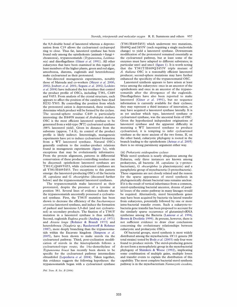
the 8,9-double bond of lanosterol whereas a deproto-nation from C19 allows the cycloartenol cyclopropylring to close. Thus far, lanosterol synthase has beenfound only among the opisthokonts (animalsCfungiCchoanozoa), trypanosomatids (Trypanosoma, Leishma-nia) and dinoflagellates (Giner et al. 1991). All othereukaryotes that have been examined in this regard (atleast members of the higher plants, green and red algae,amoebozoa, diatoms, euglenids and heterolobosea)make cycloartenol as their protosterol.
Site-directed mutagenesis experiments, notablythose of Matsuda and co-workers (Meyer et al. 2000,2002; Joubert et al. 2001; Segura et al. 2002; Lodeiroet al. 2004) have indicated the key residues that controlthe product profile of OSCs, including T381, C449and V453. From analysis of the crystal structure, eachappears to affect the position of the catalytic base dyadH232–Y503. By controlling the position from whichthe protosterol cation is deprotonated, these residuesdetermine which product will be formed by the cyclase.The second-sphere residue C449 is particularlyinteresting: the H449N mutant of Arabidopsis thalianaOSC is the most efficient lanosterol synthase to begenerated from a wild-type (WT) cycloartenol synthase(88% lanosterol yield). Given its distance from thesubstrate (approx. 7.4 A), its control of the productprofile is likely indirect. Interestingly, mutagenesisexperiments have yet to induce cycloartenol formationfrom a WT lanosterol synthase. Natural OSCsgenerally conform to the residue–product relationsfound in mutagenesis experiments (figure 3a), withexceptions that may be evolutionarily informative.From the protein alignment, patterns in differentialconservation of these product-controlling residues canbe discerned: opisthokont lanosterol synthases areT381/C,Q449/V453, while cycloartenol synthases areall Y381/H449/I453. Two exceptions to this patternemerge: the lanosterol-producing OSCs of the bacteriaM. capsulatus and G. obscuriglobus (discussed furtherbelow) and the trypanosomatid lanosterol synthases.
The trypanosomatids make lanosterol as theirprotosterol, despite the presence of a tyrosine atposition 381. Several lines of evidence indicate thatthe trypanosomatids ancestrally possessed a cycloarte-nol synthase. First, the T381Y mutation has beenshown to decrease the efficiency of the Saccharomycescerevisiae lanosterol synthase, and induce the formationof parkeol and lanostene-3,9-diol (and not cycloarte-nol) as secondary products. The fixation of a T381Ymutation in a lanosterol synthase is thus unlikely.Second, euglenids Euglena gracilis (Anding et al. 1971)and Astasia longa (Rohmer & Brandt 1973) andheterolobosea (Naegleria sp.; Raederstorff & Rohmer1987), more deeply branching than the trypanosoma-tids within the Excavate kingdom (Simpson et al.2005), have been shown to make sterols via thecycloartenol pathway. Third, post-cyclization modifi-cation of sterols in the kinetoplastids follows acycloartenol-type route; the 14a-demethylase ofTrypanosoma brucei has recently been shown to bespecific for the cycloartenol pathway intermediateobtusifoliol (Lepesheva et al. 2004). Taken together,this evidence suggests the following hypotheses: thetrypanosomatids began with a cycloartenol synthase
(Y381/H449/I453) which underwent two mutations,H449Q and I453V (each requiring a single nucleotidechange) to yield a lanosterol synthase. Downstreammodification of the protosterol remained essentially asthe cycloartenol pathway, but at least some of theenzymes must have adapted to different substrates; inparticular smt1 and smo1 (figure 1). It is worth notingthat the Y381T/H449Q/I453V triple mutant ofA. thaliana OSC is a reasonably efficient lanosterolproducer; second-sphere mutations may have furtherenhanced the specificity of the trypanosomatid OSC.
Lanosterol synthesis appears to have arisen at leasttwice among the eukaryotes: once in an ancestor of theopisthokonts and once in an ancestor of the trypano-somatids after the divergence of the euglenids.Dinoflagellates have also been reported to makelanosterol (Giner et al. 1991), but no sequenceinformation is currently available for their cyclases;they may represent a third instance of innovation, ormay have acquired a lanosterol synthase laterally. It isas yet unclear which type, lanosterol synthase orcycloartenol synthase, was the ancestral form of OSC.Given the hypothesized independent originations oflanosterol synthase and the apparent difficulty inmutating a WT lanosterol synthase to producecycloartenol, it is tempting to infer cycloartenolsynthase as the more ancient of the two forms. If, onthe other hand, eukaryotic phylogeny is rooted in thebranch leading to the opisthokonts (Arisue et al. 2005)there is no strong parsimony argument either way.
(iii) Prokaryotic oxidosqualene cyclasesWhile sterol synthesis is nearly ubiquitous among theEukarya, only three instances are known amongprokaryotes, all bacteria: M. capsulatus (a g-proteo-bacterium), G. obscuriglobus (a planctomycete) and aparaphyletic group of myxobacteria (d-proteobacteria).These organisms are not closely related and the reasonfor the sparse appearance of sterol synthesis inphylogenetically distant bacterial taxa remains unclear.If it is the result of vertical inheritance from a common,sterol-synthesizing bacterial ancestor, dozens of paral-lel losses of the entire pathway in many lineages wouldbe required. Alternatively, sterol biosynthesis genesmay have been acquired by bacteria via lateral transferfrom eukaryotes, potentially followed by one or moreintra-bacterial transfer events. Such a eukaryote-to-bacteria gene transfer has been proposed to account forthe similarly sparse occurrence of glutaminyl-tRNAsynthetase among the Bacteria (Lamour et al. 1994;Brown & Doolittle 1999). At present, however, there isnot sufficient evidence to draw clear conclusionsconcerning the evolutionary relationships betweeneukaryotic and prokaryotic OSCs.
Of bacterial groups, sterol synthesis is most widelydistributed among the myxobacteria. Of 11 genera (88total strains) tested by Bode et al. (2003) only four werefound to produce sterols. The sterol-producing generado not form a monophyletic group in the myxobacterialphylogeny of Shimkets & Woese (1992), implicatingsome combination of multiple gains, multiple lossesand transfer events to explain the distribution of thiscapability. The most complete bacterial sterol synthesispathway is in the myxobacterium Nannocystis excedens,
Steroids, triterpenoids and molecular oxygen R. E. Summons and others 957
Phil. Trans. R. Soc. B (2006)
333
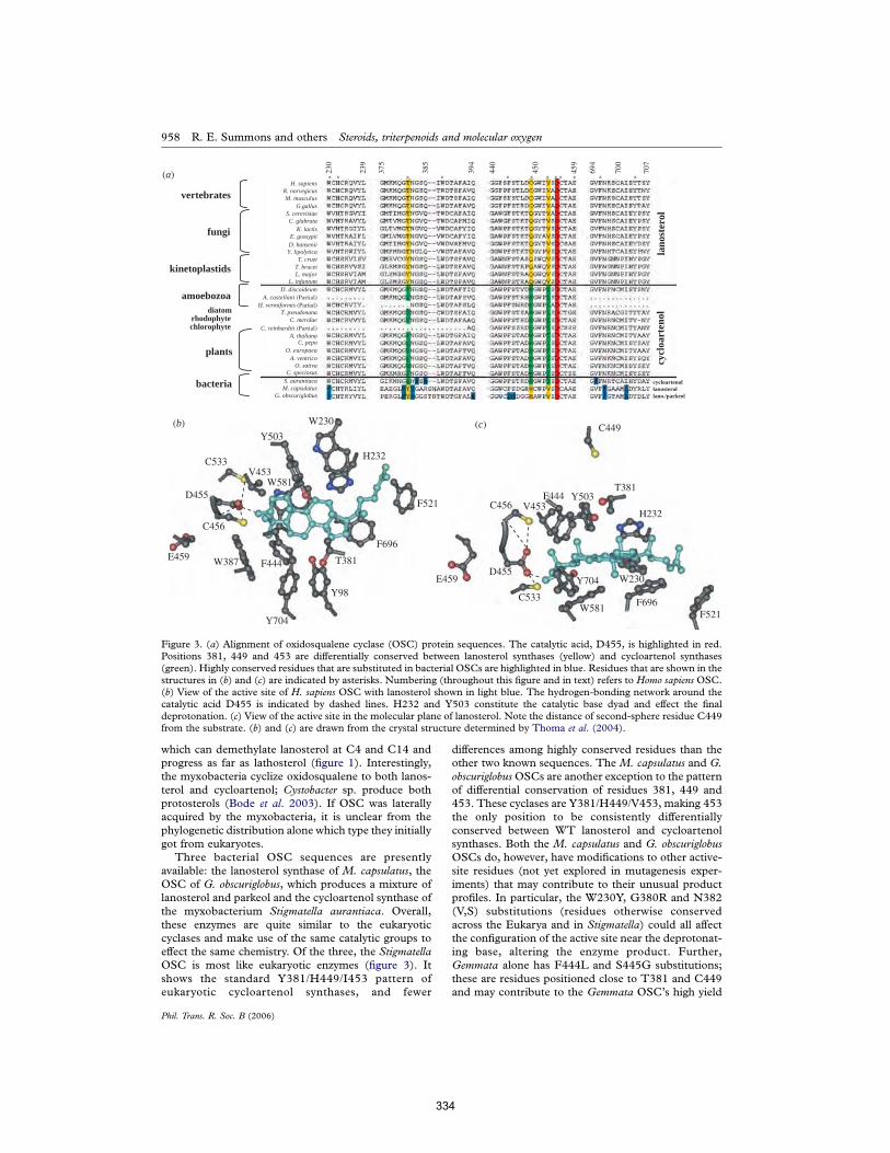
which can demethylate lanosterol at C4 and C14 andprogress as far as lathosterol (figure 1). Interestingly,the myxobacteria cyclize oxidosqualene to both lanos-terol and cycloartenol; Cystobacter sp. produce bothprotosterols (Bode et al. 2003). If OSC was laterallyacquired by the myxobacteria, it is unclear from thephylogenetic distribution alone which type they initiallygot from eukaryotes.
Three bacterial OSC sequences are presentlyavailable: the lanosterol synthase of M. capsulatus, theOSC of G. obscuriglobus, which produces a mixture oflanosterol and parkeol and the cycloartenol synthase ofthe myxobacterium Stigmatella aurantiaca. Overall,these enzymes are quite similar to the eukaryoticcyclases and make use of the same catalytic groups toeffect the same chemistry. Of the three, the StigmatellaOSC is most like eukaryotic enzymes (figure 3). Itshows the standard Y381/H449/I453 pattern ofeukaryotic cycloartenol synthases, and fewer
differences among highly conserved residues than theother two known sequences. The M. capsulatus and G.obscuriglobusOSCs are another exception to the patternof differential conservation of residues 381, 449 and453. These cyclases are Y381/H449/V453, making 453the only position to be consistently differentiallyconserved between WT lanosterol and cycloartenolsynthases. Both the M. capsulatus and G. obscuriglobusOSCs do, however, have modifications to other active-site residues (not yet explored in mutagenesis exper-iments) that may contribute to their unusual productprofiles. In particular, the W230Y, G380R and N382(V,S) substitutions (residues otherwise conservedacross the Eukarya and in Stigmatella) could all affectthe configuration of the active site near the deprotonat-ing base, altering the enzyme product. Further,Gemmata alone has F444L and S445G substitutions;these are residues positioned close to T381 and C449and may contribute to the Gemmata OSC’s high yield
H. sapiensR. norvegicusM. musculus
G.gallusS. cerevisiaeC. glabrata
K. lactisE. gossypiiD. hanseniiY. lipolytica
T. cruziT. bruceiL. major
L. infantumD. discoideum
A. castellani (Partial)H. vermiformis (Partial)
T. pseudonanaC. merolae
C. reinhardtii (Partial)A. thaliana
C. pepoO. europaea
A. ventricoO. sativa
C. speciosusS. aurantiacaM. capsulatus
G. obscuriglobus
vertebrates
fungi
kinetoplastids
amoebozoa
plants
bacteria
diatomrhodophytechlorophyte
lano
ster
olcy
cloa
rten
ol
cycloartenollanosterollano./parkeol
230
239
375
385
394
440
450
459
694
700
707
Y98
W230
H232
T381W387 F444
V453
D455
C456
E459
Y503
F521
C533
W581
F696
Y704
W230
H232
T381F444
C449
V453
D455
C456
E459
Y503
F521
C533W581 F696
Y704
* * * * * * * * * * * *(a)
(b) (c)
Figure 3. (a) Alignment of oxidosqualene cyclase (OSC) protein sequences. The catalytic acid, D455, is highlighted in red.Positions 381, 449 and 453 are differentially conserved between lanosterol synthases (yellow) and cycloartenol synthases(green). Highly conserved residues that are substituted in bacterial OSCs are highlighted in blue. Residues that are shown in thestructures in (b) and (c) are indicated by asterisks. Numbering (throughout this figure and in text) refers to Homo sapiens OSC.(b) View of the active site of H. sapiens OSC with lanosterol shown in light blue. The hydrogen-bonding network around thecatalytic acid D455 is indicated by dashed lines. H232 and Y503 constitute the catalytic base dyad and effect the finaldeprotonation. (c) View of the active site in the molecular plane of lanosterol. Note the distance of second-sphere residue C449from the substrate. (b) and (c) are drawn from the crystal structure determined by Thoma et al. (2004).
958 R. E. Summons and others Steroids, triterpenoids and molecular oxygen
Phil. Trans. R. Soc. B (2006)
334
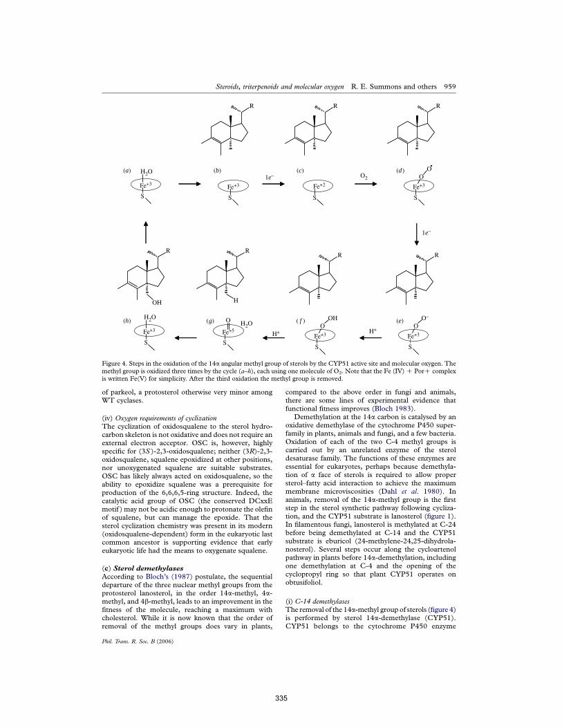
of parkeol, a protosterol otherwise very minor amongWT cyclases.
(iv) Oxygen requirements of cyclizationThe cyclization of oxidosqualene to the sterol hydro-carbon skeleton is not oxidative and does not require anexternal electron acceptor. OSC is, however, highlyspecific for (3S )-2,3-oxidosqualene; neither (3R)-2,3-oxidosqualene, squalene epoxidized at other positions,nor unoxygenated squalene are suitable substrates.OSC has likely always acted on oxidosqualene, so theability to epoxidize squalene was a prerequisite forproduction of the 6,6,6,5-ring structure. Indeed, thecatalytic acid group of OSC (the conserved DCxxEmotif ) may not be acidic enough to protonate the olefinof squalene, but can manage the epoxide. That thesterol cyclization chemistry was present in its modern(oxidosqualene-dependent) form in the eukaryotic lastcommon ancestor is supporting evidence that earlyeukaryotic life had the means to oxygenate squalene.
(c) Sterol demethylasesAccording to Bloch’s (1987) postulate, the sequentialdeparture of the three nuclear methyl groups from theprotosterol lanosterol, in the order 14a-methyl, 4a-methyl, and 4b-methyl, leads to an improvement in thefitness of the molecule, reaching a maximum withcholesterol. While it is now known that the order ofremoval of the methyl groups does vary in plants,
compared to the above order in fungi and animals,there are some lines of experimental evidence thatfunctional fitness improves (Bloch 1983).
Demethylation at the 14a carbon is catalysed by anoxidative demethylase of the cytochrome P450 super-family in plants, animals and fungi, and a few bacteria.Oxidation of each of the two C-4 methyl groups iscarried out by an unrelated enzyme of the steroldesaturase family. The functions of these enzymes areessential for eukaryotes, perhaps because demethyla-tion of a face of sterols is required to allow propersterol–fatty acid interaction to achieve the maximummembrane microviscosities (Dahl et al. 1980). Inanimals, removal of the 14a-methyl group is the firststep in the sterol synthetic pathway following cycliza-tion, and the CYP51 substrate is lanosterol (figure 1).In filamentous fungi, lanosterol is methylated at C-24before being demethylated at C-14 and the CYP51substrate is eburicol (24-methylene-24,25-dihydrola-nosterol). Several steps occur along the cycloartenolpathway in plants before 14a-demethylation, includingone demethylation at C-4 and the opening of thecyclopropyl ring so that plant CYP51 operates onobtusifoliol.
(i) C-14 demethylasesThe removal of the 14a-methyl group of sterols (figure 4)is performed by sterol 14a-demethylase (CYP51).CYP51 belongs to the cytochrome P450 enzyme
S
H2O
R
S
R
S
R
S
OO
R
S
OO–
R
S
OOH
R
S
O
H
R
S
OH
H2O
1e–
1e–
O2
H+H+
H2O
Fe+3 Fe+3 Fe+2 Fe+3
Fe+3Fe+3Fe+5Fe+3
(a)
(h) (g) ( f ) (e)
(b) (c) (d)
Figure 4. Steps in the oxidation of the 14a angular methyl group of sterols by the CYP51 active site and molecular oxygen. Themethyl group is oxidized three times by the cycle (a–h), each using one molecule of O2. Note that the Fe (IV)C PorC complexis written Fe(V) for simplicity. After the third oxidation the methyl group is removed.
Steroids, triterpenoids and molecular oxygen R. E. Summons and others 959
Phil. Trans. R. Soc. B (2006)
335
superfamily, which includesmore than 2000members inall three domains of life. All P450s are used in oxidativereactions on various molecules and all require molecularoxygen as a substrate. The active site of P450s contains aFe-protoporphyrin IX (haem). CYP51 is the onlycytochrome P450 that performs the same function indifferent biological domains. Some researchers havesuggested that CYP51 is the ancestral P450 (Nelson &Strobel 1989; Aoyama et al. 1994; Rezen et al. 2004).CYP51 operates on one of four substrates—lanosterol(in animals and fungi), dihydrolanosterol (animals),obtusifoliol (plants and kinetoplastids), or eburicol(fungi). These substrates differ only in the nature of theside chain and thepresence or absence of a secondmethylgroup at C-4.
The small differences between substrates probablyaccount for a general lack of substrate specificity amongthe demethylases. Most CYP51s can demethylate anyof the four substrates, although a few plant CYP51s areobtusifoliol-specific. In humans, a defect in CYP51causes Antley–Bixler syndrome. In yeast, 14a-demethylase inhibition is fatal, and this makes theenzyme an attractive target for fungicides. Fungicidesmay take advantage of the differences between fungaland animal CYP51 active sites to selectively inhibit thefungal enzyme.
Rezen et al. (2004) found that CYP51s separatephylogenetically into plant (obtusifoliol), animal(lanosterol) and fungal (eburicol) groups. BacterialCYP51s including those of M. capsulatus and Myco-bacterium tuberculosis both fall within the plant lineage.The purified M. tuberculosis protein will demethylatelanosterol in vitro although obtusifoliol is preferred.However, despite the phylogenetic placement of itsCYP51, M. capsulatus synthesizes lanosterol. It has yetto be demonstrated whether lanosterol is the substratefor M. capsulatus CYP51. Jackson et al. (2002) notethat theM. capsulatusCYP51 is novel in that it is linkedto a ferredoxin domain, but that the CYP51 inM. tuberculosis is part of an operon in which it isfollowed by ferredoxin. The M. capsulatus gene may bethe result of a lateral transfer event from M. tuberculosisfollowed by a mutation. Perhaps the best example ofthe broad substrate specificity of these enzymes isStreptomyces coelicolor, which contains a gene with low-level homology to bacterial CYP51s and that demethy-lates eburicol but not lanosterol (Lamb et al. 2003).However, this gene is not a CYP51, and the conservedsites differ significantly from CYP51. Streptomycescoelicolor does not contain sterols, and the in vivofunction of this protein is unknown.
The particulars of amino acid residue participationin substrate binding and catalysis of CYP51 areunknown. Podust and co-workers (Podust et al.2001b) noted that two channels with access to thehaem may serve to transport substrate and product toand from the active site. They (Podust et al. 2001a) alsoperformed modelling experiments based on the crystalstructure of M. tuberculosis CYP51 in the presence ofthe azole inhibitors fluconazole and 4-phenylimidazole.They found that the inhibitors coordinate themselveswith the haem iron in the large (2600 A3) cavityopposite the cysteine (C394) that binds the haem tothe protein. Amino acids surrounding this cavity were
considered likely to be involved in binding and/orcatalysis and showed a high degree of conservationacross CYP51s from many organisms. Only approxi-mately 10% (41 conserved residues) of CYP51s areabsolutely conserved across all domains of life (with theexception of five residues in the kinetoplastids) andmost of these are not at the active site. Half of thesesites have been examined by site-directed mutagenesisexperiments, which have shown that most of them areessential for CYP51 function. Naturally occurringazole-resistant strains of Candida albicans contain themutation Y132H, which does not directly interact withsubstrate and may reflect a more complicated inter-action between protein and substrate, and Bellamineet al. (2004) report from several site-directed mutagen-esis experiments that azole and substrate binding areuncoupled. Among the residues identified by Podustet al. (2001a,b) as participating in the active site, thereare several positions which differ between CYP51subfamilies operating on different substrates.
Other site-directed mutagenesis studies on 10residues that were believed to be strictly conservedamong CYP51s (Lepesheva & Waterman 2004) foundthat most mutants lost all demethylase activity,although one (A197G) showed enhanced demethylaseactivity. Based on a combination of mutagenesisexperiments and the crystal structure of CYP51 theypostulated potential substrate binding sites: D90 as abinding site for the sterol 3b-OH, L172 and R194associating with the side chain, and F82 binding thesterol A or B ring. Kinetoplastid genomes revealeddifferences from the ‘strictly conserved’ at five of theCYP51 residues in which mutations produced total ornear total loss of function in M. tuberculosis (D90A,L127M, G175S/C, R194C, D195H/R). Lepeshevaet al. (2004) showed that the kinetoplastid CYP51swere obtusifoliol-specific and that mutation of thesefive residues back to the conserved state did notimprove the ability of the kinetoplastid enzyme tometabolize lanosterol. A clearer understanding of thechemical role of these conserved residues will benecessary to discern the evolutionary implications ofthese changes.
The general mechanism of substrate oxidation byP450 enzymes is known from several decades of workon the camphor-oxidizing P450 of Pseudomonas putida.It consists of eight steps (Groves & Han 1995; Meunieret al. 2004):
(i) substrate binding and subsequent displace-ment of the haem Fe(III);
(ii) electron transfer to Fe(III) from a reductasecofactor to yield Fe(II) and a haem with anegative charge;
(iii) binding of molecular oxygen to the ferrous ironyielding a Fe(III)–dioxygen bond;
(iv) transfer of a second electron to the haem toyield a negatively charged Fe(III)–peroxocomplex which is a very strong nucleophile;
(v) protonation of the Fe(III)–peroxo complexyielding a P450–Fe(III)–OOH which alsobehaves as a nucleophile. This protonationlikely involves the action of an acidic residue(D251 in P450cam) near the active site;
960 R. E. Summons and others Steroids, triterpenoids and molecular oxygen
Phil. Trans. R. Soc. B (2006)
336
(vi) a second protonation of the distal oxygen atomand cleavage of the O–O bond, yielding amolecule of water and the formation of thereactive electrophilic iron–oxo species Fe(IV);
(vii) transfer of the oxygen atom from the iron–oxocomplex to the substrate;
(viii) dissociation of the product.
In CYP51, this process operates three times on the14a-methyl group of the sterol which successivelyconverts the 14a-methyl group to 14a-hydroxymethyl,14a-carboaldehyde and 14a-formyl intermediates,subsequently eliminating formic acid and leaving aD14,15 double bond in the sterol. It is significant thatthe initial hydroxylation of the methyl, which requiresthe abstraction of H%, is achieved with the high redoxpotential associated with the Fe(IV) complex, which isachieved only through the action of molecular oxygen.This complex has an effective oxidation state of Fe(V)due to the additional charge on the porphyrin. SeeMeunier et al. (2004) for a detalied review.
(ii) C-4 demethylasesDemethylation of a C-4 methyl group requires theaction of a suite of three enzymes working sequentially(Gachotte et al. 1998, 1999; Benveniste 2004):
(i) C-4a-methyl oxidase (ERG25 in yeast andsmo1/smo2 in plants), which operates on the4a-methyl carbon three times with molecularoxygen to produce a 4a-carboxylic acid (Darnet& Rahier 2003, 2004);
(ii) 4a-carboxysterol-C-4-dehydrogenase/C-4-dec-arboxylase (4a-CD or ERG26 in yeast) whichdecarboxylates the 4a-acid and produces a3-oxosteroid (Gachotte et al. 1998; Rondetet al. 1999);
(iii) NADPH-dependent sterone reductase(ERG27) which stereospecifically reduces the3-oxosteroid to a 3b-OH.
These enzymes always act on the 4a-methyl group.In the first demethylation, the 4a-methyl is removed,and the 4b-methyl group rearranges to the 4a position.In both animals and fungi, the two methyl groups aresequentially removed following 14a-demethylation.The C-4 demethylase enzymatic suite converts 4,4-dimethyl-5a-cholesta-8,14,24-3b-ol to 4a-methylzymosterol, which is subsequently converted by thesame suite of enzymes to zymosterol (Benveniste2004). In plants, the first methyl group is removed atthe level of 24-methylene cycloartenol, which isconverted to cycloeucalenol. This pathway goesthrough several subsequent steps, including theremoval of the 14a-methyl group before beingdemethylated at C-4 a second time at the level of 24-ethylenelophenol, which is converted to 24-ethylene-lathosterol. Plant genomes show the presence of twodistinct sterol methyl oxidases (smo1 and smo2)(Darnet & Rahier 2004), and gene silencing exper-iments in A. thaliana have demonstrated that each ofthese operate with high substrate specificity—smo1 on24-methylene cycloartenol and smo2 on 24-ethylene-lophenol (Benveniste 2004).
Other taxa which synthesize C-4 desmethyl sterolsinclude the bacteria M. capsulatus and N. excedens, andthe kinetoplastids. Genome sequences of M. capsulatusand three kinetoplastid species are available inGenBank and a comparison of the sequenced genometo known sequences for erg25, smo1 and smo2 revealedno significant homologues to any of these genes amongthese organisms. It is possible that these organisms areusing an alternative enzyme for C-4 steroldemethylation.
(iii) Energetic constraints and oxygen usageThe mechanism of sterol demethylation functionalizesa methyl group attached to a quaternary carbon byattaching an oxygen atom. CYP51 achieves this bythe homolytic cleavage of a C–H bond to create amethyl radical, which subsequently reacts with theoxygen distally attached to the haem of the P450(Meunier et al. 2004). This is an energetically expensiveprocess which is overcome in part by using the mostpowerful oxidizing agent available: molecular O2.
The C–H bond dissociation energy (D) of a methylgroup attached to a quaternary carbon is 401 kJ molK1
(March 1992). However, bond energies of the tran-sition state in the demethylase enzymes are unknownand so this does not indicate actual activation energy ofthe methyl group, but gives an indication of the stabilityof the radical. This dissociation energy is higher(indicating a less stable radical) than that of secondary(401 kJ molK1) and tertiary (401 kJ molK1) carbons,but not as high as that of the C–H bond in primary(419 kJ molK1) carbons, methane (438 kJ molK1) orbenzene (464 kJ molK1).
Microbial degradation of both benzene andmethanetakes place readily in the presence of oxygen, but is alsopossible under many conditions as mildly exergonicprocesses with sulphate as a terminal electron acceptor.This indicates that abstraction of C–H bonds strongerthan those in sterol methyl groups is possible withoutmolecular oxygen. Although thermodynamically feas-ible, an enzyme that demethylated sterols anaerobicallywould be energetically much more expensive.
Sterol demethylases have evolved at least twice, andin each case require three molecules of molecularoxygen to catalyse the reaction. Constructed phyloge-netic trees of CYP51 cluster those demethylases intogroups that parallel the families of sterol cyclases,suggesting that oxidative sterol demethylation is anancient and conserved pathway that has existed at leastsince the time of the split between plants, kinetoplastidsand opisthokonts (Rezen et al. 2004). Nature maycontain at least one undescribed sterol demethylase(the C-4 demethylase in M. capsulatus and kinetoplas-tids). As this undescribed enzyme occurs in obligateaerobes, it is likely to require molecular oxygen.
On strict chemical grounds it may be possible todevise biosynthetic routes to sterols that proceedanaerobically as has been recently proposed (Raymond& Blankenship 2004). However, any postulatedanaerobic pathway for sterol synthesis must replacefive enzymes which use a combined 11 or 12 moleculesof O2 with anaerobic enzymes capable of performingthe equivalent process, and further postulate that all ofthese enzymes have been lost or are unknown. Any
Steroids, triterpenoids and molecular oxygen R. E. Summons and others 961
Phil. Trans. R. Soc. B (2006)
337
hypothesis that proposes enzymes existed in the past,and for which all evidence has been lost, is not testable.
(d) On the occurrence of sterols in cyanobacteriaIn connection with earlier studies of 2-methylhopa-noids and other biomarkers in strains of culturedcyanobacteria (Summons et al. 1999; Jahnke et al.2004), we checked for the presence of sterols in thetotal lipid extracts of some of the genera previouslyreported to contain them. Samples were hydrolysedwith acid in order to render conjugated sterols in thefree form and then converted to trimethylsilyl deriva-tives for GC–MS. As figure 5 shows, our culturedsamples contained an abundance of sterols. Moreover,the distributions were similar in all samples with manyof the same compounds reported by previous workers
including a strong predominance of C29D5, C29D5,22and C29 D5,24(28) (figure 5).
These results prompted us to examine other options,one of which was to re-culture the organisms in mediawith defined sterol contents and in the presence ofcycloheximide, a compound known to inhibit thegrowth of eukaryotes by blocking protein synthesis.After several sub-cultures in the presence of cyclohex-imide we could only identify traces of a C27 and a C28
sterol that were subsequently found to be componentsof the BG-11 medium (figure 6). After re-culturing ofthese cyanobacteria in the original media, and in theabsence of cycloheximide, they continued to be free ofdetectable sterols.
The results of these experiments indicated that ouroriginal cultures were contaminated by an organismthat produced C29 sterols in abundance. The sourceof contamination was investigated using, firstly,
Phormidium sp. RCO4
Phormidium sp. OSS4
Chlorogloeopsis fritschii
Phormidium luridum
time--> 62 64 66 68 70
C27:0
C28:1#5
C29#5
C29#5,22
C29#5,24(28)
I.S.RI
RI
RI
RI
(a)
(b)
(c)
(d)
Figure 5. Total ion chromatograms for showing sterols in thetotal lipid extracts of four of the investigated cyanobacterialcultures (a–d ). Phormidium sp. RCO4 and OSS4 are isolatesfrom Yellowstone National Park. All organisms were grownfor a biomarker and isotopic investigation of mat-formingcommunities (Jahnke et al. 2004). RI, relative intensity; I.S.,internal standard.
Phormidium luridum
I.S. cholesterol D4
42 46 50 54 58time -->
Gloeobacter sp. TS
C28:1
Chlorogloeopsis fritschii
C28:1
RI
RI
Anabaena cylindrica
C28:1
RI
(a)
(b)
(c)
(d)
RI
Figure 6. Gas chromatography–mass spectrometry data,depicted as the m/z 129 ion which is diagnostic fortrimethylsilyl (TMS) sterols, for some cyanobacteria culturedin the presence of cycloheximide (a–d ). The only detectablesterol is ergosterol which was also present in blank analyses ofthe BG-11 culture medium and attributable to that source.
962 R. E. Summons and others Steroids, triterpenoids and molecular oxygen
Phil. Trans. R. Soc. B (2006)
338
a universal gene probe for eukaryotes which waspositive and, secondly, a probe specific for Basidomy-cetes (rust fungi) which was also positive. Unlike otherfungi which produce ergosterol (C28D5) or cholesterol(C27D5) as their major sterols, Uredospores such asUromyces phaseoli (bean rust), flax rust and Cronartiumfusiforme (fusiform rust) all produce C29 sterols liketheir host plants. In these organisms, the principalsterols are C29D7 and C29D7,24(28) (Jackson & Frear1968; Lin et al. 1972; Carmack et al. 1976).
Lack of sterols in cyanobacteria is further evidencedby their genome sequences, which reveal that the onlygenes significantly homologous to sterol synthases aresqualene–hopene synthases. As microbial genomesequencing progresses, diverse new sterol producersmay be discovered on the basis of gene content; theutility of this approach has already been demonstrated(Pearson et al. 2003). Such searches will be aided by thehigh degree of conservation among sterol synthesisgenes, which makes them readily recognizable on thebasis of sequence similarity. It is worth noting that,among the 258 prokaryotic genomes sequenced andavailable as of this writing, only one previouslyunknown sterol producer, G. obscuriglobus (Pearsonet al. 2003), has been discovered.
4. RELATING BIOMARKERS TO BIOLOGICALAND GEOCHEMICAL EVOLUTION(a) Membrane function of sterols andevolutionary and ecological adaptationThe function of sterols in cellular membranes has beena topic of long-standing interest among biochemistsand cell biologists. Fifty years after the central steps inthe sterol synthesis pathway were elucidated by Blochand co-workers, understanding of the structural andfunctional roles of these cardinal eukaryotic lipidsremains incomplete and an active area of research. Itwas recognized early on that sterols modulate themicro-scale fluidic properties of the membrane—itsdensity, viscosity, and so on—and that sterols that differby only the addition of a methyl group or a double bondcan produce measurably different effects. The principalmechanism for this structural effect of sterols is theirinduction of a liquid-ordered phase in membranes, astate intermediate between high-temperature liquid-disordered and low temperature solid-ordered (gel)phases. Further, the liquid-ordered and liquid-dis-ordered phases can coexist in the same membrane,allowing for spatial heterogeneity and the notion of themembrane as a ‘fluid mosaic’ with discrete domains(lipid rafts) (Simons & Vaz 2004). A functional role forsterols has been suggested in the reduction ofpermeability of membranes to cations, particularlyprotons and sodium, hence assisting in energy con-servation (Haines 2001). This is likely due to enhancedexclusion of water clusters or chains from themembrane, though the precise mechanism remainsunder investigation (Tepper & Voth 2005).
The foregoing discussion of the structural andfunctional characteristics of steroids could applyessentially equally well to hopanoids, which aremembrane constituents of many bacteria. The twoclasses of lipids share the basic polycyclic skeleton side
chain structure and are of nearly identical moleculardimensions (approx. 8 A by 19 A). Hopanoids havebeen demonstrated to influence membrane orderingand fluid properties similarly to steroids (Kannenberget al. 1983). On the basis of such comparisons,hopanoids have been termed ‘sterol surrogates’ and‘functionally equivalent’ in membranes (Ourisson et al.1987). This begs the question: why should functionallyequivalent molecules be so strongly differentiallyconserved across the breadth of the diversity of cellularlife?
While steroids and hopanoids are structurallysimilar, they differ in a key respect: steroids have theirpolar group attached directly to the ring structure atC3, while the polar functions in hopanoids are attachedto the side chain. As a result, the ring structure ofsteroids sits near the edge of the lipid bilayer, but that ofhopanoids is nearer the centre. This suggests that thetwo types of terpenoid may move quite differently inmembranes, particularly with regard to their ability totranslocate from one leaflet of the bilayer to the other, aphenomenon known as ‘lipid flip-flop’.
Flip-flop is an important property of membranelipids because in order for a membrane to deform—i.e.to curve inward or outward—one leaflet of the bilayermust become longer while the other becomes shorter.This curvature is effected by flipping lipid moleculesfrom one leaflet to the other. Sterols have among theshortest t1/2 values for transbilayer flip-flop of anymembrane lipid (Holthuis & Levine 2005), meaningthat steroid-containing membranes are readilydeformed. This was elegantly demonstrated (Baciaet al. 2005) in a cell-free system of giant unilamellarvesicles, where it was found that not only does theaddition of sterols to lipid vesicles induce domainformation and budding, but the type of sterol controlsthe direction of curvature. Cholesterol and lophenolinduce positive (outward) curvature, while lanosteroland cholesteryl sulphonate cause inward (negative)budding. Varying the proportions of a mixture ofcholesterol and cholesteryl sulphonate controlled bothdomain size and budding behaviour. Eukaryotic cellshave highly specific structural requirements for theirmembrane sterols: changing even the position ofunsaturation in the ring system or the stereochemistryof the hydroxyl group attachment can result in anincompetent cell envelope (Xu et al. 2005). Takentogether, this evidence suggests that a membrane with awell-regulated sterol composition is a powerful tool forexport and import across the cell membrane.
Eukaryotes, both unicellular and multicellular,make extensive use of endo- and exocytosis. Theinnovation of sterol biosynthesis, in allowing rapidmembrane deformation, may have been a key step inthe evolution of these processes. In eukaryotes,phagocytosis and membrane biogenesis are closelycoupled. When part of a membrane is drawn in toengulf a particle, lipid synthesis is stimulated (throughthe sterol regulatory element binding protein transcrip-tional regulators) to just the degree to replace theconsumed membrane segment (Castoreno et al. 2005).With a flexible, deformable membrane, many mech-anisms to generate curvature are possible, includingprotein scaffolding, helix insertion and active
Steroids, triterpenoids and molecular oxygen R. E. Summons and others 963
Phil. Trans. R. Soc. B (2006)
339
cytoskeletal remodelling (McMahon & Gallop 2005).Much of the dynamic character of the eukaryoticmembrane system can be attributed to these curvaturemechanisms. Though experimental quantification ofthe transbilayer movement of hopanoids (particularlytheir flip-flop half-time) is lacking, the absence of endo-and exocytosis among the bacteria may indicate thathopanoids are not functionally equivalent to sterols inthis regard.
The ability to perform this type of transmembranetransport had profound evolutionary and ecologicalconsequences. In essence, the invention of endocytosisis the dawn of predation. Prior to endocytosis,heterotrophy proceeded largely through the dissolvedphase, and no stratified trophic relationships existed.Once large particles (including other cells) could beimported and enzymatically degraded intracellularly,the predator–prey dynamic, that shaped much ofevolutionary history, was established.
(i) Possible role of O2 in the biosynthesisof 2-methylbacteriohopanepolyolsPrecise details of the biosynthetic pathway leading to2-methylbacteriohopanepolyols (2Me-BHP) are notknown although the methyl group is known to betransferred intact from L-methionine (Zundel &Rohmer 1985). Genomes of sequenced cyanobacteriaand M. capsulatus (which produces 3Me-BHP) revealthat they contain homologues of sterol-methyltransfer-ases found in plants. The transfer of a methyl group tothe hopanoid ring structure is presumably preceded bydesaturation at the 2–3 position. Aerobic steroldesaturases are present in the genomes of severalcyanobacteria, with unknown function. It has yet to bedemonstrated that either sterol-methyltransferases orsterol desaturases are involved in the methylation of thehopanoid A-ring, but their potential should beinvestigated.
(ii) Alternative oxidants on the early EarthOxidizing power may have been scarce on the Earth’ssurface before the oxygenation of the atmosphere.Under such conditions, it is possible that cellular lifemade use of oxidants that have since been supplantedby nearly ubiquitous O2. Postulated scenarios for theuse of such alternative oxidants should uphold criteriaof geochemical and biochemical viability; nitrogenoxides fail the first test, while water, as discussedabove for SQMO, generally fails the second. Onefeasible alternative is hydrogen peroxide. SignificantH2O2 is generated by the reaction of water withpyrite under anaerobic, UV-illuminated conditions(Blankenship & Hartman 1998; Borda et al. 2003), aplausible scenario on the early Earth. The use ofperoxide as a ‘transitional’ redox partner (both as anoxidant and as a reductant) in biogeochemicalevolution has been discussed previously (Kasting et al.1985; Blankenship & Hartman 1998; Borda et al.2003). Hydrogen peroxide may have been a suitableoxidant for biosynthetic oxygenation reactions, such asthose described above in sterol synthesis. Such ascenario has, at minimum, three prerequisites to befulfilled: (i) H2O2 must have been produced ingeochemically significant quantities and have been
available to micro-organisms in a variety of habitats.(ii) The enzymes of the pathway of interest must beable to use H2O2 as an oxidant, and themselves bestable in concentrations of peroxide thought likely toarise. (iii) Cells must be able to use exogenous peroxideanabolically to produce the biochemicals at question.Even if only the first condition can be demonstrated,further chemistry (such as the iron-catalysed Haber–Weiss reaction) should be considered as sources forredox partners for metabolism. Exploration of thesepossibilities will likely lead to new insights into thecoevolution of the redox chemistry of the geosphereand biosphere, and highlight the importance of under-standing the evolutionary biochemistry of reactiveoxygen species.
5. SUMMARY AND FUTURE DIRECTIONSThe sequences of key enzymes in steroid biosynthesisare very highly conserved within the eukaryotic domainand it appears likely that the initial steps of the pathwaywere present in their modern form in the last commonancestor of eukaryotes.
Steroid biosynthesis is an oxygen intensive processwith, for example, 11 molecules of O2 being requiredfor the synthesis of one molecule of cholesterol. It isalso energetically expensive. While one can postulateanaerobic alternatives to some steps in the pathway,these would be even more energy intensive. Anypostulate for an ancestral anaerobic pathway to sterolsmust explain the replacement of five enzymes withanaerobic equivalents and, further, that all of thesehave been lost or are unknown.
Previous reports of sterol biosynthesis in cyanobac-teria appear to be erroneous. It seems that cyanobac-terial cultures are easily contaminated by fungi relatedto rusts. The sterol biosynthetic capability of otherBacteria is patchily distributed, characterized by path-ways that are either anomalous or incomplete, andlikely gained from Eukarya by lateral gene transfer.
The generally accepted hypothesis that hopanoidsare sterol surrogates in bacteria deserves re-visitingwith investigations of the localization and functionalroles of BHP. In particular, studies of the phylogeneticdistribution, biosynthesis and functional role of 2Me-BHP in cyanobacteria would be particularly valuable.As a starting point, one could hypothesize that thebiosynthesis of 2Me-BHP in cyanobacteria involves anoxygen-dependent desaturase and a methyltransferaseanalogous to those employed in sterol biosynthesis.
Understanding early steps in cellular evolution willbe aided by more detailed studies of hydrocarbons inArchaean and Proterozoic rocks. Further studies of themembrane function of sterols and their role inevolutionary and ecological adaptation will also bevaluable.
We thank Tsegereda Embaye (NASA) and Janet Hope(Geoscience Australia) for technical assistance in the analysisof cyanobacterial lipids.We also thank Yanek Hebting (MIT),Ken Cullings and Chris Raleigh (NASA Ames) for helpfuldiscussion. Lee Kump, Katja Meyer, Ann Pearson and JohnVolkman provided insightful and constructive reviews thatimproved the manuscript. This work was supported by theNASA Exobiology Program (Award NNG05GN62G) andNSF (Award EAR 0418619).
964 R. E. Summons and others Steroids, triterpenoids and molecular oxygen
Phil. Trans. R. Soc. B (2006)
340
REFERENCESAbe, I., Rohmer, M. & Prestwich, G. D. 1993 Enzymatic
cyclization of squalene and oxidosqualene to sterols andtriterpenes. Chem. Rev. 93, 2189–2206. (doi:10.1021/cr00022a009)
Adl, S. M. et al. 2005 The new higher level classification ofeukaryotes with emphasis on the taxonomy of protists.J. Eukaryot. Microbiol. 52, 399–451. (doi:10.1111/j.1550-7408.2005.00053.x)
Altschul, S. F., Madden, T. L., Schaffer, A. A., Zhang, J.,Zhang, Z.,Miller,W.&Lipman,D. J. 1997GappedBLASTand PSI-BLAST: a new generation of protein databasesearch programs.Nucl. Acids Res. 25, 3389–3402.
Anding, C., Brandt, R. D. & Ourisson, G. 1971 Sterolbiosynthesis in Euglena gracilis Z. Sterol precursors inlight-grown and dark-grown Euglena gracilis Z. Eur.J. Biochem. 24, 259–263. (doi:10.1111/j.1432-1033.1971.tb19679.x)
Aoyama, Y., Funae, Y., Noshiro, M., Horiuchi, T. & Yoshida,Y. 1994 Occurrence of a P450 showing high homology toyeast lanosterol 14-demethylase (P450(14DM)) in the ratliver. Biochem. Biophys. Res. Commun. 201, 1320–1326.(doi:10.1006/bbrc.1994.1848)
Arisue, N., Hasegawa, M. & Hashimoto, T. 2005 Root of theEukaryota tree as inferred from combined maximumlikelihood analyses of multiple molecular sequence data.Mol. Biol. Evol. 22, 409–420. (doi:10.1093/molbev/msi023)
Bacia, K., Schwille, P. & Kurzchalia, T. 2005 Sterol structuredetermines the separation of phases and the curvature ofthe liquid-ordered phase in model membranes. Proc. NatlAcad. Sci. USA 102, 3272–3277. (doi:10.1073/pnas.0408215102)
Bekker, A., Holland, H. D., Wang, P. L., Rumble, D., Stein,H. J., Hannah, J. L., Coetzee, L. L. & Beukes, N. J. 2004Dating the rise of atmospheric oxygen. Nature 427,117–120. (doi:10.1038/nature02260)
Bellamine, A., Lepesheva, G. & Waterman, M. 2004Fluconazole binding and sterol demethylation in threeCYP51 isoforms indicate differences in active sitetopology. J. Lipid Res. 45, 2000–2007. (doi:10.1194/jlr.M400239-JLR200)
Benveniste, P. 2004 Biosynthesis and accumulation of sterols.Ann. Rev. Plant Biol. 55, 429–457.
Bird, C. W., Lynch, J. M., Pirt, F. J. & Reid, W. W. 1971Steroids and squalene in Methylococcus capsulatus grownon methane. Nature 230, 473. (doi:10.1038/230473a0)
Blankenship, R. E. & Hartman, H. 1998 The origin andevolution of oxygenic photosynthesis. Trends Biochem. Sci.23, 94. (doi:10.1016/S0968-0004(98)01186-4)
Blanksby, S. J. & Ellison, G. B. 2003 Bond dissociationenergies of organic molecules. Accounts Chem. Res. 36,255–263. (doi:10.1021/ar020230d)
Bloch, K. 1983 Sterol structure and membrane function.CRC Crit. Rev. Biochem. 14, 47–92.
Bloch, K. 1987 Summing up. Annu. Rev. Biochem. 56, 1–18.(doi:10.1146/annurev.bi.56.070187.000245)
Bode, H. B., Zeggel, B., Silakowski, B., Wenzel, S. C.,Reichenbach, H. & Muller, R. 2003 Steroid biosynthesisin prokaryotes: identification of myxobacterial steroidsand cloning of the first bacterial 2,3(S)-oxidosqualenecyclase from the myxobacterium Stigmatella aurantiaca.Mol. Microbiol. 47, 471–481. (doi:10.1046/j.1365-2958.2003.03309.x)
Borda, M. J., Elsetinow, A. R., Strongin, D. R. & Schoonen,M. A. 2003 A mechanism for the production of hydroxylradical at surface defect sites on pyrite. Geochim.Cosmochim. Acta 67, 935–939. (doi:10.1016/S0016-7037(02)01222-X)
Brocks, J. J., Logan, G. A., Buick, R. & Summons, R. E. 1999Archean molecular fossils and the early rise of eukaryotes.Science (Washington, DC) 285, 1033–1036. (doi:10.1126/science.285.5430.1033)
Brocks, J. J., Buick, R., Logan, G. A. & Summons, R. E. 2003Composition and syngeneity of molecular fossils from the2.78 to 2.45 billion-year-old Mount Bruce Supergroup,Pilbara Craton, Western Australia. Geochim. Cosmochim.Acta 67, 4289–4319. (doi:10.1016/S0016-7037(03)00208-4)
Brown, J. R. & Doolittle, W. F. 1999 Gene descent,duplication, and horizontal transfer in the evolution ofglutamyl- and glutaminyl-tRNA synthetases. J. Mol. Evol.49, 485. (doi:10.1007/PL00006571)
Bruice, T. C., Noar, J. B., Ball, S. S. & Venkataram, U. V.1983 Monooxygen donation potential of 4a-hydroperoxy-flavins as compared with those of a percarboxylic acid andother hydroperoxides. Monooxygen donation to olefin,tertiary amine, alkyl sulfide, and iodide ion. J. Am. Chem.Soc. 105, 2452–2463. (doi:10.1021/ja00346a057)
Buick, R., Anbar, A. D., Mojzsis, S. J., Kaufman, A. J., Kieft,T. L., Lyons, T. W. & Humayun, M. 2004 The case forscientific drilling of Precambrian sedimentary sequences:a mission to early Earth. American Geophysical Union, FallMeeting 2001, abstract #P22B-0544.
Carmack, C. L., Weete, J. D. & Kelly, W. D. 1976Hydrocarbons, fatty acids and sterols of Cronartiumfusiforme. Physiol. Plant Pathol. 8, 43–49.
Castoreno, A. B., Wang, Y., Stockinger, W., Jarzylo, L. A.,Du, H., Pagnon, J. C., Shieh, E. C. & Nohturfft, A. 2005Transcriptional regulation of phagocytosis-induced mem-brane biogenesis by sterol regulatory element bindingproteins. Proc. Natl Acad. Sci. USA 102, 13 129–13 134.(doi:10.1073/pnas.0506716102)
Cloud, P. E. 1972 A working model of the primitive Earth.Am. J. Sci. 272, 537–548.
Dahl, C., Dahl, J. & Bloch, K. 1980 Effect of alkyl-substituted precursors of cholesterol on artificial andnatural membranes and on the viability of Mycoplasmacapricolum. Biochemistry 19, 1462–1467. (doi:10.1021/bi00548a031)
Darnet, S. & Rahier, A. 2003 Enzymological properties ofsterol-C4-methyl-oxidase of yeast sterol biosynthesis.Biochim. Biophys. Acta Mol. Cell Biol. Lipids 1633,106–117.
Darnet, S. & Rahier, A. 2004 Plant sterol biosynthesis:identification of two distinct families of sterol 4a-methyloxidases. Biochem. J. 378, 889–898.
Des Marais, D. J. 2000 Evolution: when did photosynthesisemerge on Earth? Science 289, 1703–1705.
Des Marais, D. J., Strauss, H., Summons, R. E. & Hayes,J. M. 1992 Carbon isotope evidence for the stepwiseoxidation of the Proterozoic environment. Nature 359,605–609. (doi:10.1038/359605a0)
DeSousa, N. J. & Nes, W. R. 1968 Sterols: isolation from ablue-green alga. Science 162, 363–364.
Eigenbrode, J. L. 2004 Late Archean microbial ecology: anintegration of molecular, isotopic and lithological studies.Ph.D. thesis, Earth Sciences, the Pennsylvania StateUniversity.
Eigenbrode, J. L., Freeman, K. H., Brocks, J. J., Summons,R. E. & Logan, G. A. 2001 Late Archean biomarkers ofcarbonate and shale lithofacies from the Hamersley Basin,Pilbara Craton, Western Australia. In 11th V.M. Gold-schmidt Conference, Hot Springs, VA, USA, p. 3461.
Eigenbrode, J. L., Freeman, K. H. & Summons, R. E. 2004Biogeochemical processes in Late Archean marine bio-sphere revealed by isotopic and molecular records.American Geophysical Union, Fall Meeting 2004, abstract#B33B-0260.
Steroids, triterpenoids and molecular oxygen R. E. Summons and others 965
Phil. Trans. R. Soc. B (2006)
341
Farquhar, J., Bao, H. & Thiemens, M. 2000a Atmosphericinfluence of Earth’s earliest sulfur cycle. Science 289,756–758. (doi:10.1126/science.289.5480.756)
Farquhar, J., Savarino, J., Jackson, T. L. & Thiemens, M.2000b Evidence of atmospheric sulphur in the Martianregolith from sulphur isotopes in meteorites. Nature 404,50–52. (doi:10.1038/35003517)
Fischer, W.W., Summons, R. E. & Pearson, A. 2005 Targetedgenomic detection of biosynthetic pathways: anaerobicproduction of hopanoid biomarkers by a commonsedimentary microbe. Geobiology 3, 33–40. (doi:10.1111/j.1472-4669.2005.00041.x)
Gachotte, D., Barbuch, R., Gaylor, J., Nickel, E. & Bard, M.1998 Characterization of the Saccharomyces cerevisiaeERG26 gene encoding the C-3 sterol dehydrogenase(C-4 decarboxylase) involved in sterol biosynthesis. Proc.Natl Acad. Sci. USA 95, 13794–13799.
Gachotte, D., Sen, S. E., Eckstein, J., Barbuch, R., Krieger,M., Ray, B. D. & Bard, M. 1999 Characterization of theSaccharomyces cerevisiae ERG27 gene encoding the 3-ketoreductase involved in C-4 sterol demethylation. Proc. NatlAcad. Sci. USA 96, 12655–12660.
Giner, J.-L., Wunsche, L., Andersen, R. A. & Djerassi, C.1991 Dinoflagellates cyclize squalene oxide to lanosterol.Biochem. Syst. Ecol. 19, 142–145.
Groves, J. T. & Han, Y.-Z 1995 Models and mechanisms ofcytochrome P450 action. In Cytochrome P450: structure,mechanism, and biochemistry (ed. P. R.Ortiz deMontellano),2nd edn, pp. 1–45. New York: Plenum Press.
Hai, T., Schneider, B., Schmidt, J. & Adam, G. 1996 Sterolsand triterpenoids from the cyanobacterium Anabaenahallensis. Phytochemistry 41, 1083. (doi:10.1016/0031-9422(95)00778-4)
Haines, T. H. 2001 Do sterols reduce proton and sodiumleaks through lipid bilayers? Prog. Lipid Res. 40, 299–324.(doi:10.1016/S0163-7827(01)00009-1)
Halverson, G. P., Hoffman, P. F., Schrag, D. P., Maloof, A. C.& Rice, A. H. N. 2005 Toward a Neoproterozoiccomposite carbon-isotope record. Geol. Soc. Am. Bull.117, 1181–1207. (doi:10.1130/B25630.1)
Hayes, J. M. & Waldbauer, J. R. 2006 The carbon cycle andassociated redox processes through time. Phil. Trans. R.Soc. B 361, 931–950. (doi:10.1098/rstb.2006.1840)
Hoffman, P. F. & Schrag, D. P. 2002 The snowball Earthhypothesis: testing the limits of global change. Terra Nova14, 129–155. (doi:10.1046/j.1365-3121.2002.00408.x)
Holland, H. D. 1984 The chemical evolution of the atmosphereand oceans. Princeton, NJ: Princeton University Press.
Holland, H. D. 2002 Volcanic gases, black smokers, and theGreat Oxidation Event. Geochim. Cosmochim. Acta 66,3811–3826. (doi:10.1016/S0016-7037(02)00950-X)
Holland, H. D. & Beukes, N. J. 1990 A palaeoweatheringprofile fromGriqualandWest, South Africa: evidence for adramatic rise in atmospheric oxygen between 2.2 and 1.9bybp. Am. J. Sci. 290-A, 1–34.
Holthuis, J. & Levine, T. 2005 Lipid traffic: floppy drives anda superhighway. Nat. Rev. Mol. Cell Biol. 6, 209–220.(doi:10.1038/nrm1591)
Hurtgen, M. T., Arthur, M. A. & Halverson, G. P. 2005Neoproterozoic sulfur isotopes, the evolution of microbialsulfur species, and the burial efficiency of sulfide assedimentary pyrite. Geology 33, 41–44. (doi:10.1130/G20923.1)
Jackson, L. L. & Frear, D. S. 1968 Lipids of rust fungi—II.Stigmast-7-enol and stigmasta-7,24(28)-dienol in flax rusturedospores. Phytochemistry 7, 651. (doi:10.1016/S0031-9422(00)88242-4)
Jackson, C. J., Lamb, D. C., Marczylo, T. H., Warrilow,A. G. S., Manning, N. J., Lowe, D. J., Kelly, D. E. & Kelly,S. L. 2002 A novel sterol 14a-demethylase/ferredoxin
fusion protein (MCCYP51FX) from Methylococcus capsu-latus represents a new class of the c cytochrome P450superfamily. J. Biol. Chem. 277, 46 959–46 965. (doi:10.1074/jbc.M203523200)
Jahnke, L. L. 1992 The effects of growth temperature on themethyl sterol and phospholipid fatty acid composition ofMethylococcus capsulatus (Bath). FEMS Microbiol. Lett. 15,209–212.
Jahnke, L. L. & Klein, H. P. 1983 Oxygen requirements forformation and activity of the squalene epoxidase inSaccharomyces cerevisiae. J. Bacteriol. 155, 488–492.
Jahnke, L. L., Embaye, T., Hope, J., Turk, K. A., Van Zuilen,M.,DesMarais,D. J., Farmer, J.D.&Summons,R.E. 2004Lipid biomarker and carbon isotopic signatures for stroma-tolite-forming, microbial mat communities andPhormidiumcultures from Yellowstone National Park. Geobiology 2,31–47. (doi:10.1111/j.1472-4677.2004.00021.x)
Joubert, B. M., Nguyen, L. N., Matsuda, S. P. T. & Buckner,F. S. 2001 Cloning and functional characterization of aTrypanosoma brucei lanosterol 14a-demethylase gene.Mol.Biochem. Parasitol. 117, 115–117. (doi:10.1016/S0166-6851(01)00337-1)
Kannenberg, E., Blume, A., McElhaney, R. N. & Poralla, K.1983Monolayer and calorimetric studies of phosphatidyl-cholines containing branched-chain fatty acids and of theirinteractions with cholesterol and with a bacterial hopanoidin model membranes. Biochim. Biophys. Acta 733,111–116.
Karhu, J. A. & Holland, H. D. 1996 Carbon isotopes and therise of atmospheric oxygen. Geology 24, 867–870. (doi:10.1130/0091-7613(1996)024!0867:CIATROO2.3.CO;2)
Kasting, J. F., Holland, H. D. & Pinto, J. P. 1985 Oxidantabundances in rainwater and the evolution of atmosphericoxygen. J. Geophys. Res. 90, 10 497–10 510.
Kirschvink, J. L., Galdos, E. J., Bertani, L. E., Beukes, N. J.,Jens, G., Maepa, L. N. & Steinberger, R. E. 2000Paleoproterozoic snowball Earth: extreme climatic andgeochemical global change and its biological conse-quences. Proc. Natl Acad. Sci. USA 97, 1400–1405.(doi:10.1073/pnas.97.4.1400)
Kohl,W., Gloe, A. & Reichenbach, H. 1983 Steroids from themyxobacterium Nannocyctis excedens. J. Gen. Microbiol.129, 1629–1635.
Kohlhase, M. & Pohl, P. 1988 Saturated and unsaturatedsterols of nitrogen-fixing blue-green algae (cyanobacteria).Phytochemistry 27, 1735–1740. (doi:10.1016/0031-9422(88)80434-5)
Kopp, R. E., Kirschvink, J. L., Hilburn, I. A. & Nash, C. Z.2005 The Paleoproterozoic snowball Earth: a climatedisaster triggered by the evolution of oxygenic photosyn-thesis. Proc. Natl Acad. Sci. USA 102, 11 131–11 136.(doi:10.1073/pnas.0504878102)
Laden, B. P., Tang, Y. & Porter, T. D. 2000 Cloning,heterologous expression, and enzymological characteriz-ation of human squalene monooxygenase. Arch. Biochem.Biophys. 374, 381–388. (doi:10.1006/abbi.1999.1629)
Lamb, D. C., Ikeda, H., Nelson, D. R., Ishikawa, J., Skaug,T., Jackson, C., Omura, S., Waterman, M. R. & Kelly,S. L. 2003 Cytochrome P450 complement (CYPome) ofthe avermectin-producer Streptomyces avermitilis andcomparison to that of Streptomyces coelicolor A3(2).Biochem. Biophys. Res. Commun. 307, 610–619. (doi:10.1016/S0006-291X(03)01231-2)
Lamour, V., Quevillon, S., Diriong, S., N’Guyen, V. C.,Lipinski, M. & Mirande, M. 1994 Evolution of the Glx-tRNA synthetase family: the glutaminyl enzyme as a caseof horizontal gene transfer. Proc. Natl Acad. Sci. USA 91,8670–8674.
Lee, H. K., Denner-Ancona, P., Sakakibara, J., Ono, T. &Prestwich, G. D. 2000 Photoaffinity labeling and
966 R. E. Summons and others Steroids, triterpenoids and molecular oxygen
Phil. Trans. R. Soc. B (2006)
342
site-directed mutagenesis of rat squalene epoxidase. Arch.Biochem. Biophys. 381, 43–52. (doi:10.1006/abbi.2000.1966)
Lee, H. K., Zheng, Y. F., Xiao, X. Y., Bai, M., Sakakibara, J.,Ono, T. & Prestwich, G. D. 2004 Photoaffinity labelingidentifies the substrate-binding site of mammalian squa-lene epoxidase. Biochem. Biophys. Res. Commun. 315, 1–9.(doi:10.1016/j.bbrc.2004.01.012)
Lepesheva, G. I. & Waterman, M. R. 2004 CYP51—theomnipotent P450. Mol. Cell. Endocrinol. 215, 165–170.(doi:10.1016/j.mce.2003.11.016)
Lepesheva, G. I., Nes, W. D., Zhou, W., Hill, G. C. &Waterman, M. R. 2004 CYP51 from Trypanosoma brucei isobtusifoliol-specific. Biochemistry 43, 10 789–10 799.(doi:10.1021/bi048967t)
Levin, E. Y. & Bloch, K. 1964 Absence of sterols in blue-green algae. Nature 202, 90–91.
Lin, H.-K., Langenbach, R. J. & Knoche, H. W. 1972 Sterolsof Uromyces phaseoli uredospores. Phytochemistry 11,2319–2322. (doi:10.1016/S0031-9422(00)88399-5)
Liu, Y., Yao, Z.-X. & Papadopoulos, V. 2005 CytochromeP450 17a-hydroxylase/17,20 lyase (CYP17) function incholesterol biosynthesis: identification of squalene mono-oxygenase (epoxidase) activity associated with CYP17 inLeydig cells. Mol. Endocrinol. 19, 1918–1931. (doi:10.1210/me.2004-0271)
Lodeiro, S., Segura, M., Stahl, M., Schulz-Gasch, T. &Matsuda, S. 2004 Oxidosqualene cyclase second-sphereresidues profoundly influence the product profile. Chem-BioChem 5, 1581–1585. (doi:10.1002/cbic.200400086)
March, J. 1992 Advanced organic chemistry: reactions, mechan-isms, and structure, 4th edn. New York: Wiley.
McMahon, H. T. & Gallop, J. L. 2005 Membrane curvatureand mechanisms of dynamic cell membrane remodelling.Nature 438, 590–596. (doi:10.1038/nature04396)
Meunier, B., de Visser, S. P. & Shaik, S. 2004 Mechanism ofoxidation reactions catalyzed by cytochrome P450enzymes. Chem. Rev. (Washington, DC, United States)104, 3947–3980.
Meyer, M., Segura, M., Wilson, W. & Matsuda, S. 2000Oxidosqualene cyclase residues that promote formation ofcycloartenol, lanosterol, and parkeol.Angew. Chem. Int. Ed.39, 4090–4092. (doi:10.1002/1521-3773(20001117)39:22!4090::AID-ANIE4090O3.0.CO;2-8)
Meyer, M. M., Xu, R. & Matsuda, S. P. T. 2002 Directedevolution to generate cycloartenol synthase mutants thatproduce lanosterol. Org. Lett. 4, 1395–1398. (doi:10.1021/ol0257225)
Nelson, D. & Strobel, H. 1989 Secondary structureprediction of 52 membrane-bound cytochromes P450shows a strong structural similarity to P450cam. Biochem-istry 28, 656–660. (doi:10.1021/bi00428a036)
Ourisson, G., Rohmer, M. & Poralla, K. 1987 Prokaryotichopanoids and other polyterpenoid sterol surrogates.Annu. Rev. Microbiol. 41, 301–333. (doi:10.1146/annurev.mi.41.100187.001505)
Pancost, R. D., Sinninghe Damste, J. S., de Lint, S., van derMaarel, M. J. E. C., Gottschal, J. C. & Party, M. S. S.2000 Biomarker evidence for widespread anaerobicmethane oxidation in Mediterranean sediments by aconsortium of methanogenic Archaea and Bacteria.Appl. Environ. Microbiol. 66, 1126–1132. (doi:10.1128/AEM.66.3.1126-1132.2000)
Paoletti, C., Pushparaj, B., Florenzano, G., Capella, P. &Lerker, G. 1976 Unsaponifiable matter of green and blue-green algal lipids as a factor of biochemical differentiationof their biomass. II. Terpenic alcohol and sterol fractions.Lipids 11, 266–271.
Pearson, A., Budin, M. & Brocks, J. J. 2003 Phylogenetic andbiochemical evidence for sterol synthesis in the bacteriumGemmata obscuriglobus. Proc. Natl Acad. Sci. USA 100,15 352–15 357. (doi:10.1073/pnas.2536559100)
Peters, K. E., Walters, C. C. & Moldowan, J. M. 2004 Thebiomarker guide, 2nd edn. Cambridge, UK: CambridgeUniversity Press.
Podust, L. M., Poulos, T. L. & Waterman, M. R. 2001aCrystal structure of cytochrome P450 14a-steroldemethylase (CYP51) from Mycobacterium tuberculosis incomplex with azole inhibitors. Proc. Natl Acad. Sci. USA98, 3068–3073. (doi:10.1073/pnas.061562898)
Podust, L. M., Stojan, J., Poulos, T. L. & Waterman, M. R.2001b Substrate recognition sites in 14a-sterol demethy-lase from comparative analysis of amino acid sequencesand X-ray structure of Mycobacterium tuberculosis CYP51.J. Inorg. Biochem. 87, 227–235. (doi:10.1016/S0162-0134(01)00388-9)
Raederstorff, D. & Rohmer, M. 1987 Sterol biosynthesis viacycloartenol and other biochemical features related tophotosynthetic phyla in the amoebae Naegleria lovaniensisand Naegleria gruberi. Eur. J. Biochem. 164, 427–434.(doi:10.1111/j.1432-1033.1987.tb11075.x)
Rasmussen, B. & Buick, R. 1999 Redox state of the Archeanatmosphere: evidence from detrital heavy minerals in ca3250–2750 Ma sandstones from the Pilbara Craton,Australia. Geology 27, 115–118. (doi:10.1130/0091-7613(1999)027!0115:RSOTAAO2.3.CO;2)
Raymond, J. & Blankenship, R. E. 2004 Biosyntheticpathways, gene replacement and the antiquity of life.Geobiology 2, 199–203. (doi:10.1111/j.1472-4677.2004.00037.x)
Rezen, T., Debeljak, N., Kordis, D. & Rozman, D. 2004 Newaspects on lanosterol 14a-demethylase and cytochromeP450 evolution: lanosterol/cycloartenol diversification andlateral transfer. J. Mol. Evol. 59, 51–58.
Rohmer, M. & Brandt, R. 1973 Sterols and their precursorsin Astasia longa Pringsheim. Eur. J. Biochem. 36, 446–454.(doi:10.1111/j.1432-1033.1973.tb02929.x)
Rohmer, M., Bouvier, P. & Ourisson, G. 1979 Molecularevolution of biomembranes: structural equivalents andphylogenetic precursors of sterols. Proc. Natl Acad. Sci.USA 76, 847–851.
Rohmer, M., Bouvier-Nave, P. & Ourisson, G. 1984Distribution of hopanoid triterpanes in prokaryotes.J. Gen. Microbiol. 130, 1137–1150.
Rondet, S., Taton, M. & Rahier, A. 1999 Identification,characterization, and partial purification of 4 alpha-carboxysterol-C3-dehydrogenase/C4-decarboxylase fromZea mays. Arch. Biochem. Biophys. 366, 249–260.
Rosing, M. T. & Frei, R. 2004 U-rich Archaean seafloorsediments from Greenland—indications of O3700 Maoxygenic photosynthesis. Earth Planet. Sci. Lett. 217,237–244. (doi:10.1016/S0012-821X(03)00609-5)
Rothman, D. H., Hayes, J. M. & Summons, R. E. 2003Dynamics of the Neoproterozoic carbon cycle. Proc. NatlAcad. Sci. USA 100, 8124–8129. (doi:10.1073/pnas.0832439100)
Rouxel, O. J., Bekker, A. & Edwards, K. J. 2005 Iron isotopeconstraints on the Archean and Paleoproterozoic oceanredox state. Science 307, 1088–1091. (doi:10.1126/science.1105692)
Sallal, A. K., Ghannoum, M. A., Al-Hasan, R. H., Nimer,N. A. & Radwan, S. S. 1987 Lanosterol and diacylglycer-ophosphocholines in lipids fromwhole cells and thylakoidsof the cyanobacterium Chlorogloeopsis fritschii. Arch.Microbiol. (Hist. Arch.) 148, 1–7. (doi:10.1007/BF00429638)
Segura, M., Lodeiro, S., Meyer, M., Patel, A. & Matsuda, S.2002 Directed evolution experiments reveal mutations at
Steroids, triterpenoids and molecular oxygen R. E. Summons and others 967
Phil. Trans. R. Soc. B (2006)
343
cycloartenol synthase residue His477 that dramaticallyalter catalysis. Org. Lett. 4, 4459–4462. (doi:10.1021/ol0269897)
Shen, Y., Buick, R. & Canfield, D. E. 2001 Isotopicevidence for microbial sulphate reduction in the EarlyArchaean era. Nature 410, 77–81. (doi:10.1038/35065071)
Shimkets, L. & Woese, C. R. 1992 A phylogenetic analysis ofthe myxobacteria: basis for their classification. Proc. NatlAcad. Sci. USA 89, 9459–9463.
Simons, K. & Vaz, W. L. C. 2004 Model systems, lipid raftsand cell membranes. Annu. Rev. Biophys. Biomol. Struct.33, 269–295. (doi:10.1146/annurev.biophys.32.110601.141803)
Simpson, A. G. B., Inagaki, Y. & Roger, A. J. 2005 Theevolutionary relationships amongst excavates: a conca-tened protein analysis. J. Eukaryot. Microbiol. 52, 7S–27S.(doi:10.1111/j.1550-7408.2005.05202003_1_68.x)
Sleep, N. H., Meibom, A., Fridriksson, T., Coleman, R. G. &Bird, D. K. 2004 H2-rich fluids from serpentinization:geochemical and biotic implications. Proc. Natl Acad. Sci.USA 101, 12 818–12 823. (doi:10.1073/pnas.0405289101)
Summons, R. E., Jahnke, L. L., Hope, J. M. & Logan, G. A.1999 2-Methylhopanoids as biomarkers for cyanobacterialoxygenic photosynthesis. Nature 400, 554–556. (doi:10.1038/23005)
Summons, R. E., Waldbauer, J. R., Buick, R., Dunlop, J. S. &Bonser, L. C. 2004 Hydrocarbon analysis of HamersleyBasin deep drill cores: preliminary results. AmericanGeophysical Union, Fall Meeting 2004, abstract #B32B-05.
Tepper, H. L. & Voth, G. A. 2005 Protons may leak throughpure lipid bilayers via a concerted mechanism. Biophys. J.88, 3095–3108. (doi:10.1529/biophysj.104.056184)
Thiel, V., Peckmann, J., Seifert, R., Wehrung, P., Reitner, J. &Michaelis, W. 1999 Highly isotopically depleted isopre-noids: molecular markers for ancient methane venting.Geochim. Cosmochim. Acta 63, 2959–3966. (doi:10.1016/S0016-7037(99)00177-5)
Thiel, V., Blumenberg, M., Pape, T., Seifert, R. & Michaelis,W. 2003 Unexpected occurrence of hopanoids at gas seepsin the Black Sea. Org. Geochem. 34, 81–87. (doi:10.1016/S0146-6380(02)00191-2)
Thoma, R., Schulz-Gasch, T., D’Arcy, B., Benz, J., Aebi, J.,Dehmlow, H., Hennig, M., Stihle, M. & Ruf, A. 2004Insight into steroid scaffold formation from the structureof human oxidosqualene cyclase.Nature 432, 118. (doi:10.1038/nature02993)
Tice, M. M. & Lowe, D. R. 2004 Photosynthetic microbialmats in the 3164-Myr old ocean. Nature 431, 549–552.(doi:10.1038/nature02888)
Torres, R. A. & Bruice, T. C. 1999 Theoretical investigationof the [1,2]-sigmatropic hydrogen migration in themechanism of oxidation of 2-aminobenzoyl-CoA by2-aminobenzoyl-CoA monooxygenase/reductase. Proc.Natl Acad. Sci. USA 96, 14 748–14 752. (doi:10.1073/pnas.96.26.14748)
Volkman, J. K. 2003 Sterols in microorganisms. Appl.Microbiol. Biotechnol. 60, 495–506.
Volkman, J. K. 2005 Sterols and other triterpenoids: sourcespecificity and evolution of biosynthetic pathways. Org.Geochem. 36, 139–159. (doi:10.1016/j.orggeochem.2004.06.013)
Wakeham, S. G., Sinninghe Damste, J. S., Kohnen, M. E. L.& De Leeuw, J. W. 1995 Organic sulfur compoundsformed during early diagenesis in Black Sea sediments.Geochim. Cosmochim. Acta 59, 521–533. (doi:10.1016/0016-7037(94)00361-O)
Walker, J. C. G., Klein, C., Schidlowski, M., Schopf,J. W., Stevenson, D. J. & Walter, M. R. 1983Environmental evolution of the Archean–Early Proter-ozoic Earth. In Earth’s earliest biosphere: its origin andevolution, pp. 260–290.
Wendt, K. U. 2005 Enzyme mechanisms for triterpenecyclization: new pieces of the puzzle. Angew. Chem. Int.Ed. 44, 3966–3971. (doi:10.1002/anie.200500804)
Wendt, K. U., Poralla, K. & Schulz, G. E. 1997 Structure andfunction of a squalene cyclase. Science 277, 1811–1815.(doi:10.1126/science.277.5333.1811)
Wendt, K. U., Schulz, G. E., Corey, E. J. & Liu, D. R. 2000Enzyme mechanisms for polycyclic triterpene formation.Angew. Chem. Int. Ed. 39, 2812–2833. (doi:10.1002/1521-3773(20000818)39:16!2812::AID-ANIE2812O3.3.CO;2-R)
Woodward, R. B. & Bloch, K. 1953 The cyclization ofsqualene in cholesterol synthesis. J. Am. Chem. Soc. 75,2023–2024. (doi:10.1021/ja01104a535)
Xu, F., Rychnovsky, S. D., Belani, J. D., Hobbs, H. H.,Cohen, J. C. & Rawson, R. B. 2005 Dual roles forcholesterol in mammalian cells. Proc. Natl Acad. Sci.USA 102, 14 551–14 556. (doi:10.1073/pnas.0503590102)
Zundel, M. & Rohmer, M. 1985 Prokaryotic triterpenoids.3. The biosynthesis of 2 beta-methylhopanoids and 3beta-methylhopanoids of Methylobacterium organophilumand Acetobacter pasteurianus ssp. pasteurianus. Eur.J. Biochem. 150, 35–39. (doi:10.1111/j.1432-1033.1985.tb08984.x)
968 R. E. Summons and others Steroids, triterpenoids and molecular oxygen
Phil. Trans. R. Soc. B (2006)
344
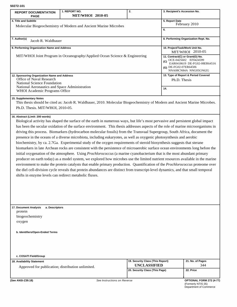
1. REPORT NO.
4. Title and Subtitle
7. Author(s)
9. Performing Organization Name and Address
12. Sponsoring Organization Name and Address
15. Supplementary Notes
16. Abstract (Limit: 200 words)
17. Document Analysis a. Descriptors
b. Identifiers/Open-Ended Terms
c. COSATI Field/Group
18. Availability Statement
REPORT DOCUMENTATION
PAGE
2. 3. Recipient's Accession No.
5. Report Date
6.
8. Performing Organization Rept. No.
10. Project/Task/Work Unit No.
11. Contract(C) or Grant(G) No.
(C)
(G)
13. Type of Report & Period Covered
14.
50272-101
19. Security Class (This Report)
20. Security Class (This Page)
21. No. of Pages
22. Price
OPTIONAL FORM 272 (4-77)
(Formerly NTIS-35)Department of Commerce
(See ANSI-Z39.18) See Instructions on Reverse
UNCLASSIFIED
2010-05
February 2010Molecular Biogeochemistry of Modern and Ancient Marine Microbes
Jacob R. Waldbauer
2010-05MIT/WHOI Joint Program in Oceanography/Applied Ocean Science & Engineering
OCE-0425602 EF0424599 EAR0418619 DE-FG02-08ER64516DE-FG02-07ER64506NNA08CN84A NNG05GN62G
Ph.D. Thesis
Biological activity has shaped the surface of the earth in numerous ways, but life’s most pervasive and persistent global impact has been the secular oxidation of the surface environment. This thesis addresses aspects of the role of marine microorganisms indriving this process. Biomarkers (hydrocarbon molecular fossils) from the Transvaal Supergroup, South Africa, document the presence in the oceans of a diverse microbiota, including eukaryotes, as well as oxygenic photosynthesis and aerobic biochemistry, by ca. 2.7Ga. Experimental study of the oxygen requirements of steroid biosynthesis suggests that sterane biomarkers in late Archean rocks are consistent with the persistence of microaerobic surface ocean environments long before the initial oxygenation of the atmosphere. Using Prochlorococcus (a marine cyanobacterium that is the most abundant primary producer on earth today) as a model system, we explored how microbes use the limited nutrient resources available in the marineenvironment to make the protein catalysts that enable primary production. Quantification of the Prochlorococcus proteome over the diel cell-division cycle reveals that protein abundances are distinct from transcript-level dynamics, and that small temporal shifts in enzyme levels can redirect metabolic fluxes.
proteinbiogeochemistryoxygen
344Approved for publication; distribution unlimited.
This thesis should be cited as: Jacob R. Waldbauer, 2010. Molecular Biogeochemistry of Modern and Ancient Marine Microbes.Ph.D. Thesis. MIT/WHOI, 2010-05.
Office of Naval ResearchNational Science FoundationNational Aeronautics and Space AdministrationWHOI Academic Programs Office
MIT/WHOI
MIT/WHOI