Joint Bit Allocation and Precoding for

MIMO Systems with Decision Feedback

Detection

To Appear in IEEE Transactions on Signal Processing

Received: November 2008

c© 2009 IEEE. Accepted for publication in IEEE Trans. on Signal Processing.Personal use of this material is permitted. However, permission to

reprint/republish this material for advertising or promotional purposes or forcreating new collective works for resale or redistribution to servers or lists, or toreuse any copyrighted component of this work in other works, must be obtainedfrom the IEEE. Contact: Manager, Copyrights and Permissions / IEEE ServiceCenter / 445 Hoes Lane / P.O. Box 1331 / Piscataway, NJ 08855-1331, USA.

Telephone: + Intl. 908-562-3966.

SVANTE BERGMAN, DANIEL P. PALOMAR ANDBJORN OTTERSTEN

Stockholm 2009

ACCESS Linnaeus Center

Signal Processing LabRoyal Institute of Technology (KTH)

IR-EE-SB 2009:035

1

Joint Bit Allocation and Precoding for MIMOSystems with Decision Feedback Detection

To Appear in IEEE Transactions on Signal Processing

Svante Bergman,Student Member, IEEE,and Daniel P. Palomar,Senior Member, IEEE,and Björn Ottersten,Fellow, IEEE

Abstract— This paper considers the joint design of bit loading,precoding and receive filters for a multiple-input multiple-output(MIMO) digital communication system employing decision feed-back (DF) detection at the receiver. Both the transmitter aswellas the receiver are assumed to know the channel matrix perfectly.It is well known that, for linear MIMO transceivers, a diagon altransmission (i.e., orthogonalization of the channel matrix) isoptimal for some criteria. Surprisingly, it was shown five yearsago that for the family of Schur-convex functions an additionalrotation of the symbols is necessary. However, if the bit loadingis optimized jointly with the linear transceiver, then this rotationis unnecessary. Similarly, for DF MIMO optimized transceiversa rotation of the symbols is sometimes needed. The main resultof this paper shows that for a DF MIMO transceiver wherethe bit loading is jointly optimized with the transceiver fil ters,the rotation of the symbols becomes unnecessary, and becauseof this, also the DF part of the receiver is not required. Theproof is based on a relaxation of the available bit rates on theindividual substreams to the set of positive real numbers. Inpractice, the signal constellations are discrete and the optimalrelaxed bit loading has to be rounded. It is shown that the lossdue to rounding is small, and an upper bound on the maximumloss is derived. Numerical results are presented that confirm thetheoretical results and demonstrate that orthogonal transmissionand the truly optimal DF design perform almost equally well.

Index Terms— MIMO systems, Communication systems, Pre-coding, Fading channels, Channel coding

EDICS: MSP-CODR, SPC-MODL, SPC-MULT

I. I NTRODUCTION

Multiple-input multiple-output (MIMO) systems have re-ceived much attention in recent years due to the tremendouspotential for high data throughput [1]. Under the assumptionthat the transmitter knows the channel perfectly, the capacity-optimal precoding strategy is to linearly orthogonalize the

Manuscript received November 14, 2008, and revised March 9,2009.Copyright (c) 2008 IEEE. Personal use of this material is permitted. However,permission to use this material for any other purposes must be obtained fromthe IEEE by sending a request to pubs-permissions@ieee.org.

This work was supported in part by the European Commission FP6 projectCOOPCOM no 033533, RGC 618008 research grant, and from the EuropeanResearch Council under the European Commission FP7, ERC grant agreementno 228044. S. Bergman and B. Ottersten are with: ACCESS LinnaeusCenter, School of Electrical Engineering, Royal Instituteof Technology(KTH) SE-100 44 Stockholm, Sweden. Fax: +46-8-7907260. B. Otterstenis also with: securityandtrust.lu, University of Luxembourg. D. P. Palomaris with: Department of Electronic and Computer Engineering, Hong KongUniversity of Science and Technology, Clear Water Bay, Kowloon, SAR HongKong. Individual contact information: S. Bergman: (email:svaberg@ee.kth.se,phone: +46-8-7908472), D. P. Palomar: (email: palomar@ust.hk, phone: +852-23587060), B. Ottersten: (email: bjorn.ottersten@ee.kth.se, phone: +46-8-7908436)

channel matrix using the singular value decomposition (SVD).Information is optimally conveyed over the orthogonal sub-channels using infinitely long and Gaussian distributed code-words, with data rates assigned to the subchannels given bythe so called waterfilling solution [1].

One downside with the capacity-optimal transmissionscheme is the (infinitely) long codewords and the delay thisbrings to the system. Clearly, long delay has some practicaldisadvantages, especially when considering time-varyingchan-nels, systems with packet retransmission, or delay-sensitiveapplications. In most cases it is mathematically intractable toprovide a global performance analysis of the delay-sensitivesystem as a whole, let alone to jointly optimize the system.By only optimizing the lowest layer of the communicationchain, our hope is that the overall performance also can bebrought close to the optimum. This motivates the separateanalysis of the modulation part of the physical layer—beforewe apply outer error-correcting codes. When not consideringerror correcting codes, the system will suffer from an inherentnon-zero probability of detection error. Thus, not only must theoptimal design tradeoff uncoded data rate against power usage,but it needs to consider the bit error rate as well. AlthoughSVD based, orthogonal, transmission is optimal in the senseof maximizing the mutual information, it is not necessarilyoptimal in this uncoded case.

In [2], [3], it was shown that given a single-user linkwith a linear receiver, for the class of Schur-concave ob-jective functions of the mean squared errors the orthogonaltransmission is indeed optimal, while for the class of Schur-convex objectives it is not (an additional rotation of thetransmitted symbols is required). This conclusion, however, isfor systems with fixed signal constellations. Arguably the mostcommon approach to multi-channel digital communication isto adapt the constellations for the subchannels according totheir respective channel gains. This adaptation, sometimesreferred to as adaptive modulation or bit loading [4], [5],will subsequently affect the objective function that we usein the precoder design. In the case of linear detection atthe receiver, optimizing the constellations leads to a Schur-concave objective function [6]. The conclusion is that if theoptimal constellations are used and if the receiver is linear,then the optimal precoder will orthogonalize the subchannelsjust as the case was for the capacity-optimal precoder.

Interestingly, the same conclusion does not hold when usingan optimal maximum-likelihood (ML) detector at the receiver.A joint constellation–precoder design was proposed in [7] that

demonstrated the suboptimality of orthogonal transmissionfor this specific case. Another design was proposed in [8]that gives the minimum BER solution for a2 × 2 MIMOsystem with quadrature phase-shift keying modulation. Bothof these designs include a rotation of the precoder suchthat the effective channel is not orthogonalized. Apparentlythe ML detector can resolve very complex multi-dimensionalconstellations that are more power efficient than the linearlyseparable constellations of the SVD-based precoder.

An intermediate solution between the linear receiver andthe ML receiver is the decision feedback (DF) receiver [9],[10], [11], [12], [13], [14], [15], [16], [17]. In general, the DFreceiver has low decoding complexity compared to the MLreceiver [18], and for channels with inter-symbol interferencethe DF receiver outperforms the linear receiver in terms oferror performance (the linear receiver is a special case of theDF receiver). In [17], [16] it was shown that for multiplicativeSchur-concave objective functions orthogonal transmission isoptimal, while for multiplicative Schur-convex objectives arotation of the signal vector is needed (similar to the linearcase). This conclusion is for systems with fixed constellations.

This work investigates the problem of jointly optimizingthe precoder, receiver filters, and bit loading when using theDF receiver on a point-to-point communication system. Themain result is that the optimal bit loading will result in anorthogonalizing precoder design. Decision feedback becomessuperfluous when the signal constellations are chosen properly.That said, DF may still be advantageous since it allows us toredistribute the bit loading on high-rate subchannels at a verylow cost in terms of reduced performance, which in turn meansthat a suboptimal bit loading will perform almost as well asthe optimal one. Another reason for using DF detection is thatperfect transmitter-side CSI may be an unrealistic assumption.Imperfect transmitter-side CSI inevitably cause inter-symbolinterference that can be reduced using DF (note that perfectCSI is required for orthogonal transmission).

In addition to the results regarding bit loading, we showthat the problem of computing the optimal precoder andreceiver filters for a fixed bit loading can be posed as aconvex problem. An algorithm that solves the convex problemwith linear computational complexity is provided. Becauseofthe low computational complexity of the filter optimization,an exhaustive search for the optimal bit loading becomespractically feasible—although the main result of the papersuggests that an exhaustive search is not necessary in mostcases.

A. Notation

For anN ×N matrix X, denote the vector of the diagonalelementsd(X) =

(

[X]1,1, ..., [X]N,N

)T. For a vector,x, of

length N , denote the diagonalN × N matrix with diagonalx as D(x). For notational simplicity, define alsoD(X) =D(

d(X))

. Thei’th element of the vectorx is denotedxi. Thevector of dimensionN with all ones is denoted1N , where theN may be scrapped if the dimension is clearly given from thecontext. The function(x)+ is defined as(x)+ = x if x > 0,and (x)+ = 0 if x ≤ 0. Rounding a real numberx to the

s

s

sF H W†

-Bv

y

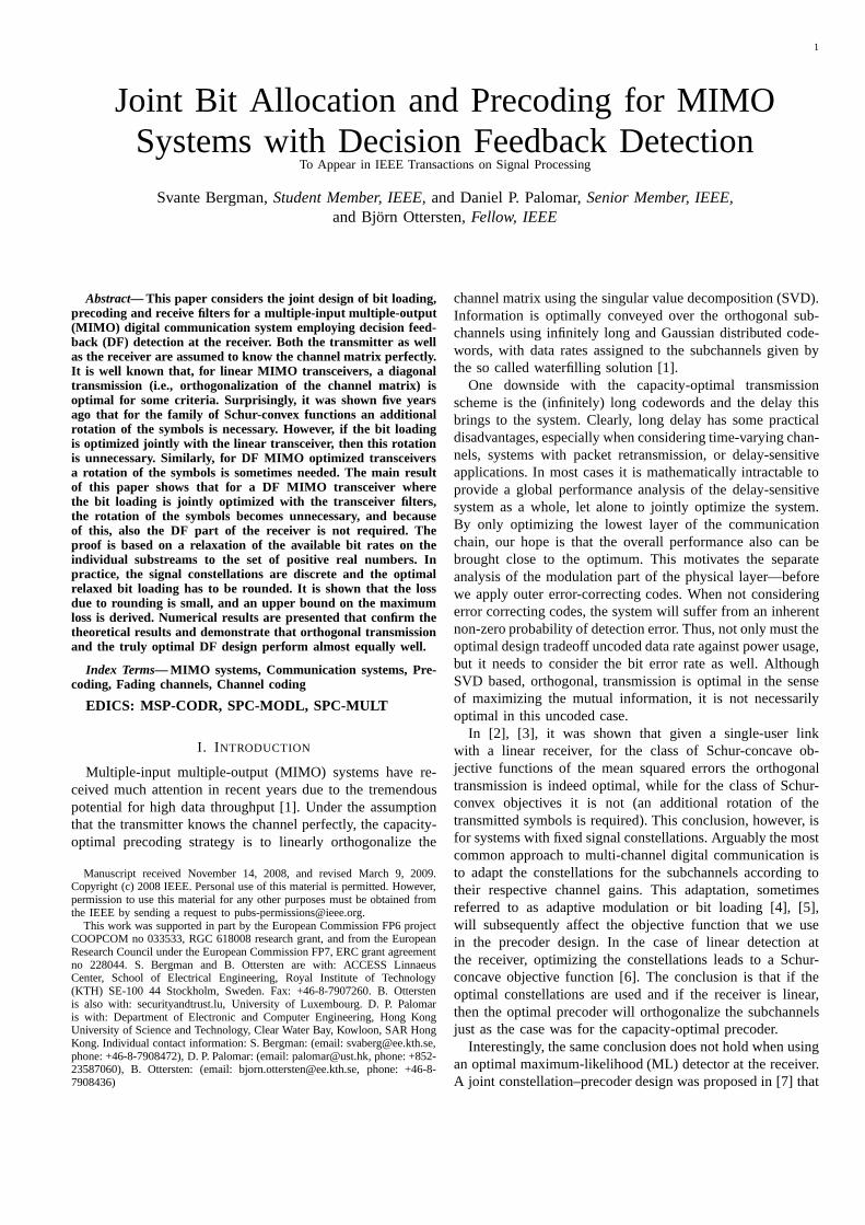
Fig. 1. Schematic view of the MIMO communication system withDFdetection.

closest integer is denoted⌊x⌉. The vector of element-wiseabsolute values of a vectorx is denoted|x|. The expectedvalue of a random matrixX is denoted E[X].

II. SYSTEM MODEL AND PROBLEM FORMULATION

Consider the discrete-time flat-fading linear model of aNr ×Nt MIMO communication system

y = HFs + v, (1)

wherey ∈ CNr is the received signal,H ∈ CNr×Nt is thechannel matrix,F ∈ CNt×N is a precoding matrix,s ∈ CN isthe data-symbols vector, andv ∈ CNr is circularly symmetricadditive white Gaussian noise. The data symbols and thenoise are assumed to be normalized as E[ss†] = I, andE[vv†] = I. The average transmitted power is limited suchthat Tr{FF†} ≤ P, is satisfied.

A. Decision feedback receiver

In this work we assume that the receiver employs DFequalization, a schematic view of the system is depicted inFig. 1. The received signal is linearly equalized using aforward filter, W†, and subsequently passed to an elemen-twise detector of the data symbols. From the outcome ofthe detection, we reconstruct the transmitted data symbols,s, then use the reconstructed symbols to remove interferencebetween the symbols in the equalized signal. In order toensure that the DF detection is sequential, i.e. that we do notfeedback symbols that has not yet been detected, we enforcethe feedback matrixB to be strictly lower triangular. Thesignal after the interference subtraction,s, is then passed onto the detector again. Taking the feedback into account, theerror prior detection is

e = s− s = (W†HF− I)s−Bs + W†v. (2)

If the probability of detection error is small, one can assumethat s and s are zero mean and have close to identicalcorrelation and cross-correlation matrices, and thats is un-correlated with the noisev. Using these approximations theerror covariance matrix is given by

RMSE = E[

ee†]

= (W†HF−B− I)(W†HF−B− I)† + W†W.(3)

Since the detection of the symbolss = s + e is madeelementwise, we can regard the detection problem simply asdetecting a scalar signal in additive complex Gaussian noise1.

1Strictly speaking the interference part of the error is not complex Gaussiandistributed. However, combined with the noise we can tightly approximate theinterference as such by the law of large numbers.

To appear in IEEE Transactions on Signal Processing

We denote each virtual transfer functionsi = si + ei as asubchannel, for which the performance is determined by itsvirtual noise power,[RMSE]i,i.

In general, sequential decision feedback does not restrictus to use only lower-triangular feedback matrices, any jointrow–column permutation is also possible. However, in thiscase where we are free to design both the precoder and thebit loading, such permutation loses its purpose since it canbeabsorbed into the other optimization parameters.

B. Cost functions based on the weighted mean squared error

A general framework was presented in [17] for optimizingthe DF system (i.e. the filtersF, W†, and B) based onmonotonic cost functions of the MSEs of the subchannels.Our goal here is to optimize not only these DF filters, but alsothe signal constellations that are used on the subchannels.Formathematical tractability in the later analysis we narrow downthe class of cost functions top-norms of weighted MSEs. Moreprecisely, consider the cost function‖d(RMSEDw)‖p, whereDw is a weighting matrix assumed to be diagonal and non-negative, and the function

‖d(X)‖p =

( N∑

i=1

[X]pi,i

)1/p

, (4)

is the p-norm of the diagonal elements ofX. The p-norm isdefined forp ≥ 1.

To illustrate how to apply the cost function (4) in practice,consider minimizing the probability of detection error. Usingthe Gaussian-tail function

Q(x) =1√

2π

∫ ∞

x

e−t2/2 dt, (5)

the probability of error of subchanneli can be approximatedas

Pe,i ≃ 4 Q

(√

d2min(bi)

2 [RMSE]i,i

)

, (6)

where d2min(bi) denotes the squared minimum distance of a

signal constellation that was modulated usingbi informationbits and has been normalized to unit variance [19]. Equa-tion (6) allows us to relate the MSE with the performancein terms of error probability. It also indicates how we shouldchose the MSE weighting matrixDw in our cost function.Namely, in order to have symmetry among the subchannels,the weights should be inversely proportional to the squaredminimum distance as

[Dw]i,i = d−2min(bi) ∀ i = 1, ..., N. (7)

This will make the subchannels (approximately) symmetricwith respect to symbol error rate (SER), which is a relevantmeasure, for example, if we want to minimize the jointprobability of detection error. In the case when outer errorcorrecting codes are used it may be more relevant to havesymmetric bit error rates (BER) rather than SERs. AssumingGray coded bit mapping the BERs can be approximated as

BERi ≈1

biPe,i. (8)

For moderately low, to low BERs, it can be shown that thedependency onbi in the BER expression is dominated by theSER factor,Pe,i. Hence symmetric SERs can serve as a goodapproximation to attain symmetric BERs as well.

For most classes of constellations used in practice, theminimum distance typically decreases exponentially with thenumber of bitsbi. For example, quadrature amplitude modu-lated (QAM) constellations with even bit loading has minimumdistance

d2min(bi) =

6

2bi − 1, (9)

resulting in a weighting matrix (disregarding constant factors)

Dw = D(2b1 − 1, ..., 2bN − 1). (10)

One objective could be to minimize the maximum errorprobability, Pe,i, of the subchannels. Under the high-SNRassumption, this objective translates into a cost function

‖d(RMSEDw)‖∞ = maxi

[RMSEDw]i,i, (11)

corresponding to thep =∞ norm.Summarizing, if the SNR is high, the probability of error on

a subchannel depend to a large extent on the minimum distanceof the signal constellations. The minimum distance scales theMSE of the subchannels, which leads to imbalances whendifferent types of signal constellations are used on differentsubchannels. Using a cost function with weighted MSE thisimbalance can be compensated for. The parameterp of the costfunction can be used to control how ‘flexible’ the system is interms of the spread of the error rates among the subchannels.Low p results in more spread, which may be disadvantageoussince the worst subchannel typically dominates. In general,and specifically for high SNRs, the infinity norm seems totranslate into the lowest SERs in most cases.

C. Problem formulation

With the definitions of the MSE matrix (3) and the costfunction (4) in place, our problem can be mathematicallyformulated as

minimizeF,B,W†,b

∥

∥d(

RMSE(F,B,W†)Dw

)∥

∥

p(12a)

subject to Tr{FF†} ≤ P, (12b)

[Dw ]i,i = d−2min(bi) ∀ i = 1, ..., N, (12c)

bi ∈ B ∀ i = 1, ..., N, (12d)N∑

i=1

bi = R, (12e)

where the vectorb is the bit loading vector, and the setBdenotes the set of feasible bit rates which is determined by theavailable signal constellations. Typically, due to the discretenature of bits, this set is equal to the set of positive integers.

For a fixed bit loading,b, the problem of designing the DFfilters can be reformulated as a convex problem that can besolved numerically. In Section III, it is shown how to applythe framework in [17] to the particular problem consideredhere. In fact, the problem can be solved very efficiently with

To appear in IEEE Transactions on Signal Processing

linear computational complexity. Once the optimal bit ratesare known, the remaining problem is therefore fairly simple.

As for the optimization of the bit loading, the setB isdiscrete and it is possible to numerically try out all feasible bitloading combinations in order to find the global optimum. Analternative to such an exhaustive search is to relax the problemand extend the setB to allow for arbitrary positive bit rates.We do this by using (9) to relate these real-valued bit ratesto virtual minimum-distance weights. This relaxation allowsus to optimize the bit loading for any given MSE matrix.In Section IV, the optimal relaxed bit loading is derived.The remaining problem of jointly optimizing the DF filtersis characterized in Section V, together with a discussion onthe loss due to rounding of the bit rates. Finally, in Sections VIand VII, various practical strategies for solving the jointproblem are presented and evaluated numerically.

III. D ESIGN OFOPTIMAL FILTERS

Because the set of feasible bit loads is discrete, its optimiza-tion is not easy to combine with the filter and precoder design.This section treats the filter design problem alone, assuminga fixed bit loading. The problem is formulated as

minimizeF,B,W†

‖d(RMSEDw)‖p (13a)

subject to Tr{FF†} ≤ P. (13b)

In [17, Theorem 4.3] it was shown how problems of this type(with monotonic cost functions of the MSEs) can be reduced toa power-loading problem involving a multiplicative majoriza-tion constraint2. In subsections III-A, III-B, and III-C, we will,for completeness, apply this procedure to problem (13), andgive the filter expressions that are obtained in the process.In subsection III-D, we then show how the resulting problemwith a majorization constraint can be replaced with a convexproblem that is easy to solve numerically.

A. Optimal forward receiver filter

For a given transmit matrix,F, and receive DF matrix,B,the optimal forward filter,W†, in the receiver is the wellknown minimum MSE (MMSE) equalizer

W† = (B + I)(F†H†HF + I)−1F†H†. (14)

The proof is given by completing the squares of (3) andthen applying the matrix inversion lemma3. Using the optimalforward filter, the resulting vector of weighted MSEs is

d(RMSEDw) = d(

(B+D1/2w )(F†H†HF+I)−1(B+D1/2

w )†)

,(15)

whereB , D1/2w B. Note that the MMSE equalizer minimizes

any monotonic increasing function of the MSEs and is thusoptimal for a wider class of cost functions than consideredhere.

2A short recapitulation on vector majorization is provided in Appendix A.3(A + BCD)−1 = A−1

− A−1B(DA−1B + C−1)−1DA−1

B. Optimal feedback receiver filter

Consider the Cholesky factorization of

(F†H†HF + I)−1 = LL†, (16)

whereL is lower triangular. Inserting (16) into (15) we obtainthe weighted MSE of subchanneli as

[RMSEDw]i,i =

i∑

j=1

|[(B + D1/2w )L]i,j |

2. (17)

SinceBL is a strictly lower-triangular matrix (zero diagonal)it can only affect the non-diagonal elements of the lower-triangular matrixBL + D

1/2w L. Hence, the feedback matrix,

B, that minimizes the MSEs in (17) satisfies

BL = −Lstrict(

D1/2w L

)

, (18)

whereLstrict(

X)

the matrix that contains the strictly lower-diagonal part ofX. The optimalB is then

B = −D1/2w

(

L−D(L))

L−1, (19)

and the resulting minimum MSE of subchanneli is

[RMSEDw]i,i = [D1/2w D(L)]2i,i = [Dw]i,i[L]2i,i. (20)

C. Optimal precoder: Left and right unitary matrices

The remaining filter to optimize is the precoder,F. Considerthe SVD of the precoder matrix

F = UFΣ1/2F V

†F, (21)

where UF and VF are unitary matrices, andΣ1/2F is non-

negative and diagonal with decreasing diagonal. For arbitrarymonotonic increasing objective functions of the MSEs, theoptimal left unitary matrix has been shown to match the matrixof eigenvectors ofH†H = UHΛHU

†H [2], [17, Theorem 4.3]:

UF = UH, (22)

where it is assumed that the diagonal ofΛH is decreasing.Using (22), the right unitary matrix,VF, can readily beobtained from the SVD ofL as

F†H†HF + I = VF(ΣFΛH + I)V†F =⇒

L = VF(ΣFΛH + I)−1/2Q†,(23)

whereQ is a unitary matrix that makesL lower triangular.Note here that the diagonal matrix with the singular valuesΛL , (ΣFΛH+I)−1/2 is in this case ordered with increasingdiagonal. Finally, also assumingL is known, the singularvalues ofF are obtained fromΛL andΛH as

ΣF = Λ−1H (Λ−2

L − I). (24)

With the optimalW†, B, andUF, the remaining optimizationproblem is

minimizeVF,Q,σ

∥

∥Dw|d(L)|2∥

∥

p(25a)

subject to L = VF(D(σ)ΛH + I)−1/2Q†, (25b)

[L]i,j = 0 ∀ i < j, (25c)

VF,Q ∈ U , (25d)

σ ≥ 0, (25e)

1Tσ ≤ P, (25f)

To appear in IEEE Transactions on Signal Processing

where we introduced the power vectorσ = d(ΣF), thatrepresents the power assigned to each spatial channel, andwhereU is the set of allN -dimensional unitary matrices.

Now, optimizing the unitary matricesVF, Q, directly isvery difficult. From the expressions of the optimal DF filterswe see that the filters either implicitly or explicitly dependon the lower triangular matrixL. By optimizing L insteadof VF, Q, we can avoid the unitary constraints. In orderto do this we need a way to specify the singular values ofL as an optimization constraint, fortunately this is possible.The diagonal elements of a triangular matrix represents theeigenvalues of the same matrix. It is known that the absolutevalues of the eigenvalues are always multiplicatively majorizedby the singular values (cf. [20]). Interestingly, this necessarycondition is also a sufficient condition on the triangularmatrix L: For a given power load,ΣF, and a specifiedvector d(L), one can uniquely determine (using generalizedtriangular decomposition [21]) the lower triangular matrix L

if and only if

|d(L)|−2 �× d(ΣFΛH + I), (26)

where�× denotes multiplicative majorization [22], [17]. Theproof of this statement was given in [21]. With this necessaryand sufficient condition on the diagonal elements of a triangu-lar matrix we can replace the constraints (25b), (25c), (25d),in problem (25). Matrix notation becomes tedious (and unnec-essary) to work with at this point, instead define the vectorsw = logd(Dw), y = log |d(L)|−2, and use (26) to pose theequivalent optimization problem in vector notation as

minimizey,σ

‖ exp(w − y)‖p (27a)

subject to y � log(ΛHσ + 1), (27b)

σ ≥ 0, (27c)

1Tσ ≤ P, (27d)

where� denotes additive majorization. The vectorw relatesto the MSE weights of the problem and we call it the log-weights vector. The vectory has the interpretation of datarate (see (27b)) and we name it rate vector4.

D. Optimal precoder: Power allocation

The optimization problem (27) is somewhat difficult towork with due to the majorization constraint. Fortunately asimpler convex problem can be considered instead. Becausethep-norm is symmetric and because a majorization inequalityis invariant to permutations of the vector elements, we canwithout loss of generality assume the subchannels are orderedsuch that bothw andλ = d(ΛH) are decreasing.

Now that we have fixed the ordering ofw andλ, we may

4Note also, thaty is the logarithm of the inverse of the MSEs, whichcorresponds to the mutual information over AWGN channels using Gaussiancodebooks.

Alg. 1

b Ly, σ W†F, B

ΛH UH VH

GTD SVD

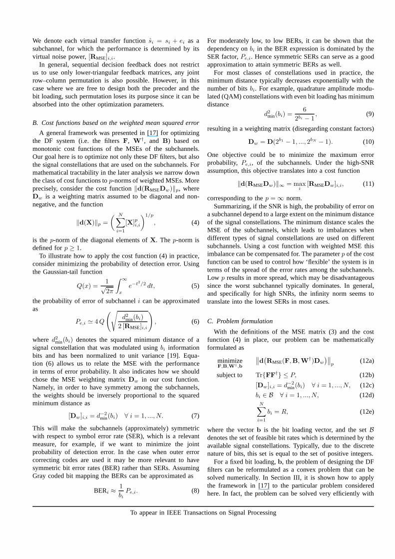
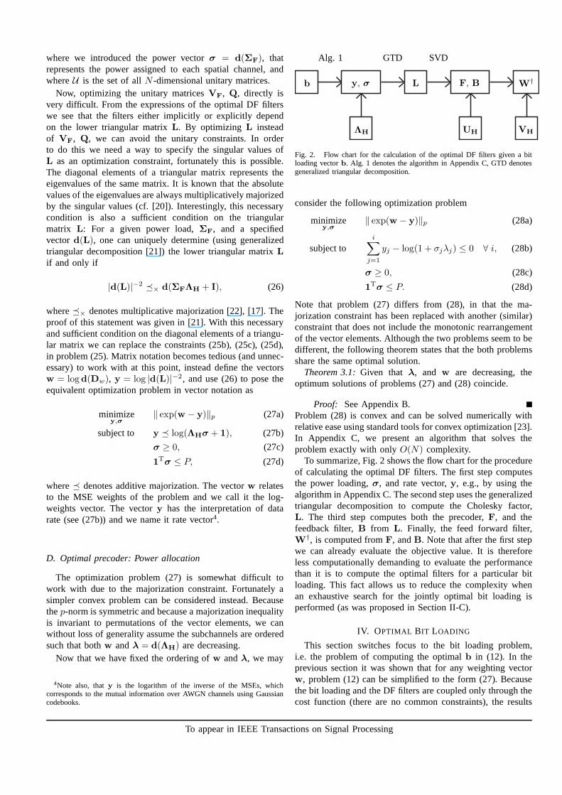
Fig. 2. Flow chart for the calculation of the optimal DF filters given a bitloading vectorb. Alg. 1 denotes the algorithm in Appendix C, GTD denotesgeneralized triangular decomposition.

consider the following optimization problem

minimizey,σ

‖ exp(w − y)‖p (28a)

subject toi∑

j=1

yj − log(1 + σjλj) ≤ 0 ∀ i, (28b)

σ ≥ 0, (28c)

1Tσ ≤ P. (28d)

Note that problem (27) differs from (28), in that the ma-jorization constraint has been replaced with another (similar)constraint that does not include the monotonic rearrangementof the vector elements. Although the two problems seem to bedifferent, the following theorem states that the both problemsshare the same optimal solution.

Theorem 3.1:Given that λ, and w are decreasing, theoptimum solutions of problems (27) and (28) coincide.

Proof: See Appendix B.Problem (28) is convex and can be solved numerically withrelative ease using standard tools for convex optimization[23].In Appendix C, we present an algorithm that solves theproblem exactly with onlyO(N) complexity.

To summarize, Fig. 2 shows the flow chart for the procedureof calculating the optimal DF filters. The first step computesthe power loading,σ, and rate vector,y, e.g., by using thealgorithm in Appendix C. The second step uses the generalizedtriangular decomposition to compute the Cholesky factor,L. The third step computes both the precoder,F, and thefeedback filter,B from L. Finally, the feed forward filter,W†, is computed fromF, andB. Note that after the first stepwe can already evaluate the objective value. It is thereforeless computationally demanding to evaluate the performancethan it is to compute the optimal filters for a particular bitloading. This fact allows us to reduce the complexity whenan exhaustive search for the jointly optimal bit loading isperformed (as was proposed in Section II-C).

IV. OPTIMAL BIT LOADING

This section switches focus to the bit loading problem,i.e. the problem of computing the optimalb in (12). In theprevious section it was shown that for any weighting vectorw, problem (12) can be simplified to the form (27). Becausethe bit loading and the DF filters are coupled only through thecost function (there are no common constraints), the results

To appear in IEEE Transactions on Signal Processing

from Section III can be incorporated into the original problemformulation (12) as

minimizey,σ,b

‖ exp(w − y)‖p (29a)

subject to y � log(ΛHσ + 1), (29b)

σ ≥ 0, (29c)

1Tσ ≤ P, (29d)

wi = − log d2min(bi) ∀ i, (29e)

bi ∈ B ∀ i, (29f)

1Tb = R. (29g)

In general, the set of available constellations,B, is discrete.In particular, if QAM constellations are used the bit rates arerestricted to positive, even integers. The set of feasible bit ratesis then

bi ∈ {0, 2, 4, ...} ∀ i, (30a)

1Tb = R. (30b)

Clearly, the feasible set is finite and it is possible to com-pute the optimal bit loading numerically by trying out allpossible candidates. This observation does however providelittle insight into the overall behavior of the system. It isalsoquestionable whether it is worth the computational burden toglobally search all possible bit loading candidates. In orderto gain more insight and to find heuristics for computing thebit rates more efficiently, the following subsection considersoptimizing b while the vectorsy andσ remain fixed (recallthat Section III was optimizingy andσ for a fixedb). Then,later, Section V will be devoted to the joint optimization ofall three vectorsy, σ, andb.

A. Continuous bit loading relaxation

Optimization of the discrete valued bit loading is difficultinclosed form. One way to approach this optimization problem isto relax the set of bit rates to the continuous domain (by ignor-ing the constraint (30a)) to allow for us to analytically optimizeb. This leads to the continuous relaxation of problem (29),where B = R+. In order to specify constraint (29e), weassume for simplicity that the constellations are QAM. Then,using (10), the log-weights,w, depend on the bit allocationsas

ew = d(Dw) = eb − 1, (31)

where the unit of the rate has been changed to nats (rather thanbits) in order to simplify the notation below. For a giveny andσ, using weights defined by (31), the continuous relaxation ofproblem (29) withy, σ fixed, is then formulated as

minimizeb1,...,bN

N∑

i=1

(ebi − 1)pe−pyi, (32a)

subject toN∑

i=1

bi = R, (32b)

bi ≥ 0 ∀ i, (32c)

where we use the fact that‖ · ‖p and ‖ · ‖pp are minimizedsimultaneously5. Note (by inspection) that the problem isconvex.

Theorem 4.1:The optimum bit allocation in (32) is givenby

bi = g(µ + yi) ∀ i = 1, ..., N, (33)

where the functiong(x) is defined as{

x = (1− p−1) log(

1− e−g(x))

+ g(x), if p > 1g(x) = (x)+, if p = 1

,

(34)and whereµ is chosen so that

N∑

i=1

g(µ + yi) = R. (35)

Proof: In the following proof we assumep ∈ (1,∞).The proofs forp = 1 andp→∞ are similar but needs to betreated separately. Disregarding for a while the constraint thatb must be positive, minimizing the Lagrangian cost functionof (32) yields the optimal solution to the problem as

p ebi(ebi − 1)p−1e−pyi = θ ∀ i = 1, ..., N, (36)

where θ is the dual variable such that constraint (32b) issatisfied. Equation (36) contains multiple roots. However,ifthere exists a root with strictly positivebi’s, then it must alsobe a global optimum to the convex problem (32) (a convexproblem does not have local optima unless they also are globaloptima).

Taking the logarithm of (36) and performing some rear-rangements yields

f(bi) , (1− p−1) log(1 − e−bi) + bi = p−1 log(θ p−1) + yi.(37)

Note that the functionf(bi) is real valued when allbi’s arepositive. By inspection,f(bi) is strictly increasing, concave,and it maps the set(0,∞) to the set(−∞,∞). Becausef(bi)is strictly increasing and concave, the inverse functiong(x)exists and is strictly increasing and convex. Following (37),the functiong(x) must satisfy

x = (1− p−1) log(

1− e−g(x))

+ g(x). (38)

This implies that for any vectory there exists one and onlyone solution to (36) with strictly positive bit rates,b, givenby

bi = g(µ + yi) ∀ i = 1, ..., N, (39)

whereµ , p−1 log(θ p−1).Given a rate vectory, equations (33) and (35) uniquelydetermines the optimal bit loading (as well asµ). Theseequations will later be applied to eliminateb from the jointoptimization problem.

The observant reader may have noticed that the optimalrelaxed bit loading will never be exactly zero on any sub-channel. Instead of switching off weak subchannels with zero

5The infinity norm is not well defined at this point and has to be treatedseparately. The conclusions of the following discussion are however valid forthe infinity norm as well.

To appear in IEEE Transactions on Signal Processing

bit loading, it turns out that it is more favorable to use aninfinitesimal (positive) bit rate. Of course there is no suchthing as infinitesimal bit rates in practice, recall that therelaxation is merely a tool that we can use to obtain practicallyimplementable bit-loading candidates by means of rounding.Fortunately, as will be shown in Section V-B, the impact thata low-rate subchannel has on the rest of the system is limited,i.e., the performance will remain close to optimal if we turnoff the low-rate subchannels. After the bit loading these low-rate subchannels will in any case be rounded to zero when weperform the rounding. The next subsection contains a commenton the sensitivity of the relaxed optimum towards rounding.

B. Rounded bit loading

In practice, arbitrary real-valued bit rates are not imple-mentable and the impact of rounding or quantization of the bitrates has to be considered. Assumeb, is the optimal solutionto the relaxed bit loading problem for some given rate vectory, and assume thatb′ is the rounded or quantized version ofb such that the sum rate isR. Denote the logarithm of theobjective function (29a) as

J(b,y) = p−1 log(

N∑

i=1

(ebi − 1)pe−pyi

)

, (40)

where we have chosen the weights according to (31). The firstorder Taylor expansion of (40) around the optimal bit loadingb yields

J(b′,y) ≈ J(b,y) +

∑Ni=1(e

bi − 1)p−1ebie−p yi δi

ep J(b,y), (41)

whereδ = b′ − b. Now, using (36), and assuming bothb′

and b satisfy (32b) so that1Tδ = 0, the first order term in

the expansion sums to zero

J(b′,y) ≈ J(b,y) +θ∑N

i=1 δi

p ep J(b,y)= J(b,y). (42)

This result indicates that rounding of the optimal relaxedbit loading can be performed without too much loss inperformance, although it is not clear how to quantify the loss.In the following section the loss is quantified for the jointoptimum by making a distinction between low-rate and high-rate subchannels.

V. JOINT OPTIMIZATION OF BIT LOADING AND FILTERS

Now that we know how to obtain the optimal DF filters (viay andσ) for a given bit allocation (cf. Section III), and howto optimize the bit allocationb given vectorsy and σ (cf.Section IV), our next step is to combine these results into ajoint optimization problem.

A. The bit-loading optimized objective

The optimal relaxed bit allocation from Section IV dependson the rate vectory. By inserting the optimal bit loading intothe refined transceiver problem (27), we obtain a new objectivewith a dependence ony that is not as easily characterized

as before. This subsection analyzes the behavior of this bit-loading optimized objective with respect toy. As it turns out,even though the dependency ony is complicated, it is stillpossible to determine the optimaly as a function ofσ.

The optimal relaxed bit-loading vectorb, obtained from (32)in the original objective, yields the following objective func-tion

J(y1, ..., yN) = p−1 log(

N∑

i=1

(ebi − 1)pe−pyi

)

, (43)

where the logarithm is introduced for later mathematicalsimplicity. The optimal bit allocation must satisfy (33), whichcan be reformulated to

(ebi − 1)pe−pyi = epµ(1− e−bi) ∀ i. (44)

Using bi = g(µ + yi), the bit-loading optimized cost functionis then formulated without the vectorb as

J(y1, ..., yN ) = µ + p−1 log

N∑

i=1

(

1− e−g(µ+yi))

, (45)

whereµ is chosen such that

N∑

i=1

g(µ + yi) = R. (46)

Note that (45) is also valid for the∞-norm whenp−1 = 0.Using the new bit-optimized cost function, the remaining

optimization problem (that determines the DF filters) is

minimizey,σ

J(y1, ..., yN) (47a)

subject to y � log(ΛHσ + 1), (47b)

σ ≥ 0, 1Tσ ≤ P. (47c)

Although the problem is non-convex and perhaps difficult tosolve, it turns out the cost function is symmetric and concavewhich enables us to solve at least parts of the problem withrelative ease.

Theorem 5.1:The functionJ(y1, ..., yN ) is Schur-concavewith respect toy1, ..., yN .

Proof: See Appendix D.A direct consequence of Theorem 5.1 is the following impor-tant corollary

Corollary 5.2: Orthogonal SVD-based transmission withno decision feedback is always an optimal solution to thedecision feedback problem given that the optimal relaxed bitloading is used.

Proof: Because the objective is Schur-concave (seeAppendix A for definition), the optimal vectory must satisfythe majorization constraint with equality (cf. [24]), i.e.wehave y = log(1 + ΛHσ). This means thatVF in (21)can be chosen as the identity matrix so that the subchannelsare orthogonalized. Orthogonal subchannels implies thatL isdiagonal and that the optimal feedback matrixB is zero (seeSection III-B).Although the remaining problem of computing the optimalpower load,σ, is a non-convex problem with a non-trivialsolution, the result above shows that it suffices to use stateof

To appear in IEEE Transactions on Signal Processing

the art SVD-based bit and power loading schemes (e.g., [6])to compute a close-to-optimal bit loading.

Theorem 5.1 relies on the continuous relaxation, and thebehavior ofJ(y) for discrete constellation sets is not clear atthis point. On the other hand, as was shown in Section IV-B,small perturbations of the optimal relaxed bit load will notsignificantly alter the value of the cost function. So, roundingthe optimal bit loading should still remain close to optimal.In the next subsection, an upper bound on the loss due torounding of the bit rates is derived.

B. Turning off low-rate subchannels

Essentially, rounding the bit loading corresponds to turningoff low-rate subchannels and slightly perturbing the bit rateson the remaining high-rate subchannels. In this subsectionwewill show that the loss by turning off low-rate subchannels isrelatively small, and then, that a system with no active low-ratesubchannels is insensitive to reallocations of the bit loading.

An interesting property ofg(x) is that its asymptotes6

coincide with the function(x)+. Therefore, by analyzing (45),(46), we see that weak subchannels with values ofx that arenegative or close to zero will have almost no impact onµ or onJ(y1, ..., yN ). These subchannels can consequently be turnedoff at a very low cost in terms of performance. To formalizethis, assume thaty is decreasing and that allN −K weakestsubchannels with indicesi > K are turned off. This will resultin a new dual variableµ and cost functionJ(y1, ..., yK) as

J(y1, ..., yK) = µ + p−1 log

K∑

i=1

(

1− e−g(µ+yi))

, (48)

K∑

i=1

g(µ + yi) = R. (49)

The following theorem quantifies the loss.Theorem 5.3:The loss when turning off theN−K weakest

subchannels can be upper bounded as

J(y1, ..., yK)− J(y1, ..., yN) ≤

∑Ni=K+1 g(µ + yi)

K −∑K

i=11−p−1

eg(µ+yi)−p−1

.

(50)Proof: See Appendix E.

In order to get a sense of how this bound behaves, denote thesum rate of the truncated subchannels

∆R =

N∑

i=K+1

g(µ + yi). (51)

Assuming the active subchannels satisfyeg(µ+yi) ≫ 1, thenthe denominator in (50) can be approximated withK, and thebound becomes

J − J ≤∆R

R·

R

K. (52)

As an example, typical figures for∆R/R could be on the orderof 10% while the average data rate per active subchannel is

6First note that the range ofg(x) is non-negative, then from (34) we seethat g(x) ≫ 1 ⇒ x ≈ g(x) andg(x) ≈ 0 ⇒ x ≈ (1 − p−1) log g(x).

typically less than, lets say,3 nats. This would correspond toa maximum loss of around 1 dB.

The next step is to see how the cost function behaves whenall low-rate subchannels have been turned off. Given that allsubchannels are high rate we can applyeg(µ+yi) ≫ 1 to thedefinition (34) and obtain

g(µ + yi) ≈ µ + yi. (53)

By applying the asymptote to (49), the cost function (48) tendsto

J(y1, ..., yK) ≈R

K−

1

K

K∑

i=1

yi + p−1 log(K). (54)

Given that the majorization constraint (47b) is satisfied, thefollowing equality holds

K∑

i=1

yi =

K∑

i=1

log(λiσi + 1), (55)

and we can eliminatey completely from (54). Interestingly,any y that satisfies (47b) can be used and still be optimal.Since there is a direct connection between the optimalb andy, this result implies that we can redistribute the bit allocationsat a very low cost, provided the resultingy satisfies (47b) andthe data rates on the active subchannels remain sufficientlyhigh.

The results in this subsection predicts very limited losseswhen rounding the relaxed bit loading. This fact is furthermotivated by the numerical results in Section VII wherealmost identical performance of the truly optimal bit loading(achieved by a global search) and the rounded optimal relaxedbit loading is shown.

VI. T RANSMISSION SCHEMES

Due to the potential high complexity of the truly optimaljoint bit loading and filter design, this section defines (inaddition to the optimal design) three suboptimal schemes. Twoof which, in theory, should perform very close to optimal.

A. Optimal design

This transmission scheme is optimal in terms of (12). Thestrategy is to exhaustively search all combinations of bitloading allocations. For each bit loading candidate, optimizethe rate vector,y, and the power loading vector,σ, by solvingproblem (28). Compute the weighted MSEs, and use the bitloading with the least weighted MSE.

B. Suboptimal bit loading

As Theorem 5.1 shows, the optimal relaxed bit loading willmake the DF optimized system orthogonal. In [6], the so calledgap approximation was used for determining the constellationsof an orthogonal system. The gap approximation is close tooptimal for the orthogonal system, and since the optimal bitloading with DF results in an orthogonal system it must beapproximately optimal in this case as well.

To appear in IEEE Transactions on Signal Processing

In short, using the gap approximation the bit loading canbe computed as

bi = 2

⌊

1

2log2

(

σiλiΓ−1 + 1

)

⌉

, (56)

where the gap,Γ, is chosen such that∑

i bi = Rtot, and whereσi is the waterfilling power allocation, given by

σi = (Φ− Γλ−1i )+, (57)

where the water levelΦ is chosen such that∑

i σi = P .Insertion of the waterfilling power allocation yields

bi = 2

⌊

1

2log2(λi) + α

⌉+

, (58)

where α is a constant such that∑

i bi = R. The precoder,forward filter, and feedback filter are then optimized for thisparticular bit loading.

C. Orthogonal design

As was shown in Section V, the optimal relaxed bit loadingmakes the subchannels orthogonal. It was also shown thatthe first order Taylor expansion around the optimal relaxedbit loading is constant. Hence, an optimal design under theconstraint that the subchannels are forced to be orthogonalshould perform almost as well as the two schemes above.

Use the gap approximation to compute the bit rates, thendesign the optimalorthogonalizingprecoder and forward filterfor this particular bit loading. That is, design the optimalprecoder such that the interference among the subchannels iszero. Since the subchannels are orthogonal for this scheme,the optimal feedback matrix will be zero.

D. Equal rate design

The bit rates are distributed uniformly among all availablesubchannels. Again, the precoder, the forward filter, and thefeedback filter are subsequently optimized for this particularbit loading.

VII. N UMERICAL RESULTS

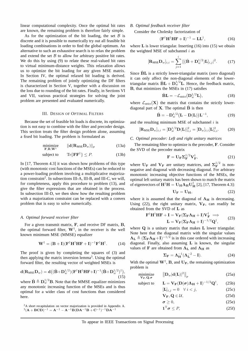
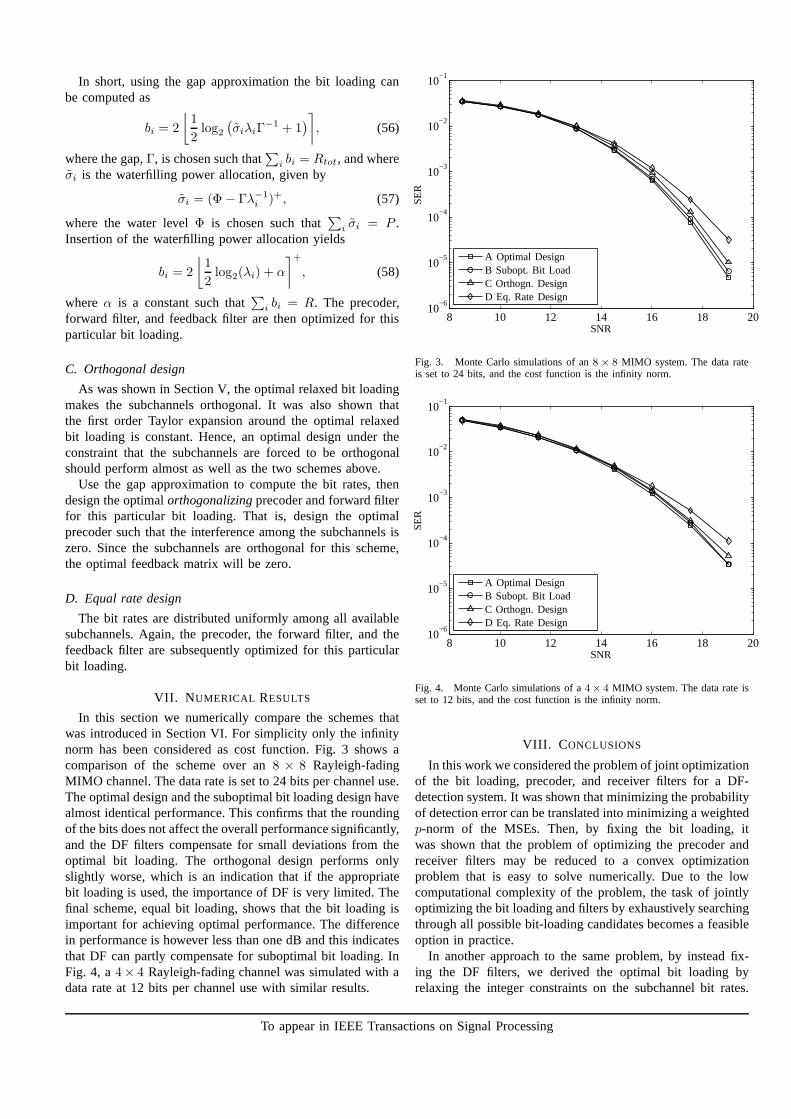
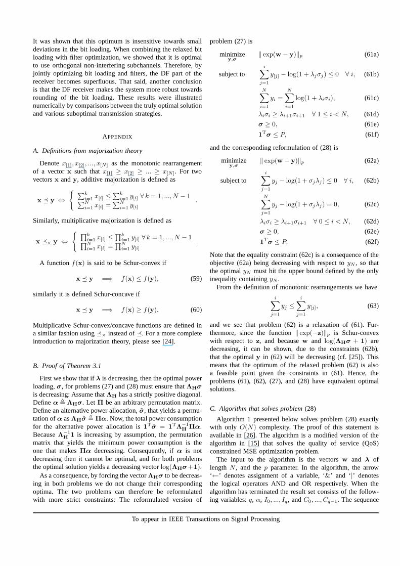
In this section we numerically compare the schemes thatwas introduced in Section VI. For simplicity only the infinitynorm has been considered as cost function. Fig. 3 shows acomparison of the scheme over an8 × 8 Rayleigh-fadingMIMO channel. The data rate is set to 24 bits per channel use.The optimal design and the suboptimal bit loading design havealmost identical performance. This confirms that the roundingof the bits does not affect the overall performance significantly,and the DF filters compensate for small deviations from theoptimal bit loading. The orthogonal design performs onlyslightly worse, which is an indication that if the appropriatebit loading is used, the importance of DF is very limited. Thefinal scheme, equal bit loading, shows that the bit loading isimportant for achieving optimal performance. The differencein performance is however less than one dB and this indicatesthat DF can partly compensate for suboptimal bit loading. InFig. 4, a4× 4 Rayleigh-fading channel was simulated with adata rate at 12 bits per channel use with similar results.

8 10 12 14 16 18 2010

−6

10−5

10−4

10−3

10−2

10−1

SNR

SE

R

A Optimal DesignB Subopt. Bit LoadC Orthogn. DesignD Eq. Rate Design

Fig. 3. Monte Carlo simulations of an8 × 8 MIMO system. The data rateis set to 24 bits, and the cost function is the infinity norm.

8 10 12 14 16 18 2010

−6

10−5

10−4

10−3

10−2

10−1

SNR

SE

R

A Optimal DesignB Subopt. Bit LoadC Orthogn. DesignD Eq. Rate Design

Fig. 4. Monte Carlo simulations of a4× 4 MIMO system. The data rate isset to 12 bits, and the cost function is the infinity norm.

VIII. C ONCLUSIONS

In this work we considered the problem of joint optimizationof the bit loading, precoder, and receiver filters for a DF-detection system. It was shown that minimizing the probabilityof detection error can be translated into minimizing a weightedp-norm of the MSEs. Then, by fixing the bit loading, itwas shown that the problem of optimizing the precoder andreceiver filters may be reduced to a convex optimizationproblem that is easy to solve numerically. Due to the lowcomputational complexity of the problem, the task of jointlyoptimizing the bit loading and filters by exhaustively searchingthrough all possible bit-loading candidates becomes a feasibleoption in practice.

In another approach to the same problem, by instead fix-ing the DF filters, we derived the optimal bit loading byrelaxing the integer constraints on the subchannel bit rates.

To appear in IEEE Transactions on Signal Processing

It was shown that this optimum is insensitive towards smalldeviations in the bit loading. When combining the relaxed bitloading with filter optimization, we showed that it is optimalto use orthogonal non-interfering subchannels. Therefore, byjointly optimizing bit loading and filters, the DF part of thereceiver becomes superfluous. That said, another conclusionis that the DF receiver makes the system more robust towardsrounding of the bit loading. These results were illustratednumerically by comparisons between the truly optimal solutionand various suboptimal transmission strategies.

APPENDIX

A. Definitions from majorization theory

Denotex[1], x[2], ..., x[N ] as the monotonic rearrangementof a vectorx such thatx[1] ≥ x[2] ≥ ... ≥ x[N ]. For twovectorsx andy, additive majorization is defined as

x � y ⇔

{

∑ki=1 x[i] ≤

∑ki=1 y[i] ∀ k = 1, ..., N − 1

∑Ni=1 x[i] =

∑Ni=1 y[i]

.

Similarly, multiplicative majorization is defined as

x �× y ⇔

{

∏ki=1 x[i] ≤

∏ki=1 y[i] ∀ k = 1, ..., N − 1

∏Ni=1 x[i] =

∏Ni=1 y[i]

.

A function f(x) is said to be Schur-convex if

x � y =⇒ f(x) ≤ f(y), (59)

similarly it is defined Schur-concave if

x � y =⇒ f(x) ≥ f(y). (60)

Multiplicative Schur-convex/concave functions are defined ina similar fashion using�× instead of�. For a more completeintroduction to majorization theory, please see [24].

B. Proof of Theorem 3.1

First we show that ifλ is decreasing, then the optimal powerloading,σ, for problems (27) and (28) must ensure thatΛHσ

is decreasing: Assume thatΛH has a strictly positive diagonal.Defineα , ΛHσ. Let Π be an arbitrary permutation matrix.Define an alternative power allocation,σ, that yields a permu-tation ofα asΛHσ , Πα. Now, the total power consumptionfor the alternative power allocation is1T

σ = 1TΛ−1H Πα.

BecauseΛ−1H 1 is increasing by assumption, the permutation

matrix that yields the minimum power consumption is theone that makesΠα decreasing. Consequently, ifα is notdecreasing then it cannot be optimal, and for both problemsthe optimal solution yields a decreasing vectorlog(ΛHσ+1).

As a consequence, by forcing the vectorΛHσ to be decreas-ing in both problems we do not change their correspondingoptima. The two problems can therefore be reformulatedwith more strict constraints: The reformulated version of

problem (27) is

minimizey,σ

‖ exp(w − y)‖p (61a)

subject toi∑

j=1

y[j] − log(1 + λjσj) ≤ 0 ∀ i, (61b)

N∑

i=1

yi =

N∑

i=1

log(1 + λiσi), (61c)

λiσi ≥ λi+1σi+1 ∀ 1 ≤ i < N, (61d)

σ ≥ 0, (61e)

1Tσ ≤ P, (61f)

and the corresponding reformulation of (28) is

minimizey,σ

‖ exp(w − y)‖p (62a)

subject toi∑

j=1

yj − log(1 + σjλj) ≤ 0 ∀ i, (62b)

N∑

j=1

yj − log(1 + σjλj) = 0, (62c)

λiσi ≥ λi+1σi+1 ∀ 0 ≤ i < N, (62d)

σ ≥ 0, (62e)

1Tσ ≤ P. (62f)

Note that the equality constraint (62c) is a consequence of theobjective (62a) being decreasing with respect toyN , so thatthe optimalyN must hit the upper bound defined by the onlyinequality containingyN .

From the definition of monotonic rearrangements we have

i∑

j=1

yj ≤

i∑

j=1

y[j], (63)

and we see that problem (62) is a relaxation of (61). Fur-thermore, since the function‖ exp(−z)‖p is Schur-convexwith respect toz, and becausew and log(ΛHσ + 1) aredecreasing, it can be shown, due to the constraints (62b),that the optimaly in (62) will be decreasing (cf. [25]). Thismeans that the optimum of the relaxed problem (62) is alsoa feasible point given the constraints in (61). Hence, theproblems (61), (62), (27), and (28) have equivalent optimalsolutions.

C. Algorithm that solves problem(28)

Algorithm 1 presented below solves problem (28) exactlywith only O(N) complexity. The proof of this statement isavailable in [26]. The algorithm is a modified version of thealgorithm in [15] that solves the quality of service (QoS)constrained MSE optimization problem.

The input to the algorithm is the vectorsw and λ oflength N , and thep parameter. In the algorithm, the arrow‘←’ denotes assignment of a variable, ‘&’ and ‘|’ denotesthe logical operators AND and OR respectively. When thealgorithm has terminated the result set consists of the follow-ing variables:q, α, I0, ..., Iq, andC0, ..., Cq−1. The sequence

To appear in IEEE Transactions on Signal Processing

I0, ..., Iq is an ordered subset of the indices0, ..., N and itdefines the indices for which the constraints (28b) are satisfiedwith equality. Within each intervalIi +1, ..., Ii+1 the optimalpower allocation follows a waterfilling-like solution where thewater levels are given byeCi−α. From the result set we cancalculate the optimal power assignmentsσ1, ..., σN , and MSEexponentsy1, ..., yN , as:

• For all j = Ii + 1, ..., Ii+1, and for all i = 0, ..., q − 1,assign

σj =(

eCi−α − λ−1j

)+, yj = wj − p−1Ci − α. (64)

• For all j = Iq + 1, ..., N , assignσj = 0, yj = 0.

Algorithm 1 Power allocation algorithm1: Allocate memory for the following vectors of lengthN + 1:

I [0], ..., I [N ], C[0], ..., C[N ], K[0], ..., K[N ].2: Initialization of variables:

I [0]← 0, q ← 0, n← 0, k← 0,s← 0, A← true, B ← true.For all i = 1, ..., N :wi ←

∑i

j=1 wj , gi ←∑i

j=1 λ−1j , hi ←

∑i

j=1 log λ−1j ,

w0 = h0 = g0 = 0.3: while A |B do4: Given I [q] andn, calculate the highestk ∈

{

I [q] + 1, ..., n}

such thatγ ≥ log λ−1k + (1 + β)α, where

γ =wn − wI[q] + hk − hI[q]

k + np−1 − (1 + p−1)I [q],

β =(n− k)

k + np−1 − (1 + p−1)I [q],

and finally α that is evaluated by solving the non-linearequation

(P + gk)eα = s + (k − I [q]) eγ−αβ

.

5: K[q]← k − I [q]6: C[q]← γ − βα7: if (q > 0) & (C[q − 1] ≤ C[q]) then8: q ← q − 19: s← s−K[q] eC[q]

10: else11: if n ≤ N then12: A← (k = n) &

(

wn+1 − α > p−1(log λ−1n+1 + α)

)

13: B ← (p−1C[q] < wn+1 − α)14: else15: A← false,B ← false16: end if17: if A |not(B) then18: s← s + K[q] eC[q]

19: q ← q + 120: I [q]← n21: end if22: n← n + 123: end if24: end while

D. Proof of Theorem 5.1

First we will derive the second order derivative of the costfunction (45), then, using the second order derivatives, wewillshow that the cost function is concave.

Let φ = p−1 ∈ [0, 1]. The derivative ofg(x) is

g′ =∂g

∂x=

eg − 1

eg − φ. (65)

Rearranging the equation yields

φg′e−g = g′ + e−g − 1. (66)

Definegi = g(µ+yi), andg′i = g′(µ+yi), then the derivativewith respect toyn is

∂gi

∂yn=

∂g(µ + yi)

∂yn=( ∂µ

∂yn+ δn,i

)

g′i, (67)

where δn,i = 1 if n = i, and zero otherwise. Differentiat-ing (46) with respect toyn results in

∂µ

∂yn= −

g′n∑

i g′i. (68)

Using (67), then (66), and finally (68), the derivative of (45)with respect toyn is

∂J

∂yn=

∂µ

∂yn+

∑

i φe−gig′i∑

i 1− e−gi

∂µ

∂yn+

φe−gng′n∑

i 1− e−gi

=

∑

i g′i∑

i 1− e−gi

∂µ

∂yn+

g′n + e−gn − 1∑

i 1− e−gi

= −1− e−gn

∑

i 1− e−gi

(69)

The second order derivative ofJ(·) with respect toyn, ym, isgiven by

∂2J

∂yn∂ym= −

e−gn

∑

i 1− e−gi

∂gn

∂ym+

+1− e−gn

(∑

i 1− e−gi)2

(

∑

i

e−gi∂gi

∂ym

)

.(70)

Using (67) and (68) we can obtain

∂gn

∂ym=√

g′n

(

δn,m −

√

g′n√

g′m∑

j g′j

)

√

g′m. (71)

In order to show thatJ(y) is concave, we will compute theHessian matrix. To do that, we first introduce the followingdiagonal matrices

[A]i,i = g′i, [B]i,i = 1− e−gi . (72)

Note that sinceg ≥ 0, andg′ ≥ 0, bothA andB are positivesemi-definite (PSD). With these definitions we can define amatrix G as

[G]n,m =∂gn

∂ym=⇒

G = A1/2

(

I−A1/211TA1/2

1TA1

)

A1/2,

(73)

and then, using (70), we can derive the Hessian matrix ofJ(·)as

H = −(I−B)G

1TB1+

B11T(I−B)G

(1TB1)2. (74)

BecauseGT1 = 0, the Hessian can be simplified as

H = −CG

1TB1. (75)

To appear in IEEE Transactions on Signal Processing

where

C , I−B +B11TB

1TB1. (76)

We will show in a few steps that this Hessian,H, is a negativesemi-definite matrix. As a reference regarding the variousproperties of PSD matrices we refer to [27]. The center factorof G is a projection matrix (thus PSD), and consequently theentire matrixG is PSD. By inspection, the matricesI − B

and B11TB are both PSD, and because the sum of twoPSD matrices is also PSD,C is PSD. The eigenvalues of theproduct of two PSD matrices are always real and non-negative,and consequently we know that the Hessian has non-positivereal eigenvalues. Any real, symmetric matrix with non-positivereal eigenvalues is negative semi-definite, hence the Hessianis negative semi-definite7. By inspection, the functionJ(·)is component-wise symmetric and thus, because it is jointlyconcave, it is also Schur-concave [24].

E. Proof of Theorem 5.3

Due to (46), the dual variableµ will inevitably be affectedwhen reducing the number of subchannels. Denote the newdual variableµ, and equation (46) gives

K∑

i=1

g(µ + yi) =N∑

i=1

g(µ + yi). (77)

Sinceg(x) ≥ 0 andg′(x) ≥ 0, we haveµ ≥ µ. The convexityof g(x) implies

g(µ + yi)− g(µ + yi) ≥ g′(µ + yi)(µ− µ), (78)

where the derivative is specified in (65). Apply (78) to (77)as

µ− µ ≤

∑Ni=K+1 g(µ + yi)

K −∑K

i=11−p−1

eg(µ+yi)−p−1

. (79)

Note that, becauseµ ≥ µ, g(x) is positive and increasing, andbecauseyK+1, ..., yN correspond to the weakest subchannels;the vectors

b =[

g(µ + y1), ..., g(µ + yK), 0, ..., 0]T

,

b =[

g(µ + y1), ..., g(µ + yN)]T

,(80)

of length N satisfy b � b. Since 1Te−b is a Schur-convex function we therefore have1Te−b ≤ 1Te−b, andconsequently

logK∑

i=1

(

1− e−g(µ+yi))

≤ logN∑

i=1

(

1− e−g(µ+yi))

. (81)

This together with (79) proves the theorem.

7Symmetry is perhaps not apparent from (75). However, all second orderderivatives of J(·) are continuous and consequently we know that theHessian matrix (75) is symmetric. The interested reader canalternatively showsymmetry of (75) by applying (66), but this requires a few extra steps ofderivations.

REFERENCES

[1] E. Telatar, “Capacity of multi-antenna Gaussian channels,” TechnicalMemorandum, Bell Laboratories (Published in European Transactionson Telecommunications, Vol. 10, No.6, pp. 585-595, Nov/Dec1999),1995.

[2] D.P. Palomar, J.M. Cioffi, and M.A. Lagunas, “Joint Tx-Rxbeamform-ing design for multicarrier MIMO channels: A unified framework forconvex optimization,”IEEE Transactions on Signal Processing, vol. 51,no. 9, pp. 2381–2401, September 2003.

[3] Y. Ding, T.N. Davidson, Z. Luo, and K.M. Wong, “Minimum BERblock precoders for zero-forcing equalization,”IEEE Transactions onSignal Processing, vol. 51, no. 9, pp. 2410–2423, September 2003.

[4] G.D.Jr. Forney and M.V. Eyuboglu, “Combined equalization and codingusing precoding,”Communications Magazine IEEE, vol. 29, no. 12, pp.25–34, December 1991.

[5] A.J. Goldsmith and S. Chua, “Variable-rate variable-power MQAM forfading channels,”IEEE Transactions on Communications, vol. 45, no.10, pp. 1218–1230, October 1997.

[6] D.P. Palomar and S. Barbarossa, “Designing MIMO communicationsystems: Constellation choice and linear transciever design,” IEEETransactions on Signal Processing, vol. 53, no. 10, pp. 3804–3818,October 2005.

[7] S. Bergman and B. Ottersten, “Lattice based linear precoding for multi-carrier block codes,”IEEE Transactions on Signal Processing, vol. 56,no. 7, pp. 2902–2914, July 2008.

[8] L. Collin, O. Berder, P. Rostaing, and G. Burel, “Optimalminimumdistance-based precoder for MIMO spatial multiplexing systems,” IEEETransactions on Signal Processing, vol. 52, no. 3, pp. 617–627, March2004.

[9] C.A. Belfiore and J.H.Jr. Park, “Decision feedback equalization,”Proceedings of the IEEE, vol. 67, no. 8, pp. 1143–1156, August 1979.

[10] G. Ginis and J.M. Cioffi, “On the relation between V-BLAST and theGDFE,” Communications Letters, IEEE, vol. 5, no. 9, pp. 364–366,September 2001.

[11] P.W. Wolniansky, G.J. Foschini, G.D. Golden, and R.A. Valenzuela, “V-BLAST: An architecture for realizing very high data rates over the rich-scattering wireless channel,”URSI International Symposium on Signals,Systems, and Electronics, pp. 295–300, October 1998.

[12] T. Guess, “Optimal sequences for CDMA with decision-feedbackreceivers,” IEEE Transactions on Information Theory, vol. 49, no. 4,pp. 886–900, April 2003.

[13] A. Stamoulis, G.B. Giannakis, and A. Scaglione, “BlockFIR decision-feedback equalizers for filterbank precoded transmissionswith blindchannel estimation capabilities,”IEEE Transactions on Communica-tions, vol. 49, no. 1, pp. 69–83, January 2001.

[14] F. Xu, T.N. Davidson, J. Zhang, and K.M. Wong, “Design ofblocktransceivers with decision feedback detection,”IEEE Transactions onSignal Processing, vol. 54, no. 3, pp. 965–978, March 2006.

[15] Y. Jiang, W.W. Hager, and J. Li, “Tunable channel decompositionfor MIMO communications using channel state information,”IEEETransactions on Signal Processing, vol. 54, no. 11, pp. 4405–4418,November 2006.

[16] M.B. Shenouda and T.N. Davidson, “A framework for designing MIMOsystems with decision feedback equalization or Tomlinson-Harashimaprecoding,” IEEE Journal on Selected Areas in Communications, vol.26, no. 2, pp. 401–411, February 2008.

[17] D.P. Palomar and Y. Jiang,MIMO Tranceiver Design via MajorizationTheory, Now Publishers Inc., 2007.

[18] J. Jaldén and B. Ottersten, “On the complexity of spheredecoding indigital communications,”IEEE Transactions on Signal Processing, vol.53, pp. 1474–1484, April 2005.

[19] J.G. Proakis,Digital Communications, McGraw-Hill, 2001.[20] R.A. Horn and C.R. Johnson,Topics in Matrix Analysis, Cambridge

University Press, 1991.[21] Y. Jiang, W.W. Hager, and J. Li, “The generalized triangular decompo-

sition,” Mathematics of Computation, vol. 77, no. 262, pp. 1037–1056,April 2008.

[22] A. Marshall and I. Olkin, Inequalities: Theory of Majorization and ItsApplications, Academic Press, Inc., 1979.

[23] S. Boyd and L. Vandenberghe,Convex Optimization, CambridgeUniversity Press, 2004.

[24] E. Jorswieck and H. Boche, “Majorization and matrix-monotonefunctions in wireless communications,”Foundations and Trends inCommunications and Information Theory, vol. 3, pp. 553–701, 2006.

To appear in IEEE Transactions on Signal Processing

[25] S. Bergman, S. Järmyr, E. Jorswieck, and B. Ottersten, “Optimizationwith skewed majorization constraints: Application to MIMOsystems,”in Proceedings of PIMRC, September 2008.

[26] S. Bergman,Bit loading and precoding for MIMO communication sys-tems with various receivers, Ph.D. thesis, Royal Institute of Technology(KTH), 2009, In preparation.

[27] R.A. Horn and C.R. Johnson,Matrix Analysis, Cambridge UniversityPress, 1985.

Svante BergmanSvante Bergman (S’04) was born 1979 in Karlstad, Sweden.He received a Master of Science degree in Electrical Engineering from theRoyal Institute of Technology (KTH), Stockholm, in 2004. His undergraduatestudies where pursued at Chalmers University of Technology(1998-2000),Göteborg, KTH (2001-2002, 2004), and Stanford University (2002-2003),California. During 2000 and 2001, he was a software developer at room33AB, based in Stockholm. Since April 2004, he has been a memberof theSignal Processing Laboratory at KTH where he is working towards a PhDdegree in telecommunications. During the spring 2008, he was visiting theECE department at the Hong Kong University of Science and Technology as aguest researcher. His research interests are linear precoding and constellationadaptation schemes for MIMO and block based communication systems.

Daniel P. Palomar Daniel P. Palomar (S’99-M’03-SM’08) received theElectrical Engineering and Ph.D. degrees (both with honors) from theTechnical University of Catalonia (UPC), Barcelona, Spain, in 1998 and2003, respectively. Since 2006, he has been an Assistant Professor in theDepartment of Electronic and Computer Engineering at the Hong KongUniversity of Science and Technology (HKUST), Hong Kong. Hehas heldseveral research appointments, namely, at King’s College London (KCL),London, UK; Technical University of Catalonia (UPC), Barcelona; StanfordUniversity, Stanford, CA; Telecommunications Technological Center of Cat-alonia (CTTC), Barcelona; Royal Institute of Technology (KTH), Stockholm,Sweden; University of Rome “La Sapienza”, Rome, Italy; and PrincetonUniversity, Princeton, NJ. His current research interestsinclude applicationsof convex optimization theory, game theory, and variational inequality theoryto signal processing and communications. Dr. Palomar is an Associate Editorof IEEE Transactions on Signal Processing, a Guest Editor ofthe IEEE SignalProcessing Magazine 2010 special issue on “Convex Optimization for SignalProcessing,” was a Guest Editor of the IEEE Journal on Selected Areas inCommunications 2008 special issue on “Game Theory in CommunicationSystems,” as well as the Lead Guest Editor of the IEEE Journalon SelectedAreas in Communications 2007 special issue on “Optimization of MIMOTransceivers for Realistic Communication Networks.” He serves on the IEEESignal Processing Society Technical Committee on Signal Processing forCommunications (SPCOM). He is a recipient of a 2004/06 Fulbright ResearchFellowship; the 2004 Young Author Best Paper Award by the IEEE SignalProcessing Society; the 2002/03 best Ph.D. prize in Information Technologiesand Communications by the Technical University of Catalonia (UPC); the2002/03 Rosina Ribalta first prize for the Best Doctoral Thesis in InformationTechnologies and Communications by the Epson Foundation; and the 2004prize for the best Doctoral Thesis in Advanced Mobile Communications bythe Vodafone Foundation and COIT.

Björn Ottersten Björn Ottersten (S’86-M’89-SM’99-F’04) was born inStockholm, Sweden, 1961. He received the M.S. degree in electrical engi-neering and applied physics from Linköping University, Linköping, Sweden,in 1986. In 1989 he received the Ph.D. degree in electrical engineeringfrom Stanford University, Stanford, CA. Dr. Ottersten has held researchpositions at the Department of Electrical Engineering, Linköping University,the Information Systems Laboratory, Stanford University,and the KatholiekeUniversiteit Leuven, Leuven. During 96/97 Dr. Ottersten was Director ofResearch at ArrayComm Inc, San Jose, California, a start-upcompany basedon Ottersten’s patented technology. He has co-authored papers that received anIEEE Signal Processing Society Best Paper Award in 1993, 2001, and 2006.In 1991 he was appointed Professor of Signal Processing at the Royal Instituteof Technology (KTH), Stockholm. From 2004 to 2008 he was deanof theSchool of Electrical Engineering at KTH and from 1992 to 2004he was headof the department for Signals, Sensors, and Systems at KTH. Dr. Otterstenis also Director of securityandtrust.lu at the University of Luxembourg. Dr.Ottersten has served as Associate Editor for the IEEE Transactions on SignalProcessing and on the editorial board of IEEE Signal Processing Magazine.He is currently editor in chief of EURASIP Signal ProcessingJournal anda member of the editorial board of EURASIP Journal of Advances SignalProcessing. Dr. Ottersten is a Fellow of the IEEE and EURASIP. He is afirst recipient of the European Research Council advanced research grant.His research interests include wireless communications, stochastic signalprocessing, sensor array processing, and time series analysis.

To appear in IEEE Transactions on Signal Processing