Iterative local-global energy minimization for automatic extraction of object of interest

SUMBMISSION TO TPAMI: OOI EXTRACTION BY LOCAL-GLOBAL ENERGY MINIMIZATION 1

Iterative local-global energy minimization for

automatic extraction of objects of interest

Gang Hua,Member, IEEE,Zicheng Liu,Senior Member, IEEE,

Zhengyou Zhang,Fellow, IEEE,and Ying Wu,Member, IEEE

Gang Hua and Dr. Ying Wu are with the Department of ElectricalEngineering and Computer Science, Northwest-

ern University, 2145 Sheridan Road, Evanston, IL 60208. Phone: 847-491-4466, Fax: 847-491-4455, E-mail:{ganghua,

yingwu}@ece.northwestern.edu.

Dr. Zicheng Liu and Dr. Zhengyou Zhang are with the Multimedia Collaboration Group, Microsoft Research, One Microsoft

Way, Redmond, WA 98052. E-mail:{zliu,zhang}@microsoft.com

March 27, 2006 DRAFT


Abstract

We propose a novel global-local variational energy to automatically extract objects of interest from

images. Previous formulations only incorporate local region potentials, which are sensitive to incorrectly

classified pixels during iteration. We introduce a global likelihood potential to achieve better estimation

of the foreground and background models, and thus better extraction results. Extensive experiments

demonstrate its efficacy.

Index Terms

Variational energy, Level set, Semi-supervised learning

I. INTRODUCTION

Automatic extraction of objects of interest (OOI) is very important in early vision with

applications to object recognition, image painting, visual content analysis, etc. Given an arbitrary

image, the OOI is usually subjective, but should be at the focus of attention. When one takes a

picture of an OOI, one normally tries to put it roughly at the center. With this weak assumption,

we are able to build a fully automatic extraction system. Note that this assumption does not tell

us where the OOI boundary is.

To extract the OOI, we need to model both the OOI and background regions, e.g., the models

can be Gaussian [1], Gaussian mixture(GMM) [2], [3], [4] or kernel densities [5]. The OOI

extraction and the estimation of the models is achicken-and-eggproblem, i.e., knowing one

leads to the other. When both are unknown, the problem can be solved iteratively as an energy

minimization problem [1], [5], [4], i.e., fixing the models,perform the segmentation, and fixing

the segmentation, re-estimate the models.

Previous variational energy formulations only incorporate local region potentials. One chal-

lenge is that at each iteration the model estimations are based on inaccurately labeled image pixels

since the current segmentation is usually not perfect. The incorrect labels affect the accuracy of

the estimated models which in turn affects the subsequent segmentation. To relieve this problem,

our energy formulation incorporates an additional potential term that represents the global image

data likelihood. The intuition is that instead of just fitting the models locally on the current

segmented subregions, we also seek for the best global description of the whole image, which

results in more accurate model estimations, and thus betterOOI extraction.



The local-global energy minimization involves two steps: fixing the models, optimizing the

OOI boundary by level set; and fixing the boundary curve, estimating the OOI and background

models by fixed-point iterations. The fixed-point iterations, called quasi-semi-supervised EM,

is a robust method for estimating GMMs when some unknown portion of the data are labeled

incorrectly. The added global likelihood potential increases the robustness.

Related work is summarized in Sec. II. Our local-global energy formulation is presented in

Sec. III. In Sec. IV, we describe the energy minimization algorithm. Extensive experimental

results are presented in Sec. V. Finally we conclude in Sec. VI.

II. RELATED WORK

Image segmentation by variational energy minimization canbe traced back to SNAKES [6].

Later works include the Mumford-Shah model [7], [8], activecontour with balloon forces [9],

region competition approach [1], geodesic active contours[10], [11], region based active con-

tour [12], [13], [14], [15], geodesic active region [16], [2], [5], active contour with shape

derivatives [17], etc. In practice, energy formulation purely based on image gradient [6], [9],

[10], [8], [11] are vulnerable to a local solution, while using various image cues such as the

intensity, color and texture [1], [13], [2], [18], [14], [17], [15] can largely overcome this problem.

Region based energy formulation can be categorized into two: supervisedmethod [16], [2],

[12], [18], [17] andunsupervisedmethod [1], [5], [13], [14], [15]. Supervised methods assume the

region models be known, while unsupervised methods need to jointly perform the segmentation

and estimate the region models, which are normally solved byminimizing an energy w.r.t. the

region boundary and region models alternatively. The methods of minimizing the energy w.r.t.

the region boundary has evolved from the finite difference method (FDM) [6], [1] and finite

element method (FEM) [9] to the level set method [19], [20], [10], [13], [2], [14], [17], [15].

Our local-global energy formulation combines different image cues including gradient, color,

and spatial coherence of the pixels. It is different from previous works because of the additional

global image likelihood potential.

III. ROBUST VARIATIONAL ENERGY FORMULATION

For segmentation, it is essential to define the “coherence” of different image regions to group

the pixels. It is natural to model it probabilistically. Forgeneral OOI extraction, it is not realistic



to assume either the OOI or the background model to be a singleGaussian. In our formulation,

we use GMM to model the OOI, denoted byF , and the background, denoted byB. That is, for

M ∈ {F ,B}

PM(u(x, y)) = P (u(x, y)|(x, y) ∈ M) =KM∑

i=1

πMi N (u(x, y)|~µM

i , ~ΣMi ) (1)

where πi, ~µi and ~Σi are respectively the weight, mean and covariance of thei-th mixture

component,K is the number of mixtures, andu(x, y) is the feature vector at pixel(x, y).

Denote the image dataI = F ∪B. Assuming image pixels are drawni.i.d. from the two GMMs,

the image data likelihood model is simply a mixture of the two, i.e.,

PI(u(x, y)) = ωFPF(u(x, y)) + ωBPB(u(x, y)) (2)

whereωF = P ((x, y) ∈ F), ωB = P ((x, y) ∈ B) are the priors such thatωF + ωB = 1.

A. Local region potential

DenoteAF andAB as the estimates of OOI and background regions, whereI = AF ∪ AB.

The estimation quality can be evaluated by the local region likelihoods [1], [2], [16], i.e.,

Ehl =∏

(x,y)∈AF

P (u(x, y), (x, y) ∈ F)∏

(x,y)∈AB

P (u(x, y), (x, y) ∈ B)

=∏

(x,y)∈AF

ωFPF(u(x, y))∏

(x,y)∈AB

ωBPB(u(x, y)), (3)

Taking the logarithm on both sides, we obtain the local region likelihood potential, i.e.,

Eh =∫

AF

{log PF(u(x, y)) + log ωF} +∫

AB

{log PB(u(x, y)) + log ωB}. (4)

Our local region potential is more general than those in [1],[2], [16] since we incorporate the

priors ωF andωB in it. When we have noa priori knowledge aboutωF andωB (i.e., they are

equal), Eq. (4) boils down to what is used in [1], [2], [16].

B. Global image data likelihood potential

Notice that Eq. (4) only locally evaluates the fitness ofAF and AB. When they are close

to the ground truth, maximizing Eq. (4) gives the maximum likelihood estimation for the OOI

and background models. But in practice, the initial estimates ofAF andAB are usually quite

different from the ground truth.AF may not contain all the OOI pixels and it may even contain



some background pixels. The same problem exists withAB. This affects the accuracy of the

estimates of the model parameters, which in turn affects thesubsequent segmentation. This

problem arises because we ignore the optimality of the global description of the entire image

if we only maximize Eq. (4). Therefore, we propose to add a global image likelihood potential

describing the entire image data. The intuition is that seeking for an optimal global description

at the same time may largely reduce the negative effects of those erroneously labeled pixels.

The global image data likelihood is

Ell =∏

(x,y)∈AF∪AB

PI(u(x, y)) =∏

(x,y)∈I

ωFPF(u(x, y)) + ωBPB(u(x, y)). (5)

Taking the logarithm on both sides, the image data likelihood potential is defined as

El =∫

Ilog{ωFPF(u(x, y)) + ωBPB(u(x, y))}. (6)

Later in the experiments we will demonstrate that incorporating it does significantly reduce the

negative effects of the erroneously labeled pixels in the model estimation step.

C. Boundary potential

Image edges provide valuable information for segmentation. A lot of work incorporates a

boundary edge potential in a variational energy formulation [6], [9], [2]. DenotingΓ(c) : c ∈

[0, 1] → (x, y) ∈ R2 as the closed curve betweenAF andAB such thatΓ(c) = AF ∩ AB, we

adopt a geodesic boundary potential to evaluate the alignment of Γ(c) to image edges, i.e.,

Ee(Γ(c)) =∫ 1

0

1

1 + |gx(Γ(c))| + |gy(Γ(c))||Γ(c)|dc =

∫ 1

0G(Γ(c))|Γ(c)|dc (7)

where(gx, gy) is the image gradient vector, andΓ(c) is the derivative ofΓ(c). Minimizing Ee

will align Γ(c) to the image pixels with maximum gradient whileΓ(c) ensures the smoothness.

D. Boundary, region and data likelihood synergism

Our energy functional is then defined as the synergism of the above three potentials, i.e.,

Ep(Γ(c), PI) = αEe − βEh − γEl, (8)

whereα, β andγ are positive, which balance the three potentials andα + β + γ = 1.



IV. ENERGY MINIMIZATION ALGORITHMS

The energy is minimized iteratively. Each iteration consists of two steps. First, we fixPI(u)

and solve forΓ(c) by level set. Second, we fixΓ(c) and re-estimatePI(u) by fixed-point iteration.

A. Boundary optimization by level set

At the first step, we fixPI(u) and minimizeEp w.r.t. Γ(c). This is achieved by gradient

decent. Taking the variation ofEp(Γ(c), PI) w.r.t. Γ(c), we have

∂Ep

∂Γ(c)=

{

β log

[

ωFPF(u(Γ(c)))

ωBPB(u(Γ(c)))

]

+ α [G(Γ(c))K(Γ(c)) −∇G(Γ(c))·~n(Γ(c))]

}

·~n(Γ(c)), (9)

where ~n(·) is the normal vector ofΓ(c) pointing outwards, andK(·) is the curvature. One

interesting observation is that the partial variation in Eq.9 is very similar to that in [2], [16]

except that it contains the additional parametersωF andωB. This is easy to understand because

the global image likelihood potentialEl does not rely on the boundaryΓ(c).

We use the level set technique to solve the above PDE. At each step t during the curve

optimization,Γ(c, t) is represented by the zero level set of a two dimensional surfaceϕ(x, y, t)

(e.g., a signed distance function), i.e.,Γ(c, t) := {(x, y)|ϕ(x, y, t) = 0}. Then we have

∂ϕ(x, y, t)

∂t=

{

β log

[

ωFPF(u(x, y))

ωBPB(u(x, y))

]

+ α

[

G(x, y)K(x, y) −∇G(x, y) ·∇ϕ

|∇ϕ|

]}

|∇ϕ|, (10)

whereK(x, y) =ϕxxϕ2

y−2ϕxyϕxϕy+ϕyyϕ2x

(ϕ2x+ϕ2

y)3

2

among whichϕx andϕy, andϕxx, ϕyy andϕxy are the

first and second order partial derivatives ofϕ(·). The surface evolution is then calculated by

ϕ(x, y, t + τ) = ϕ(x, y, t) + τ ·

{

β log

[

ωFPF(u(x, y))

ωBPB(u(x, y))

]

|∇ϕ(·)|

+ α

[

G(x, y)K(x, y) −∇G(x, y) ·∇ϕ(·)

|∇ϕ(·)|

]

|∇ϕ(·)|

}

, (11)

where τ is the step size. We haveΓ(c, t + τ) = {(x, y)|ϕ(x, y, t + τ) = 0}. In practice, all

derivatives are replaced by discrete differences, i.e.,ϕt is approximated by forward differences,

andϕx andϕy are approximated by central differences.

B. Image data model estimation

At the second step, we fixΓ(c) and minimizeEp w.r.t. PI(u). This involves the minimization

of Ep w.r.t.Θ ={

ωF , ωB, {πFi , ~µF

i , ~ΣFi }

KF

i=1, {πBi , ~µB

i , ~ΣBi }

KB

i=1

}

, the parameter set ofPI(u). Notice



thatEe is independent ofΘ. By taking the derivatives ofEp w.r.t. all parameters and setting them

to zero, after easy manipulations, we obtain the following fixed-point equations: forM ∈ {F ,B}

ω∗M =

β∫

AM1 + γ

∫

I2ωMPM(u)

ωFPF (u)+ωBPB(u)

γ∫

IPM(u)

ωFPF (u)+ωBPB(u)

(12)

πM∗i =

β∫

AM

πMi

N (u|~µMi

,~ΣMi

)

ωMPM(u)

β∫

AM

2N (u|~µMi

,~ΣMi

)

ωMPM(u)+ γ

∫

IN (u|~µM

i,~ΣM

i)

ωFPF(u)+ωBPB(u)

(13)

~µM∗i =

β∫

AM

uN (u|~µMi

,~ΣMi

)

ωMPM(u)+ γ

∫

IuN (u|~µM

i,~ΣM

i)

ωFPF (u)+ωBPB(u)

β∫

AM

N (u|~µMi

,~ΣMi

)

ωMPM(u)+ γ

∫

IN (u|~µM

i,~ΣM

i)

ωFPF (u)+ωBPB(u)

(14)

~ΣM∗i =

β∫

AM

(u−~µMi

)(u−~µMi

)T N (u|~µMi

,~ΣMi

)

ωMPM(u)+ γ

∫

I(u−~µM

i)(u−~µM

i)T N (u|~µM

i,~ΣM

i)

ωFPF (u)+ωBPB(u)

β∫

AM

N (u|~µMi

,~ΣMi

)

ωMPM(u)+ γ

∫

IN (u|~µF

i,~ΣF

i)

ωFPF (u)+ωBPB(u)

(15)

During the fixed-point iterations,ω∗F , ω∗

B, πF∗i , and πB∗

i are normalized so thatω∗F + ω∗

B =

1,∑KF

i=1 πF∗i = 1,

∑KB

i=1 πB∗i = 1. This set of fixed-point equations, called quasi-semi-supervised

EM, is a robust scheme for estimating the GMMs of two classes in the case when all the data are

labeled, but some unknown portion of the labels are erroneous. Here the OOI and background

are the two classes, andAF andAB are the inaccurate labels of the OOI and background pixels.

It is easy to figure out that estimating the model parameters by optimizing the local region

potentialEh is purely a supervised estimation, while estimating the model parameters by opti-

mizing the global likelihood potentialEl is purely an unsupervised estimation. In the iterative

energy minimization process, purely supervised estimation is confronted by the erroneously

labeled pixels, while purely unsupervised estimation doesnot have this problem but it totally

ignores the useful information from those correctly labeled pixels. In [21], a robust method of

estimating Fisher discriminant under the presence of labelnoise is presented, but it restricts to

Gaussian distributions which may not be that interesting inour case of estimation GMMs.

The fixed-point equations derived above indeed seek a tradeoff between the supervised esti-

mation and the unsupervised estimation. This can be easily observed in the numerator of Eq.14,

where the first integral overAM is the estimation from the inaccurately labeled data while the

second integral overI is a soft classification of the image pixels by the current estimation of

the image data model. Those image pixels which have been labeled to be inAM and which

have also been classified with high confidence asM will be assigned with more weights. This

suppresses the negative effects of those erroneously labeled data.



V. EXPERIMENTS

We first use a synthetic example to demonstrate that the additional global likelihood potential

does improve the accuracy of the model estimation. Since themodel estimation is independent

of the boundary potential, the synthetic example does not include the boundary energy term. We

then present extensive experiments on real data to automatically extract OOI from images.

A. Validation of minimizing the local-global energy

In this experiment, the ground-truth of the one-dimensional data model is

P (d|Θ) = ω1P1(d|Θ1) + ω2P2(d|Θ2)

= ω1

(

π11N (d|µ11, σ211) + π12N (d|µ12, σ

212)

)

+ ω2

(

π21N (d|µ21, σ221) + π22N (d|µ22, σ

222)

)

, (16)

whereΘ is the parameters set. We denoteω as a binomial random variable with p.m.f.{ω1, ω2}.

With a specificΘ, we randomly draw a setD of 20000 data samples and record the setL

of ground-truth labels, which indicates whether a sample isfrom P1 or P2. We denoteL1 =

{li = 1} and L2 = {li = 2}. To simulate the inaccurate labeling, we randomly exchange

30% labels betweenL1 andL2. We denote the exchanged label set asZ1 andZ2, which are

regarded as the known conditions for model estimation. We then compare the model estimated

by minimizing the local energy−Eh and the model estimated by minimizing the local-global

energy−βEh − (1 − β)El. In the experiments, the local-global energy minimization(LGEM)

is performed by the quasi-semi-supervised EM algorithm similar to that in Sec. IV-B. The

local energy minimization (LEM) is performed by applying the classical EM algorithm [22]

independently to the two data sets induced byZ1 andZ2.

DenoteP ∗(d) = ω∗1P

∗1 (d) + ω∗

2P∗2 (d) as the estimated distribution andω∗ as the binomial

random variable with p.m.f.{ω∗1, ω

∗2}. We then evaluate the quality of the estimated distribution

w.r.t. the ground truth by the followingjoint KLs distance, i.e.,

D(P ∗, P ) = KLs(ω∗, ω) + KLs(P

∗1 , P1) + KLs(P

∗2 , P2) (17)

whereKLs(f, g) = KL(f‖g)+KL(g‖f)2

is the symmetric KL distance. Notice that by definition,

when the joint KLs distance in Eq. 17 is small, we can assure that all the estimated parameters

are close to the ground truth.



TABLE I

COMPARISON OF LOCAL-GLOBAL ENERGY MINIMIZATION (LGEM) AND LOCAL ENERGY MINIMIZATION (LEM). THE

TABLE SHOWS THE AVERAGE JOINTKL S DISTANCE AND ITS STANDARD DEVIATION BETWEEN THE ESTIMATEDMODEL AND

THE GROUND TRUTH FROM1000 SIMULATIONS FOR EACHβ.

β = 0.01 β = 0.05 β = 0.1 β = 0.15 β = 0.2 β = 0.25 β = 0.3 β = 0.5

LEM 5.6 ± 3.1 5.2 ± 2.8 5.5 ± 3.0 5.4 ± 3.0 5.4 ± 3.0 5.5 ± 3.0 5.7 ± 3.2 5.4 ± 2.9

LGEM 0.2 ± 0.2 0.5 ± 0.6 1.7 ± 1.4 3.5 ± 2.6 4.8 ± 3.2 5.4 ± 3.3 5.7 ± 3.5 5.6 ± 3.3

Better LGEM (%) 100% 99.9% 99.3% 87.6% 72.1% 57.2% 49.6% 34.2%

We have extensively evaluated the quality of the estimated models from both algorithms.

Fixing a β, we randomly generate1000 data models and thus run 1000 simulations of the

experiments described above. For both algorithms, in each simulation we randomly choose10

different initializations and the best results are adopted. The experimental results are listed in

Table I. The third row of Table I presents the percentage of the 1000 simulations for a fixedβ

in which the LGEM estimated better models than the LEM.

Table I clearly shows that with30% erroneous labels, the estimated models from LGEM is

significantly more accurate than those from LEM when we setβ be 0.01 for the local-global

energy, i.e., the averageD for LGEM is only 0.2 with standard deviation0.2 over the1000

simulations. While the LEM obtains a averageD of 5.6 with standard deviation3.1. We can

also notice that if we increaseβ, the models estimated by LGEM will degrade. Whenβ > 0.2,

the performance of LGEM is almost the same or even worse than LEM.

We observed similar results for20% and10% erroneous labels, althoughβ needs to be larger

to degrade the performance of LGEM to that of LEM. All these suggested us to set a small

β for the local-global energy. We usually set it to be0.01 since we also found that setting

β < 0.01 will not improve the performance too much while the quasi-semi-supervised EM may

take much longer to converge. Following the idea of [23], theoretic analysis of choosingβ may

be possible, we defer it to our future work. As pointed out in [24], estimating the GMM in a

purely unsupervised fashion can hardly keep the identity ofthe Gaussian component. We do

not have this problem because we combine the global energy with the local region energy. We

plotted in Fig. 1 the models estimated from LGEM, from LEM, and the ground truth in one



−10 0 10 20 30 40 50 60 70 80 900

0.005

0.01

0.015

0.02

0.025

0.03

X

P

Ground truth distribution

−10 0 10 20 30 40 50 60 70 80 900

0.005

0.01

0.015

0.02

0.025

X

P

Distribution estimation by minimzing the global−local energy

−10 0 10 20 30 40 50 60 70 80 900

0.002

0.004

0.006

0.008

0.01

0.012

0.014

X

P

Distribution estimation by minimzing the local energy

(a) Ground truth ( b) Local-global energy estimation. (c)Local energy estimation

Fig. 1. Visual comparison of model estimation by local and local-global energy minimization in one simulation (β = 0.05) .

simulation whenβ = 0.05. The model from LGEM is far more accurate than that from LEM.

B. Automatic extraction of objects of interest

The weak assumption of focus-of-attention enables us to build a fully automatic system to

extract the OOI from images. Some implementation details are as follows:

• Feature: u = (L, U, V, x, y), i.e., theLUV pixel values with the image coordinates [25].

• Model: KF = 2 andKB = 8.

• Surface Initialization: The level set surface is initialized from a centered rectangle with 18

image width and length by a signed distance transform.

• Foreground initialization: We sort the pixels inside the initial rectangle according to their

L value. We take the2 average feature vectors of the lightest10% pixels and the darkest

10% pixels inside it as the seeds for the mean-shift to obtain twofeature modes. The two

modes are adopted to initialize~µF1 and~µF

2 . TheπF1 andπF

2 are initialized as0.5. Each~ΣFi

is initialized with the same diagonal matrix: the variance of (x, y) are set to be the square

of the 15

of the image width and height; the variances of(L, U, V ) are all initialized as 25.

• Background initialization: The average feature vectors inside eight10×10 rectangles around

the image borders are used as the seeds of mean-shift to obtain KB = 8 feature modes. The

modes are used to initialize the~µBi for i = 1, ..., 8. Each~ΣB

i has the same initialization as

the ~ΣFj . All the πB

i s are initialized as18.

• INITIALIZATION OF ωF AND ωB: They are initialized as12.

• Convergence criterion: When the OOI region has less than1% change in two consecutive

iterations, we consider that the algorithm is converged.



(a) (b) (c) (d)

(e) (f) (g) (h)

Fig. 2. Card segmentation results.

We now present the OOI extraction results on images including business card, road signs and

other more general objects.

1) Business card extraction:We firstly tested our OOI extraction algorithm on a set of business

card images. One interesting application is in mobile note taking. One can use his/her mobile

phone camera to scan and thus manage the business card he received from the others. The

proposed approach generally produces satisfactory results, and we achieve95% successful rate

on over300 images tested. We regard a result as being successful if it almost matches the human

segmentation. The evaluation was done subjectively. Fig. 2presents some of the result images.

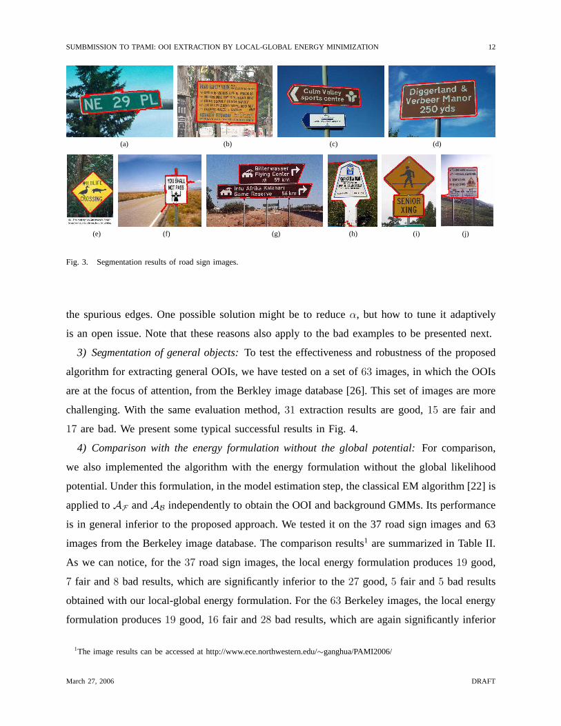
2) Segmentation of road sign images:We have collected a set of37 road sign images in

which the road signs are at the focus of attention. It contains road signs of different shapes and

different poses with a large variety of backgrounds. We asked 7 people to evaluate the quality of

the extraction results by giving a rating of “good”, “fair” or “bad” to each image. The majority

rule is adopted to categorize each result. Overall there are27 good,5 fair and5 bad. Some of

the successful results are shown in Fig. 3.

Two reasons may cause the unsatisfactory results: (1). The OOIs are too small or too thin in

the images. In that case, the initial OOI region may contain alarge number of background pixels.

(2). There are very strong spurious edges surrounding the OOI while there is not enough contrast

between the foreground and the background colors to overcome the biased energy force from



(a) (b) (c) (d)

(e) (f) (g) (h) (i) (j)

Fig. 3. Segmentation results of road sign images.

the spurious edges. One possible solution might be to reduceα, but how to tune it adaptively

is an open issue. Note that these reasons also apply to the badexamples to be presented next.

3) Segmentation of general objects:To test the effectiveness and robustness of the proposed

algorithm for extracting general OOIs, we have tested on a set of 63 images, in which the OOIs

are at the focus of attention, from the Berkley image database [26]. This set of images are more

challenging. With the same evaluation method,31 extraction results are good,15 are fair and

17 are bad. We present some typical successful results in Fig. 4.

4) Comparison with the energy formulation without the global potential: For comparison,

we also implemented the algorithm with the energy formulation without the global likelihood

potential. Under this formulation, in the model estimationstep, the classical EM algorithm [22] is

applied toAF andAB independently to obtain the OOI and background GMMs. Its performance

is in general inferior to the proposed approach. We tested iton the 37 road sign images and 63

images from the Berkeley image database. The comparison results1 are summarized in Table II.

As we can notice, for the37 road sign images, the local energy formulation produces19 good,

7 fair and8 bad results, which are significantly inferior to the27 good,5 fair and5 bad results

obtained with our local-global energy formulation. For the63 Berkeley images, the local energy

formulation produces19 good,16 fair and28 bad results, which are again significantly inferior

1The image results can be accessed at http://www.ece.northwestern.edu/∼ganghua/PAMI2006/



(a) (b) (c) (d)

(e) (f) (g) (h) (i)

(j) (k) (l) (m) (n)

Fig. 4. Extract OOIs on Berkeley image database.

TABLE II

COMPARISON RESULTS OF THE PROPOSED LOCAL-GLOBAL VARIATIONAL ENERGY FORMULATION AND THE VARIATIONAL

ENERGY FORMULATION WITHOUT THE GLOBAL POTENTIAL TERM ON THEROAD SIGN IMAGES AND BERKELEY IMAGES.

Local-global Formulation Local Formulation

Good Fair Bad Good Fair Bad

Road Sign Images 27 5 5 19 7 8

Berkeley Images 31 15 17 20 16 27

Overall 58 20 22 38 23 36

to the results obtained with our approach.

For one-on-one comparison on each image, we also found that the extraction results from our

local-global energy formulation is always superior to those from the local energy formulation.

In other words, whenever the local energy formulation produces a good result, our approach

can also produce a good result if not better. On the other hand, on a significant number of test

images, our approach produced good results while the local energy formulation failed. It is the



global image likelihood potential that makes this difference. It enables the model estimation step

to be more accurate.

VI. CONCLUSION AND FUTURE WORK

We have proposed a novel local-global variational energy formulation to automatically extract

OOI from images, and developed an efficient iterative schemeto minimize it. Our main con-

tributions are: (1) the incorporation of a global image likelihood potential for better estimating

the OOI and background models, and (2) a set of fixed-point equations which we call quasi-

semi-supervised EM for robust estimation of GMMs from inaccurately labeled data. Extensive

experiments demonstrated the efficacy of our approach. Future work includes extending the

variational energy formulation for automatic extraction of multiple objects.

ACKNOWLEDGMENT

The authors thank the reviewers for their constructive suggestions. The majority of the work

was carried out when Gang Hua was a summer intern at MicrosoftResearch, Redmond.

REFERENCES

[1] S. C. Zhu and A. Yuille, “Region competition: Unifying snakes, region growing, and bayes/mdl for multiband image

segmentation,”IEEE Transaction on Pattern Recognition and Machine Intelligence, vol. 18, no. 9, pp. 884–900, 9 1996.

[2] N. Paragios and R. Deriche, “Geodesic active regions andlevel set methods for supervised texture segmentation,”

International Journal of Computer Vision, pp. 223–247, 2002.

[3] A. Blake, C. Rother, M. Brown, P. Perez, and P. Torr, “Interactive image segmentation using an adaptive gaussian mixture

mrf model,” in Proc. of the 8th European Conference on Computer Vision, Prague, Czech Republic, 2004, pp. 428–441.

[4] C. Rother, V. Kolmogorov, and A. Blake, ““grabcut”– interactive foreground extraction using iterated graph cuts,”ACM

Transactions on Graphics (SIGGRAPH’04), pp. 309–314, 2004.

[5] M. Rousson, T. Brox, and R. Deriche, “Active unsupervised texture segmentation on a diffusion based feature space,”

in Proc. of IEEE Conference on Computer Vision and Pattern Recognition, vol. 2, Madison, Wisconsin, June 2003, pp.

699–704.

[6] M. Kass, A. Witkin, and D. Terzopoulos, “Snakes: Active contour models,”International Journal of Computer Vision,

vol. 1, pp. 321–331, 1987.

[7] D. Mumford and J. Shah, “Optimal approximations by piecewise smooth functions and associated variational problem,”

Communications on Pure and Applied Mathematics, vol. 42, pp. 577–684, 1989.

[8] A. Tsai, J. Anthony Yezzi, and A. S. Willsky, “A curve evolution approach to smoothing and segmentation using the

mumford-shah functional,” inProc. of IEEE Conference on Computer Vision and Pattern Recognition, Hilton Head Island,

South Carolina, June 2000, pp. 1119–1124.



[9] L. D. Cohen and I. Cohen, “Finite-element methods for active contour models and balloons for 2-d and 3-d images,”IEEE

Transaction on Pattern Analysis and Machine Intelligence, vol. 15, no. 11, pp. 1131–1147, 11 1993.

[10] V. Casselles, R. Kimmel, and G. Sapiro, “Geodesic active contours,”International Journal of Computer Vision, vol. 22,

no. 1, pp. 61–79, 1997.

[11] N. Paragios, O. mellina Gottardo, and V. Ramesh, “Gradient vector flow fast geodesic active contours,” inProc. of IEEE

International Conference on Computer Vision, Vancouver, Canada, July 2001, pp. 67–73.

[12] J. Anthony Yezzi, A. Tsai, and A. S. Willsky, “A statistical approach to snakes for bimodal and trimodal imagery,” in

Proc. of IEEE International Conference on Computer Vision, Kerkyra, Corfu, Greece, September 1999, pp. 898–903.

[13] T. F. Chan and L. A. Vese, “Active contours without edges,” IEEE Transaction on Image Processing, vol. 10, no. 2, pp.

266–277, Feburary 2001.

[14] S. Jehan-Besson, M. Barlaud, and G. Aubert, “Video object segmentation using eulerian region-based active contours,” in

Proc. of IEEE International Conference on Computer Vision, vol. 1, Vancouver, Canada, July 2001, pp. 353–361.

[15] J. Kim, J. W. F. III, A. J. Yezzi, M. Cetin, and A. S. Willsky, “A nonparametric statistical method for image segmentation

using information theory and curve evolution,”IEEE Transaction on Image Processing, vol. 14, no. 10, pp. 1486–1502,

Octobor 2005.

[16] N. Paragios and R. Deriche, “Geodesic active contours for supervised texture segmentation,” inIEEE Conference on

Computer Vision and Pattern Recognition, vol. 1, 1999, pp. 1034–1040.

[17] S. Jehan-Besson, M. Barlaud, and G. Aubert, “Shape gradients for histogram segmentation using active contours,” in Proc.

of IEEE International Conference on Computer Vision, vol. 1, Nice,Cote d’Azur,France, Octobor 2003, pp. 408–415.

[18] C. Samson, L. Blanc-Feraud, G. Aubert, and J. Zerubia,“A level set model for image classification,”International Journal

of Computer Vision, vol. 40, no. 3, pp. 187–197, March 2000.

[19] S. Osher and J. A. Sethian, “Fronts propagating with curvature-dependent speed: algorithms based on hamilton-jacobi

formulation,” Journal of Computational Physics, vol. 79, pp. 12–49, 1988.

[20] R. Malladi, J. A. Sethian, and B. C. Vemuri, “Shape modeling with front propagation: a level set approach,”IEEE

Transaction on Pattern Analysis and Machine Intelligence, vol. 17, no. 2, pp. 158–175, Feburary 1995.

[21] N. D. Lawrence and B. Scholkopf, “Estimating a kernel fisher discriminant in the presence of label noise,” inProc. of

the International Conference in Machine Learning, C. Brodley and A. P. Danyluk, Eds. San Francisco, CA: Morgan

Kauffman, 2001, pp. 306–313.

[22] A. P. Dempster, N. M. Laird, and D. B. Rubin, “Maximum likelihood from incomplete data via the em algorithm,”Journal

of the Royal Statistical Society, Series B, vol. 39, no. 1, pp. 1–38, 1977.

[23] A. Corduneanu and T. Jaakkola, “Continuation methods for mixing heterogenous sources,” inProc. of Uncertaity in

Artificial Intelligence, 2002, pp. 111–118.

[24] X. Zhu, J. Yang, and A. Waibel, “Segmenting hands of arbitrary color,” in Proc. IEEE International Conference on

Automatic Face Recognition. Grenoble, France: IEEE Computer Society, March 2000, pp. 446–453.

[25] D. Comaniciu and P. Meer, “Mean-shift: A robust approach toward feature space analysis,”IEEE Transaction on Pattern

Analysis and Machine Intelligence, vol. 24, no. 5, pp. 1–18, May 2002.

[26] D. Martin, C. Fowlkes, D. Tal, and J. Malik, “A database of human segmented natural images and its application to

evaluating segmentation algorithms and measuring ecological statistics,” in8th IEEE International Conference on Computer

Vision, vol. 2, July 2001, pp. 416–423.


Iterative local-global energy minimization for automatic extraction of object of interest

Documents

Transcript of Iterative local-global energy minimization for automatic extraction of object of interest