Iterative least square phase-measuring method that tolerates extended finite bandwidth illumination

Iterative least square phase-measuring method thattolerates extended finite bandwidth illumination

Florin Munteanu and Joanna Schmit*Veeco Instruments Inc., 2650 East Elvira Road, Tucson, Arizona 85711, USA

*Corresponding author: [email protected]

Received 10 October 2008; revised 15 January 2009; accepted 23 January 2009;posted 26 January 2009 (Doc. ID 102551); published 19 February 2009

Iterative least square phase-measuring techniques address the phase-shifting interferometry issue ofsensitivity to vibrations and scanner nonlinearity. In these techniques the wavefront phase and phasesteps are determined simultaneously from a single set of phase-shifted fringe frames where the phaseshift does not need to have a nominal value or be a priori precisely known. This method is commonly usedin laser interferometers in which the contrast of fringes is constant between frames and across the field.We present step-by-step modifications to the basic iterative least square method. These modificationsallow for vibration insensitive measurements in an interferometric system in which fringe contrast var-ies across a single frame, as well as from frame to frame, due to the limited bandwidth light source andthe nonzero numerical aperture of the objective. We demonstrate the efficiency of the new algorithmwithexperimental data, and we analyze theoretically the degree of contrast variation that this new algorithmcan tolerate. © 2009 Optical Society of America

OCIS codes: 120.3180, 120.5050, 120.7280, 180.3170.

1. Introduction

Phase-measuring techniques, which are often usedin interferometers or fringe projection systems, arerecognized for their precise, full-field surface profil-ing. These phase-measuring interferometers areused to measure optically smooth surfaces that rangefrom a few micrometers to a few meters in length, insetups that range frommicroscopes to large aperturesystems. Objects such as lenses, mirrors, silicon wa-fers, micromirror arrays, and the surfaces of themag-netic heads used to read hard drives can bemeasuredwith subnanometer vertical resolution in a matter ofseconds. During measurement, the phase differencebetween two coherent interfering beams is continu-ously changed as the object is scanned along the op-tical axis and frames of interference data arecollected with a CCD camera.The most common phase-measuring method, the

phase-shifting interferometry (PSI) technique [1,2],assumes that the phase shift between collected

frames is constant and of specific value, with themost common value being 90°. The quality of PSImeasurements depends on the phase difference be-tween consecutive frames remaining the same dur-ing the scan. Any factor that causes a change instep size, such as equipment vibrations, scanner non-linearities, or air turbulence, can affect the perfor-mance of the algorithm and produce a phase ripplein the measurement result, which has a characteris-tic signature of following the fringes but with twicethe fringe frequency. Many PSI algorithms aredesigned to correct for miscalibrations and slowchanges in step size due to scanner nonlinearity orsome slow vibrations [3–8].

However, the biggest challenge of these algorithmsremains their sensitivity to random changes in stepsize and certain vibration frequencies [8–10] despitethe very short measurement time. If the phase stepsare not equal but are precisely known, a least squaremethod could be employed. This method is a moregeneral PSI algorithm designed for these specificphase steps. The LS methods were first proposedby Morgan [11] and then generalized and simplifiedby Greivenkamp [12]. Other methods were then

0003-6935/09/061158-10$15.00/0© 2009 Optical Society of America

1158 APPLIED OPTICS / Vol. 48, No. 6 / 20 February 2009

developed to calculate the phase step betweenframes but, unfortunately, these step sizes werenot determined precisely and often added an addi-tional level of system difficulty. In these other meth-ods the steps between frames were first determinedduring the calibration process before any measure-ment was taken. Lai and Yatagai [13] sought to avoidthe precalibration process by collecting fringes froman object and a tilted mirror simultaneously, and cal-culating the phase steps from parallel carrier fringes.Subsequent methods that recognized the importanceof knowing the phase steps beforehand determinedthe phase steps directly from the collected interfero-grams. Farrell and Player [14] proposed Lissajousfigures to calculate steps between frames using onlymeasured interferograms. Van Brug [15] extractedphase shifts from the correlation between two inter-ferograms with carrier fringes, while Goldberg andBokor [16] proposed Fourier transform (similar toLai and Yatagai) to retrieve the phase steps fromtwo interferograms with carrier fringes. Guo et al.[17] based their phase shift calculations on an energyminimum algorithm.Conversely, more accurately knowing the phase

distribution from a better approximation of phasesteps allows for a more accurate step size determina-tion. Almost two decades ago this idea led to the de-velopment of an iterative approach in the leastsquare method (LSM) for phase measurement thateffectively reduced phase ripple error due to randomsteps [18]. However, calculation times were long and,in order to speed up and simplify the calculation pro-cess, different assumptions about the recorded inten-sities were proposed [19–26]. Faster computers ledsome authors to look at the statistical aspect ofthe measurements and local or global optimizationmethods were proposed. Some research even focusedon solutions for phase steps with spatial nonunifor-mity [27,28] or an interferogram’s background andmodulation with spatial nonuniformity [29]. How-

ever, this solution was achieved by dividing the inter-ferogram into subregions where values of theseparameters are considered uniform. The iterativetechniques that have been developed work best withmonochromatic illumination and zero numericalaperture systems that assure uniform fringe contrastover the planar and depth coordinates. However, var-iances in fringe contrast may cause a phase-ripple er-ror in the measurement. Our approach improves thecapability of iterative algorithms; we developed amodified iterative LSM for phase measuring thatis relatively insensitive to some variations in fringecontrast due to a limited source bandwidth and anonzero numerical aperture [30]. Here we presentin more depth a simple variable change mechanismthat overcomes the coupling that occurs between theplanar and depth coordinates and allows for a seam-less integration with the standard least square pro-cedure. We also present limitations analysis of thismethod imposed by the source bandwidth.

2. Separation of Terms Dependent on Step Size andPhase in Interference Fringes with Varying Contrast

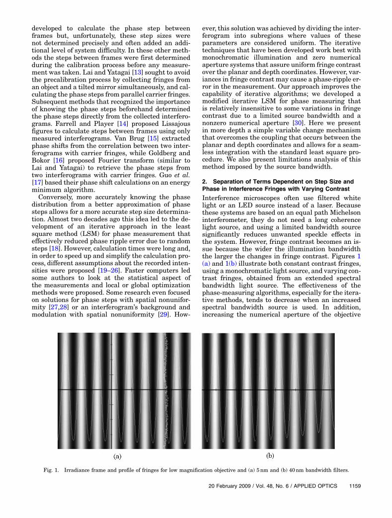
Interference microscopes often use filtered whitelight or an LED source instead of a laser. Becausethese systems are based on an equal path Michelsoninterferometer, they do not need a long coherencelight source, and using a limited bandwidth sourcesignificantly reduces unwanted speckle effects inthe system. However, fringe contrast becomes an is-sue because the wider the illumination bandwidththe larger the changes in fringe contrast. Figures 1(a) and 1(b) illustrate both constant contrast fringes,using amonochromatic light source, and varying con-trast fringes, obtained from an extended spectralbandwidth light source. The effectiveness of thephase-measuring algorithms, especially for the itera-tive methods, tends to decrease when an increasedspectral bandwidth source is used. In addition,increasing the numerical aperture of the objective

Fig. 1. Irradiance frame and profile of fringes for low magnification objective and (a) 5nm and (b) 40nm bandwidth filters.

20 February 2009 / Vol. 48, No. 6 / APPLIED OPTICS 1159

negatively affects the precision of the measurementwhen using iterative methods. These fringes must bedescribed in special forms if they are to be used initerative technique. The following equation is gener-ally used to represent the relationship between theirradiance I of a monochromatic light source of wave-length λ0 measured at each pixel x, y and the scan-ning position tk at each acquisition frame k:

Iðx; y; tk; λ0;φðx; y; λ0ÞÞ ¼ Bðx; y; tk; λ0Þ þMðx; y; tk; λ0Þ× cosðφðx; y; λ0Þ − tkðλ0ÞÞ; ð1Þ

where the phase and phase step are defined as

φðx; y; λ0Þ≡4πλ0

�hobj

0 − href0�; ð2aÞ

tkðλ0Þ≡4πλ0

zk: ð2bÞ

Here I is a function of surface position x, y, scanningposition zk, which is constant over the full field, andwavelength λ0. hobj0 and href0 are the height positionsof the object and reference surfaces, respectively, atthe beginning of the scan and B and M are back-ground and modulation amplitude parameters, func-tions of x, y, zk, and λ0. Note that zk is also a measureof the optical path change between the reference andtest beams of the interferometer during the scan. Ifnothing else is specified, all irradiance equations willbe considered to be written for a particular surfaceposition ðx; yÞ. This equation for the purpose of itera-tive least square phase-measuring technique is com-monly rewritten using trigonometric relations intothe following formula, where, for each term in thesummation, the dependence upon the step sizetkðλ0Þ and that upon the phase φðx; y; λ0Þ are comple-tely separable [18–26]:

Iðtk; λ0;φÞ ¼ Bðtk; λ0Þ þMðtk; λ0Þ cosðtkðλ0ÞÞ cosðφðλ0ÞÞþMðtk; λ0Þ sinðtkðλ0ÞÞ sinðφðλ0ÞÞ: ð3Þ

In the case of a source with an extended spectralbandwidth, the value of the intensity recorded bythe CCD will be obtained by integrating Eq. (3) overthe entire bandwidth. Because of the complicatedwavelength dependence, the variables φ and tk willnot be separable anymore. Thus, we had to createa model where the irradiance of fringes is expressedas a sum of terms for which the dependence of phaseand steps between frames is completely separable, asrequired by the standard LSM algorithm [30]. Forthis, we first summed the interference signals (fromEq. (1)) for two wavelengths ðλ0 −ΔλÞ and ðλ0 þΔλÞ

to obtain

Iðtk; λ0;Δλ;φÞ ≅ Bðtk; λ0 −ΔλÞ þMðtk; λ0 −ΔλÞ

× cos�4πλ0

�1þΔλ

λ0

�ðhobj

0 − href0 − zkÞ

�

þ Bðtk; λ0 þΔλÞ þMðtk; λ0 þΔλÞ

× cos�4πλ0

�1 −

Δλλ0

�

× ðhobj0 − href

0 − zkÞ�: ð4Þ

Defining

h≡Δλλ0

; hM ≡ΔλMλ0

;

B≡ Bðtk; λ0 −ΔλÞ þ Bðtk; λ0 þΔλÞ;M ≡Mðtk; λ0 −ΔλÞ; N ≡Mðtk; λ0 þΔλÞ:

The above formula for irradiance can be written

Iðtk; λ0;h;φÞ ¼ BþM cos½ðφ − tkÞð1þ hÞ�þN cos½ðφ − tkÞð1� hÞ�;

Iðtk; λ0;h;φÞ ¼ B − ðM −NÞ sin½hðφ − tkÞ� sinðφ − tkÞþ ðM þNÞ cos½hðφ − tkÞ� cosðφ − tkÞ: ð5Þ

Integrating this formula over the entire bandwidth isequivalent with integrating over h from 0 to hM.After the integration, we must also include the effectof the numerical aperture on fringes as a multiplica-tive factor: sinðβ � tkÞ=ðβ � tkÞ where β ¼ ½1 −

cosðΘMaxÞ�=2 [31]. Such multiplication is valid onlyfor relatively small NA. The value for the recordedirradiance becomes [30]

INAðtk;φÞ ¼ BNAðtkÞ þ ½QNAðφ; tkÞ cosðφÞþ PNAðφ; tkÞ sinðφÞ� cosðtkÞþ ½QNAðφ; tkÞ sinðφÞ − PNAðφ; tkÞ× cosðφÞ� sinðtkÞ; ð6Þ

where the following quantities are defined as

BNAðtkÞ≡ BsinðβtkÞ

βtk;

QNAðφ; tkÞ≡QsinðβtkÞ

βtk¼

�Meff ðtkÞ þNeff ðtkÞ

�

×sin½hMðφ − tkÞ�

ðφ − tkÞsinðβtkÞ

βtk;

PNAðφ; tkÞ≡ PsinðβtkÞ

βtk¼

�Meff ðtkÞ −Neff ðtkÞ

�

×cos½hMðφ − tkÞ� − 1

ðφ − tkÞsinðβtkÞ

βtk:


In the last step we have used the integral mean the-orem for continuous functions and we have definedthe new valuesMeff andNeff as the result of integrat-ing MðhÞ and NðhÞ over the wavelength.

3. Step-by-Step Explanation of Modified Iterative LeastSquare Phase-Measuring Technique for Small Degreeof Fringe Contrast Variation

So far we have derived a form of an equation for in-terference fringes that accounts for the influence ofthe wavelength bandwidth and numerical aperture.We can see that, for the monochromatic light andzero numerical aperture, this equation reduces tothe standard equation solved in the literature byan iterative LSM (hM ≅ 0 ⇒ PNA ≅ 0):

Iðx; y; tk;φÞ ¼ Bðx; y; tkÞ þQðx; y; tkÞ× cosðtkÞ cosðφðx; yÞÞþQðx; y; tkÞ sinðtkÞ sinðφðx; yÞÞ; ð7Þ

where we have shown the explicit x and y depen-dence. The phase-dependent (φ) and z-dependent(tk) variables are assumed to be completely separablealso in background (B) andmodulation amplitude (Q)of signal [18,29]:

Iðx; y; tk;φÞ ¼ B1ðx; yÞB2ðtkÞ þQ1ðx; yÞQ2ðtkÞ× cos½φðx; yÞ� cosðtkÞ þQ1ðx; yÞQ2ðtkÞ× sin½φðx; yÞ� sinðtkÞ ¼ B1ðx; yÞB2ðtkÞþ ½Q1ðx; yÞ cos½φðx; yÞ��× ½Q2ðtkÞ cosðtkÞ� þ ½Q1ðx; yÞ sin½φðx; yÞ��× ½Q2ðtkÞ sinðtkÞ�: ð8Þ

As stated before, this equation has received a lot ofattention in the literature. The preferred way of sol-ving it is the iterative LSM [18], which starts by firstdefining an error function and then trying to mini-mize this error function with respect to two sets ofvariables:

fB1ðx; yÞ; ½Q1ðx; yÞ cosðφÞ�; ½Q1ðx; yÞ sinðφÞ�g; ð9aÞ

fB2ðtkÞ; ½Q2ðtkÞ cosðtkÞ�; ½Q2ðtkÞ sinðtkÞ�g; ð9bÞ

by successive iterations.Unfortunately, this general method cannot be

applied directly to the general equation of fringes (re-written here for convenience with x and y depen-dence shown explicitly):

INAðx; y; tk;φÞ ¼ BNAðx; y; tkÞ þ ½QNAðx; y;φ; tkÞ cosðφÞþ PNAðx; y;φ; tkÞ sinðφÞ� cosðtkÞþ ½QNAðx; y;φ; tkÞ sinðφÞ− PNAðx; y;φ; tkÞ cosðφÞ� sinðtkÞ; ð10Þ

due to the strong coupling between the (φ and tk)variables in the terms

½QNAðx; y;φ; tkÞ cosðφÞ þ PNAðx; y;φ; tkÞ sinðφÞ�;ð11aÞ

½QNAðx; y;φ; tkÞ sinðφÞ − PNAðx; y;φ; tkÞ cosðφÞ�: ð11bÞ

We propose a modified version of the standardLSM algorithm that can be used to eliminate thisproblem.

Step 1: Assume that the x, y, and tk variables inthe background function Bðx; y; tkÞ can be decoupledand make the following notations:

BNAðx; y;φ; tkÞ≡ B1ðx; yÞB2ðtkÞ;Cðx; y;φ; tkÞ≡QNAðx; y;φ; tkÞ cos½φðx; yÞ�

þ PNAðx; y;φ; tkÞ sin½φðx; yÞ�;Sðx; y;φ; tkÞ≡QNAðx; y;φ; tkÞ sin½φðx; yÞ�

− PNAðx; y;φ; tkÞ cos½φðx; yÞ�;CosðtkÞ≡ cosðtkÞ; SinðtkÞ≡ sinðtkÞ: ð12Þ

The role of the last two definitions is to indicate that,during the iteration algorithm, the numerical valuesdetermined for sinðtkÞ and cosðtkÞ are expected to beonly proportional to the real “sin” and “cos” functions(SinðtkÞ ¼ E sinðtkÞ;CosðtkÞ ¼ E cosðtkÞ) and offer away of determining the plane separations from therelation tanðtkÞ ¼ SinðtkÞ

CosðtkÞ.With these notations, the irradiance equation can

be rewritten as

Iðx; y; tk;φÞ ¼ B1ðx; y;φÞB2ðtkÞ þ Cðx; y;φ; tkÞCosðtkÞþ Sðx; y;φ; tkÞSinðtkÞ: ð13Þ

Step 2: Define the error function:

TðB1;B2;C;S;CosðtkÞ;SinðtkÞÞ≡

Xx

Xy

Xk

½Iðx; y;φ; tkÞ − B1ðx; yÞB2ðtkÞ

− Cðx; y;φ; tkÞCosðtkÞ − Sðx; y;φ; tkÞSinðtkÞ�2: ð14Þ

Step 3: We start with a guess set or values for B20

and t0k:


B20ðtk0Þ ¼ 1; tk0 ¼ kΔt ⇒ Cosðtk0Þ

¼ cosðkΔtÞ;Sinðtk0Þ ¼ sinðkΔtÞ;

ð15Þ

and minimize the error function (T) with respect toB1, C, and S by solving the equations

∂T∂B1

¼ ∂T∂C

¼ ∂T∂S

¼ 0: ð16Þ

Step 4: So far, we have followed the same proce-dure described in the literature, but we notice nowthat the values of Cðx; y;φ; tkÞ and Sðx; y;φ; tkÞ con-tain a strong coupling between the φ and tk variables.In order to proceed, we need to replace the set of vari-ables ½Cðx; y;φ; tkÞ;Sðx; y;φ; tkÞ� with a new set½C1ðx; y;φÞ;S1ðx; y;φÞ� and rewrite the irradianceequation in the form

Iðx; y; tk;φÞ ¼ B1ðx; y; ÞB2ðtkÞ þ C1ðx; y;φÞCosðtkÞþ S1ðx; y;φÞSinðtkÞ; ð17Þ

where the original C and S dependence upon tk ismoved into the variables CosðtkÞ and SinðtkÞ to be de-termined in the next step of the iteration.The easiest approach to our variable change is to

determine a new set of values ½aðtkÞ; bðtkÞ� such that

Cðx; y;φ; tkÞ ¼ aðtkÞC1ðx; y;φÞ þ bðtkÞS1ðx; y;φÞ;Sðx; y;φ; tkÞ ¼ aðtkÞS1ðx; y;φÞ − bðtkÞC1ðx; y;φÞ: ð18Þ

This form of the replacement equations is suggestedby the original forms of the C and S variables:

Cðx; y;φ; tkÞ≡QNAðx; y;φ; tkÞ cos½φðx; yÞ�þ PNAðx; y;φ; tkÞ sin½φðx; yÞ�;

Sðx; y;φ; tkÞ≡QNAðx; y;φ; tkÞ sin½φðx; yÞ�− PNAðx; y;φ; tkÞ cos½φðx; yÞ�: ð19Þ

In the following steps we will not be showing the ex-plicit dependence in ðx; yÞ. Imposing the conditionC1

2 þ S12 ¼ 1, we obtain C2 þ S2 ¼ a2 þ b2, then

8<:

C1ðφÞ ¼ aCðφ;tkÞ−bSðφ;tkÞa2þb2

¼ aCðφ;tkÞ−bSðφ;tkÞCðφ;tkÞ2þSðφ;tkÞ2

S1ðφÞ ¼ aSðφ;tkÞþbCðφ;tkÞa2þb2

¼ aSðφ;tkÞþbCðφ;tkÞCðφ;tkÞ2þSðφ;tkÞ2

: ð20Þ

Substituting these values into the irradiance expres-sion (Eq. (17)), we obtain

I ¼ B1B2 þaCðφ; tkÞ − bSðφ; tkÞCðφ; tkÞ2 þ Sðφ; tkÞ2

CosðtkÞ

þ aSðφ; tkÞ þ bCðφ; tkÞCðφ; tkÞ2 þ Sðφ; tkÞ2

SinðtkÞ

¼ B1B2 þCðφ; tkÞ

Cðφ; tkÞ2 þ Sðφ; tkÞ2½aCosðtkÞ�

þ Sðφ; tkÞCðφ; tkÞ2 þ Sðφ; tkÞ2

½aSinðtkÞ�

þ Cðφ; tkÞCðφ; tkÞ2 þ Sðφ; tkÞ2

½bSinðtkÞ�

−Sðφ; tkÞ

Cðφ; tkÞ2 þ Sðφ; tkÞ2½bCosðtkÞ�: ð21Þ

In order to simplify the notation we will redefine

CðφÞ≡ Cðφ; tkÞCðφ; tkÞ2 þ Sðφ; tkÞ2

;

SðφÞ≡ Sðφ; tkÞCðφ; tkÞ2 þ Sðφ; tkÞ2

; ð22Þ

where the new values of C and S will depend only onthe variable φ, and rewrite the irradiance equationas

I ¼ B1B2 þ CðφÞ½aðtkÞCosðtkÞ þ bðtkÞSinðtkÞ�þ SðφÞ½aðtkÞSinðtkÞ − bðtkÞCosðtkÞÞ�: ð23Þ

This defines a new error function:

TðB2;aCosðtkÞ; aSinðtkÞ; bCosðtkÞ; bSinðtkÞÞ¼

Xx

Xy

Xk

½I − B1B2

− C½aðtkÞCosðtkÞ þ bðtkÞSinðtkÞ�− S½aðtkÞSinðtkÞ − bðtkÞCosðtkÞÞ��2: ð24Þ

Step 5: Determine the new values

8><>:

B2ðtkÞ½aCosðtkÞ þ bSinðtkÞ�½aSinðtkÞ − bCosðtkÞÞ�

by minimizing the previous error function [Eq. (24)]and solving

∂T∂B2

¼ ∂T∂½aCosðtkÞ þ bSinðtkÞ�

¼ ∂T∂½aSinðtkÞ − bCosðtkÞÞ�

¼ 0: ð25Þ


Step 6: Use the error function

TðB1;C;SÞ ¼Xx

Xy

Xk

½I − B1B2

− C½aCosðtkÞ þ bSinðtkÞ�− S½aSinðtkÞ − bCosðtkÞ��2 ð26Þ

to determine the values of B1ðφÞ, CðφÞ, anad SðφÞ bysolving

∂T∂B1

¼ ∂T∂C

¼ ∂T∂S

¼ 0: ð27Þ

Step 7: Next, we continue with steps 2, 4, 5, and 6until the values for atan

haðtkÞSinðtkÞ−bðtkÞCosðtkÞÞaðtkÞCosðtkÞþbðtkÞSinðtkÞ

icon-

verge to a stationary solution for the phase step. Itcan be seen that this solution will be, in general,slightly different than the true frame-to-frame se-paration because of bðtkÞ ≠ 0. A side-by-side compar-ison between the standard LSM algorithm and theproposed one is shown schematically in Fig. 2.

4. Limits of Method Applicability

To analyze the practical limitations of the substitu-tion in Eq. (18), we need to analyze a full form of Cand S for which the detailed derivation can be foundin [30]. These expressions show a strong coupling be-tween the variables φ and tk in the definitions of C

and S:

C ¼�Meff þNeff

� sin½hMðφ − tkÞ�ðφ − tkÞ

cosðφÞ

þ�Meff −Neff

� cos½hMðφ − tkÞ� − 1ðφ − tkÞ

sinðφÞ;

S ¼�Meff þNeff

� sin½hMðφ − tkÞ�ðφ − tkÞ

sinðφÞ

−

�Meff −Neff

� cos½hMðφ − tkÞ� − 1ðφ − tkÞ

cosðφÞ: ð28Þ

It is impossible to find an analytical expression thatwould decouple these terms; thus, some approxima-tions need to be made. In the case that scientistshave been considering so far, meaning in the caseof monochromatic illumination, the value for hM ≡ΔλMλ0 is assumed to be close to zero. This implies that,for sine and cosine functions, the following first-orderapproximations hold:

sin½hMðφ − tkÞ� ≈ hMðφ − tkÞ; cos½hMðφ − tkÞ� ≈ 1:

ð29Þ

These approximations simplify Eq. (28) signifi-cantly and make the separation of terms dependenton phase φ and phase step value tk quite straight-forward.

Fig. 2. Flow charts of the (a) standard LSM algorithm and (b) the one we propose.


Because we are considering illumination with alarger spectral bandwidth, we will expand the“sin” and “cos” functions up to a quadratic term:

cos½hMðφ − tkÞ� − 1ðφ − tkÞ

≅1 −

½hMðφ−tkÞ�22 − 1

ðφ − tkÞ¼ −

hM2

2ðφ − tkÞ;

ð30aÞ

sin½hMðφ − tkÞ�ðφ − tkÞ

≅hMðφ − tkÞðφ − tkÞ

¼ hM : ð30bÞ

If we assume that the argument of the sin and cosfunctions has to be less than 0.5,

��hMðφ − tkÞ��≤ 0:5⇔

ΔλMλ0

��φ − tk��≤ 0:5

⇔ΔλM ≤0:5λ0��φ − tk

�� ; ð31Þ

the expressions in Eqs. (30) are correct within 4%.For the first-order approximations, the sin and cosfunction argument [Eq. (29)] must be smaller then0.28 in order to achieve the same accuracy (4%).With these second-order expansions the value of C

and S will then be simplified to

C ¼ ðMeff þNeff ÞhM cosðφÞ

− ðMeff −Neff ÞhM2

2ðφ − tkÞ sinðφÞ; ð32aÞ

S ¼ ðMeff þNeff ÞhM sinðφÞ

þ ðMeff −Neff ÞhM2

2ðφ − tkÞ cosðφÞ: ð32bÞ

After rearranging these expressions, S and C canbe written in a form close to Eq. (18):

C ¼ ðMeff þNeff ÞhM

�1 −

ðMeff −Neff ÞðMeff þNeff Þ

hM

2φ sinðφÞcosðφÞ

�

× cosðφÞ þ�ðMeff −Neff ÞhM

2

2tk

�sinðφÞ; ð33aÞ

S ¼ ðMeff þNeff ÞhM

�1þ ðMeff −Neff Þ

ðMeff þNeff ÞhM

2φ cosðφÞsinðφÞ

�

× sinðφÞ −�ðMeff −Neff ÞhM

2

2tk

�cosðφÞ: ð33bÞ

However, this form still carries unwanted expres-sions φ sinðφÞ and φ cosðφÞ, which appear in thefactors ðMeff−Neff Þ

ðMeffþNeff ÞhM2

φ sinðφÞcosðφÞ and ðMeff−Neff Þ

ðMeffþNeff ÞhM2

φ cosðφÞsinðφÞ , re-

spectively. These factors can be considered negligible

due to the fact that jMeff−Neff jjMeffþNeff j is very small for a

relatively symmetrical source and the value of hMis assumed to be smaller then 0.5.

With these approximations, the decoupling ofterms dependent on phase and phase step wasachieved and the values for C and S derived inEq. (18) are justified:

C ¼ ðMeff þNeff ÞhM cosðφÞ þhðMeff −Neff ÞhM

2

2tki

× sinðφÞ ¼ aC1ðφÞ þ bðtkÞS1ðφÞ;

S ¼ ðMeff þNeff ÞhM sinðφÞ −hðMeff −Neff ÞhM

2

2tki

× cosðφÞ ¼ aS1ðφÞ − bðtkÞC1ðφÞ: ð34Þ

We also have calculated the spectral bandwidthlimitations for the conventional and new LSM meth-ods to be performed on a flat mirror with five fringesacross it (�5π ≤ φ ≤ 5π) with wavelength centered atλ0 ¼ 700nm and eight frames separated by π=2(�2π ≤ tk ≤ 2π). Our criterion is based on the assump-tions that the sin and cos function expansions inEqs. (29) and (30) have to be within 4% of accuracy.This is achieved for hMðφ − tkÞ < 0:28 in the case ofthe conventionalLSMandhMðφ − tkÞ < 0:5 in the caseof the new LSM. The spectral bandwidth is then cal-culated from ΔλM ≤ 0:28

7π 700nm and ΔλM ≤ 0:57π 700nm,

resulting in 9nm allowed bandwidth for the conven-tional LSM and 16nm for the new LSM methods.

In other words, the method presented here is cap-able of almost doubling the efficiency of the standardLSM when spectral bandwidth and nonzero NA arepresent. It is also worth noting that, if a higher-orderexpansion of cos

hhMðφ − tkÞ

iand sin

hhMðφ − tkÞ

iis at-

tempted in Eqs. (30a) and (30b), then the C1 and S1factors would lose their linear relationship of cosðφÞand sinðφÞ, respectively. This, in turn, would lead todifficulties in recovering the value of the phase.

5. Experimental Results

The efficiency of our new least square method forphase measuring was tested on a series of data col-lected by the interferometric optical profiler. Forcomparison purposes we used three differentphase-measuring methods: eight-frame PSI [6], stan-dard iterative least square, and our iterative methodpresented here. For the purpose of presenting the ef-ficiency of this method, we have chosen a set of col-lected representative data with a nominal phase stepof 90° between frames for the flat mirror and the pre-sence of nine diagonal fringes. Data was collectedwith a 10× objective and NA ¼ 0:3 with 40nmFWHM bandwidth at 600nm central wavelength il-lumination. This objective and illumination sourceintroduces some degree of contrast degradation withfocus position. Because of random vibrations present


during the measurement, the steps were deviatingfrom the nominal values and following step valueswere calculated by the iterative algorithm: 80.0,92.1, 82.0, 94.2, 91.2, 82.2, and 92:7 °. The iterativeprocess converges quickly such that, after five orsix iterations, it achieves a relative error better thanone in a million in determining the phase separation.The results for the collected fringes are displayed

in Figure. 3. We see that, with random phase-stepdeviation from the nominal steps, the standardPSI algorithm suffers from a significant phase rippleat twice the frequency of the original fringes. For de-tails on phase ripple in different PSI algorithms, thereader is referred to other articles [32,33]. The stan-dard LSM algorithm also results in a phase ripple,not from random phase-step errors, but from the ef-fect of the illumination bandwidth and the numericalaperture. The last figure shows that the proposedLSM method effectively decouples the planar anddepth variables and, in doing so, is not prone to er-rors due to the presence of random steps or nonzeronumerical aperture.To investigate to what degree of fringe contrast var-

iation the new algorithm is able to tolerate, we col-lected one set of data with a 10nm bandpass filterand a 5× objective and the second set of data with a

40nm bandpass filter and 10× objective, where the10× objective further increases the degradation offringe contrast. Instead of random step deviations,we have introduced vibrations of frequencies (in5Hz increments) that the system may be affectedby, for example, different motors that control the sys-tem or machinery working nearby. We introduced vi-brationsbyapplying a sinewave of aknown frequencyand amplitude to a PZT stack with a flat mirror at-tached to it. The presence of a ripple in the measuredphase was gauged by recording a root mean square(RMS) parameter. The applied sine wave signal hadan amplitude of 2V (4V range) and a fringe deviationof approximately 20nm was produced. Figure. 4shows RMS values for both sets of fringes and differ-ent frequencies. The new LSM algorithm applied todata collected with the 40nm filter results, overall,in higher noise thanwith the 10nm filter. Some smalldegree of fringe ripple starts becoming visible at themost critical frequency for PSI. Thus, the same datacollected with the 10nm filter was analyzed with theeight-frame PSI algorithm. This and many other PSIalgorithms with nominal 90° steps are most sensitiveto vibrations of frequencies at half of the cameraframe rate [9] and are very sensitive to vibrations1.5, 2.5, and so on, of the camera rate; this fact is

Fig. 3. Flat mirror measured using (a) the PSI method, Ra ¼ 0:99nm; (b) the standard LSM, Ra ¼ 1:31nm; and (c) the proposed LSM,Ra ¼ 0:67nm. All three measurements were calculated from a set of the same fringe frames, of which one frame is presented in (d).


confirmed by the high peaks of RMS at these frequen-cies. On the other hand, the data analyzed with thenew LSMmethod shows that the new method is veryinsensitive to these vibrational frequencies but, forlarger bandwidth, overall the RMS of the measure-ment increases and sensitivity to vibrations at halfof the camera rate slightly increases.

We also took ameasurement with the 10× objectiveand 40nm bandpass filter with a scratched sphericalsurface in the presence of random phase step errors.Even if the used bandpass is larger than the calcu-lated bandpass limit, we find that the new LSMmethod resulted in a smaller phase ripples thanthe PSI method (see Fig. 5).

Fig. 4. Measure of the proposed LSM method performance for data collected with a 5× objective, 0.13NA, and a 10nm bandwidth filterand a 10× objective, 0.3 NA and a 40nm filter. For comparison, one data set was analyzed with the PSI method. Data was collected in thepresence of vibrations with a 60 fps camera.

Fig. 5. Surface of spherical surface with scratches measured with (a) PSI and (b) the new iterative least square method, and (c) one of theframes with fringes.


6. Conclusion

We presented step-by-step modifications to the basiciterative least square method, modifications that al-low for vibration insensitive measurements in an in-terferometric system in which fringe contrast variesacross a single frame, as well as from frame to frame,because of the limited bandwidth light source andnonzero numerical aperture of the objective. The re-sulting fringe contrast introduces a strong couplingbetween the phase and the steps in the irradiance for-mula. The proposed algorithm performs a decouplingof these parameters by using a simple variablechange.We demonstrated the efficiency of the new al-gorithm with experimental data for 10 and 40nm il-lumination bandwidths and 0.13 and 0.3 NAobjectives and compared the data to typical LSMand PSI methods. We also analyzed theoreticallythe degree of contrast variation that this new algo-rithm can tolerate and we concluded that the newLSM method can be easily used with a 16nm band-width in the presence of five fringes of tilt. The resultswith no ripple inmeasured phase allow for better pro-cess control in the measurement of object shape androughness aswell as detection of some process defectsthat otherwise could be buried in the phase ripple.

We would like to thank Matthew Pearl for collect-ing data.

References1. J. Bruning, D. H. Herriot, J. E. Gallagher, D. P. Rosenfeld, A. D.

White, and D. J. Brangccio, “Digital wavefront measuring in-terferometer for testing optical surfaces and lenses,” Appl.Opt. 13, 2693–2703 (1974).

2. K. Creath, “Temporal phase measurement methods,” inInterferogram Analysis: Digital Fringe Pattern MeasurementTechnique, D. W. Robinson and G. T. Reid, eds. (Institute ofPhysics, 1993), Chap. 4, pp. 94–140.

3. J. Schwider, “Advanced evaluation techniques in interfero-metry,” in Progress in Optics XXVIII, E. Wolf, ed. (Elsevier,1990), Chap. 4, pp. 271–359.

4. P. Hariharan, B. F. Oreb, and T. Eiju, “Digital phase-shiftinginterferometry: a simple error-compensating phase calulationalgorithm,” Appl. Opt. 26, 2504–2505 (1987).

5. J. Schmit and K. Creath, “Extended averaging technique forderivation of error-compensating algorithms in phase shiftinginterferometry,” Appl. Opt. 34, 3610–3619 (1995).

6. J. Schmit and K. Creath, “Window function influence on phaseerror in phase-shifting algorithms,” Appl. Opt. 35, 5642–5649(1996).

7. P. J. de Groot “Derivation of algorithms for phase-shifting in-terferometry using concept of a data-sampling window,” Appl.Opt. 34, 4723–4730 (1995).

8. D. W. Phillion, “General methods for generating phase-shifting interferometry algorithms,” Appl. Opt. 36, 8098–8115(1997).

9. P. J. de Groot and L. Deck, “Numerical simulations ofvibration in phase-shifting interferometry,” Appl. Opt.35,2172–2178 (1996).

10. M. Milman, “Optimization approach to the suppression of vi-bration errors in phase-shifting interferometry,” J. Opt. Soc.Am. A 19, 992–1004 (2002).

11. C. J. Morgan, “Least square estimation in phasemeasurementinterferometry,” Opt. Lett. 7, 368–370 (1982).

12. J. E. Greivenkamp, “Generalized data reduction for hetero-dyne interferometry,” Opt. Eng. 23, 350–352 (1984).

13. G. Lai and T. Yatagai, “Generalized phase shifting interfero-metry,” J. Opt. Soc. Am. A 8, 822–827 (1991).

14. C. T. Farrell and M. A. Player, “Phase step measurement andvariable step algorithms in phase-shifting interferometry,”Meas. Sci. Technol. 3, 953–958, (1992).

15. H. van Brug, “Phase-step calibration for phase-stepped inter-ferometry,” Appl. Opt. 38, 3549–3555 (1999).

16. K. A. Goldberg and J. Bokor, “Fourier-transform method ofphase-shift determination,” Appl. Opt. 40, 2886–2893 (2001).

17. C-S. Guo, Z-Y. Rong, J-L. He, H-T. Wang, L-Z. Cai, and Y-R.Wang, “Determination of global phase shifts between interfer-ograms by use of an energy-minimum algorithm,” Appl. Opt.42, 6514–6519 (2003).

18. K. Okada, A. Sato, and J. Tsujiuchi, “Simultaneous calculationof phase distribution and scanning phase shift in phase shift-ing interferometry,” Opt. Commun. 84, 118–124 (1991).

19. G-S. Han and S-W. Kim, “Numerical correction of referencephases in phase-shifting interferometry by iterative least-squares fitting,” Appl. Opt. 33, 7321–7325 (1994).

20. I.-B. Kong, and S.-W. Kim, “General algorithm of phase-shifting interferometry by iterative least-squares fitting,”Opt. Eng. 34, 183–187 (1995).

21. S.-W. Kim, M.-G. Kang, and G.-S. Han, “Accelerated phasemeasuring algorithm of least squares for phase shifting inter-ferometry,” Opt. Eng. 36, 3101–3106 (1997).

22. H. Huang, M. Itoh, T. Yatagai, “Phase retrieval of Phase Shift-ing interferometry with iterative least-squares fitting algo-rithm: experiments,” Opt. Rev. 6, 196–203 (1999).

23. C. Wei, M. Chen, and Z. Wang, “General phase-stepping algo-rithmwith automatic calibration of phase steps,”Opt. Eng. 38,1357–1360 (1999).

24. L. Z. Cai, Q. Liu, and X. L. Yang, “Phase-shift extraction andwave-front reconstruction in phase-shifting interferometrywith arbitrary phase steps,” Opt. Lett. 28, 1808–1810 (2003).

25. Z. Wang and B. Han, “Advanced iterative algorithm for phaseextraction of randomly phase shifted interferograms,” Opt.Lett. 29, 1671–1673 (2004).

26. H. Guo and M. Chen, “Least squares algorithm for phase-stepping interferometry with unknown relative step,” Appl.Opt. 44, 4854–4859 (2005).

27. H. Guo, M. Chen, and C. Wei, “New algorithm insensitive toboth translational and tilt phase-shifting error for phase-shifting interferometry,” Proc. SPIE 4101, 254–262 (2000).

28. J. Xu, Q. Xu, and L. Chai, “Iterative algorithm for phaseextraction from interferograms with random and spatiallynonuniform phase shifts,” Appl. Opt. 47, 480–485 (2008).

29. J. Xu, Q. Xu, and L. Chai, “An iterative algorithm for interfer-ograms with random phase shifts and high-order harmonics,”J. Opt. A Pure Appl. Opt. 10, 095004 (2008).

30. F. Munteanu and J. Schmit, “Iterative algorithm for phaseshifting interferometry with fine bandwidth illumination,”Proc. SPIE 7063, 70630L (2008).

31. A. Dubois, J. Selb, L. Vabre, and A.-C. Boccara, “Phase mea-surements with wide-aperture interferometers,” Appl. Opt.39, 2326–2331 (2000).

32. M. F. Küchel, “Some progress in phase measurementtechniques” Fringe’97 in Akademie Verlag Series in OpticalMetrology, W. Jüptner and W. Osten, eds. (1997), pp. 27–44.

33. J. H. Brunning, H. Schreiber, “Phase shifting interferometry,”in Optical Shop Testing, 3rd ed., D. Malacara, ed. (Wiley-InterScience, 2007), pp. 547–666.


Iterative least square phase-measuring method that tolerates extended finite bandwidth illumination

Documents

Transcript of Iterative least square phase-measuring method that tolerates extended finite bandwidth illumination