![KAVUR, Boris. Heads apart : the invisible history of the Servite monastery in Koper. Hortus artium medievalium, ISSN 1330-7274. [Print ed.], 2013, vol. 19, str. 417-423.](https://static.fdokumen.com/doc/165x107/63254866545c645c7f099ec1/kavur-boris-heads-apart-the-invisible-history-of-the-servite-monastery-in-koper.jpg)
ISSN (Print): 0972-6268; ISSN (Online) : 2395-3454 Vol. 19, No. 1 ...
428
ISSN (Print): 0972-6268; ISSN (Online) : 2395-3454 Vol. 19, No. 1, March, 2020
-
Upload
khangminh22 -
Category
Documents
-
view
1 -
download
0
Transcript of ISSN (Print): 0972-6268; ISSN (Online) : 2395-3454 Vol. 19, No. 1 ...

ISSN (Print): 0972-6268; ISSN (Online) : 2395-3454Vol. 19, No. 1, March, 2020

(An International Quarterly Scientific Research Journal)
EDITORS
Dr. P. K. Goel Dr. K. P. SharmaFormer Head, Deptt. of Pollution Studies Former Professor, Deptt. of BotanyY. C. College of Science, Vidyanagar University of RajasthanKarad-415 124, Maharashtra, India Jaipur-302 004, India
Published by : Mrs. T. P. Goel, B-34, Dev Nagar, Tonk Road, Jaipur-302 018Rajasthan, India
Managing Office : Technoscience Publications, A-504, Bliss Avenue, Balewadi,Pune-411 045, Maharashtra, India
E-mail : [email protected]; [email protected]
Scope of the JournalThe Journal publishes original research/review papers covering almost all aspects ofenvironment like monitoring, control and management of air, water, soil and noisepollution; solid waste management; industrial hygiene and occupational health hazards;biomedical aspects of pollution; conservation and management of resources;environmental laws and legal aspects of pollution; toxicology; radiation and recyclingetc. Reports of important events, environmental news, environmental highlights andbook reviews are also published in the journal.
Format of Manuscript• The manuscript (mss) should be typed in double space leaving wide margins on both the
sides.• First page of mss should contain only the title of the paper, name(s) of author(s) and
name and address of Organization(s) where the work has been carried out along with theaffiliation of the authors.
Continued on back inner cover...
INSTRUCTIONS TO AUTHORS
www.neptjournal.com
A-504, Bliss Avenue, Balewadi,Opp. SKP Campus, Pune-411 045
Maharashtra, India

Nature Environment and Pollution TechnologyVol. 19, No. (1), March, 2020
CONTENTS
1. Li Hai-hua, Chen Jie, Hua Yong-peng, Yan Shao-feng, E. Zheng-yang and Su Hang, Study on Removal ofThallium from Wastewater by Chitosan/Fly Ash Composite Adsorbent 1-15
2. Imane EL Adnani, Abdelkader Younsi, Khalid Ibno Namr, Abderrahim El Achheb and El Mehdi Irzan,Assessment of Seasonal and Spatial Variation of Groundwater Quality in the Coastal Sahel of Doukkala, Morocco 17-28
3. Baba Imoro Musah, Lai Peng and Yifeng Xu, Adsorption of Methylene Blue Using Chemically EnhancedPlatanus orientalis Leaf Powder: Kinetics and Mechanisms 29-40
4. Madhavi Tiwari, Ashish Saraf and Meghna Shrivastava, Comparative In Vitro Assessment of HydrocarbonDegradation Potential of Pleurotus ostreatus MP 5 and Pleurotus ostreatus MTCC 1804 41-56
5. Kshipra Shukla, Alka Verma, Lata Verma, Shalu Rawat and Jiwan Singh, A Novel Approach to Utilize UsedDisposable Paper Cups for the Development of Adsorbent and its Application for the Malachite Green and Rhodamine-B Dyes Removal from Aqueous Solutions 57-70
6. Huan Ma, Qingke Zhu, Xining Zhao and Yuan Liu, Assessing Ecological Conditions of Microtopography forVegetation Restoration on the Chinese Loess Plateau 71-82
7. Ying Huang, Zhi Zhou and Qin Qin, Analysis of Spatial Heterogeneity in Coupling Development ofIndustrialization and Resource Environmental Bearing Capacity 83-92
8. Arti Choudhary, Pradeep Kumar, Manisha Gaur, Vignesh Prabhu, Anuradha Shukla and SharadGokhale, Real World Driving Dynamics Characterization and Identification of Emission Rate MagnifyingFactors for Auto-rickshaw 93-101
9. C. Vasanth Pandiyan, Gunasekaran Shylaja, Gokul Raghavendra Srinivasan and Sujatha Saravanan,Studies on use of Cashew Nut Shell Liquid (CNSL) in Biopesticide and Biofertilizer 103-111
10. Hai-tao Chen, Xiao-nan Chen, Lin Qiu and Wen-chuan Wang, Multi-objective Ecological Operation ofReservoir in Luanhe River Based on Improved Particle Swarm Optimization 113-121
11. Wenjie Yao and Huili Wang, Macroscopic Factors Decomposition of Methane Emissions from LivestockBased on the Empirical Analysis of 31 Provinces in China 123-132
12. Zhou Zi-zhen, Huang Ting-lin, Gong Wei-jin, Li Yang, Liu Yue, Zhao Fu-wang, Zhou Shi-lei andDou Yan-yan, Field Research on Nitrogen Removal Performance of Aerobic Denitrifiers in Source WaterReservoir by Mixing Aeration 133-140
13. Rongbo Wu, Environmental Pollution and Energy Efficiency of Regional Transportation Industry: A Case Study ofJilin Province, China 141-147
14. Yanyan Dong, Manuel J. Lis Arias, Chengye Hu, Wendan Wu, Liping Liang, Xinlan Mou and Xu Meng,Preparation of Polyvinyl Alcohol/Graphene Oxide Composites and Their Adsorption Properties 149-157
15. Haitao Chen, Xiaonan Chen, Lin Qiu, Wenchuan Wang, Comprehensive Assessment of Water Supply Benefitsfor South-to-North Water Diversion in China from the Perspective of Water Environmental Carrying Capacity 159-168
16. Xingwang Wang, Jiwei Wang and Shuangqing Chen, Centrifugal Reduction Treatment Process for High-Water-Content Sludge in Oilfield 169-178
17. Yu Wan, Nan Shan, Sichen Tong, Yao Chen and Jia He, Nitrogen Occurrence Characteristics and ReasonAnalysis in Different Trophic Status Freshwater Lakes 179-189
18. Yafen Han, Qi Li and Na Liu, Heavy Metal Accumulation of 13 Native Plant Species Around a Coal GangueDump and Their Potentials for Phytoremediation 191-199
19. Prabhat Kumar Singh, Shruti and Anurag Ohri, Selecting Environmental Indicators for Sustainable SmartCities Mission in India 201-210
20. G. Ninawe† and M. Tariq, Impact of Carbon Nanotubes as Additives with Cotton Seed Biodiesel Blended withDiesel in Ci Engine - An Experimental Analysis 211-219
21. Jin Zhao, Yi Wang† and Zhengwei Ma, Factors Influencing the Environmental Performance of PrefabricatedBuildings: A Case Study of Community A in Henan Province of China 221-227
22. Shuyue Zhang, Minfeng Lin, Xiuguo Zou, Steven Su, Wentian Zhang, Xuhui Zhang and Zijie Guo,LSTM-based Air Quality Predicted Model for Large Cities in China 229-236
23. Chuang Ma, Bin Hu, FU-Yong Liu, Ai-Hua Gao, Ming-Bao Wei and Hong-Zhong Zhang, Changes inthe Microbial Succession During Sewage Sludge Composting and its Correlation with Physico-Chemical Properties 237-244
24. Ju Gao, Ting-fang Yu†, Lin Wang and Run-guo Chen, Numerical Analysis of Growth of Coal-fired ParticlesPromoted by Condensation of Water Vapour in Oversaturated Environment 245-251
25. Reni Ustiatik, Siska Nurfitriani, Amrullah Fiqri and Eko Handayanto, The Use of Mercury-ResistantBacteria to Enhance Phytoremediation of Soil Contaminated with Small-scale Gold Mine Tailing 253-261

26. Pawan Kumar and Vijay Laxmi Yadav, Performance Study of Cellulose Acetate Blended PolyvinylchlorideMembranes 263-268
27. Sachin Patil, Milind Kondalkar, Umesh Fegade, Sanjay Attarde and Sopan Ingle, Extraction andSpectrophotometric Estimation of Fe3+, Cd2+, Pb2+ and Zn2+ From Industrial Effluents Using SyntheticSupramolecular Ligand 269-275
28. Azaz Khan I. Pathan and P. G Agnihotr, 2-D Unsteady Flow Modelling and Inundation Mapping for LowerRegion of Purna Basin Using HEC-RAS 277-285
29. Akshatha K. U. and Hina Kousar, Removal of Nickel and Iron from Metal Injection Moulding IndustryEffluent by Adsorbent Method: A Comparative Study 287-293
30. Ju Gao, Ting-fang Yu, Run-guo Chen, Hao-jie Zhang and Lin Wang, Numerical Investigation ofHeterogeneous Nucleation of Supersaturated Water Vapour on Coal-fired PM
102
95-302
31. Jing Guo, Guodong Zhang, Fahong Zhang, Jiali Guo, Xiaozhong Sun and Biyun Sheng, Estimationof Evaporation Trends in Six Major River Basins of China Using a New Nonlinear Formula of the ComplementaryPrinciple of Bouchet 303-309
32. Noor Fhadzilah Mansur, Megat Ahmad Kamal Megat Hanafiah and Mardhiah Ismail, Pb(II) Adsorption ontoUrea Treated Leucaena leucocephala Leaf Powder: Characterization, Kinetics and Isotherm Studies 311-318
33. Wanchao Duan, Hang Xu, Hongna Ren, Qihui Men and Hangfei Fan, Degradation of Methylene Blue Wastewater by Fe2+ Coupling Persulphate Using Online UV-Vis Spectrophotometry 319-324
34. Abhinav Srivastava, Arnab Mondal, N.A. Siddiqui and S.M. Tauseef, Analysis and Quantification of AirborneHeavy Metals and RSPMs in Dehradun City 325-331
35. Ruolin Xu, Li Han, Chengcai Huang, Hao Zhang, Rui Qin, Linli Zhang and Muqing Qiu, AdsorptionProcess of Ammonia Nitrogen in Solution by the Modified Biochar from Corn Straw 333-338
36. Shekhar Salunke and Balbhim Chavan, Imperious Approach Towards Justifiable Strategic Lake SedimentRegulation 339-348
37. SK. Jasmine Shahina, D. Sandhiya and Summera Rafiq, Bacteriological Quality Assessment of Groundwaterand Surface Water in Chennai 349-353
38. Senad Murtic, Cerima Zahirovic, Lutvija Karic, Josip Jurkovic, Hamdija Civic and Emina Sijahovic, Useof Pyrophyllite as Soil Conditioner in Lettuce Production 355-359
39. Evellin Dewi Lusiana, Nanik Retno Buwono, Mohammad Mahmudi and Pramunita Putri Noviasari,Nutrient Limit Estimation for Eutrophication Modelling at Sengguruh Reservoir, Malang, Indonesia 361-365
40. Zhang Jie and Chen Nan, Concrete Construction Waste Pollution and Relevant Prefabricated RecyclingMeasures 367-372
41. Mahima Chaurasia and Sanjeev Kumar Srivastava, Evaluation of Iron and Manganese Levels fromRamgarh Lake, Gorakhpur, U.P., India 373-377
42. Konda Durga Sindhu Sree, Surya Narayan Dash and Anagani Leelavathi, Biological Remediationof the Municipal Solid Waste Leachate - A Case Study of Hyderabad Integrated MSW Limited 379-383
43. Denesya Natalia Paris and Sarwoko Mangkoedihardjo, Detoxification of Glucose, Ammonium andFormaldehyde Using Nitrification and Plant Processes 385-388
44. Jing Dai, Xitong Zheng, Hong Wang, Hao Zhang, Linli Zhang, Tianbiao Lin, Rui Qin and Muqing Qiu,The Removal of Phosphorus in Solution by the Magnesium Modified Biochar from Bamboo 389-393
45. Alexander T. Demetillo, Rey Y. Capangpangan, Melbert C. Bonotan, Jeanne Phyre B. Lagare andEvelyn B. Taboada, Real-time Detection of Cyanide in Surface Water and its Automated Data Acquisition andDissemination System 395-402
46. Honglei Huang, Assessment of Agricultural Environmental Pollution Based on Fuzzy Comprehensive Evaluation:Case Study of the Yangtze River Economic Belt in China 403-407
47. Vidya Padmakumar and N. C. Tharavathy, First Identification of the Chlorophyte Algae Pseudokirchneriellasubcapitata (Korshikov) Hindák in Lake Waters of India 409-412
48. Vivek Kumar Kashi, N. C. Karmakar, S. Krishnamoorthi, Ekta Sonker, Pubali Adhikary andRudramani Tiwari, Reducing the Dust Generation of Haul Road by Improving Water Holding Capacitywith the Application of Synthesised Polyacrylamide at Laboratory Condition 413-419

www.neptjournal.com
The Journal
is
Currently
Abstractedand
Indexedin:
Scopus®, SJR (0.146) 2018
NAAS Rating of the Journal (2019) = 3.85
Zoological Records
Indian Citation Index (ICI)
EBSCO: Environment Index™
ProQuest, U.K.
British Library
WorldCat (OCLC) JournalSeek
Indian Science Geobase
SHERPA/RoMEO Directory of Science
Indian Science Abstracts,New Delhi, India
Elsevier BibliographicDatabases
EI Compendex of Elsevier
Access to Global Online Research in Agriculture (AGORA)
Full papers are available on the Journal’s Website:www.neptjournal.com
International Scientific Indexing (UAE) with Impact Factor 2.236 (2018)
Index Copernicus (2016) = 109.45
Paryavaran Abstract,New Delhi, India
Electronic Social and ScienceCitation Index (ESSCI)
Chemical Abstracts, U.S.A.
Pollution Abstracts, U.S.A.
Google Scholar
CSA: Environmental Sciences and Pollution Management
Environment Abstract, U.S.A.
Zetoc
Connect Journals (India)
Research Bible (Japan)
ElektronischeZeitschriftenbibliothek (EZB)
CNKI Scholar (China NationalKnowledge Infrastructure)
J-Gate
Centre for Research Libraries
AGRIS (UN-FAO)
The journal is also included in the UGC CARE (A Group) list of journals in India
UDL-EDGE (Malaysia) Products like i-Journals, i-Focus and i-Future

1. Dr. Prof. Malay Chaudhury, Department of Civil Engineering, Universiti Teknologi PETRONAS, Malaysia
2. Dr. Saikat Kumar Basu, University of Lethbridge,Lethbridge AB, Canada
3. Dr. Sudip Datta Banik, Department of Human EcologyCinvestav-IPN Merida, Yucatan, Mexico
4. Dr. Elsayed Elsayed Hafez, Deptt. of of Molecular PlantPathology, Arid Land Institute, Egypt
5. Dr. Dilip Nandwani, College of Agriculture, Human & Natu-ral Sciences, Tennessee State Univ., Nashville, TN, USA
6. Dr. Ibrahim Umaru, Department of Economics, NasarawaState University, Keffi, Nigeria
7. Dr. Tri Nguyen-Quang, Department of EngineeringAgricultural Campus, Dalhousie University, Canada
8. Dr. Hoang Anh Tuan, Deptt. of Science and TechnologyHo Chi Minh City University of Transport, Vietnam
9. Mr. Shun-Chung Lee, Deptt. of Resources Engineering,National Cheng Kung University, Tainan City, Taiwan
10. Samir Kumar Khanal, Deptt. of Molecular Biosciences &Bioengineering,University of Hawaii, Honolulu, Hawaii
11. Dr. Sang-Bing Tsai, Zhongshan Institute,University of Electronic Science and Technology, China
12. Dr. Zawawi Bin Daud, Faculty of Civil and EnvironmentalEngg., Universiti Tun Hussein Onn Malaysia, Johor, Malaysia
13. Dr. Srijan Aggarwal, Civil and Environmental Engg.University of Alaska, Fairbanks, USA
14. Dr. M. I. Zuberi, Department of Environmental Science,Ambo University, Ambo, Ethiopia
15. Dr. Prof. A.B. Gupta, Dept. of Civil Engineering, MREC,Jaipur, India
16. Dr. B. Akbar John, Kulliyyah of Science, InternationalIslamic University, Kuantan, Pahang, Malaysia
17. Dr. Bing Jie Ni, Advanced Water Management Centre,The University of Queensland, Australia
18. Dr. Prof. S. Krishnamoorthy, National Institute of Technol-ogy, Tiruchirapally, India
19. Dr. Prof. (Mrs.) Madhoolika Agarwal, Dept. of Botany,B.H.U., Varanasi, India
20. Dr. Anthony Horton, Envirocarb Pty Ltd., Australia21. Dr. C. Stella, School of Marine Sciences,
Alagappa University, Thondi -623409, Tamil Nadu, India22. Dr. Ahmed Jalal Khan Chowdhury, International Islamic
University, Kuantan, Pahang Darul Makmur, Malaysia23. Dr. Prof. M.P. Sinha, Dumka University, Dumka, India24. Dr. G.R. Pathade, H.V. Desai College, Pune, India25. Dr. Hossam Adel Zaqoot, Ministry of Environmental
Affairs, Ramallah, Palestine26. Prof. Riccardo Buccolieri, Deptt. of Atmospheric Physics,
University of Salento-Dipartimento di Scienze e TecnologieBiologiche ed Ambientali Complesso Ecotekne-Palazzina MS.P. 6 Lecce-Monteroni, Lecce, Italy
27. Dr. James J. Newton, Environmental Program Manager701 S. Walnut St. Milford, DE 19963, USA
28. Prof. Subhashini Sharma, Dept. of Zoology, Uiversity ofRajasthan, Jaipur, India
29. Dr. Murat Eyvaz, Department of EnvironmentalEngg. Gebze Inst. of Technology, Gebze-Kocaeli, Turkey
30. Dr. Zhihui Liu, School of Resources and EnvironmentScience, Xinjiang University, Urumqi , China
31. Claudio M. Amescua García, Department of PublicationsCentro de Ciencias de la Atmósfera, Universidad NacionalAutónoma de, México
32. Dr. D. R. Khanna, Gurukul Kangri Vishwavidyalaya,Hardwar, India
33. Dr. S. Dawood Sharief, Dept. of Zoology, The NewCollege, Chennai, T. N., India
34. Dr. Amit Arora, Department of Chemical Engineering Shaheed Bhagat Singh State Technical Campus Ferozepur -152004, Punjab, India
35. Dr. Xianyong Meng, Xinjiang Inst. of Ecology and Geo-graphy, Chinese Academy of Sciences, Urumqi , China
36. Dr. Sandra Gómez-Arroyo, Centre of Atmospheric SciencesNational Autonomous University, Mexico
37. Dr. Nirmal Kumar, J. I., ISTAR, Vallabh Vidyanagar,Gujarat, India
38. Dr. Wen Zhang, Deptt. of Civil and EnvironmentalEngineering, New Jersey Institute of Technology, USA
EDITORS
Dr. P. K. Goel Dr. K. P. SharmaFormer Head, Deptt. of Pollution Studies Former Professor, Ecology Lab, Deptt. of BotanyYashwantrao Chavan College of Science University of RajasthanVidyanagar, Karad-415 124 Jaipur-302 004, IndiaMaharashtra, India Rajasthan, India
Manager Operations: Mrs. Apurva Goel Garg, C-102, Building No. 12, Swarna CGHS, Beverly Park, Kanakia,Mira Road (E) (Thane) Mumbai-401107, Maharashtra, India (E-mail: [email protected])
Business Manager: Mrs. Tara P. Goel, Technoscience Publications, A-504, Bliss Avenue, Balewadi,Pune-411 045, Maharashtra, India (E-mail: [email protected])
Nature Environment and Pollution Technology
EDITORIAL ADVISORY BOARD

Study on Removal of Thallium from Wastewater by Chitosan/Fly Ash Composite AdsorbentLi Hai-hua*†, Chen Jie*, Hua Yong-peng**, Yan Shao-feng**, E. Zheng-yang* and Su Hang**Faculty of Environmental and Municipal Engineering, North China University of Water Resources and Electric Power, Zhengzhou 450011, China**Henan Academy of Environmental Protection Sciences, Zhengzhou 450011, China†Corresponding author: Li Hai-hua
ABSTRACTThallium (TI) is a kind of emerging contaminant with strong toxicity. In this study, a low-cost, renewable, biologically low-toxic and environmentally friendly fly ash/chitosan (FACS) composite adsorption material was synthesized by combining the characteristics of chitosan and fly ash to remove thallium from wastewater. SEM, FTIR and XRD analyses showed that the adsorbent mainly contained silicate compounds, and the surface of the particles contained a large number of micro porous structures. The adsorption process was rapid, reaching the adsorption equilibrium after 60min. When the pH value was 8, FACS had the best adsorption effect on TI, which was not conducive to the adsorption of TI in either strong acid or strong base environment. The co-existence of Fe3+ and Mn2+ could facilitate the adsorption of TI by FACS. The adsorption isotherm data were better fitted for the Freundlich model, while the Second-order kinetic model was more suitable for describing the kinetic data. Since the main chemical bond composition and chemical groups of FACS would not change after the adsorption of TI, the removal rate of TI was still high when it was reused after desorption. Because of its simple operation, low cost and reusability, FACS is considered to have certain potential in the removal of TI from wastewater.
INTRODUCTION
Thallium (TI) is a rare heavy metal element in the third main group, but it is widely found in nature (Liu et al. 2017, Xiao et al. 2012). In the past few decades, very low concentrations of thallium were contained in uncontaminated natural freshwater (Del-valls et al. 1999, Cheam et al. 1995). How-ever, due to the human activities such as mining, smelting and coal burning, the content of thallium in natural water is rising in recent years (Zhang et al. 2018). Once, as it was an unconventional test indicator in water, soil and solid waste, the problem of thallium pollution has been ignored. In fact, thallium, a highly toxic heavy metal contaminant, is one of the most toxic metals that poison mammals, and it is even more toxic than many of the highly regarded heavy metals such as mercury, cadmium, lead and zinc (Zhang et al. 2018, Wick et al. 2018, Xiao et al. 2018). Considering the toxicity and environmental pollution, TI has been listed as a priority pollutant by many official agencies (Liu et al. 2017). Therefore, the removal of thallium from wastewater seems to be particularly important.
So far, several technologies for removing thallium from water or wastewater have been reported, such as chemical precipitation (Liu et al. 2017), ion exchange (Li et
al. 2017), solvent extraction (Rajesh & Subramanian 2006), adsorption (Birungi & Chirwa 2015, Huangfu et al. 2017) and biological methods (Saljooghi et al. 2011, Zolgharnein et al. 2011). Among these methods, adsorption is highly regarded by the researchers because of its high removal efficiency and simple operation. Varieties of materials such as titanium peroxide (Zhang et al. 2018), manganese diox-ide (Huangfu et al. 2017), multiwalled carbon nanotubes (Pu et al. 2013), modified anion exchange resins (Li et al. 2017), Sawdust (Memon et al. 2008), fungi (Chen et al. 2018), and algae (Birungi & Chirwa 2015) have been used as adsorbents to remove TI from wastewater. Unfortunate-ly, among these adsorbents, some are expensive, some cannot be reused, and others are hardly to obtain. As a result, it is urgent to develop a highly efficient adsorbent that is not only inexpensive but also easy to prepare and regenerate to remove TI from wastewater.
Fly ash (FA), is a kind of industrial waste formed by high-temperature calcination of pulverized coal. Due to its high porosity, large specific surface area and high adsorption activity, more and more people use it to make adsorption for environmental pollutant treatment (Ge et al. 2018). Chitosan (CS) is a product of the deacetylation of
Nat. Env. & Poll. Tech.Website: www.neptjournal.com
Received: 11-06-2019Accepted: 24-07-2019
Key Words:Thallium Chitosan Fly ash Wastewater
2020pp. 1-15 Vol. 19p-ISSN: 0972-6268 No. 1 Nature Environment and Pollution Technology
An International Quarterly Scientific Journal
Original Research Papere-ISSN: 2395-3454
Open Access

2 Li Hai-hua et al.
Vol. 19, No. 1, 2020 • Nature Environment and Pollution Technology
chitin, and it is widely found in nature. Due to its biodeg-radability, biocompatibility and renewability, chitosan has been recognized as one of the most promising materials for adsorbents (Fan et al. 2012, Kuroiwa et al. 2017). So far, there have been some researches on fly ash/chitosan composite adsorbents. For example, Wen et al. (2011) used chitosan to coat fly ash to prepare a composite biosorbent and then studied the structural characteristics of the ad-sorbent and the adsorption effect on Cr(VI) in aqueous solution. Pan et al. (2011) prepared chitosan/fly-ash-ceno-spheres/γ-Fe2O3 magnetic composites by using micro-emulsion process and explored the removal of bisphenol A and 2,4,6-trichlorobenzene from aqueous solution. Yang et al. (2018) synthesized a new macromolecular xanth-ogen chitosan heavy metal chelation flocculant to treat wastewater containing Cu2+. Rathinam et al. (2018) used synthetic chitosan-lysozyme biocomposites to effectively remove dyes and heavy metals from aqueous solutions. However, there is no research on the use of fly ash/chitosan (FACS) composite adsorbents to remove TI from polluted water. So, the purpose of this research was to synthesize fly ash/chitosan (FACS) composite adsorbent and analyse its characteristics by FIRT, SEM and XRD. The effects of the adsorbent on TI were investigated by changing some influ-encing factors, such as pH of the solution, reaction time, the amount of adsorbent, coexisting ions and rotational speed. The data of adsorption kinetics was explored. Meanwhile, we used two isotherm models to evaluate this adsorbent. Finally, we tested it for its reproducibility.
MATERIALS AND METHODS
Materials
The chitosan used in this study was purchased from Beijing Solarbio Science & Technology Co. Ltd. Fly ash was pur-chased from Lanke Water Purification Materials Co., Ltd. All the chemicals used in the study were of analytical grade. TI single element standard solution, which is an international standard substance, was purchased from Steel Research Institute of Iron and Steel Testing Technology Co., Ltd.
PHS-3C pH meter manufactured by Shanghai Yidian Scientific Instrument Co., Ltd. was used to measure the pH of the solution. The atomic absorption spectrum of the sample was measured by using a PinAAcle 900Z atomic absorption spectrometer manufactured by Perkin Elmer. The sample was oscillated with zh-d type all-temperature oscillator produced by Jintan Jingda Instrument Manu-facturing Co., Ltd. Scanning electron microscopy analysis of the samples, Fourier infrared spectroscopy and X-ray diffraction analysis were performed by qualified units.
Preparation of Composite Adsorbent
The chitosan/fly ash (FACS) was thoroughly mixed at a mass ratio of 1:12.5, and then glacial acetic acid was added at a concentration of 4%, wherein the mass ratio of glacial acetic acid to the mixture was 3:5. All the materials were mixed and stirred thoroughly, and then prepared into small particles with a particle size of 1~3mm. After this, small particles were dried to obtain the FACS composite adsorbent. It should be noted that the co-existing ions were not added during the experiment, and the composite adsorbent adsorbing the aqueous solution only containing TI (I) was represented by TFACS. Similarly, the composite adsorbent, which adsorbed the solution containing only the coexisting ion Fe3+, was represented by Fe-FACS, the composite adsorbent adsorbing the solution in which Mn2+ ions were added was represented by Mn-FACS, and the composite adsorbent adsorbing the solution in which the Fe3+/Mn2+ mixed ion was added was represented by FM-FACS.
Characterization of Adsorbents
The FACS of unabsorbed heavy metal and the composite materials TFACS, Fe-FACS, Mn-FACS and FM-FACS adsorbed with heavy metals were scanned by scanning electron microscope to observe the structural characteristics. The infrared spectra of the composite TFACS, Fe-FACS, Mn-FACS and FM-FACS were tested by FTIR spectroscopy and the changes of covalent bonds and corresponding groups were observed. The XRD patterns of the FACS composite adsorbent were obtained by X-ray diffraction in the range of 2θ =10~80°, and the diffraction peaks in the spectrum were observed to analyse the crystallinity of FACS.
Experimental Design
The experimental parameters such as pH, contact time, the amount of adsorbent, presence of coexisting ions and rota-tional speed on the removal of TI were studied in a batch mode of operations. 80mL of TI-containing wastewater with an initial concentration of 0.01mg/L was added into a 250 mL volumetric flask, and the experimental conditions were changed to carry out a batch adsorption experiment. All the experiments were carried out under constant temperature conditions. After the desired time, the supernatant was taken to determine the content of thallium in the wastewater.
Adsorption Kinetics
The adsorption rate is a crucial indicator to evaluate the applicability of the given adsorbent for practical applica-tion because of its decisive role on the initial investment. The kinetics of adsorption that describes the solute uptake

3REMOVAL OF THALLIUM FROM WASTEWATER BY CHITOSAN/FLY ASH COMPOSITE
Nature Environment and Pollution Technology • Vol. 19, No. 1, 2020
rate is one of the most important characteristics that define the efficiency of adsorption (Wan et al. 2014, Xiong et al. 2013). The First-order kinetics model is expressed as the follow equation (Keskinkan et al. 2004):
order kinetics model is expressed as the follow equation (Keskinkan et al.
2004):
tkqqq ete 1ln)ln(
The Second-order kinetics model is expressed as the following equation
(Xiong et al. 2013):
eet qt
qkqt
22
1
Where, qe and qt are the amounts of Tl(I) adsorbed at equilibrium and at
time t, respectively.
Adsorption Isotherms
The adsorption isotherm describes the relationship between the
adsorption capacity of adsorbent and the equilibrium concentration of
adsorbent, and it plays an important role in understanding the adsorption
process (Zhang et al. 2008, Li et al. 2018, Tran et al. 2017). Langmuir and
Freundlich are two different isothermal adsorption models. The Langmuir
model was established based on the assumption that the adsorbent surface
was uniform, and the equation was expressed as (Rahmani et al. 2010, Saad
et al. 2018):
00
1bqq
CqC e
e
e …(3)
Where, Ce is the equilibrium concentration of the solution (mg/L), qe is the
amount of heavy metal adsorbed per unit weight of adsorbent at a specified
The Second-order kinetics model is expressed as the following equation (Xiong et al. 2013):
order kinetics model is expressed as the follow equation (Keskinkan et al.
2004):
tkqqq ete 1ln)ln(
The Second-order kinetics model is expressed as the following equation
(Xiong et al. 2013):
eet qt
qkqt
22
1
Where, qe and qt are the amounts of Tl(I) adsorbed at equilibrium and at
time t, respectively.
Adsorption Isotherms
The adsorption isotherm describes the relationship between the
adsorption capacity of adsorbent and the equilibrium concentration of
adsorbent, and it plays an important role in understanding the adsorption
process (Zhang et al. 2008, Li et al. 2018, Tran et al. 2017). Langmuir and
Freundlich are two different isothermal adsorption models. The Langmuir
model was established based on the assumption that the adsorbent surface
was uniform, and the equation was expressed as (Rahmani et al. 2010, Saad
et al. 2018):
00
1bqq
CqC e
e
e …(3)
Where, Ce is the equilibrium concentration of the solution (mg/L), qe is the
amount of heavy metal adsorbed per unit weight of adsorbent at a specified
Where, qe and qt are the amounts of Tl(I) adsorbed at equilibrium and at time t, respectively.
Adsorption Isotherms
The adsorption isotherm describes the relationship between the adsorption capacity of adsorbent and the equilibrium concentration of adsorbent, and it plays an important role in understanding the adsorption process (Zhang et al. 2008, Li et al. 2018, Tran et al. 2017). Langmuir and Freundlich are two different isothermal adsorption models. The Langmuir model was established based on the assumption that the adsorbent surface was uniform, and the equation was expressed as (Rahmani et al. 2010, Saad et al. 2018):
order kinetics model is expressed as the follow equation (Keskinkan et al.
2004):
tkqqq ete 1ln)ln(
The Second-order kinetics model is expressed as the following equation
(Xiong et al. 2013):
eet qt
qkqt
22
1
Where, qe and qt are the amounts of Tl(I) adsorbed at equilibrium and at
time t, respectively.
Adsorption Isotherms
The adsorption isotherm describes the relationship between the
adsorption capacity of adsorbent and the equilibrium concentration of
adsorbent, and it plays an important role in understanding the adsorption
process (Zhang et al. 2008, Li et al. 2018, Tran et al. 2017). Langmuir and
Freundlich are two different isothermal adsorption models. The Langmuir
model was established based on the assumption that the adsorbent surface
was uniform, and the equation was expressed as (Rahmani et al. 2010, Saad
et al. 2018):
00
1bqq
CqC e
e
e …(3)
Where, Ce is the equilibrium concentration of the solution (mg/L), qe is the
amount of heavy metal adsorbed per unit weight of adsorbent at a specified
…(3)
Where, Ce is the equilibrium concentration of the solution (mg/L), qe is the amount of heavy metal adsorbed per unit weight of adsorbent at a specified equilibrium (mg/g), q0 is the saturated adsorption capacity of monomolecular coverage (mg/g), and b is the adsorption rate constant (L/mg).
The Freundlich equation is an empirical equation for describing the surface heterogeneity of adsorbent (Rahmani et al. 2010, Saad et al. 2018) and given as:
equilibrium (mg/g), q0 is the saturated adsorption capacity of
monomolecular coverage (mg/g), and b is the adsorption rate constant
(L/mg).
The Freundlich equation is an empirical equation for describing the
surface heterogeneity of adsorbent (Rahmani et al. 2010, Saad et al. 2018)
and given as:
ee Cn
kq ln1lnln …(4)
Where, Ce is the mass concentration of solute at adsorption equilibrium
(mg/L), qe is the equilibrium adsorption quantity (mg/g), k is the Freundlich
constant representing the adsorption capacity (mg/g), and n is a constant
representing the adsorption intensity.
Results and Discussion
Characterization of Adsorbents
In order to observe the morphological changes before and after
adsorption of FACS composite adsorption materials, the original FACS and
the TFACS, Fe-FACS, Mn-FACS and FM-FACS after adsorption were
analyzed by scanning electron microscopy, and the results are presented in
Fig. 1. It can be seen from Fig. 1 that the surface of the FACS particles
contained a large number of microporous structures, and there was more
particulate matter in the outer layer. The foremost reason is that the FACS
…(4)
Where, Ce is the mass concentration of solute at adsorp-tion equilibrium (mg/L), qe is the equilibrium adsorption quantity (mg/g), k is the Freundlich constant representing the adsorption capacity (mg/g), and n is a constant representing the adsorption intensity.
RESULTS AND DISCUSSION
Characterization of Adsorbents
In order to observe the morphological changes before and after adsorption of FACS composite adsorption materials, the original FACS and the TFACS, Fe-FACS, Mn-FACS and FM-FACS after adsorption were analysed by scanning electron microscopy, and the results are presented in Fig. 1. It can be seen from Fig. 1 that the surface of the FACS particles contained a large number of microporous structures, and there was more particulate matter in the outer layer. The foremost reason is that the FACS consists of a large amount of fly ash particles, and the particles are connected to each other. It indicates that the colloidal solution formed by the dissolution of chitosan was solidified by fly ash to make both of them fully mixed together to form FACS particles. The SEM scan showed that the FACS particles were filled with micropores after the adsorption. Minimum particle sizes of TFACS, Fe-FACS, Mn-FACS and FM-FACS particles were 1.600μm, 1.840μm, 1.294μm and 0.866μm, respectively. It is not hard to find that, compared with Fe-FACS, Mn-FACS and FM-FACS, TFACS with only TI adsorption had
Fig. 1: The SEM pictures of various FACS.

4 Li Hai-hua et al.
Vol. 19, No. 1, 2020 • Nature Environment and Pollution Technology
more pore structures, indicating that the surface porosity of adsorbent particles had a small change when only TI was adsorbed. The main reason for the above phenomenon is that in the presence of co-existing ions Fe3+, Mn2+ and Fe3+/Mn2+, FACS also adsorbed Fe3+ and Mn2+ to some extent in the process of adsorbing TI, so the surface porosity of Fe-FACS, Mn-FACS and FM-FACS particles decreased significantly compared to FACS.
Fourier infrared spectroscopy was used to detect and analyse FACS, TFACS, Fe-FACS, Mn-FACS and FM-FACS re-
spectively, in order to understand the molecular structure and group changes in FACS composite adsorbents before and after adsorption. The Fourier infrared spectrum is shown in Fig. 2.
As can be seen from Fig. 2a, in the FACS spectrum, the chemical absorption peak of the O-H bond was at 3424.69 cm-1, the characteristic absorption peak of C-H bond was at 1611.81 cm-1~1449.81 cm-1, and the characteristic in-frared absorption peak of Si-O bond was at 1074.70 cm-1. In combination with the FTIR diagram to which silicate

5REMOVAL OF THALLIUM FROM WASTEWATER BY CHITOSAN/FLY ASH COMPOSITE
Nature Environment and Pollution Technology • Vol. 19, No. 1, 2020
Fig. 2: The FTIR pictures of FACS.

6 Li Hai-hua et al.
Vol. 19, No. 1, 2020 • Nature Environment and Pollution Technology
compounds were matched, it can be seen that the FACS mainly consisted of silicon-containing compound.
It can be found from Fig. 2b that in the TFACS spectrum, the stretching vibration peak of the O-H bond was at 3437.92 cm-1, C-H key characteristic absorption peak was at 1625.02 cm-1, and Si-O key characteristic in absorption peak was at 1081.20 cm-1. At the same time, in combina-tion with the FTIR diagram to which silicate compounds were matched, it can be seen that TFACS mainly consisted of silicon-containing compounds, and a special vibration peak was generated at 2918.49 cm-1 after the adsorption of thallium.
As shown in Fig. 2c, in the Fe-FACS spectrum, the characteristic chemical absorption peak of the O-H bond was at 3424.92 cm-1, the characteristic absorption peak of the C-H bond was at 1629.09 cm-1, and the characteristic infrared absorption peak of Si-O bond was at 1062.54 cm-
1. Matching the FTIR map, it can be seen that the Fe-FACS mainly consisted of silicon-containing compounds.
As described in Fig. 2d, in the Mn-FACS spectrum, the characteristic chemical absorption peak of the O-H bond was at 3431.55 cm-1, the characteristic absorption peak of the C-H bond was at 1634.08 cm-1, and the characteristic infrared absorption peak of Si-O bond was at 1077.81 cm-1.
Then based on the matching of silicate compounds with FTIR diagram, it can be considered that the Mn-FACS mainly consisted of silicon-containing compounds.
According to Fig. 2e, in the FM-FACS spectrum, the stretching vibration peak of the O-H bond was at 3463.34 cm-1, the characteristic absorption peak of C-H bond was at 1632.34 cm-1, and the Si-O bond characteristic infrared absorption peak was at 1078.32 cm-1. Compared to silicate compounds matching FTIR diagram, it can be considered that in FM-FACS there were mainly silicon-containing compounds.
In summary, FACS adsorption materials mainly contain silicate compounds, which are related to the main chemical composition of fly ash. After adsorption of TI-containing wastewater in different systems, the principal chemical bond composition and chemical groups of the adsorption materials do not change.
Chitosan has a strong hydrogen bond within and be-tween molecules, which makes the molecular chain of CS rigid to a certain extent, and then forms a certain crystal shape, which shows an adsorption peak in XRD pattern 2θ in the Angle scanning mode. However, mixing fly ash with CS to make FACS adsorption material would do harm to the crystal shape of CS. The XRD pattern of FACS is illustrated
Fig. 3: The XRD picture of FACS.
7REMOVAL OF THALLIUM FROM WASTEWATER BY CHITOSAN/FLY ASH COMPOSITE
Nature Environment and Pollution Technology • Vol. 19, No. 1, 2020
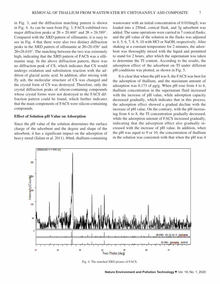
in Fig. 3, and the diffraction matching pattern is shown in Fig. 4. As can be seen from Fig. 3, FACS exhibited two major diffraction peaks at 2θ = 20.460° and 2θ = 26.589°. Compared with the XRD pattern of sillimanite, it is easy to see in Fig. 4 that there were also two distinct diffraction peaks in the XRD pattern of sillimanite at 2θ=20.456° and 2θ=26.610°. The matching between the two was extremely high, indicating that the XRD pattern of FACS was a silli-manite map. In the above diffraction pattern, there was no diffraction peak of CS, which indicates that CS would undergo oxidation and substitution reaction with the ad-dition of glacial acetic acid. In addition, after mixing with fly ash, the molecular structure of CS was changed and the crystal form of CS was destroyed. Therefore, only the crystal diffraction peaks of silicon-containing compounds whose crystal forms were not destroyed in the FACS dif-fraction pattern could be found, which further indicates that the main components of FACS were silicon-containing compounds.
Effect of Solution pH Value on Adsorption
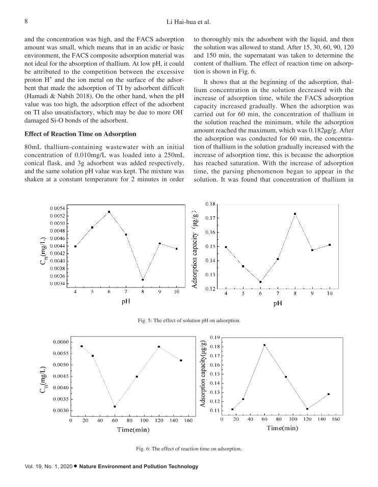
Since the pH value of the solution determines the surface charge of the adsorbent and the degree and shape of the adsorbent, it has a significant impact on the adsorption of heavy metal (Salam et al. 2011). 80mL thallium-containing
wastewater with an initial concentration of 0.010mg/L was loaded into a 250mL conical flask, and 3g adsorbent was added. The same operations were carried in 7 conical flasks, and the pH value of the solution in the flasks was adjusted to 4, 5, 6, 7, 8, 9, 10 with HCl or NaOH, respectively. After shaking at a constant temperature for 2 minutes, the adsor-bent was thoroughly mixed with the liquid and permitted to stand for 2 hours, after which the supernatant was taken to determine the TI content. According to the results, the adsorption effect of the adsorbent on TI under different pH conditions was plotted, as shown in Fig. 5.
It is clear that when the pH was 8, the FACS was best for the adsorption of thallium, and the maximum amount of adsorption was 0.173 of μg/g. When pH rose from 4 to 6, thallium concentration in the supernatant fluid increased with the increase of pH value, while adsorption capacity decreased gradually, which indicates that in this process, the adsorption effect showed a gradual decline with the increase of pH value. On the contrary, with the pH increas-ing from 6 to 8, the TI concentration gradually decreased, while the adsorption amount of FACS increased gradually, indicating that the adsorption effect also gradually in-creased with the increase of pH value. In addition, when the pH was equal to 9 or 10, the concentration of thallium in the solution was consistent with that when the pH was 4
Fig. 4: The matched XRD picture of FACS.
8 Li Hai-hua et al.
Vol. 19, No. 1, 2020 • Nature Environment and Pollution Technology
and the concentration was high, and the FACS adsorption amount was small, which means that in an acidic or basic environment, the FACS composite adsorption material was not ideal for the absorption of thallium. At low pH, it could be attributed to the competition between the excessive proton H+ and the ion metal on the surface of the adsor-bent that made the adsorption of TI by adsorbent difficult (Hamadi & Nabih 2018). On the other hand, when the pH value was too high, the adsorption effect of the adsorbent on TI also unsatisfactory, which may be due to more OH- damaged Si-O bonds of the adsorbent.
Effect of Reaction Time on Adsorption
80mL thallium-containing wastewater with an initial concentration of 0.010mg/L was loaded into a 250mL conical flask, and 3g adsorbent was added respectively, and the same solution pH value was kept. The mixture was shaken at a constant temperature for 2 minutes in order
to thoroughly mix the adsorbent with the liquid, and then the solution was allowed to stand. After 15, 30, 60, 90, 120 and 150 min, the supernatant was taken to determine the content of thallium. The effect of reaction time on adsorp-tion is shown in Fig. 6.
It shows that at the beginning of the adsorption, thal-lium concentration in the solution decreased with the increase of adsorption time, while the FACS adsorption capacity increased gradually. When the adsorption was carried out for 60 min, the concentration of thallium in the solution reached the minimum, while the adsorption amount reached the maximum, which was 0.182μg/g. After the adsorption was conducted for 60 min, the concentra-tion of thallium in the solution gradually increased with the increase of adsorption time, this is because the adsorption has reached saturation. With the increase of adsorption time, the parsing phenomenon began to appear in the solution. It was found that concentration of thallium in
ea
Fig. 5: The effect of solution pH on adsorption.
Fig. 6: The effect of reaction time on adsorption.

9REMOVAL OF THALLIUM FROM WASTEWATER BY CHITOSAN/FLY ASH COMPOSITE
Nature Environment and Pollution Technology • Vol. 19, No. 1, 2020
the solution was reduced again after 120 min, at which point the FACS composite adsorption material resorbed after desorption. Therefore, the reaction of the FACS on the thallium in the wastewater is a kind of adsorption - the alternate process of the absorption cycle. When the reaction time was at 60 min, FACS compound adsorption material reached saturated adsorption, and adsorption effect was best.
Effect of the Amount of Adsorbent on the Adsorption Effect
80mL wastewater containing thallium with an initial con-centration of 0.010mg/L was loaded into six 250mL conical flasks, and adsorbents of 1g, 2g, 3g, 4g, 5g and 6g were added, respectively. The pH of the solution was kept same in all the conical flasks, and the solution was shaken at a
Fig. 7: The effect of adsorbent dose on adsorption.
Fig. 8: Variations in the concentration of thallium with time in solutions of different systems in the presence of coexisting ions.

10 Li Hai-hua et al.
Vol. 19, No. 1, 2020 • Nature Environment and Pollution Technology
constant temperature for 2 minutes to allow the adsorbent to mix well with the liquid and let it stand. Two hours later, the supernatant was taken to determine the content of thallium, and the results are presented in Fig. 7.
It can be seen directly from the Fig. 7 that by adding the 2g adsorbent, the adsorption quantity of thallium was largest, and adsorbent adsorption effect was best. Howev-er, when the amount of adsorbent was more than 2g, the adsorption capacity of thallium by FACS was significantly less than that of the solution with 2g of adsorbent. The reason for this phenomenon may be that when the amount of adsorbent is too much, there would be an adsorption bridge between adsorbent particles, which would affect the adsorption of thallium. On the other hand, the adsorp-tion of thallium may be affected by the intermolecular interaction between ions on the surface of the adsorbent due to the high adsorption dose. In addition, when the amount of adsorbent was less than 2g, the adsorption amount of thallium was also less. Obviously, when the
amount of adsorbent was not enough, the heavy metal thallium in water cannot be fully removed.
Effect of Coexisting Ions on Adsorption
In this study, the effects of Fe3+, Mn2+ and Fe3+/Mn2+ on the removal of TI by FACS were studied respectively. 80mL thallium-containing wastewater with an initial concentra-tion of 0.010mg/L was added into the 250mL conical flask, and 5mL FeCl3 solution, MnCl3 solution and FeCl3/MnCl3 mixed solution with a concentration of 0.05mg/L were added, respectively. 3g FACS was added to each conical flask with the same pH value. The conical flasks were shaken so that the solution was fully mixed with the adsorbent. After 15, 30, 60, 90, 120 and 150min, the supernatant was successively taken to determine the content of thallium for analysis. The variations in the concentration of thallium with time in solutions of different systems are illustrated in Fig. 8 and the adsorption amounts of thallium by adsorbent are shown in Fig. 9.
Fig. 9: The variations in the amount of adsorption with time in the presence of coexisting ions.

11REMOVAL OF THALLIUM FROM WASTEWATER BY CHITOSAN/FLY ASH COMPOSITE
Nature Environment and Pollution Technology • Vol. 19, No. 1, 2020
As can be observed in the figures, when there were no coexisting ions in the solution, the adsorption capacity of FACS on TI increased rapidly between 15 to 60min, and the concentration of TI in the solution decreased significantly. The adsorption saturation was achieved at 60min, and then the concentration of thallium in the solution increased again. When the coexisting ion Fe3+ was present, the concentra-tion of thallium in the solution slowly decreases in the first 90min. From 90 to 120min, the adsorption amount increased sharply and the cesium concentration decreased rapidly. At 120min, the amount of adsorption reached its maximum and reached adsorption saturation. Probably due to the presence of the coexisting ion Fe3+, there was competitive adsorption between Fe3+ and the TI in the solution for the first 90min of the reaction. When Mn2+ was present in the solution, the concentration of strontium in the solution tended to increase continuously between 15 to 90min of the reaction. However, between 90 to 150min, the thallium concentration in the solution showed a trend of gradual decrease. Perhaps Mn2+ has a sufficiently strong preferential adsorption capacity over TI, so that the presence of Mn2+ seriously disturbed the adsorption behaviour of the adsorbent on TI during the first 90 minutes of the reaction. When TI, Fe3+ and Mn2+ were present in the solution, the TI concentration in the solution decreased significantly during the first 30 min of the reaction. Between 30 to 60min, the content of TI was still decreasing, but at a slower speed than before. Between 60 to 90min, the content of TI in the solution presented a sharp decline trend again, during which time the adsorption amount of TI by the adsorbent increased significantly. Then, at 90min, the concentration of TI reached the minimum, and the adsorption capacity of the adsorbent on TI was greater than that in the absence of coexisting ions. This is because the fact that Fe3+ and Mn2+ are hydrolysed to hydroxide.
Except for sediment, they can be used as a new adsorbent to increase the adsorption of TI (Li et al. 2016). After 90 min, the concentration of TI increased in the solution because the FACS reached saturation and desorption occurred.
Effect of Rotation Speed on Adsorption Effect
80mL thallium-containing wastewater with an initial concen-tration of 0.010mg/L was added into seven 250mL conical flasks. Then 3g adsorbent was added into each flask. Under the same pH, the adsorbent and solution were mixed evenly by shaking. The rotational speed of the thermostatic oscil-lator was set to 100, 125, 150, 175, 200, 225, and 250r/min, respectively. After the constant temperature oscillation for 120min, the solution was settled and the supernatant was taken to determine the content of thallium in the solution. According to the measurement results, the influence of dif-ferent oscillation speeds on the adsorption effect of TI was plotted (Fig. 10).
As can be seen, when the rotation speed was 225r/min, the concentration of thallium in the solution was the lowest, and the adsorption amount of the FACS composite adsorbent to TI was the largest. When the rotation speed was between 100 and 175r/min, there was fluctuation in the TI concentration in the solution, but the thallium content in the solution was always higher than that when the rotation speed was 225 r/min, and the thallium content in the solution reached a peak at 175r/min. It may be that the adsorption of TI by FACS adsorbent in the solution is a kind of “adsorption-desorp-tion-re-absorption” alternating complex phenomenon due to the low rotation speed. The adsorption effect of FACS to TI in the second stage was not ideal. At the rotational speed of 175-225r/min, the adsorption amount of TI by FACS increased gradually, while the concentration of TI in the
Fig. 10: Influence of different oscillation speeds on thallium adsorption.

12 Li Hai-hua et al.
Vol. 19, No. 1, 2020 • Nature Environment and Pollution Technology
Table 1: The First-order kinetics fitting parameters.
Reaction system qe qe* k1 R2
TI 0.04147 0.17830 0.03397 0.6260
TI+Fe 0.15138 0.20920 0.04379 0.8724
TI+Mn 0.12504 0.22350 0.03355 0.7416
TI+Fe+Mn 0.09855 0.20970 0.02046 0.8302
Fig. 11: The First-order kinetic fitting curve.
solution decreased gradually. However, the thallium concen-tration in the solution increased sharply as the rotation speed continued to increase. It can be seen that when the speed was too high, severe turbulence was not good for the adsorption of TI in the solution by FACS composite adsorbent.
Adsorption kinetics
In the present study, kinetic sorption data were treated with two simplified kinetic models including First-order kinetics model and Second-order kinetics model. First-order kinetics fitting results are shown in Table 1 and Fig. 11, and the re-sults of Second-order kinetics fitting in Table 2 and Fig. 12.
It is obvious that the second order model fitted better than the first order model, which means chemical adsorption is the main speed limit step.
Adsorption Isotherms
Both Langmuir and Freundlich models were used to fit the adsorption isotherms in this study. The higher regression coefficient (Table 3) indicates that the Freundlich model has better fitting effect on isotherm than the Langmuir model (Fig. 13), which proves that the adsorption of TI (I) by FACS belongs to multi-molecular layer adsorption on heterogeneous phase surface.

13REMOVAL OF THALLIUM FROM WASTEWATER BY CHITOSAN/FLY ASH COMPOSITE
Nature Environment and Pollution Technology • Vol. 19, No. 1, 2020
Fig. 12: The Second-order kinetics fitting curve.
Table 2: The Second-order kinetics fitting parameters.
Reaction system qe qe* k2 R2
TI 0.21589 0.17830 0.65565 0.99903
TI+Fe 0.20648 0.20920 1.05966 0.99238
TI+Mn 0.21206 0.22350 0.45198 0.99222
TI+Fe+Mn 0.21589 0.20970 0.43697 0.99069
Fig. 13: Isothermal fitting curves of Langmuir and Freundlich.

14 Li Hai-hua et al.
Vol. 19, No. 1, 2020 • Nature Environment and Pollution Technology
Reuse of Complex Adsorbent
Because the economy of the adsorption process depends on the regeneration of the adsorbent, the study of desorp-tion is of great importance. The saturated FACS composite adsorbent was repeatedly rinsed with deionized water and then dried. Then, the composite adsorbent was immersed in a sodium chloride solution with a concentration of 1 mol/L for desorption. During the desorption process, the solution was stirred for 1 minute every 2 hours. TI (I) solution was adsorbed by dried FACS for 15, 30, 45, 60, 90, 120 and 150min, respectively. The supernatant was taken in order to measure the concentration of TI (I) in the solution, and the adsorption was calculated. The results are shown in Fig. 14.
Fig. 14 shows that the adsorption step took 60 min to achieve equilibrium and the adsorption capacity was about 0.114 μg/g. The removal rate of TI (I) by FACS composite adsorption material reused after desorption was still about 43%, which proves that FACS composite adsorption material still had high activity after regeneration and could be reused in the treatment of TI polluted wastewater. FACS belongs to the adsorption of environmentally friendly materials.
CONCLUSIONS
The prepared FACS composite adsorbent is a low-cost,
Fig. 14: The change in adsorption capacity and removal rate with time.
renewable, low toxic, environmentally friendly adsorbent material. The surface of FACS particles contains lots of microporous structures and has a large porosity, which is conducive to its adsorption of TI in wastewater. It is mainly of silicate structure. After adsorption of TI-containing wastewater in different systems, the main chemical bond composition and chemical groups of the adsorption material would not change. The experiments of different influencing factors showed that with a pH value of 8, FACS had the best adsorption effect on TI in water. Whether the pH was too high or too low, it had a negative effect on the adsorption. The “adsorption-desorption” period of FACS occurred at 120min, and the adsorption effect was best when the reaction was carried out to 60min, and the adsorption saturation was achieved. When 2g adsorbent was added into 80mL thallium-containing wastewater with an initial concentration of 0.01mg/L, the removal effect was best. When coexisting ions Fe3+ and Mn2+ were separately present in the solution with TI, both of them had an adverse effect on the removal of TI. However, when Fe3+, Mn2+ and TI were simultaneously present in the solution, they had a positive effect on the adsorption. The adsorption effect was optimal when the rotation speed was 225r/min, because the turbulence in the adsorption process is not conducive to the adsorption of TI in the solution by FACS composite adsorbent. The adsorption of TI by FACS was multi-molecular layer adsorption on the surface of heterogeneous reaction. The
Table 3: Langmuir and Freundlich isothermal fitting parameters.
Langmuir isothermal fitting Freundlich isothermal fitting
q0(mg/g) b(L/mg) R2 n k R2
0.00054 76.60795 0.95820 1.29096 0.03512 0.99438

15REMOVAL OF THALLIUM FROM WASTEWATER BY CHITOSAN/FLY ASH COMPOSITE
Nature Environment and Pollution Technology • Vol. 19, No. 1, 2020
driving force of the process was the covalent force formed by ion exchange or covalent electron pair between adsorbent and adsorbate. After being analysed and reused, FACS still had superior adsorption efficiency. We believe that FACS composite adsorbent is a kind of economical material with simple operation, low price and recyclability, and has potential application in removing TI from wastewater.
REFERENCES Birungi, Z.S. and Chirwa, E.M.N. 2015. The adsorption potential and recovery
of thallium using green micro-algae from eutrophic water sources. J. Hazard. Mater., 299: 67-77.
Cheam, V., Lechner, J., Desrosiers, R., Sekerka, I., Lawson, G. and Mudroch, A. 1995. Dissolved and total thallium in Great Lakes waters. Journal of Great Lakes Research, 21: 384-394.
Chen, K.N., Li, H.S., Kong, L.J., Peng, Y., Chen, D.Y., Xia, J.R. and Long, J.Y. 2018. Biosorption of thallium (I) and cadmium (II) with the dried bio-mass of Pestalotiopsis sp. FW-JCCW: Isotherm, kinetic, thermodynamic and mechanism. J. Desalination and Water Treatment, 111: 297-309.
Del-valls, T.A., Saenz, V., Arias, A.M. and Blasco, J. 1999. Thallium in the marine environment: First ecotoxicological assessments in the Guadalquivir estuary and its potential adverse effect on the Donana European natural reserve after the Aznalcollar mining spill. J. Ciencias Marinas, 25: 161-175.
Fan, L.L., Luo, C.N., Li, X.J., Lu, F.G., Qiu, H.M. and Sun, M. 2012. Fabrication of novel magnetic chitosan grafted with graphene oxide to enhance adsorption properties for methyl blue. Journal of Hazardous Materials, 215-216: 272-279.
Ge, J.C., Yoon, S.K. and Choi, N.J. 2018. Application of fly ash as an adsorbent for removal of air and water pollutants. J. Applied Sciences, 8(7):1-24.
Hamadi, A. and Nabih, K. 2018. Synthesis of zeolites materials using fly ash and oil shale ash and their applications in removing heavy metals from aqueous solutions. Journal of Chemistry, 2018: 1-12.
Huangfu, X.L., Ma, C.X., Ma, J., He, Q., Yang, C., Zhou, J., Jiang, J. and Wang, Y.A. 2017. Effective removal of trace thallium from surface water by nanosized manganese dioxide enhanced quartz sand filtration. Chemosphere, 189: 1-9.
Keskinkan, O., Goksu, M.Z.L., Basibuyuk, M. and Forster, C.F. 2004. Heavy metal adsorption properties of a submerged aquatic plant (Ceratophyllum demersum). J. Bioresource Technology, 92(2): 197-200.
Kuroiwa, T., Takada, H., Shogen, A., Saito, K., Kobayashi, I., Uemura, K. and Kanazawa, A. 2017. Cross-linkable chitosan-based hydrogel microbeads with pH-responsive adsorption properties for organic dyes prepared using size-tunable microchannel emulsification technique. J. Colloids and Surfaces A: Physicochemical and Engineering Aspects, 514: 69-78.
Li, H.H., Yan, W.F., Meng, R.J. and Liang, Q. 2016. Influence of coexistent ions Fe3+ and Mn2+ on arsenic (iii) adsorption behaviour onto river sediment. Nature Environment & Pollution Technology, 15: 305-310.
Li, H.S., Chen, Y.H., Long, J.Y., Jiang, D.Q., Liu, J., Li, S.J., Qi, J.Y., Zhang, P., Wang, J., Gong, J., Wu, Q.H. and Chen, D.Y. 2017. Simultaneous removal of thallium and chloride from a highly saline industrial waste-water using modified anion exchange resins. Journal of Hazardous Materials, 333: 179-185.
Li, H.S., Li, X.W., Xiao, T.F., Chen, Y.H., Long, J.Y., Zhang, G.S., Zhang, P., Li, C.l., Zhuang, L.Z. and Li, K.K. 2018. Efficient removal of thal-lium(I) from wastewater using flower-like manganese dioxide coated magnetic pyrite cinder. J. Chemical Engineering Journal, 353: 867-877.
Liu, Y.L., Wang, L., Wang, X.S., Huang, Z.S., Xu, C.B., Yang, T., Zhao, X.D., Qi, J.Y. and Ma, J. 2017. Highly efficient removal of trace thallium
from contaminated source waters with ferrate: Role of in situ formed ferric nanoparticle. J. Water Research, 124: 149-157.
Memon, S.Q., Memon, N., Solangi, A.R. and Memon, J.U.R. 2008. Sawdust: A green and economical sorbent for thallium removal. J. Chemical Engineering Journal, 140: 235-240.
Pan, J.M., Yao, H., Li, X.X., Wang, B., Huo, P.W., Xu, W.Z., Ou, H.X. and Yan, Y.S. 2011. Synthesis of chitosan/γ-Fe2O3/fly-ash-cenospheres composites for the fast removal of bisphenol A and 2, 4, 6-trichlo-rophenol from aqueous solutions. Journal of Hazardous Materials, 190: 276-284.
Pu, Y.B., Yang, X.F., Zheng, H., Wang, D.S., Su, Y. and He, J. 2013. Ad-sorption and desorption of thallium(I) on multiwalled carbon nanotubes. J. Chemical Engineering Journal, 219: 403-410.
Rahmani, A., Mousavi, H.Z. and Fazli, M. 2010. Effect of nanostructure alu-mina on adsorption of heavy metals. J. Desalination, 253(1-3):94-100.
Rajesh, N. and Subramanian, M.S. 2006. A study of the extraction behavior of thallium with tribenzylamine as the extractant. J. Hazard. Mater., 135: 74-77.
Rathinam, K., Singh, S.P., Arnusch, C.J. and Kasher, R. 2018. An envi-ronmentally-friendly chitosan-lysozyme biocomposite for the effective removal of dyes and heavy metals from aqueous solutions. J. Carbo-hydrate Polymers, 199: 506-515.
Saad, A.H.A., Azzam, A.M., El-Wakeel, S.T., Mostafa, B.B. and El-latif, M.B.A. 2018. Removal of toxic metal ions from wastewater using ZnO@Chitosan coreshell nanocomposite. J. Environmental Nanotechnology, Monitoring & Management, 9: 67-75.
Salam, O.E. A., Reiad, N.A. and EIShafei, M.M. 2011. A study of the removal characteristics of heavy metals from wastewater by low-cost adsorbents. Journal of Advanced Research, 2(4): 297-303.
Saljooghi, A.S. and Fatemi, S.J. 2011. Removal of thallium by deferasirox in rats as biological model. Journal of Applied Toxicology, 31: 139-143.
Tran, H.N., You, S.J., Hosseini-Bandegharaei, A. and Chao, H.P. 2017. Mistakes and inconsistencies regarding adsorption of contaminants from aqueous solutions: A critical review. J. Water Research, 120: 88-116.
Wan, S.L., Ma, M.H., Lv, L., Qian, L.P., Xu, S.Y., Xue, Y. and Ma, Z.Z. 2014. Selective capture of thallium(I) ion from aqueous solutions by amorphous hydrous manganese dioxide. Chemical Engineering Journal, 239: 200-206.
Wen, Y., Tang, Z.R., Chen, Y. and Gu, Y.X. 2011. Adsorption of Cr(VI) from aqueous solutions using chitosan-coated fly ash composite as biosorbent . Chemical Engineering Journal, 175: 110-116.
Wick, S., Baeyens, B. and Fernandes, M.M. 2018. Thallium adsorption onto illite. J. Environmental Science & Technology, 52: 571-580.
Xiao, T.F., Yang, F., Li, S.H., Zheng, B.S. and Ning, Z.P. 2012. Thallium pollution in China: A geoenvironmental perspective. J. Science of the Total Environment, 421-422: 51-58.
Xiong, C.H., Pi, L.L., Chen, X.Y., Yang, L.Q., Ma, C.N. and Zheng, X.M. 2013. Adsorption behavior of Hg2+ in aqueous solutions on a novel chelating cross-linked chitosan microsphere. J. Carbohydrate Polymers, 98(1): 1222-1228.
Yang, K., Wang, G., Chen, X.M., Wang, X. and Liu, F.L. 2018. Treatment of wastewater containing Cu2+ using a novel macromolecular heavy metal chelating flocculant xanthated chitosan. J. Colloids and Surfaces A: Physicochemical and Engineering Aspects, 558: 384-391.
Zhang, G.S., Fan, F., Li, X.P., Qi, J.Y. and Chen, Y.H. 2018. Superior adsorp-tion of thallium(I) on titanium peroxide: Performance and mechanism. Chemical Engineering Journal, 331:471-479.
Zhang, L., Huang, T., Zhang, M., Guo, X.J. and Yuan, Z. 2008. Studies on the capability and behavior of adsorption of thallium on nano-Al2O3. J. Journal of Hazardous Materials, 157: 352-357.
Zolgharnein, J., Asanjarani, N. and Shariatmanesh, T. 2011. Removal of thallium(I) from aqueous solution using modified sugar beet pulp. J. Toxicological and Environmental Chemistry, 93: 207-214.

Vol. 19, No. 1, 2020 • Nature Environment and Pollution Technology
16

Assessment of Seasonal and Spatial Variation of Groundwater Quality in the Coastal Sahel of Doukkala, Morocco
Imane EL Adnani†, Abdelkader Younsi, Khalid Ibno Namr, Abderrahim El Achheb and El Mehdi IrzanLaboratory of Geosciences and Environment Techniques, Chouaib Doukkali University, Faculty of Sciences, Ben Maachou Road, B.P. 20 Avenue des Facultés, El Jadida, Morocco†Corresponding author: Imane EL Adnani
ABSTRACTThe current research is set in the context of the impact of climate change at the regional level, particularly focused on seasonal variations and their influence on the physico-chemical characteristics of groundwater in the rural and urban areas of coastal Sahel of Doukkala. The main objective of this study was to evaluate the quality to explain the phenomena at the origin of the mineralization of groundwater. Two measurement campaigns of sampling were carried out on 30 wells, in 2016 and 2018 (dry and wet season). The water points were piezometrically surveyed. In situ, the same water points were measured for temperature, pH, and electrical conductivity, using a multiparameter conductivity meter and a pH meter. The chemical analysis was carried out at the Laboratory of Geosciences and Environmental Technics using volumetry (Ca2+, Mg2+, Cl- and HCO3
-) and spectrophotometry methods (SO42-, Na+ and K+);
total dissolved solids (TDS) were computed by multiplying the EC by a factor (0.55 to 0.75), depending on relative concentrations of ions. Total hardness (TH) was calculated by taking the differential value between Mg2+ and Ca2+. For the reliability of the results obtained, we proceeded to the application of the ionic balance. The obtained water quality data was subjected to multivariate statistical techniques to evaluate homogeneity and heterogeneity between sampling water and to differentiate water quality variables for temporal variations.The elements are all significantly different among seasons. The dry season was positively associated with EC, TDS, Cl-, Na+, SO4
2- and K+ and negatively associated with temperature, and pH. The wet season was in contrast associated with high values of NO3
- and pH. These results show that the majority of well water in the study area represents strong mineralization that far exceeds standards, especially during the dry period, with an average EC of 416.04 µS/cm, while the wet season is lower at 382.6 µS/cm. The hydrochemical classification of water from the Piper diagram revealed only one hydro facies, which is the chlorinated sodium facies. In conclusion, the variability of groundwater quality could be explained by the fact that in the dry season, there is concentration and in the wet season, there is ionic dilution and may also reflect the effect of anthropogenic activity.
INTRODUCTION
The challenge in the coming years is undoubtedly to ensure the sustainable management of water resources without hindering economic and social development. Globally, groundwater is one of the most precious sourc-es of natural resources. Groundwater contributes to 80% of rural domestic water needs and 50% of urban water needs. According to World Health Organization (2011), 80% of diseases in human beings are caused by water. Problems associated with groundwater exploitation in-clude the following: declining water tables, wells running dry (seasonality) increasing pumping costs, competitive deepening of wells, groundwater subsidence, loss of wet-lands and flowing springs and rivers, salt water intrusion, groundwater degradation from natural toxins (fluoride and arsenic, spreading or leaking of anthropogenically used
Nat. Env. & Poll. Tech.Website: www.neptjournal.com
Received: 09-04-2019Accepted: 02-07-2019
Key Words:Groundwater quality Variability Sahel of Doukkala
2020pp. 17-28 Vol. 19p-ISSN: 0972-6268 No. 1 Nature Environment and Pollution Technology
An International Quarterly Scientific Journal
Original Research Papere-ISSN: 2395-3454
Open Access
substances from point and non-point sources (FAO 2003, Richardson et al. 2004).
In fact, this vital resource no longer seems to meet today’s growing population demand and development needs. This water deficit is caused in particular by the growth in water needs and its irrational use, as well as climate change (UNESCO 1987). In addition, these climatic variabilities have led to a disruption in the frequencies and intensities of precipitation and periods of drought (Berdai 1997). The succession of extremely loss-making and/or extremely surplus years (high and rapid rises) favours soil erosion and subsequently accelerates the transfer of surface pollution to watercourses and then to underground aquifers, which in turn deteriorates water quality. This water problem is therefore aggravated by the almost regular decrease in rainfall over the past fifty years,
18 Imane EL Adnani et al.
Vol. 19, No. 1, 2020 • Nature Environment and Pollution Technology
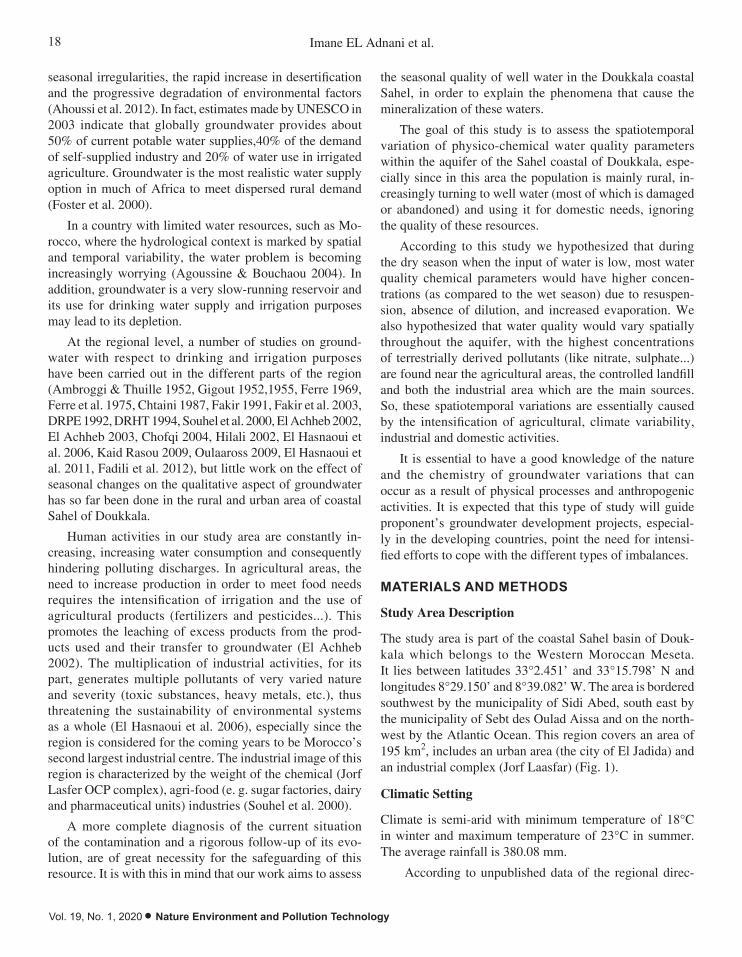
seasonal irregularities, the rapid increase in desertification and the progressive degradation of environmental factors (Ahoussi et al. 2012). In fact, estimates made by UNESCO in 2003 indicate that globally groundwater provides about 50% of current potable water supplies,40% of the demand of self-supplied industry and 20% of water use in irrigated agriculture. Groundwater is the most realistic water supply option in much of Africa to meet dispersed rural demand (Foster et al. 2000).
In a country with limited water resources, such as Mo-rocco, where the hydrological context is marked by spatial and temporal variability, the water problem is becoming increasingly worrying (Agoussine & Bouchaou 2004). In addition, groundwater is a very slow-running reservoir and its use for drinking water supply and irrigation purposes may lead to its depletion.
At the regional level, a number of studies on ground-water with respect to drinking and irrigation purposes have been carried out in the different parts of the region (Ambroggi & Thuille 1952, Gigout 1952,1955, Ferre 1969, Ferre et al. 1975, Chtaini 1987, Fakir 1991, Fakir et al. 2003, DRPE 1992, DRHT 1994, Souhel et al. 2000, El Achheb 2002, El Achheb 2003, Chofqi 2004, Hilali 2002, El Hasnaoui et al. 2006, Kaid Rasou 2009, Oulaaross 2009, El Hasnaoui et al. 2011, Fadili et al. 2012), but little work on the effect of seasonal changes on the qualitative aspect of groundwater has so far been done in the rural and urban area of coastal Sahel of Doukkala.
Human activities in our study area are constantly in-creasing, increasing water consumption and consequently hindering polluting discharges. In agricultural areas, the need to increase production in order to meet food needs requires the intensification of irrigation and the use of agricultural products (fertilizers and pesticides...). This promotes the leaching of excess products from the prod-ucts used and their transfer to groundwater (El Achheb 2002). The multiplication of industrial activities, for its part, generates multiple pollutants of very varied nature and severity (toxic substances, heavy metals, etc.), thus threatening the sustainability of environmental systems as a whole (El Hasnaoui et al. 2006), especially since the region is considered for the coming years to be Morocco’s second largest industrial centre. The industrial image of this region is characterized by the weight of the chemical (Jorf Lasfer OCP complex), agri-food (e. g. sugar factories, dairy and pharmaceutical units) industries (Souhel et al. 2000).
A more complete diagnosis of the current situation of the contamination and a rigorous follow-up of its evo-lution, are of great necessity for the safeguarding of this resource. It is with this in mind that our work aims to assess
the seasonal quality of well water in the Doukkala coastal Sahel, in order to explain the phenomena that cause the mineralization of these waters.
The goal of this study is to assess the spatiotemporal variation of physico-chemical water quality parameters within the aquifer of the Sahel coastal of Doukkala, espe-cially since in this area the population is mainly rural, in-creasingly turning to well water (most of which is damaged or abandoned) and using it for domestic needs, ignoring the quality of these resources.
According to this study we hypothesized that during the dry season when the input of water is low, most water quality chemical parameters would have higher concen-trations (as compared to the wet season) due to resuspen-sion, absence of dilution, and increased evaporation. We also hypothesized that water quality would vary spatially throughout the aquifer, with the highest concentrations of terrestrially derived pollutants (like nitrate, sulphate...) are found near the agricultural areas, the controlled landfill and both the industrial area which are the main sources. So, these spatiotemporal variations are essentially caused by the intensification of agricultural, climate variability, industrial and domestic activities.
It is essential to have a good knowledge of the nature and the chemistry of groundwater variations that can occur as a result of physical processes and anthropogenic activities. It is expected that this type of study will guide proponent’s groundwater development projects, especial-ly in the developing countries, point the need for intensi-fied efforts to cope with the different types of imbalances.
MATERIALS AND METHODS
Study Area Description
The study area is part of the coastal Sahel basin of Douk-kala which belongs to the Western Moroccan Meseta. It lies between latitudes 33°2.451’ and 33°15.798’ N and longitudes 8°29.150’ and 8°39.082’ W. The area is bordered southwest by the municipality of Sidi Abed, south east by the municipality of Sebt des Oulad Aissa and on the north-west by the Atlantic Ocean. This region covers an area of 195 km2, includes an urban area (the city of El Jadida) and an industrial complex (Jorf Laasfar) (Fig. 1).
Climatic Setting
Climate is semi-arid with minimum temperature of 18°C in winter and maximum temperature of 23°C in summer. The average rainfall is 380.08 mm.
According to unpublished data of the regional direc-
19SEASONAL AND SPATIAL VARIATION OF GROUNDWATER QUALITY
Nature Environment and Pollution Technology • Vol. 19, No. 1, 2020
torate of agriculture, from the year 2016-2018, the average annual rainfall in El Jadida station was 400 mm with a min-imum of 0 mm recorded in June, July and August respec-tively in 2016 and 2017. The maximum monthly rainfall (139 mm) was occurred during March. In terms of the regional rainfall variability, 2018 is a rainy year compared to 2016. Seasonal fluctuations in water levels during 2016-2018 correspond to rainfall (DRH 2016-2018) (Fig. 2).
Geological and Hydrogeological Setting
The study area consists of highly varied geological for-mations such as of limestone and marl formations of Cenomanian (Cretaceous) age (Fig. 3), resting in angular discordance on the basal Palaeozoic monoclinal dolomites (El Achheb 2002).
Rainfall is the main recharge source for groundwater in the area. The Cenomanian formations represent the most extensive aquifer at the study area (Ferré & Ruhard 1975). The calcareous layers form a fractured and karstic aquifer which is up to 100 m thick.
Test pumping in the vicinity of El Jadida revealed per-meability values in the range of 5 ×10⁻⁶ to 10-5 m/s for the
studied aquifer (Souhel & El Achheb 2000).
Experimental Setup and Methods
Groundwater samples collected from 30 dug wells in June during a period of two years 2016 and 2018, covering both wet and dry periods (Fig. 4), these water points are located in urban and rural areas characterized by different activities (agricultural, industrial...). The water samples were taken according to Rodier’s techniques (1984), collected in prewashed (with detergent, diluted HNO3 and double de-ionized distilled water, respectively). Prior to sampling, all the sampling containers were rinsed thoroughly with the groundwater, filled with refusal (to avoid the formation of air bubbles) and kept at low temperature (2-4°C).
Field samples were analysed immediately for hydrogen ion concentration (pH), temperature and electrical con-ductivity (EC), using a HACH multiparameter conductivity meter, model 44 600 and a WTW pH meter, pH 522 with combined electrode.
Other parameters were later analysed in Laboratory of Geosciences and Environmental Techniques of Chouaïb Doukkali University. These parameters include important
Fig. 1: Location and geology simplified map of the study area (Ferré & Ruhard 1975, Oulaarous 2009).

20 Imane EL Adnani et al.
Vol. 19, No. 1, 2020 • Nature Environment and Pollution Technology
cations such as calcium (Ca2+), magnesium (Mg2+), sodium (Na+), potassium (K+) as well as anions such as bicarbonates (HCO3
-), chlorides (Cl-) and sulphates (SO42-). Total dissolved
solids (TDS) were computed by multiplying the EC by a factor (0.55 to 0.75), depending on relative concentrations of ions (Sudhakar et al. 2013). Total hardness (TH) was calculated by taking the differential value between Mg2+
and Ca2+ (ISO 1984), these two elements were analysed titrimetrically, using standard EDTA. Sodium (Na+) and po-tassium (K+) were measured, using a flame photometer. Bi-carbonate (HCO3
-) were estimated by titrating with H2SO4.
Chloride (Cl-) was determined titrimetrically by standard AgNO3 titration. Sulphate (H2SO4) and nitrate (NO3
-) were analysed, using spectrophotometer. All parameters are expressed in milligrams per litre (mg/L) and milliequiva-lents per litre (meq/L), except pH (units) and EC. The EC is expressed in microsiemens per centimetre (µS/cm) at 25°C.
For the reliability of the results obtained, we proceeded to the application of the ionic balance (taking the rela-tionship between the total cations and the total anions) and an error of 10% was accepted (Domenico & Schwartz 1998, Rodier 2009).
Fig. 4: Location of sampling points in the study area
Fig. 2: Monthly variation of pluviometry and temperatures at El Jadida station between 2015 and 2018 (C.P.M).
Fig. 3: Portion of the synthetic stratigraphic log of the Cenomanian of the study area
(D.R.H 1990).

21SEASONAL AND SPATIAL VARIATION OF GROUNDWATER QUALITY
Nature Environment and Pollution Technology • Vol. 19, No. 1, 2020
The processing of the collected physico-chemical data was carried out using multivariate hydrochemical and statistical methods. The hydrochemical method required the use of the Piper diagram for hydrochemical classi-fication. The statistical approach that has been used to study the phenomena underlying water mineralization, water aggregation and identify the factors responsible for these aggregations is based on multivariate statistical techniques. The statistical analysis was carried out on 30 descriptors and all parameters (13 variables) in wet and dry periods. Concentration differences for each water quality variable between the wet and dry season were examined using the Mann-Whitney U test, and differences among seasons were examined using one-way ANOVA, both at a significance level of p < 0.05.
The box plot analysis was used to assess temporal var-iability in water quality parameter concentrations based on the median, minimum, maximum, and 25th and 75th percentile values (Dou et al. 2016). The reservoir water quality variables were also subjected to multivariate statis-tical techniques using principal component analysis (PCA), which is one of the most commonly used multivariate statistical techniques. Its purpose is therefore to establish a relationship between the various physico-chemical param-eters and to better assess the effect of anthropogenic ac-tivities on the quality of the groundwater sampled (Quinn & Keough 2002). The statistical analysis was performed using Statgraphics 16.1 software and IBM SPSS statistics 20.
The application of all these different methods made it
possible to assess seasonal quality in order to explain the phenomena responsible for variations in groundwater mineralization in our study area.
RESULTS
From Table 1, the results of the physico-chemical analyses of water samples are shown and the WHO prescribed guideline used in the description of groundwater quality characteristics in the study area.
Spatial descriptive statistics result of the analysed pa-rameters showed that there are parameters that express significant changes during the study period, indicating spatial variability of chemical composition among sam-pling sites (Table 1) for wet and dry seasons, respectively.
83.33% of the water analyses carried out in two seasons have an ionic balance of less than 5%, so these analyses are satisfactory. However, 16.67% of the analyses carried out on groundwater have an ionic balance of between 5 and 10%, so these analyses are of acceptable quality.
WHO- World Health Organization, SD- Standard devi-ation, CV- Coefficient of variation, WT- Water temperature TH- Total hardness, EC- Electrical conductivity, TDS- Total dissolved solids
The pH values of groundwater varied from 7.2 to 8.65 during dry season and 7.1 to 8.3 during wet season. EC values ranged from 101.9 to 955 μS/cm during dry season whereas during wet season it was 82-86.1 μS/cm. Respec-tive minimum and maximum TDS values observed were
Table 1: Descriptive characteristics of physico-chemical parameters of groundwater quality for wet and dry seasons in the study area.
WHO stand-ards
Dry season Wet season
Parameters Min Max Mean SD CV Min Max Mean SD CV
pH 6.5 - 9.5 7.2 8.65 7.77 0.33 4.31 7.1 8.3 7.69 0.34 4.42
WT (°C) < 25 21.4 24.8 22.7 0.92 4.04 19.4 24.1 21.87 1.33 6.08
TH (mg/L) 2.5 129.14 37.06 25.5 68.81 10.5 114.25 35.68 23.67 66.33
EC (µS/cm) > 400 101.9 955 416.04 215.46 5178.7 82.8 86.1 382.6 196.96 5147.77
TDS (mg/L) 50.95 477.5 208.02 107.73 2589.4 41.4 429.95 191.30 98.47 5147.77
Ca2+ (mg/L) < 100 16 372 128.57 83.21 64.72 28 420 165 99.51 60.31
Mg2+ (mg/L) < 50 1.2 460 100.77 99.06 98.31 3.6 296.4 76.96 72.85 94.67
Na+ (mg/L) < 150 220 3066 695.17 623.47 89.68 81 1500 541.84 335.28 61.88
K+ (mg/L) < 12 3.8 31.5 12.47 6.66 53.38 5.1 75 18.9 14.25 75.44
HCO3- (mg/L) 158.6 890.6 443.43 163.01 36.76 183 671 370.88 115.81 31.22
Cl- (mg/L) < 200 221.9 2644.75 1061.45 689.47 64.95 272.75 2502.8 994.58 616.02 61.93
SO42- (mg/L) < 250 25.64 454.59 112.42 91.89 81.73 41.61 714.54 264.19 190.23 72
NO3- (mg/L) < 50 6.76 165.93 52.02 37.04 71.2 9.6 383.62 69.97 76 108.62
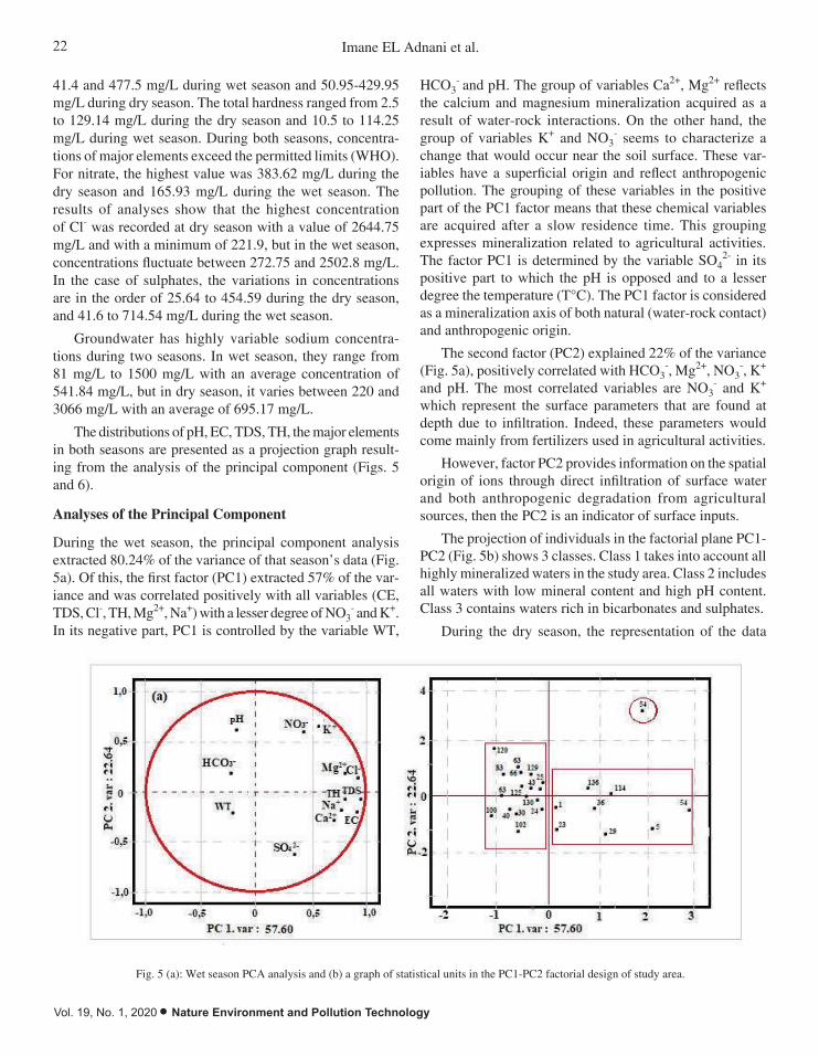
22 Imane EL Adnani et al.
Vol. 19, No. 1, 2020 • Nature Environment and Pollution Technology
41.4 and 477.5 mg/L during wet season and 50.95-429.95 mg/L during dry season. The total hardness ranged from 2.5 to 129.14 mg/L during the dry season and 10.5 to 114.25 mg/L during wet season. During both seasons, concentra-tions of major elements exceed the permitted limits (WHO). For nitrate, the highest value was 383.62 mg/L during the dry season and 165.93 mg/L during the wet season. The results of analyses show that the highest concentration of Cl- was recorded at dry season with a value of 2644.75 mg/L and with a minimum of 221.9, but in the wet season, concentrations fluctuate between 272.75 and 2502.8 mg/L. In the case of sulphates, the variations in concentrations are in the order of 25.64 to 454.59 during the dry season, and 41.6 to 714.54 mg/L during the wet season.
Groundwater has highly variable sodium concentra-tions during two seasons. In wet season, they range from 81 mg/L to 1500 mg/L with an average concentration of 541.84 mg/L, but in dry season, it varies between 220 and 3066 mg/L with an average of 695.17 mg/L.
The distributions of pH, EC, TDS, TH, the major elements in both seasons are presented as a projection graph result-ing from the analysis of the principal component (Figs. 5 and 6).
Analyses of the Principal Component
During the wet season, the principal component analysis extracted 80.24% of the variance of that season’s data (Fig. 5a). Of this, the first factor (PC1) extracted 57% of the var-iance and was correlated positively with all variables (CE, TDS, Cl-, TH, Mg2+, Na+) with a lesser degree of NO3
- and K+. In its negative part, PC1 is controlled by the variable WT,
HCO3- and pH. The group of variables Ca2+, Mg2+ reflects
the calcium and magnesium mineralization acquired as a result of water-rock interactions. On the other hand, the group of variables K+ and NO3
- seems to characterize a change that would occur near the soil surface. These var-iables have a superficial origin and reflect anthropogenic pollution. The grouping of these variables in the positive part of the PC1 factor means that these chemical variables are acquired after a slow residence time. This grouping expresses mineralization related to agricultural activities. The factor PC1 is determined by the variable SO4
2- in its positive part to which the pH is opposed and to a lesser degree the temperature (T°C). The PC1 factor is considered as a mineralization axis of both natural (water-rock contact) and anthropogenic origin.
The second factor (PC2) explained 22% of the variance (Fig. 5a), positively correlated with HCO3
-, Mg2+, NO3-, K+
and pH. The most correlated variables are NO3- and K+
which represent the surface parameters that are found at depth due to infiltration. Indeed, these parameters would come mainly from fertilizers used in agricultural activities.
However, factor PC2 provides information on the spatial origin of ions through direct infiltration of surface water and both anthropogenic degradation from agricultural sources, then the PC2 is an indicator of surface inputs.
The projection of individuals in the factorial plane PC1-PC2 (Fig. 5b) shows 3 classes. Class 1 takes into account all highly mineralized waters in the study area. Class 2 includes all waters with low mineral content and high pH content. Class 3 contains waters rich in bicarbonates and sulphates.
During the dry season, the representation of the data
Fig. 5 (a): Wet season PCA analysis and (b) a graph of statistical units in the PC1-PC2 factorial design of study area.

23SEASONAL AND SPATIAL VARIATION OF GROUNDWATER QUALITY
Nature Environment and Pollution Technology • Vol. 19, No. 1, 2020
in the factorial plane PC1-PC2 expresses 81.01% of the total variance of the point cloud including 53.79% for the factor PC1 (Fig. 6a). The physico-chemical parameters: CE, TDS, Mg2+, TH, Cl- and K+ are well correlated with each other and have a significant weight in the prevalence of the phenomenon represented by PC1. The CE and TDS elements are characteristic of the natural mineralization of water in its host (Murdey & Blavoux 1986), while Cl- and Mg2+ reflect induced mineralization. In this case, this axis expresses the residence time of the elements; it is an indi-cator of mineralization (Hani et al. 1997).
PC2 explained 27% and was determined by NO3- but
also by HCO3- and Na+. These parameters are inversely
correlated to Ca2+ and SO42-. The factor PC2 reflects the en-
vironmental conditions and their influence on the chemical variations of the water and represents the surface inputs. It is also an indicator of natural (HCO3
-) and induced (NO3-)
mineralization (Fig. 6a).
The projection of individuals in the factor plane PC1-PC2 (Fig. 6b), shows three classes. Class (1) is composed of a single water point rich in nitrates and characterized by a low sulphate content. Class (2) consists of highly miner-
Fig. 6 (a): Dry season PCA analysis and (b) a graph of statistical units in the PC1-PC2 factorial design of study area.
(a) (b)
Fig. 7: Classification of well water using the Piper diagram in the dry (a) and wet (2) season.

24 Imane EL Adnani et al.
Vol. 19, No. 1, 2020 • Nature Environment and Pollution Technology
alized waters whose ionic acquisition is under the control of mineralization-residence time. Class (3) is located in the negative part of factor 1 and includes waters with low mineral content.
Hydrochemical Classification
In order to determine the chemical facies of the waters of the studied aquifer, we used a Piper diagram (Eblin 2014) which indicated that hydrochemical classification of the groundwater sampled (Figs. 7a and 7b) shows only one facies: the chlorinated sodium facies.
DISCUSSION
We found that there was a distinct seasonal pattern in water quality of the study area. The most parameters were
higher during the dry season in contrast to the wet season.
Water temperature: The variations in water temperature show that in the wet season the temperature of groundwater is lower than in the dry season (Fig. 8a). This observed increase in the dry season is most likely associated with an elevation in surface water temperature due to the higher air temperature.
Temperature variations are strongly influenced by envi-ronmental conditions related to the geographical location of the locality, the geology of the terrain crossed, the hydrology of the ecosystem and especially the climate (Rodier 1984). In both, the dry and wet seasons, the lowest temperature values were obtained either early or late in the day. Indeed, previous studies by Reggam et al. (2015) in Algeria and Makhoukh et al. (2011) in Morocco have shown high temperature values during the dry season and the lowest during the wet season.
(a))
(b))
(d) (c)
(e) (f)
Fig. 8: Box and whisker plot of seasonal variation of water quality parameters. Water temperature (a), pH (b), Electrical conductivity (c), Total dissolved solids (d), Total hardness (e), Nitrate (f), Small red squares represent the median values, boxes represent the interquartile range, plus signs
represent the extremes, small blue dots represent the outliers, and range bars show the maximum and minimum values.

25SEASONAL AND SPATIAL VARIATION OF GROUNDWATER QUALITY
Nature Environment and Pollution Technology • Vol. 19, No. 1, 2020
Therefore, the water temperature must be determined because it is used as a good measure of contamination because it has a marked effect on bacteria and chemical reaction rates in the water (Mink 1964, Dixey 1972, Hutton 1983).
pH: The measurement of pH is one of the most frequently used tests in water chemistry (Hem 1985). The results of analyses of water samples show pH of groundwater is all within the WHO allowable limit of 7-9.2.
The high pH value during the dry season (Fig. 8b) could be due to the low water level during the dry season causing a concentration of base cations, or an excess of primary productivity over respiration during that season, con-suming CO2 and reducing H+. Further, the study area also encompasses extensive agricultural fields. Another reason for the observed low pH values could be thus related to the use of acid producing fertilizers like ammonium sulphate and super phosphate of lime as manure for agriculture use (Raghunath et al. 2001), especially that the study area also includes extensive agricultural fields is particularly important (El Adnani et al. 2018).
Electrical conductivity (EC): The EC mean values were observed to be statistically highest in dry season, in con-trast to the wet season. The distribution of EC values is presented in Fig. 8c.
The occurrence of high EC values in the study area might also be due to addition of some salts through the prevailing agricultural activities (El Achheb 2002). Compar-atively zones with low EC values (<100μS/cm) are due to dilution of soluble salts by rainfall (Raghunath et al. 2001).
The EC of most of the groundwater samples showed decreasing trend in wet season (Fig. 8c) and magnitude of decrease might have been influenced by rainfall character-istics, geology, soil and land use activities, topography of the area and its drainability (Laluraj et al. 2006).
Total dissolved solids (TDS): The concentration of total dissolved solids in groundwater are noted to be higher in wet season than in dry season (Fig. 8d). This is consistent with the findings of Bowell et al (1996) and Efe et al. (2005).
During the dry season, the increased concentration of TDS may be associated with evaporation and the absence of a dilution effect, while the lower values during the wet season are hypothesized to be due to dilution from the tributaries.
The low mineralization of groundwater during the rainy season is due to dilution by rainwater input as the majority of wells are not constructed and receive runoff directly (Laluraj et al. 2006), or it could be due to the hydrogeological properties of rocks (a strong influence
on the extent of water/rock reaction). Zones with high groundwater-flow velocities usually will have relatively low dissolved solids because of the shorter groundwater- rock contact time and high water/rock ratios, and vice-versa (Langmuir 1997).
EC and TDS were common for both wet and dry (Figs. 8c and 8d). There was a highly significant positive correla-tion of TDS with EC both in the wet and the dry season (r = 0.99 at p < 0 .01).
Total hardness (TH): The seasonal variation shows that hardness is lower during wet season (Fig. 8e), probably due to strong dilution, which can be explained by the solvent action of rainwater coming in contact with soil and especially with the rocks characterizing our study area such as limestone and marl limestone formations (Fig. 3) (Souhel et al. 2000) rocks is capable of dissolving calcium and magnesium that promote water hardness.
Although, water harness has no harmful on human health except that it can react with ordinary soap to form scum, plume solvent, scale formation in boilers and in hot water systems (Maxwell et al. 2012).
Nitrate: It is evident that concentration of nitrate was quite variable from season to season. The high values of NO3
- during the wet season (Fig. 8f) returns to the high rate of precipitation that facilitate infiltration of the amount of fertilizer applied.
The spatial variation in nitrate content in groundwater might be due to different degrees of evaporation/recharge, amount of fertilizer applied, anthropogenic activities, microbial reactions, nature of vegetation cover and ad-sorption/desorption processes in the soil system (Datta et al. 1996, 1997, Martin et al. 2006).
Chloride: The seasonal variations of chloride show an in-crease during the dry season compared to the wet season (Fig. 9a) which can be attributed to the local environment of the wells or the chemical composition of the ground-water is strongly affected by excess fertilizer spread over the last 20 years, in particular, chloride (from potassium fertilizers) (El Adnani et al. 2018).
The weakness of chlorides in the wet season is mainly related to the extent and intensity of precipitation during that season. Chloride levels in open pit and borehole wa-ters indicate that seawater in the region has a significant influence on the salt content of groundwater resources, particularly the leaching of salt crystals from aerosols and sea spray (Younsi et al. 2001). The chloride content of water is an indication of the intrusion of seawater. The levels of chloride in open-well and borehole waters indicates that

26 Imane EL Adnani et al.
Vol. 19, No. 1, 2020 • Nature Environment and Pollution Technology
sea water within the area has a great influence on the salt content of the underground water resources (Efe et al. 2005, Maxwell et al. 2012).
Sodium: The reduction in the current study of the concen-tration of sodium during the wet season (Fig. 9b) may be associated with dilution by rainwater.
As noted above, the potential source of the Na+ in water may be related to leaks of leachate from CET to studied water (El Adnani et al. 2018), or other sources can be cit-ed, such as leaching of NaCl crystals from sea spray with over-concentration by the possible effect of evaporation, recirculation of saline drainage waters in agricultural sectors (Younsi et al. 2001).
Sulphate: The results of analyses show that the highest concentration of SO4
2- was recorded at the wet season (Fig. 9c). A significant difference in sulphate concentrations was observed for both seasons which can be explained by the fact that rainwater seems to contain more sulphates than water
from wells and boreholes. This may result from high level combustion of sulphur-containing hydrocarbon emissions in the study area, specifically in the vicinity of the industrial area (El Hasnaoui et al. 2006, 2011). Oxidation of sulphur con-taining compounds after rainwater water has been charged to ground water resources may increase the acidity and toxicity of open-well and borehole water resources.
The study of the mechanism for acquiring water chem-istry in the study area using multivariate statistical analysis methods made it possible to observe, in a first approach, three main mechanisms responsible for the evolution of groundwater mineralization in the study area. The three main mechanisms are: mineralization, residence time and spatial origin of ions.
The acquisition of ions is essentially through rock-water interactions, which is the important phenomenon in water mineralization. The limestones and marls of the formations dominate the geology of the region and characterize the
(a) (b)
(c)
Fig. 9: Box and whisker plot of seasonal variation of water quality parameters. Chloride (a), Sodium (b) and Sulphate (c).

27SEASONAL AND SPATIAL VARIATION OF GROUNDWATER QUALITY
Nature Environment and Pollution Technology • Vol. 19, No. 1, 2020
Cenomanian aquifer, which explains the dominant Ca2+ contents for cations in groundwater.
The acidity of the waters and the abundance of precip-itation cause a very intense and complete alteration of the primary minerals of the parent rock by hydrolysis (Eblin et al. 2014). This hydrolysis is, therefore, important in both the rainy and dry seasons. Indeed, in both the rainy and dry seasons, the mineralization of the waters studied is of both natural (water-rock contact) and anthropogenic origin.
In view of the findings revealed by this study, it is recommended that there is necessary to place two me-teorological stations in the area for local measurement of precipitation, temperature and evapotranspiration. The risk of contamination by seawater must be controlled, it would therefore be necessary to set up a network of monitoring piezometers (with continuous recording), in order to control the fluctuation of the piezometric surface and to regularly monitor the quality of the groundwater to preserve these resources; to conclude, authorities must be required to authorize the use of low-flow pumps and the generalization of economic irrigation methods such as drip irrigation. Propose changes in agricultural practices and especially monitor effluent treatment at landfills and industrial areas.
CONCLUSION
In this study, the measured parameters showed a sea-sonal fluctuation, with concentrations mainly higher during the dry season than during the wet season. This assessment provided information on the characteristics of groundwater in the coastal zone of the Sahel of Doukkala. Physico-chemical analyses show that the water is highly mineralized with an average electrical conductivity of 382,6 µS/cm in the wet season and 416,04 µS/cm in the dry season. Multivariate statistical analysis methods indicate that the different processes responsible for the acquisition of groundwater chemistry studied are: the residence time of the water in contact with the rock, the infiltration of substances related to anthropogenic activities (agricul-tural fertilizers, household and industrial waste...) and the intensity of rainfall.
REFERENCESAgoussine, M. and Bouchaou, L. 2004. The major problems of water
management in Morocco. Science and Planetary Changes/Drought, 15(2): 187-194.
Ahoussi, K. E., Koffi, Y. B., Kouassi, A. M., Soro, G., Soro, N. and Biemi, J. 2012. Physico-chemical and bacteriological characterization of the water resources of localities located near the Ébrié Lagoon in the commune of Marcory (District of Abidjan, Ivory Coast): case of the village of Abia Koumassi. European Journal of Scientific Research, 89(3): 359-383.
Ambroggi, R. and Thuille, G. 1952. Abada-Doukhala. In: Hydrogéologie du Maroc. Notes et Mémoires. Services Géologique Maroc, N° 97.
Berdai, H. 1997. Synthesis of work carried out in Morocco on nitric pol-lution of groundwater. Studies Division, Testing Experiments and Standardization Service, Rabat.
Bowell, R.J., McEdonney, S., Warren, A. and Bwankuzo, M. 1996. Biogeo-chemical factors affecting groundwater quality in central Tanzania. Geological Society, London, Special Publications, 113(1): 107-130.
Chofqi, A. 2004. Highlighting the mechanisms of contamination of groundwater by leachate from an uncontrolled landfill (El Jadi-da-Maroc). Geology, hydrogeology, geoelectric, geochemistry and epidemiology, pp. 184.
Chtaini, A. 1987. Hydrogeological Study of the Doukkala Sahel (Morocco). Doctoral Dissertation, Joseph Fourier University (Grenoble), pp. 157.
D.R.H . 1990. Projet de réalisation des sondages à l’air sur la région des Doukkala, Rabat, Maroc.
Datta, P.S. and Tyagi, S.K. 1996. Major ion chemistry of groundwater in Delhi area: Chemical weathering processes and groundwater flow regime. J. Geolog. Soc. India, 47(2): 179-188.
Datta, P.S., Deb, D.L. and Tyagi, S.K. 1997. Assessment of groundwater con-tamination from fertilizers in the Delhi area based on 18O, NO3
- and K+ composition. Journal of Contaminant Hydrology, 27(3-4): 249-262.
Dixey, F.A. 1972. A Practical Handbook on Water Supply. 2nd edition, Thomas Murby & Co, London.
Domenico, P. A. and Schwartz, F.W. 1998. Physical and Chemical Hydro-geology. Vol. 1, Wiley, pp. 506.
Dou, M., Zhang, Y. and Li, G. 2016. Temporal and spatial characteristics of the water pollutant concentration in Huaihe River Basin from 2003 to 2012, China. Environmental Monitoring and Assessment, 9: 188-522.
DRHT 1994. Elaboration d’un schéma d’exploitation des eaux souterraines du Sahel (Maroc). Rapp. Projet : DRPE-FAO. TCP/MOR/2251.
DRPE 1992. Etude par prospection électrique : Région des Abda et des Doukkala, (21 Mars 1990-10 Juillet 1990, 08 octobre 1992-15 novem-bre 1992). GEOATLAS. Tome 1: texte et planches.
Eblin, S.G., Soro, G.M., Sombo, A.P., Aka, N., Kambiré, O. and Soro, N. 2014. Hydrochimie des eaux souterraines de la région d’Adiaké (Sud-Est côtier de la Côte d’Ivoire). Larhyss Journal, 17: 193-214.
Efe, S.I., Ogban, F.E., Horsfall, M. and Akporhonor, E.E. 2005. Seasonal variation of physico-chemical characteristics in water resources quality in western Niger Delta region, Nigeria. Journal of Applied Science and Environmental Management, 9(1): 191-195.
El Achheb, A. 2002. Contribution à l’étude de la minéralisation et identifi-cation des sources de contaminations des eaux souterraines, application au système aquifère du Bassin Sahel Doukkala (Maroc). Thèse d’état, Univ Chouaïb Doukkali, El Jadida, pp. 206.
El Achheb, A., Mania, J. and Mudry, J. 2003. Mécanismes d’acquisition de la minéralisation des eaux souterraines dans le bassin Sahel des Doukkala (Maroc Occidental). Approche par des traceurs hydrogéochimiques. IGME. Madrid, pp. 113-123.
El Adnani, I., Younsi, A., Ibno Namr, K., El Achheb, A. and Irzan, E.M. 2018. The influence of anthropogenic activities on groundwater quality of southwest region of El Jadida city (Sahel of Doukkala, Morocco), European Journal of Scientific Research, 151: 96-111.
El Hasnaoui, B., Garmes, H., Younsi, A., Mountadar, M. and Mouhab, I. 2006. Problèmes de contamination fluorurée en zone industrielle (Cas du Jorf Lasfar, Maroc). Approche pluridisciplinaire dans le Colloque Internationale, Mines: Exploration, Exploitation et Impact environne-mentale (M3E), Bouznika, 20-21 Avril, pp. 53.
El Hasnaoui, B., Younsi, A., Mountadar, M., Garmes, H. and Mouhab, I. 2011. Impacts négatifs d’une zone industrielle sur les eaux souterraines et sur le cheptel (Cas du Jorf Lasfar, Maroc): Approches pluridisci-plinaires. Déchets sciences techniques, N°59, 2945.
Fadili, A. 2014. Etude hydrogéologique et géophysique de l’extension de l’intrusion marine dans le sahel de l’Oualidia (Maroc): Analyse

28 Imane EL Adnani et al.
Vol. 19, No. 1, 2020 • Nature Environment and Pollution Technology
statistique, hydrochimie et prospection électrique. Thèse Doct, Univ. Chouaib Doukkali, El Jadida, Maroc., pp. 289.
Fakir, Y. 2001. Caractérisation hydrogéologique et hydrochimique des aquifères côtiers du Sahel de Safi à Oualidia (Méséta côtière- Maroc). Thèse 3éme cycle. Univ. Cadi Ayyad, Marrakech, pp. 143.
Fakir, Y. and Razack, M. 2003. Hydrodynamic characterization of a Sahelian coastal aquifer using the ocean tide effect (Dridrate Aquifer, Morocco). Hydrological Sciences-Journal-des Sciences Hydrologiques, 48(3).
FAO (Food and Agriculture Organization) 1997. Seawater Intrusion in Coastal Aquifers: Guidelines for Study, Monitoring and Control. FAO Water Reports 11. Rome Italy: FAO; 163 p.
Ferre, M. 1969. Hydrologie et hydrogéologie des Abda- Doukkala. Thèse du Docteur Ingénieur- Nancy.
Ferre, M. and Ruhard, J.P. 1975. Les bassins des Abda-Doukkala et du Sahel de Azemmour à Safi. In: Ressources en eau du Maroc. Notes mém. Serv. Géol Maroc, 2(231): 261-298.
Foster, S., Chilton, J., Moench, M., Cardy, F. and Schiffler, M. 2000. Ground-water in rural development: Facing the challenges of supply and resource sustainability. World Bank Technical, Washington. Paper No 464.
Gigout, M. 1952. Les ressources en eau souterraine des Doukkala et Abda (Maroc occidental). Rapp. Inéd. Seconde thèse.
Gigout, M. 1955. Enseignement de trois forages sur la stratigraphie du Crétacé des Doukkala. Notes mém. Serv. géol. Maroc, t. 11(123): 44-55.
Hani A, Djarbri L, Mania J. 1997. Etude des caractéristiques physico-chim-iques du massif cristallophyllien de Séraïdi (nordest Algérien). Hard Rock Hydrosystems (Proceedings of Rabat Symposium S2 1997). IAHS Publ., N°.241: 41-59.
Hem, J.D. 1985. Study and Interpretation of The Chemical Characteristics of Natural Water. 3rd edition, US Geological Survey water-supply, paper 2254.
Hilali, M. 2002. Hydrogéologie et modélisation de l’intrusion marine dans les aquifères côtiers de Martil et du Sahel-Maroc. Thèse de Doctorat. Ecole Mohammadia d’Ingénieurs Rabat.
Hutton, L.G. 1983. Field testing of water in developing countries. Water Resources Center, Unwin Brothers Limited, Britain. 125 pp.
ISO 1984. Total Hardness of Water by Photocolorimetry, Standard Methods 2340C Hardness. Hach Company/ Hach Lange GmbH, 2015. Edition 1, 1-13.
Kaid Rassou, K. 2009. Etudes des interactions entre les eaux souterraines et les eaux de surface dans le bassin côteir d’Oualidia, These doctorat es science Univ. Marrakech, pp. 193.
Laluraj. C. M. and Gopinath Girish 2001. Assessment on seasonal variation of groundwater quality of phreatic aquifers-a river basin system. Envi-ronmental Monitoring and Assessment, 117: 45-57.
Langmuir, D. 1997. Aqueous Environmental Chemistry, Prentice-Hall, Inc., New Jersey, pp. 600.
Makhoukh, M., Sbaa, M., Berrahou, A. and Clooster, V.M. 2011. Contribution à l’étude physico-chimique des eaux superficielles de l’oued Moulouya (Maroc oriental). Larhyss Journal, 9: 149-169.
Martin, C., Molénat, J., Gascuel-Odoux, C., Vouillamoz, J.M., Robain, H., Ruiz, L., Faucheux, M. and Aquilina, L. 2006. Modelling the effect of physical and chemical characteristics of shallow aquifers on water and
nitrate transport in small agricultural catchments. Journal of Hydrology, 326: 25-42.
Maxwell, I.O. and Ahola, O. 2012. Seasonal variation in physico-chemical characteristics of rural groundwater of Benue State, Nigeria. Journal of Asian Scientific Research, 2(10): 574-586.
Mink, J.F. 1964. Groundwater temperatures in tropical island environment. Journal of Geophysical Research, 66: 5230-5250.
Murdey, J. and Blavoux, B.1986. Utilisation de l’analyse en composantes principales (sur variables centrées réduites) pour l’étude du fonctionne-ment hydrocinématique de trois aquifères karstiques du Sud-Est de la France. Hydrogéologie, n° 1: 53-59.
Oulaaross, Z. 2009. Etude climatologique, hydrogéologique et géophysique du Sahel Côtier des Doukkala (Maroc). Apport de l’analyse statistique et de l’inversion des données géoélectriques à l’étude du biseau salé de la lagune de Sidi Moussa Thèse Doct, Univ. Chouaib Doukkali, El Jadida, Maroc. pp. 279.
Quinn, G.P. and Keough, M.J. 2002. Experimental Design and Data Analysis for Biologists. United States of America by Cambridge University Press, New York, pp. 553.
Raghunath, R. Sreedhara, Murthy, T. R. and Raghavan, B. R. 2001. Spatial distribution of pH, EC and total dissolved solids of Nethravathi river basin, Karnataka state, India, Pollution Research, 20(3): 413-418.
Reggam, A., Bouchelaghem, H. and Houhamdi, M. 2015. Qualité physi-co-chimique des eaux de l’Oued Seybouse (Nord-Est de l’Algérie): caractérisation et analyse en composantes principales. J. Mater. Environ. Sci., 6(5): 1417-1425.
Richardson, S., Evans, R., Middlemis, H., Ross, J., Howe, P., Hiller, J. and Dyson, P. 2004. Guiding Principles for Sustainable Groundwater Management. IAH Background Paper, MDBC (Murray- Darling Basin Commission), REM (Resource & Environmental Management Pty Ltd.), Australia.
Rodier, J. 1984. L’analyse de l’eau : eaux naturelles, eaux résiduaires, et eau de mer. 7ème édition, Dunod Technique, 1136 pp.
Rodier, J. 2009. L’analyse de l’eau. 9ème édition. DUNOD, Paris, France. Souhel, A. and El Achheb, A. 2000. Cadre géologique des principaux aquifères
de la plaine des Doukkala. Actes de la 2ème session de L’université de printemps des Doukkala-Abda. Université. Chouaïb Doukkali, El Jadida, (Maroc), 3: 71-73.
Sudhakar, A. and Narsimha, A. 2013. Suitability and assessment of groundwa-ter for irrigation purpose: A case study of Kushaiguda area, Ranga Reddy district, Andhra Pradesh, India. Pelagia Research Library, Advances in Applied Science Research, 4(6): 75-81.
UNESCO 1987. Groundwater Problems in Coastal Areas. United Nations Educational, Scientific and Cultural Organization, pp. 582.
UNESCO 2003. Water for People: Water for Life. 1st edition. The United Nations’ world water development report, Berghahn Books, 543 pp.
WHO 2011. World Health Statistics. WHO Department of Health Statistics and Informatics of the Innovation, Information, Evidence and Research Cluster, France, pp. 162.
Younsi, A., Mania, J., Lhadi, E.K. and Mudry, J. 2001. Incidences de pluies exceptionnelles sur un aquifère libre côtier en zone semi-aride (Chaouia, Maroc). Revue des sciences de l’eau, 14(2): 115-130.

Adsorption of Methylene Blue Using Chemically Enhanced Platanus orientalis Leaf Powder: Kinetics and Mechanisms
Baba Imoro Musah†, Lai Peng and Yifeng XuDepartment of Environmental Science and Engineering, School of Resources and Environmental Engineering, Wuhan University of Technology, Luoshi Road No. 122, Hongshan, Wuhan, Hubei, 430070, PR China†Corresponding author: Baba Imoro Musah
ABSTRACT
The adsorption of methylene blue in an aqueous medium using two activated carbons AC1 and AC1 + H3PO4 was studied. The AC1+ H3PO4 adsorbent, which was inoculated with phosphoric acid, had better methylene blue removal capacity compared with AC1 adsorbent which had only thermal treatment. The optimum activation temperature for both adsorbents was 500°C while the suitable activation time was 180 min. The best pH in this investigation was 6. With AC1 + H3PO4 adsorbent, 100% removal of methylene blue was recorded for concentrations 20 to 100 mg.L-1 and the suitable adsorbent dosage was 3 g.L-1. The effect of temperature showed insignificant effect on the adsorption of methylene blue ions. The SEM results for AC1 + H3PO4 adsorbent showed better pores compared with AC1, an indication that, the injection of phosphoric acid into it before the activation played a significant role in enhancing the porosity of the adsorbent surface.
INTRODUCTION
Textile, paper, painting and coating industries are major sources of dye pollutants. Large amount of dye wastewater are emptied into freshwater bodies which have negative consequences on the environment and human health (Oliveira et al. 2008). When exposed to light and water, methylene blue is difficult to fade and hard to be treated in wastewater by simple techniques such as biological treatment and chemical precipitation (Oliveira et al. 2008). In the production chain, it is reported that between the range of 1 to 15% the dye is lost and it is discharged as wastewater (Galindo et al. 2001, El-Sharkawy et al. 2007). Dye wastewater that ends up in fresh water bodies cause havoc to aquatic species by increasing toxicity chemical oxygen demand (COD). It also affects the photosynthetic activities of aquatic plants through the reduction of light penetration (Oliveira et al. 2008). It has been reported that, high COD, biological oxygen demand (BOD5) values, particulate matter (PM) and sediments, grease and oil in effluents lead to the depletion of dissolved oxygen creating serious consequences on aquatic species (Wang et al. 2011).
Methylene blue (MB) wastewater can be treated by pho-tocatalytic degradation (El-Sharkawy et al. 2007). Generally, MB has poor biodegradability or resistance to environmental conditions (Tsai et al. 2001). Research indicates that, there
are over 100,000 available commercial dyes and more than 7 × 10⁵ t dye-materials are produced yearly (Lee et al. 2006). Methylene blue is used in many industries e.g. dyeing of silks, paper, plastic, leather, but it has wider usage in the synthetic textile fibre industries as the most suitable substrate (Oliveira et al. 2008). There are various classification of dyes such as anionic- direct, acid and reactive dyes; cationic - ba-sic dyes; and non-ionic- disperse dyes (Fu & Viraraghavan 2001). The textile industry emission or discharge standards vary for many countries for different indicators e.g. China is COD 100 mg.L1, BOD5 25 mg.L-1 and pH 6-9; in Germany, COD 160 mg.L-1 and BOD5 25 mg.L-1; in Jordan COD 160 mg.L-1, BOD5 60 mg.L-1 and pH 6-9; Oman COD 150 mg.L-1 and BOD5; Tunisia COD 90 mg.L-1, BOD5 30 mg.L-1 and pH 6.5-8.5 (Wang et al. 2011, WHO 2006, Sawal 1986).
Wastewater from dye-stuff and textile industries have dye concentrations below 1 g/dm3, high alkalinity, biochemical oxygen demand, chemical oxygen demand and total oxygen dissolved solids (Kaushik & Malik 2009). Methylene blue is a cationic dye widely used in silk, cotton and wool processing as dyes (El-Sharkawy et al. 2007).
There are different treatment techniques that can be employed in the removal of environmental pollutants such as dyes. They include membrane filtration (Abid et al. 2012), electrochemical (Babu et al. 2011), reduction (Wali 2015), oxidation (Murthy et al. 2011), adsorption (Weng & Pan
Nat. Env. & Poll. Tech.Website: www.neptjournal.com
Received: 30-04-2019Accepted: 02-07-2019
Key Words:AdsorptionMethylene blueChemical impregnationPlatanus orientalisLeaf powder
2020pp. 29-40 Vol. 19
p-ISSN: 0972-6268 No. 1 Nature Environment and Pollution Technology An International Quarterly Scientific Journal
Original Research Paper
e-ISSN: 2395-3454
Open Access

30 Baba Imoro Musah et al.
Vol. 19, No. 1, 2020 • Nature Environment and Pollution Technology
2007), electrocoagulation (Akyol 2012), photocatalytic deg-radation (Sleiman et al. 2007). However, in the case of meth-ylene blue C16H18ClN3S.3H2O, it is resilient to fading when exposed to water and light making it difficult to be removed from wastewaters through commonly used techniques like biological and chemical precipitation (Franca et al. 2009).
Adsorption as a technique for removing different kinds of pollutants such as heavy metals, dye among others in waste-water is reported to be an efficient method (El-Sharkawy et al. 2007). In this research adsorption technique is employed due the following reasons: environmentally friendly, ease of operation, wide range adsorbent sources among others are reported by some past studies (Saengbutr et al. 2014, Tong et al. 2010, Rashed 2013 and Lupascu & Povar 2016). With regards to industrial wastewater handling, adsorption processes serve as very interesting Alternative, especially when organic substances removal or recovering important chemicals are involved (Worch 2012).
The use of activated carbon as adsorbents are effective given that they have highly developed pore and large surface area with high degree of surface reactivity (Dias et al. 2007).
In recent times, there’s rising interest in new techniques regarding the production of cost effective, efficient and eco-friendly adsorbents for large scale utilization. In view of this, agricultural by-products or plant waste materials are of interest to research for utilization as adsorbents; wheat brand (Çiçek et al. 2007), green pea peels (Dod et al. 2012), mango leaves (Kamsonlian et al. 2012), yellow passion fruit waste (Pavan et al. 2008), rice hull ash (Wang & Lin 2008), neem leaves (Saengbutr et al. 2014), hevea brasilliensis seed coat (Hameed & Daud 2008). It is reported that plant leaves contain certain constituents, e.g. polyphenols, lignin, pig-ments and protein making it suitable to provide active sites for binding dyes (Abadian et al. 2015). This study considers platanus orientalis leaf powder as a potential adsorbent for the removal of methylene blue in an aqueous solution.
MATERIALS AND METHODS
Materials and Chemicals
The adsorbent material for this investigation was obtained in December 2015, from Wuhan University of Technology campus, China. It went through systematic processing stages until the final product (AC) was obtained. Sample activated carbons were subsequently stored in a desiccator at room temperature (25°C) to keep it free from moisture contact. Fig. 1a is the leaf sample, 1b is leaf powder inoculated with H3PO4 and 1c is activated carbon.
The following chemicals were used in the investigation e.g. methylene blue trihydrate, phosphoric acid (H3PO4), sodium hydroxide (NaOH) and hydrochloric acid (HCl). The rest of the chemicals used in the study were: sodium chloride (NaCl), potassium bromide (KBr), ethanol (CH3CH2OH), all by China Sinopharm Chemical Reagents Co. Ltd. A 1000 mg/L stock solution methylene blue was prepared using deionized water obtained from Milli-Q Direct 16 distillation machine with Vent Filter MPK01. Different concentrations of methylene blue such as 20, 40, 60, 80, 100, 120 and 140 mg.L-1 were subsequently prepared from the stock solution for use in the investigation. All chemicals and reagents used in the investigation were of analytical grade.
Sample Activation
A total of 40 g of dried fallen platanus orientalis leaf powder (FPOLP) was used for two sets of activations in this investi-gation involving methylene blue. First, 20 g of FPOLP was thermally treated (pyrolyzed) in an electric furnace for 180 min at temperature 500°C. After that, the activated sample labelled AC1 and it was allowed to cool and the black acti-vated sample obtained was reweighed. It emerged that after subjecting the FPOLP to the above temperature and duration, 63.4% of the sample got lost through the application of heat leaving only 36.6% representing 7.32 g in the process.
5
MATERIALS AND METHODS
Materials and Chemicals
The adsorbent material for this investigation was obtained in December 2015, from Wuhan
University of Technology campus, China. It went through systematic processing stages until the
final product (AC) was obtained. Sample activated carbons were subsequently stored in a
desiccator at room temperature (25°C) to keep it free from moisture contact. Fig. 1a is the leaf
sample, 1b is leaf powder inoculated with H3PO4 and 1c is activated carbon.
Fig. 1: (a) leaf, (b) leaf powder inoculated with H3PO4 and (c) activated carbon.
The following chemicals were used in the investigation e.g. methylene blue trihydrate,
phosphoric acid (H3PO4), sodium hydroxide (NaOH) and hydrochloric acid (HCl). The rest of the
chemicals used in the study were: sodium chloride (NaCl), potassium bromide (KBr), ethanol
(CH3CH2OH), all by China Sinopharm Chemical Reagents Co. Ltd. A 1000 mg/L stock solution
methylene blue was prepared using deionized water obtained from Milli-Q Direct 16 distillation
machine with Vent Filter MPK01. Different concentrations of methylene blue such as 20, 40, 60,
(b) (c) (a)
Fig. 1: (a) leaf, (b) leaf powder inoculated with H3PO4 and (c) activated carbon.
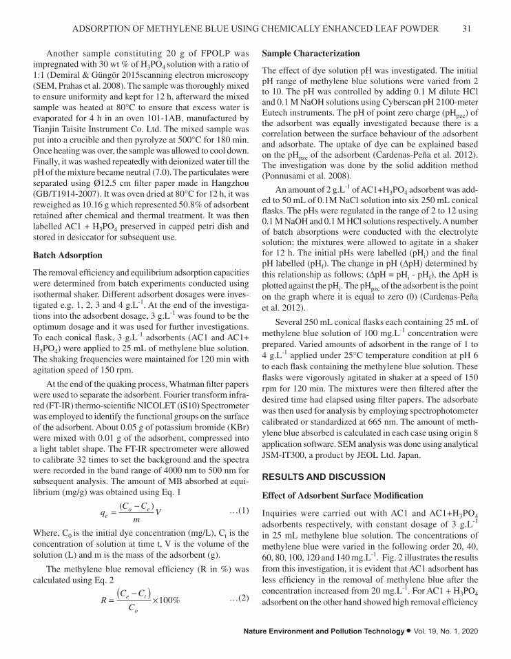
31ADSORPTION OF METHYLENE BLUE USING CHEMICALLY ENHANCED LEAF POWDER
Nature Environment and Pollution Technology • Vol. 19, No. 1, 2020
Another sample constituting 20 g of FPOLP was impregnated with 30 wt % of H3PO4 solution with a ratio of 1:1 (Demiral & Güngör 2015scanning electron microscopy (SEM, Prahas et al. 2008). The sample was thoroughly mixed to ensure uniformity and kept for 12 h, afterward the mixed sample was heated at 80°C to ensure that excess water is evaporated for 4 h in an oven 101-1AB, manufactured by Tianjin Taisite Instrument Co. Ltd. The mixed sample was put into a crucible and then pyrolyze at 500°C for 180 min. Once heating was over, the sample was allowed to cool down. Finally, it was washed repeatedly with deionized water till the pH of the mixture became neutral (7.0). The particulates were separated using Ø12.5 cm filter paper made in Hangzhou (GB/T1914-2007). It was oven dried at 80°C for 12 h, it was reweighed as 10.16 g which represented 50.8% of adsorbent retained after chemical and thermal treatment. It was then labelled AC1 + H3PO4 preserved in capped petri dish and stored in desiccator for subsequent use.
Batch Adsorption
The removal efficiency and equilibrium adsorption capacities were determined from batch experiments conducted using isothermal shaker. Different adsorbent dosages were inves-tigated e.g. 1, 2, 3 and 4 g.L-1. At the end of the investiga-tions into the adsorbent dosage, 3 g.L-1 was found to be the optimum dosage and it was used for further investigations. To each conical flask, 3 g.L-1 adsorbents (AC1 and AC1+ H3PO4) were applied to 25 mL of methylene blue solution. The shaking frequencies were maintained for 120 min with agitation speed of 150 rpm.
At the end of the quaking process, Whatman filter papers were used to separate the adsorbent. Fourier transform infra-red (FT-IR) thermo-scientific NICOLET (iS10) Spectrometer was employed to identify the functional groups on the surface of the adsorbent. About 0.05 g of potassium bromide (KBr) were mixed with 0.01 g of the adsorbent, compressed into a light tablet shape. The FT-IR spectrometer were allowed to calibrate 32 times to set the background and the spectra were recorded in the band range of 4000 nm to 500 nm for subsequent analysis. The amount of MB absorbed at equi-librium (mg/g) was obtained using Eq. 1
qC C
mVe
o e=-( ) …(1)
Where, C0 is the initial dye concentration (mg/L), Ct is the concentration of solution at time t, V is the volume of the solution (L) and m is the mass of the adsorbent (g).
The methylene blue removal efficiency (R in %) was calculated using Eq. 2
RC C
Ce t
o
=-( )
¥100% …(2)
Sample Characterization
The effect of dye solution pH was investigated. The initial pH range of methylene blue solutions were varied from 2 to 10. The pH was controlled by adding 0.1 M dilute HCl and 0.1 M NaOH solutions using Cyberscan pH 2100-meter Eutech instruments. The pH of point zero charge (pHpzc) of the adsorbent was equally investigated because there is a correlation between the surface behaviour of the adsorbent and adsorbate. The uptake of dye can be explained based on the pHpzc of the adsorbent (Cardenas-Peña et al. 2012). The investigation was done by the solid addition method (Ponnusami et al. 2008).
An amount of 2 g.L-1 of AC1+H3PO4 adsorbent was add-ed to 50 mL of 0.1M NaCl solution into six 250 mL conical flasks. The pHs were regulated in the range of 2 to 12 using 0.1 M NaOH and 0.1 M HCl solutions respectively. A number of batch absorptions were conducted with the electrolyte solution; the mixtures were allowed to agitate in a shaker for 12 h. The initial pHs were labelled (pHi) and the final pH labelled (pHf). The change in pH (DpH) determined by this relationship as follows; (DpH = pHi - pHf), the DpH is plotted against the pHi. The pHpzc of the adsorbent is the point on the graph where it is equal to zero (0) (Cardenas-Peña et al. 2012).
Several 250 mL conical flasks each containing 25 mL of methylene blue solution of 100 mg.L-1 concentration were prepared. Varied amounts of adsorbent in the range of 1 to 4 g.L-1 applied under 25°C temperature condition at pH 6 to each flask containing the methylene blue solution. These flasks were vigorously agitated in shaker at a speed of 150 rpm for 120 min. The mixtures were then filtered after the desired time had elapsed using filter papers. The adsorbate was then used for analysis by employing spectrophotometer calibrated or standardized at 665 nm. The amount of meth-ylene blue absorbed is calculated in each case using origin 8 application software. SEM analysis was done using analytical JSM-IT300, a product by JEOL Ltd. Japan.
RESULTS AND DISCUSSION
Effect of Adsorbent Surface Modification
Inquiries were carried out with AC1 and AC1+H3PO4 adsorbents respectively, with constant dosage of 3 g.L-1 in 25 mL methylene blue solution. The concentrations of methylene blue were varied in the following order 20, 40, 60, 80, 100, 120 and 140 mg.L-1. Fig. 2 illustrates the results from this investigation, it is evident that AC1 adsorbent has less efficiency in the removal of methylene blue after the concentration increased from 20 mg.L-1. For AC1 + H3PO4 adsorbent on the other hand showed high removal efficiency

32 Baba Imoro Musah et al.
Vol. 19, No. 1, 2020 • Nature Environment and Pollution Technology
for all initial methylene blue concentrations studied.
Decolourization of aqueous methylene blue solution was 100% for AC1 + H3PO4 at 20, 40, 60 mg.L-1. It declined to 99.8, 96.7, 92.9 and 90.9% at 80, 100,120 and 140 mg.L-1 respectively.
When AC1 adsorbent, removal efficiency stood at 94.7, 71.7 and 64.2% with concentration 20, 40 and 60 mg.L-1 respectively.
The removal efficiency still reduced significantly to 58.0% with a concentration of 80 mg.L-1 and 46.5% with 100 mg.L-1, consequently, an increase in methylene blue concentration to 120 mg.L-1 showed a downward trend of 34.5% removal of methylene blue and eventually reduced to 20.5% with a concentration of 140 mg.L-1.
The trends observed could be explained by the fact that, the adsorbent surface becomes saturated with the increase in methylene blue concentration as similarly reported (Xiong et al. 2010).
Effect of pH
The effect of pH on methylene blue adsorption was examined using AC1 and AC1+H3PO4 adsorbents respectively in 100 mg.L-1 initial methylene blue concentration with adsorbent dosage 3 g.L-1 at temperature 25°C. Initial pH of methylene blue solution was adjusted between 2 to 10 in Fig. 3a. The pH of point zero charge (pHpzc) of the adsorbent was studied in the range of 0 to 12 as shown in Fig. 3b.
When the initial pH was first increased from 2 to 4 in Fig. 3a, the removal efficiency of dye increased from 98.6% to 99.2%. Removal efficiency further increased to 100%
when initial pH was augmented to 6, but both pH 8 and 10 recorded same slight decline in methylene blue removal efficiencies at 99.4% as in Fig. 3a.
In the case of using AC1 adsorbent, when the pH was adjusted from pH 2 to 4, the removal efficiency increased from 49.8 to 70.5%. Additional increase in pH to 6 resulted in a rise in the methylene blue removal percentage to 82.9% in Fig. 3a. Further increase in initial methylene blue pH between 8 and 10, resulted in a minimal reduction in removal efficiency to 81.8 and 79.6% respectively as represented in Fig. 3a.
In Fig. 3b shows the results of pH at point of zero charge (pHPzc) of the adsorbent surface. The pHPzc was recorded at pH 1.8 in (Fig. 3b) lower than pH 6 at which maximum adsorption of the dye took place. There is some correlation between solution pH and pHpzc. It is reported that if the optimum pH of a solution is great than the pHPzc, the electrostatic force of attraction between positively charge dyes and negatively charged AC1+H3PO4 adsorbent is greatly enhanced and vice versa (El Qada et al. 2008). Since this study revealed pH 6 as optimum, it is clear that, pH had some influence on the adsorption of methylene blue as explained. Similar corroborative report suggests that, hydrogen reduces between pH 6 and 7, this gives rise to enhanced adsorption (Nethaji et al. 2013).
Effect of Adsorbent Dosage
The effect of adsorbent dosage was studied using AC1 and AC1+H3PO4 respectively in Fig. 4.
In order to determine the suitable quantity of the adsor-
10
Fig. 2: Effect of adsorbents surface modification (a) Removal efficiency capacity using AC1 and
AC1+H3PO4, with adsorbents dosage of 3 g.L-1 at temperature 25°C, time 2 h and neutral pH
with agitation speed at 150 rpm.
Decolourization of aqueous methylene blue solution was 100% for AC1+H3PO4 at 20, 40, 60
mg.L-1. It declined to 99.8, 96.7, 92.9 and 90.9% at 80, 100,120 and 140 mg.L-1 respectively.
When AC1 adsorbent, removal efficiency stood at 94.7, 71.7 and 64.2% with concentration 20,
40 and 60 mg.L-1 respectively.
The removal efficiency still reduced significantly to 58.0% with a concentration of 80 mg.L-1 and
46.5% with 100 mg.L-1, consequently, an increase in methylene blue concentration to 120 mg.L-1
showed a downward trend of 34.5% removal of methylene blue and eventually reduced to 20.5%
with a concentration of 140 mg.L-1.
Fig. 2: Effect of adsorbents surface modification. Removal efficiency using AC1 and AC1+H3PO4, with adsorbents dosage of 3 g.L-1 at temperature 25°C, time 2 h and neutral pH with agitation speed at 150 rpm.

33ADSORPTION OF METHYLENE BLUE USING CHEMICALLY ENHANCED LEAF POWDER
Nature Environment and Pollution Technology • Vol. 19, No. 1, 2020
bent to achieve enough removal of dyes, varied dosages in the order 1, 2, 3 and 4 g.L-1 per 25 mL solution of methylene blue were applied in each 250 mL conical flask. All other parameters e.g. initial concentration 100 mg.L-1, tempera-ture 25°C, pH 6, shaking speed 150 rpm and contact time with absorbent 2 h were kept constant while varying the adsorbent dosage. The results obtained are presented in Fig. 4. It is clear that, when AC1 adsorbent was increased from 1 g.L-1 to 3 g.L-1, the removal efficiency moved from 85.7 to 93.1%. When the adsorbent dosage was further increased
11
The trends observed could be explained by the fact that, the adsorbent surface becomes saturated
with the increase in methylene blue concentration as similarly reported (Xiong et al. 2010).
Effect of pH
The effect of pH on methylene blue adsorption was examined using AC1 and AC1+H3PO4
adsorbents respectively in 100 mg.L-1 initial methylene blue concentration with adsorbent dosage
3 g.L-1 at temperature 25°C. Initial pH of methylene blue solution was adjusted between 2 to 10
in Fig. 3a. The pH of point zero charge (pHpzc) of the adsorbent was studied in the range of 0 to
12 as shown in Fig. 3b.
Fig. 3: Effect of pH (a) removal efficiency and (b) pHpzc at temperature 25°C.
Fig. 3: Effect of pH (a) removal efficiency and (b) pHpzc at temperature 25°C.
to 4 g.L-1, the depletion of dyes slightly changed to 93.9%. Likewise, with the application of AC1+H3PO4 adsorbent, it was also noticed that, increasing adsorbent dosage resulted in increase in dyes depletion. When the adsorbent dosage was varied from 1 g.L-1 to 3 g.L-1, removal of dyes increased from 93.6% to 100%. No further variation in the adsorbent dosage was deemed necessary given the outcome recorded.
Effect of Initial Methylene Blue Concentration
Investigation was carried out to evaluate the effect of initial
13
Effect of Adsorbent Dosage
The effect of adsorbent dosage was studied using AC1 and AC1+H3PO4 respectively in Fig. 4.
Fig. 4: Effect of adsorbent dosage on methylene blue adsorption, 100 mg.L-1, temperature 25°C,
at pH 6 with agitation speed of 150 rpm and time 2 h.
In order to determine the suitable quantity of the adsorbent to achieve enough removal of dyes,
varied dosages in the order 1, 2, 3 and 4 g.L-1 per 25 mL solution of methylene blue were applied
in each 250 mL conical flask. All other parameters e.g. initial concentration 100 mg.L-1,
temperature 25°C, pH 6, shaking speed 150 rpm and contact time with absorbent 2 h were kept
constant while varying the adsorbent dosage. The results obtained are presented in Fig. 4. It is
clear that, when AC1 adsorbent was increased from 1 g.L-1 to 3 g.L-1, the removal efficiency
moved from 85.7 to 93.1%. When the adsorbent dosage was further increased to 4 g.L-1, the
Fig. 4: Effect of adsorbent dosage on methylene blue adsorption, 100 mg.L-1, temperature 25°C, at pH 6 with agitation speed of 150 rpm and time 2 h.

34 Baba Imoro Musah et al.
Vol. 19, No. 1, 2020 • Nature Environment and Pollution Technology
methylene blue concentration on adsorption. The results of the findings are shown in Fig. 5 using AC1 and AC1+H3PO4 adsorbents respectively.
The evaluation was done using constant adsorbent dosage of 3 g.L-1 in 25 mL solution of methylene blue at temperature 25°C. The initial concentrations were varied in this order 20, 40, 60, 80,100, 120 and 140 mg.L-1 at pH 6 for 2 h. For AC1 adsorbent, 100% of the dye was removed at initial concentration of 20 mg.L-1 but reduced to 84.6% at initial concentration 140 mg.L-1.
The unit adsorption capacity increased from 6.6 to 39.5 mg.g-1 using AC1 adsorbent when initial concentration was varied from 20 mg.L-1 to 140 mg.L-1. This pattern as observed in this investigation has some similarity with other studies involving methylene blue (Elizalde-González et al. 2007, Demirbas et al. 2008).
It was observed that, 100% of the methylene blue was using AC1+ H3PO4 adsorbent for initial concentrations from 20 to 100 mg.L-1. However, the removal efficiency steadily declined upon further increase in initial methylene blue con-centration between 120 and 140 mg.L-1 with corresponding removals at 96.3 and 91.9% respectively.
The adsorption capacity for AC1+ H3PO4 adsorbent increased from 6.6 to 42.9 mg.g-1 when initial concentration was augmented from 20 mg.L-1 to 140 mg.L-1. It is obvious from the above finding that, increasing concentration nega-tively affected the amount of dyes removed for adsorbents.
This finding is attributed to the saturation of empty sites within the adsorbent (Garg et al. 2004, Hameed et al. 2008).
Effect of Contact Time
This was studied in order to evaluate its impact on methylene blue uptake. This investigation was done using varied inter-vals of time as indicated in Fig. 6, as a result the equilibrium time was also determined.
Every other parameter in essentially was kept constant while time was adjusted within the intervals 5, 10, 20, 30, 40, 80 and 120 minutes since it was the only factor under evaluation in this case as indicated in Fig. 6. The results showed that, 80 min contact time was enough for the system to reach equilibrium with the given initial concentration. In Fig. 6 above, the adsorption process was a little bit rapid during the initial stages (from 0 to 40 min) with corre-sponding adsorption capacity from 28.7 to 32.8 mg.g-1. This slow incremental trend continued until the system reached equilibrium with a maximum adsorption capacity of 33.34 mg.g-1. The rapid uptake phenomenon may have occurred due to high presence of unoccupied or relatively vacant sites in the adsorbent at the initial stages. As the vacant sites were being occupied in the process of the adsorption, dye uptake slowed down due to a reduction in active vacant sites on the surface of AC1+H3PO4 adsorbent. There is a corroborative finding to what was recorded (Hameed et al. 2008)low-cost, locally available sorbent, pomelo (Citrus grandis).
14
depletion of dyes slightly changed to 93.9%. Likewise, with the application of AC1+H3PO4
adsorbent, it was also noticed that, increasing adsorbent dosage resulted in increase in dyes
depletion. When the adsorbent dosage was varied from 1 g.L-1 to 3 g.L-1, removal of dyes
increased from 93.6% to 100%. No further variation in the adsorbent dosage was deemed
necessary given the outcome recorded.
Effect of Initial Methylene Blue Concentration
Investigation was carried out to evaluate the effect of initial methylene blue concentration on
adsorption. The results of the findings are shown in Fig. 5 using AC1 and AC1+H3PO4
adsorbents respectively.
Fig. 5: Effect of initial methylene blue concentration (a) removal efficiency and (b) adsorption
capacity, with adsorbent dosage 3 g.L-1, at pH 6, time 2 h at temperature 25°C and agitation
speed of 150 rpm.
Fig. 5: Effect of initial methylene blue concentration (a) removal efficiency and (b) adsorption capacity, with adsorbent dosage 3 g.L-1, at pH 6, time 2 h at temperature 25°C and agitation speed of 150 rpm.

35ADSORPTION OF METHYLENE BLUE USING CHEMICALLY ENHANCED LEAF POWDER
Nature Environment and Pollution Technology • Vol. 19, No. 1, 2020
Effect of Temperature
The effect of temperature on methylene blue uptake was investigate studied with different temperatures ranging from 15 to 45°C. Since the evaluation here was relating to heat variation, the other parameters such as initial methylene blue concentration 100 mg.L-1, adsorbent dosage 3 g.L-1 (AC1+ H3PO4), pH 6, contact time 2 h and agitation speed at 150 rpm were maintained. Fig. 7, showed that, temperature var-iation had little or no effect on the removal percentage of methylene blue when temperature was increased from 15°C to 45°C. This outcome means temperature changes did not
16
Fig. 6: Effect of contact time on methylene blue adsorption using AC1+H3PO4 adsorbent; initial
concentration 100 mg.L-1, pH 6, at temperature 25°C, agitation speed 150 rpm and adsorbent
dosage 3 g.L-1.
Every other parameter in essentially was kept constant while time was adjusted within the
intervals 5, 10, 20, 30, 40, 80 and 120 minutes since it was the only factor under evaluation in
this case as indicated in Fig. 6. The results showed that, 80 min contact time was enough for the
system to reach equilibrium with the given initial concentration. In Fig. 6 above, the adsorption
process was a little bit rapid during the initial stages (from 0 to 40 min) with corresponding
adsorption capacity from 28.7 to 32.8 mg.g-1. This slow incremental trend continued until the
system reached equilibrium with a maximum adsorption capacity of 33.34 mg.g-1. The rapid
uptake phenomenon may have occurred due to high presence of unoccupied or relatively vacant
sites in the adsorbent at the initial stages. As the vacant sites were being occupied in the process
of the adsorption, dye uptake slowed down due to a reduction in active vacant sites on the surface
Fig. 6: Effect of contact time on methylene blue adsorption using AC1+H3PO4 adsorbent; initial concentration 100 mg.L-1, pH 6, at temperature 25°C, agitation speed 150 rpm and adsorbent dosage 3 g.L-1.
17
of AC1+H3PO4 adsorbent. There is a corroborative finding to what was recorded (Hameed et al.
2008).
Effect of Temperature
The effect of temperature on methylene blue uptake was investigate studied with different
temperatures ranging from 15 to 45°C. Since the evaluation here was relating to heat variation,
the other parameters such as initial methylene blue concentration 100 mg.L-1, adsorbent dosage 3
g.L-1 (AC1+H3PO4), pH 6, contact time 2 h and agitation speed at 150 rpm were maintained. Fig.
7, showed that, temperature variation had little or no effect on the removal percentage of
methylene blue when temperature was increased from 15°C to 45°C. This outcome means
temperature changes did not influence the adsorption process. The adsorption capacity recorded
33.34 mg.g-1.
Fig. 7: Effect of temperature on methylene blue adsorption with initial concentration 100 mg.L-1, time 2 h, adsorbent dosage 3 g.L-1 (AC1+H3PO4), agitation speed 150 rpm at pH 6.
influence the adsorption process. The adsorption capacity recorded 33.34 mg.g-1.
Adsorption Kinetics
Kinetics relates directly to thermodynamic equilibrium rate pertaining to a system that is not in an equilibrium state, thus the process of adsorption would linger on until equilibrium is established. However, in the case of desorption, the process is the reverse till the attainment of equilibrium.
The adsorption rates can effectively be evaluated using Lagergren (Ho 2004) pseudo-first-order model for kinetics
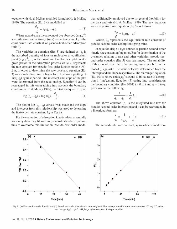
36 Baba Imoro Musah et al.
Vol. 19, No. 1, 2020 • Nature Environment and Pollution Technology
together with Ho & McKay modified formula (Ho & McKay 1999). The equation (Eq. 3) is modelled as:
d
dk q q
qt
te t= -1 ( ) …(3)
Where qe and qt are the amount of dye absorbed (mg.g-1) at equilibrium and at time, t (min) respectively and k1 is the equilibrium rate constant of pseudo-first-order adsorption (min-1).
The variables in equation (Eq. 3) are defined as: qe is the adsorbed quantity of ions or molecules at equilibrium point (mg.g-1), qt is the quantum of molecules uptaken at a given period in the adsorption process while k1 represents the rate constant for pseudo-first-order kinetic model (1/h). But, in order to determine the rate constant, equation (Eq. 3) was standardized into a linear form to allow a plotting of ln(qe-qt) against period. The intercept and slope of the plot were determined from the relationship. Equation 4 can be rearranged in this order taking into account the boundary conditions (Ho & Mckay 1998), t = 0 to t and qt = 0 to qt as:
log (qe – qt) = log (qe) - d
dtqt
…(4)
The plot of log (qe - qt) versus t was made and the slope and intercept from this relationship was used to determine the first-order rate constant, k1 in Fig 8a.
For the evaluation of adsorption kinetics data, essentially not every data may fit well in pseudo-first-order equation, thus to overcome this limitation, pseudo-first-order model
was additionally employed due to its general flexibility for the data analysis (Ho & McKay 1999). The new equation was reorganized into equation (Eq.5) as follows:
d
dtqt = k2 (qe – qt)
2 …(5)
Where, k2 represents the equilibrium rate constant of pseudo-second-order adsorption (g/mg min).
In equation (Eq. 5), k2 is defined as pseudo-second-order kinetic rate constant (g/mg min). But for determination of the dynamics relating to rate and other variables, pseudo-sec-ond-order equation (Eq. 5) was rearranged. The suitability of this model is verified after getting linear graph from the
plot of tq against t. The value of k2 was determined from the
intercept and the slope respectively. The rearranged equation (Eq. 10) is below and k2qe
2 is equal to initial rate of adsorp-tion h (mg/g.min). Equation (5) taking into consideration the boundary condition (Ho 2004) t = 0 to t and qt = 0 to qt gives rise to the following:
1 12q q q
ke t e-
= t …(6)
The above equation (6) is the integrated rate law for pseudo-second-order interaction and it can be rearranged in a linearized form as:
t
q k qt q e e
= +1 1
2 2
t …(7)
The second-order rate constant, k2 was determined from
19
The plot of log (qe-qt) versus t was made and the slope and intercept from this relationship was
used to determine the first-order rate constant, k1 in Fig 8a.
Fig. 8: (a) Pseudo-first-order kinetic and (b) Pseudo-second-order kinetic; on methylene, blue
adsorption with initial concentration 100 mg.L-1, adsorbent dosage 3 g.L-1 (AC1+H3PO4),
agitation speed 150 rpm at pH 6.
Fig. 8: (a) Pseudo-first-order kinetic and (b) Pseudo-second-order kinetic; on methylene, blue adsorption with initial concentration 100 mg.L-1, adsor-bent dosage 3 g.L-1 (AC1+H3PO4), agitation speed 150 rpm at pH 6.

37ADSORPTION OF METHYLENE BLUE USING CHEMICALLY ENHANCED LEAF POWDER
Nature Environment and Pollution Technology • Vol. 19, No. 1, 2020
a calculation using the slope and intercept of the plot tqt
versus t.
The Pseudo-first and second-order adsorption rate con-stants for 100 mg L initial methylene blue concentration are given in Table 1.
Adsorption Mechanisms
The surface morphology, and pores of an adsorbent is de-pendent on the adsorbent type. In this study, two different methods (Nowicki et al. 2010); physical and chemical acti-vation were employed in the preparation of the adsorbent for the adsorption. Physical activation involves the subjection of a raw material or waste to higher degree of heating either in an oxygen, steam or carbon monoxide condition in a tem-perature regime such as 300-1200°C (Nowicki & Pietrzak 2010). While in the chemical activation process, the dried leaf powder was largely inoculated with 1:1 phosphoric acid (H3PO3) solution (Yakout & Sharaf El-Deen 2016), air-dried and subsequently subjected to thermal treated at 500°C for 3 h. The adsorbents (FPOLP, AC1 and AC1 + H3PO4) were spectrally (FTIR) examined with the aid of a spectrometer as shown in Fig. 9. The thermal treatments of AC1 and AC1 + H3PO4 adsorbents respectively, could be responsible for the shift of peaks for AC1 graph labelled (B) and for AC1 + H3PO4 graph labelled (A) all in Fig. 9. Again, the subsequent chemical injection (H3PO4) on AC1 + H3PO4 adsorbent effectively changed its morphology, making it more porous as observed in the SEM in Fig. 10b. Apart from acids, other chemicals such as salts, e.g. ZnCl2 (Hu et al. 2009) or base, e.g. KOH (Evbuomwan et al. 2012) could have been used to enhance the porosity of surface area of the adsorbent. The main objective of the activation is essentially to optimize the surface area (micro and mesoporous) availability on the FPOLP for efficient adsorption. From the results, firmed by the SEM analysis, the chemical activation had proven to be more effective compared to the physical activation alone. Similar study has been sighted by Mohammad & Rahbar-ke-lishami (2014) has been sighted, however, it is important to stress that, the explanation given about the adsorbent preparation is quite ambiguous.
FTIR Spectra Analysis
The spectra analysis of three different samples (a) AC1 + H3PO4, (b) AC1 and (c) FPOLP are presented in Fig. 9. In
Table 1: Pseudo-first and second-order adsorption rate constants for 100 mg L initial methylene blue concentration.
Experiment Pseudo-first-order Pseudo-second-order
Exqe (mg g-1) k1 (min−1) cal qe, (mg.g-1) R2 k2 (g.mg-1 min-1) cal qe (mg.g-1) R2
42.90 0.083 27.44 0.982 0.029 38.40 0.999
Fig. 9a, the peak 1081 cm-1 may be assigned to strong C-O stretching, this functional group is associated with primary alcohol (Pradhan 2011).
Peak 1161 cm-1 is generated due to robust C-O stretching and it may be the effect of aliphatic ether. The peak at 1384 cm-1 is intermediate bending due to O-H and its functional-ity could most likely be phenol. However, the strong C=C stretching effect likely generated the peak at 1613 cm-1 (Kundu et al. 2008).
The peaks between 3400 and 3550 cm-1 on spectra Fig. 9c (FPOLP) could be allotted to great dominance O-H functional group, thus representing free hydroxyl funda-mentals located in the FPOLP. The peaks at 2850 and 2925 cm-1 may be assigned to aromatic elements, however after being subjected to higher temperature (500°C) in an oxidized environment for 180 min, led to the disappearance of the two peaks in Fig. 9a and 9b.
The peaks between 1626 and 1629 cm-1 have the char-acteristics of carbonyl functionality due to the effect of -COOH (Jokar et al. 2016). However, band 1318 cm-1 and 1400 cm-1 could be associated with aromatic nitriles which play a significant role in obtaining amines in hydrogenation process (Thusnavis et al. 2011, Wu et al. 2008). After sub-jection to different modifications in an oxidized condition, peak 1318 and 1048 cm-1 in Fig. 9c varnished in Fig. 9a and Fig. 9b, which are attributable to primary alcohol which could easily be oxidized to aldehydes or carboxylic acid depending on the reaction condition. Peak shift occurred at 1081 cm-1 (Fig. 9a) compared to the peak at 1048 cm-1 in Fig. 9c, this could possibly be the result of the modification effect. From the investigation conducted, the multiple modification had significant reflection in the adsorption attributes on adsorbent AC1 + H3PO4. It is reported that, the activation of carbon materials with oxidizing agents help generate oxygen-related functionalities that enhances the adsorption capabilities of the adsorbent during adsorption (Li et al. 2002, Do 1998).
SEM Analysis
Investigations were conducted on samples AC1 and AC1+ H3PO4 adsorbents respectively, employing scanning electron microscopic techniques. The results revealed very porous morphological features after it was treated with phosphoric acid (1:1) for 4 h prior to thermal treatment for 3 h for AC1 + H3PO4 adsorbent. Fig. 10a (AC1) adsorbent showed cell-

38 Baba Imoro Musah et al.
Vol. 19, No. 1, 2020 • Nature Environment and Pollution Technology
like pores on the surface of the adsorbent while Fig. 10b (AC1 + H3PO4) adsorbent revealed the inner pores present in the adsorbent.
The presence of both surface and inner pores on the adsorbent may have contributed significantly to the over-whelming adsorption of the dye molecules. The injection of oxygenated compounds into carbonaceous materials may have increased the level of porosity on the adsorbent which effectively enhance the adsorption capabilities as the adsorption investigation showed a remarkable removal, in some cases as earlier reported (Yakout & Sharaf 2016, Prahas et al. 2008, Altenor et al. 2009, Dias et al. 2007). The effectiveness of an adsorbent may be influenced by
23
FTIR Spectra Analysis
The spectra analysis of three different samples (a) AC1+H3PO4, (b) AC1 and (c) FPOLP are
presented in Fig. 9. In Fig. 9a, the peak 1081 cm-1 may be assigned to strong C-O stretching, this
functional group is associated with primary alcohol (Pradhan 2011).
Fig. 9: FTIR Spectra graph (a) AC1 + H3PO4 (b) AC1 and (c) FPOLP adsorbents respectively.
Peak 1161 cm-1 is generated due to robust C-O stretching and it may be the effect of aliphatic
ether. The peak at 1384 cm-1 is intermediate bending due to O-H and its functionality could most
likely be phenol. However, the strong C=C stretching effect likely generated the peak at 1613
cm-1 (Kundu et al. 2008).
FPOLP
AC1
AC1+H3 PO4
Fig. 9: FTIR Spectra graph (a) AC1 + H3PO4 (b) AC1 and (c) FPOLP adsorbents respectively.
varied parameters such as the porosity and high surface area. In addition, the solubility as well as the affinity that exist between the particulates and the adsorbent could result in a hydrophobic and hydrophilic interaction.
CONCLUSION
This study involved the investigation of Methylene blue us-ing two different absorbents prepared from fallen P. orientalis leaves powder. For AC1 adsorbent, it was thermally treated at 500°C for 2 h, while AC1+H3PO4 adsorbent was injected with phosphoric acid 1:1 solution followed by thermal treatment at same temperature and time as AC1. The removal efficiency reduced from 100% to 84.6% when MB concentration was
25
treatment for 3 h for AC1+H3PO4 adsorbent. Fig. 10a (AC1) adsorbent showed cell-like pores on
the surface of the adsorbent while Fig. 10b (AC1+H3PO4) adsorbent revealed the inner pores
present in the adsorbent.
Fig. 10: SEM results (a) AC1 and (b) AC1+H3PO4 adsorbents respectively.
The presence of both surface and inner pores on the adsorbent may have contributed significantly
to the overwhelming adsorption of the dye molecules. The injection of oxygenated compounds
into carbonaceous materials may have increased the level of porosity on the adsorbent which
effectively enhance the adsorption capabilities as the adsorption investigation showed a
remarkable removal, in some cases as earlier reported (Yakout & Sharaf 2016, Prahas et al.
2008, Altenor et al. 2009, Dias et al. 2007). The effectiveness of an adsorbent may be influenced
by varied parameters such as the porosity and high surface area. In addition, the solubility as well
as the affinity that exist between the particulates and the adsorbent could result in a hydrophobic
and hydrophilic interaction.
Fig. 10: SEM results (a) AC1 and (b) AC1+H3PO4 adsorbents respectively.

39ADSORPTION OF METHYLENE BLUE USING CHEMICALLY ENHANCED LEAF POWDER
Nature Environment and Pollution Technology • Vol. 19, No. 1, 2020
varied from 20 to 140 mg.L-1 for AC1 adsorbent, whereas for AC1+H3PO4, removal efficiency decreased from 100% to 91.6% when MB concentration increased from 20 to 140 mg.L-1. The effect of solution pH revealed pH 6 as the op-timum condition for maximum adsorption, from the range of 2 to10. The optimum adsorbent dosage was 3 g.L-1 at equilibrium time of 80 min and maximum adsorption was 42.9 mg.g-1. The surface morphology of AC1+H3PO4 after an SEM examination confirms earlier reports which suggest that phosphoric acid injection could enhance the surface characteristics of adsorbents, hence a fulfilment of one of the objectives of this study which was to ascertain the veracity of potential of phosphoric acid as activation agent for adsor-bents. FPOLP has proven to be a cheap source of activated carbon with good potential for adsorbing methylene blue.
ACKNOWLEDGEMENT
This research could not have been successfully executed without the financial backing of Wuhan University of Tech-nology (WUT:2016IVA046), Natural Science Foundation of China (Ref. 5104205) and Hubei Provincial Science Foundation (Ref. 2016CFB268), are graciously appreciated and acknowledged.
REFERENCES
Abadian, S., Rahbar-Kelishami, A., Norouzbeigi, R. and Peydayesh, M. 2015. Cu(II) adsorption onto Platanus orientalis leaf powder: Kinet-ic, isotherm, and thermodynamic studies. Res. Chem. Intermed., 41: 7669-7681.
Abid, M.F., Zablouk, M.A. and Abid-Alameer, A.M. 2012. Experimental study of dye removal from industrial wastewater by membrane tech-nologies of reverse osmosis and nanofiltration. Iranian J. Environ. Health Sci. Eng., 9: 17.
Akyol, A. 2012. Treatment of paint manufacturing wastewater by electro-coagulation. Desalination, 285: 91-99.
Altenor, S., Carene, B., Emmanuel, E., Lambert, J., Ehrhardt, J.J. and Gaspard, S. 2009. Adsorption studies of methylene blue and phenol onto vetiver roots activated carbon prepared by chemical activation. J. Hazard. Mater., 165: 1029-1039.
Babu, B.R., Parande, A.K. and Kumar, S.A. 2011. Treatment of dye ef-fluent by electrochemical and biological processes. Open J. Saf. Sci. Technol., 1: 12-18.
Cardenas-Peña, A.M., Ibanez, J.G. and Vasquez-Medrano, R. 2012. Deter-mination of the point of zero charge for electrocoagulation precipitates from an iron anode. Int. J. Electrochem. Sci., 7: 6142-6153.
Çiçek, F., Özer, D., Özer, A. and Özer, A. 2007. Low cost removal of reactive dyes using wheat brand. J. Hazard. Mater., 146: 408-416.
Demiral, H. and Güngör, C. 2015. Adsorption of copper (II) from aqueous solutions on activated carbon prepared from grape bagasse. J. Clean. Prod., 124: 103-113.
Demirbas, E., Kobya, M. and Sulak, M.T. 2008. Adsorption kinetics of a basic dye from aqueous solutions onto apricot stone activated carbon. Bioresour. Technol., 99: 5368-5373.
Dias, J.M., Alvim-Ferraz, M.C.M., Almeida, M.F., Rivera-Utrilla, J. and Sánchez-Polo, M. 2007. Waste materials for activated carbon prepa-ration and its use in aqueous-phase treatment: A review. J. Environ. Manage., 85: 833-846.
Do, D.D. 1998. Adsorption Analysis: Equilibria and Kinetics. Vol. 2, Im-perial College Press, London.
Dod, R., Banerjee, G. and Saini, S. 2012. Adsorption of methylene blue using green pea peels (Pisum sativum): a cost-effective option for dye-based wastewater treatment. Biotechnol. Bioprocess Eng., 17: 862-874.
El Qada, E.N., Allen, S.J. and Walker, G.M. 2008. Adsorption of basic dyes from aqueous solution onto activated carbons. Chem. Eng. J., 135: 174-184.
Elizalde-González, M.P., Mattusch, J., Peláez-Cid, A.A. and Wennrich, R. 2007. Characterization of adsorbent materials prepared from avocado kernel seeds: Natural, activated and carbonized forms. J. Anal. Appl. Pyrolysis, 78: 185-193.
El-Sharkawy, E.A., Soliman, A.Y. and Al-Amer, K.M. 2007. Comparative study for the removal of methylene blue via adsorption and photocat-alytic degradation. J. Colloid Interface Sci., 310: 498-508.
Evbuomwan, B.O., Abutu, A.S and Ezeh, C.P. 2012. The effects of carbon-ization temperature on some physicochemical properties of bamboo based activated carbon by potassium hydroxide (KOH) activation. Greener J. Phys. Sci., 3: 187-191.
Franca, A.S., Oliveira, L.S. and Ferreira, M.E. 2009. Kinetics and equilib-rium studies of methylene blue adsorption by spent coffee grounds. Desalination 249: 267-272.
Fu, Y. and Viraraghavan, T. 2001. Fungal decolorization of dye wastewaters: A review. Bioresour. Technol., 79: 251-262.
Galindo, C., Jacques, P. and Kalt, A. 2001. Photooxidation of the pheny-lazonaphthol AO20 on TIO2: Kinetic and mechanistic investigations. Chemosphere, 45: 997-1005.
Garg, V.K, Amita, M., Kumar, R. and Gupta, R. 2004. Basic dye (methylene blue) removal from simulated wastewater by adsorption using Indian rosewood sawdust: a timber industry waste. Dye Pigment, 63: 243-250.
Hameed, B.H. and Daud, F.B.M. 2008. Adsorption studies of basic dye on activated carbon derived from agricultural waste: Hevea brasiliensis seed coat. Chem. Eng. J., 139: 48-55.
Hameed, B.H., Mahmoud, D.K and Ahmad, Al. 2008. Sorption of basic dye from aqueous solution by pomelo (Citrus grandis) peel in a batch system. Colloids Surfaces A: Physicochem. Eng. Asp., 316: 78-84.
Ho, Y.S. 2004. Citation review of Lagergren kinetic rate equation on ad-sorption reactions. Scientometrics 59: 171-177.
Ho, Y.S. and Mckay, G. 1999. Pseudo-second order model for sorption processes. Process Biochem., 34: 451-465.
Ho, Y.S. and Mckay, G. 1998. Sorption of dyes from aqueous solution by peat. Chem. Eng. J., 70: 115-124.
Hu, C., Zhou, J., He, S., Luo, Z. and Cen, K. 2009. Effect of chemical acti-vation of an activated carbon using zinc chloride on elemental mercury adsorption. Fuel Process. Technol., 90: 812-817.
Jokar, M., Farahani, T.S. and Ramezanzadeh, B. 2016. Electrochemical and surface characterizations of Morus alba pendula leaves extract (MAPLE) as a green corrosion inhibitor for steel in 1M HCl. J. Taiwan Inst. Chem. Eng., 63: 436-452.
Kamsonlian, S., Suresh, S., Ramanaiah, V., Majumder, C.B., Chand, S. and Kumar, A. 2012. Biosorptive behaviour of mango leaf powder and rice husk for arsenic(III) from aqueous solutions. Int. J. Environ. Sci. Technol., 9: 565-578.
Kaushik, P. and Malik, A. 2009. Fungal dye decolourization: recent advances and future potential. Environ. Int., 35: 127-141.
Kundu, S., Wang, Y., Xia, W. and Muhler, M. 2008. Thermal stability and reducibility of oxygen-containing functional groups on multiwalled carbon nanotube surfaces: A quantitative high-resolution XPS and TPD/TPR study. J. Phys. Chem. C., 112: 16869-16878.
Lee, J.W. and Choi, S.P., Thiruvenkatachari, R., Shim, W.G. and Moon, H. 2006. Evaluation of the performance of adsorption and coagulation processes for the maximum removal of reactive dyes. Dye Pigment, 69: 196-203.
Li, L., Quinlivan, P.A. and Knappe, D.R.U. 2002. Effects of activated car-

40 Baba Imoro Musah et al.
Vol. 19, No. 1, 2020 • Nature Environment and Pollution Technology
bon surface chemistry and pore structure on the adsorption of organic contaminants from aqueous solution. Carbon N. Y., 40: 2085-2100.
Lupascu, T. and Povar, I. 2016. Analysis of adsorption technologies of water and wastewater treatment used in the republic of Moldova. American Journal of Chemical Engineering, 4(6): 147-153.
Murthy, U.N., Rekha, H.B. and Bhavya, J.G. 2011. Performance of elec-trochemical oxidation in treating textile dye wastewater by stainless steel anode. International Journal of Environmental Science and Development, 2(6): 483.
Nethaji, S., Sivasamy, A. and Mandal, A.B. 2013. Adsorption isotherms, kinetics and mechanism for the adsorption of cationic and anionic dyes onto carbonaceous particles prepared from Juglans regia shell biomass. Int. J. Environ. Sci. Technol., 10: 231-242.
Nowicki, P. and Pietrzak, R. 2010. Carbonaceous adsorbents prepared by physical activation of pine sawdust and their application for removal of NO2 in dry and wet conditions. Bioresour. Technol., 101: 5802-5807
Nowicki, P., Skrzypczak, M. and Pietrzak, R. 2010. Effect of activation method on the physicochemical properties and NO2 removal abilities of sorbents obtained from plum stones (Prunus domestica). Chem. Eng. J., 162: 723-729.
Oliveira, L.S., Franca, A.S., Alves, T.M. and Rocha, S.D.F. 2008. Evaluation of untreated coffee husks as potential biosorbents for treatment of dye contaminated waters. J. Hazard. Mater., 155: 507-512.
Pavan, F.A., Lima, E.C., Dias, S.L.P. and Mazzocato, A.C. 2008. Methylene blue biosorption from aqueous solutions by yellow passion fruit waste. J. Hazard. Mater., 150: 703-712.
Ponnusami, V., Vikram, S. and Srivastava, S.N. 2008. Guava (Psidium guajava) leaf powder: Novel adsorbent for removal of methylene blue from aqueous solutions. J. Hazard. Mater., 152: 276-286.
Pradhan, S. 2011. Production and characterization of activated carbon produced from a suitable Industrial sludge. Doctoral Thesis.
Prahas, D., Kartika, Y., Indraswati, N. and Ismadji, S. 2008. Activated carbon from jackfruit peel waste by H3PO4 chemical activation: Pore structure and surface chemistry characterization. Chem. Eng. J., 140: 32-42.
Rashed, M.N. 2013. Adsorption technique for the removal of organic pol-lutants from water and wastewater. In: Organic Pollutants-Monitoring, Risk and Treatment. Intech Open.
Saengbutr, K., Wangphon, N. and Wanchanthuek, R. 2014. The investigation of experimental condition and kinetic study of methylene blue adsorp-tion onto neem (Azadirachta indica) leaf powder. International Journal
of Scientific and Research Publications, 4(10): 2250-3153.Sawal, M. 1986. General standards for discharge of environmental pollut-
ants. Environ. Rules., 2: 545-560.Sleiman, M., Vildozo, D., Ferronato, C. and Chovelon, J.M. 2007. Pho-
tocatalytic degradation of azo dye Metanil yellow: Optimization and kinetic modeling using a chemometric approach. Appl. Catal. B Environ., 77: 1-11.
Thusnavis, K.P., Vinod Kumar, M. and Sankara Narayana Pillai, G.R. 2011. Seed extract of Psidium guajava as ecofriendly corrosion inhibitor for carbon steel in hydrochloric acid medium. J. Mater. Sci. Technol., 27: 1143-1149.
Tong, D.S., Hui, C., Zhou, C., Lu, Y., Yu, H., Zhang, G.F. and Yu, W.H. 2010. Applied clay science adsorption of acid red G dye on octadecyl trimethylammonium montmorillonite. Appl. Clay Sci., 50: 427-431.
Tsai, W.T., Chang, C.Y., Lin, M.C., Chien, S.F., Sun, H.F. and Hsieh, M.F. 2001. Adsorption of acid dye onto activated carbons prepared from agricultural waste bagasse by ZnCl2 activation. Chemosphere, 45: 51-58.
Wali, K.M.F. 2015. Color removal and cod reduction of dyeing bath waste-water by Fenton reaction. Int. J. Waste Resour., 5: 1-6.
Wang, L.H. and Lin, C.I. 2008. Adsorption of lead(II) ion from aqueous solution using rice hull ash. Ind. Eng. Chem. Res., 47: 4891-4897.
Wang, Z., Xue, M., Huang, K. and Liu, Z., 2011. Textile dyeing wastewater treatment. Advances in treating textile effluent, 5: 91-116.
Weng, C.H. and Pan, Y.F. 2007. Adsorption of a cationic dye (methylene blue) onto spent activated clay. J. Hazard. Mater., 144: 355-362.
Worch, Eckhard 2012. Adsorption Technology in Water Treatment: Funda-mentals, Processes, and Modeling. Walter de Gruyter.
World Health Organization 2006. A Compendium of Standards for Wastewater Reuse in The Eastern Mediterranean Region. WHO-EM/CEH/142/E. 19.
Wu, B., Zhang, J., Yang, M., Yue, Y., Ma, L.J. and Yu, X.Q. 2008. Raney Ni/KBH4: An efficient and mild system for the reduction of nitriles to amines. Arkivoc., 95-102.
Xiong, L., Yang, Y., Mai, J., Sun, W., Zhang, C., Wei, D., Chen, Q. and Ni, J. 2010. Adsorption behavior of methylene blue onto titanate nanotubes. Chem. Eng. J., 156: 313-320.
Yakout, S.M. and Sharaf EL-Deen, G. 2016. Characterization of activated carbon prepared by phosphoric acid activation of olive stones. Arab. J. Chem., 9: S1155-S1162.

Comparative In Vitro Assessment of Hydrocarbon Degradation Potential of Pleurotus ostreatus MP 5 and Pleurotus ostreatus MTCC 1804Madhavi Tiwari*†, Ashish Saraf** and Meghna Shrivastava* *MATS School of Sciences, MATS University, Raipur-494001, C.G., India**Faculty of Sciences, MATS University, Raipur-494001, C.G., India†Corresponding author: Madhavi Tiwari
ABSTRACTMycoremediation, involving the use of fungus for bioremediation, is one of the promising cost-effective methods for cleaning up the carcinogenic and mutagenic polycyclic aromatic hydrocarbons present in the environment. The present study deals with the isolation of white rot fungus from Chhattisgarh forest, India followed by identification based on ITS sequencing. Identification revealed MP 5 closely related to Pleurotus ostreatus isolate 6689 with 99% sequence similarity. Comparative primary screening assay of both the wild isolate and reference strain of Pleurotus ostreatus MTCC 1804 was performed by measuring the growth diameter of mycelia on minimal salt media enriched with 2% used engine oil (v/v). The fungal isolate MP 5 showed highest average growth rate. Confirmatory test was conducted via orbital shaking method and spectroscopic study was carried out at 600 nm which displayed degradation within 7 days and percentage of degradation was calculated. Level of degradation was 69.7 ± 0.351% and 64.7 ± 1.153% respectively for Pleurotus ostreatus MP 5 and Pleurotus ostreatus MTCC 1804. Degradation potential of both the isolates were evaluated in terms of chemical characterization via Fourier transform infrared spectroscopy (FTIR) which revealed bands formation based on the presence of different functional groups indicating oxidative degradation of hydrocarbons.
INTRODUCTION
Engine oil or motor oil is always on high demand globally and is used all over around the world in vehicles and other power generating engines. Improperly and illegitimately discharging of spent engine oil by automobile industries and other power generating stations into water bodies, farming lands and other arable lands is quite frequent. This disposed and spilled oil left unattended for several years further give rise to pollution of soil, water and air causing lethal environmental hazards. Oil contains more than 30 parent polyaromatic hydrocarbons (PAHs) which again constitutes hundreds of different hydrocarbon compounds such as paraffins, naphthene, aromatics as well as organic sulphur compounds, organic nitrogen compounds and oxygen containing hydrocarbons (Jawhari & Ihsan 2014). Increased use and demand of engines which in turn uses engine oil is the first and foremost reason for soil pollution. Leaving the spent oil unattended for several years reduces the fertility of the soil and converts it into a barren land. Both the used and unused engine oil are similar except that the used one comprises some additional chemicals which may have built up when engine runs by reacting with carcinogenic and mutagenic metals found in used motor oil that comes from engine parts
as they wear down (Adongbede & Sanni 2014). According to various researchers it’s a known fact that used motor oil contains metals and heavy polycyclic aromatic hydrocarbons which contribute to chronic hazards including mutagenic-ity and carcinogenicity (Boonchan et al. 2000, Hagwell et al. 1992, Keith & Telliard 1979). Undesirable presence of petroleum hydrocarbons in the environment is toxic, muta-genic and carcinogenic (Clemente et al. 2001). Therefore, the most ominous problems that the world is grappling today is the environmental pollution by petroleum hydrocarbons and its hazardous effects on ecosystem.
The objective of solving environmental pollution prob-lems with the application of biotechnological processes in-volving microorganism is rapidly growing in recent decades. Among such application of biotechnological processes, my-coremediation is one which can be defined as the use of fun-gal systems to catalyse the destruction or transformation of various hazardous chemicals to less harmful forms (Thomas et al. 1998). As it is simple to maintain, applicable over large areas, cost effective and leads to complete destruction of the contaminant, it has been proved out to be one of the fascinating approaches for cleaning up of the petroleum hydrocarbons (Huesemann 1994). The term mycoremedi-ation was coined by Paul Stamets which specifically refers
2020pp. 41-56 Vol. 19p-ISSN: 0972-6268 No. 1 Nature Environment and Pollution Technology
An International Quarterly Scientific Journal
Original Research Papere-ISSN: 2395-3454
Open Access
Nat. Env. & Poll. Tech.Website: www.neptjournal.com
Received: 30-06-2019Accepted: 29-08-2019
Key Words:Pleurotus ostreatusMycoremediationHydrocarbon degradationPAHsBioremediationWhite rot fungus

42 Madhavi Tiwari et al.
Vol. 19, No. 1, 2020 • Nature Environment and Pollution Technology
to the use of fungal mycelia in bioremediation. One of the primary roles of fungi in the ecosystem is decomposition, which is performed by the mycelium. It has been reported by Barr et al. (1994), that fungi secrete nonspecific extra-cellular enzymes such as laccase, lignin peroxidase and manganese peroxidase, that give these fungi the ability to degrade lignin and also used to degrade a wide range of hydrocarbon pollutants that resemble the lignin structure such as total petroleum hydrocarbons (TPHs), dichlo-rodiphenyltrichloroethane (DDT), trinitrotoluene (TNT), polychlorinated biphenyl (PCB) and polycyclic aromatic hydrocarbons (PAHs). Mycelial enzymes can decompose many resistant materials made by humans or nature, because many of the bonds that hold plant material together are like the bonds found in petroleum products including diesel and oil (Stamets 2005).
Application of higher fungi like mushrooms has been known in the remediation of polluted soil for some years now. The application of white-rot fungi in bioremediation is now considered to be economical because the fungi can be cultured on varieties of inexpensive agricultural or forest wastes such as rice straw, corn cobs and sawdust. According to the recent studies, P. ostreatus can degrade a variety of polycyclic aromatic hydrocarbons (PAH) (Sack & Gunther 1993). Emuh (2010) proclaimed that the mushroom hypha and mycelia possess the capability to break down and absorb the crude oil and heavy metals present in polluted soil through the secretion of enzymes into environmentally safe levels. Zebulun et al. (2011) reported his work on decontamina-tion of anthracene-polluted soil through a white rot fungus (P. ostreatus) which induced biodegradation. Further he divulged that lignolytic enzymes such as lignin peroxidase, laccase and manganese peroxidase by P. ostreatus catalysed the degradation of anthracene. Similarly, Okparanma et al. (2011) broadcasted that spent white-rot fungi (P. ostreatus) substrate can be utilized to remediate Nigerian oil-based drill cuttings constituting PAHs. The oyster mushroom, P. ostreatus, can degrade 80-95% of all PAHs present in soil (Steffen et al. 2007).
The utility of mushroom for biodegradation has beguiling probability because of their potentiality to degrade lignin and other resembling compounds like PAHs. According to the previous explorations involving white rot fungi and their capability to degrade petroleum hydrocarbons, several auspicious results have been reported. Hence the present investigation purposes to isolate white rot fungi and to per-form comparative evaluation of hydrocarbon degradation potential of both wild isolate and reference strain of Pleurotus ostreatus MTCC 1804 which may prove to be a promising isolate for mycoremediation studies.
MATERIALS AND METHODS
Chemicals and Reagents
All the media used during the experiment were purchased from Himedia Laboratories Pvt. Limited (Mumbai, In-dia). All the fine chemicals used were procured from SRL Chemicals, India with highest purity and analytical grade. Used engine oil of Castrol Company was procured from automobile workshop.
Source of Fungal Cultures
Fruiting bodies of the Basidiomycete samples were collected from Geedam forest spread across Dantewada district, Chhat-tisgarh, India. The samples were apparently brought to the laboratory in sterilized bags and were refrigerated at 4°C in refrigerator until they were processed. The materials were used for experimental procedures within 24 hours. Pleurotus ostreatus MTCC 1804 as reference strain was procured from Microbial Type Culture Collection (MTCC), Chandigarh, India. The fungus was propagated on Potato Dextrose Agar (PDA Himedia) at 25ºC for 7 days, maintained in agar slants and sub cultured after every 15 days.
Isolation of White Rot Fungus
The tissues of the wild isolate were inoculated into PDA (Himedia) prepared following the manufacturer’s instruc-tions. The pure culture of the test organism was incubated at room temperature for 7 days in biological oxygen demand (BOD) incubator. Culture was maintained in agar slants and subcultured after every 15 days.
Molecular Identification
Molecular characterization of the wild fungal isolate was achieved through ITS sequencing. Identification process was completed by comparing the ITS regions of the fungal isolate with NCBI data available and the closest neighbour with 99% similarity index was assigned. The identification was done by NCMR, Pune, Maharashtra, India.
Comparative Primary Screening
For primary screening, a selective carbon free media known as Mineral Salts Medium (MSM) [v/v] of Mills et al. (1978) as modified by Okpokwasili & Okorie (1988) was prepared which was later supplemented with 50 mg/mL ampicillin and 2% of filtered sterile used engine oil (Vanishree et al. 2014). 1 cm2 mycelial plug of pure fungal isolate was aseptically inoculated in MSM with the help of cork borer, and incubated at 25°C for 7 days and the growth rates were recorded daily by measuring the diameter of the radial extension of fungal mycelium (Thenmozhi et al. 2013). Pure fungal isolates

43ASSESSMENT OF HYDROCARBON DEGRADATION POTENTIAL OF FUNGUS
Nature Environment and Pollution Technology • Vol. 19, No. 1, 2020
were also inoculated on MSM without oil which served as control. All the inoculations were performed in triplicates. The growth rates of both the wild isolate and reference strain were recorded daily by measuring the diameter of the radial extension of the mycelium. Measurements were done by measuring at least two diameters per plate and average of diameters were used as the colony diameter at that time of measurement (cm/day) (dos Santos et al. 2008). According to dos Santos et al. (2008) colony growth rates were further evaluated by regressing the colony diameter against the days after inoculation. Fungal isolates which showed heavy sporulation, more abundant aerial mycelium and greater colony diameter were considered as organisms utilizing hy-drocarbons as their carbon source which were later confirmed through confirmatory screening (Thenmozhi et al. 2013).
Confirmatory Screening (Orbital Shaking Method)
To confirm the hydrocarbon degrading capability of the both the wild isolate and reference strain a modified technique based on the redox indicator 2, 6- dichlorophenol indophenol (DCPIP) was performed and purposely Bacto Bushnell- Hass (BH) broth medium was prepared (Hanson et al. 1993). A control flask without inoculum was also prepared. Three agar plugs from 7 days old culture of pure fungal isolates were picked from the surface of the Petri dish with the help of cork borer and aseptically inoculated into 50 mL of ster-ilized BH broth medium using 150 mL Erlenmeyer flask and later, also incorporated with 0.2 % (v/v) Tween 80, 2% (v/v) crude oil and redox reagent (2% 2, 6- dichlorophenol indophenols). All the flasks were incubated in orbital shaking incubator at 25°C with constant shaking at 180 rpm for 7 days. The aliquots inside the flask were supervised daily for colour change from deep blue to colourless. After 7 days of incubation period, filtration of the broth of all the flasks was accomplished with the help of filter paper for the separation of fungal biomass, proximately followed by centrifugation at 8000 rpm for 15 minutes. Supernatants obtained after centrifugation were assayed spectrophotometrically at 600 nm with the help of UV-VIS spectrophotometer (Systronics Double Beam Spectrophotometer 2203) and the percentage of biodegradation was evaluated via the following equation (Hanson et al. 1993, Tiwari et al. 2017)
Percentage (%) of Degradation = [1- Absorbance of treated sample/ Absorbance of control] x 100
Biodegradation Assay of Hydrocarbon by Fungal Cultures
Three agar discs of fresh pure cultures of duo fungal iso-lates were inoculated into 50 ml of BH broth in Erlenmeyer flask (150 mL) comprising 0.2 % (v/v) Tween 80 and 2%
(v/v) crude oil. Meanwhile control flask was also prepared accordingly but with no inoculum. Later all the flasks were incubated in orbital shaking incubator at temperature 25°C with constant shaking at 180 rpm for 7 days. Again after 7 days of incubation, broths were filtered with the help of filter paper to separate the biomass which was weighed for the dry weight of fungal biomass by constant weighing (Hanson et al. 1993).
FTIR Analysis
Two-three mycelial plugs of the fungal isolates were inoc-ulated in Czapeck dox broth with 2 % v/v used motor oil in a 250 mL Erlenmeyer flask. Control experiment containing same medium contents but without inoculum was performed. The flasks were agitated at 200 rpm at 25ºC for a period of 30 days and the content of each test including the control were harvested and subjected to FT-IR analysis (Thenmozhi et al. 2013). After harvesting all the samples including the control, were dried at 70ºC overnight before analysis to convert them into powdered form. KBr pellet was used as a background reference (Velioğlu et al. 2015). Approximately 1 mg of each of the samples were mixed with approximately 100 mg of dried KBr separately and then pressed to form a pellet for measurement. The FTIR spectra were broadcasted on the Perkin Elmer Inc. – Spectrum BX FTIR spectrometer, in the 4000-400 cm-1 spectral region.
Statistical Analysis
An analysis of variance (ANOVA) was performed to es-tablish if there were any significant differences between the growth rates of the strains and their control plates at 95% confidence level (P £ 0.05). T test was also performed to statistically compare the means of colony diameter (cm/day) of both the isolates, percentage of degradation (%) and bio-degradation assay of hydrocarbon in terms of fungal biomass (g/50 mL) at 95% confidence level (P £ 0.05).
RESULTS
Isolation of White Rot Fungus and Cultivation of Ostreatus MTCC 1804
Tissue culture of wild isolate MP 5 on PDA followed by 7 days of incubation gave pure culture of cottony white coloured mycelium with glossy surface (Fig. 1). Likewise procured culture, Pleurotus ostreatus MTCC 1804 also gave the mycelium with same appearance (Fig. 2).
Molecular Identification
The isolated white rot fungus was identified based on ITS sequencing and sequence of the identified isolate was

44 Madhavi Tiwari et al.
Vol. 19, No. 1, 2020 • Nature Environment and Pollution Technology
generated using NCBI data base, and the confidence in identification was limited by both the availability and the extent of homology shown by the ~550 bp sequence of the sample with its closest neighbour in the database. Molec-ular characterization of the wild isolate which exhibited high sequence similarity (~99%) to that of Pleurotus ostreatus isolate 6689 (accession No. AY450345.1). Fig. 3 shows the nucleotide sequence in FASTA format which was resulted out based on ITS sequencing. After identification process, MP 5 isolate was also got deposited in NCMR Pune, in general deposition repository under accession No. MCC 1815.
Colony Growth Evaluation
Colony growth rate evaluation was done to investigate the primary screening of hydrocarbon degradation potential of both the isolates based on colony diameter. As the colony growth rates (cm/day) were calculated by regressing the colony diameter against the days after inoculation it was resulted out that the growth curves of the isolates, based on colony diameters as a function of time, were typical of fungal growth. The correlation coefficients (r2) were greater than 0.95 (r2 for MP 5 = 0.99, r2 for MP 5 control = 1 and r2
for Pleurotus ostreatus MTCC 1804 = 0.99, r2 for Pleurotus ostreatus MTCC 1804 = 0.97), which indicated that the linear regression satisfactorily explained the variation of the colony diameter as a function of time.
The mean values and standard deviations for the growth rates of MP 5 and Pleurotus ostreatus MTCC 1804 strain including control are represented in Table 1. According to Table 1, it was resulted out that both the strains showed highest average colony growth each day (cm/day) in terms of diameter (mean ± sd) on MSM plates supplemented with 2 % oil as compared to their control MSM plates which was not supplemented with oil also explained graphically in Fig. 4 (for MP 5) and Fig. 5 (for P.ostreatus MTCC 1804). All these differences between the strains and their control plates was found to be significant at p £ 0.05 at 95% confidence level as calculated by ANOVA.
On comparison it was also evaluated out that the wild strain MP 5 showed highest average colony growth rate (cm/day) with mean ± sd 3.2 ± 0.057 more than Pleu-rotus ostreatus MTCC 1804 which exhibited mean ± sd 1.2 ± 0.115 as depicted graphically in Fig. 6. This comparison was also significant at p £ 0.05 at %95 confidence level as calculated by t-test.
19
Figures
Fig. 1: P. ostreatus MP 5 Fig. 2: P. ostreatus MTCC 1804
GGAAGtTTGTTGCTGGCCTCTAGGGGCATGTGCACGCTTCACTAGTCTTTCAACCACCTGTGAACTTTTGATAGATC
TGTGAAGTCGTCTCTCAAGTCGTCAGACTTGGTTGCTGGGATTTAAACGTCTCGGTGTGACTACGCAGTCTATTTAC
TTACACACCCCAAATGTATGTCTACGAATGTCATTTAATGGGCCTTGTGCCTTTAAACCATAATACAACTTTCAACA
ACGGATCTCTTGGCTCTCGCATCGATGAAGAACGCAGCGAAATGCGATAAGTAATGTGAATTGCAGAATTCAGTG
AATCATCGAATCTTTGAACGCACCTTGCGCCCCTTGGTATTCCGAGGGGCATGCCTGTTTGAGTGTCATTAAATTCT
CAAACTCACTTTGGTTTCTTTCCAATTGTGATGTTTGGATTGTTGGGGGCTGCTGGCCTTcGACAGGTCGGCTCCTC
TTAAATGCATTAGCAGGACTTCTCATTGCCTCTGCGCATGATGTGATAATTATCACTCATCAATAGCACGCATGAAT
AGAGTCCAGCTCTCTAATCGTCCGCAAGGACAATTTGACAATTTGACCTCAAATCAGGTAGGACTACCCGCTGAAC
TTAAGCATATCAATAAGCGGAGGAAGAT
Fig. 3: The~550 bp nucleotide sequence of fungal isolate MP5.
Fig. 1: P. ostreatus MP 5. Fig. 2: P. ostreatus MTCC 1804.
GGAAGtTTGTTGCTGGCCTCTAGGGGCATGTGCACGCTTCACTAGTCTTTCAACCACCTGTGAACTTT TGATAGATCTGTGAAGTCGTCTCTCAAGTCGTCAGACTTGGTTGCTGGGATTTAAACGTCTCGGTGTGACTAC GCAGTCTATTTACTTACACACCCCAAATGTATGTCTACGAATGTCATTTAATGGGCCTTGTGCCTTTAAACCATAA TACAACTTTCAACAACGGATCTCTTGGCTCTCGCATCGATGAAGAACGCAGCGAAATGCGATAAGTAATG TGAATTGCAGAATTCAGTGAATCATCGAATCTTTGAACGCACCTTGCGCCCCTTGGTATTCCGAGGGGCATGCC TGTTTGAGTGTCATTAAATTCTCAAACTCACTTTGGTTTCTTTCCAATTGTGATGTTTGGATTGTTGGGGGCTGC TGGCCTTcGACAGGTCGGCTCCTCTTAAATGCATTAGCAGGACTTCTCATTGCCTCTGCGCATGATGTGATAA TTATCACTCATCAATAGCACGCATGAATAGAGTCCAGCTCTCTAATCGTCCGCAAGGACAATTTGACAATTTGACC TCAAATCAGGTAGGACTACCCGCTGAACTTAAGCATATCAATAAGCGGAGGAAGAT
Fig. 3: The~550 bp nucleotide sequence of fungal isolate MP 5.

45ASSESSMENT OF HYDROCARBON DEGRADATION POTENTIAL OF FUNGUS
Nature Environment and Pollution Technology • Vol. 19, No. 1, 2020
Table 1: Average colony growth rates± standard deviations (cm/day) (n = 3) and statistical analysis of data of MP 5 and Pleurotus ostreatus MTCC 1804 on MSM + 2% oil and their control plates after 7 days:
No. of days Pleurotus ostreatus MP 5 Pleurotus ostreatus MTCC 1804
MSM + oil plate Control plate MSM + oil plate Control plate
Mean ± SD Mean ± SD Mean ± SD Mean ± SD
Day 1 0.2 ± 0.057 0 ± 0 0.1 ± 0.057 0 ± 0
Day 2 0.8 ± 0.1 0.2 ± 0.057 0.3 ± 0.1 0 ± 0
Day 3 1.4 ± 0.057 0.4 ± 0.1 0.5 ± 0.1 0.1 ± 0.057
Day 4 1.8±0 0.6 ± 0.057 0.7 ± 0.057 0.2 ± 0.1
Day 5 2.2 ± 0.152 0.8 ± 0.152 0.9 ± 0.057 0.3 ± 0.1
Day 6 2.8 ± 0.208 1.0 ± 0.1 1.0 ± 0.057 0.4 ± 0.152
Day 7 3.2 ± 0.057 1.2 ± 0.057 1.2 ± 0.115 0.5 ± 0.152Growth rates between the fungal isolates MP 5 and Pleurotus ostreatus MTCC 1804 and their respective control plates are significantly different from each other at the 95% confidence level and significant at p £ 0.05, p value was calculated by one-way ANOVA. Comparison of the average colony growth rates (cm/day) between MP 5 and Pleurotus ostreatus MTCC 1804 in terms of diameter is also significant at p £ 0.05 level which was calculated by t-test.
20
Fig. 4: Average colony growth rates (cm/day) of Pleurotus ostreatus MP 5 and control plates. Each bar represents Mean±SD of two separate
observations (n=2). The results were statistically significant at p≤0.05.
Fig. 5: Average colony growth rates (cm/day) of Pleurotus ostreatus MTCC 1804 and control plates. Each bar represents Mean±SD of two
separate observations (n=2). The results were statistically significant at p≤0.05.
0
0.5
1
1.5
2
2.5
3
3.5
Day 1 Day 2 Day 3 Day 4 Day 5 Day 6 Day 7
Average colony growth rates of P.ostreatus MP 5 (cm/day) and control
Average growth of MP 5 on MSM+oil plate per day (cm)
Average growth of MP 5 on MSM control plate per day (cm)
No. of days
myc
elia
l dia
met
er (c
m) e
xpre
ssed
asm
ean±
std
dev
(cm
/day
)
0
0.2
0.4
0.6
0.8
1
1.2
1.4
Day 1 Day 2 Day 3 Day 4 Day 5 Day 6 Day 7
No. of days
Average colony growth rates (cm/day) of P. ostreatus MTCC 1804 and control
Average growth of Pleurotous ostreatus MTCC 1804 on MSM+oil per day (cm)
Average growth of Pleurotous ostreatus MTCC 1804 on MSM control plate per day (cm)
myc
elia
l dia
met
er (c
m) e
xpre
ssed
as m
ean±
std
dev
(cm
/day
)
Fig. 4: Average colony growth rates (cm/day) of Pleurotus ostreatus MP 5 and control plates. Each bar represents Mean ± SD of two separate observations (n = 2). The results were statistically significant at p £ 0.05.
20
Fig. 4: Average colony growth rates (cm/day) of Pleurotus ostreatus MP 5 and control plates. Each bar represents Mean±SD of two separate
observations (n=2). The results were statistically significant at p≤0.05.
Fig. 5: Average colony growth rates (cm/day) of Pleurotus ostreatus MTCC 1804 and control plates. Each bar represents Mean±SD of two
separate observations (n=2). The results were statistically significant at p≤0.05.
0
0.5
1
1.5
2
2.5
3
3.5
Day 1 Day 2 Day 3 Day 4 Day 5 Day 6 Day 7
Average colony growth rates of P.ostreatus MP 5 (cm/day) and control
Average growth of MP 5 on MSM+oil plate per day (cm)
Average growth of MP 5 on MSM control plate per day (cm)
No. of days
myc
elia
l dia
met
er (c
m) e
xpre
ssed
asm
ean±
std
dev
(cm
/day
)
0
0.2
0.4
0.6
0.8
1
1.2
1.4
Day 1 Day 2 Day 3 Day 4 Day 5 Day 6 Day 7
No. of days
Average colony growth rates (cm/day) of P. ostreatus MTCC 1804 and control
Average growth of Pleurotous ostreatus MTCC 1804 on MSM+oil per day (cm)
Average growth of Pleurotous ostreatus MTCC 1804 on MSM control plate per day (cm)
myc
elia
l dia
met
er (c
m) e
xpre
ssed
as m
ean±
std
dev
(cm
/day
)
Fig. 5: Average colony growth rates (cm/day) of Pleurotus ostreatus MTCC 1804 and control plates. Each bar represents Mean ± SD of two separate observations (n = 2). The results were statistically significant at p £ 0.05.
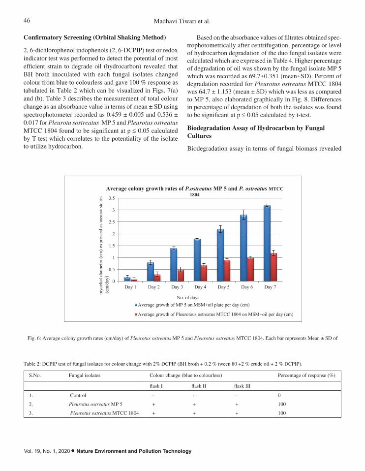
46 Madhavi Tiwari et al.
Vol. 19, No. 1, 2020 • Nature Environment and Pollution Technology
Confirmatory Screening (Orbital Shaking Method)
2, 6-dichlorophenol indophenols (2, 6-DCPIP) test or redox indicator test was performed to detect the potential of most efficient strain to degrade oil (hydrocarbon) revealed that BH broth inoculated with each fungal isolates changed colour from blue to colourless and gave 100 % response as tabulated in Table 2 which can be visualized in Figs. 7(a) and (b). Table 3 describes the measurement of total colour change as an absorbance value in terms of mean ± SD using spectrophotometer recorded as 0.459 ± 0.005 and 0.536 ± 0.017 for Pleurotu sostreatus MP 5 and Pleurotus ostreatus MTCC 1804 found to be significant at p £ 0.05 calculated by T test which correlates to the potentiality of the isolate to utilize hydrocarbon.
Based on the absorbance values of filtrates obtained spec-trophotometrically after centrifugation, percentage or level of hydrocarbon degradation of the duo fungal isolates were calculated which are expressed in Table 4. Higher percentage of degradation of oil was shown by the fungal isolate MP 5 which was recorded as 69.7±0.351 (mean±SD). Percent of degradation recorded for Pleurotus ostreatus MTCC 1804 was 64.7 ± 1.153 (mean ± SD) which was less as compared to MP 5, also elaborated graphically in Fig. 8. Differences in percentage of degradation of both the isolates was found to be significant at p £ 0.05 calculated by t-test.
Biodegradation Assay of Hydrocarbon by Fungal Cultures
Biodegradation assay in terms of fungal biomass revealed
21
Fig. 6: Average colony growth rates (cm/day) of Pleurotus ostreatus MP 5 and Pleurotus ostreatus MTCC 1804. Each bar represents Mean±SD
of two separate observations (n=2). The results were statistically significant at p≤0.05.
Fig. 7 (a): depicting DCPIP test, visualizing colour change from blue to colourless after biodegradation.
0
0.5
1
1.5
2
2.5
3
3.5
Day 1 Day 2 Day 3 Day 4 Day 5 Day 6 Day 7
Average colony growth rates of P.ostreatus MP 5 and P. ostreatus MTCC 1804
Average growth of MP 5 on MSM+oil plate per day (cm)
Average growth of Pleurotous ostreatus MTCC 1804 on MSM+oil per day (cm)
No. of days
myc
elia
l dia
met
er (c
m) e
xpre
ssed
as m
ean±
std
dev
(cm
/day
)
Fig. 6: Average colony growth rates (cm/day) of Pleurotus ostreatus MP 5 and Pleurotus ostreatus MTCC 1804. Each bar represents Mean ± SD of
Table 2: DCPIP test of fungal isolates for colour change with 2% DCPIP (BH broth + 0.2 % tween 80 +2 % crude oil + 2 % DCPIP).
S.No. Fungal isolates Colour change (blue to colourless) Percentage of response (%)
flask I flask II flask III
1. Control - - - 0
2. Pleurotus ostreatus MP 5 + + + 100
3. Pleurotus ostreatus MTCC 1804 + + + 100
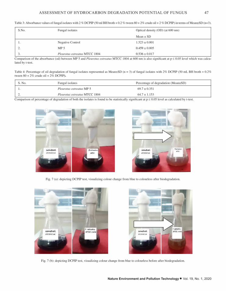
47ASSESSMENT OF HYDROCARBON DEGRADATION POTENTIAL OF FUNGUS
Nature Environment and Pollution Technology • Vol. 19, No. 1, 2020
Table 3: Absorbance values of fungal isolates with 2 % DCPIP (50 ml BH broth + 0.2 % tween 80 + 2% crude oil + 2 % DCPIP) in terms of Mean±SD (n=3).
S.No. Fungal isolates Optical density (OD) (at 600 nm)
Mean ± SD
1. Negative Control 1.523 ± 0.001
2. MP 5 0.459 ± 0.005
3. Pleurotus ostreatus MTCC 1804 0.536 ± 0.017
Comparison of the absorbance (od) between MP 5 and Pleurotus ostreatus MTCC 1804 at 600 nm is also significant at p £ 0.05 level which was calcu-lated by t-test.
21
Fig. 6: Average colony growth rates (cm/day) of Pleurotus ostreatus MP 5 and Pleurotus ostreatus MTCC 1804. Each bar represents Mean±SD
of two separate observations (n=2). The results were statistically significant at p≤0.05.
Fig. 7 (a): depicting DCPIP test, visualizing colour change from blue to colourless after biodegradation.
0
0.5
1
1.5
2
2.5
3
3.5
Day 1 Day 2 Day 3 Day 4 Day 5 Day 6 Day 7
Average colony growth rates of P.ostreatus MP 5 and P. ostreatus MTCC 1804
Average growth of MP 5 on MSM+oil plate per day (cm)
Average growth of Pleurotous ostreatus MTCC 1804 on MSM+oil per day (cm)
No. of days
myc
elia
l dia
met
er (c
m) e
xpre
ssed
as m
ean±
std
dev
(cm
/day
)
Fig. 7 (a): depicting DCPIP test, visualizing colour change from blue to colourless after biodegradation.
Table 4: Percentage of oil degradation of fungal isolates represented as Mean±SD (n = 3) of fungal isolates with 2% DCPIP (50 mL BH broth + 0.2% tween 80 + 2% crude oil + 2% DCPIP).
S. No. Fungal isolates Percentage of degradation (Mean±SD)
1. Pleurotus ostreatus MP 5 69.7 ± 0.351
2. Pleurotus ostreatus MTCC 1804 64.7 ± 1.153
Comparison of percentage of degradation of both the isolates is found to be statistically significant at p £ 0.05 level as calculated by t-test.
22
Fig. 7 (b): depicting DCPIP test, visualizing colour change from blue to colourless before after biodegradation.
Fig. 8: Percentage degradation of MP 5 and P. ostreatus MTCC 1804. Each bar represents Mean±SD of two separate observations (n=2). The
results were statistically significant at p≤0.05.
60
62
64
66
68
70
72
perc
enta
ge o
f deg
rada
tion
(%)
fungal isolates
Percentage of degradation of MP 5 and P. os treatus MTCC 1804
MP 5 Pleurotus ostreatus MTCC 1804
Fig. 7 (b): depicting DCPIP test, visualizing colour change from blue to colourless before after biodegradation.
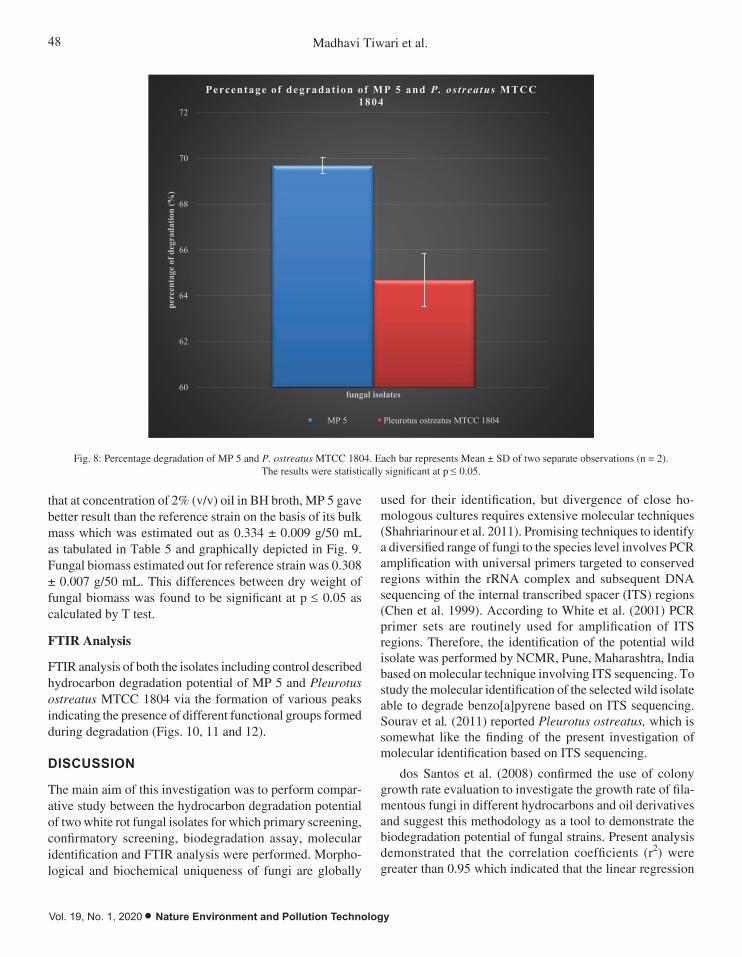
48 Madhavi Tiwari et al.
Vol. 19, No. 1, 2020 • Nature Environment and Pollution Technology
that at concentration of 2% (v/v) oil in BH broth, MP 5 gave better result than the reference strain on the basis of its bulk mass which was estimated out as 0.334 ± 0.009 g/50 mL as tabulated in Table 5 and graphically depicted in Fig. 9. Fungal biomass estimated out for reference strain was 0.308 ± 0.007 g/50 mL. This differences between dry weight of fungal biomass was found to be significant at p £ 0.05 as calculated by T test.
FTIR Analysis
FTIR analysis of both the isolates including control described hydrocarbon degradation potential of MP 5 and Pleurotus ostreatus MTCC 1804 via the formation of various peaks indicating the presence of different functional groups formed during degradation (Figs. 10, 11 and 12).
DISCUSSION
The main aim of this investigation was to perform compar-ative study between the hydrocarbon degradation potential of two white rot fungal isolates for which primary screening, confirmatory screening, biodegradation assay, molecular identification and FTIR analysis were performed. Morpho-logical and biochemical uniqueness of fungi are globally
used for their identification, but divergence of close ho-mologous cultures requires extensive molecular techniques (Shahriarinour et al. 2011). Promising techniques to identify a diversified range of fungi to the species level involves PCR amplification with universal primers targeted to conserved regions within the rRNA complex and subsequent DNA sequencing of the internal transcribed spacer (ITS) regions (Chen et al. 1999). According to White et al. (2001) PCR primer sets are routinely used for amplification of ITS regions. Therefore, the identification of the potential wild isolate was performed by NCMR, Pune, Maharashtra, India based on molecular technique involving ITS sequencing. To study the molecular identification of the selected wild isolate able to degrade benzo[a]pyrene based on ITS sequencing. Sourav et al. (2011) reported Pleurotus ostreatus, which is somewhat like the finding of the present investigation of molecular identification based on ITS sequencing.
dos Santos et al. (2008) confirmed the use of colony growth rate evaluation to investigate the growth rate of fila-mentous fungi in different hydrocarbons and oil derivatives and suggest this methodology as a tool to demonstrate the biodegradation potential of fungal strains. Present analysis demonstrated that the correlation coefficients (r2) were greater than 0.95 which indicated that the linear regression
22
Fig. 7 (b): depicting DCPIP test, visualizing colour change from blue to colourless before after biodegradation.
Fig. 8: Percentage degradation of MP 5 and P. ostreatus MTCC 1804. Each bar represents Mean±SD of two separate observations (n=2). The
results were statistically significant at p≤0.05.
60
62
64
66
68
70
72
perc
enta
ge o
f deg
rada
tion
(%)
fungal isolates
Percentage of degradation of MP 5 and P. os treatus MTCC 1804
MP 5 Pleurotus ostreatus MTCC 1804
Fig. 8: Percentage degradation of MP 5 and P. ostreatus MTCC 1804. Each bar represents Mean ± SD of two separate observations (n = 2). The results were statistically significant at p £ 0.05.

49ASSESSMENT OF HYDROCARBON DEGRADATION POTENTIAL OF FUNGUS
Nature Environment and Pollution Technology • Vol. 19, No. 1, 2020
Table 5: Dry weight of fungal isolates represented in terms of Mean±SD (n = 3) (50 mL BH broth + 0.2 % tween 80 + 2% crude oil).
S. No. Fungal isolates Dry weight of fungal biomass (mean±sd) (g/50mL)
1. Pleurotus ostreatus MP 5 0.334 ± 0.009
2. Pleurotus ostreatus MTCC 1804 0.308 ± 0.007
Dry weight of both the fungal isolates shows statistically significant differences at P £ 0.05 level as calculated by t-test.
23
Fig. 9: Fungal biomass of MP 5 and P. ostreatus MTCC 1804. Each bar represents Mean±SD of two separate observations (n=2). The results
were statistically significant at p≤0.05.
0.28
0.29
0.3
0.31
0.32
0.33
0.34
0.35
Mean dry weight (D) of fungal biomass (gm)
fung
al b
iom
ass (
gm/5
0 m
l)
FUNGAL ISOLATES
Fungal biomass (gm/50 ml) of MP5 and P.ostreatus MTCC 1804
MP 5 Pleurotus ostreatus MTCC 1804
Fig. 9: Fungal biomass of MP 5 and P. ostreatus MTCC 1804. Each bar represents Mean±SD of two separate observations (n = 2). The results were statistically significant at p £ 0.05.
satisfactorily explained the variation of the colony diameter as a function of time. dos Santos et al. (2008) supports the present analysis by reporting that during his experiments of colony growth evaluation of four fungal isolates on plates containing a specific hydrocarbon or petroleum derivative as the only carbon source, correlation coefficients (r2) were greater than 0.95 (data not shown), indicating that the linear regression adequately explained the variation of the colony diameter as a function of time.
Experiments performed by Thenmozhi et al. (2013) revealed that that the fungal isolates JJF3 Aspergillus niger and JJF9 Aspergillus luchiencis with average colony diameter as 2.7 and 3.72 cm/day as compared to other fungal isolates exhibited bigger colony diameter, heavy sporulation, and
abundant aerial mycelium on selective media (MSM) amend-ed with 1% used engine oil. These evaluations foresighted those as hydrocarbon degraders which further elaborated their capability to utilize used engine oil as a carbon source for their growth. Likewise, in the present study, the highest average colony growth rate in terms of colony diameter (cm/day) observed for Pleurotus ostreatus MP 5 on MSM amend-ed with 2 % oil was recorded as 3.2 ± 0.057 cm (mean±day) respectively which interpreted that mycelium of this fungal isolate proliferated rapidly forming heavy sporulation and dense hyphae than Pleurotus ostreatus MTCC 1804 (0.308 ± 0.007). Similarly, Popa et al. (2013) evaluated the ability of two isolates of P. ostreatus (P50, P421) and a sample of P. ostreatus collected from Chitila woods to use crude-oil

50 Madhavi Tiwari et al.
Vol. 19, No. 1, 2020 • Nature Environment and Pollution Technology
as a carbon source for which he inoculated mycelia inoc-ulum on MSM plates with crude oil (1 mL) spread on the entire carbon free mineral salt medium (MSM) surface and in plates with pieces of filter paper soaked in crude oil and placed around the inoculum. Evaluation done every day for 14 days, by measuring the radial growth of mycelia (in cm) and extrapolated as growing percentage to culture plate diameter (9 cm) revealed that both isolates of P. ostreatus
as well as P. ostreatus originated from Chitila forest were able to utilize the crude oil as a source of carbon and energy in their metabolism.
Confirmatory screening also known as orbital shaking method also known as redox indicator test and DCPIP test in the present study is based on the principle of change in colour of BH broth from blue to colourless incorporated with fungal isolates, 0.2 % (v/v) Tween 80, 2% (v/v) crude oil and 24
Fig. 10: FTIR spectrum of control sample.
Fig. 10: FTIR spectrum of control sample.

51ASSESSMENT OF HYDROCARBON DEGRADATION POTENTIAL OF FUNGUS
Nature Environment and Pollution Technology • Vol. 19, No. 1, 2020
25
Fig. 11: FTIR spectrum of P. ostreatus MP.
Fig. 11: FTIR spectrum of P. ostreatus MP 5.
redox reagent (2% 2, 6- dichlorophenol indophenols). This screening method is also known as redox indicator technique which is applied to assess the ability of fungal isolates to degrade crude oil in the presence of redox indicator 2, 6- DCPIP (Hanson et al. 1993). The main principle behind this
degradation using redox reagent is that after incorporation of an electron acceptor such as DCPIP to the broth inoculated with fungi supplemented with oil and tween 80, it becomes possible to assess the ability of fungi to utilize the substrate by visualizing the colour change of DCPIP from blue (ox-

52 Madhavi Tiwari et al.
Vol. 19, No. 1, 2020 • Nature Environment and Pollution Technology 26
Fig. 12: FTIR spectrum of P. ostreatus MTCC 1804.
Fig. 12: FTIR spectrum of P. ostreatus MTCC 1804.
idized) to colourless (reduced) (Al-Nasrawi 2012). Tween 80 acts as an emulsifier which facilitates active contact between hydrocarbon and the isolate (Hanson et al. 1993). Three indication which verifies the ability of fungi involved in biodegradation process is firstly the change in colour of broth from dark blue to colourless, secondly the disappear-ance of crude oil from the broth and thirdly developing a mass of fungal biomass growth in the bottom of the broth (Hanson et al. 1993).
Colour transformation from blue to colourless during biodegradation process involving the specific isolates ramparts the fact that isolates are potential hydrocarbon
oxidizers and the colour transformation can be measured as an absorbance value using spectrophotometer (George et al. 2009). The present investigation confirms the ability of Pleurotus ostreatus MP 5 and Pleurotus ostreatus MTCC 1804 to degrade used engine oil by displaying colour change from blue to colourless after seven days of incubation in shaking incubator.
As Yoshida et al. (2001) observed a peak in absorbance at 600 nm therefore; absorbance at a wavelength of 600 nm was recorded for fungal isolates. According to Undugoda et al. (2016) the higher hydrocarbon degrading fungi have low absorbance values after the incubation period as compared

53ASSESSMENT OF HYDROCARBON DEGRADATION POTENTIAL OF FUNGUS
Nature Environment and Pollution Technology • Vol. 19, No. 1, 2020
to the control whereas lower hydrocarbon degrading fungi possess high absorbance values. The present comparative assessment reported that wild isolate Pleurotus ostreatus MP 5 (OD = 0.459 ± 0.005) has proved itself as a more potent hydrocarbon degrader than Pleurotus ostreatus MTCC 1804 (OD = 0.536 ± 0.017) by displaying the fastest onset colour disappearance (decrease in absorbance of broth medium) and hence, highest capability of biodegradation. Thus the present investigation is supported by the reports of Khan et al. (2015) who reported that Aspergillus sp., Penicillium sp. and Rhizopus sp. displayed the colour transformation from blue to colourless in the BH broth incorporated with the fungal isolates comprised with 0.1% (v/v) Tween 80 and 1% (v/v) petrol, kerosene and diesel and 0.008 mg/50 mL of redox indicator and hence showed the highest capability of biodegradation. The high rate of petroleum products (hydrocarbon) degradation by the wild isolate may be due to their enzyme production responses during their growth phases which could be supported by the reports and findings of Bogan & Lamar (1996) according to which during the growth phases of white rot fungi, extracellular ligninolytic enzymes are produced in response to their growth phases.
Percentage of degradation of each fungal isolate was calculated on the basis of absorbance value obtained after applying the formula, according to which Pleurotus ostreatus MP 5 gave higher percentage of degradation as compared to that of Pleurotus ostreatus MTCC 1804. Percentage of hydrocarbon degradation calculated for Pleurotus ostrea-tus MP 5 and Pleurotus ostreatus MTCC 1804 was 69.7 ± 0.351% and 64.7 ± 1.153%. Similarly, Ekundayo (2014) worked on comparative Studies on biodegradative abilities of Pleurotus ostreatus and P. pulmonarius in soils contam-inated with crude and used engine Oils and investigated that P. ostreatus reduced the initial total hydrocarbon content (THC) to 8% and 9% in soils polluted with 20% of crude and used engine oils, respectively, which was lower than that of P.pulmonarius. Mineralization of various PAHs by white rot fungus Pleurotus ostreatus was reported by Bezalel et al. (1995) according to whom, Pleurotus ostreatus was able to mineralize to 7.0% of [14C]catechol, 3.0% of[14C]phenanthrene, 0.4% of [14C]pyrene, and 0.19% of [14C]benzo[a]pyrene followed by incubation of 11 days. Besides, the implication of the wild strain MP 5 as a more potent hydrocarbon degrader than that of the reference strain Pleu-rotus ostreatus MTCC 1804 from our result is similar to the findings of Sourav et al. (2013) while testing the potentiality of the isolate P. ostreatus PO-3 and P.ostreatus MTCC 142 to degrade 1 µg/mL of Benzo[a]pyrene BaP, a high molecular weight polycyclic aromatic hydrocarbon (HMW PAH) under liquid condition, reported that isolate P. ostreatus PO-3 has
better degradation potential than P. ostreatus MTCC 142 and concluded that the level of degradation were 32% and 29% respectively for Pleurotus ostreatus isolate PO-3 and Pleurotus ostreatus MTCC 142.
Proliferation of a mass of fungal growth in the bottom of culture medium supplemented with oil is one of the indications of those fungi which are capable of degrading hydrocarbon (Al-Nasrawi 2012). Therefore, biodegradation assay of both the fungal strains in terms of fungal biomass was performed according to which it was found out that at concentration of 2% oil, P. ostreatus MP 5 gave better performance in terms of biomass as compared to that of the reference strain Pleurotus ostreatus MTCC 1804. The bulk mass weighed out for P. ostreatus MP 5 and Pleurotus ostreatus MTCC 1804 was estimated as 0.334±0.009 g/50 mL and 0.308±0.007 g/50 mL respectively. Experiments performed by Sourav et al. (2013) documented that in the proximity of PAH, the biomass proliferation by the PO-3 isolate was higher than that of P. ostreatus MTCC 142 which was calculated as about 51 and 43 mg/50 mL of media which reinforces our present findings in terms of biodegradation essay.
The capability of the fungus to degrade PAH is related to its ability to produce lac case and similar enzymes (Sourav et al. 2013). Therefore, it could be concluded that P. ostreatus MP 5 isolate could degrade PAH better than P. ostreatus MTCC 142 possibly due to its ability to synthesize higher titers of laccase and manganese peroxidase. Likewise, a native isolate of P. ostreatus HP-1 (Genbank Accession No. EU420068) was discovered to comprise an excellent laccase producing ability (Rubailo et al. 2008).
Since the trends of hydrocarbon degradation were assessed overtime and FTIR was utilized and applied to elucidate the degradation of oil spilled from vehicles in the contaminated soil therefore, FTIR spectroscopy has been prove to be a very useful tool in performing preliminary tests in order to predict remediation performance so as to select an appropriate approach for clean- up technologies (Bhat et al. 2011). The present study on comparison of the hydro-carbon degradation potential of the two fungal isolates was finally confirmed by spectral analysis using FTIR to assess biodegradation experiments. Identification and interpretation of peaks indicating various functional groups were done with the reference of available literatures (Bhat et al. 2011, Sohal et al. 2019, Srivastava & Saraf 2019).
The FTIR spectrum monitored for untreated sample, i.e. control as depicted in Fig. 10 indicated a broad peak at 3419.4 cm-1 corresponding to O-H stretching vibrations of alcohols. Absorption band around 2933.5 cm-1 is assigned to C-H stretching in alkanes (aliphatic compounds), at

54 Madhavi Tiwari et al.
Vol. 19, No. 1, 2020 • Nature Environment and Pollution Technology
1643.7 cm-1 indicating C=C stretching of alkenes (aliphatic compounds). Another prominent spectrum which appeared between 1346.2 cm-1 to 1461.8 cm-1 can be ascribed to the bending vibration of C-H in alkenes (aliphatic compounds). The presence of carboxylic acid functional group in the molecule was confirmed by medium intensity band in the region of 1270.4 cm-1 and 1240.1 cm-1 for C-O stretching of carboxylic acids. Another bands revealed at 1209.8 and 1053.0 cm-1 indicating C-O stretching of alcohols; at 940.7 cm-1 indicates S-O stretching in sulphonates; at 909.2 cm-1 indicating C-H bends in alkenes; at 867.2 cm-1 indicating S-O stretching in sulphonates; at 849.8 cm-1 corresponding to C-H bends in aromatics; at lower wave length of 681.1 cm-1 and 550.7 cm-1 indicating C-Cl stretching signifying the presence of alkyl halides.
The FT-IR spectrum of treated sample with Pleurotus ostreatus MTCC 1804 (Fig. 12) after 30 days of microbial incubation indicated the formation of new bands at 3399.5 cm-1 indicating O-H stretching vibrations of alcohols; at 2929.7 cm-1 corresponding to C-H stretching of alkanes; at 1642.4 cm-1 signifying N-H bend in amides. C=C stretching in aromatic compound ring was indicated at 1451.9 cm-1. Spectrum at 1412.5 cm-1 can be ascribed to the bending vibration of O-H in carboxylic acids (-COOH). Absorption peaks at 1123.1 and 1058.2 cm-1 signified C-O stretching of alcohols (OH). Modification of functional groups at these absorption spectrum indicated the conversion of C-O stretching of carboxylic acids at 1270.4 cm-1 and 1240.1 cm-1 as depicted in control into C-O stretching of alcohols (OH) at 1123.1 cm-1 and 1058.2 may be due to the microbial oxidation of used oil which is supported with the findings of Bhat et al. (2011) who reported the same at 2363.2 cm-1. Formation of new bands at 879.3 cm-1, 840.3 cm-1 and 779.7 cm-1 indicated C-H bending in aromatics. The appearance of another prominent peak at 700.1 cm-1 confirmed C-H bending in alkenes. The absorption peak around 675.4 and 620.9 cm-1 was reported as C-Cl stretching in alkyl halides. Besides, it was observed that there is significant change in transmittance which increased in the sample treated with P. ostreatus MTCC 1804 as compared to that of control representing degradation of complex mixtures.
The FTIR spectrum obtained to assess the biodegrada-tion capability of P. ostreatus MP 5 (Fig. 11) also showed the formation of new bands with different intensity of wavelength which at first indicated a broad spectrum at 3419.4 cm-1 corresponding to O-H stretching vibrations of alcohols. Another prominent spectrum which appeared at 2220.1 cm-1 can be ascribed to C-N stretching in nitriles. Here the conversion of -C-H stretching in aliphatic com-pounds as depicted in control or the untreated sample into
nitrile groups may be due to the hydrocarbon degradation by wild isolate MP 5 which was in total accordance with the result of FTIR analysis performed by Bhat et al. (2011) for the mycoremediation of hydrocarbon contaminated soil who also concluded the conversion of aliphatic compounds into nitrile groups during hydrocarbon degradation. Another characteristic absorption band at 1644.6 cm-1 showed C=C stretching in alkenes. Absorption band around 1446.5 cm-1
is assigned to the bending vibration of asymmetric C=C stretching in aromatic. Another prominent absorption peak around 1338.3 cm-1 reported as C-H bending in alkenes. The presence of another absorption band at wavelength 1114.4 cm-1 indicated C-O stretching of alcohols may be due to the microbial oxidation of used oil. Another new band revealed at 880.8 cm-1 and 848.9 cm-1 indicated the presence of C-H bending (meta) and C-H bending (para) in aromatics which further indicated the conversion of alkenes as reported in con-trol at 909.2 cm-1 into aromatic compounds. The absorption peak around 779.7 cm-1 was reported as C-Cl stretching in alkyl halides. At lower wave length of 618.7 and 516.2 cm-1
occurrence of C- Br stretching of alkyl halides was revealed out. Apart from all these modifications of functional groups which occurred during degradation process, the percent transmittance increased as compared to that of control and P. ostreatus MTCC 1804 which finally confirmed the higher degradation potential of wild isolate MP 5.
CONCLUSION
The present study reveals that the molecular identification technique like ITS sequencing was carried out for the potent isolate which revealed that the isolate MP 5 shares a 99% sequence similarity to that of Pleurotus ostreatus isolate 6689 (accession No. AY450345.1). Primary screening assay confirmed that the wild isolate P. ostreatus MP 5 showed highest average growth rate on MSM supplement-ed with 2% oil. Confirmatory test conducted for both the isolates through orbital shaking method for detection of biodegradation by spectrophotometric method at 600 nm displayed degradation within 7 days and level of hydro-carbon degradation figured out for P. ostreatus MP 5 and Pleurotus ostreatus MTCC 1804 was 69.7 ± 0.351% and 64.7 ± 1.153%. The FTIR spectrum of control and treated samples with fungal isolates showed different peaks based on the presence of different functional groups indicating oxidative degradation of hydrocarbons by microbes. Thus, it can be concluded from the present investigation that the wild isolate P. ostreatus MP 5 had better potential for de-grading hydrocarbon in comparison to P. ostreatus MTCC 1804 which can be served as a better potential hydrocarbon degrader for mycoremediation studies.

55ASSESSMENT OF HYDROCARBON DEGRADATION POTENTIAL OF FUNGUS
Nature Environment and Pollution Technology • Vol. 19, No. 1, 2020
ACKNOWLEDGEMENT
As the research was supported by MATS school of Biological and Chemical Sciences (MSBCS), Raipur, C.G so, we are very thankful to MSBCS for providing all the laboratory facilities required for the completion of this research paper. We are also immensely great full to one of the co-author Dr. Ashish Saraf, for sharing his pearls of wisdom with us during this research. We would also like to show our gratitude to Dr. Deepak Konar, Department of Chemistry, Bose institute, Calcutta for conducting the FTIR analysis and Dr. Rohit Sharma and Dr. Abhay Bajaj, NCMR Pune for the ITS sequencing.
REFERENCESAdongbede, E.M. and Sanni, R.O. 2014. Biodegradation of engine oil by Ag-
aricus campestris (a white rot fungus). J. Bioremed. Biodeg, 5(262): 2.Al-Nasrawi, H. 2012. Biodegradation of crude oil by fungi isolated from Gulf
of Mexico. Journal of Bioremediation and Biodegradation, 3(04): 1-6.Boonchan, S., Britz, M.L. and Stanley, G.A. 2000. Degradation and mineral-
ization of high-molecular-weight polycyclic aromatic hydrocarbons by defined fungal-bacterial cocultures. Appl. Environ. Microbiol., 66(3): 1007-1019.
Barr, D.P. and Aust, S.D. 1994. Mechanisms white rot fungi use to degrade pollutants. Environmental Science & Technology, 28(2): 78A-87A.
Bogan, B.W. and Lamar, R.T. 1996. Polycyclic aromatic hydrocarbon-degrad-ing capabilities of Phanerochaete laevis HHB-1625 and its extracellular ligninolytic enzymes. Appl. Environ. Microbiol., 62(5): 1597-1603.
Bezalel, L. Hadar, Y. and Cerniglia, C.E. 1996. Mineralization of polycyclic aromatic hydrocarbons by the white rot fungus Pleurotus ostreatus. Appl. Environ. Microbiol., 62(1): 292-295.
Bhat, M.M. Kumar, D. Narain, K. Shukla, R.N. and Yunus, M. 2011. Mycore-mediation of hydrocarbon contaminated soil-FTIR based analysis. World Appl. Sci. J., 15: 1547-1552.
Clemente, A. Anazawa, T.A. and Durrant, L.R. 2001. Biodegradation of polycyclic aromatic hydrocarbons by soil fungi. Brazilian Journal of Microbiology, 32(4): 255-261.
Chen, D.H. and Ronald, P.C.1999. A rapid DNA minipreparation method suitable for AFLP and other PCR applications. Plant Molecular Biology Reporter, 17(1): 53-57.
dos Santos, E.O. da Rosa, C.C. dos Passos, C.T. Sanzo, A.V.L. Burkert, J.F.D.M. Kalil, S.J. and Burkert, C.A.V. 2008. Pre-screening of fila-mentous fungi isolated from a contaminated site in Southern Brazil for bioaugmentation purposes. African Journal of Biotechnology, 7(9): 1314-1317.
Emuh, F.N. 2010. Mushroom as a purifier of crude oil polluted soil. Inter. J. Sci. Nat.,1(2): 127-132.
Ekundayo, F.O. 2014. Comparative studies on biodegradative abilities of Pleurotus ostreatus and P. Pulmonarius in soils contaminated with crude and used engine oils. Advances in Microbiology, 4(12): 849.
George-Okafor, U. Tasie, F. and Muotoe-Okafor, F. 2009. Hydrocarbon degradation potentials of indigenous fungal isolates from petroleum contaminated soils. Journal of Physical and Natural Sciences, 3(1): 1-6.
Hagwell, I.S. Delfino, L.M. and Rao, J.J. 1992. Partitioning of polycyclic aromatic hydrocarbons in soil by microbial consortium. International Biodeterioration Biodegradation, 54: 61-67.
Huesemann, M.H. 1994. Guidelines for land‐treating petroleum hydro-carbon‐contaminated soils. Soil and Sediment Contamination, 3(3): 299-318.
Hanson, K.G., Desai, J.D. and Desai, A.J. 1993. A rapid and simple screening technique for potential crude oil degrading microorganisms. Biotech-
nology Techniques, 7(10): 745-748.Jawhari, A.L. and Ihsan, F.H. 2014. Ability of some soil fungi in biodegra-
dation of petroleum hydrocarbon. Journal of Applied & Environmental Microbiology, 2(2): 46-52.
Keith, L. and Telliard, W. 1979. ES &T special report: Priority pollutants: A perspective view. Environmental Science & Technology, 13(4): 416-423.
Khan, S.R., Ji, N.K., Kumar, R.N. and Patel, J.G. 2015. In vitro study on assessment of petrol, kerosene and diesel degrading potential of indigenous fungal isolates from different petroleum product effected soils. International Journal of Recent Research and Review, 8(1): 8-15.
Mills. A.L. Breuil, C. and Colwell, R.R. 1978. Enumeration of petroleum-de-grading marine and estuarine microorganisms by the most-probable number. Canadian Journal Microbiology, 24: 552-557.
Okparanma, R.N., Ayotamuno, J.M., Davis, D.D. and Allagoa, M. 2011. Mycoremediation of polycyclic aromatic hydrocarbons (PAH)-con-taminated oil-based drill-cuttings. African Journal of Biotechnology, 10(26): 5149-5156.
Okpokwasili, G.C. and Okorie, B.B. 1988. Biodeterioration potentials of microorganisms isolated from car engine lubricating oil. Tribology International, 21(4): 215-220.
Popa, G. Nicolcioiu, M.B. and Cornea, C.P. 2013. In vitro evaluation of crude oil degradation potential of some Pleurotus ostreatus isolates. Scientific Bulletin. Series F. Biotechnologies, 17: 143-146.
Rubailo, A.I. and Oberenko, A. V. 2008. Polycyclic aromatic hydrocar-bons as priority pollutants. Journal of Siberian Federal University, 4(1): 344-354
Stamets, P. 2005. Mycelium Running: How Mushrooms Can Help Save The World. Random House Digital, Inc.
Sack, U. and Günther, T. 1993. Metabolism of PAH by fungi and correlation with extracellular enzymatic activities. Journal of Basic microbiology, 33(4): 269-277.
Steffen, K.T. Schubert, S. Tuomela, M. Hatakka, A. and Hofrichter, M. 2007. Enhancement of bioconversion of high-molecular mass polycyclic aromatic hydrocarbons in contaminated non-sterile soil by litter-de-composing fungi. Biodegradation, 18(3): 359-369.
Shahriarinour, M. Wahab, M.N.A. Ariff, A. and Mohamad, R. 2011. Screening, isolation and selection of cellulolytic fungi from oil palm empty fruit bunch fibre. Biotechnology, 10(1): 108-113.
Sourav, B. Arijit, D. Palaniswamy, M. and Angayarkanni, J. 2013. Molecular characterization of Pleurotus ostreatus PO-3 involved in mycoremedi-ation of benzo[a]pyrene. International Research Journal of Biological Sciences, 2(8): 48-53.
Sohal, J.K. Saraf, A. Shukla, K. and Shrivastava, M. 2019. Determination of antioxidant potential of biochemically synthesized silver nanopar-ticles using aloe vera gel extract. Plant Science Today, 6(2): 208-217.
Srivastava, M. and Saraf, A. 2019. Antimicrobial activity of bioactive molecules isolated from filamentous fungi. Int. Res. J. Biological Sci., 8(3): 13-18.
Tiwari, M. and Saraf, A. 2017. Isolation, screening and identification of hydrocarbon degrading potential of indigenous fungus from oil contaminated soil of Modha Para automobile shop of Raipur, CG. International Journal of Advance Research in Science and Engineering, 6(10): 782-795.
Thomas, S. Becker, P. Pinza, M.R. and Word, J.Q. 1998. Mycoremediation of aged petroleum hydrocarbon contaminants in soil. Washington State Department of Transport. Publication No. WA-RD 464.1.
Thenmozhi, R. Arumugam, K. Nagasathya, A. Thajuddin, N and Paneer-selvam, A. 2013. Studies on mycoremediation of used engine oil con-taminated soil samples. Advances in Applied Science Research, 4(2): 1.
Undugoda, L.J.S. Kannangara, S. and Sirisena, D.M. 2016. Aromatic hydrocarbon degrading fungi inhabiting the phyllosphere of orna-mental plants on roadsides of urban areas in Sri Lanka. J. Bioremed. Biodeg., 7(328): 2.
Vanishree, M. Thatheyus, A.J. and Ramya, D. 2014. Biodegradation of

56 Madhavi Tiwari et al.
Vol. 19, No. 1, 2020 • Nature Environment and Pollution Technology
petrol using Aspergillus sp. Annual Research & Review in Biology, 4(6): 914-923.
Velioğlu, Z. and Ürek, R.Ö. 2015. Biosurfactant production by Pleurotus ostreatus in submerged and solid-state fermentation systems. Turkish Journal of Biology, 39(1): 160-166.
White, N.A. Dehal, P.K. Duncan, J.M. Williams, N.A. Gartland, J.S. Palfrey-man, J.W. and Cooke DEL. 2001. Molecular analysis of intraspecific variation between building and “wild” isolates of Serpula lacrymans
and their relatedness to S. himantioides. Mycol. Res, 105(4): 447-452.Yoshida, N. Hoashi, J. Morita, T. McNiven, S.J. Nakamura, H. and Karube,
I. 2001. Improvement of a mediator-type biochemical oxygen demand sensor for on-site measurement. Journal of Biotechnology, 88(3): 269-275.
Zebulun, H.O. Isikhuemhen, O.S. and Inyang, H. 2011. Decontamination of anthracene-polluted soil through white rot fungus-induced biodeg-radation. The Environmentalist, 31(1): 11-19.

A Novel Approach to Utilize Used Disposable Paper Cups for the Development of Adsorbent and its Application for the Malachite Green and Rhodamine-B Dyes Removal from Aqueous Solutions
Kshipra Shukla, Alka Verma, Lata Verma, Shalu Rawat and Jiwan Singh†Department of Environmental Science, Babasaheb Bhimrao Ambedkar University, Lucknow-226025, India†Corresponding author: Jiwan Singh
ABSTRACT
This study focuses on the removal of organic dyes, such as Malachite Green (MG) and Rhodamine-B (Rh-B) from an aqueous solution with the help of a novel adsorbent (activated carbon) with magnetic property prepared by used disposal paper cups (AC@PC) at 500°C. The synthesized AC@PC adsorbent was characterized by using Fourier transform infrared spectroscopy (FTIR), X-ray diffraction (XRD), scanning electron microscopy (SEM), Energy dispersive X-ray spectroscopy (EDS) and point of zero charge (pHZPC). Adsorption of MG and Rh-B onto the AC@PC adsorbent from aqueous solution was investigated systematically. Langmuir, Freundlich and Temkin isotherms were also studied, however, it has been observed that Langmuir isotherm model was best fitted for both the dyes, which describe the adsorption behaviour at equilibrium. Pseudo-first and pseudo-second order kinetic model describe the rate of adsorption. Kinetic study explained that the process of adsorption followed the pseudo-second order model. Thermodynamic parameters such as enthalpy (ΔH°), entropy (ΔS°) and Gibb’s free energy (ΔG°) were also studied and revealed that the adsorption of MG was endothermic, whereas adsorption of Rh-B was exothermic onto the AC@PC. The prepared adsorbent shows potentially high adsorption properties for both the dyes.
INTRODUCTION
India is facing very serious problem of solid waste disposal. The waste contributes to landfills and are post-consumer products that means those substances which cannot be recycled or reused any longer (Arumugam et al. 2015). Paper cup waste disposal is a major issue in terms of environment as it is mainly composed of paper with high strength that can be easily recycled but the inner layer is lined with thin film of polyethylene and make paper cups recycling very complicated (Arumugam et al. 2018). These disposable cups are widely used all over the world for serving tea, coffee, soft-drinks and for many other purposes. Generation of municipal solid waste in India is approximately 1,88,550 tonnes per day of which 35% by weight constitutes post-consumer waste that causes serious problems to the society and environment (Arumugam et al. 2018). Post-consumer waste can be elaborated as the waste generated by the end consumer (Arena et al. 2016). In India solid waste management is a very big task for the generated waste. The paper waste can be very effective for removal of pollutants from water when it converted into an adsorbent. Utilization of paper cup waste for the adsorption purpose can reduce the problem of disposable of paper cup waste.
The discharge of water from the industries may hold pollutants such as dyes, heavy metals into the aqueous solution that disrupt the ecosystem of aquatic animals and plants and also causes various health problems in human beings. Several industries, for example, cosmetics, plastics, textile, processing, rubber etc. uses different classes of dyes (Kono 2015). Dyes are growing to be a very challenging class of pollutants to the environment causing many health hazards (Ngulube et al. 2017). Dyes are mainly the chemical compounds or complex organic molecules that imparts colour to the surface or fabric when comes in contact (Yagub et al. 2014).
Many industries discharge effluent into water bodies containing highly coloured species with large amount of toxic substances that not only cause health related problems but also degrade the aesthetic values of water bodies (Kant 2012). About 10,000 dyes produced yearly of which 7.105 metric tons are available in market. Around 15% of dye materials are misplaced in effluent discharged from various manufacturing and processing operations in industrial activities (Gupta et al. 2012). The dye effluent from industries contain certain chemicals that could be lethal, carcinogenic or mutagenic to living organisms (Noel & Rajan 2014). Synthetic dyes are highly soluble in water and are the common pollutants that
Nat. Env. & Poll. Tech.Website: www.neptjournal.com
Received: 12-06-2019Accepted: 23-07-2019
Key Words:Malachite GreenRhodamine-BAdsorptionAC@PC adsorbent
2020pp. 57-70 Vol. 19
p-ISSN: 0972-6268 No. 1 Nature Environment and Pollution Technology An International Quarterly Scientific Journal
Original Research Paper
e-ISSN: 2395-3454
Open Access
58 Kshipra Shukla et al.
Vol. 19, No. 1, 2020 • Nature Environment and Pollution Technology
pollute water and normally found in industrial wastewater in trace amount (Crini 2006).
MG is usually used for the dyeing of the cotton, leather, paper, silk and also in different industries such as manufactur-ing of paints and printing inks. It is persistent in environment and acutely toxic to many aquatic and terrestrial animals (Gupta et al. 2016). While, Rh-B dye is used in textile, printing industries and photographic industries and it is a xanthene dye. Rh-B causes many health problems such as irritation of the eye, skin, and respiratory tract. This dye is carcinogenic, and also causes developmental and reproduc-tive toxicity (Bhattacharya et al. 2014).
Numerous chemicals, physical and biological techniques, comprising biosorption, ozonation, adsorption, coagulation, advance oxidation, liquid-liquid extraction and membrane filtration have been extensively used for dyes treatment from the wastewater (Pathania et al. 2017). Among all the techniques used adsorption is very efficient, cheapest and eco-friendly method as it gives the best results when used for dyes removal from aqueous medium (Yagub et al. 2014).
The waste paper cups used for the preparation of AC@PC adsorbent is used for the first time as an adsorbent for the removal of MG and Rh-B. The main objective of this work is to synthesize the low-cost adsorbent with magnetic properties from waste disposable paper cups and its appli-cation for removal of MG and Rh-B dye from an aqueous solution. The present study is focusing on the management of waste disposable cups as well as for the treatment of water pollutants.
MATERIALS AND METHODS
Materials
Rh-B dye (C21H31ClN2O3) and MG dye (C23H25N2Cl) were obtained from Thermo Fisher Scientific India Pvt. Ltd. These dyes were used directly without any purification. Double distilled water was used to prepare the solution of these dyes. PCs were collected from canteen of Babasaheb Bhimrao Ambedkar University, Lucknow, (U.P.), India.
Preparation of AC@PC Novel Adsorbents
Collected waste PCs were washed to eliminate filths present on the surface and then dried in hot air oven. After that, these paper cups were cut into small pieces and dipped into hot water (temperature 60-70°C) for 3-4 hours and then the thin lining made up of polyethylene was separated from the paper part. Wet paper clumps were removed from hot water and again dried in hot air oven at 105°C for 24h. The dried material was grinded and sieved with 0.25 mm sieve. Then
30 g of grounded material was added to the FeCl3 solution (15g FeCl3 + 150 mL distilled water). The mixture was kept on magnetic stirrer (model no. 1MLH, REMI, India) and stirred for four hours. The material was then filtered and kept overnight in an oven for drying. After drying, the material was kept in muffle furnace (IMPACT, 11C 106B) at 500°C for two hours then the material was crushed by mortar pestle to change it into powder form and was washed with deionized water for 2-3 times, oven dried for overnight and then it was used for the adsorption study (Lunge et al. 2014).
Characterization
Surface morphological structure of AC@PC sample was examined using SEM (JSM-6490 LV, JEOL, Japan). For SEM analysis the sample was coated on a tacky carbon tape and then mounted on a stub into a sample holder. EDS done for the determination of elemental composition of AC@PC.
An infrared spectrum was recorded using Infrared Spec-trometer (NicoletTM 6700, Thermo Scientific, USA) for the functional group determinations present on the surface of AC@PC. The sample were prepared mixing spectroscopy grade KBr with oven dried (at 105°C) sample in an agate mortar.
XRD (Powder Diffractometer PW3040/60, PaNanalytical Neitherland) was used for the analysis of crystalline structure of AC@PC. Scanning of sample was done at the rate of 2° min-1 from 10°-80°.
Zeta nanosizer (Nano-ZS90), was used for analysing the particle size and zeta potential of AC@PC. Zeta potential of AC@PC was done at different pH (2, 4, 6, 8 and 10).
The pHZPC of synthesized material (AC@PC) was de-termined by using 0.1 M NaCl solution with different pH (2, 4, 6, 8 and 10). These pH values were adjusted by using solutions of 0.1 N HCl and 0.1 N NaOH. A 20 mL NaCl solution and 0.2 g adsorbent were taken and left for 48 hrs after that the pH of solution was measured by a pH meter. The pHzpc value was attained by plotting the graph of initial pH against final pH (Singh et al. 2016).
Batch Adsorption Studies
Batch adsorption experiment was performed with AC@PC for MG and Rh-B removal from an aqueous medium. Initial concentrations were prepared in the range of 5-30 mg/L by di-luting standard solution of 1000 mg/L of MG and Rh-B dyes separately. Adsorption studies were performed at different temperatures 25°C, 35°C and 45°C. Different doses in g/L (0.5, 1, 1.5, 2, 3, 3.5 and 4) were taken to optimize the dose at which the maximum adsorption of dye occurs. The dose study revealed that the maximum adsorption was obtained

59USED DISPOSABLE PAPER CUPS FOR THE DEVELOPMENT OF AN ADSORBENT
Nature Environment and Pollution Technology • Vol. 19, No. 1, 2020
with the dose of 3 g/L. A fixed dose of AC@PC (3 g/L) was taken for further study. All experiments were conducted in duplicate with 100 mL of dye solution in a 250 mL conical flask at 100 rpm for 300 min.
The conical flasks having samples were taken out from orbital shaker at different interval of time (5, 15, 30, 60, 120, 180, 240 and 300 min). All experiments were performed at normal temperature of 25°C except temperature study con-ducted at 35°C and 45°C. All experiments were conducted at neutral pH except pH study (pH 4, 5, 6, 7, 8, 9 and 10). The pH of working solution was maintained by 0.1 M NaOH or HCl, solution pH was then measured by using pH meter (water analyser, 372, Systronic India Limited). After that the solution was filtered and analysed to determine the remaining concentration using UV-Vis spectrophotometer (Model No. 117, Systronic India Ltd.).
The amount of dye (MG and Rh-B) qt (mg/g) adsorbed on AC@PC, was evaluated by following equation:
Removal %C
e=-
¥C C0
0
100 …(1)
Where, C0 is the initial concentration (mg/L) and Ce is the equilibrium concentration (mg/L).
The adsorption capacity of adsorbent at equilibrium was calculated by following equation (Ibrahim et al. 2019):
qC C
mVe
e=-
¥0 …(2)
Where,
V = volume of dye solution (L)
m = mass of adsorbent (g)
RESULT AND DISCUSSION
Adsorbent Characterization
SEM and EDS analysis: Fig. 1 (a) shows that the adsorbent has an irregular porous surface with cuboid/pyramid shaped crystal structures which may be responsible for the adsorp-tion of MG and Rh-B. The EDS (Fig. 1b) analysis is mainly done to identify the elemental composition of material. The EDS analysis of AC@PC adsorbent shows the presence of various elements. AC@PC containing highest carbon content with 72.01%. Iron and aluminium content were present in the material and it was confirmed by SEM-EDS analysis. The lower point of zero charge value of AC@PC was due to the presence of Fe on the surface of adsorbent which caused acidic property (Karunanayake et al. 2018).
FTIR spectroscopy: The Fig. 1(c) shows FTIR spectrum of AC@PC before and after adsorption, that shows the presence
of several functional groups on adsorbents surface. Peak at 3339.67 cm-1 signifies -OH stretching that denotes the pres-ence of hydroxyl or phenol groups and the peak at 2926.7 cm-1 denote -CH3 and -CH2- in aliphatic compound. C=O stretch was also represented by peaks at 1713.1 cm-1 beside these groups, peaks at 1587.5 cm-1 indicates the presence of -NH2 stretch, peak at 1235.4 cm-1 represents C-N in aro-matic amines, peak at 545.99 cm-1 represents COO- group in carboxylic acid (Magdalane et al. 2017).
Fig. 1(c) also describes the FTIR spectrum after adsorp-tion of MG dye, peak at 2926.7 cm-1 represents -CH3 and -CH2- in aliphatic compound and this peak also present in after adsorption in case of both the dyes. C=C stretching in vinyl ethers represented by peak at 1619.3 cm-1 and peak 1305.5 cm-1 shows N=N-O in azoxy salts compound, peak at 773.03 cm-1 also appeared that attribute to C-O bond bending vibration (Sartape et al. 2017). The Fig. 1(c) also shows the FTIR stretches present on adsorbents surface after adsorption of Rh-B dye.
Spectrum of FTIR analysis of AC@PC after adsorption of Rh-B showed the presence of stretches at 1462.4 cm-1 that correspond to -CH3 in aliphatic compounds, peaks at 1368.7 cm-1 represents in aliphatic nitro compound, however peak at 1164.6 cm-1 represents -C-OH group of alcohol, and peak at 1031.9 cm-1 represents CH2- O-H stretching of primary alcohols.
A peak at 545.99 cm-1 which represents C-C=O stretching in carboxylic acid present on adsorbent before adsorption but after adsorption it was observed as the reduced peaks height and new peaks were identified as follows -C=C- and N=N-O stretch in case of MG and CH2-O-H in case of Rh-B. FTIR results show that after adsorption of MG and Rh-B shows a new peak having C-O and -CH3 in aliphatic compound, respectively.
X-ray diffraction analysis: Fig. 1 (d) represents the XRD pattern of AC@PC which is almost similar to the magnetite. There are five characteristic peaks were obtained for Fe3O4 (2q = 33.84°, 36.23°, 49.4°, 54.73° and 63.0°), having indices (220, 311, 400, 422 and 440) (Lunge et al. 2014). Appear-ance of narrower and sharper peaks indicates the crystalline nature of AC@PC.
Particle size analysis (PSA): The particle size of AC@PC was determined by using Zeta nanosizer (Nano-ZS90), after blending it in uniform mixture in ethyl alcohol at room temperature. Obtained result has been plotted in Fig. 2(a) that shows broad peak in between the range of 150-350 nm that means the particle of AC@PC are in micrometre. Large size of the particles might be due to the clumping of particles with each other.

60 Kshipra Shukla et al.
Vol. 19, No. 1, 2020 • Nature Environment and Pollution Technology
7
Fig. 1: Characterization (a) SEM and (b) EDS images of AC@PC, (c) FTIR spectrum of
AC@PC before and after adsorption of dyes and (d) XRD image of AC@PC adsorbent.
Fig. 1(c) also describes the FTIR spectrum after adsorption of MG dye, peak at 2926.7 cm-1
represents -CH3 and -CH2- in aliphatic compound and this peak also present in after adsorption in
case of both the dyes. C=C stretching in vinyl ethers represented by peak at 1619.3 cm-1 and peak
1305.5 cm-1 shows N=N-O in azoxy salts compound, peak at 773.03 cm-1 also appeared that
attribute to C-O bond bending vibration (Sartape et al. 2017). The Fig. 1(c) also shows the FTIR
stretches present on adsorbents surface after adsorption of Rh-B dye.
Spectrum of FTIR analysis of AC@PC after adsorption of Rh-B showed the presence of stretches
at 1462.4 cm-1 that correspond to -CH3 in aliphatic compounds, peaks at 1368.7 cm-1 represents in
aliphatic nitro compound, however peak at 1164.6 cm-1 represents -C-OH group of alcohol, and
peak at 1031.9 cm-1 represents CH2- O-H stretching of primary alcohols.
Fig. 1: Characterization (a) SEM and (b) EDS images of AC@PC, (c) FTIR spectrum of AC@PC before and after adsorption of dyes and (d) XRD image of AC@PC adsorbent.
8
A peak at 545.99 cm-1 which representing C-C=O stretching in carboxylic acid present on
adsorbent before adsorption but after adsorption it was observed as the reduced peaks height and
new peaks were identified as follows -C=C- and N=N-O stretch in case of MG and CH2-O-H in
case of Rh-B. FTIR results show that after adsorption of MG and Rh-B shows a new peak having
C-O and -CH3 in aliphatic compound, respectively.
X-ray diffraction analysis: Fig. 1 (d) represents the XRD pattern of AC@PC which is almost
similar to the magnetite. There are five characteristic peaks were obtained for Fe3O4 (2θ = 33.84°,
36.23°, 49.4°, 54.73° and 63.0°), having indices (220, 311, 400, 422 and 440) (Lunge et al. 2014).
Appearance of narrower and sharper peaks indicates the crystalline nature of AC@PC.
Particle size analysis (PSA): The particle size of AC@PC was determined by using Zeta
nanosizer (Nano-ZS90), after blending it in uniform mixture in ethyl alcohol at room temperature.
Obtained result has been plotted in Fig. 2(a) that shows broad peak in between the range of 150-
350 nm that means the particle of AC@PC are in micrometre. Large size of the particles might be
due to the clumping of particles with each other.
Fig. 2: (a) Particle size analysis and (b) Zeta potential of AC@PC.
Zeta potential: For the determination of zeta potential of synthesized AC@PC zeta nanosizer
(Nano-ZS90), was used. The stability of adsorbent is identified by the magnitude of zeta potential
in a dispersion medium. It works on the principle of electrostatic repulsion between the adsorbent
and the dispersion medium (Gautam et al. 2018). The result obtained by zeta potential analysis at
Fig. 2: (a) Particle size analysis and (b) Zeta potential of AC@PC.

61USED DISPOSABLE PAPER CUPS FOR THE DEVELOPMENT OF AN ADSORBENT
Nature Environment and Pollution Technology • Vol. 19, No. 1, 2020
Zeta potential: For the determination of zeta potential of synthesized AC@PC zeta nanosizer (Nano-ZS90), was used. The stability of adsorbent is identified by the magnitude of zeta potential in a dispersion medium. It works on the prin-ciple of electrostatic repulsion between the adsorbent and the dispersion medium (Gautam et al. 2018). The result obtained by zeta potential analysis at different pH is shown in Fig. 2(b). The adsorbent AC@PC was stable at acidic as well as at basic pH but highly stable at pH 2 (53.4 mV).
Point zero charge (pHZPC): Point zero charge determination of adsorbent is one of the very important characteristics to identify the pH value at which the adsorbent surface becomes neutral. The pHzpc of AC@PC was found to be 2.6. It means that the prepared material was acidic in nature and it may have ability to remove the cationic dyes. The high tempera-ture (500°C) used in the AC@PC preparation process and FeCl3 used to develop the magnetic properties in the material also imparts the acidic nature to the material.
10
Fig. 3: Batch adsorption (a) and (b) Effect of dose, (c) and (d) effect of initial dye concentration,
(e) and (f) effect of temperature for MG and Rh-B respectively.
Effect of concentration and contact time: In the adsorption study, initial dye concentration is
very crucial parameter; removal percentage of dye is tremendously dependent on the amount of
initial concentration of dye and also on the binding sites availability on the surface of adsorbent.
The effect of initial concentration of dye (5 mg/L to 30 mg/L) and contact time was studied at
25°C (298K), the pH 7 with altering contact time (5-300 min). Fig. 3 (c) and (d) show that the
removal percentages of MG and Rh-B were increased on increasing contact time from 5 to 300
min and decreases with increase in concentration of both the dyes. The removal percentage of MG
Fig. 3: Batch adsorption (a) and (b) Effect of dose, (c) and (d) effect of initial dye concentration, (e) and (f) effect of temperature for MG and Rh-B respectively.

62 Kshipra Shukla et al.
Vol. 19, No. 1, 2020 • Nature Environment and Pollution Technology
Batch Adsorption Studies
Effect of dosage: Adsorbent dose is considered as a sig-nificant parameter of adsorption study, since it helps in determination of adsorbent capacity that how much amount of adsorbent could adsorb the maximum amount of initial concentration of dye, by varying amount of adsorbent while keeping other factors constant like, temperature, initial dye concentration, pH etc. Effect of adsorbent doses on the ad-sorption capacity was examined by taking different quantity of adsorbent dose in the range of (0.5, 1.0, 1.5, 2.0, 2.5 and 3.0 g/L) were added with an initial MG and Rh-B dyes initial concentration of 10 mg/L with contact time of 5-300 min at constant temperature of 25°C (298K) and neutral pH with shaking speed of 100 rpm. It was observed that on increas-ing dose from 0.5 g/L to 3 g/L, the removal percentages of both the dyes were increased. As shown in Fig. 3 (a) and (b), removal of MG and Rh-B was increased from 67.19 to 88.37% and 45.33 to 92.19%, respectively, when the amount of material increased from 0.5 to 3 g/L.
An increase in removal percentage of dyes on AC@PC happened due to the availability of adsorption sites on adsor-bent surface, which provides more surface area for adsorption of dyes. Conversely, after a certain limit, increasing adsorbent concentration may cause agglomeration or overlapping of adsorbent sites, thus reducing the total surface area provided to dyes for adsorption (Gao et al. 2019).
Effect of concentration and contact time: In the adsorption study, initial dye concentration is very crucial parameter; removal percentage of dye is tremendously dependent on the amount of initial concentration of dye and also on the binding sites availability on the surface of adsorbent. The effect of initial concentration of dye (5 mg/L to 30 mg/L) and contact time was studied at 25°C (298K), the pH 7 with altering contact time (5-300 min). Fig. 3 (c) and (d) show that the removal percentages of MG and Rh-B were increased on increasing contact time from 5 to 300 min and decreases with increase in concentration of both the dyes. The removal percentage of MG was decreased from 88.43% to 71.64% while removal percentage of Rh-B was decreased from 93.08 % to 53.07 % on increasing initial dye concentration from 5 mg/L to 30 mg/L.
Usually the removal percentage of both dyes decreases as the initial concentration was increased which might be because of presence of limited adsorption sites and saturation of adsorbent (Salleh et al. 2011) and increase in initial dyes concentration, resulting an increase in adsorption capacity (Singh et al. 2015). The adsorbent having maximum adsorption capacity of 7.164 mg/g as shown in Fig. 4(c) for MG and 5.307 mg/g for Rh-B at 30 mg/L (Fig. 4e).
Effect of temperature on adsorption: The effect of tem-perature study was performed at various temperatures (25, 35 and 45°C) while retaining other experimental conditions constant such as dose of adsorbent (3 g/L), initial dyes concentration (10 mg/L) and pH 7 to check the effect of temperature on the rate of adsorption. Fig. 3(e) shows that the removal percentage was achieved about 88% at 25°C, however, when temperature increased up to 45°C, removal percentage was increased approximately 93% in case of MG and it shows the endothermic adsorption process, this might be due to the activation of some specific active sites on AC@PC surface and increasing mobility of dye molecules with increasing temperature (Yagub et al. 2014). On the other hand, Fig. 3(f) shows the exothermic adsorption of Rh-B i.e., removal percentage was decreased from 92.19% to 87.19% with an increase in temperature from 25 to 45°C. Exothermic process of adsorption might be because of adsorptive forces decreased between the active sites present on the surface of adsorbent and dye, while increasing temperature results in decrease in adsorption percentage (Salleh et al. 2011) or may be due to the dye molecules have a tendency to leave the solid phase and outflow to liquid phase at higher temperature (Nassar et al. 2016). In case of MG dye, it was observed that the adsorption was increased with increase in temperature and the maximum adsorption capacity was obtained as 3.093 mg/g at 45°C as shown in Fig. 4(d). Fig. 4(f) shows that the adsorption capacity of AC@PC was found to be the best at 25°C with 3.073 mg/g, while adsorption capacity of Rh-B was decreased from 3.070802 mg/g to 2.909148 mg/g with an increasing temperature from 25°C to 45°C.
Effect of pH value: A solution pH also affects the adsorption capacity of adsorbent, so it becomes necessary to study the effect of pH on the process of adsorption. Although varying the range of pH leads to the change of adsorptive molecules and surface assets of adsorbent. The effect of pH on the removal of MG and Rh-B through AC@PC adsorbent per-formed on different pH values in the range of 2-10 at 25°C temperature, initial dyes concentration 10 mg/L with a dose of adsorbent 3 g/L. To regulate the solution pH, 0.1 N HCl and 0.1 N NaOH was used. It was found that a slight differ-ence in removal percentages were observed at different pH (4, 5, 6, 7, 8, 9 and 10), the highest removal percentage 88.37% (MG) and 92.74% (Rh-B) was observed at pH 7, as shown in Fig. 4(a) and (b). Minimum removal percentage of MG was achieved 86.33% at pH 10 as shown in Fig. 4(a). It was reported that the highest removal of MG dye was observed at 6 pH and minimum adsorption was occurred under acidic condition i.e., at pH 3 (Amiri et al. 2017). Whereas, in this study minimum adsorption percentage of Rh-B was found 89.36% at pH 4 and maximum adsorption takes place at pH 7 (92.7 %) (Fig. 4b). It has been reported in a research that

63USED DISPOSABLE PAPER CUPS FOR THE DEVELOPMENT OF AN ADSORBENT
Nature Environment and Pollution Technology • Vol. 19, No. 1, 2020
the maximum removal of Rh-B dye was found at pH 2.1, (Guo et al. 2005) this happen because of the neutralization of OH- ions present on adsorbent’s surface and an increase in the hydrogen ions concentration (Saini et al. 2017). In the present study, the AC@PC adsorbent is of acidic nature, that means hydrogen ions were present on surface of adsorbent whereas both these dyes are cationic dyes with positive charge. At lower pH the H+ ions concentration on AC@PC was higher that causes the electrostatic repulsion between the adsorbate and adsorbent which is not favourable for dyes removal. At
11
was decreased from 88.43% to 71.64% while removal percentage of Rh-B was decreased from
93.08 % to 53.07 % on increasing initial dye concentration from 5 mg/L to 30 mg/L.
Usually the removal percentage of both dyes decreases as the initial concentration was
increased which might be because of presence of limited adsorption sites and saturation of
adsorbent (Salleh et al. 2011) and increase in initial dyes concentration, resulting an increase in
adsorption capacity
Fig. 4: Effect of pH on adsorption of (a) MG and (b) Rh-B and adsorption capacity of AC@PC for (c) (d) MG and (e)
(f) Rh-B at different concentration and temperature respectively.
(Singh et al. 2015). The adsorbent having maximum adsorption capacity of 7.164 mg/g as shown
in Fig. 4(c) for MG and 5.307 mg/g for Rh-B at 30 mg/L (Fig. 4e).
Fig. 4: Effect of pH on adsorption of (a) MG and (b) Rh-B and adsorption capacity of AC@PC for (c) (d) MG and (e) (f) Rh-B at different concentration and temperature respectively.
pH 6 and pH 7 the concentration of H+ ions decreased that protrudes the adsorption through electrostatic attraction, resulting in the neutralization of mixture of adsorbent and adsorbate and shows the maximum removal at neutral pH (Zhang et al. 2016).
Adsorption Isotherms
For optimizing the adsorption design of adsorption system of MG and Rh-B after the effective application of the adsorption techniques it is essential to explain the various adsorption
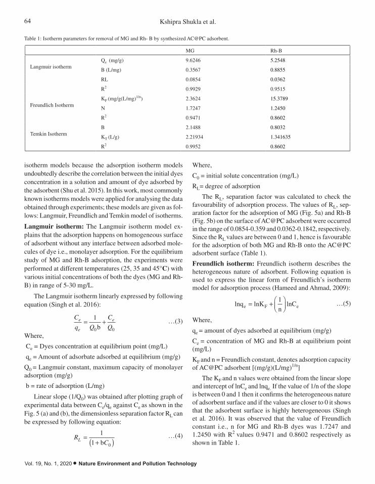
64 Kshipra Shukla et al.
Vol. 19, No. 1, 2020 • Nature Environment and Pollution Technology
isotherm models because the adsorption isotherm models undoubtedly describe the correlation between the initial dyes concentration in a solution and amount of dye adsorbed by the adsorbent (Shu et al. 2015). In this work, most commonly known isotherms models were applied for analysing the data obtained through experiments; these models are given as fol-lows: Langmuir, Freundlich and Temkin model of isotherms.
Langmuir isotherm: The Langmuir isotherm model ex-plains that the adsorption happens on homogeneous surface of adsorbent without any interface between adsorbed mole-cules of dye i.e., monolayer adsorption. For the equilibrium study of MG and Rh-B adsorption, the experiments were performed at different temperatures (25, 35 and 45°C) with various initial concentrations of both the dyes (MG and Rh-B) in range of 5-30 mg/L.
The Langmuir isotherm linearly expressed by following equation (Singh et al. 2016):
C
q Q
C
Qe
e
e= +1
0 0b …(3)
Where,
Ce = Dyes concentration at equilibrium point (mg/L)
qe = Amount of adsorbate adsorbed at equilibrium (mg/g)
Q0 = Langmuir constant, maximum capacity of monolayer adsorption (mg/g)
b = rate of adsorption (L/mg)
Linear slope (1/Q0) was obtained after plotting graph of experimental data between Ce/qe against Ce as shown in the Fig. 5 (a) and (b), the dimensionless separation factor RL can
be expressed by following equation:
RCL =
+( )1
1 0b …(4)
Where,
C0 = initial solute concentration (mg/L)
RL= degree of adsorption
The RL, separation factor was calculated to check the favourability of adsorption process. The values of RL, sep-aration factor for the adsorption of MG (Fig. 5a) and Rh-B (Fig. 5b) on the surface of AC@PC adsorbent were occurred in the range of 0.0854-0.359 and 0.0362-0.1842, respectively. Since the RL values are between 0 and 1, hence is favourable for the adsorption of both MG and Rh-B onto the AC@PC adsorbent surface (Table 1).
Freundlich isotherm: Freundlich isotherm describes the heterogeneous nature of adsorbent. Following equation is used to express the linear form of Freundlich’s isotherm model for adsorption process (Hameed and Ahmad, 2009):
lnq lnKn
lnCe F e= + ÊËÁ
ˆ¯
1 …(5)
Where,
qe = amount of dyes adsorbed at equilibrium (mg/g)
Ce = concentration of MG and Rh-B at equilibrium point (mg/L)
KF and n = Freundlich constant, denotes adsorption capacity of AC@PC adsorbent [(mg/g)(L/mg)1/n]
The KF and n values were obtained from the linear slope and intercept of lnCe and lnqe. If the value of 1/n of the slope is between 0 and 1 then it confirms the heterogeneous nature of adsorbent surface and if the values are closer to 0 it shows that the adsorbent surface is highly heterogeneous (Singh et al. 2016). It was observed that the value of Freundlich constant i.e., n for MG and Rh-B dyes was 1.7247 and 1.2450 with R2 values 0.9471 and 0.8602 respectively as shown in Table 1.
Table 1: Isotherm parameters for removal of MG and Rh- B by synthesized AC@PC adsorbent.
MG Rh-B
Langmuir isothermQe (mg/g) 9.6246 5.2548
B (L/mg) 0.3567 0.8855
RL 0.0854 0.0362
R2 0.9929 0.9515
Freundlich IsothermKF (mg/g(L/mg)1/n) 2.3624 15.3789
N 1.7247 1.2450
R2 0.9471 0.8602
Temkin IsothermB 2.1488 0.8032
KT (L/g) 2.21934 1.341635
R2 0.9952 0.8602
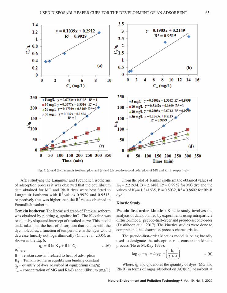
65USED DISPOSABLE PAPER CUPS FOR THE DEVELOPMENT OF AN ADSORBENT
Nature Environment and Pollution Technology • Vol. 19, No. 1, 2020
After studying the Langmuir and Freundlich isotherms of adsorption process it was observed that the equilibrium data obtained for MG and Rh-B dyes were best fitted to Langmuir isotherm with R2 values 0.9929 and 0.9515, respectively that was higher than the R2 values obtained in Freundlich isotherm.
Temkin isotherm: The linearised graph of Temkin isotherm was obtained by plotting qe against lnCe. The KT value was resolute by slope and intercept of resulted curve. This model undertakes that the heat of absorption that relates with the dye molecules, a function of temperature in the layer would decrease linearly not logarithmically (Chun et al. 2005), as shown in the Eq. 6;
q B ln K B lne T= + Ce …(6)Where,B = Temkin constant related to heat of adsorptionKT = Temkin isotherm equilibrium binding constantqe = quantity of dyes adsorbed at equilibrium (mg/g)Ce = concentration of MG and Rh-B at equilibrium (mg/L)
From the plot of Temkin isotherm the obtained values of KT = 2.21934, B = 2.1488, R2 = 0.9952 for MG dye and the values of KT = 1.341635, B = 0.8032, R2 = 0.8602 for Rh-B dye.
Kinetic Study
Pseudo-first-order kinetics: Kinetic study involves the analysis of data obtained by experiments using intraparticle diffusion model, pseudo-first-order and pseudo-second-order (Dastkhoon et al. 2017). The kinetics studies were done to comprehend the adsorption process characteristics.
The pseudo-first-order kinetics model is being broadly used to designate the adsorption rate constant in kinetic process (Ho & McKay 1999).
log.
q qk
e t- = - ÊËÁ
ˆ¯
logqe1
2 303 …(6)
Where, qe and qt denotes the quantity of dyes (MG and Rh-B) in terms of mg/g adsorbed on AC@PC adsorbent at
15
Fig. 5: (a) and (b) Langmuir isotherm plots and (c) and (d) pseudo-second order plots of MG and
Rh-B, respectively.
Freundlich isotherm: Freundlich isotherm describes the heterogeneous nature of adsorbent.
Following equation is used to express the linear form of Freundlich’s isotherm model for
adsorption process (Hameed and Ahmad, 2009):
lnqe = lnKF + (1n) lnCe …(5)
Where,
qe= amount of dyes adsorbed at equilibrium (mg/g)
Ce= concentration of MG and Rh-B at equilibrium point (mg/L)
KF and n = Freundlich constant, denotes adsorption capacity of AC@PC adsorbent
[(mg/g)(L/mg)1/n]
Fig. 5: (a) and (b) Langmuir isotherm plots and (c) and (d) pseudo-second order plots of MG and Rh-B, respectively.

66 Kshipra Shukla et al.
Vol. 19, No. 1, 2020 • Nature Environment and Pollution Technology
time t (min) at equilibrium point. K1 (min-1) represents rate constant for the MG and Rh-B adsorption. Values of k1 and qe were obtained by calculating log(qe-qt) against t plots with different dyes initial concentrations of MG and Rh-B. It was observed that adsorption data was not fitted with pseudo-first order with R2 value = 0.785-0.910 for MG and R2 value = 0.841-0.958 for Rh-B (Table 2).
Pseudo-second-order kinetics: The experimental records were examined by using pseudo-second-order kinetics (Li et al. 2013). The equation for pseudo-second-order ki-netics is expressed below:
t
qt= ( ) +
ÊËÁ
ˆ¯
1 1
22k q q
te e
…(8)
Here, k2 (g/(mg.min) is constant for pseudo second order kinetic. qe denotes the adsorption capacity at equilibrium.
Values of pseudo second order kinetic parameters were calculated from the plot of t/qt against t (Figs. 5c and d). The linear regression coefficient (R2) values for both the kinetic models are given in Table 3. The pseudo second order model was best fitted with kinetic data with R2 value =1 for MG (Fig. 5c) and R2 value = 0.999 for Rh-B (Fig. 5d).
Intraparticle diffusion model: An experimental model for intraparticle diffusion mechanism, reported by Albadarin et al. (2017) was used. The solute transfer in process of sol-id-liquid sorption is commonly illustrated by intraparticle diffusion model. Intraparticle diffusion model is represented by following equation:
qt = +k t ci1 2/ …(9)
Here, ki (mg/g.min1/2) symbolizes the rate constant for intraparticle diffusion and constant C (mg/g) is associated with the boundary layer and was calculated through graph plotted between qt and t1/2. Intraparticle diffusion model is
a rate limiting step. The intraparticle diffusion is consider as rate limiting step when a linear regression passage origin is found after plotting the graph between qt and t1/2. Fig. 6 shows that the plots did not passed through the origin in case of both the dyes (MG (Fig. 6a) and Rh-B (Fig. 6b)). This signifies that the intraparticle diffusion model was not only the rate controlling factor and other mechanisms are also involved (Saleh et al. 2016).
Thermodynamic Study
Thermodynamic study includes calculation of Gibb’s free energy (DG°), change in entropy (DS) and enthalpy (DH) from the following equations for adsorption of MG and Rh-B dyes (Singh et al. 2016)
Kc =qe
Ce …(10)
ln KcH
= -D DS
R RT …(11)
DG RT LnKc∞ = - …(12)
Where, Ce is the concentration of the dye (mg/L) in the solution and qe is the amount of dye adsorbed at equilibri-um (mg/g), T(K) is the absolute temperature and Kc is the thermodynamic equilibrium constant.
The standard Gibb’s energy (DG°) was calculated by the value of Kc (L/g) obtained at different temperatures and R is the universal gas constant (8.314 J/mol K). The values of thermodynamic constants were calculated by graph of lnKc plotted against 1/T. The thermodynamic data shows that the MG dye (Fig. 6c) adsorption by AC@PC adsorbent was endothermic that was proved by the positive value of DH° (22.51348 J/mol) (Table 3), whereas spontaneous nature of adsorption process which is favourable at all temperatures described by negative value of DG° (Mahmoodi et al. 2011).
The standard entropy i.e., DS° (83.15663 J/mol K) for MG
Table 2: Values of kinetic parameters pseudo first order and second order.
Kinetics Pseudo first order kinetics Pseudo second order
C0 (mg/L) qe (mg/g) k1 (min-1) R2 qe (mg/g) k2 (g/mg. min) R2
AC@PC
MG5 0.0742 0.002649 0.9103 1.4788 0.7453 1
10 0.3629 0.004082 0.9877 2.9612 0.2067 1
20 0.7120 0.003474 0.8811 5.5834 0.1031 1
30 0.7120 0.003561 0.7857 7.1942 0.1168 1
Rh-B5 0.2123 0.003865 0.9050 1.5610 0.3146 0.999
10 0.3202 0.004993 0.8417 3.0845 0.2841 1
20 0.4530 0.002996 0.9475 3.8343 0.1184 0.999
30 1.0690 0.004386 0.9583 5.3676 0.0678 0.999

67USED DISPOSABLE PAPER CUPS FOR THE DEVELOPMENT OF AN ADSORBENT
Nature Environment and Pollution Technology • Vol. 19, No. 1, 2020
adsorption was positive, it represents that the degree of adsorbent-adsorbate interface randomness during adsorp-tion process of dye. However, in case of Rh-B (Fig. 6d) value of DG° was positive. The negative values -23.10210 J/mol and -66.01648 J/mol K of DH° and DS°, respectively, (Table 3) confirmed that the thermodynamic process was exothermic, on increasing temperature the initial adsorption rate was decreased. It was examined that the value of DG° increases with increasing temperature which indicates greater
adsorption at lower temperature. For Rh-B negative value of DS° revealed good affinity of AC@PC. Analogous result was also reported by Shu et al. (2015). This study explained that adsorption of Rh-B onto the adsorbate (rice husk and activated carbon) was exothermic in nature with negative values of DH° and DS°.
Mechanism
Mechanism of dyes adsorption can be described by various
19
Fig. 6: (a) and (b) Intraparticle diffusion model and (c) and (d) thermodynamics plot of
MG sand Rh-B, respectively.
The standard Gibb’s energy (ΔG°) was calculated by the value of Kc (L/g) obtained at different
temperatures and R is the universal gas constant (8.314 J/mol K). The values of thermodynamic
constraints were calculated by graph of lnKc plotted against 1/T. The thermodynamic data shows
that the MG dye (Fig. 6c) adsorption by AC@PC adsorbent was endothermic that was proved by
the positive value of ΔH° (22.51348 J/mol) (Table 3), whereas spontaneous nature of adsorption
process which is favourable at all temperatures described by negative value of ΔG° (Mahmoodi et
al. 2011). The standard entropy i.e., ΔS° (83.15663 J/mol K) for MG adsorption was positive, it
represents that the degree of adsorbent- adsorbate interface randomness during adsorption process
of dye. However, in case of Rh-B (Fig. 6d) value of ΔG° was positive. The negative values -
23.10210 J/mol and -66.01648 J/mol K of ΔH° and ΔS° confirmed that the thermodynamic process
was exothermic, on increasing temperature the initial adsorption rate was decreased which shows
Fig. 6: (a) and (b) Intraparticle diffusion model and (c) and (d) thermodynamics plot of MG and Rh-B, respectively.
Table 3: Thermodynamic parameters of MG and Rh-B adsorption onto AC@PC adsorbent.
Parameters Temperature (K) AC@PC
MG Rh-B
ΔG˚ (KJ/mol) 298 -24.7582 19.64981
308 -25.5897 20.30998
318 -26.4213 20.97014
DH˚ (J/mol) 22.51348 -23.10210
DS˚ (J/mol K) 83.15663 -66.01648

68 Kshipra Shukla et al.
Vol. 19, No. 1, 2020 • Nature Environment and Pollution Technology
processes. In this study, Langmuir isotherm was best fitted. The Langmuir isotherm signifies the monolayer adsorption onto a determinate number of homogeneous sites. The ho-mogeneous nature of adsorption phenomenon can also be explained by FTIR results that represent the functional groups are present on the surface of adsorbent that may be respon-sible for enhancing the removal percentage of adsorbent. As shown in Fig. 7, FTIR results revealed the presence of several functional groups like hydroxyl, phenol, carboxylic acid, benzene ring, amine, methyl, and nitro group on the surface of adsorbent before adsorption of dyes. But after adsorption of dyes, some changes were also observed in the functional group composition. In case of MG, -NH, -CH, and C=H groups are mainly responsible groups for adsorption of dye. Whereas, in case of Rh-B adsorbent, after adsorption shows that OH, -CH, -C=O, -C-O and N-C=O functional groups had key role in removal. FTIR result revealed the possibility of ion exchange of dyes on adsorbent surface and helps to increase the adsorption percentage and provide more active binding sites for adsorption of dyes. Elemental analysis was done by EDS that shows that higher carbon content was present in adsorbent that provides large surface area to the adsorbent; more the surface area more the adsorption of dyes.
The adsorption of organic dyes onto the surface of acti-vated carbon in this study can be explained on the basis of mainly two major mechanisms i.e., electrostatic attraction and p-p interaction. The electrostatic attraction mechanism undertakes the attraction of partially negative species towards
the positively charged species, as the surface functional group (Fe) on adsorbent acts as an electron acceptor while Rh-B dye has a partially negatively charged group that attracted towards the Fe present on the adsorbent surface with positive charge. On the other hand, p-p interaction, takes place in between the benzene ring present in adsorbate and on adsorbent surface. Adsorption of MG and Rh-B through AC@PC was occurred by p-p interaction a similar mechanism was also reported by Gao et al. 2019 (MG) and Cheng et al. 2017 (Rh-B).
CONCLUSIONS
A simple and cost-effective method to synthesize adsorbent from waste disposable cups at 500°C temperature in muffle furnace and then used for removal of MG and (Rh-B) dyes from an aqueous solution. AC@PC is low cost and easily available material. Prepared AC@PC adsorbent showed excellent removal ability for MG and Rh-B dyes. The adsorption behaviour of MG and Rh-B was analysed methodically and observed that pseudo-second-order kinetic with the R2 > 0.999 was followed by both the dyes. The Langmuir model of isotherm was best fitted to the experimental data of equilibrium study. It can be concluded that disposable waste cups can be effectively used for the synthesis of adsorbent which is cost effective and the synthesized adsorbent AC@PC from waste paper cups could be used to remove effectively the basic dyes from dye contaminated water. An application of waste cups in water
21
C=O, -C-O and N-C=O functional groups had key role in removal. FTIR result revealed the
possibility of ion exchange of dyes on adsorbent surface and helps to increase the adsorption
percentage and provide more active binding sites for adsorption of dyes. Elemental analysis was
done by EDS that shows that higher carbon content was present in adsorbent that provides large
surface area to the adsorbent; more the surface area more the adsorption of dyes.
The adsorption of organic dyes onto the surface of activated carbon in this study can be
explained on the basis of mainly two major mechanisms i.e., electrostatic attraction and π-π
interaction. The electrostatic attraction mechanism undertakes the attraction of partially negative
species towards the positively charged species, as the surface functional group (Fe) on adsorbent
acts as an electron acceptor while Rh-B dye has a partially negatively charged group that attracted
towards the Fe present on the adsorbent surface with positive charge. On the other hand, π-π
interaction, takes place in between the benzene ring present in adsorbate and on adsorbent surface.
Adsorption of MG and Rh-B through AC@PC was occurred by π-π interaction a similar
mechanism was also reported by Gao et al. 2019 (MG) and Cheng et al. 2017 (Rh-B).
Fig. 7: Mechanism of dyes adsorption on AC@PC.
Conclusions
A simple and cost-effective method to synthesize adsorbent from waste disposable cups at
500°C temperature in muffle furnace and then used for removal of MG and (Rh-B) dyes from an
Fig. 7: Mechanism of dyes adsorption on AC@PC.

69USED DISPOSABLE PAPER CUPS FOR THE DEVELOPMENT OF AN ADSORBENT
Nature Environment and Pollution Technology • Vol. 19, No. 1, 2020
treatment not only treats water but also minimize the waste generation.
ACKNOWLEDGMENT
The authors are very grateful to acknowledge the support of UGC-BSR research start-up-grant (Project No. F. 30-382/2017, BSR) and Science and Engineering Research Board (SERB), Department of Science and Technology (DST) (Reference no. ECR/2016/001924), Government of India.
REFERENCES
Albadarin, A.B., Collins, M.N., Naushad, M., Shirazian, S., Walker, G. and Mangwandi, C. 2017. Activated lignin-chitosan extruded blends for efficient adsorption of methylene blue. Chem. Eng. J., 307: 264-272.
Amiri, M., Niasari, M.S., Akbari, A. and Gholami, T. 2017. Removal of malachite green (a toxic dye) from water by cobalt ferrite silica magnetic nanocomposite: Herbal and green sol-gel autocombustion synthesis. Int. J. Hydrog. Energy., 42(39): 24846-24860.
Arena, U., Ardolino, F. and Gregorio F.D. 2016. Technological, environmen-tal and social aspects of a recycling process of post-consumer absorbent hygiene products. J. Clean. Prod., 127: 289-301.
Arumugam, K., Ganesan, S., Muthunarayanan, V., Vivek, S., Sugumar, S. and Munusamy, V. 2015. Potentiality of Eisenia fetida to degrade disposable paper cups-an ecofriendly solution to solid waste pollution. Environ. Sci. Pollut. Res., 22(4): 2868-2876.
Arumugam, K., Renganathan, S., Babalola, O.O. and Muthunarayanan, V. 2018. Investigation on paper cup waste degradation by bacterial consortium and Eudrillus eugeinea through vermicomposting. Waste Manage., 74: 185-193.
Bhattacharya, K., Gupta, S. and Sharma, G. 2014. Interactions of the dye, rhodamine-B with kaolinite and montmorillonite in water. Appl. Clay. Sci., 99: 7-17.
Chun, J.H., Jeon, S.K., Kim, N.Y. and Chun, J.Y. 2005. The phase shift method for determining Langmuir and Temkin adsorption isotherms of over potentially deposited hydrogen for the cathodic H2 evaluation reaction at the poly-Pt/H2SO4 aqueous electrolyte interface. Int. J. Hydrog. Energy., 30(13-14): 1423-1436.
Cheng, Z.L., Li, Y.X. and Liu, Z. 2017. Novel adsorption materials based on graphene oxide/Beta zeolite composite materials and their adsorp-tion performance for rhodamine B. J. Alloys. Compd., 708: 255-263.
Crini, G. 2006. Non-conventional low-cost adsorbents for dye removal: A review. Bioresour. Technol., 97(9): 1061-1085.
Dastkhoon, M., Ghaedi, M., Asfaram, A., Azqhandi, M.H.A. and Purkait, M.K. 2017. Simultaneous removal of dyes onto nanowires adsorbent use of ultrasound assisted adsorption to clean waste water: Chemometrics for modeling and optimization, multicomponent adsorption and kinetic study. Chem. Eng. Res. Des., 124: 222-237.
Gao, M., Wang, Z., Yang, C., Ning, J., Zhou, Z and Li, G. 2019. Novel mag-netic graphene oxide decorated with persimmon tannins for efficient adsorption of malachite green from aqueous solutions. Colloids Surf. A Physicochem. Eng. Asp., 566: 48-57.
Gautam, A., Rawat, S., Verma, L., Singh, J., Sikarwar, S., Yadav, B.C. and Kalamdhad, A.S. 2018. Green synthesis of iron nanoparticle from ex-tract of waste tea: An application for phenol red removal from aqueous solution. Environ. Nanotechnol. Monit. Manage., 10: 377-387.
Guo, Y., Zhao, J., Zhang, H., Yang, S., Qi, J., Wang, Z. and Xu, H. 2005. Use of rice husk-based porous carbon for adsorption of Rhodamine B from aqueous solutions. Dyes Pigm., 66(2): 123-128.
Gupta, N., Kushwaha, A.K. and Chattopadhyaya, M.C. 2016. Application of potato (Solanum tuberosum) plant wastes for the removal of meth-ylene blue and malachite green dye from aqueous solution. Arab. J. Chem., 9: 707-716.
Gupta, V.K., Pathania, D., Agarwal, S. and Singh, P. 2012. Adsorptional photocatalytic degradation of methylene blue onto pectin-CuS nano-composite under solar light. J. Hazard. Mater., 243: 179-186.
Hameed, B.H. and Ahmad, A.A. 2009. Batch adsorption of methylene blue from aqueous solution by garlic peel, an agricultural waste biomass. J. Hazard. Mater., 164(2-3): 870-875.
Ho, Y.S. and McKay, G. 1999. Pseudo-second order model for sorption processes. Process Biochem., 34(5): 451-465.
Ibrahim, M., Siddiqe, A., Verma, L., Singh, J. and Koduru, J.R. 2019. Adsorptive removal of fluoride from aqueous solution by biogenic iron permeated activated carbon derived from sweet lime waste. Acta Chim. Slov., 66(1): 123-136.
Kant, R. 2012. Adsorption of dye eosin from an aqueous solution on two different samples of activated carbon by static batch method. J. Water Resource Prot., 4(02): 93-98.
Karunanayake, A., Todd, O.A., Crowely, M., Ricchetti, L., Pittman, Jr C.U., Anderson, R., Mohan, D. and Mlsna, T. 2018. Lead and cadmium re-mediation using magnetized and nonmagnetized biochar from Douglas fir. Chem. Eng. J., 331: 480-491.
Kono, H. 2015. Preparation and characterization of amphoteric cellulose hydrogels as adsorbents for the anionic dyes in aqueous solutions. Gels., 1(1): 94-116
Li, Y.H., Du, Q.J., Liu, T.H., Sun, J.K., Wang, Y.H., Wu, S.L., Wang, Z.H., Xia, Y.Z. and Xia, L.H. 2013. Methylene blue adsorption ongraphene oxide/calcium alginate composites. Carbohydr. Polym., 95(1): 501-507.
Lunge, S., Singh, S. and Sinha, A. 2014. Magnetic iron oxide (Fe3O4) nano- particles from tea waste for arsenic removal. J. Magn. Magn. Mater. 356: 21-31.
Magdalane, C.M., Kaviyarasu, K., Vijaya, J.J., Jayakumar, C., Maaza, M. and Jeyaraj, B. 2017. Photocatalytic degradation effect of malachite green and catalytic hydrogenation by UV illuminated CeO2/CdO multilayered nanoplatelet arrays: Investigation of antifungal and antimicrobial activities. J. Photochem. Photobiol. B., 169: 110-123.
Mahmoodi, N., Hayati, M.B., Arami, M. and Lan, C. 2011. Adsorption of textile dyes on pine cone from colored wastewater: kinetic, equilibrium and thermodynamic studies. Desalination, 268(1-3): 117-125.
Nassar, M.Y., Mohamed, T.Y., Ahmed, I.S. and Sami, I. 2017. MgO nano-structure via a sol-gel combustion synthesis method using different fuels: An efficient nano-adsorbent for the removal of some anionic textile dyes. J. Mol. Liq., 225: 730-740.
Ngulube, T., Gumbo, J.R., Masindi, V. and Maity, A. 2017. An update on synthetic dyes adsorption onto clay based minerals: A state-of-art review. J. Environ. Manage., 191: 35-57.
Noel, D.S. and Rajan, M.R. 2014. Impact of dyeing industry effluent on groundwater quality by water quality index and correlation analysis. J. Pollut. Eff. Control., 2: 1-4.
Pathania, D., Sharma, S. and Singh, P. 2017. Removal of methylene blue by adsorption onto activated carbon developed from Ficus carica bast. Arab. J. Chem., 10: 1445-1451.
Saini, J., Garg, V.K. and Kataria, N. 2017. Removal of Orange G and Rhodamine B dyes from aqueous system using hydrothermally syn-thesized zinc oxide loaded activated carbon (ZnO-AC). J. Environ. Chem. Eng., 5(1): 884-892.
Saleh, T.A., Siddiqui, M.N. and Al-Arfaj, A.A. 2016. Kinetic and intrapar-ticle diffusion studies of carbon nanotubes-titania for desulfurization of fuels. Petrol. Sci. Technol., 34(16): 1468-1474.
Salleh, M.A.M., Mahmoud, D.K., Karim, W.A. and Idris, A. 2011. Cationic anionic dye adsorption by agricultural solid waste: a comprehensive review. Desalination, 280(1-3): 1-13.

70 Kshipra Shukla et al.
Vol. 19, No. 1, 2020 • Nature Environment and Pollution Technology
Sartape, A.S., Mandhare, A.M., Jadhav, V.V., Raut, P.D., Anuse, M.A. and Kolekar, S.S. 2017. Removal of malachite green dye from aqueous solution with adsorption technique using Limonia acidis-sima (wood apple) shell as low cost adsorbent. Arab J. Chem., 10: 3229-3238.
Shu, J., Wang, Z., Huang, Y., Huang, N., Ren, C. and Zhang, W. 2015. Adsorption removal of Congo red from aqueous solution by polyhe-dral Cu2O nanoparticles: Kinetics, isotherms, thermodynamics and mechanism analysis. J. Alloys Compd., 633: 338-346.
Singh, J. and Lee, B.K. 2015. Hydrometallurgical recovery of heavy metals from low grade automobile shredder residue (ASR): an application of
advance Fenton process (AFP). J. Environ. Manage., 161: 1-10.Singh, J., Reddy, K.J., Chang, Y.Y., Kang, S.H. and Yang, J.K. 2016. A novel
reutilization method for automobile shredder residue as an adsorbent for the removal of methylene blue: Mechanisms and heavy metal recovery using an ultrasonically assisted acid. Process Saf. Environ., 99: 88-97.
Yagub, M.T., Sen, T.K., Afroze, S. and Ang, H.M. 2014. Dye and its removal from aqueous solution by adsorption: A review. Adv. Colloid Interface Sci., 209: 172-184.
Zhang, F., Ma, B.L., Jiang, X.P. and Ji, Y.F. 2016. Dual function magnetic hydroxyapatite nano powder for removal of malachite green and Congo red from aqueous solution. Powder Technol., 302: 207-214.

Assessing Ecological Conditions of Microtopography for Vegetation Restoration on the Chinese Loess Plateau
Huan Ma *(***)†, Qingke Zhu**, Xining Zhao* and Yuan Liu****College of Water Resources and Architectural Engineering, Northwest Agricultural & Forestry University, Yangling 712100, P.R. China**Forestry Ecological Engineering Research Center (Ministry of Education), Beijing Forestry University, Beijing 100083, P.R. China***Powerchina Northwest Engineering Corporation, Xi’an 710065, P.R. China†Corresponding author: Ma Huan
ABSTRACT
Microtopographies affect large portions of the Chinese Loess Plateau after years of water erosion. Vegetation restoration has proven to be an effective way to conserve water and soil, however, studies of the influence of microtopography on naturally recovered vegetation on the Chinese Loess Plateau have long been absent. The objective of this study was to determine the influence of microtopography on the vegetation structure and plant diversity of naturally restored vegetation and compare the soil physicochemical properties of different microtopographies with those of undisturbed slopes on the Loess Plateau. We identified five types of microtopographies that are mainly shaped by runoff in the study area, and examined vegetation structures, plant diversity, soil nutrients and soil water storage compared with undisturbed slopes. The results show that vegetation communities on loess slopes are still in an early successional stage after 14 years of natural recovery. Vegetation diversity was significantly different among microtopographies. Four types of microtopography have better soil conditions for vegetation restoration; scarps are the exception. Our results suggest that microtopographies can create some better condition plots for precision designed artificial restoration of vegetation, which is necessary to accelerate the succession process on the Loess Plateau.
INTRODUCTION
The Loess Plateau in China covers a large area totalling 624,000 km2. The soil erosion on the Loess Plateau not only leads to the degradation of local land but also sends sediment to the lower reaches of the Yellow River, increasing the flooding risk (Mcvicar et al. 2007). Vegetation restoration on the Loess Plateau has been proven to be an effective way to improve soil texture (Li et al. 2006) and decrease the soil erosion ratio (Zheng 2006). To control soil erosion, the Chinese government has historically focused on a series of vegetation restoration projects on the Loess Plateau. To pursue an endpoint in which forests can rapidly develop a closed canopy with minimal labour investment, a vegetation restoration model on the Loess Plateau in which plants are planted with the same row spacing along contours based on the site conditions of slopes using fast growing trees and shrubs has often been adopted for restoration (Zhu et al. 2012). However, these projects have met with mixed success (Jiao et al. 2012). After years of water erosion on the Loess Plateau, there are numerous potholes and gullies distributing all over slopes. This type of topographic
heterogeneity can lead to the redistribution of precipitation by affecting overland flow (Liu et al. 2004) and evaporation (Price et al. 1998). The unevenness of soil water moisture and inappropriate selection of species together result in forest degradation and the development of low productivity forests with small but old trees (Zhu et al. 2012). However, better soil water conditions can also be created by the uneven surface (Mott et al. 1974). Higher species diversity can appear in the sites where the micro-environment has greater heterogeneity in both the horizontal and vertical directions, and a complex community structure implies the use of multiple environmental resources (He et al. 1997).
Topographic heterogeneity on a fine scale has long been recognized as an important factor in vegetation restoration (Rossell et al. 2009). Early in the 1960s, studies found that small topographic differences can significantly affect species distributions and succession in herbaceous communities (Zedler et al. 1969). Subsequent studies have illustrated that a small amount of heterogeneity in topography can affect the microenvironment of the understory (Beatty 1984), soil texture (Martinez-Turanzas et al. 1997), and soil nutrients
Nat. Env. & Poll. Tech.Website: www.neptjournal.com
Received: 14-06-2019Accepted: 24-07-2019
Key Words:Loess plateau Microtopographic hetero-geneity Plant diversity Soil nutrients Soil water
2020pp. 71-82 Vol. 19
p-ISSN: 0972-6268 No. 1 Nature Environment and Pollution Technology An International Quarterly Scientific Journal
Original Research Paper
e-ISSN: 2395-3454
Open Access

72 Huan Ma et al.
Vol. 19, No. 1, 2020 • Nature Environment and Pollution Technology
(Moser et al. 2009). This small topographic heterogeneity is often created by disturbances, such as tree fall (Moser et al. 2009), animal activities (Pavone et al. 1985), soil erosion (Zhu et al. 2012), sedimentation (Werner et al. 2002) and landslides (Sakai et al. 1993). These disturbances create bare soil with different characteristics that different pioneer plants can opportunistically invade, and the pioneer plants can
establish communities different from those in surrounding forests (Guariguata 1990). A small amount of topographic heterogeneity can also affect the vegetation structure (Hara et al. 1996), composition (Milton et al. 1985), and succession (Gilland et al. 2014) of early successional plants and eventually the development of different late-successional communities.
Fig.1: The distribution of sample plots in the Hegou watershed.
Classification of Microtopography
According to field observations, slopes in the Loess Plateau usually can be classified as
undisturbed slope and disturbed slope due to the severe soil erosion. The disturbed slope part
formed several kinds of microtopographies. The microtopographies on the Loess Plateau are
usually larger in extent compared with those in wetlands. We defined 5 main forms of
microtopography on the Loess Plateau, which are scarp, ephemeral gully, sinkhole, platform and
gully (Fig. 2). Most of the slopes in the Loess Plateau are consisted of these microtopographies
and the undisturbed slopes. The scarp is an area with a substantially steeper than the other parts of
the slopes. The ephemeral gully is the primary stage of gully erosion development, and it is larger
Fig.1: The distribution of sample plots in the Hegou watershed.

73ECOLOGICAL CONDITIONS OF MICROTOPOGRAPHY FOR VEGETATION RESTORATION
Nature Environment and Pollution Technology • Vol. 19, No. 1, 2020
Previous studies have primarily focused on microtopog-raphy in wetlands (Domínguez-Cadena et al. 2016), where the microtopography is often created by tree fall (Šamonil et al. 2016). These microtopographies, such as mounds, pools and pits, are usually on a scale of less than 5 m due to the specific hydrological and environmental conditions (Beatty 1984). Microtopographies that are created by landslides on a larger scale in hilly area were also reported (Nagamatsu et al. 1997). There are also lots of microtopographies exist in the Loess Plateau. These microtopographies were different from those mentioned in previous studies both in scale and the cause they emerged. Microtopography on the Loess Plateau was shaped by several types of soil erosion, among which water erosion is the main type (Fang et al. 2008), and on a spatial scale larger than 1 m2. Studies have assessed the soil properties and vegetation structure responses after vegetation restoration projects on the Loess Plateau (Zeng et al. 2016), but none have addressed the effect of microtopog-raphy on edaphic or botanical factors. In addition, vegetation restoration on the Loess Plateau focuses on matching tree species with site in slope scale, whereas the small scale of topographic heterogeneity that under the slope scale may significantly impact the quality of vegetation restoration. No studies have assessed the influence of microtopography to natural recovered vegetation on the Chinese Loess Plateau. The objects of this study were to (1) analyse the impact of microtopography, relative to other topographical factors, on vegetation structure and species diversity, (2) determine the vegetation structures and species diversity among different microtopographies, and (3) compare soil physiochemical properties among different microtopographies in order to de-termine precisely suitable position using microtopography as an indicator for vegetation restoration on the Loess Plateau.
MATERIALS AND METHODS
Study Site
The study was conducted in the 4.25 km2 Hegou (36°54’09” - 36°54’23” N, 108°12’50” - 108°13’01” E) watershed, located in Wuqi County, northern Shaanxi Province. The area is characterized by a temperate continental monsoon climate that is warm and dry, with an annual mean temperature of 7.8°C and mean annual precipitation of 466 mm (based on data spanning 1957-2009). The annual variation in precipitation is large, and there is an uneven distribution in different seasons, with most precipitation occurring from June to September. The soil type of this area is cultivated loessal soils. The land surface can easily be eroded and forms many types of microtopographies due to the specific character of precipitation and human activities. Fig. 1 shows the distribution of the sample plots in the Hegou watershed.
Classification of Microtopography
According to field observations, slopes in the Loess Plateau usually can be classified as undisturbed slope and disturbed slope due to the severe soil erosion. The disturbed slope part formed several kinds of microtopographies. The microtopographies on the Loess Plateau are usually larger in extent compared with those in wetlands. We defined 5 main forms of microtopography on the Loess Plateau, which are scarp, ephemeral gully, sinkhole, platform and gully (Fig. 2). Most of the slopes in the Loess Plateau are consisted of these microtopographies and the undisturbed slopes. The scarp is an area with a substantially steeper than the other parts of the slopes. The ephemeral gully is the primary stage of gully erosion development, and it is larger than a rill and smaller than a gully. The sinkhole is a crater on the ground shaped by running water. The platform is an area with a substantially gentle gradient than the other parts of the slopes. The gully is a landform created by running water, eroding sharply into soil and with a V-shaped cross section. Besides the five kinds of microtopographies mentioned above, we also took undisturbed slope, the rest of slope where no microtopography developed, into consideration as reference.
Data Collection
Vegetation data were collected in July 2012, and 8 transects were established across the watershed from the head to the outlet for four different slope aspects. Sample plots were placed in every microtopography on transects and undisturbed slopes nearby as reference. The sample size was 1 m × 1 m because shrubs and trees are rare. Along each transect, 14-17 plots were located. A total of 95 plots were recorded, within which there were 14 scarp samples, 15 ephemeral gully samples, 17 sinkhole samples, 14 platform samples, 15 gully samples and 15 undisturbed slope samples. The cover of each sample plot and species was estimated visually by two observers working together. Shrubs and trees were recorded when encountered. Slope gradient, aspect and position on slope were all recorded. We adopted the common classification of slope aspects (Zhu et al. 2012) on the Loess Plateau, which are sunny slope (157.5°-247.5° N), semi-sunny slope (112.5°-157.5° N and 247.5°-292.5° N), semi-shady slope (67.5°-112.5° N and 292.5°-337.5° N) and shady slope (0-67.5° N and 337.5°-360° N).
Soil sample plots were also taken in vegetation plots. Soil samples were taken from six points in an S-shaped pattern to a depth of 60 cm in each plot. Soil analysis was carried out according to the methods described by the Agricultural Chemistry Committee of the Chinese Soil Academy (1984): organic matter by the K2Cr2O7 method; total N by the K2SO4 – CuSO4 – Se distillation method; total P by the HClO4 –

74 Huan Ma et al.
Vol. 19, No. 1, 2020 • Nature Environment and Pollution Technology
H2SO4 colorimetric method; extractable ammonium-N by the diffusion method with 1N NaOH 10 mL, 2% H3BO3, and 0.005N HCl at a temperature of 40°C for 24 hours; extractable P by the 0.5 M NaHCO3 extraction (1:20) colorimetric method; and extractable K with the atomic absorption spectrum method with 1 M NH4OAC extraction (1:20, pH = 7).
For long-term observations, soil water content was monitored in fixed plots. Three PVC pipes with lengths of 2 m were pounded into the soil for each type of microtopography and undisturbed slopes. Plots that were analogous in slope gradient and aspect were arranged on the slopes to eliminate unnecessary disruption. A portable Time Domain Reflectometry (TDR) instrument was used to measure the soil water content twice per month from May 2011 to April 2012. The measurement was made from the ground surface downward to a depth of 200 cm at 20 cm intervals. For each depth interval, the soil moisture content was measured three times, and the means of the three measurements were taken as the soil moisture content of the depth interval.
Data Analysis
The measures of vegetation structure included vegetation cover, height and relative importance value (RIV). Margalef’s (Clifford et al. 1976) index for species richness, the Alatalo index (Alatalo 1977) for evenness, and the Shannon-Wiener diversity index (Shannon et al. 1950) were used as the measures of plant diversity. Soil nutrient levels and soil water storage were used as measures to assess ecological conditions. The differences among microtopographies and undisturbed slopes were compared with analysis of variance (ANOVA) and a least significant difference (LSD) test using
SPSS V20.0 (SPSS Inc., Chicago IL, USA). The equations used to calculate Margalef’s index, the Alatalo index, the Shannon-Wiener index, RIV and soil water storage are as follows:
Margalef’s index: M S Na = -( )1 / ln …(1)
Alatalo index: E P ea is
iH= - -=( / )( )1 1 11
2S …(2)
Shannon-Wiener index: ¢ = - =H lnSiS
i iP P1( ) …(3)
Relative importance value: RIV /= +( )C Hr r 200 …(4)
Soil water storage: D VSWC Hwn
s= 0 1 1. S * …(5)
Where, S is the number of species, Pi is the proportion of individuals or the abundance of the ith species expressed as a proportion of the total number in the community, ln is the log base-e, N is the total number of all species. Cr is relative coverage and Hr is relative height. VSWC is the soil volumetric water content of each soil layer, n is the number of soil layers, and Hs is the depth of each soil layer.
A canonical correlation analysis was used to examine the relationship between plant community characteristics and topographical factors. A canonical correlation analysis (CCA) is a way of making sense of cross-covariance matrices. If there are two vectors X = (X1, ..., Xn) and Y = (Y1, ..., Ym) of random variables, and there are correlations among the variables, then a canonical-correlation analysis will find linear combinations of Xi and Yj that have the maximum correlation with each other (Härdle et al. 2007). The two vectors here represent plant community characteristics and topographical factors. The plant community characteristics vector includes vegetation cover (X1), average height (X2), biomass (X3), and Shannon-Weiner index (X4). The topographical factors
than a rill and smaller than a gully. The sinkhole is a crater on the ground shaped by running water.
The platform is an area with a substantially gentle gradient than the other parts of the slopes. The
gully is a landform created by running water, eroding sharply into soil and with a V-shaped cross
section. Besides the five kinds of microtopographies mentioned above, we also took undisturbed
slope, the rest of slope where no microtopography developed, into consideration as reference.
Fig. 2: Demonstration of undisturbed slope and five types of microtopographies: scarp, ephemeral gully, sinkhole, platform and gully.
Data Collection
Vegetation data were collected in July 2012, and 8 transects were established across the watershed
from the head to the outlet for four different slope aspects. Sample plots were placed in every
microtopography on transects and undisturbed slopes nearby as reference. The sample size was 1
m × 1 m because shrubs and trees are rare. Along each transect, 14-17 plots were located. A total
of 95 plots were recorded, within which there were 14 scarp samples, 15 ephemeral gully samples,
17 sinkhole samples, 14 platform samples, 15 gully samples and 15 undisturbed slope samples.
The cover of each sample plot and species was estimated visually by two observers working
together. Shrubs and trees were recorded when encountered. Slope gradient, aspect and position
on slope were all recorded. We adopted the common classification of slope aspects (Zhu et al.
2012) on the Loess Plateau, which are sunny slope (157.5°-247.5° N), semi-sunny slope (112.5°-
Fig. 2: Demonstration of undisturbed slope and five types of microtopographies: scarp, ephemeral gully, sinkhole, platform and gully.

75ECOLOGICAL CONDITIONS OF MICROTOPOGRAPHY FOR VEGETATION RESTORATION
Nature Environment and Pollution Technology • Vol. 19, No. 1, 2020
vectors include slope aspect (Y1), slope gradient (Y2), slope position (Y3) and microtopography position (Y4). The slope aspect, slope position and microtopography were all quantified as follows: sunny slope 1, semi-sunny slope 2, semi-shady slope 3, shady slope 4; top of slope 1, middle of slope 2, bottom of slope 3; and scarp 1, ephemeral gully 2, sinkhole 3, platform 4, gully 5.
RESULTS
Relationship between Topographical Factors and Plant Communities
The canonical correlation analysis shows that for topographical factors and plant communities, there are four canonical dimensions, of which only the first two are statistically significant at the 0.05 level (Table 1). Characteristic roots of the four canonical dimensions show that 70% of total information was explained by the first two dimensions. For the first canonical dimension, the linear combination of the topographical factors v1, correlation coefficient of v1 and raw data Y1 indicate that slope aspect and microtopography position have an obvious positive correlation with v1. Correspondingly, u1, the linear combination of the plant community characteristics, has a positive correlation with the Shannon index. For the second canonical dimension, the linear combination of the topographical factors, v2, was most relevant to microtopography position. Correspondingly, the Shannon-Weiner index has a negative correlation with the linear combination of the plant community characteristics u2.
Table 1: Canonical variables and their correlation coefficients with original variables. s, Standardized canonical coefficients for each variable; r, correlation coefficient between standardized canonical coefficients and variables; R, correlation coefficient of canonical variables Xi and Yi; **, significance level of 0.01; *, significance level of 0.05.
Canonical variable Plant community characteristics vectors Topographical factors vectors
X1 X2 X3 X4 Y1 Y2 Y3 Y4
I s 0.079 0.238 0.368 0.804
R = 0.644** 0.768 0.077 0.230 0.461
r 0.633 0.503 0.557 0.287 0.833 -0.099 0.291 0.652
II s -0.499 -0.584 0.871 1.596
R = 0.477* -0.589 -0.404 -0.217 0.787
r -0.232 0.035 0.387 -0.721 -0.385 -0.545 0.039 0.713
III s -0.571 -0.009 0.842 1.403
R = 0.366 -0.351 0.768 0.430 0.373
r -0.167 0.291 0.505 0.390 -0.377 0.706 0.554 0.233
IV s -0.600 -0.746 0.638 -3.281
R = 0.112 0.008 0.555 -0.903 0.478
r 0.110 -0.531 0.135 0.166 0.126 0.442 -0.779 0.106
Vegetation Structure
A total of 64 species were found in the Hegou watershed, among which 55 species were present in the undisturbed slope plots and 64 species were present in the microtopography plots. Only 4 shrub species were found in scarps, sinkholes and gullies: Prinsepia uniflora, Caragana korshinskii, Spiraea blumei and Armeniaca vulgaris. Most (approximately 53.5%) of species belong to the Leguminoseae, Gramineae and Asteraceae (Fig. 3), which accounted for 25.5%, 16.4% and 12.7% of species, respectively. Asteraceae occupied a relatively small proportion in ephemeral gullies and undisturbed slopes, and grasses accounted for a relatively high percentage in sinkholes. A higher cover (73.33%) was recorded in gullies than in the other microtopographies (p = 0.03) (Table 3). The average cover in all microtopographies was greater than on undisturbed slopes, and the average height of herbs in sinkholes (p = 0.03) was 48.11 cm and in gullies (p = 0.02) was 42.00 cm, which were nearly double the heights of those in other microtopographies and slopes.
Table 2 gives the relative importance values (RIVs) greater or equal to 0.05 for species found in the Hegou watershed in microtopographies and undisturbed slopes. Artemisia giraldii and Artemisia sacrorum were the dominant species on undisturbed slopes and all microtopographies that had the maximum RIV. The accompanying species were primarily Stipa capillata, Lespedeza bicolor and Poa annua L. in all sites. However, scarps had Prinsepia uniflora, gullies had Caragana korshinskii, and platforms had Phragmites

76 Huan Ma et al.
Vol. 19, No. 1, 2020 • Nature Environment and Pollution Technology
australis as unique accompanying species. In addition, the RIV of Artemisia giraldii in the sinkholes was much greater than in the other microtopographies.
Plant Diversity
Table 3 presents the plant diversity indices of microtopographies in the Hegou watershed. Margalef’s richness index values were in the following order: scarp > platform > gully > ephemeral gully > undisturbed slope. The scarp had the highest Margalef index value of 2.49, but the difference was not significant among the microtopographies. The Alatalo
(Table 3). The average cover in all microtopographies was greater than on undisturbed slopes, and
the average height of herbs in sinkholes (p = 0.03) was 48.11 cm and in gullies (p = 0.02) was
42.00 cm, which were nearly double the heights of those in other microtopographies and slopes.
Fig. 3: Species compositions of different microtopographies in the Hegou watershed. Bars indicate the number of
species in microtopographies and on undisturbed slopes. Arrows indicate plots in which shrubs appeared. SP: scarp;
EG: ephemeral gully; SH: sinkhole; PL: platform; GL: gully; MT: take all the microtopographies above as a whole; US:
undisturbed slope.
Table 2 gives the relative importance values (RIVs) greater or equal to 0.05 for species found in
the Hegou watershed in microtopographies and undisturbed slopes. Artemisia giraldii and
Artemisia sacrorum were the dominant species on undisturbed slopes and all microtopographies
that had the maximum RIV. The accompanying species were primarily Stipa capillata, Lespedeza
bicolor and Poa annua L in all sites. However, scarps had Prinsepia uniflora, gullies had
Caragana korshinskii, and platforms had Phragmites australis as unique accompanying species.
In addition, the RIV of Artemisia giraldii in the sinkholes was much greater than in the other
microtopographies.
Table 2: Relative importance values (RIVs) for species found in the Hegou watershed across different
0
10
20
30
40
50
60
70
SP EG SH PL GL MT US
Num
ber
of sp
ecie
s
Microtopography
Others
Leguminosae
Gramineae
Asteraceae
↓↓↓
Fig. 3: Species compositions of different microtopographies in the Hegou watershed. Bars indicate the number of species in microtopographies and on undisturbed slopes. Arrows indicate plots in which shrubs appeared. SP: scarp; EG: ephemeral gully; SH: sinkhole; PL: platform; GL: gully; MT:
take all the microtopographies above as a whole; US: undisturbed slope.
Table 2: Relative importance values (RIVs) for species found in the Hegou watershed across different microtopographies. SP: scarp; EG: ephemeral gully; SH: sinkhole; PL: platform; GL: gully; US: undisturbed slope.
Plant Species Microtopography
SP EG SH PL GL US
Artemisia giraldii Pamp. 0.155 1.173 0.269 0.110 0.198 0.169
Artemisia sacrorum Ledeb. 0.162 0.178 0.144 0.182 0.192 0.179
Stipa capillata Linn. 0.118 0.152 0.088 0.065 0.093
Lespedeza bicolor Turcz. 0.062 0.064 0.094 0.084
Poa annua L. 0.092 0.064 0.066 0.056
Potentilla acaulis L. 0.074
Thymus mongolicus Ronn 0.054 0.054
Prinsepia uniflora Batal. 0.062 0.059
Phragmites australis 0.052
Potentilla chinensis Ser. 0.052
Caragana korshinskii Kom 0.050
evenness index differed among the microtopographies. The maximum Alatalo index appeared in ephemeral gullies (p = 0.02) at 0.618. The minimum Alatalo index appeared in the platform (0.03) at 0.414. The Shannon-Wiener index in scarps was the highest but not significantly (p = 0.354). In general, compared with microtopographies, fewer species were distributed on undisturbed slopes in a relatively uniform pattern, implying an unstable community structure on undisturbed slopes. Among all microtopographies, scarps, gullies and ephemeral gullies had more species and more homogeneous plant distribution. Sinkholes were primarily

77ECOLOGICAL CONDITIONS OF MICROTOPOGRAPHY FOR VEGETATION RESTORATION
Nature Environment and Pollution Technology • Vol. 19, No. 1, 2020
Table 3: Cover, average height, species richness and diversity values of microtopographies and undisturbed slopes in the Hegou watershed. SP: scarp; EG: ephemeral gully; SH: sinkhole; PL: platform; GL: gully; US: undisturbed slope. Average height was calculated excluding shrubs and tree seedlings. All values are means±SE. Letters indicate significant pairwise differences between means within a row at p = 0.05.
Microtopography
SP EG SH PF GL US
Cover (%) 68.07 ± 3.91b 67.35 ± 3.87b 66.39 ± 4.20b 64.64 ± 3.97b 74.33 ± 3.89a 63.35 ± 2.29b
Average height (cm) 28.00 ± 2.80ab 24.57 ± 2.39a 48.11 ± 4.53b 23.79 ± 2.18a 42.00 ± 5.56b 26.30 ± 1.72a
Margalef’s index 2.491 ± 0.102 2.256 ± 0.093 1.984 ± 0.081 2.339 ± 0.122 2.346 ± 0.077 2.023 ± 0.082
Shannon-Wiener index 1.695 ± 0.082a 1.62 ± 0.091ab 1.375 ± 0.087b 1.39 ± 0.120b 1.58 ± 0.084ab 1.36 ± 0.063b
Alatalo index 0.56 ± 0.027bc 0.618 ± 0.032c 0.46 ± 0.029ab 0.41 ± 0.037a 0.52 ± 0.022abc 0.517 ± 0.027abc
Fig. 4: The soil nutrient in the 0-60 cm layers of different microtopographies. SP: scarp; EG: ephemeral gully; SH:
sinkhole; PL: platform; GL: gully; US: undisturbed slope. Bar heights indicate means, arrows indicate SE, and letters
indicate significant differences at p = 0.05.
Soil Water
Fig. 5 gives the precipitation characteristics of the Loess Plateau region in northern Shaanxi. The
uneven annual rainfall makes it very dry in winter and rainy in summer. According to the soil
water storage value, microtopographies and undisturbed slopes showed significant differences (F
= 11.916, df = 5, p < 0.001), which, arranged in descending order, were gully > ephemeral gully >
platform > sinkhole > undisturbed slope > scarp. Among all the microtopographies, gullies
showed a remarkable ability to store water. Gullies maintained soil water at a high level and could
Fig. 4: The soil nutrient in the 0-60 cm layers of different microtopographies. SP: scarp; EG: ephemeral gully; SH: sinkhole; PL: platform; GL: gully; US: undisturbed slope. Bar heights indicate means, arrows indicate SE, and letters indicate significant differences at p = 0.05.
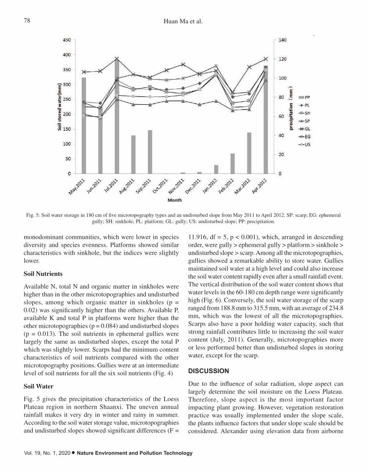
78 Huan Ma et al.
Vol. 19, No. 1, 2020 • Nature Environment and Pollution Technology
monodominant communities, which were lower in species diversity and species evenness. Platforms showed similar characteristics with sinkhole, but the indices were slightly lower.
Soil Nutrients
Available N, total N and organic matter in sinkholes were higher than in the other microtopographies and undisturbed slopes, among which organic matter in sinkholes (p = 0.02) was significantly higher than the others. Available P, available K and total P in platforms were higher than the other microtopographies (p = 0.084) and undisturbed slopes (p = 0.013). The soil nutrients in ephemeral gullies were largely the same as undisturbed slopes, except the total P which was slightly lower. Scarps had the minimum content characteristics of soil nutrients compared with the other microtopography positions. Gullies were at an intermediate level of soil nutrients for all the six soil nutrients (Fig. 4)
Soil Water
Fig. 5 gives the precipitation characteristics of the Loess Plateau region in northern Shaanxi. The uneven annual rainfall makes it very dry in winter and rainy in summer. According to the soil water storage value, microtopographies and undisturbed slopes showed significant differences (F =
Fig. 5: Soil water storage in 180 cm of five microtopography types and an undisturbed slope from May 2011 to April 2012. SP: scarp; EG: ephemeral gully; SH: sinkhole; PL: platform; GL: gully; US: undisturbed slope; PP: precipitation.
11.916, df = 5, p < 0.001), which, arranged in descending order, were gully > ephemeral gully > platform > sinkhole > undisturbed slope > scarp. Among all the microtopographies, gullies showed a remarkable ability to store water. Gullies maintained soil water at a high level and could also increase the soil water content rapidly even after a small rainfall event. The vertical distribution of the soil water content shows that water levels in the 60-180 cm depth range were significantly high (Fig. 6). Conversely, the soil water storage of the scarp ranged from 188.8 mm to 315.5 mm, with an average of 234.8 mm, which was the lowest of all the microtopographies. Scarps also have a poor holding water capacity, such that strong rainfall contributes little to increasing the soil water content (July, 2011). Generally, microtopographies more or less performed better than undisturbed slopes in storing water, except for the scarp.
DISCUSSION
Due to the influence of solar radiation, slope aspect can largely determine the soil moisture on the Loess Plateau. Therefore, slope aspect is the most important factor impacting plant growing. However, vegetation restoration practice was usually implemented under the slope scale, the plants influence factors that under slope scale should be considered. Alexander using elevation data from airborne

79ECOLOGICAL CONDITIONS OF MICROTOPOGRAPHY FOR VEGETATION RESTORATION
Nature Environment and Pollution Technology • Vol. 19, No. 1, 2020
laser scanner found microtopographies at a small spatial scale of a few decimetres could be an indicator of vegetation (Alexander et al. 2016). More severe disturbance to create microtopographies was also found to have potential benefits when introducing specialist species of calcareous grassland for restoration in Pegsdon Hills, Bedfordshire, UK (Wagner et al. 2016). These former studies have well illustrated that microtopographies have obvious impact to vegetation. Similarly, results of a canonical correlation analysis suggested that characteristics of microtopography were the main factors affecting the characteristics of vegetation, with the exception of slope aspect.
The vegetation species richness corresponds to habitat heterogeneity. In this study, we found that there were more species on the microtopography plots compare with undisturbed slope plots. Unlike vegetation in wetland, where excessive water in pools usually leads to lower plant cover (Sleeper et al. 2016), microtopographies on the Loess Plateau have opposite effect. Amongst all the microtopographies, plants in gullies have higher cover and plant height. Pioneer tree species with rapid growth can seize the habitat in gullies where they have an adequate water supply (Hu et al. 2007). Shrubs and pioneer tree species appeared firstly in gullies. Qin (2009) found that the dominant species and primary companion species are usually xerophytic because
create microtopographies was also found to have potential benefits when introducing specialist
species of calcareous grassland for restoration in Pegsdon Hills, Bedfordshire, UK (Wagner et al.
2016). These former studies have well illustrated that microtopographies have obvious impact to
vegetation. Similarly, results of a canonical correlation analysis suggested that characteristics of
microtopography were the main factors affecting the characteristics of vegetation, with the
exception of slope aspect.
Fig. 6: Soil water content in the 0–180 cm layers of five types of microtopography and an undisturbed slope. SP:
scarp; EG: ephemeral gully; SH: sinkhole; PL: platform; GL: gully; US: undisturbed slope.
The vegetation species richness corresponds to habitat heterogeneity. In this study, we found
that there were more species on the microtopography plots compare with undisturbed slope plots.
Unlike vegetation in wetland, where excessive water in pools usually leads to lower plant cover
(Sleeper et al. 2016), microtopographies on the Loess Plateau have opposite effect. Amongst all
the microtopographies, plants in gullies have higher cover and plant height. Pioneer tree species
with rapid growth can seize the habitat in gullies where they have an adequate water supply (Hu et
al. 2007). Shrubs and pioneer tree species appeared firstly in gullies. Qin (2009) found that the
Fig. 6: Soil water content in the 0–180 cm layers of five types of microtopography and an undisturbed slope. SP: scarp; EG: ephemeral gully; SH: sinkhole; PL: platform; GL: gully; US: undisturbed slope.
of the droughty soil water conditions on the Loess Plateau. However, in this study, we found hygrophytes on platforms, such as Phragmites australis, indicating that habitat heterogeneity come out of microtopographies. Sinkholes are a type of microtopography that can easily obtain water supply and accumulate fertile soil from runoff, which enables plants to reach greater heights. The microtopographies described above exhibited better growing environments for plants compared to undisturbed slope.
Soil nutrients can affect biomass production, species composition, and diversity (Critchley et al. 2002). Grazing exclusion was improved that had significant positive effects on improving soil nutrients (Li et al. 2016). Peng et al. (2005) showed that total N was gradually increased along with vegetation restoration years in An ‘Sai on the Loess Plateau. In our study, soil nutrients content was increased in every site more or less compared with Peng’s result and microtopographies performed more remarkably. Phosphorus is closely related to plant biomass (Jiao et al. 2008), and we found that it is significantly higher on platforms indicating that platforms have aggregation effect to some of the nutrient elements.
Soil water is one key factor limiting vegetation restoration (Chen et al. 2007). However, we found soil water among microtopographies that under the slope scale has significant

80 Huan Ma et al.
Vol. 19, No. 1, 2020 • Nature Environment and Pollution Technology
difference. The soil stored water in gullies was approximately 100mm more that undisturbed slopes every month in the year 2011-2012. Additionally, the disturbed slope soil water content in our study was similar compared to Wang et al. (2014) found on grass land in Suide, Shannxi Province. Microtopographies, especially gullies, ephemeral gullies and platforms indeed performed relatively wetter soil condition than undisturbed slopes.
Soil and water conservation is one of the main functions of ecological restoration on the Loess Plateau (Chen et al. 2008). One of the main reasons for revegetation is to achieve the recovery goal in a short time. Some researchers advocate natural recovery as more suitable for the ecosystem on the Loess Plateau (Jiao et al. 2012) due to the shortage of precipitation. Soil desiccation is common in current reforestation activities on the Loess Plateau (Cao et al. 2010) because too many tree seedlings are planted in small watersheds, where the incoming water cannot match the water outflow. Our study indicates that soil properties vary with the heterogeneity of topography on a fine scale. Small heterogeneity of topography can lead to fertile areas on slopes, especially with regard to the soil water content. Our study shows that soil water content is significantly different within the slope scale, implying that not every plot on slopes is necessarily inappropriate for planting. In addition, our study shows that pioneer species were still dominant in the study area after 14 years of natural recovery. Previous study suggests that successful revegetation should plant a mix of grass, shrubs and trees (Fu et al. 2000). Because actively sowing species on the Loess Plateau is likely to enhance species diversity and optimize species composition (Wang 2006), it is useful to develop an effective way to restore vegetation artificially. Creating topographic heterogeneity proved to be an active and effective approach to ecological restoration (Gilland et al. 2014). However, implementing similar measures is not easy on the Loess Plateau due to the poor local economic situation. In this case, artificially vegetation restoration using naturally formed microtopographies as indicator for species choosing may be an economic and effective way.
The soil water content and appearance of shrubs imply that platforms have a higher carrying capacity for plants compared to undisturbed slopes. Sinkholes can cluster soil nutrients and collect water, which is similar to what was found in a bottomland hardwood forest in Texas (Simmons et al. 2011) Relatively better soil water conditions suggest that sinkholes can be treated as natural tree planting locations. Ephemeral gullies are the initial stage of gully erosion, which will lead to greater soil erosion as they develop (Xu et al. 2016). However, plants grow in frequent soil erosion,
and deposition environment requires a greater water supply and need to be resistant to rushing runoff. Gully erosion is the primary source of sediment loss on the Loess Plateau (Li et al. 2015). In this paper, we found that gullies have a remarkable water storage capacity and maintain a surplus of water after it is taken up by plants. The emergence of aquatic plants also indicates gullies have humid environment. Species that are resistant to flooding should be chosen for vegetation restoration in gullies, and higher densities are acceptable. Slope gradient largely influences soil erosion (Fox et al. 2000), which lowers the soil water storage and soil nutrients in scarps compared with other four microtopographies. To improve ecological restoration, we suggest maintaining the status of scarps and reducing human interference during artificial vegetation restoration.
CONCLUSION
Microtopography was the second main factor affecting the characteristics of vegetation besides slope aspect on the Loess Plateau. In the natural recovery site, vegetation structure, plant diversity, soil nutrients and soil water content were significantly different across microtopographic features. According to the soil water storage value, microtopographies and undisturbed slopes arranged in descending order were gully > ephemeral gully > platform > sinkhole > undisturbed slope > scarp. An effective vegetation configuration mode requires more accurate design. Vegetation configuration on slopes should be in accordance with the microtopography. Species that require more water can be planted in gullies, ephemeral gullies and platforms. A small number of seedlings could also be planted in sinkholes to prevent further soil erosion. In addition, species planted on undisturbed slopes should have a lower water requirement compared with those planted on the microtopographies described above. Scarps should maintain the status quo and recover naturally.
ACKNOWLEDGEMENTS
We would like to extend our sincere gratitude to Zong Kai Wu and Guang Liang Liu for their help in providing local support during the study. We are grateful to Yingying Zhang and Wenjuan Ma for valuable assistance. We would like to thank Matthew R. and Jennie L. for linguistic improvement of the manuscript.
REFERENCES
Alatalo, R. 1977. Components of diversity: Multivariate analysis with interaction. Ecology, 58(4): 900-906.
Alexander, C., Deák, B. and Heilmeier H. 2016. Micro-topography driven vegetation patterns in open mosaic landscapes. Ecological Indicators, 60: 906-920.
81ECOLOGICAL CONDITIONS OF MICROTOPOGRAPHY FOR VEGETATION RESTORATION
Nature Environment and Pollution Technology • Vol. 19, No. 1, 2020
Beatty, S.W. 1984. Influence of microtopography and canopy species on spatial patterns of forest understory plants. Ecology, 65(5): 1406-1419.
Cao, S., Tian, T., Chen, L., Dong, X., Yu, X. and Wang, G. 2010. Damage caused to the environment by reforestation policies in arid and semi-arid areas of China. Annals of Biology, 39(4): 279-283.
Chen, H., Shao, M. and Li, Y. 2008. Soil desiccation in the Loess Plateau of China. Geoderma, 143(1): 91-100.
Chen, L., Huang, Z., Gong, J., Fu, B. and Huang, Y. 2007. The effect of land cover/vegetation on soil water dynamic in the hilly area of the loess plateau, China. Catena, 70: 200-208.
Clifford, H. T. and Stephenson, W. 1976. An Introduction to Numerical Classification. Academic Express, London.
Critchley, C.N.R., Chambers, B.J., Fowbert, J.A., Sanderson, R.A., Bho-gal, A. and Rose, S.C. 2002. Association between lowland grassland plant communities and soil properties. Biological Conservation, 105: 199-215.
Domínguez-Cadena, R., Riosmena-Rodríguez, R., León-De, La Luz and J.L. 2016. Forest structure and species composition of mangroves in the eastern Baja California Peninsula: The role of microtopography. Wetlands, 36(3): 515-523.
Fang, H.Y., Cai, Q.G., Chen, H. and Li, Q.Y. 2008. Effect of rainfall regime and slope on runoff in a gullied loess region on the Loess Plateau in China. Environmental Management, 42(3): 402-411.
Fox, D. M. and Bryan, R. B. 2000. The relationship of soil loss by interrill erosion to slope gradient. Catena, 38(3): 211-222.
Fu, B. J. and Chen, L. D. 2000. Agricultural landscape spatial pattern analysis in the semi-arid hill area of the Loess Plateau, China. Journal of Arid Environments, 44(3): 291-303.
Gilland, K. E. and Mccarthy, B. C. 2014. Microtopography influences early successional plant communities on experimental coal surface mine land reclamation. Restoration Ecology, 22(2): 232-239.
Guariguata, M. R. 1990. Land slide disturbance and forest regeneration in the upper Luquillo mountains of Puerto Rico. The Journal of Ecology, 78: 814-832.
Hara, M., Hirata, K., Fujihara, M. and Oono, K. 1996. Vegetation structure in relation to micro-landform in an evergreen broad-leaved forest on Amami Ohshima Island, south-west Japan. Ecological Research, 11(3): 325-337.
Härdle, W. and Simar, L. 2007. Applied Multivariate Statistical Analysis. Springer Verlag, NewYork.
He, J. S. and Chen, W. L. 1997. A review of gradient changes in species diversity of land plant community. Acta Ecologica Sinica, 17(1); 93-101.
Hu, Z. W. and Shen, Z. H. 2007. Impacts of topography on the spatial pattern of the age of forest community. Chinese Journal of Plant Ecol-ogy, 31(4): 814-824.
Jiao, J., Tzanopoulos, J., Xofis, P. and Mitchley, J. 2008. Factors affecting distribution of vegetation types on abandoned cropland in the hilly- gullied Loess Plateau region of China. Pedosphere, 18(1): 24-33.
Jiao, J., Zhang, Z., Bai, W., Jia, Y. and Wang, N. 2012. Assessing the eco-logical success of restoration by afforestation on the Chinese Loess Plateau. Restoration Ecology, 20(2): 240-249.
Li, H., Zhang, F., Mao, S., Zhu, J., Yang, Y., He, H. and Li, Y. 2016. Effects of grazing exclusion on ssoil properties in Maqin Alpine Meadow, Tibetan Plateau, China. Polish Journal of Environmental Studies, 25(4): 1583-1587.
Li, Y. Y. and Shao, M. A. 2006. Change of soil physical properties under long-term natural vegetation restoration in the Loess Plateau of China. Journal of Arid Environments, 64(1): 77-96.
Li, Z., Zhang, Y., Zhu, Q., He, Y. and Yao, W. 2015. Assessment of bank gully development and vegetation coverage on the Chinese Loess Plateau. Geomorphology, 228: 462-469.
Liu, Q. Q. and Singh, V. P. 2004. Effect of microtopography, slope length and gradient, and vegetative cover on overland flow through simulation.
Journal of Hydrologic Engineering, 9(5): 375-382. Martinez-Turanzas, G.A., Coffin, D. P. and Burke, I. C. 1997. Development
of microtopography in a semi-arid grassland: Effects of disturbance size and soil texture. Plant and Soil, 191(2): 163-171.
McVicar, T.R., Li, L., Van Niel, T.G., Zhang, L., Li, R., Yang, Q., Zhang, X., Mu, X., Wen, Z., Liu, W. and Zhao, Y.A. 2007. Developing a decision support tool for China’s re-vegetation program: Simulating regional impacts of afforestation on average annual streamflow in the Loess Plateau. Forest Ecology and Management, 251(1): 65-81.
Milton, L., Lieberman, D., Hartshorn, G.S. and Peralta, R. 1985. Small-scale altitudinal variation in lowland wet tropical forest vegetation. Journal of Ecology, 73(2): 505-516.
Moser, K. F., Ahn, C. and Noe, G. B. 2009. The influence of microtopog-raphy on soil nutrients in created mitigation wetlands. Restoration Ecology, 17(5): 641-651.
Mott, J. J. and Mccomb, A. J. 1974. Patterns in annual vegetation and soil microrelief in an arid region of Western Australia. Journal of Ecology, 62(1): 115-126.
Nagamatsu, D. and Miura, O. 1997. Soil disturbance regime in relation to micro-scale landforms and its effects on vegetation structure in a hilly area in Japan. Plant Ecology, 133(2): 191-200.
Pavone, L. V. and Reader, R.J. 1985. Effect of microtopography on the survival and reproduction of Medicago lupulina. The Journal of Ecol-ogy, 73: 685-694.
Peng, W.Y., Zhang, K.L., Chen, Y. and Yang, Q.K. 2005. Research on soil quality change after returning farmland to forest on the loess sloping croplands. Journal of Natural Resources, 20(2): 272-278 (in Chinese).
Price, J., Rochefort, L. and Quinty, F. 1998. Energy and moisture consid-erations on cutover peatlands: Surface microtopography, mulch cover and sphagnum regeneration. Ecological Engineering, 10(4): 293-312.
Qin, W., Zhu, Q.K., Zhang, Y.Q. and Zhao, L.L. 2009. Dynamics of plant community species diversity in the process of ecological rehabilitation in north Shaanxi loess area. Chinese Journal of Applied Ecology, 20(2): 403-409 (in Chinese).
Rossell, I.M., Moorhead, K.K., Alvarado, H. and Warren, R.J. 2009. Succession of a southern Appalachian mountain wetland six years following hydrologic and microtopographic restoration. Restoration Ecology, 17(2): 205-214.
Sakai, A. and Ohsawa, M. 1993. Vegetation pattern and microtopography on a landslide scar of Mt Kiyosumi, central Japan. Ecological Research, 8(1): 47-56.
Šamonil, P., Valtera, M., Schaetzl, R.J., Adam, D., Vašíčková, I., Dančk, P., Janík, D. and Tejnecký, V. 2016. Impacts of old, comparatively stable, tree throw microtopography on soils and forest dynamics in the northern hardwoods of Michigan, USA. Catena, 140: 55-65.
Shannon, C. E., Weaver, W. and Wiener, N. 1950. The Mathematical Theory of Communication. University of Illinois Press, Urbana.
Simmons, M. E., Ben, Wu X. and Whisenant, S. G. 2011. Plant and soil responses to created microtopography and soil treatments in bottomland hardwood forest restoration. Restoration Ecology, 19(1): 136-146.
Sleeper, B. E. and Robert, L. F. 2016. Edaphic and vegetative responses to forested wetland restoration with created microtopography in Arkansas. Ecological Restoration, 34(2): 117-123.
Wagner, M., Bullock, J.M., Hulmes, L., Hulmes, S., Peyton, J., Amy, S.R., Savage, J., Tallowin, J.B., Heard, M.S. and Pywell, R.F.2016. Creation of micro-topographic features: A new tool for introducing specialist species of calcareous grassland to restored sites? Applied Vegetation Science, 19(1): 89-100.
Wang, G. 2006. Can the restoration of natural vegetation be accelerated on the Chinese Loess Plateau? A study of the response of the leaf carbon isotope ratio of dominant species to changing soil carbon and nitrogen levels. Ecological Research, 21(2): 188-196.
Wang, X., Zhang, W., Wang, Z., Liu, X. and Wang, S. 2014. Soil moisture status under deep-rooted and shallow-rooted vegetation in the semi-

82 Huan Ma et al.
Vol. 19, No. 1, 2020 • Nature Environment and Pollution Technology
arid area of Loess Plateau in China. Polish Journal of Environmental Studies, 23(2): 511-520.
Werner, K. J. and Zedler, J. B. 2002. How sedge meadow soils, microto-pography, and vegetation respond to sedimentation. Wetlands, 22(3): 451-466.
Xu, M. X., Qiang, L. and Glenn, W. 2016. Degradation of soil physico-chemical quality by ephemeral gully erosion on sloping cropland of the hilly Loess Plateau, China. Soil and Tillage Research, 155(1): 9-18.
Zedler, J. B. and Zedler, P. H. 1969. Association of species and their rela-
tionship to microtopography within old fields. Ecology, 50(3): 432-442. Zeng, Q., Li, X., Dong, Y., An, S. and Darboux, F. 2016. Soil and plant
components ecological stoichiometry in four steppe communities in the Loess Plateau of China. Catena, 147: 481-488.
Zheng, F. 2006. Effect of vegetation changes on soil erosion on the Loess Plateau. Pedosphere, 16(4): 420-427.
Zhu, Q. K., Zhang, Y. and Zhao, L. L. 2012. Vegetation Restoration and Simulated Natural Forestation in the Loess Plateau, Northern Shaanxi, China. Science Press, Beijing (in Chinese).

Analysis of Spatial Heterogeneity in Coupling Development of Industrialization and Resource Environmental Bearing Capacity
Ying Huang*, Zhi Zhou** and Qin Qin****College of Information Engineering, Wuhan University of Engineering Science, Wuhan, 430200, China**College of Land and Resources, Agricultural University of Hebei, Baoding, 071001, China***Department of Tourism, Sport and Society, Lincoln University, Christchurch, 7674, New Zealand†Corresponding author: Zhi Zhou
ABSTRACT
The contradiction between supply and demand of resource environment has become increasingly severe because of population expansion and the rapid development of industrial economy. Spatial quantitative evaluation of coupling strength and mutual promotion between industrialization and resource environmental bearing capacity based on panel data can facilitate industrialization and promote sustainable and healthy development of regional economy objectively, scientifically, and rationally. This study proposed a three-level comprehensive evaluation matrix for clustering and comparative analysis of 31 provinces in China to analyse the characteristics of spatial heterogeneity in the coordinated development of industrialization and resource environmental bearing capacity. First, a comprehensive evaluation index system for resource environmental bearing capacity was established based on the differences in resource environmental bearing capacities in various regions of China. Combined with the coordination degree for evaluation model, the coordination between the resource environmental bearing capacity and the industrialization of the 31 provinces in 2018 was evaluated and compared based on their comprehensive evaluation index. Finally, a cluster comparison analysis was performed in the 31 provinces using the three-level comprehensive evaluation matrix of coupling development of regional economy and resource environmental bearing capacity. Moreover, the accuracy of the coordination degree model was verified according to the clustering results. Results show that the regions with good ordination between industrialization and resource environmental bearing capacity include East and North China. Meanwhile, the provinces with poor coordination mainly include Southwest and Northwest China. Resource environment still restricts the coordination between resource environmental bearing capacity and industrialization development. This study provides reference for developing differentiated resource environment management measures and countermeasures in various regions in China.
INTRODUCTION
Industrialization, as an important approach for realizing social and economic development, has certainly brought severe challenges in the current resource environmental bearing capacity. This study aims to realize the coupling and harmonious development between industrialization and pop-ulation, resources, and environment. Resources not only refer to scarce natural resources but also to rare assets with high significance in social development; scholars have become increasingly concerned with these matters. The contradiction between supply and demand of resource environment has become increasingly severe because of population expan-sion and the rapid development of industrial economy. The continuous social and economic development has brought challenges to resource environmental bearing capacity, and their relationship has become increasingly complex. The thorough summarization of the coordination relationship
between industrial economy and resource environmental bearing capacity is difficult. New-type urbanization and industrialization have continuously developed, and its co-ordination and coupled development with regional resource environmental bearing capacity should be explored from an innovative perspective. Industrial economy and resource environment are two subsystems of the entire socioeconomic system. These subsystems interact, cooperate, collaborate, and form a virtuous development cycle, which is a strong driving force for the sustainable and healthy development of the regional economy. Therefore, the spatial quantitative evaluation of coupling strength and mutual promotion be-tween industrialization and resource environmental bearing capacity based on panel data is of great significance to facili-tate industrialization and promote the sustainable and healthy development of regional economy objectively, scientifically, and rationally.
Nat. Env. & Poll. Tech.Website: www.neptjournal.com
Received: 14-12-2019Accepted: 18-01-2020
Key Words:IndustrializationResource environmental bearing capacityCoordination degree Comprehensive evaluation Spatial heterogeneity
2020pp. 83-92 Vol. 19
p-ISSN: 0972-6268 No. 1 Nature Environment and Pollution Technology An International Quarterly Scientific Journal
Original Research Paper
e-ISSN: 2395-3454
Open Access

84 Ying Huang et al.
Vol. 19, No. 1, 2020 • Nature Environment and Pollution Technology
Scholars have conducted numerous studies regarding the coordination between industrialization and resource environmental bearing capacity. However, some challenges have been encountered in selecting the appropriate coordination degree models for measuring coordination relationship. The accurate evaluation, measurement, and clustering of the coordinated coupling relationship between industrialization and resource environmental bearing capacity in China are urgent problems (Wang et al. 2015). To this end, the present study first evaluated the two subsystems of industrial economy and resource environment comprehensively. Second, the coordinated coupling relationship was analysed according to the comprehensive evaluation index, which is expected to measure the coordinated relationship accurately and comprehensively and provide a reference for evaluating the dissimilarities among different regions in China.
STATE OF THE ART
At present, researchers have conducted numerous studies on the relationship of industrialization and resource environmental bearing capacity. The study on the bearing capacity of individual resources has achieved abundant results. For example, Joardar et al. studied the bearing capacity of urban water resources from the perspective of water supply and integrated it into urban development planning, which was not coupled with economic development (Joardar et al. 1998). Rijsberman et al. also used bearing capacity as a standard for measuring the security of water resources in urban water resource evaluation and management system; however, they did not evaluate the whole resource environment system comprehensively (Rijsberman et al. 2000). Varis et al. focused on the development and utilization of water resources and analysed the pressures on water resource system caused by rapid industrialization, growth of food demand, and deterioration of ecological environment in the Yangtze River region in China. Moreover, the status of the socioeconomic development of the Yangtze River Basin was compared with its water environment bearing capacity according to the economic development process in different regions. Unfortunately, the coordination degree was not analysed (Varis et al. 2001). Scholars have investigated the relationship between economic development and geographical environment. For example, Selden et al. analysed the empirical data and proposed the “inverted U-shaped” curve relationship between economic development and environmental quality, that is, the environmental Kuznets curve. However, they did not perform the cluster analysis combined with the sample area (Selden et al. 1994). Hildebrand investigated the contradictions
and conflicts between economic development and resource environment in coastal regions and analysed the vulnerability of the coastal zone and the impact of human activities based on the idea of man–earth relationship (Hildebrand 1992). Moreover, special attention was paid on the influence of the sustainable development of the coastal zone caused by global changes and their corresponding countermeasures. However, the coordination degree was not modelled or verified. The study of the quantitative relationship between industrial economy and resource environment mainly focused on the construction of indicator systems and model calculation. For example, Ayres et al. and Tapio investigated the decoupling relationship between economic development and resource consumption (Ayres et al. 2003). Both factors analysed the time series data and selected the sample area; however, they did not evaluate spatial heterogeneity (Tapio 2005). Dietz et al. and Bartelmus et al. used the System of Integrated Environmental and Economic Accounting (SEEA) to estimate resource consumption, environmental pollution, sustainable development capabilities, and currency (Dietz et al. 2007). They all used the idea of comprehensive evaluation; however, the coordinated development of the two systems of economy and environment was not analysed thoroughly (Bartelmus et al. 2007).
Qualitative study of the threat of industrialization to resource environment has achieved abundant results in China. However, few studies reported on the coordinated development of industrialization and resource environmental bearing capacity. Liao proposed the measures for industrial development in Dehong Autonomous Prefecture under the constraints of resource environment but failed to compare with other regions (Liao 2014). Guo et al. discussed the production efficiency of industrial land under environmental constraints considering the unexpected output of 33 typical cities in China; however, this study did not draw a cluster evaluation of development models in different regions (Guo et al. 2014). Zhu et al. analysed the main reasons and key issues that might cause current resource environment over-load through industrialization and urbanization development and proposed to position economic and social development based on resource environment. However, their study lacked the support of quantitative data (Zhu et al. 2015). Liao et al. reviewed the importance, evaluation indicators, and standard of the four types of resource bearing capacity (e.g., land resources, water resources, energy resources, and biological resources) and two types of environmental bearing capacity (e.g., air environment and water environ-mental bearing capacity) that are closely related to regional sustainable development (Liao et al. 2016). Similarly, the indicator system and evaluation standard were not tested

85SPATIAL HETEROGENEITY IN COUPLING DEVELOPMENT OF INDUSTRIALIZATION
Nature Environment and Pollution Technology • Vol. 19, No. 1, 2020
empirically in combination with the sample area data. Some Chinese scholars have explored the coupled development of industry, resources, and environment, but most of them used micro regions as samples. For example, Wang et al. studied and evaluated the coupled development of industry, resources, and environment of Dongping City from the perspective of ecological civilization, which was somewhat one-sided (Wang et al. 2015). Zhen constructed a regression equation and a responsiveness model based on a compre-hensive measurement of the industrialization process and ecological environmental quality of Inner Mongolia Zhen. In addition, they conducted a timing analysis of the influence and response characteristics of ecological environment in the industrialization process of Inner Mongolia from 1990 to 2010; however, spatial difference characteristics were neglected (Zhen 2015).
Many qualitative results about the coordinated devel-opment of regional and industrial economy and resource environment have been obtained based on the aforemen-tioned study results. The quantitative results are mainly
based on the study of micro regions; meanwhile, few results were reported about the comparison of the coordi-
nation between resource bearing capacity and industrial development in different regions. Particularly, the analysis and comparison of the spatial heterogeneity of the interac-tive development of regional industrialization and resource
environmental bearing capacity in different regions are still blank. The present study first constructed a com-
prehensive evaluation index system of regional resource environmental bearing capacity to analyse and evaluate the
change characteristics of the spatial heterogeneity of the coordination between industrialization and resource envi-
ronment in different regions in China. Second, principal component analysis was conducted to evaluate resource environmental bearing capacity comprehensively based
on Chinese interprovincial panel data in 2018. Third, the comprehensive scores of resource environmental bearing capacity and industrialization development were used to
calculate the regional coordination score based on the co- ordination degree model. Fourth, the comprehensive evalu-
ation matrix of the three-level cluster was constructed, and the three-level cluster analysis of the sample area was conducted according to the comprehensive evaluation and the regional economic growth rate. Finally, the empirical
suggestions for rational and orderly development of indus-trialization, regional economy, and resource environment
were proposed according to the analysis results.
The remainder of this study is organized as follows. Section 3 proposes a coordination model by constructing a comprehensive evaluation index system of resource
environmental bearing capacity. Section 4 calculates the resource environmental bearing capacity index of different regions in China and uses the coordination model to analyse the spatial differentiation characteristics of coupled development of resource environmental bearing capacity and industrialization. Finally, Section 5 summarizes the study and draws the conclusions.
METHODOLOGY
Comprehensive Evaluation Indicator System of Resource Environmental Bearing Capacity
Resourced environment is a dynamic ecosystem, and the indicator system for the comprehensive evaluation of the bearing capacity can be classified based on the theoretical composition of the resource environment. Meanwhile, this system also considers the role and evolution that resulted from socioeconomic interaction. “Pressure–State–Response (PSR)” is an evaluation model commonly used in the dis-cipline of environmental quality assessment to achieve sus-tainable and healthy development between ecosystems and socioeconomics. In this study, the evaluation index system first divides the resource environmental bearing capacity according to the three aspects of pressure, state, and response, and then reflects the resource environment as the support of water, land, and environment for population and economy at each level. The comprehensive evaluation index system for resource environmental bearing capacity is shown in Table 1. The proposed index system is composed of relative and absolute indicators. The original values of the indicators include the performance values in 2018. The data were col-lected from the official website of the National Bureau of Statistics. The indicators were calculated on the basis of the absolute indicators in combination with the characteristics and representative meaning.
Coordination Model
Industrial economy and resource environmental bearing ca-pacity are two subsystems in the socioeconomic system. The evaluation score of industrialization development speed is measured using the growth rate of the industrial added value in 2018 relative to that in 2017. The resource environmental bearing capacity is a complex system with multivariate meas-ures. Moreover, this system is evaluated comprehensively using the principal component analysis method for the public factor extraction of the multi-index evaluation system, and the public factor score is calculated by SPSS software based on the sample data. The weighted comprehensive model is used to calculate the comprehensive evaluation scores of each sample area. Finally, the spatial differences and comparison

86 Ying Huang et al.
Vol. 19, No. 1, 2020 • Nature Environment and Pollution Technology
Table 1: Comprehensive evaluation index system of resource environmental bearing capacity.
Category Dimension Evaluation index Index calculation Unit Correlation
Pressure Economy GDP per capita yuan +
Population Population density Ten thousand people/ha
-
Status Land resource
Grain yield per unit area Kg/ha +
Water resource
Water resources per capita M³/person +
Water consumption per capita Total water consumption/population
M³/person -
Urban water penetration rate % -
Water consumption per 10,000 yuan of industrial output value
Industrial water consump-tion/industrial added value
T/10,000 yuan -
Environment Wastewater discharge per 10,000 yuan of industrial output value
Wastewater discharge/industrial added value
T/10,000 yuan -
COD emissions per 10,000 yuan GDP
COD emissions/GDP T/10,000 yuan -
Sulfur dioxide emissions per 10,000 yuan GDP
Sulfur dioxide emissions/GDP
T/10,000 yuan -
Nitrogen oxide emissions per 10,000 yuan GDP
Nitrogen oxide emissions/GDP
T/10,000 yuan -
Soot emissions per 10,000 yuan GDP
Soot emissions/GDP T/10,000 yuan -
Response Water resource
Daily sewage treatment capacity 10,000 cubic meters +
Cumulative people benefited from rural water improvement
person +
Effective irrigation area Ha +
Land resource
Soil erosion control area Ha +
Arable land per capita Ha/person +
Investment in fixed assets per unit area
10,000 yuan/ha +
Environment Daily harmless garbage disposal capacity
10,000 tons +
Harmless treatment rate of domes-tic garbage
% +
Completed investment in industri-al pollution control
10,000 yuan +
Completed investment in ecolog-ical construction and protection
10,000 yuan +
of resource environmental bearing capacity can be realized based on the evaluation scores.
After obtaining comprehensive measurement values for industrialization and resource environmental b earing capacity, the coordination degree is evaluated and calculated using the following model:
2j
2j IR
IRD
i
jiIiR
+
+= ,
where Ri and Ij represent the comprehensive evaluation indexes of the resource environmental bearing capacity and

87SPATIAL HETEROGENEITY IN COUPLING DEVELOPMENT OF INDUSTRIALIZATION
Nature Environment and Pollution Technology • Vol. 19, No. 1, 2020
industrialization development, respectively; and DRiIj is the coordination degree. According to the research achievements of scholars before (Wang et al. 2016), DRiIj is positively relat-ed to the coordination degree between the two systems, and the value range is [–1.414, 1.414]. The relationship between the symbols of the calculation results and the two system indexes and their definitions are listed in Table 2:
Comprehensive Evaluation Matrix
Regional economy, as a dynamic economic subsystem, is not solely determined by industrial development after evaluating the coordination between the industrialization and the resource environmental bearing capacity of the 31 provinces in China. Meanwhile, to combine time and space measures effectively, regional differences are combined with dynamic measures to display the spatial and temporal differentiation characteristics of regions from multiple per-spectives intuitively.
This study combines regional resource, environment bearing capacity, and regional economic development speed in constructing a comprehensive evaluation matrix for a systematic and reasonable clustering.
Regional economic development speed can be reflected by dynamic measurement indicators. For example, the growth
Table 2: Meaning of coordination degree between industrialization and resource environmental bearing capacity in different regions.
RiIj
Ri ≥ 0 Ri < 0
Ij ≥ 0 DRiIj ≥ 0, highly coordinated, and both have high development levels
DRiIj ≥ 0, slight imbalance, and the former has lower devel-opment levelDRiIj < 0, severe imbalance, and the former has lower devel-opment level
Ij < 0 DRiIj ≥ 0, the overall coordination is good, and the former has higher development level
DRiIj < 0, highly uncoordinated, and both have low develop-ment levels
DRiIj < 0, basically coordinated, and the former has higher
development level
rate of the regional GDP in 2018 relative to that in 2017. The comprehensive evaluation matrix of resource carrying capacity is listed in Table 3. The evaluation scores of the resource environmental bearing capacity of all regions and the growth rate of regional GDP in 2018 relative to that in 2017 are considered the dividing criteria. Accordingly, the resource environmental bearing capacity and the regional economic growth rate are divided into three evaluation levels. Through pairwise combination of levels, the 31 regions can be divided into 9 categories (Table 3).
RESULT ANALYSIS AND DISCUSSION
Comparative Analysis of The Coordination Degree Between Industrialization and Resource Environmental Bearing Capacity of 31 Provinces, Municipalities and Autonomous Regions in China
The evaluation results of the coordination degree between industrialization and resource environmental bearing capacity in different regions of China in 2018 were calculated according to the comprehensive evaluation index matrix of resource environmental bearing capacity and the coordination model (Table 4 and Fig. 1). The coordination scores show that Zhejiang has obvious advantages and ranks first, followed by
Table 3: Evaluation matrix on resource environmental bearing capacity.
Growth rate of regional economy
Resource environmental bearing capacity
1st–10th 11th–20th 21st–31st
1st–10th Strong resource bearing capacity-fast economic growth
Strong resource bearing capacity- general economic growth
Strong resource bearing capacity-poor economic growth
11th–20th General resource bearing capacity-fast economic growth
General resource bearing capacity- general economic growth
General resource bearing capacity-poor economic growth
21st–31st Weak resource bearing capacity-fast economic growth
Weak resource bearing capacity- general economic growth
Weak resource bearing capacity-poor economic growth

88 Ying Huang et al.
Vol. 19, No. 1, 2020 • Nature Environment and Pollution Technology
Henan, Guangdong, Jiangsu, Shandong, and Ningxia ranking second to sixth, respectively. These regions have coordination scores greater than 1 and belong to highly coordinated regions. Inner Mongolia, Xinjiang, Anhui, Hebei, Shanghai, and Heilongjiang ranked 7th to 12th, respectively, and their coordination scores are greater than 0, all of which belong to moderately coordinated regions. From Liaoning at the 13th place and Shanxi at the 14th place, the coordination scores begin to decline sharply and become negative; however, the industrialization and resource environmental bearing capacity are still coordinated. Jilin Province, which also belongs to the basically coordinated area, ranked 17th. Guangxi, Hubei, Hunan, Fujian, Chongqing, Guizhou, Jiangxi, and Tibet belong to severely uncoordinated regions, which rank from 15 to 23 (except 17), and the eight remaining regions belong to highly uncoordinated regions. Combined with the geographical distribution of regions with different coordination types in Fig. 1, the highly and moderately coordinated regions are mainly distributed in East China and North China. Some regions, such as Zhejiang, Guangdong, and Jiangsu, have relative advantages in resource environment and industrial development and have high coordination scores. In the later period, they can maintain such a development momentum and continue to achieve the coordinated development of resource environment and
industrial economy; some regions have moderate industrial development that matches with their source environment bearing capacity, and the coordination scores are also high. These regions can accelerate the development of industrial economy moderately on the premise of ensuring a good resource environmental bearing capacity. The majority of the basically coordinated regions is distributed in Northeast China and has general resource environmental bearing capacity and industrial economic development level. However, the coordination and matching advantages are not evident. In the later period, the development pace of industrialization can be adjusted appropriately to achieve the optimal matching with the resource environmental bearing capacity. Severely coordinated regions are mainly in Central China, South China, and Southwest China. Some of these provinces and cities (regions) have rapid industrial development but general or weak source environment bearing capacity and poor coordination degree. Therefore, these regions should slow the pace of industrialization moderately and enhance the self-repair flexibility of resource environment to achieve coupled and coordinated development. The highly uncoordinated regions are mainly in Southwest and Northwest China, and they have weak resource environmental bearing capacity. However, the development of the industrial economy is extremely fast or does not match the local resource bearing
Fig. 1: Classification results based on the comprehensive evaluation matrix on coordination degree.
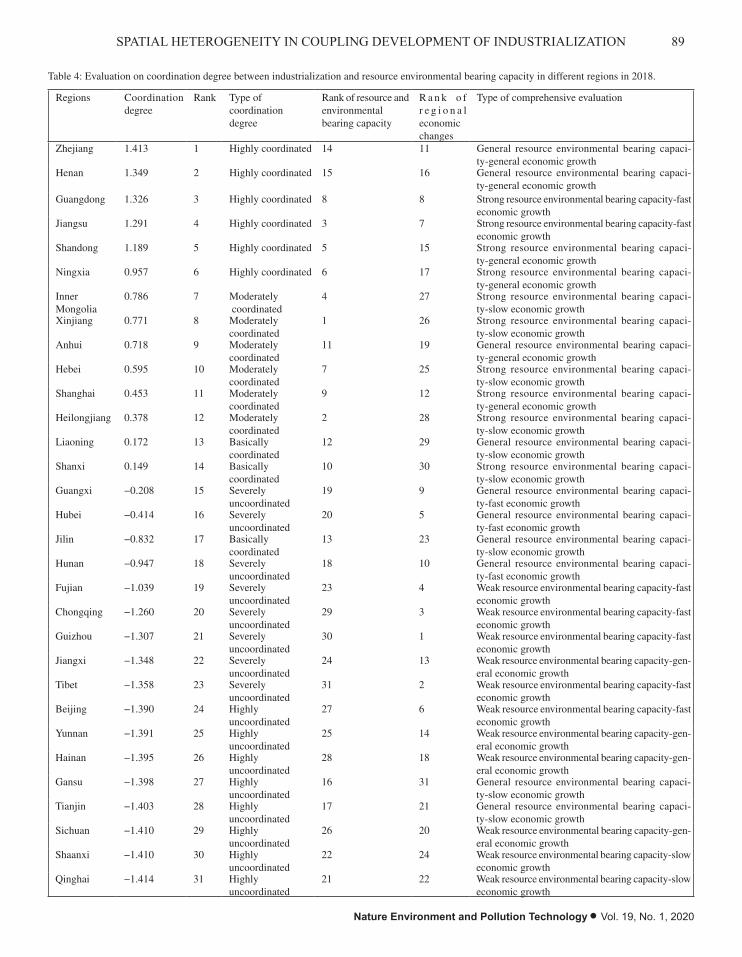
89SPATIAL HETEROGENEITY IN COUPLING DEVELOPMENT OF INDUSTRIALIZATION
Nature Environment and Pollution Technology • Vol. 19, No. 1, 2020
Table 4: Evaluation on coordination degree between industrialization and resource environmental bearing capacity in different regions in 2018.
Regions Coordination degree
Rank Type of coordination degree
Rank of resource and environmental bearing capacity
R a n k o f r e g i o n a l economicchanges
Type of comprehensive evaluation
Zhejiang 1.413 1 Highly coordinated 14 11 General resource environmental bearing capaci-ty-general economic growth
Henan 1.349 2 Highly coordinated 15 16 General resource environmental bearing capaci-ty-general economic growth
Guangdong 1.326 3 Highly coordinated 8 8 Strong resource environmental bearing capacity-fast economic growth
Jiangsu 1.291 4 Highly coordinated 3 7 Strong resource environmental bearing capacity-fast economic growth
Shandong 1.189 5 Highly coordinated 5 15 Strong resource environmental bearing capaci-ty-general economic growth
Ningxia 0.957 6 Highly coordinated 6 17 Strong resource environmental bearing capaci-ty-general economic growth
Inner Mongolia
0.786 7 Moderately coordinated
4 27 Strong resource environmental bearing capaci-ty-slow economic growth
Xinjiang 0.771 8 Moderately coordinated
1 26 Strong resource environmental bearing capaci-ty-slow economic growth
Anhui 0.718 9 Moderately coordinated
11 19 General resource environmental bearing capaci-ty-general economic growth
Hebei 0.595 10 Moderately coordinated
7 25 Strong resource environmental bearing capaci-ty-slow economic growth
Shanghai 0.453 11 Moderately coordinated
9 12 Strong resource environmental bearing capaci-ty-general economic growth
Heilongjiang 0.378 12 Moderately coordinated
2 28 Strong resource environmental bearing capaci-ty-slow economic growth
Liaoning 0.172 13 Basically coordinated
12 29 General resource environmental bearing capaci-ty-slow economic growth
Shanxi 0.149 14 Basically coordinated
10 30 Strong resource environmental bearing capaci-ty-slow economic growth
Guangxi −0.208 15 Severely uncoordinated
19 9 General resource environmental bearing capaci-ty-fast economic growth
Hubei −0.414 16 Severely uncoordinated
20 5 General resource environmental bearing capaci-ty-fast economic growth
Jilin −0.832 17 Basically coordinated
13 23 General resource environmental bearing capaci-ty-slow economic growth
Hunan −0.947 18 Severely uncoordinated
18 10 General resource environmental bearing capaci-ty-fast economic growth
Fujian −1.039 19 Severely uncoordinated
23 4 Weak resource environmental bearing capacity-fast economic growth
Chongqing −1.260 20 Severely uncoordinated
29 3 Weak resource environmental bearing capacity-fast economic growth
Guizhou −1.307 21 Severely uncoordinated
30 1 Weak resource environmental bearing capacity-fast economic growth
Jiangxi −1.348 22 Severely uncoordinated
24 13 Weak resource environmental bearing capacity-gen-eral economic growth
Tibet −1.358 23 Severely uncoordinated
31 2 Weak resource environmental bearing capacity-fast economic growth
Beijing −1.390 24 Highly uncoordinated
27 6 Weak resource environmental bearing capacity-fast economic growth
Yunnan −1.391 25 Highly uncoordinated
25 14 Weak resource environmental bearing capacity-gen-eral economic growth
Hainan −1.395 26 Highly uncoordinated
28 18 Weak resource environmental bearing capacity-gen-eral economic growth
Gansu −1.398 27 Highly uncoordinated
16 31 General resource environmental bearing capaci-ty-slow economic growth
Tianjin −1.403 28 Highly uncoordinated
17 21 General resource environmental bearing capaci-ty-slow economic growth
Sichuan −1.410 29 Highly uncoordinated
26 20 Weak resource environmental bearing capacity-gen-eral economic growth
Shaanxi −1.410 30 Highly uncoordinated
22 24 Weak resource environmental bearing capacity-slow economic growth
Qinghai −1.414 31 Highlyuncoordinated
21 22 Weak resource environmental bearing capacity-slow economic growth

90 Ying Huang et al.
Vol. 19, No. 1, 2020 • Nature Environment and Pollution Technology
capacity. In the later stage, the investment in improving resource environment should be enhanced while formulating relevant policies.
Clustering Results and Cause Analysis of Spatial Heterogeneity of Coordination between Industrialization and Resource Environmental Bearing Capacity
The regional difference in the coordination between industrialization and resource environmental bearing capacity based on the coordination degree alone is not particularly significant. Therefore, the last column in Table 4 lists the comprehensive clustering results of 31 provinces (cities, districts) in China according to the comprehensive evaluation matrix in Section 2.3. Meanwhile, future improvement direction can be determined accurately by combining coordination and comprehensive evaluation types. Combined with the evaluation level of resource environmental bearing capacity in Table 4, first, the regions with high coordination degree have moderate and good resource environmental bearing capacity, which indicates the importance of resource environmental bearing capacity in coupled development. Guangdong and Jiangsu have perfectly realized the high coordination between resource environmental bearing
capacity and regional economic development. As highly coordinated regions, both of regions have advantages in environment pollution control and other indicators and belong to the type of “strong resource environmental bearing capacity-fast economic growth.” Other highly coordinated regions, such as Zhejiang and Henan, have general resource environmental bearing capacity, which is benefited from the balanced indicators. However, their advantages in water and land resources and environmental governance are not evident. Therefore, the resource bearing capacity has not exhibited the best performance, but it is relatively matched with the local regional economic development. The GDP growth of Shandong and Ningxia have been slowed down relatively but still matches the resource environmental bearing capacity. Second, many moderately coordinated regions, such as Inner Mongolia, Heilongjiang, and Xinjiang, have strong resource environmental bearing capacity. However, these regions fail to realize the coordinated development of resource environment and regional economy. Third, uncoordinated and even severely uncoordinated regions have weak resource environmental bearing capacity, but most regions still have rapid regional economic growth, which indicates that the regional economic development based on resource consumption and environment pollution is common.
Table 5: Factor loading of indexes regarding resource environmental bearing capacity.
Extraction dimensions Index Factor loading eigenvalues proportion
Water use Water resources per capita 0.875 4.196 18.243
Water consumption per 10,000 yuan of industrial output value −0.851
Daily sewage treatment capacity 0.814
Wastewater discharge per 10,000 yuan of industrial output value −0.753
Urban water penetration rate −0.724
Water consumption per capita −0.781
Industrial pollutant emissions
nitrogen oxide emissions per 10,000 yuan GDP −0.761
Sulphur dioxide emissions per 10,000 yuan GDP −0.732
Soot emission per 10,000 yuan GDP −0.661
Pollution control and improvement of resource environment
Cumulative people benefited from rural water improvement 0.822 3.763 16.360
Harmless treatment rate of domestic garbage 0.817
Harmless daily garbage disposal capacity 0.774
Effective irrigation area 0.726
Completed investment in industrial pollution control 0.680
Land bearing Grain production per unit area 0.927 3.434 14.930
Arable land per capita 0.848
GDP per capita −0.628
Investment in fixed assets per unit area 0.798 2.516 10.937
Population density 0.784

91SPATIAL HETEROGENEITY IN COUPLING DEVELOPMENT OF INDUSTRIALIZATION
Nature Environment and Pollution Technology • Vol. 19, No. 1, 2020
These regions should vigorously use green development measures to improve the current state effectively and slow down the economic growth as necessary. Meanwhile, some uncoordinated regions have no resource advantage and slow economic growth. Therefore, they should accelerate the speed of economic development while improving the resource environment in the future.
CONCLUSION
To obtain the current spatial differentiation characteristics of the resource environmental bearing capacity of 31 provinces (municipalities and autonomous regions) in China, this study established a comprehensive evaluation index system for resource bearing capacity from the three levels of PSR of resource environment theoretical system and its population and socioeconomic support and guarantee. A comprehensive evaluation matrix was constructed on the basis of the dy-namic evaluation indexes of regional economic development changes, and the 31 provinces in China were divided into 9 categories according to the coordination degree clustering. Finally, the following conclusions were drawn:
1. The evaluation results of the coordination degree be-tween industrialization and resource environmental bearing capacity in the 31 sample regions in 2018 from high to low is ranked as follows: Zhejiang, Henan, Guangdong, Jiangsu, Shandong, Ningxia, Inner Mon-golia, Xinjiang, Anhui, Hebei, Shanghai, Heilongjiang, Liaoning, Shanxi, Guangxi, Hubei, Jilin, Hunan, Fujian, Chongqing, Guizhou, Jiangxi, Tibet, Beijing, Yunnan, Hainan, Gansu, Tianjin, Sichuan, Shaanxi, and Qinghai. The majority of the provinces with good coordination between industrialization and resource environmental bearing capacity are in East and North China. Mean-while, the provinces with poor coordination are mostly in Southwest and Northwest China. Resources and environment are still the main factors that restrict coor-dination.
2. According to the classification results based on the three-level clustering comprehensive evaluation matrix: Guangdong and Jiangsu belong to the regions with “strong resource environmental bearing capacity-fast economic growth;” Zhejiang, Henan, and Anhui have “general resource environmental bearing capacity-gen-eral economic growth;” Shaanxi and Qinghai belong to the regions with “weak resource environmental bearing capacity-slow economic growth.”
3. According to the panel data analysis of 31 provinces and autonomous regions in 2018, the main factors that influence the resource environmental bearing capacity include per capita water resources, water consumption
per 10,000 Yuan of industrial output value, daily treat-ment capacity of urban sewage, wastewater discharge per 10,000 yuan of industrial output value, urban water penetration rate, per capita water consumption, nitrogen oxide emissions per 10,000 Yuan GDP, sulphur dioxide emissions per 10,000 Yuan GDP, soot emissions per 10,000 yuan GDP, cumulative beneficiaries of rural water conversion, harmless treatment rate of domestic waste, average daily harmless garbage disposal capac-ity, effective irrigated area, completed investment in industrial pollution control, grain yield per unit area, cultivated land per capita, GDP per capita, fixed asset investment per unit area, and population density.
A three-level clustering comprehensive evaluation matrix was established by combining the indicator system construction and model measurement. The evaluation matrix cannot only refine the internal differences in the types of coordination evaluation but also thoroughly present the im-provement direction of resource bearing capacity, industrial development, and even regional economic growth combined with the main factor load. In addition, effective empirical suggestions are made to alleviate the contradiction between resource bearing capacity and regional economic develop-ment in China, and effective reference in policy formulation is provided to the Chinese government. However, the compre-hensive evaluation index system of resource environmental bearing capacity should be continuously updated according to the development trend of resources and environment to measure the coupling relationship accurately and thoroughly because of the limited availability of the latest environmental indicator data.
ACKNOWLEDGEMENT
This study was supported by the Hubei Province Teaching and Research Projects of Colleges and Universities in 2017 (Grant No. 2017495), the Hubei Education Department Scientific Research Projects in 2018(Grant No. B2018347), and the Hebei Province Social Science Foundation in 2018 (Grant No. HB18GL053).
REFERENCES
Ayres, R.U., Ayres, L.W. and Warr, B. 2003. Energy, power and work in the US economy, 1900-1998. Energy, 28(3): 219-273.
Bartelmus, P. 2007. SEEA-2003: Accounting for sustainable development? Ecological Economics, 61(4): 613-616.
Dietz, S. and Neumayer, E. 2007. Weak and strong sustainability in the SEEA: Concepts and measurement. Ecological Economics, 61(4): 617-626.
Guo, G.C. and Wen, Q.Y. 2014. Industrial land productivity research un-der the environmental restriction based on unexpected outputs of 33 typical cities in China. China Population Resources and Environment, 24(6): 121-127.

92 Ying Huang et al.
Vol. 19, No. 1, 2020 • Nature Environment and Pollution Technology
Hildebrand, L.P. and Norrena, E.J. 1992. Approaches and progress toward effective integrated coastal zone management. Marine Pollution Bulletin, 25(1-4): 94-97.
Joardar, S.D. 1998. Carrying capacities and standards as bases towards ur-ban infrastructure planning in India: A case of urban water supply and sanitation. Habitat International, 22(3): 327-337.
Liao, H.X., Ji, Y.L. and Peng, S.L. 2016. Resource and environmental carry-ing capacity and sustainable development. Ecology and Environmental Science, 25(7): 1253-1258.
Liao, Y.C. 2014. The Dilemma of industry in Dehongzhou under the restriction of resources and environment. Journal of the Party School of CPC Yunnan Provincial Committee, 15(2): 105-107.
Rijsberman, M.A., Van de Ven, F.H.M. 2000. Different approaches to assess-ment of design and management of sustainable urban water systems. Environmental Impact Assessment Review, 20(3): 333-345.
Selden, T.M. and Song, D. 1994. Environmental quality and development: Is there a Kuznets Curve for air pollution emissions? Journal of Environ-mental Economics and Management, 27(2): 147-162.
Tapio, P. 2005. Towards a theory of decoupling: Degrees of decoupling in the EU and the ease of road traffic in Finland between 1970 and 2001.
Transport Policy, 12(2): 137-151.Varis, O. and Vakkilainen, P. 2001. China’s 8 challenges to water resources
management in the first quarter of the 21st Century. Geomorphology, 41(2-3): 93-104.
Wang, R. and Yuan, Y.R. 2016. Research on the coordinated evolution law of industrialization and resource environment in China’s mining economic zone. Ecological Economy, 302(2): 69-73.
Wang, X.Y., Wang, C.X. and Zhao, M.H. 2015. Research on the coupling development of regional industry, resources and environment from the perspective of ecological civilization-taking Dongying city as an example. Coal Economic Research, 35(4): 60-63.
Wang, Z. and Su, X. 2015. Dynamically hierarchical resource-allocation algorithm in cloud computing environment. The Journal of Supercom-puting, 71(7): 2748-2766.
Zhen, J., Li, L., He, S. and Luo, S. 2015. Ecological environment impact and its response to the process of industrialization in Inner Mongolia. Journal of Arid Land Resources and Environment, 29(11): 86-92.
Zhu, T., Wang, T.T. and Gao, S. 2015. Orientate the development of economic society based on the environmental carrying capacity by following ecological civilization concept. environmental protection, 43(16): 12-14.

Real World Driving Dynamics Characterization and Identification of Emission Rate Magnifying Factors for Auto-rickshaw
Arti Choudhary*†, Pradeep Kumar**, Manisha Gaur*, Vignesh Prabhu***, Anuradha Shukla* and Sharad Gokhale*****Transport Planning and Environment Division, Central Road Research Institute, New Delhi, India**Department of Physics, Institute of Science, Banaras Hindu University, Varanasi, India***Centre for Study of Science, Technology & Policy, Bengaluru, India****Department of Civil Engineering, Indian Institute of Technology, Guwahati, India†Corresponding author: Arti Choudhary
ABSTRACT
Most urgent transport related problems in India are traffic congestion and concomitant air pollutant emissions. During traffic flow, the common causes of congestion in urban centres are pedestrian interruption, unregulated traffic signals, unregulated bus stoppages and unauthorized roadside parking, which together, particularly during peak hours, create erratic traffic pattern causing higher emissions. In this study, we characterized auto-rickshaw driving dynamics by instantaneous measurements of speed and emission at different times of the day. Traffic speed is an important factor that is perceived by commuters. The speed variables and traffic volume are used as a base variable to examine the traffic flow patterns. The speed variables such as average speed (AS), velocity noise (VN, standard deviation of speed), and the coefficient of variation of speed (CV, the ratio of VN and AS) were examined with respect to traffic volume. The polynomial fit of CV shows three distinct zones of variations with increasing traffic volume, explaining the dynamics of traffic flow. Further, time, speed and mileage variable were investigated for the emission rate analysis in different traffic flow pattern. The analysis depicted that the combined factor of lower speed (speed ≤12 km/h) and higher time of travel in correspondence cause higher emission rate. Similarly, vehicle mileage of ≥52,000 km has significant impact on emission for pollutants CO, HC and NOx. The results provide real-time information on traffic flow characteristics and impacts of dynamic and age variables on emission rate in on-road driving condition, which may be useful for the public and transport related agencies.
INTRODUCTION
Road traffic is one of the primary sources of air quality deterioration (Gulia et al. 2015). Due to increasing urbanization and economic development, number of trips per day are increasing (Guttikunda & Mohan 2014). Urban streets are characterized as intense roadside development and intense traffic density at access point of signalized intersection, no lane discipline that cause frequent interruption and congestion (Asaithambi et al. 2016, Choudhary & Gokhale 2019a). These conditions result in higher traffic conflicts. The speed of vehicles on urban streets is influenced by three main factors, street environment, interaction a.m. Ong vehicles, and traffic control (Mohapatra 2012). As a result, these factors affect quality of service (Grote et al. 2016). Traffic flow can be interrupted due to various conditions such as road work, peak hour traffic, accidents, and weather conditions. The pedestrians also create conflicts and lane obstructions
created due to stopping or standing taxis, buses, trucks and parking vehicles generates disturbance in traffic-flow. These complex characteristics of urban roadway aid to the development of congestion, like interruption of traffic flow, especially during peak hours it is very significant, causing significant rise of emission (Chen et al. 2007, Choudhary & Gokhale 2019b). Traffic interruption and congestion is a regular phenomenon on urban roads, and it becomes critical at traffic intersections and junctions. It increases commuting time, fuel consumption and cause higher pollutant emissions. Vehicular emissions depend on vehicle speed, vehicle-km, age of vehicle, and emission rate (Pandian et al. 2009). The quantity of major air pollutants, such as NOx, HC, CO and CO2 drastically increases with reduction in motor vehicle speeds. For example, at a speed of 75 km/h, emission of CO is 6.4 g/veh-km, which increases by five times to 33 g/veh-km at a speed of 10 km/h (Singh 2012). Problem is aggravated due to high average age and poor maintenance of vehicles.
Nat. Env. & Poll. Tech.Website: www.neptjournal.com
Received: 07-05-2019Accepted: 21-06-2019
Key Words:Urban traffic flowTraffic congestionVehicular emissionSpeed-time factor
2020pp. 93-101 Vol. 19
p-ISSN: 0972-6268 No. 1 Nature Environment and Pollution Technology An International Quarterly Scientific Journal
Original Research Paper
e-ISSN: 2395-3454
Open Access

94 Arti Choudhary et al.
Vol. 19, No. 1, 2020 • Nature Environment and Pollution Technology
Auto-rickshaws (the three-wheeler vehicle) are important in the Indian traffic as they are used as an intermediate public transport. They fill a vital niche in developing cities between private vehicles ownership and fixed-route and large-capacity public transit systems (i.e. bus and metro) (Reynold et al. 2009). Auto-rickshaws are the popular mode of private transportation because of the low initial and low running cost (Singh 2006, Reddy & Balachandra 2012, Iyer 2003). Because of its small size it negotiates the smaller streets and weaves through the mixed traffic (Iyer 2003). Different types of auto–rickshaws are found on Indian roads, but the auto–rickshaws of capacity less than 4 persons including the driver, occupy roads are more in number and also have the largest market share, close to 80% (Iyer et al. 2013). Considerable share of auto-rickshaws in Indian traffic fleet and lack of adherence to lane marking (no-lane discipline) are unique and important features. Auto-rickshaw generally undergoes large wear and tear of the engines due to overloading, idling, and operating at less than ideal conditions, and lack of timely engine maintenance (Reynold et al. 2011). In real-word, auto-rickshaws consume 15% more fuel and emit 49% more HC and 16% more P.M.2.5 (Grieshop et al. 2012). The present study will analyse the real-world driving dynamics of auto-rickshaw and impacts of dynamic variables on exhaust emission rate.
EXPERIMENTAL DESIGN
A highly trafficked stretch of an urban traffic corridor in Guwahati was selected for the study. This road segment represents typical urban traffic-flow with high traffic volume, mix vehicles, no-lane discipline, frequent interruption and congestion due to interaction with pedestrians and vehicles. The test-run was of 4 km long, double lane, of 16 m wide each. The road segment does not have traffic lights and both the lanes are heavily trafficked, particularly, during peak hours. Field work was carried out to collect traffic volume data, tail-pipe instantaneous emission data of the test vehicles (auto-rickshaws) along with the driving profile. The traffic volume count was done with a video camera recording. It was done for a full week, each day twelve hours from 7 a.m. to 7 p.m. The videotapes were analysed manually for a 100 m stretch on the road. Such method has also been followed by Robertson (1994). The traffic count data were analysed to determine traffic-flow patterns and traffic composition. The videotapes analysis revealed that traffic volume, commercial activity, and roadside parking on the both lanes were similar. The traffic composition was classified into four categories- two-wheelers (scooters, motorbikes and moped; 2W), three-wheelers (auto-rickshaws; 3W), four-wheelers (cars, jeeps
and medium-utility vehicles; PC-MUV), and light-heavy commercial vehicles (bus, minibus and small trucks; LHCV). The speeds were estimated for each category vehicle for 5 min travel time.
The real-world measurements of instantaneous speed, acceleration, and deceleration and tail-pipe emissions of auto-rickshaws were measured with an auto-gas analyser and a V-Box. Different mileage test vehicles were selected, each test vehicle was run at three different times of the day to capture the real characteristics of the range of speed and acceleration, deceleration of urban traffic. During each time, test-run was repeated to produce at least two sets of data and each run lasting for 25 to 45 min depending upon the traffic on the road. Tests were carried out during 7:00-8:30 a.m., which is an off-peak time, during 10:30-11:30 a.m., which covers the morning peak time and 4:30-5:30 p.m., which covers the evening peak time. These time periods are described as off-peak hours (OPH), morning peak hours (MPH) and evening peak hours (EPH) respectively. Thus, collected data were analysed for the traffic composition, traffic flow pattern analysis, correlation of speed, time of travel and mileage with the emission. The detailed methodology of data analysis is described by Choudhary & Gokhale (2016).
RESULTS AND DISCUSSION
Traffic-Flow and Traffic Composition
The traffic-flow on working days exhibits a typical trend with two peaks, around noontime and in the evening. The lowest traffic was observed during 7-8 a.m. and higher traffic during 10 a.m.-12 noon and 4-7 p.m., however, the traffic composition changed every hour, especially the proportion of two-wheelers and three-wheelers. Fig. 1 shows the hourly variation of traffic-flow of different category vehicles on working days, averaged from Monday to Friday. Table 1 shows the descriptive statistics of hourly traffic volume and traffic speed for working days. The positive value of kurtosis coefficient of hourly traffic volume indicates that data distribution has heavier tails and a sharper peak than the normal distribution and the negative value of skewness of traffic volume suggest that distribution is toward left, whereas traffic speed data is slightly skewed toward right. It has been observed that about 87% of the total traffic was comprised of two and four-wheelers (2W+PC–MUV) followed by 9 to 10% of three-wheelers (3W) and mere 3 to 4% of buses (LHCV). During the OPH, PC-MUV and 2W shared 52% and 28%, respectively, while during the PH, it was observed to be 34%, and 53%, respectively (Figs. 2d, e, f).

95DRIVING DYNAMICS AND IDENTIFICATION OF EMISSION RATE
Nature Environment and Pollution Technology • Vol. 19, No. 1, 2020
Table 1: Descriptive statistics for hourly traffic composition and traffic fleet speed.
Descriptive ParametersWorking days
Hourly traffic volume (veh/h) Hourly traffic speeds (km/h)
Mean 7676.0 33.5
Std. error 621.4 3.2
Median 8245.0 32.2
Std. deviation 2152.4 11.1
Sample variance 4632925.8 123.9
Kurtosis 2.4 0.4
Skewness -1.8 0.9
Minimum 2591.0 19.7
Maximum 9368.0 57.5
Count 12 12
Fig. 1: The hourly variation of the proportion of traffic composition for working days
(average of Monday to Friday).
Fig. 1: The hourly variation of the proportion of traffic composition for working days (average of Monday to Friday).
Traffic-Flow vs Speed
Traffic speed and volume are two important characteristics, which directly affect the traffic-flow on roads (Anjaneyulu & Nagaraj 2009). Therefore, the time variation of speed due to traffic volume has been used to describe and define the traffic–flow patterns. The videotapes were analysed for traffic volume (veh/5 min) and traffic speed (km/h) analysis were done for defining the various traffic-flow patterns. Three descriptive statistics were used to represent the relationship, viz.-average speed (AS) in km/h; velocity noise (VN) a standard deviation of speed in km/h and the coefficient of variation of speed (CV), the ratio of VN and AS. Fig. 3-I (a, b, c) shows the relationships of-AS, VN and CV with
traffic volume (veh/5 min) in which the minimum volume suggests the free-flow condition and higher volume suggests the density near roadway capacity. As the traffic volume increased, the AS decreased and VN and CV increased, which after reaching the volume of about 400, dropped continuously indicating the higher level of vehicle to vehicle interactions, which further increases.
As traffic volume increases, the interaction between the vehicles increases, i.e. the speed of a vehicle is affected by the vehicles plying together with it, which results in the increase of variation in the speed, as has been observed from the sharp rise in CV and VN. Further, increase in volume forces a vehicle to reduce its speed. In this condition, fluctuation
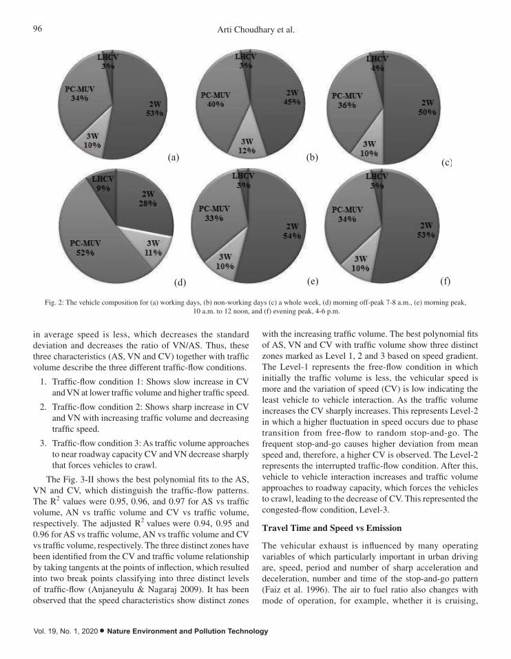
96 Arti Choudhary et al.
Vol. 19, No. 1, 2020 • Nature Environment and Pollution Technology
in average speed is less, which decreases the standard deviation and decreases the ratio of VN/AS. Thus, these three characteristics (AS, VN and CV) together with traffic volume describe the three different traffic-flow conditions.
1. Traffic-flow condition 1: Shows slow increase in CV and VN at lower traffic volume and higher traffic speed.
2. Traffic-flow condition 2: Shows sharp increase in CV and VN with increasing traffic volume and decreasing traffic speed.
3. Traffic-flow condition 3: As traffic volume approaches to near roadway capacity CV and VN decrease sharply that forces vehicles to crawl.
The Fig. 3-II shows the best polynomial fits to the AS, VN and CV, which distinguish the traffic-flow patterns. The R2 values were 0.95, 0.96, and 0.97 for AS vs traffic volume, AN vs traffic volume and CV vs traffic volume, respectively. The adjusted R2 values were 0.94, 0.95 and 0.96 for AS vs traffic volume, AN vs traffic volume and CV vs traffic volume, respectively. The three distinct zones have been identified from the CV and traffic volume relationship by taking tangents at the points of inflection, which resulted into two break points classifying into three distinct levels of traffic-flow (Anjaneyulu & Nagaraj 2009). It has been observed that the speed characteristics show distinct zones
(a) (b) (c)
(d) (e) (f)
Fig. 2: The vehicle composition for (a) working days, (b) non-working days (c) a whole week, (d) morning off-peak 7-8 a.m., (e) morning peak, 10 a.m. to 12 noon, and (f) evening peak, 4-6 p.m.
Traffic-Flow vs Speed Traffic speed and volume are two important characteristics, which directly affect the traffic-flow on roads (Anjaneyulu & Nagaraj 2009). Therefore, the time variation of speed due to traffic volume has been used to describe and define the traffic–flow patterns. The videotapes were analysed for traffic volume (veh/5 min) and traffic speed (km/h) analysis were done for defining the various traffic-flow patterns. Three descriptive statistics were used to represent the relationship, viz.-average speed (AS) in km/h; velocity noise (VN) a standard deviation of speed in km/h and the coefficient of variation of speed (CV), the ratio of VN and AS. Fig. 3-I (a, b, c) shows the relationships of-AS, VN and CV with traffic volume (veh/5 min) in which the minimum volume suggests the free-flow condition and higher volume suggests the density near roadway capacity. As the traffic volume increased, the AS decreased and VN and CV increased, which after reaching the volume of about 400, dropped continuously indicating the higher level of vehicle to vehicle interactions, which further increases.
As traffic volume increases, the interaction between the vehicles increases, i.e. the speed of a vehicle is affected by the vehicles plying together with it, which results in the increase of variation in the speed, as has been observed from the sharp rise in CV and VN. Further, increase in volume forces a vehicle to reduce its speed. In this condition, fluctuation in average speed is less, which decreases the standard deviation and decreases the ratio of VN/AS. Thus, these three
Fig. 2: The vehicle composition for (a) working days, (b) non-working days (c) a whole week, (d) morning off-peak 7-8 a.m., (e) morning peak, 10 a.m. to 12 noon, and (f) evening peak, 4-6 p.m.
with the increasing traffic volume. The best polynomial fits of AS, VN and CV with traffic volume show three distinct zones marked as Level 1, 2 and 3 based on speed gradient. The Level-1 represents the free-flow condition in which initially the traffic volume is less, the vehicular speed is more and the variation of speed (CV) is low indicating the least vehicle to vehicle interaction. As the traffic volume increases the CV sharply increases. This represents Level-2 in which a higher fluctuation in speed occurs due to phase transition from free-flow to random stop-and-go. The frequent stop-and-go causes higher deviation from mean speed and, therefore, a higher CV is observed. The Level-2 represents the interrupted traffic-flow condition. After this, vehicle to vehicle interaction increases and traffic volume approaches to roadway capacity, which forces the vehicles to crawl, leading to the decrease of CV. This represented the congested-flow condition, Level-3.
Travel Time and Speed vs Emission
The vehicular exhaust is influenced by many operating variables of which particularly important in urban driving are, speed, period and number of sharp acceleration and deceleration, number and time of the stop-and-go pattern (Faiz et al. 1996). The air to fuel ratio also changes with mode of operation, for example, whether it is cruising,
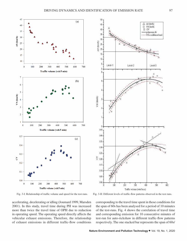
97DRIVING DYNAMICS AND IDENTIFICATION OF EMISSION RATE
Nature Environment and Pollution Technology • Vol. 19, No. 1, 2020
Fig. 3-I: Relationship of traffic volume and speed for the test runs.
Fig. 3-II: Different levels of traffic-flow patterns observed in the test runs.
Travel Time and Speed vs Emission The vehicular exhaust is influenced by many operating variables of which particularly important in urban driving are, speed, period and number of sharp acceleration and deceleration, number and time of the stop-and-go pattern (Faiz et al. 1996). The air to fuel ratio also changes with mode of operation, for example, whether it is cruising, accelerating, decelerating or idling (Joumard 1999,
Fig. 3-I: Relationship of traffic volume and speed for the test runs. Fig. 3-II: Different levels of traffic-flow patterns observed in the test runs.
accelerating, decelerating or idling (Joumard 1999, Marsden 2001). In this study, travel time during PH was increased more than twice the travel time of OPH due to reduction in operating speed. The operating speed directly affects the vehicular exhaust emissions. Therefore, the relationship of exhaust emissions in different traffic-flow conditions
corresponding to the travel time spent in those conditions for the span of 60s has been analysed for a period of 10 minutes of the test-runs. Fig. 4 shows the correlation of travel time and corresponding emission for 10 consecutive minutes of test-run for auto-rickshaw in different traffic-flow patterns respectively. The one stacked bar represents the span of 60s/

98 Arti Choudhary et al.
Vol. 19, No. 1, 2020 • Nature Environment and Pollution Technology
minute, so total 10 stacked bar, each representing one minute, were analysed (Fig. 4). The stacked bar colours indicating the different traffic flow patterns and the height of stacked bar depicting time spent in each traffic flow patterns. To study the correlation of operating speed and corresponding travel time, the vehicle speed categorized into 0 – 2 ± 2, 3 – 15 ± 3, 16 – 30 ± 3 and above 31 ± 3 km/h corresponding to idle–flow, congested flow (CF), interrupted flow (IF) and free-flow (FF), respectively. It was found that during the test-run auto-rickshaws travelled for over 80% of the time in the speed range 10-30 km/h.
Fig. 4 also depicting the emission rate of CO, HC, NOx and CO2 corresponding to different traffic-flow patterns and time spent in particular traffic-flow. It has been observed that the magnitude of emission rate in auto-rickshaw is higher due to longer time of travel and lower operating speed for the pollutants CO and HC. The emission rate of NOx significantly increased for speed of > 30 km/h but did not show any effect for time of travel. The magnitude of CO2 emission rate was
found higher for IF condition as compared to the combination of higher travel time and lower speed.
Combined Effect of Speed-Time on Emission Rate
To determine the combined effect of travel time and associated speed on exhaust emission, a speed-time spent factor, which is a multiplication of average speed of particular speed interval and the time spent of that traffic flow, was used. Details of speed-time spent factor are tabulated in Table 2. The Fig. 5 shows the relationship of pollutants emission rate with the speed-time spent factor for auto-rickshaw. It was observed that CO, HC and CO2 emission increase as the speed-time factor increases. It indicates that the speed at which vehicles run and the time they spend directly affects the emission rate. However, the emission of NOx shows opposite trends; has higher emission for combination of higher speed and lesser time spent and similarly very low emission was observed for combination of lower speed and higher time spent.
Fig. 4: The variation of pollutants emission in different traffic-flow pattern corresponding to time spent in each traffic-flow pattern during pH in auto-rickshaw.
Table 2: Speed-time factor analysis.
Speed range (km/h)
Speed (m/s)
Frequency Factor (V*frequency)
HC (g/s) CO (g/s) NOx (g/s)
CO2 (g/s)
0-5 0.72 69 49.68 0.004 0.052 0.020 0.599
5-10 2.14 60 128.40 0.009 0.121 0.013 1.601
10-15 3.50 83 290.50 0.008 0.149 9.00e-3 1.698
15-20 4.82 81 390.42 0.010 0.192 7.20e-3 2.422
20-25 6.24 84 524.16 0.014 0.158 1.21e-3 2.256
25-30 7.51 49 367.99 0.012 0.174 9.21e-4 3.273
30-35 9.03 36 325.08 0.010 0.171 1.92e-4 3.000
35-40 10.35 27 279.45 0.012 0.147 5.00e-4 2.536
Fig. 4: The variation of pollutants emission in different traffic-flow pattern corresponding to time spent in each traffic-flow pattern during pH in auto-rickshaw.

99DRIVING DYNAMICS AND IDENTIFICATION OF EMISSION RATE
Nature Environment and Pollution Technology • Vol. 19, No. 1, 2020
Table 2: Speed-time factor analysis.
Speed range (km/h) Speed (m/s) Frequency Factor (V*frequency) HC (g/s) CO (g/s) NOx (g/s) CO2 (g/s)
0-5 0.72 69 49.68 0.004 0.052 0.020 0.599
5-10 2.14 60 128.40 0.009 0.121 0.013 1.601
10-15 3.50 83 290.50 0.008 0.149 9.00e-3 1.698
15-20 4.82 81 390.42 0.010 0.192 7.20e-3 2.422
20-25 6.24 84 524.16 0.014 0.158 1.21e-3 2.256
25-30 7.51 49 367.99 0.012 0.174 9.21e-4 3.273
30-35 9.03 36 325.08 0.010 0.171 1.92e-4 3.000
35-40 10.35 27 279.45 0.012 0.147 5.00e-4 2.536
Fig. 5: The relationship of speed-time spent with the emission of pollutants (a) HC, (b) CO, (c) NOx and (d) CO2.
Mileage vs Emission The vehicle mileage is another factor that determines the amount of emissions from a vehicle (Ntziachristos et al. 2000). The one-way ANOVA analysis was used to analyse the effect of mileage on exhaust emission. The completely randomised single-factor analysis of variance test (ANOVA) was applied to identify the statistically significant effects of vehicle mileage on emissions (Ntziachristos & Samaras 2000). Using this test, the average emission values of different mileage classes of test vehicles were compared to find any statistically significant differences between them (rejection of the null hypothesis of equal means). With the Tukey-Kramer emission
Fig. 5: The relationship of speed-time spent with the emission of pollutants (a) HC, (b) CO, (c) NOx and (d) CO2.

100 Arti Choudhary et al.
Vol. 19, No. 1, 2020 • Nature Environment and Pollution Technology
Mileage vs Emission
The vehicle mileage is another factor that determines the amount of emissions from a vehicle (Ntziachristos et al. 2000). The one-way ANOVA analysis was used to analyse the effect of mileage on exhaust emission. The completely randomised single-factor analysis of variance test (ANOVA) was applied to identify the statistically significant effects of vehicle mileage on emissions (Ntziachristos & Samaras 2000). Using this test, the average emission values of different mileage classes of test vehicles were compared to find any statistically significant differences between them (rejection of the null hypothesis of equal means). With the Tukey-Kramer emission mileage matrix (Barnes 1994), correlation of mileages with different mean values can be revealed. The double input matrix in Table 3 presents the results of this procedure. The cells of the matrix correspond to pair-wise comparison of different mileage classes of test vehicles found in the same row and column of the cell. This matrix has been built with 189 observations for auto-rickshaws. According to these results, it has been observed that for 52,000 km and above, mileage has significant impact on emission for pollutants CO, HC and NOx. Summary of the mean emission values obtained from ANOVA for each mileage class is given in Table 4, which leads to the conclusion that there is a statistically significant correlation of CO, CO2 and HC emissions with mileage.
CONCLUSIONS
Urban traffic-flow governed by many factors which mainly resulted from the poor traffic management, an unregulated roadside parking and a frequent pedestrian to vehicle interaction. These factors restrict the urban mobility and the most severe outcomes of the restricted urban mobility are increased pollutant emissions. The study identified three
Table 3: The Tukey-Kramer emission-mileage matrix.
Test Vehicles Test vehicle mileage
9,200 km 52,000 km 142,000 km
Test vehicle mileage 9,200 km - CO, HC CO, HC, NOx
52,000 km - CO, HC, CO2, NOx
142,000 km -
Table 4: Summary of mean emission values ANOVA analysis.
Test vehicles Mileage in km
CO (g/s)
HC(g/s)
NOx (g/s)
CO2(g/s)
9,20052,000142,000
0.120.170.22
0.00020.0020.012
0.00060.00050.018
9.505.188.40
traffic-flow patterns classified as free-flow, interrupted-flow and congested-flow from the on-road traffic volume and traffic speed. The variable composition of vehicles on road governs the rate of exhaust emissions. The dynamic and age-related variables such as, time, speed and mileage were analysed for analytically categorized traffic-flow patterns. The analysis depicted that the combined factor of lower speed (speed ≤12 km/h) and higher time of travel cause higher emission rate, especially for pollutants HC and CO. NOx emission is higher with increasing speed irrespective of time of travel. The magnitude of CO2 emission rate mostly found higher for interrupted flow condition as compared to the combination of higher travel time and lower speed. Similarly, vehicle mileage of ≤52,000 km has significant impact on emission for pollutants CO, HC and NOx.
The effective transport planning and environmental policies depends on the accurate assessment of vehicle exhaust emissions. Therefore, the finding of this study can be handy for the consideration in policy formulation and worthy for differentiation between measured and modelled results.
ACKNOWLEDGEMENTS
Arti Choudhary thankfully acknowledges the financial assistance provided by Science and Engineering Research Board (SERB), New Delhi, India, under the scheme of SERB National Post-Doctoral Fellowship (PDF/2017/001284).
REFERENCES
Anjaneyulu, M.V.L.R. and Nagaraj, B.N. 2009. Modelling congestion on urban roads using speed profile data. Journal of the Indian Roads Congress, 1: 65-74.
Asaithambi, G., Kanagaraj, V., Srinivasan, K. K. and Sivanandan, R. 2016. Study of traffic flow characteristics using different vehicle-following models under mixed traffic conditions. Transportation Letters, 1-12.
Barnes, J.W. 1994. Statistical Analysis for Engineers and Scientists: A

101DRIVING DYNAMICS AND IDENTIFICATION OF EMISSION RATE
Nature Environment and Pollution Technology • Vol. 19, No. 1, 2020
Computer-based Approach. McGraw-Hill, Inc.Chen, C., Huang, C., Jing, Q., Wang, H., Pan, H., Li, L. and Schipper, L.
2007. On-road emission characteristics of heavy-duty diesel vehicles in Shanghai. Atmospheric Environment, 41(26): 5334-5344.
Choudhary, A. and Gokhale, S. 2016. Urban real-world driving traffic emissions during interruption and congestion. Transportation Research Part D: Transport and Environment, 43: 59-70.
Faiz, A., Weaver, C.S. and Walsh, M.P. 1996. Air Pollution from Motor Vehicles: Standards and Technologies for Controlling Emissions. World Bank Publications.
Choudhary, A. and Gokhale, S. 2019a. Evaluation of emission reduction benefits of traffic flow management and technology upgrade in a con-gested urban traffic corridor. Clean Technologies and Environmental Policy, 21(2): 257-273.
Choudhary, A. and Gokhale, S. 2019b. On-road measurements and model-ling of vehicular emissions during traffic interruption and congestion events in an urban traffic corridor. Atmospheric Pollution Research, 10(2): 480-492.
Grieshop, A.P., Boland, D., Reynolds, C.C., Gouge, B., Apte, J.S., Rogak, S.N. and Kandlikar, M. 2012. Modeling air pollutant emissions from Indian auto-rickshaws: Model develop.m.ent and implications for fleet emission rate estimates. Atmospheric Environment, 50: 148-156.
Grote, M., Williams, I., Preston, J. and Kemp, S. 2016. Including conges-tion effects in urban road traffic CO2 emissions modelling: do local government authorities have the right options? Transportation Research Part D: Transport and Environment, 43: 95-106.
Gulia, S., Nagendra, S.S., Khare, M. and Khanna, I. 2015. Urban air quality management-A review. Atmospheric Pollution Research, 6: 286-304.
Guttikunda, S.K. and Mohan, D. 2014. Re-fueling road transport for better air quality in India. Energy Policy, 68: 556-561.
Iyer, N.V. 2003. Three-wheelers take to South Asian streets. Smart Urban Transport, 2(2).
Iyer, N. V., Posada, F. and Bandivadekar, A. 2013. Technical assessment of emission and fuel consumption reduction potential from two and three wheelers in India (No. 2013-26-0050). SAE Technical Paper.
Joumard, R., Philippe, F. and Vidon, R. 1999. Reliability of the current models of instantaneous pollutant emissions. Science of the Total Environment, 235: 133-142.
Marsden, G., Bell, M. and Reynolds, S. 2001. Towards a real-time micro-scopic emissions model. Transportation Research Part D: Transport and Environment, 6(1): 37-60.
Mohapatra, S.S. 2012. Level of service criteria of urban streets in Indian context using advanced classification tools. M.Tech. Thesis.
Ntziachristos, L. and Samaras, Z. 2000. Speed-dependent representative emission factors for catalyst passenger cars and influencing parameters. Atmospheric Environment, 34(27): 4611-4619.
Ntziachristos, L., Samaras, Z., Eggleston, S., Gorissen, N., Hassel, D. and Hickman, A.J. 2000. COPERT III, Computer programme to calculate emissions from road transport, methodology and emission factors (version 2.1). European Energy Agency (EEA), Copenhagen.
Pandian, S., Gokhale, S. and Ghoshal, A.K. 2009. Evaluating effects of traffic and vehicle characteristics on vehicular emissions near traffic intersections. Transportation Research Part D: Transport and Environ-ment, 14(3): 180-196.
Ramachandra, T. 2009. Emissions from India’s transport sector: state wise synthesis. Atmospheric Environment, 43(34): 5510-5517.
Reddy, B. S. and Balachandra, P. 2012. Urban mobility: A comparative analysis of megacities of India. Transport Policy, 21: 152-164.
Reynolds, C. Grieshop, A. and Kandlikar, M. 2009. Measuring auto-rick-shaw emission to inform air quality policy. University of British Co-lumbia. Accessed on 5th March 2016, http://indiaenvironmentportal.org.in/files/EmissionTestinginInda.pdf.
Reynolds, C.C., Grieshop, A.P. and Kandlikar, M. 2011. Climate and health relevant emissions from in-use Indian three-wheelers fueled by natural gas and gasoline. Environmental Science & Technology, 45: 2406-2412.
Robertson, H.D. 1994. Queuing studies. In: Robertson, H.D., Hummer, J.E., Nelson, D.C. (Eds.), Manual of Transportation Engineering Studies, Washington, DC, pp. 347-358.
Singh, S. K. 2006. Future mobility in India: Implications for energy demand and CO2 emission. Transport Policy, 13(5): 398-412.
Singh, S.K. 2012. Urban transport in India: Issues, challenges, and the way forward. European Transport/Trasporti Europei, Issue 52.

Vol. 19, No. 1, 2020 • Nature Environment and Pollution Technology
102

Studies on use of Cashew Nut Shell Liquid (CNSL) in Biopesticide and Biofertilizer
C. Vasanth Pandiyan*†, Gunasekaran Shylaja*, Gokul Raghavendra Srinivasan** and Sujatha Saravanan**Department of Biotechnology, Bharath Institute of Higher Education and Research, Selaiyur, Chennai-600073, Tamil Nadu, India**Department of Mechanical Engineering, Bharath Institute of Higher Education and Research, Selaiyur, Chennai-600073, Tamil Nadu, India †Corresponding author: C. Vasanth Pandiyan
ABSTRACT
Cashew is an immigrant tree from eastern Brazil and is regarded as one of the top three commercial crops of India. In general, Cashew nut shell contains 25-34% oil and was not much used earlier; however, commercial and industrial applications are being developed in the recent decade. In this present study, 100 kg of dried cashew shells yielded around 18.5 to 22.6% of cashew nut shell liquid (CNSL) while 58-63% of waste dark solid oil cake retained in extraction chamber. Eventually, these oil cakes were rich in fibre, protein and energy contents and offered as good alternative to traditional applications in the production of environmentally friendly organic fertilizer for vegetable crops. Also, this study investigated the safety of using CNSL cake as fertilizer for leaf & vegetable; and also noted improvised physico-chemical properties of soil which enhanced the soil fertility thereby leading to high crop yield and nutritional quality. Furthermore, CNSL was also proven to be a phytopesticide for eradication of serious pests, Odontopus varicornis, on cotton plant. Interestingly, toxicity study proved that the applications of CNSL was not only limited to biofertilizer but was also proven to be an effective biopesticide for the control of pest and insects.
INTRODUCTION
The developing and developed countries are seeing the rapid growth of specific wastes, such as electrical and electronics equipment waste, agricultural biomass waste, and plastic waste. These specific wastes require proper management, as most of the materials could be reduced, recycled or re-used with the help of environmentally friendly methods and technologies.
Cashew nut is one of the greatest yielded item on the plan-et, with production capacity more than 3.35 million tonnes per year and yet expanding in coming years. It is likewise considered as a standout amongst the most critical nuts in universal market because of its well acknowledged demand (MacLeod et al. 1982, Maia et al. 2000). Crude cashew nut contains both edible kernel with health significance; and a shell, which has been considered as waste and may bring an ecological issue if not dealt with appropriately.
The primary component of cashew plant is its cashew nuts, while the least regarded product was cashew nut shell liquid (CNSL). At a level of about 50% of cashews weight (Patel et al. 2006), a heavy liquid called cashew nut shell liquid (CNSL) is produced, which is considered an important
material in view of the high centrality of unsaturated long-chain phenols, for example, cardanol, cardol and isomers (Rodriguez et al. 2006). Both anacardic and cardol corrosion were included as corrosion inhibitors (Kozubek et al. 2001, Kubo et al. 1993), antimicrobial inhibitory (Kubo et al. 1993) and lipoxygenase activities (Kubo et al. 1993). On the other hand, cardanol, because of its remarkable protection against the photolytic activity of mineral oils and the high protection of acids, alkalis, microorganisms, termites and creepers widely used in the production of caps and fabrics.
Cashew nut shell fluid or CNSL or CNSL oil is an ad-aptable by-product of the cashew business. CNSL is widely used in polymer-based businesses, for example, contact linings, paints and varnishes, overlaying tars, rubber aggra-vating saps, cashew bonds, polyurethane based polymers, surfactants, epoxy tars, foundry synthetics and intermediates for concoction industry and automobiles. In its existing form, CNSL is accounted as an effective chemical against termites and has water repellency (Lepage & Delelis l980). With the end goal of using the cashew nutshell, we have made an endeavour to change over the CNSL oils and waste cake to bio-insecticide against and bio-fertilizer. We hypothesize that if not the neat form, some particular blend may actually be
Nat. Env. & Poll. Tech.Website: www.neptjournal.com
Received: 08-06-2019Accepted: 23-07-2019
Key Words:Cashew nut shell liquid Biopesticide Biofertilizer Oil cake
2020pp. 103-111 Vol. 19
p-ISSN: 0972-6268 No. 1 Nature Environment and Pollution Technology An International Quarterly Scientific Journal
Original Research Paper
e-ISSN: 2395-3454
Open Access

104 C. Vasanth Pandiyan et al.
Vol. 19, No. 1, 2020 • Nature Environment and Pollution Technology
good enough for commercial use. The objective of the study was to characterize the physicochemical quality of oil from cashew nut shell and to evaluate the potential of cashew nut shell cake as natural insecticide against termites.
MATERIALS AND METHODS
Collection of Cashew Nut Shells
Cashew nut shells crude and unshelled cashew nuts were collected from the trees grown in the Panruti, Cuddalore area in Tamil Nadu (India) amid August to September 2012. Cuddalore region was chosen for the examination since this locale has the most extreme territory of cashew generation than different areas of the state. Towns from Panruti and Virudhachalam obstructs in Cuddalore locale were chosen for this examination.
Preparation of samples
The piece nuts were broken, the nuts were collected, washed, dried in a stove at 40°C. The dried, clean nuts were pro-cessed using manual blender on account of the hardness of the nut (Figs. 1 & 2). During the timeframe of August to September, 2018, four samples were gathered and CNSL oil was separated.
Extraction of Cashew Nut Shell Liquid (CNSL)
This is the most well-known technique for extraction of CNSL these days. The cashew nut shells are gathered in the chamber, where steam warming is connected at temperatures around 200-250°C for 2-3 minutes, CNSL is then discharged out of shells. Figs. 3, 4A & 4B show the small-scale extrac-tion units at Panruti, Cuddalore area in Tamil Nadu (India).
CNSL as Biopesticide Studies
Adult insects of Odontopus varicornis, collected from the
Annamalai University campus, were brought to the labora-tory and reared in wooden cage (45 × 32 × 30 cm dimen-sion), at laboratory temperature of 29°±1°C with 12 hours of light and dark cycle. The sides of the insect cages were fabricated with wire meshes to provide sufficient aeration and light also easy for observation. The cage surface was covered with fine sand with moderate humidity maintained by adding a little amount of water frequently. The soaked cotton seeds of Bombax ceiba as well as seeds of its host plant, Stericulia foetida and Gossypium sp. were fed daily to the insects. Additionally, the pieces of Sechium edule (Chow chow) were also fed to the insects. The cages were maintained properly by cleaning on alternative days by eliminating the excreta and other waste substances. The continuous culture was maintained by transferring the laid eggs to other cages.
The nuts A. Occidentale were collected from cashew plantation area of Cuddalore district, Tamil Nadu, India. Cashew nut shell liquid (CNSL) has a structure of soft honey comb with dark brownish red viscose liquid. It is a one of the by-products of the cashew production which is the pericarp fluid of the nut.
To evaluate the acute toxicity in the atmosphere, the LD50 values (medium tolerance limit) are positive measures to test the toxicity of the test toxicant, under definite environmental conditions. The application of LD50 value has significantly gained more importance among toxicologists and it is the most consistent measure to evaluate potential hazards of aquatic and terrestrial life. The LD50 value for the same tox-icant varies due to the mode of action and animal responses. In this viewpoint, the study has been done to evaluate the LD50 values for the male Odontopus varicornis on exposure to the phytopesticide, cashew shell oil. To provide a basis for evaluating and comparing the acute toxicity with other, 24, 48, 72 and 96 hours median lethal dose (LD50) values are determined for the cashew nut shell oil commercial product. The LD50 is a statistical estimate of the concentration of the
Fig. 1: Manually separating activity for cashew kernel and shells.
Fig. 2: Picture of cashew nut shells.

105USE OF CASHEW NUT SHELL LIQUID IN BIOPESTICIDE AND BIOFERTILIZER
Nature Environment and Pollution Technology • Vol. 19, No. 1, 2020
toxic material that kills 50 percent of the test species under experimental conditions during a specific time interval. The LD50 values are used because of the concentration required to affect a response in 50 percent of the test insects is more reproducible than any other values.
Range Finding Test
The solutions were made at varying range of concentrations. The tests were performed in adult insects, by injecting 0.025 mL, to each insect with a 2.6-gauge syringe needle. Ten treated insects were moved into a little insect cage (29 × 25 × 11cm) and their mortality was noted from 24 hours thereafter up to 96 hours. The results observed from the exploratory test indicated the range of the insecticide concentration.
Full Scale Test of Toxicity Evaluation
Different concentration of cashew nut shell oil was prepared. Insecticide treated and control insect were maintained for each bioassay. One hundred insects were administered with each concentration and allowed in separate insect cages. The observations on mortality are made at 25, 48, 72 and 96 hours. Insects showing no activities or response to physical stimulus were noted as dead and taken out instantly. The recorded values were used for calculating LD50 values.
Calculation of LD50
The test was done to find the series of concentration for mortality. The mortality was recorded for Odontopus var-icornis at 24, 48, 72 and 96 hours of exposure by injecting the insecticide of various concentrations. The LD50 value was determined by the profit analysis method depending on the measured percentages of test animal existing at con-centrated lethal to more than half and less than half of the test subject (Huson method). This method described a quick and exact method of determining the median lethal dose (LD50 or ED50). The method can be used to drive point and interval estimates or percentage points other than the LD50. It is claimed that the method is less accurate for points other than the medium but equal to other approximate techniques. Following the probit analysis procedure, the LD50 values of 24, 48, 72 and 96 hours were evaluated. By using the LD50 values, a toxicity curve was constructed on a centimetre graph sheet (Fig. 10).
The LD50 values were derived by probit regression, i.e. taking test concentration and the respective mortality per-centages on log values and probit scales, respectively. From the line drawn to the concentration ordinates, LD50 values were fixed and also calculated their 95% upper and lower
Fig. 2: Picture of cashew nut shells.
Extraction of Cashew Nut Shell Liquid (CNSL)
This is the most well-known technique for extraction of CNSL these days. The cashew nut
shells are gathered in the chamber, where steam warming is connected at temperatures around
200-250°C for 2-3 minutes, CNSL is then discharged out of shells. Figs. 3, 4A & 4B show the
small-scale extraction units at Panruti, Cuddalore area in Tamil Nadu (India).
Fig. 3: Top view - Input loading cylinder with cover.
Fig. 4A: Input loading cylinder with cover. 4B: Collection container of small-scale extraction.
CNSL as Biopesticide Studies
Adult insects of Odontopus varicornis, collected from the Annamalai University campus, were
brought to the laboratory and reared in wooden cage (45 × 32 × 30 cm dimension), at laboratory
temperature of 29°±1°C with 12 hours of light and dark cycle. The sides of the insect cages
were fabricated with wire meshes to provide sufficient aeration and light also easy for
observation. The cage surface was covered with fine sand with moderate humidity maintained
by adding a little amount of water frequently. The soaked cotton seeds of Bombax ceiba as well
as seeds of its host plant, Stericulia foetida and Gossypium sp. were fed daily to the insects.
A B
Fig. 4A: Input loading cylinder with cover. 4B: Collection container of small-scale extraction.
Fig. 2: Picture of cashew nut shells.
Extraction of Cashew Nut Shell Liquid (CNSL)
This is the most well-known technique for extraction of CNSL these days. The cashew nut
shells are gathered in the chamber, where steam warming is connected at temperatures around
200-250°C for 2-3 minutes, CNSL is then discharged out of shells. Figs. 3, 4A & 4B show the
small-scale extraction units at Panruti, Cuddalore area in Tamil Nadu (India).
Fig. 3: Top view - Input loading cylinder with cover.
Fig. 4A: Input loading cylinder with cover. 4B: Collection container of small-scale extraction.
CNSL as Biopesticide Studies
Adult insects of Odontopus varicornis, collected from the Annamalai University campus, were
brought to the laboratory and reared in wooden cage (45 × 32 × 30 cm dimension), at laboratory
temperature of 29°±1°C with 12 hours of light and dark cycle. The sides of the insect cages
were fabricated with wire meshes to provide sufficient aeration and light also easy for
observation. The cage surface was covered with fine sand with moderate humidity maintained
by adding a little amount of water frequently. The soaked cotton seeds of Bombax ceiba as well
as seeds of its host plant, Stericulia foetida and Gossypium sp. were fed daily to the insects.
A B
Fig. 3: Top view - Input loading cylinder with cover.

106 C. Vasanth Pandiyan et al.
Vol. 19, No. 1, 2020 • Nature Environment and Pollution Technology
confidence limits. The method of calculation is as below:
Step 1: The doses (d1); number of insects tested (n1); number of insects died (r1) were wrote down; then the natural log for the doses (x1) were found out.
Step 2: The method of finding y1 is as follows.
y Inr
n r11
1 1
=-
, if number of insects (r1) died is less than
number of insects tested (n1).
y n1 12 1= -( ) , if number of insects died is equal to number of insects tested.
y Inn11
2 1=
-( ), if number of insects died is ‘zero’.
Step 3: The transformed data were divided and then set into upper lower halves.
Step 4: The total amount of transformed doses and the responses were calculated and the values were denoted as yu, yl, xu, xl where subscript U and 1 refer upper and lower halves of the data set.
Step 5: The mean of all transformed doses and the responses included in Step 3 were calculated. The means denoted as
X and Y respectively. Step 6: The slope (b) was calculated as:
b
yu y
Xu X=
--
( )
( )
1
1
Step 7: The intercept (a) was calculated as:
a y bx= -
Step 8: LD50 was found as follows:
LD50 = ec
Where, cF a
b=
-( )F is the log of LD50
F In=-
ÈÎÍ
˘˚˙ =
50
100 500
( )
Step 9: The total number of insects tested (N) in the data included in Step 3 was calculated.Step10: Sc was found using the formula:
Scb N
=¥5
2( )
Step 11: The standard error (S) of the desired percentage was estimated as follows:
S (LD50) = LD50 x ScStep 12: The approximate 95% confidence interval was calculated by using the following formula:
LD50 ± 1.96 × S(LD50)
Bionomics
The details of its systematic position, distribution, habitat, morphology, feeding habits, cannibalism, longevity, sexual dimorphism, mating habits, oviposition, eggs, metamor-phosis and adult characters are briefly presented in Table 1 and Table 2.
CNSL as Biofertilizer
Farm site: All the green leaves crops were grown in the farm house at Vallambadugai nearer to Chidambaram town. The plantation of green leaves and ornamental plants located in the region of plant research farm nearer to Annamalai University. This region is located in the central plain of Chidambaram town and characterized as clay loan soil.
De-oiled CNSL seed cake: The de-oiled CNSL cake was generously processed. The seedcake was kept back at room temperature for 90 days before using as a fertilizer.
Fig. 5: Odontopus varicornis in mating condition.
Fig. 5: Odontopus varicornis in mating condition.
Fig. 6A: Adult male Odontopus varicornis; 6B: Adult female Odontopus varicornis.
ODONTOPUS VARICORNIS
Fig. 7: Adult male and female Odontopus varicornis in mating condition.
Bionomics
A B
Fig. 6A: Adult male Odontopus varicornis; 6B: Adult female Odontopus varicornis.
Fig. 5: Odontopus varicornis in mating condition.
Fig. 6A: Adult male Odontopus varicornis; 6B: Adult female Odontopus varicornis.
ODONTOPUS VARICORNIS
Fig. 7: Adult male and female Odontopus varicornis in mating condition.
Bionomics
A B
Fig. 7: Adult male and female Odonto-pus varicornis in mating condition.

107USE OF CASHEW NUT SHELL LIQUID IN BIOPESTICIDE AND BIOFERTILIZER
Nature Environment and Pollution Technology • Vol. 19, No. 1, 2020
Plant material and propagation: All the leaves and ornamental plants need different agricultural practices such as the ratio of chemical fertilizers for each plant varies based on the recommendation by the Department of Agriculture, Annamalai University, India. The devel-opment of the plant and yield is independent of each other. However, the intention of this study is to trace the growth of leaves bushiness height as well as ornamental plant height, growth etc. Different rates of CNSL cake would have the variation in influencing the growth of each plant, but propagation methods were varied between these plants. The addition of CNSL cake at land preparation would exacerbate the phorbol ester content in the soil which was reported to decompose at time of harvesting (Joshi et al. 2011).
Plant Experiments
Amaranthus seeds were planted in control medium and allowed to grow for 4 weeks (Figs. 11 & 12). seedlings were transplanted individually into different test potting media and placed in a greenhouse maintained at 28°C, 16-h day/20°C 8-h night utilizing both natural light and supplemental artificial lighting to maintain an average light intensity of approximately 600 µmol m-2 s-1. Change in plant heights were recorded from transplanting, when further growth ceased.
RESULTS AND DISCUSSION
Extraction of CNSL
The shell is about 0.3 inches thick having a sensitive cush-
Table 2: Details of O. varicornis.
Distribution Ethiopiean and Oriental regions, Odontopus cultellaris, O. nigricornis, O. varicornis, and O. sanguinolens are found in different parts of India. O. varicornis and O. sanguinolens are found in the State of Tamil Nadu and Puducherry.
Habitat Fallen leaves of host plants such as Stericulia foetida and Gossypium sp.
Feeding Habits Phytophagus insect with piercing and sucking type of mouth parts. The bug exhibits minimum feeding during hot hours of the day.
Cannibalism Cannibalism is exhibited by these insects. The eggs laid by them as well as newly moulted insects are found to be susceptible to this activity. Field observations have shown that these insects are Cannibalistic occasionally and moreover feed on snails and dead animals.
Longevity Adult male lives for about 75 days and female for about 70 days under laboratory conditions of 282±oC and 80 * 5% RH
Sexual dimorphism Adult male is smaller in size than the female with pointed aedeagus female with broader abdomen (Figs. 6A and 6B).
Mating habits Exactly on 7th day after last imaginable moult; it exhibits mating behaviour (Fig. 5); Male crawls over the body of the female, after gripping the male inserts its aedeagus into the gonopore and remains in end to end position in natural and laboratory condition (Fig. 7), all usual activities like roaring, feeding, etc. are carried out by the pair in copula conditions (Ranganathan 1984), it mates continuously for three days without any separation.
Oviposition At the time of oviposition, the female separates from the male and scoops at the sand and finally lays its eggs. The first ovipo-sition occurs at about 25 days after the last moult, depositing 80 to 120 eggs in 2 to 3 hours; second oviposition occurs a week after the first oviposition producing 50 to 70 eggs.
Meta Morphosis Incomplete metamorphosis with five nymphal instars; to reach its final moulting, it takes about 42 to 45 days.
Adults The fifth nymphal instar on its final moulting becomes an adult with attains sexual maturity on the 7th day of its imaginal moult.
Table 1: Systematic position of O. varicornis.
Systematic Position
Phylum Arthropoda
Class Insecta
Order Hemiptera
Suborder Heteroptera
Series Geocorisae
Super family Pyrrhocoroidea
Family Pyrrhocoridae
Genus Odontopus
Species varicornis

108 C. Vasanth Pandiyan et al.
Vol. 19, No. 1, 2020 • Nature Environment and Pollution Technology
ioned outside skin and a pitiful hard internal skin. CNSL inside the shell is the segment wrapped by a pitiful skin known as the test. 20 to 25% partition liquid, 20 to 25% test, 2% others, rest being the shell. The raw material for the creation of CNSL is the cashew shells. Cashew nuts contain 35-45% of seeds and 55-65% of shells. The shells contain 15-30% oil. CNSL is used as oil in industries. In extraction process of 100kg of dried cashew shells, oil range between 18.5 to 22.6% was extracted (Table 3). The colour of the solution became reddish brown or dark brown as shown in Fig. 8. The end products or waste like dark solid is shown in Fig 9. It was observed that 58-63% of end product like oil cake retains in chamber.
The most generally utilized technique, the hot oil shower, removes about half of the CNSL (7-15% of nut weight) from the shell (Ohler 1966, Gedam et al.1986). A few unique medications before simmering can convey the rate up to 90-95% and with solvents 100% can be accomplished, however these strategies are costly and their utilization relies upon the CNSL value (Ohler 1966).
Toxicity Studies
The present mortality values of Odontopus varicornis when injected with different concentrations of cashew nut shell oil for different are presented in Table 4. Detailed probit analysis of cashew nut shell oil concentrations and present mortality of Odontopus varicornis for 24, 48, 72 and 96 hours of exposure were determined. The LD50 values were calculated for 24, 48, 72 and 96 hours as 3.3, 3.5, 3.6, and
3.8 respectively. The mortality rate showed the mode of action and toxicity of for different concentrations. Toxicity test revealed that the rates of mortality increased with the increased concentrations.
Plant Growth and Yield
To measure the growth of Amaranthus tricolour, five pa-rameters were subjected to be analysed, namely leaf length, leaf width, plant height, canopy height, canopy width. The trends toward these five characters were not similar. Among all, the one with biofertilizer provided the best outcome as an appearance of the largest of the plant growth characters than control. Whereas, the control plant resulted in a medi-um-sized growth of the same plant. The highest yield was obtained from the treatment of biofertilizer. Therefore, it could be implied that the treatment of CNSL oil cake would be able to partly replace the usage of chemical fertilizer. The usage of CNSL oil cake as fertilizer could, therefore alleviate the problem of high price of chemical fertilizer. Among these treatments, the control without adding biofertilizer gave the poor yield of Amaranthus plants.
Peace lily plant planted in a pot (Fig. 13) showed compar-atively more growth in height of about 6.2 cm and increased the leaf surface area of about 4.8% compared to control when the soil was mixed with CNSL cake. Further, the same trail was showed for sword fern Nephrolepis obliterate in both height and leaf area. Plant height exhibited around1.2cm increase and height surface area comparatively increased about 7.6% when compared to control.
Table 3: Process and recovery rate of cashew shells.
Sample 1 2 3 4
Processing quantity of Cashew shells (kg) 100 100 100 100
Recovery of cashew nut shell oil (mL) 18.8 22.6 21 21.5
Oil cake (kg) 58.8 62.4 57.4 60.4
this study is to trace the growth of leaves bushiness height as well as ornamental plant height,
growth etc. Different rates of CNSL cake would have the variation in influencing the growth
of each plant, but propagation methods were varied between these plants. The addition of
CNSL cake at land preparation would exacerbate the phorbol ester content in the soil which
was reported to decompose at time of harvesting (Joshi et al. 2011).
Plant Experiments
Amaranthus seeds were planted in control medium and allowed to grow for 4 weeks (Figs. 11
& 12). seedlings were transplanted individually into different test potting media and placed in
a greenhouse maintained at 28°C, 16-h day/20°C 8-h night utilizing both natural light and
supplemental artificial lighting to maintain an average light intensity of approximately 600
µmol m-2 s-1. Change in plant heights were recorded from transplanting, when further growth
ceased.
RESULTS AND DISCUSSION
Extraction of CNSL
The shell is about 0.3 inches thick having a sensitive cushioned outside skin and a pitiful hard
internal skin. CNSL inside the shell is the segment wrapped by a pitiful skin known as the test.
20 to 25% partition liquid, 20 to 25% test, 2% others, rest being the shell. The raw material for
the creation of CNSL is the cashew shells. Cashew nuts contain 35-45% of seeds and 55-65%
of shells. The shells contain 15-30% oil. CNSL is used as oil in industries. In extraction process
of 100kg of dried cashew shells, oil range between 18.5 to 22.6% was extracted (Table 3). The
colour of the solution became reddish brown or dark brown as shown in Fig. 8. The end products
or waste like dark solid is shown in Fig 9. It was observed that 58-63% of end product like oil
cake retains in chamber.
Fig. 8: Raw cashew nut shell liquid Fig. 9: End products like oil cake
this study is to trace the growth of leaves bushiness height as well as ornamental plant height,
growth etc. Different rates of CNSL cake would have the variation in influencing the growth
of each plant, but propagation methods were varied between these plants. The addition of
CNSL cake at land preparation would exacerbate the phorbol ester content in the soil which
was reported to decompose at time of harvesting (Joshi et al. 2011).
Plant Experiments
Amaranthus seeds were planted in control medium and allowed to grow for 4 weeks (Figs. 11
& 12). seedlings were transplanted individually into different test potting media and placed in
a greenhouse maintained at 28°C, 16-h day/20°C 8-h night utilizing both natural light and
supplemental artificial lighting to maintain an average light intensity of approximately 600
µmol m-2 s-1. Change in plant heights were recorded from transplanting, when further growth
ceased.
RESULTS AND DISCUSSION
Extraction of CNSL
The shell is about 0.3 inches thick having a sensitive cushioned outside skin and a pitiful hard
internal skin. CNSL inside the shell is the segment wrapped by a pitiful skin known as the test.
20 to 25% partition liquid, 20 to 25% test, 2% others, rest being the shell. The raw material for
the creation of CNSL is the cashew shells. Cashew nuts contain 35-45% of seeds and 55-65%
of shells. The shells contain 15-30% oil. CNSL is used as oil in industries. In extraction process
of 100kg of dried cashew shells, oil range between 18.5 to 22.6% was extracted (Table 3). The
colour of the solution became reddish brown or dark brown as shown in Fig. 8. The end products
or waste like dark solid is shown in Fig 9. It was observed that 58-63% of end product like oil
cake retains in chamber.
Fig. 8: Raw cashew nut shell liquid Fig. 9: End products like oil cake Fig. 8: Raw cashew nut shell liquid Fig. 9: End products like oil cake

109USE OF CASHEW NUT SHELL LIQUID IN BIOPESTICIDE AND BIOFERTILIZER
Nature Environment and Pollution Technology • Vol. 19, No. 1, 2020
Nursery trial on oil extracted CNSL cake act as biofer-tilizer when peace lily, cobra plant, Spathiphyllum wallisii was planted in pot and observed that in the oil cake treated plant, the height increased by 6.2cm and leaf surface area was also increased as compared to control plant (Fig. 14).
CNSL Used as Biopesticide
The toxicity tests were ideally suited for assessing the rela-tive impact of cashew nut shell liquid concentration on the insect for different time intervals. The toxicity level was also influenced by the size and age of the insect under study. The toxicity level also is influenced by sex; similarly, the nutrient supply to the assaying insect (Arunachalam et al. 1980) and the pH. It can be seen that the toxic action is specific for a particular insecticide in a particular insect which has been
substantiated by the researchers in their studies.
The toxicity values denote the nature of cashew nut shell oil on the organism. It indicates whether the action is regular or irregular or cumulative in its effect. In the present investigation on Odontopus varicornis treated with cashew nut shell oil of phytopesticide, the acute toxicity level was expressed in terms of LD50. The LD50 values of the cashew nut shell oil of Odontopus varicornis were 3.3, 3.5, 3.6, 3.8 at 24, 48, 72 and 96 hours, respectively.
The present experimental results were obtained with increased concentration of phytopesticide cashew nut shell liquid with decreased time of exposure, to bring about 50% mortality of insects. This trend was showing a risk in mortality rate with increasing concentration and period of administration sub-cutaneously, revealing the regular mode
Table 4: LD50 value and their 95% confidence limit (µg/insect) of cashew nut shell liquid and the difference between upper and lower confidence limits for male Odontopus varicornis.
Exposure time inter-vals (in hours)
Number of ani-mal introduction
Number of animals died in exposure concentration (%)LD50
95% Confidence limits (upper- lower)
0.26 0.28 0.30 0.32 0.34 0.36
24 100 - - 10 20 30 40 3.3 3.6-3.1
48 100 5 10 20 30 40 50 3.5 3.6-3.4
72 100 10 25 40 55 70 85 3.6 3.4-3.1
96 100 15 30 50 65 80 100 3.8 3.4-3.9
Table 4: LD50 value and their 95% confidence limit (µg/insect) of cashew nut shell liquid and the
difference between upper and lower confidence limits for male Odontopus varicornis.
Exposure time intervals (in hours)
Number of animal introduction
Number of animals died in exposure concentration (%) LD50
95% Confidence limits (upper- lower)
0.26 0.28 0.30 0.32 0.34 0.36
24 100 - - 10 20 30 40 3.3 3.6-3.1
48 100 5 10 20 30 40 50 3.5 3.6-3.4
72 100 10 25 40 55 70 85 3.6 3.4-3.1
96 100 15 30 50 65 80 100 3.8 3.4-3.9
0
0.5
1
1.5
2
2.5
3
3.5
4
4.5
5
0 20 40 60 80 100 120
LD50
Expo
sure
tim
e in
terv
als
(hr
s)
LD50 Values for 24h, 48h, 72h and 96h of O. Varicornis (Toxicity Curve)
Fig. 10: LD50 values for 24h, 48h, 72h and 96h of O. varicornis (Toxicity Curve).
Fig. 10: LD50 values for 24h, 48h, 72h and 96h of O. varicornis (Toxicity Curve).
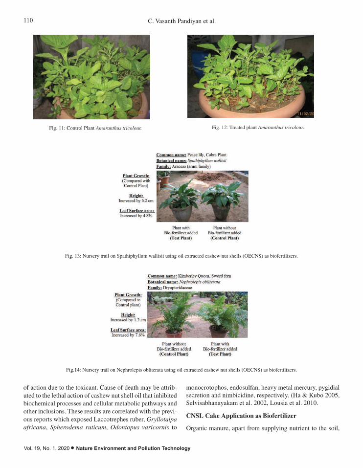
110 C. Vasanth Pandiyan et al.
Vol. 19, No. 1, 2020 • Nature Environment and Pollution Technology
of action due to the toxicant. Cause of death may be attrib-uted to the lethal action of cashew nut shell oil that inhibited biochemical processes and cellular metabolic pathways and other inclusions. These results are correlated with the previ-ous reports which exposed Laccotrephes ruber, Gryllotalpa africana, Spherodema ruticum, Odontopus varicornis to
monocrotophos, endosulfan, heavy metal mercury, pygidial secretion and nimbicidine, respectively. (Ha & Kubo 2005, Selvisabhanayakam et al. 2002, Lousia et al. 2010.
CNSL Cake Application as Biofertilizer
Organic manure, apart from supplying nutrient to the soil,
Fig. 11: Control Plant Amaranthus tricolour.
Fig. 12: Treated plant Amaranthus tricolour.
Fig. 13: Nursery trial on oil extracted cashew nut shells (OECNS) for biofertilizer.
Control plantOil extracted cake
Height : 6.2 cm increasing Leaf Surface area: 4.8% increasing compare to
control plant
Common name: Peace lily, Cobra plant Botanical name: Spathiphyllum wallisiiFamily: Araceae (arum family)
Nursery trial on Oil extracted cashew nut shells (OECNS) for bio-fertilizer
Fig. 12: Treated plant Amaranthus tricolour. Fig. 11: Control Plant Amaranthus tricolour.
Fig. 12: Treated plant Amaranthus tricolour.
Fig. 13: Nursery trial on oil extracted cashew nut shells (OECNS) for biofertilizer.
Control plantOil extracted cake
Height : 6.2 cm increasing Leaf Surface area: 4.8% increasing compare to
control plant
Common name: Peace lily, Cobra plant Botanical name: Spathiphyllum wallisiiFamily: Araceae (arum family)
Nursery trial on Oil extracted cashew nut shells (OECNS) for bio-fertilizer
Fig. 11: Control Plant Amaranthus tricolour.
Fig. 13: Nursery trail on Spathiphyllum wallisii using oil extracted cashew nut shells (OECNS) as biofertilizers.
Fig.14: Nursery trail on Nephrolepis obliterata using oil extracted cashew nut shells (OECNS) as biofertilizers.
111USE OF CASHEW NUT SHELL LIQUID IN BIOPESTICIDE AND BIOFERTILIZER
Nature Environment and Pollution Technology • Vol. 19, No. 1, 2020
conserves soil moisture, moderates soil pH, improves bulk density, increase carbon dioxide level in plant canopy, alle-viates the toxicity of A3+, improves aeration and activity of beneficial soil microbes, increase cation exchange capacity and retards nitrification for longer time. The increased yield resulting from the application of fertilizer was as a result of the improved soil fertility. It has been shown that crops respond more to fertilizer application. The improved nutritional value of the crop resulting from the application of the formulations may be attributed to the increased soil fertility. Increase in yield attributes and nutritional value of crops arising from the use of combination of organic and chemical fertilizers has also been reported. It has been sug-gested from the present study that CNSL oil cake helps to improve the growth and canopy of both test plant. Further, the present study revealed that the use of CNSL oil cake used for both plants increased the height and leaf surface area, especially in sword fern, which absorbed the air pollutants and Amaranthus tricolor, which produce pure air, in addition to controlling environmental contamination.
CONCLUSIONS
Oil cakes are rich in fibre, protein and energy contents. They offer potential benefits when used as substrates in develop-ing bioprocesses for the production of organic chemicals and bio-molecules. Also, the use of oil cakes offers good alternative to traditional applications by their exploitation in the production of environmentally friendly green biofuel. Another key point to be noted is that the bioprocess utilizing oil cakes is attractive due to relatively cheaper availability of the oil cakes throughout the year, making it even more favourable when economics is considered. The utilization of de-oiled CNSL oil cake was proven to have potential for being used as an organic fertilizer for vegetable crops. These studies implied the safety of an application of CNSL cake as fertilizer in leaf and vegetable. It has also been proved that CNSL acted as phytopesticide for the eradication of one of the serious pests on cotton plant, Odontopus varicornis. Toxicity study also proved the hypothesis that CNSL has an
application not only as biofertilizer but also as biopesticide for the control of pest and insects.
REFERENCES
Arunachalam, S., Jeyalakshmi, K. and Aboobucker, S. 1980. Toxic and sublethal effects of carbaryl on a freshwater catfish, Mystus vittatus (Bloch). Archives of Environmental Contamination and Toxicolo-gy, 9(3): 307-316.
Gedam, P.H. and Sampathkumaran P.S. 1986. Cashew nut shell liquid: Extraction, chemistry and applications. Prog. Org. Coat., 14: 115-157.
Ha, T.J. and Kubo, I. 2005. Lipoxygenase inhibitory activity of anacardic acids. J. Agric. Food Chem., 53: 4350-4354.
Joshi, C., Mathur, P. and Khare, S.K. 2011. Degradation of phorbol esters by Pseudomonas aeruginosa PseA during solid-state fermentation of deoiled Jatropha curcas seed cake. Bioresour. Technol., 102: 4815-4819.
Kozubek, A., Zarnowski, R., Stasiuk, M. and Gubernator, J.E.R.Z.Y. 2001. Natural amphiphilic phenols as bioactive compounds. Cell. Mol. Biol. Lett., 6: 351-355.
Kubo, I., Muroi, H., Himejima, M., Yamagiwa, Y., Mera, H., Tokushima, K., Ohta, S. and Kamikawa, T. 1993. Structure-antibacterial activity relationships of anacardic acids. J. Agric. Food Chem., 41: 1016-1019.
Lepage, E.S. and De Lelis, A.T. 1980. Protecting wood against dry-wood termites with cashew nut shell oil. Forest Prod. J., 30: 35-36.
Lousia, M. and Selvisabhanayakam, V.M. 2010. Effects of pygidial secretion (zoopesticide) on histopathological changes in the male accessory re-productive glands of adult male insect Odontopus varicornis in relation to reproduction. Toxicol. Int., 17: 22.
MacLeod, A.J. and De Troconis, N.G. 1982. Volatile flavour components of cashew ‘apple’ (Anacardium occidentale). Phytochem., 21(10): 2527-2530.
Maia, J.G.S., Andrade, E.H.A. and Maria das Gracas, B.Z. 2000. Volatile constituents of the leaves, fruits and flowers of cashew (Anacardium occidentale L.). J. Food Compos. Anal., 13: 227-232.
Ohler, J.G. 1966. Cashew nut processing. Trop. Abs., 21: 549-554.Patel, R.N., Bandyopadhyay, S. and Ganesh, A. 2006. Extraction of cashew
(Anacardium occidentale) nut shell liquid using supercritical carbon dioxide. Bioresour. Technol., 97: 847-853.
Ranganathan, L., Sriramulu, V., Balasundaram, D. and Sridharan, G. 1984. Role of glycogen-glucose in the accessory reproductive gland and sperm transfer in Aspongopus janus (Fabr.). Curr. Sci., 53: 713-714.
Rodriguez, F.H.A., Feitosa, J., Ricardo, N.M., Franca, F.C.F.D. and Carioca, J.O.B. 2006. Antioxidant activity of cashew nut shell liquid (CNSL) derivatives on the thermal oxidation of synthetic CIS-1, 4-Polyisoprene. J. Braz. Chem. Soc., 17: 265-271.
Selvisabhanayakam, R., V. and Mathivanan, V. 2002. Toxicity studies on the impact of heavy metal mercury on Sphaerodema rusticum (Heteroptera: Belostomatidae). Indian J. Environ. and Ecoplan., 6(3): 431-434.

Vol. 19, No. 1, 2020 • Nature Environment and Pollution Technology
112

Multi-objective Ecological Operation of Reservoir in Luanhe River Based on Improved Particle Swarm Optimization
Hai-tao Chen*†, Xiao-nan Chen**, Lin Qiu* and Wen-chuan Wang**School of Water Resources, North China University of Water Resources and Electric Power, Zhengzhou City, Henan Province, 450045, PR China**Construction and Administration Bureau of South-to-North Water Diversion Middle Route Project, Haidian, District Beijing, 100038, PR China†Corresponding Author: Hai-tao Chen
ABSTRACT
River ecosystem is one of the most important ecosystems, and it provides many ecosystem services for human beings. However, river health has also been damaged by over-exploitation and water pollution. In the process of reservoir operation, the ecological flow demand of rivers should be fully considered and multi-objective ecological dispatch of reservoirs should be implemented. On basis of the traditional particle swarm optimization (PSO), the improved PSO with adaptive random inertia weights (ARIW) is proposed to deal with the problem of ecological optimal operation of reservoir in the paper. According to the evolutionary process, based on the probability distribution density function of triangle, the inertia weight can be adjusted randomly and adaptively to meet the global or local optimization requirements. By typical mathematical function, the improved PSO algorithm is compared with traditional PSO and genetic algorithm (GA), and is proved to be more efficient and accurate. Taking Panjiakou Reservoir on the main stream of Luanhe River in China as an example, the multi-objective ecological optimal dispatch of reservoir has been analysed and calculated with the improved PSO algorithm under different target years, considering flood control, water supply, and ecological demand. The research results can provide reference for developing rationally Luanhe River water resources, and making scientifically ecological dispatch plan of Panjiakou reservoir.
Nat. Env. & Poll. Tech.Website: www.neptjournal.com
Received: 11-05-2019Accepted: 22-07-2019
Key Words:Luanhe river River health Ecological operation Particle swarm optimization
2020pp. 113-121 Vol. 19
p-ISSN: 0972-6268 No. 1 Nature Environment and Pollution Technology An International Quarterly Scientific Journal
Original Research Paper
e-ISSN: 2395-3454
Open Access
INTRODUCTION
River ecosystem is one of the most important ecosystems for human survival. A healthy river ecosystem has stability and sustainability, and has a good ability for adjusting and restoring under the external pressure and disturbance. It can provide many ecosystem services such as water, food and transportation for human production and living (Zhang et al. 2015, Hao et al. 2014). However, when the rivers contribute to the development of human society, they have also been damaged. Water resources depletion, water quality deteri-oration and other problems are widespread in China. It is urgent to protect river ecosystems. It is an important measure to carry out reservoir ecological dispatch to guarantee river ecosystem health.
In the past, various researchers applied a series of typical methods such as linear programming, nonlinear program-ming, dynamic programming, etc., to solve multipurpose reservoir operation problems (Zhao et al. 2014, Zhao et al. 2011, Liu et al. 2011). In fact, reservoir system is a complex and non-linear system, and the problems of multipurpose
reservoir operation are far more complex than for single object regulation. In spite of improvement of these traditional algorithms, it is difficult to achieve satisfied performance for such a reservoir system with traditional optimization methods. Generally, the problems of multipurpose reservoir operation that have nonconvexities in domain and nonline-ar relationships in objectives and constrains are complex, and the linear programming method is not fit. Dynamic programming and stochastic dynamic programming have been applied into many fields including optimal operation of reservoir, but these approaches face the problem of the dimensionality disaster. As far as traditional nonlinear pro-gramming is concerned, slow convergence rate and large amounts of calculation time are the shortage of the method. In addition, nonlinear programming easily falls into local optimal solutions (Bai et al. 2015, Huang et al. 2004).
In recent years, many heuristic algorithms have been applied into optimization. By the evolution techniques, the optimal problem can be treated better and described more realistically. Some optimal models and algorithms, which

114 Hai-tao Chen et al.
Vol. 19, No. 1, 2020 • Nature Environment and Pollution Technology
are easy in handling the nonconvex and nonlinear relation-ship, are provided. In the multiple dimension optimization calculation categories, genetic algorithm (GA) (Goldberg et al. 1989) and particle swarm optimization (PSO) (Eberhart et al. 1995) are used widely, and some operation models of res-ervoir are established base on these algorithms. For example, Oliveira & Loucks (1997) derived multi-reservoir operation rules based on genetic algorithms. Wardlaw & Sharif (1999) made a study of alternative formulations of GA for reservoir. Chen et al. (2008) established the large scale system model based on particle swarm optimization to optimal allocation of water resources in irrigation areas. Chang et al. (2010) developed the modified adaptive PSO to deal with optimal operation of hydropower station. Yang et al. (2016) proposed the Multi-objective operating rules for Danjiangkou reservoir in China under climate change. Chang et al. (2013) employed the PSO and GA as tools to research the optimization of water resources utilization. Swarm intelligence algorithms or evolutionary algorithms (Cheng et al. 2012), such as GA and PSO, have become popular in the optimal operation and improved management of reservoir system.
According to the new mechanism, the model of PSO with adaptive random inertia weights (ARIW) is applied into solving problems for multipurpose reservoir system. To test the usefulness of PSO with ARIW, it is tested firstly by the Rastrigin function that is the one of classic nonlinear functions. To show the practical utility, operation model for reservoir based on PSO with ARIW is then applied into an existing reservoir, namely the Panjiakou reservoir in Hebei Province, China.
PARTICLE SWARM OPTIMIZATION
Traditional Particle Swarm Optimization
The swarm intelligence, which is used to describe algo-rithms and distributed solutions, is inspired by the collective behaviour of animals and insects. PSO is a kind of swarm intelligence technology for deal with multiple dimension optimal problems. In 1995, Eberhart and Kennedy originally put forward the particle swarm optimization algorithm, which is inspired by the social behaviour of bird flock in catching food process (Shi et al. 1998). PSO is like other evolutionary methods in some aspects, such as GA. PSO is initialized by generating randomly many feasible solutions, which are described by vectors. By a given heuristic rule, the parent population will be evolving to new generation, and search for optimum by updating generations. Different algorithm has different heuristic rule. In contrast to GA, the basic PSO has not genetic operators which are applied to generate a new generation of candidate solutions. The evolution is driven by the exchange of information between individuals
and population. In evolution process, each particle adjusts its velocity to its own previous best position and towards the best position attained by all particle’s trajectories. It will be easy to deal with the optimal problem of nonlinearity and nonconvexity with the standard PSO.
Suppose that the search space is n dimensional, the ith feasible solution called particle is described by n dimensional vector, Xi = (xi1, xi2,…, xin). The previous best position of the ith particle is represented as XPi = (xpi1, xpi2,…, xpin), which corresponds to the individual optimum P. The best particle in the swarm is denoted as XGi = (xgi1, xgi2,…, xgin), which corresponds to the popular optimum G. The velocity that represents the change of particle is denoted as Vi = (vi1, vi2,…,vin). The superscripts of variants represent the iteration number, and the evolution of swarm is manipulated as follows:
v wv c r xp x c r xg xidk
idk
idk
idk
dk
idk+ = + - + -1
1 1 2 2( ) ( ) …(1)
x x vidk
idk
idk+ += +1 1 …(2)
Where d = 1,2,…,n; i = 1,2,…,N; N is the size of the particle swarm; w is inertial weight; c1 and c2 are positive constant parameters, generally let c1 = c2 = 2.0; r1, r2 are random numbers, which subject to uniform distribution in [0,1]; and k is iteration number.
By equation (1) and (2), each particle will oscillate in the feasible region (search space), between its own previous best position and the best solution of swarm, attempting to reach the new optimal position in its trajectory. In order to avoid escaping the constrains space in updating process because of the fast velocity, in evolution process, restricting the velocity of each particle into an interval, |vid| £ vmax, vmax is the maximum speed, which can be obtained by trial. The inertia weight w is to control the impact of local and global searching ability. A large inertia weight facilitates global search, while small inertia is helpful to local exploration. It is very important to select suitable value of inertia weight w for reduction of iteration times and optimal effect. The standard PSO usually uses the strategy of linear decreasing weight (LDW) for regulation weight of particle (Shi et al. 1998) as follows:
w w w K k K wkini end= - - +( )( ) /max max end …(3)
Where, k is the iteration number; Kmax is the maximal iteration number; wk is the inertia weight after iteration of k times; wini is the initial inertia weight of particle; wend is the inertia weights corresponding to the iteration number Kmax. Even though PSO is faster than other evolutionary algorithms in searching optimal solution, it faces still premature conver-gence and poor fine-tuning capability of the final solution. Using the LDW strategy, in the early evolutionary phases,
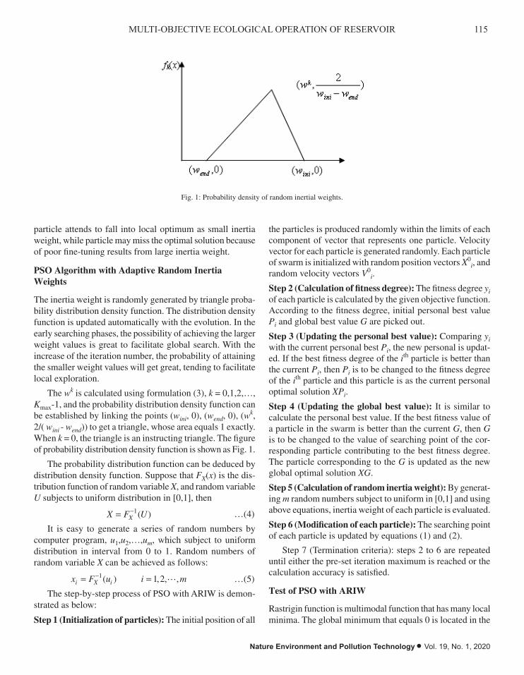
115MULTI-OBJECTIVE ECOLOGICAL OPERATION OF RESERVOIR
Nature Environment and Pollution Technology • Vol. 19, No. 1, 2020
particle attends to fall into local optimum as small inertia weight, while particle may miss the optimal solution because of poor fine-tuning results from large inertia weight.
PSO Algorithm with Adaptive Random Inertia Weights
The inertia weight is randomly generated by triangle proba-bility distribution density function. The distribution density function is updated automatically with the evolution. In the early searching phases, the possibility of achieving the larger weight values is great to facilitate global search. With the increase of the iteration number, the probability of attaining the smaller weight values will get great, tending to facilitate local exploration.
The wk is calculated using formulation (3), k = 0,1,2,…, Kmax-1, and the probability distribution density function can be established by linking the points (wini, 0), (wend, 0), (wk, 2/( wini - wend)) to get a triangle, whose area equals 1 exactly. When k = 0, the triangle is an instructing triangle. The figure of probability distribution density function is shown as Fig. 1.
The probability distribution function can be deduced by distribution density function. Suppose that FX(x) is the dis-tribution function of random variable X, and random variable U subjects to uniform distribution in [0,1], then
X F UX= -1( ) …(4)
It is easy to generate a series of random numbers by computer program, u1,u2,…,um, which subject to uniform distribution in interval from 0 to 1. Random numbers of random variable X can be achieved as follows:
x F u i mi X i= =-1 1 2( ) , , , …(5)
The step-by-step process of PSO with ARIW is demon-strated as below:
Step 1 (Initialization of particles): The initial position of all
the particles is produced randomly within the limits of each component of vector that represents one particle. Velocity vector for each particle is generated randomly. Each particle of swarm is initialized with random position vectors X0
i, and random velocity vectors V0
i.
Step 2 (Calculation of fitness degree): The fitness degree yi of each particle is calculated by the given objective function. According to the fitness degree, initial personal best value Pi and global best value G are picked out.
Step 3 (Updating the personal best value): Comparing yi with the current personal best Pi, the new personal is updat-ed. If the best fitness degree of the ith particle is better than the current Pi, then Pi is to be changed to the fitness degree of the ith particle and this particle is as the current personal optimal solution XPi.
Step 4 (Updating the global best value): It is similar to calculate the personal best value. If the best fitness value of a particle in the swarm is better than the current G, then G is to be changed to the value of searching point of the cor-responding particle contributing to the best fitness degree. The particle corresponding to the G is updated as the new global optimal solution XG.
Step 5 (Calculation of random inertia weight): By generat-ing m random numbers subject to uniform in [0,1] and using above equations, inertia weight of each particle is evaluated.
Step 6 (Modification of each particle): The searching point of each particle is updated by equations (1) and (2).
Step 7 (Termination criteria): steps 2 to 6 are repeated until either the pre-set iteration maximum is reached or the calculation accuracy is satisfied.
Test of PSO with ARIW
Rastrigin function is multimodal function that has many local minima. The global minimum that equals 0 is located in the
Fig. 1: Probability density of random inertial weights.

116 Hai-tao Chen et al.
Vol. 19, No. 1, 2020 • Nature Environment and Pollution Technology
position X* = (0,0,..,0). Rastrigin function with n dimension is described as follows:
f X x x xd dd
n
d( ) ( cos( ) ) . .= - + - < <=
 2
1
10 2 10 5 12 5 12p
…(6)
In this paper, suppose that the test functions are 10 dimen-sional; size of the swarm is N=30; the maximal velocity is 10; PSO other parameters c1=c2=2.0, wini=0.9, and wend=0.4. In order to compare the performance for the PSO with ARIW, standard PSO with LDW and GA, three testing methods are suggested. Firstly, on the condition of the given calculation accuracy, compare the number of iterations. In the paper, number of iterations is Kmax=10000, and models will be run for 100 trials. The average of iteration numbers is taken as the index to evaluate efficiency in different methods. Secondly, giving the maximal evolutionary generations, analyse the calculation accuracy in different algorithms. At last, on the condition of the same parameters and accuracy, calculate and compare the probability of achieving to the global optimum by 100 trials.
According to the given parameters, probability distri-bution function and corresponding density function, which are used to generate random inertia weight, are evaluated as follows:
F x
x
x x
x0
2
0 0 4
4 0 4 0 4 0 9
1 0 9
( )
.
( . ) . .
.
=
£
- < £>
Ï
ÌÔ
ÓÔ
…(7)
F x x x01 0 4 0 5 0 1- = + £ £( ) . . …(8)
F x
x
wx
wx
wx w
w
k
k k kk
( )
.
.
.
.
.
..
.
=
£
--
-+
-< £
--
0 0 4
2
0 4
1 6
0 4
0 32
0 40 4
2
0 9
2
kk k
k
kkx
wx
w
ww x
x
2 3 6
0 9
0 72
0 90 9
1 0 9
+-
-+-
< £
>
Ï
Ì
ÔÔÔ
Ó
ÔÔÔ
.
.
.
..
.
…(9)
F xx w x w
x wk
k k
k
- =+ - £ £ -
- - -
1 0 4 0 5 0 4 0 2 0 4
0 9 0 5 1 0 9 2( )
. . ( . ) ( . )
. . ( )( . ) (( . )w xk - £ £
ÏÌÔ
ÓÔ 0 4 1
…(10)
Where, k = 1,2,…,Kmax-1.
The test results by three methods are presented in Table 1 and Table 2.
The data in these tables show clearly that the PSO with ARIW can reach the best solution, with least number of function evaluations and higher precision as compared to other models. The detailed discussion is following:(1) It is very clear to know that the PSO with ARIW in performance is better than other algorithms, by three dif-ferent testing methods, according to the results of Tables 1 to 2. Particularly, when the accuracy demanded is same, the number of iterations calculated by ARIW mechanism is much less than the calculation number by LDW. Algorithm based on the ARIW mechanism can automatically regulate suitable weight for each particle, by the evolution process.(2) The best results calculated by PSO with ARIW in 100 tri-als are picked out. For Rastrigin function, the best solution is X* = 3.586×10⁻¹⁰, 4.732×10⁻¹¹, -4.675×10⁻¹⁰, -4.321×10-
10, -5.794×10⁻¹⁰, 3.635×10⁻¹¹, 4.299×10⁻¹⁰, 9.017×10⁻¹¹, 4.118×10⁻¹⁰, 4.711×10⁻¹¹),and the global minimum is f(X*) = 0.0000. By comparing with theory optimum of testing functions, the calculation outcomes are satisfied.
APPLICATION OF THE IMPROVED PSO
Introduction of Panjiakou Reservoir
To calculate the practical effect of the proposed model, an existing reservoir, namely Panjiakou Reservoir, was taken up as a case study. The Panjiakou Reservoir is in the main-stream of the Luanhe River, in Hebei province, China. The reservoir has the total storage capacity of 29×108 m3 and the water-spread area at full reservoir level is about 70 km2. The Panjiakou Reservoir is multipurpose and serves for flood control, water supply, hydropower generation and ecological water demand of river. In these served objects, hydropower generation subjects to water supply. Only during the pro-cess of water supply, hydropower is generated according to the discharge and water level of the reservoir. The detailed information related to regulation of Panjiakou Reservoir is described below:
(1) The process of water demand: The primary areas of water supply from Panjiakou Reservoir are Tianjian and
Table 1: Comparison of evolution generations among different methods at certain accuracy.
Accuracy GA LDW ARIW
1 6645 5794 4718
Table 2: Comparison of accuracy among different methods at certain evolution generations.
Iterations number GA LDW ARIW
2000 2.8465 2.7173 2.4844

117MULTI-OBJECTIVE ECOLOGICAL OPERATION OF RESERVOIR
Nature Environment and Pollution Technology • Vol. 19, No. 1, 2020
Tangshan, which are the important cities. According to the data of actual monthly water supply from 1983 to 2002, the averages of monthly water supply for many years are evaluated as given in Table 3.
(2) The ecological water demand of Luanhe River: In the paper, ecological water demand of each month was evaluated using Tennant methods, considering ecolog-ical base flow, the river evaporation and water leakage and so on. The monthly ecological water demand is calculated as given in Table 4.
(3) Rules of flood control of Panjiakou Reservoir: In major flood period (21 July~15 August), if the water level of reservoir is below 216 m, the main task is storing water, with ensuring the water demand of downstream; while the water level is between 216 to 222 m, reservoir dis-charges flood steadily by the 10000 m3/s; when the water level is in the interval from 222 to 225 m, the release of reservoir is controlled by the 28000 m3/s; and while the water level is beyond 225 m, all flood discharge facilities of reservoir are opened entirely.
In later flood season (16 August~30 September), the water level raised gradually to 222 m from 16 August to 31 August, and the highest water level of reservoir can be controlled in 225 m from 1 September to 30 September.
(4) Water leakage and evaporation of reservoir: By ob-servation and experience of many years for Panjiakou Reservoir, the water leakage and evaporation can be estimated to be about 16.4 ×10⁴ m3 every day.
Mathematical Model Formula
The two objectives considered in the model are minimization of the deficits for water supply and ecological water of river, and the regulation rules of flood control are taken as one of the constraints. Because of the limitation of water storage in reservoir, the two objectives are conflicting. To handle these multipurpose, a weighted approach is adopted in this study. By giving the weights to the objects, multipurpose problem is transferred to single objective question. The object function is following:
ob min= ◊ + ◊( ( , , , ) ( , , , ))2a f x x x b g y y ym m1 2 1 …(11)
Where, f x x xm( , , , )1 2 is object of water supply, which reflects the comprehensive extent of water deficits for water supply, and is calculated by the following equation.
f x x x x wm i ii
m
( , , , ) ( - )212
1
==Â …(12)
Where, xi is the actual water supply of each calculation period (108 m3); wi is the water demand of each period (108 m3); and m=18, is the number of calculation periods. From July to September, the length of calculation period is 10 days, and the rest calculation periods are evaluated by the interval of a month. g(y1,y2,…,ym) is the ecological water object, reflecting the integral deficits extent of ecological water, and is evaluated as follows:
g y y y y sm i ii
m
( , , , ) ( - )212
1
==Â …(13)
Where, yi is the actual water released to the river in each calculation period (108 m3); si is the ecological water demand of river in each period (108 m3); the number of calculation periods m=18. a, b are the weight coefficients, represent the importance of object s for decision maker subject to the following constrains:
(1) Water level of reservoir:
Z Z Zi i imin, ,£ £ max …(14)
Where, Zi is water level of the ith calculation period (m); Zmin,i is the allowed lowest water level (m); Zmax,i is the allowed highest water level (m).
(2) Discharge limits:
0 0£ £ £ £x w y qi i i max …(15)
Where, qmax is the discharge capacity of each period (108 m3).
(3) Mass balance equation:
V V Q q tt t t t+ = ◊ D1- ( - ) …(16)
Where, Vt+1 is the reservoir storage in the end of period (108 m3); Vt is the reservoir storage in the beginning
Table 3: Average of monthly water supply (108 m3) from Panjiakou Reservoir.
Month 1 2 3 4 5 6
Water 0.35 0.07 0.91 0.53 1.13 1.12
Month 7 8 9 10 11 12
Water 0.40 0.48 0.84 0.49 0.54 0.72
Table 4: Ecological water demand of Luanhe River (108 m3).
Month 1 2 3 4 5 6
Water 0.178 0.19 0.312 0.337 0.208 0.38
Month 7 8 9 10 11 12
Water 1.76 2.424 0.988 0.551 0.363 0.23

118 Hai-tao Chen et al.
Vol. 19, No. 1, 2020 • Nature Environment and Pollution Technology
of period (108 m3); Qt is the inflows average during the period (m3/s); qt is the release average during the period (m3/s); ⊿t is the length of calculation period.
(4) Rules of flood control: In flood season, reservoir regu-lations obey the rules of flood control.
Regulation Results
According to historical data of the inflows of Panjiakou Res-ervoir, three typical years were chosen, which respectively represent the low flow year, normal flow year and high flow year, and the periods corresponding to typical years are July 1981 to June 1982, July 1993 to June 1994, and July 1994 to June 1995. The multipurpose ecological regulation model of Panjiakou Reservoir is solved using PSO with ARIW, for three typical years.
(1) Low flow year: The inflows of Panjiakou reservoir in low flow year are given in Table 5.
The initial water level that is also the allowed lowest lev-el during regulation was 164.48 m, which was achieved by the end water level of reservoir in 30 June, 1981. Let the weight of water supply object=0.9, the weight of the object for ecological water=0.1. By PSO with ARIW, the regulation results of Panjiakou Reservoir are as given in Table 6.
Water deficits of each month are shown Figs. 2-3.
(2) Middle flow year: The inflows of Panjiakou Reservoir in middle flow year are presented in Table 7.
The initial water level that is also the allowed lowest level during regulation is 208.73 m, which is achieved by the end water level of reservoir on 30 June, 1993. Weights of the objects are same with values of low flow year, respectively. The regulation results of Panjiakou Reservoir are as given in Table 8.
Water deficits of each month in middle flow year are shown in Figs. 4-5.
(3) High flow year: The inflows of Panjiakou Reservoir in high flow year are as given in Table 9.
The initial water level that is also the allowed lowest level during regulation is 213.13 m, which is achieved by the end water level of reservoir on 30 June, 1995. Weights of tow objects are same with values of low flow year, middle flow year. Using the improved PSO to solve the regulation model of Panjiakou Reservoir, results are as given in Table 10.
According to the calculation results for three typical years, it is easy to draw the following conclusions: In high flow year, by optimal regulation for Panjiakou Reservoir, the requirement of water supply can be fulfilled, and the
Table 5: Inflows of Panjiakou Reservoir in low flow year.
No. Period Water (108 m3)
1 Early July 0.1520
2 Middle July 0.2220
3 Late July 0.5830
4 Early August 0.1587
5 Middle August 0.2546
6 Late August 0.2805
7 Early September 0.2297
8 Middle September 0.3030
9 Late September 0.3887
10 October 0.7727
11 November 0.4821
12 December 0.3026
13 January 0.2268
14 February 0.2658
15 March 0.5704
16 April 0.6286
17 May 0.3537
18 June 0.8303
Table 6: Regulation results of Panjiakou Reservoir in low flow year.
PeriodWater supply(108 m3)
Ecological water(108 m3)
Water level(m)
Early July 0.1290 0.0066 164.4800
Middle July 0.1290 0.0766 164.4800
Late July 0.1419 0.4230 164.4800
Early August 0.1423 0.0000 164.4800
Middle August 0.1548 0.0834 164.4800
Late August 0.1703 0.0921 164.4800
Early September 0.2133 0.0000 164.4800
Middle September 0.2800 0.0066 164.4800
Late September 0.2800 0.0923 164.4800
October 0.2727 0.0208 168.6631
November 0.3793 0.0800 168.4064
December 0.4200 0.0217 166.5753
January 0.0205 0.0113 167.9942
February 0.0335 0.0728 169.0675
March 0.6875 0.0451 167.0107
April 0.1882 0.0555 170.1893
May 0.7393 0.0057 165.9912
June 0.8899 0.0465 164.4800

119MULTI-OBJECTIVE ECOLOGICAL OPERATION OF RESERVOIR
Nature Environment and Pollution Technology • Vol. 19, No. 1, 2020
Fig. 4: Water deficit of each month in middle flow year.
Fig. 5: Ecological water deficit of each month in middle flow year.
Table 7: Inflows of Panjiakou Reservoir in middle flow year.
No. Period Water (108 m3)
1 Early July 0.5235
2 Middle July 1.8023
3 Late July 2.2656
4 Early August 3.6091
5 Middle August 2.5993
6 Late August 1.2993
7 Early September 0.6274
8 Middle September 0.8672
9 Late September 0.5012
10 October 1.3479
11 November 0.9953
12 December 0.566
13 January 0.4085
14 February 0.4302
15 March 0.6186
16 April 1.0012
17 May 0.822
18 June 0.3161
Fig. 2: Water deficit of each month in low flow year.
Fig. 3: Ecological water deficit of each month in low flow year.
Table 8: Regulation results of Panjiakou Reservoir in middle flow year.
PeriodWater supply (108 m3)
Ecological water (108 m3)
Water level (m)
Early July 0.1290 0.3781 208.7300
Middle July 0.1290 1.6568 208.7300
Late July 0.1419 2.1057 208.7300
Early August 0.1548 3.4379 208.7300
Middle August 0.1548 2.4281 208.7300
Late August 0.1703 1.1109 208.7300
Early September 0.2800 0.3310 208.7300
Middle September 0.2800 0.5708 208.7300
Late September 0.2800 0.2048 208.7300
October 0.4057 0.1094 210.3341
November 0.4953 0.0953 210.9975
December 0.6104 0.0929 210.6496
January 0.2789 0.0593 210.6890
February 0.0561 0.0524 211.1973
March 0.9006 0.1893 210.2263
April 0.4742 0.0233 211.0741
May 1.0036 0.0562 210.5387
June 1.0856 0.0746 208.7300

120 Hai-tao Chen et al.
Vol. 19, No. 1, 2020 • Nature Environment and Pollution Technology
ecological water demand can be satisfied. Ecological water deficits are happened only in few periods in flood season. In these periods of deficit, as the inflows are less than ecological water demand, release flood by the inflow amount to keep current water level; in middle flow year, by regulation, the water needs in season can be mainly met, but water supply is lacking in non-flood season; in low flow year, water demands cannot be satisfied whether water supply or ecological water. By optimal calculation using improved PSO, the extent of water deficits will be flatted to reduce the destructions de-riving from water shortage.
ACKNOWLEDGEMENTS
This work was supported by the Key Scientific and Tech-nological Research Projects in Henan Province (Grants No. 192102110199).
REFERENCES
Bai, T., Wu, L.Z., Chang, J.X. and Huang Q. 2015. Multi-objective optimal operation model of cascade reservoirs and its application on water and sediment regulation. Water Resour. Manage., 29(3): 2751-2770.
Chang, J.X., Meng X.J. and Wang Z.Z. 2014. Optimized cascade reservoir operation considering ice flood control and power generation. J. Hy-drol., 519: 1042-1051.
Chang, J.X., Bai, T. and Huang Q. 2013. Optimization of water resources utilization by PSO-GA. Water Resour. Manag., 27(4): 3525-3540.
Chang, L.C. and Chang F.J. 2009. Multi-objective evolutionary algorithm for operating parallel reservoir system. Journal of Hydrology, 377: 12-20.
Chang, L.C., Chang, F.J. and Wang, K.W. 2010. Constrained genetic algorithms for optimizing multi-use reservoir operation. J. Hydrol., 390: 66-74.
Chen, X.N., Duan, C.Q., Qiu, L. and Huang, Q. 2008. Application of large scale system model based on particle swarm optimization to optimal allocation of water resources in irrigation areas. Transactions of the CSAE, 24(3): 103-106.
Cheng, C.T., Shen, J.J. and Wu, X.Y. 2012. Short-term hydroscheduling with discrepant objectives using multi-step progressive optimality algorithm. J. Am. Water Resour. Assoc., 48(3): 464-479.
Eberhart, D.E. and Kennedy, J. 1995. A new optimizer using particle swarm theory. In: Proc., 6th Symp. on Micro Machine and Human Science, IEEE Service Center, Piscataway, N.J.. 39-43.
Goldberg, D.E. 1989. Genetic Algorithms in Search, Optimization, and Machine Learning. Addison-Wiley, Reading, N.Y.
Hao, L.X., Sun, R.H. and Chen, L.X. 2014 Health assessment of river ecosystem in Haihe River Basin, China. Environmental Science, 35(10): 3692-3710.
Huang, W.C. and Yuan, L.C. 2004. A drought early warning system on real-time multi-reservoir operation. Water Resour. Res., 40(6): W06401.
Liu, P., Cai, X.M. and Guo, S.L. 2011. Deriving multiple near-optimal solutions to deterministic reservoir operation problems. Water Resour. Res., 47: W08506.
Oliveira, R. and Loucks, D.P. 1997. Operating rules for multi-reservoir systems. Water Resour. Res., 33(4): 839-852.
Shi, Y. and Eberhart, R.C. 1998. A modified particle swarm optimizer. In: Proceedings of the 1998 IEEE International Conference on Evolutionary Computation, IEEE Press. Pp. 69-73.
Table 9: Inflows of Panjiakou Reservoir in high flow year.
No. Period Water (108 m3)
1 Early July 0.3393
2 Middle July 0.5319
3 Late July 3.0473
4 Early August 5.9128
5 Middle August 1.8991
6 Late August 1.5059
7 Early September 1.0206
8 Middle September 0.6249
9 Late September 1.0583
10 October 2.6076
11 November 1.4466
12 December 0.7827
13 January 0.5594
14 February 0.4284
15 March 0.7688
16 April 0.9787
17 May 0.5485
18 June 0.9722
Table 10: Regulation results of Panjiakou Reservoir in high flow year.
PeriodWater supply
(108 m3)
Ecological
water (108 m3)
Water level
(m)
Early July 0.1290 0.1938 213.1300
Middle July 0.1290 0.3864 213.1300
Late July 0.1419 2.8874 213.1300
Early August 0.1548 5.7416 213.1300
Middle August 0.1548 1.7278 213.1300
Late August 0.1703 1.3175 213.1300
Early September 0.2800 0.7242 213.1300
Middle September 0.2800 0.3285 213.1300
Late September 0.2800 0.7619 213.1300
October 0.5510 0.4900 215.8820
November 0.3630 0.5400 216.7286
December 0.230 0.7200 216.3578
January 0.1780 0.3500 216.3274
February 0.1900 0.0700 216.5315
March 0.3120 0.9100 215.6712
April 0.3370 0.5300 215.7782
May 0.2080 1.1300 214.2832
June 0.3800 1.1200 213.2067

121MULTI-OBJECTIVE ECOLOGICAL OPERATION OF RESERVOIR
Nature Environment and Pollution Technology • Vol. 19, No. 1, 2020
Wardlaw, R. and Sharif, M. 1999. Evaluation of genetic algorithms for optimal reservoir system operation. Water Resour. Planning Manage., 125(1): 25-33.
Yang, G., Guo, S.L., Li, L.P., Hong, X.J. and Wang, L. 2016. Multi-objective operating rules for Danjiangkou reservoir under climate change. Water Resour. Manage., 30: 1183-1202.
Zhao, T.T.G. and Zhao, J.S. 2014. Improved multiple-objective dynamic programming model for reservoir operation optimization. Journal of
Hydroinformatics, 16(5): 1142-1157. Zhao, J.S., Cai, X.M. and Wang, Z.J. 2011. Optimality conditions for a
two-stage reservoir operation problem. Water Resour. Res., 47: W08503Zhang, Y.Z., Huang, W.D. and Wang, Z.Y. 2015. Evaluation of aquatic
ecosystem health in Aojiang Basin, Fujian Province. Journal of Lake Science, 27(6): 1079-1086.
Zheng, J., Yang, K. and Ni, F.Q. 2013. Research on overall improved genetic algorithm applied in optimal operation. J Hydra. Eng., 44(2): 205-211.

Vol. 19, No. 1, 2020 • Nature Environment and Pollution Technology
122

Macroscopic Factors Decomposition of Methane Emissions from Livestock Based on the Empirical Analysis of 31 Provinces in China
Wenjie Yao*† and Huili Wang***Research Institute of Water Culture and Resources Economy, Zhejiang University of Water Resources and Electric Power, Hangzhou, 310018, China**School of Economy and Management, Zhejiang University of Water Resources and Electric Power, Hangzhou, 310018, China†Corresponding author: Wenjie Yao
ABSTRACT
This paper builds a factor decomposition model of methane emissions from livestock from the three dimensions of technology, economy and population, by using the panel data covering 31 provincial regions in China during 2003-2016, and aims to reveal the macroscopic causes of methane emissions from livestock. The research shows that technical, economic and population factors of methane emissions from livestock have diminishing marginal contribution. The methane emissions from intestinal fermentation is mainly restricted by livestock’s physiological structure. Following increase or decrease of livestock feeding quantity, it changes with a relatively stable parameter and has little controllability. Methane emissions from faecal management is limited little by livestock’s physiological structure and it is largely controllable. The government should increase technical input to reduce methane emission factors of livestock, deal with livestock manure through resource utilization, and reduce raising scale by using a certain market mechanism in due course.
INTRODUCTION
Since the beginning of the new century, animal husbandry, as the most dynamic pillar industry in China’s agricultural economy, has achieved rapid development again with increasing policy support. According to China Statistical Yearbook (2017), by 2016, the output value of animal husbandry in China (excluding Taiwan, Hong Kong and Macao) had accounted for 28.3% of the total agricultural output value and 4.2% of the total GDP. At the end of the year, the stock of cattle, goats and sheep had reached 106.679 million head, 139.769 million head and 161.351 million head respectively, and the number of pigs kept and raised had reached 435.037 million and 685.02 million respectively. However, the rapid growth of animal husbandry inevitably brought about some environmental problems, especially the emissions of carbon dioxide, methane, nitrous oxide and other greenhouse gases that cause global warming. Livestock accounts for an estimated 18 percent of global greenhouse gas emissions (Fao 2006). Methane contributes 15 percent of global warming to greenhouse gases (Dui 2003), and although it emits less overall than carbon dioxide, the greenhouse effect of the same volume is 20 to 25 times that of carbon dioxide (Shengli et al. 2010). Methane emissions from livestock mainly come from intestinal fermentation
and faecal management (Chianese et al. 2009). With the substantial increase of livestock feeding quantity, methane emissions from livestock also increases year by year. According to statistics, global methane emissions were 5.5 ×10⁸ tons, while livestock methane emissions were 8.5 ×10⁷ tons, accounting for 15.5% (Mcginn et al. 2006), and cattle and sheep were the largest emitters. In China, methane emissions from livestock that are fermented in the gut alone account for 29.7 percent of total methane emissions, excluding those from manure management (Renhua 2010). Therefore, it is extremely urgent for China to establish low-carbon production mode of animal husbandry and promote energy conservation and emission reduction to cope up with climate change.
Carbon dioxide emissions have been paid great attention by researches on greenhouse gas emissions that cause climate change. In spite of this, still some scholars remain highly alert to persistent warming caused by methane emissions from livestock. Taking cows, sheep and other major methane emitters as research objects, many workers analysed the bio-logical and chemical mechanism of methane emissions from intestinal fermentation and faecal management, calculated the corresponding emission factors by various methods, and finally proposed scientific methods to curb methane
Nat. Env. & Poll. Tech.Website: www.neptjournal.com
Received: 16-05-2019Accepted: 22-07-2019
Key Words:Methane emissionsLivestockFactor decompositionPopulation
2020pp.123-132 Vol. 19
p-ISSN: 0972-6268 No. 1 Nature Environment and Pollution Technology An International Quarterly Scientific Journal
Original Research Paper
e-ISSN: 2395-3454
Open Access

124 Wenjie Yao and Huili Wang
Vol. 19, No. 1, 2020 • Nature Environment and Pollution Technology
emissions from livestock at the micro level (Bo et al. 2009, Min et al. 2013, Zhi et al. 2017, Yunlong et al. 2018). Some scholars, like Jing et al. (2012) after subdividing the livestock categories, found that the number of pigs, cows, sheep and other livestock had a significant impact on methane emis-sions through regression analysis of the number of livestock raised in China in the past 20 years, so as to determine the reasonable path for the low-carbon development of animal husbandry in China. At the macro level, however, what causes methane emissions from livestock? How to combine the micro-level scientific methods to control methane emis-sions from livestock for effective policy regulation? To these questions, the existing literature so far has little discussion. Therefore, we used panel data of 31 provinces in China from 2003 to 2016 to construct decomposition models from three dimensions of technology, economy and population, aiming at revealing the cause of methane emissions of livestock, to supplement the strength of macro explanation in addition to micro explanation. This is of great significance for China to improve the efficiency of livestock breeding, optimize the strategy of reducing greenhouse gas emission and promote the sustainable development of animal husbandry.
MATERIALS AND METHODS
Econometric Model
The study on the decomposition of factors influencing en-vironmental variation began with the IPAT model proposed by Ehrlich P. R. and Holdren J. P. The basic form of this model is as follows:
I P A T= ◊ ◊ …(1)
Here, I, P, A and T respectively stand for environmental indicator, population indicator, economic indicator and tech-nical indicator. The combination of population and economy will cause great environmental pressure, which must be alleviated through technical adjustment. Later, in order to facilitate empirical analysis, Yorker et al. (2002) proposed the following STIRPAT model based on IPAT model.
I a P A Tb c d= ◊ ◊ ◊ ◊m …(2)
Here, a represents constant term, b, c, d are the exponents of P, A, T, and μ represents error term.
So far, both the models have been widely used, mainly focusing on the decomposition of the influencing factors of carbon emission (Ang et al. 1998, Zhang 2000, Pou-manyvong & Kaneko 2010, Qiang et al. 2012, Xiao & Yaohui 2012, Zhangqi et al. 2018) and industrial emission (Nan & Weiyang 2016, Ling et al. 2017), but empirical analysis of agricultural non-point source pollution (Yuzhuo et al. 2017, Yigen et al. 2017) is rare. Based on the existing empirical studies, we will decompose and investigate the influencing factors of methane emissions from livestock based on the
two models. Firstly, according to equation (1), the decom-position form of influencing factors of methane emissions from livestock is set as below:
MM
A
A
A
A
Y
Y
PP
n
n
g
g= ◊ ◊ ◊ ◊ …(3)
Here, M is methane emissions from livestock, An is animal husbandry output value, Ag is total agricultural output value, Y is total output value, and P is population. We set M (methane emissions from livestock) as an environmental indicator, MPA = M/An (methane emissions from livestock per unit animal husbandry output value) as a technical indi-cator, AAP = An/Ag (proportion of animal husbandry output value in total agricultural output value) and AGP = Ag/Y (proportion of total agricultural output value in total output value) as economic structure indicators, PGDP = Y/P (per capita total output value) as an economic scale indicator, and POP = P (population) as a population indicator. Secondly, according to equation (2), the decomposition form of influ-encing factors of methane emissions from livestock can be further obtained as follows:
M MPA AAP AGP PGDP POP= ◊ ◊ ◊ ◊ ◊ ◊a da a a a a0
1 2 3 4 5
…(4)
Here, a0 is a constant term, a1, a2, a3, a4, a5 are the indices of MPA, AAP, AGP, PGDP, POP, respectively, and d is a random error. After taking the logarithm form of both sides of the equal sign, equation (4) is changed into as below:
ln ln ln ln ln
ln ln ln
M MPA AAP AGP
PGDP POP
= + + ++ + +a a a a
a a d0 1 2 3
4 5 …(5)
Method for Estimating Methane Emissions from Livestock
There are two main sources of methane emissions from livestock, namely, intestinal fermentation and faecal man-agement, so a set of equations can be set as follows:
M M M= +1 2 …(6)
M u Qi ii
n
11
= ◊( )=Â …(7)
M v Qi ii
n
21
= ◊( )=Â …(8)
Here M1 and M2 are respectively methane emissions from intestinal fermentation and methane emissions from faecal management, ui is the intestinal fermentation methane emission factor of category i livestock, vi is the faecal man-agement methane emission factor of category i livestock, and Qi is the feeding quantity of category i livestock.

125FACTORS DECOMPOSITION OF METHANE EMISSIONS FROM LIVESTOCK
Nature Environment and Pollution Technology • Vol. 19, No. 1, 2020
Methane emissions from livestock are estimated to in-volve cattle, horse, donkey, mule, camel, pig, goat and sheep in eight categories. The feeding cycle of 7 kinds of livestock other than pig is long, and the amount of livestock raised at the end of every year is small, so the amount of livestock kept at the end of every year is used to indicate the feeding quantity. The feeding cycle of pig is generally 180 days, and the feeding quantity is calculated by adding up the annual output and annual stock at the end of every year. The data of the amount of 8 categories of livestock kept and raised at the end of every year are all derived from China Statistical Yearbook from 2004 to 2017. The methane emission factors of intestinal fermentation and faecal management of all kinds of livestock were mostly taken from IPCC Guidelines for National Greenhouse Gas Inventories (2006) in existing researches. In order to better adapt to the actual situation of each province in China, we refer to Provincial Greenhouse Gas Inventory Compilation Guide (Trial) (China National Development and Reform Commission, 2011) compiled by the Climate Division of China National Development and Reform Commission, as given in Table 1 and Table 2.
It should be noted that the methane emission factors of intestinal fermentation of cattle or sheep in different feeding methods in Table 1 are not consistent. Because it is difficult to count the number of cattle or sheep in each province under various feeding methods, and the cattle and sheep in China are still mainly raised by grazing, we decide to adopt the methane emission factors of intestinal fermentation of cattle and sheep under grazing feeding. At the same time, still given that it is difficult to distinguish the number of cows, non-cows and buffaloes in a province, the mean value
Table 1: Methane emission factors of intestinal fermentation of livestock [kg/(h.a)].
Feeding way Cow Bull Water buffalo Sheep Goat Pig Horse Donkey/Mule Camel
Large-scale feeding 88.1 52.9 70.5 8.2 8.91 18 10 46
Cage-free feeding 89.3 67.9 87.7 8.7 9.4
Grazing feeding 99.3 85.3 - 7.5 6.7
Table 2: Methane emission factors of faecal management of livestock [kg/(h.a)].
District Cow Non-cow Buffalo Sheep Goat Pig Horse Donkey/Mule Camel
North 7.46 2.82 - 0.15 0.17 3.12 1.09 0.60 1.28
Northeast 2.23 1.02 - 0.15 0.16 1.12 1.09 0.60 1.28
East 8.33 3.31 5.55 0.26 0.28 5.08 1.64 0.90 1.92
South-central
8.45 4.72 8.24 0.34 0.31 5.85 1.64 0.90 1.92
Southwest 6.51 3.21 1.53 0.48 0.53 4.18 1.64 0.90 1.92
Northwest 5.93 1.86 - 0.28 0.32 1.38 1.09 0.60 1.28
of methane emission factors of intestinal fermentation of cow, non-cow and buffalo under grazing feeding in Table 1 (excluding the default term) is unified as the methane emis-sion factor of intestinal fermentation of cattle, and the mean value of methane emission factors of faecal management of cow, non-cow and buffalo in Table 2 (excluding the default term) is unified as the methane emission factor of faecal management of cattle. In addition, according to Provincial Greenhouse Gas Inventory Compilation Guide (Trial), in Table 2, North District consists of five provinces (Beijing, Tianjin, Hebei, Shanxi, Inner Mongolia), Northeast District consists of three provinces (Liaoning, Jilin, Heilongjiang), East District consists of seven provinces (Shanghai, Jiangsu, Zhejiang, Anhui, Fujian, Jiangxi, Shandong), South-central District consists of six provinces (Henan, Hubei, Hunan, Guangdong, Guangxi, Hainan), Southwest District consists of five provinces (Chongqing, Sichuan, Guizhou, Yunnan, Tibet), and Northwest District consists of five provinces (Shaanxi, Gansu, Qinghai, Ningxia, Xinjiang).
Other Variables
Methane emissions from livestock per unit animal husbandry output value is calculated by dividing methane emissions of livestock by animal husbandry output value. Proportion of animal husbandry output value in total agricultural output value is calculated by dividing animal husbandry output value by total agricultural output value. The data of animal husbandry output value, total agricultural output value, pro-portion of total agricultural output value in total output value, per capita total output value, and population are all directly derived from China Statistical Yearbook from 2004 to 2017.

126 Wenjie Yao and Huili Wang
Vol. 19, No. 1, 2020 • Nature Environment and Pollution Technology
RESULTS AND ANALYSIS
Estimation of Results and Comparative Analysis of Methane Emissions from Livestock
We estimated the methane emissions from all types of live-stock in China from 2003 to 2016. In order to facilitate the comparison among livestock categories, we calculated the means of methane emissions from intestinal fermentation and the means of methane emissions from faecal management of all kinds of livestock during 14 years, and the corresponding proportions, as given in Table 3.
Among the 8 types of livestock, cattle have the highest methane emissions from intestinal fermentation, about 10 times as much as pig, goat and sheep, and account for nearly 75% of all kinds of livestock. However, since the number of cattle is smaller than that of goats and sheep, and much smaller than that of pigs, obviously, high emission factor is the main reason for high emissions. Both goat and sheep are similar, and both have low emission factors, but both have a higher breeding, so their emissions are high. On the contrary, the emission factor of pig is the lowest, but the number of pigs is 9-10 times that of goats or sheep, so the emissions are almost no less than those of goat or sheep. Although the emission factors of horse, donkey, mule and camel are much higher than those of goat and sheep, the emissions of these four types of livestock are very low due to the small number of breeding, accounting for no more than 1% of all kinds of livestock.
Among the 8 types of livestock, pig has the highest methane emissions from faecal management, about 10 times as much as cattle, 100 times as much as goat, and account for nearly 90% of all kinds of livestock. Obviously, higher breeding is the main reason for high emissions, while high emission factor is the second. Cattle has the highest emission factor, and therefore has the high emissions, accounting for nearly 10% of all kinds of livestock. Both, goat and sheep are equivalent. Although both have a higher breeding, but have the lowest emission factors, so their emissions are low. On the contrary, the emission factors of horse, donkey, mule and
Table 3: Means and proportions of the methane emissions for various types of livestock in China from 2003 to 2016.
Livestock Cattle Horse Donkey Mule Camel Pig Goat Sheep
Methane emissions from intestinal fermentation
Quantity (10,000 t/a)
1,061.63 12.09 6.60 2.85 1.31 112.82 106.27 114.27
Proportion (%)
74.88 0.85 0.47 0.20 0.09 7.96 7.49 8.06
Methane emissions from faecal manage-ment
Quantity (10,000 t/a)
54.54 0.92 0.43 0.20 0.04 509.63 5.03 3.70
Proportion (%)
9.49 0.16 0.07 0.03 0.01 88.71 0.88 0.64
camel are all higher than those of goat and sheep. However, due to the low breeding, the emissions of these four types of livestock are very low. Except for horse, the proportions of these four types of livestock do not exceed 0.1% of all kinds of livestock.
Given that cattle, pig, goat and sheep are the main sources of methane emissions from livestock, we calculated the pro-portions of methane emissions from intestinal fermentation and the proportions of methane emissions from faecal man-agement of these four types of livestock in all districts and provinces of China in 2016, as given in Table 4 and Table 5.
The regions with the largest proportion of methane emissions from intestinal fermentation of cattle, pig, goat and sheep are southwest, south-central, southwest and north respectively and the provinces are Sichuan, Sichuan, Henan and Inner Mongolia respectively. This is determined by the breeding quantity of each major livestock under a certain animal husbandry structure. In general, southwest and south-central are the main regions for raising cattle and goat, south-central, east and southwest are the main regions for raising pig, and northwest and north are the main regions for raising sheep, each region accounting for more than 20% of the total emissions. Sichuan, Henan, Yunnan, Inner Mongolia and Tibet are the main provinces for raising cat-tle, Sichuan, Henan, Hunan, Shandong, Hubei, Yunnan and Guangdong are the main provinces for raising pig, Henan, Sichuan, Inner Mongolia, Shandong and Yunnan are the main provinces for raising goat, Inner Mongolia, Xinjiang, Gansu, Qinghai, Shandong, Tibet and Hebei are the main provinces for raising sheep, each province accounting for more than 5% of the total emissions.
The regions with the largest proportion of methane emissions from faecal management of cattle, pig, goat and sheep are south-central, south-central, southwest and northwest respectively, and the provinces are Henan, Henan, Sichuan and Xinjiang respectively. This is deter-mined by the different emission factors in different regions in addition to the breeding quantity of each major livestock under a certain livestock husbandry structure. Overall, the

127FACTORS DECOMPOSITION OF METHANE EMISSIONS FROM LIVESTOCK
Nature Environment and Pollution Technology • Vol. 19, No. 1, 2020
Table 4: Proportions of the methane emissions from intestinal fermentation from major types of livestock in the regions of China in 2016 (%).
District Province Methane emissions from intestinal fermentation
Cattle Pig Goat Sheep
North
Beijing 0.15
11.28
0.39
8.04
0.13
16.95
0.26
34.34Tianjin 0.28 0.50 0.04 0.26
Hebei 3.71 4.69 3.36 5.68
Shanxi 1.00 1.07 2.60 3.39
Inner Mongolia 6.14 1.38 10.82 24.75
NortheastLiaoning 3.75
12.393.58
8.663.37
5.082.59
9.19Jilin 4.01 2.29 0.38 2.39
Heilongjiang 4.63 2.79 1.33 4.20
East
Shanghai 0.05
10.14
0.24
22.99
0.18
17.73
0.01
6.87
Jiangsu 0.28 4.05 2.82 0.06
Zhejiang 0.14 1.56 0.29 0.45
Anhui 1.57 3.88 4.69 0.01
Fujian 0.62 2.41 0.92 0.00
Jiangxi 2.83 4.21 0.44 0.00
Shandong 4.65 6.63 8.40 6.35
South-central
Henan 8.32
22.77
9.19
34.66
12.46
21.86
0.73
0.73Hubei 3.33 5.94 3.37 0.00
Hunan 4.28 8.80 3.79 0.00
Guangdong 2.19 5.01 0.31 0.00
Guangxi 3.92 4.91 1.46 0.00
Hainan 0.72 0.82 0.48 0.00
Southwest
Chongqing 1.36
28.43
3.07
21.71
1.55
25.75
0.00
7.50Sichuan 9.09 10.36 11.24 1.18
Guizhou 4.86 2.91 2.36 0.12
Yunnan 7.40 5.32 6.93 0.47
Tibet 5.72 0.05 3.67 5.73
Northwest
Shaanxi 1.39
14.99
1.76
3.94
3.97
12.64
0.76
41.38Gansu 4.19 1.12 2.91 9.11
Qinhai 4.53 0.23 1.31 7.49
Ningxia 1.06 0.15 0.80 2.91
Xinjiang 3.83 0.69 3.64 21.11
top three regions with the highest cattle emission factor are in turn south-central [7.14kg/(h.a)], east [5.73kg/(h.a)] and north [5.14kg/(h.a)], with the highest pig emission factor are in turn south-central, east and southwest, with the highest goat emission factor are in turn southwest, northwest and south-central, and with the highest sheep emission factor are in turn southwest, south-central and northwest. Thus, it can be seen that the large number of breeding mainly determines the high emissions of cattle breeding in south-west, goat breeding in south-central, and sheep breeding in northwest and north, the high emission factors mainly
determine the high emissions of cattle and goat breeding in south-central, and both the large number of breeding and the high emission factors determine the high emissions of pig in south-central, east and southwest and those of goat in southwest, each region accounting for more than 20% of the total emissions. Further, at the provincial level, the higher breeding mainly determines the high emissions of cattle breeding in Sichuan, Yunnan and other provinces, those of pig breeding in Sichuan, Shandong and other provinces, those of goat breeding in Henan, Shandong and other provinces, those of sheep breeding in Inner Mongolia, Gansu, Qinghai,

128 Wenjie Yao and Huili Wang
Vol. 19, No. 1, 2020 • Nature Environment and Pollution Technology
Table 5: Proportions of the methane emissions from faecal management from major types of livestock in the regions of China in 2016 (%).
District Province Methane emissions from faecal management
Cattle Pig Goat Sheep
North
Beijing 0.17
12.50
0.27
5.57
0.07
8.70
0.16
21.69Tianjin 0.31 0.35 0.02 0.16
Hebei 4.11 3.25 1.73 3.59
Shanxi 1.11 0.74 1.34 2.14
Inner Mongolia
6.80 0.96 5.55 15.64
NortheastLiaoning 1.31
4.340.89
2.151.63
2.451.64
5.80Jilin 1.40 0.57 0.18 1.51
Heilong-jiang
1.62 0.69 0.64 2.66
East
Shanghai 0.06
12.53
0.27
25.92
0.15
14.98
0.01
7.52
Jiangsu 0.35 4.57 2.39 0.06
Zhejiang 0.17 1.75 0.24 0.50
Anhui 1.94 4.37 3.96 0.01
Fujian 0.77 2.72 0.77 0.00
Jiangxi 3.49 4.75 0.37 0.00
Shandong 5.74 7.48 7.10 6.95
South-central
Henan 12.80
35.04
11.93
45.01
11.66
20.45
1.04
1.04Hubei 5.12 7.72 3.15 0.00
Hunan 6.59 11.43 3.54 0.00
Guangdong 3.38 6.50 0.29 0.00
Guangxi 6.04 6.37 1.36 0.00
Hainan 1.10 1.06 0.45 0.00
Southwest
Chongqing 1.10
22.99
2.85
20.14
2.48
41.20
0.00
15.16Sichuan 7.35 9.61 17.99 2.38
Guizhou 3.93 2.70 3.78 0.24
Yunnan 5.99 4.93 11.08 0.95
Tibet 4.62 0.05 5.87 11.58
Northwest
Shaanxi 1.17
12.59
0.54
1.21
3.84
12.21
0.90
48.79Gansu 3.52 0.34 2.82 10.74
Qinhai 3.81 0.07 1.26 8.83
Ningxia 0.89 0.05 0.77 3.43
Xinjiang 3.21 0.21 3.52 24.89
Shandong and other provinces. The high emission factors mainly determine the high emissions of cattle breeding in Henan, Inner Mongolia, Hunan, Guangxi, Shandong, Hubei and other provinces, those of pig breeding in Henan, Hunan, Hubei, Guangdong, Guangxi and other provinces, those of goat breeding in Sichuan, Yunnan, Tibet, Inner Mongolia and other provinces, those of sheep breeding in Xinjiang, Tibet and other provinces; each province accounting for more than 5% of the total emissions.
General Regression Results and Analysis
We made a general regression of the factors affecting methane emissions from livestock. Before the regression estimation, the variance inflation factor (VIF) was used to verify that the VIF values of all explanatory variables in the model were within the interval [1.00,4.50], far less than 10, and there was no multicollinearity. LSDV test showed that the individual effect of the panel data was obvious, indicating

129FACTORS DECOMPOSITION OF METHANE EMISSIONS FROM LIVESTOCK
Nature Environment and Pollution Technology • Vol. 19, No. 1, 2020
that mixed OLS regression should not be used. According to Hausman test, compared with fixed effect regression, random effect regression was more consistent with the statistical characteristics of the panel data. Therefore, we used the random effect regression results of clustering robust standard deviation, as provided in Table 6.
The results of Regression 1 show that the model fits well. The influence coefficient of each explanatory variable on methane emissions from livestock is within the range (0.8, 1), that is, the marginal contribution of technical, economic and population factors to environmental variation is decreasing, and higher the influence coefficient is, the smaller the rate of diminishing marginal contribution is. In fact, except for proportion of total agricultural output value in total output value, the influence coefficients of other explanatory vari-ables on methane emissions of livestock are all close to 1, with a very small rate of diminishing marginal contribution. Specifically, the impact coefficient of population on meth-ane emissions from livestock is the highest, indicating that expansion of consumption demand for livestock caused by increase of population is the most important reason for high methane emissions from livestock. The impact coefficient of methane emissions from livestock per unit animal hus-bandry output value on methane emissions from livestock is second only to population, and poor technology is not conducive to controlling methane emissions from livestock. The impact coefficient of per capita total output value on methane emissions from livestock is high, meaning that greater economic size drives livestock production growth and increases methane emissions from them. Proportion of animal husbandry output value in total agricultural output value and proportion of total agricultural output value in
total output value are two economic structural factors, the former undoubtedly has a higher influence coefficient on methane emissions of livestock than the latter, and the larger the proportion of livestock production value is, the larger the relative economic scale of livestock will be, and the higher the methane emissions of livestock will be.
In order to test the robustness of the regression model, we combine the two economic structure factors of proportion of animal husbandry output value in total agricultural output value (AAP) and proportion of total agricultural output value in total output value (AGP) into one, that is, proportion of animal husbandry output value in total output value (AAGP), and the calculation method is AAGP = An/Y. After testing, we used the random effect regression results of clustering robust standard deviation, as given in Table 6. The results of Regression 2 show that the sign and significance of the influence coefficient of each explanatory variable on meth-ane emissions from livestock are consistent with the results of Regression 1, and the values of each coefficient are only slightly changed, indicating that the results of Regression 1 are robust.
CLASSIFICATION REGRESSION RESULTS AND ANALYSIS
Furthermore, we made two separate regressions of the factors affecting methane emissions from livestock from intestinal fermentation and faecal management. For each regression, LSDV test showed that the individual effects of the panel data were obvious, indicating that mixed OLS regression should not be used. According to Hausman test, compared with random effect regression, fixed effect regression was
Table 6: Regression results for the methane emissions from livestock.
Influencing factors Regression 1 Regression 2
Coefficient Z-value Coefficient Z-value
lnMPA 0.985 6*** 45.89 0.981 1*** 43.55
lnAAP 0.959 0*** 30.02 - -
lnAGP 0.870 6*** 25.40 - -
lnAAGP - - 0.893 0*** 25.88
lnPGDP 0.966 6*** 50.01 0.963 9*** 42.77
lnPOP 0.998 9*** 44.47 0.992 9*** 39.47
Intercept -17.122 5*** -53.12 -12.769 1*** -38.85
Wald-Statistic 4 810.22*** 2 956.27***
Adj-R2 0.945 5 0.944 2
VIF 2.54 2.88
Observations 434 434
Note: ***, ** and * respectively indicate that the estimated results are significant at the levels of 1%, 5% and 10%, respectively; is the default.

130 Wenjie Yao and Huili Wang
Vol. 19, No. 1, 2020 • Nature Environment and Pollution Technology
more consistent with the statistical characteristics of the panel data. Therefore, we used the fixed effect regression results of clustering robust standard deviation, as provided in Table 7.
The results of each regression show that the model fits well. Each explanatory variable has a significant positive effect on methane emissions both from intestinal fermenta-tion and from faecal management. Differently, on the one hand, the influence coefficient of each explanatory variable on methane emissions from intestinal fermentation is close to 1, which indicates that methane emissions from intestinal fermentation is mainly restricted by livestock’s physiolog-ical structure. Following increase or decrease of livestock feeding quantity determined by each explanatory variable, it changes with a relatively stable parameter and has little controllability. On the other hand, the influence coefficient of each explanatory variable on methane emissions from faecal management is within the range (0.5, 0.8), lower than the influence coefficient of each explanatory variable on methane emissions from livestock in the results of Re-gression 1, and technical, economic and population factors all have diminishing marginal contribution, which indicates that methane emissions from faecal management is limited little by livestock’s physiological structure, and it is largely controllable. In fact, whether and to what extent methane emissions, both from intestinal fermentation and from faecal management, are constrained by livestock’s physiological structure can be reflected in methane emission factors of livestock. Table 1 and Table 2 show that the methane emission factors of intestinal fermentation are relatively stable, while those of faecal management have large regional differences.
DISCUSSION
Due to different degrees of constraints by livestock’s phys-
iological structure, it is necessary to distinguish methane emissions between from intestinal fermentation and from faecal management to control methane emissions from livestock at the macro level. To control methane emissions from intestinal fermentation, which is more restricted by livestock’s physiological structure, the primary task is to in-crease technical input to reduce methane emission factors of intestinal fermentation, and then reduce methane emissions from livestock per unit animal husbandry output value. First, through breeding and improvement, the level of yield per unit can be improved, and the number of livestock breeding can be reduced under the premise of meeting the established demand for livestock products. Second, the quantity and quality of food intake should be standardized, and the specific measures include promotion of straw silage and ammonification, rational preparation of fine/coarse ration of daily food, and appropriate use of nutritional additives. Third, the production of methane in the rumen can be inhibited by inhibiting methanogenic bacilli. In addition, to adjust economic structure in order to reduce proportion of animal husbandry output value in total agricultural output value, in turn, reduce proportion of total agricultural output value in total output value, or to shrink economic scale in order to reduce per capita total output value, or to control population size to reduce population, will have a negative impact on the overall economic quality, and thus is not desirable. For the areas with a large stock of livestock, reducing scale of breeding may be the most direct and effective measure, but the policy of prohibition and restriction should be avoided, and it can be solved through a certain market mechanism, that is, taxes can be levied on the ruminant animal (cattle, goat or sheep) husbandry industry, on the one hand, to promote industrial substitution from the supply side, and on the other hand, to encourage reduction of meat consumption from the demand side.
Table 7: Regression results for the methane emissions from intestinal fermentation and faecal management.
Influencing factorsMethane emissions from intestinal fermentation
Methane emissions from faecal management
Coefficient T-value Coefficient T-value
lnMPA 1.107 3*** 16.95 0.600 0*** 5.90
lnAAP 0.995 9*** 11.28 0.786 6*** 6.65
lnAGP 0.989 0*** 9.05 0.615 1*** 8.47
lnPGDP 1.032 1*** 13.85 0.711 0*** 7.21
lnPOP 1.117 8*** 5.40 0.526 5*** 2.89
Intercept -19.288 8*** -7.82 -11.908 2*** -4.85
F-Statistic 69.35*** 33.38***
Adj-R2 0.875 7 0.610 2
Observations 434 434
Note: ***, ** and * indicate that the estimated results are significant at the levels of 1%, 5% and 10%, respectively.

131FACTORS DECOMPOSITION OF METHANE EMISSIONS FROM LIVESTOCK
Nature Environment and Pollution Technology • Vol. 19, No. 1, 2020
The diminishing marginal contribution of technological level, economic structure, economic scale and population scale essentially reflects the effective role of some external forces in controlling methane emissions from faecal manage-ment. Due to small degree of restriction by livestock’s phys-iological structure, in the exogenous factors of controlling methane emissions from manure management, it is very important to deal with livestock manure through resource utilization, and using biogas project to recover methane is particularly effective. Enterprises or farmers should be given a certain subsidy for purchase and construction of biogas facilities according to livestock type and breeding scale, at the same time, fines should be imposed for illegal discharge and release of livestock waste. Of course, methane emissions from livestock per unit animal husbandry output value could still be reduced by investing more in technology to reduce methane emission factors of faecal management. There are two specific ways: first, to reduce faecal production through scientific selection of feed, precise control of food, the use of feed additives and other methods; second, to realize updating and upgrading of the technology for cleaning up faeces by changing water flushing and blisters into dry cleaning or adopting automatic dry and wet separation to clean.
CONCLUSION
Finally, we came to five conclusions. Firstly, the methane emissions of four main types of livestock are different in categories. Large number of breeding is the main reason for high emissions of pig, goat and sheep, and high emission factor is the main reason for high emissions of cattle. Sec-ondly, the methane emissions of four main types of livestock are different in regions. Methane emissions from intestinal fermentation is determined by breeding quantity of each ma-jor livestock under a certain animal husbandry structure, and methane emissions from faecal management is determined by different emission factors in different regions in addition to breeding quantity of each major livestock under a certain livestock husbandry structure. Thirdly, in general, technical, economic and population factors of methane emissions from livestock have diminishing marginal contribution. Fourthly, methane emissions from intestinal fermentation are mainly restricted by livestock’s physiological structure. Following, increase or decrease of livestock feeding quantity, it changes with a relatively stable parameter and has little controllabil-ity. Methane emissions from faecal management is limited little by livestock’s physiological structure, and it is largely controllable. Fifthly, in order to control methane emissions from intestinal fermentation, technical investment should be increased to reduce methane emission factors of intestinal fer-mentation and a certain market mechanism should be used in due course to reduce raising scale. In order to control methane
emissions from faecal management, it is very important to deal with livestock manure through resource utilization, but technical input should still be increased to reduce methane emission factors of faecal management.
REFERENCES
Ang, B.W., Zhang, F.Q. and Choi, K.H. 1998. Factorizing changes in energy and environmental indicators through decomposition. Energy, 23(6): 489-495.
Bo, Z., Rongzhen, Z. and Zhiliang, T. 2009. Methane emission and abatement strategy in animal husbandry. Chinese Journal of Eco-Agriculture, 17(4): 811-816
Chianese, D.S., Rotz, C.A. and Richard, T.L. 2009. Whole-farm greenhouse gas emissions: A review with application to a Pennsylvania dairy farm. Applied Engineering in Agriculture, 25(3): 431-442
China National Development and Reform Commission 2011. Provincial Greenhouse Gas Inventory Compilation Guide (Trial). The Climate Division of China National Development and Reform Commission, Beijing, China
Dui, W. 2003. Greenhouse gases and greenhouse effect. China Meteorological Press, Beijing, China
Ehrlich, P.R. and Holdren, J.P. 1971. Impact of population growth. Science, 171 (3977): 1212-1217.
Fao, 2006. Livestock a major threat to the environment: Remedies urgently need-ed. Available at: http://www.fao.org./newsroom/en/news/2006/1000448/index.html
Jing, Z., Junna, Z. and Rongrong, D. 2012. Path selection for low-carbon development of animal husbandry in China: Based on regression analysis of emission sources of animal husbandry to methane growth. Guangxi Social Science, 9: 50-54.
Ling, B., Lei, J. and Yaobin, L. 2017. Spatio-temporal characteristics of environ-mental pressures of the urban agglomeration in the middle reaches of the Yangtze River: A case study based on industrial SO2 emissions. Economic Geography, 37(3): 174-181.
McGinn, S.M., Flesch, T.K., Harper, L.A. and Beauchemin, K.A. 2006. An approach for measuring methane emissions from whole farms. Journal of Environmental Quality, 35(1): 14-20.
Min, G., Honglian, H. and Ruiping, D. 2013. Ruminant methane emission and emission reduction strategies. Chinese Journal of Animal Science, 49(18): 35-41.
Nan, H. and Weiyang, Y. 2016. Spatial characteristics and influencing fac-tors of industrial waste gas emission in China. Scientia Geographica Sinica, 36(2): 196-203.
Poumanyvong, P. and Kaneko, S. 2010. Does urbanization lead to less energy use and lower CO2 emissions? A cross-country analysis. Ecological Economics, 70(2): 434-444.
Qiang, D., Qiao, C. and Ning, L. 2012. Forecast of China’s carbon emis-sions based on modified IPAT model. Acta Scientiae Circumstantiae, 32(9): 2294-2302.
Renhua, N. 2010. Effects of diet composition on methane and nitrogen emissions from lactating cattle. Chinese Academy of Agricultural Sciences, Beijing, China.
Shengli, L., Jin, X., Fan, X., Huang, W. and Cao, Z. 2010. Ruminant pro-duction and carbon emission reduction measures. Chinese Journal of Animal Nutrition, 22 (1): 2-9.
Xiao, G. and Yaohui, Z. 2012. Influence factors and environmental Kuznets curve relink effect of Chinese industry’s carbon dioxide emission: Empirical research based on STIRPAT model with industrial dynamic panel data. China Industrial Economics, 1: 26-35
Yigen, W., Kaiwen, F. and Gucheng, L. 2017. Population growth, structural adjustment and agricultural non-point source pollution: An empirical study based on STIRPAT model of spatial panel. Journal of Agrotech-nical Economics, 3: 75-87.

132 Wenjie Yao and Huili Wang
Vol. 19, No. 1, 2020 • Nature Environment and Pollution Technology
Yorker, R., Rosae, E. A. and Dietz, T. 2002. Bridging environmental science with environmental policy: Plasticity of population, affluence, and technology. Social Science Quarterly, 83(1): 18-31.
Yunlong, L., Bing, W., Qiyu, D. et al. 2018. Study on the methane emission pattern and the methane inhibition methods in sheep. Feed Industry, 39 (15):43-47.
Yuzhuo, S., Gangyi, W., Xinhui, W. et al. 2017. Analysis of water’s nitro-gen pollution caused by hog industry agglomeration: Based on the analytical framework of IPAT. Chinese Journal of Animal Science, 53 (11): 117-122.
Zhangqi, Z., Lei, J., Lingyun, H., Zheng, W. et al. 2018. Global carbon emissions and its environmental impact analysis based on a con-sumption accounting principle. Acta Geographica Sinica, 73(3): 442-459.
Zhang, Z.X. 2000. Decoupling China’s carbon emissions increase from economic growth: An economic analysis and policy implications. World Development, 28(4): 739-752.
Zhi, C., Tingning, W., Yang, L. et al. 2017. Methane emission of animal husbandry and reduction measures in Ningxia. Journal of Agricultural Sciences, 38(1): 7-9.

Field Research on Nitrogen Removal Performance of Aerobic Denitrifiers in Source Water Reservoir by Mixing Aeration
Zhou Zi-zhen*†, Huang Ting-lin**(***), Gong Wei-jin*, Li Yang*, Liu Yue*, Zhao Fu-wang*, Zhou Shi-lei**** and Dou Yan-yan* *School of Energy and Environment, Zhongyuan University of Technology, Zhengzhou, 450007, China**School of Environmental and Municipal Engineering, Xi’an University of Architecture and Technology, Xi’an, 710055, China***Key Laboratory of Northwest Water Resource, Environment and Ecology, MOE, Xi’an University of Architecture and Technology, Xi’an, 710055, China ****School of Environment Science and Engineering, Hebei University of Science and Technology, Shijiazhuang, 050018, China†Corresponding author: Zhou Zi-zhen
ABSTRACTChanges of total nitrogen (TN), organic matter, microbial metabolic activity, aerobic denitrifying bacteria and aerobic denitrifying genes (nirS and nirK) in water and surface sediments under mixing aeration were studied in Heihe Jinpen Reservoir. Results showed that compared with the control area, the total nitrogen concentration of water and surface sediments in the enhanced area decreased by 29.7%~49.2% and 17.9%. Metabolic activity of microorganisms increased by more than 14%, the utilization rate of carbon source increased by 30% and the McIntosh diversity index of microorganisms increased by 20%. The number of aerobic denitrifiers and genes of aerobic denitrifiers were also increased by 20%. Illumina high-throughput DNA sequencing results showed that the proportion of aerobic denitrifiers such as Acidovorax increased from 0.01% to 0.15%, showing an increase by 15 times. The production practice showed that mixed aeration can improve the metabolic activity and denitrification characteristics of indigenous aerobic denitrifiers, providing theoretical support and technical guarantee for denitrification and carbon removal of slightly polluted source water.
Nat. Env. & Poll. Tech.Website: www.neptjournal.com
Received: 18-05-2019Accepted: 22-07-2019
Key Words:Water reservoir Nitrogen Denitrification Microbial diversity
2020pp. 133-140 Vol. 19p-ISSN: 0972-6268 No. 1 Nature Environment and Pollution Technology
An International Quarterly Scientific Journal
Original Research Papere-ISSN: 2395-3454
Open Access
INTRODUCTION
More and more lakes and reservoirs have become the sources of drinking water in cities, and most lakes and reservoirs have problems of eutrophication of different degrees (Huang et al. 2014). Higher concentrations of nitrogen and phosphorus led to excessive algae reproduction, which not only endangers the aquatic ecosystem of lakes and reservoirs, but also threatens the safety of water supply. Excess nitrogen in the water also produced certain disinfection by-products, which directly affects human health (Kang et al. 2014). Physical, chemical and biological methods have been reported for nitrogen re-moval. However, both physical and chemical methods have problems of high cost and incomplete removal of nitrogen. More and more attention has been paid to biological nitrogen removal (Song et al. 2014, Sun et al. 2010, Patureau et al. 1998, Chen et al. 2015).
It is generally believed that nitrogen removal mainly de-pends on bacterial autotrophic nitrification and heterotrophic
denitrification, and nitrification was carried out under aerobic conditions; denitrification was carried out under anaerobic conditions, and finally nitrogen was formed to N2, achieving the purpose of removal (Patureau et al. 2001). Strict anaer-obic condition was required for denitrification, which made denitrification process difficult to be used in drinking water treatment. Robertson (1982) first reported aerobic denitrifica-tion at the beginning of 1980s. Aerobic denitrifying bacteria using oxygen and nitrate as electron acceptors provided a new perspective for biological denitrification of drinking water. Aerobic denitrification and nitrification existed si-multaneously in a system and can provide a certain basicity to balance the acidity produced by nitrification. Robertson separated aerobic denitrifying bacteria from desulfurization and denitrification wastewater treatment systems (Robertson et al. 1982). Other studies showed that aerobic denitrifying bacteria were also isolated from marine sediment (Gao et al. 2010) and constructed wetland system (Coban et al. 2015). In recent years, more and more aerobic denitrifying bacteria

134 Zhou Zi-zhen et al.
Vol. 19, No. 1, 2020 • Nature Environment and Pollution Technology
have been isolated from lake sediments: three aerobic de-nitrifying bacteria H-30, X-10 and C-30 with total nitrogen removal rate of more than 80% under laboratory conditions were separated by Kang et al. (2014); 14 strains with high aer-obic denitrification characteristics from reservoir sediments, mainly Acinetobacter spp. and Nova spp. were isolated and enriched by Zhou et al. (2016). The removal rates of TN (total nitrogen) and TOC (total organic matter) were 80.42% and 98.30% respectively. The isolation and screening of many aerobic denitrifying bacteria not only enriched and improved the theory of aerobic denitrification, but also laid a foundation for its engineering application (Huang et al. 2015, Xu et al. 2018, Epsztein et al. 2016, Alzate et al. 2016).
In order to improve the water quality, water-lifting aera-tors were installed in the reservoirs to supply oxygen to the water column, which provided a good experimental platform for the study of aerobic denitrification. Nitrate nitrogen concentration in the mixed aeration area decreased from 1.71 mg/L to 0.80 mg/L, and the TN removal rate reaching 38.33% were observed in a previous study (Zhou et al. 2016). Under the conditions of production scale of mixed aeration, the mechanism of water quality improvement, especially the removal of TN, was explored at the genetic level from the perspective of microorganisms, which provided theoretical support and technical support for the application of aerobic denitrifying bacteria in engineering and the nitrogen removal of water source reservoirs.
MATERIALS AND METHODS
Sampling Sites and Sampling Methods
As shown in Fig. 1, Heihe Jinpen Reservoir (latitude: 34°13′N- 34°42′N, longitude: 107°43′E-108°24′E) was
a canyon shaped reservoir located at the foot of Qinling Mountains. Heihe Jinpen Reservoir was the important drink-ing water source of Xi’an City (its water supply accounted for 80% of the total drinking water of Xi’an City). The total reservoir capacity of Heihe Jinpen Reservoir is 2.0 × 10⁸ m3 and the effective reservoir capacity is 1.8 × 10⁸ m3. The main function of the reservoir was water supply and auxiliary functions were flood control and irrigation. Eight water-lifting aerators were installed in the main reservoir area. Detailed introduction is given in the previous report (Zhou et al. 2017). Enhanced area was in the middle of the main reservoir area, which was affected by the operation of the water-lifting aerator, represented by E. The control area was about 2 km away from the main reservoir area, and was less affected by water-lifting aerator, represented by C, as shown in Fig. 1.
Water samples were drawn every 3 days. Water temper-ature, dissolved oxygen (DO) and pH were measured in situ by HACH DS5 multi-parameter water quality analyser. Water quality indicators such as total nitrogen (TN), nitrate nitro-gen, total phosphorus (TP) and total organic carbon (TOC) were measured in the reservoir field laboratory according to the “Water and Wastewater Monitoring and Analysis Meth-ods (4th edition)”. Surface sediments were sampled once a week with a columnar sampler. Surface sediments of 0.5 cm were sampled and stored at 4°C.
Methods for Determination of Chemical Indicators of Water and Sediments
TN and nitrate nitrogen were determined by AA3 continuous flowing analyser (SEAL, Germany); TOC was determined by TOC-L analyser of Shimadzu, Japan. Sediment samples were dried, ground and sifted. TN in sediments was digested
Fig. 1: Distribution map of mixing aeration area (Enhanced area) and reference area (Control area) of Heihe Jinpen Reservoir.

135NITROGEN REMOVAL PERFORMANCE OF AEROBIC DENITRIFIERS
Nature Environment and Pollution Technology • Vol. 19, No. 1, 2020
at 121°C for 1 hour and then determined by zinc-cadmium reduction spectrophotometry (Jiyeon et al. 2016). Organic matter in sediments was determined by potassium dichromate method (Jiyeon et al. 2016).
Methods for Determination of Microbial Metabolic Activity and Carbon Source Utilization
Microbial samples were collected at the same time as water samples for determination of chemical indicators. Microbial metabolic activity, carbon source utilization and McIntosh diversity index were measured by Biolog ECO microporous plate. Microbial metabolic activity was expressed by AWCD (average well colour development). AWCD = S(C590 - C
750)/31. Carbon source utilization (dimensionless) was calcu-lated by the average absorbance of microorganisms to each carbon source in each pore (Fang et al. 2016). For example, amino acid = (CL-arginine+ CL-asparagine+ CL-phenylalanine+ CL-ser-
ine+ CL-threonine+ CL-glutamic-acid)/6. McIntosh diversity index was also calculated by absorbance.
Aerobic Denitrifying Bacteria Count and Denitrifying Functional Gene Quantification
Through gradient dilution, the number of aerobic denitri-fying bacteria in enhanced area and control area was deter-mined by plate counting method. The preparation method of gradient dilution solution is as follows: 10-3, 10-4, 10-5, 10-6 and 0.2 mL diluent was added to solid denitrification screening medium (The composition of the medium was: CH3COONa, 0.10 g∙L-1; NaNO3, 0.02 g∙L-1; K2HPO4.3H2O, 0.02 g∙L-1; CaCl2, 0.01 g∙L-1; MgCl2.6H2O, 0.01 g∙L-1; agar, 20 g∙L-1, and the pH was adjusted to 7.2 (Kang et al. 2018). Culturing of bacteria was carried out for 5 days at 30°C, then counted and calculated.
The copies of denitrifying functional genes nirS and nirK were determined by quantitative PCR. 2-L water samples were filtered by 0.22 µm filter membrane and extracted by a rapid DNA kit. The amplification sequence of nirS and nirK genes is given in Table 1. QPCR was tested by ABI 7500 of Life Technologies, USA, and the amplification reaction method was found in the previous study (Zhou et al. 2016).
Illumina High Throughput Sequencing
2-L water sample was filtered by 0.22 µm filter membrane and stored at ultra-low temperature. The determination was completed by Meiji Biology in Shanghai.
Operating Conditions of Water-Lifting Aerator
Destroying water stratification and improving water quality was the purpose of the operation of water-lifting aerator. In this stage, the algal density of surface layer of the reservoir was only about 200×104 cells/L, which was quite low, and there was no control of algae. The compressed air flow rate of each water-lifting aerator was 30-40 m3/h, and the air supply of 8 water-lifting aerators was controlled in this range. During this researching period, 8 water-lifting aerators operated 24 hours a day, uninterruptedly. The power of the air compressor (Anruiko, Bengbu) was 132 kW, 2975 r/min, dual-purpose equipment.
RESULTS AND DISCUSSION
Changes of TN and Organic Compounds in Water and Surface Sediments
The basic situation of water quality in the control area and enhanced area before the operation of the water-lifting aer-ation system is given in Table 2. Before the operation of the system, water quality of the two areas tended to be consistent. For example, the results of October 10 water sample showed that the TN concentrations of the two areas were 1.81 mg∙L-1 and 1.70 mg∙L-1, respectively, and the difference between the two areas was only 0.11 mg∙L-1, with a difference of about 6%. The TOC concentrations of the two regions were almost the same. The density of aerobic denitrifying bacteria (ADB) was 4.34×10⁴ cfu∙mL-1 and 4.03×10⁴ cfu∙mL-1, re-spectively, with a difference of 7%. According to the above analysis, there was a slight difference in the concentrations of TN, TOC and aerobic denitrifying bacteria between the two areas before the operation of the aeration system, and the difference was less than 10%.
In this study, the surface water temperature in the en-hanced area decreased from 17.1°C (Oct-15) to 14.8°C (Nov-02), and the bottom water temperature increased from 10.1°C (Oct-15) to 14.3°C (Nov-02). DO increased from 0 mg∙L-1 (Oct-15) to 9.8 mg∙L-1 (Nov-02) in the enhanced area. While there was still a temperature difference of 6°C between the upper and lower water layers in the control area. On Nov-02, the concentration of DO in the control area was still 0 mg∙L-1 (Nov-02) in the bottom water, which indicated that the operation of the water-lifting aeration system accelerated the damage of water stratification and had a significant effect on mixing aeration.
Table 1: Primer sequences for gene amplification.
Gene Primer sequence
nirS cd3aF, 5′-GTSAACGTSAAGGARACSGG-3′
R3cd, 5′-GASTTCGGRTGSGTCTTGA-3′
nirK F1aCu, 5′-ATYGGCGGVCAYGGCGA-3′
R3Cu, 5′-GCCTCGATCAGRTTRTGGTT-3′

136 Zhou Zi-zhen et al.
Vol. 19, No. 1, 2020 • Nature Environment and Pollution Technology
The variations of TN and organic matter concentrations in the enhanced area during operation are given in Table 3. The DO concentration in the water body, especially in the bottom water, increased gradually with the operation of the system. After 19 days of operation, TN and TOC in different water layers in the enhanced area reduced sharply. The TN concentration in the bottom water body decreased from 2.36 mg∙L-1 to 1.20 mg∙L-1, with a reduction rate of 49.2%, and the TOC reduction rate in vertical water body also reached more than 22.5%. Compared with enhanced area, in the control area the highest removal rate of TN was only 7.7%, and the removal rate of TOC 6.5%.
Compared with the control area, the removal rate of TN and TOC in the enhanced area was higher. In order to further explore that where nitrogen and organic matter gone, surface sediment samples were also taken under the corresponding water column of the sampling site and their TN and OC were determined. As presented in Table 3, the concentration of TN and OC in surface sediment also decreased by 17.9% and 20.5% respectively. However, the concentration of TN and OC in surface sediment of the control area was almost the same.
Based on the above results, not only in the water, but also in the surface sediment nitrogen and organic matter in the enhanced area have been greatly reduced, and the accu-mulation of nitrite nitrogen was not found. Previous studies
showed that the activities of indigenous microorganisms and community structure have changed during this process, and the presence of aerobic denitrifying bacteria have been found. Biolog technology was used to explore metabolic activity of microorganisms in water and surface sediments and utilization of different carbon sources in this study.
Microbial Metabolic Activity and Carbon Source Utilization in Water and Surface Sediments
Biolog ECO microporous plate was used to measure micro-bial metabolic activity in water and surface sediments (gra-dient dilution 104 times) in enhanced area and control area, respectively, on Oct-15 at the beginning and on Nov-02 at the end of the operation of the water-lifting aeration system. Results are shown in Fig. 2, and the microbial metabolic ac-tivity of water and surface sediments in enhanced area have been greatly increased. For example, at 144-hour time, after 19 days of mixed aeration, the microbial metabolic activity in water increased by 14.3%, while that in the control area increased by only 3%. As for the surface sediments, the mi-crobial metabolic activity in the enhanced area increased by 14.9%, while that in the control area increased by only 6%.
Thirty-one different carbon sources available to micro-organisms were classified into 6 categories. The utilization rates of microorganisms in water and surface sediments were determined by using Biolog ECO microporous plate as given
Table 3: Total nitrogen and organic matter concentrations in water and surface sediments and their reduction rates in mixing aeration area.
Indicators Sites Oct-15 Oct-21 Oct-28 Nov-02 Reduction rate(%)
Water
TN (mg/L)
0.5m 1.72 1.48 1.39 1.21 29.7
40m 1.75 1.56 1.42 1.23 29.7
90m 2.36 2.09 1.53 1.20 49.2
TOC (mg/L)
0.5m 3.69 3.02 2.87 2.72 26.3
40m 3.42 3.09 2.88 2.65 22.5
90m 4.02 3.56 3.08 2.85 29.1
SedimentTN (mg/L) 0.5m 1532 1482 1314 1258 17.9
OC (%) 0.5m 3.42 2.95 2.79 2.72 20.5
Table 2: Distribution of TN, TOC and aerobic denitrifying bacteria in water and surface sediments in control area and mixing aeration area before oper-ation of the system.
Indicators Sites Oct-01 Oct-05 Oct-10
Water
TN (mg•L-1)E 1.74 1.68 1.81
C 1.68 1.65 1.70
TOC (mg•L-1)E 3.51 3.58 3.62
C 3.60 3.58 3.56
ADD (×104 cfu/mg•L-1)EC
4.323.84
4.354.24
4.344.03
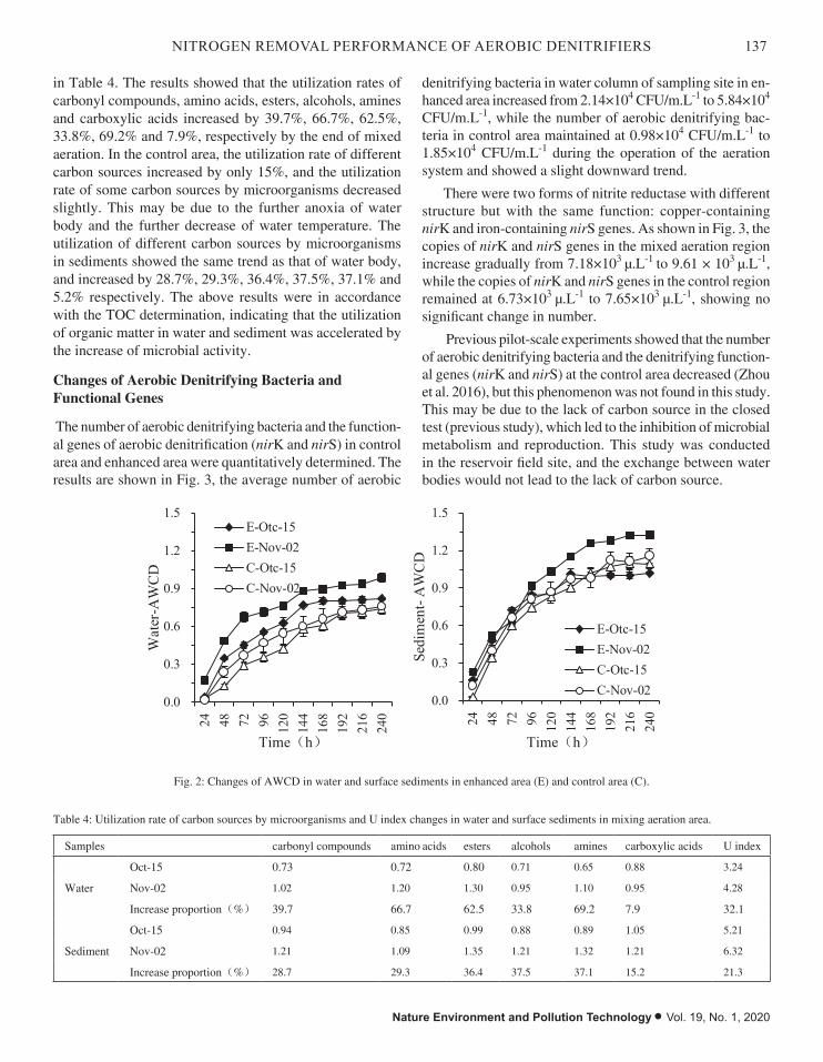
137NITROGEN REMOVAL PERFORMANCE OF AEROBIC DENITRIFIERS
Nature Environment and Pollution Technology • Vol. 19, No. 1, 2020
in Table 4. The results showed that the utilization rates of carbonyl compounds, amino acids, esters, alcohols, amines and carboxylic acids increased by 39.7%, 66.7%, 62.5%, 33.8%, 69.2% and 7.9%, respectively by the end of mixed aeration. In the control area, the utilization rate of different carbon sources increased by only 15%, and the utilization rate of some carbon sources by microorganisms decreased slightly. This may be due to the further anoxia of water body and the further decrease of water temperature. The utilization of different carbon sources by microorganisms in sediments showed the same trend as that of water body, and increased by 28.7%, 29.3%, 36.4%, 37.5%, 37.1% and 5.2% respectively. The above results were in accordance with the TOC determination, indicating that the utilization of organic matter in water and sediment was accelerated by the increase of microbial activity.
Changes of Aerobic Denitrifying Bacteria and Functional Genes
The number of aerobic denitrifying bacteria and the function-al genes of aerobic denitrification (nirK and nirS) in control area and enhanced area were quantitatively determined. The results are shown in Fig. 3, the average number of aerobic
denitrifying bacteria in water column of sampling site in en-hanced area increased from 2.14×10⁴ CFU/m.L-1 to 5.84×10⁴ CFU/m.L-1, while the number of aerobic denitrifying bac-teria in control area maintained at 0.98×10⁴ CFU/m.L-1 to 1.85×10⁴ CFU/m.L-1 during the operation of the aeration system and showed a slight downward trend.
There were two forms of nitrite reductase with different structure but with the same function: copper-containing nirK and iron-containing nirS genes. As shown in Fig. 3, the copies of nirK and nirS genes in the mixed aeration region increase gradually from 7.18×10³ µ.L-1 to 9.61 × 10³ µ.L-1, while the copies of nirK and nirS genes in the control region remained at 6.73×10³ µ.L-1 to 7.65×10³ µ.L-1, showing no significant change in number.
Previous pilot-scale experiments showed that the number of aerobic denitrifying bacteria and the denitrifying function-al genes (nirK and nirS) at the control area decreased (Zhou et al. 2016), but this phenomenon was not found in this study. This may be due to the lack of carbon source in the closed test (previous study), which led to the inhibition of microbial metabolism and reproduction. This study was conducted in the reservoir field site, and the exchange between water bodies would not lead to the lack of carbon source.
Table 4: Utilization rate of carbon sources by microorganisms and U index changes in water and surface sediments in mixing aeration area.
Samples carbonyl compounds amino acids esters alcohols amines carboxylic acids U index
Water
Oct-15 0.73 0.72 0.80 0.71 0.65 0.88 3.24
Nov-02 1.02 1.20 1.30 0.95 1.10 0.95 4.28
Increase proportion(%) 39.7 66.7 62.5 33.8 69.2 7.9 32.1
Sediment
Oct-15 0.94 0.85 0.99 0.88 0.89 1.05 5.21
Nov-02 1.21 1.09 1.35 1.21 1.32 1.21 6.32
Increase proportion(%) 28.7 29.3 36.4 37.5 37.1 15.2 21.3
0.0
0.3
0.6
0.9
1.2
1.5
24 48 72 96 120
144
168
192
216
240
Wat
er-A
WC
D
Time(h)
E-Otc-15E-Nov-02C-Otc-15C-Nov-02
0.0
0.3
0.6
0.9
1.2
1.5
24 48 72 96 120
144
168
192
216
240
Sedi
men
t-A
WC
D
Time(h)
E-Otc-15E-Nov-02C-Otc-15C-Nov-02
Fig. 2: Changes of AWCD in water and surface sediments in enhanced area (E) and control area (C).

138 Zhou Zi-zhen et al.
Vol. 19, No. 1, 2020 • Nature Environment and Pollution Technology
High-throughput sequencing was used to analyse the pro-portion of aerobic denitrifying bacteria in the operation of the water-lifting aeration system. The results (Table 5) showed that after the operation of the system, the density of the main aerobic denitrifying bacteria Acidovorax, Novosphingobium, Hydrogenophaga, Pseudomonas, Methylophaga, Bacteroi-detes and Sphingomonadaceae increased significantly. For example, the proportion of Acidovaxor increased from 0.01% before the operation of the system to 0.15%. The operation of water-lifting aeration system increased the proportion of aerobic denitrifying bacteria in total bacteria. This conclu-sion also helped to reveal the mechanism of denitrification nitrogen removal in water.
Principal Component/Redundancy Analysis of Environmental Factors and Microorganisms
Principal Component Analysis (PCA) is a powerful tool for
analysing sample differences. In this paper, PCA was carried out based on environmental factors (water quality parame-ters) and microbial composition, respectively, to analyse the differences between enhanced and control areas in the op-eration of water-lifting aeration system. The results showed that the principal component analysis of the environmental factors and microbial composition can explain 95.41% and 87.19% of water quality and microbial composition respec-tively, which can well reflect the whole process. As shown in Fig. 4, at the beginning, there was no obvious difference in water quality and microorganisms composition between the enhanced area and the control area, and the distribution of sample sites in each depth was concentrated. However, with the operation of the aeration system, DO and T in the enhanced area changed, and the microbial population also changed. The difference between the enhanced area and the control area was more and more obvious. It was clear
Table 5: Variations of aerobic denitrifying bacteria in water in mixing aeration area (E) and control area (C).
Species/sampling sites-dates E-Oct-15 E- Nov-02 C-Oct-15 C-Nov-02
Acidovorax 0.01% 0.15% - 0.02%
Novosphingobium 0.01% 0.10% 0.01% -
Hydrogenophaga - 0.05% 0.02% 0.01%
Pseudomonas 0.01% 0.02% 0.01% 0.01%
Methylophaga 0.01% 0.06% 0.01% -
Bacteroidetes 0.02% 0.02% 0.01% 0.03%
Sphingomonadaceae 0.01% 0.03% 0.02% 0.02%
Note: “-” means undetected
0
1
2
3
4
5
6
7
8
0
2
4
6
8
10
12
Aer
obic
den
itrify
ig b
acte
ria lg
(cfu
/Lm)
Func
tiona
l gen
es 1
03 /μL
nirK nirS
E-Bacteria number C-Bacteria number
Fig. 3: Changes of aerobic denitrification genes and density of aerobic denitrifying bacteria in water in enhanced area (E) and control area (C).
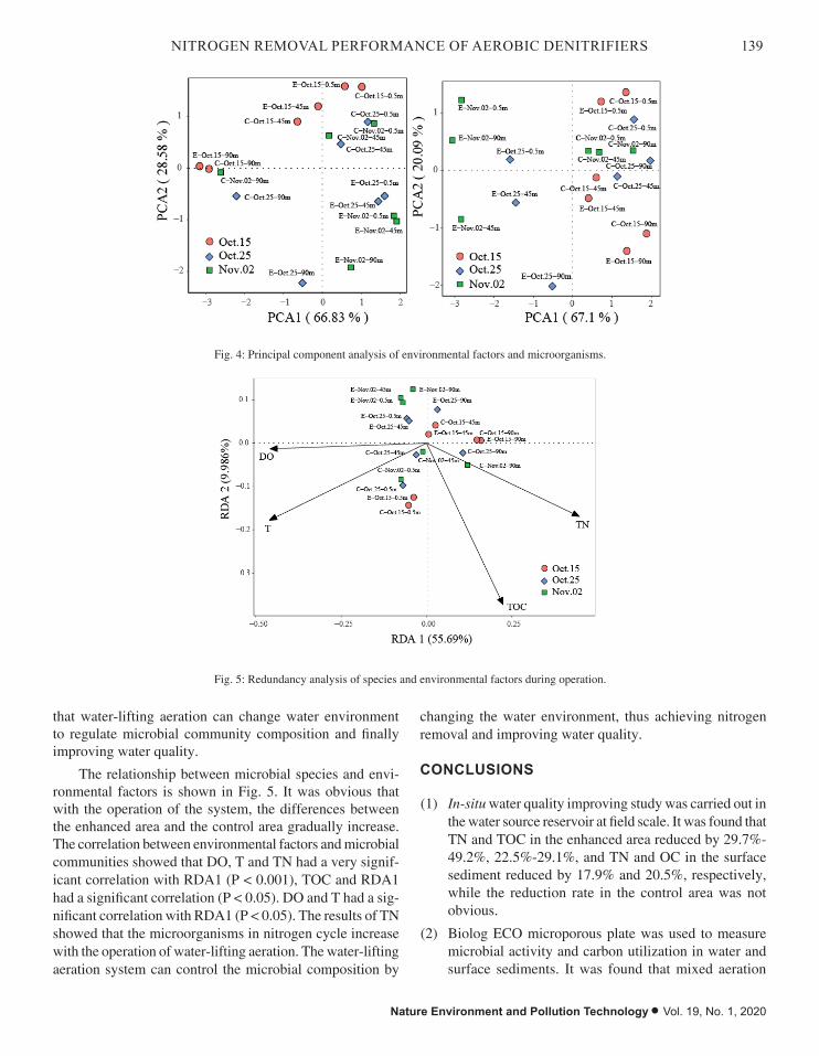
139NITROGEN REMOVAL PERFORMANCE OF AEROBIC DENITRIFIERS
Nature Environment and Pollution Technology • Vol. 19, No. 1, 2020
that water-lifting aeration can change water environment to regulate microbial community composition and finally improving water quality.
The relationship between microbial species and envi-ronmental factors is shown in Fig. 5. It was obvious that with the operation of the system, the differences between the enhanced area and the control area gradually increase. The correlation between environmental factors and microbial communities showed that DO, T and TN had a very signif-icant correlation with RDA1 (P < 0.001), TOC and RDA1 had a significant correlation (P < 0.05). DO and T had a sig-nificant correlation with RDA1 (P < 0.05). The results of TN showed that the microorganisms in nitrogen cycle increase with the operation of water-lifting aeration. The water-lifting aeration system can control the microbial composition by
changing the water environment, thus achieving nitrogen removal and improving water quality.
CONCLUSIONS
(1) In-situ water quality improving study was carried out in the water source reservoir at field scale. It was found that TN and TOC in the enhanced area reduced by 29.7%-49.2%, 22.5%-29.1%, and TN and OC in the surface sediment reduced by 17.9% and 20.5%, respectively, while the reduction rate in the control area was not obvious.
(2) Biolog ECO microporous plate was used to measure microbial activity and carbon utilization in water and surface sediments. It was found that mixed aeration
Fig. 5: Redundancy analysis of species and environmental factors during operation.
Fig. 4: Principal component analysis of environmental factors and microorganisms.

140 Zhou Zi-zhen et al.
Vol. 19, No. 1, 2020 • Nature Environment and Pollution Technology
increased microbial metabolic activity by more than 14%, carbon utilization by more than 30% and micro-bial McIntosh diversity index by more than 20% in the enhanced area.
(3) The results of high-throughput sequencing and amplifi-cation of aerobic denitrifying functional genes (nirK and nirS) showed that the number of functional genes and their proportion of aerobic denitrifying bacteria in the enhanced area increased by the mixed aeration process.
(4) Mixed aeration can improve microbial metabolic activ-ity, the number of aerobic denitrifying bacteria and the number of functional genes (nirK and nirS) and enhance their denitrification performance. Satisfying results of denitrification and carbon removal have been achieved in field experiments of reservoirs, which further en-riched the mechanism and practice of denitrification and carbon removal in source water.
(5) In order to destroy the stratification of water body and the oxygen-filled the bottom in field research, the air supply can be controlled at 30-40 m3/h from the point of view of energy saving.
ACKNOWLEDGEMENT
This research was funded by National Natural Science Foundation of China (51909056), Key Scientific Research Projects of Higher Education Institutions in Henan Province (20A560023), Science and Technology Guidance Project of China Textile Industry Federation (2018040), Research Team Development Project of Zhongyuan University of Technology (K2018TD004), Young Backbone Teachers Grant Scheme of Zhongyuan University of Technology.
REFERENCESAlzate Marin, J.C., Caravelli, A.H. and Zaritzky, N.E. 2016. Nitrification
and aerobic denitrification in anoxic-aerobic sequencing batch reactor. Bioresource Technology, 200: 380-387.
Chen, Q., Ni, J., Ma, T., Liu, T. and Zheng, M. 2015. Bioaugmentation treatment of municipal wastewater with heterotrophic-aerobic nitro-gen removal bacteria in a pilot-scale SBR. Bioresource Technology, 183: 25-32.
Coban, O., Kuschk, P., Kappelmeyer, U., Spott, O., Martienssen, M., Jetten, M. S. M. and Knoeller, K. 2015. Nitrogen transforming community in a horizontal subsurface-flow constructed wetland. Water Research, 74: 203-212.
Epsztein, R., Beliavski, M., Tarre, S. and Green, M. 2016. Simplified model for hydrogenotrophic denitrification in an unsaturated-flow pressurized reactor. Chemical Engineering Journal, 306: 233-241.
Fang, J.J., Li, Q., Liu, C., Jin, Z., Liang, Y., Huang, B., Lu, Xiao. and Peng, W. 2018. Carbon metabolism characteristics of the karst soil microbial community for Pb-Zn mine tailings. Environmental Science, 39(5): 2420-2430.
Gao, H., Schreiber, F., Collins, G., Jensen, M.M., Svitlica, O., Kostka, J.E., Lavik, G., Zhou, H. and Kuypers, M. 2010. Aerobic denitrification in permeable Wadden Sea sediment. Isme Journal, 4(3): 417-426.
Huang, T. L. and Li, X., H. Rijnaarts, Grotenhuis, T., Ma, W., Sun, X. and Xu, J. 2014. Effects of storm runoff on the thermal regime and water quality of a deep, stratified reservoir in a temperate monsoon zone, in Northwest China. Science of the Total Environment, 485-486(3): 820-827.
Huang, T.L., Zhang, L.N., Zhang, H.H., Su, J.F., Guo, L., Zhao, J.Y. and Zhang K. 2015. Screening and nitrogen removal characteristics of a heterotrophic nitrification-aerobic denitrification strain. Ecology and Environmental Sciences, 24(1): 113-120.
Jiyeon, C., Maniquiz, M.C., Byungsik, L., Jeong, S. and Kim, L. 2012. Characteristics of contaminant and phosphorus existence types in sediment of a constructed wetland. Desalination & Water Treatment, 38(1-3): 285-291.
Kang, P. L., Chen, S.N., Huang, T.L., Zhang, H.H., Shang, P.L., Zhao, Z.F., Wang, Y. and Tan, X. L. 2018. Denitrification characteristics and functional genes of denitrifying bacteria under aerobic or anaerobic conditions. Environmental Science, 8: 3790-3796.
Kang, P.L., Zhang, H.H., Huang, T.L. Zhang, H.H., Shang, P.L., Zhao, Z.F., Wang, Y. and Tan, X. L. 2018. Denitrification characteristics and community structure of aerobic denitrifiers from lake and reservoir sediments. Environmental Science, 39(5): 2431-2437.
Patureau, D., Godon, J., Dabert, P., Bouchez, T., Bernet, N., Delqenses, J.P. and Moletta, R. 1998. Microvirgula aerodenitrificans gen. nov. sp. nov. a new Gram-negative bacterium exhibiting co-respiration of oxygen and nitrogen oxides up to oxygen-saturated conditions. Int. J. Syst. Bacteriol., 48 Pt 3(3): 775-782.
Patureau, D., Helloin, E., Rustrian, E., Bouchez, T., Delgenese, J.P. and Moletta, R. 2001. Combined phosphate and nitrogen removal in a sequencing batch reactor using the aerobic denitrifier, Microvirgula aerodenitrificans. Water Research, 35(1): 189-197.
Robertson, L.A. and Kuenen, J.G. 1982. Thiosphaera pantotropha gen. nov. sp. nov. a facultatively anaerobic, facultatively autotrophic sulphur bacterium. Journal of General Microbiology, 129(9): 2847-2855.
Song, Z.F., An, J., Fu, G.H. and Yang, X. L. 2011. Isolation and charac-terization of an aerobic denitrifying Bacillus, sp. YX-6 from shrimp culture ponds. Aquaculture, 319(1): 188-193.
Sun, S.P., Pelliceri, N. C. Merkey, B., Zhou, Q., Xia, S.Q., Yang, D.H. and Sun, J.H., Barth, S. 2010. Effective biological nitrogen removal treatment processes for domestic wastewaters with low C/N ratios: A review. Environmental Engineering Science, 27(2): 111-126.
Xu, Z., Dai, X. and Chai, X. 2018. Effect of different carbon sources on denitrification performance, microbial community structure and de-nitrification genes. Science of the Total Environment, 634: 195-204.
Zhou, S., Huang, T., Zhang, H., Zeng, M., Liu, F., Bai, S., Shi, J., Qiu, X. and Yang, X. 2016. Nitrogen removal characteristics of enhanced in situ indigenous aerobic denitrification bacteria for micro-polluted reservoir source water. Bioresource Technology, 201: 195-207.
Zhou, S.L., Huang, T.L., Huu, H.N., Zhang, H., Liu, F., Zeng, M., Shi, J. and Qiu, X. 2016. Nitrogen removal characteristics of indigenous aerobic denitrifiers and changes in the microbial community of a reservoir enclosure system via in situ oxygen enhancement using water lifting and aeration technology. Bioresour. Technol., 214: 63-73.
Zhou, S.L., Huang, T.L., Bai, S.Y. and He, X. 2016. Isolation, identification, and nitrogen removal characteristics of oligotrophic aerobic denitrifiers. China Environmental Science, 36(1): 238-248.
Zhou, Z.Z., Huang, T.L., Li, Y., Long, S. and Zhou, S. 2017. Improvement of water quality and sediment control by WLAs in a source water reservoir. China Environmental Science, 37(1): 210-217.

Environmental Pollution and Energy Efficiency of Regional Transportation Industry: A Case Study of Jilin Province, China
Rongbo WuSchool of Railway Transportation, Jilin Railway technology college , Jilin, 132001, China†Corresponding author: Rongbo Wu
ABSTRACT
The transportation industry is the fundamental and strategic industry for social and economic development. However, this industry becomes a considerable barrier against green, sound, and sustainable economic and social development due to the rapid increase in energy consumption and greenhouse gas emission. Transportation industry becomes one of weakness of energy saving and emission reduction with its increasing energy consumption and carbon emission. Environmental pollution caused by the transportation industry can be relieved effectively by increasing energy efficiency. A case study based on Jilin Province, China is carried out. First, environmental pollution types caused by regional transportation industry are analysed. Second, energy efficiency of transportation industry in eight prefecture-level cities in Jilin Province from 2011 to 2017 is determined using the DEA-Malmquist index. Finally, measures to control environmental pollution caused by the transportation industry are proposed. Results show that in Jilin Province, environmental pollution caused by the transportation industry manifests through increasing energy consumption, pollution from car exhaust, and degree of traffic jams. In its eight prefecture-level cities, the average energy efficiency change index of transportation industry is 1.054, which is higher than 1. The means of technological efficiency and progress are 0.973 and 1.084, respectively. The mean pure technological efficiency of energy use slightly increases, while the mean scale efficiency decreases significantly. Results can provide beneficial references for full understanding on energy consumption and environmental emission of transportation industry in Jilin Province. This understanding can lead to the exploration of scientific and reasonable energy-saving and emission-reduction ways and countermeasures, aiming to offer decision-making references for energy saving and emission reduction of the transportation industry in Jilin Province.
INTRODUCTION
The transportation industry is the fundamental and strategic industry for social and economic development. However, this industry becomes a considerable barrier against green, sound, and sustainable economic and social development due to the rapid increase of energy consumption and greenhouse gas emission. Moreover, the transportation industry is typically characterized by high-energy consumption, which increases with continuous economic, social, and industrial develop-ments and proposes a huge challenge to the whole society and energy-saving development of the industry. Nevertheless, industry energy consumption show significant regional dif-ferences in China. Lack of regional energy-saving goals and policy may cause mutual restraints between development and energy saving of regional transportation industries.
Jilin Province experiences continuous economic pros-perity and accelerating urbanization. As such, pressure over resources and environment intensifies due to the rapid growth of urban population and dramatically expanding ur-
ban scale, accompanied with increasing prominent negative externality of economic agglomeration. “Urban diseases,” which are centred at atmospheric pollution and traffic jams, are becoming important factors that restrict the develop-ment of different cities in Jilin Province. In this province, the transportation industry is the pillar industry of national economic development, attracting wide attention and serv-ing as a key industry with high-energy consumption and pollutant emission. Table 1 shows that this transportation industry accounts for high-energy consumption and causes heavy environmental pollution. As a response to economic development and rising population and number of vehicles in Jilin Province, transportation demands continuously increase. Moreover, problems such as traffic jams, transportation pollution, energy consumption, and public health become more prominent. Therefore, full understanding on energy consumption and pollutant emission of Jilin Province under various transportation policies is significant to the future sustainable development of the province. In addition, this understanding can provide decision-making references to
Nat. Env. & Poll. Tech.Website: www.neptjournal.com
Received: 12-12-2019Accepted: 20-01-2020
Key Words:Transportation industry Environmental pollution Energy efficiency Jilin Province
2020pp. 141-147 Vol. 19
p-ISSN: 0972-6268 No. 1 Nature Environment and Pollution Technology An International Quarterly Scientific Journal
Original Research Paper
e-ISSN: 2395-3454
Open Access
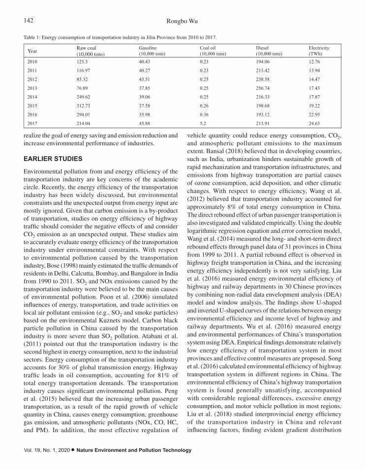
142 Rongbo Wu
Vol. 19, No. 1, 2020 • Nature Environment and Pollution Technology
realize the goal of energy saving and emission reduction and increase environmental performance of industries.
EARLIER STUDIES
Environmental pollution from and energy efficiency of the transportation industry are key concerns of the academic circle. Recently, the energy efficiency of the transportation industry has been widely discussed, but environmental constraints and the unexpected output from energy input are mostly ignored. Given that carbon emission is a by-product of transportation, studies on energy efficiency of highway traffic should consider the negative effects of and consider CO2 emission as an unexpected output. These studies aim to accurately evaluate energy efficiency of the transportation industry under environmental constraints. With respect to environmental pollution caused by the transportation industry, Bose (1998) mainly estimated the traffic demands of residents in Delhi, Calcutta, Bombay, and Bangalore in India from 1990 to 2011. SO2 and NOx emissions caused by the transportation industry were believed to be the main causes of environmental pollution. Poon et al. (2006) simulated influences of energy, transportation, and trade activities on local air pollutant emission (e.g., SO2 and smoke particles) based on the environmental Kuznets model. Carbon black particle pollution in China caused by the transportation industry is more severe than SO2 pollution. Atabani et al. (2011) pointed out that the transportation industry is the second highest in energy consumption, next to the industrial sectors. Energy consumption of the transportation industry accounts for 30% of global transmission energy. Highway traffic leads in oil consumption, accounting for 81% of total energy transportation demands. The transportation industry causes significant environmental pollution. Peng et al. (2015) believed that the increasing urban passenger transportation, as a result of the rapid growth of vehicle quantity in China, causes energy consumption, greenhouse gas emission, and atmospheric pollutants (NOx, CO, HC, and PM). In addition, the most effective regulation of
vehicle quantity could reduce energy consumption, CO2, and atmospheric pollutant emissions to the maximum extent. Bansal (2018) believed that in developing countries, such as India, urbanization hinders sustainable growth of rapid mechanization and transportation infrastructures, and emissions from highway transportation are partial causes of ozone consumption, acid deposition, and other climatic changes. With respect to energy efficiency, Wang et al. (2012) believed that transportation industry accounted for approximately 8% of total energy consumption in China. The direct rebound effect of urban passenger transportation is also investigated and validated empirically. Using the double logarithmic regression equation and error correction model, Wang et al. (2014) measured the long- and short-term direct rebound effects through panel data of 31 provinces in China from 1999 to 2011. A partial rebound effect is observed in highway freight transportation in China, and the increasing energy efficiency independently is not very satisfying. Liu et al. (2016) measured energy environmental efficiency of highway and railway departments in 30 Chinese provinces by combining non-radial data envelopment analysis (DEA) model and window analysis. The findings show U-shaped and inverted U-shaped curves of the relations between energy environmental efficiency and income level of highway and railway departments. Wu et al. (2016) measured energy and environmental performances of China’s transportation system using DEA. Empirical findings demonstrate relatively low energy efficiency of transportation system in most provinces and effective control measures are proposed. Song et al. (2016) calculated environmental efficiency of highway transportation system in different regions in China. The environmental efficiency of China’s highway transportation system is found generally unsatisfying, accompanied with considerable regional differences, excessive energy consumption, and motor vehicle pollution in most regions. Liu et al. (2018) studied interprovincial energy efficiency of the transportation industry in China and relevant influencing factors, finding evident gradient distribution
Table 1: Energy consumption of transportation industry in Jilin Province from 2010 to 2017.
YearRaw coal(10,000 tons)
Gasoline(10,000 tons)
Coal oil(10,000 tons)
Diesel(10,000 tons)
Electricity(TWh)
2010 125.3 40.43 0.23 194.06 12.76
2011 116.97 40.27 0.23 213.42 13.94
2012 85.32 43.51 0.25 238.58 14.47
2013 76.89 37.85 0.25 256.74 17.43
2014 249.62 39.06 0.25 216.33 17.87
2015 312.73 37.58 0.26 198.68 19.22
2016 294.01 35.98 0.36 193.12 22.95
2017 214.04 45.88 5.2 213.91 24.63

143POLLUTION AND ENERGY EFFICIENCY OF REGIONAL TRANSPORTATION INDUSTRY
Nature Environment and Pollution Technology • Vol. 19, No. 1, 2020
of energy efficiency. The highest energy efficiency among the transportation industries are found in provinces in East China, followed by those in central and West China. This interprovincial difference in energy efficiency is gradually narrowing. Liu et al. (2019) evaluated energy and environmental efficiencies of the highway transportation industry in China. Empirical proof shows that diffusion and use of optical production technology in the highway transportation industry in Western and Central China is superior to technological innovation progress. Omrani et al. (2019) evaluated energy efficiency of transportation departments in 20 Iran provinces by combining DEA and cooperative game method. Compared with large economic provinces, several small economic provinces show better energy efficiency in their transportation industry. Extant studies show that the transportation industry cause heavy environmental pollution during its development, but such pollution can be relieved effectively through technological progress and improvements in energy efficiency. Increasing energy utilization of the transportation industry is the most important way to solve the contradiction between its rapid development and the goals of energy saving and emission reduction. Therefore, scientific evaluation of energy efficiency of the transportation industry in prefecture cities of Jilin Province (China), exploring key factors to improve energy efficiency, and proposing specific suggestions present important practical significance to green sound development of the transportation industry.
TRAFFIC POLLUTION STATUS OF JILIN PROVINCE
Continuous Increase of Energy Consumption by the Transportation Industry
The automobile industry of Jilin Province is flourishing. The quantity of cars in cities is quickly increasing in recent
years. Fig.1 shows that the quantity of cars for highway transportation in Jilin Province increased from 179,700 in 2006 to 351,900 in 2018. This sharp increase causes energy consumption and tail gas pollution that are difficult to avoid. The transportation industry is a major energy consumer, and the proportion of its energy consumption to total social energy consumption increases continuously.
Continuous Intensification of Tail Gas Pollution of Cars
Most cities in Jilin Province have developed highway trans-portations and various types of motor vehicles, resulting in highly excessive tail gas emission compared with standard figures. Dust particle density is relatively high and urban air pollution is observed. Fig. 2 shows the external diseconomies brought by rapid development of the transportation indus-try and inappropriate transportation development in Jilin Province. PM2.5 emission is rapidly intensifying. Vehicle emission has become a primary pollution source such as CO and hydrocarbon. Tail gas emission from cars is extremely high in most cities of Jilin Province. In addition, externality of air pollution caused by the increased tail gas emission of vehicles cannot be ignored, thus resulting in chronic intox-ication of the central nervous system and functions of the human body, manifested by headaches and crossing eyes.
Gradual Intensification of Traffic Jams
With the increasing traffic demands of residents in Jilin Province, road traffic changes from smooth to disordered, and commuting takes longer to reach destinations. When traffic demands further increase and exceed the ultimate traffic efficiency in places with minimum traffic capacity, the road traffic state changes accordingly. Traffic jams not only cause invalid waiting and wasted times, but also decreases efficiency of the transportation system and causes traffic accidents.
exploring key factors to improve energy efficiency, and proposing specific suggestions present important practical
significance to green sound development of the transportation industry.
TRAFFIC POLLUTION STATUS OF JILIN PROVINCE Continuous Increase of Energy Consumption by the Transportation Industry The automobile industry of Jilin Province is flourishing. The quantity of cars in cities is quickly increasing in recent
years. Fig.1 shows that the quantity of cars for highway transportation in Jilin Province increased from 179,700 in
2006 to 351,900 in 2018. This sharp increase causes energy consumption and tail gas pollution that are difficult to
avoid. The transportation industry is a major energy consumer, and the proportion of its energy consumption to
total social energy consumption increases continuously.
Fig.1: Number of car ownership for highway transportation in Jilin Province in 2006-2018.
(Data source: Jilin Statistical Yearbook)
Continuous Intensification of Tail Gas Pollution of Cars Most cities in Jilin Province have developed highway transportations and various types of motor vehicles, resulting
in highly excessive tail gas emission compared with standard figures. Dust particle density is relatively high and
urban air pollution is observed. Fig. 2 shows the external diseconomies brought by rapid development of the
transportation industry and inappropriate transportation development in Jilin Province. PM2.5 emission is rapidly
intensifying. Vehicle emission has become a primary pollution source such as CO and hydrocarbon. Tail gas
emission from cars is extremely high in most cities of Jilin Province. In addition, externality of air pollution caused
by the increased tail gas emission of vehicles cannot be ignored, thus resulting in chronic intoxication of the central
nervous system and functions of the human body, manifested by headaches and crossing eyes.
Fig.1: Number of car ownership for highway transportation in Jilin Province in 2006-2018. (Data source: Jilin Statistical Yearbook)

144 Rongbo Wu
Vol. 19, No. 1, 2020 • Nature Environment and Pollution Technology
More importantly, traffic jams cause negative external cost. Fuel utilization decreases whereas energy consumption and pollutant emissions increase, because pollutant emissions from incomplete combustion during traffic jams are far higher than pollutant emissions during normal driving.
Brief Introduction to The Model and Data Specification
Introduction to the model: Following Färe et al. (1992), the DEA-Malmquist Index, which is under variable returns to scale, oriented to output, and uses t and t+1 as technical references, is defined in formula (1):
Mt ttv
tv
tv
tc
tD
D
D
D
D,
( )
( )
( )
( )+
+ += ¥ ∏11 x ,y
x ,y
x ,y
x ,y
t+1 t+1
t t
t t
t t
11
1
1
v
tc
tc
tc
D
D
D
( )
( )
( )
(
x ,y
x ,y
x ,y
x ,
t+1 t+1
t+1 t+1
t t
t
+
+
È
ÎÍÍ
˘
˚˙˙
¥yy
x ,y
x ,yt
t+1 t+1
t+1 t+1)
( )
( )¥
È
ÎÍÍ
˘
˚˙˙+
D
Dtc
tc
1
1
2
…(1)
Where D x yc ( , ) is the distance function under constant returns to scale and Dv ( , )x y is the distance function
under variable returns to scale. D
Dtv
tv
+1( )
( )
x ,y
x ,y
t+1 t+1
t t
is
the change of pure technological efficiency (PTEC),
D x y
D x y
D x y
D x ytv
t t
tc
t t
tv
t t
tc
t t
( , )
( , )
( , )
( , )∏ + + +
+ + +
1 1 1
1 1 1
is the change of scale efficiency
(SE), D x y
D x y
D x y
D x ytc
t t
tc
t t
tc
t t
tc
t t
( , )
( , )
( , )
( , )+
+ +
+ + +
¥È
ÎÍÍ
˘
1
1 1
1 1 1 ˚˙˙
1
2 and is technological
progress (TC). In other words, the product of the previous two terms is the change of technological efficiency (EC).When Mt t, +1
>1, total factor productivity (TFP) progresses. When Mt t, +1 < 1, TFP regresses. When Mt t, +1 =1, TFP is constant. In the panel data analysis of the transportation industry in Jilin Province, TFP decomposes into the product of TC and EC. EC is further decomposed into the product of PTEC and SE. On this basis, the influence of PTEC and SE on technological efficiency can be determined. Contributions of pure technological inefficiency and scale inefficiency to influences of PTEC and SE, respectively, can be recognized separately as long as nontechnological efficiency is discovered in efficiency estimation of the transportation industry. On the basis of these results, policy suggestions are proposed. Specific meanings of different indexes are introduced as follows: Malmquist Index refers to the change process of TFP. The change index of EC is to measure whether production meets the optimal resource allocation. The change index of TC reflects changes of production technologies. The change index of PTEC is part of production technological inefficiency caused by pure technological inefficiency. The change index of SE is to judge whether the decision-making units are in the optimal production scale.
Data specification: Input indexes include capital, labour, and energy input. Capital input refers to fixed-asset invest-ments (10,000 Yuan) to transportation industry in different cities of Jilin Province. Labour input refers to the number of employees in the transportation industry at year-end (10,000 persons). Energy input refers to energy consumption of the transportation industry (10,000 tons of standard coal). Energy resources consumed by transportation industry, such as coal, oils, natural gas, heating power, and electricity, are all trans-formed to standard coal. Output indexes include turnover vol-
0
100000
200000
300000
400000
500000
600000
700000
05
101520253035404550
2006
2007
2008
2009
2010
2011
2012
2013
2014
2015
2016
Tota
l nitr
ogen
oxi
de
emis
sion
s(to
ns)
pm2.
5(μg
/m³)
Year
Fig. 2: PM2.5 and total Nitrogen oxide emissions in Jilin Province in 2006-2016. (Data source: Jilin Statistical Yearbook)

145POLLUTION AND ENERGY EFFICIENCY OF REGIONAL TRANSPORTATION INDUSTRY
Nature Environment and Pollution Technology • Vol. 19, No. 1, 2020
ume of passenger traffic and of freight transport. The former is mainly expressed by annual passenger person-kilometres (10,000 persons km) and the latter is mainly expressed by freight turnover (10,000 tons km) in each city. This study uses panel data of eight prefecture cities of Jilin Province from 2011 to 2017. Data of various input and output indexes are all collected from Statistics Yearbook of Jilin Province.
RESULT ANALYSIS
Energy efficiency of the transportation industry in different prefecture cities of Jilin Province was decomposed dynamically using the Malmquist Index by estimating the comprehensive efficiency of energy utilization. Regional differences and their causes were analysed. Annual variations of TFP of the transportation industry in Jilin Province from 2011 to 2017 were estimated using the DEAP2.1-XP software package from the perspective of output. Table 2 lists the results.
Table 2 shows that in eight cities of Jilin Province, the mean energy efficiency change index of transportation industry was 1.054 from 2011 to 2017, which was higher than 1. Energy utilization of transportation industry in Jilin Province increased to a certain extent during the study period. In view of the decomposition results, the mean EC and TC are 0.973 and 1.084, respectively. This finding reflects that energy utilization of the transportation industry increased by 0.54%, including 0.84% attributed to TC and 0.27% at-tributed to EC. Specifically, EC hindered the improvement of energy utilization. The mean PTEC of energy utilization increased slightly whereas the mean SE decreased signifi-cantly, indicating that EC reduction was mainly attributed to SE reduction. EC and SE were relatively low and could potentially increase. EC reached 1.015, and could further increase. The energy utilization of the transportation indus-try in Jilin Province was generally low due to low SE. EC and SE of the transportation industry in Jilin Province from 2011 to 2017 generally decreased, but PTEC was relatively stable. This finding possibly occurred because of the in-
creased efforts in external industrial structural transfer and transportation enterprises made fundamental investments in response to the government’s call of “industrial transfer”. Enterprises were in the investment period and were explor-ing new technologies. Meanwhile, production scale was not controlled at a reasonable level. Enterprises were adapting to new policies. After 2012, Jilin Province increased investment to traffic infrastructure, released various successive policies, and encouraged investments of abundant capital and labour forces into the “Harbin-Changsha Urban Agglomeration” and “Changsha-Jilin-Tumen Development and Opening Up Pilot Region”. These programs promoted the overall technological innovation transportation industry in Jilin Province, and comprise one possible cause why the EC of the transportation industry in Jilin Province was retained over 0.9 before 2012. However, SE was not as high as PTEC, because huge capital investment was mainly applied to technological innovation and expansion in the enterprise scale. Instead, enterprise problems of production efficiency were ignored, thus resulting in high PTEC and low SE.
POLICY SUGGESTIONS
Improve the Transportation Structure and Accelerate Development Transportation Mode with Low Energy Consumption
Jilin Province can accelerate energy-saving comprehensive transportation system, develop relative advantages of dif-ferent transportation modes by planning the transportation system, and promote reasonable equilibrium development of different transportation modes by closely combining natural geological environment and economic development status. These improvements likewise increase the connection and informatization level of infrastructures of the comprehensive transportation system, realize fast transit of passenger and freight, and improve quality and efficiency of transporta-tion services. Jilin Province can increase investment and support for railway, shipment, and pipeline transportation, increase proportion of transportation modes with low
Table 2: Variations of energy production efficiency indexes of the transportation industry of Jilin Province.
Year EC TC PTEC SE TFP
2011-2012 0.755 1.021 1.087 0.695 0.771
2012-2013 0.832 0.976 1.002 0.830 0.812
2013-2014 0.925 1.286 0.982 0.942 1.190
2014-2015 0.987 1.042 0.998 0.989 1.028
2015-2016 1.123 1.153 1.008 1.114 1.295
2016-2017 1.214 1.025 1.012 1.200 1.244
Mean 0.973 1.084 1.015 0.958 1.054
146 Rongbo Wu
Vol. 19, No. 1, 2020 • Nature Environment and Pollution Technology
single consumption, and guide transfer of bulk cargo to energy-saving environment-friendly transportation mode. Railway transportation in the market can be increased, and attention is necessary to improve service quality of railway passenger transportation. The speed and comfort advantages of railway, in relation to highway, can be improved through the development of high-speed rails. Considerable efforts can be made to develop urban public transport and railway system to increase public commuting rates.
Reduce Energy Consumption Intensity and Increase Energy Utilization of The Transportation Industry
Jilin Province can formulate more energy-saving policies to decrease energy intensity. With the improvement of trans-port tools and development of clean energies, the existing transportation industry still has high energy-saving potential. For highway transportation, old vehicles with high-energy consumption can be eliminated. Instead, highway transpor-tation vehicles can be developed in larger sizes and fuelled by diesel. Moreover, Jilin Province can promote the devel-opment of new energy automobiles, improve quick charge technology of electric cars and cruising ability of batteries, in-crease subsidies for electric cars, and strengthen competitive advantages of new energy cars in relation to traditional vehi-cles. For railway transportation, Jilin Province can promote the application of electric locomotives, gradually decrease proportion of diesel locomotives, and decrease dependence on petroleum products. In addition, the province can update old ships to larger sizes and professional makes, increase proportions of ships using clear energy dynamics, decrease energy-saving construction of civil air transportation system, choose the latest energy-saving transportation vehicles, and improve organization and management technologies of civil transportation.
Strengthen Energy Saving and Emission Reduction of the Transportation Industry, and Develop Public Transport System
Jilin Province can pay much attention to energy saving and emission reduction of land transportation, such as by im-plementing policies of public transport priority, perfecting relevant infrastructure equipment, and decreasing energy wastes while assuring and increasing transportation capacity. In addition, Jilin Province can increase proportion of clean energy in land transportation and shipment. Pilot projects and construction of relevant infrastructures from aspects which are easy to be regulated, including public bus, taxi, and water bus, can also be implemented. Good commuting conditions can be achieved to encourage citizens to choose biking and walking and advocate slow commuting. Moreover, these conditions enrich transportation mode, optimize trans-
portation layout, combine land transportation and shipment organically, and take advantage of both transportation modes.
Pay Attention to the Development of Energy-Saving Technologies and Increase Technological Input
As a significantly effective transition direction, energy-saving technological development for the transportation industry can effectively save energies and decrease emissions in a relatively short period, which is a strong stimulus of the market and consumers. TC not only increases traditional energy efficiency, but also accelerates transition of other transportation modes such as electrification. Attention and investment to energy-saving technologies can be increased appropriately, while diversified parties, including scientific research units and enterprises, can be encouraged to participate in R&D. As such, potentials of technological energy saving from aspects of light weight, small size, and low-resistance electronic control, car network and intelligent driving, and applications of new materials, biofuel, and liquid hydrogen can be explored. Such enhancements can quickly and effectively accomplish energy transition of the transportation industry. With respect to transportation energy technologies, Jilin Province can respond to national policies to develop energy-saving technologies and assure marketing of energy-saving vehicles. For energy structure in the transportation industry, energy updating of urban transportation requires completion as soon as possible through economic means from private sectors and relevant enterprises, mandatory requirements on public sectors, and increased promotion of new clean energy vehicles.
CONCLUSIONS
Influences of the transportation industry on environmental pollution in urban areas of a certain region are increasing gradually. Energy consumption and atmospheric pollution are intensifying gradually. The transportation industry has rapidly become the highest contributor to energy consumption in the region. Accordingly, CO2 emission from the transportation industry is increasing gradually. Hence, its energy transition development is urgently necessary. Development modes in foreign countries prove that the main direction to realize such energy transition in urban transportation is through increased energy efficiency of the industry by adjusting energy structure and developing energy-saving technologies. In this study, a case study is carried out on Jilin Province, China. Types of environmental pollutions caused by the regional transportation industry are analysed. Additionally, energy efficiency of the transportation industry in eight prefecture cities of Jilin Province from 2011 to 2017 is estimated using DEA-Malmquist. The results demonstrate that in Jilin
147POLLUTION AND ENERGY EFFICIENCY OF REGIONAL TRANSPORTATION INDUSTRY
Nature Environment and Pollution Technology • Vol. 19, No. 1, 2020
Province, continuously increasing energy consumption of the transportation industry, tail gas pollution of vehicles, and degree of traffic jams are the main types of environmental pollutions caused by the transportation industry. In the eight prefecture cities of Jilin Province, the mean energy efficiency change index of the transportation industry is 1.054, indicating the improvement of energy efficiency. The mean EC and TC are 0.973 and 1.084, respectively. The mean PTEC slightly increases whereas the mean SE significantly decreases. Further exploration is suggested for the factor decomposition of energy consumption of the transportation industry, interaction mechanism among different influencing factors of energy efficiency, systematic dynamic simulation between transportation industry and ecological environment, practicability of transportation energy policies in different regions, and effects of environmental and economic policies on transportation-induced environmental pollution control in cities with different development degrees.
REFERENCES
Atabani, A. E., Badruddin, I. A., Mekhilef, S. and Silitonga, A. S. 2011. A review on global fuel economy standards, labels and technologies in the transportation sector. Renewable and Sustainable Energy Reviews, 15(9): 4586-4610.
Bansal, A. 2018. Analysis of traffic related environment pollution in Indian cities: Need of the hour. Asian Journal of Engineering and Applied Technology, 7(1): 70-73.
Bose, R. K. 1998. Automotive energy use and emissions control: A sim-ulation model to analyse transport strategies for Indian metropolises.
Energy policy, 26(13): 1001-1016.Färe, R. and Grosskopf, S. 1992. Malmquist productivity indexes and Fisher
ideal indexes. The Economic Journal, 102(410): 158-160.Liu, H., Wu, J. and Chu, J. 2019. Environmental efficiency and technological
progress of transportation industry-based on large scale data. Techno-logical Forecasting and Social Change, 144: 475-482.
Liu, W. and Lin, B. 2018. Analysis of energy efficiency and its influencing factors in China’s transport sector. Journal of cleaner production, 170: 674-682.
Liu, Z., Qin, C. X. and Zhang, Y. J. 2016. The energy-environment efficiency of road and railway sectors in China: Evidence from the provincial level. Ecological indicators, 69: 559-570.
Omrani, H., Shafaat, K. and Alizadeh, A. 2019. Integrated data envelopment analysis and cooperative game for evaluating energy efficiency of transportation sector: a case of Iran. Annals of Operations Research, 274(1-2): 471-499.
Peng, B., Du, H., Ma, S., Fan, Y. and Broadstock, D. C. 2015. Urban passenger transport energy saving and emission reduction potential: a case study for Tianjin, China. Energy Conversion and Management, 102: 4-16.
Poon, J. P., Casas, I. and He, C. 2006. The impact of energy, transport, and trade on air pollution in China. Eurasian Geography and Economics, 47(5): 568-584.
Song, M., Zheng, W. and Wang, Z. 2016. Environmental efficiency and energy consumption of highway transportation systems in China. International Journal of Production Economics, 181: 441-449.
Wang, H., Zhou, P. and Zhou, D. Q. 2012. An empirical study of direct rebound effect for passenger transport in urban China. Energy Eco-nomics, 34(2): 452-460.
Wang, Z. and Lu, M. 2014. An empirical study of direct rebound effect for road freight transport in China. Applied Energy, 133: 274-281.
Wu, J., Zhu, Q., Chu, J., Liu, H. and Liang, L. 2016. Measuring energy and environmental efficiency of transportation systems in China based on a parallel DEA approach. Transportation Research Part D: Transport and Environment, 48: 460-472.

Vol. 19, No. 1, 2020 • Nature Environment and Pollution Technology
148

Preparation of Polyvinyl Alcohol/Graphene Oxide Composites and Their Adsorption Properties Yanyan Dong*, Manuel J. Lis Arias**, Chengye Hu*, Wendan Wu*, Liping Liang*, Xinlan Mou* and Xu Meng*(***)† *College of Textile and Garment, College of Life Science, Shaoxing University, Shaoxing, 312000, China**Textile Research Institute of Terrassa (INTEXTER-UPC), 08222, Terrassa, Spain***Key Laboratory of Clean Dyeing and Finishing Technology of Zhejiang Province, Shaoxing University, Shaoxing, 312000, China†Corresponding author: Xu Meng
ABSTRACTThe polyvinyl alcohol/graphene oxide (PVA/GO) hydrogel was prepared. It was confirmed that the adsorption performance of polyvinyl alcohol/graphene oxide hydrogel composite material was improved, and it does not cause secondary pollution. According to adsorption experiments, it was found that PVA/GO adsorbent with a content of 30 % graphene oxide has the best comprehensive performance. The suitable environment of adsorption was under 25°C, 12-18 h for adsorption time and acidic conditions. The suitable adsorbent dosage was 0.3g and the suitable concentration of the dye was 10 mg/L.
INTRODUCTION
With the development of industrial activities, a large amount of industrial wastewater has resulted in a number of envi-ronmental problems. Effective separation of wastewater is regarded as a potential solution for environmental protection (Gan et al. 2015, Nevárez et al. 2011, Sehaqui et al. 2015). There are various methods being used nowadays. Among them, adsorption has been confirmed to be a promising treat-ment because of its low cost and simple operation (Hameed et al. 2009, Adebajo et al. 2003, Gore et al. 2016). This method is especially suitable for printing and dyeing wastewater treatment. One of the most critical factors about the treatment is the properties of adsorbent, which determines the effect of adsorption. Graphene is the most widely used adsorbent in the adsorption. It has a large specific surface area as one of the structure features, but such as poor hydrophilicity, decreased adsorption effect in the later stage, and difficulty in removing after adsorption are its disadvantages (Kumar et al. 2016, Satti et al. 2010).
Compared to graphene’s single molecular layer, GO has some advantages such as large number of hydrophilic groups, good dispersibility in water and easy surface modification (Russo et al. 2013). However, GO has tiny size and low cytotoxicity to normal cell. These cause the problem of secondary pollution if GO disperses in water. Researchers tried
to compound GO with other compounds to form membranes, pellets or fibres (Shen et al. 2015). But these methods rely on the other compounds to wrap GO for forming, which reduces the content of graphene oxide in the compound and hinders the advantage of specific surface area (Tiwari et al. 2013). In order to solve the above problems and ensure the adsorption effect at the same time, polyvinyl alcohol and GO will be combined into hydrogel materials in this experiment, and its adsorption properties will be explored further.
PVA is a kind of white, non-toxic and odourless solid, with a large number of hydrophilic groups on the molecular chain, which is the reason of its excellent water-solubility (Wahab et al. 2019). The intermolecular interaction force of polyvinyl alcohol molecules is large, which can form a high strength film in close contact. In the experiment, PVA/GO composite hydrogel was synthesized by using PVA as the carrier and fixing GO on the polyvinyl alcohol matrix to form a three-dimensional hydrogel adsorbent with net-work structure. This hydrogel can be deposited in water after adsorption and separated well without affecting the adsorption effect of GO. PVA/GO composite material is simple to prepare and easy to operate. It is also an excellent adsorption material due to which it not only guarantees the adsorption performance of adsorbent, but also overcomes the disadvantage of secondary pollution.
Nat. Env. & Poll. Tech.Website: www.neptjournal.com
Received: 18-06-2019Accepted: 30-08-2019
Key Words:PVA/GO Polymer Composite material Adsorption
2020pp. 149-157 Vol. 19
p-ISSN: 0972-6268No. 1 Nature Environment and Pollution Technology
An International Quarterly Scientific Journal
Original Research Papere-ISSN: 2395-3454
Open Access

150 Yanyan Dong et al.
Vol. 19, No. 1, 2020 • Nature Environment and Pollution Technology
After the PVA/GO composites were successfully pre-pared, a series of batch adsorption experiments were designed to explore their adsorption properties. The influencing factors on the adsorption process were investigated, such as the content of GO in the composites, material dosage, initial concentration of dye solution, adsorption temperature, ad-sorption time and pH value.
MATERIALS AND METHODS
Preparation of graphene oxide: All the test specimens were prepared by adding 2 g graphene and 1 g sodium nitrate to 46 mL concentrated sulphuric acid in an ice bath, and stirring for 15 min. At the time of the specimens keeping at a temperature of 20°C, 6 g KMnO4 was added slowly and stirred fully for 2 h, and then the specimens were placed at 35°C for 30min. 92 mL of deionized water was added to them for diluting it. After standing about 15 min, 20 mL of 30% H2O2 was added after adding 280 g of water into the test specimens for further dilution. Then the samples reacted to bright yellow. After filtrating, the final product was washed in 5% diluted hydrochloric acid firstly and then washed in deionized water to neutral. Samples were dried under vacuum at 50°C. Finally, the samples were ground to a fine powder and stored for reserve.
Preparation of PVA/GO composites: All the working solutions were prepared by adding 90 g deionized water in a beaker with 10 g PVA and stirred to dissolve PVA at 90°C. 9.2 g NaOH and 6mL epichlorohydrin were added and stirred in the beaker. Samples were reacted over 6 h in the oven at 35°C. After forming gel material, freeze dryer was used to dry the material until its weight is constant. Finally, PVA
hydrogel without graphene oxide was obtained. According to the above method and on the basis of the above steps, new samples were prepared by adding 0.1 g and 0.2 g, 0.3 g and 0.4 g of graphene oxide powder into the hydrogel, and reacted over 6 h at 35°C in the oven until forming gelatinous material. With the help of the freeze dryer, the material was dried until its weight became constant. Then the gel composite was cut up and labelled for storage.
Pre-experimental treatment: The standard navy-blue dye was configured with a concentration of 1 g/L. The absorbance of the standard navy-blue dye was measured at different con-centrations (10 mg/L, 20 mg/L, 30 mg/L, 40 mg/L, 50 mg/L, 60 mg/L, 70 mg/L), and the standard curve was obtained. According to the curve equation, R2 = 0.999, which proved that the prepared solution could meet the standard.
Diluting part of the standard dye solution and five groups of dye solution with a concentration of 10 mg/L (200 mL in each group) were obtained. Some dye was kept before adsorption, and then adsorbed with 0.5 g composite ma-terials with different contents of grapheme oxide. Soaking the samples over 12 h at the constant temperature of 25°C, it was observed that the colour of dye became shallow after the reaction, and the adsorbent was adhered with navy-blue, which proved that composite material has good adsorption effect and deserved the follow-up study.
Batch adsorption experiments: To explore the adsorption effect of different contents of graphene oxide, 0.3 g PVA/GO composite hydrogel was taken separately which contains 0, 10 %, 20 %, 30 %, 40 % of graphene oxide and these samples were added to 200 mL navy-blue dye solution, whose initial concentration was 10 mg/L. The samples were placed in an
To explore the effect of pH on adsorption, pH of the solutions was adjusted to 1,
3, 5, 7, 9, 11, and 13 by adding HCl or NaOH. 0.3 g PVA/GO composite hydrogel
(containing 30 % graphene oxide) was added to 200 mL navy-dye with initial
concentration of 10 mg/L at different pH values. The samples were oscillated for
about 15 h until adsorption saturation. The absorbance of the dye was measured
before and after adsorption.
RESULTS AND DISCUSSION
Infrared Spectroscopy
4000 3500 3000 2500 2000 1500 1000
Tran
smitt
ance
(%)
Wavenumber (cm-1)
a-before adsorption b-after adsorption
a
b
Fig. 1: Infrared spectra of PVA/GO composite before and after adsorption.
In Fig.1, curve a is the infrared spectrum of the adsorbent before adsorption.
3420 cm-1 is the stretching vibration peak of the hydroxyl group, and such strong
peaks also appear at 1400 cm-1 and 1630 cm-1, which indicated the symmetric and
asymmetric stretching vibration peaks of the carbonyl group. This indicated that GO
was fixed on the substrate of PVA, the hydroxyl group of PVA, and the carboxyl
group of GO were esterified. The two formed a three-dimensional network structure
Fig. 1: Infrared spectra of PVA/GO composite before and after adsorption.
through covalent cross-linking. Curve b is the infrared spectra of the adsorbent after
adsorption. It found that strong peak appeared in the front position obviously. The
adsorption mechanism depends on hydrogen bonding, electrostatic effect, and
molecular inter-atomic forces between the adsorbent and dye molecules. Contrasting
with the images, the adsorbent adsorbing on dye made polymer material structure to
change, and proved that adsorbent’s success for the efficiency of dye adsorption.
Thermo Gravimetric Characterization
150 200 250 300 350 400 450 50040
60
80
100
Wei
ght (
%)
Temperature (0C)
b-after adsorption a-before adsoption
a b
Fig. 2: Thermo gravimetric characterization of PVA/GO composite before and after adsorption.
Fig. 2 shows the thermo gravimetric characterizations of PVA/GO composite
material with 30 % GO before and after the adsorption. Curve b is the thermo
gravimetric characterization of the composite after adsorption, and the results show
that the weight loss occurs between 100°C to 200°C, and the main reason for this
change is the thermal decomposition of functional groups. Compared to curve a, the
thermal decomposition temperature increases after adsorption, which proved the
successful adsorption of the dye by the adsorbent.
Fig. 2: Thermo gravimetric characterization of PVA/GO composite before and after adsorption.

151POLYVINYL ALCOHOL/GRAPHENE OXIDE COMPOSITES FOR ADSORPTION
Nature Environment and Pollution Technology • Vol. 19, No. 1, 2020
oscillator with a constant temperature and oscillated for about 15 h until adsorption saturation. The absorbance of the dye was measured before and after adsorption.
To explore the effect of the adsorbent dosage on the ad-sorption, different doses (0.1 g, 0.3 g, 0.5 g, 0.7 g, 0.9 g) of the PVA/GO composite hydrogel (containing 30 % GO) respec-tively were taken and added to 200 mL navy-blue dye with an initial concentration of 10 mg/L. The samples were placed in an oscillator with a constant temperature and oscillated for about 15 h until the adsorption saturation. The absorbance of the dye was measured before and after adsorption.
To explore adsorption effect of adsorbent on different concentrations of the dye, 200 mL navy-blue dye with concentrations of 10 mg/L, 20 mg/L, 30 mg/L, 40 mg/L, 50 mg/L respectively was prepared. 0.3 g PVA/GO composite hydrogel (containing 30 % graphene oxide) was added into these samples. The samples were placed in an oscillator with a constant temperature and oscillated for about 15 h until ad-sorption saturation. The absorbance of the dye was measured by ultraviolet spectrophotometer before and after adsorption.
To explore the influence of temperature on the adsorption process, 0.3 g PVA/GO composite hydrogel (containing 30 % graphene oxide) was added to 200 mL navy-blue dye (initial concentration of 10 mg/L) at different temperatures of 25°C, 35°C, 45°C, 55°C and 65°C, respectively. The samples were
placed in an oscillator with a constant temperature and oscil-lated for about 15 h until adsorption saturation. The absorb-ance of the dye was measured before and after adsorption.
To explore the influence of reaction time on adsorp-tion, 0.3 g PVA/GO composite hydrogel (containing 30 % graphene oxide) was added to 200 mL navy-blue dye with the initial concentration of the dye at 10mg/L. The adsorption time was 6 h, 9 h, 12 h, 18 h and 24 h. The absorbance of the dye was measured by ultraviolet spectrophotometer before and after adsorption.
To explore the effect of pH on adsorption, pH of the solutions was adjusted to 1, 3, 5, 7, 9, 11, and 13 by adding HCl or NaOH. 0.3 g PVA/GO composite hydrogel (contain-ing 30 % graphene oxide) was added to 200 mL navy-dye with initial concentration of 10 mg/L at different pH values. The samples were oscillated for about 15 h until adsorption saturation. The absorbance of the dye was measured before and after adsorption.
RESULTS AND DISCUSSION
Infrared Spectroscopy
In Fig.1, curve a is the infrared spectrum of the adsorbent before adsorption. 3420 cm-1 is the stretching vibration peak of the hydroxyl group, and such strong peaks also appear at
SEM Characterization
Fig. 3: a. SEM image of PVA hydrogel; b. SEM image of PVA/GO composite before adsorption; c.
SEM image of PVA/GO composite after adsorption.
Fig. 3a is the SEM image of PVA without GO, and sparse holes are observed on
the material surface. Fig. 3b is the SEM image of PVA/GO with a content of 30 %
graphene oxide, showing a more regular layered porous structure. This is due to the
covalent cross-linking reaction between PVA and GO, and forming a three-
dimensional network structure. At the same time, during the preparation of hydrogel
composites, some pores appeared by water evaporation during drying. Fig. 3c is the
SEM image of the composite after adsorption. There are no empty holes and the
texture is flat. This is because the dye molecules are attached to the composite during
the adsorption process and the water grains appeared during the oscillation adsorption.
Fig. 3: a. SEM image of PVA hydrogel; b. SEM image of PVA/GO composite before adsorption; c. SEM image of PVA/GO composite after adsorption.

152 Yanyan Dong et al.
Vol. 19, No. 1, 2020 • Nature Environment and Pollution Technology
1400 cm-1 and 1630 cm-1, which indicated the symmetric and asymmetric stretching vibration peaks of the carbonyl group. This indicated that GO was fixed on the substrate of PVA, the hydroxyl group of PVA, and the carboxyl group of GO were esterified. The two formed a three-dimensional network structure through covalent cross-linking. Curve b is the infrared spectra of the adsorbent after adsorption. It found that strong peak appeared in the front position obviously. The adsorption mechanism depends on hydrogen bonding, electrostatic effect, and molecular inter-atomic forces be-tween the adsorbent and dye molecules. Contrasting with the images, the adsorbent adsorbing on dye made polymer material structure to change, and proved that adsorbent’s success for the efficiency of dye adsorption.
Thermo Gravimetric Characterization
Fig. 2 shows the thermo gravimetric characterizations of PVA/GO composite material with 30 % GO before and after the adsorption. Curve b is the thermo gravimetric characterization of the composite after adsorption, and the results show that the weight loss occurs between 100°C to 200°C, and the main reason for this change is the thermal decomposition of functional groups. Compared to curve a, the thermal decomposition temperature increases after adsorption, which proved the successful adsorption of the dye by the adsorbent.
SEM Characterization
Fig. 3a is the SEM image of PVA without GO, and sparse holes are observed on the material surface. Fig. 3b is the SEM image of PVA/GO with a content of 30 % graphene oxide, showing a more regular layered porous structure. This is due
to the covalent cross-linking reaction between PVA and GO, and forming a three-dimensional network structure. At the same time, during the preparation of hydrogel composites, some pores appeared by water evaporation during drying. Fig. 3c is the SEM image of the composite after adsorption. There are no empty holes and the texture is flat. This is be-cause the dye molecules are attached to the composite during the adsorption process and the water grains appeared during the oscillation adsorption.
Langmuir, Freundlich and Temkin Adsorption Isotherm Fitting
The adsorption isotherm can be used to evaluate the ad-sorption capacity of the adsorbent (Qe=V×(co-ce)/m). Fig. 4 shows the adsorption performance of PVA/GO with 30 % GO with the blue dye. It was found that higher the initial concentration, higher the adsorption capacity. Because the dye molecules with high concentration distribution have greater diffusion driving force, they overcome more mass transfer resistance of solid phase and water phase, and more dye molecules combine with adsorbent molecules fully to play a role. Langmuir equation is as below:
Langmuir, Freundlich and Temkin Adsorption Isotherm Fitting
10 20 30 40 500
5
10
15
20
25
30
35
Qe (m
g/g)
Ce (mg/L)
Fig. 4: Adsorption isotherm of PVA/GO composites with a content of 30% GO.
The adsorption isotherm can be used to evaluate the adsorption capacity of the
adsorbent (Qe=V×(co-ce)/m). Fig. 4 shows the adsorption performance of PVA/GO
with 30 % GO with the blue dye. It was found that higher the initial concentration,
higher the adsorption capacity. Because the dye molecules with high concentration
distribution have greater diffusion driving force, they overcome more mass transfer
resistance of solid phase and water phase, and more dye molecules combine with
adsorbent molecules fully to play a role. Langmuir equation is as below:
𝐶𝐶𝑒𝑒𝑞𝑞𝑚𝑚
= 1𝑞𝑞𝑚𝑚𝑏𝑏
+ 𝐶𝐶𝑒𝑒𝑞𝑞𝑒𝑒
Where, qe is the equilibrium adsorption capacity and qm is the limit adsorption
capacity. Ce is the equilibrium concentration, and b is the adsorption equilibrium
constant.
The above adsorption isotherm data were fitted by the Langmuir isotherm
equation, and the curve in Fig. 5 was obtained. The curve equation y =
Where, qe is the equilibrium adsorption capacity and qm is the limit adsorption capacity. Ce is the equilibrium concentration, and b is the adsorption equilibrium constant.
The above adsorption isotherm data were fitted by the Langmuir isotherm equation, and the curve in Fig. 5 was ob-tained. The curve equation y = 0.5031x+0.0062(R2=0.9894) indicated that the adsorption of navy blue dye by the com-
Langmuir, Freundlich and Temkin Adsorption Isotherm Fitting
10 20 30 40 500
5
10
15
20
25
30
35
Qe (m
g/g)
Ce (mg/L)
Fig. 4: Adsorption isotherm of PVA/GO composites with a content of 30% GO.
The adsorption isotherm can be used to evaluate the adsorption capacity of the
adsorbent (Qe=V×(co-ce)/m). Fig. 4 shows the adsorption performance of PVA/GO
with 30 % GO with the blue dye. It was found that higher the initial concentration,
higher the adsorption capacity. Because the dye molecules with high concentration
distribution have greater diffusion driving force, they overcome more mass transfer
resistance of solid phase and water phase, and more dye molecules combine with
adsorbent molecules fully to play a role. Langmuir equation is as below:
𝐶𝐶𝑒𝑒𝑞𝑞𝑚𝑚
= 1𝑞𝑞𝑚𝑚𝑏𝑏
+ 𝐶𝐶𝑒𝑒𝑞𝑞𝑒𝑒
Where, qe is the equilibrium adsorption capacity and qm is the limit adsorption
capacity. Ce is the equilibrium concentration, and b is the adsorption equilibrium
constant.
The above adsorption isotherm data were fitted by the Langmuir isotherm
equation, and the curve in Fig. 5 was obtained. The curve equation y =
Fig. 4: Adsorption isotherm of PVA/GO composites with a content of 30% GO.

153POLYVINYL ALCOHOL/GRAPHENE OXIDE COMPOSITES FOR ADSORPTION
Nature Environment and Pollution Technology • Vol. 19, No. 1, 2020
posite material was consistent with the Langmuir isotherm adsorption model, indicating that the composite material had excellent adsorption performance.
In addition, in the Langmuir isothermal model, the dimensionless equilibrium parameter RL = 1/(1+KL×Co) was used to obtain the RL values of different initial con-centrations of the colourant. When RL = 0, the adsorption process is irreversible; when 0<RL<1, the adsorption process is favourable; when RL = 1, the adsorption process is linear; when RL>1, the adsorption process is unfavourable. When the RL values ranged from 0.19 to 0.32, the adsorption pro-cess was favourable.
Freundlich’s isothermal equation is as follows:
log qe = log KF + log Ce
Where, KF and n are the adsorption empirical constants, Ce is the adsorption equilibrium concentration (mg/L), and qe is the equilibrium adsorption quantity (mg/g). The curve in Fig. 6 was obtained, and the equation of the curve was y = 1.0749x-0.324, R2=0.9899.
The equation of Temkin is as follows:
qe = A + B log Ce
The Temkin equation describes the energy relation of adsorption heat decreasing linearly with adsorption amount, and the curve in Fig. 7 is obtained. The curve equation is y = 50.266x-30.21, R2 = 0.8986, which does not conform to the Temkin isothermal equation.
Based on the above three isothermal adsorption equations, the data in Table 1 are obtained. It can be known that the adsorption of PVA/GO composite on navy dye conforms to Langmuir and Freundlich equations, but not to Temkin equation. In addition, the isothermal adsorption model proves
that PVA/GO composite has a good adsorption effect.
The Effect of PVA/GO Composites with Different GO Content
The (0) bottle in Fig. 8 is the navy blue dye with a concentra-tion of 10 mg/L before adsorption, and the (a) - (e) bottles are 0.3 g dye which were fully adsorbed by PVA/GO composites containing 0, 10 %, 20 %, 30 % and 40 % GO respectively. It was found that the composites containing 30 % and 40 % GO have better adsorption effect. The absorbance of the solution was further measured. The concentration of the solution was calculated according to the standard curve of the dye, and then the adsorption rates were obtained, which were used to draw the graph as shown in Fig. 8. According to the data analysis, the adsorbent containing 30 % graphene oxide can be selected.
The Effect of PVA/GO Composites with Different Dosage
No. 0 bottle in Fig. 9 is navy blue dye with a concentration of 10 mg/L, while Nos. 1-5 bottles are PVA/GO composite hydrogel (containing 30 % graphene oxide) with dosages of 0.1 g, 0.3 g, 0.5 g, 0.7 g and 0.9 g, respectively, and the colour is a result of the full adsorption with the dye. It was observed that more the dosage, better the adsorption effect, but with the increase of the dosage, the adsorption effect did not change much. The absorbance of the solution was further measured, and the solution concentration was calculated according to the standard curve of the dye. According to the data analysis, the selection of 0.3 g adsorbent is fine to adsorb on 200 mL navy blue dye with a concentration of 10 mg/L.
The effect of PVA/GO Composites with Different Dye Concentrations
1.0749x-0.324, R2=0.9899.
1.0 1.2 1.4 1.6 1.80.6
0.9
1.2
1.5
lnq e (g
/mg)
lnCe (mg/L)
Fig. 6: Adsorption isotherm of Freundlich.
The equation of Temkin is as follows:
𝑞𝑞𝑒𝑒 = 𝐴𝐴 + 𝐵𝐵 log 𝐶𝐶𝑒𝑒
The Temkin equation describes the energy relation of adsorption heat decreasing
linearly with adsorption amount, and the curve in Fig. 7 is obtained. The curve
equation is y = 50.266x-30.21, R2 = 0.8986, which does not conform to the Temkin
isothermal equation.
Fig. 6: Adsorption isotherm of Freundlich.
0.5031x+0.0062(R2=0.9894) indicated that the adsorption of navy blue dye by the
composite material was consistent with the Langmuir isotherm adsorption model,
indicating that the composite material had excellent adsorption performance.
In addition, in the Langmuir isothermal model, the dimensionless equilibrium
parameter RL = 1/(1+KL×Co) was used to obtain the RL values of different initial
concentrations of the colorant. When RL = 0, the adsorption process is irreversible;
when 0<RL<1, the adsorption process is favourable; when RL = 1, the adsorption
process is linear; when RL>1, the adsorption process is unfavourable. When the RL
values ranged from 0.19 to 0.32, the adsorption process was favourable.
0.02 0.04 0.06 0.08 0.10 0.12 0.14 0.16 0.18 0.20
0.02
0.04
0.06
0.08
0.10
1/q e(g
/mg)
1/Ce (L/mg)
Fig. 5: Adsorption isotherm of Langmuir.
Freundlich’s isothermal equation is as follows:
log 𝑞𝑞𝑒𝑒 = log𝐾𝐾𝐹𝐹 + log 𝐶𝐶𝑒𝑒
Where, KF and n are the adsorption empirical constants, Ce is the adsorption
equilibrium concentration (mg/L), and qe is the equilibrium adsorption quantity
(mg/g). The curve in Fig. 6 was obtained, and the equation of the curve was y =
Fig. 5: Adsorption isotherm of Langmuir.

154 Yanyan Dong et al.
Vol. 19, No. 1, 2020 • Nature Environment and Pollution Technology
The above figure in Fig. 10 shows the navy blue dye before adsorption with concentrations of 10 mg/L, 20 mg/L, 30 mg/L, 40 mg/L and 50 mg/L. The below figure in Fig.10 is the effect picture which shows the full adsorption of 200 mL navy blue dye and 0.3 g PVA/GO composite hydrogel (containing 30 % graphene oxide). The absorbance of the
solution was further measured. The solution concentration was calculated according to the standard curve of the dye, and then the adsorption rates were obtained. According to the data analysis, 0.3 g adsorbent (containing 30 % graphene oxide) has the best adsorption effect on 200 mL dye with a concentration of 10 mg/L.
0.6 0.8 1.0 1.2 1.4 1.6
10
20
30
40
50
q e (mg/
g)
lnCe (mg/L)
Fig. 7: Adsorption isotherm of Temkin.
Based on the above three isothermal adsorption equations, the data in Table 1 are
obtained. It can be known that the adsorption of PVA/GO composite on navy dye
conforms to Langmuir and Freundlich equations, but not to Temkin equation. In
addition, the isothermal adsorption model proves that PVA/GO composite has a good
adsorption effect.
Table 1: The Langmuir, Freundlich and Temkin isothermal adsorption model constants and their correlations for the adsorption of colorants by composites.
Isothermal equation of Langmuir Isothermal equation of Freundlich Isothermal equation of Temkin
R2 Qm k R2 k N R2 A B
0.9894 0.5031 0.0062 0.9899 1.0749 0.324 0.8986 50.266 30.21
The Effect of PVA/GO Composites with Different GO Content
The (0) bottle in Fig. 8 is the navy blue dye with a concentration of 10 mg/L before
adsorption, and the (a) - (e) bottles are 0.3 g dye which were fully adsorbed by
PVA/GO composites containing 0, 10 %, 20 %, 30 % and 40 % GO respectively. It
Fig. 7: Adsorption isotherm of Temkin.
Table 1: The Langmuir, Freundlich and Temkin isothermal adsorption model constants and their correlations for the adsorption of colorants by composites.
Isothermal equation of Langmuir Isothermal equation of Freundlich Isothermal equation of Temkin
R2 Qm k R2 k N R2 A B
0.9894 0.5031 0.0062 0.9899 1.0749 0.324 0.8986 50.266 30.21
was found that the composites containing 30 % and 40 % GO have better adsorption
effect. The absorbance of the solution was further measured. The concentration of the
solution was calculated according to the standard curve of the dye, and then the
adsorption rates were obtained, which were used to draw the graph as shown in Fig. 8.
According to the data analysis, the adsorbent containing 30 % graphene oxide can be
selected.
0 10 20 30 4046
48
50
52
54
56
58
60
62
64
Ads
orpt
ion
rate
(%)
GO content (%)
Fig. 8: Adsorption curves of composite materials with different GO contents.
The Effect of PVA/GO Composites with Different Dosage
No. 0 bottle in Fig. 9 is navy blue dye with a concentration of 10 mg/L, while Nos. 1-
5 bottles are PVA/GO composite hydrogel (containing 30 % graphene oxide) with
dosages of 0.1 g, 0.3 g, 0.5 g, 0.7 g and 0.9 g, respectively, and the colour is a result of
the full adsorption with the dye. It was observed that more the dosage, better the
adsorption effect, but with the increase of the dosage, the adsorption effect did not
change much. The absorbance of the solution was further measured, and the solution
concentration was calculated according to the standard curve of the dye. According to
Fig. 8: Adsorption curves of composite materials with different GO contents.

155POLYVINYL ALCOHOL/GRAPHENE OXIDE COMPOSITES FOR ADSORPTION
Nature Environment and Pollution Technology • Vol. 19, No. 1, 2020
The Adsorption Rates of PVA/GO Composite at Different Temperatures
In Fig. 11, No. 0 bottle is dye with a concentration of 10 g/L before adsorption and Nos. (a)-(e) bottles are adsorbed fully by 0.3 g PVA/GO composite hydrogel (containing 30% graphene oxide) at the temperature of 25°C, 35°C, 45°C and 55°C, 65°C respectively. It was observed that the adsorption effect decreased when the temperature was too high. The absorbance of the solution was further measured. The solution concentration was calculated according to the standard curve of the dye, and then the adsorption rates were obtained, which were used to draw the graph shown in Fig. 11. According to the data analysis, the adsorption effect is
suitable under 25°C.
The Adsorption of PVA/GO Composites at Different Adsorption Time
In Fig. 12, bottle (0) was the dye before adsorption, and bottle (a)-(e) were the navy blue dye, which were prepared by adding 0.3 g (graphene oxide content was 30 %) PVA/GO composite hydrogel to 200 mL dye with the initial concentration of 10 mg/L and being adsorbed for 6 h, 9 h, 12 h, 18 h and 24 h. The absorbance of the solution was further measured. The solution concentration was calculated according to the standard curve of the dye, and then the ad-sorption rates were calculated, which were used to draw the
the data analysis, the selection of 0.3 g adsorbent is fine to adsorb on 200 mL navy
blue dye with a concentration of 10 mg/L.
0.0 0.3 0.6 0.944
46
48
50
52
54
56
58
60
62
64
Ads
orpt
ion
rate
(%)
GO use quantity (g)
Fig. 9: Adsorption curves of composites with different dosage.
The effect of PVA/GO Composites with Different Dye Concentrations
The above figure in Fig.10 shows the navy blue dye before adsorption with
concentrations of 10 mg/L, 20 mg/L, 30 mg/L, 40 mg/L and 50 mg/L. The below
figure in Fig.10 is the effect picture which shows the full adsorption of 200 mL navy
blue dye and 0.3 g PVA/GO composite hydrogel (containing 30 % graphene oxide).
The absorbance of the solution was further measured. The solution concentration was
calculated according to the standard curve of the dye, and then the adsorption rates
were obtained. According to the data analysis, 0.3 g adsorbent (containing 30 %
graphene oxide) has the best adsorption effect on 200 mL dye with a concentration of
10 mg/L.
Fig. 9: Adsorption curves of composites with different dosage.
10 20 30 40 5025
30
35
40
45
50
55
60
Ads
orpt
ion
rate
(%)
C of dye solution (mg/L)
Fig. 10: The adsorption rate of PVA/GO composite for different concentrations of dye.
The Adsorption Rates of PVA/GO Composite at Different Temperatures
In Fig. 11, No. 0 bottle is dye with a concentration of 10 g/L before adsorption and
Nos. (a)-(e) bottles are adsorbed fully by 0.3 g PVA/GO composite hydrogel
(containing 30% graphene oxide) at the temperature of 25°C, 35°C, 45°C and 55°C,
65°C respectively. It was observed that the adsorption effect decreased when the
temperature was too high. The absorbance of the solution was further measured. The
solution concentration was calculated according to the standard curve of the dye, and
then the adsorption rates were obtained, which were used to draw the graph shown in
Fig. 11. According to the data analysis, the adsorption effect is suitable under 25°C.
Before adsorption
After adsorption
Fig. 10: The adsorption rate of PVA/GO composite for different concentrations of dye.

156 Yanyan Dong et al.
Vol. 19, No. 1, 2020 • Nature Environment and Pollution Technology
following graph. According to the data analysis, the longer the adsorption time, the better the effect.
The Adsorption Rates of PVA/GO Composites at Different pH
In Fig. 13, (a1)-(g1) were the solutions before adsorption with pH values of 1, 3, 5, 7, 9, 11 and 13 respectively. In the figure, (a2)-(g2) were the navy blue dye, which was prepared by adding 0.3 g PVA/GO composite hydrogel (containing 30 % graphene oxide) and adsorbing on the 200 mL dye with initial concentration of 10 mg/L at pH values of 1, 3, 5, 7, 9, 11 and 13 respectively. The absorbance of the solution was
further measured. The solution concentration was calculated according to the standard curve of the dye, and then the ad-sorption rates were obtained. According to the data analysis, the adsorption effect of the adsorbent is the best under acidic conditions, moderate under the neutral environment, and the worst under the alkaline environment.
CONCLUSION
The polyvinyl alcohol/graphene oxide (PVA/GO) hydrogel as adsorbent was prepared, and the adsorption performance was investigated. The results showed that the GO content, dosage, dye concentrations, temperatures, adsorption time,
20 30 40 50 60 700
10
20
30
40
50
60
Ads
orpt
ion
rate
(%)
Temperature (oC)
Fig. 11: Adsorption rates of PVA/GO composite at different temperatures.
The Adsorption of PVA/GO Composites at Different Adsorption Time
In Fig. 12, bottle (0) was the dye before adsorption, and bottle (a)-(e) were the navy
blue dye, which were prepared by adding 0.3 g (graphene oxide content was 30 %)
PVA/GO composite hydrogel to 200 mL dye with the initial concentration of 10 mg/L
and being adsorbed for 6 h, 9 h, 12 h, 18 h and 24 h. The absorbance of the solution
was further measured. The solution concentration was calculated according to the
standard curve of the dye, and then the adsorption rates were calculated, which were
used to draw the following graph. According to the data analysis, the longer the
adsorption time, the better the effect.
Fig. 11: Adsorption rates of PVA/GO composite at different temperatures.
6 9 12 15 18 21 2450
52
54
56
58
60
62
64
Ads
orpt
ion
rate
(%)
Time (h)
Fig. 12: The adsorption rates of PVA/GO composite for different adsorption time.
The Adsorption Rates of PVA/GO Composites at Different pH
In Fig. 13, (a1)-(g1) were the solutions before adsorption with pH values of 1, 3, 5, 7,
9, 11 and 13 respectively. In the figure, (a2)-(g2) were the navy blue dye, which was
prepared by adding 0.3 g PVA/GO composite hydrogel (containing 30 % graphene
oxide) and adsorbing on the 200 mL dye with initial concentration of 10 mg/L at pH
values of 1, 3, 5, 7, 9, 11 and 13 respectively. The absorbance of the solution was
further measured. The solution concentration was calculated according to the standard
curve of the dye, and then the adsorption rates were obtained. According to the data
analysis, the adsorption effect of the adsorbent is the best under acidic conditions,
moderate under the neutral environment, and the worst under the alkaline
environment.
Fig. 12: The adsorption rates of PVA/GO composite for different adsorption time.

157POLYVINYL ALCOHOL/GRAPHENE OXIDE COMPOSITES FOR ADSORPTION
Nature Environment and Pollution Technology • Vol. 19, No. 1, 2020
and pH value have an influence on the removal rate of the dye from wastewater. It was confirmed that PVA/GO ad-sorbent with a content of 30 % graphene oxide had the best comprehensive performance. The suitable environment of adsorption is at 25°C, 12-18 h for adsorption time and acidic conditions. The suitable adsorbent dosage is 0.3 g and the suitable concentration of the dye is 10 mg/L.
ACKNOWLEDGEMENT
The authors gratefully acknowledge the financial sup-port of the Shaoxing Public Welfare Project (Grant No. 2017B70042), and the International Science and Technolo-gy Cooperation Project of Shaoxing University (Grant No. 2019LGGH1004).
REFERENCESAdebajo, M.O., Frost, R.L., Kloprogge, J.T., Carmody, O. and Kokot, S. 2003.
Porous materials for oil spill cleanup: A review of synthesis and absorbing properties. Journal of Porous Materials, 10: 159-170.
Gan, L., Shang, S., Hu, E., Yuen, C.W.M. and Jiang, S.X. 2015. Konjac glucomannan/graphene oxide hydrogel with enhanced dyes adsorption capability for methyl blue and methyl orange. Applied Surface Science, 357: 866-872.
Gore, P.M., Dhanshetty, M. and Balasubramanian, K. 2016. Bionic creation of nano-engineered Janus fabric for selective oil/organic solvent absorption. Rsc Advances, 6: 111250-111260.
0 2 4 6 8 10 12 1445
50
55
60
65
70
75
Ads
orpt
ion
rate
(%)
pH
Fig. 13: Adsorption rates of PVA/GO composites in different pH environments.
CONCLUSION
The polyvinyl alcohol/graphene oxide (PVA/GO) hydrogel as adsorbent was
prepared, and the adsorption performance was investigated. The results showed that
the GO content, dosage, dye concentrations, temperatures, adsorption time, and pH
value have an influence on the removal rate of the dye from wastewater. It was
confirmed that PVA/GO adsorbent with a content of 30 % graphene oxide had the best
comprehensive performance. The suitable environment of adsorption is at 25°C, 12-
18 h for adsorption time and acidic conditions. The suitable adsorbent dosage is 0.3 g
and the suitable concentration of the dye is 10 mg/L.
ACKNOWLEDGEMENT
The authors gratefully acknowledge the financial support of the Shaoxing Public
Welfare Project (Grant No. 2017B70042), and the International Science and
Technology Cooperation Project of Shaoxing University (Grant No.
2019LGGH1004).
Fig. 13: Adsorption rates of PVA/GO composites in different pH environments.
Hameed, B., Ahmad, A. and Aziz, N. 2009. Adsorption of reactive dye on palm-oil industry waste: Equilibrium, kinetic and thermodynamic studies. Desalination, 247: 551-560.
Kumar, A.S.K. and Jiang, S.J. 2016. Chitosan-functionalized graphene ox-ide: A novel adsorbent an efficient adsorption of arsenic from aqueous solution. Journal of Environmental Chemical Engineering, 4: 1698-1713.
Nevárez, L.M., Casarrubias, L.B., Canto, O.S., Celzard, A., Fierro, V., Gómez, R.I. and Sánchez, G.G. 2011. Biopolymers-based nanocomposites: Membranes from propionated lignin and cellulose for water purification. Carbohydrate Polymers, 86: 732-741.
Russo, P. and Hu, A.G. 2013. Compagnini, Synthesis, properties and poten-tial applications of porous graphene: A review. Nano-micro Letters, 5: 260-273.
Satti, A., Larpent, P. and Gun’ko, Y. 2010. Improvement of mechanical properties of graphene oxide/poly (allylamine) composites by chemical crosslinking. Carbon, 48: 3376-3381.
Sehaqui, H., de Larraya, U.P., Tingaut, P. and Zimmermann, T. 2015. Humic acid adsorption onto cationic cellulose nanofibers for bioinspired removal of copper(II) and a positively charged dye. Soft Matter, 11: 5294-5300.
Shen, Y. and Chen, B. 2015. Sulfonated graphene nanosheets as a superb adsorbent for various environmental pollutants in water. Environmental Science & Technology, 49: 7364-7372.
Tiwari, J.N., Mahesh, K., Le, N.H., Kemp, K.C., Timilsina, R., Tiwari, R.N. and Kim, K.S. 2013. Reduced graphene oxide-based hydrogels for the efficient capture of dye pollutants from aqueous solutions. Carbon, 56: 173-182.
Wahab, A.H.A., Saad, A.P.M., Harun, M.N., Syahrom, A., Ramlee, M.H., Sulong, M.A. and Kadir, M.R.A. 2019. Developing functionally graded PVA hydrogel using simple freeze-thaw method for artificial glenoid labrum. Journal of the Mechanical Behavior of Biomedical Materials, 91: 406-415.

Vol. 19, No. 1, 2020 • Nature Environment and Pollution Technology
158

Comprehensive Assessment of Water Supply Benefits for South-to-North Water Diversion in China from the Perspective of Water Environmental Carrying Capacity
Haitao Chen*, Xiaonan Chen**†, Lin Qiu* and Wenchuan Wang**School of Water Resources, North China University of Water Resources and Electric Power, Zhengzhou, 450045, PR China**Construction and Administration Bureau of South-to-North Water Diversion Middle Route Project, Beijing, 100038, PR China†Corresponding Author: Xiaonan Chen
ABSTRACT
The South-to-North Water Diversion Project in China is an important measure to promote the ecological civilization construction in the receiving areas. Since the operation of the east and middle routes, the comprehensive benefits are more and more remarkable. It is very significant to quantitatively evaluate the comprehensive benefits of the South-to-North Water Diversion Project. The idea of quantitative evaluation by the improved degree of the carrying capacity of regional water environment after water diversion is put forward in this paper. On the basis, combining with variable fuzzy set and cloud theory, a new comprehensive assessment model is established. According to the evaluation index system of water environmental carrying capacity and the index values of research area, the linear difference function value is generated randomly by triangular forward cloud generator, and then the variable fuzzy comprehensive evaluation is carried out. Taking Haihe River Basin and Beijing City as typical research areas respectively, the comprehensive benefits of water supply from the diversion project in 2030 are analysed. The comprehensive evaluation method with variable cloud model considers both “good” and “bad” aspects and considers both randomness and fuzziness. Results show that the model is feasible and efficient. It is worth popularizing and applying.
INTRODUCTION
Water is the basis of ecology and the basic resource for the construction of ecological civilization. The South-to-North Water Diversion Project is an important measure to promote the construction of ecological civilization in the receiving area. The project that is planned east, middle, and west three lines is a major strategic infrastructure to relieve the severe water shortages in northern China, and promote the optimal allocation of water resources. In November 2013 and December 2014, the East Route Project and the Middle Route Project were put into operation respectively. Since the operation of the East and Middle Routes of the South-to-North Water Diversion Project, the total amount of water transported has been nearly 24 billion m3, and the beneficiary population has exceeded 100 million. The guarantee rate of water supply of cities along the route has been improved, the regional sustainable development has been promoted, and the social, economic and ecological comprehensive benefits have become increasingly prominent. It is of great signifi-cance to scientifically evaluate the comprehensive benefits
of the South-to-North Water Diversion Project. At present, many people have carried out preliminary studies on the water supply benefits of the South-to-North Water Diversion Project and obtained some achievements, but most of the researches are only statistical analysis for some aspects. The comprehensive evaluation system has not been established and the quantitative calculation of the comprehensive benefits has not been realized. Benefits assessment of South-to-North Water Diversion Project is a complex system. The following aspects should be considered.
Firstly, it is necessary to establish a scientific evaluation index system. Select indicators reflect social, economic, ecological and other aspects. Based on the principle of sus-tainable development and on the premise of maintaining the virtuous development of ecological environment, the critical value of evaluation grade for individual indicators is deter-mined. Secondly, there are many factors to promote regional development, and the effect of water resources is affected by the optimal allocation of regional water resources, indus-trial structure, science and technology, etc. Studies on the
Nat. Env. & Poll. Tech.Website: www.neptjournal.com
Received: 11-06-2019Accepted: 24-07-2019
Key Words:Water environment Variable cloud model Water diversion Carrying capacity
2020pp. 159-168 Vol. 19
p-ISSN: 0972-6268 No. 1 Nature Environment and Pollution Technology An International Quarterly Scientific Journal
Original Research Paper
e-ISSN: 2395-3454
Open Access

160 Hai-tao Chen et al.
Vol. 19, No. 1, 2020 • Nature Environment and Pollution Technology
contribution of water diversion to the receiving area should be based on certain technical level and conditions. Thirdly, benefits evaluation involves many indexes and belongs to multiple objective comprehensive assessments, which gen-erally involve fuzziness and randomness. A comprehensive evaluation model established should reflect these character-istics to realize quantitative analysis scientifically. At last, in order to facilitate practical application, index selection should consider achieving index data easily.
The main research results about water resources carrying capacity and water environmental carrying capacity were completed by Chinese scholars. Pan et al. (2007) studied the evaluation method for water resources carrying capacity based on GIS techniques. Cheng et al. (2015) evaluated the capacity of water resources in Heilongjiang Province based on entropy weight and cloud model. Dong et al. (2010) studied population carrying capacity of Beijing in China by dynamic simulation. Duan et al. (2010) made preliminary research on regional water resources carrying capacity conception and method. Sun et al. (2006) pro-posed a quantification and appraisal method for carrying capacity of water resources. Wang et al. (2017) studied on index system and judgment criterion of water resources carrying capacity. Zhao et al. (2008) analysed the evolu-tion of water resources carrying capacity of Haihe River Basin in China. Li et al. (2017) simulated dynamically the policy implications for water resources carrying capacity of megacities. At present, there is no completely unified understanding and definition, but they all emphasize the supporting capacity of water environment to the socio-eco-nomic system and ecological system, reflect the principle of sustainable development, and take into account all aspects of society, economy and ecological environment. Over the past decades, abundant achievements have been made in the research of water environmental carrying capacity. The evaluation index system has been also established and applied to practice. Therefore, the comprehensive benefits of water diversion can be analysed from the point of view of improving the carrying capacity of water environment in the receiving area.
At present, there are many comprehensive evaluation methods, each of which has its own characteristic. Chen et al. (2007, 2008) proposed variable fuzzy set considering “good” and “bad” two aspects of things to apply optimum decision making for flood control dispatch, land suitability evaluation and so on. Li (2000) suggested cloud models by combining randomness and fuzziness. Chen et al. (2008) applied cloud model into making of the medium and long term irrigation schedule. Sun et al. (2015) established the cloud model based on entropy weight method to study the
capacity evaluation of flood disaster prevention and reduction in Chaohu Basin in China. Zhang et al. (2017) suggested the cloud theory-based regional water resources carrying capacity evaluation model. In this paper, the improvement of regional water environmental carrying capacity by water di-version is taken as the standard to quantify the comprehensive benefits of water supply. A comprehensive evaluation model based on variable cloud model is established by combining the basic ideas of variable fuzzy set theory and cloud theory.
EVALUATION INDEX SYSTEM OF WATER SUPPLY BENEFITS
Evaluation of comprehensive benefits of water supply is transformed into evaluation of water environmental carrying capacity before and after regional water diversion. Water environmental carrying capacity refers to the maximum supporting capacity of water environment for social and economic development under a specific historical develop-ment condition, based on the level of technology, economic and social development, the principle of sustainable devel-opment, and the condition of maintaining the virtuous cycle of ecological system. After the development of more than several decades, the research results have gradually matured, and some representative definitions and methods have been formed. The analysis methods of water environmental car-rying capacity can be divided into two categories. One is to evaluate comprehensively the water environmental carrying capacity of the study area according to the established eval-uation index system, and to evaluate the saturation degree or potential of water environmental carrying capacity under giv-en social, economic and technological conditions. The other is to calculate the population size, social and economic scale that can be carried by water environment after optimizing the allocation of water resources, under certain conditions of water resources development and utilization. Considering the simplicity of calculation and the accessibility of data, this paper uses the method of evaluation to analyse the carrying capacity of water environment.
Determine the evaluation index system of regional water environmental carrying capacity with the existing research results. The grade of comprehensive evaluation of water environmental carrying capacity is divided into five grades. The smaller the grade value is, the greater the carrying ca-pacity of water environment is, and the larger the grade value is, the closer the carrying capacity of water environment is to saturation. Considering the economy, water resources, ecology and other factors, as well as the easy access to data, the evaluation index is selected, and the threshold of the classification of each index is determined. Among them, some indicators belong to the “bigger is better” type, while

161ASSESSMENT OF WATER SUPPLY BENEFITS FOR WATER DIVERSION IN CHINA
Nature Environment and Pollution Technology • Vol. 19, No. 1, 2020
others are the opposite. The specific evaluation index system is given in Table 1 and Table 2.
According to the index system suggested, water envi-ronmental carrying capacity of receiving area in typical year can be evaluated respectively under water diversion and without water diversion conditions. Suppose that the grade value of water environmental carrying capacity in the
area before water diversion is D0, and after water diversion, the carrying capacity of water environment is D1. The com-prehensive benefit of water diversion can be defined by the following formula:
B =-D D
D0 1
0
…(1)
Table 1: Evaluation index system of water environmental carrying capacity.
Category Evaluation index Number
Socio-economic conditions
GDP per capita (Yuan/person) 1
Proportion of the tertiary industry (%) 2
Population density (person/km2) 3
Urbanization rate (%) 4
Water consumption of 10 thousand Yuan GDP (m3/104 Yuan) 5
Water resources conditions
Annual per capita water resources (m3) 6
Utilization rate of water resources development (%) 7
Water supply modulus of other sources (104 m3/km2) 8
Annual water shortage rate (%) 9
Ecological environment conditions
Water quality standard rate of rivers and lakes (%) 10
Sewage treatment rate (%) 11
Forest coverage rate (%) 12
Ecological environment water consumption rate (%) 13
Table 2: Criteria for evaluating water environmental carrying capacity.
Grade 1 Grade 2 Grade 3 Grade 4 Grade 5
50000~35000 35000~21000 21000~7000 7000~4000 4000~0
70~60 60~50 50~30 30~20 20~0
0~10 10~100 100~200 200~400 400~600
70~60 60~50 50~30 30~15 15~0
0~80 80~110 110~250 250~600 600~700
3000~2200 2200~1700 1700~1000 1000~500 500~0
0~10 10~40 40~50 50~60 60~100
30~20 20~10 10~5 5~1 1~0
0~10 10~20 20~30 30~40 40~100
100~70 70~50 50~30 30~10 10~0
100~80 80~60 60~40 40~20 20~0
40~30 30~25 25~20 20~10 10~0
50~40 40~30 30~20 20~10 10~0
Fig. 1: Sketch of relative position.

162 Hai-tao Chen et al.
Vol. 19, No. 1, 2020 • Nature Environment and Pollution Technology
Where, B is the comprehensive benefit of water diversion; D1 is the quantitative value of water environmental carrying capacity evaluation after water diversion; D0 is the quantita-tive value of regional water environmental carrying capacity evaluation without water diversion.
COMPREHENSIVE EVALUATION MODEL BASED ON VARIABLE CLOUD
Variable Fuzzy Set Theory
The theory of variable fuzzy set is a dynamic variable theory, model and method of fuzzy set about things, phenomena and concept membership. Based on relative difference function and considering advantages and disadvantages, the theory of variable fuzzy set has been widely applied into hydrology and water resources fields.
Suppose that A and Ac are a pair of concepts (things or phenomena) in discourse domain U, u UΠ. As for the point on the reference continuum axis of the relative member-ship function, the relative membership degree of u to A is
mA u( ) , and the degree of u to Ac is m
Acu( ) , m
A u( ) [0,1]Œ, m
Acu( ) [0,1]Π. Let
D u u uA A Ac
( ) ( )= -m m ( ) …(2)
D uA ( ) is called the relative difference degree of u to A .
Because m m A Au u
c( ) + =( ) 1 , the relation between m
A u( ) and m
Acu( ) can be described as follows:
m A Au D u( ) (1 2= + ( )) / ...(3)
The mapping
D D
u D uA
A
: [ , ]
| ( ) [ , ]
Æ -
Æ Œ -ÏÌÔ
ÓÔ
1 1
1 1 ...(4)
is called the relative difference function of u to A . Let
V u D u U D u u u DA A Ac= Π= - Π-{( , )| , 1 1( ) ( ) ( ), [ , ]}m m ...(5)
A u u U D uA+ = Œ < £{ | ,0 1
( ) } ...(6)
A u u U D uA- = Œ £ <{ | ,-1 0
( ) } ...(7)
A u u U D uA0 { | , 0= Π=
( ) } ...(8)
V is called variable fuzzy set. A A A+ -, , 0 are the at-traction domain, exclusion domain and gradual qualitative change boundary.
Set the attraction domain of variable fuzzy set V is (a, b), the exclusion domain is [c, a) and (b, d]. D uA ( ) 1= at the point M. Let x be any point in interval [c, d], the relative difference function can be calculated by the relative position of the points on the real axis, as shown in Fig. 1.
When x is on the left side of point M, the relative differ-ence function can be calculated by the following formula:
D u
x a
M ax a MA ( ) , [ , ]=
--
ÊËÁ
ˆ¯
Œb
…(9)
D u
x a
c ax c aA ( ) , [ , ]= -
--
ÊËÁ
ˆ¯
Œb
…(10)
When x is on the right side of point M, the relative dif-ference function can be computed as follows:
D ux b
M bx M bA ( ) , [ , ]=
--
ÊËÁ
ˆ¯
Œb
…(11)
D u
x b
d bx b dA ( ) , [ , ]= -
--
ÊËÁ
ˆ¯
Œb
…(12)
Where, b is non-negative exponent. Generally, let b = 1.
Cloud Theory
Cloud theory is formed on the basis of probability statistics and fuzzy mathematics to realize the uncertainty transforma-tion between qualitative and quantitative concepts. The cloud model uses numerical characteristics of expectation, entropy and hyper entropy to describe fuzziness and randomness. The fuzziness is used to describe by membership degree based on expectation and entropy and the randomness of membership degree is described by hyper entropy.
Let U={u} be the domain of discourse described numer-
eae
Fig. 2: Sketch of one-dimensional Normal Cloud.

163ASSESSMENT OF WATER SUPPLY BENEFITS FOR WATER DIVERSION IN CHINA
Nature Environment and Pollution Technology • Vol. 19, No. 1, 2020
ical value, and C be the qualitative conception associated with U. The membership degree of u to U for the conception C, m( )u , is a random number generated in the interval [0, 1]. That is,
m m: [ , ] ( )U u U u uÆ " Œ Æ0 1 ...(13)
The mapping from the universe U to the interval [0, 1] is called a compatibility cloud, and each u is called a cloud drop.
Normal cloud described by expectation Ex, entropy En and hyper entropy He is the most widely used cloud model at present. It is based on normal distribution function. Set x submit to normal distribution, taking Ex as expectation,
¢En as standard deviation. En
' is also a random variable that obeys normal distribution of expectation En and standard deviation He. The certainty degree of x, m( )u , is calculated by the following formula:
m( )xx E
Ex
n
= --Ï
ÌÔ
ÓÔ
¸˝ÔÔ
exp( )
’
2
22 …(14)
The distribution of x is called normal cloud (Fig. 2).
Normal distribution function is universal and widely used, but linear distribution is often used in practice. For example, membership functions of triangle style or linear style that can be taken as a side of triangle are often used in evaluation. Based on the idea of cloud theory, the cloud model with triangle distribution is deduced in this paper. The method of generating random numbers subjecting to triangle distribution density is introduced.
Let the probability density function of triangle distribu-tion be an isosceles triangle, as shown in Fig. 3.
The probability distribution function can be calculated by distribution density function.
F x
x E E
Ex
E E
Ex
E E
EE E x E
x n
n
x n
n
x n
nx n
( )( ) ( )
( )
( )=
£ -
--
+-
- < £
0
1
2 222
2
2
2 xx
n
x n
n
x x n n
nx x n
Ex
E E
Ex
E E E E
EE x E E- +
+-
+ -< £ +
1
2
2
222
2
2 2
2( ) ( )
( ) ( )
( )
11 x E Ex n> +
Ï
Ì
ÔÔÔÔ
Ó
ÔÔÔÔ
…(15)
The inverse function of distribution function is shown as follows:
F xE E E x x
E E E x x
x n n
x n n
-1 2 0 1 2
2 1 1 2 1( )
( ) /
( ) ( ) /=
- + £ £
+ - - < £
ÏÌÔ
ÓÔ …(16)
According to the inverse function, take a series of random numbers submitting to uniform distribution in interval [0, 1] into equation (16), and achieve random numbers subjecting to triangle distribution with the numerical characters Ex and En.
Let three numerical characters of cloud based on triangle distribution density be (Ex, En, He). The steps of triangular cloud generator are as follows:
(1) According to the method of generating random num-ber of triangle distribution, produce random samples En
' that are based on the numerical characters (En, He). He can be selected by experience.
(2) According to the parameters ( , )E Ex n' , generate the
random number x obeying triangle distribution density.
(3) The certainty degree of x, m( )x , can be calculated by the following equation:
m( )x
x E E
EE E x E
E E x
EE x E E
x n'
n' x n
'x
x n'
n' x x n
'
=
- +- £ £
+ -< £ +
Ï
Ì
ÔÔ
Ó
ÔÔ
…(17)
Fig. 4: One-dimensional triangular cloud map.
Ex+En Ex
1/En
Ex-En
Fig. 3: Probability density function submitting to triangle distribution.

164 Hai-tao Chen et al.
Vol. 19, No. 1, 2020 • Nature Environment and Pollution Technology
(4) xi with the certainty degree mi is called the cloud drop. Repeat the above steps to create n cloud drops, and form the triangular cloud.
Giving a number a, the corresponding certainty degree can be calculated by forward cloud generator as follows:
(1) According to the numerical characters (En, He), gen-erate random number En
' subjecting to triangle distribution.
(2) According to the given number a, compute the corre-sponding certainty degree by the formula (17).
Let Ex=0, En=5, He=0.01. Generate 200 cloud drops, and form the cloud map as given in Fig. 4.
Evaluation Method Based on Variable Cloud Model
The comprehensive evaluation method with variable cloud is established by combining variable fuzzy set with cloud theory. According to the evaluation index system, the trian-gular cloud model is used to generate the difference degree randomly, and then the variable fuzzy comprehensive eval-uation is carried out by difference degree. The specific steps are as follows:
(1) According to the above evaluation index system and classification criteria, the relative difference function of each evaluation grade is established for each index. Taking the population density index as an example, the corresponding grade 3 difference functions can be seen in Fig. 5.
(2) According to the graph of relative difference function, the expectation and entropy digital characteristics of each index for different grades are determined, and the hyper entropy value is determined according to expe-rience. On the basis of the relative difference function corresponding to each grade, according to each index value of the evaluated object, the corresponding dif-ference degree is randomly generated by the forward
triangular cloud generator.
(3) According to the relative difference degree, the relative membership degree of each grade can be calculated.
(4) Suppose that the number of evaluation indicators is m and the number of evaluation grade is c. According to the relative membership degree generated above, the comprehensive grade of the evaluated object is calcu-lated according to the following formula:
ud
d
h ch'
hg
hb
=
+ÊËÁ
ˆ¯
È
ÎÍÍ
˘
˚˙˙
=1
1
1 2a
, , ,
...(18)
d w uhg i A ihp / p
i
m
= -=Â{ [ ( ( ))] }1 1
1
m
...(19)
d w uhb i A ihp / p
i
m
==Â[ ( )) ]m
1
1
...(20)
Where, uh' is the membership degree corresponding grade
h; p is the distance parameter. Generally, let p=2; a is the parameter of optimization criterion. Let a=1; wi is the weight of the ith evaluation index; m
A ihu( ) is the relative membership degree of the ith evaluation index to the hth grade.
Take the normalized membership degrees as weights, and calculate the comprehensive grade as follows:
D u hhh
c
= ◊=Â
1 ...(21)
u
u
uh
h'
h'
h
c=
=Â
1
...(22)
Where D is the comprehensive grade of evaluated object.
Fig. 5: Relative difference function.

165ASSESSMENT OF WATER SUPPLY BENEFITS FOR WATER DIVERSION IN CHINA
Nature Environment and Pollution Technology • Vol. 19, No. 1, 2020
APPLICATION OF THE VARIABLE CLOUD MODEL
Evaluation of Comprehensive Benefits for Haihe River Basin
The Haihe River Basin is taken as a typical research area. The basin is bordered by the Mongolian Plateau in the north, the Yellow River in the south, the Bohai Sea in the east and Shanxi in the west. The total area of the basin is 318,200 km2, accounting for about 3.3% of the total area of the country. The administrative areas of Haihe River Basin include Beijing, Tianjin, most of Hebei Province, eastern part of Shanxi Prov-ince, northern part of Shandong and Henan Province, and parts of Liaoning Province and Inner Mongolia Autonomous
Region. The Haihe River Basin has a rapid economic devel-opment, and many large and medium sized cities, but the total amount of water resources is small, and the spatial and tem-poral distribution is uneven. The shortage of water resources is restricting the sustainable development of regional social economy. The South-to-North Water Diversion Project is a strategic project to alleviate the shortage of water resources in northern China. The East Route Project and the Middle Route Project have begun to operation since December 2013 and December 2014, respectively. By the end of March 2019, the cumulative water supply to the receiving area along the line exceeded 24 billion m3, and the comprehensive benefits of the project are remarkable. According to relevant planning and information, by 2030, on the basis of diverting water
Fig. 6: Water environmental carrying capacity under different conditions in Haihe River Basin.
Table 3: Evaluation index value of Haihe River Basin in 2030.
Evaluation index Without South-to-North Water Diversion After water transferring
GDP per capita (Yuan/person) 81000 81000
Proportion of the tertiary industry (%) 53 53
Population density (person/km2) 497 497
Urbanization rate (%) 60 60
Water consumption of 10 thousand Yuan GDP (m3/104 Yuan) 95 95
Annual per capita water resources (m3) 266 342
Utilization rate of water resources development (%) 96 96
Water supply modulus of other sources (104 m3/km2) 1.57 5.34
Annual water shortage rate (%) 30 9.5
Water quality standard rate of rivers and lakes (%) 40 40
Sewage treatment rate (%) 82 82
Forest coverage rate (%) 18 18
Ecological environment water consumption rate (%) 12.1 12.1

166 Hai-tao Chen et al.
Vol. 19, No. 1, 2020 • Nature Environment and Pollution Technology
about 5 billion m3 from the Yellow River each year, about 12 billion m3 of water will be diverted to the Haihe River Basin through the South-to-North Water Diversion Project. Taking 2030 as a typical year, by relevant research results and data, according to the above evaluation index system and variable cloud model, the impact of South-to-North Water Diversion on water environmental carrying capacity of Haihe River Basin is analysed. In 2030, without considering the South-to-North Water Diversion and after water transferring, the index values of water environmental carrying capacity under the two kinds of conditions are indicated as given in Table 3.
Using analytic hierarchy process, the weight of each index is determined as follows: (0.127, 0.089, 0.111, 0.057, 0.155, 0.073, 0.047, 0.021, 0.023, 0.036, 0.051, 0.095, 0.116).
Based on the above evaluation system and index values, the carrying capacity of water environment in Haihe River Basin is calculated and analysed by using variable cloud model. Set hyper entropy equal 0.1. Thirty calculations have been made in this paper, and the results are as shown in Fig. 6.
According to the Fig. 6, there is certain randomness in the calculation results using the variable cloud model, that is, the results are not exactly the same each time, but results have a stable tendency value. The cloud model reflects the fuzzy uncertainty and random uncertainty. Without considering the water conveyance from South-to-North Water Diversion Project, the average value of water environmental carrying capacity in Haihe River Basin in 2030 is 2.8458. After water diversion, the average grade of water environmental carrying capacity is 2.8298. It is considered that the carrying capacity
of water environment in Haihe River Basin will be increased by 0.5625% by water diversion from the South-to-North Water Diversion Project. According to the calculation results, the analysis is as follows:
(1) In 2030, with the advancement of technology, the improvement of water use efficiency and the optimization of industrial structure, the carrying capacity of water envi-ronment in Haihe River Basin will be basically at the middle level. Water environment could bear the social and economic scale at that time, but still at the general level.
(2) To a certain extent, the carrying capacity of regional water environment can be improved through water diversion, but it is more important that the region itself should vigor-ously save water, optimize the industrial structure, improve the utilization rate of water resources, improve the ecological environment and implement green development.
(3) The benefits of water diversion are not only related to the total amount of water diversion, but also to the degree of local social and economic development, technological level and optimal allocation of water resources. Therefore, the evaluation of water diversion benefits is dynamic.
(4) This paper takes Haihe River Basin as an example, and the scope of the research object is large. If a small area is chosen for research, such as province or city, the proportion of water diversion in the total water supply is larger, and the contribution of water diversion to the improvement of water environmental carrying capacity in the local area is greater. Therefore, the evaluation results of water diversion benefits are also related to the study object.
Table 4: Evaluation index value of Beijing City in 2030.
Evaluation index Without South-to-North Water Diversion After water transferring
GDP per capita (Yuan/person) 215983 215983
Proportion of the tertiary industry (%) 82.43 82.43
Population density (person/km2) 1402 1402
Urbanization rate (%) 88.8 88.8
Water consumption of 10 thousand Yuan GDP (m3/104 Yuan) 11 11
Annual per capita water resources (m3) 149 210
Utilization rate of water resources development (%) 100 100
Water supply modulus of other sources (104 m3/km2) 0 8.53
Annual water shortage rate (%) 38.79 13.37
Water quality standard rate of rivers and lakes (%) 90 90
Sewage treatment rate (%) 99 99
Forest coverage rate (%) 45 45
Ecological environment water consumption rate (%) 14.58 14.58
167ASSESSMENT OF WATER SUPPLY BENEFITS FOR WATER DIVERSION IN CHINA
Nature Environment and Pollution Technology • Vol. 19, No. 1, 2020
Evaluation of Comprehensive Benefits for Beijing City
Taking Beijing as an example, which is the main receiving area of South-to-North Water Diversion Middle Route Pro-ject, the model can be validated. Beijing is located at the north-west end of the North China Plain, adjacent to Tianjin in the east, surrounded by Hebei Province in the west, south and north. The total area of the city is about 16410 km2, of which the mountainous area accounts for about 60% and the plain area accounts for about 40%. The seasonal variation of precipitation in Beijing is great, and the precipitation is most-ly concentrated in summer. The average annual precipitation in Beijing is about 585 mm. The shortage of water resources in Beijing is very serious. The per capita water resources are less than 9% of the national level. In order to alleviate the shortage of water resources in Beijing, from September 2008 to April 2014, the Middle Route Project diverted water from reservoirs in Hebei Province by using the pre-built Beijing-Shijiazhuan section project, and implemented four emergency water supplies to Beijing, with a total water supply of 1.6 billion m3. Since December 2014, the Middle Route Project has been in operation, and by the end of March 2019, about 4.4 billion m3 of water from Dajiankou reservoir has been transported to Beijing. Taking 2030 as a typical year, by relevant research results and development plan, on basis of the above evaluation index system and variable cloud model, the impact of South-to-North Water Diversion on water environmental carrying capacity of Beijing is ana-lysed. In 2030, without considering the South-to-North Water Diversion and after water transferring, the index values of water environmental carrying capacity under the two kinds of conditions are indicated as given in Table 4.:
The weight is the same as the previous example. Let hy-per entropy be 0.1. Thirty calculations have been made. The
Fig. 7: Water environmental carrying capacity under different conditions in Beijing City.
results calculated with the variable cloud model have certain randomness, and each result is not completely the same, but the calculated results have a stable tendency value. Without considering the water conveyance from South-to-North Water Diversion Project, the average value of water environmental carrying capacity of Beijing in 2030 is 2.4685. After water diversion, the average grade of water environmental carrying capacity is 2.4112. It is considered that the carrying capacity of water environment in Beijing will be increased by 2.32% by water diversion from the South-to-North Water Diver-sion Project. The carrying capacity of water environment in Beijing is basically in the middle level. Water environment can bear the social and economic scale at that time, but it is still at the general level. Although water transfer can im-prove the carrying capacity of water environment in water receiving areas, it mainly depends on local efforts to save water and improve the utilization rate of water resources. The calculated results under different conditions for Beijing are as shown in Fig. 7.
CONCLUSIONS
Considering the uncertainty and multiple criteria feature of the comprehensive benefits evaluation of the South-to-North Water Diversion Project, the idea of benefits evaluation based on the improvement of water environmental carrying capacity in the receiving area is put forward. On this basis, combined with variable fuzzy set theory and cloud theory, a new com-prehensive evaluation model based on variable cloud model is established. The model not only considers the membership degree of “good” and “bad” in comprehensive evaluation, but also takes into account the fuzziness and randomness in evaluation. Examples show that the method based on variable cloud model is reasonable and easy to use. It provides a new

168 Hai-tao Chen et al.
Vol. 19, No. 1, 2020 • Nature Environment and Pollution Technology
idea for the quantitative evaluation of the benefits produced by the South-to-North Water Diversion Project.
ACKNOWLEDGEMENT
This research was supported by the Key Scientific and Tech-nological Research Projects in Henan Province (Grant No. 192102110199).
REFERENCES
Chen, S.Y. 2008. Theory of variable fuzzy sets and variable model sets. Mathematics in Practice and Theory, 38(18): 146-453.
Chen, S.Y., Chai, C.L. and Su, Y.N. 2007. Variable fuzzy sets methods and application on land suitability evaluation. Transactions of the Chinese Society of Agriculture Engineering, 23(3): 95-97.
Chen, X.N., Duan, C.Q., Qiu, L. and Huang, Q. 2008. Application of cloud reasoning model in making of the medium and long term irrigation schedule in irrigation area. Systems Engineering-Theory & Practice, 28(11): 115-121.
Cheng, K., Fu, Q., Ren, Y.T., Guo, J. and Lu, X.P. 2015. Evaluation of bearing capacity of water resources in Heilongjiang Province based on entropy weight and cloud model. Journal of Northeast Agricultural University, 46(8): 75-80.
Dong, Y.F. 2010. Dynamic simulation and analysis to population carrying capacity of Beijing. China Population Resources and Environment, 20(9): 42-47.
Duan, C.Q., Liu, C.M., Chen, X.N., Liu, W.H. and Zheng, H. X. 2010. Preliminary research on regional water resources carrying capacity conception and method. Acta Geographica Sinica, 65(1): 82-90.
Li, D.Y. 2000. Uncertainty in knowledge representation. Engineering Science, 2(10): 73-79.
Li, L.L. and Xu L.Y. 2017. Dynamic simulation of policy implications for the water resources carrying capacity of megacities. China Environment Science, 37(11): 4388-4393.
Pan, X.Y., Xiao, J., Li, F.H., Li, F.H., Liu, H.L., Ma, M., Liu, C.Z. and Li, R.X. 2007. Applied study of evaluation method for water resources carrying capacity based on GIS techniques in typical north district. Journal of Natural Resources, 22(4): 664-671.
Sun, F.X., Zheng, C.Y. and Wang, Z.H. 2006. Quantification and appraisal method for carrying capacity of water resources. Water Resources and Hydropower Engineering, 37(3): 1-4.
Sun, H.H., Cheng, X.F., Ni L. and Zhu, M. 2015. Capacity evaluation of flood disaster prevention and reduction in Chaohu Basin based on cloud model and entropy weight method. Journal of Catastrophology, 30(1): 222-226
Wang, J.H., Zhai, Z.L., Sang, X.F. and Li, H.H. 2017. Study on index system and judgment criterion of water resources carrying capacity. Shuili Xuebao, 48(9): 1023-1029.
Zhang, A., He, J. and Chen X.N. 2017. Study on cloud theory-based regional water resources carrying capacity evaluation model. Water Resources and Hydropower Engineering, 48(1): 18-22.
Zhao, J.X., Wang Z.J., Qin T. and Li, H. H. 2008. Analysis on evolution of water resources carrying capacity of Haihe River Basin. Shuili Xuebao, 39(6): 647-651.

Centrifugal Reduction Treatment Process for High-Water-Content Sludge in Oilfield
Xingwang Wang†, Xiaoxuan Xu, Wei Dang, Changchao Hu, Zhiwei Tang and Bei Wei Petroleum Exploration and Production Research Institute, SINOPEC, Beijing 100083, China†Corresponding author: Xingwang Wang
ABSTRACT
To ensure that injection water quality reaches the standard, oil field sewage stations adopt a continuous sludge dredging process to reduce the content of suspended solids and sand. A large amount of high-water-content oily sludge is produced, which results in increased costs of transportation and subsequent harmless treatment. Therefore, a sludge reduction treatment is necessary. A set of centrifugal reduction processes for oily sludge was designed in this study, with the horizontal screw centrifuge as the key piece of equipment. In the laboratory, CPAM flocculant was screened. In the field test, the effects of four factors rotational speed, differential speed, the feeding quantity of sludge, and flocculant dosage on the reduction effect were determined. The results show that when the rotational speed is higher, the differential speed is lower, and the feeding quantity of sludge remains lower, and the flocculant dosage remains higher, after treatment, the water content of the sludge is lower and the solid content of the sludge is higher. The optimal parameters of the centrifugal reduction process were determined using an orthogonal experimental design as follows: rotational speed 2,607 rpm, differential speed 8 rpm, the feeding quantity of sludge 7 m3/h, and flocculant dosage 100 g/m3. After treatment, the average water content of the sludge decreased from 92.75% to 56.57%, and the average solid content of the sludge increased from 2.30% to 36.72%. The split ratio of the water-outlet and sludge-outlet was in the range of 8.71:1 to 12.57:1, and the corresponding sludge reduction ratio was 89.70% to 92.63%, confirming successful sludge reduction.
INTRODUCTION
With the popularization of polymer flooding technology in oilfields, the suspended solids and sand contents in oilfields producing water have increased, placing an enormous amount of pressure on the sewage treatment system, causing substandard injection water quality and formation pollution. This has negatively influenced the oilfield development efficiency. These problems are effectively alleviated by the continuous sludge dredging process in the sewage treatment system, and shortening the dredging cycle. However, the water content of sludge dredged from the sewage treatment system can be up to 90%, which requires a significant capacity increase in the accumulation, transportation, and subsequent treatment of sludge. If this sludge is not rapidly and effectively treated, risks to safety and the environment increase. Firstly, the crude oil component in the sludge easily volatilizes, which makes the total hydrocarbon concentration exceed the standard in the production area. Secondly, many toxic and hazardous wastes are present in the sludge, such as petroleum, sulfide, benzene series, and phenols.
At present, the harmless treatment methods of oily sludge mainly include ultrasonic pretreatment, incineration, pyrolysis,
and extraction (Leonardo et al. 2012, Galil et al. 2015, Wang et al. 2013). Ultrasonic treatment has a sponge and local heating effect on sludge, which can increase sludge dewatering (Hu et al. 2014, 2016, Gao et al. 2015, Zhang et al. 2013). Short-term and low-intensity ultrasonic treatment can simultaneously reduce the sludge water content to below 85% and reduce the flocculant dosage by 25%–50%. Incineration obviously reduc-es the volume of sludge and eliminates pathogenic bacteria, and it is the primary method of sludge harmless treatment (Braguglia et al. 2016, Heidarzadeh et al. 2010, Nima et al. 2009). The cost of incineration is high, and burning one ton of sludge uses 18.5 kg of fuel. When oxygen is sufficient, py-rolysis is used to convert the heavy components in oily sludge into light components, and then the volatile and semi-volatile organic compounds are recovered (Wu et al. 2003, Hou et al. 2012, Marcelo et al. 2016). Using the different solubilities of the solutes in the solvent, the extraction method can be used to extract the lighter oil components, and the residual heavy oil components are combined with other processes for treatment (Kumar et al. 2015, Liang et al. 2014, Zubaidy et al. 2010, Hu et al. 2015, Kumar et al. 2013). These sludge harmless treatment methods are expensive. Therefore, it is necessary to reduce the water content in sludge that is produced by
Nat. Env. & Poll. Tech.Website: www.neptjournal.com
Received: 02-06-2019Accepted: 24-07-2019
Key Words:Oilfield sludgeHorizontal screw centrifugeReduction treatmentProcess design
2020pp. 169-178 Vol. 19
p-ISSN: 0972-6268 No. 1 Nature Environment and Pollution Technology An International Quarterly Scientific Journal
Original Research Paper
e-ISSN: 2395-3454
Open Access

170 Xingwang Wang et al.
Vol. 19, No. 1, 2020 • Nature Environment and Pollution Technology
the continuous sludge dredging process. Such a method would help reduce transportation costs and the amount of subsequent processing, and ensure the efficient operation of harmless treatment processing and devices.
Oilfield sewage stations are common and widely distribut-ed. Considering treatment capacity, energy consumption, and costs, the conditioning-mechanical separation method is used for sludge reduction treatment. By adjusting the characteristics and arrangement of the sludge solid particles, the method can ensure the sludge solid particles are suitable for mechanical separation, which can remarkably improve the dehydration effect. This method is often applied when the water content of sludge is 30%-70%. However, the water content of sludge dredged from the sewage treatment system can reach 90%. Therefore, a centrifugal reduction process must be designed to manage high-water-content sludge in oilfields. This process could be employed to determine the factors influencing the reduction effect and to optimize the process’ parameters.
OILY SLUDGE COMPONENT ANALYSIS
In the continuous sludge dredging process, sludge samples were obtained from the sludge outlet of the gravity sedimen-tation tank. According to the analysis of the oil component in the sludge in Table 1, we found that the volatile organic
Table 1: Analysis of crude oil components in sludge.
Crude oil component Content (%)
saturated hydrocarbons 50.76-51.97
aromatic hydrocarbon 16.03-17.36
non-hydrocarbon 7.91-8.56
asphaltene 13.68-14.27
colloid 9.09-10.15
4
in oily sludge were aluminosilicate (66.24%-67.64%) and carbonate (16.37%-
18.29%), produced during the process of oilfield development, and iron oxide
(11.21%-11.93%), due to the corrosion of pipelines and facilities in the process of
transportation. These inorganic substances are characterized by high density and loose
structure. Therefore, a good separation effect could be obtained by centrifugation.
Table 1: Analysis of crude oil components in sludge.
Crude oil component Content (%)
saturated hydrocarbons 50.76-51.97
aromatic hydrocarbon 16.03-17.36
non-hydrocarbon 7.91-8.56
asphaltene 13.68-14.27
colloid 9.09-10.15
Fig. 1: Sludge micro-morphology (6,000 magnification). Fig. 2: Energy spectrum of spectrometer.
Table 2: Analysis of inorganic components in sludge.
Inorganic component Content (%) Inorganic component Content (%)
SiO2 53.08-53.77 Na2O 0.67-1.01
Al2O3 13.16-13.87 K2O 0.72-0.88
Fe2O3 11.21-11.93 SrSO4 0.34-0.46
BaCO3 9.36-10.04 TiO2 0.21-0.31
CaCO3 3.89-4.42 ZnO 0.27-0.36
MgCO3 3.12-3.83
CENTRIFUGAL REDUCTION PROCESS FOR OILY SLUDGE According to the structure, working principle, and efficiency of factors
influencing a horizontal screw centrifuge, the centrifugal reduction process for oily
sludge was designed as shown in Fig. 3. Here, pressurized-boiler hot water is applied
to jet and strip oily sludge when artificial dredging is engaged, and sludge is then
discharged to the buffer pool outside the gravity sedimentation tank. The submerged
pump in the buffer pool delivers high-water-content sludge to the conditioning stirred
Fig. 1: Sludge micro-morphology (6,000 magnification). Fig. 2: Energy spectrum of spectrometer.
compound content in the sludge was high. If not treated in time, the total hydrocarbon concentration of the ambient air in the production area may exceed the limit, posing a security risk. From the micro-morphology presented in Fig. 1, oily sludge is formed by the accumulation and cementation of fine particles, and the minerals within it show no regular mor-phology, with spherical calcium carbonate and amorphous silicon dioxide displaying a packing appearance. According to the analysis of the relative content of the elements (Fig. 2), the main elements of inorganic substances in oily sludge are Si, O, C and Al. Table 2 shows that the main inorganic substances in oily sludge were aluminosilicate (66.24%-67.64%) and carbonate (16.37%-18.29%), produced during the process of oilfield development, and iron oxide (11.21%-11.93%), due to the corrosion of pipelines and facilities in the process of transportation. These inorganic substances are characterized by high density and loose structure. Therefore, a good separation effect could be obtained by centrifugation.
CENTRIFUGAL REDUCTION PROCESS FOR OILY SLUDGE
According to the structure, working principle, and efficien-cy of factors influencing a horizontal screw centrifuge, the centrifugal reduction process for oily sludge was designed

171CENTRIFUGAL REDUCTION TREATMENT FOR HIGH-WATER-CONTENT SLUDGE
Nature Environment and Pollution Technology • Vol. 19, No. 1, 2020
as shown in Fig. 3. Here, pressurized-boiler hot water is applied to jet and strip oily sludge when artificial dredging is engaged, and sludge is then discharged to the buffer pool outside the gravity sedimentation tank. The submerged pump in the buffer pool delivers high-water-content sludge to the conditioning stirred tank to heat, mix, and homogenize it. Flocculant is added to the tank to create the suspended solids, and solids in the sludge flocculate reduce the fragmentation and dispersion of the solid phase during high-speed centrifu-gal treatment. Mixing in the tank can significantly reduce the required dosage of the flocculant. After centrifugal treatment, the water phase in the sludge is discharged into the recovery pool, and the concentrated sludge loading is outbound. Before treatment, the water content, oil content, and solid content of sludge were 92.9%, 4.43% and 2.67%, respectively.
SCREENING AND DOSAGE OF FLOCCULANT
Flocculant Screening
Adding flocculant in the centrifugal test helped with sludge
Table 2: Analysis of inorganic components in sludge.
Inorganic component Content (%) Inorganic component Content (%)
SiO2 53.08-53.77 Na2O 0.67-1.01
Al2O3 13.16-13.87 K2O 0.72-0.88
Fe2O3 11.21-11.93 SrSO4 0.34-0.46
BaCO3 9.36-10.04 TiO2 0.21-0.31
CaCO3 3.89-4.42 ZnO 0.27-0.36
MgCO3 3.12-3.83
5
tank to heat, mix, and homogenize it. Flocculant is added to the tank to create the
suspended solids, and solids in the sludge flocculate reduce the fragmentation and
dispersion of the solid phase during high-speed centrifugal treatment. Mixing in the
tank can significantly reduce the required dosage of the flocculant. After centrifugal
treatment, the water phase in the sludge is discharged into the recovery pool, and the
concentrated sludge loading is outbound. Before treatment, the water content, oil
content, and solid content of sludge were 92.9%, 4.43% and 2.67%, respectively.
Fig. 3: Centrifugal reduction process for oily sludge.
SCREENING AND DOSAGE OF FLOCCULANT
Flocculant screening
Adding flocculant in the centrifugal test helped with sludge dewatering, so it was
necessary to screen the commonly used flocculants in the laboratory, including PAC,
CPAM, and alum. The high-water-content sludge that is produced by a continuous
sludge dredging process is a kind of suspension liquid, so the standard Q/SY90-2007
Technical Requirements for Flocculant Used in Oilfield Water Treatment was adopted
to screen the flocculant (Zhao et al. 2007). The specific operation method was as
follows. Take 500 mL of high-water-content sludge at a 50℃ constant temperature
and stir for 5 min at 11,000 rpm. Add 5 mL flocculant solution, so that the
concentration is 100 mg/L, and mix the sludge and flocculant solution using inertia
after the blender is closed. Then, pour the suspension liquid into the cylinder with a
plug, and invert and shake the cylinder 60 times. After 15 min static settlement, use a
pipetting gun to extract a sample from the central section. The absorbance was
measured at the wavelength of 650 nm using a spectrophotometer, with distilled water
gravity seimentation tank
conditioning stirred tank
horizontal screw centrifuge
submerged pump
buffer pool
sludge
sewage
flocculant dosing device
screw pump
Fig. 3: Centrifugal reduction process for oily sludge.
dewatering, so it was necessary to screen the commonly used flocculants in the laboratory, including PAC, CPAM, and alum. The high-water-content sludge that is produced by a continuous sludge dredging process is a kind of suspension liquid, so the standard Q/SY90-2007 Technical Requirements for Flocculant Used in Oilfield Water Treatment was adopt-ed to screen the flocculant (Zhao et al. 2007). The specific operation method was as follows. Take 500 mL of high-wa-ter-content sludge at a 50°C constant temperature and stir for 5 min at 11,000 rpm. Add 5 mL flocculant solution, so that the concentration is 100 mg/L, and mix the sludge and flocculant solution using inertia after the blender is closed. Then, pour the suspension liquid into the cylinder with a plug, and invert and shake the cylinder 60 times. After 15 min static settlement, use a pipetting gun to extract a sample from the central section. The absorbance was measured at the wavelength of 650 nm using a spectrophotometer, with distilled water as the reference. The following formula was applied to calculate absorbance decrease rate, and the specific results are given in Table 3.

172 Xingwang Wang et al.
Vol. 19, No. 1, 2020 • Nature Environment and Pollution Technology
0 1 0( )/ 100%R A A A= - ´ …(1)
Where, R is the rate of absorbance decrease after adding flocculant, A0 is the absorbance of the blank suspension liquid, and A1 is the absorbance of suspension liquid after adding flocculant.
The experimental results showed that compared with the other two kinds of flocculant, CPAM has a neat interface, fast settling speed, and high absorbance decrease rate. The positivey charged group of CPAM has a good electrical neutralization effect on the negatively charged organic colloids of sludge. Through its excellent polymer bridging and aggregation ability, CPAM prompts colloidal particles to gather into large pieces of flocs and obviously separates them from the suspension liquid. Therefore, CPAM was chosen for the field test.
Flocculant Dosage
A flocculant can be used to flocculate the dispersed particles in the sludge and enhance the solid-liquid separation effect with a centrifuge. The solid and water contents in sludge before and after the centrifugal treatment provides an eval-uation index of the field test results. Using the Device and Method for Measuring Oil or Water Content in Samples that was published by the China University of Petroleum for reference, the assembled sludge testing device is shown in Fig. 4 (Zhang et al. 2012). The device, through the distrib-
Table 3: Flocculant screening.
Flocculant Phase interface Settling speed Absorbance decrease rate (%)
PAC neat fast 45.01
CPAM neat fast 81.65
Alum relatively neat slow 25.97
uted tube, reads out the water content, and the solid content is obtained by Soxhlet extraction and dry weighing, after which the difference is obtained to determine the oil content.
As shown in Fig. 5, the change law of the flocculant dos-age and the treatment effect was determined with a flocculant dosage of 100-350g/m3, centrifuge rotational speed of 2,530 rpm, differential speed of 11 rpm, and feeding quantity of sludge of 6 m3/h.
The sludge particles are negatively charged and repel each other. After the addition of the flocculant, the particles’ po-tential decreases, and the particles attract each other to form flocs. Simultaneously, the adsorption and bridging action of the flocculant cause the small flocs to form larger flocs. This is beneficial to the solid phase separation under centrifugal action. Therefore, as shown in Fig. 5, with the increase in flocculant dosage, the water content of treated sludge decreases and the solid content of treated sludge increases. The dosage increases from 100 to 200 g/m3, and the water content of sludge decreases sharply. When the dosage was within 200-350 g/m3, the water content of sludge decreases slowly. When the dosage increases within 100-350 g/m3, the solid content of sludge increases continuously. The sludge in the conditioning stirred tank is maintained at 60°C, which helps the flocculant play a better role in flocculation. Because the water viscosity is related to temperature, the higher temperatures reduce the water viscosity. This enhances the Brown exercise intensity of solid particles and oil-containing
7
Fig. 4: Oily sludge testing device.
As shown in Fig. 5, the change law of the flocculant dosage and the treatment
effect was determined with a flocculant dosage of 100-350g/m3, centrifuge rotational
speed of 2,530 rpm, differential speed of 11 rpm, and feeding quantity of sludge of 6
m3/h.
Fig. 5: Flocculant dosage on treatment effect.
The sludge particles are negatively charged and repel each other. After the
addition of the flocculant, the particles’ potential decreases, and the particles attract
each other to form flocs. Simultaneously, the adsorption and bridging action of the
flocculant cause the small flocs to form larger flocs. This is beneficial to the solid
phase separation under centrifugal action. Therefore, as shown in Fig. 5, with the
increase in flocculant dosage, the water content of treated sludge decreases and the
solid content of treated sludge increases. The dosage increases from 100 to 200 g/m3,
and the water content of sludge decreases sharply. When the dosage was within 200-
350 g/m3, the water content of sludge decreases slowly. When the dosage increases
within 100-350 g/m3, the solid content of sludge increases continuously. The sludge in
the conditioning stirred tank is maintained at 60℃, which helps the flocculant play a
better role in flocculation. Because the water viscosity is related to temperature, the
higher temperatures reduce the water viscosity. This enhances the Brown exercise
24
28
32
36
40
50
55
60
65
70
100 150 200 250 300 350
Solid
con
tent
(%)
Wat
er co
nten
t (%
)
Flocculant dosage (g/m3)
water content
solid content
Fig. 4: Oily sludge testing device.

173CENTRIFUGAL REDUCTION TREATMENT FOR HIGH-WATER-CONTENT SLUDGE
Nature Environment and Pollution Technology • Vol. 19, No. 1, 2020
colloidal particles, thus increasing the chance of collision and condensation.
CENTRIFUGE PARAMETERS TEST
Rotational Speed
The treatment effect of different rotational speeds on sludge in the same conditioning was studied. The samples were obtained 10 min after adjusting the speed to ensure that the sample corresponded to the rotational speed. The specific process parameters were as follows: centrifuge rotational speed 2000-3000 rpm, differential speed 10 rpm, the feeding quantity of sludge 5 m3/h, and flocculant dosage 100 g/m3.
Fig. 6 shows that when the rotational speed ranges from 2,000 to 2,600 rpm, with the increase in rotational speed,
7
Fig. 4: Oily sludge testing device.
As shown in Fig. 5, the change law of the flocculant dosage and the treatment
effect was determined with a flocculant dosage of 100-350g/m3, centrifuge rotational
speed of 2,530 rpm, differential speed of 11 rpm, and feeding quantity of sludge of 6
m3/h.
Fig. 5: Flocculant dosage on treatment effect.
The sludge particles are negatively charged and repel each other. After the
addition of the flocculant, the particles’ potential decreases, and the particles attract
each other to form flocs. Simultaneously, the adsorption and bridging action of the
flocculant cause the small flocs to form larger flocs. This is beneficial to the solid
phase separation under centrifugal action. Therefore, as shown in Fig. 5, with the
increase in flocculant dosage, the water content of treated sludge decreases and the
solid content of treated sludge increases. The dosage increases from 100 to 200 g/m3,
and the water content of sludge decreases sharply. When the dosage was within 200-
350 g/m3, the water content of sludge decreases slowly. When the dosage increases
within 100-350 g/m3, the solid content of sludge increases continuously. The sludge in
the conditioning stirred tank is maintained at 60℃, which helps the flocculant play a
better role in flocculation. Because the water viscosity is related to temperature, the
higher temperatures reduce the water viscosity. This enhances the Brown exercise
24
28
32
36
40
50
55
60
65
70
100 150 200 250 300 350
Solid
con
tent
(%)
Wat
er co
nten
t (%
)
Flocculant dosage (g/m3)
water content
solid content
Fig. 5: Flocculant dosage on treatment effect.
8
intensity of solid particles and oil-containing colloidal particles, thus increasing the
chance of collision and condensation.
CENTRIFUGE PARAMETERS TEST
Rotational Speed
The treatment effect of different rotational speeds on sludge in the same
conditioning stirred tank was studied. The samples were obtained 10 min after
adjusting the speed to ensure that the sample corresponded to the rotational speed.
The specific process parameters were as follows: centrifuge rotational speed 2000-
3000 rpm, differential speed 10 rpm, the feeding quantity of sludge 5 m3/h, and
flocculant dosage 100 g/m3.
Fig. 6: Rotational speed on treatment effect.
Fig. 6 shows that when the rotational speed ranges from 2,000 to 2,600 rpm, with
the increase in rotational speed, the sludge discharged from the sludge-outlet has a
lower water content and a higher solid content. However, when the rotational speed is
more than 2,600 rpm, the water content increases and the solid content decreases with
the increase in rotational speed. This occurs because the flocs formed by flocculation
are not stable and can be separated by an external force. The interior of the oily sludge
is combined by the bridging action and van der Waals forces, including flocculant,
solid phase, and oil-contained colloidal particles. For the three as a whole, the density
is slightly higher than the oil-water mixture. However, at the individual level, the
density of oil-containing colloidal particles is lower than that of the flocculant.
Therefore, with the increase in the centrifuge rotational speed, the centrifugal force
caused by the density difference increases. When the centrifugal force is larger than
the bridging action and van der Waals forces that are between internal components of
20
22
24
26
28
30
32
55
60
65
70
75
80
2000 2200 2400 2600 2800 3000
Solid
con
tent
(%)
Wat
er c
onte
nt (%
)
Rotational speed (r/min)
water content
solid content
Fig. 6: Rotational speed on treatment effect.
the sludge discharged from the sludge-outlet has a lower water content and a higher solid content. However, when the rotational speed is more than 2,600 rpm, the water content increases and the solid content decreases with the increase in rotational speed. This occurs because the flocs formed by flocculation are not stable and can be separated by an external force. The interior of the oily sludge is combined by the bridging action and Van der Waals forces, including flocculant, solid phase, and oil-contained colloidal particles. For the three as a whole, the density is slightly higher than the oil-water mixture. However, at the individual level, the density of oil-containing colloidal particles is lower than that of the flocculant. Therefore, with the increase in the centrifuge rotational speed, the centrifugal force caused by the density difference increases. When the centrifugal force is larger than the bridging action and Van der Waals forces

174 Xingwang Wang et al.
Vol. 19, No. 1, 2020 • Nature Environment and Pollution Technology
that are between internal components of relatively stable flocs, the flocculation is weakened and the stable flocs are destroyed. Therefore, an excessively high rotational speed will result in a poor treatment effect.
Differential Speed
The speed difference of the rotary drum and screw conveyor push the solid phase to separate the solids and liquids. The magnitude of the differential speeds has an important influ-ence on the treatment effect. As shown in Fig. 7, the change law of the differential speed and the treatment effect were determined under a differential speed of 8-13 rpm, rotational speed of 2,300 rpm, the feeding quantity of sludge 6 m3/h, and flocculant dosage of 100 g/m3.
In the test, with the increase in differential speed, the water content of the sludge increased and the solid content of
sludge decreased after treatment. This occurred because the magnitude of the differential speed influences the amount of solids resulting from the centrifuge. If the differential speed is too high, the disturbance effect of the fluid in the rotary drum is strengthened. This strengthens the fluid scoured to the deposited solid phase on the inner wall of the rotary drum, thereby affecting the separation effect.
The Feeding Quantity of Sludge
The amount of sludge determines the processing load, which is the residence time of the sludge in the centrifuge, which influences the treatment effect. As shown in Fig. 8, the change law of the feeding quantity of sludge and the treatment effect were determined under the feeding quantity of sludge of 5-10 m3/h, rotational speed of 2,370 rpm, differential speed of 11 rpm, and flocculant dosage of 150 g/m3.
9
relatively stable flocs, the flocculation is weakened and the stable flocs are destroyed.
Therefore, an excessively high rotational speed will result in a poor treatment effect.
Differential Speed
The speed difference of the rotary drum and screw conveyor push the solid phase
to separate the solids and liquids. The magnitude of the differential speeds has an
important influence on the treatment effect. As shown in Fig. 7, the change law of the
differential speed and the treatment effect were determined under a differential speed
of 8-13 rpm, rotational speed of 2,300 rpm, the feeding quantity of sludge 6 m3/h, and
flocculant dosage of 100 g/m3.
Fig. 7: Differential speed on treatment effect.
In the test, with the increase in differential speed, the water content of the sludge
increased and the solid content of sludge decreased after treatment. This occurred
because the magnitude of the differential speed influences the amount of solids
resulting from the centrifuge. If the differential speed is too high, the disturbance
effect of the fluid in the rotary drum is strengthened. This strengthens the fluid
scoured to the deposited solid phase on the inner wall of the rotary drum, thereby
affecting the separation effect.
The Feeding Quantity of sludge
The amount of sludge determines the processing load, which is the residence
time of the sludge in the centrifuge, which influences the treatment effect. As shown
in Fig. 8, the change law of the feeding quantity of sludge and the treatment effect
were determined under the feeding quantity of sludge of 5-10 m3/h, rotational speed
of 2,370 rpm, differential speed of 11 rpm, and flocculant dosage of 150 g/m3.
15
20
25
30
56
61
66
71
76
8.0 9.0 10.0 11.0 12.0 13.0
Solid
con
tent
(%)
Wat
er c
onte
nt (%
)
Differential speed (r/min)
water content
solid content
Fig. 7: Differential speed on treatment effect.
10
Fig. 8: The feeding quantity of sludge on the treatment effect.
With the increase in the feeding quantity of sludge, the water content of the
sludge increased and the solid content of sludge decreased after centrifugal treatment.
The centrifugal force generated by the high-speed rotation of the rotary drum forces
the solid phase to cling to the inner wall of the drum. Under the effect of the axial
force of the spiral vane of the screw conveyor, sludge is tightly pressed to the drum
cone and the solid phase is discharged from the sludge-outlet along the spiral flow
path of the screw conveyor. With the increase in the feeding quantity of sludge, the
residence time of the unit volume sludge in the centrifuge decreases, and the treatment
effect worsens.
PROCESS OPTIMIZATION
Parameter Optimization
The combined action of the rotational speed, differential speed, the feeding
quantity of sludge, and flocculant dosage determines the effect of the centrifugal
treatment of oily sludge. The orthogonal experimental design method was used to
optimize the process plan (Jean et al. 1999, Lin et al. 2005, Bo et al. 2004, Chang et
al. 2001, Verma et al. 2010). The test scheme and results are shown in Tables 4-6.
Table 4: Factor levels table.
S.
No.
A (rotational speed)
(rpm)
B (differential speed)
(rpm)
C (the feeding quantity of
sludge) (m3/h)
D (flocculant dosage)
(g/m3)
1 2023 8 5 100
2 2371 9 7 200
3 2607 11 10 250
4 2920 13 350
20
22
24
26
28
30
50
55
60
65
70
5 6 7 8 9 10
Solid
cont
ent (
%)
Wat
er co
nten
t (%
)
The feeding quantity of sludge (m3/h)
water content
solid content
Fig. 8: The feeding quantity of sludge on the treatment effect.

175CENTRIFUGAL REDUCTION TREATMENT FOR HIGH-WATER-CONTENT SLUDGE
Nature Environment and Pollution Technology • Vol. 19, No. 1, 2020
With the increase in the feeding quantity of sludge, the water content of the sludge increased and the solid content of sludge decreased after centrifugal treatment. The centrif-ugal force generated by the high-speed rotation of the rotary drum forces the solid phase to cling to the inner wall of the drum. Under the effect of the axial force of the spiral vane of the screw conveyor, sludge is tightly pressed to the drum cone and the solid phase is discharged from the sludge-outlet along the spiral flow path of the screw conveyor. With the increase in the feeding quantity of sludge, the residence time of the unit volume sludge in the centrifuge decreases, and the treatment effect worsens.
PROCESS OPTIMIZATION
Parameter Optimization
The combined action of the rotational speed, differential speed, the feeding quantity of sludge, and flocculant dosage
determines the effect of the centrifugal treatment of oily sludge. The orthogonal experimental design method was used to optimize the process plan (Jean et al. 1999, Lin et al. 2005, Bo et al. 2004, Chang et al. 2001, Verma et al. 2010). The test scheme and results are shown in Tables 4-6.
After centrifugal treatment, the lower the water content and the higher the solid content of the sludge, the better the treatment effect. The calculation results for the ranges of water and solid contents are RW_A > RW_B > RW_D > RW_C and RS_A > RS_B > RS_D > RS_C, respectively. Within the numerical range of the factor level, the range results show that the rotational speed is the main factor affecting the centrifugal treatment effect, and the other influential factors are the differential speed, the flocculant dosage, and the feeding quantity of sludge, in decreasing order. The factor level change of factor A influences the experimental result. The results of kW_A3 < kW_A2 < kW_A4 < kW_A1 and kS_A3 > kS_A2 >kS_A4 > kS_A1 show that A3 is the optimal factor level
Table 4: Factor levels table.
S. No. A (rotational speed) (rpm)
B (differential speed)(rpm)
C (the feeding quantity of sludge) (m3/h)
D (flocculant dosage)(g/m3)
1 2023 8 5 100
2 2371 9 7 200
3 2607 11 10 250
4 2920 13 350
Table 5: Test scheme and results.
S. No. A B C D Water content (%) Solid content (%)
1 1 1 1 1 68.91 28.15
2 1 2 3 4 71.44 25.09
3 1 3 1 2 72.01 21.38
4 1 4 2 3 74.95 19.83
5 2 1 1 3 64.34 29.58
6 2 2 2 2 65.17 28.91
7 2 3 1 4 66.25 27.72
8 2 4 3 1 68.24 24.96
9 3 1 2 4 58.8 33.71
10 3 2 1 1 61.20 32.45
11 3 3 3 3 63.08 28.68
12 3 4 1 2 65.86 27.39
13 4 1 3 2 65.08 28.58
14 4 2 1 3 67.19 27.96
15 4 3 2 1 67.87 27.43
16 4 4 1 4 70.44 24.39
176 Xingwang Wang et al.
Vol. 19, No. 1, 2020 • Nature Environment and Pollution Technology
of factor A (rotational speed). Similarly, B1, C2, and D1 can be identified as the optimal factor levels for factors B, C, and D, respectively. The best factor level combination of this test is A3B1C2D1, which means that the optimal operation scheme of this test is a rotational speed of 2,607 rpm, differential speed of 8 rpm, the feeding quantity of sludge of 7 m3/h, and flocculant dosage of 100 g/m3.
Process Stability Analysis
To examine the stability of the process, the optimal scheme was operated continuously for three hours. During this peri-od, samples were taken five times each hour from the inlet, water outlet, and sludge outlet. The test results are given in Table 7. As shown in Fig. 9, the physical properties of the treated sludge were stable under these process parameters. The fluctuation in water content and solid content of the sludge discharged from the sludge outlet was small. After treatment, the average water content of sludge decreased from 92.75% to 56.57%, and the average solid content of sludge increased from 2.30% to 36.72%.
The split ratio is the ratio of the amount of fluid media flowing out from the water outlet and sludge outlet, which is a key parameter for evaluating centrifuge performance. The total mass flow of sludge that flows into the centrifuge through the inlet is defined as 1, and the mass flows of fluid medium discharged from the water outlet and sludge outlet are a and b. The mass conservation equations of oil, water, and solid phases are established:
1 1 1
1 1 1
¥ = ¥ ¥ + ¥ ¥
¥ = ¥ ¥ + ¥ ¥
W a W b W
W a W b Wwin w wout w sout w
win o wout o
_ _ _
_ _ ssout o
win s wout s sout sW a W b W_
_ _ _1 1 1¥ = ¥ ¥ + ¥ ¥ …(2)
Where, Wwin_w is inlet water content, Wwin_o is inlet oil content, Wwin_s is inlet solid content, Wwout_w is water outlet
Table 6: The results of range calculation.
Index Water content Solid content
Factors A B C D A B C D
K1 287.31 257.13 536.20 266.22 94.45 120.02 219.02 112.99
K2 264.00 265.00 266.79 268.12 111.17 114.41 109.88 106.26
K3 248.94 269.21 267.84 269.56 122.23 105.21 107.31 106.05
K4 270.58 279.49 266.93 108.36 96.57 110.91
k1 71.83 64.28 67.03 66.56 23.61 30.01 27.38 28.25
k2 66.00 66.25 66.70 67.03 27.79 28.60 27.47 26.57
k3 62.24 67.30 66.96 67.39 30.56 26.30 26.83 26.51
k4 67.65 69.87 66.73 27.09 24.14 27.73
R 9.59 5.59 0.33 0.84 6.95 5.86 0.64 1.74
water content, Wwout_o is water outlet oil content, Wwout_s is water outlet solid content, Wsout_w is sludge outlet water content, Wsout_o is sludge-outlet oil content, and Wsout_s is sludge-outlet solid content.
The equations are overdetermined equations that the number of equations is greater than the number of unknowns. The least square method was used to calculate the equations in Lingo software, and the results show that the split ratio of the water outlet and the sludge outlet is in the range of 8.71:1 to 12.57:1, meaning the sludge reduction ratio is 89.70% to 92.63%. The aim of sludge reduction was thus achieved.
CONCLUSIONS
In this paper, we introduced a centrifugal reduction process for oily sludge using a horizontal screw centrifuge as the key piece of equipment, which is combined with a buffer pool, submerged pump, conditioning stirred tank, floccu-lant dosing device, and recovery pool. The flocculant was important in the field test, and according to the standard, the CPAM flocculant was screened from PAC, CPAM, and alum in the laboratory as the ideal flocculant. Field tests were conducted to analyze the factors influencing the centrifugal reduction process for oily sludge, including the rotational speed, differential speed, the feeding quantity of sludge and flocculant dosage. The results show that if the rotational speed is higher, the differential speed is lower, the feeding quantity of sludge remains at a lower level, and the floc-culant dosage remains higher, which considerably reduces the water content and improves the solid content of sludge. The optimal parameters of the centrifugal reduction process were obtained through an orthogonal experimental design as follows: rotational speed 2,607 rpm, differential speed 8 rpm, the feeding quantity of sludge 7 m3/h, and flocculant dosage 100 g/m3. After treatment, the average water content of sludge decreased from 92.75% to 56.57%, and the average

177CENTRIFUGAL REDUCTION TREATMENT FOR HIGH-WATER-CONTENT SLUDGE
Nature Environment and Pollution Technology • Vol. 19, No. 1, 2020
solid content of sludge increased from 2.30% to 36.72%. The physical properties of the treated sludge were stable under these process parameters. The split ratio of the water outlet and the sludge outlet ranged from 8.71:1 to 12.57:1, and the corresponding sludge reduction ratio was 89.70% to 92.63%. The sludge was therefore effectively reduced.
ACKNOWLEDGEMENTS
This research was supported by the National Natural Science
13
10 92.76 2.15 5.09 97.52 0.95 1.53 55.19 35.93 9.28
11 92.80 2.37 4.83 97.47 0.86 1.67 58.49 37.46 4.43
12 93.53 2.01 4.46 97.43 0.93 1.64 56.49 35.69 8.22
13 92.94 2.33 4.73 98.09 0.77 1.14 57.54 34.46 8.40
14 92.96 2.18 4.86 97.99 0.80 1.21 56.59 36.59 7.22
15 92.75 2.07 5.18 98.26 0.61 1.13 56.48 35.52 8.40
Fig. 9: Process stability test (15 samples).
The split ratio is the ratio of the amount of fluid media flowing out from the
water outlet and sludge outlet, which is a key parameter for evaluating centrifuge
performance. The total mass flow of sludge that flows into the centrifuge through the
inlet is defined as 1, and the mass flows of fluid medium discharged from the water
outlet and sludge outlet are a and b. The mass conservation equations of oil, water,
and solid phases are established:
…(2)
Where, Wwin_w is inlet water content, Wwin_o is inlet oil content, Wwin_s is inlet solid
content, Wwout_w is water outlet water content, Wwout_o is water outlet oil content,
Wwout_s is water outlet solid content, Wsout_w is sludge outlet water content, Wsout_o is
sludge-outlet oil content, and Wsout_s is sludge-outlet solid content.
The equations are overdetermined equations that the number of equations is
greater than the number of unknowns. The least square method was used to calculate
the equations in Lingo software, and the results show that the split ratio of the water
outlet and the sludge outlet is in the range of 8.71:1 to 12.57:1, meaning the sludge
reduction ratio is 89.70% to 92.63%. The aim of sludge reduction was thus achieved.
CONCLUSIONS
0
20
40
60
80
100
1 2 3 4 5 6 7 8 9 10 11 12 13 14 15
Perc
enta
ge (%
)
Sample numbers
water content
solid content
w _ w _ s _
w _ w _ s _
w _ w _ s _
1 1 11 1 11 1 1
in w out w out w
in o out o out o
in s out s out s
W a W b WW a W b WW a W b W
Fig. 9: Process stability test (15 samples).
Table 7: Sludge test results of process stability.
Inlet Water outlet Sludge outlet
S. No. Water content(%)
Solid content(%)
Oil content(%)
Water content(%)
Solid content(%)
Oil content(%)
Water content(%)
Solid content(%)
Oil content(%)
1 92.10 2.11 5.79 97.26 0.97 1.77 56.11 36.67 7.62
2 92.23 2.79 4.98 97.64 1.09 1.27 55.06 38.04 7.30
3 92.52 2.16 5.32 97.52 0.81 1.67 56.18 35.72 8.51
4 92.88 2.39 4.73 97.86 0.83 1.31 56.08 37.41 6.91
5 93.16 2.73 4.11 97.17 1.27 1.56 58.05 38.04 4.31
6 92.41 2.19 5.40 97.57 0.79 1.64 55.92 37.56 6.91
7 93.27 2.06 4.67 97.97 0.68 1.35 58.13 37.08 5.19
8 93.42 2.29 4.29 98.09 0.75 1.16 57.27 36.44 6.69
9 91.53 2.69 5.78 97.15 1.07 1.78 54.96 38.23 7.21
10 92.76 2.15 5.09 97.52 0.95 1.53 55.19 35.93 9.28
11 92.80 2.37 4.83 97.47 0.86 1.67 58.49 37.46 4.43
12 93.53 2.01 4.46 97.43 0.93 1.64 56.49 35.69 8.22
13 92.94 2.33 4.73 98.09 0.77 1.14 57.54 34.46 8.40
14 92.96 2.18 4.86 97.99 0.80 1.21 56.59 36.59 7.22
15 92.75 2.07 5.18 98.26 0.61 1.13 56.48 35.52 8.40
Foundation of China (Grant No. 51508573, 51674086).
REFERENCES
Bo, J., Wilén, B.M. and Paul, L. 2004. Impacts of morphological physical and chemical properties of sludge flocs on dewaterability of activated sludge. Chemical Engineering Journal, 98(1): 115-126.
Braguglia, C.M., Bagnuolo, G. and Gianico, A. 2016. Preliminary results of lab-scale investigations of products of incomplete combustion during incineration of primary and mixed digested sludge. Environmental Science and Pollution Research, 23(5): 4585-4593.

178 Xingwang Wang et al.
Vol. 19, No. 1, 2020 • Nature Environment and Pollution Technology
Chang, G.R., Lee, D.J. and Liu, J.C. 2001. Co-conditioning and dewater-ing of chemical sludge and waste activated sludge. Water Research, 35(3): 786-794.
Galil, N. and Rebhun, M. 2015. Waste management solutions at an integrated oil refinery based on recycling of water, oil and sludge. Water Science & Technology, 25(3): 101-106.
Gao, Y.X., Ding, R. and Wu, S. 2015. Influence of ultrasonic waves on the removal of different oil components from oily sludge. Environmental Technology, 36(14): 1771-1775.
Heidarzadeh, N., Gitipour, S. and Mohammad, A.A. 2010. Characteriza-tion of oily sludge from a tehran oil refinery. Waste Management and Research: The Journal of The International Solid Wastes and Public Cleansing Association, ISWA, 28(10): 921-927.
Hou, B., Xie, S.X. and Chen, M. 2012. Recycling oily sludge pyrolysis residues as nano-adsorbents. Journal of Residuals Science and Tech-nology, 9(3): 95-99.
Hu, G., Li, J. and Hou, H. 2015. A combination of solvent extraction and freeze thaw for oil recovery from petroleum refinery wastewater treatment pond sludge. Journal of Hazardous Materials, 283: 832-840.
Hu, G.J., Li, J.B. and Huang, S.H. 2016. Oil recovery from petroleum sludge through ultrasonic assisted solvent extraction. Journal of Environmental Science and Health, Part A: Toxic/Hazardous Substances and Environ-mental Engineering, 51(11): 921-929.
Hu, G.J., Li, J.B. and Thring, R.W. 2014. Ultrasonic oil recovery and salt removal from refinery tank bottom sludge. Journal of Environmental Science and Health, Part A, 49(12): 1425-1435.
Jean, D.S. and Lee, D.J. 1999. Expression deliquoring of oily sludge from a petroleum refinery plant. Waste Management, 19(5): 349-354.
Kumar, B. and Mohan, B.R. 2013. Petroleum refinery oily sludge: the quantitative and qualitative analysis of its composition. Indian Streams Research Journal, 3(10): 1-6.
Kumar, B. and Mohan, B.R. 2015. Microwave-assisted extraction of wax from oily sludge: an experimental study and its process variables optimization using response surface methodology. Soil and Sediment Contamination: An International Journal, 24(5): 588-607.
Leonardo, J.S., Flávia, C.A. and Francisca, P.F. 2012. A review of the tech-nological solutions for the treatment of oily sludges from petroleum refineries. Waste Management and Research, 30(10): 1016-1030.
Liang, J.L., Zhao, L.X. and Du, N. 2014. Solid effect in solvent extraction treatment of pre-treated oily sludge. Separation and Purification Tech-nology, 130: 28-33.
Lin, Y., George, N. and Amarjeet, B. 2005. Electro-kinetic dewatering of oily sludges. Journal of Hazardous Materials, 125(1-3): 130-140.
Marcelo, M.V., Brites, F.R. and Alex, N.J. 2016. Semi-pilot scale sewage sludge pyrolysis and characterization of obtained fractions by ther-mal analysis. Journal of Thermal Analysis and Calorimetry, 123(2): 981-991.
Nima, H., Saeid, G. and Ali, A.M. 2009. Statistical sampling and sludge characterization at Tehran oil refinery. Research Journal of Chemistry and Environment, 13(4): 41-47.
Verma, S., Prasad, B. and Mishra, I.M. 2010. Pretreatment of petrochemical wastewater by coagulation and flocculation and the sludge characteris-tics. Journal of Hazardous Materials, 178(1-3): 1055-1064.
Wang, Q., Qu, C.T. and Qin, F.L. 2013. Development of resource processing technology for heavy oil sludge. Advanced Materials Research, 807: 1402-1408.
Wu, R.M., Chu, C.P. and Lee, D.J. 2003. Modeling sludge as continuous mixture during thermal pyrolysis. Journal of the Chinese Institute of Chemical Engineers, 34(5): 587-593.
Zhang, J., Li, J.B. and Ronald, T. 2013. Application of ultrasound and Fenton’s reaction process for the treatment of oily sludge. Procedia Environmental Sciences, 18: 686-693.
Zhang, K. and Zhu, J.H. 2012. The device and method for measuring oil or water content in sample. Chinese patent.
Zhao, J.Y. and Su, H.M. 2007. Q/SY90-2007 technical requirements for flocculant used in oilfield water treatment. Chinese standard.
Zubaidy, E.A.H. and Abouelnasr, D.M. 2010. Fuel recovery from waste oily sludge using solvent extraction. Process Safety and Environmental Protection: Transactions of the Institution of Chemical Engineers, Part B, 88(5): 318-326.

Nitrogen Occurrence Characteristics and Reason Analysis in Different Trophic Status Freshwater Lakes
Yu Wan*(**), Nan Shan***†, Sichen Tong*, Yao Chen and Jia He*****School of River and Ocean Engineering, Chongqing Jiaotong University, Chongqing, China**College of Resources and Environment, Southwest University, Chongqing, China***Nanjing Institute of Environmental Sciences, Ministry of Ecology and Environment of the People’s Republic of China, Nanjing, China****National Research Center for Upper Yangtze Economy, Chongqing Technology and Business University, Chongqing, China†Corresponding author: Nan Shan
ABSTRACT
Based on one-year monitoring about the different trophic status freshwater regions of Lake Taihu, the temporal-spatial distribution and occurrence characteristics of nitrogen in the water, porewater, and sediments and their correlation with main aquatic environmental factors were analysed. The results showed that the concentrations of TN in overlying water and sediment ranged from 0.22 to 7.74 mg/L and 551.5 to 1542.8 mg/kg, respectively. The concentrations of NO3
- -N in overlying water, sediment, and porewater ranged from 0.04 to 3.86 mg/L, 14.3 to 42.5 mg/kg, and 0.01 to 0.72 mg/L, respectively. The concentrations of NH4
+-N in overlying water, sediment, and porewater ranged from 0.03 to 0.25 mg/L, 17.7 to 78.2 mg/kg, and 0.41 to 7.03 mg/L, respectively. NH4
+-N in overlying water had no significant spatial-temporal variation, and the annual mean of NH4
+-N in sediments was highest in Meiliang Bay. The annual mean of TN and NO3
--N in overlying water and sediments was highest in Western Taihu Lake. The spatial and temporal distribution characteristics of NH4
+-N and NO3- -N in porewater were roughly
consistent with those in sediments. Nitrogen in the sediment occurs in the form of organic nitrogen. Nitrogen in the overlying water was principally of NO3
--N in Meiliang Bay and Gonghu Bay, and was principally of organic nitrogen in Xukou Bay. In the Western Taihu Lake, nitrogen in the overlying water was principally of NO3
--N in summer and fall, and organic nitrogen in spring and winter. The results suggest that the type of organic matter in sediments was an important factor affecting the nitrogen occurrence characteristics and trophic status in aquatic environment. The correlation analysis showed that TN and NO3
--N in overlying water was positively correlated with various forms of nitrogen in sediments, indicating that there was a strong exchange of nitrogen nutrients between water and sediments.
INTRODUCTION
Lake Taihu is the third largest freshwater lake in China. Eutrophication caused by human activities was particularly serious and the trophic states of lake regions were quite different. Therefore, identifying the nitrogen occurrence characteristics, recognizing its spatial-temporal variation pattern, and analysing its causes of formation has important significance for control of lacustrine eutrophication.
In order to control the eutrophication of Lake Taihu in recent years, a considerable number of researches about the temporal and spatial distribution of nitrogen in Lake Taihu have been made. These investigations helped to establish a broad understanding concerning the physical properties of sediment and its contribution to waterbody eutrophication. For example, Wang et al. (2010), Zhao et al. (2007) and Jin et al. (2006) analysed the temporal and spatial distribution
characteristics of various forms of nitrogen in the heavily polluted region of northern Lake Taihu. In addition, Deng et al. (2008) studied the spatial distribution characteris-tics of nitrogen in overlying water of Lake Taihu and its relationship with algae and chlorophyll, and contribute to understood the relationship between phytoplankton and nitrogen occurrence characteristics in overlying water. The above results indicate that previous studies focused on the nitrogen occurrence characteristics and its spatial-temporal variation pattern in eutrophication lake region. However, the detailed information about the spatial-temporal variation pattern of nitrogen occurrence characteristics and its genesis analysis in different trophic status regions of Lake Taihu was still insufficient. More importantly, due to the migration and transformation of various forms of nitrogen in different media of the lacustrine environment, nitrogen in the sediment was released into the porewater and overlying water by molec-
Nat. Env. & Poll. Tech.Website: www.neptjournal.com
Received: 27-05-2019 Accepted: 22-07-2019
Key Words:NitrogenTrophic stateSpatial-temporal variationInfluence factorsLake Taihu
2020pp.179-189 Vol. 19
p-ISSN: 0972-6268 No. 1 Nature Environment and Pollution Technology An International Quarterly Scientific Journal
Original Research Paper
e-ISSN: 2395-3454
Open Access

180 Yu Wan et al.
Vol. 19, No. 1, 2020 • Nature Environment and Pollution Technology
ular diffusion and bioturbation, thus the trophic status of the waterbody has changed (Wang et al. 2008). Therefore, sediment play a critical role in trophic status of waterbody and occurrence characteristics of nitrogen. Consequently, a thorough understanding of the nitrogen spatial-temporal variation characteristics in overlying water, pore water, and sediment was critical for us to understand the pattern of nitrogen migration and transformation in various media of lacustrine environments.
Lake Taihu is a typical large shallow eutrophic lake. Due to geographical features and differences in river input, there were a series of environmental gradients from Meiliang Bay in the northern to Eastern Lake Taihu in the southeast. Therefore, taking Western Lake Taihu (west), Meiliang Bay (north), Gonghu Bay (northeast), and Xukou Bay (east) as research region, one-year monitoring of lacustrine environ-ment was carried out. The aim of this study is to dissect spa-tial-temporal variation of nitrogen in sediments, porewater, and overlying water of different trophic status lake regions (1) to recognized the change regularity of trophic status in lake regions, (2) to determine the relations of various nitrogen occurrence forms with aquatic environmental factors, (3) and to identify nitrogen migration and transformation pattern in various media.
MATERIALS AND METHODS
Sampling Sites and Procedure
The study area (Fig. 1) is located at the north to east side of the Lake Taihu with total nitrogen decreasing from Western Lake Taihu (region A-1, west) and Meiliang Bay (region A-2, north), to Gonghu Bay (region A-3, northeast), and finally to Xukou Bay (region A-4, east). Area A-1 and A-2 are highly enriched with nutrients and have frequent algal blooming incidents. In contrast, the low nutrient waterbody in A-4 is characterized by submersed vegetation and diverse communities of fishes and invertebrates and, in fact, is a drinking water source for local communities. The water in A-3 was similar to that in A-1 and A-2 till about 15 years ago but has since improved its quality due to the interference of local government.
Sample collection was carried out in fall of 2015, and winter, spring, and summer of 2016. For sediments, loose sediment samples in the depth of less than 5 cm was collected using a 1/16 m2 Petersen grab sampler. Triplicate samples from three separate grabs were homogenized to generate one composite sample in each sampling site. Water samples were taken together at the same locations. All the samples were immediately stored in an icebox and transported back to the lab within 3 hours. Once in the lab, an aliquot of the
sediment samples was stored in a 100 mL sterile centrifuge tube at -80°C until the analysis of physico-chemical index was completed. The remaining portion was further processed (freeze-dried to collect sediment particles, and centrifuged to collect the porewater) for physico-chemical analyses.
Physicochemical Analyses
Sixteen physicochemical parameters of the overlying wa-ter, porewater, and freeze-dried sediments were analysed (Table 1).
Details of the measurement procedures for each param-eter can be found in Lu (1999), Wei (2002). Temperature (T), chlorophyll-a (Chla), algal density (AD), and dissolved oxygen (DO) of the overlying water were measured in situ using an YSI 6600 Multi-Parameter Water Quality Sonde, whereas the transparency was determined by a standard Secchi disc (SD) (diameter 20 cm) with black and white quadrants (Canfield et al. 1985).
Statistics Analysis
The Trophic Status Indices (TSI) (Aizaki 1981) at all the sampling sites were calculated using the measured Chl-a, W-TP, W-TN, COD, and SD by the following expression:
TSI w TSI ji
m
j∑ ∑( ) = ( )=1 ...(1)
Where, TSI ∑( ) is the completed TSI; wj is the relative
weight of TSI of the j parameter; and TSI(j) is TSI of the j pa-rameter. The mean value of all the samples in each region was used to represent the local trophic status, which based upon
the value of TSI ∑( ) , can be classified as: oligotrophication
(0 < TSI £ 30), mesotrophication (30 < TSI £ 50), light eutrophication (50 < TSI £ 60), medium eutrophication (60 < TSI £ 70), and hypereutrophication (70 < TSI £ 100) on a scale of 0 to 100.
Pearson’s correlation analysis (SPSS, v20.0) was per-formed to determine the links between environmental fac-tors (AD, Chl-a, DO) and various forms of nitrogen in the overlying water, sediment, and porewater (W-TN, W-NH4, W-NO3, S-TN, S-NH4, S-NOx, P-NH4, P-NO3). Analysis of similarity (ANOSIM) was conducted to statistically test the variation of aquatic environmental indexes across seasons and regions. ANOSIM is a nonparametric test of significant difference between 2 or more groups based on any distance measure (Clarke 1993). ANOSIM then generates a test statistic, R, the magnitude of which indicates the degree of separation between groups, with a score of 1 indicating complete separation and 0 indicating no separation.
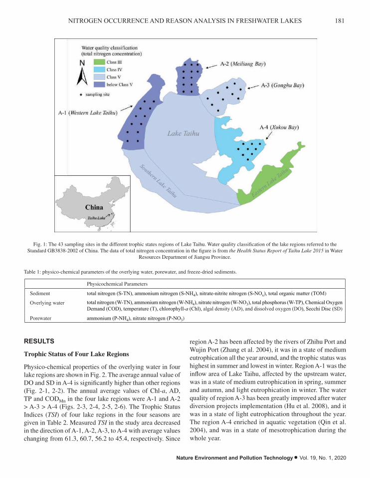
181NITROGEN OCCURRENCE AND REASON ANALYSIS IN FRESHWATER LAKES
Nature Environment and Pollution Technology • Vol. 19, No. 1, 2020
RESULTS
Trophic Status of Four Lake Regions
Physico-chemical properties of the overlying water in four lake regions are shown in Fig. 2. The average annual value of DO and SD in A-4 is significantly higher than other regions (Fig. 2-1, 2-2). The annual average values of Chl-a, AD, TP and CODMn in the four lake regions were A-1 and A-2 > A-3 > A-4 (Figs. 2-3, 2-4, 2-5, 2-6). The Trophic Status Indices (TSI) of four lake regions in the four seasons are given in Table 2. Measured TSI in the study area decreased in the direction of A-1, A-2, A-3, to A-4 with average values changing from 61.3, 60.7, 56.2 to 45.4, respectively. Since
region A-2 has been affected by the rivers of Zhihu Port and Wujin Port (Zhang et al. 2004), it was in a state of medium eutrophication all the year around, and the trophic status was highest in summer and lowest in winter. Region A-1 was the inflow area of Lake Taihu, affected by the upstream water, was in a state of medium eutrophication in spring, summer and autumn, and light eutrophication in winter. The water quality of region A-3 has been greatly improved after water diversion projects implementation (Hu et al. 2008), and it was in a state of light eutrophication throughout the year. The region A-4 enriched in aquatic vegetation (Qin et al. 2004), and was in a state of mesotrophication during the whole year.
FIGURES
Fig. 1: The 43 sampling sites in the different trophic states regions of Lake Taihu. Water quality
classification of the lake regions referred to the Standard GB3838-2002 of China. The data of total
nitrogen concentration in the figure is from the Health Status Report of Taihu Lake 2015 in Water
Resources Department of Jiangsu Province.
Fig. 1: The 43 sampling sites in the different trophic states regions of Lake Taihu. Water quality classification of the lake regions referred to the Standard GB3838-2002 of China. The data of total nitrogen concentration in the figure is from the Health Status Report of Taihu Lake 2015 in Water
Resources Department of Jiangsu Province.
Table 1: physico-chemical parameters of the overlying water, porewater, and freeze-dried sediments.
Physicochemical Parameters
Sediment total nitrogen (S-TN), ammonium nitrogen (S-NH4), nitrate-nitrite nitrogen (S-NOx), total organic matter (TOM)
Overlying water total nitrogen (W-TN), ammonium nitrogen (W-NH4), nitrate nitrogen (W-NO3), total phosphorus (W-TP), Chemical Oxygen Demand (COD), temperature (T), chlorophyll-a (Chl), algal density (AD), and dissolved oxygen (DO), Secchi Disc (SD)
Porewater ammonium (P-NH4), nitrate nitrogen (P-NO3)

182 Yu Wan et al.
Vol. 19, No. 1, 2020 • Nature Environment and Pollution Technology
Fig. 2: The indexes of trophic status in the four lake regions in four seasons. A monitoring index
concentration of each lake was calculated by taking average value of the monitoring index
concentration of the all sample site in this lake.
Fig. 3: Physico-chemical properties of the overlying water in different trophic states lake in four
seasons. A monitoring index concentration of each lake was calculated by taking average value of the
monitoring index concentration of the all sample site in this lake.
Fig. 2: The indexes of trophic status in the four lake regions in four seasons. A monitoring index concentration of each lake was calculated by taking average value of the monitoring index concentration of the all sample site in this lake.
Table 2: The trophic status of the five lake regions.
Lake regions Season TLI (Chl-a) TLI (TP) TLI (TN) TLI (SD) TLI (CODMn) TLI(S) Trophic statesWestern Lake Taihu(region A-1)
Spring 48.3 61.4 86.9 76.2 39.6 62.4 Medium eutrophicationSummer 44.8 72.2 69.9 76.2 48.5 62.7Autumn 43.1 70.2 69.4 80.3 46.7 61.9Winter 36.8 57.9 73.1 78.7 42.5 58.3 Light eutrophication
Meiliang Bay (region A-2)
Spring 55.8 53.7 74.1 77.7 43.4 60.5 Medium eutrophicationSummer 53.7 64.8 65.6 75.7 47.1 61.3Autumn 47.9 59.9 63.8 80.5 58.7 60.6Winter 48.6 57.4 70.2 80.6 50.6 60.2
Gonghu Bay (region A-3)
Spring 51.9 56.6 73.5 69.6 34.5 57.0 Light eutrophicationSummer 48.0 62.6 62.6 69.3 44.1 56.5Autumn 45.2 55.9 62.6 68.8 63.3 58.0Winter 45.0 46.2 68.6 72.3 38.4 53.2
Xukou Bay (region A-4)
Spring 42.0 40.5 63.3 65.6 37.4 49.0 MesotrophicationSummer 39.0 44.9 59.0 65.1 42.9 49.1Autumn 35.2 45.7 43.1 64.6 25.6 42.2Winter 30.9 39.0 32.9 66.2 42.9 41.4

183NITROGEN OCCURRENCE AND REASON ANALYSIS IN FRESHWATER LAKES
Nature Environment and Pollution Technology • Vol. 19, No. 1, 2020
Table 3: Analysis of similarity (ANOSIM) R statistics for comparisons of spatial differences in overlying water environmental indexes.
Meiliang Bay (A-2) Gonghu Bay (A-3) Western Lake Taihu (A-1)
Gonghu Bay (A-3) 0.04
Western Lake Taihu (A-1) 0.11 0.10
Xukou Bay (A-4) 0.43 0.45 0.64
Table 4: Analysis of similarity (ANOSIM) R statistics for comparisons of seasonal differences in overlying water environmental indexes.
Spring Summer Autumn
Summer 0.28
Autumn 0.28 0.06
Winter 0.15 0.18 0.09
Temporal and Spatial Distribution Characteristics of Nitrogen in Overlying Water
As shown in Fig. 3 (3-1), the average annual concentration of TN decreased in the same direction as TSI does, and TN concentration of each lake region was highest in spring. The temporal and spatial distribution characteristics of NO3
--N were consistent with TN (Fig. 3-3). The spatiotemporal var-iation of NH4
+-N in the overlying water was not significant (Fig. 3-2).
The main form of nitrogen occurrence in overlying wa-ter of four lake regions is shown in Fig. 4. Nitrogen in the overlying water was principally of NO3
--N in region A-2 (Fig. 4-2) and region A-3 (Fig. 4-3), and was principally of organic nitrogen (ON) in region A-4 (Fig. 4-4). In region A-1, nitrogen in the overlying water was principally of NO3
-
-N in summer and fall, and organic nitrogen in spring and winter (Fig. 4-1).
The result of ANOSIM showed that there were significant spatial variations in nitrogen distribution characteristics of the overlying water between eutrophication and mesotroph-ication region (Table 3), and the seasonal variation was not significant (Table 4).
Temporal and Spatial Distribution Characteristics of Nitrogen in Sediment and Porewater
As shown in Fig. 5 (5-1), the TN content in sediment in re-gion A-1, A-2, A-3, and A-4 was highest in summer, spring, autumn and spring, respectively. The sediment NH4
+-N (Fig. 5-2) and NOx
--N (Fig. 5-3) content in four lake regions reach-ing their maximal level in autumn. In addition, the contents of TN, NH4
+-N and NOx--N in sediments were reduced with
decreasing trophic status (Fig. 5). The main form of nitrogen occurrence in sediment of four lake regions was organic ni-trogen, and the main form of inorganic nitrogen occurrence in sediment and porewater were NH4
+-N (Fig. 7).
Spatial and temporal distribution trend of NH4+-N in
porewater was similar to that in sediment Fig. 6 (Fig. 6-1). The concentration of NO3
--N in porewater showed a strong seasonal variation with NO3
--N reaching its maximal level in summer (Fig. 6-2).
Relationship Between Various Nitrogen Occurrence Forms and Aquatic Environmental Factors
Pearson’s correlation analysis indicated that chlorophyll-a and algal density in the study area appeared to be correlated
Fig. 3: Physico-chemical properties of the overlying water in different trophic states lake in four seasons. A monitoring index concentration of each lake was calculated by taking average value of the monitoring index concentration of the all sample site in this lake.

184 Yu Wan et al.
Vol. 19, No. 1, 2020 • Nature Environment and Pollution Technology
Table 5: Relationship between environmental factors and various forms of nitrogen in the overlying water, sediment and porewater.
Chl W-TN AD DO W-NH4 W-NO3 P-NH3 P-NO3 S-TN S-NH4
spring W-TN
AD 0.66 0.77
DO
W-NH4 0.91 0.66
W-NO3 0.48 0.84 0.73 0.74
P-NH3 0.61 0.75 0.88 0.73 0.68
P-NO3
S-TN 0.66 0.49 0.55 0.48
S-NH4 0.62 0.47 0.73 0.57 0.57 0.58
S-NOx 0.48 0.61 0.77 0.52 0.59 0.76 0.78
summer W-TN 0.57
AD 0.83 0.60
DO -0.71 -0.75 -0.68
W-NH4 0.60
W-NO3 0.74 0.85 0.77 -0.68 0.62
P-NH3 0.50 0.78 -0.63 0.72
P-NO3
S-TN 0.63 0.68 0.60 -0.58 0.64 0.68
S-NH4 0.83 0.49 0.71 -0.47 0.48 0.69 0.49 0.57
S-NOx 0.52 0.47 0.67 0.64 0.74
autumn W-TN 0.81
AD 0.90 0.83
DO -0.72 -0.89 -0.68
W-NH4
W-NO3 0.45 0.72 0.47 -0.70
P-NH3 0.64 0.83 0.76 -0.70 0.64
P-NO3 0.75 0.78 0.70 -0.79 0.64 0.58
S-TN 0.57 0.46 -0.59 0.54
S-NH4 0.64 0.50 0.65 0.50
S-NOx 0.58 -0.58 0.65 0.58
winter W-TN 0.74
AD 0.67 0.79
DO -0.69 -0.65 -0.66
W-NH4
W-NO3 0.77 0.70 0.65 -0.86
P-NH3 0.68 0.43 0.54
P-NO3
S-TN 0.79 0.57
S-NH4 0.76 0.42 -0.56 0.74 0.87
S-NOx 0.50 0.68 0.51 0.70
Only p < 0.01 shown in the table

185NITROGEN OCCURRENCE AND REASON ANALYSIS IN FRESHWATER LAKES
Nature Environment and Pollution Technology • Vol. 19, No. 1, 2020
Fig. 4: various forms of nitrogen occurrence in the overlying water in different trophic states lake
regions in four seasons.
Fig. 5: Physico-chemical properties of the sediment in different trophic states lake regions in four
seasons. A monitoring index concentration of each lake was calculated by taking average value of the
monitoring index concentration of the all sample sites in this lake.
Fig. 5: Physico-chemical properties of the sediment in different trophic states lake regions in four seasons. A monitoring index concentration of each lake was calculated by taking average value of the monitoring index concentration of the all sample sites in this lake.
Fig. 6: Physico-chemical properties of the porewater in different trophic states lake regions in four seasons. A monitoring index concentration of each lake region was calculated by taking average value of the monitoring index concentration of the all
sample sites in this lake.
Fig. 4: various forms of nitrogen occurrence in the overlying water in different trophic states lake
regions in four seasons.
Fig. 5: Physico-chemical properties of the sediment in different trophic states lake regions in four
seasons. A monitoring index concentration of each lake was calculated by taking average value of the
monitoring index concentration of the all sample sites in this lake.
Fig. 4: various forms of nitrogen occurrence in the overlying water in different trophic states lake regions in four seasons.

186 Yu Wan et al.
Vol. 19, No. 1, 2020 • Nature Environment and Pollution Technology
positively with the W-TN, W-NO3, P-NH3, S-TN, S-NH4, and S-NOx but negatively with DO (Table 5). For the differ-ent nitrogen occurrence forms in various media, a positive correlation between TN and NO3
--N in overlying water and TN, NH4
+-N, and NO3--N in sediment was observed (Table
5). Meanwhile, TN and NH4+-N in sediment exhibited a
significant correlation with NH4+-N in porewater (Table 5).
DISCUSSION
Analysis of Temporal and Spatial Distribution Characteristics of Nitrogen Forms
The type of organic matter in sediment has an important influence on the migration and transformation of nitrogen (Zhu et al. 2011). Therefore, in this study, various sedi-mentary organic matter types will cause the difference of nitrogen occurrence forms in overlying water and trophic status of lake region. Different organic matter types have different mineralization products. On the one hand, organic compounds rich in carbon chains (cellulose, sugars, simple hydrocarbons, and lipids) produced monosaccharides in the degradation process, and eventually released CO2 and CH4
after mineralization (Xiao et al. 2009). On the other side, organic compounds rich in peptide ammonia bonds were degraded to amino acids, and finally NH4
+-N was released through mineralization (Xiao et al. 2009).
In the algal bloom and eutrophic region, A-2 and A-3, the main source of organic matter was the algae which settled in the lake regions after death. While algae rich in nitrogen, sedimentary organic matter released a large amount of nitro-gen such as NH4
+-N during degradation and mineralization. The reason why nitrogen in the overlying water of regions A-2 and A-3 was principally of NO3
--N may be two-fold. First of all, phytoplankton preferred to absorb NH4
+-N than NO3
--N, and NH4+-N was preferentially absorbed by algae.
Secondly, due to the high content of DO in the lake regions (mean 8.5 mg/L), NH4
+-N would be transformed into NO3-
-N under aerobic conditions. In the mesotrophic region A-4, the main source of organic matter was aquatic plants rich in cellulose. While cellulose was mainly composed of C, H and O, sedimentary organic matter released CO2 and CH4 during degradation and mineralization, therefore, organic nitrogen was the main form of nitrogen occurrence in re-gion A-4. In the algal bloom and eutrophic region, A-1, as
Fig. 7: various forms of nitrogen occurrence in the sediment in different trophic states lake regions of four seasons.

187NITROGEN OCCURRENCE AND REASON ANALYSIS IN FRESHWATER LAKES
Nature Environment and Pollution Technology • Vol. 19, No. 1, 2020
the main inflow regions of Lake Taihu, the impact of inflow rivers on the main form of nitrogen occurrence in overlying water was more pronounced. Previous analysis of nitrogen sources in region A-1 show that nitrogen in the inflow river was mainly from fertilizers during dry seasons, while from sewage during wet seasons (Wu et al. 2015). Thus, it caused that nitrogen in the overlying water was principally of NO3
-
-N in summer and fall (wet season), and organic nitrogen in spring and winter (dry season).
The growth cycle of algae was short (1~2 weeks), and nutrients in the algae were quickly released into the water after algal death. Therefore, algae cannot fix nitrogen in water body for a long time as plants do. After algal death, nitrogen released into water in the form of ion state or gel state and reused by algae again (Sun et al. 2007). Whereas, aquatic plants cannot be decomposed quickly, and released nitrogen slowly by mineralization after their death. The released nitrogen quickly absorbed by aquatic plants, and significantly reduce the concentration of nutrients in water (Zhang et al. 2004). In conclusion, regions A-1, A-2 and A-3 with frequent algal bloom were in a state of eutrophication, while region A-4 with rich in aquatic vegetation was in a state of mesotrophication.
In the same sampling site, NO3--N concentration in the
porewater was much lower than that in the overlying water. This was due to a significant denitrification took place in the sedimentary environment, and NO3
--N, as an oxidant, par-ticipated in denitrification and degradation of organic matter in sediments. Besides, in the same sampling site, NH4
+-N concentration in the porewater was much higher than that in the overlying water. NH4
+-N in porewater mainly came from the ammonification of organic nitrogen in sediments under the action of anaerobic microorganisms (Hou et al. 2014), and its content was determined by the decomposition rate of organic nitrogen and the diffusion rate of NH4
+-N in the sediment-water interface. The sediment of lake Taihu was rich in organic nitrogen and low in dissolved oxygen, which was easy to form a reducing environment (Qiao et al. 2012), and denitrification and ammonification were significant under microbial action. Hu et al. (2004) reported that the particulate matter of sediment had a strong adsorption on NH4
+-N, while it had a weak even negative adsorption on NOx
--N. NH4+-N
usually exist in the sediment in the form of adsorption state and free state, and NH4
+-N adsorbed on the sediment was the main source of NH4
+-N in porewater (Bao et al. 2006).
Difference Analysis of Nitrogen Occurrence Characteristics
Agreeing with previous studies in other similar eutrophicated freshwater lakes (Shu et al. 2012, Zhao et al. 2013), the result
of ANOSIM showed that the seasonal variation of nitrogen distribution characteristics in overlying water was not sig-nificant. Besides, there were significant spatial variations in nitrogen distribution characteristics of the overlying water between eutrophication and mesotrophication region. The reason might be that the northern and western lake regions had been affected by the input of polluted upstream water for a long time, and they were the main algal bloom areas of Lake Taihu. The death and subsidence of algae caused the release of nitrogen nutrients to overlying water (Qin et al. 2004), further aggravating the eutrophication state of the lake region. The region A-4 had no input of nitrogen pollutants and was rich in aquatic vegetation. Aquatic plants not only purified water quality (Li et al. 2010), but also inhibited the release of nutrients in sediment (Barko et al. 1998), which lowers the trophic status of lake region. Therefore, due to the exogenous input and endogenous release of nitrogen, cause a significant difference of nitrogen occurrence characteristics between mesotrophication and eutrophication lake regions.
Influence Factors of Nitrogen Occurrence Characteristics
Chlorophyll-a was one of the important components of the algae, its content reflected the biomass and growth of phyto-plankton, and was closely related to the species and quantity of algae (Agawin et al. 2000), so the algal density and chloro-phyll-a showed significant positive correlation. The negative correlation between algal density and dissolved oxygen indi-cated that with the increasing of algal density, algae consumed more dissolved oxygen in water through respiration, which results in the decrease of dissolved oxygen concentration.
In this study, the concentration of TN in overlying water showed a significant positive correlation with algal density in the four seasons. Previous studies had shown that TN not only affected the growth and reproduction of algae, but also affected the algal community structure (Zhu et al. 2010). Zhu et al. (2013) discussed the relationship between algal community structure and environmental factors in Southern Lake Taihu, and found that TN had a more significant impact on the growth of algae than other environmental factors. After the death of algae, the nitrogen in the algae could be released into the water quickly, providing nutrients for the growth of more algae, and at the same time, the concentration of TN in the overlying water increased. This conclusion could explain that, in the eutrophicated algae-dominated lake regions, the algal density in summer and autumn was higher than that in winter and spring, but the TN concentration in overlying water was lower.
Consistent with the observations made in freshwater lake (Trevisan et al. 2007), algal density and chlorophyll showed

188 Yu Wan et al.
Vol. 19, No. 1, 2020 • Nature Environment and Pollution Technology
a positive correlation with NO3--N concentration, that might
be because phytoplankton usually tend to absorb ammonia, nitrite, and nitrate nitrogen in water to synthesize amino acids and other substances needed by algal cells (Wafar et al. 2004). Chlorophyll and algal density were positively correlated to P-NH3, S-TN, S-NH4, and S-NOx, which might be due to the release of nitrogen from sediment to overlying water and porewater, thus indirectly affecting the algal density and chlorophyll content in the overlying water.
Nitrogen in overlying water, porewater, and sediment was transferred and transformed under different conditions. On the one hand, nitrogen in porewater and sediment was exchanged with overlying water through molecular diffusion, which affected the occurrence form and characteristics of nitrogen in overlying water. On the other hand, sediment had adsorption effect on nitrogen in porewater and overlying water. Driven by the concentration gradient, the nitrogen in the sediment and porewater diffused to the overlying water (Zhang et al. 2013). Therefore, the forms and contents of nitrogen in various media could influence each other through migration and transformation.
W-TN and W-NO3 in overlying water of each lake region showed a positive correlation with P-NH3, S-TN, S-NH4 and S-NOx, indicating that there was a strong nitrogen exchange between water and sediment. The endogenous nutrients en-tered the overlying water from the sediments mainly through the resuspension process of surface sediments and the con-centration diffusion of porewater. Some scholars considered that the process of nitrogen release into overlying water was a mechanism that nitrogen in the sediment supply nutrients to the overlying water (Xia et al. 2009). Therefore, while the exogenous source was effectively controlled, the endogenous release could not be ignored.
Nitrogen nutrients not only diffused between overlying water and porewater, but also migrated and transformed between sediment and porewater. There was a significant correlation between various forms of nitrogen in sediments and porewater, among them, the correlation of NH4
+-N in the two media was the best, indicating that NH4
+-N in porewa-ter was mainly affected by NH4
+-N in sediment. The effect was mainly manifested in two aspects. On the one hand, the organic matter in sediments generated NH4
+-N through min-eralization under anaerobic environment, and then releases NH4
+-N into porewater by adsorption and desorption. For another, the concentration of NH4
+-N in porewater also af-fected the adsorption capacity of sediment for NH4
+-N. The study about NH4
+-N adsorption characteristics of shallow lakes surface sediment in the middle and lower Yangtze River, confirmed the existence of the interaction (adsorption and desorption) in the sediment of Lake Taihu (Wang et al. 2007).
A positive correlation between NH4+-N in porewater and
TN in sediment suggest that, as the main component of TN in sediment (more than 90%), organic nitrogen transformed to NH4
+-N by ammonification, and NH4+-N migrated to
porewater and overlying water through diffusion. Previous studies suggest that the above process was the main way of nitrogen exchange between sediment and overlying water (Li et al. 2009).
ACKNOWLEDGEMENTS
This research was supported by Natural Science Foundation of Chongqing, China (cstc2019jcyj-bshX0007, cstc2018j-cyjAX0534, cstc2017jcyjAX0292), Central Public-interest Scientific Institution Basal Research Fund (GYZX190306), National Natural Science Foundation of China (51709024), and Science and Technology Project of Chongqing Urban Administration (2019-23).
REFERENCES
Agawin, N.S., Duarte, C.M. and Agustí, S. 2000. Nutrient and temperature control of the contribution of picoplankton to phytoplankton biomass and production. Limnol. Oceanogr., 45: 591-600.
Aizaki, M. 1981. Application of modified Carlson’s trophic state index to Japanese lakes and its relationships to other parameters related to trophic state. National Institute for Environmental Studies, Japan 23: 13-31.
Bao, X., Chen, K. and Fan, C. 2006. Effects on nitrogen and phosphorus distribution in interstitial water and sediment-water nitrogen and phosphorus release with growing of submerged macrophytes. Journal of Lake Sciences, 18: 515-522.
Barko, J.W. and James, W.F. 1998. Effects of submerged aquatic macrophytes on nutrient dynamics, sedimentation, and resuspension. The structuring role of submerged macrophytes in lakes. Springer, New York, NY, pp. 197-214.
Canfield, D.E., Langeland, K.A., Linda, S.B. and Haller, W.T. 1985. Relations between water transparency and maximum depth of macrophyte colonization in lakes. J. Aquat. Plant Manage., 23: 25-28.
Clarke, K.R. 1993. Non-parametric multivariate analyses of changes in community structure. Australian journal of Ecology, 18: 117-143.
Deng, J.C., Chen, Q., Zhai, S.J., Yang, X.C., Han, H.J. and Hu, W.P. 2008. Spatial distribution characteristics and environmental effect of N and P in water body of Taihu Lake. Environmental Science, 29: 3382-3386.
Hou, D., He, J., Lu, C., Dong, S., Wang, J., Xie, Z. and Zhang, F. 2014. Spatial variations and distributions of phosphorus and nitrogen in bottom sediments from a typical north-temperate lake, China. Environmental Earth Sciences, 71: 3063-3079.
Hu, W., Zhai, S., Zhu, Z. and Han, H. 2008. Impacts of the Yangtze River water transfer on the restoration of Lake Taihu. Ecological Engineering, 34: 30-49.
Hu, Z.T., Sun, H.W. and Tan, Y. 2004. Adsorptive characteristic of nutrient elements and influential factors in Taihu Lake sediment. Journal of Agro-Environment Science, 23: 1212-1216.
Jin, X.C., Jiang, X. and Xu, Y.H. 2006. Seasonal variation of dissolved nitrogen and phosphorus in sediments in northeast part of Lake Taihu. China Environmental Science, 26: 409-413.
Li, X.N., Song, H.L., Li, W., Lu, X.W. and Nishimura, O. 2010. An integrated ecological floating-bed employing plant, freshwater clam and biofilm carrier for purification of eutrophic water. Ecol. Eng., 36: 382-390.

189NITROGEN OCCURRENCE AND REASON ANALYSIS IN FRESHWATER LAKES
Nature Environment and Pollution Technology • Vol. 19, No. 1, 2020
Li, Y., Hu, X. and Nian, Y. 2009. Experimental Comparison of Nutrient Characters of Pore Water Between Macrophytic and Algal Lakes. Journal of Hydroecology, 5: 5.
Lu, R.K. 1999. Soil Argrochemistry Analysis Protocoes. China Agriculture Science Press, Beijing.
Qiao, J., Yang, L., Yan, T., Xue, F. and Zhao, D. 2012. Nitrogen fertilizer reduction in rice production for two consecutive years in the Taihu Lake area. Agr. Ecosyst. Environ. 146: 103-112.
Qin, B.Q. , Hu, W.P. and Chen, W.M. 2004. Process and Mechanism of Environmental Changes of the Taihu Lake. Science Press, Beijing.
Shu, F.Y., Liu, Y.P., Zhao, Y., Wu, Y.P. and Li, A.H. 2012. Spatio-temporal distribution of TN and TP in water and evaluation of eutrophic state of Lake Nansi. Environmental Science, 33: 3748-3752.
Sun, X., Qin, B.Q. and Zhu, G.W. 2007. Release of colloidal phosphorus, nitrogen and organic carbon in the course of dying and decomposing of cyanobacteria. China Environmental Science, 27: 341-345.
Trevisan, G.V. and Forsberg, B.R. 2007. Relationships among nitrogen and total phosphorus, algal biomass and zooplankton density in the central Amazonia lakes. Hydrobiologia, 586: 357-365.
Wafar, M., L’Helguen, S., Raikar, V., Maguer, J.F. and Corre, P. L. 2004. Nitrogen uptake by size-fractionated plankton in permanently well-mixed temperate coastal waters. J. Plankton Res., 26: 1207-1218.
Wang, J., Wang, S., Jin, X. and Zhu, S. 2007. Ammonium adsorption characteristics onto the sediments from shallow lakes in the middle and lower reaches of the Yangtze River. Journal of Agro-Environment Science, 26: 1224-1229.
Wang, Q., Li, Y., Jiang, X., Wang, S. and Jin, X. 2010. The distribution of nitrogen speciation in three lake regions of North of Taihu Lake. China Environmental Science, 30: 1537-1542.
Wang, S.R., Jiao, L.X. and Jin, X.C. 2008. Distribution of total, exchangeable and fixed nitrogen in the sediments from shallow lakes in the middle and lower reaches of the Yangtze River. Acta Scientiae Circumstantiae, 28: 37-43.
Wei, F.S. 2002. Determination Methods for Examination of Water and
Wastewater. China Environmental Science Press, Beijing.Wu, Q.L., Ruan, X.H., Wu, C.M., Li, R.F., Wang, C.W. and Wan, Y. 2015.
Analysis of sources and transformation of nitrogen as a contaminant in the river and lake water in the western region of the Taihu Lake basin. Acta Sci. Circum. 35: 3883-3889.
Xia, X., Yang, Z. and Zhang, X. 2009. Effect of suspended-sediment concentration on nitrification in river water: Importance of suspended sediment-water interface. Enviro. Sci. Technol., 43: 3681-3687.
Xiao, L., Yang, L., Zhang, Y., Gu, Y., Jiang, L. and Qin, B. 2009. Solid state fermentation of aquatic macrophytes for crude protein extraction. Ecol. Eng., 35: 1668-1676.
Zhang, L., Fan, C.X., Chi, Q.Q., Wang, J.J. and Qin, B.Q. 2004. Phosphorus species distribution of sediments in Lake Taihu and its main inflow rivers. Geochimica, 33: 423-432.
Zhang, L., Wang, L., Yin, K., Lu, Y., Zhang, D., Yang, Y. and Huang, X. 2013. Porewater nutrient characteristics and the fluxes across the sediment in the Pearl River estuary and adjacent waters, China. Estuar. Coast. Shelf S., 133: 182-192.
Zhao, H., Wang, S., Jiao, L., Yang, S. and Liu, W. 2013. Characteristics of temporal and spatial distribution of different forms of phosphorus in the sediments of Erhai Lake. Research of Environmental Sciences, 26: 227-234.
Zhao, X.Q., Yang, L.Y., Yu, Z.Y., Fan, Q.H., Zhan, Z., Xiao, Y. and Qin, B. 2007. Temporal and spatial distribution of physicochemical characteristics and nutrients in sediments of Lake Taihu. J. Lake Sci., 19: 698-704.
Zhu, M., Zhu, G., Zhao, L., Yao, X., Zhang, Y., Gao, G. and Qin, B. 2013. Influence of algal bloom degradation on nutrient release at the sediment-water interface in Lake Taihu, China. Environ. Sci. Pollut. R., 20: 1803-1811.
Zhu, W., Wan, L. and Zhao, L. 2010. Effect of nutrient level on phytoplankton community structure in different water bodies. J. Environ. Sci-China, 22: 32-39.
Zhu, Z.Y., Zhang, J., Wu, Y., Zhang, Y.Y., Lin, J. and Liu, S.M. 2011. Hypoxia off the Changjiang (Yangtze River) Estuary: Oxygen depletion and organic matter decomposition. Marine Chemistry, 125: 108-116.

Vol. 19, No. 1, 2020 • Nature Environment and Pollution Technology
190
Heavy Metal Accumulation of 13 Native Plant Species Around a Coal Gangue Dump and Their Potentials for Phytoremediation Yafen Han*, Qi Li*(**)† and Na Liu**School of Environment and Surveying Engineering, Suzhou University, Suzhou 234000, China**National Engineering Research Center of Coal Mine Water Hazard Controlling, Suzhou 234000, China†Corresponding author: Qi Li
ABSTRACTThis study was designed to investigate the heavy metal accumulation characteristics of 13 native plant species and associated rhizosphere soils around Taoyuan coal gangue dump, and to determine their potentials for phytoremediation. The mean concentrations of Cu, Cd, Pb and Cr in rhizosphere soils were 46.70, 0.43, 16.86 and 109.67 mg·kg-1, respectively. According to the pollution load index, the soils were strongly contaminated by Cd, moderately contaminated by Cu, slightly contaminated by Cr and uncontaminated by Pb. The concentrations of Cu, Cd, Pb and Cr in shoots of the 13 plant species ranged as 1.86-33.10, 0.10-0.94, 2.04-14.72 and 0.49-9.03 mg·kg-1, respectively, while in roots ranged as 0.44-91.56, 0.31-1.82, 4.83-50.49 and 0.37-99.63mg·kg-1, respectively. No plant species satisfied the concentration criteria of hyperaccumulator, but two high Cd-enriched species of M. falcata and C. japonicum, whose BCF and TF values were all greater than one, were recorded. Based on the Individual Phytoremediation Factors (IPF), S. viridis showed the strongest remediating capability per a single plant for Cu, while M. falcata, S. viridis, C. eragrostis and C. japonicum had relatively strong remediating capability per a single plant for Cd. The four plant species were proposed to be preferentially taken as the candidates for phytoremediation.
INTRODUCTION
Coal gangue, produced during the coal ore mining and utilization processing, is one of the greatest industrial solid wastes in China (Xue et al. 2014). Currently, the annual discharged amount of coal gangue is up to 1.5 × 10⁸ t in China and only about 40% of it can be comprehensively utilized. The excessive coal gangues are inevitably piled up in the open in most coal mining areas of China. Under the long-term effect of external factors (weathering, leaching and biological reaction), heavy metals in these coal gangues will be released and cause serious pollution to the surrounding soil
(You et al. 2016). Jiang et al. (2014) reported that potential ecological damage degrees of heavy metals in soils around Yangcaogou coal gangue dump were moderate to strong, and it decreased with increasing distance from the coal gangue dump. He et al. (2016) found high accumulation of toxic metals, especially Mn, Fe and Cr, in the soils within 250 m away from Liejiaqiao coal gangue dump.
Heavy metals accumulated in soils can cause great dam-age to the stability of the ecological environment, and harm human health through the food chain (Ahmad et al. 2011). It is necessary to reduce the negative effect of heavy metals and make the land resource available for agricultural production.
Traditional remediation techniques, including excavation, leaching, electro kinetics, chemical stabilization, etc., for removing heavy metals from contaminated soils or reduc-ing their availabilities are expensive and environmentally destructive. In contrast, phytoremediation is a less expensive and environmentally non-destructive restoration method for decreasing the environmental risk from the contaminated soils (Ali et al. 2013). This technology is carried out by us-ing plants to extract the toxic metals from soil or to render them harmless in the contaminated sites. The efficiency of phytoremediation strongly depends on the accumulation and tolerance abilities of heavy metals in soil by the selected plant species. Thus, screening appropriate plant species is a critical step for successful phytoremediation. However, the species suitable for phytoremediation are relatively rare, and even usually endemic at the metal-enriched sites, because the accumulation and tolerance abilities of plant were generally evolved from the long-term stress of high concentration of heavy metals in soils (Ghaderian et al. 2012). Moreover, compared with the introduced plant species from other envi-ronment, the native species have more excellent adaptability of survival, growth and reproduction in the contaminated area. Therefore, increasing interests have been focused on the investigation and seeking of suitable metal-accumulator
Nat. Env. & Poll. Tech.Website: www.neptjournal.com
Received: 18-05-2019Accepted: 22-07-2019
Key Words:Heavy metal Phytoremediation Rhizosphere soil Coal gangue dump
2020pp. 191-199 Vol. 19
p-ISSN: 0972-6268No. 1 Nature Environment and Pollution Technology
An International Quarterly Scientific Journal
Original Research Papere-ISSN: 2395-3454
Open Access

192 Yafen Han et al.
Vol. 19, No. 1, 2020 • Nature Environment and Pollution Technology
from the native plant species growing in metalliferous soils
(Liu et al. 2014).
Taoyuan coal mine, located in the Huaibei coalfield in Anhui province of China, has a mining history of more than 20 years. The present study was conducted to investigate the accumulation characteristics of Cu, Cd, Pb and Cr in the 13 native plant species and associated rhizosphere soils around the coal gangue dump of Taoyuan mine, and to screen the species with phytoremediation potentials. This research is of important practical value for polluted soil treatment and ecological restoration in the coal mining area.
MATERIALS AND METHODS
Study Area and Sample Collection
Taoyuan coal mine is located in north-eastern Anhui Prov-ince, about 12 km from Suzhou urban area (Fig. 1). This region is characterized by a sub-humid monsoon climate, with an annual average rainfall of 890 mm and an annual average temperature of 14.4°C. The main soil types in Suzhou are Yellow fluvo-aquic soil and Lime concretion black soil. Taoyuan mine began production in October 1995 with an annual coal output of 1.6 million tons. During the past two decades, large amounts of coal gangue were produced go-ing with coal exploitation, and a large coal gangue dump, covering an area of approximately 38800 m2, was formed in eastern of the mining area. The height of the coal gangue
dump is 65 m and the coal gangue stock is approximately 1.3 million tons.
Field sampling was carried out in October 2017. Fifty two plants and their corresponding rhizosphere soils were collected form the wastelands within 200 m from the coal gangue dump in Taoyuan mining area. The collected plants were consisted of thirteen species and eight families (Table 1). All the plant species were the common species in the mining area. For each species, three to five individual plants were selected randomly. Each soil sample was approximately 0.5 kg. After collection, the plant and soil samples were put into plastic self-sealing bags and labelled.
Sample Analysis and Quality Control
After the collected samples were transported to the labora-tory, bulk density and moisture contents of soil were tested immediately. Then, each soil sample was air-dried at room temperature for two weeks and pulverised to pass through a 0.25-mm sieve. Soil pH was determined in a 1:2.5 soil/water (w/v) suspension using a pH meter. Organic matter of soil was measured by the Walkley-Black method. Total nitrogen (TN), total phosphate (TP) and total potassium (TK) were estimated by the standard methods of the Soil Science Society of China. Soil samples were digested with the mixed acids of aqua regia, HClO4 and HF (4:1:1, v/v) in Teflon beakers, and the concentrations of Cu, Cd, Pb and Cr in soils were tested by an atomic absorption spectrophotometer (AAS, Model
Fig. 1: Location of Taoyuan coal mine in Suzhou City, Anhui Province, China.

193HEAVY METAL ACCUMULATION IN PLANT SPECIES AROUND A COAL GANGUE DUMP
Nature Environment and Pollution Technology • Vol. 19, No. 1, 2020
TAS-990FG, Purkinje General Instrument, Beijing, China).
Each wheat sample was carefully cut into two parts of root and shoot with a scissors. All the parts were thoroughly washed with running tap water to remove dirt and rinsed three times with deionized water. Then, the plant tissues were oven-dried at 80°C to constant weight and ground to pass through a 0.25-mm sieve. The plant powder samples were digested with the mixed acids of HNO3, HCl and HClO4 (5:1:1, v/v) in glass beakers, and the concentrations of Cu, Cd, Pb and Cr in different plant parts were also determined by AAS.
To ensure experimental accuracy, the reference materials (GBW07430 for soils and GBW007604 for plants) were per-formed through the digestion and determination processes. The recoveries of Cu, Cd, Pb and Cr in the soil and plant reference materials were all in the range of 100±10%. Rea-gent blanks were also employed in the analysis to eliminate
analytical bias. All chemicals used in the experiment were of analytical grade, and all the vessels were treated with dilute nitric acid for 24 h followed by rinsing with MilliQ water for three times before use.
Data Analysis
Pollution load index (PLI) was applied in this study to evaluate the extent of the contamination by heavy metals in soil samples. It can be calculated by the following formula
(Muhammad et al. 2011):
6
blanks were also employed in the analysis to eliminate analytical bias. All chemicals used in the
experiment were of analytical grade, and all the vessels were treated with dilute nitric acid for 24 h
followed by rinsing with MilliQ water for three times before use.
Data Analysis
Pollution load index (PLI) was applied in this study to evaluate the extent of the contamination by
heavy metals in soil samples. It can be calculated by the following formula (Muhammad et al. 2011):
n
1
21 nCFCFCFPLI …(1)
Where, CF represents contamination factor of a single metal, and is obtained by dividing the
concentration of each metal in the soil by the local background value. Based on the values of CF and
PLI, the classification criterion of contamination level is listed in Table 2.
Background
metal
C
CCF …(2)
Table 2: Pollution load index and classification criterion of contamination level.
Contamination degree
CF PLI Value range Contamination Level Value range Contamination Level
0 CF≤0.7 No contamination PLI≤1.0 No contamination 1 0.7<CF≤1.0 Light contamination 1.0<CF≤2.0 Slight contamination 2 1.0<CF≤2.0 Slight contamination 2.0<CF≤3.0 Moderate contamination 3 2.0<CF≤3.0 Moderate contamination CF>3.0 Strong contamination 4 CF>3.0 Strong contamination
Bioconcentration factor (BCF) and Translocation factor (TF) of the studied plant species were
calculated based on the following equations.
soil
root
C
CBCF …(3)
root
shoot
C
CTF …(4)
In the above equations, Cshoot (mg·kg-1), Croot (mg·kg-1) and Csoil (mg·kg-1) are the concentrations of
a particular metal in shoot (including seed, leaf and stem aboveground), root and rhizosphere soil,
respectively.
…(1)
Where, CF represents contamination factor of a single metal, and is obtained by dividing the concentration of each metal in the soil by the local background value. Based on the values of CF and PLI, the classification criterion of con-tamination level is listed in Table 2.
Table 2: Pollution load index and classification criterion of contamination level.
Contamination degreeCF PLI
Value range Contamination Level Value range Contamination Level
0 CF £ 0.7 No contamination PLI £ 1.0 No contamination
1 0.7<CF £ 1.0 Light contamination 1.0<CF£2.0 Slight contamination
2 1.0<CF £ 2.0 Slight contamination 2.0<CF£3.0 Moderate contamination
3 2.0<CF £ 3.0 Moderate contamination CF>3.0 Strong contamination
4 CF > 3.0 Strong contamination
Table 1: Plant species collected from the investigated area and number of samples.
Family Plant species Species Code Brief nameSample number
Biomass (g·plant-1, dry weight)
Shoot Root
Compositeae
Artemisia argyi Levl. Et Vant. 1 A. argyi 4 0.82±0.16 0.19±0.05
Conyza canadensis (Linn.) Cronq. 2 C. canadensis 5 5.02±0.63 0.21±0.04
Cirsium japonicum Fisch. ex DC. 3 C. japonicum 3 3.83±0.47 0.33±0.02
Xanthium sibiricum Patrin ex Widder 4 X. sibiricum 4 2.77±0.31 2.34±0.58
Artemisia annua Linn. 5 A. annua 4 2.71±0.54 0.31±0.04
GramineaeEleusine indica (Linn.) Gaertn. 6 E. indica 3 8.76±1.98 0.16±0.04
Setaria viridis (Linn.) Beauv. 7 S. viridis 5 12.25±2.05 0.18±0.02
Leguminoseae Medicago falcata Linn. 8 M. falcata 4 5.95±1.36 0.78±0.05
Amaranthaceae Amaranthus spinosus Linn. 9 A. spinosus 4 2.26±0.51 0.16±0.02
Crucifereae Capsella bursa-pastoris (Linn.) Medic. 10 C. bursa-pastoris 4 1.93±0.10 0.15±0.01
Cyperaceae Cyperus eragrostis Lam. 11 C. eragrostis 4 5.16±0.95 0.14±0.04
Solanaceae Physalis pubescens Linn. 12 P. pubescens 4 0.59±0.11 0.13±0.03
Plantaginaceae Plantago asiatica Linn. 13 P. asiatica 4 1.36±0.17 0.22±0.02

194 Yafen Han et al.
Vol. 19, No. 1, 2020 • Nature Environment and Pollution Technology
6
blanks were also employed in the analysis to eliminate analytical bias. All chemicals used in the
experiment were of analytical grade, and all the vessels were treated with dilute nitric acid for 24 h
followed by rinsing with MilliQ water for three times before use.
Data Analysis
Pollution load index (PLI) was applied in this study to evaluate the extent of the contamination by
heavy metals in soil samples. It can be calculated by the following formula (Muhammad et al. 2011):
n
1
21 nCFCFCFPLI …(1)
Where, CF represents contamination factor of a single metal, and is obtained by dividing the
concentration of each metal in the soil by the local background value. Based on the values of CF and
PLI, the classification criterion of contamination level is listed in Table 2.
Background
metal
C
CCF …(2)
Table 2: Pollution load index and classification criterion of contamination level.
Contamination degree
CF PLI Value range Contamination Level Value range Contamination Level
0 CF≤0.7 No contamination PLI≤1.0 No contamination 1 0.7<CF≤1.0 Light contamination 1.0<CF≤2.0 Slight contamination 2 1.0<CF≤2.0 Slight contamination 2.0<CF≤3.0 Moderate contamination 3 2.0<CF≤3.0 Moderate contamination CF>3.0 Strong contamination 4 CF>3.0 Strong contamination
Bioconcentration factor (BCF) and Translocation factor (TF) of the studied plant species were
calculated based on the following equations.
soil
root
C
CBCF …(3)
root
shoot
C
CTF …(4)
In the above equations, Cshoot (mg·kg-1), Croot (mg·kg-1) and Csoil (mg·kg-1) are the concentrations of
a particular metal in shoot (including seed, leaf and stem aboveground), root and rhizosphere soil,
respectively.
…(2)
Bioconcentration factor (BCF) and Translocation factor (TF) of the studied plant species were calculated based on the following equations.
…(3)
…(4)
In the above equations, Cshoot (mg·kg-1), Croot (mg·kg-1) and Csoil (mg·kg-1) are the concentrations of a particular metal in shoot (including seed, leaf and stem aboveground), root and rhizosphere soil, respectively.
For comparing the phytoremediation potentials of differ-ent plant species, the coefficient of Individual phytoremedi-ation factor (IPF) proposed by Li et al. was used in this study
(Li et al. 2011). The formula is as follows:
…(5)
Where, Biomassshoot (g·plant-1) is the dry weight of plant shoot.
Data reported in this article were analysed by Excel 2013 and SPSS 22.0 package for Windows, and all the figures were drawn by CorelDraw 2017. The mean values and the standard deviation of the metal concentrations in soil and different plant parts, and of BCF, TF and IPF were calculated.
RESULTS AND DISCUSSION
Physico-chemical Properties and Heavy Metal Contents in Rhizosphere Soil
The physico-chemical properties and heavy metal contents in rhizosphere soils around the coal gangue dump in Taoyuan mine are presented in Tables 3 and 4. As shown in Table 3, the investigated soils were found to be weakly alkalic,
with the mean pH value of 7.81. The mean values of bulk density and moisture content were 1.32 g·cm-3 and 15.83%, respectively. Organic matter, total nitrogen, phosphate and potassium are the important indicators of soil nutrients and fertility. Compared with the classification criteria for soil nutrients in the second national census of soil in China, organic matter and total nitrogen in the studied soil samples were both in lacking level, total phosphate belonged to very lacking level, and total potassium remained at medium level.
Obvious differences between the minimum and maxi-mum concentrations of Cu, Cd, Pb and Cr in rhizosphere soils were observed (Table 4), and indicated that metal con-centrations varied widely among the soil samples collected from the studied area. It could be explained from the two respects. On one hand, heavy metals accumulated in soil around gangue dump were mostly released from the coal refuses, and their transporting process might be affected by many factors, such as landform, wind direction, the distance away from the gangue dump, etc. On the other hand, 13 plant species growing in different sampling sites had different up-take capacities for heavy metals from rhizosphere soil. The mean concentrations of Cu, Cd and Cr in rhizosphere soils were 46.70, 0.43 and 109.67 mg·kg-1, respectively, which were evidently higher than the soil background values of Anhui province, while Pb concentration was lower compared to the background Pb level in Anhui. Based on Environmental Quality Standard for Agricultural Soil in China (GB15618-2018, Grade II), the levels of Cu, Pb and Cr satisfied grade II quality, and only Cd concentration significantly exceeded the standard.
According to the equation (1) and (2), contamination factor (CF) and pollution load index (PLI) of heavy metals in soils were calculated and given in Table 5. The highest mean CF value of selected metals was Cd (4.45), followed by Cu (2.29), Cr (1.62) and Pb (0.63), suggesting that soil in the investigated area was strongly contaminated by Cd, moderately contaminated by Cu, slightly contaminated by Cr and uncontaminated by Pb. Taking all metals as a whole,
Table 3: Physico-chemical properties of soils around the coal gangue dump in Taoyuan mine, Suzhou, Anhui Province, China (N=52).
Parameters Values (Mean±Standard deviation)
pH 7.81±0.79
Bulk density (g·cm-3) 1.32±0.08
Moisture content (%) 15.83±1.87
Organic matter (g·kg-1) 13.76±2.02
Total nitrogen (g·kg-1) 0.95±0.18
Total phosphate (g·kg-1) 0.33±0.05
Total potassium (g·kg-1) 16.91±2.43

195HEAVY METAL ACCUMULATION IN PLANT SPECIES AROUND A COAL GANGUE DUMP
Nature Environment and Pollution Technology • Vol. 19, No. 1, 2020
the mean PLI value was 1.76, which indicated that the soil suffered moderate compositive contamination from the investigated metals.
Heavy Metal Contents in Different Parts of the Investigated Plants
Heavy metal contents in different parts of the investigated plants growing around the coal gangue dump are presented in Table 6. As given in Table 6, heavy metal contents in the plants of different species displayed great differences. The highest Cu content in plant shoot was found in X. sibiricum (33.10 mg·kg-1), and in root was found in C. bursa-pastoris (91.56 mg·kg-1). Besides, compared to other plant species, P. pubescens accumulated considerably higher Cu content in both shoot (31.86 mg·kg-1) and root (82.61 mg·kg-1). The lowest Cu content in shoot and in root were found in E. indica (1.86 mg·kg-1) and C. japonicum (0.44 mg·kg-1), respectively. Total Cd contents in plant samples were ranged from 0.10 to 0.94 mg·kg-1 in shoot and from 0.31 to 1.82 mg·kg-1 in root, and the highest content in the shoot and root were obtained in C. japonicum and P. pubescens, respectively. Pb contents differed among plant species from 2.04 to 14.72 mg·kg-1 in shoot and from 4.83 to 50.49 mg·kg-1 in root. Among the 13 plant species, P. asiatica had the maximum Pb content in shoot and the minimum Pb content in root. For Cr in plants, the highest content in shoot of P. asiatica (9.03 mg·kg-1) and in root of A. annua (99.63 mg·kg-1) were recorded, while the lowest content in shoot was found in E. indica (0.49 mg·kg-1) and in root was found in C. japonicum (0.37 mg·kg-1).
Bioconcentration Factor and Translocation Factor
To evaluate the ability of different plant species for metal accumulation and translocation, BCF and TF values of 13 plant species were calculated and listed in Table 7. As given in Table 7, BCF values of Cd of most plant species were higher than those of the other three metals, indicating that Cd in soil environment was more readily absorbed by plant roots. Among the four metals, BCF values of Cr of almost all the plant species were lowest, with only one exception of A. annua. The highest BCF values of Cd and Pb were 4.97 and 2.77 by P. pubescens, of Cu was 2.08 by C. bursa-pastoris, and of Cr was 1.58 by A. annua. Conversely, the lowest BCF values of Cu (0.01), Pb (0.29) and Cr (0.003) by C. japonicum, and of Cd (0.77) by X. sibiricum were found.
Metal translocation abilities from roots to shoots can be quantitative as indicated by the TF values, which varied greatly among different plant species in this study. C. japon-icum and A. argyi were found to be the excellent transporter of Cu, with the TF values of 9.09 and 8.93, respectively, which were over 100 times than the lowest TF value of Cu by C. bursa-pastoris (0.07). Among all the plant species, M. falcata and C. japonicum were the only two species whose TF values of Cd were greater than one, while P. asiatica was the only one species whose TF value of Pb was greater than one. Besides, the highest TF value of Cr was also found in P. asiatica (15.74), showing its exceptional ability of Cr transferring from roots to aerial parts.
Table 5: Contamination factor (CF) and pollution load index (PLI) of heavy metals in soils (n=52).
ItemCF
PLICu Cd Pb Cr
Min. 1.25 2.73 0.41 0.79 1.21
Max. 3.91 7.03 0.94 3.61 2.25
Mean 2.29 4.45 0.63 1.62 1.76
Contamination level Moderate Strong No contamination Slight Moderate
Table 4: Heavy metal contents (mg·kg-1) in soils around the coal gangue dump in Taoyuan mine, Suzhou, Anhui Province, China (N=52).
Cu Cd Pb Cr
Min. 25.52 0.26 10.94 53.32
Max. 79.72 0.68 25.08 243.79
Mean 46.70 0.43 16.86 109.67
SD 12.90 0.09 3.19 34.41
Backgrounda 20.4 0.097 26.6 67.5
EQSb 100 0.3 120 200aBackground values of Cu, Cd, Pb, Cr in soil of Anhui Province; bEnvironmental quality standard for agricultural soil in China (GB15618-2018, Grade II)

196 Yafen Han et al.
Vol. 19, No. 1, 2020 • Nature Environment and Pollution Technology
Accumulated Amount of Heavy Metal in The Investigated Plants
Combined with plant biomass, metal amounts accumulated in different parts of 13 plant species were calculated and il-lustrated in Fig. 2. As shown in Fig. 2, S. viridis accumulated the largest amounts of Cu (202.1 µg·plant-1) and Pb (60.73 µg·plant-1), M. falcate had the largest accumulated amount of Cd (4.65 µg·plant-1), while A. annua had the largest accumulated amount of Cr (38.63 µg·plant-1). The lowest amounts of Cu (8.45 µg·plant-1), Cd (0.37 µg·plant-1), Pb (3.72 µg·plant-1) and Cr (0.99 µg·plant-1) were found in the plant species of A. argyi. Compared with the different parts of plant, the mean amounts of Cu, Cd, Pb and Cr in shoots of the 13 plant species were 52.25, 1.82, 18.32 and 7.73
µg·plant-1, respectively, which were significantly higher than that of 10.38, 0.23, 5.43 and 4.05 µg·plant-1 in roots (two-tailed t test, p<0.05, n=52). In most plant species, the aerial part, occupying over 80% of the total metal amount in the whole plant, was proved to be the dominant organ involved in heavy metal accumulation.
Screening for The Plant Species with Phytoremediation Potential
The plant species naturally growing on the metal contaminat-ed soil are precious germplasm resources for phytoremedia-tion. For the purpose of identifying hyper accumulator and the native plant species with phytoremediation potentials, several judging standards have been given in the previous
Table 6: Heavy metal contents in different parts of plant samples from the investigated area.
Plant species Plant partCu Cd Pb Cr
Content (mg·kg-1) Content (mg·kg-1) Content (mg·kg-1) Content (mg·kg-1)
A. argyiShoot 9.95±2.14 0.35±0.05 2.96±0.77 0.75±0.28
Root 1.12±0.05 0.48±0.14 6.98±2.32 1.98±0.55
C. canadensisShoot 10.65±2.17 0.53±0.15 4.49±0.49 1.54±0.60
Root 40.25±3.96 1.26±0.09 20.03±6.95 8.44±3.17
C. japonicumShoot 4.00±0.27 0.94±0.02 3.50±0.37 0.77±0.10
Root 0.44±0.01 0.88±0.48 4.83±1.87 0.37±0.06
X. sibiricumShoot 33.10±3.46 0.10±0.02 4.73±1.71 8.14±3.80
Root 30.11±5.83 0.31±0.07 14.31±0.93 4.53±1.91
A. annuaShoot 18.64±1.88 0.35±0.22 6.14±0.74 3.03±0.81
Root 6.50±1.30 0.52±0.17 12.25±4.14 99.63±23.72
E. indicaShoot 1.86±0.01 0.11±0.02 2.04±0.40 0.49±0.17
Root 53.82±5.16 0.78±0.15 10.68±3.68 2.33±1.03
S. viridisShoot 15.83±3.57 0.30±0.14 4.77±1.29 1.31±0.67
Root 38.28±8.60 1.04±0.24 16.81±5.64 4.38±2.10
M. falcataShoot 4.98±1.36 0.74±0.21 3.88±1.17 1.31±0.34
Root 6.22±0.34 0.47±0.15 7.71±1.68 5.90±2.05
A. spinosusShoot 20.38±1.34 0.22±0.04 4.61±1.39 0.86±0.22
Root 42.30±9.31 0.45±0.12 11.12±2.42 1.56±0.69
C. bursa-pastorisShoot 6.06±0.74 0.34±0.10 2.19±0.66 2.57±0.65
Root 91.56±15.31 0.58±0.26 16.11±3.50 8.87±5.55
C. eragrostisShoot 11.52±1.26 0.77±0.13 3.83±1.16 1.12±0.46
Root 12.83±3.15 1.50±0.46 23.43±5.09 5.34±1.41
P. pubescensShoot 31.86±5.90 0.31±0.08 3.21±0.97 0.56±0.18
Root 82.61±7.92 1.82±0.21 50.49±10.98 7.44±1.83
P. asiaticaShoot 7.66±0.86 0.52±0.17 14.72±4.44 9.03±1.03
Root 1.97±0.50 0.85±0.27 4.83±1.05 0.63±0.19

197HEAVY METAL ACCUMULATION IN PLANT SPECIES AROUND A COAL GANGUE DUMP
Nature Environment and Pollution Technology • Vol. 19, No. 1, 2020
Table 7: Bioconcentration factors (BCF) and translocation factor (TF) of the studied plant species.
Plant speciesBCF TF
Cu Cd Pb Cr Cu Cd Pb Cr
A. argyi 0.03±0.01 1.66±0.58 0.43±0.21 0.02±0.01 8.93±2.18 0.78±0.30 0.43±0.04 0.40±0.18
C. canadensis 1.07±0.34 2.66±0.58 1.28±0.63 0.08±0.02 0.27±0.06 0.42±0.12 0.25±0.09 0.19±0.06
C. japonicum 0.01±0.00 1.81±0.82 0.29±0.14 0.00±0.00 9.09±0.44 1.26±0.71 0.77±0.22 2.10±0.09
X. sibiricum 0.46±0.06 0.77±0.15 0.86±0.07 0.05±0.03 1.11±0.09 0.33±0.08 0.33±0.11 2.20±1.64
A. annua 0.22±0.07 1.26±0.10 1.04±0.38 1.58±0.37 3.00±0.97 0.69±0.40 0.55±0.23 0.03±0.00
E. indica 1.29±0.47 1.75±0.05 0.65±0.23 0.03±0.00 0.03±0.00 0.15±0.05 0.20±0.03 0.25±0.19
S. viridis 1.04±0.37 2.22±0.30 0.79±0.21 0.04±0.02 0.43±0.13 0.31±0.21 0.33±0.19 0.36±0.27
M. falcata 0.15±0.03 1.14±0.39 0.45±0.06 0.06±0.02 0.80±0.23 1.71±0.87 0.50±0.11 0.26±0.17
A. spinosus 0.65±0.09 1.12±0.32 0.69±0.31 0.02±0.01 0.50±0.16 0.53±0.24 0.41±0.09 0.68±0.49
C. bursa-pastoris 2.08±0.39 1.35±0.54 1.02±0.32 0.08±0.05 0.07±0.01 0.65±0.27 0.14±0.03 0.36±0.20
C. eragrostis 0.24±0.10 2.85±1.22 1.38±0.12 0.05±0.02 0.92±0.12 0.54±0.19 0.16±0.04 0.22±0.11
P. pubescens 1.75±0.28 4.97±1.12 2.77±0.46 0.04±0.02 0.39±0.10 0.17±0.04 0.06±0.01 0.08±0.03
P. asiatica 0.04±0.01 2.09±0.80 0.34±0.15 0.01±0.00 4.13±1.52 0.61±0.03 3.04±0.68 15.74±7.00
Fig. 2: Accumulated amount of heavy metals in the investigated plants.
literatures. Baker & Brooks (1989) suggested that the critical contents of different metals and metalloids in the stems or foliage of hyper accumulator were 100 mg·kg-1 for Cd, 1000 mg·kg-1 for Cu, Pb, Co, Ni and As, and 10000 mg·kg-1 for Zn and Mn. Subsequently, Van der Ent et al. (2013) proposed that these values should be 100 mg·kg-1 for Cd, 300 mg·kg-1 for Cu, Cr and Co, 1000 mg·kg-1 for Pb, Ni and As, 3000 mg·kg-1 for Zn, and 10000 mg·kg-1 for Mn. In this study, metal concentrations in all the 13 plant species were far below these criteria, thus none of them could be considered as a hyper accumulator.
Generally, metal concentration in plant is directly asso-ciated with that in the soil where it grows. In the polluted sites, bioconcentration factor (BCF) and translocation factor (TF) have been considered to be the important indicators widely used for determining metal accumulation abilities and distinguishing phytoremediation potentials of different plant species. Plant species with both BCF and TF values greater than one can potentially be used for heavy metal phytoreme-diation (Boechat et al. 2016, Yoon et al. 2006). Based on this view, only two species M. falcata and C. japonicum in this investigation satisfied the criteria for phytoremediation of Cd.

198 Yafen Han et al.
Vol. 19, No. 1, 2020 • Nature Environment and Pollution Technology
Furthermore, phytoremediation potential does not merely depend on the concentration of heavy metal in the plant. The dry biomass of plant is also considered to be a very influential factor. Large dry biomass is the indispensable requirement for an efficient phytoremediator, as a plant with low biomass production could hardly possess excellent capability for ac-cumulating the elevated amount of heavy metal though the metal concentration in the plant would be very high. Besides, to be an efficient phytoremediator, the plant species, even though sharing a large dry biomass and high concentration of heavy metal, should also satisfy another requirement that a considerable metal amount accumulate in the easily har-vestable plant organs (e.g., shoots). For screening the native plant species with phytoremediation potentials in the inves-tigated area, the individual phytoremediation factor (IPF), reflecting the remediating capability per a single plant, was used to compare metal removing capabilities of the 13 plant species. This factor refers to the ratio of the metal amount accumulated in plant shoot to the metal concentration in soil. The IPF values of 13 plant species were calculated and listed in Table 8. As provided in Table 8, the IPF value of S. viridis for Cu and Pb was obviously higher than that of the other plant species. M. falcata showed the highest IPF value for Cd, while S. viridis, C. eragrostis and C. japonicum also had relatively high IPF values for Cd. Considering that the soils in the investigated area were strongly contaminated by Cd and moderately contaminated by Cu (Table 5), the above 4 screened plant species with excellent remediating capability per a single plant can be preferentially taken as the candidates for further examining, since the plant biomass per unit area and the growth cycle of different plant species are not taken into consideration in the present study.
CONCLUSION
According to the results of this study, obvious accumulation of heavy metals, especially Cd and Cu, were found in the soils around Taoyuan coal gangue dump compared to the background values. Heavy metal concentrations in the plant of different species varied greatly. For most plant species, the accumulated amounts of Cu, Cd, Pb and Cr mainly existed in the aerial part. Among the 13 native plant species, none of them satisfied the concentration criteria of hyperaccumu-lator, but two high Cd-enriched species of M. falcata and C. japonicum with both BCF and TF values greater than one were recorded. Finally, based on the individual phytoreme-diation factor (IPF), four species of M. falcata, S. viridis, C. eragrostis and C. japonicum with strong remediating capability per a single plant were screened and proposed to be further studied for restoring Cd and Cu contaminations of the soils in the mining area.
ACKNOWLEDGEMENTS
This work was financially supported by Domestic Studying Foundation for Outstanding Young Scholar of Anhui Prov-ince (Gxgnfx2018054), Key Natural Science Foundation of Suzhou University (2016yzd07, 2017yzd10) and Workstation for Promoting Application Ability for Teacher of Suzhou University (2016XJYY03).
REFERENCESAhmad, A., Ghufran, R. and Zularisam, A.W. 2011. Phytosequestration of
metals in selected plants growing on a contaminated Okhla industrial areas, Okhla, New Delhi, India. Water, Air, & Soil Pollution, 217: 255-266.
Table 8: Individual phytoremediation factor (IPF) of the studied plant species.
Plant speciesPM
Cu Cd Pb Cr
A. argyi 0.24±0.10 0.96±0.09 0.15±0.08 0.01±0.00
C. canadensis 1.42±0.61 5.76±2.51 1.39±0.39 0.07±0.02
C. japonicum 0.28±0.04 7.59±0.02 0.78±0.08 0.02±0.00
X. sibiricum 1.42±0.27 0.72±0.32 0.77±0.24 0.26±0.17
A. annua 1.70±0.30 2.19±0.87 1.39±0.28 0.13±0.05
E. indica 0.40±0.20 2.15±0.25 1.06±0.03 0.05±0.02
S. viridis 5.33±2.22 8.46±5.33 2.93±1.60 0.16±0.06
M. falcata 0.67±0.16 10.21±1.9 1.35±0.52 0.08±0.04
A. spinosus 0.70±0.04 1.26±0.44 0.68±0.40 0.02±0.00
C. bursa-pastoris 0.27±0.07 1.54±0.42 0.27±0.09 0.05±0.02
C. eragrostis 1.13±0.49 7.84±3.50 1.19±0.51 0.05±0.02
P. pubescens 0.40±0.10 0.50±0.20 0.11±0.04 0.00±0.00
P. asiatica 0.22±0.07 1.78±0.78 1.45±0.80 0.09±0.02
199HEAVY METAL ACCUMULATION IN PLANT SPECIES AROUND A COAL GANGUE DUMP
Nature Environment and Pollution Technology • Vol. 19, No. 1, 2020
Ali, H., Khan, E. and Sajad, M.A. 2013. Phytoremediation of heavy metals-concepts and applications. Chemosphere, 91(7): 869-881.
Baker, A.J.M. and Brooks, R.R. 1989. Terrestrial higher plants which hyperaccumulate metallic elements- A review of their distribution, ecology and phytochemistry. Biorecovery, 1: 811-826.
Boechat, C.L., Pistóia, V.C., Gianelo, C. and Camargo, F.A.O. 2016. Accumulation and translocation of heavy metal by spontaneous plants growing on multi-metal-contaminated site in the Southeast of Rio Grande do Sul state, Brazil. Environmental Science and Pollution Research, 23(3): 2371-2380.
Ghaderian, S.M. and Ravandi, A.A.G. 2012. Accumulation of copper and other heavy metals by plants growing on Sarcheshmeh copper mining area, Iran. Journal of Geochemical Exploration, 123: 25-32.
He, H., Hong, F.F., Tao, X.X., Huang, G.H., Leng, Y.W., Shao, J.F. and Zhao, Y.D. 2016. A study on soil basic characteristics, main microbial flora and typical metal fraction surrounding coal gangue dump in Xiangtan Hunan Province, south of China. Environmental Earth Sciences, 75(6): 488.
Jiang, X., Lu, W.X., Yang, Q.C. and Yang, Z.P. 2014. Potential ecological risk assessment and prediction of soil heavy metal pollution around coal gangue dump. Natural Hazards and Earth System Sciences, 2(3): 1977-2010.
Li, G.Y., Hu, N., Ding, D.X., Zheng, J.F., Liu, Y.L., Wang, Y.D. and Nie, X.Q. 2011. Screening of plant species for phytoremediation of
uranium, thorium, barium, nickel, strontium and lead contaminated soils from a uranium mill tailings repository in south China. Bulletin of Environmental Contamination and Toxicology, 86(6): 646-652.
Liu, J., Zhang, X.H., Li, T.Y., Wu, Q.X. and Jin, Z.J. 2014. Soil char-acteristics and heavy metal accumulation by native plants in a Mn mining area of Guangxi, South China. Environmental Monitoring and Assessment, 186(4): 2269-2279.
Muhammad, S., Shah, M. T. and Khan, S. 2011. Heavy metal concentra-tions in soil and wild plants growing around Pb-Zn sulfide terrain in the Kohistan region, northern Pakistan. Microchemical Journal, 99(1): 67-75.
Van der Ent, A., Baker, A.J.M., Reeves, R.D., Pollard, A.J. and Schat, H. 2013. Hyperaccumulators of metal and metalloid trace elements: Facts and fiction. Plant Soil, 362: 319-334.
Xue, Q., Lu, H.J., Zhao, Y. and Liu, L. 2014. The metal ions release and microstructure of coal gangue corroded by acid-based chemical solution. Environmental Earth Sciences, 71(7): 3235-3244.
Yoon, J., Cao, X., Zhou, Q. and Ma, L.Q. 2006. Accumulation of Pb, Cu, and Zn in native plants growing on a contaminated Florida site. Science of the Total Environment, 368: 456-464.
You, M., Huang, Y.E., Lu, J. and Li, C.P. 2016. Fractionation charac-terizations and environmental implications of heavy metal in soil from coal mine in Huainan, China. Environmental Earth Sciences, 75(1): 78.

Vol. 19, No. 1, 2020 • Nature Environment and Pollution Technology
200

Selecting Environmental Indicators for Sustainable Smart Cities Mission in India
Prabhat Kumar Singh, Shruti† and Anurag OhriDepartment of Civil Engineering, Indian Institute of Technology (BHU), Varanasi-221005, Uttar Pradesh, India†Corresponding author: Shruti
ABSTRACT
Government of India (GOI) initiated Smart Cities Mission in June 2015. In order to guide the process, evaluate the performance, and finally move towards making a Sustainable Smart Cities program, the objective is to develop software based Environmental Decision Support System for Sustainable Smart Cities in India (EDSS-SSCI). Identification and finalization of indicators to be used in the framework for evaluation of Sustainable Smart Cities in Indian context is the objective of the present study. The analyses indicate that Smart Cities Mission guidelines of GOI include 14 performance parameters related with environment, out of which 11 qualify the criteria required for being considered as environmental indicator as per World Bank Environment Development (WBED) considerations and 3 of them do not meet the requirements in terms of clarity of design and quantification for development costs. Further, a set of 20 additional environmental performance indicators are identified from the available literatures on requirements of Sustainable Cities, many of which are generally used as monitoring parameters in various programs of GOI. Subjecting these 20 additional indicators for suitability as environmental indicators based on WBED criteria and City Key Indicators criteria, results in finalizing a set of 13 indicators which meet all requirements and qualify to be used in development of framework for EDSS-SSCI. 10 of these indicators are already part of monitoring programs of Ministry of Urban Development (MoUD), 2 have been suggested by Bureau of Standards (BIS 2016) and 1 considered important by Japan International Corporation Agency (JICA 2016). Thus, taking 11 environmental indicators from Smart Cities Mission Guidelines and 13 selected indicators for Sustainable Cities, a total of 24 environmental indicators are finalised to be used in the framework of EDSS-SSCI for benchmarking, performance evaluation and guiding the investment plans for most effective resource utilization under Indian conditions.
INTRODUCTION
Rapid growth of urbanisation has taken place over the years in India. As per available records, there were 5161 classified towns and 384 urban agglomerations in the country in 2001, which increased to 7935 classified towns and 475 urban agglomerations in 2011 (Khadke et al. 2018). This massive growth made India the second largest urban system in the world (Abbu et al. 2015). According to UN Report, India is estimated to add 300 million more urban residents by 2050 to its existing 377 million populations. In July 2015, Min-istry of Urban Development (MoUD), Government of India (GOI) announced the program for developing 100 Smart Cities in the country with emphasis on use of technologies to convert existing cities into Smart Cities to face the chal-lenge of accommodating the needs of growing population (MoUD 2015).
The philosophical background of Smart City may be seen in the ‘hierarchy of needs’ given by great psychologist Abra-ham Maslows in 1943. It says that human motivations move through five levels of needs as shown in the pyramid (Fig.1).
The physiological needs, such as clean air, healthy food, pure water, shelter etc. are the first level of requirements as they are the basic components for human survival. The humans cannot prosper unless these physiological needs are fulfilled. Safety and security needs, which include health and employ-ment are the next level of requirements. Family, affection, belongingness constitutes the third level of human needs. As such, Smart Cities Mission in its current form has been targeted to achieve up to the second level of human needs.
It is common to understand that the conditions of each city differ from other; hence the meaning of smartness may also change from one situation to another. In larger perspec-tive, parameters of a Smart City depend upon its current development level, available resources and the willingness of people to change for the decided objectives.
Application of information and communication technolo-gy (ICT) in the city development program is the core feature of Smart City initiatives. As noted by Lazaroiu & Roscia (2012), “Smart City” is a city, well performing in 6 charac-teristics: smart people, smart governance, smart living, smart
Nat. Env. & Poll. Tech.Website: www.neptjournal.com
Received: 15-06-2019Accepted: 23-07-2019
Key Words:Smart cities Sustainable cities Environment decision support system (EDSS), Environmental indicators
2020pp. 201-210 Vol. 19
p-ISSN: 0972-6268 No. 1 Nature Environment and Pollution Technology An International Quarterly Scientific Journal
Original Research Paper
e-ISSN: 2395-3454
Open Access

202 Prabhat Kumar Singh et al.
Vol. 19, No. 1, 2020 • Nature Environment and Pollution Technology
environment, smart economy and smart mobility. These six characteristics are the smart combination of activities and endowments of citizen awareness. As many cities of Europe and other parts of the world have been working towards ‘Sus-tainable Cities’ since past several decades, there is a renewed impetus to add smartness in the program using ICT. Thus, there are several definitions for “Smart Sustainable Cities”, based on specific conditions and objectives of the program. On the other hand, there has been no specific sustainability focused City Development Plan in India. Smart Cities Mis-sion is a major initiative by the Government to reinforce the urban life to face the growing challenges. Hence, planning towards “Sustainable Smart Cities” may be just required and appropriate for the country.
The International Telecommunication Union (ITU 2014) gave a comprehensive definition of Smart Sustainable City as ‘a novel city which uses ICTs for urban services delivery and improving the quality of life, without compromising the needs of the present and future generations. Höjer & Wangel (2015) states that ‘a Smart Sustainable City is a city that meets the needs of its present inhabitants without compromising the ability for other people or future gener-ations to meet their needs, and thus, does not exceed local or planetary environmental limitations, and where this is supported by ICT.’ Bibri & Krogstie (2017) summarised that a Sustainable City improves environmental quality by adopting sustainable development strategies for innovation
and advancement. Sustainable cities optimize the use of its resources with reduced pollution and zero-waste system to promote liveability. But sustainable cities overlook smart solutions, i.e. the use of ICT which is the characteristic of Smart Cities. For cities to foster sustainability they should incorporate smart targets and Smart Cities should be in line with the vision of sustainability. Thus, there is emphasis towards “Smart Sustainable City” in developed parts of the world. In contrast, the focus of Indian Smart Cities Mission is on the use of ICTs and providing technology-based solutions to urban challenges, thus sustainability is not the objective part of program. Under the condition, planning and moti-vating for ‘Sustainable Smart Cities’ in India appears very much timely and desirable for long term benefits from the infrastructure developed and investment made. The objective of the present study is to select environmental indicators applicable in the framework of ‘Sustainable Smart Cities’, which can be used for evaluation and guidance of initiatives for long term sustainability and maximum environmental benefits.
SMART CITIES MISSION (SCM) IN INDIA
Smart Cities Mission (SCM) in India was launched in June 2015. Guidelines have been proposed by the Ministry of Urban Development (MoUD 2015) to highlight the re-quirements for development of a smart city. SCM is a bold initiative by the government to reduce the urban service de-
Fig. 1: Maslow’s hierarchy of needs (Maslow 1943).

203ENVIRONMENTAL INDICATORS FOR SUSTAINABLE SMART CITIES MISSION
Nature Environment and Pollution Technology • Vol. 19, No. 1, 2020
ficiencies and focuses towards making the cities sustainable and inclusive. The launch of SCM has brought an optimistic approach among decision-makers and had attracted financial investors. The core infrastructure development through SCM in Indian scenario comprises of 10 features: i. Adequate water supply of 24×7, ii. Assured electricity supply, iii. Sanitation, iv. Urban mobility, v. Affordable housing, vi. ICT and digi-talization, vii. e-governance, viii. Sustainable environment, ix. Security, safety, and good health and, x. Compulsory education for all (MoUD 2015).
Smart City needs to create an approach towards social-ly inclusive communities with a low ecological imbalance (MEM 2015). Accordingly, environmental sustainability must be of greater importance along with other indicators in a Smart City. Thus, a wider model of City Development Plan including elements of environmental sustainability along with information-communication technology (ICT) appears desirable to be adopted for Smart Cities Mission in India. The environmental indicators included in the present SCM guidelines are as given in Table 1.
Need of a Framework for ‘Sustainable Smart Cities’ in India
European cities, which have been working in this direction since many years and have taken initiatives in various forms, such as green cities, eco- cities, sustainable cities and alike are desirous to include ‘smartness’ through application of ICT in urban infrastructure and services systems. However, in India, although several city development plans and programs have been implemented so far, ‘environmental sustainability’
has not been an included objective (Randhawa et al. 2017). Hence, the Smart Cities Mission, which is a focussed 5 years (2015-20) program, may be taken as an opportunity to plan and develop models of ‘Sustainable Smart Cities’ for the country which may serve as examples for smaller towns to follow and grow in the given socio-economic environment.
It is proposed to develop an Environmental Decision Support System for Sustainable Smart Cities in India (EDSS-SSCI) to be used as a decision-making tool for sus-tainable development and growth of Smart Cities. It may also help in strategic planning especially in the context of policy decisions for investment in city infrastructure development. The first step towards developing this tool is the selection of indicators, which are commonly monitored under various plans of the Government and may be used as parameters of sustainability and smartness with improving social infra-structure and increasing investments.
The key functional role of the indicator is to reduce the information complexity being conveyed to the decision makers. The indicators should be precise, measurable and independent. It should not be affected by other factors leading to ambiguous results. Data availability is major challenging task while selecting the indicators. The data should be easily gathered from Government reports, public sources, interviews, or from observations. Data which are expensive to obtain or needs extensive calculations (such as carbon footprint indicators) should not generally be included. Non-availability of data affects the overall result of index developed. Thus, there is a need to enlist the usable indicators
Table 1: Environmental indicators in smart cities mission of government of India.
Environmental Component Indicators (Smart solutions+ Essential features)
A. Solid Waste Management 1. Waste to energy and fuel
2. Waste to compost
3. Recycling and reduction of construction and demolition waste
4. Solid waste management programs carried in the city during last 3 years
B. Water Supply Management 5. Smart meters and Management
6. Leakage identification
7. Water quality monitoring
8. Adequate water supply
9. Extent of cost recovery in water supply services
C. Sewerage and Sanitation 10. Coverage of toilets
11. Waste water recycling
12. Extent of cost recovery
D. Storm Water Drainage 13. Storm water reuse
E. Pollution 14. Improvement in air quality

204 Prabhat Kumar Singh et al.
Vol. 19, No. 1, 2020 • Nature Environment and Pollution Technology
and prepare a framework for evaluating the improvements in quality of life with developing infrastructure.
Selection of Environmental Indicators for Sustainable Smart Cities
The 14 environmental indicators included in the MoUD (2015) guidelines for Smart Cities Mission of Government of India were tested for their appropriateness based on World Bank Environment Development (WBED) 2002 criteria (Segnestam 2002). Six criteria used to decide the appropriateness of indicators are: (i) Direct relevance to objectives (ii) Direct relevance to the target group (iii) Clar-ity in design (iv) Realistic collection or development costs (v) High quality and reliability (vi) Appropriate spatial and temporal scale (Segnestam, 2002). Table 2 summarises the appropriateness of indicators used in Smart Cities Mission
of GoI based on WBED (2002) criteria. It is observed that 11 indicators fully satisfy all the six criteria of WBED (2002). However, three indicators (A.1, A.2 and D.13) do not fully meet the appropriateness criteria fully. It is observed that the indicators A.1: Waste to energy and fuel, and A.2: Waste to compost do not meet the requirements of appropriateness in terms of clarity in design and realistic collections or development costs. The Smart Cities Mission guidelines does not have a target-based plan on these areas. However, in Swachh Bharat Mission (MoUD 2017) the degree of waste treatment is measured in terms of decreasing amount of waste going to landfill. If a city manages to dispose less than 20% of its total solid waste generated to landfills, it gets the highest score of 45 and if the waste going to landfill is more than 20%, it gets zero score. From this, it is may be inferred that in Smart Cities, 80% or more of the total
Table 2: Appropriateness of environmental indicators used in smart cities mission of GOI based on WBED (2002) Criteria.
Environmental Indicators
WBED (2002) Criteria(Segnestam 2002)
(i) Direct relevance to objectives
(ii) Direct rel-evance to the target group
(iii) Clarity in design
(iv) Realistic collection or development costs.
(v) High quality and reliability
(vi) Appropri-ate spatial and temporal scale
% of compli-ance out of six criteria
A. Solid Waste Management
1.Waste to energy and fuel 66.6%
2.Waste to compost 66.6%
3.Recycling and reduction of construction and demo-lition waste
100%
4. Solid waste management programs carried in the city during last 3 years.
100%
B. Water Supply Management
5.Smart Meters 100%
6.Leakage identification 100%
7.Water quality monitoring 100%
8.Adequate water supply 100%
9.Extent of cost recovery in water supply services
100%
C. Sewerage and Sanitation
10.Coverage of toilets 100%
11.Waste water recycling 100%
12.Extent of cost recovery 100%
D. Storm Water Drainage
13.Storm water reuse 66.6%
E. Pollution
14. Improvement in air quality
100%

205ENVIRONMENTAL INDICATORS FOR SUSTAINABLE SMART CITIES MISSION
Nature Environment and Pollution Technology • Vol. 19, No. 1, 2020
criteria for appropriateness were further tested on criteria given by City Key Indicators (Bosch et al. 2017)indicators have been selected that can function as Key Performance Indicators for tracking the progress towards city and project objectives. The indicators for assessing smart city projects serve to assess or evaluate single projects. They indicate the difference the project has made, by comparing the situation without the project with the situation after the implementa-tion of the project. As such they can also serve to benchmark projects against each other. The indicators for smart cities focus on monitoring the evolution of a city towards an even smarter city. The time component -\u201cdevelopment over the years\u201d- is an important feature. The city indicators may be used to show to what extent overall policy goals have been reached, or are within reach. With a starting point in the smart city definition, and taking into account the wishes of cities and citizens with regard to smart city projects and indicators, the indicators are arranged in an extended triple bottom line sustainability framework, including the themes people, planet, prosperity, governance and propagation. Under the main themes subthemes conforming with major policy ambitions have been identified. Under these sub-themes in total 99 project indicators and 76 city indicators have been selected. Not all indicators are equally suited for evaluating all types of smart city projects. Although there is a considerable body of common indicators, for specific sector projects a relevant subset of these may be used (i.e. some indicators are specifically suited for transport projects, other for building related projects, etc.. The criteria include (i) Relevance (ii) Completeness (iii) Availability (iv) Measur-ability (v) Reliability (vi) Familiarity (vii) Non-Redundancy and (viii) Independence (Table 5). In the evaluation process of appropriateness, the redundancy of the indicators needs to be examined with due care.
In planning a sustainable smart city, 100% coverage of collection of the solid waste appears essential. Hence, household coverage in terms of percentage of houses has been taken as redundant. Instead, efficiency of collection which is reflected in the sanitary and aesthetic environment of the city has been considered relevant. For water supply management, ‘coverage of the area’ is expressed in terms of total number of households with direct water supply connection in reference to the total number of households in the city. ‘Adequate water supply’ is expressed in the terms of total quantity of water supplied into the distribution system with respect to the total population of the city. Hence the first (coverage of area) is considered redundant. In the sewerage and sanitation sector, ‘coverage of sewerage network’ denotes the extent to which wastewater management facilities are available to individual properties across the city whereas ‘collection efficiency’ denotes the actual proportion of waste water generated in
organic waste generated should be targeted to be processed for energy conversion or composting. With a clear mention of proportion of waste planned to be converted to energy or fuel (A.1) and waste to fertilizer as compost (A.2), these two environmental indicators included in SCM guidelines may also qualify as appropriate as per WBED (2002) criteria. The indicator D.13: Storm water reuse does not fulfil the criteria in terms of clarity in design and realistic collection. In line with environment guidelines of Mauritius, (MEM 2015), if achievable targets with probable cost of storm water reuse such as toilet flushing, car washing, garden irrigation etc. are defined in Smart Cities Mission monitoring program, this indicator may also be considered appropriate. In cases where cities report groundwater depletion, ground water recharge through storm water reuse may be an option. Till the time these parameters are made objective and target based, in the present form they cannot be considered appropriate indicators for measuring environmental sustainability of the proposal. Hence, these three indicators are not included in the proposed framework for Sustainable Smart Cities.
Additional Indicators for Sustainable Cities and Evaluation of Their Appropriateness
From the perspectives of environmental sustainability, apart from 14 indicators included in the Smart Cities Mission Guidelines (Table 1), 20 additional indicators were screened from available literature on Sustainable Cities (Table 3). Significantly, these indicators have largely been considered important are being used as monitoring parameters in differ-ent plans of Government of India. Appropriateness of these additional 20 indicators screened from available literature for Sustainable Cities have been examined similarly based on WBED (2002) criteria, as given in Table 4. It is observed that among these 20 indicators, 4 do not fully meet the re-quirements of criteria for being considered appropriate. In the Smart Cities Mission, frequency of street sweeping per day has not been decided based on total amount of waste generation. Hence the indicator A.1: Street Sweeping may not be considered appropriate at this stage to be included as a measure of Sustainable Smart City framework design. A7: Availability of collection bin is considered inappropri-ate because for a smart city, zero bin concept is desirable objective. A.9: Availability of roadmap does not fulfil the requirements of appropriateness in terms of clarity in design. D.18: Incidence of water logging defined in the terms of number of times water logging reported per year does not give the clear picture in terms of percentage of area flooded with respect to the total area of the city. Hence, this indicator also does not provide clarity in design and hence may not be considered appropriate to be included in the framework. The remaining 16 indicators which fulfil the WBED (2002)
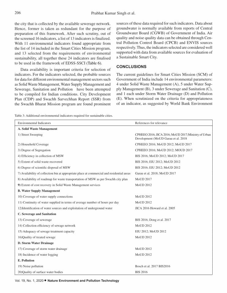
206 Prabhat Kumar Singh et al.
Vol. 19, No. 1, 2020 • Nature Environment and Pollution Technology
Table 3: Additional environmental indicators required for sustainable cities.
Environmental Indicators References for relevance
A. Solid Waste Management
1) Street Sweeping CPHEEO 2016; JICA 2016; MoUD 2017;Ministry of Urban Development (MoUD Garau et al. 2018
2) Household Coverage CPHEEO 2016; MoUD 2012; MoUD 2017
3) Degree of Segregation CPHEEO 2016; MoUD 2012; MOUD 2017
4) Efficiency in collection of MSW BIS 2016; MoUD 2012; MoUD 2017
5) Extent of solid waste recovered BIS 2016; EIU 2012; MoUD 2012
6) Degree of scientific disposal of MSW BIS 2016; EIU 2012; MoUD 2012
7) Availability of collection bin at appropriate place at commercial and residential areas Garau et al. 2018; MoUD 2017
8) Availability of roadmap for waste transportation of MSW as per Swachh city plan MoUD 2017
9) Extent of cost recovery in Solid Waste Management services MoUD 2012
B. Water Supply Management
10) Coverage of water supply connections MoUD 2012
11) Continuity of water supplied in terms of average number of hours per day MoUD 2012
12)Identification of water sources and exploitation of underground water JICA 2016 Howard et al. 2005
C. Sewerage and Sanitation
13) Coverage of sewerage BIS 2016; Dong et al. 2017
14) Collection efficiency of sewage network MoUD 2012
15) Adequacy of sewage treatment capacity EIU 2012; MoUD 2012
16)Quality of treated sewage MoUD 2012
D. Storm Water Drainage
17) Coverage of storm water drainage MoUD 2012
18) Incidence of water logging MoUD 2012
E. Pollution
19) Noise pollution Bosch et al. 2017 BIS2016
20)Quality of surface water bodies BIS 2016
the city that is collected by the available sewerage network. Hence, former is taken as redundant for the purpose of preparation of this framework. After such scrutiny, out of the screened 16 indicators, a list of 13 indicators is finalized. With 11 environmental indicators found appropriate from the list of 14 included in the Smart Cities Mission program, and 13 selected from the requirements of environmental sustainability, all together these 24 indicators are finalised to be used in the framework of EDSS-SSCI (Table 6).
Data availability is important criteria for selection of indicators. For the indicators selected, the probable sources for data for different environmental management sectors such as Solid Waste Management, Water Supply Management and Sewerage, Sanitation and Pollution have been attempted to be compiled for Indian conditions. City Development Plan (CDP) and Swachh Sarvechhan Report (SSR) from the Swachh Bharat Mission program are found prominent
sources of these data required for such indicators. Data about groundwater is normally available from reports of Central Groundwater Board (CGWB) of Government of India. Air quality and noise quality data can be obtained through Cen-tral Pollution Control Board (CPCB) and ENVIS sources respectively. Thus, the indicators selected are considered well supported with data from available sources for evaluation of a Sustainable Smart City.
CONCLUSIONS
The current guidelines for Smart Cities Mission (SCM) of Government of India include 14 environmental parameters: 4 under Solid Waste Management (A), 5 under Water Sup-ply Management (B), 3 under Sewerage and Sanitation (C), and 1 each under Storm Water Drainage (D) and Pollution (E). When scrutinized on the criteria for appropriateness of an indicator, as suggested by World Bank Environment

207ENVIRONMENTAL INDICATORS FOR SUSTAINABLE SMART CITIES MISSION
Nature Environment and Pollution Technology • Vol. 19, No. 1, 2020
Table 4: Appropriateness of 20 additional environmental indicators for sustainable cities based on WBED (2002) criteria.
Suitability of Indicator based on World Bank (2002) Criteria (Segnestam 2002)
Environmental Indicators for Sustainable Cities
(i) Direct relevance to objec-tives
(ii)Direct rel-evance to the target group
(iii) Clarity in design
(iv) Realistic collec-tion or development costs.
(v)High qual-ity and relia-bility
(vi)Appro-priate spatial and tempo-ral scale
A. Solid Waste Management
1 Street Sweeping 50%
2 Household Coverage 100%
3 Degree of Segregation 100%
4 Efficiency in collection of MSW
100%
5 Extent of solid waste recovered
100%
6 Degree of scientific dis-posal of MSW
100%
7 Availability of collection bin at appropriate place at commercial and residential areas
66.6%
8 Extent of cost recovery in 100%
9 Availability of roadmap for waste transportation of MSW as per Swachh city plan
66.6%
B. Water Supply Management
10. Coverage of water sup-ply connections
100%
11. Continuity of water supplied in terms of av-erage number of hours per day
100%
12. Identification of water sources and exploitation of underground water
100%
C. Sewerage and Sanitation
13. Coverage of sewerage 100%
14. Collection efficiency of sewage network
100%
15.Adequacy of sewage treatment capacity
100%
16.Quality of treated sew-age
100%
D. Storm Water Drainage
17.Coverage of storm water drainage
100%
18.Incidence of water log-ging
33.3%
E. Pollution
19.Noise pollution 100%
20.Quality of surface water bodies
100%
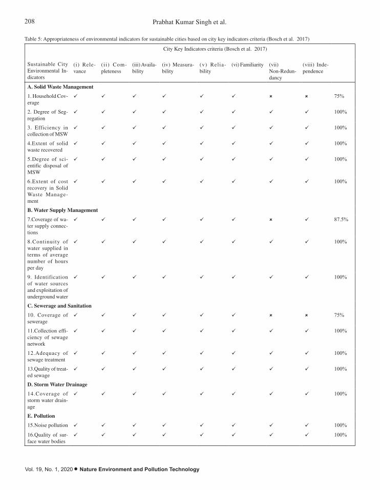
208 Prabhat Kumar Singh et al.
Vol. 19, No. 1, 2020 • Nature Environment and Pollution Technology
Table 5: Appropriateness of environmental indicators for sustainable cities based on city key indicators criteria (Bosch et al. 2017)
City Key Indicators criteria (Bosch et al. 2017)
Sustainable City Environmental In-dicators
(i) Rele-vance
(i i ) Com-pleteness
(iii) Availa-bility
(iv) Measura-bility
(v) Relia-bility
(vi) Familiarity (vii) Non-Redun-dancy
(viii) Inde-pendence
A. Solid Waste Management
1. Household Cov-erage
75%
2. Degree of Seg-regation
100%
3. Efficiency in collection of MSW
100%
4.Extent of solid waste recovered
100%
5.Degree of sci-entific disposal of MSW
100%
6.Extent of cost recovery in Solid Waste Manage-ment
100%
B. Water Supply Management
7.Coverage of wa-ter supply connec-tions
87.5%
8.Continuity of water supplied in terms of average number of hours per day
100%
9. Identification of water sources and exploitation of underground water
100%
C. Sewerage and Sanitation
10. Coverage of sewerage
75%
11.Collection effi-ciency of sewage network
100%
12.Adequacy of sewage treatment
100%
13.Quality of treat-ed sewage
100%
D. Storm Water Drainage
14.Coverage of storm water drain-age
100%
E. Pollution
15.Noise pollution 100%
16.Quality of sur-face water bodies
100%

209ENVIRONMENTAL INDICATORS FOR SUSTAINABLE SMART CITIES MISSION
Nature Environment and Pollution Technology • Vol. 19, No. 1, 2020
Development (WBED 2002), only 11 (2 under category A. 5 under B, 3 under C and 1 under E) are found suitable, while 3 are considered inadequately defined in terms of clarity or objective evaluation.
In order to propose and plan Smart Cities as ‘Sustainable Smart Cities’ in India, a set of 20 additional parameters are screened from available literature related with sustainable cities across the world. Out of these 20 additional parame-ters, only 16 could be found satisfying the requirements of appropriateness as indicator, as per WBED (2002) criteria. When these 16 indicators are further subjected to evaluation on 7 criteria, used by City Key Indicator program, only 13 (5 under category A, 2 under category B, 3 under category C, 1 under D and 2 under category E) are found fully satisfying the requirements as environmental indicators and 3 parameters are found to be inadequately defined. Accordingly, a set of 24 indicators are finalized (7 for Solid Waste Management, 7 for Water Supply Management, 6 for Sewerage and Sanitation, 1 for Storm Water Management and 3 under Pollution) which can be used in the scientific framework, named as Envi-ronmental Decision Support System for Sustainable Smart
Cities in India (EDSS-SSCI) for evaluation and monitoring purposes. The sources of data under Indian administrative set up and programs have also been identified. On the lines of the indices developed for Smart Cities, the selected in-dicators are envisaged to be used to develop a Sustainable Smart Cities Index (SSCI) which may be used to assess the comparative performance of cities on the scale of smartness and sustainability with increasing investment and improving urban infrastructure.
ACKNOWLEDGEMENTS
All the necessary facilities for this work have been provided by the Indian Institute of Technology (Banaras Hindu Uni-versity) Varanasi.
REFERENCES
Abbu, N., Kumar, E. and Saini, V. 2015. Urban green growth strategies for In-dian cities. ICLEI-Local Government for Sustainability, South Asia (1).
Bibri, S. and Krogstie, J. 2017. Smart sustainable cities of the future: An ex-tensive interdisciplinary literature review. Sustainable Cities and Society.
Bosch, P., Jongeneel, S., Rovers, V., Neumann, H.M., Airaksinen, M. and
Table 6: Finalized environmental indicators suggested for ‘Sustainable Smart Cities’ framework.
Indicators included in Smart Cities Mission (MoUD 2015) Additional indicators desirable to be included for ‘Sustainable Smart Cities’ and their sources in India
A. Solid Waste Management
1. Recycling and reduction of construction and demolition waste 1. Degree of segregation (MoUD 2012, MoUD 2017)
2. Solid waste management programs carried in the city during last 3 years.
2. Efficiency in collection of MSW (MoUD 2012, MoUD 2017)
3. Extent of solid waste recovered (MoUD 2012)
4. Degree of scientific disposal of MSW (MoUD 2012)
5. Extent of cost recovery in Solid Waste Management (MoUD 2012)
B. Water Supply Management
3. Adequate water supply 6. Continuity of water supplied in terms of average no of hrs per day (MoUD 2012)
4. Smart meters and Management 7. Identification of water sources and Exploitation of underground water (JICA 2016)
5. Leakage identification
6. Water quality monitoring
7. Extent of cost recovery in water supply services
C. Sewerage and Sanitation
8. Coverage of toilets 8. Adequacy of sewage treatment capacity (MoUD 2012)
9. Waste water recycling 9. Collection efficiency of sewage network (MoUD 2012)
10. Extent of cost recovery 10. Quality of treated sewage (MoUD 2012)
D. Storm Water Drainage
11. Coverage of storm water drainage (MoUD 2012)
E. Pollution
11. Improvement in Air Quality 12. Noise Pollution (BIS 2016)
13. Quality of surface water bodies (BIS 2016)

210 Prabhat Kumar Singh et al.
Vol. 19, No. 1, 2020 • Nature Environment and Pollution Technology
Huovila, A. 2017. CITYkeys indicators for smart city projects and smart cities.
BIS 2016. Smart Cities-Indicators ICS 13.020.20.CPHEEO 2016. Municipal Solid Waste Management Manual (12).Khadke, P.A. and Waghmare, P.B. 2018. Class and size wise distribution of
urban centre and their determinants in Maharashtra. Research Review. International Journal of Multidisciplinary and Current Research, 8(3): 722-730.
Dong, Y. and Hauschild, M.Z. 2017. Indicators for Environmental Sustaina-bility. In Procedia CIRP, 61: 697-702.
EIU 2012. The Green City Index. The Economist Intelligence Unit (EIU), 25. Retrieved from http://aiph.org/wp-content/uploads/2015/04/Green City - Guidelines.pdf
Garau, C. and Pavan, V. M. 2018. Evaluating urban quality: Indicators and assessment tools for smart sustainable cities. Sustainability (Switzerland), 10(3): 575.
Howard, G. and Bartram, J. 2005. Effective water supply surveillance in urban areas of developing countries. J. Water Health, 3: 31-42.
Höjer, M. and Wangel, S. 2015. Smart sustainable cities: Definition and challenges.In: L. Hilty & B. Aebischer (Eds.), ICT Innovations for Sustainability. Berlin, Springer-verlag, pp. 333-349.
ITU 2014. Agreed definition of a smart sustainable city, Focus Group on Smart
Sustainable Cities, SSC-0146 version Geneva, 5-6 March. JICA 2016. Republic of India Data Collection Survey on Improvement of En-
vironment in Varanasi City, Republic of India Final Report (Main Report).Lazaroiu, G.C. and Roscia, M. 2012. Definition methodology for the smart
cities model. Energy, 47(1): 326-332.Maslow, A.H. 1943. A theory of human motivation.Psychological Review,
50: 370-396.MEM 2015. Cleaner greener and safer Mauritius, environmental guideline
for smart cities. Ministry of Environment, Sustainable Development, and Disaster and Beach Management.
MoUD 2017. Swachh Survekshan 2017, A Guidebook for Urban Local Bodies.
MoUD 2012. Service levels in urban water and sanitation sector. Retrieved from http://mohua.gov.in/upload/uploadfiles/files/SLB%20National%20Data%20Book_0.pdf
MoUD 2015. Mission statements and Guidelines. Retrieved from http://smartcities.gov.in/upload/uploadfiles/files/SmartCityGuidelines(1).pdf
Segnestam, L. 2002. Indicators of Environment and Sustainable Development. World Bank Environment Development (WBED), Paper No. 89.
Randhawa, A. and Kumar, A. 2017. Exploring sustainability of smart devel-opment initiatives in India. International Journal of Sustainable Built Environment, 6(2):.701-710.

Impact of Carbon Nanotubes as Additives with Cotton Seed Biodiesel Blended with Diesel in Ci Engine - An Experimental Analysis
G. Ninawe† and M. TariqDepartment of Mechanical Engineering, Sam Higginbottom University of Agriculture, Technology and Sciences, Prayagraj (Allahabad), India†Corresponding author: G. Ninawe
ABSTRACT
In the present global scenario, fossil fuels are facing challenges due to escalating costs, increasing demand and impact on environmental pollution. In internal combustion engines, the emission characteristics and economy of the fuel are controlled by the chemical and physical properties of the fuel. Various additives are being used to act like catalysts with the fuels to improve quality of fuel, to obtain better combustion and to reduce exhaust emissions. At the time of combustion process, fuel instability reactions get accelerated by the catalysts which improve the performance of the engine. In this study, the B10, B15 and B20 fuel blends of cotton seed oil and diesel were mixed with the carbon nanotubes (CNTs) as an additive to analyse the performance and exhaust emissions of a CI engine. The carbon nanotubes were mixed with each fuel blend with the concentration of 50 ppm. All the tests were carried out for different engine loads. Tested characteristics were power, brake thermal efficiency (BTE), specific fuel consumption (SFC), and analysis of exhaust gases like hydrocarbons (HC), CO2, CO and smoke. The experimental results showed that there was significant reduction of SFC and improved combustion by addition of CNTs. It was also observed that the exhaust emissions, CO, HC and smoke percentage got decreased by the influence of CNTs.
INTRODUCTION
The environmental degradation and atmospheric pollution are the two main factors which cause imminent harm to the existence of the world. There are number of reasons for the pollution, but the pollution caused by the exhaust emissions from automobiles and power generation unit takes major part in degradation of environment and global warming. The primary source of energy for vehicles and power generators are the petroleum fuels which are depleting very rapidly. In country like India, 2/3rd of the total economy was spent to acquire petroleum products despite they being responsible for environmental pollution. But the use of transportation vehi-cles and power generation cannot be neglected as they both are the foundation for the economic growth of the country (Perumal & Ilangkumaran 2017). Therefore, the search for renewable alternative fuels which are environment friendly has been enforced. Particularly, biofuels are the replacement for the fossil fuels and becoming a renewable source of energy. Hence, the use of biodiesel blend with diesel fuel in engines is a promising option. The reason behind using biodiesel as an alternative fuel is that, it can be used without any modification in engine and the power generated from engine using biodiesel fuels are similar to the engine using
diesel fuel (Caliskan 2017). The commercialization of bio fuel and related projects enforces the employment either in direct or indirect manner. These projects are responsible to employ all the categories of people, including skilled and unskilled workers from different departments. The govern-ment has already initiated programs for urban, industrial and commercial applications. These programs aimed to evaluate energy from vegetable wastes, agriculture residue, municipal wastes, and industrial wastes (Gaurav et al. 2017).
Biodiesel is nothing but methyl or ethyl ester of fatty acids which is made from both edible and non-edible veg-etable oils and animal fats. For the production of biodiesel the main resources are non-edible oils extracted from plant species such as Calophyllum inophyllum, Pongamia pinnata, Jatropha curcas, Hevea brasiliensis etc. Biodiesel can be used in its unadulterated form in engine or can be blended with pure diesel fuel in any proportion. Like petroleum diesel, biodiesel has similar properties and works in compression ignition engine with minor or no engine modifications. It can be stored just like pure diesel and does not require any separate storage. The use of biodiesel in compression ignition engines results in reduction of emissions like carbon monox-ide, unburned hydrocarbons and particulate matters (Agarwal 2007) Presently, the first-generation biofuels are dominating
Nat. Env. & Poll. Tech.Website: www.neptjournal.com
Received: 10-06-2019Accepted: 23-07-2019
Key Words:Diesel engineAdditivesDiesel-biodiesel blendsCarbon nanotubes
2020pp. 211-219 Vol. 19
p-ISSN: 0972-6268 No. 1 Nature Environment and Pollution Technology An International Quarterly Scientific Journal
Original Research Paper
e-ISSN: 2395-3454
Open Access

212 G. Ninawe and M. Tariq
Vol. 19, No. 1, 2020 • Nature Environment and Pollution Technology
the biofuel sector, such as bioethanol and biodiesel. These biofuels can be used as blends with petroleum fuels in low percentage and can be utilized with existing infrastructure. The main advantage of using vegetable oils as alternative to conventional fuels exist in their renewable nature and there is wide availability from different variety of sources. There are also some disadvantages of using these vegetable oils which has incompatibility with petroleum lubricating oils, higher viscosity and problem of foul injector nozzles. To minimize the viscosity as well as problems related to lubrication, trans-esterification method and de-gumming of vegetable oil has been used (Eevera & Pazhanichamy 2013).
MATERIALS AND METHODS
In this research, the cotton seed biodiesel was produced from the cotton seed oil, using trans-esterification process. The carbon nanotubes (CNTs) used with the dose of 50 ppm and then mixed with B10, B15 and B20 fuel blends. Each fuel blends were made of 500 mL sample to be tested in the engine.
Multi-walled carbon nanotubes (MWNTs) were supplied from Platonic Nanotech Private Limited, India with purity more than 97%. The average diameter of the carbon nano-tubes varied from 10-15 nm and their length from 2-10 µm.
MATERIALS AND METHODS
In this research, the cotton seed biodiesel was produced from the cotton seed oil, using trans-
esterification process. The carbon nanotubes (CNTs) used with the dose of 50 ppm and then
mixed with B10, B15 and B20 fuel blends. Each fuel blends were made of 500 mL sample to be
tested in the engine.
Multi-walled carbon nanotubes (MWNTs) were supplied from Platonic Nanotech Private
Limited, India with purity more than 97%. The average diameter of the carbon nanotubes varied
from 10-15 nm and their length from 2-10 µm. Carbon nanotubes acts as an useful additives for
improving the quality of the fuels (Hosseini et al. 2017). Recently, several researchers have
incorporated different additives to improve the fuel properties of the biofuels. Addition of CNTs
with the diesel fuel increases the cetane number, burning rate and suppresses the smoke
formation in the engine cylinder during combustion process (Basha 2015, Tennent et al. 2002).
The carbon nanotubes contain amide group and has property of reacting with many chemicals.
The TEM (transmission electron microscopy) image of carbon nanotubes which was used with
diesel-biodiesel blended fuel is shown in Fig.1. The CNTs added to all fuel blends were stirred
for 15 min to get the homogeneous emulsion fuel.
Fig. 1: TEM image of carbon nanotubes.
Fig. 1: TEM image of carbon nanotubes.
Experimental Set-up
The experimental system consists of one cylinder, four strokes, VCR (Variable Compression
Ratio) diesel engine which was connected to eddy current type dynamometer for loading with its
main parameters are given in Table 1.
In order to compute and assess the exhaust gas emissions a mobile AVL DITEST GAS
analyser was also used for this experiment. A smoke opacity meter was used to calculate the
amount of soot coming out from the exhaust which is attached to exhaust gas duct coming from
engine. An onboard computer system is used to perform the common combustion calculations to
eliminate the use of tables and complex calculations. Details of the measuring instruments used
for testing are given in Table 1.
Fig. 2: Measurement setup and devices for the experiments. Fig. 2: Measurement setup and devices for the experiments.

213IMPACT OF CARBON NANOTUBES WITH COTTON SEED BIODIESEL BLENDED WITH DIESEL
Nature Environment and Pollution Technology • Vol. 19, No. 1, 2020
Carbon nanotubes acts as an useful additives for improving the quality of the fuels (Hosseini et al. 2017). Recently, several researchers have incorporated different additives to improve the fuel properties of the biofuels. Addition of CNTs with the diesel fuel increases the cetane number, burning rate and suppresses the smoke formation in the engine cylinder during combustion process (Basha 2015, Tennent et al. 2002). The carbon nanotubes contain amide group and has property of reacting with many chemicals. The TEM (transmission electron microscopy) image of carbon nanotubes which was used with diesel-biodiesel blended fuel is shown in Fig.1. The CNTs added to all fuel blends were stirred for 15 min to get the homogeneous emulsion fuel.
Experimental Set-up
The experimental system consists of one cylinder, four strokes, VCR (Variable Compression Ratio) diesel engine which was connected to eddy current type dynamometer for loading with its main parameters are given in Table 1.
In order to compute and assess the exhaust gas emissions a mobile AVL DITEST GAS analyser was also used for this experiment. A smoke opacity meter was used to calculate the amount of soot coming out from the exhaust which is attached to exhaust gas duct coming from engine. An onboard computer system is used to perform the common combus-tion calculations to eliminate the use of tables and complex calculations. Details of the measuring instruments used for testing are given in Table 1.
Experimental Procedure
For the experiment different fuel blends (i.e. diesel base, B10, B15, B20, B10C50, B15C50, B20C50) were prepared. The blending of diesel fuel with biodiesel was made in 500 mL flask which was directly poured in fuel tank. The kinematic viscosity, fire point, flash point, density and calorific value were calculated immediately after the biodiesel preparation.
The experiments were performed under variable loads on engine to get different speeds. Various parameters such as torque, specific fuel consumption (SFC), mechanical efficiency, power, volumetric efficiency and brake thermal efficiency were recorded and the data was transferred to the computer which was connected to the engine setup. The analysis done for the performance of engine is for 500 mL quantity of fuel for each fuel blend. To establish the baseline data, first the diesel fuel was used in the engine at varied loading conditions. Similarly, the testing was execut-ed for different biodiesel blends at different load conditions. To attain the steady state conditions and to minimize the residual from previous fuel blends each test was started by a 10 min start-up period.
RESULTS AND DISCUSSION
Table 2 gives the characteristics, which were measured based on ASTM (American Society for Testing and Materi-als) standards for the tested fuel blends. By adding carbon nanotubes in fuel blends the viscosity decreases and makes it easier to slip. Because of this the spraying and powdering of fuel inside combustion chamber is more proper. Durais-amy & Gowrishankar (2011) proved that the volatility and viscosity have interdependency with the dose of carbon nanotubes (20-80 ppm).
Engine Torque and Power
Table 3 gives the effect of addition of CNTs with diesel-bio-diesel blends on engine torque. It is observed that maximum torque for each fuel blends is at higher loads and as the load decreases there is decrease in torque. By decreasing the engine load from 12 to 0 kg the torque decreases on an average by 4.20%. It can be observed that use of CNTs with diesel-biodiesel blends leads to improve the engine torque at certain loads compared to pure diesel and diesel-biodiesel blends. The output torque increases by raising the concen-
Table 1: Specifications of all equipment and devices used in the experiments.
Engine type 4-stroke VCR diesel engine
Number of cylinders One
Bore × stroke 87.5 × 110 mm
Swept volume 661 cc
Compression ratio 17.5:1
Rated power 3.5 kW at 1500 rpm
Fuel injection timing 23º BTDC
Dynamometer type Eddy current, water cooled with loading unit
Emission Analyzer AVL DITEST GAS 1000, Emission diagnostics of HC, CO, CO2
Smoke Opacity Meter Model AVL DiSmoke 480 BT

214 G. Ninawe and M. Tariq
Vol. 19, No. 1, 2020 • Nature Environment and Pollution Technology
tration of CNTs in fuel blends, which improves the complete combustion inside the cylinder.
Table 4 gives the power variation at different loads for all fuel blends. As seen from the table, the power increases sharply as the load is increased. B0, B10 and B20 have lower power output as compared to B10C50, B15, B15C50, B20C50. In general, the brake power increases with the use of CNTs in fuel blends at variable loads. The reason for increased power with CNTs and fuel blends is energy pro-duced inside the cylinder. According to the earlier research, the catalyst reduces the combustion duration and ignition delay, which leads to faster heat release rate and higher peak pressure inside the cylinder (Heydari-Maleney et al. 2017, Ma et al. 2013, Kannan et al. 2011). The addition of nano-particles modifies the mechanism of ignition for liquid fuels, which accelerates the thermal interchangeability between the surrounding air and fuel droplets (Solero 2012).
Brake Thermal Efficiency (BTE)
The brake thermal efficiency for all the fuel blends is given in Table 5. Due to reduction in volumetric efficiency the BTE
Table 2: Properties of all the fuel blends.
Properties Diesel base B10 B15 B20
Kinematic Viscosity (mm2/sec) 2.25 2.38 2.56 2.73
Density (kg/m3) 790 802 810 817
Calorific value (MJ/kg) 43.25 42.89 42.16 41.35
Flash point (ºC) 56 71.60 80.25 88.5
Table 3: Torque at different loads for all the fuel blends.
Load (kg) B0 B10 B10C50 B15 B15C50 B20 B20C 50
0 kg 0.91 0.97 0.98 0.98 0.98 0.99 0.70
3 kg 5.81 5.84 6.03 5.85 5.73 5.88 5.76
6 kg 11.24 11.29 11.27 11.27 11.28 11.28 11.21
9 kg 16.68 16.71 16.70 16.71 16.87 16.70 16.64
12 kg 21.91 22.14 22.10 22.29 22.10 22.11 22.06
Table 4: Power at different loads for all the fuel blends.
Load (kg) B0 B10 B10C50 B15 B15C50 B20 B20C 50
0 kg 0.14 0.15 0.15 0.15 0.15 0.15 0.11
3 kg 0.89 0.91 0.91 0.90 0.88 0.90 0.90
6 kg 1.71 1.72 1.72 1.73 1.73 1.71 1.72
9 kg 2.53 2.54 2.54 2.54 2.56 2.52 2.52
12 kg 3.29 3.32 3.32 3.35 3.31 3.30 3.31
increases as the load on engine increases. The lowest values of BTE are for B20C50, B0 and B10 fuels and the maximum values of BTE are related to B10C50, B15, B15C50 and B20 fuel blends. Therefore, adding CNTs (50ppm) in fuel blends shows increase in amount of BTE due to better fuel spraying and dropped viscosity for some of the fuel blends.
Specific Fuel Consumption (SFC)
The variations of SFC of all fuel blends for the different loads are shown in Table 6. At different loads the SFC is lower for B15, B15C50, B20 and B10C50, whereas B0, B10, and B20C50 had the higher SFC. The reason for higher SFC is higher viscosity, lower heating value and oxygenated characteristic of biodiesel fuels (Singh et al. 2012, Porteiro et al. 2007). Therefore, addition of CNTs to the diesel-bio-diesel fuel blends improves combustion, increases power and decreases the SFC of the engine. It has been observed from Table 6 that as the load is increased there is reduction in SFC. The reason for lower SFC values is the higher BTE of the fuels with CNTs, which is due to existence of oxygen molecules and CNTs.

215IMPACT OF CARBON NANOTUBES WITH COTTON SEED BIODIESEL BLENDED WITH DIESEL
Nature Environment and Pollution Technology • Vol. 19, No. 1, 2020
Analysis of Emissions
Carbon monoxide (% Vol)
The carbon monoxide emissions which comes from engine exhaust represents the loss of chemical energy which is not fully employed to generate engine power. Fig. 3 shows the percentage of concentration of CO emissions for all the fuel blends at variable loads. It has been noticed that at higher loads the CO emissions are less and at medium loads the CO emissions are highest in all the fuel blends. B10, B10C50, B15C50 had the lower CO content, whereas B0, B15, B20, B20C50 had the higher CO content. The average CO emis-sions decreased 27.27 % for the fuel blends with CNTs when compared to neat diesel and biodiesel blends. It was observed that there is significant lowering of CO emissions when CNTs, biodiesel and its blends were used as compared to pure diesel. The reason behind lowering of CO emission is existence of more oxygen content in biodiesel than pure diesel fuel, which causes to make complete combustion of the mixture present in combustion chamber and ensures less CO emissions (Taghizadeh-Alisaraei and Rezaei-Asl 2016). Decreased viscosity of the fuel plays significant role in min-imizing CO emissions by improving fuel atomization. As the CNTs had larger surface area, it increases the chemical reactivity by which the ignition delay gets consecutively shortened. Due to the effect of shortened ignition delay uniform burning and fuel-air mixing had been improved which promotes complete combustion of fuels in presence of potential CNTs (Javed et al. 2016, Srinivas et al. 2016).
Carbon dioxideFig. 4 shows the carbon dioxide emissions at different loads
Table 5: Brake thermal efficiency at different loads for all fuel blends.
Load (kg) B0 B10 B10C50 B15 B15C50 B20 B20C 50
0 kg 3.50 3.74 3.81 4.42 4.40 3.81 2.69
3 kg 17.01 17.36 17.71 17.25 16.88 17.25 15.45
6 kg 26.72 26.85 26.80 27.10 27.07 26.74 24.67
9 kg 31.08 31.17 31.12 31.27 31.53 31.04 30.93
12 kg 35.43 33.61 33.48 33.93 33.55 33.45 31.61
Table 6: Brake specific fuel consumption at different loads for all fuel blends.
Load (kg) B0 B10 B10C50 B15 B15C50 B20 B20C 50
0 kg 2.45 2.29 2.25 1.94 1.95 2.25 3.18
3 kg 0.50 0.49 0.48 0.50 0.51 0.50 0.55
6 kg 0.32 0.32 0.32 0.32 0.32 0.32 0.35
9 kg 0.28 0.28 0.28 0.27 0.27 0.28 0.28
12 kg 0.24 0.26 0.26 0.25 0.26 0.26 0.27
for various fuel blends. After comparing CO and CO2 emis-sions, it has been noted that the molecular component and balance for a given fuel have opposite behaviours. Therefore, the carbon present in exhaust gas has potential to become CO2 or CO. As the load on the engine was increased then the CO2 content got increased. B15, B20, B10C50, B15C50 had the higher CO2 content while B0, B10, B20C50 had the lower CO2 content.
As a rule, the most cost effective and efficient use of fuel takes place when the CO2 content in the exhaust is maximized. This happens only when there is sufficient O2 present in the supplied air to react with carbon present in the fuel. Therefore, as the amount of air gets increased in the combustion chamber the concentration of CO molecules gets decreased. Due to this, the additional atoms of oxygen present in the air reacts with this CO molecules and form CO2. The maximum amount of CO2 depends upon the category of fuel used (TSI 2004).
Hydrocarbons emissions
The unburned hydrocarbon present in the exhaust is the con-sequence of incomplete combustion of fuel. The variations of HC emissions are shown in Fig. 5 for all the fuel blends at variable loads. The minimum and maximum HC emissions are observed at lower and higher loads respectively. The larger reduction of HC emissions is for the B20C50, B20, B15C50 and B15 fuel blends. This is because of higher oxygen content present in the biodiesel which makes possible to obtain more complete combustion inside the combustion chamber (Sahoo et al. 2007). The HC emissions are found to be noticeably reduced due to addition of CNTs to the fuel blends. The reason behind this is significant fuel distribution

216 G. Ninawe and M. Tariq
Vol. 19, No. 1, 2020 • Nature Environment and Pollution Technology
and intensive atomization with the existence of CNTs in combustion chamber which causes CO and HC oxidation during the combustion (Sadhik Basha & Anand 2014).
Smoke
Fig. 6 shows the trend of smoke opacity at different loads for different fuel blends. The percentage of smoke opacity for pure diesel was higher while for the fuel blends with CNTs were drastically lesser. The reason for reduction of smoke for the fuel blends is probably due to intensive atomization, better fuel-air mixing and enhanced air spray momentum (Subramanian & Ramesh 2002, Armas et al. 2005, Rao & Anand 2016)50 and 100 ppm. In case of B20 and B20C50 the smoke opacity is minimum than that of other fuel blends.
Fig. 3: CO for different fuel blends at different loads.
Carbon dioxide
Fig. 4 shows the carbon dioxide emissions at different loads for various fuel blends. After
comparing CO and CO2 emissions, it has been noted that the molecular component and balance
for a given fuel have opposite behaviours. Therefore, the carbon present in exhaust gas has
potential to become CO2 or CO. As the load on the engine was increased then the CO2 content
got increased. B15, B20, B10C50, B15C50 had the higher CO2 content while B0, B10, B20C50
had the lower CO2 content.
As a rule, the most cost effective and efficient use of fuel takes place when the CO2
content in the exhaust is maximized. This happens only when there is sufficient O2 present in the
supplied air to react with carbon present in the fuel. Therefore, as the amount of air gets
increased in the combustion chamber the concentration of CO molecules gets decreased. Due to
this, the additional atoms of oxygen present in the air reacts with this CO molecules and form
CO2. The maximum amount of CO2 depends upon the category of fuel used (TSI 2004).
0
0.02
0.04
0.06
0.08
0.1
Diesel B-10 B-10 C-50
B-15 B-15 C-50
B-20 B-20 C-50
CO (% Vol.)
Fuel Blend
0 Kg 3 Kg 6 Kg 9 Kg 12 Kg
Fig. 3: CO for different fuel blends at different loads.
Fig. 4: CO2 for different fuel blends at different loads.
Hydrocarbons emissions
The unburned hydrocarbon present in the exhaust is the consequence of incomplete combustion
of fuel. The variations of HC emissions are shown in Fig. 5 for all the fuel blends at variable
loads. The minimum and maximum HC emissions are observed at lower and higher loads
respectively. The larger reduction of HC emissions is for the B20C50, B20, B15C50 and B15
fuel blends. This is because of higher oxygen content present in the biodiesel which makes
possible to obtain more complete combustion inside the combustion chamber (Sahoo et al.
2007). The HC emissions are found to be noticeably reduced due to addition of CNTs to the fuel
blends. The reason behind this is significant fuel distribution and intensive atomization with the
existence of CNTs in combustion chamber which causes CO and HC oxidation during the
combustion (Sadhik Basha & Anand 2014).
0
1
2
3
4
5
DieselBase
B-10Base
B-10 C-50
B-15Base
B-15 C-50
B-20Base
B-20 C-50
CO2 (% Vol.)
Fuel blend
0 Kg 3 Kg 6 Kg 9 Kg 12 Kg
Fig. 4: CO2 for different fuel blends at different loads.
This is due to higher oxygen content present in the biodiesel which facilitates the complete combustion. Because of heter-ogeneous nature of the diesel combustion there is variation of fuel-air ratios inside the cylinder of diesel engine, which affects the smoke formation. The smoke formation primarily takes place at higher pressure and temperature in the fuel rich zone of the engine cylinder. As the fuel used in diesel engine is partially oxygenated the major smoke formation can be reduced (Puhan et al. 2005).
Optimal Fuel
In all the fuel blends, addition of CNTs proved to be a better additive which increased the amount of torque. It can be observed that larger power and BTE belongs to B15C50,

217IMPACT OF CARBON NANOTUBES WITH COTTON SEED BIODIESEL BLENDED WITH DIESEL
Nature Environment and Pollution Technology • Vol. 19, No. 1, 2020
B20C50, B15 and B10C50 fuel blends respectively. Sim-ilarly, the torque trend follows the power table and has matching results. B15, B15C50, B20 and B10C50 have the minimum SFC.
According to the emissions results, B10C50, B15C50 had the lower CO content. B20C50, B20, B15C50 and B15 fuel blends have the lowest HC emissions. The smoke opacity is lesser for all the fuel blends with CNTs than the pure diesel. Based on these results, the optimal fuel can be selected as B15C50 fuel blend. Therefore, B15C50 is considered as the best fuel in terms of performance and emissions parameters. The greatest variations occurred for all the parameters are for higher loads.
Fig. 5: HC for different fuel blends at different loads.
Smoke
Fig. 6 shows the trend of smoke opacity at different loads for different fuel blends. The
percentage of smoke opacity for pure diesel was higher while for the fuel blends with CNTs were
drastically lesser. The reason for reduction of smoke for the fuel blends is probably due to
intensive atomization, better fuel-air mixing and enhanced air spray momentum (Subramanian &
Ramesh 2002, Armas et al. 2005, Rao & Anand 2016). In case of B20 and B20C50 the smoke
opacity is minimum than that of other fuel blends. This is due to higher oxygen content present
in the biodiesel which facilitates the complete combustion. Because of heterogeneous nature of
the diesel combustion there is variation of fuel-air ratios inside the cylinder of diesel engine,
which affects the smoke formation. The smoke formation primarily takes place at higher pressure
and temperature in the fuel rich zone of the engine cylinder. As the fuel used in diesel engine is
partially oxygenated the major smoke formation can be reduced (Puhan et al. 2005).
020406080
100120
DieselBase
B-10Base
B-10C-50
B-15Base
B-15C-50
B-20Base
B-20C-50
HC (Ppm)
Fuel Blend
0 Kg 3 Kg 6 Kg 9 Kg 12 Kg
Fig. 5: HC for different fuel blends at different loads.
Fig. 6: Variation of smoke opacity for different fuel blends at different loads.
Optimal Fuel
In all the fuel blends, addition of CNTs proved to be a better additive which increased the
amount of torque. It can be observed that larger power and BTE belongs to B15C50, B20C50,
B15 and B10C50 fuel blends respectively. Similarly, the torque trend follows the power table
and has matching results. B15, B15C50, B20 and B10C50 have the minimum SFC.
According to the emissions results, B10C50, B15C50 had the lower CO content.
B20C50, B20, B15C50 and B15 fuel blends have the lowest HC emissions. The smoke opacity is
lesser for all the fuel blends with CNTs than the pure diesel. Based on these results, the optimal
fuel can be selected as B15C50 fuel blend. Therefore, B15C50 is considered as the best fuel in
terms of performance and emissions parameters. The greatest variations occurred for all the
parameters are for higher loads.
Cost Analysis
The cost of the CNTs used in the present experiments is about 384 US$ per kg in India and the
0
10
20
30
40
50
DieselBase
B-10Base
B-10 C-50
B-15Base
B-15 C-50
B-20Base
B-20 C-50
Smoke (%)
Fuel Blend
0 Kg 3 Kg 6 Kg 9 Kg 12 Kg
Fig. 6: Variation of smoke opacity for different fuel blends at different loads.
Cost Analysis
The cost of the CNTs used in the present experiments is about 384 US$ per kg in India and the dose of 50 ppm are respectively 0.05 g per 500 mL for B10, B15 and B20 fuel blends. The specific cost for 50 ppm CNT is 0.0192 US$ for per 500 mL of B10, B15 and B20 fuel blends. In addition, the diesel fuel cost in India is about 0.92 US$. Adding CNTs with the dose of 50 ppm to B10, B15 and B20 fuel blends, the fuel price increases by 2%. In country like India the higher price of diesel fuel enforces the use of additives as it results in reduction of SFC. Hence, the use of CNTs with diesel fuel is much more economical and affordable in India. However, other advantage such as reduction in exhaust emissions can also be contemplated.

218 G. Ninawe and M. Tariq
Vol. 19, No. 1, 2020 • Nature Environment and Pollution Technology
CONCLUSIONS
In this study, the B10, B15 and B20 fuel blends included with carbon nanotubes (CNTs) were used to analyse the exhaust emissions and performance characteristics of a single cylinder CI engine. The CNTs were mixed with the dosage of 50 ppm to all the fuel blends. The experiments were conducted by varying the loads on the engine. The results indicated that the performance characteristics such as power, torque, BTE, SFC of B15C50 fuel blend is optimum as compared to other fuel blends and pure diesel. The exhaust emissions of B15C50 fuel blend like CO, HC and smoke opacity were found minimum as
compared to pure diesel and other fuel blends. The existence and translocation of CNTs in the fuel molecules improved the fuel atomization and decreased the viscosity. Overall, it has been found that the CNT used with fuel blends has potential advantage to improve the performance and to reduce the ex-haust emissions from the diesel engine.
ACKNOWLEDGMENT
The first author would like to express his gratitude to Dha-nushkar S., Naik S. N., Centre for Rural Development and Technology, IIT Delhi, India for their support.
B0 Pure Diesel nm nanometer
B10 90% Diesel + 10% Biodiesel µm micrometer
B15 85% Diesel + 15% Biodiesel ppm part per million
B20 80% Diesel + 20% Biodiesel CI Compression ignition
B10C50 B10 + 50 ppm CNTs HC Hydro carbons
B15C50 B10 + 50 ppm CNTs CO Carbon monoxide
B20C50 B10 + 50 ppm CNTs CO2 Carbon dioxide
BTE Brake thermal efficiency (%) rpm Revolutions per minute
CNTs Carbon Nanotubes SFC Specific fuel consumption
kW kilo Watt Nm Newton meter
REFERENCES
Agarwal, Avinash Kumar. 2007. Biofuels (alcohols and biodiesel) applica-tions as fuels for internal combustion engines. Progress in Energy and Combustion Science, 33(3): 233-71.
Armas, O., Ballesteros, R., Martos, F.J. and Agudelo, J.R. 2005. Char-acterization of light duty diesel engine pollutant emissions using water-emulsified fuel. Fuel, 84: 1011-18.
Basha, J.S., 2015. Applications of functionalized carbon-based nanomate-rials. In: Chemical Functionalization of Carbon Nanomaterials, CRC Press, pp. 598-613.
Caliskan, Hakan 2017. Environmental and enviroeconomic researches on diesel engines with diesel and biodiesel fuels. Journal of Cleaner Production, 154: 125-29.
Duraisamy, Ganesh and Gowrishankar, G. 2011. Effect of nano-fuel addi-tive on emission reduction in a biodiesel fuelled CI engine. In 2011 International Conference on Electrical and Control Engineering, IEEE, pp. 3453-3459.
Eevera, T. and Pazhanichamy, K. 2013. Cotton seed oil: a feasible oil source for biodiesel production. Energy Sources, Part A: Recovery, Utilization and Environmental Effects, 35(12): 1118-28.
Gaurav, N., Sivasankari, S., Kiran, G.S., Ninawe, A. and Selvin, J. 2017. Utilization of bioresources for sustainable biofuels: A review. Renew-able and Sustainable Energy Reviews, 73: 205-14.
Heydari-Maleney, K., Taghizadeh-Alisaraei, A., Ghobadian, B. and Abbaszadeh-Mayvan, A. 2017. Analyzing and evaluation of carbon
nanotubes additives to diesohol-B2 fuels on performance and emission of diesel engines. Fuel, 196: 110-23.
Hosseini, S.H., Taghizadeh-Alisaraei, A., Ghobadian, B. and Abbasza-deh-Mayvan, A. 2017. Performance and emission characteristics of a ci engine fuelled with carbon nanotubes and diesel-biodiesel blends. Renewable Energy, 111: 201-13.
Javed, S., Murthy, Y.S., Baig, R.U. and Rao, T.N. 2016. Vibration analysis of a diesel engine using biodiesel fuel blended with nano particles by dual fueling of hydrogen. Journal of Natural Gas Science and Engi-neering, 33: 217-30.
Kannan, G. R., Karvembu, R. and Anand, R. 2011. Effect of metal based additive on performance emission and combustion characteristics of die-sel engine fuelled with biodiesel. Applied Energy, 88(11): 3694-3703.
Ma, Y., Zhu, M. and Zhang, D. 2013. The effect of a homogeneous combus-tion catalyst on exhaust emissions from a single cylinder diesel engine. Applied Energy, 102: 556-62.
Perumal, V. and Ilangkumaran, M. 2017. Experimental analysis of engine performance, combustion and emission using pongamia biodiesel as fuel in CI engine. Energy, 129: 228-36.
Porteiro, J., Granada, E. and Mora, J. C. 2007. Performance and exhaust emissions in the use of biodiesel in outboard diesel engines. Fuel, 86: 1765-71.
Puhan, S., Vedaraman, N., Ram, B.V., Sankarnarayanan, G. and Jeychan-dran, K., 2005. Mahua oil (Madhuca Indica seed oil) methyl ester as biodiesel-preparation and emission characterstics. Biomass and Bioenergy, 28(1): 87-93.
NOMENCLATURE

219IMPACT OF CARBON NANOTUBES WITH COTTON SEED BIODIESEL BLENDED WITH DIESEL
Nature Environment and Pollution Technology • Vol. 19, No. 1, 2020
Rao, M. Srinivasa and Anand, R.B. 2016. Performance and emission character-istics improvement studies on a biodiesel fuelled DICI engine using water and AlO(OH) nanoparticles. Applied Thermal Engineering, 98: 636-45.
Sadhik Basha, J. and Anand, R.B. 2014. Performance, emission and combus-tion characteristics of a diesel engine using carbon nanotubes blended jatropha methyl ester emulsions. Alexandria Engineering Journal, 53(2): 259-73.
Sahoo, P. K., Das, L. M., Babu, M.K.G. and Naik, S. N. 2007. Biodiesel development from high acid value polanga seed oil and performance evaluation in a CI Engine. Fuel, 86(3): 448-54.
Singh, Bhupendra, Naveen Kumar and Haeng Muk, 2012. A study on the performance and emission of a diesel engine fueled with jatropha bio-diesel oil and its blends. Energy, 37(1): 616-22.
Solero, Giulio 2012. Experimental analysis of the influence of inert nano-ad-ditives upon combustion of diesel sprays. Nanoscience and Nanotech-
nology, 2(4): 129-33.Srinivas, Dilip, Puneesh Puri and Vigor Yang 2016. A general theory of
ignition and combustion of nano- and micron-sized aluminum particles. Combustion and Flame, 169: 94-109.
Subramanian, K. A. and Ramesh, A. 2002. Use of diethyl ether along with water-diesel emulsion in a di diesel engine. In: SAE Technical Paper, SAE International.
Taghizadeh-Alisaraei, Ahmad and Abbas Rezaei-Asl. 2016. The effect of added ethanol to diesel fuel on performance, vibration, combustion and knocking of a CI engine. Fuel, 185: 718-33.
Tennent, Howard, Kennett Square and References Cited 2002. (12) United States Patent (10) Patent No.: 2(0): 4-7.
TSI 2004. Combustion analysis basics: An overview of measurements, methods and calculations used in combustion analysis. TSI Incorpo-rated, 2004

Vol. 19, No. 1, 2020 • Nature Environment and Pollution Technology
220

Factors Influencing the Environmental Performance of Prefabricated Buildings: A Case Study of Community A in Henan Province of China
Jin Zhao, Yi Wang† and Zhengwei MaSchool of Civil and Transportation Engineering, Henan University of Urban Construction, Pingdingshan 467000, China†Corresponding author: Yi Wang
ABSTRACT
Various problems of traditional cast-in-place buildings, such as heavy energy consumption, severe environmental pollution, and low labour productivity, have hindered the development of the construction industry. Prefabricated buildings have a direct bearing on national economic development and transformation of people’s lifestyle because of their high economic, environmental, social, and safety benefits. The technological research and development level for prefabricated buildings and system policies in China are still in the initial stage, and the environmental performance and influencing factors of prefabricated buildings limit their large-scale implementation. The literature in developed countries regarding the environmental performance and influencing factors of prefabricated buildings was first reviewed in this study. Community A in Zhengzhou City, Henan Province was used as the case study. AHP (Analytic Hierarchy Process) was applied to measure the factors influencing the environmental performance of prefabricated buildings, and policy suggestions were proposed to improve their environmental performance. Results indicate that developed countries tend to construct prefabricated buildings in large areas because of their remarkable economic, environmental, social, and safety benefits. Measurement results of Community A in Zhengzhou City, Henan Province show that the main environmental pollution factor of prefabricated buildings is waste discharge, accounting for 40%, followed by noise pollution, energy consumption, and dust pollution. The environmental performance of prefabricated buildings can be improved by promoting their development, reducing their environmental pollution, establishing a standard prefabricated concrete system, enhancing the environmental standards for buildings, expanding the application scope of prefabricated concrete, encouraging environmental technology innovation of buildings, cultivating prefabricated building bases, and strengthening environmental governance of construction sites. The findings will serve as reference in determining the main factors influencing the environmental performance of prefabricated buildings, establishing an evaluation system for the environmental benefits of prefabricated buildings, promoting their improvement and optimized development, and enriching and perfecting an evaluation research system for their comprehensive benefits.
INTRODUCTION
As a pillar industry in China, building construction has experienced remarkable development and improved produc-tion with rapid urbanization. Buildings should satisfy basic requirements, such as construction quality and use functions, and should minimize resource and energy consumption, improve labour productivity, and protect the environment during construction and use. The emergence of prefabricated buildings has provided a new direction in the development of the construction industry. The components and members of prefabricated buildings are prefabricated in a plant based on design standards and transported to the construction site for assembly, thereby accelerating the construction speed, reducing the construction period, and has remarkable ad-vantages in terms of improved labour productivity, energy consumption reduction, and environment protection.
Henan Province in China has a large population with rapidly developing construction industry. As shown in Fig. 1, the gross output value of construction in Henan Province has increased from RMB 359.649 billion in 2009 to RMB 1,136.052 billion in 2018 with an average annual growth rate of 23.98%. The development of prefabricated buildings in Henan Province is still in the initial stage, and their prefab-rication degree remains at a low level. Incomplete technical specifications, low modulus coordination degree between product materials, absence of standard modulus system that can be implemented at the national level, and the uncertainty in the comprehensive benefits of prefabricated buildings hinder their development progress. The development of pre-fabricated buildings should be accelerated and the innovation of building construction and high-efficiency coordination between production departments should be promoted on the
Nat. Env. & Poll. Tech.Website: www.neptjournal.com
Received: 09-12-2019Accepted: 16-01-2020
Key Words:Prefabricated building Environmental performanceInfluencing factor
2020pp.221-227 Vol. 19
p-ISSN: 0972-6268 No. 1 Nature Environment and Pollution Technology An International Quarterly Scientific Journal
Original Research Paper
e-ISSN: 2395-3454
Open Access

222 Jin Zhao et al.
Vol. 19, No. 1, 2020 • Nature Environment and Pollution Technology
basis of the modernization requirements and development tendency of the current construction industry. An evaluation research system should be developed to identify the compre-hensive benefits of prefabricated buildings for satisfying the fundamental realities existing in the development of China’s construction industry. The evaluation research system should cover the entire life cycle of prefabricated buildings and analyse and evaluate their comprehensive benefits during construction, operation, use, recycling, and demolition to support the development of the construction industry.
PAST STUDIES
Foreign prefabricated buildings have originated from Western Europe. Prefabricated buildings can overcome the limitations of current buildings, such as slow construction and long construction period, and they have been implemented in de-veloped countries, such as America and Japan, in the 1960s. Construction technologies and related theoretical studies on prefabricated buildings are the most mature in western countries among other foreign studies. Most of these stud-ies have focused on the production system of prefabricated construction accessories, energy conservation, and emission reduction, and studies on their comprehensive benefits have mainly concentrated on single aspects, such as economic and environmental benefits. Tam et al. analysed and investigated the reduction of construction wastes from four prefabricated buildings compared with traditional cast-in-place buildings, and their results showed that prefabricated buildings have satisfactory environmental benefits in energy conservation and emission reduction, where the quantity of construction wastes and concrete use and template consumption are re-duced by approximately 55% and 80% compared with those of traditional cast-in-place buildings (Tam et al. 2005). Altes conducted a statistical analysis on the factors influencing the development of prefabricated buildings and indicated that the
prefabrication degree worldwide is low because of unstable industrial chain and the lack of long-term strategic cooper-ative relationship of enterprises between industrial (Altes 2005). Jaillon et al. believed that a standardized design of pre-fabricated buildings could effectively improve the production efficiency of product components and achieve remarkable environmental advantages, such as energy conservation and emission and environmental pollution reduction (Jaillon et al. 2009). Begum et al. compared the prefabrication mode with the traditional cast-in-place mode of buildings and stated that the prefabrication mode could reduce the use of building materials and improve the environmental performance of buildings in terms of reduced construction period, energy source conservation, and environment protection (Begum et al. 2010). Mohamad et al. mainly studied the ability of indus-trial prefabrication to solve the shortage of houses, discussed the results using a SWOT (Strength Weakness Opportunity Threat) method, and concluded that prefabricated buildings could effectively reduce environmental pollution and realize large-scale house provision (Mohamad et al. 2012). Bari et al. selected four low-rise buildings using IBS and conventional construction methods as a case study. Their results showed that prefabricated buildings could help reduce waste pollu-tion from the environmental perspective and provide their positive economic benefits and environmental performance (Bari et al. 2012). Silva et al. analysed the module transfor-mation scheme for exterior walls of existing prefabricated buildings, including 3D model construction and cost effec-tiveness analysis. Their results showed that prefabricated buildings could notably realize energy conservation and greenhouse gas emission reduction (Silva et al. 2013). Agren et al. presented the five phases of prefabricated buildings from appearance to mature development and analysed their environmental performance under different phases (Agren et al. 2014). Yashiro explained the concept of prefabricated buildings and related theories, proposed a whole-life-cycle
Fig. 1: Gross output values of the construction industry in Henan Province during 2009-2018.
(Data derived from Henan Statistical Yearbook)

223FACTORS INFLUENCING ENVIRONMENTAL PERFORMANCE OF PREFABRICATED BUILDINGS
Nature Environment and Pollution Technology • Vol. 19, No. 1, 2020
management method for prefabricated buildings, and indi-cated that the organizational form of prefabricated building construction is crucial in the environmental performance of prefabricated buildings (Yashiro 2014). Hong et al. explored the life-cycle energy utilization of prefabricated members and their influence on overall energy utilization by using actual building projects as the study objects. Their results showed that prefabricated buildings could reduce wastes and con-serve energy sources, and minimize whole-life-cycle energy consumption by approximately 4%-14% (Hong et al. 2016). Chang et al. (2018) believed that the Chinese government should actively promote building prefabrication, analysed the advantages and disadvantages of building prefabrication in China in terms of productivity, resources, and environmental sustainability, and constructed a strategic concept of obtain-ing green benefits through prefabricated buildings (Chang et al. 2018). Li et al. conducted qualitative and quantitative analyses of the indoor thermal environment of prefabricated houses by taking Zhengzhou City in central China as an example. Their results indicated that prefabricated build-ings have important advantages in terms of energy source conservation (Li et al. 2019). Navaratnam et al. reviewed the existing literature related to the structural behaviour, advantages, limitations, and challenges of prefabricated building systems by taking Australia as an example and believed that prefabricated buildings have good application prospects (Navaratnam et al. 2019). Lindblad analysed the environmental pollution caused by prefabricated concrete components during transportation (Lindblad 2019). Wang et al. utilized a performance analysis method to investigate the critical risk factors related to prefabricated buildings in China, and the results indicated that the risks of prefabricated buildings are caused by incomplete decomposition system, low plant management level, imperfect quality assurance system, and to-be-improved environmental benefits (Wang et al. 2019). Existing studies have indicated that prefabricated buildings are a kind of architectural model with high cost and scientific and technological level. Prefabricated build-ings have remarkable economic, environmental, social, and safety benefits. Most studies on prefabricated buildings have analysed and evaluated their quality and cost. Some scholars
have investigated the environmental benefits of prefabricated buildings, and few studies have comprehensively evaluated the angles of society and safety. Some case studies have ignored the factors influencing the environmental perfor-mance of prefabricated buildings and the specific solutions. Therefore, the environmental performance of prefabricated buildings was analysed and evaluated in this study. Commu-nity A in Zhengzhou City, Henan Province was used as the study object. Analytic hierarchy process (AHP) was used to assign weight values for various indicators of prefabricated buildings, followed by an analysis of factors influencing environmental performance of prefabricated buildings. The results of this study will serve as reference for standardizing the market of prefabricated buildings.
MODEL PROFILE AND INDEX CONSTRUCTION
AHP
AHP, which is proposed by an American operational research expert T. L. Saaty, is an analytical method combining quali-tative analysis and quantitative research. AHP has systematic and hierarchical characteristics with high practicability and effectiveness for complex decision problems by modelling and quantifying the decision-making process of a decision maker of a complex system.
Construction of a hierarchical structure model: Problems are analysed with a priori knowledge and data, and the factors influencing them and their mutual relations are established. The factors are decomposed into several layers based on their property, and the factors at the same layer are subjected to the factors in a previous layer or a layer that impacts them. The factors can dominate the factors in the previous layer or be influenced by them. The top layer is the target layer, that is the general objective that must be reached by AHP. The bottom layer contains measures or schemes used to solve the problem. The middle layer is the criterion layer that includes intermediate processes, such as adopted rules to realize a preset goal.
Construction of paired comparison matrix: A comparison matrix is constructed through paired comparison and 1-9
Table 1: Comparison matrix.
B1 B2 … … Bn
B1 b11 b12 … … b1n
B2 b21 b22 … … b2n
… … … … … …
… … … … … …
Bn bn1 bn2 … … bnn

224 Jin Zhao et al.
Vol. 19, No. 1, 2020 • Nature Environment and Pollution Technology
scale until the bottom layer is reached on the basis of related data, expert opinions, and analyser experience by starting from the middle layer of the hierarchical structure model to determine the relative importance of factors at the same layer that are subject to each factor at the previous layer. The paired comparison matrix is shown in Table 1.
As shown in Table 1, the corresponding relation between the bij value in the matrix and the relative importance of the compared factor is presented as follows: Bi is as important as Bj because bij = 1 and bji = 1; Bi is slightly more important than Bj because bij=3 and bji = 1/3; Bj is more important than Bj because bij = 5 and bji = 1/5; Bj is more important than Bj because bij = 7 and bji = 1/7; Bj is more important than Bj because Bj and bji = 1/9.
Weight calculation and consistency test: The maximum characteristic root and its eigenvector are calculated using the comparison matrix of factors. Consistency index (C.I.), random consistency (R.I.), and consistency ratio (C.R.) are
used to perform the consistency test. C In
n. .
max=
--
l1
,
where C.I. denotes the deviation degree of the comparison
matrix through crash consistency. R.I. is a given constant that changes with the order number of the comparison matrix.
C RC I
R I. .
. .
. .= . The comparison matrix has acceptable consist-
ency, and the eigenvector (normalized) is the weight value when C.R. < 0.10 . Otherwise, the judgment matrix should be adjusted and corrected to satisfy the consistency requirement.
Synthetic weights and ranking: The weight vectors in all layers are calculated, and the weights of factors are synthesized and ranked. The weight value of each evaluation index relative to the overall objective is expressed as
w l aj jj
k
ij==P
1, and i = 1, 2, ..., n, where lj is the weight value
obtained by evaluation index vi in hierarchical single sorting at the bottom layer, k is the number of ancestors used to evaluate index vi in the target tree, aij is the weight value of ancestor j of index vi in hierarchical single sorting, and ai1 1= is the root node.
Index Construction
Resource consumption: Material and resource consump-tion during building construction mainly include water, rebar, and template consumption. The material expenses in building construction account for approximately 70% of the total construction and installation costs. The generation of prefabricated buildings has provided a new idea to reduce the resource consumption in the construction industry.
Energy consumption: The total energy consumption during
building construction, operation, and use refers to the total energy quantity consumed in the usage of buildings, includ-ing daily use of heating, air conditioning, and illuminating lamps. Related energy-saving designs can be combined with the standardized design of prefabricated buildings to reduce energy consumption.
Waste discharge: The total waste discharge generated during building construction, recycling, and demolition specifically includes solid building wastes, waste gases, and wastewater.
Dust pollution: Dust pollution is generated during building construction. The dust pollution in the current construction industry of China must be solved to improve air quality and protect and enhance the atmospheric environment.
Noise pollution: Harmful noise pollution is generated by large-scale mechanical equipment during building con-struction. During the entire building construction, the noise pollution generated by the construction of a major structure has a great impact on the surrounding environment. There-fore, the noises generated by concrete pump truck, vibrating equipment, electric generator, and electric saw, which are used in the major structure construction, are all higher than the limiting noise value in the environment.
EMPIRICAL ANALYSIS
A survey questionnaire method was adopted based on the evaluation model of environmental performance of prefabricated buildings to analyse the index weights. The questionnaires were mainly provided to the relevant tech-nical personnel of prefabricated buildings in Community A in Zhengzhou City, Henan Province and technology R & D personnel and constructors of enterprises constructing prefabricated buildings. A total of 1,032 questionnaires were distributed. Invalid questionnaires and those with incom-plete information were excluded from the study. The valid questionnaires (876) obtained an effective rate of 84.9%, indicating the validity of the survey. The judgment matrix of index systems at all levels is shown in Table 2.
1. Calculation of importance ranking
Wb
b
i j nBij
ij
n
n
i= =
ÂÂ
1
1
1 2( , , ,..., ) , where
( , , , , )W W W W WB B B B B1 2 3 4 5= (0.55, 0.81, 1.96, 0.82, 0.86).
Vector W W W W W WB B B B BA =( , , , , )1 2 3 4 5
is normalized to
obtain eigenvector WA = (0.11, 0.16, 0.40, 0.16, 0.17), which yields:
.

225FACTORS INFLUENCING ENVIRONMENTAL PERFORMANCE OF PREFABRICATED BUILDINGS
Nature Environment and Pollution Technology • Vol. 19, No. 1, 2020
BWA =
Ê
Ë
ÁÁÁÁÁÁÁÁÁÁÁ
ˆ
¯
˜˜˜˜˜˜˜
11
2
1
3
1
21
2 11
21
1
23 2 1 3 3
2 11
31 1
1 21
31 1
˜˜˜˜
∑
Ê
Ë
ÁÁÁÁÁÁ
ˆ
¯
˜˜˜˜˜
=
0 11
0 16
0 40
0 16
0 17
0 576
0 828
2 053
.
.
.
.
.
.
.
.
00 849
0 899
.
.
Ê
Ë
ÁÁÁÁÁÁ
ˆ
¯
˜˜˜˜˜
The maximum characteristic root of the matrix is
lmax( )
= Â BW
nWA i
i
n
1
.
2. Consistency test
C.I. = 0.049 is obtained using C In
n. . max=
--
l1
of the
matrix. Random consistency ratio is C RC I
R I. .
. .
. .= , where
R.I. = 1.24 under a five-order matrix, and C.R. = 0.044 < 0.10, indicating that the judgment matrix has satisfactory consistency. The weights of five influencing factors are listed in Table 3.
As shown in Table 3, the main environmental pollu-tion factor of prefabricated buildings is waste discharge, accounting for 40%. The main problem existing in the current prefabricated buildings is the connection between the prefabricated portion and cast-in-place structure node because of the lack of fundamental studies on prefabricated buildings in China. In the broad application of prefabricated concrete shear wall structures, the effective occlusal force of sleeve grouting connection remains unclear in practical engineering construction. The longitudinal bars on the wall body are mainly connected through sleeve grouting, and
the connection of concrete-reinforced sandwich panels is influenced by many external factors, such as stress bearing, endurance, and expansion under heating and contraction un-der cold conditions. Thus, a complete construction scheme has not been formed for node connection. Therefore, a large quantity of waste discharge is generated in the construction of prefabricated buildings.
The secondary factor influencing environmental pollution of prefabricated buildings is noise pollution. The prefabricated concrete structures used in housing construction should be completed in a plant without requiring additional workers, and these prefabricated concrete structures should be spliced. Therefore, noise pollution is mainly generated in the construc-tion site. Night-time construction is absolutely forbidden in the building field, and noisy construction is not allowed at midday break in residential areas. The punishment imposed on building enterprises violating the rules in noise pollution during building construction process is heavy, forcing them to optimize their designs and construction schemes and immedi-ately complete the noisy construction in their plants.
In the aspects of energy consumption and dust pollution, the transportation of prefabricated parts is expensive. A large quantity of manpower, transportation, and moving workload are needed from raw materials to the completion of major structure. Prefabricated parts in the construction site are di-rectly transported to the workbench for on-site assembly, and cooperation with cast-in-place after parts are produced on the plant production line in the plant is maintained to reach the construction intensity. Therefore, the energy consumption generated in the transportation and loading and unloading processes is the main factor causing environmental pollution of prefabricated buildings. Meanwhile, beams, plates, and col-umns of building structures in the construction site is directly manufactured in the plant production line and transported to the construction site, thereby generating dust pollution.
Table 2: Judgment matrix of environmental benefits.
Target layer A
Resource consumptionB1
Energy consumptionB2
Waste dischargeB3
Dust pollutionB4
Noise pollutionB5
Resource consumption B1 1 1/2 1/3 1/2 1
Energy consumption B2 2 1 1/2 1 1/2
Waste discharge B3 3 2 1 3 3
Dust pollution B4 2 1 1/3 1 1
Noise pollution B5 1 2 1/3 1 1
Table 3: Weights of environmental pollution factors of prefabricated buildings.
Index Resource consumption Energy consumption Waste discharge Dust pollution Noise pollution
Weight 0.11 0.16 0.40 0.16 0.17

226 Jin Zhao et al.
Vol. 19, No. 1, 2020 • Nature Environment and Pollution Technology
POLICY SUGGESTIONS
Promoting the Development of Prefabricated Buildings and Reducing Their Environmental Pollution
The proportion occupied by prefabricated concrete build-ings in the industrial production technology should be enhanced, and technical and economic policies conform-ing to the construction features of prefabricated concrete buildings should be provided. National policies should be partial to links, such as approval and initiation of projects, planning, and construction, the supporting force of financial funds should be enlarged, and the research and application of crucial technologies should be supported. Local govern-ments should reinforce their policy support and implement supporting policies, including area calculation, area reward, financial fund reward, forward sale of houses, and scientific research. Following the development trend of prefabricated buildings, governments at all levels in China should guide government investment projects, newly built public rental and settlement houses for shantytown transportation to implement prefabricated buildings. Under the support of governmental preferential policies, additional enterprises will be attracted to join the development team of prefab-ricated buildings.
Build A Standard System for Prefabricated Buildings and Promote Their Environmental Standard
The building goals should be understood and the solving of actual system problems of prefabricated buildings should be used as the criterion to build a standard system for prefab-ricated concrete buildings. A supporting system should be built, and the integrated industrialization of prefabricated buildings, including the entire set of systematic and diver-sified standard systems for prefabricated concrete buildings from design, R & D, and member production to on-site installation, should be realized. The standard system, node design, and standard schematic handbook of prefabricated concrete structures must be compiled and completed in designing a standard system. Appropriate prefabricated concrete buildings should be selected based on different conditions to meet the concrete requirements of some special areas, such as high seismic intensity, collapsible loess, and some western underdeveloped areas. Special pre-fabricated structure systems and construction technologies should be investigated for special areas. Should focus on investigating the construction precision, separation system, high-efficiency node, and technology implementation of prefabricated concrete buildings.
Expand the Application Scope of Prefabricated Concrete Buildings and Encourage Environmental
Technology Innovation of Buildings
The government should encourage the use of prefabricated concrete buildings. We should actively implement pre-fabricated concrete buildings in public buildings, such as medical, cultural, sports, and commercial buildings. The government should invest on constructing prefabricated con-crete buildings. The construction of prefabricated concrete buildings should be considered a key project plan in urban construction. The management reform should be accelerated, and the original cast-in-place construction mode should be transformed into the mechanical hoisting mode. Building members should be spliced in the plant assembly to reduce the wet construction workload. The training of constructors should be orderly implemented. Workers should be trans-formed from laborers to technology-based employees. The certification work of corresponding industrial workers should be strengthened to realize production efficiency improvement under the precondition of guaranteed construction quality, thereby reducing the cost and labour intensity.
Cultivate Prefabricated Building-Based Enterprises and Strengthen Environmental Governance on Construction Sites
Although supported by national policies, prefabricated concrete buildings should be encouraged to set as typical examples. We should enlarge the input of advanced construc-tion technologies and production equipment and improve the production quality of related components of prefabri-cated concrete buildings through R & D of new products and new materials in this field. The construction technol-ogy and construction facilities should be correspondingly improved. Plants for the prefabrication of small members can be constructed in the construction sites, thereby real-izing the member production in the production line of the construction site, followed by assembly after the intensity is reached. This process can remarkably reduce transporta-tion cost and accelerate the transformation of construction workers, thereby cooperating with flow construction and improving construction speed. The prefabricated parts in the construction site are directly transported to the workbench for on-site assembly, and cooperation with cast-in-place after parts produced in the plant production line are maintained to reach the construction intensity, thereby reducing the transportation and loading and unloading costs to a great extent. Beams, plates, and columns of building structures in the construction site are directly manufactured in the plant production line and transported in the construction site, thereby reducing construction speed and cost. Meanwhile, corresponding standards, such as manufacturing standards of prefabricated parts, should be completed.

227FACTORS INFLUENCING ENVIRONMENTAL PERFORMANCE OF PREFABRICATED BUILDINGS
Nature Environment and Pollution Technology • Vol. 19, No. 1, 2020
CONCLUSION
The rapid economic development in China cannot be separated from the support of building infrastructures, and limited urban resources should be utilized to provide a large social value. However, unreasonable occupation and utilization of land resources, destruction of ground vegetation, flowing dust caused by earth excavations, and heavy construction noise have led to severe environmental pollution. Prefabricated buildings can realize continuous construction, effectively reduce cost and energy, protect the environment, and reach the goal of green construction through design diversification, function modernization, manufacturing standardization, and construction assembly. In this study, Community A in Zhengzhou City, Henan Province was used as the study area, and AHP was utilized to measure the factor weights influencing the environmental performance of prefabricated buildings. Policy suggestions were proposed to improve their environmental performance. The study results indicate prefabricated buildings have remarkable economic, environmental, social, and safety benefits. The primary factor of prefabricated buildings causing environmental pollution is waste discharge, accounting for 40%, followed by noise pollution, energy consumption, and dust pollution based on the measurement results of Community A in Zhengzhou City. Policy suggestions to improve the environmental performance of prefabricated buildings are proposed as follows: promote the development of prefabricated buildings and reduce their environmental pollution, build a standard system for prefabricated buildings and enhance their environmental standard, expand the application scope of prefabricated concrete and encourage the environmental technology innovation of buildings, cultivate prefabricated building-based enterprises, and strengthen the environmental governance in construction sites. Continuous in-depth study should be conducted on the aspects of whole-life-cycle environmental performance evaluation of prefabricated buildings, comparative analysis of environmental benefits between prefabricated and traditional cast-in-place buildings, and environmental performance and benefit testing of prefabricated buildings.
ACKNOWLEDGEMENT
This work was supported by the Foundation of Henan
Educational Committee (20A560004), Foundation of Henan Science and Technology Project (182102311086), and Foundation for University Key Teacher (990/G2019001, YCJXSJSDTR201801).
REFERENCES
Agren, R. and Wing, R.D. 2014. Five moments in the history of industrialized building. Construction Management and Economics, 32(1-2): 7-15.
Altes, W.K.K. 2005. The capacity of local government and continuing the decentralized urban regeneration policies in the Netherlands. Journal of Housing and the Built Environment, 20(3): 287.
Bari, N.A.A., Abdullah, N.A., Yusuff, R., Ismail, N. and Jaapar, A. 2012. Environmental awareness and benefits of industrialized building sys-tems (IBS). Procedia-Social and Behavioral Sciences, 50: 392-404.
Begum, R.A., Satari, S.K. and Pereira, J.J. 2010. Waste generation and recycling: Comparison of conventional and industrialized building systems. American Journal of Environmental Sciences, 6(4): 383.
Chang, Y., Li, X., Masanet, E., Zhang, L., Huang, Z. and Ries, R. 2018. Un-locking the green opportunity for prefabricated buildings and construc-tion in China. Resources, Conservation and Recycling, 139: 259-261.
Hong, J., Shen, G.Q., Mao, C., Li, Z. and Li, K. 2016. Life-cycle energy analysis of prefabricated building components: An input-output-based hybrid model. Journal of Cleaner Production, 112: 2198-2207.
Jaillon, L. and Poon, C.S. 2009. The evolution of prefabricated residential building systems in Hong Kong: A review of the public and the private sector. Automation in Construction, 18(3): 239-248.
Lindblad, F. 2019. A comparative study of the environmental impact from transportation of prefabricated building elements using wood or concrete. International Journal of Engineering and Technology, 11(3): 154-161.
Li, R., Wang, M. and Zhu, J. 2019. indoor thermal environment monitoring and evaluation of double-deck prefabricated house in central china-tak-ing Zhengzhou area as an example. Energy Procedia, 158: 2812-2819.
Mohamad, M.I., Nekooie, M.A., Taherkhani, R., Saleh, A.L. and Mansur, S.A. 2012. Exploring the potential of using industrialized building system for floating urbanization by SWOT analysis. Journal of Applied Sciences (Faisalabad), 12(5): 486-491.
Navaratnam, S., Ngo, T., Gunawardena, T. and Henderson, D. 2019. Per-formance review of prefabricated building systems and future research in Australia. Buildings, 9(2): 38.
Silva, P.C.P., Almeida, M., Bragança, L. and Mesquita, V. 2013. Devel-opment of prefabricated retrofit module towards nearly zero energy buildings. Energy and Buildings, 56: 115-125.
Tam, C.M., Tam, V.W.Y., Chan, J.K.W. and Ng, W.C.Y. 2005. Use of pre-fabrication to minimize construction waste - A case study approach. International Journal of Construction Management, 5(1): 91-101.
Wang, Z.L., Shen, H.C. and Zuo, J. 2019. Risks in prefabricated buildings in China: Importance-performance analysis approach. Sustainability, 11(12): 3450.
Yashiro, T. 2014. Conceptual framework of the evolution and transformation of the idea of the industrialization of building in Japan. Construction Management and Economics, 32(1-2): 16-39.

Vol. 19, No. 1, 2020 • Nature Environment and Pollution Technology
228

LSTM-based Air Quality Predicted Model for Large Cities in China
Shuyue Zhang*, Minfeng Lin*, Xiuguo Zou*†, Steven Su**, Wentian Zhang**, Xuhui Zhang* and Zijie Guo**College of Engineering, Nanjing Agricultural University, Nanjing, Jiangsu, 210031, China**Faculty of Engineering and Information Technology, University of Technology Sydney, NSW 2007, Australia†Corresponding author: Xiuguo Zou
ABSTRACT
In this paper, the LSTM model is used to predict the PM2.5 concentrations in five representative Chinese cities with the GDP exceeding 1 trillion Yuan, including Beijing, Chengdu, Shanghai, Shenzhen and Wuhan. The PM2.5 concentration data in 2015-2017 are selected for training, and the results are optimized to achieve an efficient solution by adjusting the parameters. Based on the optimized solution, a test is carried out to predict the PM2.5 concentration in 2018, and the results are compared with the real value obtained from the monitoring centre. According to the comparison results, the correlation coefficient of Wuhan and Chengdu is 0.86724 and 0.80070, which are the highest in these five cities. While the correlation coefficient of Shenzhen and Shanghai, are 0.78225, 0.72147, Beijing, as the capital city of China achieved the lowest correlation coefficient which is 0.64118. The LSTM-based predictive model has relatively good reliability and transferability. More effective predictive results can be achieved by implementing deep learning to analyse PM2.5 concentration.
INTRODUCTION
Due to the speeding up of the industrialization, environmental pollution issues have rapidly escalated since the 20th century. Particularly, the air pollution caused by PM2.5 becomes more and more prominent. According to the findings by research scholars, PM2.5, compared with other pollutants, contains more substances that damage human health, especially for the respiratory system. Moreover, PM2.5 also has a severe effect on the visibility of atmospheric, and climate change. Therefore, PM2.5 becomes a key research topic in the field of environmental science. Based on the assessment of U.S. Environmental Protection Agency (EPA), the economic loss caused by death accounted for 89% of the total loss caused by the health losses related to PM2.5 pollution (Evans et al. 2019). In China, considering the research methods of PM2.5 concentration is restricted by many factors (e.g. the vast terri-tories, complex topographic changes, variable meteorological conditions, and large populations, etc.), general research methods like projection pursuit regression are not suited to solve PM2.5 issues (Liu et al. 2019). Therefore, the methods of multivariate statistical analysis and traditional machine learning have been chosen by most scholars. In 2016, Fu et al. (2016) proposed five factors contributing to the smog pollution in Jiangsu Province based on the data collected from 2000 to 2014. By using the multiple linear regression model, a quantitative measure of the influence degree and significance level of these factors are studied in this paper.
This paper also researched the specific measures for smog management from factors with significant influence. In the same year, He et al. (2016) analysed the spatial distribution features of PM2.5 concentration in 2014 in Jiangsu Province using Kriging interpolation method. A grey correlation model is used to calculate the degree of association between PM2.5 concentration and influence factors and shown its superiority compared with the other methods. Therefore, the method of multivariate statistical analysis plays an important role in PM2.5 concentration analysis. However, it is not possible to use this method to obtain a good fitting model for air pollution prediction and to cope with sudden environmental changes. As a result, it has been mostly used in the auxiliary study of atmospheric pollution in recent years.
George et al. (2000) used the traditional machine learn-ing method Bayesian Maximum Entropy (BME) mapping to study the influence factors of PM2.5 concentration. Wang et al. (2009) explored a new urban air pollution prediction model based on Bayesian network, which is mainly designed for the middle and small cities in China. Zhou et al. (2004) proposed a BP network model for predicting air pollution indexes and researched comparative prediction. According to the verification result, the predictive model generated based on the BP method can provide an accurate prediction of mutational trends and is better than the stepwise regres-sion model. Bai et al. (2013) researched the ten years (2001 to 2010) surface meteorological observation data and air
Nat. Env. & Poll. Tech.Website: www.neptjournal.com
Received: 29-04-2019Accepted: 02-07-2019
Key Words:Air QualityLSTM modelPM2.5
2020pp. 229-236 Vol. 19
p-ISSN: 0972-6268 No. 1 Nature Environment and Pollution Technology An International Quarterly Scientific Journal
Original Research Paper
e-ISSN: 2395-3454
Open Access

230 Shuyue Zhang et al.
Vol. 19, No. 1, 2020 • Nature Environment and Pollution Technology
pollution indexes in Beijing using the BP neural network model. In this paper, the air pollution index predictive model which trained in different seasons shows the superior perfor-mance of the BP model.
Relatively high accuracy can be obtained in using the machine learning method to predict atmospheric pollutant concentration, but how to combine the various attributes of nodes more effectively and achieve the better performance is that we need to do. The traditional machine learning methods have very poor transferability and limited appli-cation. Since 2012, the deep learning method has attracted considerable attention all over the world and stepped into a booming development stage. Deep learning has given rise to many frameworks which can be applied to various practical problems. Besides, the performance of the deep learning model is rapidly improved and its accuracy in dig data pre-diction is far beyond other models. The algorithms for deep learning are regenerated constantly, therefore the problems in PM2.5 concentration analysis can be well solved with the development of the more effective models. Yin et al. (2015) used the deep learning framework DBN to establish an air pollution predictive model, through which they found out that the predictability of this model is higher than other classical predictive models under the two evaluation indexes set by them. Sun (2018) predicted the air quality indexes using the deep belief network predictive model, where the accuracy of predicted results is 91.4%, which is 32.2% and 25.7% higher than that of the integrated auto-regressive moving average model and BP neural network model. The LSTM model has been widely used by scholars considering its long-term and short-term memory function and forgetting mechanism. Li et al. (2018) designed an experiment based on the power plant load data and found out that the predicted effect of LSTM recurrent neural network algorithm based on Tensor Flow is better than that of the traditional machine learning algorithms. The model showed good robustness with the increasing number of data. An et al. (2018) established an LSTM model and analysed the degree of fitting and accuracy of the model, providing a reference for tilapia breeding and cultivation. Besides, LSTM also has good effects on practical problems such as short-term traffic flow (Qiao et al. 2017), stock price trend (Liu 2016), ship track (Quan et al. 2018) and other data trends that are difficult to determine.
In this paper, the original features of PM2.5 concentration data can be well turned into a new feature space by using the LSTM algorithm. This method can obtain a more hierar-chical feature representation through active learning, which can improve the predicted performance. Compared with the traditional methods, this method is paid more attention to the change rules of PM2.5 concentration. In addition, according to the results obtained with other existing air pollutant
predicted methods, the appropriate application range and advantages and disadvantages of models could be learned through active learning.
MATERIALS AND METHODS
Study Objects
There are 14 cities with GDP reaching 1000 billion Yuan in China, and all these cities are in the southeast of “Hu Line”, which makes “Hu Line” become the dividing line of urban-ization level to a certain extent. “Hu Line” is a boundary dividing the population density in China by “Aihui-Teng-chong” Line (from Heihe City of Heilongjiang Province to Tengchong City of Yunnan Province) proposed by Chinese geographer Huanyong Hu in 1935 (Guo et al. 2016). Pursuant to the fifth national population census in 2000, the calcula-tion by using ArcGIS software shows that the south-eastern region accounts for 43.8% of the total national area and the population accounts for 94.1% according to the “Hu Line”. It suggests great significance in economic production, social development, and scientific research.
The spatial distribution of the 14 cities is shown in Fig. 1, where the city locations are represented by blue dots, and the straight line represents “Hu Line”. The PM2.5 concentration data at 3-9 monitoring points of each city has been recorded.
Five representative cities, including Shanghai, Shenzhen, Chengdu, Beijing, and Wuhan, are selected from these 14 cities as the study objects for air quality analysis. The selected cities are separate in the East of China, the South of China, the West of China, the North of China, and Central China respectively. All of them are in the southeast of “Hu Line, and located in East China, South China, West China, North China, and Central China respectively.
Data Acquisition
China National Environmental Monitoring Centre releases the monitoring concentration data of PM2.5 and other standard pollutants every hour in Shanghai, Shenzhen, Chengdu, Beijing and Wuhan. The PM2.5 concentration data at 3-9 monitoring points of each city has been recorded every one hour. We have downloaded the data of each point from January 2015 to December 2018. The statistical analysis results of PM2.5 data are shown in Table 1.
There are some unavoidable errors in the large sample test. Improving data quality is an effective way to reduce errors. For this reason, null values in the measurement are eliminated. The table in the above shows the result after abnormal data is eliminated. From the statistical analysis of PM2.5 concentration data combined with the urban spatial distribution map, it can be found that while Beijing has

231LSTM-BASED AIR QUALITY PREDICTED MODEL FOR LARGE CITIES
Nature Environment and Pollution Technology • Vol. 19, No. 1, 2020
the largest PM2.5 mean value, the smallest PM2.5 mean value is recorded in Shenzhen. The PM2.5 concentration in north-western China is higher than that in the southeast.
Data Processing Method
Data normalization: Data normalization is a processing method of transforming dimensional data into non-dimen-sional data. In order to improve the rate of convergence and the accuracy of the models, the data were normalized.
The purpose of data normalization is to concentrate all values into the interval of (0,1). The commonly-used data normalization methods are linear function normalization, and 0 mean standardization. The 0 mean standardization method is usually used when the data distribution approx-imates to Gaussian distribution. It is obvious that the data in the study does not meet this condition. Therefore, we adopted linear function normalization. The normalization
Fig. 1: The spatial distribution of the 14 cities with “Hu Line”.
Five representative cities, including Shanghai, Shenzhen, Chengdu, Beijing, and Wuhan, are selected from these 14 cities as the study objects for air quality analysis. The selected cities are separate in the East of China, the South of China, the West of China, the North of China, and Central China respectively. All of them are in the southeast of “Hu Line, and located in East China, South China, West China, North China, and Central China respectively.
Data Acquisition China National Environmental Monitoring Centre releases the monitoring concentration data of PM2.5 and other standard pollutants every hour in Shanghai, Shenzhen, Chengdu, Beijing and Wuhan. The PM2.5 concentration data at 3-9 monitoring points of each city has been recorded every one hour. We have downloaded the data of each point from January 2015 to December 2018. The statistical analysis results of PM2.5 data are shown in Table 1.
Table 1: The statistical analysis results of PM2.5 data.
City Data Volume Mean value Standard Deviation Maximum value Minimum value Beijing 339119 63.27370 56.62778 457.97570 4.32110
Shanghai 287847 41.47401 25.61609 204.22689 5.64216 Wuhan 297741 57.22271 35.14301 280.37768 8.24057
Shenzhen 358087 27.70851 14.34911 100.72137 6.56870 Chengdu 260548 55.46151 37.24526 290.30208 7.26984
There are some unavoidable errors in the large sample test. Improving data quality is an
effective way to reduce errors. For this reason, null values in the measurement are eliminated. The
Fig. 1: The spatial distribution of the 14 cities with “Hu Line”.
Table 1: The statistical analysis results of PM2.5 data.
City Data Volume Mean value Standard Deviation Maximum value Minimum value
Beijing 339119 63.27370 56.62778 457.97570 4.32110
Shanghai 287847 41.47401 25.61609 204.22689 5.64216
Wuhan 297741 57.22271 35.14301 280.37768 8.24057
Shenzhen 358087 27.70851 14.34911 100.72137 6.56870
Chengdu 260548 55.46151 37.24526 290.30208 7.26984
equation is shown in Equation (1).
XX
X Xnorm =-max min
…(1)
Where, Xnorm represents normalized data, X represents original data, Xmax represents the maximum in original data, and Xmin represents the minimum in original data.
LSTM model: The LSTM model, namely long short-term memory model, was adopted in the study. In LSTM, a node like the valve is added to the RNN structure. There are three kinds of valves: forgetting valve, input valve, and output valve. According to the on-off status of these valves, it can be determined that whether the network’s memory state has reached the threshold in the output results of the layer and then is added to the calculation of the layer (Graves et al. 2012). RNN is still a neural network. The recurrent neural network can be sued to find the sequence correlation be-tween samples. As a result, it is often used for modelling of

232 Shuyue Zhang et al.
Vol. 19, No. 1, 2020 • Nature Environment and Pollution Technology
sequence data (Lipton et al. 2015).
The calculation equations of the recurrent neural network are shown in Equation (2) and Equation (3).
O V St t= ◊s ( ) …(2)
S f U X W St t t= ◊ + ◊ -( )1 …(3)
Where, O represents the value of the output layer, and S represents the value of the hidden layer. The weight matrix of the hidden layer to the output layer is represented by V. The weight matrix of input layer to the hidden layer is rep-resented by U. W is the weight matrix with the last value as this time input of the hidden layer.
f () function is an activation function which can filter out unimportant information. The commonly-used activation functions are sigmoid function and tanh function, and the function expression is shown in Equation (4) and Equation (5).
f zz
( )exp( )
=+ -
1
1 …(4)
f ze e
e e
z z
z z( ) =
-+
-
- …(5)
This study uses tanh as the activation function, and the LSTM network structure is shown in Fig. 2.
Where, xt and ht represent the inputs and outputs of the current cyclic neural network, respectively.
The calculation of the input gate during forwarding propagation is according to Equation (6); Equation (7) shows the calculation of the forgetting gate, and the output gate is based on Equation (8).
a w x w b w slt
il it
i
I
hlh
H
ht
clc
C
ct= + +
= =
-
=
-Â Â Â1 1
1
1
1 …(6)
a w x w b w sti i
t
i
I
hh
H
ht
cc
C
ct
j j j j= + += =
-
=
-Â Â Â1 1
1
1
1 …(7)
a w x w b w swt
iw it
i
I
hwh
H
ht
cwc
C
ct= + +
= =
-
=
-Â Â Â1 1
1
1
1 …(8)
Where, wij represents the connection weight from nerve cell i to nerve cell j. The input of nerve cells is represented by “a” and their output is indicated by “b”. Subscripts l, j and w refer to the input gate, output gate, and forgetting gate respectively. Subscript c refers to the cell. The peephole weights from cell to the input gate, forgetting gate, and output gate are wcl, wcj, and wcw respectively. sc refers to the status of cell c. f refers to the activation function of the control gate, and h is the output activation function of the cell.
During back propagation, suppose that:
ect
ct
l
b=
∂∂
est
ct
l
s=
∂∂
…(9)
Then, the calculation of the output gate is as shown in Equation (10) and the status is shown in Equation (11).
d ewt
wt
ct
ct
c
C
f a h s= ¢=
Â( ) ( )1
…(10)
e e e d d dj j jst
wt
ct
ct t
st
cl lt
ct
cw wtb h s b w w w= + + + ++ + + +’( ) 1 1 1 1
…(11)
The Adam algorithm was used for model optimization in this study. The squared-gradient normalized learning rate was used for gradient descent in the Adam algorithm (Kingma 2015). Firstly, a first-order momentum equivalent to the gradient was maintained. Then a momentum equivalent to the squared gradient was maintained. At last, the learning rate was normalized using the squared gradient v, as shown in Equation (12). The update amplitude is gradient m which is shown in Equation (13).
v v Q wt t= + - ◊—-b b121( ) ( ) …(12)
m m Q wt t= + - ◊—-a a1 1( ) ( ) …(13)
)exp(11)(
zzf
…(4)
zz
zz
eeeezf
)( …(5)
This study uses tanh as the activation function, and the LSTM network structure is shown in Fig. 2.
Fig. 2: LSTM network structure.
Where, xt and ht represent the inputs and outputs of the current cyclic neural network, respectively. The calculation of the input gate during forwarding propagation is according to Equation (6);
Equation (7) shows the calculation of the forgetting gate, and the output gate is based on Equation (8).
1
1
1
11
t
c
C
ccl
th
H
hhl
I
i
tiil
tl swbwxwa …(6)
1
1
1
11
t
c
C
cc
th
H
hh
I
i
tii
t swbwxwa …(7)
1
1
1
11
t
c
C
ccw
th
H
hhw
I
i
tiiw
tw swbwxwa …(8)
Where, wij represents the connection weight from nerve cell i to nerve cell j. The input of nerve cells is represented by “a” and their output is indicated by “b”. Subscripts l, φ and ω refer to the input gate, output gate, and forgetting gate respectively. Subscript c refers to the cell. The peephole weights from cell to the input gate, forgetting gate, and output gate are wcι, wcφ, and wcω
respectively. sc refers to the status of cell c. f refers to the activation function of the control gate, and h is the output activation function of the cell.
During back propagation, suppose that:
tc
tc b
l
tc
ts s
l
…(9)
Then, the calculation of the output gate is as shown in Equation (10) and the status is shown in
Fig. 2: LSTM network structure.

233LSTM-BASED AIR QUALITY PREDICTED MODEL FOR LARGE CITIES
Nature Environment and Pollution Technology • Vol. 19, No. 1, 2020
LSTM Algorithm Framework and Parameter Setting
Algorithm framework: The training algorithm of LSTM is a back-propagation algorithm. According to the above LSTM model algorithm, the steps are as follows.
Step 1: Calculate the output value of each nerve cell through forwarding propagation.
Step 2: Calculate the error value of each nerve cell through back-propagation.
Step 3: Calculate the weighted gradient.
In this paper, the Pytorch was applied for all experiments. The Pytorch is a Python-first deep learning framework which can realize acceleration on GPU, with the function of a dy-namic neural network. The basic code framework of LSTM algorithm is shown in Table 2.
Parameter setting: We took the 2015-2017 data as a training set for predicting the data of 2018. For details of parameters are set in Table 3.
RESULTS AND DISCUSSION
Model Prediction Results
We predicted based on the above parameters and com-
Table 2: Basic Code Framework of LSTM.
Function Code framework
Model-based category nn.Module
Establish RNN layers nn.LSTM (input_size, hidden_size, num_layers)
Establish linear layers nn.Linear (hidden_size, output_size)
Loss function torch.nn
Optimization function torch.optim
Back propagation optimizer.zero_gradloss.backwardoptimizer.step
Table 3: Parameter Setting.
Parameter Parameter value
Training set The data of 2015-2017
Test set The data of 2018
Activation function of the hidden layer Sigmoid
Batch size 3
Input dimension 2
Hidden layer dimension 4
Number of network layers 3
Activation function of the output layer tanh
Learning rate 0.01
pared the prediction results of the five cities with the real values in 2018. Besides, we provided a decreasing figure of loss functions in the iteration. The results are shown in Fig. 3-7.
According to Figs. 3-7, the prediction results are very close to the real values and the loss ratio finally outputted by the loss function after 1000 times of iteration is close to 0. It can be seen from the trend of PM2.5 concentration in 2018, the data (recorded or something else) for these five cities are the lowest in summer and the highest in winter.
Output Analysis
Hereinbefore, we have obtained a predicted model and out-putted the predicted results. Table 4 shows the test results of the predicted values and the real ones.
The coefficient of association between the PM2.5 means, standard deviations, the correlation coefficient between real values and predicted values in 2018 of the five cities are given in Table 4. The mean values of the real values and predicted values are approximate. According to the standard deviation, the PM2.5 concentration data of Beijing, Chengdu and Wuhan are very discrete. It indicates that there is a large fluctuation

234 Shuyue Zhang et al.
Vol. 19, No. 1, 2020 • Nature Environment and Pollution Technology
Activation function of the hidden layer Sigmoid Batch size 3
Input dimension 2 Hidden layer dimension 4
Number of network layers 3 Activation function of the output layer tanh
Learning rate 0.01
RESULTS AND DISCUSSION Model Prediction Results We predicted based on the above parameters and compared the prediction results of the five cities with the real values in 2018. Besides, we provided a decreasing figure of loss functions in the iteration. The results are shown in Fig. 3-7.
Fig. 3: Model prediction result of Beijing City. (a) Comparison between prediction values and real values (b)Loss rate during iteration
Fig. 4: Model prediction result of Chengdu City. (a) Comparison between prediction values and real values (b) Loss rate during iteration
Fig. 3: Model prediction result of Beijing City. (a) Comparison between prediction values and real values (b) Loss rate during iteration.
Activation function of the hidden layer Sigmoid Batch size 3
Input dimension 2 Hidden layer dimension 4
Number of network layers 3 Activation function of the output layer tanh
Learning rate 0.01
RESULTS AND DISCUSSION Model Prediction Results We predicted based on the above parameters and compared the prediction results of the five cities with the real values in 2018. Besides, we provided a decreasing figure of loss functions in the iteration. The results are shown in Fig. 3-7.
Fig. 3: Model prediction result of Beijing City. (a) Comparison between prediction values and real values (b)Loss rate during iteration
Fig. 4: Model prediction result of Chengdu City. (a) Comparison between prediction values and real values (b) Loss rate during iteration
Fig. 4: Model prediction result of Chengdu City. (a) Comparison between prediction values and real values (b) Loss rate during iteration.
Fig. 5: Model prediction result of Shanghai City. (a) Comparison between prediction values and real values (b)Loss rate during iteration
Fig. 6: Model prediction result of Shenzhen City. (a) Comparison between prediction values and real values
(b)Loss rate during iteration
Fig. 7: Model prediction result of Wuhan City. (a) Comparison between prediction values and real values
(b)Loss rate during iteration
According to Figs. 3-7, the prediction results are very close to the real values and the loss ratio finally outputted by the loss function after 1000 times of iteration is close to 0. It can be seen from the trend of PM2.5 concentration in 2018, the data (recorded or something else) for these five cities are the lowest in summer and the highest in winter.
Fig. 5: Model prediction result of Shanghai City. (a) Comparison between prediction values and real values (b)Loss rate during iteration.

235LSTM-BASED AIR QUALITY PREDICTED MODEL FOR LARGE CITIES
Nature Environment and Pollution Technology • Vol. 19, No. 1, 2020
in the PM2.5 concentration of these three cities. From the coefficient of association, except that the correlation coeffi-cient of Beijing between the real values and predicted ones is 0.64118, the coefficients of the other four have exceeded 0.7, while that of Wuhan reaches 0.86724. This shows a relatively strong association. It also indicates that the trend of predicted values is the same as that of the real ones.
CONCLUSION
In this paper, by using the LSTM model, the PM2.5 con-centrations in five Chinese cities with GDP reaching 1000 billion Yuan were predicted based on the PM2.5 data selected from 2015-2017 Based on the training results, the number of hidden neurons and neural network layers, the learning rate, and other parameters were adjusted. Then, the PM2.5 concentration in 2018 was predicted after 1000 times of iteration and compared with the real PM2.5 data collected in
Fig. 5: Model prediction result of Shanghai City. (a) Comparison between prediction values and real values (b)Loss rate during iteration
Fig. 6: Model prediction result of Shenzhen City. (a) Comparison between prediction values and real values
(b)Loss rate during iteration
Fig. 7: Model prediction result of Wuhan City. (a) Comparison between prediction values and real values
(b)Loss rate during iteration
According to Figs. 3-7, the prediction results are very close to the real values and the loss ratio finally outputted by the loss function after 1000 times of iteration is close to 0. It can be seen from the trend of PM2.5 concentration in 2018, the data (recorded or something else) for these five cities are the lowest in summer and the highest in winter.
Fig. 6: Model prediction result of Shenzhen City. (a) Comparison between prediction values and real values (b) Loss rate during iteration.
Fig. 5: Model prediction result of Shanghai City. (a) Comparison between prediction values and real values (b)Loss rate during iteration
Fig. 6: Model prediction result of Shenzhen City. (a) Comparison between prediction values and real values
(b)Loss rate during iteration
Fig. 7: Model prediction result of Wuhan City. (a) Comparison between prediction values and real values
(b)Loss rate during iteration
According to Figs. 3-7, the prediction results are very close to the real values and the loss ratio finally outputted by the loss function after 1000 times of iteration is close to 0. It can be seen from the trend of PM2.5 concentration in 2018, the data (recorded or something else) for these five cities are the lowest in summer and the highest in winter.
Fig. 7: Model prediction result of Wuhan City. (a) Comparison between prediction values and real values (b) Loss rate during iteration.
2018. According to the comparison results, the real values and predicted values are approximately the same, and the coefficients of association between the real values and pre-dicted ones of all cities are around 0.8. The predicted results have relatively high reliability and universality.
The LSTM model studied in this paper can be used to realize the good predicted of PM2.5 concentration data with relatively high fluctuation. The model is applicable to cities with large air quality difference, especially the large cities with rapid industrial development. As an accurate method for predicting urban air quality, the LSTM model can help large cities to reduce the harm of PM2.5 pollution to the hu-man body by taking timely measures to predict and control PM2.5 pollution.
ACKNOWLEDGEMENTS
This study was supported by the Fundamental Research Funds

236 Shuyue Zhang et al.
Vol. 19, No. 1, 2020 • Nature Environment and Pollution Technology
for the Central Universities of China (No. KYTZ201661), China Postdoctoral Science Foundation (No. 2015M571782), and Jiangsu Agricultural Machinery Foundation (No. GXZ14002), Student Research Training Project of College of Engineering, Nanjing, Agricultural University (No. 1830C29). Thanks to Qingyue Open Environmental Data Centre (https://data.epmap.org) for support on Environmental data processing.
REFERENCES
An, F., Yuan, Y., Ma, X. and Shen, N. 2018. Tilapia growth prediction model based on Long Short-term Memory neural network. Journal of Southern Agriculture, 49(10): 2110-2116.
Bai, H., Shen, R., Shi, H. and Dong, Y. 2013. Forecasting model of air pollution index based on BP neural network. Environmental Science & Technology, 36(3): 186-189.
Christakos, G. and Serre, M.L. 2000. BME analysis of spatiotemporal particulate matter distributions in North Carolina. Atmospheric Envi-ronment, 34(20): 3393-3406.
Evans, J., van Donkelaar, A., Martin, R.V., Burnett, R., Rainham, D.G., Birkett, N.J. and Krewski, D. 2013. Estimates of global mortality attributable to particulate air pollution using satellite imagery. Environ. Res., 120: 33-42.
Fu, L., Yang, M. and Chen, Y. 2016. Factors influencing PM2.5 and the gov-ernance strategies in Jiangsu, China. Nature Environment and Pollution Technology, 15(4): 1401-1408.
Graves, A. 2008. Supervised Sequence Labelling with Recurrent Neural Networks. Ph.D. Dissertation.
Guo, H., Wang, X., Wu, B. and Li, X. 2016. Cognizing population density demarcative Line (Hu Huanyong-Line) based on space technology. S&T and Society, 31(12): 1385-1394.
He, X., Lin, Z., Liu, H. and Qi, X. 2016. Analysis of the driving factors of PM2.5 in Jiangsu province based on grey correlation model. Acta Geographica Sinica, 71(7): 1119-1129.
Kingma, D.P. and Ba, J.L. 2015. Adam: A method for stochastic optimi-zation. International Conference on Learning Representations, 1-15.
Li, S. 2018. LSTM recurrent neural network short-term power load forecast-ing based on TensorFlow. Shanghai Energy Conservation, 12: 974-977.
Lipton, Z.C., Berkowitz, J. and Elkan, C. 2015. A critical review of recur-rent neural networks for sequence learning. Computer Science, 1-38.
Liu, Q. 2016. Short term stock price forecasting based on fuzzy deep learning network algorithm. Harbin Institute of Technology.
Qiao, S., Sun, R. and Liu, J. 2017. Short-term traffic flow forecast based on deep learning. Journal of Qingdao University (Natural Science Edition), 30(4): 65-69.
Quan, B., Yang, B., Hu, K., Guo, C. and Li, Q. 2018. Prediction model of ship trajectory based on LSTM. Computer Science, 45(11): 126-131.
Sun, M. 2018. Prediction model of air quality index based on optimized deep belief network. China University of Geosciences (Beijing).
Wang, Q., Xia, S., Wan, Y. and Jin, L. 2009. A new idea for urban air pollution forecast. Environmental Science & Technology, 32(3): 195-198.
Yin, W., Zhang, D., Yan, J., Zhang, C., Li, Y. and Rui, X. 2015. Deep learn-ing based air pollutant forecasting with big data. Chinese Journal of Environmental Management, 7(6): 46-52.
Zhou, X., Su, X. and Yuan, M. 2004. Forecast of air pollution index based on BP neural network. Journal of Harbin Institute of Technology, 36(5): 582-585.
Table 4: The test results of the predicted values and the real ones.
City Real ValuePredicted value
Mean value
Standarddeviation
Correlationcoefficient
Beijing Real Value 45.43884 31.55345 0.64118
Predicted value 48.81304 21.91014
Chengdu Real Value 47.06011 29.95005 0.80070
Predicted value 48.50343 24.61025
Shanghai Real Value 31.99997 17.01369 0.72147
Predicted value 33.00228 11.96767
Shenzhen Real Value 25.22512 11.71571 0.78225
Predicted value 25.54528 9.60629
Wuhan Real Value 47.94295 24.91919 0.86724
Predicted value 46.56945 21.82955

Changes in the Microbial Succession During Sewage Sludge Composting and its Correlation with Physico-Chemical Properties
Chuang Ma*, Bin Hu*, FU-Yong Liu*, Ai-Hua Gao***, Ming-Bao Wei* and Hong-Zhong Zhang**†*Zhengzhou University of Light Industry, Zhengzhou 450001, PR China**Collaborative Innovation Center of Environmental Pollution Control and Ecological Restoration, Henan Province, Zhengzhou 450001, PR China*** Zhengzhou Sewage Purifying Co., Ltd., Zhengzhou 450000, PR China†Corresponding author: Hong-Zhong Zhang
ABSTRACT
Sewage sludge composting is a process entailing a continuous succession of microorganisms. To understand the microbial mechanisms involved in sewage sludge composting, we performed an aerobic static composting of sewage sludge and sawdust (ratio = 3:1 m/m) in medium-scale bioreactor systems. The associated changes in physico-chemical parameters (i.e., temperature, organic matter, pH, ammonium nitrogen) were studied parallelly to those in the microbial (i.e., bacteria, fungi, archaea) succession. Additionally, we discussed correlations between these physico-chemical parameters and the microbial communities. The results showed that the pile temperature went through mesophilic phase, thermophilic phase, and cooling phase. The pile temperature reached a maximum of 78.68°C by day 3 and remained above 55°C for more than 6 days, complying with the harmless composting requirements. The organic matter content decreased gradually, the pH increased after a first decrease, and the NH4
+-N content showed a consistent trend. The dominant bacteria during composting were Ureibacillus, Bacillus, Sphaerobacter and Thermobifida, while the dominant fungi were unclassified_f_Trichocomaceae, unclassified_d_Eukaryota, Hypocrea and Thysanophora; finally, the dominant archaea were Methanobrevibacter, Methanosaeta, Methanobacterium and unclassified_k_norank. The composting stages were characterized by different microbial compositions. The mesophilic phase presented a relatively uniform proportion of bacterial genera, while the thermophilic and cooling phases were dominated by Ureibacillus and Bacillus, respectively. The fungus unclassified_f_Trichocomaceae played a major role during the mesophilic, thermophilic, and cooling phases, while unclassified_d_Eukaryota played a major role during the mesophilic and thermophilic phases. For what concerns the archaea, Methanobrevibacter played a major role in the mesophilic, thermophilic, and cooling phases, Methanosaeta during the mesophilic and thermophilic phases, and Methanobacterium during the thermophilic and cooling phases. Additionally, the bacterium Ureibacillus and the archaea Methanospirillum were positively correlated with temperature, while the bacteria norank_Pem15, norank_JG30-KF-CM45, and the archaea Methanosphaera were negatively correlated with temperature. The fungi Thysanophora, unclassified_d_Eukaryota, and unclassified_p_Ascomycota were negatively correlated with pH. Moreover, the bacterium norank_c_1-20, the fungi Trichosporon, norank_o_Saccharomycetales, unclassified_o_Pleosporales, and the archaea Methanosaeta, Methanomethylovorans were positively correlated with organic matter. On the other hand, the bacteria Bacillus, Thermobifida, the fungus unclassified_f_Trichocomaceae, and the archaea Methanobrevibacter were negatively correlated with organic matter. Finally, the bacteria Bacillus, Thermobifida, the fungus unclassified_f_Trichocomaceae, and the archaea Methanobrevibacter were positively correlated with ammonium nitrogen, while the bacterium norank_c_1-20, the fungi Trichosporon, norank_o_Saccharomycetales, unclassified_o_Pleosporales, and the archaea Methanosaeta, Methanomethylovorans were negatively correlated with ammonium nitrogen. This paper provides new solid bases to understand changes in microbial composition and their correlation with physico-chemical parameters during sewage sludge composting.
Nat. Env. & Poll. Tech.Website: www.neptjournal.com
Received: 08-05-2019Accepted: 22-07-2019
Key Words:Sewage sludge Composting Microbial succession Physico-chemical properties
2020pp. 237-244 Vol. 19
p-ISSN: 0972-6268 No. 1 Nature Environment and Pollution Technology An International Quarterly Scientific Journal
Original Research Paper
e-ISSN: 2395-3454
Open Access
INTRODUCTION
Due to the high moisture content and biodegradability of sewage sludge (SS), its treatment is considered a pressing environmental challenge, especially in developing countries (Onwosi et al. 2017). Aerobic composting is an eco-friendly and inexpensive method to convert SS into a relatively steady
humus, which can be used to improve soil structure, fertility, and quality (Han et al. 2019, Yuan et al. 2016). Composting is a biological process, through which aerobic microorgan-isms consume organic matter (OM) as food and convert it into CO2 and H2O, releasing heat (Bernal et al. 2009) and generating stabilized organic compounds (e.g., humic

238 Chuang Ma et al.
Vol. 19, No. 1, 2020 • Nature Environment and Pollution Technology
compounds) (Jalili et al. 2019). Microorganisms (mainly bacteria, fungi, and archaea) play a key role during the SS composting process (Zhao et al. 2019). Bacteria and fungi are both functional communities in this process, although bacteria are more influential, due to their metabolic versatil-ity. Some researchers have tried to evaluate the influence of bacterial, but not of fungal communities, on the composting performance (López-González et al. 2015). Overall, fungi occur in relatively low abundances during composting and their role in the process is considered minor compared to that of bacteria (Bonito et al. 2010); however, fungi tend to dominate during the maturation or mesophilic phase, perhaps due to lignin degradation and to the maturity of sludge composting (Amir et al. 2008). On the other hand, archaea are important participants to the aerobic compost-ing process and play an important role in CH4 production, although their dynamic change is still not well understood. Hence, the monitoring of bacterial, fungal, and archaea population structure dynamics can provide comprehensive information on the microbial community succession during SS composting.
This paper focuses on several aspects of the SS compost-ing process: 1) dynamic changes in the physico-chemical parameters; 2) dynamic changes in the bacterial, fungal, and archaeal communities; 3) correlations between the physico-chemical parameters and the bacterial, fungal, and archaeal communities. The results of our study contribute to the understanding of microbial mechanisms during SS composting.
MATERIALS AND METHODS
Compost Materials and Environmental Design
Dewatered SS was collected from the Zhengzhou Wulongkou municipal wastewater treatment plant (China). The sawdust used for our experiment consisted of pine wood particles (1-2 mm). The SS and sawdust were used as raw materials and homogenized to obtain a mixture (ratio of 3:1 m/m, fresh weight), for a total weight of 132.5 kg. The initial
physico-chemical properties of the raw materials and of the mixture are shown in Table 1.
Composting System and Sampling
The SS aerobic composting was performed in a medium-scale (400 L) bioreactor, described in detail in one of our previ-ous studies (Du et al. 2019). This study focused on the first fermentation stage of aerobic composting, which usually takes 10-12 days and indicated the microbial metabolic process. The sampling was done on days 1, 3, 5, 7, and 10 (after aerobic fermentation), so to include the composting mesophilic (sample 1d), thermophilic (samples 3d, 5d, 7d), and cooling (sample 10d) phases. Three samples of com-posting material were obtained from each pile at a depth of ~ 50 cm. Approximately 500 g of material was collected during each sampling and divided into two parts: one part was used for enzyme activity measurements, while the other part was homogenized and kept in a refrigerator at -80°C for subsequent DNA analysis (Du et al. 2019).
The diversity of bacterial, fungal, and archaeal commu-nities during the composting process were calculated based on the microbial DNA extracted from each pile (on days 1, 3, 5, 7, and 10), using a FastDNA® SPIN Kit for Soil (Mpbio, USA) according to the manufacturer’s protocols. The DNA was hence purified and its concentration was determined using a NanoDrop 2000 UV-vis spectrophotometer (Thermo Scientific, Wilmington, USA). The V3-V4 hyper variable regions of the bacterial 16S rRNA gene were amplified with primers 338F (ACTCCTACGGGAGGCAGCAG) and 806R (GGACTACHVGGGTWTCTAAT), while the V5-V7 regions of the fungal 18S rRNA gene were amplified with primers SSU0817F (TTAGCATGGAATAATRRAATAGGA) and 1196R (TCTGGACCTGGTGAGTTTCC); finally, the archaeal gene were amplified with primers 524F10extF (5¢-TGYCAGCCGCCGCGGTAA-3¢) and Arch958RmodR (5¢-YCCGGCGTTGAVTCCAATT-3¢).
Analysis Methods
The moisture content (MC) of the raw materials and compost-ing mixtures were determined by drying samples at 105°C for 24 h (Tiquia & Tam 1998). The OM content was determined instead by measuring the loss of dry solid mass after ignition at 550°C in a muffle furnace for 24 h (Awasthi et al. 2015). The change in NH4
+-N content was determined according to the method used by Fang et al. (1999). The pH value was measured at a ratio of 1:5 (wet weight of composting sam-ple/water volume), after shaking equilibration for ~30 min, using a combination pH meter (E-201-C, Lei-ci, Shanghai, China). The total carbon and nitrogen contents were instead detected using a Vario EL elemental analyser (Elemental Vario MICRO, Germany).
Table 1: Initial physico-chemical properties of the raw materials and of the mixture.
Parameters SS Sawdust Mixture
pH 8.12 5.55 8.30
Moisture content 80.52% 8.23% 51.34%
Total carbon 28.11% 52.82% 35.79%
Total nitrogen 2.05% 0.41% 3.23%
C/N ratio 13.32 140.30 35.51

239CHANGES IN MICROBIAL SUCCESSION DURING SEWAGE SLUDGE COMPOSTING
Nature Environment and Pollution Technology • Vol. 19, No. 1, 2020
RESULTS AND DISCUSSION
Dynamic Changes in Physico-Chemical Parameters During Composting
Temperature: Temperature is one of the most important pa-rameters for the composting process (Zhou 2016), since it reflects the degradation of organic components and is used to evaluate the composting efficiency (Wu et al. 2017). As shown in Fig. 1, the pile experienced three stages: a meso-philic phase, a thermophilic phase, and a cooling phase. Due to the decomposition of degradable components during the mesophilic phase (Guo et al. 2012), the pile temperature rapidly increased to over 50°C by day 2 and reached a max-imum of 78.68°C by the day 3 (heating rate = 26.43 °C/day). During the thermophilic phase (i.e., ≥ 50°C), which lasted for 8 days, the temperature remained >55°C for more than 6 days; these high temperatures destroyed the pathogens (Sadef et al. 2014), complying with the harmless compost-ing requirements (United States Environmental Protection Agency, 1994). On day 8 the pile entered the cooling phase, during which temperatures dropped from 65.04°C (day 8) to 41.19°C (day 10), at a rate of 11.9°C/day.
Organic matter (OM): Readily biodegradable OM gets de-graded by microorganisms during composting into CO2 and H2O, generating heat and promoting the thermophilic phase (Petric et al. 2012), which results in a stable final product. The stability of a compost is determined in relation to the rate of OM decomposition (Xiao et al. 2009). As shown in the Fig. 2a, the OM content decreased continuously during the whole composting process, consistently with the results obtained by Liu et al. (2019). Between days 1-3, due to the
decomposition of easily degradable OM, its content signifi-cantly (p < 0.05) decreased from 84.42% (day 1) to 81.72% (day 3). Subsequently, the degradation rate of OM began to decrease, due to the almost complete decomposition of easily degradable OM and to the start of refractory OM (Lignin and Cellulose) degradation. Between days 3-10, the degradation rate of the OM decreased gradually, but its content did not decrease significantly (from 81.72% on day 3, to 77.44% on day 10).
NH4+-N: The change in NH4
+-N content during composting reflects the nitrogen transformation process (Fang et al. 1999). As shown in Fig. 2b, the NH4
+-N content increased during the whole composting process: from a minimum of 0.3 mg/g (day 1) to a maximum of 1.68 mg/g (day 10). The maximum rate of NH4
+-N increase was between the fifth day to the seventh day of thermophilic phase, reflecting sig-nificant increases in the NH4
+-N content of all samples (p < 0.05). NH4
+-N contents increased due to the degradation of urea, uric acid, and proteins during the composting process. The results of our experiment are similar to those of Ren et al. (2010). In this study, the NH4
+-N content increased during the composting process, reached its maximum at the end; these results were attributed to the occurrence of ammonification and to the particularly strong inhibition of nitrification at high temperatures (Thompson et al. 2004).
pH: The pH of the compost material tends to be directly related to the amount of NH3 released as well as to the mi-crobial activity (Spencer et al. 2013). As shown in the Fig. 2c, the pile pH first decreased and then increased during the composting process. The pH of the first day to the third day of compost showed a significant (p < 0.05) decreased from
Fig. 1: Evolution of temperature during the composting process.

240 Chuang Ma et al.
Vol. 19, No. 1, 2020 • Nature Environment and Pollution Technology
day 1 (8.3) to day 3 (8.13), and then fell to a minimum of 8.11 on day 5, due to the formation of volatile fatty acids (Gajalakshmi & Abbasi 2008). The release of ammonia during ammonification and the mineralization of organic nitrogen during composting caused an increase of the com-posting mixture pH (Wang et al. 2013). Between days 5-10 the pile pH increased significantly (p < 0.05), from 8.11 to 9, and then remained at alkaline levels (Hosseini et al. 2013).
Microbial Composition
The bacterial community dynamics at the genus level are shown in Fig. 3a. Ureibacillus, Bacillus, Sphaerobacter, and Thermobifida were overall the dominant genera within the bacterial community. On the first day of composting, the bacterial community was relatively homogeneous: the bacterial genera showed similar relative abundances. The thermophilic phase was dominated by Ureibacillus and Bacillus; however, while Ureibacillus decreased gradually, Bacillus increased gradually with time (Zhang et al. 2018). These two genera accounted for 46.4% and 2.2% of the bacterial community, respectively, on day 3 (early stage of the thermophilic phase). Between days 3-7 (late stage of the thermophilic phase), the proportion of Ureibacillus decreased to 8.8%, while that of Bacillus increased to 27.7%. The relative abundance of other bacteria did not
change significantly during the thermophilic phase. On day 10 (cooling phase), the abundance of Ureibacillus and Bacillus decreased slightly (to 7.1% and 16.3%, respectively), while that of Sphaerobacter and Thermobifida increased significantly (from 0% and 0.7%, to 7% and 6.6%, respectively): Ureibacillus, Bacillus (Vieira et al. 2019), Sphaerobacter, and Thermobifida were the dominant bacterial general during the cooling phase.
Fungi are considered an important microbial group in composting materials, due to their superior ability in de-composing recalcitrant acid (Langarica-Fuentes et al. 2014a) and low-nitrogen substrates compared to bacteria (Langar-ica-Fuentes et al. 2014b). Unclassified_f_Trichocomaceae, unclassified_d_Eukaryota, Hypocrea, and Thysanophora represented the major fungal genera, whose dynamic changes are shown in Fig. 3b. Unclassified_f_Trichocomaceae was overall the most abundant fungus in our samples. Its rel-ative abundance increased during the composting process (from 30.2% on day 1, to 90.8% on day 10). The relative abundances of unclassified_d_Eukaryota and Thysanophora accounted for a higher proportion during the mesophilic and thermophilic phase of composting. They reached 17.5% and 8.0% on day 5 (during the middle thermophilic phase), respectively; during the cooling phase they corresponded instead to only 0% and 1.4%, respectively. These results
0 1 2 3 4 5 6 7 8 9 10 11
76
78
80
82
84
86
88
90
0 1 2 3 4 5 6 7 8 9 10 11
0.3
0.6
0.9
1.2
1.5
1.8
0 1 2 3 4 5 6 7 8 9 10 117.0
7.5
8.0
8.5
9.0
9.5
e
d
d
d
b
c
c
c
b
b
bc
b
a
a
Org
anic
mat
ter (
%)
Time (d)
(a)
a
NH
4-N
(mg/
g)
Time (d)
(b)
pH
Time (d)
(c)
Fig. 2: Evolution of the physico-chemical parameters during the sludge composting process. Note:The letters indicate the occurrence of significant
differences (p < 0.05) among samples. The same below.

241CHANGES IN MICROBIAL SUCCESSION DURING SEWAGE SLUDGE COMPOSTING
Nature Environment and Pollution Technology • Vol. 19, No. 1, 2020
indicate that unclassified_d_Eukaryota and Thysanophora were among the major fungal genera during the mesophilic and thermophilic phases. Hypocrea increased gradually from 5.2% (day 1) to 11.7% (day 7), reaching a minimum of 2.2% during the cooling phase: it also represented a major fungal genus during both the mesophilic and thermophilic phases.
The archaeal community composition is shown in Fig. 4c. Throughout the composting process, the archaeal communi-ties were dominated by (from the most to the less abundant): Methanobrevibacter, Methanosaeta, Methanobacterium, and unclassified_k_norank. During the mesophilic phase, Meth-anobrevibacter, Methanosaeta, Methanobacterium, and un-classified_k_norank accounted for 30.0%, 44.7%, 7.3%, and 3.2% of the total archaeal community, respectively. Between days 2-10 the relative abundance of Methanobrevibacter rose gradually: from 20.3% (during the early period of the thermophilic phase) to 55.8% (during the cooling phase).
The temporal evolution of Methanosaeta was completely opposite to that of Methanobrevibacter: Methanosaeta gradually decreased between days 2-10: from 54.4% (during the early period of the thermophilic phase) to 4.0% (during the cooling phase). Methanobacterium gradually increased between days 2-7: from 7.0% (during the thermophilic phase) to 21.9% (during the late thermophilic phase); then, it slightly decreased to 14.6% (during the cooling phase). Unclassified_k_norank showed an increasing and then de-creasing trend: increased from 3.2% (on day 1) to 12.7% (on day 7, during the middle of the thermophilic phase); then, it gradually decreased to 8.2% (during the cooling phase). Methanosaeta was most active during the mesophilic phase and the early stage of the thermophilic phase, while Methano-brevibacter, Methanobacterium, and unclassified_k_norank were more active during the middle and late stages of the thermophilic and cooling phases.
Fig. 3: Evolution of the microbial composition during sludge composting.

242 Chuang Ma et al.
Vol. 19, No. 1, 2020 • Nature Environment and Pollution Technology
Correlation Between Physico-Chemical Parameters and Microorganisms
The diversity of the microbial community was closely cor-related with the physico-chemical properties of the compost (Hosseini et al. 2013). A correlation heat map (Fig. 4a) showed that several physico-chemical parameters influenced the functional bacterial community. It is known that microbial activities can be enhanced by increasing temperatures (Yuan et al. 2016). In the studied bacterial communities, Ureibacil-lus (r = 1, p = 0) was significantly and positively correlated with temperature, while norank_Pem15 (r = -1, p = 0) and norank_JG30-KF-CM45 (r = -1, p = 0) were negatively corre-lated. Additionally, we observed that norank_c_1-20 (r = 0.9, p = 0.037) was significantly and positively correlated with OM, while Bacillus (r = -0.9, p = 0.037) and Thermobifida (r = -0.975, p = 0.005) were negatively correlated. Moreover, Bacillus (r = 0.9, p = 0.037) and Thermobifida (r = 0.975, p = 0.005) were significantly and positively correlated with
NH4+-N, while norank_c_1-20 (r = -0.9, p = 0.037) was
negatively correlated to NH4+-N.
Fungi have the ability to survive in extremely adverse habitats, due to their great physiological adaptability (Sarsaiya et al. 2018). Our correlation heat map (Fig. 4b) shows that several physico-chemical parameters should have influenced the functional fungal community. Firstly, Thysanophora (r = -1, p = 0), unclassified_d_Eukaryota (r = -0.9, p = 0.037), and unclassified_p_Ascomycota (r = -0.9, p = 0.037) significantly and negatively correlated with pH. Secondly, Trichosporon (r = -1, p = 0), norank_o_Saccha-romycetales (r = -1, p = 0), and unclassified_o_Pleosporales (r = -1, p = 0) were significantly and negatively correlated with NH4
+-N, while unclassified_f_Trichocomaceae (r = 0.9, p = 0.037) was positively correlated with NH4
+-N. Thirdly, Trichosporon (r = 1, p = 0), norank_o_Saccharomycetales (r = 1, p = 0), and unclassified_o_Pleosporales (r = 1, p = 0) were significantly and positively correlated with OM,
Fig. 4: Spearman correlation maps, showing the correlations between several physico-chemical parameters and the microbial community at the genus level.

243CHANGES IN MICROBIAL SUCCESSION DURING SEWAGE SLUDGE COMPOSTING
Nature Environment and Pollution Technology • Vol. 19, No. 1, 2020
while unclassified_f_Trichocomaceae (r = -0.9, p = 0.037) was negatively correlated with OM.
The archaeal community is known for being strongly influenced by environmental factors (e.g., temperature, pH, and various forms of nitrogen; Sun et al. 2019). Our correla-tion heat map (Fig. 4c) showed that several physico-chemical parameters should have influenced this functional archaeal community during the composting process. Firstly, Methano-brevibacter (r = 0.9, p = 0.037) was significantly and posi-tively correlated with NH4
+-N, while Methanomethylovorans (r = -1, p = 0) and Methanosaeta (r = -0.9, p = 0.037) were negatively correlated with NH4
+-N. Secondly, Methanosaeta (r = 0.9, p = 0.037) and Methanomethylovorans (r = 1, p = 0) were significantly and positively correlated with OM, while Methanobrevibacter (r = -0.9, p = 0.037) was negatively correlated with OM. Thirdly, Methanospirillum (r = 0.9, p = 0.037) was significantly and positively correlated with temperature, while Methanosphaera (r = -0.9, p = 0.037) was negatively correlated with temperature.
CONCLUSION
The microbial succession during the SS composting pro-cess and its correlation with the analysed physico-chemical parameters are complex. The OM content of the compost-ing material decreased gradually with time, while its pH increased after a first decrease, and the NH4
+-N gradually increased. The composting stages were characterized by different microbial compositions; nevertheless, bacteria generally dominated the community, followed by fungi and, finally, archaea. The most abundant bacterial genera were Ureibacillus, Bacillus, Sphaerobacter, and Thermobifida. They showed different temporal evolutions; in particular, the proportion of Ureibacillus gradually decreased, while that of Bacillus gradually increased. The most abundant fungal genera were unclassified_f_Trichocomaceae, un-classified_d_Eukaryota, Hypocrea, and Thysanophora. The proportion of unclassified_f_Trichocomaceae showed a gradual increase with time. Finally, the most abundant archaeal genera were Methanobrevibacter, Methanosaeta, Methanobacterium, and unclassified_k_norank. Within this group, we noticed that the proportion of Methanobrevibacter gradually increased with time, while that of Methanosaeta gradually decreased. The bacterial communities were strong-ly correlated with temperature, while fungi were strongly and negatively correlated with pH; additionally, fungi and archaea were strongly correlated with OM and ammonium nitrogen. The results of this study provide new information about not only the structure and diversity of microbial com-munities during the SS composting process, but also about the interrelationships between microorganisms and various
physico-chemical parameters. Overall, this information im-proves our understanding of microbial mechanisms during SS composting.
ACKNOWLEDGEMENTS
This research was financially supported by the Key Projects of National Water Pollution Control and Management of China (2017ZX07403002-06), and the Zhengzhou University of Light Industry (Grant No. 2013BSJJ022).
REFERENCES
Amir, S., Merlina, G., Pinelli, E., Winterton, P., Revel, J.C. and Hafidi, M. 2008. Microbial community dynamics during composting of sewage sludge and straw studied through phospholipid and neutral lipid anal-ysis. Journal of Hazardous Materials, 159(2): 593-601.
Awasthi, M.K., Pandey, A.K., Bundela, P.S. and Khan, J. 2015. Co-compost-ing of organic fraction of municipal solid waste mixed with different bulking waste: Characterization of physico-chemical parameters and microbial enzymatic dynamic. Bioresource Technology, 182: 200-207.
Bernal, M., Alburquerque, J. and Moral, R. 2009. Composting of animal manures and chemical criteria for compost maturity assessment. A review. Bioresource Technology, 100: 5444-5453.
Bonito, G., Isikhuemhen, O.S. and Vilgalys, R. 2010. Identification of fungi associated with municipal compost using DNA-based techniques. Bioresource Technology, 101(3): 1021-1027.
Du, J., Zhang, Y., Qu, M., Yin, Y., Fan, K., Hu, B., Zhang, H., Wei, M. and Ma, C. 2019. Effects of biochar on the microbial activity and community structure during sewage sludge composting. Bioresource Technology, 272: 171-179.
Fang, M. and Wong, J.W.C. 1999. Effects of lime amendment on availa-bility of heavy metals and maturation in sewage sludge composting. Environmental Pollution, 106(1): 0-89.
Gajalakshmi, S. and Abbasi, S.A. 2008. Solid waste management by com-posting: State of the art. Critical Reviews in Environmental Science and Technology, 38: 311-400.
Guo, R., Li, G., Jiang, T., Schuchardt, F., Chen, T., Zhao, Y. and Shen, Y. 2012. Effect of aeration rate, C/N ratio and moisture content on the sta-bility and maturity of compost. Bioresource Technology, 112: 171-178.
Han, Z., Qi, F., Wang, H., Li, R. and Sun, D. 2019. Odor assessment of NH3 and volatile sulfide compounds in a full-scale municipal sludge aerobic composting plant. Bioresource Technology, 282: 447-455.
Hosseini, S.M. and Aziz, H.A. 2013. Evaluation of thermochemical pretreat-ment and continuous thermophilic condition in rice straw composting process enhancement. Bioresource Technology, 133(133C): 240-247.
Jalili, M., Mokhtari, M., Eslami, H., Abbasi, F., Ghanbari, R. and Ebrahimi, A.A. 2019. Toxicity evaluation and management of co-composting pistachio wastes combined with cattle manure and municipal sewage sludge. Ecotoxicology and Environmental Safety, 171: 798-804.
Langarica-Fuentes, A., Handley, P.S., Houlden, A., Fox, G. and Robson, G.D. 2014a. An investigation of the biodiversity of thermophilic and thermotolerant fungal species in composts using culture-based and molecular techniques. Fungal Ecology, 11: 132-144.
Langarica-Fuentes, A., Zafar, U., Heyworth, A., Brown, T., Fox, G. and Robson, G.D. 2014b. Fungal succession in an in-vessel composting system characterized using 454 pyrosequencing. Fems Microbiology Ecology, 88(2): 296-308.
Liu, H., Wang, L. and Lei, M. 2019. Positive impact of biochar amendment on thermal balance during swine manure composting at relatively low ambient temperature. Bioresource Technology, 273: 25-33.

244 Chuang Ma et al.
Vol. 19, No. 1, 2020 • Nature Environment and Pollution Technology
López-González, J.A., Suárez-Estrella, F., Vargas-García, M.C., López, M.J., Jurado, M.M. and Moreno, J. 2015. Dynamics of bacterial microbiota during lignocellulosic waste composting: studies upon its structure, functionality and biodiversity. Bioresource Technology, 175: 406-416
Onwosi, C.O., Igbokwe, V.C., Odimba, J.N., Eke, I.E., Nwankwoala, M.O., Iroh, I.N. and Ezeogu, L.I. 2017. Composting technology in waste stabilization: On the methods, challenges and future prospects. Journal of Environmental Management, 190: 140-157.
Petric, I., Helic, A. and Avdic, E.A. 2012. Evolution of process parameters and determination of kinetics for co-composting of organic fraction of municipal solid waste with poultry manure. Bioresource Technology, 117: 107-116.
Ren, L., Schuchardt, F., Shen, Y., Li, G. and Li, C. 2010. Impact of struvite crystallization on nitrogen losses during composting of pig manure and cornstalk. Waste Management, 30: 885-892.
Sadef, Y., Poulsen, T.G. and Bester, K. 2014. Impact of compost process temperature on organic micro-pollutant degradation. Science of The Total Environment, 494-495: 306-312.
Sarsaiya, S., Awasthi, S.K., Awasthi, M.K., Awasthi, A.K., Mishra, S. and Chen, J. 2018. The dynamic of cellulase activity of fungi inhabiting organic municipal solid waste. Bioresource Technology, 251: 411-415.
Spencer, J.L. and Heyst, B.J.V. 2013. Effect of different intermediate amend-ments on pH and ammonia emissions of composted poultry mortalities. Journal of Applied Poultry Research, 22(4): 700-714.
Sun, Y., Zhu, L., Xu, X., Meng, Q., Men, M., Xu, B. and Deng, L. 2019. Correlation between ammonia-oxidizing microorganisms and envi-ronmental factors during cattle manure composting. Revista Argentina de Microbiologia.
Thompson, A.G., Wagner-Riddle, C. and Fleming, R. 2004. Emissions of N2O and CH4 during the composting of liquid swine manure. Environ-mental Monitoring and Assessment, 91: 87-104.
Tiquia, S.M. and Tam, N.F. 1998. Composting of spent pig litter in turned and forced-aerated piles. Environmental pollution (Barking, Essex: 1987), 99: 329-37.
United States Environmental Protection Agency. 1994. Composting: yard trimmings, and municipal solid waste. Lancaster.
Vieira, F.R., Pecchia, J.A., Segato, F. and Polikarpov, I. 2019. Exploring oyster mushroom (Pleurotus ostreatus) substrate preparation by var-ying phase I composting time: changes in bacterial communities and physico-chemical composition of biomass impacting mushroom yields. Journal of Applied Microbiology, 126(3): 931-944.
Wang, Z., Gao, M., Wang, Z., She, Z., Hu, B., Wang, Y. and Zhao, C. 2013. Comparison of physico-chemical parameters during the forced-aeration composting of sewage sludge and maize straw at different initial C/N ratios. Journal of the Air & Waste Management Association, 63(10): 1130-1136.
Wu, J., He, S., Liang, Y., Li, G., Li, S., Chen, S., Nadeem, F. and Hu, J. 2017. Effect of phosphate additive on the nitrogen transformation during pig manure composting. Environmental Science and Pollution Research, 24(21): 17760-17768.
Xiao, Y., Zeng, G.M., Yang, Z.H., Shi, W.J., Huang, C., Fan, C.Z. and Xu, Z.Y. 2009. Continuous thermophilic composting (CTC) for rapid biodegradation and maturation of organic municipal solid waste. Bi-oresource Technology, 100(20): 4807-4813.
Yuan, J., Chadwick, D., Zhang, D., Li, G., Chen, S., Luo, W., Du, L., He, S. and Peng, S. 2016. Effects of aeration rate on maturity and gaseous emissions during sewage sludge composting. Waste Management, 56: 403-410.
Zhang, M., Luo, J., Yan, S., Chen, W., Liu, X. and Zhang, Z. 2018. Chang-es in bacterial communities during two agricultural solid wastes’ co-composting processes. Annals of Microbiology, 68(11): 743-754.
Zhao, X., Wei, Y., Zhang, F., Tan, W., Fan, Y. and Xi, B. 2019. How do fungal communities and their interaction with bacterial communities influence dissolved organic matter on the stability and safety of sludge compost? Environmental Science and Pollution Research, 26(4): 4141-4146.
Zhou, J.M. 2017. The effect of different C/N ratios on the composting of pig manure and edible fungus residue with rice bran. Compost Science & Utilization, 25(2): 120-129.
Numerical Analysis of Growth of Coal-fired Particles Promoted by Condensation of Water Vapour in Oversaturated Environment
Ju Gao, Ting-fang Yu†, Lin Wang and Run-guo ChenSchool of Mechanical and Electrical Engineering, Nanchang University, Jiangxi Nanchang 330031, China†Corresponding author: Ting-fang Yu
ABSTRACT
A kinetics model was established to investigate the effects of condensation of water vapour on the growth of coal-fired particles. The effects of operating parameters on particle growth were numerically studied, including growth time, supersaturation, flue gas temperature and particle number concentration. The results showed that almost all the particles could grow rapidly more than 2.7 microns in tens of milliseconds. When initial super saturation is constant, the higher the temperature of flue gas, the larger the amount of condensable vapour and the final diameter of particles. Moreover, when the gas temperature is constant, the higher the degree of saturation, the larger the driving force for vapour condensation and the particle size distribution becomes narrower. Additionally, with the increasing of particle number concentration, the competition between particles for water vapour become more intense, and the final diameter for particles are smaller.
INTRODUCTION
In recent years, frequent occurrence of haze weather has aroused people’s extensive attention to fine particle matters. The particles with an aerodynamic diameter less than 2.5 microns are defined as PM2.5. These small particles can not only cause serious environmental problems but also pose a serious threat to people’s health (Curtis et al. 2006). As those fine particles commonly carry multiple hazardous and toxic substances, such as poisonous heavy metals, bacteria, viruses, acid oxides and so on. Even more seriously, PM2.5 could enter human respiratory tract and deposit in the lungs, and then participate in human blood circulation, which could induce a variety of diseases and causes serious harm to the functions of heart and lung (Bentayeb et al. 2012).
Analysis of the source of particulate matter in the am-bient atmosphere shows that the flue gas emitted from the coal-fired power station carries a large amount of fly ash fine particles, which is one of the main sources of fine particles in the atmosphere (Hao et al. 2016a). At present, electrostatic precipitators are widely used in large coal-fired power sta-tions to remove fly ash particles in the flue gas, and the mass removal efficiency can reach more than 99%. However, due to limited by the mechanism of charging, the removal efficiency of submicron particles is inefficient and a large number of fine particles are emitted into the atmosphere (Zhou et al. 2016). Therefore, it has become an urgent problem that how to re-move fine particles more effectively. However, high removal
efficiency could be achieved if the size of particle could be enlarged by means of preconditioning techniques such as heterogeneous condensation of water vapour (Tammaro et al. 2012), turbulent agglomeration (Chen et al. 2016), acoustic agglomeration (Liu et al. 2017) and chemical agglomeration (Hu et al. 2018) and so on.
According to many researchers, condensation of water vapour on the surface particles is one of the most promising preconditioning technologies to promote fine particle to be larger. Heidenreich et al. (1995) carried out the study of removing sub-micron quartz and paraffin oil particles in the tower by using the technology of multi-stage packed tower in series and alternately spraying cold and hot water. Yan et al. (2007) injected water vapour into the flue gas to achieve super saturation and coal-fired particles become larger by vapour condensation of steam in front of the scrubber, and the grown particles can be more effectively removed by wet scrubber. Fan et al. (2013) investigated the effects of different operational parameters on PM2.5 particle size dis-tribution based on the theory of polydisperse particle. Wen et al. (2014) studied the condensation growth characteristics of soluble ammonium sulphate particles in supersaturated steam environment by numerical analysis. Hao et al. (2016b) proposed a novel process for fine particles abatement via heterogeneous condensation of water vapour coupling two impinging steams technique. Bao et al. (2017) reported that nearly all the fine particles could be activated and grow up to be larger droplets in the desulfurized flue gas by adding
Nat. Env. & Poll. Tech.Website: www.neptjournal.com
Received: 16-04-2019Accepted: 02-07-2019
Key Words:Coal-fired particlesCondensation growthSupersaturationParticle size
2020pp. 245-251 Vol. 19
p-ISSN: 0972-6268 No. 1 Nature Environment and Pollution Technology An International Quarterly Scientific Journal
Original Research Paper
e-ISSN: 2395-3454
Open Access

246 Ju Gao et al.
Vol. 19, No. 1, 2020 • Nature Environment and Pollution Technology
steam to form a supersaturated environment, and these drop-lets could be removed by the mesh wire demister. All the above studies had proved that the principle of condensation of water vapour could effectively promote the growth of fine coal-fired particles in flue gas.
At present, the large coal-fired power plants are gener-ally equipped with wet flue gas desulfurization system, and the temperature of the outlet flue gas is between 313.15K ~ 333.15K, the flue gas is close to saturation state and it is easy to realize the construction of a supersaturated environment. Therefore, studying the condensation growth characteristics of coal-fired particles in supersaturated water vapour envi-ronment is of great significance for realizing the ultra-low emission of fine particulate matters in coal-fired power plants.
Based on the previous studies, a kinetics model was estab-lished for the growth of coal-fired particles by the condensa-tion of water vapour. Additionally, the effects of operational parameters such as growth time, degree of saturation, gas temperature and particle number concentration, on particle growth were numerically studied. Then the results could pro-vide theoretical support for removing of fine particles, which could be larger by using vapour condensation technology.
PHYSICAL MODEL
Simplification Assumption
The researches on the fly ash fine particles of coal-fired power plants indicate that the fine particles in the flue gas are mostly spherical and the surface is smooth (Sun et al. 2015). In addition, the compositions of fine particles are silicon-aluminous minerals insoluble in water (Li et al. 2009).
Based on the above research results, the model calculation can be simplified by the following assumptions.
1. Coal-fired particles are regarded as spherical insoluble particles and the collision between particles is ignored.
2. At the beginning of steam condensation, the particles can be completely covered by the liquid and the number concentration of particles are considered to be constant.
3. The system is an adiabatic system, and the heat transfer process between steam and droplets is a quasi-static process.
4. The temperature is uniformly distributed inside the environment and dust-containing droplets, the temperature between droplets and flue gas is defined as the temperature difference.
Model of Condensation Growth Kinetics
The water vapour condenses on the surface of coal-fired
particles to form dust-containing droplets and the surface equilibrium steam pressure of droplets are:
P P TM
RT dva sat ll l
l l p
= ÊËÁ
ˆ¯
( )exp4s
r …(1)
Where, Psat is the droplet surface saturation vapour pressure, Pa; Tl is the temperature of droplet, K; sl is the surface tension of droplet, N · m-1; Ml represents the molar mass of the droplet, kg·mol-1; R is the ideal gas constant, R = 8.314 J·mol-1 · K-1; rl is the density of droplet, kg · m-3; dp is the diameter of droplet, m.
The surface tension and saturation vapour pressure of droplet are given by (Yu et al. 2014).
P TT
T
sat ll
l
( ) exp ( ..
. ln .
= -
- + ◊ -
77 344912967235 424651
8 2 5 7113 10 3TTl ) …(2)
s l lT= - ◊( )-0 001 4 859191 1 951091 10 3. exp . . …(3)
The density of droplet is a function of temperature, which is given by:
rlw
w= 1
2
…(4)
Where,
w T T
T
c c13 2
5
999 83952 16 945176 7 9870401 10
4 6170461 10
= + - ◊
- ◊
-
-
. . .
. cc c
c
T
T
3 7 4
10 5
1 0556302 10
2 8054253 10
+ ◊
- ◊
-
-
.
. …(5)
w Tc221 1 687985 10= + ◊ -. …(6)
T Tc l= - 273 15. …(7)
The mass flux of the vapour diffusing to the droplet surface is written as (Heidenreich et al. 1995).
qd M D P p Kn
RT Kn Knm
p v v v va v
l v v
=- +( )
+ +( )•2 1
1 1 71 1 33 2
p ( )
. . …(8)
Where, Mv represents the molar mass of vapour, kg·mol-1; Dv is the diffusion coefficient, m2·s-1; Pv• is the ambient vapour pressure, Pa; Knv is the Knusen number of vapour, Knv = 2lv/dp; lv is the vapour molecular mean free path, m;
And (Fan et al. 2013):
D P P T T
M M
T
T T
v cg cv cg cv
g v cg c
= ¥ ( ) ( )
+Ê
ËÁ
ˆ
¯˜
-
•
2 50 10
1 1
3 1 3 5 12
1 2
./ /
/
vv P
Ê
ËÁÁ
ˆ
¯˜˜ •
2 334
1.
…(9)

247NUMERICAL ANALYSIS OF GROWTH OF COAL-FIRED PARTICLES
Nature Environment and Pollution Technology • Vol. 19, No. 1, 2020
Where, Pcg and Pcv are the critical pressure of flue gas and steam, Pa; Tcg and Tcv are the critical temperature of the flue gas and steam, K; Mg represents the molar mass of flue gas, kg·mol-1; T• is the temperature of flue gas, K; P• is the total pressure of flue gas, Pa.
The growth rate of droplet diameter is defined as:
dd
dt
q
d
p m
p l
=2
2p r …(10)
When the steam condenses, the latent heat is released to the droplet, causing the rise of droplet temperature. Accord-ing to the law of conservation of energy, the raised droplet temperature is (Wen et al. 2014):
T Tq L Kn Kn
d Knl
m g g
p g
= ++ +( )
+( )•
1 1 71 1 33
2 1
2. .
p l …(11)
Where, L represents latent heat of phase change, J · kg-1; Kng is the Knusen number of flue gas, Kng = 2lg/dp; lg is the molecular mean free path of flue gas, m; l is the thermal conductivity of flue gas, W · m-1 · K-1.
The rate of change of the ambient vapour pressure is:
dp
dt
RT
Mn qv
vi
i
K
m i• •
== - Â
1, …(12)
Where, n is the number concentration of particles, m-3; the subscript i represents different intervals.
The release of latent heat of vapour will also cause the
rise of flue gas temperature, and the change rate of flue gas temperature is:
dT
dt
RT L
P P M c P M cn q
v g pg v v pvi
i
K
m i• •
• • • == -
-( ) + Â1
, …(13)
Where, cpg and cpv are the constant pressure specific heat of flue gas and vapour, J·kg-1·K-1.
Initial Size Distribution
It is assumed that the initial particle size distribution of coal particle complies to log-normal distribution, in which the geometric standard deviation sg0 = 1.5, average particle size dg0 = 0.25 μm. The number density function of the initial distribution for coal-fired particles is expressed as:
dn
dd
n
d
d d
p
t
p g
p g
g
= -( )È
ÎÍÍ
˘
˚˙˙2 20
0
20p s sln
expln /
ln …(14)
Fig.1 shows the initial particle size distribution. Among the fine particle groups of the distribution, the particles with the diameters ranging from 0.07 μm to 0.84 μm account for 99.73% of the total particles.
RESULTS AND DISCUSSION
The Evolution of Particle Size Distribution with Growth Time
In order to investigate the evolution of particle size distribu-tion with growth time, we set the calculation conditions as
Where, n is the number concentration of particles, m-3; the subscript i represents different
intervals.
The release of latent heat of vapour will also cause the rise of flue gas temperature, and the
change rate of flue gas temperature is:
,1
K
i m iiv g pg v v pv
dT RT L n qdt P P M c P M c
…(13)
Where, cpg and cpv are the constant pressure specific heat of flue gas and vapour, J·kg-1·K-1.
Initial Size Distribution
It is assumed that the initial particle size distribution of coal particle complies to log-normal
distribution, in which the geometric standard deviation g0 = 1.5, average particle size dg0 = 0.25
μm. The number density function of the initial distribution for coal-fired particles is expressed as:
02
00
ln /exp
2ln2 lnp gt
p gp g
d dndndd d
…(14)
Fig.1 shows the initial particle size distribution. Among the fine particle groups of the
distribution, the particles with the diameters ranging from 0.07 μm to 0.84 μm account for 99.73%
of the total particles.
0.01 0.1 1 100.00
0.05
0.10
0.15
0.20
0.25
0.30
0.35
0.40
0.45
0
20
40
60
80
100
120
Diameter/m
C
umul
ativ
e nu
mbe
r per
cent
age
/%
Rel
ativ
e nu
mbe
r con
cent
ratio
n
Fig. 1: Initial particle size distribution.
RESULTS AND DISCUSSION The Evolution of Particle Size Distribution With Growth Time
Fig. 1: Initial particle size distribution.

248 Ju Gao et al.
Vol. 19, No. 1, 2020 • Nature Environment and Pollution Technology
follows: the temperature of flue gas is 323.15 K, the number concentration of particles is 106/cm3, the initial super sat-uration is 1.25. Fig. 2 shows the evolution of particle size distribution with time. It can be seen from Fig. 2 that with the prolongation of growth time for coal-fired particles in the super saturation vapour environment, the final particle size becomes larger and the distribution becomes more concen-trated. When the growth time is 20 ms, almost all particle sizes are concentrated at 3.33~3.87 μm.
Fig. 3. shows the evolution of typical particle size and ambient vapour pressure with time. It can be seen that the pro-cess of particle growth is basically completed in the first 20 ms, fine particles larger than 0.05 μm can grow to more than 3.33 μm and the grown particles can be effectively removed by conventional dust removal equipment. The conclusion is consistent with the result of Heidenreich et al. (1995). In addition, it is found that as the growth time increases, the growth speed becomes slower. It could be explained
2.0 2.2 2.4 2.6 2.8 3.0 3.2 3.4 3.6 3.8 4.00.00
0.05
0.10
0.15
0.20
0.25
0.30
0.35
0.40
0.45
R
elat
ive
num
ber c
once
ntra
tion
Diameter/(m)
5ms 10ms 15ms 20ms
Time of growth
Fig. 2: Evolution of typical particle as a function of time.
0 5 10 15 20 25 300.0
0.5
1.0
1.5
2.0
2.5
3.0
3.5
4.0
4.5
Time/(ms)
Dia
met
er/(
m)
0.05m 0.30m 0.60m 1.20m
Initial diameter
0 5 10 15 20 25 3012000
12500
13000
13500
14000
14500
15000
15500
Time/(ms)
Am
bien
t vap
or p
ress
ure
/(Pa)
Fig. 3: Evolution of typical particle size and ambient vapour pressure with time. (a) Evolution of typical particle
size with time (b) Evolution of ambient vapour pressure with time
Effects of Supersaturation on Condensation Growth of Particles
To research the effects of super saturation on condensation growth of particles, the calculation
conditions are as follows: the temperature of flue gas is 323.15 K, the number concentration of
particles is 106/cm3, the growth time is 30 ms and the initial degree of saturation are set as 1.15,
1.20, 1.25 and 1.30, respectively. Fig. 4 shows the effects of super saturation on condensation
growth of particles. As the increase of super saturation, the final diameter of particle increases and
the range of particle size becomes narrower. This is because when the gas phase temperature is
constant, the greater the super saturation of vapour, the higher the ambient vapour pressure and the
larger vapour condensation driving force, which is conductive to the growth of coal-fired particle.
Under the condition of superstation 1.3, the final diameter for coal-fired particles is ranging from
Fig. 2: Evolution of typical particle as a function of time.
2.0 2.2 2.4 2.6 2.8 3.0 3.2 3.4 3.6 3.8 4.00.00
0.05
0.10
0.15
0.20
0.25
0.30
0.35
0.40
0.45
Rel
ativ
e nu
mbe
r con
cent
ratio
n
Diameter/(m)
5ms 10ms 15ms 20ms
Time of growth
Fig. 2: Evolution of typical particle as a function of time.
0 5 10 15 20 25 300.0
0.5
1.0
1.5
2.0
2.5
3.0
3.5
4.0
4.5
Time/(ms)
Dia
met
er/(
m)
0.05m 0.30m 0.60m 1.20m
Initial diameter
0 5 10 15 20 25 3012000
12500
13000
13500
14000
14500
15000
15500
Time/(ms)
Am
bien
t vap
or p
ress
ure
/(Pa)
Fig. 3: Evolution of typical particle size and ambient vapour pressure with time. (a) Evolution of typical particle
size with time (b) Evolution of ambient vapour pressure with time
Effects of Supersaturation on Condensation Growth of Particles
To research the effects of super saturation on condensation growth of particles, the calculation
conditions are as follows: the temperature of flue gas is 323.15 K, the number concentration of
particles is 106/cm3, the growth time is 30 ms and the initial degree of saturation are set as 1.15,
1.20, 1.25 and 1.30, respectively. Fig. 4 shows the effects of super saturation on condensation
growth of particles. As the increase of super saturation, the final diameter of particle increases and
the range of particle size becomes narrower. This is because when the gas phase temperature is
constant, the greater the super saturation of vapour, the higher the ambient vapour pressure and the
larger vapour condensation driving force, which is conductive to the growth of coal-fired particle.
Under the condition of superstation 1.3, the final diameter for coal-fired particles is ranging from
Fig. 3: Evolution of typical particle size and ambient vapour pressure with time. (a) Evolution of typical particle size with time (b) Evolution of ambient vapour pressure with time

249NUMERICAL ANALYSIS OF GROWTH OF COAL-FIRED PARTICLES
Nature Environment and Pollution Technology • Vol. 19, No. 1, 2020
as follow: on the one hand, as the vapour condenses on the particle surface, the ambient vapour pressure decreases and the amount of condensable vapour in the environment is reduced, resulting in the reduction of condensation power. On the other hand, water vapour condenses on the surface of coal-fired particles and releases latent heat of phase transformation resulting in the increase temperature and equilibrium steam pressure of particle, which is conducive to growth of particles.
Effects of Supersaturation on Condensation Growth of Particles
To research the effects of super saturation on condensation growth of particles, the calculation conditions are as follows: the temperature of flue gas is 323.15 K, the number concen-tration of particles is 106/cm3, the growth time is 30 ms and the initial degree of saturation are set as 1.15, 1.20, 1.25 and 1.30, respectively. Fig. 4 shows the effects of super satura-tion on condensation growth of particles. As the increase of super saturation, the final diameter of particle increases and the range of particle size becomes narrower. This is because when the gas phase temperature is constant, the greater the super saturation of vapour, the higher the ambient vapour pressure and the larger vapour condensation driving force, which is conductive to the growth of coal-fired particle. Under the condition of superstation 1.3, the final diameter for coal-fired particles is ranging from 3.56 μm to 4.08 μm, which is consistent with the results of Wen et al. (2014).
Effects of Flue Gas Temperature on Condensation Growth of Particles
In order to explore the effects of flue gas temperature on condensation growth of particles, we set the calculation conditions as follows: the number concentration of particles is 106/cm3, the growth time is 30 ms, the initial saturation is set as 1.25 and the gas temperature are set as 313.15K, 318.15K, 323.15K and 328.15K, respectively. Fig. 5 shows the effects of flue gas temperature on condensation growth of particles. It can be seen that when the flue gas temperatures are 313.15K, 318.15K, 323.15K and 328.15K, respectively, the final diameters for particles are concentrated at 2.73~3.52 μm, 3.69~3.03 μm, 3.89~3.33 μm and 4.12~3.64 μm, re-spectively. When the degree of super saturation is constant, the higher the gas phase temperature, the larger the final diameter of particles after condensation growth. It could be explained that when the saturation of vapour is constant, the higher the temperature of flue gas is, the larger the amount of condensable vapour in the environment. Thereby, more steam can condense on particle surface, increasing the final size of the particle.
The wet desulfurization of coal-fired power stations produce high-humidity flue gas with a temperature ranging from 313.15K to 333.15K, only a small amount of steam is added to the flue gas to build an over-saturated environment, which is meaningful for phase change condensation to promote the growth of coal-fired particles.
3.56 μm to 4.08 μm, which is consistent with the results of Wen et al. (2014).
2.6 2.8 3.0 3.2 3.4 3.6 3.8 4.0 4.20.00
0.05
0.10
0.15
0.20
0.25
0.30
0.35
0.40
0.45
Diameter/(m)
Rela
tive
num
ber c
once
ntra
tion
1.15 1.20 1.25 1.30
Supersaturation
Fig. 4: Effects of super saturation on condensation growth of particles.
Effects of Flue Gas Temperature on Condensation Growth of Particles
In order to explore the effects of flue gas temperature on condensation growth of particles, we set
the calculation conditions as follows: the number concentration of particles is 106/cm3, the growth
time is 30 ms, the initial saturation is set as 1.25 and the gas temperature are set as 313.15K,
318.15K, 323.15K and 328.15K, respectively. Fig. 5 shows the effects of flue gas temperature on
condensation growth of particles. It can be seen that when the flue gas temperatures are 313.15K,
318.15K, 323.15K and 328.15K, respectively, the final diameters for particles are concentrated at
2.73~3.52 μm, 3.03~3.69 μm, 3.33~3.89 μm and 3.64~4.12 μm, respectively. When the degree of
super saturation is constant, the higher the gas phase temperature, the larger the final diameter of
particles after condensation growth. It could be explained that when the saturation of vapour is
constant, the higher the temperature of flue gas is, the larger the amount of condensable vapour in
the environment. Thereby, more steam can condense on particle surface, increasing the final size
of the particle.
The wet desulfurization of coal-fired power stations produce high-humidity flue gas with a
temperature ranging from 313.15K to 333.15K, only a small amount of steam is added to the flue
gas to build an over-saturated environment, which is meaningful for phase change condensation to
Fig. 4: Effects of super saturation on condensation growth of particles.

250 Ju Gao et al.
Vol. 19, No. 1, 2020 • Nature Environment and Pollution Technology
Effects of Particle Number Concentration on Condensation Growth of Particles
To study the effects of particle number concentration on condensation growth of particles, the calculation conditions are as follows: the initial super saturation is 1.25, the temperature of flue gas is 323.15K, the growth time is 30ms and the number concentration of particles are 4 × 10⁵/cm3,
6 × 10⁵/cm3, 8 × 10⁵/cm3 and 1 ×10⁶/cm3, respectively. Fig. 6 shows the effects of particle number concentration on condensation growth of particles. It can be seen from Fig. 6 that the smaller the number concentration of particles, the better growth effect of particles. When the number concentration of fine particles is 4 × 10⁵/cm3, the fine particles after growth are ranging from 4.58 μm to 5.01 μm. It could be explained as follow: when the flue gas temperature and initial
promote the growth of coal-fired particles.
2.6 2.8 3.0 3.2 3.4 3.6 3.8 4.0 4.20.00
0.05
0.10
0.15
0.20
0.25
0.30
0.35
0.40
0.45
Diameter/(m)
Rel
ativ
e nu
mbe
r con
cent
ratio
n
313.15K 318.15K 323.15K 328.15K
Gas temperature
Fig. 5: Effects of gas temperature on condensation growth of particles.
Effects of Particle Number Concentration on Condensation Growth of Particles
To study the effects of particle number concentration on condensation growth of particles, the
calculation conditions are as follows: the initial super saturation is 1.25, the temperature of flue
gas is 323.15K, the growth time is 30ms and the number concentration of particles are 4×10⁵/cm3,
6×10⁵/cm3, 8×10⁵/cm3 and 1×10⁶/cm3, respectively. Fig. 6 shows the effects of particle number
concentration on condensation growth of particles. It can be seen from Fig. 6 that the smaller the
number concentration of particles, the better growth effect of particles. When the number
concentration of fine particles is 4×10⁵/cm3, the fine particles after growth are ranging from 4.58
μm to 5.01 μm. It could be explained as follow: when the flue gas temperature and initial super
saturation are constant, the amount of condensable steam in the environment is certain. Increasing
the number concentration of fine particles is bound to intensify the competition for steam among
particles. Therefore, the amount of steam obtained by a single particle is reduced and the final
diameter of particle after condensation growth will be smaller. Therefore, an appropriate
supersaturated steam field should be constructed, according to the number and concentration of
fine particles.
Fig. 5: Effects of gas temperature on condensation growth of particles.
3.2 3.4 3.6 3.8 4.0 4.2 4.4 4.6 4.8 5.0 5.20.00
0.05
0.10
0.15
0.20
0.25
0.30
0.35
0.40
0.45
R
elat
ive
num
ber c
once
ntra
tion
Diameter/(m)
4cm3
6cm3
8cm3
1cm3
Particle number concentration
Fig. 6: Effects of particle number concentration on condensation growth of particles.
CONCLUSION
A dynamics model was established for condensation of water vapour on the surface of coal-fired
particles. The influences of operational parameters, including growth time, degree of saturation,
temperature of flue gas and particle number concentration on particle growth were numerically
investigated. The calculation results show that coal-fired particles can grow rapidly in the over
saturated steam environment, the growth process can complete within a few tens of milliseconds,
and the size distribution of fine particles becomes narrower after the growth. Increasing the initial
super saturation and temperature of flue gas can increase the amount of condensable steam and
enhance the driving force of condensation, which effectively promotes the condensation growth of
particles. Additionally, increasing the number concentration of coal-fired particles will intensify
the competition between particles for water vapour, which is not conducive to the condensation
growth of particles.
ACKNOWLEDGEMENTS
This study was supported by National Natural Science Foundation of China (No. 61262048).
REFERENCES
Bao, J. J., Xu, J.L., Tang, J.G., Xie, G., Liu, H.T. Sun, L.C and Yang, H. M. 2017.
Study on the nucleation and growth of fine particles in flue gas promoted by
Fig. 6: Effects of particle number concentration on condensation growth of particles.

251NUMERICAL ANALYSIS OF GROWTH OF COAL-FIRED PARTICLES
Nature Environment and Pollution Technology • Vol. 19, No. 1, 2020
super saturation are constant, the amount of condensable steam in the environment is certain. Increasing the number concentration of fine particles is bound to intensify the competition for steam among particles. Therefore, the amount of steam obtained by a single particle is reduced and the final diameter of particle after condensation growth will be smaller. Therefore, an appropriate supersaturated steam field should be constructed, according to the number and concentration of fine particles.
CONCLUSION
A dynamics model was established for condensation of water vapour on the surface of coal-fired particles. The influences of operational parameters, including growth time, degree of saturation, temperature of flue gas and particle number con-centration on particle growth were numerically investigated. The calculation results show that coal-fired particles can grow rapidly in the over saturated steam environment, the growth process can complete within a few tens of milliseconds, and the size distribution of fine particles becomes narrower after the growth. Increasing the initial super saturation and temperature of flue gas can increase the amount of conden-sable steam and enhance the driving force of condensation, which effectively promotes the condensation growth of particles. Additionally, increasing the number concentration of coal-fired particles will intensify the competition between particles for water vapour, which is not conducive to the condensation growth of particles.
ACKNOWLEDGEMENTS
This study was supported by National Natural Science Foun-dation of China (No. 61262048).
REFERENCES
Bao, J. J., Xu, J.L., Tang, J.G., Xie, G., Liu, H.T. Sun, L.C and Yang, H. M. 2017. Study on the nucleation and growth of fine particles in flue gas promoted by heterogeneous condensation of water vapour. Advanced Engineering Sciences, 49(5): 171-177.
Bentayeb, M., Simoni, M., Baiz, N., Norback, D., Baldacci, S., Maio, S., Viegi, G. and Annesi-Maesano, I. 2012. Adverse respiratory effects of outdoor air pollution in the elderly. International Journal of Tuberculosis & Lung Disease, 16(9): 1149-1161.
Chen, D.L., Wu, K. and Mi, J.C. 2016. Experimental investigation of aero-dynamic agglomeration of fine ash particles from a 330 MW PC-fired boiler. Fuel, 165: 86-93.
Curtis, L., Rea, W., Smith-Willis, P., Fenyves, E. and Pan, Y. 2006. Adverse health effects of outdoor air pollutants. Environment International, 32(6): 815-830.
Fan, F.X. and Zhang, M.J. 2013.Influence of vapour heterogeneous con-densation on the PM2.5 particle size distribution. Journal of China Coal Society, 38(4): 694-699.
Hao, W., Pan, D.P., Xiong, G.L., Jiang, Y.Z., Yang, L.J., Yang, B., Peng, Z.M. and Hong, G.X. 2016a. The abatement of fine particles from des-ulfurized flue gas by heterogeneous vapour condensation coupling two impinging steams. Chemical Engineering and Processing, 108: 174-180.
Hao, W., Pan, D.P., Huang, R.T., Hong, G.X., Bing, Y., Peng, Z.M. and Yang, L.J. 2016b. Abatement of fine particle emission by heterogeneous vapour condensation during wet limestone-gypsum flue gas desulfur-ization. Energy & Fuels, 30(7): 6b00673b.
Heidenreich, S. and Ebert, F. 1995. Condensational droplet growth as a preconditioning technique for the separation of submicron particles from gases. Chemical Engineering & Processing, 34(3): 235-244.
Hu, B., Yang, Y., Cai, L., Yuan, Z.L., Roszak, S. and Yang, L.J. 2018. Ex-perimental study on particles agglomeration by chemical and turbulent agglomeration before electrostatic precipitators. Powder Technology, 335: 186-194.
Li, H. L., Zhang, J. Y., Zhao, Y. C., Zhang, K., Zhang, L. L. and Zheng, C. G. 2009. Study on the physicochemical characteristic and wetting mechanism of fly ash in coal fired power plant. CIESC Journal, 30(9): 1597-1600.
Liu, D. P. and Luo, W. L. 2017.Investigation into coagulation of fine par-ticles by combination of seed particles with acoustic wave. Journal of South China University of Technology (Natural Science Edition), 45(6): 131-138.
Sun, D.S., Zhu, T., Hu, X.J., Ji, Y. Q., Xi, H. H. and Fang, L. 2015. Physico-chemical properties and wettability of fine particles of fly ash from dif-ferent combustions. Environmental Science & Technology, 38(8): 6-10.
Tammaro, Marco, Natale, D. I., Francesco, Salluzzo, Antonio, Lancia and Amedeo 2012. Heterogeneous condensation of submicron particles in a growth tube. Chemical Engineering Science, 74(22): 124-134.
Wen, G.S. and Fan, F.X. 2014. Numerical analysis on growth of soluble PM2.5 by vapour heterogeneous condensation. China Environmental Science, 34(5): 1119-1124.
Yan, J.P., Yang, L.J., Zhang, X., Sun, L.J., Zhang, Y. and Shen, X.L. 2007. Experimental study on separation of inhalable particles from coal combustion by heterogeneous condensation enlargement. Proceeding of the CSEE, 27(35): 12-16.
Yu, F., Qin, F.H., L, X.S., Zhang, J.S., Jie, W., Gui, H.Q. and Liu, J.G. 2015. A modified expression for the steady-state heterogeneous nucleation rate. Journal of Aerosol Science, 87: 17-27.
Zhou, D. L., Li, S.Q., Jin, X., Xiong, G.L. and Huang, W. 2016. Experi-ments and numerical simulations of the removal of fine particles in the coupling field of electrostatic precipitators. Proceedings of the CSEE, 36(2): 453-458.

Vol. 19, No. 1, 2020 • Nature Environment and Pollution Technology
252

The Use of Mercury-Resistant Bacteria to Enhance Phytoremediation of Soil Contaminated with Small-scale Gold Mine Tailing
Reni Ustiatik*, Siska Nurfitriani*, Amrullah Fiqri** and Eko Handayanto*† *Postgraduate Program, Faculty of Agriculture, Brawijaya University, Jl. Veteran No. 1, Malang 65145, East Java, Indonesia**Gunung Rinjani University, Suralaga, East Lombok, West Nusa Tenggara 83661, Indonesia†Corresponding author: Eko Handayanto
ABSTRACT
In the phytoremediation process, there is an interaction between plants and microorganisms in the soil. The objective of this study was to explore the effect of mercury-resistant bacteria on phytoremediation of soil contaminated with small-scale gold mine tailings that contain mercury. Two isolates of mercury-resistant bacteria (Brevundimonas vesicularis and Nitrococcus mobilis) were applied to Paspalum conjugatum as a mercury accumulator plant that was grown for 70 days on gold mine tailing-contaminated soil. Ammonium thiosulfate was used as a chelating agent to stimulate mercury extraction by the plant. After P. conjugatum was harvested (60 days), the remaining soil in the pot was planted with maize until the maximum vegetative period. The results showed that the application of mercury-resistant bacteria and ammonium thiosulfate increased 157-162% of P. conjugatum biomass compared to that without the application of mercury-resistant bacteria. The application of mercury-resistant bacteria with ammonium thiosulfate in soil phytoremediation with P. conjugatum reduced 18% and 20% mercury content in the soil contaminated with small-scale gold mine tailings containing mercury. The decrease in mercury content in the soil due to the application of B. vesicularis and N. mobilis in soil phytoremediation with P. conjugatum increased biomass production of a maize plant by 131% and 145%, respectively.
Nat. Env. & Poll. Tech.Website: www.neptjournal.com
Received: 31-05-2019Accepted: 24-07-2019
Key Words:Mercury-resistant bacteria Phytoremediation Gold mine tailings Contaminated soil
2020pp. 253-261 Vol. 19
p-ISSN: 0972-6268 No. 1 Nature Environment and Pollution Technology An International Quarterly Scientific Journal
Original Research Paper
e-ISSN: 2395-3454
Open Access
INTRODUCTION
The declining production of crops due to contamination of tailings from traditional gold processing to agricultural land is one of the negative effects of small-scale gold mining activities in Lombok, Indonesia. The tailings contain mer-cury and several other heavy metals that are toxic to plant growth. The results of a survey conducted by Krisnayanti et al. (2012a) at small-scale gold mining sites in West Lom-bok showed that tailings of the gold amalgamation process contained 3002 mg Hg/kg which caused high Hg content (25-40 mg/kg) in soil contaminated with the tailings (Kris-nayanti et al. 2012b). Mercury ion (Hg2+) in the soil can be taken up by plants causing toxicity (Su et al. 2009, Tangahu et al. 2011). The presence of mercury in planting media inhibits the growth and biochemical composition of maize seeds (Muddarisna et al. 2013a). Hyperaccumulator plants can be used to extract or eliminate metals polluting the soil (Tangahu et al. 2011). Muddarisna et al. (2013b) reported that Paspalum conjugatum, Cyperus kylingia, and Lindernia crustacea are three local plant species having the potential to be used as mercury accumulator plants on agricultural soils contaminated with small-scale gold mine tailings containing
mercury in West Lombok, Indonesia. Phytoremediation of heavy metals can be driven through the addition of chelating agents (Wang et al. 2013). Ammonium thiosulfate has been used as a chelating agent to stimulate the accumulation of Hg in a plant grown in gold mine tailings contaminated with Hg (Moreno et al. 2004). Handayanto et al. (2016) reported that the high mercury accumulation (30.09 mg/kg) was found in the P. conjugatum shoot with the addition of ammonium thiosulfate. The addition of ammonium thiosulfate increased the accumulation of Hg in the shoot by 71% compared to the treatment without the addition of ammonium thiosulfate.
Although phytoremediation of heavy metals can be stimulated through the addition of chelating agents, phytore-mediation is not only carried out by plants because there is always an interaction between plants and microorganisms in the soil which causes increased activity associated with remediation (Compant et al. 2010). Some bacteria can reduce enzymatically Hg2+ to Hg with mercuric reductase, MerA. Another enzyme, organomercurial lyase (MerB), which is present in several bacteria, catalyses the release of Hg-carbon bonds from several forms of organic mercury (Wang 2004). Therefore, efforts to find an application of heavy metal ac-

254 Reni Ustiatik et al.
Vol. 19, No. 1, 2020 • Nature Environment and Pollution Technology
cumulator plants combined with soil microbial communities that are resistant to mercury are thought to further increase the efficiency of phytoremediation of heavy metal contam-inated soils. Some bacteria can survive in an environment contaminated with mercury even though the mechanism of resistance to mercury is not known (Nascimento & Char-tone-Souza 2003). Chasanah et al. (2018) who isolated and identified mercury-resistant bacteria from small-scale gold mine tailings in Central Lombok obtained four isolates of mercury-resistant bacteria that were indicated as Brevun-dimonas vesicularis, Nitrococcus mobilis, Fusobacterium aquatile and Fusobacterium necrogenes. Tests for mercury accumulation in the laboratory showed that these four species were able to accumulate more than 70% of mercury from small scale gold mine tailings.
The purpose of this study was, therefore, to study the ef-fect of the combined application of mercury-resistant bacteria and mercury accumulator plant in the phytoremediation of soil contaminated by gold mine tailings containing mercury.
MATERIALS AND METHODS
Site Description
A pot experimental study was conducted in a 4 m × 5 m screen house situated at the Bonjeruk Village, Jonggat Dis-trict of Central Lombok Regency, Indonesia (8o24’ - 8o57’ S and 116o05’ - 116o24’ E). The study was carried out from November 2018 to March 2019. The location of the screen house was at the farmers’ land that had been buried/contam-inated with gold amalgamation tailings containing mercury since 2011. Soil contaminated with the tailings used for this study had the following characteristics: pH = 6.4, C = 0.95%, N = 0.10%, P = 0.98 mg/kg, S = 8.92 mg/kg, cation exchange capacity = 14.25 cmol/kg, K = 3.25 cmol/kg, Ca = 3.04 cmol/kg, Mg = 1.26 cmol/kg, Na = 0.89 cmol/kg, and Hg = 41.37 mg/kg. The total value of Hg exceeded the threshold of the Indonesian Government Regulation for Hg in solid waste of 0.03 mg/kg. The research materials used were two isolates of mercury-resistant bacteria (Brevundimonas vesicularis and Nitrococcus mobilis) (Chasanah et al.2018), Paspalum conjugatum P.J. Bergius, ammonium thiosulfate ([NH4]2S203) as a chelating agent, and maize seeds.
Experiment 1: Mercury Extraction by P. conjugatum
The research treatments consisted of a combination of applications of mercury-resistant bacterial isolates (B. ve-sicularis and N. mobilis), ammonium thiosulfate with doses of 0 and 2 g/kg that were applied together with the use of P. conjugatum as a mercury accumulator plant. The treatment combinations were (1) B1K0 (B. vesicularis isolate without
ammonium thiosulfate), (2) B2K0 (N. mobilis isolate without ammonium thiosulfate), (3) B1K1 (B. vesicularis isolate with ammonium thiosulfate, (4) B2K1 (N. mobilis isolate with ammonium thiosulfate, (5) B0K0 (without isolates of mercury-resistant bacteria, and ammonium thiosulfate), and (6) B0K1 (without isolates of mercury-resistant bacteria, and with ammonium thiosulfate).
Each bacterial isolate of 12.5 mL (103 cfu/mL) (Chasanah et al. 2018) was applied to each pot containing small-scale gold mine tailing-contaminated soil. The six treatments were arranged in a randomized block design with four replications. Each pot received NPK fertilizer of 100kg/ha and organic matter of 10t/ha (Handayanto et al. 2016). The NPK ferti-lizer is produced by PT. Petrokimia Gresik, Indonesia, as Phonska, which contains 15% N, 15% P2O5, 15% K2O and 10% S. The organic matter used for this study was local cow manure containing 1.46% N, 0.98% P2O5 and 0.65% K2O. Before being planted, the 2-week-old P. conjugatum seedling was acclimatized for one week in a polybag containing soil contaminated with small-scale gold mine tailings.
For all the treatments, each plant seedling was grown in a 30 cm diameter plastic pot filled with fifteen kilograms of soil contaminated with small-scale gold mine tailings (air-dried and sieved to pass through a 2 mm sieve) and placed in the screen house. During the experiment, well water was supplied daily to each pot in order to keep the moisture content of the soil at the approximate water holding capacity so as not to inhibit the growth of P. conjugatum. The ammonium thiosul-fate (2 g/kg) was supplied at 8 weeks after planting (Wang et al. 2013). At harvest (70 days after planting), P. conjugatum shoots and roots were separated manually from the soil by sieving and rinsing with water. The shoots and roots were then oven-dried at 60oC for 48 hours, weighed and ground to pass through a 1 mm sieve for analysis of mercury content. Measurement of Hg content in plant samples was carried out following the method of Moreno et al. (2005). A total of 0.2 g of ground plant sample was put into a 50mL borosilicate beaker, added with 10 mL of nitric acid, and then left for 10-15 hours. The next day the mixture of plant sample and nitric acid was heated for 2 hours at 120°C and then added with 20 mL of distilled water. Standard determination of 0.5, 1, 2, 4, 7.5 and 10 ppb Hg referred to the standard of tomato leaves containing 0.034 ppm Hg. Mercury concentration was measured by a Cold Vapour Atomic Absorption Spectrometer F732-S (Shanghai Huaguang Instrument Company). The ability of P. conjugatum for mercury translocation upwards from root to shoot was evaluated by determining the trans-location factor (TF) (Yoon et al.2006). TF = concentration of mercury in shoots/ concentration of mercury in roots.
The data obtained were analysed by performing the
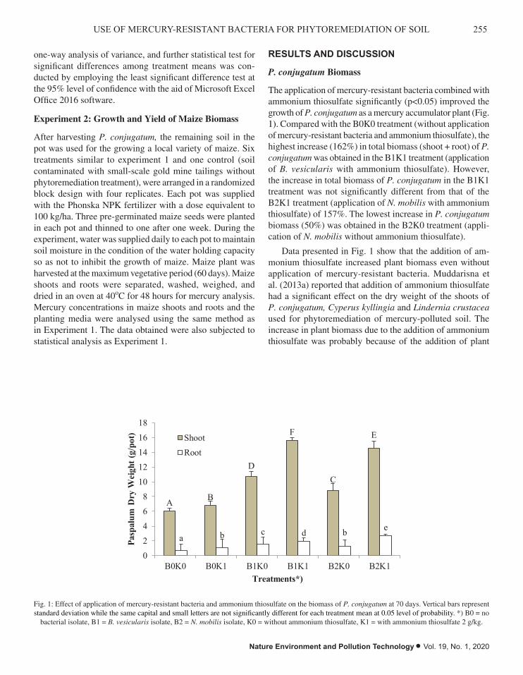
255USE OF MERCURY-RESISTANT BACTERIA FOR PHYTOREMEDIATION OF SOIL
Nature Environment and Pollution Technology • Vol. 19, No. 1, 2020
one-way analysis of variance, and further statistical test for significant differences among treatment means was con-ducted by employing the least significant difference test at the 95% level of confidence with the aid of Microsoft Excel Office 2016 software.
Experiment 2: Growth and Yield of Maize Biomass
After harvesting P. conjugatum, the remaining soil in the pot was used for the growing a local variety of maize. Six treatments similar to experiment 1 and one control (soil contaminated with small-scale gold mine tailings without phytoremediation treatment), were arranged in a randomized block design with four replicates. Each pot was supplied with the Phonska NPK fertilizer with a dose equivalent to 100 kg/ha. Three pre-germinated maize seeds were planted in each pot and thinned to one after one week. During the experiment, water was supplied daily to each pot to maintain soil moisture in the condition of the water holding capacity so as not to inhibit the growth of maize. Maize plant was harvested at the maximum vegetative period (60 days). Maize shoots and roots were separated, washed, weighed, and dried in an oven at 40oC for 48 hours for mercury analysis. Mercury concentrations in maize shoots and roots and the planting media were analysed using the same method as in Experiment 1. The data obtained were also subjected to statistical analysis as Experiment 1.
RESULTS AND DISCUSSION
P. conjugatum Biomass
The application of mercury-resistant bacteria combined with ammonium thiosulfate significantly (p<0.05) improved the growth of P. conjugatum as a mercury accumulator plant (Fig. 1). Compared with the B0K0 treatment (without application of mercury-resistant bacteria and ammonium thiosulfate), the highest increase (162%) in total biomass (shoot + root) of P. conjugatum was obtained in the B1K1 treatment (application of B. vesicularis with ammonium thiosulfate). However, the increase in total biomass of P. conjugatum in the B1K1 treatment was not significantly different from that of the B2K1 treatment (application of N. mobilis with ammonium thiosulfate) of 157%. The lowest increase in P. conjugatum biomass (50%) was obtained in the B2K0 treatment (appli-cation of N. mobilis without ammonium thiosulfate).
Data presented in Fig. 1 show that the addition of am-monium thiosulfate increased plant biomass even without application of mercury-resistant bacteria. Muddarisna et al. (2013a) reported that addition of ammonium thiosulfate had a significant effect on the dry weight of the shoots of P. conjugatum, Cyperus kyllingia and Lindernia crustacea used for phytoremediation of mercury-polluted soil. The increase in plant biomass due to the addition of ammonium thiosulfate was probably because of the addition of plant
A B
D
F
C
E
a b c d b e
02468
1012141618
B0K0 B0K1 B1K0 B1K1 B2K0 B2K1
Pasp
alum
Dry
Wei
ght (
g/po
t)
Treatments*)
ShootRoot
Fig. 1: Effect of application of mercury-resistant bacteria and ammonium thiosulfate on the biomass of P. conjugatum at 70 days. Vertical bars represent standard deviation while the same capital and small letters are not significantly different for each treatment mean at 0.05 level of probability. *) B0 = no
bacterial isolate, B1 = B. vesicularis isolate, B2 = N. mobilis isolate, K0 = without ammonium thiosulfate, K1 = with ammonium thiosulfate 2 g/kg.

256 Reni Ustiatik et al.
Vol. 19, No. 1, 2020 • Nature Environment and Pollution Technology
nutrients (nitrogen and sulphur) supplied through ammonium thiosulfate at the 8-week old plant that was able to enhance plant growth (Handayanto et al. 2016). Chelating agents, such as ammonium thiosulfate, have been used as soil extractants, a source of micronutrient fertilizers and to maintain solubility of micronutrient in hydroponic solutions (Salt et al. 1995). If the addition of ammonium thiosulfate was combined with the application of mercury-resistant bacteria, it further en-hanced the improvement of accumulator plant growth, which in turn improved the absorption of mercury by the mercury accumulator plant.
Liagat & Eltem (2016) reported that B. vesicularis is an endophytic bacterium that can produce indole acetic acid (IAA) phytohormone to stimulate plant growth (Ying et al. 2015), and produce more nutrient uptake from the soil (Li et al. 2008). Endophytic bacteria can supply nutrients for plant growth by dissolving phosphate and fixing nitrogen (Marra et al. 2012). In addition, endophytic bacteria can also protect plants against pathogenic microorganisms (Khalifa et al.2015) and degradation of toxic compounds (Sheng et al. 2008). N. mobilis is known as an ammonia-oxidizing bacterium which can oxidize nitrite to nitrate (Yu et al. 2012, Koide et al.2014). This bacterium can derive energy from the oxidation of ammonia and nitrite in the degradation of organic wastes and recycling of nutrients in subterranean habitat (Koilraj et al. 2012). N. mobilis is also an important and dominant ammonia-oxidizing bacterium in various
wastewater treatment systems (Thandar et al. 2016).
Accumulation of Mercury by P. conjugatum
Referring to the P. conjugatum biomass and mercury concen-tration in the P. conjugatum plant, mercury accumulation in P. conjugatum plant can be calculated. The highest mercury accumulation (8.29 mg/kg dry weight) was found in the B1K1 treatment (B. vesicularis with ammonium thiosulfate), and the lowest was found in the B0K0 treatment (without bacterial isolates and ammonium thiosulfate) (Fig. 2). The application of mercury-resistant bacteria with ammonium thiosulfate to P. conjugatum reduced the mercury content in the soil contaminated by small-scale gold mine tailings which was 41.73 mg/kg, reduced by 3% (B0K0 treatment) up to 20% (B1K1 treatment). Microbes have developed a mechanism for detoxifying mercury based on intracellular reduction of Hg2+ to Hg0 which is non-toxic by mercury reductase enzymes and the loss of diffusional Hg0 from cells (Wagner-Dobler 2003).
From the accumulation of mercury in the P. conjugatum plant, more than 80% of Hg accumulation was found in the shoot of the plant. In line with the dry weight of plant biomass, the use of ammonium thiosulfate stimulated Hg uptake by plants. This is thought to occur because mercury has a strong affinity with thiol groups, especially sulphide and bisulphide complexes (Moreno et al. 2004, Selin 2009). Moreno et al. (2005) reported that Bracia juncea could ac-
AB
D
F
C
E
a b c d b e
0
1
2
3
4
5
6
7
8
9
B0K0 B0K1 B1K0 B1K1 B2K0 B2K1
Hg
accu
mul
atio
n by
Pas
palu
m(m
g/kg
dry
wei
ght)
Treatments*)
ShootRoot
Fig. 2: Effect of application of mercury-resistant bacteria and ammonium thiosulfate on the accumulation of mercury by P. conjugatum at 70 days. Vertical bars represent standard deviation while the same capital and small letters are not significantly different for each treatment mean at 0.05 level of probability. *) B0 = no bacterial isolate, B1 = B. vesicularis isolate, B2 = N. mobilis isolate, K0 = without ammonium thiosulfate, K1 = with ammoni-
um thiosulfate 2 g/kg.

257USE OF MERCURY-RESISTANT BACTERIA FOR PHYTOREMEDIATION OF SOIL
Nature Environment and Pollution Technology • Vol. 19, No. 1, 2020
cumulate Hg to 40 mg/kg in plant tissue after the application of ammonium thiosulfate to mine tailings contaminated with 2.8 mg Hg/kg. However, the use of ammonium thiosulfate can also create the risk of underground water pollution by Hg which is mobilized by the thiosulfate.
The increase in mercury accumulation by P. conjuga-tum in the B1PK1 treatment (B. vesicularis and ammonium thiosulfate) was probably due to the symbiotic relationship between microorganisms and plants that increased heavy metal extraction from the soil (Tangahu et al. 2011). In this study, the symbiosis of mercury-resistant bacteria and mer-cury accumulator plant increased mercury accumulation up to 459% (B1PK1 treatment) compared to treatments without the application of mercury-resistant bacteria. High mercury accumulation in the P. conjugatum plant caused mercury content in the soil to decrease up to 20% (B1PK1 treatment) from the original mercury content in the soil of 41.37 mg/kg. This technology can be used to extract mercury from agricultural soil before it is used to grow food crops. How-ever, this technology still raises the problem of processing the biomass of extracting plants containing mercury so as not to re-pollute the environment.
Translocation Factor of Mercury
As the effect on Hg accumulation of shoot and root, the application of mercury-resistant bacteria and ammonium thiosulfate also had a significant effect on the P. conjugatum
translocation factor (TF) values for mercury which were all greater than 1 (Fig. 3). The highest translocation factor value (1.54) was found in the B1K1 treatment (B. vesicularis and ammonium thiosulfate) which was not significantly different from the TF value in the B2K1 treatment (N. mobilis and ammonium thiosulfate) of 1.47 (Fig. 3). The lowest TF value (1.02) in the B0K0 treatment (without mercury-resistant bac-teria and ammonium thiosulfate). Differences in TF values in the treatments showed differences in the effectiveness of each treatment in the transport of mercury from the root system to the shoot as a place of accumulation (Selin 2009). This difference is also thought to be related to the modification of plant growth under conditions of heavy metal stress as a result of the absence of certain amino acids in plants (Ashraf et al. 2011).
Growth and Biomass Yield of Maize
At harvest time of the maximum vegetative age (60 days), the height of maize plants varied from 45.7 cm (control) to 105.8 cm (B1K1 treatment) (Fig. 4). Compared with the control, phytoremediation of soil with P. conjugatum and application of mercury-resistant bacteria and ammonium thiosulfate increased plant height by 96% (B1K0), 108% (B2K0), 145% (B1K1), 131% (B2K1), 110% (B0K1), and 69% (B0K0). Application of mercury-resistant bacteria in the soil phytoremediation process further enhanced the growth of maize plants. The combination of treatment in the soil
a ab c
c
ab
c
0.00.20.40.60.81.01.21.41.61.8
B0K0 B0K1 B1K0 B1K1 B2K0 B2K1
Tra
nslo
catio
n Fa
ctor
(TF)
Treatments*)
Fig. 3: Effect of application of mercury-resistant bacteria and ammonium thiosulfate on the translocation factor of mercury by P. conjugatum at 70 days. Vertical bars represent standard deviation while the same letters are not significantly different for each treatment mean at 0.05 level of probability.
*) B0 = no bacterial isolate, B1 = B. vesicularis isolate, B2 = N. mobilis isolate, K0 = without ammonium thiosulfate, K1 = with ammonium thiosulfate 2 g/kg.

258 Reni Ustiatik et al.
Vol. 19, No. 1, 2020 • Nature Environment and Pollution Technology
phytoremediation process which then resulted in the best growth of maize plant was the B1K1 treatment. This is in line with the results of the highest Hg reduction in soil by the B1K1 treatment (Fig. 2).
The dry weight of the shoots and roots of maize plants
increased on the soils which had been remediated with a combination of P. conjugatum and mercury-resistant bac-teria. Consistent with the capability of the B1K1 treatment (B. vesicularis with ammonium thiosulfate) in accumulating the highest Hg, the highest increase in the dry weight of
A
BB
CD
C
D
a
bcd
cd
ab
cd
bc bc
0
5
10
15
20
25
Control B0K0 B0K1 B1K0 B1K1 B2K0 B2K1
Mai
ze D
ry W
eigh
t (g/
pot)
Treatments*)
ShootRoot
Fig. 5: Shoot and root dry weight of maize grown on post-phytoremediation soil at 60 days. Vertical bars represent standard deviation while the same capital and small letters are not significantly different for each treatment mean at 0.05 level of probability. *) B0 = no bacterial isolate, B1 = B. vesicu-
laris isolate, B2 = N. mobilis isolate, K0 = without ammonium thiosulfate, K1 = with ammonium thiosulfate 2 g/kg, Control = soil not subjected to phytoremediation.
a
b b
bcc
bc
0
20
40
60
80
100
120
Control B0K0 B0K1 B1K0 B1K1 B2K0 B2K1
Mai
ze P
lant
Hei
ght (
cm)
Treatments*)
Fig. 4: Height of maize grown on post-phytoremediation soil at 60 days. Vertical bars represent standard deviation while the same letters are not signifi-cantly different for each treatment mean at 0.05 level of probability. *) B0 = no bacterial isolate, B1 = B. vesicularis isolate, B2 = N. mobilis isolate, K0
= without ammonium thiosulfate, K1 = with ammonium thiosulfate 2 g/kg, Control = soil not subjected to phytoremediation.

259USE OF MERCURY-RESISTANT BACTERIA FOR PHYTOREMEDIATION OF SOIL
Nature Environment and Pollution Technology • Vol. 19, No. 1, 2020
shoots and roots were also found in the B1K1 treatment although it was not significantly different from the B2K1 treatment (Fig. 5). Compared to the control, the increase in maize biomass (shoot and root) grown on soil previously remediated through the B1K1 and B2K1 treatments were 145% and 131%, respectively, while those grown on soil pre-viously remediated through the B1K0 and B2K0 treatments were 96% and 108% respectively. Biomass of maize plants grown on the soil remediated with P. conjugatum without mercury-resistant bacteria and ammonium thiosulfate were low and not significantly different from the control. The low increase of maize plant growth and yield of maize biomass on post-phytoremediation without the addition of mercu-ry-resistant bacteria and ammonium thiosulfate compared to those grown on post-phytoremediation with the addition of mercury-resistant bacteria and ammonium thiosulfate was associated with mercury uptake by plants (Fig. 6).
The remaining mercury in the growing media without the addition of mercury-resistant bacteria and ammonium thiosulfate was higher than in the growing media with the addition of ammonium thiosulfate, thus inhibiting plant growth. In plants, mercury causes damage to enzymes, pol-ynucleotides, nutrient transport systems, and disrupts cell membrane integrity (Nagajyoti et al. 2010). Root extension is often used as the first indication that plants are poisoned by Hg elements (Moldovan et al. 2013). Symptoms of mer-cury toxicity, in general, are the inhibition of seed and root
growth, and the inhibition of photosynthesis, which in turn reduces crop production. In addition, mercury accumulated in plant root can inhibit the absorption of K by plants (Hooda 2010). Mercury absorbed by plants can cause some enzymes to be inactive because of the incorporation of mercury into sulfhydryl peroxide through the formation of reactive oxy-gen compounds, such as superoxide, hydroxyl radicals, and hydrogen peroxide (Chen & Yang 2012).
Mercury Uptake by Maize
The results of the analysis of mercury in the maize shoots and roots showed that the accumulation of Hg in the maize plant was mostly found in the roots. From the average accumu-lation of Hg in the maize shoots and roots in all treatments, about 98% of the mercury was accumulated in the roots, while in the shoot was only 2% or an average of 0.008 mg/kg dry weight. This was in line with a study on the potential of maize for phytoremediation of soil contaminated with gold mine tailings conducted in Lombok by Afandi et al. (2019) that 95.7-98.6% of the Hg absorbed by the maize plant was concentrated in the maize root, and no mercury was detected in maize seeds. Therefore, it can be stated that the maize shoot is safe to be used as livestock feed because it is below the threshold of mercury content according to the threshold of the Indonesian Government Regulation of 0.03 mg Hg/kg.
Maize is capable of continuous phytoextraction of metals from contaminated soils by translocating them from roots
B B A A A A A
a
dc
ab
abc
abbc
0.0
0.1
0.2
0.3
0.4
0.5
0.6
0.7
0.8
0.9
Control B0K0 B0K1 B1K0 B1K1 B2K0 B2K1
Hg
accu
mul
atio
n by
mai
ze
(mg/
kg d
ry w
eigh
t)
ShootRoot
Fig. 6: Accumulation of mercury by maize grown on post-phytoremediation soil at 60 days. Vertical bars represent standard deviation while the same capital and small letters are not significantly different for each treatment mean at 0.05 level of probability. *) B0 = no bacterial isolate, B1 = B. vesicu-
laris isolate, B2 = N. mobilis isolate, K0 = without ammonium thiosulfate, K1 = with ammonium thiosulfate 2 g/kg, Control = soil not subjected to phytoremediation.
260 Reni Ustiatik et al.
Vol. 19, No. 1, 2020 • Nature Environment and Pollution Technology
to shoots (Nascimento & Xing 2006). The maize plant has been even shown to accumulate certain heavy metals such as Cd (Kimenyu et al. 2009) and Pb (Pereira et al. 2007) above levels that define metal hyperaccumulation. Máthé-Gáspár & Anton (2005) have grouped maize as an accumulator and a metal tolerant plant. The potential use of maize in phytoextraction technology is thus advocated, especially for developing countries with scarce funds available for environ-mental restoration (Wuana & Okieimen 2010).
CONCLUSION
The application of B. vesicularis and N. mobilis combined with ammonium thiosulfate as a chelating agent enhanced the growth and biomass of P. conjugatum in the phytoreme-diation process of soil contaminated with small-scale gold mine tailings. This, in turn, increased mercury accumulation in plants so that it reduced 18-20% of mercury content in the soil contaminated with gold mine tailings. The decrease of mercury content in the soil led to improved growth and yield of maize planted after soil phytoremediation through the application of B. vesicularis and N. mobilis.
ACKNOWLEDGEMENTS
The authors thank the Ministry of Research, Technology, and Higher Education of Indonesia for supporting this study through Project No. 054/SP2H/LT/DRPM/2018. Field and technical assistance of the Bonjeruk Farmers of Central Lombok is gratefully acknowledged.
REFERENCES
Afandi, Y., Tejowulan, R.S. and Krisnayanti, B.D. 2019. Mercury uptake by Zea mays L. grown on an inceptisol polluted by amalgamation and cyanidation tailings of small-scale gold mining. Journal of Degraded and Mining Lands Management, 6(3): 1821-1828.
Ashraf, M.A., Maah, M.J. and Yusoff, I. 2011. Heavy metals accumulation in plants growing in ex-tin mining catchment. International Journal of Environmental Science and Technology, 8: 401-416.
Chasanah, U., Nuraini, Y. and Handayanto, E. 2018. The potential of mer-cury-resistant bacteria isolated from small-scale gold mine tailings for accumulation of mercury. Journal of Ecological Engineering, 19(2): 236-245.
Chen, J. and Yang, Z.M. 2012. Mercury toxicity, molecular response and tolerance in higher plants. BioMetals, 25: 847-857.
Compant, S., Clément, B. and Sessitsch, A. 2010. Plant growth-promoting bacteria in the rhizo- and endosphere of plants: their role, colonization, mechanisms involved and prospects for utilization. Soil Biology and Biochemistry, 42: 669-678.
Handayanto, E., Nuraini, Y. and Muddarisna, N. 2016. Optimization of plant species and chelating agents in phytoextraction of gold from small-scale gold mine tailings. Nature Environment and Pollution Technology, 5(3): 1083-1088.
Hooda, P.S. 2010. Trace Elements in Soils. Blackwell Publishing Ltd.Khalifa, A.Y.Z., Alsyeeh, A.M., Almalki, M.A. and Farag, A. 2015. Char-
acterization of the plant growth promoting bacterium, Enterobacter cloacae MSR1, isolated from roots of non-nodulating Medicago sativa. Saudi Journal of Biological Science, 23(1): 79-86.
Kimenyu, P.N., Oyaro, N., Chacha, J.S. and Tsanuo, M.K. 2009. The potential of Commelina bengalensis, Amaranthus hybridus, Zea mays for phytoremediation of heavy metals from contaminated soils. Sains Malaysiana, 38(1): 61-68.
Koide, M., Higa, F., Tateyama, M., Cash, H.L., Hokama, A. and Fujita, J. 2014. Role of Brevundimonas vesicularis in supporting the growth of Legionella in nutrient-poor environments. New Microbiologica, 37: 33-39.
Koilraj, A.J., Prabhavathi, P., Rajendran, R., Kuberan, T., Gowri, R.S. and Selvi, C.P. 2012. Degradation of organic wastes and recycling of nu-trients enhanced by microbes in subterranean habitat. African Journal of Microbiology Research, 6(21): 4449-4456.
Krisnayanti, B.D., Anderson, C.W.N., Utomo, W.H., Feng, X., Handayanto, E., Muddarisna, N., Ikram, H. and Khususiah. 2012a. Assessment of environmental mercury discharge at a four-year-old artisanal gold mining area on Lombok Island, Indonesia. Journal Environmental Monitoring, 14: 2598-2607.
Krisnayanti, B.D., Arifin, Z. Bustan, Sudirman, and Yani, A. 2012b. Mer-cury Concentration on Tailing and Water from One Year of ASGM at Lantung, Sumbawa, Indonesia. In: Environmental, Socio-economic, and Health Impacts of Artisanal and Small-Scale Minings. E. Handayanto, B.D. Krisnayanti and Suhartini (Eds). pp. 61-66, ISBN: 978-602-203-276-2, UB Press, Malang, Indonesia.
Li, J.H., Wang, E.T., Chen, W.F. and Chen W.X. 2008. Genetic diversity and potential for promotion of plant growth detected in nodule endophytic bacteria of soybean grown in Heilongjiang province of China. Soil Biology and Biochemistry, 40: 238-246.
Liagat, F. and Eltem, R. 2016. Identification and characterization of en-dophytic bacteria isolated from in vitro cultures of peach and pear rootstocks. 3 Biotech, 6(2): 120.
Marra, L.M., Soares, C.R.F.S., de Oliveira, S.M., Ferreira, P.A.A., Soares, B.L., de Fráguas Carvalho, R., de Lima J.M. and de Souza Moreira, F.M. 2012. Biological nitrogen fixation and phosphate solubilization by bacteria isolated from tropical soils. Plant and Soil, 57: 289-307.
Máthé-Gáspár, G. and Anton, A. 2005. Phytoremediation study: Factors influencing heavy metal uptake of plants. Acta Biologica Szegediensis, 49(1-2): 69-70.
Moldovan, O.T., Meleg, I.N., Levei, E. and Terente, M. 2013. A simple method for assessing biotic indicators and predicting biodiversity in the hyporheic zone of a river polluted with metals. Ecological Indicators, 24: 412-420.
Moreno, F.N., Anderson, C.W.N., Robinson, B.H. and Stewart R.B. 2004. Phytoremediation of mercury-contaminated mine tailings by induced plant-Hg accumulation. Environmental Practice, 6(2): 165-175.
Moreno, F.N., Anderson, C.W.N., Stewart, R.B., Robinson, B.H., Nomura, R., Ghomshei, M. and Meech, J.A. 2005. Effect of thiol ligands on plant-Hg accumulation and volatilization from mercury-contaminated mine tailings. Plant and Soil, 275: 233-246.
Muddarisna, N., Krisnayanti, B.D., Utami, S.R. and Handayanto, E. 2013a. Effects mercury on growth and biochemical constituents of maize seedlings. Plant Sciences Feed, 3(4): 50-55.
Muddarisna, N., Krisnayanti, B.D., Utami, S.R. and Handayanto, E. 2013b. The potential of wild plants for phytoremediation of soil contaminated with mercury of gold cyanidation tailings. Journal of Environmental Science, Toxicology and Food Technology, 4(1): 15-19.
Nagajyoti, P.C., Lee, K.D. and Sreekanth, T.V.M. 2010. Heavy metals, occurrence and toxicity for plants: a review. Environmental Chemistry Letters 8: 199-216.
Nascimento, A.M.A. and Chartone-Souza, E. 2003. Operon mer: Bacterial resistance to mercury and potential for bioremediation of contaminated

261USE OF MERCURY-RESISTANT BACTERIA FOR PHYTOREMEDIATION OF SOIL
Nature Environment and Pollution Technology • Vol. 19, No. 1, 2020
environments. Genetics and Molecular Research, 2(1): 92-101.Nascimento, C.W.A. and Xing, B. 2006. Phytoextraction: A review on
enhanced metal availability and plant accumulation. Scientia Agricola (Piracicaba, Brazil), 63(3): 299-311.
Pereira, B.F.F., de Abreu, C.A., Romeiro, S., Lagôa, A.M.M.A. and Paz-Gonzále, A. 2007. Pb-Phytoextraction by maize in a Pb-EDTA treated oxisol. Scientia Agricola (Piracicaba, Brazil), 64(1): 52-60.
Salt, D.E., Blaylock, M., Kumar, P.B.A.N., Dushenkov, V., Ensley, B.D., Chet, L. and Raskin, L. 1995. Phytoremediation: a novel strategy for the removal of toxicants from the environments using plants. Biotechnology, 13: 468-474.
Selin. N.E. 2009. Global biogeochemical cycling of mercury: A review. Annual Review of Environment and Resources, 34: 43-63.
Sheng, H.M., Gao, H.S., Xue, L.G., Ding, S., Song, C.L., Feng, H.Y. and An, L.Z. 2011. Analysis of the composition and characteristics of culturable endophytic bacteria within subnival plants of the Tianshan Mountains, northwestern China. Current Microbiology, 62: 923-932.
Su, Y., Han, F.X., Chen, J., Shiyab, S. and Monts, D.L. 2009. Phytotoxicity and phytoremediation of mercury in Indian mustard and two Ferns with mercury-contaminated water and Oak Ridge soil. WM2009 Conference.
Tangahu, B.V., Abdullah, S.R.S., Idris, H.B.M., Anuar, N. and Mukhlisin, M. 2011. Review on heavy metal (As, Pb and Hg) uptake by plants through phytoremediation. International Journal of Chemical Engi-neering, 31: 20-26,
Thandar S.M., Ushiki, N., Fujitani, H., Sekiguchi, Y. and Tsuneda, S. 2016. Ecophysiology and comparative genomics of Nitrosomonas mobilis
Ms1 isolated from autotrophic nitrifying granules of wastewater treatment bioreactor. Frontiers in Microbiology, Volume 7, Article 1869.
Wagner-Dobler, I., von Canstein, H., Li Y., Timnis, K.N. and Deckwer, W.D. 2000. Removal of mercury from chemical wastewater by micro-organisms in technical scale. Environmental Science and Technology, 34: 4628-4634.
Wang, J., Feng, X. and Anderson, C.W.N. 2013.Thiosulfate assisted phyto-extraction of mercury (Hg) contaminated soils at The Wanshan Mercury Mining District, Southwest China. Journal of Degraded and Mining Lands Management, 1(1): 1-8.
Wang, Y. 2004. Phytoremediation of Mercury by Terrestrial Plants. Doctoral thesis in Botany. Department of Botany, Stockholm University.
Wuana, R.A. and Okieimen, F.E. 2010. Phytoremediation potential of maize (Zea mays L.). A Review. African Journal of General Agriculture, 6(4): 275-287.
Ying, W., Cheng-de, Y., Yu-ling, Y., Yu-qin, W., Zhen-fen, Z. and Li, X. 2015. The diversity and potential function of endophytic bacteria iso-lated from Kobreasia capillifolia at alpine grasslands on the Tibetan Plateau, China. Journal of Integrative Agriculture, Advance Online Publication 2015.
Yoon, J., Cao, X. and Zhou, O. 2006. Accumulation of Pb, Cu, and Zn in native plants growing on a contaminated Florida site. Science of the Total Environment, 368: 456-464.
Yu, L., Peng, D. and Pan, R. 2012. Shifts in nitrification kinetics and mi-crobial community during bioaugmentation of activated sludge with nitrifiers enriched on sludge reject water. Journal of Biomedicine and Biotechnology, Article ID 691894.

Vol. 19, No. 1, 2020 • Nature Environment and Pollution Technology
262

Performance Study of Cellulose Acetate Blended Polyvinylchloride Membranes
Pawan Kumar and Vijay Laxmi Yadav†Department of Chemical Engineering and Technology, IIT-BHU, Varanasi-221005, Uttar Pradesh, India†Corresponding author: Vijay Laxmi Yadav
ABSTRACT
In this paper, polymeric membranes were prepared by uniformly dispersing the cellulose acetate, polyethylene glycol and polyvinyl pyrrolidone particles in a polyvinyl chloride matrix for resolving the demand for azeotropic mixture separations. The polymeric membranes were characterized using SEM, FTIR and XRD analysis. The results show that the blending of cellulose acetate and plasticizer diethyl phthalate significantly improved the separation performance of the membranes. The selectivity was increased by adding cellulose acetate up to 2% wt and polyethylene glycol 1% wt. Pervaporation setup was used to separate azeotropic mixture using the prepared membrane. The optimum results were obtained for dehydration of alcohol where the composition plasticizer was 0.5% wt. Based on the findings of the research, it was observed that the PVC membrane can be modified with CA and PEG due to their hydrophobic nature. The results show that the synthesized membrane can be used for removal of water from alcohol.
INTRODUCTION
In the present scenario, the most established membrane separation processes are reverse osmosis, microfiltration, ultra-filtration, and electro dialysis. Except them, two new growing industrial processes are gas separation and pervaporation for separation of an azeotropic mixture (Qureshi 2016). Pervaporation is among the least studied of all membrane separation processes (Pramanik 2017). The work herein has the motive to show the effect of fabrication conditions on membrane performance. The work is mainly focused on the preparation of hydrophobic membranes for the separation of ethanol water mixture. In recent decades, membranes have occupied a major role worldwide in chemical technologies because of a vast diversity of separations can be done by membranes such as separation of gaseous mixtures, filtration of particles from solutions, even membrane are separating close boiling liquids from each other, to name a few (Yamamoto 2017). There is a large number of industries in which such separations are carried out on a large scale such as pharmaceutical, food science and chemical processes (Ayman 2012).
This paper i s concerned wi th the advanced development of polymeric membranes for pervaporation by solution casting method (Sadri 2017). All membranes were prepared using a phase inversion process. Early research was focused on the development of viable membranes (Han 2017 and Zhao 2017).
By the start of the 20th-century, membranes became popular and by the late 1960s onwards many improvements also started in the field of dialysis in medicine and controlled drug delivery by the membranes. This led to the development of microfiltration, ultrafiltration, reverse osmosis and electrodialysis during the 1970’s (Chun 2016). Last two decades of the 20th century showed the development of gas separation and pervaporation membrane technologies and current membrane industries took its shape (Imbrogno 2017 and Gu 2016).
A variety of research has been done on the preparation of membranes using polyvinylchloride (PVC) because of their flexibility in operation, durability and better performance and resistance to chemicals. PVC membranes are hydrophobic in nature (Bandi 2016, El-Gendi 2012 and El-Gendi 2014). Commonly, PVC is one of the most common and easily available polymers because of its low price which is less than 1/10 of most common commercial polymer for membrane, i.e. PVDF polymer. Hence, PVC is a major concern for researchers for membrane preparation as it is very competitive to other polymers (Mokhtari 2016).
The objective of this study was to prepare a suitable blend of PVC/CA/PEG membrane for separation of alcohol from an alcohol-water mixture by non-solvent induced phase inversion technique. The prepared membranes were characterized with SEM, X-ray diffractometer and Fourier
Nat. Env. & Poll. Tech.Website: www.neptjournal.com
Received: 08-05-2019Accepted: 21-06-2019
Key Words:Polyvinyl chlorideCellulose acetateAntifouling membraneAlcohol water mixture
2020pp. 263-268 Vol. 19
p-ISSN: 0972-6268 No. 1 Nature Environment and Pollution Technology An International Quarterly Scientific Journal
Original Research Paper
e-ISSN: 2395-3454
Open Access

264 Pawan Kumar and Vijay Laxmi Yadav
Vol. 19, No. 1, 2020 • Nature Environment and Pollution Technology
transform infrared (FTIR) (Oh & Jang 2016). Performance of lab made membranes was investigated by treating a sample of an alcohol-water mixture with different concentration.
MATERIALS AND METHODS
Materials
Polyvinylchloride (PVC) the base polymer, cellulose acetate (CA), polyvinyl pyrrolidone (PVP) and polyethylene glycol (PEG) were purchased from Sigma Aldrich. Tetrahydrofuran (THF) was used as a solvent and was purchased from Spectrochem, Mumbai. Absolute alcohol was used to check the performance of the membranes.
Preparation of Membranes
Blended PVC/CA/PVP membranes were prepared by the phase inversion process (Saljoughi et al. 2009). The known amounts of polymers were dissolved in NMP and compositions of samples are shown in Table 1. After this, the solution was stirred for 12 hr. The solution of polymer was cast on a glass plate, and glass plate was subsequently dipped in a non-solvent bath of deionized water. The water was changed three times for complete exchange of solvent THF. And finally, the membrane was dried in the oven at 50oC and then used further.
Membrane Characterization
Surface morphology of prepared membrane samples was investigated by scanning electron microscopy (SEM). Samples were pre-coated with gold to provide electrical conductivity. The instrument used for the purpose was EVO - Scanning Electron Microscope MA15/18, Carl Zeiss Microscopy Ltd., USA. The crystalline or amorphous nature of polymeric membranes was investigated using X-ray diffractometer (XRD, model - EDS System, Carl Zeiss Microscopy Ltd., USA) with a scanning rate of 5o per minute in the range of 0o to 70o (2q). The functional changes in the polymeric membranes were analysed in the transmittance mode from 4000 to 400 cm-1 wavelength range using Fourier Transform Infrared Spectroscopy (FTIR) Varian 1000, USA.
A lab scale dead end pervaporation setup was used to study the performance of samples using an alcohol water mixture. Performance of membrane was expressed in terms of permeate flux.
RESULTS AND DISCUSSION
Thickness of Membrane
The thickness of the different membrane samples, measured using digital Vernier callipers, is given in Table 3. The
Table 1: Polymeric membrane composition for PVC/CA, for different samples of (S-1 to S-4) membrane (weight percentage).
PVC % CA % PEG % THF % Plasticizer %
S-1 18 0 2 80 0
S-2 16 2 2 80 0
S-3 15 3 2 80 0
S-4 15 2.5 2 80 0.5
Table 2: Performance of different membranes for separation of ethanol-water.
Membrane Product Flux for feed conc. 15% alcohol (kg.m-2hr-1)
Product Flux for feed conc. 30% alcohol (kg.m-2hr-1)
Product Flux for feed conc. 45% alcohol (kg.m-2hr-1)
S-1 5.93 5.8 5.88
S-2 4.88 4.99 5.02
S-3 3.773 3.01 3.134
S-4 2.5 2.62 2.53
Table 3: Thickness of prepared membrane samples.
Membrane Thickness (mm)
S-1 0.41
S-2 0.14
S-3 0.24
S-4 0.30

265PERFORMANCE OF CELLULOSE ACETATE BLENDED PVC MEMBRANES
Nature Environment and Pollution Technology • Vol. 19, No. 1, 2020
thickness of the membrane increased when the amount of the cross linker was increased. This occurs due to high bonding between cross linker and polymer. It is seen that as the amount of cross-linking agent is increasing, membrane thickness is also increasing due to the formation of an intermediate layer of fillers due to the polymerization of cross linker.
Membrane Morphology
SEM micrographs of different samples have been shown in Fig. 1(a-d). SEM images show a cross section of the (S-1) membrane. Expected asymmetric pores are observable in the entire surface as the CA was added to the system. At the same
time S-2 shows different surface pattern. It was seen in the image of S-2 that surface become rougher and pores become denser as the result of blending. Saljoughi et al. (2009) had also shown similar changes. Similarly, by addition of more CA in S-3, number of pores decreased and it was visible in SEM image. In S-4, plasticizer was added to see its effect on the surface. It was seen that by addition of plasticizer, pores became large which in turn increased the flux through the membrane and this phenomenon was verified by performance studies where S-4 shown better flux.
FTIR Analysis
Membranes were further characterized by Fourier Transform
Table 4: Wavelength for cellulose acetate group.
Wavelength cm-1 Chemical bond
2918.9-3406.1 -OH
1633.3-1738.2 C=O
1370.9-1489.7 CH3
1769.7 -CH
1044.9 C-O-C
669.3 R-COH
9
669.3 R-COH
Figures
Fig. 1: SEM images of prepared PVC membranes (a)- sample S-1, (b)- sample S-2, (c)- sample S-3, (d)- sample S-4.
Fig. 1: SEM images of prepared PVC membranes (a)- sample S-1, (b)- sample S-2, (c)- sample S-3, (d)- sample S-4.

266 Pawan Kumar and Vijay Laxmi Yadav
Vol. 19, No. 1, 2020 • Nature Environment and Pollution Technology
Infrared (FTIR) spectroscopy in the range 4000-400 cm-1 to know the functional groups present in the samples to verify the formation of desired composites. The membrane samples (S1 - S4) were tested for comparison and the result is shown in Fig. 2. The peaks corresponding to 2520 cm-1 for sample S-1, 2640 cm-1 for sample S-2, 2750 cm-1 for sample S-3, 2610 cm-1 for sample S-4 and at 2595 cm-1 for sample S-4 corresponding to C-H stretching (Saljoughi et al. 2009).
Functional groups and their peaks which are common for CA are given in Table 4. A peak at 1470 cm-1 was observed (except in sample-1) corresponding to -CH2 bonding. The C-Cl stretching was indicated by the 4 peaks at 727 cm-1, 685 cm-1, 715 cm-1 and 750 cm-1 for the sample S-1, S-2, S-3, and S-4 respectively. The effect of adding PEG was observed in sample-1 at peak 683 cm-1, indicating that PEG mostly influences the membrane structure.
After blending of PVC with CA and PEG, a shift was observed for PVC and CA peaks.
X-Ray Diffraction (XRD) Analysis
The crystalline and amorphous character of the membrane was studied by X-ray diffraction measurement and has been
shown in Fig. 3. We can see from Fig. 3(a) of sample-1 the XRD patterns two peaks are observed. Here peaks are seen at a 2-theta value of 17° and 26°. Broad peaks appeared at 26° and smaller peak appeared at 17°.
Further, from Fig. 3(b) of sample-2, we can also see that when we increase the amount of PVC again, we observed 2 peaks at a 2-theta value of 27° and 38°, but the peak corresponding to 27° is more intense and higher. These peaks are sharper than sample-1 that can be attributed to the involvement of cellulose acetate. Such results are also observed by Saeki et.al (2013) while preparing poly amide membrane with similar procedure.
From the Fig. 3(c) of sample-3, we observe the same XRD pattern as in the graph of sample-2. There are 2 peaks at a 2-theta value of 27° and 38°, but this time high peak appears at 27° and a smaller peak at 38°. The intensity of peaks is higher than those of sample-2. This can be due to the addition of 2% PEG as a pore creator.
From the Fig. 3(d) of sample-4 in which 0.5% plasticizer was also added to increase the elastic nature of the sample. In this case, it was observed same XRD pattern as in Fig. 3(b) of sample-2 and in Fig. 3(c) of sample-3. In this, we
10
Fig. 2: FTIR spectra of prepared membranes (a) sample S-1, (b) sample S-2, (c) sample S-3, (d) sample S-4.
Fig.3: XRD patterns for different samples.
Fig. 2: FTIR spectra of prepared membranes (a) sample S-1, (b) sample S-2, (c) sample S-3, (d) sample S-4.
(d)(c)
(b) (a)

267PERFORMANCE OF CELLULOSE ACETATE BLENDED PVC MEMBRANES
Nature Environment and Pollution Technology • Vol. 19, No. 1, 2020
observed 2 peaks at 26.5° and 33°, but this time high peak appears at 26.5°, and smaller one appears at 33°, but the intensity of peaks is higher than in Fig. 3(b) of sample-2 and in Fig. 3(c) of sample-3. This can be due to the addition of 0.5% plasticizer to increase elasticity.
Membrane Performance
In order to check the performance of the membrane, the ethanol-water mixture was used as the feed. Several compositions of the ethanol-water mixture were used to measure the flux of ethanol across the membrane to study the performance of the prepared membrane. Table 2 shows the observations regarding the flux of product for various samples.
From Table 2 we can say that the total flux through the membrane is in the order of S-1 > S-2 > S-3 > S-4. In S-1, equal amount of PVC and PEG were involved and porosity of this membrane is highest resulting in maximum flux compared to other membrane samples.
In S-2 (PVC blend with CA and PEG), we observed less product flux compared to S-1. This can be due to the fact that on increasing the amount of PVC and adding one more additive PEG, the porosity goes down.
10
Fig. 2: FTIR spectra of prepared membranes (a) sample S-1, (b) sample S-2, (c) sample S-3, (d) sample S-4.
Fig.3: XRD patterns for different samples.
Fig. 3: XRD patterns for different samples.
(d) (c)
(b) (a)
In the preparation of S-3 flux of product again decreases and is less than S-2. This can be due to the fact that on adding more polymer, particles started aggregating and, pore would be denser, hence the resulting flux decreases. When we use S-4 membrane for pervaporation of given feed, we observed that the flux decreases but the change in amount was less than S-2 and S-3. In S-4 membrane we have added a plasticizer to enhance the elasticity.
CONCLUSION
PVC/CA/PEG and PVP blended membrane were successfully prepared via wet phase inversion technique using different concentrations of the component polymers. The following conclusions can be drawn from the above work: From SEM analysis membranes were found to be a dense and asymmetric membrane. Characterization results indicate that membrane S-4 is the best membrane among the prepared membranes S-1 to S-4. The durability test of membrane S-4 was conducted, and the membrane performance was approximately constant and stable over 20 days. FTIR and XRD analysis showed the proper formation of the composite by the process and by performance studies, it was observed

268 Pawan Kumar and Vijay Laxmi Yadav
Vol. 19, No. 1, 2020 • Nature Environment and Pollution Technology
that membrane containing PVC, CA and plasticizer has the highest flux, so the blend of sample 4 was optimum according to our study for separation of alcohol water mixture.
REFERENCES
Ayman, E.G., Heba, A. and Sahar A. 2012. Construction of ternary phase diagram and membrane morphology evaluation for polyamide/formic acid/water system. Australian J. Basic App. Sci., 6(5): 62-68.
Bandi, C.S., Uppaluri, R. and Kumar, A. 2016. Global optimization of MSF seawater desalination processes. Desalination, 394: 30-43.
Chun, Y., Zaviska, F., Kim, S.J. and Mulcahy, D. 2016. Yang, E., Kim, I. S. and Zou, L., Fouling characteristics and their implications on cleaning of a FO-RO pilot process for treating brackish surface water. Desali-nation, 394: 91-100.
El-Gendi, A., Ali, S.S., Ahmed, S.A. and Talaat, H.A. 2012. Development of membrane blend using casting technique for water desalination. Mem-brane Water Treatment, 3(3): 201-209.
El-Gendi, A., Deratani, A., Ahmed, S.A. and Ali, S.S. 2014. Development of polyamide-6/chitosan membranes for desalination. Egyptian J. Petro., 23(2): 169-173.
Gu, H., Rahardianto, A., Gao, L.X., Christofides, P.D. and Cohen, Y. 2016. Ultrafiltration with self-generated RO concentrate pulse backwash in a novel integrated seawater desalination UF-RO system. J. Memb. Sci., 520: 111-119.
Han, S., Rhee, Y.W. and Kang, S.P. 2017. Investigation of salt removal using cyclopentane hydrate formation and washing treatment for seawater desalination. Desalination, 404: 132-137.
Ibrahim, S.M., Nagasawa, H., Kanezashi, M. and Tsuru, T. 2015. Robust organosilica membranes for high temperature reverse osmosis (RO) application: Membrane preparation, separation characteristics of solutes and membrane regeneration. J. of Memb. Sci., 493: 515-523.
Imbrogno, J., Keating IV, J.J., Kilduff, J. and Belfort, G. 2017. Critical aspects of RO desalination: A combination strategy. Desalination, 401: 68-87.
Mokhtari, H. and Sepahvand, M. 2016. Thermoeconomic and exergy analysis in using hybrid systems (GT+ MED+ RO) for desalination of brackish water in Persian Gulf. Desalination, 399: 1-15.
Oh, J.H. and Jang, A. 2016. Application of chlorine dioxide (ClO2) to reverse osmosis (RO) membrane for seawater desalination. J. Taiwan Inst. Chem. Engg., 68: 281-288.
Pramanik, B.K., Gao, Y., Fan, L., Roddick, F.A. and Liu, Z. 2017. Antiscaling effect of polyaspartic acid and its derivative for RO membranes used for saline wastewater and brackish water desalination. Desalination, 404: 224-229.
Qureshi, B.A., Zubair, S.M. 2016. Exergetic efficiency of NF, RO and EDR desalination plants. Desalination, 378: 92-99.
Sadri, S., Ameri, M. and Khoshkhoo, R.H. 2017. Multi-objective opti-mization of MED-TVC-RO hybrid desalination system based on the irreversibility concept. Desalination, 402: 97-108.
Saeki, D., Nagao, S., Sawada, I., Ohmukai, Y., Maruyama, T. and Matsuy-ama, H. 2013. Development of antibacterial polyamide reverse osmosis membrane modified with a covalently immobilized enzyme. J. Memb. Sci., 428: 403-409.
Saljoughi, E. and Mohammadi, T. 2009. Cellulose acetate (CA)/polyvi-nylpyrrolidone (PVP) blend asymmetric membranes: Preparation, morphology and performance. Desalination, 249(2): 850-854.
Yamamoto, K., Koge, S., Gunji, T., Kanezashi, M., Tsuru, T. and Ohshita, J. 2017. Preparation of POSS-derived robust RO membranes for water desalination. Desalination, 404: 322-327.
Zhao, Y., Zhang, Z., Dai, L., Mao, H. and Zhang, S. 2017. Enhanced both water flux and salt rejection of reverse osmosis membrane through combining isophthaloyl dichloride with biphenyl tetra acyl chloride as organic phase monomer for seawater desalination. J. Memb. Sci., 522: 175-182.

Extraction and Spectrophotometric Estimation of Fe3+, Cd2+, Pb2+ and Zn2+ From Industrial Effluents Using Synthetic Supramolecular Ligand
Sachin Patil*, Milind Kondalkar*, Umesh Fegade**, Sanjay Attarde*† and Sopan Ingle* *School of Environmental and Earth Sciences, KBC North Maharashtra University, Jalgaon, Maharashtra, India**Department of Chemistry, Bhusawal Arts, Science and P. O. Nahata Commerce College, Bhusawal, Maharashtra, India†Corresponding Author: Sanjay B. Attarde
ABSTRACT
Increased water pollution due to toxic heavy metals is becoming a serious threat which has been faced by the entire world in the last few decades. To overcome this problem a suitable complex ligand was designed for removal of Fe3+, Cd2+, Pb2+ and Zn2+ from the effluents. The work incorporated the synthesis of (4Z)-4-((2Z)-2-(2,5-dihydro-2,3-dimethyl-5-oxo-1-phenyl-1H-pyrazol-4-ylimino) ethylidene amino)-1,2-dihydro-1,5-dimethyl-2-phenylpyrazol-3-one (Supramolecular Ligand) by the condensation method and confirmed by FTIR and 1HNMR spectroscopic methods. The batch extraction experiments designed to examine the effect of various experimental parameters on the extraction efficiency of the heavy metals. The experimental results depicted that up to 30 min time for supramolecular ligand is enough for the significant extraction of all the metals under study. The pH level, slightly acidic to the neutral condition is favourable for maximum extraction of metals. The percent extraction at optimized conditions of time and pH were found to be 98.29, 96.63, 96.95 and 95.64% for Fe3+, Cd2+, Pb2+ and Zn2+ respectively. The extraction efficiency was governed by chloroform as a solvent. Simple to synthesize, faster extraction of metals, slightly acidic to neutral pH conditions for extraction are the characteristic features of the compound which governs its applicability.
INTRODUCTION
Water, being a limited resource, an increase in water pollution due to metal ions and other pollutants is of great concern throughout the world (Jethave et al. 2017). The different pollutants responsible for water pollution are organic dyes, inorganic oxyacids and heavy metals etc. Amongst these, heavy metals are considered as more dangerous because even trace quantity in water is considered as carcinogenic (Li et al. 2011, Tang et al. 2008). Though the metals play a vital role in human metabolism and photosynthesis, an excess of these metals in living organisms is responsible for genetic and metabolic diseases (Fraga 2005). Heavy metals have widespread applications in different industrial units, viz. paint, fertilizer, metal industry and electroplating industries (Hua et al. 2012). Particularly in developing countries like India, the local communities have often encountered hazardous effects of pollutants (Himadri et al. 2014).
Different methods like solid-phase extraction and liquid-liquid extraction, adsorption, co-precipitation, and ion exchange have been applied for the removal of heavy metals from water. (Oliva et al. 2002, Saracoglu et al. 2003, Okamoto et al. 2000, Jethave & Fegade 2018, Fegade et al. 2018, Kondalkar et al. 2018). Amongst these, liquid-liquid
extraction is considered more effective because it is a simple, low cost, highly selective and has more removal efficiency. Till now, diverse complexing agents have been synthesized for metal extraction (Sarode et al. 2015, Costa et al. 2013). The aim of the present study is to synthesize a suitable chelating agent for liquid-liquid extraction of Fe3+, Cd2+, Pb2+ and Zn2+
from effluents. For this purpose, a supramolecular ligand was synthesized by a simple condensation reaction between 2 moles of 4-amino antipyrine and one mole of glyoxal in methanol. This chelating agent was characterized by NMR, FTIR and mass spectroscopy. The effect of various analytical parameters such as time, pH, concentrations, stripping agents and the presence of other ions on the extraction efficiency was examined. The experimental sets carried out to optimize the above parameters for removal of Fe3+, Cd2+, Pb2+ and Zn2+
from industrial wastewater. The remaining concentration of these metals in the reaction mixture was estimated by atomic absorption spectrophotometer.
MATERIALS AND METHODS
All chemicals and reagents used for the experiment and preparation of ligand were of analytical grade and procured from Sigma Aldrich and applied without further purification. Milli-Q water was used at every stage of the experiment.
2020pp. 269-275 Vol. 19
p-ISSN: 0972-6268 No. 1 Nature Environment and Pollution Technology An International Quarterly Scientific Journal
Original Research Paper
e-ISSN: 2395-3454
Open Access
Nat. Env. & Poll. Tech.Website: www.neptjournal.com
Received: 28-06-2019Accepted: 29-08-2019
Key Words:Toxic metalsExtractionLigandSolvent

270 Sachin Patil et al.
Vol. 19, No. 1, 2020 • Nature Environment and Pollution Technology
Digital pH-meter (India, EQUIP-TRONICS model EQ 610) was used for pH determination. Concentration of chro-mium was estimated using AAS. FTIR spectrum (in the range of 500-4000 cm-1) of the ligand was obtained using FTIR spectrophotometer (Germany, Model: Bruker). H1NMR was recorded on (Germany, Model: Bruker Advance) 400MHz.
Batch Extraction Experiment for Metal Removal
Optimization of diverse analytical parameters on extraction efficiency for metals was carried out by conducting exper-iments at various experimental parameters. For the choice of solvent, the extraction experiments were performed on different solvents like chloroform, N-butanol, ethyl acetate, toluene and N-hexane. In these experiments, the solvent was optimized based on contact time for chromium extraction at a various time interval. Suitable pH for maximum extraction of chromium was determined by running the experiments at a particular pH range from 2 to 10, provided other optimized variables kept constant. The percent metals extracted (% E) was calculated by applying an Eq. 1.
% E = (concentration of metals after extraction/ total concentration of metals) × 100 …(1)
RESULTS AND DISCUSSION
Synthesis of the Ligand Compound
The 0.2 moles of 4-amino antipyrine were poured in a 100 mL round bottom flask containing 25 mL methanol and the mixture was homogeneously mixed by a magnetic stirring. To these solutions, 0.1 moles of glyoxal was added drop-wise and the reaction solution was refluxed for 1 hr till the yellow residue was obtained and then filtered by a Whatman filter pa-per. The obtained yellow residue washed with distilled water several times to remove unreacted compounds and impurity forms. The obtained compound was stored in a bottle for characterization and batch extraction purpose. The possible mechanism for the ligand synthesis proposed in Fig. 1.
Characterization of the Compound
The formations of the compound were confirmed by various structural elucidation techniques like FTIR and 1HNMR and presented in Fig. 2 and 3 respectively. FTIR spectrum of the compound showed stretching frequency at 1557 cm-1 which indicates the presence of NH2 which in term indicates the
4
The formations of the compound were confirmed by various structural elucidation techniques
like FTIR and 1HNMR and presented in Fig. 2 and 3 respectively. FTIR spectrum of the
compound showed stretching frequency at 1557 cm-1 which indicates the presence of NH2
which in term indicates the formation of a compound. The different IR frequencies with
functional groups are summarized in Table 1. The 1HNMR spectrum of the compound shows
a peak near 7.5 which is assigned to N C C N
H H
. This peak confirms the
formation of the compound. The 1HNMR peaks with functional groups are summarized in
Table 2. Both FTIR and 1HNMR characterization showed the formation of the compound.
NN O
N
C
NNO
N
CH H
NN O
NH2
+ HC CH
O O
+N
NO
H2N
2 moles of 4-amino antipyrine
GlyoxalMethanol
Reflux for 1 hrN
N O
HN
+ HC CH
HO OH
+N
NO
HN
- H2O
Final product
Fig. 1: Possible mechanism of the formation for supramolecular ligand compound.
Fig. 1: Possible mechanism of the formation for supramolecular ligand compound.

271ESTIMATION OF Fe3+, Cd2+, Pb2+ AND Zn2+ FROM INDUSTRIAL EFFLUENTS
Nature Environment and Pollution Technology • Vol. 19, No. 1, 2020
5
Fig. 2: FTIR spectrum of the supramolecular ligand.
Fig. 3: H1NMR spectrum of the supramolecular ligand.
10 9 8 7 6 5 4 3 2 1 0 ppm
-0.0
004
1.73
95
2.43
17
3.17
51
7.26
257.
3215
7.33
997.
3683
7.37
097.
3843
7.38
927.
3926
7.45
487.
4595
7.47
357.
4938
9.35
32
3.03
3.04
1.15
2.16
2.22
1.00
NAME Apr03-2018-AdministratorEXPNO 180PROCNO 1Date_ 20180404Time 12.48INSTRUM spectPROBHD 5 mm SEI 1H/D-PULPROG zg30TD 65536SOLVENT CDCl3NS 8DS 2SWH 12019.230 HzFIDRES 0.183399 HzAQ 2.7263477 secRG 2050DW 41.600 usecDE 6.50 usecTE 295.5 KD1 1.00000000 secTD0 1
======== CHANNEL f1 ========NUC1 1HP1 6.40 usecPL1 -3.00 dBPL1W 15.78739738 WSFO1 400.1324710 MHzSI 32768SF 400.1300086 MHzWDW EMSSB 0LB 0.30 HzGB 0PC 1.00
SDP-1BRUKERAVANCE II 400 NMRSpectrometerSAIFPanjab UniversityChandigarh
Fig. 2: FTIR spectrum of the supramolecular ligand.
5
Fig. 2: FTIR spectrum of the supramolecular ligand.
Fig. 3: H1NMR spectrum of the supramolecular ligand.
10 9 8 7 6 5 4 3 2 1 0 ppm
-0.0
004
1.73
95
2.43
17
3.17
51
7.26
257.
3215
7.33
997.
3683
7.37
097.
3843
7.38
927.
3926
7.45
487.
4595
7.47
357.
4938
9.35
32
3.03
3.04
1.15
2.16
2.22
1.00
NAME Apr03-2018-AdministratorEXPNO 180PROCNO 1Date_ 20180404Time 12.48INSTRUM spectPROBHD 5 mm SEI 1H/D-PULPROG zg30TD 65536SOLVENT CDCl3NS 8DS 2SWH 12019.230 HzFIDRES 0.183399 HzAQ 2.7263477 secRG 2050DW 41.600 usecDE 6.50 usecTE 295.5 KD1 1.00000000 secTD0 1
======== CHANNEL f1 ========NUC1 1HP1 6.40 usecPL1 -3.00 dBPL1W 15.78739738 WSFO1 400.1324710 MHzSI 32768SF 400.1300086 MHzWDW EMSSB 0LB 0.30 HzGB 0PC 1.00
SDP-1BRUKERAVANCE II 400 NMRSpectrometerSAIFPanjab UniversityChandigarh
[email protected]. 3: H1NMR spectrum of the supramolecular ligand.

272 Sachin Patil et al.
Vol. 19, No. 1, 2020 • Nature Environment and Pollution Technology
formation of a compound. The different IR frequencies with functional groups are summarized in Table 1. The 1HNMR spectrum of the compound shows a peak near 7.5 which is
assigned to
4
The formations of the compound were confirmed by various structural elucidation techniques
like FTIR and 1HNMR and presented in Fig. 2 and 3 respectively. FTIR spectrum of the
compound showed stretching frequency at 1557 cm-1 which indicates the presence of NH2
which in term indicates the formation of a compound. The different IR frequencies with
functional groups are summarized in Table 1. The 1HNMR spectrum of the compound shows
a peak near 7.5 which is assigned to N C C N
H H
. This peak confirms the
formation of the compound. The 1HNMR peaks with functional groups are summarized in
Table 2. Both FTIR and 1HNMR characterization showed the formation of the compound.
NN O
N
C
NNO
N
CH H
NN O
NH2
+ HC CH
O O
+N
NO
H2N
2 moles of 4-amino antipyrine
GlyoxalMethanol
Reflux for 1 hrN
N O
HN
+ HC CH
HO OH
+N
NO
HN
- H2O
Final product
Fig. 1: Possible mechanism of the formation for supramolecular ligand compound.
. This peak confirms the formation of the compound. The 1HNMR peaks with functional groups are summarized in Table 2. Both FTIR and 1HNMR characterization showed the formation of the compound.
Selection of A Suitable Solvent for Metal Extraction
Solvent selection is an important part of liquid-liquid ex-traction. Stability of a complex formed between ligand and metal is highly dependent on the polarity of a solvent (In et al. 2008). Five different solvents were used for extraction of met-als by supramolecular ligand, viz., chloroform, N-butanol, ethyl acetate, toluene and N-hexane. The obtained results from the experiment are illustrated in Fig. 4 and showed that chloroform is a suitable solvent for the extraction of metals. The percent extraction of Fe3+, Cd2+, Pb2+ and Zn2+
using chloroform found to be 86%, 61%, 66% and 44% respectively. The extraction of the above metals using other solvents was less as compared to chloroform (Sarode et al. 2012). In liquid-liquid extraction, replacement of solvent molecules by either ligand or cation is highly favourable (Nezhadali et al. 2007). This condition seems to have fulfilled by chloroform. So, chloroform is selected as a solvent for further extraction experiment.
Effect of Extraction Time
The definite time required for ligand molecules and cation to dissolve into an organic phase altogether affects the overall extraction (Dadfarnia et al. 2010). The effect of contact time on percent extraction efficiency of the ligand was observed by conducting extraction experiments at a different time interval from 5 to 40 min. The obtained results are portrayed in Fig. 5 and show that the prominent extraction efficiency for metals is noted up to 25 min and after that, no significant extraction was observed. The optimized condition of contact time of 20 min was elaborated for Fe+3 and Pb+2 while in case of Cd+2 and Zn+2 it was found to be 25 and 30 min, respectively. The percent extraction at an optimized time was noted as 85.34, 60.21, 64.12 and 43.67% for metals Fe+3, Pb+2, Cd+2 and Zn+2 respectively.
Optimization of pH for the Extraction of Metals
As pH of the solvent controls the stability of the complex formed between ligand and cation, it is a prime variable in the liquid-liquid extraction (Ramo et al. 2000). The effect of solution pH on the extraction efficiency of metals was observed at 0.5 to 9. The results of various experiments depicted that acidic to neutral pH condition is favourable for metal extraction (Fig. 6). In complex formation, ligand behaves like Lewis base and donate its lone pair of an electron to a metal cation to form a complex. In the case of supra-molecular ligand, nitrogen and oxygen are the donor atoms and at suitable pH facilitates the formation of a complex by donating a lone pair of electrons.
Table 1: FTIR frequencies assigned to the functional groups of supramolecular ligand.
Sr. No. FTIR frequencies (cm-1) Functional groups
1. 3062 =C-H
2. 2982 -C-H
3. 1648 C=O
4. 1557 C=N
5. 1486, 1410, 1375 and 1345 CH3 bending
6. 755, 694, 659 and 629 C-H monosubstituted benzene derivative
Table 2: Assignment of H1NMR chemical shifts to the functional groups of supramolecular ligand.
Sr. No. Chemical shifts (d) Functional groups
1. 7.49
4
The formations of the compound were confirmed by various structural elucidation techniques
like FTIR and 1HNMR and presented in Fig. 2 and 3 respectively. FTIR spectrum of the
compound showed stretching frequency at 1557 cm-1 which indicates the presence of NH2
which in term indicates the formation of a compound. The different IR frequencies with
functional groups are summarized in Table 1. The 1HNMR spectrum of the compound shows
a peak near 7.5 which is assigned to N C C N
H H
. This peak confirms the
formation of the compound. The 1HNMR peaks with functional groups are summarized in
Table 2. Both FTIR and 1HNMR characterization showed the formation of the compound.
NN O
N
C
NNO
N
CH H
NN O
NH2
+ HC CH
O O
+N
NO
H2N
2 moles of 4-amino antipyrine
GlyoxalMethanol
Reflux for 1 hrN
N O
HN
+ HC CH
HO OH
+N
NO
HN
- H2O
Final product
Fig. 1: Possible mechanism of the formation for supramolecular ligand compound.
2. 7.45-7.26 Aromatic C-H
3. 2.43 N-CH3
4. 1.73 CH3-C=C-
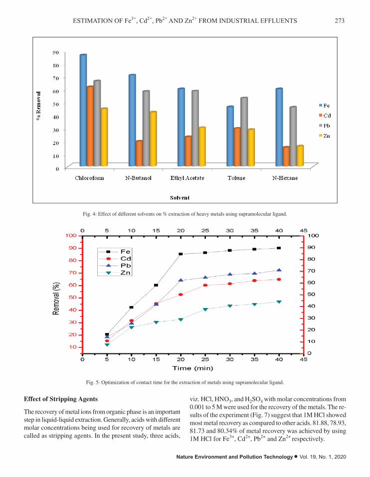
273ESTIMATION OF Fe3+, Cd2+, Pb2+ AND Zn2+ FROM INDUSTRIAL EFFLUENTS
Nature Environment and Pollution Technology • Vol. 19, No. 1, 2020
6
Selection of A Suitable Solvent for Metal Extraction
Solvent selection is an important part of liquid-liquid extraction. Stability of a complex
formed between ligand and metal is highly dependent on the polarity of a solvent (In et al.
2008). Five different solvents were used for extraction of metals by supramolecular ligand,
viz., chloroform, N-butanol, ethyl acetate, toluene and N-hexane. The obtained results from
the experiment are illustrated in Fig. 4 and showed that chloroform is a suitable solvent for
the extraction of metals. The percent extraction of Fe3+, Cd2+, Pb2+ and Zn2+ using chloroform
found to be 86%, 61%, 66% and 44% respectively. The extraction of the above metals using
other solvents was less as compared to chloroform (Sarode et al. 2012). In liquid-liquid
extraction, replacement of solvent molecules by either ligand or cation is highly favorable
(Nezhadali et al. 2007). This condition seems to have fulfilled by chloroform. So, chloroform
is selected as a solvent for further extraction experiment.
Fig. 4: Effect of different solvents on % extraction of heavy metals using supramolecular
ligand.
Effect of Extraction Time
The definite time required for ligand molecules and cation to dissolve into an organic phase
altogether affects the overall extraction (Dadfarnia et al. 2010). The effect of contact time on
percent extraction efficiency of the ligand was observed by conducting extraction
experiments at a different time interval from 5 to 40 min. The obtained results are portrayed
in Fig. 5 and show that the prominent extraction efficiency for metals is noted upto 25 min
Fig. 4: Effect of different solvents on % extraction of heavy metals using supramolecular ligand.
7
and after that, no significant extraction was observed. The optimized condition of contact
time of 20 min was elaborated for Fe+3 and Pb+2 while in case of Cd+2 and Zn+2 it was found
to be 25 and 30 min, respectively. The percent extraction at an optimized time was noted as
85.34, 60.21, 64.12 and 43.67% for metals Fe+3, Pb+2, Cd+2 and Zn+2 respectively.
Optimization of pH for the Extraction of Metals
As pH of the solvent controls the stability of the complex formed between ligand and cation,
it is a prime variable in the liquid-liquid extraction (Ramo et al. 2000). The effect of solution
pH on the extraction efficiency of metals was observed at 0.5 to 9. The results of various
experiments depicted that acidic to neutral pH condition is favorable for metal extraction
(Fig. 6). In complex formation, ligand behaves like Lewis base and donate its lone pair of an
electron to a metal cation to form a complex. In the case of supramolecular ligand, nitrogen
and oxygen are the donor atoms and at suitable pH facilitates the formation of a complex by
donating a lone pair of electrons.
Fig. 5: Optimization of contact time for the extraction of metals using supramolecular ligand. Fig. 5: Optimization of contact time for the extraction of metals using supramolecular ligand.
Effect of Stripping Agents
The recovery of metal ions from organic phase is an important step in liquid-liquid extraction. Generally, acids with different molar concentrations being used for recovery of metals are called as stripping agents. In the present study, three acids,
viz. HCl, HNO3, and H2SO4 with molar concentrations from 0.001 to 5 M were used for the recovery of the metals. The re-sults of the experiment (Fig. 7) suggest that 1M HCl showed most metal recovery as compared to other acids. 81.88, 78.93, 81.73 and 80.34% of metal recovery was achieved by using 1M HCl for Fe3+, Cd2+, Pb2+ and Zn2+ respectively.
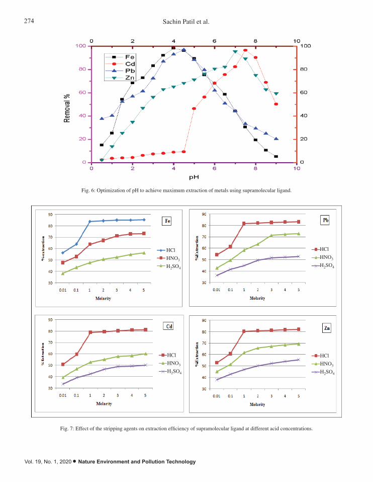
274 Sachin Patil et al.
Vol. 19, No. 1, 2020 • Nature Environment and Pollution Technology
8
Fig. 6: Optimization of pH to achieve maximum extraction of metals using supramolecular
ligand.
Effect of Stripping Agents
The recovery of metal ions from organic phase is an important step in liquid-liquid
extraction. Generally, acids with different molar concentrations being used for recovery of
metals are called as stripping agents. In the present study, three acids, viz. HCl, HNO3, and
H2SO4 with molar concentrations from 0.001 to 5 M were used for the recovery of the metals.
The results of the experiment (Fig. 7) suggest that 1M HCl showed most metal recovery as
compared to other acids. 81.88, 78.93, 81.73 and 80.34% of metal recovery was achieved by
using 1M HCl for Fe3+, Cd2+, Pb2+ and Zn2+ respectively.
Application of Supramolecular Ligand for Industrial Wastewater Samples
Real sample analysis was carried out on samples collected from local metal industry over the
optimized condition of time, pH and other variables. The ligand showed impressive
extraction efficiency for all four metals over optimized conditions of experimental variables.
The reproducibility of the results confirmed by conducting the above experiments five times
and mean of the results obtained did not show deviation above 5% from individual results.
This shows the reliability and reproducibility of the results. The results of the real sample
analysis are summarized in Table 3.
Fig. 6: Optimization of pH to achieve maximum extraction of metals using supramolecular ligand.
9
Fig. 7: Effect of the stripping agents on extraction efficiency of supramolecular ligand at
different acid concentrations.
CONCLUSION In this work, synthesis of a suitable complexing ligand was performed and characterized by
FTIR and H1NMR. The extraction efficiency of the compound was tested at various
experimental variables such as solvent, time, pH, etc. In addition, the effect of stripping agent
on extraction efficiency over industrial samples was observed. The results obtained from
batch extraction experiments revealed that chloroform could efficiently remove the metals
more than other solvents. 30 min is the time in which the synthesized ligand can significantly
extract metals from solvents. It was noted that slightly acidic to neutral pH conditions are
favorable for extraction. The significant recovery of the metals can be achieved using 1M
HCl. Application of the compound for extraction of metals from real samples at optimized
conditions has shown impressive results which signify the applicability of the compound for
industrial purpose.
Fig. 7: Effect of the stripping agents on extraction efficiency of supramolecular ligand at different acid concentrations.
HCl
HNO3
H2SO4
HCl
HNO3
H2SO4
HCl
HNO3
H2SO4
HCl
HNO3
H2SO4

275ESTIMATION OF Fe3+, Cd2+, Pb2+ AND Zn2+ FROM INDUSTRIAL EFFLUENTS
Nature Environment and Pollution Technology • Vol. 19, No. 1, 2020
Application of Supramolecular Ligand for Industrial Wastewater Samples
Real sample analysis was carried out on samples collected from local metal industry over the optimized condition of time, pH and other variables. The ligand showed impres-sive extraction efficiency for all four metals over optimized conditions of experimental variables. The reproducibility of the results confirmed by conducting the above experiments five times and mean of the results obtained did not show deviation above 5% from individual results. This shows the reliability and reproducibility of the results. The results of the real sample analysis are summarized in Table 3.
CONCLUSION
In this work, synthesis of a suitable complexing ligand was performed and characterized by FTIR and H1NMR. The extraction efficiency of the compound was tested at various experimental variables such as solvent, time, pH, etc. In ad-dition, the effect of stripping agent on extraction efficiency over industrial samples was observed. The results obtained from batch extraction experiments revealed that chloroform could efficiently remove the metals more than other sol-vents. 30 min is the time in which the synthesized ligand can significantly extract metals from solvents. It was noted that slightly acidic to neutral pH conditions are favourable for extraction. The significant recovery of the metals can be achieved using 1M HCl. Application of the compound for extraction of metals from real samples at optimized conditions has shown impressive results which signify the applicability of the compound for industrial purpose.
REFERENCES
Costa, M. C., Assunção, A., Ana M. Rosa da Costa, Nogueira, C. and Paiva, Ana P. 2013. Liquid-liquid extraction of platinum from chloride media by N, N′-Dimethyl, N, N′-Di cyclohexyltetradecylmalonamide. Solvent Extraction and Ion Exchange, 31: 12-23.
Dadfarnia, S., Shabani, A.M.H., Bidabadi, M.S. and Jafari, A.A. 2010. A novel ionic liquid/micro-volume back extraction procedure combined with flame atomic absorption spectrometry for determination of trace nickel in samples of nutritional interest. J. Hazard. Mater., 173: 534-538.
Fegadea, U., Jethavea, G., Su, K., Huang, W. and Wu, R. 2018. A multi-function Zn0.3Mn0.4O4 nanospheres for carbon dioxide reduction to methane via photocatalysis and reused after fifth cycles for phosphate adsorption. J. Environ. Chem. Eng., 6: 1918-1925.
Fraga, C.G. 2000. Relevance, essentiality and toxicity of trace elements in human health. Mol. Aspects Med., 26: 235-244.
Himadri, B. S., Tripathy, S., Equeenuddin, Sk. Md. and Sahoo, P. K. 2014. Utilization of ochre as an adsorbent to remove Pb(II) and Cu(II) from contaminated aqueous media. Environ. Earth Sci., 72: 243-250.
Hua, M., Zhang, S., Pan, B., Zhang, W., Lv, L. and Zhang, Q. 2012. Heavy metal removal from water/wastewater by nanosized metal oxides A review. J. Hazard. Mater., 317-331.
In, G., Kim, Y. and Choi, J. 2008. Study on solvent extraction using salen (NEt2)2 as a chelating agent for determination of trace Cu(II), Mn(II) and Zn(II) in water samples. Bull. Korean Chem. Soc., 29: 969-973.
Jethave, G., Fegade, U., Attarde, S. and Ingle, S. 2017. Facile synthesis of lead doped zinc- aluminum oxide nanoparticles (LD-ZAO-NPs) for efficient adsorption of anionic dye: kinetic, isotherm and thermody-namic behaviors. J. Ind. Eng. Chem., 53: 294-306.
Jethaveb, G. and Fegadeb, U. 2018. Design and synthesis of Zn0.3Fe0.45O3 nanoparticle for efficient removal of Congo red dye and its kinetic and isotherm investigation. International Journal of Industrial Chem-istry, 9: 85-97.
Kondalkar, M., Fegadec, U., Attarde, S. and Ingle, S. 2018. Experimental investigation on phosphate adsorption, mechanism and desorption properties of Mn-Zn-Ti oxide trimetal alloy nanocomposite. Journal of Dispersion Science and Technology, 39: 1-9.
Li, Z., Huang, P., Xi, L., Xie, G., Shi, Y., Liu, H., Xu, M., Chen, F. and Zeng, Z. 2011. A highly selective fluorescent chemo sensor for Cd (II) based on 8-hydroxyquinoline platform. Inorg. Chem. Commun., 14: 1241-1244.
Nezhadali, A., Hosseini, H. A. and Langara, P. 2007. Study of complex formation between iodoquinol (IQ) and Co2+, Mn2+, Cd2+, Pb2+ and Zn2+ cations in binary aqueous/non-aqueous solvent using spectropho-tometry. E-J Chem., 4: 581-586.
Okamoto, Y., Nomura, Y., Nakamura, H., Iwamaru, K., Fujiwara, T. and Kumamaru, T. 2000. High pre concentration of ultra-trace metal ions by liquid-liquid extraction using water/oil/water emulsions as liquid surfactant membranes. Microchem. J., 65: 341-346.
Oliva, A., Molinari, A, Zuniga, F. and Ponce, P. 2002. Studies on the liquid-liquid extraction of nickel(II), zinc(II), cadmium(II), mercu-ry(II) and lead(II) with 1-phenyl-3hydroxy-4-dodecyldithiocarboxy-late-5-pyrazolone. Microchim. Acta., 140: 201-203.
Ramo, J., Sillanpää, M., Vickackaite, V., Orama, M. and Niinistö, L. 2000. Chelating ability and solubility of DTPA, EDTA, and ′-ADA in alkaline hydrogen peroxide environment. J. Pulp Pap. Sci., 26: 125-131.
Saracoglu, S., Soylak, M. and Elci, L. 2003. Separation/preconcentration of trace heavy metals in urine, sediment and dialysis concentrates by co-precipitation with samarium hydroxide for atomic absorption spectrometry. Talanta., 59: 287-293.
Sarode, D., Ingle, S. and Attarde, S. 2012. Formula establishment of colorless Pb(II) complex with N-Benzoyl-N-Phenyl hydroxylamine (BPA) using atomic absorption spectroscopy. Indo. J. Chem., 12: 12-19.
Sarode, D.B., Attarde, S.B., Ingle, S.T., Srivastava, V. and Sillanpää M.E. 2015. Separation and removal of Cu2+, Fe2+& Fe3+ from environmental waste samples by N-benzoyl-n-phenylhydroxylamine. Environmental Technology, 36: 521-528.
Tang, X. L., Peng, X. H., Dou, W., Mao, J., Zheng, J. R., Qin, W. W., Liu, W.S., Chang, J. and Yao, X.J. 2008. Design of a semirigid molecule as a selective fluorescent chemosensor for recognition of Cd (II). Org. Lett., 10: 3653-3656.
Table 3: Application of supramolecular ligand for heavy metals extraction from industrial effluent.
Metal ion Before extraction (ppm) After extraction (ppm) % extraction of metal from industrial effluent
Fe+3 0.3152 0.0004 99.87
Cd+2 0.2398 0.0211024 91.20
Pb+2 0.5856 0.00105408 99.82
Zn+2 0.5043 0.04055176 91.95

Vol. 19, No. 1, 2020 • Nature Environment and Pollution Technology
276

2-D Unsteady Flow Modelling and Inundation Mapping for Lower Region of Purna Basin Using HEC-RAS
Azaz Khan I. Pathan† and P. G Agnihotri Department of Civil Engineering, Sardar Vallabhbhai National Institute of Technology, Surat, Gujarat, India†Corresponding author: Azaz Khan I. Pathan
ABSTRACT
Present investigations utilize two-dimensional flow modelling abilities of (HEC-RAS) Hydrologic Engineering Centres River Analysis System for flood inundation mapping in the downstream area of Purna basin, exposed to recurrent flooding. Floods are natural disasters, which cause loss of life and damages to properties and nature. 2-D Hydrodynamic model is utilized to assess geomorphic viability of floods in downstream side of Purna basin. In this research study, downstream region geometry of Purna river basin, the flood plain of the study area and historical observed flood data of unsteady flow have been used to develop the 2-D hydrodynamic model. For analysis of flooding, a reach of 20 km of river situated downstream of Purna River basin has been considered. Point-by-point fundamental terrain data is taken from a Digital Elevation Model (DEM) of 30-meter resolution image and is utilized to produce the (2D) two-dimensional flow area and stream geometries. River flow information like daily discharge during rainy months, slope available along the river reach from Mahuva gauging station close to Navsari city is utilized for the unsteady flow modeling. Depth of water, velocity distribution and water surface height obtained after 2D flow simulation are utilized to decide the degree of flooding. RAS-mapper is an effective tool in HEC-RAS, which can be utilized for inundation of research area. For unsteady flow analysis, each time step was done based on inflow hydrograph using RAS mapper tool in HEC-RAS, which gives the spatial distribution of the river flow. The outcomes from this research examination can be utilized for disaster management, flood management, early warning system by authorities in addition to infrastructure growth decisions.
INTRODUCTION
The issues of expanding environmental carbon dioxide fixations in the Earth’s atmosphere is analysed and the conceivable future climatic changes which may result considering such issues. As the amount of CO2 prone to be discharged into the environment because of fossil fuel combustion, the normal increments of other greenhouse gases that impact the world’s radiation spending plan, how and when climatic changes can be distinguished, and the anticipated changes in ocean level coming about because of global warming (Bolin et al. 1989). Environmental change is required to quicken water cycles and, in this way, boost the accessible renewable freshwater resources (RFWR) that as it may, fluctuations in occasional forms and the expanding likelihood of extreme events may balance this impact. Diminishing current vulnerability will be the initial step to get ready for such foreseen changes (Oki et al. 2006). The research depicts an appraisal of the ramifications of climate change for worldwide hydrological administrations and water assets. By 2025, it is assessed that around 5 billion individuals, out of an all-out populace of around 8
billion, will live in nations suffering from water pressure (Arnell 1999). The Inter-governmental Panel on Climate Change (IPCC) ventures that more prominent fluctuation and precipitation force will build flooding risk in numerous territories on account of environmental change (Ishiwatari 2010). The ascent in worldwide temperature expands the risk of the flood disaster. Radiative impacts of anthropogenic fluctuations in atmospheric structure are relied upon to cause atmosphere fluctuations, specifically an escalation of the worldwide water rotation with a subsequent increment in flood hazard (Milly et al. 2002). Each year, flooding causes a catastrophic effect on the population, environment, economy, and everywhere throughout the world. Federal Emergency Management Agency (FEMA) has of late refreshed their flood-plain standard according to the high-level official request in 2015 on the Federal Flood Risk Management Standard. This examination joins the recently refreshed floodplain mapping standard in the flood hazard appraisal of roughly 11.3 km stretch of the Patapsco River close Ellicott City, U.S (Thakali et al. 2017). Hazard can be built up as a well-characterized strategy for taking care of flood risk because of man-made, ecological and natural risks, of which
2020pp. 277-285 Vol. 19
p-ISSN: 0972-6268 No. 1 Nature Environment and Pollution Technology An International Quarterly Scientific Journal
Original Research Paper
e-ISSN: 2395-3454
Open Access
Nat. Env. & Poll. Tech.Website: www.neptjournal.com
Received: 27-06-2019Accepted: 29-08-2019
Key Words:Flood inundation mapping2-D unsteady flowHEC-RASPurna basin

278 Azaz Khan I. Pathan and P. G Agnihotri
Vol. 19, No. 1, 2020 • Nature Environment and Pollution Technology
floods are a delegate. Flood risk management plans, described at three level say project planning, project design, and the real expense of a structure, are assessed and contrasted and the advantages from the strategic scheme (Plate 2002). Of late, the tsunami in South East Asia triggered approximate 220,000 passing which makes it likely a standout amongst the most appalling floods. Amid the International Decade of Natural Disaster Reduction (IDNDR) from 1990 to 1999, it was valued that the past worldview of “flood assurance” was wrong (Schanze 2006).
Additionally, as of now ecological and local arrangements in numerous nations are beginning to move from flood assurance to flood hazard management (Dworak & Görlach 2005). Geospatial techniques are very useful to detect the flooding events through combine approach of Arc GIS and HEC-RAS.(Pathan & Agnihotri 2019a)
Decision support system (DSS) is a significant tool for decision makers throughout various period of flood organization to mitigate the major flood and develop different models like economic, forecasting and hydrodynamic to connect with each other and share information which play a crucial role for decision makers (Ahmad & Simonovic 2006). The vision of FEMA’s is to fill in as an impetus that drives expanded understanding and proactive activity to help individuals in networks to reduce their losses from natural risks. To fulfil this vision, FEMA subsidizes three Hazard Mitigation Assistance (HMA) programs. Flood risk relief estimates are any manageable moves made to decrease or dispose of long-term hazard to individuals and property from future fiascos. With the continuous event of an outrageous event in urban zones, floodplain maps and flood models have become necessary for disaster authorities to mitigate flood (Knebl et al. 2002). One dimensional modelling approach has given an accurate outcome for determining flooding at different cross sections of the Purna River basin (Pathan & Agnihotri 2019b).
Now a day’s different water resources models are utilized to simulate the flooding phenomena, to quantify risk and damage estimation and to help the decision-making procedure with respect to the forecast and counteractive action of floods (Todini 1999). Different examinations have exposed the ability of globally accessible adaptation of 2-Dimensional numerical simulation methods (Johns et al. 1971, Vojinovic 2013). Comparison between 1-Dimensional model over a 2-Dimensional model shows more difference in HEC-RAS when unsteady flow has been carried out; results show almost 200m horizontal difference in inundated area at high discharge (Alho et al. 2008). Generally, the results obtained from 1-D models are not accurate for the flat or flatter flood plain areas, in this way, numerous 1-Dimensional
hydrodynamic models are supplanted by 2-Dimensional hydrodynamic models (Merwade et al. 2008). In spite of the fact that there is enormous vulnerability of the qualities of flood events, 2-Dimensional numerical investigation suggests an approach to all the more likely describe the flood. Hydrologic Engineering Centre- River Analysis System (HEC-RAS) hydrodynamic model has been generally utilized related to Environmental System Research Institute (ESRI), HEC-GeoRAS and Arc-GIS programming for 1-Dimensional investigation and mapping of a flood extent. The most recent adaptation, HEC-RAS 5.0.1 offers the independent ability to accomplish 2-Dimensioanal directing and capacities to fully examine and mapping of flood inside the RAS mapper in HEC-RAS model itself. Research examination investigates the 2-D presenting limit of HEC-RAS to show the Purna River around Navsari region, which is exposed to flooding during high discharge. The most recent capacities of RASmapper in HEC-RAS are used for the improved mapping of the floodplain periphery by using past flood information of the Purna River. The objective of the research study is to accomplish unsteady flow analysis, set up a flood inundation map of the study area and to plot the flood inclined territories by utilizing the 2-dimensional hydrodynamic modelling and inundation mapping capacities of most recent variant of HEC-RAS 5.0.1. Computational techniques are very effective in flood management to identify flooding scenarios at different reaches of the study area (Pathan & Agnihotri 2019c).
MATERIALS AND METHODS
Research Study Area
Navsari region lies on floodplain in the periphery of Purna. The length of Purna river considered is about 20 km for research. The river basin starts from Saputara near Maharashtra. Purna river floodplain has centroidal facilitate of 200º41’ to 210º05’ North latitude and 720º45’ to 740º00’ East longitudes. The purpose behind choosing this study area is the regular occurrence of flood events, affecting densely the populated urban area around it. The absolute catchment locale of the Purna basin is 2433 km2. Location map and google map of the research area are as shown in Fig 1. and Fig 2 respectively. Catchment area distribution of Purna River is given in Table 1.
Digital Elevation Model (DEM) of 30-meter resolution is utilized for building the terrain of the research area in RAS-mapper tools (HEC-RAS), acquired from Indian Space Research Organization Bhuvan (ISRO BHUVAN). High resolution images are downloaded from Google earth, the water level and river discharge information of yearly and daily scales are gathered from Central Water Commission

2792-D UNSTEADY FLOW MODELLING AND INUNDATION MAPPING OF PURNA BASIN
Nature Environment and Pollution Technology • Vol. 19, No. 1, 2020
Fig. 1: Location map of study area.
Fig. 2: Google map of study area.
Methodology
Fig. 1: Location map of study area.
Table 1: Catchment area distribution of Purna River.
Sr. No. State Catchment area (km2) % of the total catchment area
1 Gujarat 2373 97.61
2 Maharashtra 58 2.39
3 Total 2431 100.00
(C.W.C), State Water Data Center (SWDC), Gandhinagar and Irrigation Department.
Methodology
Digital Elevation Model (DEM) of 30-meter resolution taken from ISRO Bhuvan is imported to HEC-RAS software. Now, from Tools menu in RAS-Mapper, create terrain from selected Digital Elevation Model (DEM) which is then used in RAS-Mapper to work on the hydrodynamic properties and building up the geometry of 2-D flow region of study area. Moreover, cell size of 200 m × 200 m was provided, which are created along the selected 2-D flow area of the River of the study area. Now, we utilize the geometric pre-processing tools in Ras-Mapper for creation of hydraulic properties of each cell of the reach.
Manning’s roughness coefficient is allocated for the 2D area, considered for the research area in RAS-mapper. The allocated land cover value and corresponding Manning’s n value are shown in Table 2.
For unsteady flow simulation in RAS-mapper, provide upstream and downstream boundary conditions of the area of the river. For upstream, Mahuva gauge station hydrograph is used for simulation, and in the downstream normal depth of channel slope (0.000425) is used as boundary condition. The created geometric layer for 2D area of river with the used boundary conditions are mentioned in Table 2 and Fig. 3.
In this research study, daily discharge data is used for two flooding events of time intervals 29th June 1976 to 26th September 1976 and from 21st July 2004 to 26th September 2004. As per past flood data, most severe flooding events occurred in Purna basin on 31st July 1976 with a peak discharge of 4380.2 m3/s and on 04th August 2004 with a peak discharge of 8836 m3/s. Upstream hydrographs used in check for the two flooding events are shown in Fig. 4. and Fig. 5.
Flood inundation mappings for years 1976 and 2004 events are plotted in RAS-mapper for peak discharge. For better visualization in mapping, google earth layers can be

280 Azaz Khan I. Pathan and P. G Agnihotri
Vol. 19, No. 1, 2020 • Nature Environment and Pollution Technology
Table 2: Manning’s n for the channel (Chow 1959).
Type of Channel and Description Minimum Normal Maximum
Main Channels
a. clean, straight, full stage, no rifts or deep pools 0.025 0.030 0.033
b. same as above, but more stones and weeds 0.030 0.035 0.040
c. clean, winding, some pools and shoals 0.033 0.040 0.045
d. same as above, but some weeds and stones 0.035 0.045 0.050
e. same as above, lower stages, more ineffective slopes and sections 0.040 0.048 0.055
f. same as “d” with more stones 0.045 0.050 0.060
g. sluggish reaches, weedy, deep pools 0.050 0.070 0.080
h. very weedy reaches, deep pools, or floodways with heavy stand of timber and underbrush
0.075 0.100 0.150
Fig. 3: Generated geometric layer with 2D flow area cell mesh.
Fig. 4: Hydrograph for flooding event-1976 yr.
Fig. 5: Hydrograph for flooding event-2004 yr.
Fig. 3: Generated geometric layer with 2D flow area cell mesh.
Fig. 1: Location map of study area.
Fig. 2: Google map of study area.
Methodology
Fig. 2: Google map of study area.

2812-D UNSTEADY FLOW MODELLING AND INUNDATION MAPPING OF PURNA BASIN
Nature Environment and Pollution Technology • Vol. 19, No. 1, 2020
Fig. 4: Hydrograph for flooding event-1976 yr.
Fig. 5: Hydrograph for flooding event-2004 yr.
In this research study, daily discharge data is used for two flooding events of time intervals
29th June 1976 to 26th September 1976 and from 21st July 2004 to 26th September 2004. As
per past flood data, most severe flooding events occurred in Purna basin on 31st July 1976
with a peak discharge of 4380.2 m3/s and on 04th August 2004 with a peak discharge of 8836
m3/s. Upstream hydrograph used in check for the two flooding events are shown in Fig. 4.
and Fig. 5.
Flood inundation mappings for years 1976 and 2004 events are plotted in RAS-mapper for
peak discharge. For better visualization in mapping, google earth layers can be imported into
RAS-mapper. The outline of methodology is shown in the Fig. 6.
Fig. 6: Conceptual 2D model diagrams for floodplain mapping in HEC-RAS.
RESULTS AND DISCUSSION
Over the 2D flow area considered in this study, a total of 15,221 cells are generated for the
year 1976 flooding event and 9207 cells are generated for the year 2004 flooding event, for
the 20 km river reach. Terrain information used for 2D flow area of research zone is from the
geometry editor tools in HEC-RAS.
In this research work, for the study area considered, the computational time interval for the
model is taken as 6 hours and output interval of the model is taken as 1 day for both flooding
events with cell sizes of 200 m × 200 m used for analysis. Using a lesser value of time
Fig. 6: Conceptual 2D model diagrams for floodplain mapping in HEC-RAS.

282 Azaz Khan I. Pathan and P. G Agnihotri
Vol. 19, No. 1, 2020 • Nature Environment and Pollution Technology
imported into RAS-mapper. The outline of methodology is shown in the Fig. 6.
RESULTS AND DISCUSSION
Over the 2D flow area considered in this study, a total of 15,221 cells are generated for the year 1976 flooding event and 9207 cells are generated for the year 2004 flooding event, for the 20 km river reach. Terrain information used for 2D flow area of research zone is from the geometry editor tools in HEC-RAS.
In this research work, for the study area considered, the computational time interval for the model is taken as 6 hours and output interval of the model is taken as 1 day for both flooding events with cell sizes of 200 m × 200 m used for analysis. Using a lesser value of time intervals and smaller cell sizes can produce better results, but the simulation would take more effort to complete. Initial condition of river reach for the study area was supposed to be wet for unsteady flow analysis in HEC-RAS. After considering all conditions, the entire mesh is filled up till warm-up period
and when simulation is finished, fill up all cells of the river reach as open channel flow implementing diffusion wave equation in which finite volume approximation is considered.
Hydraulic properties of every cell must be assigned before doing the analysis in RAS-mapper. RAS-mapper has good capability for making hydrodynamic properties of every mesh generated in each cell, which in turn depends on the terrain data considered in the study area and their Manning’s “n” values.
The 2D output results can be observed in the form of inundation area, velocity and water surface elevation profile within RAS Mapper tools in HEC-RAS.
Comparison of 1976 and 2004-Year Flood Depth Map
It is observed that in the 1976-year flood, the depth of flooded water at Purna River Bridge, Navsari is 20.550 m and in 2004-year flood, depth of flood water is 23.490 m (Fig. 7 & 8). We have simulated both flood year data in RAS-mapper
intervals and smaller cell sizes can produce better results, but the simulation would take more
effort to complete. Initial condition of river reach for the study area was supposed to be wet
for unsteady flow analysis in HEC-RAS. After considering all conditions, the entire mesh is
filled up till warm-up period and when simulation is finished, fill up all cells of the river
reach as open channel flow implementing diffusion wave equation in which finite volume
approximation is considered.
Hydraulic properties of every cell must be assigned before doing the analysis in RAS-
mapper. RAS-mapper has good capability for making hydrodynamic properties of every
mesh generated in each cell, which in turn depends on the terrain data considered in the study
area and their Manning’s “n” values.
Fig. 7: Observed vs simulated water surface elevation for 1976 yr flood event.
Fig. 8: Observed vs simulated water surface elevation for 2004 yr flood event.
The 2D output results can be observed in the form of inundation area, velocity and water
surface elevation profile within RAS Mapper tools in HEC-RAS.
Comparison of 1976 and 2004-Year Flood Depth Map
Fig. 7: Observed vs simulated water surface elevation for 1976 yr flood event.
intervals and smaller cell sizes can produce better results, but the simulation would take more
effort to complete. Initial condition of river reach for the study area was supposed to be wet
for unsteady flow analysis in HEC-RAS. After considering all conditions, the entire mesh is
filled up till warm-up period and when simulation is finished, fill up all cells of the river
reach as open channel flow implementing diffusion wave equation in which finite volume
approximation is considered.
Hydraulic properties of every cell must be assigned before doing the analysis in RAS-
mapper. RAS-mapper has good capability for making hydrodynamic properties of every
mesh generated in each cell, which in turn depends on the terrain data considered in the study
area and their Manning’s “n” values.
Fig. 7: Observed vs simulated water surface elevation for 1976 yr flood event.
Fig. 8: Observed vs simulated water surface elevation for 2004 yr flood event.
The 2D output results can be observed in the form of inundation area, velocity and water
surface elevation profile within RAS Mapper tools in HEC-RAS.
Comparison of 1976 and 2004-Year Flood Depth Map
Fig. 8: Observed vs simulated water surface elevation for 2004 yr flood event.

2832-D UNSTEADY FLOW MODELLING AND INUNDATION MAPPING OF PURNA BASIN
Nature Environment and Pollution Technology • Vol. 19, No. 1, 2020
and developed the inundation map for both 1976-year flood depth and 2004-year flood depth and are shown as in Fig. 9 and Fig.10.
Comparison of 1976 and 2004-Year Flood Velocity Map
It is observed that in 1976-year flood, velocity of flood water was 3.13 m/sec at Purna River Bridge, Navsari and for 2004-year flood, velocity of flood water was 2.57 m/sec. We have simulated both flood year data in RAS mapper and developed velocity maps of both 1976-year flood and 2004-year flood as shown in Fig. 11 and Fig.12.
It is observed that in the 1976-year flood, the depth of flooded water at Purna River Bridge,
Navsari is 20.550 m and in 2004-year flood, depth of flood water is 23.490 m (Fig. 7 & 8).
We have simulated both flood year data in RAS-mapper and developed the inundation map
for both 1976-year flood depth and 2004-year flood depth and are shown as in Fig. 9 and
Fig.10.
Fig. 9: Inundation map of 1976 year flood.
Fig. 10: Inundation map of 2004 year flood.
Fig. 9: Inundation map of 1976 year flood
It is observed that in the 1976-year flood, the depth of flooded water at Purna River Bridge,
Navsari is 20.550 m and in 2004-year flood, depth of flood water is 23.490 m (Fig. 7 & 8).
We have simulated both flood year data in RAS-mapper and developed the inundation map
for both 1976-year flood depth and 2004-year flood depth and are shown as in Fig. 9 and
Fig.10.
Fig. 9: Inundation map of 1976 year flood.
Fig. 10: Inundation map of 2004 year flood.
Fig. 10: Inundation map of 2004 year flood.
CONCLUSION
This analysis is meant to lead 2D unsteady flow simulation using HEC-RAS 5.03 in downstream of Purna River, Navsari city. For the stream of 20 km reach, stream hydrograph of 1976-year flood event, occurred between 29th June 1976 and 1st December 1976 and for 2004-year flood event, occurred between 22th June 2004 and 29th September 2004 are routed. Assessment of unsteady flow conditions for the stormy month just as flooding event is completed. From the analysis, following conclusions can be drawn.
∑ During the study period, the maximum depth of water found was 19.976 m and maximum velocity of water

284 Azaz Khan I. Pathan and P. G Agnihotri
Vol. 19, No. 1, 2020 • Nature Environment and Pollution Technology
found was 0.4 m/s for 1976 year flood event with a peak discharge of 4380.20 m3/sec, the maximum depth of water found was 21.325 m and maximum velocity of water was 0.038 m/s for 2004 year flood event with a peak discharge of 8836 m3/sec at the Purna River Bridge, Navsari.
∑ When maximum discharge of 8836 m3/s is routed, areas near Purna River Bridge like Viraval, Jalalpur are found to be inundated. The highest flood level reached was 24.8 m.
∑ To develop flood warning and using this information for protecting areas of Navsari district from inundation.
Comparison of 1976 and 2004-Year Flood Velocity Map
It is observed that in 1976-year flood, velocity of flood water was 3.13 m/sec at Purna River
Bridge, Navsari and for 2004-year flood, velocity of flood water was 2.57 m/sec. We have
simulated both flood year data in RAS mapper and developed velocity maps of both 1976-
year flood and 2004-year flood as shown in Fig. 11 and Fig.12.
Fig. 11: Velocity map of 1976 year flood.
Fig. 12: Velocity map of 2004 year flood.
Fig. 11: Velocity map of 1976 year flood.
Comparison of 1976 and 2004-Year Flood Velocity Map
It is observed that in 1976-year flood, velocity of flood water was 3.13 m/sec at Purna River
Bridge, Navsari and for 2004-year flood, velocity of flood water was 2.57 m/sec. We have
simulated both flood year data in RAS mapper and developed velocity maps of both 1976-
year flood and 2004-year flood as shown in Fig. 11 and Fig.12.
Fig. 11: Velocity map of 1976 year flood.
Fig. 12: Velocity map of 2004 year flood.
Fig. 12: Velocity map of 2004 year flood.
The outcome proposed correlates the parameter’s maximum depth and velocity distribution with the past flood events. Smaller cell size and smaller computational intervals give better results but take more time to complete the unsteady flow simulation.
The process described in this study can be upgraded to facilitate analysis and better visualisation capacities. Some additional research recommended for this study are as mentioned below.
∑ Analysis of the Purna River may help the areas for demarcating safe and vulnerable zones based on the extent of the flood. Such analysis can also be used for

2852-D UNSTEADY FLOW MODELLING AND INUNDATION MAPPING OF PURNA BASIN
Nature Environment and Pollution Technology • Vol. 19, No. 1, 2020
the prediction of flood hazard as well as its extent.
∑ The peak urban runoff might also be the cause behind such unpredicted flooding, which would require additional research to validate.
∑ The future work can be useful for applying the methodology to produce the flood risk map of entire Navsari district.
REFERENCES
Ahmad, S. and Simonovic, S.P. 2006. An intelligent decision support sys-tem for management of floods. Water Resources Management, 20(3): 391-410.
Alho, P. and Aaltonen, J. 2008. Comparing a 1D hydraulic model with a 2D hydraulic model for the simulation of extreme glacial outburst floods. Hydrological Processes: An International Journal, 22(10): 1537-1547.
Arnell, N.W. 1999. Climate change and global water resources. Global Environmental Change, 9: S31-S49.
Bolin, B. and Doos, B. R. 1989. Greenhouse Effect. John Wiley & Sons.Chow, V.T. 1959. Open-channel Hydraulics. MacGraw-Hill Book Co., NYDworak, T. and Görlach, B. 2005. Flood risk management in Europe@ the
development of a common EU policy. International Journal of River Basin Management, 3(2): 97-103.
Ishiwatari, M. 2010. Climate Change Adaptation in Flood Risk Management Through Utilizing Datasets Produced by Supercomputer.
Johns, P. B. and Beurle, R. L. 1971. Numerical solution of 2-dimensional scattering problems using a transmission-line matrix. In: Proceedings of the Institution of Electrical Engineers, 118(9): 1203-1208).
Knebl, M. R., Yang, Z. L., Hutchison, K. and Maidment, D. R. 2005. Regional scale flood modeling using NEXRAD rainfall, GIS, and HEC-HMS/RAS: a case study for the San Antonio River Basin Summer 2002 storm event. Journal of Environmental Management, 75(4): 325-336.
Merwade, V., Cook, A. and Coonrod, J. 2008. GIS techniques for creating river terrain models for hydrodynamic modeling and flood inundation mapping. Environmental Modelling & Software, 23(10-11): 1300-1311.
Milly, P. C. D., Wetherald, R. T., Dunne, K. A. and Delworth, T. L. 2002. Increasing risk of great floods in a changing climate. Nature, 415(6871): 514.
Oki, T. and Kanae, S. 2006. Global hydrological cycles and world water resources. Science, 313(5790): 1068-1072.
Pathan, A. I. and Agnihotri, P. G. 2019a. A combined approach for 1-D hydrodynamic flood modeling by using Arc-GIS, Hec-Georas, Hec-Ras Interface - A case study on Purna River of Navsari City, Gujarat. IJRTE, 8(1): 1410-1417.
Pathan, A. I. and Agnihotri, P. G. 2019b. One dimensional floodplain modelling using soft computational techniques in HEC-RAS - A case study on Purna basin, Navsari District. In: International Conference on Intelligent Computing & Optimization, Springer, Cham., pp. 541-548).
Pathan, A. I. and Agnihotri, P. G. 2019c. Use of Computing Techniques for Flood Management in a Coastal Region of South Gujarat – A Case Study of Navsari District. In International Conference on Intelligent Computing & Optimization. Springer, Cham., pp. 108-117.
Plate, E. J. 2002. Flood risk and flood management. Journal of Hydrolo-gy, 267(1-2): 2-11.
Schanze, J. 2006. Flood risk management–a basic framework. In: Flood Risk Management: Hazards, Vulnerability and Mitigation Measures (pp. 1-20). Springer, Dordrecht.
Thakali, R., Bhandari, R., Kandissounon, G. A. A. D., Kalra, A. and Ahmad, S. 2017. Flood risk assessment using the updated FEMA floodplain standard in the Ellicott City, Maryland, United States. World Environ-mental and Water Resources Congress 2017.
Todini, E. 1999. An operational decision support system for flood risk mapping, forecasting and management. Urban Water, 1(2): 131-143.
Vojinovic, Z., Seyoum, S., Salum, M. H., Price, R. K., Fikri, A. K. and Abebe, Y. 2013. Modelling floods in urban areas and representation of buildings with a method based on adjusted conveyance and storage characteristics. Journal of Hydroinformatics, 15(4): 1150-1168.

Vol. 19, No. 1, 2020 • Nature Environment and Pollution Technology
286

Removal of Nickel and Iron from Metal Injection Moulding Industry Effluent by Adsorbent Method: A Comparative Study
Akshatha K. U. and Hina Kousar†Department of P.G Studies & Research in Environmental Science, Kuvempu University, Jnana Sahyadri, Shankaraghatta, Shivamogga, Karnataka, India†Corresponding author: Hina Kousar
ABSTRACT
In the present investigation, the efficiency of rice husk in removal of nickel and iron from metal injection moulding industry effluent has been investigated. Adsorption was carried out in a batch experiment to investigate the parameters such as initial metal ion concentration, adsorbent dose, pH and contact time, under constant shaking of 100 mL sample in a heavy rotatory shaking apparatus for 2 hours. Analysis of physico-chemical characteristics of effluent was also carried out. The results revealed that maximum adsorption capacity of rice husk was about 92.84% for nickel using 8 g and about 90.12% for iron using 9 g at pH 9. Due to its good uptake capacity, rice husk has proved to be an excellent low-cost adsorbent for removing nickel and iron from effluent. The result showed that the percentage removal of nickel was high compared to iron.
INTRODUCTION
Toxic industrial waste, runoff from agricultural waste and discharge of untreated domestic waste are the main sources of water pollution (Adegoke et al. 2014). Heavy metal pollution is a major issue due to its toxic effect even at low concentration. Nickel and iron are the heavy metals used in the manufacturing process in metal injection moulding industry. Nickel is a non-biodegradable toxic metal which causes chronic bronchitis, reduced lung function, cancer, nasal sinus, etc. Iron is the 2nd most important metal for the survival and growth of the living organisms on the earth. But it is very toxic to the cells when given endogenous. Therefore, it becomes imperative to remove toxic metals like nickel and iron before discharging industrial effluent into water bodies.
Adsorption process is one of the best water treatment technique among various available methods. Adsorbent removes different pollutants in an easy way and economical and eco-friendly in nature. Rice husk is used as an adsorbent to remove nickel and iron from metal injection moulding industry effluent. The composition of main organic compounds like cellulose, hemicellulose and lignin renders rice husk as a possible adsorbent. In the present study, the applicability of rice husk for the removal of nickel and iron from industry waste water and effects of various parameters
such as initial concentration of effluent, adsorbent dosage and pH has been investigated.
Rice Husk
Rice is a strategic crop all over the world and every year large amount of rice husk is produced. Structurally, it consists of crude protein (3%), ash (including silica 17%), lignin (20%), hemicellulose (25%) and cellulose (35%) which renders it suitable for metallic cations fixation. It has been used in the removal of some of the metal ions (Ajmal et al. 2003, Bishnoi et al. 2004, Dadhlich et al. 2004).
MATERIALS AND METHODS
Rice husk was collected from a rice mill at Ripponpete, Shivamogga Dist., Karnataka State and used as adsorbent for the removal of nickel and iron from effluent. It was washed with distilled water and dried in an oven at about 60°C for 4h and again washed with acetone and NaOH (0.3M) to remove dirt and other contaminants, dried in an oven at about 60°C for 4h and crushed until powdered fine particles were obtained. The powdered sample was examined by XRD (X-Ray Diffraction), SEM and BET analysis to assess the purity of the expected phases and the degree of crystallization, i.e. size, composition and crystal structure. The effect of
Nat. Env. & Poll. Tech.Website: www.neptjournal.com
Received: 21-03-2019Accepted: 31-05-2019
Key Words:NickelIronIndustry effluentRice huskAdsorption
2020pp. 287-293 Vol. 19
p-ISSN: 0972-6268 No. 1 Nature Environment and Pollution Technology An International Quarterly Scientific Journal
Original Research Paper
e-ISSN: 2395-3454
Open Access

288 Akshatha K. U. and Hina Kousar
Vol. 19, No. 1, 2020 • Nature Environment and Pollution Technology
different parameters, adsorbent and pH on the adsorption was carried out. pH was adjusted by HCL and NaOH (Thakur et al. 2013).
Instrumentation
Characterization of rice husk powder was performed by X-Ray diffraction (Rigaku Diffractometer) using Cu-Ka radiation (105406A°) in a q - 2q configuration and the average size of powder was calculated using Debye Scherrer’s formula. Scanning Electron Micrograph determines the morphology of rice husk. Specific Surface Area (SSA) of rice husk was measured at 77 K by Brunauer-Emmett-Teller (BET) nitrogen adsorption-desorption (NOVA-1000 version 3.70 Instrument) (Morlu & Bareki 2017).
RESULTS AND DISCUSSION
Physico-chemical Properties of the Effluent
The physico-chemical properties of the metal injection moulding industry effluent are mentioned in Table 1.
Characterization of Rice Husk
X- Ray diffraction (XRD)
Using Cu-Ka radiation (105406A°) in a q - 2q configuration characterization of rice husk was performed by powder X- Ray diffraction (Rigaku Diffractometer). The average crystalline size of examined powdered rice husk was found to be around 28 nm and it was calculated using Debye Scherrer’s formula (Fig. 1).
D = (Kl /(b cos q)) …(1)
Table 1: Characterization of metal injection moulding industry effluent.
S.NO Parameter Before treatment After treatment Nickel/Iron
1 pH 1 7/7
2 Temperature (°C) 28.9 24.4/25.1
3 Biological Oxygen Demand (mg.L-1) 30 25/26
4 Chemical Oxygen Demand (mg.L-1) 1250 956/980
The physico-chemical properties of the metal injection moulding industry effluent are mentioned
in Table 1.
Table 1: Characterization of metal injection moulding industry effluent.
S.NO Parameter Before treatment After treatment
Nickel/Iron
1 pH 1 7/7
2 Temperature (°C) 28.9 24.4/25.1
3 Biological Oxygen Demand (mg.L-1) 30 25/26
4 Chemical Oxygen Demand (mg.L-1) 1250 956/980
Characterization of Rice Husk
X- Ray diffraction (XRD)
Using Cu-K radiation (105406A°) in a - configuration characterization of rice husk
was performed by powder X- Ray diffraction (Rigaku Diffractometer). The average crystalline
size of examined powdered rice husk was found to be around 28 nm and it was calculated using
Debye Scherrer’s formula (Fig. 1).
D= (Kλ / (𝛽𝛽𝛽𝛽𝛽𝛽𝛽𝛽𝛽𝛽)) …(1)
Fig. 1: XRD of the powdered rice husk.
0 10 20 30 40 50 60 70 800
30
60
90
120
150
180
210
240
270
300
330
Inten
sity
2
Fig. 1: XRD of the powdered rice husk.Scanning Electron Microscope (SEM)
Fig. 2: Scanning Electron Micrograph of powdered rice husk.
The SEM image of powdered rice husk is shown in Fig: 2 indicating the aggregation particles
and cluster shape with sharp edge. The properties of the powdered rice husk are mentioned in
Table 2
Table 2: Surface properties of powdered rice husk.
Rice husk Surface area Pore volume Average pore diameter
13.386 m2/g 0.022 cc/g 1.557 nm
Bet Surface Analysis
To determine the adsorption efficiency of nickel and iron, batch experiments were conducted and
the effect of parameters such as adsorbent dose, pH and contact time was studied.
A known weight of rice husk with 100 mL effluent of different dilutions was kept for treatment in
heavy rotatory shaking apparatus for 2 hours. Initial concentration of nickel and iron was
determined and found to be as follows. Nickel - 15.01 mg/L in 25% concentration, 18.02 mg/L in
50% concentration, 20.22 mg/L in 75% concentration and 23.14 mg/L in raw effluent (100%
concentration). After treatment samples were filtered using Whatman No. 41 filter paper and
measured by AAS. The concentration of nickel reduced to 6.93 mg/L (25% concentration), 5.65
mg/L (50% concentration), 10.97 mg/L (75% concentration) and 13.94 mg/L (raw effluent) (Table
Fig. 2: Scanning Electron Micrograph of powdered rice husk.

289REMOVAL OF NICKEL AND IRON FROM METAL INJECTION MOLDING INDUSTRY EFFLUENT
Nature Environment and Pollution Technology • Vol. 19, No. 1, 2020
Scanning Electron Microscope (SEM)
The SEM image of powdered rice husk is shown in Fig. 2 indicating the aggregation particles and cluster shape with sharp edge. The properties of the powdered rice husk are mentioned in Table 2
Bet Surface Analysis
To determine the adsorption efficiency of nickel and iron, batch experiments were conducted and the effect of parameters such as adsorbent dose, pH and contact time was studied.
A known weight of rice husk with 100 mL effluent of different dilutions was kept for treatment in heavy rotatory shaking apparatus for 2 hours. Initial concentration of nickel and iron was determined and found to be as follows. Nickel, 15.01 mg/L in 25% concentration, 18.02 mg/L in 50% concentration, 20.22 mg/L in 75% concentration and 23.14 mg/L in raw effluent (100% concentration). After treatment samples were filtered using Whatman No. 41 filter paper and measured by AAS. The concentration of nickel reduced to 6.93 mg/L (25% concentration), 5.65 mg/L (50% concentration), 10.97 mg/L (75% concentration) and 13.94 mg/L (raw effluent) (Table 3). Maximum reduction of 18.02 mg/L (68.64%) was observed in 50% concentration (Fig. 3) i.e. from 18.02 ± 0.01 to 5.65 ± 0.01 (Table 3).
Initial concentration of iron was 21.82 mg/L in 25% effluent concentration, 24.31 mg/L in 50% concentration, 27.63 mg/L in 75% concentration and 30.47 mg/L in raw effluent. After treatment the concentration of iron reduced to 12.02 mg/L (25% concentration), 9.64 mg/L (50% concentration), 16.59 mg/L (75% concentration) and 19.64 mg/L in raw effluent (Table 3). Maximum reduction of iron was found to be 24.31 mg/L (60.34%) in 50% concentration (Fig. 4) i.e. 24.31 ± 0.005 to 9.64 ± 0.01 (Table 3) because of availability of more adsorption activated sites. Metal ions
are easily adsorbed on vacant sites at low concentration. The percent removal of nickel and iron was calculated by the formula:
Percent removal = C C
Co i
o
-¥ 100 …(2)
Where, Co is initial concentration and Ci is final concentration of nickel/iron metal. Further experiment was carried out based on the results obtained.
To know the effect of adsorbent, experiment was carried out with different dosage of rice husk from 1-10g/100 mL at pH 7 in conical flasks in a heavy rotatory shaking apparatus for 2 hours. Maximum percentage removal of nickel was 92.84% at 8g/100 mL (Fig. 5) and iron was 90.12% at 9g/100 mL in 50% concentration (Fig. 6).
Nickel reduced from 18.02 ± 0.01 to 1.29 ± 0.01 andiron decreased from 24.31 ± 0.005 to 2.40 ± 0.005 in 50% concentration (Table 4). It was observed that the percentage removal of nickel and iron increased with increased adsorbent dose which means that when the concentration of adsorbent increases, the availability of high active sites will increase the adsorption capacity which helps to remove the metal ion.
In the adsorption process, pH is considered as the speciation and surface charge of the adsorbent because of its great impact in the metal ion removal. Experiment was carried out with a pH range of 1, 3, 5, 7, 9 and 11. The results show that nickel removal increased from 30.24% to 92.23% (Fig. 3) i.e. 18.02 ± 0.01 to 1.40 ± 0.005 (Table 5) and iron increased from 16.7% to 90.25% (Fig. 4) i.e. 24.31 ± 0.005 to 1.93 ± 0.01 in 50% effluent concentration. Maximum removal of nickel was at pH 9 with 8 g of rice husk and it slightly decreased at pH 11 (Fig. 7). Maximum removal of iron was at pH 9 with 9 g of rice husk and it gradually decreased at pH 11 (Fig. 8). The results easily show that the removal of nickel and iron by rice husk increases with increasing pH and culminates at pH 9.
Table 2: Surface properties of powdered rice husk.
Surface area Pore volume Average pore diameter
Rice husk 13.386 m2/g 0.022 cc/g 1.557 nm
Table 3: Concentration of nickel and iron before and after treatment with rice husk.
Concentration of Effluent Nickel (mg/L) Iron (mg/L)
Before After Before After
25%50%75%100%
15.01 ± 0.005 18.02 ± 0.01 20.22 ± 0.005 23.14 ± 0.005
6.93 ± 0.0055.65 ± 0.0110.97 ± 0.0113.94 ± 0.01
21.82 ± 0.00524.31 ± 0.00527.63 ± 0.00530.47 ± 0.005
12.02 ± 0.0059.64 ± 0.0116.59 ± 0.0119.64 ± 0.01

290 Akshatha K. U. and Hina Kousar
Vol. 19, No. 1, 2020 • Nature Environment and Pollution Technology
Fig. 3: Removal of nickel with rice husk at different effluent concentration.
Fig. 4: Removal of iron with rice husk at different effluent concentration.
Table 4: Effect of adsorbent on nickel and iron before and after treatment (1-10g/100 mL at pH
7).
Adsorbent
dosage (g)
Nickel (mg/L) Iron (mg/L)
Before After Before After
1
2
18.02±0.01
18.02±0.01
9.91±0.02
8.97±0.005
24.31±0.005
24.31±0.005
18.73±0.005
16.93±0.005
61.54%68.64%
39.12%
22.64%
01020304050607080
25% 50% 75% 100%
% o
f Nic
kel R
emov
al
Effluent concentration
50.55%
60.34%
31.75%
19.21%
0
10
20
30
40
50
60
70
25% 50% 75% 100%
% o
f Iro
n Re
mov
al
Effluent concentration
Fig. 3: Removal of nickel with rice husk at different effluent concentration.
Fig. 3: Removal of nickel with rice husk at different effluent concentration.
Fig. 4: Removal of iron with rice husk at different effluent concentration.
Table 4: Effect of adsorbent on nickel and iron before and after treatment (1-10g/100 mL at pH
7).
Adsorbent
dosage (g)
Nickel (mg/L) Iron (mg/L)
Before After Before After
1
2
18.02±0.01
18.02±0.01
9.91±0.02
8.97±0.005
24.31±0.005
24.31±0.005
18.73±0.005
16.93±0.005
61.54%68.64%
39.12%
22.64%
01020304050607080
25% 50% 75% 100%
% o
f Nic
kel R
emov
al
Effluent concentration
50.55%
60.34%
31.75%
19.21%
0
10
20
30
40
50
60
70
25% 50% 75% 100%
% o
f Iro
n Re
mov
al
Effluent concentration
Fig. 4: Removal of iron with rice husk at different effluent concentration.
Similar work has been reported by Abbas et al. (2013) on utilization of Iraqi rice husk in the removal of heavy metals from wastewater. The results showed that maximum removal of Ni by Iraqi rice husk was 95.82% and the percentage removal
decreased with increasing pH respectively. Hegazi (2013) worked on removal of heavy metals from wastewater using agricultural and industrial wastes as adsorbents. The result indicated that the maximum removal of iron was 99.25%.
Table 4: Effect of adsorbent on nickel and iron before and after treatment (1-10g/100 mL at pH 7).
Adsorbent dosage (g) Nickel (mg/L) Iron (mg/L)
Before After Before After
12345678910
18.02 ± 0.0118.02 ± 0.0118.02 ± 0.0118.02 ± 0.0118.02 ± 0.0118.02 ± 0.0118.02 ± 0.0118.02 ± 0.0118.02 ± 0.0118.02 ± 0.01
9.91 ± 0.028.97 ± 0.0057.80 ± 0.0056.97 ± 0.015.65 ± 0.0054.41 ± 0.012.97 ± 0.011.29 ± 0.011.52 ± 0.101.56 ± 0.005
24.31 ± 0.00524.31 ± 0.00524.31 ± 0.00524.31 ± 0.00524.31 ± 0.00524.31 ± 0.00524.31 ± 0.00524.31 ± 0.00524.31 ± 0.00524.31 ± 0.005
18.73 ± 0.00516.93 ± 0.00513.44 ± 0.0111.65 ± 0.0059.62 ± 0.057.88 ± 0.0055.94 ± 0.014.12 ± 0.0052.40 ± 0.0052.50 ± 0.005

291REMOVAL OF NICKEL AND IRON FROM METAL INJECTION MOLDING INDUSTRY EFFLUENT
Nature Environment and Pollution Technology • Vol. 19, No. 1, 2020
3
4
5
6
7
8
9
10
18.02±0.01
18.02±0.01
18.02±0.01
18.02±0.01
18.02±0.01
18.02±0.01
18.02±0.01
18.02±0.01
7.80±0.005
6.97±0.01
5.65±0.005
4.41±0.01
2.97±0.01
1.29±0.01
1.52±0.10
1.56±0.005
24.31±0.005
24.31±0.005
24.31±0.005
24.31±0.005
24.31±0.005
24.31±0.005
24.31±0.005
24.31±0.005
13.44±0.01
11.65±0.005
9.62±0.05
7.88±0.005
5.94±0.01
4.12±0.005
2.40±0.005
2.50±0.005
Fig. 5: Removal of nickel for different adsorbent dosage (1-10g/100 mL at pH 7).
Fig. 6: Removal of iron for different adsorbent dosage (1-10g/100 mL at pH 7).
45% 50
.22%
56.7
1%
61.3
2% 68.6
4%
75.5
2% 83.5
1%
92.8
4%
91.5
6%
91.3
4%
1 2 3 4 5 6 7 8 9 1 0
%RE
MO
VAL
OF
NIC
KEL
ADSORBENT DOSAGE 1-10G AT PH 7
Fig. 5: Removal of nickel for different adsorbent dosage (1-10g/100 mL at pH 7).
Fig. 6: Removal of iron for different adsorbent dosage (1-10g/100 mL at pH 7).
Table 5: Effect of pH on the adsorption of nickel and iron before and after treatment with rice husk.
pH range Nickel (mg/L) Iron (mg/L)
Before After Before After
1357911
18.02 ± 0.0118.02 ± 0.0118.02 ± 0.0118.02 ± 0.0118.02 ± 0.0118.02 ± 0.01
12.57 ± 0.018.20 ± 0.0055.07 ± 0.0052.93 ± 0.0051.40 ± 0.0051.97 ± 0.005
24.31 ± 0.00524.31 ± 0.00524.31 ± 0.00524.31 ± 0.00524.31 ± 0.00524.31 ±0.005
20.25 ± 0.0112.63 ± 0.0059.12 ± 0.0052.37 ± 0.011.93 ± 0.012.02 ± 0.01

292 Akshatha K. U. and Hina Kousar
Vol. 19, No. 1, 2020 • Nature Environment and Pollution Technology
CONCLUSION
The adsorption efficiency of rice husk and comparative study of nickel and iron removal has been studied. XRD and SEM analysis showed that the average crystalline size of powdered rice husk was around 28 nm and morphologically was cluster shape with sharp edge. BET analysis explained the surface properties like pore diameter, pore volume and surface area of powdered rice husk. It was observed that 92.84% nickel was removed by 8 g of rice husk and 90.12% iron was removed with 9 g of rice husk in 50% concentration with 2-hour treatment at 25°C. The maximum removal of nickel
Fig. 7: Effect of pH on the adsorption of nickel.
Fig. 8: Effect of pH on the adsorption of iron.
CONCLUSION
The adsorption efficiency of rice husk and comparative study of nickel and iron removal has been
studied. XRD and SEM analysis showed that the average crystalline size of powdered rice husk
was around 28 nm and morphologically was cluster shape with sharp edge. BET analysis explained
the surface properties like pore diameter, pore volume and surface area of powdered rice husk. It
was observed that 92.84% nickel was removed by 8 g of rice husk and 90.12% iron was removed
with 9 g of rice husk in 50% concentration with 2-hour treatment at 25°C.The maximum removal
Series1, 1, 30.24
54.49%
71.86%
83.47%
92.23%
89.06%
0102030405060708090
100
1 3 5 7 9 11
% re
mov
al o
f Nic
kel
pH
16.7%
48.04%
62.48%
90.25%92.06% 91.69%
0
10
20
30
40
50
60
70
80
90
100
1 3 5 7 9 11
% re
mov
al o
f Iro
n
pH
and iron was obtained at pH 9. Comparatively rice husk was found to be efficient in removal of nickel than iron.
REFERENCES
Abbas, M.N. and Abbas, F.S. 2013. Utilization of Iraqi rice husk in the removal of heavy metals from wastewater. Research Journal of Envi-ronmental and Earth Sciences, 5(7): 370-380.
Adegoke, K.A., Bello, O.S., Bello, O.U. and Lateef, I.O. 2014. Sequestering nickel (II) ions from aqueous solutions using various adsorbents: A review. Pakistan Journal of Analytical & Environmental Chemistry, 15(1): 17.
Ajmal, M. Rao R.A.K., Anwar, S., Ahmad, J. and Ahmad R. 2003. Adsorp-tion studies on rice husk: Removal and recovery of Cd(II) from waste
Fig. 8: Effect of pH on the adsorption of iron.

293REMOVAL OF NICKEL AND IRON FROM METAL INJECTION MOLDING INDUSTRY EFFLUENT
Nature Environment and Pollution Technology • Vol. 19, No. 1, 2020
water. Bioresource Technology, 86: 147-149.Bishnoi, N.R., Baja, J. M., Sharma, N. and Gupta, A. 2004. Adsorption of
Cr(VI) on activated rice husk carbon and activated alumina. Bioresource Technology, 91: 305-307.
Dadhlich, A.S., Beebi, S.K. and Kavitha, G.V. 2004. Adsorption of Ni (II) using agro waste, rice husk. J. Environ. Sci. Eng., 46: 179-185.
Hegazi, H.A. 2013. Removal of heavy metals from wastewater using ag-ricultural and industrial wastes as adsorbents. Housing, Building and
Research Center Journal, 9: 276-282.Morlu, Stevens and Bareki, Batlokw 2017. Removal of nickel (II) and cobalt
(II) from wastewater using vinegar-treated eggshell waste biomass. Journal of Water Resource and Protection, 9: 931-944.
Thakur, L.S. and Parmar, M. 2013. Adsorption of heavy metal (Cu2+, Ni2+ and Zn2+) from synthetic waste water by tea waste adsorbent. International Journal of Chemical and Physical Sciences, 2(6): 6-19.

Vol. 19, No. 1, 2020 • Nature Environment and Pollution Technology
294

Numerical Investigation of Heterogeneous Nucleation of Supersaturated Water Vapour on Coal-fired PM10
Ju Gao, Ting-fang Yu†, Run-guo Chen, Hao-jie Zhang and Lin Wang†School of Mechanical and Electrical Engineering, Nanchang University, Jiangxi, Nanchang 330031, China†Corresponding author: Ting-fang Yu
ABSTRACT
The kinetic model is adopted to describe heterogeneous nucleation of supersaturated water vapour on coal-fired PM10. To verify the accuracy of the kinetic model, it is compared with the Fletcher model and experimental data. Additionally, the comparison for condensation and evaporation coefficients and the relative importance of two diffusion condensation mechanisms are systematically analysed during embryo growth process. Furthermore, the influence of vapour temperature on nucleation rate and critical supersaturation for coal-fired PM10 are researched. The results show that the predicted critical supersaturation for Kinetic model is far closer to the experimental data compared with the Fletcher model. What is more, once the embryo radius rn reaches to the critical embryo radius r*, it can grow spontaneously, and the indirect surface diffusion mechanism is more important than the direct addition mechanism to embryo growth, the value of RTO is always above 100. It is also found that increase in the vapour temperature is conductive to nucleation process, which can increase the nucleation rate and decrease the barrier of nucleation free energy.
INTRODUCTION
The frequent haze weather has attracted people’s extensive attention to the particulate matters in recent years (Siddharth et al. 2008). Coal-fired power plants are one of the main sources for particulate matter in the atmosphere environment (Liu et al. 2016). These particles can not only cause serious environmental problems but also pose a serious threat to people’s health. Particles with the diameter less than 10 microns can enter the respiratory system of the human body, causing damage to the heart and lung functions, resulting in arrhythmia, myocardial infarction, heart failure, atherosclerosis and other diseases (Bentayeb et al. 2012).
However, conventional particle abatement devices such as cyclone separator, water scrubber, fabric filters, electrostatic precipitator and so on have less effective in collecting submicron particles (Hu et al. 2018, Zhou et al. 2016). Therefore, to find a valid preconditioning method to improve the removal efficiency for fine particles has become an urgent problem. Heterogeneous condensation as a promising preconditioning technique has been widely used in the traditional particle separation processes (Heidenreich et al. 1995, Hao et al. 2016). At present, a large number of experimental and theoretical researches focus on the removal efficiency for fine particles by means of vapor heterogeneous condensation technology, while ignoring the heterogeneous nucleation process at the initial stage of heterogeneous
condensation of water vapor (Hao et al. 2016, Zhou et al. 2016, Wen et al. 2014). Fan et al. (2013) pointed out that the whole process for heterogeneous condensation include three stages: nucleation, transition and growth stage. The heterogeneous nucleation stage plays an important role in the process of steam heterogeneous condensation, so it is of great significance to study the heterogeneous nucleation characteristics for supersaturated steam on particle surface.
Studies on heterogeneous nucleation have a long history. Fletcher (1958) was the first to study heterogeneous nucleation of vapor on insoluble spherical particles, which contained the effect of particle size. Fan et al. (2007) numerically investigated the water vapor (with or without wetting agents) on PM2.5 heterogeneous nucleation behaviour according to Fletcher’s classical nucleation theory. However, Chen et al. (2000) revealed that the prediction of critical supersaturation for Fletcher classical nucleation theory was flawed, which was too high compared with experimental data. In recent years, the kinetic model has been widely used to investigate heterogeneous nucleation of supersaturated vapor on particles. Luo et al. (2014) derived the growth rate for the cap shaped embryo formed on the particle surface based on the kinetic nucleation model. Fan et al. (2015) put forward to a modified expression for the steady-state heterogeneous nucleation rate based on the kinetic model and validated the advantage of the expression. All these
Nat. Env. & Poll. Tech.Website: www.neptjournal.com
Received: 16-06-2019Accepted: 24-07-2019
Key Words:Heterogeneous nucleationCoal-fired PM10Critical supersaturationNucleation rate
2020pp. 295-302 Vol. 19
p-ISSN: 0972-6268 No. 1 Nature Environment and Pollution Technology An International Quarterly Scientific Journal
Original Research Paper
e-ISSN: 2395-3454
Open Access

296 Ju Gao et al.
Vol. 19, No. 1, 2020 • Nature Environment and Pollution Technology
researches indicate that the kinetic model is a valid tool to investigate the phenomenon for heterogeneous nucleation of supersaturated water vapor on particle.
In this paper, we apply the kinetic model (Luo et al. 2014), in which three factors are taken in account, including the effect of line tension, two mechanisms of embryo growth and coal-fired PM10 surface wettability, to research the heterogeneous nucleation characteristics of supersaturated vapor on spherical coal-fired PM10. In addition, the effects of operational parameters including temperature and supersaturation of vapor on heterogeneous nucleation parameters are also investigated.
Physical Model
Fig.1 shows the growth process of embryo formed on coal-fired PM10 surface. The embryo can grow via the condensation of water vapor molecules direct diffusion from the vapor phase and the indirect diffusion for particle surface absorbed water at the rate of Cn(a) and Cn(b), respectively. Meanwhile, condensation and evaporation occur simultaneously, the embryo droplet could also shrink by evaporation of water molecules to both the vapor phase and
particle surface at the rate of En (a) and En (b), respectively.
Fig. 2. shows the process of the number changes for embryo. The number of embryos formed on particle surface per unit area is defined as fn and the change rate of fn is written as:
df
dtC f C E f E fn
n-1 n n n n n n= - +( ) +- + +1 1 1 …(1)
Where, Cn and En denote the coefficients of condensation and evaporation for embryo droplet, respectively.
When we take into account the effect of line tension in kinetic nucleation model, the free energy for forming an embryo on coal-fired PM10 is given by (Luo et al. 2014).
D = + + -( ) +G G V S S Lv lv lv sl sv sl scvD s s s t …(2)
Where, V is the volume of embryo droplet (m3), DGv represents the free energy difference between vapor phase and liquid phase unit volume (J·m-3), sij (N·m-1) is the surface free energy between phase i and j, and Sij is the surface area of the interface (m2). t (N) is the line tension at the triple phase boundary between embryo, substrate, and vapor phase and Lscv is the total length for the three-phase contact line (m).
From Fig. 1, the geometric parameters are written as:
grow via the condensation of water vapor molecules direct diffusion from the vapor phase and the
indirect diffusion for particle surface absorbed water at the rate of Cn(α) and Cn(β), respectively.
Meanwhile, condensation and evaporation occur simultaneously, the embryo droplet could also
shrink by evaporation of water molecules to both the vapor phase and particle surface at the rate of
En (α) and En (β), respectively.
Fig. 1: Schematic diagram for the growth process of embryo.
Fig. 2. shows the process of the number changes for embryo. The number of embryos formed
on particle surface per unit area is defined as fn and the change rate of fn is written as:
1n1nnnn1n1-nn
fEfECfCdtdf …(1)
Where, Cn and En denote the coefficients of condensation and evaporation for embryo droplet,
respectively.
Fig. 2: Kinetic process for the change rate of the embryo number.
When we take into account the effect of line tension in kinetic nucleation model, the free energy
for forming an embryo on coal-fired PM10 is given by (Luo et al. 2014).
v lv lv sl sv sl scvG G V S S L …(2)
Fig. 1: Schematic diagram for the growth process of embryo.
grow via the condensation of water vapor molecules direct diffusion from the vapor phase and the
indirect diffusion for particle surface absorbed water at the rate of Cn(α) and Cn(β), respectively.
Meanwhile, condensation and evaporation occur simultaneously, the embryo droplet could also
shrink by evaporation of water molecules to both the vapor phase and particle surface at the rate of
En (α) and En (β), respectively.
Fig. 1: Schematic diagram for the growth process of embryo.
Fig. 2. shows the process of the number changes for embryo. The number of embryos formed
on particle surface per unit area is defined as fn and the change rate of fn is written as:
1n1nnnn1n1-nn
fEfECfCdtdf …(1)
Where, Cn and En denote the coefficients of condensation and evaporation for embryo droplet,
respectively.
Fig. 2: Kinetic process for the change rate of the embryo number.
When we take into account the effect of line tension in kinetic nucleation model, the free energy
for forming an embryo on coal-fired PM10 is given by (Luo et al. 2014).
v lv lv sl sv sl scvG G V S S L …(2)
Fig. 2: Kinetic process for the change rate of the embryo number.

297NUCLEATION OF SUPERSATURATED WATER VAPOUR ON COAL-FIRED PM10
Nature Environment and Pollution Technology • Vol. 19, No. 1, 2020
V r
R
n n n
n n
= - +( )- - -( )
1
32 3
1
32 3
3 3
3 3
p y y
p
cos cos
cos cosF F …(3)
S rlv n n= -( )2 12p ycos …(4)
S Rsl n= -( )2 12p cosF …(5)
L rscv = 2p yn nsin …(6)
d r R mr Rn n= + -2 2 2 …(7)
cosy n =-mR r
dn …(8)
cosFnm
=-R r
dn …(9)
Where, rn represents embryo radius (m), R is the radius of coal-fired particle (m), d is the distance between the centre of embryo droplet and that of particle (m), m is the cosine of microscopic contact angle qn.
The microscopic contact angle qn is a function of line tension t and macroscopic contact q• (Hienola et al. 2007).
cos coscos
sinq q
t q
s q• = +-( )
nn
lv n n
R r
r R …(10)
The radius of the critical embryo is:
rV
k T Snlv wm
B
*
ln=
2s …(11)
Where, kB is the Boltzmann constant (1.38 ×10⁻²³J·K-1), T (K) is the temperature of water vapour, Vwm is the volume of a water molecule (m3), S is water vapour supersaturation, which is the ratio of the ambient vapour pressure to saturation vapour pressure.
The heterogeneous nucleation free energy barrier corresponds to the maximum value of DG, which is the formation energy for the critical embryo (Hienola et al. 2007).
DF
FG
rf m x Rlv n
n
**
,cos
sin= ( ) +
-ÊËÁ
ˆ¯
2
32
12p sp t …(12)
Where, f(m,x) is the geometrical factor (Fan et al. 2007).
The expression of condensation coefficient in the kinetic model for embryo is (Xu et al. 2017):
C C Cn n n= ( ) +a b( ) …(13)
Cp
m k TS rv
wm Bcvn n na a
p( ) = ( )
2 …(14)
C NG
k TL r
diff
Bcvsn nb ud( ) = -
Ê
ËÁ
ˆ
¯˜ ( )1 exp
D …(15)
Np
m k T
G
k Tv
wm B
des
B1
2=
ÊËÁ
ˆ¯u p
expD …(16)
Where, Pv is the ambient pressure of water vapor (Pa), u denotes the vibration frequency of one molecule on the surface (s-1), d is the mean jump distance for one water molecule (m), DGdiff is the surface diffusion energy for one water molecule (J), ag denotes the sticking coefficient of embryo droplet. N1 is the surface concentration of water molecules. DGdes is the desorption energy for individual water molecule (J).
The explicit expression of evaporation coefficient is written as (Fan et al. 2015):
E E En n n= ( ) + ( )a b …(17)
EV
k Tr
P
m k TS rn
wm
B n
vsat
wm Bcv na
s
p( ) =
ÊËÁ
ˆ¯
( )exp2
2 …(18)
EV
k TrN
G
k TL rn
wm
B n
sat diff
Bcvs nb
sd u( ) =
ÊËÁ
ˆ¯
Ê
ËÁˆ
¯( )exp exp
21
D
…(19)
The heterogeneous nucleation rate is one of crucial parameters to research heterogeneous nucleation process and the expression of nucleation rate is (Fan et al. 2015):
J = ◊ ( ) + ( )ÈÎ ˘ ◊ -Ê
ËÁˆ
¯Z C C
G
k Tn nB
* **
expa bD
…(20)
and
Zk T
V
rB n
wm
n n
=+( ) ◊
-( )s
y p y2 12cos cos* * *
…(21)
Table 1: Parameters for the coefficients of condensation and evaporation in heterogeneous nucleation on coal-fired particle.
Parameter Symbol Value
Mean jump distance d (nm) 0.32
Line tension t (N·m-1) -1 ¥ 10-11
Macroscopic contact angle q• (°) 40
Surface diffusion energy DGdiff (J·molecule-1) 2.9 ¥ 10-21
Desorption energy DGdes (J·molecule-1) 2.9 ¥ 10-20

298 Ju Gao et al.
Vol. 19, No. 1, 2020 • Nature Environment and Pollution Technology
Where, Z is the Zeldovich non-equilibrium factor, the superscript ‘*’ denotes the parameters for critical embryo.
The parameters that we used in the kinetic model is listed in Table 1 (Fan et al. 2019 & Xu et al. 2017).
RESULTS AND DISCUSSION
Comparison with the Experimental Data
When the heterogeneous nucleation rate J = 1 s-1, the supersaturation is defined as critical supersaturation, which is the minimum barrier to form a new phase from vapor phase. Fig. 3 shows the comparison of predicted critical supersaturation for Fletcher model (Fletcher 1956) and kinetic model (Luo et al. 2014) with the experimental data (Chen et al. 2000) in heterogeneous nucleation of water vapor on SiO2 particles. It is found that compared with Fletcher model, the predicted critical supersaturation for kinetic model is much closer to the experimental data. Our prediction results are more consistent with the experimental data for small particles. With the increase of particle size, the prediction data for kinetic model are a little larger than the experimental data, which may be accounted by the roughness of particles.
Contribution of Two Diffusion Mechanisms to Embryo Growth
To investigate the relative importance of the two mechanisms to embryo growth, we define a dimensionless number RTO
as:
RTO C Cn n= ( ) ( )a b/ …(22)
Fig. 4 shows the variations of RTO with particle diameter and embryo radius. The temperature for supersaturated water vapour is 40°C (313.15K), the supersaturation is 1.2, and under this condensation the critical embryo radius r* is about 5.31nm. It is found from Fig. 4 that when rn < r*, the particle surface diffusion mechanism plays a dominant action in embryo growth and the value of RTO is always above 100. Additionally, for a given particle diameter, the value of RTO decreases remarkably with the increasing of embryo radius, which indicates that the mechanism of direct diffusion condensation begins to make more contributions to embryo growth. All these results indicate that the surface diffusion mechanism is more important than the direct addition mechanism when the embryo radius is less than critical embryo radius, and the direct diffusion mechanism plays a significant contribution to the growth of embryo with the increase of embryo size, which is consistent with the conclusion of Fan et al. (2019).
Coefficients of Evaporation and Condensation
Fig. 5 shows the variation of the coefficients of evaporation and condensation with the radius of embryo under different temperatures. It is found that the coefficients of evaporation and condensation increase nearly linearly with the increase of embryo radius rn. When the embryo radius is less than the
results are more consistent with the experimental data for small particles. With the increase of
particle size, the prediction data for kinetic model are a little larger than the experimental data,
which may be accounted by the roughness of particles.
0 20 40 60 80 100 120
1.00
1.05
1.10
1.15
1.20
1.25
1.30
1.35
Cirti
cal s
uper
satu
ratio
n
Particle diameter (mm)
Experimental data Kinetic model Fletcher model
Fig. 3: Comparison with the experimental data.
Contribution of Two Diffusion Mechanisms to Embryo Growth
To investigate the relative importance of the two mechanisms to embryo growth, we define a
dimensionless number RTO as:
/n nRTO C C …(22)
Fig. 4 shows the variations of RTO with particle diameter and embryo radius. The temperature
for supersaturated water vapor is 40°C (313.15K), the supersaturation is 1.2, and under this
condensation the critical embryo radius r* is about 5.31nm. It is found from Fig. 4 that when rn<r*,
the particle surface diffusion mechanism plays a dominant action in embryo growth and the value of
RTO is always above 100. Additionally, for a given particle diameter, the value of RTO decreases
remarkably with the increasing of embryo radius, which indicates that the mechanism of direct
diffusion condensation begins to make more contributions to embryo growth. All these results
indicate that the surface diffusion mechanism is more important than the direct addition mechanism
Fig. 3: Comparison with the experimental data.

299NUCLEATION OF SUPERSATURATED WATER VAPOUR ON COAL-FIRED PM10
Nature Environment and Pollution Technology • Vol. 19, No. 1, 2020
critical embryo radius rn < r*, the evaporation coefficient is larger than condensation coefficient and the formed embryo tends to disappear. When rn > r*, the evaporation coefficient is less than condensation coefficient and the formed embryo tends to be larger. When rn = r*, the value of evaporation coefficient is equal to condensation coefficient, which means that the embryo is in metastable state and the size of the embryo keeps constant.
Moreover, with the increase of temperature, the value
of evaporation and condensation coefficients are enlarged and the laws between them remain the same at different temperatures, which manifests that the improvement of vapour temperature can accelerate the growth of embryo and benefit the heterogeneous nucleation process.
Nucleation Rate
Nucleation rate refers to the number of critical embryos formed on coal-fired PM10 surface unit time. Fig. 6 shows
when the embryo radius is less than critical embryo radius, and the direct diffusion mechanism
plays a significant contribution to the growth of embryo with the increase of embryo size, which is
consistent with the conclusion of Fan et al. (2019).
02
46
810
0.01
0.1
1
100
100
200
300
400
500
Diameter of particle (mm)
RTO
Radius of embryo (nm)
8.000
58.20
108.4
158.6
208.8
259.0
309.2
359.4
409.6
459.8
510.0
T=40℃
Fig. 4: Variations of RTO with particle diameter and embryo size.
Coefficients of Evaporation and Condensation
Fig. 5 shows the variation of the coefficients of evaporation and condensation with the radius of
embryo under different temperatures. It is found that the coefficients of evaporation and
condensation increase nearly linearly with the increase of embryo radius rn. When the embryo
radius is less than the critical embryo radius rn<r*, the evaporation coefficient is larger than
condensation coefficient and the formed embryo tends to disappear. When rn>r*, the evaporation
coefficient is less than condensation coefficient and the formed embryo tends to be larger. When
rn=r*, the value of evaporation coefficient is equal to condensation coefficient, which means that the
embryo is in metastable state and the size of the embryo keeps constant.
Moreover, with the increase of temperature, the value of evaporation and condensation
coefficients are enlarged and the laws between them remain the same at different temperatures,
Fig. 4: Variations of RTO with particle diameter and embryo size.
which manifests that the improvement of vapor temperature can accelerate the growth of embryo
and benefit the heterogeneous nucleation process.
1 2 3 4 5 6 7 8 9 100
5
10
15
20
25
30
35
r2*=4.80nm
r1*=5.31nm
S=1.2
Coe
ffic
ient
s(10
11 s-1
)
rn (nm)
Evaporation 1 Condensation 1 Evaporation 2 Condensation 2
T1=40℃T2=60℃
Fig. 5: Variations of evaporation and condensation coefficients with embryo radius.
Nucleation Rate
Nucleation rate refers to the number of critical embryos formed on coal-fired PM10 surface unit
time. Fig. 6 shows that the nucleation rate varies with supersaturation at different particle surface. It
can be seen from Fig. 6(a) that the nucleation rates increase exponentially with the increase of
supersaturation for a given particle diameter. In the case of particles with the diameter of 2.5
microns, the nucleation rate increases from 6.5105 to 6.91018, when the supersaturation increases
from 1.2 to 1.3. This is because the increase of supersaturation can reduce the free energy barrier of
nucleation and decrease the size of critical embryo radius. Additionally, with the increase of
supersaturation, the number of water vapor molecules around the particles is further increased, and
there will be more water vapor molecules condensed on particle unit time, all these reasons can
account for the changes of nucleation rate.
Fig. 6(b) shows the variations of nucleation rate with vapor supersaturation under different
temperatures. It is found that nucleation rate is increased with temperature when the supersaturation
is constant. With the temperature increased from 313.15K to 333.15K, the nucleation rate is
Fig. 5: Variations of evaporation and condensation coefficients with embryo radius.

300 Ju Gao et al.
Vol. 19, No. 1, 2020 • Nature Environment and Pollution Technology
that the nucleation rate varies with supersaturation at different particle surface. It can be seen from Fig. 6(a) that the nucleation rates increase exponentially with the increase of supersaturation for a given particle diameter. In the case of particles with the diameter of 2.5 microns, the nucleation rate increases from 6.5 × 10⁵ to 6.9 × 10¹⁸, when the supersaturation increases from 1.2 to 1.3. This is because the increase of supersaturation can reduce the free energy barrier of nucleation and decrease the size of critical embryo radius. Additionally, with the increase of supersaturation, the number of water vapor molecules around the particles is further increased, and there will be more water vapor molecules condensed on particle unit time, all these reasons can account for the changes of nucleation rate.
Fig. 6(b) shows the variations of nucleation rate with vapor supersaturation under different temperatures. It is found that nucleation rate is increased with temperature when the supersaturation is constant. With the temperature increased from 313.15K to 333.15K, the nucleation rate is increased from 1.39 × 1025 to 3.45 × 1026 under the condition S = 1.5. This is because the improvement of temperature can dramatically increase the diffusion condensation rates for water vapor molecules and decrease the surface tension of embryo droplet. Furthermore, as the supersaturation to be larger, temperature is not the dominant factor to affect the condensation rate and the increase of temperature is not obvious to accelerate the improvement of nucleation rate.
Critical Supersaturation
Fig. 7 shows the variation of critical supersaturation with
particle diameter and temperature. It can be seen from Fig. 7; the critical supersaturation decreases remarkably with the increase of particle diameter when the particle diameter is less than 0.1μm at different temperatures. As the particle diameter becomes larger, the trend of decrease for critical supersaturation tends to level off. Additionally, the critical supersaturation decreases with vapour temperature for a given particle, when the temperature rises from 313.15K (40°C) to 333.15K (60°C), and the critical supersaturation for coal-fired particles with a diameter of 2.5μm is reduced from 1.180 to 1.152. This is because the increase of temperature can not only decrease the critical embryo size, but also reduce the barrier of free energy for heterogeneous nucleation, which can also account for the increase of nucleation rate with the increase of temperature. Therefore, the improvement of temperature is conducive to the occurrence of heterogeneous nucleation of supersaturated vapour on coal-fired PM10 surface.
CONCLUSIONS
1. The kinetic model, in which three factors are considered including the effect of line tension, two mechanisms of embryo growth and the wettability of coal-fired PM10 can be used to accurately predict the heterogeneous nucleation process.
2. When the embryo radius is less than critical embryo radius rn < r*, the mechanism of particle surface diffusion plays a dominant action in embryo growth and the value of RTO is always above 100.
3. The heterogeneous nucleation rate is very sensitive to
increased from 1.391025 to 3.451026 under the condition S=1.5. This is because the improvement
of temperature can dramatically increase the diffusion condensation rates for water vapor molecules
and decrease the surface tension of embryo droplet. Furthermore, as the supersaturation to be larger,
temperature is not the dominant factor to affect the condensation rate and the increase of
temperature is not obvious to accelerate the improvement of nucleation rate.
1.1 1.2 1.3 1.4 1.5 1.6 1.7 1.8 1.9 2.0100
103
106
109
1012
1015
1018
1021
1024
1027
1030
Nuc
leat
ion
rate
(s-1
)
Supersaturation
0.01μm 0.05μm 0.10μm 0.50μm 1.00μm 2.50μm 5.00μm 10.0μm
Particle diameterT=40℃
1.1 1.2 1.3 1.4 1.5 1.6 1.7 1.8 1.9 2.0100
103
106
109
1012
1015
1018
1021
1024
1027
1030
Nuc
leat
ion
rate(
s-1)
Supersaturation
T=40℃ T=50℃ T=60℃
dp=2.5mm
(a) (b)
Fig. 6: Variations of nucleation rate with the supersaturation.
Critical Supersaturation
Fig. 7 shows the variation of critical supersaturation with particle diameter and temperature. It
can be seen from Fig. 7; the critical supersaturation decreases remarkably with the increase of
particle diameter when the particle diameter is less than 0.1μm at different temperatures. As the
particle diameter becomes larger, the trend of decrease for critical supersaturation tends to level off.
Additionally, the critical supersaturation decreases with vapor temperature for a given particle,
when the temperature rises from 313.15K (40℃) to 333.15K (60℃), and the critical supersaturation
for coal-fired particles with a diameter of 2.5μm is reduced from 1.180 to 1.152. This is because the
increase of temperature can not only decrease the critical embryo size, but also reduce the barrier of
free energy for heterogeneous nucleation, which can also account for the increase of nucleation rate
with the increase of temperature. Therefore, the improvement of temperature is conducive to the
(a) (b)
Fig. 6: Variations of nucleation rate with the supersaturation.

301NUCLEATION OF SUPERSATURATED WATER VAPOUR ON COAL-FIRED PM10
Nature Environment and Pollution Technology • Vol. 19, No. 1, 2020
supersaturation, and it increases exponentially with the increase of supersaturation.
4. The critical supersaturation decreases remarkably with the increase of particle diameter when the particle diameter is less than 0.1μm at different temperatures. With the increase of particle diameter, the trend of the decrease of critical supersaturation tends to level off.
5. The improvement of supersaturated vapour temperature can decrease critical embryo size, increase diffusion condensation rates, thereby increasing the nucleation rate then decreasing the critical supersaturation, which is beneficial to heterogeneous nucleation on coal-fired particles.
ACKNOWLEDGEMENT
This study was supported by the National Natural Science Foundation of China (No. 61262048), the Key Research and Development Project of Jiangxi Province (No. 2017ACG70012).
REFERENCES
Bentayeb, M., Simoni, M., Baiz, N., Norback, D., Baldacci, S., Maio, S., Viegi, G. and Annesi-Maesano, I. 2012. Adverse respiratory effects of outdoor air pollution in the elderly. International Journal of Tuberculosis & Lung Disease, 16(9): 1149-1161.
Chen, C.C. and Tao, C. J. 2000. Condensation of supersaturated water va-
pour on submicrometer particles of SiO2 and TiO2. Journal of Chemical physics, 112(22): 9967-9977.
Fan, F. X., Yang, L. J., Yuan, Z. L. and Yan, J. P. 2007. Numerical prediction of water vapour nucleation behaviour on PM2.5 from coal combustion. Jour-nal of Chemical Industry and Engineering (China), 58(10): 2561-2566.
Fan, F.X., Zhang, S.H., Peng, Z. B., Chen, J., Su, M. X., Moghtaderi, B. and Doroodchi E. 2019. Numerical investigation of heterogeneous nucleation of water vapour on PM10 for particulate abatement. The Canadian Journal of Chemical engineering, 97: 930-939.
Fan, Y., Qin, F. H., Luo, X. S., Zhang, J. S., Wang, J., Gui, H. Q. and Liu, J. G. 2015. A modified expression for the steady-state heterogeneous nucleation rate. Journal of Aerosol Science, 87: 17-27.
Fan, Y., Qin, F.H., Luo, X.S., Lin, LY., Gui, H.Q., and Liu, J.G. 2013. Heter-ogeneous condensation on insoluble spherical particles: Modeling and parametric study. Chemical Engineering Science, 102: 387-396.
Fletcher, H. N. 1958. Size effect in heterogeneous nucleation. The Journal of Chemical Physics, 29: 572-576.
Hao, W., Pan, D.P., Huang, R.T., Hong, G.X., Bing, Y., Peng, Z.M. and Yang, L.J. 2016. Abatement of fine particle emission by heterogeneous vapour condensation during wet limestone-gypsum flue gas desulfurization. Energy & Fuels, 30(7): 6103-6109.
Heidenreich, S. and Ebert, F.1995. Condensational droplet growth as a pre-conditioning technique for the separation of submicron particles from gases. Chemical Engineering & Processing, 34(3): 235-244.
Hienola, A. I., Winkler, P. M., Wagner, P. E., Vehkamäki, H., Lauri, A., Napari I. and Kulmala, M. 2007. Estimation of line tension and contact angle from heterogeneous nucleation experimental data. The Journal of Chemical Physics, 126: 094705.
Hu, B., Yang, Y., Cai, L., Yuan, Z.L., Roszak, S. and Yang, L.J. 2018. Ex-perimental study on particles agglomeration by chemical and turbulent agglomeration before electrostatic precipitators. Powder Technology, 335: 186-194.
Liu, Q.Z., Shen, Z.G. and Tao, L.X. 2016. Research on the application of a wet electrostatic precipitator in coal-fired power plant for “Gypsum
occurrence of heterogeneous nucleation of supersaturated vapor on coal-fired PM10 surface.
0.01
0.1
1
10
40
45
50
55
601.10
1.15
1.20
1.25
1.30
1.35
1.40
Temperature (℃)
Criti
cal s
uper
satu
ratio
n
Diameter of particle (mm)
1.143
1.166
1.189
1.212
1.235
1.258
1.280
1.303
1.326
1.349
1.372
Fig. 7: Variations of critical supersaturation with particle diameter and temperature.
CONCLUSIONS
(1) The kinetic model, in which three factors are considered including the effect of line tension, two
mechanisms of embryo growth and the wettability of coal-fired PM10 can be used to accurately
predict the heterogeneous nucleation process.
(2) When the embryo radius is less than critical embryo radius rn<r*, the mechanism of particle
surface diffusion plays a dominant action in embryo growth and the value of RTO is always above
100.
(3) The heterogeneous nucleation rate is very sensitive to supersaturation, and it increases
exponentially with the increase of supersaturation.
(4) The critical supersaturation decreases remarkably with the increase of particle diameter when
the particle diameter is less than 0.1μm at different temperatures. With the increase of particle
diameter, the trend of the decrease of critical supersaturation tends to level off.
(5) The improvement of supersaturated vapor temperature can decrease critical embryo size,
Fig. 7: Variations of critical supersaturation with particle diameter and temperature.

302 Ju Gao et al.
Vol. 19, No. 1, 2020 • Nature Environment and Pollution Technology
Rain” prevention and treatment. Nature Environment and Pollution Technology, 15(3): 867-872.
Luo, X. S., Fan, Y., Qin, F. H., Gui, H.Q. and Liu, J.G. 2014. A kinetic model for heterogeneous condensation of vapour on an insoluble spherical particle. The Journal of Chemical Physics, 024708.
Siddharth, K. Sharma and Gupta, A.B. 2008. Ambient air interactions between particulate matter and gases of combustion. Nature Environment and Pollution Technology, 7(2): 257-260.
Wen, G.S. and Fan, F.X. 2014. Numerical analysis on growth of soluble
PM2.5 by vapour heterogeneous condensation. China Environmental Science, 34(5): 1119-1124.
Xu, J. C., Yu, Y., Zhang, J. and Zhong, H. 2017. Kinetics study of droplet growth on surface of coal-fired fine particles. Journal of Southeast Uni-versity (Natural Science Edition), 47(3): 506-512.
Zhou, D.L., Li, S.Q., Jin, X., Xiong, G.L. and Huang, W. 2016. Experi-ments and numerical simulations of the removal of fine particles in the coupling field of electrostatic precipitators. Proceedings of the CSEE, 36(2): 453-458.

Estimation of Evaporation Trends in Six Major River Basins of China Using a New Nonlinear Formula of the Complementary Principle of Bouchet
Jing Guo*, Guodong Zhang**, Fahong Zhang*, Jiali Guo***†, Xiaozhong Sun* and Biyun Sheng**PowerChina Huadong Engineering Corporation Limited, Hangzhou 311122, China**Henan Yellow River Hydrological Survey and Design Institute, Zhengzhou 450004, China***College of Hydraulic and Environmental Engineering, China Three Gorges University, Yichang 443002, China†Correspondence: Jiali Guo
ABSTRACT
Evaporation (Ea) is a key component of the hydrological cycle. Under the impact of global change, Ea has changed significantly, both globally and regionally. A number of methods have been developed to estimate Ea and its trends. Among them, methods based on the complementary principle of Bouchet estimate Ea using only routine meteorological data as inputs and greatly simplify the Ea estimation. In this study, a new nonlinear formulation of this principle was tested for estimating Ea trends in 6 major river basins of China. The results indicate that the estimated annual Ea trends were in good agreement with that obtained from the water balance approach with the relative errors ranging from -12.0 to 11.2%. In addition, in two humid basins of this study, decreasing Ea trends were estimated from decreasing potential evaporation, although the nonlinear formulation is based on the complementary principle between Ea and potential evaporation. One advantage of the method is that only routine meteorological data are required as inputs and that it can be used to estimate Ea trends, wherever such data are available.
INTRODUCTION
Evaporation (Ea) is the crucial link between surface water and energy balances. In the context of global warming, Ea has changed significantly both globally and regionally (Zhang et al. 2007, Zhang et al. 2016, Jung et al. 2010, Brutsaert 2015, Yang et al. 2017). Accurate estimation of Ea trends is a fundamental task for hydrologic research. A number of methods such as land surface models, global climate models and hydrologic models have been developed to estimate regional and global Ea trends (Mueller et al. 2011, Wang & Dickinson 2012, Liu et al. 2016). These models need land, soil and vegetation information as inputs, and using these methods in practice sometimes remains a challenge due to lack of input data. Over the years among various methods for estimating Ea, methods based on the complementary principle (Bouchet 1963) estimate Ea using only routine meteorological data as inputs and greatly simplify the Ea estimation (Hobbins et al. 2001, Han et al. 2014, Ma et al. 2015).
The original complementary principle involved only one boundary condition and resulted in a series of linear formulations (Brutsaert & Sticker 1979, Morton 1983, Granger 1989, Brutsaert 2005). Using a linear formulation, Brutsaert (2006) obtained the increasing trend of land surface Ea as 0.44 mm a-2 during the second half of the 20th century,
which is close to the value (i.e., 0.42 mm a-2) estimated based on the global FLUXNET network in Jung et al. (2010). Using the same linear formulation, Brutsaert (2013) estimated that the Ea trend on the Tibetan Plateau was 0.69 mm a-2 during 1966 to 2000, which is in agreement with the value (0.70 mm a-2) estimated based on the water balance approach in Zhang et al. (2017).
By imposing three additional but necessary boundary conditions based on strictly physical considerations, a nonlinear formulation of the complementary principle was proposed in Brutsaert et al. (2017). The nonlinear formulation has a better physical meaning than former linear formulations and has been evaluated in flux stations of China and Australia (Brutsaert 2015, Zhang et al. 2017). While the nonlinear formulation had good performance for estimating Ea in flux stations, its capability of simulating basin Ea trends has not yet been evaluated. It is the objective of the present study to test the nonlinear formulation for estimating Ea trends in 6 major river basins of China. The result will advance the application of the nonlinear formulation to estimate Ea trends under global warming.
METHODS, STUDY AREA AND DATA USED
The nonlinear formulation of the complementary principle
Nat. Env. & Poll. Tech.Website: www.neptjournal.com
Received: 19-06-2019Accepted: 30-08-2019
Key Words:Evaporation trendMeteorological dataPrinciple of BouchetRiver basinsEvaporation trend
2020pp. 303-309 Vol. 19
p-ISSN: 0972-6268 No. 1 Nature Environment and Pollution Technology An International Quarterly Scientific Journal
Original Research Paper
e-ISSN: 2395-3454
Open Access

304 Jing Guo et al.
Vol. 19, No. 1, 2020 • Nature Environment and Pollution Technology
is written as follows:
EE
EE Ea
po
papa po=
Ê
ËÁ
ˆ
¯˜ -( )
2
2 …(1)
Here, Epa is the evaporation that would take place from a small saturated surface inside the large (normally) drier surface, from which Ea is taking place. It can be obtained from measurements by different types of pans. The variable Epo is the true potential evaporation, i.e., the evaporation that would take place from the same large surface as Ea, when it is well supplied with water. Epo can be calculated by Priestley and Taylor equation (Priestley & Taylor 1972):
E R Gpo e n=+
-( )ag
DD
…(2)
Where, Rn - G is the available energy flux, in which Rn is the net radiation and G the heat flux into the ground. When the variables were daily means, the ground heat flux G could be neglected. D is the slope of saturat-ed vapour pressure at the given air temperature (Ta),
D = + +4098 0 6108 17 27 237 3 237 3 2( . . ( . )) ( . )exp ( / /T T Ta a a;
g is the psychrometric constant. Combining (1) and (2), the nonlinear formulation is written as follows:
E f R E TR
EE Ra n pa a
e n
papa e n= ( ) =
Ê
ËÁÁ
ˆ
¯˜ -
+ÊËÁ
ˆ¯
+, ,
aa
gg
DD D
D
2
2
…(3)
Where, a e is the only adjustable parameter. We note that a e is not quite the Priestley-Taylor parameter, but merely a weak analog of it. When Rn, Epa and Ta are time-dependent, one obtains for the Ea trend as follows:
dE
dt
E
E
dE
dt
E
T
dT
dt
E
R
dR
dta a
pa
pa a
a
a a
n
n=∂∂
+∂∂
+∂∂
… (4)
Based on (3), ∂∂
∂∂
E
E
E
Ta
pa
a
a
, and ∂∂E
Ra
n
can be calculated as follows:
∂∂
=-
∂∂
= -Ê
ËÁ
ˆ
¯˜
E
E
E E E
E
E
TR
E
E
E
E
a
pa
po po pa
pa
a
ae n
po
pa
po
pa
2
4 3
2
3
( )
a
22
2
2
3623 571 2
237 3
4
È
Î
ÍÍ
˘
˚
˙˙ +( )
-( )+( )
∂∂
=+
U
D U
D
aD
D U
.
.
T
T
E
R
E
a
a
a
ne
ppo
pae
po
paE
E
E-
+
Ê
ËÁ
ˆ
¯˜
Ï
Ì
ÔÔÔÔÔÔÔ
Ó
ÔÔÔÔÔÔÔ
3
2
aD
D U …(5)
The water balance approach is typically used to estimate the reference value of Ea for a basin:
E Sa = - -P R / tD D …(6)
Where, P is the total precipitation (mm a-1), R is the river discharge (mm a-1), and D DS T/ is the change in
3 of 8
The water balance approach is typically used to estimate the reference value of 𝐸𝐸𝑎𝑎 for a basin: 𝐸𝐸𝑎𝑎 = P − R − Δ𝑆𝑆 Δt⁄ …(6)
Where, P is the total precipitation (mm a-1), R is the river discharge (mm a-1), and ∆𝑆𝑆 ∆𝑇𝑇⁄ is the change in terrestrial water storage (mm a-1).
Six major river basins in China, namely the Songhua River, Liao River, Yellow River, Huai River, Yangtze River and Pearl River basin, were chosen to estimate Ea trends in this study (Fig. 1). The 6 basins are located from northern China to southern China, with areas ranging from 120,764 to 1,705,383 km2 (Table 1). Mean annual air temperatures of the 6 basins range from 2.4 to 18.8 °C, and mean annual precipitations range from 410.4 to 1352.9 mm. The monthly streamflow data for the 6 basins from 1960 to 2000 were provided by the China Hydrological Bureau (http://www.hydroinfo.gov.cn/).
Fig. 1: The location of the 6 major river basins and corresponding hydrological stations.
Table 1: The hydro-meteorological information of the 6 basins.
Basin Control Station Control Area (km2) Ta (°C) P (mm)
Songhua Haerbin 389, 769 2.4 492.9
Liao Tieling 120, 764 6.1 410.4 Yellow Huayuankou 730, 036 6. 6 430.0
Huai Wujiadu 121, 330 14.9 906.3 Yangtze Datong 1,705, 383 12.5 1020.3
Pearl Wuzhou 327, 006 18.8 1352.9
Monthly meteorological data from 1960 to 2000 at 2407 national meteorological stations, which
include precipitation (P), air temperature (Ta), China D20 pan evaporation (Epa) and sunshine hours, were acquired from the National Meteorological Information Center of the China Meteorological Administration (http://data.cma.cn/en). The net radiation (Rn) at the national meteorological stations was estimated from sunshine hours following the method recommended by Allen et al. (1998). All the meteorological data were spatially averaged across each of the 6 basins by the CoKriging interpolation algorithm using ArcGIS software, which takes a digital elevation model as an additional input. Annual ∆𝑆𝑆 ∆𝑇𝑇⁄ were derived from the Global Land Data Assimilation System (GLDAS) Noah land surface model (Rodell et al. 2004)
Fig. 1: The location of the 6 major river basins and corresponding hydrological stations.

305EVAPORATION TRENDS IN MAJOR RIVER BASINS OF CHINA
Nature Environment and Pollution Technology • Vol. 19, No. 1, 2020
terrestrial water storage (mm a-1).
Six major river basins in China, namely the Songhua River, Liao River, Yellow River, Huai River, Yangtze River and Pearl River basin, were chosen to estimate Ea trends in this study (Fig. 1). The 6 basins are located from northern China to southern China, with areas ranging from 120,764 to 1,705,383 km2 (Table 1). Mean annual air temperatures of the 6 basins range from 2.4 to 18.8°C, and mean annual precipitations range from 410.4 to 1352.9 mm. The monthly streamflow data for the 6 basins from 1960 to 2000 were provided by the China Hydrological
Table 1: The hydro-meteorological information of the 6 basins.
Basin Control Station Control Area (km2) Ta (°C) P (mm)
Songhua Haerbin 389, 769 2.4 492.9
Liao Tieling 120, 764 6.1 410.4
Yellow Huayuankou 730, 036 6. 6 430.0
Huai Wujiadu 121, 330 14.9 906.3
Yangtze Datong 1,705, 383 12.5 1020.3
Pearl Wuzhou 327, 006 18.8 1352.9
Bureau (http://www.hydroinfo.gov.cn/).
Monthly meteorological data from 1960 to 2000 at 2407 national meteorological stations, which include precipitation (P), air temperature (Ta), China D20 pan evaporation (Epa) and sunshine hours, were acquired from the National Meteorological Information Center of the China Meteorological Administration (http://data.cma.cn/en). The net radiation (Rn) at the national meteorological stations was estimated from sunshine hours following the method recommended by Allen et al. (1998). All the meteorological data were spatially averaged across each
4 of 8
(http://daac.gsfc.nasa.gov/services/grads-gds/gldas). These values have a spatial resolution of 0.25°×0.25° from 1960 to 2000.
Results
The only parameter of the nonlinear formulation, namely 𝛼𝛼𝑒𝑒, was calibrated based on the minimal error between the average annual Ea calculated from the multiyear average water budget equation (6) and that from the nonlinear formulation (3) for each basin. The optimized αe for the 6 basins is 1.08, 1.03, 1.04, 1.13, 1.18 and 1.22, respectively. Fig. 2 shows the comparisons of estimated annual Ea values using the nonlinear formulation (E_GF) against water budget approach (E_WB) for the 6 basins. The Nash-Sutcliffe efficiency coefficient (NSE) between E_GF and E_WB was 0.70, 0.63, 0.72, 0.72, 0.85 and 0.73 for the 6 basins, respectively. Generally, the nonlinear formulation had good performance for annual Ea estimation in the 6 basins.
Fig. 2: Comparisons of estimated annual evaporation values using the nonlinear formulation (E_GF) against
water budget approach (E_WB) for the 6 basins.
Annual Ea trends of the 6 basins were estimated using (Eq. 4), and the detailed estimation equations for each basin are listed in Table 2. The trends of annual Rn, Epa and Ta used to estimate Ea trend for each basin are also listed in Table 2. With these trends together, (Eq. 4) yielded the trends of Ea as 0.63, 0.69, 0.57, 1.47, -0.23 and -0.61 mm a-2 for the 6 basins, respectively. Fig. 3 shows that Ea trends obtained from the water balance approach were 0.67, 0.67, 0.52, 1.67, -0.25 and -0.55 mm a-2 for the 6 basins, respectively. The relative errors between Ea trends from the nonlinear formulation and that from the water balance approach were -4.9, 2.6, 10.1, -12.0, -9.1 and 11.2%, respectively. The nonlinear formulation produced good agreement with annual Ea trends obtained from the water balance approach in the 6 basins.
Fig. 2: Comparisons of estimated annual evaporation values using the nonlinear formulation (E_GF) against water budget approach (E_WB) for the 6 basins.
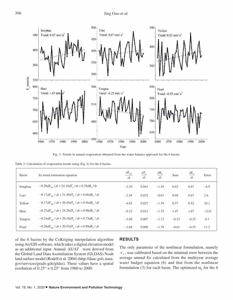
306 Jing Guo et al.
Vol. 19, No. 1, 2020 • Nature Environment and Pollution Technology
of the 6 basins by the CoKriging interpolation algorithm using ArcGIS software, which takes a digital elevation model as an additional input. Annual D DS T/ were derived from the Global Land Data Assimilation System (GLDAS) Noah land surface model (Rodell et al. 2004) (http://daac.gsfc.nasa.gov/services/grads-gds/gldas). These values have a spatial resolution of 0.25° × 0.25° from 1960 to 2000.
5 of 8
Fig. 3: Trends in annual evaporation obtained from the water balance approach for the 6 basins.
Table 2: Calculation of evaporation trends using (Eq. 4) for the 6 basins.
Basin Ea trend estimation equation 𝑑𝑑𝐸𝐸𝑝𝑝𝑝𝑝𝑑𝑑𝑑𝑑
𝑑𝑑𝑇𝑇𝑝𝑝𝑑𝑑𝑑𝑑
𝑑𝑑𝑅𝑅𝑛𝑛𝑑𝑑𝑑𝑑 Sum
𝑑𝑑𝐸𝐸𝑝𝑝𝑑𝑑𝑑𝑑 Error
Songhua −0.20𝑑𝑑𝐸𝐸𝑝𝑝𝑝𝑝 𝑑𝑑𝑑𝑑⁄ + 24.10𝑑𝑑𝑇𝑇𝑝𝑝 𝑑𝑑𝑑𝑑⁄ + 0.70𝑑𝑑𝑅𝑅𝑛𝑛 𝑑𝑑𝑑𝑑⁄ -2.29 0.041 -1.16 0.63 0.67 -4.9
Liao −0.17𝑑𝑑𝐸𝐸𝑝𝑝𝑝𝑝 𝑑𝑑𝑑𝑑⁄ + 21.49𝑑𝑑𝑇𝑇𝑝𝑝 𝑑𝑑𝑑𝑑⁄ + 0.66𝑑𝑑𝑅𝑅𝑛𝑛 𝑑𝑑𝑑𝑑⁄ -2.44 0.032 -0.61 0.69 0.67 2.6 Yellow −0.17𝑑𝑑𝐸𝐸𝑝𝑝𝑝𝑝 𝑑𝑑𝑑𝑑⁄ + 20.45𝑑𝑑𝑇𝑇𝑝𝑝 𝑑𝑑𝑑𝑑⁄ + 0.56𝑑𝑑𝑅𝑅𝑛𝑛 𝑑𝑑𝑑𝑑⁄ -4.65 0.027 -1.39 0.57 0.52 10.1
Huai −0.27𝑑𝑑𝐸𝐸𝑝𝑝𝑝𝑝 𝑑𝑑𝑑𝑑⁄ + 24.20𝑑𝑑𝑇𝑇𝑝𝑝 𝑑𝑑𝑑𝑑⁄ + 0.98𝑑𝑑𝑅𝑅𝑛𝑛 𝑑𝑑𝑑𝑑⁄ -9.23 0.012 -1.35 1.47 1.67 -12.0 Yangtze −0.24𝑑𝑑𝐸𝐸𝑝𝑝𝑝𝑝 𝑑𝑑𝑑𝑑⁄ + 20.10𝑑𝑑𝑇𝑇𝑝𝑝 𝑑𝑑𝑑𝑑⁄ + 0.73𝑑𝑑𝑅𝑅𝑛𝑛 𝑑𝑑𝑑𝑑⁄ -3.69 0.007 -1.72 -0.23 -0.25 -9.1
Pearl −0.28𝑑𝑑𝐸𝐸𝑝𝑝𝑝𝑝 𝑑𝑑𝑑𝑑⁄ + 20.93𝑑𝑑𝑇𝑇𝑝𝑝 𝑑𝑑𝑑𝑑⁄ + 0.99𝑑𝑑𝑅𝑅𝑛𝑛 𝑑𝑑𝑑𝑑⁄ -3.68 0.006 -1.78 -0.61 -0.55 11.2
𝑑𝑑𝐸𝐸𝑝𝑝𝑝𝑝𝑑𝑑𝑑𝑑 , 𝑑𝑑𝑇𝑇𝑝𝑝𝑑𝑑𝑑𝑑 and 𝑑𝑑𝑅𝑅𝑛𝑛𝑑𝑑𝑑𝑑 denote annual trend in Epa, Ta and Rn respectively. Sum denotes the sum of the
right-side hand of (Eq. 4); 𝑑𝑑𝐸𝐸𝑝𝑝𝑑𝑑𝑑𝑑 annual Ea trend obtained from the water balance approach. Error denotes the relative errors between Ea trends estimated from (Eq. 4) and that obtained from the water balance approach.
Discussion
Table 2 shows that Ta has increasing trends for all the 6 basins, while Rn and Epa had decreasing trends. According to the detailed estimation equation of Ea trend in Table 2, the increasing Ta trends and decreasing Epa trends will lead to an increase in Ea, while decreasing Rn will result in a decrease in Ea. Ea trends for a basin were the combined effects of Rn, Epa and Ta. The increasing Ea trends in the Songhua River, Liao River, Yellow River and Huai River basin indicate that the negative Rn trend term was not strong enough to overcome the positive Epa and Ta trend terms. In the Yangtze River and Pearl River basin, the negative Rn trend term overcame the positive Epa and Ta trend terms and resulted in decreasing Ea trends.
The Songhua River, Liao River, Yellow River and Huai River basins are located in northern China and belong to water-limited basins, where annual precipitation is less than atmospheric evaporative demand. The Yangtze River and Pearl River basins are located in southern China and
Fig. 3: Trends in annual evaporation obtained from the water balance approach for the 6 basins.
Table 2: Calculation of evaporation trends using (Eq. 4) for the 6 basins.
Basin Ea trend estimation equationdE
dtpa dT
dta dR
dtn Sum
dE
dta Error
Songhua - + +0 20 24 10 0 70. / . / . /dE dt dT dt dR dtpa a n –2.29 0.041 –1.16 0.63 0.67 –4.9
Liao - + +0 17 21 49 0 66. / . / . /dE dt dT dt dR dtpa a n –2.44 0.032 –0.61 0.69 0.67 2.6
Yellow - + +0 17 20 45 0 56. / . / . /dE dt dT dt dR dtpa a n –4.65 0.027 –1.39 0.57 0.52 10.1
Huai - + +0 27 24 20 0 98. / . / . /dE dt dT dt dR dtpa a n –9.23 0.012 –1.35 1.47 1.67 -12.0
Yangtze - + +0 24 20 10 0 73. / . / . /dE dt dT dt dR dtpa a n –3.69 0.007 –1.72 –0.23 –0.25 -9.1
Pearl - + +0 28 20 93 0 99. / . / . /dE dt dT dt dR dtpa a n –3.68 0.006 –1.78 –0.61 –0.55 11.2
RESULTS
The only parameter of the nonlinear formulation, namely a e , was calibrated based on the minimal error between the average annual Ea calculated from the multiyear average water budget equation (6) and that from the nonlinear formulation (3) for each basin. The optimized ae for the 6

307EVAPORATION TRENDS IN MAJOR RIVER BASINS OF CHINA
Nature Environment and Pollution Technology • Vol. 19, No. 1, 2020
basins is 1.08, 1.03, 1.04, 1.13, 1.18 and 1.22, respectively. Fig. 2 shows the comparisons of estimated annual Ea values using the nonlinear formulation (E_GF) against water budget approach (E_WB) for the 6 basins. The Nash-Sutcliffe efficiency coefficient (NSE) between E_GF and E_WB was 0.70, 0.63, 0.72, 0.72, 0.85 and 0.73 for the 6 basins, respectively. Generally, the nonlinear formulation had good performance for annual Ea estimation in the 6 basins.
Annual Ea trends of the 6 basins were estimated using (Eq. 4), and the detailed estimation equations for each basin are listed in Table 2. The trends of annual Rn, Epa and Ta used to estimate Ea trend for each basin are also listed in Table 2. With these trends together, (Eq. 4) yielded the trends of Ea as 0.63, 0.69, 0.57, 1.47, -0.23 and -0.61 mm a-2 for the 6 basins, respectively. Fig. 3 shows that Ea trends obtained from the water balance approach were 0.67, 0.67, 0.52, 1.67, -0.25 and -0.55 mm a-2 for the 6 basins, respectively. The relative errors between Ea trends from the nonlinear formulation and that from the water balance approach were -4.9, 2.6, 10.1, -12.0, -9.1 and 11.2%, respectively. The nonlinear formulation produced good agreement with annual Ea trends obtained from the water balance approach in the 6 basins.
dE
dt
dT
dtpa a, and
dR
dtn denote annual trend in Epa, Ta and
Rn respectively. Sum denotes the sum of the right-side hand
of (Eq. 4); dE
dta annual Ea trend obtained from the water
balance approach. Error denotes the relative errors between Ea trends estimated from (Eq. 4) and that obtained from the water balance approach.
DISCUSSION
Table 2 shows that Ta has increasing trends for all the 6 basins, while Rn and Epa had decreasing trends. According to the detailed estimation equation of Ea trend in Table 2, the increasing Ta trends and decreasing Epa trends will lead to an increase in Ea, while decreasing Rn will result in a decrease in Ea. Ea trends for a basin were the combined effects of Rn, Epa and Ta. The increasing Ea trends in the Songhua River, Liao River, Yellow River and Huai River basin indicate that the negative Rn trend term was not strong enough to overcome the positive Epa and Ta trend terms. In the Yangtze River and Pearl River basin, the negative Rn trend term overcame the positive Epa and Ta trend terms and resulted in decreasing Ea trends.
The Songhua River, Liao River, Yellow River and Huai River basins are located in northern China and belong to
water-limited basins, where annual precipitation is less than atmospheric evaporative demand. The Yangtze River and Pearl River basins are located in southern China and belong to energy-limited basins, where annual precipitation is larger than atmospheric evaporative demand (Mcvicar et al. 2012). In this study, decreasing Epa was accompanied by increasing Ea in the 4 water-limited basins, while decreasing Epa was accompanied by decreasing Ea in the 2 energy-limited basins. This result is consistent with the findings that Ea and Epa could be generally complementary in water-limited basins and proportional in energy-limited basins (Yang et al. 2006, Yang et al. 2007, Cong et al. 2010, Zhang et al. 2017). Interestingly, although the nonlinear formulation is based on the complementary principle between Ea and Epa, decreasing trends in Ea were still estimated from decreasing Epa in the two energy-limited basins. This provides additional support for the plausibility of the nonlinear formulation for estimating Ea trends.
While the agreement is excellent, admittedly Ea trends here and also the equation (4) used to estimate Ea trends are subject to some uncertainty. Firstly, the reference Ea trends were obtained from the water balance approach with D DS T/ simulated by the GLDAS Noah land surface model. Errors existed between the simulated and the true values of D DS T/ (Long et al. 2017). Such errors can then lead in turn to inconsistencies between Ea trends from the water balance approach and that from the nonlinear formulation. We note that these errors had limited effect on the calibration of a e for each basin, because a e was calibrated by the multiyear average water balance equation during 1960 to 2000, and D D DS T/ can be assumed to equal zero (Miao et al. 2015, Sun et al. 2018). Secondly, on the right-side hand of (Eq. 4), Rn, Epa and Ta could impact each other, and were not totally independent (Liu et al. 2011). However, the differential equations assumed that they were independent. This could lead to errors of Ea trends estimated from (Eq. 4). This issue will require further research.
Different methods have been developed to estimate Ea trends. One of the difficulties is that Ea trends could be significantly impacted by human activities, such as irrigation (Kong et al. 2015, Miao et al. 2016, Yang et al. 2017) and reservoir construction (Yang et al. 2017). Mao et al. (2016) indicates that with or without considering the water storage change due to reservoir construction can even obtain opposite Ea trends in the major river basins of China. However, the human influences on hydrologic cycle are typically difficult to quantify due to lack of data. The nonlinear formulation of the complementary principle can avoid directly estimating human influences on Ea, while it can indirectly reflect human influences on Ea (Liu et al. 2017). Theoretically, the observed

308 Jing Guo et al.
Vol. 19, No. 1, 2020 • Nature Environment and Pollution Technology
trends in Rn, Epa and Ta were already influenced by human influences such as irrigation and reservoir construction, and thus the corresponding Ea trends estimated using the nonlinear formulation reflected these human influences.
CONCLUSIONS
A nonlinear formulation of complementary principle was tested for estimating Ea trends in 6 major river basins of China. The resulting method is shown to be fairly accurate in estimating annual Ea trends from routine meteorological data. In the two energy-limited basins, namely the Yangtze River Basin and Pearl River Basin, both Ea and Epo had decreasing trends during 1960 to 2000. Although the nonlinear formulation is based on the complementary principle between Ea and Epo, it accurately simulated the decreasing Ea trends in the two basins. In the context of global warming, accurate prediction of Ea trends is of great importance for estimating the changes in hydrologic cycle. The results from this study are promising as they indicate the potential of this method for predicting Ea trends from projections of changes in routine meteorological variables.
ACKNOWLEDGEMENTS
We thank China Meteorological Administration for providing the routine meteorological data (http://data.cma.cn/en) and China Hydrological Bureau for providing the streamflow data of the six basins (http://www.hydroinfo.gov.cn/).
REFERENCES
Allen, R. G., Pereira, L. S., Raes, D. and Smith, M. 1998. Crop evapotranspiration: Guidelines for computing crop requirements. Irrigation Drainage Pap. 56, Food and Agric. Organ., Rome.
Bouchet, R. J. 1963. Evapotranspiration réelle, évapotranspirationpotentielle, et production agricole. Ann. Agron., 14: 743-824.
Brutsaert, W. and Stricker, H. 1979. An advection-aridity approach to estimate actual regional evapotranspiration. Water Resour. Res., 15: 443-450.
Brutsaert, W. 2005. Hydrology: An Introduction. 605 pp., Cambridge Univ. Press, New York.
Brutsaert, W. 2006. Indications of increasing land surface evaporation during the second half of the 20th century. Geophys. Res. Lett., 33: 4.
Brutsaert, W. 2013. Use of pan evaporation to estimate terrestrial evaporation trends: The case of the Tibetan Plateau. Water Resour. Res., 49: 3054-3058.
Brutsaert, W. 2015. A generalized complementary principle with physical constraints for land-surface evaporation. Water Resour. Res., 51: 8087-8093.
Brutsaert, W., Li, W., Takahashi, A., Hiyama, T., Zhang, L. and Liu, W. 2017. Nonlinear advection-aridity method for landscape evaporation and its application during the growing season in the southern Loess Plateau of the Yellow River basin. Water Resour. Res, 53(1): 270-282.
Cong, Z., Zhao, J., Yang, D. and Ni, G. 2010. Understanding the hydrological trends of river basins in China. J. Hydrol., 388(3): 350-356.
Granger, R. J. 1989. A complementary relationship approach for evaporation
from non-saturated surfaces. J. Hydrol., 111: 31-38.Han, S., Tian, F. and Hu, H. 2014. Positive or negative correlation between
actual and potential evaporation? Evaluating using a nonlinear complementary relationship model. Water Resour. Res., 50(2): 1322-1336.
Hobbins, M.T., Ramírez, J. A. and Brown, T. C. 2001. The complementary relationship in estimation of regional evapotranspiration: An enhanced advection-aridity model. Water Resour. Res., 37(5): 1389-1403.
Jung, M., Reichstein, M., Ciais, P., Seneviratne, S.I., Sheffield, J., Goulden, M.L., Bonan, G., Cescatti, A., Chen, J., De Jeu, R. and Dolman, A.J. 2010. Recent decline in the global land evapotranspiration trend due to limited moisture supply. Nature, 467(7318): 951-954.
Kong, D.X., Miao, C.Y., Borthwick, A.G.L., Duan, Q.Y., Liu, H., Sun, Q.H., Ye, A.Z., Di, Z.H. and Gong, W. 2015. Evolution of the Yellow River Delta and its relationship with runoff and sediment load from 1983 to 2011. J. Hydrol., 520: 157-167.
Liu, X., Liu, C. and Brutsaert, W. 2016. Regional evaporation estimates in the eastern monsoon region of China: Assessment of a nonlinear formulation of the complementary principle. Water Resour. Res., 52: 9511-9521.
Liu, X., Luo, Y., Zhang, D., Zhang, M. and Liu, C. 2011. Recent changes in pan-evaporation dynamics in China. Geophys. Res. Lett., 38(13): 1-4.
Liu, X., Yang, T., Hsu, K., Liu, C. and Sorooshian, S. 2017. Evaluating the streamflow simulation capability of PERSIANN-CDR daily rainfall products in two river basins on the Tibetan Plateau. Hydrol. Earth Syst. Sci., 21(1): 169-181.
Long, D., Pan, Y., Zhou, J., Chen, Y., Hou, X., Hong, Y., Scanlon, B. R. and Longuevergne, L. 2017. Global analysis of spatiotemporal variability in merged total water storage changes using multiple GRACE products and global hydrological models. Remote Sens. Environ., 192: 198-216.
Ma, N., Zhang, Y., Szilagyi, J., Guo, Y., Zhai, J. and Gao, H. 2015. Evaluating the complementary relationship of evapotranspiration in the alpine steppe of the Tibetan Plateau. Water Resour. Res, 51(2): 1069-1083.
Mao, Y., Wang, K., Liu, X. and Liu, C. 2016. Water storage in reservoirs built from 1997 to 2014 significantly altered the calculated evapotranspiration trends over China. J. Geophys. Res., 121: 10,097-10,112.
McVicar, T.R., Roderick, M.L., Donohue, R.J., Li, L.T., Van Niel, T.G., Thomas, A., Grieser, J., Jhajharia, D., Himri, Y., Mahowald, N.M. and Mescherskaya, A.V. 2012. Global review and synthesis of trends in observed terrestrial near-surface wind speeds: Implications for evaporation. J. Hydrol., 416-417: 182-205.
Miao, C.Y., Ashouri, H., Hsu, K., Sorooshian, S. and Duan, Q.Y. 2015. Evaluation of the PERSIANN-CDR daily rainfall estimates in capturing the behavior of extreme precipitation events over China. Journal of Hydrometeorology, 16: 1387-1396.
Miao, C.Y., Kong, D.X., Wu, J.W. and Duan, Q.Y. 2016. Functional degradation of the water-sediment regulation scheme in the lower Yellow River: Spatial and temporal analyses. Science of the Total Environment, 551-552: 16-22.
Morton, F. I. 1983. Operational estimates of areal evapotranspiration and their significance to the science and practice of hydrology. J. Hydrol., 66(1-4): 1-76.
Mueller, B., Seneviratne, S.I., Jimenez, C., Corti, T., Hirschi, M., Balsamo, G., Ciais, P., Dirmeyer, P., Fisher, J.B., Guo, Z. and Jung, M. 2011. Evaluation of global observations-based evapotranspiration datasets and IPCC AR4 simulations. Geophys. Res. Lett., 38: 1-7.
Priestley, C. H. B. and Taylor, R. J. 1972. On the assessment of surface heat flux and evaporation using large-scale parameters, Mon. Weather Rev., 100: 81-92.
Rodell, M., Houser, P.R., Jambor, U.E.A., Gottschalck, J., Mitchell, K., Meng, C.J., Arsenault, K., Cosgrove, B., Radakovich, J., Bosilovich, M. and Entin, J.K. 2004. The global land data assimilation system. Bull. Am. Meteorol. Soc., 85(3): 381-394.

309EVAPORATION TRENDS IN MAJOR RIVER BASINS OF CHINA
Nature Environment and Pollution Technology • Vol. 19, No. 1, 2020
Sun, Q.H., Miao,C.Y., Duan, Q.Y., Ashouri, H., Sorooshian, S. and Hsu, K. 2018. A review of global precipitation datasets: data sources, estimation, and intercomparisons. Reviews of Geophysics, 56(1): 79-107.
Wang, K. and Dickinson, R. 2012. A review of global terrestrial evapotranspiration: Observation, modeling, climatology, and climatic variability. Rev. Geophys.,50: RG2005
Yang, D., Sun, F., Liu, Z., Cong, Z. and Lei, Z. 2006. Interpreting the complementary relationship in non-humid environments based on the Budyko and Penman hypotheses. Geophys. Res. Lett., 33(18): 1-5.
Yang, D., Sun, F., Liu, Z., Cong, Z., Ni, G. and Lei, Z. 2007. Analyzing spatial and temporal variability of annual water-energy balance in nonhumid regions of China using the Budyko hypothesis. Water Resour. Res., 43: W04426.
Yang, T., Akbari Asanjan, A., Welles, E., Gao, X., Sorooshian, S., and Liu, X. 2017. Developing reservoir monthly inflow forecasts using artificial intelligence and climate phenomenon information. Water Resour. Res, 53(4): 2786-2812.
Yang, T., Asanjan, A.A., Faridzad, M., Hayatbini, N., Gao, X. and Sorooshian, S. 2017. An Enhanced Artificial Neural Network with A
Shuffled Complex Evolutionary Global Optimization with Principal Component Analysis. Information Sciences.
Yang, T., Tao, Y., Li, J., Zhu, Q., Su, L., He, X. and Zhang, X. 2017. Multi-criterion model ensemble of CMIP5 surface air temperature over China. Theoretical and Applied Climatology, 132(3-4): 1057-1072.
Zhang, L., Cheng, L. and Brutsaert, W. 2017. Estimation of land surface evaporation using a generalized nonlinear complementary relationship. J. Geophys. Res., 122(3): 1475-1487.
Zhang, Y., Chiew, F., Peña-Arancibia, J., Sun, F., Li, H. and Leuning, R. 2017. Global variation of transpiration and soil evaporation and the role of their major climate drivers. J. Geophys. Res., 122: 6868–6881.
Zhang, Y., Liu, C., Tang, Y. and Yang, Y. 2007. Trends in pan evaporation and reference and actual evapotranspiration across the Tibetan Plateau. J. Geophys. Res., 112: D 12.
Zhang, Y., Peña-Arancibia, J. L., McVicar, T. R., Chiew, F. H., Vaze, J., Liu, C., Lu, X., Zheng, H., Wang, Y. and Liu, Y.Y. 2016. Multi-decadal trends in global terrestrial evapotranspiration and its components, Sci. Rep., 6 (19124): 1-12.

Vol. 19, No. 1, 2020 • Nature Environment and Pollution Technology
310

Pb(II) Adsorption onto Urea Treated Leucaena leucocephala Leaf Powder: Characterization, Kinetics and Isotherm Studies
Noor Fhadzilah Mansur*, Megat Ahmad Kamal Megat Hanafiah*(**)† and Mardhiah Ismail**Faculty of Applied Sciences, Universiti Teknologi MARA, 26400, Jengka, Pahang, Malaysia**Institute of Science (IOS), Universiti Teknologi MARA, 40450, Shah Alam, Selangor, Malaysia†Corresponding author: Megat Ahmad Kamal Megat Hanafiah
ABSTRACT
The use of Leucaena leucocephala leaf powder treated with urea (treated-ULLP) as an alternative adsorbent for the adsorption of Pb(II) ions has been investigated. The adsorption studies were performed under batch mode and focused on the effects of pH, adsorbent dosage and initial Pb(II) concentrations. The pseudo-second order kinetics model fitted well the adsorption data with the values of correlation coefficient (R2) > 0.97. Large amounts of hydroxyl, carboxyl and amine as detected by the Fourier transform infrared (FTIR) spectrophotometer suggested that these functional groups were responsible for the adsorption of Pb(II) ions. Treated-ULLP demonstrated a good potential for Pb(II) ions removal with the maximum adsorption capacity of 90.09 mg/g, calculated from the Langmuir isotherm model.
INTRODUCTION
A lot of heavy metals are released into the environment, which include copper (Cu), chromium (Cr), lead (Pb), zinc (Zn), cadmium (Cd), nickel (Ni), manganese (Mn), and mercury (Hg) (Babarinde et al., 2006). Volesky (2001) stated that lead [Pb(II)] is one of the most toxic metals that has gained major attention due to its health impact on humans. Pb(II) could be stored in human tissues such as kidney and liver and can pose health hazards even in small concentrations (Puranik & Pakniker 1997). Pb(II) may originate from different types of industrial activities such as electronic, fossil fuel, painting, mining, automobile, sewage wastewater and fertilizer (Singh et al. 2008). A few decades ago, various conventional methods such as ion exchange, filtration, chemical precipitation, reverse osmosis, and electro deposition have been applied to remove Pb(II) from industrial wastewaters (Zheng et al. 2008). However, these treatments suffered some limitation such as production of sludge at the end of the treatment process (Papandreou et al. 2007), and less effective at trace levels of Pb(II). So, adsorption is an alternative process which has several advantages such as low cost, simple, more effective and records a high adsorption capacity value (qmax). A variety of adsorbent materials have been applied to remove Pb(II) from aqueous solutions, which include activated carbon,
zeolites, resins and plant wastes. Leucaena leucocephala leaves was used in this study because it contains various organic compounds such as lignin, cellulose, hemicellulose, polyphenols, protein, lipids, flavonoids, mimosine and tannins (Zarin et al. 2016), which can act as the active sites for Pb(II) adsorption. The main objectives of this work were to evaluate the parameters that could influence the uptake of Pb(II) on urea treated L. leucocephala leaves, to determine the rate of Pb(II) adsorption based on kinetics models, and to determine the maximum adsorption capacity based on the Langmuir isotherm model.
MATERIALS AND METHODS
Materials
Leucaena leucocephala leaves were collected in Jengka, Malaysia. The leaves were brought to the lab and washed several times with deionized water. The leaves were dried in an oven overnight at 353 K. Then, the leaves were ground and sieved to obtain the particle size of 180-355 µm. Working solutions of Pb(II) were prepared from a 1000 mg/L Pb(II) stock solution and diluted to desired concentrations using deionized water. The chemical treatment of L. leucocephala leaf powder was performed according to the method proposed by Kong et al. (2014). In brief, 3 g of L. leucocephala leaf
Nat. Env. & Poll. Tech.Website: www.neptjournal.com
Received: 27-06-2019Accepted: 30-08-2019
Key Words:AdsorptionIsothermsKineticsLeadLeucaena leucocephala
2020pp. 311-318 Vol. 19
p-ISSN: 0972-6268 No. 1 Nature Environment and Pollution Technology An International Quarterly Scientific Journal
Original Research Paper
e-ISSN: 2395-3454
Open Access

312 Noor Fhadzilah Mansur et al.
Vol. 19, No. 1, 2020 • Nature Environment and Pollution Technology
powder was mixed with 50% (w/v) of urea [CO(NH2)2] solution and underwent steamed process at 398 K for 30 min by using a steam bath. The urea solution was placed in a round bottom flask with steam below it and this process was carried out for 30 min. During the treatment, the mixture was stirred by using a glass rod, cooled and washed several times with deionized water until the solution reached near neutral. The sample was dried in an oven at the temperature of 378 K for 24 h. The adsorbent sample was designated as Treated-ULLP.
Characterization of Treated-ULLP
The pHslurry was determined by mixing 0.10 g of Treated- ULLP with 100 mL deionized water in a stoppered flask. The mixture was shaken at 100 strokes/min for 24 h at room temperature (298 K) in a water bath shaker. The mixture was filtered, and the final pH of this solution was determined by a pH meter. The zero-point charge of Treated-ULLP at a particular pH or pHzpc was also determined. Firstly, 25 mL of 0.01 M KNO3 was placed in a series of 100 mL conical flasks. The initial pH of the solution (pHi) was adjusted from 2 to 9 by adding drops of 0.05 M HCl or NaOH solution. Then, 0.10 g of Treated-ULLP was added to each flask and shaken in a water bath shaker for 24 h at 100 strokes/min. Finally, the mixture was filtered and the final pH (pHf) of each solution in the flasks was measured by using a pH meter. The pHzpc value was determined from the curve that intercepts the x-axis of the plot ∆pH (pHi – pHf) versus pHi. The functional groups responsible for uptake of Pb(II) were
analysed by a Fourier transform infrared spectrophotometer (PerkinElmer, Spectrum 100, USA). The total content of carbon, hydrogen, nitrogen, oxygen and sulphur in Treated-ULLP was determined by a CHNS analyser (vario MACRO cube CHNS, Germany). The scanning electron microscope (SEM, Carl Zeiss SMT, Germany) coupled with energy dispersive x-ray (EDX, Oxford Instrument, UK) spectrometer was used to analyse the surface morphology and the elemental composition of Treated-ULLP. Prior to this analysis, Treated-ULLP was coated with a thin layer of gold to improve conductivity, signal to noise ratio, and to reduce charging of the adsorbent material. The SEM image was scanned at 500 X magnification.
Adsorption Experiments
The pH ranging from 2 to 5 was selected and the adsorbent dosage was varied from 0.02 to 0.10 g for the effects of pH and adsorbent dosage, respectively. Drops of 0.05 M NaOH or HCl solution were added to adjust the pH. Three different concentrations of Pb(II) (50, 100, 150 mg/L) were used in the kinetics study and the concentrations were varied from 50 to 250 mg/L in the isotherm study. The dosage of Treated-ULLP was maintained at 0.02 g while the volume of Pb(II) solution was fixed at 50 mL. All Pb(II) solutions were shaken in a water bath shaker at 100 strokes/min. After adsorption, the adsorbent was filtered and the filtrates were analysed for unadsorbed Pb(II) by an Atomic Absorption Spectrometer (AAS, Perkin Elmer, PinAAcle 900T, USA). The linear range for Pb(II) in the calibration curve was from 0
RESULTS AND DISCUSSION
Characterization of Treated-ULLP: The pHslurry of Treated-ULLP was found to be 6.74, which
is slightly acidic, possibly due to the presence of carboxylic acid group (Zayed & Samling 2016).
The pHzpc plot is shown in Fig. 1 and the value was found to be 6.90. At pH < pHzpc, the surface
of Treated-ULLP would carry more positive charge than the negative charge. More negative
charge, however, would appear at pH > pHzpc.
Fig. 1: The pHzpc plot of Treated-ULLP.
Fig. 2 shows the FTIR spectra for Treated-ULLP before and after Pb(II) adsorption. The strong
and broad peak from 2600 to 3600 cm-1 confirmed the presence of carboxylic acid group (-
COOH) (Kong et al. 2013), which overlapped with -OH and -NH groups. The peak observed at
2923 cm-1 was assigned to the stretching C-H of alkyl group. The peak at 1647 cm-1 was
attributed to the stretching of C=O or C=C groups. The peaks appeared at 1160 and 1052 cm-1
indicated the stretching of C-N and C-O-C groups, respectively (Chen et al. 2010, Saygideger et
al. 2005). The presence of -CH group of aromatics was represented by the peak at 850 cm-1.
-2.0
-1.0
0.0
1.0
2.0
3.0
4.0
0.0 2.0 4.0 6.0 8.0 10.0 12.0∆pH
(pH
i -pH
f)
pHi
Fig. 1: The pHzpc plot of Treated-ULLP.

313LEAD ADSORPTION ONTO UREA TREATED LEUCAENA LEUCOCEPHALA
Nature Environment and Pollution Technology • Vol. 19, No. 1, 2020
to 20 mg/L. All the experiments were conducted in duplicate and the results were presented as the average. The relative standard deviation was < 3%. The amount of Pb(II) adsorbed at equilibrium (q )e and the percentage removal (%) were calculated by using the following equations:
qV C C
ee=
-( )0
m …(1)
Removal %C C
Ce( ) =
-¥0
0
100 …(2)
Where, C0 and Ce represent the Pb(II) concentration before and after adsorption (mg/L), respectively. V is the volume of adsorbate (L), qe is the amount of Pb(II) adsorbed (mg/g) at equilibrium and m is the weight of Treated-ULLP (g).
RESULTS AND DISCUSSION
Characterization of Treated-ULLP
The pHslurry of Treated-ULLP was found to be 6.74, which is slightly acidic, possibly due to the presence of carboxylic
Fig. 2: FTIR spectra of Treated-ULLP before and after adsorption of Pb(II) ions.
The wavenumber at 3420 cm-1 had shifted to 3406 cm-1, indicating that Pb(II) was adsorbed to the
hydroxyl, -COOH and amine groups. The wavenumber at 1647 cm-1 shifted to 1638 cm-1,
suggesting the involvement of C=O and C=C groups in the removal of Pb(II). Other functional
groups possible for attracting Pb(II) ions would be the C-N and C-O-C as there was a decrease in
the intensity of the peak at 1160 cm-1 and the shift in wavenumber from 1052 to 1034 cm-1,
respectively. The presence of hydroxyl, amino, ether, aromatics and carbonyl functional groups
acted as the active sites for adsorption process to occur. Meanwhile, the elemental composition of
the Treated-ULLP is given in Table 1. The percentage of N contained in the Treated-ULLP was
much higher than pristine L. leucocephala leaf (4.2 %), reported by Meena Devi et al. (2013).
This finding concludes that after chemical modification, the urea was successfully introduced in
the Treated-ULLP.
Table 1: CHNOS content of Treated-ULLP.
Elemental composition (%) C H N S O*
47.67 7.19 7.58 0.29 37.27 *by difference
cm-1
Fig. 2: FTIR spectra of Treated-ULLP before and after adsorption of Pb(II) ions.
Table 1: CHNOS content of treated-ULLP.
Elemental composition (%)
C H N S O*
47.67 7.19 7.58 0.29 37.27
*by difference
acid group (Zayed & Samling 2016). The pHzpc plot is shown in Fig. 1 and the value was found to be 6.90. At pH < pHzpc, the surface of Treated-ULLP would carry more positive charge than the negative charge. More negative charge, however, would appear at pH > pHzpc.
Fig. 2 shows the FTIR spectra for Treated-ULLP before and after Pb(II) adsorption. The strong and broad peak from 2600 to 3600 cm-1 confirmed the presence of carboxylic acid group (-COOH) (Kong et al. 2013), which overlapped with -OH and -NH groups. The peak observed at 2923 cm-1 was assigned to the stretching C-H of alkyl group. The peak at 1647 cm-1 was attributed to the stretching of C=O or C=C groups. The peaks appeared at 1160 and 1052 cm-1 indicated the stretching of C-N and C-O-C groups, respectively (Chen et al. 2010, Saygideger et al. 2005). The presence of -CH group of aromatics was represented by the peak at 850 cm-1.
The wave number at 3420 cm-1 had shifted to 3406 cm-1, indicating that Pb(II) was adsorbed to the hydroxyl, -COOH and amine groups. The wave number at 1647 cm-1 shifted to 1638 cm-1, suggesting the involvement of C=O and C=C groups in the removal of Pb(II). Other functional groups possible for attracting Pb(II) ions would be the C-N and

314 Noor Fhadzilah Mansur et al.
Vol. 19, No. 1, 2020 • Nature Environment and Pollution Technology
The SEM and EDX images of Treated-ULLP before and after Pb(II) adsorption are shown in Fig.
3. Treated-ULLP (Fig. 3a) possesses rough, irregular and nonporous surface morphology.
Important minerals for plants such as Na, Mg, K and Ca were clearly detected EDX as shown in
Fig. 3b. Pb(II) however, was not present. After adsorption (Figs. 3c and 3d), Pb(II) was clearly
detected on the surface of Treated-ULLP at 1.8, 2.3 and 2.7 keV (Fig. 3d). This finding concludes
the success of removal of Pb(II) from the aqueous solution onto the adsorbent surface.
a
b (a) (b)
c
d
Fig. 3: SEM (500 X magnification) and EDX images of Treated-ULLP before (a and b) and after Pb(II) adsorption (c and d).
Effects of pH and Dosage: The effects of pH and adsorbent dosage on Pb(II) adsorption are
shown in Fig. 4. Pb(II) adsorption increased with increasing pH of the solution, started from pH 2
to 5 for initial Pb(II) concentration of 50 mg/L [Fig. 4(a)]. The amount of Pb(II) adsorbed was
very low at pH 2 due to the stiff competition between protons (H+) in the solutions and the Pb(II)
for the adsorption sites. Furthermore, it was also due to the stronger electrostatic repulsion
between Pb(II) and the positively charged adsorbent surface. At pH 3, the amount of Pb(II)
adsorbed started to increase because the -COOH started to dissociate to liberate more -COO-
groups, which could easily adsorb the positively charged Pb(II) (Lalhruaitluanga et al. 2010). The
amount of Pb(II) adsorbed continued to increase at pH 4 and 5 due to a much lower concentration
of H+ in the solution, hence less competition between H+ and the metal ions (Wu et al. 2011).
Therefore, more Pb(II) could easily be adsorbed to the adsorption sites. The subsequent
(c) (d)
Fig. 3: SEM (500 X magnification) and EDX images of treated-ULLP before (a and b) and after Pb(II) adsorption (c and d).

315LEAD ADSORPTION ONTO UREA TREATED LEUCAENA LEUCOCEPHALA
Nature Environment and Pollution Technology • Vol. 19, No. 1, 2020
C-O-C as there was a decrease in the intensity of the peak at 1160 cm-1 and the shift in wave number from 1052 to 1034 cm-1, respectively. The presence of hydroxyl, amino, ether, aromatics and carbonyl functional groups acted as the active sites for adsorption process to occur. Meanwhile, the elemental composition of the Treated-ULLP is given in Table 1. The percentage of N contained in the Treated-ULLP was much higher than pristine L. leucocephala leaf (4.2 %), reported by Meena Devi et al. (2013). This finding concludes that after chemical modification, the urea was successfully introduced in the Treated-ULLP.
The SEM and EDX images of Treated-ULLP before and after Pb(II) adsorption are shown in Fig. 3. Treated-ULLP (Fig. 3a) possesses rough, irregular and nonporous surface morphology. Important minerals for plants such as Na, Mg, K and Ca were clearly detected EDX as shown in Fig. 3b. Pb(II) however, was not present. After adsorption (Figs. 3c and 3d), Pb(II) was clearly detected on the surface of Treated-ULLP
adsorption experiments were conducted at pH 4 only to avoid the formation of precipitate
(Pb(OH)2) or Pb(OH)- due to the high number of OH- ions present in the solution at pH > 5
(Sheng et al. 2004). Adsorbent dosage experiment was conducted to give an idea on the
effectiveness of the amount of adsorbent used. The percentage removal of Pb(II) increased as the
adsorbent dosage increased from 0.02 to 0.10 g [Fig. 4(b)].
(a) (b)
Fig. 4: Effects of pH (a) and dosage (b) on the Pb(II) adsorption on Treated-ULLP.
This phenomenon confirmed that more active sites as well as surface area were available for the
binding of Pb(II) with increasing the adsorbent dosage. However, the amount of Pb(II) adsorbed
showed the opposite trend and it was associated to the increased number of unadsorbed sites
when the dosage was increased (Yu et al. 2002). Aggregation also occurred due to the particles
interaction that led to the surface area reduction of Treated-ULLP.
Effects of initial Pb(II) concentrations and contact time: The effect of initial concentration and
contact time of Pb(II) on Treated-ULLP is shown in Fig. 5. The plots showed that three main
phases were involved during the adsorption process. The first phase was called the initial rapid
adsorption process followed by slow adsorption process and the last phase was dynamic
0
20
40
60
80
0 2 4 6
q e(m
g/g)
pH
(a) (b)
Fig. 4: Effects of pH (a) and dosage (b) on the Pb(II) adsorption on treated-ULLP.
equilibrium time. The initial rapid adsorption process occurred in the first 3 min. It was possibly
due to high number of available adsorption sites (Kousha et al. 2012), causing the rapid transfer
of Pb(II) to the external surface of Treated-ULLP. The slow adsorption rate was observed in the
range of 5 to 10 min due to the less availability of active sites or stiff competition among the
Pb(II) ions for the active sites. After 30 min, there was only a small change in the amount of
Pb(II) adsorbed, which the process was considered to have achieved the equilibrium time.
Fig. 5: Effects of concentration and contact time on the Pb(II) adsorption.
Adsorption kinetics models: Adsorption kinetics models were applied to further investigate the
rate of Pb(II) adsorption process. The pseudo-first-order (Ho & McKay 1999) and pseudo-
second-order models (Ho & McKay 2000) were expressed in Equations 3 and 4, respectively.
log (qe − qt) = log qe − k12.303 t … (3)
tqt
= 1ℎ + 1
qet … (4)
0
12
24
36
48
0 20 40 60 80 100 120 140
q t(m
g/g)
t (min)
50 mg/L
100 mg/L
150 mg/L
Fig. 5: Effects of concentration and contact time on the Pb(II) adsorption.
at 1.8, 2.3 and 2.7 keV (Fig. 3d). This finding concludes the success of removal of Pb(II) from the aqueous solution onto the adsorbent surface.
Effects of pH and Dosage
The effects of pH and adsorbent dosage on Pb(II) adsorption are shown in Fig. 4. Pb(II) adsorption increased with increasing pH of the solution, started from pH 2 to 5 for initial Pb(II) concentration of 50 mg/L [Fig. 4(a)]. The amount of Pb(II) adsorbed was very low at pH 2 due to the stiff competition between protons (H+) in the solutions and the Pb(II) for the adsorption sites. Furthermore, it was also due to the stronger electrostatic repulsion between Pb(II) and the positively charged adsorbent surface. At pH 3, the amount of Pb(II) adsorbed started to increase because the -COOH started to dissociate to liberate more -COO- groups, which could easily adsorb the positively charged Pb(II) (Lalhruaitluanga et al. 2010). The amount of Pb(II) adsorbed

316 Noor Fhadzilah Mansur et al.
Vol. 19, No. 1, 2020 • Nature Environment and Pollution Technology
continued to increase at pH 4 and 5 due to a much lower concentration of H+ in the solution, hence less competition between H+ and the metal ions (Wu et al. 2011). Therefore, more Pb(II) could easily be adsorbed to the adsorption sites. The subsequent adsorption experiments were conducted at pH 4 only to avoid the formation of precipitate (Pb(OH)2) or Pb(OH)- due to the high number of OH- ions present in the solution at pH > 5 (Sheng et al. 2004). Adsorbent dosage experiment was conducted to give an idea on the effectiveness of the amount of adsorbent used. The percentage removal of Pb(II) increased as the adsorbent dosage increased from 0.02 to 0.10 g [Fig. 4(b)].
This phenomenon confirmed that more active sites as well as surface area were available for the binding of Pb(II) with increasing the adsorbent dosage. However, the amount of Pb(II) adsorbed showed the opposite trend and it was associated to the increased number of unadsorbed sites when
Table 2: Adsorption kinetics parameters at different Pb(II) concentrations.
Kinetics models Pb(II) concentrations
Parameters 50 mg/L 100 mg/L 150 mg/L
Pseudo-first-order qe,cal (mg/g) 46.71 91.41 276.24
qe,exp (mg/g) 35.63 41.27 48.90
k1 (1/min) 0.049 0.025 0.008
R2 0.673 0.413 0.050
Pseudo-second-order qe,cal (mg/g) 36.54 41.28 48.12
qe,exp (mg/g) 35.63 41.27 48.90
k2 (g/mg.min)) 0.008 0.046 0.039
R2 0.999 1.000 0.999
the dosage was increased (Yu et al. 2002). Aggregation also occurred due to the particles interaction that led to the surface area reduction of Treated-ULLP.
Effects of Initial Pb(II) Concentrations and Contact Time
The effect of initial concentration and contact time of Pb(II) on Treated-ULLP is shown in Fig. 5. The plots showed that three main phases were involved during the adsorption process. The first phase was called the initial rapid adsorption process followed by slow adsorption process and the last phase was dynamic equilibrium time. The initial rapid adsorption process occurred in the first 3 min. It was possibly due to high number of available adsorption sites (Kousha et al. 2012), causing the rapid transfer of Pb(II) to the external surface of Treated-ULLP. The slow adsorption rate was observed in the range of 5 to 10 min due to the less availability
Ceqe
= Ceqmax
+ 1qmaxK𝐿𝐿
… (5)
Where, qmax is the maximum adsorption capacity and KL represents the Langmuir constant. The
Langmuir plots showed good linearity (R2 > 0.96) and the predicted maximum adsorption
capacity values were close to the experimental values (Table 3 & Fig. 7). The increase in the
maximum adsorption capacity values with increasing temperatures suggested the endothermic
type of adsorption. The adsorption mechanism of Pb(II) onto Treated-ULLP could be understood
in terms of hard-soft acid base principle (HSAB). Table 3 shows that Treated-ULLP contains N
(a borderline ligand), S (a soft-base ligand) and O (a hard-base ligand). These three types of
atoms could act as metal-binding donor atoms for Pb(II). As Pb(II) is classified as a borderline
metal ion (Nieboer & Richardson 1980), it would be attracted to all categories of ligands to form
stable complexes.
Fig. 6: Pb(II) adsorption isotherm plots at different temperatures.
0102030405060708090
100
0 50 100 150 200 250
q e(m
g/g)
Ce (mg/L)
300 K310 K320 K
Fig. 6: Pb(II) adsorption isotherm plots at different temperatures.

317LEAD ADSORPTION ONTO UREA TREATED LEUCAENA LEUCOCEPHALA
Nature Environment and Pollution Technology • Vol. 19, No. 1, 2020
of active sites or stiff competition among the Pb(II) ions for the active sites. After 30 min, there was only a small change in the amount of Pb(II) adsorbed, which the process was considered to have achieved the equilibrium time.
Adsorption Kinetics Models
Adsorption kinetics models were applied to further investigate the rate of Pb(II) adsorption process. The pseudo-first-order (Ho & McKay 1999) and pseudo-second-order models (Ho & McKay 2000) were expressed in Equations 3 and 4, respectively.
log q q qk
te t e-( ) = -log.
1
2 303 …(3)
t
q qt
t e
= +1 1
h …(4)
Where the symbols qe and qt indicate the amount of Pb(II) adsorbed (mg/g) at equilibrium and at time t (min), respectively. k1 (1/min) is the rate constant of adsorption process for the pseudo-first-order model. The initial adsorption rate (mg/g.min) is represented by the symbol of h while the k2 [g/(mg.min)] is the rate constant for the pseudo-second-order model. The values of k2 and h were obtained
by using an equation of h = k qe22
.
Fig. 7: Langmuir isotherm plots at different temperatures.
Table 3: Langmuir adsorption isotherm parameters at different temperatures.
Isotherm model Parameters Temperatures (K) 300 310 320
Langmuir qmax (mg/g) 82.65 86.21 90.09 qe,exp (mg/g) 78.00 83.65 87.90 KL (L/mol) 0.046 0.050 0.063 R2 0.965 0.966 0.978
CONCLUSION
Treated-ULLP showed a satisfactory removal of Pb(II) from aqueous solutions under batch mode
sorption techniques. Based on the FTIR spectrum of Treated-ULLP, the detected functional
groups such as carbonyl (C=O), hydroxyl (-OH) carboxylic acid (-COOH), amino (-NH2) and
ether (C-O-C) acted as the active sites for Pb(II). The attachment of Pb(II) on Treated-ULLP was
confirmed by the EDX images. The rate of Pb(II) removal was considered quite rapid as the time
to reach equilibrium was less than 30 min. Pb(II) adsorption was more favoured at a higher
temperature, an indication of endothermic adsorption process.
0
0.5
1
1.5
2
2.5
3
0 50 100 150 200 250
Ce/q
e(g
/L)
Ce (mg/L)
300 K310 K320 K
Fig. 7: Langmuir isotherm plots at different temperatures.
Table 3: Langmuir adsorption isotherm parameters at different temperatures.
Isotherm model Parameters Temperatures (K)
300 310 320
Langmuir qmax (mg/g) 82.65 86.21 90.09
qe exp, (mg/g) 78.00 83.65 87.90
KL (L/mol) 0.046 0.050 0.063
R2 0.965 0.966 0.978
Both the plots have not shown, but the values of correlation coefficient (R2) were close to unity (0.999-1.000) as in the case of the pseudo-second-order kinetics model. In addition, the values of calculated adsorption capacities (qe,cal) were almost match to the values of experimental (qe,exp). Based on these two observations, it can be concluded that the adsorption kinetics fitted well the pseudo-second-order kinetics model (Table 2).
Adsorption Isotherms
The adsorption isotherm plots at three different temperatures are presented in Fig. 6. In general, the adsorption capacities were found to increase with increasing temperatures, an indication of an endothermic reaction. The plots were further analyzed using the most widely used isotherm model, which is the Langmuir model (Langmuir 1918), developed based on the assumption that all the adsorption sites have the same energy and is given by Equation 5:
C
q
C
q q Ke
e
e
max max
= +1
L
…(5)
Where, qmax is the maximum adsorption capacity and KL represents the Langmuir constant. The Langmuir plots showed good linearity (R2 > 0.96) and the predicted

318 Noor Fhadzilah Mansur et al.
Vol. 19, No. 1, 2020 • Nature Environment and Pollution Technology
maximum adsorption capacity values were close to the experimental values (Table 3 & Fig. 7). The increase in the maximum adsorption capacity values with increasing temperatures suggested the endothermic type of adsorption. The adsorption mechanism of Pb(II) onto Treated-ULLP could be understood in terms of hard-soft acid base principle (HSAB). Table 3 shows that Treated-ULLP contains N (a borderline ligand), S (a soft-base ligand) and O (a hard-base ligand). These three types of atoms could act as metal-binding donor atoms for Pb(II). As Pb(II) is classified as a borderline metal ion (Nieboer & Richardson 1980), it would be attracted to all categories of ligands to form stable complexes.
CONCLUSION
Treated-ULLP showed a satisfactory removal of Pb(II) from aqueous solutions under batch mode sorption techniques. Based on the FTIR spectrum of Treated-ULLP, the detected functional groups such as carbonyl (C=O), hydroxyl (-OH) carboxylic acid (-COOH), amino (-NH2) and ether (C-O-C) acted as the active sites for Pb(II). The attachment of Pb(II) on Treated-ULLP was confirmed by the EDX images. The rate of Pb(II) removal was considered quite rapid as the time to reach equilibrium was less than 30 min. Pb(II) adsorption was more favoured at a higher temperature, an indication of endothermic adsorption process.
ACKNOWLEDGEMENT
Special thanks are due to the Malaysian Ministry of Education for the financial support of this work (Grant no. 600 – RMI/RAGS 5/3 (3/2013).
REFERENCES
Babarinde, N.A.A., Babalola, J.O. and Sanni, R. A. 2006. Biosorption of lead ions from aqueous solution by maize leaf. International Journal of Physical Sciences, 1: 23-26.
Chen, W., Yan, L. and Bangal, P. R. 2010. Preparation of graphene by the rapid and mild thermal reduction of grapheme oxide induced by microwaves. Carbon, 48: 1146-1152.
Ho, Y. S. and McKay, G. 1999. The sorption of lead (II) ions on peat. Water Research, 33: 578-584.
Ho, Y.S. and McKay, G. 2000. The kinetics of sorption of divalent metal ions onto Sphagnum moss peat. Water Research, 34: 735-742.
Kong, J., Yue, Q., Sun, S., Gao, B., Kan, Y., Li, Q. and Wang, Y. 2014. Ad-sorption of Pb(II) from aqueous solutions using keratin waste-hide waste. Equilibrium, kinetic and thermodynamic modeling studies. Chemical Engineering Journal, 241: 393-400.
Kong, J., Yue, Q., Huang, L., Gao, Y., Sun, Y., Gao, B., Li, Q. and Wang, Y. 2013. Preparation, characterization, and evaluation of leather waste base activated carbon via physical and chemical activation. Chemical Engineering Journal, 221: 62-71.
Kousha, M., Daneshvar, E., Sohrabi, M. S., Jokar, M. and Bhatnagar, A. 2012. Adsorption of acid orange II dye by raw and chemically modified brown macroalga Stoechospermum marginatum. Chemical Engineering Journal, 192: 67-76.
Lalhruaitluanga, H., Jayaram, K., Prasad, M. N. V. and Kumar, K. K. 2010. Lead(II) adsorption from aqueous solutions by raw and activated char-coals of Melocanna baccifera Roxburgh (bamboo). A comparative study. Journal of Hazardous Materials, 175: 311-318.
Langmuir, I. 1918. The adsorption of gases on plane surfaces of glass, mica and platinum. Journal of the American Chemical society, 40(9): 1361-1403.
Meena Devi, V.N., Ariharan, V. N. and Nagendra Prasad, P. 2013. Nutritive value and potential uses of Leucaena leucocephala as biofuel-A mini review. Research Journal of Pharmaceutical, Biological and Chemical Sciences, 4(1): 515-521.
Nieboer, E. and Richardson, D.H.S. 1980. The replacement of the nonde-script term ‘heavy metals’ by a biologically and chemically significant classification of metal ions. Environmental Pollution (Series B): 1, 3-26.
Papandreou, A., Stournars, C. J. and Panias, D. 2007. Copper and cadmium adsorption on pellets made from fired coal fly ash. Journal of Hazardous Materials, 148: 538-547.
Puranik, P.R. and Pakniker, K.M. 1997. Biosorption of lead and zinc from solutions using Streptoverticillium cinnamoneum waste biomass. Journal of Biotechnology, 55: 113-124.
Saygideger, S., Gulnaz, O., Istifli, E.S. and Yucel, N. 2005. Adsorption of Cd(II), Cu(II), and Ni(II) ions Lemna minor L : Effect of physicochemical environment. Journal of Hazardous Materials, 126: 96-104.
Sheng, P. X., Ting, Y. P. and Hong, L. 2004. Sorption of lead, copper, cadmium, zinc and nickel by marine algal biomass: characterization of biosorptive capacity and investigation of mechanisms. Journal of Colloid and Inter-face Science, 275: 131-141.
Singh, C. K., Sahu, J. N., Mahalik, K. K., Mohanty, C. R., Mohan, B. R. and Meikap, B. C. 2008. Studies on the removal of Pb(II) from wastewater by activated carbon developed from tamarind wood activated with sulphuric acid. Journal of Hazardous Materials, 153: 221-228.
Volesky, B. 2001. Detoxification of metal-bearing effluents: Biosorption for the next century. Hydrometallurgy, 59: 203-216.
Wu, J. L., Fan, X. Z., Hong, J. and Xue, S. Z. 2011. Adsorption of lead (Pb) from aqueous solution with Typha angustifolia biomass modified by SOCl2 activated EDTA. Chemical Engineering Journal, 170: 21-28.
Yu, L.J., Shukla, S.S., Dorris, K.L., Shukla, A. and Margrave, J.L. 2002. Adsorption of chromium from aqueous solutions by maple sawdust. Journal of Hazardous Materials, 100: 53-63.
Zarin, M.A., Wan, H.Y., Isha, A. and Armania, N. 2016. Antioxidant, anti-microbial and cytotoxic potential of condensed tannins from Leucaena leucocephala hybrid-rendang. Food Science and Human Wellness, 75-65 :(2)5.
Zayed, M.Z. and Samling, B. 2016. Phytochemical constituents of the leaves of Leucaena leucocephala from Malaysia. International Journal of Phar-macy and Pharmaceutical Sciences, 12(8): 174-179.
Zheng, W., Li, X. M., Wang, F., Yang, Q., Deng, P. and Zheng, G. M. 2008. Adsorption removal of cadmium and copper from aqueous solution by areca- a food waste. Journal of Hazardous Materials, 157: 490-495.

Degradation of Methylene Blue Wastewater by Fe2+ Coupling Persulphate Using Online UV-Vis Spectrophotometry
Wanchao Duan, Hang Xu†, Hongna Ren, Qihui Men and Hangfei FanChemical Engineering and Pharmaceutics School, Henan University of Science and Technology, Luoyang 471023, China†Corresponding author: Hang Xu
ABSTRACT
Online UV-Vis spectrophotometer technology as accurate, convenient and fast monitoring method was used to detect instantaneous dye concentration in aqueous medium. Ferrous ion coupling with Persulphate to degrade methylene blue (MB) exhibited a very high degradation rate, and therefore online UV-Vis spectrophotometer showed great advantage in this study. The effects of ferrous ion concentration, sodium Persulphate concentration, pH value and initial MB concentration on MB degradation were investigated. The online spectrophotometer could minimize the systematic error caused by the termination of adding chemicals and manual operation. At room temperature, the optimal condition was acquired with 73.6% MB removal after 100s at neutral medium when initial ferrous dosage and sodium Persulphate were 1.25 mmol/L and 0.2 mmol/L, respectively. Fe2+/S2O8
2- system exhibited a great degradation efficiency in acidic or neutral environment.
INTRODUCTION
Dyes are widely used in textile industry, leather industry, printing industry and food industry. According to statistics, one million tons of dyes were produced in the world every year, of which about 15% dyes entered the natural environ-ment in the process of production and usage (Yang et al. 2011). The dye entering the natural environment not only influenced the natural water colour, but also had a negative impact on the ecological environment (Zhu et al. 2013). Conventional wastewater treatment such as adsorption, filtration and flocculation mainly transferred pollutants to other phases which were easy to cause secondary pollution (Zhang et al. 2015).
Advanced oxidation technology (AOP) has been proved to be a very effective method to remove organic pollutants from water because of fast degradation speed, high treatment efficiency and little secondary pollution (Jia et al. 2017, Feng et al. 2015). The reason was that high active hydroxyl radical could be produced during AOP and hydroxyl radical could non-selectively destroy the structure of organic matter in water. Because hydroxyl radical only stably existed in acidic medium, this problem restricted its application in wastewater treatment. Sulphate radical was another high active radical to use pollutant degradation especially in neutral and acidic medium (Deng et al. 2015) which was more beneficial for wastewater treatment.
Fenton reagent (ferrous ions/hydrogen peroxide) was one of the AOPs which could produce hydroxyl radical and display a high degradation performance in acidic medium (2-4 pH value). Ferrous ion also could catalyse Persulphate to produce sulphate radical for the degradation of organic pollutants. In this study, methylene blue (MB) was used as the target pollutant which was degraded by ferrous ion coupling sodium Persulphate. Because of very high reactive speed, the online UV-Vis spectrophotometry was used to monitor instantaneous concentration of MB in dyeing wastewater (Xu et al. 2018, Xu et al. 2016). The effects of ferrous ion concentration, sodium Persulphate (SP) concentration, pH value and initial MB concentration on MB degradation were investigated.
MATERIALS AND METHODS
Experimental Reagents
The methylene blue (MB), ferrous sulphate (FeSO4), sodium Persulphate (Na2S2O8, SP), sodium hydroxide (NaOH), hydro-chloric acid (HCl) were of analytical grade and purchased from Tianjin Chemical Reagent Technology Company (China).
Experimental Apparatus
The online reaction and spectrophotometric analysis system are shown in Fig. 1. This system consisted of a reaction
Nat. Env. & Poll. Tech.Website: www.neptjournal.com
Received: 29-06-2019Accepted: 30-08-2019
Key Words:Ferrous ionPersulphateMethylene blueWastewater
2020pp. 319-324 Vol. 19
p-ISSN: 0972-6268No. 1 Nature Environment and Pollution Technology
An International Quarterly Scientific Journal
Original Research Paper
e-ISSN: 2395-3454
Open Access

320 Wanchao Duan et al.
Vol. 19, No. 1, 2020 • Nature Environment and Pollution Technology
container, a digital display thermostat magnetic stirrer (85-2 Shanghai instrument manufactory), a digital pH meter (PHS-3C-01 experimental pH meter Hangzhou instrument limited corporation), a UV-Vis spectrophotometer (SP-756PC Shanghai spectrometric instrument manufactory), a peristaltic pump (HL-1D Beijing instrument manufactory) and a computer. A plastic hose with an inner diameter of 2 mm linked the reactive solution with the flowing cell cuvette within the spectrophotometer with the solution pumped by the peristaltic pump. The return liquid was sent back to beaker to form the cycle. UV-Vis spectrophotometry was used to monitor the colour change in the flowing cell cuvette at 1s-1.
Experimental Method
200 mL MB wastewater was added in 250 mL beaker. Next, the ferrous sulphate and hydrochloric acid were added in MB wastewater. The detected wavelength was adjusted to 664 nm. When the sodium Persulphate was added, the computer began to record the absorbance at different times. The degradation rate (R) of methylene blue is shown in Eq. 1.
RA A
At=
-¥0
0
100% …(1)
Where, At is the absorbance of wastewater solution when t = t s and A0 is the absorbance of wastewater solution when t = 0 s.
Fig. 1: Online spectrophotometric system.
The online reaction and spectrophotometric analysis system are shown in Fig. 1. This system
consisted of a reaction container, a digital display thermostat magnetic stirrer (85-2 Shanghai
instrument manufactory), a digital pH meter (PHS-3C-01 experimental pH meter Hangzhou
instrument limited corporation), a UV-Vis spectrophotometer (SP-756PC Shanghai spectrometric
instrument manufactory), a peristaltic pump (HL-1D Beijing instrument manufactory) and a
computer. A plastic hose with an inner diameter of 2 mm linked the reactive solution with the
flowing cell cuvette within the spectrophotometer with the solution pumped by the peristaltic
pump. The return liquid was sent back to beaker to form the cycle. UV-Vis spectrophotometry was
used to monitor the colour change in the flowing cell cuvette at 1s-1.
Experimental Method
200 mL MB wastewater was added in 250 mL beaker. Next, the ferrous sulphate and
hydrochloric acid were added in MB wastewater. The detected wavelength was adjusted to 664 nm.
When the sodium persulfate was added, the computer began to record the absorbance at different
times. The degradation rate (R) of methylene blue is shown in Eq. 1.
0
0
100%tA ARA
…(1)
Where, At is the absorbance of wastewater solution when t = t s and A0 is the absorbance of
wastewater solution when t = 0 s.
Results and Discussion
Effect of Ferrous Ion Concentration
Fig. 1: Online spectrophotometric system.
Fig. 2: Effect of initial Fe2+ concentration on MB degradation (MB = 7.5mg/L, SP = 0.5mmol/L, pH = 6.99, room temperature).

321DEGRADATION OF METHYLENE BLUE BY Fe2+ COUPLING PERSULPHATE
Nature Environment and Pollution Technology • Vol. 19, No. 1, 2020
RESULTS AND DISCUSSION
Effect of Ferrous Ion Concentration
Sodium Persulphate is difficult to decompose by itself to produce sulphate radicals because of its stable ionic compound structure. Ferrous ion can catalyse Persulphate to produce sulphate radicals. The initial concentrations of methylene blue and sodium Persulphate were 7.5 mg/L and 2.0 mmol·L-1, respectively. Fig. 2 showed the effect of the change of initial Fe2+ concentration in the range of 0.05 to 0.4 mmol/L for the MB removal at 100s at neutral medium. From Fig. 2, it could also be seen that the MB removal in-creased rapidly in the first 60s and increased slowly after 60s to 100s. With the addition of Fe2+, the sulphate radicals were produced with Persulphate (Shang et al. 2017). It is shown in Eq. 2. The MB in aqueous solution was decomposed by sulphate radicals because of its strong oxidizability. With the reaction proceeding, the Fe2+ in system was continuously consumed, resulting in the reduction of sulphate radicals, so the degradation efficiency of MB showed a gentle upward tendency (Wang et al. 2010).
S O SO SO Fe2 82 2
4 42 3- + - - ++ Æ ◊ + +Fe …(2)
SO Fe SO Fe42
42 3◊ + Æ +- + - + …(3)
The MB removal increased from 19.2% to 50.5% with the rise of initial Fe2+ dosage from 0.05 to 0.2 mmol/L after 100s. When Fe2+ dosage continuously added to 0.3 mmol/L,
the MB removal was decreased to 43.8% at 100s. The MB removal was only 31.1% with 0.4 mmol/L Fe2+ dosage. The optimal initial Fe2+ dosage was 0.2 mmol/L with 50.5% MB removal after 100s. This phenomenon suggested that appropriate concentration of ferrous ions could promote the degradation of MB, and when the concentration of ferrous ions was excessive, it would inhibit the degradation. This was because when the system contained excessive ferrous ions, it would react with sulphuric acid radical and result in consuming SO4
2- in the system, thus inhibiting the degrada-tion of methylene blue (Shao et al. 2017). The mechanism of SO4
2- consumption is shown in Eq. 3. Taking ferrous ion dosage and degradation efficiency into consideration, ferrous ion concentration of 0.2 mmol·L-1 was selected for the next experiment.
Effect of Sodium Persulphate Concentration
Sodium Persulphate is a strong oxidizing agent, which was the source of sulphate radical in this system. The initial Persulphate dosage was an important factor for affecting the MB removal. The effects of initial sodium Persulphate dosage from 0.25 to 1.5 mmol/L on MB removal was inves-tigated at neutral medium and the results are shown in Fig. 3, when the initial concentration of methylene blue was 7.5 mg·L-1, and the concentration of ferrous ions 0.2 mmol·L-1. As could be seen from Fig. 3, when the concentration of sodium Persulphate increased from 0.25 to 1.25 mmol/L, the
0 10 20 30 40 50 60 70 80 90 1000
10
20
30
40
50
60
70
80
90
100
0.25mmol/L 0.50mmol/L 0.75mmol/L 1.00mmol/L 1.25mmol/L 1.50mmol/L
R/%
t /sFig. 3: Effect of sodium persulfate concentration on MB degradation system (MB = 7.5mg/L, Fe2+ = 0.2mmol/L, pH = 6.99, room temperature).

322 Wanchao Duan et al.
Vol. 19, No. 1, 2020 • Nature Environment and Pollution Technology
MB removal increased from 24.8% to 73.6% at 100s. When sodium Persulphate continued to increase to 1.5 mmol/L, the MB removal decreased to 60.7%. The best sodium Persul-phate dosage was 1.25 mmol/L with the 73.6% MB removal.
SO S O SO S O4 2 82
42
2 8◊ + Æ + ◊- - - - …(4)
SO SO S O4 4 2 82◊ + ◊ Æ- - - …(5)
This was because the ferrous ion acted as an electron donor to catalyse the decomposition of Persulphate to pro-duce sulphate radicals which could result in stability in the system removing MB (Liang et al. 2009). With the increase
of sodium Persulphate concentration, more sulphate radicals were generated to improve degradation efficiency of MB. When the sodium Persulphate concentration was excessive, S2O8
2- would interact with sulphate radical in the system and consume sulphate radical in the system, thus inhibiting MB degradation (Xu et al. 2011). The reaction equation was shown in Eq.4. In addition, because there was a large number of sulphate radicals in the system, there would be a certain disproportionate reaction between them, and sulphate rad-ical was also consumed. The reaction equation is shown as Eq. 5, thus reducing the concentration of sulphate radicals
10 20 30 40 50 60 70 80 90 1000
10
20
30
40
50
60
70
80
90
100
1.68 4.06 9.41 2.25 5.51 10.25 3.49 6.99 11.55
R/%
t/s
Fig. 4: Effect of pH value on MB degradation system (MB=7.5mg/L, Fe2+=0.2mmol/L,
SP=1.25mmol/L, room temperature).
FeOHHOHFe 22 …(6)
22 )(OHFeOHFe …(7)
The pH value in solution is one of the important factors to influence the reaction process in
advanced oxidation technology (Ye et al. 2016). In this study, the effect of pH value on the MB
degradation system was investigated in Fig. 4 when the initial concentrations of sodium persulfate
and ferrous ions were 1.25 mmol/L and 0.2 mmol/L, respectively at room temperature. It could be
seen from Fig. 4 that the initial pH value significantly affected the MB degradation efficiency.
When the pH values of the oxidizing environment ranged from 2.25 to 6.99, there were similar
MB removal efficiencies which were over 70% after 100s. When the pH value of solution was
1.68, the MB removal was 67.7%, which exhibited a slight decline. When the pH value increased
from 9.49 to 11.25, the MB removal significantly decreased from 55.7% to 9.3%. Fe2+/S2O82-
system revealed an excellent oxidizing ability in weak acidic and neutral medium. The alkaline or
strong acidic medium were disadvantage for degradation process. The reason for the decrease of
MB removal in alkaline environment is that ferric divalent ions in solution changed to the ferric
composite [Fe(OH)2 or FeOH+] and mechanism is shown in Eq. 6 and Eq. 7. As the result, the
amount of ferric divalent ions, which reacted with persulfate in the system were reduced, thereby
reducing the degradation efficiency of MB (Yuan et al. 2014). And Fe(OH)2 and FeOH+ had no
Fig. 4: Effect of pH value on MB degradation system (MB = 7.5mg/L, Fe2+ = 0.2mmol/L, SP = 1.25mmol/L, room temperature).
0 10 20 30 40 50 60 70 80 90 1000
10
20
30
40
50
60
70
80
90
100
2.5mg/L 5mg/L 7.5mg/L 10mg/L
R/%
t /sFig. 5: Effect of different initial concentrations of MB on degradation system (Fe2+ = 0.2mmol/L, SP = 1.25mmol/L,
pH = 6.99, room temperature).

323DEGRADATION OF METHYLENE BLUE BY Fe2+ COUPLING PERSULPHATE
Nature Environment and Pollution Technology • Vol. 19, No. 1, 2020
in the system and affecting the degradation efficiency of MB. Considering the dosage and cost of the oxidant, sodium Persulphate concentration of 1.25 mmol·L-1 was selected for the next experiment.
Effect of pH Value
Fe H O H FeOH22
+ + ++ Æ + …(6)
Fe OH Fe OH22
+ + Æ- ( ) …(7)
The pH value in solution is one of the important factors to influence the reaction process in advanced oxidation technol-ogy (Ye et al. 2016). In this study, the effect of pH value on the MB degradation system was investigated in Fig. 4 when the initial concentrations of sodium Persulphate and ferrous ions were 1.25 mmol/L and 0.2 mmol/L, respectively at room temperature. It could be seen from Fig. 4 that the initial pH value significantly affected the MB degradation efficiency. When the pH values of the oxidizing environment ranged from 2.25 to 6.99, there were similar MB removal efficiencies which were over 70% after 100s. When the pH value of solu-tion was 1.68, the MB removal was 67.7%, which exhibited a slight decline. When the pH value increased from 9.49 to 11.25, the MB removal significantly decreased from 55.7% to 9.3%. Fe2+/S2O8
2- system revealed an excellent oxidizing ability in weak acidic and neutral medium. The alkaline or strong acidic medium were disadvantage for degradation process. The reason for the decrease of MB removal in alkaline environment is that ferric divalent ions in solution changed to the ferric composite [Fe(OH)2 or FeOH+] and mechanism is shown in Eq. 6 and Eq. 7. As the result, the amount of ferric divalent ions, which reacted with Persul-phate in the system were reduced, thereby reducing the deg-radation efficiency of MB (Yuan et al. 2014). And Fe(OH)2 and FeOH+ had no catalytic activity resulting in reduced number of sulphuric acid radical in the system, thus reducing the degradation efficiency of MB (Miao et al. 2018). The greatest advantage of Fe2+/S2O8
2- system was that it had a great degradation effect in acidic or neutral environment.
Effect of the Initial Concentration of Methylene Blue
The initial concentration of pollutant in printing and dyeing wastewater is an important factor influencing the reaction process. In this study, the effect of different initial methyl-ene blue concentrations on MB degradation system were investigated when the sodium Persulphate and ferrous ion concentration were 1.25 mmol.L-1 and 0.2 mmol.L-1 at neu-tral environment. The experimental results are shown in Fig. 5. It could be seen that when the initial concentration of MB increased from 2.5 mg·L-1 to 10.0 mg·L-1, the degradation efficiency was 100%, 92.2%, 73.6% and 45.1%, respectively after 100s. As the initial concentration of MB increased, the
degradation efficiency of MB decreased. This was because the ferrous ion and concentration of sodium Persulphate were constant. Therefore, the number of sulphate radicals were constant. When the initial concentration of MB in the system increased, the molar ratio of sulphate radical to MB was lower, and the amount of degraded methylene blue was limited. Therefore, when the concentration of the ferrous ions and sodium Persulphate was constant, the degradation efficiency of low MB concentration was higher.
CONCLUSION
The oxidizing efficiency of ferrous/Persulphate system to degrade methylene blue in aqueous solution was investi-gated in this study using online monitoring technology. The ferrous ion coupling Persulphate exhibited a very fast MB degradation process. The online spectrophotometer showed a great advantage to measure the change of MB concentration in a quick, accurate and convenient way. It could minimize the systematic error caused by the termination of adding chemicals and manual operation. At room temperature, the optimal condition was acquired with 73.6% MB removal after 100s at neutral medium when initial ferrous dosage and sodium Persulphate were 1.25 mmol.L-1 and 0.2 mmol.L-1, respectively. Fe2+/S2O8
2- system exhibited a great degrada-tion efficiency in acidic or neutral environment.
REFERENCES
Deng, J., Yuan, L.U. and Xiao, Y.M. 2015. Degradation of carbamazepine by Persulphate activated with Fe3O4/GO nanocomposites. Journal of China University of Mining & Technology, 67: 120-123.
Feng, M., Qu, R. and Zhang, X. 2015. Degradation of flumequine in aqueous solution by Persulphate activated with common methods and polyhydroquinone-coated magnetite/multi-walled carbon nanotubes catalysts. Water Research, 85: 1-10.
Jia, Z., Liang, S.X. and Zhang, W.C. 2017. Heterogeneous photo Fenton-like degradation of cibacron brilliant red 3B-A dye using amorphous Fe 78 Si 9 B 13, and Fe 73.5 Si 13.5 B 9 Cu 1 Nb 3, alloys: The influence of adsorption. Journal of the Taiwan Institute of Chemical Engineers, 452: 71.
Liang, C. and Su, H.W. 2009. Identification of sulphate and hydroxyl radicals in thermally activated Persulphate. Industrial & Engineering Chemistry Research, 48: 472-475.
Miao, J., Zhang, R. and Zhang, L. 2018. Photocatalytic degradations of three dyes with different chemical structures using ball-milled TiO2. Materials Research Bulletin, 97: 47-48.
Shang, K., Wang, X. and Li, J. 2017. Effect of Persulphate on the degradation of acid orange 7 (AO7) by dielectric barrier discharge plasma. Topics in Catalysis, 60: 1-7.
Shao, Y., Xiao, L. and Yun, X.W. 2017. Research progress of sodium Persulphate degradation of dyeing wastewater. Applied Chemical Industry, 89: 34-37.
Wang, P., Yang, S. and Shan, L. 2010. Waste heat-activated Persulphate degradation of dye wastewater. International Conference on Bioinfor-matics and Biomedical Engineering. IEEE, 57: 1-4.
Xu H., Yu T.L., Guo X.X. and Wang J.X. 2016. Fe3+/H2O2 Fenton degrada-tion of wastewater containing dye under UV irradiation. Desalination

324 Wanchao Duan et al.
Vol. 19, No. 1, 2020 • Nature Environment and Pollution Technology
and Water Treatment, 57: 18028-18037.Xu, H. and Tang, Q. 2011. Degradation kinetics and mechanics of methylene
blue by complex ultraviolet and hydrogen peroxide process. Advanced Materials Research, 360: 1066-1069.
Xu, H., Liu, BB., Yu T.L. Wu F.M. and Lin, K. 2018. Online spectrometric decolorization of Rhodamine B and Acid Yellow G by homogeneous cobalt-activated peroxymonosulphate reaction. Nature Environment and Pollution Technology, 17: 93-98.
Yang, S., Yang, X. and Shao, X. 2011. Activated carbon catalyzed Per-sulphate oxidation of azo dye acid orange 7 at ambient temperature. Journal of Hazardous Materials, 186: 659.
Ye, W., Zhao, B. and Gao, H. 2016. Preparation of highly efficient and
stable Fe, Zn, Al-pillared montmorillonite as heterogeneous catalyst for catalytic wet peroxide oxidation of Orange II. Journal of Porous Materials, 23: 301-310.
Yuan, R., Wang, Z. and Hu, Y. 2014. Probing the radical chemistry in UV/persulfate-based saline wastewater treatment: Kinetics modeling and byproducts identification. Chemosphere, 109: 106-112.
Zhang, B.T., Zhang, Y. and Teng, Y. 2015. Sulfate radical and its application in decontamination technologies. Critical Reviews in Environmental Science and Technology, 45: 1756.
Zhu, L., Ai, Z. and Ho, W. 2013. Core-shell Fe-Fe2O3 nanostructures as effective Persulphate activator for degradation of methyl orange. Sep-aration and Purification Technology, 108: 159.
Analysis and Quantification of Airborne Heavy Metals and RSPMs in Dehradun City
Abhinav Srivastava*†, Arnab Mondal**, N.A. Siddiqui* and S.M. Tauseef**University of Petroleum and Energy Studies, Bidholi campus, Energy Acres, Dehradun-248007, Uttarakhand, India**Banaras Hindu University, Varanasi, U.P., India†Corresponding author: Abhinav Srivastava
ABSTRACT
Air pollution is becoming a major environmental and public health problem worldwide. Exposure to different air pollutant have several adverse effects on human health. In the present study, we attempt to determine the concentration of respirable suspended particulate matters (RSPMs) and levels of the heavy metals in ambient air of Dehradun city. The RSPM concentration of all the areas under study were well under the NAAQ standard limit. The Ghantaghar area reported the maximum RSPMs of 87.5507 µg.m-3. The samples collected from four different locations of Dehradun were primarily analysed for heavy metals like Pb, Fe, Cr and Cd using atomic absorption spectrophotometer. The measured concentrations were compared with the standard safe limits provided by United States Environmental Protection Agency (USEPA). It is seen that all the heavy metals as well as the RSPM are well under permissible safe limits set by USEPA, OSHA and CPCB. It can therefore be concluded that the ambient air quality of Dehradun, in terms of heavy metal contamination as well as RSPM concentration in air is safe. Strict monitoring of heavy metal emissions in air should be done regularly to maintain the ambient air of Dehradun area as healthy.
INTRODUCTION
The immense growth of the human population lead to ex-tensive utilization of natural resources and the technological advances have significantly affected the atmospheric air. The contamination of air occurs from both natural sources as well as anthropogenic sources. Usually, any substance that gets introduced to the atmosphere due to the above activities can become the cause of air pollution and they may have a detrimental effect on human health. The air pollutant gen-erally includes particulate matter (smoke, dust, fumes and aerosols), gases (sulphur dioxides, nitrogen dioxides, hydro-carbons, etc.), radioactive materials, hazardous air pollutants (HAPs), heavy metals and many others (Godish 2004, Rana 2006). The presence of heavy metals in the environmental air above safe limits as approved by international and na-tional agencies like U.S. Environmental Protection Agency (USEPA), Occupational Safety and Health Administration (OSHA), and Central Pollution Control Board (CPCB) are of important concern as they cause many health problems when they get absorbed, ingested/inhaled inside the human body (Duruibe et al. 2007).
It has been found that the natural emission of heavy metal pollutants are minimal and their concentration in the air is rising due to anthropogenic activities such as mining
and smelting operations, industrial production and use, and domestic and agricultural use of metals and metal-containing compounds (Goyer 2001, He et al. 2005, Herawati et al. 2000, Shallari et al. 1998). Some studies have reported that the anthropogenic activity generates about 2000 tons of lead and 6000 tons of cadmium which contributed the most i.e. 333 times more than natural (lead) activities in the environment (Nriagu & Pacyna 1988, Chen & Graedel 2012).
Heavy metals are the metallic elements that have a rela-tively high density compared to water. With the assumption that heaviness and toxicity are inter-related, heavy metals also include metalloids, such as arsenic, that are able to induce toxicity at a low level of exposure. It has been described that metals such as cobalt (Co), copper (Cu), chromium (Cr), iron (Fe), magnesium (Mg), manganese (Mn), molybdenum (Mo), nickel (Ni), selenium (Se) and zinc (Zn) are essential nutrients that are required for various biochemical and physiological functions but these metals become toxic when present in larger quantities. Other heavy metals like Cr, Cd, Hg, Pb, etc. are extremely fatal for human health (Yu et al. 2011). Their presence is also associated with severe diseases in human bodies like metal plume fever, itai-itai (Tohyama et al. 1982), mina-mata, Hunter-Russel syndrome, etc. They promote insomnia, sleep disorder, blurred vision, speech and hearing impairment, etc. Due to the above concerns,
Nat. Env. & Poll. Tech.Website: www.neptjournal.com
Received: 24-07-2019Accepted: 26-08-2019
Key Words:Heavy metalsAir pollutionRSPMsDehradun city
2020pp. 325-331 Vol. 19
p-ISSN: 0972-6268 No. 1 Nature Environment and Pollution Technology An International Quarterly Scientific Journal
Original Research Paper
e-ISSN: 2395-3454
Open Access

326 Abhinav Srivastava et al.
Vol. 19, No. 1, 2020 • Nature Environment and Pollution Technology
extensive study has been carried out to find out the heavy metal presence in water, air, and soil all around the world to inform the local and Government agencies for taking suitable measures for controlling toxic elements in the environment.
The prescribed concentration limits of the heavy metals set by the USPEA and OSHA are summarised in Table 1. Table 2 provides information about the permissible limit of respirable suspended particulate matter (RSPM) and sus-pended particulate matter (SPM) as per the National Ambient Air Quality Standards (NAAQ).
Different research work has been reported in various parts of India for determining the number of heavy metals in the air as well as their impacts on human beings (Kulshrestha et al. 2009, Mohanraj et al. 2004, Sharma et al. 2008, Sharma & Maloo 2005, Shridhar et al. 2010, Thakur et al. 2004). But till date, no such study has been performed to quantify the heavy metals particles in the ecologically sensitive region i.e. Dehradun city. The present study is extremely important as Dehradun is a valley and the dispersion of contaminated air entirely depends on the rain. Herein the present study, we have chosen four different locations of Dehradun city (Sa-haspur, Ballupur, Dalanwala, and Ghantaghar) to determine the concentration of RSPM and levels of the heavy metals in the air of Dehradun. The RSPM levels were compared with the NAAQ standard limits. The samples collected from four different locations of Dehradun were further analysed for heavy metals like Pb, Fe, Cr and Cd using atomic absorption spectrophotometer (AAS). The measured concentrations were then compared with the standard safe limits provided by USEPA.
MATERIAL AND METHODS
Sites for sample collection: The air samples for the study were collected from four different localities of Dehradun city. The different locations were:
∑ Location I- Sahaspur: Sahaspur is an industrialised area with many manufacturing units of various MNCs and other small-scale industries.
∑ Location II- Ballupur: Ballupur is a residential cum market area with heavy population and witness a large no of vehicular movement throughout the day.
∑ Location III- Dalanwala: Dalanwala is an extensively populated area consisting of many slum areas and sit-uated nearby the railway station.
∑ Location IV- Ghantaghar: Ghantaghar area is the prime location and main market place of Dehradun area, consisting of many residential complexes and shopping malls and other markets drawing huge population to-wards it. Different locations have been depicted in the Fig. 1.
Estimation of RSPM: The air samples were collected using Ecotech AAS127 Air Sampler for PM10 on a glass-fibre filter paper (GFF) cut-out of radius 2 cm. The initial weight of filter-paper cut-out were recorded after conditioning them in hot air oven at 105°C for 2 hrs and the kept in desiccator for 2 hrs. Each filter papers were weighed five times and the mean weight was recorded. The filter-papers were carried in a filter-paper holder to avoid any kind of contamination.
The instrument was operated for around 23 hrs approx-imately at a height of around 5 ft above the ground and the flow rates before and after each experiment run were recorded. After 24 hrs, the filter paper was removed from the instrument and was kept again in filter paper holder carefully to retain the actual deposition of particulate matters on filter paper. The filter papers were kept in desiccator for 2 hrs. Then the filter papers were first weighed and then digested to extract out the particulate matters.
Estimation of heavy metals: The extraction and analysis of heavy metals from the filter paper were conducted as per
Table 1: Maximum permissible limit for heavy metals as per USEPA1 and OSHA2
S. No. Heavy Metal Prescribed Conc. Limit1 Living Standards (in (µg.m-3)
Max Permissible Limit2 Industrial Standards(in (µg.m-3)
1 Lead (Pb) 0.5000 1 1.0000 2
2 Iron (Fe) 5.0000 1 10.000 2
3 Chromium (Cr) 0.5000 1 1.0000 2
4 Cadmium (Cd) 0.1000 1 0.5000 2
Table 2. Maximum permissible limit for SPMs and RSPMs as per NAAQ standards.
S. No. Type Prescribed Limit
1. Suspended Particulate Matters (SPMs) 200 µg.m-3
2. Respirable Suspended Particulate Matters (RSPMs) 100 µg.m-3

327QUANTIFICATION OF AIRBORNE HEAVY METALS AND RSPMS
Nature Environment and Pollution Technology • Vol. 19, No. 1, 2020
USEPA method of hot-acid digestion (USEPA 1999). The filter papers were digested using 15 mL HCl and HNO3 acid mixture (3:1). The concentration of the heavy metals was analysed using AAS (ThermoScientificiCE 3000 Series). For quality control, standard stock solutions were prepared for each metal. The standard Reference Materials (SRMS) were prepared using Certipur® standard solution (1000 ppm).
Detection range: The calibration plot method was used for the analysis. The air-acetylene gas was used for the analysis of Pb, Cd and Hg while nitrous-oxide gas along with air-acetylene gas was used for the analysis of Cr. The wavelengths for the determination of the elements were 217.0 nm, 228.8 nm, 248.3 nm and 357.9 nm for Pb, Cd, Fe and Cr respectively.
Quality control: For precision and accuracy, all the glass-ware’s and filter assemblies were acid-washed and dried in hot-air oven. Only the calibrated glassware’s were used. HPLC Grade de-ionised water was used for calibration of the device.
RESULTS AND DISCUSSION
Presence of respirable suspended particulate matters: The concentration of PM10 in the air at different locations of Dehradun city were taken under study and the RSPMs data collected from the study locations is presented in Table 3. All the data at study stations are under 100 µg.m-3 that is under considered safe by NAAQ standards (for 24-hour duration; annual avg. of 60 µg.m-3) as shown in Fig. 2. The results show that high content and concentration of RSPMs are responsible for some difficulties for some age groups like toddlers and old-age groups, lung diseases causing difficulty in breathing and may trigger respiratory as well as cardiovascular diseases (Kim et al. 2015, Li et al. 2018). Hence, the results prove that the particulate matter present in the air can be very fatal and is severe for human health as they reach deep into the respiratory system. Particulate matter pollution in ambient air has been labelled as Group-1
Table 3: Respirable suspended particulate matters in air and their probable causes.
Sr. No.
Location Name
Initial Wt(Filter Paper)
Final Wt(Filter Paper)
Difference InitialFlow Rate(L/min)
Final Flow Rate(L/min)
Avg. Flow Rate(L/min)
Total Sampling Time(min)
RSPM (µg.m-3)
Activities around the sampling sites
1. Sahaspur 1.14317 1.24695 0.10378 1.6 1.4 1.5 1380 50.2810 Industrial area
2. Ballupur 1.25693 1.33635 0.07942 1.3 1.2 1.25 1380 46.0405 Vehicular emissions
3 Dalanwala 1.12291 1.22973 0.10682 1.2 1.1 1.15 1380 67.8006 Vehicular emission, construction sites, roadside piles of gar-bage
4 Ghantaghar 1.14133 1.32256 0.18123 1.6 1.4 1.5 1380 87.5507 Heavy pollution due to vehicles, generator, roadside dust piles, construction sites
19
Fig.1 (a): Dehradun district map (b) Dehradun City map.
(Image Courtesy: http://www.indiainmaps.com)
Fig. 2: Presence of RSPMs at different locations of the Dehradun city.
Fig.1 (a): Dehradun district map (b) Dehradun City map.
(Image Courtesy: http://www.indiainmaps.com)

328 Abhinav Srivastava et al.
Vol. 19, No. 1, 2020 • Nature Environment and Pollution Technology
Carcinogen by the International Agency for Research on Cancer (IARC) (Loomis et al. 2013).
Presence of heavy metals in the air: The heavy metals concentration in the particulates were found by digesting the filter paper and analysing the presence of the metals in the sample using the atomic absorption spectrophotometer. Table 4 depicts the concentration of Pb, Cr, Cd, and Fe at different locations of Dehradun. From the acquired data it was found that Pb and Fe concentration is higher in Sahaspur and Ghantaghar area respectively, however the Cr and Cd concentrations found negligible in these areas. The concen-trations of all the heavy metals taken into consideration are considered toxic if the concentrations in air are found beyond permissible safe limits.
The concentration of Pb in ambient air is demonstrated in the Fig. 3. The data confirmed that the concentration of Pb at different locations of study was slightly higher in the Sahaspur area (0.1288 µg.m-3) but in other areas it is below the permissible safe limit set by USEPA.
The trend of Cr concentration in the environment can be seen steady and almost negligible as shown in Fig. 4. The concentration is way below than the standards set by USEPA for safe living.
The Cd concentration was also studied at different areas of Dehradun (Fig. 5) which depicts that Cd is present at prescribed safe limits and are almost negligible as compared to other pollutants.
As shown in Fig. 6 the concentrations of Fe were found slightly higher in the Ghantaghar location (0.70068 µg.m-3) and at Sahaspur area (0.56594 µg.m-3). The level of Fe was not much higher in other two areas.
The data obtained for heavy metals from the four different locations was compared with the prescribed concentration limits set by USEPA considered safe for living for the in-habitants of the areas. The data predicts that the heavy metal presence is inconsequential as their concentrations in ambient air are negligible and are documented under the safe limits as shown in Table 5 which suggest that the peak concentration of Pb was recorded to be 74.24% less than the prescribed safe concentration by USEPA, which is the highest among the percentages of other heavy metals in air. On the other hand, the concentration of iron being maximum still is 99.86% less than that of the prescribed safe limits set by USEPA. It also confirms that the maximum concentrations of heavy metals taken for the under study were found in Ghantaghar area.
Fig. 7 depicts the bar graph showing the comparison of
Table 4: The actual concentrations of heavy metals in ambient air of Dehradun.
S. No. Location I.D. Location Name Pb (µg.m-3) Cr (µg.m-3) Cd (µg.m-3) Fe (µg.m-3)
1. I Sahaspur 0.12882 0.01661 0.00664 0.56594
2. II Ballupur 0.01434 0.01232 0.00115 0.14085
3. III Dalanwala 0.04607 0.01161 0.00280 0.22782
4. IV Ghantaghar 0.02185 0.02319 0.01220 0.70068
19
Fig.1 (a): Dehradun district map (b) Dehradun City map.
(Image Courtesy: http://www.indiainmaps.com)
Fig. 2: Presence of RSPMs at different locations of the Dehradun city. Fig. 2: Presence of RSPMs at different locations of the Dehradun city.

329QUANTIFICATION OF AIRBORNE HEAVY METALS AND RSPMS
Nature Environment and Pollution Technology • Vol. 19, No. 1, 2020
the presence of different heavy metals (Pb, Cr, Cd, Fe) in the environment. The iron concentration has been found higher in almost all the study locations. Although its concentration is way more than the other heavy metals concentration, its impact on human health is negligible since it is about 99.86% less than the prescribed safe limits. The other significant heavy metal present in air is Pb whose concentration is maximum in Sahaspur area is comparatively higher with respect to the safe concentration limits. Other heavy metals are negligible and can be ignored safely.
Finally, we have compared our results with different study performed in various other locations as summarised
20
Fig. 3: Presence of lead at different locations of Dehradun.
Fig. 4: The occurrence of chromium at different locations of Dehradun.
Fig. 5: The graph demonstrates the presence of cadmium as a pollutant in different locations
of Dehradun.
Fig. 3: Presence of lead at different locations of Dehradun.
20
Fig. 3: Presence of lead at different locations of Dehradun.
Fig. 4: The occurrence of chromium at different locations of Dehradun.
Fig. 5: The graph demonstrates the presence of cadmium as a pollutant in different locations
of Dehradun.
Fig. 4: The occurrence of chromium at different locations of Dehradun.
20
Fig. 3: Presence of lead at different locations of Dehradun.
Fig. 4: The occurrence of chromium at different locations of Dehradun.
Fig. 5: The graph demonstrates the presence of cadmium as a pollutant in different locations
of Dehradun.
Fig. 5: The graph demonstrates the presence of cadmium as a pollutant in different locations of Dehradun.
in the Table 6. Here, we have also taken up the study of the three other major cities (Delhi, Kanpur, Mumbai) of India into account. From all the comparative study we found the conclusion that the air quality of Dehradun is comparatively safe than other Indian cities.
CONCLUSION
The pollutants get added up in the environment through both the natural sources as well as anthropogenic sources. The air pollutant generally includes particulate matter, harmful gases, and heavy metals. In the study, we have obtained the data from different locations of Dehradun which firmly illustrates
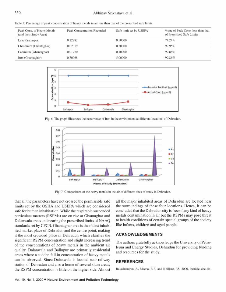
330 Abhinav Srivastava et al.
Vol. 19, No. 1, 2020 • Nature Environment and Pollution Technology
that all the parameters have not crossed the permissible safe limits set by the OSHA and USEPA which are considered safe for human inhabitation. While the respirable suspended particulate matters (RSPMs) are on rise at Ghantaghar and Dalanwala areas and nearing the prescribed limits of NAAQ standards set by CPCB. Ghantaghar area is the oldest inhab-ited market place of Dehradun and the centre point, making it the most crowded place in Dehradun which clarifies the significant RSPM concentration and slight increasing trend of the concentrations of heavy metals in the ambient air quality. Dalanwala and Ballupur are primarily residential areas where a sudden fall in concentration of heavy metals can be observed. Since Dalanwala is located near railway station of Dehradun and also a home of several slum areas, the RSPM concentration is little on the higher side. Almost
all the major inhabited areas of Dehradun are located near the surroundings of these four locations. Hence, it can be concluded that the Dehradun city is free of any kind of heavy metals contamination in air but the RSPMs may pose threat to health conditions of certain special groups of the society like infants, children and aged people.
ACKNOWLEDGEMENTS
The authors gratefully acknowledge the University of Petro-leum and Energy Studies, Dehradun for providing funding and resources for the study.
REFERENCES
Balachandran, S., Meena, B.R. and Khillare, P.S. 2000. Particle size dis-
21
Fig. 6: The graph illustrates the occurrence of Iron in the environment at different locations of
Dehradun.
Fig. 7: Comparisons of the heavy metals in the air of different sites of study in Dehradun.
Fig. 6: The graph illustrates the occurrence of Iron in the environment at different locations of Dehradun.
21
Fig. 6: The graph illustrates the occurrence of Iron in the environment at different locations of
Dehradun.
Fig. 7: Comparisons of the heavy metals in the air of different sites of study in Dehradun.
Fig. 7: Comparisons of the heavy metals in the air of different sites of study in Dehradun.
Table 5: Percentage of peak concentration of heavy metals in air less than that of the prescribed safe limits.
Peak Conc. of Heavy Metals (and their Study Area)
Peak Concentration Recorded Safe limit set by USEPA %age of Peak Conc. less than that of Prescribed Safe Limits
Lead (Sahaspur) 0.12882 0.50000 74.24%
Chromium (Ghantaghar) 0.02319 0.50000 99.95%
Cadmium (Ghantaghar) 0.01220 0.10000 99.88%
Iron (Ghantaghar) 0.70068 5.00000 99.86%

331QUANTIFICATION OF AIRBORNE HEAVY METALS AND RSPMS
Nature Environment and Pollution Technology • Vol. 19, No. 1, 2020
tribution and its elemental composition in the ambient air of Delhi. Environ. Int., 26: 49-54.
Chen, W.Q. and Graedel, T.E. 2012. Anthropogenic cycles of the elements: A critical review. Environ. Sci. Technol., 46: 8574-8586.
Duruibe, J.O., Ogwuegbu, M.O.C. and Egwurugwu, J.N. 2007. Heavy metal pollution and human biotoxic effects. Int. J. Phys. Sci., 2(5): 112-118.
Fung, Y.S. and Wong, L.W.Y. 1995. Apportionment of air pollution sources by receptor models in Hong Kong. Atmos. Environ., 29: 2041-2048.
Godish, T. 2004. Air quality, Chapter 2. In: Atmospheric Pollution and Pollutants, 4th Edition, Lewis Publishers.
Goyer, R.A. 2001. Toxic effects of metals. In: Klaassen C.D., (ed.) Cas-sarett and Doull’s Toxicology: The Basic Science of Poisons. New York: McGraw-Hill Publisher, pp. 811-867.
He, Z.L., Yang, X.E. and Stoffella, P.J. 2005. Trace elements in agro-ecosystems and impacts on the environment. J. Trace Elem. Med. Biol., 19: 125-140.
Herawati, N., Suzuki, S., Hayashi, K., Rivai, I.F. and Koyama, H. 2000. Cadmium, copper, and zinc levels in rice and soil of Japan, Indonesia, and China by soil type. Bull. Environ. Contam. Toxicol., 64: 33-39.
Kim, K.H., Kabir, E. and Kabir, S. 2015. A review on the human health impact of airborne particulate matter. Environ. Int., 74: 136-143.
Kulshrestha, A., Satsangi, P.G., Masih, J. and Taneja, A. 2009. Metal concentration of PM2.5 and PM10 particles and seasonal variations in urban and rural environment of Agra, India. Sci. Total Environ., 407: 6196-6204.
Kumar, A.V., Patil, R.S. and Nambi, K.S.V. 2001. Source apportionment of suspended particulate matter at two traffic junctions in Mumbai, India. Atmos. Environ., 35: 4245-4251.
Li, T., Hu, R., Chen, Z., Li, Q., Huang, S., Zhu, Z. and Zhou, L.F. 2018. Fine particulate matter (PM2. 5): The culprit for chronic lung diseases in China. Chronic. Dis. Transl. Med., 4: 176-186.
Loomis, D., Grosse, Y., Lauby-Secretan, B., El Ghissassi, F., Bouvard, V., Benbrahim-Tallaa, L., Guha, N., Baan, R., Mattock, H. and Straif, K. 2013. The carcinogenicity of outdoor air pollution. Lancet Oncol., 14: 1262-1263.
Mohanraj, R., Azeez, P.A. and Priscilla, T. 2004. Heavy metals in airborne
Table 6: Comparison of concentration of heavy metals in air at different parts of the world.
Location Pb Cd Cr Fe References
Spain 0.008 - 0.698 0.0001 - 0.004 0.0001 - 0.022 0.2 - 10.0 (Querol et. al. 2002)
Taiwan 0.133 -- 0.656 6.99 (Fung & Wong 1995).
Norway 0.00036 -0.01036 0.00001 -0.00028 0.00021 - 0.00156 -- (NILU 2002b).
Delhi 0.6 - 1.9 0.020 - 0.150 0.3 - 0.7 5.0 - 20.0 (Balachandran et. al. 2000).
Mumbai 1.06 -- 0.15 -- (Kumar et. al. 2001).
Kanpur 0.07 - 1.03 0.002 - 0.043 0.032 - 0.4 0.3 - 6.17 (Sharma & Maloo 2005).
Dehradun (Present Study) 0.0205 0.01178 0.0056975 0.4088 --
particulate matter of urban Coimbatore. Arch. Environ. Con. Tox., 47: 162-167.
NILU, 2002b. Heavy metals and POPS within the EMEP region 2000. EMEP/CCC-Report 9/2002, Norwegian Institute of Air Research, Kjeller, Norway.
Nriagu, J.O. and Pacyna, J.M. 1988. Quantitative assessment of worldwide contamination of air, water and soils by trace metals. Nature, 333: 134.
Querol, X., Alastuey, A., de la Rosa, J., Sánchez-de-la-Campa, A., Plana, F. and Ruiz, C.R. 2002. Source apportionment analysis of atmospheric particulates in an industrialised urban site in southwestern Spain. Atmos. Environ., 36: 3113-3125.
Rana, S. V. S. 2006. Environmental Pollution, Health and Toxicology. Alpha Science International Ltd., pp. 10-40.
Shallari, S., Schwartz, C., Hasko, A. and Morel, J.L. 1998. Heavy metals in soils and plants of serpentine and industrial sites of Albania. Sci. Total Environ., 209: 133-142.
Sharma, M. and Maloo, S. 2005. Assessment of ambient air PM10 and PM2.5 and characterization of PM10 in the city of Kanpur, India. Atmos. Environ., 39: 6015-6026.
Sharma, R.K., Agrawal, M. and Marshall, F.M. 2008. Atmospheric dep-osition of heavy metals (Cu, Zn, Cd and Pb) in Varanasi city, India. Environ. Monit. Assess., 142: 269-278.
Shridhar, V., Khillare, P.S., Agarwal, T. and Ray, S. 2010. Metallic species in ambient particulate matter at rural and urban location of Delhi. J. Hazard. Mater., 175: 600-607.
Thakur, M., Deb, M.K., Imai, S., Suzuki, Y., Ueki, K. and Hasegawa, A. 2004. Load of heavy metals in the airborne dust particulates of an urban city of central India. Environ. Monit. Assess., 95: 257-268.
Tohyama, C., Shaikh, Z.A., Nogawa, K., Kobayashi, E. and Honda, R. 1982. Urinary metallothionein as a new index of renal dysfunction in “Itai-itai” disease patients and other Japanese women environmentally exposed to cadmium. Arch. Toxicol., 50: 159-66.
USEPA 1999. Compendium of methods for the determination of inor-ganic compounds in ambient air. Compendium of Method IO-3.2, EPA/625/R-96/010a.
Yu, M., Tsunoda, H. and Tsunoda, M. 2011. Environmental Toxicology: Biological and Health Effects of Pollutants. CRC Press.

Vol. 19, No. 1, 2020 • Nature Environment and Pollution Technology
332

Adsorption Process of Ammonia Nitrogen in Solution by the Modified Biochar from Corn Straw
Ruolin Xu*, Li Han*, Chengcai Huang*, Hao Zhang**, Rui Qin*, Linli Zhang* and Muqing Qiu*†*College of Life Science, Shaoxing University, Shaoxing, 312000, P.R. China**Key Laboratory of Agro-Ecological Processes in Subtropical Region, Institute of Subtropical Agriculture, Chinese Academy of Sciences, Changsha, 410125, China†Corresponding Author: Muqing Qiu
ABSTRACT
The biochar was prepared by pyrolyzing corn straw at 773 K temperature under an oxygen-limited condition. Then, the gained biochar samples were further modified with MgCl2 solution through mixing method for 3 h at the speed of 120 rpm. The physicochemical properties of the modified biochar from corn straw were investigated by surface area analysis, elemental analysis, scanning electron microscope, X-ray diffraction and Fourier transform infrared spectroscopy spectra. The adsorption experiments of ammonia nitrogen in aqueous solution by modified biochar were carried out. The results showed that the modified biochar contains high surface area, rough surface and a lot of oxygen-containing functional groups. The adsorption process fits well with the pseudo-second-order kinetics equation and Langmuir isotherm equation. The adsorption mechanism of modified biochar to NH4
+ ion in aqueous solution includes ion exchange and physical adsorption. The ion exchange is primary in the process of adsorption.
INTRODUCTION
With the rapid development of industry and agriculture, the emission of eutrophic substances, such as nitrogen element and phosphorus element, has also increased in China (Liu et al. 2010). The eutrophication of water bodies is harmful to environment. Therefore, research on an efficient method to treatment the eutrophication of water bodies has become a hot studying area for many scholars (Duan et al. 2012, Haseena et al. 2016).
For a long time, in order to control the eutrophication of water bodies, many scholars have begun to study on the removal methods of nitrogen and phosphorus in water bodies, such as adsorption, chemical oxygen, ions exchange and so on (Christoph & Thomas 2009, García-Martínez et al. 2018). Among these methods, the adsorption method is widely applied because of its simple operation process, high efficiency and nontoxic by-products (Qiu et al. 2018, Seabra et al. 2019). The development and utilization of ad-sorbents is an important research content of the adsorption method (Tokay et al. 2010). Biochar is a rich carbon solid prepared by pyrolyzing biomass under anoxic or anaerobic and low temperature conditions. It is an excellent adsorption material with well-developed pore structure, large specific surface area, rich oxygen-containing functional groups and excellent adsorption properties (Rahmati & Modarress 2009,
Paz-Ferreiro et al. 2018). Therefore, in order to obtain biochar with superior adsorption performance, many scholars began to explore the effects of biochar raw materials, pyrolysis temperature and modification conditions on the physical and chemical properties of biochar (Herrera et al. 2008, Hu et al. 2017). Raw materials for the production of biochar include agricultural and forestry waste, such as straw, weeds, wood chips, manure and so on. Among them, the agricultural straw waste is the main biochar raw material. It consists mainly of cellulose, hemicellulose and lignin (Ryu et al. 2000, Moghaddam et al. 2010, Vinitnantharat et al. 2010, Siswoyo et al. 2014). In China, every year, a large amount of agricul-tural straw is produced, but the utilization rate of agricultural straw is very low. The new method of seeking the resource utilization of agricultural straw has been concerned by many researchers (Sprynskyy et al. 2005, Gendel & Lahav 2013).
In this paper, the biochar was prepared by pyrolyzing corn straw under an oxygen-limited condition. Then, the biochar samples were modified with MgCl2 solution. The adsorption experiments of ammonia nitrogen in solution were carried out. The main object of this study is, (1) the characteristic of the modified biochar from corn straw. The obtained modified biochar from corn straw was determined by surface area analysis, elemental analysis, scanning electron microscope, X-ray diffraction and Fourier transform infrared spectroscopy spectra respectively. (2) The
Nat. Env. & Poll. Tech.Website: www.neptjournal.com
Received: 03-04-2019 Accepted: 02-07-2019
Key Words:Adsorption Ammonia nitrogen Modified biochar Corn straw
2020pp. 333-338 Vol. 19
p-ISSN: 0972-6268 No. 1 Nature Environment and Pollution Technology An International Quarterly Scientific Journal
Original Research Paper
e-ISSN: 2395-3454
Open Access

334 Chengcai Huang et al.
Vol. 19, No. 1, 2020 • Nature Environment and Pollution Technology
adsorption kinetic and adsorption isotherm of ammonia nitrogen in solution by the modified biochar were studied. (3) The adsorption mechanism of ammonia nitrogen in solution by the modified biochar is discussed in details.
MATERIALS AND METHODS
The Preparation of The Modified Biochar
The corn straws are collected from farmland in the suburbs of Dongyang City, Zhejiang Province. They were washed several times with water, and dried to a constant weight at 378 K, pulverized and passed through a 40 meshes sieve. 20 g of sample was pyrolyzed for 3 h under a nitrogen atmosphere at a temperature of 773 K. After cooling to room temperature, it was pulverized to 80 meshes. Then, the biochar from corn straw was obtained.
10 g biochar was added to the 1000 mL beaker containing 500 mL 0.01 mol/L MgCl2. Then the mixture was stirred for 3 h at the speed of 120 rpm. The sample is filtered, washed with distilled water and dried to constant weight at 378 K. Then, the modified biochar by MgCl2 solution was obtained.
Adsorption Experiments
Adsorption experiments were conducted in a set of 250 mL Erlenmeyer flasks containing modified biochar and 100 mL of NH4
+ with initial concentrations in aqueous solution. The flasks were placed in a shaker at a constant temperature of 298 K and 120 rpm. The samples were then filtered and the residual concentration of NH4
+ was analysed using Nessler reagent spectrophotometry.
Analytical Method
The concentration of NH4+ ion in solution was measured with
a UV-1600 spectrophotometer. The adsorption capacity of NH4
+ was calculated as following:
qC C
mee=
-( ) ¥0 V …(1)
Where, C0 and Ce (mg/L) are the initial and equilibrium concentrations of NH4
+ in solution respectively. qe (mg/g) is adsorption amount per unit mass of the modified biochar at adsorption equilibrium. V (mL) is volume of solution, m (g) is the mass of the modified biochar.
The physicochemical properties of the modified biochar from corn straw were investigated by surface area analy-sis (ASAP 2460), elemental analysis (EURO EA 3000), scanning electron microscope (Ultra 55), X-ray diffraction (Ulitma IV) and Fourier transform infrared spectroscopy spectra (Nicolet 5700).
RESULTS AND DISCUSSION
The Structural Characteristics and Properties of the Modified Biochar
The elements of C, H, O and N of the modified biochar are determined. They are 69.24%, 3.64%, 15.21% and 0.51% respectively. BET specific surface area of the modified biochar is 98.86 m2/g, and the total of pore volume is 0.1236 cm3/g.
The scanning electron micrograph of the modified bio-char is shown in Fig. 1. From Fig.1, it can be shown that the microporous edge on the surface of the modified biochar is ablated by high temperature, and the distribution of the pores becomes disordered. It increases the surface roughness of the modified biochar, and it will benefit to improve the adsorption capacity.
The XRD spectrum is shown in Fig. 2. From Fig. 2, it can be thought that it is assigned to be broad and diffuse peak when 2q is ranged from 15° to 22°. It is assigned to be quartz diffraction peak at 26.5°. It is assigned to be three potassium salt diffraction peaks at 28.5°, 40.6° and 50.5°. It
Fig. 1: SEM image of the modified biochar.
The XRD spectrum is shown in Fig. 2. From Fig. 2, it can be thought that it is
assigned to be broad and diffuse peak when 2θ is ranged from 15° to 22°. It is
assigned to be quartz diffraction peak at 26.5°. It is assigned to be three potassium salt
diffraction peaks at 28.5°, 40.6° and 50.5°. It is assigned to be diffraction peaks at
42.7°. This peak should be the characteristic peak of MgO. It indicates that Mg2+ ions
have been loaded on the biochar.
Fig. 2: X-ray diffraction spectrum of the modified biochar from corn straw.
From Fig. 3, there is a C = O absorption peak at 1702 cm-1. They were assigned to be
acyclic ring C = C stretching vibration peak, C = O stretching vibration peak and
phenolic hydroxyl stretching vibration peak respectively, at 1609 cm-1, 1442 cm-1 and
1259 cm-1. It was assigned to be C – O stretching vibration peak at 1068 cm-1. They
were assigned to be C - H stretching vibration peak between 649 cm-1 and 878 cm-1.
The modified biochar contains an increased number of oxygen-containing functional
groups and an increased polarity.
Fig. 1: SEM image of the modified biochar.

335ADSORPTION OF AMMONIA IN SOLUTION BY MODIFIED BIOCHAR
Nature Environment and Pollution Technology • Vol. 19, No. 1, 2020
In order to describe the adsorption kinetic of NH4+ ion
by the modified biochar, pseudo-first-order kinetic equation and pseudo-second-order kinetic equation were adopted in this study. Their equations are as follows (Eugene 2016):
q q et eK t= -( )-1 1 …(2)
t
q K q
t
qt e e
= +1
22
…(3)
Where qt (mg/g) and qe (mg/g) are adsorption capacity of NH4
+ ion solution by modified biochar at adsorption time t and adsorption equilibrium respectively. K1 (min-1) and K2 (min-1) are the adsorption rate constant.
According to Eq. (2) and Eq. (3), the results are shown in Table 1.
From Table 1, it can be shown that the adsorption process fits well with the pseudo-second-order kinetics equation according to the value of R2 (0.9984). It implies that the predominant process is chemisorption, which involves a sharing of electrons between the adsorbate and the surface of the adsorbent.
Adsorption Isotherm
In order to investigate the adsorption isotherm, the adsorption test was carried out. Adsorption experiments were conduct-ed in a set of 250 mL Erlenmeyer flasks containing 0.05 gmodified biochar and 50 mL of NH4
+ ion with initial concentrations (5, 10, 25, 40, 50 mg/L) in aqueous solution. The flasks were placed in a shaker at a constant
is assigned to be diffraction peaks at 42.7°. This peak should be the characteristic peak of MgO. It indicates that Mg2+ ions have been loaded on the biochar.
From Fig. 3, there is a C = O absorption peak at 1702 cm-1. They were assigned to be acyclic ring C = C stretching vibration peak, C = O stretching vibration peak and phenolic hydroxyl stretching vibration peak respectively, at 1609 cm-1, 1442 cm-1 and 1259 cm-1. It was assigned to be C – O stretching vibration peak at 1068 cm-1. They were assigned to be C - H stretching vibration peak between 649 cm-1 and 878 cm-1. The modified biochar contains an increased number of oxygen-containing functional groups and an increased polarity.
Adsorption Kinetic
In order to investigate the adsorption kinetics, the adsorption test was carried out. Adsorption experiments were conducted in a set of 250 mL Erlenmeyer flasks containing 0.05 g modified biochar and 50 mL 25 mg/L of NH4Cl in aqueous solution. The flasks were placed in a shaker at a constant temperature of 298 K and 120 rpm. The reaction time is 5, 10, 15, 20, 30, 40, 60, 80, 120, 180, 240, 360 and 420 min respectively. The samples were then filtered and the residual concentration of NH4
+ was analysed using Nessler reagent spectrophotometry.
The experimental results were shown in Fig. 4. In the initial stage, the adsorption amount of NH4
+ ion by the modified biochar increases rapidly. Then, it tends to balance slowly.
Fig. 1: SEM image of the modified biochar.
The XRD spectrum is shown in Fig. 2. From Fig. 2, it can be thought that it is
assigned to be broad and diffuse peak when 2θ is ranged from 15° to 22°. It is
assigned to be quartz diffraction peak at 26.5°. It is assigned to be three potassium salt
diffraction peaks at 28.5°, 40.6° and 50.5°. It is assigned to be diffraction peaks at
42.7°. This peak should be the characteristic peak of MgO. It indicates that Mg2+ ions
have been loaded on the biochar.
Fig. 2: X-ray diffraction spectrum of the modified biochar from corn straw.
From Fig. 3, there is a C = O absorption peak at 1702 cm-1. They were assigned to be
acyclic ring C = C stretching vibration peak, C = O stretching vibration peak and
phenolic hydroxyl stretching vibration peak respectively, at 1609 cm-1, 1442 cm-1 and
1259 cm-1. It was assigned to be C – O stretching vibration peak at 1068 cm-1. They
were assigned to be C - H stretching vibration peak between 649 cm-1 and 878 cm-1.
The modified biochar contains an increased number of oxygen-containing functional
groups and an increased polarity.
Fig. 2: X-ray diffraction spectrum of the modified biochar from corn straw.
Fig. 3: Infrared spectrum of the modified biochar from corn straw.
Adsorption Kinetic
In order to investigate the adsorption kinetics, the adsorption test was carried out.
Adsorption experiments were conducted in a set of 250 mL Erlenmeyer flasks
containing 0.05 g modified biochar and 50 mL 25 mg/L of NH4Cl in aqueous solution.
The flasks were placed in a shaker at a constant temperature of 298 K and 120 rpm.
The reaction time is 5, 10, 15, 20, 30, 40, 60, 80, 120, 180, 240, 360 and 420 min
respectively. The samples were then filtered and the residual concentration of NH4+
was analysed using Nessler reagent spectrophotometry.
The experimental results were shown in Fig. 4. In the initial stage, the adsorption
amount of NH4+ ion by the modified biochar increases rapidly. Then, it tends to
balance slowly.
Fig. 3: Infrared spectrum of the modified biochar from corn straw.
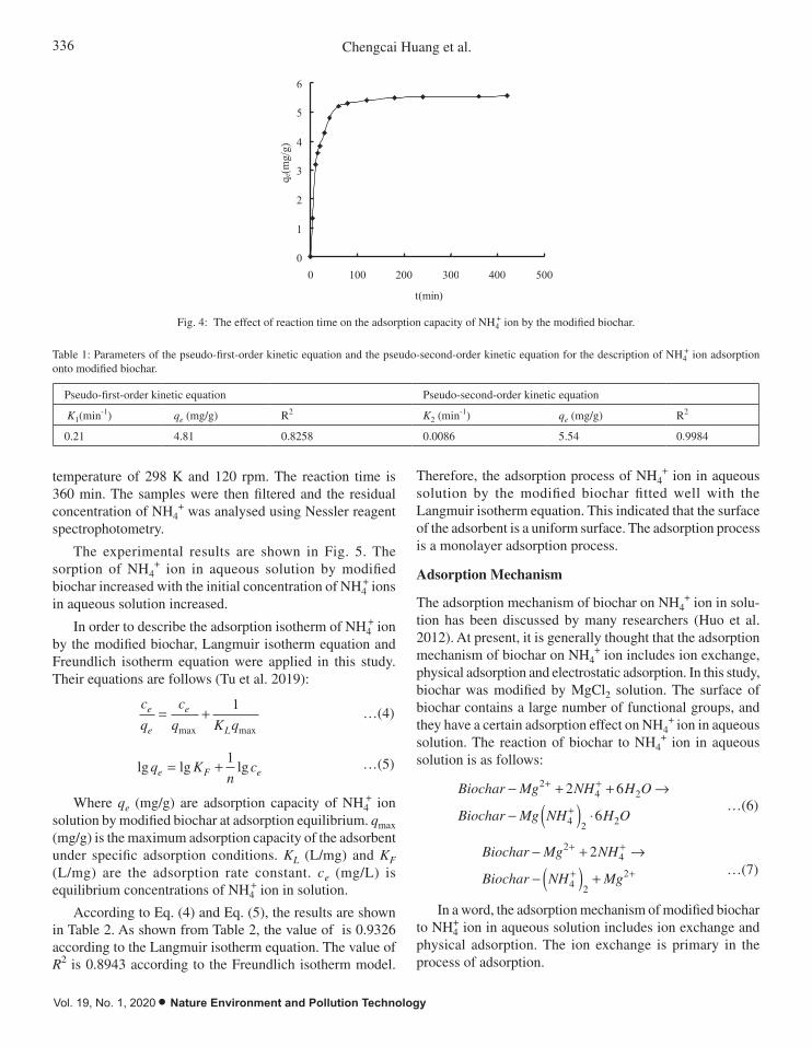
336 Chengcai Huang et al.
Vol. 19, No. 1, 2020 • Nature Environment and Pollution Technology
temperature of 298 K and 120 rpm. The reaction time is 360 min. The samples were then filtered and the residual concentration of NH4
+ was analysed using Nessler reagent spectrophotometry.
The experimental results are shown in Fig. 5. The sorption of NH4
+ ion in aqueous solution by modified biochar increased with the initial concentration of NH4
+ ions in aqueous solution increased.
In order to describe the adsorption isotherm of NH4+ ion
by the modified biochar, Langmuir isotherm equation and Freundlich isotherm equation were applied in this study. Their equations are follows (Tu et al. 2019):
c
q
c
q K qe
e
e
L
= +max max
1 …(4)
lg lg lgq Kn
ce F e= +1 …(5)
Where qe (mg/g) are adsorption capacity of NH4+ ion
solution by modified biochar at adsorption equilibrium. qmax (mg/g) is the maximum adsorption capacity of the adsorbent under specific adsorption conditions. KL (L/mg) and KF(L/mg) are the adsorption rate constant. ce (mg/L) is equilibrium concentrations of NH4
+ ion in solution.
According to Eq. (4) and Eq. (5), the results are shown in Table 2. As shown from Table 2, the value of is 0.9326 according to the Langmuir isotherm equation. The value of R2 is 0.8943 according to the Freundlich isotherm model.
Therefore, the adsorption process of NH4+ ion in aqueous
solution by the modified biochar fitted well with the Langmuir isotherm equation. This indicated that the surface of the adsorbent is a uniform surface. The adsorption process is a monolayer adsorption process.
Adsorption Mechanism
The adsorption mechanism of biochar on NH4+ ion in solu-
tion has been discussed by many researchers (Huo et al. 2012). At present, it is generally thought that the adsorption mechanism of biochar on NH4
+ ion includes ion exchange, physical adsorption and electrostatic adsorption. In this study, biochar was modified by MgCl2 solution. The surface of biochar contains a large number of functional groups, and they have a certain adsorption effect on NH4
+ ion in aqueous solution. The reaction of biochar to NH4
+ ion in aqueous solution is as follows:
Biochar Mg NH H O
Biochar Mg NH H O
- + + Æ
- ( ) ◊
+ +
+
24 2
4 2 2
2 6
6 …(6)
Biochar Mg NH
Biochar NH Mg
- + Æ
- ( ) +
+ +
+ +
24
4 2
2
2 …(7)
In a word, the adsorption mechanism of modified biochar to NH4
+ ion in aqueous solution includes ion exchange and physical adsorption. The ion exchange is primary in the process of adsorption.
Fig. 4: The effect of reaction time on the adsorption capacity of NH4+ ion by the
modified biochar.
In order to describe the adsorption kinetic of NH4+ ion by the modified biochar,
pseudo-first-order kinetic equation and pseudo-second-order kinetic equation were
adopted in this study. Their equations are as follows (Eugene 2016):
tKet eqq 11 …(2)
eet qt
qKqt
22
1 …(3)
Where qt (mg/g) and qe (mg/g) are adsorption capacity of NH4+ ion solution by
modified biochar at adsorption time t and adsorption equilibrium respectively. K1
(min-1) and K2 (min-1) are the adsorption rate constant.
According to Eq. (2) and Eq. (3), the results are shown in Table 1.
Table 1: Parameters of the pseudo-first-order kinetic equation and the pseudo-second-
0
1
2
3
4
5
6
0 100 200 300 400 500
t(min) q e
(mg/
g)
Fig. 4: The effect of reaction time on the adsorption capacity of NH4+ ion by the modified biochar.
Table 1: Parameters of the pseudo-first-order kinetic equation and the pseudo-second-order kinetic equation for the description of NH4+ ion adsorption
onto modified biochar.
Pseudo-first-order kinetic equation Pseudo-second-order kinetic equation
K1(min-1) qe (mg/g) R2 K2 (min-1) qe (mg/g) R2
0.21 4.81 0.8258 0.0086 5.54 0.9984

337ADSORPTION OF AMMONIA IN SOLUTION BY MODIFIED BIOCHAR
Nature Environment and Pollution Technology • Vol. 19, No. 1, 2020
CONCLUSIONS
Through the above experiments and discussions, the follow-ing results can be obtained.
1. The elements of C, H, O and N of the modified biochar were determined. They are 69.24%, 3.64%, 15.21% and 0.51% respectively. BET specific surface area of the modified biochar is 98.86 m2/g, and the total of pore volume is 0.1236 cm3/g. The distribution of the pores on the surface of modified biochar becomes disordered. The modified biochar contains a lot of oxygen-contain-ing functional groups.
2. The adsorption process fits well with the pseudo-sec-ond-order kinetics equation. The predominant process is chemisorption, which involves a sharing of electrons between the adsorbate and the surface of the adsorbent. The adsorption process of NH4
+ ion in aqueous solution by the modified biochar fitted well with the Langmuir isotherm equation. The adsorption process is a mon-olayer adsorption process.
3. The adsorption mechanism of modified biochar to NH4
+ ion in aqueous solution includes ion exchange and physical adsorption. The ion exchange is primary in the process of adsorption.
ACKNOWLEDGEMENTS
This study was financially supported by the project of science and technology plan in Zhejiang Province (LG-
Fig. 5: The effect of initial concentration of NH4
+ ion on the adsorption capacity of
NH4+ ion by the modified biochar.
In order to describe the adsorption isotherm of NH4+ ion by the modified biochar,
Langmuir isotherm equation and Freundlich isotherm equation were applied in this
study. Their equations are follows (Tu et al. 2019):
maxmax
1qKq
cqc
L
e
e
e …(4)
eFe cn
Kq lg1lglg …(5)
Where qe (mg/g) are adsorption capacity of NH4+ ion solution by modified biochar at
adsorption equilibrium. qmax (mg/g) is the maximum adsorption capacity of the
adsorbent under specific adsorption conditions. KL (L/mg) and KF (L/mg) are the
adsorption rate constant. ce (mg/L) is equilibrium concentrations of NH4+ ion in
solution.
According to Eq. (4) and Eq. (5), the results are shown in Table 2. As shown from
Table 2, the value of 2R is 0.9326 according to the Langmuir isotherm equation. The
value of 2R is 0.8943 according to the Freundlich isotherm model. Therefore, the
adsorption process of NH4+ ion in aqueous solution by the modified biochar fitted
well with the Langmuir isotherm equation. This indicated that the surface of the
0
2
4
6
8
10
12
14
0 10 20 30 40 50 60
C0(mg/L)
q e(m
g/g)
Fig. 5: The effect of initial concentration of NH4+ ion on the adsorption capacity of NH4
+ ion by the modified biochar.
Table 2: Parameters of Langmuir isotherm equation and Freundlich isotherm equation for the description of NH4+ ion adsorption onto the modified biochar.
Langmuir Freundlich
qmax (mg/g) KL R2 KF n R2
5.12 0.26 0.9326 1.74 4.09 0.8943
F19C030001), Guangxi Key Research and Development Program (AB17129002 and AB18050018) and the project of science and technology plan in Shaoxing City (2017B70058).
REFERENCES
Christoph, R. and Thomas, B. 2009. Adsorption of nitrogen and ammonia at zirconia surfaces. J. Mol. Struc., Theochem., 903: 89-99.
Duan, X.H., Srinivasakannan, C., Qu, W.W., Wang, X., Peng, J.H. and Zhang, L.B. 2012. Regeneration of microwave assisted spent activated carbon: process optimization, adsorption isotherms and kinetics. Chem. Eng. Process., 53: 53-62.
Eugene, A.U. 2016. Effect of crystallization and surface potential on the nitrogen adsorption isotherm on graphite: A refined Monte Carlo sim-ulation. Carbon, 100: 52-63.
García-Martínez, J.C., González, H.A., Uribe, M.M., González-Bram-bila, J.A., Colín-Luna, Y.E., Escobedo-García, A., López-Gaona, L. and Alvarado, P. 2018. Selective adsorption of nitrogen compounds using silica-based mesoporous materials as a pretreatment for deep hydrodesulfurization. Catal. Today, 305: 40-48.
Haseena, P.V., Padmavathy, K.S., Krishnan, P.R. and Madhu, G. 2016. Adsorption of ammonium nitrogen from aqueous systems using chitosan-bentonite film composite. Procedia Tech., 24: 733-740.
Herrera, L.F., Do, D.D. and Birkett, G.R. 2008. Comparative simulation study of nitrogen and ammonia adsorption on graphitized and non graphitized carbon blacks. J. Colloid Interf. Sci., 320: 415-422.
Hu, B.W., Qiu, M.Q., Hu, Q.Y., Sun, Y.B., Sheng, G.D., Hu, J. and Ma, J.Y. 2017. Decontamination of Sr(II) on magnetic polyaniline/graphene oxide composites: evidence from experimental, spectroscopic, and modeling investigation. ACS Sustain. Chem. Eng., 5: 6924-6931.
Huo, H.X., Lin, H., Dong, Y.B., Cheng, H., Wang, H. and Cao, L.X. 2012. Ammonia-nitrogen and phosphates sorption from simulated reclaimed waters by modified clinoptilolite. J. Hazard. Mater., 229-230: 292-297.
Gendel, Y. and Lahav, D. 2013. A novel approach for ammonia removal

338 Chengcai Huang et al.
Vol. 19, No. 1, 2020 • Nature Environment and Pollution Technology
from fresh-water recirculated aquaculture systems, comprising ion exchange and electrochemical regeneration. Aquacult. Eng., 52: 27-38.
Liu, H.E., Dong, Y.H., Liu, Y. and Wang, H.Y. 2010. Screening of novel low-cost adsorbents from agricultural residues to remove ammonia nitrogen from aqueous solution. J. Hazard. Mater., 178: 1132-1136.
Moghaddam, S.S., Moghaddam, M.R.A. and Arami, M. 2010. Coagulation/flocculation process for dye removal using sludge from water treatment plant: Optimization through response surface methodology. J. Hazard. Mater., 175: 651-657.
Paz-Ferreiro, J., Marinho, M.A., Abreu, C.A. and Vidal-Vázquez, E. 2018. Soil texture effects on multifractal behaviour of nitrogen adsorption and desorption isotherms. Biosystems Eng., 168: 121-132.
Qiu, M.Q., Wang, M., Zhao, Q.Z., Hu B.W. and Zhu, Y.L. 2018. XANES and EXAFS investigation of uranium incorporation on nZVI in the presence of phosphate. Chemosphere, 201: 764-771.
Rahmati, M. and Modarress, H. 2009. Nitrogen adsorption on nanoporous zeolites studied by Grand Canonical Monte Carlo simulation. J. Mol. Struc. Theochem., 901: 110-116,
Ryu, Z.Y., Zheng, J.T., Wang, M.Z. and Zhang, B.J. 2000. Nitrogen adsorp-tion studies of PAN-based activated carbon fibers prepared by different activation methods. J. Colloid Interf. Sci., 230: 312-319.
Seabra, R., Ribeiro, A.M., Gleichmann, K., Ferreira, A.F.P. and Rodrigues, A.E. 2019. Adsorption equilibrium and kinetics of carbon dioxide, methane and nitrogen on binderless zeolite 4A adsorbents. Micropor. Mesopor. Mat., 277: 105-114.
Siswoyo, E., Mihara, Y. and Tanaka, S. 2014. Determination of key compo-nents and adsorption capacity of a low cost adsorbent based on sludge of drinking water treatment plant to adsorb cadmium ion in water. Appl. Clay Sci., 97-98: 146-152.
Sprynskyy, M., Lebedynets, M., Zbytniewski, R., Namiesnik, J. and Busze-wski, B. 2005. Ammonium removal from aqueous solution by natural zeolite, transcarpathian mordenite, kinetics, equilibrium and column tests. Sep. Purif. Technol., 46: 155-160.
Tokay, B., Karvan, O. and Erdem-Şenatalar, A. 2010. Nanoparticle silicalite-1 crystallization as monitored by nitrogen adsorption. Micropor. Mesopor. Mater., 131: 230-237.
Tu, Y.N., Feng, P., Ren, Y.G., Cao, Z.H., Wang, R. and Xu, Z.Q. 2019. Adsorption of ammonia nitrogen on lignite and its influence on coal water slurry preparation. Fuel, 238: 34-43.
Vinitnantharat, S., Kositchaiyong, S. and Chiarakorn, S. 2010. Removal of fluoride in aqueous solution by adsorption on acid activated water treatment sludge. Appl. Surf. Sci., 256: 5458-5462.

Imperious Approach Towards Justifiable Strategic Lake Sediment Regulation
Shekhar Salunke* and Balbhim Chavan** *Dept. of Environmental Science, Solapur University, Solapur, Maharashtra, India** Dept of Environmental Science, Dr. B.A.M. University, Aurangabad, Maharashtra, India
ABSTRACT
Lakes are extremely appreciated for the ecological, aesthetic and recreational values supporting rich biodiversity. As such, their preservation is of supreme importance. A global common problem of sedimentation that eventually seems to be responsible for eutrophication should be immediately attended to, before the degradation begins, since the restoration measures are expensive and may go beyond control. Erosion causes detachment, transportation and deposition of sediments and is the prime source of contamination where it accumulates in lakes and interrupts the ecological processes and functioning in the lake ecosystem, hence it is important to determine the risk to design management strategies for control.For the present investigation, thematic layers slope identification, NDVI, LULC, lineament density and RUSLE were employed to compute spatially distributed erosion and contaminant sources for the lake Ekrukh of Solapur district of Maharashtra State, India. The research identifies five hazardous erosion zones as; low, moderate, high, very high and severe, through the applied model and dictates formulation and implementation of innovative control strategies preventing soil and water (surface) pollution. The Soil Erosion in Maharashtra, Technical Bulletin, 2001 (Challa et al. 2001) was also referred for the studies.
INTRODUCTION
Exploration and delineation of erosion zones is important to design control strategies to prevent erosion at lakes, since the main problem faced by the lakes across the globe is siltation. Massive quantities of sediments add to the lake waters resulting in decreased water retaining capacity and increased nutrients that deteriorates the ecological health of the lakes. The eutrophic conditions of the lake indicate the presence of abundant aquatic weeds along the shoreline. As a lake or reservoir becomes rich in nutrients, it develops dense populations of planktonic algae that usually dominate. Such intense populations create unacceptable taste and odour problems, along with an increase in organic loading of the lower layers as the algae complete their life cycle and fall to the bottom. This reduces the aesthetic value of the lakes. Aside from the aesthetic deterioration of water quality, eu-trophication presents many other difficulties for the aquatic life. Such water is less palatable, algae-laden water has high chlorine and coagulant demands. It often reduces filter runs, necessitating excessive backwash; it may also require certain specific forms of taste and odour control such as activated carbon, chlorine, dioxide, or permanganate. This increases the cost of lake management programmes. Certainly, a pre-ventive measure calls an immediate attention rather than to cure later. As such the siltation through soil erosion should be controlled as an action with respect to the phrase ‘prevention is better than cure’. For the reason, it is necessary to ascertain the erosion possibilities at the lakes and to define the control
measures to avoid siltation. The aim can be better achieved by operating various methodological processes through Remote Sensing and Geographic Information System (GIS) techniques. As such, to define restoration strategies, a study was undertaken to understand the erosion sources and status of the lake Ekrukh. Previously our studies indicated two models to prevent or avoid siltation at the lake and were assessed to be effective in reducing the silt loads at the lake waters. However, to determine the sites of installations for the designed models to reduce silt loading, Lake Ekrukh was assessed for the significant sites of silt loading.
MATERIALS AND METHODS
Digital Data
The conduct of the investigative approach included the use of LANDSAT-7. Enhanced Thematic Mapper (ETM+) digital data was used, during fieldwork 200 Ground Control Points (GCPs) were collected with attributes using a handheld Global Positioning System (GPS) receiver with an expected error of 3-4 m. This data was used for georeferencing and ground truthing, as well as for accuracy assessment of the imageries and DEMs. Soil samples were also collected for the Revised Universal Soil Loss Equation (RUSLE).
NDVI Classification
NDVI (Normalized Difference Vegetation Index) at red wave-lengths and lower reflectance at near-infrared wavelengths was used to differentiate between healthy, stressed vegetation
Nat. Env. & Poll. Tech.Website: www.neptjournal.com
Received: 03-07-2019Accepted: 29-08-2019
Key Words:Erosion Sedimentation Control strategies Restoration actions
2020pp.339-348 Vol. 19
p-ISSN: 0972-6268 No. 1 Nature Environment and Pollution Technology An International Quarterly Scientific Journal
Original Research Paper
e-ISSN: 2395-3454
Open Access

340 Shekhar Salunke and Balbhim Chavan
Vol. 19, No. 1, 2020 • Nature Environment and Pollution Technology
and sparse or non-vegetated surface. High NDVI was classi-fied as healthy and growing vegetation and low NDVI was considered to locate areas that absorb red and near-infrared radiations, like water. The analysis of the topography was done by constructing. NDVI was used for identification of bare and sparse vegetation surface, where infiltration of contaminated water is more. Using the reflectance images of band 3 (red) and band 4 (Near InfraRed – NIR) NDVI map of the study areas were generated as followed by Joshi et. al (2004).
LULC Classification
Land Use/Land Cover (LULC) classification map was gen-erated for analysis using ERDAS Imagine 9. Ground truth and topographic sheets were used for accuracy assessment. Digital Terrain Model (DTM) was created with the help of DEM data by creating terrain surface and adding attributes and colour code to each pixel. A classified slope map was prepared with the spatial analyst module in ArcGIS envi-ronment. Soil erosion zones were identified along with the accumulation points.
DTM
DTM was carried out for the basins of study areas for the interpretation of geomorphology of the area, to delineate lineaments and to generate digital drainage from DEM, rep-resented in the respective figures for the DTM of the basins under the study areas.
Ground Data
Regarding the ground data, during fieldwork 200 ground control points (GCPs) were collected with attributes using a handheld global positioning system (GPS) receiver with an expected error of 3-4 m. This data was used for georeferenc-ing and ground truthing, as well as for accuracy assessment of the imageries and DEMs. Soil samples were also collected for the Revised Universal Soil Loss Equation (RUSLE). Filled and finished Shuttle Radar Topographic Mission (SRTM) data of 3arc second WRS-2 of 90 m resolution was downloaded from the GLCF website. Two tiles of height data (SRTM_ff03_p145r048.tifand SRTM_ff03_p146r047.tif) of WRS-2 have been used for the pre-processing and generation of the DEM followed by mosaic and image subset of the study area clipped from the whole scene. This work analyses LANDSAT 7 ETM+ and SRTM DEM data for the generation of erosional and contamination zones in the study areas. The flow chart has been applied for the lake studies.
RUSLE Parameters
All the RUSLE parameters determined for the study area were either in spatial format and/or in numerical format. The results of R, K, and C factors are assigned to each pixel of DEMs of the basin, as there is no variation in the results. The variables in the results of LS and P factors assigned to DEMs of the basin is presented in, for LS-factor 7 and 8 for P factor. The spatial maps were integrated using RUSLE
Fig. 1: NDVI classification of Ekrukh Lake basin.

341IMPERIOUS APPROACH FOR STRATEGIC LAKE SEDIMENT REGULATION
Nature Environment and Pollution Technology • Vol. 19, No. 1, 2020
Fig. 2: LULC classification of Ekrukh.
empirical formula for the lake, basin. In the present study, LANDSAT-7 Enhanced Thematic Mapper (ETM+) digital data was used. Landsat-7 ETM+ as it is a multispectral scanner that provides a multispectral image data set in eight spectral bands. Pre-processing of images was carried out by ortho-rectification and geometrical correction. A Landsat 7 ETM+ image (path 146/ row 047 and path 145/ row 048) of Solapur and surroundings was acquired, for the study. The digital data was radiometrically corrected to remove atmospheric effects. Further the digital numbers of the pixels were converted to reflectance to understand reflectance of the objects on the earth. The soil credibility factor K of the USLE is evaluated according to soil texture classification using the values from Stewart et al. (1975) considering that the organic matter content is less than 4%.
RESULTS AND DISCUSSION
NDVI
Low NDVI values (Fig. 1) in all three lakes indicate water bodies while higher values dictate healthy vegetation. The NDVI of Ekrukh Lake Basin shows healthy vegetation (green colour), either cultivated or non-cultivated, are located along its periphery. The blue coloured area, even near to lake, indicates presence of non-healthy vegetation around Tama-lwadi, Mardi, Raleras, Kasegaon and Ule may be because of contaminated sediments transported from upper reaches of the streams.
LULC
Fig. 2 represents LULC classification of Ekrukh. The area
denoted as artificial area is settlement zone. The area is con-sidered as a source of contamination and assigned a highest number in statistical and weighted overlay analysis.
DTM
DTM was carried out for the Ekrukh lake basin for the interpretation of geomorphology of the area, to delineate lineaments and to generate digital drainage from DEM. Fig. 3 represents the DTM of the basin in the study area.
Geomorphology of The Area
The study area falls in the sub-basin of Seena River, which is a tributary of Bhima River. The Bhima River itself is a tributary of Krishna River. The Krishna River has developed its basin in regional scale. Krishna River generated its plain by depositing transported load of sediments. The study area is a small part of the Krishan River basin. Geomorpholog-ically three basins of the area are lying in the almost plain to rolling topography. Variations in the elevation are very less. This topography represents peneplain stage of erosion cycle. The streams in the area have reached their graded stage and they are flowing over the sediments deposited by their own.
Two small hillocks are located in the NE direction of Ekrukh basin at an elevation of 589 m above mean sea level (Fig. 3). The elevation difference is about 139 m spatially distributed in the 378.6309 sq. km. area of the Ekrukh basin. Geomorphologically these small isolated hillocks are insel-bergs, ruminants of hills after erosion. The slopes on these hills are sources of sediments for erosion and transportation.

342 Shekhar Salunke and Balbhim Chavan
Vol. 19, No. 1, 2020 • Nature Environment and Pollution Technology
Drainages and Lineaments
Digital drainage network extraction and analysis has been carried out using DEM. Digital data (SRTM DEM) and non-digital data (1:50,000 scale topographic maps) were used to extract channel networks. An extraction of the channel network from digital data was carried out in the ArcGIS 9.3 environment using D8 algorithm of ArcHydromodule. Both river ‘basins’ and ‘watersheds’ are areas of land that drain to a water body, such as a lake, stream, river or estuary. In a river basin, all the water drains to a large river. The term ‘watershed’ is used to describe a smaller area of land that drains to a smaller stream, lake or wetland. Figs. 4 and 5 exhibit digital drainages of Ekrukh basin. Stream order calculated using Strahler Stream Order (Strahler 1952) in hydrography deals with the hierarchy of streams from the source (or headwaters) downstream.
Ekrukh basin shows dendritic pattern of the stream, in-dicating plain, uniform and homogeneous surface on which these streams are flowing. The general slope of the area is
towards south. The accumulation points (marked by ‘x’) are the sites of accumulation of water and sediments transported by headwaters. These accumulated water and sediments are further driven away when the kinetic energy of the stream increases. The increase in kinetic energy of the stream depend on the factors like increase in velocity, amount of water due to heavy rainfall, steepness of slopes, amount of vegetation, amount of load to be carried etc.
The lineaments are the surface expressions of weaknesses in the underlying rock. These are mainly fracturing, faults, dykes, jointed zones etc. The lengths of lineaments vary from 1.833303 km to 9.529145 km in Ekrukh basin, while it varies from 1.760651 km to 7.959094 km. These lineaments are deeply incised in the ground and are connected to un-derground fractures or joints, which are yet not reached on the surface. Therefore, water from rainfall or surface runoff infiltrate into subsurface and travel through this underground network of fractures and settled below the water table. Water table is a level, at subsurface, below which all the fractures, cracks, voids, fissures, crevices and joints are filled with
Fig. 3: Digital Terrain Map of the Ekrukh Lake basin.

343IMPERIOUS APPROACH FOR STRATEGIC LAKE SEDIMENT REGULATION
Nature Environment and Pollution Technology • Vol. 19, No. 1, 2020
Fig. 4: Watershed boundary, drainages and lineaments of Ekrukh basin.
Fig. 5: Watershed boundary, drainages and lineaments of Ekrukh basin.
water. At downstream direction, when water table intersects with ground surface, the groundwater sips out in the form of spring, seepage or lake. Hence, the contamination can occur on the surface during transportation, at the accumulation points and during the infiltration through fractures and joints. This contaminated water can come up in the lakes or in the major river where these tributaries joins. Fig. 5 shows both
the lineaments and accumulation points. The most possible contamination sites are intersection of lineaments and ac-cumulation points. The density of such intersections occurs at Tamalwadi, industry of Balaji Amine units and Mardi in the Ekrukh basin. Streams flowing from Shanti Nagar and combination of stream and lineament trending NE-SW are the sources of contamination of groundwater.

344 Shekhar Salunke and Balbhim Chavan
Vol. 19, No. 1, 2020 • Nature Environment and Pollution Technology
Fig. 6: The integration of data of lineaments density and buffer of accumulation points of Ekrukh basin.
Fig. 7: Slope map of the Ekrukh Lake basin.

345IMPERIOUS APPROACH FOR STRATEGIC LAKE SEDIMENT REGULATION
Nature Environment and Pollution Technology • Vol. 19, No. 1, 2020
To understand and delineate erosion hazard zones of such intersection of accumulation points and lineaments, integrat-ed maps lineament density (2 km periphery) and buffer zone (2 km) around accumulation points have been prepared for Ekrukh Lake basin. Fig. 6 shows the integration of data of lineaments density and buffer of accumulation points of the Ekrukh basin.
The bright coloured zones reveal high values that indicate higher possibilities of contamination hazards, while dark pixels indicate lower ordered contamination hazard zones. The accumulation points are processed for the buffer analysis in ArcGIS. The buffer was set for 100 m periphery around each accumulation points. There are more possibilities of accumulation of contaminants in these points from their area around 100 m radius. The overlapping buffers are more hazardous for contamination.
Slope
Slope is one of the controlling factors of erosion. The slope (also called grade, incline, gradient, pitch or rise) of a phys-ical feature or landform refers to the tangent of the angle of that surface to the horizontal. It is a special case of the slope, where zero indicates horizontality. The slope angle is maximum as 90 degrees. The slope accelerates erosion as it increases the velocity of the flowing water. Table 1 gives the classes.
A slope of 9° is ideal for the soil erosion, greater than 9° causes increase in rate of erosion of soil (Challa et. al 1995 and 2001). The Ekrukh Lake basin exhibit highest slope angle of 15.7997° of moderately steep slope. Slopes of moderately steep category are situated at the northern border and eastern border of the basin at Dhotri and Kasegaon villages. Strongly sloping grounds are bordering the whole basin. These slopes are prone to weathering and erosion and can be classified as hazardous for erosion. The slope angle in this basin has
very little effect on erosion, but these may take a vital part in contamination of surface flow of water.
Soil Erosion Zones by RUSLE Analysis
The goal of this study was to test the RUSLE model in the study area for prediction of erosion risk. All the RUSLE parameters determined for the study area were either in spatial format and/or in numerical format (Table 2). The results of R, K, and C factors are assigned to each pixel of DEMs of all basins, as there is no variation in the results. The variables in the results of LS and P factors assigned to DEMs of all basins are presented in Fig. 7 for LS-factor and Fig. 8 for P factor. The spatial maps were integrated using RUSLE empirical formula Equation (1) and presented in Fig. 9 for Ekrukh basin.
Topographic influence on LS factor can be noted in LS-factor map of three basin. The slope mainly controls this factor. Light coloured pixels indicate areas of high LS factor and these pixels are spatially distributed in the basin. Clusters of high LS factor occur at eastern border of the basin as well as at the highest elevation in the basin. General slope direction of the basin is east to west; hence, LS factors are clustered near eastern side of the basin. This eastern region can be considered as high erosion zone. The high LS factor is well conglomerated around the drainage lines. The spatial distribution of P-factor presented in maps 8, where P-factors are found to be aligned well with the LS-factors of Ekrukh basin.
The annual average soil loss estimated using RUSLE for the study area are 25.8593 tonnes/ha/year for Ekrukh Lake basin. The zones of higher soil erosion are linearly accumu-lated around the drainage line in Ekrukh basin. It indicates that the major drainage lines are eroding more than its trib-utaries. The soil loss for Ekrukh basin is 25.8593 tonnes/ha/year. The K factor for soils for various organic carbon contents (%) was studied and calculated using guidelines provided by Stewart et al., (1975) (Table 3),
Referring the Table 3a., the rate of soil erosion for Ekrukh lake basin (25.8593 tonnes/ha/year) is severe.
Weighted Overlay Analysis
Table 1: Slope classes.
Class Slope range (in %) Slope Class
1 0 - 1 Nearly level
2 1 - 3 Very gently sloping
3 3 - 5 Gently sloping
4 5 - 10 Moderately Sloping
5 10 - 15 Strongly Sloping
6 15 - 25 Moderately steep to steep Sloping
7 25 - 33 Steep Sloping
8 33 - 50 Very steep
9 >50 Extremely steep slope
Source: Soil Survey Manual (Anonymous 1971)
Table 2: Results of RUSLE parameters.
RUSLE factors Ekrukh Lake values
R-Factor 412.809
K-Factor 0.25
LS-Factor 0.0 - 2.15
C-Factor 0.43
P-Factor 0.270 - 0.50

346 Shekhar Salunke and Balbhim Chavan
Vol. 19, No. 1, 2020 • Nature Environment and Pollution Technology
Weighted overlay is a type of suitability analysis that helps in analysing site conditions based on multiple criteria. Weighted overlay analysis allows to combine, weight and rank several different types of information and visualize it so one can evaluate multiple factors at once.
As with all overlay analysis, in weighted overlay anal-ysis, to define the problem, breaking of the major model in to sub-model is essential. Hence, layers of the sub-models are created and weights are assigned to their attributes. The raster layers for each sub-models (basins) generated are: 1. Slope, 2. NDVI, 3. LULC, 4. lineament and accumulation
point’s density and 5. soil erosion model by RUSLE. Since the input criteria layers will be in different numbering systems with different ranges, to combine them in a single analysis, each cell for each criterion is reclassified into a common preference scale such as 1 to 5, with 5 being the most affinity for erosion. An assigned preference on the common scale implies the phenomenon’s preference for the criterion. The preference values not only should be assigned relative to each other within the layer but should have the same meaning between the layers. For example, if a location for one criterion is assigned a preference of 5, it will have
Fig. 7: LS factor map of Ekrukh basin.
Fig. 9: Average annual soil loss map and zones of erosion of Ekrukh basin.
Fig. 8: P factor map of Ekrukh basin.
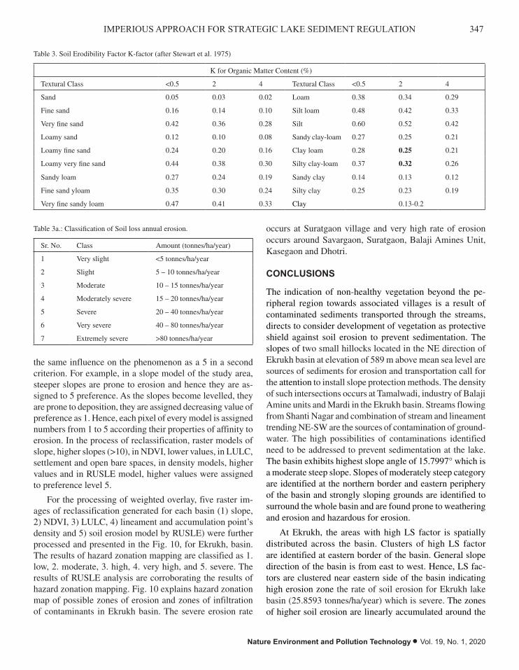
347IMPERIOUS APPROACH FOR STRATEGIC LAKE SEDIMENT REGULATION
Nature Environment and Pollution Technology • Vol. 19, No. 1, 2020
the same influence on the phenomenon as a 5 in a second criterion. For example, in a slope model of the study area, steeper slopes are prone to erosion and hence they are as-signed to 5 preference. As the slopes become levelled, they are prone to deposition, they are assigned decreasing value of preference as 1. Hence, each pixel of every model is assigned numbers from 1 to 5 according their properties of affinity to erosion. In the process of reclassification, raster models of slope, higher slopes (>10), in NDVI, lower values, in LULC, settlement and open bare spaces, in density models, higher values and in RUSLE model, higher values were assigned to preference level 5.
For the processing of weighted overlay, five raster im-ages of reclassification generated for each basin (1) slope, 2) NDVI, 3) LULC, 4) lineament and accumulation point’s density and 5) soil erosion model by RUSLE) were further processed and presented in the Fig. 10, for Ekrukh, basin. The results of hazard zonation mapping are classified as 1. low, 2. moderate, 3. high, 4. very high, and 5. severe. The results of RUSLE analysis are corroborating the results of hazard zonation mapping. Fig. 10 explains hazard zonation map of possible zones of erosion and zones of infiltration of contaminants in Ekrukh basin. The severe erosion rate
occurs at Suratgaon village and very high rate of erosion occurs around Savargaon, Suratgaon, Balaji Amines Unit, Kasegaon and Dhotri.
CONCLUSIONS
The indication of non-healthy vegetation beyond the pe-ripheral region towards associated villages is a result of contaminated sediments transported through the streams, directs to consider development of vegetation as protective shield against soil erosion to prevent sedimentation. The slopes of two small hillocks located in the NE direction of Ekrukh basin at elevation of 589 m above mean sea level are sources of sediments for erosion and transportation call for the attention to install slope protection methods. The density of such intersections occurs at Tamalwadi, industry of Balaji Amine units and Mardi in the Ekrukh basin. Streams flowing from Shanti Nagar and combination of stream and lineament trending NE-SW are the sources of contamination of ground-water. The high possibilities of contaminations identified need to be addressed to prevent sedimentation at the lake. The basin exhibits highest slope angle of 15.7997° which is a moderate steep slope. Slopes of moderately steep category are identified at the northern border and eastern periphery of the basin and strongly sloping grounds are identified to surround the whole basin and are found prone to weathering and erosion and hazardous for erosion.
At Ekrukh, the areas with high LS factor is spatially distributed across the basin. Clusters of high LS factor are identified at eastern border of the basin. General slope direction of the basin is from east to west. Hence, LS fac-tors are clustered near eastern side of the basin indicating high erosion zone the rate of soil erosion for Ekrukh lake basin (25.8593 tonnes/ha/year) which is severe. The zones of higher soil erosion are linearly accumulated around the
Table 3a.: Classification of Soil loss annual erosion.
Sr. No. Class Amount (tonnes/ha/year)
1 Very slight <5 tonnes/ha/year
2 Slight 5 – 10 tonnes/ha/year
3 Moderate 10 – 15 tonnes/ha/year
4 Moderately severe 15 – 20 tonnes/ha/year
5 Severe 20 – 40 tonnes/ha/year
6 Very severe 40 – 80 tonnes/ha/year
7 Extremely severe >80 tonnes/ha/year
Table 3. Soil Erodibility Factor K-factor (after Stewart et al. 1975)
K for Organic Matter Content (%)
Textural Class <0.5 2 4 Textural Class <0.5 2 4
Sand 0.05 0.03 0.02 Loam 0.38 0.34 0.29
Fine sand 0.16 0.14 0.10 Silt loam 0.48 0.42 0.33
Very fine sand 0.42 0.36 0.28 Silt 0.60 0.52 0.42
Loamy sand 0.12 0.10 0.08 Sandy clay-loam 0.27 0.25 0.21
Loamy fine sand 0.24 0.20 0.16 Clay loam 0.28 0.25 0.21
Loamy very fine sand 0.44 0.38 0.30 Silty clay-loam 0.37 0.32 0.26
Sandy loam 0.27 0.24 0.19 Sandy clay 0.14 0.13 0.12
Fine sand yloam 0.35 0.30 0.24 Silty clay 0.25 0.23 0.19
Very fine sandy loam 0.47 0.41 0.33 Clay 0.13-0.2

348 Shekhar Salunke and Balbhim Chavan
Vol. 19, No. 1, 2020 • Nature Environment and Pollution Technology
drainage line in Ekrukh basin, indicating major drainage lines eroding more than its tributaries. Ekrukh basins shows dendritic pattern of the stream, indicating plain, uniform and homogeneous surface on which these streams are flowing. The general slope of the area is towards south. The accumulation points (marked by ‘x’) are the sites of accumulation of water and sediments transported by headwaters and are the reasons for sedimentation. The lineament lengths vary from 1.833303 km to 9.529145 km in Ekrukh basin are the indicators of contamination on the surface during transportation, at the accumulation points and during the infiltration through fractures and joints, at downstream direction. The intersection of lineaments and accumulation points are identified as the most possible contamination sites at the lake.
The study calls immediate attention to implement inte-grated approaches for implementation of control measures towards prevention of soil erosion and pollution measures. In the subsequent phase, the research embarks upon designing innovative approaches to address the same.
ACKNOWLEDGEMENT
The author expresses gratitude to Dr. Vinay Dixit, Depart-
ment of Geology, Dayanand College, Solapur, M.S., for his proficient and crucial directions and inputs towards the course of action and pivotal analytical assistance for the entire venture, devoid of which, it was unattainable to disembark. Sum of all the efforts has generated the organized scientific evidence supporting the investigative conclusions directing action plan for sustainable development.
REFERENCES
Anonymous 1971. Soil Survey Manual. All India Soil, Landuse Survey Organisation, IARI, New Delhi.
Challa, O., R.S. Kurothe and K.S. Gajbhiye, 2001. Soil Erosion in Maha-rashtra. NBSS Publ. No. 82, NBSS and LUP, Nagpur, 51 p + 1 sheet of map (1:1 M scale).
Challa, O., Vadivelu, S. and Sehgal, I. 1995. Soils of Maharashtra for optimising land use. NBSS Publ. 54b (Soils of India Series), National Bureau of Soil Survey and Land Use Planning, Nagpur, India, 112p + 6 sheets of Map (1:500,000 scale).
Joshi, P.K. Kumar, Roy, P.S., Singh Sarnam, Agrawal, Shefali and Yadav, Deepshikha 2004. Vegetation cover mapping in India using multi-tem-poral IRS Wide Field Sensor (WiFS) data.
Stewart, B.A. (Bobby Alton) 1932 Woolhiser, D. A., Wischmeier, W. H. and Caro, J. H. 1975. Control of Pollution from Cropland. U.S. EPA Report No. 600/2-75-026 or U.S.D.A. Rep No. ARS-H-5-1. Washington, DC.
Strahler, A.N. 1952. Hypsometric (area-altitude) analysis of erosion topol-ogy, Geol. Soc. of America Bulletin 63(11): 1117-1142.
Fig. 10: Hazard zonation map of Ekrukh lake basin.
Bacteriological Quality Assessment of Groundwater and Surface Water in Chennai
SK. Jasmine Shahina†, D. Sandhiya and Summera RafiqDepartment of Microbiology, Justice Basheer Ahmed Sayeed College for Women, Chennai, Tamil Nadu, India†Corresponding author: SK. Jasmine Shahina
ABSTRACT
Water bodies have played a vital role throughout civilizations in the growth and continue to be a factor of importance in the modern economic growth of all the contemporary societies. Contamination of water sources with microbes can occur through rainfall overflow and agricultural inputs, mixing with sewage effluents. Water acts as a medium for the proliferation and dissemination of bacteria which cause human disease. Therefore, consumption of safe water is one of the most important requirements in public health. A total of 20 water samples were collected from both surface and groundwater from in and around Chennai. The MPN index of the surface water was found to be high when compared with groundwaters. Total coliform count of as many as 1100 MPN/100 mL and greater were obtained. A total of 11 different bacterial species were identified from both ground and surface water samples. The prevalence of bacterial isolates was of Staphylococcus aureus, CoNS, Enterococcus faecalis, Escherichia coli, Klebsiella pneumoniae, Enterobacter aerogenes, Pseudomonas aeruginosa, Vibrio cholera, Salmonella typhi, Aeromonas hydrophila and Citrobacter freundii. These organisms were resistant to many classes of antibiotics. The facts on multiple antibiotic resistance profiles of bacteria isolated from water and the resistance patterns suggested that there has been an indiscriminate use of the antibiotics tested. High occurrence of these multiple antibiotic resistant organisms in the drinking water distribution system could potentially pose a threat to humans consuming this water.
INTRODUCTION
About 75% of the earth’s surface is covered by water which is vital for all forms of life. Groundwater refers to water that occurs below the water-table in the zone of saturation. Groundwater is the only source of fresh water which is uti-lized in many parts of the world, whereas most of the times surface waters are either absent or polluted (Haniffa et al. 1993). Surface water is water that gets collected in a stream, river, lake, wetland etc. Many industries and municipalities use treated surface water due to high cost of drinking water. In the recent past there has been a steady increase in the pollution of river waters with deleterious microbes, including bacteria, viruses, parasites, as well as fungi (Niyogi 2005, Abraham et al. 2007). Majority of microbes in water are from faeces from human and other mammals. Pathogens can enter waters either from a point source, non-point sources or both. Rainwater surface run-offs, storm sewer spillages or overflow cause non-point microbial pollution of waters, while point-source pollution comes from discharge of untreated or partially treated effluents from wastewater treatment plants (Donovan et al. 2008, Musyoki et al. 2013).
When the water is contaminated with faecal material a wide range of pathogenic microorganisms can be trans-
mitted to humans. Some of them include enteropathogenic agents such as Salmonella, Shigella, Enteroviruses, and multi cellular parasites as well as opportunistic pathogens, like Pseudomonas aeruginosa, Klebsiella sp., Vibrio para-haemolyticus and Aeromonas hydrophila (Hodgkiss 1988). The occurrence and spread of antibiotic-resistant bacteria (ARB) are grave public health problems worldwide. Now aquatic ecosystems are a recognized reservoir for ARB and antibiotic resistance genes. An emerging issue for the general public and the drinking water industry is the presence of trace levels of antibiotics and ARB in source water and finished drinking water which affects public health (Scott et al. 2000). The aim of the present study was to characterize the presence of coliforms from surface and groundwater bodies in and around Chennai and to determine the resistance pattern of the isolates towards commonly used antibiotics. This study was done keeping in view the recent Chennai floods and Vardah cyclones that caused devastations to both human lives and the environment.
MATERIALS AND METHODS
Study Area
A total of 20 water samples were collected, of which 10 were
Nat. Env. & Poll. Tech.Website: www.neptjournal.com
Received: 18-06-2019Accepted: 23-07-2019
Key Words:GroundwaterSurface waterBacteriaAntibiotic resistantMPN
2020pp. 349-353 Vol. 19
p-ISSN: 0972-6268 No. 1 Nature Environment and Pollution Technology An International Quarterly Scientific Journal
Original Research Paper
e-ISSN: 2395-3454
Open Access

350 SK. Jasmine Shahina et al.
Vol. 19, No. 1, 2020 • Nature Environment and Pollution Technology
from surface waters (Lakes) and 10 from groundwater (Well) in and around Chennai. Water samples were collected from North Jaganadhan Nagar, Thathan Kuppam, Villivakkam, Teynam-pet, Chrompet, Chitlapakkam, Pallavaram, Hasthinapuram, Velachery, Chembarabakkam, Chitlapakkam, Namangalam, Pallikaranai, Puzhal, Ambattur and Porur.
Collection of Samples
Water samples were aseptically collected in 1 litre sterile bottles. Prior to sampling, the bottles were rinsed thoroughly with the water of the same source from which the sample was to be collected and rinsed water was discarded. The bottle cap was aseptically removed, and the bottle was immersed into the lake to collect the water. The bottle was brought up to the surface and covered with the bottle cap.
In open wells, water is available from 1 meter below from the ground. A sterile sampler was introduced into the well with the help of a rope and the water was taken out. The sampling bottle was kept unopened until the moment at which it was required for filling. During sampling the stopper and neck of the bottle were protected from contamination. Samples were labelled and transported in ice packs to the laboratory. They were examined for precipitate, colour, pH and odour. They were further processed for microbiological examination of coliforms and other pathogens.
Processing of the Water Samples
The water samples were subjected to MPN (Most Probable Number) technique to detect the quality of water. MPN is most commonly applied for quality testing of water, i.e. to ensure whether the water is safe or not in terms of bacteria present in it. A group of bacteria commonly referred as faecal coliforms act as an indicator for faecal contamination of water. It was done by multiple tube fermentation test to determine the total coliform count as per the standard methods. (Bartram & Pedley 1996)
Detection of Selected Pathogenic Bacteria from Water Samples
One mL of each water sample was inoculated into 5 mL of nutrient broth, selenite F enrichment broth and alkaline peptone water and was incubated at 37°C for 6-8 hrs. They were further inoculated on to MSA (Mannitol salt agar) media, Cetrimide agar, DCA (Deoxycholate citrate agar) media and TCBS (Thiosulfate citrate bile salt agar) and the plates were incubated for about 24-48 hrs at 37°C, respectively.
Antibiotic Sensitivity Testing
Once the organism was identified, the antibiotic sensitivity
testing was carried out as per the standard protocol by Kirby Bauer disc diffusion method (Bauer et al. 1966) towards the following antibiotics - Erythromycin (15 mcg), Nalidixic acid (30mcg), Rifampicin (30 mcg), Teicoplanin (30 mcg), Vancomycin (30 mcg), Amoxyclav (30 mcg), Amikacin (30 mcg), ceftazidime/clavulanic acid (30/10 mcg), ceftriaxone (30 mcg), ciprofloxacin (5 mcg), ceftazidime (30 mcg) and gentamicin (10 mcg).
RESULTS
Physical Properties of Water Samples
Water samples were tested for their physical properties like pH, colour, odour and precipitate. The pH of all the ground as well as the surface water was found to be neutral. The colour of the water samples ranged from being colourless to slight yellowish. Strong odour and precipitates were observed pre-dominantly in surface waters when compared to groundwaters.
MPN Technique
The water samples were subjected to MPN technique to de-tect the quality of water. MPN is the most commonly applied method for quality testing of water to ensure whether the water is potable or not. The MPN index of the surface water was found to be high when compared with groundwater. Total coliforms of as many as 1100 MPN/100 mL and greater were enumerated in surface water. With respect to groundwater, MPN index of >1100 MPN/100 mL was observed at North Ja-ganadhan Nagar and the least MPN index of 28 MPN/100 mL was observed at Teynampet. All the sampling places of both ground and surface waters showed the presence of coliform bacteria. Hence, it can be concluded that the water samples were heavily contaminated with coliform bacteria and were found to be unsatisfactory for drinking purpose (Tables 1 & 2).
Prevalence of Bacterial Isolates from Water Samples
A total of 11 different bacterial species were identified from both ground and surface water samples. The prevalence of bacterial isolates was Staphylococcus aureus, CoNS, Entero-coccus faecalis, E. coli, Klebsiella pneumoniae, Enterobac-ter aerogenes, Pseudomonas aeruginosa, Vibrio cholerae, Salmonella typhi, Aeromonas hydrophila and Citrobacter freundii (Table 3).
Determination of MPN Index for Boiled Water
As a control study, one surface and one groundwater sample was boiled to check the efficiency of boiling in killing the coliforms present in them. MPN technique was done and it was found to be negative for the presence of coliforms.
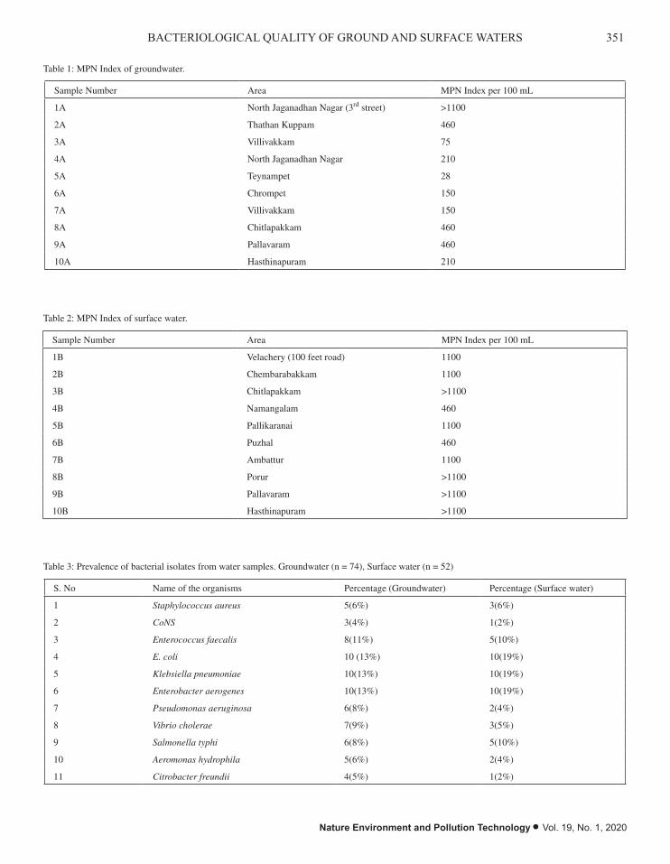
351BACTERIOLOGICAL QUALITY OF GROUND AND SURFACE WATERS
Nature Environment and Pollution Technology • Vol. 19, No. 1, 2020
Table 1: MPN Index of groundwater.
Sample Number Area MPN Index per 100 mL
1A North Jaganadhan Nagar (3rd street) >1100
2A Thathan Kuppam 460
3A Villivakkam 75
4A North Jaganadhan Nagar 210
5A Teynampet 28
6A Chrompet 150
7A Villivakkam 150
8A Chitlapakkam 460
9A Pallavaram 460
10A Hasthinapuram 210
Table 2: MPN Index of surface water.
Sample Number Area MPN Index per 100 mL
1B Velachery (100 feet road) 1100
2B Chembarabakkam 1100
3B Chitlapakkam >1100
4B Namangalam 460
5B Pallikaranai 1100
6B Puzhal 460
7B Ambattur 1100
8B Porur >1100
9B Pallavaram >1100
10B Hasthinapuram >1100
Table 3: Prevalence of bacterial isolates from water samples. Groundwater (n = 74), Surface water (n = 52)
S. No Name of the organisms Percentage (Groundwater) Percentage (Surface water)
1 Staphylococcus aureus 5(6%) 3(6%)
2 CoNS 3(4%) 1(2%)
3 Enterococcus faecalis 8(11%) 5(10%)
4 E. coli 10 (13%) 10(19%)
5 Klebsiella pneumoniae 10(13%) 10(19%)
6 Enterobacter aerogenes 10(13%) 10(19%)
7 Pseudomonas aeruginosa 6(8%) 2(4%)
8 Vibrio cholerae 7(9%) 3(5%)
9 Salmonella typhi 6(8%) 5(10%)
10 Aeromonas hydrophila 5(6%) 2(4%)
11 Citrobacter freundii 4(5%) 1(2%)

352 SK. Jasmine Shahina et al.
Vol. 19, No. 1, 2020 • Nature Environment and Pollution Technology
Antibiotic Sensitivity Testing
Antibiotic sensitivity testing of the bacterial isolates was done as per Kirby Bauer’s disc diffusion method. Gram positive organisms showed 100% resistance towards vancomycin, nalidixic acid, erythromycin, ciprofloxacin and teicoplanin. They were 100% sensitive towards rifampicin. Gram negative organisms exhibited 100% resistance towards ceftazidime/clavulanic acid, amoxyclav followed by gentamicin, ceftri-axone and ceftazidime. These isolates were sensitive towards amikacin and ciprofloxacin.
DISCUSSION
Potable water must be free from pathogenic microorgan-isms and chemical substances that are hazardous to health (Lamikanra 1999). Bacteria indicative of faecal pollution or pathogens should not be found in drinking water. A sensi-tive method of quality assessment of drinking water is the detection of faecal indicator bacteria as it is not possible to examine water for every possible pathogen that might be present (WHO 2004). There has been an imbalance between supply and demand and it is the main reason which has led to competition and thereby resulted in pollution and envi-ronmental degradation. Failure of disinfection methods of raw water at the treatment area or mixing of sewage through cross-connections, leakages could cause bacteriological pollution of drinking water supplies.
Main cause of water pollution is due to human impact (Palit 2012). By studying the physico-chemical and micro-bial characteristics, the significance of water as a potent ecological factor can be appreciated. In the present study, water samples were tested for their physical properties like pH, colour, odour and precipitate found. The pH of all the ground as well as the surface water was found to be neutral. The colour of the water samples ranged from being colour-less to slight yellowish. Strong odour and precipitates were observed predominantly in surface waters when compared to groundwaters. The negative logarithm of hydrogen ion concentration is known as pH. It expresses the intensity of acidic or alkaline condition of a solution. pH is an extremely important variable because most microorganisms can survive within a narrow range of pH and it also helps in the solubility of most metals. pH is also an important factor with respect to chemical treatment of water including disinfection process.
Microbial contamination of drinking water is the most common and wide spread health risk and therefore its control must always be of supreme importance. Monitoring microbial presence, especially faecal coliform bacteria (FC) determines the quality of water. In this study, the MPN index was high for surface waters when compared to groundwater. The water
analysed in this study has clearly shown that they are loaded with indicator organisms which are the indication of faecal pollution and thus the human interference.
In our study, a total of 11 different bacterial species were identified from both ground and surface water samples. The prevalence of bacterial isolates was Staphylococcus aureus, CoNS, Enterococcus faecalis, E. coli, Klebsiella pneumoniae, Enterobacter aerogenes, Pseudomonas aeruginosa, Vibrio cholerae, Salmonella typhi, Aeromonas hydrophila and Cit-robacter freundii. According to EPA, the presence of E. coli indicates recent sewage or animal waste contamination (EPA 2001). The temperature and the presence of nutrients in the tank favours the survival of enteric bacteria, like Salmonella spp. and E. coli (Leclerc et al. 2002). Enteric pathogens such as Salmonella, Shigella and Vibrio are principally transmitted through contaminated drinking water, as reported by Edberg et al. (2000).
P. aeruginosa is ubiquitous, free-living bacterium in the environment. It is often found in natural waters such as lakes and rivers in concentrations of 10/100 mL to >1,000/100 mL. Nevertheless, it is not often found in drinking water. Pseudomonas is usually found in 2% of samples, or less, and at concentrations up to 2,300 mL or more often at 3-4 CFU/mL. The occurrence of Pseudomonas in drinking water is due to its ability to form biofilms and colonize the plumbing fixtures (i.e., faucets, showerheads, taps, pipelines, etc.) than its presence in the water system or treated drinking water (Mena & Gerba 2009).
The occurrence and spread of antibiotic-resistant bacteria (ARB) globally are serious public health problems. Aquatic ecosystems are a designated reservoir for ARB and antibiotic resistance genes. The existence of trace levels of antibiotics and ARB in source water and finished drinking water may also greatly affect public health and is an emerging issue for the general public and the drinking water industry (Scott et al. 2000). In our study, antibiotic sensitivity testing of the bacterial isolates was done as per Kirby Bauer’s disc diffusion method. Gram positive organisms showed 100% resistance towards vancomycin, nalidixic acid, erythromycin, ciprofloxacin and teicoplanin. They were 100% sensitive to-wards rifampicin. Gram negative organisms exhibited 100% resistance towards cefotaxime/clavulanic acid, and amoxy-clav followed by gentamicin, ceftriaxone and ceftazidime. These isolates were sensitive to amikacin and ciprofloxacin.
CONCLUSION
An assessment of the bacteriological quality of drinking water in the present study confirmed the presence of various bacterial species including opportunistic pathogens such as
353BACTERIOLOGICAL QUALITY OF GROUND AND SURFACE WATERS
Nature Environment and Pollution Technology • Vol. 19, No. 1, 2020
Aeromonas and Pseudomonas spp. This drastic effect in the increase of microorganisms may be because of the recent Chennai floods followed by Vardah cyclone. This has caused the mix up of sewage with the water bodies resulting in water pollution. This could have been the reason for all the water samples showing the presence of coliforms and other organisms. The isolated bacteria were found to be resistant to several classes of antibiotics. The data on multiple antibiotic resistance (MAR) profiles of bacterial isolates from water and the resistance patterns of organisms in drinking water suggested that there has been an indiscriminate use of the antibiotics tested. The high occurrence of multi-drug resistant organisms in the drinking water system may possibly pose a risk to humans consuming this water.
ACKNOWLEDGEMENT
The authors would like to thank the Management and Principal of Justice Basheer Ahmed Sayeed College for Women, for the financial support given under the Post Graduate student project scheme sanctioned through the Multi-Disciplinary Research and Consultancy Centre (MRCC) of the College for the promotion of research.
REFERENCES
Abraham, W. R. 2010. Megacities as sources for pathogenic bacteria in rivers and their fate downstream. International Journal of Microbiology, 2011.
Bartram, J. and Pedley, S. 1996. Water quality monitoring - a practical guide to the design and implementation of freshwater quality studies and monitoring programmes. Chapter 10 - Microbiological Analyses. Published on behalf of United Nations Environment Programme and the World Health Organization © 1996 UNEP/WHO.
Bauer, A.W., Kirby, W.M., Sherris, J.C. and Turck, M. 1966. Antibiotic susceptibility testing by a standardized single disk method. Am. J. Clin. Pathol. 45(4): 493-496.
Donovan, E., Unice, K., Roberts, J. D., Harris, M. and Finley, B. 2008. Risk of gastrointestinal disease associated with exposure to pathogens in the water of the Lower Passaic River. Applied and Environmental Microbiology, 74(4): 994-1003.
Edberg, S.C., Rice, E.W., Karlin, R.J. and Allen, M.J. 2000. Escherichia coli: The best biological drinking water indicator for public health protection. Symp. Ser. Soc. Appl. Microbiol., 29: 106S-116S.
EPA 2001. Environment Public Authority Decision No. 210/2001 Pertaining to the Executive By-Law of the Law of Environment Public Authority.
Haniffa, M.A., Arockiasamy, S. and Martin, P. 1993. Physico-chemical and microbiological studies in the Perenial River Thabaraparani for the assessment of water quality. Indian J. of Env. Protec., 13(7): 533-538.
Hodgkiss, I.J. 1988. Bacteriological monitoring of Hong Kong marine water quality. Environment International, 14(6): 495-499.
Lamikanra, A. 1999. Essential Microbiology for Students and Practitioner of Pharmacy, Medicine and Microbiology. Amkra Books, pp. 406.
Leclerc, H., Schwartzbrod, L. and Dei-Cas, E. 2002. Microbial agents associated with waterborne diseases. Critical Reviews in Microbi-ology, 28(4): 371-409.
Mena, K.D. and Gerba, C.P. 2009. Risk assessment of Pseudomonas aeruginosa in water. In: Reviews of Environmental Contamination and Toxicology, 201: 71-115.
Musyoki, A.M., Abednego, M., Suleiman, M.A., Mbithi, J.N. and Maingi, J.M. 2013. Water-borne bacterial pathogens in surface waters of Nairobi river and health implication to communities downstream Athi river. International Journal of Life Science and Pharma Re-search, 3(1): 4-10.
Niyogi, S.K. 2005. Shigellosis. Journal of Microbiology (Seoul, Ko-rea), 43(2): 133-143.
Palit, A., Batabyal, P., Kanungo, S. and Sur, D. 2012. In-house contam-ination of potable water in urban slum of Kolkata, India: a possible transmission route of diarrhea. Water Science and Technology, 66(2): 299-303.
Scott, K.P., Melville, C.M., Barbosa, T.M. and Flint, H.J. 2000. Occurrence of the new tetracycline resistance gene test (W) in bacteria from the human gut. Antimicrobial Agents and Chemotherapy, 44(3): 775-777.
WHO 2004. Guidelines for Drinking Water Quality: Recommenda-tions, (Vol. 1). World Health Organization, Geneva.

Vol. 19, No. 1, 2020 • Nature Environment and Pollution Technology
354

Use of Pyrophyllite as Soil Conditioner in Lettuce Production
Senad Murtić*†, Ćerima Zahirović**, Lutvija Karić**, Josip Jurković***, Hamdija Čivić*** and Emina Sijahović****Department of Plant Physiology, Faculty of Agriculture and Food Science University of Sarajevo, 71 000 Sarajevo, Bosnia and Herzegovina**Department of Vegetable, Faculty of Agriculture and Food Science, University of Sarajevo, 71 000 Sarajevo, Bosnia and Herzegovina***Department of Plant Nutrition, Faculty of Agriculture and Food Science, University of Sarajevo, 71 000 Sarajevo, Bosnia and Herzegovina†Corresponding author: Senad Murtić
ABSTRACT
In recent years, there has been an increasing interest in the possibility of the use of aluminosilicate minerals in order to maintain and improve soil productivity. The unique ion-exchange and adsorption properties of pyrophyllite minerals indicate the possibility of its application in agriculture as soil conditioner. The aim of this study was to evaluate whether the application of pyrophyllite could reduce the use of mineral fertilizers in lettuce production without adverse effects on its yield and quality. The experiment was carried out from November 2018 to April 2019 inside a polyethylene covered greenhouse in Gornji Moranjci, Bosnia and Herzegovina. The following quality parameters were analysed using standard methods: ascorbic acid content, total phenolic content, total antioxidant capacity and content of potentially toxic heavy metals (Cr, Pb, Ni, Cu, Zn and Mn) in lettuce. The results of this study showed that the substitution of fertilizers with pyrophyllite in amount of 25% and 50% of recommended fertilizer rate under experimental conditions increase lettuce yield and total antioxidant capacity compared to the control treatment, i.e. 100% recommended fertilizer rate. The results of this study also support the hypothesis that pyrophyllite could be used as remediation material in polluted soils by heavy metals. However, further investigation is necessary to confirm these hypotheses across different soil ecosystems.
INTRODUCTION
Applying fertilizer in agricultural production has shown a steady increase in recent decades, resulting in the gradual soil degradation. The numerous other processes, such as nu-trient depletion, leaching and pollution of soils by hazardous substances from industry have also contributed to the soil degradation (Lal 2015). Although the soil degradation is a worldwide phenomenon, it is fact that is in most developing countries the phenomenon is being hastened by land use mismanagement. Better use of soil resources through opti-mizing fertilization, increasing biodiversity and improving soil quality has therefore been considered as a priority for achieving sustainable agriculture (Gomiero 2016).
In recent years, there is an increasing interest for using of natural aluminosilicates in order to maintain and improve soil productivity. Clay minerals, e.g. zeolite and bentonite are known to have ability to increase soil capacity to hold available forms of nutrients (Ghazavi 2015, Jakkula & Wani 2018). Contrary to zeolite and bentonite, pyrophyllite appli-cation in agriculture is not substantially present due to its
lower availability and insufficient knowledge of its potential use in agriculture.
Pyrophyllite is a dioctahedral 2:1 clay mineral with the chemical formula Al2Si4O10(OH)2. It resembles closely with talc and the only difference between them is that talc contains Mg2+ instead Al3+ in octahedral positions. The elementary sheet of pyrophyllite is composed by aluminium-oxygen/hydroxyl octahedra between two layers of silicon-oxygen tetrahedra. The basal surfaces of this elementary sheet do not contain hydroxyl groups, which explains the hydrophobicity of pyrophyllite (Drits et al. 2012).
Resemblance to the structure with talc and some other clay minerals indicate that pyrophyllite application in soil could also be effective in increasing soil’s ability to hold nu-trients and thus reducing leaching. The fact that pyrophyllite is used in the agriculture industry as a carrier for fertilizers and pesticides supports this hypothesis.
The present study was conducted to evaluate whether the application of pyrophyllite can reduce the use of mineral fertilizers in lettuce production without adverse effects on its
Nat. Env. & Poll. Tech.Website: www.neptjournal.com
Received: 19-05-2019Accepted: 22-07-2019
Key Words:AgricultureEnvironmentFertilizerPyrophylliteSoil conditioner
2020pp. 355-359 Vol. 19
p-ISSN: 0972-6268 No. 1 Nature Environment and Pollution Technology An International Quarterly Scientific Journal
Original Research Paper
e-ISSN: 2395-3454
Open Access

356 Senad Murtić et al.
Vol. 19, No. 1, 2020 • Nature Environment and Pollution Technology
yield and quality. If that is possible, the additional aim of this study was to determine the optimal ratio between fertilizer and pyrophyllite in order to achieve this purpose. Lettuce was selected as the subject of this study, primarily because the production of this vegetable is consistently increasing in this country and therefore any effort to improve lettuce production is of great interest for both the producer and the consumer.
MATERIALS AND METHODS
Aluminosilicate minerals (pyrophyllite): The pyrophyllite materials used in this study were obtained by grinding and sieving pyrophyllite ore from deposits in Parsovići-Konjic, Bosnia and Herzegovina and characterized by following properties: alkaline, hydrophobic material, very soft and white to grey in colour. The hardness on the Mohs’ scale is 1.5 and cation exchange capacity (CEC) ranges between 50 and 70 meq/100g. Median total SiO2, Al2O3, K, Ca, Mg, Cu, Ni, Zn, Co, Mn, Pb and Cr contents were 67.55%, 19.10%, 0.3%, 6.65%, 0.14%, 1.40 mg/kg, 2.74 mg/kg, 25.68 mg/kg, 0.4 mg/kg, 93.14 mg/kg, 7.97 mg/kg and 0.76 mg/kg, respectively. The above-mentioned results of pyrophyllite chemical analysis were obtained at Faculty of Agriculture and Food Sciences University of Sarajevo.
Lettuce (Lactuca sativa L. var. shangore): This lettuce is one of the favourite butterhead lettuce varieties in Bosnia for producers as well as consumers. It is cultivated from late autumn to spring in greenhouses and its vegetation period ranges from 45 to 50 days after planting in a heated greenhouse. This lettuce is adaptable to most soil types, it has green leaves and form tight and heavy heads, more than 0.3 kg. It grows fast and keeps the leaves out upright.
Study area: The experiment was carried out from November 2018 to April 2019 inside a polyethylene covered greenhouse in Gornji Moranjci, Srebrenik Municipality, Bosnia and Herzegovina (44°41¢N, 18°26¢E and altitude 275 m). The length, width, eaves height and ridge height of the exper-imental greenhouse were 50 m, 8 m, 2.2 m and 3.7 m, re-spectively. Humidity regulation in greenhouse was achieved by opening of two side roll-up vents while the row cover was used to protect the lettuce against frosts. The climate in studied area is classified as Cfb by Köppen and Geiger climate classification (Rubel & Kottek 2010). The annual mean air temperature is 11.1°C and precipitation 856 mm with significant rainfall even in the dry months. The soil of the experimental site is classified as Dystric Cambisol, according to FAO Soil Classification (FAO 2014). This type of soil is characterized by an ochric (Aoh horizon) or umbric (Aum horizon), which lies directly above the cambic horizon (B)v horizon, acidic reaction, base saturation less than 50%, low
to moderate water storage capacity and a medium nutrient storage capacity.
Soil pH in KCl, organic matter, available phosphorus (P2O5) and potassium (K2O) contents in the 0-30 cm stud-ied soil layer before lettuce planting were 5.1, 3.83%, 15.1 mg/100g and 31.3 mg/100g, respectively. Median total Cr, Pb, Ni, Cu and Zn contents were 128.48 mg/kg, 17.68 mg/kg, 104.55 mg/kg, 15.76 mg/kg and 36.95 mg/kg, respectively. In accordance with results of soil chemical analysis and nutrient needs of lettuce, the following fertilization recommendation was given: 300 kg/ha NPK 7:20:30 (nitrogen-phosphorus-po-tassium) as part of the basic fertilization and if necessary 100 kg/ha KAN (calcium ammonium nitrate) as part of fertilization during vegetation (recommended fertilizer rate was recalculated based on plot area).
Experimental design and treatments: The experimental area in greenhouse was divided into twenty-one equal plots. Each plot had an area of 5 m2. The experiment was laid out in randomized complete block design with seven treatments in three replications. Experiment treatments (T) were as follows:
T1 - recommended fertilizer rate (RFR) without pyrophyllite (PP), i.e. control treatment (150 g NPK 7:20:30 at each plot)
T2 - 25% of RFR was replaced with PP particle size 3 mm (112.5 g NPK 7:20:30 + 37.5 g PP)
T3 - 25% of RFR was replaced with PP particle size 0.1 mm (112.5 g NPK 7:20:30 + 37.5 g PP)
T4 - 50% of RFR was replaced with PP particle size 3 mm (75 g NPK 7:20:30 + 75 g PP)
T5 - 50% of RFR was replaced with PP particle size 0.1 mm (75 g NPK 7:20:30 + 75 g PP)
T6 - 75% of RFR was replaced with PP particle size 3 mm (37.5 g NPK 7:20:30 + 112.5 g PP)
T7 - 75% of RFR was replaced with PP particle size 0.1 mm (37.5 g NPK 7:20:30 + 112.5 g PP)
Fertilizers and pyrophyllite material in the all experimen-tal plots were applied two weeks before planting lettuce (7 December 2019). No other fertilizers were added during the lettuce vegetation. All other agrotechnical measures needed for optimum lettuce growth (pest control measures, irriga-tion) were performed identically on all experimental plots until the time of lettuce technological maturity.
Analysis of lettuce yield and quality: All lettuce plants in the experiment area were harvested at the same time (31 March 2019). Average yield was determined as the average fresh harvest weight per m2.

357PYROPHYLLITE AS SOIL CONDITIONER IN LETTUCE PRODUCTION
Nature Environment and Pollution Technology • Vol. 19, No. 1, 2020
Lettuce nutritional quality was analysed by detecting the following parameters: ascorbic acid content, total phenolic content, total antioxidant capacity and content of potentially toxic heavy metals (Cr, Pb, Ni, Cu, Zn and Mn). Ascorbic acid (AA) was estimated by 2,6-dichlorophenolindophenol titration method (AOAC 2006). Lettuce extract for estima-tion of total phenolics, total flavonoids and total antioxidant capacity was prepared by macerating of lettuce powder (1 g) in 30% ethanol for 6 hours. Thereafter, the extract was filtered. Total phenolic content (TPC) was estimated by the Folin-Ciocalteu method (Ough & Amerine 1988) and total antioxidant capacity (TAC) by ferric reducing antioxidant power (FRAP) assay (Benzie & Strain 1996).
Extraction of heavy metals from lettuce powder was performed using HNO3-H2SO4 solution (Lisjak et al. 2009) as follows: 1 g of lettuce powder was placed into 100 mL round bottom flask and then 10 mL 65% HNO3 and 4 mL 95-98% H2SO4 were added. The reaction mixture in flask was covered with a watch glass, allowed to stand for few hours and then heated gently on a hot plate for 30 min. Thereafter, the flask with reaction mixture was allowed to cool to room temperature, filtered through quantitative filter paper into 50 mL flask and diluted to the mark with distilled water. The content of Cr, Pb, Ni, Cu, Zn and Mn in obtained extract was determined by atomic absorption spectrophotometry on AA-7000 Shimadzu, according to method ISO 11047 (ISO 1998). Standard solutions of the examined heavy metals were prepared by appropriate dilution of stock standards (Merck) with deionized water.
Statistic data processing: All the experimental measure-ments were made in triplicate and the results were expressed as mean ± standard deviation. Analysis of variance (ANOVA) was performed using Microsoft Excel 2013 software pro-gram, and the significant differences between the variants were determined using Least Significant Differences test at 0.05 level of probability (P £ 0.05).
RESULTS
The results of the analysis of yield and some quality param-eters of lettuce depending on the experimental treatment are given in Table 1.
As presented in Table 1, the partial replacement of ferti-lizer by pyrophyllite did not negatively affect the yield and quality compared to the control treatment. Moreover, the yield and examined lettuce quality parameters were mainly higher in the treatment where the pyrophyllite was applied as a replacement for a part of the fertilizer. The highest yield was obtained in treatment 2 and 3 where pyrophyllite was applied as a replacement for 25% of recommended fertilizer rate. The
data in Table 1 also indicate that all treatments with pyroph-yllite increase the antioxidant capacity of lettuce, especially where pyrophyllite (particle size 0.1 mm) was applied as a replacement for 75% of recommended fertilizer rate.
Heavy metal contents (Zn, Cu, Mn, Ni, Cr, Pb) in the plant samples depending on the experimental treatment are presented in Table 2. Presented data have shown that the content of Zn, Cu, Ni, Cr and Pb in lettuce was below the maximum permissible value of heavy metals in food crops reported by FAO/WHO (2001). Accordingly, the maximum permissible value for Zn, Cu, Ni and Cr is 100 mg/kg, 40 mg/kg, 4 mg/kg and 2.3 mg/kg on dry weight basis, respec-tively. Upper limits of Pb in edible products is regulated by EU Legislation (2011). Accordingly, Pb threshold limit for lettuce is 3.6 mg/g on dry mass basis.
DISCUSSION
The results of this study showed that the substitution of fertilizers with pyrophyllite in amount of 25% and 50% of recommended fertilizer rate increase lettuce yield compared to the yield achieved in the control treatment, i.e. 100% NPK recommended rate. Only the treatments where the pyrophyl-lite was applied as a replacement for 75% of recommended fertilizer rate did not show a positive effect on lettuce yield. The above-mentioned results indicate that pyrophyllite may increase soil’s ability to hold and slow release of nutrients, thus preventing fertilizer leaching. Consistently, the inclu-sion of the pyrophyllite in fertilizer management can play a significant role in food crops production as a soil conditioner for improving fertilizer efficiency.
Mukherjee (2013) noted that the increase in crop yield due to the pyrophyllite addition in soil is result of its ability to release the tightly bound phosphates already existing in the soil making them available for plants. At the same time, pyrophyllite contains certain amounts of potassium, calcium, magnesium and iron, contributing significantly to the plant growth and development.
The results of this study also showed that treatments with pyrophyllite, to a greater or lesser extent, increase the content of phenolics and antioxidant capacity of lettuce, especially where pyrophyllite (particle size 0.1 mm) was applied as a replacement for 75% of recommended fertilizer rate. We assume that the lettuce in treatments where pyrophyllite was applied as a partial replacement for fertilizer had a lower amount of available nutrients in the soil resulting in its temporary stress, and consequently in higher synthesis of phenolics and other antioxidants. Relationship between treatment with pyrophyllite and ascorbic acid content in lettuce in the present study was not observed.

358 Senad Murtić et al.
Vol. 19, No. 1, 2020 • Nature Environment and Pollution Technology
Another important effect of pyrophyllite is related to the removal of toxic heavy metals from soil (Prasad & Saxena 2008) and results of the present study support this hypothesis. Namely, the content of all examined heavy metals in lettuce in treatments with pyrophyllite was lower compared to the content of heavy metals in lettuce obtained in the control treatment. These differences between treatments were not only significant for the content of Cr and Ni in lettuce. We assume that the reason for that was the high content of Cr and Ni in the studied soil and therefore the amount of applied py-rophyllite was not adequate to significantly reduce mobility of Cr and Ni in the soil and thus their availability to plants. Namely, the average content of Ni and Cr in studied soil was 104.55 mg/kg and 128.48 mg/kg, respectively. These values greatly exceeded the limit value prescribed by legislation in Bosnia and Herzegovina (Official Gazette of FBIH 2009) or by legislation in some European countries (Pérez et al. 2002). Accordingly, the maximum permissible value for Ni and Cr
in soil is 40 mg/kg and 100 mg/kg, respectively.
Many scientists agree that the ability of clay minerals to decrease the mobility of heavy metals in soils is the result of adsorption of heavy metals in their interlayers or on its surface areas (Ijagbemi et al. 2009, Khan & Singh 2010, Ararem et al. 2011, Demirkiran et al. 2016) but this adsorption mechanism is still not fully understood. Some clay minerals that have high cation exchange capacity, i.e. montmorillonite and bentonite in principle achieve this effect through ion exchange reaction (Önal 2007, Wigger & Loon 2017). The cation exchange capacity for pyrophyllite is lower, but not its efficiency in removing heavy metals from the soil, and results of many studies confirm this hypothe-sis (Scheidegger et al. 1996, Caporale & Vioalante 2016, Uddin 2017). Bergaya et al. (2006) reported that pyrophyllite has ability to easily disperse in water due to weak van der Waals bounds, resulting in less clumping. This dispersing property allows higher exposure area for pyrophyllite in soil
Table 1: Yield, ascorbic acid content (AA), total phenolic content (TPC) and total antioxidant capacity (TAC) in lettuce.
Treatment1 Yield (kg/m2) AA (mg/100 g) TPC (mg/100 g) TAC µmol Fe2+/100 g
T1 7.00 ± 1.47d 12.88 ± 8.31 6.13 ± 13.61d 109.47 ± 76.93c
T2 9.57 ± 1.28ab 15.97 ± 8.31 18.46 ± 29.13bc 188.84 ± 195.69bc
T3 9.74 ± 0.50a 12.28 ± 4.75 30.56 ± 8.84ab 263.78 ± 241.65ab
T4 9.08 ± 1.31abc 15.89 ± 8.31 8.05 ± 5.85d 157.77 ± 103.25bc
T5 7.46 ± 1.65d 14.58 ± 4.26 9.93 ± 3.63d 182.50 ± 50.35bc
T6 6.82 ± 2.62d 12.20 ± 7.32 8.24 ± 4.49d 145.07 ± 154.71bc
T7 6.86 ± 0.14d 13.88 ± 8.31 39.00 ± 17.77a 365.80 ± 166.83a
LSD0.05 1.34 - 13.52 125.57
* Means denoted by the same letter indicate no significant difference (P £ 0.05)1 Experimental treatment: T1 - recommended fertilizer rate (RFR) without pyrophyllite (PP), i.e. control treatment; T2 - 25% of RFR was replaced with PP (3 mm); T3 - 25% of RFR was replaced with PP (0.1 mm); T4 - 50% of RFR was replaced with PP (3 mm); T5 - 50% of RFR was replaced with PP (0.1 mm); T6 - 75% of RFR was replaced with PP (3 mm); T7 - 75% of RFR was replaced with PP (0.1 mm)
Table 2: Heavy metal contents in lettuce (mg/kg dry mass).
Treatment1 Zn Cu Ni Cr Pb
T1 74.2 ± 14.2abcd 3.71 ± 0.7a 1.88 ± 0.6 2.0 ± 1.2 3.28 ± 1.4a
T2 78.4 ± 9.1a 3.39 ± 0.9abc 1.39 ± 0.8 1.9 ± 1.1 3.23 ± 2.8ab
T3 58.0 ± 13.2e 3.69 ± 0.9ab 1.22 ± 0.4 2.5 ± 1.5 2.55 ± 0.2abc
T4 76.6 ± 11.4abc 3.32 ± 1.2abcd 1.51 ± 0.2 1.9 ± 0.4 2.0 ± 0.9abcd
T5 77.8 ± 11.5ab 3.3 ± 0.5abcde 1.69 ± 0.6 1.2 ± 0.4 2.0 ± 1.9abcde
T6 51.3 ± 12.1ef 2.7 ± 0.7cdef 1.12 ± 0.2 2.2 ± 0.8 0.77 ± 1.2def
T7 42.4 ± 15.2f 2.2 ± 1.3f 1.41 ± 1.3 1.6 ± 0.3 0.46 ± 0.1f
LSD0.05 11.81 0.91 - - 1.34
* Means denoted by the same letter indicate no significant difference (P £ 0.05) 1 Experimental treatment: T1 - recommended fertilizer rate (RFR) without pyrophyllite (PP), i.e. control treatment; T2 - 25% of RFR was replaced with PP (3 mm); T3 - 25% of RFR was replaced with PP (0.1 mm); T4 - 50% of RFR was replaced with PP (3 mm); T5 - 50% of RFR was replaced with PP (0.1 mm); T6 - 75% of RFR was replaced with PP (3 mm); T7 - 75% of RFR was replaced with PP (0.1 mm)

359PYROPHYLLITE AS SOIL CONDITIONER IN LETTUCE PRODUCTION
Nature Environment and Pollution Technology • Vol. 19, No. 1, 2020
and therefore more heavy metals or other pollutants could potentially be absorbed and thus neutralized. Furthermore, pyrophyllite contributes to the increase of soil pH, resulting in lower mobility and thus the availability of heavy metals for plant.
In general, the results of this study indicate that the ap-plication of pyrophyllite under experimental conditions can reduce the use of mineral fertilizers in lettuce production without adverse effects on its yield and quality, especially where the pyrophyllite is applied in the amount of 25% of recommended fertilizer rate. The results of this study also support the hypothesis that pyrophyllite could be used as the resort to help clean up the soils from the damage caused by heavy metal pollution.
REFERENCES
AOAC 2006. Vitamin C in juices and vitamin preparations, method 967.21. In: AOAC Intl. (ed.) Official Methods of Analysis (ed.) Arlington, USA.
Ararem, A., Bouras, O. and Arbaoui, F. 2011. Adsorption of caesium from aqueous solution on binary mixture of iron pillared layered montmorillonite and goethite. Chem. Eng. J., 172(1): 230-236.
Benzie, I.F. and Strain J.J. 1996. Ferric reducing ability of plasma (FRAP) as a measure of antioxidant power: The FRAP assay. Anal. Biochem., 239(1): 70-76.
Bergaya, F., Theng, B.K.G. and Lagaly, G. 2006. Handbook of Clay Science. Elsevier, Amsterdam, London, pp. 231-296.
Caporale A.G. and Vioalante, A. 2016. Chemical processes affecting the mobility of heavy metals and metalloids in soil environments. Current Pollution Reports, 2(1): 15-27.
Demirkiran, A.R., Acemioglu, B. and Gonen, T. 2016. Sorption of copper and nickel ions from solution by clay minerals. Oxid. Commun., 39(1): 817-829.
Drits, V.A., Guggenheim, S., Zviagina, B.B. and Kogure, T. 2012. Structures of the 2:1 layers of pyrophyllite and talc. Clays Clay Miner., 60(6): 574-587.
EU 2011. Commission Regulation (EU) No 420/2011 of 29 April 2011 amending Regulation (EC) No. 1881/2006 setting maximum levels for certain contaminants in foodstuffs. Available online: https://www.fsai.ie/uploadedFiles/Reg420_2011.pdf
FAO 2014. World Reference Base for Soil Resources. Available online: http://www.fao.org/3/i3794en/I3794en.pdf
FAO/WHO 2001. Report on the 32nd Session of the Codex Committee on Food Additives and Contaminants, Codex Alimentarius Commission, Geneva, Switzerland.
Ghazavi, R. 2015. The application effects of natural zeolite on soil runoff, soil drainage and some chemical soil properties in arid land area. International Journal of Innovation and Scientific Research, 13(1): 172-177.
Gomiero, T. 2016. Soil degradation, land scarcity and food security: reviewing a complex challenge. Sustainability, 8(3): 1-41.
Ijagbemi, C.O., Baek, M.H. and Kim D.S. 2009. Montmorillonite surface properties and sorption characteristics for heavy metal removal from aqueous solutions. J. Hazard. Mater., 166(1): 538-546.
ISO 1998. International Standard ISO 11047: Soil quality determination of cadmium, chromium, cobalt, copper, lead, manganese, nickel and zinc- Flame and electrothermal atomic absorption spectrometric methods. International Organization for Standardization, Geneva, Switzerland.
Jakkula, V.S. and Wani, S.P. 2018. Zeolites: Potential soil amendments for improving nutrient and water use efficiency and agriculture productivity. Sci. Revs. Chem. Commun., 8(1): 119.
Khan, T.A. and Singh, V.V. 2010. Removal of cadmium (II), lead (II), and chromium (VI) ions from aqueous solution using clay. Toxicol. Environ. Chem., 92(8): 1435-1446.
Lal, R. 2015. Restoring soil quality to mitigate soil degradation. Sustainability, 7(5): 5875-5895.
Lisjak, M., Spoljarevic, M., Agic, D. and Andric, L. 2009. Practicum-Plant Physiology. Joseph George Strossmayer University of Osijek, pp. 24-25.
Mukherjee, S. 2013. The Science of Clays: Applications in Industry, Engineering, and Environment. Springer, New York, USA, pp. 54-68.
Official Gazette of FBiH 2009. Rulebook on determination of allowable quantities of harmful and hazardous substances in soils of Federation of Bosnia and Herzegovina and methods for their testing, No. 72/09. Edit. Official Gazette of FBiH, Sarajevo, Bosnia and Herzegovina. Available online: http://www.fzofbih.org.ba/userfiles/file/izmj_zakon_otpad.pdf
Önal, M. 2007. Swelling and cation exchange capacity relationship for the samples obtained from a bentonite by acid activations and heat treatments. Appl. Clay Sci., 37(1-2): 74-80.
Ough, C.S. and Amerine, M.A. 1988. Phenolic compounds. In: Wiley (ed.) Methods for Analysis of Must and Wines. New York, USA.
Pérez, C., Martínez, M.J., Vidal, J. and Navarro, C. 2002. Proposed reference values for heavy metals in calcaric fluvisols of the Huerta de Murcia (SE Spain). In: Quaderna Editorial (ed.) Sustainable Use and Management of Soils in Arid and Semiarid Regions. Cartagena, Murcia, Spain, pp. 495-496.
Prasad, M. and Saxena, S. 2008. Attenuation of divalent toxic metal ions using natural sericitic pyrophyllite. J. Environ. Manage., 88(4): 1273-1279.
Rubel, F. and Kottek, M. 2010. Observed and projected climate shifts 1901-2100 depicted by world maps of the Köppen-Geiger climate classification. Meteorol. Z., 19(2): 135-141.
Scheidegger, A.M., Sparks, D.L. and Fendorf, M. 1996. Mechanisms of nickel sorption on pyrophyllite: macroscopic and microscopic approaches. Soil Sci. Soc. Am. J., 60(6): 1763-1772.
Uddin, M.K. 2017. A review on the adsorption of heavy metals by clay minerals, with special focus on the past decade. Chem. Eng. J., 308: 438-462.
Wigger, C. and Loon, L.R.V. 2017. Importance of interlayer equivalent pores for anion diffusion in clay-rich sedimentary rocks. Environ. Sci. Technol., 51(4): 1998-2006.

Vol. 19, No. 1, 2020 • Nature Environment and Pollution Technology
360

Nutrient Limit Estimation for Eutrophication Modelling at Sengguruh Reservoir, Malang, Indonesia
Evellin Dewi Lusiana*(**)†, Nanik Retno Buwono*(**), Mohammad Mahmudi*(**) and Pramunita Putri Noviasari**Department of Water Resources Management, Faculty of Fisheries and Marine Science, Universitas Brawijaya, Malang 65138, Indonesia**AquaRES Research Group, Universitas Brawijaya, Malang 65138, Indonesia†Corresponding author: Evellin Dewi Lusiana
ABSTRACT
Sengguruh Reservoir located in Malang Regency has important function as sediment barriers for Sutami Reservoir. The water contains many organic matters that will cause eutrophication. The effect of eutrophication can reduce the biodiversity in the reservoir. The purpose of this study is to identify the trophic status of Sengguruh Reservoir using TSI method and to estimate the nutrient limit (nitrate and phosphate) to predict the eutrophication using quantile regression approach. The results show that Sengguruh Reservoir is in heavy eutrophic state. On the other hand, the nutrient limit estimation to predict heavy eutrophication is at 0.853 mg/L for nitrate and 0.862 mg/L for phosphate.
Nat. Env. & Poll. Tech.Website: www.neptjournal.com
Received: 30-04-2019Accepted: 22-07-2019
Key Words:Trophic statusTSI methodNutrient limitQuantile regression
2020pp. 361-365 Vol. 19
p-ISSN: 0972-6268 No. 1 Nature Environment and Pollution Technology An International Quarterly Scientific Journal
Original Research Paper
e-ISSN: 2395-3454
Open Access
INTRODUCTION
Aquatic ecosystems can be divided into natural and artificial waters. The artificial waters were usually built for many purposes such as irrigation, power generation, navigation, flood control, water supply, and recreation. Reservoir is one example of artificial waters which is made by damming rivers, and has distinguished characteristics where it receives waters continuously from the rivers that are embodied with organic and inorganic matters. Moreover, they also contain fertilizer residues from agricultural activities and lead to nutrient (nitrogen and phosphorus) enrichment that is affecting phytoplankton community (Sugiura et al. 2004, Suryanto 2011).
Sengguruh reservoir is located in Malang regency, in the lower reaches of the Brantas River and Lesti River; also, at the end of the Sutami Reservoir inundation area. It is cate-gorized as a multipurpose reservoir which aims to meet the availability of irrigation water, power plant, and the most im-portant function as a sediment barrier that enters the Sutami Reservoir. Sedimentation in Sengguruh Reservoir increases every year. Since 2000, there is significant rise in population and industry around the reservoir area which result into the increasing of water use and pollution, especially by organic pollutants from domestic and industry wastes (Yetti 2007).
As an aquatic ecosystem, Sengguruh Reservoir contains high biodiversity because it is the habitation for aquatic
organisms. The addition of organic matters in aquatic eco-system can boost the nutrient (nitrogen and phosphorus) enrichment, and at any level results into eutrophication. The phenomenon of eutrophication brings negative effects for aquatic ecosystems such as mass mortalities of aquatic organisms and creating a dead zone where no organisms can survive. Thus, the biodiversity will reduce (Isnaini et al. 2014, Paiki & Kalor 2017, Putri et al. 2014, Rashidy et al. 2013, Widyastuti et al. 2015). Therefore, in order to prevent the eutrophication, it can be sought through making an observation to nutrient concentration in the waters. The estimation of nutrient limit that may cause eutrophication can be performed by use of quantile regression. The method has advantages to model the relationship between nutrient concentrations thoroughly, not only at mean level of response variable as in linear regression (Lusiana et al. 2019, Xu et al. 2015, Yu & Moyeed 2001).
The purpose of this study is to identify the eutrophication state of Sengguruh Reservoir by using Trophic State Index (TSI) and estimating the nutrient limit as the indicators to predict the eutrophication. Since this study concerns to the high abundance of phytoplankton which indicates eutrophication, then the relationship between nutrient and phytoplankton abundance will be modelled at upper quantile. The index was introduced by Carlson (1977) and has been widely used to assess the trophic status of many lakes and reservoirs (Bekteshi & Cupi 2014).
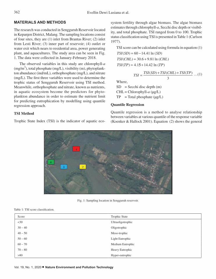
362 Evellin Dewi Lusiana et al.
Vol. 19, No. 1, 2020 • Nature Environment and Pollution Technology
MATERIALS AND METHODS
The research was conducted in Sengguruh Reservoir located in Kepanjen District, Malang. The sampling locations consist of four sites, they are (1) inlet from Brantas River; (2) inlet from Lesti River; (3) inner part of reservoir; (4) outlet or water exit which nears to residential area, power generating plant, and aquacultures. The study area can be seen in Fig. 1. The data were collected in January-February 2018.
The observed variables in this study are chlorophyll-a (mg/m3), total phosphate (mg/L), visibility (m), phytoplank-ton abundance (ind/mL), orthophosphate (mg/L), and nitrate (mg/L). The first three variables were used to determine the trophic status of Sengguruh Reservoir using TSI method. Meanwhile, orthophosphate and nitrate, known as nutrients, in aquatic ecosystem become the predictors for phyto-plankton abundance in order to estimate the nutrient limit for predicting eutrophication by modelling using quantile regression approach.
TSI Method
Trophic State Index (TSI) is the indicator of aquatic eco-
The purpose of this study is to identify the eutrophication state of Sengguruh
Reservoir by using Trophic State Index (TSI) and estimating the nutrient limit as the
indicators to predict the eutrophication. Since this study concerns to the high abundance of
phytoplankton which indicates eutrophication, then the relationship between nutrient and
phytoplankton abundance will be modelled at upper quantile. The index was introduced by
Carlson (1977) and has been widely used to assess the trophic status of many lakes and
reservoirs (Bekteshi & Cupi 2014).
MATERIALS AND METHODS
The research was conducted in Sengguruh Reservoir located in Kepanjen District,
Malang. The sampling locations consist of four sites, they are (1) inlet from Brantas River;
(2) inlet from Lesti River; (3) inner part of reservoir; (4) outlet or water exit which nears to
residential area, power generating plant, and aquacultures. The study area can be seen in Fig.
1. The data were collected in January-February 2018.
Fig. 1: Sampling location in Sengguruh reservoir.
The observed variables in this study are chlorophyll-a (mg/m3), total phosphate
(mg/L), visibility (m), phytoplankton abundance (ind/mL), orthophosphate (mg/L), and
nitrate (mg/L). The first three variables were used to determine the trophic status of
Sengguruh Reservoir using TSI method. Meanwhile, orthophosphate and nitrate, known as
nutrients, in aquatic ecosystem become the predictors for phytoplankton abundance in order
to estimate the nutrient limit for predicting eutrophication by modelling using quantile
regression approach.
Fig. 1: Sampling location in Sengguruh reservoir.
Table 1: TSI score classification.
Score Trophic State
<30 Ultraoligotrophic
30 – 40 Oligotrophic
40 – 50 Meso-trophic
50 – 60 Light Eutrophic
60 – 70 Medium Eutrophic
70 – 80 Heavy Eutrophic
>80 Hyper-eutrophic
system fertility through algae biomass. The algae biomass estimates through chlorophyll-a, Secchi disc depth or visibil-ity, and total phosphate. TSI ranged from 0 to 100. Trophic status classification using TSI is presented in Table 1 (Carlson 1977).
TSI score can be calculated using formula in equation (1)
TSI SD SD
TSI CHL CHL
TSI TP
( ) . ln ( )
( ) . . ln ( )
( ) .
= -= +
=
60 14 41
30 6 9 81
4 155 14 42+ . ln ( )TP
TSITSI SD TSI CHL TSI TP
=+ +( ) ( ) ( )
3…(1)
Where,SD = Secchi disc depth (m)CHL = Chlorophyll-a (μg/L)TP = Total phosphate (μg/L)
Quantile Regression
Quantile regression is a method to analyse relationship between variables at various quantile of the response variable (Koenker & Hallock 2001). Equation (2) shows the general

363NUTRIENT LIMIT ESTIMATION FOR EUTROPHICATION MODELLING
Nature Environment and Pollution Technology • Vol. 19, No. 1, 2020
form of quantile regression model (Buhai 2005).
yi i= ( ) +xitb q e q( ) 0 < q < 1 …(2)
Where,yi = response variable of the ith observation
xit = 1 1 2, , ,...,x x xi i pi( )
b(q) = parameter regression at the qth quantile
e q( )i = error/residual model of the qth quantile
i = 1, 2, ..., nAccording to Koenker & Basset (1978), parameter
estimation of equation (3) and (4) is the solution of mini-mization.
min ( ) ( ) ( ){ : ’ } { : ’ }b b bŒ Œ ≥ Œ <
- + - -Â Â p
i i i i
y f y fi ii i y
i ii i y
q qx xx x
1ÈÈ
ÎÍÍ
˘
˚˙˙
…(3)
min ( ){ : ’ }b bŒ Œ ≥
-( )È
ÎÍÍ
˘
˚˙˙
 p
i i
y fi ii i y
rq xx
…(4)
r qq ( ) ( ){ }u uu= - <1 0 , is called as check function which is illustrated in Fig. 2.
According to Chen (2005), equation (4) does not have fixed derivative form, so that a common numerical iteration cannot be performed to obtain the parameter estimation.
( )i iy tix β 0< <1 …(2)
Where,
iy = response variable of the ith observation
tix = 1 21, , ,...,i i pix x x
( β = parameter regression at the θth quantile
( )i = error/residual model of the θth quantile
i = 1, 2, ..., n
According to Koenker & Basset (1978), parameter estimation of equation (3) and (4) is
the solution of minimization.
{ : ' } { : ' }min ( ) (1 ) ( )
p
i i i i
i i i ii i y i i y
y f y f
β x β x βx x …(3)
{ : ' }
min ( )p
i i
i ii i y
y f
β x βx …(4)
{ 0}( ) ( 1 )uu u , is called as check function which is illustrated in Fig. 2.
Fig. 2: Check function.
According to Chen (2005), equation (4) does not have fixed derivative form, so that a
common numerical iteration cannot be performed to obtain the parameter estimation. Thus,
an alternative method of linear programming was considered namely simplex method.
Fig. 2: Check function.
Thus, an alternative method of linear programming was considered namely simplex method.
RESULTS AND DISCUSSION
Trophic Status of Sengguruh Reservoir
The TSI scores of each sampling site in Sengguruh Reservoir are given in Table 2.
According to Table 2, it can be seen that the TSI scores of the four sampling sites in Sengguruh Reservoir are between 68.64 and 74.35. It means that the trophic status is catego-rized as medium eutrophic and heavy eutrophic, but mostly the status is heavy eutrophic. These results show that the TSI score for medium eutrophic almost reach the upper limit for this category. So, on the whole, the eutrophication status in Sengguruh Reservoir is heavy eutrophic.
The status indicates that Sengguruh Reservoir has high fertility and this condition can reduce fishery production and biodiversity. The increase of fertility in aquatic ecosystem due to nutrient enrichment by the addition of organic matters into waters. According to Firdaus (2015), there is a tendency of land use changes and use of natural resources that do not consider aspects of soil and water conservation around the upstream Brantas River (Site 1) and Lesti River (Site 2) which cause the decline in watershed function, specifically
Table 2: Result of TSI Scores in Sengguruh Reservoir.
Site Week TSI Scores Remarks1 1 71.1025 Heavy eutrophic
2 73.2234 Heavy eutrophic3 72.269 Heavy eutrophic
2 1 69.805 Medium eutrophic2 74.0642 Heavy eutrophic3 72.0439 Heavy eutrophic
3 1 68.6458 Medium eutrophic2 74.2981 Heavy eutrophic3 73.8333 Heavy eutrophic
4 1 70.5054 Heavy eutrophic2 74.3593 Heavy eutrophic3 73.864 Heavy eutrophic

364 Evellin Dewi Lusiana et al.
Vol. 19, No. 1, 2020 • Nature Environment and Pollution Technology
to hold sediment materials.
As the consequence, the water entry of Brantas River and Lesti River into Sengguruh Reservoir embodied by a lot of sediments and organic matters as the result of domestic and agricultural wastes. Moreover, the residential areas and aquaculture activities (Site 4) around the Sengguruh Res-ervoir also contribute to the accumulation of sediment and organic matter in the waters. Especially, the use of fertilizer in agricultural activities and fish feed residues in aquaculture activities that contain nitrogen and phosphate may result in nutrient enrichment in the reservoir ecosystem.
Eutrophication Model
Eutrophication predictive model through nitrate and phos-phate concentration in Sengguruh Reservoir as the predictors conducted using quantile regression. The scatterplot to de-scribe the relationship between nutrients and phytoplankton abundance is shown in Fig. 3.
Fig. 3(a) reveals that the relationship between nitrate and phytoplankton abundance is not uniform of each quan-tile. Negative relationship was found in quantile 0.25 and 0.75, and the rest quantiles showed positive relationship. Meanwhile in Fig. 3b, the positive relationship carried out on quantile 0.25 and 0.75, but the remaining quantiles have negative relationship. The positive relationships of the variables explain that the increasing of nutrient content will
result in the higher abundance of phytoplankton. This find-ing is relevant to the eutrophication theory due to nutrient enrichment. However, in some quantiles, the relationship is negative or in other words the increase of nutrient will cause the phytoplankton abundance to decrease instead.
According to Table 2, current Sengguruh Reservoir is in heavy eutrophic state. It means that the eutrophication modelling at high quantile (q = 0.95) level will be used to predict heavy eutrophication. The parameter estimates of quantile regression are presented in Table 3.
Based on Table 3, nitrate and phosphate concentration of 0.853 mg/L and 0.862 mg/L respectively will cause me-dium eutrophication in Sengguruh Reservoir. If the results compared are to Wetzel (2001), then such concentration of nitrate and phosphate indicate the that the water is ol-igotrophic. These findings indicate that the classification cannot be used to identify the eutrophication in Sengguruh Reservoir since the sedimentation has been too high, and moreover a bit increase of nutrients will boost the abundance of phytoplankton.
CONCLUSION
Trophic status of Sengguruh Reservoir is classified as heavily eutrophic. The level of nitrate concentration to predict the heavy eutrophication is 0.853 mg/L, and phosphate is 0.862 mg/L. This result indicates that when the measurement of
to nutrient enrichment by the addition of organic matters into waters. According to Firdaus
(2015), there is a tendency of land use changes and use of natural resources that do not
consider aspects of soil and water conservation around the upstream Brantas River (Site 1)
and Lesti River (Site 2) which cause the decline in watershed function, specifically to hold
sediment materials.
As the consequence, the water entry of Brantas River and Lesti River into Sengguruh
Reservoir embodied by a lot of sediments and organic matters as the result of domestic and
agricultural wastes. Moreover, the residential areas and aquaculture activities (Site 4) around
the Sengguruh Reservoir also contribute to the accumulation of sediment and organic matter
in the waters. Especially, the use of fertilizer in agricultural activities and fish feed residues
in aquaculture activities that contain nitrogen and phosphate may result in nutrient
enrichment in the reservoir ecosystem.
Eutrophication Model
Eutrophication predictive model through nitrate and phosphate concentration in
Sengguruh Reservoir as the predictors conducted using quantile regression. The scatterplot to
describe the relationship between nutrients and phytoplankton abundance is shown in Fig. 3.
(a) (b)
Fig. 3: Scatterplot of phytoplankton abundance with quantile lines
(a) nitrate; (b) phosphate.
(a) (b)
Fig. 3: Scatterplot of phytoplankton abundance with quantile lines (a) nitrate; (b) phosphate.

365NUTRIENT LIMIT ESTIMATION FOR EUTROPHICATION MODELLING
Nature Environment and Pollution Technology • Vol. 19, No. 1, 2020
nitrate and phosphate almost reach such concentrations, then handling action must be carried out in order to prevent heavy eutrophication.
ACKNOWLEDGEMENTS
This research was funded through Hibah Peneliti Pemula (HPP) of Brawijaya University in 2019. The authors would like to thank all those who helped to complete the research.
REFERENCES
Bekteshi, A. and Cupi, A. 2014. Use of Trophic State Index (Carlson, 1977) for assessment of trophic status of the Shkodra Lake. Journal of Environmental Protection and Ecology, 15(1): 359-365.
Buhai, I.S. 2005. Quantile regression: Overview and selected applications. Ad Astra, 4: 1-17.
Carlson, R.E. 1977. A trophic state index for lakes. Limnology and Ocean-ography, 22(2): 361-369.
Chen, C. 2005. An Introduction to Quantile Regression and The QUANT-REG Procedure. Retrieved October 20th, 2014, from http://www2.sas.com/proceedingd/sugi30/213-30.pdf
Firdaus, M.R. 2015. Analisis Sedimentasi DAS Lesti dengan Perubahan Tata Guna Lahan di Kabupaten Malang. Rekayasa Sipil, 3(1): 19-28.
Isnaini, Surbakti, H. and Aryawati, R. 2014. Komposisi dan Kelimpahan Fitoplankton di Perairan Sekitar Pulau Maspari, Ogan Komering Ilir. Maspari Journal, 6(1): 39-45.
Koenker, R. and Basset, G. 1978. Regression Quantiles. Econometrica, 46: 33-50.
Koenker, R. and Hallock, K. 2001. Quantile regressions. Journal of Eco-nomic Perspectives, 15: 143-156.
Lusiana, E.D., Arsad, S., Kusriani, Buwono, N.R. and Putri, I.R. 2019. The application of Bayesian quantile regression to analyse the relationship
Table 3: Parameter estimates of quantile regression.
Quantile Phytoplankton-abundance (ind/mL)
Parameter estimates
Nitrate Phosphate
Intercept Slope Intercept Slope
0.05 650.92 7.137 4.282 7.092 4.012
0.25 749.80 3.687 -18.637 9.199 17.428
0.50 899.11 9.140 14.636 5.839 -6.349
0.75 1380.00 7.230 0.000 7.230 0.000
0.95 1586.91 9.799 15.254 5.849 -10.224
between nutrients content and phytoplankton abundance in Sutami reservoir. IOP Conference Series: Earth and Environmental Science, 230: 1-5.
Paiki, K. and Kalor, J.D. 2017. Distribusi Nitrat dan Fosfat Terhadap Kelimpahan Fitoplankton di Perairan Pesisir Yapen Timur. Journal of Fisheries and Marine Science, 1: 65-71.
Putri, F.D.M., Widyastuti, E. and Christiani 2014. Hubungan Perbandingan Total Nitrogen dan Total Fosfor dengan Kelimpahan Fitoplankton di Perairan Waduk Panglima Besar Soedirman, Banjarnegara. Scripta Biologica, 1: 96-101.
Rashidy, E.A., Litaay, M., Salam, M.A. and Umar, M.R. 2013. Komposisi dan Kelimpahan Fitoplankton Di Perairan Pantai Kelurahan Tekolab-bua, Kecamatan Pangkajene, Kabupaten Pangkep, Provinsi Sulawesi Selatan. Jurnal Alam dan Lingkungan, 4(7): 1-6.
Sugiura, N., Utsumi, M., Wei, B., Iwami, N., Okano, K., Kawauchi, Y. and Maekawa, T. 2004. Assessment for the complicated occurence of nuisance odours from phytoplankton and environmental factors in a eutrophic lake. Lake & Reservoirs: Res. and Man, 9: 195-201.
Suryanto, A.M. 2011. Abundance and phytoplankton composition in Se-lorejo Reservoir, Ngantang District, Malang Regency. Jurnal Kelautan, 4(2): 34-39.
Wetzel, R.G. 2001. Limnology: Lake and River Ecosystems. Elsevier Academic Press, New York.
Widyastuti, E., Sukanto and Setyaningrum, N. 2015. Pengaruh Limbah Organik terhadap Status Tropik, Rasio N/P serta Kelimpahan Fitoplank-ton di Waduk Panglima Besar Soedirman Kabupaten Banjarnegara. Biosfera, 32(1): 36-40.
Xu, Y., Schroth, A., Isles, P. and Rizzo, D. 2015. Quantile regression improves models of lake eutrophication with implications for eco-systems-specific management. Freshwater Biology, 60: 1841-1853.
Yetti, E. 2007. Evaluasi Kualitas Air Sungai-sungai di Kawasan DAS Brantas Hulu Malang dalam Kaitannya dengan Tata Guna Lahan dan Aktivitas di Sekitarnya. (Post Graduate), Institut Pertanian Bogor, Bogor.
Yu, K. and Moyeed, R.A. 2001. Bayesian quantile regression. Statistics and Probability Letters, 54: 437-447.

Vol. 19, No. 1, 2020 • Nature Environment and Pollution Technology
366

Concrete Construction Waste Pollution and Relevant Prefabricated Recycling Measures
Zhang Jie† and Chen NanDepartment of Architectural Engineering, Jiyuan Vocational and Technical College, Jiyuan 459000, China†Corresponding author: Zhang Jie
ABSTRACT
Architectural construction has expanded continuously in recent years as a response to China’s accelerating urbanization, thus further leading to the dramatic increase of concrete usage. This expansion may cause serious threats to the ecological environment because the production and construction of traditional concrete materials may consume abundant resources, such as coals and limestone, and thus emit air pollutants. Prefabricated concrete building can significantly reduce the use of water, timber, thermal insulation materials, and cement mortar, thereby decreasing construction waste and carbon emissions greatly. Based on the review of the measures for concrete construction waste recycling in developed countries, this study summarized the types of hazards of concrete construction waste pollution, analysed the advantages of prefabricated concrete constructions, and proposed prefabricated recycling measures of concrete construction wastes. Results demonstrate that developed countries have relatively perfect concrete construction waste recycling systems. The hazards of concrete construction wastes are mainly manifested by the embezzlement of lands, water pollution, atmosphere pollution, soil pollution, and damage to physical health. The advantages of prefabricated concrete construction are manifested by high production efficiency, energy conservation, environmental protection, and overall high quality. Finally, several recycling measures were proposed, including strengthened policy support to prefabricated concrete construction; appropriate relevant laws, regulations, and standard systems; improved prefabricated construction enterprises; and enhanced environmental protection in prefabricated construction sites. Research conclusions can serve as reference for understanding the hazards of concrete construction-induced environmental pollution, recognizing the advantages of prefabricated concrete construction mode, increasing prefabricated concrete market shares comprehensively, and alleviating environmental pollutions.
INTRODUCTION
China’s construction industry improves residents’ quality of life and drives the growth of GDP (Gross Domestic Product). The sustainable, sound development of construction industry is vital to the development of China. Construction waste refers to the waste soil and other materials produced by construction companies and units during new construction, reconstruction, expansion, and demolishment of various buildings, structures, and pipe networks and by residents during home decoration. Currently, the construction wastes in urban areas in China are a major proportion of the total urban waste. If these construction wastes cannot be recycled reasonably, then they would increase continuously, and their proportion in the total urban waste may further increase with the China’s continuous urbanization. Muck, waste concrete blocks, waste mortar, brick fragments, cullets, tile fragments, waste asphalt blocks, waste plastics, waste metals, and waste bamboo and timber materials are the major components of construction wastes. Most construction wastes, especially
concrete construction wastes from demolishing buildings, can be recycled after screening, deletion, or smashing. Cur-rently, the majority of concrete construction wastes in China are not reused. Instead, concrete construction wastes are transported to suburbs or rural areas and disposed in dump sites or landfills in open spaces, thus causing serious hazards to the ecological environment.
China’s construction industry has recently achieved rapid development. Fig. 1 shows that the total output of China’s construction industry rose from 6,203.681 billion Yuan in 2008 to 23,508.553 billion Yuan in 2018, showing an annual average growth of 28%. The building area of China’s con-struction industry increased from 5,305,186,300 m2 in 2008 to 14,089,204,000 m2 in 2018, showing an annual average growth rate of 17%. These numbers fully reflect the consid-erable consumption of basic materials, such as concrete, in China’s construction industry, resulting in massive amounts of construction wastes. However, the traditional dump sites or landfills of concrete construction wastes may occupy
Nat. Env. & Poll. Tech.Website: www.neptjournal.com
Received: 10-12-2019Accepted: 16-01-2020
Key Words:Concrete architecture Construction wasteWaste pollutionRecycling measures
2020pp. 367-372 Vol. 19
p-ISSN: 0972-6268 No. 1 Nature Environment and Pollution Technology An International Quarterly Scientific Journal
Original Research Paper
e-ISSN: 2395-3454
Open Access

368 Zhang Jie and Chen Nan
Vol. 19, No. 1, 2020 • Nature Environment and Pollution Technology
large areas of cultivated land. Moreover, long-term piling or landfills of concrete construction wastes may cause soil, underwater, and atmosphere pollution. In addition, concrete construction wastes are generally transported by open ve-hicles. Waste leakage, dusts, and lime sands may influence urban appearance and environmental health seriously and bring serious threats to the production and life of residents during transport. To sum up, the existing disposal means of concrete construction wastes cannot satisfy the needs of sustainable urban development, and the recycling of concrete construction wastes is essential in realizing the sustainable development of China’s construction industry and a harmo-nious ecological environment.
PAST STUDIES
With the strengthening of environmental protection and resource saving consciousness, countries worldwide are enhancing the recycling of urban construction wastes. Many studies and applications on recycling technologies for construction wastes have been undertaken. Developed countries, such as US, Germany, and Japan, have achieved high construction waste recycling rates, whereas the recycling rate of construction wastes in China remains low. Hsiao et al. believed that the concrete logistics amount produced by new construction and demolishment projects was increasing dramatically in Taiwan. They simulated concrete wastes in the material flow based on a dynamic model and found that the concrete construction wastes were expected to increase continuously. Concrete construction waste recycling must be increased comprehensively to decrease the environmental pollution in Taiwan (Hsiao et al. 2002). Gotoh et al. analysed the total suspended particulates concentration in regions damaged seriously during the Hanshin Earthquake and
found that the elements in the concrete dusts (Ca and S) in construction wastes are similar to those in mortar dust, which is one of the major sources of air pollution (Gotoh et al. 2002). Andersson M. et al. studied polychlorinated biphenyl (PCB) pollution in gypsum on the external building walls in Bergen, Norway and reported that the PCB concentration in soil and plaster of residential buildings and schools was higher than those in office buildings, warehouses, or industrial buildings (Andersson et al. 2004). Lindgren investigated a concrete contamination indoor ammonia event in an office of one airline in Beijing and found that the ammonium hydroxide pollution in the Beijing Office might come from the additives in concretes (Lindgren 2010). Taylor-Lange et al. predicted the specific activity of radium and the probability of radon precipitation through Monte Carlo simulation and estimated the indoor radon concentration and the effective annual dose under two different concrete floors (one has fly ash, whereas the other has no fly ash) in a typical single-family house in the US. Their results show that exposure to radon in concrete buildings could influence human health significantly (Taylor-Lange et al. 2012). Arunvivek et al. believed that commercial concrete industries worldwide are producing abundant wastewater and fresh concrete waste aggregate, which may cause serious environmental pollution upon improper disposal (Arunvivek et al. 2015). Wu et al. believed that the accelerating modern industrialization and urbanization in China might cause construction dust emission. He investigated the current dust control situations in China’s construction industry, determined the main sources of construction dust, and proposed a case study to interpret the major dust control measures in construction sites (Wu et al. 2016). With respect to the recycling measures of concrete construction wastes, Eguchi et al. proposed a concrete recycling method that was different from that of
0
200000
400000
600000
800000
1000000
1200000
1400000
1600000
0
50000
100000
150000
200000
250000
2008 2009 2010 2011 2012 2013 2014 2015 2016 2017 2018
Cons
truct
ion
indu
stry
hous
ing
cons
truct
ion
area(
mill
ion
squa
re m
eter
s)
The
tota
l out
put v
alue
of t
he co
nstru
ctio
n in
dustr
y (
billi
on /R
MB)
Fig. 1: Total output and building areas of China’s construction industry during 2008-2018. (Data source: China Statistical Yearbook 2009-2019).
369CONCRETE CONSTRUCTION WASTE POLLUTION AND RECYCLING MEASURES
Nature Environment and Pollution Technology • Vol. 19, No. 1, 2020
ordinary concrete, thus obtaining data needed to determine the mixing ratio design and the quality control method. The economic efficiency and environmental loads of this method were assessed, and the validity of this method was verified (Eguchi et al. 2007). Rao et al. reviewed the international production of C&D wastes and the utilization of recycled aggregates (RAs) and summarized influences of RA use on fresh and hardened concretes’ performance (Rao et al. 2007). Tam believed that construction materials were poured to landfills, and abundant wastes might be produced from construction sites. As a method of reducing concrete wastes, using recycled concrete wastes as RA can be an economical and effective method for China’s construction industry; this method is also conducive to environmental protection (Tam 2008). Naik believed that Portland cement is an important component of concrete, and abundant greenhouse gas, that is, CO2, is released during the production of Portland cement. He suggested the construction of a sustainable concrete structure to ensure minimum influence on the environment within its service life (Naik 2008). Khatib et al. suggested the reduction of urban pollution through the innovative use of building materials, the reduction of the dependence on traditional concrete construction, and the effective recycling of concrete construction wastes (Khatib et al. 2018). Xing et al. pointed out that dust pollution is a key problem in the construction process that must be addressed, and the government should assume partial responsibility and reduce dust emission at construction sites for the public. According to data analysis, the preferred technologies and organization measures of the Chinese government, institutional guarantees, and technological innovation are prerequisites of dust-free construction (Xing et al. 2018). Akhtar et al. pointed out that the production of concretes and construction wastes are among the major causes of continuous CO2 emission in the atmosphere. According to the sorting and critical analysis of information from 40 countries in six continents, he suggested the use of 30%-50% RA-assisted concrete with binding materials to achieve the strength of natural aggregate concrete (Akhtar et al. 2018). Colangelo et al. suggested the use of “green” RA in concrete production to mitigate the potential adverse effects on environment and energy (Colangelo et al. 2018). Based on existing studies, developed countries have relatively perfect recycling systems of concrete construction wastes and carried out abundant studies on waste concrete RA and prepared RA concretes. On the basis of the comprehensive analysis of the pollution hazards of concrete construction wastes, this study analysed the advantages of prefabricated concrete construction and proposed prefabricate construction waste recycling measures to provide references for solving construction waste pollution control problems, standardizing
construction waste management, and reducing abundant construction resource wastes.
HAZARDS OF CONCRETE CONSTRUCTION WASTES
Embezzlement of Lands
In China, construction waste results in considerable annual embezzlement of land areas. Moreover, the output of con-struction wastes will increase continuously as a result of China’s economic development, the continuous expansion of the urban construction scale, and the increasing demand for living conditions. The embezzlement of lands will in-tensify continuously because of the delayed processing and utilization of concrete buildings. Concrete is essential to construction and transportation infrastructure construction. In particular, the demands for concrete will increase greatly with China’s continuous urbanization, thus resulting in increased demands for sands and stones, which are used as concrete aggregates. Such huge demands for sands and stones will surely lead to large-scale mountain quarrying and the exploitation of river sands, which will in turn cause serious damages to the ecological environment.
Water Pollution
Concrete in construction waste is rich in water soluble cal-cium silicate and calcium hydroxide. Waste plaster contains many sulphate ions. Waste metals involves the dissolution of heavy metal ions. Through anaerobic degradation, waste paper plates and timbers may generate lignins and tannin, which are further decomposed into organic acids. Thus, the percolating water of concrete construction waste after immersion in rainwater in landfill is generally strong in alkali and contains heavy metal ions, hydrogen sulphide, and certain amounts of organic matters. If this percolating water is not controlled and flows into rivers and lakes or penetrated underground, then the surface and underground water pollution is intensified accordingly, thus damaging the survival of aquatic organisms and affecting the secondary use of water resources. This phenomenon will cause irreversible damage to the water environment.
Atmospheric Pollution
Waste plaster in concrete construction waste contains abundant sulphate ions, which are transformed to hydrogen sulphide and volatile organic acids under anaerobic con-ditions. These harmful gases cause atmospheric pollution once emitted to the air. Resource reserves and output, such as natural sands and stones, are decreasing annually due to exploitation. Particularly, natural river sands cannot satisfy

370 Zhang Jie and Chen Nan
Vol. 19, No. 1, 2020 • Nature Environment and Pollution Technology
the demands, a shortcoming that is worsened by the in-creasing supply–demand contradictions. Resource shortage is particularly serious in certain big cities. Thus, finding alternative resources is an urgent concern. Many artificial sands have been put into use. In coastal regions with rela-tively high economic development, sea sands are applied to prepare concretes by taking advantage of geology. However, sea sands have a relatively high Cl-content. The illegal or unreasonable use of sea sands can easily cause the corrosion of reinforcement in concrete, eventually bringing potential safety risks in architectural structures.
Soil Pollution
Harmful substances in construction wastes and their per-colating water cause soil pollution, which is manifested in changes in physical structures and in the chemical properties of soil. Soil pollution influences the nutrient adsorption and growth of plants and the activity of microorganisms in soils, breaks the ecological balance in soils, and promotes the accumulation of harmful substances in soils. Consequently, the harmful substances in soils exceed the standards, thus inhibiting plant growth and even causing plant death. In addition, harmful substances may be transferred to fruits through plant adsorption and further influence the physical health of humans and animals through the food chain.
Threats to Physical Health
Concrete construction wastes, which are piled up randomly without processing, produce harmful substances that may enter the atmosphere, water, and soil. Subsequently, these harmful substances may enter the human body through various ways, thus resulting in poisoning. Many toxic and harmful components in concrete construction wastes enter the food chain through animals and plants, which further lead to lesions and affect the physical health of humans. During respiration, harmful dusts from concrete construction wastes may enter the human body through the respiratory tract and diffuse in the circulatory system, thus causing substantial damage to the human body.
ADVANTAGES OF PREFABRICATED CONCRETE CONSTRUCTION
High Production Efficiency
The prefabricated parts of prefabricated concrete construction are manufactured through assembly lines in factories and then transported to construction sites for mechanical hoisting assembly. This path not only saves in labour force and materials significantly but also increases concrete construction efficiency. Furthermore, the convenience
and efficiency of construction work is increased. Thus, planned tasks can be accomplished in a short period, which is desirable. The construction of prefabricated buildings is affected slightly by severe weather conditions. Therefore, prefabricated concrete construction significantly increases production efficiency and shortens construction period in comparison with traditional construction means.
Coexistence of Energy Saving and Environmental Protection
Traditional architectural construction requires the frequent casting-in-situ of concretes, which may cause serious dust and wastewater pollution as well as noise pollution in con-struction sites. On the contrary, prefabricated concrete con-struction can decrease casting-in-situ significantly. The direct assembly and installation of prefabricated components not only save in field wetting operation to a large extent but also decrease dust and wastewater pollution and the production of construction wastes. They result in a green construction environment. During the production of prefabricated com-ponents, reusing moulds and assembly line-based production can maximize resources. Mechanical hoisting assembly is basically applied in installing parts, which decreases the use of many scaffolds and templates and promotes resource saving and environmental protection.
Guarantee of Overall High Quality
Prefabricated components are manufactured through standard production line. Improving production technologies and the standardized production procedure can guarantee the satis-factory quality of prefabricated components. Components, such as prefabricated external wall panels, can maintain the stability of walls, while water-proofing, heat insulation, and thermal insulation are considered. This strategy decreases field construction and promotes quality components. The manufacturing of prefabricated components in factories plays an important role in effectively controlling architec-tural quality.
PREFABRICATED RECYCLING OF CONCRETE CONSTRUCTION WASTES
Strengthen Policy Supports to Prefabricated Concrete Construction
The guidance and support of governments provide a development direction for prefabrication construction and guarantee benefits for prefabricated construction enterprises. The reasonable management by the government determines the development of prefabricated construction. The development of prefabricated construction realizes the
371CONCRETE CONSTRUCTION WASTE POLLUTION AND RECYCLING MEASURES
Nature Environment and Pollution Technology • Vol. 19, No. 1, 2020
philosophy of China’s green energy-saving push. China should increase its investment on prefabricated construction development; formulate various supporting policies that provide capital subsidies, preference policies for land bidding, loans with discounted interests, and preferences to economic technological indexes (like plot ratio and building area); set up a special promotion department for the large-scale propaganda of the advantages of prefabricated construction; formulate an excitation mechanism; and develop the guidance of government. To provide reliable guarantees to real estate developers and construction units, the government of China can apply special funds for prefabricated construction, formulate preference policies to attract foreign investment, and increase marketing efforts. Moreover, the Chinese government should set up a series of special key subjects of prefabricated construction in colleges and universities, offer financial assistance to relevant experiments and practices in universities, train talented individuals with technological and management skills, and establish key technology R&D funds to promote R&D and the innovation of structure and technological systems for prefabricated construction.
Perfect Laws and Regulations of Prefabricated Concrete Construction
Currently, the prefabricated component manufacturing market in China is chaotic. Owing to the lack of production standards and norms, the component cost remains high, thereby restricting the expansion of prefabricated com-ponent manufacturing. Provinces and cities have released relevant laws and regulations, and some standards have been formed in local regions. However, these laws, regulations, and standards are independent from one another and are lacking in authority and universality, thus resulting in di-versity and chaotic national industrial standards. China has published the industrial standards of Technical Regulations on Prefabricated Concrete Structure several years ago. The standards propose explicit technical regulations in different links of the entire process, and they restrict construction chaos to a certain extent. Thus, relevant departments of Chi-na should concentrate their industrial powers to formulate China’s standards or norms, implement specific rules, realize standardized production, expand the manufacturing scale of prefabricated components, and decrease the production cost of single components, thereby lowering the engineering cost and facilitating the industrialized development of construc-tion. In addition, the formulation and further perfection of universal standard atlas or technical design scheme must be accelerated; unique, standardized, systematic, and supporting technical standard systems must be formed; the requirements of different provinces and cities for building functions and performances should be met; laws for reference throughout
the prefabricated construction process must be offered; and technical foundations for expanding the prefabricated con-struction scale must be laid out.
Improve Levels of Prefabricated Construction Enterprises
The prefabricated construction industry is developing slowly in China and remains in the initial stage. China has successive-ly released many supporting policies and incentive measures to guide the sound development of prefabricated construc-tion. Owing to hindering factors, such as excessively high investment, prefabricated component manufacturers are few and are lacking enthusiasm to scale up. Thus, prefabricated component manufacturers are costly, which further restricts scale expansion. Therefore, different provinces and cities of China should perfect supporting policies, implement specific rules, provide certain guarantee, stimulate the enthusiasm of manufacturers, introduce benefits to manufacturers, expand market demands, improve the productivity, and form scale benefits. Additionally, local governments should improve the professional quality of workers in prefabricated component manufacturers and train professional technicians and man-agers through regular professional trainings to improve the production efficiency and professional degree of enterprises and bring them additional benefits. To encourage prefabri-cated construction industrial development, the provinces and cities of China launched many pilot projects. Through these pilot projects, China should integrate resources effectively, increase the R&D of key technologies and talent training, and accelerate the training of professional production and construction and leading enterprises that integrate the design, production, and construction of prefabricated components.
Strengthen Environment Protection at Prefabricated Construction Site
Enterprises should pay attention to the environmental management of construction sites. Enterprise protection is an important factor in modern construction industry. The management level of enterprises determines the construction schedule and level. Therefore, managers with rich management experiences and strong coordination ability should be selected for construction site management. Additionally, several management measures should be adopted to increase the management level and decrease unnecessary expenditures. The construction schedule should be planned reasonably to control the construction period, and the use of expensive heavy hoisting equipment should be minimized. Moreover, construction sites should be managed through an environmental protection method that includes material wastes reduction, reasonable arrangement of construction order, and slowdown phenomenon prevention.

372 Zhang Jie and Chen Nan
Vol. 19, No. 1, 2020 • Nature Environment and Pollution Technology
The assembly efficiency should be improved to increase the components produced in factories, decrease the field management of components, increase the construction efficiency, and save cost.
CONCLUSIONS
The output of construction wastes in China is increasing annually, resulting in the increasingly prominent problem of construction waste pollution control. Construction wastes not only occupy large-scale land resources but also cause sub-stantial damage to soil, air, and water environments. Moreo-ver, China has failed in recycling construction wastes. With continuous urbanization, the volume of construction waste may increase, and its proportion in total urban wastes may increase further. This study reviewed the recycling measures of concrete construction wastes in developed countries, sum-marized the types of hazards of concrete construction waste pollutions, and analysed the advantages of prefabricated concrete construction. Results demonstrate that developed countries have relatively perfect recycling systems for con-crete construction wastes. The embezzlement of lands, water pollution, atmospheric pollution, soil pollution, and threats to physical health are the five types of concrete construction waste hazards. Prefabricated concrete construction has sev-eral major advantages, such as high production efficiency, energy saving and environmental protection, and overall high quality. Certain measures can be adopted to decrease the environmental pollutions from concrete construction wastes, including the strengthening of policy supports for prefabricated concrete construction, appropriate relevant laws, regulations and standard systems, improving the levels of prefabricated construction enterprises, and enhancing the environmental protection of prefabricated construction sites. Intensive studies on concrete construction waste recy-cling systems, information disclosure systems that connect different stages of concrete waste disposal, comprehensive evaluation of prefabricated concrete construction quality, and environmental pollution control at prefabricated concrete construction sites must be continued.
REFERENCES
Akhtar, A. and Sarmah, A. K. 2018. Construction and demolition waste generation and properties of recycled aggregate concrete: A global perspective. Journal of Cleaner Production, 186: 262-281.
Arunvivek, G. K., Maheswaran, G. and Senthil Kumar, S. 2015. Eco-friendly solution to mitigate the toxic effects of hazardous construction industry waste by reusing in concrete for pollution control. Nature Environment & Pollution Technology, 14(4): 963-966.
Andersson, M., Ottesen, R. T. and Volden, T. 2004. Building materials as a source of PCB pollution in Bergen, Norway. Science of the Total Environment, 325(1-3): 139-144.
Colangelo, F., Forcina, A., Farina, I. and Petrillo, A. 2018. Life cycle assessment (LCA) of different kinds of concrete containing waste for sustainable construction. Buildings, 8(5): 70.
Eguchi, K., Teranishi, K., Nakagome, A., Kishimoto, H., Shinozaki, K. and Narikawa, M. 2007. Application of recycled coarse aggregate by mixture to concrete construction. Construction and Building Materials, 21(7): 1542-1551.
Gotoh, T., Nishimura, T., Nakata, M. and Nakaguchi, Y. 2002. Air pollution by concrete dust from the great hanshin earthquake. Journal of Environmental Quality, 31(3): 718-723.
Hsiao, T. Y., Huang, Y. T., Yu, Y. H. and Wernick, I. K. 2002. Modeling materials flow of waste concrete from construction and demolition wastes in Taiwan. Resources Policy, 28(1-2): 39-47.
Khatib, J. M., Elkordi, A. A. and Saleh, Z. A. 2018. Mitigating Urban Pollu-tion through Innovative use of construction materials. Urban Pollution: Science and Management, pp. 235-247.
Lindgren, T. 2010. A case of indoor air pollution of ammonia emitted from concrete in a newly built office in Beijing. Building and Environment, 45(3): 596-600.
Naik, T.R. 2008. Sustainability of concrete construction. Practice Periodical on Structural Design and Construction, 13(2): 98-103.
Rao, A., Jha, K. N. and Misra, S. 2007. Use of aggregates from recycled construction and demolition waste in concrete. Resources, conservation and Recycling, 50(1): 71-81.
Taylor-Lange, S. C., Stewart, J. G., Juenger, M. C. G. and Siegel, J. A. 2012. The contribution of fly ash toward indoor radon pollution from concrete. Building and Environment, 56: 276-282.
Tam, V. W. Y. 2008. Economic comparison of concrete recycling: A case study approach. Resources, conservation and recycling, Resources, Conservation and Recycling, 52(5): 821-828.
Wu, Z., Zhang, X. and Wu, M. 2016. Mitigating construction dust pollution: State of the art and the way forward. Journal of Cleaner Production, 112: 1658-1666.
Xing, J., Ye, K., Zuo, J. and Jiang, W. 2018. Control dust pollution on construction sites: What governments do in China? Sustainability, 10(8): 2945.
Evaluation of Iron and Manganese Levels from Ramgarh Lake, Gorakhpur, U.P., India
Mahima Chaurasia*† and Sanjeev Kumar Srivastava***Institute of Engineering & Technology, Dr. R. M. L. Avadh University, Ayodhya, U.P., India**Department of Basic Science, SRMS College of Engineering & Technology, Bareilly, U.P., India†Corresponding author: Mahima Chaurasia
ABSTRACT
Natural waters vary in chemical composition and the factors controlling the composition include physical, chemical and biological processes. Water is one of the most important natural resources for all the living organisms because it is required for various metabolic activities. In addition, water is required for various domestic purposes, irrigation and power generation and the industries. Amongst various organic components, the iron and manganese are an important trace metal required for all the biological systems. The occurrence of iron and manganese, in the present study, was reported from Ramgarh Lake in Gorakhpur, India. Two sampling stations were selected for the present study. The iron and manganese have several effects due to their high concentration. The study was carried out for one year (January 2017 to December 2017). The significance of iron and manganese is discussed in the present investigation.
INTRODUCTION
The environment is a system of physical, chemical and biological factors and dynamic equilibrium. The indiscriminate industrial, domestic water discharged into natural water system has created the hazards to the aquatic life. Water is the most versatile, vital and essential component for all life forms. It is abundant on our planet occurring as a universal solvent, an indispensable component of nature holding both biotic and abiotic entities in a complex, dynamic and delicate ecological balance by virtue of its unique capacity existing in solid, liquid and gaseous states. Energy and water are indeed two essential components for the propagation of life. Quality of water, therefore, bears profound significance for conditioning the quality of life and environment in both aquatic and terrestrial.
The increasing industrialization, urbanization and de-velopment activities to cope with the population explosion have brought inevitable water crisis (Rao & Rameshwari 1998). The discharge of industrial effluent into the natural water bodies causing severe water pollution. Alteration in the chemical composition of a natural aquatic environment by industrial effluents usually induces changes in the aquatic ecosystem particularly aquatic organisms. Pollution is be-fouling the environment by man’s activities particularly by the disposal of solid, gaseous and liquid waste products. Most
of our water bodies, rivers and streams have become polluted and unfit for human use. Ramgarh Lake in Gorakhpur district is no exception. Gorakhpur city and several villages and residential colonies are settled around the Ramgarh Lake. The load of pollutants is increasing day by day in Ramgarh Lake and this poses a formidable challenge to water quality. (Srivastava et al. 2006, 2007).
Food and water are the main sources of our daily requirements of essential metals. These (with the addition of air) are also the media through which we are constantly exposed to the various toxic metals. The body, through urine and faeces, exerts metals, which are in excess, otherwise, there may be a chance of their accumulation in various body tissues. Metals are indestructible poison. Their dispersion into streams, rivers and oceans for a long duration may be highly dangerous, because they may affect the production of atmospheric oxygen, contaminate the water and affect the life of freshwater ecosystem influenced by air-heavy metals and addition from anthropogenic sources. At present, several metals are believed to be essential for life; some of them are iron, copper, zinc, manganese, cobalt, molybdenum, selenium, chromium, nickel, tin and vanadium, etc. Metals usually considered to be toxic at ‘physiological dose’ may be stimulatory or essential in very minute doses depending upon the environment and state of the organism.
Nat. Env. & Poll. Tech.Website: www.neptjournal.com
Received: 27-04-2019Accepted: 21-06-2019
Key Words:IronManganeseRamgarh lakeWater analysis
2020pp. 373-377 Vol. 19
p-ISSN: 0972-6268 No. 1 Nature Environment and Pollution Technology An International Quarterly Scientific Journal
Original Research Paper
e-ISSN: 2395-3454
Open Access

374 Mahima Chaurasia and Sanjeev Kumar Srivastava
Vol. 19, No. 1, 2020 • Nature Environment and Pollution Technology
The indispensability, deficiency or toxicity of metal is manifestations of dose response effect. However, environmental conditions, natural and biological factors, such as age, sex, species differences, stress, and relationship of one metal with the other metal and metal ion imbalance in biological system, in turn influences the toxicity of metal. Uptake of heavy metals through food chain in human beings may cause various physiological disorders, like hypertension, sporadic fever, renal damage, cramps, etc. The bioaccumulation of metal toxicants in plants and fish depends on availability and persistence of the contaminants in water and the physic-chemical properties of the toxicants. Iron is the second most abundant metal after aluminium in the earth’s crust. Iron is an essential trace metal, required as a constituent of oxygen-carrying and oxidative-reductive micro molecules, such as haemoglobin, myoglobin and cytochrome. Manganese is a greyish similar to the appearance of cast-iron. Manganese, an essential element for animals and man, occurs in the cells of all living organisms. It is the twelfth most abundant element and the fifth most abundant metal. Manganese is also an essential trace element required by the plants. In some waters, it may limit either directly or indirectly the growth of algae. The present study has been carried out to find the levels of iron and manganese in Ramgarh lake in Gorakhpur.
MATERIALS AND METHODS
The Ramgarh lake is spread over 669.73 ha near Gorakhpur city on Gorakhpur-Deoria highway, which lies between Lat. 26°13’N-27°29’N and Long. 83°05’E-83°56’ E. The height above sea level ranges from 107 meters in northwest to 93 meters in the southeast. The lake receives urban sewage through a wide network of the drain during the past few years. The water of this lake is widely used for agricultural, irrigation, domestic and industrial purposes. The lake is useful for fish culture and, nearly 20 to 25 villages water supply is carried out from the lake. Metals transported from the nearby silts, rocks, etc., can play a vital role in supplying micro-metals for the human consumption. It is very important to investigate a few metals, which are very essential for our life. Hence, we selected the useful two metals present in the lake. For the present analytical study, we divided the lake into two parts. A good population of submerged aquatic plants is found in this area.
The study of iron and manganese content from the Ramgarh Lake was undertaken and it was estimated by spectrophotometer method. The water samples from both sampling stations were brought to the laboratory regularly in clean containers at early hours. Standard methods prescribed by APHA (2012) were applied for the collection
and analysis of the water samples. The concentration of iron and manganese was measured on a spectrophotometer at a specific filter. Results were expressed as mg/L and compared with permissible levels.
RESULTS AND DISCUSSION
Several heavy metals are essential for the growth and survival of plants and animals. These are originated from both natural and anthropogenic sources (Wintz et al. 2002). The results obtained in the present work are illustrated in Tables 1 and 2. The iron concentration of the water sample-1 varied from 0.65 mg/L to 1.69 mg/L. Sample-2 showed iron content ranging between 1.32 to 1.98 mg/L (Fig. 1). The mean values for the sample-1 and 2 were 1.17 mg/L and 1.67 mg/L, respectively. Overall results showed the minimum iron content in monsoon and maximum in summer season. Iron is an essential heavy metal for higher plants and algae, particularly for photosynthesis. Higher concentration of iron in water imparts a bitter taste and inky flavour (Khurshid et al. 1997, Rana et al. 2016). Iron in surface water is generally present in the ferric (Fe+3) state. The maximum allowable concentration of iron in drinking water is 1.0 mg/L, according to WHO (2004) report. Indian Standard Institute (ISI) and Indian Council of Medical Research (ICMR), the permissible concentration of iron and manganese in drinking water is 1.0 and 0.3 mg/L, respectively. In the present investigation, the mean iron concentration was observed more than the permissible limit. Increased concentration of iron has earlier been reported in river Kali and Hindon waters (Ajmal & Razi-Uddin 1988) and in river Ganga (Ray 1989).
Sharma et al. (2000), monitored the iron content in the 13 drinking water sources from a predominantly rural area of Goalpara district (Assam). They reported 0.02 to 1.50 mg/L iron concentration, which is quite low from the present investigation. Mohapatra & Singh (1999), reported iron content in Mahanadi river water fluctuates between 0.468 and 2.18 mg/L with a mean value of 1.35 mg/L. Nag & Das (1995) analysed surface drinking water in the Purulia district of West Bengal and reported iron content from 0.1 to 13.22 mg/L. However, the mean value was found to be 0.2 mg/L. Manganese is an essential element which does not occur naturally as a metal but is found in various salts and minerals frequently in association with iron compounds (Dwivedi & Tiwari 1997, Srivastava & Pandey 2008, Priyadarshinee & Verma 2016). In the present investigation, sample-1 showed the minimum manganese ion content (0.24 mg/L) in the month of June and maximum value (0.47 mg/L) in the month of December. Sample-2 showed lowest manganese concentration (0.37 mg/L) in the month of June and highest (0.58 mg/L) in the month of December (Fig. 2). The average

375IRON AND MANGANESE LEVELS IN RAMGARH LAKE
Nature Environment and Pollution Technology • Vol. 19, No. 1, 2020
concentration was 0.36 mg/L and 0.47 mg/L for Sample-1 and 2, respectively. The permissible limit for manganese set by WHO is 0.05 mg/L. Both water samples have higher mean values than the permissible limit.
Some workers previously reported manganese levels of river water. Sinha (2004), monitored the Mn+2 content in water of Sai river at Rai Bareilly, and reported that it varied from 0.08 to 2.2 mg/L. They further reported that manganese in high concentration becomes toxic to plants also. Manganese is found as a cofactor in several enzyme systems. It plays a role in the proper functioning of flavour-proteins and in the synthesis of cholesterol, haemoglobin and in many other important metabolic processes (Tale & Bhosle 2010, Ingole et al. 2016). The water samples having more than 0.1 mg/L of manganese for long exposure is harmful for all animals (WHO 1988). Israili (1991), analysed
water of Ganga river from eight different sampling stations and reported that Mn+2 content varies from 35.0 to 211.0 µg/L. Furthermore, Israili & Khurshid (1991) studied the distribution of heavy metals in Yamuna river water, which they observed within the permissible limit. Dwivedi & Tiwari (1997) studied Mn+2 content of Ganga river and reported the mean Mn+2 values ranged from 19.1 to 15.2 µg/L.
From the present investigation, both iron and manganese ion values were observed higher than the permissible limit due to the discharge of sewage, municipal and small-scale industrial waste. Thus, the toxic impact of sewage rendering the lake water unsuitable for sustenance and propagation of aquatic life and unfit for animal and human consumption. Authorities should make concrete efforts, particularly effective and feasible plans for the treatment of waste released into lake.
Fig. 1: The iron levels (mg/L) from Ramgarh Lake during January to December 2017.
Fig. 2: The manganese levels (mg/L) from Ramgarh Lake during January to December 2017.
Table 1: The iron levels from Ramgarh Lake during January to December 2017 in mg/L.
Month Sample-1 Sample-2
January 1.45 ± 0.12 1.95 ± 0.16
February 1.43 ± 0.13 1.87 ± 0.17
March 1.31 ± 0.12 1.81 ± 0.16
0
0.5
1
1.5
2
2.5
3
3.5
4
Jan Feb Mar Apr May Jun Jul Aug Sep Oct Nov Dec
Sample 2
Sample 1
0
0.1
0.2
0.3
0.4
0.5
0.6
0.7
Jan Feb Mar Apr May Jun Jul Aug Sep Oct Nov Dec
Sample 1
Sample 2
Fig. 1: The iron levels (mg/L) from Ramgarh Lake during January to December 2017. Fig. 1: The iron levels (mg/L) from Ramgarh Lake during January to December 2017.
Fig. 2: The manganese levels (mg/L) from Ramgarh Lake during January to December 2017.
Table 1: The iron levels from Ramgarh Lake during January to December 2017 in mg/L.
Month Sample-1 Sample-2
January 1.45 ± 0.12 1.95 ± 0.16
February 1.43 ± 0.13 1.87 ± 0.17
March 1.31 ± 0.12 1.81 ± 0.16
0
0.5
1
1.5
2
2.5
3
3.5
4
Jan Feb Mar Apr May Jun Jul Aug Sep Oct Nov Dec
Sample 2
Sample 1
0
0.1
0.2
0.3
0.4
0.5
0.6
0.7
Jan Feb Mar Apr May Jun Jul Aug Sep Oct Nov Dec
Sample 1
Sample 2
Fig. 2: The manganese levels (mg/L) from Ramgarh Lake during January to December 2017.

376 Mahima Chaurasia and Sanjeev Kumar Srivastava
Vol. 19, No. 1, 2020 • Nature Environment and Pollution Technology
ACKNOWLEDGMENT
The authors are grateful to the authorities of Dr. R. M. L. Avadh University, Ayodhya and Sri Ram Murti Smarak College of Engineering and Technology, Bareilly, for rendering their support and help for completion of this work.
REFERENCES
Ajmal, M. and Razi-Uddin 1988. Studies on the pollution of Hindon river and Kali Nadi. In: R. K. Trivedy (ed.) Ecology and Pollution of Indian Rivers. Ashish Publishing House, New Delhi. 87-112.
APHA 2012. Standard Methods for the Examination of Water and Waste-water, 22nd edn., American Public Health Association, Washington DC.
Dwivedi, S. and Tiwari, I. C. 1997. A study on heavy metals in the Ganga water at Varanasi. Poll. Res., 16(4): 265-270.
Table 1: The iron levels from Ramgarh Lake during January to December 2017 in mg/L.
Month Sample-1 Sample-2
January 1.45 ± 0.12 1.95 ± 0.16
February 1.43 ± 0.13 1.87 ± 0.17
March 1.31 ± 0.12 1.81 ± 0.16
April 0.94 ± 0.10 1.66 ± 0.15
May 0.78 ± 0.09 1.45 ± 0.13
June 0.65 ± 0.05 1.32 ± 0.14
July 0.68 ± 0.06 1.42 ± 0.13
August 0.93 ± 0.07 1.54 ± 0.14
September 1.23 ± 0.11 1.64 ± 0.15
October 1.42 ± 0.10 1.67 ± 0.14
November 1.56 ± 0.12 1.78 ± 0.18
December 1.69 ± 0.11 1.98 ± 0.16
All the values have been represented as mean ± SEM of three replicates
Table 2: The manganese levels from Ramgarh Lake during January to December 2017 in mg/L.
Month Sample-1 Sample-2
January 0.46 ± 0.02 0.55 ± 0.06
February 0.39 ± 0.02 0.51 ± 0.05
March 0.37 ± 0.02 0.49 ± 0.05
April 0.31 ± 0.03 0.45 ± 0.04
May 0.29 ± 0.03 0.42 ± 0.04
June 0.24 ± 0.02 0.37 ± 0.04
July 0.26 ± 0.01 0.39 ± 0.03
August 0.29 ± 0.02 0.43 ± 0.03
September 0.36 ± 0.02 0.47 ± 0.04
October 0.39 ± 0.03 0.49 ± 0.05
November 0.43 ± 0.03 0.50 ± 0.04
December 0.47 ± 0.04 0.58 ± 0.04
All the values have been represented as mean ± SEM of three replicates
Ingole, Nandkishor A., Ram, R. N. and Nain, A. S. 2016. Study of present status of fish fauna and water level at Tumaria wetland from U. S. Nagar of Uttarakhand. J. Env. Bio-Sci., 30(1): 123-126.
Israili, A. W. 1991. Occurrence of heavy metals in Ganga river water and sediments of western Uttar Pradesh. Poll. Res., 10(2): 103-109.
Israili, A. W. and Khursid, S. 1991. Distribution of heavy metals in Yamuna river water and sediments from Delhi to Allahabad. Poll. Res., 10(4): 215-222.
Khurshid, S., Mohd, Z. and Shabeer, U. 1997. Degradation of water quality to heavy metal pollution in Faridabad district, Haryana. Poll. Res., 16(1): 41-43.
Mohapatra, U. K. and Singh, B. C. 1999. Trace metals in drinking water from different sources in the old capital city of Cuttack. Indian J. Env. Health, 41(2): 115-120.
Nag, J. K. and Das, A. K. 1995. Status of drinking water in the Purulia district of West Bengal. Poll. Res., 14(1): 113-121.

377IRON AND MANGANESE LEVELS IN RAMGARH LAKE
Nature Environment and Pollution Technology • Vol. 19, No. 1, 2020
Priyadarshinee, Amrita and Verma, P. K. 2016. Limnological investigation of Sunderdam reservoir of Godda district (Santal Pargana) Jharkhand. J. Env. Bio-Sci., 30(1): 39-46.
Rao, L. M. and Rameshwari, K. 1998. Incidence of heavy metal pollution in Mehadrigedda stream of Vishakhapatanam. Poll. Res., 17(2): 153-155.
Rana N., Verma, M. and Jain, S. 2016. Assessment of different water quality parameters of water sources of Meerut region (Uttar Pradesh, India) for suitability of fish production. J. Env. Bio-Sci., 30(2): 381-382.
Ray, P. K. 1989. Measurement of Ganga River Water Quality - Heavy Metals and Pesticides. Final Report. Industrial Toxicological Research Centre, Lucknow.
Sharma, B. C., Mishra, A. K. and Bhattacharyya, K. G. 2000. Metal in drinking water in a predominantly rural area. Indian J. Env. Protec., 21(4): 315-322.
Sinha, D. K. 2004. Level of some heavy metals in waters from Sai river at Rae Bareli for the pre-monsoon period and after the onset of monsoon. Poll. Res., 23(1): 113-116.
Srivastava, Sanjeev K., Pandey, G. C., Mahanta, P. C., Patiyal, R. S. and Lakra, W. L. 2006. Seasonal variations in hydrological
parameters of Ramgarh Lake, Gorakhpur, U.P. J. Adv. Zool., 27(1): 46-51.
Srivastava, Sanjeev K., Pandey, G. C., Mahanta, P. C. and Gopal, K. 2007. Assessment of water quality of a freshwater body, Ramgarh Lake, Gorakhpur, U. P. Asian Jr. of Microbiol. Biotech. Env. Sci. 9(3): 683-686.
Srivastava, Sanjeev K. and Pandey, G. C. 2008. Study of hydrological characteristics and level of metals present in four sites of sewage released into holy river Saryu of Ayodhya-Faizabad. The ICFAI Jr. of Env. Science., 2(2): 54-62.
Tale, S. S. and Bhosle, A. B. 2010. Evaluation of iron and manganese ion levels from Manar Dam of Barul, Maharashtra. Indian J. Env. Protec., 30(2): 110-114.
WHO 1988. Guidelines for Drinking Water Quality, Vol. II. World Health Organization, Geneva.
WHO 2000. Guidelines for Drinking Water Quality, Vol. I. Recommen-dations (3rd edn). World Health Organization, Geneva. pp 210-438.
Wintz, H., Fox, T. and Vulpe, C. 2002. Functional genomics and gene regula-tion in biometals research. Biochem. Soc. Transactions., 30(1): 166-168.

Vol. 19, No. 1, 2020 • Nature Environment and Pollution Technology
378

Biological Remediation of the Municipal Solid Waste Leachate - A Case Study of Hyderabad Integrated MSW Limited
Konda Durga Sindhu Sree*, Surya Narayan Dash* and Anagani Leelavathi**† *Department of Chemical Engineering, GMR Institute of Technology, Rajam-532 127, India**Environment Protection Training and Research Institute, Gachibowli, Hyderabad-500 032, India †Corresponding author: Anagani Leelavathi
ABSTRACT
A prominent issue associated with the handling of municipal solid waste is the generation of a highly toxic semi-solid matter namely, leachate. The consequences of mishandling the aforementioned are widespread. Hence, the present study tried to take an initiative to remediate the same in an eco-friendly way. The research included a detailed investigation of the existing conditions in terms of quality, quantity, climatic condition, etc. The entire study primarily focused on the biodegradability of the toxic pollutants with the help of EM.1 solution procured from Pragati Enterprises and bringing down the pollution level during the treatment tenure. The major three parameters of interest include chemical oxygen demand (COD), biochemical oxygen demand (BOD), and total dissolved solids (TDS). A pilot pond of 7.5 kL capacity was prepared at the east corner of Hyderabad Integrated MSW facility to facilitate the practical studies. Four major remediates, i.e. coir pith powder, Bokashi balls, EM culture, and Bokashi powder were added weighing 34 MT, 560 kg, 10.5 kL, and 75 kg respectively, over the due course of 4 months and successive reduction in pollution levels were noted. Depletion in the level of all the prior-mentioned parameters was observed ranging 42.6%, 45.4%, and 37.8% respectively for COD, BOD and TDS. Furthermore, a notable reduction in obnoxious odour was observed around the pilot plant after the 15th day of the initiation of the operation. It signifies the feasibility of the experimented technology towards the treatment of municipal solid waste leachate (MSWL), and hence the study recommends the usage of the same as a potential pre-treatment before the tertiary purification units.
INTRODUCTION
Despite a considerable amount of effort has been made to ex-tend realistic solutions for the MSWL treatment, an ultimate wholesome treatment is still unachieved. Treating leachate and bringing down the pollution level to the disposal limits or reuse is not an easy task. It requires a series of operations. Otherwise, it may cause serious environmental concern such as groundwater contamination, odour formation etc. Fur-thermore, an ancillary headache associated with advanced treatment is the disposal of secondary pollutants (Heng et al. 2012). In most of the cases the process reject goes for the forced evaporation and finally, the salts land up in the secured land filling. In the majority of the cases due to the absence of any pertinent pre-treatment method, direct pollution load gets subjected to the tertiary unit, resulting in fouling of the mem-brane and other complicated and expensive issues. Thus, a simple, scalable, and inexpensive pre-treatment technology is the need of the hour. A diverse range of secondary treatment techniques have been already investigated and demonstrat-ed by several researchers (Choudhury et al. 2019, Er et al. 2018, Jeyapriya & Saseetharan 2007), but most of it lags in
terms of up-scalability and affordability. Moreover, utilizing the external researches and products in Indian conditions is again questionable due to the contradictory climatic and native conditions (Gupta et al. 1998, Jampala et al. 2016, Jeyapriya & Saseetharan 2007, Krishna et al. 2015, Ramesh et al. 2009). Therefore, it’s highly recommended to check the adaptability of certain products and its functionality. Based on the aforementioned, it’s advisable to go for the mixed consortium of organisms instead of indigenous culture, moreover the usage of native species is utterly recommended (Choudhury et al. 2018a, Choudhury et al. 2018b, Tighiri & Erkurt 2019, Snehlata et al. 2015). Zhang et al. (2016) have also investigated on the effectiveness of native species of organisms towards the removal of substances such as vol-atile fatty acids, micro-scale xenobiotic organic chemicals, and refractory aquatic humic substances and stated that the native organisms remove the pollution load more proficiently when compared to externally introduced indigenous species. Ultimately, the superiority of biological process towards the stabilization of organic pollutants is a well-established fact and Kurniawan et al. (2010) have reviewed a wide range of biological applications based on the target pollutants.
Nat. Env. & Poll. Tech.Website: www.neptjournal.com
2020pp. 379-383 Vol. 19
p-ISSN: 0972-6268 No. 1 Nature Environment and Pollution Technology An International Quarterly Scientific Journal
Original Research Paper
e-ISSN: 2395-3454
Open Access
Received: 21-06-2019Accepted: 23-07-2019
Key Words:Biological treatmentMunicipal solid wasteBODCODLeachateOdourTDS
380 Konda Durga Sindhu Sree et al.
Vol. 19, No. 1, 2020 • Nature Environment and Pollution Technology
Finally, it was concluded by them that the bio-aerobic treat-ment units are most useful in terms of pollution removal if energy recovery is not possible.
The objective of the present research was to understand the behavioural characteristics and the functionality of certain organisms towards the bioremediation of the RO reject of MSWL and also to demonstrate a realistic secondary treat-ment mechanism to be utilized as the pre-treatment technique prior to advanced treatment units.
MATERIALS AND METHODS
The present study was conducted within the premises of Hyderabad Integrated MSW processing and disposal facility (HIMSW), which handles approx. 5000-6000 tons of MSW on a regular basis. The facility is located at Jawahar Nagar Gram Panchayat area, at the outskirts of Hyderabad city and operating in Public-Private Partnership (PPP) mode. The work has been carried out as a joint venture between HIMSW and Environment Protection Training and Research Institute (EPTRI). Further details are delineated below.
Preparation of Pilot Pond
The study involved the formation of an open circular pond of 7.5 kL capacity. The same was prepared with the help of JCB by digging up the soil at the east corner of the facility at a coordinate value of approx 78°35’39.51” E and 17°31’32.94” N. The dimensions of the pond include 2 m of radius and 0.6 m of depth. The depth was kept minimal to maximise the surface area and thus the evaporation. The pond was protected with the help of high-density polyethylene liner to arrest the downward leachate movement, garland drains to avoid the risk of any sort of spillage, and protective barriers to mitigate human and animal interference.
Leachate Source Selection
Due to the intrusion of leachate into the rainwater ponds (i.e. Malkaram Pond) located at the North-East side of the facility, approx. 6.5 lakh m3 of fresh surface water was pre-viously transformed into diluted leachate, locally termed as legacy leachate. At present, the same is getting treated with the help of reverse osmosis (RO) technique by Rochem Separation Systems India Pvt Ltd. The present research work incorporated remediation for the RO reject generated by the aforementioned and used the same as influent.
Characterization
The leachate sample was collected following the BIS stand-ard method and analysed during the different periods of the research tenure. The primary parameters taken into consid-eration include pH, Electrical conductivity (EC), TDS, BOD,
COD, and NH3-N. Additionally, monitoring parameters in-cluded temperature and precipitation. The onsite parameters such as pH, TDS, temperature etc. were analysed using the portable mobile probes of EZDO PH5011A and TDS5031 and MEXTECH multi-thermometer, respectively. Where-as, the gas generation in and around the area was strictly monitored with multi-gas analyser of INSTRUKART (i.e., CO, CO2, H2S, CH4, NH3). The frequency of analysis was optimized as once a day.
Factors of Interest
As the study aimed to constitute a comparison between the pre and post-monsoon data, therefore, it was necessary to undertake two parameters for the primary comparisons namely, temperature and precipitation. The total research tenure so far is 4 months (Feb’ 19-May’19) and the rain has been observed on 12th of April. Based on that, the entire period was divided into two parts, pre and post-monsoon period. The pre-monsoon study was carried out over a period of February to March 2019 whereas, post-monsoon studies were undertaken after 20th April to 31st of May 2019.
Introduction of the Conversion Agents
The study inculcated inclusion of four major conversion cum stabilization agents, which are EM.1 solution, Bokashi balls, Bokashi powder, and coir pith powder. Blower with suitable piping & diffusers were utilized to spray the EM culture after the successive intervals. While other solid products were manually mixed and stirred with the help of Noble NPEAG281450 MI High-Speed Stirrer. The set of operation performed alongside the sequence are showcased in Table 1.
Therefore, a total amount of 34MT of coir pith powder, 560 kg of Bokashi balls, 10.5 kL of EM culture, and 75 kg of Bokashi powder were added during the treatment tenure.
RESULTS
The remediation system was prepared and operated under the open atmospheric condition and hence atmospheric agents and seasonal variation found to play a significant role in the performance of it. The culture utilized for the study was majorly mesospheric to minimise the impact of temperature and can be easily found in the open environment. The natural habitats for all the three primary organisms include lactose substrate for lactobacillus, bread and such similar products for yeast, and roots of the plants/trees for certain essential prototroph. Other crucial information is depicted below.
Reduction of Pollution Load
Generally, RO reject constitutes elevated TDS concentration thus safe handling of the same possesses a major challenge.

381BIOLOGICAL REMEDIATION OF MUNICIPAL SOLID WASTE LEACHATE
Nature Environment and Pollution Technology • Vol. 19, No. 1, 2020
Initially, up to the first 30 days, the treatment rate was moderately lower. Possibly due to the activation and the acclimatization to the local conditions, but a steep growth in performance was observed after the initiation period. The observation on the reduction of leachate volume over the treatment tenure is portrayed in Table 2.
Reduction in Concentration
The target liquid was the reject of the RO process and hence it is obvious that the same should be highly concentrated and toxic in nature. Therefore regular monitoring was performed for the operating parameters. Onsite parameters were tested on a regular basis, which includes pH, temperature and
precipitation. The range of pH found to be varying between 8.77 and 6.54. Though high pH value such as 8.70 or above was observed during the initial phase, the same got lowered to up to 6.50 during the treatment process. Probably, due to the inhibition of the anoxic activities during the later stage of the study. Whereas, the day and night temperature also increased between February to April 2019. The max and min temperature of Feb was recorded as 19°C and 39°C respectively. On the other hand, a much high min temperature of 25°C was observed during April’19, which facilitated higher rates of evaporation. Precipitation was only observed during the middle half of April, ranging approx. 62 mm with a maximum value of 37 mm on 12th of the month, which had
Table 1: Set of operations.
Days Date Particulars
Product Quantity added
DAY -1 20/02/2019 Bokashi balls 60.0 kg
EM culture (Raw) 3.0 L
Bokashi powder 15 kg
DAY -4 23/02/2019 Bokashi balls 60 kg
EM culture (Raw) 3.0 L
Bokashi powder 15.0 kg
DAY -11 01/03/2019 Bokashi balls 60.0 kg
EM culture (Raw) 3.0 L
Bokashi powder 15.0 kg
DAY -13 03/03/2019 Coir pith powder 14.0 MT*
DAY -19 09/03/2019 Bokashi powder 25.0 kg
Bokashi balls 200.0 kg
DAY -29 19/03/2019 Coir pith powder 10.0 MT
DAY -56 17/04/2019 Maida 100.0 kg
Bokashi balls 200.0 kg
Coir pith powder 10.0 MT
*MT stands for Metric ton
Table 2: Reduction in leachate quantity.
Days Date Height Reduction (inch) Volume Reduction* (m3)
DAY -1 20/02/2019 N.A. N.A.
DAY -4 23/02/2019 3.0 0.96
DAY -11 01/03/2019 6.0 1.91
DAY -13 03/03/2019 6.5 2.07
DAY -19 09/03/2019 8.0 2.55
DAY -29 19/03/2019 10.2 3.25
DAY-56 17/04/2019 22.0 7.02
*Values are subjected to local conditions

382 Konda Durga Sindhu Sree et al.
Vol. 19, No. 1, 2020 • Nature Environment and Pollution Technology
little to no effect on the study. The characteristics of the raw influent and treated effluent over the different time frame are depicted in Table 3.
Further the DO content of the influent was tested with the help of the Winkler method (APHA 2005) and found to be nil. Due to the prior mentioned condition, the influent liquid can be considered as septic and caused a possible delay in the activation of the externally introduced organisms. Later the same was elevated up to 5 mg/L, because of the mixing of atmospheric oxygen as a natural phenomenon, though the re-oxygenation process was considerably slow due to the lack of turbulence of static body. Therefore, it is recommended to install air diffusers if budget is available. It can optimise the treatment period by minimising the activation period. The overall efficiency during the pre and post monsoon period
in term of percentage is shown in Fig. 1.
Both COD and TDS showed a clear pattern of reduced concentration and better treatment efficiency from post to pre-monsoon session, ranging approx. 42 and 38% respectively over the values of 31 and 23%. But though the concentration of BOD got reduced between both the sessions, a higher depletion rate was noted during the post-monsoon from 27% to 45.4%, recording an elevation of 68% enhancement in the treatment efficiency. The value is significantly almost two times the efficiency increment value of COD, which is 37.42% and the possible reason behind the same is the activation of the dormant organisms. Certainly, the boom in the ultimate removal efficiency was also dependant on a few more factors worked positively towards the treatment, includes a mesophilic range of temperature, minimal precipitation etc.
Table 3: Variation in treatment efficiency during pre and post monsoon period.
Sl. No. Name of the Parameter Units Method Raw* Pre-monsoon Post-monsoon
1 pH --- APHA 4500 H+ B 8.73@25°C 7.78@25°C 6.77@25°C
2 Electrical Conductivity µSm-1 APHA 2150 B 85800 64521 ± 1000 53890 ± 1000
3 COD mg/L APHA 5220 B 10524 7240 ± 00 6041 ± 200
4 Chlorides mg/L APHA 4500 Cl B 18802 14516 ± 200 11845 ± 200
5 Total Solids mg/L APHA 2540 B 44350 32473 ± 1000 29710 ± 1000
6 Total Dissolved Solids mg/L APHA 2540 C 43960 33985 ± 1000 27695 ± 1000
7 BOD(3days @27°C)
mg/L IS: 3025 1020 740 ± 50 557 ± 25
8 Ammoniacal Nitrogen (NH3-N)
mg/L A P H A 4 5 0 0 NH3-C
68 47 ± 5 32 ± 5
*All the heavy metal values were below detection limit
introduced organisms. Later the same was elevated up to 5 mg/L, because of the mixing of
atmospheric oxygen as a natural phenomenon, though the re-oxygenation process was
considerably slow due to the lack of turbulence of static body. Therefore, it is recommended
to install air diffusers if budget is available. It can optimise the treatment period by
minimising the activation period. The overall efficiency during the pre and post monsoon
period in term of percentage is shown in Fig. 1.
Fig. 1: Pre and post monsoon performance evaluation.
Both COD and TDS showed a clear pattern of reduced concentration and better treatment
efficiency from post to pre-monsoon session, ranging approx. 42 and 38% respectively over
the values of 31 and 23%. But though the concentration of BOD got reduced between both
the sessions, a higher depletion rate was noted during the post-monsoon from 27% to 45.4%,
recording an elevation of 68% enhancement in the treatment efficiency. The value is
significantly almost two times the efficiency increment value of COD, which is 37.42% and
the possible reason behind the same is the activation of the dormant organisms. Certainly, the
boom in the ultimate removal efficiency was also dependant on a few more factors worked
positively towards the treatment, includes a mesophilic range of temperature, minimal
precipitation etc.
DISCUSSION
The ultimate treatment efficacy is a local phenomenon and its dependant on the various
factors such as the effectivity of the organism, climatic condition, influent characteristics etc.
0
10
20
30
40
50
60
Red
uctio
n E
ffic
ienc
y (%
)
Pre-monsoon (%)
Post-monsoon (%)
Fig. 1: Pre and post monsoon performance evaluation.

383BIOLOGICAL REMEDIATION OF MUNICIPAL SOLID WASTE LEACHATE
Nature Environment and Pollution Technology • Vol. 19, No. 1, 2020
DISCUSSION
The ultimate treatment efficacy is a local phenomenon and its dependant on the various factors such as the effectivity of the organism, climatic condition, influent characteristics etc. (Choudhury & Dandapani 2018, Reddy & Reddy 2018a, Reddy & Reddy 2018b). Reddy & Nandini (2011) have reported a much lower concentration of the MSWL which clearly strengthen the factor of local influence. Moreover, Er et al. (2018) have reported much superior efficacy of micro-organic treatment towards the purification of leachate, raging approx. 75-80%. The higher rate of efficiency is prob-ably due to the introduction of additional air diffusers and a combination of the variety of organisms utilized. Contrarily, Raghab et al. (2013) explicitly claimed the superiority of the chemical treatment over the biological mechanism and reported a much-depleted efficacy of approx. 15-20% on the overall reduction. Based on the characteristics showcased for the influent leachate for the prior mentioned study, the particular sample carried mostly inorganic pollutants and therefore biological treatment found to be quite ineffective (Sarala & Babu 2012).
CONCLUSION
The treatment depicted an explicit fact that through biolog-ical treatment units are significantly slower and moderately vulnerable to the external factors, it can yield good results if properly maintained. The present system produced a con-siderably acceptable treatment efficacy of 42.6%, 45.4%, and 37.8% respectively for COD, BOD, and TDS over a period of approx. 55 days. Furthermore, a notable reduction in obnoxious odour was also observed around the pilot plant after the 15th day of the beginning of the operation. It signi-fies the feasibility of the experimented technology towards the treatment of MSWL and thus the study recommends the usage of the same as a potential pre-treatment before the tertiary purification units.
REFERENCES
Choudhury, A.R. and Dandapani, G. 2018. Proposed waste management strategies for small pockets of greater Hyderabad city: A technical review. International Journal of Creative Research Thoughts, 6(2): 608-617.
Choudhury, A.R., Veeraraghavan, A., Kesavarapu, S. and Reddy, G.M. 2019. Bio-treatment of organic leachate and domestic wastewater, using upflow anaerobic sludge blanket reactor. International Journal of Biology, Pharmacy and Allied Sciences, 8(1): 104-18.
Choudhury, A.R., Natarajan, A.K., Kesavarapu, S., Veeraraghavan, A.,
Reddy, G.M. 2018a. Integrated waste management through symbiotic culture, a holistic approach. Int. J. Sci. Res. Environ. Sci. Toxicol., 3(3): 1-7.
Choudhury, A.R., Natarajan, A.K., Kesavarapu, S., Veeraraghavan, A., Dugyala, S.K., Rao, K. and Thota, K.R. 2018b. Technical feasibility of Hermetia illucens in integrated waste management, renovated with sewage water, an overview. Open Access Library Journal, 5: e4421.
Er X.Y., Seow, T.W., Lim, C.K., Ibrahim, Z. and Sarip, S.H.M. 2018. Biological treatment of closed landfill leachate treatment by using Brevibacillus panacihumi strain ZB1. IOP Conf. Ser.: Earth Environ. Sci., 140: 012012.
Gupta, S., Mohan, K., Prasad, R. and Kansal, A. 1998. Solid waste man-agement in India: Options and opportunities. Resource, Conservation and Recycling, 24: 137-154.
Heng, G.C., Elmolla, E.S. and Chaudhuri, M. 2012. Optimization of photo-Fenton treatment of mature landfill leachate. Nat. Env. & Poll. Tech., 11(1): 65-72.
Jampala, S., Gellu, A. and Kala, D.S. 2016. Current scenario on urban solid waste with respect to Hyderabad city. International Journal of Research Studies in Science, Engineering and Technology, 3: 10-13.
Jeyapriya, S.P. and Saseetharan, M.K. 2007. Study on municipal solid waste refuse characteristics and leachate samples of Coimbatore city. Nat. Env. & Poll. Tech., 6(1): 149-52.
Krishna, V.K., Reddy, V. and Rao, P.R. 2015. Municipal solid waste man-agement using landfills in Hyderabad city. International Journal of Engineering Research & Technology, 4: 1047-1054.
Kurniawan, T.A., Lo, W., Chan, G. and Sillanpaa, M.E.T. 2010. Biological processes for treatment of landfill leachate. Journal of Environmental Monitoring, 12: 2032-2047.
Raghab, S.M., Meguid, A.M.A.E. and Hegazi, H.A. 2013. Treatment of lea-chate from municipal solid waste landfill. HBRC Journal, 9(2): 187-192.
Ramesh, N., Meenambal, T. and Murugan, K. 2009. Quantification, charac-terization and leachate analysis of the municipal solid waste from erode municipality, Tamilnadu, India. Nat. Env. & Poll. Tech., 8(1): 21-28.
Reddy, M.R. and Reddy, U.V.B. 2018a. Smart solid waste management practice and scientific disposal for the greater Hyderabad city: a sus-tainable approach. International Journal of Advanced Research Trends in Engineering and Technology, 5(5): 39-43.
Reddy, M.R. and Reddy, U.V.B. 2018b. Assessment of the environmental quality in and around the municipal solid waste processing and disposal facility, HiMSW. International Journal of Research and Analytical Reviews, 5(3): 1832-36.
Reddy, P.S. and Nandini, N. 2011. Leachate characterization and assessment of groundwater pollution near municipal solid waste landfill site. Nat. Env. & Poll. Tech., 10(3): 415-18.
Sarala, C. and Babu, P.R. 2012. Assessment of groundwater quality param-eters in and around Jawaharnagar, Hyderabad. International Journal of Scientific and Research Publications, 2(10): 1-6.
Snehlata, Lohchab R. and Nain, A. 2015. Anaerobic treatment of MSW using leachate recirculation bioreactor: A case study of Rohtak City. Nat. Env. & Poll. Tech., 14(4): 919-922
Tighiri, H.O. and Erkurt, E.A. 2019. Biotreatment of landfill leachate by microalgae-bacteria consortium in sequencing batch mode and product utilization. Bioresource Technology, 286: 121396.
Zhang, D., Vahala, R., Wang, Y. and Smets, B.F. 2016. Microbes in biolog-ical processes for municipal landfill leachate treatment: Community, function and interaction. International Biodeterioration & Biodegra-dation, 113: 88-96.

Vol. 19, No. 1, 2020 • Nature Environment and Pollution Technology
384
Detoxification of Glucose, Ammonium and Formaldehyde Using Nitrification and Plant Processes
Denesya Natalia Paris and Sarwoko Mangkoedihardjo†Department of Environmental Engineering, Faculty of Civil, Environmental and Geo Engineering, Institut Teknologi Sepuluh Nopember (ITS), Surabaya, Indonesia†Corresponding author: Sarwoko Mangkoedihardjo
ABSTRACT
The purpose of this study was to obtain the removal efficiency values from glucose, ammonium and formaldehyde based on toxicity units. The nitrification process is applied using nitrifying bacteria and the process of plants using water hyacinth. The toxicity tests used were bacterial respiration test and test with batch reactor system for plants. The results show that the EC50 value of formaldehyde was smaller than ammonium and glucose. Formaldehyde was the most toxic substance among these substances, but its detoxification efficiency was high; this may be due to an antagonistic effect (from toxic to less toxic) mixture of substances.
INTRODUCTION
Toxic substances can be either organic or inorganic. These toxic substances have target selectivity, which can affect many tissues and many cells, or biological processes, and the second is that they can affect certain tissues or cells (Hayes 2003). A substance can be tested for its toxicity using expo-sure to the test biota. In reality, biota is exposed not only to one type of substances, but to be exposed to toxic substances that contain many substances. Negative effects are toxic for living things based on the interaction of many substances in the environment (Di Poi et al. 2018).
In this study 3 types of substances namely ammonium, glucose and formaldehyde were used. Ammonium is a source of nutrition for the growth of plants and bacteria. Glucose is also the main energy source in metabolism, the process of respiration, the growth of new cells, and in high concentrations can stimulate the growth of biota, especially acting as a carbon source for bacteria to grow (Ebel et al. 2007). Formaldehyde, when released into water, will be toxic. Formaldehyde does not last long in the environment, but its continuous release and formation can result in chronic exposure to biota near sources that produce formaldehyde (Mendez et al. 2015).
The existence of water hyacinth and nitrifying bacteria as biota can be used as indicators of certain types of pollution
in water bodies and adverse effects on the surrounding ecosystem. With this toxicity test, it is intended to find out the effects of ammonium, glucose and formaldehyde on aquatic biota which can be in the form of effects on growth that results in ecosystem changes. This can show the level of certain pollutions in the environment and their adverse effects on the surrounding ecosystem.
MATERIALS AND METHODS
Initial Data Collection
The preliminary data needed in the study were the characteri-zation of leachate in the solid waste disposal site of Surabaya city, which was located in Benowo. These data are used as the basis for making the concentration of ammonium and organic substances as BOD and COD and specifically, formaldehyde.
Preparation of Test Biota
All water hyacinth (Eichhornia crassipes) plants used in toxicity tests must be acclimatized in clean water for 7-14 days. After the propagules revealed that the new shoots have emerged, the latter were used for the test biota. The plants used from the propagation stage are second generation with criteria: number of leaves 3 strands, leaves that are still fresh and not yellowing, plant age is about 20 days and plant height 24-25 cm (Ebel et al. 2007, Hartanti et al. 2014).
Nat. Env. & Poll. Tech.Website: www.neptjournal.com
Received: 18-05-2019Accepted: 22-07-2019
Key Words:DetoxificationToxicity unitsNitrificationPlant processes
2020pp. 385-388 Vol. 19
p-ISSN: 0972-6268 No. 1 Nature Environment and Pollution Technology An International Quarterly Scientific Journal
Original Research Paper
e-ISSN: 2395-3454
Open Access

386 Denesya Natalia Paris and Sarwoko Mangkoedihardjo
Vol. 19, No. 1, 2020 • Nature Environment and Pollution Technology
Acclimatization was carried out for at least 7-14 days. During this process the plants must get enough sunlight for photosynthesis, the space to grow is large, the water is calm, and the temperature is between 20-30oC. The reactor is placed in greenhouse and the pH for the growth of water hyacinth ranges from 4.5 to 7.5. The microorganism, which was used in this study was Nitrosomonas europaea. This bacterium is in the form of liquid culture that is ready to use.
Range Finding Test
In each container 4 plants were placed with a height of about 24-25 cm. The total volume of the solution in the reactor was 4 litres. Variations in toxic concentrations are distinguished in the percentage of toxicity, which are equal to 0% (con-trol); 20%; 40%; 60%; 80% and 100%. For control, it only contains water hyacinth and diluent water without toxicity. Range finding test (RFT) is carried out for 4 days.
In the range finding stage the toxicity test for Nitro-somonas europaea was carried out to determine the max-imum levels of substances that could be tolerated by the test bacteria. Toxicity tests were carried out using liquid media, namely Nutrient Broth (NB) media commonly used for bacterial culture. Toxicity testing with liquid media was carried out by growing bacteria on NB media, each of which was contaminated with toxins namely ammonium, glucose and formaldehyde. The toxicity concentration used is 0, 20%, 40%, 60%, 80% and 100%. Bacteria inoculated into NB media contaminated with toxicants were then seen to decrease CO2 gas in the test reactor. The initial number of inoculated bacteria is 10% v/v (William & Dilosi 2018).
Acute Toxicity Test
The acute toxicity test aims to determine the toxic concentra-tion that can cause a 50% effect of the test biota in a relatively short time. For each different concentration, the test was repeated 3 times. In each reactor in the plant test, 10 water hyacinth plants were kept in 10 litres of water. Toxicants like ammonium, glucose and formaldehyde were mixed and put into the reactor according to the concentration obtained from the RFT results. Negative effect data that occur in plants obtained at 96 hours were used to determine the EC50 value. Variations in toxic concentration were determined in the narrowed range finding test. For control, it only contains water hyacinth and diluent water without toxicity.
Nitrosomonas europaea bacteria was put into a reactor containing NB media contaminated with ammonium, glu-cose, formaldehyde mixed. Variations in toxic concentration were determined in the narrowed range finding test. For the control, it only contained NB media without toxicity and it was incubated with Nitrosomonas europaea as much as 10%
v/v. For the bacterial test using respiration test to determine the concentration of toxicity, which caused the inhibition of the function of respiration activity from the bacteria Nitro-somonas europaea, can be seen from the volume of air (CO2 gas), which decreased 50% of the gas volume in the control at the respiration test reactor. Negative effect data on bacteria obtained at 24-hour observation were used to determine the EC50 value. The reactor used is the same as the RFT.
Detoxification Efficiency
The detoxification efficiency of toxicants was determined using toxicity units with the following equation:
TU = 1/EC50
Detoxification efficiency (%) = TU TU
TUin eff
in
- × 100%
TUin = toxicity unit influent (in this experiment in the reactor of nitrification process using N. europaea)
TUeff = toxicity unit effluent (in this experiment in the reactor of plant process using E. crassipes)
RESULTS AND DISCUSSION
Characteristics of Leachate
Leachate used came from the Benowo landfill collection pool. Samples were analysed to determine the initial char-acteristics of leachate. The parameters used were BOD, COD, pH, temperature, turbidity and NH4. Table 1 shows the characteristics of Benowo landfill leachate.
Table 1 was used as the basis for making artificial waste concentrations. Artificial waste used comes from chemicals that are made from pro analyst or pure. This study did not use original leachate in the study. This is intended because using artificial waste, desired concentration is obtained and the achievement can be close to what we want rather than original waste.
Test Against N. europaea
Ammonium solution used was 147 mg/L, 294 mg/L, 441 mg/L, 588 mg/L and 735 mg/L and control solution (without ammonium). The results of the range finding test revealed that the highest ammonium concentration which showed a decrease in the volume of water in the measuring cup was 294 mg/L, which was as much as 25 mL.
The glucose concentration used in the RFT stage was 203.44 mg/L; 406.88 mg/L; 610.32 mg/L, 813.76 mg/L, 1,017.2 mg/L and control solution (without glucose). The results of the range finding test showed that the highest glu-cose concentration which showed a decrease in the volume

387DETOXIFICATION OF GLUCOSE, AMMONIUM AND FORMALDEHYDE
Nature Environment and Pollution Technology • Vol. 19, No. 1, 2020
of water in the measuring cup was 1,017.2 mg/L, which was 27 mL.
Formaldehyde concentration used was 0 mg/L as control, 0.24 mg/L, 1.2 mg/L, 2.4 mg/L, 12 mg/L, 24 mg/L, 120 mg/L, 240 mg/L, 480 mg/L, 960 mg/L, 1,440 mg/L, 1,920 mg/L and 2,400 mg/L. The results of the range finding test showed that glucose concentration which showed a decrease in the volume of water in the measuring cup was 0.24 mg/L which is 10 mL.
After obtaining the concentration range in each test solu-tion, namely the concentration where Nitrosomonas europaea is able to produce CO2 gas reduction seen from the decrease in water volume in the reverse measuring cup, the three test solutions, namely NH4Cl, glucose and formaldehyde were mixed to determine the effect that occurs when these substances interact. In this main test, NB media was mixed with toxic substances, NH4Cl, glucose and formaldehyde, then the bacterium was added to the reactor by 10% of the volume of the test media.
Test Against E. crassipes
At this stage it will be known that what maximum toxic con-centration that can be received by E. crassipes. Definition of toxic effects of exposure to NH4 solution on water hyacinth is that which does not appear to produce new shoots in plant tissues due to pollution (Mangkoedihardjo & Samudro 2014).
The results of the range finding test that will be selected are ammonium concentrations that do not have a negative effect on plants, namely the concentration that makes water hyacinth show new shoots and remain fresh. In this case NH4 inhibits the growth of shoots, but not the leaves and stems so they remain green. In the first stage, namely with NH4 until the fourth day, so the concentration of NH4 used is at 40%, namely the concentration of NH4 294 mg/L in plants of E. crassipes, because at concentrations of 60%, 80% and 100% all do not show new shoots. The highest concentration of ammonium which is toxic or inhibits growth is unknown, but water hyacinth begins to experience stunted growth at
concentrations of NH4 in water at 370 mg/L (Qin et al. 2016).
In glucose solutions, water hyacinth is able to show new shoots in all the toxic concentrations within 2 days. In RFT glucose solution using a concentration of 100%, which is 1.017 mg/L for the main test. This is because each plant pro-duces glucose in the photosynthesis process which is used as an energy source by these plants. Therefore, organic matter, namely glucose, is a carbon source that is non-toxic, so it does not have a toxic effect on all the concentrations above (Lastdrager et al. 2014). The temperature and pH during the study were 29-30°C and 6.9-7 respectively, which allowed water hyacinth to grow.
In formaldehyde, water hyacinth is able to show new shoots at a concentration of 1% which is 24 mg/L within 3 days, while concentrations above 1% some do not show new shoots. Formaldehyde includes non-biodegradable organic substances which are toxic. Formaldehyde is a toxic organic matter, and with the increasing level of toxicity it can cause the biota to die.
Concentration where water hyacinth is able to live 100% or show new shoots, the three test solutions, namely NH4Cl, glucose and formaldehyde were mixed to determine the effects that occur when these substances interact. In the main test 10 hyacinth plants were put into each reactor containing toxicant and diluted water with a total volume of 10 L. The mixture of ammonium, glucose and formaldehyde has a 50% toxic effect on biota at the concentration of each substance when mixed, i.e. 360 mg/L, 1300 mg/L and 40 mg/L, respectively.
EC50 and Detoxification Efficiency
The EC50 value of non-biodegradable organic substance, namely formaldehyde, is smaller than ammonium solution and biodegradable organic substances, namely glucose (Table 2). This shows that formaldehyde is more toxic than glucose and ammonium. In addition, plant processes can reduce the level of substance toxicity.
Table 1: Characteristics of Benowo landfill leachate.
No. Parameter Unit Results
1 Temperature °C 28°C
2 pH - 8.21
3 Turbidity NTU 478
4 DO mg/L 0.8
5 BOD mg/L 1085
6 COD mg/L 2560
7 NH4 mg/L 735

388 Denesya Natalia Paris and Sarwoko Mangkoedihardjo
Vol. 19, No. 1, 2020 • Nature Environment and Pollution Technology
Based on Table 2 data, the detoxification efficiency can be calculated with the following results: glucose (16%) > formaldehyde (15%) > ammonium (7%). Formaldehyde is the most toxic substance among these substances, but its efficiency is high, this may be due to an antagonistic effect (from toxic to less toxic) mixture of substances.
CONCLUSION
The results of the study of the effects of glucose, ammonium and formaldehyde concentration on N. europaea bacterium and plant E. crassipes showed that the most toxic substance was formaldehyde. However, the efficiency of detoxifying mixed substances indicates the possibility of an antagonistic effect of the mixture of substances. And, that possibility requires further research.
REFERENCES
Di Poi, C., Costil, K., Bouchart, V., Lemeille, H. and Pierre, M. 2018. Toxicity assessment of five emerging pollutants, alone and in binary or ternary mixtures, towards three aquatic organisms. Journal of Environment Science & Pollution Resources, 25: 6122-6134.
Table 2: EC50-96h (mg/L) for the test toxicants.
Toxicants N. europaea E. crassipes
Glucose 1066.2 1307.12
Ammonium 329.07 361.31
Formaldehyde 0.34 0.4033
Ebel, M., Evangelou, M.W.H and Schaeffer, A. 2007. Cyanide phytore-mediation by water hyacinths (Eichhornia crassipes). Chemosphere, 66: 816-823.
Hartanti, P.I., Haji, A.T.S. and Wirosoedarmo, R. 2014. Pengaruh Kerap-atan Tanaman Eceng Gondok Terhadap Penurunan Logam Kromium Pada Limbah Cair Penyamakan Kulit. Jurnal Sumberdaya Alam dan Lingkungan, 1(2): 31-37.
Hayes, A.W. (eds). 2003. Principles and Methods of Toxicology. CRC Press.
Lastdrager, J., Hanson, J. and Smeekens, S. 2014. Sugar signal and the control of plant growth and development. Journal of Experimental Botany, 65(3): 799-807.
Mangkoedihardjo, S. and Samudro, G. 2014. Research strategy on kenaf for phytoremediation of organic matter and metals polluted soil. Advances in Environmental Biology, 8(17): 64-67.
Mendez, J.A.O., Melian, J.A.H., Arana, J., Rodriguez, J.M.D and Diaz, O.G. 2015. Detoxification of waters contaminated with phenol, for-maldehyde and phenol–formaldehyde mixtures using a combination of biological treatments and advanced oxidation techniques. Journal Catalysis Environmental, 163: 63-73.
Qin H., Zhang Z., Liu M., Liu H., Wang Y., Wen X., Zhang Y. and Yan S. 2016. Site test of phytoremediation of an open pond contaminated with domestic sewage using water hyacinth and water lettuce. Ecological Engineering, 95(1): 753-762.
William, J.O. and Dilosi, L.B. 2018. Response of chemolithotrophic Nitro-bacter, Nitrosomonas to toxicity of organophoshphate and pyrethroid pesticides. Asian Journal of Biology, 7(1): 1-8.

The Removal of Phosphorus in Solution by the Magnesium Modified Biochar from Bamboo
Jing Dai*, Xitong Zheng*, Hong Wang**, Hao Zhang**, Linli Zhang, Tianbiao Lin, Rui Qin* and Muqing Qiu*†*College of Life Science, Shaoxing University, Shaoxing, 312000, P.R. China**Key Laboratory of Agro-Ecological Processes in Subtropical Region, Institute of Subtropical Agriculture, Chinese Academy of Sciences, Changsha 410125, China†Corresponding author: Muqing Qiu
ABSTRACT
The eutrophication of water would cause the quality of the water to deteriorate and the algae to grow in large quantities. The recovery of phosphorus from sewage can not only purify the water quality, but also achieve the recycling of phosphorus. Its environmental and economic benefits are considerable. In this study, bamboo was used as raw material and modified with MgCl2 solution to prepare Mg-loaded biochar from bamboo (Mg@B). The adsorption experiments of phosphorus in solution by Mg@B were carried out. The adsorption kinetics of phosphorus by Mg@B was depicted by pseudo-first order kinetic and pseudo-second order kinetic models. The results showed that the surface of Mg@B is covered with the compound of Mg(OH)2. The adsorption process fits well with the pseudo-second order kinetics equation. The predominant process is chemisorption, which involves a sharing of electrons between the adsorbate and the surface of the adsorbent. The factor limiting the rate of reaction is primarily the number of surface-active sites of the adsorbent. The mechanism of Mg@B adsorbing phosphate ions in solution has physical adsorption, electrostatic adsorption and chemical precipitation.
INTRODUCTION
With the rapid development of industry and agriculture, the emissions of eutrophic substances, such as N, P, and so on, have also increased dramatically. The eutrophication of water would cause the water quality of the water to deteriorate and the algae to grow in large quantities (Jiang et al. 2019, Pinto et al. 2019). For a long time, in order to control the eutrophication of water bodies, many scholars have carried out related scientific research work, such as A/O, A/A/O, UASB and so on (Shamim & Joann 2016, Elsa et al. 2018, Khouloud et al. 2018, Zhang et al. 2018). These wastewater treatment methods are effective in treatment of phosphorus in solution, and the effect is better. As a non-renewable resource, phosphorus is a kind of the indispensable resource in agricultural development. The recovery of phosphorus from sewage can not only purify the water quality, but also achieve the recycling of phosphorus. Its environmental and economic benefits are considerable (Sarah et al. 2018, Sun et al. 2018). At present, the development direction of phosphorus treatment technology has shifted from removal of phosphorus in solution to recovery of phosphorus in wastewater (Fang et al. 2015). The treatment methods used for phosphorus recovery mainly include chemical precipitation, crystallization, ion exchange, adsorption, and so on (He et al. 2014, Huang et al. 2018, Qiu et al. 2018,
Sanna et al. 2018). The adsorption method is applied widely because of its simple operation, no secondary pollution, and low price. The most commonly used adsorbents are activated carbon, modified cellulose, etc., but these adsorbents are limited in their application due to their high cost (Jessica et al. 2017). Therefore, some researchers have begun to use low-cost agricultural waste to prepare biochar, such as bamboo, peanut shell, tangerine skin, corn straw, rice straw, sawdust, reeds, and so on (Gottipati & Mishra 2013, Xu et al. 2014, Hu et al. 2017, Sarah et al. 2018). However, the surface of the prepared biochar contains a large amount of negative charge (Yigit & Mazlum 2007). These negative charges are very easy to generate electrostatic repulsion with anions, so it is difficult to adsorb PO4
3- ions in solution. In order to improve their adsorption capacity of anions, many scholars apply acid, alkali, iron oxide, magnesium ion, rare earth and so on to modify the surface of these biochars (Stratful et al. 2001, Tansel et al. 2018).
In this study, bamboo was used as raw material and modified with MgCl2 solution to prepare Mg-loaded biochar from bamboo (Mg@B). The adsorption experiments of phosphorus in solution by Mg@B were carried out. The adsorption kinetics of phosphorus by Mg@B was depicted by pseudo-first order kinetic and pseudo-second order kinetic models. The adsorption characteristics of phosphorus in
Nat. Env. & Poll. Tech.Website: www.neptjournal.com
Received: 14-06-2019Accepted: 24-07-2019
Key Words:PhosphorusMagnesium modifiedbiocharBamboo
2020pp. 389-393 Vol. 19
p-ISSN: 0972-6268 No. 1 Nature Environment and Pollution Technology An International Quarterly Scientific Journal
Original Research Paper
e-ISSN: 2395-3454
Open Access

390 Hong Wang et al.
Vol. 19, No. 1, 2020 • Nature Environment and Pollution Technology
solution were studied by scanning electron microscope (SEM), Fourier infrared spectroscopy (FTIR) and X-ray diffraction spectrum (XRD) techniques. The adsorption mechanisms have also been discussed.
MATERIALS AND METHODS
Preparation of Mg@B
The biochar from bamboo is ground and passed through a 100 meshes sieve. Its specific surface area is 60.125 m2/g, and average pore size is 10. 2.109 nm. The 10 g biochar from bamboo was added to the 500 mL Erlenmeyer flasks containing 100 mL 2 mol/L MgCl2 solution. Then, 100 mL 4.5 mg/L NaOH was added slowly. They were shaken in an ultrasonic shaker for 60 minutes. The mixture solution was filtered through a qualitative filter paper. The precipitate was washed three times with the deionized water. The precipitate was dried at 60°C for 48 hours in an oven and calcined at 450°C for 2 hours in a muffle furnace to obtain the Mg-loaded biochar from bamboo (Mg@B).
Characterization of Mg@B
The morphology of Mg@B was observed with SEM (JEOL 6500F, Japan). The XRD analysis was conducted in a D/Max-IIIA powder X-ray diffraction spectrum (Rigaku Corp., Japan). FTIR spectra of the samples were recorded on a Nexus 670 FTIR spectrometer (Thermo Nicolet, Madison) in the wave number range of 500-4000 cm-1.
Adsorption Experiment
Adsorption experiments were conducted in a set of 250 mL Erlenmeyer flasks containing 0.02 g Mg@B and 100 mL of 50 mg/L PO4
3- ion solutions. The initial pH was adjusted to 4.0 with 1 mol/L HCl. The flasks were placed in a shaker at
a constant temperature of 298 K and 200 rpm. The samples were filtered and analysed.
Analytical Methods
The concentration of PO43- ion was analysed by UV-722 UV-
visible spectrophotometry. The removal rate of PO43- ion was
calculated as follows:
QC C
Ct=
-¥0
0
100% …(1)
Where, C0 and Ct (mg/L) are the initial and equilibrium concentrations of PO4
3- ion in solution respectively. Q is the removal rate of PO4
3- ion.
Statistical Analyses of Data
All the experiments were repeated in duplicate and the data of results were the mean and the standard deviation (SD). The value of the SD was calculated by Excel software. All the error estimates given in the text and error bars in figures are standard deviation of means (mean ± SD). All the statistical significance was noted at a = 0.05 unless otherwise noted.
RESULTS AND DISCUSSION
Characterization of Mg@B
The morphology of biochar and Mg@B were observed with SEM. The results are shown in Fig. 1.
From Fig. 1, it can be seen that biochar from bamboo is a porous material. After modification of magnesium, the surface of biochar is covered with a thick layer of flocculent material. This flocculent substance should be a compound of magnesium. The magnesium compound is uniformly
Fig. 1: The SEM images of biochar and Mg@B (a, biochar; b, Mg@B).
From Fig. 1, it can be seen that biochar from bamboo is a porous material. After
modification of magnesium, the surface of biochar is covered with a thick layer of
flocculent material. This flocculent substance should be a compound of magnesium.
The magnesium compound is uniformly supported on the surface of the biochar and
inside the pore diameter.
The XRD analysis of biochar and Mg@B were conducted in a D/Max-IIIA Powder X-
ray diffraction spectrum. The results are shown in Fig. 2.
Fig. 2: The XRD spectra of biochar and Mg@B.
As shown in Fig. 2, it can be concluded that after modification of magnesium, many
high-intensity diffraction peaks of Mg(OH)2 appeared. It also indicates that the
modified magnesium has been successfully loaded on the biochar from bamboo. It
Fig. 1: The SEM images of biochar and Mg@B (a, biochar; b, Mg@B).

391REMOVAL OF PHOSPHORUS IN SOLUTION BY MAGNESIUM MODIFIED BIOCHAR
Nature Environment and Pollution Technology • Vol. 19, No. 1, 2020
supported on the surface of the biochar and inside the pore diameter.
The XRD analysis of biochar and Mg@B were conducted in a D/Max-IIIA Powder X-ray diffraction spectrum. The results are shown in Fig. 2.
As shown in Fig. 2, it can be concluded that after modification of magnesium, many high-intensity diffraction peaks of Mg(OH)2 appeared. It also indicates that the modified magnesium has been successfully loaded on the biochar from bamboo. It can also be shown in FTIR spectra of Mg@B (Fig. 3). There is a distinct characteristic absorption peak of Mg(OH)2 at a wavelength of 3694.2 cm-1.
Adsorption Experiment
The effect of adsorption time on the PO43- ion removal rate
by Mg@B is shown in Fig. 4.
As shown in Fig. 4, it can be seen that the removal rate of PO4
3- ion in solution by Mg@B increased rapidly within 30 minutes. At 60 minutes, the amount of PO4
3- ion adsorbed is near saturation. After 240 minutes, the adsorption process reached equilibrium. The removal rate of PO4
3- ion by Mg@B was reached 64.12%.
Adsorption Kinetics
In this study, the pseudo-first order and pseudo-second order were chosen to depict the adsorption kinetics. The pseudo-first order (Choudhary & Paul 2018) and pseudo-second order (Reguyal et al. 2017) reactions were described as Eqs. (1) and (2):
dq
dtk q qt
e t= -1( ) …(1)
dq
dtk q qt
e t= -( )22 …(2)
Where, qe (mg/g) is the amount of adsorbed solute at equilibrium conditions, qt (mg/g) is the amount of adsorbed solute at any time t (min), k2
(min-1) and k1 (min-1) are the constants of pseudo-second order and pseudo-first order kinetic models respectively.
According to the experimental data from Fig. 4 and Equations (1) and (2), the corresponding calculated parameters are listed in Table 1.
From Table 1, it can be shown that the adsorption process fits well with the pseudo-second order kinetics equation according to the value of R2 (0.9917). It implies that the predominant process is chemisorption, which involves a sharing of electrons between the adsorbate and the surface of the adsorbent. The factor limiting the rate of reaction is primarily the number of surface active sites of the adsorbent.
Adsorption Mechanism
The mechanism of biochar adsorbing phosphate ions is that phosphate ions can be bonded to certain metal cations in biochar by electrostatic adsorption or ligand bonding (Mukherjee & Zimmerman 2013). After the biochar is modified with magnesium, the following reaction would occur between the biochar and the phosphate ions in solution.
Biochar Mg OH PO H O
Biochar Mg PO H O
- + +
Æ - ◊ Ø
-( )
( )2 4
32
3 4 2 2
6
6 …(3)
In brief, the mechanism of Mg@B adsorbing phosphate ions in solution has physical adsorption, electrostatic adsorption and chemical precipitation.
Fig. 1: The SEM images of biochar and Mg@B (a, biochar; b, Mg@B).
From Fig. 1, it can be seen that biochar from bamboo is a porous material. After
modification of magnesium, the surface of biochar is covered with a thick layer of
flocculent material. This flocculent substance should be a compound of magnesium.
The magnesium compound is uniformly supported on the surface of the biochar and
inside the pore diameter.
The XRD analysis of biochar and Mg@B were conducted in a D/Max-IIIA Powder X-
ray diffraction spectrum. The results are shown in Fig. 2.
Fig. 2: The XRD spectra of biochar and Mg@B.
As shown in Fig. 2, it can be concluded that after modification of magnesium, many
high-intensity diffraction peaks of Mg(OH)2 appeared. It also indicates that the
modified magnesium has been successfully loaded on the biochar from bamboo. It
can also be shown in FTIR spectra of Mg@B (Fig. 3). There is a distinct characteristic
absorption peak of Mg(OH)2 at a wavelength of 3694.2 cm-1.
Fig. 3: FTIR spectra of biochar and Mg@B.
Adsorption Experiment
The effect of adsorption time on the PO43- ion removal rate by Mg@B is shown in
Fig. 4.
0
10
20
30
40
50
60
70
0 100 200 300 400
Time(min)
Rem
oval
rate
(%)
Fig. 2: The XRD spectra of biochar and Mg@B. Fig. 3: FTIR spectra of biochar and Mg@B.

392 Hong Wang et al.
Vol. 19, No. 1, 2020 • Nature Environment and Pollution Technology
CONCLUSIONS
1. The surface of Mg@B is covered with a thick layer of flocculent material. This flocculent substance should be a compound of magnesium. According to the results of XRD spectrum and FTIR spectrum, the compound of magnesium on the surface of Mg@B is Mg(OH)2.
2. The adsorption process fits well with the pseudo-second order kinetics equation. The predominant process is chemisorption, which involves sharing of electrons between the adsorbate and the surface of the adsorbent. The factor limiting the rate of reaction is primarily the number of surface active sites of the adsorbent.
3. The mechanism of Mg@B adsorbing phosphate ions in solution has physical adsorption, electrostatic adsorption and chemical precipitation.
ACKNOWLEDGEMENTS
This study was financially supported by the project of science and technology plan in Zhejiang Province (LGF19C030001), Guangxi Key Research and Development Program (AB17129002 and AB18050018)) and the project of science and technology plan in Shaoxing City (2017B70058).
REFERENCES
Choudhary, B. and Paul, D. 2018. Isotherms, kinetics and thermodynamics of hexavalent chromium removal using biochar. J. Environ. Chem. Eng., 6: 2335-2343.
Elsa, A., Mohan, V.J., Graham, B. and Philip, A.S. 2018. Isotherms, kinetics and mechanism analysis of phosphorus recovery from aqueous solu-tion by calcium-rich biochar produced from biosolids via microwave pyrolysis. J. Environ. Chem. Eng., 6: 395-403.
Fang, C., Zhang, T., Li, P., Jiang, R.F., Wu, S.B., Nie, H.Y. and Wang, Y.C. 2015. Phosphorus recovery from biogas fermentation liquid by Ca-Mg loaded biochar. J. Environ. Sci., 29: 106-114.
Gottipati, R. and Mishra, S. 2013. Preparation of microporous activated carbon from Aegle marmelos fruit shell by KOH activation. Canadian J. Chem. Eng., 91: 1215-1222.
He, H., Qian, T.T., Liu, W.J., Jiang, H. and Yu, H.Q. 2014. Biological and chemical phosphorus solubilization from pyrolytical biochar in aqueous solution. Chemosphere, 113: 175-181.
Hu, B.W., Qiu, M.Q., Hu, Q.Y., Sun Y.B., Sheng, G.D., Hu, J. and Ma, J.Y. 2017. Decontamination of Sr(II) on magnetic polyaniline/graphene oxide composites: Evidence from experimental, spectroscopic, and modeling investigation. ACS Sustain. Chem. & Eng., 5: 6924-6931.
Huang, D.L., Deng, R., Wan, J., Zeng, G.M., Xue, W.J., Wen, X.F., Zhou, C.Y., Hu, L., Liu, X.G., Xu, P., Guo, X.Y. and Ren X.Y. 2018. Reme-diation of lead-contaminated sediment by biochar-supported nano- chlorapatite: Accompanied with the change of available phosphorus and organic matters. J. Hazard. Mater., 348: 109-116.
Jessica, G.S., Wolfram, B., Saran, P.S. and Kate, V.H. 2017. Bioavailability of phosphorus, other nutrients and potentially toxic elements from marginal biomass-derived biochar assessed in barley (Hordeum vulgare)
Table 1: Pseudo-first order kinetic and pseudo-second order kinetic parameters of PO43- ions removal by Mg@B.
Pseudo-first order Pseudo-second order
qe (mg/g) ka (min-1) R2 qe (mg/g) kb (g/mg-1/min-1) R2
125.17 0.0853 0.9241 130.25 0.001 0.9917
can also be shown in FTIR spectra of Mg@B (Fig. 3). There is a distinct characteristic
absorption peak of Mg(OH)2 at a wavelength of 3694.2 cm-1.
Fig. 3: FTIR spectra of biochar and Mg@B.
Adsorption Experiment
The effect of adsorption time on the PO43- ion removal rate by Mg@B is shown in
Fig. 4.
0
10
20
30
40
50
60
70
0 100 200 300 400
Time(min)
Rem
oval
rate
(%)
Fig. 4: Effect of adsorption time on the PO43- ion removal rate by Mg@B.
393REMOVAL OF PHOSPHORUS IN SOLUTION BY MAGNESIUM MODIFIED BIOCHAR
Nature Environment and Pollution Technology • Vol. 19, No. 1, 2020
growth experiments. Sci. Total Environ., 584-585: 448-457.Jiang, Y.H., Li, A.Y., Deng, H., Ye, C.H., Wu, Y.Q., Linmu, Y.D. and Hang,
H.L. 2019. Characteristics of nitrogen and phosphorus adsorption by Mg-loaded biochar from different feedstocks. Bioresource Technol., 276: 183-189.
Khouloud, H., Salah, J., Mejdi, J., Aida, B.H.T. and Lionel, L. 2018. Investigations on phosphorus recovery from aqueous solutions by biochars derived from magnesium-pretreated cypress sawdust. J. Environ. Manag., 216: 305-314.
Mukherjee, A. and Zimmerman, A.R. 2013. Organic carbon and nutrient release from a range of laboratory-produced biochars and biochar-soil mixtures. Geoderma, 193: 122-130.
Pinto, M.C.E., Silva, D.D., Gomes, A.L.A., Santos, R.M.M., Couto, R.A.A., Novais, R.F., Constantino, V.R.L., Tronto, J. and Pinto, F.G. 2019. Biochar from carrot residues chemically modified with mag-nesium for removing phosphorus from aqueous solution. J. Clean. Prod., 222: 36-46.
Qiu, M.Q., Wang, M., Zhao, Q.Z., Hu, B.W. and Zhu, Y.L. 2018. XANES and EXAFS investigation of uranium incorporation on nZVI in the presence of phosphate. Chemosphere, 201: 764-771.
Reguyal, F., Sarmah, A.K. and Gao, W. 2017. Synthesis of magnetic biochar from pine sawdust via oxidative hydrolysis of FeCl2 for the removal off sulfamethoxazole from aqueous solution. J. Hazard Mater., 321: 868-878.
Sanna, S., Mari, R., Maarit, H. and Perttu, V. 2018. Biochar addition changed the nutrient content and runoff water quality from the top layer of a grass field during simulated snowmelt. Agr. Ecosyst. En-viron., 265: 156-165.
Sarah, V.N., Mariana, D.O.Z., Jairo, T., Rafaela, F.C. and Carlos, E.P.C. 2018. Poultry manure and sugarcane straw biochars modified with MgCl2 for phosphorus adsorption. J. Environ. Manag., 214: 36-44.
Sarah, V.N., Mariana, D.O.Z., Matheus, S.C.B., Célia, R.M. and Carlos, E.P.C. 2018. Phosphorus removal from eutrophic water using modified biochar. Sci. Total Environ., 633: 825-835.
Shamim, G. and Joann, K.W. 2016. Biochemical cycling of nitrogen and phosphorus in biochar-amended soils. Soil Biol. Biochem., 103: 1-15.
Stratful, I., Scrimshaw, M.D. and Lester, J.N. 2001. Conditions influencing the precipitation of magnesium ammonium phosphate. Water Res., 35: 4191-4199.
Sun, D.Q., Hale, L., Kar, G., Soolanayakanahally, R. and Adl, S. 2018. Phosphorus recovery and reuse by pyrolysis: Applications for agri-culture and environment. Chemosphere, 194: 682-691.
Tansel, B., Lunn, G. and Monje, O. 2018. Struvite formation and decom-position characteristics for ammonia and phosphorous recovery: A review of magnesium-ammonia-phosphate interaction. Chemosphere, 194: 504-512.
Xu, G., Sun, J.N., Shao, H.B. and Chang, S.X. 2014. Biochar had effects on phosphorus sorption and desorption in three soils with differing acidity. Ecol. Eng., 62: 54-60.
Yigit, N.O. and Mazlum, S. 2007. Phosphate recovery potential from wastewater by chemical precipitation at batch conditions. Environ. Technol. Lett., 28: 83-93.
Zhang, T., Xu, H.Y., Li, H.H., He, X.Y., Shi, Y.J. and Kruse, A. 2018. Microwave digestion-assisted HFO/biochar adsorption to recover phosphorus from swine manure. Sci. Total Environ., 621: 1512-1526.

Vol. 19, No. 1, 2020 • Nature Environment and Pollution Technology
394

Real-time Detection of Cyanide in Surface Water and its Automated Data Acquisition and Dissemination System
Alexander T. Demetillo*†, Rey Y. Capangpangan**, Melbert C. Bonotan***, Jeanne Phyre B. Lagare** and Evelyn B. Taboada*****College of Engineering and Geosciences, Caraga State University, Butuan City 8600, Philippines**College of Arts and Sciences, Caraga State University, Butuan City 8600, Philippines***College of Computing and Information Systems, Caraga State University, Butuan City 8600, Philippines****School of Engineering, University of San Carlos, Talamban, Cebu City 6000, Philippines†Corresponding author: Alexander T. Demetillo
ABSTRACT
Use of cyanide in developing countries is rampant, especially in gold mining areas. Though it could cause serious environmental problems, cyanide contamination is of less priority for government monitoring because of the limited resources. The current detection and monitoring schemes of cyanide are the conventional and expensive laboratory-based methods, which need technical capabilities to conduct the actual testing and preparing manual data recording, making it tedious and too laborious. More efforts were directed towards digitizing the data recording from manual laboratory analyses as the manual data recording usually cause problems like delayed information, lost data, and erroneous data entry. Hence, the goal of this study is to provide a cost-effective and zero manual-recording measurement method for cyanide in water samples. This work focuses on the design of electrochemical measuring device with the same capability with the portable or benchtop-type of cyanide meter but with an automated and real-time data recording using global system for mobile communications (GSM) technology. Results of this study showed that with the existing GSM technology and infrastructure of the new monitoring system, the measurements are comparable to that of a commercial bench-type cyanide meter with an R-squared (R2) of 0.9907. It was also noted that data being recorded were intact during wireless transmission testing using the GSM Network. The results obtained suggest that wireless communication using GSM Technology could be applied to environmental monitoring. Importantly, the new developed online system for cyanide monitoring offers significant advantages over the conventional techniques such as low-cost, easy deployment, and ease of use. It can increase spatiotemporal data for better analysis of the data. The automated data acquisition and display through cellular phones are also made readily-available.
INTRODUCTION
Human beings are aware of cyanide toxicity since early civilization. Cases of cyanide exposures in the Philippines, a developing country, have been reported (Stark et al. 2006). In developed countries, the cyanide disaster is well documented especially in the mining industry in which tons of cyanide were accidentally released to rivers, lakes, and oceans (Mudder et al. 2004). The need for more programs related to cyanide detection, monitoring, and fast information dissemination should be done to curtail more cyanide-related incidents.
Cyanide detection and monitoring are essential because of its toxicity to human beings and other living organisms (Ramzy 2014). Although nature produces cyanide through cyanogenic glucoside through plants, it is mostly man-made and intended for industries ranging from metal mining to
medicine (Barnes et al. 2000). Cyanide toxicity is associated with various accidents, human diseases, and deaths (Guimar-aes et al. 2011, Holden 2015).
Because of cyanide’s toxicity and the possible damage, it could bring to humanity, several methods were developed to detect and monitor its presence. Some research deals on how to mitigate the effect of cyanide released to the environment (Gacsi et al. 2005). Despite these previous efforts, some researchers continue to pursue and explore the improvement of cyanide detection methods, protocols, and implementation. Most of these researches focus on increas-ing the frequency of data sensing by using mobile vehicle (Demetillo & Taboada 2019), lowering the cost to encourage implementation of monitoring and detection especially in developing countries (Nemiroski et al. 2014), improving information dissemination, effective methods of continuous monitoring, and other enhancement opportunities. Some
Nat. Env. & Poll. Tech.Website: www.neptjournal.com
Received: 06-06-2019Accepted: 24-07-2019
Key Words:Real-time cyanidedetectionWater quality monitoringElectrochemical analysis
2020pp. 395-402 Vol. 19
p-ISSN: 0972-6268 No. 1 Nature Environment and Pollution Technology An International Quarterly Scientific Journal
Original Research Paper
e-ISSN: 2395-3454
Open Access

396 Alexander T. Demetillo et al.
Vol. 19, No. 1, 2020 • Nature Environment and Pollution Technology
conventional methods involve atomic absorption spectros-copy (AAS), voltammeter (Safavi et al. 2004), titrations, high-performance liquid chromatography (HPLC) (Gamoh 2002), ion chromatography (IC), amperometry, polarograph, ion-selective electrodes (potentiometry), and fluorimetry. There are also new methods developed for cyanide detection which include electrochemical detection (ECD) (Abbaspour et al. 2005), optical sensors, gas chromatography (GC) (Gambaro et al. 2007, Murphy et al. 2006), quartz-crystal microbalance (QCM) (Sun et al. 2005), and mass spectrom-etry (MS). These traditional and new methods which mostly involve tedious laboratory analysis are also only capable of detecting low-level cyanide content. While these methods are accurate, they however, still have many limitations ranging from large sample size requirements, long detection period, limited frequency (limited information), and few sampling places (more sampling places increase cost). Analytical methods are also in need of expensive laboratory with high-end instruments, labor-intensive, and require highly skilled and specialized personnel, where scarcity of numbers exist in developing countries.
Cyanide concentration profile and distribution varies because of some environmental factors; thus, a need for real-time analysis is highly desirable. With much of the affected areas being far from the laboratory and considering the time of travel, it is difficult to get the real-time scenario of cyanide level especially rural and far-flung areas. Besides, the information provided by conventional off-line techniques cannot give managers and authorities, the lead time needed for mitigation measures in case of some accidents. Moreover, dynamic information through real-time data as updates and input to decision making and planning is vital for researchers, environmental managers, and other stakeholders (Bokingkito & Llantos 2017). With these, there is a need for fast and accurate acquisition of data, and it is reasonable to design alternative solutions, which could monitor the dynamic changes of cyanide concentrations in real-time. The automated detection system replaces the conventional laboratory-based cyanide detection methods because of several drawbacks like complexity, high-cost and slow information dissemination (Reddy et al. 2017, Gillooly et al. 2019).
Nowadays, the electrochemical technique has been the driving force for the continuous development and enhancement of cyanide monitoring (Jackson & Logue 2017). Advances in electronics, mobile communication technology, smartphone technology, and open source software served as enabling tools in the development of enhanced-sensing instruments. Improvement in electronics, in both size and capability, makes the new electrodes more low-cost, with the capacity for faster in-situ analysis, easy
to prototype and deploy (Mross et al. 2015, Qin et al. 2018, Xu et al. 2016, Zhou et al. 2017). However, much of the improvement focused on the enhancement of the electrode (Ma & Dasgupta 2010) and very few for a complete system or set-up for automated cyanide monitoring (Randviir & Banks 2015).
This study aims to design, develop and implement real-time detection of cyanide in surface water and its auto-mated data acquisition. This enables for faster information dissemination of the cyanide level of an area and automa-tion of data recording which eliminates error caused by the manual methods.
MATERIALS AND METHODS
Chemical Reagents
All the chemical reagents used in this work were obtained from Hannah Instrument (USA). Deionized water, ionic strength (pH) adjuster (HI 4001-00) and dried KCN salt were mixed for the preparation of the standard solution. The cyanide electrode was filled with a reference fill solution (HI 7072) before starting new measurements based on the standard procedures in using ISE.
Apparatus, Electronics Components and Software
One of the most common methods in cyanide detection is using the commercial benchtop cyanide ion-selective elec-trode (ISE). The utilization of the customized electronics circuit and its ability to perform automation, especially in data acquisition, makes this research unique compared with the existing methods.
A commercial benchtop cyanide meter (Hannah Instru-ment-USA) serves as a reference method to validate the accuracy of the newly designed system. Both the methods, reference and the new system, employed a combination type of ion-selective electrode (ISE) from Hannah Instrument. This type of electrode is known for its easy usability and cost-efficiency compared to using two or three electrode systems.
The primary purpose of the interface circuit is to link the microcontroller and the ISE and condition the signal gener-ated from the ISE as an input signal to the microcontroller. It is a customized circuit which consists of instrumentation (Philips, Japan) and an operational amplifier (Motorola, USA).
The microcontroller is an Arduino Mega 2560 (Arduino, Italy). Wireless communication transmitter and receiver (transceiver) is a GSM/GPRS module from Arduino (Italy). The system relies on battery as a power source with a lithium-ion battery (Panasonic, Japan) as the preferred battery type

397REAL-TIME DETECTION OF CYANIDE IN SURFACE WATER
Nature Environment and Pollution Technology • Vol. 19, No. 1, 2020
for its high-energy capacity. It also has a timer circuit for its energy management, battery booster circuit and data backup circuitry (SD Card). Results generated from the new system are sent to a pre-defined cellphone (any cellphone type) using any GSM technology like 2G, 3G and 4G.
Arduino integrated development environment (IDE) is the software used for the development of the system’s pro-grams like pre-processing and conversion of signals from analog-to-digital and vice versa. Microsoft Excel VBA pro-gramming was employed to develop a tool to facilitate down-loading of data from cellphone and SD card to a computer system for data banking and additional processing purposes.
Electrochemical Experiments
ISE calibration: The direct calibration method was adopted for the preparation and calibration of the cyanide ISE. A series of CN- standard solutions with a concentration range from 0.1 ppm to 100 ppm were prepared, and the actual cyanide concentration reading (ppm) was measured using the cyanide ISE. Automatic offsetting by dipping the electrode to the prepared cyanide solutions with concentrations ranging from 0.01 to 100 ppm CN- was conducted. Benchtop meter was calibrated using the cyanide ISE in a concentration range of 0.1 to 100 ppm. Fig. 1 is the calibration curve of cyanide sample. This graph is linear and highly reproducible which indicates good correlation with the standard samples.
Quality control: To confirm the validity and the performance of the newly-designed system, several electrochemical tests were conducted using the commercial bench-top cyanide meter and the new system under the same condition. Real water samples from the creek taken in a 15-minute interval were tested alternatively using the cyanide ISE and the newly-designed system utilizing the same electrode. Several samples were tested for its accuracy like combining water
samples taken from a different location with the addition of the ionic strength adjuster (ISA) at 1000, 100 and 10 ppm.
Sampling Site
The sampling site is the creek running within the Caraga State University campus. The samples were taken at the various locations of the creek.
RESULTS AND DISCUSSION
Introduction to the Design of the System
Systems overview and design: Fig. 2 shows the block diagram of the overall system. It includes a commercial ISE as an electrochemical sensor to detect and monitor cyanide, a customized interface circuit, a controller, energy source, and the wireless transmission system. It also in-cluded other necessary electronics peripherals like a timer circuit, battery energy booster and back-up memory (SD card). The ISE through the interface circuit connected to the microcontroller using the I2C protocol. The electrode is a commercial ISE subjected to an international standard calibration and testing. Availability and easy acquisition for future implementation was also a reason for selecting the ISE based on the study (Hu et al. 2016). A customized interface circuit was designed and implemented to facilitate detection even with a small concentration of cyanide and to condition it for microcontroller input. The microcontroller preprocesses the signal into information (value of cyanide level in terms of mV). Before sending the newly processed information to the transceiver, the microprocessor converts the information into a suitable format ready for transmission using the GSM transceiver module. The receiver sent the information to the pre-identified cellphone users or computer systems. Backup information saved in the SD Card (attached
6
ISE calibration: The direct calibration method was adopted for the preparation and calibration
of the cyanide ISE. A series of CN- standard solutions with a concentration range from 0.1 ppm
to 100 ppm were prepared, and the actual cyanide concentration reading (ppm) was measured
using the cyanide ISE. Automatic offsetting by dipping the electrode to the prepared cyanide
solutions with concentrations ranging from 0.01 to 100 ppm CN- was conducted. Benchtop meter
was calibrated using the cyanide ISE in a concentration range of 0.1 to 100 ppm. Fig. 1 is the
calibration curve of cyanide sample. This graph is linear and highly reproducible which indicates
good correlation with the standard samples.
Fig. 1: Calibration curve of the cyanide sample.
Quality control: To confirm the validity and the performance of the newly-designed system,
several electrochemical tests were conducted using the commercial bench-top cyanide meter and
the new system under the same condition. Real water samples from the creek taken in a 15-
minute interval were tested alternatively using the cyanide ISE and the newly-designed system
utilizing the same electrode. Several samples were tested for its accuracy like combining water
samples taken from a different location with the addition of the ionic strength adjuster (ISA) at
1000, 100 and 10 ppm.
Sampling Site
y = 0.0241x + 220.68R² = 0.9983
215
220
225
230
235
240
245
250
0 200 400 600 800 1000Rea
ding
from
real
-tim
e cy
anid
e de
tect
ion
syst
em i
n m
V
Concentration in ppm
Fig. 1: Calibration curve of the cyanide sample.

398 Alexander T. Demetillo et al.
Vol. 19, No. 1, 2020 • Nature Environment and Pollution Technology
to the microcontroller) can be retrieved anytime if the need arises.
Circuit system: The primary circuits of the system are the interface circuit, a microcontroller, the energy source, and management system, the wireless communication systems and other peripheral components like the SD card and re-al-time clock.
The customized interface circuit is based on the require-ment of detecting ionic concentration which is a high input impedance. A schematic diagram of the interface circuit
is shown in Fig. 3. ISE produces a small signal based on the cyanide level of the samples which the microcontroller cannot read directly. The primary function of the interface circuit is to boost and condition the detected cyanide level to be compatible with the microcontroller.
The microprocessor coordinates all the operations of the system. It preprocesses the gathered data into a usable format. Another function of the microcontroller is to prepare the signal for long-distance transmission using the wireless transceiver. The microcontroller is an Arduino Mega 2560. It
7
The sampling site is the creek running within the Caraga State University campus. The samples
were taken at the various locations of the creek.
Results and Discussion
Introduction to the Design of the System
Systems overview and design: Fig. 2 shows the block diagram of the overall system. It includes
a commercial ISE as an electrochemical sensor to detect and monitor cyanide, a customized
interface circuit, a controller, energy source, and the wireless transmission system. It also
included other necessary electronics peripherals like a timer circuit, battery energy booster and
back-up memory (SD card). The ISE through the interface circuit connected to the
microcontroller using the I2C protocol. The electrode is a commercial ISE subjected to an
international standard calibration and testing. Availability and easy acquisition for future
implementation was also a reason for selecting the ISE based on the study (Hu et al. 2016). A
customized interface circuit was designed and implemented to facilitate detection even with a
small concentration of cyanide and to condition it for microcontroller input. The microcontroller
preprocesses the signal into information (value of cyanide level in terms of mV). Before sending
the newly processed information to the transceiver, the microprocessor converts the information
into a suitable format ready for transmission using the GSM transceiver module. The receiver
sent the information to the pre-identified cellphone users or computer systems. Backup
information saved in the SD Card (attached to the microcontroller) can be retrieved anytime if
the need arises.
ISE (cyanide)
Inter face
Circuit
Microcontroller Arduino Mega
SD Card Module
RTC
Arduino G transceiver
Timer Circuit
Computer system with GSM
transceiver
Cellphone
Fig. 2: Block diagram of the overall system.
8
Fig. 2: Block diagram of the overall system.
Circuit system: The primary circuits of the system are the interface circuit, a microcontroller,
the energy source, and management system, the wireless communication systems and other
peripheral components like the SD card and real-time clock.
The customized interface circuit is based on the requirement of detecting ionic concentration
which is a high input impedance. A schematic diagram of the interface circuit is shown in Fig. 3.
ISE produces a small signal based on the cyanide level of the samples which the microcontroller
cannot read directly. The primary function of the interface circuit is to boost and condition the
detected cyanide level to be compatible with the microcontroller.
The microprocessor coordinates all the operations of the system. It preprocesses the gathered
data into a usable format. Another function of the microcontroller is to prepare the signal for
long-distance transmission using the wireless transceiver. The microcontroller is an Arduino
Mega 2560. It is one of the latest among Arduino development board. One of its features is the
presence of an ample number of analog and digital (18) input pins for future expansion.
Fig. 3: Schematic diagram of the interface circuit.
The timer circuit is an essential circuitry for power management. It allows the system to go to
a sleep mode or wake-up mode on a prescribed time, and signal the ISE to gather data again thus,
saving the much-needed battery energy and in effect extending the lifespan of the system.
Another circuitry is the SD card module which hosted the micro-type of an SD memory card and
served as the primary backup of the whole system. It is a backup mechanism that triggered every
Fig. 3: Schematic diagram of the interface circuit.

399REAL-TIME DETECTION OF CYANIDE IN SURFACE WATER
Nature Environment and Pollution Technology • Vol. 19, No. 1, 2020
is one of the latest among Arduino development board. One of its features is the presence of an ample number of analog and digital (18) input pins for future expansion.
The timer circuit is an essential circuitry for power management. It allows the system to go to a sleep mode or wake-up mode on a prescribed time, and signal the ISE to gather data again thus, saving the much-needed battery energy and in effect extending the lifespan of the system. Another circuitry is the SD card module which hosted the micro-type of an SD memory card and served as the primary backup of the whole system. It is a backup mechanism that triggered every time the sensor-transmitted data or informa-tion. The format of the backup data is customized to fit the base station database format for easy transfer and retrieval of backup data if needed.
To energize the sensor, a lithium-ion battery with a capacity of 4350 mAh/3.7V was used. Within the sensor unit, some electronic components need up to 5 volts for their operation like the GSM module, which is an energy booster installed as part of the sensor component.
The GSM transceiver is a commercial GSM/GPRS module used to send data to a base station or directly to a pre-identified cellphone number. It can also receive SMS from the remote station for utilization during unscheduled data gathering, maintenance purposes, and others. The wireless transmission also used GSM/GPRS module which utilizes the commercial telecommunications infrastructure for the transmission.
Calibration: Before using the electrochemical probe (ISE), standard calibration sample with cyanide solutions was maintained at room temperature and stirred continuously. Calibration measurements were made with 100 mL of test solution in a suitable Pyrex beaker. All glassware was always decontaminated and washed several times with double-distilled water (DDW). Cyanide standard solutions were prepared using DDW and ionic strength (pH) adjuster (10-mL of HI 4001-00).
ISE characteristics and features: This work utilizes the ISE (HI4109) from Hannah Instrument (Rhode Island, USA), which is a solid state combination ion-selective electrode (ISE) for the determination of cyanide (CN-). The output of the ISE is a potential difference due to changes in the sample’s ionic activity. Typically, ISE parts comprise of the following (i) connector to readout circuit or meter, (ii) cap, (iii) sensor body, and (iv) the sensing membrane. Protection was provided to the sensing element of the electrode by the polyetherimide (PEI) body, being the most sensitive part of the electrode and where accuracy and sensitivity set within its small and sensitive circuitry. It has a detection limit from 0.026 to 260 mg/L CN-.
Evaluation of the efficiency of the electrodes was con-ducted by comparing the specifications from the manufac-turer (Hannah Instrument) to the actual output during the actual determination of cyanide in the laboratory or field. Also, this company specification serves as the reference in terms of the limits of detection, slope, response time and long-term stability as essential parameters to measure electrode performance. Calibrations are conducted using the manufacturer’s manual of operation.
The potential response from the two testing additions of ionic strength adjuster (ISA) was linear. Tests with only fresh-water samples (no mixing of ISA) show an erratic reading except for the 1st reading which shows an accurate measure-ment. The potential drift was approximately 20 mVh−1. The response time of the ISE is approximately 10-20 seconds.
Repeatability and Accuracy of Cyanide Detection and Monitoring
In establishing the validity of the research methods, a stand-ard sampling solution was tested by both the systems (new and a commercial benchtop meter) using the same electrodes resulting in a high R-squared value which constitute to a good accuracy of the new systems. To check the validity of the proposed method, measurement of the prepared cy-anide standards solutions was made using the cyanide ISE (as the reference method) and the newly-designed system. The results of the analysis suggest that there is a higher correlation (high R2 value) of the obtained results between the cyanide ISE method and the proposed method resulting to high R2 value which constitutes to a good accuracy of the new systems. The results of the analysis suggest that there is a higher correlation (high R2 value) of the obtained results between the cyanide ISE method and the proposed method.
Fig. 4 depicts the results obtained from the measure-ments of a mixed standard solution and the real samples. The results show that the recorded potential (200 mV) in a solution with a known cyanide concentration is in good agreement for both the applied methods. This further suggests that indeed, the newly-designed system is able to detect an accurate measurement in the manner as the cyanide ISE technique. However, it was observed that for water samples the potential reading was slightly higher using the cyanide ISE as compared to the newly-designed system. The reason for the observed nonconformity of results may be due to the effect of the ionic nature of the real water sample. For water samples, the values obtained through the commercial bench top tester was observed to be higher than those measurement readings from the new system.
Fig. 4 shows the results of twelve different setups con-sisting of 7 sampling sites. Data show that results from the

400 Alexander T. Demetillo et al.
Vol. 19, No. 1, 2020 • Nature Environment and Pollution Technology
commercial benchtop meter are almost the same with the results generated from the new system with an R-squared of 0.99 as shown in Fig. 5. The average of the difference between the results of the ten samples is approximately 2mV. The lowest of these differences is 0.07 mV, and the highest is 3.35 mV. It shows that the newly developed system is capable of detecting cyanide at par with the commercial techniques available with an additional capability of automated data acquisition and reporting using GSM technology.
Fig. 6 shows the results of testing wherein the samples are tested without ISA. As expected, sample has erratic and unstable results. Fig. 7 shows the results of the testing where-in the required water samples and ISA are mixed (standard
method) and resulted in stable readings.
In this work, the demonstration of the accuracy and suitability of an automated detection with real-time data acquisition and reporting prototype using ISE and wireless communication technology performed using a prototype is reported. A good correlation (R2 = 0.99) between the levels determined by the accepted reference method (benchtop meter) and those measured by the new system were obtained and with no observed systematic errors.
CONCLUSIONS
Cyanide concentration can be monitored in real-time from
10
234210
175
213240 247
166145 149
172
108
176
237213
175210
238 248
169147 152
169
111
175
0
50
100
150
200
250
300
1 2 3 4 5 6 7 8 9 10 11 12
parameters to measure electrode performance. Calibrations are conducted using the
manufacturer’s manual of operation.
The potential response from the two testing additions of ionic strength adjuster (ISA) was
linear. Tests with only freshwater samples (no mixing of ISA) show an erratic reading except for
the 1st reading which shows an accurate measurement. The potential drift was approximately 20
mVh−1. The response time of the ISE is approximately 10-20 seconds.
Repeatability and Accuracy of Cyanide Detection and Monitoring
In establishing the validity of the research methods, a standard sampling solution was tested by
both the systems (new and a commercial benchtop meter) using the same electrodes resulting in
a high R-squared value which constitute to a good accuracy of the new systems. To check the
validity of the proposed method, measurement of the prepared cyanide standards solutions was
made using the cyanide ISE (as the reference method) and the newly-designed system. The
results of the analysis suggest that there is a higher correlation (high R2 value) of the obtained
results between the cyanide ISE method and the proposed method resulting to high R2 value
which constitutes to a good accuracy of the new systems. The results of the analysis suggest that
there is a higher correlation (high R2 value) of the obtained results between the cyanide ISE
method and the proposed method.
Commercial bench top tester
de Tester
Real-time (new system)
Different Sample Type
Cyanide level (mV)
Fig. 4: Results obtained from the measurements of a mixed standard solution and the real samples.
11
Fig. 4: Results obtained from the measurements of a mixed standard solution and the real
samples.
Fig. 4 depicts the results obtained from the measurements of a mixed standard solution and
the real samples. The results show that the recorded potential (200 mV) in a solution with a
known cyanide concentration is in good agreement for both the applied methods. This further
suggests that indeed, the newly-designed system is able to detect an accurate measurement in the
manner as the cyanide ISE technique. However, it was observed that for water samples the
potential reading was slightly higher using the cyanide ISE as compared to the newly-designed
system. The reason for the observed nonconformity of results may be due to the effect of the
ionic nature of the real water sample. For water samples, the values obtained through the
commercial bench top tester was observed to be higher than those measurement readings from
the new system.
Fig. 4 shows the results of twelve different setups consisting of 7 sampling sites. Data show that
results from the commercial benchtop meter are almost the same with the results generated from
the new system with an R-squared of 0.99 as shown in Fig. 5. The average of the difference
between the results of the ten samples is approximately 2mV. The lowest of these differences is
0.07 mV, and the highest is 3.35 mV. It shows that the newly developed system is capable of
detecting cyanide at par with the commercial techniques available with an additional capability
of automated data acquisition and reporting using GSM technology.
y = 0.9601x + 6.7405R² = 0.9902
160170180190200210220230240250
160 170 180 190 200 210 220 230 240 250
new
syst
em (m
V)
Commercial cyanide benchtop meter (mV)
Fig. 5: Results generated from the new system with an R2 of 0.99.

401REAL-TIME DETECTION OF CYANIDE IN SURFACE WATER
Nature Environment and Pollution Technology • Vol. 19, No. 1, 2020
the actual site and data can be transmitted immediately to the intended user’s cellphones display or a centralized database system. The new system offered advantages like reduction of cost in doing multiple sampling and lesser resources both technical personnel and equipment, fewer chances of human error during the manual recording, and fast information dissemination using cellular phone technology.
Finally, the study provides proof of concept in auto-mating the cyanide detection, analysis, and dissemination using customized circuit, electrochemical analysis, and open source software. The new system can perform the task of the commercial portable cyanide meter at a much-reduced price. It also addresses the issue of erroneous manual data recording through automated wireless transmission of data
to an intended user-cellphone or computer systems. These advantages could encourage individuals, government agen-cies, researchers and other stakeholders from developing countries to perform cyanide monitoring in water bodies of their respective areas.
ACKNOWLEDGMENT
The authors are grateful for the funding and support given by the Philippines’ Department of Science and Technology through the Engineering Research and Development for Technology (DOST-ERDT). The technical assistance was given by Engr. Freddie Homecillo, during the design and construction of the whole system. Our sincere thanks also to Engr. Ronnieto Mendoza for the technical advice. To
12
Fig. 5: Results generated from the new system with an R2 of 0.99.
Fig. 6 shows the results of testing wherein the samples are tested without ISA. As expected,
sample has erratic and unstable results. Fig. 7 shows the results of the testing wherein the
required water samples and ISA are mixed (standard method) and resulted in stable readings.
In this work, the demonstration of the accuracy and suitability of an automated detection with
real-time data acquisition and reporting prototype using ISE and wireless communication
technology performed using a prototype is reported. A good correlation (R2 = 0.99) between the
levels determined by the accepted reference method (benchtop meter) and those measured by the
new system were obtained and with no observed systematic errors.
Conclusions
Cyanide concentration can be monitored in real-time from the actual site and data can be
transmitted immediately to the intended user's cellphones display or a centralized database
system. The new system offered advantages like reduction of cost in doing multiple sampling
and lesser resources both technical personnel and equipment, fewer chances of human error
during the manual recording, and fast information dissemination using cellular phone
technology.
Fig. 6: Results of testing wherein the samples are tested without ISA.
100120140160180200220
15 30 45 60 75 90cyan
ide
leve
l (m
V)Time (15mins interval)
location 1 location 2 location 3
Fig. 6: Results of testing wherein the samples are tested without ISA.
13
Fig. 7: Results of the testing wherein the required water samples and ISA are mixed (standard
method).
Finally, the study provides proof of concept in automating the cyanide detection, analysis,
and dissemination using customized circuit, electrochemical analysis, and open source software.
The new system can perform the task of the commercial portable cyanide meter at a much-
reduced price. It also addresses the issue of erroneous manual data recording through automated
wireless transmission of data to an intended user-cellphone or computer systems. These
advantages could encourage individuals, government agencies, researchers and other
stakeholders from developing countries to perform cyanide monitoring in water bodies of their
respective areas.
Acknowledgment
100110120130140150160170
15 30 45 60 75 90
cyan
ide
(mV)
Time (15 mins interval)
location 1 location 2 location 3
Fig. 7: Results of the testing wherein the required water samples and ISA are mixed (standard method).
402 Alexander T. Demetillo et al.
Vol. 19, No. 1, 2020 • Nature Environment and Pollution Technology
CRAFT, Fablab Caraga and Caraga Center for Nanotech for the laboratory and equipment use.
REFERENCES
Abbaspour, A., Asadi, M., Ghaffarinejad, A. and Safaei, E. 2005. A selective modified carbon paste electrode for determination of cyanide using tetra-3,4 pyridinoporphyrazinatocobalt(II). Talanta, 66(4): 931-936.
Barnes, D.E., Wright, P.J., Graham, S.M. and Jones‐Watson, E.A. 2000. Techniques for the determination of cyanide in a process environment: a review. Geostandards Newsletter, 24(2): 183-195.
Bokingkito, P. B. and Llantos, O. E. 2017. Design and implementation of real-time mobile-based water temperature monitoring system. Procedia Computer Science, 124: 698-705.
Demetillo, A. T. and Taboada, E. B. 2019. Real-time water quality monitor-ing for small aquatic area using unmanned surface vehicle. Engineering, Technology & Applied Science Research, 9(2): 3959-3964.
Gacsi, M., Czegeny, I., Nagy, G. and Banfalvi, G. 2005. Survival of fish upon removal of cyanide from water. Environmental Research, 97(3): 293-299.
Gambaro, V., Arnoldi, S., Casagni, E., Dell’Acqua, L., Pecoraro, C. and Froldi, R. 2007. Blood cyanide determination in two cases of fatal intoxication: Comparison between headspace gas chromatography and a spectrophotometric method. Journal of Forensic Sciences, 52(6): 1401-1404.
Gamoh, K. 2002. Postcolumn liquid chromatographic method for the de-termination of cyanide with flourimetric detection. Analytica Chimica Acta, 250(2): 255-259.
Gillooly, S. E., Zhou, Y., Vallarino, J., Chu, M. D. T., Michanowicz, D. R., Levy, J. I. and Adamkiewicz, G. 2019. Development of an in-home, real-time air pollutant sensor platform and implications for community use. Environmental Pollution, 244: 440-450.
Guimaraes, J. R. D., Betancourt, O., Miranda, M. R., Barriga, R., Cueva, E. and Betancourt, S. 2011. Long-range effect of cyanide on mercury methylation in a gold mining area in southern Ecuador. Science of the Total Environment, 409(23): 5026-5033.
Holden, W. N. 2015. Mining amid typhoons: Large-scale mining and typhoon vulnerability in the Philippines. Extractive Industries and Society, 2(3): 445-461.
Hu, J., Stein, A. and Bühlmann, P. 2016. Rational design of all-solid-state ion-selective electrodes and reference electrodes. TrAC - Trends in Analytical Chemistry.
Jackson, R. and Logue, B. A. 2017. A review of rapid and field-portable analytical techniques for the diagnosis of cyanide exposure. Analytica Chimica Acta, 960: 18-39.
Ma, J. and Dasgupta, P. K. 2010. Recent developments in cyanide detection:
A review. Analytica Chimica Acta, 673(2): 117-125. Mross, S., Zimmermann, T., Winkin, N., Kraft, M. and Vogt, H. 2015.
Integrated multi-sensor system for parallel in-situ monitoring of cell nutrients, metabolites and cell mass in biotechnological processes. Procedia Engineering, 120: 372-375.
Mudder, T. I., Botz, M. M., Engineering, E. C. and Lane, G. 2004. Cyanide and society : A critical review. The European Journal of Mineral Pro-cessing and Environmental Protection, 4(1): 62-74.
Murphy, K. E., Schantz, M. M., Butler, T. A., Benner, B. A., Wood, L. J. and Turk, G. C. 2006. Determination of cyanide in blood by isotope-di-lution gas chromatography-mass spectrometry. Clinical Chemistry, 52(3): 458-467.
Nemiroski, A., Hennek, J. W., Christodouleas, D. C., Fernandez-Abedul, M. T., Maxwell, E. J., Whitesides, G. M. and Kumar, A. A. 2014. Universal mobile electrochemical detector designed for use in resource-limited applications. Proceedings of the National Academy of Sciences, 111(33): 11984-11989.
Qin, Y., Alam, A. U., Pan, S., Howlader, M. M. R., Ghosh, R., Hu, N. X. and Deen, M. J. 2018. Integrated water quality monitoring system with pH, free chlorine, and temperature sensors. Sensors and Actuators, B: Chemical, 255: 781-790.
Ramzy, E. M. 2014. Toxicity and stability of sodium cyanide in fresh water fish Nile tilapia. Water Science, 28(1): 42-50.
Randviir, E. P. and Banks, C. E. 2015. The latest developments in quan-tifying cyanide and hydrogen cyanide. TrAC - Trends in Analytical Chemistry, 64: 75-85.
Reddy, P. M., Hsieh, S. R., Chang, C. J. and Kang, J. Y. 2017. Detection of cyanide ions in aqueous solutions using cost effective colorimetric sensor. Journal of Hazardous Materials, 334: 93-103.
Safavi, A., Maleki, N. and Shahbaazi, H. R. 2004. Indirect determination of cyanide ion and hydrogen cyanide by adsorptive stripping voltammetry at a mercury electrode. Analytica Chimica Acta, 503(2): 213-221.
Stark, J., Li, J. and Terasawa, K. 2006. Environmental Safeguards and Community Benefits in Mining: Recent Lessons from the Philippines. Foundation for Envi Sec & Sust/USAID, (1).
Sun, H., Zhang, Y. Y., Si, S. H., Zhu, D. R. and Fung, Y. S. 2005. Piezoelectric quartz crystal (PQC) with photochemically deposited nano-sized Ag particles for determining cyanide at trace levels in water. Sensors and Actuators, B: Chemical, 108(1-2 SPEC. ISS.), 925-932.
Xu, Z., Dong, Q., Otieno, B., Liu, Y., Williams, I., Cai, D. and Li, B. 2016. Real-time in situ sensing of multiple water quality related parameters using micro-electrode array (MEA) fabricated by inkjet-printing tech-nology (IPT). Sensors and Actuators, B: Chemical, 237: 1108-1119.
Zhou, B., Bian, C., Tong, J. and Xia, S. 2017. Fabrication of a miniature multi-parameter sensor chip for water quality assessment. Sensors (Switzerland), 17(1): 1-14.

Assessment of Agricultural Environmental Pollution Based on Fuzzy Comprehensive Evaluation: Case Study of the Yangtze River Economic Belt in China
Honglei HuangSchool of Economics and Management, Hubei Engineering University, Xiaogan, Hubei, 43200, China
ABSTRACT
The Yangtze River Economic Belt is an important production area of grains, oil, livestock, and aquatic products across three regions in China; thus, its agricultural environment is of particular importance. However, the agricultural environment of the Yangtze River Economic Belt has been polluted for a long time by three industrial wastes, agricultural fertilizers, pesticides, and livestock wastes. Although effort to prevent and control pollution has been increased in recent years, the situation remains severe. The assessment of agricultural environmental pollution was explored by using fuzzy comprehensive evaluation and the data from the 11 provinces and cities in the Yangtze River Economic Belt in the period of 2008-2016. The results show that agricultural environmental pollution in the Yangtze River Economic Belt is at a serious level on the basis of research on the current situation of such pollution, the use of relevant environmental pollution index data of the provinces and cities in the region from 2007 to 2016, and the performance of fuzzy comprehensive evaluation. Countermeasures to improve agricultural environmental pollution in the Yangtze River Economic Belt are proposed. They include strengthening the control of pollution caused by the three industrial wastes, pesticides, chemical fertilizers, and livestock) and the environmental education of farmers through various forms.
INTRODUCTION
The Yangtze River Economic Belt encompasses 11 provinc-es and cities, namely, Shanghai, Jiangsu, Zhejiang, Anhui, Jiangxi, Hubei, Hunan, Chongqing, Sichuan, Yunnan, and Guizhou. It covers an area of approximately 2.05 million km2, with a population and gross domestic product (GDP) of more than 40% of the entire country. It is the economic and activity centres of China; it also supports the sustainable development of the nation. After years of development and construction, the traditional mode of economic development has still not fundamentally changed, and the situation of the ecological environment remains serious. In July 2017, the Ministry of Environmental Protection, in cooperation with the National Development and Reform Commission and the Ministry of Water Resources, formulated a plan for the protection of the ecological environment of the Yangtze River Economic Belt. This plan mandated that all economic activities involving the Yangtze River should be conducted on the premise of not damaging the ecological environment. Protection must be extensively implemented and large-scale developments should be avoided. In October 2018, the National Develop-ment and Reform Commission, the Ministry of Ecological Environment, the Ministry of Agriculture and Rural Areas, the Ministry of Housing and Urban Rural Development,
and the Ministry of Water Resources jointly issued a notice presenting the guidelines for accelerating the treatment of agricultural non-point source pollution in the Yangtze River Economic Belt. The guidelines clearly proposed specific objectives in treating farmland, livestock breeding, and rural residential environment pollution. In recent years, the 11 provinces and cities in the Yangtze River Economic Belt have considered the restoration of the ecological envi-ronment of the Yangtze River an overwhelming task. They have made progress and achievements in pollution control and ecological restoration, exerting coordinated effort in the upper, middle, and lower reaches of the river, to implement major conservation projects. However, the state of pollution prevention and control in the Yangtze River Economic Belt remains discouraging. Hundreds of thousands of chemical enterprises are found along the Yangtze River. The total discharge of major pollutants exceeds the environmental capacity, and the environmental protection measures of some enterprises are insufficient. In addition, agricultural pollution and rural non-point source pollution remain serious due to the intensity of resource development, unreasonable produc-tion and management mode, and huge historical debts. The Yangtze River Economic Belt is a major production area of grains, oil, livestock, and aquatic products in China. It plays an important role in agricultural production safety. To further
Nat. Env. & Poll. Tech.Website: www.neptjournal.com
Received: 09-12-2019Accepted: 16-01-2020
Key Words:Yangtze river economic belt Agricultural environment Fuzzy comprehensive evaluation
2020pp. 403-407 Vol. 19
p-ISSN: 0972-6268 No. 1 Nature Environment and Pollution Technology An International Quarterly Scientific Journal
Original Research Paper
e-ISSN: 2395-3454
Open Access
404 Honglei Huang
Vol. 19, No. 1, 2020 • Nature Environment and Pollution Technology
implement precise measures, the government must strive to achieve detailed pollution prevention and control strate-gies, quantitatively evaluate the agricultural environmental pollution situation in the Yangtze River Economic Belt, and implement targeted pollution prevention and control. Im-proving the agricultural environment in the Yangtze River Economic Belt and promoting the sustainable development of the region are highly significant.
PAST STUDIES
Many scholars have studied the agricultural environment from different perspectives. Lu et al. identified the total amount of ecological resources, pollution damage, economic development, and environmental protection as major factors that affect the agricultural ecological environment (Lu et al. 2012). Han demonstrated that the overall efficiency of agricultural environmental technology is low in China, and environmental pollution causes a large degree of efficiency loss (Han 2013). On the basis of data from China’s compre-hensive social survey, the research of Chang showed that residents’ cognition of agricultural environmental pollution is high (Chang 2015). Liang et al. reported that ecological environment problems caused by the agricultural production of farmers primarily include ecological environment damage caused by the direct development and utilization of agricul-tural resources, pollution caused by agricultural production (e.g., large-scale use of chemical fertilizers, pesticides, and plastic films), land pollution caused by sewage irrigation, crop straw burning, or waste pollution. However, for coun-tries in different stages of development, agricultural ecolog-ical environment problems caused by farmers’ agricultural production behaviour also vary (Liang et al. 2016). The major problem in developing countries is that the environmental cost of farmers in agricultural production is excessively high, causing a series of ecological environmental problems, such as the degradation of natural resources, food pollution, soil pollution, and rural water pollution. In developed countries, environmental problems caused by agricultural production are also serious. The primary reason is the excessive use of pollution causes, such as pesticides and fertilizers (Meijl et al. 2006). Zhang et al. indicated that factors that affect agricultural environmental pollution mostly include the large-scale discharge of three industrial wastes, dry and wet deposition, large-scale use of pesticides and chemical ferti-lizers, unreasonable use of agricultural films, and pollution from aquaculture waste (Zhang et al. 2017). Wang W. et al. showed that the relationship and interaction among society, economy, resources, and environment in the Yangtze River Economic Belt are continuously being strengthened, and the degree of development consistency and coordination is con-stantly being improved. In the coordinated development of
society, economy, resources, and environment in the Yangtze River Economic Belt, we should focus on the contradiction among economic development, resource consumption, and environmental pollution (Wang et al. 2019). Shi demonstrated that the use of pesticides and other agricultural chemicals has a negative impact on soil fertility and quality (Shi 2011). In addition, the influences of the family structure, cultural level and ability, economic behaviour, and characteristics of farmers, along with the endowment of cultivated land re-sources in the agricultural environment, have been the focus of scholars (Hao et al. 2011, Tambo et al. 2012, Gorman et al. 2001, Li et al. 2016).
In summary, the major influencing factors of the agri-cultural environment include the three wastes discharged from industrial production, chemical fertilizer and pesticide pollution from agricultural production, livestock and poultry pollution from the breeding industry, and the environmental awareness of farmers.
RESEARCH METHODS
Data Collection
Based on the current research situation, this study uses the major influencing factors of the agricultural environment as the database: the three wastes discharged from industrial production, chemical fertilizer and pesticide pollution from agricultural production, and related indexes in the discharge of livestock sewage from the breeding industry. The key indicators are industrial wastewater discharge, industrial SO2 discharge, industrial smoke (powder) dust discharge, agricultural fertilizer application, pesticide use, agricultural film use, and animal husbandry wastes (no such statistical data are available, replaced with animal husbandry output value). The data are mostly obtained from the 11 provinces and cities in the Yangtze River Economic Belt in the period of 2008-2016 from the China Urban Statistical Yearbook and the China Rural Statistical Yearbook.
Construction of Fuzzy Comprehensive Evaluation Model
The evaluation factor set of agricultural environmental pol-lution in the Yangtze River Economic Belt is U = (u1, u2, un); ui indicates the i-th evaluation factor, i = 1, 2, …, n. This study can be defined as U = (u1, u2, u3, u4, u5, u6, u7), i.e., U = [industrial wastewater discharge, industrial SO2 discharge, industrial smoke (powder) dust discharge, agricultural ferti-lizer application, pesticide use, agricultural film use, animal husbandry output value].
The evaluation of agricultural environmental pollution in the Yangtze River Economic Belt is set as V = (v1, v2, …,

405AGRICULTURAL POLLUTION BASED ON FUZZY COMPREHENSIVE EVALUATION
Nature Environment and Pollution Technology • Vol. 19, No. 1, 2020
vm); vj indicates the evaluation standard, j = 1, 2, …, m. This study considers five grades: v = (very serious, more serious, general, light, very light).
The weight distribution set of the model is set as A =
(a1, a2, …, an), where ai > 0, and ai
i
n
=Â =
1
1; ai represents the
weight of the i-th factor, which reflects a trade-off of each factor. In accordance with the characteristics of the agricul-tural environmental pollution assessment in the Yangtze River Economic Belt, the weight distribution set of each assessment factor in this study is determined using the Delphi method, i.e., A = (0.2, 0.1, 0.1, 0.2, 0.2, 0.1, 0.1).
The relationship between the evaluation factors and the evaluation grades can be described by a fuzzy relation matrix R from U to V.
R r
r r r
r r r
r r r
ij m n
m
m
n n nm
= ( )Ê
Ë
ÁÁÁÁ
ˆ
¯
˜˜˜˜
¥
11 12 1
21 22 2
1 2
…(1)
The element rij (i = 1, 2, …, n; j = 1, 2, …, m) indicates the possibility of making the j-th evaluation from the perspective of the i-th factor. Fixed I, (ri1, ri2, rim) is the fuzzy subset of the single-factor evaluation for the evaluation object from the i-th factor.
A fuzzy comprehensive evaluation problem is to trans-form a fuzzy set A in the evaluation factor set U into a fuzzy set B in the evaluation set V through the fuzzy relation R, i.e., to establish a fuzzy comprehensive evaluation model: B = A × R = (b1, b2, …, bm). By using this fuzzy evaluation model, an M-dimensional fuzzy row vector can be obtained. After normalization, the values of each vector in the vector indicate the corresponding evaluation grades (v1, v2, ..., vm).
Given that B is still an M-dimensional vector; thus, if we provide another evaluation score column vector C = (c1, c2, cm)T, then the agricultural environmental pollution in the Yangtze River Economic Belt will become a clear algebraic value Q by calculating Q = B × C. Accordingly, evaluators can obtain the evaluation results intuitively and quickly.
Fuzzy Comprehensive Evaluation Model Evaluation
This study evaluates the agricultural environmental pol-lution in the Yangtze River Economic Belt by using the fuzzy comprehensive evaluation model. Nine experts are recruited to form a group that will evaluate each factor in the evaluation factor set U. On the basis of their assessment, a single-factor
evaluation table is established (Table 1).
From Table 1, the fuzzy relation matrix R is established as follows:
R =
2 9 4 9 3 9 0 0
1 9 3 9 3 9 1 9 1 9
2 9 2 9 2 9 2 9 1 9
3 9 3 9 2 9 1 9 0
2
/ / /
/ / / / /
/ / / / /
/ / / /
/99 3 9 3 9 1 9 0
1 9 4 9 2 9 1 9 1 9
1 9 3 9 2 9 2 9 1 9
/ / /
/ / / / /
/ / / / /
Ê
Ë
ÁÁÁÁÁÁÁÁÁ
ˆ
¯
˜˜˜˜˜˜˜˜˜
…(2)
By using the established fuzzy comprehensive evaluation model, we can obtain
B A R= ¥ = ( )0 2 0 1 0 1 0 2 0 2 0 1 0 1
0 22 0 45 0 33 0 0
0 11 0 34 0
. , . , . , . , . , . , .
. . .
. . .. . .
. . . . .
. . . .
. .
33 0 11 0 11
0 22 0 22 0 22 0 23 0 11
0 33 0 34 0 22 0 11 0
0 22 0 34 0.. .
. . . . .
. . . . .
33 0 11 0
0 11 0 45 0 22 0 11 0 11
0 11 0 34 0 22 0 22 0 11
Ê
Ë
ÁÁÁÁÁÁÁÁÁÁ
ˆ
¯
˜˜˜˜˜˜˜˜˜
= ( . , . , . , . , . )0 231 0 361 0 275 0 111 0 044 …(3)
The calculation result B=(0.231, 0.361, 0.275, 0.111, 0.044) shows that 23.1% of the respondents believe that agricultural environmental pollution in the Yangtze River Economic Belt is “very serious,” 36.1% consider it “serious,” 27.5% think it is “general,” 11.1% regard it as “light,” and 4.4% believe it is “very light.”
Given the evaluation score column vector C, let C = (100, 80, 60, 40, 20)T. Then, the final score value of agricultural environmental pollution in the Yangtze River Economic Belt is Q = B×C = (0.231, 0.361, 0.275, 0.111, 0.044) (100, 80, 60, 40, 20)T = 73.8.
From the preceding calculation, agricultural environ-mental pollution in the Yangtze River Economic Belt is at a serious level. Further measures should be taken to improve the agricultural environment in the region.
RESULT ANALYSIS AND DISCUSSION
In accordance with the research results, the state of agricul-tural environmental pollution in the Yangtze River Economic Belt is serious, requiring strict implementation of relevant policies issued by the state, joint management, and coordi-nated governance.
First, the treatment of pollution from the three industrial wastes should be strengthened. To ensure a clean environ-ment for agricultural production, all provinces and cities

406 Honglei Huang
Vol. 19, No. 1, 2020 • Nature Environment and Pollution Technology
in the Yangtze River Economic Belt should strengthen law enforcement and eliminate industrial projects and machin-ery/equipment that cause serious pollution during opera-tion and production in accordance with relevant national environmental protection system standards, prohibiting the spread of heavy industrial pollution to rural areas. Simul-taneously, supervision should be strengthened, particularly the emission reduction of industrial enterprises in the rural economic industry along the Yangtze River. Strict regulations on pollutant emission supervision should be formulated in accordance with relevant laws and regulations and the actual local situation. The total amount of pollutants discharged by industrial enterprises must be strictly controlled.
Second, the prevention and control of pesticide and chemical fertilizer pollution should be strengthened. The key to controlling pesticide pollution is to reduce the use of pesticides as much as possible and to actively explore the use of comprehensive treatment measures. In the prevention and control of diseases and insect pests, physical, agricultural, biological, and chemical pesticide control methods should be effectively combined to minimize the use of pesticides and reduce the degree of environmental pollution. Simulta-neously, new pesticides with low toxicity, low residue, and high efficiency should be actively developed, and their usage guidance must be strengthened. In addition, the supervision of the pesticide market should be reinforced, the use of drugs should be standardized, and farmers should strictly abide by the scope and standards of pesticide use. While strengthening the prevention and control of chemical fertilizer and pesticide pollution, the government must also reinforce propaganda and technical training for standardized and rational use of chemical fertilizers, guiding farmers to apply chemical fer-tilizers scientifically, reasonably, and effectively.
Third, the prevention and control of livestock waste pollution should be strengthened. In the process of preven-tion and control, the pollution-free, resource-based, and reduction principles should be adhered to. The excrement in breeding houses should be cleaned immediately, washed after cleaning, and disinfected after washing. The collected excrement should be treated in a centralized manner. An-aerobic fermentation can be applied. On the one hand, this process can save energy; on the other hand, it can lead to the development of biogas industry projects in rural areas. The collected excrement can also be fermented into an organic fertilizer, which can be used in combination with chemical fertilizers to improve agricultural production efficiency.
Fourth, the environmental education of farmers should be strengthened through various forms. Through basic ed-ucation, mass media, street publicity, and the explanation and guidance of technical personnel, publicity and education
regarding the agricultural environment and its protection are implemented in a simple and convenient manner. Farmers are actively guided to participate in daily environmental protection activities. In combination with activities, such as poverty alleviation through science and technology, bringing literature and art to the countryside, and organizing an envi-ronmental protection day and other important activities, and in cooperation with social organizations and associations, such as trade unions and science and technology associa-tions, we will vigorously conduct activities that will bring environmental protection knowledge to the countryside and educate the rural population. Through text circulation, or-ganization personnel can prepare environmental protection brochures and posters that are related to rural life and easy to understand. Accordingly, the majority of farmers can under-stand environmental pollution and its serious consequences in rural areas. Farmers will be educated to pay attention to environmental protection in their daily life.
CONCLUSION
This study evaluated the current situation of agricultural en-vironmental pollution in the Yangtze River Economic Belt in accordance with the major factors of such pollution, namely, industrial wastewater discharge, industrial SO2 discharge, industrial smoke (dust) discharge, agricultural chemical fertilizer application, pesticide use, agricultural film use, and animal husbandry and breeding wastes. Agricultural environmental pollution in the Yangtze River Economic Belt was quantitatively evaluated based on the relevant data from the region and the fuzzy comprehensive evaluation method. We attempted to quantify qualitative analysis problems as much as possible. We drew the conclusion that agricultural environmental pollution in the Yangtze River Economic Belt is at a serious level. The countermeasures were proposed to improve the state of agricultural environmental pollution in the region.
REFERENCES
Chang, Y. Q. 2015. An empirical study on the cognition of agricultural environmental pollution and its influencing factors. Environmental Science and Management, 40(10): 80-84.
Gorman, M. and Mannion, J. 2001. Connecting environmental management and farm household livelihoods: The rural environment protection scheme in Ireland. Journal of Environmental Policy and Planning, 3(2): 137-147.
Han, H. B. 2013. Analysis of technical efficiency of agricultural environ-ment and its influencing factors in China. Research on Economy and Management, 10(9): 61-68.
Hao, H. G. and Li, X. B. 2011. Agricultural land use intensity and its determinants in ecologically-vulnerable areas in North China: A case study of Taipusi County, Inner Mongolia Autonomous Region. Journal of Resources and Ecology, 2(2): 117 -125.

407AGRICULTURAL POLLUTION BASED ON FUZZY COMPREHENSIVE EVALUATION
Nature Environment and Pollution Technology • Vol. 19, No. 1, 2020
Li, Q., Liu, Z., Zander, P., Hermanns, T. and Wang, J. 2016. Does farmland conversion improve or impair household livelihood in smallholder agriculture system? A case study of Grain for Green project impacts in China’s Loess Plateau. World Development Perspectives, 2: 43-54.
Liang, L.T. and Zhai, B. 2016. Research progress and review of ecolog-ical environment problems at the behavioral level of farmers. China Agricultural Resources and Regionalization, 37(11): 72-80.
Lu, L. and Hu, S.D. 2012. Analysis of factors affecting agricultural eco-logical environment and construction of evaluation index system. Journal of Northeast Agricultural University (Social Science Edition), 10(3): 12-14.
Meijl, V. H., Van Rheenen, T., Tabeau, A. and Eickhout, B. 2006. The impact of different policy environments on agricultural land use in Europe. Agricultural Ecosystem and Environment, 114: 21-38.
Shi, X., Heerink, N. and Futian, Q.U. 2011. Does off-farm employment contribute to agriculture-based environmental pollution? New insights from a village-level analysis in Jiangxi Province, China. China Eco-
nomic Review, 2(2): 524-533.Tambo, J.A. and Abdoulaye, T. 2012. Climate change and agricultural
technology adoption: the case of drought tolerant maize in rural Nigeria. Mitigation and Adaptation Strategies for Global Change, 17(3): 277-292.
Wang, J.J., Li, H., Su, X. and Du, N. 2010. Study on the coupling rela-tionship of agricultural eco economic system in loess hilly area of Northern Shaanxi Based on the level of farmers. Journal of Natural Resources, 25(11): 1888-1897.
Wang, W. and Yu, J. 2019. Coordination mechanism and space-time pattern of society economy resource environment in Yangtze River economic belt. Journal of Capital Normal University (Natural Science Edition), 40(5): 73-82.
Zhang, G. Y. and L, Li. 2017. The current situation of agricultural en-vironmental non-point source pollution in Hebei Province and its influencing factors and countermeasures. Hebei Agricultural Science, 21(3): 93-95.

Vol. 19, No. 1, 2020 • Nature Environment and Pollution Technology
408

First Identification of the Chlorophyte Algae Pseudokirchneriella subcapitata (Korshikov) Hindák in Lake Waters of India
Vidya Padmakumar and N. C. TharavathyDepartment of Studies and Research in Biosciences, Mangalore University, Mangalagangotri, Mangaluru-574199, Dakshina Kannada, Karnataka, India
ABSTRACT
The species Pseudokirchneriella subcapitata is a freshwater microalga belonging to Chlorophyceae. It is one of the best-known bio indicators in eco-toxicological research. It has been increasingly prevalent in many fresh water bodies worldwide. They have been since times used in many landmark toxicological analyses due to their ubiquitous nature and acute sensitivity to substances. During a survey of chlorophytes in effluent impacted lakes of Attibele region of Southern Bangalore, Pseudokirchneriella subcapitata was identified from the samples collected from the Giddenahalli Lake as well as Zuzuvadi Lake. This is the first identification of this species in India. Analysis based on micromorphology confirmed the status of the organism to be Pseudokirchneriella subcapitata.
INTRODUCTION
Pseudokirchneriella subcapitata was previously called as Selenastrum capricornatum (NIVA-CHL 1 strain). But according to Nygaard & Komarek et al. (1986, 1987), this alga does not belong to the genus Selenastrum instead to Raphidocelis (Hindak 1977) and was renamed Raphidocelis subcapitata (Korshikov 1953). Hindak in 1988 made the name Kirchneriella subcapitata Korshikov, and it was his type species of his new Genus Kirchneria. But by the year 1990, Hindak realized that the name Kirchneria had already been in use for two other botanicals and hence further modified the name to Pseudokirchneriella subcapitata. Therefore, the species hence was correctly renamed as Pseudokirchneriella subcapitata (Korshikov) Hindak.
Though ubiquitous, this species has been recorded only in recent national and state lists which employed extensive analyses and hence a general indication of the distribution as Pseudokirchneriella subcapitata states its presence in Europe: Netherlands (Veen et al. 2015), Scandinavia, Slovakia, Spain and Korea (Cambra Sanchez et al. 1998).
Pseudokirchneriella subcapitata is a crescent shaped/sickle shaped unicellular alga with an approximate 40-60 µm3 in dimension. It belongs to the class Chlorophyceae (green algae).
Classification:
Empire: Eukaryota
Kingdom: Plantae
Subkingdom: Viridiplantae
Infrakingdom: Chlorophyta
Phylum: Chlorophyta
Subphylum: Chlorophytina
Class: Chlorophyceae
Order: Sphaeropleales
Family: Selenastraceae
Genus: Pseudokirchneriella
It has a uniform morphology and does not form chains. Colonies formed are non-mucilaginous with 4-16 cells form-ing matrix attaching their dorsal sides to each cell. Each cell has a single chloroplast. It is an extremely sensitive species which acts as a bio indicator detecting toxins and nutrient levels in extensively minute quantities. Hence it is considered one of the most important organisms in bioassays of water quality, algecides and environmental assessments. It has an exponentially high growth rate allowing large quantities to be grown in limited period of time (Guiry & Guiry 2017).
In March 2018, a water sample was collected from the
Nat. Env. & Poll. Tech.Website: www.neptjournal.com
Received: 13-06-2019Accepted: 23-07-2019
Key Words:BioindicatorEcotoxicologyLakes of IndiaPseudokirchneriella subcapitata
2020pp. 409-412 Vol. 19
p-ISSN: 0972-6268 No. 1 Nature Environment and Pollution Technology An International Quarterly Scientific Journal
Original Research Paper
e-ISSN: 2395-3454
Open Access

410 Vidya Padmakumar and N.C. Tharavathy
Vol. 19, No. 1, 2020 • Nature Environment and Pollution Technology
Lake Giddenahalli, and Lake Zuzuvadi, as part of algal diver-sity studies and water quality assessment in fresh water lakes of Tamil Nadu-Karnataka border zones of the south end of Bangalore region. The dominant species in both the samples collected were identified and confirmed as Pseudokirch-neriella subcapitata by micro morphological analyses. The discovery of this species in fresh water samples in India is the first reported occurrence.
MATERIALS AND METHODS
Lake Giddenahalli (Fig. 1) is a shallow (4 ft max depth) olig-otrophic lake in the Attibele region of Karnataka (12.7825°N, 77.7593°E). It is surrounded by industries that produce bulk drugs and plastics. It is a lake with a circumference of ap-proximately 900 meters facing the Hosur-Bangalore National Highway No. 7 on one side.
Lake Zuzuvadi (Fig. 2) is a eutrophic lake located in the Hosur district of Tamil Nadu (12.7706°N, 77.7817°E). It is also located amidst a set of industries at the Sipcot Industrial area (Phase 2). It has a circumference of 1.9 kms with one side of the lake facing the residential villa colony ‘Upkar Royal Gardens’.
A two-litre sample of water from both the lakes collected during March 2018, using a 100 µ plankton net as part of algal diversity studies and water quality assessment of the freshwater lakes in the area. The samples collected were
allowed to settle and the 200 mL of concentrated settled subsample was separated and preserved in Lugol’s Iodine solution for identification of algae.
Enumeration of the algae along with the morphological studies were done using an Olympus microscope at 40x and 100x and Utermohl’s settling chamber at 200x magnification for abundance was used.
Pseudokirchneriella subcapitata was noted to be found in abundance compared to other algae and hence came into im-mediate notice due to its unique morphological characteristics.
Further isolation of the algal species was done using Agar plating technique for studies on micromorphology and to estab-lish correct identity documentation of the discovered species.
RESULTS
The concentration of the algae Pseudokirchneriella sub-capitata in the samples collected in March 2018 from the lake Giddenahalli and Zuzuvadi was 6.3 × 10⁵ cells/mL and 5.4 × 10⁵cells/mL respectively. The strain obtained from both the lakes confirmed to species descriptions suggested from natural populations as explained by Hindak (1990).
The observed micro morphological characteristics that pertained for confirmation of the species type included the following: Unicellular and solitary species-forming non-mucilaginous colonies (few-celled clusters) during cell
9
Korshikov, O.A. 1987. The Freshwater Algae of the Ukranian SSR. V. Subclass
Protococcineae Vacuolales and Protococcales. Bishen Singh Mahendra Pal Singh,
Dehradun and Koeltz Scientific Books, pp. 412.)
Nygaard, G. and Komarek, J. 1986. Opera Botanica, pp. 90.
Nygaard, G. and Komarek, J. 1987 Opera Botanica, pp. 46.
Veen, A., Hof, C.H.J., Kouwets, F.A.C. and Berkhout, T. 2015. Rijkswaterstaat
Waterdienst, Informatihuis Water [Taxa water management the Netherlands
(TWN)].
Vigneault, B. and Campbell, P.G.C. 2005. Uptake of cadmium by freshwater green algae:
Effects of pH and aquatic humic substances. Journal of Phycology, 41: 55-61.
Fig. 1: Lake Giddenahalli - An overview. Fig. 1: Lake Giddenahalli - An overview.

411IDENTIFICATION OF PSEUDOKIRCHNERIELLA SUBCAPITATA IN LAKE WATERS
Nature Environment and Pollution Technology • Vol. 19, No. 1, 2020
division occasionally. Cells are helical shaped with semi circularly curved during the vegetative phase twisting one and half turns. The diameter of the 154-360° arc ranges from 4.8-10.8µm, width from 1.6-4.4µm and depth/width ratio being 1.7-4.1 (Fig. 3). The chloroplast is parietal, devoid of pyrenoid. Reproduction is generally by division of the mother cell into 2, 4 and 8 autospores (Nygaard & Komarek 1986). It is often described as a common species in planktonic environments representing both oligotrophic and eutrophic fresh water ecosystems (Vigneault & Campbell 2005).
DISCUSSION
This study has been successful in providing micro morphological clarifications for the presence of Pseudokirchneriella subcapitata in the freshwater lakes of the Indian Subcontinent. It is seen to be a ubiquitous species but still has received only recent mentions in National as well as State lists of few countries. It has been recorded in the Netherlands by Veen et al. (2015) and Slovakia, Scandinavia, Spain and Korea by Cambra Sanchez et al. (1998), which are a few to mention. Studies on different lakes in many other countries have led to
10
Fig. 2: Lake Zuzuvadi - An overview.
Fig. 3: The alga Pseudokirchneriella subcapitata.
Fig. 2: Lake Zuzuvadi - An overview.
10
Fig. 2: Lake Zuzuvadi - An overview.
Fig. 3: The alga Pseudokirchneriella subcapitata.
Fig. 3: The alga Pseudokirchneriella subcapitata.

412 Vidya Padmakumar and N.C. Tharavathy
Vol. 19, No. 1, 2020 • Nature Environment and Pollution Technology
the mention of the species in national and state level lists that are issued in public interest in many countries.
This species has been of wide use in eco toxicological studies and algal toxicity tests. Records of the Karnataka Biodiversity Board and the authorities were referred for clarification and establishment of this work being the first identification of occurrence of the algae in Indian fresh water ecosystems.
Over the last decade, large number of works has been done on aquatic eco toxicity using the species and has been discovered in many lakes across countries growing espe-cially in oligotrophic and eutrophic lakes and hence being bio indicators.
Micro morphological data observed in this study clearly suggest that it is Pseudokirchneriella subcapitata. This is the first report of the organism in India. Since the species is not been mentioned in the standard checklists published by the state as well as central Biodiversity board, it is plausible that the species was either left unidentified or misidentified.
Increased taxon sampling from other parts of India is necessarily needed to elucidate the presence and distribution of the species in the country. Further research and investiga-tions on the genetic and phylogenetic diversity needs to be conducted in future.
REFERENCES
Cambra Sanchez, J., Alvarez Cobelas, M. and Aboal Sanjurjo, M. 1998. Floristic and bibliographic list of chlorophytes (Chlorophyta) of the Iberian Peninsula, Balearic Islands and Canary Islands. Spanish Association of Limnology, Burgos.
Guiry, M.D. and Guiry, G.M. 2017. Algaebase, world-wide electronic publication. Galway: National University of Ireland, Retrieved from https://www.algaebase.org
Hindak, F. 1977. Studies on the Clorococcal algae (Chlorophyceae) I Biologicke Prace 6. XXIV, Bratislava.
Hindak, F. 1988. Contribution to the taxonomy of some Cyanophyte genera. Preslia, 60: 289-308.
Hindak, F. 1990. Studies on the Chlorococcal algae (Chlorophyceae). V Biologicke Prace, 36: 1-227.
Korshikov, O.A. 1953. Viznachnik prisnovodnihk vodorostey Ukrainsykoi RSR [Vyp] V. Pidklas Protokokovi (Protococcineae) Bakuol ‘ni (Vacuolales) ta Protokokovi (Protococcales). The Freshwater Algae of the Ukrainian. (English translation by Lund, J.W.G. and Tylka, W. 1987).
Korshikov, O.A. 1987. The Freshwater Algae of the Ukranian SSR. V. Subclass Protococcineae Vacuolales and Protococcales. Bishen Singh Mahendra Pal Singh, Dehradun and Koeltz Scientific Books, pp. 412.)
Nygaard, G. and Komarek, J. 1986. Opera Botanica, pp. 90. Nygaard, G. and Komarek, J. 1987 Opera Botanica, pp. 46. Veen, A., Hof, C.H.J., Kouwets, F.A.C. and Berkhout, T. 2015.
Rijkswaterstaat Waterdienst, Informatihuis Water [Taxa water management the Netherlands (TWN)].
Vigneault, B. and Campbell, P.G.C. 2005. Uptake of cadmium by freshwater green algae: Effects of pH and aquatic humic substances. Journal of Phycology, 61-55: 41.

Reducing the Dust Generation of Haul Road by Improving Water Holding Capacity with the Application of Synthesised Polyacrylamide at Laboratory Condition
Vivek Kumar Kashi*†, N. C. Karmakar*, S. Krishnamoorthi**, Ekta Sonker**, Pubali Adhikary** and Rudramani Tiwari***Department of Mining Engineering, IIT (BHU), Varanasi-221005, U.P., India**Department of Chemistry, Institute of Science, BHU, Varanasi-221005, U.P., India†Corresponding author: Vivek Kumar Kashi
ABSTRACT
Surface mining method enormously affects the environment in terms of fugitive dust emission than underground mining method. All the several sources of dust emission from opencast mining, haul road transportation system are the main source of fugitive dust. In this research article, a biodegradable polyacrylamide (PAM) was used to suppress dust generation from haul road of mine. It improves the moisture carrying capacity of haul road than the water. PAM has been synthesized by free radical polymerization process using ceric ammonium nitrate initiator. It was characterized by 1H NMR, IR & intrinsic viscosity measurements, whereas size distribution of haul road dust was measured by sieve analysis. Laboratory work has been carried out to investigate the water holding capacity of haul road dust particles using PAM solution and compared with only water for 8 hours duration. The temperature of the chamber was kept constant at 35°C while relative humidities (RH) varied from 40% to 70%. It was observed that moisture retention of dust with the application of PAM solution and only water were 25.65% and 20.4% at 70% RH and 7.14% and 1.65% at 40% RH, respectively after 8 hours.
INTRODUCTION
In India, coal production from opencast mining (OCM) has risen to 250 million tons (MT), which represented about 70 percent of total coal production in 2000 (Ghose 2007). After 17 years, 618.445 MT (93.31%) coal production was through OCM in 2016-17, whereas only 44.347 MT was through underground mining (UGM) (Coal India Report 2017). Excavation of minerals, done both through UGM or OCM, is extremely risky and affects the environment adversely. OCM has a high rate of production and is less risky than UGM, but at the same time, it affects the atmosphere more than UGM due to more exposure to the outside environment. Dust emission of opencast mine is high due to multiple operations take place simultaneously like drilling, blasting, coal extraction, coal handling and stockpile, screening plant, topsoil handling, overburden removal, haul road transportation system and other miscellaneous activities (Shao & Lu 2000).
Out of these, haul road transportation system produces a huge amount of dust which polluted the environment as shown in Fig. 1 (Chaulya et al., 2011). Transportation of overburden, reaching to ore and then carrying of useful material i.e. ore to mineral processing plants is done over the road with a specific direction that is known as the haul road.
Movement of haul trucks and other heavy machines over the haul road system has been identified as the immense source of fugitive dust generation. It contributes approximately 78% to 97% of total dust emission (Addo et al. 2004, Reed & Organiscak 2007).
Dust generation from haul road shows that if the dust emissions are uncontrolled, there is a high risk of the safety hazard by weakening the operator’s visibility and damaging his efficiency. The SIMRAC report (Simpson et al. 1996) found that 74% of the accidents were associated with ore or overburden transfer by haul tracks and service vehicle operation on haul road surface mines in South Africa (Thompson & Visser 2001). Therefore, the probability of haul road accidents will increase, and that makes a high fatality rate. Various other adverse effects can also occur by emission of dust including human health, annoyance, biological and ecological impacts. (McHattie 2015).
Spraying of water is the most common mode for handling the dust generation in the different types of mining activities (Reed & Organiscak 2008). Earlier, either due to abundance of water source or easy availability or lack of proper innovative techniques, dust suppression on haul roads mostly depended on water. But in the present scenario, water is scarce around the mining area as well as the need of people
Nat. Env. & Poll. Tech.Website: www.neptjournal.com
Received: 14-06-2019Accepted: 23-07-2019
Key Words:Fugitive dustHaul roadPolyacrylamideDust emissionMoisture holding capacity
2020pp. 413-419 Vol. 19
p-ISSN: 0972-6268 No. 1 Nature Environment and Pollution Technology An International Quarterly Scientific Journal
Original Research Paper
e-ISSN: 2395-3454
Open Access

414 Vivek Kumar Kashi et al.
Vol. 19, No. 1, 2020 • Nature Environment and Pollution Technology
around the mining site is also increasing especially during the summer season. Several published research reports have shown that different dust suppressants, when applied after mixing with water or without water, provide more effective dust control results (Cecala et al. 2012). Recently many chemical dust suppressants are applied for controlling the haul road dust generation like calcium chloride, magnesium chloride, petroleum emulsions, lignosulphonates and polymers (Bolander 1999, Zhang et al. 2018). These may be hazardous to the environment and damaging to haul tracks to varying degree (Foley et al. 1996, Cecala et al. 2012). This has led the mining industry to look forward to reducing the application of water as well as such hazardous chemicals and introducing a suitable alternative which has the capability to reduce dust emission and is also eco-friendly in its nature.
The objective of this study is to examine the effects of PAM as a chemical dust suppressant on fugitive dust emission from haul roads at the most viable temperature of 35°C under Indian context and low as well as high relative humidity (RH) condition of 40% & 70% respectively. These experiments show the role of temperature and humidity on the performance of PAM. This paper gives a behavioural idea of controlling the dust generated by the haul road system and assist in minimising the threat of fugitive dust to workers’ health and safety.
MATERIALS AND METHODS
Description of the Case Study Mine Area
Dust sample was collected from haul road of a mine which comes under Block-II of Bharat Coking Coal Limited in Dhanbad district of Jharkhand state.
Block-II area is situated about 40 km west of Dhanbad town with Latitude-23º 47’30’ to 23º 46’30’ and Longitude-86º 13’30’ to 86º 10’30’.
Materials
Acrylamide, ceric ammonium nitrate, hydroquinone and acetone were supplied by S.D. Fine Chemicals, Mumbai, India. All the chemicals were used as they were procured without further purification.
Size Distribution
In the design of a haul road, a mining company takes into consideration the wheel load of the haul truck and the particle size distribution of the soil before deciding what type of soil will be added to the wearing course materials (Thompson & Visser 2007, Mandal et al. 2012). According to the typical design standard for the mine haul road, the particle size distribution of the used soil sample, as shown in Table 1, falls within the design limit.
The sample was screened by sieve analysis of the size of 10, 12, 20, 35, 50, 100 and 200 mesh size of ASTM standard. Screening opening size was 10 mess, particles above this size have not played any crucial role in the dust generation due to high weight.
Polyacrylamide (PAM) as a Dust Suppressant
PAM is a water soluble polymeric organic substance formed from acrylamide units (CH2CHCONH2) that dissolve, disperse or swell in water. The polymer is hydrophilic (displays an affinity for water) and can form aqueous solutions of very high concentration (Abdollahi & Gomes 2006). Usually, it has repeating units containing hydrophilic groups of the amide as in Fig. 2. PAM is most often used as a viscosifying agent (creating a thicker solution) (Woodrow et al. 2008). The main advantage of the application of PAM as a dust suppressant is because of its non-toxic nature as well as its biodegradability. Therefore, they find an extensive usage in industrial applications such as in drinking and industrial wastewater treatment, oil sand tailings treatment, improvements of soil stability, and enhanced oil recovery.
in PAM treated and with tap water treated samples at different time intervals was measured.
Experimental reading was taken up to eight hours at one-hour intervals. Graphs have been plotted
for moisture content of dust sample versus time. It was observed that moisture retention in the dust
sample with tap water and PAM treated water is 8.32% and 25.65% respectively after 8 h. Thus,
PAM solution shows higher efficiency than tap water, at same condition, to reduce dust emission
from haul road of opencast mining.
INTRODUCTION
In India, coal production from opencast
mining (OCM) has risen to 250 million tons
(MT), which represented about 70 percent of
total coal production in 2000 (Ghose 2007).
After 17 years, 618.445 MT (93.31%) coal
production was through OCM in 2016-17,
whereas only 44.347 MT was through
underground mining (UGM) (Coal India
Report 2017). Excavation of minerals, done
both through UGM or OCM, is extremely
risky and affects the environment adversely.
OCM has a high rate of production and is
less risky than UGM, but at the same time, it
affects the atmosphere more than UGM due
to more exposure to the outside
environment. Dust emission of opencast
mine in which multiple operations take place
simultaneously like drilling, blasting, coal
extraction, coal handling & stockpile,
screening plant, topsoil handling,
overburden removal, haul road
transportation system and other
miscellaneous activities (Shao & Lu 2000).
Fig. 1: Emission of dust from haul road.
Out of these, haul road transportation system
produces a huge amount of dust which
polluted the environment as shown in Fig. 1
(Chaulya et al. 2011). Transportation of
overburden, reaching to ore and then
carrying of useful material i.e. ore to mineral
processing plants is done over the road with
a specific direction that is known as the haul
road. Movement of haul trucks and other
heavy machines over the haul road system
has been identified as the immense source of
fugitive dust generation. It contributes
approximately 78% to 97% of total dust
emission (Addo et al. 2004, Reed &
Organiscak 2007).
Dust generation from haul road shows that if
the dust emissions are uncontrolled, there is
a high risk of the safety hazard by
Fig. 1: Emission of dust from haul road.

415REDUCING THE DUST GENERATION OF HAUL ROAD
Nature Environment and Pollution Technology • Vol. 19, No. 1, 2020
Synthesis of PAM
PAM was synthesized by a free radical polymerization reaction mechanism in the laboratory. Free radical polymerization is a type of chain growth polymerization. It is a process of polymer synthesis in which polymer grows by sequential addition of the monomer units. Free radical propagates at double bond of monomer units by successive braking of monomer double bond (Fig. 3). Five g of the monomer was dissolved in 20 mL of distilled water in a conical flask. This solution was stirred for 20 min in the nitrogen atmosphere. 20 mg of ceric ammonium nitrate (CAN) was mixed with a solution as initiator and N2 purging was done for the next 30 min at 50°C. It got viscous and left for cooling at room temperature. The reaction was terminated by adding 2 mL
of a saturated solution of hydroquinone. The product was precipitated by using acetone as a non-solvent. The resultant polymer was broken into small pieces and then pulverized. It was dried into oven for 24 h at 70°C and preserved in a desiccator.
Characterization
Polyacrylamide was characterized by 1H NMR spectroscopy, IR Spectroscopy and intrinsic viscosity measurements.1H NMR spectroscopy: 1H NMR spectra of the polymers were recorded by FT-NMR spectrometer (Model JEOL AL 500) with sample solution in D2O. Tetramethylsilane (TMS) was used as an internal reference.
IR Spectroscopy: Thermo Nicolet FT-IR spectrophotometer (Model JASCO FT-IR-5300) was used to record the IR
Dust sample was collected from haul road of
a mine which comes under Block-II of
Bharat Coking Coal Limited in Dhanbad
district of Jharkhand state.
Block-II area is situated about 40 km west of
Dhanbad town with
Latitude-23º 47’30’ to 23º 46’30’ and
Longitude-86º 13’30’ to 86º 10’30’.
Materials
Acrylamide, ceric ammonium nitrate,
hydroquinone and acetone were supplied by
S.D. Fine Chemicals, Mumbai, India. All the
chemicals were used as they were procured
without further purification.
Size Distribution
In the design of a haul road, a mining
company takes into consideration the wheel
load of the haul truck and the particle size
distribution of the soil before deciding what
type of soil will be added to the wearing
course materials (Thompson & Visser 2007,
Mandal et al. 2012). According to the
typical design standard for the mine haul
road, the particle size distribution of the
used soil sample, as shown in Table 1, falls
within the design limit.
The sample was screened by sieve analysis
of the size of 10, 12, 20, 35, 50, 100 and 200
mesh size of ASTM standard. Screening
opening size was 10 mess, particles above
this size have not played any crucial role in
the dust generation due to high weight.
Polyacrylamide (PAM) as a Dust
Suppressant
PAM is a water soluble polymeric organic
substance formed from acrylamide units
(CH2CHCONH2) that dissolve, disperse or
swell in water. The polymer is hydrophilic
(displays an affinity for water) and can form
aqueous solutions of very high concentration
(Abdollahi & Gomes 2006). Usually, it has
repeating units containing hydrophilic
groups of the amide as in Fig. 2. PAM is
most often used as a viscosifying agent
(creating a thicker solution) (Woodrow et al.
2008). The main advantage of the
application of PAM as a dust suppressant is
because of its non-toxic nature as well as its
biodegradability. Therefore, they find an
extensive usage in industrial applications
such as in drinking and industrial
wastewater treatment, oil sand tailings
treatment, improvements of soil stability,
and enhanced oil recovery.
NHO
H
ONH
H
ONH
H
ONH
H
ONH
H
n
Fig. 2: Chemical structure of polyacrylamide. Fig. 2: Chemical structure of polyacrylamide.
Synthesis of PAM
PAM is synthesized by a free radical
polymerization reaction mechanism in the
laboratory. Free radical polymerization is a
type of chain growth polymerization. It is a
process of polymer synthesis in which
polymer grows by sequential addition of the
monomer units. Free radical propagates at
double bond of monomer units by
successive braking of monomer double bond
(Fig. 3). 10 g of the monomer is dissolved in
30 mL of distilled water in a conical flask.
This solution is stirred for 20 min in the
nitrogen atmosphere. 50 mg of ceric
ammonium nitrate (CAN) is mixed with a
solution as initiator and N2 purging is done
for the next 30 min at 50°C. It gets viscous
and left for cooling at room temperature.
The reaction is terminated by adding 2 mL
of a saturated solution of hydroquinone. The
product is precipitated by using acetone as a
non-solvent. The resultant polymer is broken
into small pieces and then pulverized. It is
dried into oven for 24 h at 70°C and
preserved in a desiccator.
Fig. 3: Polymerization process of polyacrylamide.
Characterization
Polyacrylamide samples were characterized
by 1H NMR spectroscopy, IR Spectroscopy
and intrinsic viscosity measurements.
1H NMR spectroscopy: 1H NMR spectra of
the polymers were recorded by FT-NMR
spectrometer (Model JEOL AL 500) with
sample solution in D2O. Tetramethylsilane
(TMS) was used as an internal reference.
IR Spectroscopy: Thermo Nicolet FT-IR
spectrophotometer (Model JASCO FT-IR-
5300) was used to record the IR spectra
within the range of 4000-400 cm-1 by using
solid state KBr pellet method.
Intrinsic viscosity measurements:
Viscosity measurements of the aqueous
solution of polyacrylamide were carried out
with the help of Ubbelohde viscometer
(P/2741) at 25±0.1°C. Intrinsic viscosity
was determined from the point of
intersection of two extrapolated (to zero
concentration) plots i.e., inherent viscosity
Fig. 3: Polymerization process of polyacrylamide.
Table 1: Illustration of the particle size distribution of the dust sample used for the experiment.
Sieve size (mess) Sieve size (mm) Weight (g) Weight (%)
b/t 10 to 12 2.04 to 1.68 125 25%
20 0.84 47 9.4%
35 0.5 22 4.4%
50 0.297 100 20%
100 0.14 73 14.6%
200 0.074 31 6.2%
Below 200 0.074 102 20.4%
416 Vivek Kumar Kashi et al.
Vol. 19, No. 1, 2020 • Nature Environment and Pollution Technology
spectra within the range of 4000-400 cm-1 by using solid state KBr pellet method.
Intrinsic viscosity measurements: Viscosity measurements of the aqueous solutions of polyacrylamide were carried out with the help of Ubbelohde viscometer (P/2741) at 25 ± 0.1°C. Intrinsic viscosity was determined from the point of intersection of two extrapolated (to zero concentration) plots i.e., inherent viscosity (hinh) versus concentration (C) and reduced viscosity (hred) versus concentration (C).
Methodology of the Experiment
A general experimental procedure was followed for testing the tested chemical dust suppressant at each considered dosages under fixed temperature and humidity. 20 g dried dust sample of below 2.04 mm (sieve mess size 10, ASTM standard) was taken for an experiment (ASTM-D6913/D6913M, 2017). The dust sample was weighed on the Petri dish before the dosage of a chemical suppressant was applied. After several trials, a depth of one cm was selected as the thickness of the dust sample on the Petri dish so that solution was equally distributed. The measured solution was applied through a plastic spray bottle. The sample was weighed along with the Petri dish after the application of 10 mL dosage before putting Petri dish into a temperature and humidity controller. 10 mL of solution was applied in a way to avoid under or over usage of the solution. The sample was then put in the temperature and humidity controller chamber. Efficiency of the chemical to retain water was studied up to 8 h. For this, at an interval of 1 h, the sample was weighed and again put in the temperature and humidity control chamber.
The experiment has been done with application of only water to compare the effectiveness of dust suppressant PAM in haul road. The same procedure was applied for knowing the % of moisture retention of water as a dust suppressant
for every 1 h of duration up to 8 h. Each test was repeated 3 times to get average results.
RESULTS AND DISCUSSION
Size Distribution
A research has been done by Sinha & Banerjee (1997), on the haul road of Noamundi opencast iron ore mine, located at West Singhbhum, Jharkhand, where 60% of total suspended particulate matter was within the size range of 0 – 10 µm, remaining other 40% of SPM were size of 10 to 100 µm range. For the present experiment, haul road dust sample was screened by sieve size range of 2.04 mm to 74 µm. Particle size below 75 µm is known as silt. In this haul road dust sample, 20.4% of silt was present in total weight percentage. Emission of dust depends on the size of the road surface materials. The probability of dust emission from haul road increases as the percentage of silt increases (Kavouras et al. 2009).1H NMR spectroscopy: PAM was characterized by 1H NMR spectroscopic study and the respective spectra are shown in Fig. 4. A broad peak observed at 2.07 ppm was attributed to the -CH protons present in acrylamide units and the peak observed at 1.51 ppm was because of the methylene protons present in polyacrylamide. The characteristic signals of N-H protons of amide groups present in polyacrylamide units were exchanged by deuterium present in D2O and thus no corresponding peak was observed. Thus, the 1H NMR spectroscopic data confirm the formation of polyacrylamide.
IR spectroscopy: Synthesized polyacrylamide was characterized by IR spectroscopy and its spectra are shown in Fig. 5. A broad band at 1660 cm-1 and 1613 cm-1 were due to the stretching vibrations of the >C=O group and
is increased as the percentage of silt
increased (Kavouras et al. 2009).
Table 1: Illustration of the particle size distribution of the dust
sample used for the experiment.
Sieve size (mess)
Sieve size (mm)
Weight (g)
Weight (%)
b/t 10 to 12 2.04 to 1.68 125 25%
20 0.84 47 9.4%
35 0.5 22 4.4%
50 0.297 100 20%
100 0.14 73 14.6%
200 0.074 31 6.2%
Below 200 0.074 102 20.4%
1H NMR spectroscopy: PAM was
characterized by 1H NMR spectroscopic
study and the respective spectra are shown
in Fig. 4. A broad peak observed at 2.07
ppm was attributed to the -CH protons
present in acrylamide units and the peak
observed at 1.51 ppm was because of the
methylene protons present in
polyacrylamide. The characteristic signals of
N-H protons of amide groups present in
polyacrylamide units were exchanged by
deuterium present in D2O and thus no
corresponding peak was observed. Thus, the
1HNMR spectroscopic data confirms the
formation of polyacrylamide.
Fig. 4: 1H NMR spectrum for PAM.
IR spectroscopy: Synthesized
polyacrylamide was characterized by IR
spectroscopy and its spectra are shown in
Fig. 5. A broad band at 1660 cm-1 and 1613
cm-1 were due to the stretching vibrations of
the >C=O group and bending vibration of
NH2 group respectively. Absorption bands at
1451 and 1419 cm-1 were due to the scissor
and bending vibrations of CH2 and CH-CO
groups, respectively. Furthermore, the
absorption band at 2930 cm-1 corresponded
to the stretching vibrations of CH2 groups. A
broad absorption band at 3419 cm-1 was due
to the absorption band of N-H group.
Finally, the absorption bands at 1350 cm-1
region were due to the stretching vibrations
of C-N group, while the broad absorption
bands in the 600 to 700 cm-1 regions were
due to out of plane bending vibration of NH2
group.
Fig. 5: IR Spectra of PAM.
Intrinsic viscosity measurement: Intrinsic
viscosity measurements of the aqueous
solutions of all PAM were carried out with
the help of Ubbelohde viscometer. The
intrinsic viscosities are tabulated in Table 2
and their intrinsic viscosity vs concentration
plots are shown in Fig. 6.
Table 2: Calculation of reduced and inherent viscosity of PAM.
Concentr
ation
(g/dL)
Flow
time
(sec)
Relative
viscosity
(ηr =t/t0)
Specific
viscosity
(ηsp
=ηr -1)
Reduce
d
viscosit
y ηsp/C
(dL/g)
Inherent
viscosity
ln ηr/C
(dL/g)
1 271 15.06 14.06 14.06 2.71
0.5 87.2 4.84 3.84 7.69 3.16
0.25 44.5 2.47 1.47 5.89 3.62
0.125 27.3 1.52 0.52 4.13 3.33
0.0625 22.2 1.23 0.23 3.73 3.36
Fig. 6: Intrinsic viscosity plots of PAM.
The Performance of Water as Dust
Suppressant
Performance of water as a dust suppressant
was studied at 35°C by varying the humidity
level for evaporation of moisture. Low
humidity of 40% RH and high humidity of
70% RH have been considered in this study.
Fig. 7 showed the percentage retention of
moisture when 10 mL tap water was applied
to the haul road sample at 35°C temperature,
and 40% and 70% of RH at every 1 h
duration respectively.
After 1 h the moisture retention capacity
was 90.37 % and 88.60 % for 70% and 40%
of RH respectively. However, moisture
retention capacity started to decrease with
time continuously in both cases. The
retention of moisture is 20.40% and 0.92%
after 8 h. The rate of moisture retention was
decreasing faster in case of 40% RH
compared to 70% of it. As the relative
humidity increases, because of the
Fig. 4: 1H NMR spectrum for PAM. Fig. 5: IR spectrum of PAM.

417REDUCING THE DUST GENERATION OF HAUL ROAD
Nature Environment and Pollution Technology • Vol. 19, No. 1, 2020
bending vibration of NH2 group respectively. Absorption bands at 1451 and 1419 cm-1 were due to the scissor and bending vibrations of CH2 and CH-CO groups, respectively. Furthermore, the absorption band at 2930 cm-1 corresponded to the stretching vibrations of CH2 groups. A broad absorption band at 3419 cm-1 was due to the absorption band of N-H group. Finally, the absorption bands at 1350 cm-1 region were due to the stretching vibrations of C-N group, while the broad absorption bands in the 600 to 700 cm-1 regions were due to out of plane bending vibration of NH2 group.
Intrinsic viscosity measurement: Flow time of water (t0) was measured 18 sec with the help of Ubbelohde viscometer. Flow time of PAM solution (t) at various concentrations were measured. Relative, specific, reduced and inherent viscosities were calculated and tabulated in Table 2. From Fig. 6, intrinsic viscosity was calculated and its value was 3.33 dL/g.
The Performance of Water as Dust Suppressant
Performance of water as a dust suppressant was studied at 35°C by varying the humidity level for evaporation of moisture. Low humidity of 40% RH and high humidity of 70% RH have been considered for this study.
Fig. 7 showed the percentage retention of moisture when 10 mL tap water was applied to the haul road sample at 35°C temperature, and 40% and 70% of RH at every 1 h duration respectively. After 1 h, the moisture retention capacity was 90.37 % and 88.30 % for 70% and 40% of RH respectively. However, moisture retention capacity was started to decrease with time continuously in both cases. The retention of moisture was 20.40% and 1.65% after 8 h. The rate of moisture retention was decreasing faster in case of 40% RH compared to 70% of it. As the relative humidity increases, because of the availability of more moisture in the air at the same temperature, the rate of evaporation of water from the surface of the dust sample will be slow. The vapour pressure of moisture is more when RH is 70% as compared to 40%. This helps to reduce evaporation of water from the surface of the haul road.
The Performance of PAM as Dust Suppressant
The % of moisture retention associated with each time interval was plotted corresponding to 40% and 70% of RH of PAM solution of 1000 ppm concentration applied to dust sample at 35°C temperature in Fig. 8. After 1 h inside chamber, the percentage of moisture retention was 92.27%
Table 2: Calculation of reduced and inherent viscosity of PAM.
Concentration(g/dL)
Flow timet (sec)
Relative viscosity(hr = t/t0)
Specific viscosity(hsp = hr -1)
Reduced viscosityhsp/C (dL/g)
Inherent viscosity [ln (hr)/C] (dL/g)
1 271 15.06 14.06 14.06 2.71
0.5 87.2 4.84 3.84 7.69 3.16
0.25 44.5 2.47 1.47 5.89 3.62
0.125 27.3 1.52 0.52 4.13 3.33
0.0625 22.2 1.23 0.23 3.73 3.36
bands in the 600 to 700 cm-1 regions were
due to out of plane bending vibration of NH2
group.
Fig. 5: IR Spectra of PAM.
Intrinsic viscosity measurement: Intrinsic
viscosity measurements of the aqueous
solutions of all PAM were carried out with
the help of Ubbelohde viscometer. The
intrinsic viscosities are tabulated in Table 2
and their intrinsic viscosity vs concentration
plots are shown in Fig. 6.
Table 2: Calculation of reduced and inherent viscosity of PAM.
Concentr
ation
(g/dL)
Flow
time
(sec)
Relative
viscosity
(ηr =t/t0)
Specific
viscosity
(ηsp
=ηr -1)
Reduce
d
viscosit
y ηsp/C
(dL/g)
Inherent
viscosity
ln ηr/C
(dL/g)
1 271 15.06 14.06 14.06 2.71
0.5 87.2 4.84 3.84 7.69 3.16
0.25 44.5 2.47 1.47 5.89 3.62
0.125 27.3 1.52 0.52 4.13 3.33
0.0625 22.2 1.23 0.23 3.73 3.36
Fig. 6: Intrinsic viscosity plots of PAM.
The Performance of Water as Dust
Suppressant
Performance of water as a dust suppressant
was studied at 35°C by varying the humidity
level for evaporation of moisture. Low
humidity of 40% RH and high humidity of
70% RH have been considered in this study.
Fig. 7 showed the percentage retention of
moisture when 10 mL tap water was applied
to the haul road sample at 35°C temperature,
and 40% and 70% of RH at every 1 h
duration respectively.
After 1 h the moisture retention capacity
was 90.37 % and 88.60 % for 70% and 40%
of RH respectively. However, moisture
retention capacity started to decrease with
time continuously in both cases. The
retention of moisture is 20.40% and 0.92%
after 8 h. The rate of moisture retention was
decreasing faster in case of 40% RH
compared to 70% of it. As the relative
humidity increases, because of the
availability of more moisture in the air at the
same temperature, the rate of evaporation of
water from the surface of the dust sample
will be slow. The vapour pressure of
moisture is more when RH is 70% as
compared to 40%. This helps to reduce
evaporation of water from the surface of the
haul road.
Fig. 7: Trend of moisture loss with duration of time by application
of water in haul road dust.
The Performance of PAM as Dust
Suppressant
Performance of PAM as a dust suppressant
was studied at 35°C by varying the humidity
level for evaporation of moisture. The low
humidity of 40% RH and high humidity of
70% RH have been considered in this study.
Fig. 7 shows the percentage loss and
retention of moisture of 10 mL of PAM
solution having an optimal concentration of
1000 ppm as a dust suppressant applied to
the haul road dust sample at every 1 h
duration up to 8 h.
The % of moisture retention associated with
each time interval was plotted corresponding
to 40% & 70% of RH of PAM solution of
1000 ppm concentration applied to dust
sample at 35°C temp in Fig. 8. After 1 h
inside chamber, the percentage of moisture
retention was 92.27% and 89.89% at 70% &
40% RH respectively. Fall of moisture
present in the dust sample in 40% was at a
higher rate than of 70% RH. After 8 h
interval, moisture retention in the case of
70% RH was 25.65% which was higher than
8.32% at 40% RH. Moisture loss difference
was 2.38% whereas 17.33% after 8 h. This
shows that capacity of holding moisture in
the haul road dust was high when RH was
70%.
Fig. 8: Trend of moisture retention with duration of time by
application of PAM in haul road dust.
Fig. 6: Intrinsic viscosity plots of PAM. Fig. 7: Trend of moisture loss with duration of time by application of water in haul road dust.

418 Vivek Kumar Kashi et al.
Vol. 19, No. 1, 2020 • Nature Environment and Pollution Technology
and 89.51% at 70% and 40% RH respectively. Fall of moisture present in the dust sample in 40% was at a higher rate than of 70% RH. After 8 h interval, moisture retention in the case of 70% RH was 25.65% which was higher than 7.14% at 40% RH. When RH was 70%, this shows that capacity of moisture holding in the haul road dust was high.
Comparing between the Effectiveness of Water and PAM
A comparative study of the effectiveness of water and PAM can easily be done by analysing Fig. 9. Initially, there is very less variation in moisture evaporation in both the cases. It has happened because a saturated amount of water molecules are present in each of the haul road dust sample. Gradually with an increase of time, the rate of evaporation in case of water spray sample is found to be higher as compared to the PAM spray sample. The deviation of moisture loss in case of 70% RH is lower than 40% RH due to the more amount of moisture present in the surrounding. The moisture retention in case of PAM treated sample is more compared to water treated sample. Every acrylamide group attach in the polyacrylamide chain have one amide group. Each amide molecules have the tendency to hold four molecules of water by hydrogen bond. Thus, water retention capability of PAM increases which facilitates better bonding between dust particles.
CONCLUSIONS
PAM has been synthesized by free radical polymerization
availability of more moisture in the air at the
same temperature, the rate of evaporation of
water from the surface of the dust sample
will be slow. The vapour pressure of
moisture is more when RH is 70% as
compared to 40%. This helps to reduce
evaporation of water from the surface of the
haul road.
Fig. 7: Trend of moisture loss with duration of time by application
of water in haul road dust.
The Performance of PAM as Dust
Suppressant
Performance of PAM as a dust suppressant
was studied at 35°C by varying the humidity
level for evaporation of moisture. The low
humidity of 40% RH and high humidity of
70% RH have been considered in this study.
Fig. 7 shows the percentage loss and
retention of moisture of 10 mL of PAM
solution having an optimal concentration of
1000 ppm as a dust suppressant applied to
the haul road dust sample at every 1 h
duration up to 8 h.
The % of moisture retention associated with
each time interval was plotted corresponding
to 40% & 70% of RH of PAM solution of
1000 ppm concentration applied to dust
sample at 35°C temp in Fig. 8. After 1 h
inside chamber, the percentage of moisture
retention was 92.27% and 89.89% at 70% &
40% RH respectively. Fall of moisture
present in the dust sample in 40% was at a
higher rate than of 70% RH. After 8 h
interval, moisture retention in the case of
70% RH was 25.65% which was higher than
8.32% at 40% RH. Moisture loss difference
was 2.38% whereas 17.33% after 8 h. This
shows that capacity of holding moisture in
the haul road dust was high when RH was
70%.
Fig. 8: Trend of moisture retention with duration of time by
application of PAM in haul road dust.
Comparing Between the Effectiveness of
Water And PAM
Figure 9. Comparison of moisture retention with duration of time
by application of water & PAM in haul road dust
A comparative study of the effectiveness of
tape water and PAM can easily be done by
analysing Fig. 9. Initially there is very less
variation in moisture evaporation in every
case. It has happened because a saturated
amount of water molecules are present in
each of the haul road dust sample. Gradually
with an increase of time, the rate of
evaporation in case of water spray sample is
found to be higher as compared to the PAM
spray sample. The deviation of moisture loss
in case of 70% RH is due to the more
amount of moisture present in the
surrounding. The moisture retention in case
of PAM treated sample is more compared to
water treated sample. Every acrylamide
group attach in the polyacrylamide chain
have one amide group. Each amide
molecules have the tendency to hold four
molecules of water by hydrogen bond. Thus,
water retention capability of PAM increases
which facilitates better bonding between
dust particles.
CONCLUSIONS
PAM has been synthesized and
characterized by 1H NMR, IR and intrinsic
viscosity measurements. The effect of PAM
solution in water as a chemical dust
suppressant on fugitive dust emission from
haul road at 35°C and at 40% and 70% RH
have been examined. Moisture retention was
found to be more at 70% RH than 40% RH
both in case of PAM solution treated sample
and only tap water treated sample. Thus,
PAM solution showed better efficiency to
reduce dust emission from haul road of
opencast coal mining.
REFERENCES
Addo, J. Q., Sanders, T. G. and Chenard, M.
2004. Road dust suppression: Effect on
maintenance stability, safety and the
Fig. 8: Trend of moisture retention with duration of time by application of PAM in haul road dust.
Fig. 9. Comparison of moisture retention with duration of time by application of water and PAM in haul road dust.
process and confirmed through characterization by 1H NMR, IR and intrinsic viscosity measurements. From sieve analysis, 20.4% silt was contented in the haul road. From results, the deviation of moisture loss in case of 70% RH is lower than of 40% RH due to the more amount of moisture present in the nearby surrounding. Also, amide group of PAM has abilities to hold the water molecules. Water molecules release slowly from PAM chain that helps to bind small particles with larger particles for a long period. Thus, PAM solution shows better efficiency than water to reduce dust emission by enhancing moisture carrying capacity of haul road of opencast coal mining. This led to the enhanced mine’s productivity through improvement in visibility and health safety of miners.
REFERENCES
Addo, J. Q., Sanders, T. G. and Chenard, M. 2004. Road dust suppression: Effect on maintenance stability, safety and the environment phases 1-3. Department of Roads and Bridges, Colorado State University, 1-64.
ASTM-D6913/D6913M. 2017. Standard test methods for particle-size distribution (gradation) of soils using sieve analysis. ASTM Interna-tional, 04(9): 1-34.
Bolander, P. 1999. Dust palliative selection and application guide application guide. San Dimas Technology and Development Center, San Dimas, California, 1-20.
Cecala, A.B., O’brien, A.D., Schall, J., Colinet, J.F., Fox, W.R., Franta, R.J. and Schultz, M. J. 2012. Dust Control Handbook for Industrial Minerals Mining and Processing. Retrieved from https://www.spray.com/pdf/Dust_Control_Hanbook_RI9689.
Chaulya, S.K., Kumar, A., Mandal, K., Tripathi, N., Singh, R.S., Mishra, P. K. and Bandyopadhyay, L.K. 2011. Assessment of coal mine road
419REDUCING THE DUST GENERATION OF HAUL ROAD
Nature Environment and Pollution Technology • Vol. 19, No. 1, 2020
dust properties for controlling air pollution. International Journal of Environmental Protection, 1(2): 1-7.
Foley, G., Cropley, S. and Giummarra, G. 1996. Evaluation of chemical dust suppressants performance. AROB Transport Research, Special Report 54: 1-143.
Ghose, M. K. 2007. Opencast coal mining in India: Analyzing and address-ing the air environmental impacts opencast. Environmental Quality Management, 49(4): 71-87.
Government of India, Coal India Report, Ministry of Coal 2017. 16-17, https://www.coal.nic.in/content/annual-report-2016-17.
Kavouras, I.G., Etyemezian, V., Nikolich, G., Gillies, J., Sweeney, M., Young, M. and Shafer, D. 2009. A new technique for characterizing the efficacy of fugitive dust suppressants. Journal of the Air and Waste Management Association, 59(5): 603-612.
Mandal, K., Kumar, A., Tripathi, N., Singh, R. S., Chaulya, S. K., Mishra, P. K. and Bandyopadhyay, L. K. 2012. Characterization of different road dusts in opencast coal mining areas of India. Environmental Monitoring and Assessment, 184: 3427-3441.
McHattie, R.L. 2015. Dust Control Field Guide for Gravel Driving Surfaces. Dust Control Field Guide for Alaska Department of Trans-portation, 1-35.
Reed, W.R. and Organiscak, J.A. 2007. Haul road dust control fugitive dust characteristics from surface mine haul roads and methods of control. NIOSH-PRI, pp. 1-4.
Shao, Y. and Lu, H.A. 2000. Simple expression for wind erosion threshold friction velocity. J. Geophys. Res., 105(22): 437-443.
Simpson, G.C., Rushworth, A.M., Von Glehn, F.H. and Lomas, R.H. 1996.
Investigation into the causes of transport and tramming accidents on mines other than coal, gold and platinum. SIMRAC project report: OTH, 202, Pretoria, South Africa.
Sinha, S. and Banerjee, S.P. 1997. Characterization of haul road dust in an Indian opencast iron ore mine. Atmospheric Environment, 31(17): 2809-2814.
Thompson, R.J. and Visser, A.T. 2001. Mine haul road fugitive dust emission and exposure characterisation. Journal of the Mine Ventilation Society of South Africa, 1-20.
Thompson, R. J. and Visser, A.T. 2007. Selection, performance and economic evaluation of dust palliatives on surface mine haul roads. The Journal of The Southern African Institute of Mining and Metallurgy, 107: 435-450.
Wen, Q., Chen, Z., Zhao, Y., Zhang, H. and Feng, Y. 2010. Biodegradation of polyacrylamide by bacteria isolated from activated sludge and oil-contaminated soil. Journal of Hazardous Materials, 175(1-3): 955-959.
Woodrow, J.E., Seiber, J.N. and Miller, G.C. 2008. Acrylamide release re-sulting from sunlight irradiation of aqueous polyacrylamide/iron mix-tures. Journal of Agricultural and Food Chemistry, 56(8): 2773-2779.
Zhang, H., Nie, W., Wang, H., Bao, Q., Jin, H. and Liu, Y. 2018. Preparation and experimental dust suppression performance characterization of a novel guar gum-modi fi cation-based environmentally-friendly degra-dable dust suppressant. Powder Technology, 339: 314-325. https://doi.org/10.1016/j.powtec.2018.08.011.
Zohreh Abdollahi and Vincent G. Gomes 2006. Synthesis and Character-ization of Polyacrylamide with Comtrolled Molar Weight. Chemeca Conference, 1-8.

Vol. 19, No. 1, 2020 • Nature Environment and Pollution Technology
420

• The text of the manuscript should run into Abstract, Introduction, Materials & Methods, Results,Discussion, Acknowledgement (if any) and References or other suitable headings in case ofreviews and theoretically oriented papers. However, short communication can be submitted inrunning with Abstract and References. The references should be in full with the title of the paper.
• The figures should preferably be made on a computer with high resolution and should be capable ofwithstanding a reasonable reduction with the legends provided separately outside the figures.Photographs may be black and white or colour.
• Tables should be typed separately bearing a short title, preferably in vertical form. They should beof a size, which could easily be accommodated in the page of the Journal.
• References in the text should be cited by the authors’ surname and year. In case of more than onereference of the same author in the same year, add suffix a,b,c,.... to the year. For example:(Thomas 1969, Mass 1973a, 1973b, Madony et al. 1990, Abasi & Soni 1991).
List of ReferencesThe references cited in the text should be arranged alphabetically by authors’ surname in the followingmanner: (Note: The titles of the papers should be in running ‘sentence case’, while the titles of thebooks, reports, theses, journals, etc. should be in ‘title case’ with all words starting with CAPITALletter.)
Dutta, A. and Chaudhury, M. 1991. Removal of arsenic from groundwater by lime softening withpowdered coal additive. J. Water Supply Res. Techno. Aqua., 40(1) : 25-29.
Hammer, D.A. (ed.) 1989. Constructed Wetlands for Wastewater Treatment-Municipal, Industrialand Agricultural. Lewis Publishers Inc., pp. 831.
Haynes, R. J. 1986. Surface mining and wetland reclamation. In: Harper, J. and Plass, B. (eds.) NewHorizons for Mined Land Reclamation. Proceedings of a National Meeting of the American Societyfor Surface Reclamation, Princeton, W.V.
Submission of Papers• The paper can be submitted by e-mail as an attachment in a single WORD file at
[email protected]• The paper can also be submitted online in a single WORD file through the journal’s website:
www.neptjournal.com
Attention
1. Any change in the authors’ affiliation may please be notified at the earliest.2. Please make all the correspondence by e-mail, and authors should always quote the manuscript
number.
Note: In order to speed up the publication, authors are requested to send the publication charges assoon as they get the ‘initial acceptance’ letter, and also correct the galley proof immediately after
... Continued from inner front cover

Published by
Technoscience PublicationsA-504, Bliss Avenue, Opp. SKP Campus
Balewadi, Pune-411 045, Maharashtra, India
In association withTechnoscience Knowledge Communications
Mira Road, Mumbai, India
Published for Proprietor, Printer and Publisher: Mrs. T. P. Goel, B-34, Dev Nagar, TonkRoad, Jaipur, Rajasthan, India; Editors: Dr. P. K. Goel and Prof. K. P. Sharma
(Abbreviation: Nat. Env. Poll. Tech.)(An International Quarterly Scientific Journal)
©Technoscience Publications: The consent is hereby given that the copies of the articles publishedin this Journal can be made only for purely personal or internal use. The consent does not includecopying for general distribution or sale of reprints.
For further details of the Journal please visit the website. All the papers published ona particular subject/topic or by any particular author in the journal can be searchedand accessed by typing a keyword or name of the author in the ‘Search’ option onthe Home page of the website. All the papers containing that keyword or author willbe shown on the home page from where they can be directly downloaded.
www.neptjournal.com