To print PROGRAMSdwdw

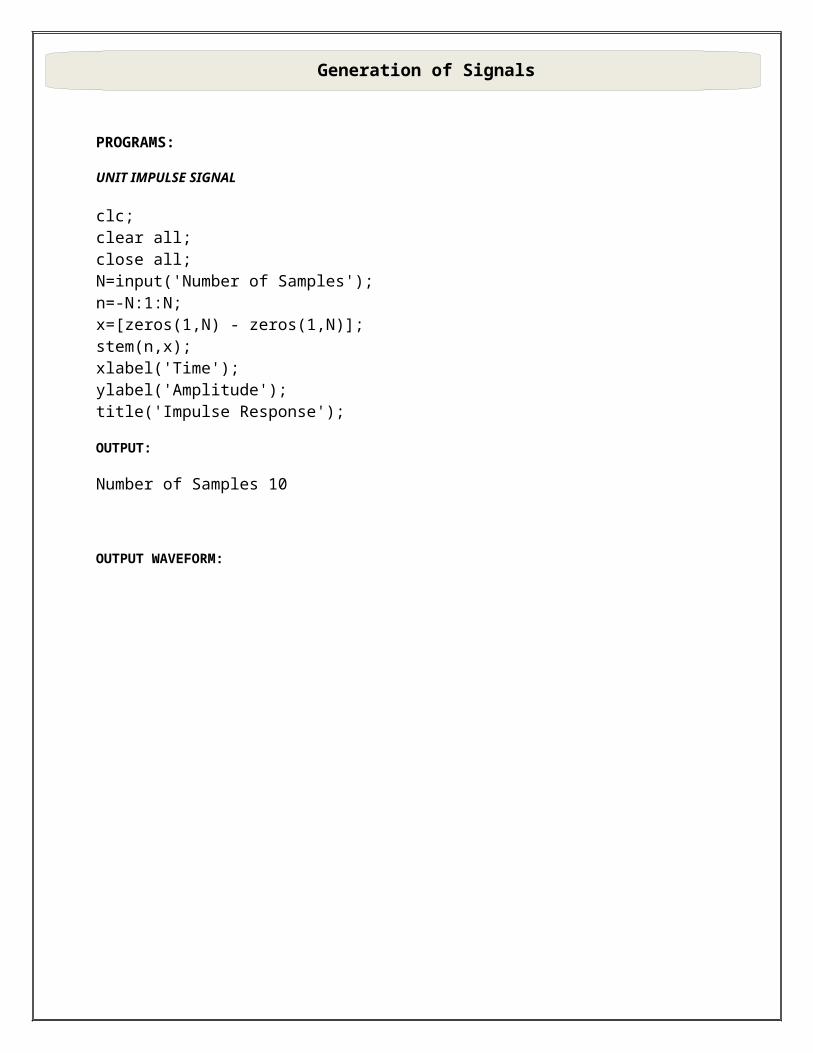
PROGRAMS:

UNIT IMPULSE SIGNAL

clc;clear all;close all;N=input('Number of Samples');n=-N:1:N;x=[zeros(1,N) - zeros(1,N)];stem(n,x);xlabel('Time');ylabel('Amplitude');title('Impulse Response');

OUTPUT:

Number of Samples 10

OUTPUT WAVEFORM:

Generation of Signals

UNIT STEP SIGNAL

clc;clear all;close all;N=input('Number of Samples = ');n=-N:1:N;x=[zeros(1,N) 1 ones(1,N)];stem(n,x);xlabel('Time');ylabel('Amplitude');title('Unit Step Response');

OUTPUT:

Number of Samples =10

OUTPUT WAVEFORM:

S

UNIT RAMP SIGNAL

clc;clear all;close all;disp('Unit Ramp Signal');N=input('Number of Samples = ');a=input('Amplitude = ');n=-N:1:N;x=a*n;stem(n,x);xlabel('Time');ylabel('Amplitude');title('Unit Ramp Response');

OUTPUT:

Number of Samples =10

OUTPUT WAVEFORM:

EXPONENTIAL DECAYING SIGNAL

clc;clear all;close all;disp('Exponential Decaying Signal');N=input('Number of Samples = ');a=0.5n=0:.1:Nx=a.^nstem(n,x);xlabel('Time');ylabel('Amplitude');title('Exponential Decaying Signal Response');

OUTPUT:

Exponential Decaying SignalNumber of Samples =10

OUTPUT WAVEFORM:

EXPONENTIAL GROWING SIGNAL

clc;clear all;close all;disp('Exponential Growing Signal');N=input('Number of Samples = ');a=0.5;n=0:.1:N;

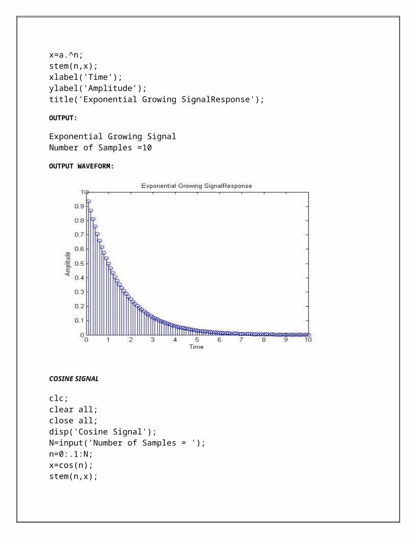
x=a.^n;stem(n,x);xlabel('Time');ylabel('Amplitude');title('Exponential Growing SignalResponse');

OUTPUT:

Exponential Growing SignalNumber of Samples =10

OUTPUT WAVEFORM:

COSINE SIGNAL

clc;clear all;close all;disp('Cosine Signal');N=input('Number of Samples = ');n=0:.1:N;x=cos(n);stem(n,x);

xlabel('Time');ylabel('Amplitude');title('Cosine Signal');

OUTPUT:

Cosine SignalNumber of Samples =10OUTPUT WAVEFORM:

SINE SIGNALclc;clear all;close all;disp('Sine Signal');N=input('Number of Samples = ');n=0:.1:N;

x=sin(n);stem(n,x);xlabel('Time');ylabel('Amplitude');title('sine Signal');

OUTPUT

Sine SignalNumber of Samples =10

OUTPUT WAVEFORM:

PROGRAM:

clear all;

Linear and circular convolution of two sequences

x=[1,1,1,2,1,1];h=[1,1,2,1];Nx=length(x);Nh=length(h);N=max(Nx,Nh);yc=cconv(x,h,N);y=conv(x,h);n=0:1:Nx-1;subplot(2,2,1),stem(n,x);xlabel('n');ylabel('x(n)');title('input sequences');n=0:1:Nh-1;subplot(2,2,2),stem(n,h);xlabel('n'),ylabel('h(n)');title('impulse sequence');n=0:1:N-1;subplot(2,2,3),stem(n,yc);xlabel('n'),ylabel('y(n)');title('output sequence(circular convolution)');n=0:1:Nx+Nh-2;subplot(2,2,4),stem(n,y);xlabel('n'),ylabel('y(n)');title('output sequence(linear convolution)');OUTPUT WAVEFORM :

0 2 4 60

0.5

1

1.5

2

n

x(n)

input sequences

0 1 2 30

0.5

1

1.5

2

n

h(n)

im pulse sequence

0 2 4 60

2

4

6

8

n

y(n)

output sequence(circular convolution)

0 2 4 6 80

2

4

6

8

n

y(n)

output sequence(linear convolution)

Sampling and effect of aliasing

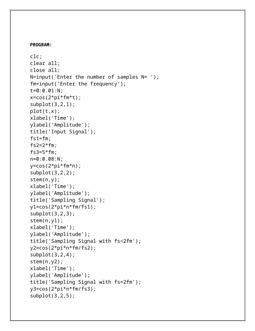
PROGRAM:

clc;clear all;close all;N=input('Enter the number of samples N= ');fm=input('Enter the frequency');t=0:0.01:N;x=cos(2*pi*fm*t);subplot(3,2,1);plot(t,x);xlabel('Time');ylabel('Amplitude');title('Input Signal');fs1=fm;fs2=2*fm;fs3=5*fm;n=0:0.08:N;y=cos(2*pi*fm*n);subplot(3,2,2);stem(n,y);xlabel('Time');ylabel('Amplitude');title('Sampling Signal');y1=cos(2*pi*n*fm/fs1);subplot(3,2,3);stem(n,y1);xlabel('Time');ylabel('Amplitude');title('Sampling Signal with fs<2fm');y2=cos(2*pi*n*fm/fs2);subplot(3,2,4);stem(n,y2);xlabel('Time');ylabel('Amplitude');title('Sampling Signal with fs=2fm');y3=cos(2*pi*n*fm/fs3);subplot(3,2,5);

stem(n,y3);xlabel('Time');ylabel('Amplitude');title('Sampling Signal with fs>2fm');

OUPUT:

Enter the number of samples N= 9Enter the frequency12

OUTPUT WAVEFORM:

PROGRAMS:

HAMMING WINDOW

clc; clear all; close all; format long rp=input('enter the passband ripple…'); rs=input('enter the stopband ripple…'); fp=input('enter the passband freq…'); fs=input('enter the stopband freq…'); f=input('enter the sampling freq…'); wp=2*fp/f;ws=2*fs/f; num=-20*log10(sqrt(rp*rs))-13; dem=14.6*(fs-fp)/f; n=ceil(num/dem); n1=n+1; if (rem(n,2)~=0) n1=n; n=n-1; end; y=hamming(n1);

LOW PASS FILTER

b=fir1(n,wp,y); [h,o]=freqz(b,1,256); m=20*log10(abs(h));

Design of FIR filters

subplot(2,2,1); plot(o/pi,m); xlabel('(a) normalised frequency -->'); ylabel('gain in db -->');

HIGH PASS FILTER

b=fir1(n,wp,'high',y); [h,o]=freqz(b,1,256); m=20*log10(abs(h)); subplot(2,2,2); plot(o/pi,m); xlabel('(b) normalised frequency -->'); ylabel('gain in db -->');

BAND PASS FILTER

wn=[wp ws]; b=fir1(n,wn,y); [h,o]=freqz(b,1,256); m=20*log10(abs(h)); subplot(2,2,3); plot(o/pi,m); xlabel('(c) normalised frequency -->'); ylabel('gain in db -->');

BAND STOP FILTER

b =fir1(n,wn,'stop',y); [h,o]=freqz(b,1,256); m=20*log10(abs(h)); subplot(2,2,4); plot(o/pi,m); xlabel('(d) normalised frequency -->'); ylabel('gain in db -->');

OUTPUT:

Enter the passband ripple = 0.01

Enter the stopband ripple = 0.02

Enter the passband frequency = 1200

Enter the stopband frequency = 1700

Enter the sampling frequency = 9000

OUTPUT WAVEFORM:

0 0.5 1-150

-100

-50

0

50ga

in in

db -->

(a) norm alised frequency -->0 0.5 1

-100

-50

0

50

gain

in db

-->

(b) norm alised frequency -->

0 0.5 1-150

-100

-50

0

gain

in db

-->

(c) norm alised frequency -->0 0.5 1

-15

-10

-5

0

5

gain

in db

-->

(d) norm alised frequency -->

RECTANGULAR WINDOW

clc; clear all; close all; rp=input('Pass band ripple='); rs=input('Stop band ripple='); fs=input('Stop band frequency in rad/sec='); fp=input('Pass band frequency in rad/sec='); f=input('Sampling frequency in rad/sec='); wp=2*fp/f; ws=2*fs/f; num=-20*log10(sqrt(rp*rs))-13; dem=14.6*(fs-fp)/f; n=ceil(num/dem) n1=n+1;

if(rem(n,2)~=0); n1=n; n=n-1; end y=boxcar(n1);

LOW PASS FILTER b=fir1(n,wp,y); [h,o]=freqz(b,1,256); m=20*log10(abs(h)); subplot(2,2,1); plot(o/pi,m,'k'); xlabel('Normalized frequency---->'); ylabel('Gain in db---->'); title('LOW PASS FILTER');

HIGH PASS FILTER

b=fir1(n,wp,'high',y); [h,o]=freqz(b,1,256); m=20*log10(abs(h)); subplot(2,2,2); plot(o/pi,m,'k'); xlabel('Normalized frequency---->'); ylabel('Gain in db---->'); title('HIGH PASS FILTER');BAND PASS FILTER

wn=[wp,ws]; x=fir1(n,wn,y); [h,o]=freqz(b,1,256); subplot(2,2,3); plot(o/pi,m,'k'); xlabel('Normalized frequency---->'); ylabel('Gain in db---->'); title('BAND PASS FILTER');

BAND STOP FILTER

b=fir1(n,wn,'stop',y);

[h,o]=freqz(b,1,256); m=20*log10(abs(h)); subplot(2,2,4); plot(o/pi,m,'k'); xlabel('Normalized frequency---->'); ylabel('Gain in db---->'); title('BAND STOP FILTER');

OUTPUT:


Enter the stopband ripple = 0.02




OUTPUT WAVEFORM:

PROGRAMS:

BUTTERWORTH LOWPASS FILTER

clc; clear all; close all; format long rp=input('enter the passband ripple'); rs=input('enter the stopband ripple'); wp=input('enter the passband freq'); ws=input('enter the stopband freq'); fs=input('enter the sampling freq'); w1=2*wp/fs;w2=2*ws/fs; [n,wn]=buttord(w1,w2,rp,rs); [b,a]=butter(n,wn);

Design of IIR filters

w=0:.01:pi; [h,om]=freqz(b,a,w); m=20*log10(abs(h)); an=angle(h); subplot(2,1,1);plot(om/pi,m); xlabel('(a) normalised frequency--->'); ylabel('Gain in db-->'); subplot(2,1,2); plot(om/pi,an); xlabel('(b) normalised frequency--->'); ylabel('phase in radians -->');

OUTPUT:


Enter the stopband ripple = 50




OUTPUT WAVEFORM:

0 0.1 0.2 0.3 0.4 0.5 0.6 0.7 0.8 0.9 1-400

-300

-200

-100

0Ga

in in

db-->

(a) norm alised frequency--->

0 0.1 0.2 0.3 0.4 0.5 0.6 0.7 0.8 0.9 1-4

-2

0

2

4

(b) norm alised frequency--->

phas

e in

radia

ns -->

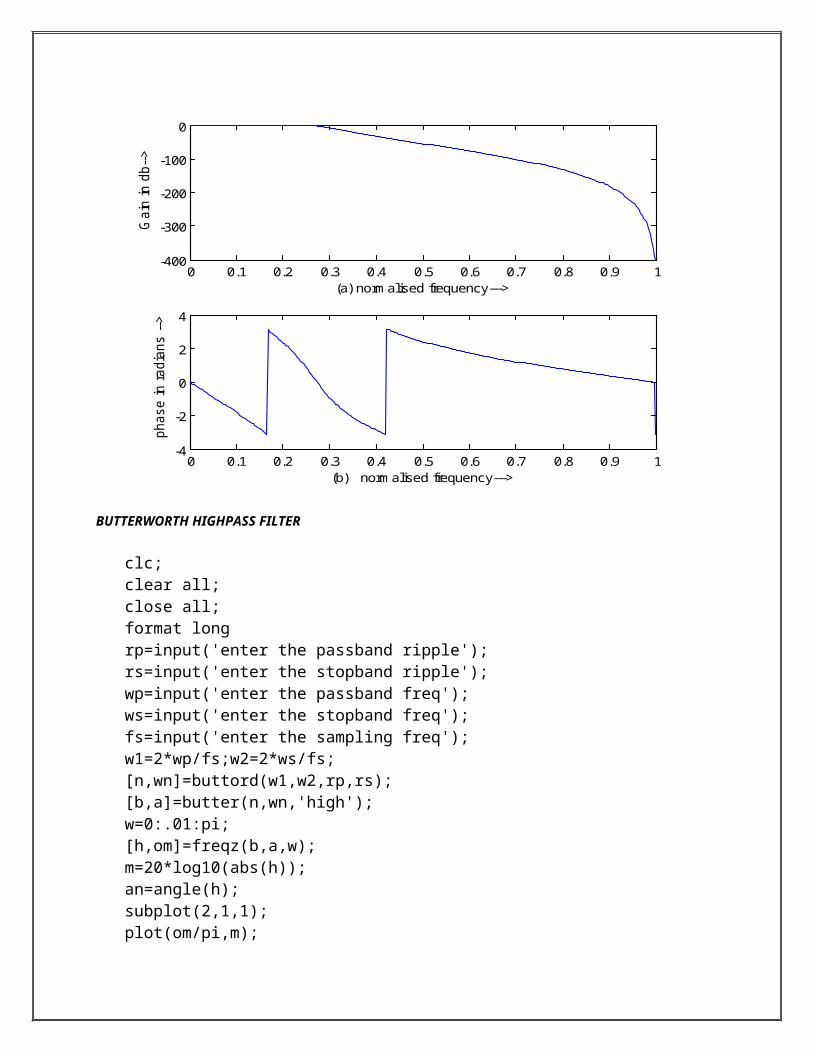
BUTTERWORTH HIGHPASS FILTER

clc; clear all; close all; format long rp=input('enter the passband ripple'); rs=input('enter the stopband ripple'); wp=input('enter the passband freq'); ws=input('enter the stopband freq'); fs=input('enter the sampling freq'); w1=2*wp/fs;w2=2*ws/fs; [n,wn]=buttord(w1,w2,rp,rs); [b,a]=butter(n,wn,'high'); w=0:.01:pi; [h,om]=freqz(b,a,w); m=20*log10(abs(h)); an=angle(h); subplot(2,1,1); plot(om/pi,m);

xlabel('(a)normalised frequency--->'); ylabel('Gain in db-->'); subplot(2,1,2); plot(om/pi,an); xlabel('(b)normalised frequency--->'); ylabel('phase in radians -->');

OUTPUT

Enter the passband ripple = 0.5 Enter the stopband ripple = 50 Enter the passband frequency = 1200 Enter the stopband frequency = 2400 Enter the sampling frequency = 10000

OUTPUT WAVEFORM:

0 0.1 0.2 0.3 0.4 0.5 0.6 0.7 0.8 0.9 1-300

-200

-100

0

100

Gain

in db

-->

(a) norm alised frequency--->

0 0.1 0.2 0.3 0.4 0.5 0.6 0.7 0.8 0.9 1-4

-2

0

2

4

(b) norm alised frequency--->

phas

e in

radia

ns --

>

CHEBYCHEV LOWPASS FILTER:

clc ; close all; clear all; format long rp=input ('enter the passband ripple...'); rs=input ('enter the stopband ripple...'); wp=input ('enter the passband freq...'); ws=input ('enter the stopband freq...'); fs=input('enter the sampling freq...'); w1=2*wp/fs; w2=2*ws/fs; [n,wn]=cheb1ord (w1,w2,rp,rs); [b,a]=cheby1 (n,rp,wn); w=0:.01:pi; [h,om]=freqz(b,a,w); m=20*log10(abs(h)); an=angle(h); subplot(2,1,1); plot(om/pi,m); xlabel('(a) normalised frequency-->'); ylabel('gain in db-->'); subplot(2,1,2); plot(om/pi,an); xlabel('(b) normalised frequency-->'); ylabel('phase in radians-->');

OUTPUT :






OUTPUT WAVEFORM:

0 0.1 0.2 0.3 0.4 0.5 0.6 0.7-400

-300

-200

-100

0

gain in db-->

(a) norm alised frequency-->

0 0.1 0.2 0.3 0.4 0.5 0.6 0.7-4

-2

0

2

4

(b) norm alised frequency-->

phase in radians--->

CHEBYCHEV HIGHPASS FILTER

clc; close all;clear all; format long rp=input('enter the passband ripple...'); rs=input('enter the stopband ripple...'); wp=input('enter the passband freq...'); ws=input('enter the stopband freq...'); fs=input('enter the sampling freq...'); w1=2*wp/fs; w2=2*ws/fs;

[n,wn]=cheb1ord(w1,w2,rp,rs); [b,a]=cheby1(n,rp,wn,'high'); w=0:.01/pi:pi; [h,om]=freqz(b,a,w); m=20*log10(abs(h)); an=angle(h); subplot(2,1,1); plot(om/pi,m); xlabel('(a) normalised frequency-->'); ylabel('gain in db-->'); subplot(2,1,2); plot(om/pi,an); xlabel('(b) normalised frequency-->'); ylabel('phase in radians--->');

OUTPUT :






OUTPUT WAVEFORM:

0 0.1 0.2 0.3 0.4 0.5 0.6 0.7 0.8 0.9 1-600

-400

-200

0

200ga

in in

db-->

(a) norm alised frequency-->

0 0.1 0.2 0.3 0.4 0.5 0.6 0.7 0.8 0.9 1-4

-2

0

2

4

(b) norm alised frequency-->

phas

e in

radia

ns--->

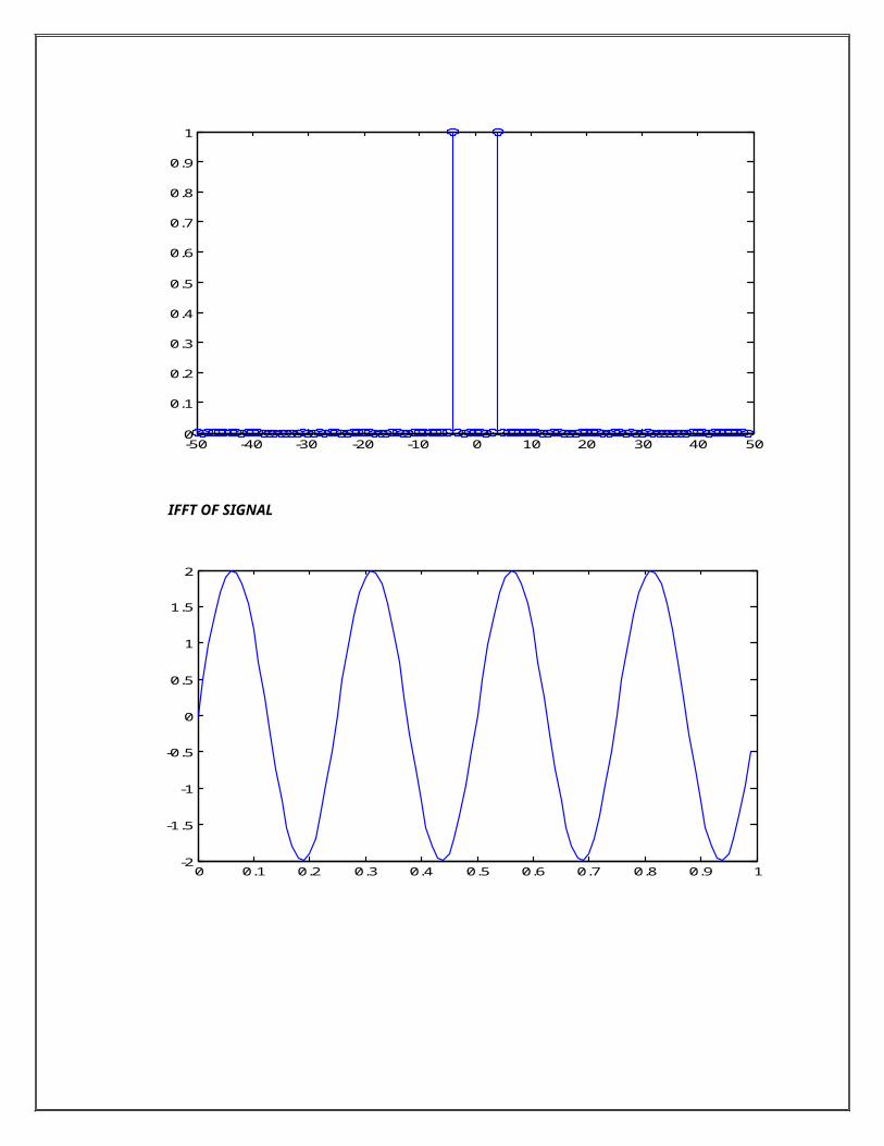
PROGRAMS:

fo=4; Fs=100; Ts=1/Fs; t=0:Ts:1-Ts; n=length(t); y=2*sin(2*pi*fo*t); figure(1); plot(t,y) Y freq Domain=fft(y)./n; N=n; F axis=(-ceil((N-1)/2):N-1-ceil((N-1)/2))/N/Ts; figure(2); stem(faxis,fftshift(abs(YfreqDomain)));

Calculation of FFT of

y_ret=ifft(YfreqDomain).*n; figure(3); plot(t,y_ret);

OUTPUT WAVEFORM:

GENERATION OF SIGNAL

0 0.1 0.2 0.3 0.4 0.5 0.6 0.7 0.8 0.9 1-2

-1.5

-1

-0.5

0

0.5

1

1.5

2

FFT OF SIGNAL

-50 -40 -30 -20 -10 0 10 20 30 40 500

0.1

0.2

0.3

0.4

0.5

0.6

0.7

0.8

0.9

1

IFFT OF SIGNAL

0 0.1 0.2 0.3 0.4 0.5 0.6 0.7 0.8 0.9 1-2

-1.5

-1

-0.5

0

0.5

1

1.5

2

PROGRAM:

clear all; clc; close all; x=input(‘enter the input sequence=’); h=input(‘enter the FIR filter coefficients=’); M=input(‘enter the decimation factor=’); N1=length(x); N=0:1:N1-1; subplot(2,1,1); stem(n,x); x label(‘time’); y label(‘amplitude’); title(‘X sequence response’); N2=length(h); n=0:1:N2-1; subplot(2,1,2); stem(n,h); x label(‘time’); y label(‘amplitude’); title(‘H sequence response’); H=length(h); P=floor((H-1)/M)+1; X=length(x); Y=floor((X+H-2)/M)+1; U=floor((X+M-2)/M)+1; R=zeros(1,X+P-1); for m=1:M R=R+conv(x(1,:),r(m,:)); end Disp(R); N=length(R); n=0:1:N-1; figure(2); stem(n,R); x label(‘time’);

Decimation by polyphase decomposition

y label(‘amplitude’); title(‘Decimation of polyphase decomposition sequence response’);

OUTPUT :

enter the input sequence=5enter the FIR filter coefficients=3enter the decimation factor=1

OUTPUT WAVEFORM:

To print PROGRAMSdwdw

Documents

Transcript of To print PROGRAMSdwdw