IsotopeTechniquesinWeterResourcesDevelopment1991

PROCEEDINGS OF ASYMPOSIUM,VIENNA,11-15 MARCH 1991 ORGANIZED BY IAEAIN CO-OPERATION WITH UNESCO

The cover picture shows “ Der Schleierfall bei Gastein” , 1830, by Rudolf von Alt (1812-1905).Graphische Sammlung Albertina Museum, Vienna.

ISOTOPE TECHNIQUES IN WATER RESOURCES DEVELOPMENT 1991

PROCEEDINGS SERIES

ISOTOPE TECHNIQUES IN WATER RESOURCES

DEVELOPMENT 1991

PROCEEDINGS OF AN INTERNATIONAL SYMPOSIUM ON ISOTOPE TECHNIQUES

IN WATER RESOURCES DEVELOPMENT ORGANIZED BY THE

INTERNATIONAL ATOMIC ENERGY AGENCY IN CO-OPERATION WITH THE

UNITED NATIONS EDUCATIONAL, SCIENTIFIC AND CULTURAL ORGANIZATION

AND HELD IN VIENNA, 11-15 MARCH 1991

INTERNATIONAL ATOMIC ENERGY AGENCY VIENNA, 1992

VIC Library Cataloguing in Publication Data

Isotope techniques in water resources development 1991 : proceedings of an International Symposium on Isotope Techniques in Water Resources Development organized by the International Atomic Energy Agency in co-operation with the United Nations Educational, Scientific and Cultural Organization and held in Vienna, 11-15 March 1991. Vienna : IAEA, 1992.

xv, 789 p. ; 24 cm. — (Proceedings series,ISSN 0074-1884)STI/PUB/875 ISBN 92-0-000192-0

1. Radioactive tracers in water pollution research.2. Water resources development — Environmental aspects.3. Water, Underground — Pollution. I. International Atomic Energy Agency. II. Unesco. III. International Symposium on Isotope Techniques in Water Resources Development (1991 : Vienna, Austria). IV. Series:Proceedings series (International Atomic Energy Agency).

VICL 91-0004

© IAEA, 1992

Permission to reproduce or translate the information contained in this publication may be obtained by writing to the International Atomic Energy Agency, Wagramerstrasse 5, P.O. Box 100, A-1400 Vienna, Austria.

Printed by the IAEA in Austria January 1992

FOREWORD

Water resources are scarce in many parts of the world. Often, the only water resource is groundwater. Overuse usually invites a rapid decline in groundwater resources which are recharged insufficiently, or not at all, by prevailing climatic conditions. Also, in industrialized countries, groundwater is endangered by over­exploitation and, consequently, by degradation in quality. Moreover, groundwater is being progressively threatened by the insidious long term effects of pollution, which could permanently impair groundwater resources with unpredictable implica­tions for present and future generations.

These and other problems currently encountered in hydrology and associated environmental fields have prompted an increasing demand for the utilization of iso­tope methods. Such methods have been recognized as being indispensable for solving problems such as the identification of pollution sources, characterization of palaeowater resources, evaluation of recharge and evaporative discharge under arid and semi-arid conditions, reconstruction of past climates, study of the interrelation­ships between surface and groundwater, dating of groundwater and validation of con­taminant transport models. Moreover, in combination with other hydrogeological and geochemical methods, isotope techniques can provide useful hydrological infor­mation, such as data on the origin, replenishment and dynamics of groundwater.

It was against this background that the International Atomic Energy Agency, in co-operation with the United Nations Educational, Scientific and Cultural Organi­zation and the International Association of Hydrological Sciences, organized this symposium on the Use of Isotope Techniques in Water Resources Development, which took place in Vienna from 11 to 15 March 1991. The main themes of the sym­posium were the use of isotope techniques in solving practical problems of water resources assessment and development, particularly with respect to groundwater pro­tection, and in studying environmental problems related to water, including palaeo- hydrological and palaeoclimatological problems. A substantial part of the oral presentations was concerned with the present state and trends in groundwater dating, and with some methodological aspects.

These proceedings contain the papers of 37 oral and the extended synopses of 47 poster presentations. It is hoped that they will contribute to the widespread and efficient use of isotope techniques in hydrology and associated environmental disciplines.

EDITORIAL NOTE

The Proceedings have been edited by the editorial staff o f the IAEA to the extent considered necessary for the reader’s assistance. The views expressed remain, however, the responsibility o f the named authors or participants. In addition, the views are not necessarily those o f the governments o f the nominating Member States or o f the nominating organizations.

Although great care has been taken to maintain the accuracy o f information contained in this publication, neither the IAEA nor its Member States assume any responsibility for consequences which may arise from its use.

The use o f particular designations o f countries or territories does not imply any judge­ment by the publisher, the IAEA, as to the legal status o f such countries or territories, o f their authorities and institutions or o f the delimitation o f their boundaries.

The mention o f names o f specific companies or products (whether or not indicated as registered) does not imply any intention to infringe proprietary rights, nor should it be construed as an endorsement or recommendation on the part o f the IAEA.

The authors are responsible for having obtained the necessary permission for the IAEA to reproduce, translate or use material from sources already protected by copyrights.

Material prepared by authors who are in contractual relation with governments is copyrighted by the IAEA, as publisher, only to the extent permitted by the appropriate national regulations.

CONTENTS

INTERFACE PROCESSES BETWEEN THE ATMOSPHERE AND THE HYDROSPHERE

Evaluating pathways of sulphate between the atmosphere and hydrosphereusing stable sulphur and oxygen isotope data (IAEA-SM-319/31) ............ 3B. Mayer, P. Fritz, K. Knief, G. Li, M. Fischer, K.-E. Rehfuess,H.R. Krouse

Evaluation of the use of 36C1 in recharge studies (IAEA-SM-319/2) ............ 19G.R. Walker, I.D. Jolly, M.H. Stadter, F.W. Leaney, R.F. Davie,L.K. Fifield, T.R. Ophel, J.R. Bird

SURFACE WATER AND SEDIMENTS

Conjunctive use of isotopic techniques to elucidate solute concentrationand flow processes in dryland salinized catchments (IAEA-SM-319/1) .... 33 J.V. Turner, J.M. Bradd, T.D. Waite

Development of isotopically heterogeneous infiltration watersin an artificial catchment in Chuzhou, China (IAEA-SM-319/7) ............... 61C. Kendall, Weizu Gu

Estimation using 180 of the water residence time in small watersheds(IAEA-SM-319/4) ............................... .............. ............................................ 75P.R. Leopoldo, J.C. Martinez, J. Mortatti

Hydraulic parameters of the Magdalena River (Colombia) derived fromlarge scale tracer experiments (IAEA-SM-319/9) ........................................ 85A. Plata Bedmar, L. Araguás, E. Torres, E. Obando, G. Jimenez,A. Zapata

Techniques de marquage pour l’étude des circulations des masses d’eau dans les lacs: Application à la retenue de Pareloup(IAEA-SM-319/11) ....................................................................................... 107P. Calméis, M.-J. Salençon

Chernobyl fallout nuclides used as tracers of sedimentationand sediment mixing in four Finnish lakes (IAEA-SM-319/10) ................ 123P.H. Kansanen, T. Jaakkola, J. Seppàld, M. Hôkkà, S. Kulmala,R. Suutarinen

GROUNDWATER DATING: PROBLEMS AND NEW APPROACHES

Radiocarbon contents of dissolved organic and inorganic carbonin shallow groundwater systems: Implications for groundwater dating(IAEA-SM-319/5) ......................................................................................... 143L.I. Wassenaar, R. Aravena, P. Fritz

Possible evidence for 14C isotope exchange between groundwater and carbonate rocks in the eastern Donau Ried, Bavaria, Germany(IAEA-SM-319/15) ........................................................................ .............. 153M. Fischer, M. Wolf, P. Fritz, S. Geyer, S. Weise, M. Forster,W. Rauert, K. Ramm

The 14C time-scale of groundwater: Correction and linearity(IAEA-SM-319/17) ...................................................................................... 167M.A. Geyh

Neon-21 — A possible tool for dating very old groundwaters?(IAEA-SM-319/16) ....................................................................................... 179S. Weise, P. Faber, M. Stute

Argon-37 and argon-39: Measured concentrations in groundwatercompared with calculated concentrations in rock (IAEA-SM-319/28) ....... 189H.H. Loosli, B.E. Lehmann, C. Thalmann, J.N. Andrews,T. Florkowski

Argon-39 dating of groundwater and its limiting conditions(IAEA-SM-319/13) ....................................................................................... 203M. Forster, K. Ramm, P. Maier

Some aspects of the underground production of radionuclides usedfor dating groundwater (IAEA-SM-319/24) ............................................... 215T. Florkowski

Evaluation of isotopic methods for the dating of very old groundwaters:A case study of the Milk River Aquifer (IAEA-SM-319/37) .................... 229M. Ivanovich, K. Frôhlich, M.J. Hendry, J.N. Andrews,S.N. Davis, R.J. Drimmie, J. Fabryka-Martin, T. Florkowski,P. Fritz, B.E. Lehmann, H.H. Loosli, E. Nólte

Importance of the in situ production of 36C1, 36Ar and 14C in hydrologyand hydrogeochemistry (IAEA-SM-319/12) ............................................... 245J.N. Andrews, J.-C. Fontes

GROUNDWATER DATING: PROBLEMS AND NEW APPROACHES — METHODOLOGICAL ASPECTS AND MODELS

On the statistical treatment of environmental isotope data in hydrology(IAEA-SM-319/36) .........................:....... :................................................... 273B.R. Payne

Compartmental modelling approach for simulation of spatial isotopicvariations in the study of groundwater dynamics: A case study of a multi-aquifer system in the Bangkok Basin, Thailand(IAEA-SM-319/29) ....................................................................................... 291Y. Yurtsever, S. Buapeng

Estimation dés flux d’évaporation diffuse sous couvert sableuxen climat hyper-aride (Erg de Bilma, Niger) (IAEA-SM-319/39) ............. 309J.F. Aranyossy, A. Filly, A.A. Tandia, D. Louvat, B. Ousmane,A. Joseph, J.-C. Fontes

GROUNDWATER

Flow dynamics in an Alpine karst massif studied by meansof environmental isotopes (IAEA-SM-319/3) .............................................. 327D. Rank, G. Vôlkl, P. Maloszewski, W. Stickler

Detailed geohydrology with environmental isotopes: A case studyat Serowe, Botswana (IAEA-SM-319/25) ................................................... 345B.T. Verhagen

Radium isotopes in geothermal fluids in central Italy(IAEA-SM-319/21) ....................................................................................... 363A. Battaglia, A. Ceccarelli, A. Ridolfi, K. Frôhlich, C. Panichi

Utilización de isótopos ambientales en el valle bajo y delta del Rio Llobregat (Barcelona, España) para resolver problemas de flujo y transporte de masa en los acuiferos (IÀEA-SM-319/26) ............... 385E. Custodio, V. Iribar, M. Manzano, E. Skupien

Environmental isotope study related to the origin, salinizationand movement of groundwater in the Mekong Delta (Viet Nam)(IAEA-SM-319/38) ....................................................................................... 415Huu Dung Ho, J.F. Aranyossy, D. Louvat, Minh Quan Hua,Trac Viet Nguyen, Kien Chinh Nguyen

Isotopic investigation of the interrelationship between surface water and groundwater in the Mardan and Chaj Doab areas in Pakistan(IAEA-SM-319/23) ....................................................................................... 429S.D. Hussain, M.l. Sajjad, M. Ahmad, M.A. Tasneem,Y. Yurtsever, W. Akram

ENVIRONMENTAL PROBLEMS AND WATER POLLUTION

Environmental isotopes and noble gases in brines from theKonrad Iron Mine, Salzgitter (IAEA-SM-319/14) .........C. Sonntag

447

The radionuclide migration experiment at Nagra’s Grimsel underground test site: A comprehensive programme including field, laboratoryand modelling studies (IAEA-SM-319/27) .................. ............................... 463U. Frick, W.R. Alexander, W. Drost

Use of hydrochemical and isotopic criteria for the evaluation of theinfluence of technogenic sulphur on surface waters (IAEA-SM-319/30) ... 477 Yu.A. Fedorov, V.A. Grinenko, H.R. Krouse, A.M. Nikanorov

Isotope studies of groundwater degradation at a riverside pumping sitein Lanzhou City (IAEA-SM-319/8) .......................... .............................. 495Yanqing Lian, Datong Li, Gu Yang

Interlaboratory comparison of methods to determine the stable isotopecomposition of soil water (IAEA-SM-319/40) ........................................... 509G.R. Walker, P.H. Woods, G.B. Allison

PALAEOHYDROLOGY AND PALAEOCLIMATOLOGY

Monitoring the response of arid zone hydrology to environmental change by means of the stable isotope composition of groundwaters(IAEA-SM-319/20) ...........::.......................................... .............................. 521J. R. Gat

A record of climatic and environmental change contained in interstitial waters from the unsaturated zone of northern Senegal(IAEA-SM-319/35) ...................................................................................... 533W.M. Edmunds, C.B. Gaye, J.-C. Fontes

Travertines in central Jordan: Implications for palaeohydrology and dating(IAEA-SM-319/6) ....'i......... ........... ..:........................... .............................. 551l.D. Clark, H.N. Khoury, E. Salameh, P. Fritz, Y. Gôksu,A. Wieser, C. Causse, J.-C. Fontes

Isotope variations in water in the hydrological cycle as a toolin a climate change mechanism study (IAEA-SM-319/33) ........................ 567V.I. Ferronsky, V.A. Pólyakov, S.V. Ferronsky

Oxygen-18 in permafrost ice (IAEA-SM-319/34) ........................................... 587R. Vaikmae

Isotope hydrological evidence of geomorphological changesin northeastern Hungary (IAEA-SM-319/18) .............................................. 603E. Hertelendi, L. Martón, L. Miko

POSTER PRESENTATIONS

Determination of the protective column and time characteristics of the restabilizing process in fractured zone rocks produced during exploitation of subaquatic mineral objects: An application in theValiasi Coal Mine (IAEA-SM-319/IP) ....................................................... 617S. Ahmataj, R. Eftimiu, J. Ihereska

Deuterium and 180 as indicators of evaporation losses from rice cropsin semi-arid climate zones (IAEA-SM-319/3P) ............... .......................... 620A.L. Herczeg, H.J. Simpson, R. Whitehead, F.W. Leaney, W. S. Meyer

A new automated sealed sampler for use in hydrograph analysis(IAEA-SM-319/4P) ....................................................................................... 623C.J. Barnes, J. Bums, P.F. Crapper, P. Darton, P.G. Fitch,I.H. Durham

Idéntifícation of palaeowaters by means of environmental isotopecorrelation (IAEA-SM-319/6P) ..................................................................... 625H. Zojer

Uranium isotopes in the spring waters of Aguas da Prata, Sâo Paulo,Brazil (IAEA-SM-319/7P) .................... ..... .................................................. 628D.M. Bonotto

Mesure du transport sédimentaire par l’emploi d’une jauge à transmission(IAEA-SM-319/9P) ..................................... ................................................. 631B. Long, O. Gagné

Fine tuning the cellulose model for dendroclimatological interpretation(IAEA-SM-319/ЮР) ................................... .................................................. 632W.M. Buhay, T.W.D. Edwards, R. Aravena

Origin of groundwater in the Tertiary volcanic complexin central Slovakia (IAEA-SM-319/14P) ..................................................... 634J. Silar, L. Skvarka

Localización de fugas en el embalse de Sabaneta (IAEA-SM-319/16P) .......... 639A. Plata Bedmar, J. Febrillet, A. Torres, J. Saint-Hilaire, E. Bueno

Sources of water recharge identified by isotopes in El Minya Governate(Nile Valley, middle Egypt) (IAEA-SM-319/17P) ..................................... 643A. El Bakri, A. Tantawi, B. Blavoux, M. Dray

Isotopic studies of deep and surface waters in the French Massif Central(IAEA-SM-319/ 18P) ...................................................................................... 646C. Fouillac, A.-M. Fouillac, L. Chery

Méthode et appareillage pour la mesure, à l’aide d’un traceur radioactif, de très faibles débits d’infiltration verticale de l’eau au travers des sols en place (IAEA-SM-319/19P) ....................................................... 648B. Gaillard, P. Calméis, R. Margrita, P. André

Apports des données isotopiques à la connaissance de l’origineet du temps de séjour des eaux souterraines dans le socle fissuréen Afrique de l’ouest (LAEA-SM-319/20P) ................................................. 650J. Sarrot-Reynauld, J. Biemi, J.-P. Jourda, N. Soro, A.Z. Traore

Hydrochimie, teneurs isotopiques et origine des saumures associéesaux gisements de potasse d’Alsace (IAEA-SM-319/21P) .......................... 654D. Poutoukis, J.-L. Michelot, J.-C. Fontes, P.-L. Blanc, M. Ansart

Approche isotopique du fonctionnement du drainage en milieu argileux(IAEA-SM-319/22P) ...................................................................................... 656P. Vachier, C. Coulomb, L. Dever, R. Calvet

Preliminary isotope hydrological study in the arid Gurinai Grassland area,Inner Mongolia (IAEA-SM-319/23P) .......................................................... 661M.A. Geyh, Weizu Gu

Modelling of water and tritium transport in the unsaturated zone(IAEA-SM-319/24P) ...................................................................................... 663V. Dunger

Radium and radon isotope investigations in groundwaters fromnorthern Bavaria (Germany) (IAEA-SM-319/26P) ..................................... 664L. Eichinger, M. Forster, S. Hurst, F. Buheitel

Use of lead and nitrate isotopes to identify the source of lead contaminationin a deep aquifer (IAEA-SM-319/27P) ....................................................... 665S. Voerkelius, L. Eichinger, S. Hôlzl

Stable isotopes (2H and 180) as tools for hydrograph separation in a small catchment area and as tracers for moisture movementin the unsaturated soil zone (IAEA-SM-319/29P) .................................... 666H. Jacob, C. Sonntag, U. Schmitz

Groundwater research in selected areas of the northern Sudan usingenvironmental isotopes (2H, 3H, 180) (IAEA-SM-319/30P) .................... 668H. Jacob, A.R. Mukhtar

Estimates of dispersivities by the interpretation of statistically anisotropic filtration velocity vectors in fluvioglacial aquifers(IAEA-SM-319/31P) ...................................................................................... 670W. Drost, E. Hoehn, L. Kovac

Isotope investigations and hydraulic measurements for the delimitationof a groundwater protection area (IAEA-SM-319/33P) ............................ 671B. Bertleff, R. Watzel, L. Eichinger, P. Trimbom

Evaporation from soil water under humid climate conditionsand its impact on deuterium and 180 concentrations in groundwater(IAEA-SM-319/34P) ...................................................................................... 674H.-M. Burger, K.-P. Seiler

Groundwater flow measurements using the radiotracer techniqueat a waste disposal site barrier (IAEA-SM-319/35P) ................................... 678L. Baranyai, F. Ivicsics

Stable isotope study in geothermal fields in Kamojang and Dieng,Java Island (IAEA-SM-319/39P) .................................................................. 681Zaenal Abidin, Wandowo, Indroyono, Alip, Djiono

Hydrogeological characterization of an aquitard:The Avdat Group (Eocene) chalk, northern Negev Desert, Israel(IAEA-SM-319/40P) ...................................................................................... 683R. Nativ, E. Nissim

Use of isotope techniques in studies of limestone karstic aquifersof Marche, central Italy (IAEA-SM-319/41P) ............................................. 686G.F. Ciancetti, G.S. Tazioli, M. Coltorti

Salt waters, brines and the geological structure of the Apennine Front(northern Italy) (IAEA-SM-319/42P) .......................................................... 691M. Chiarle, G. Martinelli, T. Nanni, G. Patrizi, L. Venturini,G.M. Zuppi

Study of groundwater salinization in Algarve, Portugal, usingenvironmental isotope techniques (IAEA-SM-319/44P) ............................. 694J.M.P. Cabral, P.M. Carreira, M.C. Vieira, J. Braga dos Santos,M.J. Leitâo de Freitas, R. Gonfiantini

Assessment of aquifer resources from hydrokarstic structures by multitracing experiments using artificial tracers(IAEA-SM-319/45P) ...................................................................................... 698E. Gaspar, S. P. Stanescu, O.M. Farcasiu, S. Spiridon, I. Oraseanu

Application of environmental isotope methods in the studyof a karstic hydrostructure in Romania (IAEA-SM-319/46P) .................... 701A. Tenu, A. Slavescu, F.D. Davidescu

Le rôle de l’évapotranspiration dans la formation des dépressionspiézométriques: hypothèses et modélisation (IAEA-SM-319/47P) ............. 703B. Ndiaye, J.F. Aranyossy, B. Dieng, A. Faye

Variation of stable isotopes in the monsoonal rains of Sri Lanka(IAEA-SM-319/49P) ...................................................................................... 707J.K. Dharmasiri, C.J. Atuluwage

Application of the 222Rn technique for estimating the residence times of artificially recharged groundwater: Hengsen water catchment area,Dortmunder Stadtwerke AG (IAEA-SM-319/50P) ..................................... 712E. Hoehn, U. Willme, R. Hollerung, U. Schulte-Ebbert,H.R. von Gunten

Environmental isotopes in precipitation and shallow aquifers: A sensitivity study of the impact of climate change on the water balance of smallcatchment areas in Switzerland (IAEA-SM-319/5IP) ................................. 715U. Schotterer, H. Oeschger, U. Siegenthaler, W. Stickler

Environmental isotope study of thermal, mineral and normal groundwater within the Bursa and Kuzuluk/Adapazari areas of northwestern Turkey(IAEA-SM-319/52P) ...................................................................................... 720W. Balderer, E. Greber, T. Imbach, W. Rauert, P. Trimbom,S. Giiler

Application of radioactive tracers to measure turbulent dispersionof pollutants in water bodies and rivers (IAEA-SM-319/54P) .................. 724V.A. Vetrov

Палеоводы северной Эстонии и их влияние на изменение ресурсов и качества пресных подземных вод крупных береговых водозаборов(IAEA-SM-319/55Р) ..................................................................................... 728М.П. Ежова, В.А. Поляков, А.Е. Ткаченко, В.Я. Белкина,JJ.A. Савицкий(Ancient waters o f northern Estonia and their effect on changes in the quantity and quality o f fresh groundwater in large coastal reservoirs:M.P. Ezhova, V.A. Polyakov, A.E. Tkachenko, V.Ya. Belkina,L.A. Savitskij)

Пространственная уран-изотопная модель формирования и динамики минеральных вод Ессентукского и Кумского месторождений в большом районе Кавказских минеральных вод(IAEA-SM-319/56P) ..................................................................................... 731П.И. Чалов, А .И . Тихонов, Г.П. Киселев, К.И. Меркулова,И.А. Васильев(Three dimensional uranium isotope model simulating the formation and dynamics o f mineral water resources in the Yessentuki and Кита deposits o f the greater Caucasian mineral water region: P. I. Chalov,A.I. Tikhonov, G.P. Kiselev, K.I. Merkulova, I.A. Vasil’ev)

Water balance of lakes in the Kenya Rift Valley (IAEA-SM-319/57P) ........ 733W.G. Darling, D.J. Allen, J.C. Talbot

Origin and transport of C02 in the highly mineralized water system of the Pannonian Tertiary Basin (northeast Slovenia)(IAEA-SM-319/58P) ..................................................................................... 735J. Pezdié, T. Dolenec, D. Zizek, P. Fritz, M. Wolf

Study of the hydrological relationship between Lakes Ohrid and Prespa(IAEA-SM-319/59P) ..................................................................................... 737T. Anovski, B. Andonovski, B. Minceva

Environmental isotope studies on seawater intrusion into thesoutheastern coastal aquifer on Cheju Island (IAEA-SM-319/60P) ........... 740J.S. Ahn, S.J. Kim, J.W. Kim

Evaluating the origin and distribution of methane and dissolved organic carbon in a confined aquifer using isotope techniques(IAEA-SM-319/62P) ..................................................................................... 747R. Aravena, L.I. Wassenaar, J.F. Barker

Environmental isotopes as indicators of recharge, residence time andmixing relations in groundwaters from the Otway Basin, South Australia(IAEA-SM-319/63P) ..................................................................................... 749A.J. Love, A.L. Herczeg, F.W. Leaney, J.C. Dighton

Use of activated sediment in field measurements of bed load transferin a mountain stream (IAEA-SM-319/64P) ................................................. 752F. Giussani, F. Maraga, E. Pirastru, G.M. Zuppi

Chairmen of Sessions and Secretariat of the Symposium................................... 759List of Participants ............................................................................................ 761Author Index ...................................................................................................... 783Transliteration Index ......................................................................................... 787Index of Papers and Posters by Number ............................................................ 789

INTERFACE PROCESSES BETWEEN THE ATMOSPHERE AND THE HYDROSPHERE

ChairmanB.R. PAYNE

United Kingdom

IAEA-SM-3X9/31

EVALUATING PATHWAYS OF SULPHATE BETWEEN THE ATMOSPHERE AND HYDROSPHERE USING STABLE SULPHUR AND OXYGEN ISOTOPE DATA*

B. MAYER, P. FRITZ, K. KNIEF, G. LI Institut fur Hydrologie,Gesellschaft fiir Strahlen- und Umweltforschung mbH München,Neuherberg

M. FISCHER, K.-E. REHFUESS Lehrstuhl fiir Bodenkunde,Ludwig-Maximilians-Universitât München,Munich

Germany

H.R. KROUSEDepartment of Physics and Astronomy,University of Calgary,Calgary, Alberta,Canada

Abstract

EVALUATING PATHWAYS OF SULPHATE BETWEEN THE ATMOSPHERE AND HYDROSPHERE USING STABLE SULPHUR AND OXYGEN ISOTOPE DATA.

Stable isotopes in the sulphate ion can be used to gain a better understanding of sulphur sources and transformations between the atmosphere and hydrosphere. Because of its low iso­topic selectivity in internal soil processes in well aerated forest soils, ô34S is a suitable tracer for monitoring what happens to deposited sulphate, if it is isotopically different from the soil sulphur. The oxygen isotope composition of sulphate can be used as a tracer for geochemical reactions in the unsaturated zone, since during sulphate formation oxygen can be acquired from various oxygen reservoirs. Immobilization as organic sulphur and subsequent minerali­zation is the only known process in the biochemical soil sulphur cycle which affects the 180 content of sulphate. An irrigation experiment showed that sulphate in seepage water is a mix­ture of percolated atmospheric derived or desorbed sulphate and sulphate mineralized from organic soil sulphur. Sulphate participates actively in biogeochemical processes of the soil

* Financial support was provided by the Bundesministerium fiir Forschung und Tech­nologie (BMFT) under Projects 0339162B and 0339319A, and the Natural Sciences and Engineering Research Council of Canada. This project also received support from the BMFT under the Germany/Canada Science and Technology Cooperation Programme.

3

4 MAYER et al.

zone. Redox reactions, which can change the isotopic integrity of the deposition sulphate, are important for the turnover of sulphur in the unsaturated zone. Knowledge of the extent of the isotopic modification is important if the sulphur and oxygen isotope data of sulphate are to be used for interpretation of the past geochemistry of groundwater systems.

1. INTRODUCTION

Recent studies [1-4] document a depletion of several per mille in the ô180 values of sulphate between atmospheric deposition and groundwater, whereas the ô34S values are often identical. This suggests that sulphate undergoes transforma­tions during its movement through the unsaturated zone.

Although sulphate is sometimes considered to be a ‘conservative’ compound in watershed studies, more detailed investigations have shown that sulphate is subject to transformations and exchange processes in the soil [3, 5]. Sulphate, which in cen­tral Europe originates mainly from atmospheric deposition, can either be sorbed in the inorganic soil sulphur pool or immobilized as organic sulphur. However, desorp­tion of sulphate and mineralization of soil sulphur can buffer the sulphate concentra­tion in seepage water and can have a profound influence on the isotopic composition of sulphate.

2. MATERIALS AND METHODS

All experiments were performed on a selection of five forest soil samples from southern Germany ; they are described in Refs [6 , 7]. Since sulphur transformations presumably occur in the uppermost horizons of the soil, the top 60 cm of these soils were the focus of the investigation.

2.1. Sulphur chemistry of soil and water

The total sulphur content of the soil horizons was determined by an alkaline oxidation method [8], followed by Johnson-Nishita reduction [9] and colorimetric determination using methylene blue [10]. Total inorganic sulphate was determined by ion chromatography after phosphate extraction (soil:solution, 1:10) and soluble sulphate after extraction with deionized water. Because reduced inorganic sulphur forms are few in well aerated forest soils, total inorganic sulphate equals total inor­ganic sulphur.

Total organic sulphur is calculated as the difference between total sulphur and total inorganic sulphur. The classification of soil organic sulphur is based on its reac­tivity with reducing agents, i.e. the chemical bonding of sulphur in organic matter.

IAEA-SM-319/31 5

The reduction or non-reduction of organic sulphur to H2S by hydriodic acid (HI) is considered to be a means to distinguish between non-carbon bonded and carbon bonded sulphur [11]. Since HI reduction [12] mobilizes organic as well as inorganic sulphate, organic (ester) sulphate of the general formula R -0 -S -0 3~ was deter­mined by subtracting total inorganic sulphate from the HI reducible values. As a con­sequence, carbon bonded sulphur is the difference between total organic sulphur and organic sulphate.

Sulphate concentrations in water were determined with a Dionex ion chromato­graph. The overall precision is ±2% of the measured sulphate concentration.

2.2. Stable isotope measurements

For isotope measurements the aqueous sulphate was precipitated with 0.5M BaCl2 solution as BaS04 and acidified below pH4 to remove co-precipitated BaC03. The sulphate precipitate was washed several times with deionized water, filtered and dried for mass spectrometric determinations of 180 and 34S contents using standard analytical procedures [13]. For l80 measurements C 02 was produced through the combustion of BaS04 with pure graphite in molybdenum foil at more than 1000°C, followed by a conversion of CO to C02 in a discharge chamber. The S02 for 34S measurements was obtained through the combustion of BaS04 with V20 5 and Si02. The overall analytical precision is ±0.37oo for the <534S values and ±0.57oo for oxygen isotope analyses of sulphate.

3. EXPERIMENTAL

What happens to sulphate between deposition and runoff was studied in an irri­gation experiment designed to compare isotopically labelled irrigation inputs with quantitatively recovered seepage water. Additional laboratory studies were per­formed to determine the isotopic composition of sulphate mineralized from organic soil sulphur.

3.1. Irrigation experiment

Seventy-five lysimeters were constructed from undisturbed, large (0.3 m diameter, 0.6 m length) cores of the five south German forest soil samples. Artificial irrigation consisted of three different treatments corresponding to 25, 50 and 100 kg sulphate-ha'1- a 1, reflecting moderate, high and extreme levels of atmospheric deposition in Central Europe. The concentrations of other dissolved constituents cor­respond to typical canopy throughfall. The sulphate used in the artificial irrigation was derived from Silurian gypsum of the Salina Formation (Ontario, Canada) and is a suitable tracer because of its high <534S (+28.0°/Оо Canyon Diablo Troilite (CDT)) and <5,80 values (+14.7700 standard mean ocean water (SMOW)).

6 MAYER et al.

3.2. Mineralization experiment

Sieved and homogenized L horizons of three different south German forest soil samples were placed field-moist in triplicate percolation columns (9 cm diameter, 30 cm length). The columns were percolated twice on the first day after placement with 0.4 L of deionized water in order to remove all soluble sulphate from the soil. The soils were then stored at 20° С in darkness to allow mineralization of organic sulphur. Twice a week mineralized sulphate was removed from the columns with 400 mL of deionized water, the <5180 values of which were -10.4, -14.7 and —27.8°/0o relative to SMOW in the triplicates of each soil sample, respectively. The extracted sulphate was concentrated using an ion exchange column and precipitated as BaS04 for subsequent isotope analysis.

4. RESULTS AND DISCUSSION

4.1. Soil chemistry

All horizons of the five soil samples were analysed for different sulphur species prior to artificial irrigation (Table I). In the top 60 cm of the forest soils investigated, total sulphur varies between 504 and 2625 kg/ha. Even for the sulphur poor soils this represents an enormous source of sulphur, exceeding by more than sixty times the lowest annual atmospheric deposition. In the uppermost hurnic О and in most A horizons, organic sulphur is the dominant sulphur form, with carbon bonded sulphur normally exceeding the quantities of organic sulphate. In the acid forest soils investigated, inorganic sulphate is most abundant in В horizons; it is mostly adsorbed on Fe and A1 hydrous oxides and hydroxides. Nevertheless, with the exception of Hôglwald, the organic sulphur pool exceeds the inorganic sulphur pool over the entire soil profile.

If only small portions of these soil sulphur pools participate actively in the sul­phur Cycle, and they remove or contribute sulphate to the soil solution, considerable changes in sulphate concentrations, and possibly in the isotopic composition of sul­phate in the seepage water, can be expected.

4.2. Irrigation experiment

The irrigation experiment with isotopically labelled sulphate began in March 1989. The purpose of the experiment was to investigate the mechanisms which con­trol sulphate concentration and isotopic composition in seepage water.

IAEA-SM-319/31 7

4.2.1. Sulphate concentrations in seepage water

The sulphate concentrations in the seepage water of the five different forest soil samples are given for a period of 20 months in Fig. 1. The sulphate concentrations in the National Park lysimeters were not affected by the three sulphate treatments. Even for Hoglwald, Steinach and Stalldorf, the difference in concentrations for sul­phate in outflow was minimal, especially for the low and middle irrigation treatment (II, 12), whereas the highest irrigation solution (13) led, after more than ten months* to increasing sulphate concentrations. The sulphate concentrations for Stalldorf decreased significantly from the initial value due to the export of extraordinarily high amounts of water soluble sulphate in the В horizon of this soil profile (Table I).

Concentration data for the first 20 months of irrigation show a distinct level of sulphate in seepage water for each of the five different forest soil samples. However, taking into account the three different input treatments, the sulphate con­centrations in the seepage water of the lysimeters were not much affected. In particu­lar, in the sulphur rich soil of the National Park, no influence on the sulphate concentrations in seepage water has so far been observed. With higher sulphur con­tent of the soil and lower sulphate irrigation, only minor effects on the sulphate con­centration in the seepage water were observed.

Nationalpark Hoglwald Bamberg Steinach StalldorfPeriod: 1989-03-09 - 1990-11-22

FIG. 1. Sulphate concentrations in outflow water o f lysimeters for five different forest soils over an observation period o f 20 months.

TABLE I. SULPHUR QUANTITIES (kg S/ha) IN SULPHUR FRACTIONS OF SOUTH GERMAN FORÊST SOILS (0-60 cm) 00

Soil type‘Genetichorizon’

Size(cm)

Stot

(kg/ha)Sorg

(kg/ha)

С bonded sulphur (kg/ha)

Organicsulphate(kg/ha)

c .° in o rg

(kg/ha)

Sorbedsulphate(kg/ha)

Watersoluble

sulphate(kg/ha)

Nationalpark Bayrischer Wald (NP)

Dystric Cambisol 0 7 203.27 199.52 180.43 19.08 3.75 0 . 0 0 3.75A(e)v 4 188.14 177.31 147.39 29.91 10.84 6.75 4.11AhBv 16 593.11 419.11 322.57 96.54 173.99 136.73 37.26B(s)v 29 1348.53 554.96 400.73 154.23 793.57 710.95 82.62Bv 11 292.04 109.95 27.77 82.18 182.69 154.87 27.22Sum total 2625.08 1460.84 1078.89 381.94 1164.24 1009.31 155.17

Hoglwald (HW)

Dystric Luvisol О 4 79.07 77.67 66.35 11.32 1.39 0.27 1.12A(e)h 5 150.42 143.84 103.59 40.25 6.58 3.37 3.21Alh 5 58.03 45.68 27.95 17.91 12.17 6.31 5.87A1 25 427.63 127.91 53.21 74.69 299.73 202.78 96.95Bt 15 204.25 33.58 27.66 5.92 170.67 126.65 44.01B(t)v 10 54.08 10.22 10.22 0 . 0 0 62.15 41.38 20.77Sum total 973.48 439.07 288.98 150.09 552.69 360.75 171.93

MAYER

et al.

Ferro-orthic Podzol

Dystric Cambisol

Orthic Luvisol

0 7 164.61Ahe 10 93.69Bhsl 15 110.31Bhs2 15 86.84BvCv 20 48.59Sum total 504.04

0 4 85.37Aeh 11 99-05Bv 35 260.17IIBv 14 123.53Sum total 568.12

0 4 81.54Ah 3 129.64Ahl 17 233.95AlBv 30 373.31Btv 10 261.71Sum total 1080.15

Bamberg (BAM)

161.81 153.59 8.2186.05 82.07 3.9838.16 38.16 0.0043.07 43.07 0.0046.89 46.89 0.00

375.79 363.79 12.19

Steinach (ST)

82.15 62.69 19.2191.81 84.05 7.76

160.83 147.21 13.6259.67 16.67 42.99

394.46 310.89 83.57

Stalldorf (SD)

79.37 63.26 16.11123.31 84.19 39.11181.58 111.49 70.09168.51 133.17 35.3282.91 42.93 39.97

635.65 435.04 200.61

2.81 0.51 2.317.64 4.36 3.29

82.42 55.11 27.3149.91 27.78 22.1214.31 0.48 13.83

157.08 88.24 68.86

3.21 0.34 2.877.24 5.81 1.43

99.43 68.84 30.5163.87 25.03 38.84

173.66 100.02 73.64

2.17 0.08 2.096.34 1.31 5.03

52.37 21.62 30.75204.81 33.86 170.95178.81 26.34 152.47444.49 83.21 361.29

о

IAEA

-SM-319/31

10 MAYER et al.

4.2.2. Sulphur isotopes in seepage water

During transformation processes in the well aerated forest soils, only minor sulphur isotope fractionation occurred [14]. Thus, ôMS values can be used for trac­ing the penetration of irrigation sulphate, which is enriched by more than 25700 with respect to the initial seepage water in this experiment. ô34S data for the initial seepage water of the five different forest soils and after 18 months of artificial irriga­tion in three different treatments are given in Table II.

As a result of the artificial irrigation, the <534S values in the seepage water increased depending upon the soil type and irrigation treatment. The lowest sulphate irrigation solution (II) generally caused the smallest increase for each soil, whereas the largest shifts can be identified with the highest sulphate input (13). From the ô34S data, the percentage of irrigated, isotopically labelled sulphate in the seepage water can be calculated (Table П). In none of the lysimeters irrigated with moderate sulphate loadings (II) did more than 15% irrigation sulphate appear in the outflow after 18 months of irrigation. Higher sulphate deposition (12 and 13) caused higher percentages of irrigated sulphate in the seepage water. For the sulphur poor soils from Bamberg, Steinach and Hoglwald, the highest percentages of irrigated sulphate can be identified in the seepage water, although the concentrations were not affected much by the three different irrigation treatments. For the sulphur rich National Park soil, for which concentration data show no effect, sulphur isotope data indicate significantly different portions of irrigated sulphate in the outflow water, between 10.2% and 18.8%. The comparatively small amounts of irrigated sulphate in the Stalldorf lysimeters, compared with the quantity of sulphur in the soil, are a result of the export of water soluble sulphate with a low ô34S value of +1.470o.

After 18 months of irrigation, the ô34S data of sulphate in seepage water of the lysimeter indicate a discharge of less than 15% of the irrigated sulphate for the lowest sulphate inputs, although the water in the lysimeters must have been exchanged more than twice. Even for the highest sulphate deposition, less than 55% of the labelled sulphate appeared in the outflow water of the lysimeters in all soil types. This suggests that the turnover of sulphate in the unsaturated zone is a matter of years, rather than months or weeks. Isotope data show that increasing sulphate deposition leads to an increasing outflow of irrigated sulphate, although concentra­tion data show no, or a minor, response to the different inputs. This implies that internal soil transformations control the sulphate concentrations in seepage water and buffer varying input concentrations, at least over shorter periods of time.

4.2.3. Oxygen isotopes in the sulphate o f seepage water

In the initial seepage water of all the soil profiles investigated, a depletion of 6-9700 was found for the ¿>,80 values of sulphate relative to the former

TABLE II. STABLE ISOTOPE DATA FOR SULPHATE IN INITIAL SEEPAGE WATER AND AFTER 18 MONTHS OF IRRI­GATION WITH DIFFERENT SOLUTIONS (II, 12,13). THE PERCENTAGE OF IRRIGATED SULPHATE IN THE SEEPAGE WATER CALCULATED WITH THE 034S VALUES IS GIVEN IN PARENTHESES

Site

5S-34cdt (700) (% irrigation sulphate) ÔO-18 5MOW (7oo)

Initial

After 18 months irrigation with

Initial

After 18 months irrigation with

11 12 13 11 12 13

NP 2.6 ± 0.5 5.2 (10.2) 5.7 (12.2) 7.1 (17.7) 3.4 ± 1.8 5.2 5.6 7.0

HW - 0 .9 ± 0.5 3.4 (14.9) 8.2 (31.5) 14.6 (53.6) 3.6 ± 0.8 6.5 7.5 8.3

BAM 2.1 ± 0.3 5.5 (13.1) 9.3 (27.8) 15.5 (51.7) 2.9 ± 0.9 7.0 7.0 7.0

ST 2.4 ± 0.2 6.0 (14.1) 9.9 (29.3) 14.4 (46.9) 4.3 ± 0.4 6.8 8.4 9.8

SD 0.9 ± 0.4 3.0 (7.8) 4.5 (13.3) 5.5 (17.0) 3.1 ± 0.5 6.0 6.9 7.6

IAEA

-SM-319/31

12 MAYER et al.

atmospheric input (Table II); the latter has an approximate mean value of +11700 in southern Germany. This depletion can neither be explained by the percolation of sulphate, since oxygen atoms do not readily exchange between H20 and SO4" under normal conditions [15], nor by soil sorption, which does not fractionate sulphate oxygen significantly [16]. In' both cases, deposition sulphate would retain its isotope integrity of +11700 for Ô l80 , until it recharges the groundwater. The depleted ô180 values of 3.1-4.3°/00 in seepage water sulphate must originate from sulphate, which is mineralized from organic soil sulphur. During the mineralization of carbon bonded sulphur, as well as during the hydrolysis of ester sulphate, the newly formed sulphate can acquire oxygen from soil water (negative <5180 values, depending on the location) and 0 2 (atmospheric <5180 value of +23.5700 SMOW). The new isotopic composition depends, therefore, on both oxygen sources and oxida­tion mechanisms (see below). Since the use of water oxygen is preferred [17], a depletion in ô180 of sulphate was generally observed.

After 18 months of irrigation with labelled sulphate (ôl80 = +14.7700), the <5i80 values in seepage water sulphate increased by 1.8 to 5.5700, depending on the soil type and irrigation solution (Table II). For the irrigation solution with the lowest sulphate concentration (II), the shift in ¿¡l80 was minimal at every site, whereas the maximum shifts were observed in 13. The exception was Bamberg soil, where the shift was 4.1700 for all three irrigation treatments. The artificial irrigation was roughly 4700 higher in S180 than the former natural irrigation at the place of origin of the different soil types. This indicates incomplete redox cycling of the added sulphate. Clearly, a new constant level for the <5180 values of sulphate has been approached, which is again depleted by 7.7700 with respect to the input sulphate. As a consequence, the seepage water of those lysimeters must also contain sulphate mineralized from organic soil sulphur.

4.3. Mineralization of organic sulphur

The biological cycling of sulphur, which includes bioassimilation of sulphate and mineralization of organic sulphur, appears to be the major cause of the sulphate oxygen shift in soil [3]. ô180 analysis of sulphate indicates that sulphate in seepage and groundwater contains an unknown quantity of sulphate mineralized from organic soil sulphur. To evaluate the portions of mineralized sulphate in the water and to assess mineralization rates, it is necessary to determine the isotopic composition of mineralized sulphate.

4.3.1. Pathways of sulphate mineralization

The microbial assimilation of sulphate can be an important sulphur sink in forest soils [5] relative to sulphate transport. During this biologically mediated process, atmospheric sulphate-S is assimilated into two major forms of organic

IAEA-SM-319/31 13

sulphur, carbon bonded sulphur and ester sulphate. Four sulphate oxygens are removed in the first case (e.g. amino acids), but only one during ester sulphate for­mation, which preserves three oxygens from the initial sulphate. The isotopic com­position of sulphate formed during subsequent microbial mineralization depends, therefore, on the initial organic sulphur form, on oxidation mechanisms leading to sulphate formation and on oxygen sources.

If carbon bonded sulphur (C-S) is oxidized, four new oxygen atoms are incor­porated, which can be derived from water or atmospheric oxygen sources. Analo­gous to chemical and microbial oxidation experiments of inorganic sulphur [17-19], this oxidation process can be expected to follow as a first approximation equation:

ô i8Os04 = 0 .66 0180H2o + 0.33 (0180 q 2 - 8.7)

Assuming a ¿ 180 value of water of -1 0 7 oo and negligible evaporative enrichment, mineralized sulphate from carbon bonded sulphur would have a ô180 So4 value of about -1 .7 7 00.

Organic or ester sulphate compounds have received little detailed study, although they are an important sulphur fraction of forest soils. During ester sulphate formation, atmospheric sulphate is incorporated in organic binding forms of the type R -O -S -O f, whereby only one oxygen of the four sulphate oxygens is removed. During the subsequent hydrolysis of ester sulphate, either one water oxygen, or an oxygen of an organic residual is incorporated, depending upon whether arylsulfatase or alkylsulfatase is the predominant enzyme. If the mineralization proceeds via oxi­dation pathways in which adenosine-phosphosulphate (APS, PAPS) is an intermedi­ate [20], the new sulphate would incorporate one phosphate oxygen from APS or PAPS. Apart from the different oxygen sources in each pathway, three oxygens in the newly formed sulphate are still preserved from the atmospheric input. Conse­quently, the above equation can, in theory, be rewritten as:

¿>18Os04 = 0.25 0 180 , + 0.75 ¿>18Os04 input

where x stands for water oxygen, phosphate oxygen or oxygen from organic residues. Of these, only the <5180 values of water are well known. Assuming incor­poration of water oxygen, a calculation with typical values for south German forest ecosystems (ôl8Owater = -1 0 .0 7 oo, <518Os04 inpw = +11.07oo) gives a value of +5.8700 for the <5180 of mineralized sulphate.

Which pathway leads to the formation of sulphate, the oxidation of reduced organic sulphur forms or hydrolysis of ester sulphate clearly affects the oxygen iso­tope composition of the mineralized sulphate. The difference in ô180 of mineralized sulphate from ester sulphate and other organic S forms causes difficulties in inferring the relative amounts of biological cycling relative to sulphate transportation in the upper soil horizons.

TABLE III. ISOTOPIC COMPOSITION OF MINERALIZED SULPHATE FROM LABORATORY LEACHING EXPERIMENTS

Site5S-34 value of sulphate

<50-18 value of sulphate (in °/00) (percentage of water control)

(7„c) SO-18„2o = —10.47,0 ÔO-18„2o = —14.7700 50-18„2o = -2 7 .8 7 oe

Schluchsee -3 .3 9.3 (22%) 7.7 (24%) 6.9 (19%)

Villingen -3 .2 7.5 (29%) 7.4 (25%) 7.9 (16%)

Hoglwald -3 .7 13.2 (6%) 8.9 (20%) 8.6 (15%)

MAYER

et al.

IAEA-SM-319/31 15

4.3.2. Isotopic composition o f mineralized sulphate

From the О horizons of three south German forest soils, sulphate was mineral­ized in a laboratory leaching experiment as a function of water ô180 . The isotopic composition of mineralized sulphate and soil sulphur is given in Table III.

The <534S values for mineralized sulphate from О horizons, which consist of more than 98% organic sulphur, are depleted less than 3°/00 relative to the initial seepage water (Table II). This suggests minor sulphur isotope fractionation during the mineralization of organic soil sulphur to sulphate.

Comparing the leachates of a soil with isotopically different water indicates that not more than 29% of the sulphate oxygen was derived from water. The deple­tion in <5180 of sulphate relative to the former deposition sulphate on the place of origin of the soils is only 2-47 00. Therefore, mineralization or hydrolysis of ester sulphates seems to be the predominant mechanism. This is in good agreement with literature data [21] predicting sulphate mineralization largely by the fission of organic sulphates due to sulphur stress. Even in laboratory experiments [22], natur­ally occurring sulphate ester mineralized to inorganic sulphate in the soil water within a relatively short time.

The more depleted ô180 values of sulphate in the natural environment and lysimeter experiments suggest that secondary sulphate is a mixture of both oxidized carbon bonded sulphur and hydrolized ester sulphate. These findings complement earlier 35 S evidence that indicates rapid sulphate formation from reduced organic sulphur (methionine) in upland forest soil [23]. Biological cycling seems to exert an important control on net release or retention of sulphur by soils [3]. This is con­firmed by a field experiment, where more than 50% of artificially added sulphate was retained in the first 20 cm of the soil, presumably in organic soil sulphur forms [24].

5. CONCLUSIONS

Stable isotopes in the sulphate ion can be used to gain a better understanding of sulphur sources and transformations between the atmosphere and hydrosphere. Because of its small isotopic selectivity in internal soil processes in well aerated forest soils, ¿>34S is a suitable tracer for monitoring what happens to deposited sulphate if it is isotopically different from the soil. The oxygen isotope composition of sulphate can be used as a tracer for geochemical reactions in the unsaturated zone, since during sulphate formation oxygen can be acquired from various oxygen reser­voirs. Immobilization and subsequent mineralization is the only known process in the biochemical soil sulphur cycle which affects the ô,80 of sulphate.

The irrigation experiment showed that sulphate in seepage water is a mixture of percolated, atmosphere derived or desorbed sulphate and sulphate mineralized

16 MAYER et al.

from organic soil sulphur. Thus, sulphate is not a conservative compound in the unsaturated zone, but participates actively in the biogeochemical processes of the soil zone. The turnover time of sulphate in the first 60 cm of the soil profile is a matter of years, owing to adsorption and desorption of sulphate or immobilization and mineralization. Biological cycling is the only way known by which the isotopic integrity of the deposition sulphate can be determined. Data from the irrigation experiment suggest that redox reactions could control the net release or retention of sulphur in soil. It is important to know the extent to which the isotopic composition of sulphate has been altered by biological cycling if sulphur and oxygen isotope data are to be used for the interpretation of the past geochemistry of groundwater systems.

REFERENCES

[1] FEENSTRA, S., The Isotopic Evolution of Sulphate in a Shallow Groundwater Flow System on the Canadian Shield, MSc Thesis, University of Waterloo, Waterloo, ON (1980).

[2] GELINEAU, M ., et al., Study of the transit of sulphate in a Canadian Shield watershed with stable oxygen isotope ratios, Appl. Geochem. 4 (1989) 195-201.

[3] VAN STEMPVOORT, D.R., Using Stable Isotope Techniques to Investigate the Sul­phur Cycle in Upland Forests of Central and Southern Ontario, PhD Thesis, University of Waterloo, Waterloo, ON (1989).

[4] MAYER, B., et al., “ Sulphur dynamics in forest soils of southern Germany” , Use of Stable Isotopes in Plant Nutrition, Soil Fertility and Environmental Studies (Proc. Conf. Vienna, 1990), IAEA, Vienna (1991).

[5] DAVID, M .B., MITCHELL, M .J., Transformations of organic and inorganic sulphur: Importance to sulphate flux in an Adirondack forest soil, J. Air Pollut. Control Assoc. 37 (1987) 39-44.

[6] FISCHER, M., Schwefel-Vorrâte und -Bindungsformen siiddeutscher Waldboden in Abhângigkeit von Gestein und atmogener Schwefel-Deposition, Forstl. Forschungsber. München No. 100 (1989) 1-245.

[7] ZENKER, K., Schwefelausstattung von fünf repràsentativen bayerischen Waldboden- formen unter besonderer Beriicksichtigung der Sulfatextraktion, MSc Thesis, Univer­sity of Munich (1990).

[8] TABATABAI, M .A., BREMNER, J.M ., An alkaline oxidation method for the deter­mination of total sulphur in soils, Soil Sci. Soc. Am. Proc. 34 (1970) 62-65.

[9] JOHNSON, C.M ., NISHITA, H., Microestimation of sulphur in plant materials, soils, and irrigation waters, Anal. Chem. 24 (1952) 736-742.

[10] GUSTAFSSON, L., Determination of ultramicro amounts of sulphate as methylene blue. I. The colour reaction, Talanta 4 (1960) 227-235.

[11] TRUDINGER, P.A., “ Chemistry of the sulphur cycle” , Sulphur in Agriculture (TABATABAI, M.A., Ed.), Monograph 27, American Society of Agronomy, Madi­son, WI (1986) 1-22.

IAEA-SM-319/31 17

[12] FRENEY, J.R., “ Forms and reactions of organic sulphur compounds in soils” , ibid., pp. 207-232.

[13] REES, C.E., HOLT, B.D., “ The isotopic analysis of sulphur and oxygen” , Scientific Committee on Problems in the Environment, No. 43 (KROUSE, H.R., GRINENKO, V.A., Eds), Wiley, Chichester (in press).

[14] KROUSE, H.R., “ Stable isotope studies of sulphur flows and transformations in agricultural/forestry ecosystems” , Use of Stable Isotopes in Plant Nutrition, Soil Fertil­ity and Environmental Studies (Proc. Conf. Vienna, 1990), IAEA, Vienna (1991).

[15] CHIBA, H ., SAKAI, H ., Oxygen isotope exchange rate between dissolved sulphate and water at hydrothermal temperatures, Geochim. Cosmochim. Acta 49 (1985) 993-1000.

[16] VAN STEMPVOORT, D.R., et al., Fractionation of sulphur and oxygen isotopes in sulphate by soil sorption, Geochim. Cosmochim. Acta 54 (1990) 2817-2826.

[17] LLOYD, R.M., Oxygen-18 composition of oceanic sulphate, Science 156 (1967) 1228-1231.

[18] HOLT, B.D., et al., Oxygen-18 study of the aqueous-phase oxidation of sulphur diox­ide, Atmos. Environ. 15 (1981) 557-566.

[19] QURESHI, R.M., The Isotopic Composition of Aqueous Sulphate, PhD Thesis, University of Waterloo, Waterloo, ON (1986).

[20] RENNENBERG, H., et al., “ Sulphur nutrition and sulphur assimilation in higher plants” , Proc. Sulphur Metabolism Workshop (RENNENBERG, H., Ed.), SPB Aca­demic Publishing (1990).

[21] McGILL, W.B., COLE, C.V., Comparative aspects of cycling of organic C, N, S and P through soil organic matter, Geoderma 26 (1981) 267-286.

[22] HOUGHTON, C., ROSE, F.A ., The liberation of sulphate from sulphate esters by soils, Appl. Environ. Microbiol. 31 (1976) 969-976.

[23] FITZGERALD, J.W ., ANDREW, T.L., Mineralization of methionine sulphur in soils and forest floor layers, Soil Biol. Biochem. 16 (1984) 565-570.

[24] FISCHER, M., Auswirkungen künstlich erhôhter Sulfat-Deposition auf den Schwefel- Status eines Waldbodens, DVWK Mitt. 17 (1989) 133-139.

IAEA-SM-3X9/2

EVALUATION OF THE USE OF 36C1 IN RECHARGE STUDIES

G.R. WALKER*, I.D. JOLLY*, M.H. STADTER**, F.W. LEANEY*, R.F. DAVIE***, L.K. FIFIELD+, T.R. OPHEL + , J.R. BIRD***

* Division of Water Resources,Commonwealth Scientific and Industrial Research Organisation andCentre for Groundwater Studies

Glen Osmond, South Australia

** Department of Mines and Energy,Naracoorte, South Australia

*** Australian Nuclear Science and Technology Organisation,Sydney, New South Wales

+ Australian National University,Canberra, ACT

Australia

Abstract

EVALUATION OF THE USE OF 36C1 IN RECHARGE STUDIES.The concentration of 36C1 in rainfall increased three orders of magnitude during the

oceanic nuclear testing of the 1950s and 1960s. This provides a marker of rainfall derived chloride from that period which may be used to indicate soil water movement. In the semi-arid areas of Australia, where Eucalyptus vegetation was cleared for agriculture, the leaching of chloride stored in the soil profile can also be used to indicate soil water movement following clearing of the native vegetation. These two tracers were used in conjunction to estimate soil water fluxes below the root zone of non-irrigated pastures in southern Australia. The estimates obtained were in agreement with those obtained from the semi-independent chloride leaching method. To the knowledge of the authors, the 36C1 profiles represent the first such data from the Southern Hemisphere and the first from agriculture. The total mass of 36C1 above back­ground level in the soil is similar to that found at similar latitudes in the Northern Hemisphere.

19

20 WALKER et al.

1. INTRODUCTION

One of the simplest concepts in hydrology is the use of an applied tracer — one applies the tracer and then monitors the distance it moves in a given time. Bromide and tritium have been used in this way to estimate long term vertical fluxes in the soil that lead to recharge [1, 2]. The difficulty in using these tracers in semi- arid or arid non-irrigated situations is the length of time required for sufficient tracer movement to estimate the low fluxes.

Another method that is based on the same principle, but avoids the time constraints associated with applied tracers uses radionuclides — usually tritium or 36C1 [3, 4]. The concentration of these tracers in rainfall increased significantly during and after the period of nuclear testing in the late 1950s and early 1960s and then decreased to near background levels [4]. This then forms the ‘natural’ equivalent of spreading bromide over most soil surfaces 30 years ago. In the Southern Hemisphere, tritium levels in the soil have decayed to near modern levels and therefore tritium has ceased to be a useful tracer. The long half-life of 36C1 (3 x 105 a) has meant that the concentration of 36C1 in soil water has not decayed in the same manner. However, it has only been the recent development of acceler­ator mass spectrometry (AMS) facilities [5] that has permitted the measurement of environmental levels of 36C1. Despite the apparent advantages of using 36C1 in recharge studies, there have been few unsaturated zone studies [4-6]. To the knowledge of the authors, all of the studies have been in arid areas in the Northern Hemisphere and under native vegetation or bare ground.

This paper reports on the results of a study in a subhumid region under agriculture in the Southern Hemisphere, which was part of a larger investigation of regional recharge being carried out to provide data in order to develop equitable groundwater allocation policies for irrigation. Part of the investigation was a soil based study to estimate recharge under the predominant land use, dryland pasture. An evaluation of the use of 36C1 in soil based recharge studies was carried out as part of this study. While there have been relatively few investigations of the move­ment of 36C1 in the unsaturated zone, there have been numerous studies of other tracers that are pertinent to the understanding of 36C1. Some of the concepts from these other studies will be discussed first and the results of the 36C1 study then compared with them.

2. CENTRE OF MASS OF 36C1

The simplest measure of the movement of the tracer is the depth, zc, of the centre of the mass of solute. This is defined by:

(1 )

IAEA-SM-319/2 21

where 6(z, t) is the volumetric content at depth г and time t, с is the concentration of the tracer in the soil water and M is the total mass of the solute. For tracers such as chloride, bromide and 36C1, which are generally not taken up by the plants in significant amounts, it is reasonable to ignore plant water uptake (and hence vegetation recycling) and so M is constant. Differentiating Eq. (1) with respect to time and using the conservation equation for the solute, one obtains:

dzc _ (\.r. 0 _ 4 w (Z c i® — r (Zf) t) (2)

dt в(гс, t)c(zc, t) d(zc, t)

where qs(zc, t) is the flux of the solute at depth zc and time t, qw is the flux of water and V is the mean pore water velocity. The approximation in Eq. (2) is based on the expectation that the movements of tracers mirror the movement of water. This is true if the average soil water concentration of the tracer at zc is equal to that of the water passing zc- Anion exclusion, bypass flow, retardation, diffusion, vapour movement of water and aggregate dispersion will affect this approximation. Bypass flow is expected to become less important with depth as the number of pores connected to the soil surface decreases. For tritium, not only is M(f) not constant, but because the rate of root extraction generally decreases with depth, the centre of mass of tritium will, in theory, travel faster than the average pore water velocity within the root zone.

The mean flux of water can be expected to decrease from the mean infiltration rate, /, from precipitation and irrigation at the soil surface to the mean recharge rate,

(a) (b)

Time Time (years)

FIG. 1. Relationship between water storage to the depth o f the centroid, zc, and time for (a) theoretical situation and (b) the field sites.

22 WALKER et al.

R, at the bottom of the root zone. The ratio R/I varies from less than 1 % for native vegetation in semi-arid and arid areas [7] to greater than 30% in irrigation areas. One can thus schematically represent the movement of the centre of the mass of solute with time, as in Fig. 1(a). This ignores the temporal variability associated with rainfall patterns. However, the long time-scales associated with leaching in low recharge areas will average out the rainfall patterns. For high recharge areas, the curve in Fig. 1(a) is relatively straight and hence it may be appropriate to use transfer function methods [1, 2]. However, as R/I decreases, transfer function methods are usually not appropriate. This is illustrated in Ref. [8], where the centre of mass travelled 1.5 m in the first 399 d and then no significant distance in the following 399 d. For small RII ratios, the curvature of the curve in Fig. 1(a) means that for a single tracer to be successfully used to estimate R, the final position of the centre of mass must be well below the root zone. This permits the non-linear part of the curve to be ignored.

It has been suggested that the amount of water above the 36C1/C1 peak could be used to indicate the recharge rate [4]. This is not recommended for three reasons. First, the 36C1/C1 ratio only has physical significance in the case of piston flow. Under more general flow conditions, quantities must be used that obey conservation laws and hence have fluxes that can be used in ways similar to those described above. For 36C1, the concentration of 36C1 in soil water serves this purpose. Second, for the reasons described above, the pore water velocity decreases through the root zone and so the position of the 36C1 pulse would reflect this rather than the recharge rate alone. Third, the amount of water would depend on the time of sampling.

3. CHLORIDE FRONT

The native Eucalyptus vegetation in Australia is generally a very efficient user of the available rainfall, with estimated recharge rates beneath this vegetation as low as 0.1 mm/a [7]. As a result, the vegetation concentrates salts from the rainfall. In the last 100 years, large areas of native vegetation have been cleared for agriculture. The crops and pastures grown after clearing are generally not as efficient at using the available rainfall, which leads to increased drainage below the root zone. For example, in the Mallee region in southeastern Australia, it has been estimated that the drainage below the root zone may increase by as much as 100 times [7]. After a significant period of time, this increased drainage has or will lead to increased recharge to the unconfined aquifer [9]. The increased drainage causes the salts stored in the unsaturated zone to leach. The pattern of the chloride profile is often retained as it is leached, giving the suggestion of a chloride front slowly moving towards the groundwater. The rate of movement of this chloride front has been used to estimate the new equilibrium recharge rate [7, 10].

IAEA-SM-319/2 23

In this paper the centre of mass of 36C1 is used, together with a variant of the chloride front. The position of the centre of mass of 36C1 results from leaching over 33 years, while the position of the chloride front results from leaching over the time since clearing (which is greater than 33 years). This would then provide two points on the curve in Fig. 1(a) which, if both lie on the straight section, would permit estimation of the recharge rate. For this purpose, the centre of mass of 36C1 must be at or below the base of the root zone. We define the variant of the chloride front to be similar to Eq. (1), except that M(t)/2 is replaced by the constant

Î n4 вс dz (3)

Here zncf is the chloride front defined by

where Zb is some depth in the plateau section of the chloride profile and cb is the soil water concentration in that plateau section. For clayey soils, the chloride front under native vegetation is near the soil surface [10].

4. FIELD STUDY

A field study was conducted in the Naracoorte Ranges Region (140-141 °E, 36-37°S) of South Australia, where the mean annual rainfall varies from 490 mm in the north to 650 mm in the south. The chloride concentration of rainfall measured at a site in the study area was found to be 6.6 mg/L [11]. The hydrogeology of the area is described in Ref. [12]. Groundwater was sampled at five bores in a north- south transect through the region. The 36C1/C1 ratio of these samples ranged between 14 and 26 X 10~15 and was consistent with the estimated pre-nuclear 36C1/C1 ratio of rainfall, as calculated from the chloride concentration of rainfall and the latitudinal dependence of 36C1 fallout [13]. Native Eucalyptus vegetation was cleared about 100 years ago for agriculture, which consists mostly of dryland pastures.

Three field sites were used: Tatiara (depth to groundwater: 37 m), Binnum (20 m) and Joanna (13 m). At each site the unsaturated soil zone was sampled to the water table. Soil samples were analysed for gravimetric water content, soil matric suction and soil water chloride concentration. Selected soil samples were analysed for the 36C1 concentration of soil water. The methods are given in Ref. [14]. At

24 WALKER et al.

each site the soil profile consisted of a shallow sand layer overlying a clay layer of variable thickness and containing ~50% clay. The sampling was conducted after a long dry summer.

5. RESULTS .

The profiles with depth of gravimetric water content, soil matric suction, soil water chloride concentration for the core hole Tatiara are given in Fig. 2. The profiles for Tatiara are typical of the deeper unsaturated profiles. A description of these profiles is given in Ref. [14].

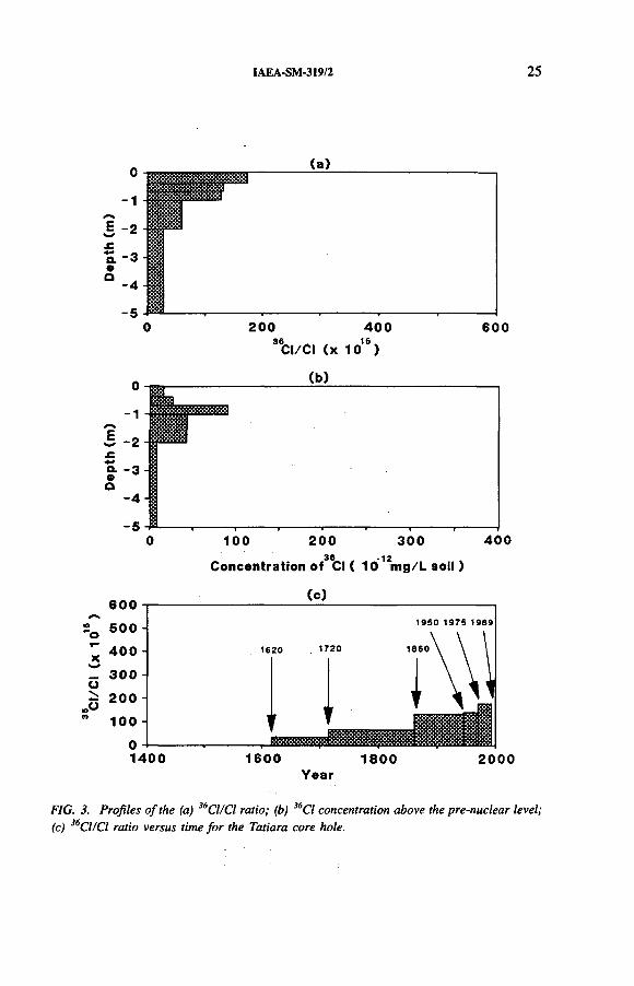
Three representations of the 36C1 profile for the Tatiara core hole are shown in Fig. 3. The first is the profile with depth of 36C1/C1 in the soil water. If piston flow was a reasonable approximation, this would show a peak, with the peak corresponding to the chloride deposited during the late 1950s-early 1960s. Figure 3(b) shows the profile with depth of the 36C1 concentration above pre- nuclear levels in the soil. This is essentially a ‘photograph’ showing what has hap­pened to the high levels of 36C1 in the rainfall during the period of nuclear testing.

CHLORIDE SUCTION

0 9 (g/g)(Thousands)

CHLORIDE (m g/L)(Thou sands)-

MATRIC SUCTION (kPa)

FIG. 2. Gravimetric water content, chloride and matric suction profiles for the Tatiara core hole.

Cl/

Cl

(x 1

0

IAEA-SM-319/2 25

(a)

200 400

36ci/Ci (x io1s)600

3 6 - 1 2Concentration of Cl ( 10 mg/L soil )

1400 1600 1800Year

2 0 0 0

FIG. 3. Profiles o f the (a) 36Cl!Cl ratio; (b) 36Cl concentration above the pre-nuclear level; (c) 36Cl/Cl ratio versus time for the Tatiara core hole.

к>On

TABLE I. SUMMARY OF DATA FROM THE THREE CORE HOLES

HolePre-nuclear

C1-36/C1Cumulative Cl-36 above pre-nuclear

(atoms/m2)

Depth of Cl-36 . centre of mass

(m)

Depth of chloride front (m)

Recharge rate from Cl-36 centre of mass

(mm/a)

Recharge rate from chloride front

(mm/a)

Tatiara 28 x 10 '15 1.2 x 1012 1.0 2.5 7 6-7

Binnum 23 x 1 0 15 2.3 x 1012 1.0 1.2 1 2-3

Joanna 15 x 1 0 15 1.2 x 10'2 1.2 3.5 10 8-9

WALKER

et al.

IAEA-SM-319/2 27

(a)

Concentration of3 l ( 1 0 12mg/L soil )

(b)

о- 4 -

-5 J --------,---------.-------- -------------------,--------- .---------.---------0 100 2 0 0 300 400

Concentration of3b l ( 1 0 ' mg/L soil )

FIG. 4. Profiles o f the 36Cl concentration above the pre-nuclear level for core holes(a) Binnum and (b) Joanna.

Again, if piston flow is a reasonable approximation, the profile should have a peak coinciding with that of the 36C1/C1 profile. In Fig. 3(c), the 36C1/C1 ratio is plotted against cumulative chloride (the total amount of chloride down to a given depth). The cumulative chloride was normalized using the concentration of chloride in the rain­fall to give the year of deposition, assuming that piston flow is a reasonable approximation.

For the Tatiara site, it is clear that the depth of the peak in the 36C1/C1 profile does not correspond to that of the centre of mass of the 36C1 profile. Moreover, the distribution in the 36C1 profile, when plotted against cumulative chloride (years), is very skewed, showing mixing between recent chloride deposition and pre-nuclear chloride. The deeper 36C1/C1 ratio is 28 ± 6 X 10“15, somewhat higher than the predicted level. This is due presumably to the chloride fallout being lower than the assumed level. This value matches that of a sample from deeper in the profile (23 m) (measured to be 31 ± 3 x 10~15) and a sample from the top 3 m of the

28 WALKER et al.

groundwater (26 + 5 X 10~15). The cumulative 36C1 in the profile (assuming a pre- nuclear background of 28 x 10'15) is 1.2 x 1012 atoms/m2. This is similar to the mass of 36C1 found at similar latitudes in the Northern Hemisphere and not much lower as might be expected from measurements of 185W produced in the same tests as for 36C1 [4]. The 36C1 centre of mass for this hole is located at 1.0 m and the chloride front is at 2.5 m. The cumulative water between the 36C1 centre of mass and the chloride front is approximately 480 mm, or 7 mm/a. This compares well with the 6-7 mm/a predicted by the chloride leaching method. A summary of the above data is given in Table I.

Figure 4 shows the profiles with depth of the 36C1 concentration above pre- nuclear levels in the soil water for the Binnum and Joanna core holes. A summary of the data for these holes is also given in Table I.

6. DISCUSSION

While the principle of applied tracers is simple, the implementation is some­times difficult, particularly for semi-arid and arid areas. In these areas, the majority of the tracer is often in the root zone, where interpretation can be ambiguous. The method suggested in this paper for environmental tracers avoids this by only considering the movement of tracers below the root zone. The suggested conjunctive use of the 36C1 centre of mass and the chloride front permits estimation of the drainage flux below the root zone for certain field situations in Australia. The method is opportunistic in that it exploits a characteristic of the Australian situation that is not common elsewhere.

The storage of water to the depth of the centre of mass is plotted in Fig. 1(b). The graph differs from Fig. 1(a) in two of the three holes. The method described in Ref. [4] for using the 36C1 profile would provide estimates consistent with those in this paper for two of the three holes if the method was adapted to use the centre of mass. The discrepancy with the schematic in Fig. 1(a) could be due to the sampling after a long dry summer, so that the soil zone above the 36C1 centre of mass is close to wilting point.

The chloride leaching method is not an independent method. First, the chloride front is used for both methods. Second, one dimensional flow is assumed for both methods. Third, the leaching of chloride is the basis of both methods. However, the position of the centre of mass of 36C1, which is not used for the chloride leaching method, was important in the estimation of the recharge rate for two of the three holes described in this paper. Thus, the position of the centre of mass was consistent with the recharge rate and the two methods can be described as being semi­independent.

A difficulty with this method, not dealt with here, is spatial variability. Bromide studies [1, 2, 8] have shown considerable variability in the solute profiles.

IAEA-SM-319/2 29

Calculations have been made for an average profile, obtained by aggregating several individual profiles. Because of the high cost of analyses for environmental levels of radionuclides, such aggregation is not possible, apart from the direct bulking of samples.

REFERENCES

[1] JURY, W.A., Simulation of solute transport using a transfer function model, Water Resour. Res. 18 (1982) 363-368.

[2] SHARMA, M .L., “Use of applied tracers in studies of natural groundwater recharge” , Groundwater Recharge (Proc. Int. Symp. Mandurah, 1987) (SHARMA, M., Ed.), A.A. Balkema, Rotterdam (1989) 11-23.

[3] ALLISON. G.B., HUGHES, M.W., The use of environmental chloride and tritium to estimate total recharge to an unconfined aquifer, Aust. J. Soil Res. 16 (1978) 181-195.

[4] PHILLIPS, F.M ., et al., Chlorine-36 and tritium from nuclear weapons fallout as tracers for long-term liquid and vapor movement in desert soils, Water Resour. Res. 24 (1988) 1877-1891.

[5] BENTLEY, H.W., DAVIS, S.N., “Applications of AMS to hydrology” , Acceleration Mass Spectrometry (Proc. 2nd Annual Symp. Argonne National Laboratory, 1981), Rep. ANL/PHY-81-1, National Technical Information Service, McLean, VA (1982).

[6] NORRIS, A.E., et al., Infiltration at Yucca Mountain, Nevada, traced by 36C1, Nucl. Instrum. Methods Phys. Res. B29 (1987) 376-379.

[7] ALLISON, G.B., et al., Land clearance and river salinization in the western Murray Basin, Australia, J. Hydrol. 119 (1990) 1-20.

[8] SCHULIN, R., et al., An experimental study of solute transport in stony field soil, Water Resour. Res. 23 (1987) 1785-1794.

[9] JOLLY, I.D ., et al., Simultaneous water and solute movement through an unsaturated soil following an increase in recharge, J. Hydrol. I l l (1989) 391-396.

[10] WALKER, G.R., et al., A new chloride leaching approach to the estimation of diffuse recharge following a change of land use, J. Hydrol. (to be published).

[11] BLACKBURN, G., McLEOD, S., Salinity of atmospheric precipitation in the Murray-Darling drainage division, Australia, Aust. J. Soil Res. 21 (1983) 411-434.

[12] STADTER, M .H., Reassessment of Groundwater Resources for Zones 2A to 8A of the South Australian Designated Area, Border Groundwater Agreement, Report Book No. 89/27, South Australian Department of Mines and Energy, Adelaide (1989).

[13] BENTLEY, H.W ., PHILLIPS, F.M ., DAVIS, S.N., “Chlorine-36 in the terrestrial environment” , Handbook of Environmental Isotope Geochemistry: The Terrestrial Environment (FRITZ, P., FONTES, J.-C., Eds), Vol. 2b, Elsevier, Amsterdam (1986) 427-480.

[14] WALKER, G.R., et al., Estimation of Diffuse Recharge in the Naracoorte Ranges Region, South Australia, Report No. 21, Centre for Groundwater Studies, Adelaide, SA (1990).

SURFACE WATER AND SEDIMENTS

Chairman E. CUSTODIO

Spain

IAEA-SM-319/1

CONJUNCTIVE USE OF ISOTOPIC TECHNIQUES TO ELUCIDATE SOLUTE CONCENTRATION AND FLOW PROCESSES IN DRYLAND SALINIZED CATCHMENTS

J.V. TURNERDivision of Water Resources,Commonwealth Scientific and Industrial Research Organisation,Perth

J.M. BRADD, T.D. WAITE Environmental Science Programme,Australian Nuclear Science and Technology Organisation,Sydney

Australia

Abstract

CONJUNCTIVE USE OF ISOTOPIC TECHNIQUES TO ELUCIDATE SOLUTE CONCENTRATION AND FLOW PROCESSES IN DRYLAND SALINIZED CATCHMENTS.

A range of isotopic techniques and geochemical methods has been used to investigate the mechanisms of solute concentration and surface and groundwater flow processes in selected small (< 1 0 km2) catchments in New South Wales, Australia. The catchments were selected for study as they are typical of the dryland salinized catchments in the region. Environmental isotopes used include the radioactive isotopes 238U and its decay product 234U, 36C1, tritium (3H), and the stable isotopes deuterium (2H), l80 , and l3C. Stream hydro­graph separation based on deuterium and chloride concentrations was used to study stream flow generation and to estimate the extent of salt export from the catchments. Results from the study have provided considerable insight into likely recharge zones and dominant salt concentration mechanisms, and have proved useful in the ‘fingerprinting’ of particular groundwater provenances. In addition, stream hydrograph separation using isotopic techniques has provided an insight into sources of stream flow generation and the rate and flow path of water (and salt) movement to streams following rainfall events. These are factors that could be managed by alteration in land use practices in these catchments.

33

34 TURNER et al.

1. INTRODUCTION

1.1. Background

Land salinization is one of Australia’s most critical environmental problems. It is particularly severe in the Murray-Darling Basin, one of the most important agricultural regions in Australia. The development of a sound understanding of the processes responsible for land salinization is a necessary condition for the implemen­tation of effective land management strategies and remedial measures.

The purpose of the investigations is to understand the processes that lead toland salinization from the viewpoint of total catchment management. In particular, the issues that need to be dealt with are:

(a) Definition of recharge/discharge areas in the catchment.(b) Estimation of recharge rates to groundwater resources.(c) Definition of groundwater flow paths.(d) Definition of groundwater provenances and the extent of mixing between

waters from different provenances.(e) Determination of groundwater residence times in aquifers.(f) Elucidation of the mechanisms that cause dryland salinization in small upland

catchments of large scale basins.(g) Estimation of the magnitude of salt export from catchments.(h) Estimation of proportional contribution of rainfall and groundwater to stream

flow.

This investigation uses environmental isotopes as tools to aid in land manage­ment and remediation of salinized land. The paper presents two Australian case studies using isotopic techniques that deal with several of the above issues.

1.2. General and hydrogeological setting

The selected research catchments are located within the upland regions of the Murray-Darling Basin, as shown in Fig. 1. Figure 2 gives a more detailed description of each catchment, showing the locations of piezometer transects through saline groundwater seepage areas. The Wattle Retreat catchment (area: 600 ha) has a significantly lower average elevation (300 m) than that of the Williams Creek catchment (600 m, area: 1000 ha). The climate of these upland regions ranges from temperate to semi-arid, with annual rainfall usually between 500 and 750 mm. Of the two catchments, Wattle Retreat has a warmer and drier climate, with a mean annual rainfall of 500 mm. The mean annual rainfall at Williams Creek is 640 mm. Most rain falls in the winter months and potential evaporation exceeds rainfall for ten months of the year. Native Eucalyptus forest vegetation was progressively cleared from the catchments over the past 70 years. The land use of both catchments

IAEA-SM-319/1 35

FIG. I. Regional setting o f the investigation catchments in the Murray-Darling Basin (NSW: New South Wales; QLD: Queensland; &4: South Australia; VIC: Victoria).

36 TURNER et al.

FIG. 2. Detailed catchment layout for the Wattle Retreat and Williams Creek investigation sites showing the locality o f the bores and piezometers (ANSTO: Australian Nuclear Science and Technology Organisation).

IAEA-SM-319/1 37

is pasture at the present time. The two catchments differ geologically; basement rocks at Wattle Retreat consist of a homogeneous rhyodacitic tuff of ash flow origin [1], while Williams Creek is composed almost entirely of folded and often highly fractured Ordovician sediments and meta-sediments. The most common sediments and meta-sediments are grey shale, slate and phyllite, occasionally interbedded with carbonaceous slate containing pyrite. Basement rocks outcrop in the upland flanks of both catchments. Also in both catchments, the shallow water table aquifer has a higher head than deeper groundwater in the fractured basement rocks of upslope flanking areas of the catchments. In the lower valley slopes, where soil salting and groundwater seepage occur, the deeper groundwater has a higher head and thus groundwater flow is vertically upward. Deep groundwater bores in the lower valley slopes frequently have a potentiometric level above the ground surface. Soils at Wattle Retreat comprise up to 20 m thicknesses of clays and sandy clays, while at Williams Creek the soils comprise mainly clays, but of shallower depths up to 4 m. A more detailed geological and hydrogeological description is given for both catchments elsewhere [1-3].

1.3. Research catchment instrumentation

Deep and shallow investigation bores were drilled into basement rocks and soils in each catchment. Six 100 mm diameter bores were drilled into basement rocks and sixteen 50 mm diameter shallow piezometers of varying depths were augered into soil and weathered rock at the Wattle Retreat catchment. Six deep and 17 shal­low bores were drilled at Williams Creek. An additional four transects of nested piezometers were drilled into the weathered bedrock. Other instrumentation included stream stage height recorders, automatic stream samplers, rain gauges and rainfall samplers.

2. GROUNDWATER SAMPLING AND SAMPLE PREPARATION TECHNIQUES

Samples for major cation and uranium analysis were filtered through 0.45 /xm membrane filters and acidified in the field to pH < 2 using concentrated HN03. Atomic absorption spectrophotometry (AAS) was used for analysing potassium. Inductively coupled plasma (ICP) was used to measure sodium, calcium, magnesium, iron and silicon. Uranium was analysed following standard radio­chemical methods [4]. Unacidified, unfiltered samples were analysed for chloride, sulphate phosphate, bromide and nitrate and analysed by ion chromatography. Bicarbonate was calculated from alkalinity measurements made in the field.

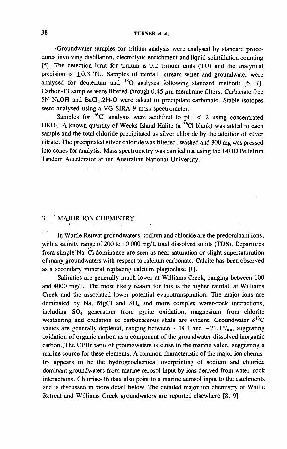
38 TURNER et al.

Groundwater samples for tritium analysis were analysed by standard proce­dures involving distillation, electrolytic enrichment and liquid scintillation counting [5]. The detection limit for tritium is 0.2 tritium units (TU) and the analytical precision is ±0.3 TU. Samples of rainfall, stream water and groundwater were analysed for deuterium and 180 analyses following standard methods [6, 7]. Carbon-13 samples were filtered through 0.45 ¿im membrane filters. Carbonate free 5N NaOH and BaCl2.2H20 were added to precipitate carbonate. Stable isotopes were analysed using a VG SIRA 9 mass spectrometer.

Samples for 36C1 analysis were acidified to pH < 2 using concentrated HN03. A known quantity of Weeks Island Halite (a 36C1 blank) was added to each sample and the total chloride precipitated as silver chloride by the addition of silver nitrate. The precipitated silver chloride was filtered, washed and 300 mg was pressed into cones for analysis. Mass spectrometry was carried out using the 14UD Pelletron Tandem Accelerator at the Australian National University.

3. MAJOR ION CHEMISTRY

In Wattle Retreat groundwaters, sodium and chloride are the predominant ions, with a salinity range of 200 to 10 000 mg/L total dissolved solids (TDS). Departures from simple Na-Cl dominance are seen as near saturation or slight supersaturation of many groundwaters with respect to calcium carbonate. Calcite has been observed as a secondary mineral replacing calcium plagioclase [1].

Salinities are generally much lower at Williams Creek, ranging between 100 and 4000 mg/L. The most likely reason for this is the higher rainfall at Williams Creek and the associated lower potential évapotranspiration. The major ions are dominated by Na, MgCl and S04 and more complex water-rock interactions, including S04 generation from pyrite oxidation, magnesium from chlorite weathering and oxidation of carbonaceous shale are evident. Groundwater <513C values are generally depleted, ranging between —14.1 and -2 1 .1 7 00, suggesting oxidation of organic carbon as a component of the groundwater dissolved inorganic carbon. The Cl/Br ratio of groundwaters is close to the marine value, suggesting a marine source for these elements. A common characteristic of the major ion chemis­try appears to be the hydrogeochemical overprinting of sodium and chloride dominant groundwaters from marine aerosol input by ions derived from water-rock interactions. Chlorine-36 data also point to a marine aerosol input to the catchments and is discussed in.more detail below. The detailed major ion chemistry of Wattle Retreat and Williams Creek groundwaters are reported elsewhere [8, 9].

IAEA-SM-319/1 39

4. ENVIRONMENTAL ISOTOPES

4.1. Tritium

Rainwater was collected for tritium analysis at Williams Creek in April 1990 and yielded values ranging between 2.5 and 3.3 tritium units (TU)1. This is in accord with the mean concentration of about 3 TU expected in Australian rainwater at the present time [10].

Although the tritium concentration in rainfall is only slightly greater than pre-bomb (1952) background tritium concentrations, it is still possible to use tritium for determining recharge areas and to estimate the depth of penetration of recent recharge waters less than 30 years old.

Most bores and piezometers sampled in Wattle Retreat show very low tritium concentrations, of less than 1 TU, suggesting a predominance of pre-bomb recharge to these groundwaters. Only bores 36748/1 and 36748/2 (see Fig. 2) have high tritium concentrations of 5.8 and 5.7 TU, respectively, that can be interpreted as being due to recharge that occurred within the past 30 years. These bores penetrate fractured bedrock that outcrops on the catchment flanks which, from these tritium data, appears to be a recharge area. The low TDS value in these samples ( < 200 mg/L) indicates that these groundwaters have not interacted with the mineral environment for an extended period and also suggests little mixing with ‘older’ groundwaters. By including the low salinity bores R15 and R19, which were not analysed for tritium, definition of a local recharge area for the catchment is possible. Other bores that have measurable tritium (> 1 TU) are R8, 36749 and R3/1, which indicates mixing of infiltrated recent recharge with older waters.

A much higher proportion of groundwater samples from Williams Creek show tritium concentrations above 1 TU than in Wattle Retreat, indicating more widespread recharge. For this catchment, Fig. 3 shows tritium activity plotted against the bore depth from which the sample was taken. From this, the recharge rate can be quantified by multiplying the aquifer porosity by the depth of maximum penetration of bomb pulse tritium, and dividing this by the time since anthropogenic tritium entered the atmosphere (in 1953). This method is described in Ref. [11]. By assuming an average porosity of 0.2 for the aquifer matrix, which is comprised mainly of clays, a tritium interface depth range of between 8 and 12 m, the calculated recharge rate for the Williams Creek catchment is between 4.3 and 6.5 cm/a. The anomalous values (1-2-C, Pratt’s Bore and 36761) can be explained by the high fracture intensity at these sites, allowing groundwaters to penetrate deeper.

1 One tritium unit corresponds to an atomic ratio of one atom of tritium for 1018 atoms of hydrogen.

40 TURNER et al.

FIG. 3. Tritium activity versus sample depth at Williams Creek.

4.2. Uranium-234/uranium-238 and 226Ra geochemistry

Absolute uranium concentrations, 234U/238U activity ratios and 226Ra activities for groundwaters from the Williams Creek and Wattle Retreat catchments are given in Table I. Uranium concentrations range from 0.007 to 27 ¿ig/kg at Williams Creek and are, on average, much lower than the range from 0.4 to over 100 /¿g/kg observed at Wattle Retreat. Concentrations above 10-20 /¿g/kg are considered to be unusually high and presumably reflect a high uranium content in the aquifer strata. The bedrock in this region comprises rhyodacites and granites that are generally considered to have a high abundance of uranium [12].

While the dominant dissolved uranium species will depend on the Eh-pH conditions and the availability of complexing ions, U(VI) forms particularly strong complexes with carbonate and, above pH5, with typical groundwater partial pres­sures of C 02, uranyl carbonate complexes typically dominate. Calculations using the code MINTEQA1 [13] indicate that the monocarbonate species UO2CO3 dominates in the lower pH waters of 36748/1 and 36748/2, while U02(C03) | ' is the principal uranyl species in all other groundwaters at Wattle Retreat. In both study areas, there is a positive correlation between total uranium and bicarbonate concen­tration, as shown in Fig. 4. This confirms the importance of carbonate complexation

IAEA-SM-319/1 41

in controlling the uranium geochemistry of the groundwaters and implies that the groundwaters, particularly at Wattle Retreat, have a sufficiently long residence time to allow extensive mineral-water interaction. This strong complexation will serve to both enhance the tendency of uranium bearing minerals to dissolve and limit the tendency of U(VI) to be lost from solution via adsorption. The association between uranium and bicarbonate is particularly evident in groundwaters from transect 2 at Williams Creek.

The 234U/238U activity ratios of groundwaters fall typically between 1.0 and2.0. Some Wattle Retreat groundwaters do fall in this range, but many samples exhibit ratios between 2.0 and 3.0. Such high ratios are observed typically when the ratio of leachable uranium in the aquifer matrix to dissolved uranium is high. Marked differences in the activity ratios of groundwaters are indicative of waters of distinctly different source and history. At Wattle Retreat, groundwaters from lower areas of the catchment along transect A-A' from bores 36748/2 and R16 with activity ratios of 1.68 and 1.69, respectively , are confirmed to be quite distinct from groundwaters from the flowing bores R4, R5, R3/2 and 36746 with activity ratios of 2.90, 2.87, 2.81 and 2.82, respectively. These activity ratio groupings represent the extremes that have been observed at Wattle Retreat and may be considered as being repre­sentative of ‘end members’ for this catchment, characterizing the deep and shallow groundwater systems. At Williams Creek, most groundwaters exhibit activity ratios in the range of 1.0 to 2.0 (Table I). Those groundwaters with activity ratios higher than 2.0 tend to be those from deep bores and those which are flowing, for example, bores 36761, 36763, 36764, 36768 and 36791/1 and 36791/4. A qualitative interpre­tation, equally applicable to both catchments, is that deeper groundwaters with longer residence times attain higher activity ratios than do shallow groundwaters.

Radium-226 activities range from 0.1 to 13 Bq/kg at Williams Creek but, in contrast to the uranium concentrations, are significantly higher than the observed0.03 to 2.7 Bq/kg at Wattle Retreat. The 226Ra activities for both Wattle Retreat and Williams Creek groundwaters are shown plotted against the 238U concentration in Fig. 5. The 226Ra content is not related to the dissolved uranium content in groundwaters from Williams Creek; however, a weak correlation can be seen at Wattle Retreat, presenting the possibility that 226Ra activity is controlled by decay processes in solution. The average dissolved uranium content at Wattle Retreat is high and of the order of 40 Mg/kg. Radium-226 activity of the order of 1.2 Bq/kg could be supported by this uranium concentration in solution, under equilibrium conditions. The observed radium activities are clearly in this range at Wattle Retreat, and thus may be accounted for by the 234U -230Th-226Ra decay sequence in solution. The measurements of 230Th in solution are not available, but thorium has a relatively short residence time in groundwaters due to the ease of hydrolysis of Th4+ and the extremely low solubility of thorium hydroxide. As 230Th forms it is removed from solution by precipitation or adsorption and 226Ra formed on its decay could be rapidly returned to solution. Following the same reasoning, it is unlikely

42 TURNER et al.

TABLE I. URANIUM AND RADIUM ISOTOPE DATA ON GROUND­WATERS FROM EXPERIMENTAL CATCHMENTS IN NEW SOUTH WALES

Sample No. [U] /.g/kg U-234/U-238 Ra-226(Bq/kg)

Wattle Retreat catchment

RI 82.9 ± 3.6 1.94 ± 0.02 1.87 ± 0.06

R3/1 39.6 ± 1.6 2.12 ± 0.02 —

R3/2 54.6 ± 2.1 2.81 ± 0.02 0.94 ± 0.03

R4 49.7 ± 2.2 2.9 ± 0.03 1.58 ± 0.05

R5 38 ± 1.3 2.87 ± 0.03 1.26 ± 0.04

R6 108 ± 5.0 2.58 ± 0.02 0.03 ± 0.01

R7 41.3 ± 1.5 2.46 ± 0.04 0.44 ± 0.02

R8 11.1 ± 0.4 1.64 ± 0.04 1.56 ± 0.06

R9 12.7 ± 0.5 2.51 ± 0.05 0.66 ± 0.03

RIO 21.5 ± 0.8 2.69 ± 0.05 0.51 ± 0.02

R ll 47.3 ± 1.8 2.18 ± 0.02 2.43 ± 0.08

R12 25.8 ± 0.7 2.53 ± 0.03 0.59 ± 0.02

R13 7.6 ± 0.2 4.18 ± 0.1 0.65 ± 0.03

R15 1.71 ± 0.06 2.11 ± 0.07 0.16 ± 0.01

R16 71.4 ± 2.3 1.69 ± 0.01 1.06 ± 0.03

R17 48.9 ± 2.0 2.18 ± 0.02 2.35 ± 0.08

36746 42.3 ± 1.7 2.82 ± 0.03 1.69 ± 0.05

37648/1 0.4 ± 0.01 1.7 ± 0.05 0.65 ± 0.02

36748/2 0.42 ± 0.02 1.71 ± 0.08 0.51 ± 0.02

36749 25.5 ± 1.0 2.89 ± 0.04 1.23 ± 0.04

36754 52.8 ± 2.0 2.2 ± 0.02 2.7 ± 0.07

36755 74.9 ± 3.6 2.48 ± 0.02 2.49 ± 0.07

Williams Creek catchment

36761 0.12 ± 0.02 1.6 ± 0.20 1.92 ± 0.05

36762 0.04 ± 0.01 1.11 ± 0.15 1.13 ± 0.04

36763 0.007

8О-H 3.0 ± 2.60 8.29 ± 0.17

IAEA-SM-319/1 43

TABLE I. (cont.)

Sample No. [U] ng/kg U-234/U-238

36764 0.188 ± 0.02 2.64 ± 0.23 8.64 ± 0.25

36767 0.03 ± 0.01 0.93 ± 0.17 5.21 ± 0.15

36768 0.123 ± 0.01 2.01 ± 0.19 13.11 ± 0.42

36791/1 0.153 ± 0.01 2.46 ± 0.20 1.96 ± 0.06

36791/4 0.019 ± 0.01 2.03 ± 0.40 12.0 ± 0.30

Pratt’s Bore 0.19 ± 0.01 1.37 ± 0.14 4.61 ± 0.09

40659 0.008 ± 0.00 1.44 ± 0.26 0.38 ± 0.02

40661 0.555 ± 0.02 1.17 ± 0.05 0.61 ± 0.02

SCS604 1.98 ± 0.09 1.98 ± 0.07 0.13 ± 0.06

1-1-C 0.24 ± 0.01 1.46 ± 0.09 0.19 ± 0.08

1-2-C 2.802 ± 0.10 1.9 ± 0.05 0.61 ± 0.02

1-3-C 1.928 ± 0.09 1.81 ± 0.05 0.46 ± 0.03

1-4-C 8.353 ± 0.31 1.6 ± 0.08 0.94 ± 0.07

2-1-B 0.321 ± 0.02 1.1 ± 0.10 0.52 ± 0.03

2-1-C 0.268 ± 0.01 0.78 ± 0.05 0.55 ± 0.03

2-2-B 6.349 ± 0.27 1.27 ± 0.05 1.59 ± 0.09

2-2-C 2.647 ± 0.14 1.04 ± 0.04 2.31 ± 0.06

2-3-B 3.396 ± 0.13 1.09 ± 0.03 1.73 ± 0.06

2-3-C 27.1 . ± 4.11 0.83 ± 0.03 2.88 ± 0.06

2-4-B 17.89 ± 0.66 1.57 ± 0.05 1.55 ± 0.11

2-4-C 6.559 ± 0.22 1.93 ± 0.09 0.8 ± 0.06

that uranium and thorium in solution are the sources of the higher 226Ra activities at Williams Creek.

It may also be expected that the behaviour of 226Ra in solution is related to the solution chemistry of calcium as well as barium and strontium. Figure 6 shows plots of 226Ra activity against the calcium concentration for both catchments. A good correlation is seen for Wattle Retreat, suggesting that the concentration of radium in groundwaters is controlled more by the groundwater chemistry than the radium

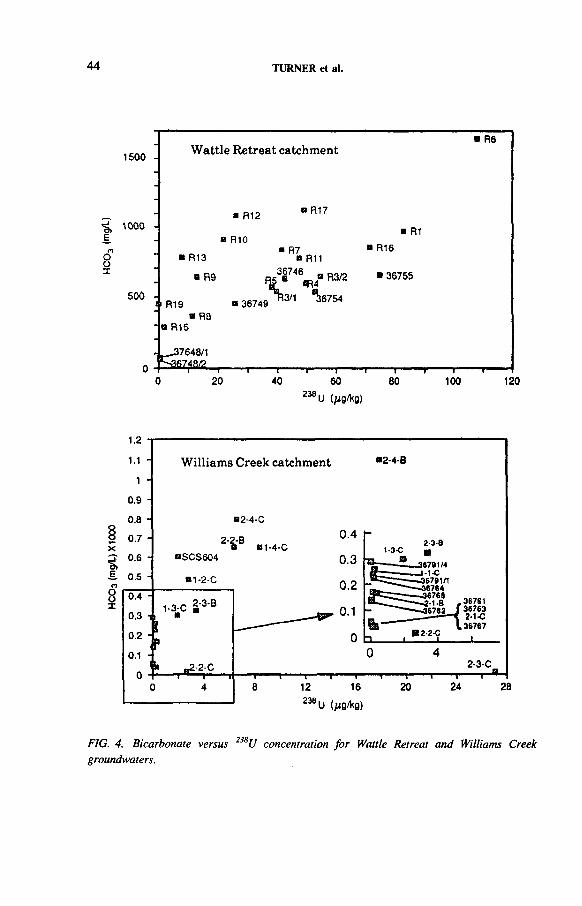
44 TURNER et al.

1500Wattle Retreat catchment

■ R6

’á, 1000 E

ООX

и R12

и R10

в R13

В R9

500 -11 R19 а 36749

в R17

■ R7 и R11

3о746 о R3/2 4 43/1 ^36754

и R8BR15

17648/1§7Ш

и R1

R16

■ 36755

- г -20

—г-40

—г—60

23880

U (fig/kg)

100 120

U (/¿g/kg)

FIG. 4. Bicarbonate versus 238U concentration for Wattle Retreat and Williams Creekgroundwaters.

IAEA-SM-319/1 45

Wattle Retreat catchment B 36754B R11

aR17

в 36755

C3 □ R1

и R8в 36746

и R4

37648/1/ R13 _ л l в ■ R91 36748/2

в 36749 “ Rs

В R3/2

R12

Н R“ ° - R7

и R16

a R15 R6 _____ в.i ------- 1-------1 i i i i i i i i

0 20 40 60 80 100

238 U (^g/Kg)

FIG. 5. Radium-226 activities versus 238U concentrations for Wattle Retreat and WilliamsCreek groundwaters.

46 TURNER et al.

enСГmсоОСюoj

CM

2.8

2.62.4

2.2

2

1.8

1.6

1.4

1.2

1

0.8

0.6

0.40.2

0

в 36754

i R11

36749,

I R167648/1

g12 в13 в Я9 о RIO

°R7 36748/2

и ПО

i 36755B R17

в R1R4 B 36746

0 B R8

B R5

B R3/2

Wattle Retreat catchment

200—i—400 600

Calcium (mg/L)

o>СГCÛ00CCCD

a

14

13

12

11

10

9

8

7

6

5

4

3

2

1

0

Williams Creek catchment ■36768

B36763

B36767 в Pratt's Bore

2-3-B

- 40659 в

36761 2-4-С в b /2-1-С « il SCS604

2-4-B2 - 2-

в36764

«2-2-С

40661

В2-3-С .,.0 в 36791/1

2-С B l-^ê6762-1-1-С . >1-3-С

20 40

Calcium (mg/L)60 80

FIG. 6. Radium-226 activities versus calcium concentrations for Wattle Retreat and WilliamsCreek groundwaters.

IAEA-SM-319/1 47

TABLE II. CHLORINE-36 DATA ON GROUNDWATERS FROM EXPERIMENTAL CATCHMENTS IN NEW SOUTH WALES

Sampleidentity

Cl(mg/L)

Cl-36 x 106 (atoms/L)

C1-36/C1 x 10~

Wattle Retreat catchment

R1 2890 9561 ± 1961 195 ± 40

R3/1 1719 4200 ± 408 144 ± 14

R5 1119 3379 ± 285 178 ± 15

R6 491 1383 ± 133 166 ± 16

R8 1064 3069 ± 542 170 ± 30

R ll 1142 2906 ± 581 150 ± 30

R16 3527 9335 ± 957 156 ± 16

36748/2 41 1043 ± 139 1500 ± 200

36748/2 (repeat) 41 995 ± 76 1430 ± 110

36749 1529 4462 ± 389 172 ± 15

36754 738 2115 ± 396 160 ± 30

Williams Creek catchment

36767 40.69 110 ± 13 156 ± 19

36791/1 140.38 322 ± 26 135 ± 11

36791/4 152.79 290 ± 52 112 ± 20

SCS604 245.83 709 ± 50 170 ± 12

36762 155.58 390 ± 37 148 ± 14

2-3-C 175.22 458 ± 36 154 ± 12

2-2-C 177.34 385 ± 39 128 ± 13

36764 296.97 584 ± 55 116 ± 11

2-1-B 123 296 ± 23 142 ± 11

2-2-B 203 489 ± 45 142 ± 13

36761 31 63 + 7 119 ± 14

2-2-A 230 695 ± 51 178 ± 13

2-1-A 236 685 ± 52 171 ± 13

48 TURNER et al.

•aEо' S

ô

2 3Chloride (mg/Lx 1000)

2000

1500

U)7о

* 1000 о5

s

500

00 1 2 3 4

Chloride (mg/Lx 1000)

FIG. 7. Chlorine-36 concentration and the 36Cl/Cl ratio versus chloride for Wattle Retreat and Williams Creek groundwaters.

> 36748/2*36748/2 (REPEAT)

180

160

140

120

100,

•2-2-A2-i-A**SCS604

•36767 3676¿ . 2-3-С 2-1-B* ‘2-2-B

36791-1 .2-2-C•36761

•36791-4 36764

100 200 300

,S ee Inset

R8R5 36749Р6 * 675Л п ° “ R3/1

■ Wattle Retreat 0 Williams Creek

■ R1 в R16

IAEA-SM-319/1 49

content of aquifer minerals or the 234U -230Th-226Ra decay sequence in solution. Weaker 226Ra-Ca systematics are observed at Williams Creek. However, high radium activities are observed in deeper groundwaters (36767, 36763, 36764, 36768 and 36791/4), consistent with an expected longer residence time.

4.3. Chlorine-36

The ratio of 36C1 to chloride, the 36C1 concentration and the chloride concen­trations from Wattle Retreat and Williams Creek groundwaters are shown in Table II. Data from both catchments are combined and plotted together as the 36C1 concentration and the 36C1/C1 ratio versus the chloride concentration in Fig. 7. The reported data are the most intensive set available to date for relatively localized groundwater studies in Australia and provide valuable insight into the source of chloride within the catchments and groundwater mixing processes.

Groundwater 36C1/C1 ratios exhibit a range of between 110 and 200 x 10~15, with an average value of 165 X 10“15. Data from the two catchments form two distinct groupings because of the lower total salinity, and hence chloride content, of groundwaters from Williams Creek in comparison with Wattle Retreat. A single but important exception to the 36C1/C1 ratio range is noted in sample 36748/2 from Wattle Retreat. Values of the 36C1/C1 ratio in modern atmospheric precipitation in this area of the Murray Basin have been calculated to be approximately 60 X 10~15[14]. This value is between a half and a third of values observed in groundwaters reported here. The range of 36C1/C1 ratios in groundwaters reported here is also comparable to those observed in preliminary regional data from the Lachlan Fan and Murray-Mallee aquifers reported by Bird et al. [15].

The 36C1 concentration data plotted against the chloride concentration in Fig. 7 show a strong correlation for samples from both catchments. The slope of the correlation is defined by a 36C1/C1 ratio of 160 X 10~15. This is similar to that determined for the regional data from the Lachlan Fan of 140 X 10“15 [14] and suggests that similar processes control the 36C1 distribution in groundwaters over the different scales represented by Lachlan Fan data and the data presented here. The strong linear correlation between 36C1 and Cl over a large range in chloride concentrations for these groundwater samples shows that évapotranspiration and mixing of groundwaters are the dominant processes determining the 36C1 distri­bution. Stable isotope data (<32H and <5I80) discussed in Section 4.4 do not show significant deviation from the local meteoric water line caused by evaporation. This, combined with the 36C1 results, indicates that water uptake by tree roots and transpiration in the pre-cleared catchment rather than surface evaporation is the important solute concentrating process in these catchments. The absence of deviation from the strong linear correlation in Fig. 7 also indicates that radioactive decay is not an important process, as would be expected in these shallow groundwater

50 TURNER et al.

systems, with residence times expected to be very much shorter than the 36C1 half- life of 300 000 a.

As can be seen in Fig. 7, the sample from bore 36748/2 has a 36C1/C1 ratio and 36C1 concentration significantly higher than all other samples. Resampling and reanalysis of groundwater from this bore confirmed this anomalous result. The result suggests strongly that the 36C1 content of this sample is dominated by inputs of 36C1 from atmospheric nuclear weapons testing in the 1950s. This implies that ground­water sampled from this bore contains a significant component of recharge that occurred at that time, and since then has not mixed significantly with groundwater from within the catchment.

The occurrence of this sample with an elevated 36C1 concentration also suggests an explanation for the overall higher than expected 36C1/C1 ratios in the catchments. Assuming that sample 36748/2 is a single unmixed remnant of the 36C1/C1 ratio in bomb pulse input, then this analysis assumes that the widespread input of chloride with this or an even higher ratio would have occurred. If this high 36C1/C1 ratio input has subsequently mixed with pre-existing chloride in the catch­ments, then the effect of this input can be determined. For example, assume two end members, such as 36748/2 and R16, but R16 with an initial (premixing) 36C1/C1 ratio of 60 x 10-15, the estimated 36C1/C1 ratio of atmospheric input [14], and a chloride concentration of 3700 mg/L. A 90% mixture of such a groundwater with 10% of a groundwater characterized by a 36748/2 end member would give ground­water with 3400 mg/L of chloride and a 36C1/C1 ratio of 190 X 10-15. Thus, if the occurrence of groundwater of the 36748/2 36C1/C1 ratio is (or was, prior to mixing) more widespread than we have sampled, and mixing occurred, then a widespread observation of 36C1/C1 ratios over a regional scale higher than that estimated from atmospheric input can be explained.

4.4. Stable isotopes — deuterium and 180

Groundwater samples were collected from the Wattle Retreat catchment in June and August 1988 and at Williams Creek between April and June 1990. Stable isotope data obtained on groundwaters from both catchments are shown in Fig. 8. At Wattle Retreat, most 62H and <520 values lie in the range of -3 9 to -3 4 7 00 and -6 .4 to -5.4°/oo, respectively, a range that agrees closely with limited data on the amount weighted mean value of rainfall. Outliers to the main groundwater groupings are identified in Fig. 8. At Williams Creek, the range for 02H and ¿>20 is from 39 to -6 2 7 00 and -6 .5 to -9 .0 7 oo, respectively. Groundwaters from Williams Creek are slightly depleted relative to Wattle Retreat owing to its higher altitude. Isotopic data on rainfall have been used to define the local meteoric water line (LMWL) of <52H = 8.5 <5180 + 15 shown in Fig. 8. The groundwater data from both catch­ments fall close to the LMWL and are thus consistent with recharge occurring without exposure to evaporation.

IAEA-SM-319/1 51

О

-20

-40

о

-60Iсмсо

-80

-100

-120-20 -15 -10 -5 0

8 180 ( % о )

FIG. 8. Deuterium versus 18О for Wattle Retreat and Williams Creek groundwaters and rainfall at Williams Creek (*: Wattle Retreat groundwaters; U : Williams Creek ground­waters; Д : rainfall at Williams Creek).

Samples R5, R4, 36746, R3/2, R6 and R7 along transect A-A' at Wattle Retreat are considered to be well mixed groundwaters based on other chemical and isotopic parameters, and this interpretation is confirmed by the stable isotope data. Similarly, the close match between samples 36748/1 and 36748/2 suggest that these are identical groundwaters in accord with previous results. Samples RI, R16 and R17 are isotopically distinct groundwaters that have not mixed with other ground­waters. These samples are also distinguished as the three highest salinity ground­waters in the catchment and R16 is the only groundwater to show evidence of isotopic enrichment caused by evaporation, owing to its displacement to the right of the LMWL.

Groundwaters at Williams Creek show a much wider scatter of stable isotope composition, although values do cluster close to the LMWL and none show any evidence of evaporative enrichment. The depleted groundwaters indicated in Fig. 8 were sampled following particularly depleted rainfall events in April and May 1990 and are most likely caused by rapid recharge and incomplete mixing of these particular groundwaters with the pre-existing shallow groundwater in the catchment.

52 TURNER et al.

The May 1990 rainfall data resulted in a significant response in the isotopic composition of stream water, as discussed in the following section. Since few groundwater samples show even slight evidence of isotopic enrichment, the predominant salt concentration mechanism is most likely the process of ion exclusion[16] during the uptake of water by pre-cleared vegetation.

5. STREAM HYDROGRAPH ANALYSIS USING DEUTERIUMAND CHLORIDE

Variations in the <52H value of the stream flow, particularly during rainfall events, can be used to gain a better understanding of the mechanisms of stream flow generation and, accordingly, salt export from small catchments. In its simplest form, stream flow during an event can be regarded as being generated from a combination of pre-event groundwater and the event rainfall.

Studies by numerous researchers have shown that pre-event groundwater is frequently a major component of stream flow generated during an event and can exceed 50% of the total water discharged [17]. In contrast, this investigation has shown two cases where, for selected events, between 65 and 75 % of the event runoff was derived from rainfall.

At Wattle Retreat, groundwater 02H values ranged between -3 9 and -3 4 7 00, while rainfall 62H values varied between events. The most significant rainfall event (about 30 mm) recorded during the study was one on 5 and 6 July 1988, with <52H values becoming as depleted as -7 5 700. This was a significant level of depletion relative to the <52H of the stream flow and groundwater in the catchment at that time. These pre-event values permit the establishment of an isotopic baseline for subsequent comparison of stream flow isotopic responses.

In the rainfall event of 5 and 6 July, the stream flow showed a rapid shift in <52H to a minimum of —707oo indicating qualitatively that the initial stream flow hydrograph response had a high proportion of rainfall. The response of the stream flow isotopic composition to individual rainfall events was used to partition stream flow into its pre-event groundwater and rainfall components. A simple two compo­nent mass balance equation was used to calculate the stream flow partitioning. The deuterium data show that approximately 75 % of the runoff was rainfall from the 5-6 July event (Fig. 9). The chloride method estimated the rainfall component as 50%, significantly less than that calculated from <52H measurements. A groundwater chloride concentration of 3800 mg/L is required in order for a hydrograph separation based on chloride to give results identical to that based on deuterium. This value is significantly higher than the measured groundwater chloride concentrations used in the calculation of between 1600 and 1800 mg/L. The discrepancy between the deuterium and chloride analysis is most likely due to the accumulation of salt efflorescences at the ground surface in regions of groundwater seepage. The flushing

IÀEA-SM-319/1 53

LEGEND QROUNDWATER RANGE RÀINFALJ. COMPOSITE RAINFALL SPECIFIC EVENT

07 Aug 27 Aug I в Sep 06 Ocl

DATE (1988)

DATE - JULY 1988

DATE - JULY 1988

FIG. 9. (a) Deuterium variations in stream flow from Wattle Retreat during 1988 showing the seasonal context o f the response to thé 5-6 July event; (b) event rainfall and detail o f the event hydrograph showing the rainfall component o f the hydrograph separated by deuterium and chloride; (c) the cumulative total flow and cumulative rainfall component for the event.

54 TURNER et al.

18 Mar 07 May 26 Jun IS Aug 04 O d 23 Nov

DATE (1990)

да300 -

240 -

*200 -

оEu

150 •

100 '

60 -

. TOTAL FLOW

,C I SEPARATION (200 mg/L)

-DEUTERIUM SEPARATION

23 24 25DATE- MAY 1990

DATE-M AY 1990

FIG. 10. (a) Deuterium variations in stream flow for Williams Creek during 1990 showing the seasonal context o f the 23 May event; (b) event rainfall and detail o f the event hydrograph showing the rainfall component o f the hydrograph separated by chloride (200 mg/L as the groundwater chloride concentration) and deuterium; (c) cumulative total flow and cumulative rainfall component for the event.

IAEA-SM-319/1 55

of this accumulated chloride into the stream during an event would have the effect of apparently overestimating the groundwater component in stream flow. On the basis of a total catchment area for Wattle Retreat of 600 ha, the cumulative volume of stream flow calculated by the deuterium method to have originated from rainfall corresponds to runoff from an area of 80 ha (i.e. 13% of the total catchment area). This analysis can be useful for the calculation of a salt balance for the catchment by permitting estimation of the true groundwater component and, hence, salt export in subsequent events.

Preliminary hydrograph results from Williams Creek also indicate a high proportion of rainwater in event stream flow. Figure 10 shows the <52H variation in stream flow during 1990 at Williams Creek. Two features are particularly notable. First, the rainfall event of 23 May, where 80 mm of rainfall of ô2H = — 1107oo had a marked isotopic response On the stream flow isotopic composition. Again, a simple two component mass balance equation was used to calculate the stream flow partitioning. The deuterium data show that approximately 63% of the runoff was rainfall from the 23 May event (Fig. 10). The chloride method using a groundwater chloride concentration of 155 mg/L estimated the rainfall component as 66%, in good agreement with that calculated from the <52H analysis.

Second, following this important event, it can be seen that about one month elapsed before the stream flow ô2H returned to its pre-event composition. Compa­rison of subsequent stream flow <52H with rainfall <52H for the remainder of the year shows the stream flow <52H tracking the rainfall <52H quite closely during the remainder of the year. These two observations lead to the tentative conclusion that neither deep nor shallow groundwater is a substantial component of stream flow at Williams Creek during the flow period, and that rainfall, if not discharged during the event itself, has a relatively short residence time in the shallow groundwater system prior to discharge.

6. CONJUNCTIVE INTERPRETATION OF CATCHMENTISOTOPE HYDROLOGY

By conjunctive examination of the range of parameters analysed, a number of common features are identified. This permits groupings of water types to be made that assists in defining groundwater provenances within the catchments. Alterna­tively, where differences are found, these can be interpreted as delineating separate groundwater provenances, for example, recently recharged groundwaters. The conjunctive interpretation can be summarized into five main points for each catchment.

56 TURNER et al.

6.1. Wattle Retreat

(1) Recently recharged waters have been identified by bores 36748/1 and 36748/2, R15, R19 and 36749. Evidence for this includes the 36C1 concentrations, the presence of 3H, low TDS, low 238U concentrations and a similar major ion distribution. This defines a recharge area for the catchment that is useful for setting salinity management strategies, such as tree planting programmes. Recharge appears to be occurring upland, flanking areas of the catchment, and is associated with outcrops of basement rocks. Chlorine-36 and chloride data form a linear relation consistent with concentration/dilution processes and mixing. In conjunction with the <52H and S20 data, this is consistent with the uptake of water and transpiration by pre-clearing native Eucalyptus vegetation as the primary solute concentrating mechanism.

(2) A perched saline groundwater system of low transmissivity with little flushing by recharge is defined by RI, R16 and R17. The evidence for this is the very high TDS level (9000-10 000 mg/L), no tritium, similar major ion chemistry and stable isotope data distinct from the main field by enrichment, suggesting that the solute concentrating mechanism may be partly evaporation.

(3) R16 appears to be derived from concentration of waters from 36748/1 and 36748/2, probably by evaporation as seen from stable isotope data (see Fig. 8). Further evidence for this is that they have identical 234U/238U activity ratios and a constant dilution factor of 200 based on uranium and chloride concentrations.

(4) A well mixed groundwater flow system moving down gradient from west to east of similar origin was defined by bores R5, R4, 36746, R3/1, R3/2, R6 and R7 in transect A-A', and RIO, R9 and R8 in transect B-B'. The evidence supporting this is: TDS values all ranged between 2000 and 3000 mg/L, similar 234U/238U ratios, and negligible tritium (except in R3/1 and R8, where the waters are derived most likely from shallow surface mixing or rainfall infiltration).

(5) Hydrograph analysis based on <52H and chloride gave differing results owing to salt accumulation in groundwater seepage areas. Results showed a high proportion of rainwater in one event hydrograph.

6.2. Williams Creek

(1) In comparison with Wattle Retreat, recent recharge is more widespread, asshown by the 3H distribution in groundwaters. Waters of less than 30 years have penetrated up to 6.0 m in the upper parts of the catchment, where downward groundwater flow is observed, and up to 3.0 m in the lower portion of the catchment, where upward groundwater flow predominates. This is evident from the tritium free and tritium bearing interface at these depths, and

IAEA-SM-319/1 57

also the low uranium concentrations. This may also reflect the low uranium contents in the aquifer strata.

(2) Solute concentration caused by évapotranspiration appears to be less significant in this catchment, as seen by low solute concentrations and the stable isotope and 36C1 data. This highlights the point that waterlogging of soils by discharging groundwater must be considered to be of at least equal importance to soil salinization as the process causing soil erosion in this catch­ment. Chlorine-36 and chloride concentrations form a much narrower range than at Wattle Retreat and reflect greater recharge and mixing of groundwaters.

(3) Low 238U concentrations in groundwaters reflect low concentrations in aquifer strata and also relatively short groundwater residence times. The higher 238U values are associated with HCO3 dominant waters.

(4) A hydraulic connection appears to occur regionally between catchments, as observed by the similarity in isotopic and major ion composition of bores 36768 and 36791/4. This suggests that a hydraulic connection possibly exists in the deeper aquifers between the adjacent Dick’s Creek and Williams Creek.

(5) Hydrograph analysis based on ô2H and chloride give identical results and point again to a high proportion of rainwater in one event hydrograph.

7. CONCLUSIONS

Conjunctive use of environmental isotopes in selected catchments exhibiting salinization have proved to be useful in elucidating groundwater and surface flow processes and salt concentration mechanisms. This application is particularly useful in fractured rock terrains where hydraulic continuity is not readily apparent. Environmental isotopes can be used in this situation to provide a signature for the various groundwater sources, hence flow paths and mixing of different sources can be traced. In addition, isotopic techniques have provided insight into the rate and flow path of water (and salt) movement to streams following rainfall events. This can then be used to test whether a particular model accurately represents catchment processes appropriately.

ACKNOWLEDGEMENTS

The authors wish to thank the Australian Water Research Advisory Council (AWRAC) and the New South Wales Department of Water Resources (DWR) who have funded these investigations. D. Hill, R. Stokes and S. Short from the Australian Nuclear Science and Technology Organisation are gratefully acknowledged for the analysis of major ion, tritium and uranium samples, respectively. Chlorine-36

58 TURNER et al.

analyses were carried out at the Australian National University. V. Gailitis (Division of Water Resources, CSIRO, Perth) is thanked for stable isotope analyses. The New South Wales Soil Conservation Service at Yass is gratefully acknowledged for drilling additional bores at Williams Creek and for providing invaluable information.

REFERENCES

[1] BRADD, J.M ., Hydrogeological Controls on Dryland Salinity at Wattle Retreat, Cootamundra, New South Wales, BSc Honours Thesis, University of New South Wales, Sydney (1988).

[2] GATES, G.W.B., VAN DER LELIG, A., Dryland Salinity Studies: “Wattle Retreat” — Cootamundra Interim Data Report, Technical Rep. No. 88/023, New South Wales Department of Water Resources, Sydney (1988).

[3] NEW SOUTH WALES DEPARTMENT OF WATER RESOURCES, Dryland Salinity Studies: Williams Creek Drilling Completion Report, Technical Rep. No. 88/017, New South Wales Department of Water Resources, Sydney (1989).

[4] LALLY, A., “Chemical procedures” , Uranium Series Disequilibrium: Applications to Environmental Problems (IVANOVICH, М., HARMON, R.S., Eds), Chap. 4, Oxford University Press, New York (1982) 79-106.

[5] CALF, G.E., SEATONBERRY, B.W., SMITH, L.W ., The Measurement of Natural Levels of Tritium in Water, Rep. AAEC/E373, Australian Atomic Energy Commission Research Establishment, Lucas Heights (1976).

[6] COLEMAN, M.L., SHEPHERD, T.J., DURHAM, J.J., DOUSE, J.E., MOORE, G .J., Reduction of water with zinc for hydrogen isotope analysis, Anal. Chem. 54 (1982) 993-995.

[7] ROETHER, W., W ater-C02 exchange set up for routine l80 assay of natural waters, Int. J. Appl. Radiat. Isot. 21 (1970) 379-387.

[8] WAITE, T.D., TURNER, J.V., Solute Concentration and Flow Processes in the Cootamundra Region of New South Wales: Application of Hydrogeochemical and Isotope Techniques, Rep. ANSTO/C97, Australian Nuclear Science and Technology Organisation, Lucas Heights (1989).

[9] BRADD, J.M ., WAITE, T.D ., TURNER, J.V., The Application of Hydrogeo­chemical and Isotope Techniques in Relation to Dryland Salinization and Waterlogging at Williams Creek, Yass, New South Wales, Rep. ANSTO/C189, Australian Nuclear Science and Technology Organisation, Lucas Heights (1990).

[10] CALF, G.E., Tritium Activity in Australian Rainwater 1962-1986, Rep. ANSTO/E68O, Australian Nuclear Science and Technology Organisation, Lucas Heights (1988).

[11] DELCORE, M.R., LARSON, G.J., Application of the tritium interface method for determining recharge rates to unconfined drift aquifers. II. Non-homogeneous case, J. Hydrol. 19 (1987) 73-82.

[12] HARMON, R., ROSHOLT, J.N., “Igneous rocks” , Uranium Series Disequilibrium: Applications to Environmental Problems (IVANOVICH, М., HARMON, R.S., Eds), Chap. 6, Oxford University Press, New York (1982) 145-166.

IAEA-SM-319/1 59

[13] BROWN, D., ALLISON, J.D., MINTEQA1. An Equilibrium Metal Spéciation Model: User’s Manual, Rep. EPA/600/3-87/012, United States Environmental Protection Agency, Athens, GA (1987).

[14] DAVIE, R.F., et al., 36C1 measurements in the Murray Basin: Preliminary results from the Victorian and South Australian Mallee Region, Bureau of Mineral Resources, Canberra, J. Geol. Geophys. 11 243 (1989) 261-272.

[15] BIRD, J.R., et al., The role of 36C1 and l4C measurements in Australian groundwater studies, Radiocarbon 31 3 (1989) 877-883.

[16] BENTLEY, H.W ., PHILLIPS, F.M ., DAVIS, S.N., “Chlorine-36 in the terrestrial environment” , Handbook of Environmental Isotope Geochemistry: The Terrestrial Environment (FRITZ, P., FONTES, J.C., Eds), Vol. 2b, Elsevier, Amsterdam (1986) 427-480.

[17] SKLASH, M ., Environmental isotope studies of storm and snowmelt runoff generation, Process Studies in Hillslope Hydrology (ANDERSON, M.G., BURT, T.P., Eds), Wiley, New York (1990) 401-435.

IAEA-SM-319/7

DEVELOPMENT OF ISOTOPICALLY HETEROGENEOUS INFILTRATION WATERS IN AN ARTIFICIAL CATCHMENT IN CHUZHOU, CHINA

C. KENDALLUnited States Geological Survey,Menlo Park, California,United States of America

Weizu GUNanjing Research Institute of Hydrology and Water Resources,Ministry of Water Resources,Nanjing,China

Abstract

DEVELOPMENT OF ISOTOPICALLY HETEROGENEOUS INFILTRATION WATERS IN AN ARTIFICIAL CATCHMENT IN CHUZHOU, CHINA.

The existence of spatial and temporal isotopic variability of infiltration waters during storm events can pose substantial difficulties in the use of stable isotopes for tracing sources and flow paths of water contributing to storm flow. The 490 m2 Hydrohill experimental catchment near Nanjing, China, was used to investigate the development of isotopic hetero­geneity in subsurface waters. This catchment contains a network of lysimeters, troughs and wells installed within a i m thick layer of silty loam emplaced above a concrete aquiclude. During a storm on 1989-07-05, a complete suite of samples (precipitation, surface runoff, unsaturated zone flow from four lysimeters, saturated zone flow and groundwater from 16 sites) was collected and analysed for ô l80 . The contributions of rain water to subsurface flow ranged from 5 to 95 %, depending on the time, location and depth of sampling. During peak flows, many subsurface waters are apparently composed of mixtures of rapidly moving rain water travelling through macropores, with smaller amounts of pre-storm water flowing downwards by matrix flow; as the soils drain between rain pulses, the subsurface samples approach their pre-storm isotopic compositions. Surface and shallow subsurface processes appear to have a significant effect on the development of isotopic variability in soil waters and shallow groundwaters. Thus, if such shallow hill slope waters are a significant source of water to streams during storm events, then an understanding of the processes and flow paths on the hill slope is critical to the development of accurate models of storm flow generation.

61

62 KENDALL and GU

1. INTRODUCTION

1.1. Terminology

This paper discusses the isotopic composition and movement of subsurface waters. Because there is some variation in the literature about how to describe these waters, the definitions used in this paper are listed below:

— subsurface flow: flowing water beneath the ground surface,— interflow: subsurface flow within the unsaturated zone,— groundwater: subsurface water occupying the saturated zone,— soil water: non-flowing water in the unsaturated zone prior to the infiltration

of new storm water.

1.2. Background

Generally, isotope hydrograph separations are made using only average iso­topic compositions for rain and groundwater, and water stored in the unsaturated zone is assumed to be negligible in quantity or isotopically similar to groundwater [1, 2]. Until recently, only a few investigators had concluded that soil waters are an important component of storm runoff [3-5]. And in only a few studies had complete suites of rain, unsaturated zone water and groundwater been collected during storms; even fewer investigators attempted to model the temporal and possible spatial varia­tions in these source waters [6 , 7]. Little is known about the mixing of waters from various sources on the hill slope and how these waters contribute to interflow and saturated zone flow. We find that in this silty loam, large quantities of water are stored in the unsaturated zone and are delivered (displaced and/or mixed with new water) to the saturated zone during storms by various combinations of macropore and matrix flow.

1.3. Description of the study area

The Hydrohill No. 2 artificial catchment is located in the Chuzhou Hydrology Laboratory (the field experimental base of the Nanjing Research Institute of Hydro­logy and Water Resources), near Nanjing, China. It has a drainage area of 490 m2 and was constructed with a concrete aquiclude consisting of two intersecting slopes with 14° gradients overlaying bedrock. Impermeable walls enclose the catchment on the top and sides. The aquiclude was covered with 1 m of a silty loam that was free of concretions. The bulk density was adjusted to approximate the natural soil profile. Grass was then planted over the surface. After three years of settling, a drainage trench was dug at the intersection of the two slopes and the water sampling instrumentation was installed.

IAEA-SM-319/7 63

mm

FIG. 1. Schematic cross-section o f rain, surface runoff and subsurface flow collectors at the Hydrohill catchment (see Fig. 3 for plan view o f catchment).

Five troughs, each 40 m long and constructed of fibreglass, were placed longi­tudinally in the trench. These troughs were stacked on top of each other to create a set of long zero tension lysimeters (Fig. 1). Each trough has a 20 cm aluminium lip that extends horizontally into the soil layer to prevent leakage between layers. Waters collected in each trough pass through V notch weirs, where discharge was continuously monitored and recorded. Water samples were collected manually above the ponding at the weir.

As illustrated in Fig. 1, the uppermost trough collects rain; the next lower trough collects surface runoff. The next three troughs collect subsurface flow from soil layers spanning the depths of, respectively, 0-30 cm, 30-60 cm and 60-100 cm. The source of the water in these troughs (i.e. whether the water is derived from inter­flow or groundwater) varies locally and during storms. The lowermost trough collects either saturated flow (groundwater) or interflow, depending on the height of the water table. When the water table is high, groundwater may be collected in both of the lower two troughs.

64 KENDALL and GU

Two smaller pan lysimeters were installed at a depth of 1 m. Lysimeter 1 was designed as a geometric simulation of a unit width of the slope and lysimeter S as a point simulation, and were constructed of 4 m X 8 m and 1 m X 2 m sheets, respectively, placed horizontally (<5°). Lysimeter S was located outside of, but adjacent to, the catchment.

A network of 21 access tubes for neutron moisture gauges and 21 wells for water table measurements and water sample collection were also installed. The wells were drilled to the aquiclude and were slotted for the lowermost 20 cm. After instal­lation of the well pipes, the space around the pipes was packed with clay to prevent vertical leakage along the outside of the pipes. Rain amounts were monitored continuously and samples collected for analysis during storms.

This artificial catchment drains rapidly. A laterally continuous water table develops only for fairly large storms. Within hours after rainfall ceases, saturated conditions begin to disappear. Many cracks through the soil profile can be seen at the surface.

1.4. Methods

Water samples for oxygen isotopic compositions were collected in 50 mL plastic bottles, which were subsequently sealed with wax to prevent evaporation. Samples were analysed at the stable isotope laboratory of the Water Resources Divi­sion, United States Geological Survey, in Reston, Virginia. All isotopic composi­tions are expressed in per mille relative to standard mean ocean water (SMOW) by laboratory calibration to Vienna-SMOW (V-SMOW) and standard light Antarctic precipitation (SLAP) reference waters. The 1 a standard error of analysis is ±0.05 °/00.

2. RESULTS

2.1. Hydrology

Over a 22 h period, two storm pulses produced 10 cm of rain, with 4 cm in the first 3 h. Sequential bulk (total) samples from the rain gauge and grab samples from the rain trough were collected simultaneously. Because subsurface samples were also ‘grab’ samples, they were more analogous to the rain trough samples than to the sequential bulk rain samples which contained the total rain collected over various time periods.

This catchment was very responsive; hydrographs of interflow and saturated flow closely resembled the rain trough and surface runoff samples (Fig. 2). Flow peaks seen at 0-30 cm depth arrived at the saturated zone (60-100 cm) 30-90 min later.

IAEA-SM-319/7 65

<o. cо<2О

4.0

2.0

0.0

2.0

1.0

0.0

0.2

0.1

0.0

0 .4

0.2

0.0

1

liliJ U

Jl_ iSurface runoff

U L

Interflow 0-30 cm

Interflow 30-60 cm

Saturated zone 60-100 cm

10 20 30Hours after 5 July, 00:00

40

FIG. 2. Discharge hydrographs for the storm on 1989-07-05.

Sampling time: 10:00 19:00 35:00

FIG. 3. Four schematics o f the catchment showing which wells had achieved saturation at four monitoring times. The locations o f the wells are indicated by letter-number pairs. Circled well numbers indicate saturated conditions at the wells at the monitoring time. Water collec­tion times are indicated at the bottom o f the figure. The isotopic compositions o f these well samples are shown in Fig. 4(d).

ONOs

(e)

£zо>rrвsa

ОC

Hours after 5 July, 00:00S am p lin g tim e 35 :00

(H o u rs a f te r Ju ly 5. 00 :00)

FIG. 4. (a) Amount o f rain collected at the rain gauge at 2 h intervals; (b)-(d) blsO values o f samples collected during the storm; (e) spatial variation in Sls0 values o f groundwater samples.

IAEA-SM-319/7 67

Groundwater levels were monitored throughout the storm. Figure 3 has four schematics of the catchment which show the locations of the wells and indicate by circles around the well numbers which wells had become saturated at four selected monitoring times; uncircled wells were dry. Prior to the storm, the entire soil layer was unsaturated. The first well to become saturated was D3, at 06:30 h. The satu­rated zone developed unevenly; a laterally continuous water table did not develop until 25 h. In general, up slope wells and wells closest to the drainage trough achieved saturated conditions first. Samples were collected at 10, 17 and 35 h (Figs. 3 and 4(d)).

2.2. Isotopic compositions

To use 180 as a tracer of intrastorm changes in water sources and flow paths, the new water must (1) be different from the old water, and (2) the intrastorm varia­tion in rain isotopic composition must either be small enough that a constant compo­sition can reasonably be assumed, or the composition must show a simple pattern. If the isotopic composition varies erratically, tracing the infiltration of this water is extremely difficult. A storm on 1989-07-05 fit these criteria.

The bulk storm oxygen isotopic composition was -11 .607oo. The isotopic composition of the 14 sequential samples of rain collected gradually changed from an initial — 8.3700, to -12.5 700 during peak rainfall, and to -9 .6 5 7 00 at the end of the storm.

A few samples of pre-storm waters were available. Prior to this storm, the last quantity of rain was 7 mm on 1989-07-01. Saturated flow from this storm was —5.85700; the soils remained unsaturated until the 5 July storm. Surface runoff prior to the 5 July storm was —8.35%0. On the basis of these limited data, the soil water present in the soil prior to the 5 July storm was enriched in 180 relative to the rain water, probably in the range of —6 to —8700.

The isotopic compositions of samples collected from the three subsurface flow troughs and the two pan lysimeters provided information on the mixing of rain and pre-storm waters, and on the timing of mixing, as infiltration waters arrived at differ­ent soif horizons. All of the hydrographs were similar and all the samplers showed a pattern of isotopically depleted ô180 values during high flow and enriched values during low flow. However, in general, the shallower the water collection depth, the more variable and more depleted in 180 was the water composition, and the more closely the ô180 values of the samples resembled surface runoff values (Fig. 4). The temporal changes in isotopic composition of 30-60 cm and saturated zone (60-100 cm) samples were similar, although the deeper samples were l-2 7 0O more enriched in 180 . The pan lysimeter (1 m depth) samples were less variable and generally more enriched in 180 than shallower samples; during intense rain these samples temporarily became more depleted, but then increased in ¿>180 again as the

6 8 KENDALL and GU

soils drained. The spatial variation in the isotopic composition of saturated zone samples is sometimes significant (Fig. 4(e)).

Samples from below 30 cm showed a clear relation between discharge and iso­topic composition. As the discharge decreased from 10 to 20 h, the 30-60 cm and 60-100 cm samples showed gradually increasing ô180 values. An increase in dis­charge caused by increased rain intensity at 21 h was associated with more depleted <5i80 values, and then <5I80 values increased again as the soils drained. The final water flowing at the 0-30 and 30-60 cm interflow troughs has identical <5180 values to the last rain samples. Water continued to flow at the 60-100 cm sampler for several hours past the end of the rain, and the <5I80 values of the saturated zone water continued to increase towards the original composition of pre-storm water. Lysimeter 1 samples also showed increases in ôl80 as discharge decreased after the first rain pulse, but then showed a sudden decrease in composition about 4 h before the other deep samplers did; at the end of the storm, the water was enriched in 180 similar to those seen in the isotopically enriched wells (Fig. 4(d)). Lysimeter S samples showed much less variation than the other collectors and actually decreased in isotopic composition over the storm, unlike the rest of the sampling sites.

Wells can be divided into two categories on the basis of their isotopic response to the storm (Fig. 4(d)): (1) wells where the initial water had enriched compositions of —6.5 to —7.5°/oo and remained approximately constant during the storm; and (2) wells where the initial waters were considerably more depleted in 180 (-1 0 to— 12°/eo) and became l-3 7 00 more enriched over time. Many of the wells showing the most isotopically enriched water compositions were wells that achieved satura­tion last and were located at the down slope end or extreme edge of the catchment.

3. DISCUSSION

On the basis of the isotopic compositions of the subsurface samples, the surface runoff and 0-30 cm water was composed almost entirely of new water. Because the hydrological response in the low conductivity silty loam was so rapid (Fig. 2), the water in this shallow horizon must have been travelling mainly as macropore flow. Below this horizon, there was isotopic evidence that new water was mixing with pre­storm water. Although at peak discharge at the 30-60 cm layer, for example, all of the water may be from macropore flow, while the soils drained, in view of the rela­tively enriched values of the samples, pre-storm waters must have contributed significant amounts of water to subsurface flow.

3.1. Modelling of rain contributions to subsurface flow

The amount of rain water contributing to subsurface flow at any sampling time can be calculated theoretically using simple conservative mixing models, although

IAEA-SM-319/7 69

such complex subsurface flow hydrographs (Fig. 2) really require more frequent samples than are available. In the simplest application of the ‘isotope hydrograph separation technique’, one assumes that all subsurface water results from the mixing of only two components, rain and unsaturated zone water, both having spatially and temporally constant isotopic compositions. For these calculations, a number of other assumptions must be made about the water sources.

First, it is not clear what value should be used for the unsaturated zone water. On the basis of pre-storm values, this water was likely to be in the range of —6 to - 8 7 00- Lysimeter S, which appeared to be little affected by rain water, probably because of poor drainage conditions, had an initial ôl80 of about - 8 7 00; however, several samples from lysimeter 1, the 60-100 cm trough, and groundwater wells had compositions as enriched as -6 .5 7 00. Because the most enriched water found in subsurface samples during the storm was about —6.5700, this value was chosen for unsaturated zone water. If a more typical value of - 7 or - 8°/00 was used, the calcu­lated percentage of rain water contributing to subsurface waters exceeded 100% for many sampling times, indicating that the isotopic compositions of these subsurface waters are not intermediate in composition between the two proposed end member, source water compositions. The true unsaturated zone water value could have been even more enriched than —6.5700, or the compositions in the soils could be verti­cally or horizontally stratified; or they could just be heterogeneous in composition because of the poor mixing of waters from the previous storm.

FIG. 5. Estimates o f the percentage o f subsurface flow at the 60-100 cm collector that is derived from rain, calculated using soil water = - 6 .5 % 0, and using both the sequential rain values f « J and the volume weighted cumulative values (—o—J.

70 KENDALL and GU

Three possible approaches for estimating the rainwater component are: (1) the conventional approach [1, 2], which would be to use the volume weighted bulk composition of rain as one component; (2) use of the actual, sequential rain value at the time each subsurface sample is collected; and (3) use of the cumulative volume weighted average of all the rain preceding each sampling time. Because of the large range of rain compositions during the storm and the existence of these same isotopic variations in the subsurface waters at 0-30 cm, it was clear that the bulk rain compo­sition could not be used in this modelling effort. For the other two approaches, the water composition collected at either the gauge or the trough, or even as runoff, could be used as an estimate of the rainwater composition; all of these rain choices give the same calculated values for the percentage of rain (±5-10%). However, use of the two latter approaches often yields significant differences in the percentages calculated for different water sources [6].

The percentages of rain in samples from the three subsurface flow troughs can be calculated using -6 .5 700 for the soil water and using both of the latter two approaches for estimation of the rainwater composition. The calculated rain contri­butions to the discharge at the 60-100 cm sampler are shown graphically on the hydrograph in Fig. 5; the vertical height of any point along the two curves below the hydrograph represents the amount of the total discharge at that point derived from rain, as calculated by the two approaches.

Given the complexity of the storm hydrograph and the limited numbers of sub­surface samples collected (9), the model curves in Fig. 5 are highly speculative and it would be very risky to make sweeping generalizations about subsurface water sources based on this plot. Nevertheless, some patterns can be seen. The main obser­vation from this modelling exercise was that when subsurface flow was high, the contribution of new water, probably delivered through macropores, was high. Other­wise, as the soils drained, the contributions of pre-storm water increased. Not surprisingly, there appeared to be more rain water present on the rising than on the falling limbs of each discharge peak. During flow peaks, the amount of rain water ranged from 50 to 95 % of the subsurface flow; between peaks, the flow possibly con­tained only 20-60% rain. The longer the draining time between discharge peaks, the less rain water present in the subsequent discharge peaks.

During the first part of the storm until the increase in rain intensity at 21 h, the use of cumulative rain values produced higher (by 5-20%) estimates of the quan­tity of subsurface water derived from this storm than the use of sequential rain compositions. After this time, the cumulative rain values produced markedly lower estimates of rain contributions than the sequential rain values. This change, shown by a ‘cross-over’ in Fig. 5, occurred during a period of low rainfall intensity.

Because the quick responses of the subsurface hydrographs indicated that con­siderable water moved rapidly downwards and/or displaced deeper water during high flow, the sequential rain approach probably produced more accurate estimates of the amount of rain at the beginning of the storm or during peak discharge. During times

IAEA-SM-319/7 71

of low flow, water of the current rain composition may not have infiltrated very rapidly; this approach was thus less valid. Ideally, lag times should be applied for each sampling time. However, because there are insufficient data for the estimation of appropriate transit times for periods of low flow, no lag times were assigned. The cumulative rain approach is probably most valid during the early part of the storm, while the soils are becoming saturated. By the start of the second rain pulse at 21 h, much of the early, isotopically depleted rain water may have already drained from the soil.

3.2. Groundwater samples

Using the same assumptions as above, the percentage of rain water in the wells can be calculated. The samples collected from 16 wells in this small (490 m2) catch­ment showed surprisingly large spatial and temporal variations in isotopic composi­tion and, hence, in the calculated amount of rain water in the groundwater.

The wells with consistently ‘heavy’ water (Fig. 4(c)) contained only 10-20% rain water at 10 h, decreasing to generally less than 5% rain water at 35 h; essentially the same percentages were calculated regardless of whether the sequential or the cumulative rain value was used. Because these wells contained essentially no new water, the infiltration of new water at the surface must have displaced pre-storm heavy soil water downwards to create local saturated conditions above the aquiclude.

The wells that showed increases in ô180 values with time contained 50-100% rain water at 10 h when they first produced groundwater; by 35 h, many of these wells contained only 20-50% rain water. The water in these wells was apparently a mixture of rapidly moving, isotopically depleted, rain water travelling through macropores with increasing amounts of pre-storm heavy water flowing downwards by matrix flow.

The choice of rainwater composition is critical for the calculation of the percentage of rain water in these isotopically variable wells. Use of the cumulative rain composition at 10 h results in rain contents up to 20% higher than calculated using the sequential rain composition; at 18 h, the results were identical for the two rain compositions. At 35 h, use of the cumulative rain value produced rain quantities 20-40% lower than with the sequential rain value. The explanation for the discrep­ancy between the two approaches to calculating rain amounts is probably, again, a result of the draining of the soil between the rain pulses and demonstrates the need for a transient model.

4. CONCLUSIONS

Despite the large quantity of rain that fell (10 cm) over a 24 h period, the new water did not completely displace the pre-storm water out of the saturated zone. In

72 KENDALL and GU

fact, by the end of the storm, the last of the water flowing into all of the subsurface samplers, except the small (and possibly not very representative) lysimeter, S, was of more enriched isotopic composition than the initial flow samples. These final waters ranged in ô180 values from -6 .5 to —107oo. Thus, it appears that the remaining water in the unsaturated zone available to mix with the next storm water showed considerable spatial and vertical variation in isotopic composition. If this same type of variability existed in the unsaturated zone prior to the July 5 storm, then the use of a constant -6 .5 7 00 for the soil water component resulted in erroneous calculated amounts of rain water in the subsurface samples. Furthermore, if substan­tial amounts of unsaturated zone water were depleted relative to —6.5700, then the contributions from rain were greater than those calculated in Fig. 5. However, without detailed information about the distribution of unsaturated waters of various compositions and the timing of their mixing with infiltrating rain waters, more accurate estimates of the relative rain and unsaturated water contributions cannot be made.

Down slope transport of infiltration water via macropores, displacement of pre-storm unsaturated zone water by matrix flow, and mixing of these two types of water caused widespread temporal and spatial variability in the isotopic compositions of interflow, groundwater and post-storm unsaturated zone water in this artificial catchment; a similar pattern of chemical heterogeneity has probably also been produced. The variability of rain and unsaturated zone samples can pose substantial difficulties in the use of stable isotopes for tracing sources and flow paths of water contributing to storm flow. Specifically, if hill slope waters contribute much water to streams, then the conventional isotope hydrograph separation technique will need to be amended to include source components with isotopic compositions that may be temporally and spatially variable and have transit times that are neither constant nor instantaneous. In addition, if hill slope waters are a significant source of water to streams during storms, then a better understanding of the processes and flow paths on the hill slope is critical to the development of accurate models of storm flow generation.

ACKNOWLEDGEMENTS

The authors wish to thank V.C. Kennedy, N.E. Peters, R. Gonfiantini and Y. Yurtsever for their technical advice on this study.

The fieldwork was supported by the International Atomic Energy Agency, under Research Contract No. 5001/RB. This study was sponsored by the United States of America-People’s Republic of China Surface Water Hydrology Protocol.

IAEA-SM-319/7 73

REFERENCES

[1] SKLASH, M .G., FARVOLDEN, R.N ., FRITZ, P ., A conceptual model of watershed response to rainfall, developed through the use of oxygen-18 as a natural tracer, Can. J. Earth Sci. 13 (1976) 271-283.

[2] SKLASH, M.G., FARVOLDEN, R.N., “ The use of environmental isotopes in the study of high-runoff events in streams” , Isotope Studies of Hydrologie Processes (PERRY, E.C., MONTGOMERY, C.W., Eds), Northern Illinois University Press, Dekalb, IL (1982) 65-73.

[3] KENNEDY, V.C., KENDALL, C., ZELLWEGER, G.W., WYERMAN, T.A., AVANZINO, R .J., Determination of the components of stormflow using water chemis­try and environmental isotopes, Mattole River basin, California, J. Hydrol. 84 (1986) 107-140.

[4] DEWALLE, D.R., SWISTOCK, B.R., SHARPE, W .E., Three-component tracer model for stormflow on a small Appalachian forested catchment, J. Hydrol. 104 (1987) 301-310.

[5] HOOPER, R.P., CHRISTOPHERSEN, N., PETERS, N.E., Modelling streamwater chemistry as a mixture of soilwater end-members — an application to the Panola Moun­tain Catchment, Georgia, USA, J. Hydrol. 116 (1990) 321-343.

[6] McDONNELL, J.J., BONELL, М., STEWART, M.K., PEARCE, A.J., Deuterium variations in storm rainfall: Implications for stream hydrograph separation, Water Resour. Res. 26 (1990) 455-458.

[7] TURNER, J.V., MACPHERSON, D.K., Mechanisms affecting stream flow and stream water quality: An approach via stable isotope, hydrogeochemical and time-series analysis, Water Resour. Res. 26 (1990) 3005-3019.

IAE A-SM-319/4

ESTIMATION USING 180 OF THE WATER RESIDENCE TIME IN SMALL WATERSHEDS

P.R. LEOPOLDOFaculdade de Ciências Agronómicas,Universidade Estadual Paulista,Botucatu, Sâo Paulo

J.C. MARTINEZFaculdade de Engenharia de Guaratinguetá,Universidade Estadual Paulista,Guaratinguetá, Sao Paulo

J. MORTATTICentro de Energia Nuclear na Agricultura,Universidade de Sâo Paulo,Piracicaba, Sâo Paulo

Brazil

Abstract

ESTIMATION USING l80 OF THE WATER RESIDENCE TIME IN SMALL WATER­SHEDS.

The l80 technique was used to study the precipitation-runoff relationship and other hydrological characteristics of two small agricultural watersheds. These two watersheds, located in the State of Sâo Paulo, Brazil, have surface areas of 1.58 km2 and 3.27 km2, and are drained by the Búfalos and Paraiso streams, respectively. They are also characterized by sandy soils with very high permeability. Soil conservation techniques are practised in the Búfalos watershed, covering about 40% of its total area. From the 180 hydrograph separa­tion method applied earlier, it was found that groundwater contribution is the principal compo­nent of the total discharge produced by these two catchment areas. The weighted mean of the l80 concentration in the precipitation, obtained for a four year period, was close to -6 .0 7 oo, with a variation in range of +2.3700 to -1 6 .3 7 00. For Búfalos stream water the weighted mean of l80 values during the same period (1984-1987) was —6.3700, with a variation from —2.5700 to - 10.1700) whereas for Paraiso this mean was —6.4700, with extreme values of -3 .1 700 and -9 .8 7 00. From these values it was found that the amplitude damping 04r¡velV/iprec¡p¡tation) was 0.41 for the Búfalos watershed and 0.36 for Paraiso. Using the appropriate equation to estimate the mean residence time of water in the subsurface reser­voir of the Búfalos and Paraiso watersheds, the results of 4.3 and 5.0 months, respectively, were obtained. Other hydrological characteristics of these watersheds were taken from the 180 results and are also presented in the paper.

75

76 LEOPOLDO et al.

1. INTRODUCTION

The natural abundances of environmentally stable isotopes acting as tracers in watershed water constitute an important tool in the study of the hydrological cycle. In many cases they result in a better approach than other more common techniques used in classical hydrology [1]. Several authors have used this procedure to study the precipitation-runoff relationship.

The use of environmental 180 to estimate the direct runoff and base flow con­tributions to a total hydrograph produced by a storm can be shown in Refs [2, 3], among others. As a first approximation, the isotopic input (precipitation) on a watershed and its output (stream water) curves can be described by sine functions and, if an age distribution is assumed, the mean residence time for the water in the subsurface reservoir can be estimated, in addition to other watershed hydrological characteristics [4, 5].

This paper examines the use of the precipitation-runoff 180 relationship for two small agricultural watersheds in order to determine their mean water residence time, as well as other properties derived from this relationship, using the isotopic methodologies proposed by Herrmann and Stichler [4] and Burgman et al. [5].

2. BÚFALOS AND PARAISO WATERSHEDS

The work was carried out at two small watersheds located at co-ordinates 22°44'50" S and 48°33'40" W, in the State of Sâo Paulo, Brazil (Fig. 1). These watersheds are drained by the Búfalos and Paraiso streams, which have surface areas of 1.58 km2 and 3.27 km2, respectively. The two watersheds are characterized by highly permeable, sandy soils with annual and perennial crops and pasture as vegeta­tion cover, and completed by small areas of artificial and natural forests. This land­scape is common for a large region within the State of Sâo Paulo and is where agriculture is normally practised.

The Búfalos watershed is also characterized by a soil conservation system that covers about 40% of its total surface area, besides two small earth dams on the Búfalos stream, which are used for irrigation and cattle. Soil conservation practices at the Paraiso watershed are negligible.

At the outlet of each watershed a Parshall flume was constructed for measuring the stream discharges, in both cases with a water level recorder. As can be seen in Fig. 1, three pluviometers were also installed at these watersheds to measure the mean rainfall.

IAEA-SM-319/4 77

FIG. I. Map of the Búfalos and Paraíso watersheds ( ▼ : water level recorder; • : rain gauge; O : rain recorder; □ : piezometers).

3. OXYGEN-18 MEASUREMENTS

Stream water samples were collected weekly at the Búfalos and Paraíso dis­charge gauging stations in order to carry out 180 analyses. Rainwater samples were taken from only one pluviometer, located near the Búfalos discharge gauging station (Fig. 1). These samples were collected once a day, or as soon as possible after a rain­fall event. The stream and rainwater samples were taken from the beginning of 1984 until the end of 1987.

All of the samples collected were analysed by the Centro de Energía Nuclear na Agricultura (CENA), Piracicaba, Sâo Paulo, in accordance with Matsui’s method[6]. The 180 content values were expressed as deviations defined by the following equation:

0180 7oo = (As - Ap) X 10 3IAp ( 1)

78 LEOPOLDO et al.

In Eq. (1), As is the l80 content of the sample and Ap is the 180 content of the international standard sample, standard mean ocean water (SMOW).

4. ESTIMATION OF THE WATER RESIDENCE TIME

In an attempt to estimate the mean water residence time in these two watersheds using the natural variation in 180 values, a model by Herrmann and Stichler [4] was used.

If the isotopic input (precipitation) and output (stream water) curves are taken, in a first approximation, as sine functions, and an exponential age is assumed, the mean residence time for the water in the watersheds can be given by the following equation [4]:

Tr = [{MA2) - 1]1/21/2tt (2)

where A is the amplitude damping, given by the ratio of /Iriver precipitation. and Tr is the mean residence time in years (Fig. 2).

As observed by Burgman et al. [5], two interesting properties can be derived from the mean 180 values: the difference between the river and precipitation means (AM = Mriver - Mprecipitation) and the amplitude damping (see Fig. 2).

FIG. 2. Seasonal components o f precipitation and river water [5].

IAEA-SM-319/4 79

TABLE I. ANNUAL AND MONTHLY PRECIPITATION OBSERVED DURING THE PERIOD OF THE EXPERIMENT

MonthPrecipitation (mm)

1984 1985 1986 1987

January 86.0 151.0 264.0

February 76.2 222.2 182.0 249.7

March 100.9 153.4 272.9 50.4

April 99.4 162.4 60.8 39.0

May 16.7 70.4 74.5 182.0

June 0.0 22.2 0.0 138.5

July 3.0 17.1 13.0 22.4

August 124.6 10.8 156.8 12.4

September 80.0 100.4 72.0 90.4

October 20.8 36.0 34.8 74.1

November 97.6 84.8 106.1 253.6

December 135.9 66.0 375.8 120.5

Total 753.1 1031.7 1499.7 1495.4

The difference in means (AM) will be close to 0 if the isotopic content is con­sidered to be a ‘conservative’ property in the water cycle. Thus, if there is more evaporation of the water between the time of its precipitation until its sampling in the river, a larger AM value will result.

On the other hand, the amplitude damping (A) will be close to 1 if not much water mixing is observed, with the water keeping its identity. The larger the mixing, the more attenuated the amplitude, with a decrease in the A value.

5. RESULTS

Table I shows the annual and monthly rainfall distributions observed during the period of the experiment, while the I80 weighted means for this rainfall are

80 LEOPOLDO et al.

TABLE II. WEIGHTED ANNUAL AND MONTHLY MEANS OF THE 180 VALUES IN PRECIPITATION

Month0-18 (6700)

1984 1985 1986 1987

January — -1 2 .8 -4 .4 -5 .7

February -2 .3 - 7 .6 -1 2 .2 -5 .0

March -4 .0 - 9 .0 -6 .3 -1 1 .4

April -6 .0 -8 .1 -5 .3 - 6 .6

May -3 .5 -6 .3 -6 .1 -5 .6

June -4 .5 — -4 .3

July •1.3 -4 .4 -3 .5 -3 .6

August - 4 .0 -1 .2 -4 .2 -2 .6

September -3 .1 -1 .6 -2 .7 +0.3

October -1 .9 - 3 .6 -7 .8 -6 .6

November -4 .8 - 2 .2 -2 .4 -8 .9

December -8 .5 - 2 .0 -7 .3 -6 .4

Mean - 4 .8 -6 .5 -6 .4 -5 .9

included in Table П. These values (Table П) are also given in Fig. 3, which includes their annual weighted means and a general one for the entire period.

As can be seen in Fig. 3, the weighted mean of the 180 rainwater concentra­tions was -6 .07oo, with the variation in their individual values ranging from + 2 .3 7 00 to — 16.37oo. For Búfalos stream waters, the weighted mean for the entire period was - 6 .3 7 00, although a variation from - 2 .5 7 00 to -1 0 .1 7 oo was observed. Their weighted monthly means are given in Fig. 4, which were estimated taking into account the stream discharges.

Figure 4 also gives the 180 values for Paraiso stream waters in the same period. The mean was '-6 .4 7 00 for the entire period, with a maximum value of - 3 .1 700 and a minimum of -9 .8 7 00.

IAEA-SM-319/4 81

FIG. 3. Monthly weighted means o f lsO concentrations in precipitation fo r the 1984-1987period (------ : monthly weighted m ean;-------- : annual weighted mean; —X — x —: weightedmean, 1984-1987).

( a )

1984 1985 1986 1987

FIG. 4. Monthly weighted means o f the 18О concentrations in the (a) Búfalos, (b) Paraisostreams for the period 1984-1987 (------ : monthly weighted m ean;---------: annual weightedmean; — x — x —: weighted mean for the period 1984-1987).

82 LEOPOLDO et al.

TABLE HI. ANNUAL WEIGHTED MEANS OF THE ,80 CONCENTRATIONS IN STREAM AND RAIN WATERS

Water0-18 (6°/00)

1984 1985 1986 1987

Rain -4 .8 -6 .5 -6 .4 - 5 .9

Búfalos -6 .7 - 6 .4 -6 .3 -5 .8

Paraiso -6 .5 -6 .7 -6 .5 -6 .2

For a better comparison between the stream and rain water annual means of the 180 concentrations, these values are included in Table HI and can also be seen in Figs 3 and 4.

Taking into consideration the results obtained, amplitude damping values (A) of 0.41 for the Búfalos watershed and 0.36 for Paraiso were found; according to Eq. (2) the resulting mean residence times of the water in the subsurface reservoirs of the Búfalos and Paraiso catchment areas are 4.3 and 5.0 months, respectively.

The AM values calculated from the weighted mean of 180 verified for the entire period are - 0 .3 / oo and —0.4o/oo, respectively.

6. DISCUSSION AND CONCLUSIONS

The normal mean precipitation for the region is 1451 mm/a, as obtained from the data of the 1950-1987 period. It is interesting to observe that 1983 was the wettest during this period, with a total of 2297 mm of rain, while 1984 was one of the driest for the last 20 years.

In general, as can be seen in Table П, the individual 180 values of the rain­water were more negative for the so-called ‘wet period’ (from November to April) than those observed for the ‘dry’ ones (from May to October).

It can be seen that the weighted annual mean of the 1984 rain water was -4.8°/oo (Table П1), which is high when compared with the other values. This mean can be explained by the total quantity of rain that fell during the dry year of 1984, when the rainfall events, for the most part, produced quantities of less than 30 mm.

Groundwater that drained through a watershed has an isotopic composition which is close to the annual weighted mean of the precipitation observed [7].

IAEA-SM-319/4 83

Nevertheless, the mean values of the 180 concentrations in the Búfalos and Paraiso stream waters were, respectively, -6 .7 7 00 and -6 .5 °/00 in 1984 (Table III), with a very large deviation from that in rainwater in the same year. Consequently, it is presumed that the groundwater recharge comes from rains that fell in 1983, which probably had lower 180 concentrations.

On the basis of these observations, it can also be assumed that the water resi­dence time was about one year during this period, with little or no recharge from the rains that fell in 1984.

The water yields from the streams for the entire experimental period were greatest in 1984, which was also the driest year. This water production can be explained by the total rainfall in the previous year, resulting in greater water storage in the watersheds.

As can be seen in Fig. 4, the monthly oxygen values for Búfalos stream water showed an amplitude (from -2 .6 7 00 to -8 .6 7 00) which was larger than that veri­fied for the Paraiso watershed, where this range variation was attenuated (from —4.8700 to -7 .8 700). It is possible that these range variations are the result of differences in the agricultural activities practised, which are more intensive in the Búfalos watershed, with a large number of mechanical operations, besides the specific soil conservation system. Certainly, these differing characteristics have an effect on the infiltration process of rainwater, and the time taken by the infiltration process affects the conservation of the soil water isotopic composition.

As already mentioned, the mean water residence times of 4.3 and 5.0 months for the Búfalos and Paraiso catchment areas, respectively, were calculated from Eq. (2) and the individual extreme values of the 180 concentrations in the rain­water. However, if the amplitude resulting from the weighted monthly mean, as shown in Figs 3 and 4, are used, these values will change to 4.1 and 7.4 months, respectively.

If the observations made during the first year of the experiment (when a water residence time of about one year was assumed) are taken into consideration, the results obtained by employing the methodology of Herrmann and Stichler [4] will be quite different. However, looking at the period of the experiment, it is believed that the model was effective in estimating the mean residence times within a certain range of variability. They were consistent with the soil conditions of the two watersheds and with the normal phreatic depths.

Another aspect that can be considered in order to verify the model’s effective­ness comes from Figs 3 and 4: extreme l80 input values from rainwater and their responses in the stream waters, or the time differences between these responses. The ДM results ( -0 .3 7 oo for the Búfalos watershed and -0 .4 7 oo for Paraiso) show that rainwater was not affected greatly by evaporation from the time of its input in the top soil until its sampling in the streams. The AM results are in accord with the soil type, which is of a sandy texture, with high porosity and very high permeability, allowing rapid infiltration of the rain water.

84 LEOPOLDO et al.

The results of the amplitude dampings demonstrated a relative attenuation of the output stream values, showing a mixing of waters during their runoff into the soil. This mixture may occur as a result of the soil characteristics, mainly the porous size.

The volume of the groundwater system can be estimated from both the mean residence time and discharge [4]. Thus, if a mean low discharge of 8.9 L/s and a residence time of 4.3 months are assumed, the minimum subsurface storage volume will be about 1 X105 m3 in the Búfalos watershed. In the same way it is possible to determine the volume of 3.7 x 105 m3 for Paraiso, if a mean low discharge of 28.5 L/s and 5.0 months as the mean residence time are assumed.

The direct and indirect runoff components, as proposed by Herrmann and Stichler [4], were also calculated, but the results were incorrect and inadequate.

ACKNOWLEDGEMENT

The authors would like to express their thanks to the Fundaçao de Amparo a Pesquisa do Estado de Sâo Paulo (Foundation of the State of Sâo Paulo for Research Support) for its financial support which made it possible to carry out the present research work and also its presentation at this symposium.

REFERENCES

[1] DINCER, T., PAYNE, B.R., FLORKOWSKI, T., MARTINEC, D.,TONGIORGE, E., Snowmelt runoff from measurements of tritium and oxygen-18, Water Resour. Res. 6 (1970) 110-114.

[2] FRITZ, P., CHERRY, J.A., WEYER, K.U., SKLASH, М., “ Storm runoff analysis using environmental isotopes and major ions” , Interpretation of Environmental Isotope and Hydrochemical Data in Groundwater Hydrology (Proc. Advisory Group Mtg Vienna, 1975), IAEA, Vienna (1976) 111-130.

[3] LEOPOLDO, P .R ., MARTINEZ, J.C ., MORTATTI, J . , 1 ‘Runoff hydrograph analy­sis in agricultural watersheds by oxygen-18” , Isotope Techniques in Water Resources Development (Proc. Symp. Vienna, 1987), IAEA, Vienna (1987) 521-538.

[4] HERRMANN, A., STICHLER, W., “ Runoff modelling using environmental iso­topes” , Water and Nutrient Simulation Modes (Proc. IUFRO Workshop Zurich, 1981), Swiss Federal Institute of Forestry Research, Zurich (1981) 41-58.

[5] BURGMAN, I.O ., CALLES, B., WESTMAN, F., “ Conclusions from a ten yearstudy of oxygen-18 in precipitation and runoff in Sweden” , Isotope Techniques in Water Resources Development (Proc. Symp. Vienna, 1987), IAEA, Vienna (1987) 579-590.

[6] MATSUI, E .( A simple method using a disposable syringe to prepare samples for oxygen-18 measurements in water samples, Anal. Chem. Acta 120 (1980) 423-425.

[7] MAZOR, E ., “ Multitracing and multisampling in hydrological studies” , Interpretation of Environmental Isotope and Hydrochemical Data in Groundwater Hydrology (Proc. Advisory Group Mtg Vienna, 1975), IAEA, Vienna (1976) 8-36.

IAEA-SM-319/9

HYDRAULIC PARAMETERS OF THE MAGDALENA RIVER (COLOMBIA) DERIVED FROM LARGE SCALE TRACER EXPERIMENTS

A. PLATA BEDMAR, L. ARAGUÁS Isotope Hydrology Section,Division of Physical and Chemical Sciences,International Atomic Energy Agency,Vienna

E. TORRES, E. OBANDO, G. JIMENEZ Instituto de Asuntos Nucleares,Bogota,Colombia

A. ZAPATAUniversitát für Bodenkultur,Vienna,Austria

Abstract

HYDRAULIC PARAMETERS OF THE MAGDALENA RIVER (COLOMBIA) DERIVED FROM LARGE SCALE TRACER EXPERIMENTS.

The paper describes the results obtained in two large scale tracer experiments carried out in the Magdalena River (Colombia) using artificial tritium, 82Br and uranine as tracers. A 1083 km stretch of the river, with flow rates ranging between 950 and 11 320 m 3/s, was studied. The tritium injected was measured at seven different stations distributed along the river. From the concentration-time distributions, the basic parameters of the river were deter­mined, including information on the water dynamics in the flooded areas distributed over the last 400 km of the river. The concentration-time distributions under no-flooding conditions seem to obey a single analytical function with a constant coefficient of skewness. A single fitting model is proposed, which is based on the combined use of a Gaussian distribution and an exponential function starting at the peak of this distribution. The dispersion coefficient of the Gaussian distribution, as well as the coefficient of the exponential term (slope), are the basic parameters needed for fitting the model to experimental curves or for prediction of the concentration-time distributions. Simple relationships have been found between these two parameters and the usual river parameters, such as flow rate, flow velocity and the distance between the injection and measuring stations.

85

86 PLATA BEDMAR et al.

1. INTRODUCTION

The Magdalena River is among the 20 biggest rivers in the world, with a drainage basin area of about 2.7 X 105 km2, a total length of 1550 km and a mean annual runoff of 240 km3. The average monthly flow rates at the mouth range between approximately 4000 m3/s and 14 000 m3/s. Problems of water pollution exist along the river. The most significant polluted water discharges come from the Bogotá and Cauca Rivers. Furthermore, problems of flooding exist over the last 400 km stretch, where the slope of the riverbed has a mean value of about 0.064 700.

In order to determine the basic hydraulic parameters of the river, artificial tritium, 82Br and uranine (in the second experiment) were instantaneously injected at a section located near the mouth of the Bogotá River, and the distributions of the concentration as a function of time (passage curves) were determined at seven different stations downstream (Fig. 1). The length of the stretch that was investigated was 1083 km, covering about 83% of the total river basin area. The tracer experi­ments were carried out under high and low water conditions (11 320 and 4200 m3/s total discharge into the sea, respectively).

2. BACKGROUND AND THEORY

The primary mechanism responsible for dispersion in open flows is the varia­tion in convective velocity within the cross-section. In a pioneering study [1], a one dimensional Fickian diffusion equation was proposed for the description of this process:

+ D i î £ (1)dt dx dx

where С is the cross-sectional average concentration of a conservative tracer, x is the distance from the injection point (instantaneous injection at time t = 0), t is the time, U is the cross-sectional velocity and D is the dispersion coefficient. The distri­bution function for the tracer concentration as a function of distance and time is:

M / ~(x - Ut)2 \C(x, t) = — !- — exp ( ----------------- )S V4ttDí V 4Dt )

(2)

where M is the mass of tracer injected (activity in the case of a radioactive tracer) and S is the average cross-section.

IAEA-SM-319/9 87

FIG. 1. Locations o f the injection and measuring stations along the Magdalena River.

88 PLATA BEDMAR et al.

Taylor’s theory of longitudinal dispersion [1] works more satisfactorily when it is applied to artificial channels of constant cross-section, but not in the case of rivers. However, this theory remains the most widely used in practice, even for rivers. The main reason for this is that most of the experiments on tracer dispersion have been carried out with short distances (several kilometres) between the injection and measuring stations. Under these circumstances, the deviation from the Gaussian tracer concentration distribution is apparently small. The results obtained in the present study show that this deviation is significant even for such short distances.

Many recent investigations [2-17] have shown that the longitudinal dispersion in natural waterways does not fit the Fickian model owing to the presence of ‘dead zones’. The passage curves obtained at fixed stations usually present long tails which cannot be explained by the asymmetry of Eq. (2) when the concentration is calculated as a function of time. Dead zone models have been suggested, which divide the flow into two different zones: the main flow, or ‘thalweg’, in which the Fickian type diffu­sion equation is believed to apply, and well mixed, separated dead zones distributed along the bed and banks for which the residence time of the conservative tracer is given by the expression 1 /KRa, where К is the mass exchange coefficient between the dead zone and the main flow and Ra is the ratio of interfacial area between the main flow and the dead zone to the main flow volume. The expression KRa(Cm - Cout) is added to the second member of Eq. (1), Cin being the tracer concentration input in the dead zone and Cout the tracer concentration output after complete mixing. For obvious reasons, it is not possible to give an explicit analytical form to the previous expression and the parameters involved can only be determined as average values from tracer experiments.

The dead zone model was applied by Nordin and Troutman in different rivers where almost ideal conditions were present [14] (almost constant flow rate and veloc­ity). They concluded that the model can explain qualitatively the greater degree of skewness of the concentration-time distributions observed compared with the one predicted by Fickian theory. However, both models are characterized by a fairly rapid decay in skewness with distance, x, which is not exhibited by the observed concentration-time distributions. On the other hand, it is questionable whether the model can provide reasonable skewness fittings for experiments carried out under natural, non-ideal conditions, where the flow rate and flow velocity are not kept constant, due mainly to the contribution of tributaries.

Models composed of serially connected mixing compartments, or reaches, have also been suggested in order to simulate the dispersion process in rivers. Beer and Young [15] have described an ‘aggregated dead zone model’, in which each reach of the river is treated as being composed of a length in which the tracer under­goes pure translational or plug flow with a concentration, Cin, and then enters a mixing cell from which it emerges with the concentration C0ut- These input and output functions of the tracer are determined for each reach from the tracing experi­ment and the parameters of the reach defining the dispersion and residence time of

IAEA-SM-319/9 89

the tracer which fit the experimental data are calculated. Instead of the dispersion coefficient, the model is based on the concept of the residence time of the tracer. This represents a certain advantage because the term ‘dispersion coefficient’ is only meaningful if the Fickian equation can be applied, which is not the case. Even in the above mentioned dead zone model, this term is not entirely appropriate because the dead zone element added to the Fickian equation also has associated dispersive properties (for D = 0, a dispersive effect remains). The main disadvantages of the ‘aggregated dead zone model’ are the difficulty in determining the appropriate reach sizes and the flow distribution at each reach (plug and complete mixing zones) which fit the experimental observations, and the practical difficulty in obtaining the input and output functions for each reach, especially when a large number of reaches are necessary because of variation in the hydraulic parameters.

A simple model is proposed in this paper based on parameters which can easily be obtained from some tracer experiments, as will be shown later.

3. EXPERIMENTAL DATA AND PARAMETER ESTIMATION

As indicated above, two experiments were carried out. In the first experiment, 50 Ci1 of tritiated water and 2.2 Ci of 82Br were injected simultaneously at the point shown in Fig. 1. The flow rate ranged between about 1090 m3/s at the injection point and 11 320 m3/s as total discharge into the sea. In the second experiment, 99 Ci of tritiated water, 3.4 Ci of 82Br and 10 kg of uranine were injected at the same point. The flow rate ranged between 950 and 4200 m3/s.

The passage curves obtained for tritium are shown in Figs 2 and 3. In the first experiment, sampling station 2 was not operating and station 4 did not provide satis­factory results because the sampling was carried out at a point in the river where incomplete mixing was observed because of the presence of a tributary. The passage curves for 82Br and uranine are omitted due to lack of space. However, it should be mentioned that these curves were, as expected, almost identical to the ones obtained for tritium, and the flow rates calculated by integration of the total area were also the same within the normal deviations linked to the experimental technique (about 5%). Owing to tracer dilution and decay (in the case of 82Br), these two tracers could only be measured at the first three stations (at a distance of 196 km from the injection point). The uranine behaved as a conservative tracer in spite of the water pollution, and no significant photo decomposition was observed during the 37 h of travel time, although this can be explained by the prevailing cloudy weather. Maxi­mum peak concentrations at station 3 were 0.58 mg/m3 for uranine and 135 counts/min for 82Br, measured using a VÁ in Nal(Tl) scintillation detector2 with a background of —65 counts/min.

1 1 curie (Ci) = 3.70 x 10ю Bq.2 1 inch = 25.4 mm.

TRIT

IUM

CONC

ENTR

ATIO

N (T

U)

90 PLATA BEDMAR et al.

TIME AFTER TRACER INJECTION (k )

FIG. 2. Concentration-time distributions obtained at different stations during the first experi­ment (November 1988) (TU: tritium units).

TRIT

IUM

CONC

ENTR

ATIO

N (T

U)

IAEA-SM-319/9 91

200 90STATION 5 STATION <S

150• Ш 70 I \

100 1 К50

■ / Л Ia7 T 1 Y/ Ni 30 I \

50 / /10

« ■— « • ■ •140 150 160 170 180 190 200 210 220 180 200 220 240 260 280 300 320 340

TIME AFTER TRACER INJECTION (h)

FIG. 3. Concentration-time distributions obtained at different stations during the second experiment (April 1990).

TABLE I. SUMMARY OF FLOW DATA AND COMPUTED PARAMETERS

1 2 3 4 5 6 7 8 9 10 11 12 13 14 15 16 17 18

Campaign StationX T(h) J g_

h

Q (nv’/s) U a) G,D

(Gauss.).Cm ax (TU)

(('max)G(Qnax)cxp

A к

(km) Gauss. Exp. HIMAT Exp. (m/s) (h2) Gauss. Exp. (m2/s) Gauss. Exp. (m) ( s '1 x 10-4)

1 29.3 4.37 4.40 1.0069 1070 1092 1.85 0.21 0.222 0.734 150 4960 3800 1.035 2690 5.87

3 196.0 33.0 33.9 1.0273 1425 1385 1.61 4.15 0.117 0.580 250 960 630 1.524 6977 1.18

1 5 705.1 174^2 150.3 1.0211 <6600 5560 1.3 75.6 0.116 0.965 650 58 46 1.261 7493 0.29

6 915.7 — 219.0 - 9900 10 379 1.16 656.9 - - - 13.9 - - -

7 1083.1 — 327.5 10 400a 16 990 0.92 12 680 - - - 4.3 - - -

PLATA BEDM

AR et

al.

1 2 3 4 5 6 7 8 9 10 11 12 13 14 15 16 17 18

Campaign StationX

(km)

t (h) — Q (m-’/s) U

(m/s)

°/2

(h2)

G,D

(Gauss.)(m2/s)

Cmax (TU)(Cmax)G

( niax^cxpA

(m) (s-

к

1 x 10"4)Gauss. Exp. HIMAT Exp. Gauss. Exp. Gauss. Exp.

1 29.3 5.03 5.18 1.0298 970 942 1.57 0.24 0.175 0.765 80 11 200 7850 1.427 6 767 5.80

2 96.0 21.1 21.4 1.0142 -1 3 0 0 1367 1.24 1.48 0.134 0.708 130 2 630 2214 1.190 8 396 2.00

3b 196.0 36.6 37.2 1.0164 1380 1526 1.46 2.76 0.096 0.730 150 1 905 1490 1.279 16 000 1.52

2 4 452.6 96.5 99.2 1.0280 <2400 . 1883 1.27 44.2 0.121 0.621 500 459 330 1.391 4 032 0.41

5 705.1 167.6 173.3 1.0340 3060 2987 1.12 143.6 0.104 1.038 500 197 157 1.255 7 050 0.30

6 915.7 226.9 235.3 1.0370 -3 8 0 0 3283 1.08 307.6 0.135 0.888 1050° 104 79 1.316 1 915 0.13

7 1083.1 290.1 - -3 9 0 0 a 4900 1.04 344.8 - - - 62 - - -

a For the comparison with the experimental values, the flow rates measured at the Canal del Dique (see Fig. 1) have to be added. These flowrates were about 921 m 3/s during the first experiment and 264 m3/s during the second one, as reported by HIMAT.

b A non-steady-state condition was observed during the passage of the tracer cloud.c This value includes the additional dispersion derived from the presence of the two branches between stations 5 and 6.

VOl*>

IAEA

-SM-319/9

94 PLATA BEDMAR et al.

In Table I, the relevant river parameters, as well as parameters calculated from the tracer experiments, are shown. Some of these parameters are explained later. The experimental average transit time (column 5) was calculated, as usual, as the first moment of the passage curve:

The velocity of column 9 was calculated using this time.Columns 7 and 8 show, respectively, the flow rate obtained from the data

corresponding to the nearest gauging station of HIMAT3 and the one obtained by integration of the tritium passage curves. In most cases, both results are very similar. The differences observed for stations 5 (first experiment) and 4 (second experiment) are explained by the presence of important tributaries between our sampling station (located upstream) and the HIMAT gauging station.

Special mention must be made of the results obtained at stations 6 and 7, where the passage curves show a different shape characterized by an unusually high disper- sivity and long tail. This is a consequence of the following three effects:

(1) The bifurcation of the water flow between stations 5 and 6 creates two tracer clouds which arrive at station 6 with different time distributions. A difference of several hours can be expected.

(2) Two important rivers join the Magdalena River at the southern branch (the Cauca and San Jorge Rivers), which are responsible for the large increase in flow rate between stations 5 and 6. A parallel increase in the velocity and dispersivity of the flow circulating through this branch can be expected.

(3) With the high flow rate prevailing during the first experiment, the water level in the river between station 5 and the mouth (390 km) is very close to the ground level, and thus flood conditions are attained. Under these circum­stances, significant quantities of water are diverted from the river through small natural channels which, in some cases, return to the river at a certain distance downstream or, in other cases, are temporarily stored in the swamp. The average slope of the river bed in this 390 km stretch is only 0.0647oo, while between the tracer injection point and station 5 it is 0.397oo. As a result of this flow diversion, a significant fraction of tracer is, most probably, sepa­rated from the main flow for long periods of time, causing a decrease in the expression jCdt and, consequently, an increase in the flow rate calculated from this integral. For station 7, this effect might explain the large differences in flow rate shown in Table I between the HIMAT values (after adding the flow

5 HIMAT is the Colombian organization responsible for river management.

IAEA-SM-319/9 95

Centroid time (h)

FIG. 4. Relationship between the variance and the centroid time obtained for the experimen­tal curves ( A : first experiment; Ш .-second experimènt).

rate diverted through the Canal del Dique) and the experimental values. Owing to the large statistical error of the tritium concentration data, the tracer losses cannot be accurately evaluated. However, tritium losses seem to have occurred, especially between stations 6 and 7, which are explained by the presence of swamps. From the experimental data, without considering statis­tical error, the activity of tritium crossing station 7 would be about 67% and 85% for the first and second experiments, respectively, calculated on the basis of the HIMAT flow rate. The investigation of this point would require specific experiments, where the tracer is injected at a point located some kilometres upstream from station 5.

The variance obtained from the experimental data âs the second central moment (column 10) does not show a linear increase with the centroid time, r, as reported by other authors [14]. Such a relationship seems to exist between the square root of the variance and the time, t, as shown in Fig. 4. The large values of the variance for stations 6 and 7 in the first experiment are explained by the overflowing of the river.

96 PLATA BEDMAR et al.

The coefficient of skewness, G, (column 12), is calculated by the following expression:

c ' * W * <3)

where /¿3 is the third central moment. It is important to note that this coefficient remains more or less constant: no increasing or decreasing trend is observed with the centroid time or with the flow rate. Similar results were also obtained by Nordin and Troutman in four rivers in the United States of America, where long distance experiments were carried out [4]. Average values of G, between 0.877 and 1.373 were obtained. The average values obtained in the present study are 0.760 for the first three stations of the first experiment and 0.792 for the first six stations of the second experiment. As expected, these values are much higher than the ones corresponding to the Gaussian distribution (column 11). These results are interpreted in what follows.

4. THE PROPOSED MODEL

As reported elsewhere [1, 9, 10, 14, 17], the higher values of the coefficient of skewness with respect to the Gaussian model and therefore the longer tail of the passage curves, are due to the effect of the dead zones or, more correctly, low velocity zones which are mainly located along the river banks. If the river is consid­ered to be formed from a large number of compartments or mixing cells, all types of intermediate situations exist between the compartments with almost stagnant water and the compartments with the highest velocities. Owing to the permanent exchange of tracer between the different compartments, the passage curve at a given station is determined by the residence time distribution for all compartments located between the tracer injection point and this station. In principle, all tracer molecules have the same probability of travelling through the different compartments and, therefore, the retardation effect produced by the dead zones affects the whole tracer cloud. The probability of one tracer molecule always travelling through the lowest or the highest velocity compartments between the injection and measuring stations is extremely low and thus both the beginning and the tail of the passage curve show an asymptotic form. This retardation effect is partially responsible for the differences usually found between the tracer and wave velocities, amounting to factors ranging from 1.5 to 3 [17].

The fact that the coefficient of skewness maintains a more or less constant value independent of the flow rate means that the relative residence time distribution for the theoretical compartments mentioned above does not vary significantly along

Trac

er c

once

ntra

tion

Trac

er c

once

ntra

tion

(nor

mal

ized

)IAEA-SM-319/9 97

Time (normalized)

FIG. 5. Normalized concentration-time distributions for stations 1-6.

tmax Time

FIG. 6. Illustration o f the suggested model.

Tritiu

m co

ncen

tratio

n (T

U)

Tritiu

m co

ncen

tratio

n (T

U)

98 PLATA BEDMAR et al.

Time (h)

Time (h)

FIG. 7. Examples o f application o f the proposed fitting model to two experimental curves.

IAEA-SM-319/9 99

the river. The tracer concentration distribution, as a function of the distance meas­ured after ‘freezing the flow’, must correspond to an asymmetric distribution because the Gaussian model no longer applies, due to the dead zone effect. The skewness for the concentration-time distribution must be higher as a result of the uneven dispersion probability for the tracer located at different distances from the measuring station.

The shape of the concentration-time distributions obtained for the first six control stations is shown normalized in Fig. 5. It appears that all of these distribu­tions can be expressed with the same analytical function, though this will not be discussed here. The main problem in defining this function is the identification of relevant parameters which have hydrological meaning and can be determined experimentally.

On the basis of these observations, a new method is proposed for the construc­tion of passage curves using hydraulic parameters which are known or can easily be determined. The method is based on the following observations:

(1) The front of the experimental passage curve can be fitted to the one cor­responding to a Gaussian distribution with respect to time, which is deliber­ately constructed with the same area.

(2) The tail of the experimental passage curve shows approximately an exponential trend and can be fitted to an exponential line which crosses the previous Gaus­sian distribution at the point of maximum concentration. The slope of this exponential line can be determined from the experimental data, or chosen in such a way that the best fit is obtained.

The method is illustrated in Figs 6 and 7. The Gaussian distribution is con­structed according to Eq. (2), using the experimental value of M and a weighted value of the average cross-section, Sw, obtained by the ratio Q JU W (w means weighted values) along the river. The terms D and U are combined in such a way that the best fit of the front of the curve is obtained. In order to obtain correct tracer concentration values, the second term in Eq. (2) has to be multiplied by the ratio Qw/Qexp, where Qexp is the real flow rate measured at the particular station. Qexp is higher than Qw due to the contribution of the tributaries.

The exponential function used to fit the tail of the passage curve is given, approximately4, by the expression:

C,. = —— M exp - k(t - fmax) (fori > fmax) (4)ôexp Sw \/4irD(x/U)

4 Approximately, because of the small difference between the Cmax values, respec­tively, for the C(x) and C(t) functions in the Gaussian model.

100 PLATA BEDMAR et al.

where ?max is the time corresponding to the peak of the Gaussian distribution and к is a coefficient expressed in Г 1, which represents the slope of the exponential func­tion. The expression before the exponential term gives the maximum concentration of the Gaussian function (for t = rmax). The coefficient к can be obtained directly from the experimental curve or can be estimated, as will be shown later with predic­tion exercises. In the first case, this coefficient also has to be combined with D and Uw in order to get the best fit to the experimental curve. This is done in a very sim­ple way using a computer program.

The intersect of the function (4) with the Gaussian function is obtained by the equation:

+ + ^ valid only for r > (5)

A first approximation solution is obtained by assuming V7 = \lx/U. A second grade equation is then obtained which provides the two intersects. The time corresponding to the second intersect (the higher value of t) is then substituted in the term V7 of Eq. (5); the new solution provides a better value of the intersect. Usually, this inter­sect is very close to the inflection point of the Gaussian curve. It should be pointed out that areas 1 and 2 in Fig. 6 must be the same. This fact, together with the ratios^exp^Gauss. and (Cmax)Gauss /(Cmax)exp (Table I) and the shape of the model distribution (Fig. 5), reduces the uncertainty in defining the part of the passage curve inside the Gaussian curve when the method is used for purposes of prediction.

Table I also shows the parameters obtained for the fitting of the experimental curves. Column 5 shows the ratio between the experimental centroid time and the centroid time for the Gaussian distribution. An almost constant value is obtained for this ratio (mean value of 1.021).

The dispersion coefficients of column 13 were taken as the ones providing the best fit of the Gaussian equation to the front of the experimental curve. The fitting to the tail is determined for the height of the Gaussian peak and the coefficient к of Eq. (4). For purposes of prediction, an attempt was made to relate this dispersion coefficient to other river parameters which are known or can easily be determined, overcoming the difficulties inherent in the use of the Liu equation [11]. In principle, it seemed interesting to relate D with the expression 'JQU, because both have the same dimension, but no satisfactory correlation was found. The following semi- empirical expression was found to give the best correlation:

(6)

IAEA-SM-319/9 101

Distance (km)0 100 200 300 400 500 600 700 800

Centroid time (h)

FIG. 8. Variation o f the parameter 1/к (Eq. (4)) with the centroid time and the distance to the injection point ( Ш : distance (x); • : time (t)).

where A is a constant coefficient with the dimension of a length. For long stretches, where Q and U are not kept constant, a weighted value of the product QU can be used.

The values of A obtained in the present case are given in column 17 of Table I. An average value of A = 7700 m was obtained, though no meaning for this value was found. The large deviations of this parameter can be explained by the distortion of some experimental curves as a result of the lack of steady state conditions during the passage of the tracer cloud.

The values of Cmax for the Gaussian and experimental curves are given in columns 15 and 16, and the ratio between them is shown in column 16. A mean value of this ratio equal to 1.330 was obtained.

The values of the coefficient к obtained from the experimental curves are indi­cated in the last column of the table. It was found that this coefficient showed, approximately, a hyperbolic relationship with the distance from the injection point; the same relationship was found with the mean transit time t (centroid time), given by the equations:

fcc = 20.8 ± 3.9 (m/s) (7)

kt = 14.9 ± 3.4 (dimensionless) (8)

102 PLATA BEDMAR et al.

Figure 8 shows the plots of 1/ к versus distance and time. Good correlations are obtained in both cases, but the correlation is better with respect to distance. The exponential function (4) accounts for the tail of the passage curves derived from the presence of dead zones. The coefficient к represents the inverse of the average residence time of the conservative tracer in these zones (к = Q/U). The increase with the distance from the injection point of this residence time is a result of the parallel increase in the total volume of the dead zone.

5. SAFETY CONSIDERATIONS

It is assumed that the use of radioactive tracers for hydrological experiments can represent a certain risk for the population. Simple calculations show that the risk of the above described experiments was negligible. The most unfavourable situation was in the second experiment, when 99 Ci of tritium was injected, with a minimum flow rate of 942 m3/s. Let us suppose that water is pumped at a constant flow rate from the river and supplied to the population. According to the definition of the ‘Reference Man’ described in Ref. [18], the average water consumption of a person amounts to 2.2 L/d. Therefore, the total intake of tritium by one person supplied with this tritiated water would be:

™ . -, in 2.2 x 10-3 x 8.6 x 10-4 „A = 99 x 3.7 x 1010 ----------------------------------- = 7357 Bq942

This is only a fraction of the 2.4 x 10~5 of the maximum accepted annual limit of intake (ALI) value for members of the public (300 MBq).

On the other hand, the derived maximum tritium concentration (DMC) for per­manent water consumption comes to 300 X 106/(2.2 X 365) = 3.7 x 10s Bq/L. Using Eq. (2), with a dispersion coefficient of 80 m2/s and an average cross-section of Q/t = 181.9 m2, the peak concentration would theoretically attain the previous concentration in only 3 s. Thus, it can be stated that several hundred metres from the injection point the tracer concentration at the peak was below the DMC.

6. CONCLUSIONS

The following conclusions can be derived from the experimental work carriedout at the Magdalena River:

(1) Tritium is the only available artificial tracer for large scale investigation ofriver dynamics when high flow rates (more than about 500 m3/s) and long distances (more than several hundred kilometres) are involved. Owing to its

IAEA-SM-319/9 103

high sensitivity for detection and low radiotoxicity, this radionuclide can be used with negligible risk to the population. It can provide useftil information in cases of river overflow; the average residence time of water in flooded areas, as well as water losses, can be determined.

(2) As observed by many authors, the Gaussian model does not apply for the concentration-time distributions in natural open flows. The experimental dis­tributions usually show a higher coefficient of skewness in comparison with the Gaussian model, which is explained by the presence of dead zones. In the case of the Magdalena River, the concentration-time distributions measured at different stations with different flow rates all seem to obey the same analytical function (same shape and skewness). This is not valid for stations located downstream of overflowing stretches and, probably, also not for very low flow velocities (below about 0.2 m/s) where high dispersion coefficients can be expected [16]. A more or less linear relationship between the square root of the variance and the centroid time was observed. However, further studies are necessary in order to confirm this statement of single model distribution, as well as to investigate its applicability to other rivers.

(3) For the fitting of experimental curves, as well as for the prediction ofconcentration-time distributions, a simple model based on the combined use of a theoretical Gaussian distribution and an exponential function starting at the peak of this distribution can be used as a reasonable approach for practical pur­poses. The Gaussian distribution is adjusted to fit the left front of the experimental curve, while the exponential function accounts for the tail. The Gaussian distribution is determined basically by experimental parameters and only the dispersion coefficient and, to a small extent, the velocity have to be adjusted to fit the experimental curve. For prediction purposes, a semi- empirical equation relating the dispersion coefficient to usual river parameters (flow rate, velocity and distance) can be established. Once the Gaussian distri­bution has been defined, the exponential function is fully determined by the coefficient responsible for the slope. This coefficient can easily be related to the distance from the injection point or to the centroid time. Linear relation­ships are obtained in both cases. The applicability of this model to other rivers has to be investigated. !

(4) In principle, it seems that the overall behaviour dynamics of a large river can be studied with a level of precision sufficient for practical purposes through the methodology described in this paper. No more than eight or ten large scale experiments using artificial tritium under different conditions would be neces­sary. The main goal of such a study is prediction of the concentration-time and concentration-distance distribution of a conservative tracer injected at any specific point along the river. Experiments using both artificial tritium and a given pollutant can be planned to investigate the behaviour of this pollutant on location.

104 PLATA BEDMAR et al.

ACKNOWLEDGEMENTS

HIMAT is acknowledged for providing information on the river parameters during the experimental campaigns, and for licensing these experiments. Also, the assistance of the Institute of Nuclear Affairs in providing the logistic support is appreciated.

REFERENCES

[1] TAYLOR, G.T., The dispersion of matter in turbulent flow through a pipe, Proc. R. Soc. London Ser. A 223 (1954) 446-468.

[2] FISCHER, H.B., The mechanics of dispersion in natural streams, J. Hydraul. Div. Am. Soc. Civ. Eng. 93 HY6 (1967) 187-216.

[3] FISCHER, H.B., Dispersion in prediction in natural streams, J. Sanit. Eng. Div. Am. Soc. Civ. Eng. 94 SA5 (1968) 927-944.

[4] TRACKSTON, E.L., KRENKEL, P.A., Longitudinal mixing in natural streams, J. Sanit. Eng. Div. Am. Soc. Civ. Eng. 93 SA5 (1967) 67-90.

[5] HAYS, J.R., KRENKEL, P.A., “ Mathematical modelling of mixing phenomena in rivers” , Advances in Water Quality Improvement (Proc. Water Resources Symp.), No.1 (1968).

[6] GODFREY, R.G., FREDERICK, B.J., Dispersion in Natural Streams, Professional Paper 433-K, United States Geological Survey, Reston, VA (1970).

[7] TRACKSTON, E.L., SCHENELLE, K.B., Jr., Predicting effects of dead zones on stream mixing, J. Sanit. Eng. Div. Am. Soc. Civ. Eng. 96 (1970) 319-331.

[8] DAY, T .J., Longitudinal dispersion in natural channels, Water Resour. Res. 11 6 (1975) 909-918.

[9] VALENTINE, E.M ., WOOD, I.R., Longitudinal dispersion with dead zones, J. Hydraul. Div. Am. Soc. Civ. Eng. 103 (1977) 975-990.

[10] PEDERSEN, F.B., Prediction of Longitudinal Dispersion in Natural Streams, Series Paper No. 14, Inst, of Hydrodynamics and Hydraulic Engineering, Technical Univer­sity of Denmark, Lyngby (1977).

[11] LIU, H., Predicting dispersion coefficients of streams. J. Environ. Eng. Div. Proc. Am. Soc. Civ. Eng. 103 (1977) 56-69,

[12] WHITEHEAD, P.G., YOUNG, P.C., HORNBERGER, G.E., A system model of flow and water quality in the Bedford Ouse River system: Part I — Stream modelling, Water Resour. 13 (1979) 1155-1169.

[13] BELTAOS, S., Longitudinal dispersion in rivers, J. Hydraul. Div. Am. Soc. Civ. Eng. 106 (1980) 151-172.

[14] NORDIN, C .F., Jr., TROUTMAN, B.M., Longitudinal dispersion in rivers. The per­sistence of skewness in observed data, Water Resour. Res. 16 (1980) 123-128.

[15] BEER, T., YOUNG, P.C., Longitudinal dispersion in natural streams, J. Environ. Eng. Div. Am. Soc. Civ. Eng. 109 5 (1983) 1049-1067.

IAEA-SM-319/9 105

[16] BRADY, J.A., JOHNSON, P., Predicting times of travel, dispersion and peak concen­trations of pollution incidents in streams, J. Hydrol. 53 (1981) 135-150.

[17] WHITEHEAD, P.G., WILLIAMS, R.J., HORNBERGER, G.M., On the identifica­tion of pollutant or tracer sources using dispersion theory, J. Hydrol. 84 (1986) 273-286.

[ 18] INTERNATIONAL COMMISSION ON RADIATION PROTECTION, Report of the Task Group on Reference Man, ICRP Publication 23, Pergamon Press, Oxford (1975).

IAEA-SM-319/11

TECHNIQUES DE MARQUAGE POUR L’ETUDE DES CIRCULATIONS DES MASSES D’EAU DANS LES LACS Application à la retenue de Pareloup

P. CALMELSSection d’application des traceurs,CEA, Centre d’études nucléaires de Grenoble,Grenoble

M.-J. SALENÇONDépartement Environnement aquatique et atmosphérique, Direction des études et recherches,Electricité de France,Chatou

France

Abstract-Résumé

LABELLING TECHNIQUES FOR STUDYING THE CIRCULATION OF WATER MASSES IN LAKES: APPLICATION TO THE PARELOUP DAM.

Companies like Electricité de France which utilize the water of natural or artificial lakes are obliged to maintain the equilibrium of lacustrine ecosystems. This type of environmental protection requires a good knowledge of the ecosystems and hence involves multidisciplinary studies, including both experimentation and modelling. Labelling techniques have been used to study the circulation of water masses in lakes with a view to obtaining a better understanding of the physical phenomena which need to be reproduced by thermal and hydrodynamic models. The first part of the paper describes tracer methodology, the choice and practical use of tracers, techniques for locating and following a labelled plume of water, sampling and measuring methods and the interpretation of results. The second part presents the results of labelling at a dam selected as an experimental site. Monitoring of water injected at the bottom of the dam by pumping shows that the evolution of the plume is guided by density and depth effects. The plume always remains confined below the thermocline, since it cannot cross the density gradient of the thermocline, and proceeds horizontally in the reservoir at the same level. Exchanges on either side of a narrow section show that circulation by vertical or horizontal plumes directly related to the wind is established in the epilimnion and hypolimnion without the plumes ever crossing the thermocline. This type of circulation is particularly important when the water mass is well stratified and subject to strong established winds. It also plays an active role in the horizontal spatial homogenization of the reservoir and in the autumnal erosion of the thermocline through shearing. In addition to providing important scientific results, these experiments made it possible to test the reliability of the method and its limitations in terms of equipment and personnel.

107

108 CALMELS et SALENÇON

TECHNIQUES DE MARQUAGE POUR L’ETUDE DES CIRCULATIONS DES MASSES D’EAU DANS LES LACS: APPLICATION A LA RETENUE DE PARELOUP.

Les sociétés comme Electricité de France, qui exploitent l’eau des lacs naturels ou artificiels, ont le souci de préserver l’équilibre des écosystèmes lacustres. Cette protection de l’environnement passe par une bonne connaissance des écosystèmes, ce qui implique des études pluridisciplinaires associant expérimentation et modélisation. Les techniques de mar­quage ont été utilisées pour l’étude des circulations des masses d ’eau dans les lacs en vue d ’une meilleure compréhension des phénomènes physiques que doivent reproduire les modèles ther­miques et hydrodynamiques. Une première partie présente la méthodologie des traçages, le choix des traceurs et de leur mise en œuvre, les techniques de localisation et de suivi d’un panache d ’eau marquée, les techniques d’échantillonnage, de mesure et d ’interprétation. Une seconde partie présente les résultats de marquages réalisés sur une retenue choisie comme site expérimental. Le suivi du rejet d ’eau injectée au fond de la retenue par pompage montre que l’évolution du panache est guidée par les effets de densité et la bathymétrie. Ce panache reste toujours confiné sous la thermocline, dont il ne peut franchir le gradient de densité, et progresse horizontalement dans la retenue en se maintenant à la même cote. Les échanges de part et d ’autre d ’un rétrécissement montrent que des circulations par boucles verticales ou horizontales, directement liées au vent, s’établissent dans l’épilimnion et l’hypolimnion sans jamais franchir la thermocline. Ces circulations sont particulièrement importantes lorsque la masse d ’eau est bien stratifiée et soumise à des forts vents établis. Elles participent activement à l’homogénéisation spatiale horizontale de la retenue, ainsi qu’à l’érosion automnale de la thermocline par cisaillement. Outre les importants résultats scientifiques, ces campagnes ont permis d ’éprouver la fiabilité de la méthode et ses contraintes en matériel et en personnel.

1. INTRODUCTION

La ressource en eau que constitue un lac naturel ou artificiel doit satisfaire de multiples usages parfois contradictoires.

Gérer cette ressource nécessite de préserver l’équilibre de l’écosystème, ce qui demande une bonne connaissance de son fonctionnement. Pour cela, le modèle de simulation d’un écosystème est un outil qui permet пор seulement de décrire mais aussi de prévoir l’évolution de la qualité physico-chimique et biologique des eaux en fonction de la gestion hydraulique, de conditions météorologiques différentes, etc. [1].

Le développement de cet outil s’appuie sur des études expérimentales permet­tant d’identifier et de quantifier les phénomènes prépondérants [2].

Pour cela, les techniques de marquage des masses d’eau ont été utilisées pour l’étude des phénomènes hydrodynamiques dans un lac, dont la connaissance est fondamentale pour la modélisation.

La méthodologie de mise en œuvre des traceurs par la Section d’application des traceurs et une application à l’étude de la retenue expérimentale de Pareloup par Electricité de France (EDF) sont présentées.

IAEA-SM-319/11 109

2. TECHNIQUES DE MARQUAGE DE L’EAU D’UN LAC

Les techniques utilisées pour marquer l’eau d’un lac [3] afin d’en suivre les circulations sont dérivées des techniques mises en œuvre pour marquer les cours d’eau et les rejets en mer.

Cependant, les phénomènes hydrodynamiques qui s’établissent dans un lac directement liés à la géométrie des fonds et aux conditions météorologiques nécessitent une méthodologie particulière.

2.1. Comportement thermique et hydrodynamique d’un lac

L’évolution de la structure thermique verticale d’un réservoir résulte des échanges atmosphériques et des apports et retraits d’eau au réservoir. Cette structure verticale est fondamentale pour l’écosystème car elle est le vecteur des mouvements internes des masses d’eau.

Au printemps, sous l’action combinée du vent et du rayonnement solaire, un gradient thermique (thermocline) s’établit à une certaine profondeur, stratifiant le lac en deux couches distinctes, l’épilimnion et l’hypolimnion. La thermocline, qui reste stable tout l’été, se comporte comme une barrière, empêchant quasiment tout échange entre les deux couches [4].

A l’automne, le refroidissement érode progressivement la thermocline jusqu’au mélange hivernal.

2.2. Informations apportées par les marquages

Les mouvements des masses d’eau dans un lac sont généralement trop faibles pour être mesurés avec précision par les techniques hydrographiques usuelles.

Ils sont accessibles d’une manière relativement simple par la mesure de la migration d’une masse d’eau marquée avec un traceur radioactif ou chimique décelable, dans l’eau, à très faible concentration.

Les informations recueillies concernent:

— la pénétration et la dispersion d’un apport dans un lac (cours d’eau);— les circulations sublacustres engendrées par le vent en présence ou non d’une

stratification thermique.

A partir du marquage de l’eau qui pénètre dans le lac, il est possible de mesurer les vitesses de propagation du flux entrant, la répartition longitudinale, transversale et verticale de l’apport dans le lac et son taux de dilution à des dates précises.

Outre les circulations locales créées par les apports ou les soutirages, les circu­lations sublacustres sont principalement engendrées par le vent et les gradients de densité.

110 CALMELS et SALENÇON

Des injections de traceur en des points judicieusement choisis permettront d’individualiser ces circulations sur de grandes distances (plusieurs kilomètres), de déterminer les conditions de leur déclenchement (vitesse et direction du vent) et de mesurer les paramètres hydrauliques des courants qu’elles engendrent (direction, vitesses, périodes caractéristiques, coefficient de dispersion).

2.3. Principe de la mesure des mouvements de l’eau

Le déplacement d’une masse d’eau et la dispersion qui en résulte peuvent être observés à partir du moment où cette masse d’eau a été individualisée par un traceur.

La méthode consiste donc à injecter une solution aqueuse de traceur dans l’apport ou en un point du lac, choisi pour sa représentativité (épilimnion — hypo- limnion — détroit — ...), puis à suivre l’évolution du panache d’eau marquée avec un dispositif de mesure in situ afin de pouvoir:

— décrire directement le déplacement et le volume occupé par l’eau marquée en fonction du temps;

— mesurer avec précision la concentration du traceur sur des échantillons d’eau prélevés sur la boucle de mesure in situ.

2.3.1. Détermination des vitesses

Des prélèvements réalisés en des points fixes situés sur l’axe des circulations étudiées permettront l’acquisition de la fonction concentration-temps de transfert de la masse d’eau marquée entre le point d’injection et le point de mesure.

Les paramètres temporels de transfert entre ces deux points, à savoir le temps d’arrivée (ta), le temps modal (tm), le temps de séjour moyen (t), permettent le calcul des vitesses correspondantes sur la distance L d’observation.

2.3.2. Détermination des coefficients de dispersion

Le calcul des coefficients de dispersion est fait à partir des valeurs des concen­trations en traceur mesurées sur des profils transversaux et longitudinaux réalisés sur le nuage d’eau marqué à un temps moyen t tel que la durée At d’acquisition des profils peut être considérée comme négligeable par rapport au temps écoulé depuis l’origine to du marquage.

L’interprétation des mesures de concentration peut être réalisée à l’aide d’un modèle numérique représentatif de la diffusion tridimensionnelle d’un fluide conser- vatif, à partir du rejet instantané et ponctuel effectué à une profondeur donnée dans un milieu horizontalement illimité, mais de profondeur finie (fig. 1).

IAEA-SM-319/11 111

transversales

X --- >

Sur un axe parallèle à l’axe des Y Cyi = Cymr exp(-Y /2oy2)

Sur l’axe des XCxm¡ = Cym¡ = CG • exp (- ХУ2ах2)

FIG. 1. Détermination des coefficients de dispersion.

Il est montré que, sur un profil transversal réalisé à une distance x constante, ou sur un profil longitudinal réalisé dans la direction du déplacement, l’expression de la concentration est de la forme:

c = Cm(z,t)-exp ( -А 2/2 стд)

où A est égal à x ou y selon qu’il s’agit d’une exploration longitudinale ou trans­versale et Cm(z,t) est la concentration maximale sur une traversée dans le plan horizontal à la cote z et au temps moyen t.

112 CALMELS et SALENÇON

Pour satisfaire l’équation de diffusion turbulente à une profondeur donnée, les variances a\ et <т2 doivent vérifier les relations:

d allât = 2 Dx et d Сту/dt = 2 Dy

avec Dx incluant la diffusion turbulente et la dispersion longitudinale, cette dernière étant provoquée par les courants, et Dy étant le coefficient de diffusion turbulente transversale.

En pratique, les fonctions С (x,y,t) obtenues à la cote z sont ajustées, par la méthode des moindres carrés, à des gaussiennes qui permettent de déterminer les écarts-types <rx et ay horizontaux en fonction du temps.

2.4. Techniques des marquages

L’utilisation des traceurs pour marquer l’eau n’est pas récente. Cependant, le choix des produits, leur mise en œuvre et les sensibilités de leurs mesures réduisent d’un facteur 10 voire 100 les quantités de produit injectées avec pour conséquences directes:

— un marquage de l’eau de meilleure qualité (pas de gradient de densité);— une mise en œuvre allégée (pas de grandes masses de traceur à diluer dans de

grands volumes d’eau).

2.4 .1 . Sélection des traceurs

Les produits utilisés pour marquer l’eau doivent répondre aux principaux critères suivants:

— être un bon marqueur de l’eau (sans en modifier la densité),— ne pas interagir avec le milieu ni se dégrader trop rapidement,— ne pas présenter de risques biologiques pour l’homme, la faune et la flore, ni

esthétiques pour l’environnement,— avoir une teneur naturelle et une concentration minimale mesurable aussi faible

que possible (de l’ordre de quelques ptg • L-1) permettant la mise en œuvre de quantités modestes,

— être facilement détëctables in situ à ces très faibles concentrations.

Des traceurs radioactifs tels que 82Br et I3II répondent parfaitement à ces critères.

Toutefois, l’utilisation de fortes activités [3] (de l’ordre de 370 GBq), la période de décroissance, le coût, l’approvisionnement, la mise en œuvre (conteneurs très lourds, radioprotection), et les réglementations nationales et internationales d’utilisation des radio-isotopes limitant notablement leur usage amènent les

IAEA-SM-319/11 113

expérimentateurs à les remplacer par des produits fluorescents qui peuvent être mesurés in situ avec des sensibilités similaires.

Ces produits sont:

— la Rhodamine WT en solution sodique et la Rhodamine В en solution acétique;— la fluorescéine et l’Amino G acid (en poudre).

Leurs caractéristiques de fluorescence étant différentes, ces produits sont aisé­ment différentiables à l’analyse, même simultanément présents dans un même échantillon d’eau.

La concentration minimale mesurable, qui correspond à un doublement de la teneur naturelle, est de l’ordre de 2 x 10" '1 kg-L-1 pour les Rhodamines et de 2 x 10“9 kg-L' 1 pour les deux autres produits.

2.4 .2 . M éthodologie des injections

Deux modes d’injection sont utilisés pour marquer les masses d’eau dont on veut suivre la migration dans un lac. Ce sont l’injection continue, qui permet le mar­quage d’un flux d’eau en continu, et l ’injection instantanée, qui individualise un volume d’eau bien localisé dans le temps et dans l’espace.

2.4.2.1. L’injection continue

Pour que le traceur soit réparti d’une manière homogène dans toute la section de l’apport, il est nécessaire que l’injection du traceur soit réalisée en amont de l’entrée dans la retenue et à une distance dite «de bon mélange». Il y a alors création d’un panache d’eau marquée qui individualise l’apport dont on pourra suivre la pénétration et la dispersion dans le lac.

La méthode consiste à injecter à débit constant plusieurs centaines de litres de la solution aqueuse du traceur. Cette opération se faisant à l’aide d’une cuve à niveau constant ou d’une pompe doseuse.

L’ordre de grandeur des quantités de traceurs utilisées est de 10 à 30 L pour les Rhodamines et de 20 à 50 kg pour la fluorescéine et l’Amino G acid.

2.4.2.2. L’injection instantanée

Cette injection très brève permet la création d’un petit volume d’eau marqué en un point bien localisé afin de suivre son évolution dans le temps et l’espace (flg. 2). C’est le seul mode d’injection qui permette l’interprétation proposée en 2.3.2.

L’utilisation d’un dispositif de dilution de la solution mère réduit les risques de création d’un gradient de densité.

FIG. 2. Dispositifs nécessaires à l ’étude des circulations de l ’eau dans un lac.

IAEA-SM-319/11 115

2.4 .3 . M éthodologie de mesure

Le dispositif de mesure comprend:

a) Un ensemble de détection continue embarqué, qui permet la recherche et la détermination des dimensions des panaches d’eau marquée. Cet ensemble est constitué d’une ligne de mesure composée d’un tuyau gradué lesté à son extré­mité, d’une électropompe de circulation de l’eau dans la ligne et d’un ou deux fluorimètres équipés des filtres optiques adaptés aux traceurs fluorescents utilisés. Par ailleurs, des échantillons d’eau sont systématiquement prélevés au rejet de cette ligne afin de procéder à des mesures précises des concentrations en traceurs.

b) Un dispositif de laboratoire constitué de fluorimètres équipés pour des mesures statiques des concentrations en traceurs dans les échantillons d’eau prélevés manuellement ou automatiquement.

c) Un dispositif de localisation qui permet, par liaison radio, de positionner l’embarcation d’exploration et de suivre la progression du panache.

3. APPLICATION A L’ETUDE DE L’ECOSYSTEME DE LA RETENUE DE PARELOUP

La retenue du barrage de Pareloup se situe en France dans le département de l’Aveyron.

Cette retenue, occasionnellement eutrophe, fait partie d’un important complexe hydroélectrique dans lequel elle est utilisée comme réservoir de stockage saisonnier.

Elle a été choisie comme site expérimental pour l’étude et la modélisation d’un écosystème dans le cadre d’une convention entre le ministère français de l’environnement et Electricité de France (Département Environnement aquatique et atmosphérique, Direction des études et recherches) [1].

Le lac est composé d’un corps principal orienté est-ouest correspondant à la vallée du cours d’eau sur lequel est construit le barrage et de bras dont les trois principaux sont situés au sud et orientés nord-sud.

L’objectif des marquages était d’estimer les échanges des masses d’eau aux périodes de l’année où la stratification thermique est établie pour mettre en évidence:

— l’impact du flux d’eau pompée et rejetée au fond de la retenue, durant les périodes de faible demande énergétique;

— les échanges d’eau entre un bras peu profond et le corps principal de la retenue;— le régime de circulation des eaux de part et d’autre du détroit qui sépare la

retenue en deux grandes parties est et ouest.

Prof

onde

ur

(m)

Concentration0 2 0 0 4 0 0 6 0 0 8 0 0

Bouée AANDERAA du barrage

1000 1200

Température 8 10 12 14 16 l a 2 0 22 24

-10

- 1 5

-20

- 2 5

- 3 0

-3 5

-40

Thermocline

*##****

x 4

Гi • k

*---IT-#*#_*__*#

**##tt

x Concentration traceur (unités arbitraires) * Température (°C)

Concentration

0 100 2 0 0 3 0 0

Plateforme de mesure EDF

4 0 0 500 600

FIG. 3. Profils de concentration et de température relevés au barrage et au centre de la partie ouest de la retenue.

CALM

ELS et

SALEN

ÇO

N

IAEA-SM-319/11 117

3.1. Dispersion dans la retenue du rejet du pompage de stockage

Les deux campagnes réalisées pour des débits d’alimentation de la retenue de6,3 et 12 it^-s ' 1 ont nécessité respectivement 20 et 54 L de Rhodamine В dilués dans 200 et 450 L d’eau qui ont été injectés dans la conduite d’amenée durant 26 et 47 heures.

Le marquage a eu lieu à partir de la cheminée d’expansion de la canalisation d’amenée située à proximité du barrage à 35 m de profondeur et à 100 m de l’exutoire.

Le suivi du panache d’eau marquée a commencé dès le début de son arrivée dans la retenue et s’est poursuivi durant deux jours avec interruption de la navigation pendant la nuit.

Le panache s’est étiré progressivement au-dessus des thalwegs jusqu’au détroit central, prenant la forme d’une langue. Son évolution a été guidée par la bathymétrie et les écarts de densité entre cette langue d’eau plus chaude injectée dans le lac et l’eau environnante. Plus léger, le panache a eu tendance à s’étendre horizontalement en remontant légèrement pour trouver son niveau de densité, sans jamais franchir la thermocline. La partie inférieure du panache n’est pas venue au contact du fond (fig. 3).

Par ailleurs, dans les deux cas de rejet, la surface occupée deux jours après le début du marquage était sensiblement la même, mais l’épaisseur du panache était plus importante pour un débit double.

Le taux de dilution moyen calculé à partir des nombreuses mesures de concen­tration était compris entre 19 pour un rejet de 6 m3-s~' et 12 pour un rejet de12 m3-s_l au milieu de la partie ouest de la retenue.

La durée importante (48 heures) du rejet était néanmoins insuffisante pour que son eau traverse le détroit et atteigne la partie est de la retenue.

3.2. Echange des masses d’eau entre un bras et la retenue

Les fonds peu profonds des bras jouent un rôle prépondérant pour la reproduc­tion des espèces et le renouvellement de l’eau est très important.

Le bras central, dont la section de jonction avec le corps de la retenue est rétrécie par la présence des hauts fonds d’une île, a été marqué à plusieurs reprises afin d’étudier la complexité de ses échanges avec le reste de la retenue.

3.2.1. Marquage de septembre 1988 (vent de nord-ouest)

Lors du premier marquage, une injection de fluorescéine (5 kg) réalisée verticalement au-dessus de la thermocline (sur toute la hauteur de l’épilimnion) a mis en évidence une répartition symétrique du traceur de part et d’autre de l’axe vertical d’injection.

118 CALMELS et SALENÇON

FIG. 4. Evolution des masses d ’eau marquées et schéma des écoulements dans les couches stratifiées du bras par vent de nord-ouest.

IAEA-SM-319/11 119

Le traceur injecté en surface s’est déplacé vers le sud avec le vent, avant qu’une grande partie ne plonge pour rejoindre le courant inverse de la couche inférieure de l’épilimnion. De l’autre coté, une série d’émergences de bouffées d’eau marquée s’est répartie jusqu’à la sortie du bras, en amont du haut fond qui relie l’île du Puech à la presqu’île de Charouzech. Cette boucle bien délimitée avait une longueur de 650 m et les vitesses des courants étaient de l’ordre de 100 m-h' 1 en surface et 200 m-h“' près de la thermocline (fig. 4).

Cette différence de vitesse était due au rétrécissement progressif de la section des écoulements en fonction de la profondeur.

Les marquages réalisés dans l’hypolimnion ont mis en évidence une alimenta­tion et un échappement de l’eau du fond par le thalweg étroit qui contourne l’île du Puech par l’ouest.

3.3. Echange des masses d ’eau dans le détroit de Charouzech

Le détroit de Charouzech correspond à un rétrécissement en gorge de la vallée du Vioulou, avec un dénivelé de quelques mètres sur une courte distance.

Lorsque la retenue est pleine, la largeur en surface du détroit ( « 400 m) ne permet pas de soupçonner les phénomènes hydrodynamiques dont il est le siège lorsque soufflent les vents dominants (du nord-ouest principalement et du sud-est moins fréquemment).

Les marquages réalisés en septembre 1988, puis en juin et septembre 1989 dans des conditions de vent différentes ont progressivement mis en évidence le rôle fondamental que joue ce détroit sur les échanges hydrauliques entre les parties est et ouest du lac du fait du rétrécissement de la section d’échange et du dénivelé.

3.3.1. Marquage de juin 1989 (vent de nord-nord-ouest)

Une thermocline transitoire a été observée vers -5 m et la thermocline saison­nière était située vers -10 m.

Une injection de fluorescéine (3 kg) a été réalisée à -5 m au milieu de l’entrée est du détroit par vent établi au nord-nord-ouest à une vitesse moyenne de13 km-lT1.

Quelques minutes après le début de l’injection et durant les 2,5 heures qui ont suivi, des volutes de remontée de la fluorescéine vers la surface ont été observées dans une zone d’environ 200 m de long et de 20 m de large située au nord-est du point d’injection. Le panache de surface ainsi formé était entraîné vers le sud-est par les courants de surface engendrés par le vent, avec une vitesse maximale égale à 440 rri'h '1, tandis que l’autre extrémité du panache était alimentée par les émergences.

Ces phénomènes traduisent la présence de boucles verticales de circulation dans la couche de l’épilimnion comprise entre la surface et la thermocline transitoire,

N>О

FIG. 5. Position du panache dans Vhypolimnion six jours après une injection de traceur.

CALM

ELS et

SALEN

ÇO

N

IAEA-SM-319/11 121

de la partie est de la retenue, dont la limite amont de remontée des eaux serait l’entrée est du détroit.

Des injections de fluorescéine (3 kg et puis 10 kg) puis de Rhodamine (12,5 L) dans la couche de l’épilimnion comprise entre la thermocline saisonnière et la thermocline transitoire n’ont pas été suivies de remontée en surface des colorants. Elles ont mis en évidence l’existence de boucles verticales de circulation de part et d’autre du point central de l’entrée est du détroit et, par suite, la présence d’une petite boucle de circulation centrée dans le détroit.

3.3.2. Marquages de septembre 1989 (vent de sud)

Une injection de 10 kg de fluorescéine dans l’épilimnion à -4 m, au milieu de l’entrée est du détroit, a permis l’observation de boucles verticales de circulation tournant sur des plans perpendiculaires à l’axe du détroit par vent de sud établi.

Ces boucles verticales de circulation font obstacle à des transferts directs de l’eau entre l’est et l’ouest de la retenue, excepté pour les eaux de surface entraînées par le vent.

Pour étudier les circulations dont l ’hypolimnion est le siège par vent de sud-est établi, une injection ponctuelle de Rhodamine (10 L) a été réalisée à -16 m au milieu de l’entrée est du détroit.

Dans un premier temps, un panache très allongé s’est formé et s’est déplacé vers le nord-ouest, conformément aux circulations par boucles verticales observées auparavant à -20 m, avec une vitesse maximale de 170 m -h '1.

Ensuite, le panache a continué à envahir progressivement le thalweg du Vioulou en direction du barrage en se dispersant entre la thermocline (-12 m) et une cote située vers -25 m, sans atteindre le fond. Par ailleurs, le front amont s’est arrêté au centre du détroit pour y rester fixe durant les 6 jours qu’ont duré les observations, sans jamais repartir vers la partie est de la retenue (fig. 5).

Cette occupation progressive de toute la partie ouest de la retenue (entre le barrage et le détroit) est similaire à celle qui avait été observée lors de l’étude du panache de rejet du pompage de stockage.

Le fait que la limite amont du panache soit restée à proximité du détroit implique l’existence de boucles verticales de circulation plus ou moins longues, qui alimentent le panache en amont et le font progresser vers l’aval.

4. CONCLUSIONS

Les techniques de marquage des eaux d’un lac, élaborées par la Section d’ap­plications des traceurs, permettent l’acquisition des paramètres hydrodynamiques peu accessibles par les méthodes conventionnelles.

122 CALMELS et SALENÇON

A la suite de marquages judicieusement positionnés, les courants engendrés, par le vent ou les apports, peuvent être directement décrits; et leurs vitesses seront calculées à partir des fonctions concentration-temps de passages des masses d’eau marquées en un ou plusieurs points fixes.

La répartition spatiale de la concentration en traceur permet la détermination de coefficients de dispersion longitudinale et transversale sur un ou plusieurs plans horizontaux, par ajustement sur des fonctions gaussiennes de la dispersion.

L’application de ces techniques à l’étude des mouvements des masses d’eau dans la retenue de Pareloup a mis en évidence l’existence de phénomènes hydro­dynamiques locaux (boucles verticales de circulation, verrou du détroit) qui jouent un rôle important sur le transfert des nutriments dans un lac.

Les faibles quantités de traceur mises en oeuvre, l’absence de pollution et la simplicité des mesures font de cette technique un outil particulièrement adapté à l’acquisition de paramètres hydrodynamiques nécessaires à la modélisation.

REFERENCES

[1] SALENÇON, M.J., Modélisation de l’eutrophisation des lacs et retenues, EDF,Direction des études et recherches, HE 31/86.08 (1986).

[2] SALENÇON, M.J., Etude de la retenue de Pareloup: synthèse des travaux, EDF, Direction des études et recherches, HE 31/90.18 (1990).

[3] GILATH, Ch., GONFIANTINI, R., «Lake dynamics», Guidebook on NuclearTechniques in Hydrology, 1983 Edition, Collection Rapports techniques n° 91, AIEA,Vienne (1983).

[4] DUSSART, B., Limnologie: l’étude des eaux continentales (géobiologie, écologie, aménagement), Editions Gauthier-Villars, Paris (1966).

IAEA-SM-319/10

CHERNOBYL FALLOUT NUCLIDES USED AS TRACERS OF SEDIMENTATION AND SEDIMENT MIXING IN FOUR FINNISH LAKES

P.H. KANSANEN* + , T. JAAKKOLA**, J. SEPPÀLÀ***,M. HOKKÀ*, S. KULMALA**, R. SUUTARINEN**

* Paavo Ristola Oy,Hollola

** Department of Radiochemistry,University of Helsinki,Helsinki

*** National Board of Waters and the Environment,Helsinki

Finland

Abstract

CHERNOBYL FALLOUT NUCLIDES USED AS TRACERS OF SEDIMENTATION AND SEDIMENT MIXING IN FOUR FINNISH LAKES.

Fallout from the Chernobyl accident in April-May 1986 provided a pulsed release of radionuclides into the environment and thus an excellent opportunity to study sedimentation and sediment mixing processes in lakes. The lakes studied are located in southern Finland, where the l37Cs deposition varied between 23 and 78 kBq/m2. Undisturbed sediment cores were taken with a new type of gravity corer (‘Limnos’). Frozen sediment blocks were also taken with a freezing device to study the microstructure of the sediment. Cores were dated by the 2l0Pb technique or on the basis of annual laminae. The dry mass sedimentation rates and radionuclide flux to the sediments were measured at two sites with sediment traps after the Chernobyl accident. The abundance and vertical distribution of both macroscopic benthic animals (> 0 .5 mm) and meiozoobenthos (>0 .05 mm) were studied at the core sites. A mixing-advection-decay model designed to include time variable input capabilities and a depth dependent mixing coefficient was used to simulate the radionuclide profiles and to com­pute the concentrations by solving numerically a one dimensional mass balance equation. In this model the nature of the mixing process is unspecified. By assigning various vertical distri­butions for the mixing coefficient, sedimentation velocities and time varying activities of accumulative matter, a series of curves was generated for comparison with measured Cs pro­files. Lead-210 profiles were used for calibrating the model. The model used in this study was able to simulate the observed distributions of radionuclides in various mixing conditions.

+ Present address: Helsinki City Environmental Centre, Helsinginkatu 24, SF-0530 Helsinki, Finland.

123

124 KANSANEN et al.

Although some resuspension caused by water movements can exist, bioturbation was sus­pected to be the most important mechanism of sediment mixing in the lakes studied. In the cores with annual laminae, the values of the estimated mixing coefficients were at least one order of magnitude smaller than in mixed cores. As all of the profiles have a high clay mineral content, the molecular diffusion of radiocaesium is slow in relation to mechanical or biological mixing in these lakes.

1. INTRODUCTION

Lake sediments have been widely used as archives of recent environmental pollution trends. One of the basic requirements of a representative sediment core is that the sediment layers at the core site must have been deposited continuously, with no interruptions caused by erosion [1]. In some cases, cores from accumulation bottoms can be dated by the presence of time markers (e.g. pollen and annual varves) that reflect changes in the ecosystem. More often, the dating is done by interpreting the vertical profiles of the natural radionuclide 210Pb or the artificial anthropogenic radionuclides 137Cs, 238Pu, 239Pu and 240Pu [2, 3].

Mixing processes caused by biological activity and water movements are known to significantly perturb the upper layer of many sediments. These processes affect the rates of exchange of substances between the overlying water and benthic material [4]. Mixing can also delay the burial of toxic substances deposited on sedi­ments [5]. Mechanical stirring of sediments complicates palaeolimnological interpre­tations, including estimation of sediment accumulation rates based on the radio­nuclide stratigraphy [1, 2].

The radioactive fallout from the Chernobyl nuclear power plant accident in April 1986 provided an excellent opportunity in Finland to study sediment mixing and many other limnological processes [6]. This was due to the pulse-like character of the fallout and its greater magnitude than earlier fallouts from atmospheric nuclear weapons tests in the 1950s and 1960s. The lakes studied are located in southern Finland, where 137Cs deposition varied between 28 and 78 kBq/m2 [7].

The aim of the present study was to test the suitability of a mathematical sedi­ment mixing model in combination with radioactive fallout nuclides ( l34Cs and l37Cs) as tracers, and in the interpretation of the stratigraphy of the uppermost sedi­ment layers in four Finnish lakes of different limnological types and sediment mixing conditions.

2. MATERIALS AND METHODS

The lakes studied are located in southern Finland, roughly between 24° and 26°E, and 61° and 62°N. A description of the lakes is given in Table I. All of the

TABLE I. DESCRIPTION OF THE LAKES AND CORE SITES

IAEA-SM-319/10 125

BasinPaijanne,

AsikkalanselkâVesijàrviEnonselkà

Vanajanselkâ Lovojárvi

Surface area (km2) 52.8 26 119.2 0.05

Mean depth (m) 10 6.8 7.9 7.7

Max depth (m) 53 33 24 17.5

Volume (106 m3) 805 176 937 0.04

Theoretical retention time (a)

2.7a 5.6 1.3 Unknownb

Near catchment area (km2)

124 84 545 5.7

Limnological lake type

Oligotrophic Highly eutrophic Eutrophic Highly eutrophic

Core sites (water depths)

A3 (52 m) A5 (19 m)

ES 1 (24 m) ES 2 (14 m)

VS1 (18 m) LJ (17 m)

Bottom quality at the core site

Brown to grey fine

clay gyttja0FeS gyttja

Grey clay gyttja

Laminated FeS gyttja

a Estimated for the whole of Lake Paijanne. b The lowest part of the hypolimnion is meromictic. c Gyttja: mud.

core sites are located in places where sediments are accumulating continuously. This was verified in 1987 by echo sounding of the bottoms [6].

Sediment cores were taken with a Kajak gravity corer (tube diameter 44 mm) in the winter of 1988. The best results were obtained with a new type of gravity corer, the ‘Limnos’ corer, in use from winter 1989 onwards [6]. This corer causes minimum disturbance during penetration into the sediment, lifting and sectioning of subsamples. To study possible sediment laminations in detail, sediment blocks frozen in situ were obtained with a freezing device [8] used on the ice cover in the winters of 1988 and 1989.

Settling material was collected with sediment traps at core sites A3 and A5. They were kept in position continuously in the lake during the period August 1986-August 1987, excluding short periods during freezing and breakup of the ice. Sampling was continued until September 1988 [8].

The population density of macrofauna was studied by taking six replicate samples with an Ekman-Birge grab (A = 263 cm2). The samples were passed

126 KANSANEN et al.

through a sieve with a 0.5 mm mesh. The vertical occurrence of meiobenthos in the sediment was studied on sectioned Kajak samples by passing the sediment through a sieve with a 0.05 mm mesh.

Lead-210 analyses and dating of cores A3, A5, ESI and ES2 were carried out according to the method described in detail by, for example, Kansanen and Jaakkola[9]. Core VS1 was dated earlier using the 210Pb technique [9]. Core LJ was dated by counting the annual laminae on a frozen profile.

Gamma activity was determined with a high purity germanium (HPGe) (Ortec, GEM-25195) detector connected to a microcomputer analogue-digital converter (ADC) (Nucleus, Inc., PC A card). Sediment samples were measured in a Williams beaker (diameter 80 mm, volume 90 mL). Calibration was performed using Amer- sham’s mixed gamma solution. Quantitative analysis of the gamma spectra was done with a Micro-Sampo program (Canberra) [10].

Diffusion-advection-decay models have been widely used to describe the vertical mass transport of particle-associated radionuclides in sediment systems [11-13]. The general basic equation is one dimensional and it can be written as:

A is the specific activity of the radionuclide in sediment (for example,

DB is the particle diffusion coefficient (cm2/a),U is the sediment accumulation rate (cm/a), average velocity of the sediment

bed load,\ is the radioactive decay constant (1 a -1),z is the depth below the sediment/water interface (cm),t is the time (a).

The model includes time variable input capability and a depth dependent mix­ing coefficient. The nature of the mixing process is completely unspecified. The diffusion coefficient (D) includes three processes. One is mechanical mixing, which depends upon both the water currents and the nature of the sediment system (sedi­ment materials, bottom morphometry) where currents exist. The second process is biological mixing (bioturbation), and the third is molecular diffusion. For this reason, the term mixing coefficient is used for D in the following text.

Sediment tends to consolidate with time, owing to pressure from overlying material. Equation (1) does not include this process. In sediments in which compac­tion is significant, depth corrected activity profiles can be constructed. For further details on the use of the model, see Ref. [14].

дА d(1)

where

Bq/kg),

IAEA-SM-319/10 127

3. RESULTS

3.1. Lake Paijânne, Asikkalanselka (A3, A5)

In the oligotrophic Lake Pàijànne, the density of both the macro and meiofauna is low (Table II) and the mean size of the animals is also smaller than in eutrophic lakes. The vertical distribution of the meiofauna shows that animals occur mainly in the uppermost 3 cm, with a maximum at the sediment surface (Fig. 1).

The total accumulated 137Cs activity in cores A3 and A5 was as follows in the winter of 1988-1990 (the activities are corrected to the sampling dates):

1988 1989 1990

A3

A5

140

75 ± 23

93

50

154 ± 46

64 + 21

kBq/m

kBq/m

There is considerable spatial variation in caesium activity even on flat accumu­lation bottoms in Asikkalanselka (±20-30%). This is probably due to the very low sedimentation rate and certain drifting of the loose uppermost sediment material [6]. This variation makes it difficult to use modelling to follow the development of the caesium stratigraphy in time on sediment cores from Asikkalanselka.

There is a sharp peak of both l34Cs and 137Cs in the surface layers (0-3 cm) of the sediment (Fig. 2). Clear changes in the stratigraphy for the years 1988-1990 were not detected.

As a first step, the mixing model was fitted to the observed 2l0Pb distribution of A3 and A5 (Figs 3 and 4). The activity of 2l0Pb in material deposited on the sedi­ment surface (Aw) was 630 Bq/kg in A3 and 530 Bq/kg in A5. The model assumes a constant rate of sedimentation, which fits the observed distribution well. The dry mass sedimentation rate was about 0.020 g-cm '2-a_l and 0.014 g-cm“2-a '', respectively. Correspondingly, the linear sedimentation rates at the sediment surface were 0.25 and 0.15 cm/a. The 210Pb distributions were also interpreted by the ‘constant rate of supply’ model (CRS) [6]. There was little temporal variation in the sedimentation rates and the results were almost identical to the mixing model calculations.

The input function was based on the sedimentation measurements from August 1986 to August 1988 [6] (Fig. 5). Most of the activity was accumulated during the period May-July 1986. The part of the deposition occurring in these three months was estimated mainly on the basis of the observations of Santschi et al. [15].

TABLE II. TOTAL NUMBER AND BIOMASS OF MACROSCOPIC BENTHIC ANIMALS (0.5 mm MESH SIEVE) AND THE NUMBER OF MEIOBENTHIC ANIMALS (0.05 mm MESH) AT THE CORE SITES IN WINTER 1988. THE MEAN WEIGHTS OF MACROSCOPIC ANIMALS AND THE TOTAL NUMBER OF ANIMALS/CORE AREA (69.4 cm2) ARE ALSO GIVEN

Macrobenthos (individual m 2)

Oligocheata

Chaoboridae

Chironomidae

Others

Total individual rrT2

g/m2

Mean weight (mg)

Individual core/area

Core site

A3 A5 ESI

129 151 1 118

130 289 662

106 69 46

365 509 1 826

0.38 0.54 18.6

1.0 1.1 10.2

2.5 3.5 12.7

ES2 VS1 LJ

2 059 1 460 -

- 874 101

704 411

26 15

2 780 2 760 101

16.5 8.11 0.67

5.9 2.9 6.6

19.3 19.2 0.7

Core site

Meiobenthos (individual m~2)

Rotifera

Nematoda

Cyclopoida

Others

Total individual m“2

Individual/core area

5 260 660

42 100 22 400

14 500 63 100

33 500 25 800

95 400 112 000

660 780

128 000 102 000

353 000 556 000

443 000 252 000

31 000 73 000

955 000 983 000

6 630 6 820

71 000 2 640

34 200 660

449 000 48 700

28 800 6 580

583 000 58 600

4 050 410

(oVO

IAEA

-SM-319/10

130 KANSANEN et al.

ES1— ES 2

Ed

6810

JZ 12Q .0) 14

Q 1b182022

,-r¡-

íi

10000 20000 30 000 ДО ООО 50 ООО

VS1<>2и

F 6о В

10 -- С 12ClФ

UО 16

1820-22-

г

Í

LJ

Individual dm'35000 10000

Individual dm-35000 10000

Individual dm'3FIG. 1. Vertical distribution o f meiofauna (individual dm ) in cores.

The effect of mixing is small in both cores. The same sedimentation and mixing parameters (diffusion coefficient D for different levels of sediment) were used in both the 2l0Pb and caesium calculations (Figs 3 and 4). In core A3, the value of Dwas 0.1 cm2/a at a surface layer of 0- 0.2 cm, and 0.01 cm2/a at a depth of1.0-1.2 cm. In core A5, the value of D was 0.3 cm2/a at the surface and0.01 cm2/a at a depth of 1.8- 2.2 cm.

3.2. Lake Vanajanselkâ (VS1)

In the eutrophic Lake Vanajanselkâ, the density of the macro and meiofauna is high (Table II). Most of the macrofauna are large in size. The vertical distribution

Dept

h (cm

) De

pth

(cm)

Dept

h (c

m)

IAEA-SM-319/10 131

A3n ____

1000 2000 3000 4000 5000 6000 7000

1000 2000 3000 /,000 5000 6000 7000Cs (Bq/dm3)

ES1 ES2 VS1

Cs (Bq/dm3)

о2

U6810-

12U16182022

LJ

1000

FIG. 2. Vertical distribution o f ,34Cs (dotted line) and l37Cs activity (Bq/dm3) in cores in the winter o f 1989. Activities are decay corrected to the sampling date.

132 KANSANEN et al.

( a ) A3 ( b ) A3 0

&

Bq/kg5000 10000 15000 20000

Bq/kg

FIG. 3. Measured activities and calculated values o f unsupported (a) 2l0Pb and (b) l34Cs in core A3 in winter 1989. The effect o f sediment compaction is corrected in the depth scales o f Figs 3-8 [14] (XJ = 0.25 cm/a, D = 0.1 cm2/a (at the surface); —— : measured value;■ ■ ■ ■ : calculated value).

( a ) A5 ( b ) A5 о

1

2

3

U

l b6

7

8

j~-

d

Bq/kg1000 3000 5000 7000 9000

Bq/kg

FIG. 4. Measured activities and calculated values o f unsupported (a) 2l0Pb and (b) 134core A5 in winter 1989 (XJ = 0.15 cm/a; D = 0.3 cm /a (at the surface); value; ■ ■ ■ ■ : calculated value).

Cs in measured

IAEA-SM-319/10 133

FIG. 5. Sedimentation rate o f ‘34Cs (kBq/m2) in core A3 according to sedimentation measurements [6].

of meiofauna shows that animals can be found in the uppermost 9-10 cm, although in large numbers mainly in the 0-4 cm layer (Fig. 1).

In winter 1988, the total accumulated l37Cs activity was 101 kBq/m2 and in winter 1989, 95 kBq/m2. The spatial variation seemed to be lower (Fig. 2) at this site than in Lake Pâijânne.

The 210Pb distribution at VS1 was shown in Ref. [9] to be affected by surficial mixing. Fitting of the present mixing model gave a dry mass sedimentation rate which was identical to that of the steady state mixing model of Robbins and Edging- ton [2, 14]: 0.054 g-cm '2-a ''. The assumption of a constant rate of sedimentation seems to be valid for core VS1.

Kansanen and Seppàlà [14] used the following input function in the case of caesium: 95% of the total deposition in 1986, 4% in 1987 and 1% in 1988. Rapid accumulation of fallout caesium in sediments is most probable in eutrophic lakes with a high clay content in the water and sediments. ■ .

The mixing coefficient, D,.was estimated to be 10 cm2/a in the uppermost 4 cm and 0.16 cm2/a at a depth of 10 cm [14]. The calculated and measured l34Cs distribution is given in Fig. 6.

LJ VS1

134 KANSANEN et al.

FIG. 6. Measured activities and calculated values o f l34Cs in cores U and V.SI in winter 1989 (XJ = 1.0 cm/a; D = 0.8 cm2 la for LJ and for VS1, U = 0.4 cm/a, D = 10 cm2/a (at the surface;)-----: measured value; ■ ■ ■ ■: calculated value).

3.3. Lake Lovojarvi (LJ)

The density of macro and meiofauna is very low in Lake Lovojarvi, where the deposition of annually laminated sediment is possible because of anoxic conditions in the hypolimnion (Table II) [14]. The occurrence of meiofauna is limited mainly to the uppermost 2 cm (Fig. 1).

The distribution of radiocaesium shows a rapid increase in the layer deposited during 1986 (Fig. 2), followed by a clear decrease during 1987-1988.

According to the annual laminae, the present sedimentation rate is about1 cm/a. In Lovojarvi, the mixing conditions are different from those at core site VS1, as is shown by the results of the model simulations of 134Cs in Fig.-6. The curve of 134Cs at Lovojarvi caused by the Chernobyl fallout has a sharp peak because sediment mixing can almost be disregarded. The total deposition of l34Cs

Bq/kg Bq/kg Bq/kg

FIG. 7. Measured activities and calculated values o f 137Cs in core ESI in the winters o f 1988-1990. Case I: U — 3.1 cm/a; D = 0.1 cmz/a (0-3.2 cm); 0.01 cm2fa (3.6-4.0 cm); case II: U = 2.5 cm/a, D = 15 cm2/a (0-1.6 cm); 1 cm2/a (3.2-3.6 cm). Cases 1 and II also have slightly different input functions.

136 KANSANEN et al.

ES 2

Bq/kg

FIG. 8. Measured activities of l37Cs in core ES2 in the winters of 1988-1990. Activities are corrected to the sampling date.

on the lake bottom (9 kBq/m2) is about one sixth of that at core site VS1 (51 kBq/m2). The total deposition of l37Cs in 1989 was 19 kBq/m2.

As the shape of the input function of the radionuclides is not known exactly, the values of the mixing coefficients can vary from those used in the model calcula­tions. The sensitivity analysis of the model input values shows, however, that the magnitude of those values is realistic [14].

The values of D were 0.8 cm2/a for the layer of 0-0.2 cm, and 0.01 cm2/a for 2.2-2.4 cm. The situation is very similar to that in Lake Paijànne.

3.4. Lake Vesijârvi, Enonselka (ESI, ES2)

In the highly eutrophic Lake Vesijârvi, the density of macro and meiofauna is high (Table II). The vertical distribution of the meiofauna extends down to 16-17 cm in the core (Fig. 1).

The total accumulated ,37Cs activity was fairly constant in core ESI in the years 1988-1989:

1988 1989 1990

ESI

ES2

109 106 122 ± 7 kBq/m2

94 84 63 kBq/m2

IAEA-SM-319/10 137

The vertical distribution of 2,0Pb activity varied irregularly, which indicates strong mixing and variable deposition rates at site ESI. The assumption of a constant sedimentation rate is not valid here. On the basis of the CRS model, an average sedimentation rate of about 0.2-0.3 g-cm '2-a '’ can be estimated (ESI).

There is a sharp peak in the 134Cs distribution in core ESI (Fig. 7). The rate of sedimentation can be estimated by comparing the vertical distributions between successive years. The mixing affects the caesium stratigraphy. The mixing model was fitted with the observed distributions by using different mixing parameters and slightly different input functions (Fig. 7). The input function has roughly the same shape in both cases as in Lake Vanajavesi. In case I an average sedimentation rate of 3.1 cm/a was estimated, while in case II the rate was 2.5 cm/a. The high rate of sedimentation diminishes the impact of mixing on the caesium distribution. The mixing activity and sedimentation rate can have some spatial or temporal variation which disturbs model calculations.

In core ES2, the caesium stratigraphy already showed strong mixing (D > 10 cm2/a) in 1988 (Fig. 8). There was no clear peak in the distribution. The changes in the distribution were also small in 1988-1990. There is no possibility of estimating the sedimentation rate accurately on the basis of the radionuclide stratigra­phy. The average sedimentation rate was probably lower ( = 0.5 cm/a) than in core ESI.

4. CONCLUSIONS

(1) The distribution of radiocaesium activity in the sediment is a function of the sedimentation rate, input values and vertical movements caused by diffusion and mixing. The mixing model used in this study could be used successfully to interpret most of the observed distributions. To estimate accurately фе mix­ing parameters, the rate of sedimentation and the input function have to be measured by sediment traps, as in the case of Lake Paijanne.

(2) The sharp peak of radiocaesium caused by the Chernobyl fallout remains for many years in the sediment, allowing direct estimation of the rate of sedimenta­tion in lakes where the mixing of the surface sediment is negligible. If, however, the sedimentation rate is low (a few mm/a, Lake Paijanne), methodo­logical difficulties are encountered in separating different years when rather thick (0.5-1.0 cm) sediment slices are used. The best possibilities for dating are found in lakes where there is rapid deposition of annually laminated sedi­ments (Lake Lovojarvi).

(3) In productive lakes, such as Vanajanselkâ and Vesijàrvi, mixing seems to have a significant impact on the caesium distribution. The effective mixing and vari­able sedimentation rates in core ES2 make the estimation of sedimentation parameters very difficult. In the case of a high sedimentation rate (ESI), and

138 KANSANEN et al.

therefore lower mixing effect, the rate of sedimentation can be estimated by comparing cores taken in successive years. Mixing affects the distribution even there and interpretation has to be carried out using the mixing model.

(4) In eutrophic lakes, mixing is suspected to be due mainly to bioturbation. Although the cores were taken from accumulation bottoms, some resuspension activity can occur even in those places. The ebullition of gas bubbles can also have a role in the mixing process. The rate of molecular diffusion in clayey sediments (all cores) is too low (about 0.04 cm2/a) [13] to explain the observed redistribution in the caesium profiles. An aim of ongoing studies is to quantify the relationships between macro and meiofauna and mixing coefficients.

ACKNOWLEDGEMENTS

This study is part of Project No. 1010679 financed by the Academy of Finland. Financial aid from the Helsinki Metropolitan Area Water Company is also acknowledged.

REFERENCES

[1] HÀKANSON, L., JANSSON, М., Principles of Lake Sedimentology, Springer- Verlag, Berlin (1983).

[2] ROBBINS, J.A., EDGINGTON, D.N., Determination of recent sedimentation rates in Lake Michigan using Pb-210 and Cs-137, Geochim. Cosmochim. Acta 39 (1975) 285-304.

[3] CHARLES, M .J., HITES, R.A., “ Sediments and archives of environmental pollution trends” , Sources and Fates of Aquatic Pollutants (HITES, R.A., EISENREICH, S.J., Eds), American Chemical Society, Washington, DC (1987) 365-389.

[4] PETR, T., .“ Bioturbation and exchange of chemicals in the mud-water interface” , Interaction between Sediments and Freshwater (GOLTERMAN, H.L., Ed.), Martinus Nijhoff/Dr. W. Junk, The Hague (1977) 216-226.

[5] EISENREICH, S.J., “ The chemical limnology of nonpolar organic contaminants: polychlorinated biphenyls in Lake Superior” , Sources and Fates of Aquatic Pollutants (HITES, R.S., EISENREICH, S.J., Eds), American Chemical Society, Washington, DC (1987) 393-469.

[6] KANSANEN, P.H., JAAKKOLA, T., KULMALA, S., SUUTARINEN, R., Sedimentation and distribution of gamma-emitting radionuclides in bottom sediments of southern Lake Paijanne, Finland, after the Chernobyl accident, Hydrobiologia (in press).

[7] ARVELA, H., MARKKANEN, M., LEMMELÀ, H., BLOMQVIST, L., Environ­mental Gamma Radiation and Fallout Measurements in Finland, 1986-87, Rep. STUK- A-76, Finnish Centre for Radiation and Nuclear Safety, Helsinki (1989).

IAEA-SM-319/10 139

[8] HUTTUNEN, P., MERILÀINEN, J., New freezing device providing large unmixed sediment samples from lakes, Ann. Bot. Fennici 15 (1978) 128-130.

[9] KANSANEN, P., JAAKKOLA, T., Assessment of pollution history from recent sedi­ments in Lake Vanajavesi, southern Finland. I. Selection of representative profiles, their dating and chemostratigraphy, Ann. Zool. Fennici 22 (1985) 27-69.

[10] AARNIO, P.A., ROUTTI, J.T ., SANDBERG, J.V., Micro-SAMPO-personal com­puter based advanced gamma spectrum analysis system, J. Radioanal. Nucl. Chem. 124 (1988) 457-466.

[11] GUINASSO, N.L., SCHINK, D.R., Quantitative estimates of biological mixing rates in abyssal sediments, J. Geophys. Res. 80 (1975) 3022-3043.

[12] ROBBINS, J.A., KREZOSKI, J.R., MOZLEY, S.C., Radioactivity in sediments of the Great Lakes: Post-depositional redistribution by deposit — feeding organisms, Earth Planet. Sci. Lett. 36 2 (1977) 325-333.

[13] OLSEN, C.R., SIMPSON, H.J., PENG, Т.Н., BOPP, R .F., TRIER, R.M., Sediment mixing and accumulation rate effects on radionuclide depth profiles in Hudson estuary sediments, J. Geophys. Res. 86 (1981) 11020-11028.

[14] KANSANEN, P.H., SEPPÀLÀ, J., Interpretation of mixed sediment profiles by means of a sediment mixing mode] and radioactive fallout, Hydrobiologia (to be published).

[15] SANTSCHI, P.H., et al., Chernobyl radionuclides in the environment: Tracers for the tight coupling of atmospheric, terrestrial and aquatic geochemical processes, Environ. Sci. Technol. 22 (1988) 510-516.

GROUNDWATER DATING: PROBLEMS AND NEW APPROACHES

Chairmen V.I. FERRONSKY

Union of Soviet Socialist Republics

H. MOSERGermany

IAEA-SM-319/5

RADIOCARBON CONTENTS OF DISSOLVED ORGANIC AND INORGANIC CARBON IN SHALLOW GROUNDWATER SYSTEMS Implications for groundwater dating

L.I. WASSENAAR*, R. ARAVENA Centre for Groundwater Research,Department of Earth Sciences,University of Waterloo,Waterloo, Ontario,Canada

P. FRITZInstitut für Hydrologie,Gesellschaft für Strahlen- und Umweltforschung mbH München, Neuherberg,Germany

Abstract

RADIOCARBON CONTENTS OF DISSOLVED ORGANIC AND INORGANIC CARBON IN SHALLOW GROUNDWATER SYSTEMS: IMPLICATIONS FOR GROUNDWATER DATING.

Radiocarbon dating of dissolved organic carbon (DOC) fractions advecting in groundwater flow systems have recently shown potential as an alternative to the conventional dissolved inorganic carbon (DIC) method for determining the age of l4C water. A noteworthy advan­tage is that DOC is not affected by the many problems that have an impact on the isotopic composition of DIC, such as carbonate dissolution or precipitation, isotope exchange reactions and volcanic C 0 2 input, among others. The recharge environments of three unconfined groundwater systems were examined by comparing the l4C activities of DOC, DIC and tritium. From these results some key aspects for the DOC method are identified and discussed. These are: (1) factors affecting the ‘initial’ l4C contents of DOC in infiltrating waters, and(2) factors that could potentially modify or dilute the 14C content of DOC along groundwater flow systems.

* Present address: National Hydrology Research Institute, Environment Canada,11 Innovation Blvd, Saskatoon, Saskatchewan S7N 3H5, Canada.

144 WASSENAAR et al.

1. INTRODUCTION

Measurement of the radiocarbon activities of dissolved organic carbon (DOC) fractions in groundwater have recently shown promise as an alternative isotopic groundwater age dating method [1-4]. In principle, the DOC method is akin to the conventional dissolved inorganic carbon (DIC) method, in that radioactive decay of the carbon bearing species advecting along the flow path can be used to calculate l4C ages. The simplest form of the decay equation common to both DOC and DIC is:

Age (years) = 8267 \n(A0IAs) (1)

where As is the measured 14C activity and A0 is the ‘initial’ 14C content at the introduction of the flow system. Valid estimates of the initial 14C content, Л0, has been and continues to be one of the more difficult aspects of using DIC for ground­water dating.

Some fundamental differences exist between the dissolved organic and inor­ganic carbon pools. The first obvious difference is a matter of definition. Dissolved organic carbon is not comprised of aqueous carbon species controlled and driven by equilibrium reactions, as is the case for DIC, but is composed of a complex mixture of water soluble, reduced organic carbon compounds. For this reason, DOC has been arbitrarily defined as that molecular continuum of water soluble organic matter that passes through a 0.45 ¡xm filter [5]. Consequently, this means that any DOC frac­tionation and/or extraction scheme must be strictly operational in nature. For the purposes of this study, we have therefore focused only on the aquatic fulvate fraction of the DOC pool in groundwater, which is operationally defined by the XAD-8 extraction technique accepted and endorsed by the International Humic Substance Society (see, for example, Ref. [6]). This fulvate fraction accounts for 30-50% of the total DOC load in most groundwaters.

A second aspect with respect to isotopic groundwater age dating is related to the origin and dynamics of DIC and DOC in groundwater. For example, for the DIC equilibration of atmospheric or soil C02 gas, a 14C activity of about 100 per cent modern carbon (pmc) is generally valid or assumed for the initial pre-bomb recharge conditions, which is subsequently complicated by geochemical reactions, such as carbonate mineral dissolution (see, for example, Ref. [7]). Dissolved organic carbon in groundwater, on the other hand, may originate from soil zone organic matter and from ancient sedimentary organic carbon (SOC) disseminated throughout the aquifer matrix [6]. If the latter origin for DOC can be proved to be insignificant in a ground­water system, then the ‘initial’ 14C content of infiltrating DOC is controlled only by the turnover time of decomposing water soluble organic matter in the soil and unsaturated zone, and the flux of this DOC to the groundwater.

IAEA-SM-319/5 145

Finally, the dynamics of DOC along a flow system differ substantially from the DIC. While the l4C content of the DIC in a groundwater system may be dramat­ically affected by the dissolution and/or precipitation of carbonates, isotopic exchange processes, or biogenic and volcanic C02 gas, etc., the DOC pool is not affected by these inorganic geochemical processes (see, for example, Ref. [8]). This appears to be the major advantage of the DOC method [1, 3, 4]. However, the DOC 14C content could be affected by the addition of ‘dead’, or variable age, organic carbon from SOC sources, provided these sources exist and a mechanism for dissolution is possible [1, 9, 10].

The objective in this paper is to examine controls on the ‘initial’ and subse­quent radiocarbon activities of fulvate DOC fractions in the recharge environments of three shallow groundwater systems. Comparisons are made between the 14C

TABLE I. CARBON ISOTOPE DATA OF DOC, DIC AND TRITIUM IN SHALLOW GROUNDWATER SYSTEMS IN ONTARIO, CANADA (radiocarbon activities are reported in pmc, bI3C in per mille relative to PDBa and tritium in tritium units (TU))

Depth(m)

DOCl4C

0I3CDICl4C

5 I3CTritium

(TU)

1.2 w .t.b 92/97

A. Rodney

-2 7 .3 /-2 6 .2 69 -9 .9 35

2.5 76 -30 .5 71 -9 .8 40

2 101

B. Sturgeon Falls

-2 6 .4 81 -1 3 .9 55e

8 86 -2 6 .2 56 -1 3 .9 217e

18 75 -2 6 .6 45 -1 4 .8 < 0 .1 c

4 w.t. 96

C. Alliston

-2 7 .9 110 -1 2 .4 73

10 87 -2 8 .3 80 -1 1 .9 75

16 99 -2 7 .7 63 -1 1 .5 139

a PDB: Pee Dee Belemnite. b w.t.: water table. c From Ref. [11].

146 WASSENAAR et al.

activities of the ful vate DOC and DIC and tritium in these shallow systems. Interpre­tation of the data permits discussion of the potential advantages and difficulties in using l4C in DOC fractions as an alternative groundwater dating method.

2. FIELD SITES AND METHODS

The recharge environments of three sandy, unconfined aquifer systems, located in south and central Ontario, Canada, were chosen for DOC, DIC and tritium comparisons (Table I). The hydrology and organic carbon cycle of these sites have already been extensively investigated and are described elsewhere [2, 9, 11]. In short, groundwater systems A and С underlie well developed agricultural fields, whereas system В underlies an undisturbed mixed boreal forest. Water table depths are relatively shallow, ranging from 1 m to 4 m. Groundwater at sites A and В is characterized by sequential, bacterially mediated redox processes (0 2 consumption, NOj, SO4- reduction) that oxidize DOC over the depth intervals studied. Ground­water at site C, however, is aerobic throughout and no bacterially mediated redox processes occur. The highest DOC concentrations occur near the water table (5-12 ppm C) at sites A and B, and decrease rapidly with depth to about 1-2 ppm C. Site С has consistent DOC values of around 1.5 ppm C. The groundwaters were previ­ously sampled for carbon isotopic studies of the DOC [2,9, 11]. For this paper, addi­tional sampling for DIC l4C and tritium was undertaken. Dissolved inorganic carbon and tritium analyses were performed at the Environmental Isotope Labora­tory, University of Waterloo, Ontario, Canada. Dissolved organic carbon 14C ana­lyses were carried out using tandem accelerator mass spectrometry (AMS) at the Isotrace Laboratory, University of Toronto, Ontario, Canada.

3. RESULTS AND DISCUSSION

All carbon isotope results of DOC, DIC and tritium analyses are summarized in Table I. The tritium data serve to indicate clearly that the groundwaters are modern, which is consistent with their hydrological settings. Groundwater at site A, the shal­lowest site, has tritium contents similar to 1980s precipitation in Ottawa, indicating that this groundwater is only a few years old. Groundwater at site В ranges in age from present to the 1930s, based on tritium and flow modelling by Robertson and Cherry [12]. Three DOC and DIC samples collected here represent waters from the 1980s, the mid-1960s and the pre-bomb 1930s. Site С contains groundwaters recharged during the 1960s, with the tritium peak occurring at a depth of 16 m.

IAEA-SM-319/5 147

3.1. ‘Initial’ 14C contents

The initial 14C contents of DOC samples from water table wells at the study sites are shown in Table I. They are all relatively close to modern, ranging from 92 to 101 pmc. Radiocarbon activities of DOC samples at the agricultural sites (A, C) are, however, somewhat lower (92-97 pmc) than at the undisturbed forested site (101 pmc). It is likely that the reduced 14C activities of DOC recharging the water table at the agricultural sites result from enhanced mixing of older soil organic matter with recent organic matter as a result of soil turnover by tillage. The water table well at site A was sampled twice, in July 1987 (92 pmc), and the following year in March (97 pmc). The 14C discrepancy exhibited here suggests temporal and/or seasonal variations in recharge, and DOC flux could also affect the initial radiocarbon activity of DOC in very shallow groundwater systems.

The radiocarbon data indicate that DOC recharging the groundwater systems is not derived solely from modern surficial vegetation, but originates in the soil and unsaturated zone from a mixture with older organic carbon. Radiocarbon contents of soil fulvic matter from cores at sites A and В were found to be already 75 and 80 pmc at depths of only 15 and 50 cm, respectively [2, 11]. It is thus apparent that DOC is originating from the upper centimetres of the soil zone at the study sites and is carried with infiltrating waters into the groundwater system.

With respect to groundwater dating it is worth noting that these groundwater systems are all characterized by relatively shallow water tables (less than 4 m). The expectation exists that the ‘initial’ 14C content of DOC recharging aquifers through very thick unsaturated zones (e.g. tens of metres) may be considerably less than modern, possibly due to increased residence times, sorption-desorption, oxidation and mixing with older organic carbon. This hypothesis and the possible mechanisms have not yet been fully tested and provide an area for further research on DOC.

The initial l4C activities of the DIC from water table wells at sites A and В are considerably less than modern (69-81 pmc), and are much less than the DOC (92-101 pmc). The reduced 14C activities of the DIC near the water table are con­trolled by semiclosed or closed system carbonate dissolution, as inferred from the <5 l3C values and water chemistries. Only at the water table of site С is the initial DIC modern (110 pmc) and higher than the DOC (96 pmc). Here the initial l4C content of the DIC appears to be controlled by open system conditions. In many groundwater systems, initial 14C activities for DIC are calculated or estimated to range between 50 and 80 pmc and are, in most cases, subsequently further diluted with ‘dead’ carbon from carbonate dissolution within the groundwater flow system. Thus, a substantial advantage in using DOC is that the organic carbon pool is not affected by carbonate dissolution, resulting in significantly higher ‘initial’ l4C DOC input into the groundwater system, and thereby extending the detection limits for 14C. In practical terms, this means that DOC has the potential to expand the l4C

148 WASSENAAR et al.

dating range for groundwater by at least 5000 years beyond the DIC range (e.g. A0 DOC: 100 pmc; A0 DIC: 50 pmc in Eq. (1)).

3.2. Subsurface sources and isotopic modification

A potential problem in using DOC as a groundwater dating tool are subsurface sources or modification of the carbon isotopic composition of DOC by biogeochemi­cal processes. Subsurface DOC sources could arise from the disscjlution of buried peats, lignites, coals, etc. [10]. It is obvious that groundwater systems containing considerable quantities of buried or sedimentary organic matter would not be suitable for determining groundwater ages using DOC. Fortunately, many Palaeozoic water bearing formations have extremely low SOC contents that tend to be highly refrac­tory and relatively insoluble.

Modification of the DOC (and DIC) and its carbon isotopic composition could occur as a result of biogeochemical processes. For example, bacterial sulphate reduction in groundwater proceeds via the oxidation of labile DOC or SOC sources to C02 and, as a result, the DOC content should decrease. Bacterial fermentation, on the other hand, is a process where SOC or DOC is broken down into smaller water soluble molecules and C02 by bacteria and, as a result, the DOC content could increase. Frequently, by-products of microbial fermentation of SOC (e.g. ace­tate) can be further oxidized by sulphate or methane producing bacteria. Bio­geochemical processes in groundwater are still poorly understood in terms of direct involvement in the organic carbon cycle, but are known to directly affect the isotopic composition of the DIC pool (see, for example, Ref. [13]).

At sites A and B, large reductions in the 14C activities of the DOC occur below the microbial redox zones that cannot be explained by groundwater residence times (Table I). The decreasing DOC content observed with depth and mass balance calculations suggests that microbial oxidation processes involved in 0 2 consump­tion, sulphate and nitrate reduction may be consuming a ‘younger’, more readily available, component of the DOC, resulting in an apparently ‘older’ residual DOC with respect to ,4C [14]. At site B, reductions in DIC 14C activity occur over the same depth interval as a result of carbonate dissolution.

At site C, on the other hand, where the groundwater is aerobic and no bacterial processes occur, the 14C content is nearly modern throughout (Table I). The highest DOC 14C activity (99 pmc) occurs in the deepest well at 16 m, concurrent with the 1960s tritium peak. The l4C content of the DIC, however, continues to be diluted as a result of carbonate dissolution over the same depth interval (Table I). The DOC 14C data here suggest that in groundwaters where bacterial processes do not occur and no significant diluting SOC pool occurs, the DOC may behave ‘conservatively’. This idea seems to be confirmed by the successful application of the DOC dating approach in the Milk River Aquifer [4].

IAEA-SM-319/5 149

Although dilution of the DOC by subsurface sources of old SOC is not appar­ent at the study sites based on mass balance constraints, the data suggest that bacterial processes could seriously affect the carbon isotope composition of DOC in ground­water. Therefore, it is recommended that groundwater dating using DOC be used with caution where substantial microbially mediated redox processes are known to occur.

4. CONCLUSIONS

Radiocarbon measurements of DOC fractions in some groundwater systems have yielded improved estimates of isotopic groundwater ages compared with the DIC 14C method [4]. However, on the basis of the data presented in this paper, some key aspects in using l4C in DOC as a dating method were identified and should be considered in any DOC study. First, concerning the ‘initial’ 14C content of DOC infiltrating into the groundwater, it cannot be assumed a priori that the radiocarbon activity of DOC in recharge is modern (e.g. 100 pmc for pre-bomb recharge). Although in this study DOC samples from shallow groundwater recharge

TABLE II. SOME ADVANTAGES AND DISADVANTAGES OF THE DOC AND DIC ISOTOPIC METHODS OF DATING GROUNDWATER(some o f the disadvantages may be overcome by further research)

Advantages Disadvantages

DOC method — Not affected by carbonatedissolution or inorganic geo­chemical processes.

— Large volumes of water needed.— Longer processing times.— Potential subsurface sources.

— Higher ‘initial’ l4C than DIC, resulting in extended dating ranges for groundwater.

— No correction of raw data needed.

— AMS needed for small samples.— Operational nature of extraction— Unknown ‘initial’ l4C.

DIC method — Well established method.— Smaller samples needed.— Many geochemical age correction

models available.

— Rigorous correction of data for inorganic geochemical processes may be needed; i.e. carbonate dissolution/precipitation, isotope exchange, biogenic or volcanic C02 gas input, methanogenesis.

— Unknown ‘initial’ l4C.

150 WASSENAAR et al.

were all nearly modern, the apparent DOC 14C ages of hundreds to perhaps thou­sands of years could result from the mixing of young and old organic carbon sources in the soil or thick unsaturated zones. If possible, DOC samples should be collected from the recharge zone to evaluate this possibility. In this study, all groundwater samples but one had DOC 14C activities significantly higher than the DIC. Thus, it seems likely that the ‘initial’ and subsequent 14C content of DOC in many ground­water systems will be markedly higher than the DIC, since DOC is not affected by the dissolution of carbonates.

Second, subsurface sources of ‘dead’ or variable age DOC or isotopic modifi­cation should be considered, especially in organic rich sediments or where bacterial redox processes occur that utilize or transform organic carbon. The possibility of subsurface DOC sources would seem least likely in groundwater systems where the aquifer matrix contains only very low quantities of highly refractory SOC (most ancient rocks), and biogeochemical redox processes are insignificant.

Although the DOC method has the potential to extend the 14C dating range of groundwater significantly, further research is still needed and comparisons with other isotopic and hydrological investigations are preferable. Geochemical and iso­topic criteria need to be developed in order to be able to recognize and/or quantify subsurface DOC sources and/or isotopic modifications. Table II summarizes some of the advantages and disadvantages of the DOC and DIC groundwater dating methods used at present.

REFERENCES

[1] MURPHY, E.M ., DAVIS, S.N., LONG, A., DONAHUE, D., JULL, A.J.T., Characterization and isotopic composition of organic and inorganic carbon in the Milk River Aquifer, Water Resour. Res. 25 8 (1989) 1893-1905.

[2] WASSENAAR, L.I., ARA VENA, R., FRITZ, P., The geochemistry and evolution of natural organic solutes in groundwater, Radiocarbon 31 3 (1989) 865-876.

[3] WASSENAAR, L.I., HENDRY, M.J., ARA VENA, R., FRITZ, P., Organic carbon isotope geochemistry of clayey deposits and their associated pore waters, Southern Alberta, J. Hydrol. 120 (1990) 251-270.

[4] WASSENAAR, L.I., ARA VENA, R., HENDRY, M.J., FRITZ, P., Radiocarbon in dissolved organic carbon — a potential groundwater dating method: Case studies from Western Canada, Water Resour. Res. (in press).

[5] THURMAN, E.M ., Organic Geochemistry of Natural Waters, Martinus Nijhoff/ Dr. W. Junk, The Hague (1985).

[6] THURMAN, E.M ., “ Humic substances in groundwater” , Humic Substances in Soil, Sediment and Water (AIKEN, G.R., McCARTHY, P., McKNIGHT, D., WERSHAW, R., Eds), Wiley, New York (1985) 87-103.

IAEA-SM-319/5 151

[7] FONTES, J.-Ch., “ Dating of groundwater” , Guidebook on Nuclear Techniques in Hydrology: 1983 Edition, Technical Reports Series No. 91, IAEA, Vienna (1983) 285-317.

[8] FISCHER, M., et al., Paper IAEA-SM-31/15, these Proceedings.[9] WASSENAAR, L.I., ARAVENA, R., BARKER, J.F ., FRITZ, P., Isotopic composi­

tion ( l3C ,'4C ,2H) and geochemistry of aquatic humic substances from groundwater, Org. Geochem. IS 4 (1990) 383-396.

[10] ARAVENA, R., WASSENAAR, L.I., BARKER, J.F ., Poster IAEA-SM-31/62P, these Proceedings.

[11] WASSENAAR, L.I., ARAVENA, R., BARKER, J.F., FRITZ, P., Controls on the transport and carbon isotopic composition of dissolved organic carbon in a shallow groundwater system, Central Ontario, Canada, Isot. Geosci. (in press).

[12] ROBERTSON, C., CHERRY, J.A., Tritium as an indicator of recharge and dispersion in a groundwater system in Central Ontario, Water Resour. Res. 25 6 (1989) 1097-1109.

[13] CHAPELLE, F.H., MORRIS, J.T., McMAHON, P.B., ZELIBOR, J.L ., Jr., Bac­terial metabolism and the ¿>I3C composition of groundwater, Floridian aquifer system, South Carolina, Geology 16 (1988) 117-121.

[14] WASSENAAR, L.I., Geochemistry, Isotopic Composition, Origin and Role of Dis­solved Organic Carbon Fractions in Groundwater Systems, PhD Thesis, University of Waterloo, Ontario (1990).

IAEA-SM-319/15

POSSIBLE EVIDENCE FOR 14C ISOTOPE EXCHANGE BETWEEN GROUNDWATER AND CARBONATE ROCKS IN THE EASTERN DONAU RIED, BAVARIA, GERMANY

M. FISCHER, M. WOLF, P. FRITZ, S. GEYER,S. WEISE, M. FORSTER, W. RAUERT, K. RAMM Institut fur Hydrologie,Gesellschaft fiir Strahlen- und Umweltforschung mbH München, Neuherberg,Germany

Abstract

POSSIBLE EVIDENCE FOR l4C ISOTOPE EXCHANGE BETWEEN GROUNDWATER AND CARBONATE ROCKS IN THE EASTERN DONAU RIED, BAVARIA, GERMANY.

Isotope hydrological investigations of groundwaters in the Donau Ried, Bavaria, Ger­many, yielded very low l4C contents, together with normal ô '3C values for dissolved inor­ganic carbon (DIC) and correspondingly high l4CDlc model ages. However, the 2H, l80 and 4He contents suggested a Holocene age for most of the groundwaters. New data from l4C measurements on dissolved organic carbon (DOC) and 39Ar indicate significantly lower groundwater ages (<7500 years). Furthermore, the isotopic composition (34S and l80 ) of the aqueous sulphates accounts for its meteoric origin. Such values also characterize recent karst groundwaters on the Swabian-Franconian Alb. The discrepancies between the different isotopic ages are possibly explained by carbon isotope exchange with terrestrial carbonates found in this area.

1. INTRODUCTION

Radiocarbon dating of groundwater based on l4C analyses of dissolved inor­ganic carbon (DIC) can be affected strongly by carbon isotope exchange with the rock matrix. This is particularly true at elevated temperatures, although the possibil­ity of l4C isotope exchange between normal groundwater and carbonate rocks was discussed in several papers (e.g. Ref. [1]). However, only indirect evidence for car­bon isotope exchange involving the rock matrix has been reported (e.g. Ref. [2]).

Isotope hydrological investigations of Upper Jurassic karst groundwaters in the Molasse Basin in southern Germany revealed a region with a surprisingly low 14C d i c content [3]. All models used in studying these groundwaters gave initial I4 C Di c quantities of between 50 and 70 per cent modern carbon (pmc), with calcu­lated radiometric ages ranging from 14 000 to 32 000 years. They suggest that the

153

154 FISCHER et al.

groundwaters recharged during the Pleistocene. In contrast to 14CDIc values, the contents of 2H and l80 corresponded to values more typical of Holocene ground­waters. Also, the noble gas temperature of the Binswangen sample reflected infiltra­tion under warm climatic conditions and supports the conclusions drawn from stable isotopes [3]. Holocene ages were further delineated by the slight 4He excesses which have accumulated during groundwater evolution. Lastly, the isotopic compo­sition of the aqueous sulphates in the Binswangen area differed from that observed in old groundwaters of the interior Molasse Basin.

Within the area investigated, the decreasing I4Cdic contents were not accom­panied by a decisive enrichment of 13Cdic- Thus, carbon isotope interactions between groundwater and marine carbonates of the karst system could not be taken into account as the reason for the apparently high 14Cdic ages. To clarify these con­tradictions, geochemical calculations and analyses of 14C on dissolved organic car­bon (DOC), as well as 39Ar measurements, were carried out.

2. HYDROGEOLOGY

The boreholes of concern are located in the Donau Ried and the region south­west of the Ries Crater (Fig. 1). The Upper Jurassic, which outcrops in the Swabian-Franconian Alb, dips about 2° SSE and its top reaches a depth of up to 190 m in the Binswangen area. South of the Danube River, the karst aquifer was found to be strongly confined. Either the limestones and marls of the Kimmeridge or overlying Tertiary sediments act as an aquiclude. Locally, Tertiary freshwater carbonates superpose the Malm karst. These carbonates, deposited in shallow lakes during the Oligocene and Miocene, often showed high porosities and are considered to be part of the aquifer complex. The main aquifer is formed by limestones and dolomites belonging to the Kimmeridgian 2 and 3. Figure 2 shows the stratigraphical and lithological sequence of the Upper Jurassic [4]. The biogenic carbonates tend to intensive karstification and hold large groundwater resources. Hydraulic conduc­tivity coefficients varying between 1.5 x 10~4 and 3.5 x 10~5 m/s were determined by pumping tests for the karst system in the eastern Donau Ried [5]. The karst drill­ings recovered groundwater occurrences up to 150 m beneath the impermeable beds. In most cases, the productive aquifer already appeared within the upper zones.

The contour lines of the karst groundwater table (Fig. 1) illustrate the general directions of groundwater motion. In the western Donau Ried, two major ground­water flow systems converge: from the Swabian-Franconian Alb, young ground­water moves towards the southeast or south, while a second component arrives from the deeper Molasse Basin [6, 7]. Both currents enter directly or through the Tertiary and Quaternary gravels of the Donau Ried at Langenau (e.g. Ref. [8]). This hydraulic situation is reflected by a depression of the karst potentiometric surface. The depression ‘crosses’ the Danube River north of Gundremmingen. In the

IAEA-SM-319/15 155

FIG. 1. Location map of the wells and contour lines of the karst groundwater (after Ref. [5])(—400— : contour lines of the karst groundwater table (metres above sea level); ......:Upper Jurassic Tertiary boundary aquifer; A : Tertiary; • : Upper Jurassic).

1 2S tra t ig ra p h y "N o rm a i'T a c ie s oí well bedded M iles Aljat-spoage B io h e rm /b ilith iie s

3 4 Ammonlte^iones 6 P e tr o 7 q ra p h y 8 Facies дМ аш пЫ кI i i

T•ë :|

PC n re s ii

gtgas itds separated by - 1 l 1 1 1 rAlgal-sponge bio- herms only beat X

Coral reef lime- and ‘ tM,n .bioclastic-oolilh.

J JS.gnres/ ш -■100

; ! ; N

Со£к

NБ*E

e

.ae

e

“ 1

ML !

0-120 Kith mirjit* lim#- "

Algal-sponge bio­herm limetlones w ith , calcereous c r u s ÿ ^ x ^

‘•M

I in limited areas lot high energyL Intraformation. / slumping and

r- u Local :bioctastic- .✓

Micrile limfslonesj

Atgat-sponge bio* breccias

•»S i « * 5 л

VLithicocens tintas Ochetecens no Ptrisphmctes stliceui

f30-50

herm limestones With stromatolite structu­res

!2 Biqhn! t ile o<dolomilization •and recryilalli-

m *»,

«1 B OC e .E S кСэл t-W•» °

Viigaosphincicssedtus 20-30 ¡ ¡ ¡ 7 ,Г ‘ 4 « ‘ - i — ’ ,_____ ^

ï ï L s,r I• E « Sj t j f . I U t m i i subeumtli Glauconite

marker bed

с.g6»Г)

CMj?

o*

EE 6

Aulicostephtnus pstudomuiibihs

=.Glauconile bed" A.eodoxus

SO-БС

. . 1 w IMíenle limestones— l . — "

ÍÜ ÍS ü L m ír l'w't*1 layare 1 1 M 1 .— |

!2 also in bio­herm areas

<ü£F

£ 2x J

A. m utibilis É l í í " 1 >! h ' ?Algal sponge bio­herm limestenes vith calcareous crusl structures on sponges a*d other. Idocens bilderum Calcareous marls i ¡ i ¡ i * ! ' .~^y i ' ■ 1 ^ — ■ !2

!2 l ï . E S S3C

GJ3E Ï5

V A tu io ce fis h/psele c/c<v/n

20-60 with micrilelime* *— - r . ^ stonebeds — :

fossils

s e Sutneris p litynodr\j

Jg и Sutnerii g»Ur 1 ‘ т-Ч 1 . ' j ^ . 1 i ‘ t ^ L 1 J3— Micrile limestones Г v ,ц » < 1 < » 1 ,> T ! ’ , v^ y hanks senarated 1 ^ .Ц .Ц п .Ц .Ц !,!.,^ , ■.| .KfJ.1. l1t± L»4

laven i i 1 i J i 1 i 111111- 11 i * i 1 i 1 i .

s

cn>

OJs 5

Oxfor

dlim

esto

m

p Id o ctn s ptitw li 20-90

T>2Xо

8

Oxfo

rd-H

erge

l

1

2

a

,

PeUoctwbimimmitum

P e lto c e n stttnsrtrsinem

25-10

Calcareous marts \

s

LnO n

V,ПЯwso

FIG. 2. Lithological and stratigraphical sequence o f the Upper Jurassic in the Swabian Alb [4].

IAEA-SM-319/15 157

Binswangen area, the contour lines refer to a flow system more or less parallel to the Danube River. An immediate hydraulic contact between the karst aquifer and the Danube River is prevented by thick Tertiary sediments.

3. RESULTS AND DISCUSSION

Tables I and II summarize the measured chemical and isotopic data. On the basis of the hydrochemistry, stable isotopes, 4He and 14C, no significant deviations from the results in Ref. [3] were found. Consequently, a steady state flow not signifi­cantly influenced by the withdrawal of groundwater can be assumed over a period of at least five years.

3.1. Regional survey

The isotope data show that the Donau Ried as far as Weisingen represents a zone of mixing between waters recharged during the Holocene and Pleistocene. In Offingen, all of the isotope data investigated indicate a Pleistocene groundwater age. Towards the Binswangen area, a gradual increase in the 2H and 180 contents is evi­dent (Fig. 3). In the same direction the 4He excess concentrations decrease. Correspondingly, Ca-Mg-HC03 type water replaces, in a ‘step by step’ manner, the more evolved Ca-Mg-Na-HC03 type. The latter, resulting from cation exchange processes, frequently characterizes karst groundwaters of the deeper Molasse Basin, which were partially recharged through Tertiary sediment cover (e.g. Ref. [9]). Following these observations, it must be concluded that the ground­water ages decrease in the direction ENE. Up to Weisingen, the i4Cdic contents agree with this development, though not at Binswangen, where a local 14Cdic mini­mum appears. Although further to the ENE, the |4Сис contents again increase, while Buttenwiesen and Mertingen waters show relatively low 14Cdic contents as regards groundwater dating. The N-S directed isotope hydrological development from Nordheim to Mertingen at the eastern edge of the Donau Ried demonstrates that 14Cdic does not vanish abruptly, but is controlled by continuous processes.

The groundwaters of the Binswangen area, as well as the samples collected in Bergheim and Bissingen, reveal a Ca-Mg-HC03 chemistry. Apart from this there are only negligible differences in 2H and 180 , and the 14Cdic content is evidence of a recent age of those groundwaters.

3.2. Isotopic investigations

3.2.1. Dissolved organic carbon-14С age

In situ extraction of dissolved organic carbon (DOC) in Binswangen was car­ried out using a liquid adsorption chromatography column with XAD-8 [10]. About

00

TABLE I. RESULTS OF CHEMICAL ANALYSES ON GROUNDWATERS SAMPLED IN 1990

LocationTemp.(°C) pH

Eh(mV)

o2(mg/L)

C 02(mg/L)

Ca2+(mg/L)

Mg2+(mg/L)

Na + (mg/L)

K +(mg/L)

HCO3(mg/L)

cr(mg/L)

S042'(mg/L)

Bergheim 12.0 7.24 216 0.2 35.2 80.9 16.8 3.7 0.85 366 2.4 5.9

Bissingen 11.4 7.21 227 0.1 37.1 72.7 27.3 5.2 1.90 384 4.8 11.0

Nordheim 11.1 7.18 99 0 20.4 66.6 22.1 2.3 1.58 293 4.6 28.0

Heissesheim 15.0 7.36 169 0 24.5 70.8 27.0 4.0 2.03 357 5.6 12.0

Mertingen 16.1 7.19 121 0.1 27.5 71.6 27.3 4.6 2.38 360 2.1 18.0

Buttenwiesen 16.7 6.89 36 0 58.6 64.8 22.8 2.3 1.46 320 4.0 7.7

Lauterbach 12.6 7.76 342 0.1 8.4 42.7 21.3 26.3 3.10 284 4.2 21.3

Binswangen 18.1 7.23 128 0 23.6 60.2 21.0 5.2 1.30 311 1.0 8.5 .

Weisingen 17.7 6.93 119 0 31.9 73.6 22.4 3.8 1.69 336 4.6 16.2

Gundremmingen 20.0 7.30 121 0.1 19.5 67.0 20.8 4.6 1.73 302 2.4 23.9

Offingen 17.5 7.72 -1 4 0 7.4 37.8 15.2 33.6 2.60 287 1.9 12.5

FISCHER et

al.

TABLE II. RESULTS OF ISOTOPE ANALYSES ON GROUNDWATERS SAMPLED IN 1990

LocationÔH-2("/..)

50-18H-3(TU)( ± 2a)

(He-3/He-4)prd x 10 6 ( ± 2ct)

He-4prd x 10-8 (NmL/cm3)

( ± 2a)

ÔS-34("/..)

<50-18 (SO 42->

ÔC-13(°/.o)

C-14(pmc)( ± 2ff)

Bergheim -67 .7 -9 .7 4 <0.9 0.96 ± 0.72 0.58 ± 0.25 -3 .2 — -1 3 .9 52.7 ± 2.6

Bissingen -67.1 -9 .7 4 5.2 ± 1.0 2.04 ± 0.17 1.2 ± 0.32 - 1 .9 16.5 -1 1 .3 60.1 ± 2.7

Nordheim -71 .7 -10.15 0.9 ± 0.7 3.4 ± 6.1 < 0 .4 -2 .3 12.3 -1 0 .5 27.6 ± 2.6

Hiesesheim -69 .9 -10.28 < 1.0 <0.25 1.7 ± 0.27 2.0 — -1 0 .5 10.5 ± 1.4

Mertingen -71 .2 -10.18 < 1.2 <0.40 5.1 ± 1.5 1.7 12.2 - 10.8 7.1 ± 1.1

Buttenwiesen -6 9 .9 - 10.01 <0.7 0.25 ± 0 .1 1 3.9 ± 0.37 3.4 12.0 - 10.1 5.3 ± 1.2

Lauterbach -8 0 .0 -11.33 2.6 ± 0.7 < 0.01 22 ± 2.9 0.4 12.7 -1 2 .4 5.2 ± 0.7

Binswangen -7 1 .2 -10.23 < 0.8 0.24 ± 0.17 7.41 ± 1.63 4.8 10.4 - 10.2 1.5 ± 0.8

Weisingen -7 1 .6 -10.27 <0.9 0.39 ± 0 .1 1 21 ± 3.3 7.4 10.2 - 10.8 11.6 ± 1.5

Gundremmingen -7 8 .2 - 11.01 < 0.8 0.47 ± 0.15 101 ± 22 9.7 — - 10.6 7.4 ± 1.2

Offmgen -9 1 .4 - 12.68 < 0.9 0.25 ± 0.06 320 ± 49 24.1 10.9 -1 0 .5 2.3 ± 0.7

vO

IAEA

-SM-319/15

160 FISCHER et al.

8ieO (%•>)

FIG. 3. ô2H versus ôl80 plot o f groundwaters. Hydrogen-2 and l80 elucidate the nature o f mixing between Holocene and Pleistocene groundwater components in Lauterbach and Gundremmingen.

100 mg of organic carbon was obtained from a 420 L water sample for isotopic measurements. The extracted DOC consisted of 100% fulvic acid. The <5l3C value of —27.7°/00 Pee Dee Belemnite (PDB) reflects a terrestrial origin. A l4C content of 40.6 ± 0.6 pmc (2<r) was measured. Assuming rapid infiltration through the unsaturated zone to the groundwater in the recharge area and a DOC input of 100 pmc [11], the radiocarbon age of Binswangen groundwater can be calculated to be 7500 years. The high l4C content in DOC was confirmed by a second DOC sam­ple from Binswangen. In this case, 500 L of water was transported to the laboratory and DOC was extracted there within three weeks. The I4C content of this sample was 52.0 ± 0.5 pmc (2cr), with a radiocarbon age of 5500 years. Both results show that Binswangen groundwater is much younger than indicated by the 14C d i c age. Because DOC could be influenced by dead organic carbon of sedimentary origin, these DOC ages are maximum 14C ages for the groundwater.

5.2.2. Argon-39

The methods applied are described in Ref. [12]. In Nordheim groundwater, an 39Ar content of 90 ± 20 pmAr was measured. A first measurement of the Binswan­gen sample yielded a value >50pmAr. When 39Ar data are used for dating

IAEA-SM-319/15 161

groundwaters, subsurface isotope production must be excluded. Such production can be excluded in this system, as indicated by 222Rn and 224Ra,226Ra and 228Ra iso­topes, and U and Th contents in this aquifer which showed mean values of only0.44 ppm U and 0.33 ppm Th. Consequently, the karst groundwaters in Binswan­gen and Nordheim showed remarkably low 222Rn contents of 0.5 ± 0.5 Bq/L and 12.1 + 1.0 Bq/L, respectively. These results are consistent with the data obtained on Ra isotope measurements. In both cases, the total Ra content does not exceed the mBq/L range. As can be derived from model assumptions, the 39Ar data would reflect groundwater ‘ages’ of <300 a for Binswangen and < 100 a for Nordheim.

In Nordheim, the 39Ar content fits well with a 3H content (0.9 ± 0.7 tritium units (TU) (2a)) near the detection limit. With regard to 14Cdic dating, 39Ar and 3H data suggest that the measured i4CDIC content (27.6 pmc) indicates a possible initial 14CDic content in the eastern Donau Ried. The isotopic pattern does not indicate a mixing of very heterogeneous groundwater components. In addition to 14CDOc> even the preliminary value for the 39Ar content of the Binswangen sample could be an indication for the hypothesis of a I4Cdic anomaly in this area. Nevertheless, the calculated 39Ar model age would necessitate the assumption of much higher appar­ent flow velocities than commonly estimated by means of 14Cdic [7, 13, 14] for the deep phreatic karst.

3.2.3. Helium isotopes

The 3He/4He ratios, in relation to the 4He contents of all samples, from Ter­tiary aquifers as well as from the Malm karst aquifer, are compatible with the assumption that there is a mixture of mainly radiogenic helium with, if present, small amounts of 3He from bomb tritium (for the methodology, see Refs [3, 15]). Helium-4 excess values for Malm karst groundwaters increase at a low rate from Nordheim to Binswangen and at a significantly higher rate from Binswangen to Gundremmingen. With regard to dating, this ‘monotone’ trend contradicts the 14C ‘sink’ in Binswangen. Because of the uncertainties involved in 4He dating, a simple translation of the 4He excess content to arrive at groundwater age is suspect. However, 4He model ages based on the in situ production of helium, as well as on a diffusive helium flux out of the underlying rock material, are significantly lower than those for 14Cdic, supporting the results of 2H, 180 , 14Cdoc, and 39Ar meas­urements.

3.2.4. Sulphur-34 and 18О in aqueous sulphate

Sulphates in groundwater systems originate mainly from three different sources: (a) éluviation from the atmosphere and pedosphere. In southern Germany, these ‘fallout’ sulphates are influenced by agricultural and industrial activities. The ô34S and ôl80 values which characterize fallout sulphates in industrial regions are

162 FISCHER et al.

8 34S (% o )

FIG. 4. Isotopic composition o f the aqueous sulphates in the Binswangen area compared with data obtained on young groundwaters from the Franconian Alb (data taken from Ref. [3]) and a sample from the Ries Crater (Nôrdlingen 2))(* : Donau Ried; X ; Ries Crater; +: Franco­nian Alb).

described in Refs [16, 17]. (b) In addition, aqueous sulphates derive from the oxida­tion of reduced inorganic and organic sulphur compounds in the unsaturated zone and the aquifer (‘terrestrial’ sulphates), (c) Finally, the dissolution of evaporites should be mentioned. The isotopic composition of marine evaporites follows specific trends in geological time and, consequently, provides an opportunity to identify the evaporite layer which was in contact with the groundwater. Depending on the sul­phate inflow from rivers to interior basins, which involves the addition of isotopi­cally light sulphur, the evaporites precipitated in terrestrial environments can be significantly depleted in 34S (see, for example, Ref. [18]).

The results of the isotope analyses on the aqueous sulphates are summarized in Fig. 4. It can be seen that the sulphur isotopes also reflect the hydrogeological situation in the Donau Ried. The enriched 34S content in Offingen (24°/00 Canyon Diablo Troilite (CDT)) is caused by bacterial reduction. This biochemical alteration of the primary isotopic composition is typical for old groundwaters of the central Molasse Basin [19, 20]. Small amounts of H2S were detected in nearly all inves­tigated karst wells. Towards Gundremmingen and Weisingen the <534S values decrease continuously and indicate, as do all other isotope data, the mixing of young and old groundwaters.

IAEA-SM-319/15 163

The karst groundwaters in the Binswangen area and the region southwest of the Ries Crater have sulphate concentrations below 0.25 mmol/L. As a consequence, these waters could have been exposed only to a small sulphur reservoir. The aqueous sulphates are generally characterized by low 34S contents. Thus, the dissolution of marine evaporites must be excluded as a possible source for these sulphates. On the other hand, the 180 contents are too high to be explained by the oxidation of reduced sulphur in the presence of normal waters. Young karst groundwaters, where such a source seems to prevail, often show low <534S and comparably low ô180 values. Isotope data obtained from recent karst groundwaters of the Franconian Alb [3] support this assumption. Thus the high <5180 values in the Donau Ried and the southern Ries areas are interpreted as being of meteoric origin. In addition to natural variations in the input, partial bacterial reduction is also responsible for the spectrum of the measured <534S values.

It is interesting to see that the sulphate of the groundwater sampled from a well in the Ries Crater (Nôrdlingen 2) shows the same isotopic composition as the sul­phates in the Binswangen area. However, in Nôrdlingen 2 the source of the aqueous sulphate is assumed to be different. As documented by the hydrochemical data, this groundwater was subject to intensive cation exchange. The Tertiary lake sediments of the Ries, which have probably acted as exchangers, contain gypsum inclusions. Consequently, such terrestrial evaporites could have been dissolved during ground­water evolution.

Looking at 14Cdic, it can be concluded that the meteoric character of the aqueous sulphates in the Binswangen area and their isotopic conformity with those from Bissingen and Nordheim are a further argument for Holocene groundwater ages.

3.3. Hydrogeochemical modelling

Chemical and physical processes, such as the incongruent dissolution of dolo­mite, microbial oxidation of organic matter through sulphate reduction, methanogen- esis of organic matter, carbon isotope exchange with the rock matrix, matrix diffusion and the admixture of older groundwaters, could be reasons for lower 14C contents or greater l4C model ages, respectively. To investigate these processes, model calculations were carried out using the geochemical code PHREEQE [21] or PHREEQE/CSOTOP [22]. The results show that incongruent dissolution of dolo­mite (a mean ¿>13C value of approximately 27o0 [9]), sulphate reduction, methano- genesis and the admixture of old (Pleistocene) groundwater can explain a 14C dilution up to a maximum of 307oo. Only carbon isotope exchange processes, including terrestrial carbonates with <513C values around —7700 [9], are effective in reducing the initial 14C contents to very low values [3]. Because these terrestrial carbonates are identified in this area as being very fine grained Tertiary freshwater

164 FISCHER et al.

carbonates and/or recalcites of the karst aquifer, this process could possibly explain the relatively low 14C contents of groundwaters in this area. Additionally, matrix diffusion of l4C may be of importance (e.g. Ref. [23]).

4. CONCLUSIONS

In the Donau Ried, large discrepancies exist between high i4Cdic ages and lower 39Ar, 4He and 14CDOc ages of the groundwater. Geochemical modelling shows that incongruent dissolution of dolomite, sulphate reduction, methanogenesis and the admixture of old (Pleistocene) groundwater cannot explain these large age differences. No evidence exists at this time that the oxidation of old sedimentary organic matter affects the I4Cdic content in this region. Only carbon isotope exchange with terrestrial carbonates, which are present in this area, and/or matrix diffusion processes could so strongly affect the 14C content of the DIC in this aquifer. It is assumed that l4C exchange involves very fine grained Tertiary fresh­water carbonates and/or recalcites of the karst aquifer. Because their ô,3C values are as low as -7 ° /00, it is not possible to recognize exchange processes on the basis of ô13Cdic values. In future work it is proposed that matrix diffusion processes and petrological aspects be investigated, together with additional isotope measurements made of the different types of carbonates in the Donau Ried.

ACKNOWLEDGEMENTS

For their careful isotope analyses, the authors thank the staff of the Institut fur Hydrologie, Gesellschaft fiir Strahlen- und Umweltforschung mbH München (GSF). Special thanks are due to C. Rohde for the extraction and preparation of DOC sam­ples. Carbon-14 measurements of DOC were carried out using accelerator mass spectrometry by the Isotrace Laboratory, University of Toronto, Ontario, Canada. The stable isotopes were analysed under the supervision of P. Trimborn. Hydrochemical analyses were carried out by the Institut für Ôkologische Chemie, GSF (Dr. Schramel). For U and Th measurements the authors thank Dr. Ruppert (Bayrisches Geologisches Landesamt). Radon and radium isotope measurements were performed by Hydroisotop mbH. The study was partly supported by the Deutsche Forschungsgemeinschaft.

REFERENCES

[1] MOZETO, A.A., FRITZ, P., REARDON, E.J., Experimental observations on carbon isotope exchange in carbonate water systems, Geochim. Acta 48 (1984) 495-504.

[2] GONFIANTINI, R., “ Carbon isotope exchange in karst groundwater” , Hydrology and Karst Environment Protection (Proc. 21st Int. Congr. Guilin, China, 1988), Interna­tional Association of Hydrological Sciences, The Hague (1988) 832-837.

IAEA-SM-319/15 165

[3] WEISE, S., et al., Isotopenhydrologische Untersuchungen im siiddeutschen Molasse- becken, Geol. Jahrb. (in press).

[4] GWINNER, M .P., Origin of the Upper Jurassic limestones of the Swabian Alb (south­west Germany), Contrib. Sedimentol. 5 (1976) 75.

[5] ANDRES, G., FRISCH, H., Hydrogeologie und Hydraulik im Malmkarst des Molas- sebeckens und der angrenzenden Frânkisch-Schwâbischen Alb, Schriftenr. Bayer. Landesamt Wasserwirtsch. 15 (1981) 108-117.

[6] VILLINGER, E ., Über Potentialverteilung und Stromungssysteme im Karstwasser der Schwâbischen Alb (Obérer Jura, SW-Deutschland), Geol. Jahrb. С 18 (1977) 3-93.

[7] BERTLEFF, B., Das Strômungssystem der Grundwàsser im Malm-Karst des West- Teils des siiddeutschen Molassebeckens, Abh. Geol. Landesamt Baden-Württemberg 12 (1986).

[8] SCHLOZ, W., Das Aquifersystem des Langenauer Donaurieds, Jahrb. Geol. Lan­desamt Baden-Württemberg 30 (1988) 441-455.

[9] PRESTEL, R ., Untersuchungen zur Diagenese von Malm-Karbonatgesteinen und Ent- wicklung des Malm-Grundwassers im süddeutschen Molassebecken, Thesis, University of Stuttgart (1990).

[10] WASSENAAR, L.I., ARAVENA, R., FRITZ, P., Paper IAEA-SM-319/5, these Proceedings.

[11] GEYER, S., et al., Isotopendatierung ( l4C, l3C) von gelostem organischen Koheln- stoff (DOC) aus Grundwasser (in preparation).

[12] FORSTER, М., MOSER, H., LOOSLI, H., “ Isotope hydrological study with carbon-14 and argon-39 in the Bunter sandstones of the Saar region” , Isotope Hydrol­ogy 1983 (Proc. Symp. Vienna, 1983), IAEA, Vienna (1984) 515-533.

[13] APEL, R., Hydrogeologische Untersuchungen im Malmkarst der Südlichen und Mittleren Frankenalb, Geol. Bavarica 64 (1971) 268-355.

[14] GEYH, М., GROSCHOPF, P., Isotopenphysikalische Studie zur Karsthydrogeologie der Schwâbischen Alb, Abh. Geol. Landesamt Baden-Württemberg 8 (1978) 7-58.

[15] WEISE, S., MOSER, H., “ Groundwater dating with helium isotopes” , Isotope Tech­niques in Water Resources Development (Proc. Symp. Vienna, 1987), IAEA, Vienna (1987) 105-126.

[16] NRIAGU, J.O., DOUGLAS, A.H., COKER, R.D., Biogenic sulfur and the acidity of rainfall in remote areas of Canada, Science 237 (1987) 1189-1192.

[17] HOLT, B.D., CUNNINGHAM, P.T., ENGELKEMEIER, A.G., GRASZYK, D.G., KUMAR, R., Oxygen-18 study of nonaqueous-phase oxidation of sulfur dioxide, Atmos. Environ. 17 (1983) 625-632.

[18] HOLSTER, W .T., KAPLAN, I.R., Isotope geochemistry of sedimentary sulfates, Chem. Geol. 1 (1966) 93-135.

[19] FRITZ, P., STICHLER, W., RAUERT, W., WOLF, М., Sulfat und Sulfid in den Grundwàssern des Süddeutschen Molassebeckens, Jahresbericht, Institut ffir Hydrologie, Gesellschaft für Strahlen- und Umweltforschung mbH München, Neuher- berg (1988) 60-65.

[20] NIELSEN, H ., Schwefelisotope und ihre Aussage zur Entstehung der Schwefelquellen, Mitt. Bayer. Landesamt Wasserwirtsch. 15 (1981) 99-107.

166 FISCHER et al.

[21] PARKHURST, D.L., THORSTENSON, D., PLUMMER, L.N., PHREËQE — A Computer Program for Geochemical Calculations, Water Resources Investigation No. 80-96, United States Geological Survey, Reston, VA, revised and reprinted (1985).

[22] CHENG, S.L., LONG, A., “ Implementation of a carbon isotope subroutine to the computer program PHREEQE and the application to l4C groundwater dating” , Hydrology and Water Resources in Arizona and the Southwest, Vol. 14, Arizona- Nevada Academy of Science, Phoenix, AZ (1984) 121-135.

[23] MALOSZEWSKI, P., ZUBER, A., Influence of matrix diffusion and exchange reac­tions on radiocarbon ages in fissured carbonate aquifers, Water Resour. Res. (in press).

IAEA-SM-319/17

THE 14C TIME-SCALE OF GROUNDWATER Correction and linearity

M.A. GEYHNiedersàchsisches Landesamt fur BodenforschungHannover,Germany

Abstract

THE l4C TIME-SCALE OF GROUNDWATER: CORRECTION AND LINEARITY.Radiocarbon dating of groundwater using total dissolved inorganic carbon (TDIC) is

still a source of dispute owing to problems in correcting for possible changes in l4C content resulting from hydrochemical and physical processes occurring after groundwater recharge. However, this contrasts with experience in applied hydrological studies. The question arises as to the value of the results of correction models that take into account hydrochemical reactions and isotope fractionation. A similar trend is often found in freshwater systems: the difference between uncorrected and corrected l4C ages (correction bias) of TDIC samples increases rapidly within the recharge area and approaches a rather constant value with increas­ing distance from the recharge area. This shows that hydrochemical and isotope fractionation have little or no influence on the l4C content in correction models for freshwater systems. However, the absolute value of the correction bias calculated with the models differs greatly, with no possibility for assessing the validity of these values. On the other hand, the scatter of the correction bias for samples from an aquifer depends upon the complexity of the correc­tion model: the more parameters, the greater the scatter due to the error propagation law. According to published case studies, the actual variation in the correction bias with time seems to be less than ±600 a. These empirical results are confirmed by comparison of conventional 14C dates from TDIC with those from dissolved organic carbon compounds. The differences are more or less constant over wide age ranges, confirming that neither isotope exchange between dissolved compounds nor between solid and liquid phases play a decisive role. The different values for the correction bias calculated by different correction models throw doubts on their value for adjusting the l4C time scale based on TDIC. Comparison of l4C dates with absolutely dated palaeoclimatic and archaeological events in humid and arid regions in the Northern Hemisphere yields better estimates of the correction bias.

1. INTRODUCTION

The use of l4C analysis for dating groundwater with an age of up to about 40 000 years before present (BP) was introduced by Münnich [1, 2]. If the piston flow model, which assumes simple convective flow without mixing, describes water movement [3-5], the age, t, can be calculated from the specific l4C activities, A, of

167

168 GEYH

atmospheric or soil C 02 and the total dissolved inorganic carbon compounds (TDIC) using the expression

t = —— In —^s01' = tc H---- — (In/ - lnüO (1)ln 2 In 2

where

t is the half-life of l4C;;/lsoil is the initial 14C value of TDIC, which is smaller than 100 per cent

modern carbon (pmc);i is considered to be a constant and is determined by hydrochemical

bicarbonate-carbonate reactions within the area of groundwater recharge;

d is a diminution factor for secondary changes in 14C content other thanradioactive decay.

If no changes take place, d = 1.The term common, or conventional, l4C age, tc, is used here for i = d = 1;

the 14C water age, tw, is obtained for any value of i and d = 1 ; and the expression ‘secondarily modified 14C water age’, ts, is used for any d ^ 1.

If we modify Eq. (1) we see that there is a linear relationship between ts andtw-

ts = tw - In d (2)ln2

as long as d is not a function of the time t. From Eq. (2) we can derive for the correc­tion bias Д:

A = tc - ts = - — (1ш - lnd) (3)ln2

A decrease of d in time may be caused by physical and/or chemical processes. The effects of physical processes considered so far can be ignored (e.g. diffusion for ages below about 20 000 a [6] and isotope exchange between bicarbonate and the aquifer rock [2]) or cannot yet be corrected for (e.g. matrix diffusion and retardation).

The situation is different for chemical processes. Dissolution and re­precipitation of carbonates [7, 8], reduction of sulphates and other reactions may result in a gradual decline in d with time. For this, various correction models have been developed that take hydrochemical and carbon isotope fractionation into account [8-15]. Their relevance to applied hydrological studies is discussed in this paper.

IAEA-SM-319/17 169

шo>я? 4 .

• 1

X • • 1 _

----- TAMERS•

/ °•

» • • •

/ □ •T----------- — D PEARSON

/ ° - » ---□----□

♦ FONTES

f t Y\ ° CM---------B-►

T3n

I J■ 7 '

1 ♦1—— * -------

♦ □>----------- n ---- VOGEL

/ >►

J-------- ♦ □

♦

ai01a

O'10 35 40 4515 20 25 30

Conventional TDIC 14C age (ka)

FIG. 1. Correction bias values calculated using different correction models from data pub­lished by Phillips et al. [5]. The simple approach by Tamers [11] yields the narrowest scatter o f only ± 590 a for the data plateau after termination o f groundwater recharge. The more sophisticated models, using 6I3C values and hydrochemical data, show much wider scatter over the 14С time-scale (Table I) and indicate the negative influence o f the error propagation law on the precision o f the estimated correction bias. In any case, it is probable that the correction bias is independent o f the time.

TABLE I. MEANS AND STANDARD DEVIATIONS OF THE VALUES OF THE CORRECTION BIAS DERIVED FROM VARIOUS CORRECTION MODELS USING DATA FROM REF. [5]

ModelA(a)

A(a)

ParametersNo. of

parameters

Vogel 1300 — 0 0

Tamers 6120 ±590 1, 2, 4, 5 4

Reaction path 1650 ±760 ? ?

Ingerson and Pearson 1140 ±1490 1-4, 6, 8 6

Fontes and Garnier 2690 ±1800 1, 3, 4, 5, 8, 9, 11, 12 8

Mook 1960 ±2030 1-12 12

Parameters: 1: 14C value of gaseous C 02; 2: l4C value of dissolved C 02; 3: l4C value of soil lime; 4-7: molar concentrations of C 0 2, bicarbonate, carbonate and TDIC; 8-11: 5 I3C values of gaseous C 0 2, bicarbonate, soil lime and TDIC; 12: temperature.

170 GEYH

2. HYDROCHEMICAL AND ISOTOPE FRACTIONATION CORRECTIONMODELS

In the mid-1960s, Ingerson and Pearson [9] and Geyh and Wendt [10] dis­cussed, independently of each other, the importance of carbon chemistry in ground­water for transforming TDIC 14C dates into actual water ages. The contents of both bicarbonate and dissolved carbon dioxide are the decisive parameters for the initial 14C content. These models assume 100 pmc for soil C02, zero for solid carbonate and stoichiometry for reactions involving carbon. Tamers [11] presented a slightly modified model. The ô l3C value for TDIC provides an additional means of estimat­ing the initial 14C content [7, 8, 13-15]. These papers dealing with the problems of the correction of TDIC l4C dates and hydrochemical and carbon isotope fractiona­tion data give the impression that hydrochemical processes, rather than radioactive decay and hydrodynamic mixing, are the main factors controlling the 14C content of TDIC. The possibility of dating groundwater through 14C was questioned.

These statements, derived from theoretical approaches, do not agree with noble gas analysis of dated groundwater samples [16], nor with experience gathered in many hydrological studies of freshwater systems [5, 17]. In most cases, the cor­rection bias equals a maximum of a few thousand years and seems to be more or less constant after termination of groundwater recharge. This can best be demonstrated by the results of Phillips et al. [5] (Fig. 1). They published hydrochemical and iso­tope data for 32 groundwater samples collected in a multilayer aquifer system in the central San Juan Basin in New Mexico, USA. The means of the correction bias for different correction models and the corresponding standard deviations are compiled in Table I. It is evident that the standard deviation, a A, increases with the complexity of the correction model, i.e. the number of parameters used in the models, owing to the error propagation law. The simplest model, by Tamers [11], yields a standard deviation of ±590 a, while the most complex one, by Mook [13], yields ±2030 a. An exception seems to be the reaction path model; however, only six dates were available for this. In other words, Д appears to be a constant rather than a time dependent function. The deviation of

[т/ln 2 (1пг - lnrf)]

from a constant is less than ±590 a for the case study in Ref. [5]. Hence, hydro­chemical and isotope fractionation do not seem to affect 14C content after termina­tion of the processes involved in groundwater recharge.

A similar attempt using data published by Bath et al. [4] yielded only ±350 a for Д. Kroitoru et al. [18] also found no significant water-rock interactions in the saturated zone of a karstified aquifer in the mountains 30 km to the west of Jerusalem (‘Judean Mountains’), with data from wells that are 15 km apart.

These findings do not mean that d must be a constant. They only reveal that the correction models do not correct for secondary changes in l4C content apart

IAEA-SM-319/17 171

from the radioactive decay, if any such changes take place at all. However, this discussion of large errors introduced by the correction models raises the question of whether these models can be used to reconstruct the isotopic and hydrochemical evolution of groundwater.

The means of the different values for the correction bias cover a wide range (960-6120 a), although the results of the most complex models are close together (960-2690 a). It is not possible to decide objectively which of the more sophisticated models yields the best results. However, even if it were possible, Tamers [19] has already questioned the value of theoretical estimates of the initial 14C content owing to their intrinsic inaccuracy. Moreover, this author [20] demonstrated that the most fundamental assumption is seldom fullfilled, i.e. that the soil carbonate is free of l4C and has a <513C value of 0°/oo. Measurements may not solve the problem, as only the outer parts of the lime particles are contaminated [20, 21] and seasonal vari­ation exists [22]. As a result of this, the theoretically estimated initial 14C content may be too low by up to 20% [20].

3. CARBON-14 DATES OF TDIC AND TDOC COMPONENTS

Dissolved organic carbon compounds (DOC; total dissolved organic carbon (TDOC)) are often present in groundwater in the ppb1 to ppm range. Their origin and hydrochemical properties are completely different from those of TDIC. Hence, a comparison of the corresponding l4C ages may provide an insight into the cause of changes in the 14C values during and after groundwater recharge [23-25]. Total dissolved organic carbon consists mainly of organic acids that originate in the soil or fossil hydrocarbons found in the recharge area of the aquifer system [26].

Two aquifers were selected: a semiconfined Quaternary sand aquifer in north­ern Germany in the Lüchow-Dannenberg area near the Elbe River, and a confined Miocene aquifer in western Berlin. The extraction of DOC and TDOC was carried out by precipitation with acids at pHl and with Al(OH)3 at pH6.5 (the addition of 10 g A1(N03)3 to 50 L of water). Total dissolved inorganic carbon was extracted using a saturated Ba(OH)2 solution. In all cases, 50-120 L were used. The 14C values of the small samples were measured, using C02 as the counting gas, in miniature counters [27]. The results are shown in Fig 2.

The differences between the conventional 14C ages from TDIC and TDOC for two samples from the Lüchow-Dannenberg area are +6065 ± 210 and +6245 + 220 a and are constant over a time range of 5600 a. During this period, the 14C contents of the two components underwent no change, neither by chemical reaction nor by carbon isotope fractionation, as each would have been affected differently.

1 1 billion = 109.

172 GEYH

FIG. 2. Difference between the conventional 14С ages o f the TDIC and TDOC fractions o f groundwater samples from a Quaternary and Miocene aquifer in northern Germany.

The Holocene age of these groundwater samples is confirmed by the <5180 values. A third sample from the same aquifer was recharged in the Early Holocene or Late Glacial. The corresponding results yielded a higher difference, of +11 010 ± 600 a between the 14C ages of the TDIC and TDOC components. This is tentatively explained by the decomposition of interstadial peat deposits during the disappearance of permafrost [28], forming large quantities of C 02 in soil with a low 14C value and a <513C value typical for biogenic carbon dioxide. About 50% of the soil C02 might have been from this source. The <5180 value, which is similar to those of the other two samples, suggests that C 02 from melt water was not present.

The corresponding differences for the TDOC and TDIC components of two Holocene groundwater samples from western Berlin (the ô180 values are similar to the present precipitation) are close to each other (—24 110 ± 510 and —20 580 ± 835 a). This again confirms that hydrochemical reactions and isotope fractionation did not change the i4C values of the TDIC and TDOC components over a period of 1710 ± 190 a. The two TDIC 14C ages are 3360 and 5070 a, respectively.

The extremely high TDOC 14C ages are due to lignite decomposition products in the upper part of the Miocene sand aquifer. These organic constituents were introduced into the groundwater during recharge without influencing the 14C value of the TDIC fraction. Later admixture of fossil components did not occur, in contrast to assumptions by Wassenaar et al. [25] and Murphy et al. [24]. In this case, the age differences would not have been so close to each other.

IAEA-SM-319/17 173

The ôl80 value for a third sample is 1.07oo and more negative than those of the others, thus revealing a Pleistocene age; the age was later determined via 14C to be about 24 000 a. The difference between the TDIC and TDOC 14C ages of— 14 850 ± 1800 a is somewhat smaller than the corresponding difference for the two Holocene samples. This may be due to slight contamination of the older sample, which would easily explain the assumed lowering of the 14C age. Wassenaar et al. [25] found that hydrochemically different TDOC components with distinct 14C values may occur in groundwater.

In summary, the rather constant differences between the l4C ages of the TDIC and TDOC components provide further evidence that hydrochemical reactions and isotope fractionation do not change the 14C contents after groundwater recharge [25].

4. PALAEOHYDROLOGICAL IMPLICATION

The difficulties in obtaining precise and accurate estimates of the initial l4C content of groundwater by means of hydrochemical models justify any attempt to make an empirical estimate of the correction bias [19]. In the simplest case, the geology of the recharge area provides an initial estimate [29]. This estimate can be improved considerably by comparing histograms of l4C dates for groundwater sam­ples with absolute dates for palaeoclimatic and archaeological events. This is based on the well verified observation that notable groundwater recharge takes place only in moderate warm and humid climates and is interrupted, or at least considerably diminished, during glacial [3, 4, 29] or arid periods [32]. An application of this procedure is demonstrated using the results of a case study from Pakistan (Fig. 3).

Ten groundwater samples from a huge freshwater reservoir in the arid Cholistan area, which was explored by electromagnetic soundings, were dated using l4C. The wells tap the channel of the ancient Hakra River, which was last perennial about 4000 a BP [30]. Hydrogeologists assume this river recharged the freshwater aquifer. At this time, the pre-Harappa and Harappa cultures started to decline rapidly and, further east, the Lunkaransar and Sambhar salt lakes in northern India disap­peared after existing for about 6000 a [31]. The 14C dates of the Cholistan ground­water samples fall in the period 12 500 to 7500 a BP, from which a correction bias of —3000 a is derived relative to the 4000 a historical and limnological time mark. The initial 14C values derived solely from the hydrochemical data [11] yield about —5000 a. The ôl3CTDIC values of —4.7 ± 0.77oo may be explained by ground­water recharge via seepage of river water or an ancient plant cover with a predominant C4 assimilation cycle for which evidence is lacking. It is concluded from all of these results that recent groundwater recharge does not play an important role.

174 GEYH

-3 0 0 a

Conventional 14C age (a BP)

FIG. 3. Histograms o f TDIC I4C dates for groundwater samples collected in Cholistan, Pakistan, and the Hamad area (Iraq, Jordan, Syrian Arab Republic and Saudi Arabia). Speleothem samples are also shown from the caves in Galilee and 14С dates from organic sediments from two ancient lakes in the Indian desert [31], as well as a comparison with a palaeoclimatological reconstruction for North Africa [33]. These palaeoclimatic data reflect coinciding pluvial and arid periods. The small deviations are due to the mixing o f groundwater from succeeding pluvial periods or the disappearance o f groundwater due to discharge. The empirically estimated correction biases for the Cholistan and Hamad groundwater samples, as well as for the speleothem samples, are —3000, —1300 and —300 a, respectively.

Of interest is a comparison of the palaeohydrological development in Pakistan, as shown by a histogram of 14C groundwater dates from the Hamad area, which stretches from the Syrian Arab Republic to northern Saudi Arabia and Jordan to Iraq [32]. On the basis of a correction bias of -1300 a determined in a similar way, the pluvial period lasted from 10 500 to about 3500 a BP. This is confirmed by a histo­gram of 14C dates of speleothem samples collected in the caves of Galilee (correc­tion bias: -300 a). The period of high rainfall coincides with pluvial periods in other

IAEA-SM-319/17 175

areas. Muzzolini [33] demonstrated a pluvial climate (with one 1000 a interruption between 7000 and 6000 a BP) in Africa during the same period. In conclusion, the palaeohydrological situation in the arid to semi-arid belt stretching from North Africa to India apparently underwent similar changes (Fig. 3). Marginal differences may be due to inaccuracies in dating.

The procedure described above can also be applied to humid areas where numerous detailed pollen and archaeological records exist for most parts of the Northern Hemisphere.

5. CONCLUSIONS

In summary, fresh groundwater older than 1000 a can be dated reliably by the 14C method. This radioisotope acts as a rather conservative tracer in many fresh­water systems. Evidence for this is provided, for example, by the narrow scatter of the ô l3C and bicarbonate data. An empirical procedure is recommended for estimation of a reliable correction bias for TDIC 14C ages. When the latter are used for solute transport modelling, uncorrected 14C dates can be used to improve hydrogeological concepts and groundwater budget estimates, as well as to determine regional hydraulic conductivities of the aquifer and aquitards [5, 34]. The results of solute transport modelling are superior to those of numerical modelling if steady state conditions are assumed and varying groundwater recharge conditions in the past are not considered [17].

ACKNOWLEDGEMENTS

Discussions with D. Plôthner and W. Müller were very helpful. C. Newcomb read the paper critically.

REFERENCES

[1] MÜNNICH, K.O., Messung des l4C-Gehaltes von hartem Grundwasser, Natur- wissenschaften 34 (1957) 32-33.

[2] MÜNNICH, К.О., Isotopen-Datierung von Grundwasser, Naturwissenschaften 55 (1968) 158-163.

[3] ANDRES, G., GEYH, M.A., Isotopenphysikalische Untersuchungen iiber den Grund- wasserhaushalt im überdeckten Sandsteinkeuper mit Hilfe von 14C- und 3H-Wasser- analysen, Wasserwirtschaft 8 (1970) 259-263.

[4] BATH, A.H., EDMUNDS, W.M., ANDREWS, J.N., “ Palaeoclimatic trends deduced from the hydrochemistry of a Triassic sandstone aquifer, United Kingdom” , Isotope Hydrology 1978 (Proc. Symp. Vienna, 1978), Vol. 2, IAEA, Vienna (1979) 545-566.

176 GEYH

[5] PHILLIPS, F.М., TANSEY, M.K., PEETERS, L.A., CHENG, S., LONG, A., An isotopic investigation of groundwater in the Central San Juan Basin, New Mexico: Carbon 14 dating as a basis for numerical modelling, Water Resour. Res. 25 (1989) 2259-2273.

[6] KLITZSCH, E., SONNTAG, C., WEISTROFFER K., EL SHAZLY, E.M., Grund- wasser der Sahara: Fossile Vorráte, Geol. Rundsch. 65 (1976) 264-287.

[7] WIGLEY, T.M .L., Carbon-14 dating of groundwater from closed and open systems, Water Resour. Res. 11 (1977) 324-328.

[8] WIGLEY, T.M .L., PLUMMER, L.N., PEARSON, F.J., Jr., Mass transfer and carbon isotope evolution in natural water systems, Geochim. Cosmochim. Acta 42 (1978) 1117-1139.

[9] INGERSON, E., PEARSON, F.J., Jr., “ Estimation of age and rate of motion of groundwater by the 14C method” , Recent Research in the Fields of the Hydrosphere, Atmosphere and Nuclear Geochemistry, Maruzen, Tokyo (1964) 263-283.

[10] GEYH, M.A., WENDT, I., “ Results of water sample dating by means of the model by Miinnich and Vogel” , Radiocarbon and Tritium Dating (Proc. Int. Conf. Pullman, 1965), pp. 597-603.

[11] TAMERS, M. A ., “ Surface-water infiltration and groundwater movement in arid zones of Venezuela” , Isotopes in Hydrology (Proc. Symp. Vienna, 1967), IAEA,Vienna (1967) 339- 353.

[12] GONFIANTINI, R., Notes on Isotope Hydrology, internal report, IAEA, Vienna (1972).

[13] MOOK, W.G., “ The dissolution-exchange model for dating groundwater with 14C” , Interpretation of Environmental Isotope and Hydrochemical Data in Groundwater Hydrology (Proc. Advisory Group Mtg Vienna, 1975), IAEA, Vienna (1976) 213-225.

[14] REARDON, E.J., FRITZ, P.E., Computer modelling of groundwater l3C and l4C isotope compositions, J. Hydrol. 36 (1978) 201-224.

[15] FONTES, J.-C., GARNIER, J.-M., Determination of the initial l4C activity of total dissolved carbon. A review of the existing models and a new approach, Water Resour. Res. 15 (1979) 399-413.

[16] RUDOLF, J., RATH, H.K., SONNTAG, C., “ Noble gases and stable isotopes in 14C dated palaeowaters from Central Europe and the Sahara” , Isotope Hydrology 1983 (Proc. Symp. Vienna, 1983), IAEA, Vienna (1984) 467-477.

[17] FRÔHLICH, K., GEYH, M.A., VERHAGEN, B.Th., WIRTH, K., Isotopen- hydrologische Methoden zur Begutachtung von Grundwasser in Trockengebieten. Entwicklung eines Instrumentariums fur die Beurteilung gefahrdeter Vorkommen, For- schungsberichte des Bundesministeriums fur wirtschaftliche Zusammenarbeit, Vol. 85, Weltforum-Verlag, Cologne (1987).

[18] KROITORU, L., CARM1, I., MAZOR, E., Groundwater 14C activity as affected by initial water-rock interactions in the Judean Mountains, Israel, Chem. Geol. 79 (1989) 259-274.

[19] TAMERS, M.A., Validity of radiocarbon dates of groundwater, Geophys. Surv. 2 (1975) 217-239.

[20] GEYH, M.A., “ Carbon-14 concentration of lime in soils and aspects of the carbon-14 dating of groundwater” , Isotope Hydrology 1970 (Proc. Symp. Vienna, 1970), IAEA, Vienna (1970) 215-222.

IAEA-SM-319/17 177

[21] EICHINGER, L., Investigating gas-water-rock carbon isotope exchange in the field, Radiocarbon 33 (1989) 934-939.

[22] SALOMONS, W., MOOK, W.G., Isotope geochemistry of carbonate dissolution and reprecipitation in soils, Soil Sci. 122 (1976) 15-24.

[23] MURPHY, E.M ., Carbon-14 Measurements and Characterization of Dissolved Organic Carbon in Groundwater, PhD Thesis, Department of Hydrology and Water Resources, University of Arizona, Tucson (1987).

[24] MURPHY, E.M ., DAVIS, S.N., LONG, A., DONAHUE, D., JULL, A.J.T., l4C in fractions of dissolved organic carbon in groundwater, Nature (London) 337 (1989) 153-155.

[25] WASSENAAR, L., ARAVENA, R., FRITZ, P., The geochemistry and evolution of natural organic solutes in groundwater, Radiocarbon 31 (1989) 865-876.

[26] THURMANN, E.M ., Organic Geochemistry of Natural Waters, Martinus Nijhoff/ Dr. W. Junk, The Hague (1985).

[27] JELEN, K., GEYH, M.A., A low-cost miniature counter system for radiocarbon dating, Radiocarbon 28 2A (1986) 578-585.

[28] NISBET, E.G., The end of the ice age, Can. J. Earth Sci. 27 (1990) 148-157.[29] GEYH, M.A., “ Basic studies in hydrology and l4C and 3H measurements” , Proc.

24th Int. Geol. Congr. Montreal, 1972, Vol. 11 (1972) 227-234.[30] WILHELMY, H., Das Urstromtal am Ostrand der Indusebene und das Sarasvati-

Problem, Z. Geomorph. Suppl. 8 (1969) 76-93.[31] SINGH, G., JOSHI, R.L., SINGH, A.P., Stratigraphie and radiocarbon evidence for

the age and the development of three salt lake deposits in Rajasthan, India, Quaternary Res. 2 (1972) 496-505.

[32] GEYH, M.A., KHOURI, J., RAJAB, R., WAGNER, W., Environmental isotope study in the Hamad Region, Geol. Jahrb. C38 (1985) 3-15.

[33] MUZZOLINI, A., Les climats au Sahara et sur ses bordures, du Pléistocène final àl’aride actuel, Empieries 47 (1985) 8-27.

[34] GEYH, M.A., BACKHAUS, G., ANDRES, G., RUDOLPH, J., RATH, H.К.,“ Isotope study on the Keuper sandstone aquifer with a leaky cover layer” , IsotopeHydrology 1983 (Proc. Symp. Vienna, 1983), IAEA, Vienna (1984) 499-513..

IAEA-SM-319/16

NEON-21 — A POSSIBLE TOOL FOR DATING VERY OLD GROUNDWATERS?

S.M. WEISE Institut für Hydrologie,Gesellschaft für Strahlen- und Umweltforschung mbH München,Neuherberg

P. FABERInstitut für Tieflagerung,Gesellschaft für Strahlen- und Umweltforschung mbH München, Braunschweig

Germany

M. STUTELamont-Doherty Geological Observatory of Columbia University,Palisades, New York,United States of America

Abstract

NEON-21 - A POSSIBLE TOOL FOR DATING VERY OLD GROUNDWATERS?The importance of dating very old groundwaters requires the development of new

dating methods. Such methods are available using 36C1 and 8lKr, but their range is limited to about 1 million years. Older fluids must be dated by in situ produced noble gas nuclides. The use of 2'Ne is discussed for groundwaters of the north German Salzgitter District. It is likely that the use of 2'Ne will not develop into a routine tool; nonetheless, 2'Ne excess gives information on the level of in situ production of gases, a fact which is important for more reli­able 4He dating.

1. INTRODUCTION

The increasing use of deep groundwater resources, as well as the safety assess­ment of chemical and nuclear waste disposal, requires information on the age of very deep and very old groundwaters. The well known l4C method is limited by its half- life to about 40 000 a and exchange reactions with aquifer rock can lower this limit even further (see, for example, Ref. [1]). Dating with naturally occurring 36C1 (half-life: 301 000 a) can be complicated by chlorine input, as well as natural 36C1 production, in such a way that the dating range is below 1.5 million years [2, 3].

179

180 WEISE et al.

A dating method based on naturally occurring 81Kr (half-life: 210 000 a) is under development [4], though it too is limited in range to about 1.5 million years. Further­more, the 36C1 and 81Kr methods both require very sophisticated and expensive equipment [5, 6].

Owing to its permanent natural production through the radioactivity of uranium and thorium, 4He can also be used for dating very old groundwaters, but its source function is doubtful (see, for example, Ref. [7]). As an additional method for very old groundwaters, the natural production of 21Ne will be discussed here for some deep groundwaters of the Salzgitter District, north Germany.

2. GEOLOGICAL AND ISOTOPIC SETTING

Two groundwater reservoirs were found to be suitable for the noble gas sam­pling procedure, one in the Jurassic Korallenoolith Formation, at about 1000 m, and the other in the Cretaceous Hils formation, at a depth of about 500 m below the surface.

The chemical composition of the groundwaters is most probably controlled by water-rock interactions. The waters are highly mineralized thermal brines, with a total dissolved solids content of about 160 g/L (for Hils) and 210 g/L (for Korallenoolith). Temperatures of 25°C and 40°C correspond to a normal geothermal gradient. The pH is close to 6.

Tritium was not detected in both groundwater types andl4C, if present in the Hils groundwater, is below 2 per cent modern carbon (pmc). As regards the 2H /180 ratio, both groundwater types are far below the meteoric water line (<52H: between —27 and — 307oo; <5180: between —0.7 and — 2.8700)- Their groundwater dis­solved inorganic carbon (DIC) contents vary in ô l3C between about -2 5 7 00 and -4 .5 7 00 (for Hils and Korallenoolith, respectively).

3. METHOD

For noble gas analysis, a groundwater sample can only be collected from pressurized wells in copper tubes in order to avoid degassing effects [8]. In the laboratory, the water sample is degassed into a vacuum system and helium and neon are separated from the other gases by cold traps. The separation of these two noble gases takes place in an additional, specifically designed cold trap [9]. The helium content is analysed by its pressure, while the neon content determination and isotopic measurements are carried out in a static mode VG Micromass MM-3000 mass spec­trometer. The spectrometer is calibrated by measuring defined quantities of air before and after a sample is analysed.

IAEA-SM-319/16 181

4. RESULTS

The 4He content is high, i.e. 4 X 10~4 cm3 STP /g of fluid1 in Hils ground­water and about 8 x 1СГ4 cm3 STP /g in the Korallenoolith samples, more than four orders of magnitude above the shallow water saturation level.

The neon contents of 7 X 10' 8 and 6 x 10“8 cm3 STP /g, respectively,appear to be very low, but are compatible with solubility at the high mineralization level of these groundwaters [10].

Both groundwaters show 2lNe to be in excess. Using the 6 notation,

ô21Nesample = ( (212 e/202 e)samp'e - Л x 100% (1)sample ^ (21Ne/20Ne)air )

where

ô21NeHils = (7 ± 1)%

ô21 NeKoralienooiith = (17 ± 2)%

These values correspond to a 21Neexcess value of (1.5 ± 0.2) X 10“' 1 cm3 STP /g and (2.9 ± 0.4) X 10' 11 cm3 STP /g, respectively.

5. DISCUSSION

The very high 4He contents, Q He, seem to be a clear indication of very oldgroundwater. Commonly, the highest model age value, т4не, can be derivedwith the simple assumption of 4He in situ production in a closed system (e.g.Refs [7, 11]):

= " 7 ^ ( 2 )4He

with the accumulation rate in groundwater с4не being:

c4He (cm3 STP -g' 1 -a”1) = У4не (2a)

1 STP: standard temperature and pressure (0°C, 1 atmosphere).

182 WEISE et al.

and the production rate in rock, У4не:

У4не (cm3 STP -g - '-a '1) =1.2 X 1 0 13 (cm3 STP -p.g ^ - a '1) Cv

+ 2.9 x 10' 14 (cm3 STP -Mg'1-a '1) CTh (2b)

whereЛ is the efficiency of the 4He transport from an a source into the

groundwater;p is the bulk density, in g/cm3;(p is the porosity;Cy is the uranium content of rock, in /¿g/g;Cxh is the thorium content of rock, in /xg/g.

Because of the very high level of 4He excess, it is not necessary to decide here between the 4He excess and the 4He due to solubility (approximately2 x 10“8 cm3 STP /g at the given mineralization level).

With the parameters Л = 1, p = 1.9 g/cm3, <p = 0.2, Cv — 3 f ig /g and Cxh = 7 /xg/g (Си and CTh are calculated from the mean values of activity measurements of daughter products), the accumulation rate, c4u , is about/ « a nC7.3 x 10 cm STP He per gram of fluid in an accumulation time of one millionyears. The upper limit of 4He based groundwater model age calculations is, there­fore, 75 million years (Hils) and 155 million years (Korallenoolith). In addition to possible inhomogeneities in the uranium and thorium distributions, porosity is the factor of most uncertainty in these model age calculations. First, only the flow porosity should, in principle, be chosen in Eq. (2a). In the porous medium of a sedimentary aquifer, the difference between flow and total porosity commonly does not exceed one order of magnitude, but in granitic rock the difference can reach more than two orders of magnitude [12]. Second, even the total porosity can vary over a great range along the aquifer. The porosity assumed here (<p = 0.2) seems to represent the upper boundary of reliable values for the sedimentary but fractured aquifer material of the Korallenoolith and the porous material of the Hils Sandstone, which were taken to estimate the upper limit of 4He model ages.

The most accepted process for producing the excess 2’Ne is the 180 (a ,n )21Ne reaction. Craig and Lupton [13] have calculated that the production rate, J2iN , of -1

Ne in a silicate rock containing 45% oxygen with the U and Th decay chains at secular equilibrium would be:

J2lNe (cm3 STP -g_1 -a"') = U~ 6.7 x 10“21 (cm3 STP -Mg’1-a '1) (3)

IAEA-SM-319/16 183

where

U" = Си (Mg/g) [1 + 0.123 (CTh/Cu - 4)] (3a)

The factor 6.7 x 10' 21 cm3 STP •/ng'1-a"1 contains the estimate of the efficiency of the 180 (a, n)21Ne reactions. Consequently, the groundwater 2lNe model age, r2iNe, can be calculated as follows:

* 2 1 Ne = C 2 l N e^ 2 l Ne ( 4 )

where

c2lNe (cm3 STP -g' 1 - a '1) = J2,Ne (4a)

For the parameters Си and CTh the production rate, 72iNe> of 2'Ne is approximately 1.6 x 10-20 cm3 STP 21Ne per gram of rock per year, corresponding to accumula­tion ages, r2lNe, of between 100 million years (Hils) and 190 million years (Korallenoolith). Because of the similarity between Eqs (2a) and (4a), and also the 2INe model ages, the main source of uncertainty is porosity, <f>. Assuming a total porosity of only 0.02 and a ratio of flow to total porosity of 0 .1, the model ages are lowered by approximately two orders of magnitude.

A preliminary conclusion is that dating with 21Ne leads to the same problems that are encountered with the use of the 4He dating method, with the added uncer­tainty involved in estimating the efficiency of 21Ne bearing processes. The coinci­dence of the 2lNe and 4He model ages depends, therefore, on the correct estimation of ^2iNe 4He. as well as on the lack of isotope fractionating processes, such as diffusion.

Figure 1 [14] shows the 2lNe and 4He excesses, together with the range of y2iNe 4He ratios calculated in the literature, which have a spread between 2.8 x 10' 8 and 1.1 x 10“7 (see Refs [13, 15, 16]). Thus, the 21Ne ages of ground­waters from both Hils and Korallenoolith can be fitted to 4He groundwater ages only by choosing the suitable parameters within this range. The light and dark shaded areas in Fig. 1 mark the detection limits for 21Ne in fresh water and in brine, respectively. The difference between the two is caused by the different solubilities of neon. In cold fresh water, the solubility reaches its maximum and therefore the background for any additional neon produced is higher there than in neon poor brines. The detection limit of <52lNe with the given parameters A ,p and <p is 2%, corresponding to groundwater ages of 55 million years (for fresh water) and 20 mil­lion years (for brine) at the maximum.

For comparison, data from Bottomley et al. [14] are also plotted in Fig. 1. These authors, who took groundwater samples from the fissured uranium and

184 WEISE et al.

1 Х 1 0 -8 Ч

1X1CM 1X10-3 1Х 10-2 1X10-1

4He excess (cm3STP/g)

FIG. 1. Hils and Korallenoolith data points in a 2,N e-4He excess diagram. Dark and light shaded areas at the bottom are detection limits fo r brine and fresh water, respectively. The large increasing line marks the range for the ratio o f 21Ne excesses produced to 4He excesses calculated in the literature (see text). For comparison, data from Ref. [14] are also plotted ( □ : this work; * : Ref. [14]).

thorium rich rock of the Whiteshell Nuclear Research Establishment (WNRE) at Pinawa, Manitoba, in the Canadian Shield, noticed that the

“ bedrock groundwaters at WNRE appear to have helium and 21Ne ages that are unreasonably high when compared to 14C analyses or when considered in terms of the hydrogeology of the WNRE site” .

The Hils and Korallenoolith samples contained less than 2 pmc 14C, but 2lNe and 4He excesses are significantly lower in these sediment related groundwaters than in those of the WNRE granitic rock test site. This indicates that 21Ne and 4He excesses in cm3 STP per gram of fluid can be used only as relative age indicators in a limited test site.

As mentioned above, deviations in measured 21Ne and 4He excess data from the calculated production ratio can be caused by such isotope fractionating processes

IAEA-SM-319/16 185

as diffusion. In Fig. 2, the ‘production line’ for calculated 2'Ne and 4He excesses based on the correlation

72,Ne = 2.8 x КГ8 / 4не (5)

are derived from Eqs (2b) and (3). The arrows in Fig. 2 indicate the principal shifts due to diffusion. Two key factors have to be taken into account:

(1) Diffusion affects the transfer from the location of nuclei production to ground­water. In this case, 4He is usually released into the groundwater in preference to 21Ne because of the latter’s greater diffusion constant. As a result, the groundwater data points fall below the production line in Fig. 2, which was calculated for rock material (arrow 1). The slope of arrow 1 depends very much on the different diffusion constants in rock, as well as on the distribution of the originating elements. For example, uranium is often in direct contact with groundwater, whereas the oxygen atoms in rock material are well distributed.

4He excess (cm3STP/g)

FIG. 2. Principal shifts in 21 Ne excess-4He excess ratios in groundwater due to diffusion processes. The meaning o f the arrows is explained in the text. The ‘production line’ bases in Eq. (5) are calculated fo r mean crustal rock [13].

186 WEISE et al.

(2) The quantities of the noble gas isotopes in groundwater changed as a result of diffusion. Arrow 2 gives the direction of shift if a diffusive outflux were to occur, while arrow 3 indicates a diffusive influx from neighbouring areas into groundwater. The concentration gradient and diffusion constant of 4He exceed those of 21Ne, so that these arrows have to show nearly no slope.

Most of the data points in Fig. 1 follow a test-site-specific production line; only one point from Ref. [14] falls far below, representing the only sample of the set from an upper groundwater horizon (133 m) with low salinity. As with Fig. 2, the localization of this data point could be caused by a diffusional influx of helium. Such an explanation is supported by the occurrence of high saline groundwater with a presumably high 4He excess content in a deeper groundwater horizon (about 450 m; not collected for noble gas analyses) opened by the same borehole.

6. CONCLUSIONS

For the first time, the 2'Ne excess in groundwater from sedimentary aquifers is reported. Its radiogenic origin is supported by high 4He excess, as well as the agreement with values calculated in the literature and the measured ratio of 2'Ne and 4He excesses. In contrast to a data set from groundwater samples from granitic rock [14] in both sediment related groundwaters, no indication of the influence of strong diffusion was found. Moreover, while one of these granitic rock groundwater samples, reported in Ref. [14] to have a 4He excess of about0.1 cm3 STP /g (!), contained 26.5 pmc 14C, the 14C content of sediment related groundwaters in this study was below 2 pmc at a much lower 4He excess level (below 0.001 cm3 STP /g). This example demonstrates the strong influence of such parameters as porosity, the uranium and thorium distribution in radiogenic noble gases in groundwaters, the wide range in time-scale for 4He and 2lNe excesses, and the corresponding problems of groundwater dating using these noble gas quantities.

Neon-21 basically exhibits the same difficulties when used for groundwater dating as does 4He, with the efficiency of the a to 2lNe conversion on I80 target nuclei an additional source of uncertainty. However, the ratio of the 21Ne and 4He excess can indicate the diffusional in or outflux of 4He with respect to the ground­water under investigation. This information can be important in selecting the correct model assumptions for 4He dating. In the case of the two sediment related ground­water samples in the Salzgitter District, it is concluded that the assumption of in situ produced 4He, and the correspondingly high model ages, are more reliable than assuming that a diffusive flux dominates the 4He content, which would yield signifi­cantly lower model ages.

Therefore, although the local distribution of U/Th in these Mesozoic sediments is not yet known, it appears that 2'Ne can, in well defined systems, be used for

IAEA-SM-319/16 187

indirect age dating. Most likely, it will not develop into a routine tool. Nonetheless, the 21Ne excess gives information on the level of in situ production, a fact which is important for more reliable 4He dating.

ACKNOWLEDGEMENTS

The authors wish to thank the staff of the Institut für Hydrologie, Gesellschaft für Strahlen- und Umweltforschung mbH München for 3H, 13C, 14C and 2H /I80 data and helpful discussions. The technical assistance of N. Kadlec and H. Haider in the analyses of helium and neon isotopes is also greatly appreciated.

REFERENCES

[1] FISCHER, M., et al., Paper IAEA-SM-319/15, these Proceedings.[2] BENTLEY, H.W., et al., Chlorine-36 dating of very old groundwater. 1. The Great

Artesian Basin, Australia, Water Resour. Res. 22 (1986) 1991-2001.[3] NOLTE, E., et al., Measurements and interpretations of 36C1 in groundwater samples

from the Milk River aquifer, Paper No. 326, special issue, Appl. Geochem. (to be published).

[4] LEHMANN, B.E., et al., Counting 81Kr atoms for analysis of groundwater, J. Geophys. Res. 90 (1985) 11,547-11,551.

[5] BENTLEY, H.W ., DAVIS, S.N., “ Applications of AMS to hydrology” , Accelerator Mass Spectrometry (Proc. 2nd Annual Symp. Argonne, 1981) (KUTSCHERA, W., Ed.), Argonne National Laboratories, Argonne, IL (1981) 193-227.

[6] HURST, G.S., et al., Method for counting noble gas atoms with isotopic selectivity, Rep. Prog. Phys. 48 (1985) 1333-1370.

[7] WEISE, S.М., MOSER, H., “ Groundwater dating with helium isotopes” , Isotope Techniques in Water Resources Development (Proc. Symp. Vienna, 1987), IAEA, Vienna (1987) 105-126.

[8] WEISS, R.F., Piggyback sampler for dissolved gas studies on sealed water samples, Deep Sea Res. 15 (1968) 695-699.

[9] REYNOLDS, J.H ., JEFFERY, P.M., McCRORY, G.A., VARGA, P.M., Improved charcoal trap for rare gas mass spectrometry, Rev. Sci. Instrum. 49 (1978) 547-548.

[10] SMITH, S.P., KENNEDY, B.M., The solubility of noble gases in water and in NaCl brine, Geochim. Cosmochim. Acta 47 (1983) 503-515.

[11] ANDREWS, J.N., LEE, D.J., Inert gases in groundwater from the Bunter Sandstone of England as indicators of age and palaeoclimatic trends, J. Hydrol. 41 (1979) 233-252.

[12] NORDSTROM, D.K., Hydrogeological and Hydrochemical Investigations in Bore­holes — Final Report of the Phase I Geochemical Investigations of Stripa Ground­waters, Technical Rep. 85-06, Swedish Nuclear Fuel and Waste Management Company, Stockholm (1985).

188 WEISE et al.

[13] CRAIG, H., LUPTON, J.E ., Primordial neon, helium and hydrogen in oceanic basalts, Earth Planet. Sci. Lett. 31 (1976) 369-385.

[14] BOTTOMLEY, D.J., ROSS, J.D., CLARKE, W.B., Helium and neon isotope geochemistry of some ground waters from the Canadian Precambrian Shield, Geochim. Cosmochim. Acta 48 (1984) 1973-1985.

[15] KYSER, Т .К ., RISON, W., Systematics of rare gas isotopes in basic lavas and ultra- mafic xenoliths, J. Geophys. Res. 87 (1982) 5611-5630.

[16] SHUKOLYUKOV, Y.A., VERKHOVSKIJ, A.B., Neon isotopes in the earth’s lithosphere and atmosphere (review), Isotopenpraxis 13 7 (1977) 229-237.

IAEA-SM-319/28

ARGON-37 AND ARGON-39: MEASURED CONCENTRATIONS IN GROUNDWATER COMPARED WITH CALCULATED CONCENTRATIONS IN ROCK

H.H. LOOSLI, B.E. LEHMANN, C. THALMANN Physikalisches Institut,Universitàt Bern,Bern,Switzerland

J.N. ANDREWSPostgraduate Research Institute for Sedimentology,University of Reading,Reading, Berkshire,United Kingdom

T. FLORKOWSKIInstitute of Physics and Nuclear Techniques,Cracow,Poland

Abstract

ARGON-37 AND ARGON-39: MEASURED CONCENTRATIONS IN GROUNDWATER COMPARED WITH CALCULATED CONCENTRATIONS IN ROCK.

Measured 37Ar and 39Ar activities in groundwaters from various formations are com­pared with calculated equilibrium ratios in rock, which originate from subsurface production. For a selected set of samples the 39Ar/37Ar ratios measured in water and the 39Ar/37Ar equilibrium ratios calculated in rock appear to be of the same order of magnitude. Since the half-lives of the two nuclides differ by more than three orders of magnitude, it is concluded that the transfer from rock to water is most likely not controlled by diffusion. For porous media such as sandstone and carbonate rock, the escaping fraction is of the order of 0.5-3% for both nuclides. Under the assumption that recoil is the dominant process, specific surfaces between 1000 and 5000 cm2/cm3 are calculated. Groundwater dating using atmospheric 39Ar seems possible for sedimentary aquifers; ingrowth of subsurface produced 39Ar can help to estimate water residence times in crystalline aquifers.

189

190 LOOSLI et al.

1. INTRODUCTION

The concentrations of the two argon isotopes 39Ar (half-life: 269 a) and 37Ar (half-life: 35 d) were measured simultaneously in 24 groundwater samples from various geological formations. Since the activity of these two radionuclides in natural samples is extremely low, up to 15 000 L of water had to be degassed, and even then measurements were only possible using sophisticated low level counting techniques [1].

Argon-39 is produced by cosmic rays in spallation reactions in the atmosphere. The atmospheric activity is constant at a level of 1.78 Bq/m3 STP1 Ar (= 100 per cent modern). During recharge 39Ar dissolves in water and if the groundwater sys­tem is closed 39Ar decays along the water flow path with its characteristic decay constant. In an ideal situation 39Ar measurements can be used to calculate water residence times up to approximately 1000 years.

In addition to its atmospheric origin, 39Ar is also produced in rocks by 39K(n,p)39Ar reactions. Subsurface production in rock followed by the escape of 39Ar atoms from rock into groundwater can be negligible, but it can also dominate over the atmospheric contribution depending on the specific situation. It is therefore necessary to study subsurface production and escape in more detail in order to decide if a measured 39Ar concentration can be used for groundwater dating [2].

It is a fortunate coincidence that not only 39Ar, but also 37Ar is produced by neutrons in rock. The dominant reaction in this case is 40Ca(n, a )37Ar. The 37Ar atoms that are transferred to groundwater lead to 37Ar activity which turns out to be of the same order of magnitude as the 39Ar activity. Because of the short half- life, an atmospheric contribution for 37Ar is negligible. Therefore, a simultaneous measurement of 39Ar and 3?Ar can possibly resolve interferences between atmospheric and subsurface produced 39Ar for groundwater dating. To attain this goal it is necessary to calculate the production in rock and to understand how atoms escape from rock to groundwater.

The comparison of calculated equilibrium 39Ar/37Ar ratios in rock with meas­ured 39Ar/37Ar ratios in water is a powerful tool in the study of such transfer processes from rock to groundwater. A key factor in this application is the difference in the half-lives of the two noble gas radioisotopes.

2. MEASURED ACTIVITIES IN GROUNDWATER

All data available for both isotopes are presented in Fig. 1. Subsurface produc­tion of 39Ar is obviously a dominant source in waters from crystalline formations.

1 STP: standard temperature and pressure (0°C, 1 atmosphere).

IAEA-SM-319/28 191

1 0 .0 0 0 -

1.000-

>N<0ош•о

0. 100-

0.001 •

T -

I

---------4_.I

о ILG 2 I

:Aqu¡

“ ГI

-4~

I__‘ StrigaJ^* S tripa Ei

IiS tr ip a Vi I

-----------------1..

. Siblingen 1 341 m

Yv oDFG-1 IDFG-4Q I oPratte|n I

Siblingen F m ¡n< о T f Leuggern 183 m о W eiere | River 8 Riehen 2 | 705 m ¡

W e ie re lio S* nG u ¡*-o LG1 Falke o S to ck ach er

a L euggern 1643 m

__ __________________ oE ich

jBlickw eiler

10-1— I I M I I------

100 1000 10 000

39Ar (per cent modem)

FIG. 1. Measured 37Ar and 39Ar activities in groundwater samples from various formations (100 per cent modem 39Ar: 0.107 decays/min per litre ofAr). ( □ : Molasse; A : crystalline;• : sandstone; О : Muschelkalk. ) Note that 39Ar results o f 5-8 per cent modem are close

to the detection limit fo r present low level counting techniques (for errors, see Table II).

Values above 100 per cent modern 39Ar were found, for example, in samples from Stripa and Leuggern. On the lower side a number of samples from Muschelkalk, sandstones and other sediments (Molasse) were found where the 39Ar activity is near or below the detection limit (3-8% modern) and where, therefore, subsurface production must be small (LG1, LG2, Aqui, Siblingen 183 m, Milk River 9, Blickweiler).

In the intermediate range each sample must be discussed individually. In some situations (Pratteln, Riehen 2, Siblingen 341 m), the high 39Ar concentrations in water sampled from sedimentary aquifers is an indication of a possible infiltration of water from the crystalline basement underneath the sediment formation. In other cases (Stôckacher, Gu), a young water component with atmospheric 39Ar is clearly present, as shown by 3H, 85Kr and I4C data.

Overall, there appears to be some general correlation between 39Ar and 37Ar activities. In the sections that follow, an attempt is made to compare measured groundwater values with calculated equilibrium ratios in rock.

192 LOOSLI et al.

Neutron energy (MeV)

FIG. 2. Neutron energy spectrum used for the calculation of the subsurface production of 39Ar and 37Ar.

3. SUBSURFACE PRODUCTION IN ROCKS

In earlier publications [2-5], it was assumed that thermal neutrons made the main contribution in the i9K(n,p)39Ar and 40Ca(n, a )3?Ar reactions. However, as was first pointed out by Florkowski [6], both nuclides are also produced by fast neu­trons originating from (a, n) reactions and from the spontaneous fission of 238U in the rock matrix and during their slowing down to thermal energies. Although the neutron flux at higher energies is smaller than the thermal flux, the production of both argon isotopes is nevertheless larger because the cross-sections in the energy range from 2 to 10 MeV are quite high for both reactions.

The neutron production rate in rocks from spontaneous fission and (a, ri) reac­tions is calculated here following the approach by Andrews [3], with neutron yields adopted from Feige et al. [7]. The energy spectrum of the primary neutrons is taken to be a Ra-Be source distribution, as illustrated in Fig. 2. On the basis of a detailed analysis of the reaction energies of the most important (a, n) reactions in natural rocks, it is concluded that the Ra-Be distribution is a good approximation of the natural primary neutron spectrum in rocks [8].

IAEA-SM-319/28 193

100.000

10.000

с~ 1.000 о 0) от¿ 0.100 о

О

0.010

0.0011x10~8 1x1 О '7 1x1 0_6 1x1 О-5 1x1 О- 4 1x1 0“ 3 1x1 0~2 1x10-1 1x10 1x1

Neutron energy (MeV)

FIG. 3. Neutron cross-sections used for the calculation of the subsurface production of 39Ar and 37Ar.

An adapted personal computer version of a neutron moderation program devel­oped by Czubek [9] is then used to simulate the slowing down process of neutrons in different rocks with variable elemental compositions. The thermal neutron flux is calculated independently of the moderation program using thermal neutron absorp­tion cross-sections for the 25 most important elements in rock [8].

For 39Ar and 37Ar, production, the cross-sections given in Fig. 3 are used. They are taken from the Evaluated Neutron Data File (ENDF)/B-IV neutron data­base for the high energy region and connected by (1/v) energy dependence to values for the thermal cross-section, which, however, are still quite uncertain. Since the production of argon isotopes is dominated by fast neutrons, the overall uncertainty is not affected very much. The ENDF/B-IV neutron database uses a value of 2.5 mb for the cross-section of the 37Ar reaction, as measured in 1958 by Münnich [10]. The value of 51 mb for 39Ar is only a “ standards subcommittee recommendation” . Direct measurements of the thermal cross-sections on n irradiated rock samples by Forster et al. [11] yielded values of 15 ( + 5) mb for the 37Ar and 32 (±16) mb for the 39Ar reaction.

TABLE I. CALCULATED 39Ar AND 37Ar PRODUCTION IN ROCKS

1Stripabulk

2Stripa

fraction

3Leuggem

705 m

4Leuggem 1643 m

5MilkRiver

6Siblingen

183 m

Rock type Crystal Crystal Crystal Crystal Sandstone Carbonate

Density 2.6 2.6 2.6 2.6 2.4 2.2

Porosity 1.0 1.0 1.0 1.0 10 10

U (ppm) 44 44 3.5 10.0 2.4 2.5

Th (ppm) 33 33 6.0 17.0 6.3 2.0

K (% ) 3.8 1.0 3.0 5.8 1.1 0.5

Ca (%) 0.5 15 2.7 0.12 3.9 21

n-prod. 67 65 6.6 19 2.8 2.8

n-abs. 1.7 1.7 1.8 2.0 1.5 0.84

n-flux (th) 33 33 3.9 9.9 1.7 3.0

Ar-39 concn 1100 290 88 470 11 5.4

Ar-37 concn 21 620 11 1.4 5.3 26

Ratio 53 000 470 8000 340 000 2000 210

Abbreviations and units:Density — bulk rock density (g/cm3).Porosity — water content of rock (cm3 of water/100 cm3 of volume), n-prod. — neutron production (x 10'7 neutrons• cm '3-s"1).n-abs. — macroscopic thermal neutron absorption cross-section (x 10'2 cm2/cm3). n-flux(th) — thermal neutron flux (x 10~5 neutrons-cm"2- s '1).Ar-37 concn — equilibrium concentration in a closed volume of rock (atoms/cm3).Ar-37 concn — equilibrium concentration in a closed volume of rock (x 10'3 atoms/cm3). Ratio — calculated atomic Ar-39/Ar-37 equilibrium ratio.

LOOSLI et al.

IAEA-SM-319/28 195

4. CALCULATED EQUILIBRIUM CONCENTRATIONS IN ROCK

In order to compare calculated equilibrium concentrations of 39Ar and 37Ar in rock with measured concentrations in groundwater, the following discussion is restricted to those samples in Fig. 1 where:

(a) Enough information is available on the elemental composition of the rock for­mation from which the water was sampled (in particular, the U, Th, К and Ca concentrations);

(b) It can be reasonably assumed that the measured concentrations in groundwater originate mostly from subsurface sources within the formation from which the water was sampled.

The following subset of samples was selected on the basis of: Stripa (samples Nb E] and V)), Leuggern 705 m and 1643 m, Milk River (well Nos 8 and 9) and Siblingen 183 m. While this selection is somewhat arbitrary, it forms a useful first set for a discussion ranging from samples with extremely high 39Ar activities in water from crystalline rocks with high neutron production (1600 per cent modern in Stripa Nj) to samples with very low values in groundwater from a sandstone (7 + 3.7 per cent modern in Milk River well No. 9) and from a carbonate rock (5.7 ± 2.5 per cent modern in Siblingen 183 m). However, these two last samples may only represent an upper limit for subsurface production in sedimentary rocks. The results of the calculations are summarized in Table I.

The samples selected were measured as parts of large international pro­grammes where almost all existing isotope methods were tested for their use in groundwater dating. These include the following:

(1) Stripa: The international Stripa project is described in detail in Ref. [12]. Deep saline groundwaters from a granitic intrusion in central Sweden with extremely high U and Th contents were studied. Samples Vb E, and N¡ are from three boreholes at a level of 360 m below the surface. The results for 39Ar, 37Ar, 85Kr and 222Rn were discussed by Loosli et al. in Ref. [4]. At that time only thermal neutrons were considered to be important in subsurface production. However, even then it was concluded that the measured concentrations of Ar isotopes could be better explained if the target material was not the bulk granite itself but fracture fillings with quite different К and Ca concentrations. Table I compares the measured values in water with the production of both nuclides, not only for bulk granite (column 1) but also for fractures filled with a mixture of calcite, chloride and illite (column 2).

(2) Milk River: Results from an international isotope hydrogeochemistry project in the Milk River sandstone aquifer in Canada are presented in Ref. [13]. In the interpretation of the 39Ar and 37Ar results an earlier version of the neutron moderation program was used for the first time. Slightly different cross- sections for the production channels for 39Ar and 37Ar were used at that time.

TABLE П. MEASURED 39Ar AND 37Ar ACTIVITIES IN GROUNDWATERVOO'

StripaN,

StripaE,

Stripav,

Leuggem 705 m

Leuggem 1643 m

Milk River No. 8

Milk River No. 9

Siblingen 183 m

А„- 39 29 14 5.9 3.0 10.5 0.33 0.12 0.10

±1.8 ±0.45 ±0.16 ±0.09 ±0.18 ±0.058 ±0.063 ±0.044

A„-31 220 97 33 <1.4 0.48 0.67 0.20 0.93

±13 ±15 ±0.83 ±0.058 ±0.12 ±0.15 ±0.12

Ar concn 7.1 6.6 8.0 5.0 5.3 4.5 5.2 4.4

N„-39 250 110 59 18 68 1.8 0.76 0.54

N„-31 630 280 110 <2 .9 1.1 1.3 0.45 1.8

Ratio w 390 400 540 >6200 62 000 1400 1700 300

±34 ±63 ±20 7600 ±350 ±1600 ±140

Ratio r 470 470 470 8000 340 000 2000 2000 210

Abbreviations and units:A„-39 — measured Ar-39 activity in water (Bq/m3 Ar).N„-37 — measured Ar-37 activity in water (Bq/m3 Ar).Ar concn — measured Ar concentration in water ( x 1(T4 m 3 Ar/m3 H20). N„-39 — Ar-39 concentration of water (atoms/cm3 of water).Nw-37 — Ar-37 concentration of water (Х1СГ3 atoms/cm3 of water).Ratio w — (Nw-39/Nw-31): measured atomic ratio in water.Ratio r — calculated equilibrium ratio in rock (from Table I).

LOOSLI et al.

IAEA-SM-319/28 197

FIG. 4. Comparison of measured atomic concentrations in water with calculated equilibrium concentrations in rock for a selected set of samples (for data identification, see Fig. 1 and Tables I and II). (LEU: Leuggem; MR: Milk River, SIB: Siblingen; A : 39Ar; • : 37Ar.) Straight lines represent the ratios of Nw/Nr = 0.1 and 1.0 (see text).

In particular, a lower estimate for the thermal cross-section of 39Ar was used than in the present study.

(3) Northern Switzerland: As part of an extensive hydrogeochemical programme, seven deep boreholes were drilled down to depths of up to 2000 m by Nagra, the Swiss National Co-operative for the Storage of Radioactive Waste [14]. The samples, called “ Leuggern” , were taken from a crystalline section at depths of 706 and 1643 m. The sample ‘Siblingen 183 m’ represents a water sample from a large aquifer in carbonate rock (Muschelkalk, 171-196 m below the surface).

5. COMPARISON OF CALCULATED EQUILIBRIUM CONCENTRATIONS IN ROCK WITH MEASURED CONCENTRATIONS IN GROUNDWATER

In Table II the measured 39Ar and 37Ar activities of the subset under discus­sion are listed, together with measured Ar gas concentrations in groundwater. The data are then converted into atomic concentrations for comparison with the rock data.

198 LOOSLI et al.

In Fig. 4, the measured atomic concentrations in groundwater (from Table II) are plotted against the calculated equilibrium concentrations in rock (from Table I) for both nuclides.

There are two main features:

— The measured 39Ar/37Ar ratios in water appear to be of the same order of magnitude as the calculated equilibrium 39Ar/37Ar ratios in rock.

— The atomic ratios /Vwater /jVrock (Nw /Nr) are nearly all between approximately 0.1 and 1.0 (represented by the two straight lines in Fig. 4). This is generally confirmed by a number of other measurements for which only a 39Ar result is available. However, it must be pointed out that there are also exceptions. Values as low as 0.01 for N,JNr have also been observed [8].

6 . DISCUSSION

It was not expected that measured 39Ar/37Ar ratios in water would be similar to equilibrium ratios in rock. Not only do the half-lives of the two nuclides differ by a factor of 2800, but the spatial distribution of the target elements Ca and К must also be quite different on a microscopic scale. Secondary calcites, for example, are expected to form a very efficient 37Ar source owing to their proximity to the water phase.

The Stripa data are only matched if the production is mainly in fracture fillings which have the assumed composition level. When the measured ratios are compared with calculated ratios in the bulk granite of Stripa, no such correspondence exists. A certain degree of agreement is also observed for Milk River samples and for the carbonate rock of Siblingen, though with large uncertainties as a result of the difficult measurements. At concentrations of 1 37Ar atom and 500 39Ar atoms per litre of water, low level counting is at its limit. For Leuggern samples the agreement is even less compelling. At a depth of 705 m, the 37Ar measurement is only an upper limit and no further conclusions can be drawn from that data point. The extremely high calculated ratio at Leuggern 1643 m originates from the very low Ca content of that section of the borehole. It represents a granite zone which is hydrothermally strongly altered and it is not known if a value of 0.12% Ca, which was used in the calculation, is indeed representative for the region of which the large water sample (10 000 L) was actually pumped. It might be that a higher Ca content is responsible for the higher value of 37Ar measured. This would bring the calculated 39Ar/37Ar ratio in rock closer to the measured ratio in water. Further measurements are planned to obtain additional data, especially from a more typical crystalline environment.

Although the agreement observed between measured 39Ar/37Ar ratios in water and calculated 39Ar/37Ar equilibrium ratios in rock is at present based only on a small number of samples and is limited by uncertainties in both the measure­ments and the calculations, it is concluded that the transfer from rock to water is most

IAEA-SM-319/28 199

likely not controlled by diffusion. Otherwise an enrichment of 39Ar in water would be expected, unless the effect of the longer lifetime of 39Ar is just compensated for by the effect of a shorter distance for 37Ar between the site of production (Ca atoms) and the water phase.

In discussing the second finding that most N„/Nr ratios are between about 0.1 and 1.0, the following terms are used. If all atoms, NR, that are produced in 1 cm3 of volume are transferred to the available pore space (given by the porosity value p), a maximum number Nm.ix = (NR/p) of atoms could be expected per cm3 of water. The actual measured value, Nw, is only a fraction of this number:

Nw = e(NR/p)

The ratio NW/NR is thus equal to the ratio e/p in this approach. We call e the ‘escape factor’.

For sandstone and carbonate rock, a typical value for the porosity isp = 10%. From Tables I and II escape factors of approximately e = 0.5-3% can then be calcu­lated. No systematic difference between 39Ar and 37Ar is found at the current level of precision and with the limited set of samples.

It is more difficult to assume representative values for the porosity in a crystal­line rock where water flow occurs mostly in fractured zones which can partly be filled with minerals. Bulk porosity values for granites are generally in the range of0.2 to 1 %, but flow porosity can be as much as 100 times smaller [15]. The effective porosity of the porous material within the fractured zones, which is in contact with the water, can be considerably higher. If the value of e = 2% for the fractional escape of both 39Ar and 37Ar from sedimentary rocks is taken to be representative also for crystalline rocks, and the porosities of the fractured zones are then calculated from Tables I and II, values between aboutp = 2% andp = 15% result for the effec­tive porosity of the fracture zone, which may be reasonable.

If the transfer of atoms from rock to water is by recoil only, it is possible to calculate the specific surface S (cm2/cm3) of a material from the measured activity A (Bq/cm3 water) in groundwater, the generation rate G (atoms-cm'3- s '1) in rock, the porosity p (cm3 of water/cm3 of rock) and the recoil range R (cm) of the nuclide according to:

A = 0.285 SR G (Up)

The value of 0.285 is a geometry factor for the escaping fraction of atoms from below a flat surface [13]. The ratio А/G is equal to the ratio NW/NR and, therefore, to the expression elp used earlier. The specific surface 5 can then simply be calcu­lated in such a model from

0.285 R

200 LOOSLI et al.

Since 39Ar and 3?Ar atoms are produced at various energies, mainly in the range of 5-10 MeV, the recoil range R is not constant. Our current best estimates are [8]: /?39 = 150 nm and Я37 = 650 nm. Using these numbers and a typical, but still preliminary, value of e = 0.02, as derived from our 39Ar and 37Ar results, specific surfaces in a range of about 1000 cm2/cm3 to 5000 cm2/cm3 result.

These values are at least one order of magnitude larger than the specific surface of, for example, an average sandstone with a particle size distribution in the range of 0.1 to 1.0 mm. However, the specific surface of a material can increase drasti­cally by weathering or if a small fraction of the material is present in the form of, for example, clay minerals. Such minerals (kaolinite, illite or montmorillonite) exist in small platelets which are smaller than the recoil ranges of 39Ar and 37Ar. A frac­tion of only 1 % (by weight) can produce a specific surface of about 50 000 cm2/cm3 of rock [16].

The model of surface controlled release is no longer applicable if the two noble gas nuclides are produced as such small particles and are completely released to the water phase at the moment of production. However, it would reproduce exactly the observed correspondence between the measured 39Ar/37Ar ratios in water and in rock. The arguments used in the Stripa example would then have to be used in all cases, namely that the K/Ca ratios of these minerals, rather than those from bulk rock, control the 39Ar/37Ar ratio in water.

In reality, surface controlled release by recoil from larger grains or from secondary depositions (such as calcite) and complete release from smaller particles probably contribute to the activities measured in groundwater.

Several additional results for 39Ar from sandstone (e.g. Blickweiler in Fig. 1) yield values for e/p as low as 0.016. For an average porosity ofp = 10%, a specific surface of about 400 cm2/cm3 is calculated in this case, close to the expected geo­metric surface of an average sand type [16]. This may indicate that in such a situation a contribution from very small particles is not important. A more detailed study of all available results is in progress [8].

7. DATING WITH 39Ar

If the present understanding of subsurface production and transfer of atoms from rock to groundwater is correct, dating of groundwater in sedimentary aquifers is possible. However, it is important that representative concentrations of U, Th, К and Ca from the formation are available from which the water was sampled. The comparison of measured and calculated 39Ar/37Ar ratios for a particular sample with a growing database of such values should give a realistic interpretation for a measured value.

In addition, a new method of 39Ar dating based on the ingrowth of subsurface produced atoms appears to be possible. If the activities in water are indeed controlled

IAEA-SM-319/28 201

by an immediate release of atoms from rock to water, the ratio in water can onlyapproach the equilibrium ratio in rock if the water remains in the formation for atleast 1000 years.

REFERENCES

[1] LOOSLI, H.H., A dating method with 39Ar, Earth Planet. Sci. Lett. 63 (1983) 51.[2] FORSTER, М., MOSER, H., LOOSLI, H.H., “ Isotope hydrological study with

carbon-14 and argon-39 in the Bunter sandstones of the Saar region” , Isotope Hydrol­ogy 1983 (Proc. Symp. Vienna, 1983), IAEA, Vienna (1984) 515.

[3] ANDREWS, J.N ., et a l., The in-situ production of radionuclides in rock matrices with particular reference to the Stripa granite, Geochim. Cosmochim. Acta 53 (1989) 1803.

[4] LOOSLI, H.H., LEHMANN, B.E., BALDERER, W., Argon-39, argon-37 and krypton-85 isotopes in Stripa groundwaters, Geochim. Cosmochim. Acta 53 (1989) 1825.

[5] LOOSLI, H.H., LEHMANN, B.E., “ Transfer of underground produced 37Ar, 39Ar and 40Ar from rock into water” , Water-Rock Interactions (Proc. 6th Int. Symp. Malverne, UK, 1989), A.A. Balkema, Rotterdam (1989) 445.

[6] FLORKOWSKI, T ., Estimation of the natural production of radionuclides in geological formations from reactions with fast neutrons, Nucl. Geophys. 3 4 (1989) 281.

[7] FEIGE, Y., OLTMAN, B.G., KASTNER, J., Production rates of neutrons in soil due to natural radioactivity, J. Geophys. Res. 73 10 (1968) 3135.

[8] THALMANN, Ch., 39Ar and 37Ar in Water and in Rocks, thesis, University of Bern (in preparation).

[9] CZUBEK, J. A ., SLOWN2.BAS Program for Calculation of the Rock Neutron Slowing Down Parameters, Rep. INP-1397/AP, Institute of Nuclear Physics, Cracow (1988).

[10] MÜNNICH, F., Untersuchung der Energietônung und des Wirkungsquerschnitts einiger durch thermische Neutronen ausgelôster (n, a)-Prozesse, Z. Phys. 153 (1958) 106.

[11] FORSTER, M ., MOSER, H ., RAMM, K ., HIETEL, B ., Investigating «-induced sub­surface production of environmental isotopes 37Ar, 39Ar, 3H and 36C1 with neutron irradiation of aquifer material, Chem. Geol. 79 (1989) 325.

[12] Report on the International Stripa Project, Special Volume, Geochim. Cosmochim. Acta 53 8 (1989).

[13] ANDREWS, J., FLORKOWSKI, T., LEHMANN, B.E., LOOSLI, H.H., Under­ground production of radionuclides in the Milk River aquifer, J. Appl. Geochem. (sub­mitted for publication).

[14] PEARSON, F.J., et al., “ Applied isotope hydrogeology — A case study in northern Switzerland” , Studies in Environmental Science, Vol. 43, Elsevier, Amsterdam and New York (1991).

[15] NORTON, D., KNAPP, R., Transport phenomena in hydrothermal systems: The nature of porosity, Am. J. Sci. 227 (1977) 913.

[16] HILLEL, D., Introduction to Soil Physics, Academic Press, New York (1980).

IAEA-SM-319/13

ARGON-39 DATING OF GROUNDWATER AND ITS LIMITING CONDITIONS

M. FORSTER, K. RAMM, P. MAIER Institut fïir Hydrologie,Gesellschaft fur Strahlen- und Umweltforschung mbH München, Neuherberg,Germany

Abstract

ARGON-39 DATING OF GROUNDWATER AND ITS LIMITING CONDITIONS.The 39Ar method for dating groundwater is a routine technique to investigate the age

of groundwater in the range of from 100 to 1000 years. Another advantage which is derived from the use of this method, in addition to that of the special range of dating, is knowledge of noble gas properties. These advantages compensate for the efforts required in applying this method in groundwater research. As the 39Ar content in groundwater can be influenced in certain aquifers through subsurface production of this isotope through 39K(n, p )39Ar, labora­tory experiments and field investigations were carried out to collect experimental data for the investigation of subsurface 39Ar, 37Ar and 3H isotope production. Argon-39 and 222Rn iso­tope data from field investigations are presented to demonstrate the applicability of the 39Ar method in groundwater dating. In this context, 39Ar data are given for groundwater where subsurface isotope production could be excluded and which could not be dated using the 3H or l4C methods. In addition, 39Ar samples, taken from aquifers where subsurface isotope production could be expected because of the elevated U and Th content in the aquifer, and 222Rn data (as part of the integrating groundwater system) are shown to be low cost indica­tors of isotope production requiring only low field and laboratory effort.

1. INTRODUCTION

Investigating the mean residence times of groundwater in the range of 100 to 1000 years is accomplished by measuring the activity of 39Ar in argon which is dissolved in the groundwater. The atmospheric 39Ar content in argon is constant over time, which implies a constant input function for evaluating the age of ground­water (e.g. Ref. [1]). Another advantage in using the 39Ar method for groundwater dating, in addition to this aspect which is of major importance, is the collection of information on the interaction of noble gases within the aquifer. Thus, although the method offers basic advantages, the effect of subsurface 39Ar production appears to be an inherent methodological problem which has, together with the significant field and laboratory effort involved, limited its application.

203

204 FORSTER et al.

Since the technical problems involved in sampling some 200 L of gas dissolved in 10 m3 of groundwater, preparing 2 to 3-L argon samples from the gas fraction and installing a proportional tube counting device with extremely low background count rates have been solved [1, 2], efforts are now focused on both subsurface production of this isotope and on collecting new 39Ar data, with the 39Ar content in argon used as a tool for dating groundwater.

2. LABORATORY EXPERIMENTS

The number of isotopes generated from subsurface isotope production per unit volume of rock depends, among other parameters, on the nuclear reaction cross- sections, the target nuclei available and the number and energy of neutrons generated through {a, n) processes:

NP = X' 1 N, j Ф£(п) aE (n) dE (1)

where

NP is the number of isotopes produced per volume of rock under secular equilibrium conditions (cm-3),

N, is the number of target nuclei per volume of rock (cm"3),\ is the decay constant of the isotope produced (s_l),ФE(n) is the neutron intensity (cm-2-s '1),aE(n) is the nuclear reaction cross-section (b).

For a discussion of Eq. (1), see Ref. [3].Although some of the parameters can be determined from core reference sam­

ples, the effectiveness of (a, n) conversion and the valid reaction and absorption cross-sections are still subject to certain assumptions, especially in view of their dependence on the a and n energy distributions in aquifer material. These assump­tions consequently contribute to the total uncertainty of any calculated isotope results. To quantify subsurface isotope production, basic data on (a, n) conversion rates, on diffusion processes and on neutron induced nuclear reactions producing 39Ar, 37Ar and 3H isotopes must be evaluated.

2.1. (a, n) conversion rates in aquifer material

Continuing earlier experiments [4], samples from sandstone, granite and lime­stone were irradiated with a particles of known energy at a rate of 3.1 X 1011 per second. In our experiment, the neutrons generated through (a, n) reactions were measured with a BF3 and proton recoil counter.

IAEA-SM-319/13 205

гашEа%

4 5 6 7 8 9

a particle energy (MeV)

FIG. 1. The dependence o f the measured (a, n) conversion rates on a energy is given fo r two granites, fo r a sandstone and a limestone target. The hatched region is deduced from Ref. [4]. It shows good agreement with our experimental data obtained from a irradiation o f Stripa (ш ) and Wildbad ( a ) granites, sandstone ( a ) and limestone ( о ) targets. The shaded area is based on Ref. [4].

On the basis of geochemical analyses of core samples, the (a, n) conversion rates are calculated; they can be compared with (a, n) rates measured in different core materials. In Fig. 1, the (a, n) conversion rates measured are shown for differ­ent a energies and are given for comparison with the conversion rates, which are calculated as in Ref. [4].

As can be seen in Fig. 1, the (a, n) conversion rates measured in different rock materials show no strong differences. However, a more detailed look at the 6.4 MeV experiment reveals some indication of a slightly higher conversion rate in both granites.

In view of the geochemical parameters, the (a, n) conversion rates depend mainly on the Si and A1 contents of the rock material, while showing only slight dependence on the Mg and О contents.

An a energy distribution can be approximated on the basis of a certain U/Th ratio for aquifer material. Since the conversion rate for 4.2 MeV a particles is3 X 10-8 (ttn/tta) and 1 x 10' 6 (ttn/tta.) for 6.4 MeV a particles, a mean conver­sion rate in the range of 4 x 10“7 (#n/#a) for the natural a energy distribution is used as a reasonable approach to most aquifer materials.

206 FORSTER et al.

2.2. Neutron induced 39Ar, 37Ar and 3H production

In order to provide preliminary experimental data for the reaction cross- sections of 40Ca(«, a )37Ar and 39K(n,/?)39Ar, and to check data from the literature (e.g. Ref. [5]) covering the 6Li(n, a )3H and 35Cl(n, y)36Cl reactions, different core samples were irradiated with neutrons moderated in water.

As detailed in Ref. [6], in this experiment a neutron intensity near 5.6 X 1011 # neutrons/cm2 was obtained from 36C1/C1 measurements (University of Rochester, Rochester, New York) for neutrons moderated in water. However, the neutron energy distribution can be approximated by using the usual formulas to describe neu­tron slowing down processes. In our experiment, the neutron energy distribution was checked with activation probes. It was determined that 95% of the neutrons were in the energy range of 0.025 to 1 eV, with only 5% being above 1 eV. The mean remaining n energy is calculated to be < 50 keV due to a neutron travel distance through water of at least 8 cm.

It was deduced from the 37Ar measurements recorded in this experiment that for moderated neutrons the mean reaction cross-section for 40Ca(n, a )37Ar was in the range of 10-19 mb. For 39K(n,/?)39Ar, the measurement of the 39Ar activity produced revealed a reaction cross-section of about 32 mb. Even considering a spread in the total procedure of at the most 50%, it can be concluded that for 40Ca(n, a )37Ar the reaction cross-section (10-19 mb) appears to be at least four times higher than the value of 2.5 mb given in Ref. [5].

Since the neutron induced production of 3H — and the conversion from 3H + to 3HH in the rock material — was also measured, it was possible to present from our experiments another contribution to the problem of 3H production. Because the measured 3H content was less than the per mille of the expected 3H content, no evi­dence was obtained for the effective conversion from 3H + to 3HH and its release.

If a certain process can provide effective 3H +- 3HH conversion, overcoming 3H + retention within the mineral, additional effective transformations from 3HH to 3HHO in the aquifer material would be necessary to find the tritium in groundwater which is produced through 6Li(n, a )3H. Furthermore, taking into account that the small indication of subsurface 3HHO production through 6Li(n, a )3H undergoes a high level of 3HH0/H20 dilution in the groundwater and that some of the 3H iso­topes decay during migration into groundwater, the possibility can be excluded that subsurface 6Li(n, a )3H production will affect the use of the 3H method in ground­water investigations.

3. ISOTOPE DATA ON 39Ar, 222Rn, 3H, 14C AND 13C FROM DIFFERENTAQUIFER SYSTEMS

To contribute to the continuing 3H, 14C and 13C isotope investigations, ana­lyses of 39Ar and 222Rn data were carried out whenever the groundwater under

IAE A-SM-319/13 207

10a -csФ>.

c3Q .

Erc

Фaо%

10 ' -

10b -

SampleJean-Paul

vGranitic

rock

Sample

VSandstoneLimestone

Basalt Blickweiler

U Th(ppm) (ppm)

„ ------- „ - — 97 8.0" " 32 33

Stripa9ranite _____ 10 39

■ Sample -------- 5 . 5 39Pfutterlochi_____ g 1 3

Sample ----------- » 3.5 18Kondrau

---------------2.0 8.5

__________ 1 4-------------- - 0.85 2.9

-------------- - 0.45 1.7

—I— 0.1 1 10 100

Per cent modern 33Ar

1000

FIG. 2. Depending on the values for the U and Th content measured in rock samples or taken from the literature [7, 8] (indicated on the right side), a generation rates (ft a per gram per year) are given for different aquifer materials. Thus, the 39Ar content expected from calcula­tions and from the geochemical mean values of elements (V) are compared with the 39Arcontent (Ш) measured in adjacent groundwaters, literature [9, 10].

Results (1, 2) are taken from the

study seemed to be of interest with regard either to 39Ar groundwater dating (iso­tope production must then be excluded on the basis of, for example, U, Th and Rn data for the aquifer or groundwater), or to investigate 39Ar, 36C1 and 222Rn iso­tope production in aquifers. In these cases the U and Th contents in core material and/or the ,222Rn content in groundwater were then measured in these aquifers. Figure 2 [7-10] compares part of the 39Ar content measured in groundwaters with the calculated 39Ar content. In the figure the 39Ar content is plotted against the a generation rate per gram of rock per year and the U and Th contents of the aquifer materials under consideration. In order to calculate the expected 39Ar content, an a particle energy distribution is drawn from the U/Th ratio determined, and an (a, n) conversion rate around 4 X 10“7 (#n/tta) is derived. To calculate the 39Ar produc­tion, a reaction cross-section of 16 mb, following Refs [5, 6], is taken as the 39K(n,/>)39Ar reaction cross-section, though an 39Ar escape fraction of <5% must still be assumed, following Ref. [11].

The isotope contents and hydrochemical parameters of the most interesting groundwaters within this project are given in Table I and are also partly mentioned in Ref. [12].

TABLE I. ISOTOPE, HC03 AND C02 CONTENT IN GROUNDWATERS STUDIED WITH A VIEW TO EITHER APPLYING THE 39Ar METHOD FOR GROUNDWATER DATING OR FOR INVESTIGATING THE SUBSURFACE PRODUCTION OF THE ISOTOPE

1

Bad Steben

II IIISpring Kondrau Mitterteich Norderney

Island

HCO3 (mg/L) 115.9 742 397 1342 897 183 317

C 0 2 (mg/L) 80.5 3760 2228 1880 1603 52.8 76

C-14 (per cent modern) 65 < 6 <3.5 <3.4 <1 .4 52.4 83

ÔC-13 (•/„ ) -19 .1 - 2!2 -7 .5 -0 .9 2 -4 .9 7 -1 4 .2 -1 1 .3

H-3 (TU) 20.3 3.7 13.6 < 1.2 <0.7 <0.7 < 2

Kr-85 ((dis/min)/mL Kr) 23.2 — — — — 0.51 —

Ar-39 (per cent modern) 70 ± 20 200 ± 50 140 ± 40 — 220 ± 40 <20 <10

Heex (КГ8 NmL/g H20) 100 5800 3700 66 13 600 120 ± 20 ND

Rn-222 (Bq/kg H20) 1645 68 13 5.2 345 17.5 4

Note: 1 dis/min = 1/60 Bq. ND: not detectable.

FORSTER et al.

IAEA-SM-319/13 209

3.1. Groundwaters in Bad Steben, Kondrau and Mitterteich in Oberpfalz,Germany

3.1.1. Bad Steben

Two different aquifer layers can be distinguished in Bad Steben on the basis of differing C 02 and 222Rn contents. First 3H data have revealed recent ground­waters in both aquifers (Bad Steben, wells 1-3). However, the 3H content from a nearby spring indicated an underlying older groundwater.

Mineralized waters rich in C02 are found in the aquifer system at depths of 60 and 120 m (Bad Steben, wells 2 and 3). Groundwater with a high 222Rn content (Bad Steben, well 1) is found in layers at aquifer depths of about 20 m. The 39Ar and 222Rn contents of groundwaters from all wells were consequently investigated in view of isotope production in a recent 222Rn rich groundwater system which interacts with C02 rich groundwater.

As can be deduced from the l3C and 14C contents and from hydrochemistry, the application of ,4C for dating purposes is not successful for groundwater from wells 2 and 3 with a 3H content of 3.7 and 13.6 tritium units (TU) under the given conditions.

On the basis of 3H, 85Kr and 14C /13C isotope results and hydrochemistry, the recent groundwater in well 1 indicates that there is an admixture of an old ground­water component. With regard to the apparent isotope production in groundwater from wells 2 and 3, it must be taken into account that the 39Ar content also present in the groundwater from well 1 is influenced as a result of isotope production. As the 39Ar content measured in groundwater from well 1 is below the atmospheric 39Ar content, additional evidence for the influence of an old component in the groundwater mixing system of well 1 is obtained from the 39Ar content. This con­clusion is valid for subsurface 39Ar production under non-steady-state conditions and also applies even if atmospheric 39Ar is the only source of 39Ar in this ground­water. The high 222Rn content in the groundwater from well 1 contradicts the 39Ar content measured at first glance because, as a result of the hydrogeochemistry in this aquifer layer, secondary Ra deposition is probable and, in addition, it increases in situ 222Rn production.

Groundwater from wells 2 and 3 reflect a groundwater mixing system, but, in contrast to the groundwater from well 1, 39Ar production must be included in these groundwaters, which correlates with their He excess data and their high C02 con­tent. This may be the indication of a C02 and He contribution from deeper aquifer layers, where at least part of the 222Rn has decayed and/or originates from aquifer layers which show different U, Th and Ra contents and, consequently, cannot be compared with the shallow aquifer (well 1).

210 FORSTER et al.

3.1.2. Kondrau

The deep well in Kondrau reaches a depth of 200 m. The casing of the well goes down to 50 m and, additionally, protects the artesian groundwater against the admixture of near surface groundwaters. Because the U and Th contents in drilling cuts reached 10 mg U/kg and 39 mg Th/kg (see Fig. 2), the isotope content of this mineralized water, and especially its 39Ar content, was studied because of sub­surface isotope production.

As can be seen from Table I, the l4C dating method cannot be used success­fully because of the high C02 content and apparent С isotope mixing and exchange. As with Bad Steben, a value of —7.7700 for ôl3C was measured in the C02 gas fraction of the 39Ar sample, giving evidence of magmatic C 02 influencing the 14C content of the dissolved inorganic carbon (DIC) in the groundwater. The 13C con­tent in drilling cuts varied between -0 .5 ° /Oo <5I3C and + l° /0o <513C. For the 13C content in C02, this explains the value of —5°/00 6 l3C as measured in the DIC. In parallel with the elevated U and Th contents in drilling cuts and supported by the value of 345 Bq 222Rn/kg H20 in the groundwater, it is concluded that the value of 220 + 40 per cent modern 39Ar is due completely to subsurface production.

Since it can be assumed that subsurface produced 39Ar is in equilibrium in this groundwater system, the measured 39Ar content can be correlated with the 222Rn content. This shows once more that 222Rn is an indicator of subsurface 39Ar and 37Ar production.

Measurements of 36C1/C1 in drilling cuts and in groundwater are now in progress to evaluate the natural neutron generation rates. With regard to the He excess (and the high C02 content) in this groundwater, the situation in Kondrau has proved to be comparable with the groundwater situation in Bad Steben.

3.1.3. Mitterteich

The well in Mitterteich reaches a depth of 86 m. Tubing down to 34 m pre­vents the recent surface groundwater component from being admixed in the ground­water. The absence of recent waters was confirmed by the 3H content being below0.7 TU. The 222Rn content of this groundwater showed a value as low as 17.5 Bq 222Rn/kg H20 and it was expected that the 39Ar content would not be influenced by subsurface isotope production.

Since isotope geochemistry permits correlation of the measured 13C and 14C content of —14.2°/00 613C and 52.4 per cent modern carbon (pmc) (DIC) with groundwater age, a mean residence time of less than 2000 years can be deduced (the initial l4C content is calculated to vary between 60 and 70 pmc). Because the mean residence time of this groundwater would be too low for 14C dating, it can only be determined using the 39Ar method.

IAEA-SM-319/13 211

From a 39Ar content of below 20 per cent modern 39Ar, a 39Ar groundwater age greater than at least 620 years can be deduced using the Piston Flow model. Combining the results from l4C and 39Ar dating of this groundwater, we find that its mean residence time should be in the range of between 600 and about 2000 years.

3.2. Dating old salt water on the island of Norderney, North Sea

Drinking water on the island of Norderney, in the North Sea, is supplied by a shallow aquifer, which is directly recharged from precipitation. The boundaries of the drinking water lens are given by the surrounding salt water, which is also the lower boundary of the near surface aquifer [13]. From a well reaching a depth of 58 m, drinking water is pumped out which reflects the hydrochemical composition of North Sea water. In contrast to recent groundwater from the shallow aquifer, the salt water underlying the drinking water corresponds to 3He-free, apparently older sea water with 83 pmc, - 1 1 .3700 ô 13C and a 222Rn content as low as 4 Bq/kg H20 (Table I).

Isotope investigations, and especially 39Ar data, are well suited to provide the first basic information for future monitoring of the drinking water/salt water system. In view of the complex hydrochemistry which affects the 14C dating method, 39Ar is the only dating method to reveal the age of the underlying salt water. Conse­quently, and as part of an extended isotope investigation, the 39Ar content was determined to be <10 per cent modern 39Ar. To evaluate a lower limit for the mean residence time, an age greater than 900 years can be concluded for the salt water. Future monitoring of the system will include 2H /180 - 3H, 14C and 39Ar isotope measurements accompanying the hydrochemical investigations, thereby con­tributing to the question of whether recharge and discharge of the near surface aquifer follows steady state conditions.

4. CONCLUSIONS

First experimental measurements of neutron induced isotope production in aquifer material are presented. As a consequence of 37Ar, 39Ar and 3H being induced in aquifer materials through moderated neutrons, an experimental value for reaction cross-sections was deduced which almost fits with the expected value for 39K(n,p)39At, but indicates a more effective rate of 37Ar production than was calculated.

As an experimental check of the effectiveness of (a , n) conversion, a irradia­tion of different aquifer material was carried out, revealing that (a, n) conversion rates calculated following Ref. [4] for a particles between 4.2 and 6.4 MeV coin­cided with those rates obtained in a irradiation of granites, sandstone and limestone.

212 FORSTER et al.

10 ООО-

оOJX

crm

1000-

сОС

1 0 -

STRIPA

♦ BS 1

♦ KO

♦ BS 2

♦ MT

♦ BW

♦ NO

NH ♦ ♦ BS 3

0.01~ I I г

0.1 0.2 0.5Measured 39Ar content ((dis/min)/L Ar)

i i 11 111 il 1.0 1.6

FIG. 3. Correlation o f the 39Ar and 222Rn content in the groundwaters investigated. The values fo r the 39Ar and 222Rn content o f Stripa groundwaters are taken from Ref. [10]. KO corresponds to groundwaters in Kondrau, BS to those in Bad Steben, NO to the groundwater from the well in Norderney and MT to the groundwater from the well in Mitterteich. (1 dis/min = 1/60 Bq.)

In the investigation of natural subsurface 39Ar production, 39Ar measurements were carried out in groundwaters where elevated U and Th contents in the aquifer material and/or elevated 222Rn contents in the groundwater indicated subsurface production and vice versa. Summarizing, a 222Rn-39Ar correlation is given in Fig. 3. The figure shows that the elevated 222Rn content in groundwater can be used as an inexpensive, easy to sample isotope method which can, in most cases, be used as a marker for subsurface isotope production.

The 39Ar content measured in the Mitterteich and Norderney Island samples showed no detectable quantities of 39Ar. As with the 39Ar content presented in Ref. [12], low 222Rn contents are accepted as a first indication of the absence of isotope production. The evaluation of groundwater age from 39Ar data in these cases is a valuable contribution to 14C groundwater dating and — in cases where the l4C dating method fails — proves to be the only isotope technique for dating groundwater in the range between 100 and 1000 years.

IAEA-SM-319/13 213

ACKNOWLEDGEMENTS

H. Loosli, B. Lehmann and S. Weise are acknowledged for their contributions to the discussions, for their close laboratory co-operation and for the He measure­ments. Thanks go to H. Moser and P. Fritz for their continuous support for these investigations, which are financed by the DFG (German Research Foundation) under Contract No. 59/36. The 14C, 3H and 222Rn measurements were made by the staff of the Institut für Hydrologie, Gesellschaft fiir Strahlen- und Umweltforschung mbH München, and Hydroisotop GmbH, and they are also thanked for providing valuable hints on interesting groundwater. M. Baumann (Technical University of Munich) contributed not only to the valuable discussions, but also supplied information on the hydrogeochemistry of the groundwaters investigated.

REFERENCES

[1] LOOSLI, H., Eine Altersbestimmungsmethode mit 39Ar, dissertation, University of Bern, Bern (1979).

[2] FORSTER, М., MAIER, P., LOOSLI, H., “ Current techniques for measuring the activities of 37Ar and 39Ar in the environment” , Isotopes of Noble Gases as Tracers in Environmental Studies (Proc. Consultants Mtg Vienna, 1989), IAEA, Vienna (in press).

[3] LOOSLI, H., LEHMANN, B., THALMANN, C., ANDREWS, J.N., Paper IAEA- SM-319/28, these Proceedings.

[4] FEIGE, Y., OLTMAN, B.G., KASTNER, J., Production rates of neutrons in soils due to natural radioactivity, J. Geophys. Res. 73 (1968) 3135.

[5] HOWERTON, R. J . , et al., The LLL Evaluated Nuclear Data Library: Graphs of Cross Sections from the Library, System for Production of Neutronics and Photonics Cons­tants, Rep. UCRL-50400, Vol. 15, Part B, Lawrence Berkeley Laboratory, Berkeley, С A (1976).

[6] FORSTER, М., MOSER, H., RAMM, K., HIETEL, B., Investigating the neutron- induced subsurface production of environmental isotopes 37Ar, 39Ar, 3H and 36C1 with neutron irradiation of aquifer material, Chem. Geol. 79 (1989) 325-332.

[7] NORDSTROM, D.K., et al., Hydrogeological and Hydrogeochemical Investigations in Boreholes, Final Report of the Phase I Geochemical Investigations of the Stripa Groundwaters, Rep. 85-06, Swedish Nuclear Fuel and Waste Management Company, Stockholm (1985).

[8] RÔSLER, H.J., LANGE, H., Geochemische Tabellen 2. Auflage, Ferdinand Enke Verlag, Stuttgart (1976).

[9] LOOSLI, H., FORSTER, М., Ein Beitrag zum Vergleich von 39Ar- und l4C- Konzentrationen im Grundwasser, Rep. GSF-R-290, Gesellschaft fiir Strahlen- und Umweltforschung mbH München, Neuherberg (1982).

[10] LOOSLI, H., LEHMANN, B., BALDERER, W., Argon-39, argon-37 and krypton-85 isotopes in Stripa groundwaters, Geochim. Cosmochim. Acta 58 8 (1989).

214 FORSTER et al.

[11] LOOSLI, H., LEHMANN, B., “ Subsurface production of 3He, 4He, 36C1, 37Ar, 39Ar, 40Ar, l29I and 222Rn in the crystalline basement and the sediments of Northern Switzerland” , Water-Rock Interactions (Proc. 6th Symp. Malverne, UK, 1989), A. A. Balkema, Rotterdam (1989).

[12] FISCHER, М., et al., Paper IAEA-SM-319/15, these Proceedings.[13] GERHARDY, H., HOFFMANN, B., MAYER, H.H., WICHMANN, K., Was-

serhaushalt der ostfriesischen Inseln — geologische und hydrologische Datenbestand-saufnahme fur die Inseln Norderney, Rep. SFB-79, Technical Rep. 9, TechnicalUniversity of Hannover (1976).

IAEA-SM-319/24

SOME ASPECTS OF THE UNDERGROUND PRODUCTION OF RADIONUCLIDES USED FOR DATING GROUNDWATER

T. FLORKOWSKIInstitute of Physics and Nuclear Techniques,Cracow,Poland

Abstract

SOME ASPECTS OF THE UNDERGROUND PRODUCTION OF RADIONUCLIDES USED FOR DATING GROUNDWATER.

Radionuclides used for dating groundwater (3H, 14C, 36C1, l29I, 39Ar, 37Ar, 85Kr and 8lKr) are produced undergound by spontaneous and neutron induced fission of 238U, which is present in the rock, and nuclear reactions with neutrons originating mainly from (a, rt) reactions in light elements and the spontaneous fission of 238U. Calculations require information on the chemical composition of the rock, the porosity and the degree of water saturation. Several data, such as neutron reaction cross-sections (which are often neutron energy dependent), a particle reaction cross-sections, fission yields, etc., are not known with a sufficient level of accuracy and must be estimated. For certain radionuclides (e.g. 39Ar and 37Ar) the contribution due to production by fast neutrons is essential. A method for the calcu­lation of neutron spectra in rocks with different levels o f water saturation has been developed and the method of determination of radionuclide production by fast neutrons has been demon­strated. The calculated values for the neutron flux are compared with measurements of neutron intensities underground. Recent measurements performed in carbonate, salt and granitic rocks are presented and the method of interpreting the measured intensity values into neutron flux data are discussed.

1. INTRODUCTION

Radionuclides routinely used for the dating of groundwater (3H, l4C and 36C1) and those still in the experimental stage (129I, 39Ar, 37Ar, 85Kr and 81Kr) are produced underground by various nuclear processes. Some of these have been found to have groundwater concentrations that are higher than in recharging meteoric water and this has been reported in several publications.

In general, the transit time of old water is estimated on the basis of radio­nuclides which have long half-lives in the range of many thousands of years. However, certain short lived radionuclides, such as 3H, 39Ar, or 85Kr are also used to provide an indication of the possible admixture of recent water with the old water body. The underground production of these radionuclides should thus also be considered.

215

216 FLORKOWSKI

Methods of calculation of the underground production of radionuclides of interest are necessary in order to determine their possible presence in the ground­water under study. The physical processes leading to the production of radionuclides underground are spontaneous and neutron induced fission of 238U present in the rock and nuclear reactions with neutrons which originate mainly from (a, n) reac­tions in light elements and in the spontaneous fission of 238U. In shallow depths the natural flux of neutrons is increased by neutrons produced from the reactions of muons with nuclei [1].

Calculations require information on the type of rock, its chemical composition, including trace concentrations of elements, the porosity and the degree of water satu­ration. Several physical data, such as neutron reaction cross-sections (often neutron energy dependent), a particle reaction cross-sections, fission yields, etc., needed for calculations, are not always known with a sufficient level of accuracy and must be estimated. In earlier studies, the production of radionuclides by reactions with ther­mal neutrons only was considered. However, with regard to 39Ar, 37Ar and certain other radionuclides important, for example, in the study of geological analogues in connection with the underground disposal of radioactive wastes, the contribution due to production by fast neutrons is essential.

In order to determine radionuclide production by reactions with fast neutrons, the neutron energy spectrum in the rock must be known. A method for the calculation of neutron spectra in various rocks with different levels of water saturation has been developed and the manner of determination of radionuclide production by fast neutrons has been demonstrated [2].

2. DETERMINATION OF THE THERMAL NEUTRON ABSORPTIONPROPERTIES OF ROCK

The macroscopic cross-section for the absorption of thermal neutrons determines the thermal neutron flux in the rock and the radionuclide production by thermal neutrons. When the chemical composition of the rock is known a computer program is used to calculate the macroscopic cross-sections and, if necessary, other rock parameters, such as diffusion length, transport length, etc. [3]. The standard chemical analysis does not usually provide the concentrations of elements with high cross-sections for neutron capture (Li, B, Gd, Sm and others). For such cases, and when the rock sample is available, the laboratory method with a 252Cf neutron source has been developed [4, 5].

Table I gives a comparison of calculated and measured thermal neutron absorption macroscopic cross-sections for three samples of granite. As trace concentrations of elements with high cross-sections were not analysed, the calculation was made assuming zero concentrations (first column) and average concentrations of these elements in granite [6].

IAEA-SM-319/24 217

TABLE I. COMPARISON OF CALCULATED AND MEASURED MACRO­SCOPIC CROSS-SECTIONS FOR THERMAL NEUTRONS

SampleCross-section (cm2/g)

Calculated Measured

Granite A 0.0048 0.0098 0.006 96 ± 0.000 11

Granite В 0.0037 0.0088 0.004 59 ± 0.000 13

Granite С 0.0037 0.0088 0.005 16 ± 0.000 10

3. MEASUREMENTS OF THE UNDERGROUND NEUTRON FLUX

Experimental measurements of the underground neutron flux are in fairly good agreement with calculations, although the interpretation of results still needs improvement. The production of neutrons by cosmic muons is important only to a depth of about a hundred metres and is slightly dependent on the rock type (see, for example, Ref. [1]).

The rate of neutron production in (a, n) reactions with light nuclei and during the spontaneous fission of 238U depends very much on the U and Th content of the rock and the concentrations of Na, Al, Mg and other light elements.

Measurements of the underground neutron flux are carried out in order to experimentally check neutron production in the rock formation, which is calculated on the basis of the chemical composition of the rock and, sometimes, by additional laboratory determination of certain neutron parameters of the rock.

3.1. Early measurements

Neutron measurements underground were carried out more than 30 years ago, but no attempt was made to correlate these measurements quantitatively with calcula­tions. Precise calculations were not possible owing to the lack of quantitative infor­mation on underground nuclear reactions [7, 8].

More systematic measurements were made between 1954 and 1959 by Cher- dyncev and his group. Measurements were made in the shafts of rare element deposits in Kazakhstan using a BF3 counter. Measurements made in boreholes showed a positive correlation with fluorine content and negative correlation with boron content.

218 FLORKOWSKI

In 1962, Gorshkov measured the neutron flux in various rocks at depths of 40 to 200 metres of water equivalent (mwe) using the Scillard-Chalmers method and activitation of indium foil. For the first time he compared experimental results with calculations and obtained fairly good agreement, although the method of calculation of the neutron flux was not given in detail. All measurements mentioned were sum­marized by him in Ref. [9].

3.2. Neutron flux production rate

In recent years, underground measurements of the neutron flux have been made by Andrews et al. [10] and Kuhn [11]. Andrews et al. [10] calculated the neu­tron flux as:

where

P is the production rate (in n-cm"3-s"’),£a is the macroscopic cross-section for neutron absorption (1/cm).

Kuhn [11] used the formula:

* = P

and Gorshkov’s formula was [9]:

Ф = ^ -

where p is the probability of escaping resonant capture. For normal rocks, p = 0.8. Then:

Kreft [12] calculated the probabilities of non-capture during the slowing down of fast neutrons in various rock (sandstone, limestone, or dolomite) saturated with water. The conclusion is that water in pores increases the probability of non-capture to values, in general, above 0.9. Thus the formula used by Andrews et al. [10] appears to be sufficiently accurate.

IAEA-SM-319/24 219

TABLE П. COMPARISON OF THE MEASUREMENTS OF THE UNDER­GROUND NEUTRON FLUX WITH CALCULATED DATA

RockU

(ppm)Th

(ppm)

Neutron production (n -g - '-a_l)

Calculated Measured

Salt 0.3 2.06 3.57 0

Carbonate 1.84 0.35 1.18 1.17 ± 0.5

Granite 6.72 1.27 9.98 9.21 ± 1.1

Shale 423.24 0.34 341.7175 ± 15

Granite/gneiss 44.13 6.83 61.2 ]

3.3. Recent measurements

Measurements of the underground neutron flux in granite, salt and carbonate rocks have been made by this author’s group. Table II shows the comparison of measurements with calculated data. All measurements were made in underground mines: at the Wieliczka salt mine, at a depth of approximately 200 m; at the zinc- lead ore mine in Olkusz, at a depth of approximately 400 m; and at the old uranium mine in Kowary, in a gallery with about 100 m of rock above.

The last series of measurements were made in the horizontal borehole penetrat­ing the granite/gneiss formation with inclusions of uraniferous shale. The results found averaged production of neutrons in both types of host rock.

In salt the production of neutrons occurs mainly in the (a, n) reaction in sodium. However, owing to high neutron capture in chlorine, the neutron flux is practically zero.

Calculations of neutron production in (a, n) reactions in matrix elements were carried out on the basis of the neutron equilibrium yields for U and Th, as tabulated by Heaton et al. [13]. The contribution of neutrons originating from the spontaneous fission of 238U is 0.421 n-g' 1 - a' 1 per 1 ppm of U. A homogeneous distribution of elements in the bulk rock is assumed, which is only an approximation as the radio­nuclides are usually concentrated within inhomogeneities. Nevertheless, the agree­ment between calculated and measured neutron production values is very good. The error due to inhomogeneity is probably much lower than the error of neutron measurement.

2 2 0 FLORKOWSKI

4. PRODUCTION OF 81Kr

Krypton-81 is produced as a result of spontaneous and neutron induced fission. The fission yield is not well known and must be estimated, though the range of esti­mated values is between 10“5 [14] and 7 X 10“" [1]. If the second value is selected (based on Wahl’s empirical function for fractional yield [15]), the production rate of 8lKr in rock with a U content of 1 ppm is 1.5 X 10“’1 atoms-g_1 - a"1, the equi­librium value being 4.5 x 10-6 atoms/g. Also, neutron induced fission, even in U ores, does not result in meaningful 81Kr production. The second possibility is the activation of 80Kr with thermal neutrons. The cross-section for this reaction is 14 b, with the abundance of 80Kr in natural krypton being 2.25%. Since krypton is not present in the rock and only in very small concentrations in porous air or dissolved in pore water, its production is negligible.

The estimated concentration of cosmic 81Kr in meteoric water is 1.4 atoms/cm3. It follows that even in rocks with a high U content the natural produc­tion of 81Kr is negligible and thus this radionuclide is a very good potential dating tracer for very old groundwaters.

5. PRODUCTION OF 14C

The production of l4C in deep geological formations is possible through the following nuclear reactions:

170 (n ,a ) I4CиВ (а,р)14С13C(n,7) 14Cl4N(«, p) 14C and ‘exotic decay’ of Ra with emission of l4C.

For the first reaction the thermal neutron cross-section is 0.235 b. For the second reaction the cross-section for a energies found in the U and Th series is estimated to be about 100 mb. The other reactions are much less important.

In rocks with low U and Th contents the production of 14C atoms is low and the apparent age of water due to I4C atoms which can migrate from the rock to the pore water can be about 30-40 000 years [16]. In U ores the number of 14C atoms in 1 cm3 is several million and the resulting 14C /I2C ratio in the rock matrix (assuming homogeneous distribution of elements) is of the order of 10“14, i.e. one to a few per cent of the 14C /I2C ratio in contemporary carbon.

Jull et al. [17], using accelerator mass spectrometry, found 14C concentra­tions in samples of U and Th ore to be of the order of a few times 106 atoms/g. They concluded that in calculations the neutron reactions were not important, owing to the low neutron flux, and they considered only the nB(a,/?)14C reaction and the exotic decay of radium isotopes by the emission of 14C nuclei. However, the

IAEA-SM-319/24 221

170(n, a ) 14C reaction seems to be of equal importance and should not be ignored. In U ore with 26.17% U (sandstone), the number of 14C atoms produced in this reaction is 1.6 x 106 atoms/cm3, i.e. roughly the same order of magnitude as for the nB(a:, n) reaction. This is also in agreement with the calculations of Fabryka- Martin [18].

6. PRODUCTION OF 37Ar

The first reaction considered for the production of 37Ar is 40Ca(n, c*)37Ar. The abundance of 40Ca is 96.94%; the cross-section for this reaction is not well known. The measurement by Urech et al. [19] for neutrons with an energy of 5.95 MeV resulted in a cross-section of 0.43 b. Values given by Erdtmann [20] for slow and fast reactor neutrons are 2.5 mb and 13 mb, respectively.

The production rate of 37Ar is estimated by dividing the neutron energy spectrum into three groups: 4-6.5 MeV, 1 keV-4 MeV and 0.5-1000 eV. In sand­stone with a calcium content of 39 100 ppm, the production rate at a greater depth is 0.05 atoms-cm'3-a"1 and at equilibrium it is 0.007 atoms/cm3.

In Stripa granite the equilibrium concentration calculated in this manner is 0.02 atoms/cm3, which is 20 times higher than the number of 0.001 atoms/cm3 calculated by Loosli et al. [21] assuming only production by thermal neutrons. It follows that the so called ‘escape factors’ [21] are more realistically of the order of several per cent only and do not exceed 100% as cited in the paper.

Just below the surface (0.5 mwe), where the neutron production due to cosmic muons is high, the production rate is 5.8 atoms-cm'3-a-1 and at equilibrium it is0.8 atoms/cm3. The primary energy of neutrons created by cosmic muons is assumed to be 4 MeV.

The second reaction which can lead to the production of 37Ar is the activation of 36Ar. The abundance of 36Ar is only 0.337%. The cross-section for this reaction is 5 b for thermal neutrons. In the unsaturated zone of sandstone with a porosity of 10%, at a depth of 0.5 mwe, activation of 36Ar present in the pore air results in a production rate of 0.0107 atoms-cm-3-a-1 and at equilibrium it is 0.0015 atoms/cm3 of rock, which is a much lower figure.

The direct production of 37 Ar atoms by cosmic muons is possible in such reactions as:

39К(ц~, 2n)37Ar40Ca(fi~, p2n)37 Ax41K0T, 4n)37Ar

The total rate of production from these reactions can, at a depth of 0.5 mwe, reach 7.7 atoms-cm'3-a '1, and at equilibrium can reach 1 atom/cm3.

2 2 2 FLORKOWSKI

TABLE III. PRODUCTION OF 39Ar FROM THE 39К (и,р)39Аг REACTION (DEPTH >50 m)

RockContent

Th Ar-39 production rate Equilibrium concentration

К(%)

U(ppm)

(ppm) (atoms-cm"3-a"1) (atoms/cm3)

Sandstone (Milk River)

1.07 2.4 6.3 0.021 8.36

Sandstone (no water)

0.0314 12.18

Granite (Stripa) 3.84 44.1 33.0 2.16 840

Shale (average) 2.43 2.6 12.3 0.14 56.4

Carbonate(average)

0.27 2.2 1.7 0.0037 1.44

Salt (Wiel.) 0.17 0.3 2.1 0.007 2.7

7. PRODUCTION OF 39Ar

The important reaction which leads to the underground production of 39Ar is: 39K(w, p Ÿ 9Ar. The cross-section for this reaction has been taken from the evaluated data file INDL/V-1930, received from the Nuclear Data Section of the IAEA, as a mean for each neutron group, as follows:

Neutron energy group Cross-section(MeV) (b)

0.4-0.8 0

0.8- 1.4 0.0159

1.4-2.5 0.0711

2.5-4.0 0.1881

4.0-6.5 0.3001

6.5-10.5 0.3377

IAEA-SM-319/24 223

TABLE IV. PRODUCTION OF 39Ar IN SHALLOW DEPTHS OF MILK RIVER SANDSTONE (U: 2.4 ppm; Th: 6.3 ppm; DENSITY: 2.4 g/cm3; POROSITY: 10%)

Depth(m)

n 'cm 3-a~’Unsaturated Saturated

(atoms-cm'3■a'1) (atoms/cm3) (atoms-cm'3-a ') (atoms/cm3)

0.1 4884 15.3 5937 10.5 4074

1.0 1714 5.4 2095 3.7 1436

5.0 115 0.36 140 0.25 97

10.0 70 0.22 85.4 0.15 58.2

25.0 20 0.0626 24.3 0.043 16.7

50.0 10.8 0.0338 13.1 0.023 8.9

>50.0 10.0 0.0314 12.2 0.021 8.4

Using the neutron energy distribution in rock, the production rate and equilibrium concentrations of 39Ar were calculated for several rock types. The results are shown in Table III. Argon-39 atoms partly migrate to the pore water; the problem of the transfer rate of produced atoms from the rock to water is still open and not discussed here. The production of 39Ar atoms in sandstone (Milk River) with a porosity of 10% and saturated with water and not saturated is shown; the proportion of high energy neutrons is higher in the latter case as thermalization of neutrons is less.

In shallow depths, where the neutron flux from cosmic ray interactions dominates, the 39Ar production is higher. Table IV illustrates the 39Ar production rate and equilibrium values in shallow depths of Milk River sandstone. The calcula­tions were for full water saturation (with 10% porosity) and for unsaturated (dry) rock. It is obvious that the concentration of 39Ar atoms can reach values which exceed by many times the concentration in meteoric water.

Production in the 42Ca(n, a )39Ar reaction is of less importance as the abun­dance of 42Ca is only 0.65%. The cross-section for this reaction, evaluated from the JENDL-2 library (Nuclear Data Section, IAEA) for the energy groups under con­sideration is as follows:

TABLE V. ESCAPE FACTORS (IN %) FOR ARGON IN STRIPA GRANITE

224 FLORKOWSKl

Maximum possible concentration in ground­

water (atoms/cm3)

Escape factors

VI El N1

Ar-37 4.25 2.35 7.0 14.8

Ar-39 1.79 x 105 0.02 0.06 0.13

Kr-85 83.8 4.6 11.9 19.1

1-129 (MR)a 1.5-14.5

I (MR)a 1.1-30

U (MR)a (0.6-2.2) x 10-4

a MR: Milk River.

Energy group Cross-section(MeV) (b)

1.4-2.5 0.022.5-4.0 0.124.0-6.5 0.246.5-10.5 0.30

The production rate in Milk River sandstone is 2.19 X 1СГ6 atoms-cm-3-a"1 and at equilibrium it is 8.5 X 10~4 atoms/cm3, which is four orders of magnitude less than from the (n ,p ) reaction in 39K and can thus be ignored.

In Stripa granite the calculated equilibrium concentration of 39Ar is 840 atoms/cm3. Loosli et al. [21] calculated this figure to be 130 atoms/cm3, but only the production by thermal neutrons has been considered. The ratio of 39Ar/37Ar is thus 4.2 X 104 (the value in Ref. [21] is 1.3 x 105), which is closer to the measured values of 3.8-5.1 X 102.

The calculated escape factors for 39Ar are one hundred times lower than those for 37Ar, as shown in Table V, which is a modified version of the Table 6 in Ref. [21]. For purposes of comparison the escape factor for 85Kr is shown, as are the escape factors for 129I, total I and U in the Milk River Aquifer.

TABLE VI. PRODUCTION RATE AND EQUILIBRIUM CONTENT OF 85Kr

IAEA-SM-319/24 225

Rock Atoms-cm '3-a"1 Atoms/cm3

Sandstone (Milk River) 1.23 x 10-3 1.9 X 10'2

Granite 1.73 x 10'3 2.7 x 10'2

Granite (Stripa) 2.55 x 10-2 0.396

Shale 1.33 x 10~3 2.07 x 10'2

Salt 1.41 x 10-4 2.19 x 10“3

Carbonate 1.26 x 10'3 1.96 x 10“2

The striking constant escape factor ratio (approximately 100) for the two argon isotopes, calculated by combining the calculated and measured values and assuming that both of the isotopes migrate from rock to pore water at the same rate, can only be explained in two ways:

— Production of 37Ar is understimated,— Production of 39Ar is overestimated.

It is this author’s guess that the first possibility is the correct explanation.

8. PRODUCTION OF 85Kr

Krypton-85 is produced in the spontaneous fission of 238U; production by neutron induced fission in 235U is lower by several orders of magnitude. The mass chain yield is 0.5026% and the cumulative yield for 85Kr is about 0.2 of the chain yield. As the fission rate in 1 ¿¿g of U is 0.213 fissions/а, for 1 ppm of U content in the rock the production rate of 85Kr atoms is 2.14 x 10"4 atoms-g'1-a '1. The production of 85Kr in various rock types is illustrated in Table VI.

9. PRODUCTION OF 129I

Iodine-129, with a half-life of 1.6 x 107 a, is produced underground during the spontaneous fission of 238U atoms present in rock. The fission yield was esti­mated by Sabu [22] on the basis of mass spectrometric measurements of Xe and Kr in uranium minerals, to be 0.03 ± 0.01%. The spontaneous fission decay constant

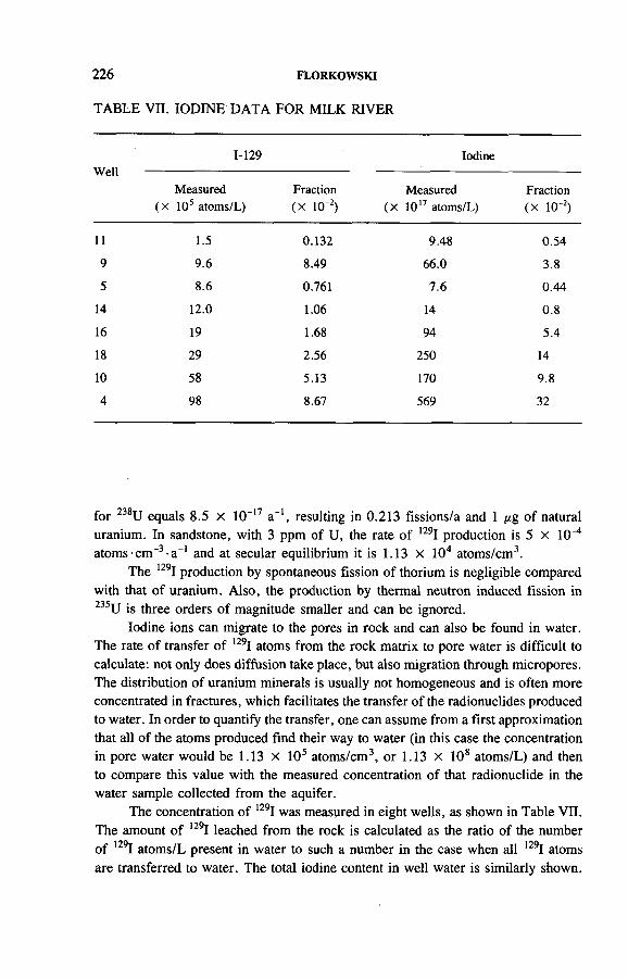
TABLE VII. IODINE DATA FOR MILK RIVER

226 FLORKOWSKI

Well1-129 Iodine

Measured (x 105 atoms/L)

Fraction (x 10'2)

Measured (X 1017 atoms/L)

Fraction (x 10'2)

11 1.5 0.132 9.48 0.54

9 9.6 8.49 66.0 3.8

5 8.6 0.761 7.6 0.44

14 12.0 1.06 14 0.8

16 19 1.68 94 5.4

18 29 2.56 250 14

10 58 5.13 170 9.8

4 98 8.67 569 32

for 238U equals 8.5 X 10~17 a-1, resulting in 0.213 fissions/а and 1 ¡ig of natural uranium. In sandstone, with 3 ppm of U, the rate of 129I production is 5 X 10 * atoms-cm'3-a-1 and at secular equilibrium it is 1.13 X 104 atoms/cm3.

The 129I production by spontaneous fission of thorium is negligible compared with that of uranium. Also, the production by thermal neutron induced fission in 235U is three orders of magnitude smaller and can be ignored.

Iodine ions can migrate to the pores in rock and can also be found in water. The rate of transfer of I29I atoms from the rock matrix to pore water is difficult to calculate: not only does diffusion take place, but also migration through micropores. The distribution of uranium minerals is usually not homogeneous and is often more concentrated in fractures, which facilitates the transfer of the radionuclides produced to water. In order to quantify the transfer, one can assume from a first approximation that all of the atoms produced find their way to water (in this case the concentration in pore water would be 1.13 X 105 atoms/cm3, or 1.13 x 108 atoms/L) and then to compare this value with the measured concentration of that radionuclide in the water sample collected from the aquifer.

The concentration of 129I was measured in eight wells, as shown in Table VII. The amount of 129I leached from the rock is calculated as the ratio of the number of 129I atoms/L present in water to such a number in the case when all 129I atoms are transferred to water. The total iodine content in well water is similarly shown.

IAEA-SM-319/24 227

The fraction of 129I atoms leached to water is around 10“2 and tends to increase with increasing iodine content in water. There is, in general, good correla­tion between the fraction of 129I leached and the fraction of leached iodine (assum­ing constant content of iodine in rock in the area), which would suggest a common origin for iodine (rock formation). However, there is no correlation between the fraction of 129I leached and the general direction of flow of groundwater. It seems that at the present stage of development, the use of 129I for dating groundwater is not yet feasible.

REFERENCES

[1] FLORKOWSKI, T ., MORAWSKA, L ., ROZANSKI, K ., Natural production of radio­nuclides in geological formations, Nucl. Geophys. 2 (1988) 1-14.

[2] FLORKOWSKI, T ., Estimation of the natural production of radionuclides in geological formations from reactions with fast neutrons, Nucl. Geophys. 4 (1989) 281-287.

[3] CZUBEK, J.A., The NEROTH.BAS Program for Rock Thermal Neutron Parameter Calculations, Rep. 1403, Institute of Nuclear Physics, Cracow (1988).

[4] KREFT, A., DYDEJCZYK, A., GYURCSAK, J., Determining the thermal neutron absorption cross section of rocks, Int. J. Appl. Radiat. Isot. 35 (1984) 573-575.

[5] KREFT, A., BOLEWSKI, A., Jr., CIECHANOWSKI, М., MORSTIN, K., A tech­nique for determining the neutron slowing down parameters of rocks using small sam­ples, Nucl. Geophys. 3 (1989) 367-372.

[6] MIELKE, J.M ., “ Composition of the earth’s crust and distribution of the elements” , Review of Research on Modern Problems in Geochemistry (SIEGEL, F.R., Ed.), UNESCO, Paris (1979) 13-39.

[7] ENGSTER, J., Rev. Sci. Instrum. 25 (1954) 5.[8] MATHER, K., Aust. J. Phys. 9 (1956) 147.[9] GORSHKOV, G.V., ZYABKIN, V.A., LATKOVSKAYA, N.M ., CVYETKOV,

O.S., Natural Neutron Background of the Atmosphere and Earth, Atomizdat, Moscow (1966) (in Russian).

[10] ANDREWS, J.N., FONTES, J.-Ch., MICHELOT, J.L., ELMORE, D., Earth Planet. Sci. Let. 77 (1986) 49.

[11] KUHN, M.W., Subsurface Neutron Production and its Impact on 36C1 Groundwater Dating, Thesis, University of Arizona, Tucson (1984).

[12] KREFT, A., The Question of Fast Neutron Absorption in Moisture Measurements by the Neutron Method, Rep. INT-33/I, Institute of Physics and Nuclear Techniques, Cracow (1973).

[13] HEATON, R., LEE, H., SKENSVED, P., ROBERTSON, B.C., Alpha-induced neu­tron activity in materials, Nucl. Geophys. 4 4 (1990) 499-510.

[14] ANDREWS, J.N., et al., The in situ production of radioisotopes in rock matrices with particular reference to the Stripa granite, Geochim. Cosmochim. Acta 53 (1989) 1803.

[15] WAHL, A.C., Nuclear-charge distribution in fission: Cumulative yields of short lived krypton and xenon isotopes from thermal neutron fission of 235U, J. Inorg. Nucl. Chem. 6 (1958) 263-277.

2 2 8 FLORKOWSKI

[16] ZITO, R., DONAHUE, D.J., DAVIS, S.N., BENTLEY, H.W., FRITZ, P., J. Geophys. Res. Lett. 7 (1980) 235-238.

[17] JULL, A.J.T., BARKER, D.L., DONAHUE, D.J., On the 14C content in radioactive ores, Chem. Geol. 66 (1987) 35-45.

[18] FABRYKA-MARTIN, J., Production of Radionuclides in the Earth and their Hydro­geologic Significance, with Emphasis on Chlorine-36 and Iodine-129, Thesis, Univer­sity of Arizona, Tucson (1988).

[19] URECH, S., JEANNET, E., ROSSEL, J., Les réactions (n , p) et (n, a) de ^C a avec des neutrons de 6 MeV, Helv. Phys. Acta 34 (1961) 954.

[20] ERDTMANN, G., Neutron Activation Tables, Chemie-Verlag, Weinheim (1976).[21] LOOSLI, H.H., LEHMANN, B.E., BALDERER, W., Argon-39, argon-37 and

krypton-85 isotopes in Stripa groundwaters, Geochim. Cosmochim. Acta 53 (1988) 1825.

[22] SABU, D.D., J. Inorg. Nucl. Chem. 33 (1971) 1509-1513.

IAEA-SM-319/37

EVALUATION OF ISOTOPIC METHODS FOR THE DATING OF VERY OLD GROUNDWATERSA case study of the Milk River Aquifer

M. IVANOVICH Isotope Geoscience Section,AEA Technology,Harwell Laboratory,Harwell, Oxfordshire,United Kingdom

K. FRÔHLICH Isotope Hydrology Section,Division of Physical and Chemical Sciences,International Atomic Energy Agency,Vienna

M.J. HENDRYNational Hydrology Research Institute,Saskatoon, Saskatchewan,Canada

J.N. ANDREWS*School of Chemistry,University of Bath,Bath, Somerset,United Kingdom

S.N. DAVISDepartment of Hydrology and Water Resources,University of Arizona,Tucson, Arizona,United States of America

R.J. DRIMMIE Department of Earth Sciences,University of Waterloo,Waterloo, Ontario,Canada

* Present address: Postgraduate Research Institute for Sedimentology, University of Reading, Whiteknights, Reading, Berkshire RG6 2AB, United Kingdom.

229

230 IVANOVICH et al.

J. FABRYKA-MARTIN Isotope Geochemistry Group,Los Alamos National Laboratory,Los Alamos, New Mexico,United States of America

T. FLORKOWSKIInstitute of Physics and Nuclear Techniques,Cracow,Poland

P. FRITZInstitut für Hydrologie,Gesellschaft für Strahlen- und Umweltforschung mbH München, Neuherberg,Germany

B.E. LEHMANN, H.H. LOOSLI Physikalisches Institut,Universitàt Bern,Bern,Switzerland

E. NOLTE Faculty of Physics,Technical University of Munich,Garching,Germany

Abstract

EVALUATION OF ISOTOPIC METHODS FOR THE DATING OF VERY OLD GROUNDWATERS: A CASE STUDY OF THE MILK RIVER AQUIFER.

The objective of the work presented is to evaluate the use of isotopic methods for the dating of very old groundwaters. It represents an IAEA sponsored study designed to test vari­ous methods available for that purpose. The Milk River Aquifer, in Alberta, Canada, was chosen for this study because it fits the definition of an idealized artesian system that dips gently from the recharge area and is confined by aquitards above and below. This feature, cou­pled with the fact that the groundwater in the Milk River Aquifer becomes ‘old’ (beyond l4C dating range) a short distance downflow from the dominant recharge area, makes this aquifer potentially useful in evaluating various dating techniques for old groundwaters. Numerous wells have been sampled in the course of many studies of the aquifer. Sampling for the IAEA

IAEA-SM-319/37 231

sponsored campaign in 1985 took place in 16 wells. Samples for the following measurements were taken: major and minor ions (Alberta Agriculture and the IAEA), the stable isotopes Sl80 , 62H and ¿>I3C, and 14C (IAEA, Universities of Waterloo and Arizona), 39Ar, 81Kr and 85Kr (University of Bern), noble gases, including Rn (University of Bath), 36C1 (Univer­sity of Arizona and Technical University of Munich), n9l (University of Arizona) and ura­nium isotopes (Harwell Laboratory). The study concluded that groundwater ages based on the hydrodynamic model should be considered as being a lower limit of the average groundwater age in the Milk River Aquifer (<0.500 Ma), while those based on 36C1/C1 data uncorrected for any dilution by dead Cl should be considered as being an upper limit ( < 2 Ma). The Milk River Aquifer project is an excellent illustration of a successful flow system analysis when multiple, independent dating methods are combined with detailed hydrogeological studies. The conclusion of the present study is that the potential for the dating of very old groundwaters by a variety of isotope techniques is veiy high provided a combination of methods is applied (i.e. never a single method by itself).

1. INTRODUCTION

The objective of this work was to evaluate the use of isotopic methods for the dating of very old groundwaters. It represents an IAEA sponsored study designed to test various methods available for that purpose. The Milk River Aquifer, in Alberta, Canada, was chosen for this study because it fits the definition of an ideal­ized artesian system that dips gently from the recharge area and is confined by aquitards above and below [1, 2]. This feature, coupled with the fact that the ground­water in the Milk River Aquifer becomes ‘old’ (i.e. beyond 14C dating range) a short distance downflow from the dominant recharge area, makes this aquifer poten­tially useful for evaluating various dating techniques for old groundwaters.

Sampling of the Milk River Aquifer was undertaken on several occasions. Dur­ing the IAEA sponsored campaign in 1985, samples from 16 wells (the locations are shown in Fig. 1 [3]) were collected and analysed for major and minor ions, the stable isotopes of 2H, 13C, 180 , 3H, 14C, 39Ar, 81Kr, 85Kr and the noble gases, includ­ing 222Rn, 36C1, 129I and U isotopes. Additional samples for the analyses of selected isotopes and chemical constituents, such as dissolved organic carbon (DOC) in the recharge zone of the aquifer, were collected as recently as 1988.

This paper presents a summary of the results and a comparative discussion of the findings, with emphasis on the question of groundwater age in the Milk River Aquifer system.

о Core• g ro u n d w a te r sam ples

<Щ]) O utcrop a re a

0 10 20 km

FIG. 1. Location o f sampled wells in the Milk River Aquifer. Two flow paths identified are indicated by arrows (from Ref. [3]).

232 IVANOVICH

et al.

IAEA-SM-319/37 233

2. GEOLOGICAL, HYDROLOGICAL AND GEOCHEMICALBACKGROUND

The Milk River system consists of thin (30-75 m thick) sandstone and is con­fined by marine shale above by the Pakowki Formation (typically 120 m thick) and below by the Colorado Group (ranging in thickness from 500 to 650 m). This aquifer underlies 15 000 km2 of southern Alberta. Most of the area is covered by Pleisto­cene glacial drift [1]. The aquifer outcrops in southern Alberta, and more dominantly on the flanks of the Sweetgrass Hills of northern Montana. At the southern end of the study area the groundwater flows generally towards the north, west and east, following the dip of the aquifer. The two flow paths identified along the valleys of the low Cl concentrations in the eastern and western parts of the study area (see Fig. 3) reach a maximum length of about 80 km. The transmissivity decreases from the south to the north, west and east. This change is caused by a general thinning of the aquifer in these directions and a decrease in hydraulic conductivity towards the north owing to an increase in the shale content.

Dissolved Cl and I concentrations increase in the direction of the flow from <0.05 and 0.001 mmol/L, respectively, near the recharge area to >140 and0.15 mmol/L at the northern edge of the aquifer [1]. Similarly, ¿>l80 and ô2H values become higher towards the north. The ¿>180 and <52H values of groundwater samples collected from the recharge area plot on the global meteoric water line, but increasingly deviate from it with distance downflow [4]. Four mechanisms have been proposed to explain the origin of the chemical and isotopic patterns: (1) the introduc­tion of connate formation water through the aquitard from below and subsequent mixing with infiltrating meteoric water [2, 5]; (2) a finite source of meteoric recharge mixing with more saline water in the aquifer [6]; (3) chemical and isotopic enrichment due to ion filtration [7] ; and (4) aquitard diffusion based on diffusion gra­dients between saline, isotopically enriched water in the lower aquitard and fresher, isotopically depleted water in the aquifer [4].

The last of the above models was tested using a mass transport model [4]. The period during which the flow system has operated in the manner observed at present,1.e. active inflow of meteoric water in the system originally filled with formation water, was estimated to be 1-2 Ma. Although the model parameters are subject to large uncertainties, the calculations showed that the observed chemical patterns in the aquifer can be explained by diffusion from the aquitard. The best model fit to both Cl and 180 data yielded an effective diffusion coefficient D' for these species through the aquitard (the most critical parameter in the model) 6 X 10' 12 m2/s. The flow rate was assumed to be constant along the flow paths. For path 1 (see Fig. 1), the flow rate was 0.3 m/a, yielding a groundwater age at 80 km downflow from the outcrop of 0.25 Ma. The flow rate along path 2 was estimated to be half of the flow rate obtained for path 1, requiring 0.51 Ma for groundwater to travel 80 km. These estimates of the maximum groundwater residence times in the aquifer bracket earlier estimates of 0.3 Ma based on hydraulic modelling [8].

234 IVANOVICH et al.

3. ISOTOPIC STUDIES IN THE MILK RIVER AQUIFER

3.1. Stable isotopes and radiocarbon in groundwater and dissolved constituents

At least three distinct zones can be recognized in the plot of ô l80 against <52H:cluster A with ô l80 values o f ---- 19°/00, cluster В with a ô180 value of -16°/00and cluster С with a 5180 value of - 8°/00 (see Fig. 2 [9]). Cluster A represents groundwaters near the recharge area in the southern part of the aquifer (some sam­ples contained measurable levels of bomb 3H). The isotopic signatures are not followed by even more negative ôl80 and ô2H values downflow as might be expected were Pleistocene recharge present. This absence of a glacial signature sug­gests that these groundwaters were recharged less than 15 ka before present (BP) and that the Pleistocene period of that region is characterized by insignificant recharge during long periods. The uniform ô2H and <5I80 values found in groundwaters up to a distance of ~ 20 km from the recharge zone indicate a minimum flow rate of -1 -1 .5 m/a in this part of the aquifer. The data in cluster В fall close to the modern meteoric water line for the region. However, these groundwaters contain no meas­urable 14C and, thus, could have recharged before the last glaciation. Assuming constant flow rates beyond the Milk River of the order of 0.1 m/a, groundwater ages

FIG. 2. Plot o fb ,sO against 6D, including the global meteoric water line (GMWL), showing three zones and isotope values (zone A: recent recharge; zone B: older recharge; and zone C: mixing o f older recharge and Bow Island Formation water) [9].

IAEA-SM-319/37 235

in excess of 50 ka BP, and possibly as much as 600 ka BP along path 1, are sug­gested [9]. Cluster С data represent groundwaters in the most distant section of the Milk River Aquifer. They deviate from the meteoric water line and may indicate mixing with formation brines. This may occur through diffusive transport of isotopi­cally enriched groundwaters from the confining shales, resulting in alteration of the warm climate meteoric water isotopic signatures.

Radiocarbon was measurable only in groundwaters sampled from the wells located within 20 km of the recharge zone. Comparison of l4C data from two wells near the recharge area of the aquifer obtained from dissolved inorganic carbon (DIC), DOC-HMW and DOC-LMW fractions has revealed that they are very simi­lar [9]. Although the DIC 14C per cent modern carbon (pmc) values are much lower than those for DOC in both wells, the age differences between the two wells are quite similar, averaging ~ 14 ka. The lower DIC values lead to the conclusion that the ini­tial DIC 14C content when the water entered the aquifer was as low as 30 pmc. From these data a flow rate of ~ 1 m/a has been estimated for the distance of 12 km between the two wells. This flow rate agrees surprisingly well with the stable isotope data, but is an order of magnitude higher than the flow rates obtained from hydraulic considerations [4, 8] or based on age determinations from 36C1 [3, 7] and from U isotopes [10] for the northern part of the aquifer. Similarly, extrapolation of l4C groundwater ages obtained in the southern area of the aquifer near the recharge along the flow path north of the Milk River yields low ages of only 70-100 ka for ground­waters in the northernmost locations. Clearly these results cannot be reconciled eas­ily with other isotopic and hydraulic evidence for older groundwater ages. The 14C is absent in any significant amounts in groundwaters north of the Milk River, so that detailed extrapolation over the entire flow system may not be valid. It is therefore concluded that the groundwater movement in the southern part of the aquifer is rather fast (~ 1 m/a) up to the Milk River. The river acts as a point of discharge, rather than a recharge [11]. In consequence, lower flow rates ( — 0.1 m/a) may exist north of the river. Furthermore, 36C1 and Cl data from the zone near the end of the flow paths suggest a further decrease in flow rates in the northern part of the Milk River Aquifer owing to distributed discharge along the flow path (see discussion on 36C1 data below). This observation is consistent with the observed decrease of the aquifer transmissivity downflow [4].

3.2. Dissolved gases and Kr isotopes

The inferred recharge temperatures based on noble gases (He, Ne, Ar, Kr and Xe), the 36Ar/40Ar isotope ratio, N2 and CH4 and stable isotope data, together with the observed correlation between the He and Cl contents of the groundwaters, shed further light on the origin and age of the groundwaters in the aquifer [12]. Specifi­cally, the recharge temperature difference inferred from the noble gas data of ~4-5°C is consistent with stable isotope data considerations [12].

236 IVANOVICH et al.

Krypton-81 and 85Kr were measured in well 9, a well intermediate between the outcrop and the northern end of the aquifer [13]. The activity of 85Kr is only0.3% of the modern atmospheric activity, indicating the absence of any admixture with younger groundwaters at that location. The measurement of 81Kr yields an upper age limit of ~ 140 ka, in excellent agreement with the hydraulic models and 36C1 and U isotope dating techniques used with the groundwaters in that part of the aquifer.

3.3. Chloride and 36C1 measurements

The interpretation of the Cl isotopic data (see Fig. 3) is based on two approaches [9]. (1) The evolution of 36C1 and Cl concentrations along the two flow paths is described by a simple exponential decrease in 36C1 and linear increase in Cl

FIG. 3. Measured 36Cl/Cl ratios in units o f 10~15 and a contour plot o f 36Cl/Cl. The num­bers for the contour plot are 36Cl/Cl ratios in units o f 10~'5. Samples 2-17 (see Fig. 1) were measured by Nolte et al. [3] and the others by Phillips et al. [7].

IAEA-SM-319/37 237

with distance from the recharge area. This approach assumes a constant flow rate whose value is a function of the amount of in situ 36C1 production. (2) The evolu­tion of 36C1 and Cl concentrations along the two flow paths is described by 36C1 decay and by diffusive exchange of both 36C1 and Cl between the aquifer and the underlying Colorado shale aquitard. The groundwater flow rate is then inferred from a diffusion model in which the flow rate is assumed to be constant.

Considerations of in situ production of 36C1 in the first of the two models have yielded groundwater flow rates which are 75% lower than when zero in situ produc­tion is assumed. The flow rates inferred from the diffusion model are only slightly higher than the corresponding values obtained by the first model. The results given above lead to the conclusion that the radioactive decay of 36C1, rather than diffusive losses, controls the 36C1 concentration in groundwater during advective transport in the Milk River Aquifer [3]. Thus, groundwater ages based on 36C1/C1 data for the aquifer range up to 2 Ma if uncorrected for any dilution by subsurface sources of ‘dead’ Cl [7]. If the assumption is made that the subsurface contributions of Cl range from low values in the fresh waters in the south to high values (up to 90% of total Cl) in the much older saline waters in the northern parts of the aquifer, then maxi­mum ages are reduced to less than 1 Ma, making the 36C1 based ages more consis­tent with those based on other isotope techniques considered here [14].

3.4. Geochemistry of halogens

The three halides (Cl, Br and I) are highly correlated [14]. Concentrations are low in the freshwater zones of the aquifer, but increase by as much as two orders of magnitude along the margins. The Cl/I and Cl/Br ratios are well above those of sea water and are consistent with the origin derived from the diagenesis of organic matter in the sediment. However, moving downflow, the halide ratios reach nearly constant values, suggesting the dominance of a common subsurface source for these ions [14]. Halide ratios rule out unaltered sea water or leakage and/or diffusion from the underlying Bow Island sandstone as a major influence on the groundwater chemistry in the Milk River Aquifer. The hypothesis that the primary source of the halides is evolved connate sea water diffusing from low permeability units within the Milk River Formation is favoured [14]. This fifth conceptual model (see the descrip­tion of the other four models earlier in this paper) does not require mixing with an external water body, or complex mechanisms such as ion filtration [15, 16].

Arguments consistent with this fifth hypothesis are derived from the observed deviations from halide mixing curves [14]. These deviations are interpreted in terms of differences in the chemical composition of the saline water in the smaller pores of the less permeable sediments of the Milk River Formation.

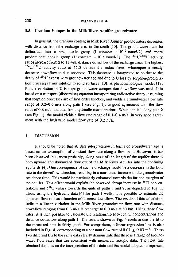
238 IVANOVICH et al.

3.5. Uranium isotopes in the Milk River Aquifer groundwater

In general, the uranium content in Milk River Aquifer groundwaters decreases with distance from the recharge area in the south [10]. The groundwaters can be delineated into a small oxic group (U content: ~ 10~5 mmol/L) and more predominant anoxic group (U content: ~ 10“7 mmol/L). The 234U/238U activity ratios increase from 2 to 11 with distance downflow of the recharge area. The highest 234U/238U activity ratio of 11.8 defines the redox front, whereupon a steady decrease downflow to 4 is observed. This decrease is interpreted to be due to the decay of 234U excess with groundwater age and due to U loss by sorption/precipita­tion processes from solution to solid surfaces [10]. A phenomenological model [17] for the evolution of U isotope groundwater composition downflow was used. It is based on a transport (dispersion) equation incorporating radioactive decay, assuming that sorption processes are of first order kinetics, and yields a groundwater flow rate range of 0.2-0.6 m/a along path 1 (see Fig. 1), in good agreement with the flow rates of 0.3 m/a obtained from hydraulic considerations. When applied along path 2 (see Fig. 1), the model yields a flow rate range of 0.1-0.4 m/a, in very good agree­ment with the hydraulic model flow rate of 0.2 m/a.

4. DISCUSSION

It should be noted that all data interpretation in terms of groundwater age isbased on the assumption of constant flow rate along a flow path. However, it hasbeen observed that, most probably, along most of the length of the aquifer there is both upward and downward flow out of the Milk River Aquifer into the confining aquitards [4]. One consequence of such a discharge would be a decrease in the flow rate in the downflow direction, resulting in a non-linear increase in the groundwater residence time. This would be particularly enhanced towards the far end margins of the aquifer. This effect would explain the observed abrupt increase in 36C1 concen­trations and <5lsO values towards the ends of paths 1 and 2, as depicted in Fig. 1. Thus, using the hydraulic data [4] for path 1 wells, it is possible to estimate the apparent flow rate as a function of distance downflow. The results of this calculation indicate a linear variation in the Milk River groundwater flow rate with distance downflow ranging from 0.3 m/a at recharge to 0.0 m/a at 80 km. Using these flow rates, it is then possible to calculate the relationship between Cl concentrations and distance downflow along path 1. The results shown in Fig. 4 confirm that the fit to the measured data is fairly good. For comparison, a linear regression line is also included in Fig. 4, corresponding to a constant flow rate of 0.07 ± 0.03 m/a. These two different fits to the same data clearly demonstrate that there is a range of ground­water flow rates that are consistent with measured isotopic data. The flow rate obtained depends on the interpretation of the data and the model adopted to represent

IAEA-SM-319/37 239

D istance fro m o u tc ro p (km)

FIG. 4. Semi-logarithmic plot o f the 36Cl concentration in Milk River Aquifer groundwatersagainst distance along path 1 from the recharge zone ( я : measured data;------ : calculationsbased on the linearly varying groundwater flow rate with distance from the recharge zone;------: the best fit to the data regression line based on the constant flow rate model (see textfor further details)).

the chosen interpretation. In the example given above for 36C1 data, the more realis­tic approach appears to be the one based on the assumption of variable flow rate decreasing linearly with the distance downflow from the recharge zone. A similar conclusion is valid for path 2.

The 129I/I ratio observed in groundwaters collected near the recharge area corresponds to the meteoric value. However, the 129I/I ratios in groundwaters collected further downflow are only 8-10% of the initial meteoric value. Taking into account that the half-life of 129I is 16 Ma, these data can be interpreted as an indica­tion that most of the increase in dissolved iodine cannot derive from concentration of a meteoric source by ion filtration, but must have a subsurface origin [14]. This conclusion may not be definitive.

Figure 5 shows a plot of the measured 129I concentrations against distance downflow from the recharge zone of the Milk River Aquifer along path 1. The plot demonstrates that with the exception of wells 4 and 10, all of the 129I data reflect the same evolutionary trend, which can be fitted by a straight line. This straight line can be considered to represent a mixing of two components, the recharge waters (meteoric input), with an initial I29I concentration of I29I0, and an older component representing l29I concentration due to in situ production by fission released from the aquifer matrix into solution (‘stationary’ value 12%). The plot in Fig. 5 also con­tains the results of two different models, an exchange model and an ion filtration

240 IVANOVICH et al.

D istance from ou tc ro p (km)

FIG. 5. Plot o f the 1291 concentration in Milk River Aquifer groundwaters against distancefrom the recharge zone, (a , m : measured data;------ : results o f a diffusion exchange modelcalculation; - ■ - • - ; results ofan ion filtration model calculation;------: best fit to the dataregression line based on the constant flow rate model (see text for further details)).

model. The exchange model assumes temporal change in the groundwater l29I con­centration and is given by:

d l29IIdt = fc(129Ij - I) (1)

where A: is a rate constant reflecting diffusion controlled exchange between theaquifer matrix and the groundwater. The ion filtration model assumes:

d 129l / 129I = (1 - a) dv/v (2)

where v is the groundwater flow rate and (1 — a) represents the ion filtration effi­ciency. In both cases it is assumed that the groundwater flow rate decreases linearly downflow from v0 at the recharge zone to zero at the end of the flow path at x0.

Integration of the two equations yields:

129I = 12% + ( 129Io - 12%) (1 - x / x q ) k x ° h ’° (3)

and

129I = 129Io (1 - x/xo)a - 1 (4)

IAEA-SM-319/37 241

The calculated points plotted in Fig. 5 were based on the following parameters: v0 = 0.3 m/a [4], x0 = 100 km and к = 1.5 X 10-6 a-1. It is beyond the scope of this paper to discuss these models in detail. Nevertheless, it can be recognized from Fig. 5 that all three different approaches (including the linear regression line representing the constant flow rate case) are consistent with the measured 129I data. Thus, the ion filtration model cannot be ruled out by the available I29I data. The same situation exists for 36C1 data, which were successfully modelled both by the ion filtration model [7] and by diffusion models [3, 4].

The solution for this apparent ambiguity is offered in a statement made in Ref. [14]:

“ Other saline sources proposed by other authors cannot be ruled out altogether and are probably contributing to the groundwater geochemistry to some extent, but the model in which the solute source resides mainly within the Milk River Formation is the simplest one and is able to account for most of the observed data.”

More generally, this ambivalence in interpreting measured data by conceptual models appears to be inherent in regional groundwater studies, such as the Milk River Aquifer study. It seems to be a consequence not only of the limited database available (new data often open up the possibilities of additional interpretations), but also of inherent complexities of regional groundwater systems. Therefore, the parallel use of different approaches in interpreting the available data is a positive advantage in the Milk River Aquifer study. Thus, the groundwater ages based on the hydrodynamic model should be considered as a lower limit of the average ground­water ages in the Milk River Aquifer, while those based on the 36C1/C1 data uncor­rected for dilution by dead Cl should be considered as an upper limit.

One of the basic requirements for the isotopic dating of groundwaters is that no unaccounted for radiogenic sources exist in the aquifer. For this reason, the underground production of various radionuclides of relevance in both the ground­water and the sandstone matrix have been considered in the Milk River Aquifer [18]. In sandstones, generally, the underground production of 3H, 85Kr and 14C is below detection limits. Thus, in wells 5 and 8 located close to the recharge area and in well 9, which is situated about 20 km downflow, the absence of 85Kr shows that there is no admixture with young groundwaters. The 37Ar and 39Ar are produced within the sandstone. The latter is measurable in wells 8 and 9 (about 20 and 7 per cent modern, respectively), where the hydrological age shows that cosmogenic input should have decayed. Release efficiencies for these radionuclides are estimated to be less than a few per cent and are similar to the release efficiency for 222Rn. The 39Ar/37Ar ratio is rather similar to the calculated ratio for in situ production within the sandstone and is very different from the ratio for production within the underly­ing Colorado shale. Therefore, it is plausible that both groundwaters have dissolved these isotopes from sandstone in their in situ production ratio and that the efficiency

242 IVANOVICH et al.

of release at these locations is different. Furthermore, this result appears to be an argument in favour of the fifth model, which assumes an internal source for halide concentrations observed in Milk River Aquifer groundwater [14].

The l29I produced in situ by fission is probably released with high efficiency and is then isotopically equilibrated with dissolved I. The fractional release (ratio of 129I atoms measured in solution to that expected for total solution of the in situ production) is of the order of several per cent and shows a general trend of increase with increasing groundwater age. This seems to be an argument against the ion filtra­tion hypothesis, because, at least, it shows that the increase in 129I with ground­water age is controlled by the release of in situ produced 129I rather than by enrichment of cosmogenic 129I.

In general, the in situ production of 36C1 in aquifer matrices has been shown to be significant. However, in the case of the Milk River Aquifer, the high cosmo­genic input of 36C1 limits the effects of in situ production on groundwater 36C1 con­tent. Thus, groundwater ages calculated with the in situ production of 36C1 are lower by 30% in the case of path 2, to 50% in the case of path 1 than the respective ages calculated for zero in situ production. This difference does not appear to be par­ticularly large when the total range of uncertainty in the groundwater age estimates between different models and isotopic methods is taken into account.

5. CONCLUSIONS

The goal of this project was to evaluate the usefulness of available geochemical and isotope techniques for dating very old groundwater. The Milk River Aquifer was selected for this study because several preceding investigations had established that this regional groundwater system contains waters whose ages range from recent recharge to — 1 Ma. The present study has established that the Milk River Aquifer system is very complex both in terms of groundwater origin and in terms of the evo­lution of its chemical and isotopic contents. However, this apparent complexity proved to be an interesting challenge with respect to the use of different, but com­plementary, approaches to interpreting the geochemical and isotope data in terms of groundwater residence time.

This project has demonstrated that different approaches were necessary to understand the geochemical and isotopic patterns observed in the measured data and to interpret them in terms of the origin, evolution and age of groundwater in the Milk River Aquifer. In the case of 36C1 and U isotopes, the most useful of the isotope dating methods, different dating models were found to be equally applicable. This apparent ambivalence in interpretation of the measured data by conceptual models appears to be inherent in regional groundwater studies such as this. It seems to be a consequence not only of the limited database available (new data often lead to addi­tional possibilities of interpretation), but also of the inherent complexities of regional

IAEA-SM-319/37 243

groundwater systems. Thus, the parallel and complementary use of different approaches in the interpretation of the available database is a positive advantage. In the present case, the groundwater ages based on the hydrodynamic model should be considered as being a lower limit of the average groundwater age in the Milk River Aquifer, while those based on 36C1/C1 data, uncorrected for any dilution by dead Cl, should be considered as an upper limit.

The results of this study demonstrate that the potential of isotope techniques for dating very old groundwaters is high provided a combination of techniques is applied (never a single technique by itself). This study has also demonstrated that isotopic and geochemical data may represent a more realistic record of average flow conditions in a regional aquifer containing very old groundwaters than present day (or even reconstructed) hydraulic data. The Milk River Aquifer International Project is an excellent illustration of a successful flow system analysis when multiple, independent dating methods are combined with detailed hydrogeological studies.

ACKNOWLEDGEMENTS

The authors are grateful to many colleagues too numerous to name here who have been involved in this project over the years. B. Boardman, of the Harwell Laboratory, is thanked for producing this manuscript.

REFERENCES

[1] HENDRY, M .J., SCHWARTZ, F.W ., ROBERTSON, C., Geology and hydrochemis­try of the Milk River Aquifer system — A review, Appl. Geochem. 6 (1991) (in press).

[2] SCHWARTZ, F.W ., MUCHLENBACHS, K., Isotope and ion geochemistry of groundwaters in the Milk River Aquifer, Alberta, Water Resour. Res. 15 (1979) 259-269.

[3] NOLTE, E., et al., Measurements and interpretation of 36C1 in groundwater samples from the Milk River Aquifer, Appl. Geochem. 6 (1991) (in press).

[4] HENDRY, M.J., SCHWARTZ, F.E., An alternative view on the origin of chemical and isotopic patterns in groundwater from the Milk River Aquifer, Alberta, Canada, Water Resour. Res. 10 (1988) 1747-1764.

[5] SCHWARTZ, F.W ., MUCHLENBACHS, K., CHORLEY, D.W ., Flow-system con­trols of the chemical evolution of groundwater, J. Hydrol. 54 (1981) 225-243.

[6] DOMENICO, P.A., ROBBINS, G.A., The displacement of connate water from aquifers, Bull. Geol. Soc. Am. 96 (1985) 328-335.

[7] PHILLIPS, F.M ., BENTLEY, H.W., DAVIS, S.N., ELMORE, D., SWANICK, G.B., Chlorine-36 dating of very old groundwater in the Milk River Aquifer, Alberta, Canada, Water Resour. Res. 22 (1986) 2003-2016.

[8] SWANICK, G.B., The Hydrochemistry and Age of the Water in the Milk River Aquifer, Alberta, Canada, MSc Thesis, University of Arizona, Tucson (1982).

244 IVANOVICH et al.

[9] DRIMMIE, R .J., et a l., Radiocarbon and stable isotopes in water and dissolved consti­tuents of the Milk River Aquifer, Appl. Geochem. 6 (1991) (in press).

[10] IVANOVICH, M., FRÔHLICH, К., HENDRY, M.J., Uranium-series radionuclides in fluids and solids from the Milk River Aquifer, Alberta, Canada, Appl. Geochem. 6 (1991) (in press).

[11] ROBERTSON, C., Potential Impact of Subsurface Irrigation Flow on a Portion of the Milk River and Milk River Aquifer in Southern Alberta, MSc. Thesis, University of Alberta, Calgary (1988).

[12] ANDREWS, J.N., LOOSLI, H.H., DRIMMIE, R., HENDRY, M .J., Dissolved gases in the Milk River Aquifer, Alberta, Canada, Appl. Geochem. 6 (1991) (in press).

[13] LEHMANN, B.E., LOOSLI, H.H., RAUBER, D., THONNARD, N., WILLIS, R.D., 8lKr and 85Kr in groundwater, Milk River Aquifer, Alberta, Canada, Appl. Geochem. 6 (1991) (in press).

[14] FABRYKA-MARTIN, J., WHITTEMORE, D.O., DAVIS, S.N., KUBIK, P.W ., SHARMA, P., Geochemistry of halogens in the Milk River Aquifer, Appl. Geochem. 6 (1991) (in press).

[15] PHILLIPS, F.M ., KNOWLTON, R.G., BENTLEY, H.W., Comment on ‘An alterna­tive view on the origin of chemical and isotopic patterns in groundwater from the Milk River Aquifer, Canada’, by HENDRY, M.J., SCHWARTZ, F.W ., Water Resour. Res. 26 (1990) 1693-1698.

[16] HENDRY, J.M ., SCHWARTZ, F.W ., Reply to Phillips et al. (1990), Water Resour. Res. 26 (1990) 1699-1703.

[17] FRÓHLICH, K., GELLERMANN, R., On the potential use of uranium isotopes for groundwater dating, Isot. Geosci. 65 (1987) 67-77.

[18] ANDREWS, J.N., FLORKOWSKI, T., LEHMANN, B.E., LOOSLI, H.H., Under­ground production of radionuclides in the Milk River Aquifer, Appl. Geochem. 6 (1991) (in press).

IAEA-SM-319/12

IMPORTANCE OF THE IN SITU PRODUCTION OF 36C1, 36Ar AND 14C IN HYDROLOGY AND HYDROGEOCHEMISTRY

J.N. ANDREWSPostgraduate Research Institute for Sedimentology,University of Reading,Reading, Berkshire,United Kingdom

J.-C. FONTESLaboratoire d’hydrologie et de géochimie isotopique,Université de Paris-Sud,Orsay,France

Abstract

IMPORTANCE OF THE IN SITU PRODUCTION OF 36C1, 36Ar AND l4C IN HYDRO­LOGY AND HYDROGEOCHEMISTRY.

The paper critically discusses the conditions for the in situ production of 36C1, 36Ar and 14C. For several confined aquifers in Australia, Canada and North Africa, the 36C1 con­tent (in atoms/L) close to recharge is about one hundred times greater than can be accounted for by reasonable évapotranspiration values. Possible additional sources of 36C1 include cosmic ray irradiation in the shallow unsaturated zone and solutions of rock chloride in environments where the in situ production of 36C1 is large. Dating of old groundwaters with 36C1 should be limited to cases where chlorinity is constant. The age of СГ, and hence of groundwater, may then be deduced from the decay of the cosmic 36C1 input or, where the groundwater migrates into a U/Th rich environment, from the subsequent ingrowth of 36C1 because of irradiation by the high in situ neutron flux. In the case of 36Ar, after about 1.5 Ma, the accumulation rate of 36C1 is equal to the 36C1 production rate. In the uppermost few metres of continental crust and of the ocean, cosmic ray interactions enhance production by up to several orders of magnitude. Oceanic production amounts to about one-half of the total production. For СГ rich fluid inclusions in minerals which remained exposed for a long time close to the surface, values of the 36A r/40Ar ratio may become much higher than the atmospheric value (3.385 x 10"3). For 14C, in situ production reactions in both the fluid and the rock matrix and the extent to which they may interfere with the use of l4C for ground­water dating have been assessed. The reactions considered include neutron interactions, the exotic decay of radium and a particle reactions. Groundwater of very low alkalinity in high neutron flux environments (e.g. Stripa granite in central Sweden) may gain in situ produced 14C which is equivalent to a few per cent modern carbon.

245

246 ANDREWS and FONTES

1. INTRODUCTION

Many nuclear reactions generate isotopes of hydrological and geological interest in the Earth’s crust. In the shallow crust, the reactions are cosmic ray induced and include spallation by cosmic protons, reactions with secondary neutrons and muon induced reactions [1, 2]. At depths greater than 50 m of rock, these cosmic ray influences are almost completely attenuated and in situ nuclear reactions, which involve principally the a emissions from the uranium and thorium decay series, become predominant. Some nuclides may be produced directly by a irradiation, but the most significant reactions involve the neutron flux generated by (a, n) reactions on light nuclei, such as within the rock matrix [3]. Although the most effective (a, n) reactions occur with Be, Li, В and F targets, the most important crustal reactions involve the high abundance targets Al, Na, Si, О and Mg in silicate rocks, or Mg and О in carbonate rocks. The direct formation of nuclides by irradiation with a par­ticles is dependent upon the relative distribution of the a emitting radioelements and target nuclei in the rock. The range of the most energetic a particle emitted in the natural decay series (8.78 MeV) is 8.7 cm in air, or about 37 /¿m in silicate or car­bonate rock matrices. The a particles generated within one mineral component of the matrix therefore cannot generally reach targets in adjacent minerals.

The in situ production of 36C1 (and its daughter 36Ar in comparison with radiogenic 40Ar) and of 14C, which is of special interest for groundwater studies, is discussed in this paper in relation to geological environments.

2. CHLORINE-36 (Т,л = 3.01 ± 0.02 X 105 years [4])

The isotopic ratio R = 36C1/(35C1 + 37C1) may be determined by accelerator mass spectrometry (AMS) measurements with a detection limit of about 1 x 10~15. For convenience, values of R are reported in units of 10~15. The first AMS meas­urements on environmental water samples were reported a decade ago [5, 6]. The isotopic ratio does not depend upon evaporation, whereas the 36C1 concentration, A (in atoms/L, generally multiplied by 10"7), increases as evaporation increases. The decrease in either R or A due to 36C1 decay may be used for groundwater dating provided: (1) there is no mixing with other chloride sources or that the effect of such mixing may be corrected; and (b) the effect of in situ 36C1 production may be assessed.

2.1. Chlorine-36 production reactions and sources

2.1.1. Atmospheric production

The cosmic production of 36C1 has been attributed to the (1) spallation and(2) activation reactions which occur in the high atmosphere:

IAEA-SM-319/12 247

FIG. 1. Variation in the fallout o f 36Cl from spallation with geomagnetic latitude (adapted from Ref. [4]).

40Ar(p, na) 36C1 67% of production (1)

36Ar(n, p) 36C1 33% of production (2)

The total production is dependent upon geomagnetic latitude, and ranges from 5 a t o m s n e a r the equator and the poles to a maximum of 28 atoms-m“2-s' 1 at about 40°N [4, 7]. The average production rate from spallation is 11 atoms-m"2-s' 1 for the whole atmospheric column. An additional 5 atoms -m '2-s_1 was thought to arise from reaction (1) based on the cross-section estimate (1.83 b) by Onufriev [8]. However, recent measurements suggest that the latter should be reduced by a factor of about 0.0001 [9]. A new determination of the cross-section (< 1 .5 mb, Ref. [10]) confirms tht it is insignificant. The fallout value for 36C1 reported by Bentley et al. [4] should therefore be reduced by a factor of 11/16 (Fig. 1).

2.1.2. Crustal environments

Although the atmosphere attenuates cosmic ray intensity, the residual fluxes of fast protons and secondary particles at sea level cause neutron and 36C1 produc­

248 ANDREWS and FONTES

tion in surface ocean water and continental rocks. Cosmic ray induced reactions are negligible at depths greater than about 50 m of rock, below which reactions caused by the in situ neutron flux continue to generate 36C1. This flux is principally the result of (a ,n ) reactions due to the irradiation of light nuclei by a particles emitted by the natural radioelements within the rock [3, 11]. An additional 10-20% contribu­tion to the in situ neutron flux occurs by the spontaneous fission of 238U. Because of the large activation cross-section of 35C1, the reaction:

35Cl(n, t ) 36C1 (3)

is particularly important in high Cl" environments. The importance of this reaction for 36C1 production was demonstrated in the case of Stripa groundwater [12-15]. Measurements of the in situ neutron flux [14] showed that the secular equilibrium 36C1 content of СГ in Stripa granite was as high as 240 X 10-15 atoms of 36C1 per atom of stable СГ. There are additional minor contributions to the production from the following reactions:

39K(n, a )36Cl (4)

40Ca(«, pa)26Cl (5)

The number, 36N, of 36C1 atoms produced after time, t, for irradiation by a constant neutron flux, ф, is:

36N = a35Nф(\ - e_x')/X (6)

where 3SN is the number of 35C1 atoms present, a is the activation cross-section (44 X 10“28 m2) and X is the 36C1 decay constant. Equilibrium is attained after irradiation for about 5 half-lives (i « 1.5 Ma).

2.1.3. Shallow continental environments

The production of 36C1 varies with depth and with the СГ content of the rock. The latter may range from 1 ppm for saturated porous sediments (for a porosity of 30% and a soil-water СГ content of 3 ppm) to 400 000 ppm for pure halite deposits in closed evaporitic basins.

2.1.4. Oceanic environment (Table I)

In the topmost few metres of the ocean, the calculated 36C1 production is about 30 atoms-m'3- s '1. For this production rate, the equilibrium 36C1/C1 atomic ratio (R) in sea water would be 1.3 x 10~12 (conventionally written as

IAE A-SM-319/12 249

TABLE I. CHLORINE-36 PRODUCTION IN THE OCEAN, IN SALINE SOLU­TIONS AND FLUID INCLUSIONS IN GRANITE AT A GEOMAGNETIC LATI­TUDE OF 54.3°N AND FOR ALTITUDES OF (a) 0 m AND (b) 1500 m: R = ATOMIC RATIO 36C1/(35C1 + 37C1); A = 36C1 ATOMS/L

Depth (m) 0.5 1.5 2.5 5.5 100

R x 1015 sea water (a) 1160 730 470 160 <1

(b) 3100 1900 1200 340 <1

A x 10 '7 sea water (a) 37 400 23 600 15 200 5200 <32

(b) 100 000 60 400 37 400 10 800 <32

R x 1015 evaporite3 (a) 28.0 11.4 5.4 1.4 <0.1

(b) 74.8 27.0 11.4 2.4 <0.1

A x 10'7 evaporite3 (a) 900 370 170 45 <3 .2

(b) 12 400 870 370 80 <3 .2

R x 1015 granite (a) 2380 2690 270 75 30

(b) 6350 1630 550 110 30

A x 10'7 granite (a) 76 800 22 300 8800 2400 980

(b) 205 000 52 600 17 700 3500 980

a Evaporite refers to sea water evaporated to dryness.

R = 1300 x 10 15). Oceanic circulation, however, leads to dilution with 36Cl-dead chloride from deep waters and the R value for oceanic chloride is <4.2 x 10~15 [6].

2.2. Chlorine-36 in precipitation

Thermonuclear weapons tests which took place in the marine environment between 1952 and 1958 caused an increase in the atmospheric fallout of 36C1 because of the radioactivation of seawater chloride. This increase was first identified by 13 counting of the 36C1 activity [16]. Subsequent measurements by the more pre­cise AMS technique have shown that the record of bomb generated 36C1 is preserved in ice cores from Greenland. In 1957, the 36C1 content of the ice cor­responded to an atmospheric fallout of 500 times the natural level [17-19]. Detailed results obtained on an ice core from the Dye 3 site show that the atomic and

250 ANDREWS and FONTES

thermonuclear weapons testing of the past 47 years was probably still influencing the 36C1 content of precipitation as late as 1985 [19]. Minor fluctuations may still be occurring owing to releases from nuclear installations and reactor accidents, such as that at Chernobyl. The natural 36C1 fallout rate can therefore only be determined from measurements of precipitation from before 1945. Such measurements can be made in ice cores, but not many studies have yet been completed because of the problems associated with sample pre-concentration and recovery from these dilute СГ sources.

Interpretation of the data is also sometimes difficult. For example, in medieval ice from Camp Century [20], extreme fluctuations in the 36C1 content of the ice were found (1500-4500 atoms/kg). This may have resulted from a variation in the annual amounts of precipitation such as has been reported for varved ice from Dye 3 [19]. These results show that the ice accumulation rate during the years 1945-1985 has varied by a factor of 3 (298-935 mm/a in water equivalent). Such variations could readily explain the observed variations in the 36C1 content (atoms/kg) of the Camp Century ice. It is therefore justifiable to use the pre-1952 average of the Camp Century record (A * 3.0 x 107 atoms/kg) to estimate the natural 36C1 fallout. For a mean ice accumulation rate of 500 kg-m“2-a_1, the calculated 36C1 fallout is * 48 atoms-m'2- s '1. This value is one order of magnitude greater than the fallout due to 40Ar spallation at the geomagnetic latitude (72.5°N) of Camp Century. It is also greater than the maximum in the cosmic fallout curve (at 42 °N geomagnetic lati­tude, see Fig. 1) and so cannot be caused by transport from mid-latitudes.

The above estimate of the cosmic fallout of 36C1 is reasonably close to the average value of 26 atoms-m“2-s’1 obtained for ice from the Dye 3 core at depths corresponding to the 1945-1950 period [19]. In this period, nuclear explosions were few in number, were of low yield and took place in continental environments. Their contribution to the atmospheric inventory of 36C1 was consequently not significant. As stated by Suter et al. [18], the cosmogenic 36C1 fallout rate is thus greater than that for 40Ar spallation, as calculated by Lai and Peters [7]. A precise evaluation of the natural input will require further investigations of ice cores from the pre-nuclear era and from various latitudes. Present indications are that the 36C1 fallout is signifi­cantly underestimated by 40Ar spallation (Fig. 1).

2.2.1. Input function of 36Cl

The recharge zones of major confined aquifers in Australia [21], Canada [22, 23] and in Africa [24, 25] have high values (100-500 x 10~15) of the atomic ratio, R, in groundwaters with rather high СГ contents, although 14C measurements proved that these waters are free of contamination by thermonuclear 36C1. In the absence of thermonuclear 36C1 input, the observed 36C1 contents (atoms/L) of the groundwaters can only be explained by concentration of the cosmic input, which would require unacceptably high values for évapotranspiration (Table П). In the

TABLE IL CHLORINE-36 CONTENTS IN RECENT, BUT PRE-BOMB, WATERS IN THE RECHARGE ZONE OF SOME MAJOR CONFINED AQUIFERS

Sampling site Geomagnetic lat. (°N)

СГ(ppm)

¡5 Cl-36 atoms/ * X 10 L x 10-

Fallout2 (atoms Cl-36-m~2-s_1)

Rainfall(mm/a)

Rechargeb(mm/a)

41c 57 6.7C

Milk River Aquifer (Canada)

327 ± 16e 3.7C 13 400d 11

42c 57 15.7 C 538 ± 40c 14.4 C 13 3

26c 57 59.9° 494 ± 25c 50.3C 13 0.8

8e 57 54.9C 470 ± 80f 44.0 f 13 0.9

Berriane 37 170b

Continental Intercalaire (Algeria)

95 ± 8b 27b 19

J=¡ОЙ 2.2

Metlili F5 37 200b 99 ± 34b 34b 19 1.8

Plevna Downs 4 19 858

Great Artesian Basin (Australia)

121 ± 78 178 9 = 400h 1.7

Gladys Vale 5 19 265* 93 ± 5* 428 9 0.7

Connomara 2 19 1978 114 ± 88 388 9 0.7

a Reference [4], corrected for low cross-section of the 36Ar(n, p )36Ar reaction (Ref. [10]). b This work. The estimated infiltration rate per surface unit of the recharge zone calculated from the 36C1 content of the groundwater and the local fallout. c Reference [22], corrected for 36 Ar activation. d Swanick (1982) in Ref. [34]. e Reference [32]. f Reference [23]. 8 Reference [21]. h Reference [26].

252 ANDREWS and FONTES

Continental Intercalaire of the northern Sahara, for example, the 36C1 content is of the order 108 atoms/L, which corresponds to a net infiltration of about 5 mm/a for a 36C1 cosmic input of 20 atoms -m"2- s '1. This requires that most of the rainfall should have evaporated. Similar low infiltrations are estimated for recharge of the Milk River Aquifer in Canada from the data of Phillips et al. [22] and for the Great Artesian Basin in Australia from the data of Bentley et al. [21]. More acceptable values for recharge would require either a higher atmospheric supply or an alterna­tive source of 36C1. The ice core data suggest that the atmospheric supply of 36C1 is significantly greater [18, 19] than that estimated by Lai and Peters [7], and con­siderable evaporation would still be required to produce the observed 36C1 inputs. The in situ production of 36C1 at a depth greater than 50 m in geological formations cannot produce R values greater than « 15 X 10'15, so the additional 36C1 at recharge cannot be derived from irradiated chloride at depth within the rocks. Values of R as high as those found near recharge for these aquifers can only be produced by bomb supplies or by cosmic ray interactions at shallow depths. Recent 36C1 input can be identified by the presence of high 14C content and possibly of 3H. The acti­vation of chloride by cosmic ray exposure is even more significant at high elevations for the catchment.

2.2.2. Reassessment of 36Cl for dating very old groundwater

The advantages of 36C1 as a radiochronometer for groundwater dating have been outlined by Bentley et al. [21]. Briefly, these are: (a) its long half-life would permit age estimates to about 1.5 Ma; (b) the strong electron affinity of chlorine makes the C l' ion a very stable ionic species in aqueous environments; (c) the high solubility of chloride, even in high ionic strength solutions, conserves СГ, and hence 36C1 in solution. These properties have led to much interest in groundwater dating by decay of the cosmogenic 36C1 input (reviewed by Bentley et al. [4]). However, the hydrophilic nature of the Cl" ion is also disadvantageous because it makes the dissolution of chloride from low permeability sediments, especially from the aquicludes, probable so that mixing of the cosmic input with 36C1 formed by in situ production in rocks must generally occur.

2.2.3. Mixing o f cosmogenic and in situ produced 36Cl

The chloride content of groundwater often increases along the flow direction in the aquifer. The input of cosmogenic 36C1 is therefore diluted by the addition of chloride from the acquifer or its aquitards. Such chloride would have a 36C1/C1 ratio which is in equilibrium with 35C1 activation by the in situ neutron flux.

IAEA-SM-319/12 253

X 1 (H S

Cl- content (mg/L)

X107

FIG. 2. (a) The 36Cl/Cl atomic ratio, R, o f groundwater in the Great Artesian Basin o f Australia plotted against Cl" content (data from Ref. [21]). The asterisk indicates the probable composition o f the unevaporated recharge. Groundwaters currently in the recharge zone have concentrated Cl~ by evapora­tion without affecting the ratio, R. Groundwaters from the distal zone ( • ) lie close to the calculated mixing line ( Ь ) for dissolution o f chloride equilibrated with the in situ neutron flux o f the Hooray Sand­stone (see text) with an unevaporated recharge. ( О ; Recharge zone; □ : intermediate zone.) (b) The 36Cl content of groundwaters o f the Great Artesian Basin in Australia plotted against Cl" content (data from Ref. [21]). Groundwaters from the recharge zone lie on a line with a greater specific activity than that for groundwaters from the distal zone ( • ), where the specific activity approaches that characteristic o f in situ production within the Hooray Sandstone (see text). ( О : Recharge zone; □ : intermediate zone.)

254 ANDREWS and FONTES

In what follows, the discussion considers the extensive 36C1 studies which have been made on two major confined aquifers, the Great Artesian Basin, in Austra­lia [21], and the Milk River Aquifer, in Canada [22, 23]. In both cases, mixing of the chloride from recharge with aquifer derived chloride is strongly indicated.

2.2.3.1. The Great Artesian Basin

The hydrogeology and hydrogeochemistry of this multilayered aquifer have been described by Habermehl [26], Airey et al. [27, 28] and Calf and Habermehl [29]. The 36C1 contents of groundwaters from the main freshwater sandstone aquifer (Jurassic) have been determined for distances of up to 800 km from the recharge zone [21]. A plot of the isotopic ratio, R, against the СГ content reveals two distinct groundwater groups (Fig. 2(a)). One group is distinguished by high values of R which are independent of the СГ content. The constant value of R for these waters can only be explained as being a consequence of the concentration of chloride by evaporation. Waters which have not been evaporated should lie to the left of the group, somewhere close to the point indicated by an asterisk. All of these waters are from the recharge zone and contain some 14C [29].

The second groundwater group lies much below this group of constant R groundwaters. The lower R values were interpreted in terms of radioactive decay and therefore as being indicative of groundwater ageing [21] in these samples, which are located downdip in the aquifer. However, Fig. 2(a) shows that these samples could also be regarded as lying along a hyperbolic mixing line. The end members for this mixing are apparently non-evaporated (or little evaporated) recharge water, as indi­cated by an asterisk, and chloride which is in equilibrium with the in situ neutron flux in the sandstone. We have calculated the in situ neutron flux for the mean U and Th contents of the Hooray Sandstone [30], which constitutes the main aquifer of the Great Artesian Basin. The equilibrium value of R for activation by the in situ neutron flux is * 5 X 10"15. The calculated mixing curve between these end mem­bers is indicated by the diamond symbols in Fig. 2(a) for unevaporated recharge water with an initial СГ content of 15 ppm and R = 110 X 10~15. Such mixing is independent of any age effect and implies that recharge of the downdip zone of the aquifer involves less saline waters than the present recharge. This would explain the unusual hydrological situation, in which downdip waters are less saline than recharge water.

The alternative hypotheses of mixing and decay may be discussed further in relation to a plot of 36C1 against the СГ content (Fig. 2(b)). If 36C1 decay is an important process, then there is no reason for the two independent variables of this plot to be correlated. A constant slope on this plot indicates a characteristic R value and it is clear that the recharge waters are scattered about a line which represents a supply with a constant R value. Evaporation of a water containing such chloride would move towards higher chlorinity along the characteristic line. Dissolution of

IAEA-SM-319/12 255

chloride from a rock matrix should generate solutions which lie along a line with a slope determined by the equilibrium ratio, R, for in situ production in the rock. The downdip groundwaters lie close to the in situ production line characteristic for Hooray Sandstone (R = 5 x 10“15). Some waters with lower salinities plot just above the in situ production line, indicating that some mixing between the two СГ sources has occurred. Groundwaters which fall clearly between the two characteris­tic lines of Fig. 2(a) could indicate that 36C1 decay has taken place and that the groundwater is intermediate in age between the recharge and downdip water. However, it could equally well be that the point represents mixing between evapo­rated water of the recharge zone and rock equilibrated chloride. An example is well 2049 [21], which is indicated in Fig. 2 by a square symbol. Radioactive decay involves a vertical movement on both diagrams and does not involve any chlorinity change.

It is concluded that in the Great Artesian Basin (a) the large variations in 36C1 content (A values in atoms/L) are explained by variable evaporation of recent meteoric inputs; (b) such evaporation explains the high СГ content of groundwaters in the recharge zone; (c) the 36C1/C1 ratio, R, changes as the meteoric input is diluted by chloride with a ratio characteristic of in situ production in the aquifer; (d) there has been a major climatic change between recent infiltration and that which recharged the downdip zone; (e) this climatic change has resulted in much stronger evaporation in recent times and thus explains why groundwater chlorinity decreases downdip of the recharge zone.

2.2.3.2. The Milk River Aquifer

The hydrogeology and hydrochemistry of this confined sandstone aquifer (Middle Cretaceous) have been described by Schwartz and Muehlenbachs [31], Phillips et al. [22] and Hendry and Schwartz [32, 33]. The chlorinity of groundwater in the aquifer varies in a rather complex way, generally increasing northwards from the Milk River and indicating relatively recent recharge in the south of the aquifer along two distinct flow directions [32]. As discussed above, very high values (up to 540 X 10“15) of the 36C1/C1 ratio in the near recharge zone of this aquifer cannot reasonably be obtained by evaporative concentrations of the meteoric input. The atmospheric input of 36C1 for a fallout of 13 atoms -m '2- s' 1 and an infiltration of about 160 mm/a (Swanick (1982) in Ref. [34]) is 0.26 x 107 atoms/L. If ther­monuclear 36C1 can be excluded, the high inputs could be caused by a solution of cosmic ray irradiated chloride at shallow depth [24], in the sandstone or its confining beds at the outcrop [34]. Equilibrium R values of 60 000 x 10~15 for the first 10 cm of Milk River sandstone and 16 000 X 10“15 at a depth of 1 m were calcu­lated [34]. Dissolution of a small amount of such chloride can readily account for the R values (up to 550 x 10~15) found in the recharge zone, provided that the erosion rate of the superficial layers is sufficiently low to permit 36C1 ingrowth.

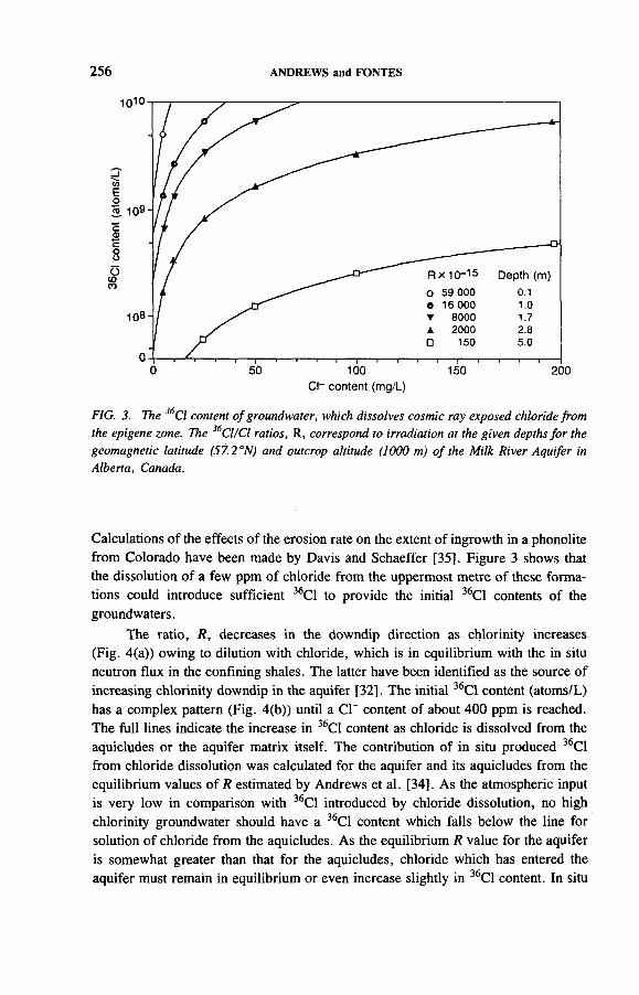
256 ANDREWS and FONTES

1010

100Cl- content (mg/L)

200

FIG. 3. The Cl content o f groundwater, which dissolves cosmic ray exposed chloride from the epigene zone. The 36Cl/Cl ratios, R , correspond to irradiation at the given depths fo r the geomagnetic latitude (57.2°N) and outcrop altitude (1000 m) o f the Milk River Aquifer in Alberta, Canada.

Calculations of the effects of the erosion rate on the extent of ingrowth in a phonolite from Colorado have been made by Davis and Schaeffer [35]. Figure 3 shows that the dissolution of a few ppm of chloride from the uppermost metre of these forma­tions could introduce sufficient 36C1 to provide the initial 36C1 contents of the groundwaters.

The ratio, R, decreases in the downdip direction as chlorinity increases (Fig. 4(a)) owing to dilution with chloride, which is in equilibrium with the in situ neutron flux in the confining shales. The latter have been identified as the source of increasing chlorinity downdip in the aquifer [32]. The initial 36C1 content (atoms/L) has a complex pattern (Fig. 4(b)) until а СГ content of about 400 ppm is reached. The full lines indicate the increase in 36C1 content as chloride is dissolved from the aquicludes or the aquifer matrix itself. The contribution of in situ produced 36C1 from chloride dissolution was calculated for the aquifer and its aquicludes from the equilibrium values of R estimated by Andrews et al. [34]. As the atmospheric input is very low in comparison with 36C1 introduced by chloride dissolution, no high chlorinity groundwater should have a 36C1 content which falls below the line for solution of chloride from the aquicludes. As the equilibrium R value for the aquifer is somewhat greater than that for the aquicludes, chloride which has entered the aquifer must remain in equilibrium or even increase slightly in 36C1 content. In situ

IAEA-SM-319/12 257

200 400 600 800 1000Cl- content (mg/L)

1200 1400

Cl- content (mg/L)

FIG. 4. (a) The 36Cl/Cl atomic ratio, R, o f groundwater in the Milk River Aquifer plotted against the Cl" content (data from Ref. [22]). As the Cl' content increases, R approaches the calculated value for chloride equilibrated with the in situ neutron flux in the aquitards o f the aquifer (solid line), (b) The 36Cl content o f groundwaters o f the Milk River Aquifer plotted against Cl" content (data from Ref. [22]). Groundwaters along the eastern and western flow paths merge with the calculated 36Cl contents for chlo­ride dissolution from the aquitards at Cl~ contents o f about 200 and 400 mg/L, respectively (dashed lines). The ‘forbidden zone ' cannot be entered either by the decay o f 36Cl or by chloride dissolution because o f in situ production within the sandstone. ( О : Ref. [22]; • : Ref. [23]; Д solution o f СГ from aquitards; A : Cl~ equilibrated in the aquifer.)

258 ANDREWS and FONTES

production can account for the increase in A values downdip without any need for the ultrafiltration effects proposed by Phillips et al. [22]. The high 36C1 contents for groundwaters with chlorinities much less than 400 ppm are clearly well above the dissolution line. The decrease in 36CI content as the СГ content increases is caused by a combination of 36C1 decay and 36C1 addition as the chloride is dissolved. Nolte et al. [23] have resolved these competing processes and have derived groundwater velocities of 0.04 and 0.11 m/a for the two directions along which fresh water moved into the aquifer.

It is also evident that the initial 36C1 input varies by about an order of magni­tude (about 109 and 108 atoms/L for the eastern and western flow paths, respec­tively). This variability could possibly be explained by variable hydrological conditions at recharge which affect the quantities of chloride dissolved from the shal­low zone of the aquifer or its aquicludes. A satisfactory explanation for these variable inputs is an essential prerequisite for using 36C1 in groundwater dating. Ground­water cannot be dated beyond chlorinities of « 150 ppm and =400 ppm for the eastern and western flow paths, respectively, because at greater chlorinities the 36C1 content is entirely due to dissolution of aquiclude chloride. If the 36C1 inputs can be proved to occur as a result of natural processes, such as those discussed above, then it is probable that the decay trends delineated by Nolte et al. [23] are real and that groundwater dating over a limited salinity range is possible. However, if future work was to show that significant 36C1 input cannot be derived from the soil zone, the input would have to be attributed to variable leakage of bomb pulse 36C1 into the flowing part of the aquifer, and dating by 36C1 would not be possible. Such leakage would be less likely (and more readily diluted) in the relatively static high salinity parts of the system which are clearly in equilibrium with in situ production.

2.2.4. Age determination through in situ buildup of 36Cl

As discussed by Andrews et al. [14, 15], Fontes et al. [13] and Michelot et al. [12, 36-38], it is possible to evaluate groundwater residence time from the ingrowth of 36C1 towards equilibrium.

The 36C1 balance at time t may be expressed as [37, 38]:

R, = Д0С0<ГХ' + tfeqC0( l - g - Xi) + R ^ C -C o ) (7)

where С is the СГ1 concentration; R is the atomic ratio; the indices 0 and eq stand for initial conditions and secular equilibrium, respectively, and X is the decay con­stant of 36C1. The initial input refers to the values of R and С when groundwaters entered into the host rock in which strong radioactivation takes place. Under these conditions, C0 and R0 may be meteoric (and cosmic) or rock derived if groundwater is passing from a uranium poor to a uranium rich environment.

IAEA-SM-319/12 259

Favourable conditions for age estimation require that the relative increase in C l' content (C, - C0)/C0 by solution from the host rock is very small. This is the situation in which а СГ rich solution infiltrates into the fracture network of a crys­talline rock. This occurs, for example, in Stripa granite [12-15, 39], where most of the C l' content of deep groundwater is allochthonous to the rock [40]. Here, finite values of the residence time of the chloride in the granite ranging from some tens to some hundreds of ka can be inferred from the 36C1 contents obtained at Stripa [12, 14, 15, 37]. These variations are probably linked to changing drainage condi­tions for saline solutions caused by mining operations. The situation is clearer for the saline (6 g/L) samples obtained from deep boreholes in northern Switzerland, where the saline solution is derived from evaporite deposits in which equilibrium R values are significantly lower than in the adjacent granite. Age estimates of 135 ± 60 and 610 + 390 ka have been derived [37].

2.2.5. Conclusions on the importance of in situ 36Cl production

The review shows that:

(1) In situ produced 36C1 may seriously constrain the application of 36C1 for groundwater dating;

(2) The cosmic fallout is possibly higher than predicted and can be enhanced by orders of magnitude through the admixture of radioactivated chloride in the soil zone;

(3) The deep in situ produced chloride released from the aquiclude would gener­ally overwhelm the initial cosmic input soon after the Cl" content became higher than some tens of ppm;

(4) In situ production can explain the increase in A values (atoms/L) which are observed in the distal parts of aquifers, without concentration by ultrafiltration processes.

It is also concluded that the use of 36C1 for dating purposes is probably easier and safer for hydrogeological situations in which the time-scale is given by the ingrowth of 36C1 rather than by its decay. This may be the case for groundwater penetrating into uranium or thorium rich rocks or sediments.

While 36C1, and especially the thermonuclear bomb peak, is an efficient tracer of recharge processes, its use as a dating tool for very old groundwater in porous media is possible only in cases where the chloride geochemistry and in situ produc­tion of 36C1 are fully understood.

3. ARGON-36

For geochemical and geochronological applications, 36Ar is generally consid­ered to be derived exclusively from the atmosphere. Corrections for the presence of

260 ANDREWS and FONTES

atmospheric 40Ar owing to contamination during argon extraction or to admixture of air during rock crystallization are thus based on the presence of 36Ar. However, 36Ar is continuously formed in minerals and fluids through the beta decay of 36C1 and it is interesting to evaluate to what extent such in situ production may influence the 40Ar/36Ar or 38Ar/36Ar ratios.

3.1. Sources

Argon-40 accumulation in a reservoir through 40K decay is given by:

N(wAr) = TV(40K) x Xf/X x |>x' - 1] (8)

where N is the number of atoms in the reservoir, X is the total decay constant of 40K (X = \ + \p) and \ e/ \ is the branching ratio leading to 40Ar formation. Adopted values are \ e = 0.581 x 10' 10 a-1, X = 4.962 x 10~10 a"1 and 40K/K = 1.167 x 10' 4 [41].

Argon-36 accumulation at equilibrium is derived from Eq. (6):

W(36 Cl) = ct/V(35C1)0/X36 (9)

and from the time dependence:

dN(36Cl)/dt = -X 36/V(36C1) = dN(36Ar)/dt (10)

so that

dN(36Ar) = о35ЩЪ5С1)Ф dt (11)

3.2. In situ 36Ar production on continents and oceans

Calculations, which will be detailed elsewhere, show that the total production of 36Ar since the formation of the Earth’s atmosphere (3.4 Ga) is 7.6 x 1033 and 5.3 x 1033 atoms for the continental and the oceanic crusts plus the ocean, respec­tively (1/5 and 4/5 of the global surface, respectively).

The total accumulation was somewhat enhanced during major evaporitic epi­sodes, which accumulated brines and salt over large areas of the crust exposed to cosmic radiations.

IAEA-SM-319/12 261

3.3. Total 40Ar and 36Ar generation rates in the crust

The 40Ar production rate is:

d(N40Ar)/dt = (X£/X) X X N(wK) = X ^(40K) (12)

For an average crustal К content of 25 900 ppm [42] this becomes:

d(NwAr)/dt = (0.581 X 10“10)x (2.59 x 10“2 x 1.167 x 10~4 x 6.02 x 1023/39.1)

= 2.70 x 106 atoms-g"1-a' 1 = 0.086 atoms-g'1-s' 1

Using the value of the isotopic abundance of 35C1 = 0.7577, the average crustal abundance of СГ is 130 ppm [42] and an average deep neutron flux of 2 x 10“5 n -c n r '-s ' 1 [34], we have:

d(N36Ar)ldt = (44 x 10‘24) x (1.3 x 10' 4 x 6.02 x 1023 x 0.7577/3545) x 2 x 10“5

= 1.47 X 10' 9 atoms-g"1-s' 1

The contribution from 39K, calculated for an isotopic abundance of 0.9326 and a cross-section for reaction (4) of 4.3 mb, is 3.2 X 10~" atom s-g1 -s"1. The total production is thus 1.50 x 10"9 atoms-g"1 - s '1, i.e. 3.60 x 1016 atoms/s for the total mass of the crust (2.4 X 1025 g). It is clear that for an average chemical com­position of the crust, the 40Ar buildup is much more significant than that of 36Ar. However, for a mean 36C1 fallout rate of 11 atoms -nT2- s' 1 (see above) over the global surface of 5.10 x 1014 m2, the equilibrium 36Ar production is 5.6 X 1015 + 3.6 x 1016 = 4.16 X 1016 atoms/s. All must migrate into the atmosphere, those in the ocean within about 2000 a and those on the continents within the average turnover time of crustal erosion. Within 3.4 Ga, the accumulation of radiogenic 36Ar in the atmosphere would be 4.45 x 1033 atoms. This estimate is lower by a factor of 3 with respect to the detailed evaluation because the latter takes into account the continuous cosmic production of 36C1 at the ocean surface. However, the 36Ar content of the atmosphere is 3.33 X 1039 atoms, about five orders of magnitude greater than the radiogenic accumulation over 3.4 Ga. The latter therefore contributes only a few ppm to the 36Ar atmospheric inventory.

3.4. Argon isotope distribution in chlorine rich environments

The radiogenic production ratio may be calculated from Eqs (11) and (12):

dN(wAT)/dN(36 Ar) = [XeW(40K)]/[<735W(35Cl)</>] (13)

262 ANDREWS and FONTES

Using consistent units, the ratio becomes:

40Ar/36Ar = 5.85 ф X [K]/[C1] (14)

where [K] and [Cl] are the К and Cl contents in mass fraction.To influence the Ar ratio in a crystal or fluid inclusion would require both a

very high flux and very low К/Cl. For a [K]/[C1] mass concentration ratio of 1.2 x 10~3 as an average value for the V2 deep borehole at Stripa [43] and a neu­tron flux of 4.7 x 10~5 n-cm' 2^ " 1 as measured at depth in Ref. [14], the equilibrium value given by Eq. (14) is 14.9. This value is about 20 times smaller than the normalized (Nier) value of 295.5 for the ratio 40Ar/36Ar in air [41]. If deep saline solutions were in equilibrium with the rock or derived from the leaching of fluid inclusions, this would imply that 40Ar formed in the К bearing minerals of the Stripa granite would not diffuse towards the liquid phase of the fractures. However, values of the 40Ar/36Ar ratios from dissolved gases in Stripa deep groundwater (V2) show a clear excess in 40Ar [15], indicating that rock derived gases are diffusing into the fracture fluids or that К has been incorporated in secondary minerals.

Anomalous values of the 40Ar/36Ar ratios have been observed in fluid inclu­sions from diamonds [44] and recently from inclusions in quartz and fluorite from the North Pennines ore field where “ 36Ar concentrations up to 10 times ASW” (air saturated water) were reported and attributed to “ a major unidentified fractionation mechanism” [45]. As several of these saline inclusions seem to be К depleted, in situ production of 36C1 and 36Ar could account for the high 36Ar contents. The solu­bility of argon is 3.89 x 10-4 mL/mL at 10°C. Assuming that Henry’s Law coeffi­cient is the same for 36Ar and 40Ar, the 36Ar in ASW is 3.8 X 10“4/295.5 = 1.32 X 10~6 mL/mL. A factor of ten would lead to 1.32 x 105 mL/mL, or3.54 x 1017 atoms 36Ar/kg of pure water. A brine saturated with respect to NaCl contains « 6 mol/kg, or 2.74 x 1024 35C1 atoms/kg. The flux to produce3.54 x 1017 atoms of 36Ar/L of brine in 265 Ma (the age of the quartz [46]), calcu­lated from Eq. (10), is: 0.35 n-cm '2 s_1. This value of the neutron flux is much too large even for surface irradiation by cosmic rays and may suggest that some primor­dial 36Ar rich argon is entrapped in the inclusion.

Excess of 36Ar, as compared with the air content, has been found in gases extracted by the melting of minerals for geochronological analyses. The most fre­quent explanation for this excess is fractionation either during analytical processes or by diffusional processes into or from the magma [47]. Isotope fractionation is probable when the 38Ar and 36Ar contents are correlated [47, 48].

Values of the ^A r/^ar ratio significantly lower than 295.5 were found recently [49] in lavas from the Quaternary volcanism of East Eifel (Germany). All crystals with clear 36Ar excesses are CP bearing feldspathoids (hauyne and nosean). Application of Eq. (14) with the values of 0.35 and 3.5% for the Cl and К contents, respectively [49], gives a high equilibrium value of about 6000 for the

IAEA-SM-319/12 263

40Ar/36Ar atomic ratio for a neutron flux ф of about 1000 x 10'5 n-cm“2-s"’, which is the maximum value likely to occur in the uppermost tens of centimetres of rock exposed to cosmic radiation at high altitudes. In such a case, the deep produc­tion of 36Ar from 36C1 decay following 35C1 radioactivation could not account for the anomalous values of the 40Ar/36Ar ratio. However, feldspathoids are also sul­phur bearing minerals. Other reactions involving a particles from the Th/U decay series as, for example, 33S(a, n)36Ar [50], should be taken into consideration.

3.5. Conclusions on the possible role of in situ 36Ar production

The effect of in situ production on the 40Ar/36Ar ratio needs to be investigated in more detail. Calculations suggest that under extreme geochemical conditions (high Cl/К ratios and high fluxes of particles), in situ 36Ar production may become significant.

The accumulation of 36Ar in К depleted СГ solutions (fluid inclusions or saline solutions from crystalline rocks) may easily lead to values for the 40Ar/36Ar ratio which are lower than those for the atmosphere.

4. CARBON-14 (Тй = 5730 ± 40 years)

Accelerator mass spectrometry has made 14C measurements possible for sam­ples as small as a few tens of micrograms of carbon with a relative uncertainty of about ±1%. The reduction in sample size by about 104 times compared with nuclear counting for l4C is an important advantage for groundwater studies. Meas­urements are now possible for small samples collected under natural flow conditions and for groundwaters with very low total dissolved carbon, either organic or inor­ganic. The latter occurs in groundwaters with high pH which forces the carbonatesystem equilibria towards COf~ and carbonate precipitation. The collection andtreatment of a water sample of one or two litres for AMS measurements, without contamination by atmospheric C02, is much more assured than for processing the several cubic metres of sample required for conventional counting.

4.1. Sources of 14C

The primary production of 14C by cosmic ray secondary neutrons in the atmosphere by the 14N(n, p) l4C reaction is generally the most significant 14C source in old groundwaters. Groundwater which has been recharged subsequent to 1945 may contain 14C produced by the neutron irradiation of atmospheric nitrogen as a result of nuclear weapons testing or 14C02 emissions from nuclear power plants. Carbon-14 production by cosmic ray interactions in soils and shallow aquifers can generally be neglected in comparison with the atmospheric input. Although this

264 ANDREWS and FONTES

production may be several orders of magnitude greater than in situ production atdepths below 100 m, its effect on the specific activity of 14C in carbon isdiminished by the extreme dilution caused by the high total dissolved inorganic car­bon (TDIC) content of shallow groundwater.

4.2. In situ production of 14C at a depth > 100 m

Several nuclear reactions can produce 14C in deep hydrogeological environ­ments [51]. However, for environments which are deeper than the penetration of cos­mic radiation the significant production mechanisms are restricted to the following:

170(n, a) l4C in rock matrix and fluid,l4N(n, p )i4C in dissolved N2 or nitrate in fluid,uB(a, p)XAC in rock matrix and fluid226Ra/223Ra/224Ra (exotic decay by 14C emission) in rock matrix and fluid.

All of these reactions are initiated directly or indirectly by the decay of the U and Th series radioelements.

The radiocarbon which is produced within the rock matrix must migrate to the fluid if it is to be effective in mixing with the input of comosgenic 14C from the atmosphere. This migration may occur by diffusion, which is a very slow process in solids, or by direct leaching of 14C atoms, which are produced at the rock/water interface. Such release must therefore be very dependent on matrix porosity and permeability.

A significant production of 14C occurs within the fluid itself because of neu­tron irradiation of the 170 of the water molecule and 14N dissolved in the water. The l4C so formed contributes directly to the TDIC activity. The nB(a, p) l4C reaction must depend upon the relative spatial distribution of boron and the a emit­ting elements in the rock matrix and upon the migration distance to the pore fluids. Radiocarbon produced by exotic decay or 226Ra and other Ra isotopes [52] must likewise migrate to the pore fluids. The occurrence of high concentrations of U in fracture minerals which are in direct contact with fracture fluids is of special interest. The 14C produced by exotic decay may migrate to the fluid relatively easily in such cases and this is especially probable where the 222Rn content of the fluid is high, indicating relatively easy diffusion paths for the short lived 222Rn atoms from the 226Ra sites where they have been generated. If the TDIC of the fracture fluid is low, then the specific activity of 14C in the fluid is particularly susceptible to increase because of additions of in situ produced radiocarbon (Table П1).

Uranium concentrations of up to 150 000 ppm have been identified in fracture minerals of the granitic pluton at Stripa in central Sweden [53] and the TDIC content of the fluids is very low. Values as low as 0.81 mg/L (in deep well V2) of TDIC are calculated from the measured values of alkalinity which include all of the weak acids (and principally Si04H4 and B03H3). These low TDIC concentrations imply

IAEA-SM-319/12 265

TABLE III. EQUILIBRIUM IN SITU PRODUCTION OF 14C FOR STRIPA GRANITE

Equilibrium activity within the fluid (per cent modern)

(mg/L) (a) (b) (c) (d) (e) (f)

1.0 3.70 3.78 13.6 27.4 850 1280

10.0 0.37 0.38 1.36 2.74 85 128

50.0 0.07 0.08 0.27 0.55 17 26

(a) Owing to production reactions within the fluid by reactions on nitrogen and oxygen (Ref. [15]).

(b) Same as (a), plus reaction uB(a, n ) l4C on aqueous boron.(c) Same as (a), plus 50% of exotic decay of U series Ra isotopes.(d) Same as (a), plus all exotic decay (U + Th series Ra isotopes).(e) Same as (a), with total transfer of all production within rock except uB(a, л )14С.(f) Same as (a) with total transfer of all production within the rock.Note: Columns (c)-(f) require transfer of l4C from the rock to a volumetric 1 % of fracture

fluid. It is considered that columns (d)-(f) should be reduced by two orders of magni­tude because of the incomplete transfer of 14C and, in the case of (f), because of non-uniform U, Th and В distribution.

that even without any release from the rock matrix, significant activity values (see Table III) should be observed in Stripa deep groundwater. Deep production might account for most of the 14C contents found in deep groundwater at Stripa [54-57].

4.3. Conclusions on the in situ production of radiocarbon

In situ radiocarbon production may become significant in hydrological environments where soil generated TDIC is not present (e.g. it is removed by car­bonate precipitation) and where the uranium and thorium contents are high. This is especially the case for low fracture flows in crystalline acidic rocks. More investiga­tions are needed of porous media where TDIC contents are generally high enough to dilute the in situ produced 14C below the detection level. However, in situ production is a further limitation which should be considered for the interpretation of low 14C content in old groundwater.

266 ANDREWS and FONTES

ACKNOWLEDGEMENTS

J.N. Andrews thanks the Natural Environment Research Council for a research grant. J.-C. Fontes thanks the Institut national des sciences de l’univers for its sup­port, and S. Pageau-Maurice for her patience in typing the successive versions of the manuscript.

REFERENCES

[1] LAL, D., Cosmogenic isotopes produced in-situ in terrestrial solids, Nucl. Instrum. Methods Phys. Res. B29 (1987) 238-240.

[2] LAL, D., In-situ produced cosmogenic isotopes in terrestrial rocks, Annu. Rev. Earth Planet Sci. 16 (1988) 255-388.

[3] FEIGE, Y., OLTMAN, B.G., KASTNER, J., Production rates of neutrons in soils due to natural radioactivity, J. Geophys. Res. 73 (1968) 3135-3142.

[4] BENTLEY, H.W ., PHILLIPS, F.M., DAVIS, S.N., “ Chlorine-36 in the terrestrial environment” , Handbook of Environmental Isotope Geochemistry: The Terrestrial Environment (FRITZ, P., FONTES, J.-C., Eds), Vol. 2b, Elsevier, Amsterdam(1986) 427-480.

[5] ELMORE, D., et al., Analysis of 36C1 in environmental water samples using an elec­trostatic accelerator, Nature (London) 277 (1979) 22-25.

[6] FINKEL, R.C., NISHIIZUMI, K., ELMORE, D., FERRAZO, R.D., GOVE, H.E., 36C1 in polar ice, rainwater and seawater, Geophys. Res. Lett. 7 11 (1980) 983-986.

[7] LAL, D., PETERS, B., “ Cosmic ray produced radioactivity on the earth” , Handbuch der Physik (SITTE, K., Ed.), 46/2, Springer-Verlag, Berlin (1967) 551-612.

[8] ONUFRIEV, V.G., Formation of chlorine-36 in nature, Yad. Geofiz. Geokhim. 4 (1968) 331-340 (in Russian).

[9] HOSSAIN, T.Z., “ Measurement of the 36Ar(n, />)36C1 capture cross section” , Annual Report of the Nuclear Structure Research Laboratory, University of Rochester, Rochester, New York (1988) 157-159.

[10] JIANG, S.S., et al., “ Measurements of the 36Ar(n,/?)36C1 cross section at thermal energies using the AMS technique” , Accelerator Mass Spectrometry (Proc. 5th Int. Conf. Paris, 1990) (YIOU, F., RAISBECK, G.M., Eds), Nucl. Instrum. Methods Phys. Res. B52 (1990) 608-611.

[11] KUHN, M.W., DAVIS, S.N., BENTLEY, H.W ., Measurements of thermal neutrons in the subsurface, Geophys. Res. Lett. 11 (1984) 607-610.

[12] MICHELOT, J.L ., BENTLEY, H.W., BRISSAUD, I., ELMORE, D., FONTES, J.Ch., “ Progress in environmental isotope studies (36C1, 34S, 180 ) at the Stripa site” , Isotope Hydrology 1983 (Proc. Symp. Vienna, 1983), IAEA, Vienna (1984) 207-229.

[13] FONTES, J.Ch., BRISSAUD, I., MICHELOT, J.L ., Hydrological implications of deep production of chlorine 36, Nucl. Instrum. Methods Phys. Res. B5 (1984) 303-307.

[14] ANDREWS, J.N., FONTES, J.Ch., MICHELOT, J.L ., ELMORE, D., In-situ neu­tron flux, 36C1 production and groundwater evolutions in crystalline rocks at Stripa, Sweden, Earth Planet. Sci. Lett. 77 (1986) 49-58.

IAEA-SM-319/12 267

[15] ANDREWS, J.N., et al., The in-situ production of radioisotopes in rock matrices with particular reference to the Stripa granite, Geochim. Cosmochim. Acta 53 (1989) 1803-1815.

[16] SCHAEFFER, O.A., THOMPSON, S.O., LARK, N.L., Chlorine-36 radioactivity in rain, J. Geophys. Res. 65 (1960) 4013-4016.

[17] ELMORE, D., et al., 36C1 pulse measured in a shallow ice core from Dye 3, Green­land, Nature (London) 300 (1982) 735-737.

[18] SUTER, M., et al., “ 36C1 studies at the ETH/SIN-AMS facility” , Accelerator MassSpectrometry (Proc. 4th Int. Conf. Niagara Falls, NY, 1987) (GOVE, H.E., LITHER- LAND, A.E., ELMORE, D., Eds), Nucl. Instrum. Methods Phys. Res. B29 1, 2(1987) 211-215.

[19] SYNAL, H.A., BEER, J., BONANI, G., SUTER, M., WÔLLI, W., “ Atmospheric transport of bomb produced 36C1” , Accelerator Mass Spectrometry (Proc. 5th Int. Conf. Paris, 1990) (YIOU, F., RAISBECK, G.M., Eds), Nucl. Instrum. Methods Phys. Res. B52 (1990) 483-488.

[20] ELMORE, D., et al., “ 36C1 and l0Be profiles in Greenland ice: Dating and production rate variations” , Accelerator Mass Spectrometry (Proc. 4th Int. Conf. Niagara Falls, NY, 1987) (GOVE, H.E., LITHERLAND, A.E., ELMORE, D., Eds), Nucl. Instrum. Methods Phys. Res. B29 1, 2 (1987) 207-210.

[21] BENTLEY, H.W ., et al., Chlorine 36 dating of very old groundwater. 1. The Great Artesian Basin, Australia, Water Resour. Res. 22 (1986) 1991-2001.

[22] PHILLIPS, F.M ., BENTLEY, H.W ., DAVIS, S.N., ELMORE, D., SWANICK, G.B., Chlorine 36 dating of very old groundwater. 2. Milk River Aquifer, Alberta, Canada, Water Resour. Res. 22 (1986) 2003-2016.

[23] NOLTE, E., KRAUTHAN, P., HEIN, U., KORSCHINEK, G., “ 36C1 measurements and dating of groundwater samples from the Milk River Aquifer” , Accelerator Mass Spectrometry (Proc. 5th Int. Conf. Paris, 1990) (YIOU, F., RAISBECK, G.M., Eds), Nucl. Instrum. Methods Phys. Res. B52 (1990) 447-482.

[24] FONTES, J.Ch., GUENDOUZ, A., MICHELOT, J.L ., Etude par le chlore 36 des eaux souterraines du Sahara septentrional, Rep. RAF/8/007, IAEA, Vienna (1985).

[25] ANDREWS, J.N., FONTES, J.Ch., GUENDOUZ, A., MAMOU, A., MICHELOT, J .L ., Isotope geochemistry of the Continental Intercalaire aquifer in the northern Sahara (in preparation).

[26] HABERMEHL, M.A., The Great Artesian Basin, Australia, Bur. Min. Resour. J. Aust. Geol. Geophys. 5 (1980) 9-38.

[27] AIREY, P.L., et al., “ Aspects of the isotope hydrology of the Great Artesian Basin, Australia” , Isotope Hydrology 1978 (Proc. Symp. Neuherberg, 1978), Vol. 1, IAEA, Vienna (1979) 205-219.

[28] AIREY, P.L., CALF, G.E., HARTLEY, P.E., ROMAN, D., “ Aspects of the isotope hydrology of the two sandstone aquifers in arid Australia” , Arid Zone Hydrology: Investigations with Isotope Techniques (Proc. Advisory Group Mtg Vienna, 1978), IAEA, Vienna (1980) 93-111.

[29] CALF, G.E., HABERMEHL, M.A., “ Isotope hydrology and hydrochemistry of the Great Artesian Basin, Australia” , Isotope Hydrology 1983 (Proc. Symp. Vienna, 1983), IAEA, Vienna (1984) 397-413.

268 ANDREWS and FONTES

[30] TORGERSEN, T., CLARKE, W.B., Helium accumulation in groundwater. I: An evaluation of sources and the continental flux of crustal 4H in the Great Artesian Basin, Australia, Geochim. Cosmochim. Acta 49 (1985) 1211-1218.

[31] SCHWARTZ, W .F., MUEHLENBACHS, F., Isotope and ion geochemistry of groundwaters in the Milk River Aquifer, Alberta, Water Resour. Res. 15 (1979) 259-268.

[32] HENDRY, M .J., SCHWARTZ, F.W ., An alternative view on the origin of chemical and isotopic patterns in groundwater from the Milk River Aquifer, Canada, Water Resour. Res. 24 10 (1988) 1747-1763.

[33] HENDRY, M .J., SCHWARTZ, F.W ., The chemical evolution of groundwater in the Milk River Aquifer, Canada, Groundwater 28 (1990) 253-261.

[34] ANDREWS, J.N., FLORKOWSKI, T., LEHMANN, B., LOOSLI, H.H., Under­ground production of radionuclides in the Milk River Aquifer, Alberta, Canada, Appl. Geochem. (in press).

[35] DAVIS, R., Jr., SCHAEFFER, O.A., Chlorine-36 in nature, Ann. N.Y. Acad. Sci 62 (1955) 105-122.

[36] MICHELOT, J.L., et al., “ Teneurs en chlore 36 et problèmes de circulation des eaux profondes du socle de Suisse septentrionale” , Isotope Techniques in Water Resources Development (Proc. Symp. Vienna, 1987), IAEA, Vienna (1987) 738.

[37] MICHELOT, J.L ., “ Chlorine-36 in deep groundwaters and host-rock of Northern Switzerland: Sources, evolution and hydrological implications” , Water-Rock Interac­tions (Proc. 6th Int. Symp. Malverne, UK, 1989), A.A. Balkema, Rotterdam (1989) 483-486.

[38] MICHELOT, J.L ., Hydrochimie isotopique des écoulements lents en milieu cristallin fracturé: essai méthodologique, PhD Thesis, Université Paris-Sud (1988).

[39] FABRYKA-MARTIN, J., DAVIS, S.N., ELMORE, D., Applications of 129I and 36C1 to hydrology, Nucl. Instrum. Methods Phys. Res. B29 (1987) 361-371.

[40] FONTES, J.Ch., FRITZ, P., LOUVAT, D., MICHELOT, J.L., Aqueous sulphates from the Stripa groundwater system, Geochim. Cosmochim. Acta 53 (1989) 1783-1789.

[41] STEIGER, R.H., JÀGER, E., Subcommission on geochronology: Convention on the use of decay constants in geo- and cosmochronology, Earth Planet Sci. Lett. 36 (1977) 359-362.

[42] MASON, B., Principles of Geochemistry, 3rd edn, Wiley, New York (1966).[43] NORDSTROM, D.K., BALL, J.W., DONAHUE, R.J., WHITTEMORE, D.,

Groundwater chemistry and water-rock interactions at Stripa, Geochim. Cosmochim. Acta 53 (1989) 1727-1740.

[44] MELTON, C.E., GIARDINI, A. A., The isotopic composition of argon included in an Arkansas diamond and its significance, Geophys. Res. Lett. 7 6 (1980) 461-464.

[45] TURNER, G., STUART, F.M ., BANNON, М., SAXTON, J.M ., “ Noble gas iso­topes and halogens in fluid inclusions” , Geochronology Cosmochronology and Isotope Geology (Proc. 7th Int. Conf. Canberra, 1990), Geological Society of Australia, Can­berra (1990) (abstracts, p. 103).

[46] TURNER, G., Hydrothermal fluids and argon isotopes in quartz veins and cherts, Geochim. Cosmochim. Acta 52 (1988) 1443-1448.

IAEA-SM-319/12 269

[47] KRUMMENACHER, D., Isotopic composition of argon in modern surface volcanic rocks, Earth Planet. Sci. Lett. 8 (1976) 109-117.

[48] KANEOKA, I., Rare gas isotopes and mass fractionation: An indicator of gas transport into or from a magma, Earth Planet Sci. Lett. 48 (1980) 284-292.

[49] LIPPOLT, H.J., TROESCH, М., HESS, J.C., Excess argon and dating of QuaternaryEifel volcanism. IV. Common argon with higher and lower than atmospheric40A r/36Ar ratios in phonolitic rocks, East Eifel, FRG, Earth Planet Sci. Lett. 101 (1990) 19-33.

[50] FLEMING, W.H., THODE, H.G., Argon-38 in pitchblende minerals and nuclearprocesses in nature, Phys. Rev. 90 5 (1953) 457-458.

[51] ZITO, R., DONAHUE, D.J., DAVIS, S.N., BENTLEY, H.W., FRITZ, P., Possible subsurface production of carbon-14, Geophys. Res. Lett. 7 (1980) 235-238.

[52] BARKER, D., JULL, A.J.T., DONAHUE, D.J., Excess carbon-14 abundances in ura­nium cores: Possible evidence for emission from uranium-series isotopes, Geophys. Res. Lett. 12 (1985) 737-740.

[53] WOLLENBERG, H., FLEXSER, S., ANDERSSON, L., Petrology and Radiogeology of the Stripa Pluton, Rep. LBL-11654, Lawrence Berkeley Laboratory, Berkeley, CA (1980).

[54] FRITZ, P., BARKER, J.F., GALE, J.E ., Geochemistry and Isotope Hydrology of Groundwaters in the Stripa Granite. Results and Preliminary Interpretation, Rep. LBL-8285; SAC-12, Lawrence Berkeley Laboratory, Berkeley, С A (1979).

[55] FRITZ, P., et al., The isotope geochemistry of carbon in groundwater at Stripa, Geochim. Cosmochim. Acta 53 (1989) 1765-1775.

[56] LOUVAT, D., Géochimie isotopique du soufre et du carbone et circulations aquifères en roches cristallines de Suède Centrale (Stripà) et de Finland, Thesis, Université Paris- Sud (1987).

[57] MURPHY, E.M ., Carbon-14 Measurements and Characterization of Dissolved Organic Carbon in Groundwater, Thesis, University of Arizona, Tucson (1987).

GROUNDWATER DATING: PROBLEMS AND NEW APPROACHES

Methodological aspects and models

ChairmanH. MOSER

Germany

IAEA-SM-319/36

ON THE STATISTICAL TREATMENT OF ENVIRONMENTAL ISOTOPE DATA IN HYDROLOGY

B.R. PAYNE Vienna,Austria

Abstract

ON THE STATISTICAL TREATMENT OF ENVIRONMENTAL ISOTOPE DATA IN HYDROLOGY.

The paper summarizes the ways in which statistical methods may be used to attach a given level of confidence to conclusions based on the interpretation of environmental isotope data, with particular reference to stable isotopes. The topics covered are variability of data, estimation of the parameters of a water body, significance of the difference between two groups of data, errors in mixing problems and regression analysis. With respect to the latter, the differences between different regression methods are presented. Guidance is provided on the appropriateness of least squares, orthogonal or major axis and reduced major axis regres­sion in isotope hydrology. Details are provided of the errors in estimates of the population regression line for a given value of one variable and also for the errors when a regression line is used for prediction.

1. INTRODUCTION

There is an inherent variation in all data. Firsdy, there is the variation due to the precision of the measurements by the analytical process. If repeated analyses of the same sample are made, precision refers to how closely the results are clustered about their mean. For example, in the case of stable isotope analyses most labora­tories quote precisions of 0.1700 and 1700 for ô180 and ô2H, respectively. Secondly, variation results from the accuracy of any estimates based upon the data. How close is an estimate to the true value? In the estimation of the stable isotopic composition of a water body, the measurement may be very precise, but the estimate may be inaccurate. The population characteristics of a system are estimated on the basis of samples. Statistical inferences permit one to say how accurate are the estimates at a given level of confidence.

This paper focuses on the principal questions which arise in the interpretation of environmental isotope data and suggests ways in which statistical methods can be used to arrive at robust conclusions.

273

274 PAYNE

2. VARIABILITY OF A PARAMETER

In order to estimate whether there is any variability beyond that due to measurement errors, one computes the sample standard deviation of the set of samples. It should be emphasized that the comparison concerns the sample standard deviation (Eq. (1)) and not the standard deviation of the mean (s/'JÑ ). The sample standard deviation of the mean decreases with the increase in the sample size, so it should be clear that its use is erroneous for assessing variability:

I

i i r n r -

The variability of different parameters cannot be assessed only on the basis of the standard deviation of the different parameters because of the different units. Consider a set of ô180 data having a mean of —6.5°/00 and a standard deviation of0.5 700, and a set of chloride data with a mean of 495 mg/L and a standard deviation of 40 mg/L. The comparison should be based upon the coefficient of variation which, expressed as a percentage, is 100 s/X. The coefficients of variation for the above example are 7.7% and 8.1%, respectively, which illustrates the similarity in variability in <5180 and chloride.

3. ESTIMATION OF THE COMPOSITION OF A WATER BODY

It may seem obvious, but it should be emphasized that an isolated value cannot be used to estimate the true composition of a water body. It could be near the true value, or it could be an extreme value. Clearly, the more values which are used for the estimation of the mean, the more accurate will be the estimate. Having said this, it should be recognized that in environmental isotope hydrology one is usually dealing with small samples, therefore the sample standard deviation of the mean should be adjusted to take this fact into account by multiplying it by the value of the Student’s t value for the number of degrees of freedom at the required confidence level (Eq. (2)). At the 95% confidence level the value of t is 2 even for a sample size of 61 and increases to 2.776 when the sample size is 5. In making this correction one is concerned with a two tailed value. Student’s t tables sometimes quote two tailed and sometimes one tailed values. If the latter is used, then one should look up the a /2 value where a is the level of significance (100 — confidence level):

IAEA-SM-319/36 275

4. SIGNIFICANCE OF THE DIFFERENCE IN COMPOSITIONOF TWO GROUPS

In the comparison of the means of two independent samples with means Xx and X2 (which are estimates of their respective population means ц\ and /*2), the tests of significance and confidence intervals may be based on the Student’s t distribution. If the variances are not significantly different (this may be checked by analysis of variance of the ratio of the variances), the pooled estimate of the variance (s2) of the groups is given by Eq. (3):

s = —----- ------- ----- —------------- (3)(Nt + N 2 - 2 )

For samples of equal size (N), the t value is computed according to Eq. (4a).For samples differing in size, but still not differing in variance, t is computedaccording to Eq. (4b). The t values so computed are checked against the tabulatedt value at (Nx + N2 — 2) degrees of freedom:

f = (Xt - X2)V 2 s2/N (4a)

t = (Xx - X2)V i2[(A ! + /V2)W j^2] (4b)

When the variances differ, then the t value does not follow the Student’s t distribution when the population means are equal. However Satterthwaite [1] has proposed assigning an approximate number of degrees of freedom, и', as defined in Eq. (6), to t', defined in Eq. (5):

(X, - X2)t = -p- 1 2 = (5)

+ s\IN2

«' - 1<u,+ulf (6) (Uyhi + u2lv2)

where Ui = sj/Ni with vi (Nl — 1) degrees of freedom and u2 = s2/N2 with v2(N2 - 1) degrees of freedom. The approximate number of degrees of freedom (u ') is rounded down when using the Student’s t table.

276 PAYNE

In all the above treatment it is assumed that Xf and X2 are normally distri­buted. Bearing in mind this fact and the usually small number of data defining the two groups, it is recommended that the significance of the difference between means be checked by a non-parametric method, namely the Mann-Whitney test. It is more powerful than the t test.

The first sample of size n from the first population is represented by the values X1,X 2,X i , The second sample of size m from the second population isrepresented by the values Уь У2, ......Ym. Ranks are assigned from 1 to (n + m)to the combination of samples from both groups. That is, the first rank is assigned to the smallest value (/?)) and the highest rank RN (where N = n + m) to the largest value. Where there are cases of equal values, so-called ties, the average rank is allocated to each of the ties. During the ranking the identity of the members of each group is maintained.

TABLE I. DECISION RULES FOR THE MANN-WHITNEY TEST

Hypotheses®

A (two tailed test) В (one tailed test) С (one tailed test)

H0: E(X) = E(Y) H0: E(X) > E(Y) H0: E(X) < E(Y)

Ha: E (X ) * E(Y) Ha: E(X) < E(Y) Ha: E (X ) > E(Y)

Reject H0 at significance level a if

T < 4all T < qa T > tfi-„ or Г < qa

or T > Í1-C/2 or Г, < —1.645 or Г, > 1.645

or T¡ < -1 .9 6 or T, > 1.96

Accept H0 at significance level a if

ЯаП ^ T < Я\-аП T * q a т ^ Ч\-а

or —1.96 < Г, < 1.96 Г, > -1 .645 Г, < -1 .645

a E(X) and E(Y) are the population means.

IAEA-SM-319/36 277

Test statistic:

If there are few or no ties the sum of the ranks assigned to group 1 can be used as the test statistic:

7 = £ R(X,) (7)

If there are many ties, use T¡ where T\ is:

(N+1)— 2—

T, = ... , - — (8)I nm _ nm(N + *)2

А Щ Л Г - 1 ) " 4 ( N - l )

where HR? refers to the sum of the squares of all N of the ranks or average ranks of both groups. The approximate quantiles for T{ may be obtained from the normal distribution.

The quantiles qp of T are given in tables for this test. The upper quantiles iq\_p) may be computed by subtraction from n(N + 1) (see Eq. (9)):

q ^p = n(N + I) - qp (9)

However, if an upper quantile test is required, then the statistic T ', defined in Eq. (10), may be used with the lower quantiles. The decision rules for testing different hypotheses are given in Table I:

T = n(N+ 1) - T (10)

5. ERRORS IN MIXING PROBLEMS

When one estimates a parameter which is derived from a number of measured parameters, then the error of the estimated parameter is a function of the random errors of the measured parameters.

' Stable isotope data are often lised to estimate the proportions of two different types of waters which contribute to the sample under examination. If ámix, <5, and 62 are the stable isotope indices of the mixture, component 1 and component 2, respec­

278 PAYNE

tively, then the mass balance given in Eq. (11) enables the fraction (J), expressed as a percentage, of component 1 to be estimated from Eq. (12):

/ 0 , + (1 - / ) 0 2 = ¿ w (11)

/ = 100 (12) (ôi - à2)

The general law of propagation of errors is given in Eq. (13):

= к . * ) 2 ( Ч г - У + Ю 2 f - ^ y + Ю 2 m 2 (» )dàmix) \ d ô j У&2> y d0J

From Eq. (12) one obtains the following partial derivatives:

Э/ _ 100

d<5mix (ô, - ô2)(14)

df = 100 -(¿2- (15)dây (ô, - 62)2

dô2 ( ô , - ô 2)2

Thus the percentage error (Err) on the estimated fraction may be obtained from the following equation:

100 V - 2 , /1 0 0 (0 , - Ô ^ V -2 , / 10 0 (« m ix - 0l ) V -2<J2Л Ь х - Ы ) V (ôi-ô2)2 J \ (ô,-ô2)

(17)

The standard deviations of the mean at the 95% confidence level for ôI( <52 and <5mix are estimated from Eq. (2). The implication of the propagation of errors in a mixing problem based on 180 data is illustrated in Fig. 1.

This treatment may be used to estimate the limits of resolution in problems relating to the potential contributions of water sources, such as from a lake or river to a groundwater system. The values of 5mix and <5mjx are equated to the corres-

IAEA-SM-319/36 279

0.05%o 0.10%o 0.25%o

FIG. 1. Error in the estimation o f a fraction in a mixture as a function o f the difference between the two end components. The three curves refer to standard deviations o f the mean o f 0.05, 0.10 and 0.25°/oo for all components.

ponding parameters of one or the other component in Eq. (17). In a study of the possible losses from Lake Chala to groundwater [2], it was concluded that there was no significant contribution. The standard deviation of the mean for the lake was0.127oo for S180 . The difference in 6180 between the lake and the average of the groundwater was 6.047oo. If <5, and represent the lake, then the last term in Eq. (17) cancels and the percentage contribution which would not be detected would be 4%.

6. REGRESSION

Regression is used in environmental isotope hydrology for many purposes. Among the most common uses are:

— Estimation of the altitude effect,— Estimation of the mean altitude of recharge,— Estimation of the local meteoric water line,— Extrapolation of an evaporation line to the local meteoric water line to estimate

the original stable isotopic composition of the evaporated waters,— Extrapolation of a mixing line in a salinity problem to estimate the stable

isotopic composition of the non-saline component.

280 PAYNE

The most common method of regression analysis is that of least squares. However, in this model the dependence of one variable, the dependent variable, is assessed on the basis of changes in the other variable, known as the independent variable, which strictly should be known without error. This implies that there is reason to believe that changes in the dependent variable are the result of changes in the independent variable. Only the first two problems listed above are appropriate to least squares regression analysis.

The presentation of ô180 and ¿>2H data almost always displays <52H as the dependent variable. It has been realized for a long time that this has no basis at all. One could just as well use <5180 as the dependent variable. There are two regression techniques which overcome this objection. The first is orthogonal regression, some­times known as the major axis line. The second is the reduced major axis line.

The symbolism for the sums of squares of the deviations of X, Y and XY is defined as follows:

The mathematical model for linear regression is given in Eq. (21), where e is a random variable which takes into account the fact that individual Y values do not fall directly on the regression line. Greek letters are used to reflect that this is the population regression line. Ordinary letters refer to sample estimates. The model further assumes that the deviations, e, are normally distributed with a mean of zero and variance of a2x:

The sample estimates of the population slope (@) and intercept (a) are b and a, respectively. The correlation coefficient is defined in the normal way:

CSSX = £ (X - X) (18)

CSSY = £ (У - Y)2 = £ Y2 - / (19)

CSCP = £ (XY - XY)2 = £ ХУ - £ x £ Y/N (20)

Y = a + 0(X — X) + e (21)

CSCP (22)у/(CSSX-CSSY)

The regression on the sample data has a standard error of estimate which is defined as:

IAEA-SM-319/36 281

N

E № - Yi)1

N - 2(23)

where Y is the value of Y estimated from the regression.No matter which method of regression is used, a quantitative interpretation,

with a given degree of confidence, can only be made if the errors involved in the various aspects of regression are taken into account. A distinction should be made between two cases. The first concerns the errors in the estimate of the population or true regression. The second embraces the errors involved when the regression is used for predicting a value of one variable on the basis of a value of the other variable.

6.1. Least squares regression analysis

The regression line in this analysis results from minimizing the sum of the squares of the deviations, measured along the Y axis, from the points to the best fit line.

The slope and intercept of the line and their associated errors are defined as:

6.2. Orthogonal regression-major axis line

The regression line in this analysis results from minimizing the sum of the squares of the deviations of the points perpendicular to the line.

The slope b is defined by Eq. (26):

(24)

(25)

- B ± V b 2 + 4 Cfx(26)

2 Cfy

where

(■CSSX-CfЬ - (CSSY-Cfy) CSCP ■ Cfx- Cfy

(27)

282 PAYNE

The sign preceding the square root in Eq. (26) is determined by the sign of CSCP. The major axis line is at an angle of в to the X axis, where в is equal to arctan b. In the major axis regression line the perpendicular distance to the line has components in all directions. Therefore, both variables must be expressed in the same units. Thus, in Eqs (26) and (27) the terms Cjf refer to the scaling factors for each variable. With stable isotope data a suitable factor is the reciprocal of the analytical errors of ô180 and S2H, respectively. The error (sb) on the slope is given by Eq. (28):

The intercept of the regression can be found in the normal way, namely,

a = Ÿ - bX (29)

The error of the intercept is:

(sy - s xb)2 + (1 - r ) b ( ls xsy + X Ь + Г) ) (30)

The sums of squares of the deviations normal to the line т а У befound according to Eq. (31). Dividing by (N — 2) and taking the square root and dividing by cos 0 gives syx (Eq. (32)), measured along the Y axis:

^ CSSX+CSSY /CSSY2 - CSSX2\ 2E d = --------j ----------- s j ( CSCPï + [ -----------j --------- J ( }

CSSX + CSSY - J(CSCP)2 +(32)

cosí \ (N — 2)

In order to estimate the confidence limits of the regression at a given confi­dence interval, say 95%, syx in Eq. (32) should be multiplied by the value of Student’s t at the required level of significance for (N — 2) degrees of freedom.

6.3. Reduced major axis line

In this technique the line is obtained by minimizing the sum of the products of the deviations measured in the directions of the X and Y axes. This is the same as minimizing the areas of the right angle triangles enclosed by the horizontal and

IAEA-SM-319/36 283

vertical deviations of the points from the line. The slope and intercept of the line and their associated errors are defined as:

b =CSSYCSSX

= ^ ± b sr

(33)

a = Y — b X ± syN

1 + X'(34)

6.4. Choice between the major axis and reduced major axis lines

It has already been pointed out in Section 6.2 that the major axis line is not invariant with respect to scale. This therefore requires that the variables be adjusted by scaling factors. This may be avoided if one uses the reduced major axis line which is invariant with respect to scale and easier to compute using spreadsheet software. However, there is a more important consideration illustrated in Fig. 2. With a decrease in the value of the correlation coefficient the error in the major axis regression increases more rapidly than that of the reduced major axis line. Although the line in Fig. 2 extends down to a value of 0.3 for the correlation coefficient, it

Correlation coefficient

FIG. 2. Increase in the error o f the major axis regression with lower correlation coefficient.

284 PAYNE

should be remembered that for a given regression there is a value of the correlation coefficient below which there is no significant correlation at a given level of significance.

6.5. Prediction of Y from X

Regression analysis may be applied to three types of problems:

(1) Prediction of Y(n) of the population regression line at a value of X,(2) Prediction of Y(Y) for a value of X,(3) Prediction of the mean У(У) of a random set of p samples for a value of X.

The solution of the third type of problem leads to the solution of the other two. Since the mean of (X - X) is zero, Eq. (21) reduces to:

Ÿ = « + (35)

where In is the mean of a random set of n residuals. Thus, the predicted mean (У) is:

F = Ÿ + b(X - X) = a + b(X - X) + e„ (36)

However, from Eq. (21) the value predicted is:

? = a + 0 ( X - X ) + Ip (37)

Subtracting Eq. (37) from Eq. (36), we have:

Ÿ - ? = (e„ - Fp) + Ф - p)QC-X) (38)

The term (?„ - ep) is the difference between the means of the two independent samples of size n and p. The variance of the difference is:

The right hand term involves the variance of the slope which is different for each of the regression methods. Thus, the general equation for the sample estimate of the standard error of s(Y) is given by Eq. (39), where sb is the error of the slope:

s&> = J s> x ( j + j ) + Sfe2(X “ X)2 (39)

IAEA-SM-319/36 285

For the first problem, prediction of Y(¡jl) of the population regression line at a value of X, lip is put equal to zero. Thus, Eq. (39) reduces to Eq. (40). In the case of the second problem, prediction of Y(Y) for a value of X, p is put equal to one. In this case, Eq. (39) reduces to Eq. (41). The confidence limits are established by the factor ta (n — 2 degrees of freedom), where a is the level of significance:

*00 = J 7 ) + sb(x - *)2 (4°)

J(F) = ta J s 2yx{ 1+-^- ) + s l ( X - X ) ¿ (41)

6.5.1. Prediction in least squares regression

Since the variance of the slope in least squares regression is a2xICSSX, it follows from Eq. (40) that the error, at the 95% confidence level, for the population line at X is given by Eq. (42):

(42)

As an example, the following set of data is used to estimate the altitude effect:

0-18 -8 .9 -8 .3 -10.3 -10 .4 -9 .9 - 10.2 -10.5 - 6.8

Mean elevation (m) 1100 850 1500 1550 1400 1500 1650 200

The regression indicates an altitude effect of 0.277oo for a 100 m change in elevation:

0180 = -(0.002 68 ± 0.0001) elevation - (6.146 ± 0.046) (43)

s.о - 0.13; r = 0.9958; n = 8О-elevation

It will be noted from Fig. 3 that the errors increase moving away from the mean of the values of the independent variable.

286 PAYNE

To continue with the example of the altitude effect, the inverse of Eq. (43) must be used to estimate the mean elevation of recharge for various waters sampled in the area. The reason is that elevation is now the dependent variable:

Mean elevation = -(370.0 ± 13.8) 180 - (2264.3 ± 131.2),

r = 0.9958; s .. = 48; n = 8 (44)elevation l80

The prediction errors, estimated from Eq. (41), are shown in Fig. 4.In Fig. 4, the errors again increase, moving away from the mean of the values

of the independent variable. This implies that the use of the regression for estimating the mean elevation of recharge should be limited to the range in elevation over which the altitude effect was estimated.

0-18 -1 2 -11 -1 0 -9.41 - 9 - 8 - 7

Mean elevation (m)Error (95 % confidence level)

2176±160

1806±143

1436±133

1219±131

1066±132

696±141

326±157

6.5.2. Prediction in orthogonal-major axis regression

Since the variance of the slope in orthogonal regression is:

Ê! (1 - r2)r2 N

then, from Eqs (41) and (42), the errors at the 95% confidence level of s(¡x) and s{Y) are given by Eqs (45) and (46):

■*(M) = ta J s * x Q j + b (*2 пГ) (X - X )2 (45)

*0-0 = '« J s 2yx (1 + 7) + ~b~r2 ~r ) ~ (* ~ V 2 <46>

Mea

n ele

vatio

n of

rech

arge

(m

) iso

(%

<>)

IAEA-SM-319/36 287

FIG. 3. Errors in estimation o f the altitude effect.

180 (%o)

FIG. 4. Errors in prediction o f the mean elevation o f recharge.

6.5.3. Prediction in reduced major axis regression

The variance of the slope in reduced major axis regression is:

N

Then, from Eqs (41) and (42), the errors at the 95% confidence level of s(fi) and s(Y) are given by Eqs (47) and (48):

si») = ta J s n Q j + — (1 ~j2 ) (X - X)2 (47)

*00 = ta J s 2yx ( l + ^ ) + ~ 2~ ~ - } ( X - X ) 2 (48)

The original stable isotopic composition of evaporated waters may be estimated by extrapolating the evaporation line back to the local meteoric water line. In order to estimate the errors, it is necessary to determine the intersections of the error limits

2 8 8 PAYNE

FIG. 5. Errors at the 95 % confidence level falling in the domain ABCD.

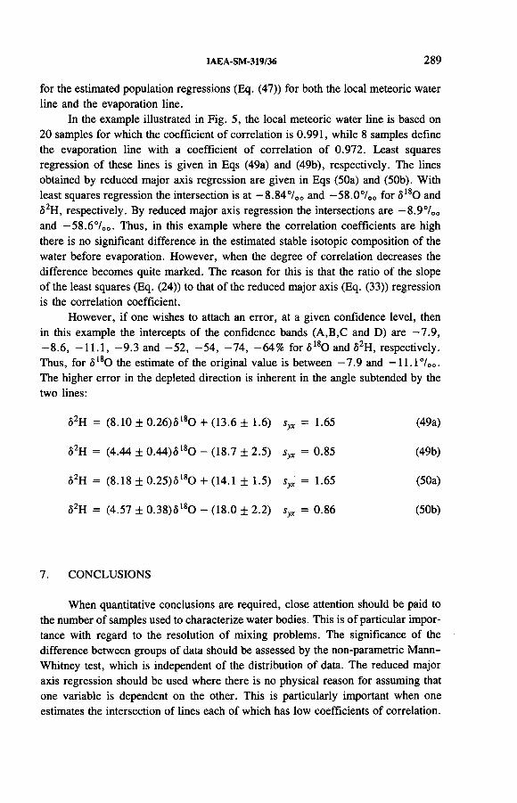
IAEA-SM-319/36 289

for the estimated population regressions (Eq. (47)) for both the local meteoric water line and the evaporation line.

In the example illustrated in Fig. 5, the local meteoric water line is based on 20 samples for which the coefficient of correlation is 0.991, while 8 samples define the evaporation line with a coefficient of correlation of 0.972. Least squares regression of these lines is given in Eqs (49a) and (49b), respectively. The lines obtained by reduced major axis regression are given in Eqs (50a) and (50b). With least squares regression the intersection is at -8 .8 4 7 00 and -5 8 .0 7 oo for <5i80 and <52H, respectively. By reduced major axis regression the intersections are -8 .9 7 00 and — 58.6700. Thus, in this example where the correlation coefficients are high there is no significant difference in the estimated stable isotopic composition of the water before evaporation. However, when the degree of correlation decreases the difference becomes quite marked. The reason for this is that the ratio of the slope of the least squares (Eq. (24)) to that of the reduced major axis (Eq. (33)) regression is the correlation coefficient.

However, if one wishes to attach an error, at a given confidence level, then in this example the intercepts of the confidence bands (A,B,C and D) are -7 .9 , - 8.6, —11.1, -9 .3 and -5 2 , -5 4 , -74 , -64% for 6180 and ô2H, respectively. Thus, for <5180 the estimate of the original value is between -7 .9 and -1 1 .1 7 00. The higher error in the depleted direction is inherent in the angle subtended by thetwo lines:

02H = (8.10 ± 0.26)5180 + (13.6 ± 1.6) s yx = 1.65 (49a)

<52H = (4.44 ± 0.44)0180 - (18.7 ± 2.5) s yx = 0.85 (49b)

<52H = (8.18 ± 0.25)5180 + (14.1 ± 1.5) s yx = 1.65 (50a)

<52H = (4.57 ± 0.38)ô180 - (18.0 ± 2.2) Syx = 0.86 (50b)

7. CONCLUSIONS

When quantitative conclusions are required, close attention should be paid to the number of samples used to characterize water bodies. This is of particular impor­tance with regard to the resolution of mixing problems. The significance of the difference between groups of data should be assessed by the non-parametric Mann- Whitney test, which is independent of the distribution of data. The reduced major axis regression should be used where there is no physical reason for assuming that one variable is dependent on the other. This is particularly important when one estimates the intersection of lines each of which has low coefficients of correlation.

290 PAYNE

ACKNOWLEDGEMENTS

The author appreciates the fruitful discussions with R. Gonfiantini and Y. Yurtsever during the preparation of this paper.

REFERENCES

[1] SATTERTHWAITE, F.E., Biom. Bull. 2 (1946) 110.[2] PAYNE, B.R., Water balance of Lake Chala and its relation to groundwater from

tritium and stable isotope data, J. Hydrol. 11 (1970) 47-58.

IAEA-SM-319/29

COMPARTMENTAL MODELLING APPROACH FOR SIMULATION OF SPATIAL ISOTOPIC VARIATIONS IN THE STUDY OF GROUNDWATER DYNAMICS A case study o f a multi-aquifer system in the Bangkok Basin, Thailand

Y. YURTSEVER Isotope Hydrology Section,Division of Physical and Chemical Sciences,International Atomic Energy Agency,Vienna

S. BUAPENG Groundwater Division,Department of Mineral Resources,Bangkok,Thailand

Abstract

COMPARTMENTAL MODELLING APPROACH FOR SIMULATION OF SPATIAL ISO­TOPIC VARIATIONS IN THE STUDY OF GROUNDWATER DYNAMICS: A CASE STUDY OF A MULTI-AQUIFER SYSTEM IN THE BANGKOK BASIN, THAILAND.

The paper summarizes the basic formulation of the compartmental simulation approach as a distributed parameter modelling methodology that can be employed for the quantitative interpretation of isotope and tracer data in hydrology. Application of the approach in the multi­aquifer groundwater system of the Bangkok Basin, in Thailand, is given as an illustration of the method for evaluating the spatial variations observed in isotope data.

1. INTRODUCTION

Quantitative evaluations of isotope data collected from hydrological systems require proper model formulations that permit calculation of the concentration of specific isotopes at a given place and time in the system. While simplified lumped parameter models often employed for this purpose may, in certain cases, be adequate for the interpretation of observed isotope data in the ‘time’ domain, information inherent in the observed spatial variations of isotope concentrations requires the use of the distributed parameter modelling approach.

291

292 YURTSEVER and BUAPENG

Environmental isotope techniques are usually applied, particularly in regional scale aquifer systems, for an improved understanding of the genesis of water; its replenishment source(s) and rate(s); the mixing ratios of different fluxes (fluid sources); and regional flow dynamics, including the residence and/or transit times involved during the flow. Quantitative evaluations from isotope data aim at obtaining estimates related to the aspects cited above, taking into account bulk flow charac­teristics at the prescribed boundaries and within the system.

Compartmental simulation models are being used more progressively to describe the transport of reactive and non-reactive components in groundwater systems. Their use in the simulation of dispersion and mixing processes involved in complex flow systems also facilitates the distributed parameter simulation approach as a basis for evaluating isotope data in groundwater systems. The use of the approach is also most advantageous in cases where more than one flow component (fluid source), each with different isotopic input concentrations, exists and the spatial isotope variations are caused essentially by mixing processes.

The paper summarizes the basic formulation of the compartmental simulation approach as a conceptual model of mass transport in hydrological systems which can be used for the evaluation of environmental isotope data. The results of a case study applied to isotope data in the multi-aquifer groundwater system in the Bangkok Basin, Thailand, are provided as an illustration of the approach.

2. FINITE STATE COMPARTMENTAL SIMULATION APPROACH

The basic formulation in the approach is to characterize the system by a net­work of interconnected compartments (volume subdomains), as shown in Fig. 1(a), through which flow occurs in an assigned pattern. Mass transport through the system is studied on a discrete time basis through considerations of mass balance combining input, output and sink/source terms, and hydraulic continuity.

The building block in the approach is an elementary compartment (Fig. 1(b)) on which the mass balance during an incremental time (between n — 1 and n) results in the following tracer input-output relationship for a conservative tracer:

(1)

where

С is the concentration term of the related parameters,V is the volume of the compartment,1 is the volumetric inflow during the time interval,Q is the volumetric outflow during the time interval.

IAEA-SM-319/29 293

(а) (Ы

© © ®

FIG. 1. The compartmental model, (a) Overall view; (b) detail view.

The above formulation assumes instantaneous uniform mixing of the incoming flux within the compartment prior to displacement of an equal amount as the outflow. The conditions at the end of a given time interval become initial conditions for the next time increment. For a radioactive tracer, the right hand side of Eq. (1) will include a decay correction factor given by:

DCF = e"XAi (2)

Application of the mass balance equation above to every compartment during each time increment for a given input (inflow and tracer) facilitates the study of the tracer distribution within the system and at its outlet(s). Assumption of uniform mix­ing within a compartment at a given time increment provides a means of conceptual simulation of dispersion and mixing during bulk flow through the system, which can be represented by interconnected (one, two or three dimensional) compartments.

Comparison of this discrete procedure with the analytical solutions available for simple cases (i.e. a cascade of equal sized compartments with an input to the first compartment) has been made [1] and application of the recursive equation above is shown to provide identical results if the ratio of incoming flux to the volume of the compartment is selected to be sufficiently small. Application of the above approach for the evaluation of isotope data in several case studies has already been reported in the literature [2-4].

2.1. Compartmental simulation as a model of convective dispersion

The basic theory underlying mass transport modelling in groundwater based on the macroscopic dispersion equation, specific formulations describing the distinct processes involved, and numerical solution algorithms available for this purpose are

294 YURTSEVER and BUAPENG

FIG. 2. Unidirectional flow field.

all described extensively in the literature. The compartmental modelling approach can also be used for this purpose, and the relationships between the parameters of the compartmental model and those of the convective dispersion equation can be derived for both approaches to yield identical results. Unidirectional stationary trans­port of a non-reactive component, as shown in Fig. 2, i.e. the relationship of the length of each compartment to the parameters of the dispersion equation, is given by the following equation [5]:

v2At vAx+ D = 0 (3)

For a constant compartment length, the above relationship yields:

Дг =Ax — 2a

(4)

where

D is the unidirectional dispersion coefficient (assumed to be D = av, a being dispersivity),

v is the flow velocity.

Dividing both sides of Eq. (4) by Ax and noting that the term (v At I Ax) is the ratio of the incoming flux to the total volume of the compartment (IIV or Q/V), the following relationship between the two approaches can be derived:

IAEA-SM-319/29 295

It should be mentioned that the compartmental simulation model can be further extended to include simulation of diffusive transport, or to account for other physical retardation processes, such as ‘dead’ zones (immobile volume).

2.2. Compartmental simulation as a conceptual model of mass transport in hydrological systems

A further extension of the compartmental approach in order to incorporate the hydraulic response of hydrological systems, where each compartment is assumed to be a ‘linear storage element’, has been proposed [6, 7]. In this regard, the functional relationship between the discharge rate and the volume of the compartment is assumed to be linear at all times, so that

V(t) = Kq(i) (6)

where the constant К is usually referred to as a ‘storage coefficient’ (or characteristic storage delay time). For steady state flow, it is equivalent to the ‘turnover time’, or the ‘mean transit time’ of the compartment. The usually observed exponential reces­sion characteristics of the outflows from hydrological systems make such an assump­tion necessary in order to be a practically acceptable approximation of the hydraulic response of natural systems.

The incoming flow rate to a linear compartment is routed through the volume to provide time dependent outflows governed by the coefficient K, rather than caus­ing the displacement of an equal amount of outflow within the same time increment. The routing equation to be used for calculation of outflow volume during n, the time interval of duration t for a given inflow volume is as follows:

Qn = Щh + щ1п- \ + m2Q„-i (7)

where

Q terms are the outflow volumes at the indicated time interval,I terms are the inflow volumes at the indicated time interval, m terms are the routing coefficients, which are given by the following

equations:

щ = 1 - (KIM) (1 - e(~A,/fr>) (8)

mx = (К/At) (1 - e(-A,/f°) - e(-Am

296 YURTSEVER and BUAPENG

(9)

m2 = е(~л,/К) ( 10)

The mass balance equation (Eq. (1)) is then applied during the time interval for the known inflow and calculated outflow, also taking into account the changes in the volume of the compartment. Application of the above formulation for the interpretation of long term tritium data in a karstic aquifer system for variable flow conditions has already been reported [8, 9]. It should be noted that simulation with the above formulation should provide satisfactory agreement on both observed tracer output and observed outflows from the system when it is used for time variant condi­tions. Furthermore, the above formulation is a general one that can also be used for stationary transport, since the sum of the routing coefficients (given by Eqs (8)-(10)) is unity, and all the inflow and outflow terms in Eq. (7) are equal.

3. CASE STUDY OF A GROUNDWATER SYSTEM IN THE BANGKOKBASIN, THAILAND

The genesis, replenishment characteristics and regional flow dynamics of groundwater in the lower Chao-Phraya River Basin (Bangkok Basin), Thailand, were the subjects of isotope investigations between 1987 and 1990 within the scope of a research project carried out by the Groundwater Division of the Department of Mineral Resources, Bangkok, and also supported by the IAEA. The results available from this study are used to illustrate the compartmental approach for quantitative evaluations as regards the replenishment sources and residence time distribution of groundwater through simulation of the observed spatial isotopic variations.

3.1. Summary of the basic hydrogeological features of the Bangkok Basin

The groundwater system of the Bangkok Basin is in the broad deep alluvial deposits of the lower Chao-Phraya River Basin, which is being developed exten­sively for municipal water supply and industrial use in Bangkok. The whole basin is a very flat plain located only a few metres above sea level. The unconsolidated deposits of sand, gravel and clay form multilayered aquifers up to a total depth of about 600 m. Eight different aquifers can be recognized in the basin, each separated by a semi-pervious clay layer. The aquifers have a rather uniform depth of about50 m and the underlying clay formations are usually 10-15 m thick. Groundwater recharge to the aquifers is expected to be mostly from rainfall along the periphery of the basin. A detailed water balance study of the overall basin (total area of

IAEASM-319/29 297

FIG. 3. Sketch map o f the area under study (O'- wells, aquifer No. 2; • : aquifer No. 3; ■ ; aquifer No. 4; □ : deeper aquifers (Nos 5-8); ►: river samples).

53 400 m2) indicates an average replenishment rate of 3.8% from a mean annual rainfall of 1190 mm [10]. Extensive use of groundwater over the last three to four decades has caused a progressive decline in groundwater levels, particularly in the upper aquifers, and has possibly also stimulated saltwater encroachment, resulting in a deterioration in the quality of the groundwater. The environmental isotope inves­tigations conducted were part of an extensive research study initiated in the area with the aim of delineating replenishment characteristics and improving thé understanding of regional flow dynamics in order to arrive at better management policies.

3.2. Isotope data and evaluations

The study area, location of the sampled sources for isotopic analyses and other basic features of the region are shown in Fig. 3. The findings and evaluations of the

298 YURTSEVER and BUAPENG

Or

-10

-20

$о£(ЛО

£X

- 3 0

-40

-5 0

- 6 0

L e a s t s q u a r e s r e g r e s s i o n line fo r long te rm d a t a on p r e c ip i t a t io n (Bangkç

Long t e r m m e a n fo r p r e c ip i t a t io n

(B angkok)

6180 = -6 .6 0

River w a t e r a t d o w n s t r e a m p a r t (t idal s e a w a t e r in trus ion)

Mixing owing to s a l t w a t e r in t ru s io n

River w a t e r a t u p s t r e a m p a r t

-Mixing of r iver w a t e r with u p p e r a q u if e r l a y e r s (Aq. Nos 1-4)

'G r o u n d w a t e r a w a y from river (in Aq. N os 1-4)

G r o u n d w a t e r in d e e p e r a q u i f e r u n i ts (5-8)i i i i i I i i i i i i i i i i i i i i i i i i i i i i i i i i i i i i i i i i i

-7 - 6 -5 -4 -3,80 (%o SMOW)

-2 -1

FIG. 4. Plot o f the stable isotope relationship ( • : river water; Я: wells, aquifer Nos 1-4; □ : wells, aquifer Nos 5-8; Q : wells with high salinity; SMOW: standard mean ocean water).

overall isotope results and a full description of the details of investigations have already been published [10]. The stable isotopic composition of the groundwater and potential sources of recharge are shown in a <5180-<5D plot in Fig. 4. The least squares line of best fit to the long term stable isotope data available for precipitation at the Bangkok station [11] is also shown in Fig. 4, which has the following equation:

ô2H = (7.82 ± 0.21) 0180 + (8.02 ± 1.10) r = 0.973, n = 152(11)

The long term mean value (amount weighted) for 180 of precipitation, as measured at the Bangkok station, is ¿S180 = —6.60°/oo, as shown in Fig. 4, which indicates the expected stable isotopic content of groundwater replenished by local rainfall.

As can be seen from Fig. 4, the groundwater in the upper aquifer layers (aquifer Nos 1-4) has a similar isotopic composition to that of the mean value of precipitation, confirming that local rainfall is the main source of recharge. However, the groundwater (in aquifer Nos 1-4) in the area adjacent to the Chao-Phraya River should also be receiving replenishment from the river as an additional source, as

IAEA-SM-319/29 299

SCQle km

FIG. 5. Representative stretch and cross-section o f the regional aquifer system. (See Fig. 4 for explanation o f symbols.)

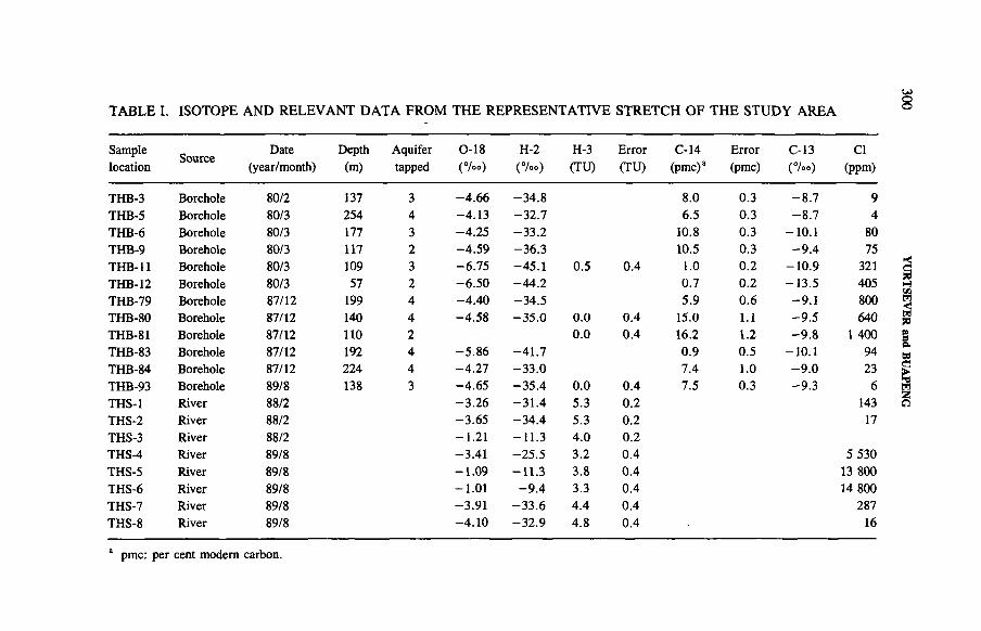
TABLE I. ISOTOPE AND RELEVANT DATA FROM THE REPRESENTATIVE STRETCH OF THE STUDY AREA

SampleSource

Date Depth Aquifer 0-18 H-2 H-3 Error C-14 Error C-13 Cllocation (year/month) (m) tapped (%») (°/=0) (TU) (TU) (pmc)a (pmc) (% 0) (ppm)

THB-3 Borehole 80/2 137 3 -4 .6 6 -3 4 .8 8.0 0.3 -8 .7 9THB-5 Borehole 80/3 254 4 -4 .1 3 -3 2 .7 6.5 0.3 -8 .7 4THB-6 Borehole 80/3 177 3 -4 .2 5 -3 3 .2 10.8 0.3 -10 .1 80THB-9 Borehole 80/3 117 2 -4 .5 9 -3 6 .3 10.5 0.3 - 9 .4 75THB-11 Borehole 80/3 109 3 -6 .7 5 -45 .1 0.5 0.4 1.0 0.2 -1 0 .9 321TUB-12 Borehole 80/3 57 2 -6 .5 0 -4 4 .2 0.7 0.2 -1 3 .5 405THB-79 Borehole 87/12 199 4 -4 .4 0 -3 4 .5 5.9 0.6 -9 .1 800THB-80 Borehole 87/12 140 4 -4 .5 8 -3 5 .0 0.0 0.4 15.0 1.1 -9 .5 640THB-81 Borehole 87/12 110 2 0.0 0.4 16.2 1.2 - 9 .8 1 400THB-83 Borehole 87/12 192 4 -5 .8 6 -4 1 .7 0.9 0.5 -10 .1 94THB-84 Borehole 87/12 224 4 -4 .2 7 -3 3 .0 7.4 1.0 - 9 .0 23THB-93 Borehole 89/8 138 3 -4 .6 5 -3 5 .4 0.0 0.4 7.5 0.3 -9 .3 6THS-1 River 88/2 -3 .2 6 -3 1 .4 5.3 0.2 143THS-2 River 88/2 -3 .6 5 -3 4 .4 5.3 0.2 17THS-3 River 88/2 -1 .21 -1 1 .3 4.0 0.2THS-4 River 89/8 -3 .41 -2 5 .5 3.2 0.4 5 530THS-5 River 89/8 -1 .0 9 -1 1 .3 3.8 0.4 13 800THS-6 River 89/8 -1 .01 - 9 .4 3.3 0.4 14 800THS-7 River 89/8 -3 .91 -3 3 .6 4.4 0.4 287THS-8 River 89/8 -4 .1 0 -3 2 .9 4.8 0.4 16

a pmc: per cent modern carbon.

300 YURTSEVER

and BU

APEN

G

IAEA-SM-319/29 301

R i v e r w a t e r i n f i l t r a t i o n R e c h a r g e

FIG. 6. Configuration adopted for the compartmental model (values above the line: observed isO content (°/oo); values below the line: observed 14С content (pmc)).

indicated clearly by the isotopic data in Fig. 4. Another feature of the isotope data is the effect of seawater intrusion, particularly in the southwestern part of the basin. The river water contribution, as an additional source of replenishment (shaded area in Fig. 4), only affects the upper aquifer layers (aquifer Nos 1-4) adjacent to the river, while the mixing of river water with the deeper aquifer layers (aquifer Nos 5-8) does not occur.

Similarly, the results of 14C analyses on the samples collected from the wells in the study area exhibit an increase in the I4C content in this mixing zone, which is obviously the result of the mixing of river water with the incoming lateral regional flow. Thus, groundwater ages from 14C data in the mixing zone cannot be calcu­lated with the usual radioactive decay equation. All of the wells sampled in the study area have also been analysed for their tritium content, and the values are all less than 1.0 tritium unit (TU).

The compartmental simulation approach has thus been used to evaluate the relative importance of river water replenishment in the upper aquifer layers using the spatial variations observed in the stable isotope data of 180 . The mixing propor­tions estimated on the basis of stable isotope data were then used to simulate the 14C variations observed in the mixing zone in order to arrive at groundwater residence time estimates of the water. The cross-section of the area is shown in Fig. 5, which refers to the multi-aquifer system of the upper four aquifers, in a representative stretch of the regional aquifer system. The wells tapping different aquifer units are assumed to represent the compartments, as shown in Fig. 5.

302 YURTSEVER and BUAPENG

The data for the wells located in the representative stretch are given in Table I. The main concept of the model is therefore to simulate the 180 and 14C distributions observed in the upper aquifers, which are assumed essentially to be the result of mix­ing between the incoming lateral regional flow and the vertical infiltration of river water, each with distinct isotopic input concentrations. The configuration adopted for the compartmental model and the isotope data observed, which is used as a basis for the calibration of the model, is shown in Fig. 6. The observed water level increase in groundwater wells in response to water levels in the river during higher river stages is also evidence of the hydraulic relationship between the river and the aquifer in the area adjacent to the river [12].

The simulation model adopted is used under steady state flow conditions. The isotope input for regional lateral flux is assumed to be <5180 = -6 .6 0 7 oo, equal to the long term mean isotope value of rainfall, and for the river water component it is assumed to be 0180 = -3 .4 6 7 00, as measured in river water samples near the representative stretch. The simulation model is run with relative units, assuming that the total recharge to the aquifers at the periphery of the basin is unity. The amount of lateral flux relative to the vertical flux from river water infiltration and the fluxes within the compartments have been allowed to vary until the observed 180 distribu­tion in the system could be reasonably simulated. On the basis of the distribution of the fluxes, as determined from the adopted compartmental model, the observed 14C distribution was then simulated by assigning an appropriate mean residence time to each compartment. In this regard, each compartment is assumed to represent the aquifer layer and the underlying clay formation. Thus, the observed 14C distribution in the system is assumed to be the result of mixing of the two component fluxes (at proportions derived from stable isotope simulation) and radioactive decay. For this purpose, the 14C isotope input to the system is taken to be 55 per cent modern carbon (pmc). The 13C data of the wells in the representative stretch used are very uniform (Table I). The intial 14C values for all of these wells are estimated by the following equation:

100(0 - 5C) / 2e \C0 = ------ -------— ( 1 + ----- ) (12)

ÔG - Sr + 6 V 1000/

where the 13C contents of 07oo, and -2 5 7 00 were used for aquifer carbonate and soil C 02, respectively. The value of the fractionation factor (e) between bicarbonate and soil C 02 is taken to be 8700.

The results of the above estimates for all of the wells located within the representative stretch indicate that the initial 14C values are within the range of 50-60 pmc, with an average value of 55 pmc, which is the input value used for the simulation. It should be noted that the total bicarbonate content of groundwater away from the mixing zone is in the range of 400-500 ppm, and that of river water is in

IAEA-SM-319/29 303

L a t e r a l flow

>> о с ф ,з ¿O’ai

River

100 200 300 400НС03 con ten t (ppm)

500 600

Fig. 7. Histogram o f H C03.

the range of 120-140 ppm, as can be seen from the histogram given in Fig. 7. Since the water flux from regional lateral flow is found to be smaller by a similar factor than that of the river infiltration flux, the bicarbonate fluxes of the two mixing com­ponents are comparable, and it can be assumed that the observed 14C contents are not significantly affected by this parameter.

Final results of the best fitting parameters of the compartmental model are given in Table II. The observed isotope data versus model simulated isotope data are plotted in Fig. 8. In the case of the 14C results, the error bars shown in Fig. 8 refer to simulations performed with input values of 50 and 60 pmc, in order to highlight the sensitivity of the model to this particular parameter.

The residence time distribution curves for each aquifer unit at the outlet (last compartment in the flow direction) are calculated from the calibrated compartmental model through simulation for the case of unit mass of input of a conservative tracer distributed proportionally to the water flux inputs. The shapes of the residence time distribution curves for each aquifer unit obtained in this way are shown in Fig. 9. The first moments of the residence time distribution curves also provide the mean residence time values for each aquifer, which are 7700, 12 100, 22 000 and 26 200 years for aquifer units 1-4, respectively. The curves for the cumulative distribution of the residence times, as derived from the calibrated model, are also shown in Fig. 10; they were obtained through simulation of a steady state tracer input of unit concentration.

U )

g

TABLE П. PARAMETERS OF THE BEST FIT MODEL

CompartmentNo.

Mean residence

time (x 100 a)

InflowLateraloutflow

Verticaloutflow

(all in relative units)

1.1 67 0.6250 0.7250 0.62502.1 25 0.6250 0.7250 0.03753.1 38 0.6250 0.1375 0.62504.1 400 1.0000 0.1375 0.86251.2 27 0.5000 0.13752.2 5 0.0125 0.13753.2 38 0.1125 0.62504.2 460 0.1125 0.75001.3 1 0.6750 0.13752.3 2 0.6350 0.13753.3 38 0.6750 0.03754.3 600 0.0875 0.66251.4 7 0.1125 0.08752.4 4 0.0625 0.08753.4 7 0.0125 0.08754.4 670 0.0625 0.6000

YURTSEVER and

BUA

PENG

Obs

erve

d U

C co

nten

t (p

mc)

Model c a l c u l a t e d WC c o n t e n t (pmc) Model c a l c u l a t e d ie0 (%©)

FIG. 8. Comparison o f model simulated and actual observed isotope data for (a) 14C and (b) 180.

ОLA

IAEA

-SM-319/29

‘• г

306 YURTSEVER and BUAPENG

0 1 2 3 ¿ 5 6Time [ y e a r s ! (xIO*)

FIG. 9. Shapes o f the residence time distributions o f water in different aquifer units( ------aquifer No. 1 ; ------------ : aquifer No. 2 ; ------------ : aquifer No. 3 ; ------- : aquiferNo. 4).

Time ( y e a r s ) (x10*)

FIG. 10. Shapes o f the cumulative residence time distributions in different aquifer units(------: aquifer No. 1; -------- : aquifer No. 2 ; ------------ : aquifer No. 3 ; ------- : aquiferNo. 4).

IAEA-SM-319/29 307

The result of the simulation model calibrated with the isotope data, as dis­cussed above, provides quantitative estimates of the relative importance of different sources in replenishment, internal flow dynamics and residence time distribution within the system. In this regard, river water infiltration is a significant source of recharge in an area adjacent to the river, and the average replenishment rate is 80% higher than the replenishment of the upper four aquifers from the rainfall on the periphery of the basin. In this regard, it should be noted that the relative contribution of river water is directly a function of the assumed stable isotopic composition for river water input. In the event of intermediate evaporation that may occur prior to recharge, the stable isotopic content will be further enriched and, consequently, the relative contribution of the river will be proportionally less. Therefore, the estimate given above is rather an upper limit.

The model also permits determination of the residence time distribution and mean residence times involved in groundwater flow within each aquifer unit. The use of 14C data in estimating these time parameters for the case where the water is a mixture of different component flows is not possible by the use of a simple age dating equation.

4. CONCLUDING REMARKS

The advantage of the compartmental simulation approach discussed in this paper lies in the simplicity of its application and the flexibility it provides in incor­porating known temporal and/or spatial variations in the input(s) and/or in relevant parameters of the system under consideration. The sizes and configurations of the compartments can be selected so as to replicate, as closely as possible, the known hydrogeological features of the system. Perhaps the most important aspect of the approach is its applicability under time variant flow conditions and/or time variant boundary conditions. Thus, the compartmental simulation approach provides a distributed parameter deterministic model that can be used as an interpretative tool for the quantitative evaluation of isotope data in hydrological systems under station­ary or non-stationary transport conditions.

ACKNOWLEDGEMENTS

The field research in the Bangkok Basin was supported by the IAEA through its research contract programme. The isotopic analyses were undertaken at the Isotope Hydrology Laboratory of the Agency Laboratory, Vienna. The contribution of B.R. Payne in the development of the computer code on the compartmental approach used in the paper is acknowledged.

308 YURTSEVER and BUAPENG

REFERENCES

[1] PRZEW-LOCKI, K., YURTSEVER, Y., “ Some conceptual mathematical models and digital simulation approach in the use of tracers in hydrological systems” , Isotope Techniques in Groundwater Hydrology 1974 (Proc. Symp. Vienna, 1974), Vol. 2, IAEA, Vienna (1974) 425-450.

[2] SIMPSON, S.E., “ Finite state mixing-cell models” , Proc. United States of America- Yugoslavia Seminar on Karst Hydrology and Water Resources, Dubrovnik, 1975.

[3] YURTSEVER, Y., PAYNE, B.R., “ A digital simulation approach for a tracer case in hydrological systems: Multicompartmental mathematical model” , Finite Elements in Water Resources (Proc. 2nd Int. Conf. London, 1978) (BREBBIA, C.A., GRAY, W .E., PINDER, G.E., Eds), Pentech Press, London (1978).

[4] CAMPANA, M.E., MAHIN, D.A., Model-derived estimates of groundwater mean ages, recharge rates, effective porosities and storage in a limestone aquifer, J. Hydrol. 76 3/4 (1985) 247-264.

[5] VAN OMMEN, H.C., The ‘mixing-cell’ concept applied to the transport of non­reactive and reactive components in soils and groundwater, J. Hydrol. 78 3/4 (1985) 201-214.

[6] YURTSEVER, Y., PAYNE, B.R., Time-Variant Linear Compartmental Model Approach to Study Flow Dynamics of a Karst Groundwater System by the Aid of Environmental Tritium, Publication No. 161, International Association of Hydro- logical Sciences, The Hague (1985).

[7] YURTSEVER, Y „ PAYNE, B.R., GOMEZ MARTOS, М., “ Use of linear compart­mental simulation approach for quantitative interpretation of isotope data under time variant flow conditions” , Mathematical Models for Interpretation of Tracer Data in Groundwater Hydrology (Proc. Advisory Group Mtg Vienna, 1984), IAEA- TECDOC-381, IAEA, Vienna (1986) 203-222.

[8] YURTSEVER, Y., PAYNE, B.R., “ Mathematical models based on compartmental simulation approach for quantitative interpretation of tracer data in hydrological sys­tems” , Proc. 5th Int. Symp. on Groundwater Tracing, Athens, 1986.

[9] YURTSEVER, Y., “ Concepts and model formulations for quantitative evaluations with natural isotopes in groundwater systems” , Groundwater and the Environment (Proc. 2nd Int. Conf. Kota Bahru, 1990), Universiti Kebangsaan Malaysia, Bangi, Selangor (1990).

[10] BUAPENG, S., The Use of Environmental Isotopes on Groundwater Hydrology in Selected Areas in Thailand, final report of a research contract submitted to the IAEA, 1990.

[11] INTERNATIONAL ATOMIC ENERGY AGENCY, Statistical Treatment of Environ­mental Isotope Data in Precipitation, Technical Reports Series No. 206, IAEA, Vienna (1981).

[12] Groundwater Resources in the Bangkok Area: Development and Management Study, Department of Mineral Resources and Asian Institute of Technology, Bangkok (1982).

IAEA-SM-319/39

ESTIMATION DES FLUX D’EVAPORATION DIFFUSE SOUS COUVERT SABLEUX EN CLIMAT HYPER-ARIDE (ERG DE BILMA, NIGER)

J. F. ARANYOSSY*, A. FILLY**, A.A. TANDIA0,D. LOUVAT00, B. OUSMANE +, A. JOSEPH ++',J.-C. FONTES**

* Projet AIEA RAF/8/012,Dakar, Sénégal

** Laboratoire d’hydrologie et de géochimie isotopique, Université de Paris-Sud,Orsay, France

0 Département de géologie,Université C.A. Diop,Dakar, Sénégal

00 Section d’hydrologie isotopique,Agence internationale de l’énergie atomique,Vienne

+ Direction de la recherche scientifique,Ministère de l’enseignement supérieur,Niamey, Niger

++ Département de géologie,Université de Niamey,Niamey, Niger

Abstract-Résumé

ESTIMATION OF DIFFUSE EVAPORATION RATES UNDER SANDY COVER IN A HYPER-ARID CLIMATE (ERG DE BILMA, NIGER).

The hyper-arid Erg de Bilma, in the far east of Niger, combines favourable climatic, pedological and hydrogeological conditions which are ideal for calibration of the steady state evaporation model based on the isotopic evolution of water (180 and 2H) in the unsaturated zone. The only variable is the water table depth. Sensitivity tests on the various parameters introduced in the model have made it possible to obtain the best fit for the five profiles presented (from a depth of 25 cm to 2.3 m). These tests show the importance of temperature, relative humidity, isotopic composition of the reservoir and isotopic composition of atmospheric water vapour. The evaporation rate decreases exponentially as a function of water table depth: it is close to the potential évapotranspiration rate when the water table is near the

309

310 ARANYOSSY et al.

surface (900 mm per year at 25 cm) and about 10 mm per year when the water table is at a depth of 2 m.

ESTIMATION DES FLUX D’EVAPORATION DIFFUSE SOUS COUVERT SABLEUX EN CLIMAT HYPER-ARIDE (ERG DE BILMA, NIGER).

L ’erg hyper-aride de Bilma, à l’extrême est du Niger, réunit des conditions climatiques, pédologiques et hydrogéologiques très favorables à la calibration du modèle d’évaporation en régime permanent fondé sur l’évolution isotopique de l’eau ( l80 et 2H) dans la zone non saturée. La seule variable est la profondeur de la zone noyée. Les tests de sensibilité des différents paramètres introduits dans le modèle ont permis de procéder au meilleur ajustement des cinq profils présentés (25 cm à 2,3 m de profondeur). Ces tests montrent l’importance de la température, de l’humidité relative, de la composition isotopique du réservoir et de la composition isotopique de la vapeur d ’eau atmosphérique. Le flux évaporatoire décroît de façon exponentielle en fonction de la profondeur de là nappe: les valeurs sont proches de l ’évapotranspiration potentielle lorsque la nappe est proche du sol (900 mm/an à 25 cm), et d ’une dizaine de millimètres par an à 2 m de profondeur.

1. INTRODUCTION

L’estimation de la recharge directe des nappes libres par les précipitations et des pertes évaporatoires demeure, particulièrement en zones arides et semi-arides, un problème majeur pour les hydrogéologues et gestionnaires. L’application des méthodes dites «classiques» fondées sur les paramètres climatiques (formules empi­riques), sur l’enregistrement des fluctuations piézométriques ou sur la mesure des paramètres hydrodynamiques du sol est fortement limitée en raison des valeurs très faibles de l’infiltration efficace ou du flux évaporatoire net annuel.

Les études théoriques et les expériences en laboratoire [1-3] ont montré que l’interprétation des profils de teneurs en isotopes stables de l’eau interstitielle du sol non saturé permet l’estimation du flux évaporatoire en régime permanent à partir d’un réservoir d’eau souterraine. Cette méthode, appliquée sur le terrain dans de nombreuses régions du globe (Egypte [3], Australie [4], Tunisie [5], Algérie [6- 8], Chili [9], Chine [10]), s’est également développée ces dernières années dans la bande sahélienne [11-13]. Cependant, les imprécisions de la méthode et les difficultés rencontrées dans l’interprétation des profils obtenus en zones semi-arides résident principalement dans: 1) l’alternance de phases de recharge et de reprise évapora­toire, qui ne permet probablement pas l’installation du régime de flux permanent requis par le modèle; 2) la difficulté d’estimation de certains paramètres du modèle;

%) l’hétérogénéité des recouvrements de sol dans lesquels sont réalisés les profils.Nous avons donc recherché une zone aux conditions climatiques, pédologiques

et hydrogéologiques favorables à l’application du modèle afin de préciser l’influence respective des paramètres utilisés sur la valeur calculée du flux évaporatoire.

IAEA-SM-319/39 311

FIG. 1. Carte de situation de Bilma: 1) Môle d ’In Guézam; 2) Socle du bouclier Touareg; 3) Isohyète; 4) Température moyenne annuelle.

2. CARACTERISTIQUES DU SITE DE BILMA

Dans la partie orientale hyper-aride du Niger (fig. 1), la cuvette de Bilma (18°41N, 12°55E) satisfait à ces conditions par:

— l’absence quasi complète de précipitations (P < 20 mm/an), qui garantit la réalisation d’un régime permanent du flux évaporatoire aussi bien en phase vapeur qu’en phase liquide;

312 ARANYOSSY ét al.

— les fortes températures (46°C en juin-juillet, 27°C moyenne annuelle) ainsi que la très faible humidité relative (5% avril-mai, 13% moyenne annuelle), qui engendrent une évaporation très élevée (ETP 4500 mm/an);

— la présence d’une nappe fossile, sub-affleurante en certains points de la dépres­sion de Bilma, situation qui permet de choisir l’épaisseur de la zone non saturée à échantillonner;

— la granulométrie très homogène des sables dunaires de recouvrement qui assure la bonne constance des paramètres moyens du sol (porosité, tortuosité);

— l’absence de végétation qui permet de s’affranchir des problèmes d’estimation de Г évapotranspiration [14].

L’alimentation per ascensum de la nappe phréatique par les eaux holocènes en charge très faiblement salines, en provenance des formations gréseuses du Crétacé supérieur, ne donne pas lieu à des précipitations salines dans les profils. Seules, de minces croûtes de sel sont visibles à la superficie du sol dans les parties les plus déprimées de la cuvette où la nappe est proche de la surface du sol.

3. PROTOCOLE ÉXPERIMENTAL

3.1. Prélèvements de sol

Les échantillons de sol non saturé sont prélevés à différentes profondeurs (si possible, jusqu’à la nappe), afin de procéder à l’extraction et à l’analyse de l’eau interstitielle. Pour les horizons superficiels très secs (humidité volumique inférieure à 1%), l’emploi d’une tarière spéciale à clapet [8] et le tubage à l’avancement sont nécessaires. Les échantillons sont immédiatement conditionnés dans des boîtes étanches afin d’éviter toute évaporation ultérieure au prélèvement. Afin de tenir compte de l’évolution isotopique dans le profil, l’échantillonnage est modulé en fonc­tion de la profondeur: prélèvements centimétriques en surface, puis décimétriques et métriques à partir de 5 m (tableau I). L’extraction de l’eau interstitielle est obtenue par la méthode de distillation sous vide sur des fractions aliquotes des échantillons de sol [15].

3.2. Prélèvements des gaz du sol

Dans le cas de forts recouvrements sableux très secs, comme les dunes de sable, nous avons adopté le principe de Thoma et al. [16] simplifié [8, 17]. )Une aiguille creuse munie en son extrémité d’une pointe crépinée est introduite à la profondeur choisie. La pointe est reliée à une ampoule à vide par un tube fin en poly­éthylène dont l’atmosphère est lentement remplacée par celle du sol par pompage manuel. L’ouverture progressive de l’ampoule à vide permet le prélèvement des gaz du sol en quelques minutes sans effet de vaporisation.

IAEA-SM-319/39 313

TABLEAU I. RESULTATS ANALYTIQUES DISPONIBLES SUR LE SITE DE BILMA(Z1-Z2: intervalle de prélèvement; Hv: humidité volumique)

H Z1 Z2 Hv 0-18 H-2(m) (m) (X) <X.) (X.)

BlL-1- 1 0.00 0.01 0.22BH-1- 2 0.01 0.03 0.238IL-1- 3 0.03 0.05 0.40BlL-1- u 0.05 0.08 0.3681L-1- 5 0.08 0.11 0.30 16.6 -21.0BIl-1- 6 0.11 0.15 0.75 15.96 -24.9BIL-1- 7 0.15 0.20 1.80 2.52 -52.4BtL-1- 8 0.20 0.25 2.85 2.66 -47.9BIL-1- 9 0.25 0.30 1.95 -1.27 -56.6BIl-1- 10 0.30 0.35 2.55 -3.67 -60.7BIl-1- 11 0.35 0.40 3.45 -5.25 -66.4BIL-1- 12 0.40 0.48 3.45 -6.25 -68.7BlL-1- 13 0.48 0.55 4.05 -7.68 -73.7Bll-1- U 0.55 0.65 6.45 -8.47 -75.2BlL-1- 15 0.65 0.75 7.95 -8.2 7 -71.4BIL-1- 16 0.75 0.85 17.40 -8.58 -71.6BlL-1- 17 0.85 1.00 28.05 -8.94 -73.18JL-2- 1 0.00 0.02 0.56 5.47BlL-2- 2 0.02 0.04 4.07 15.14BIL-2- 3 0.04 0.06 6.62 3.55BIL-2- 4 0.06 0.08 6.86 -2.47BlL-2- 5 0.08 0.10 7.41 -4.58BU-2- 6 0.10 0.15 9.77 -8.58BIL-2- 7 0.15 0.20 12.15 -10.71 -85.3B1L-2- 8 0.20 0.25 14.88 -9.31BIL-2- 9 0.25 0.30 1S.69 -9.42BIL-2- 10 0.30 0.35 17.52 -9.45BIl-2- 11 0.35 0.40 18.78 -9.54811-2- 12 0.40 0.45 24.44 -9.14BIl-2- 13 0.45 0.50 26.19 -9.00BIl-2- U 0.50 0.55 26.67 -8.92BIL-2- 15 0.55 0.75 32.48 -8.74BIL'2* 16 0.65 0.85 34.95 -9.14BR-10- 1 0.00 0.01 30.75 0.68 -31.50BIL-10- 2 0.01 0.02 25.95 -4.50 -52.90BIL-10- 3 0.02 0.04 15.75 -8.16 -64.40BIL-10- 4 0.04 0.06 18.60 -8.24 -65.20BtL-10- 5 0.06 0.08 18.00 -8.21 -64.70BIL-10- 6 0.08 0.10 17.70 -7.98 -65.60BIL-10- 7 0.10 0.15 22.35 -8.41 -65.00BIL-10- 8 0.15 0.20 26.55 -8.46 -64.90BIL-10- 9 0.20 0.25 28.35 -8.37 -66.10BIL-10- 10 0.25 0.30 29.40 -8.44 -64.50

314 ARANYOSSY et al.

TABLEAU I. (suite)

N ZI Z2 Hv 0-18 H-z

(m) (m) (X) (X.) (X.)

BIl-8- 1 0.00 0.02Bll-8- 2 0.02 0.05BIl-8- 3 0.05 0.088IL-8- « 0.08 0.10BIL-8- 5 0.10 0.15 7.20 -15.20BlL-8- 6 0.15 0.20 8.55 9.04 -31.10BIL-8- 7 0.20 0.25 10.95 -0.39 -44.60BIL-8- 8 0.25 0.30 9.75 3.21 -39.70BIl-8- 9 0.30 0.35 10.65 -2.49 -53.00Bll-8- 10 0.35 0.40 11.10 -4.00 -56.70BIl-8- 11 0.40 0.45 13.50 -4.22 -54.80BIl-8- 12 0.45 0.50 14.85 -5.62 -61.10BIL-8- 13 0.50 0.60 15.15 -6.34 -62.40B1C.-8- 14 0.60 0.70 16.35 -6.08 -63.50BIl-8- 15 0.70 0.80 19.95 -8.64 -79.30BIL-8- 16 0.80 0.90 21.30 -6.71 -64.50BIL-8- 17 0.90 1.00 23.85 -6.80 -62.00BIL-8- 18 1.00 1.10 24.30 -7.06 -61.90BIL-8- 19 1.10 1.20 26.70 -7.09 -61.00BIL-8- 20 1.20 1.30 30.00 -11.70 -96.80

BIL-9- 1 0.00 0.03 0.29BIL-9- 2 0.03 0.05 0.30 -9.58BIl-9- 3 0.05 0.10 0.53 -2.24BIL-9- 4 0.10 0.20 2.48 5.37 -42.8Bll-9- 5 0.20 0.30 0.51 8.30 -37.3BIL-9- 6 0.30 0.40 0.41 7.84 -40.9BtL-9- 7 0.40 0.50 0.26 6.67 -41.2BU-9- 8 0.50 0.60 0.22 7.30 -34.5BtL-9- 9 0.60 0.70 2.60 3.42 -57.8BIl-9- 10 0.70 0.80 2.84 4.92 -61.0BtL-9- 11 0.80 0.90 3.05 3.70 -49.2BIl-9- 12 0.90 1.00 4.35 0.79 -51.4BlL-9- 13 1.00 1.10 4.65 -1.29 -56.2BIL-9- 14 1.20 1.30 16.95 -6.13 -66.1.BIL-9- 15 1.30 1.40 8.70 -4.98 -67.0BIL-9- 16 1.50 1.60 27.30 -9.04 -80.5Bll-9- 17 1.70 1.80 17.55 -7.67 -65.7Bll-9- 18 1.80 1.90 19.95 -7.79 -65.7BlL-9- 19 2.00 2.10 21.90 -7.77 -65.3BIL-9- 20 2.20 2.30 25.20 -7.89 -65.5

4. RESULTATS

Huit profils de sol correspondant à des profondeurs de nappe entre 25 cm et 400 cm ont été réalisés. Ils ont été complétés par deux profils de gaz de plus grande profondeur (6 et 10 m) et par des prélèvements de la vapeur atmosphérique du site. Cinq profils isotopiques de sol sont à ce jour disponibles (tableau I).

IAEA-SM-319/39 315

Humidité volumique (%) 0-18 (%o / SMOW)

Humidité volumique (%) 0-18 (%o / SMOW)

FIG. 3. Profil «long» (BIL-9).

Sauf pour le profil le plus court, l’humidité (fig. 2 et 3) évolue régulièrement entre des teneurs extrêmement faibles en surface (inférieures à 1 %) et la saturation du sable dunaire (30 à 35%). Ceci suggère l’absence de recharge verticale par les rares épisodes pluvieux qui sont totalement et rapidement repris par évaporation.

4.1. Les profils isotopiques

Les profils isotopiques présentent des allures sensiblement différentes suivant la profondeur de la nappe.

316 ARANYOSSY et al.

Sur les profils très courts (BIL-10: 25 cm, BIL-2: 65 cm), l’effet de capillarité prédomine et maintient inchangée la valeur de la composition isotopique du réservoir sur la majeure partie de l’épaisseur de la zone non saturée (fig. 2). L’enrichissement isotopique dû à l’évaporation n’apparaît qu’à proximité immédiate du sol (3 cm pour BIL-10, 15 cm environ pour BIL-2). L’échange diffusif avec la vapeur atmosphé­rique n’est pas visible sur le profil de 25 cm — où il n’affecte sans doute que les premiers millimètres du sol — tandis qu’il n’atteint que 3 cm de profondeur sur le profil de 65 cm. Ceci suggère qu’en condition d’évaporation intensive et permanente le régime permanent peut s’établir même à proximité immédiate du sol.

Sur les profils d’épaisseur plus importante (à partir d’un mètre environ) se développe en profondeur la forme caractéristique de l’évolution isotopique (fig. 3) due à l’effet combiné de: 1) la remontée de l’eau de la nappe vers le haut du profil par capillarité; 2) l’enrichissement isotopique à l’évaporation; 3) la rétrodiffusion des isotopes lourds vers la nappe; 4) l’échange et le mélange avec les isotopes légers de la vapeur d’eau atmosphérique par rétrodiffusion de celle-ci dans la zone de transit gazeux dominant. Le profil est caractérisé par la production d’un maximum d’en­richissement à une profondeur considérée comme la limite entre le transit liquide dominant et le transit gazeux dominant [1]. Quelques valeurs erratiques attribuées à des artefacts ne sont pas prises en compte dans la modélisation.

Les calculs de corrélation ô2H/ô180 (fig. 4) donnent généralement des valeurs de pente très faibles et bien groupées autour de 2. Ces valeurs souvent obtenues au laboratoire ou sur le terrain dans des conditions similaires [3, 18] n’ont pas reçu d’explication théorique. Seul le profil court (BIL-10) fournit une valeur de pente supérieure (a = 3,67; r2 = 0,99) qui peut être liée à l’influence prépondérante des transports en phase liquide dans ce profil.

FIG. 4. Relation oxygène 18/deutérium (BIL-1).

IAEA-SM-319/39 317

4.2. Interprétation quantitative

Les formes des profils de teneurs en eau et en isotopes lourds indiquent que les conditions de régime permanent d’évaporation sont établies. Les flux évaporatoires peuvent être estimés selon les deux approches semi-indépendantes de Barnes et Allison [1] dont on rappelle ci-dessous le formalisme.

Dans la zone où domine le transfert liquide, l’équation de bilan isotopique s’écrit:

dans laquelle ô représente la teneur isotopique à la cote z, l’indice i désigne l’isotope considéré ( 180 ou 2H); ôres est la teneur en isotopes lourds de l’eau du réservoir en état d’évaporation et ôef la teneur isotopique du pic d’enrichissement à la profondeur zefi le paramètre z représente la «profondeur caractéristique» du système, liée au taux d’évaporation E par la relation:

où в est l’humidité volumique moyenne dans le profil, r le coefficient de tortuosité et Diiq le coefficient de diffusion de l’espèce isotopique dans l’eau, assimilable à la diffusivité de l’eau dans elle-même (D)iq[10' 9 m2-s"’] = exp (0,127 + 0,0236 t), [t en degrés Celsius]). Le coefficient z est déterminé par calcul de la pente de la corrélation linéaire ln [(ó¡ - ôres)/(ôef - ôres)] vsf(z).

La fonction f(z) «fonction de profondeur» est définie soit par la relation:

qui rend compte de la variation de l’humidité volumique, soit par la «relation f(z) modifiée» afin de prendre en compte la redistribution isotopique en phase gazeuse dans le profil [19]:

où Nsat représente la masse de vapeur d’eau par unité de volume à saturation (N53, [g‘m 3] = exP (1.68 + 0,0562 t), [t en degrés Celsius]), Dvap la diffusivité de la vapeur dans l’air à la température considérée (Dvap = 0,0126 t + 2,17) [20], p la porosité totale et p la masse volumique de l’eau liquide.

ô, - ôres = (ôef - Ôres) exp [f(z)/£] (D

Z = в rDliq/E (2)

(3)

(4)

318 ARANYOSSY et al.

H-2 (%» / SMOW)-80 -70 -60 -50 -40 -30 -20 -10О --------—----------- 1---------- 1-----------1---------- 1------ -----1----------

0,1

0,7

FIG. 5. Influence du choix de la «fonction de profondeur» (f(z)) sur la simulation des profils (exemple du profil B1L-1).

Si le choix de la fonction f(z) semble avoir peu d’influence sur la valeur du coefficient de corrélation de la relation ln [(ô; - ôres)/(ôef - ôres)] versus f(z), l’ajustement des courbes simulées à la courbe expérimentale est en revanche nette­ment meilleur en utilisant la fonction f(z) corrigée (fig. 5). Avec f(z) corrigée, les estimations du taux d’évaporation sont nettement plus élevées (par exemple de 8,5 à 40,1 mm/an pour le profil BIL-1). Ceci démontre l’importance de la redistribution isotopique en phase vapeur sous le front d’évaporation dans les profils particulière­ment secs. Nous utiliserons donc la fonction f(z) corrigée pour l’estimation des flux évaporés.

Peu de résultats sont pour le moment disponibles pour une comparaison avec l’évolution isotopique dans la zone de transfert vapeur dominant.

La simulation est basée sur l’équation de bilan [1]:

où a est le facteur de fractionnement entre l’eau vapeur et l’eau liquide (ln a lg = 1137T'2 - 0,4156т"1 - 0,00207 et ln a2 = 24844T'2 - 76,248T-' + 0,05261 avec T en K) [21], e le facteur d’enrichissement (6 = 1 - a), ha l’humidité relative atmosphérique, ôa la teneur en isotopes lourds de la vapeur d’eau atmosphérique. Le paramètre rj rend compte de «l’effet cinétique» dû à la diffusion plus ou moins rapide des espèces isotopiques dans l’air:

ô> = « i1 {ôa + e, + [rji (1 - ôres) 4- (ôres - ôa)] [z/(z + haz)]} (5)

r,, = (Dvap/D*)n - 1 (6)

avec D* coefficient de diffusion dans l’air de la vapeur comportant l’isotope i; n exposant de diffusivité dépend de l’agitation de l’air dans le milieu et est certaine­ment proche de 1,0 pour l’atmosphère sans turbulence des sols [22].

IAEA-SM-319/39 319

Le calcul du flux évaporatoire est effectué à partir de la relation entre l’humidité atmosphérique moyenne et la profondeur du pic d’enrichissement:

ha = 1 - (zef/z) (7)

où z, la «profondeur de pénétration», est définie par Barnes et Allison [1]:

z = Nsat D*//oE (8)

et D* est la diffusivité réelle dans le profil liée aux caractéristiques du sol par la relation:

Dv* = (p - 0) rDv (9)

r étant la tortuosité.Les profils en phase gazeuse sont beaucoup plus sensibles aux variations

saisonnières de température que la partie plus profonde du sol pour laquelle on adopte la valeur de température moyenne annuelle. En utilisant une température cor­respondant à la valeur moyenne de la période de prélèvement, les équations (7), (8) et (9) donnent des résultats similaires à ceux qui sont obtenus pour la phase liquide.

4.3. Estimation et poids des différents paramètres

L’influence respective des différents paramètres sur l’ajustement des profils isotopiques expérimentaux et calculés ainsi que sur la valeur finale du flux évaporatoire est traitée avec un logiciel tableur. Les paramètres, fonctions liées et valeurs calculées sont interactifs et permettent la visualisation des modifications introduites, spécifiquement pour la partie inférieure du profil à transit liquide dominant.

La température, bien que n’apparaissant pas directement dans les formules du modèle, intervient dans le calcul de nombreux paramètres (a, Nsat, D)iq, Dvap). Elle influence de manière très sensible le calcul du flux d’évaporation. Une variation de1 °C entraîne une différence d’environ 7% de la valeur calculée du taux d’évapora­tion (fig. 6). L’influence de cette variation sera d’autant plus grande que le profil est plus superficiel et davantage soumis aux variations saisonnières. Cette variabilité impose la connaissance précise des profils de température pour l’utilisation de la méthode.

La valeur de la composition isotopique du pic (ôef) pèse de façon significative dans l’ajustement de la courbe simulée mais n’influence pas le calcul du flux E; seule change l’ordonnée à l’origine de la relation: ln [(ó¡ — ôrcs)/(ôef — <5res)]/f(z).

L’ajustement des courbes ainsi que la valeur du flux E sont très sensibles au choix de la teneur isotopique du réservoir (ôres) (fig. 6). Pour un intervalle de

320 ARANYOSSY et al.

2000

'с* flj£ 1500 g фI 1000 b.Оa<Qî 5003 LL

0-10 -9,5 -9 -8,5 -8

Teneur isotopique du réservoir (0-18%o / SMOW)

FIG. 6. Sensibilité du modèle en phase liquide. Variation de l ’évaporation en fonction de la teneur isotopique du réservoir et de la température (profil BIL-10).

ôresl80 de -9 ,5°/00 à -8 ,5700, la variation relative du flux d’évaporation calculé est de 80%. Il est donc important de pousser l’échantillonnage jusqu’à la nappe au bas du profil ou au moins jusqu’à une valeur constante de la composition isotopique de chaque profil — pour une bonne estimation de ce paramètre. Par ailleurs, la comparaison des résultats des profils l80 et 2H sur site donné ne peut être effectuée que si les valeurs de <5res l80 et ôres2H obéissent à la corrélation ô2H/ô l80 de l’ensemble du profil en phase liquide.

La tortuosité, paramètre difficilement mesurable — pour lequel nous avons adopté la valeur, classique pour le sable, de 0,66 [23] — intervient cependant de façon directement proportionnelle dans le calcul du flux évaporatoire (formule 2) et devrait donc faire l’objet d’une évaluation plus précise pour chaque type de sol étudié.

La densité humide intervenant dans les calculs de l’humidité volumique doit être également déterminée précisément par des prélèvements non destructifs d’échantillons de sol sur le terrain.

Pour la partie supérieure du profil à transit dominant en phase gazeuse, l’ajustement des courbes est très sensible au choix de la teneur isotopique de la vapeur d’eau atmosphérique et de la valeur de l’exposant de diffusivité. Le meilleur ajustement du profil BIL-9 (pic 0,4 m) est obtenu pour la valeur mesurée de ô180 = -16,4 et pour n proche de 1. Ces paramètres n’interviennent cependant pas directement dans le calcul du flux d’évaporation pour lequel les facteurs les plus sensibles sont:

— la profondeur (zef) du pic d’enrichissement, à laquelle E est inversement proportionnel. La détermination précise de zef impose de détailler l’échantil­lonnage jusqu’à une profondeur de l’ordre du mètre sous la surface, dans le cas des profils secs et à granulométrie fine;

IAEA-SM-319/39 321

FIG. 7. Sensibilité du modèle en phase gazeuse. Variation de l'évaporation en fonction de la température et de l'humidité atmosphérique (BIL-9).

TABLEAU II. RESULTATS DES SIMULATIONS EN PHASE LIQUIDE

Profil Profil nappe (m)

Profil pic (m)

Oxygène 18 Deutérium

f(z)cor.

f(z)ncor.

f(z)cor.

f(z)ncor.

BIL-10 0,3 0,05 900,1 715,4 916,9 758,4

BIL-2 0,6 0,03 147,5 96,5

BIL-1 0,9 35,5 8,5 34,6 8,5

BIL-8 1,3 30,7 25,3 28,6 20,4

BIL-9 2,3 12,2 0,6

— Y humidité relative atmosphérique: une variation de 5% dans son estimation entraîne une erreur de 10% sur le calcul de l’évaporation (fig. 7);

— la température, qui influence de façon exponentielle le coefficient de diffusion (fig. 7);

— la porosité, qui conditionne le transit en phase vapeur.

4.4. Taux d’évaporation en fonction de la profondeur de la nappe

Les résultats des calculs pour les différents profils sont présentés dans le tableau II. Ils démontrent une décroissance très rapide du flux évaporatoire en fonc-

322 ARANYOSSY et al.

Flux évaporatoire (mm/an)0 100 200 300 400 500 600 700 800 900 1000

FIG. 8. Résultats des calculs de simulation. Evaporation en fonction de la profondeur de la nappe.

tion de la profondeur (une dizaine de millimètres à 2 m) de la nappe (fig. 8). Ils s’ajustent de façon satisfaisante à une courbe de décroissance exponentielle de forme:

E = Eq е-№ (10)

où h est la profondeur de la zone noyée, E0 l’évaporation potentielle, k un paramètre de forme (dimension L 1) qui caractérise la résistance du terrain au transit de l’eau entre la nappe et l’atmosphère.

Il est remarquable que, même à la base des profils les plus courts, la teneur en isotopes lourds est différente de celle de la nappe. Ceci suggère que la rétro­diffusion isotopique dans le profil reste sensible même lorsque le flux d’évaporation est intense. La partie supérieure de la nappe ne serait pas homogénéisée. Ceci ouvre des perspectives sur l’intérêt d’une étude détaillée des variations de teneurs en iso­topes lourds entre un aquifère libre et sa frange capillaire dans les régions fortement évaporantes.

IAEA-SM-319/39 323

REMERCIEMENTS

La mission d’échantillonnage et les analyses ont été effectuées dans le cadre des activités du projet régional de coopération technique de l’AIEA (RAF/8/012) sur «le développement de techniques isotopiques et nucléaires en hydrologie dans les pays du Sahel» (qui inclut le Sénégal, le Mali, le Niger et le Cameroun) en collabora­tion avec le Laboratoire d’hydrologie et de géochimie isotopique de l’Université de Paris-Sud. Le programme a été soutenu par le projet «Campus» entre l’Université de Niamey et l’Université de Paris-Sud.

Nous remercions tous ceux qui ont prêté leur concours à la réalisation de la mission d’échantillonnage, aux extractions et aux analyses en laboratoire.

REFERENCES

[1] BARNES, C.J., ALLISON, G.B., The distribution of deuterium and l80 in dry soils, 1. Theory, J. Hydrol. 60 (1983) 151-156.

[2] MÜNNICH, К.О., SONNTAG, С., CHRISTMANN, D., THOMA, G., Isotope fractionation due to evaporation from sand dunes, 2. Mitt. Zentral Isot. Strahlenforsch. 29 (1980) 319-322.

[3] SONNTAG, C., CHRISTMANN, D., MÜNNICH, K.O., «Laboratory and field experiments on infiltration and evaporation of soil water by means of deuterium and oxygen-18», Stable and Radioactive Isotopes in the Study of the Unsaturated Soil Zone,IAEA-TECDOC-357, AIE A, Vienne (1985) 145-159.

[4] ALLISON, G.B., BARNES, C.J., Estimation of evaporation from the normally «dry» Lake Frame in South Australia, J. Hydrol. 78 (1985) 229-242.

[5] ZOUARI, K., ARANYOSSY, J.F ., MAMOU, A., FONTES, J.-Ch., «Etude isoto- pique et géochimique des mouvements et de l’évolution des solutions de la zone aérée des sols sous climat semi-aride (Sud tunisien)», Stable and Radioactive Isotopes in the Study of the Unsaturated Soil Zone, I AEA-TECDOC-357, AIEA, Vienne (1985) 121-143.

[6] YOUSFI, М., ARANYOSSY, J.F., DJERMOUNI, В., FONTES, J.-Ch., «Etude isotopique des mouvements de l ’eau en zone non saturée sous climat aride (Algérie)», ibid., 161-178.

[7] FONTES, J.-C., YOUSFI, M., ALLISON, G.B., Estimation of long-term diffuse groundwater discharge in the northern Sahara using stable isotope profiles in soil water, J. Hydrol. 86 (1986) 315-327.

[8] COLIN-KACZALA, C., Profils isotopiques ( l80 et 2H) de fluides (eau liquide, vapeur et C 0 2) de la zone non saturée sous climat désertique: application à l’évalua­tion de l’évaporation des nappes libres au Sahara Nord Occidental, Thèse Université de Paris-Sud (1988).

[9] GRILLI, A., POLLASTRI, A., ORTIZ, J., AGUIRRE, E., «Evaluación de tasas de evaporación desde salares, utilizando técnicas isotópicas — Aplicación en el Salar de Bellavista, Chile», Isotope Hydrology Investigations in Latin America, IAEA- TECDOC-502, AIEA, Vienne (1989) 155-168.

324 ARANYOSSY et al.

[10] FONTES, J.-C., et al., «Estimating seasonal recharge/discharge processes through the unsaturated zone of the Chinese loess from tritium and stable isotope profiles» (Proc. 2nd Chino-Japan Joint Symp. on Geochron. Cosmochim. and Isot. Geol.), Chinese Soc. of Min. Petrochemistry, Beijing (1991).

[11] GAYE, C.B., Etude isotopique et géochimique du mode de recharge par les pluies et de la décharge évaporatoire des aquifères libres sous climat semi-aride au nord du Sénégal, Thèse d ’Etat, Université C.A. Diop, Dakar (1990).

[12] TANDIA, A.A., Revue critique des méthodes d’évaluation de la recharge des nappes. Contribution de l’approche géochimique et isotopique (Louga, Nord-Sénégal), Thèse 3ème cycle, Université C.A. Diop, Dakar (1990).

[13] TAUPIN, J .D ., Evaluation isotopique de l’évaporation en zone non saturée sous climat sahélien et évolution géochimique des solutions du sol (vallée du Moyen-Niger), Université de Paris-Sud, Orsay (1990).

[14] ALLISON, G.B., BARNES, C.J., HUGHES, M.W., LEANEY, F.W .J., «Effect of climate and vegetation on oxygen-18 and deuterium profiles in soil», Isotope Hydrology 1983 (C.R. Coll. Vienne, 1983), AIEA, Vienne (1984) 105-123.

[15] GOUVEA DA SILVA, R., Migration des sels et des isotopes lourds à travers des colonnes de sédiments non saturés sous climat semi-aride, Thèse 3ème cycle, Université de Paris VI (1980).

[16] THOMA, G., ESSER, N., SONNTAG, C., WEISS, W., RUDOLPH, J., LEVEQUE, P.,«New technique of in-situ soil-moisture sampling for environmental isotope analysis applied at Pilât sand dune near Bordeaux: HETP modelling of bomb tritium propagation in the unsaturated sand saturated zones», Isotope Hydrology 1978 (C.R. Coll. Neuherberg, 1978), Vol. 2, AIEA, Vienne (1979) 753-768.

[17] ALLISON, G.B., COLIN-KACZALA, C., FILLY, A., FONTES, J.-Ch., Measure­ment of isotopic equilibrium between water, water vapour and soil C 0 2 in arid zone soils, J. Hydrol. 95 (1987) 131-141.

[18] SONNTAG, C., THOMA, G., MÜNNICH, K.O., DINÇER, T., KLITZSCH, E., «Environmental isotopes in North African groundwaters, and the Dahna sand-dune study, Saudi Arabia», Arid Zone Hydrology: Investigations with Isotope Techniques (C.R. Réunion groupe d ’étude Vienne, 1978), AIEA, Vienne (1980) 77-84.

[19] BARNES, C.J., ALLISON, C.B., The distribution of deuterium and oxygen-18 in dry soils: III. Theory for non-isothermal water movement, J. Hydrol. 74 (1984) 119-155.

[20] DE VRIES, D.A., KRUGER, A.J., «On the value of the diffusion coefficient of water vapour in air», Phénomènes des transports avec changements de phases dans les milieux poreux ou colloïdes (C.R. Coll. CNRS, Paris, 1967), CNRS, Paris (1967) 61-72.

[21] MAJOUBE, M., Fractionnement en oxygène-18 et en deutérium entre l’eau et sa vapeur, J. Chim. Phys. 68 (1971) 1423-1436.

[22] CRAIG, H., GORDON, I.L., «Deuterium and oxygen-18 variations in the ocean and the marine atmosphere», Stable Isotopes in Oceanographic Studies and Paleotempera- tures, Cons. Nazion. delle Ricerche, Pise (1965) 9-31.

[23] PENMAN, H.L., Gas and vapour movement in soil, Int. Agrie. Sci. 30 (1940) 437-462.

GROUNDWATER

Chairman WANDO WO

Indonesia

IAEA-SM-319/3

FLOW DYNAMICS IN AN ALPINE KARST MASSIF STUDIED BY MEANS OF ENVIRONMENTAL ISOTOPES

D. RANKBundesversuchs- und Forschungsanstalt Arsenal

G. VÓLKL Umweltbundesamt

Vienna,Austria

P. MALOSZEWSKI Institut fur Hydrologie,Gesellschaft fur Strahlen- und Umweltforschung mbH München, Neuherberg,Germany

W. STICHLER Isotope Hydrology Section,Division of Physical and Chemical Sciences,International Atomic Energy Agency,Vienna

Abstract

FLOW DYNAMICS IN AN ALPINE KARST MASSIF STUDIED BY MEANS OF ENVIRONMENTAL ISOTOPES.

The Schneealpe is located some 100 km southwest of Vienna, in the northern Kalk- alpen. This plateau bearing karst massif (90 km2) consists mainly of Triassic limestone and dolomite, with a thickness of up to 1000 m, and with underlying impermeable layers. The karst water is used to supply the City of Vienna. In the years 1965-1968, a 9.7 km long gallery was driven through this karst massif at the base of the carbonate rock. This gallery allowed, for the first time, the study of hydrological conditions in the depths of an Alpine karstic aquifer. The results of hydrological and chemical investigations during the construction of the gallery showed a zonal structure of the aquifer with a core of old water at depth in its central part. From 1967 to 1990, the deuterium, 180 and 3H contents were measured from about 50 outflows in the gallery at intervals of about three years. In addition to these investigations, measurements of environmental isotopes in precipitation and spring waters have been carried out since 1973. The 3H content of gallery waters confirms the zonal structure of the aquifer. Some waters of the central part of the gallery never exceeded a 3H level of more than 20 tritium units (TU). On the other hand, in the marginal regions 3H contents up to 400 TU

327

328 RANK et al.

were measured. The waters of individual sampling points showed characteristic differences in the long term behaviour of their 3H concentrations. The stable isotope content, on the other hand, has remained constant since 1967 in individual outflows, but it differs in absolute value. The existing data are used for modelling the flow dynamics in this karst massif. The model used was originally developed for steady state conditions. By examining extreme hydro- logical situations, the model has also proved to be applicable for non-steady-state systems with different water components.

1. INTRODUCTION

The construction of the 9681 m long water gallery through the Schneealpe massif between 1965 and 1968 provided information, for the first time, on the hydro- logical relationships in the interior of an Alpine karst massif. This gallery was driven to provide a water conduit from the ‘Siebenquellen’, near Neuberg on the Mürz River, to the ‘1. Wiener Hochquellenleitung’, near Naflwald (Fig. 1). Most of the gallery cuts through the Schneealpe massif at the base of the limestone just above the underlying impermeable layers. The southern portion of the gallery passes through these layers for a length of 1078 m. The gallery runs through the basal region of the karst water body. The thickness of the limestone that overlies the gallery is more than 900 m. Before the construction of the gallery, the discharge from the central part of the Schneealpe massif took place for the most part through the ‘Wasseralmquelle’ and Siebenquellen karstic springs, located near each end of the gallery. A large amount of this water now flows into the gallery.

An evaluation of the discharge, temperature and chemical data of the water outflows in the gallery and of the springs revealed several hydrological zones in the northern part (‘Nordtrum’ — up to gallery metre 8101) of the gallery (Figs 2(a)-2(f) [1-3]). In the first zone (a), which is approximately 1 km long, the outflows react quickly through discharge, temperature and chemical parameter characteristics to precipitation. In the following 1.7 km long transitional zone (b), precipitation and snowmelt do have a definite effect on the water chemical parameter characteristics, but only a mild or hardly noticeable effect on water temperature and discharge. The water outflows from the inner zones, from gallery metre 2700 to 7756 (c, e), only seldom show small indications of seasonal variations in chemical parameter charac­teristics: most outflows are constant in discharge, temperature and chemical parameter characteristics. An exception is a larger water outflow (d) at gallery metre 6445, which has a mean discharge of 10 L/s and reacts much more strongly in discharge, temperature and chemical parameter characteristics to snowmelt than do most karstic springs. Here, there must be a direct connection with the uppermost part of the karstic water body. South of gallery metre 7756 (f), where the gallery cuts across the impermeable layers, there are only insignificant outflows of water, which are of no consequence to the evaluation of the karst water body.

IAEA-SM-319/3 329

FIG. 1. Site plan o f the Schneealpe, karstic springs, gallery alignment and tracing experiments.

u>U )о

m above sea level

0 1000m 1580 8101 7000 G000 5000 4000 3000 2000 1000m 0

1 S Ü 0 T.RUM N 0 R 0 T R U M 1

-

! A I В i 1i t

iiti

С. 1 1, 1 , . 1. II,..,..il , J . . 1 1

___________________d_____________________________________________ _________ _T ё 1 с 1 ь

F/G. 2. Longitudinal profile o f the Schneealpe gallery, as in Refs [1-3]. 1: Graywacke zone (breccias and conglomerates); 2: ‘Werfener’ layers (shales and sandstones); 3: embedded ‘Gosau’ conglomerate; 4: ‘Gutensteiner’ limestone and dolomite; 5: 'Wetterstein’ limestone and dolomite; 6: 'Dachstein ’ limestone; S-Qu: Siebenquellen (karstic spring); WA-Qu: Wasseralmquelle (karstic spring); A: Siebenquellen water outflow zone; B: no water outflows (impermeable rocks); C: main water outflows in the northern part (‘Nordtrum ’) o f the gallery, with mean discharges; a-f: hydrological zones described in the text.

RANK et al.

IAEA-SM-319/3 331

The zoning reflects the layered structure of the karst water body: in the highest part, runoff of precipitation and snowmelt water to the springs mainly takes place, while the deepest (central) parts are hardly affected by these influences. The results of tracing experiments [1] with dye tracers have also shown very long transit times through the central core of the karst water body. Even today, traces of dye from experiments performed in the 1960s can still be found.

This paper provides a first evaluation of a series of isotope measurements collected over the course of many years and should serve as a basis for a new project in the Schneealpe region. Until his death in 1989, the investigations were conducted by F. Bauer, who studied the problems of the Schneealpe gallery for over 20 years and who collected a significant amount of data. Some of the water samples collected for the isotope measurements have not yet been examined, but will be investigated in the near future.

2. MODELLING AND RESULTS

2.1. Karstic springs: Wasseralmquelle and Siebenquellen

The karstic reservoir is approximated by two different parallel flow systems which provide water from the surface to the karstic springs. The first flow system, with a very high storage capacity, consists mainly of mobile water in the fissures and quasi-immobile water in the porous matrix. The water enters this system through the

Input: precipitated (infiltrated) water

"I Сю (t) П ^ 'n WQc (t) Qp (t)

X7

Fissured-porous aquifer

Vp, tt (top)

Drainage channels Vc. toe

J4 Output: -\У karstic !spring

С (t)Q(t) = Qc (t) + Qp(t)

FIG. 3. Conceptual model o f water flow in the karst massif.

332 RANK et al.

whole surface of the catchment area and is collected into the drainage channels con­nected with the karstic springs. The drainage channels separately create a second flow system with a very high velocity and small groundwater volume (very short mean transit time of water). This system is connected with sinkholes, which introduce precipitation water directly into this system. As a result, in karstic springs there is a mixture of two water components: (1) flowing from the surface through a fissured-porous medium to the drainage channels and then to the springs; and (2) flowing directly from the sinkholes through the drainage channels to the springs. The conceptual model of the water flow in the karstic catchment areas is shown in Fig. 3. The idea of the groundwater flow in the karstic catchment area is the same as that presented in Refs [4, 5].

The environmental tracers are injected into the groundwater with the infiltrat­ing precipitation water and flow through the system in the two ways mentioned above. In this study it is assumed that the mean transit time of water through the drainage channel (i0c) is constant:

* Î T Î (1>(where Vc is the mean volume of the water in the drainage channels and Qc is the mean volumetric flow rate of water into the channels) and is negligibly small in com­parison with the mean transit time of water in the fissured-porous aquifer (to p) :

Уn + Vrip —h p = - * L ~ c (2)

(where Vp is the mean volume of the water in the fissured-porous system and Qp is the mean volumetric flow rate of water through the system), which is also assumed to be constant.

For such a hydrological model (Fig. 3), the mass balance equations of tracer and water in the karstic spring can be written for variable flow rates as follows:

<2(0 C(0 = Qp(t)Cp(t) + Qc(t)Cc(t) (3)

(2(0 = QP(t) + Qc(t) (4)

where

Q(t) is the total volumetric flow rate measured in the spring (dischargeas a function of time);

d t) , Cp(i) are the tracer concentrations in the spring and in the outflow from the fissured-porous aquifer into the drainage channels, respectively;

IAEA-SM-319/3 333

Cc(t) is the tracer concentration in the spring obtained as a result ofdirect flow from the sinkholes.

The relationship between input tracer concentration Cin(f) (tracer concentra­tion in the infiltrating water) and the concentrations measured in the output from different flow systems is generally given by the following convolution integral:

C0J t) = j CjT)g(t - t) exp [—X(i - T)]dr (5)

where

g(r) is the ‘weighting function’ (transit time distribution function);

X is the radioactive decay constant (equal to 0 for stable isotopes);

t is the time variable.

Cout(r) is equal to Cp(t) for the output from the fissured-porous system and is equalto Cc(t) for the output from the drainage channels as a result of recharge directly into the sinkholes.

TABLE I. HYDROLOGICAL DATA FOR THE PERIOD 1973-1980

W asseralmquelle Siebenquellen

Precipitation (mm/month)

Mean 87.5

Summer mean 100

Winter mean 75

Discharge (103 m 3/month)

Mean 507 814

Summer mean 700 1168

Winter mean 314 460

Base flow, QB< 300 400

Extremely high discharge, QH> 1000 1500

Infiltration coefficient 0.45 0.38

Surface of the catchmentarea (S), approximate 23 km2

334 RANK et a).

The input function Cin(t) was calculated for 3H as a yearly mean value using the tracer concentrations in precipitation, precipitation amounts and a constant infiltration coefficient (summer to winter infiltration ratio) equal to 0.45 for Wasser- almquelle and 0.38 for Siebenquellen (see, for example, Ref. [6]). These infiltration coefficients were found from hydrological and 180 data, as was shown in Ref. [7]. The input function for stable isotopes was calculated on a monthly basis using a simple infiltration model [8]. The main hydrological data for both springs are sum­marized in Table I.

Equation (5) is generally valid for steady state conditions (constant volumetric flow rate) and can also be successfully used in some cases (see Ref. [9]) to model variable flow systems. To describe tracer transport through a fissured-porous sys­tem, the ordinary dispersion model introduced in Ref. [10] was used. In the case of a double porosity medium and a mean transit time of water, t0, greater than one year, this model yields a mean transit time of tracer t, instead of tQ [11]. The parameter t, (see Eq. (9)) permits only an approximation of the whole volume of the water in the system (the sum of the mobile and immobile water). A simple piston flow model was used to model tracer transport on the direct flow path between sink holes and springs in the drainage channels.

The weighting function for the dispersion model is then written as:

1 / D t \~°-5 I 0 - т/г<)2 .g(r) = — ( 4 t t ------) exp I --------------- J (6)

t \ v x t j \ 40

vx

whereas for the piston flow model it is:

(т/t,)

g(r) = 6(t - t0) (7)

where D/vx is an artificial dispersion parameter [10, 11]. The model parameters t„ t(¡ and D/vx are called ‘flow parameters’.

To determine the flow parameters for both flow systems by using Eq. (5), it is necessary to separate the two output concentrations, Cc(t) and Cp(t). This can be achieved only by applying model calculations to extremely different discharge condi­tions. In the first step, only the tracer concentrations measured during base flow con­ditions (the times when the discharge, Q(t), reaches minimal values < QB) are taken into account. At these times, the direct (sinkhole-spring) component does not exist and the output concentrations measured in the springs, C(i), are equal to the concen­tration in the outflow from the fissured-porous system, Cp(t). The flow parameters t0p and D/vx for this system can easily be found in the fitting procedure.

In the second step, only the extremely high discharges <2(0 > Q h ar® consid­ered. It is assumed that these high discharges are caused by water infiltrating mainly

IAEA-SM-319/3 335

Year

FIG. 4. Comparison o f the input l80 contents and the observed output I80 contents in the Wasseralmquelle and Siebenquellen karstic springs.

through sinkholes. The output concentrations measured in the springs then result mainly from the fast component flowing directly through the channels. The mean transit time for this system, t0c, can then be calculated directly by comparing input and output concentrations (piston flow model).

This method was applied to 3H data to determine the flow parameters: t, ( top)

and D/vx, whereas 180 data were used to calculate i0c. The mean transit time of water in the channels was the same for both springs, and equal to a t0c of two

336 RANK et al.

Year

Year

FIG. 5. Theoretical 3H output concentrations obtained as thé best f i t fo r the tracer concen­trations measured during base flow conditions fo r (a) Wasseralmquelle and (b) Siebenquellen ( О : measured; □ : computed values).

IAEA-SM-319/3 337

months. The comparison of input-output 180 contents in both springs is shown in Fig. 4. The mean transit time in the fissured-porous medium was t0p = 4.5 years for Wasseralmquelle and t0p = 2.5 years for Siebenquellen, whereas the dispersion parameter, D/vx, was the same and equalled 0.5. The best fit curves obtained for 3H concentrations measured in both springs during base flow conditions are shown in Fig. 5.

With the flow parameters for both flow systems and the input tracer concentra­tion Cin(f), one can find the theoretical output concentrations Cp(t) and Cc(t) for the whole observation period using Eq. (5). Finally the system of the two equations (3) and (4) can be used to determine the volumetric flow rates Qp(t) and Qc(t). After the rearrangement of Eqs (3) and (4), the volumetric flow rates Qp(t) and Qc(t) can be calculated as follows:

Qn(t) = Qif)Cc(t) - C(t) C M - CM)

Qc(t) = Q(t) - Qpif)

(8)

(9)

TABLE II. FINAL RESULTS OF MODEL CALCULATIONS

Wasseralmquelle Siebenquellen

t0p (months) 54 30

D/vx 0.5 0.5

t0c (months) 2 2

Qp (103 m3/month) 439 638

Qc (103/month) 68 176

Vp (106 m3) 22.7 17.5

Vc (106 m3) 1.0 1.6

Ум = Ус+Ур (106 m 3) 23.7 19.1

Volume of water in bothcatchment areas (106 m3), V 42.8

Water equivalent, H = V/S 1.9 m

Mean saturated aquifer thickness for an assumed total porosityof 0.03 63 m

Tritiu

m un

its

Tritiu

m

units

338 RANK et al.

Y ear

Y ear

FIG. 6. Theoretical 3H output concentrations obtained as the best f i t fo r the tracer concen­trations measured in the outflows (a) N7560 m and (b) N4012 m in the Schneealpe gallery ( О : measured; О : computed values).

IAEA-SM-319/3 339

On the basis of these equations, calculations were performed using 180 data measured and calculated for each month separately. Then the mean values of the volumetric flow rates through the fissured aquifer and the drainage channel, Qp and Qc, were found for both springs during the observation period of 96 months (Janu­ary 1973 to December 1980). The mean values for Qc were 68 x 103 m3/month (13% of total discharge) for Wasseralmquelle and 176 x 103 m3/month (22% of total discharge) for Siebenquellen. Finally, by combining Eqs (1) and (2), the mean volumes of water in both systems were calculated. The final results are summarized in Table П. It is necessary to point out that the volume of water obtained for the fissured-porous system cannot be understood as a volume of mobile water, but as the whole volume of water (mobile and immobile) in the system. The difference between mobile and whole water volumes depends on the diffusion of the tracer between the mobile and immobile water, which causes a delay in the tracer flow in comparison with the water flow [11].

2.2. Gallery

The 3H measurements in the outflows in the gallery were interpreted using the same 3H input function as before, assuming the mean value of the infiltration coefficient from both springs (0.42). The model calculations were performed using the dispersion model (Eq. (6)) introduced into Eq. (5). Owing to the fact that the tracer flows through a fissured-porous medium, it is necessary to take into account the diffusion of 3H between mobile water in the fissures and immobile water in the porous matrix. As already mentioned, the parameters obtained by using the ordinary dispersion model are, in such a situation, the mean transit time of tracer t, and the artificial dispersion parameter D/vx. The relationship between mean transit time of water t0 and the mean transit time of the tracer t, is as follows:

where np and n¡ are matrix and fissure porosities, respectively. To find the mean transit time of water, which is the most interesting parameter for hydrology, it is necessary to determine both porosities, np and nf , independently. The best fit obtained from 3H data at two locations, 7560 m and 4012 m, is shown in Fig. 6. For some springs, it was not possible to obtain any fitting between the measured C o b s ( 0 and theoretical Cout(f) 3H curves. For these outflows, it was necessary to assume that the concentrations measured are a mixture of tracer content in the water flowing from the surface through the karstic system with very old water, which is free of 3H. For these outflows, the portion of the old component in the whole out­flow was additionally calculated. The results of the model calculations are summa­rized in Table Ш.

(10)

340 RANK et al.

TABLE Ш. CALCULATED MEAN TRANSIT TIME OF 3H IN THE GALLERY OUTFLOWS

Location(m)

t,(years)

D/vx Portion of H-3 free component

1227 2.0 0.15 —1450 3.0 0.15 —1980 1.6 0.15 —2509 0.5 0.10 —2640 1.2 0.15 —2690 1.5 0.15 —3034 2.0 0.15 —3040 1.8 0.12 —3533 1.2 0.15 —

27.0 0.50 —3794 2.8 0.15 —3978 24.0 0.50 0.20

4012 11.0 0.50 —4037R 21.0 0.50 —

2.0 0.15 —4207 3.0 0.15 —4268 3.0 0.15 —4381R 24.0 0.50 0.20

4384L 19.0 0.50 0.25

4471R 21.0 0.50 0.25

4472 25.0 0.50 0.25

4502 2.0 0.12 —4532A 22.0 0.50 0.20

4532B 18.0 0.50 0.35

4655 30.0 0.50 —4748 35.0 0.50 0.30

4940 80.0 0.50 —5085 65.0 0.50 —5141 77.5 0.50 —

IAEA-SM-319/3 341

TABLE Ш. (cont.)

Location(m)

h(years)

D/vxPortion of H-3 free

component

5258 70.0 0.5 —

5562 76.0 0.50

6080 36.0 0.50

6445 36.0 0.50 0.20

6798 75.0 0.50 0.45

6851 72.0 0.50 0.50

6925 40.0 0.50 0.40

6927L 75.0 0.50 0.50

6927R 55.0 0.50 0.52

7064 65.0 0.50 0.60

7064B 60.0 0.50 0.65

7232 77.0 0.50 0.60

7425L 55.0 0.50 0.50

7425R 56.0 0.50 0.20

68.0 0.50

7560 70.0 0.50 0.20

78.0 0.50 —

7650 92.5 0.50 —

7662 92.5 0.50 —

3. CONCLUSIONS

The 9681 m long Schneealpe gallery at the base of a limestone massif, which is up to 1000 m thick, offers a unique opportunity to investigate the hydrological conditions within the depths of a typical Alpine karst massif. Advantages are the rela­tively simple geological stratigraphie sequence — but with faults — of the Schneealpe and the series of chemical and isotope measurements that have already been made over the course of many years.

342 RANK et al.

The results indicate the inhomogeneity of the water flow within a karst massif. There are channels with very high flow velocities directly next to zones containing extremely old water.

To evaluate isotope data for the karstic springs, a model designed for steady state conditions was used. Through the investigation of extreme hydrological condi­tions, the model also proved to be applicable to non-steady-state systems with various water components. The thickness of the karst water body found by the model calcula­tions seems to be realistic. Such evaluations demand a series of measurements of dis­charge, 3H, I80 and 2H contents taken over the course^of many years.

In order to determine matrix and fissure porosities, investigations with artifi­cial tracers are necessary. To determine the age of water of the old, 3H free compo­nent in gallery waters, additional dating (i.e. 14C, 3He/4He measurements) is necessary.

This paper dealt with an initial evaluation of a series of measurements taken over the course of many years. On the basis of these results, a new investigation programme in the Schneealpe region will be initiated.

ACKNOWLEDGEMENTS

The authors wish to thank the Wiener Wasserwerke for its support of thiswork.

REFERENCES

[1] BAUER, F., Karsthydrologische Untersuchungen im Schneealpenstollen in den steirisch-niederôsterreichischen Kalkalpen, Steir. Beitr. Hydrogeol. 21 (1969) 193-214.

[2] BAUER, F., Aufgaben der karsthydrologischen Forschung in Osterreich, Ósterr. Wasserwirt. 22 (1970) 127-138.

[3] GATTINGER, T ., Geologie und Baugeschichte des Schneealpenstollens der I. Wiener Hochquellenleitung, Abhandlungen der Geologischen Bundesanstalt 30, Vienna (1973).

[4] BENISCHKE, R., ZOJER, H., FRITZ, P., MALOSZEWSKI, P., STICHLER, W., “ Environmental and artificial tracer studies in an alpine karst massif (Austria)” , Karst Hydrogeology and Karst Environmental Protection, Publ. No. 176, International Association of Hydrological Sciences, The Hague (1988) 938-947.

[5] SEILER, K.-P., MALOSZEWSKI, P., BEHRENS, H., Hydrodynamic dispersion in karstified limestones and dolomites in the upper Jurassic of the Franconian Alb, FRG, J. Hydrol. 108 (1989) 235-247.

[6] MALOSZEWSKI, P., RAUERT, W., STICHLER, W., HERRMANN, A., Applica­tion of'flow models in an alpine catchment area using tritium and deuterium data, J. Hydrol. 66 (1983) 319-330.

IAEA-SM-319/3 343

[7] GRABCZAK, J., MALOSZEWSKI, P., ROZANSKI, K., ZUBER, A., Estimation of the tritium input function with the aid of stable isotopes, Catena 11 (1984) 105-114.

[8] BERGMANN, H ., SACKL. B ., MALOSZEWSKI, P ., STICHLER, W ., ‘ ‘Hydrologi­cal investigations in a small catchment area using isotope data series” , Underground Water Tracing (Proc. 5th Int. Symp. Athens, 1986), Institute of Geology and Mineral Exploration, Athens (1986) 255-272.

[9] ZUBER, A., MALOSZEWSKI, P., STICHLER, W., HERRMANN, A., “ Tracer relation in variable flow” , ibid. pp. 355-360.

[10] MALOSZEWSKI, P ., ZUBER, A ., Determining the turnover time of groundwater sys­tems with the aid of environmental tracers. 1. Models and their applicability, J. Hydrol. 57 (1982) 207-231.

[11] MALOSZEWSKI, P., ZUBER, A., On the theory of tracer experiments in fissured rocks with a porous matrix, J. Hydrol. 79 (1985) 333-358.

IAEA-SM-319/25

DETAILED GEOHYDROLOGY WITH ENVIRONMENTAL ISOTOPES A case study at Serowe, Botswana

B.T. VERHAGEN Schonland Research Centre,University of the Witwatersrand,Johannesburg,South Africa

Abstract

DETAILED GEOHYDROLOGY WITH ENVIRONMENTAL ISOTOPES: A CASE STUDY AT SEROWE, BOTSWANA.

The Karoo sedimentary system, which underlies the generally flat Kalahari thirstland, has an unusual topographic feature in the area west of Serowe, Botswana, characterized by a.low scarp. On the plateau to the west of the scarp, the Karoo is covered by Kalahari sands and calcretes. The hydrogeology is complicated by intensive faulting, downthrown blocks and intrusions. A groundwater mound has steep rest level gradients towards the village in the east and a more gradual decline to the west. Numerical modelling ascribes the mound to a local microclimate, which would generate enhanced recharge just west of the scarp. Mound stability and chloride mass balance considerations produce recharge estimates which tend towards zero, with decreasing rest level gradients and increasing salinity, in a westerly direction. Extensive environmental isotope observations were conducted in the area during several studies. Depth profiles of isotopic values show occasional measurable first strike tritium, and increasing l4C age with depth, reaching limiting ages for some confined sections. For the first time, geohydrological and environmental isotope methods have independently demon­strated significant recharge through substantial thicknesses of sand overburden. Chloride balance calculations of recharge are shown to be questionable as they are influenced by the mobility and provenance of the groundwater. Radiocarbon values failed to demonstrate locally enhanced infiltration suggested by the microclimate theory. The mound is shown to be due to topographical and hydrogeological, rather than meteorological, factors. Very uniform stable isotope values, similar to other areas of the Kalahari, demonstrate the averaging of recharge through the Kalahari Beds cover of 10-30 m thickness. Calculations based on aquifer porosity, borehole depths and radiocarbon model ages give mean rain recharge rates of some 2-4 mm/a. This indicates that recharge estimates based on mound stability probably employ an overestimate of regional transmissivity. Environmental isotope data therefore proved to be an indispensable component in assessing this geohydrological system and the assumptions used in its evaluation.

345

346 VERHAGEN

1. INTRODUCTION

Environmental isotope techniques have had an important impact on arid zone geohydrology, which is often controlled by extreme climatic variability and subtle processes often ignored in more temperate environments [1]. A case in point is the Kalahari, a vast, sand covered region occupying most of Botswana and extending into the neighbouring territories of Namibia, Angola, Zimbabwe and South Africa. Whereas the widespread, substantial groundwater reserves of the region were tradi­tionally regarded as being essentially fossil [2-5], numerous isotope studies [6-9] have led to a fundamental reappraisal of their recharge potential. During the past decade, most groundwater development projects (e.g. Refs [10, 11]) have included an assessment of rain recharge as an essential component, often involving isotope techniques.

The Kalahari is characterized by its extremely flat topography and near horizontal hydrogeology, controlled by the underlying sedimentary Karoo Basin. Only near the basin margins is the rather featureless regional groundwater regime with its low gradients disturbed, such as around the village of Serowe in Botswana. The area to the west of Serowe is dominated by a low scarp. It introduces topo­graphic, structural and possibly microclimatic complexity to the geohydrological system which can put to the test the approaches and assumptions which have charac­terized the study of the Kalahari, and also throw some light on arid zone geohydrol­ogy in general.

2. PHYSIOGRAPHY AND CLIMATE

The large, still partly tribal village of Serowe in northeastern Botswana (Fig. 1) is situated at the foot of a low (90-130 m) scarp. This tectonic feature separates the Kalahari sandveld to the west, with little or no surface drainage, from the lower lying terrain to the east, with an intensive ephemeral surface drainage system directed eastwards. Springs which earlier this century used to emanate from the foot of the scarp, and determined the location of Serowe and other villages, have all stopped flowing — whether through groundwater abstraction and/or climatic change is not clear. One of the last of these (Leithlo Spring, since dried up) was sampled in 1971. The country on both sides of the scarp is well vegetated, with particularly thick bush occurring on the highest part of the sandveld just to the west of the scarp.

The winters in the region are dry. Evapotranspiration exceeds average rainfall in every month of the year. Annual rainfall (mean 447 mm) occurs from October to April. The highest recorded in 66 years is 970 mm, the lowest is 130 mm. These figures for rainfall do not completely reveal its marked degree of variability in space and time. An entire month’s total and more may fall within a few hours over a small

FIG. I. The area west o f Serowe showing land surface elevation contours in metres above sea level (m asl). Note the highest elevations around the Serwe Pan. The shaded areas are for different assigned groundwater recharge rates employed in modelling, dropping from 6 mm/a in the east to 0 in the west (inset: location map).

IAEA

-SM-319/25

m ab

ove

sea

leve

l

Distance (km)

FIG. 2. The ENE-WSW section A-В (see Fig. 3), showing main hydrogeological units and some structure (after Ref. [10]). Structural features run mostly parallel to this section. The groundwater mound is shown, consisting partially o f either a piezometric or a phreatic surface. Note the consider­able thickness o f the Kalahari Beds to the west o f the scarp and confined sandstone in the extreme west.

VER

HA

GEN

IAEA-SM-319/25 349

area. Such observations, difficult to quantify or predict, are fundamental to the recharge potential, especially in the sand covered areas.

3. HYDROGEOLOGY

Almost the entire Kalahari Basin is underlain by the Carboniferous to Jurassic sedimentary Karoo sequence. In the area to the west of Serowe, the complete sequence is present (Fig. 2). The most important aquifer over most of the Karoo Basin underlying the Kalahari is the massive Ntane sandstone. It is largely aeolian, poorly cemented and friable over most of its thickness which generally exceeds 50 m, reaching 130 m. The sandstone overlies the Mosolotsane Formation, which is largely argillaceous and constitutes an aquitard. The sequence is topped by exten­sive lower Jurassic sheet lavas, the Stormberg basalt, a poor aquifer which generally forms a confining layer over the Ntane sandstone. Fissuring, often developed by weathering, produces a measure of local vertical permeability. The thickness of the basalt, largely controlled by structure, reaches more than 100 m in the north, but decreases towards the south, where it is locally absent.

Covering the Karoo are the Tertiary to Pleistocene Kalahari Beds. At the surface, these deposits are unconsolidated aeolian, silicious sands. At depth, these sands become more cemented, with the development of calcretes and silcretes. Except for isolated instances of minor perched groundwater horizons, often associated with pans or playas, the Kalahari Beds are not saturated, groundwater occurring below the Kalahari/pre-Kalahari interface.

To the west of the scarp at Serowe, the Karoo has undergone major faulting, usually trending WNW-ESE, with throws up to 100 m, which has bisected the area into a series of horsts and grabens (Figs 2 and 3). Some of these faults have been intruded by dolerite. This has rendered the area hydrogeologically highly heter­ogeneous, with sections of deep basalt development juxtaposed against sections of practically complete erosion of the Ntane aquifer.

A groundwater mound is observed along the scarp, with its highest elevation towards the northeast (Figs 2 and 4). It is made up partially of phreatic levels and partially of piezometric surfaces, where the Ntane sandstone is confined. These surfaces reflect little of the underlying structure, except for some steps across major dykes in the north and the south. A gradual decline in groundwater levels is observed to the west, a more abrupt decline to the east. Groundwater is found at depths of 50-80 m to the west of the scarp. To the east, it is shallower (20-40 m).

4. NUMERICAL MODELLING AND OTHER RECHARGE ASSESSMENTS

The groundwater mound is either a fossil remnant of an earlier ‘pluvial’ phase, not yet decayed away, or evidence of ongoing, diffuse rain recharge.

и>Lnо

<м

►оиZ

FIG. 3. The area west o f Serowe [10], showing geological exposures at the foot o f the scarp and major structural features (grabens and dykes) which bisect the Karoo underneath the Kalahari cover. Also shown are isolines o f groundwater salinity (total dissolved solids (TDS)), in mg/L, illustrating deteriorating groundwater quality from east to west.

FIG. 4. The area west o f Serowe [10], showing groundwater level contours in m asl. Note the mound along the scarp with the highest point at the Serwe Pan. The shaded areas are for sandstone subcropping under Kalahari cover. The location o f wells with radiocarbon values, in pmc, is given occasionally for both the shallow and deep water. The profiles o f well Nos 1-3 are shown in Fig. 7. For section A -В, see Fig. 2.

352 VERHAGEN

Pump testing of numerous specially drilled wells [10] in the area allows for the assessment of mean regional values of the hydraulic conductivity and the confined and unconfined storativity. With these figures as a basis, a simple modelling exercise has shown that, in the absence of present day recharge, the mound would decay to a half-value of its present maximum elevation (taken to be some 20-25 m above datum) in a few years for confined and about a century for unconfined condi­tions, respectively. Diffuse recharge should therefore be maintaining the mound.

Chloride concentrations increase westwards from the mound, although local­ized areas of higher mineralization are observed, e.g. around Serwe Pan (Fig. 4). Using the method of chloride balance, in which the chloride concentrations in groundwater and rainwater are compared, recharge estimates were made [10] along different assumed groundwater flow paths, ranging from about 12 mm/a near the scarp to almost zero some 30 km further west.

Finite element modelling [10], using decreasing assigned recharge rates from east to west (Fig. 2), was able to successfully reconstruct the observed piezometric contours. In order to explain the recharge rate gradient, a zone of enhanced rainfall was postulated along the scarp. Such enhanced rainfall has, however, not yet been conclusively proved by direct observation. The more prolific vegetation along the top of the scarp is taken as evidence in support of this supposed microclimate.

5. ENVIRONMENTAL ISOTOPE INVESTIGATIONS

5.1. Tritium and radiocarbon

Environmental isotope data on the area have been gathered in the course ofseveral studies over a period of some 20 years [7, 12, 13]. During the first of these[12], several time series of the tritium concentration were measured in a number ofwells in the village of Serowe. A study in the early 1980s [11], also involvingradiocarbon and stable isotope data [14], confirmed these conclusions. The resultsof these and other studies (Fig. 5) clearly showed considerable local recharge and the concomitant danger of pollution to the village groundwater supplies.

An investigation of the area immediately to the west of the village [11] was aimed at establishing a well field providing an alternative water supply. As an adjunct to this study, environmental isotope data [14], largely on existing supply wells, confirmed the conclusion that two broad groups of groundwater are present in the sandstone aquifer to the west of the scarp. The one is relatively shallow and recent (high 14C; Ca, Mg-HC03 type), providing evidence of ongoing diffuse recharge; the other is either deep seated and/or confined and much older, with a distinctive chemistry (low 14C; Na-HC03, Cl type).

A major groundwater study [10] was undertaken in the mid-1980s with a view to establishing a major well field producing some 3000 m3/day. During this study,

IAEA-SM-319/25 353

FIG. 5. Wells sampled in Serowe Village, most located in sandstone under variable cover o f locally decomposed basalt, with groundwater tritium and radiocarbon values for the period 1968-1972. The area is largely without sand cover. Note the well developed drainage system and the position o f the spring, now dry.

5 15 25 35 45 55 65 75 85pmc

FIG. 6. Frequency histogram o f groundwater radiocarbon values to the west o f the scarp. There are two distinct, well separated groups. The older group, fo r deep seated and/or confined groundwater, has distinctive chemistry. The younger group is fo r shallower water in the Ntane sandstone, generally with higher TDS values.

FIG. 7. Chemical and radiocarbon depth profiles for boreholes 1-3 (Fig. 3). Well No. 1 was sampled during drilling, well Nos 2 and 3 after completion. In wells 1 and 2, a sharp drop in 14С values is seen in the upper part o f the Ntane sandstone. Significant leakage occurred past the packers designed to seal the wells.

354 V

ERH

AG

EN

1 о 51-68mamsl

1300

1200

1100

юоо

900

800

FIG. 8. The WNW-ESE section fo r the area between Orapa and Serowe (after Ref. [16]). Radiocarbon values are low wherever wells tap the confined sandstone. Higher values are observed, even for deep wells, wherever unconfined water is tapped in basalt under Kalahari cover. No isotopic evidence is seen o f significant regional flow from the mound west o f Serowe to Orapa.

u>tn(-Л

IAE

A-SM

-319/25

356 VERHAGEN

numerous samples were taken for full isotopic analysis. These were obtained from first strike water, from packered pumping during drilling, from packered sections sampled after borehole completion, and from pump tests on completed wells.

Significant tritium (>0.5 tritium units (TU)) was observed only in some of the first strike samples. In the plateau area, all radiocarbon values lie below 80 per cent modern carbon (pmc). It is assumed that these values are established during recharge and are not further modified in the saturated zone. Especially in the sandstone aquifer, no isotopic or hydrochemical corrections are attempted.

The geographical spread of observed radiocarbon values in individual wells is shown in Fig. 3. The data displayed are derived from the various studies mentioned above. These values are plotted on a frequency histogram in Fig. 6 . There is a clear distinction between the radiocarbon values for shallower, phreatic groundwater (40-80 pmc) and for deeper and confined groundwater (1-13 pmc). Apart from this classification, there is little evidence to suggest that any area is particularly favoura­ble for recharge. The top of the mound area is near Serwe Pan, where the Kalahari cover is thinnest, and was assumed to be the zone of highest recharge. However, it contains l4C values whose mean lies somewhat below the maximum of the distribu­tion for the recent group.

The mean of the radiocarbon concentration in the recent group lies at about С = 63 pmc and is taken to apply to the upper H = 50 m of the saturated sandstone. The initial pre-bomb 14C activity established during recharge is taken to lie in the range of C0 = 80-90 pmc. The porosity of the sandstone is variable, depending on its state of induration, grain sorting and degree of fracturing. Specific yields (effec­tive porosity) of various sandstone cores measured average 12%. A total porosity, as applied to a tracer such as 14C, of P = 10-15% is therefore a conservative regional estimate.

The range of diffuse areal recharge rates, R, for the unconfined sandstone can be calculated by:

* = ________________ln(C0/C) x 8268

= (1.7-3.8) mm/a

This range lies well below the value of 6 mm/a, based on mound decay and chloride balance calculations, and used in the model for the area immediately to the west of the scarp.

Low radiocarbon values (Fig. 3) are observed in the extreme west. This area is characterized by a thick basalt cover (Fig. 2) over the sandstone aquifer, in which the groundwater is generally confined. They therefore clearly belong to the deep groundwater group and have little bearing on the recharge potential of the area.

IAEA-SM-319/25 357

Further west (see profile: Serowe-Orapa; Fig. 8), higher l4C values are again observed in unconfined deep groundwater in the basalt.

Some information on the depth dependence of radiocarbon as well as of some of the major ions in the groundwater column was obtained [10] from three project boreholes, indicated in Fig. 3. Number 1 was sampled by interrupting drilling, and packering a section above the base from which the sample was taken. For Nos 2 and 3, the hole was sampled after completion by packering-off sections above and below and withdrawing water between.

The results are shown in Fig. 7. In borehole No. 1, there is a sharp drop in 14C down to 110 m, accompanied by a drop in Ca and HC03, with a corresponding rise in Na and Cl. The apparent reversal in these trends below 120 m is clearly the result of leakage past the packers. The deep pumped water is practically l4C free and high in Na and S04, derived from the Mosolotsane fm. A similar pattern is seen in borehole No. 2. The initial drop in l4C is far more dramatic; the partial reversal in all indicators again bespeaks leakage. Borehole No. 3 shows little structure down the profile, suggesting complete sealing failure of the packers.

In the earlier study, mainly from existing production wells [11], similar trends were seen in shallower and deeper water from the Ntane. The deeper samples, however, although Na-HC03,Cl dominant, were at a lower ionic concentration. Similar chemical and age stratification is suggested in the Ecca sandstone (a lower Karoo member) aquifer in southern Botswana [15].

The regional hydrology further west is illustrated in the section line (Fig. 8) from Serowe to Orapa [16]. Groundwater levels seem to ignore lithology, as in the area immediately to the west of Serowe. Radiocarbon values for production wells along this section are higher only where groundwater is found in the basalt, under unconfmed conditions, even below the considerable thickness of the Kalahari Beds. In sandstone confined by basalt, groundwater turnover is invariably very slow. These data argue strongly against a model [16] that significant regional groundwater flow occurs from the recharge mound at Serowe towards Orapa, eventually draining into the Makgadigadi depression, some 250 km to the northwest.

5.2. Stable isotopes

The stable isotope data for the area to the west of Serowe for all samples from this study are plotted on a 3D-3lsO diagram in Fig. 9. The relatively close cluster­ing of data suggests that, even for the older groundwater, there is little contrast observable which could be related to climatic changes. The values lie well within the ranges obtained for groundwater sampled during other studies. Shown by way of comparison is the range of values for older, confined groundwater and shallow, very recent perched water from Orapa, some 200 km to the northwest, in the northern Kalahari [8].

358 VERHAGEN

a , 8 o ( % o )

FIG. 9: dD -dieO diagram showing the tight cluster o f values for the area west o f Serowe, the ‘looser’ group o f values for young groundwater at Serowe at the foot and to the east o f the scarp, and for the spring, which discharged very recent water. By way o f comparison, the cluster o f values observed for shallow and deep groundwater at Orapa are also given.

Groundwater from Serowe Village wells plot somewhat away from the tight field representing the plateau groundwater and scatter much more widely. This underlines the contrast between the two groundwater regimes. Direct infiltration is evident in Serowe Village (high 3H and ,4C values from 1968 to 1972), in some cases after some evaporation. To the west of the scarp, there is an averaging effect which could be expected for recharge through the considerable thickness of the Kala­hari Beds.

The single isotopically much heavier result for the erstwhile spring lies on the meteoric water line, and is therefore not the result of evaporation. Along with the high tritium and radiocarbon values, it suggests that in the present climate the springs did not represent exit points for the plateau groundwater. Rather, they reflected very local perched recharge/discharge systems, with quite different rainfall selection. A

IAEA-SM-319/25 359

similar situation was encountered at very shallow wells at the regional base level north of Orapa, presumed to express very old, regional drainage, but in fact found to contain bomb tritium and I4C [8].

6. DISCUSSION

The environmental isotope data give a fairly detailed picture of the geohydro­logical relationships of the study area, in spite of limitations inevitably imposed on the samplihg procedures. In common with most environmental isotope studies, major uncertainties remain about the integrity of individual observations. With some excep­tions, conclusions have to be based more on averages rather than on local values.

In general, the isotope data suggest that this area of the Kalahari, although atypical compared with the regional hydrogeology, is still subject to essentially the same processes as those which obtain in the rest of the area. Data from various studies in the Kalahari have led to the theory [9] that these processes are dominated by an unsaturated vertical, hydrological balance, rather than by (regional) saturated lateral drainage. Judging by the gradients associated with the groundwater mound, some local lateral drainage does take place. The fact that this water does not appear at the surface along the scarp, nor can be found in the vicinity of Serowe, shows that it is accounted for largely by évapotranspiration. The depth profiles indicate that, as expected, vertical saturated flow is at best extremely slow below the mound. There is little evidence of any special conditions, such as a microclimate, observable in the groundwater isotopic levels, nor of significant regional movement of groundwater.

The remarkably uniform stable isotope signal for the Kalahari sand covered areas requires comment. The range of ¿>D (—36 to —44700) and d 180 (—5.5 to 6.57„o) contains ages ranging from subrecent for shallower water, to 40 000 years for deeper water samples. Existing palaeoclimatic models for the region assume significant changes in rainfall, which should have been reflected in the stable isotope values. De Vries [5] proposed the filling up of the aquifers to ground surface and regional drainage during wet phases, the most recent of which is assumed to have been 20 000-12 000 years before present (BP). This author [9] concluded that such recurrent events would partially flush the aquifers of their accumulated salt content. Following the wet phase, with the return to semi-arid conditions, groundwater levels— and regional drainage — decline and evapotranspirative losses begin to dominate, resulting in a slow buildup of salinity in the shallower water. The deeper ground­water is less easily displaced. It may be either more or less saline than the shallower water, with slow cation exchange from Ca, Mg to Na dominance, depending on the climatic phase. However, it retains an ‘average’ stable isotope signal, similar to present day groundwater.

These arguments place the assessment of recharge using the chloride balance in doubt. As chloride is a conservative tracer, active groundwater drainage is a pre­

360 VERHAGEN

requisite for its application. The chloride method may have some validity in the area of the mound, where salinity is kept low owing to lateral drainage comparable with vertical losses. Further westwards, with decreasing water mobility and increasing salinity, it ceases to give meaningful results.

7. CONCLUSIONS

(1) Environmental isotope data reflect in some regional detail the rather complex geohydrological relationships which characterize the study area.

(2) On the basis of the average radiocarbon levels for the shallower sections of the saturated zone and conservative estimates of total porosity, diffuse recharge rates of some 3 mm/a can be calculated. These values are not restricted to a particular area, but are reflected wherever more or less unconfined conditions are encountered.

(3) For the first time, independent geohydrological observations are in general agreement with the isotopic assessment of significant diffuse rain recharge through a substantial (tens of metres) Kalahari sand cover.

(4) The isotope data confirm once again the basic hydrological relationship of the Kalahari found in previous studies, in which fairly general diffuse recharge, even through a thick sand blanket, is balanced by évapotranspiration, even from considerable depths.

(5) Higher recharge rates are calculated from groundwater mound stability than those estimated from radiocarbon data. This suggests that regional transmis­sivity values, extrapolated from pumping tests, are probably overestimates.

(6) It is unlikely that the observed groundwater mound west of Serowe is produced by a local microclimate. It is more likely to be the result of topographic and hydrogeological factors.

(7) In the Kalahari — and probably in other arid zone hydrological situations with very low groundwater flow rates — chloride balance estimates of recharge have to be applied with caution.

ACKNOWLEDGEMENTS

The author wishes to express his gratitude to the assistance of numerous individuals who over many years were involved in these studies. In particular, he wishes to thank a succession of Directors of the Botswana Geological Survey for their support and for the opportunity to co-operate in various groundwater projects. He is particularly indebted to the staff of the Environmental Isotope Laboratory of

IAEA-SM-319/25 361

the Schonland Research Centre for their sustained efforts in producing data. For financial support he thanks the University of the Witwatersrand and the South Afri­can Foundation for Research Development.

REFERENCES

[1] FRÓHLICH, K., GEYH, M.A., VERHAGEN, B.Th., WIRTH, K., Isotopen- hydrologische Methoden zur Begutachtung von Grundwasser in Trockengebieten. Band 85: Forschungsberichte des Bundesministeriums für Wirtschaftliche Zusammenarbeit, Weltforum Verlag (1987).

[2] MARTIN, H., “ Hydrology and water balance of some regions covered by Kalahari sands in South-West Africa” , Proc. Inter-African Conf. on Hydrology, Nairobi, 1961, CCTA Publ. No. 66 (1961) 450.

[3] BOOCOCK, C., VAN STRATEN, O.J., Notes on the geology and hydrology of the central Kalahari region, Bechuanaland Protectorate, Trans. Geol. Soc. S. Africa 65 (1962) 113.

[4] FOSTER, S.S.D., BATH, A.H., FARR, J.L ., LEWIS, W .J., The likelihood of active groundwater recharge in the Botswana Kalahari, J. Hydrol. 55 (1982) 113.

[5] DE VRIES, J.J., Holocene depletion and active recharge of the Kalahari groundwaters— a review and an indicative model, J. Hydrol. 70 (1984) 221-232.

[6] VERHAGEN, B.Th., MAZOR, E., SELLSCHOP, J.P.F., Radiocarbon and tritium evidence for direct rain recharge to ground waters in the northern Kalahari, Nature (London) 249 (1974) 643-644.

[7] MAZOR, E., VERHAGEN, B.Th., SELLSCHOP, J.P .F., ROBINS, N.S., HUTTON, L.G., “ Kalahari groundwaters: Their hydrogen carbon and oxygen isotopes” , Isotope Techniques in Groundwater Hydrology 1974 (Proc. Symp. Vienna, 1974), Vol. 1, IAEA, Vienna (1974) 203.

[8] MAZOR, E., et al., Northern Kalahari groundwaters: Hydrologie, isotopic and chemi­cal studies at Orapa, Botswana, J. Hydrol. 34 (1977) 203-234.

[9] VERHAGEN, B.Th., “ Isotope geohydrology: Some hydrochemical and water supply insights into the Kalahari” , Proc. Seminar on the Mineral Exploration of the Kalahari, 1983, Botswana Geological Survey Department, Lobatse (1985) 278-293.

[10] SWEDISH GEOLOGICAL COMPANY, Serowe Groundwater Resources Evaluation Project, final report, CTB No. 10/2/7/84-85, Botswana Geological Survey Depart­ment, Lobatse (1988).

[11] NEUMANN-REDLIN, C., SEKWALE, М., Serowe Water Supply. Groundwater Resources Study, final report, CNR/5/82; MS/11/82, Botswana Geological Survey Department, Lobatse (1982).

[12] VERHAGEN, B.Th., A Study of the Effectiveness and Application of Environmental Tritium Measurements to Some Geohydrological Problems in Southern Africa, final report, Research Contract No. 691/R1/RB, IAEA, Vienna, 1974.

362 VERHAGEN

[13] VERHAGEN, B.Th., SELLSCHOP, J.P.F., JENNINGS, C.M .H., “ Contribution of environmental tritium measurements to some geohydrological problems in SouthernAfrica” , Isotope Hydrology 1970 (Proc. Symp. Vienna, 1970), IAEA, Vienna (1970)289-313.

[14] VERHAGEN, B.Th., unpublished data.[15] BATH, A.H., Hydrochemistry of the Karoo Aquifers in Southern Botswana, Rep.

GS-10/11, Botswana Geological Survey Department, Lobatse (1980).[16] FARR, J.L ., CHENEY, C.S., BARON, J.H., PEART, R.J., GS-10 Project, final

report, Botswana Geological Survey Department, Lobatse (1981).

IAEA-SM-319/21

RADIUM ISOTOPES IN GEOTHERMAL FLUIDS IN CENTRAL ITALY

A. BATTAGLIA Tecnologie Avanzate,Centro Informazioni Studi Esperienze,Milan

A. CECCARELLI, A. RIDOLFI Attività Geotérmica (DPT-VD),Ente Nazionale per l’Energia Elletrica,Pisa

Italy

K. FRÓHLICH Isotope Hydrology Section,Division of Physical and Chemical Sciences,International Atomic Energy Agency,Vienna

C. PANICHIIstituto Internazionale per le Ricerche Geotermiche,Pisa,Italy

Abstract

RADIUM ISOTOPES IN GEOTHERMAL FLUIDS IN CENTRAL ITALY.Studies of uranium and thorium series radionuclides in geothermal fluids have recently

shown potential in geothermal exploration. In the paper, measurements of 223Ra, 224Ra, 226Ra, 228Ra and 222Rn in thermal waters and geothermal fluids, as well as 226Ra and 228Ra in rocks of the Central Italy Geothermal Area are evaluated on the basis of a simplified trans­port model. It has been found that, apart from 226Ra, the transfer of the other radium iso­topes from the rock to the fluid phase is controlled by recoil ejection rather than by chemical dissolution. Estimates of the respective rate constants are presented. The residence time of 226Ra in the fluid phase due to sorption onto the solid phase appeared to be on the order of 50 years. It is demonstrated that radium isotopes can provide information on mixing between freshwater and geothermal brines. The activity ratios 224Ra/223Ra and 228Ra/226Ra appear to be suitable indicators of the host rock composition, and thus of the origin of geothermal fluids.

363

364 BATTAGLIA et al.

1. INTRODUCTION

Studies of uranium and thorium series disequilibria were found to be useful in estimating parameters of geological interest in hydrothermal systems. In particular, measurements of radium isotopes yielded an insight into the mechanisms controlling radioisotope exchange and they permitted estimation of the rates of fluid-rock chem­ical interaction [1]. Thus, an investigation was initiated to study the potential of radium isotopes for geothermal exploration in Italy, particularly in the identification of the main reservoirs and the assessment of the dynamics of such geothermal sys­tems. In the following, preliminary results of this investigation are presented.

2. THE STUDY AREA

The study area (Fig. 1) covers the Tuscan Latium Pre-Apenninic Belt, which is characterized by a positive heat flow density anomaly reaching its maximum value of about 1000 mW/m2 in the Larderello Geothermal Field [2]. There, high enthalpy fluids tapped at depths are employed in commercial electricity production. This study focuses on the water dominated geothermal field of Latera [3, 4]. For comparison, geothermal fluids from other sites are also included.

The geological setting of the region (Fig. 2) is characterized by a superposition of several sedimentary and metamorphic complexes and the presence of neoauthoc- thonous deposits and recent volcanic products. From the hydrogeological point of view, all geothermal fields of the region feature low permeability cap rock overlying the reservoir formations. The cover consists mainly of flysch complexes and neoauthocthonous sediments. The geothermal reservoir is represented by the mostly carbonatic-evaporitic sequence of the Tuscan complex. In deeper strata, a regional metamorphism complex also sometimes acts as a geothermal reservoir. The porosity of the rocks in the reservoirs is estimated to be about 2%. The thicknesses of both the cover and the reservoir appear to be extremely variable, even at short distances, because of intense tectonic phenomena.

3. SAMPLING AND ANALYSIS OF RADIUM ISOTOPES

The sampling of geothermal fluids and groundwater for radiometric analyses included filtration of the cooled (down to 30 °C) fluids in order to separate particulate matter, and pre-concentration of the radium isotope content (a maximum of a thousandfold). For the latter purpose, special adsorbers (BaS04 activated alumina beds) [5, 6] were used. In the case of spring waters, cationic exchangers were employed in addition to the alumina beds. Using a cascade of three beds, the recov­ery of the radioactivity in the sample volume processed (up to 1000 L) was usually

q M í i I iV V«. V, X iballew Wíjl¿ a C ííiel d» Bioco v . v •/

Pagl¡*!¡>\ б Я v ) -<acold sp""« v!bjllOW*jU J< v g, <§)С>!Ы V v @ V¡§) (5) t Г, '^70 ' di Broto V V v

Минатпо Spà ьа

F/G. /. Location o f radium isotope sampling points.U>OnLU

IAEA

-SM-319/21

366 BATTAGLIA et al.

L a te ra

O ver th rus t p la n e

Potassium alkaline volcanic complex (Quaternary)

Neoautochthonous complex (Upper Miocene-Pliocene) Clays, sands, conglomerates and gypsum

Allochthonous flysch facies complex (Lower Cretaceous- Oligocene) shales, marls, limestones, sandstones and ophiolites

Tuscan nappe complex(1) Arkosic sandstones and (2) varicoloured shales

(Upper Cretaceous-Lower Miocene)(1) Mostly carbonatic sequence (Upper Triassic-

‘Upper Jurassic)(2) idem affected by thermal metamorphismTectonic wedges complex (Palaeozoic-Upper Triassic) (1) anhydrites, (2) dolomites, (3) phyllites

Metamorphic basement (Palaeozoic) Ш (1) phillites, micaschists, (2) gneiss

Acidic to intermediate intrusive bodies (1) granites, (2) syenites

X to Samples

1.30 0.29 16

- -

1.58 0.17 5

1.46 - 1

1.64 0.18 3

0 .2 6 0.15 9

1.09 0.55 6

0 .24 0.05 3

— - -

- - -

1.32 0 3 8 11

- - —

1.15 - 1

1.18 0.08 6

FIG. 2. Geological block diagram o f southern Tuscany and northern Latium (central Italy), showing the mean values o f 228R a /226Ra for different rocks.

T1g/

( M

g+C

a)

S 0 4

IAEA-SM-319/21

00 0.2 0.4 0.6 0.8 1.0

l0K/('°K+Na)

FIG. 4. Relative chemical composition o f major cations in the water samples.

368

Na / 1000

BATTAGLIA et al.

d 'eo (%o,V-SMOW)

FIG. 6. Ь2Н versus S,80 o f the water samples (V-SMOW: Vienna standard mean ocean water).

IAEA-SM-319/21 369

99%. This sampling technique, combined with low background gamma spectrome­try, resulted in an overall sensitivity of about 1 Bq/m3 for 223Ra and approximately0.1 Bq/m3 for the other radium isotopes. The total uncertainty of the analyses was about 5 %. Radon-222 dissolved in water was measured by conventional emanation techniques using scintillation cells. Rock samples taken from outcrops and well cut­tings, as well as cores, were measured by gamma spectrometry.

4. EXPERIMENTAL RESULTS

The anionic composition of the spring waters (Fig. 3) is dominated by bicar­bonate or sulphate ions, while geothermal fluids are characterized by their high chlo­ride content. The only exception is Spring Bagnacci dell’ Osa, which is located near the coast (Fig. 1), and it thus is suggested that its high chloride content is due to sea­water influence. Considering also the alkali and alkaline earth ions, a different level of maturity of these waters can be identified [7].

In Fig. 4, the measured ion concentrations are compared with theoretical values reflecting full equilibrium between geothermal waters and average crustal rocks at different temperatures. This plot demonstrates that the geothermal fluids and most of the spring waters approach a trend line from immature to mature waters. The geothermal fluids G and I appear to be in equilibrium with rocks at about 300°C, whereas the other fluids have reached a lower level of maturity (H, C, F and D). The geothermal well E represents a relatively low level of maturity, which probably reflects the influence of fresh water injected during a production test conducted prior to the sampling. In general, the spring waters are outside of that kind of equilibrium. These findings are corroborated by another approach represented by Fig. 5 [7], as well as by examination of the environmental isotope composition of these waters (Fig. 6 and Table I).

With regard to the stable isotopes 2H and 180 , spring waters fall close to the meteoric water line in a small range for 180 near - 7 7 00. This indicates that these waters are not altered isotopically by water-rock interaction, which is also suggested by their relatively low temperature (Table I). On the other hand, some geothermal wells show the influence of high temperature conditions giving rise to an 180 shift owing to water-rock interaction (D, F); other wells reveal boiling processes at depth (G, I) and, consequently, negligible isotope exchange owing to water-rock interaction.

In general, the tritium content of the well and spring waters was found to be less than a few tritium units (TU), which indicated fairly high residence times for these waters. Only one sample, taken in 1981 from the thermal spring V. Ciciano (c),/was higher in tritium (about 24 TU), which indicates a relatively short mean resi­dence time of that water of about 60 years.

TABLE I. RADIUM AND ENVIRONMENTAL ISOTOPE WELLS IN THE STUDY AREA

Name Label1 Date Temp.(°C)

Ra-223(Bq/m3)

Ra-224(Bq/m3)

Bagn. Osa a Mar. 90 31.5 24.2 ± 3.4 195 ± 5

P.Alberese b Oct. 89 28.5 ND3 20.2 ± 0.

V.Ciciano с Oct. 81 22.0 ND 5.0 ± 0.2

S. Filippo d Маг. 90 47.0 50.1 ± 2.6 44.6 ± 1.Aronna e Mar. 90 23.0 1.6 ± 0.6 6.2 ± 0.3Galleraie f Nov. 88 32.0 28.0 ± 1.2 32.0 ± 0.Min.Camp. g Jan. 88 75.0 69 ± 5 66 ± 2

Latera 2 0 Oct. 86 204 86.6 303 ± 4Latera 2 0 Apr. 87 90.4 ± 6.5 343 ± 35Latera 3D D Jan. 85 238 126 432Latera 4 El Sep. 88 195/210 32.3 ± 1.9 226 ± 4Latera 4 E2 Sep. 88 195/210 35.8 ± 1.9 247 ± 5Latera 4 E3 Sep. 88 195/210 61.5 ± 2.3 279 ± 9Latera 4 E4 Sep. 88 195/210 47.4 ± 1.5 308 ± 16Latera 4 E5 Sep. 88 195/210 65.5 ± 1.9 348 ± 6Latera 4 E6 Sep. 88 195/210 63.4 ± 2.0 303 ± 10Latera 4 E7 Sep. 88 195/210 70.7 ± 1.6 339 ± 7Latera 4 E8 Sep. 88 195/210 69.8 ± 2.1 325 ± 10Latera 4 E9 Sep. 88 195/210 88.4 ± 1.7 363 ± 7Latera 4 ЕЮ Sep. 88 195/210 85.8 ± 1.8 386 ± 6Latera 4 E li Sep. 88 195/210 70.8 ± 2.0 303 ± 6

)ATA OF THE THERMAL SPRINGS AND GEOTHERMAL Й

Ra-226(Bq/m3)

Ra-228(Bq/m3)

Rn-222(Bq/L)

0-18

( ° U

H-2

С/oo)

H-32(TU)

1691 ± 30 143.8 ± 3.1 38.6 ± 1.4 -4.06 -22.0 3.2 ± 0.458.0 ± 1.4 11.3 ± 0.5 6.6 ± 0.2 -40.88.5 ± 0.3 2.8 ± 0.2 23.0 ± 0.4 -7.19 -47.0 23.5587 ± 2.0 65.4 ± 2.0 53.4 ± 3.5 -7.5 -39.6 4.7 ± 0.316.0 ± 0.3 3.3 ± 0.2 16.6 ± 0.9 -6.1 -40.8 1.4 ± 0.259.9 ± 1.4 33.8 ± 1.7 -6.4787 ± 10 141.0 ± 2.0 39.3 0.1228.0 ± 3.0 153.0 ± 2.0 150260 ± 23 182 ± 20 15085.0 216 92 0.12 -50.787.5 ± 1.2 44.1 ± 0.9 37892.2 ± 1.1 47.3 ± 0.7 378105.0 ± 2.0 56.6 ± 1.3 378137.0 ± 3.2 66.8 ± 1.9 378139.0 ± 1.6 75.3 ± 1.2 378124.0 ± 3.0 67.9 ± 1.6 378145.0 ± 2.0 82.9 ± 1.3 378149.6 ± 3.3 81.4 ± 2.0 378’168.9 ± 2.1 94.6 ± 1.4 378161.0 ± 1.7 88.0 ± 1.4 378135.6 ± 2.0 85.3 ± 1.4 378

Latera 4 E12 Sep. 88 195/210 77.7 ± 2.8 315 ± 9 167.9 ± 3.3 98.2 ± 1.7 378Marta 1 F Feb. 87 183 19.9 ± 2.2 167 ± 5 222.0 ± 5.0 148.0 ± 3.0La Nova s Mar. 90 15.0 ND 1.7 ± 0.3 2.0 ± 0.2 Í.5 ± 0.2 45.3 ± 2.4 -6.6 -36.9 2.1 ± 0.2B.Musign. hi Mar. 90 43.0 4.7 ± 0.6 59.3 ± 1.5 23.1 ± 0.6 56.8 ± 1.2 31.4 ± 1.0 10.5B.Musign. h2 Feb. 87 39.5 8.0 ± 0.9 45.6 ± 1.5 13.0 ± 0.8 50.6 ± 1.2 35.7 ± 2.2C.Broco i Mar. 90 23.0 49 ± 5 1276 ± 63 242 ± 10 775 ± 33 248 ± 27 -7.3 -39.5 1.0 ± 0.2Bagnaccio 1 Mar. 90 67.0 16.4 ± 1.7 299 ± 11 120.0 ± 3.0 166.0 ± 3.0 1.4 ± 0.1 -6.3 -37.4 0 ± 0.2B.Pitigl. m Mar. 90 38.0 1.1 ± 0.5 23.5 ± 1.0 36.6 ± 1.9 13.7 ± 3.0 129 ± 3 -6.7 -40.5 1.2 ± 0.2Poz.21bis n Feb. 87 29.0 ND 59.9 ± 1.7 15.3 ± 1.7 37.1 ± 3.0 3.1 ± 0.4Saturina 0 Mar. 90 37.0 3.5 ± 1.0 81.2 ± 3.0 157.2 ± 3.2 78.3 ± 2.0 5.5 ± 0.2 -6.9 -41.5 3.7 ± 0.4

C .Broceo fr. t Mar. 90 17.0 ND 30.2 ± 2.3 9.2 ± 1.0 17.7 ± 0.4 77.5 ± 3.3 3 ± 0.3Poz.Pagl. P Jul. 88 35.9 32.3 ± 0.6 9.4 ± 0.8 23.3 ± 0.9 6.5 ± 0.4 41.7 ± 4.0PC 26 G Apr. 90 300 ND 23.1 ± 1.7 128.0 ± 2.0 32.1 ± 1.1 1.9 -7.0 0.8 ± 0.2PC 27/A H Oct. 88 300 1.0 ± 0.3 7.1 ± 0.4 10.0 ± 0.2 6.5 ± 0.3

PC 33 10c Jun. 88 300 ND . 22.4 ± 9.2 21.7 ± 6.8 9.9 ± 4.0 35.3 -6.9 -45.4 0.2 ± 0.2

PC 33 10c Jun. 88 300 -6.9 2.7 ±PC 33/A Ic Jun. 88 300 -6.8 -44.3 0.1 ± 0.4PC 33/A 11 Jun. 88 300 ND 7 ± 2 9.3 ± 1.5 3.6 ± 0.3 -6.8 2.1 ±P. Marta 1 r Feb. 87 8.0 ND 11.8 ± 0.4 4.4 ± 0.2 10.7 ± 0.2T.Petriolo q Mar. 90 45.0 32.5 ± 0.9 22.9 ± 0.6 399.0 ± 5.0 8.7 ± 0.3 10.8 ± 0.3 -6.3 -38.8 0.8 ± 0.2

1 Capital letters: wells; lower case letters: springs and shallow wells.2 If there are tritium values, column 3 indicates the date of tritium sampling.3 ND: not detectable.

wо

IAEA

-SM-319/21

372 BATTAGLIA et al.

224Ra

226 228Ra

FIG. 7. Triangular diagram of 226Ra, 224Ra and 228Ra of the water samples ( □ : brine, Palo Duro Basin, Texas, USA [9]; ■ : thermal springs, Yellowstone National Park, USA [10]; • : deep wells, Saltón Sea [1]; + : saline seepages, Yilgam Block, Australia [11]).

The mean 228Ra/226Ra activity ratio characterizing the Th/U ratio of the host rocks in the study area (Fig. 2) ranged from 0.2 to about 1.6 . The cover of the reser­voir formations was generally low in 226Ra (10-20 Bq/kg) at a mean 228Ra/226Ra ratio of about 1.6. The lowest 226Ra content of rocks from the region was found in the carbonatic-evaporitic sequence representing the geothermal reservoir (about 10 Bq/kg at a ratio of 0.2). The radioactivity of limestones, which were altered by thermal metamorphism with metasomatism, depends mainly on the degree of interac­tion with hydrothermal fluids. Phyllites and mica schists showed similar 228Ra/226Ra ratios of about 1.3, with the 226Ra activity ranging from 20 to 60 Bq/kg. On the other hand, gneisses had lower ratios of about 0.3. Volcanic com­plexes and plutonic rocks are generally characterized by high U and Th activity and a very high 40K activity. Their 228Ra/226Ra activity ratio is between about 1.2 and 1.3 at a 226Ra content ranging from about 80 Bq/kg (granites) to more than 250 Bq/kg (syenites).

IAEA-SM-319/21 373

Altogether, with regard to the 228Ra/226Ra activity ratio, a clear distinction can be made between rocks of the carbonatic sequence and tectonic wedges (ratio at about 0 .2), on the one hand, and all other rocks in the study area, on the other. The latter rocks covered a range between about 1 and 1.6. The 228Ra/226Ra ratio could hardly be employed to distinguish between the rocks of this second group. However, carbonatic rocks affected by thermal metamorphism can be identified by the activity ratio if the value is found to be in the gap between the two main groups.

The radium isotope concentrations in thermal waters and geothermal fluids were found to cover a range from a few Bq/m3 up to more than 1000 Bq/m3 (Table I). Some thermal springs showed a considerably higher radium isotope con­tent than deep geothermal fluids (a, d, g and q). This was probably due to the host rock composition, which in all of these cases was dominated by anhydrites belonging mostly to the tectonic wedge complex (Fig. 2) in proximity to sulphide mineraliza­tions. In these rocks a secondary enrichment of uranium at the surface due to fluctua­

224

223N

Ra

228Ra

FIG. 8. Triangular diagram of 223Ra (normalized with respect to the 238U/235U ratio),224 228Ra and Ra of the water samples ( □ : brine, Palo Duro Basin, Texas [9]; • : deep wells, Saltón Sea [1]; + : saline seepages, Yilgam Block, Australia [11]).

374 BATTAGLIA et al.

tions in the redox conditions [8] could be the cause for their high 226Ra content. The other springs were comparable with the geothermal fluids with respect to the radium isotope concentration.

The activity ratios 228Ra/226Ra and 224Ra/228Ra, as well as 224Ra/223Ra, are expected to provide useful information on fluid-rock chemical interaction. The triangular diagram in Fig. 7 [1, 9-11], representing the relative concentrations of 224Ra, 226Ra and 228Ra, clearly shows that most of the data of the 224Ra/228Ra ratio (including data taken from Refs [9,11]) range between 1 and 3. This seems to indicate the dominance of recoil ejection in transferring the radium isotopes from the host rock into the liquid. The spread around the theoretical value of about 1.2 is indicative of other processes or conditions affecting this ratio; among them are non-equilibrium processes with respect to 228Ra and sorption processes which have a greater influence on the 228Ra concentration than on the 224Ra concentration (see Section 5).

For practical applications, the 228Ra/226Ra ratio of the thermal solutions was of particular interest. It is expected to represent the Th/U ratio in the host rock and thus to provide information on the origin of the fluid in the geothermal system. The measured ratios were subdivided into three groups (Fig. 7). The first group ranged from about 0 to 0.4 and was found to be in good correspondence with the range of the 228Ra/226Ra ratio characterizing the sedimentary rocks of the region, particu­larly the sulphate and carbonate rocks belonging to the main reservoir in the Tuscan-Nappe complex and in the tectonic wedge complex (Fig. 2). The second group, which included five geothermal wells, appeared to represent fluids derived from different host rocks, especially from carbonatic rocks affected by thermal metamorphism (see above). The third group was represented by ratios higher than about 1 and thus could be attributed to metamorphic and volcanic rocks (the excep­tional ratio of 4 was taken from the literature [12]).

A similar pattern with respect to the Th/U host rock composition is exhibited in Fig. 8, which includes the normalized 228Ra/223Ra activity ratio. However, this ratio, as well as the 224Ra/223Ra ratio implied in this figure, is generally lower than the corresponding 228Ra/226Ra ratio (see the next section).

5. INTERPRETATION

The experimental results of this study were evaluated by a phenomenological model which is based on the transport equation of natural radionuclides [13, 14]. The model describes physicochemical interactions between the radionuclides in the fluid and in the rock phase in terms of first order dissolution and precipitation processes and fast reversible exchange following a linear adsorption isotherm. In addition to dissolution, recoil ejection due to alpha decay of the radioactive progenitor is incor­porated in the model. Fluid transport is described in terms of dispersive/advective

IAEA-SM-319/21 375

flow. The analytical solution of the transport model for steady state conditions and negligible dispersive and diffusive transport is given in Ref. [14]. In the case of radium isotopes, it is assumed that their progenitors (thorium isotopes) are fixed on the solid phase. Furthermore, it is considered that a fluid sample taken from a geothermal spring or geothermal well represents a mixture of components with different residence times in the system. Characterizing this mixture by a simple exponential residence time distribution function, the following expression describing the evolution of the activity concentration a¡ of a given radium isotope i (i = 3: 223Ra, i = 4: 224Ra, etc.) was obtained:

a io + ч ь К ' Тa = —!"------ £ - i— (1)1 + K¡T

whereaio is the initial activity concentration,K¡ = R \ + p is the effective decay constant,R is the retardation factor (reversible sorption),X, is the decay constant,p is the precipitation rate (irreversible sorption).

€ 4" У'\'ais = -------- — a,r is the stationary (equilibrium) concentration (2)nK,

y ¡ \ is the recoil ejection rate,n is the porosity of the rock,e is the chemical dissolution (leaching) rate,air is the activity of the rock per volume of the rock matrix,T is the mean residence time of the fluid in contact with the host rock of the

system (water-rock reaction time) prior to supply to the surface.

For the short lived radium isotopes 224Ra and 223Ra, it can be assumed that KjT < 1 and, thus, their activity concentrations approach a stationary (equilibrium) value. Since their decay rates are very high, the slower chemical precipitation and leaching processes can be assumed to have a negligible influence on the equilibrium concentration of these two radium isotopes. Hence, from Eq. (2) it follows that:

1 Лa¡ = —— ain i = 3, 4 nR

(3)

376 BATTAGLIA et al.

Equations (1)—(3) showed that measurements of U/Th decay series radionuclides in hydrothermal fluids can be used to estimate parameters of geological interest in hydrothermal systems, such as the rates of fluid-rock interaction.

In the first place, Eq. (3) can be used to derive information on the rock (ia and n), as well as on the recoil ejection supply and the retardation factor. However, it should be noted that this information is related to the proximity of the outlet of the thermal springs and of the borehole of the geothermal wells. This is due to the short migration length of these short lived radium isotopes. Radium-223 and 222Rn, which have similar half-lives, can be used to estimate the radium retardation factor. Since the 238U/235U activity ratio is virtually invariant in rocks (21.6), from Eq. (3) it follows that:

R = ---------— ------- (4)21.6 + a6/a3

In deriving Eq. (4), it was considered that 222Rn was not subject to sorption processes (noble gas) and was produced by the decay of 226Ra in the liquid and rock phases. The recoil ejection factor y was assumed to be the same for both radio­nuclides [15]. This assumption ignores possible differences in the migration of these radionuclides through microfractures and thus might, under such conditions, over­estimate the sorption characteristics of the radium isotopes [16]. Furthermore, this approach implied that the rate constants of the reversible sorption processes defining the radium retardation factor were shorter than the half-lives of 222Rn, 223Ra and 224Ra. Hence, the retardation factor derived from Eq. (4) should be considered as being a maximum value. (An alternative approach recently published [10] considers the rate constants of fast sorption explicitly but, finally, seems to arrive at a consider­able underestimate of retardation effects.) Disregarding extreme values which might be caused by problems in sampling, the thermal springs were characterized by an average retardation factor of about 50 ± 20 and the geothermal fluids by 60 ± 15. The two samples from the Saltón Sea Scientific Drilling Project (SSSDP) were not included in those mean values. The radium values of these samples were taken from Ref. [1]. The retardation factor estimated for these samples was close to 1, which reflects the extraordinarily high mobility of radium in that very high saline geother­mal fluid [1].

As a result of this approach, the minimum value of the residence time of 226Ra in the fluid phase (the reciprocal of the retardation factor times the decay rate) appears to be on the order of 50 years (thermal springs) and 40 years (geothermal fluids), respectively. Thus, under the conditions of the Central Italy Geothermal Area, radium isotopes can provide information on the time-scale of water-rock reac­tions in the thermal reservoir prior to expansion, on the order of 50 years.

IAEA-SM-319/21 377

In an attempt to estimate the relative contribution of recoil ejection and chemi­cal dissolution in transferring 228Ra and 226Ra from rock to fluid, the relationship between the activity ratios 224Ra/228Ra and 223Ra/226Ra was examined. Combining Eqs (1) and (2) for the respective radium isotopes and adopting the approach of Krishnaswami et al. [15] with respect to the relationship between the recoil ejection factors of the different radium isotopes, the following expression was obtained:

a44 = ! + 4 g ^ i o - 3£ П + 7.7 x 1(T2(1 + E) (a3/a6)//6] (5)

where

E =76^6

/б -

1

1 +

Á =

¿Wa6 s K6T

1

1 + <*go/aSsк %т

(6)

(7)

(8)

Log ( 2 2 ï R a / 2 2 6 R a )

FIG. 9. Values for 224R a /22SRa versus the logarithm Of 223R a /226Ra o f the water samples.

378 BATTAGLIA et al.

I / 228Ra (m3 /Bq)

FIG. 10. Values for 224R a /22sRa versus l / 22SRa o f the water samples.

Parameter E represents the ratio between dissolution and the recoil ejection rate for 226Ra, while / 6 and / 8 reflect the degree of deviation from the stationary (equilibrium) state with regard to the evolution of 226Ra and 228Ra, respectively, in the system.

Figure 9 compares the measured activity ratios with curves calculated on the basis of Eq. (5) for different E values at a stationary state (f6 = / 8 = 1). Apart from well E, which will be discussed below, the geothermal fluids can be assumed to be in a stationary state. According to Fig. 9, the £ value of the geothermal fluids appear to be in the range between about 10 and less than 50. The SSSDP samples 1 and 2 fit curves with E in a range between 100 and 200. This seems to reflect the consider­ably higher temperature of the SSSDP fluids (more than 300°C) as compared with the geothermal fluids taken from the Central Italy Geothermal Area (maximum values are 240°C (D), 200°C (C) and 180°C (F)). Adopting the value of the activa­tion energy of the calcite dissolution reaction (about 35 kJ/mol [17]) and assuming E = 100 at 300°C, the following values are derived from the Arrhenius equation: E = 40 (240°C), £ = 20 (200°C), E = 14 (180°C), and below 50°C E approaches 0. This result is consistent with Fig. 9. Thus, chemical dissolution of 226Ra appears to be the dominating process in geothermal fluids with temperatures above about 100°C. This result is compatible with Ba data available for geothermal fluids and thermal waters in the study area. Barium is chemically similar to Ra, but Ba can only be transferred to the liquid phase by dissolution. The data show that geothermal fluids are generally high in Ba (between 0.06 and 0.014 ppm), while the

IAEA-SM-319/21 379

Ba content of thermal springs is found to be lower than 0.04 ppm. (Only spring waters r and f are high in Ba at low 226Ra values.)

The rate constants of dissolution and recoil ejection can be estimated if the recoil ejection factor is known. In the case of 222Rn, this factor appears to be represented by the emanation coefficient. For dry syenitic rocks and limestones taken from the study area, emanation coefficients of 6 and 25% were measured. Adopting a mean value of 15%, the following values of the recoil ejection rate are obtained: 7 x 10"5 a' 1 (226Ra), 2 x 10~2 a' 1 (228Ra), 10 a' 1 (224Ra) and3 a’1 (223Ra). Consequently, the radium dissolution rate ranges from about 6 X 10' 4 a-1 (E = 10) to 3 x 10“3 a~’ (E = 50). It should be noted that this approach implies some problems which were already dealt with in connection with the estimation of the retardation factor. Thus, the values derived should be considered as being prelimi­nary results. Finally, taking into consideration Eq. (6), it can be concluded that — apart from 226Ra in geothermal fluids — the transfer of the other radium isotopes from rock to fluid is controlled by recoil ejection rather than by chemical dissolution.

In Fig. 9, there is a considerable spread of the measured values obtained for spring water. This finding can be interpreted in terms of deviation from the station­ary state, e.g. values above the equilibrium curve for E = 0 seem to indicate non- stationary conditions with respect to 226Ra.

Concerning the data obtained for geothermal well E (El to E12), Fig. 9 seems to reveal an evolutionary trend. These samples were taken successively from the well during a production test conducted between 1 and 19 September 1988, where a fluid volume of 26 400 t was produced. The test was carried out about five months after injection of 13 500 t of fresh water into the well. Plotting 224Ra/228Ra versus l /228Ra (Fig. 10) or 223Ra/226Ra versus l / 226Ra, it turns out that the data reflect a mixing between the injected fresh water and the undisturbed geothermal fluid. The area covered by the data points appears to be triangular. Thus, a third component, probably represented by fresh water slightly altered by water-rock interaction during its residence time of a few months, could additionally be taken into account.

The examination of the experimental data (Figs 7 and 8) suggests that the 228Ra/226Ra ratio and also the 224Ra/223Ra ratio, can be employed to identify the origin (host rock) of the geothermal fluids. Assuming a stationary state with respect to the concentrations of 223Ra, 224Ra and 228Ra in the fluid phase, Eqs (2) and (3) yield the following simple relationships between the respective radium isotope con­centrations of the fluid and the rock phase:

(a4la3) n ————- = 0.96 arS/ar6 (9)21.6

a s l a 6 = 0 . 8 1 - P / ( R ^ 1 + К б Г

1 + E a^la^s + K(,T ar6(10)

380 BATTAGLIA et al.

4

3

mŒ10™ '*V7 3 2QCСОc\r j

I

00 1 2 3 4

Log H3 BO3 (mg/kg)

FIG. 11. Values for 228Ra/226Ra versus the logarithm o f H3BO¡.

Equation (9) represents the normalized activity ratio of 224Ra/223Ra (the num­ber 21.6 stands for the ratio between the 238U and 235U activity). Equation (10) implies an approximation concerning the relative effect of dissolution and precipita­tion processes on the concentration of 228Ra and 226Ra (difference in half-life). Because of Eq. (9), the normalized 224Ra/223Ra activity ratio in the fluid phase is virtually identical with the 228Ra/226Ra activity ratio of the rock. However, consid­ering the short half-lives of 224Ra and 223Ra, this ratio appears to be related to the host rock in the proximity of the outlet of the thermal spring or of the part of the geothermal well supplying the fluid. Equations (9) and (10) can be used to explain why the normalized 224Ra/223Ra ratio of most of the thermal waters and geothermal fluids is found to be lower than the corresponding 228Ra/226Ra ratio. These cases seem to reflect non-stationary conditions (in terms of the model), particularly with regard 226Ra, under which the initial concentration of 226Ra is considerably lower than the value which would be attained in full 226Ra equilibrium with the host rock in the proximity of the outlet of the system. This kind of non-stationary condition could be consistent with an enrichment of the 226Ra progenitor 230Th near the outlet.

The results obtained so far suggest that the 224Ra/223Ra ratio is related to the host rock at the outlet, while the 228Ra/226Ra ratio appears to be suitable as an indi­cator of the host rock of the main reservoir of a hydrothermal system. A more

IAEA-SM-319/21 381

detailed evaluation of the radium isotope data in terms of identifying main reservoirs could certainly be facilitated by measurements of thorium isotopes in rocks and of uranium isotopes in fluids in the study area. Furthermore, additional information can possibly be derived from correlations between radium isotope data and other non­radioactive indicators, such as boron and its isotopic composition [18]. Boron is readily leached from volcanic and sedimentary rocks with comparatively little parti­tioning into secondary minerals. In terms of the boron content, Fig. 11 reveals a clear distinction between geothermal fluids and thermal as well as cold waters (r, t) of the study area. (A discussion of this figure with regard to the origin of individual fluids reflected by the data points of this plot will be given elsewhere.)

6. CONCLUSIONS

Measurements of 223Ra, 224Ra, 226Ra, 228Ra and 222Rn in thermal waters and geothermal fluids, as well as of 226Ra and 228Ra in rocks of the Central Italy Geothermal Area, have been evaluated on the basis of a simplified transport model described in this paper. The following results were obtained.

Radium-223, in combination with 222Rn in the fluid phase, provides an esti­mate of the retardation factor, and thus of the residence time of radium in the fluid phase. In the case of 226Ra, this residence time appeared to be on the order of 50 years. Hence, under the conditions of the Central Italy Geothermal Area, radium iso­topes can provide information on the time-scale of water-rock reactions in the ther­mal reservoir prior to expansion, on the order of 50 years. There are some limitations of to approach which were discussed in the paper.

The correlation between the activity ratios 224Ra/228Ra and 223Ra/226Ra yields information on the relative contribution of recoil ejection and chemical dissolution in transferring these isotopes from the rock into the liquid phase. Including 222Rn in this evaluation, the rate constants of recoil ejection and chemical leaching can be estimated. Apart from 226Ra in geothermal fluids, the transfer of the other radium isotopes from rock to fluid appeared to be controlled by recoil ejection rather than by chemical dissolution.

Evaluating the 224Ra and 228Ra data of samples taken during a production test carried out at geothermal well Latera 4 (E), it is demonstrated that radium isotopes can provide useful information on mixing between fresh water and old geothermal brine. This information is of practical interest in connection with reinjection of fresh water in geothermal wells and in attempts to identify mixing between deep geother­mal fluids and shallow cold groundwater in thermal springs.

The identification of the host rock of geothermal systems, and thus of the origin of geothermal fluids, is of particular practical interest for geothermal exploration. In this context, the activity ratios 224Ra/223Ra and 228Ra/226Ra appeared to be a suitable indicator of host rock composition.

382 BATTAGLIA et al.

Furthermore, this study demonstrates that a detailed consideration of the chemistry of the geothermal system, including environmental isotopes, is essential for the evaluation and interpretation of radium isotopes in thermal waters and geothermal fluids. In this context, it is suggested that further studies should also include measurements of thorium isotopes in rocks and of uranium isotopes in fluids. Finally, it is recommended that samples be taken successively during production tests or during the production life of a well. Measurements of such samples could facilitate a more detailed study of the dynamics of the system.

ACKNOWLEDGEMENTS

The work described in this paper formed part of a collaborative study carried out by Tecnologie Avanzate, CISE, Milan, Attività Geotérmica (DPT-VD), ENEL, Pisa, Italy, and the International Atomic Energy Agency, Vienna. The authors thank R. Gonfiantini, IAEA, and P. Baldi, ENEL, for initiating this collaboration and for fruitful discussions during the course of this work.

REFERENCES

[1] HAMMOND, D.E., ZUKIN, J.G., KU, T.L., The kinetics of radioisotope exchange between brine and rock in a geothermal system, J. Geophys. Res. 93 B ll (1988) 13175-13186.

[2] MONGELLI, F ., ZITO, G., CIARANFI, N., PIERI, P., Interpretation of heat flow density of the Apennine chain, Italy, Tectonophysics (1989) 164.

[3] BARBERI, F ., et a l., The evolution of Latera Caldera (Central Italy) in the light of sub­surface data, Bull. Volcanol. (1984) 471.

[4] GIANELLI, G., SCANDIFFIO, G., The Latera geothermal system (Italy): Chemical composition of the geothermal fluid and hypotheses on its origin, Geothermics 18 3 (1989) 447-463.

[5] PERKINS, R.W., Radium and Radiobarium Measurements in Seawater and Fresh­water by Sorption and Direct Multidimensional Gamma-Ray Spectrometry, Rep. BNWL-1051, Battelle Pacific Northwest Laboratories, Richland, WA (1968) 23-27.

[6] SILKER, W.B., PERKINS, R.W., RIECK, H.G., A sampler for concentrating radio­nuclides from natural waters, Ocean Eng. 2 (1971) 49-55.

[7] GIGGENBACH, W .F., Geothermal solute equilibria. Derivation of Na-K-M g-Ca geoindicators, Geochim. Cosmochim. Acta 52 (1988) 2749 - 2765.

[8] LOCARDI, E., MITTEMPERGHER, М., Exhalative supergenic uranium, thorium and marcasite occurrences in Quaternary volcanites of Central Italy, Bull. Volcanol. 351 (1971) 173-184.

[9] LAUL, J.C., et al., U, Th, and Ra Concentrations in Brines from Four Deep Wells in the Palo Duro Basin, Texas: Unanalysed Data, Rep. BMI/SRP-5028, Stone and Webster Engineering Corp., Boston (1985).

IAEA-SM-319/21 383

[10] CLARK, J.F ., TUREKIAN, K.K., Time scale of hydrothermal water-rock reactions in Yellowstone National Park based on radium isotopes and radon, J. Volcanol. Geotherm. Res. 40 (1990) 169-180.

[11] DICKSON, B .L ., Radium isotopes in saline seepages, south-western Yilgarn, Western Australia, Geochim. Cosmochim. Acta 49 (1985) 361-368.

[12] GASCOYNE, M ., “ Geochemistry of the actinides and their daughters ’ ’, Uranium Ser­ies Disequilibrium, Applications to Environmental Problems (IVANOVICH, М., HARMON, R.S., Eds), Oxford University Press, Oxford (1982).

[13] FRÔHLICH, K., GELLERMANN, R., On the potential use of uranium isotopes for groundwater dating, Isot. Geosci. 65 (1987) 67-77.

[14] IVANOVICH, М., FRÔHLICH, К., HENDRY, J.M ., Uranium-series radionuclides in fluids and solids from the Milk River Aquifer, Alberta, Canada, Isot. Geosci. (in press).

[15] KRISHNASHWAMI, S.W., GRAUSTEIN, W.S., TUREKIAN, K.K., DOWD, J.F., Radium, thorium and radioactive lead isotopes in groundwaters: Applications to the in situ determination of adsorption-desorption rate constants and retardation factors, Water Resour. Res. 18 (1982) 1633-1675.

[16] DICKSON, B.L., “ Radium in groundwater” , The Environmental Behaviour of Radium, Vol. 1, Technical Reports Series No. 310, IAEA, Vienna (1990) 335-372.

[17] LASAGA, A.C., Chemical kinetics of water-rock interactions, J. Geophys. Res. 89 B6 (1984) 4009-4025.

[18] PALMER, M .R., STURCHIO, N.C., The boron isotope systematics of the Yel­lowstone National Park (Wyoming) hydrothermal system: A reconnaissance, Geochim. Cosmochim. Acta 54 (1990) 2811-2815.

IAEA-SM-319/26

UTILIZACION DE ISOTOPOS AMBIENTALES EN EL VALLE BAJO Y DELTA DEL RIO LLOBREGAT (BARCELONA, ESPAÑA) PARA RESOLVER PROBLEMAS DE FLUJO Y TRANSPORTE DE MASA EN LOS ACUIFEROS

E. CUSTODIO, V. IRIBAR*, M. MANZANO, E. SKUPIEN** Departamento de Ingeniería del Terreno,Curso Internacional de Hidrología Subterránea,Universitat Politécnica de Catalunya,Barcelona, España

Abstract-Resumen

USE OF ENVIRONMENTAL ISOTOPES IN THE LOWER VALLEY AND DELTA AREA OF THE RIVER LLOBREGAT (BARCELONA, SPAIN) TO SOLVE FLOW AND MASS TRANSPORT PROBLEMS IN AQUIFERS.

The aquifer system of the lower valley and delta of the River Llobregat is an important part of the water resources system of Barcelona and its metropolitan area, and is a valuable emergency drinking water reserve. Its destruction would cause major problems and have costly economic consequences. For that reason, detailed studies have been performed in order to gain an adequate idea of how it functions so that well founded proposals can be made to the relevant bodies to ensure that it is protected. The system is recharged mainly by river water filtering into it in the lower valley either from the actual river bed or from irrigated fields. The deep confined aquifer of the delta, which is intensively exploited, has a submarine outlet to the sea. The chemical changes produced by the flow process and the characteristic saline contamination of the river provide chemical tools which can be used to construct qualita­tive and quantitative hypotheses regarding the functioning of the acquifer as a complement to the hydrodynamic studies. By using environmental isotopes, where the volume of data is smaller, and data from studies with different objectives selected in such a way as to make them comparable, it was possible to confirm these hypotheses and define them more precisely. The stable isotopes in water confirm that river water is the recharge source both currently and in the non-disturbed state, whereas the tritium confirms that there is rapid renewal in the lower valley, delayed transit to the wells in the delta lasting some ten years, as indicated also by the chemical results, and ‘old’ fresh water which, owing to the extractions, is moving from the coast to the wells and is being followed by sea water which is currently causing a serious salinization problem. The radiocarbon content of the dissolved inorganic carbon (DIC) indi­cates that the renewal times are, at most, a few hundred years under natural conditions for the water in the deep aquifer, which confirms the connection between the confined aquifer and

* Actualmente en la Universidad del País Vasco, Bilbao, España.** Actualmente en la Dirección General de Aguas, Islas Canarias, España.

385

386 CUSTODIO et al.

the sea bottom. Recharge in the valley from the irrigated fields results in an increase in the DIC content which agrees with the 513C content. This water shows a slight evaporation effect.

UTILIZACION DE ISOTOPOS AMBIENTALES EN EL VALLE BAJO Y DELTA DEL RIO LLOBREGAT (BARCELONA, ESPAÑA) PARA RESOLVER PROBLEMAS DE FLUJO Y TRANSPORTE DE MASA EN LOS ACUIFEROS.

El sistema acuífero del Valle Bajo y Delta del Llobregat es un importante elemento del sistema de recursos de agua de Barcelona y su área metropolitana, y tiene un alto valor como reserva de agua potable de emergencia. Su destrucción puede ocasionar problemas impor­tantes y tener costosas consecuencias económicas. Por ello se han ido realizando estudios de detalle con el fin de conocer adecuadamente su funcionamiento y poder así ofrecer a los organismos responsables propuestas razonadas para su protección. La recarga procede prin­cipalmente de agua fluvial infiltrada en el Valle Bajo, bien sea en el propio cauce del río o en los campos de regadío. El acuífero cautivo profundo del Delta, intensamente explotado, tiene salida submarina al mar. Los cambios químicos producidos en el proceso de flujo y la peculiar contaminación salina del río proporcionan herramientas químicas que permiten establecer hipótesis cualitativas y cuantitativas de funcionamiento, que encajan con los estu­dios hidrodinámicos. La incorporación de los isótopos ambientales, con menor número de datos y procedentes de estudios con otros fines, una vez cribados para hacerlos comparables, ha permitido confirmar y definir más precisamente esas hipótesis. Los isótopos estables del agua confirman que el agua fluvial es la fuente de recarga, tanto actual como en estado no perturbado, mientras que el tritio confirma la rápida renovación en el Valle Bajo, un tránsito diferido hasta los pozos del Delta de 10 años, coherente con los resultados químicos, y la existencia de agua dulce “ antigua” que a causa de las extracciones se mueve desde la costa hacia los pozos, seguida por agua marina, lo que actualmente es el origen de un serio problema de salinización. El contenido en radiocarbono del carbono inorgánico disuelto señala tiempos de renovación como mucho de pocos centenares de años para el agua del acuífero profundo en condiciones naturales, lo que confirma la conexión del acuífero cautivo con el fondo del mar. La recarga en el Valle a través de los campos de regadío produce un aumento de carbono inorgánico disuelto que está de acuerdo con el contenido en 5 I3C. Este agua muestra un ligero efecto de evaporación.

1. INTRODUCCION

Los acuíferos del Valle Bajo y Delta del río Llobregat, al SE de la ciudad de Barcelona (Fig. 1), corresponden a un pequeño sistema aluvial que se extiende sobre unos 80 km2. Está limitado lateralmente y por debajo por formaciones que en primera aproximación pueden considerarse impermeables. En régimen de explota­ción la recarga procede principalmente de infiltración de agua del río, bien sea direc­tamente a lo largo del cauce, bien sea a través de excedentes de riego en los campos de cultivo sobre las terrazas fluviales del Valle Bajo. Debe añadirse la recarga artifi­cial, bien sea por escarificado del lecho del río, bien sea por inyección en pozos de

MAP *л£0'Л

E x t r a c c i o n e s n e t a s c o n p o z o s ( T o t a l - R e c a r g a a r t i f i c i a l )

100-

50-

1966 70 75

A n o s

80 82

Pr i nc ipó l es c e n t r o s d e b o m b e o

O Indust r i al Д A b a s t e c i m i e n t o □ Riego ф R e c a r g a

arti f icial

ШCanal d e r iego A r e a r e g a d a con a g u a fluvial T r am o principal de r e c a r g a en el c a u c e del río E xp o r t a t io n de a g u a

FIG. 1. Situación del área de estudio y principales usos del agua subterránea en la década de 1970. Se indican las extracciones de agua subte­rránea según los datos utilizados para la simulación numérica de 1985.

00-J

IAE

A-SM

-319/26

388 CUSTODIO et al.

agua fluvial tratada cuando hay sobrantes en la que se destina al abastecimiento público.

La extracción total de aguas subterráneas llegó al equivalente de casi 3,5 m3-s~l en continuo entre 1965 y 1975, y actualmente es del orden de 2 m3-s~’. Buena parte de la extracción es para usos industriales de factorías ubicadas en el Delta. Antes de 1955 la extracción de aguas subterráneas en el Valle Bajo, para abastecimiento a Barcelona, llegó a 2 m3-s_1. Una vez en funcionamiento la planta de tratamiento de aguas fluviales, buena parte de esos pozos de abastecimiento han pasado a una situación de uso esporádico para solucionar problemas de emergencia, tales como sequía prolongada, difícil operabilidad de la planta de tratamiento en épocas de crecidas extraordinarias o momentos de grave contaminación del agua del río.

De este modo el sistema acuífero ha adquirido el papel de fuente de suministro permanente de agua industrial y de ciertos abastecimientos poblacionales, aeropuerto y vacacionales, pero también es fuente de abastecimiento en situaciones de emergen­cia. Este último papel es de una gran transcendencia social y también económica y estratégica, al no existir alternativas asequibles para construir y mantener un almacenamiento grande de agua potable en el entorno próximo.

Esto ha justificado el que en la zona se hayan realizado diversos estudios glo­bales y de detalle por parte de la Administración del Agua y por organismos vin­culados a la explotación. Partiendo de un estudio que prácticamente refleja el estado natural del sistema [lj, en 1964 la Administración Hidráulica llevó a cabo una serie de estudios básicos para definir las características hidrogeológicas y de funciona­miento hidráulico [2], y posteriormente estudios complementarios, incluyendo modelización numérica (en informes internos).

Junto a estos trabajos dominantemente hidrodinámicos, se fueron desarrollan­do estudios hidrogeoquímicos para definir las características de funcionamiento y de relación entre los diferentes niveles permeables [3], además de dilucidar aspectos relativos a la recarga y a las relaciones con el mar, primero ante la posibilidad de intrusión marina y luego de su evolución una vez claramente detectada [4, 5]. Este tipo de estudios hidrogeoquímicos utiliza la característica contaminación salina del agua del río Llobregat a causa de los vertidos de salmueras y lavado de las escom­breras de sal asociadas a la minería potásica en la cuenca media del río.

Al irse planteando problemas concretos se ha ido introduciendo la utilización de isótopos ambientales de acuerdo con la posibilidad de utilización y desarrollo de las técnicas interpretativas. La mayoría corresponden a estudios parciales, en los que aquellos han sido un complemento.

Entre los diversos problemas planteados es importante el del reparto de la recarga entre infiltración directa del río en el cauce e infiltración indirecta del mismo en los campos agrícolas con altas dotaciones de riego, ya que la gestión territorial y las obras hidráulicas pueden afectarla notablemente. Tal es la derivación de aguas fluviales contaminadas por uno de los antiguos canales de riego [6].

IAEA-SM-319/26 389

2. CARACTERISTICAS DE LOS ACUIFEROS E HIPOTESIS DE FUNCIONAMIENTO

Las características geométricas de los acuíferos se resumen en la Fig. 2. El Valle Bajo está ocupado por depósitos de terraza fluvial, principalmente gravas car- bonáticas de alta permeabilidad (100 a 800 m -d '1), las cuales se continúan bajo el Delta morfológico actual, hacia el mar, donde se sitúan ya a profundidades de entre 50 y 70 m, y se extienden lateralmente en forma de sedimentos de abanicos aluviales de torrentes locales, y de arenas de playa y duna. Los datos geofísicos marinos seña­lan que continúan mar adentro, aflorando o subaflorando bajo el mar a unos 4 km de la costa y a profundidad del orden de 100 m, por lo menos en la región centrada en el actual Delta [7].

Estas gravas, que en el Delta constituyen el acuífero profundo, están con­finadas bajo sedimentos holocenos de estuario y prodelta, sedimentados en agua salada, que se acumularon rápidamente a partir de hace unos 8000 años [7, 8]. Estos depósitos de arcilla, limos y arenas finas, ricos en materia orgánica y con capas de turba, constituyen un acuitardo de muy baja permeabilidad vertical, pero que late­ralmente se hace arenoso, hasta casi desaparecer cerca de los bordes del Delta. Sólo penetran muy ocasionalmente en el tramo final del Valle Bajo.

Sobre esta formación semipermeable se han depositado arenas de playa y eólicas, gravas de antiguos cauces y limos de lagunas litorales (albuferas), encerradas por barras de arena (alfaques), de edad muy reciente (en su mayoría históricas). Después, el conjunto ha sido recubierto por limos fluviales de ambiente no salino correspondientes a las sucesivas inundaciones por crecidas del río, y que constituyen los campos de cultivo, hoy en parte ocupados por áreas urbanas, industriales, de comunicaciones y de servicio. Forman el acuífero superior, en general de carácter libre, y que en los laterales entra en fácil conexión hidráulica vertical con el acuífero profundo o con el acuífero del Valle Bajo, debido a la progresiva desaparición del nivel semipermeable intermedio.

La Fig. 3 refleja esquemáticamente el funcionamiento hidráulico del sistema acuífero, en estado natural y en estado influenciado. Se trata de una hipótesis coherente con los datos hidrodinámicos, elaborada a lo largo de los estudios realizados, para la que se requiere la comprobación hidroquímica e isotópica ambiental.

En estado natural se tienen los siguientes puntos esenciales:

a) La topografía del Valle Bajo en su salida al Delta fija un nivel piezométrico máximo en el entorno de +13 m (cotas relativas al nivel del mar).

b) A lo largo del Valle Bajo, en su porción inferior, el río drenaba la recarga producida por la lluvia sobre las terrazas fluviales y la prodecente de la infiltra­ción del agua de los torrentes y rieras laterales, y posiblemente también en el mismo cauce del río en la parte de aguas arriba, dada la notable pendiente del perfil del río y elevada permeabilidad del acuífero.

St. Fe l iu d e L lo b r e g a t

Cornelia

S E C C IO N I

P r a t d e L lo b r e g a t

FIG. 2. Secciones hidrogeológicas simplificadas del Valle Bajo y Delta del río Llobregat. Modificado de las Refs. [2, 4, 7].

IAEA-SM-319/26 391

c) El nivel piezométrico en el acuífero cautivo profundo del Delta era suficiente para producir la descarga de agua dulce en el fondo marino, directamente en el afloramiento o donde la cobertera de sedimentos es ya pequeña. Esto es válido para la porción central del Delta, aunque no para el lateral derecho, donde la falta de confinamiento reduce excesivamente el nivel piezométrico.

d) Los niveles semipermeables proporcionan un suficiente confinamiento en las regiones centrales de modo que la fuga de agua en sentido vertical ascendente era en todo caso pequeña.

e) A lo largo de unos pocos miles de años, en la porción central del Delta toda el agua salada de origen marino en el acuífero profundo ha sido expulsada al mar y reemplazada por agua dulce, aunque con un reajuste catiónico aún incompleto en las porciones menos permeables.

La perturbación creada por las extracciones, que como se ha comentado se sitúan principalmente en el tramo inferior del Valle Bajo y el centro del Delta (Prat del Llobregat), se traduce en un profundo embudo piezómetro que desde la década de 1960 mantiene permanentemente los niveles bajo el nivel del mar a lo largo de la costa. En el Valle Bajo el nivel freático está permanentemente bajo el cauce del río, produciéndose por lo tanto infiltración a través de medio no saturado. Existen pozos cerca de la línea de costa, pero sus caudales no cambian la forma general del embudo piezométrico. Se tienen los siguientes puntos esenciales:

a) Todo el Valle Bajo es área de recarga, que se realiza a través de medio no saturado, la cual en parte es extraída por pozos locales, y el resto pasa al acuífero profundo del Delta, donde es captada por los pozos allí existentes.

b) El agua dulce que estaba situada entre los pozos del Delta y el afloramiento submarino del acuífero fluye hacia los pozos, seguida por agua marina que penetra por el afloramiento subterráneo en los tramos favorables.

c) Los pozos del Delta situados en la parte más deprimida del embudo piezométrico reciben agua de ambos lados, es decir, la recargada en el Valle Bajo y la desplazada desde la costa, produciéndose en ellos una mezcla, con proporciones que dependen de la distribución de trasmisividades y gradientes piezómetros a ambos lados. Al crearse nuevos centros de bombeo próximos a la costa, este papel ha pasado a éstos, los cuales han sido los receptores del impacto de la intrusión marina, al tiempo que protegen otros pozos más al interior mientras estos bombeos subsistan.

d) El gradiente hidráulico vertical en el acuitardo es favorable a un flujo descen­dente desde el acuífero superficial, el cual sólo es efectivo en las áreas laterales arenosas.

Este comportamiento es coherente con los intentos de modelación de la con­taminación marina [9, 10].

Palle

jà

Est

rech

o

392 CUSTODIO et al.

FIG. 3. Esquema de las hipótesis de funcionamiento del sistema acuífero coherente con los datos hidrodinámicos y hidrogeoquímicos.

IAEA-SM-319/26 393

3. ESTUDIOS HIDROGEOQUIMICOS

Los estudios hidrogeoquímicos orientados a definir el comportamiento hidro­dinámico del sistema acuífero parten de 1965, en un momento en el que la explota­ción era ya intensa, en que el agua recargada en el Valle Bajo y afectada por la con­taminación salina del río (desde 1925) habría ya alcanzado a los pozos centrados en el Delta y la intrusión marina se insinuaba en la línea de costa [3, 4].

La Fig. 4 muestra la distribución de cloruros en 1965 en el acuífero del Valle Bajo y profundo del Delta, y el progreso de la intrusión marina. Los cambios en el contenido en cloruros en el acuífero del Valle Bajo, directamente afectado por los cambios en el río, aparecen con un retraso de 10 años (datos de 1965) en los pozos del Delta (Fig. 5), aunque amortiguados por la mezcla con agua dulce “ antigua” procedente del lado del mar, en proporción que indica la magnitud de la contribución de ambos lados. Se deduce una permeabilidad media en ese tramo de 175 m-d~’.

Determinadas anomalías salinas observadas geoeléctricamente y en pozos anti­guos con tramos corroidos frente a las formaciones del acuitardo del Delta llevaron a un estudio de detalle de las características químicas de las aguas intersticiales de ese acuitardo mediante obtención de testigos inalterados y recuperación del agua con­tenida, bien por dilución bien por compresión. Este estudio estuvo también propiciado por un conjunto de datos de contenido en tritio en aguas “ antiguas” del acuífero profundo del Delta, que según las hipótesis realizadas deberían estar exentas (<1 UT), y para las que los primeros resultados analíticos obtenidos indicaban algunas UT. Su explicación, admitiendo una entrada vertical de agua procedente del acuífero superficial a través del acuitardo, conducía a permeabilidades verticales inadmisibles al compararlas con datos físicos y modelización numérica [4]. Por otro lado, esa posibilidad mostraba la eventualidad de una elevada vulnerabilidad a la polución del acuífero profundo, por lo que se requería un estudio de detalle.

Los trabajos subsiguientes confirmaron que esos datos de tritio eran inco­rrectos, bien por contaminación atmosférica durante el muestreo, transporte y almacenamiento, bien por defectos analíticos en el laboratorio. El valor real no era distinguible de cero (con error ± 1 UT). Pero mientras tanto se habia decidido estudiar las características químicas e isotópicas ambientales del agua intersticial del acuitardo para tener un conocimiento directo del flujo de agua a través del mismo [11, 12].

Tal como muestra la Fig. 6, esos materiales contienen agua marina congénita desde la base del acuífero superficial hasta una profundidad a partir de la cual se produce una dilución hasta los valores característicos del agua dulce en estado natural en el acuífero profundo. Esta dilución se interpreta como el resultado del gradiente hidráulico vertical ascendente, desde el acuífero profundo hacia el super­ficial, que durante un periodo de 6000 a 8000 años había producido sólo un pequeño desplazamiento de la masa de agua marina. En la porción costera central, la distribución de salinidad corresponde a una dispersividad longitudinal del medio

394 CUSTODIO et al.

FIG. 4. Distribución del ión cloruro en el Valle Bajo y acuífero profundo del Delta en 1965, con el sistema ya perturbado por las extracciones pero con intrusión marina incipiente. Las aguas con más de 250 mg/L de Cl ~ lejos del mar representan agua ' ‘reciente ’ ’ contaminada por los vertidos salinos al río. Las aguas con menos de 150 mg/L de Cl~ son aguas "antiguas" del río infiltradas antes de su contaminación salina y de aportes laterales. El agua salina costera representa el inicio de la intrusión marina en el lado E (déficit de Na + respecto al Cl~) y la existencia de terrenos marinos no lavados en el lado W (exceso de Na + respecto al Cl~). La figura inferior representa un detalle del progreso de la intrusión marina por franjas de mayor permeabilidad, dejando entre ellas aguas "antiguas" menos renovables, hasta su agotamiento [4, 5].

IAEA-SM-319/26 395

У . .... Pene trac ión del agua fluvial en el Valle Bajo l/ / / À y acuífero profundo del Delta

---------Canal de riego

1 ж principal Centros de bombeo д secundar io

FIG. 5. Penacho dé cloruro en el acuífero profundo del Delta como consecuencia de la con­taminación salina del río Llobregat por vertidos de la minería potásica en la cuenca salina de curso medio. El penacho se extiende hasta los principales centros de bombeo, donde se detiene. Los pozos en el frente extraen una mezcla de agua ‘ ‘reciente ’ ' contaminada y agua ‘ "antigua ’ ’ con menor contenido de cloruros. Se muestra la respuesta a la contaminación del río de un pozo (A) en el inicio del acuífero profundo cautivo del Delta y su transposición a un pozo en el centro del Delta (B), 4 km aguas abajo, con un retraso de 10 años. El cambio en el tamaño del escalón es debido a la mezcla con agua “antigua" en el pozo В [4, 11].

u>VOо

m g . Г1 CI'1

10 20 10 20 10 20

Acuíferosupe rf ic ia l

A cu i ta rd o

Acuíferopro fundo

Arcillasp l io cen as

• • -.0-• . 4

• t • ■10ti l5 20

Ш ■30

= *0

5 50

ñ 60

70

ЕЕ 80

10 20

^ EГГ*"•• « •iv._ в

• • • . • • • « • • 1-1С»_<4\\*

• «.. i

Г1\1T“1í

4L lillll

l

âL ЕЕ■í

r

■/\z = i!L .

=/г lili! r

==sf/•/

ii r • « •» •/Jt

ü

mili IЩ I

0 0,5

D vi • «i2л/

__LIllll <»/

• 4jT>

{ 1

Illll

IllllIllll 1

0

■10

20

30

40

50

60

70

80

Pro

fund

idad

en

met

ros

FIG. 6. Salinidad del agua de los pozos del acuitardo. Contiene agua marina congénita, de alrededor de 8000 años según la sedimentología. Debido al gradiante hidráulico vertical ascendente en estado natural y a la dijusión molecular, en la porción central del Delta el agua marina ha sido ligeramente desplazada por agua dulce del acuífero profundo. El intercambio catiónico está de acuerdo con este supuesto, como muestra la figura inferior [4, 5, 11].

398 CUSTODIO et al.

(D = 1 a 2 x 10"5 m2-d_1), dominada por la difusión molecular en el medio poroso. El intercambio catiónico Na-Ca, delatado por la relación Na/Cl, indica un progresivo reemplazamiento vertical ascendente de agua salada por agua dulce, con un coeficiente de retardo de 1,5 a 2 para Na+ relativo al Cl~ [12]. Los valores del contenido en tritio del agua intersticial no son distingibles de cero, de acuerdo con la hipótesis establecida. Los valores de permeabilidad vertical que se pueden ahora deducir (1 a 5 x 10~5 m-d_1) son coherentes con algunos ensayos geotécnicos en muestras del acuitardo y aceptables en los modelos numéricos de simulación del flujo.

La posibilidad de que el agua salina del acuitardo sea el resultado de un flujo ascendente del agua salada inicial del acuitardo profundo y su posterior reemplaza­miento por agua dulce, no es aceptable en base a los otros datos.

4. ESTUDIOS ISOTOPICOS AMBIENTALES

Para completar los estudios realizados y definir mejor las hipótesis establecidas se han ido haciendo determinaciones isotópicas ambientales dentro de estudios par­ciales, con objetivos diversos, sin disponerse de ninguna campaña general y siempre con posibilidad de pocas muestras. Integrando esos datos es posible confirmar y dis­cutir el origen del agua subterránea y los mecanismos de flujo [13-15]. No obstante, el hecho de tratarse de datos de años diferentes y de laboratorios diferentes, requiere una discusión previa sobre la comparabilidad y su situación evolutiva temporal. Ello lleva a rechazar muchos datos al apreciarse diferencias sistemáticas entre los diferentes laboratorios, en especial para los isótopos estables del agua. Las mayores diferencias se encuentran en los valores <5 l80 . Ello lleva a que para efectuar com­paraciones sea preciso recurrir a datos de un mismo laboratorio y próximos en el tiempo, lo cual reduce notablemente el número de muestras utilizables. No se apre­cian diferencias significativas en los datos de tritio. En lo que respecta al carbono inorgánico disuelto, tampoco se aprecian diferencias significativas en el ¿>,3C ni en el 14C. No obstante, el hecho de que la precipitación del carbono se haya hecho unas veces con Ba(OH)2 y otras con Cl2Sr + NaOH introduce ciertas diferencias, lo mismo que en algunos pocos casos en que un alto contenido en S0 4= en agUa pudiera haber introducido algún fraccionamiento isotópico por una aplicación algo escasa de reactivo.

Una primera utilización del tritio para caracterizar el flujo a través del acuitardo ha sido comentada en el apartado anterior.

En el acuífero profundo del Delta, el hecho de ser cautivo y aceptablemente homogéneo en vertical hace que el muestreo de agua por bombeo y con toma- muestras sumergible sea comparable, con tal de asegurar que el pozo o sondeo no tenga penetración de agua del acuitardo o del acuífero superior (actualmente con mayor potencial hidráulico) a través de tramos rotos o corroídos de la entubación.

CUADRO I. VALORES ISOTOPICOS MEDIOS DEL AGUA (REFERIDOS AL SMOW) EN AREAS CARACTERISTICAS Y EN LA ZONA DE ESTUDIO (datos de diversas procedencias)

Lugar ói80 700 ó2H 700 d°/0o Observaciones

Lluvia local, 1984 -6 ,0 — —

Lluvia local, 1985//1986 —5,0//—7,0 —25,1//—47,9 14,9//8,1 (1)

Lluvia Maresme (Otoño 1990) -5 ,8 -3 1 ,7 14,7 media*

Río Llobregat -6 ,8 -4 7 ,9 6,9 media (1985, 1989 y 1990)

Río Llobregat (1989-90) -6 ,8 -4 6 ,3 8,1 media

Río Llobregat (1990) -6 ,9 -4 6 ,6 8,6 media*

Acuíferos área costera N (Maresme) —6,3 /—6,4 — —

Acuíferos Cordillera litoral (Maresme) - 6 , 8/7,0 — — (1)

Acuíferos Depresión del Vallés —6,4 /—7,0 — — (1)

Acuíferos Cordillera prelitoral (Vallés) 1 '-J O T L/i — — (1)

Acuíferos Cordillera prelitoral sur (en Capellades, tributarios al río Anoia)

40r-:i■—,1 - 4 5 / -4 9 12/15 (1)

Acuíferos Prepirineo (cabecera Llobregat) —8,0/—9,4 —50/—61 14 (1)

Valle Bajo -6 ,6 -4 6 ,7 6,1 media*

Delta -6 ,7 -4 5 ,0 8,6 media*

(1) Valores de ó2H correctos, valores de 5 180 probablemente algo más ligeros que la realidad (0,3 a 0 ,77oo) en los datos de ciertas épocas.* Mismo laboratorio, diferente del anterior.

IAEA

-SM-319/26

400 CUSTODIO et al.

б’8 0 % .

FIG. 7. Resumen de los datos isotópicos estables del agua disponibles y comparables (muchos han sido eliminados al apreciarse diferencias entre laboratorios). Solo se representan valores medios. Las bandas con linea ondulada representan datos sólo de 6I80 , los cuales además pueden tener cierto desplazamiento respecto a los otros (—0,3 a —0,7 más ligeros); la situación vertical es arbitraria. Las aguas medias del Valle Bajo y del Delta coinciden razonablemente con las del río Llobregat, y son algo más pesadas por incorporación de aguas locales, y cierta evaporación en los campos de regadío. El agua local es más pesada isotópicamente.

En el acuífero del Valle Bajo la recarga se produce a todo lo largo del mismo. Un modelo interpretativo de buena mezcla parece el más adecuado para muestras extraídas por bombeo en pozos totalmente penetrantes [10], pero teniendo en cuenta que el volumen de agua almacenada es muy variable en el tiempo y que la posición del pozo a lo largo del Valle puede suponer un diferente volumen de almacén. Para el acuífero profundo del Delta, recargado desde el acuífero del Valle Bajo, la com­binación de los modelos de buena mezcla (en el Valle Bajo) y de flujo de pistón (en el Delta) parece adecuada.

IAEA-SM-319/26 401

Las características isotópicas del agua de lluvia se conocen a través de la esta­ción nacional (también del OIEA) de Barcelona, si bien el periodo disponible de datos de ô2H y óI80 es corto y de fiabilidad variable. Estos valores pueden com­plementarse con datos de muestreos de agua subterránea en áreas próximas. Los datos seleccionados figuran en Cuadro I y se representan en la Fig. 7, junto con los valores medios característicos del río y de las aguas subterráneas del Valle y del acuífero profundo del Delta.

El agua del río Llobregat es el resultado de aportes de una cuenca que se extiende hasta la Cordillera Prepirenaica, con altitudes de 2000 m y acumulación de nieve. Por lo tanto cabe esperar un aporte de agua isotópicamente más ligera (Cuadro I). Pero aportes de áreas más bajas de la cuenca contribuyen aguas más pesadas y la acumulación en embalses y represamientos energéticos en el río, y los usos industriales a lo largo del río parecen producir cierto fraccionamiento por evaporación, que se refleja en los datos isotópicos disponibles del agua fluvial (Cuadro I).

CUADRO П. COMPARACION DE VLAORES MEDIOS <52H PARA DIFERENTES GRUPOS DE AGUAS SUBTERRANEAS (para los pozos agua salina se ha efectuado la corrección de acuerdo con el contenido en C l~ , para obtener el valor de la fracción de agua dulce)

Todos Eliminando atípicos

Tipo de agua X a X a

Acuífero profundo del Delta— “ antigua” (sin tritio) -4 5 ,6 4,2 -46 ,1 2,4— reciente (con tritio) -4 6 ,7 3,2 - A l ,2 2,3— lateral W -4 0 ,0 2,0 —

Acuífero superficial del Delta(no influido por riego)

Acuífero-3 4

del— —

Valle- 4 ^ 5 1,9'parte — — alta

— parte media -4 6 ,2 3,1 -4 7 ,4 0,9— parte baja -4 7 ,0 2,7 -4 7 ,0 2,1— lateral W -4 5 ,5 1,9 — —

Río Llobregat -4 7 ,9 4,2 — —

x = valor medio (7 00). a = desviación tipo.

402 CUSTODIO et al.

FIG. 8. Distribución del contenido en tritio (UT) en el agua del acuífero profundo del Delta. En la zona regada, los valores no son distinguibles de contenido nulo (error ± 1 UT). En la zona costera central, los datos de 1982 ya insinúan la llegada de agua marina reciente. No hay datos de la zona de penetración oriental.

Las aguas de los acuíferos del Valle Bajo y Delta tienen valores de ¿>l80 y ó2H similares a los del agua del río en toda la franja central (Fig. 7), lo que con­firma la hipótesis de recarga con agua fluvial. Esto es muy claro observando las características químicas. Estas características son comunes a las aguas “ recientes” (las que existen hasta los pozos centrales del Delta y que muestran contaminación por cloruros) y a las aguas “ antiguas” (las aguas dulces que existían o aún subsisten entre dichos pozos y la costa), lo que señala un origen común, de acuerdo con las hipótesis establecidas. En realidad, las aguas subterráneas parecen isotópicamente algo más pesadas, si bien la diferencia es poco significativa. La contribución de la recarga en los campos de cultivo del Valle Bajo, donde los excedentes de riego sufren cierta evaporación durante el encharcamiento, puede explicarlo. En el Cuadro II se comparan los valores medios de diferentes áreas. No existen diferencias sig-

IAEA-SM-319/26 403

nificativas entre los diferentes grupos y el río, aunque éste se mantiene ligeramente más negativo, con las siguientes excepciones:

— agua del lateral W del Delta y del acuífero superficial no influenciado por el riego con canal, que representan aguas locales isotópicamente más pesadas (de acuerdo con lo indicado en la Fig. 7);

— agua del lateral W del Valle Bajo, que químicamente aparece como recibiendo aportes locales, y que está de acuerdo con la tendencia isotópica algo más pesada.

La distribución del contenido en tritio (hay datos de diversos años) muestra aguas con elevado contenido en lo que se supone que son aguas “ recientes” por su composición química, pero hacia la costa caen rápidamente a valores no diferentes de cero, con una línea de separación que coincide razonablemente bien con los mínimos piezométricos y con los pozos principales de bombeo del centro del Delta más próximos a la costa (Fig. 8). Esto es una confirmación de la hipótesis establecida de funcionamiento. También el agua salina o salada de las zonas de intrusión marina muestra valores de tritio prácticamente nulos, ya que con las hipótesis establecidas se trata de agua de mar penetrada a más de 100 m de profundidad entre finales de la década de 1950 y principios de los años 60. No obstante, aunque los datos aún no son definitivos, las aguas más salinas en las áreas con intrusión marina bien establecida ya muestran contenidos apreciables de tritio (1 a 3 UT), que indican que se trata de agua de mar ya afectada por la contaminación de origen termonuclear. Ello quiere decir que por las áreas de flujo preferente el agua marina puede haber recorrido 4 km en 30 años (la salinidad actual de los puntos con tritio es de 50% de agua marina). Así, la permeabilidad media es del orden de 40 m -d '1, coherente con la evolución esperable mar adentro y el efecto de los sedimentos de fondo sobre el afloramiento submarino.

El agua del río tiene un contenido en tritio que en el corto periodo de datos coincidentes disponibles evoluciona de forma paralela a la lluvia local, con valores sólo muy ligeramente inferiores: 23,8 ± 2,6 UT en el río y 24,2 ± 2,8 UT en la lluvia de 1985. Se puede suponer que tienen evoluciones equivalentes.

En la Fig. 9 se dan los resultados esperables en las observaciones en pozos en el Valle y en el Delta de acuerdo con una mezcla según un modelo exponencial para los primeros, al que después se asocia un desplazamiento de tipo pistón para los segundos. En estos gráficos se integran los datos dispersos disponibles. Hidráulica­mente, el tiempo de tránsito por el medio no saturado puede ser desde días (recarga en el lecho del río) hasta meses (recarga por excedentes de riego). El tiempo de renovación en el Valle es de 1 a 4 años (según los pozos y su situación) y el de trán­sito hasta los pozos del centro del Delta de 13 a 14 años respecto a la recarga fluvial, lo que es coherente con los datos de Cl- entre Cornellá y Prat del Llobregat.

El proceso de recarga produce valores de ól3C en el carbono inorgánico disuelto en el agua subterránea del Valle Bajo entre —12,9 y — 14.9°/0o, sin ninguna

404 CUSTODIO et al.

a ñ o

añoFIG. 9. Concentraciones de tritio resultantes de la recarga de lluvia o del río al acuífero del Valle Bajo a lo largo del mismo: a) suponiendo mezcla completa de la muestra (figura superior); b) en el Delta, suponiendo flu jo de pistón desde el Valle Bajo (figura central), т es el tiempo de renovación, en años. Se representan los datos disponibles de los pozos, obteniéndose unos 4 años para el Valle Bajo y 13 a 14 años para los pozos del centro del Delta. E l tiempo de tránsito desde el fina l de Valle Bajo a los pozos centrales del Delta es de 9 a 10 años, coherentemente con lo representado en la Fig. 5.

IAEA-SM-319/26 405

C03H‘ en 1965

t 0 1965

• VALLE BAJO

o DELTA. CENTRO

¿ DELTA. COSTA

D DELTA. LATERAL

T ; p re se n c ia de tritio E = sin tritio (<t UT)S = agua salina SS = agua muy salina ( I = d a to de otro pozo

FIG. 10. Representación del contenido en 14С (% del carbono orgánico moderno) en jun­ción de ó13 С (°l00 PDB) para el carbono inorgánico disuelto en el agua del acuífero profundo del Delta y Valle Bajo. Se indica la presencia (T) o ausencia (E) de tritio en la mues­tra y si es agua salina (S) o muy salina (SS), así como la línea de mezcla teórica entre carbono orgánico moderno (A14C = 0%; ó,3C = —25°/00) y el carbono de carbonates marinos anti­guos (AI4C = 0%; b'3C = 0°/oo).

tendencia espacial definida. Estos valores corresponden a un proceso de recarga cerrado al C02, en un medio carbonático [10], lo que es coherente con la realidad. El C02 añadido procede del existente en el suelo y de la oxidación de la materia orgánica aportada con el agua fluvial. Ello supone que, en las actuales circunstan­cias, para el l4C es Ao = (0,54 a 0,58) Ao°, siendo Ao° el contenido en el carbono orgánico moderno.

406 CUSTODIO et al.

Los datos de contenido de 14C son más escasos, y sólo parte de ellos van acompañados de la medida de ô13C en el carbono inorgánico disuelto. En general, se aprecia que en el Delta los valores de Ô13C son más pesados que en el Valle Bajo. No está claramente dilucidado el proceso que causa este efecto, pero se supone que es debido a la incorporación de carbono de los carbonates del terreno al aumentar el pH del agua subterránea en relación con otros procesos geohidroquímicós actuantes, tales como reducción del potencial redox con reducción de NOf, solubilizacion de Fe y/o reducción de S04= cerca de la costa, y/o disolución de carbonates por salinización. En la Fig. 10 se indica la distribución de las muestras en un gráfico 14C — 513C, en el que se incluye la línea de mezcla teórica entre carbono inorgánico biogénico incorporado en proceso cerrado al C02 y carbono de los materiales carbonatados, supuesto exento de 14C (podrían existir incrustaciones y carbonates biogénicos no suficientemente viejos).

Parte de las aguas tienen claramente 14C de origen termonuclear y la mayoría de las restantes también aparecen con ese aporte al situarse claramente a la derecha de la línea de mezcla; además tienen un elevado contenido en tritio. Las tres muestras disponibles exentas de tritio quedan cerca de la recta de mezcla y la diferencia puede no ser significativa por posibles fraccionamientos en el muestreo de 13C en alguna de ellas. En todo caso, todas menos una no se pueden diferenciar de aguas recientes. La única a la izquierda de la línea de mezcla podría tener una edad de 3000 años, coherente con su situación en un área de baja renovabilidad, apreciada durante el proceso de salinización y que muestra procesos residuales de cambio iónico. Además, allí se presentan fenómenos de reducción de sulfates, acompañados de aumento de carbono inorgánico disuelto, en parte por disolución de carbonates y en parte por incorporación de C02 de materia orgánica del acuífero, supuesta de ¿>I3C = -25°/oo y unos 8000 años de edad. La duplicación del contenido en bicar­bonatos sin modificar esencialmente el valor de ô l3C reduce la estimación de la edad a agua reciente, aún en esta posición de baja renovabilidad. La consecuencia es que lo que se ha llamado agua “ antigua” , exenta de tritio medible (error ± 1 UT), es reciente (no más que unos pocos siglos), y por lo tanto el acuífero cautivo debía estar descargado al mar en estado natural, confirmando la hipótesis de relativa buena conexión.

Los altos valores de A 14C para los pozos del Valle Bajo, medidos en 1972, pueden atribuirse a la recarga en el cauce del río, con escasa amortiguación por el almacén de carbono del suelo. La disminución en el acuífero profundo del Delta, para aguas normalmente tritiadas, puede ser el efecto de un intercambio con el terreno o una dilución con agua “ antigua” , aunque es sólo una hipótesis no estudiada.

El agua intersticial del acuitardo muestra valores isotópicos que confirman su origen marino [16, 17], aunque existen algunas desviaciones (véase la Fig. 11), que en fiarte pueden ser debidas al proceso de extracción del agua por compresión (evaporación en el goteo a la salida del dispositivo, extracción variable de la

FIG. 11. Distribución vertical de ôl80 y à2H en el acuitardo del Delta del Llobregat en comparación con el de Cl , y relación entre el ô ,sO y el 62H [16, 17].

IAEA-SM-319/26

407

408 CUSTODIO et al.

to

30

20

10

7

5

4

3

m Río Llobregat

[.•.' •■I Río Anoia

Riera de Rubí

1978 - 1989

Ca** Mg** Na* S0t* co3h-

FIG. 12. Cambio en la mineralización del agua entre el río y los canales de riego, y el acuífero. Son valores medios más probables [6]. Para el acuífero (valores medidos a l fin a l del Valle Bajo) se dan las franjas más probables de variación en tres periodos y la composición media del agua fluvia l en los mismos. Se indica también el margen de variación de las composiciones del río Llobregat, del río Anoia y de la riera de Rubí. E l canal de la Infanta transporta una mezcla de estas dos últimas en proporción 1 a 2.

IAEA-SM-319/26 409

humedad contenida) y de preservación de la muestra del terreno, más que a reac­ciones entre el agua intersticial y el terreno. La fracción de agua dulce en la parte inferior del acuitardo se corresponde con la composición isotópica del agua del acuífero profundo, confirmando así el origen supuesto.

5. RECARGA EN EL VALLE BAJO

Todos los datos y elaboraciones confirman que la recarga principal del sistema acuífero se realiza con agua fluvial en el Valle Bajo, tanto en el cauce del río como por infiltración de excedentes de riego con canales. La simulación con modelo numérico del periodo 1965-1986 muestra que esta recarga ha ido decreciendo con el tiempo, a medida que se han reducido las extracciones y se ha incrementado la intrusión marina. Esta tendencia parece aún más clara en los últimos años. Las posi­bles causas son el encauzamiento del río (lecho más estable y con ausencia de desbor­damientos), las extracciones de áridos en el cauce, la regulación de caudales por embalses en cabecera de cuenca (disminución del número e intensidad de las cre­cidas), la derivación de agua para abastecimiento antes del Valle Bajo, y la mayor turbiedad mineral y orgánica del agua del río (colmatación más persistente), a las que hay que sumar la reducción de la zona agrícola por crecimiento de zonas urbanas e industriales y por ocupación por nuevas vías y áreas de comunicaciones.

La importancia de la contribución del regadío a la recarga reside en que al dis­ponerse de agua barata y abundante, se mantiene el riego a manta y se practican inun­daciones periódicas de los campos de cultivo para eliminar hierbas y gusanos, evitando así buena parte de los tratamientos químicos. Pero este agua puede tomar sales de los fertilizantes y correctores agrícolas (NOf y S04=), incorporar carbono del C02 del suelo, oxidación de la materia orgánica y de reacción de equilibrado con los materiales carbonáticos del terreno (aumento de C 03H~, Ca + + , Mg + +) (Fig. 12), y sufrir cierto fraccionamiento isotópico por evaporación. El aumento de salinidad por evapotranspiración no es significativo si se considera el aporte de agua de lluvia y las altas dotaciones de riego empleadas.

El agua de los dos canales de riego (uno por cada margen) procedía totalmente del río, pero desde 1968 el canal de la margen izquierda (canal de la Infanta) pasó a conducir casi por completo el agua de dos tributarios muy contaminados (1/3 del río Anoia y 2/3 de la Riera de Rubí), para así disminuir los problemas de depuración del agua fluvial para abastecimiento en la planta situada aguas abajo. Este agua es diferente de la del río Llobregat (más clorurada y sulfatada) y ha seguido utilizándose para riego, y por lo tanto produciendo recarga. La consecuencia ha sido un empeora­miento del agua del acuífero del Valle Bajo, manifiesta en un aumento de la dureza [10].

1100

1000

900_J

E 8001Л2 7 0 03<3 600

500

¿00

300

1200

FIG. 13. Evolución del contenido en ión cloruro en el agua del río Llobregat y en dos pozos de observación en la parte inferior del Valle Bajo, en el periodo 1978-1989. En este área de acuífero existen aportes laterales de agua menos clorurada, que producen una pequeña dilución en el piezómetro P-l (aguas arriba de los pozos de recarga artificial). El piezómetro P-2 está en la misma área, pero al otro lado del Valle, y muestra el efecto de las épocas de funcionamiento de los pozos de recarga artificial [6].

M eses d e s d e 1-1978 C lo ru ros

410 CUSTODIO

et al.

IAEA-SM-319/26 411

6 180 % o , V - S M O W

FIG. 14. Valores de ô l80 y ô2H en pozos del Valle Bajo. Existen ciertas diferencias zonales en relación con el momento de maestreo y la incorporación de otras aguas, tales como el retomo de riego (cierta evaporación y composición isotópica algo diferente en el agua de uno de ellos) y el aporte lateral de las pequeñas cuencas tributarias.

412 CUSTODIO et al.

El estudio químico de las largas series de datos disponibles (Fig. 13) confirma esta hipótesis. Aunque los datos isotópicos son pocos y no se dispone de información isotópica sobre el agua del canal de la Infanta, se puede concluir (Fig. 14):

a) el tiempo de renovación del agua del Valle Bajo es muy rápido, del orden de1 a 3 años, según la posición de los pozos;

b) existen diferencias isotópicas del agua que se corresponden con diferencias químicas. Señalan que existe una cierta contribución lateral adicional (escorrentía del lado derecho del Valle Bajo) y un posible fraccionamiento evaporativo mayor que el que muestra el agua del río, atribuible a la recarga en los campos agrícolas. Los datos isotópicos disponibles no permiten cuan- tificarla, pero el balance de C1 “ indica que esta contribución es al menos de 1/3 de la recarga total;

c) según el contenido de 13C en el carbono inorgánico disuelto, el incremento deC03H~ es debido a reacción del C 02 de origen orgánico (del suelo y deoxidación de materia orgánica reciente aportada por el agua de los ríos) con carbonates del terreno, tal como cabe esperar de la recarga en campos regados. La recarga fluvial produciría el mismo valor de ó l3C, pero sin incremento de C 03H “ , como además se encuentra en puntos de observación próximos a los pozos de recarga artificial y afectados claramente por ésta.

6. CONCLUSIONES

Los estudios químicos ambientales han permitido elaborar hipótesis de fun­cionamiento coherentes con las hidrodinámicas, en especial aprovechando los cam­bios producidos a lo largo del tiempo en la fuente principal de recarga, que es el agua fluvial. Elaborando los datos isotópicos ambientales existentes, obtenidos de estudios con otros fines e integrándolos en un modelo conceptual regional, es posible obtener comprobaciones adicionales independientes relativas a la forma de producirse la recarga, funcionamiento y tiempo de renovación del agua.

AGRADECIMIENTOS

Buena parte de los datos proceden de estudios realizados por la antigua Comisaría de Aguas del Pirineo Oriental (hoy Junta d’Aigües de Catalunya), con la colaboración del Curso Internacional de Hidrología Subterránea y la Universitat Politécnica de Catalunya, en muchos de los cuales han trabajado activamente los autores o que han sido dirigidos por uno de ellos. Buena parte de las bases hidrogeológicas fueron elaboradas por los Dres. Llamas, Vilaró y Molist, entre otros[2]. Los trabajos más recientes se han hecho con el apoyo financiero de la Sociedad

IAEA-SM-319/26 413

General de Aguas de Barcelona, de la CIRIT (Comissió Interdepartamental de Recerca i Innovació Tecnológica de Catalunya), y de la Caixa de Barcelona, me­diante convenios de estudio o ayudas a la investigación. Las determinaciones isotópicas se han realizado en diferentes momentos mediante convenios o apoyo de intercambio con el CEDEX (Madrid), el Laboratoire d’Hydrologie Isotopique (Université de Paris XI), el US Geological Survey y el OIEA, o por contrato con laboratorios privados. La colaboración de los Sres. A. Plata y L. Araguás ha sido de gran ayuda. La contribución de M.D. Peláez, poco antes de su fallecimiento, fué clave para aclarar muchos aspectos. A todos ellos el agradecimiento de los autores.

REFERENCIAS

[1] SANTA MARIA, L., MARIN, A., Estudios hidrológicos en la cuenca del río Llobregat, Boletín de la Comisión del Mapa Geológico de España, Madrid (1910) 31-52.

[2] MOP, Estudio de los Recursos Hidráulicos Totales de las Cuencas de los Ríos Besós y Bajo Llobregat, 2o informe, 4 Vols., Comisaría de Aguas del Pirineo Oriental y Ser­vicio Geológico de Obras Públicas, Barcelona (1966).

[3] CUSTODIO, E., Etudes hydrogéochimiques dans le Delta du Llobregat, Barcelone (Espagne), Int. Assoc. Sci. Hydrol., Bull. 62 (1967) 135-155.

[4] CUSTODIO, E ., Sea water encroachment in the Llobregat and Besós areas, near Barce­lona (Catalonia, Spain). Intruded and Relict Ground-Water of Marine Origin, SWIM-81, Sveriges Geologiska Undersôkning, 27 (1981) 120-152.

[5] CUSTODIO, E., IRIBAR, V., MANZANO, М., BAYO, A., GALOFRE, A., “ Evo­lution of sea water intrusion in the Llobregat Delta, Barcelona, Spain” , Proc. 9th Salt Water Intrusion Meeting, Delft University of Technology, 1986, p. 133-146.

[6] CUSTODIO, E., CANDELA, L., PAWLOWSKY, V., BADIELLA, P., GURGUI, A., Causes de la Progressiva Mineralització de las Aigües Subterrànies a la Vall Baixa del Llobregat, Curso Internacional de Hidrología Subterránea-Sociedad General de Aguas de Barcelona (interno), 1990.

[7] MANZANO, М., PELAEZ, M .D., SERRA, J., Sedimentos prodeltaicos en el Delta emergido del Llobregat, Acta Geol. Hisp. 21-22 (1986) 205-211.

[8] MARQUES, M.A., Las formaciones cuaternarias del Delta del Llobregat, Acta Geol. Hisp. 10 (1975) 21-28.

[9] CUSTODIO, E., GLORIOSO, L., MANZANO, М., SKUPIEN, E., “ Evolución y alternativas de un acuífero sobreexplotado: el Delta del Llobregat” , Congreso Nacional sobre la Sobreexplotación de Acuíferos, Almería, AIH (Grupo Español)-AEHS (1989) 207-227.

[10] IRIBAR, V., CUSTODIO, E., SKUPIEN, E., MANZANO, М., “ Hidrodinámica delos acuíferos del Baix Llobregat: estudio previo y modelación de datos hidroquímicos” , Water and Wastewater’ 90, Barcelona (1990).

414 CUSTODIO et al.

[11] CUSTODIO, E., BAYO, A., PELAEZ, M.D., “ Geoquímica y datación de aguas para el estudio del movimiento de las aguas subterráneas en el Delta del Llobregat (Barcelona)” (Actas 1er Congreso Hispano-Luso-Americano de Geología Económica, Madrid-Lisboa, 1971) Vol. 6 (1971) 51-80.

[12] PELAEZ, M.D., Hidrodinámica en Formaciones Semipermeables a Partir de la Com­posición Química y Radioisotópica del Agua Intersticial: Aplicación a los Limos Intermedios del Delta del Llobregat, Tesis doctoral, Facultad de Ciencias Físicas, Universidad de Barcelona (1983).

[13] MARQUES DA SILVA, М., CUSTODIO, E., Sintese isotópica dos aquiferos do Delta do Llobregat (Catalunha-Espanha), Geociéncias, Aveiro. 3 1-2 (1988) 275-290.

[14] CUSTODIO, E., “ Aquifer vulnerability to salinization and contamination: Benefit from using environmental chemical and isotopic tracers in Spain” , Application of Iso­tope Methods in Studying Aquifer Vulnerability to Pollution, IAEA, Vienna (in press).

[15] IRIBAR, V ., Hidrogeoquímica y Transporte de Masa en el Acuífero Profundo del Delta del Río Llobregat, Tesis doctoral en conclusión, Universitat Politécnica de Catalunya, Barcelona (1991).

[16] MANZANO, М., CUSTODIO, E., JONES, B.F., “ New insights into the groundwater flow through the intermediate aquitard of the Llobregat Delta (Barcelona, Spain)” , Water and Wastewater ’90, Barcelona (1990).

[17] MANZANO, М., Características Hidrogeológicas del Acuitardo del Delta del Río Llobregat, Tesis doctoral en conclusion, Universitat Politécnica de Catalunya, Barce­lona (1991).

IAEA-SM-319/38

ENVIRONMENTAL ISOTOPE STUDY RELATED TO THE ORIGIN, SALINIZATION AND MOVEMENT OF GROUNDWATER IN THE MEKONG DELTA (VIET NAM)

Huu Dung HO*, J.F. ARANYOSSY**, D. LOUVAT***,Minh Quan HUA*, Trac Viet NGUYEN*,Kien Chinh NGUYEN*

* Center of Nuclear Techniques,Viet Nam National Atomic Energy Commission,Ho Chi Minh City,Viet Nam

** Regional Expert,Project IAEA RAF/8/102,Dakar,Senegal

*** Isotope Hydrology Section,Division of Physical and Chemical Sciences,International Atomic Energy Agency,Vienna

Abstract

ENVIRONMENTAL ISOTOPE STUDY RELATED TO THE ORIGIN, SALINIZATION AND MOVEMENT OF GROUNDWATER IN THE MEKONG DELTA (VIET NAM).

Isotopic and chemical studies of Mekong Delta aquifers show: (1) that the Holocene aquifer is directly recharged by surface water and local precipitation; (2) that aquifers of the Pleistocene and Pliocene are isolated from each other and are recharged at different altitudes;(3) the homogeneity of the isotope content of deep aquifers (Lower Pliocene and basement);(4) the proportion of matrix dissolution with respect to seawater intrusion in groundwater salinity. The study of stable isotopes indicates the steady state conditions of groundwater circulation and permits determination of the flow velocity from l4C isochrones (2.5-5.7 m/a).

1. INTRODUCTION

The Mekong Delta, located in the extreme south of Viet Nam (8°30'-ll°00'N and 104°30'-107°00'E), covers an area of about 40 000 km2, starting at 2 m above sea level (asl) on the coast and rising to a maximum of 100 m asl. Two main rivers

415

416 HO et al.

cross the delta: the Mekong and the Bassac Rivers. The climate is tropical with a monsoonal regime. The average yearly precipitation is about 2000 mm, with a rainy season from May to November. The average yearly temperature is 27°C.

As a consequence of tidal intrusions (up to 100 km inland) and extended agricultural drainage, the surface water and soil in many parts of the delta are very saline and acidic. Thus, groundwater resources have been used intensively for water supply over the past twenty years. However, overexploitation of aquifers could lead to problems, such as aquifer salinization in the coastal area and even subsidence, as observed in other deltaic systems.

This paper presents the results of an isotopic study of the delta aquifers initiated in 1982 by the Center of Nuclear Techniques (Ho Chi Minh City, Viet Nam) in co-operation with the IAEA.

2. HYDROGEOLOGY

Outcropping to the extreme west and northwest of the delta, the ‘basement’, formed from Palaeozoic and Mesozoic formations, dips southeastwards in a tectonic graben. The graben is filled with a succession of sediment deposits from the Palaeo­gene to Holocene marked by general marine regressions/transgressions throughout South East Asia [1]. This sediment sequence contains various aquiferous horizons separated by impervious layers. Six main aquifers can be identified (Fig. 1) [2].

The Holocene formation (QiV) covers most of the delta, with a thickness of up to 55 m in the central part. The sediments are very heterogeneous, with generally low permeability. In some places sandy lenses give phreatic or semi-artesian limited aquifers.

Pleistocene formations outcrop in the northeast of the delta and along the border with Democratic Kampuchea. They host a phreatic aquifer (Qj_m) which becomes confined where Pleistocene is covered by Holocene impervious layers.

Upper Pliocene formations also outcrop in the northeast of the delta and in Kampuchean territory. In the delta area, the Upper Pliocene aquifer (N2) is con­fined and becomes artesian in the lower part of the plain. In the northeast, along the coastal zone, the groundwaters are saline (total dissolved solids (TDS) content up to 18 g/L).

The Lower Pliocene aquifer (N|) is confined and is tapped only in the lower part of the delta. In the coastal region of the Bassac and Mekong Rivers, it discharges saline water.

Two more aquifer formations are identified in the delta’s geological sequence, the Miocene aquifer (N,) and the basement (Mz). These confined aquifers are tapped only by a few boreholes.

IAEA-SM-319/38 417

3. ENVIRONMENTAL ISOTOPE STUDY

From 1982 to 1986, 83 samples were collected in the Mekong Delta area. On the basis of the results [3], complementary sampling was carried out. In total, 134 samples of surface water and groundwater were analysed for both chemical and isotopic contents. The sample locations are shown in Fig. 2. Stable isotope and tritium analyses were carried out at the Isotope Hydrology Laboratory of the Agency Laboratory and the 14C content of the total dissolved inorganic carbon (TDIC) was measured at the Center of Nuclear Techniques in Ho Chi Minh City.

3.1. Origin of groundwater

3.1.1. Precipitation

The mean isotopic content in precipitation was evaluated from data available at the IAEA/World Meteorological Organization network station in Bangkok [4]. The yearly mean stable isotope composition (<5180 = —6.53700 and ÔD = —40.2°/oo) is comparable with that of a small isolated sand dune aquifer directly recharged from precipitation (ôl80 = —6.26700 and SD = —43.4 700). The geographical location of the delta leads to the assumption that the present tritium content in precipitation is less than 10 tritium units (TU).

3.1.2. Surface and shallow water (Fig. 3)

Two groups of water can be identified. One represents shallow aquifers and small rivers of local origin (the mean isotopic composition is similar to that of .local precipitation); the second group, slightly depleted in deuterium, corresponds to big rivers coming from Democratic Kampuchea. Enriched samples 22 and 23 are evapo­rated surface water. Samples 128 and 81 result from a mixing between river and sea­water in the estuarian area. The tritium content of this group ranges from 3.2 to 8.1 TU.

3.1.3. Pleistocene aquifer (Qi-ш)

The mean isotopic composition, comparable with that of shallow waters, demonstrates that the recharge processes occur at the same altitude. A significant tritium content is measured in the outcropping areas of the formation where direct infiltration occurs. In the Bassac estuary region, the aquifer is contaminated by seawater intrusion (sample 109, Fig. 4).

01g

wïД A

in 29 31 13■ 50-Яопд Мдидп phong cao Lan h 21 m

418 HO

et al.

t?

FIG. I. Hydrogeological cross-sections of the Mekong Delta aquifer system and their geographical locations (Q¡y: Holocene aquifer; Qi-m: Pleistocene aquifer; Nb2 : Upper Pliocene aquifer; Na2: Lower Pliocene aquifer; N¡: Miocene aquifer; Mv Mesozoic; a: borehole number; b; depth of borehole; c; total dissolved solids (g/L); d; piezometric level (m)).

420 HO et al.

т105°

0 1 0 2 0 80 îookm

N

D e m o c r a t i cK a m p u c h e a

' л . Í 4

ÇHXÜ D O C 105

LONG XUVEN

67 7172

? Ж " 16 8 % ¡ , 6 6 6 5

7 Surface water О Aquifer Qj О Aquifer N«?• Aquifer hJ D Water in bedrock

FIG. 2. Location o f the sampling points.

3.1.4. Upper Pliocene aquifer (Nb2)

The mean isotopic composition of this group shows significantly depleted values in relation to those of aquifer Q^m (confirmed by a statistical test of the comparison of means), which suggests hydraulic isolation between the two forma­tions (Fig. 5). Considering an altitude gradient of — 0.37oo per 100 m [5], the recharge area is estimated to be about 170 m higher than the Pleistocene area. This

IAEA-SM-319/38

Sea water

421

FIG. 3. Graph o f b2H versus b '80 for surface and shallow water samples ( ▼: Delta; V/ rivers originating from Democratic Kampuchea).

Sea water

C o n d u c t i v i t y ( m S / c m )

FIG. 4. Graph o f SlsO versus conductivity fo r Pleistocene aquifer samples (SMOW: standard mean ocean water).

422 HO et al.

Sea water

leo (%.)FIG. 5. Graph o f b2FI versus ôlsO for Upper Pliocene aquifer samples.

Sea water

FIG. 6. Graph o f &I80 versus conductivity for Lower Pliocene aquifer samples (meq: milliequivalent).

IAEA-SM-319/38 423

FIG. 7. Graph o f 14С content versus alkalinity for Upper Pliocene aquifer samples.

area should correspond to the northeast extension of the delta and outcrops of the formation in Democratic Kampuchea.

The l80 versus chloride plot (Fig. 6) clearly demonstrates that the very high salinity observed in the coastal region of the Bassac and Mekong Rivers (samples 102, 108 and 25) results from seawater intrusion.

3.1.5. Lower Pliocene aquifer (N°)

The depletion in stable isotopic composition is statistically greater than for the Upper Pliocene. It demonstrates hydraulic isolation and provides an estimate of recharge altitude of about 270 m, which corresponds to the northeast extension of the delta.

3.1.6. Water in the basement (Mz)

Water in the basement presents more depleted values (ranging from —7.13 to -7 .3 7 °/00 standard mean ocean water (SMOW)). However, it cannot be differen­tiated from the N | group. This can be explained either by the good hydraulic con­nection between the bedrock and aquifers N! and Nf, or by the same recharge areas. Definitive conclusions on this question would need further investigation.

424 HO et al.

FIG. 8. Distribution o f l4C isochrones for the Pleistocene aquifer (PDB: Pee Dee Belemnite)..

IAEA-SM-319/38 4 2 5

L e g e n dSample nurber

a:i4C age (a) b:Sanpling depth (m) c:uC content (%) d:uC content (%*PDB)

MC isochrone of groundwater a:dctermined blpredtcted

?юпе salin* by mixing with sea water ^ (predicted)■ Point saline by mixing with sea woter

I.OC >1 000

5 1 |6 9 .0 |-2 3 .4 Î>2 500

7 5 |7 3 .C |-2 3 .9v / L )

9° —

lookm

107”_J_

FIG. 9. Distribution o f l4C isochrones for the Upper Pliocene aquifer.

426 HO et al.

L e g e n dSârrple nuntocr

a:!\: age (a) b:Sanpling depth (m) с: C content (54)«ЗГТ content t7*»TO6)

a ,4C isochrone of groundwater a:dctermined blpredlcted

7-ooe saline by mixing with sea water (predicted)

* Point saline by mixing with sea water

' 500 kj o T&Ço

■37 „ 'Л V U N G T A U i

FIG. 10. Distribution o f ,4C isochrones for the Lower Pliocene aquifer.

IAEA-SM-319/38 427

3.2. Groundwater transit time

Estimation of the groundwater residence time is based on the ,4C activities of dissolved bicarbonates.

Radiocarbon data range from 0 to more than 100 per cent modern carbon (pmc), with a variation in 13C content of the TDIC from —24 to 07oo/Pee Dee Belemnite (PDB). For the three aquifers studied, Qi_m, N2 and N |, a decrease is observed in the 14C content of the TDIC from the upper part of the delta to the lower plain which is related to the increase in water alkalinity (Fig. 7). This shows that one of the factors leading to the decrease in 14C values is the dissolution of the aquifer matrix by soil C02. Also, 13C data is used to differentiate open and closed systems with respect to soil C02.

On the basis of these observations and on the hydrogeological conditions existing in the delta, two different models were used to estimate the initial 14C con­tent of the TDIC. When open system conditions prevailed, an open system equilibrium model was used, and for closed system conditions we used the isotope mixing model, which referred to the complete exchange with C02, as proposed by Gonfiantini [6, 7].

The homogeneity of the stable isotope content within each aquifer proves that recharge climatic conditions have remained unchanged during the whole period covered by the radiocarbon dating. This demonstrates the steady conditions of groundwater circulation and permits determination of the flow velocity from l4C isochrones.

3.2.1. Aquifer Q,_m (Fig. 8)

In the southern part of the delta below the Bassac River, the calculated transit time from the recharge zone varies from 4000 to 35 000 years. Two main flow direc­tions can be identified from 14C isochrones. The average flow velocity is estimated to be 5.6 m/a.

In the region between the Bassac and Mekong Rivers, groundwater flows along the rivers towards the coast. The flow velocity is estimated to be 5.7 m/a.

3.2.2. Aquifer N2 (Fig. 9)

As shown in Fig. 9, TDIC radiocarbon values decrease from sample 90 to sample 10 in the northeast of the delta and from sample 117 to sample 98 in the southwest. Transit time determinations confirm that this represents the two major flow directions for this aquifer. For the septentrional part of the aquifer, the average flow velocity is estimated to be 2.5 m/a.

428 HO et al.

3.2.3. Aquifer Щ (Fig. 10)

Flow directions based on calculated transit times converge toward the coastal region, where the aquifer is contaminated by seawater encroachment. Estimation of flow velocity in the northern region gives 2.5 m/a.

ACKNOWLEDGEMENTS

The authors are grateful to the University of Ho Chi Minh City and to Hydrogeological Department No. 8 of Viet Nam for their assistance in carrying out field work and chemical analyses.

REFERENCES

[1] BIWAS, B., Quaternary changes in sea level in the South China Sea, Geol. Soc. Malaysia Bull. 6 (1973) 299-356.

[2] TRAN, H.P., Hydrogeological Conditions of the Mekong Delta of Vietnam and the Plan of Groundwater Use, technical report, National Project 44-04, Government of Viet Nam, Hanoi (1985).

[3] ARANYOSSY, J.F., TRAN, K.T., Etude isotopique des aquifères du Delta du Mikong, Internal Rep. VIE-8-003, IAEA, Vienna (1986).

[4] INTERNATIONAL ATOMIC ENERGY AGENCY, World Survey of Isotope Concen­tration in Precipitation; Environmental Isotope Data No. 1 to No. 9, Technical Reports Series Nos 96, 117, 129, 147, 165, 192, 226, 264 and 311, IAEA, Vienna (1969-1989).

[5] ERIKSON, E., “ Stable isotopes and tritium in precipitation” , Guidebook on Nuclear Techniques in Hydrology: 1983 Edition, Technical Reports Series No. 91, IAEA, Vienna (1983) 19-33.

[6] FONTES, J.C., ibid., pp. 285-317.[7] GONFIANTINI, R., Notes on Isotope Hydrology, internal report, IAEA, Vienna,

1972.

IAEA-SM-319/23

ISOTOPIC INVESTIGATION OF THF. INTERRELATIONSHIP BETWEEN SURFACE WATER AND GROUNDWATER IN THE MARDAN AND CHAJ DOAB AREAS IN PAKISTAN

S.D. HUSSAIN*, M.I. SAJJAD*, M. AHMAD*, M.A. TASNEEM*,Y. YURTSEVER**, W. AKRAM*

* Pakistan Institute of Nuclear Science and Technology,Nilore,Pakistan

** Isotope Hydrology Section,Division of Physical and Chemical Sciences,International Atomic Energy Agency,Vienna

Abstract

ISOTOPIC INVESTIGATION OF THE INTERRELATIONSHIP BETWEEN SURFACE WATER AND GROUNDWATER IN THE MARDAN AND CHAJ DOAB AREAS IN PAKISTAN.

Isotopic and hydrochemical studies were undertaken in Mardan Valley to ascertain the interrelationship between surface water and groundwater, and especially to determine what role upward leakage from the confined deep aquifer plays in the creation of water logging problems in the Mardan Valley. The results of another study using stable isotopes in Chaj Doab to determine the relationship between surface water and groundwater are also given. Mardan Valley is the biggest valley in the area on the west side of the Indus River. Ground­water occurs largely in two zones: (a) à shallow unconfined zone, and (b) a deep confined zone. The shallow groundwater zone receives its recharge directly from rainfall and irrigation channels. Taking into account the artesian pressure associated with the deep confined zone, a detailed isotopic study was carried out to determine the significance of upward leakage and its role in the creation of water logging problems in the valley. From the isotopic and hydrochemical data it can be concluded that water logging in the area is due mainly to seepage from the irrigation canal system. However, in some zones the upward leakage from the deep confined aquifer also contributes to this effect. The deep aquifer is generally recharged by precipitation over bedrock outcrop along the northern boundary of the project area. There is no quick movement of groundwater in the area and the residence time is on the order of tens of years. Chaj Doab is an interfluvial area bordered by the Jhelum River in the northwest and the Chenab River in the southeast. The dominant geological unit is Quaternary alluvium, which consists of unconsolidated fine to medium grained sand and silt and minor quantities of gravel and clay. Owing to heterogeneity of the alluvium, there is a great deal of variation in the isotopic values of groundwater samples collected from different locations. For inter­pretation of the results, the Chaj Doab was subdivided into three areas on the basis of 5180

429

430 HUSSAIN et al.

values. The area in the northeastern part is enriched in stable isotopes (<5180 > - 6°/00), and is recharged mainly by local rains and the runoff from adjoining hills. The middle part of the doab has a ôl80 content of —8 to -6 700 and makes a major contribution to recharge from the Jhelum River, either directly or through irrigation channels. The confluence area and the area along the Chenab River in the lower part of the doab reflect depleted á l80 values, i.e. < — 8°/00, and are fed by the Chenab River. Isotopic studies show, in general, that the shallow and deep waters are well connected.

1. INTRODUCTION

Isotopic and hydrochemical studies were undertaken in Mardan Valley to ascertain the interrelationship between surface water and groundwater, especially the role of upward leakage from the confined deep aquifer in the creation of water logging problems in Mardan Valley. The results of another study using stable isotopes in Chaj Doab for the determination of the relationship between surface water and groundwater are also given.

Mardan Valley is the biggest valley in the area on the west side of the Indus River. It is situated between longitudes 71°-45' to 72°-30'E and latitudes 34°-0' to 34°-30'N. Its gross area under irrigation is about 19 X 104 ha and it is surrounded by the low hill ranges of Swat and Khyber. The valley fills are formed of detrital material resulting from erosion of the low hills [1].

Groundwater occurs largely in two zones: (a) a shallow unconfined zone, and (b) a deep confined zone. The shallow groundwater zone receives its recharge directly from rainfall and irrigation channels. The low permeability and generally large thickness of the deposits underlying this zone restrict subsurface drainage and create a high water table condition over a considerable area. Taking into account the artesian pressure associated with the confined zone, a detailed isotopic study was carried out in order to determine the significance of upward leakage and its role in the creation of water logging problems in the Mardan Valley [2].

Chaj Doab is an interfluvial area bordered by the Jhelum River in the northwest and the Chenab River in the southeast. The dominant geological unit is Quaternary alluvium, which consists of unconsolidated fine to medium grained sand and silt and minor quantities of gravel and clay [3]. Agriculture is the main economic activity. Two major unlined canals, viz. the Lower and Upper Jhelum Canals, have been in use for irrigation purposes since the beginning of this century. However, a rise in the water table has resulted in water logging and salinity problems, which in turn have seriously affected agricultural produce.

In order to understand the relationship between surface water and groundwater in Chaj Doab, isotopic (2H, 180) studies were also undertaken. Water samples from hand pumps, tube wells, rivers and canals were collected during the period of November 1985 to October 1988.

IAEA-SM-319/23 431

2. STUDIES IN MARDAN VALLEY

2.1. Geohydrology

Soils near the foothills are generally of Piedmont type and formations contain extensive stratifications. The deposits vary at each site. Shingle beds are also found and water bearing sand formations are comparatively few in number [2].

The project area occupies the Mardan plains and is underlain predominantly by a few hundred metre thick unconsolidated Pleistocene and recent deposits of alluvial and aeolian sources. These deposits overlie a consolidated bedrock ‘base­ment’ of early Mesozoic and other rocks, which outcrop at a number of localities in the plains area and form hills and high mountain ranges off the northern project boundary. The data available for the upper 350 m or so indicate that unconsolidated material consists predominantly of fine and silty clay and silt deposits interbedded with discontinuous alluvial sand and, less commonly, gravel layers of varying thickness.

In much of the project area, groundwater occurs in a shallow unconfined zone of low permeability and a deep and generally confined zone of variable, but locally high, permeability consisting of sand and gravel beds. These zones are often separated by thick fine clay deposits of low permeability. The water level contours and the general direction of groundwater flow in the unconfined shallow zone generally conform to the land surface contours. The areas bordering the mountain front on the northern boundary of the project area are potential recharge areas for the deep zone [1].

2.2. Climate

The area has a subtropical and semi-arid climate. The summers are hot and dry in June and very humid in July and August. Winters are relatively cold, with light frost in December and January. The mean monthly maximum and minimum temperatures range from 18°C to 40°C and 4°C to 27°C, respectively. Rainfall occurs both in summer and winter, the total being about 400 mm. The mean altitude of the area is 333 m above sea level.

2.3. Results

The location of sampling points, such as open wells, tubewells and canals, spread over the entire area is given in Fig. 1. A number of water samples were periodically collected from the area during the years 1982-1986. Temperature, pH and electrical conductivity measurements were made in situ. The two canals, the Upper and Lower Swat Canals, were sampled on a monthly basis. The results [4] are as follows.

LEGEND

■ Townл » River

• Tube well » fО Dug well PABB1

4 Canal sampleCanalDrain ('nullah') О I г 5 km

FIG. 1. Location o f the sampling points in Mardan Valley.

432 HUSSAIN

et al.

IAEA-SM-319/23 433

2.3.1. Isotopic data on precipitation

The isotopic data on precipitation for the adjacent Peshawar Valley have the weighted mean for the year 1983 of 0180 = —5.07oo, ¿>D = — 30.77oo. The mean deuterium excess d (= ÔD-85180) is 9.5700.

2.3.2. Isotopic index of the canal system

The monthly isotopic data of the canal system show strong variations in <5180 , ranging from -1 2 to - 7 7 00. The weighted mean of ô180 for the years 1983-1986 is -9.07oo- The strong isotopic variations indicate that the river is fed by two or more sources, such as snowmelt and rains high in the mountains, which contribute different proportions at different times.

2.3.3. Stable isotopes o f groundwater

A <5D-5180 plot and frequency distributions of 0180 data for the sampling period from November 1982 to January 1984 (on a quarterly basis) are given in Figs 2 and 3.

6180 (% o )

- U -13 -12 -11 -10 -9 -8 -7 -6 - L -3 -2 -1

FIG. 2. Plots o f ôlsO versus 5D fo r shallow and deep water samples collected between November 1982 and January 1984 ( • : cased wells; о : open wells; a ; canals).

434 HUSSAIN et al.

о*Фi_LL

NOVEMBER 1982

MRN-59IS)

▲ о▲ о

ndex A о о •ii О о о • Rain index

A ! A о о о о о •ii

▲i ▲ о о о о • • О jO iO о • • • • • • 1 68IS)o |o • • • • • • • ! Ô ^

-12.0 -11.5 -110 -10.5 -10.0 -9.5 -9.0 -8.5 -8.0 -7.5 -7.0 -6.5 -6.0 -5.5 -5.0 -4.5 'б'*01%.)

MAY 1983

. MRN-59IS)

EL

Canal índex i II A

ojo° J ±

Rain index

O O O O •

• !o

68IS)

-12.0 -11.5 -110 -10.5 -10.0 -9.5 -9.0 -8.5 -8.0 -7.5 -7.0 -6.5 -6.0 -5.5 -5.0 -(.5 6,eO(%o)

11

10

98

>. 7O £ бo- 5 a>Ï. i

3 2 1

JANUARY 1984

Canal indéx

MRN-59IS)

/?

Rain index i

o |° io!

• !o

68(S)

12.0 -11.5 -11.0 -10.5 -10.0 -9.5 -9.0 -8.5 -8.0 -7.5 -7.0 -6.5 -6.0 -5.5 -5.0 -Í.5 6" 0 ( % . )

FIG. 3. Histograms o f ô,80 for water samples collected between November 1982 and January 1984 (isotopic data for canals on a monthly basis for the full year) ( • : cased wells;о : open welts; ▲ : canals).

IAEA-SM-319/23 435

The isotopic data have a spread along the global meteoric water line (GMWL) represented by:

ÔD = 80lsO + 10

Most of the isotopic data, especially with depleted oxygen values, lie above the meteoric water line. A few samples show the evaporation effect. The depleted samples have a deuterium excess higher than 10, while the heavier ones are around 10. The frequency distribution for the samples collected from shallow and deep aquifers during November 1982 to April 1986 (Fig. 4) shows a spread of ¿ l80 values indicating that the most of the samples lie in the range of -9 .5 to — 5°/00.

2.3.4. Deuterium excess

The deuterium excess varies between 8 and 20°/oo in shallow and deep ground­water, while in canal water it varies between 12 and 26700. The mean value of d for the canal is about 19700, while for rain samples it is 9.5700. It should be noted that the canal water which is most depleted in ô180 has a higher deuterium excess, indicating the major contribution to the canal system from snowmelt higher in the mountains.

2.3.5. Spatial distribution of b,80

The ¿>l80 values of shallow and deep wells are given in Fig. 5. In the north, usually depleted ô180 values in the range of -9 .5 to -7 .6 7 00 are found. In the lower part of the area, between the Lower Swat Canal and the Kabul River, values in the range of - 7 to - 5 700 are dominant. Similarly, the centra] area bounded by Machai Branch, Jaganat Branch and Gadar Khwar also has <5180 values in the range of - 7 to —57oo. In these two areas the depleted ô180 values are usually associated with high tritium values. In the southeast the sampling points are depleted in ô180 except for open well No. 57. Sampling point No. 59 (open well) is most depleted isotopically. Its ô180 values range from —12.8 to — 107oo, with a mean value of -11 .4 ± 0.87oo.

2.4. Discussion

The weighted mean value of <5180 for the Upper Swât Canal calculated from the monthly data over the period 1983-1986 is -9 .0 7 oo, while the deuterium excess is 19°/00. This higher excess is due to water vapours originating from the Mediterranean Sea and similar marine belts of rapid evaporation. The tritium content has a weighted mean value of 57 tritium units (TU).

436 HUSSAIN et al.

(a)

6180(°/oo)

( b )

6180(°/oo)

FIG. 4. Histograms o f ô,80 fo r (a) shallow and (b) deep water samples collected between November 1982 and April 1986.

FIG. 5. Spatial distribution o f bIS0 and tritium in Mardan Valley (------ : canal; ; canal sample; о : dug well; • : tubewell).

438 HUSSAIN et al.

6180 (V.o)

FIG. 6. Plot o f ôl80 versus tritium units fo r deep waters in Mardan Valley.

The oxygen isotopic index of rain is — 5.07oo, with a deuterium excess of 9.5700. Examining histograms of ô l80 , one finds that sampling point 68S has the same isotopic value even over a long period of time. Its mean ôI80 value is -5 .0 ± 0.2°/oo, ÔD is -32 .0 ± 3.07oo and its tritium content is approximately 35 TU. Keeping in mind its location (away from the canal), it can be assumed to be recharged only by local rain. Also, its isotopic index is identical to that of rain in nearby Peshawar Valley for 1983. Thus, the isotopic values of this sampling point can be used as a representative rain index.

The isotopic index of precipitation over the bedrock outcrop (mean altitude: 300 m), i.e. the areas bordering the project area along the northern boundary, would have similar tritium content levels, but a slightly more depleted ô180 value than in the project area (¿>180 = —5.07oo) owing to the altitude effect. Using an estimated value of -0.2°/oo per 100 m for the <5180 gradient for this area, the isotopic index of precipitation on the bedrock outcrop amounts to -5 .6 7 00.

Having identified the various isotopic indices of input sources, the isotopic data on the groundwater can be evaluated. The shallow aquifer has a <5180 variation in the range of —9.5 to —5.07OO) with a peak of the symmetric distribution around -7 .8 7 00, indicating that they receive different proportions of their recharge from the rain and canal system. The deep aquifer has ¿>l80 values in the range of -1 0 to —5 700, but the distribution is highly skewed, with a peak at ô180 = —6.07o0,

IAEA-SM-319/23 439

FIG. 7. Plot o f <5 lsO versus chloride for shallow waters in Mardan Valley, May 1983.

indicating that the deep aquifer is generally recharged by precipitation over bedrock outcrop along the northern boundary of the project area.

The oxygen isotopic index of 12 deep wells having tritium values in the range of 2-20 TU is -5 .7 ± 0.27oo. This value is the same as that determined for the areas recharging the confined aquifer.

Other deep wells with tritium values between 20 and 57 TU receive small proportions of their recharge from canals (canal index: ô180 = -9 .0 7 oo; 3H = 57 TU). Figure 6 shows such a mixing pattern, i.e. with the increase in tritium (above 20 TU) the oxygen isotopic index gets depleted. The wells with tritium contents higher than the canal system (57 TU) have been recharged after 1961-1962 when atomic weapons tests were carried out.

The ô180 and Cl relationship for some of the open wells given in Fig. 7 indicates that these wells have a considerable evaporation effect. However, no such effect is found in deep wells.

Some of the open wells have tritium contents below 20 TU and ¿ l80 values in the range of -8 .0 to -5 .5°/0o. This indicates that these wells receive their recharge from the deeper zone as a result of upward leakage along with the small proportion from the canal system. Carbon-14, along with tritium and l80 , delineates this aspect clearly. Sampling point 69S (open well) has ôl80 = -6 .2 7 00, 3H = 5 TU and l4C = 57 per cent modern carbon (pmc), clearly indicating an Upward leakage from a deep aquifer. It receives about 80% of its recharge from a

440 HUSSAIN et al.

deeper confined aquifer which is fed by precipitation on the bedrock outcrop (0180 = —5.6 °/oo) and 20% from the canal system. Similarly, the open wells nearby, i.e. 70S and 71S, receive most of their recharge from a deeper aquifer because of this upward leakage. Other sampling points where upward leakage has been detected are 26S, 40S, 46S and 8IS.

With regard to the residence time, isotopic data are to some extent indicative; in spite of large variations with time in the isotopic data of the canal system, the variations in <5180 with time at different sampling points are relatively small, indicating that there is no quick movement of groundwater. Some sampling wells have tritium contents higher than those of rainfall and canals, suggesting that they were recharged during 1963-1964, i.e. about 30 years ago. Using a combination of 14C and 3H data [5, 6], one can provide age limits for the Mardan Valley. Areas with a 14C content of more than 100 pmc, together with a tritium content of 70-100 TU, certainly point to recent water. Values around 50 pmc and a low tritium content (close to zero) refer to waters older than 50 years.

Sampling point 59S (open well) has quite a different isotopic index as compared with the rest of the area. Its mean ô180 value is —11.4°/00, with varia­tions from - 12.8°/oo to - 107oo and a tritium content of approximately 50 TU. The deuterium excess varies,from 18700 to 24700. It receives its recharge either from the Kabul or Indus Rivers, which are known to have very depleted l80 contents. The lithology of the area and the water table gradient based on the water table contours do not support the idea that open well 59S is fed by the Kabul River. It seems, therefore, that it is recharged by the Indus River.

2.5. Conclusions

It is concluded from the isotopic and hydrochemical studies in the Mardan Valley that water logging in the area is due mainly to the irrigation canal system. However, in some zones the upward leakage from the deep confined aquifer also contributes to this effect. The deep zone is generally recharged by precipitation over bedrock outcrop along the northern boundary of the project area. There is no quick movement of groundwater in the area and the residence time is of the order of tens of years. The quality of deep groundwater is better than that of the shallow ground­water. The rise in salinity in the shallow aquifer is due to dissolution of soil salts. Heavy evaporation from the shallow aquifer has also contributed to salinity, as indicated by the increase in Cl content with the increase in ¿>180.

3. STUDIES IN CHAJ DOAB

Chaj Doab is an interfluvial area bordered by the Jhelum River in the northwest and the Chenab River in the southeast. The dominant geological unit in Chaj Doab

IAEA-SM-319/23 441

is alluvium, which consists of unconsolidated fine to medium grained sand and silt and minor amounts of gravel and clay. The alluvium is heterogeneous in character and individual strata have little lateral and vertical continuity [7].

The climate of Chaj Doab is subtropical continental and is influenced by large fluctuations in temperature and rainfall. It ranges from semi-humid in the northeast to semi-arid in the southwest, with hot summers and cool winters. The average temperature during June-July is 34°C, while in December-January it is 12°C.

3.1. Isotopic (2H, 180 ) indices of different waters

The weighted average values of ô180 and <5D for rain are —4.5700 and -2 2 7 o0, respectively. Using an average value of -0 .2 5 7 oo per 100 m for the ôl80 gradient, the isotopic index (<5I80) of rains over nearby mountains (mean altitude: 600 m) in the northeast of the project works out to - 6.07oo. The ô180 content of the Jhelum River ranges from —9.7 700 to -6 .5 7 00, with a weighted average of -7 .9 5 7 00, and that of the Chenab River from -1 2 7 00 to -6 .4 7 7 00, with a weighted average of -1 0 .0 7 oo. The deuterium content of the Jhelum River ranges from -6 4 7 00 to -3 7 7 00, with a weighted average of -4 9 7 O0, and that of the Chenab River from -7 6 7 00 to -3 2 7 00, with a weighted average of -6 1 7 00. The weighted average of the deuterium excess for the Jhelum River is 15700, while that of the Chenab River is 18700. The canal system has weighted average values for <5180 , ÔD and deuterium excess of -8 .0 7 7 oo, -4 8 7 00 and 16.6700, respectively.

The 0180 values are spread over a range of — 9.6700 to — 3.1700 in shallow waters (depth: 6-25 m) and -9 .6 700 to —4.770O in deep waters (depth: 100-150 m). The <5D values range from -6 1 700 to - 15700 and -6 4 7 00 to -3 0 7 o0 in shallow and deep waters, respectively [8].

3.2. Interrelationship of different waters

On the basis of the ¿>,80 distribution, Chaj Doab can be divided into three areas. The first type of water is enriched in stable isotopes (i.e. <5180 > —6700). Almost all of the samples from the upper part of the doab up to the Upper Jhelum Canal reflect such values. The second type of water with 5180 values ranging from— 8 to — 6700 is found in the middle part of the doab, with the exception of some locations. The third type of water is depleted in 180 (i.e. ô180 values ranging from —10 to — 87o0) and is found in the confluence area and along the Chenab River in the lower part of the doab. The average values of the deuterium excess for the upper, middle and lower (confluence area) parts are 10.37oo, 13.2700 and 14.5700, respectively.

The spatial distribution of ôl80 values (Fig. 8) show that in most of the Chaj Doab area <5180 values for deep waters are similar to those of the corresponding shallow waters. The plots of ô180 versus D for shallow and deep waters [8] show

442 HUSSAIN et al.

ь — - - i ^

FIG. 8. Spatial distribution o f 6180 in Chaj Doab. (a) Deep water; (b) shallow water (L.J.C.: Lower Jhelum Canal; U.J.C. : Upper Jhelum Canal).

a similar trend. This evidence indicates that shallow and deep waters are well connected, which is also supported by the lithological conditions of the area. There are some locations where deep and shallow waters exhibit considerable differences in ô180 and D values. These differences may be due to the various pockets of waters in lenticular deposits of clay.

Generally, the shallow and deep waters are well connected, with the exception of a few locations, and can be treated as being one groundwater aquifer. Most of the samples from the upper part of the doab have ô180 values which range from —6700 to —5700, while some locations show enriched <5I80 (i.e. more than —5700). Considering the <5,80 index of rains, this part seems to be recharged by the local rains and the streams fed by the rain falling on the nearby mountains. At

IAEA-SM-319/23 443

some places, rain water takes a longer time to infiltrate and becomes enriched owing to extensive evaporation. In the 6180 versus ÔD plot, most of the points are clustered about the Jhelum River index and the samples from some locations show evaporated water originating from the same cluster. Thus, it seems that the middle part of the doab is recharged by the Jhelum River or by canals coming out from the river.

In the lower part (confluence area) most of the points have <5180 values similar to those of the Chenab River. Hence, this area seems to receive a major contribution from the Chenab River because of its flooding and direct recharge from the deeper zone.

3.3. Conclusions

Isotopic studies in Chaj Doab lead to the conclusions that, in general, shallow and deep waters are well connected. However, in some zones isolated pockets of water are found. The upper part of the doab up to the Upper Jhelum Canal is recharged mainly by local rains and the runoff from the adjoining hills. In the middle part, the major contribution to the recharge is from the Jhelum River, either directly or through the irrigation channels, while the confluence area is fed mainly by the Chenab River.

ACKNOWLEDGEMENTS

The authors are grateful to the IAEA for providing partial financial support in the form of scientific supplies under IAEA Research Contract Nos PAK/3620/RB and PAK/4255/RB. All of the expenses for field sampling and isotopic and chemical analyses were met by the Pakistan Institute of Nuclear Science and Technology. Thanks are due to Iqbal H. Khan, R.M. Qureshi, J.A. Tariq, Q.M. Hussain, M. Rafiq and other colleagues for their help during the execution of the project.

REFERENCES

[1] SIDDIQUI, M.R., Groundwater Hydrology of the Mardan Area, Water and Power Development Authority, Lahore (1972).

[2] AHMAD, N., Groundwater Resources of Pakistan, Rippon Press, Lahore (1974).[3] Hydrological Data of Chaj Doab, Vol.I, Water and Power Development Authority,

Lahore (1980).[4] SAJJAD, M .I., et al., Study of the Interrelation Between Shallow and Deep Aquifers

in Mardan Valley, internal Rep. PINSTECH/RIAD-116, Pakistan Institute of Nuclear Science and Technology, Rawalpindi (1987).

444 HUSSAIN et al.

[5] ERICKSSON, E. “Radioactivity in hydrology” , Nuclear Radiation in Geophysics, (ISRAEL, H., KREBS, A., Eds), Springer-Verlag, New York (1962) 47-60.

[6] GEYH, M.A. “On the determination of the dilution factor of groundwater” in Proc. of the 8th Int. Conf. on Radiocarbon Dating, 1972, pp. 369-380.

[7] KIDWAI, Z.U ., The Geology of Rechna and Chaj Doab, Bulletin No. 5, Water and Power Development Authority, Lahore (1962).

[8] HUSSAIN, S.D., et al., Surface Water/Groundwater Relationship in Chaj Doab, internal Rep. PINSTECH/RIAD-122, Pakistan Institute of Nuclear Science and Technology, Rawalpindi (1990).

ENVIRONMENTAL PROBLEMS AND WATER POLLUTION

Chairman J. FEBRILLET

Dominican Republic

IAEA-SM-319/14

ENVIRONMENTAL ISOTOPES AND NOBLE GASES IN BRINES FROM THE KONRAD IRON MINE, SALZGITTER

C. SONNTAGInstitute of Environmental Physics,University of Heidelberg,Heidelberg,Germany

Abstract

ENVIRONMENTAL ISOTOPES AND NOBLE GASES IN BRINES FROM THE KONRAD IRON MINE, SALZGITTER.

The Konrad Iron Mine (Salzgitter, northern Germany) is located in Upper Jurassic sedimentary rocks at a depth of 1000 m below the ground surface. The highly saline pore water in these rocks has Br/Cl ratios that are higher than in sea water, which proves that these Konrad brines contain a large fraction of concentrated salt solutions left from evaporite forma­tion with halite deposition 150 million years ago or even earlier. Such high groundwater ages are supported by high radiogenic helium and argon concentrations from U, Th and decay and by xenop isotopes from the spontaneous fission of 235U in the rock matrix. Low concen­trations of dissolved atmospheric noble gases fit the idea that the brines stem partly from sur­face waters which were at least half-concentrated salt solutions before infiltration. The 87Sr/86Sr ratio of the dissolved Sr, which is higher than in Mesozoic sea water, suggests that these solutions have developed from the evaporation of brackish water; the ÔD and ô I80 data of the Konrad brines fit this concept. Tritium and l4C are undetectably low. The 534S value of the dissolved sulphate signals microbial destruction of fossil organic material by sulphate reduction. However, the high ôl3C values of the dissolved inorganic carbon (DIC) suggest that the input of isotopically light C 0 2 must have been associated with a proper input of iso- topically heavy C 0 2 from organic substance decomposition under methane production. This flux of dead carbon through the DIC has replaced the carbon quantity of the DIC by more than 20 times, i.e. the DIC has lost its original isotopic identity.

1. HYDROGEOLOGICAL SITUATION

The Konrad Iron Mine near Salzgitter, northern Germany, is planned for use as a nuclear waste depository. The mine is situated in the southern part of a ground­water area southeast of the North German Plain. This hydrogeological investigation area extends over an area of approximately 40 km from the Salzgitter Hill Range (groundwater divide) in the south to the Aller River in the north, where deep ground­water from the area is expected to discharge. The hydrogeological cross-section [1] in Fig. 1 shows hydraulically impermeable rock salt deposits from the Upper Per­mian at 2500 to 3000 m below the ground surface which form the lower boundary

447

s w

H ydrau lic co n duc t iv i ty (m /s )I IGood to poor 10'3 to 10"8 I i»'° lUpper C r e t a c e o u s , with E m s c h e r -M e rg e l I k rc c - s a )I: - . ' . IP o o r to ve ry poor 10 'e to 10 '10 I I Lower C r e t a c e o u s , with H i l s s a n d s te in Ikrl, s)У///Л Very poor to im perm e ab le 10~TO to 1Q'W I i° iMalm (ox = Oxfordian)

Im perm eab le <10"13 I<"+* ID oaaer a n d Lias, with C o r n b r a s h (c)I ^ -~ l T r a n s g r e s s i o n I > i Keuper (ko = Rha t)l^ f-"IFnu l t I ™ I Muschelkalk (mo = U pper M uschelkalk )

I « I B u n ts a n d s te inI » I Z echs te in

FIG. 1. Hydrogeological cross-section of the southern part of the area under investigation.

IAEA-SM-319/14 449

of the groundwater system. The eastern and western boundaries are represented by various salt domes which have developed from this Zechstein salt. Thus the hydrogeological structure of the area can be described as being a long northward directed salt trough some 13 km wide and 3000 m deep filled with sedimentary rocks of Mesozoic age.

The Triassic and Jurassic rocks in the lower part of Fig. 1 contain highly saline pore water. This deep groundwater is separated from the fresh groundwater circulat­ing in the uppermost rock layers down to a depth of 200 m by an extended series some 500 m thick of hydraulically impermeable clays and marls of Lower Creta­ceous age.

The hydraulic conductivities ascribed to the Triassic and Jurassic rocks (see Fig. 1) are, in general, several orders of magnitude smaller than the values for com­mon porous aquifers. This also holds for those layers (Buntersandstone, Upper Muschelkalk, Cornbrash and Hilssandstein) to which the highest conductivity class, ranging from 10“8 to 10“3 m/s, was assigned, though conductivities greater than 10-5 m/s appear to be unrealistic. The low conductivities are the main reason why the deep groundwater flow driven by the hydraulic head imposed at the Salzgitter Hill Range is expected to be extremely low, presumably of the order of millimetres per thousand years just for the average infiltration and exfiltration rates, instead of mm/a for common deep groundwater systems which contain Late Pleistocene groundwater.

The low hydraulic conductivity of the sedimentary rocks becomes obvious from the dryness of the mine gallery, which has a total length of 36 km and extends from 800 to 1300 m below the ground surface. Hydraulic conductivities of 10"10 to 10~8 m/s are ascribed to the Upper Jurassic rocks there. The presence of dry rocks means that the pore water discharge into the mine is less than the potential evapora­tion rate for the highly saline pore water. This potential evaporation rate depends on the moisture deficit of the mine air, which shows relative humidities of about 30% and temperatures of 30°C. Such a mine climate suggests that the potential evapora­tion rate for highly saline groundwater is on the order of 1000 mm of water per year. If a logarithmic decrease in the hydraulic head from approximately 100 bar of hydrostatic pressure in the undisturbed sediment column to 1 bar at the rock surface exposed in the mine gallery is considered, the hydraulic gradient at this evaporating surface is of the order of 1 to 10. If the potential evaporation rate is divided by this gradient, upper limits for the hydraulic conductivity are obtained ranging between 3 x 10-9 and 3 x 10~8 m/s. The actual evaporation of pore water into the mine, however, is of the order of mm/a only, which yields conductivities of the order of 10' 11 and 10"10 m/s. Actual evaporation rates that were so low were found in an unpublished hydrometeorological study1 in an isolated gallery section and by a cur-

1 Institut für Tieflagerung, Gesellschaft ffir Strahlen- und Umweltforschung mbH München (GSF), Braunschweig, Germany.

Sam

ple

dept

h 2

(cm

)

Pore w a te r Na Cl s a tu ra t io n S tab le iso to p e s

FIG. 2. The stable isotopes &D and 6,sO, dissolved salt (in per cent NaCl saturation) and porosity (in per cent pore water) versus depth of the rock sample counted from the evaporating rock surface of the mine.

IAEA-SM-319/14 451

rent study on the distribution of deuterium and 180 enriched pore water under the evaporating rock surface and on the salt accumulation which is associated with the evaporation. This isotope method has been applied for a study on steady state groundwater evaporation from barren desert soils [2]. Figure 2 shows a stable iso­tope and salt profile for pore water under the evaporating rock surface in the Konrad Mine. This rock sample profile is from location 552, which has been in existence for ten years. The poorly developed enrichment of D and 180 and of the dissolved salt under the evaporating rock surface shows that the diffusion/counteradvection process occurring along with groundwater evaporation is still far from its steady state. Numerical simulation of this time dependent process yielded reasonable num­bers for the molecular diffusion coefficient and for the annual evaporation rate, being D = 1.1 x 10"6 cm2/s for excess 180 and E = 2 mm water/a.

In the Konrad Mine, only two locations of relatively high groundwater dis­charge exist. One is location 300 in the third gallery, at a depth of 900 m below the ground surface, where discharge occurs from a widespread fracture system. At the other location, near shaft 2, two valve furnished boreholes penetrate into the Corn- brash formation. A third location of high discharge exists in shaft 2, where the thin Hilssandstein layer within the Lower Cretaceous clays and marls is exposed. Moreover, about 20 short gallery sections exist where the rocks are wet and ground­water drops from various anchoring boreholes. These locations were also sampled for their isotope geochemistry, taking special precautions against contamination by bomb tritium and 14C in the mine air.

2. ORIGIN OF THE DISSOLVED SALT AND GROUNDWATER AGE

The deep groundwaters from the Konrad Mine contain more than 200 g of total dissolved solids per litre, which consists mainly of sodium chloride. The chemical analyses were carried out by the Institut fur Tieflagerung (GSF, Braunschweig). In the diagenesis of these brines, some 10 millivalence per cent of the Na+ related to СГ was replaced by Ca2+, presumably by cation exchange between the pore water solutions and clay minerals. The deficiency of Mg2+ in comparison with Ca2+ indi­cates magnesium loss by dolomitization (see Fig. 3), which may have occurred in the early phase of the diagenesis. Although the Konrad brines are saturated solutions with respect to gypsum and calcite, the relatively high Ca2+ value implies equiva­lent low sulphate and carbonate concentrations. This explains the relatively low dis­solved inorganic carbon content (DIC) of « 1 (mmol/L), or even less.

The Konrad brines show a linear increase in salt content with depth of from 50% NaCl saturation at 800 m below the ground to 65% at 1300 m. Linear extrapo­lation further down would give saturated solutions at a depth of 2000 m, where an extended rock salt deposit is found in the Middle Muschelkalk [1]. This linear profile of dissolved salt seems to also continue in an upward direction, i.e. across the pore

452 SONNTAG

Br/CI (m g/L p e r m g / L ) — -

FIG. 3. Bromide chlorine ratios of Konrad brines and of the groundwater above the Gorleben salt dome for comparison in Holser's Mg/Cl versus Br/CI diagram, which shows the trend lines of evaporating sea water in halite and potash facies.

water in the Cretaceous clay and marl series, where the profile matches the salt con­centration of groundwater samples from the Hilssandstein in shaft 2, and the salt data of the water in the cenomanian rocks above. In the fractured Plànerkalke, a strong decrease in the salt content to freshwater concentration was observed, which marks the penetration depth of freshwater circulation.

The linear salinity profile seems to indicate steady state salt transport by molecular diffusion from the rock salt deposit in the Middle Muschelkalk through the pore water of the entire sediment column above into the fresh groundwater in the top layers. The time constant needed to establish steady state diffusion through this pore water diaphragm of Zq = 2000 m thickness is given by [3]:

t = (Zq/ж)2 ID

A molecular diffusion coefficient of D = 1 X 10~5cm2/s = 3.1 X 10-2m2/a would give a time constant of т = 15 million years, which is small in comparison to the geological age of the sediment column. However, steady state diffusion implies that salt dissolved in the pore water, and thus in the Konrad brines, stems entirely from

IAEA-SM-319/14 453

rock salt subrosion, i.e. from the Muschelkalk salt deposit and/or from the Zechstein salt domes along the flanks of the groundwater area.

The Konrad brines, however, contain a large fraction of originally concen­trated salt solutions, which have been left from evaporite formation in the past. These residual solutions of concentrated surface water in the halite facies, which can be called ‘mother brines’, can be identified by Br/Cl ratios higher than in sea water. Figure 3 shows chlorinity ratios for Konrad brines and deep groundwater above the Gorleben salt dome for comparison as data points in Holser’s Mg/Cl, Br/Cl diagram[4]. This shows the trend lines of evaporating sea water in halite and potash facies. The increase in the Br/Cl ratio when NaCl is precipitated is due to the solubility of BrCl being much higher than that of NaCl (rock salt). Thus, seawater evaporation in halite facies leads to a disproportionate Br/Cl ratio between the rock salt formed and the ‘mother salt solution’ left, which is shown by the Gorleben and Konrad data points in Fig. 3.

The presence of ‘mother salt solutions’ in the sedimentary rocks of the Konrad mine provides information on the age of deep groundwater. The geological history of northern Germany is such that the last period of intense evaporite formation was during the Kimmeridge time, i.e. the minimum age of the Konrad brines is of the order of 150 million years.

Such high groundwater ages support the idea that molecular diffusion is the predominating mode of salt transport. Moreover, the presence of ‘mother salt solu­tions’ suggests the use of a diffusion coefficient, which is of the order of D = 1 x 10"6 cm2/s (see Fig. 2), one order of magnitude smaller than for salt dis­solved in free water which was used above. Diffusion coefficients for pore water solutions of this order of magnitude or even smaller are reported in the literature [5]. Thus, diffusive salt transport through the entire sediment column occurs with a trans­fer velocity of Wdiff = D/Zq = 1.5 mm per thousand years only, which can be con­sidered to be the upper limit for any convective transport over the whole geological period. If groundwater circulation is restricted to the last 20 million years only, dur­ing which the area of investigation was continuously part of the continent, the deep groundwater flow could have been higher by an order of magnitude, which gives an upper limit of 15 mm/1000 a.

3. ENVIRONMENTAL ISOTOPES AND NOBLE GASES DISSOLVED IN KONRAD BRINES

The Mesozoic age of the Konrad brines does not contradict the environmental isotope and noble gas findings. For the noble gases, proper groundwater sampling in commonly used copper tubes with stainless steel pinch-off clamps at the end was only possible at location 300 and at the Hilssandstein in shaft 2, where the valve con­

454 SONNTAG

trolled groundwater discharge is high enough to allow sampling under high water pressure (30 and 50 bar) to avoid sample degassing.

Non-atmospheric noble gases (excess 40Ar from 40K decay in the rock matrix and Xe isotopes from the spontaneous fission of 235U) in detectable quantities suggest that the high concentration of radiogenic helium (4He) found in these brine samples (1.2 x 10-3 cm3 STP Не/g water2 for location 300 and 3.7 X 10' 4 cm3 STP/g for Hilssandstein) are at least partly due to 4He, which has been produced in situ by the a decay of uranium and thorium in the rock matrix. Using reasonable numbers for the in situ He production rate, helium groundwater ages of 130 million years for location 300 and 40 million years for Hilssandstein were obtained [6]. If the excess helium is ascribed to helium accumulated from the crustal flux [7], then groundwater mean residence times greater than 10 million years are needed to explain the high helium concentrations in the two brine samples. The concentrations of atmospheric noble gases in solution equilibrium with the atmosphere at the time, when the deep groundwaters were formed, are low in com­parison with equilibrium concentrations in fresh surface water of moderate tempera­ture. The neon data of Weise [8], which are more accurate than those given here, suggest that the Konrad brines must have been formed by the infiltration of at least half concentrated salt solutions in equilibrium with the atmosphere. This supports the idea of ‘mother solutions’ from evaporite formation in the past (see previous sec­tion). However, the atmospheric noble gases of the Konrad brines together show concentration deficits when compared with equilibrium concentrations calculated for given salt contents and temperatures. These deficits increase from Ar to Xe, which so far cannot be satisfactorily explained. Thus, it is impossible to present any palaeotemperature data derived from dissolved atmospheric noble gases using the known relations between the solubilities and temperature.

Environmental isotope analyses were carried out on brine samples from ten locations in the Konrad Mine. These locations are the ones with relatively high groundwater discharge, as already mentioned. Moreover, drop water samples of up to 300 L each were collected from seven wet sections of the mine gallery, with spe­cial precautions being taken against contamination by bomb tritium and 14C from the mine air. As expected, most of these samples showed undetectable levels of tritium and 14C, that is tritium contents below 0.01 tritium units (TU) (the detection limit of the highly sensitive tritium/3He technique used) and 14C below 0.5 per cent modem carbon (pmc) (with a twofold statistical counting error). Three drop water samples which were collected over one to four weeks contained 3H and 14C con­tents which were slightly above the detection limits due to sample contamination. The groundwater from the Hilssandstein in shaft 2, however, had a 14C content of 1.2 pmc which stems, presumably, from relatively young fresh water seeping down

2 STP: standard temperature and pressure (0°C, 1 atm).

IAEA-SM-319/14 455

FIG. 4. Negative correlation between the sulphate content of Konrad brines normalized to those ofNaCl saturated solutions using a logarithmic scale and the 634S content of the dis­solved S024~.

into the Hilssandstein aquifer along (concentric) rock expansion fractures around shaft 2.

The high 13C contents of DIC, which range from ô l3C = - 7 to + 2 7 00 (<513C = -2 5 7 00 for the Hilssandstein brine is not considered here; see Fig. 5), may also be explained as being the result of surface water infiltration in isotopic equilibrium with atmospheric C02, in this case infiltration of concentrated salt solu­tions, the ‘mother solutions’ from evaporite formation mentioned in Section 2. This interpretation, however, is misleading, since evidence exists that the original DIC has been replaced many times by biogenic carbon from the bacterial destruction of fossil organic substance in the rock matrix. This is demonstrated by the isotopic com­position of the dissolved sulphate and by the high methane content of the brines from location 300 and from the Combrash formation (see Section 1). The brines from the wet sections of the mine gallery presumably also contain CH4, though the drop water samples from there appeared to be degassed.

Unpublished 634S data3 on dissolved sulphate are, on average, about 6700 higher than the ô34S content in Upper Jurassic anhydrite samples, indicating iso­

3 P. Fritz, Institut fiir Hydrologie, GSF, Neuherberg, and S. Hermann, Institut für Mineralogie und Mineralische Rohstoffe, Fachgebiet Salzlagerstatten und Untergrund- Deponien, Technische Universitat Clausthal, Germany.

456 SONNTAG

topic enrichment due to microbial sulphate reduction rather than dissolved sulphate from evaporite formation in the Early Mesozoic period, when the <534S value was higher (see Ref. [4]). Following Brammer [9], microbial sulphate reduction is sug­gested by the correlation between <534S and á lsO of SO|“, which reflects the ratio between sulphur and oxygen isotope fractionation associated with microbial sulphur reduction to H2S. Moreover, Brammer found a lack of correlation between 034S and S04~ normalized to the concentrations in saturated salt solutions and presented in logarithmic scale (Fig. 4). Such a linear relationship is expected if sulphate reduction occurred under closed system conditions, i.e. sulphate loss by reduction to H2S without any other change of the S04~. If so, isotope fractionation of < 07oo between the H2S formed and the SOf~ left leads to a progressive isotopic enrich­ment of the residual sulphate, which can be described by the Rayleigh formula

RIRo = ([S04]/[S04]o)ei = F t] (1)

where R denotes the isotope ratio of the sulphate quantity [S04] (concentration) left. R0 and [SO4]0 stand for the initial values, and F < 1 denotes the residual sulphate fraction. From the slope of the regression line in Fig. 5, an isotope fractionation

: -10

-15

-20

6014^60A

¿00A110N

300 \\

\ ¿10N\

\\\

\\\

C o r n b r a s h

\

-25

20 25 3063‘S (Vool-

35

\\Hils

I i i¿0

FIG. 5. Negative correlation between the ôI3C content of DIC and the b34S content of sul­phate dissolved in Konrad brines.

IAEA-SM-319/14 457

factor, a = 1 + £! = 0.87, is obtained, i.e. e! = -13°/00 for 34S. This number lies within the range of fractionation data 6] 5 loo to — 507oo published formicrobial sulphate reduction in nature, where et = -3 0 7 oo is the most frequent value [10]. If so, the lower value of - 13700 indicates that microbial sulphate reduc­tion was associated with another less or even non-fractionating channel of sulphate loss, presumably gypsum precipitation, due to Ca2+ input in the course of dolomiti- zation and cation exchange (Ca2+ versus 2Na+) between pore solutions and clay minerals.

Dolomitization is indicated by the high Mg deficit of Konrad brines in compari­son with the evolution of Mg2+ and Br~ during the course of evaporative seawater concentration (see Fig. 3). However, dolomitization is known to occur at the very beginning of sedimentary rock diagenesis, whereas ion exchange continues as long as clay minerals are formed. This reasoning is supported by Fig. 4. Extrapolation of the regression line to the high SO2' content of concentrated sea water [9] leads to unrealistically low ô34S values for marine sulphate, as can be seen from the geo­logical time curve of ô34S in evaporites (see Ref. [4]). Thus, the ô34S content of brines at the beginning of microbial sulphate reduction is still uncertain, though Brammer [9] presented an initial value for ô34S of 16.3700, which is close to the ô34S data of Upper Jurassic anhydrites from the Konrad Mine. If Brammer’s num­ber is correct, then microbial sulphate reduction starts when the SO2- content of the brines has already decreased to less than a tenth of the sulphate in concentrated sea water. This large drop in sulphate at the beginning compares with the Mg2+ deficit shown in Fig. 3 if the difference in the Mg/Cl ratios there is multiplied with the СГ content of solutions which are characterized by approximately 60% NaCl saturation. This partial quantitative agreement is a strong argument for dolomitization in the early phase of the sediment diagenesis and is also support for Brammer’s initial 34S value.

Under the assumption that microbial sulphate reduction is associated with low rate gypsum precipitation, as mentioned above, and that sulphate reduction and gyp­sum precipitation have occurred at a fixed rate ratio, the isotopic evolution of the dissolved sulphate can still be described by the Rayleigh formula (Eq. (1)), though the closed system condition is not fulfilled. Assuming a ei value of —307oo, a residual sulphate fraction, F = 0.8, is estimated for an average 34S enrichment of 6700. If this fraction is related to the average sulphate content of the brines, where [S04] is 14 mmol/L (see Fig. 4), about 3.5 mmol/L would have been converted into H2S according to:

2CH20 + S042- = H2S + 2HCO3- (2)

with 7 mmol HCOJ/L replacing DIC = 1 mmol/L about seven times under equiva­lent calcite precipitation conditions. This high input of biogenic carbon should have changed the original ô34S content of the DIC to the low value of biogenic carbon,

458 SONNTAG

QS/DIC

FIG. 6. The S13C content o f DIC under the influence o f dead carbon input due to the microbial destruction o f fossil organic substances under sulphate reduction and methane production.

i.e. 013Cfc of —25 700. However, as mentioned above, the <5I3C data of the Konrad brines are much higher (see also Figs 5 and 6). Hilssandstein brine has only attained the low 13C of biogenic carbon, but its extremely high ô34S indicates a much higher input of biogenic carbon. The brine in the Cornbrash formation, however, also has extremely high 034S, though high 13C (Fig. 5). This suggests that microbial sul­phate reduction is associated with bacterial methane production according to:

2CH20 + 2H20 = 2C02 + 8(H)8(H) + C02 = CH4 + 2H20 (3)

2CH20 = CH4 + C02

IAEA-SM-319/14 459

which implies additional input of biogenic carbon to DIC. This biogenic carbon, however, enters DIC with a high 13C content, since isotope fractionation of -707oo between the CH4 formed and C02 causes disproportionate 13C of the 013C¿ = -25°/oo value into <5I3C = —60°/oo for CH4 and a ¿>13C = +10°/oo for C02, raising the S13C content of the DIC, and thereby counteracting the isotopic shift towards - 2 5 7 00 because of sulphate reduction.

Assuming constant DIC, the total input

Q s - Q x + Qi

of biogenic carbon through sulphate reduction, Qt, and methane production, Q2, is balanced by an equivalent carbon output

- Q s = ~ (Q c + Qm)

by calcite precipitation, Qc, and by the methane, Qm, produced. From Eq. (3), Q m = Ô2/2 and, thus, Qc = 3/2(2i- If the inputs occur at a fixed ratio, Y = Q \/Q 2, the differential 13C change in the DIC is given by

rfô13C = ( 6n Cb - ô13C - e, - - +— еЛ ^ (4)' Y + 1 Y + 1 / DIC

where e2 = + 2 7 0O has been taken for the isotope fractionation between the calcite precipitated and DIC.

Figure 6 gives model estimates of the ô13C evolution with increasing input, Qs, of biogenic carbon in terms of DIC and with Y as the open model parameter. The starting point, ô13C = 07 00, of the solid lines represents the DIC of surface water in equilibrium with atmospheric C02, while the dashed lines start from a <513C of —16700, a typical value for groundwater formed by seepage through an unsaturated soil zone where equilibrium exists between the DIC of the seepage water and C 02 in the soil air. As can be seen from the figure, the various pairs of solid and dashed lines which have equal Y attain the same <513C value when the biogenic carbon input, &/DIC, exceeds 4. This <513C value depends only on the number for Y, the rate of the ratio of input from sulphate reduction and methane production. This means that the original 13C identity of the brines will have been lost when the DIC has been replaced more than four times by biogenic carbon.

The <5,13C data of the Konrad brines are located between the evolution lines of Y = 0.3 and Y = 0.8, Using the value for Q¡ of 7 mmol/L, already mentioned, for the average carbon input from microbial sulphate reduction, values for Q2 of 23 mmol/L and 9 mmol/L as the upper and lower limits for carbon input from

460 SONNTAG

FIG. 7. Strontium isotopes in Konrad brines. The 87Sr/ 86Sr data are presented in the geo­logical curve o f 87Sr/ 86Sr in sea water [4]. Inset: The S7Sr/ 86Sr data higher than those fo r Mesozoic sea water suggest that the Konrad brines originate from concentrated brackish water.

IAEA-SM-319/14 461

FIG. 8. Isotopic evolution o f evaporating brackish water into an atmosphere with different values o f relative humidity, h.

methane production result, i.e. DIC has been replaced by at least QJDIC = 16 times, or even 30 times. The brine from the Hilssandstein in the lower right of Fig. 6, however, has DIC from biogenic carbon input by sulphate reduction only, i.e. methane production appears to be negligibly small.

In Fig. 7, an attempt has been made to relate 87Sr/86Sr data of Konrad brines to the Upper Jurassic section of the geological time curve of 87Sr/86Sr in sea water (see Ref. [4]). The position of the data points between this curve and the 87Sr/86Sr curve of global mean river water suggests that the Konrad brines developed from concentrated brackish water rather than from concentrated sea water. This conclu­sion is plausible, since the high iron content of the sedimentary rocks can only be explained by input of river water.

Finally the <5D and ô,80 data of the brines are discussed using a model esti­mate of the isotopic evolution of evaporating brackish water, which is presented in Fig. 8. This model estimate starts with a 1:1 mixture of sea water (standard mean ocean water) and river water, with 5in as its isotope data point on the meteoric water line. Ôca represents the isotopic composition of condensed atmospheric moisture, which is assumed to be fixed. The various evaporation lines were calculated using the assumption that the evaporation loss is partly compensated for by the inflow of river water. The parameter С = 42 indicates that the evaporating water has been replenished 42 times before dryness occurred. The isotopic enrichment of the sur­face water is thus controlled by the molecular feedback of the atmospheric moisture, which increases with h, and by the continuous river water input depending on C. The

462 SONNTAG

final section of the evaporation curves (labelled a ) represent the evolution of NaCl saturated solutions (halite phase). Only in case of h > 0.6 do these final sections come close to the rectangle (in dashed lines) where the data points of Konrad brines are located. This shows that the relative humidity of the palaeoatmosphere must have been greater than 60%.

ACKNOWLEDGEMENTS

The author thanks P. Walter, Institute of Environmental Physics, University of Heidelberg, for many discussions on geochemistry. He also thanks his colleagues from the Bundesamt fur Strahlenschutz, Salzgitter, and from the Bundesanstalt fur Geowissenschaften und Rohstoffe, Hannover, for numerous critical discussions. The technical assistance of the staff of the Konrad Mine is gratefully acknowledged. Special thanks are due to C. Junghans for the many stable isotope analyses. This work was supported by the Bundesamt fur Strahlenschutz.

REFERENCES

[1] Plan Endlager fiir radioaktive Abfalle Schachtanlage Konrad/Salzgitter, Physikalisch Technische Bundesanstalt, Braunschweig (1986).

[2] CHRISTMANN, D., SONNTAG, C., “ Groundwater evaporation from East-Saharan depressions by means of deuterium and oxygen-18 in soil moisture” , Isotope Tech­niques in Water Resources Development (Proc. Symp. Vienna, 1987), IAEA, Vienna (1987) 189-204.

[3] JOST, W., Diffusion in Solids, Liquids and Gases, Academic Press, New York (1960).[4] HOLLAND, H .D ., The Chemical Evolution of the Atmosphere and Oceans, Princeton

University Press, Princeton, NJ (1984).[5] COOK, A.J., A Desk Study of Surface Diffusion and Mass Transport in Clay, report,

Commission of the European Communities, Luxembourg (1989).[6] STUTE, М., Edelgase im Grundwasser, Bestimmung von Palâotemperaturen und

Untersuchung der Dynamik von Grundwasserflieftsystemen, Thesis, University of Heidelberg (1989).

[7] MAMYRIN, B.A., TOLSTIKHIN, L.N., “ Helium isotopes in nature” , Developments in Geochemistry, Vol. 3, Elsevier, Amsterdam (1984).

[8] WEISE, S.М ., FABER, P., Paper IAEA-SM-319/16, these Proceedings.[9] BRAMMER, K.-J., Geochemische Untersuchungen an Formationswassem aus dem

Raum Salzgitter, Thesis, Institut fur Mineralogie und Mineralische Rohstoffe, Tech­nische Universitat Clausthal (1989).

[10] KROUSE, H.R., “ Sulphur isotopes in our environment” , Handbook of Environmental Isotope Geochemistry: The Terrestrial Environment (FRITZ, P., FONTES, J.-C., Eds), Vol. 1, Elsevier, Amsterdam (1986).

IAEA-SM-319/27

THE RADIONUCLIDE MIGRATION EXPERIMENT AT NAGRA’S GRIMSEL UNDERGROUND TEST SITE A comprehensive programme including field, laboratory and modelling studies

U. FRICK*Nationale Genossenschaft fiir die Lagerung radioaktiver Abfalle (Nagra), Baden

W.R. ALEXANDERGruppe fur Gestein/Wasser-Wechselwirking,Mineralogisch-petrographisches Institut an dGeologisches Institut,Universitàt Bern,Bern

Switzerland

W. DROST Institut fur Hydrologie,Gesellschaft fur Strahlen- und Umweltforschung mbH München,Neuherberg,Germany

P resen ted by A . Scholtis

Abstract

THE RADIONUCLIDE MIGRATION EXPERIMENT AT NAGRA’S GRIMSEL UNDER­GROUND TEST SITE: A COMPREHENSIVE PROGRAMME INCLUDING FIELD, LABORATORY AND MODELLING STUDIES.

An in situ radionuclide migration experiment is currently in progress in the Nagra underground research laboratory at the Grimsel pass in the Swiss Alps. A major aim of the project is to test the extrapolation of laboratory data to field conditions. Field experiments are being carried out in a water bearing single fracture, which has been extensively characterized in terms of structural geology, mineralogy, hydrochemistry and hydrology. Hydraulic explo­ration involved the drilling of eight boreholes (6-24 m long). Core logging and a variety of hydraulic tests revealed the geometrically and hydrodynamically simple nature of the fracture, which has an average transmissivity of = 10~6 m2/s. Field experiments are complemented by a programme of geochemical, hydrodynamic and transport modelling, and supporting labora­tory studies. The dominant retardation mechanism for simple tracers (Na and Sr) is cation exchange with sorption coefficients proportional to the available cation exchange capacities

* Present address: Nagra, Hardstrasse 73, CH-5430 Wettingen, Switzerland.

463

464 FRICK et al.

(CEC). After a series of conservative tracer tests, a suite of pulse injections of short lived 24Na (T1/2 = 15 h) indicated minimal retardation of Na. To prolong exposure of the tracer to the fracture material, a ten day continuous injection with 22Na (T1/2 = 2.6 a) was carried out, with monitoring of the tracer over 65 days. Laboratory rock-water interaction studies, a field scale equilibration experiment and interpretation of Na tracer breakthrough experi­ments using a dual porosity modelling approach yield consistent sorption values. With the transport model now calibrated by the Na experiments, detailed predictions for the break­through of Sr are available. Ongoing field experiments with 85Sr will provide a critical test of the applicability of the radionuclide retardation model. The Grimsel migration experiment demonstrates conclusively how the combined efforts of modelling, laboratory and field inves­tigations can substantially improve the understanding of radionuclide transport in a geological environment.

1. INTRODUCTION

In 1980, Switzerland initiated a comprehensive research programme to inves­tigate the suitability of various rock formations for deep repositories in which to store radioactive wastes. As an integral part of this research, the Nationale Genossenschaft für die Lagerung radioaktiver Abfàlle (Nagra) constructed the Grimsel Test Site (GTS) in 1983. This is an underground facility, located at 1730 m above sea level in the Aare Massif of the central Swiss Alps and under a *450 m overburden of crystalline rock. Various projects have been undertaken with the general objective of acquiring practical experience in the development of investigation methods, meas­uring techniques and in testing equipment which will be utilized during an actual repository site assessment. An overview of this programme is documented elsewhere [1].

An important part of the safety assessment of a nuclear waste repository is the evaluation of radionuclide transport in the surrounding rock in the event of a release from the repository. Such an analysis requires a modelling approach based on an extensive hydrological and hydrogeochemical characterization of the host rock, but is critically dependent on laboratory nuclide retardation data. As the modelling con­cepts and the computational codes are relatively complex, it is necessary to carry out extensive tests to check both the applicability of such models and to build confidence in their use. A simple method of conducting such tests is by means of laboratory experiments; however, they may have limited relevance to the actual conditions present in the field. Small scale field migration experiments thus appear to be appropriate for testing the extrapolation of laboratory derived data to field conditions and may also, ideally, provide some form of model validation.

The radiotracer migration experiment is conducted in a narrow shear zone within the GTS and provides an excellent example of an attempt to directly apply laboratory derived data to a field scale experiment. In this paper, the various steps

IAEA-SM-319/27 465

of the project are outlined briefly and an example will be presented on how to practi­cally link laboratory and field data. To date, such an approach has been attempted only rarely, but it is, nevertheless, instrumental in demonstrating the credibility of predictive radionuclide transport modelling and increasing the confidence of safety assessors in laboratory produced nuclide retardation data.

2. SITE DESCRIPTION

2.1. Fracture characterization

The actual migration fracture is a steeply dipping ( = 70-80°), ductile shear zone which is surrounded by relatively unfractured granodiorite. It appears almost perfectly planar on the scale of several metres and is in the direction WSW-ENE, following the regional cleavage (Fig. 1). The total width varies from 0.1 to 1 m, but only a narrow, dark grey zone of about 0.5-5 cm exhibits an increasing cleavage density, with a narrow asymmetric array of anastomosing fractures (Fig. 2) and an abrupt discontinuity at the northern rim [2]. Additional information on the zones of rock-water interaction in the migration fracture was also obtained during studies of the distribution of naturally occurring radionuclides and trace elements within this shear zone [3]. Detailed mineralogy and petrography of fault material is provided in Ref. [4] as part of the laboratory sample characterization.

2.2. Hydrogeological characterization

2.2 .1 . Site exploration

The site was initially chosen on the basis of an apparently simple geometry of a narrow shear zone which was, judging from its water discharge into the tunnel, sufficiently transmissive to allow reasonable time-scales for breakthrough experi­ments with moderately retarded tracers.

In two campaigns during the summers of 1986 and 1987, a total of eight bore­holes of 86 mm diameter, 6-25 m long, were drilled intersecting the fracture plane at distances of 3-16 m from the tunnel wall. During the drilling operations, an exten­sive hydrogeological monitoring programme was initiated to provide baseline infor­mation on the hydrogeological conditions and the stability of the system. The pétrographie features and structural data obtained from the cores revealed the geometrically relatively simple nature of the fracture.

Multipacker systems, consisting usually of three water inflated packers, were installed in the boreholes to isolate the fracture interval and the adjacent zone in the rock matrix. Details of the equipment are documented in Ref. [5].

466 FRICK et al.

Shear zone (overthrust) Ml: Migration test siteVE: Ventilation test area

____ Lampropyre dyke

Cleavage trend/ X(T) Migration shear zone

(2) Sampling shear zone (AU 126 m)

FIG. 1. (a) The Nagra Grimsel Test Site (GTS). The access tunnel, subhorizontal exploration boreholes and the location o f the migration experiment (MI) are shown, (b) The migration site (MI) and the fault zones in the southern section o f the facility are mapped.

IAEA-SM-319/27 467

Иg Grain boundary porosity 1=

Quartz ribbon (high porosity)Parallel channels in mylonitic matrix

(low porosity)

Fault gouges (interconnected channels)

FIG. 2. Sketch o f the migration fracture, which is actually a narrow, asymmetric shear zone which initially formed during ductile deformation, resulting in mica rich, dense mylonite bands and quartz ribbons. At decreasing temperatures, these mylonitic features were further sub­jected to brittle deformation, producing a 0.5-5 cm wide, highly porous network o f water con­ducting channels. These are partially filled with unconsolidated, finely ground, mica rich rock material (fault gouge).

2.2.2. Hydraulic testing

Various short term constant flow or constant head withdrawal tests in the avail­able boreholes, as well as a 35 d constant discharge withdrawal experiment, were carried out. Standard evaluation of the data for single hole and cross-hole interfer­ence analyses was carried out, revealing a certain heterogeneity within the fracture with transmissivities between approximately 10 “6 and 10~8 m2/s [6]. On the basis of these results, a heterogeneous, isotropic hydrodynamic model was constructed [7] which satisfactorily predicts steady state pressures in the fracture and approximate

468 FRICK et al.

water travel times for artificially stressed flow conditions. The spread from about 25 cross-hole determinations, however, is surprisingly small, with a mean and stan­dard deviation of 2.0 ± 0.3 X 10' 6 m2/s for the average transmissivity over dis­tances of 2-15 m [6].

2.2.3. Single borehole dilution experiments

The single borehole probe is a special packer and in situ tracer monitoring and injection system developed by the Institut fiir Hydrologie, Gesellschaft fur Strahlen- und Umweltforschung mbH München (GSF), Neuherberg. This tool was originally designed for determining the flow velocity and flow direction in rather high permea­bility homogeneous aquifers by directional monitoring of a radioactive tracer injected into the isolated interval [8,9]. The probe was first utilized for determining local velocities of the water flow within the migration fracture, driven by ‘natural gradients’ to the laboratory tunnel. Approximately 40-400 kBq of 85Br (Тй = 35.3 h) was injected into the fracture and, after an initial period of active mixing, the dilution of the tracer was monitored to obtain local flow rates; they varied from approximately 0.02 to 1 mL/min.

2.2.4. Characterization of migration water

The chemical composition of the aqueous phase critically affects the solubility, spéciation and rock-solute interaction properties of dissolved radionuclides. Aside from the material properties of the solid phase (mineralogy, etc.), detailed knowledge of the hydrochemical conditions in the natural groundwater, as well as during laboratory investigations, is required to allow extrapolation of laboratory results to field conditions.

The water in the migration fracture is suboxic, has a high pH («9.6) and a low ionic strength of 1.2 mM, with the cation population dominated by Na+ and Ca2+, while F“, HC03-, СГ, SO4 and H3SÍO4- are the major anions.

It is intended that a variety of pH and Eh sensitive tracers will be utilized in future field experiments and it is thus of paramount importance to identify the major components which exert control over these parameters in the migration site ground­water system. Not only will this permit better understanding of the mechanisms involved in radionuclide retardation within the fracture but, from a purely experimental point of view, it is necessary to have an idea of the pH and Eh buffer capacity of the rock-water system so that it can be ensured that introduction of tracers does not change the existing chemical conditions.

Calculations indicate that the pH of the rock-water system is well buffered by abundant silicate and rare calcite in the rock [10]. The Eh state of the system is much less clear, however, owing to the marked disequilibrium between various redox

IAEA-SM-319/27 469

couples and the lack of a relationship with platinum electrode measurements. It may therefore be necessary to define the redox and pH buffer capacity experimentally, with the relevant solid phases present.

3. LABORATORY PROGRAMME

3.1. Sorption studies

The laboratory support programme is centred at the Paul Scherrer Institute, Villigen, Switzerland, and is aimed at providing both baseline information on the relevant geochemical processes occurring within the rock-groundwater system at the migration site [4] and in providing the radionuclide retardation data [4,11,12] whose extrapolation to field conditions will be tested by the Grimsel radionuclide migration experiments.

TABLE I. COMPARISON OF EQUILIBRIUM SORPTION COEFFICIENTS (Kd IN mL/g) FOR Na AND Sr, OBTAINED FROM VARIOUS LABORATORY AND FIELD INVESTIGATIONS

Laboratory investigations

Na Sr

Rock-water interaction experiments [4]

Batch radiotracer sorption (< 63 ¡xm fraction) [11]

Model fit of pressure infiltration experiments [15]

0.3-0.4 16-25

2.5-3.5 110 ± 10

0.1

Field investigations

Field scale rock-water interaction experiment [10]

Transport model fit, single porosity approach [17]

Transport model fit, double porosity approach [17]

= 0 .2 b

10'3

0.3

8b

a Not analysed. b Estimate.

470 FRICK et al.

The batch radionuclide sorption experiments were performed under controlled atmosphere conditions in an attempt to mimic the in situ state (full details of the experimental procedures are provided elsewhere [11, 12]). Both the batch sorption and earlier rock-water interaction experiments [4] indicated that for simple tracers, such as Na, Sr and Cs, the dominating retardation mechanisms are cation exchange reactions. Cation exchange capacities (CECs) were found to be in the range of 3-15 microequivalents per gram (/xeq/g), depending on the grain size of the disag­gregated rock. Ideally, for systems of identical mineralogical composition, constant ion selectivities may be assumed and then sorption coefficients are proportional to the CECs [4, 10]. Typical laboratory derived sorption coefficients for Na and Sr are set out in Table I.

3.2. Pressure infiltration experiments

Special apparatus is available at the Paul Scherrer Institute to study fracture flow on a scale of a few centimetres. Radionuclide spiked groundwater is slowly pumped through a small cylindrical core sample, which includes a segment of the migration shear zone. The sample is confined in a high pressure vessel to simulate lithostatic containment [13, 14]. Preliminary runs with samples from the migration shear zone were carried out with 82Br and 22Na, but subsequent model interpreta­tion was hampered by uncertain flow conditions. These boundary conditions were defined much better after modifying the apparatus, and analyses of recent runs [15] yielded reasonable (i.e. when compared with the laboratory experiments) Kd values for 22Na when double porosity models (including a porous network of flow chan­nels and a porous rock matrix) were utilized (Table I).

4. FIELD BREAKTHROUGH TESTS

In a region of the migration fracture, hydraulic pressures increased very little with increasing distance from the tunnel. This provided ideal conditions to induce various dipole flow fields of unequal strength by pumping approximately 100-200 mL/min of water from the discharge well and injecting 5-50 mL/min into another well some 2-5 m away. Details of the experimental set-up are provided in Refs [5, 8, 16]. An initial series of pulse tests, utilizing uranine, 4He and 82Br (Ti , = 35 h) as non-interacting tracers, had the aim mainly of testing prototype equipment and finding possible cross-hole flow field configurations and their associated breakthrough characteristics for the planning of interacting tracer migra­tion experiments.

A series of new techniques was employed, including, for example, the implementation of downhole monitoring of tracers by Nal scintillators and single

IAEA-SM-319/27 471

quartz fibre fluorometry (optrodes). A novel method was also developed, permitting analysis of an inert, uncharged tracer (i.e. dissolved 3He and 4He) by vacuum dialysis and a standard leak detector.

4.1. A field scale rock-water equilibration experiment

An uncontaminated source of groundwater with similar ionic strength, but noticeably different ion concentrations from that of the migration fracture, was avail­able nearby and it appeared attractive enough to carry out a field scale rock-water interaction (equilibration) experiment before reactive radiotracers were injected for migration experiments. This was achieved by replacing the local (migration) ground­water within a closed, unequal strength doublet flow field by water of slightly differ­ent chemistry. Water samples of the discharge from the extraction well were subsequently analysed for the major solute species [10]. The results were analysed using an ion exchange model which was developed on the basis of the laboratory results. With ion selectivity values derived from the laboratory experiments, poten­tial CECs and, hence, effective sorption coefficients for Na and Sr could be deduced for the actual flow field conditions [10]. These values were factors of 2 to 3 lower than those from the rock-water interaction experiments in the laboratory and sub­stantially lower than those from laboratory batch radiotracer sorption experiments.

4.2. Interacting tracer migration experiments

For the first series of reactive tracer migration experiments, isotopes of Na and Sr were chosen. Sorption coefficients (Kd) for Na and Sr under the hydrochemical conditions prevailing in the migration fracture were expected to range from 0.3 to0.4 mL/g and from 16 to 25 mL/g, respectively. To date, only Na data are available.

First scoping experiments were carried out with uranine and short lived 24Na (Ti/2 = 15 h). Although its half-life was too short for complete monitoring of the whole Na breakthrough and recovery was only between 70 and 85%, this suite of runs provided a useful equipment test. Three subsequent experiments with different flow rates yielded breakthrough curves which apparently show little retardation for the first arrival of 24Na and significantly lower peak displacement (—1.5) than expected from laboratory sorption studies (Fig. 3).

Breakthrough data were analysed with the transport model developed for the project [17]. As a first step in the analysis of dipole migration experiments, a rela­tively simple approach was chosen. The hydrology for artificially stressed flow fields between selected boreholes is conceived as a homogeneous, two dimensional poten­tial field, governed solely by the potentials of the injection and the extraction well. The resulting flow field is divided into a number of elements which may be visual­ized as stream tubes, each bound by two flow lines. Hence, the whole doublet flow field is first approximated by a number of different one dimensional stream tubes and

472 FRICK et al.

Time (h)

FIG. 3. Typical field breakthrough experiment after pulse injection o f a conservative tracer (e.g. uranine) and weakly sorbing 24Na (Т,л = 15 h). A dipole flow field was maintained by 5 and 80 mL/min injection and extraction rates, respectively. The short lived 24Na (~ 3 MBq) decayed almost completely during the experiment.

then incorporated into the subsequent radionuclide transport calculations based on the RANCHMD code [18]. The model consists of advective transport dispersion, matrix diffusion and linear sorption isotherms (i.e. Kd values independent of the nuclide concentration).

Field breakthrough curves were matched after extensive parameter variations and sorption coefficients were estimated (Table I). As in the case of laboratory high pressure infiltration work, Kd values for Na are in reasonable agreement with both the laboratory and field rock-water interaction experiments only when the previously mentioned dual porosity concepts are applied. Once again, it is clear from Table I that the Kd values derived from the laboratory radiotracer batch sorption experi­ments are much higher than the field data.

From these pulse tests with 24Na it was concluded that continuous injection (i.e. step input) of tracer would be more appropriate in permitting substantially prolonged interaction of the tracer with fracture material and the rock matrix. Such conditions would lead to better parameter differentiation during modelling and may reduce any kinetic problems in the tracer exchange with the fracture minerals.

IAEA-SM-319/27 473

4.3. Long term continuous injection of 22Na

It was decided to continuously inject 22Na until the extracted tracer concentra­tions reached a plateau value [17]. For conservative tracers, the time required was already known to be of the order of three days under the established flow conditions between two selected boreholes (for Na, about five days were predicted). Details of the experimental set-up are provided in Ref. [16].

After first trial runs with conservative tracers, a step input experiment with uranine (conservative anion) and 22Na (weakly sorbing) over a distance of 5 m was completed. Continuous injection lasted ten days; after interruption of the tracer injec­tion, the breakthrough tail of uranine required about one week of observation to fall to 1 % of the plateau value, while Na required substantially longer ( > four weeks) to fall to 1% (Fig. 4). Except for the pronounced tailing, the characteristics of the step breakthrough were similar to the predicted curves [17]. Seven pulse injections of dissolved 4He were added for flow field checks.

The preliminary conclusions from the 22Na continuous injection experimentwere:

— Uranine reached the predicted plateau concentrations and recovery was 100%,— Sodium-22 reached only =90% of the calculated plateau concentration,— Recovery of the 22Na was only «90%.

Ф>оо0)CC

FIG. 4. Field breakthrough after a 220 h continuous injection o f 22Na, together with ura­nine. Tail monitoring continued for over 1500 h. The irregularities in the middle o f the break­through were caused by a malfunctioning tracer dosage pump, which for known time intervals pumped only 50% o f the preset flow. The interpretation o f this experiment is thus unaffected.

474 FRICK et al.

It cannot be excluded that the apparent Na loss might be related to irreversible sorp­tion effects. Within this context, it is interesting to note that during laboratory batch sorption experiments, incompletely reversible sorption/desorption processes were observed [11] for Na (tentatively explained by diffusion into the interior exchange sites of minerals). Detailed analysis of this first 22Na step input run is still in progress.

5. EXTRAPOLATION OF LABORATORY SORPTION DATATO FIELD CONDITIONS

Our results show clearly that blind utilization of batch radiotracer sorption data in any radionuclide transport model may result in retardation being grossly overesti­mated. The main reason is that for experimental reasons, laboratory experiments are usually based on rather finely disaggregated rock material, with relatively large sur­face areas and, therefore, artificially enhanced CECs and sorption coefficients [11].

A very useful experiment for understanding the Grimsel rock-groundwater system was the field scale equilibration experiment (see Section 4.1), which also provided an estimate of the in situ sorption coefficients for Na and Sr. These values match model derived results (from analysing Na breakthrough experiments [15, 17]) surprisingly well, as well as results from laboratory rock-water interaction experi­ments carried out on rather coarse grained (2 mm) samples [4].

Since the model is now calibrated by the Na field breakthrough data, and the £¿(Na)/£¿(Sr) ratio is quite well known from the laboratory, a critical test of the radionuclide retardation model will be provided from the ongoing field experiments with 85Sr.

6. OUTLOOK

Past and ongoing experimental work in the field and laboratory, as well as con­tinuing interaction with various modelling efforts, has lent increased credibility to existing concepts of flow in fractured media and has lead to a substantial buildup of know-how for repository site characterization.

A future stage of the Grimsel migration experiment will involve more com­plex, safety relevant and redox sensitive sorbing tracers (e.g. Cs, I, Se, Ni, etc.), and techniques for a final fracture excavation are currently being studied.

ACKNOWLEDGEMENTS

For this summary report, the authors acknowledge the extensive efforts of numerous colleagues from the Paul Scherrer Institute, the Institut für Hydrologie

IAEA-SM-319/27 475

(GSF, Munich), Nagra and various other institutions or contractors. The Grimsel migration experiment is со-funded by Nagra, the Paul Scherrer Institute and the Power Reactor and Nuclear Fuel Development Corporation of Japan.

REFERENCES

[1] The Grimsel Test Site (special English issue), Nagra Bulletin Nos 1 and 2, Nagra, Baden (1988).

[2] BOSSART, P., MAZUREK, М., Felslabor Grimsel: Strukturgeologische Charak- terisierung und Geometrie der Wasser-Fliesswege in der Migrationsscherzone, Nagra Internal Rep. NIB-90-44, Nagra, Baden (1990).

[3] ALEXANDER, W.R., et al., “ Verification of matrix diffusion by means of natural decay series disequilibria in a profile across a water-conducting fracture in granitic rock” , Scientific Basis for Nuclear Waste Management XIII (Proc. Int. Symp. Boston, 1989) (OVERSBY, V.M., BROWN, P.W ., Eds), Materials Research Society, Pitts­burgh, PA (1990) 567-576.

[4] BRADBURY, M.H. (Ed.), Grimsel Test Site: Laboratory Investigations in Support of the Migration Experiments, Nagra Technical Report Series NTB-88-23, Nagra, Baden(1989).

[5] THORNE, P., Grimsel Test Site: The Grimsel Migration Experiment — Borehole Equipment used for Hydrotesting and Pilot Tracer Experiments, Nagra Internal Rep. NIB-89-10, Nagra, Baden (1990).

[6] HOEHN, E., et al., Hydrogeological Characterization of the Migration Experimental Area at the Grimsel Test Site, Nagra Technical Report Series NTB-89-25, Nagra, Baden (1990).

[7] HERZOG, F., Hydrologie Modelling of the Migration Site at the Grimsel Test Site — the Steady State, Nagra Technical Report Series NTB-89-16, Nagra, Baden (1989).

[8] THORNE, P., Grimsel Test Site: The Grimsel Migration Experiment — Equipment used for Tracer Analysis During Pilot Tests, Nagra Internal Rep. NIB-89-11, Nagra, Baden (1990).

[9] DROST, W ., et a l., Point dilution methods of investigating groundwater flow by means of radioisotopes, Water Resour. Res. 4 (1968) 125-146.

[10] EIKENBERG, J., et al., The Grimsel Migration Experiment: A Hydrogeochemical Equilibration Test, Nagra Technical Report Series NTB-90-39, Nagra, Baden (1991) (in press).

[11] AKSOYOGLU, S., et al., Batch Sorption Experiments with Iodine, Bromine, Stron­tium, Sodium and Cesium on Grimsel Mylonite, Rep. PSI-83, Paul Scherrer Institute, Villigen (1991) (in press).

[12] AKSOYOGLU, S., Cesium sorption on mylonite, J. Radioanal. Nucl. Chem. 140(1990) 301-313.

[13] BISCHOFF, K., et al., Hydraulische Leitfahigkeit, Porositàt und Uranriickhaltung in Bohrkernproben von Bôttstein und Grimsel: Bohrkern-Infiltrationsversuche, Nagra Technical Report Series NTB-85-42, Nagra, Baden (1987).

[14] SMITH, P., et al., “ Dual porosity modelling of infiltration experiments on fractured granite” , Verification and Validation of Geosphere Performance Assessment Models, GEOVAL’90 (Proc. Symp. Stockholm, 1990), Swedish Nuclear Power Inspectorate, Stockholm (1991).

[15] BISCHOFF, K., SMITH P., Paul Scherrer Institute, Villigen, personal communica­tion, 1991.

[16] FRICK, U. (Ed.), Grimsel Test Site: The Radionuclide Migration Experiment —Status 1990, Nagra Technical Report Series NTB-91-04, Nagra, Baden (1991).

[17] HERZOG, F ., A Simple Transport Model for the Grimsel Migration Experiment, Paul Scherrer Institute report and Nagra technical report (in preparation).

[18] JAKOB, A., et al., Radionuclide Chain Transport with Matrix Diffusion and Non- Linear Sorption, Rep. PSI-54, Paul Scherrer Institute, Villigen (1990).

476 FRICK et al.

IAEA-SM-319/30

USE OF HYDROCHEMICAL AND ISOTOPIC CRITERIA FOR THE EVALUATION OF THE INFLUENCE OF TECHNOGENIC SULPHUR ON SURFACE WATERS

Yu.A. FEDOROV*, V.A. GRINENKO**,H.R. KROUSE***, A.M. NIKANOROV*

*Hydrochemical Institute,USSR State Committee for Hydrometeorology

(Goskomgidromet),Rostov-on-Don

♦♦Institute of Geochemistry and Analytical Chemistry,Academy of Sciences of the USSR,Moscow

Union of Soviet Socialist Republics

♦♦♦Department of Physics and Astronomy,University of Calgary,Calgary, Alberta,Canada

Abstract

USE OF HYDROCHEMICAL AND ISOTOPIC CRITERIA FOR THE EVALUATION OF THE INFLUENCE OF TECHNOGENIC SULPHUR ON SURFACE WATERS.

An initial investigation of the isotope composition of sulphate sulphur and oxygen in the natural waters of the Shakhtinsko-Nesvetaevskij coal mining area in the eastern Don Basin was carried out. Isotopic-chemical criteria were developed which could be used to identify sulphate ions of various origins. Three main sources of dissolved sulphates in natural waters were identified: sulphates in waters formed by the chemical and bacterial oxidation of coal stratum pyrite and encompassing deposits, sulphates of the ‘background’ layer waters and pore (interstitial) solutions. A graphic method for the quantification of the contribution of sulphates of different origins is presented. Considerable fluctuations in the isotopic composition of sul­phate sulphur in the surface layer of Lake Baikal water were detected, which is probably the result of its different origins. Baikal Pulp Mill wastewaters contain sulphates with relatively low values of ô^S, which contrasts greatly with the mean value for the sulphate sulphur iso­topic composition in Lake Baikal. This permits the use of ô34S values as an isotopic tracer for mapping the zone of anthropogenic sulphate distribution.

477

478 FEDOROV et al.

1. INTRODUCTION

It is known that surface waters are exposed to continuous technogenic pollu­tion. Agricultural work, urbanization, quarrying, processing and the transportation of mineral resources, as well as airplanes and ships, introduce huge quantities of anthropogenic products to surface waters and to the atmosphere, altering the original (background) distribution of elements. Most of these man-made products and sub­stances of natural origin possess similar chemical and physical characteristics, which makes differentiation of these substances using conventional methods of chemical analysis rather difficult. The determination of stable isotope ratios for a number of elements permits, in most cases, separation of the flow of natural and technogenic compounds, thus allowing wide application of mass spectrometric analysis in the field of preservation of the natural environment [1].

Sulphur compounds are included in the list of important pollutants. This fact, and the increasing rate of technogenic sulphur emission, predetermined the objec­tives of this work, which are based on the results of original investigations carried out in two ecologically ‘unhealthy’ areas in the USSR — the eastern Don Basin and Lake Baikal.

2. WATER CHEMISTRY AND THE ISOTOPIC COMPOSITION OFSULPHATE SULPHUR AND OXYGEN OF NATURAL WATERS IN THESHAKHTINSKO-NESVETAEVSKU COAL MINING DISTRICT

There is a developed hydrographic network in the Shakhtinsko-Nesvetaevskij area alongside a large number of coal mining fields characterized by a significant diversity in mine water bedding conditions. Mine waters, and waters from concen­trating mills pumped to the surface reach stabilization ponds which are intended to reduce the concentration of organic and suspended solids before they reach the stream. In some cases, mine and surface waters were treated at biological purifica­tion stations. Water samples were collected at output points of the mines, in stabili­zation ponds and in rivers; pyrite samples were collected from main coal strata (in all, 34 samples of water and 6 samples of pyrite). The sampling sites were selected in such a way as to make it possible to observe the potential accumulation of sulphur and oxygen isotopic composition in the following sequence; ‘mine waters — stabili­zation pond water — river waters’. The chemical composition, temperature and pH of the medium were measured in the water samples. In addition, in order to under­stand the influence of mine water on the isotopic composition of sulphate sulphur in river water, we collected samples of water upstream and downstream from three small rivers (Kadamovka, Ayuta and Grushevka) before and after the discharge of the main mass of mine waters (Fig. 1).

IAEA-SM-319/30 479

• : 2 У : L, Q : 6

FIG. 1. Location o f water sampling sites (1: coal mine; 2: water sampling sites; 3: biological purification station; 4: irregular stream; 5: regular stream; 6: stabilization ponds).

Mineralized sulphate mine waters with pH values from 2 to 9 are a component of the industrial cycle, comprising extraction, treatment and concentration of useful minerals, in coal mining areas of the world. These waters are known to affect aquatic and terrestrial ecosystems. They are also quite damaging to metal and concrete struc­tures, destroying them. One can thus understand the interest of investigators in the mechanism leading to the formation of high concentrations of sulphate and low pH values in water from coal deposits with hydrogeological conditions unbalanced by technogenic processes.

In the eastern Don Basin, acid waters are formed primarily in the Gukov- Sverevskij and Shakhtinsko-Nesvetaevskij areas, where anthracite strata are mined. Acid waters were not detected while mining coking coal and rich coal in the Kamensk-Gundorovskij area despite the high content of sulphur [2, 3]. In the literature on the formation of acid sulphate mine waters, there are two points of view.

According to Durov [4], the main reason for the high acidity of mine waters is the chemical oxidation of pyrite. He considered the acid pit waters of coal deposits

480 FEDOROV et al.

to be the ‘pure genetic type’ of natural sulphate waters. Further investigations [5] showed that biota is very important in pyrite oxidation, in particular Thiobacillus ferrooxidans. Mineral substances are the only source of life activity for these bac­teria. The significant influence of the bacteria on the process of pyrite oxidation is proved by their wide distribution in the mine waters of many sulphide (coal) deposits. According to some data [6], the oxidation of sulphide is influenced by thionic bacteria, causing five to tenfold acceleration of the process as compared with chemical oxidation. In an alkaline medium, intensive reproduction of Th. thioparus occurs, and when pH values are 4 or lower, Th. thiooxidans reproduction occurs.

The formation of mine waters and their chemical composition in the eastern Don Basin are described in Refs [2—5]. In particular, the investigations of Konovalov et al. [5], who carried out important field experiments on chemical and bacterial oxi­dation of pyrite in coal strata and deposits, are worthy of note. These works provide important reliable information on mine water chemistry which is used as the basis for this presentation, along with our own data and data from a number of industrial enterprises.

Mine water salinity in the area fluctuates within a range of 1.5-12 g/L. The overwhelming majority of the water samples are of predominantly sulphate-sodium type. Underground waters are characterized by wide variations in their pH values, from 2 to 9. This group of waters is mainly of sodium and sometimes magnesium- sodium type. Their sulphate concentration varies between 0.2 and 8-9 g/L. A hyper­bolic relationship between the pH values and sulphate concentration is typical for the region as a whole. An increase in the sulphate concentration is followed by a decrease in pH values. It must be noted that ‘background strata’ waters in the region are characterized mainly by salinity values of 0.2 to 2 g/L and pH values from 7 to 9 (Fig. 2).

The salinity of underground waters in the Shakhtinsko-Nesvetaevskij area varies from 3.0 to 9.0 g/L. The composition is primarily sulphate-sodium. The SOf~ concentration in the waters varies from 1.3 to 2.8 g/L and the sodium concen­tration from 0.5 to 2.5 g/L. In most cases, pit waters at the output of the mine have either a neutral or slightly alkaline reaction (pH7-8). The exceptions are two mines where the pit waters are slightly acidic. The chloride concentration grows with the depth of mining, and at a number of mines there is a transition from sulphate to chloride type of water which, according to Konovalov et al. [2], is due to the influence of saline layer waters at deeper levels.

The salinity of river water in the Shakhtinsko-Nesvetaevskij area is within the limits of 1.3-4.2 g/L. In waters of the Ayuta and Grushevka Rivers, there is a slight excess in the sodium concentration relative to the magnesium and calcium concentra­tions, while in the Kadamovka River (downstream of the discharge) the water is characterized by the sodium group. The dominating ion is SO*-.

It should be noted that the main water course in the area described by the Don River possesses a salinity level two to five times lower than that of river water in

IAEA-SM-319/30 481

+ 3 ^ 5• : í

FIG. 2. Relationship between SO$~ and pH in eastern Don Basin underground waters (1: Gukov-Sverevskij; 2: Kamensk-Gundorovskij; 3: Belokalitvensij; 4: Shakhtinsko-Nesvetaevskij districts; 5: location o f background layer water distribution).

the Shakhtinsko-Nesvetaevskij region. If it is assumed that the information on the chemical composition of the Don River water sample in the area of Aksay City, collected on 4 July 1938 [7], is close to that on the background composition, then great variations can be seen in the quantitative relationship between cations and anions relative to water samples collected in the Ayuta, Grushevka and Kadamovka Rivers. The evolution of water in these rivers exposed to the influence of pit waters is expressed by the fact that along with salinity growth, hydrocarbonate — sulphate

482 FEDOROV et al.

sodium — calcium waters transform gradually to chloride — sulphate, sulphate cal­cium — sodium or high alkaline waters. Comparison of the data on the chemical composition of waters in the Don River collected on 4 July 1939 and on 24 July 1974 [3] also revealed a tendency close to that described above for variations in the relationship between ions and salinity.

Analysis of the work carried out by Grinenko and Grinenko [8] showed that they did not believe bacterial processes had an important effect on the partitioning of sulphur isotopes during the oxidation of their reduced forms. Recent investigations by Taylor et al. [9] on pyrite oxidation does not contradict this conclusion. The AÔ34S so¡- -FeS2 value actually remained unchanged, fluctuating by only 0 • 1 Ioo in the direction of accumulation in 34S-sulphate. Under anaerobic sterile conditions, charging of the isotopic composition of sulphate sulphur during pyrite sulphur oxida­tion was greater. The maximum A<534Sso2--FeS2 value was 1700.

Because high concentrations of sulphate and low pH values in pit waters are related mainly to pyrite oxidation and the isotopic composition of the sulphate formed is close to that of sulphur, it is reasonable to assume that: (a) the isotopic composition of sulphur may be a precise criterion for the detection of the source of dissolved sulphates; (b) this parameter, along with the isotopic composition of sulphate oxygen, may be used for calculation of the sulphate sulphur balance in underground and surface waters.

The isotopic composition of sulphide sulphur in coal strata and in deposits in the Shakhtinsko-Nesvetaevskij area is at a mean value of +2.7700 [10]. Sulphate sulphur content in mine waters at the output is characterized by a relatively narrow range and by positive values of ô34S: from +5.4 to +9.2700 (the mean value is +7.4700).

It is necessary to focus attention on the difference between iron sulphide <534S and the isotopic composition of sulphates in mine waters whose formation cannot be explained as being due only to pyrite oxidation [3]. It was assumed [2] that this for­mation was the result of the biogenic reduction of sulphates while pit waters move along the worked-out space. While this process actually takes place, it cannot be con­sidered to be the only one because there is no correlation between sulphate sulphur isotopic composition, on the one hand, and the sulphate ion concentration on the other. Thus, besides sulphates in water of a ‘pure genetic type’, there are other sources, such as: (1) meteogenic waters; (2) ‘background’ layer waters in coal bearing deposits; and (3) pore (interstitial) solutions.

Meteogenic waters have a sulphate ion concentration two to three orders of magnitude lower relative to their concentration in mine waters. Thus, in later estima­tions the contribution of meteoric sulphates was not taken into account. Background layer waters contain sulphate with an isotopic composition of +6.3700. Pore solu­tions of coal at the stage of metamorphism ‘A’ are characterized in general by a salin­ity of 6.0 g/L and by sulphate ion concentrations up to 0.5 g/L. The sulphate sulphur isotopic composition in solutions was not estimated, but it is easy to do so if the iso-

FIG. 3. Evolution o f the natural water sulphate sulphur and oxygen isotopic composition (B: biological purification station).

484 FEDOROV et al.

topic composition of gypsum in the study area is known. Such estimations were made for gypsum in the rocks and soil of the eastern Don Basin [10]. The isotopic compo­sition of sulphur in halogenic minerals is +9.6700. This level may be considered to be the sulphate sulphur isotopic composition of interstitial solutions because it is known that gypsum crystallization was not actually followed by sulphur isotopes fractionating within the system’s ‘solid-liquid phase’.

Evolution of the sulphate sulphur isotopic composition in waters of ‘pure genetic type’ begins underground (Fig. 3). At the surface, where water is subjected to biological treatment, the isotopic composition of sulphur discharged to stabiliza­tion ponds for mine waters increases. However, when pit waters are introduced directly to water bodies, their sulphate sulphur isotopic composition remains unchanged or, sometimes, decreases slightly. It is possible that this is the result of the oxidation of reduced sulphur forms. Finally, mine waters subjected to partial treatment in stabilization ponds, or without treatment, are introduced to the riverine network. Further downstream there occurs in all three rivers an increase in the 34S concentration in the same direction. We believe that this is due to the bacterial reduc­tion of sulphate ions as a result of pollution by organics moving downstream of the rivers and the influence of a biological treatment station. This is proved not only by a sharp increase in the sulphate ¿¡34S concentration in river waters, but also by a decrease in the SSO^/SM ratio (where Э is the concentration of ions, expressed in mmol/L) in samples collected downstream of the discharge of the main volume of pit waters. In this respect, the samples of water selected in the Grushevka River, where there is a biological station downstream of the city of Shakhtij, are quite representative.

In Refs [3, 8], it was shown that all of the above primary sources of sulphates in coal mine waters possess not only an isotopic, but a chemical ‘marker’ as well.

For background layer waters the 3S02“/3M index equals 0.07, while for interstitial solutions it is higher: 0.1. The highest value for this index is typical of the water of ‘pure genetic type’: the mean value is 0.52. The regular relationship between the variation in the chemical composition of water and fractionation of the sulphate sulphur isotopic composition permits its geometrical presentation in co­ordinate form: (3S04~/3M) — ô34S. For this purpose, a figure was constructed con­sisting of two triangles (Fig. 4). In the case of sulphate formation according to any of the mechanisms mentioned above and the subsequent mixing of sulphates of different origins, all of the points in the figure for such samples should be within the limits of triangle ABC. As expected, most of the points appeared where they were supposed to be. However, a number of points corresponding to samples of mine and river waters appeared to be outside the triangle and, in particular, were to the right of the line AC. The extreme right position was occupied by the point corresponding to the sample collected in the Grushevka River downstream of the biological treat­ment station. All of the points for the natural water samples in triangle ACD should be considered as being subject, to some extent, to bacteriological sulphate reduction.

IAEA-SM-319/30 485

FIG. 4. Block diagram o f the relationship between bSO^/^M , b34S and 6180 in Shakhtinsko-Nesvetaevskij district natural waters (1; 100% o f ‘pure genetic type’ sulphates; 2; 100% o f background layer water sulphates; 3; 100% o f pore solution sulphates; 4: sul­phates subjected to biogenic reduction (conditionally to 100%); 5; direction o f sulphate reduc­tion for river waters).

The direction of the variation in and <534S in river waters under theinfluence of this mechanism is seen clearly in the figure. Examples of the graphical estimation of the proportion of sulphate contribution from various sources are presented here for two samples. The suggested isotopic-chemical parameters and the graphical method allows us to solve more complicated problems, as well as the quan­tification of the proportion of sulphates, when they are influenced by biogenic processes, and the degree of this influence.

However, the investigations carried out were not fully satisfactory because the use of the diagram discussed above did not lead to the detection of ‘secondary

486 FEDOROV et al.

sulphates’. In addition, it was necessary to estimate the validity of the method. For this purpose, the isotopic composition of sulphate oxygen was measured in the same samples.

The isotopic composition of sulphate oxygen formed as a result of pyrite oxida­tion was estimated from theoretical considerations and experimental data of the proportional contribution of oxygen in water and elemental oxygen to this process [9, 11, 12]. The ô180 value for sulphates of a ‘pure genetic type’ was +0.3°/oo. The mine waters contained sulphates with an oxygen isotopic composition ranging from -2 .4 to +4.7°/00 (the mean value is +2.170o). Thus, as in the case of the sulphur isotopic composition, we observed a growth in the heavy isotope con­centration starting from the point of acid sulphate water formation to the point of their output to the surface of the Earth.

Background layer waters and pore solutions are characterized by sulphate oxy­gen compositions corresponding to 0.0 and +7.7700. The sulphate oxygen composi­tion in stabilization pond waters increases when sewage is subjected to microbiological purification. If these mine waters flow directly into water bodies without microbiological purification, the oxygen isotopic composition, as well as the sulphate sulphur composition, are similar to initial values, or decrease. In addition, changes in the sulphate oxygen isotopic composition are indicated more clearly than in the sulphur isotopic composition.

The mean value of the sulphate oxygen composition upstream in the river is +4.4700. After mine waters flow into the river and there is transformation of the river waters at the biological purification station, the sulphate oxygen isotopic com­position increases in the rivers downstream.

Since the behaviour of the sulphate sulphur and oxygen isotopic composi­tions in the natural waters of this region are characterized by a great deal of similar­ity, it was decided to combine diagrams of the (Э80|"/ЭМ) - <534S, (3SO|79M)— ô 180 and ô 180 - ô34S relations on the same plot. This chart is called a block dia­gram (see Fig. 4). Significant differences were found in the position of a number of points in the triangular diagrams. Thus, only one point was outside the outlines of the overlapping triangles in the co-ordinate system (9SC>4' / 9M) — <534S, while in the (3S04_/3M) — ¿>180 co-ordinate system there were five points. A number of points on the chart (3S0473M) - 6180 moved from triangle ACD to triangle ABC, which might prove that there is no influence of biogenic reduction processes on the sulphates in the samples described. We managed to solve this problem using the chart which demonstrates the relationship between 0180 and ¿>34S (Fig. 4). Here, as in two other charts, the points of isotopic composition of the samples were detected in the (cross-hatched) area away from the point of localization of the majority of the points. Negative <518Oso^ values are typical of these samples. The formation of such sulphates is probably related to oxidation of the reduced forms of sulphur (or H2S).

IAEA-SM-319/30 487

In triangle ABC (block ô180 - ô34S) are points representing the isotopic composition of samples, the sulphates of which were formed by mixing of back­ground layer waters, interstitial solutions and coal mine waters of ‘pure genetic type’. In the dotted areas there are points ( • ) representing the isotopic composition of the samples whose sulphates were subjected to biogenic reduction. The calcula­tions based on our experimental data indicate that the slope of the lines for sulphate reduction in the block 0180 -6 34S varies for specific conditions, ranging from 0.5 to2.4. This does not contradict Krouse [13], who, in a comparison of first experimen­tal data of Mizutani and Rafter [14], presented proof of greater variations in Aô1sO/Aô34S in nature. Water samples whose sulphates were subjected to biogenic reduction were located to the left and to the right of triangle ABC. The position of the points on the chart is fixed, which permits thorough understanding of sulphate formation, depending on the mechanism of formation.

The investigations carried out proved that pit waters are actually totally respon­sible for sulphate loading in small rivers of the Shakhtinsko-Nesvetaevskij area. This has serious negative effects on the functioning of riverine ecosystems.

3. WATER CHEMISTRY AND ISOTOPIC COMPOSITION OF SULPHATESULPHUR IN THE SURFACE LAYER OF LAKE BAIKAL WATER

In August 1988, the Hydrochemical Institute carried out sampling of the sur­face layer of Lake Baikal and Angara River water. The procedure and methods of sampling are described in Ref. [15]. A total of 25 samples were taken from Lake Baikal, 2 from Angara River and 2 at the point of inflow and outflow of wastewaters from the aeration pond. Samples were collected from Baikal Pulp Mill (BPM) wastewaters using a thicker net (Fig. 5).

In 1960, the average salinity in Lake Baikal was 96.4 X 10~3 g/L. Sulphates were present in very low concentrations (the average value was 5.2 x 10' 3 g/L) [16]. The average ratio of Э80|~/ЭСГ and 3SO|'/3M was 6.9 and 0.05, respec­tively. The average salinity of surface waters and atmospheric precipitation introduced into Lake Baikal was 97.8 X 10' 3 g/L. The average value of sulphates in these waters was 5.6 X 10' 3 g/L. The ratios of SSO^'/SCI" and ЭБО^/ЭМ were3 and 0.047, respectively.

During the period of work in the field, the average salinity in Lake Baikal was 85.8 x 10'3, the average content of sulphate ions was 5.4 x 10-3 g/L and the ratios of 9S04_/ 9C r and 9S04‘/ 3M were 3.1 and 0.046, respectively.

Runoff into the lake and the transfer of substances with atmospheric water precipitating on the lake surface are the elements of the external Lake Baikal water balance which have been studied best. On the basis of work by G.V. Vereshchagin, Votinsev [16] assumed that the role of another component, underground flow, was negligible in the total chemical balance of the lake.

488 FEDOROV et al.

FIG. 5. Location o f water sampling sites in Lake Baikal (I: water sampling sites and sulphate sulphur isotopic composition; 2: zone o f influence o f BPM wastewaters; 3: area o f BPM).

IAEA-SM-319/30 489

However, it is interesting to find that in Cambrian evaporites of the Irkutsk amphitheater which adjoin metamorphic and crystalline rocks along the edge of the Baikal Depression from the northwest, there are highly concentrated brines with abnormally high concentrations of calcium chlorides and low concentrations of mag­nesium and sulphates. The salinity of the brines sampled in wells drilled in the areas adjacent to Lake Baikal varies from 50 to 480 g/L. Sulphate ion concentrations vary within the limits of 0.12-4.26 X 10~3 g/L [17]. The ratios of э80 |7эС Г and SSOf'/SM vary from 3.9 X 10“5 to 0.21 and from 1.9 x 10~5 to 0.05, respectively.

The extensive industrial pollution of water bodies did not affect Lake Baikal for a long time. The intensive input of technogenic products to the Lake began with the construction in 1966 of the Baikal Pulp Mill.

The main product of BPM is cellulose, the raw material of which is wood of such conifers as pine and larch. Sulphate is used for wood processing to obtain cellu­lose. Thus, sulphur is contained both in the raw material, which is wood, and in the chemical reagents used (Na2S04). The sulphate method used for cellulose produc­tion results in a considerable quantity of wastewaters (450-600 m3/one tonne of the product). These wastewaters contain large quantities of different mineral and organic substances in dissolved, colloidal and suspended form, among which one of the main pollutants is the sulphate ion.

Treatment plants were constructed for more intensive purification of BPM industrial wastewaters. The treatment involves three stages: biological, chemical and mechanical. Later, the purified wastewater is introduced to a sedimentation pond and then to an aeration pond. The water is saturated with oxygen here and then, after being put through dissipating output intended to result in twentyfold dilution, it is discharged into Lake Baikal 150 m offshore at a depth of about 40 m.

The average salinity of the purified BPM wastewater (long term observations) is 679 x 10' 3 g/L. The average concentration of sulphate ions is 324 X 10-3 g/L [18], and the ratios of 3SO|“/ 3C r and ЭБО^/ЭМ are 3.1 and 0.34, respectively.

It is interesting that no regularity was observed in the distribution of salinity within the lake. This is considered to be the result of a sharp decrease in the dissolved solids concentration to background values. However, an increase in the sulphate con­centration up to 9.8-11.1 x 10' 3 g/L in Lake Baikal water as compared with the background values in this area (5.4 x 10"3 g/L) was noted in most cases only at the point of wastewater discharge. We believe that this is related to the fact that slight fluctuations in the chemical composition of Lake Baikal water are not easily detected with routine chemical analysis. Thus, we attempted to solve the problem of techno­genic sulphur detection by using representative mass spectrometric analysis.

The isotopic composition of sulphate sulphur ions in the surface layer in Lake Baikal and in the Angara River varies within the limits of +3.3 to +23.9700 (the average figure is + 10.67oo). Ignoring samples collected within the area of possible influence of BPM, 034S varies from +7.6 to +23.9700 (the average figure is

490 FEDOROV et al.

+ 12.27oo). The sulphur isotopic composition in water in the aeration pond varies from +5.5 to +6.4°/oo (the average figure is + 5 .9 7 00), which is 1.5 to 2 times as low as the mean values given above for S34S for Lake Baikal water samples. The isotopic composition of sulphate sulphur in BPM wastewaters is close to the values of <534S sulphates in samples collected in the area of BPM (+3.3 to +5.6700, aver­age figure +4.2°/oo). It differs from the 534S mean value for wastewaters by only 1.7°/oo. This proves that sulphate sulphur, with an isotopic composition character­ized by low concentrations of heavy isotopes, is introduced into the lake with BPM wastewaters and that the sulphur isotopic composition may be a legitimate criterion for evaluation of the anthropogenic impact on the Lake Baikal ecosystem [15].

The Lake Baikal Depression is split into three individual basins: southern, cen­tral and northern [16]. All three basins are separated from each other by submerged ridges. The northern basin possesses the largest water surface area. The sulphate sul­phur isotopic composition of the northern basin water varies within the limits of +9.8 to +23.9700 (the average figure is +14.1700). In the central part the values of <534S sulphate ions are rather homogeneous (+9.8 to +11.1700). The magnitude (Aô34S) for two samples is only 1.3700. However, the samples collected in the coastal area are characterized by wide fluctuations in the sulphur isotopic composi­tion: 12.7 700. Thus, this A<534S value is almost ten times as high as that for sul­phates in water in the central part. The sulphate sulphur isotopic composition in the central part is + I0 .57oo on average, and it is much higher for the coastal area: + 14.8700.

The central basin is located to the south of the northern extremity of Olkhon Island and farther away from the Selenga shallow waters. The depth of Lake Baikal is the greatest here. The sulphate sulphur isotopic composition varies from +7.6 to + 11.870o (Aô34S: 4.2700), with a mean value of + 9 .6 7 00. The sulphur isotopic composition in the central part has a value of + 9 .1 7 00, close to this magnitude.

The southern basin possesses the smallest water surface area. The sulphate sul­phur isotopic composition here varies from +3.3 to + 13.9700, with the mean value being +8.1700. The range of variation of <534S is 10.67oo. In the central part the sulphate sulphur isotopic composition, according to one of the samples collected at the greatest distance from the shore, is + 10.67oo. The coastal area, including BPM, is characterized by a <534S value from +3.3 to +13.9700 (the average figure is +7.3700). The sulphate sulphur isotopic composition in the central part of the north­ern and southern basins (mean values) has the highest 034S values as compared with sulphates in the central part of the central basin. This is the result of the influence of the largest tributary of the lake, the Selenga River, whose sulphate sulphur iso­topic composition is characterized [19, 20] by ô34S values from +5.7 to +6.9700 (the average figure is +6.2700). Sulphates in the Selenga River are predominantly of anthropogenic origin.

The origin of the sulphate sulphur isotopic composition for the whole lake is considered here, without drawing on any information on geological structures, but

IAEA-SM-319/30 491

relying on the position of the points in relation to the shore line. As expected, the central area of the lake has the most homogeneous isotopic composition (<534S: +9.1 to 11.1700, with the average figure being + 10.87oo). The range of A<534S is only 2700. Variations in <534S in the coastal area are much greater, from +3.3 to +23.9700 (the average figure is +11.2700). The range of variation is 20.67oo.

The investigations carried out permitted the detection of differences in the sul­phate sulphur isotopic composition, depending on the sampling sites at the lake and their relationship with geological structures. Sulphate ions in water in the central area of the lake are characterized by the most homogeneous ô34S values, while sulphate in the samples of the coastal areas is characterized by a considerable spread in the sulphur isotopic composition. It is possible that dispersion in the concentration of 34S in the samples of the coastal area is determined by the influence of sulphates introduced to the lake with river flow. High <534S values (> +16700) may be the result of both underground water discharge [19] and dissolution of Cambrian evaporites. According to Vinogradov and Pustilnikov [21], sulphate sulphur of the Cambrian brines and gypsums is characterized by rather high concentrations of heavy isotopes — from +16 to +32700. Judging by the considerable differences between the water chemistry criteria given above (3SC>4"/9C1 and SSO^/SM) for Lake Baikal and river water on the one hand, and in the Cambrian brines on the other, we are inclined to conclude that the role of underground flow of deep water fluids in the sulphate sulphur balance in Lake Baikal is insignificant. The dissolution of evaporite outflow by surface waters and/or potential discharge into Lake Baikal of near surface water hydraulically related to groundwater bedding in the Cambrian deposits seems to be more possible. These waters are also characterized by heavy isotopic composition of sulphate sulphur (<534S = +27 to +3 1 700) [21]. If this is true, more detailed work can be directed to the solution of problems related to the mapping of the zones of mixing of river and Lake Baikal water and estimation of the iso topic and salt balance of the lake.

The isotopic composition in the estuarine area of the single river (the Angara) flowing out of the lake varies for two samples within very narrow limits: from + 10.8 to +11.4700 (+11.17oo on average), which actually corresponds to the isotopic composition of sulphate ions in the central area of Lake Baikal. It should be noted that considerable variations in sulphur isotopic composition detected in Lake Baikal water are typical for east Siberian rivers and the mean value of <5 34S for sulphates in the Angara River is identical with the mean value for sulphate river flow from Asian areas of the USSR to the Pacific and Arctic Oceans, i.e. +11.2700 [19]. We believe that this is proof of the dominating role of runoff in the formation of the lake salt mass.

In areas of the lake where purified BPM wastewaters are discharged there is a distinct plume of pollution registered from the sulphate sulphur isotopic composi­tion. This plume extends eastward from the Bolshaya Osinovka River estuary. The impact of wastewater sulphates on the Lake Baikal ecosystem is observed at a dis­

492 FEDOROV et al.

tance of 15 km along the shore from the point of discharge. With a registered plume width of 3-4 km, the area of the lake surface near the BPM exposed to the impact point-pollution source of anthropogenic origin was 45-60 km2. The zone of quite heavy pollution isolated from non-sulphate-sulphur compounds, mineral, organic and poorly soluble substances in atmospheric precipitation is about 200 km2 [22]. Regardless of distinct differences in the areas of heavy anthropogenic pollution, iso­lated using various methods, these data correlate well owing to the following rea­sons: (1) the intensity of some incoming pollutants through the atmosphere may be ten to a hundred times as much as the discharge of such compounds with purified BPM wastewaters [22]; (2) the distance for the mass transfer of pollutants through the atmosphere is much greater than that for transfer through the aquatic medium; and (3) the initial dilution of purified wastewaters before their discharge into Lake Baikal is very intensive.

4. CONCLUSIONS

The investigations carried out to study the isotopic composition of sulphate sul­phur and oxygen permitted the development of an isotopic-chemical model of under­ground and surface water formation in the Shakhtinsko-Nesvetaevskij coal bearing area. According to this model, the isotopic composition of coal mine waters depends on the chemical and biological oxidation of pyrite, leaching of the ionic salt complex of the rocks (inflow of interstitial solutions) with meteoric waters and mixing of the formed fluids with ‘background’ layer waters. Using the chart of isotopic-chemical balances, we managed to evaluate the contribution of each of the above sources and estimate the extent of the influence of sulphate reduction. It was demonstrated that sulphates were present in the water of the small rivers because of technogenic sul­phates introduced into the rivers mainly by mine waters.

The isotopic composition of sulphate sulphur in Lake Baikal can be traced mainly to ionic loading in rivers and to atmospheric precipitation. The role of under­ground discharge may be insignificant. Lake Baikal is affected by the serious impact of technogenic sulphates discharged into it. This can be seen clearly in the area of BPM, where a plume of pollution was detected from sulphur isotopes. The plume stretched eastward to a distance of 15 km from the point of wastewater discharge.

REFERENCES

[1] NIKANOROV, A.M ., FEDOROV, Y.A., Stable Isotopes in Hydrochemistry, Gidrometeoizdat, Leningrad (1988) (in Russian).

[2] POSOHOV, E.V., Total Hydrochemistry, Nedra, Leningrad (1975) (in Russian).

IAEA-SM-319/30 493

[3] GRINENKO, V.A., FEDOROV, Y.A., Investigation of the relation of sulphate sul­phur isotopic compoisition with East Don Basin mine water chemical compoisition, Water Resour. 6 (1990) 152-161.

[4] DUROV, S.A., Synthesis in Geochemistry, Rostov Press, Rostov-on-Don (1961) (in Russian).

[5] KONOVALOV, G. S., NAZAROVA, L.N., BOGUSH, I. A., “ Pyrite oxidation of East Don Basin coal mining” , Proc. Hydrochemical Symp., Vol. 51, Gidrometeoizdat, Leningrad (1969) 128-136 (in Russian).

[6] LALIKOVA, N .N ., Significance of bacteria in the oxidation of Kolsky Peninsula sul­phide Cu-Ni ore, Microbiology 30 (1961) 135-140.

[7] ALEKIN, O.A., Foundation of Hydrochemistry, Gidrometeoizdat, Leningrad (1970) (in Russian).

[8] GRINENKO, V.A., GRINENKO, L.N., Sulphur Isotope Geochemistry, Science Pub­lishers, Moscow (1974) (in Russian).

[9] TAYLOR, B.E., WHEELER, M.S., NORDSTROM, D.K., Stable isotope geochemis­try of acid mine drainage: Experimental oxidation of pyrite, Geochim. Cosmochim. Acta 48 (1984) 2669-2678.

[10] GRINENKO, V.A., NIKANOROV, A.M., FEDOROV, Y.A., Isotope-chemical criteria of the genesis of coal-district natural waters sulphate (East Don Basin), Dokl. Akad. Nauk SSSR 313 (1990) 693-696 (in Russian).

[11] LLOYD, R.M., Oxygen-18 composition of oceanic sulphate, Science 156 (1967) 1228-1231.

[12] LLOYD, R.M., Oxygen isotope behaviour in the sulphate water system, J. Geophys. Res. 73 (1968) 6099-6110.

[13] KROUSE, H.R., “ Relationships between the sulphur and oxygen isotope composition of dissolved sulphate” , Studies on Sulphur Isotope Variations in Nature (Proc. Advi­sory Group Mtg Vienna, 1985), IAEA, Vienna (1987) 19-29.

[14] MIZUTANI, Y., RAFTER, T.A., Isotopic behaviour of sulphate oxygen in the bac­terial reduction of sulphate, Geochem. J. 6 (1973) 183-191.

[15] FEDOROV, Y.A., GRINENKO, V.A., KROUSE, R., Isotopic Compoisition of Sul­phur as an Indicator of Anthropogenic Sulphate Inflow to Lake Baikal, PhD Thesis, Tallinn Technical University (1990) 27-29 (in Russian).

[16] VOTINSEV, K.K., Hydrochemistry of Lake Baikal, Science Publishers, Moscow (1961) (in Russian).

[17] VALYASHKO, M.G., POLIVANOVA, A.E., JGEREBSOVA, E.K., METTIKH, B.I., VLASOVA, N.K., Geochemistry and genesis of Irkutsk amphiteater brines, Science Publishers, Moscow (1965) (in Russian).

[18] NOMIKOS, L.E., PANKOVA, T.L., “ Chemical composition of Baikal Pulp Mill waste waters” , Proc. Hydrochemical Symp., Vol. 10, Gidrometeoizdat, Leningrad (1984) 3-12 (in Russian).

[19] RABINOVICH, A.L., GRINENKO, V.A., On sulphur isotopic composition of the runoff from the USSR territory, Geokhiymia 3 (1979) 441-454 (in Russian).

[20] CHUKHROV, F.V., CHURIKOV, V.S., ERMILOVA, L.P., NOSIK, L.P., Isotopic composition of atmospheric sulphur and its possible evolution in Earth history, Izv. Akad. Nauk USSR, Ser. Geol. 7 (1977) 5-13 (in Russian).

494 FEDOROV et al.

[21] VINOGRADOV, V.E., PUSTILNIKOV, A.M ., “ Sulphur isotopic composition in Cambrian salt deposits of the Siberian platform” , Problems of Salt Deposition (Proc. Symp. Novosibirsk, 1977), Vol. 2, Science Publishers, Novosibirsk (1977) 237-239 (in Russian).

[22] MATVEEV, A.A., VALIKOVA, B.E., PONOMARENKO, L.M., “ Baikal Pulp Mill atmospheric rejection is pollution source of Lake Baikal” , Proc. Hydrochemical Symp., Vol. 10, Gidrometeoizdat, Leningrad (1984) 108-118 (in Russian).

IAEA-SM-319/8

ISOTOPE STUDIES OF GROUNDWATER DEGRADATION AT A RIVERSIDE PUMPING SITE IN LANZHOU CITY

Yanqing LIAN, Datong LI Institute of Karst Geology,Chinese Academy of Geological Sciences,Guilin, Guangxi

Gu YANGNo. 1 Geological Party,Bureau of Geology and Mineral Resources of Gansu Province,Wushan

China

Abstract

ISOTOPE STUDIES OF GROUNDWATER DEGRADATION AT A RIVERSIDE PUMPING SITE IN LANZHOU CITY.

One hundred and one water samples, including 27 precipitation, 18 surface water and 56 groundwater samples, were collected in the study area. The hydrochemical characteristics of the groundwater indicate that the degraded area is around the pumping cone of depression on Ma Beach. Deuterium and 180 were used in the calculation of the ratios of precipitation and Yellow River water, and fresh and salt water. Using the two end mixing model, the share of Yellow River water at Cui Beach was estimated to be about 85%, while the share of precipi­tation was 15%, whereas at Ma Beach, Yellow River water was 95% and precipitation only 5%. The ratios of riverside fresh water, mountainous fresh water and young salt water to degraded groundwater were calculated using the three end mixing model. Attention was also given to the mechanism of groundwater degradation and the origin of young salt water.

1. INTRODUCTION

A riverside pumping site, which includes Ma and Cui Beaches, is the main source of water for Lanzhou City. The degradation in groundwater quality at Ma Beach attracted attention in the 1970s, with many investigations having been carried out in the area by the No. 1 Geological Party of Gansu Province. In order to ascertain the mechanism of groundwater degradation and determine its extent, as well as estimate the time required to purify it, a three year co-operative study was initiated in 1986 between the No. 1 Geological Party of Gansu Province and the Institute of Karst Geology, Guilin, Guangxi. One hundred and one water samples, including 27 precipitation, 18 surface water and 56 groundwater samples (including fixed depth samples) were collected in the study area.

495

2. GEOGRAPHY AND HYDROGEOLOGY

4 9 6 LIAN et al.

2.1. Geography

Ma and Cui Beaches, which extend like a strip along the river, are two beaches along the Yellow River. A loess plateau and a mountainous area are located to the south. The area in the interior is characterized by semi-arid weather, the annual average rainfall is 315 mm and annual average evaporation is 1650 mm. The mean temperature is 8.9°C, with a maximum of 39.1°C and a minimum of —23.1°C.

The Yellow River, which rises in Qinghai Province, has a major effect on the aquifers in the area under study. It flows through the area from west to east and discharges, on average, 1106.4 m3 of water per second. In recent years, the discharge of the Yellow River has been regulated by reservoirs, such as the Liujia Gorge reservoir built upstream of the river.

2.2. Hydrogeology

The Fanjiaping Group, of Lower Pleistocene, is the major aquifer in the area. It can be divided into two belts, from south to north, according to its lithology, i.e. pluvial gravel and a mud belt with boulders in the south, and alluvial gravel and a boulder belt in the north. The alluvial gravel and boulder belt contain gravel and boulders, as well as some intercalated thick pluvial boulder gravel beds in the upper part; the southern belt is composed of gravel and boulders, with mud, muddy gravel, muddy clay and sandy mudstone. Figure 1 illustrates the combinations and structures of the aquifers.

Groundwater was recharged by precipitation under natural conditions. The water flowed from the south, the mountainous area and the loess plateau area to the north and finally discharged into the Yellow River. However, Yellow River water has become a recharge source after a cone of depression caused by pumping was formed on the beaches. Yellow River water is also being used as irrigation water in the loess plateau area. In particular, after the South Stream on Ma Beach was blocked in 1969, the groundwater flow state was changed to a great extent, further acceler­ating the degradation of groundwater at Ma Beach.

3. ISOTOPIC CHARACTERISTICS OF PRECIPITATION AND YELLOW RIVER WATER

The relationship between <5D and <5180 values for precipitation in the Lanzhou area is given as 5D = 7.65 ô180 + 10.04, depending on 27 data samples from sampling stations at different altitudes. The mean SD and ô180 values of precipi-

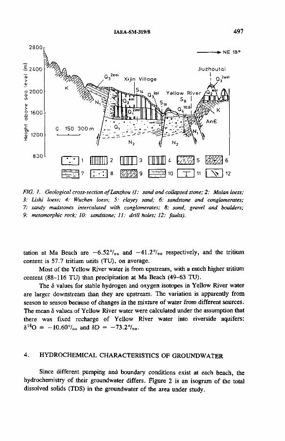
IAEA-SM-319/8 497

FIG. 1. Geological cross-section o f Lanzhou (1: sand and collapsed stone; 2: Malan loess; 3: Lishi loess; 4: Wuchen loess; 5: clayey sand; 6: sandstone and conglomerates; 7: sandy mudstones intercalated with conglomerates; 8: sand, gravel and boulders; 9: metamorphic rock; 10: sandstone; 11: drill holes; 12: faults).

tation at Ma Beach are -6 .5 2 7 00 and -4 1 .2 7 00 respectively, and the tritium content is 57.7 tritium units (TU), on average.

Most of the Yellow River water is from upstream, with a much higher tritium content (88-116 TU) than precipitation at Ma Beach (49-63 TU).

The ô values for stable hydrogen and oxygen isotopes in Yellow River water are larger downstream than they are upstream. The variation is apparently from season to season because of changes in the mixture of water from different sources. The mean ¿> values of Yellow River water were calculated under the assumption that there was fixed recharge of Yellow River water into riverside aquifers: S180 = -10 .607oo and ÔD = -7 3 .2 7 00.

4. HYDROCHEMICAL CHARACTERISTICS OF GROUNDWATER

Since different pumping and boundary conditions exist at each beach, the hydrochemistry of their groundwater differs. Figure 2 is an isogram of the total dissolved solids (TDS) in the groundwater of the area under study.

498 LIAN et al.

FIG. 2. lsôgram o f the total dissolved solids (TDS) content in groundwater in the area under study (1: TDS content; 2: boundary o f the loess plateau and the beach).

At Cui and Ma Beaches two zones were created, taking a TDS standard of 1 g/L. The TDS of fresh water was less than 1 g/L, which consisted of HC03-Ca- Mg, HC03-S04-Ca-Mg and S0 4-HCC>3-Cl-Ca-Mg types of groundwater. The slightly degraded water zone at Cui Beach had a TDS ranging from 1 to 1.5 g/L, with the following hydrochemical types: S04-Na-Ca-Mg, S04-Cl-Na-Ca, Cl-S04-Ca-Mg and HCÓ3-Na-Ca. At Ma Beach, the degraded water zone also had a TDS content in groundwater ranging from 1 to 5 g/L and comprised various hydrochemical types, such as Cl-Na, Cl-S04-Na-Mg, Cl-Ca-Mg-Na, Cl-S04-Na-Ca-Mg, but it was deeply affected by salt water.

Riverside fresh water had very stable hydrochemical characteristics, whereas degraded water was characterized as follows: (a) the groundwater TDS content increased sharply in 1969, with the indicated maximum increase being 81 mg/L between 1968 and 1969; (b) the increase in TDS in each pumping well along the two sides of the south stream became greater from west to east; (c) the increase in TDS in the deep well was larger than the increase in the shallow well.

IAEA-SM-319/8 499

Yellow River

17 - 1 2 1 2

FIG. 3. Schematic diagram o f groundwater -movement and its mixing (I: riverside fresh water; II: young salt water; III: ‘sealed’ water; IV: mountainous fresh water; V: old salt water; VI: degraded water).

5. CIRCULATION OF GROUNDWATERS

The groundwater was classified as follows: I — young salt water, П — mountainous fresh water, Ш — riverside fresh water, IV — old salt water, V — degraded water and VI — sealed water (Fig. 3).

Young salt water was found in Pengjiaping, the southern part of the loess plateau. The total dissolved salt content of the groundwater was approximately 15 g/L, and the hydrochemical type was Cl-S04-Na-Mg. Changes in the stable isotopic composition of the groundwater indicated strong evaporation, the tritium content being approximately 80 TU.

Mountainous fresh water in Huangru Village, east of Pengjiaping, was of HC03-Ca type with a TDS of less than 1 g/L and a tritium content less than 20 TU.

Riverside fresh water circulated quickly. Its tritium content was greater than 60 TU.

Old salt water exists only in the lower aquifer of the area studied. Its TDS, analysed from one sample collected from a depth of 206 m in the confined bed, was 5.6 g/L (27 August 1977), but unfortunately, this well was not being used. In degraded water at Ma Beach, the TDS content varied from 1 to 5 g/L and the several hydrochemical types reflected the complex mixture of groundwaters. The tritium content in the groundwater also varied, from 16 to 109 TU.

Sealed water in a small area in the Eocene aquifer had a tritium content of less than 20 TU and low ô hydrogen and oxygen values.

The cone of depression from pumping is now a drainage zone for young salt water, old salt water, Yellow River water, mountainous fresh water, etc.

500 LIAN et al.

FIG. 4. Map o f groundwater sampling locations in the area under study ( О : sampling location; —* : direction o f groundwater movement).

6. HYDROGEN AND OXYGEN ISOTOPES IN GROUNDWATER

Figure 4 is a map showing the groundwater samples in the study area. Most of the samples were collected from Ma and Cui Beaches. Groundwater sampling was difficult in the loess plateau because of an approximately 80 m thick unsaturated zone and few pumping wells. Fortunately, one of the most important samples was collected in Pengjiaping.

Figure 5 shows the relationship between the ÔD and <5180 contents in ground­water in the studied area. The circles (representing riverside fresh water on Ma and Cui Beaches) are distributed along with or are close to the mixing line for Yellow River water and precipitation, which implies that this groundwater is composed mainly of Yellow River water and precipitation. Only a few circles, representing evaporated groundwater, deviate from the mixing line or meteoric line. Filled circles representing mountainous fresh water appear at the upper left of the meteoric line. This water is recharged by precipitation (rain, melted ice and snow) in the mountainous area. Degraded water is shown to lie within the mixing triangle, composed of riverside fresh water, young salt water and mountainous fresh water. The mixing line (straight line) and the mixing triangle are the bases for calculations using the two and three end mixing models.

IAEA-SM-319/8 501

6180 (%.)

FIG. 5. Relationship between 5D and blsO for waters in the area under study (1: precipitation; 2: surface water; 3: rainfall recharged water; 4: riverside fresh water at Cui Beach; 5: riverside fresh water at Ma Beach; 6: degraded water; 7: young salt water; 8: mountainous fresh water; 9: sealed water).

7. CALCULATION OF THE MIXTURE OF GROUNDWATERS

7.1. Riverside fresh water

The two end mixing model was used on the basis that the riverside fresh water is composed of Yellow River water and precipitation. The calculated results are given in Tables I and П, where ay and ap in the tables represent the ratio of Yellow River water and precipitation to riverside fresh water, respectively.

We see from the calculation that Yellow River water makes up about 85 % of riverside fresh water, while precipitation makes up 15% at Cui Beach. However, Ma Beach receives much better recharge from Yellow River water, which makes up about 95% of riverside fresh water while precipitation makes up only 5%.

7.2. Degraded water

Degraded water from Ma Beach may be composed of Yellow River water (recharge and irrigation water infiltration), salt water (young and old), mountainous

502 LIAN et al.

TABLE I. CALCULATED RATIO OF YELLOW RTVER WATER AND PRECIPITATION TO RIVERSIDE FRESH WATER AT CUI BEACH

Sample No. 5D(°/oo)

50-18(7o.)

a, (%) ap (%)

D 0-18 D 0-18

38 -7 0 .7 -10 .09 92 88 8 12

11 -7 0 .6 -10 .28 92 92 8 8

3 -6 7 .2 -9 .9 8 81 85 19 15

6 -70 .1 -9 .9 0 90 83 10 17

1 -6 4 .6 -9 .2 3 73 66 27 34

4 -6 4 .4 -9 .5 2 73 74 27 26

9 -7 4 .9 -10 .74 100 100 0 0

Mean 86 84 14 16

TABLE II. CALCULATED RATIO OF YELLOW RIVER WATER AND PRECIPITATION TO RIVERSIDE FRESH WATER AT MA BEACH

Sample No. ÔD 50-18 Ъ (%) <*p (%)

D 0-18 D 0-18

37 -7 0 .5 -10 .44 92 96 8 4

36 -7 0 .6 -10.41 92 95 8 5

19 -68 .1 -10 .25 85 92 15 8

18 -7 4 .6 -1 0 .7 100 100 0 0

14 -7 5 .2 -10 .72 100 100 0 0

17 -7 1 .3 -10 .33 94 93 6 7

15 -7 1 .0 -10 .45 93 96 7 4

Mean 94 96 6 4

IAEA-SM-319/8 503

TABLE Ш. RATIO OF YOUNG SALT WATER, MOUNTAINOUS FRESH WATER AND RIVERSIDE FRESH WATER TO DEGRADED GROUNDWATER

Sample No.ÔD

(7 00)50-18(°/0„)

“ 1(%)

“2(%)

“ 3(%)

TDS(g/L)

29 -6 6 .2 -9 .31 54.6 28.7 16.7 7.1

26 -6 6 .2 -9 .9 3 3.5 53.8 42.7 5.0

27 -6 3 .9 -9 .7 5 1.3 73.2 25.5 4.1

30 -6 3 .2 -9 .6 4 5.2 76.8 18.0 5.9

fresh water, precipitation, etc., whereas in riverside fresh water (represented by Yellow River water), young salt water and mountainous fresh water predominate.

According to the principle of the conservation of mass of the isotope and water balance, a group of linear equations can be constructed as follows:

Qm = Q i + Q i + 0з

mQm = ^Dj Qi + ÔD2Q2 + ÔD3Ô3

Sl8OmQm = ¿>180 ,е , + Ô1S0 2Q2 + Ô180 3Ô3

where Q, ôD and ¿>180 represent the discharge of groundwater, Ô values of deuterium and 180 , respectively; m, 1, 2 and 3 represent degraded water, young salt water, mountainous fresh water and riverside fresh water, respectively.

Calculated results from the mixture of groundwaters in the degraded ground­water zone are listed in Table Ш, where a2 and a3 represent the ratio of salt water, mountainous fresh water and riverside fresh water, respectively, to degraded water.

Young salt water makes up the major portion at point 29. Points 26 and 27 are in the cone of depression, their TDS values are up to 4-5 g/L, while young salt water makes up about 1.3-3.5% of mixed water. One possible explanation for the high TDS value is that mountainous fresh water carried some dissolved minerals from old or young salt water bodies.

The determination of the percentage of each type of water in each zone gives us Table IV, which gives the quantity of water pumped from wells at the pumping site in 1987. The unit of Q is 106 m3/a.

504 LIAN et al.

TABLE IV. QUANTITY OF YELLOW RIVER WATER (Qy) PUMPED, PRECIPITATION (Qp), MOUNTAINOUS FRESH WATER (Qmf) AND YOUNG SALT WATER (Qs)

Zone SubzoneTDS(g/L)

a (%)ft Qs

Qf

“/ QP Qy

Ma Beach Fresh water <1 100 0 9.8 0.5 9.3Degraded water 1-6 25.7 74.3 10.3 7.6 2.7

Cui Beach Fresh water <1 21.7 3.2 18.5

8. APPROACH TO THE ORIGIN OF YOUNG SALT WATER

The high soluble salt content in the unsaturated zone results in high TDS values in groundwater. Young salt water exists in loessal clays in the upper part of the unsaturated zone where the highest soluble salt content is 618.1 mg/100 g soil. In the case of mountainous fresh water, there is sandy gravel in the upper part of the zone (Fig. 6(b)), with the highest soluble salt content less than 98 mg/100 g soil (Fig. 6). Moreover, the TDS value of salt water sampled in Pengjiaping shows very clear seasonal variations: 13.3 g/L (March 1987), 14.52 g/L (June 1987), 12.03 g/L (August 1987), 10.9 g/L (November 1987). In addition, the stable isotope compo­sition indicated strong evaporation. However, this evaporation cannot occur for groundwater at a depth of 80 m; it is possible only in the upper part of the unsaturated zone. The tritium content (80 TU) of young salt water is several times greater than that of mountainous fresh water (<20 TU). Thus, high tritium content irrigation water (Yellow River water) may be the main source of recharge and young salt water may be formed by the process of evaporation-leaching-evaporation.

9. MECHANISM OF GROUNDWATER DEGRADATION AT MA BEACH

Groundwater degradation is caused mainly by the blocking of the South Stream. Figure 7 illustrates the three stages of groundwater degradation. Under the conditions of stage A, pumped water was recharged, approximately in the early 1960s, by stream water (in fact, Yellow River water). Under the conditions prevailing for stage B, the South Stream was blocked with bricks and cement and was transformed into a drainage channel. Production wells in the south of the stream restrained saltwater intrusion into the north pumping wells of the stream. However, after all wells in the south of the stream were abandoned, because of groundwater

TDS (p p m /g ) TDS (p p m /g )

оо

0

iü ' í ! 25* 1 ' T1 гl ‘ 111* 111 * 1

50♦ o' 0 .. о

о’ 0

75

' о ,100

* о .

в • 125

о

-9150

О

О 175

о •

• 9 200

кооо

оо

СП \ ] С о Ю О о о О О О о о О О О

TDS in g r o u n d w a te r : 17681.5 m g /L

D ep th (m) \

s ' s *'> S s'/Y *y .'.У< *'•'1

S'

. v .

25

50

75

100

125

150

C7> s i C B Ü Î O О О О О О

//\

■S16

\Depth 1m)

TDS in g r o u n d w a t e r : ¿75 .6 m g /L

FIG. 6. Schematic o f geological columns and TDS content in the unsaturated zone.

оi*

IAEA

-SM-319/8

506 LIAN et a).

Pum ping wellSouth Stream

Pumping well /

P um ping well Pumping well

FIG. 7. Cross-section showing the development of groundwater degradation.

degradation, the degraded groundwater front moved to the production wells in the north. Moreover, the old salt water may have arisen when the regional cone of depression of the groundwater was formed.

10. CONCLUSIONS

The mixture of groundwaters in the area under study were calculated, and the origin of young salt water and the mechanism of groundwater degradation were discussed. However, since the degradation continued and developed, more samples taken at other times have had to be collected. This work had as its aim the prediction of the purification time of degraded groundwater using an isotopic mathematical model of tritium. However, little of the input information on precipitation and Yellow River water supported the calculations. Further work will be done by using continuous sampling techniques.

Hydrological and dispersive models were used in the area. Three aspects of the treatment of degraded water arose from the dispersive model: (1) continuing to stop pumping from production wells in the south of the South Stream will degrade the groundwater more seriously; (2) using all of the production wells in the south of the stream can, of course, slow down the rate of degradation, but it cannot help to purify the groundwater; (3) enlarging the recharge of Yellow River water by cleaning the South Stream is the only way to thoroughly purify degraded water.

IAEA-SM-319/8 507

ACKNOWLEDGEMENTS

Thanks should go to Zhang Zhigan, Wu Xinming and all co-workers. All samples were analysed by Qin Jiaming et al. in the laboratory of the Institute of Karst Geology.

BIBLIOGRAPHY

DINCER, T., PAYNE, B.R., An environmental isotope study of the Southwestern karst region of Turkey, J. Hydrol. 14 (1971) 233-258.

FERRONSKY, V.I., POLYAKOV, V.A., Environmental Isotopes in the Hydrosphere, Wiley, New York (1982).

FRITZ, P., FONTES, J.-C. (Eds), Handbook of Environmental Isotope Geochemistry: The Terrestrial Environment, Vol. 2b, Elsevier, Amsterdam (1986).

INTERNATIONAL ATOMIC ENERGY AGENCY, Statistical Treatment of Environmental Isotope Data in Precipitation, Technical Reports Series No. 206, IAEA, Vienna (1981).

LIAN, Y.Q., A multiple linear regression method for recovering the tritium contents in precipitation, Karstol. Sin. No. 2 (1990) 157-166 (in Chinese).

LIAN, Y.Q., An isotopic multi-input-single output model for estimating groundwater storage — A case study of a karst groundwater system in Linfen, Shangxi Province, China, J. Hydrol' Eng. Geol. No. 2 (1989) 25-28 (in Chinese).

LIAN, Y.Q., Environmental isotope studies in the Xi’an area for estimating the leakage and runoff of groundwaters. J. Hydrol. (in press).

MALOSZEWSKI, P., ZUBBER, A., Determining the turnover time of groundwater systems with the aid of environmental tracers. 1. Models and their applicability, J. Hydrol. 57 (1982) 207-231.

WANG, H.C., ZHOU, H., LIAN, Y.Q., “Isotopic study of the Guozhang karst groundwater system in the Linfen area, Shangxi Province, China” , Proc. 21st Conf., Vol. 2, International Association of Hydrological Sciences, The Hague (1988) 816-822.

IAEA-SM-319/40

INTERLABORATORY COMPARISON OF METHODS TO DETERMINE THE STABLE ISOTOPE COMPOSITION OF SOIL WATER

G.R. WALKER, P.H. WOODS*Division of Water Resources,Commonwealth Scientific and Industrial Research Organisation andCentre for Groundwater Studies,Glen Osmond, South Australia

G.B. ALLISONDivision of Water Resources,Commonwealth Scientific and Industrial Research Organisation,Wembley, Western Australia

Australia

Abstract

INTERLABORATORY COMPARISON OF METHODS TO DETERMINE THE STABLE ISOTOPE COMPOSITION OF SOIL WATER.

The results of an interlaboratory comparison of soil distillation techniques are presented. In the comparison, four dry soils (a sand, a gypseous sand and a clayey soil with high and low water contents) were prepared and distributed to 14 laboratories in 4 continents. Water was then extracted from those samples and analysed using the laboratories’ standard methods. Various verification procedures were used to ensure that the experiment was truly a comparison of distillation techniques and that most variation was not due to sample prepara­tion, transport or measurement. The distillation techniques included azeotropic, vacuum, cen­trifugation and microdistillation methods. Different organic solvents were used in the azeotropic distillations. The vacuum distillations were carried out across a range of tempera­tures. The results show a large variation (of up to 30°/oo for 2H and 3.4°/00 for l80 ) in the isotopic composition of the extracted water. The variation increased as the water content of the soil decreased and was greater for clays than sands at a comparable soil matric suction. The isotope value obtained was correlated with the final extraction temperature. The most probable cause for the variation was incomplete extraction. The study highlights the need to develop standard protocols for each of the major distillation methods.

* Present address: Northern Territory Department of Mines and Energy, Mines Environment Directorate, GPO Box 2901, Darwin, NT 0801, Australia.

509

510 WALKER et al.

1. INTRODUCTION

The concentrations of stable isotopes of water (2H and 180) in soil water are increasingly being used in studies of discharge, recharge and plant water use. The ability to extract isotopically unaltered water from soils is essential to these studies. Unfortunately, it is difficult to validate the methods used for extracting water. Fur­thermore, there is a range of soil water distillation techniques, each having several variations. In fact, it appears to be rare for two laboratories to use exactly the same method, and it has not been demonstrated that the different methods yield the same results. To deal with this problem, an interlaboratory comparison was organized in which a cross-section of the range of methods was represented.

Unlike many other interlaboratory comparisons which compare similar methods used in different laboratories, this comparison compares different tech­niques. If differences in analyses can be correlated with differences in techniques, the interlaboratory comparison will not only be a check of consistency, it will permit critical analysis of the bias associated with the different methods of extraction.

2. EXPERIMENTAL METHODS

Four different soils were prepared: a sand, a gypseous sand and a clay with two different water content levels. The soils were sent to each of the participating laboratories, which were requested to process the samples in the usual way and, if' possible, send an aliquot of water to the organizing laboratory . This aliquot was to be analysed to ascertain whether any biases were due to extraction methods rather than errors in the analysis. Finally, several samples were processed by the organizing laboratory in order to assess the degree of sample to sample variability.

Fourteen laboratories took part in the comparison. They are located in Australia, Austria, Canada, France, Germany, India, Israel, New Zealand, the United Kingdom and the United States of America. In this paper, laboratories are identified by letter and method only.

Four techniques were used:

(a) vacuum distillation,(b) azeotropic distillation,(c) microdistillation with zinc,(d) centrifugation with a heavy immiscible liquid.

The basic principles of the methods are described elsewhere (e.g. Refs [1, 2]). Table I identifies techniques used by different laboratories.

TABLE I. METHODS EMPLOYED BY PARTICIPATING LABORATORIES

IAEA-SM-319/40 511

Laboratory Method Final extraction temperature ГС)

A Azeotropic, kerosene 185

В Azeotropic, toluene 110

D Vacuum distillation 150

D ' Centrifugation with arklone Room temperature

D" Microdistillation 150-200

E Vacuum distillation 50

F Vacuum distillation 80

G Azeotropic, petroleum ether 120

H Vacuum distillation 35

H ' Vacuum distillation 70

I Vacuum distillation 130

J Microdistillation 200

К Microdistillation 110

M Vacuum distillation 200

N Azeotropic, kerosene 185

N ' Azeotropic, hexane 65

N" Azeotropic, kerosene after hexane 185

2.1. Soil preparation

Bulk samples of soil were crushed, sieved and, with the exception of the gypse­ous sand, oven dried at 105°C. The gypseous soil was dried at room temperature in a desiccator under vacuum. The soils were then equilibrated with atmospheric water vapour and split into subsamples. Water was added to the subsamples, which were then shaken. The average error in the amount of water added was less than0.05 g in the 10-30 g total (0.2 to 0.5%). The water used to prepare the samples was Adelaide tap water with an isotopic composition of —16.2700 for 2H and -2.73 700 for l80 . The jars containing the samples were sent to the participating laboratories by air cargo in the pressurized compartment. The air pressure of this compartment decreases to about two thirds of an atmosphere.

8180 6180

FIG. 1. Plots o f ô2H -ô ,80 fo r (a) dry clay; (b) wet clay; (c) sand; and (d) gypseous sand. Each data point associated with a distillation is denoted by the code o f the participating laboratory. The numbers 1 and 2 denote, respectively, the dope water value and a mass balance o f dope plus residual water (from an air dry sample). The line is that associated with a 35 °C Rayleigh distillation using the mass balance o f the air dry sample plus dope water as a reference. The scale fo r the clay samples is different from that used fo r the sands. Where extra analyses have been carried out, a dash has been used to distinguish the extra sample. In particular, fo r the sand, h ' denotes 70°C vacuum distillation. For the gypseous sands, d ‘ denotes centrifuged water, n ’ the hexane distillation, n" the hexane- kerosene distillation and e ' the vacuum distillation which removed more water.

WALKER

et al.

IAEA-SM-319/40 513

At the organizing laboratory, about five jars of each soil type were chosen at random for the test of sample to sample variability. Each sample was divided into two and the water extracted from each. The standard deviations of less than 1.27o0 for 2H and less than 0.37oo for 180 are similar to those quoted in Ref. [2] and suggest that the errors caused by sample to sample variability are comparable or less than those of mass spectrometry.

The final gravimetric water contents of the soils were 5.1% (sand), 10.2% (gypseous sand), 14.7% (dry clay) and 25.2% (wet clay). The soil matric suction values as measured by the filter paper technique were, respectively, 160, 47, 5000 and 150 kPa.

3. RESULTS

The root mean square differences in analyses of the same sample by the organizing and participating laboratories were 2.3700 for 2H and 0.367oo for l80 . The 2H -,80 plots for the four soils are shown in Figs l(a)-l(d). All plots show a large spread of results which is most pronounced for the dry clay and the gypseous soil. The spread of results is not random, but lies not far from the 35°C Rayleigh distillation line (note that the mass balance of dope water and air dry sample was used as a reference).

The pattern of results from the different laboratories, and hence methods, remains the same for the different non-gypseous soils. The samples with the lightest isotopic composition were consistently laboratories H, E and F. These laboratories use low temperature (<80°C) vacuum distillations. The samples from laboratories using azeotropic distillations (A, B, G, N) tend to have the most isotopically enriched samples. The samples from the laboratories using high temperature vacuum distilla­tions (D, I) are generally slightly isotopically lighter than those extracted by azeotropic distillations.

Gypsum gives up some or all of its crystallization water on heating past approximately 45°С [3]. For the gypseous soil, there were two additional azeotropic distillations, one using hexane and one using kerosene after hexane. The azeotropic temperature for hexane is 61 °C and, hence, it will remove water of crystallization of gypsum, albeit slowly. Experimental work [4] has shown that if the distillation time is restricted to two or three hours, the contribution of gypsum water is relatively small. This is consistent with its lying near the Rayleigh distillation line. For the dis­tillation with kerosene following a distillation with hexane, most of the water removed should be water of crystallization rather than soil pore water. As a result, this distillation lies far from the Rayleigh distillation line. The results from the low temperature vacuum distillations show a mixing line with end members being water extracted from sand and the water of crystallization of the gypsum and the degree of mixing dependent on the final temperature of extraction. The same is true of the

( a )-10-

( b )

-20-

aa

aa -30-

a

a v V

am

Vm

VV m

82H -40 - V v

V

~ V t--- 1--- i l i i — i— i— i— i— T--- 1----г— г— i— i—

-50-

-60-

V

■ \ 11 1— 1 1 1 1 — i— i— i—30 50 70 90 110 130 150 170 190 30 50 70 90 110 130 150 170 .190

Final extraction temperature (°C) Final extraction temperature (°C) ^

-Ю -i< с )

-10 -1( d )

rinpp watfir ---------► ►-20 -20 • с — centrifuged water

62HV

am a

a 82h ;a-h

a

-30

< < <

VV m -30 - V a y v

v V

m

aa

a-hk

-40- ' ' 1 1 " T" 1 1 1 1 i---1--- 1--- Г--Г-1---1--- г i r i— -40 -gypsum water------

, n i i20 40 60 80 100 120 140 160 180 200 20 40 60 80 100 120 140 160 180 200

Final extraction temperature (°C) Final extraction temperature (°C)

FIG. 2. Plots of&2H against the fina l extraction temperature fo r (a) dry clay; (b) wet clay; (c) sand; and (d) gypseous sand. Each data point is denoted by the letter o f the technique by which the water was extracted — ‘a ’ fo r azeotropic distillations; V fo r vacuum distillations; ‘m ’ fo r microdistillations and ‘с ’ fo r centrifugation, ‘a - h ’ denotes distillation by hexane and 'a-hk ’ the hexane-kerosene distillation.

8180

8180

-9

( a)

do p e water --------

a

a av Va

VV

V

I 1 I30

n — i— i— i— i— г50 70 90 110 130 150 170 190

Final extraction tem perature ("C)

( c )

dope w a te r______________

a

v v a vV 8 V v

Va

20 40 60 80 100 120 140 160 180 200Final extraction tem perature (°C)

8180

( b )

dope water ------- ►-

V

a v

aa

V

V a

V

30 50 70 90 110 130 150 170 190Final extraction tem pera ture (°C)

6180

( d )

gypsum water

a-hk

aV у a

aс ^ v_______v- centrifuged watetr

a-hv a

V

20 40 60 80 100 120 140 160 180 200Final extraction tem pera ture (°C)

FIG. 3. Plots o f 6 О against the final extraction temperature for (a) dry clay; (b) wet clay; (c) sand; and (d) gypseous sand. Each data point is denoted by the letter o f the technique by which the water was extracted — ‘a ' fo r azeotropic distillations; V for vacuum distillations and ‘c ’ for centrifugation, 'a -h ’ denotes distillation by hexane and ‘a -h k’ the hexane-kerosene distillation.

516 WALKER et al.

azeotropic distillations. The kerosene distillations lie closest to the gypsum water, followed by the extraction with toluene, while the extraction with petroleum ether (laboratory G) lies close to the Rayleigh distillation line.

3.1. Temperature dependence

Figures 2(a)-2(d) and 3(a)-3(d) show, respectively, the individual 2H and l80 results plotted against the final temperature of extraction. For l80 , there is a strong correlation with temperature for all soils. For 2H, this correlation is weaker. In fact, if one treats the microdistillation as a high temperature vacuum distillation, there appears to be a maximum in the 2H results from vacuum distillations in the 80-105°C range for the dry clay and sand. No explanation is offered for this. Given that the probable cause of the variation is incomplete extraction, which will tend to produce lower values, the correlation with temperature suggests that the introduction of heat may be a necessary component for acceptable distillation results.

4. DISCUSSION

This paper presents the results of the first interlaboratory comparison of soil water extraction techniques. The aim of the comparison was to test the consistency of extraction methods. Extraction of dry soils by different techniques or variations of the same technique gives unacceptably large variations of analyses (up to 307oo for 2H and 3.57oo for l80).

We show that the above variation is due to the extraction technique, rather than an artefact of the experimental design. First, the sample to sample variation was found to be comparable with the measurement error. Second, a comparison of meas­urements by the participating laboratories shows that the variation cannot be explained by mass spectrometer measurement errors. Third, the errors are sys­tematic in that they appear to lie near a Rayleigh distillation line and are correlated with temperature. This suggests that the cause of the variation is incomplete extrac­tion of the soil water.

ACKNOWLEDGEMENTS

Much of this work was carried out as part of the PhD studies of P.H. Woods, supported by the CSIRO Division of Water Resources, the Centre for Groundwater Studies in Adelaide and the Flinders University of South Australia. Thanks are expressed to J. Dighton, A. Kennett-Smith and K. McEwen for additional laboratory work, and to F. Leaney and J.-C. Fontes for useful discussions regarding the project. Naturally, thanks are expressed to all of the laboratories participating in the experiment.

IAEA-SM-319/40 517

REFERENCES

[1] JUSSERAND, C., Extraction de l’eau interstitielle des sédiments et des sols. Com­paraison des valeurs de l’oxygène 18 par différentes méthodes, premiers résultats, Catena 7 (1980) 87-96.

[2] REVESZ, K., WOODS, P.H., A method to extract soil water for isotopic analysis, J. Hydrol. 115 (1990) 397-406.

[3] HARDIE, L.A., The gypsum-anhydrite equilibrium at one atmosphere pressure, Am. Mineral. 52 (1967) 171-200.

[4] WOODS, P.H., The Extraction of Water from Porous Media, Especially Gypseous Media for Isotopic Analysis. Results of Laboratory Trials, Technical Memoran­dum 90/1, Division of Water Resources, Commonwealth Scientific and Industrial Research Organisation, Glen Osmond, SA (1990).

PALAEOHYDROLOGY AND PALAEOCLIMATOLOGY

Chairman W.R. SCHELL

United States of America

IAEA-SM-319/20

MONITORING THE RESPONSE OF ARID ZONE HYDROLOGY TO ENVIRONMENTAL CHANGE BY MEANS OF THE STABLE ISOTOPE COMPOSITION OF GROUNDWATERS

J.R. GATDepartment of Environmental Sciences and Energy Research,Weizmann Institute of Science,Rehovot,Israel

Abstract

MONITORING THE RESPONSE OF ARID ZONE HYDROLOGY TO ENVIRONMEN­TAL CHANGE BY MEANS OF THE STABLE ISOTOPE COMPOSITION OF GROUNDWATERS.

Under arid conditions (where rain is deficient), recharge to groundwaters occurs only when some degree of surface flow precedes the infiltration process. Such a formation pattern imposes a characteristic and identifiable isotopic composition on the desert water sources, involving both a selection of the more intense rainfall events which contribute preferentially to surface flooding and an isotopic fractionation which accompanies the surface exposure phase of the recharge process. Because of this set of circumstances, the formation of ground­waters under an arid climate is extremely sensitive to any environmental change and, in partic­ular, to changes in the pattern of land usage, the vegetation cover and the surface morphology. Such changes can result from climatic change on a global scale or from local anthropogenic causes through agricultural development or urbanization. The anthropogenic effect on the process of groundwater formation is a function of the scale of operation. On a small scale, water is used up and diverted from recharge pathways. However, large scale agricultural or urban development in the arid zone will usually enhance the rate of groundwater recharge. The changes in the hydrological mechanisms imprint a different isotopic signature on the groundwaters and thus the isotope composition of the water resources can serve as a monitor of such changes.

1. INTRODUCTION

Under arid conditions, i.e. where rain amounts fall short of the water deficit created in the unsaturated zone by évapotranspiration, direct recharge to ground­waters is the exception rather than the rule. Recharge can then occur only when some special sets of circumstances are satisfied. Among these is the situation where a suffi­ciently large water depth accumulates at a potential infiltration site; this is most read­ily achieved following some degree of surface flow [1]. The scale of such surface

521

522 GAT

flows was found to range from the metre scale, actuated by exposed rock surfaces and other impermeable surface features, to the flashfloods which gather waters on a regional scale [2]. Even though the water yield of such flood flows rarely exceeds a few per cent, the large areas involved result in the confluence of large amounts of water which can feed sizeable aquifer units.

The inception of surface flow under a regime of relatively small rain amounts (in excess of just a few millimetres of rain) is a characteristic of the arid zone. It results from the prevalence of exposures of bare rock surfaces [3] and the accumula­tion of fine grained windborne material on the surface which form poorly conducting layers. Both of these latter characteristics can be blamed on the absence of a stabiliz­ing plant layer and the ablation and loss of the soil cover in the desert environment.

Evidently the key elements in the evolution of surface flows are the material composition of the ground surface, the surface morphology and drainage network. These determine the surface flow pattern and occurrence of recharge to the ground­water system [4]. Moreover, the chemical composition and vulnerability to pollution of the water sources are also determined to a large extent by the events which occur prior to the infiltration proper [5, 6]. The evaporative enrichment of the heavy isotopic species H2,80 and HDO which accompanies the surface phase of the recharge process imprints a distinctive isotopic signature on the waters, which characterizes the chain of events leading to groundwater recharge [1].

Because of the circumstances described above the recharge efficiency (and indeed the very occurrence of groundwater recharge) is very sensitive to the struc­ture of the terrain. The hydrological system is a precariously balanced one. Even relatively minor man-made or other changes in land use can exercise a profound effect on water availability and water quality in general, and on groundwaters in particular.

In this paper we will address the possibility of detecting and monitoring such changes through the measurement of the stable isotope composition of the water resources.

2. ISOTOPIC COMPOSITION OF ARID ZONE WATER SOURCES

As shown in Fig. 1, which is based on previous work on desert isotope hydrol­ogy [7, 8] especially related to the Negev region [9], there are at least two factors which result in a difference between the isotopic composition of groundwaters and that of the local precipitation. The first of these is a selection between rainfall events (or between parts of a showery spell) in the inception of runoff or during infiltration (in those cases where direct infiltration can take place, for example, a sand dune area) [10]. The second effect stems from the isotopic fractionation which accompa­nies evaporation from surface water or shallow subsurface water.

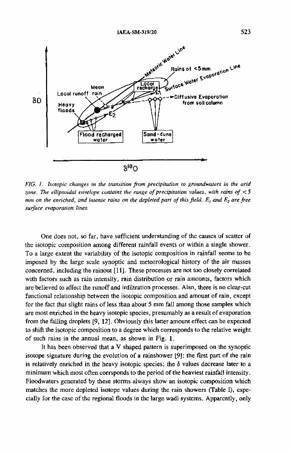
IAEA-SM-319/20 523

SD

Flood recharged w ater____

Sand-dunewater

\> e

Sl80

FIG. 1. Isotopic changes in the transition from precipitation to groundwaters in the arid zone. The ellipsoidal envelope contains the range of precipitation values, with rains of <5 mm on the enriched, and intense rains on the depleted part of this field. E, and E2 are free surface evaporation lines.

One does not, so far, have sufficient understanding of the causes of scatter of the isotopic composition among different rainfall events or within a single shower. To a large extent the variability of the isotopic composition in rainfall seems to be imposed by the large scale synoptic and meteorological history of the air masses concerned, including the rainout [11]. These processes are not too closely correlated with factors such as rain intensity, rain distribution or rain amounts, factors which are believed to affect the runoff and infiltration processes. Also, there is no clear-cut functional relationship between the isotopic composition and amount of rain, except for the fact that slight rains of less than about 5 mm fall among those samples which are most enriched in the heavy isotopic species, presumably as a result of evaporation from the falling droplets [9, 12]. Obviously this latter amount effect can be expected to shift the isotopic composition to a degree which corresponds to the relative weight of such rains in the annual mean, as shown in Fig. 1.

It has been observed that a V shaped pattern is superimposed on the synoptic isotope signature during the evolution of a rainshower [9]: the first part of the rain is relatively enriched in the heavy isotopic species; the b values decrease later to a minimum which most often corrsponds to the period of the heaviest rainfall intensity. Floodwaters generated by these storms always show an isotopic composition which matches the more depleted isotope values during the rain showers (Table I), espe­cially for the case of the regional floods in the large wadi systems. Apparently, only

524 GAT

TABLE I. ISOTOPIC COMPOSITION OF PRECIPITATION AND OF FLOOD FLOWS IN THE NEGEV HIGHLAND (1979-1980 SEASON)

Date of eventRain Floods

Station

О '

w 0

0 Station <50-18( ° / .o )

1979-10-5 R -3 .9 2 Z -6 .1 2M -4 .8 7

1979-11-29/30 Z -4 .2 3 Z -4 .01R -3 .31 R -4 .5 2SB -3 .9 4 M -3 .9 7

в -3 .8 0H -3 .5 5

1979-12-5/6 Z -4 .0 6R -3 .4 0 R -4 .11SB -3 .9 0 В -5 .0 4

1979-12-14 Z -6 .6 4 R -7 .91R -5 .71 M -6 .9 2SB -6 .2 2 H -6 .5 5

1980-1-23 Z -6 .9 3 Z -8 .9 6R -6 .3 9 R -8 .4 4SB -5 .1 7

1980-2-27 Z -3 .5 6 R -5 .6 2R -3 .5 6 M -5 .7 2

H -6 .6 5

Station index: В — Wadi Besor (upstream); H — Wadi Besor at Halutza; M — Masad; SB — Sdeh-Boker; R — Revivim; Z — Zavoa.

the most intense rains result in the inception of surface flows or, alternatively, flow can start only after the wetting of the surface by the initial portion of the rainfall. There is some suggestion in the data that the degree to which this selection is exer­cised is scale dependent. For example, local surface flows found at the bottom of an arid hillside are less perturbed (relative to the mean isotopic composition of precipitation) than the large desert flashfloods [9]. It should be noted that these

IAEA-SM-319/20 525

changes, by and large, shift the isotope composition along the slope —8 line in <5 space (<5D versus <5180), as shown in Fig. 1.

The second effect mentioned, namely the evaporation effect on the isotopic composition of surface waters, is more readily quantified. The ô values of the isotopic composition of residual waters increase along ‘evaporation lines’, whose slope in ÔD versus ôl80 space depends mainly on the ambient humidity and other environmental parameters [13]; as a result these waters acquire a unique and distin­guishable isotopic composition which is shifted from the meteoric water line towards lower values of the d excess parameter: d = <5D — 8<5180.

The groundwaters found in the arid environment do indeed show a large range of isotopic compositions [14] which reflect their tortuous paths of formation. Even within a rather limited geographical area and a given terrain, there is an appreciable scatter in the isotopic composition of groundwaters, as can be exemplified by water sources found under the limestone exposures of the northern Negev [9]. These varia­tions evidently reflect the relative importance of processes such as those described above during the recharge.

Another attribute of the arid zone is the survival of waters derived from distant origins (in time or space) unrelated to the present local precipitation and recharge[15]. Their possible admixture to the aquifer units by one or another mechanism is an additional cause for variations in the isotopic data.

A summary of the varied isotopic compositions encountered in the Negev region is given in Fig. 2.

3. SCALE DEPENDENT EFFECT OF LAND USE CHANGES ON THE WATER SOURCES

Anthropogenic changes in the desert due either to agricultural or urban developments run the full gamut from semi-transient encampments which exploit natural sporadic water appearances to urban settlements with a steady water supply. These activities affect the desert environment and its water balance in different ways:

(a) Meteorological: Changes in rain patterns, rain intensity, etc., follow as a result of albedo changes, changes in the near surface moisture field (due to more or less évapotranspiration) and heat island effects.

(b) Surface texture: Affecting runoff characteristics.(c) Soil moisture balance: Change in the plant cover, and thus in the moisture utili­

zation, controls the water deficiency, affecting the inception of infiltration and/or runoff characteristics.

(d) Drainage pattern: Channelling, interception of natural drainage, diversion of surface waters for alternate use, making them unavailable for natural recharge.

(e) Mixing and import: Of extraneous waters.

Table II lists some such activities as a function of their scale.

526 GAT

S180(%o)

FIG. 2. Stable isotopic composition o f meteoric and surface waters in the Negev, and o f waters which can be imported into the area (EMMWL: eastern Mediterranean meteoric water line, with d ~ 22 % 0; SMOW: standard mean ocean water).

On the lowest scale one finds the natural desert dwellers, namely a transient nomadic population, who adjust to the natural hydrological capacity and utilize water resources only to the extent that they are easily available, mainly surface waters or shallow groundwaters. The migratory population thus has a minimal hydrological impact, though through the act of overgrazing by their flocks those populations exert considerable ecological stress and contribute to the process of desertification. In contrast, the sedentary population, especially those engaged in agriculture, usually augment the naturally available supply of water by a variety of devices. A most prominent example is the Nabatean runoff farming, which was practised in the Negev almost two millennia ago [16]. Up to a point such practices simply utilize rain waters more efficiently than the natural process, without any deleterious hydrologi­cal effect. However, the diversion of surface waters may curtail the recharge of groundwaters downstream of the interception point and may adversely affect the natural groundwater balance. Moreover, the increased plant cover and the develop­ment of tilled soils with large water holdup capacity may detract from both runoff and groundwater availability.

TABLE П. ACTIVITIES LISTED IN ORDER OF INCREASING SCALE

IAEA-SM-319/20 527

Operation Predominant water source

Environmentalimpact

Hydrologicalimpact

Agricultural development

Grazing Natural rainfall Destruction of natural plant cover

Decrease of transpiration

+

Forestation;non-irrigatedagriculture

Channelling of natural runoff

Increase of plant cover

Increase ofevaporation/transpirationloss

Irrigatedagriculture

Imported water Increase of plant cover

Excess drainage+ +

Human settlement

Village Local wells, cisterns

Some plants Extraction of water .

Primitive town Wells and cisterns; runoff interception

Complete use of available water + -

Modern settlement Deep wells,surface waters

Change of land forms

Wastewaterexport +

City Imported water Pavements Wastewater export and increased runoff + +

Once the scale of settlements exceeds that of a very minimal population, it must rely on additional water supplies: these may take the form of the exploitation (by pumping) of deep water sources, the utilization of a river that runs through the arid zone (the Nile is an example), the import of water by pipeline or canal, or in the extreme case, desalinization of sea water. The salient feature of such a situation is then an excess of water over that which is naturally available.

The immediate ecological effect of an excess of water is that of greening of the desert, either directly by the imported waters or, as in the case, for example, in the desert township of Dimona, Israel, by reclaimed wastewater which is being used for the irrigation of orchards and parks. Some of the water excess, especially when discharged directly underground in septic tanks, may actually increase the recharge rate, offsetting the depletion by pumping and reactivating dormant groundwater sources. Whether such a situation can be considered beneficial or not will depend

528 GAT

on the local circumstances, especially on the hydraulic properties of the substratum and on the scale of the problem: moderate water excesses can be accommodated by the environment through an increase in the plant cover and, possibly, also the groundwater potential. However, the absorptive capacity of an arid environment is easily exceeded, resulting in a variety of environmental ‘disasters’, which range from the appearance of swamp areas to the flooding of cellars and foundations of buildings in the city itself. Such is the case, for example, in the lower lying areas of Tehran, where the drainage system did not keep pace with the import of water into the town.

We can see that with the exception of an intermediate scale where the hydro- logical deficiencies are aggravated, there is an amelioration rather than a negative effect of urbanization on the arid environment. Obviously there is a bias in such a statement in that our yardsticks for judgement are taken from non-arid areas and view an increase in the cultivated and green areas as beneficial, rather than a situation which would conserve the ‘desert look’. However, such a bias would probably be acceptable by most inhabitants of any arid zone urban centre.

From a purely hydrological (groundwater) point of view, possible effects range from a depletion of water resources to large excesses, and from quality deterioration (increased salinity) to dilution by waters of good quality which are imported into the area. The situation depends on the particular make-up of the area concerned and will have to be analysed in detail, taking into account the geological, geomorphological and ecological factors involved, as well as that of the human factor and activity.

4. EFFECT OF CHANGES IN THE HYDROLOGICAL REGIME ON THE ISOTOPIC COMPOSITION OF GROUNDWATERS

Let us examine the effect of the changes in the hydrological regime (and, in particular, the groundwater formation) on the isotopic composition according to the five points (а-e) enumerated in Section 3:

(a) Meteorological: Any change in the rain pattern can be expected to be accompa­nied by some isotopic signal [17]. This is easily monitored in the rainfall and can be accounted for. This effect will thus not be discussed further.

(b) Surface texture: Based on observations of the isotopic composition of runoff, summarized in Fig. 1, it is to be expected that a change in the runoff inception mechanism will move the isotopic composition of the runoff up or down the meteoric water line, as the case may be. Of special interest is the case of a pavement (road, parking lot, or rooftop) from which runoff is maximal and where the runoff’s isotope composition can be expected to match that of the mean rainfall.

IAEA-SM-319/20 529

TABLE III. GROUNDWATERS OF THE LIMESTONE TERRAIN (CENTRAL NEGEV)

Water source50-18 (•/..) Mean

salinity(mg/L)Average a (N)a

Nizanna (well) 5.46 0.35 (13) 642

Be'erotayim (well) 5.61 0.29 (14) 595

' Ein-Qudeirat (spring) 5.90 0.7 (8) 537

Qseima (well) 4.90 0.6 (8) 1355

'Ein-Aquev (spring) 5.0 0.5 (П ) 1083

Avdat (well) 5.60 0.35 (10) 940

'Ein-Avdat (spring) 5.42 0.7 (9) 1505

'Ein-Zig (spring) 5.58 0.38 (6) 510

a N: number of samples.

(c) Soil moisture balance: Increased utilization of soil moisture by an increasing plant cover will, in the first instance, reduce the availability of water for direct recharge (where such a mechanism is operative) and also decrease the avail­ability of water for runoff. From the isotopic point of view, however, the evaporative signature is being reduced, since the major water loss is then by évapotranspiration.

(d) Drainage pattern: The blocking of drainage paths by a road or dam structure will often cause an impoundment of surface waters (intentional in some cases, inadvertent in others) where waters are exposed to evaporation for longer periods. This then clearly increases the evaporative signature in the water sources.

(e) Mixing and import o f waters: As shown in Fig. 2, the isotopic composition of imported or extraneous waters is varied under different situations and their admixture into the recharge stream will have to be discussed for each situation.

The ability to detect changes of the kind just discussed depends, on the one hand, on the temporal stability of the stable isotope composition of any particular groundwater body (<j(ô)) and, on the other hand, on the magnitude of the (mean) isotope shift which results from the environmental change (Д0) — the ratio of Дô/o(ô) is the signal to noise ratio. As shown in Table III, which summarizes data gathered jointly with the Institute of Desert Research at Sdeh-Boker under Contract

530 GAT

-4о

5?О

оЙО

-5

-6

F1G. 3. The stable isotope composition o f two wells in the limestone terrain o f the central Negev.

No. 2812/GS on groundwater formation under desert conditions (J.R. Gat and A. Isaar, principal investigators), the stability of local groundwater pockets in the limestone terrains of the central Negev ranges from ct(5180) = ±0.3 to +0.6, whereas the signal in this data set is of the order of l °/00 (6180) and can be taken to represent different natural recharge conditions. If one considers the admixture of extraneous water sources, e.g. of palaeowaters whose isotopic composition ranges from ô180 = - 7 to - 9 °/00 [15], or of desalinized waters with an isotopic composi­tion close to the zero of the scale, then the signal/noise ratio is obviously much greater. Figure 3, in which results from a two year monitoring of isotopic composi­tion in two adjacent wells in the limestone terrain are given, of which one is affected by the diversion of flow in an adjacent wadi, shows how such activities can result in signal/noise ratios of close to 10. The sensitivity of isotopic data to environmental change can be quite considerable.

5. SUMMARY

Because of the involvement of surface phenomena in the groundwater replenishment process in the arid zone, the groundwater isotopic composition is

1 1 1 I 1 1 1 1 T ' 1 1

! \

! \; \ i » i \ i »« \ t »

M ashosh-1'~^

^ ¡ x* y * ' * *

4 «t* \

/ 1 t «

X

x X -X *

\ / x XX/ 'v J Mashash-2• V •X-X-K-X' *

• .\

• ' - * - * * * • • •• • • • • • • • • • •

• • ••

--------1------- 1____ L L 1 _ L ... 1 1 I 1 , 1 “

Jun. Jul. Aug. Sep. Oct. Nov. Dec. Jon. Feb. Mar. Apr. Moy

Month

IAEA-SM-319/20 531

very sensitive to human activity. Obviously, then, the isotopic composition can be a sensitive test for detecting changes in the system. A prerequisite for such a monitor­ing scheme, however, is the establishment of a benchmark set of measurements in the natural and undisturbed condition, including the assessment of both the averaged values and their (natural) variability. Further, it will be essential to characterize the isotopic composition of any extraneous waters which ate introduced into such a region, as well as to conduct a continuous monitoring of the local rainfall.

REFERENCES

[1] GAT, J.R., “ Groundwater recharge under arid conditions” , Infiltration Principles and Practices (Proc. Int. Conf.) (FOK, Y., Ed.), Water Resources Research Unit, Univer­sity of Hawaii, Honolulu (1988) 245-257.

[2] SCHOELLER, H., Arid Zone Hydrology — Recent Developments, UNESCO Series on Arid Zone Research No. 12, UNESCO, Paris (1959).

[3] ELBOUSHI, I., Amount of water needed to initiate flow in rubbly rock particles, J. Hydrol. 27 (1975) 275-284.

[4] ISSAR, A., GAT, J.R., Environmental isotopes as a tool in hydrogeological research in an arid basin, Groundwater 19 5 (1981) 490-494.

[5] GAT, J .R ., “ Role of the zone of aeration in recharge and establishment of the chemical character of desert groundwaters” , Recent Investigations on the Zone of Aeration (Proc. Symp. Munich, 1984), Vol. 2, Technical University of Munich (1984) 487-497.

[6] GAT, J.R., “ The chemical structure of arid zone groundwaters: Role of aeolian trans­port, surface flow and of geochemical processes prior to recharge and following discharge” , Water-Rock Interactions (Proc. 6th Symp. Malverne, UK, 1989), A.A. Balkema, Rotterdam (1989) 251-253.

[7] GAT, J.R., ISSAR, A., Desert isotope hydrology: Water sources of the Sinai desert, Geochim. Cosmochim. Acta 38 (1974) 1117-1131.

[8] ISSAR, A ., et al., ‘ ‘Isotopic evidence concerning the origin of groundwater under arid conditions” , Isotope Hydrology 1983 (Proc. Symp. Vienna, 1983), IAEA, Vienna (1984) 85-104.

[9] LEVIN, M., et al., “ Precipitation, flood and groundwaters of the Negev Highlands: An isotopic study of desert hydrology” , Arid Zone Hydrology: Investigation with Isotope Techniques (Proc. Advisory Group Mtg Vienna, 1978), Rep. IAEA-AG-158/1, IAEA, Vienna (1980) 3-22.

[10] DINCER, T., et al., Study of infiltration and recharge through the sand dunes in arid zones with special reference to the stable isotopes and thermonuclear tritium, J. Hydrol. 23 (1974) 79-109.

[11] RINDSBERGER, M., et al., Pattern of the isotopic composition of precipitation in time and space: Data from the Israeli storm-water collection program, Tellus 42B (1990) 263-270.

532 GAT

[12] GAT, J.R., “ Variability (in time) of the isotopic composition of precipitation: Conse­quences regarding the isotopic composition of hydrologie systems” , Isotopic Tech­niques in Water Resources Development (Proc. Symp. Vienna, 1987), IAEA, Vienna (1987) 551-564.

[13] GAT, J.R., Comments on the stable isotope method in regional groundwater investiga­tion, Water Resour. Res. 7 (1971) 980-993.

[14] GAT, J.R., “ Groundwater” , Stable Isotope Hydrology: Deuterium and Oxygen-18 in the Water Cycle (GAT, J.R., GONFIANTINI, R., Eds), Technical Reports Series No. 210, IAEA, Vienna (1981) 223-240.

[15] GAT, J.R., GALAI, A., Groundwaters of the Arava Valley: An isotopic study of their origin and interrelationships, Israel J. Earth Sci. 31 (1982) 25-38.

[16] TADMOR, N.H., et al., The ancient desert agriculture of the Negev, Israel J. Agrie. Res. 10 (1960) 193-222.

[17] GAT, J.R., CARMI, I., “ Effect of climate changes on the precipitation patterns and isotopic composition of water in a climate transition zone: Case of the Eastern Mediter­ranean Sea area” , Influence of Climate Change and Climate Variability on the Hydro­logie Regime and Water Resources, Publication 168, International Association of Hydrological Sciences, The Hague (1987) 513-523.

IAEA-SM-319/35

A RECORD OF CLIMATIC AND ENVIRONMENTAL CHANGE CONTAINED IN INTERSTITIAL WATERS FROM THE UNSATURATED ZONE OF NORTHERN SENEGAL

W.M. EDMUNDS British Geological Survey,Wallingford, Oxfordshire,United Kingdom

C.B. GAYE Département géologie,Université Cheikh Anta Diop,Dakar,Senegal

J.-C. FONTESLaboratoire d’hydrologie et de géochimie isotopique,Université de Paris-Sud,Orsay,France

Abstract

A RECORD OF CLIMATIC AND ENVIRONMENTAL CHANGE CONTAINED IN INTERSTITIAL WATERS FROM THE UNSATURATED ZONE OF NORTHERN SENEGAL.

Interstitial waters from the unsaturated zone of Quaternary sands in northwestern Senegal have been extracted to investigate the recharge history using chemical and isotopic methods. The two profiles are from among a group of seven obtained from a 1 km2 site at which an average recharge of 15.2 mm/a was measured using the chloride technique and assuming steady state conditions of chloride transport. The residence times of water in the pro­files are 108 and 79 years, respectively, and, as a result, recharge/input conditions going back to the 1870s are preserved. Chloride peaks correspond not only to the Sahel drought of 1968-1986, but also to periods of lower than average rainfall in the 1940s and 1900s; con­versely, wetter periods with higher recharge of the 1950s and 1920s are indicated by low chloride in interstitial waters. The calibrated profiles can be correlated with the records of (a) the flow of the Senegal River, and (b) the rainfall record of St. Louis, Senegal, since near the turn of the last century. The stable isotope profiles reflect the patterns shown by chloride. Zones of enrichment correspond to the chloride peaks, showing that each season’s charac­teristic evaporation front is being transmitted through the profile — the greater the enrichment the lower the recharge. Additional environmental information is given by bromide (Br/CI) and nitrate (N03/C1). Relatively high Br/Cl ratios are found in interstitial waters corresponding to wetter interludes. The NO3-N content is generally in excess of 10 mg/L and results from natural in situ production. High NO3/CI ratios also coincide with wetter recharge episodes.

533

534 EDMUNDS et al.

1. INTRODUCTION

Excellent records of climatic and environmental change during the Holocene have been obtained from a variety of materials, including microfauna and micro flora, sediments and from isotopic information from various sources. Records are generally quite detailed from the marine sedimentary record, as well as from tem­perate regions. In contrast, the terrestrial record from arid and semi-arid regions is usually less complete on account of erosion and oxidation. Nevertheless, a consistent picture of alternating humid and semi-arid periods emerges, for example, from studies of diatom and sedimentary records [1] and from multiple sources [2] and these have a bearing on recharge history. In the past millennium, and notably during the past 300 years, the record of climatic change may be constructed from historical archives and colonial reports [3].

Of particular interest here is the direct evidence that may be contained in groundwater that specific humid periods may have led to aquifer recharge and whether recharge is a continuing phenomenon during periods of severe drought, such as those that affected the Sahel region of Africa between 1968 and 1986. Discrete recharge events have been inferred in several areas from geochemical and isotopic study of the saturated zone on the time-scale of millennia [4-6], but because of mixing and sampling difficulties it is difficult to resolve recharge events on the scale of decades, or even centuries. In contrast, water stratification in the unsaturated zone may contain a chronological record on the scale of tens, hundreds or even thousands of years [7-9]. Unsaturated zone solute profiles, especially chloride profiles, often supported by tritium and stable isotopic information, have been used in some semi- arid regions to provide recharge estimates [7-10] which represent the mean recharge at point sources on a scale of many years and there is a review on this subject [11]. However, it has seldom been possible to resolve the information to provide evidence of the climatic record and/or the associated hydrological information.

The purpose of this paper is to present results from northwestern Senegal which have been obtained as part of a wider and as yet unpublished investigation of aquifer recharge. In addition to the record given by chloride and stable isotopes, bromide, nitrate and other elements are investigated to see whether any light can be shed on environmental changes over the time intervals represented by each profile.

2. HYDROGEOLOGY AND ENVIRONMENT OF NORTHERNSENEGAL

Senegal lies in a key position on the Sahel margin where two climatic zones of the arid north and the humid tropical south meet. The present research has been carried out in northwestern Senegal (Fig. 1), where extensive Quaternary dune sands

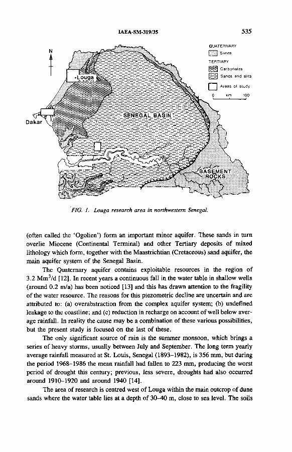
IAEA-SM-319/35 535

FIG. I. Louga research area in northwestern Senegal.

(often called the ‘Ogolien’) form an important minor aquifer. These sands in turn overlie Miocene (Continental Terminal) and other Tertiary deposits of mixed lithology which form, together with the Maastrichtian (Cretaceous) sand aquifer, the main aquifer system of the Senegal Basin.

The Quaternary aquifer contains exploitable resources in the region of3.2 Mm3/d [12]. In recent years a continuous fall in the water table in shallow wells (around 0.2 m/a) has been noticed [13] and this has drawn attention to the fragility of the water resource. The reasons for this piezometric decline are uncertain and are attributed to: (a) overabstraction from the complex aquifer system; (b) undefined leakage to the coastline; and (c) reduction in recharge on account of well below aver­age rainfall. In reality the cause may be a combination of these various possibilities, but the present study is focused on the last of these.

The only significant source of rain is the summer monsoon, which brings a series of heavy storms, usually between July and September. The long term yearly average rainfall measured at St. Louis, Senegal (1893-1982), is 356 mm, but during the period 1968-1986 the mean rainfall had fallen to 223 mm, producing the worst period of drought this century; previous, less severe, droughts had also occurred around 1910-1920 and around 1940 [14].

The area of research is centred west of Louga within the main outcrop of dune sands where the water table lies at a depth of 30-40 m, close to sea level. The soils

536 EDMUNDS et al.

are thin, semi-arid and red-brown, and the vegetation is typically Sahelian. However, the original vegetation, including Acacia radiana and Acacia albida has been greatly reduced by clearing in favour of rainfed agriculture (especially millet and groundnuts). Surface runoff in this area is negligible, and the water balance may be represented by the infiltration minus évapotranspiration.

3. METHODS

The unsaturated zone was sampled at seven sites within a 1 km2 area west of Louga (Fig. 1) and at various other sites within the study area for the estimation of recharge using chloride. The basis of the method has been described by Edmunds et al. [9]. Sampling was carried out using a hand auger with a hollow shell, enabling around 10 cm to be sampled on each round trip. Samples were bulked and homogenized over 25 cm or 50 cm according to depth, up to a maximum vertical interval of 35 m. Subsamples were stored in glass Kilner (fruit bottling) jars and transported for analysis either to Dakar or the United Kingdom.

The moisture content was determined gravimetrically. Chloride was usually measured by two techniques. Samples were elutriated using distilled, demineralized water (30 mL/50 g solid) with occasional stirring for 1 h (until constant conductivity was attained). The supernatant sample was then filtered prior to analysis by an auto­mated colorimetric technique using mercuric thiocyanate which had a detection limit of 0.5 mg/L. Interstitial waters were also extracted directly by centrifugation [15] using an immiscible liquid (‘Arklone’ — CCI3CF3) where moisture contents were sufficiently high to allow this. The interstitial waters provided the sample for a more detailed inorganic analysis using inductively coupled plasma-optical emission spec­troscopy (ICP-OES), but the elutriated samples were then used for analysis of bromide and nitrate.

Stable isotope analysis (ô180 and ô2H) was carried out on samples obtained by distillation of moist sand or, in the case of deuterium, by direct reduction of moist samples sufficient to yield 10 mg of H20 using zinc shot [16]. Samples of rainfall were collected from the Louga climatic station and from Dakar airport over a three year period to obtain information on inputs (quantity and chemistry). Samples of shallow groundwater were also collected from traditional dug wells to provide infor­mation on recent inputs to the aquifer.

4. RESULTS

Two series of results (L3 and LI8) from the total of seven profiles obtained from the research area at Louga are used to discuss the recharge history and environ­mental record. These profiles are representative of those taken and are chosen since they cover different time scales and also since a full range of measured parameters

IAEA-SM-319/35 537

is available. Results for gravimetric moisture content, chloride (élutriation and cen­trifugation), and 02H and <5180 are given for each profile in Figs 2 and 3.

The moisture content varies considerably in each profile and these variations are closely related to the grain size of the sand. Fine grained sand may have moisture contents up to 80 g/kg, while medium/coarse grained sands may have a content as low as 10 g/kg. The 35.5 m profile (L18) almost reaches the water table and the capillary fringe extends for about 2 m.

Concentrations of chloride in interstitial water, obtained by alternative methods (centrifugation and élutriation) are compared for each profile. The similar­ity of both sets of results is good (Figs 2 and 3) and the only significant discrepancy occurs in the top 2 m. This indicates the zone of fluctuation and recycling where solutes are redistributed; centrifugation may tend to extract only the water from well connected pore spaces, but the élutriation will extract from the total sand sample. Below this depth identical information is obtained from unsaturated, yet fully moistened, sand.

The mean estimates of direct recharge have been estimated using the basic formula (Rd = Cp P/Cs.) for recharge estimation [9] and the values given in Table I. At this 1 km2 site recharge estimates ranging from 4.6 to 34.4 mm/a (average15.2 mm/a) were obtained from the seven profiles, and profiles L3 and LI8 shown here represent, respectively, the lower and higher extremes of recharge. Confirma­tion of the recharge rate at the L18 site is provided by a partial tritium profile, in which a peak is developed starting at 15 m [13].

Using the long term average recharge estimates calculated using chloride, it is then possible to calibrate each profile chronologically if the moisture content and bulk density are known and, thence, to calculate the rate of movement (Vw), in metres per year:

V = -1000 x 0W

where 6W, the volumetric moisture content, is given by:

_ bd X me w ~ pw x 1000

So

w i ,bd X me

wherebd is the bulk density of the dry sediment (assumed here to be 1.5),me is the moisture content, in g/kg of dry sand,pw is the density of the soil solution.

t-ЛOJ00

FIG. 2, interstitial wafer pro/î/es /o r Louga 3. Shown here are the moisture content (unsaturated zone) and chloride concentrations obtained by two different methods (centrifugation and élutriation). The chloride profile has been calibrated using the moisture content to show the likely chronology o f the infiltrating water. The recharge rate fo r each interval (in m/a) is shown in bold type. Also shown is the partial Ь2Н profile.

Dept

h (m

)

Louga 18 moisture Louga 18 chloride Louga 18 chloride

IAEA-SM-319/35 539

Moisture content (%) Concentration (mg/L) Concentration (mg/L)

F/G. Interstitial water profile fo r Louga 18 to the water table. Data are comparable to those described fo r Louga 3 (Fig. 2). Replicate b2H profiles are given fo r two methods — reduction and distillation and 0I80 results are also reported.

540 EDMUNDS et al.

TABLE I. ESTIMATES OF DIRECT RECHARGE (Rd) OBTAINED USING THE CHLORIDE METHOD FOR THE LOUGA 3 AND 18 PROFILES

Profile Interval

(0

Meanrainfall

(P)

Mean chloride in

rainfall (Cp)

Mean concn of chloride in profile

(P.,)

Meanannual

rechargem

(m) (mm) (mg/L) (mg/L) (mm/a)

Louga 3 2.5-25.0 290 2.8 81 10.1

Louga 18 1.5-35.5 290 2.8 24 34.4

Each profile has been subdivided into several intervals corresponding to representative chloride or moisture contents (Table II). The recharge rates (Rd) and corresponding rates of movement (Vw) are therefore averages for separate parts of each profile; the total water depth, hw, in each interval is also given. In each separate calculation, those values of mean rainfall (P) are chosen which are consid­ered to be the most appropriate to each time period from the St. Louis record. The largest error is likely to be in the value of Cp for which only a three year average (1987-1989) is available so far. The precision of calibration should improve as longer term data, e.g. five to ten year rainfall chemistry, become available. This emphasizes the need for the chemistry of rainfall to be monitored in semi-arid regions.

The residence times of water in the unsaturated zone intervals sampled of Louga 3 and Louga 18 are 108 and 79 years, respectively, so that, assuming piston flow, input conditions dating from the 1870s should be preserved in the sequence. In both profiles, chloride peaks occur (at 4-6 m and 6-13 m) which are considered to correspond to the period of reduced recharge during the Sahel drought (1968-1986). Thus, the same climatic event may appear as a series of peaks over a smaller or larger vertical interval of any profile, depending upon moisture content (grain size) and recharge rates.

The Louga 3 profile presents the best model of the climatic history in preceding years. A major peak is found near 1940, which is thought to correspond with another period of dry years, and this record can also be seen in the lower section of Louga 18 by the increase in chloride concentration above the capillary zone. In Louga 3 the peak of chloride at 20 m may also correspond to a period of low recharge in the decade around 1900. This is discussed further in what follows.

The stable isotope profiles (Figs 2 and 3) follow the general trend of the chloride so that interstitial water enriched in 180 is found to be coincident with high

TABLE П. RECHARGE CHRONOLOGY ESTIM ATED FO R DISCRETE INTERVALS OF TH E LOUGA 3 AND LOUGA 18 PROFILES

i(m)

P(mm)

Rd(mm/a)

me(g/kg)

К(%) (m/a)

hw(mm)

t(a)

Louga 3

2.5-4.5 290 18.0 52.8 7.9 0.23 158 0° bo

4 .5-9.0 223 5.7 29.9 4.5 0.13 203 35.59.0-17.0 356 15.8 26.6 4.0 0.40 320 20

17.0-25.0 356 12.8 47.2 7.1 0.18 568 44

E 1249 E 108

Louga 18

1.25-6.25 290 133 28.1 4.2 3.2 210 1.66.25-11.5 223 18.1 31.6 4.7 0.38 247 13.611.5-18.5 356 39.7 59.2 8.9 0.45 623 1618.5-27.5 356 67 74.4 11.2 0.60 1008 1527.5-35.5 356 23.3 63 9.5 0.24 760 33

L 2848 £ 79

IAEA

-SM-319/35

ô,80 (%»)

FIG. 4. Interstitial waters from Louga 18 shown on a d diagram, where the uppermost 10 m and lowermost 10 m o f samples are distinguished by solid symbols. These results are compared with local shallow groundwaters and with rainfall. (Interstitial waters, Louga 18profile: л. 0.00-6.00; • : 7.00-10.00; о : 11.00-16.00; д ; 17.00-25.00; ■ : 26.00-35.00; rains, Louga 1990: ♦ : >10 mm; 0 : <10 mm; X : Dakar 1986; *: Senegal 1981 [12].)

EDMUNDS

et al.

IAEA-SM-319/35 543

chloride. The ô2H peak for Louga 3 occupies a much narrower band than for Louga 18, as is the case for chloride. This enrichment in the heavy isotope is likely to denote increased evaporation coincident with the drought. Each season a charac­teristic steady state evaporation front will be established in the zone of aeration (upper 2 m), with vapour dominant and liquid transfer sections [17, 18]. Under con­ditions of hyperaridity, such peaks may extend over several metres and can be used to measure discharge [19]. However, in the active recharge environment of northern Senegal, each seasonal heavy isotope-enriched front will be transmitted a little fur­ther into the profile [11]. Successive years of lower than average rainfall, therefore, will be expected to be represented by a positive peak, while periods of higher rainfall will be shown by lighter isotope enrichment.

The unsaturated zone waters are compared in a ó diagram (Fig. 4) for those samples having both oxygen and hydrogen isotope measurements with rainfall and shallow groundwaters. Rain is represented by Dakar (1986), with samples taken from individual rain storms falling on a line

02H = 7.64 0180 + 5.51 (n = 25)

slightly enriched compared with the world meteoric line. Data from Ref. [18] and partial data from Louga 1990 are also shown. In the latter case, the heaviest rains (>10 mm) are indicated, but no comparable results were available for Dakar. The shallow groundwaters (topmost 1 m of the saturated zone) all lie within a defined field centred on ôi80 = -4 .5 7 00 and ô2H = -3 7 7 00, but it must be remembered that these values may not correspond with present day rainfall since there is a time difference of some 75 years between the two sets of results. There may, however, be a link provided by the water in the unsaturated zone, and the data have been sub­divided on the basis of depth. The lowest 10 m of interstitial waters, shown by the filled squares, may be linked by a family of curves which intercept the field of shallow groundwaters. Other groups of data lie close to this trend, but it is not considered likely that there is a general ‘genetic’ relationship; each individual season (or group of seasons) may determine its own evaporative relationship with the parent rain water so that in effect a series of tie-lines may offer the best explanation of these data [20].

It is, however, clear that the recharge episodes that correspond closely with the times of lower rainfall, 7-16 m (1970s) and 26-30 m (1940s), are those with interstitial waters most enriched in ¿ 180 . There may be some indication here of changing rainfall source conditions or rainfall events over the time-scale represented by the unsaturated zone profiles.

Bromide has been investigated as a possible indicator of changing environmen­tal conditions in addition to chloride. It is generally enriched relative to chloride in rain over land as compared with sea water [21, 22], although marine aerosols close to the sea surface do not show any enrichment. An explanation of this phenomenon

Dept

h (m

)Louga 18 nitrate Louga 18 nitrate/chloride

C oncentration (mg/L) Nitrate/chloride

Louga 18 brom ide Louga 18 brom ide'chloride

C oncentration (mg/L) (Br/CI) x 1000

FIG. 5. NOj and Br results fo r interstitial waters from the Louga 18 profile, with corresponding NO¡/Cl and Br/CI profiles calibrated as for chloride (Fig. 2).

544 EDM

UNDS et

al.

IAEA-SM-319/35 545

is that bromine is oxidized by the action of sunlight and the resultant bromine vapour then combines with the lighter aerosols as they move overland, thus enhancing the Br/Cl ratio. Rainfall from Plynlimon, Wales (1984-1989), has a mean Br/Cl ratio of 4.4 x 10"3 [23], with higher ratios being found generally in rains with lowest chloride, with higher chloride rains showing a ‘sea salt’ effect having a correspond­ing low Br/Cl ratio. In Senegal, the mean Br/Cl ratio value in rainfall is 4.87 x 1(Г3 (Louga) and 6.30 x 10' 3 (Dakar), and there is a tendency for the Br/Cl ratio to be higher in the heaviest rains. Shallow groundwaters have a Br/Cl ratio of 3.26 x 10~3, close to that of sea water (3.43 x 10“3).

Significant enrichment in bromine is observed (Fig. 5) in interstitial waters from the unsaturated zone (LI8), where Br/Cl ratios may be as high as 0.01. Systematic variations in Br/Cl are found with depth, with Br/Cl varying inversely with chloride. The high Br/Cl ratios therefore correlate with periods with higher than average rainfall, while low ratios correlate with episodes of drought. Thus, bromine does not appear to be conservative in its behaviour and the extent of enrichment may be useful as a tracer.

There are probably two main mechanisms whereby Br/Cl ratios may increase above marine levels — oxidation to bromine gas, as described above, and concentra­tion by organic matter. Upon decomposition of organic matter the Br“ may be preferentially released to drainage water [24]. From the present evidence it is clear that some enrichment in Br first occurs in the atmosphere and it may be that this enrichment is greater in semi-arid/tropical regions as compared with temperate zones, should the model of Duce et al. [21] apply, because of greater solar radiation intensity. Coupled with this there may also be an effect due to the air mass trajectory of the solutes. Greater residence time in the atmosphere may lead to higher Br/Cl enrichment as compared with short transit from the ocean surface. Of course, it is also possible to obtain a depletion in Br/Cl should halite be entrained as dust in the rainstorm. More information on wind directions and air mass trajectory is needed to resolve the cause of apparent higher Br/Cl in rains in tropical regions. The enrich­ment in interstitial waters corresponding to times of higher rainfall is considered to more likely relate to an effect taking place in the soil zone, and it is realistic to con­sider that a greater biomass production during wet years and subsequent enhanced release of Br may account for the observations made here. A further possibility might be that microbiological activity may also lead to some enrichment of Br, but this has not been reported.

The unsaturated zone is also characterized by high concentrations of nitrate, typically as high as or in excess of 10 mg/L N 03-N. This problem is not confined to Senegal, but has been reported from semi-arid and arid zone groundwaters from several areas [25-27].

It is clear that these elevations cannot be the result of anthropogenic pollution, but that they are due to inputs from natural source(s). In the case of Senegal, it is likely that the origin is from fixation of nitrogen by leguminous plants. Of interest

546 EDMUNDS et al.

here is the variation in nitrate within the unsaturated zone. In Fig. 5 the concentration of nitrate as N 03-N, as well as the N 03/C1 ratio, are plotted with the residence times derived as above for chloride. The concentrations of nitrate lie in the range of 5-35 mg/L NO3-N. The N 03/C1 ratio closely follows the pattern seen for bromide; higher values of the ratio coinciding with low chloride, and hence wetter recharge periods. Nitrate is produced almost entirely in the soil zone rather than in the atmosphere, but its enrichment may be related to that of Br. It seems likely that nitrate production is relatively high in wetter years, which may tie in with the higher activity of leguminous plants which often cease nitrogen fixation during arid phases. An alternative or additional explanation could be that the generally higher growth and production of organic matter in wetter years leads to a corresponding decay of material, releasing relatively more N03 (and Br).

5. DISCUSSION AND CONCLUSIONS

Interstitial waters in the unsaturated zone are therefore considered to be poten­tially valuable not only to estimate recharge by measurements of chloride, but also to understand the recharge history using chemical and isotopic methods.

The records shown by profiles L3 and LI8 are considered to document the same changes in climatic history, yet the record contained in 35 m of LI8 occupies only some 10 m of L3. In order to test the unsaturated zone record, the calibrated log of chloride in L3 is compared with the record of rainfall from St. Louis and with the flow of the Senegal River at Bakel, respectively (after Refs [14, 28]) (Fig. 6). The periods of drought, from 1969 to 1986 and in the 1940s and the 1900s, are shown in the rainfall record for St. Louis, but the regional scale of the events are shown better in the river flows. The very high rainfall of the 1920s also corresponds well with the low chloride of the L3 profile.

An exact correlation of the unsaturated zone profile with the antecedent climatic record would indeed be surprising since it has been shown from tritium dis­persion, for example, that piston flow is usually accompanied by some bypass flow along rootlets or through micro fractures. The sand aquifer at Louga is considered to exhibit only intergranular flow, but some transfer via rootlets or their casts may encourage dispersion. Most of the other profiles at this site also show features which may be interpreted in the same manner as L3 and LI 8. The record also may have been disturbed if the vegetation regime changed over the period of interest; for example, if a tree(s) had grown on a particular site during the time interval represented by the unsaturated zone.

The results of this study have two major implications. It is shown that environ­mental records may be preserved under favourable conditions (in relatively homogeneous porous media), which give information on former climatic episodes which can help to link the hydrological record to results provided, for example,

IAEA-SM-319/35 547

FIG. 6. Comparison o f the calibrated Louga 3 profile with the climatic record o f the past cen­tury, based on St. Louis rainfall and the flow o f the Senegal River at Bakel.

by historical and palynological archives. In the present case, over 100 years are represented, but it is considered that in other parts of Senegal and other semi-arid regions it may be possible to build up a hydrological history for several hundred years using the chemical and isotopic technique.

From a water resources point of view, such profiles, once correlated with climate, can indicate the extremes of recharge. As well as the overall spatial variabil­ity, which may be determined using numerous profiles, each profile contains infor­mation on extremes of recharge at a given point on the map. In the case of Louga 3, where the long term average recharge is 10.1 mm/a, the lowest recharge during periods of drought must be of the order of 4 mm, while with high rainfall, e.g. the 1920s, it may be as high as 20 mm. This may help to explain the declining water tables in Senegal and other regions of the Sahel, but other factors discussed above must also be taken into account.

548 EDMUNDS et al.

ACKNOWLEDGEMENTS

The authors wish to thank J.M. Cook and J.M. Trafford for carrying out some of the chemical analyses and J. Talbot for help with interstitial water extraction and data processing. This paper has benefited from comments by G. Darling. Also thanked are O. Dia and the staff of the Geology Department, University of Dakar, for their help and support. The work was financially supported by the Overseas Development Administration and this assistance is acknowledged. This paper is pub­lished with the permission of the Director, British Geological Survey, Natural Environment Research Council.

REFERENCES

[1] SERVANT, М., SERVANT-VILDARY, S., “ L ’environnement quaternaire du bassin du Tchad” , The Sahara and the Nile. Quaternary Environments and Prehistoric Occu­pation in Northern Africa (WILLIAMS, M.A.J., FAURE, H., Eds), A.A. Balkema, Rotterdam (1980) 133-162.

[2] GASSE, F., TEHET, R., DURAND, A., GIBERT, E., FONTES, J.-Ch., The arid- humid transition in the Sahara and the Sahel during the last deglaciation, Nature (London) 346 (1990) 141-146.

[3] NICHOLSON, S.E., “ Saharan climates in historic times” , The Sahara and the Nile. Quarternary Environments ^and Prehistoric Occupation in Northern Africa (WILLIAMS, M.A.J., FAURE, H., Eds), A.A. Balkema, Rotterdam (1980) 173-200.

[4] CONRAD, G., FONTES, J.-Ch., Circulations, Aires et périodes de recharge dans les nappes aquifères du Nord-Ouest saharien: données isotopiques (180 , 13C, I4C), C.R. Seances Acad. Sci., Ser. D 275 (1972) 165-168.

[5] PEARSON, F.J., Jr., SWARZENKI, W.V., “ 14C evidence for the origin of an arid region groundwater, Northeastern Province, Kenya” , Isotope Techniques in Ground­water Hydrology (Proc. Symp. Vienna, 1974), Vol. 2, IAEA, Vienna (1974) 95-109.

[6] EDMUNDS, W .M ., WRIGHT, E.P., Groundwater recharge and palaeoclimate in the Sirte and Kufra Basins, Libya, J. Hydrol. 40 (1979) 215-235.

[7] ALLISON, G.B., HUGHES, M.W., The use of environmental chloride and tritium to estimate total chloride to an unconfined aquifer, Aust. J. Soil Res. 6 (1978) 181-195.

[8] EDMUNDS, W.M., WALTON, N.R.G., “ A geochemical and isotopic approach to recharge evaluation in semi-arid zones: Past and present” , Arid-Zone Hydrology: Investigations with Isotope Techniques (Proc. Advisory Group Mtg Vienna, 1978), IAEA, Vienna (1980) 47-68.

[9] EDMUNDS, W .M ., DARLING, W.G., KINNIBURGH, D.G., “ Solute profile tech­niques for recharge estimation in arid and semi-arid terrain” , Estimation of Natural Groundwater Recharge (SIMMERS, I., Ed.), Reidel, Dordrecht (1988) 139-157.

[10] SHARMA, M .I., HUGHES, M.W., Groundwater recharge estimation using chloride, deuterium and oxygen-18 profiles in the deep coastal sands of western Australia, J. Hydrol. 81 (1985) 93-109.

IAEA-SM-319/35 549

[11] FONTES, J.-Ch., EDMUNDS, W .M ., The Use of Environmental Isotope Techniques in Arid Zone Hydrology, Technical Documents in Hydrology, No. SC/89/WS33, UNESCO, Paris (1989).

[12] TRAVI, Y., GAC, J.-Y., FONTES, J.-Ch., FRITZ, P., Reconnaissance chimique et isotopique des eaux de pluie au Sénégal, Géodynamique 2 (1987) 43-53.

[13] GAYE, C.B., Etude isotopique et géochimique du mode de récharge par les pluies et de récharge évaporatoire des aquifères libres sous climat semi-aride au nord du Sénégal, PhD Thesis, University of Dakar, Senegal (1990).

[14] OLIVRY, J .C ., Le point en 1982 sur l ’évolution de la sécheresse en Sénégambie et aux Iles du Cap-Vert. Examen de quelques séries de longue durée (débits et précipitations), Cah. ORSTOM, Sér. Hydrol. 20 (1983) 47-69.

[15] KINNIBURGH, D.G., MILES, D.L., Extraction and chemical analysis of interstitial water from soils and rocks, Environ. Sci. Technol. 17 (1983) 362-368.

[16] DARLING, W.G., Extraction Methods for the Isotopic Analysis of Porewaters, Rep. WD/89/66, British Geological Survey, Wallingford, UK (1989).

[17] BARNES, C.J., ALLISON, G.B., Distribution of deuterium and oxygen-18 in dry soils. I. Theory, J. Hydrol. 60 (1983) 141-156.

[18] SONNTAG, C., CHRISTMANN, D., MÜNNICH, K.O., “ Laboratory and field experiments on infiltration and evaporation of soil water by means of deuterium and oxygen-18” , Stable and Radioactive Isotopes in the Study of the Unsaturated Soil Zone, IAEA-TECDOC-357, IAEA, Vienna (1985) 145-159.

[19] YOUSFI, М., ARANYOSSY, J.F ., DJERMOUNI, B., FONTES, J.-Ch., “ Etude isotopique des mouvements de l’eau en zone non saturée sous climat aride (Algérie)” , ibid., pp. 161-178.

[20] ALLISON, G.B., BARNES, C.J., HUGHES, M.W., LEANEY, F.W .J., “ Effect of climate and vegetation on oxygen-18 and deuterium profiles in soils” , Isotope Hydrol­ogy 1983 (Proc. Symp. Vienna, 1983), IAEA, Vienna (1983) 105-123.

[21] DUCE, R. A ., WINCHESTER, J.W ., VAN NAHL, T.W ., Iodine, bromine and chlo­rine in the Hawaiian marine atmosphere, J. Geophys. Res. 70 (1965) 1775-1799.

[22] WINCHESTER, J.W ., DUCE, R.A., The global distribution of iodine, bromine and chlorine in marine aerosols, Naturwissenschaften 54 (1967) 110.

[23] NEAL, C., personal communication.[24] GERRITSE, R.G ., GEORGE, R .J., The role of soil organic matter in the geochemical

cycling of chloride and bromide, J. Hydrol. 101 (1988) 83-95.[25] HEATON, T.H.E., Sources of nitrate in phreatic groundwater in the western Kalahari,

J. Hydrol. 67 (1984) 249-259.[26] HUNTER, R.B., ROMNEY, E.M ., WALLACE, A., Nitrate distribution in Mojave

Desert soils, Soil Sci. 134 (1982) 22-29.[27] MARRETT, D.J . , KHATTAK, R. A ., ELSEENI, A. A ., PAGE, A .L ., Elevated nitrate

levels in soils of the Eastern Mojave Desert, J. Environ. Qual. 19 (1990) 658-663.[28] GAC, J.-Y., Le haut bassin versant du fleuve Sénégal, report, CCE Project

(EQUESEN), 1990.

IAEA-SM-319/6

TRAVERTINES IN CENTRAL JORDAN Implications for palaeohydrology and dating

I.D. CLARK Department of Geology,University of Ottawa,Ottawa, Ontario,Canada

H.N. KHOURY, E. SALAMEH Department of Geology and Mineralogy,University of Jordan,Amman,Jordan

P. FRITZ, Y. GÔKSU, A. WIESER Institut für Hydrologie,Gesellschaft für Strahlen- und Umweltforschung mbH München, Neuherberg,Germany

C. CAUSSE, J.-C. FONTESLaboratoire d’hydrologie et de géochimie isotopique,Université de Paris-Sud,Orsay,France

Abstract

TRAVERTINES IN CENTRAL JORDAN: IMPLICATIONS FOR PALAEOHYDROLOGY AND DATING.

The limestone/marl stratigraphy of central Jordan encompasses an extensive region characterized by brecciated ‘marbles’ and high temperature mineral suites which have been accounted for by the in situ combustion of bitumen. Pleistocene travertines found in associa­tion with this high temperature alteration zone occur on the summits of hills in this region, where relief contrasts are of the order of 50 m. Modem climatic conditions are arid, with no groundwater discharge or surface water features. The travertines are shown to have precipi­tated from hyperalkaline (pH 12.5) palaeogroundwaters which evolved through retrograde alteration and hydration reactions following the thermal metamorphism event. The 13C and l80 contents in these travertines are highly depleted (ô13C values as low as - 2 2 7 00) by kinetic isotope effects, which occur during C 0 2 uptake by high pH solutions, and are diag­nostic of their unusual origin. Their age has been estimated at 700-900 ka before present (BP)

551

552 CLARK et al.

by the combined use of thermoluminescence (TL) and electron spin resonance (ESR) tech­niques. Both TL and ESR signals respond similarly to applied radiation and are in good agree­ment for these samples. The stable isotope data and attempts to apply both l4C and 230Th/234U disequilibrium dating to these travertines show that isotope exchange and altera­tion processes following precipitation have affected these carbonates to varying degrees. The thickness and extent of the travertines indicate that a considerably more humid climate must have dominated the region of central Jordan during the mid-Pleistocene time. The substantial ‘deflation’ of the regional landscape that has taken place suggests a deterioration in climatic conditions following travertine formation, and that dominantly arid conditions have prevailed during the later Pleistocene.

1. INTRODUCTION

The near surface stratigraphy found throughout most of Jordan comprises Upper Cretaceous marls and limestone which can be locally bituminous. A rather arcane event, documented only by proxy information, is the in situ combustion of the bitumen, causing extensive decarbonation and imparting a high temperature, low pressure metamorphism on the carbonate strata. The resulting Daba-Siwaqa ‘marble zone’ of thermally altered rocks extends through much of central Jordan [1,2] (Fig. 1). The petrology of these rocks is characterized by high temperature prograde-metamorphic minerals and a retrograde alteration assemblage established during recirculation of meteoric waters following combustion.

Travertines occur throughout much of the ‘marble zone’ as porous, laminated precipitates and calcite replaced vegetation, preserved on the summits of hills and ridges (Fig. 2). Mapped as Quaternary travertines [1, 2], the genesis and chronology of these units have remained enigmatic. In this paper, the origin and the time of for­mation of the Khan es Zabib travertines are explored through the use of stable iso­topes and Quaternary dating techniques and a modern analogue from northern Jordan. The results show a direct link between the origin of these travertines and the high temperature metamorphic event, with subsequent implications on the timing of these events and the palaeohydrological setting. Post-formational alteration through exchange and/or recrystallization is discussed on the basis of isotope information.

2. DABA-SIWAQA MARBLE

2.1. In situ combustion of bitumen and thermal metamorphism

Daba-Siwaqa marble is stratigraphically, structurally and lithologically very similar to the ‘mottled zone’ of the West Bank [1, 3, 4], which is characterized by an unusual suite of high temperature minerals within a host stratigraphie sequence

IAEA-SM-319/6 553

FIG. 1. Map showing the location o f the Daba-Siwaqa marble zone within which Pleistocene travertines occur. The Maqarin region is located in northern Jordan along the Yarmouk River which forms the border with the Syrian Arab Republic.

comprising bituminous marls and cherty limestones. The mineralogical assemblage resembles a contact metamorphic setting for which no contact or igneous component exists. Explanations have included diagenetic, tectonic and hydrothermal events, although in situ combustion of bituminous marls and limestones [5-8] has become the only substantive hypothesis.

In central Jordan, the ‘marble zone’ is restricted to a NNW-SSE striking depression affected by Miocene faulting [1]. High temperature minerals found in this setting are similar to those observed in the ‘mottled zone’ and are also accounted for

554 CLARK et al.

(b)

FIG. 2. Fossil travertines at (a) Khan es Zabib, which (b) cap these hills within the ‘marble zone’ o f thermally altered carbonate strata. Age estimates o f 700-900 ka BP by TL and ESR place these travertines in the mid-Pleistocene. The substantial deflation o f the landscape which has apparently occurred during this time period represents dominantly arid conditions.

IAEA-SM-319/б 555

by the spontaneous combustion of bitumen [3]. For such an event to occur the avail­ability of oxygen is the most important factor, which would be facilitated by fractur­ing and faulting associated with Jordan Rift Zone activity. The initial combustion and release of volatiles would rapidly open new fracture pathways for oxygen, enhanced by decarbonation, collapse and brecciation.

2.2. Mineralogy of the ‘marble zone’

Over 48 metamorphic minerals occur in these marbles, including high temper­ature prograde varieties, such as spurrite [Ca5C0 3(Si0 4)2] as the most abundant rock forming mineral, wollastonite [CaSi03], diopside [Ca(Fe, Mg)(Si20 6)], garnet [Ca(Fe3+,Ti)2 (Si04)2], fluoroapatite [Ca5(P04)3F] and anthracite, among others. Low temperature mineralization occurs along veins and in cavities, representing later, multistage retrograde alteration characterized by hydration, carbonation, sulphatization and replacement processes [9, 10]. More common minerals in this suite include secondary calcite, portlandite [Ca(OH)2], thaumasite [ C a ^ (Si04)2.S 04 (C03)2.26H20], ettringite [Ca^AlCOH)^. (S04)3.26H20] and tober- morite [Ca5H2 Si30 9)2.4H20] [9].

The age of the metamorphic event for Daba-Siwaqa marble has not previously been established, although fission track dating of apatites from the ‘mottled zone’ places this event in the Late Miocene at 13.6 ± 2 Ma [11].

3. KHAN ES ZABIB TRAVERTINES

The modern climate in central Jordan is arid and, with less than 100 mm of rainfall annually, supports no significant vegetation. The physiography of the Daba- Siwaqa region is characterized by an eroded topography with about a 50 m relief (Fig. 2). The Daba-Siwaqa marble complex outcrops on the sides and tops of hills throughout the region. Travertine formations have been identified on the higher sum­mits, having survived the considerable erosion which has apparently characterized the recent past within this region. These units are up to several metres in thickness and have a variety of textures, including: (a) fine horizontal laminations ( < 1 mm) of cryptocrystalline calcite; (b) calcite moulds and replacement of vegetation (which appear to be stems and the roots of reeds); and (c) massive, cryptocrystalline calcite occurring in bands up to several centimetres thick, interlayered with porous, friable calcite. Opaline phases occur within the travertines in the lower parts of the section and within some of the casts of vegetation in texture (b) and are interpreted as a diagenetic or late stage process [12]. Although the travertines are generally buff brown to cream colour, a green variety is common, coloured by an unusual iron free smectite, volkonskoite [13].

556 CLARK et al.

FIG. 3. Stable isotope data for modem CaC03 precipitates from hyperalkaline ground­waters (Maqarin, northern Jordan), and for Pleistocene travertines from the ‘marble zone ’ o f central Jordan (Ш- modem СаС03; Ф : Pleistocene (laminated); Д : Pleistocene (vegeta­tion); Д, : secondary CaC03; PDB: Pee Dee Belemnite).

3.1. Stable isotopes

The stable isotope content ( 180 and 13C) of the calcite in these travertines was examined for insights into their genesis. As shown in Fig. 3, a strong and unusual departure from equilibrium values for common C 02 sources is evident. Stable iso­tope kinematics under far from equilibrium conditions can impart strong and charac­teristic depletions in carbonates. Calcite precipitated during C02 uptake by hyperalkaline waters (pH > 11) can be depleted from equilibrium values by up to 28700 for 13C and 107oo for 180 owing to kinetic effects during C02 hydration[14]. Similar departures from equilibrium values have been observed in Oman for travertines forming from hyperalkaline waters [14, 15]. The isotopic depletions observed in the Khan es Zabib travertines, with 13C values as low as -2 2 7 00, sug­gest that they also originate as precipitates from hyperalkaline water. This hypothesis for travertine formation is more reasonable than it may appear, considering that the retrograde alteration of calcined (thermally metamorphosed) marl and limestone is analogous to hydration of cement [16], which has a pH of the order of 12.5 buffered by portlandite [Ca(OH)2] dissolution.

Interestingly, in the Maqarin region of northern Jordan, there is a modern ana­logue for both the formation of travertine and the retrograde alteration reactions following the combustion of bitumen in the limestone and marls.

3.2. Modern analogue for travertine formations

Outcropping in the Maqarin region along the Yarmouk River, Jordan’s north­ern border with the Syrian Arab Republic, a 'marble zone’ similar to Daba-Siwaqa

IAEA-SM-319/6 557

marble exists, with occurrences of characteristic high temperature minerals. Spon­taneous combustion of bituminous limestone is here too considered to be the meta- morphic agent [17]. Indeed, at this site piles of excavated bituminous limestone were observed burning. The Maqarin region differs from central Jordan in that the altera­tion process by recirculation of meteoric waters is a present day phenomenon, where natural, brackish groundwaters with pH values of 12.5 are found. Table I [18] gives examples of the geochemical profile for groundwaters discharging from two brec- ciated zones within the thermally altered local bedrock. In these waters, the high pH can be accounted for by equilibrium with portlandite in the subsurface (KCa(0H)2 = КГ5 01). The high concentrations of other cations and sulphate are attributed to the dissolution of soluble salts and oxides following high temperature calcination of primary minerals.

It is interesting to examine the carbonate contents in these groundwaters in view of the high pH. Despite having dissolved inorganic carbon (DIC) contents of the order of 2 mg/L, carbonate ion activity is high enough to maintain these waters very close to saturation (log acoj- = -5 .15 to -4.78; SI1 = -0 .09 to -0.24). The calculated Pco2 for these waters is of the order of 10 113. Subsequent dis­charge at the surface, where the atmospheric Pco2 of 10 3 5 is at least eight orders of magnitude greater, is accompanied by an immediate uptake of atmospheric C 02 and an eightfold increase in the calcite saturation index. Rapid precipitation of calcite ensues at the discharge points for these hyperalkaline waters, forming carbonate crusts on the surface of pools and fascinating stalactites and stalagmites on vertical seepage faces (Fig. 4). As the source of C02 in this case is atmospheric, the initial l4C activities will be very close to modern activities. Measurements by accelerator mass spectrometry (TAMS facility at Gif-sur-Yvette, France) confirm this (Wadi Sijin calcite crust: WS2 = 113.08 ± 1.78 per cent modern carbon (pmc)). Hence, travertines from the Late Pleistocene formed under similar conditions should be directly datable.

The stable isotope signature of these modern precipitates is highly depleted (Fig. 3), as has been observed for carbonates forming on hyperalkaline pools in Oman [14]. Although these depletions exceed those observed for the Khan es Zabib travertines, they present a supportive analogue for the mode of formation.

3.3. Age of travertines

3.3.1. Thermoluminescence and electron spin resonance

Attempts to date samples of the Khan es Zabib travertines by classical Quater­nary methods, discussed below, have provided only minimum age estimates.

1 SI: saturation index. SI = log(IAP/KT), where IAP is the ion activity product and K T the mineral solubility constant. SI > 0 indicates supersaturated conditions, for SI < 0 the mineral phase is undersaturated.

558 CLARK et al.

FIG. 4. Modem calcite precipitates forming on a hyperalkaline groundwater seepage face resulting from (a) excavation for construction o f the Syrian Arab Republic-Jordanian railway in the early 1900s; and (b) around hyperalkaline spring vents (MQ-6) on the bank o f the Yar- mouk River in the Maqarin region o f northern Jordan.

IAEA-SM-319/6 559

TABLE I. GEOCHEMISTRY OF MAQARIN HYPERALKALINE GROUND­WATERS (mM/L)

Parameter M Q -la MQ-6a MQ-7a

pHb 12.34 12.50 12.50

Ehb (mV) < +192 + 127.4 —

T b (°C) 24.2 26.3 —

Ca2+ 16.29 27.94 15.52

Mg2+ <0.008 <0.062 <0.004

Na + 1.82 8.39 1.50

K + 0.45 19.72 0.42

CO?" 0.033c 0.020c 0.036c

СГ 1.77 1.29 1.93

05 О 1 3.04 17.39 2.96

NO3- 0.03 0.62 0.12

Si <0.001 <0.11 0.002

a Samples from the Maqarin region; MQ-1: engineering test Adit A-6, 200 m mark; MQ-6: seepage on southern bank of Yarmouk River; MQ-7: seepage from railway cut [18].

b Field measurement. The pH: calibrated to the Ca(OH)2 saturated buffer (12.51).c Quantitatively measured by acidification and C 0 2 extraction under vacuum.

However, thermoluminescence (TL) and electron spin resonance (ESR) dating tech­niques applied to these travertines have proved to be considerably more promising. They offer the possibility of dating carbonates formed within approximately the past few million years. The basis of such dating assumes that when a crystal of calcite is formed, its trapped or metastable electron population is effectively zero. Over time, such an electron population is generated from latent radiation from radioactive impurities and from the local environment, producing an induced TL and ESR signal.

The optimum conditions for the preparation of samples [19] were followed for this work, involving the removal of outer sample surfaces and crushing prior to a dilute acetic acid wash, drying and sieving to separate the 140-200 /¿m fraction for TL and ESR measurements. Thermoluminescence glow curves were measured by a Rise TLD reader (5°C/s heating rate) in a nitrogen atmosphere using a BG-39 inter­ference filter. The g = 2.0036 ESR signal was measured with a Bruker ESP 300 spectrometer on 200 mg samples in 4 mm quartz tubes using a magnetic field modu­lation of 0.2 Gpp and 0.5 mW microwave power. A type ^Co Gamma Cell irradia­tor was used for the additive irradiations with a dose rate of 49 Gy/min at the sample

TABLE II. ANNUAL DOSE RATE CALCULATIONS BY ALPHA COUNTING

Sample Total count rate3

(ks-1)

Pair count rate

(ks-1)

Th(ppm)

U(ppm)

aDose ratebc

(mrad/a)

0Dose rateb,d

(mrad/a)

7Dose rate (mrad/a)

Total annual dose6

(mrad/a)

KZ-25 9.620 0.130 5.224 4.126 246.4 82.55 76.73 420.7

KZ-26 3.610 0.018 0.254 2.050 92.4 37.77 27.11 172.3

KZ-27 2.127 0.013 0.364 1.144 54.46 24.76 17.19 111.4

KZ-28 4.707 0.026 0.420 2.645 120.49 46.99 34.86 217.3

Adit-6 5.319 0.023 0.028 3.121 136.17 52.86 38.35 242.4

a Samples counted with a 42 mm diameter scintillator disc.b Conversion to dose rate obtained by Bell tables [20].c The a value was assumed to be 0.2, but will be measured individually.d The К content derived from similar samples is 0.1. To be measured.' 15 mrad/a is added for cosmic ray contributions.

IAEA-SM-319/6 561

position and calibrated with Alanine ESR dosimeters. All samples were left in a desiccator for 16 h at 60°С prior to TL and ESR measurement. Other pre-heating procedures used will be discussed elsewhere.

The palaeodose was evaluated by the additive dose method, which determines an exponential fit to signals from a number of separates of prepared samples which have been given different radiation doses. The palaeodose determined for the sam­ples varied between 180 and 262 krad2.

The natural dose to the travertine is derived from alpha and beta emitting nuclides within the material and from gamma emitters both within and surrounding the material. It is assumed that the samples are infinitely surrounded by travertine, and that no gains or losses of uranium or losses of radon occur. Natural annual dose calculations are given in Table II [20].

Age estimates are calculated by dividing the palaeodose by the annual dose rate. The two methods are in very good agreement, and appear to provide good and consistent age estimates of 700 to 900 ka before present (BP) for the samples tested. These estimates are preliminary, and do not account for subsequent losses of ura­nium. Such losses allow a slight overestimation of travertine age and, hence, these ages can be considered to be maximum ages.

3.3.2. Radiogenic methods — 14С and 230Th/234U

Three radiocarbon measurements were made, with ambiguous results (Table III). Sample KZ-1 has a 14C activity which is low but above background (2.2 + 0.3 pmc), suggesting an age of the order of 30 000 years BP. However, measurements on additional samples collected at stratigraphically higher points yielded 14C activities that were less than background, suggesting that the first sam­ple has experienced contamination by modern carbon. Considering the initially fine grained texture of such carbonates, recrystallization must occur at some time after formation with the possibility of 14C reactivation. Accordingly, radiocarbon dating of these travertines provides a minimum age of greater than approximately 50 000 years BP.

The uranium series isotope ratios of these travertines were examined (Table III) by classical alpha-spectrometric methods. Three samples (KZ-1, KZ-21 and KZ-26) were dissolved in acetic acid with a pH in the range of 2 to 2.5. Very little solid residue was produced, indicating that thorium contamination carried by a detrital component was not significant. A fourth sample (KZ-14), with visible detri­tus, was attacked with acetic acid, followed by aqua regia (HN03 and HC1) and an HF/HCIO4 solution. The 234U/238U activity ratio shows that secular equilibrium was reached for all samples and, thus, ages are in the > 750 ka range for the method, corroborating the TL and ESR results.

2 1 rad = 1.00 x 10-2 Gy.

TABLE Ш. URANIUM SERIES AND RADIOCARBON MEASUREMENTS

Sample U (fig/g) Th („g/g) U-234/Th-232 Th-230/Th-232 Th-230/U-234 U-234/U-238 C-14 (pmc)

KZ-1 0.295 0.131 7.156 10.192 1.424 1.035 2.2 ± 0.3

±0.006 ±0.008 ±0.461 ±0.651 ±0.038 ±0.028

KZ-21 0.228 0.028 27.000 38.452 1.424 1.096 <0.3

±0.007 ±0.003 ±2.874 ±3.997 ±0.046 ±0.040 ±0.3

KZ-26 0.488 0.090 17.614 23.173 1.316 1.051 <0.3

±0.013 ±0.010 ±2.065 ±2.698 ±0.046 ±0.033 ±0.3

KZ-14 2.744 1.559 5.263 5.552 1.049 0.972 NAa

±0.073 ±0.074 ±0.287 ±0.285 ±0.035 ±0.023

a NA: not available.

562 CLARK

et al.

IAEA-SM-319/6 563

The uranium series results, nonetheless, provide an interesting insight into possible secondary processes [21] affecting the isotope geochemistry of these traver­tines. Most striking are the high 230Th/234U ratios which exceed unity, with values between 1.3 and 1.4. As ingrowth of 230Th cannot exceed secular equilibrium with the parent 234U, this excess must be accounted for either by accumulation of detrital thorium or by the loss of uranium. However, the very low 232Th contents for these samples suggests that detrital Th is not significant. Thus, loss of uranium over time must occur in these travertines, resulting in an excess of the comparatively immobile 230Th. Such a loss must take place by dissolution rather than by leaching, as the 234U/238U activity ratio is not affected. Furthermore, because these losses are from the dilute acetic acid leachable fraction only, they represent only a minor portion of the total uranium content of the rocks, and the ESR and TL dose is probably not affected significantly. The shifts in 013C and <5I80 values observed in Fig. 3 suggest that some post-depositional processes occur, which in this case could be enhancing uranium leaching. Such secondary processes are speculative at this time, although they warrant further investigation.

4. PALAEOHYDROLOGY AND TRAVERTINE FORMATION

The textures and the stable isotope contents of the Khan es Zabib travertines are clear evidence that they were formed through the uptake of atmospheric C02 by hyperalkaline waters. The occurrence of these travertines in direct association with the Daba-Siwaqa ‘marble zone’ provides a hydrogeological scenario which accounts for the generation and discharge of such hyperalkaline waters.

Faulting and fracturing of Upper Cretaceous strata along the eastern margin of the Jordan Rift Valley would have provided access for oxygen to the highly bituminous marls and limestones within the sequence. As a consequence, spontane­ous combustion of the bitumen in these carbonate strata occurred in situ both locally and regionally. The ensuing high temperature metamorphism acted very much like a natural cement kiln, generating a host of high temperature minerals, as well as alkali and alkaline-earth oxides and sulphates. Following combustion, extensive hydration and alteration of these calcination products occurred through reaction with recirculating meteoric waters. Although some of this retrograde mineralization per­sists till today in fractures and cavities, most was flushed from the subsurface by groundwater circulation in the manner observed in the Maqarin region today. Under conditions of saturation with the most prevalent hydroxide, portlandite, these groundwaters must also have had pH values of the order of 12.5. Discharge at the surface of a landscape much different than that which is observed today resulted in the uptake of atmospheric C02, calcite precipitation and the extensive formation of travertine.

564 CLARK et al.

The 700-900 ka BP preliminary age estimate provided in this work dates not only the travertines, but the timing of the ‘marble zone’ event itself. Although neu­tralization of the calcined strata by meteoric water circulation may not occur immedi­ately following combustion, owing to hyperarid conditions or low permeability, it is likely that it would occur shortly thereafter. Hence, unlike the Miocene ‘mottled zone’ event in the West Bank, this unusual metamorphic event in Jordan must be much younger, and is probably mid-Pleistocene.

Considering the thickness of the travertine formations which have survived almost one million years of denudation of the Pleistocene landscape, and the abun­dance of vegetation inundated in growth positions by carbonate precipitation, the dis­charge from these hyperalkaline springs must have been impressive. It can be inferred, then, that a considerably more humid climate must have dominated the region of central Jordan during the mid-Pleistocene time.

Classical groundwater theory generally requires that flow occurs downward along hydraulic gradients. Accordingly, these travertines must have accumulated at low points in the regional landscape, although currently they sit at the summits of high hills >50 m. It can be speculated that perhaps in excess of 100 m of deflation of the regional landscape took place during the latter half of the Pleistocene, which suggests a deterioration in climatic conditions following travertine formation and dominantly arid conditions during the last several 100 ka.

REFERENCES

[1] BENDER, F ., Geologie von Jordanien: Beitráge zur Geologie der Erde, Vol. 7, Berlin, Borntraeger (1968).

[2] HEIMBACH W., RÓSCH, H., Die Mottled Zone in Zentraljordanien, Geol. Jahrb. B40 (1980) 3-17.

[3] KHOURY, H.N., NASSIR, S., A discussion on the origin of Daba marble, Dirsat 9(1982) 65-65.

[4] NASSIR, S., Mineralogy, Petrology and Origin of the Daba-Siwiqa Marble, MSc The­sis, University of Jordan.

[5] BENTOR, Y.K., GROSS, S., HELLER, L., High temperature minerals in non­metamorphosed sediments, Nature (London) 199 (1963) 478.

[6] BENTOR, Y.K., GROSS, S., HELLER, L., Some unusual minerals from the “ Mot­tled Zone” complex, Israel, Am. Mineral. 48 (1963) 924-930.

[7] GROSS, S., MAZOR, E., ZAK, I., The “ Mottled Zone” complex of Nahal Ayalon (Central Israel), Israel J. Earth Sci. 16 (1967) 84-96:

[8] KOLODNY, Y., GROSS, S., Thermal metamorphism by combustion of organic mat­ter; isotopic and petrological evidence, J. Geol. 82 (1974) 489-506.

[9] NASSIR, S., KHOURY, N., Geology, mineralogy and petrology of Daba marble, Jor­dan, Dirsat 9 (1982) 107-130.

IAEA-SM-319/6 565

[10] HAUF, P., Hashemite from Daba, Jordan, internal report, United States Geological Survey, Washington, DC (1979).

[11] KOLODNY, Y., BARR, N., SASS, E., Fission track age of the “ Mottled Zone Event” in Israel, Earth Planet. Sci. Lett. 11 (1971) 269-272.

[12] KHOURY, H.N., Mineralogy and petrography of some opaline phases from Jordan, Neues Jahrb. Mineral. Monatsh. 10 (1989) 433-440.

[13] KHOURY, H.N., MACKENZIE, R., RUSSELL, J., TAIT, J., An iron free volkon- skoite, Clay Miner. 19 (1984) 43-47.

[14] CLARK, I.D., FONTES, J.-Ch., FRITZ, P., Stable isotope disequilibria in travertines from high pH waters in Oman: Field and laboratory investigations, Geochim. Cos­mochim. Acta (submitted for publication).

[15] CLARK, I.D ., FONTES, J.-Ch., Paleoclimatic reconstruction in northern Oman based on carbonates from hyperalkaline groundwaters, Quaternary Res. 33 (1990) 320-336.

[16] KOLODNY, Y., “ Natural cement factory, a geological story” , Cement Production and Use (Proc. Engineering Foundation Conf., 1979) (SKALNY, J., Ed.), United States Army Research Office, Franklin Pierce College, Rindge, NH (1979).

[17] KHOURY, H.N., NASSIR, S., High temperature mineralization in Maqarin area North Jordan, Neues Jahrb. Mineral. Abh. 144 2 (1982) 197-213.

[18] KHOURY, H.N., et al., A natural analogue of high pH cement pore waters from the Maqarin area of northern Jordan. I: Introduction to the site, Chem. Geol. (submitted for publication).

[19] REGULLA, D.F., WIESER, A., GÔKSU, H.Y., Effect of sample preparation on the ESR spectra of calcite, bone and volcanic material, Nucl. Tracks 10 4-6 (1985) 825-830.

[20] BELL, W .T., Thermoluminescence dating: Radiation dose-rate data, Archaeometry 21 (1979) 243-245.

[21] GHALEB, B ., HILLAIRE-MARCEL, C ., CAUSSE, С., GARIEPY, С ., VALLIERES, S., Fractionation and recycling of U and Th isotopes in a semi-arid endoreic depression of central Syria, Geochim. Cosmochim. Acta 54 (1990) 1025-1035.

IAEA-SM-319/33

ISOTOPE VARIATIONS IN WATER IN THE HYDROLOGICAL CYCLE AS A TOOL IN A CLIMATE CHANGE MECHANISM STUDY

V.I. FERRONSKY Water Problems Institute,Academy of Sciences of the USSR

V.A. POLYAKOVAll-Union Research Institute for Hydrology

and Engineering Geology

S.V. FERRONSKY Soviet Geophysical Committee

Moscow,Union of Soviet Socialist Republics

Abstract

ISOTOPE VARIATIONS IN WATER IN THE HYDROLOGICAL CYCLE AS A TOOL IN A CLIMATE CHANGE MECHANISM STUDY.

The isotopic composition of palaeowaters was studied at a number of sites in the USSR: Karelia (~62°N , 33°E; ÔD = -1 1 0 7 oo, 0 180 = -13 .8°/00, rwc = 5000-6500 a); Baltic (~ 59°N , 25°E; ÔD = -1 7 2 7 00, 0180 = -2 1 ° /00, tmc = 8000-15 000 a); central Russia (~55°N , 36°E;<5D= - 8 8 to - 9 6 7 00, 5 ,80 = -1 2 .2 t o - 1 3 7 „ , n«c = 12000-25 000 a); the south Urals and west Siberia ( —56°N, 63°E; ÔD = -1 4 0 7 oo, ô180 = -1 8 .1 7 00, Ti4c = 8000 a); west Turkmenia (~ 45°N , 63°E; ÔD = —66 to — 78700, <5180 = —7.2 to —7.8700, t i4c = 12 000-13 000 a); south Turkmenia and south Kazakhstan (~38°N , 57°E; 6D = — 87700, 0180 = -1 1 .0 7 oo, t .«c = 12 000-14 000 a; ÔD = -9 2 to — 1047oo, á 180 = —11.7 to —12.7700, t u c = 22 000-30 000 a). Climate changes in the regions studied were identified. In particular, it was found that the colder climate in the arid regions was not always accompanied by pluvial periods with higher humidity. The possible causes for greenhouse gas accumulation in the atmosphere responsible for the variation in climate on Earth are considered. The hypothesis of the continued accumulation of greenhouse gases as a result of changes in the coming solar radiation in the annual cycle is discussed. A theoretical solution to the problem of the perturbation of the atmosphere caused by incoming solar energy is presented. Owing to the quasi-periodicity of the perturbation function, long term resonance effects occur.

567

568 FERRONSKY et al.

1. INTRODUCTION

The dependence of the oxygen and hydrogen isotope content on air temperature permits palaeotemperature studies to be carried out based not only on the isotope content of atmospheric precipitation accumulated in glaciers, but also on the form of the natural chemical compounds of organic and non-organic origin, in the forma­tion of which water plays an important role. These are clay minerals formed as a result of the weathering of silicate rocks, speleothems, travertines, calcareous tuffs and also the polysaccharides (cellulose, etc.) of plants [1].

Together with carbon isotope dating of groundwaters, the data on their isotopic composition (ÔD and ô180 values) in principle permit the reconstruction of the cli­mates of the past for the regions under study and the determination of the periods of intensive and deficient recharge of the aquifers [1, 2]. Groundwaters formed dur­ing the Late Pleistocene period can serve as the subject for palaeoclimatic reconstruction.

An important condition for groundwater climate reconstruction is conservation of the isotopic information over time. In fact, groundwater whose recharge depends on climatic changes is part of the dynamic hydrogeological system. Thus, primary water hydrogen and oxygen isotope compositions, as well as carbon in the carbonate system, change owing to dilution by waters of different origin and as a result of iso­tope exchange with water bearing rocks. It is clear that the preservation of primary information and its loss over time due to weathering are major problems in palaeo­climatic reconstructions of groundwater. The same problems are present in radioiso­tope dating of rocks and minerals [3], in palaeotemperature studies using the isotopic composition of carbonate, silicate and phosphate sediments [4, 5], speleothems and calcareous tuffs [6 , 7], plant cellulose [7-9] and the remains of bones [10]. In addi­tion to the dilution processes that have an effect on the reliability of 14C ground­water dating and palaeoclimate reconstructions based on oxygen isotope content, oxygen and carbon isotope exchange with carbonates of water bearing rocks can, in particular, have a large impact even at the low temperatures which are typical of groundwater in the zone of active water exchange [1, 2].

The extent of preservation of isotope information can be assessed by the com­parison of radiocarbon age with that based on ô180 and ÔD determinations, and also by the concentrations of inert gases, in the main helium and argon. If palaeowaters were formed in the Pleistocene and the Early Holocene and do not have modern infiltration recharge, they should not contain tritium. In a number of cases, palaeowaters differ from modern groundwaters in their chemical composition [2, 11]. Thus, interpretation of isotope data based on the isotope content of H20 molecules and dissolved components should be carried out on the basis of hydrodynamic and hydrochemical data [1, 2, 5, 12].

IAEA-SM-319/33 569

2. ISOTOPE STUDY OF PALAEOWATERS

Tertiary groundwaters were sampled near the resort of Marzial Waters, in Karelia, at a site located 45 km to the north of Petrozavodsk (~62°N, 32°E). The waters are linked to the tectonic valley of Lake Gabozero [13]. The high concentra­tions of ferrous sulphite-П, greater than 150 mg/L, are typical of these fresh waters. The isotope studies of hydrogen, oxygen, carbon, and of 234U/238U ratios, and also of radium and radon, led to the conclusion that the formation of mineral waters occurred as a result of admixing of the surface waters with their deep component. The estimate of radiocarbon age of the deep component, with corrections for the dilution of the carbonate system with fossil carbon, ranges from 5000 to 6500 years. There are no waters with indications of great radiocarbon age in the region under study. On the contrary, their oxygen and hydrogen isotopic composition is similar to that of modem atmospheric precipitations (<5Dav = — 1107oo and ô18Oav = -1 3 .8 7 00). Thus, taking account of their radiocarbon age, they can be related to the Holocene. Earlier, aquifer recharge in the region being studied did not occur owing to the development of permafrost, whose degradation took place not earlier than 6000 years ago.

The high concentrations of ferrous sulphate-II in mineral waters arose as a con­sequence of the pyrite oxidation process in shungite shales and dissolution of melan- terite (FeS04.7H20) and other sulphates, which were formed as a result of the cryogene metamorphism of shungites during the last Pleistocene glaciation and the formation at the site under study of permafrost rocks with a thickness of 400 m [14]. Melanterite is known to exist in exceedingly large quantities at permafrost rock sites where the oxidation of sulphides took place [15]. Thus, global climate warming in the Holocene resulted in reduction of the permafrost rocks in Karelia (~62°N) only about 6000 years ago.

Studies at a site on the Baltic Sea coast in Estonia (~59°N, 25°E) led to the identification of a number of peculiarities in natural groundwater occurrences which are related to long term climatic changes. In the Cambrian-Vendrian aquifer, waters with typical mineralizations ranging from 0.4 to 0.95 g/L and with ‘light’ isotopic composition (6Dav = -172 700, álJ¡0 = -2 1 7 00) were found which differed con­siderably from the mean annual isotopic composition of modern atmospheric precipi­tations (6Dav = -8 8 7 00, ¿ivO = -1 2 .4 7 00). These waters contain practically no tritium and radiocarbon concentrations are about 10% of the modem radiocarbon standard (per cent modern carbon (pmc)). Taking these corrections into account, the radiocarbon age of these waters was found to range from 8000 to 15 000 a. Their formation is related to the last Pleistocene glaciation, when degradation of the per­mafrost resulted in the aquifer filling with ice melt waters of ‘light’ isotopic composition.

The prolonged frozen (dry) stage of the Cambrian-Vendrian complex most likely resulted in accumulation of 234U in the crystalline lattice defects of minerals.

570 FERRONSKY et al.

It preferentially went into the liquid phase during the destruction of cryogene thick­nesses and filling of the aquifer with ice melt waters. This is why the measured ratios of the activities of even isotopes of uranium reach as much as 20. Degradation of the permafrost thickness in aquifers is likely to result in the formation of regions of low water pressure, such as those observed in Yakutia [16], which led to the quick filling of these aquifers with fresh water. Using a palaeoclimate temperature gradient of about —0.6%/l°C [7], it can be concluded that mean annual air temperatures in the Pleistocene during the period of the formation of glaciers in the region under study were about 14° lower than modern temperatures (5°C), i.e. —9°C. The present similar temperatures are typical of Yakutia, where the average isotopic com­position of atmospheric precipitation is close to the isotopic composition of palaeowaters in Estonia.

The reconstruction of groundwater recharge and discharge in the central regions of the European territory of the USSR was developed by using the radiocar­bon age of freshwater carbonate sediments which are formed by the discharge of groundwater into river valleys and by circulation in carbonate rocks of the Car­boniferous age. The range of the radiocarbon age in fresh groundwater carbonates and in accompanying tuffs, which appear in the Protva, Lopasnya, Nara, Shosha and other river valleys (Moscow region: ~55°N, 36°E), was 60 000 to 10 000 a. The ôI3C values for sediments ranged from -2 3 .8 7 00 to -7 .6 7 0o, which is evidence in favour of sedimentation of ferriferous carbonate minerals from HC03-Ca and S04-Ca solutions circulating at different depths and mixing at the discharge sites. In addition, the isotopic composition of stable carbon indicates that there was multistage carbonate sedimentation at the surface as a result of C02 dissipation.

Palaeotemperature studies of carbonate sedimentation, which were carried out on the basis of oxygen isotope thermometry, provided temperature values ranging from 1.5 to 14°C. An increase in temperature was seen with a reduction in the age of carbonate sediments. A wide range in the temperature variations of carbonate sedimentation reflects not only the impact of the Holocene climatic epoch, but also the effect of seasonal variation in groundwater temperatures. Calcareous tuffs with an age greater than 10 000 a were not found in the Moscow region at present after examination of more than 70 samples from 6 sites. This fact indicates the absence of groundwater discharge during the minimum of the Valday glaciation owing to the continuous formation of permafrost (18 000 years ago). There are no tuffs with an age exceeding 25 000-30 000 a, which is related most likely to their complete destruction by glaciers.

No recharge of groundwaters in sediments of the Upper Devonian in the cen­tral region of the European territory of the USSR was found in the course of a study on the exploitation of groundwater occurrences in the southwestern part of the Moscow artesian basin [17]. The towns of Orel, Bryansk and Roslavl were inves­tigated (Fig. 1). Radiocarbon dating of groundwater samples gave the following results: 46 samples were studied and only 5 of them were found to have ages within

IAEA-SM-319/33 571

(a) Orel

FIG. 1. Climatic hydrogeological section along the towns o f Orel, Bryansk and Roslavl. (a) Hydrogeological section: 1 ,2 — static and dynamic water table o f the Devonian aquifer; 3 — marl; 4 — sand; 5 — loam and clay; 6 — limestone and dolomite; 7 — clay; 8 — clay and sandstone, (b) Variation in the contents o f helium, tritium and l4C in groundwaters o f the Upper Devonian aquifer, (c) Variation in the mineralization o f water and the chlor-ion contents.

572 FERRONSKY et al.

the limits of 12 000-25 ООО а, 23 were in the interval of 0-12 000 a, and 18 were older than 25 000 a. For the Oka and Desna River valleys, where exploitation of groundwaters took place for a long time, the typical water ages ranged from 0 to 12 000 a, with an average value of about 5700 a. The concentration of dissolved helium in these waters did not exceed 20 X 10~5 mL/L. In groundwaters with radiocarbon ages of more than 25 000 a, the concentration of helium ranged from 110 to 180 x 10~5 mL/L; in waters whose radiocarbon ages were more than 30 000 a, the helium concentration exceeded 350 x 10~5 mL/L, reaching in one of the studied samples values of 1000 x 10' 5 mL/L. Most of the waters studied are virtually similar in oxygen and hydrogen isotopic compositions (<5Dav = -9 6 700; <5180 = -1 3 7 0e). Enrichment in heavy oxygen and hydrogen isotopes was ob­served only in modern recharge regions near Orel and Roslavl (<5Dav = -8 8 7 00; ô'avO = -1 2 .2 7 00). The results obtained show that approximately 12 000-25 000 years ago restrictions in feeding of the aquifers existed which can be related to the presence of permafrost. The isotopic composition of atmospheric precipitation dur­ing the Valday glaciation 25 000-30 000 years ago was similar to the modern value. According to the isotope gradient, the temperature in the regions studied during the aquifer feeding seasons was only 1-1.5°C lower than the modern temperature.

The study of the groundwater isotopic composition of waters in west Siberia and middle Asia led to a reconstruction of the changes which occurred in the site under study in the Late Pleistocene and Early Holocene.

Combined studies of oxygen, hydrogen and carbon isotopes were carried out [18] while studying hydrogeological conditions in a large region of about 40 000 km2 in the south of the west Siberia depression (~56°N, 63°E).

The maximum corrected radiocarbon age of groundwaters of the Beshcheul series of the Lower Miocene was about 8000 a. The minimum <5D and <5180 values were —140 and —18.1700, respectively. These values differ considerably from the average isotopic composition in atmospheric precipitation of <5D = — 1087oo and ô180 = - 14.270o, which are typical and which correspond to average values dur­ing the cold seasons of the year from October to May.

The experimental data obtained lead to the conclusion that the beginning of the intensive groundwater recharge in the Beshcheul series at the site studied began not earlier than 8000 years ago, probably after degradation of the permafrost rocks. The ÔD and <5180 values obtained are evidence that mean annual temperatures in the south of the west Siberia depression were lower than modem values by about 6°C. This conclusion does not contradict independent stratigraphical and radiocarbon studies which were carried out in the southern part of the west Siberia plane [19], according to which in the Holocene, 7000-9000 years ago, this territory had a cli­mate which was a little colder and more humid. Since the modern mean annual tem­perature in the region studied does not exceed 1°C and 8000 years ago it was 6°C lower, i.e. -5°C , at such low temperatures it is difficult to assume complete degra­dation of the frozen rocks and the intensive recharge of groundwaters. The ground­

IAEA-SM-319/33 573

water isotopic composition most likely reflects the climatic conditions of the Late Pleistocene in the south Ural mountain ridges, where the glaciers which recharge the surface channel network of the south of the west Siberia depression were probably formed. The fact that recharge of the surface occurrences in the Early Holocene occurred from surface watersheds and streams is evident from the regression equa­tion which relates the hydrogen and oxygen isotope compositions of groundwaters in the form:

ÔD = 3.2 Sl80 - 90

This equation is close to the regression equation for modern waters whose recharge occurs in now existing lakes:

ÔD = 3.2 ól80 - 51

Isotope studies of the Yaskhan lens of fresh waters in the central regions of Preuzboisky Karakumy (west Turkmenia (~45°N, 63°E)) [2, 20] showed that the majority of fresh waters whose mineralization is less than 0.6 g/L are rather homogeneous in their l4C content (17-22 pmc). Assuming that the lens was formed from the infiltration of waters of the Praamuludarya River (the lens is located near the dry bed of the Uzboy River), where the 14C concentration was 100 pmc, the age of the lens water is 13 000 ± 1000 a. However, as our studies of the modern rivers of the central Asian republics indicated, the 14C content there did not exceed 90% of its modern content in the atmosphere. If this assumption is valid for the Late Holo­cene, the age of the lens waters will be about 12 000 + 1000 a.

The hydrogen and oxygen isotopic compositions of the lens fresh waters and the saline waters of the Karakum Stream below it differ considerably. In the first case, the average values of ÔD and S180 are —66 and —7.20/00, respectively, while for the second type they are —78 and —7.8700. In waters of the surface part of the lens at a depth of 4 m near Yaskhan Village, where the 14C content was found to be related to the modern atmospheric recharge (the concentration of the l4C was 65 pmc), the values of 6D and <5180 were —54 and — 7.9700, respectively [21].

The excess factor d = SD — 8ôl80 , -8 .4 °/00 and -1 6 .6 7 00 for fresh and saline lens waters, respectively, indicates the considerable transformation of atmospheric precipitation recharging groundwaters owing to non-equilibrium evapo­ration processes. For modern recharge waters, d = 9.2700. The excess factor value is close to the value which is typical of the majority of meteoric waters, for which d = 107oo [22].

Isotope studies of the Yaskhan lens of fresh waters indicate that there was quick formation of the bulk of fresh waters not earlier than 14 000 years ago. According to deuterium concentrations, the climate in the Late Pleistocene-Early Holocene in the territory of west Turkmenia was colder than the modern climate. The mean

574 FERRONSKY et al.

FIG. 2. Relationship between the corrected radiocarbon age and the oxygen isotopic compo­sition for groundwater in the Syr Darya artesian basin.

annual temperatures were lower than modern ones by approximately 2-3°C. The impact of pluvial times on the formation of groundwaters in the territory of the cen­tral Asian republics is seen in the Syr Darya, Chusaryisky and Illyisky artesian basins in south Kazakhstan [23]. Figure 2 presents data on the isotopic composition of the waters being studied from the Upper Cretaceous terrigenous-sedimentary thickness, which is calculated by radiocarbon dating and taking into account corrections in the content of dissolved carbonates and in the stable carbon isotope content.

The data in Fig. 2 indicate that within the range of the given scale from 30 000 to 14 000 a, the climate in the region was cooler than in modern times. Climate warming occurred rather sharply about 14 000-12 000 years ago. Twelve thousand years ago the climate in the territory became close to what it is in modern times (Fig. 2). This conclusion is in agreement with palaeohydrogeological and palaeo- hydrological data obtained by other researchers for countries with arid climate condi­tions [24-26].

A study of groundwater formation in the Syrian Desert (~34°N, 37°E) in Upper Cretaceous sediments was carried out together with specialists of the General Company of Water Resources (Homs, Syrian Arab Republic) between 1985 and 1987. The territory of the Republic, enclosed in the west by mountains of the Antiliv- ian and Hebk Ridge and in the east by the Efrat River, contains a vast stone plateau, the mountain formations of the north and south Palmy rids, the closed drainage depressions of Ed-Dau and Sabha-Mouh and the north elevations of Rutba.

The values of ¿¡D and ô180 in groundwaters of the Syrian Desert range from -63°/00 to -1 7 700 and -9 .2 7 00 to - 2 7 00, respectively. The average ÔD and ô l80 values in modern recharge areas in the northern and southern Palmyrids,

IAEA-SM-319/33 575

FIG. 3. Relationship between corrected radiocarbon age and hydrogen isotopic composition fo r groundwater in the Syrian Desert. The temperature variation over time for the area studied using the temperature gradient AôD/At = - 5 ° /00 per 1°C is shown.

where the 14C concentration does not exceed 70 pmc and with tritium quantities of up to 50 tritium units (TU), vary from — 34700 to —257 00 and from —6.8700 to -3 .2 7 O0, respectively. In the region of the Antilivian mountains, the modern waters are depleted in heavy oxygen and hydrogen isotopes. The typical SD and <5180 values are —43700 and —8.2 to —7.970O. For groundwaters with corrected radi­ocarbon ages ranging from 20 000 to 40 000 years before present (BP), the <5D and <5180 values are —47700 and -6 .9 7 0O. Over a time interval of 20 000 to 11 000 years BP, there is depletion of <5D and 6180 values to —63 700 and —9.2 700, and from 11 000 to 9000 years BP the ÔD and S180 values increase sharply, reaching modern levels. Analysing the data given above, it can be concluded (see Fig. 3) that: 20 000 years BP and earlier the climate in the Syrian Desert was cooler than the modern one by about 3°C. The period from 20 000 to 11 000 years BP can be characterized as being the climatic minimum of temperatures when the annual average temperatures were lower than modern ones by about 6°C. Climate warming and its transition to the modern arid phase started approximately 11 000 years BP and ended by about 9000 years BP.

According to the data of some authors [7, 25, 27], in the interval from 12 000 to 20 000 years BP, a period of ‘intertropical aridity’ was observed in the southern latitudes of both hemispheres, accompanied by the formation of sandy dunes and dry­ing lakes. This climate phase corresponds to the Late Pleistocene minimum of tem­peratures from 25 000 to 16 000 years BP, when the humidity of the atmosphere was

576 FERRONSKY et al.

lower than in modern times, the amount of ice in glaciers increased by about 4 x 107 km3 and the ocean volume was reduced by about 4% [1, 4, 28].

According to our studies, the aridization of climate is typical of regions in the central Asian republics. In the Syrian Desert, there was no recharge of groundwaters during this period. Half of the total of 42 water samples exhibited radiocarbon ages from 12 000 to 20 000 a, which indicates favourable climatic conditions for recharge of groundwater occurrences. These results are in accordance with those of Geyh et al. [29] who, on the basis of groundwater isotope studies in the Hamad region, which included parts of Jordan, Saudi Arabia and Iraq, concluded that favour­able recharge conditions of groundwaters took place in the pluvial period 14 000-23 000 years ago.

On the basis of the data above and also the results of published isotope studies of groundwater formation in a number of arid areas [21, 30], it can be concluded that the coldest climate in the past in modern arid regions does not always accompany pluvial periods of high humidity. It is obvious that the decisive role in the humidifica­tion or aridization of the climate was played by the change in atmospheric circulation which transports moisture. During the last temperature minimum, the cooling by about 5-6°C of the ocean surface in an area from the North and the South Poles down to latitude 40° resulted in a sharp decrease in the evaporation rate by about 30-40%. This resulted in a reduction in moisture transportation to the Eurasian and African continents owing to the western circulation. Moisture prevailing in the Northern Hemisphere is transported to the south. In this connection, climate aridization is observed in countries where moisture arrives from the Atlantic Ocean as a result of westward circulation. In countries where the moisture regime is governed by a southern direction of transport, such as in the Arabian Peninsula, pluvial times were found.

3. ACCUMULATION OF GREENHOUSE GASES IN THE ATMOSPHERE:ANTHROPOGENIC OR NATURAL CAUSES?

There are at least nine major theories explaining ancient glaciation [30]. However, Milankovitsch’s theory [31] is supported by most researchers. It was Croll’s astronomical theory [32] to which Milankovitsch applied numerical calcula­tions. According to this theory, glacial and interglacial cycles are related to changes in the eccentricity of the Earth’s orbit (100 000 year cycles), variation in the Earth’s axis of inclination (41 000 year cycles) and a regular fluctuation in the oscillation of the Earth’s axis precession index (19 000 and 23 000 year cycles). All of these climatic cycles have been identified by oxygen isotope variation in marine carbonates and lake sediments, and also by hydrogen, oxygen and carbon isotope studies of ancient woods, fossil soils and groundwaters [1, 4].

IAEA-SM-319/33 577

In addition to long term changes, low periodic variations for periods of hundreds or even tens of years are observed. There is a large number of these cycles. The mean global temperature of such variations is determined by a value of0.5-1.0°C.

It follows, from the equality of absorbed solar radiation and energy going out­ward from the Earth, estimated from satellite data to be about 28% at its albedo, that the equilibrium temperature of the terrestrial surface should be about — 18°C. The measured mean annual temperature of the Earth’s surface at present is about + 15°C. Similar effects are known to occur on the neighbouring planets of Mars and Venus. The greenhouse effect responsible for the surface temperature of +15°C is caused by greenhouse gases which consist of water vapour, carbon dioxide, methane, etc. These gases absorb long wave terrestrial radiation and re-emit it from the upper boundary of the clouds (about 4-5 km) into outer space. Accumulation of water vapour, carbon dioxide and other greenhouse gases in the atmosphere leads to a rise in near surface temperatures and a drop in the temperature gradient between the equator and the poles and vice versa. In addition, the quantities of water, carbon dioxide and methane in the atmosphere are controlled by ocean surface temperature. The other important feedback effects in this process are ice shields, the Earth’s albedo and deep, cold ocean waters.

A recent study of gas concentrations in an ice core from Vostok Station, in Antarctica, showed that over the past 160 000 a, carbon dioxide and methane in the atmosphere closely followed changes in the temperature [33, 34]. At the same time, chronological data for carbon dioxide show that a decrease in carbon dioxide in the atmosphere precedes an increase in the quantity of ice on the Earth, which is indi­cated by an increase in <5180 values in ocean water [30]. In this connection, there is reason to assume that the temperature increase on the Earth’s surface is a conse­quence of greenhouse gas accumulation in the atmosphere, but not a cause of the outermost phenomena. If this is so, then the accumulation of gases should act as a permanent effect, independent of the orbital variation in the Earth’s parameters. In such a case, the orbital effects should influence only the amplitude and the period of the climate parameter oscillation.

A question arises about the physics and the mechanism which lead to the varia­tion in greenhouse gases that occurs when the interannual insolation is constant. It would appear that the answer can be found within the effects of the variation in the solar energy coming in on the Earth during the annual cycle. Because of the elliptic orbit, the flux of energy within the yearly time period changes and at present its global variation is about 7%, its hemispheric changes reaching 40% (±sin 22°). This is a powerful force on the atmosphere and hydrosphere and is equivalent in amplitude to the effect of one climatic epoch. In fact, during one year, a Pleistocene type period is observed, with glaciation and an interglacial optimum, as well as low climatic fluc­tuations in the form of seasonal warmings and coolings. The only difference is that the climatic effects here do not manage to develop their own parameters owing to the short periodicity of the perturbation.

578 FERRONSKY et al.

The annual cycle of perturbation is accompanied by a chain reaction of global and seasonal hemispheric variations for all of the planetary processes. The structure and circulation system of the atmosphere and hydrosphere shells, including their temperature, pressure, mass, chemical and isotopic content, change at the same time.

There is a question that follows regarding the climatic sequences of the yearly energy cycle for the next year. Are there any residual effects of the annual perturba­tion and are they stored, or do they have a zero balance? If we take into account that global variation in the incoming solar energy flux follows the elliptic (non-linear) Keplerian law, then it is clear that all of the dynamic processes in the atmosphere and hydrosphere have short and long term sequences with subsequent fixed resonance effects because of the periodicity of the perturbations. The principal approach to the theoretical solution of this problem is presented in the next section of this paper.

It is obvious that the effect of accumulation of greenhouse gases in the atmosphere, with its positive and negative feedbacks, is also the consequence of the annual energy cycle. The feedback processes develop first of all in the hydrological cycle, accumulation and melting of ice shields, the Earth’s albedo, circulation of ocean waters with periodic upwellings of cold masses in tropical zones, changes in the atmospheric circulation system, etc.

In fact, the annual cycle of water vapour, carbon dioxide and other greenhouse gases, arising as a result of variations in the solar energy flux, never runs according to equilibrated conditions. Thus, for instance, the partial pressure of water vapour in the atmosphere of 2.8 mbar is always lower than its saturated vapour pressure’, which is 16.4 mbar at + 15°C. The oceans in tropical zones are always oversaturated with dissolved carbon dioxide and the atmosphere is undersaturated, and vice versa in the polar regions. But this situation should only remain in effect up to the time when negative feedback effects exceed the positive ones.

Thus, there always exist physical conditions for the accumulation of green­house gases in the atmosphere. The role of a trigger mechanism of the reverse process may be played by the same greenhouse gases. Their accumulation in the atmosphere leads to increased absorption of solar radiation and a decrease in terres­trial surface heating. This process is intensified considerably by the accumulation of atmospheric moisture in the form of clouds. Melting of the polar shields, change in the Earth’s albedo and upwelling of deep, cold ocean water all accelerate the process.

It is worth noting that many climatologists associate the climate changes observed today with anthropogenic activity exclusively [35]. In order to prove this statement, observational data on the accumulation of greenhouse gases during the post-industrial period are presented. In particular, it was found that the atmospheric content of C02 since that time increased from 280 to 350 parts per million volumet­

1 1 bar = 1.00 x 105 Pa.

IAEA-SM-319/33 579

ric (ppmv), and its annual store is growing by 1.8 ppmv. There is no doubt that all perturbations, including anthropogenic, have an impact on climate change.

4. SOLUTION TO THE PROBLEM OF ATMOSPHERIC PERTURBATIONCAUSED BY THE ANNUAL SOLAR ENERGY FLUX

There are two approaches to the solution of this problem. The first is based on the solution of the Navier-Stokes equations, which describe the atmosphere as a continuous medium in an equilibrium state, and introduce the complementary con­dition of its perturbation. However, solution of the system of equations obtained with many variables presents analytical difficulties.

The second approach was proposed by the authors and is based on the solution of the generalized Jacobi virial equation derived from Eulerian equations [36]. The atmosphere is described here by its fundamental integral characteristics, namely the moments of inertia and potential (kinetic) energy, related to each other through a univalued dependence. The problem is in obtaining a solution that expresses the dependence of the Jacobi function (the moment of inertia) on time, or the potential (kinetic) energy of the atmosphere, which is the Earth’s upper shell. The solution describes the unperturbed virial oscillations of the atmosphere as a whole (zero approximation) which is affected by external or internal perturbations. This approach makes it posible to obtain complete solutions for the evolutionary problems of global natural processes that develop over time [36].

We assume that the climatic parameters of the Earth have a direct relation to the total energy of the atmosphere. The total energy is proportional to the power of the solar energy flux L(t) that reaches the atmosphere at a given point of the orbit.

whereLq is the mean energy flux reaching the Earth’s atmosphere, r is the radius of the orbit, a is the semimajor axis of the Earth’s orbit.

Using the property of elliptical motion, we obtain:

wheree' is the eccentricity of the Earth’s orbit,E' is the eccentric anomaly that characterizes the location of the Earth in

the orbit and is linked with time by the Keplerian equation.

Then:

a2L(t) = L o -

r( 1)

L(t) = Lo(l - e'cosE' + e '2 cos2E') 1 (2)

580 FERRONSKY et al.

E' — e' sin E ’ = n{t - t0) = (3)

where

и' = 27t / t ' is the cylindrical frequency of the Earth’s revolution around the Sun,

r ' is the period of revolution and is equal to one year,t¿ is the moment of time taken by the Earth to pass through the orbit’s

perihelion,M' is the mean of the anomaly.

In order to obtain the expression for (1 — e' cosE'), we can write the equality which follows from the Keplerian equation:

_______ 1_______ _ / dE'(1 - e' cos E ')2 ~ V dM'

Expanding the eccentric anomaly, £ ', in the Lagrangian series by the power of eccentricity, e', we obtain:

*=o

where

rw.™ 1 dk~l (sin* M')Ek(M ) = --------------- --------k\ dM

Since the absolute convergent series can be differentiated term by term, we obtain:

= ¿ e 'k Rl2) (M') (6)r2

k — 0

where

к

RÍ2) (M') = J ¡ Й, (M') Rk_s (M ')s=0

IAEA-SM-319/33 581

Then, expression (1) for the solar energy flux reaching the atmosphere can be rewritten as:

where к is a proportionality factor.In our problem of virial oscillations of the atmosphere perturbed by the solar

energy flux varying during the motion of the Earth along the orbit, the equation was written as [36]:

ф is the Jacobi function (moment of inertia),A and В are constants related to the total and potential energy of the

atmosphere,X(e', M') is the perturbation function

which, in accordance with Eqs (7) and (8), has the form:

To solve the non-linear equation (9), we have used the perturbation theory methods that are widely applied in celestial mechanics. In particular, the Picard procedure is used, which is more suitable for the application of Lagrange’s method of varying arbitrary constants.

First, the rigorous solution of Eq. (9) without the perturbation term X(e', M’) was obtained:

00U t) = Lo £ e 'kRl2) (M1) a )

and the expression for the total energy of the atmosphere is:

E(t) = E0 + к [L(t) - Lq] (8)

(9)

where

( 10)

С = —2Аф + УВ\Гф — ф2 — arccos А!В4ф - 1(И)Vi - ACI2B2

582 FERRONSKY et al.

/, AC L ( AIB'/ф — 1 V\ 2fi2 \ \V l - ACI2B2 )

± О - '<?) (12)4B

Then, the system of differential equations determining the change of the arbitrary constants С and t¿' in time was written as:

= - 2 фХ(М') ' 'j (13)

= - 2 фХ(М') ф(ф, С) ) (14)dt

where X{M') is a periodic function of the argument M’ with period 2ir and

л 4В d / А/В'Гф - 1\р{ф, С) = -------- r—------ arccos . = =(2A) dC \ V1 - AC/2B2

L AC /, ( А!В4ф - 1 \ 2\У 2В 2 >1 \у/Г -~ А С Ш i J J

Substituting Eqs (13) and (14) into (11) and (12) for

0 = ф(С, t) (15)

ф = ф(С, t¿’, t) (16)

we obtain a system of two differential equations:

~ = F,(M \ M", C, t¿') (17)dt

= F2(M \ M", С, фdt

(18)

IAEA-SM-319/33 583

where F\ and F2 are periodic functions of the arguments M' and M" for the period 2 x.

Owing to the periodicity of the right hand sides of Eqs (16) and (17), they can be expanded into a double Fourier series. In this case the system of equations can be rewritten as:

Here, the coefficients Aqq, Ak‘ k«, Bk^k», Aqo, ak' k« and bk' k« do not depend on M' and M", but are functions of the unknown quantities С and r0.

Using the Picard procedure, we determine C(>> and in the first approxi­mation by substituting the constant values C<0) and t¡¡(0) into the expressions for F,

and 0o using the corresponding formulas (11) and (12), which describe the unper­turbed virial oscillations.

After integration of systems (19) and (20) with respect to time, we have [36] :

(19)

(20)

and F2. The values C(0) and í¿'(0) can be found through the initial conditions of ф0

C(,) — Q + AQo(t — t(¡)

OO

k'n' + k"n"{A¡°\4cos(k"M" + k'M')

k', k " = - oo- cos(k"MS + к'Щ )]

- B f\.. [sin(k"M" + k'M')]} (21)

00

k'n' + k"n"{a$k» [cos(k"M" + k'M')

k \ k " = — oo- cos(fc"Mo + k’M'o)}

- b $ k.[sm(k"M" + k'M')]} (22)

584 FERRONSKY et al.

where Aqq , A (k®\«, Bf.]k«, , a f \- and bf^" are the corresponding coefficients ofthe system of equations (19) and (20), after replacing С and t¿' by C(0) and

Thus, we have obtained the analytical structure of solutions (21) and (22), as per general perturbation theory which has three types of terms: constant, periodic and secular. Of the periodic terms, the most important are resonance terms, i.e. those quantities ns = k"n" + k'n' which are substantially less than both n" and n’. These terms give a series of long periodic inequalities (their number is infinite) and they allow prediction of the development of natural processes over relatively long intervals of time.

Let us calculate, as an example, these longer resonance frequencies:

«2:12 471 =(2X 12 415 - 12 471 X 1.9 910 638)x 10 7 = 0.556 X10' 7 s“‘

«3:18 706 = (3x12 415 - 18 706x1.9 910 638) x lO '7 = 0.161X10'7 s"1

«11:68 589 = (11 x12 415 - 68 589x1.9 910 638) xlO"7 = 0.07 xlO"7 s '1

and so on; the periods corresponding to these frequencies are:

r2:12471 = 3.6 a, T3:18706 = 12.36 a, T\ i :68 589 = 28 a

and so on.It should, however, be kept in mind that the first approximation obtained in

the framework of the perturbation theory is in good agreement with observations within short (not cosmogenic) intervals of time.

5. CONCLUSIONS

We have proved theoretically the concept of the role of perturbation, brought about by the annual solar energy cycle, in short term climatic changes. We should now consider more carefully experimental data on hydrogen, oxygen and carbon iso­tope variation in seasonal and long term cycles from the point of view of the problem discussed in this paper. The data given above appear to confirm this concept.

REFERENCES

[1] FERRONSKY, V.I., POLYAKOV, V.A., Environmental Isotopes of the Hydrosphere, Wiley, Chichester, UK (1982).

[2] FERRONSKY, V.I., POLYAKOV, V.A., ROMANOV, V.V., Cosmogenic Isotopes of the Hydrosphere, Nauka, Moscow (1984) (in Russian).

IAEA-SM-3X9/33 585

[3] SHUKOLUKOV, Yu.A., GOROKHOV, I.A., LEVCHENKO, O.A., Graphic Methods in Isotope Geology, Nedra, Moscow (1974) (in Russian).

[4] FERRONSKY, V.I., POLYAKOV, V.A., Isotopes of the Hydrosphere, Nauka, Moscow (1983) (in Russian).

[5] KOLODNY, Y., EPSTEIN, S., Stable isotope geochemistry of deep sea cherts, Geochim. Cosmochim. Acta 40 (1976) 1195.

[6] LOPEZ, V.F., Significado paleoambiental de los isótopos estables de oxigeno y car­bono en espeleotemas y travertinos de la Meseta Sur Española, Bol. Geol. Miner. 4 (1989) 666.

[7] Palaeoclimates and Palaeowaters: A Collection of Environmental Isotope Studies (Proc. Advisory Group Mtg Vienna, 1980), IAEA, Vienna (1983).

[8] EPSTEIN, S., YAPP, C.J., Climatic implications of the D/H ratio of hydrogen in C-H groups in tree cellulose, Earth Planet. Sci. Lett. 30 (1976) 252.

[9] STERNBERG, L., DA SILVEIRA, L., “ Oxygen and hydrogen isotope ratios in plant cellulose: Mechanisms and applications” , Stable Isotopes in Ecological Research (1989) 124.

[10] LONGINELLI, A., PERETTI PADALINO, A., “ Oxygen isotopic composition of mammal bones as a possible tool for palaeoclimatic studies” , Palaeoclimates and Palaeowaters: A Collection of Environmental Isotope Studies (Proc. Advisory Group Mtg Vienna, 1980), IAEA, Vienna (1983) 105.

[11] ISSAR, A., Fossil water under the Sinai-Negev Peninsula, Sci. Am. 253 (1985) 82.[12] INTERNATIONAL ATOMIC ENERGY AGENCY, Guidebook on Nuclear Tech­

niques in Hydrology: 1983 Edition, Technical Reports Series No. 91, IAEA, Vienna(1983).

[13] POLYAKOV, V.A., TKACHENKO, A.E., EZHOVA, M .P., “ Genesis of ferriferous mineral water ‘Martsialnie Wody’ using isotope data” , Isotope Geochemistry (Proc. Symp. Moscow, 1986), GEOHI, Moscow (1986).

[14] FOTIEV, S.М., Hydrothermic Features of the USSR Permafrost Region, Nedra, Moscow (1978) (in Russian).

[15] BRODSKY, A.A., Fundamentals of Sulphate Ore Prospecting by Hydrogeochemical Methods, Nedra, Moscow (1964) (in Russian).

[16] EFIMOV, A.I., ZAITSEV, I.K. (Eds), Hydrogeology of the USSR, Vol. 20, Nedra, Moscow (1970) (in Russian).

[17] BOREVSKY, B.V., POLYAKOV, V.A., SUBBOTINA, L.A., Formation of ground­water in the south west of the Moscow artesian basin, Water Resour. 4 (1984) 35.

[18] FERRONSKY, V.I., POLYAKOV, V.A., DUBINTSHUK, V.T., “ Study of the gene­sis and dynamics of underground waters by using naturally occurring isotopes: Results of research and interpretation of data” , Isotope Hydrology 1983 (Proc. Symp. Vienna, 1983), IAEA, Vienna (1984) 291.

[19] ORLOVA, L.A., Holocene of Baraba: Stratigraphy and Radiocarbon Chronology, Nauka, Novosibirsk (1990) (in Russian).

[20] KARASEV, B.V., NECHAEV, V.I., POLYAKOV, V.A., SELETSKY, Yu.B., “ Genesis of Yaskhan lens of fresh water by radiocarbon data” , Geophysical and Iso­tope Methods in Hydrogeology and Engineering Geology, VSEGINGEO, Moscow (1975) (in Russian).

586 FERRONSKY et al.

[21] SELETSKY, Yu.B., POLYAKOV, V.A., JAKUBOVSKY, A.V., ISAEV, N.V., Deuterium and oxygen-18 in Groundwater, Nedra, Moscow (1973) (in Russian).

[22] DANSGAARD, W., Stable isotopes in precipitation, Tellus 19 (1964) 435.[23] SELETSKY, Yu.B., et al., Isotope studies of groundwater in South Kazakhstan, Sov.

Geol. 2 (1983) 112.[24] FONTES, J.-C., EDMUNDS, W.M., The Use of Environmental Isotope Techniques

in Arid Zone Hydrology. A Critical Review, UNESCO, Paris (1989).[25] SONNTAG, C., et al., “ Palaeoclimatic information from deuterium and oxygen-18 in

carbon-14 dated North Saharan groundwaters” , Isotope Hydrology 1978 (Proc. Symp. Vienna, 1978), Vol. 2, IAEA, Vienna (1979) 569.

[26] GONFIANTINI, R ., CONRAD, G ., FONTES, J.C h., SAUZAY, G ., PAYNE, B.R., “ Etude isotopique de la nappe du continental intercalaire et de ses relations avec les autres nappes du Sahara septentrional” , Isotope Techniques in Groundwater Hydrology 1974 (Proc. Symp. Vienna, 1974), Vol. 1, IAEA, Vienna (1974) 227.

[27] INTERNATIONAL ATOMIC ENERGY AGENCY, “ Palaeowaters” , Stable Isotope Hydrology: Deuterium and Oxygen-18 in the Water Cycle, Technical Reports Series No. 210, IAEA, Vienna (1981) 273.

[28] BOWEN, R., Palaeotemperature Analyses, Elsevier, Amsterdam (1966).[29] GEYH, M.A., KHOURI, J., RAJAB, R., WEGNER, W., Environmental isotope

study in the Hamad region, Geol. Jahrb. C38 (1985) 3.[30] IMBRIE, J., IMBRIE, K.P., The Ice Ages, Solving the Mystery, Enslow Publishing,

New Jersey (1986).[31] MILANKOVITSCH, М., Mathematische Klimalehre und astronomische Theorie der

Klimaschwankungen, Kopper-Geiger, Berlin (1930).[32] CROLL, D., Climate and Time, Appleton and Company, New York (1894).[33] BARNOLA, J.M ., RAYNAUD, D., KOROTKEVITCH, Y.S., LORIUS, C., Vostok

ice core: A 160 000 year record of atmospheric C 0 2, Nature (London) 329 (1987) 408.

[34] CHAPPELLAZ, J., BARNOLA, J.M., RAYNAUD, D., KOROTKEVITCH, Y.S., LORIUS, C., Ice core record of atmospheric methane over the past 160 000 years, Nature (London) 345 (1990) 127.

[35] WORLD METEOROLOGICAL ORGANIZATION AND UNITED NATIONS ENVIRONMENT PROGRAMME, Scientific Assessment of Climate Change, Report to the Intergovernmental Panel on Climate Change (prepared by Working Group 1, Windsor, 1990), WMO, Geneva (1990).

[36] FERRONSKY, V.I., DENISIK, S., FERRONSKY, S.V., Jacobi Dynamics, Reidel, Dordrecht (1987).

IAEA-SM-319/34

OXYGEN-18 IN PERMAFROST ICE

R. VAIKMÀEInstitute of Geology,Estonian Academy of Sciences,Tallinn, Estonia,Union of Soviet Socialist Republics

Abstract

OXYGEN-18 IN PERMAFROST ICE.The source water for most ground ice types is precipitation, the isotopic composition

of which is-dependent upon the condensation temperature. Thus the ground ice developing directly from the accumulation of unaltered precipitations can reflect climatic changes over the years. Unlike glacier ice, the range of the formation mechanism of ground ice is very wide. Hence, the conditions of formation of the isotopic composition of ice are also different. This makes the interpretation of their isotopic characteristics considerably more complicated as compared with glacier ice. Experience acquired so far shows that data on the oxygen isotopic composition of ground ice can be used primarily for palaeoclimatic and palaeopermafrost reconstructions and for the ‘genetic’ study of ground ice, as well as for studies on the stratifica­tion of permafrost. Most promising for palaeoclimatic studies are ice wedges whose isotopic composition reflects the mean winter temperatures during the period of their formation. It has been found that ice wedges of various ages differ considerably as to their ô l80 values. The most extreme changes in the <5180 values of ice wedges can be observed at the transition from Pleistocene to Holocene. According to the data acquired, the difference in ô180 values between the Pleistocene and Holocene ice wedges in northeast Siberia is approximately 6700. Similar differences in isotopic composition at the transition from Pleistocene to Holocene were detected in Arctic and Antarctic glacier ice. The ô180 values of Holocene ice wedges are close to contemporary values. Different types of surface water and ground moisture are involved in the formation of texture ice. Their isotopic composition can vary widely. Isotopic fractionation takes place during the migration and crystallization of water. However, under favourable conditions, isotopic data on texture ice facilitates the correlation of simultaneously formed permafrost layers in various regions. Isotopic studies of massive ground ice provide information on the genesis of the ice and on the climatic conditions during the time of forma­tion. Here the information is conveyed by the absolute values of the isotopic profiles and by the amplitude of the variations.

1. INTRODUCTION

The study of global climatic changes is one of the main fields of interest in the natural sciences today. To be sure, this interest has a utilitarian aspect, since the prediction of climatic changes in the near and more distant future is of economic and

587

588 VAIKMÀE

political importance. However, studies of climatic changes also make possible the integration of the latest achievements in different branches of the natural sciences [1].

One of the major areas in climatic studies is palaeoclimatology. The use of new study methods and instruments has, in recent years, facilitated the acquisition of con­siderably more exact and detailed data on the extent, time of occurrence and duration of earlier climatic changes. At the same time, it has become clear that in addition to global climatic changes, an important role is also played by regional changes. Besides, global climatic changes have not appeared to be synchronous either in time or space. As a result, particular importance has been attached lately to studies of regional and local climatic changes, and to the search for corresponding sources of information [1].

In addition to ocean and lake sediments, a classical source of palaeoclimatic information is glacier ice, particularly the isotopic curves of ice cores from the Antarctic and Greenland ice caps [2, 3]. In Antarctica, the ice shield covers practi­cally the entire continent, facilitating the study of its different regions, while in the Arctic the palaeoclimatic information stored in glacier ice is concentrated predominantly in Greenland and partly also in the ice domes of the Arctic archipelagos. However, apart from these, there are vast areas of the Arctic, espe­cially the Eurasian part, where no glaciers currently exist and where they have evidently never existed. However, ice still occurs in these regions, in the form of permafrost and ground ice complexes. As the water from which ice in the permafrost region is formed is mainly of meteoric origin, its isotopic composition is also depen­dent upon temperature. Permafrost ice can thus be viewed as a potential source of palaeoclimatic information. Unlike glacier ice, ground ice has a very wide range of formation mechanisms [4] and, as a result, the formation conditions of the isotopic composition of ice are also different. This makes the interpretation of their isotopic characteristics considerably more complicated as compared with those of glacier ice.

A number of papers provide a survey of the peculiarities in the evolution of the isotopic composition of different ground ice types [5-7]. The main aim of the present work is to find out which types of ground ice contain the most information for use in palaeoclimatic studies.

2. STUDY AREAS AND METHODS

Samples of massive ground ice were collected mainly in the north of west Siberia, from sections on both banks of the Yenisey River (Fig. 1). Samples of ice wedges and texture ice were taken chiefly from the Kolyma Lowland in the north of east Siberia and from several sites in the central and northern areas of Yakutia. Most of the samples were gathered from the river banks or ice bodies exposed in thermocirques. A layer with a thickness of a few centimetres was first removed from

IAEA-SM-319/34 589

the surface of the denudation to avoid secondary ice getting into the sample. On some occasions, expecially in the case of massive ground ice, samples were also obtained by mechanical drilling. The samples were melted in field conditions at +1 to +2°C and the water was ‘packed’ in tightly closed plastic bottles ( « 50-100 mg each). The ô lsO measurements used in the work were carried out at the Finnigan MAT Delta E mass spectrometer, at the isotope laboratory of the Institute of Geology, Estonian Academy of Sciences. The common equilibration technique was used for the preparation of samples [8]. The <S2H measurements were carried out at Waterloo University, Ontario, Canada, with the assistance of F.A. Michel (Carleton University, Ottawa, Ontario, Canada).

590 VAIKMÂE

3. ISOTOPIC CHARACTERISTICS OF DIFFERENT TYPESOF GROUND ICE

3.1. Polygonal wedge ice

The main formation mechanism of polygonal wedge ice (PWI) is frost caused cracking of the ground [4]. In the spring-summer period the fissures are filled with water which freezes there later, forming elementary wedges. Polygonal wedge ice is formed as a result of the repeated occurrence of this process. Depending on the condition of the faces, the frost caused fissures may be filled either with snowmelt waters or river water during floods. In both cases the water is of atmospheric origin and its isotopic composition reflects climatic conditions at the time of the fallout [9]. This serves as a basis for the palaeoclimatic interpretation of isotopic variations in PWI.

Studies of the isotopic composition of syngenetic PWI began in the middle of the 1970s and a large amount of data has so far been obtained on ô180 values in PWI in various regions of the cryolithozone [5, 10]. It has been ascertained that PWI of different ages vary considerably with regard to their ô180 values. The most extreme variations in these PWI values can be observed at the transition from Upper Pleistocene to Holocene. Thus, according to the data gathered in this paper, the difference in ô180 values between Pleistocene and Holocene PWI in the Lower Kolyma is approximately 6700 [7]. It should be mentioned that similar differences in isotopic composition at the transition from Pleistocene to Holocene were detected in Arctic and Antarctic glacier ice [2]. The ô180 values of Holocene PWI are close to contemporary values.

In spite of the great amount of factual material on the isotopic composition of PWI gathered so far, the palaeoclimatic interpretation of these data is only just beginning. This is because of the rather complicated formation mechanisms of the isotopic composition of PWI, which depends on several parameters that are difficult to define. The oxygen isotopic composition of PWI is determined mainly by the isotopic composition of the initial water and changes in the isotopic composition during ice formation in frost caused fissures, as well as by changes in the isotopic composition of ice during the growth of PWI.

The ¿>l80 value of the ice depends on the rate of ice formation. The slower the rate of freezing of the water, the more enriched in the isotope 180 is the ice. According to Michel and Fritz [11], the enrichment value may reach 2-37 00.

Experiments have confirmed that when the rate of water freezing increases above a certain value, virtually no fractionation of oxygen isotopes takes place. Some authors consider the critical rate of freezing of water to be 2 mm/h [12]. The ô180 value of ice growing at the rate of 2 mm/h is practically analogous to the ô180 value of the initial water.

IAEA-SM-319/34 591

Mackay [5] studied the fractionation of oxygen isotopes during the formation of various types of ground ice. He reached the conclusion that during the formation of elementary wedges virtually no fractionation of oxygen isotopes would take place owing to the high rate of freezing of water in frost caused fissures.

We checked for the presence of the fractionation effect of oxygen isotopes dur­ing the freezing of water in frost caused fissures by comparing the <5180 values of various sections of the elementary wedge [13]. It was decided to proceed from the homogeneous ô180 values of water filling the frost caused fissure, since the frac­tionation of oxygen isotopes during the freezing of water disturbs the homogeneity. It seemed that the range of fluctuation of ô180 in various parts of the elementary wedge did not exceed 0.27oo in any of the cases, which is within the level of preci­sion for measuring <5180 values with a mass spectrometer. Consequently, almost no fractionation of oxygen isotopes took place during the formation of these wedges. The conclusion was thus reached that the oxygen isotope composition of elementary wedges practically coincides with the isotopic composition of the water from which the wedges were formed. On the other hand, it was determined that in the Kolyma Lowland the isotopic composition of atmospheric precipitation correlates with the air temperature [13].

Generalizing the results of these studies and adding the data on the isotopic composition of current PWI and temperatures in other regions of the cryolithozone, it was concluded that a close correlation exists between the oxygen isotopic composi­tion of PWI and the mean winter temperature. This conclusion is of great importance for palaeoclimatic studies as it provides the basis for the isotopic analysis of ancient PWI in order to reconstruct the earlier climate. It is the opinion of this author that the most promising objects of study are small and medium sized PWI (up to 1 m high), since it is considerably more difficult to interpret <5180 variations in huge syngenetic PWI. Also, the formation process of PWI is rather slow, the evolution of an elementary ice wedge into a huge ice wedge takes thousands of years. The isotopic composition of huge PWI integrates information on climatic changes over long time intervals. Thus, because of the specific formation mechanism of the wedges, it is currently impossible to find a reliable time-scale for <5180 values at any particular point on the PWI. However, despite the high level of integration of infor­mation, the Ô180 variations of huge PWI may also be used for palaeoclimatic recon­structions [10]. Numerous investigations have shown that the variation limits of <5180 values in huge PWI permit estimation of the extent of climatic changes during the time of formation. For example, it is possible to distinguish between Pleistocene and Holocene ice complexes on the basis of the oxygen isotope composition of huge PWI [7].

3.2. Texture ice

Several types of surface water and ground moisture are involved in the formation of texture ice. Their isotopic compositions may vary widely. Isotopic

592 VAIKMÀE

fractionization takes place during the migration and crystallization of this water, making it more difficult to interpret oxygen isotope data relative to the type of the ice studied. There are thus marked differences between epigenetic and syngenetic ice formation.

In the first case, migrational ice created from the freezing of ground moisture, combined with surface water and atmospheric precipitation, is formed in the upper horizons of the ice deposit at the initial stage of freezing only. Elsewhere, it is formed from pore water. The isotopic composition of pore water can be changed considerably by fractionation during the slow progress of the freezing front [6, 11]. Experiments by Canadian scientists have shown that analogous fractionation also takes place in the freezing of isolated ‘taliks’: the degree of fractionation increases with depth [6]. Studies of Holocene and older alass deposits carried out by Mik- halyev in the Duvanny Yar denudation revealed a similar regularity. Thus, in ancient alass deposits the isotopic composition of ice decreases from -2 1 .4 7 00 in the upper, to -2 4 .0 7 oo in the lower part of the section. In alass deposits, which are of Holo­cene age, the oxygen isotopic composition changes from -18 .0 to -1 9 .7 7 00. As shown by the investigations of this author and in the literature [5,7], the oxygen isotope method appears to be somewhat uninformative when used to study epigenetic ice.

In the case of syngenetic freezing, water accumulating in the seasonally thawed layer (STL) may have very different origins (atmospheric precipitation, surface water, water from last winter’s ice) and, thus, also very different isotopic composi­tions. However, studies by this author have shown that mixing of water and homogenization of the isotopic composition take place in the STL. As a result, the oxygen isotopic composition of current STL ice is governed by approximately the same regularities as currently forming ice wedges. In addition to the ‘levelling’ of the ground moisture oxygen isotopic composition in STL, fractionation, which depends here on the freezing conditions, also takes place when the moisture turns into ice. Laboratory studies show that when there is quick freezing, there is no big change in the isotopic composition. Fractionation is observed only in cases of comparatively slow freezing in an open system [5, 6].

Numerous observations have led to the conclusion that in most cases of syngenetic ice formation, freezing conditions do not lead to noticeable fractionation. Proceeding from the above assumption, and relying upon numerous experimental data, it can be concluded that the oxygen isotopic composition of syngenetic texture ice varies closely according to climatic changes and to changes in facial accumulation conditions. For example, our studies in the Kolyma Lowland showed that periods of warming and cooling can be determined distinctly according to the oxygen isotope composition of texture ice from ‘yedoma’ sections. The isotopic composition of Holocene ice varies from —19.0 to -20 .0700 and that of the beginning of the Late Pleistocene from -23 .0 to -2 5 .0 7 oo, while ice formed at the end of the Middle Pleistocene has an isotopic composition of —27 to — 28 700. Ice from the end of the

IAEA-SM-319/34 593

Late Pleistocene has an isotopic composition of —30 to — 33 7 00 [7]. The property of syngenetic texture ice of reacting to climatic changes with changes in the isotopic composition is the basis for the suggestion that variations in ô180 in such ice can be used for the stratigraphie division of perennial ice [14].

3.3. Massive ground ice

Massive ground ice bodies, often some tens of metres thick and extending in areas to several or even several tens of square kilometres, are distributed widely in the north of west Siberia, on Chukotka, Alaska, and in the Canadian Arc­tic [12, 15, 16]. Broad genetic variety is a characteristic feature.

These massive ice bodies can be divided roughly into two genetic types. One comprises ice massifs formed in the ground by the freezing of ground and surface water under different conditions (segregational ice and injectional ice). The second genetic type is formed by ‘buried ice’, i.e. ice bodies which were formed initially on the surface of the ground and later, in the course of various geological processes, were buried under sediments. This may have been the case, for instance, with lake ice, marine ice, glacier ice, etc. Although massive ground ice bodies have already been studied for decades, it is not a simple task to decide what their origin is in every single case. Thus, one of the principal problems is whether some of the massive ice bodies in permafrost areas might be of glacial origin. The question here is not only to find out the genesis of one or another ice massifs, but to specify the distribution area of Pleistocene continental ice.

In recent years scientists have turned to isotopic methods for help in this matter. The study of different ice massifs indicates that in addition to the absolute values of isotopic composition, the character of isotopic variations in the vertical profiles of ice massifs is also an important indicator of genesis [17]. An attempt was made to find objects whose genetic origin was already known for the investigations by the author in order to connect the isotopic characteristics with a definite ice type.

One typical and well investigated site of massive ground ice in the north of west Siberia is located in a large thermocirque on the eastern bank of the Yenisey River, at the latitude of the Arctic Circle (Fig. 1). This site, known as Ledyanaya Gora (translated as ‘Ice Mountain’, or ‘Ice Hill’), is situated on a low plain at an altitude of 50-60 m above sea level. The denudation of massive ice was discovered in 1972. In 1980, a geophysical survey established that the thickness of the permafrost was approximately 190 m in the vicinity of the thermocirque. The first hypothesis concerning the nature of the massive ice was that it had an intraground injectional origin [16]. Additional investigations detailed some structural features of the ice and the same researchers came to the conclusion that the massive ice in this section was a buried remnant of an ancient glacier [17]. Further studies were carried out that examined its geomorphological, lithological, petrogenetic and cryogenetic aspects. While it is not possible to review all of the results here, it is important to note that

TABLE I. ISOTOPIC COMPOSITION OF THE LEDYANAYA GORA ICE LAYER

No. of drill holes 12 13 15 16 17 18 24 25

Depth of drill hole in ice (m) 7.9 3.3 6.9 5.8 9.8 5.3 12.0 9.5

Range of ÔO-18 variations (7 00) -1 7 .9 to -22.1

-19 .1 to -2 1 .9

-1 2 .4 to -2 1 .8

— 19.6 to -2 1 .3

-1 8 .9 to -2 2 .5

-1 5 .2 to -23 .5

-2 0 .6 to -2 1 .8

-20 .1-2 1 .6

Mean 60-18 value (700) -20 .8 -21 .1 -18 .7 -2 0 .4 -2 0 .7 -19 .7 -2 1 .0 -2 0 .7

¿0-18 in ice of underlying — — — -1 8 .6 -19 .3 -2 0 .0 -20 .1ice saturated soil

594 V

AIK

MA

E

Ó O (V.o)

E

£.О.О)D

6,80 C / . . I

IAEA-SM-319/34

PIT 18

S,e0 (Vo.)

595

PIT 17

6’eO I V . . )-2 0 -18 -16 - U -12 -103

6,eO IV ..)

e£ 1aa>о ^

[Hn — i— i— i— «— i— i— Г” -t

PIT 23

d

'1

FIG. 2. Variations in 5 О in drill cores from the massive ice in the Ledyanaya Gora section.

most researchers have reached the conclusion that Ledyanaya Gora is an example of ‘retarded deglaciation’ in west Siberia [18].

The oxygen isotope composition of the Ledyanaya Gora massive ice was investigated for the first time in 1981, when samples were collected from the surface of the denuded parts of the site [19]. The distribution of ô180 values was rather homogeneous, fluctuating between —20.9 and —22.7700, with the mean value being —21.7°/00. It was also found that of all the objects studied in this region, the ice of Ledyanaya Gora was the lightest, i.e. it had the most negative <5I80 values. In the years that followed several drill cores of the massive ice were taken from different parts of the deposit using a mechanical drill. The <5lsO content was measured in eight drill cores, the longest of which reached a depth of 12 m. Sampling of the cores was carried out with a spacing of 0.3 to 1 m.

Table I presents the generalized results of the analyses and Fig. 2 shows the vertical profiles of <5180 variations. When comparing these profiles, it should be kept in mind that the depth scales of bore holes cannot be correlated, since the surface elevations of the bore holes vary by up to 20 m. From their shape the isotopic

596 VAIKMAE

profiles presented in Fig. 2 are characteristic of a massive ice body which was formed by the aggradation of ice with a constantly changing isotopic composition. Glaciers are the most common and best studied examples of this type of accumulation[1]. The character of the observed isotopic profiles excludes totally the possibility of segregational genesis of the massive ice under study. Laboratory and natural experiments have shown that segregational ice formation under equilibrium condi­tions is accompanied by isotopic fractionation [6, 11, 20]. As a result, the ice formed can isotopically be up to 3700 heavier than the initial water. As a rule, the isotopic profiles of segregational ice have a very small range of ô variation for most of the ice and they have a consistent trend towards more negative Ô values in the direction of freezing.

The large difference in the amplitude of ô180 variations in the various drill holes is interesting. Such a distribution in isotopic composition is characteristic of deeper layers of the marginal areas of modern glaciers, especially ice caps, which may consist of ice with very different formation mechanisms and with different ages and places of formation. At the same time, the mean values of most of the isotopic profiles are similar (Table I) and coincide with the isotopic composition of samples collected from different parts of the ice surface.

6180 (%.)

FIG. 3. Plot o f S,sO/8D values for samples from the Ledyanaya Gora massive ice body (MWL: meteoric water line).

IAEA-SM-319/34 597

The large amplitude in ô 180 values for drill hole No. 15 (Fig. 1) is worthy of note as some of the samples have a much greater isotopic composition than do aver­age samples, suggesting that this part of the massive ice might contain ice of different origin. This is quite a common phenomenon in marginal areas of glaciers, where ice wedges of very different isotopic composition may be formed when fractures are filled with melt water or water of other origins. It is also possible that these variations are indicative of the original variations in precipitation (i.e. there has been very little isotopic diffusion). Since no data on the ice structure of this drill core are available, it is difficult to say anything more definite about this phenomenon.

The short isotopic profile presented in Fig. 2(d) is also of interest. Here three samples were taken from drill hole No. 23 at a depth interval of 3-4.5 m. This is the bottom layer of the massive ice which is in direct contact with the underlying till. The latter is composed of ice saturated clayey silt. The S180 value of a sample from the ice in the till is - 10.8°/oo, differing considerably from the average of the massive ice.

Examination of both the <5I80 and <52H values (Fig. 3) reveals that in most samples the relationship agrees with the general meteoric water line (GMWL) [21], suggesting an atmospheric origin for the ice. This in turn supports the hypothesis of the glacial origin of the ice. The lake water sample in Fig. 3 refers to the accuracy of the GMWL, which suggests that the sample has undergone evaporation.

A section with a low 20-25 m surface (the Tab-Salya section) covering a massive layer of ground ice with a visible thickness of about 5 m is located some 25 km south of Dorofeyevsky Cape on the left bank of Yenisey Bay (Fig. 1).

The main part of the layer goes under the water boundary and the drilling data indicate that the thickness of ice in places exceeds 15 m [22]. A peculiarity of this massive layer of ground ice is its paragenesis with the covering lake glacial varved clays with a thickness of up to 10 m. The conditions of formation of varved clays make it doubtful whether any buried ice may have been preserved under them. However, the formation of small lake basins in the course of deglaciation and the quick freezing of accumulated precipitations after soil drainage is possible in closed depressions on the glacier surface under high arctic conditions. Studies of inter­bedded sediments and the structure of the ice massif itself led to the conclusion regarding its injectional origin [22].

We carried out isotopic analysis of ice samples obtained from two drill holes in different parts of the layer under study. The amplitude of <5180 variations in the vertical profiles of both drill holes does not exceed 2.4700; the mean <5180 value of the ice is - 17.7 700. Though the range of 0180 variations in the massive ice of Tab- Salya is slightly smaller than in the ice of Ledyanaya Gora, it is still bigger than the range typical of injected ice [5, 6]. Isotopic profiles of injected ice have a smooth character, i.e. no sharp leaps occur in the isotopic composition. Variations in the iso­topic composition of Tab-Salya may be explained by the segregational mechanism of ice formation. As the segregation process is accompanied by fractionation, the iso­

598 VAIKMÁE

topic composition of segregated ice differs as a rule from that of initial water by l-37co, depending on the rate of freezing. Thus, the massive ice of Tab-Salya may be assumed to have formed from water with an isotopic composition of approxi­mately — 14.5 to —16.5700. However, neither the peculiarities of the isotopic composition nor the structure of the Tab-Salya layer exclude the possibility of buried glacier genesis.

In the summer of 1986, we investigated numerous, although relatively small, fragments of massive ice outlets and ice-soil bodies concealed in the thermocirques of the Gyda Bank of Yenisey Bay, near the village of Innokentyevsk (Fig. 1). Here a ridgelike upland with heights of more than 100 m approaches the bank. The bank is in general not steep and it is formed of numerous thermoterraces and thermocir­ques of various generations, both actively developing and already stable. Some thermocirques were discovered along a 20-25 km stretch of this bank and studied using isotopic methods.

In the course of the study of the southern most outlet of massive ice somewhat unexpected results were obtained. The wall of the thermocirque is, in this case, situated at the height of 15 m above the beach. The ice massif is exposed along a stretch of 40 m, with the ice being transparent and containing subhorizontal inter­layers enriched in gaseous inclusions. The covering deposits represent lake-bog loams with inclusions of organics. The visible thickness of loams is 6 m. Contact with the overlying massif is uneven, with pockets and tongues. The ice massif is cut by wedges of vein ice, with peaks located at a height of 2 m above the upper contact of the massif. The multitude of ice wedges cutting the massif leaves no doubt regard­ing the buried origin of the latter. In this connection, the unusual isotopic composi­tion of the ice is of special interest: it appeared to vary from - 0.8 to -4 .8 7 00 ( —7.2°/oo in the case of one sample). Only marine ice has an isotopic composition similar to those indicated. However, the chemical composition of ice was fresh, with insignificant contents of Cl" (from 4.6 to 7.3 mg/L). Such an association of the iso­topic and chemical compositions of ice is, to the knowledge of the author, unique. Only a preliminary conclusion can be drawn at this time, which is that we are dealing here with a preserved ice raft from the fresh marine basin. Metamorphism and recrystallization of buried ice may even have led to greater dilution.

The next thermocirque studied is situated some kilometres north of the one described so far. Its escarpment is located at a height of 10 m above the beach. The massif is covered by multicoloured boulder loams with a thickness of approximately2 m. Ice-soil, with interlayers of pure ice exposed at a height of 3 m from the ‘talus’, can be observed lower down.

The isotopic composition of the ice-soil, with interlayers of pure ice, varies in a small interval from - 21.8 to 22.1700, i.e. it is comparable with the ice compo­sition in Ledyanaya Gora and is even slightly lighter than the latter. In another thermocirque, an ice-soil of analogous structure was drilled and three measurings

IAEA-SM-319/34 599

of the isotopic composition were carried out on the core. The values obtained are as follows: —20.1, —17.3 and 11.7700.

Ice-soil with interlayers of pure ice pressed in sloping deformations was sam­pled 4 km north of the village of Innokentyevsk. The ice-soil abounds in unevenly distributed boulders. The isotopic composition ranges from -20.1 to -2 2 .1 7 00.

Thus, all of the sections in the region of Innokentyevsk Village, with the excep­tion of the first one, are of similar structure and have an isotopic composition of ice- soil that ranges within narrow limits, which in general confirms that the origin is a buried glacier. As to the conclusion about the occurrence of fresh marine ice in buried state in one of the sections, this one and only discovery of the author may only be confirmed by new examples of this kind.

The studies performed of the oxygen isotope contents and the structure of massive ground ice layers, as well as the composition of interbedded sediments indicated that some of the layers (the Ledyanaya Gora, a part of the Innokentyevsk layers) evidently are of glacier origin. At the same time the isotopic data on the Tab-Salya section and on another part of the Innokentyevsk layers do not allow us as yet to make any definite conclusions about their genesis. More detailed investiga­tions are necessary using a wide variety of isotope-geochemical methods together with the study of geological structure of the entire ice complex.

4. CONCLUSIONS

Isotopic records of various types of permafrost and ground ice are becoming an important source of information about past climatic changes. Buried ice wedges are one of the most promising objects of study. As they are formed mainly from winter precipitation, their isotopic composition reflects the winter temperature at the time of formation.

Investigations show that the isotopic composition of texture ice from various climatic periods differs remarkably. This makes it possible to develop an isotopically based stratification method for permafrost sections. Oxygen isotope data on massive ground ice permits conclusions to be made about their genesis.

REFERENCES

[1] INTERNATIONAL GEOLOGICAL CORRELATION PROGRAMME, The Interna­tional Geosphere-Biosphere Programme: A Study of Global Change, The Initial Core Projects, Rep. No. 12, IGCP, Stockholm (1990).

[2] ROBIN, G. de Q. (Ed.), The Climatic Record in Polar Ice Sheets, Cambridge Univer­sity Press, Cambridge (1981).

600 VAIKMAE

[3] OESCHGER, H., LANGWAY, C.C., Jr., (Eds), The Environmental Record in Glaciers and Ice Sheets (Rep. Dahlem Workshop Berlin, 1988), Wiley-Interscience, New York (1989).

[4] WASHBURN, A.L., Geocryology, Edward Arnold, London (1979).[5] MACKAY, J.R., Oxygen isotope variations in permafrost, Tuktoyaktuk Peninsula

area, Northwest Territories, Pap. Geol. Surv. Canada В 18 (1983) 67-74.[6] MICHEL, F. A ., Isotope Investigations of Permafrost Waters in Northern Canada, PhD

Thesis, University of Waterloo, Waterloo, Ontario (1982).[7] ARKHANGELOV, A.A., VAIKMÀE, R.A., KONYAKHIN, M.A., MIKHALYOV,

D.V., Oxygen Isotopic Composition of Ground Ice and Surface Waters in the Kolyma Lowland, Rep. VINITI-2635, All-Union Institute for Scientific Information and Litera­ture, Moscow (1989) (in Russian).

[8] EPSTEIN, S., MAYEDA, T., Variations of 180 content of waters from natural sources, Geochim. Cosmochim. Acta 4 (1953) 213-224.

[9] DANSGAARD, W., Stable isotopes in precipitation, Tellus 16 (1964) 463-468.[10] VASILCHUK, Yu.K., TROFIMOV, V.T., Isotopic oxygen diagram of reformed ice

wedges of West Siberia. Its radiological and paleogeocryological interpretation, Dokl. Akad. Nauk SSSR 275 2 (1984) 425-428 (in Russian).

[11] MICHEL, F.A ., FRITZ, P., “ Significance of isotope variations in permafrost waters at Illisarvik, NWT” , Proc. 4th Canadian Permafrost Conf. (FRENCH, H.M., Ed.), National Research Council, Ottawa (1982) 173-181.

[12] LORRAIN, R.D., DEMUR, P., Isotopic evidence for relic Pleistocene glacier on Vic­toria Island, Canadian Arctic Archipelago, Arctic and Alpine Res. 17 (1985) 89-98.

[13] VAIKMAE, R., KONYAKHIN, М., Formation of Oxygen Isotope Composition of Current Polygonal Ice Wedges, Rep. VINITI-8684, All-Union Institute for Scientific Information and Literature, Moscow (1988) (in Russian).

[14] ARKHANGELOV, A.A., VAIKMAE, R.A., MIKHALYOV, D.V., PUNNING, J.-M.K., SOLOMATIN, V.I., “ Stratigraphie division of permafrost in Kolyma Lowland using the oxygen isotope method” , New Data in Quaternary Geochronology, Nauka, Moscow (1987) 143-149 (in Russian).

[15] FUJINO, К., КАТО, K., “ Oxygen isotopic composition of massive ice at Tuktoyaktuk, North Canada” , Joint Studies on Physical and Biological Environments in the Permafrost, North Canada (KINOSHITA, S., Ed.), Hokkaido University, Sapporo (1981) 13-20.

[16] KARPOV, E.G., GRIGORYEV, N.F., A Thick Layer of Ground Ice on the Bank of the Yenisey River on the Latitude of the Arctic Circle. Massive Ice of Cryolithozone, Permafrost Institute of Siberia, Academy of Sciences of the USSR, Yakutsk (1982) 62-71 (in Russian).

[17] VAIKMÀE, R.A., SOLOMATIN, V.I., KARPOV, E.G., “ Oxygen isotopic composi­tion of some massive ground ice layers in the north of west Siberia” , Proc. 5th Permafrost Conf. Trondheim, Norway, 1988, Vol. 1, pp. 484-488.

[18] ASTAKHOV, V.I., ISAYEVA, L.L., The “ Ice Hill” : An example of retarded deglaciation in Siberia, Quatem. Sci. Rev. 7 (1988) 29-40.

IAEA-SM-319/34 601

[19] VAIKMAE, R.A., KARPOV, E.G., Study of massive ground ice bodies from the Ledyanaya Gora Section in the Yenisey Valley using the oxygen isotope method, Glaciol. Stud. 52 (1985) 209-214.

[20] SOUCHEZ, R.A., JOUZEL, J., On the isotopic composition in ÔD and ô l80 of water and ice during freezing, J. Glaciol. 30 (1984) 369-372.

[21] CRAIG, H., Isotopic variation in meteoric waters, Science 133 (1961) 1702-1703.[22] KARPOV, E.G., Ground Ice in the North of the Yenisey Region, Nauka, Novosibirsk

(1986) (in Russian).

IAEA-SM-319/18

ISOTOPE HYDROLOGICAL EVIDENCE OF GEOMORPHOLOGICAL CHANGES IN NORTHEASTERN HUNGARY

E. HERTELENDIInstitute of Nuclear Research of the Hungarian Academy

of Sciences

L. MARTON, L. MIKORegional Geological Service,Hungarian Geological Survey

Debrecen,Hungary

Abstract

ISOTOPE HYDROLOGICAL EVIDENCE OF GEOMORPHOLOGICAL CHANGES IN NORTHEASTERN HUNGARY.

An isotope hydrological survey of groundwaters in the northeastern part of Hungary has shown a distribution of stable isotopic composition that cannot be explained by climatic changes alone. Detailed geomorphological studies have pointed out that during the Upper Pleniglacial and Late Glacial, the morphology of the territory, and consequently its catchment area, underwent considerable changes. Data gathered by the authors are consistent with the geomorphological results. The distribution of the isotopic composition data of groundwater provides evidence of both climatic changes and tectonic movements in the area.

1. INTRODUCTION

Geomorphological studies performed over the last three decades resulted in a new concept for the evolution of present day formations in northeastern Hungary [1]. It was pointed out that during the Upper Pleniglacial and Late Glacial periods, the central area rose with respect to its margins owing to significant tectonic movements. As a result, the catchment area and the general hydrogeological conditions also changed.

The scope of this work is to compare the stable isotope variations observed in groundwater samples from Quaternary aquifers of the region with the geomorpho­logical evolution and climatic changes. Attempts are made to show that the isotope data and radiocarbon ages are consistent with the geomorphological results, thereby providing isotope hydrological evidence of significant tectonic movements in the area.

603

604 HERTELENDI et al.

p Border of the 1 study area

FIG. 1. Landscapes o f the Alfôld (Great Hungarian Plain) and the study area [1].

2. THE STUDY AREA

2 .1. Morphological evolution of the area

The Great Hungarian Plain, or Alfôld, the largest sedimentary region of Hungary (52 000 km2), has been under extensive investigation since the beginning of the 1960s and its geology and hydrogeology are, in general, fairly well understood[2]. The area under study occupies the northeastern part of the Alfôld; its location within Hungary is illustrated in Fig. 1. The area includes the landscapes of Nyírség, Hajdúság and Hajdúhát, their areal extent amounting to approximately 8000 km2.

During the Quaternary period, an extensive, compound alluvial fan was created in the northeastern part of the Alfôld by the water courses coming from the northeastern Carpathians and from northern Transylvania.

During the Wiirm glaciation, there were considerable changes in the Alfôld. At the beginning of the Late Pleniglacial period, the territories bordering the Nyírség in the east and north began to sink. The Tisza River was diverted from the Ér valley and turned to the northwest; it then flowed in the direction of the Bodrogkôz. The evolution of the fans and the river network are shown in Fig. 2 [3].

IAEA-SM-319/18 605

FIG. 2. Network o f rivers in the northeastern part o f the Alfôld as constructed by Borsy and Félegyházi [3]. (a) At the beginning of the W iirm glaciation; (b) at the beginning o f the Upper Pleniglacial period; (c) 16 000-14 000 years ago.

606 HERTELENDI et al.

During the Late Glacial period, and even in the Holocene Epoch, this tendency continued [4] and now the Nyírség is surrounded from the north, northwest and northeast by extensive alluvial plains, giving a ‘relief island’ character to the region. The average relief elevation of the central part of the area is now 150 m, with its highest point 183 m above sea level. In the north and south the ground surface declines with smooth slopes to levels of 100 to 115 m.

2.2. Clim atic changes in the study area

During the Late Pleniglacial period (28 000 - 13 000 a before present (BP) the climate became colder and more arid than before. The annual amount of precipitation was 180-250 mm. Under these cold, arid climatic conditions the surface was covered only with scanty vegetation characteristic of cold steppe regions. In unprotected areas sand movements took place and at places loess formation occurred.

At the beginning of the Holocene Epoch, as a result of gradual warming and an increased quantity of precipitation, the sand surfaces became more and more over­grown by vegetation, and forests also appeared. At present the mean annual tempera­ture in the Nyírség is 9.5°C and the mean annual precipitation is 550 mm.

2.3. Changes in hydrogeological conditions

Prior to tectonic movements in the Quaternary, the Nyírség was watered by precipitation, with its catchment area mostly in the surrounding mountains. Accord­ing to current knowledge, the central part of the Nyírség rose practically 30 m, with the margins sinking at a different rate. The depressions in the northwest amount to 20-25 m. After some time the buildup of relative level differences resulted in a change in the direction of the local hydraulic gradient, leading to a change in the direction of water movement in the aquifers. In reality, this hydraulic ‘overturning’ does not imply a short time interval. Its duration must have been at least several thou­sand years. The tectonic movements also caused a marked change in the drainage system of the previous recharge areas. The groundwaters became recharged since then by precipitation at the site, progressively expelling pre-existing groundwater masses from the aquiferous layers.

The thickness of the Pleistocene formations ranges from 120 to 300 m. The Lower Pleistocene sequences comprise a classical confined aquifer system, with highly permeable coarse grained layers on a regional scale. The piezometric contour map of this system is shown in Fig. 3. These aquifers are overlain by silt and silty clay aquitards of low permeability as Middle Pleistocene formations. The Upper Pleistocene sandy layers are aquifers with much less permeability than the lower ones.

IAEA-SM-319/18 607

FIG. 3. Groundwater contour map o f the Lower Pleistocene aquifers in the Nyírség (------- :contours above sea level (m );......... : contours without the drawdown effect o f the DebrecenWaterworks (m).

608 HERTELENDI et al.

A recharge rate of 20 ± 2 mm/a to the major Lower Pleistocene aquifers in the central part of the area and an average rate of 7 ± 1 mm/a in the whole area was determined earlier by environmental isotope methods and radiocarbon dating [5].

3. ISOTOPE MEASUREMENTS

A standard C 02-H20 equilibration method was used in ô l80 analysis of water samples. Zinc and U reduction and H2-H20 isotope exchange methods were used

-Nyirbótor i

ф *>

/ NyíradonygfJ" *564 V/ 667- j .__ж :Я

/^83^

10 20 Km

» *559 / ‘ bï.\ x 695^tepôktadàny , (¡D

\ h a j d ù s a g 652 ^N . Qftf.gT"

FIG. 4. Location o f sampling sites o f groundwaters stored in Pleistocene aquifers in north­eastern Hungary ( О : samples from Upper Pleistocene aquifers; О : samples from Lower Pleistocene aquifers).

IAEA-SM-319/18 609

-10.5 -10.0

¿ 1в° SMOW (У™FIG. 5. Correlation o f 8D and 6I80 o f groundwaters o f known age in Pleistocene aquifers (SMOW: standard mean ocean water).

for hydrogen preparation. The ÔD and ô l80 values were measured with a home made stable isotope ratio mass spectrometer [6].

Water sampling for radiocarbon dating was carried out in the field in 50 L glass containers by precipitating the dissolved carbonates with barium chloride. The precipitates were transported to the laboratory, where C02 was produced using an acid evolution method. The carbon dioxide was converted into methane and the activities were measured in a low level counting facility using proportional counters [7].

4. DISCUSSION

Seventy-nine wells were sampled for isotope analysis (<5D, 6I80 , 5 l3C and l4C). The map of the sampling sites is shown in Fig. 4. Sampling sites from the central elevated area are in group I, where — according to the hydrogeological model

610 HERTELENDI et al.

s “0 (%o)

FIG. 6. Histograms o f the ôl80 values o f groundwater, (a) Histogram for samples in group I; (b) histogram for all samples.

sketched before — the dominance of local recharge by meteoric water is to be expected. Sampling sites in the marginal regions (group II) were supposed to supply water samples richer in ‘older’ components, derived mainly from recharge areas out­side the study area and/or from the central parts of the region as a result of hydraulic overturn. The region comprising group III sampling sites represents a small, distinct area with special hydrological conditions justifying the separate treatment of this area. From a plot of <5D against <5I80 (marking also the radiocarbon ages of the samples) in Fig. 5, it is clear that all of the points are located between the meteoric water line and a line assumed to be valid for the Late Pleistocene period [8], with a distinct grouping of group I and II (and group III) waters.

It is also evident that the waters of different groups cover a wide range of Ô values, something to be expected from the secular character of the processes forming the actual isotopic compositions. The distribution of the <5I80 values is shown in Fig. 6. The inhomogeneity of all of the observed data is well illustrated by the histo­gram in Fig. 6(a), showing a positively skewed distribution. In Fig. 6(b), the near normal distribution of ôl80 values of group I waters (according to Fig. 5) can be seen. The isotopic composition of groundwaters in group II refers to a meteoric water cycle of a cooler climatic period. In reality, there is no direct information on the isotopic composition of the precipitations during this cooler period, so this should be treated only as a general statement.

Comparing the radiocarbon ages of the waters, it appears that other effects also have to be taken into account. Waters in group II occupy markedly different positions

FIG. 7. ôla0 values versus radiocarbon activity, in pmc (and versus radiocarbon ages)( • : groundwaters in Lower Pleistocene aquifers; О : groundwaters in Upper Pleistocene aquifers).

612 HERTELENDI et al.

along the meteoric water lines in Fig. 5, as compared with samples of similar age in group I. Samples under codes 43, 531, 675, 688 and 694 in group II (ages range from 13 000 to 14 700 a) are more depleted in heavy isotopes than samples 566, 665, 666, 672 and 700 (12 800 to 14 700 a) in group I. This depletion can be explained by the modification and change in the catchment area resulting in an altitude effect.

Further information can be deduced from the dependence of isotopic compo­sition on the age of the waters. In Fig. 7, the <5,80 values are plotted against 14C activity. Older waters have a regression as follows:

ôl80 = 0.084/4 - 11.62 ( 7 o c ) (r = 0.74)

where A is the radiocarbon activity of the sample in per cent modern carbon (pmc). Samples with activities over 20 pmc have the regression

<5180 = 0.0153/4 - 10.13 (°/00) (r = 0.53)

The distinct nature of the regression, as well as the dominance of ages over 12 000 a in group II is in agreement with both the restraints of changing climatic conditions and the expectations based on the hydrodynamic model.

The third group of groundwaters with a mean value of ôl80 = -11.75700 does not fit any of the regressions above and should be treated separately.

Summarizing the preceding discussion, groundwaters in the area can be dis­tributed into three groups and characterized as follows:

(1) Groundwaters in Upper Pleistocene aquifers, with ages of 2400 to 12 300 a, together with groundwaters in Lower Pleistocene aquifers, with ages of 9700 to 14 700 a, recharged by precipitation at the very site following the topographical changes, progressively expelling the pre-existing groundwater masses from the layers.

(2) Groundwaters recharged by meteoric waters that precipitated mostly at higher elevations prior to topographical changes, with radiocarbon ages of 13 000 to 35 000 a and stored in the Lower Pleistocene aquifers in the marginal parts of the area, showing altitude and climatic effects.

(3) A special group of groundwaters, the catchment area of which seems to be at higher altitudes, having larger delta deviations than samples of the same radio­carbon ages in group I. These waters are stored in less permeable, silty sand and fine grained sand layers and are restricted to a relatively small area of the region.

5. CONCLUSIONS

As shown in the discussion, in addition to the primary temperature effect, geomorphological changes in the region also seem to control isotopic variations. It

IAEA-SM-319/18 613

appears that older waters show the character of mixed waters precipitated at the site and in catchment areas located at higher elevations in the surrounding mountains. The marked isotopic depletion of samples having radiocarbon ages of 13 000 to 28 000 a in group II are explained by the altitude effect. Unfortunately, for oldest waters there are no comparable values.

The isotope data are consistent with geomorphological results and with the hydrological model based on them, providing isotope hydrological evidence of a geodynamical event during the Late Pleniglacial and Late Glacial periods.

All of the groundwater ages reported in this work were determined from the observed radiocarbon activity on the basis of an initial A0 = 85 per cent modern. It seems that groundwater ages computed with A0 = 70 per cent modern were in better agreement with the known climatic change boundary. In this case, all of the radiocarbon ages would be 1560 a less than previously discussed.

REFERENCES

[1] BORSY, Z., “ Evolution of the alluvial fans of the Alfôld” , Alluvial Fans — A Field Approach (RACHOCKI, A.H., CHURCH, М., Eds), Wiley, New York (1990) 229-246.

[2] DEÁK, J., STUTE, М., RUDOLPH, J., SONNTAG, C., “ Determination of the flow regime of Quaternary and Pliocene layers in the Great Hungarian Plain (Hungary) by D, l80 , l4C and noble gas measurements” , Isotope Techniques in Water Resources Development (Proc. Symp. Vienna, 1987), IAEA, Vienna (1987) 335-350.

[3] BORSY, Z., FÉLEGYHÁZI, E., “ Evolution of the network of water courses in the north-eastern part of the Great Hungarian Plain from the end of the Pleistocene to our days” , Quaternary Studies in Poland (1983) 115-124.

[4] RÓNAI, A., Az alfôld negyedidôszaki fôldtana (The Quaternary of the Hungarian Plain), Ser. Geol. 21 (1985).

[5] MARTON, L., Isotope hydrological models and calculation methods for investigations of groundwater flow, Hidr. Kôzl. 62 12 (1982) 525-533 (in Hungarian).

[6] HERTELENDI, E., et al., “ Stable isotope mass spectrometer” , Isotopes in Nature (Proc. 4th Working Mtg Leipzig, 1986) (WAND, U., STRAUCH, G., Eds), Zentralin- stitut fur Isotopen und Strahlenforschung, Leipzig (1986) 323-335.

[7] HERTELENDI, E., et al., Counter system for high precision 14C dating, Radio­carbon 31 3 (1989) 399-407.

[8] HARMON, R.S., SCHWARTZ, H.P., Changes of 2H and 180 enrichment of meteoric water and Pleistocene glaciation, Nature (London) 290 (1981) 125-128.

POSTER PRESENTATIONS

IAEA-SM-319/1P

DETERM INATIO N OF TH E P R O TECTIVE COLUMN AND TIM E CH A R A CTER ISTICS OF TH E R ESTA B ILIZIN G PROCESS IN FRACTU RED ZONE RO CKS PRODUCED DURING EXPLO ITA TIO N OF SUBAQUATIC M IN ERAL O BJECTS An application in the Valiasi Coal Mine

S. AHMATAJ*, R. EFTIMIU**, J. THERESKA*

* Institute of Nuclear Physics

** Hydrogeological Service

Tirana,Albania

The coal bearing complex in the Valiasi Mine consists of some Tortonian for­mations with very small water content and low permeability. They fall in the east- west and southeast-northwest directions at 10°-12° and 3°-4°, respectively. Above them are Quaternary gravels 30-35 m in thickness, a permeability of 10-70 m/d and a specific flow rate of up to 20 L- s’1 •m_l, followed by clayey loams 10-15 m in thickness. Coal is extracted from the so-called ‘llav’, which is a belt some 50 m wide dredged inside the coal bed vertical to its slope. In this ‘llav’ rock cover there occur different mechanical deformations that lead to the creation of a ‘falling down’ or cave-in zone; directly above the coal bed ceiling is a fractured zone and the zone of bending deformations which continue up to the ground surface, forming within it large pools with a depth of about 2 m (Fig. 1).

Under the existing conditions, the height of the fractured zone above the ‘llav’ is one of the most fundamental issues in mine working and in protection of the mine against inundation from Quaternary gravel groundwater. Its determination was car­ried out experimentally under in situ conditions using the single well method [1] and by studying all possible effects induced in groundwater movement as a result of a particular zone with improved filtration characteristics created in the cover rocks (due to the addition of secondary porosity).

During the study of coal bed XXVI, experiments were carried out in three wells drilled on both sides and On the axis of ‘llav’-0.2, as well as in a fourth well situated farther away, which was used to confirm the natural field of groundwater movements. In each well, at different times, relative measurements were performed of the filtration velocity profile and later present gradient currents injecting low activity Na131I aquatic solutions at different points of the water column and observ­ing the time and spatial evolution of the radioactive clouds so produced.

617

618 POSTER PRESENTATIONS

« 2m

Clayey Igams __ _x_ _______________л i ’ 1 J. x .................. ' — — — — -------- ~~ ~ -T__T_~ ' ~ ~~ ~ ~

D e f o r m a t io n s funne l

FIG. I. Schematic view o f rock movement zones as a result o f exploitation o f the Valiasi Coal Mine.

The first experiment in the reference well confirmed a very low level of groundwater activity all along the cover section. This gave us a suitable reference point for the different modifications to be expected in the well section as further extraction works approach. Other experiments carried out 28, 87 and 110 d after the first one showed a general increase in the filtration velocity all along a certain part of the well. This growth was especially intensive during the two last experiments, when the well was totally included in the deformations funnel. This indicated that the fractured zone began about 90 m below the ground surface.

The assumption that the rocky cover is homogeneous throughout its extent above coal bed XXVI permitted us to interpret the information from the experiments carried out in the other three wells, which were initially situated inside the deforma­tions funnel. It was found that the fractured zone on both sides of ‘llav’ XXVI-02 was deeper, at a depth of about 95 m. The construction of a 57 m high protective column was recommended above the coal bed ceiling (about 90 m below the ground surface for the ‘llav’ in question).

A similar study was carried out to determine the size of this column for coal bed XXIX in the same mine. However, in this case another interpretation was made owing to the fact that the common feature for all wells inside the ‘llav’ was the presence of descending vertical currents which were interrupted once a given depth

POSTER PRESENTATIONS 619

of the water column was reached. Since such a phenomenon was missing in the refer­ence well, it was clear that the vertical currents observed and the tracer loss intensifi­cation below the depth of the interruption were generated by the fractured zone in these wells.

On this basis the size of the protective column for the ilav’ under study was determined, as was the period of time the fractured rocks would need to reconsoli- date (about 36 months) [2, 3].

REFERENCES

[1] HALEVY, E., MOSER М., ZELLHOFER, D., ZUBER, A., “ Borehole dilution tech­niques: A critical review” , Isotopes in Hydrology (Proc. Symp. Vienna, 1966), IAEA, Vienna (1967) 531-564.

[2] AHMATAJ, S., THERESKA, J., EFTIMIU, R., Localization using radiotracers of the fractured zone created by extracting works in the covering rocks of the XXIX-02 llav in Valiasi mine, Bul. Shkencave Minerare Nos 1-2 (1987) (in Albanian).

[3] AHMATAJ, S., THERESKA, J., Radiotracer investigation of restabilizing processes in the fractured zone above the llav XXIX-02 in the Valiasi coal mine, Bui. Shkencave Minerare Nos 1-2 (1988) (in Albanian).

620 POSTER PRESENTATIONS

DEUTERIUM AND I80 AS IN DICATO RS OF EVAPO RATIO N LO SSES FROM R IC E CROPS IN SEM I-ARID CLIM A TE ZONES

A.L. HERCZEG*, H.J. SIMPSON**, R. WHITEHEAD*,F.W. LEANEY*, W.S. MEYER***

* Centre for Groundwater Studies andDivision of Water Resources,Commonwealth Scientific and Industrial Research Organization, Glen Osmond, South Australia,Australia

** Lamont-Doherty Geological Observatory of Columbia University, andDepartment of Geological Sciences,Columbia University,Palisades, New York,United States of America

*** Division of Water Resources,Commonwealth Scientific and Industrial Research Organization, Griffith, New South Wales,Australia

IAEA-SM-319/3P

Rice requires the highest water application rate of any of the major grain crops, with total water demand per unit area of crop at least twice that of maize or wheat. Most of the water used for rice production in semi-arid climates is lost to the atmosphere through the combined effects of evaporation and transpiration. Evapora­tion leads to substantial enrichment of residual liquid phase water molecules contain­ing heavier isotopes (deuterium and 180 ) because of preferential loss to the atmosphere of lighter isotope molecules. In contrast, transpiration leads to little net enrichment of the heavier isotopes in residual waters [1]. This difference between the effects on the stable isotopic composition of surface water of the two loss modes to the atmosphere offers the potential to estimate arid zone evaporation losses independent of transpiration, both in natural waters, such as swamps [2], and in regional scale irrigation networks [3].

POSTER PRESENTATIONS 621

Time (d)

FIG. 1. Deuterium and 18 О composition o f rice bay 3 at Griffith, New South Wales. The first sample was taken about ten days after filling (—o — : deuterium; — • — : ]80; input: —40°/00; SMOW: standard mean ocean water).

FIG. 2. Deuterium versus ls0 for Griffith rice bay waters. The slope o f 5.2 is consistent with stable isotope measurements done on evaporation pans in the same region.

We measured the stable isotopic composition of rice crop irrigation water in southeastern Australia from initial flooding prior to seeding through full develop­ment of the plants. Following flooding, deuterium values in the rice fields increased over several weeks from ÔD = —407oo (relative to standard mean ocean water (SMOW)) to a maximum of about +307oo (Fig. 1). Similarly, 180 ranged from —5.97oo to +6.7700.

622 POSTER PRESENTATIONS

All water lost to the atmosphere prior to the emergence of rice plants was through evaporation. As the rice crop emerged above the water surface and dense stands were established, the deuterium composition of water in the fields shifted back towards values much closer to those typical of the input irrigation water( ---- 40°/oo). By mid-summer, ten weeks after the initial flooding, the rice fieldwaters were only 10% heavier than input irrigation waters, indicating the dominance of transpiration losses.

The slope of a deuterium versus I80 plot (Fig. 2) is 5.2, which is consistent with open water evaporation for the region. Order of magnitude estimates for the effects of evaporation on residual water heavy isotope composition, based on both model calculations and evaporation pan experiments, indicate that evaporation losses were less than 15% of transpiration loss once the rice crop was well established (>ten weeks).

The approach discussed here outlines a method that permits a direct integrated estimate in field environments of evaporation, which represents the greatest non­productive loss of water in rice cropping in arid and semi-arid irrigation networks. Controlled experiments involving stable isotope measurements could effectively minimize the ratio of evaporation to transpiration losses to the atmosphere. In addi­tion, the same approach can be used to obtain estimates of integrated evaporation losses from large networks with a variety of irrigated crops.

REFERENCES

[1] ZIMMERMAN, U., EHHALT, D., MÜNNICH, K.O., “ Soil-water movement and évapotranspiration: Changes in the isotopic composition of the water” , Isotopes in Hydrology (Proc. Symp. Vienna, 1966), IAEA, Vienna (1967) 567-583.

[2] DINÇER, T ., HUTTON, L.G., KUPEE, B.B.J., “ Study, using stable isotopes, of flow distribution, surface-groundwater relations and évapotranspiration in the Okavango Swamp, Botswana” , Isotope Hydrology 1978 (Proc. Symp. Neuherberg, 1978), Vol. 1, IAEA, Vienna (1978) 3-24.

[3] SIMPSON, H.J., HAMZA, M.S., WHITE, J.W .C., NADA, A., AWAD, M.A., “ Evaporative enrichment of deuterium and l80 in arid zone irrigation” , Isotope Tech­niques in Water Resources Development (Proc. Symp. Vienna, 1987), IAEA, Vienna(1987) 241-256.

POSTER PRESENTATIONS 623

A NEW AUTOMATED SEALED SAMPLER FOR USE IN HYDROGRAPH ANALYSIS

C.J. BARNES, J. BURNS, P.F. CRAPPER,P. DARTON, P.G. FITCH, I.H. DURHAM Division of Water Resources,Commonwealth Scientific and Industrial Research Organisation, Canberra,Australia

IAEA-SM-319/4P

The time record of stream flow from a catchment in response to a rainfall event is called a hydrograph. Attempts have been made to separate hydrographs into differ­ent components in order to obtain a linear relationship with rainfall inputs. Recently, the use of stable isotopic species of water, involving deuterium and 180 , has indi­cated that some of the fundamental concepts involved in the classical approach are not physically correct. In particular, even for highly responsive catchments, the peak of the hydrograph may contain a large proportion of pre-storm water. Inappropriate assumptions occasionally lead to nonsensical results, such as greater than 100% or less than 0% for the contribution of pre-storm water. It has been shown that some of these anomalies result from the averaging of the rainfall isotopic input [1].

In order to resolve some of these anomalies, relatively high frequency sam­pling of both stream flow and rainfall is required, and possibly groundwater as well. Existing water samplers were found to be inappropriate; while they generally obtained much larger samples than necessary for stable isotope analysis (e.g. 0.5 L), the maximum number of samples taken was too restricted (generally 24). Simul­taneous recording of stream flow (stage height), rainfall rate and sample times was also a problem.

A new type of water sampler suitable for this sort of work was developed [2]. The sampler was designed to be robust and use minimal power, for use in remote locations where solar panels are used to recharge portable batteries, and to operate unattended for long periods of time. The capacity of the sampler is limited only by the size of the hopper from which the sample bottles are fed continuously. Electroni­cally controlled stepper motors allow the sample vials to be positioned precisely; the sample is then automatically injected through a septum. The initial models were designed to inject water samples into vials which could be placed directly in the carousel of an auto-injector attached to a VG AQUA-SIRA mass spectrometer, but minor modifications allow other bottle sizes to also be used.

624 POSTER PRESENTATIONS

SITE LABEL-BUSHRANGERS SAMPLER,TOTAL RAIN=190 TIPS, TOTAL SAMPLES-258TRIGGER LEVEL-50 SAMPLES AFTER EVENT-72 REC INTVL-30MNS, SAMPLING MODE-3, TRIGGER MODE-3 TIPS TO TRIGGER» 6 VIALS/SAMPLE- 1 BUSHRANGERS SAMPLER TIME 13:47 DATE 23/ 1/1991

REC , STAGE , TIPS , SAM PLE, DAY , HRS, MIN, ERROR0 125 0 0 23 13 47 001 125 1 0 23 14 17 00

22 140 4 0 24 0 47 0023 144 15 2 24 1 17 0324 148 7 4 24 1 47 13

FIG. 1. Example o f output from the sealed sampler.

A low power data logger is an integral part of the sampler. The logger provides a record of rainfall, stage height and sampling times, though other information could, in principle, also be recorded if necessary. In the current configuration, one of several operating modes may initially be selected for either of two sources (e.g. rain or stream). One operating mode is to trigger the sampler after a certain amount of rainfall is recorded in a tipping bucket rain gauge at a specified time, while another mode allows the sampler to trigger at a predetermined stage height. Combinations of these modes are possible, together with a background mode, where one sample is taken at (say) daily intervals in the absence of a rainfall event for information on antecedent conditions.

The sampling and data logging functions are microprocessor controlled, with the controlling program and set-up changes down loaded using a standard IBM PC compatible computer, and data retrieved as an ASCII file (see Fig. 1). At present the microprocessor used is an Australian produced board using an 8086 chip together with 64K of RAM and running BASIC, but future versions will use a much lower power single chip microprocessor with 128K or 256K non-volatile RAM, using an 8051 instruction set and programmed in С or PASCAL.

Power requirements are primarily for the small peristaltic pumps which pro­vide water from the different sources and for the operation of the stepper motors on the injector and bottle feed mechanism. The amount of power used in any given application depends on the length of the water lines, but typically it should be possi­ble to take up to 100 samples a week without the need to recharge or change the sealed batteries. With a solar panel, virtually unrestricted operation is possible, even under prolonged overcast conditions.

In operation, the sampler is typically connected hydraulically to a rainfall collector and a small stilling pond for stream flow samples. Purge times are adjusted

POSTER PRESENTATIONS 625

to ensure that fresh samples are taken and the computer clock time is adjusted if necessary. Time-outs and flow detectors are used both to govern sampling charac­teristics and to detect error conditions. An error code is recorded with each sample, giving the nature of any error condition present, while a second code records the sample source. The sampler is also connected to output from a capacitance type stage height probe, and the reed switch from a tipping bucket.

Difficulties in development have included problems with draining the hoses, with excessive elevation of the sampler above the water surface, in adjusting the volume of the rainfall reservoir, and in interpreting error conditions correctly, but all have been overcome with experience. One problem outstanding has been with the belts which carry the bottles coming apart and for this reason it has been decided to develop a beltless model, where bottles are fed through the sampler and stored by gravity. Currently, a model is under construction which uses 40 mL EPA vials in this configuration. Testing of this model will commence early in 1991.

REFERENCES

[1] BARNES, C.J., BURNS, J., CRAPPER, P., OLLEY, J., “ The analysis of catchment response using environmental stable isotopes” , Hydrology and Water Resources (Proc. Symp. Canberra, 1988), National Conference Publication No. 89/19, Institution of Engineers, Canberra (1989) 404-407.

[2] DURHAM, I.H ., BARNES, C.J., “ Development of an automated sealed sampler of unlimited capacity for hydrological use” , ibid., pp. 475-476.

IAEA-SM-319/6P

IDENTIFICATION OF PALAEOWATERS BY MEANS OF ENVIRONMENTAL ISOTOPE CORRELATION

H. ZOJERInstitut für Geothermik und Hydrologie,Johanneum Research Centre,Graz,Austria

It can generally be assumed that carbonate rocks do not contain any radio­carbon because of their long genesis. Deep groundwater therefore contains only that quantity which originates from the time of infiltration and which has not decayed up

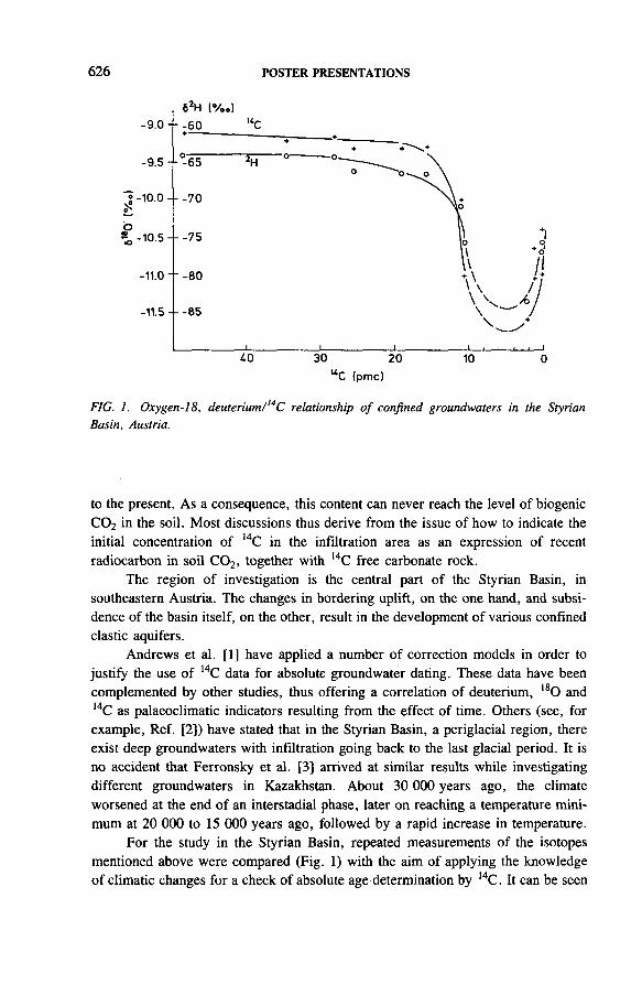
626 POSTER PRESENTATIONS

- 9 .0 - - - 6 0

-9 .5 - - - 6 5

5 - 1 0 . 0 -O4

- -70

О% -10.5 - - - 7 5

-11.0 -- - 8 0

-11.5 - - - 8 5

62H |% e)

СО 30 20

UC (pmc)

10

FIG. 1. Oxygen-18, deuterium/l4C relationship o f confined groundwaters in the Styrian Basin, Austria.

to the present. As a consequence, this content can never reach the level of biogenic C02 in the soil. Most discussions thus derive from the issue of how to indicate the initial concentration of 14C in the infiltration area as an expression of recent radiocarbon in soil C 02, together with 14C free carbonate rock.

The region of investigation is the central part of the Styrian Basin, in southeastern Austria. The changes in bordering uplift, on the one hand, and subsi­dence of the basin itself, on the other, result in the development of various confined clastic aquifers.

Andrews et al. [1] have applied a number of correction models in order to justify the use of 14C data for absolute groundwater dating. These data have been complemented by other studies, thus offering a correlation of deuterium, 180 and l4C as palaeoclimatic indicators resulting from the effect of time. Others (see, for example, Ref. [2]) have stated that in the Styrian Basin, a periglacial region, there exist deep groundwaters with infiltration going back to the last glacial period. It is no accident that Ferronsky et al. [3] arrived at similar results while investigating different groundwaters in Kazakhstan. About 30 000 years ago, the climate worsened at the end of an interstadial phase, later on reaching a temperature mini­mum at 20 000 to 15 000 years ago, followed by a rapid increase in temperature.

For the study in the Styrian Basin, repeated measurements of the isotopes mentioned above were compared (Fig. 1) with the aim of applying the knowledge of climatic changes for a check of absolute age determination by 14C. It can be seen

POSTER PRESENTATIONS 627

from Fig. 1 that groundwaters with a radiocarbon content down to about 16 per cent modern carbon (pmc) represent infiltration conditions comparable with present ones; the 180 concentration reaches -9 .5 to 9.07oo. Referring to Ref. [3], these waters must be younger than 14 000 years.

The next older group of groundwaters (11 pmc) are slightly lower in their stable isotope content, indicating a lower temperature during their infiltration. The lowest stable isotope concentration was found in groundwater at a depth of 80 m, representing l80 data some 2.5700 lower than recent ones. This would result in an infiltration temperature which is 7°C lower than today.

However, this water is still not the oldest. There are others with a radiocarbon content lower than 2 pmc, but definitely more enriched in deuterium and 180 . It appears that they originate from an ending interstadial period, indicating a better climate than that existing later. Some researchers suggest a late interstadial climatic optimum some 30 000 to 40 000 years ago.

From the stable isotope/l4C relationship, a clear age can be deduced, depend­ing on the differentiation of groundwaters correlated with climatic changes within the Late Pleistocene. It is thus possible that age determination by radiocarbon can be limited by approximately 40 000 years. Furthermore, isotope data indicate that the climate did not change significantly within the last 10 000 years, or it did over time intervals that were too short to be detectable.

REFERENCES

[1] ANDREWS, J.N., et al., “ Environmental isotope studies in two aquifer systems. A comparison of groundwater dating methods” , Isotope Hydrology 1983 (Proc. Symp. Vienna, 1983), IAEA, Vienna (1983).

[2] FERRONSKY, V.I., et al., “ Relationships between climatic changes and variations in isotopic composition of groundwater, precipitation and organic soil matter in the Quaternary period” , Palaeoclimates and Palaeowaters: A Collection of Environmental Isotope Studies (Proc. Advisory Group Mtg Vienna, 1983), IAEA, Vienna (1983) 13-36.

[3] MOSER, H., et al., Altersgliederung von tiefliegenden artesischen Wàssern durch Messung des Deuteriumgehaltes, Naturwissenschaften 59 (1972).

628

IAEA-SM-319/7P

POSTER PRESENTATIONS

URANIUM ISOTOPES IN THE SPRING WATERS OF AGUAS DA PRATA, SÂO PAULO, BRAZIL

D.M. BONOTTOInstituto de Geociências e Ciências Exatas,UNESP, Rio Claro,Sâo Paulo,Brazil

Uranium isotopic analyses were performed on mineral water samples from several springs in Águas da Prata to determine whether enhanced 234U/238U activity ratios could be generated in the area, to discuss the possible mechanisms responsible for the generation of such enhancement and to find out if the mechanisms related to the migration of 238U and 234U isotopes can generate concentrations that are greater than the gross alpha activity contaminant limit.

The city is an important tourist site in Sâo Paulo State, Brazil, located at the western edge of the Poços de Caldas Plateau. The plateau and its circular rim have an area of about 800 km2, and underlying them are mainly alkaline igneous rocks. Tinguaite is the predominant rock type of the plateau. The springs of Águas da Prata, in which uranium isotopic analyses were made, issue from diabase (Vitória, Prata- Antiga and Prata-Nova Springs), phonolite, foyaite, volcanic breccia and tuffs (Platina and Paiol Springs) and silicified sandstone (Prata-Radioativa, Villela and Boi Springs).

These waters were first identified in 1885 because of the high content of dis­solved HCO3 and subsequently they were used for commercial and medical pur­poses. They are also well known because they have high radioactivity owing to dissolved 222Rn. Isotopic data on ÔD and ô180 for several samples indicated that they are of meteoric origin [1]. The tritium concentration of rainfall measured in Rio de Janeiro (1973) was 11.6 tritium units (TU). The 3H content was measured in duplicate in samples of Vitória and Platina Springs and the average values were 8.8 and 7.1 TU, respectively, which indicate that recent recharge predominates in the area (with residence times lower than ten years) [2].

The analytical method for the measurement of U isotopes involved the addition of 232U tracer (about 6.6 dis/min) 1 and 500 mg of Fe3+ carrier to each sample. Uranium was recovered by co-precipitation on Fe(OH)3 and subsequendy separated from Fe, Ca, Mg and other elements by solvent extraction and anion exchange proce­dures. Finally, U was extracted with 0.4M thenoyl tri-fluoracetone (TTA) diluted

1 1 dis/min = 1/60 Bq.

POSTER PRESENTATIONS 629

TABLE I. URANIUM CONTENT AND THE 234U/238U ACTIVITY RATIO IN SPRING WATERS FROM ÁGUAS DA PRATA, SÂO PAULO, BRAZIL. THE 222Rn CONTENTS AND CHEMICAL DATA ARE THE MEAN VALUES OF ONE YEAR MEASUREMENTS [2]

SpringUa

(iig/kg)

U-234/U-238activityratio3

Rn-222(nCi/L)

Baseexchange

indexb

TDS(mg/L)

F"(mg/L)

Prata-Antiga 0.59 9.12 1.61 -31 .12 2257.17 13.50

Prata-Radioativa 0.03 6.05 3.50 -5 .6 3 82.00 0.54

Prata-Nova 3.87 6.97 2.30 -34 .54 2258.08 14.80

Vitória 1.04 4.04 26.20 -21 .64 1042.00 8.30

Boi 0.08 4.04 14.34 -5 .61 54.00 0.66

Platina 0.24 8.28 3.40 -28 .80 935.67 16.90

Paiol 0.60 11.68 0.53 -59 .88 2625.42 20.60

Villela 0.53 3.66 34.30 -7 .21 43.08 0.56

a Uncertainty ±10% corresponding to la standard deviation. b Evaluated from the Na + , K + and СГ contents [2].

in a benzene solution, deposited on a stainless steel planchet and counted in a silicon surface barrier alpha spectrometer. The 234U/238U activity ratios were measured directly from the alpha spectra and the U contents calculated from the 238U count using the 232U count to determine the chemical yield. Table I reports the results obtained in this investigation and some chemical data on the various waters.

The compositions of these waters are not identical. The water sources derived from diabases and volcanic rocks are Na +-HCOj dominated and water sources de­rived from sandstones vary between the Na+-HC03 and Ca2+/Mg2+-HC03 com­position [2]. The base exchange index for the samples varies between —5.6 and— 59.9, which indicates that the strata of the aquifers supply alkaline elements to the water by dissolution.

No gross alpha or gross beta radioactivity measurements were reported for these waters in the evaluation of whether the values are higher than the contaminant limits established for members of the public. The highest activities for 234U and 238U nuclides were measured for the waters of Prata-Nova Spring (8.9 and1.3 pCi/L, respectively)2. However, they are lower than the 15 pCi/L limit [3].

2 1 curie (Ci) = 3.70 x 1010 Bq.

630 POSTER PRESENTATIONS

No estimates of etch rates were made for these aquifers. However, they are expected to be greater than 10“6 ц&~1. Under these conditions, alpha recoil can produce a 234U enhancement in solution corresponding to about 0.02, according to the isotopic model using zero order rate constants for 234U and 238U [4].

An inverse logarithmic correlation was found between the 234U/238U activity ratio and the 2Z2Rn content of the waters studied which appears to be related to different solution mechanisms of 222Rn and 234U nuclides at the water-rock interface.

There is a linear correlation between the 234U/238U activity ratios of the waters studied and the base exchange index, which indicates that the enhancement of 234U in solution increases with the grade of weathering of the strata of the aquifers. The same relationship is observed if the 234U/238U activity ratios are plot­ted against the total mineralization, total dissolved solids (TDS) (or electrical con­ductivity), or fluoride contents of the waters. The F" concentrations in the spring waters derived from sandstones are lower than the recommended range of 1 to 1.5 mg/L for drinking water. No occurrences of dental fluorosis have been reported in the area, in spite of the high values of F" in waters derived from diabases and volcanic rocks. Intense weathering of porous volcanics, together with profuse seasonal rainfall, could explain the occurrence of these highly fluoridic waters, which are of Na(HC03) type and poor in Ca. The same situation was observed in other areas [5].

REFERENCES

[1] SZIKSZAY, М., TEISSEDRE, J.M., BARNER, U., MATSUI, E., Geochemical and isotopic characteristics of spring and groundwater in the state of Sao Paulo, Brazil, J. Hydrol 54 (1981) 23-32.

[2] SZIKSZAY, М., Hidrogeoquimica das fontes de Águas da Prata, Estado de Sâo Paulo, Thesis, University of Sâo Paulo, Sâo Paulo (1981).

[3] UNITED STATES ENVIRONMENTAL PROTECTION AGENCY, Interim Primary Drinking Water Regulations, Federal Register 158, United States Government Printing Office, Washington, DC (1975).

[4] ANDREWS, J.N., KAY, R .L.F., The U contents and U-234/U-238 activity ratios of dissolved uranium in groundwaters from some Triassic sandstones in England, Isot. Geosci. 1 (1983) 101-117.

[5] LAHERMO, P., SANDSTRÔM, H., “ The occurrence and geochemistry of fluorides in natural waters with reference to their geomedical implications” , Geochemical Explo­ration (Proc. 13th Int. Symp. Rio de Janeiro, 1989), Sociedade Brasileira de Geoquím­ica, Rio de Janeiro (1989).

POSTER PRESENTATIONS 631

MESURE DU TRANSPORT SEDIMENT AIRE PAR L’EMPLOI D’UNE JAUGE A TRANSMISSION

B. LONG, O. GAGNÉ INRS-Océanologie,Université du Québec,Rimouski, Québec, Canada

IAEA-SM-319/9P

La mesure du transport sédimentaire in situ reste un problème toujours difficile à résoudre. Le transport du matériel sableux se fait principalement par charriage; or, durant un transport par charriage, les sédiments migrent depuis le flanc exposé d’une dune pour venir sédimenter sur le flanc de progradation. Ce grain alors piégé reste inactif durant tout le passage de la dune. Ce processus induit une erreur importante de la mesure du transport sédimentaire par l’utilisation de traceurs radioactifs.

Le but du travail que nous avons accompli est de déterminer le transport sédimentaire par charriage en utilisant une jauge nucléaire à transmission qui mesure non pas le transport d’un grain de sable mais le mouvement des dunes de sable. Cette jauge a mesuré la vitesse de déplacement des figures sédimentaires. Parallèlement, des mesures de courants ont été établies à l’aide de courantomètres électro­magnétiques.

La jauge nucléaire développée est un appareil ayant une autonomie de 45 jours et pouvant emmagasiner une donnée toutes les 12 s (356 000 données). Elle utilise une source de 137Cs de 92,5 MBq, une sonde SR4 Saphimo Steel et un système d’acquisition modifié CRIO de Cambell. Sa précision est de l’ordre de 1 mm sur un comptage de 12 s. Cet appareil est conçu pour travailler jusqu’à des profondeurs de50 m.

Les travaux de terrain que nous avons entrepris montrent que, dès 9 cm/s, des microdunes, de 3 mm de hauteur, se déplacent. Elles sont remplacées à 20 cm/s par des petites dunes (1 à 2 cm de hauteur), puis par des dunes moyennes (4 à 7 cm de hauteur) lorsque le courant dépasse les 30 cm/s. Au cours d’un cycle de marées, nous avons ainsi déterminé les seuils de début d’entraînement des particules (dunes) et les seuils de fin d’entraînement des particules. D’autre part, nous avons mesuré pour des diverses vitesses de courants des vitesses différentes de déplacement des dunes; ainsi, pour des courants de l’ordre de 30 cm/s, trois rides passent sous le détecteur, alors que seulement deux passent lorsque le courant est de 25 cm/s.

En période agitée, en présence de houles, le seuil de transport devient moindre; en effet, dès 20 cm/s, les figures dont les hauteurs sont comprises entre 1,5 et 1,7 cm se mettent en mouvement.

632 POSTER PRESENTATIONS

Le déplacement des dunes géantes (1 m de hauteur et 120 m de longueur d’onde) a été mesuré en calculant la vitesse de déplacement du flanc abrupt (en progradation); ainsi, il a été déterminé que 5 cm d’accumulation représentent un déplacement horizontal de 2 m en 18 jours.

IAEA-SM-319/10P

FINE TUNING THE CELLULOSE MODEL FOR DENDROCLIMATOLOGICAL INTERPRETATION

W.M. BUHAY, T.W.D. EDWARDS, R. ARAVENADepartment of Earth SciencesandQuaternary Sciences Institute,University of Waterloo,Waterloo, Ontario,Canada

Changes in the oxygen and hydrogen isotopic composition of wood cellulose primarily reflect changes in the isotopic composition of meteoric water taken up by trees and the subsequent evapotranspirative enrichment of plant water [1]. There­fore, cellulose based isotope palaeoclimatic interpretations are possible owing to the strong relationships between the mean annual temperature and meteoric water isotopic composition [2] and between relative humidity and evapotranspirative enrichment [3]. The empirical ‘cellulose model’ [1] allows for the quantitative esti­mation of 5 I80mw and h values from ô2D and ôl80 measurements on wood cellulose.

The cellulose model has been used with §180 and ô2H data from a modern elm (Ulmus) to investigate the climatic variation in southern Ontario over the period 1735-1968. Systematic divergent shifts in ô180 and ô2H over the 233 year growth period strongly suggest commensurate variability in the isotopic composition of meteoric water and humidity that is broadly consistent with the pattern of tempera­ture and moisture fluctuation indicated by other information.

Although the cellulose model appears to provide a good qualitative estimate of climate change, the inferred ô l8Omw and humidity changes are believed to be excessive with respect to the available instrumental climate records over the 70 years prior to 1968 (e.g. 6°C inferred temperature variation versus 2°C measured temper­ature variation in the Great Lakes region [4]).

POSTER PRESENTATIONS 633

(а) (Ы

FIG. 1. Inferred relative humidity versus ôl8Omv/ (mean annual temperature) for the inter­val 1900-1970 AD. (a) Temperature variation for the unmodified cellulose model [1] is 6°C; (b) temperature variation for the modified cellulose model is 3.2 °C, similar to the 2 °C temper­ature variation recorded by instruments.

Consideration of new data from modern trees suggests that the original model formulation underestimated the kinetic effects for oxygen isotopes during évapo­transpiration of plant waters. Increasing the kinetic separation in accordance with results from recent growth experiments [5] reduces the apparent sensitivity of the model to changing temperature and humidity, and leads to reasonable quantitative estimates of recent climate variation in southern Ontario.

Recalculation of <5180 and h from the Kitchener, Ontario, data using revised kinetic effects reduces the variation in mean relative humidity during the growth season from 0.29 (0.43-0.72) to 0.15 (0.57-0.72). The estimated S18Omw variation declines from 4% 0 (-15 .3 to —11.3700) to 2700 (13.1 to 11.07oo), which indi­cates a temperature variation of about 3°C, assuming the modern gradient of about 0.65 700 per °C between the mean annual temperature and the isotopic composition of meteoric water (Fig. 1).

REFERENCES

[1] EDWARDS, T.W .D., FRITZ, P., Assessing meteoric water composition and relative humidity from l80 and 2H in wood cellulose: Paleoclimatic implications for southern Ontario, Canada, Appl. Geochem. 1 (1986) 715-723.

[2] CRAIG, H., GORDON, L.I., “ Deuterium and oxygen-18 variations in the ocean and marine atmosphere” , Stable isotopes in Oceanographic Studies and Paleotemperatures (Proc. 3rd Spoletto Conf., 1965) (TONGIORGI, E., Ed.) (1965).

[3] EDWARDS, T.W .D., ARAVENA, R.O., FRITZ, P., MORGAN, A.V., Interpreting paleoclimate from l80 and 2 H in plant cellulose: Comparison with evidence from fossil insects and relict permafrost in southwestern Ontario, Can. J. Earth Sci. 22 (1985) 1720-1726.

[4] PHILLIPS, D.W., “ Climate change in the Great Lakes region” , Proc. 1st United States of America-Canada Symp. on Impacts of Climatic Change in the Great Lakes Basin, Chicago, 1989.

[5] BARIAC, T., JUSSERAND, C., MARIOTTI, A., Evolution spatio-temporelle de la composition isotopique de l’eau dans le continuum sol-plante-atmosphère, Geochim. Cosmochim. Acta 54 (1990) 413-424.

634 POSTER PRESENTATIONS

IAEA-SM-319/14P

ORIGIN OF GROUNDWATER IN THE TERTIARY VOLCANIC COMPLEX IN CENTRAL SLOVAKIA

J. SILAR Charles University,Prague

L. SKVARKA Comenius University,Bratislava

Czechoslovakia

On the inner side of the Carpathian Mountain arch in central Slovakia, there is a sequence of Miocene to Pleistocene volcanic rocks predominantly of andesite type and their pyroclastics, forming a stratovolcanic structure up to 1500 m thick over an area of about 5400 km2. Frequent systems of faults run northwest- southeast through the volcanics, and regional faults cross the entire Carpathian arch in a north-south direction. The volcanics are underlain by Mesozoic carbonate and by earlier crystalline rocks. The andesites were considered to be poor aquifers. A recent systematic hydrogeological investigation has confirmed that there is a concen­tration of groundwater flow in fractured zones along faults, this flow discharging into streams.

POSTER PRESENTATIONS 635

FIG. 1. Map o f the sampling sites with major tectonic zones (1: pre-Neogene formation; 2 ; contour lines o f the surface o f the pre-Neogene bedrock; 3: tectonic zones; 4: groundwater flow direction; 5: number o f sample and borehole code).

Most of the groundwater in the volcanics is of Ca(Mg)-HC03 type, with tem­peratures between 10 and 15°C and exhibiting shallow or intermediate circulation. A deeper origin in the underlying crystalline or carbonate rocks is indicated by a higher concentration of SO4’, free C02 and by higher temperatures (up to 52.5°C).

Isotope analyses of groundwater from springs and boreholes within the area of the volcanics (Fig. 1) have shown differences in the water’s isotopic composition. These analyses also reflect the influence of earlier underlying geological units on the groundwater’s chemical and isotopic composition.

Thirteen samples were analysed. The <5180 value of the samples is between -9 .8 and —11.5700, which applies also to thermal springs. The ôl3C value is between -2 .2 and -2 0 .3 7 oo. In two thermal springs it is -2 .5 and -5 .7 7 00, and in five other samples of cold water it is less than — 8.8 700. In the remaining six sam­ples, the <513C value is between —11.0 and -2 0 .3 7 oo. Thus, about half of the groundwater samples investigated seem to be influenced by the contribution of C02 with a deep magmatic or metamorphic origin (see Fig. 2 and Table I).

TABLE I. ISOTOPIC CHARACTERISTICS OF GROUNDWATER FROM THE AREA OF NEOGENE VOLCANIC ROCKS IN CENTRAL SLOVAKIA

No. LocalityPoint of sampling Aquifer

Water level

( + , - )

No. of samples

No. of C-14

measure­ments

Radiocarbon(pmc)

гс-13(7 00 PDB)a

5C-13 ( 7 „ SMOW)b

H-3(TU)

t(°C) Notes

1 Cajkov Borehole HS 6 Pyroxeneandesite(Tertiary)

+ 355 CU 973 22.49 ± 3.80 -8 .0 -1 1 .2 5 ± 5

2 Vyhne Outflow of a mining gallery

Limestone + 351 CU 965 4.52 ± 16.16 -2 .5 -1 1 .4 < 3 35 Thermalwater

3 Podzámcok HS 1 Andesite - 350 CU 964 70.79 ± 1.82 -1 8 .4 -9 .8 < 3 14.7

4 Dobrá Niva Borehole HS 7 Andesite Originally + 349 CU 963 55.14 ± 2.08 -1 3 .5 -1 0 .0 < 3 14.0

5 Zajezová Borehole Z 1 Andesite + 348 CU 962 78.19 ± 1.74 -1 8 .2 -1 0 .5 5 ± 5 10.8

6 ViglasskáHuta,Kalinka

Viera Spring Andesite + 352 CU 972 0.15 ± 475.19 - 2 .2 -1 1 .5 < 3Mineral water

10.0 containing C 0 2

7 SlatinskéLazy Lohyña Spring Andesite + 353 CU 974 65.46 ± 3.45 -8 .8 -1 0 .3 < 3 7.5

8 BanskÿStudenec

Borehole HBS 3 & HBS 4

Andesite - 354 CU 968 81.91 ± 1.71 -2 0 .3 -1 0 .6 < 3 13.0

9 SklenéTeplice

Borehole ST 1 Limestone + 345 CU 958 75.14 ± 1.78 -5 .7 -1 0 .6 < 3 53.0 Thermalwater

10 RevistskéPodzâmcie

Borehole HS 11 Andesite — 358 CU 969 Contaminated -1 3 .6 -1 0 .6 < 3 13.0

636 POSTER

PRESENTATIONS

11 Lukavica pri Borehole LKC 4 CarbonateZarnovice rocks

underlyingandesite

12 Detva Borehole JS 1 Andesite

13 Horny Borehole JS 3 AndesiteTisovnik

a PDB: Pee Dee Belemnite. b SMOW: standard mean ocean water.

CU 967 49.60 ± 2.23 -1 1 .0

CU 960 71.08 ± 1.82 -1 9 .5

CU 961 95.40 ± 1.60 - 5 .4

10.0 < 3 30

10.3 10 ± 5 12.0

10.8 < 3 15.5

POSTER PRESEN

TATIO

NS

638 POSTER PRESENTATIONS

Ca(Mg)SO«Ca(Mg)Cl

GRAF A.M. PIPERA

FIG. 2. Chemical character o f groundwater from an area containing Neogene volcanic rocks in central Slovakia ( • : fresh water; О : thermal water; I : water containing carbon dixode; the numbers correspond to the sample numbers in Fig. 1 and Table I).

A majority of samples (ten) showed tritium activity levels below 3 tritium units (TU), two samples 5 ± 5 TU and one 10 ± 5 TU, i.e. only one of the samples may be considered to contain a component of groundwater of truly modern origin.

Radiocarbon analyses were performed on 12 samples. The 14C activities are in a wide range, between very close to zero (for one spring containing C02) and 95.40 per cent modern carbon (pmc). Only the latter sample can be considered to be modern, according to the 14C concentration. Samples from eight localities can be considered to be Holocene in age. The radiocarbon age of three samples could be considered to be Pleistocene and would be in accordance with the geological struc­ture and deep origin of groundwater. However, this is not reliable owing to the potential influence of non-active magmatic or metamorphic C02. One sample is a

POSTER PRESENTATIONS 639

mixture of Holocene and modern water (according to the higher 3H and low I4C concentrations). Owing to the draining activity of the fault zones in the volcanic rocks, mixing of Holocene and recent shallow groundwater also has to be expected in the remaining cases of Holocene groundwater samples.

In the mining district of Banská Stiavnica, the groundwater of the volcanics is influenced by mining activities and is drained into the underlying crystalline rocks, which is also reflected by inducing tritium rich water into the circulation system.

The isotope analyses helped to explain the groundwater structure in the vol­canic rocks in relation to the earlier structures, and contributed to knowledge on the development of groundwater and the evaluation of its resources.

IAEA-SM-319/16P

LOCALIZACION DE FUGAS EN EL EMBALSE DE SABANETA

A. PLATA BEDMAROrganismo Internacional de Energía Atómica,Viena

J. FEBRILLET, A. TORRES, J. SAINT-HILAIRE, E. BUENO Instituto Nacional de Recursos Hidráulicos (INDRHI),Santo Domingo,República Dominicana

El embalse de Sabaneta tiene una influencia decisiva en la vida económica de la región de San Juan de la Maguana en la República Dominicana, donde se en­cuentra enclavado, siendo utilizado para regadío y producción de energía eléctrica. La presa, construida de materiales sueltos, presentó problemas de filtraciones a los cinco años, aproximadamente, de su construcción (1986). Un caudal de agua, que ha llegado hasta unos 400 L/s, emerge a través de la base de un túnel de descarga existente en el estribo derecho (Fig. 1). El mayor problema planteado se refiere al riesgo de este flujo de agua para la estabilidad de la presa.

El estudio de las filtraciones se ha realizado utilizando, entre otras, las siguien­tes técnicas:

1) Análisis químicos e isotópicos del agua (D, l80).2) Perfiles de temperatura, conductividad y gamma natural en piezómetros y/o

embalse.

Cot

a to

po

grá

fica

(m

.s.n

.m.)

640 POSTER PRESENTATIONS

660

650

6 40

630

620

610

600

590

580

570

560

0 20 40 60 80 100 120 НО 160 180 200D is tanc ia re la tiv a (m etros)

FIG. 2. Horizontes permeables detectados con ensayos de trazadores.

Pozo 6

C o n ta c to p re s a -te rre n o _. (in ferido)

Nivel p iezom etricoI m p e r m e a b l e

Horizontespermeables

\ _ F r a c t u r a . d e t e c t a d a ' " " P e r m e a b l e

. H o rizon tes pe rm eab les

Corona de la p re sa

Nivel máxim o

C uerpo de p re saNivel a c tu a l

Im perm eable

Túnel a liv ia d e ro : de s e rv ic io )Im perm eable

Túnel de d e s c a rg a '

Zona de flu jo p re fe re n c ia li i i i ______i______i______i______ i______i_____

POSTER PRESENTATIONS 641

6 3 0

62 0

610

enоао

59 0

М а уо , 1989

T e m p e r a t u r a f i l t r a c io n e s

N ive l d e l a g u a

C o ta m ín im a d e l f o n d o

20 21 22 23 2 UT e m p e r a t u r a

25*C)

26 27

FIG. 3. Perfiles de temperatura medidos en el embalse en épocas diferentes. Se indica la tem­peratura de las filtraciones en la misma época.

FIG. 4. Zona posible de infiltración del agua definida a través de la temperatura.

642 POSTER PRESENTATIONS

3) Medida de flujos en el interior de los piezómetros utilizando yodo 131 y salcomún como trazadores.

(4) Experiencias de interconexión entre embalses, piezómetros y surgencias.

Siete piezómetros fueron construidos para estudiar la zona afectada por las filtraciones. Los flujos existentes en el interior de estos piezómetros fueron determi­nados por el método basado en el marcado de toda la columna de agua y mediante inyecciones puntuales de trazador para la medida de flujos verticales [1, 2]. En todos los piezómetros se detectaron flujos verticales ascendentes, debido a la presencia de un estrato carstificado profundo por donde circula la mayor parte del agua proce­dente del embalse. Dicho estrato se encuentra separado del cuerpo de la presa por una secuencia de estratos permeables e impermeables, tal como se muestra en la Fig. 2. Los estratos permeables superiores no contribuyen de forma significativa a las filtraciones, lo cual fué comprobado a través de ensayos con trazadores en dos piezómetros antes de penetrar hasta el estrato profundo. Los estratos permeables in­dicados en la Fig. 2 se detectaron asimismo por medio de perfiles gamma natural (menor flujo de radiación gamma en zonas de cavidades). Siete experiencias de inter­conexión inyectando fluoresceina o l3lI en los piezómetros confirmaron la existen­cia de la vía preferencial de circulación del agua mostrada en la Fig. 2.

Por otro lado, el embalse mostró un alto grado de estratificación térmica que varió de unas épocas a otras del año (Fig. 3). Comparando los perfiles de temperatu­ra del embalse con la temperatura del agua de los afloramientos, pudo comprobarse que este agua sólo puede provenir de infiltración de los niveles más profundos del embalse entre las cotas 606 y 590 m.s.n.m. (cota mínima del fondo). La zona respon­sable de las filtraciones quedó así reducida a una superficie del fondo de unos0,5 km2. A través de diversas experiencias de interconexión inyectando trazadores en el embalse (yodo 131 y uranina), pudo localizarse la zona de infiltración efectiva, la cual se indica en la Fig. 4.

REFERENCIAS

[1] BOANZA, E., PLATA-BEDMAR, A., PILES, E., “ Aplicación de la técnica del pozo único mediante el marcado de toda la columna piezométrica” , Isotope Hydrology 1970 (Actas Simp. Viena, 1970), OIEA, Viena (1970) 695-711.

[2] PLATA-BEDMAR, A., “ Single well techniques using radioactive tracers” , Tracer Methods in Isotope Hydrology (Proc. Advisory Group Mtg Vienna, 1982), IAEA- TECDOC-291, OIEA, Viena (1983) 17-46.

POSTER PRESENTATIONS 643

SOURCES OF WATER RECHARGE IDENTIFIED BY ISOTOPES IN EL MINYA GOVERNATE (NILE VALLEY, MIDDLE EGYPT)

A. EL BAKRI, A. TANTAWI Faculty of Sciences,Minya University,Minya,Egypt

B. BLAVOUX, M. DRAY Faculté des sciences,Université d’Avignon,Avignon,France

IAEA-SM-319/17P

1. INTRODUCTION

The present isotopic study deals with the alluvial aquifer linked to the Nile River, and its irrigation and drainage canals in Minya District, for a better under­standing of the origin of groundwater in space and time.

2. METHODS

Seventy three groundwater and 20 surface water samples were collected and analysed for the presence of isotopes and major chemical elements during the period October 1987 to August 1988. The analyses were performed mainly at the Agency Laboratory, in Vienna, and partly at the Avignon, Thonon and Paris University laboratories in France.

3. RESULTS

On the basis of the isotopic data, three groups of waters can be defined:

— The first group (Gl) is characterized by a 3H content lower than 3.9 tritium units (TU), a ôl80 value between —1.3 and +0.97oo and a ô2H value vary­ing between -3 .7 and +13.6700.

644 POSTER PRESENTATIONS

( a )

8180 (%.)( b )

-38180 (%o)

FIG. 1. (a) Relationship between S,sO and &2H fo r surface water and groundwater, (b) Detail view o f groups G1 and G2 ( □ ; G1 before 1953 (?); Ш : G2 present waters; *: mixed waters; A : surface waters).

POSTER PRESENTATIONS 645

— The second group (G2) is characterized by a 3H content in the range between15.3 and 64.0 TU, a <5,80 value between +2.3 and +3.86700 and a <52H value between +20 and +307oo versus standard mean ocean water.

— The third group (G3), represented only by two deep boreholes reaching the Eocene limestone aquifer lying under the alluvial deposits, is marked by a very depleted stable isotope content between —6.6 and — 8.4ô700, <5180 and ¿>2H values of -5 4 and -6 8 7 00, respectively, and a low tritium content (2.7 and 9.2 TU). Varying degrees of mixing between G1 and G2 can be found. The surface waters are similar to G2.

4. INTERPRETATION AND CONCLUSIONS

Group G1 is attributed to old Nile water inundations before thermonuclear tests (i.e. before 1953). These waters are less affected by evaporation due to the high discharges of the river and the absence of a reservoir upstream. Most of the samples are located along the El Moheet Drain.

Group G2 corresponds to the recent recharge (i.e. in the last decade) from Nile water and its irrigation network. These waters are located along this network and reach the western desert fringe, which was recently irrigated (i.e. as of 1968) for land reclamation.

The third group, G3, represents palaeowaters recharged during the pluvial period when colder climatic conditions than those currently existing prevailed. It is similar to Nubian sandstones or Continental Intercalaire aquifers extending mainly into central and north Africa.

Figure 1 shows that most of the G1 and G2 water samples lie along an evaporation line with a slope of =6.0 and a deuterium excess of 6.5. This slope (3.6) is steeper than that obtained with evaporation pans during the period 1987-1988.

These results are essential for the protection of the aquifers and for better management of the water resources along the Nile River in this area.

ACKNOW LEDGEM ENTS

The authors are very grateful to the Isotope Hydrology Section of the IAEA, and particularly to K. Frôhlich for his assistance and support. They also acknowledge the help of El Minya University, which financed M. Tantawi during his fellowship in Avignon, France.

646 POSTER PRESENTATIONS

ISO TO PIC STUDIES OF DEEP AND SURFACE W ATERS IN TH E FREN CH M ASSIF CEN TRAL

C. FOUILLAC, A.-M. FOUILLAC, L. CHERY Département géochimie,Bureau de recherches géologiques et minières, Orleans,France

IAEA-SM-319/18P

The isotopic composition of thermomineral waters in the Massif Central region in France has been studied extensively from 1974 until the present. The principal support for these studies has been provided by geochemical surveys of hot water for geothermal resource assessment purposes and hydrogeological studies linked to the ‘Géologie profonde de la France’ (GPF) scientific drilling programmes [1-3]. These programmes have helped us to build a database comprising 105 dilute superficial waters (springs, rivers and shallow boreholes) and more than 200 hot geothermal waters and warm-to-cold mineralized waters. All of the samples were analysed for oxygen and hydrogen stable isotopes. The tritium content was also measured for some samples and the chemical composition of the deep water samples was studied in great detail. Although some of the isotopic data have already been published, the majority have not.

Data on the 105 superficial waters helped to establish the following equation for the regional meteoric water line (RMWL):

<5D = 8ôi80 + 13.1

The deuterium excess value (13.1) has a standard deviation (2E) of 2.9.It is interesting to note that slightly different equations can be derived locally

for limited sets of samples located in restricted areas. For example, superficial sam­ples from the Ardèche area give:

ÔD = 8ô180 + 15

whereas

ôD = 8ôi80 + 11.4

defines the regression for the Cézallier samples.

POSTER PRESENTATIONS 647

FIG. 1. Comparison o f the isotopic composition o f deep waters with that o f the RMWL (SMOW: standard mean ocean water).

The chemical composition, tritium content and certain physical parameters (outlet temperature, flow rate) were used as criteria to select the most representative of all of the water samples for each geothermal area and for each separate mineral water system. We were then able to compare the isotopic composition of the deep waters with that of the RMWL (Fig. 1). Although most of the samples fall within 2E of the RMWL, several exhibit remarkable behaviour.

One sample, Co (from the southeastern edge of the large basaltic Volcano Cantal), and, to a lesser extent, two samples issuing from the granitic basement of the northern Massif Central, Ba and Bl, show a clear positive l80 shift. These samples all exhibit fairly high dissolved solids contents and the chemical composi­tions typical of deep waters. The l80 shift is therefore probably due to isotopic exchange between rock and water at high temperature [4].

Some samples, on the other hand, are significantly shifted in the opposite direction from the RMWL (see AR51, for example). This kind of shift is rather uncommon and its significance is still open to discussion. It could, for example, be explained by isotopic exchange between water and C 02 gas percolating through it. This area is, in fact, characterized by widespread high magmatic C02 flux [5]. Another explanation can be found in a modification of the RMWL equation over time in conjunction with climatic events.

648 POSTER PRESENTATIONS

REFEREN CES

[1] FOUILLAC, С., Chemical geothermometry in C 0 2 rich thermal waters: Example of the French Massif Central, Geothermics 12 2, 3 (1983) 149-161.

[2] VUATAZ, F.D., FOUILLAC, A.-М., FOUILLAC, С., MICHARD, G., BRACH, M ., Etude isotopique et suivi géochimique des eaux des sondages de Chassole et de quelques sources minérales du Cézallier, Géologie de la France No. 4 (1987) 121-131.

[3] FOUILLAC, C., FOUILLAC, A.-M., Chemical and isotopic study of the mineral springs of Ardèche, Hydrogéologie No. 3 (1989) 229-236.

[4] TRUESDELL, A.-H., HULSTON, J.-R., “ Isotopic evidence of environments of geothermal systems” , Handbook of Environmental Isotope Geochemistry, The Terrestrial Environment (FRITZ, P., FONTES, J.-C., Eds), Vol. 1, Elsevier, Amsterdam (1986) 179-226.

[5] MATTHEWS, A., FOUILLAC, C., HILL, R., O’NIONS, R.-K., OXBURGH, E.-R., Mantle-derived volatiles in the continental crust: The Massif Central of France, Earth Planet. Sci. Lett. 85 (1987) 117-128.

IAEA-SM-319/19P

M ETHODE E T A PPA R EILLA G E POUR LA M ESURE,A L ’A ID E D’UN TRACEU R R A D IO A CTIF, DE TRES FA IB LES D EBITS D’IN FILTR A TIO N V E R TIC A LE DE L ’EAU AU TRAVERS DES SOLS EN PLA CE

B. GAILLARD, P. CALMELS, R. MARGRITA Section d’application des traceurs,CEA, Centre d’études nucléaires de Grenoble,Grenoble

P. ANDRÉDivision Etude des sites,CEA, Agence nationale pour la gestion des

déchets radioactifs (ANDRA),Fontenay-aux-Roses

France

Cette méthode a été développée pour qualifier ou contrôler des sites de stockages de déchets toxiques (radioactifs ou industriels) dont la très faible perméabi­lité verticale doit garantir la protection de la qualité des eaux des aquifères sous-jacents.

POSTER PRESENTATIONS 649

tu b e d 'équil ibre i n e r t em o te u r tu b e d 'équ i l ib re

c o n t e n a n t le t r a c e u r

7Ш7777Ш7ШШ^

FIG. I. Appareil pour la mesure des faibles perméabilités verticales.

Le principe original de cette mesure consiste à quantifier l’accroissement en fonction du temps de la concentration d’un traceur introduit, au travers d’un circuit d’équilibre hydrostatique avec le milieu extérieur, dans un volume d’eau confiné au contact du sol (fig. 1).

La mesure s’effectue sous une charge d’eau minimale de 0,5 m, généralement dans une fouille d’environ 4 m2 de surface creusée dans le sol. La cloche de confinement de forme lenticulaire délimite au contact du fond de la fouille une surface circulaire de 1 m2. Le circuit d’équilibre hydrostatique contenant la solution de traceur est constitué d’une longue tubulure de faible diamètre lovée sur un support extérieur et raccordée à la partie supérieure de la cloche de confinement. A l’intérieur de celle-ci sont disposés un détecteur à scintillation et un agitateur de façon à homogénéiser le volume confiné avant chaque mesure d’activité.

Une fois l’appareil en place, les mesures à deux dates distinctes t, et t2 per­mettent de déterminer le taux de comptage N¡ correspondant au volume de solution de traceur entré dans le volume confiné en remplacement du volume infiltré dans le sol pendant le temps At = t2 — t,. Ensuite, l’introduction dans le volume confiné d’une partie aliquote de la solution de traceur permet de déterminer le taux de comptage volumique Na de celle-ci. Alors, le quotient N¡/Na traduit directement le volume v de solution de traceur introduit sous la cloche, égal au volume d’eau infiltré dans le sol et donc le débit spécifique Q d’infiltration:

Q = v/Дt (m3-s_l - m"2)

sous une charge d’eau connue.Le traceur radioactif utilisé est le technétium 99 (99Tcm) qui émet un rayonne­

ment de faible énergie (140 keV) ne nécessitant pas pour sa manipulation de protec­tion d’épaisseur importante et dont la courte période radioactive (T,/2 = 6 h) est suffisante pour la durée de mesure et n’entraîne pas de contamination résiduelle du sol au-delà de quelques jours. Cet élément est aisément disponible sur le terrain à

650 POSTER PRESENTATIONS

l’aide d’un générateur isotopique (ELUMATIC III) à partir du molybdène 99 (99Mom) dont la période radioactive est de 66 h.

Avant de procéder à des mesures in situ, les performances de l’appareillage ont été testées en laboratoire à l’aide d’un banc d’étalonnage spécialement conçu pour simuler des débits spécifiques très faibles, jusqu’à 10 '11 m3-s~' -m-2. La sensibilité de mesure est élevée et dépend en grande partie de l’activité spécifique de la solution de traceur. Elle est cependant limitée par les phénomènes de diffusion moléculaire au travers de la faible surface d’entrée de la solution de traceur dans le volume confiné. Dans ces conditions, la précision des mesures évolue de + 5% pour Q = 10-7 m3-s~‘ -m '2 à ±50% pour Q = 5 x 10-n m3-s~' -m-2.

Depuis sa réalisation, cet appareillage a plusieurs fois été mis en œuvre, par exemple sur le site d’Aube (Soulaines, Dhuys) en France, retenu par l’ANDRA pour le stockage en surface des déchets radioactifs de faible et moyenne activité à vie courte.

IAEA-SM-319/20P

APPORTS DES DONNEES ISOTOPIQUES A LA CONNAISSANCE DE L ’O RIGIN E E T DU TEM PS DE SEJOUR DES EAUX SOUTERRAINES DANS LE SO CLE FISSURE EN AFRIQ UE DE L ’OUEST

J. SARROT-REYNAULD Laboratoire d’hydrogéologie,Université de Grenoble 1,Grenoble, France

J. BIEMI, J.-P. JOURDA, N. SORO Département des sciences de la Terre,Université d’Abidjan,Abidjan, Côte d’ivoire

A.Z. TRAOREEcole nationale d’ingénieurs,Bamako, Mali

Les teneurs en isotopes (180 , 2H, 3H) des eaux souterraines prélevées dans des puits et forages, à des profondeurs importantes pouvant atteindre plus de 120 mètres dans les roches fissurées précambriennes (granites et migmatites anté- birrimiens, assises volcanosédimentaires birrimiennes) et infracambriennes (grès,

POSTER PRESENTATIONS 651

schistes, calcaires et jaspes) ou les dolérites panafricaines d’Afrique de l’Ouest, per­mettent de déterminer l’origine et le temps de séjour dans l’aquifère de ces eaux qui sont souvent en charge sous la couverture d’altérités.

Les échantillons étudiés ont été prélevés entre les latitudes de 5° 15' et 13°35' Nord et les longitudes de 3°30' et 8°00' Ouest, en Côte d’ivoire et au Mali. Les résultats d’analyses ont été regroupés avec ceux concernant le secteur de Kolokani- Nara au nord du Mali, le Burkina Faso et l’ouest du Nigéria. L’ensemble de ces don­nées couvre le secteur compris entre le golfe de Guinée et la frontière mauritanienne sur une distance de plus de 1200 km du sud au nord. On passe ainsi des zones de lagunes littorales à la forêt tropicale, puis à la savane arbustive et, enfin, aux zones subdésertiques du Sahel.

Dans toute cette région, les précipitations, réparties en grande et petite saisons des pluies, proviennent de l’avancée de la mousson du sud-ouest vers le nord-est lors du déplacement du front intertropical, de la condensation de l’évaporation sur la forêt tropicale ou même sur le delta intérieur du Niger.

Les teneurs en tritium des eaux souterraines étudiées montrent, comme dans beaucoup d’autres régions du monde, l’existence d’eaux anciennes très pauvres en tritium, d’eaux récentes ayant des teneurs voisines de celles des précipitations dans les divers secteurs aux époques voisines de celles des prélèvements, et d’eaux résultant de mélanges en proportions diverses d’eaux anciennes et d’eaux récentes.

Un grand nombre d’échantillons correspond à des eaux anciennes non renou­velées comme l’indiquait déjà la baisse quasi continue des niveaux piézométriques observée ces dernières années du fait d’une exploitation importante. La part d’eaux récentes dans les mélanges reste faible, même dans les régions à forte pluviosité, du fait de l’importance du ruissellement superficiel, de la reprise par évapotranspiration et des difficultés d’infiltration dues à l’épaisseur du recouvrement d’altérites.

Les points représentatifs des teneurs en l80 et 2H de chacune des eaux étudiées se répartissent sur un diagramme ô700 180 - ô700 2H sur une série de droites de corrélation de pentes très voisines de 8, d’équation ô70O 2H = 8 ô°/00 l80 + d, qui se différencient les unes des autres par des valeurs de l’excès en deutérium, échelonnées de -0,3 à +17. Mais, sur chacune de ces droites sont représentées des eaux pouvant avoir des teneurs en tritium et des minéralisations différentes (fig. 1).

Dans les zones tropicales, Г «effet de masse» limite le fractionnement par évaporation entre l80 et 2H qui ne se traduit alors que par une réduction de l’excès en deutérium.

Dans les zones sahéliennes, l’influence des lignes de grains qui modifient les conditions thermiques lors des précipitations peut également expliquer l’absence de droites dites d’évaporation.

Les points représentatifs des eaux de chacun des puits ou forages ne s’ordon- nent pas de façon régulière sur les droites de corrélation en fonction de la latitude ou de la longitude des points de prélèvement, ce qui implique l’existence de transferts

6 (%

o)

652 POSTER PRESENTATIONS

6180 (•/„.)

FIG. 1. Relations entre les teneurs en IH0 et 2H dans les eaux souterraines du socle fissuré d ’Afrique de l ’Ouest.

POSTER PRESENTATIONS 653

inégaux entre les zones d’alimentation par les précipitations et les points de prélève­ment, soit à travers les fractures et fissures du socle parfois sur de longues distances, soit par transit des eaux dans les cours d’eau superficiels avant infiltration.

Il est possible de déterminer un gradient moyen de continentalité qui est de l’ordre de 0,5 <5700 l80 et de 4 <57OD 2H pour 100 km, mais ce gradient varie en réalité dans d’assez fortes proportions pour les différentes droites de corrélation, ce qui traduit des conditions très différentes lors de l’infiltration des recharges.

Même si la composition isotopique des pluies varie au cours de chaque épisode pluvieux et d’un épisode à l’autre, les variations de même type observées sur des eaux prélevées à plusieurs centaines de kilomètres de distance sont liées à des condi­tions climatiques différentes des conditions actuelles et, plus particulièrement, à celles régnant lors des périodes anciennes du Quaternaire.

En fait, dans le socle fissuré, l’infiltration est rapide mais n’est qu’épisodique. Elle ne se produit que lors d’événements importants et est très faible dans les condi­tions habituelles du fait de l’intensité de l’évaporation, surtout dans la zone sahélienne, de l’épaisseur et de la nature de la couverture d’altérites qui déterminent un seuil de recharge des aquifères profonds.

Si l’importance des pompages tend à favoriser le mélange d’eaux d’origines et d’âges différents, les eaux souterraines captées dans le socle fissuré d’Afrique de l’Ouest sont le plus souvent des eaux anciennes non renouvelées dont les origines sont liées aux successions de périodes humides et de périodes sèches qui ont régné dans cette région et dont les temps de séjour sont déterminés par la structure même du milieu fissuré et, plus particulièrement, par Г interconnection ou non des réseaux de discontinuités et par l’épaisseur de la couverture d’altérites. La gestion à long terme de ces ressources en eaux doit tenir compte de ces données.

654 POSTER PRESENTATIONS

IAEA-SM-319/21P

HYDROCHIMIE, TENEURS ISOTOPIQUES ET ORIGINE DES SAUMURES ASSOCIEES AUX GISEMENTS DE POTASSE D’ALSACE

D. POUTOUKIS, J.-L. MICHELOT, J.-C. FONTES Laboratoire d’hydrologie et de géochimie isotopique, Université de Paris-Sud,Orsay

P.-L. BLANCInstitut de protection et de sûreté nucléaire, Commissariat à l’énergie atomique, Fontenay-aux-Roses

M. ANSART Département de géologie,MDPA Ingénierie,Mulhouse

France

Des études hydrochimiques et isotopiques ont été entreprises en 1986 sur les très faibles venues de saumures qui apparaissent sporadiquement dans les galeries des gisements oligocènes de potasse d’Alsace.

Les rapports Br7Cl“ et les teneurs en СГ mesurées sur les échantillons cor­respondent à ceux d’une solution marine évoluée par évaporation, postérieure au stade de précipitation de l’epsomite [1, 2]. Toutefois, les teneurs élevées en Ca2 + excluent la simple préservation d’une telle solution.

Deux types d’hypothèses peuvent être avancées pour rendre compte de ces caractéristiques chimiques:

— modification d’une solution marine résiduaire après évaporation, au cours de phénomènes diagénétiques (dolomitisation);

— remise en solution de dépôts évaporitiques marins anciens par une eau continentale et reconcentration par évaporation.

Les bilans chimiques sur les teneurs en Ca2 + , Mg2+ et SO4- peuvent s’accorder avec l’hypothèse de dolomitisation: l’excès de Ca2+ par rapport à une solution marine est compensé par un déficit en Mg2+ et SO4".

POSTER PRESENTATIONS 655

FIG. 1. Teneurs en 18О et 2 H des saumures.

En revanche, les teneurs isotopiques des sulfates, aqueux et solides, sont très différentes de celles des sulfates marins de l’Oligocène et sont voisines de celles des évaporites sulfatées marines du Permien [3]. Ce fait constitue donc un argument favorable à la seconde hypothèse, remobilisation d’évaporites anciennes. Cette remobilisation, pour être conciliable avec les rapports Вг“/СГ mesurés, aurait dû affecter l’ensemble d’une série évaporitique, y compris les stades ultimes. L’excès en Ca2 + pourrait être expliqué soit par le phénomène de dolomitisation, soit par la richesse initiale en Ca2+ de l’eau de dissolution. Un mélange entre ce type de solu­tion continentale et une eau marine désulfatée (par précipitation ou par réduction) avant évaporation pourrait également rendre compte des caractéristiques de ces saumures.

Les teneurs en isotopes stables de l’eau ( l80 , 2H) ne permettent pas de trancher en faveur de l’une ou l’autre hypothèse. Elles reflètent un stade poussé d’évaporation, probablement proche des conditions d’équilibre avec l’atmosphère, sans qu’il soit possible de préciser si cette évaporation a affecté à l’origine une eau marine ou une eau de type continental (fig. 1). Elles permettent toutefois, en conjonction avec la chimie, d’exclure pratiquement une participation d’eau météorique postérieurement aux phénomènes évaporatoires.

656 POSTER PRESENTATIONS

REFERENCES

[1] VALYASHKO, M.G., Geochem. Int. 6 (1956) 570.[2] HERRMANN, A.G., KNAKE, D., SCHNEIDER, J., PETERS, H., Contrib.

Mineral. Petrol. 40 (1973) 1.[3] CLAYPOOL, G.E., HOLSER, W.T., KAPLAN, I.R., SAKAI, H., ZAK, I., Chem.

Geol. 28 (1980) 199.

IAEA-SM-319/22P

APPROCHE ISOTOPIQUE DU FONCTIONNEMENT DU DRAINAGE EN MILIEU ARGILEUX

P. VACHIER*, C. COULOMB**,L. DEVER**, R. CALVET*

Laboratoire des sciences du sol,Institut national de la recherche agronomique, Thiverval-Grignon

Laboratoire d’hydrologie et de géochimie isotopique, Université de Paris-Sud,Orsay

France

Cette étude est destinée à décrire les schémas de circulation de l’eau dans un sol argileux sous culture, drainé à 90 cm de profondeur. Elle doit permettre de quantifier la contribution respective des phases d’eau mobile et immobile à la compo­sition de la solution percolante dans la zone non saturée, lors du drainage. L’outil isotopique est utilisé en complément d’une approche hydrodynamique classique [1].

Un site a été aménagé pour permettre le suivi isotopique des eaux du sol ainsi que des eaux collectées dans le drain pendant les différents épisodes pluvieux. L’étude est complétée par un suivi tensiométrique et d’humidimétrie neutronique du sol (fig. 1 et 2).

Les profils de teneurs isotopiques obtenus dans les eaux extraites par bougies poreuses dans la zone sus-jacente au drain sont homogènes et peu variables dans le temps. Ils ont une composition isotopique proche de la teneur moyenne des précipita­tions dans le nord de la France (fig. 3) [3]. En revanche, les profils isotopiques

POSTER PRESENTATIONS 657

Potentiel de l’eau -300 -200 -100 0

0

- - 1 0

--20

1 -3 0 ,“4о

- - 4 0 ÔD CL

- - 5 0 ®

- - 6 0 g"

- - 7 0

- -80

- - 9 0

- -10 0

FIG. 1. Profil tensiométrique (le 19 mars 1990).

Humidité volumique (%)30 35 40 45 50 55 60

<1>"O

CL -

FIG. 2. Evolution du stock d ’eau du sol: évaporation au-dessus du PFN et pas de variation au-dessous.

658 POSTER PRESENTATIONS

6180 vs SMOW (%»)-8 -7 -6 -5

FIG. 3. Variation des teneurs isotopiques de l'eau du sol extraite par bougies poreuses en hiver.

obtenus sur des eaux extraites par distillation sous vide (fig. 4) montrent un enrichissement continu du plan du flux nul à la surface (en cela comparable aux variations enregistrées sous climat à faible pluviométrie [2]) et, d’autre part, sont appauvris d’environ l°/00 par rapport à l’eau extraite par bougies poreuses. Cette différence met en évidence l’existence de deux «réservoirs» d’eau localisés dans la microporosité.

Lors des cycles de drainage, suite à deux épisodes pluvieux très appauvris (fig. 5), il apparaît une forte diminution en l80 des eaux de drainage, mettant en évidence des écoulements préférentiels extrêmement rapides qui se localisent dans des macrofissures.

POSTER PRESENTATIONS 659

8180 vs SMOW (%o)

FIG. 4. Comparaison entre les teneurs isotopiques de l ’eau du sol extraite par deux méthodes différentes.

L’eau drainée résulte alors d’un mélange entre l’eau qui transite dans les macrofissures et l’eau mobile de la microporosité. Les proportions du mélange sont variables en fonction du débit.

Les premiers résultats sur Г hydrodynamisme indiquent d’autre part que l’influence du drain sur la circulation de l’eau dans l’argile ne s’étend pas au-delà d’un mètre. Ces observations recoupent d’autres études physiques menées sur des parcelles drainées [1]. Le drain n’affecte donc pas les durées de séjour des solutions dans la zone interdrain, mais crée des chemins latéraux de circulation préférentielle en subsurface.

660 POSTER PRESENTATIONS

FIG. 5. Evolution de la composition isotopique des eaux de drainage en fonction des débits et de la composition isotopique de la pluie.

REFERENCES

[1] ZIMMER, D., Transferts hydriques en sols drainés par tuyaux enterrés, Thèse, Université de Paris VI (1988).

[2] ALLISON, G.B., BARNES, C.J., HUGHES, M.W., LEANEY, F.W .J., «Effect ofclimate and vegetation on oxygen-18 and deuterium profiles in soils», IsotopeHydrology 1983 (C.R. Coll. Vienne, 1983), AIE A, Vienne (1984) 105-123.

[3] VACHIER, P., DEVER, L., FONTES, J.-C., «Mouvements de l’eau dans la zone nonsaturée et alimentation de la nappe de la craie de Champagne (France)», Isotope Techniques in Water Resources Development (C.R. Coll. Vienne, 1987), AIEA, Vienne (1987) 367-379.

POSTER PRESENTATIONS 661

PRELIMINARY ISOTOPE HYDROLOGICAL STUDY IN THE ARID GURINAI GRASSLAND AREA,INNER MONGOLIA

M.A. GEYH,Niedersàchsisches Landesamt fiir Bodenforschung,Hannover,Germany

Weizu GUNanjing Research Institute of Hydrology and Water Resources, Ministry of Water Resources,Nanjing,China

IAEA-SM-319/23P

The Gurinai Grassland area in Inner Mongolia (mean annual precipitation of about 40 mm) is surrounded by the Gobi Desert. This arid region in China was chosen as a region with problems, such as freshwater scarcity and salination, typical of the worldwide arid belt.

The Gurinai area, covering 3000 km2, was a former lake which became dry in about 1920. Today, approximately 1000 nomads inhabit the area, along with their camels. Anthropogenic causes are presumed to be responsible for the increasing desertification. An acceleration of this process is expected as a result of the planned canalization of the Black River, about 80 km to the west of the Gurinai Grassland area.

The results of conventional isotope hydrological analyses — 14C, 3H, 513C, ô l80 and ô2H — carried out on water samples collected monthly from one meteoro­logical station, from a well on the Black River and the river itself in 1987-1988, as well as from various dug wells, from one borehole and from a spring in and around the Gurinai Grassland area, yield a different picture of the hydrogeological situation.

One group of data falls on the meteoric water line (MWL); the other fits a regression line with ô2H values that are separated by about —30 с/u from the MWL (Fig. 1). Samples of the first group are from precipitation measured at the meteoro­logical station on the Black River (to the west of the Gurinai area) and one snow sample from the Gurinai Grassland, from the river itself, from wells in the alluvium of the river valley and at the foot of the mountains to the south. These samples contain tritium and are young.

662 POSTER PRESENTATION

-20

-30

-40

S3f4«3 -60

-80

-TO

а /++ +*

/ + *У д

-t+КГ Ь

/Д

+ Уу Г - Х

КК аí

Уy ú

£йГ

-9 -8 -8 -6 -4 -3

Ôu O (%o)-2 -1

FIG. 1. Stable isotopic data from the Black River, precipitation from the meteorological station and from dug wells in the Gurinai area. Line a is the MWL, while line b is a parallel regression line o f the data from groundwater samples collected from dug wells in the Gurinai Grassland area. The isotopic data which fit an evaporation line belong to Black River samples collected during the summer months.

Isotopic results for the two groups are quite distinct and are reproducible in time. All of the samples, except one from the spring, were collected from dug wells in the Gurinai Grassland area. Surprisingly, these groups include many rather fresh water samples containing tritium and often have 14C values exceeding 100 per cent modern carbon (pmc). Hence, there is evidence of recent groundwater recharge. The two groups, however, include water up to 5000 14C years in age, which does not contain 3H and which may be fresh or have salinities of up to 50 g/L of salt. The source of the high salinization is not obvious, as the isotope data indicate only moder­ate evaporation, although the groundwater table is only 50-70 cm below ground level. The humidity is low all year round.

The isotope data do not seem to support the assumed hydraulic connection between the Black River and the Gurinai Grassland area. The groundwater is too young and too isotopically distinct. Most likely, this groundwater is recharged by sporadically occurring rain of very high intensity (up to 100 mm/h), but of very limited areal extent (only a few km2). This local rainfall can explain the isotopically distinct freshwater pockets of different age and salinity. The groundwater flow from the surrounding Gobi Desert may make a contribution. The isotopic depletion of the groundwater may be due to rain from the northern continent or isotopic exchange with the humidity in air. Since anthropogenic effects can be excluded as being the reason for the increasing aridity up to now, global warming, with a steep rise around 1920, may have been responsible.

POSTER PRESENTATIONS 663

MODELLING OF WATER AND TRITIUM TRANSPORT IN THE UNSATURATED ZONE

V. DUNGERFachbereich Geowissenschaften,Bergakademie Freiberg,Freiberg,Germany

IAEA-SM-319/24P

The paper discusses model calculations of water and tritium transport in the unsaturated zone. This is especially important for the quantification of the input func­tion with reference to isotope hydrogeological interpretation and for investigations of pollutant transport in the unsaturated zone.

For the simulation, the BOWAM(M) model, a conceptual box model, was used. Recording and modelling of the water and tritium balance were carried out according to monthly time steps. The model takes into consideration different soil, plant and exploitation conditions.

For the input data, monthly values of the temperature, atmospheric humidity, solar radiation, precipitation and tritium activity in precipitation were used. The main simulation results are monthly values of the infiltration and percolation rates, potential and real évapotranspiration, snow accumulation and ablation, soil moisture distribution, groundwater recharge, tritium distribution in the unsaturated zone and the tritium activity of percolating water into groundwater.

The model permitted quantification of the tritium input function based on its dependence on actual soil physical, plant physiological, meteorological and exploitation conditions.

The simulation period covered the years 1951-1990. Meteorological data and the tritium activity in precipitation were taken from observations in Freiberg. The investigations include a comparison with results from other input calculations.

664 POSTER PRESENTATIONS

RADIUM AND RADON ISOTOPE INVESTIGATIONS IN GROUNDWATERS FROM NORTHERN BAVARIA (GERMANY)

L. EICHINGËR, M. FORSTER, S. HURST Hydroisotop GmbH,Attenkirchen

F. BUHEITEL Radioanalytisches Labor,Reichertshofen

Germany

IAEA-SM-319/26P

The content of radium isotopes in groundwater depends on the activities of their parent U and Th isotopes in the host rock, and — because of dissolution and precipitation processes — they also depend on the hydrogeochemistry of the system groundwater/aquifer. As a result of this, and owing to their different half-lives, measurements of Ra isotope activities and ratios permit the investigation of:

— Transport processes within the groundwater.— Interactions between the groundwater and aquifer.

Because all Ra isotopes are daughters of Th isotopes which easily precipitate on the host rock surface, negligible quantities of Ra isotopes are produced in the groundwater itself. The situation is the reverse in the host rock. By investigating Ra isotope activities and ratios in groundwater and on the surfaces of fissures, secon­dary depositions of Ra — especially of 226Ra, the mother of the easily diffusing 222Rn — can be studied.

A variety of processes influence the Ra content and Ra isotope ratio of groundwater and the rock surface, e.g.

— Different kinds of rocks in the wells investigated,— Differences in the depths of the wells and the influence of the weathering zone,— Extreme variations in the groundwater chemistry and the geohydraulic and

technohydraulic situations.

Within this range of influences, measurements of the Ra and Rn isotope contents and the Ra isotope ratios offer a pattern for the interpretation of all samples when combined with hydrochemical, geological and hydraulic data.

POSTER PRESENTATIONS 665

As a result, the following can be stated:

— In magmatic rock aquifers the Ra content generally increases with increasing depth. This is partly due to the fact that the content of total dissolved solids increases, and partly due to the elevated chlorine content. Also, the fact that there are less clay minerals and negligible iron/manganese precipitations plays a role. These dependences lead to the high Ra contents (226Ra: 2.7 Bq/L; 228Ra: 17 Bq/L) which were found in groundwater samples of the KTB-VB at depths between 3000 and 4000 m.

— In the weathering zone, Ra isotopes are adsorbed within layers of clay minerals or within iron and manganese oxyhydroxides. From these locations Rn is produced and easily escapes into the groundwater. Consequently, the Rn/Ra ratio in the groundwater samples reaches very high values (e.g. Sibyllenbad T l, D, F and Pechbrunn Silvana, St. Linus).

— In Tertiary sediments (e.g. the Mitterteich Basin), the content of Ra isotopes in groundwater samples is generally lower than in magmatic rocks. Ground­waters in Palaeozoic sediment aquifers with high uranium contents (alum schists) result in higher Ra or (if Ra is fixed in clay minerals) Rn contents.

Special cases from three different types of investigations thus show the value of radium and radon investigations in practical uses.

IAEA-SM-319/27P

USE OF LEAD AND NITRATE ISOTOPES TO IDENTIFY THE SOURCE OF LEAD CONTAMINATION IN A DEEP AQUIFER

S. VOERKELIUS, L. EICHINGER Hydroisotop GmbH,Attenkirchen

S. HÔLZLMineralogisch-Petrologisches Institut,Munich

Germany

In a deep well in northern Bavaria, high lead concentrations in groundwater from an Upper Triassic aquifer have been measured. The aim of the investigations was to ascertain the source of the lead. Previous research had revealed a correlation

666 POSTER PRESENTATIONS

between lead and nitrate concentrations. Hence, a common source was assumed. To discover the origin of the lead and nitrate, their isotopic composition was determined.

The investigated water samples were collected at different depths of deep well II. Two additional samples were collected in a pond which possibly belongs to the catchment area of the well. This was shown by pumping experiments and the determination of the tritium content, which indicate an infiltration of water in the aquifer. Another sample was from a second well (I), near to well II.

The measured 206Pb/207Pb and 208Pb/207Pb ratios of the water samples from the upper part of both wells indicate geogenic lead. At a depth of 130 m in well II, lead shows a quite different isotopic content. Its source must be anthropogenic. The water samples of the pond show intermediate isotopic values.

The ô15N and <5I80 values of nitrate in the well I water sample indicate natural formation of nitrate by nitrification. Corresponding to its isotopic content, the nitrate of the water samples from the pond must be primarily industrial. The <5 values of N03- in well II show an increasing trend with depth and must reflect a mixture of NO3- from the sources mentioned above.

IAEA-SM-319/29P

STABLE ISOTOPES (2H AND 180 ) AS TOOLS FOR HYDROGRAPH SEPARATION IN A SMALL CATCHMENT AREA AND AS TRACERS FOR MOISTURE MOVEMENT IN THE UNSATURATED SOIL ZONE

H. JACOB, C. SONNTAG, U. SCHMITZ Institute of Environmental Physics,University of Heidelberg,Heidelberg,Germany

The area of investigation is the catchment of the Weiherbach, a brook in the Kraichgau, a hilly landscape about 30 km south of Heidelberg, Germany. The whole catchment area (6 km2) is used predominantly for agriculture. Several scientific institutions (most of them of Karlsruhe University) are participating in a joint research project funded by the Federal Ministry of Research and Technology. The main goal of the project is to establish input-output balances for some anthropologi­cally induced and natural substances. A computer model is being developed and calibrated using field data. This model should be transferable to similar rural areas.

POSTER PRESENTATIONS 667

Measurements of the variation in <5D and <5180 in precipitation, stream flow and in soil moisture profiles in 1989 and 1990 yielded significant information on the behaviour of the hydrological system.

The isotope content of the brook is fairly constant for most of the year. This fact made it possible to determine the isotope content of the base flow very exactly. During and after certain rain storm events, when surface runoff occurred, the isotope content of the stream flow varied greatly for some hours. (The stream flow sampling was done at intervals between 15 min and 1 h.) After each event the isotope content of the brook returned to its pre-event value. The stream flow components (base flow and surface runoff) were separated using the isotope data. A separation by electrical conductivity data gave similar, but less reliable, results. The data set obtained by stream flow separation will be used to calibrate the computer model developed within the joint research project.

ÔD and ô ,80 are also used as tracers to indicate soil moisture movement. In order to estimate their quality, a chemical tracer (bromide) was applied on a hillslope in the catchment area. Soil cores were taken at regular intervals with an auger and the depth profiles of the isotope content in soil moisture compared with the vertical profiles of the bromide concentration in the soil solution. The quality of bromide as a water tracer had been tested beforehand in a laboratory and in field experiments, where bromide was applied together with the isotopic tracer tritium. (In the agri­cultural field area an application of tritium was not possible.) In principle, stable iso­topes are good tracers to indicate soil moisture movement, while bromide is subject to anion exclusion which is not negligible in the clayey silt soil of the Weiherbach area. However, the following difficulties arise when using stable isotopes as tracers for soil moisture movement: (1) strong short term variations are superimposed on the seasonal variation of the stable isotope content in precipitation; (2) evaporation from the bare soil leads to an enrichment of <5D and ô180 in the soil moisture of the uppermost layer (down to a depth of 20 cm) during fairly dry summer months. This evaporatively enriched soil moisture, however, makes only a small contribution to the annual and seasonal soil moisture balance.

BIBLIOGRAPHY

RODHE, A., “ Groundwater contribution to stream flow in Swedish forested till soil as esti­mated by oxygen-18” , Isotope Hydrology 1983 (Proc. Symp. Vienna, 1983), IAEA, Vienna (1984) 55-66.

SAXENA, R.K., DRESSIE, Z., “ Estimation of groundwater recharge and moisture move­ment in sandy formations by tracing natural oxygen-18 and injected tritium profiles in the unsaturated zone” , ibid., pp. 139-152.

668 POSTER PRESENTATIONS

GROUNDWATER RESEARCH IN SELECTED AREAS OF THE NORTHERN SUDAN USING ENVIRONMENTAL ISOTOPES (2H, 3H, 180)

H. JACOBInstitute of Environmental Physics,University of Heidelberg,Heidelberg,Germany

A.R. MUKHTAR National Water Corporation,Khartoum,Sudan

IAEA-SM-319/30P

The northern Sudan is an arid region, its northern part (between 18° N and 22° N) belonging to the Nubian Desert and its southern part representing a transition zone between the Sahara and the Sahel region. The mean annual rainfall at Khartoum (15.5° N) amounts to 158 mm, with high year to year variability.

During the years 1988 to 1990, about 100 groundwater samples were collected from three selected areas of the northern Sudan between 14° N and 18° N. The first group consists of samples from wells only a few kilometres away from the Nile River between Khartoum and Atbara. The second set of samples was collected in the Wadi Mugadam, northwest of Khartoum. The rest of the samples are from El Gezira, a partly irrigated and agricultural area located south of Khartoum, between the White Nile and the Blue Nile.

In addition to the chemical analyses, the contents of the stable isotopes 2H (deuterium) and ,80 of all samples and the 3H (tritium) concentration of most of the samples were measured. The investigations are part of the ‘Water Resources in the Nile Valley’, a co-operative project between the IAEA and the National Water Corporation of Sudan.

The water bearing formation along the Nile River up to Atbara is the Nubian Sandstone. The stable isotopic composition of all groundwater samples can be explained assuming a mixture between a component derived from formerly infiltrated Nile water and a palaeowater component which was formed during pluvial times in the past and has a ô2H value of about —70 to — 75700. These results are in good agreement with similar findings of previous investigations in the Nile Valley north of 18° N (see, for example, Refs [1, 2]).

POSTER PRESENTATIONS 669

Under the prevailing climatic conditions, the bed of Wadi Mugadam is only rarely flooded. After heavy rains in August 1988, the wadi flood reached the Nile River for the first time in 25 years. The isotopic composition of the uppermost layer of groundwater varies strongly within distances of a few kilometres. Some samples have ô2H and <5180 values much higher than those of the palaeowater which is represented by other samples. It has to be assumed, therefore, that in some areas small perched aquifers do exist below the wadi bed. These aquifers were recharged during more humid climatic periods, or during recent wadi floods. The recent recharge must be very small, however, as can be deduced from tritium values below or close to the detection limit of 0.5 tritium units.

The water bearing formation in El Gezira is composed of lens shaped and interfingering units of sand, clay and sandy clay, with small beds of carbonates and gypsum nodules. The agriculture in this area is based on irrigation. The water is dis­tributed from the Blue Nile to the Gezira by means of a large channel system in oper­ation since the third decade of this century. Isotopic data show that the groundwater at distances of up to 20 km from the Blue Nile and the White Nile is replenished by river infiltration. At larger distances from both rivers, only the influence of Blue Nile water can be detected, which means that there is an artificial recharge by irrigation water. As water directly infiltrating from the river and Blue Nile water infiltrating via irrigation channels cannot be distinguished isotopically, it is not possible to quan­tify both processes. It does not appear very likely that there is also a natural recharge of groundwater by local rain in El Gezira.

REFERENCES

[1] DARLING, W.G., EDMUNDS, W.M., KINNIBURGH, D.G., KOTOUB, S., “ Sources of recharge to the basal Nubian Sandstone aquifer, Butana region, Sudan” , Isotope Techniques in Water Resources Development (Proc. Symp. Vienna, 1987), IAEA, Vienna (1987) 205-224.

[2] KHEIR, O.M ., Hydrogeology of the Dongola Region, Northern Sudan, PhD Thesis, Berliner Geowissenschaftliche Abhandlungen, No. 74, Berlin (1986).

670 POSTER PRESENTATIONS

ESTIMATES OF DISPERSIVITIES BY THE INTERPRETATION OF STATISTICALLY ANISOTROPIC FILTRATION VELOCITY VECTORS IN FLUVIOGLACIAL AQUIFERS

W. DROST Institut für Hydrologie,Gesellschaft fur Strahlen- und Umweltforschung mbH München, Neuherberg,Germany

E. HOEHNPaul Scherrer Institute,Villigen,Switzerland

L. KOVACInstitute for Geotechnology,Technical University of Bratislava,Bratislava,Czechoslovakia

IAEA-SM-319/31P

Aquifer dispersivities are found to increase as scale increases if they are meas­ured by point to point tracer evolutions. The increase in dispersivity is attributed to formation heterogeneity. The ultimate dispersivity is supposed to reach an asymp­totic level. Recent works have analysed longitudinal dispersivity by treating the variability in the hydraulic conductivity of an aquifer as a stochastic process, which produces the ultimate dispersivity, since it is mainly proportional to some measure of the variance in the conductivity of the medium.1

Thus, the ultimate dispersivity may be derived from frequency distributions of filtration velocities and flow directions of groundwater in an aquifer, where the filtration velocity is related in a stochastic sense to the aquifer’s hydraulic conduc­tivity. The stochastic approach was applied to several fluvioglacial aquifers of different scale in southern Bavaria, Germany, and northern Switzerland, where filtration flow vectors were measured by point dilution techniques using 82Br as a tracer. Using typical log velocity covariance parameters, the effective hydraulic conductivity tensor and the ultimate dispersivity tensor are estimated.

1 GELHAR, L.W ., Stochastic subsurface hydrology from theory to applications, Water Resour. Res. 22 (1986) 135-145.

POSTER PRESENTATIONS 671

In a study of bank infiltration of river water to groundwater at the Glatt River site in northern Switzerland, we compared the frequency distributions of filtration velocities and hydraulic conductivities, which were measured using different independent techniques. Because of the similarity of the two distributions, the random velocity field was studied by determining the correlation scale of the log­normal velocity distribution with exponential variograms. The ultimate dispersivity was then calculated from the variance of the velocity data. Thereafter, we compared it with that estimated from earlier tracer breakthrough observations, which extended up to 500 m. A linearly scale dependent dispersivity reached a value comparable with that derived from the analysis of the filtration velocity field.

IAEA-SM-319/33P

ISOTOPE INVESTIGATIONS AND HYDRAULIC MEASUREMENTS FOR THE DELIMITATION OF A GROUNDWATER PROTECTION AREA

B. BERTLEFF, R. WATZEL Geologisches Landesamt Baden-Württemberg,Freiburg

L. EICHINGER Hydroisotop GmbH,Attenkirchen

P. TRIMBORN Institut für Hydrologie,Gesellschaft für Strahlen- und Umweltforschung mbH München, Neuherberg

Germany

In order to delimit a groundwater protection area in an inhomogeneous Quaternary gravel aquifer, combined hydraulic, hydrochemical and isotope investi­gations ( l80 and 2H) were carried out. Pumping tests yielded various complex groundwater flow patterns at different pumping rates (Fig. 1). Interpretation of

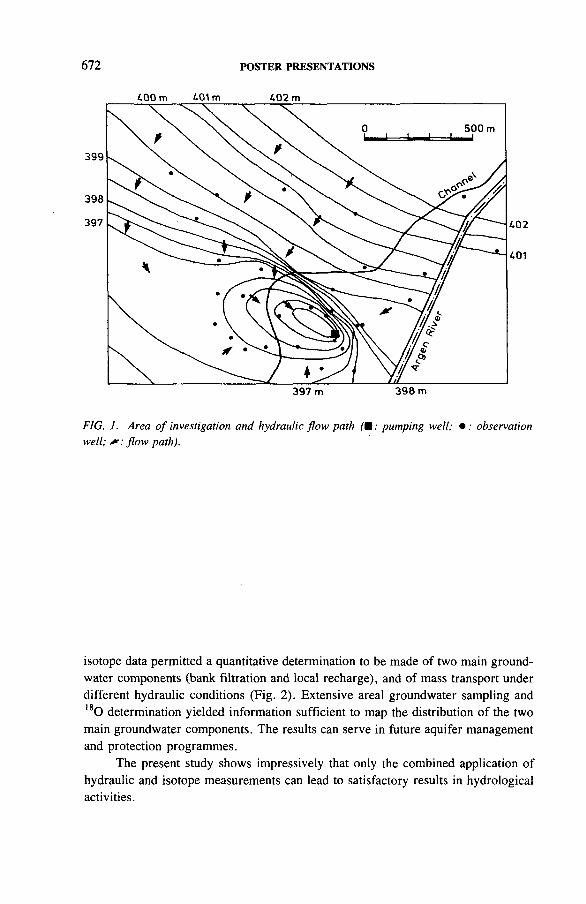
672 POSTER PRESENTATIONS

¿ 0 0 m A01 m 4 0 2 m

FIG. 1. Area o f investigation and hydraulic flow path (Ш : pumping well; • : observation well; flow path).

isotope data permitted a quantitative determination to be made of two main ground­water components (bank filtration and local recharge), and of mass transport under different hydraulic conditions (Fig. 2). Extensive areal groundwater sampling and ,80 determination yielded information sufficient to map the distribution of the two main groundwater components. The results can serve in future aquifer management and protection programmes.

The present study shows impressively that only the combined application of hydraulic and isotope measurements can lead to satisfactory results in hydrological activities.

POSTER PRESENTATIONS 673

□ Pumping wellI 0 - 25%

□ 26 - 50%

Ш 51 ' 75%Щ 76 - 100%

FIG. 2. Temporal variation in the per cent rate o f bank filtrate deduced from varying b ,80 values.

674 POSTER PRESENTATIONS

EVAPORATION FROM SOIL WATER UNDER HUMID CLIMATE CONDITIONS AND ITS IMPACT ON DEUTERIUM AND lsO CONCENTRATIONS IN GROUNDWATER

H.-M. BURGER, K.-P. SEILER Institut fiir Hydrologie,Gesellschaft fiir Strahlen- und Umweltforschung mbH München,Neuherberg,Germany

According to the literature [1], the deuterium and I80 contents of meteoric groundwater in humid climates approximately match the longer term weighted mean of the isotopic composition of precipitation in the recharge area. In upper Bavaria, this is also observed for groundwater occurring in different types of aquifers, such as fluvioglacial gravels and riverborne sediments with widely spaced grain size dis­tributions, ranging from sandy gravel to sandy clay, karstified limestones and dolo­mites and fractured sandstones.

Whereas the stable isotope composition of actual groundwaters reflects a frac­tion of the winter precipitation of about 40-50% on total annual recharge (Fig. 1), the hydrological balance indicates that, with the exception of coarse gravels, it amounts to nearly 70%. Evaporation is thus thought to cause during the summer sea­son an enrichment of stable isotopes in soil water stored near the surface. This process is well known in arid zones, but is poorly documented for humid climate conditions [2, 3], especially under vegetation cover.

To document the impact of evaporation on percolation water, detailed stable isotope analyses were performed over a 24 month period at four experimental sites with different types of sediment and land use. The test sites were situated within 5-12 km of each other with almost identical climate conditions.

At all sites precipitation was registered with a rain gauge and samples of each rain event were analysed for their stable isotope content. These data in general formed a sinusoidal input function, with low concentration values in winter and high values in summer ranging, within the observation time, from —136.0 to —23.1700 for deuterium and from -19.5 to —2.84700 for 180 , respectively. The weighted average of summer rains was —57.9°/00 for 2H and -8 .3 7 0/00 for 180 in 1987 and -5 0 .4 7 oo for 2H and -7 .3 1 700 for 180 in 1988; for winter rains average values of —84.5700 for 2H and -11 .65700 for 180 were found in 1987-1988.

Percolation water was collected using two different methods. The first was drilling undisturbed soil cores up to a depth of 2 m to determine stable isotope con-

IAEA-SM-319/34P

б 180 (Veo)

-14 -12 -10 . -8

POSTER PRESENTATIONS 675

FIG. 1. Stable isotope composition o f recent groundwater (>20 TU) in Tertiary sediments and local rains (1978-1987), both from an area north o f Munich (— - — : mean values o f local rain (1978-1987);----------: groundwater with >20 TU (1982)).

centrations and actual water content in thin sections (Fig. 2). Additionally, sediment material was obtained to determine the water content-suction head relationship in laboratory experiments.

The second method involved collection at any site within an area of about 10 m2 using a set of ceramic suction cups which were implanted 25, 50, 75 and 150 cm below the surface. Soil water was sampled from these cups in 14 day intervals.

Regardless of the type of sediment, at all sites a dual porosity system was found to exist which was responsible either for quick or slow percolation of infiltrating precipitation, as discussed, for example, by Darling and Bath [4] for English chalk. In the area of research, flow velocities reach about 10-100 m/a in macropores and about 0.5-4 m/a in the matrix flow system.

Water stored in the micropores near the surface during the summer is con­sumed by evaporation, the residual part being enriched in stable isotopes. Thus, in fine grained sands, the <52H concentration in the soil water of the uppermost 3 cm below the surface exceeded within the observation time the value of corresponding

( a ) 6 2 Н(%о) : н (%») б2 Н (%о)

( Ь )(а) (Ы

25 50 75 100 vol.(%) 0 25 50 75 100 00

(с)

25 50 75 100 vol.(%)

-0.5-

-1.5

-2-

1988-7-27

w р Total porosity

Water content

-25 4

Depth (m) Depth (m)

FIG. 2. (a) Deuterium content o f soil waters taken from the same site at different seasons; and (b) the respective total porosities and water content at the same site and date.

a\оo\

POSTER PRESENTATIO

NS

POSTER PRESENTATIONS 677

б 180

XUO

FIG. 3. Schematic 18 О/ 2 H diagram demonstrating summer enrichment o f stable isotopes by means o f evaporation in Tertiary sediments and mixing between enriched summer and depleted winter rains in the unsaturated zone (W: winter; S: summer).

rainfalls (monthly weighted mean) up to about 307oo (Fig. 2) on arable land and up to about 15700 in spruce tree forested areas. The averages for this enrichment were approximately 10 and 7700, respectively, for deuterium compared with the values of summer precipitation (Fig. 2(a)). In test sites used for agricultural purposes, the enrichment increased slightly from about 9 700 before harvest to about 12700 after­wards, whereas no variation was found in forested areas.

Micropores, however, replenish much more at each rain event in the summer than macropores, resulting in a predominant piston flow. In winter time, however, recharge from macropores is predominant, diluting isotopically enriched matrix water from the previous summer season (Fig. 2(b)). Thus, the stable isotope concen­tration in groundwaters reflects mixing between enriched summer and depleted winter rainfall, the mixing ratio being dependent on the portion and penetration depth of the macropore system (Fig. 3).

These evaporation/dilution effects (Fig. 3) may occur in all types of sediments in temperate climates. However, they are pronounced only in sediments with a high storage capacity for infiltrating rains, say more than 12 vol.% as a first criterion. Furthermore, a low or, with decreasing water content, quickly declining unsaturated hydraulic conductivity is required.

REFERENCES

[1] GAT, J.R., “ Groundwater” , Stable Isotope Hydrology: Deuterium and Oxygen-18 in the Water Cycle, Technical Reports Series No. 210, IAEA, Vienna (1981) 223-238.

[2] EICHLER, R., Deuterium-Isotopengeochemie des Grund- und Oberflàchenwassers, Geol. Rundsch. 55 (1966) 144-159.

[3] ZIMMERMANN, U., EHHALT, D., MÜNNICH, K.O., “ Soil-water movement and évapotranspiration: Changes in the isotopic composition of the water” , Isotopes in Hydrology (Proc. Symp. Vienna, 1966), IAEA, Vienna (1967) 567-485.

[4] DARLING, W.G., BATH, A.H., A stable isotope study of recharge processes in English chalk, J. Hydrol. 101 (1988) 31-46.

678 POSTER PRESENTATIONS

IAEA-SM-319/35P

GROUNDWATER FLOW MEASUREMENTS USING THE RADIOTRACER TECHNIQUE AT A WASTE DISPOSAL SITE BARRIER

L. BARANYAI Institute of Isotopes,Hungarian Academy of Sciences

F. IVICSICSResearch Institute for Water Resources

Budapest,Hungary

Flow rate and flow direction measurements were carried out by means of the single well technique using Na82Br and |40ЬаСОз radiotracers. The aim of the investigations was to: (1) develop a measuring technique and apparatus for a large series of field measurements; (2) determine flow parameters in the vicinity of an underground barrier surrounding a waste disposal site and check whether the barrier performs satisfactorily; and (3) prepare the measuring technique and train personnel in large series field measurements.

POSTER PRESENTATIONS 679

Sampl i ng t i me (mi n)

FIG. 1. Decrease in tracer concentrations over time in the wells investigated ( • : well I; □ : well II; X : well III).

Figure 1 presents the measured concentration diagrams for flow rate measure­ments, while Fig. 2 gives isoconcentration curves for evaluating the flow direc­tion. The flow rate far from the barrier was found to be two orders of magnitude greater than that in close vicinity to the barrier. Since the accuracy of the first flow direction measurements was not satisfactory, further efforts are being made to improve it.

680 POSTER PRESENTATIONS

N

S

FIG. 2. Isoconcentration curves fo r determining flow direction.

BIBLIO GRAPH Y

BARANYAI, L., “ Environmental application of the radiotracer technique” , Proc. 12th Radiochemical Conf. Marianske-Lázne, Czechoslovakia, 1990.

INTERNATIONAL ATOMIC ENERGY AGENCY, Guidebook on Nuclear Techniques in Hydrology: 1983 Edition, Technical Reports Series No. 91, IAEA, Vienna (1983).

POSTER PRESENTATIONS 681

STA BLE ISO TO PE STUDY IN GEO THERM AL FIELD S IN KAM OJANG AND D IEN G , JAVA ISLAND

Zaenal ABIDIN, WANDOWO, INDROYONO, ALIP, DJIONO Centre for the Application of Isotopes and Radiation,National Atomic Energy Agency,Jakarta,Indonesia

IAEA-SM-319/39P

A survey of the stable isotope composition of geothermal sources was initiated at several geothermal fields on the island of Java during 1988-1990. A further study was carried out in two geothermal fields, Kamojang and Dieng, which are approxi­mately 400 km apart. The study was intended to provide an isotope database to moni­tor geothermal evolution resulting from exploitation and to identify the recharge area of the geothermal system. In addition, data on stable isotope composition can be used to describe the characteristics of the geothermal system itself. The field of Kamojang (a vapour dominated system) lies on a pyroxine andesite formation and has been exploited for electric power generation (of 143 MW) since 1988, while the field of Dieng (a water dominated system) lies on a basaltic andesite formation and is being exploited only for a pilot electric power plant of 2 MW. A thorough study is being carried out at Dieng to develop the electric power capacity to 55 MW.

Samples of water were taken from various sources, such as hot spring water, cold spring water, fumaroles, meteoric water, well heads and downholes. Samples of rain water from different altitudes at Kamojang were taken during the rainy season in 1988-1989 and from Dieng during the rainy season in 1989-1990.

The local meteoric water lines from these two locations are virtually the same and can be represented as follows (Fig. 1):

ÔD = 7.9 0 180 + 16.0

On the basis of the altitude effect on the D/H ratio of rain water, the depletion value of deuterium is —1.5 and —2.2700 for each 100 m increase in altitude for Kamojang and Dieng, respectively. The recharge area of Kamojang field is estimated to be at an approximate height of 1400 m, while the Dieng field is at approximately 1700 m. These figures are based on the geothermal lines of each field, which show a different setting, and were also supported by the isotope composition of cold spring water at the recharge area. The 180 shift at the geothermal line of Kamojang is 2 .1700, corresponding with the isotope composition of the local meteoric water line at —7.9 and —46.3700 for l80 and deuterium, respectively. Oxygen-18 originating

682 POSTER PRESENTATIONS

O r

- 2 0 -

I -¿0 -

-60 -

-12 -10 -8 -6 - i - 7 0"0 (V..1

FIG. 1. Graph o f ô l80 versus 6D at the Kamojang and Dieng fields ( O: Kamojang well­head samples; A : Kamojang cold springs; • : Dieng downhole samples; A ; Dieng cold springs).

from wells in the western boundary shows a depleted value of less than the value of l80 at the corresponding point of local recharge. The 180 shift at the geothermal line of the Dieng field shows a remarkable value, 9 .8700, corresponding to an iso­tope composition of the local meteoric line at —8.7 and — 52.2700 for 180 and deuterium, respectively. The difference in the value of the l80 shift at Kamojang and Dieng may reflect differences in the characteristics of each geothermal system.

BIBLIO GRAPH Y

BAFI-BATAN, Inventarisasi data isbtop dan data analisa kimia air daerah pulau Jawa dan lapangan Kamojang, 1989 (unpublished).

D’AMORE, F., e ta l., Secondary changes in the chemical and isotope composition of geothermal fluids in Larderello, Geothermics 5 (1977) 153-163.

FAUZI, A., Mineralogy and Fluids Composition at Dieng Geothermal Field, Indonesia, Master’s Thesis, Victoria University of Wellington (1987).

GRANT, M.A., Water content of the Kawah Kamojang geothermal reservoir, Geothermics 5 (1977) 21-30.

POSTER PRESENTATIONS 683

MANALU, P., Geothermal development in Indonesia, Geothermics 17 2/3 (1988) 415-420.

PANICHI, C., GONFIANTINI, R., Environmental isotopes in geothermal studies, Geo­thermics 6 (1978) 143-161.

RADJA, V.T., Bisakah uap panas bumi Dieng digunakan sebagai sumber pembangkit listrik, Energi and Listrik 2 (1989).

IAEA-SM-319/40P

H YD RO G EO LO GICAL CH A R A CTER IZA TIO N OF AN AQUITARD: TH E AVDAT GROUP (EOCENE) CH A LK ,NORTHERN N EGEV D ESERT, ISR A EL

R. NATIV, E. NISSIMThe Seagram Center for Soil and Water Sciences,Hebrew University of Jerusalem,Rehovot,Israel

During the last 15 years, owing to political, demographic, climatological and geological reasons, the northern Negev Desert (with 50-200 mm of mean annual precipitation) has become a prime area for siting a variety of primarily chemical industries that were rejected by, or transferred from, more populated areas. In addi­tion, the national site for the isolation and treatment of hazardous wastes has been in operation there since 1980. A site in the northwestern Negev is currently under evaluation for the construction of the first nuclear power plant in Israel.

The northern Negev is underlain by chalk formations of the (Eocene) Avdat Group, with a low matrix permeability (core analyses indicate mean values of 1.2 md). However, abundant joints and fractures create shortcuts for contaminant migration from the land surface to groundwater in the chalk. Groundwater is brackish (500-1300 ppm СГ), but local nomads throughout the northern and central Negev, Israel, and western Sinai, Egypt, use it for their cattle. The water also discharges as springs in desert oases, which sustain a large population of wild desert animals that live in the vicinity of what are the only water supplies available.

The Avdat Group aquitard overlies shales and marls of varying thickness of the Mount Scopus Group, which is underlain by a major aquifer — the Judea aquifer of Cenomanian age. Annual production of water from this aquifer exceeds 30 x 106 m3; the water is supplied to the city of Beersheba (pop. 150 000), northern Negev, and its vicinity.

684 POSTER PRESENTATIONS

1989 1989

FIG. 1. Seasonal fluctuations in water levels in two wells (X : Maravim; + : Leah).

8180

FIG. 2. Plot o f 8IS0 versus ÔD, Avdat aquitard groundwaters. The upper solid line is the Mediterranean water line ( + : fall; x ; spring).

POSTER PRESENTATIONS 685

Until now, neither the hydrogeology nor the hydrochemistry of the Avdat aquitard has been studied because of its low water quantity and quality. Geological investigations and environmental impact studies that preceded the construction of the various industries in the area either ignored the presence of the aquitard or assumed that the combination of arid climate and low permeability cover rocks was sufficient to prevent any solute movement into its groundwater. Contaminant transport through joints, fractures and solution channels present in this aquitard was never considered, but was, however, observed recently in groundwater samples from monitoring wells at the premises of the local industries. Because the hydraulic connection with the underlying aquifer is not clear, the threat of groundwater contamination is of major concern. Our investigations focused on the assessment of (1) the aquitard regional continuity; (2) its groundwater flow directions and velocity; (3) the nature and methods of its recharge; and (4) potential leakage into the underlying aquifer.

The potentiometric surface of groundwater in the aquitard slopes from the eastern Negev to the west toward the Mediterranean Sea, reflecting the regional sur­face topography. Its regular and undisturbed gradient suggests hydraulic continuity within the aquitard.

Seasonal fluctuations in groundwater levels were observed (Fig. 1), suggesting current groundwater recharge by winter precipitation and runoff water despite the region’s aridity and the low permeability of the covering chalk. Delayed response to seasonal effects in adjacent wells may, however, suggest the presence of separate fracture systems that feed these wells.

The groundwater is brackish (total dissolved solids (TDS): 1400-8000 mg/L) and has Na-Cl facies typical of groundwater in arid terrain. The salinity varies widely, but not systematically, with the geographical position. The absence of any shift in groundwater samples from the local meteoric water line (Fig. 2) suggests a relatively fast recharge rate and rules out the possibility of groundwater salinization as a result of evaporation. Owing to the arid climate and the low permeability of the chalk matrix, such fast recharge could occur only through fractures, joints and solution channels.

The presence of tritium (0.3-15.9 tritium units) in groundwater throughout the entire study area, regardless of spatial variations in precipitation or the geographical location along groundwater flow paths, indicates that recharge occurs rapidly along fractures in all regions and is not restricted to the hydrologically updip areas. The slow movement of groundwater along the porous matrix could not account for the tritium values observed everywhere in the aquitard’s groundwater.

The varying percentage of modern 14C (61-112.7), in combination with measurable tritium, suggests mixing of recently recharged waters with the base flow of older waters. Older groundwater may flow along smaller, less developed fracture systems or through the porous matrix, whereas young water probably moves along wider fractures or along karst channels formed underneath the ephemeral streams.

6 8 6 POSTER PRESENTATIONS

IAEA-SM-319/41P

USE OF ISO TO PE TECHNIQ U ES IN STUDIES OF LIM ESTO N E K A R STIC AQUIFERS OF M ARCHE, CEN TRA L IT A LY

G.F. CIANCETTI, G.S. TAZIOLI Dipartimento di Scienze dei Materiali e della Terra, Université di Ancona,Ancona

M. COLTORTIDipartimento di Scienze della Terra,Université di Camerino,Camerino

Italy

Isotope techniques were used to investigate groundwater circulation in the Marche Apennines and to obtain information on the origin of karstification of the Frasassi caves 60 km from Ancona (Fig. 1).

The outcropping rocks are comprised of a limestone series, Mesozoic- Palaeogenic in age; the series is estimated to be up to 1500 m thick. The structural framework displays folds oriented SE-NW and a series of faults that are NW-SE and NE-SW. The principal tectonic events (Middle Pleistocene) have determined the uplifting of the area, with consequent deepening of the valleys.

Rock permeability is conditioned by lithology and by a very complicated tec­tonic pattern. The direction of groundwater flow follows the direction of the prin­cipal folds and is conditioned by the main river valleys, which represent the local base level of groundwater. The discharges of the springs vary from some litres per minute to 1 m 3 /s. The most important springs are localized along some river tracts. The hydrological and thermic regime is, in most cases, variable. Generally, the seasonal variation is very strong and is connected with springs of lower discharge. This variation also induces detectable changes in the chemical and environmental iso­tope contents.

The groundwater chemistry is generally of calcium bicarbonate type, with a total dissolved solids (TDS) content between 200 and 500 mg/L and a temperature between 9 and 13°C. The karstic area of Frasassi is characterized by water generated by mixing between fresh calcium bicarbonate waters and mineralized sulphur water having a sodium chloride facies. The TDS reaches 2000 mg^L and the mean temper­ature reaches about 14.5°C.

POSTER PRESENTATIONS 687

FIG. 1. Location o f the area under investigation (1: main spring; 2: sulphur spring; 3: non- continuous spring; 4; поп-sampled spring; 5; linear spring; 6; seepage; 7: rain station; 8; karstic area o f Frasassi; 9; area o f the Gorgovivo Spring).

The study was carried out between 1985 and 1990 and many springs were sam­pled monthly. The isotope content in precipitation was checked at two rain stations located at different altitudes. The environmental isotopes utilized ( 1 80 , 2 H, 3H and 3 4 S) allowed localization of the principal areas of infiltration and evaluation of the dynamics of groundwater circulation.

Triti

um

(TU

) Tr

itium

(T

U)

Pre

cip

itat

ion

(m

m)

200

150

100

5 0

0

2 5 0

LU Im J

CD P i a n d e l l 'E lm o r a i n s t a t i o n Cingoli r a i n s t a t i o n

Ш Ш iU лCU P i a n d e l l 'E lm o r a i n s t a t i o n

Cingoli r a i n s t a t i o n

L i ni

IIG o r g o v i v o s p r i n g

1 nullIllllll IIni пин20

Ю

J F M A M J J A S O N D J F M A M J J A S 0 N D J F M À M J J A S 0 N D J F H A H J J A S 0 N D 1987 1988 1989 1990

FIG. 2. Monthly rainfall and mean tritium content in precipitation at the Cingoli (702 m above sea level) and Pian dell 'Elmo (950 m above sea level) rain stations and the tritium content o f the Gorgovivo Spring.

POSTER PRESENTATIONS 689

зо

о

□ D rip p in g w a te r

Э 20inЁD

£ to

о S u lp h u r s p r in g

J F M A M J J A S O N D J F M A M J J A S O N D 1988 1989

FIG. 3. Tritium content in dripping waters o f 'Sala С ’ o f the karstic caves o f Frasassi and o f the sulphur spring in the same area.

For the Frasassi karstic area, it was possible to establish the origin of the sulphur mineralized water from Triassic anhydrites [1]. The values of 6 I80 are between -1 1 and —7°/00- The expression ô2 H/ôlsO for groundwater of the area under consideration (Fig. 1) displays an angular coefficient of about 5, revealing that part of the recharge comes from stream runoff.

The altitude effect on the isotopic composition of local precipitation was obtained by using the values of certain springs located at different elevations and fed by small aquifers. These values give an altitude gradient of 0.247oo per 100 m. This gradient is slightly different from that obtained in the central Apenines by other authors [2, 3]. By using this gradient, it was possible to localize the infiltration areas of recharge of the aquifer feeding the Gorgovivo Spring, which is the most important spring in the area at a mean elevation of about 1300 m (01 80: 9.507oo) and the recharge of Frasassi springs at a mean elevation of 900 m (<5,80: —8.6700). In the Frasassi area, recharge also takes place from seepage of the Sentino Torrent (Fig. 1).

690 POSTER PRESENTATIONS

The seasonal variation in ô180 is greater in springs with low discharge than in the major springs. The annual weighted tritium contents in precipitation registered in two sampling stations located at altitudes of 702 and 950 m are between 10 and 14 tritium units (TU), with noticeable variations between the summer and autumn- winter seasons. During the summer, the tritium contents are generally twice those of the autumn-winter period (Fig. 2). The tritium content in groundwater is, in many cases, two or three times higher than that in precipitation.

During the last five years, the tritium contents in groundwater have decreased by 30-40% from the initial values. Springs with low discharge are generally charac­terized by tritium contents that are higher than those in precipitation (20-30 TU), while in the presence of karstic aquifers of high permeability, which are character­ized by a short water transit time, the tritium content is of the same order of magni­tude as that in current precipitation (10-14 TU).

The reason for this behaviour might be the long residence time of water in those aquifers with low permeability, which also contain a high percentage of reten­tion water and are thus characterized by older water, which is more radioactive than current rain water.

In the Frasassi karstic area, dripping water has the same tritium content as rain water, while the sulphur spring is characterized by higher tritium activities (Fig. 3).

The seasonal indications of tritium are recorded in the Gorgovivo Spring with a lag of five to six months.

REFERENCES

[1] TAZIOLI, G.S., COCCHIONI, М., COLTORTI, М., DRAMIS, F., MARIANI, М., Mem. 1st. Speleologia, 4, Ser. П (1990) 93-108 (in Italian).

[2] CELICO, P., GONFIANTINI, R., KOIZUMI, М., MANGANO, F ., “ Environmental isotope studies of limestone aquifers in central Italy” , Isotope Hydrology 1983 (Proc. Symp. Vienna, 1983), IAEA, Vienna (1984) 173-192.

[3] ZUPPI, G.M., FONTES, J.Ch., LETOLLE, R., “ Isotopes du milieu et circulations d ’eaux sulfurées dans le latium” , Isotope Techniques in Groundwater Hydrology 1974 (Proc. Symp. Vienna, 1974), Vol. 1, IAEA, Vienna (1974) 341-361.

POSTER PRESENTATIONS 691

SA LT W ATERS, BRINES AND TH E G EO LO G ICA L STRU CTURE OF TH E APENNINE FRONT (NORTHERN ITA LY )

M. CHIARLE*, G. MARTINELLI**, T. NANNI***,G. PATRIZI+, L. VENTURINI+, G.M. ZUPPI*

♦Dipartimento di Scienze della Terra,Université degli Studi di Torino,Turin

**Regione Emilia-Romagna,Bologna

***Dipartimento di Scienze dei Materiali e della Terra,Université degli Studi di Ancona,Ancona

+Singea,Ravenna

Italy

1. GEOLOGICAL PATTERNS

In the Apennine Front, Mesozoic carbonate substrates underlie shaly Mesozoic-Cenozoic allochthonous units and clastic Neogene formations accumu­lated in continental and marine basins at a depth of approximately 3000 m. The struc­tural setting is characterized by several fault systems combined with folds and overthrusts. The present structural behaviour results from several tectonic phases differing in stress and age. The last and most important phase is related to the Pliocene.

IAEA-SM-319/42P

2. CHEMICAL CHARACTERISTICS

The chemical characteristics shift from calcium sulphate to sodium chloride waters, with a total dissolved solids content greater than 1.5 g/L, a pH close to 6

and a redox potential ranging between -1 5 0 and 0 mV. Trace elements, such as Br, I, Sr, Li, B, As, V, Se, Sb and U sampled in solid and solution phases common

692 POSTER PRESENTATIONS

CQ\ОСПо

D

□ ' ó : В□ □ □ • : С

□ О : D

I f f с Р I Л : Е

™ ц в ^ ап .....^ 4 ^ ° “ i?а 0 n eа а сР \

\н

А : F G

1 2 3 4

Log Cl (m g/L)

FIG. 1. Halogen ratio versus chloride concentration (A; sea water; B; calcit'e precipitation; C; gypsum precipitation; D; halite precipitation; E: epsomite precipitation; F; silvite precipi­tation; G; camallite precipitation; H; Bischofite precipitation; I: water points).

♦ A• В▲ С□ D

Cl (m g/L)

FIG. 2. Oxygen-18 versus chloride concentration (A: sea water; B; calcite precipitation; C: gypsum precipitation; D; water points; E: seawater evolution during evaporation; V-SMOW: Vienna standard mean ocean water).

POSTER PRESENTATIONS 693

6 180 (%o)

FIG. 3. Deuterium versus ,sO in Po Valley brines (GML: global meteoric line).

in reduced environments, permit interpretation of brines (Fig. 1) as connate waters of the Pliocene Padanus Gulf [1 ,2] locally submitted to dilution processes with hydrothermal waters (Figs 2, 3). Isotopic exchange between the brine and the miner- alogical matrix has been recognized, chiefly in connection with the main structural lines and with local seismic activity. Isotopic data on the co-existing sulphates and sulphides suggest both sedimentary (Messinian) and gaseous (deep steam) sources. Starting with the original sulphate, a succession of geochemical processes takes place in the aquifer which are directly controlled by redox conditions.

These processes permit the calculation of an equilibrium temperature which can sometimes be higher than 200°C. The radioactive isotopes ( 3 H, 14C and 3 6 C1) indicate a very old age, i.e. more than 1 0 0 0 0 0 years.

3. CONCLUSIONS

The following conclusions were reached:

— The salty waters are connected with the lifting of deep brines trapped in Plio­cene sediments.

— The Upward movements still taking place occur at two separate times and at two different levels. The first, and deeper, level is caused by tectonic stresses which squeeze out brines on the Apennine Front. The second, and shallow,

694 POSTER PRESENTATIONS

level is connected with the infiltration of vadose waters. Brines rise to the sur­face pushed by the gases typically associated with them (CH4, H2 S, He, Rn, etc.).

REFEREN CES

[1] COGGIOLA, C., et al., Origin of brackish waters and brines in the northern front of Apennines” , Proc. Symp. Water-Rock Interactions, Reykjavik, 1986.

12] NANNI, T., ZUPPI, G.M., Mem. Soc. Geol. It. 35 (1986).

IAEA-SM-319/44P

STUDY OF GROUNDW ATER SA LIN IZATIO N IN A LG A R VE, PO RTUGAL, USING ENVIRO NM ENTAL ISO TO PE TECHNIQ UES

J.M.P. CABRAL, P.M. CARREIRA, M.C. VIEIRA Departamento de Química (ICEN),Laboratorio Nacional de Engenharia e Tecnología Industrial,Sacavém

J. BRAGA dos SANTOS Direcçâo Geral de Recursos Naturais,Lisbon

M.J. LEITÂO de FREITASGrupo de Estudios dos Recursos Hídricos do Algarve,Faro

Portugal

R. GONFIANTINI Isotope Hydrology Section,Division of Physical and Chemical Sciences,International Atomic Energy Agency,Vienna

Tertiary karstified limestones and Quaternary alluvial deposits are the major water bearing formations in the coastal belt of Algarve, southern Portugal. Here severe groundwater salinization occurs, which may reach values of several grams of

POSTER PRESENTATIONS 695

dissolved salts per litre. The source for this salinization is twofold: (a) seawater encroachment as a consequence of intense exploitation; and (b) dissolution from the several diapiric structures of evaporitic origin intruded in the aquifers. An environ­mental isotope study was carried out in order to identify the origin of salinization and to complement the chemical investigations which, in some cases, do not seem to be able to clearly solve the problem.

During the years 1986-1989, more than 150 drilled wells and springs were repeatedly sampled on the Algarve coast between Portimâo in the west and the Spanish border in the east. The electrical conductivity of the samples ranged between < 1000 to < 10 000 /¿S/cm. Sea water (average conductivity: 51 000 ¿¿S/cm) was also sampled for comparison. The oxygen isotopic composition of water was deter­mined in all samples, while the deuterium and tritium concentrations were measured only in the first set of samples collected in April 1986. The chemical analysis was carried out on the last set of samples collected in October 1989.

The repeated sampling showed that in a number of sites groundwater salinity and isotopic composition can vary considerably with time, although not always in parallel. In particular, an exceptional rain event (162 mm of rain in one day) just before the last sampling in October 1989 seems to have determined a small but appreciable decrease in the 1 8 0 content of groundwater.

The area under investigation was subdivided into three main zones. In the first zone, close to Portimâo, the karst springs at Estombar, along the banks of the Arade River, and wells drilled through the karstic aquifer in the same locality are clearly

Conductivity (mS/cm)

FIG. I. Oxygen-18 versus electrical conductivity in groundwater at Portimâo. The regression line almost coincides with the seawater - mixing line (D : wells; x : springs;------: sea m ixture;------- : regression line; SMOW: standard mean ocean water).

696 POSTER PRESENTATIONS

Conductivity (mS/cm)

FIG. 2. Oxygen-18 versus electrical conductivity in groundwater at Armaçâo de Pera. Regression 1 refers to samples collected from April 1986 to February 1989 and regression 2 refers to samples collected after the exceptional rain event o f October 1989 (O : April 1986-February 1989; Ш : October 1989; — : regression line 1 ; .... : regression line 2; ------: sea mixture).

Conductivity (mS/cm)

FIG. 3. Oxygen-18 versus electrical conductivity in groundwater in Algarve coastal aquifers from Faro to Tavira. No significant correlation is observed i f the spring is excluded ( О ; 1986-February 1989; Ш : October 1989; •—x -— : spring;------; sea mixture).

POSTER PRESENTATIONS 697

shown to be fed by a mixture of sea and fresh water, as evidenced by the correlation between l80 and conductivity in Fig. 1. The theoretical mixing line and the regres­sion line almost coincide. These results confirm the findings of Geirnaert et al. 1

who also applied stable isotopes in this zone. The relatively high tritium content (5-8 tritium units (TU)) indicates that the mixing process is still active and that the fresh­water component at least is modern.

Perhaps more complex is the case of Armaçâo de Pera (Fig. 2). Here two regression lines are shown, the first referring to samples collected in April 1986, July 1988 and February 1989, and the second to samples collected in October 1989 after the exceptional rain event already mentioned. Both regressions have a good correlation coefficient (r = 0.690, with n = 16; r = 0.736, with n = 13, respec­tively), but in both cases the slope of correlation is somewhat lower than the mixing slope (0.073 ± 0.021 and 0.080 ± 0.021 versus 0.107 ± 0.008 ô 180 per mS/cm for the mixing). Considering the correlation of 180 with chloride (October 1989), the results are very similar to those obtained with a conductivity of r = 0.751 (n = 13), with a slope of 0.252 ± 0.067 versus 0.267 ± 0.020 ô l80 per g Cl/L for pure mixing with sea water. Our conclusion is that seawater intrusion is the main mechanism of groundwater salinization in the Armaçâo de Pera zone, clearly prevail­ing over salt dissolution.

The last zone is that which extends from Faro to Tavira, close to the Spanish border. Here (Fig. 3) the correlations of 1 80-conductivity are poor: r = 0.180, with n = 8 8 , for samples collected before October 1989, and r = 0.342, with n = 49, for samples collected in October 1989. In the latter case, the lsO-chloride regression produces r = 0.321. In this zone, an increase in the salt concentration is usually not accompanied by an isotopic effect: dissolution from salt diapires appears, therefore, as the prevailing mechanism of groundwater salinization, rather than seawater intrusion. Chemical analysis of trace elements may help in confirming this conclusion.

A particular case is that of the spring near Fuseta, which has a very low dis­charge, high and variable salinity, slightly enriched l80 content (Fig. 3) and a high tritium content (7.6 ± 0.4 TU). Seawater intrusion does not seem to be the main reason for the high salt concentration, because no l 8 0 increase accompanies the increase in salinity. However, additional investigations are needed to clarify this point.

' GEIRNAERT, W., RADSTAKE, F., KLEINENDORST, T., A salinization mechanism for the springs at Estombar, Algarve, Portugal, Comun. Serv. Geol. Port 72 (1968) 59-69.

698 POSTER PRESENTATIONS

IAEA-SM-319/45P

ASSESSM ENT OF AQ UIFER RESOURCES FROM H YD RO KARSTIC STRUCTURES BY M U LTITR ACIN G EXPERIM EN TS USING A R T IFIC IA L TRACERS

E. GASPAR, S.P. STANESCU,0.M . FARCASIU, S. SPIRIDON Institutul de Fizica Atómica

1. ORASEANUIntreprinderea de Prospecîiuni Geologice §i Geofizice

Bucharest,Romania

The intensive exploitation of aquifer resources in karstic zones, various water development works, the location of mining, industrial and farming units and towns, and the ecological aspects of these activities all call for massive research work into karstic structures.

Tracer experiments supply thorough knowledge of the karst, facilitate confir­mation or rejection of hydraulic connections between sinkholes and water emer­gences, and provide for the discovery of new connections. They are an ideal means of studying the vulnerability of the karst to pollutants. Tracer labelling also permits verification of the flow patterns of hydrokarstic structures and the performance of methodological and comparative studies concerning the behaviour of the karst between low flow and flood; important quantities of the tracer may remain in its auxiliary systems for a long period of time. Consequently, investigation of hydrokarstic structures should be performed through simultaneous or repeated label­ling using different ‘conservative’ tracers.

Multitracing experiments are employed to shorten the duration of research work by avoiding repeated trials and the necessity of performing investigations under analogue hydraulic conditions. They are also used because the main cost of introduc­ing tracers in karsts depends, more often than not, on the activities of the personnel taking the samples. The level of spending implied by these operations is independent of the number of labellings that are carried out.

The first labelling in a karst in Romania was performed in 1904, by Mihutia, using powdered coal. In the last 20 years, multitracer experiments in karsts were per­formed using radioactive tracers (82Br and l3 lI), tracers that are activated (In-

POSTER PRESENTATIONS 699

TABLE I. METHODOLOGICAL PARAMETERS FOR TRACERS THAT CAN BE ACTIVATED

Tracer Nuclide h(min)

tr tm(min)

r .vmin(g/mL)

In-EDTA In-116m 20-60 10 min 5 9 x 10"13

Dy-EDTA Dy-165 60 60 min 5 2 X 10 '12

La-EDTA La-140 60 24 h 15 1 x 10~10

KI, Nal 1-128 20 5 min 3 1 x 10 '10

BrNH4 Br-82 60 24 h 15 1 x 10'9

EDTA1, Dy-EDTA, La-EDTA, Г and Br“), fluorescent dye tracers (uranine, rhodamine B), salts (NaCl, ammonium dichromate), biological tracers (E. coli) and optical brighteners (stralex).

The best results were obtained with tracers that could be activated. They have great stability over time, react slowly with the labelled environment and most of them can be considered to be conservative tracers.

As a general rule, the labelling operation is accomplished with stable chemical compounds and is followed by sampling of water emergences. The analytical processing of the samples is carried out under laboratory conditions: the tracer ele­ments are separated from the water samples by precipitation in the form of insoluble hydroxides or bismuth salts with a hydroxide gel as bismuth hydroxide; these are then filtered through a nuclear membrane filter, dried at room temperature, encapsu­lated and irradiated with a pneumatic ‘rabbit’ tube at a nuclear reactor. The concen­tration was determined by gamma ray emission measurements of the irradiated samples using a gamma ray spectrometer system with a Ge(Li) detector and a multichannel analyser included [1—3].

The main parameters of activated tracer analysis are presented in Table I, where i, is the irradiation time of the sample, tr is the decay time of the samples, tm is the measurement time and Cmin is the minimum detectable concentration of the tracer elements [4] (see also Fig. 1).

Since activated tracers can be measured routinely at concentrations under 1СГ9 g/mL, they can be used as ecological tracers for direct labelling of drinking water. Also, because of their variety they can be used in multitracing and multisam­pling experiments.

1 EDTA: ethylenediaminetetra acetic acid.

700 POSTER PRESENTATIONS

Tim e (d)

FIG. I. Transfer curve from a field experiment using the tracer In-EDTÀ at the Scorota sink­hole, Valea Cemei Spring (flow: 2.7-0.95 m3Is; Cmi„: (9.7 ± 0.48) X 10~13 g/mL).

The goals of tracer labelling in Romanian karst were:

(1) Delimitation of hydrological basins and elaboration of hydrological maps.(2) Highlighting of karstic capture phenomena.(3) Studying the influence of water development activities on water catchments in

the karst.(4) Estimation of groundwater reserves of a karstic aquifer.(5) Studying mine drainage in karsts.(6 ) Investigation of geothermal waters in limestones and dolomites and detecting

the invasion of reinjected water into the production zone.

ACKNOW LEDGEM ENT

The authors particularly wish to to thank the International Atomic Energy Agency, which helped in obtaining tracers and instruments for the investigations (IAEA Project No. ROM/3/002).

POSTER PRESENTATIONS 701

R EFEREN CES

[1] BEHRENS, H., MOSER, H., WILDNER, E., J. Radioanal. Chem. 38 (1977) 491.[2] STANESCU, S.P., GASPAR, E., SPIRIDON, S., FARCASIU, O.M., Rep. NP-24,

Institute of Atomic Physics, Bucharest (1982).[3] GASPAR, E., STANESCU, S.P., ORASEANU, I., FARCASIU, O.M., SPIRIDON,

S., Theor. Appl. Karstology 2 (1985) 149.[4] STANESCU, S.P., GASPAR, E., FARCASIU, O.M., SPIRIDON, S., Rep.

INDC-018/19, IAEA, Vienna (1988).

IAEA-SM-3I9/46P

APPLICATIO N OF ENVIRO NM ENTAL ISO TO PE M ETHODS IN TH E STUDY OF A KA R STIC HYDROSTRUCTURE IN ROM ANIA

A. TENU, A. SLAVESCU, F.D. DAVIDESCU Institute of Meteorology and Hydrology,Bucharest,Romania

The study dealt with the Domogled karstic hydrostructure, located in south­western Romania. The focus of the study was the Domogled Spring, one of the many emergences of the karstic massive, because its water is of a very high quality and is intended to be used as a bottled water product.

The main objects of the isotopic research were the determination of the ground­water transit time and the degree of mixing of the various sequences of annual recharge, and establishing the relationships between ground and surface waters in the area.

The study covered the period 1987-1989 and consisted mainly of prospecting and sampling of all karstic springs, of surface and groundwaters in the area and of a monthly systematic sampling of the Domogled Spring.

Deuterium, 180 and 3H analyses were carried out, as well as specific conduc­tivity measurements. The best results were finally obtained by using tritium analyses (Table I).

These summarized results reveal the previously unknown fact that the Domo­gled Spring drains into its own hydrogeological subsystem, which is different from the zonal system common to other springs.

TABLE I. RANGE OF TRITIUM CONTENT IN VARIOUS TYPES OF WATER

702 POSTER PRESENTATIONS

Water type H-3 content (tritium units)

Surface water (river water, snow melt water) 15-20

Domogled Spring0 26-42

Other karstic springs 23-25

Thermal springs < 5

a Seasonal mean values for the period 1987-1989.

1982 1983 1984 1985 1986 1987 1988 1989

FIG. 1. Completely mixed reservoir model for the Domogled karstic subsystem (1 : input func­tion curve; 2: experimental curve using three month values; a-d: theoretical curves for various turnover times (t0)).

On the basis of the input curve for 3H in Romania [1] and the experimental curve obtained for the Domogled Spring, the following major mathematical models [2 ] have been applied: the piston flow model, the completely mixed reservoir model (Fig. 1) and the dispersive reservoir model with the use of the binomial age distribu­tion function.

A turnover time of r0 = 8 years appears to approximate the actual situation with regard to the Domogled Spring, while for the entire karstic system the same parameter is of about 1 - 2 years.

POSTER PRESENTATIONS 703

The study emphasized several conclusions, out of which we cite two:

— With karst, even in apparently clear situations, the use of the environmental isotope technique can lead to the discovery of unexpected aspects.

— By determining the turnover time of the Domogled Spring subsystem, the need to extend sanitary and hydrogeological protection areas was revealed.

REFEREN CES

[ 1 ] TENU, A., SLAVESCU, A ., DAVIDESCU, F . D., Level and Evolution of the TritiumConcentrations in the Natural Waters of Romania, special report, Institute of Meteorol­ogy and Hydrology, Bucharest (1989) 41-48.

[2] YURTSEVER, Y., “ Models for tracer data analysis” , Guidebook on Nuclear Tech­niques in Hydrology: 1983 Edition, Technical Reports Series No. 91, IAEA, Vienna (1983) 381-402.

IAEA-SM-319/47P

L E RO LE DE L ’EVAPO TRANSPIRATION DANS LA FORM ATION DES DEPRESSIONS PIEZO M ETRIQ U ES: HYPOTHESES ET M ODELISATION

B. NDIAYE*, J. F. ARANYOSSY**,В. DIENG*, A. FAYE*

* Département de géologie,Université C.A. Diop,Dakar

** Projet AIEA RAF/8/102,Dakar

Sénégal

1. LE PROBLEME DES DEPRESSIONS PIEZOMETRIQUES

La découverte des grandes dépressions piézométriques ou «nappes en creux» remontent aux années 50, lors des premières investigations hydrogéologiques en Afrique. Beaucoup de théories ont été émises pour leur explication, mais aucune n’a

704 POSTER PRESENTATIONS

encore remporté l’unanimité. Les recherches en cours dans le cadre du projet régional sahélien de l ’AIEA sur «le développement des techniques nucléaires en hydrologie dans les pays du Sahel» (RAF/8 / 102) semblent donner un rôle pré­pondérant à l’évapotranspiration dans la configuration de la surface piézométrique des nappes libres en zone sahélienne. Sur la base d’un schéma conceptuel élaboré à partir de cette hypothèse, des modèles mathématiques sont mis au point.

2. LE SCHEMA CONCEPTUEL

Les premiers résultats des études isotopiques au Mali et au Sénégal montrent une prédominance des mouvements verticaux sur la circulation latérale. Ainsi, on note clairement un enrichissement isotopique croissant lorsque la nappe se rapproche du sol (fig. 1). Ces résultats, que corroborent les fluctuations piézométriques obser­vées, suggèrent un déficit entre l’infiltration saisonnière et la reprise évaporatoire. Le schéma conceptuel considère une nappe à niveau de remplissage maximum (fin de la période humide Holocène) alimentée latéralement sur les bordures du bassin (fleuves ou zones de pluviosité favorable) et soumise à un déficit d’alimentation ver­ticale. Pendant une période transitoire, la nappe se creuse, puis parvient à un état d’équilibre dans lequel le très faible flux latéral compense la reprise évaporatoire de quelques dixièmes de mm/an dans la partie la plus profonde (fig. 2 ).

□ C a m b r ie n de N a ra • P r é c a m b r i e n t a b u la i r e О Q u a t e r n a i r e la t é r i t iq u e

FIG. 1. Teneur isotopique en fonction de la profondeur des nappes au Mali.

POSTER PRESENTATIONS 705

ч \ n a p p e

■s. ▲

FIG. 2. Schéma conceptuel expliquant la formation des dépressions piézométriques. En tout point, l ’évaporation nette est légèrement supérieure à l ’infiltration.

3. LE MODELE ANALYTIQUE

L’estimation de l’évaporation par les méthodes isotopiques, par les profils de pressions dans la zone non saturée et par calage de modèles hydrodynamiques suggère un déficit d’alimentation décroissant de façon exponentielle avec la pro­fondeur D = (at + Do)e~kh. En considérant une nappe libre d’extension infinie remplie au maximum et soumise à un déficit D, la variation piézométrique en fonction du temps est donnée par:

1 , Г / ka \ 2 /к D o\h = ------ ln 1 + 1 ------- I t2 + ------ t

k L \ 2 S / \ S /

L’évolution de la piézométrie sur une période de 8000 ans montre des valeurs de profondeurs en accord avec celles observées sur le terrain et l’importance du paramètre de forme k (dépendant des caractéristiques granulométriques du terrain) avec un Ah de 70 m environ (fig. 3).

4. LE MODELE NUMERIQUE

Une nappe remplie au maximum, alimentée latéralement et soumise à un déficit d’alimentation verticale, est simulée par un modèle unidimensionnel écrit en Basic et utilisant la méthode explicite. La simulation sur 8000 ans a montré qu’au bout de 2 0 0 0 ans la forme de la nappe est quasi stationnaire avec un gradient hydraulique diminuant de la périphérie vers le centre de la dépression (fig. 4).

706 POSTER PRESENTATIONS

фааосиэ4)

73СО

V aleu r d e К

FIG. 3. Résultat du modèle analytique: profondeur de la nappe en fonction des caractéris­tiques granulométriques du terrain (paramètre k) à différentes périodes.

FIG. 4. Résultat du modèle numérique (largeur de maille: 20 km).

CONCLUSION

L’hypothèse du rôle prépondérant de la reprise évaporatoire semble compatible avec la configuration des grandes dépressions piézométriques observées dans toute la frange sahélienne. Des modèles à 2D seront mis au point pour mieux prendre en compte les conditions aux limites réelles.

POSTER PRESENTATIONS 707

VA RIATIO N OF STA BLE ISOTOPES IN TH E MONSOONAL RAINS OF SR I LANKA

J.K. DHARMASIRIRadioisotope Centre,University of Colombo

C.J. ATULUWAGE Atomic Energy Authority

Colombo,Sri Lanka

IAEA-SM-319/49P

The variation in stable isotopes in monthly rainwater samples at seven locations from 1983 to 1986 were studied as a means of understanding the input of these isotopes into groundwater. Sri Lanka experiences two main monsoon rainy seasons, the southwest monsoon, from May to September, and the northeast monsoon, from December to February. The locations of these stations are marked in Fig. 1. Colombo, Hambantota, Batticaloa and Mannar are coastal stations. Tanamalwila and Anuradhapura are located on the coastal plain about 100 m above sea level. Nuwara Eliya is located in the central hills, 1894 m above sea level. The negative numbers (in 7 0 0 units) are the known <5I80 values for groundwater at different locations, given for comparison.

The ô 180 and ¿¡D values correlate very well with a R 2 = 0.98 for 202 obser­vations, giving the following regression line:

ÔD = 7.9 (5i80 + 11.0

This is comparable with the meteoric water lines of Craig [1] and the IAEA. The frequency distribution of <5lsO values for all of the stations during the four years is given in Fig. 2(a). Figures 2(b) and 2(c) represent the separated ô 180 frequency distributions for the southwest and northeast monsoon rains, respectively. Figure 2(a) is a superimposition of the distributions in Figs 2(b) and 2(c). The arithmetic averages of all ô l 8 0 values for the southwest and northeast monsoons were - 3 . 1 7 00 and -5.8°/oo, respectively. The weighted averages (weighted for the monthly amount of rainfall) for southwest and northeast monsoon rains were— 3.47oo and —7.0°/oo, respectively. These significantly different stable isotope compositions for the two monsoon rainy seasons may be due to the different origins of water vapour. It is known that the winds causing the southwest monsoon rains have their origins in the Indian Ocean above Australia and near the island of

708 POSTER PRESENTATIONS

8 0 ° 81° 8 2 ° E

FIG. 1. Location o f the stations in Sri Lanka where m onthly rainw ater sam ples were studied.

POSTER PRESENTATIONS 709

FIG. 2. (a) Frequency distribution o f b '8О values for all o f the stations during the period 1983-1986. (b) The separated ôl80 frequency distributions for the southwest monsoon rains (May-September; 80 observations), and (c) northeast monsoon rains (December-February, 46 observations), 1983-1986.

710 POSTER PRESENTATIONS

Madagascar. After crossing the equator, these winds strike the west coast of Sri Lanka in a southwesterly direction loaded with water vapour from the Indian Ocean. The central hills rising up to about 2500 m above sea level within a short distance from the coast cause orographic lifting of air masses, resulting in copious rains on the windward side of the hills. Little rain is received on the lee side of the hills and dry winds develop and pass over the rest of the country [2]. A weighted mean ô 180 value of —3.4 ° / 0 0 is typical of rain water derived from evaporation over the ocean. It is known that southwest monsoon development is usually limited to the lower 1 km of the atmosphere. The origin of water vapour for the northeast monsoon rains is complicated and not fully understood. The winds causing this monsoon arise owing to the high pressure systems that develop after September over Mongolia and north India. It is also known [3] that these winds develop at a height of up to 6 km in the atmosphere, in contrast to 1 km for the southwest monsoon. However, the very negative stable isotope contents for the northeast monsoon suggest that fast evapo­ration takes place under non-equilibrium conditions and condensation at low temperatures.

The weighted mean 0180 contents for Colombo ( - 3 .7 7 00) and Hambantota ( - 4 .8 7 00) are close to those of the southwest monsoon rains over the four years, as these are coastal stations that benefit from the monsoon and rains due to convective lifting of air masses over the warm seas. The coastal station at Batticaloa, with a <5180 content of - 4 .9 7 00, benefits from northeast monsoon rains, but does not show the expected stable isotope depletion found in that monsoon. This may be due to the availability of a great deal of moisture of oceanic origin for exchange and convective rain. Anuradhapura (weighted 5 180 content: —6.1700) and Mannar Island (weighted Ô l80 content: — 6.2700) show the significant contribution of rain from the depleted northeast monsoon. At Mannar, the continental effect is somewhat obscured owing to the exchange of water vapour of seawater origin. The altitude effect is clearly seen at Nuwara Eliya for the northeast monsoon only. The weighted average ô 180 content for Nuwara Eliya ( - 6 .7 7 00) indicates the greater influence of southwest monsoon rains with more enriched stable isotope contents. Hence, one cannot simply use the change in the stable isotope content in rain water with altitude to obtain information on the altitude of recharge of groundwater.

The ‘amount effect’ [4] in the stable isotope compositions of the two monsoons is worthy of further discussion. Generally, most of the stations fall within a narrow range, from —2.0 to —4.07oo in the case of the southwest monsoon. For Colombo, and even for some very wet months at Nuwara Eliya, the expected amount effect is not evident. The few months of moderate rainfall for Nuwara Eliya lie outside this trend. In addition, the coastal stations also receive heavy rains owing to convective lifting of air from warm seas. The expected amount effect is apparently masked by the exchange of moisture of seawater origin. In the case of the northeast monsoon rains, the general trend of the amount effect is evident, with the exception of a few stations during some months. These exceptional months with heavy precipitation

POSTER PRESENTATIONS 711

were found to have been influenced by the effect of cyclones and east-west low pressure systems originating in the Bay of Bengal. These add to the complexity of rain making processes taking place during monsoon seasons. The results warrant further studies based on a network representing two more stations located on the hill slopes to the southwest and northeast of Nuwara Eliya.

REFEREN CES

[1] CRAIG, H., Isotope variation in meteoric waters, Science 133 (1961) 1702-1703.[2] DOMROS, М., Geological Research. Vol. 2: The Agroclimate of Ceylon, Franz

Steiner Verlag, Wiesbaden (1974).[3] NOMOTA, S., YOSHINO, M.M., YAMASHITA, S., “A preliminary study of rain

fall distribution over Sri Lanka and its linked upper-level winds” , Climate, Water and Agriculture in Sri Lanka (YOSHINO, Y., Ed.) (1983) 207.

[4] DANSGAARD, W., Stable isotopes in precipitations, Tellus 16 4 (1964) 436-468.

712 POSTER PRESENTATIONS

APPLICATIO N OF TH E 222Rn TECHN IQ U E FOR ESTIM ATIN G TH E RESID EN CE TIM ES OF A R T IFIC IA L L Y RECHARGED GROUNDW ATER Hengsen water catchment area, Dortmunder Stadtwerke AG

E. HOEHNPaul Scherrer Institute,Villigen,Switzerland

U. WILLME, R. HOLLERUNG, U. SCHULTE-EBBERT Institut für Wasserforschung GmbH Dortmund,Schwerte,Germany

H.R. VON GUNTEN Radiochemisches Laboratorium,Universitàt Bern,BernandPaul Scherrer Institute,Villigen,Switzerland

IAEA-SM-319/50P

Recently, a new technique was established to estimate groundwater residence times of up to about 15 days [1]. The technique assumes that the ingrowth of 222Rn upon infiltration and movement in the ground can be described by the growth law of radioactivity. Radon-222 emanates from mineral grains by alpha recoil or by diffusion. It dissolves in the groundwater and migrates in the aquifer without interac­tions. This was confirmed at two sites of naturally infiltrating rivers and at a canal where the saturated aquifer is recharged. In this poster, we give results from the application of the method to a water catchment area with artificial groundwater recharge.

Since 1936, the water supply of the city of Dortmund, in Germany, relies on artificially recharged groundwater (see Fig. 1). ‘Raw’ water is taken from the Ruhr River and diverted to the reservoir, Lake Hengsen. After pre-filtration in gravel basins, water from the lake is routed to slow sand filters at different rates. In

POSTER PRESENTATIONS 713

L a k e H e n g s e n

т т х | / T vt"II/A

G ravel p re filte rs H/F,

О О

. ' I l / G w Tllli) f l/E о [ ______ 0 _0 * О1 ___

I * lll/Д о

г г п ч т п т г й ......I 'n T I ’ I 'I 'I'I ' I ' I ' I ' I'I 'I 'IT C y i ' I ' I 'I 'I ' I 'I ' f r l ' l ' l ' l ' r f f l ' l ' l ' r i ' I ' I ' f t ' r

о P V C , old o b se rv a tio n w ells P V C . o b s e rv a tio n w ells totally s c r e e n e d

® P V C . th re e o b se rva tio n w ells p a rt ly s c re e n e d

■ S t a in le s s ste e l, three o b se rva tio n w e lls p a rtly scre e n e d

* P V C » S t a in le s s ste e l, four o b se rva tio n w e lls p a rt ly scre e n e d

Î In ve stig a tio n \ a r e a s and ‘ t r a n s e c t s

0 50 100m

FIG. 1. Plan view o f the Hengsen water catchment area and the observation wells.

addition, water infiltrates naturally from the lake into a 5-10 m thick Quaternary sand and gravel aquifer with a hydraulic conductivity on the order of 1 0 - 4 to 10“ 2 m/s. The groundwater of both artificial and natural recharge is extracted from this aquifer by a horizontal filter drain at variable mixing ratios and pumping rates[2]. The groundwater at this site suffers from the reduction of iron, manganese and sulphate. Knowledge of the groundwater’s residence time is of importance in studies of the behaviour of redox dependent species.

In an area of groundwater recharge for public drinking water, the use of artifi­cial tracers to measure groundwater residence times is prohibited. Groundwater flow velocities were calculated from flow models. In a mixture of waters of equal oxygen and hydrogen isotopic composition, the 222Rn technique proved to be the best at estimating groundwater residence times. The flow was studied in groundwater obser­vation wells with a diameter of 2 in1, along two transects of the site (see Fig. 1). The transects represent more or less the direction of the groundwater flow. Most observation wells consist of several boreholes with piezometer tubes at different depths, which permit sampling in three dimensions. Since the noble gas radon is sub­ject to outgassing, we sampled the groundwater using submersible pumps.

1 1 inch (in) = 25.4 mm.

714 POSTER PRESENTATIONS

Water from the reservoir lake infiltrates through the lake bed, rather than through the dam with a low hydraulic conductivity. In general, the radon concentra­tions increased with flow distance and confirmed the ingrowth model. Waters with residence times of less than about 4 d were of particular interest because they showed mixing of naturally infiltrated water with younger water. In two cases, leaky under­ground water pipes were detected. In one case, a strong artificial recharge from the slow sand filters was traced.

The radon technique proved to be very useful in the groundwater protection area at Hengsen, where groundwater is used for drinking purposes. Knowledge of the residence times of up to about 15 d is of special interest in the light of the decay kinetics of many faecal bacteria and the microbial consumption of oxygen in groundwater.

REFERENCES

[1] HOEHN, E., VON GUNTEN, H.R., Radon in groundwater: A tool to assess infiltra­tion from surface waters to aquifers, Water Resour. Res. 25 8 (1989) 1795-1803.

[2] SCHÓTTLER, U., SOMMER, H., Hydrogeologische Untersuchung des Ruhrtales im Bereich der Wassergewinnungsanlagen der Dortmunder Stadtwerke AG, Band 5: Wassergewinnungsanlage Hengsen, Arbeitsbericht des Institutes fiir Wasserforschung GmbH Dortmund (1987).

POSTER PRESENTATIONS 715

ENVIRO NM ENTAL ISO TO PES IN PR ECIPITA TIO N AND SHALLOW AQUIFERSA sensitivity study o f the impact o f climate changeon the water balance o f small catchment areas in Switzerland

U. SCHOTTERER, H. OESCHGER, U. SIEGENTHALER Physikalisches Institut,Universitàt Bern,Bern,Switzerland

W. STICHLER Isotope Hydrology Section,Division of Physical and Chemical Sciences,International Atomic Energy Agency,Vienna

IAEA-SM-3I9/51P

1. INTRODUCTION

Significant changes in the water cycles of the past are archived by the isotopic composition of the water molecules in palaeowaters [1] and in ice cores [2]. Accord­ing to model calculations, the expected change in global temperature resulting from the enhanced greenhouse effect could be of the same order of magnitude as from that associated with the transition from the Pleistocene to the Holocene [3]. In Switzer­land, the water supplies of Alpine communities are fed mainly by shallow aquifers, which are potentially endangered by the anticipated retreat of glaciers and by chang­ing permafrost conditions. This work, part of a long term interdisciplinary study [4], seeks to detect the response of these shallow aquifers to climatic changes through the study of stable isotopes.

2. RESULTS AND DISCUSSION

Under certain boundary conditions, the deuterium excess, d, can be used as a source indicator for atmospheric moisture [5]. The Alpine mountain chain divides the pathways of precipitation, which are influenced by either the Atlantic Ocean or the Mediterranean Sea. Before and after a ten week long dry period, during the winter of 1988-1989, the d values for extreme monthly precipitation events showed distinct differences north (Bern, Santis) and south (Locarno) of the Alps. To what

716 POSTER PRESENTATIONS

d in precipitation: May, Dec. 1988 - Feb., May 1989 о d in groundwater

Q d in snow and ice

30 km

FIG. 1. Location o f sampling sites in Switzerland used to evaluate the deuterium excess, d.

Colie Gnifetti, Monte Rosa

FIG. 2. Deuterium excess, d, fo r a section o f an ice core taken from a glacier at an elevation o f 4500 m.

POSTER PRESENTATIONS 717

Precipitation Bern 500 m above sea level

Yearly deviation from the mean, 73-80

-8.5 -9 +

-9.5 -10

-Ю .5 --

-11- - I-11.5 -L

1974 76 78 80 82 84 86 88 90

Precipitation Scheidegg 2000 m above sea level

-11.50-

Ï Ï- 12 . 0 0 -

-12.50- -13.00-

9 -13.50--14.00- -14.50- -1 5 .0 0 -■-15.50--

1980 82 84 86 88 90

Precipitation Locarno 350 m above sea level Yearly deviation from the mean, 73-80

SpringFirst 2000 m above sea level

FIG. 3. Time series diagrams o f I80 for precipitation and spring water from a shallow aquifer.

extent groundwaters store this information is unclear because of the limited number of samples that have been analysed (Fig. 1). However, we know from stable isotope measurements on Alpine ice cores that long term changes in d values, hence in precipitation sources, are preserved. An example of a rather systematic pattern of changing d from 1967 to 1974 is shown in Fig. 2. Throughout the last decade, 180 has been increasing in precipitation on both sides of the Alpine divide. The yearly values, plotted as deviations from the 1973-1980 mean, are more scattered in Locarno than in Bern, possibly reflecting the extreme precipitation regime south of the Alps. Precipitation and spring water at higher elevations follow this general upward trend (Fig. 3). Further details are given in Fig. 4, During the 1980s, the air temperature 2000 m above sea level rose by approximately 1.5 °C and the fraction of 180 in precipitation increased about 1.5700. The 180 content of the Grindelwald- First Spring, obtained from the means of daily sampling, increased steadily by 0.67 00 between 1983 and 1989, and then jumped by the same order of magnitude

,80 in precipitation- 8.00

- 10.0

- 12.0-14.0-16.0-18.0- 20.0

- 22.0

t Й.1,1 иЧЧЧМн а

IT JiL i JL tt|l|l-l,l I I I I I l!l|

T

Attenuation ф 0.05 0.06 0.05 0.04 0.06 0.08 0.08 0.13

Year 1981 1982

FIG. 4. Detailed time series diagrams o f air temperature (°C) and I80(°/00) for precipitation and spring water 2000 m above sea level. The plotted values are monthly deviations from the individual years.

POSTER PRESENTATIONS 719

during the final year of the record alone. The spring emerges from a shallow aquifer consisting of sandy marls, schists, moraines and debris from surrounding slopes. The seasonal values of discharge and conductivity vary from 2 to 35 L/s and from 190-240 /xS/cm, respectively. The mean residence time, obtained by tritium measurements, is three years. The seasonal 180 distribution for the spring — nor­mally in antiphase with that of precipitation — is becoming increasingly disturbed. The apparent residence time for water in the aquifer, calculated from the attenuation of input (precipitation) and output (spring) isotopic values, has also changed in recent years. This is a result of changing input conditions: less snow cover in winter allows more direct runoff and frequent melting, thus leading to shorter apparent residence times. Although it is not yet possible to link such fluctuations causally with a chang­ing climate, more systematic stable isotope measurements in precipitation and groundwater can meet this challenge.

ACKNOW LEDGEM ENTS

This study was supported by the Swiss National Science Foundation. K. Hànni performed the 180 analyses and H. Bürki assisted in DTP.

REFEREN CES

[1] ROZANSKI, K., Deuterium and oxygen-18 in European groundwaters — Links to atmospheric circulation in the past, Chem. Geol. 52 (1985) 349-363.

[2] JOHNSEN, S.J., DANSGAARD, W., WHITE, J.W .C., The origin of Arctic precipi­tation under present and glacial conditions, Tellus 41B (1989) 452-468.

[3] WORLD METEOROLOGICAL ORGANIZATION/UNITED NATIONS ENVIRON­MENT PROGRAMME, Climate Change. The IPCC Scientific Assessment (HOUGH­TON, J.T., JENKINS, G.J., EPHRAUMS, J.I., Eds), Cambridge University Press, Cambridge (1990).

[4] ZWAHLEN, F ., et a l., “ ISHYDRO: Projet de recherche sur l’application des traceurs hydrochimiques et isotopiques naturels à l’étude des écoulements souterrains” , Proc. 22nd IAH Congr. on Water Resources in Mountainous Regions, Lausanne, 1990.

[5] LEGUY, С., RINDSBERGER, М., ZANGWIL, A., ISSAR, A., GAT, J.R., “ The relation between the l80 and deuterium contents of rain water in the Negev Desert and air-mass trajectories” , Isotope Geoscience, Vol. 1, Elsevier, Amsterdam (1983) 205-218.

720 POSTER PRESENTATIONS

ENVIRO NM ENTAL ISO TO PE STUDY OF THERM AL, M IN ERAL AND NORM AL GROUNDW ATER W ITH IN TH E BURSA AND KUZULUK/ADAPAZARI AREAS OF NORTHW ESTERN TU R KEY

W. BALDERER, E. GREBER, T. IMBACH Geologisches Institute,Ingenieurgeologie,Eidgenôssische Technische Hochschule Hônggerberg,Zurich,Switzerland

W. RAUERT, P. TRIMBORN Institut fur Hydrologie,Gesellschaft fur Strahlen- und Umweltforschung mbH München, Neuherberg,Germany

S. GÜLER Isotope Laboratory,Technical Research and Quality Control Department,DSi Ankara,Turkey

IAEA-SM-319/52P

Within the framework of an interdisciplinary project of the Eidgenôssische Technische Hochschule, thermal water systems in the Bursa and Kuzuluk/Adapazari areas (northwestern Turkey) were studied. In the Bursa area, thermal springs that have been used ever since the Roman-Byzantine period arise within two locations, Kükürtlü and Çekirge, at the northern slope of Mount Uludag just above the plain (150-200 m).

Cold groundwaters with tritium contents between 10 and 23 tritium units (TU), sampled at altitudes between 100 and 2300 m in the Bursa area and on Mount Uludag, align a local meteoric water line (LMWL) with a 02H excess of 17.4700 (Fig. 1). Some values that deviate from this line may be explained by subsurficial evaporation.

Çekirge thermal waters (Ca-Mg-Na-HC03 -S 0 4, total mineralization - 0 .5 g/L and maximum temperature 46°C), with tritium contents between <1.3 and 6.3 TU, correspond to the LMWL (Fig. 2).

POSTER PRESENTATIONS 721

8 ,80 (%o)FIG. 1. Ь,80 -6 2Н diagram o f precipitation and groundwaters, Bursa area (□.' cold groundwater; +: precipitation 1810 m; О : precipitation 2100 m; sampling dates (month/year) are indicated).

0 I80 (%o)FIG. 2. 6lsO-62H diagram o f thermal and cold groundwaters, Bursa area (+: cold ground­water; О : Çekirge hot water; □ : Kükürtlü hot water).

722 POSTER PRESENTATIONS

5180 (%o)FIG. 3. 6,80 -6 2H and 3H diagram o f shallow groundwater, thermal and cold mineral waters, Kuzuluk/Adapazari area (marginal group: ■ < 1.3 TU, ♦ 1.3-8 TU; central group: □ < 1.3 TU, О 1.3-8 TU; shallow groundwater: + > 8 TU).

g

О00'бО

- 1 0 -

0 4 8 12 16 20 24 28

Dissolved СО2 (mmol/L)FIG. 4. 6I80(water)-dissolved C02 plot (C02 values from field titration), Kuzuluk/ Adapazari area (Я: marginal group; □ : central group; +: shallow groundwater).

POSTER PRESENTATIONS 723

Kükürtlü thermal waters (Na-Ca- HCO -SO4 , total mineralization ~ 1 g/L and maximum temperature 82°C) originate at the top of a travertine complex overly­ing a tectonic contact zone. These waters, with tritium contents between <1.3 and6.7 TU, differ from the LMWL in terms of their enriched 180 contents, which may be explained by water-rock interactions (Fig. 2).

The groundwater recharge is concentrated on Mount Uludag and dominated by snow melt and heavy rainfall in winter. Judging from the 2H contents, different recharge areas on Mount Uludag must be assumed for the two thermal waters, namely: (a) the central high plateau and the highest peaks on Mount Uludag for the Kükürtlü thermal waters (1600 -2 5 0 0 m); (b) the travertine terraces in the western part of Mount Uludag for the Çekirge thermal waters (300-600 m). The thermal water system has to be considered as being part of the present water circulation sys­tem with known recharge and discharge areas. Considering the low mineralization of these thermal waters, a strong heat flow is very likely.

The research area of Kuzuluk/Adapazari is situated about 150 km ESE of Istan­bul. Some 40 thermal and cold mineral waters arise in a subsidence basin, which developed in the stress regime of the active north Anatolian transform fault. All the waters are of Na-(Ca)-(Mg)-HC03-Cl type and can be divided into ‘central springs’ (only hot waters, temperatures up to 80°C, total mineralization 3 g/L) and ‘marginal springs’ (many cold mineral waters, low temperature springs, higher mineralization up to 7 g/L) with respect to their chemical and geographical character. In particular, the central springs show very low ô2H values, which cannot be explained by recent recharge (Fig. 3). One of the possible explanations could be recharge during a period of cooler climate (Pleistocene, see, for example, Ref. [1]). This requires long residence times by long and deep flow paths and/or slow or even stagnant conditions within the deeper part of the system.

The distinct deviation of the <5I80 values from the shallow groundwater line to more positive values (especially in the marginal group) can be attributed to water- rock interaction and the isotopic exchange of water with large amounts of C 0 2 (g) (Fig. 4). This would infer 6 180 values of C 0 2 (g) in the range of marine carbonates and silica deposits [2, 3]. That C 0 2 (g) bubbling through the water has a strong effect not only on isotopic but also on the chemical composition of all thermal and cold mineral springs, is related to the tectonic activity of the north Anatolian fault.

REFEREN CES

[1] GAT, J.R., “ Precipitation, groundwater and surface waters: Control of climate parameters on their isotopic composition and their utilization as palaeoclimatological tools” , Palaeoclimates and Palaeowaters: A Collection of Environmental Isotope Studies (Proc. Advisory Group Mtg Vienna, 1980), IAEA, Vienna (1983) 3-12.

[2] MAGARITZ, М., GAT, J.R., “ Review of the natural abundance of hydrogen and oxy­gen isotopes” , Stable Isotope Hydrology: Deuterium and Oxygen-18 in the Water Cycle, Technical Reports Series No. 210, IAEA, Vienna (1981) 85-102.

[3] INTERNATIONAL ATOMIC ENERGY AGENCY, Isotope Techniques in the Hydrogeological Assessment of Potential Sites for the Disposal of High-Level Radio­active Wastes, Technical Reports Series No. 228, IAEA, Vienna (1983).

7 2 4 POSTER PRESENTATIONS

IAEA-SM-319/54P

APPLICATIO N OF R A D IO A CTIVE TRACERS TO M EASURE TURBULENT DISPERSION OF POLLUTANTS IN W ATER BODIES AND R IVER S

V.A. VETROV*Environmental and Climate Monitoring Laboratory,USSR State Committee on Hydrometeorology andAcademy of Sciences of the USSR Moscow,Union of Soviet Socialist. Republics

The most general form of the dilution of pollutants in natural waters can be expressed as a three dimensional field of values for the dilution factor D under predetermined stable hydrological and hydraulic conditions:

D(r) = (1)C(r)

where C0 is the initial concentration of the pollutants in the sewage and C(r) is the concentration of sewage formed at the observation point r in the body of water.

Here, a brief survey is made of experience in the application of radioactive tracers based on the study of sewage dispersion in a large deep water body (Lake Baikal) and a water course with variable flow (Selenga River). The aim of the tracer experiments was to provide a basis for norms establishing the quality of sewage from major pulp and paper plants which discharge their liquid wastes into these water bodies [1 ].

In our experiments, we used the radioactive isotope 198Au as a tracer (half-life2.7 d, gamma radiation 0.411 MeV) to label a solution of gold in hydrochloride acid.

*Present address: Agrochemicals and Residues Section, Joint FAO/IAEA Division of Nuclear Techniques in Food and Agriculture, P.O. Box 100, A-1400 Vienna, Austria.

POSTER PRESENTATIONS 725

An experimental version of the ‘Kedrach’ submersible gamma radiometer was developed to measure the concentration of the radioactive tracer in natural waters during the tracer experiments [2]. The detector unit consists of a 63 x 63 mm2

scintillation spectrometric crystal Nal(Tl) in conjunction with a photomultiplier. The scintillation detector is placed in a steel hermetic container designed for submersion up to depths of 100 m. High voltage power is supplied to the photomultiplier via the coaxial cable from the instrument control panel. The signal from the detector is trans­ferred to the input of the measuring channel of the instrument on board a ship along the same cable.

The sensitivity of the submersible radiometer at the 60 keV discrimination threshold is 50 pulses/s for a concentration of 1 /xCi/m3 of the 198Au type tracer. 1

The sensitivity threshold when using a low background scintillation unit is 10_n Ci/L for a 198Au type tracer diluted in slightly mineralized natural waters. This is almost 5000 times lower than the maximum permissible concentration for 198Au (4.6 X 10' 8 Ci/L).

Two types of injection of the tracer into the sewage were used — continuous and pulsed (instantaneous).

It can be shown [3] that the dilution factor D at the point of observation in the case of instantaneous injection of a tracer can be calculated by integrating the pulse response with respect to time:

where q is the flow of sewage at a continuous discharge rate, in m 3 /s; p is the total quantity of tracer released in the pulse; C*(t) is the pulse response, in units of tracer concentration; and Дт is the duration of the pulse response.

If a radioactive isotope is used as a tracer, then Eq. (2) has the form:

where A is the total activity released in the tracer pulse, in curies; S is the sensitivity of the detector to the radiation emitted by the tracer, in pulses/s per Ci/m3; and n(t) is the counting rate during measurement of the pulse response, excluding back­ground, in pulses/s.

From 1972 to 1976 we carried out a series of tracer measurements on sewage in the littoral waters of Lake Baikal. One of the main tasks was to develop a method

(2)

n (t)dt (3)

1 1 curie (Ci) = 3.70 X 1010 Bq.

726 POSTER PRESENTATIONS

T e m p e r a t u r e d e p thDepth contamination profiles profile (1975-3-17)

FIG. 1. Results o f trace experiments using radioactive indicators in sewage o f the Baikal Pulp and Paper Mill [1] in the ice period (March), 1974-1975 (~ : dilution factors greater than 1000).

for carrying out measurements in deep water bodies [1]. The optimum version of the method proved to be the following:

— For measurements at flow rates in the lake of less than 10 cm/s, the pulsed tracer injection method was used; at rates of more than 1 0 cm/s, continuous tracer injection could be used, but the area of measurements was limited to a distance of 500-600 m from the place of discharge of sewage into the lake.

POSTER PRESENTATIONS 727

— The distribution of the tracer in the lake has to be studied at fixed measuring points (stations), a network of which is.established beforehand and corrected during the experiment. At each station, repeated measurements of the vertical tracer concentration profile are made. From these measurements the pulse responses or establishment of steady state conditions at all depths of the station can be determined.

In Fig. 1 typical results are presented of tracer experiments in the winter in Lake Baikal with instantaneous tracer injection to sewage waters from the Baikal Pulp and Paper Mill. The bulk of the tracer distribution data for the Lake Baikal water body was used to calculate the horizontal eddy diffusion coefficients for pollutant dispersion in deep lake water bodies, which was of the order of 3-5 x 1 0 3 cm2/s for the characteristic 200-2000 m transport scale at a current velocity of 5-10 cm/s.

In our development of the method from 1976 to 1977, a series of tracer experi­ments were carried out with sewage from the Selenga Pulp and Paper Plant which was discharged into the Selenga River. The experiments were carried out at the periods of minimum (March, about 10 m3 /s) and maximum (August, about 1 0 0 0 m3 /s) water flow rates in the channel into which the sewage is discharged.

In addition to determining dilution at the control river section (500 m below sewage outfall), the tracer experiment helped to determine a number of factors associated with the effect of sewage from the Selenga Pulp and Paper Plant on the hydrochemical system of the Selenga River. These included:

(1) Determination of the sewage transport pathway along the main channel of the river;

(2) Rate of transport and dilution of pollutants in the main channel during the period of lowest water level (February-March);

(3) Distance from the sewage outfall to the complete mixing section as a function of the sewage flow;

(4) Evaluation of the longitudinal eddy coefficient, which was of the order of 103 cm2/s for the maximum flow rate of 5-10 cm/s at the distance of 1000 m from the point of sewage discharge during the winter (during which the river is covered by ice).

Thus, natural simulation of the transport and turbulent dispersion of conserva­tive pollutants in natural surface waters by means of radioactive tracer experiments is a very useful tool for solving a whole series of practical problems in isotope hydrology associated with the protection of the hydrosphere against pollution by industrial wastes. Tracer experiments with short lived artificial radioactive tracers (such as 1 9 8 Au) cause hardly any ecological damage. They permit rapid, clearly reliable and relatively inexpensive determination of all the pollutant transport and dispersion parameters needed to provide a comprehensive picture of the pollution of

728 POSTER PRESENTATIONS

water bodies and water courses caused by individual sources of pollution, as well as prediction of the levels of pollution resulting from facilities being designed or constructed.

REFERENCES

[1] VETROV, V.A., DEKIN, S.A., “ Determination of main dilution parameters of sew­age waste waters in deep water bodies by means of radioactive tracers (Lake Baikal)” , Modern Problems in Self-Purification and Water Quality Control (Proc. 5th All-Union Symp. Tallinn, 1975) (in Russian).

[2] VETROV, V.A., GUSEV, V.S., et al., “ Specific characteristics of radiometer gauge for trace experiments” , Atomic Science and Technology Topics: Nuclear Instruments Design, Vol. 2, issues 34, 35, Atomizdat, Moscow (1977) 20-28 (in Russian).

[3] HARREMOËS, P ., Prediction of pollution from planned waste-water outfalls, J. Water Pollut. Control 38 8 (1966) 1323.

IAEA-SM-319/55P

ПАЛЕОВОДЫ СЕВЕРНОЙ ЭСТОНИИ И ИХ ВЛИЯНИЕ НА ИЗМЕНЕНИЕ РЕСУРСОВ И КАЧЕСТВА ПРЕСНЫХ ПОДЗЕМНЫХ ВОД КРУПНЫХ БЕРЕГОВЫХ ВОДОЗАБОРОВ

М.П. ЕЖОВА, В.А. ПОЛЯКОВ, А.Е. ТКАЧЕНКО Всесоюзный научно-исследовательский институт гидрогеологии

и инженерной геологии (ВСЕГИНГЕО),Москва

В.Я. БЕЛКИНА, Л.А. САВИЦКИЙ Производственное объединение “ Эстонгеология” ,Таллинн

Союз Советских Социалистических Республик

Изучены условия формирования подземных вод в районах морского побережья Эстонии. Многолетняя интенсивная эксплуатация подземных вод кембро-вендского, кембро-ордовикского и ордовикского водоносных комплексов вызвала на некоторых участках их засоление. Причиной изме­нения качества воды может быть подтягивание к водозаборным скважи­нам соленых морских вод или поступление солоноватых вод из ниже­лежащих водоносных горизонтов.

POSTER PRESENTATIONS 729

Для выявления причин изменения качества вод водозаборов был использован комплекс изотопных и гидрохимических методов. В подзем­ных и поверхностных водах определялся изотопный состав кислорода, водорода, углерода и урана, а также изучался общий химический состав этих вод, концентрации в них урана и радия-226. Некоторые результаты представлены в нижеприведенной таблице.

№п

Водо-пунктопробо­вания

Глу­бина,

м

Мине­рали­зация,

г /л

5 180 , Т, |4С, 700 ТЕ %

6 |3С,°/00

7ед.акт.

Концентрация урана, радия- г /л 226, г /л п-10~7 п-10“ '2

Воды кембро-вендского водоносного комплекса

1 С КВ. 616 136 0,80 -2 1 ,0 0,0 13,5 -1 7 ,7 4,1 2,5 20,02 скв. 8 130 0,92 -2 0 ,6 0,0 16,8 -1 6 ,2 3,3 2,5 23,03 скв. 615 140 0,88 -2 0 ,8 0,0 6,7 -1 4 ,4 6,0 2,5 20,04 С КВ. 6 132 0,95 -1 9 ,8 0,0 9,4 -1 5 ,9 8,8 0,5 32,05 скв. 746 170 0,44 -21 ,1 0,0 7,8 -1 6 ,2 16,0 0,5 17,06 скв. 709 220 0,43 -2 1 ,3 0,0 7,6 -16 ,5 26,0 0,5 19,07 скв. 815 173 0,46 -2 1 ,5 0,0 16,7 -1 5 ,0 6,1 2,5 1,9

Воды четвертичных отложений

8 Колодец 5 0,45 -1 2 ,7 20,3 62,4 -1 8 ,7 1,1 2,5 1,8

Морские воды

9 Финский По- 5,4 -9 ,4 - 1,2 1,0 1,0залив верх-

ность

10 Балтий­ По­ 6,1 - 8 ,7 - 100,8 -0 ,0 3 1,3 1,0 0,6ское верх­море ность

Воды кембро-ордовикских отложений

11 Скв. на 400 3,50 -12 ,5 - 53,5 1,0 20,6о. Сааремаа

Воды кембро-вендских отложений практически однородны по кон­центрации в них кислорода-18 и резко отличаются от современных атмос­ферных осадков и вод четвертичных отложений. Радиоуглеродный возраст вод кембро-венда 10-15 тыс. лет. Формирование этих вод связано

730 POSTER PRESENTATIONS

с периодом распада последнего плейстоценового оледенения, когда после деградации многолетней мерзлоты горизонт заполнился легкими по изо­топному составу кислорода водами ледниковых потоков.

Длительное существование пород кембро-вендского комплекса в мерзлом (сухом) состоянии [1 ], вероятно, способствовало накоплению урана-234 в нарушениях кристаллической решетки минералов. В резуль­тате деградации мерзлой толщи в водоносных горизонтах формирова­лись области пониженных пластовых давлений, подобные наблюдаемым в настоящее время на территории Якутии [2], что способствовало быст­рому заполнению этих горизонтов пресными водами поверхностных водотоков, агрессивность которых приводила к десорбции накопившегося урана-234 и переходу его в жидкую фазу. Природа формирования уникаль­ного изотопного состава урана в солоноватых водах, вскрытых на острове Сааремаа, пока не ясна и требует дополнительных изотопно­гидрогеологических исследований.

По степени обогащения вод ураном-234 в сочетании с гидрохимиче­скими и радиохимическими показателями выделены зоны тектонических нарушений, по которым к водозаборным скважинам поступают солоно­ватые воды коры выветривания гранитов архейского фундамента. Уста­новлено также, что рост минерализации вод кембро-венда на некоторых участках происходит за счет поступления солей из менее проницаемых, а следовательно, и менее промытых в позднечетвертичное время зон этого горизонта.

Отсутствие в подземных водах кембро-вендского комплекса трития свидетельствует о надежной защищенности водозаборов от поверхност­ных загрязнений.

Таким образом, практически все крупные береговые водозаборы Эстонии срабатывают естественные запасы подземных вод кембро- венда, и изменение качества этих вод не связано с поступлением в эксплуа­тируемые водоносные горизонты морских вод.

ЛИТЕРАТУРА

[1] ФОТИЕВ С.М ., Гидротермические особенности криогенной области СССР, Москва, Недра (1978) 235.

[2] Гидрогеология СССР. Якутская АССР, Недра, 20 (1979) 383.

POSTER PRESENTATIONS 731

ПРОСТРАНСТВЕННАЯ УРАН-ИЗОТОПНАЯ МОДЕЛЬ ФОРМИРОВАНИЯ И ДИНАМИКИ МИНЕРАЛЬНЫХ ВОД ЕССЕНТУКСКОГО И КУМСКОГО МЕСТОРОЖДЕНИЙ В БОЛЬШОМ РАЙОНЕ КАВКАЗСКИХ МИНЕРАЛЬНЫХ ВОД

П.И. ЧАЛОВ, А.И. ТИХОНОВ, Г.П. КИСЕЛЕВ,К.И. МЕРКУЛОВА, И.А. ВАСИЛЬЕВ Институт физики АН Киргизской ССР,Фрунзе,Союз Советских Социалистических Республик

На месторождениях Большого района Кавказских минеральных вод (КМВ) проведены исследования формирования и динамики подземных вод Ессентукского и Кумского месторождений на основе естественного разделения четных изотопов урана [1 ].

Неравновесный уран подземных вод, возникающий в процессах фи­льтрации вод через дренируемые породы, несет информацию, которая не может быть получена с помощью других методов [2, 3]. Пространствен­ная уран-изотопная модель формирования и динамики минеральных вод получена нами на основе изучения объемного распределения избытка 234U в водах. С этой целью определено отношение активностей 2 3 4 U/238U =- у и содержание урана (Си) в 240 источниках, представляющих мине­ральные и пресные воды, = вскрытые скважинами, родниками и колодцами.

Результаты измерений величины у и Си показали, что эти пара­метры на изученных месторождениях изменяются существенно (см. табл.), что является одним из. главных условий для получения достовер­ных результатов при уран-изотопном моделировании. При этом для обоих месторождений не отмечено зависимости уран-изотопного отно­шения (7 ) от состава дренируемых пород пресными и минеральными водами. Установлено возрастание у и уменьшение концентрации урана с глубиной отбора проб в области развития минеральных вод. Обогащение ураном минеральных вод в отдельных случаях может быть связано с его повышенной концентрацией в герцинских и альпийских гранитоидах.

На основе уран-изотопной съемки составлены схемы изолиний у и Си по ряду разрезов и в плане для различных горизонтов, которые позво­ляют объяснить сложные изменения минерализации, напоров и темпера­туры подземных вод и выявить куполообразные структуры распределе-

IAEA-SM-319/56P

РЕЗУЛЬТАТЫ УРАН-ИЗОТОПНЫХ ИССЛЕДОВАНИЙ

732 POSTER PRESENTATIONS

Источники Количество Пределы измененийподземных вод проб ___________________________________

7 Си -10-б г /л

Ессентукское месторождение

Углекислые воды:

Ессентуки-4 14 (1,6—2,6)±0,04 0 ,01 -6 ,4Ессентуки-17 8 (1 ,8 -2 ,7 ) ±0,07 0 ,02 -0 ,2

Пресные воды 99 (1 ,1 -1 ,7 ) ±0,02 0 ,3 -3 0 ,0

Кумское месторождение

Углекислые воды 21 (2,1 —7,2)±0,02 0 ,08-280Пресные воды 98 (1,1 -1 ,8 ) ±0,04 0 ,2 -6 ,9

ния подземных вод с большим избытком 2 3 4 U. Некоторые из этих купо­лов достигают земной поверхности и создают в верхнем горизонте квази- концентрические аномалии. На Ессентукском месторождении купол пере­ходит в трубку, что создает возможность эксплуатировать месторожде­ние неглубокими скважинами.

Интерпретация этих результатов проведена на основе установлен­ных ранее [4] закономерностей формирования больших изотопных сдви­гов урана подземных вод преимущественно на больших глубинах. В дан­ном случае это может происходить в области термометаморфизма как результат альпийского магматогенного процесса, где формируются ще­лочные и углекислые воды. Последние по разломам и ослабленным зонам выходят в пласты мезокайнозойских пород и разгружаются в водопрони­цаемых породах. По уран-изотопным данным доля глубинных вод на раз­личных участках месторождений составляет от 30-40 до 90 и более процентов.

Показано, что аномалии с большим избытком 234U в водах верхних частей разреза (по сравнению с фоновым) для района могут рассматри­ваться в качестве перспективных участков для поисков новых месторож­дений и проявлений минеральных вод.

Уран-изотопные модели исследованных месторождений дают новые представления о формированиии и динамике месторождений КМВ, позво­ляют произвести существенную переоценку запасов минеральных вод.

POSTER PRESENTATIONS 733

ЛИТЕРАТУРА

[1] ЧЕРДЫ Н Ц ЕВ В.В., ЧАЛОВ П .И ., Открытия в СССР, Москва (1977) 317.[2] ЧАЛОВ П .И ., Водные ресурсы, 5 (1982) 24.[3] CHALOV, P.I., TIKHONOV, A.I., J. Appl. Radiat. Instrum. 4 1 (1990) 1.[4] ЧАЛОВ П .И ., ТУЗОВА T.B., АЛЕХИНА B.M., И зотопные параметры вод

разломов земной коры в сейсмически активной зоне, Фрунзе, Илим (1980) 104.

IAEA-SM-319/57P

W ATER BALAN CE OF LA K ES IN TH E KEN YA R IFT V A LLE Y

W.G. DARLING, D.J. ALLEN, J.C. TALBOT Hydrogeology Group,British Geological Survey,Wallingford, Oxfordshire,United Kingdom

The Rift Valley of Kenya contains lakes which cover the spectrum from comparatively fresh to hypersaline (here denoting high bicarbonate rather than chloride concentration). Lake water chemistry is the product of the balance between inflows, outflows and evaporation, and therefore provides a key to the understanding of lake hydrology. Isotope techniques are particularly important in an area like the Rift Valley, where lakes have no surface egress, but may have considerable subsurface outflow [ 1 ].

Lake Turkana is by far the largest lake in the Rift. It is relatively deep, and well buffered with regard to chemical and probably isotopic change. A considerable inflow from rivers in the north and west is countered by high evaporation, and also some outflow to the south beneath a volcanic barrier into the discharge area seasonally occupied by Lake Logipi.

Lake Baringo is the second freshest lake in the Rift Valley. There is a considerable inflow from rivers draining both flanks of the Rift, which must be balanced by subsurface outflow in addition to evaporation. The lake is very shallow and its isotopic and chemical compositions vary greatly from season to season in response to fluctuations in river runoff. Outflow to the north has been identified from hot spring and fumarole samples, and isotopic and chemical mass balances have been attempted.

734 POSTER PRESENTATIONS

б1 8 0 (%о)

FIG. 1. Delta plot o f Rift Valley lake waters ( О : lakes; ❖ : hot springs; Л : rivers; RVML: Rift Valley meteoric line; WML: world meteoric line; T: Turkana; BA: Baringo; B: Bogoria; N: Nakuru; E: Elmenteita; NA: Naivasha; M: Magadi).

Lake Bogoria receives significant recharge from thermal springs and these have contributed to the lake’s alkaline composition. The lake is the second most saline in the Kenya Rift, which suggests that there is little or no subsurface leakage to the north.

Lakes Nakuru and Elmenteita occupy a basin from which there is no apparent outflow. They are fed by a combination of thermal springs and groundwater leakage from Naivasha, and tend towards hypersalinity. They are very shallow and their surface area fluctuates considerably from season to season.

Lake Naivasha is the freshest of the rift valley lakes and provides much water for agriculture. It is fed mainly by river water rising on the high flanks of the Rift to the northeast. The lake’s situation on the culmination of the gently arching rift floor potentially allows water to flow out both to the north and south, and this has been confirmed by isotope data from wells and fumaroles [1]. Isotopic and chemical mass balances have been attempted on the lake.

Lake Magadi is a hypersaline lake in the southern discharge area of the Rift which has formed considerable deposits of trona and other minerals in commercially exploitable amounts. The lake’s composition has resulted from a combination of high evaporation, lack of any outflow and a predominantly hot spring source of inflow.

POSTER PRESENTATIONS 735

Figure 1 shows a stable isotope cross-plot of lake water samples collected at various times. The fresher lakes all plot on or near the local meteoric line established for the area1, while the more alkaline lakes lie on evaporative trends of a lower gradient. Hot springs and rivers associated with the lakes are also plotted. It is apparent that some of the lakes can significantly change their isotopic composition over relatively short periods of time, presumably in response to seasonal changes in rainfall and evaporation rate.

All of the lakes have chemical compositions dominated by Na+ and HCO3

to varying extents; this can be attributed mainly to the large scale hydrothermal activity found throughout the Rift.

IAEA-SM-319/58P

O RIGIN AND TRANSPORT OF C 0 2 IN TH E H IG H LY M IN ERA LIZED W ATER SYSTEM OF TH E PANNONIAN TER TIA R Y BASIN (NORTHEAST SLO VEN IA)

J. PEZDIC, T. DOLENEC Institut Jozef Stefan,Ljubljana

D. ZIZEKZdravilisce Radenska,Radenci

Yugoslavia

P. FRITZ, M. WOLF Institut für Hydrologie,Gesellschaft fur Strahlen- und Umweltforschung mbH München,Neuherberg,Germany

Thermal waters with high bicarbonate mineralization (up to 7500 ppm) were examined. The origin and transport of C 0 2 are the main questions which will be addressed in discussing the evolution of this fluid system.

1 DARLING, W.G., ALLEN, D .J., ARMANNSSON, H., Indirect detection of subsurface outflow from a rift valley lake, J. Hydrol. 113 (1990) 297-305.

736 POSTER PRESENTATIONS

Geological data show that after the Middle Miocene a great quantity of clastic material with very variable mineralogical composition was deposited over a palaeorelief of Palaeozoic metamorphic schists (phyllites). Some relicts of Triassic dolomites have also been found below the Tertiary cover. The environment of sedimentation changed from marine in the Miocene to fresh water during the Plio­cene and Pleistocene. The investigated area is characterized by an elevated palaeorelief of the basement surrounded by two depressions 500-4000 m deep. Alternating strata with differing effective porosities (up to 20%) and permeabilities (10~ 3 to 10~ 7 cm/s) were deposited in rapid succession. High geothermal gradients from 40°C/1000 m up to 100°C/1000 m have been observed.

The isotopic composition of C 0 2 gas varies for ôI3C between —10.77 and —2.2 1 7 0 0 and for <5180 between —18.3 and —7.07oo. The ô180 values of the water vary from -7 .9 to - 12.45°/00. Not far from the project area, Miocene strata contain formation water with <5180 = 4- 0.857oo. In addition to isotopic data and HCO3 concentrations, the different ratios of dissolved components (i.e. Na-Cl, Na-Cl-S04, Na-Ca, Ca-Mg) characterize specific portions of the aquifer. The gas phase in the project area is mostly C0 2 (92-99.9%), with increasing amounts of hydrocarbons towards the east. Higher concentrations of N2 (up to 42.2%) are also observed locally in the eastern area [1 ].

According to these data, and by using thermodynamic calculations (including geothermometry and rock-fluid equilibrium balances) [2 ], as well as by considering hydrogeological possibilities of transport through the system, the origin of the C 0 2

and/or HCO3 could be traced to different sources:

(1) The most likely C 0 2 source is found in the decomposition of dolomite in the dolomite-Si02-chlorite system (or similar silicate interactions) at tempera­tures of over 80°C [3]. Dolomite occurs in relict blocks with clay impurities, or is found in clastic sediments, where it comprises up to 2 0 % of the rock mass. Isotope data as well as geological considerations and observations support this interpretation. The effects of précipitation-dissolution processes and equilibration of the water with the rocks have been observed at several places.

(2) Some of the C0 2 could be produced during sulphate reduction, as well as the maturation of organic matter. The organic matter participating in both reactions is found in organic-rich layers with varying amounts of pyrite. The 34S contents of both aqueous sulphate and pyrite, sulphate concentrations, the isotope composition of hydrocarbons and the vitrinite reflectance were determined. Results indicate that locally C 0 2 is formed by these processes.

(3) Less probable is a high temperature metamorphic origin of the C02. The basement rocks were already metamorphosed during the Palaeozoic and will no longer contribute. Dolomite is absent. However, a mantle origin of a por­tion of the gas cannot be excluded a priori and to assess its importance helium isotope analyses are required.

POSTER PRESENTATIONS 737

The discharge of highly mineralized waters in the Radenci region is dependent on geological and hydraulic conditions in the basin which permit regional gas and fluid movements. Thus the variable permeability of the sedimentary strata and the distribution of major fracture systems control the mixing of C02, which is produced by the different processes discussed above. The chemical composition of water is the result of re-equilibration during this mixing and migration.

REFEREN CES

[1] P E Z D IC , J ., Isotopes in Thermo-Mineral Water Systems, PhD Thesis, University o f

Ljubljana (1991) (in preparation).

[2] P A R K H U R S T , D .L . , T H O R S T E N S O N , D .S ., P L U M M E R , L .N . , P H R E E Q E - A

Computer Program for Geochemical Calculations, Water Resources Investigations

80-96, United States Geological Survey, Reston, V A (1980) (revised and reprinted

1985).

[3] F Y F E , W .S ., P R IC E , N .J ., T H O M P S O N , A .B ., “ Fluids in the earth’s crust” ,

Developments in Geochemistry, V o l. 1, Elsevier, Amsterdam (1978).

IAEA-SM-319/59P

STUDY OF TH E H YD R O LO GICAL RELATIO N SH IP BETW EEN LA K ES OHRID AND PRESPA*

T. ANOVSKI, B. ANDONOVSKI, B. MINCEVACentre for the Application of Radioisotopes in Science and Industry,Skopje,Yugoslavia

In contrast to Lake Ohrid, which is at an elevation of 695 m above sea level (asl), has a surface area of 348 km2 and a maximum depth of approximately 290 m (see Fig. 1), Lake Prespa is at a higher elevation (850 m asl), has a smaller surface area (274 km2) and a depth not exceeding 60 m. While Lake Ohrid has significant inflow (St. Naum Spring, Biljana Spring, etc.) and outflow (Drim River), Lake Prespa has no visible outflow or significant inflow.

* Research supported by the I A E A under Research Contract No. 3638, and the

Republic Committee for Science and Technology, Skopje, Yugoslavia, under Contract

No. P .09-113.

738 POSTER PRESENTATIONS

FIG. 1. Map o f the area under investigation (1: precipitation station at Stenje, Lake Prespa, 850 m asl; 2: precipitation station at St. Naum, Lake Ohrid, 750 m asl; 3: precipitation station at v. Velestovo, Mount Galicica, 1100 m asl; 4: precipitation on Mount Galicica, 1600 m asl; 5: Lake Prespa, 850 m asl, maximum depth 60 m; 6: Lake Ohrid, 695 m asl, maximum depth 290 m; 7; St. Naum Spring, 700 m asl; 8; Biljana Spring, 700 m asl; 9; a spring on Mount Galicica, 1200 m asl).

Because Mount Galicica (mostly karst) [1] is located between these two lakes, on one side, and because there are several sinkholes under the water close to the shore of Lake Prespa on the other side, Cvijic [2] postulated, almost 100 years ago, that water from Lake Prespa sinks through Mount Galicica and recharges Lake Ohrid. The similarity in the water levels of Lake Ohrid and St. Naum Spring with that of Lake Prespa supports this hypothesis. However, as this hypothesis has neither been confirmed nor rejected until now, we concentrated from the beginning [3] on the different origins of water in several springs located along the shore of Lake Ohrid, as well as those on Mount Galicica.

In addition to the geological and hydrometeorological research [4] that has been done, an enlarged programme of investigation was carried out on the natural (180 and 2H) isotope distribution in local precipitation, in several springs and in

POSTER PRESENTATIONS 739

FIG. 2. ô2H as a function o f b ,sO values fo r different samples from the Ohrid-Prespa hydro system (* : local precipitation; V : Lake Prespa (LP); □ : Lake Ohrid (LO);о : St. Naum Spring (SNS); + : Biljana Spring (BS); ^ : spring on Mount Galicica (GS);

&,sOin : surface inflows plus precipitation in Lake Prespa).

waters of both Lakes Ohrid and Prespa. The hydrochemistry of the observed ground­water was also investigated.

The results from <5180 and <52H determinations for different water samples from the Ohrid-Prespa hydro system.are presented in Fig. 2.

While <5180 and 02H data from precipitation fit the straight line with an excess of +14, water samples from sampling points 5 and 6 (Lake Prespa and Ohrid) show enriched values. This can be explained by the evaporation effect; this natural labelling of the water from these lakes permits us to more easily distinguish their flow into the groundwater.

In contrast to the water samples from sampling points 8 and 9 (Biljana Spring and the spring on Mount Galicica), which have 6180 and ô2H values that fit the meteoric water line (MWL), water samples from the St. Naum Spring show some deviation from the MWL, with values that are intermediate between those from precipitation on Mount Galicica and from water from Lake Prespa. This is an indica­tion that water in St. Naum Spring could be a mixture of precipitation from Mount Galicica and water from Lake Prespa sinking through Galicica.

740 POSTER PRESENTATIONS

The results obtained from chemical analysis confirmed the different origins of Biljana Spring and St. Naum Spring water (the main springs along the shore of Lake Ohrid).

On the basis of results from the determination of the distribution of the natural isotopes (<52H and ô180), as well as water chemistry analysis and the relevant hydrometeorological data, the hydrological relationship between Lakes Ohrid and Prespa is the following: an estimated 42% of Lake Prespa water is in the St. Naum Spring; this represents only 25% of the total quantity of water that sinks through Lake Prespa.

REFEREN CES

[1] IV A N O V S K I , T ., Fossil Trias on Galicica Mountain, Bulletin o f the Institute

for Geological Survey o f the Socialist Republic o f Macedonia, Skopje (1959)

(in Macedonian).

[2] C V IJIC , J ., Fundamentals o f Geography and Geology o f Macedonia and old Serbia,

Special Edition V m + 689, Belgrade (1906) (in Serbo-Croat).

[3] A N O V S K I , T . , A study o f the origin o f water o f St. Naum Spring, Lake Ohrid,

Fizika 12 (1980) 165 (in Serbo-Croat).

[4] T O D O R O V S K I , B ., K IR O V S K I, S ., “ The influence o f the Prespa rivers basin upon

the water regime o f Lake O hrid” , Problems Connected with the Regulation o f Lake

Ohrid (Proc. Symp. Skopje, 1974), Macedonian Academy o f Arts and Sciences, Skopje

(1974) (in Macedonian, with an English abstract).

IAEA-SM-319/60P

ENVIRO NM ENTAL ISO TO PE STUDIES ON SEAW ATER INTRUSION INTO TH E SOUTHEASTERN CO ASTAL AQ U IFER ON CH EJU ISLAND

J.S. AHN, S.J. KIM, J.W. KIM Korea Atomic Energy Research Institute,Daeduk, Taejon,Republic of Korea

1. INTRODUCTION

Cheju Island, formed by several episodes of Quaternary volcanisms, is located 180 km south of the Korean peninsula and has an area of 1825 km2.

POSTER PRESENTATIONS 741

To meet the increasing demand for water, groundwater wells have been inten­sively developed along the coast. However, there is concern that excessive develop­ment of wells and heavy pumping of groundwater might cause seawater intrusion into fresh groundwater in the southeastern part of the island.

2. HYDROLOGY AND GEOLOGY

The annual average precipitation on the island is about 1577 mm. Despite this heavy rainfall, there is little sustained stream flow on the island because of the high permeability of volcanic rocks. Since surface water infiltrates underground very rapidly, streams are usually short, steep and small. In some cases, groundwater flows out through springs at various altitudes and forms small streams. Many of these streams flow for only a few hundred metres and then disappear. Along the southern coast, streams formed by several springs flow a few hundred metres and fall in a cascade into the sea below.

FIG. 1. Map o f the sampling locations ( • : sampling location; ♦ site o f tidal effect measurement).

742 POSTER PRESENTATIONS

3. SAMPLING AND ANALYSIS

Water samples were collected seasonally from 23 different sites (Fig. 1) (19 groundwater, 2 spring water1 and 2 sea water2. The temperature, pH, main anion and cation contents and the electrical conductivity of the samples were measured.

The tritium content was measured at the Korea Advanced Energy Research Institute (KAERI)3, and deuterium and 180 analyses were carried out by the Centre for the Application of Isotopes and Radiation, Indonesia. An abandoned well was used to measure the electrical conductivity of groundwater with the change in the water table (Fig. 1).

4. RESULTS AND DISCUSSION

4.1. Isotope analysis

The tritium contents of groundwaters and spring waters in May and July are generally higher than those in March (Table I). The tritium content of rain water in May is higher than in March and April [1 ,2] (Table II).

In spite of differences in absolute values between the tritium contents of Cheju Island and those of Daejon City, their seasonal variations show a very similar trend; the tritium content in rain water is generally low in March and increases in May and June, then decreases. Since most groundwaters in Cheju also show this trend, it is believed that such a similar trend in groundwater is the result of the rapid infiltration of rain water into aquifers.

The 180 and deuterium contents of groundwaters range from —6.6 to4 .1 °/0о and from -5 0 to 28.3 7 00, respectively. Those of spring water range from

—6.4 to —5.4°/oo and from —43.3 to —34.7°/00, respectively (Table I).When data, previously studied, from the western part of the island (Aewol and

Halrim [3]) are plotted with the data from the present study (Fig. 2), two sets of data cluster around the world meteoric water line. Since the earlier study [3] showed that groundwaters in the western part of the island retained the character­istics of fresh groundwater, this comparison provides clear evidence of seawater intrusion into the groundwater in the eastern part of the island.

1 (S8, S21).

2 (S7, S15).

3 Now Korea Atom ic Energy Research Institute.

POSTER PRESENTATIONS 743

TABLE I. ENVIRONMENTAL ISOTOPE COMPOSITIONS OF WATER SAMPLES

Sample

M arch M ay July

0-18 Da rjpb

(TU)0-18

("/..)

Da(°/o.)

'j’b

(TU)0-18

(“/..)

Da(°/o„)

jb

(TU)

SI -6 .2 4 -3 7 .3 7.44 -5 .4 4 -4 9 .3 10.67 -5 .8 7 -3 6 .5 10.72

S2 -4 .5 3 -2 9 .1 7.5 -4 .5 4 -4 7 .2 8.7 -6 .5 7 -3 8 .8 10.31

S3 -5 .5 2 -3 0 .9 5.4 -6 .7 9 -5 1 .1 7.47

S4 -5 .8 5 -3 3 .3 5.31 -6 .3 8 -4 9 .5 7.88 -6 .2 8 -4 0 .0 9.77

S5 -6 .5 3 -4 9 .4 6.43 -5 .9 3 -4 6 .8 9.73 -6 .3 0 -3 7 .4 10.40

S6 -6 .4 9 -4 8 .9 5.7 -5 .4 4 -3 6 .7 7.98 -5 .8 9 -3 9 .7 9.27

S8 -5 .6 4 -4 3 .3 — -5 .8 3 -4 6 .6 — -5 .3 6 -3 4 .7 9.41

S9 -6 .1 7 -4 8 .2 8.22 -6 .4 0 -5 0 .2 11.88

S10 -5 .0 9 -2 8 .3 7.9 -6 .2 0 -4 8 .0 10.99 -6 .0 0 -4 5 .1 11.29

S l l -5 .0 9 -2 8 .4 9.77 -4 .5 7 -3 9 .1 9.9 8.85

S12 -6 .1 7 -4 9 .9 12.16 -5 .1 5 -2 6 .9 11.97 -5 .6 6 -4 6 .0 10.98

S13 -5 .8 5 -4 6 .9 10.57 -5 .0 3 -2 8 .3 9.51 -5 .1 0 -3 4 .1 8.98

S14 -5 .2 0 -4 3 .6 15.49 -4 .3 7 -2 5 .3 16.71 -5 .8 7 -4 8 .1 15.60

S16 -5 .7 5 -4 7 .4 10.82 -5 .2 1 -3 1 .1 10.5 -6 .1 0 -4 8 .2 10.20

S17 -5 .1 3 -4 7 .3 10.71 — —

S18 -5 .7 1 -4 9 .4 11.72 5 67 -2 9 .6 11.04 -4 .9 4 -4 1 .0 11.60

S19 -5 .7 1 -4 7 .0 9.12 -5 .7 7 -3 1 .5 8.52 -4 .1 4 -2 9 .2 6.30

S20 -5 .4 0 -4 6 .7 9.88 -5 .5 0 -4 5 .6 8.88

S21 -6 .0 9 -4 1 .7 11.5 -5 .9 9 -3 3 .3 — -5 .7 6 -3 8 .8 11.22

S22 -5 .5 3 -4 1 .7 10.49 -5 .9 7 -3 6 .2 9.62 -6 .0 7 -2 8 .2 11.26

S23 -5 .9 2 -4 8 .8 9.86 — — — -5 .7 4 -3 0 .9 10.33

a D: deuterium.

b T: tritium.

4.2. Chemical analysis

The anion and cation contents, and the electrical conductivities of water sam­ples from the Kujwa area, are higher than those of other areas (e.g. Cheju City [1], Daijung [2] and Aewol and Halrim [3]) by 3-10 times in groundwater and by 20-60 times in spring water.

744 POSTER PRESENTATIONS

TABLE II. TRITIUM CONTENT OF RAIN WATER IN THE REPUBLIC OF KOREA (IN TRITIUM UNITS)

Cheju Island K A E R I

1983 M ar. 5.9

Apr. 13.9

M ay 12.1

Jun. 17.4

1989 Jan. 8.6

Feb. 12.6

M ar. 12.3

Apr. 19.1

M ay 22.3

Jun. 12.0

Jul. 5.4

Aug. 11.4

Sep. 2.4 8.5

Oct. 8.3

Nov. 3.6 10.7

Dec. 10.2

1990 Jan. 5.8

Feb.

M ar. 5.7 10.2

Apr. 6.0 15.7

M ay 9.0

On the basis of trilinear diagrams, groundwaters with a high salt content (SI, S2, S3, S5, S6, S9, S10, S12, S13, S16, S17, S19, S23) are classified as Na-Cl type. And although there are slight seasonal variations, groundwaters with low salt content (SI8 and S22) are classified as Ca-Cl or Ca-HC03 type, which are considered to be volcanic in origin. Most wells located close to the coast exhibit high electrical conductivity. Two wells (SI8 and S22) close to the sea, but with low electrical con­ductivities, are located in the southeastern part of the island.

Chloride is abundant in sea water, whereas it exists in trace amounts in fresh groundwater. However, the situation for bicarbonate is the reverse. Moreover, these ions are not affected by the various chemical reactions, such as ion exchange and

POSTER PRESENTATIONS 745

S180 (%o)

FIG. 2. Oxygen-18 and deuterium composition o f water samples. Data on the western part, sea water and rain water are from Ahn et al. ( О : groundwater in the eastern part; • : groundwater in the western part; ♦ : rain water; a ; sea water).

sulphate reduction, when sea water is mixed with groundwater [4]. Revelle [5] used the CI/HCO3 ratio to evaluate the extent of the mixing of sea water in groundwater; if the CI/HCO3 ratio is less than 0.5, there is no seawater contamination (see also Ref. [6]). The range of 0.5-1.3 indicates slight contamination, the range of 1.3-2.8 indicates intermediate and 2.8- 6.6 indicates serious contamination.

On the basis of these criteria, all wells in the Kujwa and Songsan areas (north­eastern part of the island) are considered to be seriously contaminated (4-88). Even wells (S3, S5, S6) 3 km from the coast show values higher than 4.

The situation in the southeastern part (Pyoson) is somewhat different. Wells (SI8, S22) about 1 km from the coast show ratios of less than 2. Only wells located within 700 m of the coast show ratios greater than 5, up to 50. However, one groundwater sample (S23) whose location was just 300 m from the coast is less than 4. Thus, the contamination of groundwater by sea water is especially serious in the northeastern part of the island (Kujwa and Songsan). Previous studies [1-3] on other parts of the island indicated that seawater contamination was limited mostly to areas near the coast (less than 1 km from the sea).

746 POSTER PRESENTATIONS

One exceptional case is groundwater from S13. It shows high electrical con­ductivity and salt content, but has a C1/HC03 ratio of about 1.5, which indicates the minimal influence of sea water. Interestingly, the N03 content of about 10 ppm is the highest value in the area studied. Since the sample site of S13 is very close to a highly populated town (Songsan), it is believed that these characteristics reflect the mixing of groundwater with city sewage water.

It is estimated reliably that the boundary of fresh groundwater in the north­eastern part (Kujwa and Songsan) lies 3-5 km from the coast. However, in the southeastern part (Pyoson) this boundary might lie about 700 m from the coast.

4.2.1. Tidal effect on electrical conductivity o f groundwater

An electrical conductivity meter with a recorder was installed in an abandoned well (Fig. 1) and the electrical conductivity of the water level was measured. The results show an apparent positive relationship between the seawater level and electri­cal conductivity. That is, when the seawater level rises, the water level of the well also rises and the conductivity of the groundwater increases simultaneously. When the seawater level goes down, the conductivity of the groundwater decreases at the same time.

ACKNOW LEDGEM ENTS

This work was initiated and has been supported by KAERI since 1984. The authors deeply thank Pil Soon Han, President of KAERI, whose advice and support made this work successful. Sincere thanks are also extended to G.E. Calf, Australian Nuclear Science and Technology Organisation, who guided the first author to this work and provided technical and scientific advice. The authors also thank Wandowo, of the Centre for the Application of Isotopes and Radiation, Indonesia, who analysed the stable isotope compositions of the water samples.

REFEREN CES

[1] A H N , J .S ., H A N , J .S ., L E E , J .H ., JE O N G , C .J ., Y O O , J .H ., Environmental isotope

aided studies on water resources in the region o f Cheju, J. Korea Assoc. Hydro. Sci.

17 (2) (1984) 72-79.

[2] A H N , J .S ., Y O O , J .H ., J E O N G , C .J ., S O N G , S .J ., Environmental Isotope Aided

Studies on Water Resources in the Region o f Cheju (VI), Rep. KAERI/RR-824/89,

Korea Advanced Energy Research Institute, Daeduk (1989).

[3] A H N , J .S ., Y O O , J .H ., JE O N G , C .J ., S O N G , S .J., Environmental Isotope Aided

Studies on W ater Resources in the Region o f Cheju (III), Rep. KAERI/RR-527/86,

Korea Advanced Energy Research Institute, Daeduk (1986).

POSTER PRESENTATIONS 747

[4] A H N , J .S ., Y O O , J .H ., JE O N G , C .J ., S O N G , S.J., Environmental Isotope Aided

Studies on Water Resources in the Region o f Cheju (II), Rep. KAERI/RR-482/85,

Korea Advanced Energy Research Institute, Daeduk (1985).

[5] R E V E L L E , R ., Criteria for recognition of sea water in groundwaters, Trans. Am .

Geophys. Union 22 (1941) 593-597.

[6] L O V E , S .K ., Cation exchange in groundwater contaminated with sea water near

M iam i, Florida, Trans. Am . Geophys. Union 25 (1944) 951-955.

IAEA-SM-319/62P

EVALU A TIN G TH E O RIGIN AND DISTRIBU TIO N OF M ETHANE AND DISSO LVED ORGANIC CARBON IN A CO NFINED AQ U IFER USING ISO TO PE TECHNIQ UES

R. ARAVENA, L.I. WASSENAAR, J.F. BARKER Centre for Groundwater Research,University of Waterloo,Waterloo, Ontario,Canada

Methane is a major contaminant in the groundwater from a regional confined aquifer located in southern Ontario, Canada. The aquifer is a major source of water for several cities located in this area. This poster presents data from research whose main objectives were the evaluation of (a) the origin and distribution of methane; (b) the geochemistry of dissolved organic carbon (DOC) and dissolved inorganic carbon (DIC). The last objective was to study the potential of 14C-DOC analyses as an alternative to the use of conventional 14C-DIC for groundwater dating in an aquifer affected by methanogenesis. The geochemical characterization of DOC is also intended to provide information on carbon sources for methane.

Environmental isotopes have been used as tracers to provide information on the origin of methane and to evaluate the residence time and origin of groundwater. Groundwater and gas samples from bedrock and overburden wells were collected for isotopic and chemical characterization. Carbon-13 and 14C analyses were carried out on CH4, DOC and DIC, and 2H(CH4) and 180 analyses in water. Geological and hydrological tools were used to evaluate the role of the bedrock as a source of methane to the overlying sediments and the role of the groundwater as a transport medium for the methane.

The regional distribution of methane and the areal distribution of the bedrock indicate that the bedrock does not exert any control on the presence of methane in

748 POSTER PRESENTATIONS

the aquifer. Underlying the aquifer is limestone (Trenton Group) in the northern part of the study area. Those rocks that are overlain by shales (Collingwood and Blue Mountain Groups) in the southern parts of the aquifer are reservoirs for natural gases in other parts of southern Ontario [1].

The mean <5I3C value for methane is around — 75700 and no significant iso­topic differences were observed in methane from overburden and bedrock wells. These data indicated that methane is microbial in origin [2]. This eliminates the pos­sibility that the bedrock was the source of the methane, since methane in this type of rock is thermocatalytic in origin [1]. These results are supported by 14C data in methane samples. The radiocarbon age of the carbon sources for methane range from30 000 to 40 000 years before present (BP). Data on 2H in methane and water indi­cate that the main reaction pathway for methane formation is C02 reduction. The average concentration of the main components, CH4 and N2, of the gases extracted from groundwater are 80% and 20%, respectively. However, in some groundwater the opposite is observed. Argon and 15N contents are being used to identify the nitrogen sources.

Dissolved organic carbon concentrations range from 1.5 to 17 ppm. The typi­cal DOC concentration in groundwater is around 3 ppm [3]. A plume of high DOC is observed in the centre of the southern and central parts of the aquifer. A direct correlation is observed between the DOC and methane concentration. These results indicate that DOC and methane are related to a similar carbon source in some part of the aquifer. This source is Holocene in age and should be present in the aquifer materials. Evidence of organic rich sediments in the aquifer are reported in the strati­graphie records of wells.

Most of the 14C data on DOC (hydrophobic fraction) from groundwater characterized by high concentrations of methane are in the same range as methane. This supports the idea of a similar carbon source for both carbon pools. However, significantly younger 14C ages for DOC compared with methane are observed in some parts of the aquifer. This suggests that methane is transported by groundwater from production zones to other parts of the aquifer. This idea is also supported by ôn C data in DIC. Groundwater characterized by high concentrations of methane present enriched ¿>13C values on the order of +3 to + 4 7 00, which are typical values for groundwater affected by methanogenesis. However, depleted <5I3C values on the order of — 107oo are also observed in other parts of the aquifer in similar groundwater.

Stable isotope data in overburden and bedrock groundwater shows an isotopic range between -14.3 and -1 0 .7 7 oo for l80 and -9 2 and -7 8 7 00 for 2H. This significant isotopic difference implies that at least two types of groundwater are present in the aquifer. The isotopic composition of modem groundwater in the study area ranges between —10.8 and —11.5700 for 180 and —78 to —81700 for 2H. The presence of isotopically depleted groundwaters suggest that these waters were recharged under cooler climatic conditions than those of today.

POSTER PRESENTATIONS 749

The main findings of this research are as follows. The nature of the bedrock does not control the distribution of CH4 in the aquifer; CH4 is microbial in origin and not thermocatalytic, as is the case for many bedrock CH4 sources in southern Ontario; CH4 and DOC are linked to a common organic rich sediment carbon source present in a part of the aquifer; groundwater acts as a transport medium for methane; and some parts of the aquifer contain old groundwater which was recharged under climatic conditions that were different from those in existence today.

R EFEREN CES

[1] B A R K E R , J .K ., P O L L O C K , S.J., The geochemistry and origin o f natural gases in

southern Ontario, Bull. Can. Pet. Geol. 32 3 (1984) 313-326.

[2] S C H O E L L , М ., The hydrogen and carbon isotopic composition o f methane from

natural gases o f various origins, Geochim. Cosmochim. Acta 44 (1980) 649-661.

[3] W A S S E N A A R , L .I ., A R A V E N A , R ., F R IT Z , P ., B A R K E R , J .F . , Isotopic composi­

tion (13C , 14C , 2H) and geochemistry o f aquatic humic substances from groundwater,

Org. Geochem. 15 4 (1983) 383-396.

IAEA-SM-319/63P

ENVIRO NM ENTAL ISO TO PES AS IN DICATO RS OF R ECH AR G E, RESID EN CE TIM E AND M IXIN G RELATIO N S IN GROUNDW ATERS FROM TH E OTW AY BASIN, SOUTH AU STRALIA

A.J. LOVE, A.L. HERCZEG, F.W. LEANEY, J.C. DIGHTONCentre for Groundwater StudiesandDivision of Water Resources,Commonwealth Scientific and Industrial Research Organisation,Glen Osmond, South Australia,Australia

The Otway Basin in southeastern Australia contains a thick accumulation of mixed marine and terrestrial sediments deposited during the Cretaceous and Ter­tiary. Potable groundwater occurs within two major Tertiary groundwater systems; a multi-lithological unconfined system (Gambier Limestone) and a sand and clay

750 POSTER PRESENTATIONS

,e0 (%„. SMOW)

FIG. 1. 6D versus 5,sO fo r Otway Basin groundwaters (c : unconfined; • : confined; LMWL: local meteoric water line; SMOW: standard mean ocean water).

FIG. 2. Per cent m odem carbon transect near the northern boundary o f the Otway Basin. The apparent input o f modem radiocarbon past kilometre point 86 suggests active recharge in that region.

_ -20

£о2 -25 i/i гэ4?£ -30

E

I -35эшQ -40

Dilwyn aq u i fe r

J10 000 20000 30 000

C o r r e c t e d KC ' a g e ' (y e a r s )

40000

FIG. 3. Relationship between &D and 14С groundwater age. The modern groundwater input fo r SD ranges from —24 to —28°/00.

POSTER PRESENTATIONS 751

confined groundwater system (Dilwyn Formation). Declining potentiometric water levels in the high quality confined system are of concern for the long term sustain­ability of the resource and also as a potential backup for the increasingly polluted unconfined system.

Groundwater samples were collected and analysed for major ions, stable iso­topes and radiocarbon along two transects for the northern and southern sections of the basin. The transects followed along the inferred direction of groundwater flow as determined from the phreatic and confined potentiometric surfaces.

The deuterium and 180 compositions of groundwaters in the Otway Basin display a wide range ( — 10.2 to —36.4°/00 for <5D; —1.3 to —7.1700 for ô180) (Fig. 1). Most waters plot on or near the meteoric water line. A group of ground­waters for both aquifers plot to the right of the local meteoric water line. The data suggest that recharge takes place via two mechanisms:

— Directly via rapid infiltration without isotopic fractionation,— Water subject to evaporation, either within the soil zone or possibly in swamps

that are scattered throughout the region.

Radiocarbon determination of groundwater inorganic carbon in the Dilwyn Aquifer indicates that there is active flow and that the residence time of the water is more than 30 000 years. Carbon-14 data also indicate significant input to the con­fined aquifer along the hydraulic gradient away from the basin margin (Fig. 2). This occurs as preferred recharge to the confined aquifer via downward leakage through the unconfined aquifer and confining beds where hydrogeological conditions are suitable. Beyond this point, the Dilwyn Aquifer does not receive any additional input from the unconfined aquifer.

Stable isotope ratios for 180 and deuterium for the confined aquifer in the northern transect show a clear trend of depletion either along the hydraulic gradient or with reference to per cent modern carbon. Confined groundwater with a 14C age greater than 104 years before present (BP) (Fig. 3) are isotopically lighter (up to 8700) with respect to younger groundwaters, suggesting that these groundwaters were recharged under a different climatic regime than today. Recharge, at least since the Holocene, appears to have occurred through the two mechanisms described above. However, recharge prior to that does not appear to have undergone evapora­tion during the recharge process.

752 POSTER PRESENTATIONS

IAEA-SM-319/64P

USE OF A CTIVA TED SEDIM ENT IN FIELD M EASUREM ENTS OF BED LOAD TRANSFER IN A MOUNTAIN STREAM

F. GIUSSANP, F. MARAGA**,E. PIRASTRU*, G.M. ZUPPI***

* Centro Ricerche Energía,Comitato Nazionale per la Ricerca e per

lo Sviluppo dell’Energia Nucleare e delle Energie Alternative (ENEA),

Saluggia, Vercelli

** Istituto di Ricerca per la Protezione Idrogeologica, Consiglio Nazionale delle Ricerche

*** Dipartimento Scienze della Terra,Université di Torino

Turin,Italy

Bed load transport measurements using radioisotopes were carried out in a field experiment, using as a radioactive tracer the same stream sediment which was activated in a nuclear reactor at a flux of 1012 n*cm-2,s_1. The tracers so obtained preserve the original hydrodynamic characteristics. This method is easier than sur­rounding the sediment with a thin layer of radioactive material, or inserting a radio­active isotope into drilled pebbles [1].

The aim was to investigate sediment transportation capacity in a natural bed under different geometrical conditions by measuring the distances travelled by sandy and gravel tracers.

Field measurements of sediment transfer were carried out in a gravel stream bed of a pre-Alpine area in northwestern Italy, which was characterized by average annual precipitation of 1300-1500 mm, mainly due to rainfall. The stream is the main channel of a small experimental basin (Valle della Gallina, Lozzolo, Vercelli) which has been instrumented and surveyed since 1981 by the Istituto de Ricerca per la Protezione Idrogeologica (IRPI), Consiglio Nazionale delle Ricerche (CNR), Turin, to record rainfall-runoff-sediment yield processes [2].

The catchment area is 1.1 km2, with a mean elevation of 417 m and a basin slope of 0.45. An identical lithology characterizes the watershed, which is con­stituted by volcanic rocks (riolites) that are widely fractured and weathered.

POSTER PRESENTATIONS 753

TABLE I. RADIOISOTOPES AFTER ACTIVATION OF RIO GALLINA SEDIMENT

Radioisotope

Half-

life

(d)

Activity Radiation energy Percentage

of

gamma raysG*Ci) Bq (106) M e V %

Fe-59 45 56 2.07 1.099-1.2920 100 7.4444

Sc-46 84 201 7.43 0.889-1.1200 200 53.4432

Ce-141 32.5 6 0.22 0.146- 70 0.5583

Co-60 1898 7 0.26 1.173-1.3320 200 1.8612

Cs-134 803 21 0.77 0.57-0.60-0.79 200 5.5836

Ta-182 115 220 8.14 1.12-1.19-1.22 100 29.2475

Hf-181 44.6 7 0.26 0.13-0.34-0.48 200 1.8618

Total 518 19.14 100.000

Sediment transport proved to be bed loading, with a sediment size distribution from 0.06 to 253 mm. The coarse sediment is derived mainly from banks (in frac­tured bedrock) and its wearing processes can be ignored; flat shapes prevail over round shapes, owing to the natural breakage of bedrock, depending on the joint spac­ing. The volume of sediment delivered in the stilling basin was 35.7 m3/a (1982-1989), and the estimated inner diameter was 50.3 X 102 kg/km2 per year. The distances travelled by the sandy and gravel tracers were observed at the outlet of the basin in the reach of a stream bed about 600 m long, upstream of the stilling basin. The reach has a movable gravel bed 3-6 m wide and 0-1 m thick, with irregu­lar patterns and a slope varying between 3.5 and 0.8%, depending on the outcrops of the bedrock. Tracers were selected from the bed material to represent sandy and coarser grain sizes.

Two types of sediments were irradiated (Table I) and two tests were carriedout;

(1) Sand (0.06-4 mm) for 42 h of irradiation,(2) Gravel (29-123 mm) for 10 h of irradiation.

In both cases, after decay of the short lived isotopes, only 46Sc, 59Fe, 182Ta, l8lHf, 141Ce, 134Cs and ^Co were found in the activated sediment, with a total

TABLE П. PERCENTAGE DISTRIBUTION OF ACTIVATED SEDIMENT RELATING TO THE DISTANCE FROM THEINJECTION POINT(Tracer injected on 1989-6-22)

Distance(m)

Date of measurements

1989-6-29 1989-7-5 1989-7-14 1989-7-19 1989-7-26 1989-8-8 1989-8-29 1989-9-6 1989-11-13

0-2 67.5 62.5 10.0 6.1 5.8 5.7 5.0 5.0 1.4

2-4 10.6 10.6 10.9 9.3 9.3 8.9 8.7 5.0 2.0

4-6 1.5 2.6 3.7 3.6 2.6 1.0 2.0 1.2 0.2

6-8 0.7 1.0 2.7 2.1 2.1 2.0 1.8 1.2 0.5

8-10 — 0.1 2.1 1.0 1.1 0.9 0.8 0.3 0.5

10-12 0.1 — 2.1 1.3 0.7 0.6 0.6 0.3 0.2

12-14 0.1 0.1 4.0 3.0 2.7 2.0 0.6 0.7 1.1

14-16 — — 6.5 3.1 2.3 1.2 0.5 3.5 0.8

16-18 0.1 — 4.0 1.5 1.3 2.1 0.5 0.5 —

18-20 0.1 2.0 2.1 1.4 0.3 0.2

20-22 4.2 — 2.7 0.9 2.0 0.7 1.4

22-24 7.3 2.5 0.3 0.1 3.5 0.2

24-26 5.7 1.7 2.1 0.1 0.5 2.6

26-28 3.1 2.1 1.9 0.3 0.3 3.3 0.2

754 P

OSTER

P

RE

SE

NT

AT

ION

S

28-30 1.9 2.5 2.1 — 0.3 2.6 0.2

30-32 2.3 1.5 0.3 0.3 0.7 0.2

32-34 2.7 1.8 0.3 0.3 — —

34-36 1.6 1.4 — 0.6 0.1 —

36-38 1.2 1.7 0.4 0.3 0.1 —

38-40 — 0.3 6.2 2.5 0.7 —

40-42 3.1 0.1 6.2 4.1 2.1 0.8

42-44 3.7 — 3.7 4.6 4.2 1.4

44-46 3.7 6.5 1.5 0.1 5.1 2.8

46-48 3.1 6.5 7.8 6.3 5.1 0.8

48-50 3.7 6.5 6.2 4.1 0.5

50-52 2.9 0.1

52-54 0.1 — 2.9 0.1 0.2

54-56 0.1 — 1.0 0.1 0.2

56-58 — - 0.3 0.1 —

58-60 0.1 0.2

60-62 0.3 0.3 0.3 0.3 0.3 0.5

80.6 77.0 70.5 67.3 64.9 57.6 54.7 49.2 16.5

Tracer not

recovered

19.4 23.0 29.5 32.7 35.1 42.4 45.3 50.8 83.5

PO

STER

PR

ES

EN

TA

TIO

NS

756 POSTER PRESENTATIONS

activity of 1.5 //Ci/g* for the sand granules and, on average, 0.020 /xCi/g (0.37-0.14) for gravel. All of these radioisotopes have a half-life and gamma ray energy suitable for this type of measurement; 46Sc, l82Ta and 59Fe provide more than 90% of the total radioactivity.

The experiment with sandy tracers was undertaken in 1989 (Table II). The dis­tances travelled were measured in a reach with a mean slope of 3.5%, a mean width of 3 m and with the bed characterized by an outcrop of bedrock. During the period of measurement (1989-6-22 to 1989-11-13), 12 flood events occurred with a maxi­mum discharge of 513 L/s (the mean discharge during the same period was 11 L/s).

The reach was subdivided into areas of 1 m2 and completely checked with a scintillation counter which, in every measurement, covered a surface of 50 cm2. The counter was laterally screened in order to measure only the radiation coming from the soil directly under the counter. The radioactive decay was taken into con­sideration and the quantity of thin material transported in suspension by water was evaluated on the basis of the difference between the initial and subsequent total radia­tion count, excluding the background. The influence of photoelectric absorption was also taken into account.

On the basis of ten measurements carried out after the flood events, the sandy tracers showed the following characteristics:

— The first two floods (with the flood rate of about 100 L/s) distributed the sedi­ment to a maximum distance of about 20 m. More than half of the sediment remained within a 2 m radius of the starting position.

— The following flood, the largest in the period under consideration (513 L/s), effectively destroyed the mass of activated sediment, transporting part of it 60 m from the injection point.

— The floods that followed (about 10 L/s each) later mixed the sediment well, changing its centre of gravity by approximately 10 m.

No high radioactivity values were found more than 60 m away from the injec­tion point. The experiment with gravel tracers is still in progress.

This experiment started when there were no longer any high radioactivity values from the previous application of sandy tracers. Gravel acts as a gamma radia­tion source and is easy to discover even if it is covered by several centimetres of material.

The gravel tracers were set down on 1990-9-26 in the same reach as the sandy tracers (reach A), as well as another reach (reach B) with a mean slope of 1.3%, a width of 3-6 m, and a movable gravel bed. After the injection of tracers, nine flood events occurred, with a maximum discharge of 1.3 m3/s, and four field measure­ments were performed up to 1991-1-17. In this experiment, the displacements were

* 1 curie (Ci) = 3.70 x 1010 Bq.

POSTER PRESENTATIONS 757

measured after a single peak discharge of 1 m3/s, after a sequence of five flow events with peak discharge of from 140 to 800 L/s, and after two flow events with peak discharges of 0.4 and 1.3 m3/s. The transport distance was 12.5 m in reach A and 7.5 m in reach B; 52 m in reach A and 7.5 m in reach B; and 54 m in reach A and 55.5 m in reach B.

The data collected suggest:

(1) The threshold of discharge for tracer movements is 11 L/s on the bed with a 3.5% slope; the maximum distance covered could be considered to be 60 m in approximately five months and the average velocity would result in about12 m/month. The average velocity, evaluated from the centre of gravity move­ment, is 5 m/month.

(2) A discharge of 100 L/s is not able to move the gravel tracers. The longest dis­tances were travelled by larger size tracers; the longest distances and the largest number of displacements were measured in the reach with the higher slope and bedrock outcropping in the stream.

REFEREN CES

[1] C A I L L O T , A . , “ Bedload transport” , Guidebook on Nuclear Techniques in H ydrol­

ogy: 1983 Edition, Technical Reports Series No. 91, I A E A , Vienna (1983).

[2] G O D O N E , F ., M A R A G A , F ., “ Distances de transport par charriage en milieu pré­

alpin” , European Network o f Representative and Experimental Basins (Proc. 2nd

General M tg Perugia, 1988), Quad. Idrol. 9 (1988) 83-102.

CHAIRMEN OF SESSIONS

B.R. PAYNE

E. CUSTODIO

V.I. FERRONSKY

H. MOSER

WANDOWO

J. FEBRILLET

W.R. SCHELL

United Kingdom

Spain

Union of Soviet Socialist Republics

Germany

Indonesia

Dominican Republic

United States of America

SECRETARIAT OF THE SYMPOSIUM

K. FRÔHLICH T. NIEDERMAYRG.V. RAMESH J.-N. AQUISTAPACE T. BRYABRINA L. HERRERO

Scientific Secretary Symposium Organizer Proceedings Editor French Editor Russian Editor Spanish Editor

759

LIST OF PARTICIPANTS

Abidin , Z .

Ahmataj, S.

Ahn, J.S.

Aleicandre Campos, J.

A lip

Almomani, M .

AÍsagaby, I .A .

Alvarado, J.

Centre for the Application o f Isotopes and Radiation,

Jl. Ciñere, Ps Jumat,

P .O . Box 2, Kebayoran Lama,

Jakarta 12240, Indonesia

Institute o f Nuclear Physics,

Tirana, Albania

Hydrology Department,

Korea Atom ic Energy Research Institute,

P .O . Box 7,

Daeduk-Danji,

Daejeon-City, Republic o f Korea

Centro de Estudios y Experimentación

de Obras Públicas,

Ministerio de Obras Públicas y Urbanismo,

Alfonso Х П , No. 3,

E-28014 M adrid, Spain

Centre for the Application o f Isotopes and Radiation,

Jl. Ciñere, Ps Jumat,

P .O . Box 2, Kebayoran Lama,

Jakarta 12240, Indonesia

Water Authority,

P .O . Box 2412-5012,

Am m an, Jordan

Natural Resources and Environment

Research Institute,

K ing Abdulaziz C ity for Science and Technology,

P .O . Box 6086,

Riyadh 11422, Saudi Arabia

Ministerio del Ambiente y de los Recursos

Naturales Renovables,

Centro Simón Bolivar el Silencio,

Caracas 101, Venezuela

761

762 LIST OF PARTICIPANTS

Anovski, T .

Araguás, L .

Aranyossy, J .F .

Aravena, R.

Ayatollahi, M .S .

Balderer, W .P .

Baonza del Prado, E .

Baranyai, L .

Barnes, C.J.

Center for the Application o f Radioisotopes

in Science and Industry,

P .O . Box 274,

YU-91000 Skopje, Yugoslavia

Isotope Hydrology Section,

Division o f Physical and Chemical Sciences,

International Atom ic Energy Agency,

Wagramerstrasse 5,

P .O . Box 100,

A - 1400 Vienna, Austria

Office o f the United Nations Development

Programme in Senegal,

P .O . Box 154,

Dakar, Senegal

Department o f Earth Sciences,

University o f Waterloo,

Waterloo, Ontario, Canada N 2 L 3G1

Atom ic Energy Organization o f Iran,

P .O . Box 14155-1339,

Tehran, Islamic Republic o f Iran

Ingenieurgeologie,

Geologisches Institut,

Eidgenossische Technische Hochschule

Honggerberg,

CH-8093 Zurich, Switzerland

Centro de Estudios y Experimentación

de Obras Públicas,

Ministerio de Obras Públicas y Urbanismo,

Alfonso XII, No. 3,

E-28014 Madrid, Spain

Institute o f Isotopes,

Hungarian Academy of Sciences,

P .O . Box 77,

H-1525 Budapest, Hungary

Division o f Water Resources,

Commonwealth Scientific and Industrial

Research Organization,

P .O . Box 1666,

Canberra 2601, Australia

LIST OF PARTICIPANTS

Battaglia, A .

Behrens, H .K .

Bergmann, H .

Bertleff, B .W .

Bonotto, D .M .

Borshchevskij, Y u .A .

Bradd, J .M .

Buapeng, S.

Buhay, W .M .

Tecnologie Avanzate,

Centro Informazioni Studi Esperienze,

V ia Reggio Em ilia 39,

1-20090 Segrate, M ilan , Italy

Institut fiir Hydrologie,

Gesellschaft fiir Strahlen- und Umweltforschung

m bH München,

Ingolstadter Landstrasse 1,

D -W 8042 Neuherberg, Germany

Institut fiir Hydromechanik, Hydraulik

und Hydrologie,

Technische Universitat Graz,

Mandellstrasse 9,

A-8010 Graz, Austria

Geologisches Landesamt Baden-Württemberg,

Albertstrasse 5,

D -W 7800 Freiburg, Germany

Instituto de Geociencias e Ciencias Exatas,

Departamento de Petrología e Metalogenia,

Laboratorio de Geoquímica,

Caixa Postal 178,

13500 Rio Claro, Sâo Paulo, Brazil

Institute o f Lithospere,

Academy o f Sciences o f the U SSR ,

Staromonetny Pereulok 22,

109180 Moscow,

Union of Soviet Socialist Republics

Environmental Science Programme,

Australian Nuclear Science and

Technology Organisation,

Private M ail Bag 1,

Menai 2234, New South W ales, Australia

Groundwater Division,

Department o f M ineral Resources,

Rama 6 Road,

Bangkok 10400, Thailand

Department o f Earth Sciences,

University o f Waterloo,

Waterloo, Ontario, Canada N 2 L 3G1

764 LIST OF PARTICIPANTS

Burger, H.-M. Institut fur Hydrologie,

Gesellschaft fur Strahlen- und Umweltfbrschung

m bH München,

Ingolstadter Landstrasse 1,

D -W 8042 Neuherberg, Germany

Calméis, P. Centre d ’études nucléaires de Grenoble

(D TA/SAR /SAT),

B .P . 85X,

F-38041 Grenoble Cedex, France

Chery, L . Bureau de recherches géologiques et minières,

B .P . 6009,

F-45060 Orléans Cedex 02, France

Clark, I.D . Department o f Geology,

University o f Ottawa,

161 Louis Pasteur,

Ottawa, Ontario, Canada K I N 6N5

Cortes Silva, A . Insituto de Geofísica,

Universitad Nacional Autónoma de M éxico,

Circuito Exterior,

Ciudad Universitaria,

04510 M exico C ity, Mexico

Coulom b, C . Laboratoire d ’hydrologie et de géochimie isotopique,

Université de Paris-Sud, Bâtiment 504,

F-91405 Orsay Cedex, France

Csem e Deseo, E . Research Centre for Water Resources,

Kvassay J. ut 1,

H - 1095 Budapest, Hungary

Custodio, E . Departamento Ingeniería del Terreno,

Universidad Politécnica de Cataluya,

Jordi Girona Salgado 31,

E-08034 Barcelona, Spain

Darling, W .G . Hydrogeology Research Group,

British Geology Survey,

W allingford, Oxfordshire 0 X 1 0 8BB,

United Kingdom

Deák, J. Research Centre for Water Resources,

Kvassay J. ut 1,

H-1095 Budapest, Hungary

LIST OF PARTICIPANTS 765

Dever, L.G.

Dharmasiri, J.K.

Dinescu, L .

Djijono

Domocos, V .-C .

Dray, M .

Drimmie, R.J.

Drost, W .

Dubinchuk, V .

Laboratoire d ’hydrologie et de géochimie isotopique,

Université de Paris-Sud, Bâtiment 504,

F-91405 Orsay Cedex, France

Radioisotope Centre,

University o f Colombo,

P .O . Box 1490,

Colombo 03, Sri Lanka

Institute o f Physics and Nuclear Engineering,

P .O . Box M G -6 ,

R0-76900 Bucharest, Romania

Centre for the Application o f Isotopes

and Radiation,

Jl. Ciñere, Ps Jumat,

P .O . Box 2, Kebayoran Lama,

Jakarta 12240, Indonesia

Institute o f Physics and Nuclear Engineering,

P .O . Box M G -6 ,

R0-76900 Bucharest, Romania

Centre de recherches géodynamiques,

Faculté des sciences,

Université d ’Avignon,

33, rue Pasteur,

F-84000 Avignon, France

Department o f Earth Sciences,

University of Waterloo,

Waterloo, Ontario, Canada N 2 L 3G1

Institut für Hydrologie,

Gesellschaft fiir Strahlen- und Umweltforschung

m bH München,

Ingolstadter Landstrasse 1,

D -W 8042 Neuherberg, Germany

Isotope Hydrology Section,

Division o f Physical and Chemical Sciences,

International Atom ic Energy Agency,

Wagramerstrasse 5,

P .O . Box 100,

A - 1400 Vienna, Austria

766 LIST OF PARTICIPANTS

Dunger, V.

Edmunds, W .M .

Edwards, T .W .D .

Eichinger, L .

Fazlullin, M .J .

Febrillet, J.

Fedorov, Y u .A .

Ferronsky, V .I .

Fischer, M .

Fachbereich Geowissenschaften,

Bergakademie Freiberg,

Akademiestrasse 6,

D -0 9200 Freiberg, Germany

Hydrogeology Research Group,

British Geological Survey,

Wallingford, Oxfordshire 0 X 1 0 8BB,

United Kingdom

Department o f Earth Sciences,

University o f Waterloo,

Waterloo, Ontario, Canada N 2 L 3G1

Hydroisotop G m bH ,

Birkenstrasse 7a,

D -W 8053 Attenkirchen, Germany

A ll-U n ion Research Institute o f

Chemical Technology,

U SS R M inistry of Atom ic Energy and Industry,

Kashirskoe shosse 33,

115230 Moscow,

Union o f Soviet Socialist Republics

C/Caracoles N o. 7, Urb. Solimar,

Km . 7 1/2 Car. Sánchez,

Santo Domingo, Dominican Republic

Hydrochemical Institute,

U S S R State Committee for Hydrometeorology,

Stachkij Prospekt 98,

344104 Rostov-on-Don,

Union o f Soviet Socialist Republics

Water Problems Institute,

Academy o f Sciences o f the U SSR ,

Sadovaya-Chemo-gryazskaya 13/3,

103064 Moscow,

Union o f Soviet Socialist Republics

Lehrstuhl fiir Bodenkunde,

Ludwig-Maxilians-Universitat München,

Franz Schubertstrasse 7,

D -W 8025 Munich, Germany

LIST OF PARTICIPANTS 767

Florkowski, T.

Foerstel, H .

Fontes, J.-C .

Forster, M .

Fouillac, A .-M .

Frape, S .K .

Fritz, P.

Ganoza Steves,

Gaspar, E.

Gat, J.R .

Institute o f Physics and Nuclear Techniques,

Academy o f M ining and Metallurgy,

U l. M ickiew icza 30,

PL-30-059 Cracow, Poland

Institut fur Radioagronomie,

Forschungszentrum Jiilich Gm bH,

Postfach 1913,

D -W 5170 Jiilich, Germany

Laboratoire d ’hydrologie et de géochimie isotopique,

Université de Paris-Sud, Bâtiment 504,

F-91405 Orsay Cedex, France

Institut für Hydrologie,

Gesellschaft fur Strahlen- und Umweltforschung

m bH München,

Ingolstâdter Landstrasse 1,

D -W 8042 Neuherberg, Germany

Bureau de recherches géologiques et minières,

B .P . 6009,

F-45060 Orléans Cedex 02, France

Department of Earth Sciences,

University o f Waterloo,

W aterloo, Ontario, Canada N 2 L 3G1

Institut für Hydrologie,

Gesellschaft für Strahlen- und Umweltforschung m bH

München,

Ingolstâdter Landstrasse 1,

D -W 8042 Neuherberg, Germany

C .E . P R O N A S T E R ,

Jirón Washington 1894,

Lim a 1, Peru

Instituí de Fizica Atómica,

Magurele-Bucharest,

P .O . Box M G -6 ,

RO-Bucharest, Romania

Department o f Environmental Sciences

and Energy Research,

W eizmann Institute o f Science,

Rehovot 76100, Israel

768 LIST OF PARTICIPANTS

Geyer, S.

Geyh, M .A .

Gilbrich, W .H .

Glasbergen, P.

Goldbrunner, J .E ,

Gonfiantini, R.

Grassi, S .F .

Greber, E .

Grôning, M .

Institut für Hydrologie,

Gesellschaft für Strahlen- und Umweltforschung

mbH München,

Ingolstadter Landstrasse 1,

D -W 8042 Neuherberg, Germany

Niedersàchsisches Landesamt für Bodenforschung,

Stilleweg,

D -W 3000 Hannover 51, Germany

Division of Water Sciences,

United Nations Educational, Scientific

and Cultural Organization,

7, place de Fontenoy,

F-75700 Paris, France

National Institute o f Public Health

and Environmental Protection,

P .O . Box 1,

NL-3720 B A Bilthoven, Netherlands

Institut für Geothermie und Hydrologie,

Johanneum Research Centre,

Elisabethstrasse 16/11,

A-8010 Graz, Austria

Isotope Hydrology Section,

Division o f Physical and Chemical Sciences,

International Atom ic Energy Agency,

Wagramerstrasse 5,

P .O . Box 100,

A - 1400 Vienna, Austria

Istituto Intemazionale per le Ricerche Geotermiche,

Piazza Solferino 2,

1-56126 Pisa, Italy

Ingenieurgeologie,

Eidgenôssische Technische Hochschule

Hônggerberg,

CH-8093 Zürich, Switzerland

Institut fiir Umweltphysik,

Universitat Heidelberg,

Im Neuenheimer Feld 366,

D -W 6900 Heidelberg, Germany

LIST OF PARTICIPANTS 769

Gu, W eizu Nanjing Research Institute o f Hydrology

and Water Resources,

N o. 1 Xikang Road,

Nanjing 210024, China

Hebert, D. Fachbereich Physik,

Bergakademie Freiberg,

Postfach 47,

D -O 9200 Freiberg, Germany

Herczeg, A .L . Centre for Groundwater Studies,

Private M ail Bag 2,

Glen Osmond, South Australia 5064, Australia

Herrmann, A . Institut für Geographie und Geoôkologie,

Technische Universitàt Braunschweig,

Langer Kamp 19c,

D -W 3300 Braunschweig, Germany

Hertelendi, E . Institute o f Nuclear Research,

Hungarian Academy of Sciences,

P .O . Box 51,

H-4001 Debrecen, Hungary

H o , Huu Dung Center o f Nuclear Techniques,

217 Nguyen Tra i Q . l ,

H o C h i M inh C ity, Viet Nam

Hoehn, E . Paul Scherrer Institute,

CH-5232 V illigen, Switzerland

Holawe, F. Institut für Geographie,

Universitàt W ien,

Universitâtsstrasse 7/5,

A-1010 Vienna, Austria

Hurst, S. Hydroisotop Gm bH,

Birkenstrasse 7a,

D -W 8053 Attenkirchen, Germany

Imbach, T . Ingenieurgeologie,

Eidgenôssische Technische Hochschule

Hónggerberg,

CH-8093 Zürich, Switzerland

770 LIST OF PARTICIPANTS

Ivanovich, M.

Jacob, H .

Jiménez Barrero, G .A .

Kansanen, P .H .

Karamushka, V .P .

Kattan, Z .

K ay, A .L .F .

Khan, I.H .

K nief, K .

Isotope Geoscience Section,

A E A Technology,

Harwell Laboratory, H7,

Harwell, Oxfordshire 0 X 1 1 O R A , United Kingdom

Institut fiir Umweltphysik,

Universitat Heidelberg,

Im Neuenheimer Feld 366,

D -W 6900 Heidelberg, Germany

Instituto de Asuntos Nucleares,

Apartado Aéreo 8595,

Bogotá, D E , Colombia

Helsinki C ity Environmental Centre,

Helsinginkatu 24,

SF-00530 Helsinki, Finland

All-U nion Research Institute o f

Chemical Technology,

Ministry o f Atom ic Energy and Industry,

Kashirskoe shosse 33,

115230 Moscow,

Union o f Soviet Socialist Republics

Atom ic Energy Commission,

P .O . Box 6091,

Damascus, Syrian Arab Republic

Earth Scientists’ Directorate,

Nuclear Energy Research Centre,

Polars House,

North Star Avenue,

Swindon SN2 1 E U , United Kingdom

Radiation and Isotope Applications Division,

Pakistan Institute o f Nuclear Science

and Technology,

P .O . Nilore,

Islamabad, Pakistan

Institut fur Hydrologie,Gesellschaft fiir Strahlen- und Umweltforschung

m bH München,

Ingolstadter Landstrasse 1,

D -W 8042 Neuherberg, Germany

LIST OF PARTICIPANTS

Kollmann, W .F .H .

Komarov, A.V.

Kralik, M .

Kulaib, A .

Kurucz Demko, A .

Laaksoharju, M .

Lehmann. B .E .

Leontiadis, I.

Leopoldo, P .R .

Geologische Bundesanstalt,

Postfach 154,

A-1031 Vienna, Austria

A ll-U n ion Research Institute of

Chemical Technology,

Ministry o f Atom ic Energy and Industry,

Kashirskoe shosse 33,

115230 Moscow,

Union o f Soviet Socialist Republics

Bundesversuchs- und Forschungsanstalt Arsenal,

Postfach 8,

A-1031 Vienna, Austria

Ministry o f Electricity and Waters,

P .O . Box 1672,

Dubai, United Arab Emirates

Servicio de Oceanografía,

Hidrografía y Metereología de la Armada,

Capurro 980,

Montevideo, Uruguay

Geovision,

Rinkebysv. 95 Lgh 109,

S -163 74 Spanga, Sweden

Physikalisches Institut,

Universitât Bern,

Sidlerstrasse 5,

CH-3012 Bern, Switzerland

National Research Centre for the Physical

Sciences Democritos,

Atom ic Energy Commission,

Aghia Paraskevi, Attiki,

P .O . Box 60228,

GR-153 10 Athens, Greece

Departamento de Engenharia Rural,

Faculdade de Ciências Agronómicas,

Campus de Botucatu,

Universidade Estadual Paulista,

Caixa Postal 237,

18600 Botucatu, Sâo Paulo, Brazil

772 LIST OF PARTICIPANTS

L i , G .

Lian, Yanqing

Long, B.

Long, Huynh

Loosli, H .H .

López Guzmán, A .

Louvat, D.

M a, Ziuzeng

Magnavacca, C .A .

Institut fiir Hydrologie,

Gesellschaft fur Strahlen- und Umweltforschung

mbH München,

Ingolstâdter Landstrasse 1,

D -W 8042 Neuherberg, Germany

Institute o f Karst Geology,

Chinese Academy o f Geological Sciences,

40 Qixing Road,

G uilin, Guangxi 541004, China

INRS-Océanologie,

Université du Québec,

310 Allée des Ursulines,

Rimouski, Quebec, Canada G S L 3A1

Center o f Nuclear Techniques,

217 Nguyen Tra i Q . l ,

H o C h i M inh C ity, Viet Nam

Physikalisches Institut,

Universitàt Bern,

Sidlerstrasse 5,

CH-3012 Bern, Switzerland

IN E T E R ,

Apartado 2110,

Managua, Nicaragua

Isotope Hydrology Section,

Division o f Physical and Chemical Sciences,

International Atom ic Energy Agency,

Wagramerstrasse 5,

P .O . B ox 100,

A-1400 Vienna, Austria

Permanent M ission o f China to the

International Atom ic Energy Agency,

Steinfeldgasse 1,

A-1190 Vienna, Austria

Centro Atóm ico Ezeiza,

Avenida del Libertador 8250,

1429 Buenos A ires, Argentina

LIST OF PARTICIPANTS 773

Maloszewski, P.

Máltez Juárez, J .C .

Mandel, S .F .

Margrita, R.

M ayer, B.

Mendes, A .J .J .

M ichel, F .A .

M ichelot, J .L .

M im o Carreira, P .M .

Institut fur Hydrologie,

Gesellschaft fiir Strahlen- und Umweltforschung

m bH München,

Ingolstadter Landstrasse 1,

D -W 8042 Neuherberg, Germany

IN S IV U M E H ,

7a, avenida 14-57, Zona 13,

Guatemala C ity, Guatemala

Faculty o f Agriculture,

Hebrew University o f Jerusalem,

P .O . Box 12,

Rehovot 76100, Israel

Centre d ’études nucléaires de Grenoble

(D TA/SAR /SAT),

В .P. 85X,

F-38041 Grenoble Cedex, France

Institut für Hydrologie,

Gesellschaft fur Strahlen- und Umweltforschung

mbH München,

Ingolstadter Landstrasse 1,

D -W 8042 Neuherberg, Germany

Direccâo Geral dos Recursos Naturais,

A u Gago Coutinito No. 30,

1000 Lisbon, Portugal

Department o f Earth Sciences,

Carleton University,

Ottawa, Ontario, Canada K1S 5B6

Laboratoire d ’hydrologie et de géochimie isotopique,

Université de Paris-Sud, Bâtiment 504,

F-91405 Orsay Cedex, France

Laboratorio Nacional de Engenharia

e Tecnología Industrial,

Departamento de Quinica,

Estrada Nacional No. 10,

2685 Sacavem, Portugal

774 LIST OF PARTICIPANTS

M olerio León, L .F .

Montero Ramos, M .

M oser, H .

Mossbauer, L .

M urray, A .S .

Mussi, M .

Mwende, E .A .S .1

Nanni, T .

Centro de Investigaciones de los

Recursos Hidráulicos,

Instituto Nacional de Recursos Hidráulicos,

Apartado Postal 23,

General Peraza 19210,

Havana, Cuba

Centro de Estudios y Experimentación

de Obras Públicas,

Ministerio de Obras Públicas y Urbanismo,

Alfonso Х П , No. 3,

E-28014 Madrid, Spain

Institut für Hydrologie,

Gesellschaft fur Strahlen- und Umweltforschung

m bH München,

Ingolstadter Landstrasse 1,

D -W 8042 Neuherberg, Germany

Bundesversuchs- und Forschungsanstalt Arsenal,

Postfach 8,

A-1031 Vienna, Austria

Division o f Water Resources,

Commonwealth Scientific and Industrial

Research Organization,

P .O . Box 1666,

Canberra 2601, Australia

Istituto Intemazionale per le Ricerche Geotermiche,

Piazza Solferino 2,

1-56126 Pisa, Italy

Heinrich-Heine-Strasse 11/66,

D -O 9200 Freiberg, Germany

Dipartimento di Scienze dei Materiali e della Terra,

Université degli Studi di Ancona,

V ia Brecce Bianche,

1-60131 Ancona, Italy

1 Designating Member State: United Republic o f Tanzania.

LIST OF PARTICIPANTS 775

Nash, H . Blackett-Ord & Nash,

33 Chapel Street,

Appleby-in-W estmorland,

Cumbria, C A 1 6 6Q R , United Kingdom

Nasr M alik , M . N E R W R ,

P .O . Box 381,

Khartoum, Sudan

Nativ, R. Faculty o f Agriculture,

The Seagram Center for Soil and Water Sciences,

Hebrew University o f Jerusalem,

P .O . Box 12,

Rehovot 76100, Israel

Oesselmann, J. Finnigan M A T G m bH ,

Barkhausenstrasse 2,

D -W 2800 Bremen 14, Germany

Owczarczyk, A . Institute o f Nuclear Chemistry and Technology,

Dorodna 16,

PL-03-195 Warsaw, Poland

Panichi, C . Istituto Intemazionale per le Ricerche Geotermiche,

Piazza Solferino 2,

1-56100 Pisa, Italy

Papesch, W . Bundesversuchs- und Forschungsanstalt Arsenal,

Postfach 8,

A-1031 Vienna, Austria

Parra M olina, G . Com isión Ecuatoriana de Energía Atómica,

San Javier 295 y Orellana,

Quito, Ecuador

Payne, B .R . Khevenhüllerstrasse 15/1/6,

A-1180 Vienna, Austria

Perez Zavaleta, E . Centro de Estudios y Experimentación

de Obras Públicas,

Ministerio de Obras Públicas y Urbanismo,

Alfonso Х П , No. 3,

E-28014 Madrid, Spain

Pezdié, J. Institut Jozef Stefan,

Jamova 39,

YU-61000 Ljubljana, Yugoslavia

776 LIST OF PARTICIPANTS

Pirastru, B .B .

Plata Bedmar, A .

Plsko, J.

Polyakov, V .A .

Pramberger, F .

Qvale, H .

Ramin, K .

Rank, D .

Rauert, W .

Comitato Nazionale per la Ricerca e per lo Sviluppo

dell’Energia Nucleare e delle Energie Alternative

(E N E A ),

C R E Saluggia,

Vercelli, Italy

Isotope Hydrology Section,

Division o f Physical and Chemical Sciences,

International Atom ic Energy Agency,

Wagramerstrasse 5,

P .O . Box 100,

A-1400 Vienna, Austria

Nuclear Power Plants Research Institute,

Okruzná 5,

CS-918 64 Tm ava, Czechoslovakia

A ll Union Research Institute for Hydrology and

Engineering Geology,

142452 Zelenyj, Noginsk Distrikt, Moscow Oblast’ ,

Union o f Soviet Socialist Republics

Hydrographisches Zentralbüro,

Bundesministerium fur Land- und Forstwirtschaft,

Marxergasse 2,

A-1030 Vienna, Austria

Institutt for Energiteknikk,

P .O . Box 40,

N-2007 Kjeller, Norway

Institut für Hydrologie,

Gesellschaft fiir Strahlen- und Umweltforschung

mbH München,

Ingolstadter Landstrasse 1,

D -W 8042 Neuherberg, Germany

Bundesversuchs- und Forschungsanstalt Arsenal,

Postfach 8,

A-1031 Vienna, Austria

Institut für Hydrologie,

Gesellschaft für Strahlen- und Umweltforschung

mbH München,

Ingolstadter Landstrasse 1,

D -W 8042 Neuherberg, Germany

LIST OF PARTICIPANTS 111

Richtig, G .

Rozan ski, K.

Sajjad, M .I.

Sarrot-Reynauld, J .A .P .

Saxena, R .K .

Schell, W .R .

Schmitz, U .

Scholtis, A .

Institut für Hydromechanik, Hydraulik

und Hydrologie,

Technische Universitat Graz,

Mandellstrasse 9,

A-8010 Graz, Austria

Isotope Hydrology Section,

Division o f Physical and Chemical Sciences,

International Atom ic Energy Agency,

Wagramerstrasse 5,

P .O . Box 100,

A-1400 Vienna, Austria

Radiation and Isotope Applications Division,

Pakistan Institute o f Nuclear Science and Technology,

P .O . Nilore,

Islamabad, Pakistan

Laboratoire d ’hydrologie,

Institut Dolomieur,

Université de Grenoble I,

Rue Maurice Gignoux,

F-38000 Grenoble Cedex, France

Division o f Hydrology,

Uppsala University,

Vàstra Agatan 24,

S-752 20 Uppsala, Sweden

Department o f Environmental and

Occupational Health,

Graduate School o f Public Health,

University o f Pittsburgh,

Pittsburgh, P A 15261, United States o f America

Institut für Umweltphysik,

Universitat Heidelberg,

Im Neuenheimer Feld 366,

D -W 6900 Heidelberg, Germany

Nationale Genossenschaft fur die Lagerung

radioaktiver Abfalle (Nagra),

Hardstrasse 73,

CH-5430 Wettingen, Switzerland

778 LIST OF PARTICIPANTS

Schotterer, U . Physikalisches Institut,

Universitàt Bern,

Sidlerstrasse 5,

CH-3012 Bern, Switzerland

Seiler, K .-P . Institut fur Hydrologie,

Gesellschaft fiir Strahlen- und Umweltforschung

m bH München,

Ingolstâdter Landstrasse 1,

D -W 8042 Neuherberg, Germany

Silar, J. Department o f Hydrogeology and

Engineering Geology,

Faculty o f Science,

Charles Universiy,

Albertov 6,

CS-128 43 Prague 2, Czechoslovakia

Sklash, M .G . Department o f Geology,

University o f W indsor,

W indsor, Ontario, Canada N 9B 3P4

Skvarka, L . Faculty o f Natural Sciences,

Comenius University,

Mlynska dolina, pav. G ,

CS-842 15 Bratislava, Czechoslovakia

Slavescu, A . Institute o f Meteorology and Hydrology,

Sos. Bucuresti-Ploesti 97,

RO-71581 Bucharest, Romania

Sonntag, C . Institut für Umweltphysik,

Universitàt Heidelberg,

Im Neuenheimer Feld 366,

D -W 6900 Heidelberg, Germany

Soreau, S. Direction des études et recherches,

Electricité de France,

6, quai W atier,

F-78400 Chatou Cedex, France

Stichler, W . Isotope Hydrology Section,

Division o f Physical and Chemical Sciences,

International Atom ic Energy Agency,

Wagramerstrasse 5,

P .O . Box 100,

A-1400 Vienna, Austria

LIST OF PARTICIPANTS 779

Stute, M .2

Suckow, A .

Sural, A .U .

Tazioli, G .S .

Tenu, A .

Tezcan L .

Thalmann, C .

Tikhonov, A .I.

Tinajero-González, J .A .

Lamont-Doherty Geological Observatory of

Columbia University,

Palisades, N Y 10964, United States o f Am erica

Institut fiir Umweltphysik,

Universitat Heidelberg,

Im Neuenheimer Feld 366,

D -W 6900 Heidelberg, Germany

DSI Jeoteknik Hizmetler V e,

Yereltisulari Diaresi,

Yucetepe,

Ankara, Turkey

Dipartimento di Scienze dei Materiali e della Terra,

Université degli Studi di Ancona,

V ia Brecce Bianche,

1-60131 Ancona, Italy

Institute o f Meteorology and Hydrology,

Sos. Bucuresti-Ploesti 97,

RO-71581 Bucharest, Romania

Engineering Facility,

Department o f Hydrogeology,

Hacettepe University,

06532 Beytepe,

Ankara, Turkey

Physikalisches Institut,

Universitat Bern,

Sidlerstrasse 5,

CH-3012 Bern, Switzerland

Institute o f Physics,

Academy o f Sciences o f the K irg iz SSR,

Lenin Prospekt 265-A,

720071 Frunze, Union o f Soviet Socialist Republics

Com isión Nacional del Agua,

Bóvedas 78,

Jardines del Sur,

16050 M exico C ity , M exico

2 Designating Member State: Germany.

780 LIST OF PARTICIPANTS

Torres, A . Instituto Nacional de Recursos Hidráulicos,

Apartado 1407,

Santo Domingo, Dominican Republic

Turner, J .V . Division o f Water Resources,

Commonwealth Scientific and Industrial

Research Organization,

Private M a il Bag,

P .O . W embley, Western Australia,

Australia

Uberwimmer, F . Institut für Hydromechanik, Hydraulik

und Hydrologie,

Technische Universitat Graz,

Mandellstrasse 9,

A-8010 Graz, Austria

Institut Jozef Stefan,

Jamova 39,

YU-61000 Ljubljana, Yugoslavia

Laboratoire de science des sols et hydrologie,

Institut national de recherches agronomiques

Paris-Grognon,

F-78850 Thiverval-Grignon, France

Institute o f Geology,

Academy o f Sciences,

7 Estonia Avenue,

Tallinn 200101, Estonia,

Union o f Soviet Socialist Republics

Instituto de Geocronología y Geología Isotópica,

Pabellón Ingeis,

1428 Buenos A ires, Argentina

Schonland Research Centre,

University o f the Witwatersrand,

P .O . Wits 2050, Johannesburg, South Africa

Vetrov, V .A . Agrochemicals and Residues Section,

Joint F A O / IA E A Division o f Nuclear Techniques

Food and Agriculture,

International Atom ic Energy Agency,

Wagramerstrasse 5,

P .O . Box 100,

A-1400 Vienna, Austria

Urbane, J.

Vachier, P .J .E .

Vaikmáe, R.

Valencio, S .A .

Verhagen, B .T .

LIST OF PARTICIPANTS 781

Vieira, M .C . Laboratorio Nacional de Engenharia

e Tecnología Industrial,

Estrada Nacional No. 10,

2685 Sacavem, Portugal

Voerkelius, S. Hydroisotop G m bH ,

Birkenstrasse 7a,

D -W 8053 Attenkirchen, Germany

V o lk l, G . Hydrographisches Zentralbüro,

Bundesministerium fiir Land- und Forstwirtschaft,

Marxergasse 2,

A - 1030 Vienna, Austria

W alker, G .R . Division o f Water Resources,

Commonwealth Scientific and Industrial

Research Organization,

Private M ail Bag 2,

Glen Osmond, South Australia 5064,

Australia

W allner, G . Institut ffir Anorganische Chemie,

Wàhringerstrasse 42,

A - 1090 Vienna, Austria

Wandowo Centre for the Application o f Isotopes

and Radiation,

Jl. Ciñere, Ps Jumat,

P .O . Box 2, Kebayoran Lama,

Jakarta 12240, Indonesia

W ang, Zhiming Beijing Research Institute o f Uranium Geology,

P.O . Box 764,

Beijing 100029, China

Wassenaar, L .I. Department of Earth Sciences,

University o f Waterloo,

Waterloo, Ontario, Canada N 2 L 3G1

W ijland, G .C . National Institute o f Public Health and

Environmental Protection,

P .O . Box 1,

NL-3720 B A Bilthoven, Netherlands

782 LIST OF PARTICIPANTS

Wolf, M. Institut fiir Hydrologie,

Gesellschaft fiir Strahlen- und Umweltforschung

mbH München,

Ingolstâdter Landstrasse 1,

D -W 8042 Neuherberg, Germany

Yurtsever, Y . Isotope Hydrology Section,

Division o f Physical and Chemical Sciences,

International Atom ic Energy Agency,

Wagramerstrasse 5,

P .O . Box 100,

A-1400 Vienna, Austria

Zahn, M .T . Bayerisches Landesamt fur Wasserwirtschaft,

Lazarettstrasse 67,

D -W 8000 Munich 80, Germany

Zellhofer, O. Bundesministerium fur Wissenschaft und Forschung,

Sektion II,

Freyung 2,

A-1010 Vienna, Austria

Zizek, D . Radenska “ TR I S R C A ” ,

Polnilnica mineralnih vod in pijac,

YU-69252 Radenci, Yugoslavia

Zojer, H . Institut für Geothermie und Hydrologie,

Johanneum Research Centre,

Elisabethstrasse 16/П,

A-8010 Graz, Austria

Zuppi, G .M . Dipartimento di Scienze della Terra,

Université degli Studi di Torino,

1-10125 Turin , Italy

AUTHOR INDEX

Abidin, Zaenal: 681 Ahmad, М.: 429 Ahmataj, S.: 617 Ahn, J.S.: 740 Akram, W.: 429 Alexander, W.R.: 463 Alip: 681 Allen, D.J.: 733 Allison, G.B.: 509 Andonovski, B.: 737 André, P.: 648Andrews, J.N.: 189, 229, 245Anovski, T.: 737Ansart, М.: 654Araguás, L.: 85Aranyossy, J.F.: 309, 415, 703Aravena, R.: 143, 632, 747Atuluwage, C.J.: 707Balderer, W.: 720Baranyai, L.: 678Barker, J.F.: 747Barnes, C.J.: 623Battaglia, A.: 363Belkina, V.Ya.: 728Bertleff, B.: 671Biemi, J.: 650Bird, J.R.: 19Blanc, P.-L.: 654Blavoux, B.: 643Bonotto, D.M.: 628Bradd, J.M.: 33Braga dos Santos, J.: 694Buapeng, S.: 291Bueno, E.: 639Buhay, W.M.: 632Buheitel, F.: 664Burger, H.-M.: 674Burns, J.: 623Cabral, 694Calméis, P.: 107, 648

Calvet, R.: 656 Carreira, P.M.: 694 Causse, С.: 551 Ceccarelli, A.: 363 Chalov, P.I.: 731 Chery, L.: 646 Chiarle, М.: 691 Ciancetti, G.F.: 686 Clark, I.D.: 551 Coltorti, М.: 686 Coulomb, C.: 656 Crapper, P.F.: 623 Custodio, E.: 385 Darling, W.G.: 733 Darton, P.: 623 Davidescu, F.D.: 701 Davie, R.F.: 19 Davis, S.N.: 229 Dever, L.: 656 Dharmasiri, J.K.: 707 Dieng, B.: 703 Dighton, J.C.: 749 Djiono: 681 Dolenec, T.: 735 Dray, М.: 643 Drimmie, R.J.: 229 Drost, W.: 463, 670 Dunger, V.: 663 Durham, I.H.: 623 Edmunds, W.M.: 533 Edwards, T.W.D.: 632 Eftimiu, R.: 617 Eichinger, L.: 664, 665, 671 El Bakri, A.: 643 Ezhova, M.P.: 728 Faber, P.: 179 Fabryka-Martin, J.: 229 Farcasiu, O.M.: 698 Faye, A.: 703 Febrillet, J.: 639

783

784 AUTHOR INDEX

Fedorov, Yu.A.: 477Ferronsky, S.V.: 567Ferronsky, V.I.: 567Fifield, L.K.: 19Filly, A.: 309Fischer, М.: 3, 153Fitch, P.G.: 623Florkowski, T.: 189, 215, 229Fontes, J.-C.: 245, 309, 533, 551, 654Forster, М.: 153, 203, 664Fouillac, A.-М.: 646Fouillac, C.: 646Frick, U.: 463Fritz, P.: 3, 143, 153, 229, 551, 735Frohlich, K.: 229, 363Gagné, О.: 631Gaillard, В.: 648Gaspar, E.: 698Gat, J.R.: 521Gaye, C.B.: 533Geyer, S.: 153Geyh, М.A.: 167, 661Giussani, F.: 752Gôksu, Y.: 551Gonfiantini, R.: 694Greber, E.: 720Grinenko, V.A.: 477Gu, Weizu: 61, 661Güler, S.: 720Hendry, M.J.: 229Herczeg, A.L.: 620, 749Hertelendi, E.: 603Ho, Huu Dung: 415Hoehn, E.: 670, 712Hôkkà, M.: 123Hollerung, R.: 712Hôlzl, S.: 665Hua, Minh Quan: 415Hurst, S.: 664Hussain, S.D.: 429Imbach, T.: 720Indroyono: 681

Iribar, V.: 385 Ivanovich, М.: 229 Ivicsics, F.: 678 Jaakkola, T.: 123 Jacob, H.: 666, 668 Jimenez, G.: 85 Jolly, I.D.: 19 Joseph, A.: 309 Jourda, J.-P.: 650 Kansanen, P.H.: 123 Kendall, С.: 61 Khoury, H.N.: 551 Kim, J.W.: 740 Kim, S.J.: 740 Kiselev, G.P.: 731 Knief, К.: 3 Kovac, L.: 670 Krouse, H.R.: 3, 477 Kulmala, S.: 123 Leaney, F.W.: 19, 620, 749 Lehmann, B.E.: 189, 229 Leitâo de Freitas, M.J.: 694 Leopoldo, P.R.: 75 Li, Datong: 495 Li, G.: 3Lian, Yanqing: 495 Long, B.: 631 Loosli, H.H.: 189, 229 Louvat, D.: 309, 415 Love, A.J.: 749 Maier, P.: 203 Maloszewski, P.: 327 Manzano, М.: 385 Maraga, F.: 752 Margrita, R.: 648 Martinelli, G.: 691 Marton, L.: 603 Martinez, J.C.: 75 Mayer, B.: 3 Merkulova, K.I.: 731 Meyer, W.S.: 620 Michelot, J.-L.: 654

AUTHOR INDEX

Miko, L.: 603 Minceva, B.: 737 Mortatti, J.: 75 Mukhtar, A.R.: 668 Nanni, T.: 691 Nativ, R.: 683 Ndiaye, B.: 703 Nguyen, Kien Chinh: 415 Nguyen, Trac Viet: 415 Nikanorov, A.M.: 477 Nissim, E.: 683 Nolte, E.: 229 Obando, E.: 85 Oeschger, H.: 715 Ophel, T.R.: 19 Oraseanu, I.: 698 Ousmane, B.: 309 Panichi, C.: 363 Patrizi, G.: 691 Payne, B.R.: 273 Pezdic, J.: 735 Pirastru, E.: 752 Plata Bedmar, A.: 85, 639 Polyakov, V.A.: 567, 728 Poutoukis, D.: 654 Ramm, K.: 153, 203 Rank, D.: 327 Rauert, W.: 153 Rauert, W.: 720 Rehfuess, K.-E.: 3 Ridolfi, A.: 363 Saint-Hilaire, J.: 639 Sajjad, M.I.: 429 Salameh, E.: 551 Salençon, M.-J.: 107 Sarrot-Reynauld, J.: 650 Savitskij, L.A.: 728 Schmitz, U.: 666 Schotterer, U.: 715 Schulte-Ebbert, U.: 712 Seiler, K.-P.: 674 Seppâlâ, J.: 123

Siegenthaler, U.: 715 Silar, J.: 634 Simpson, H.J.: 620 Skupien, E.: 385 Skvarka, L.: 634 Slavescu, A.: 701 Sonntag, C.: 447, 666 Soro, N.: 650 Spiridon, S.: 698 Stadter, M.H.: 19 Stanescu, S.P.: 698 Stichler, W.: 327, 715 Stute, М.: 179 Suutarinen, R.: 123 Talbot, J.C.: 733 Tandia, A.A.: 309 Tantawi, A.: 643 Tasneem, M.A.: 429 Tazioli, G.S.: 686 Tenu, A.: 701 Thalmann, C.: 189 Thereska, J.: 617 Tikhonov, A.I.: 731 Tkachenko, A.E.: 728 Torres, A.: 639 Torres, E.: 85 Traore, A.Z.: 650 Trimbom, P.: 671, 720 Turner, J.V.: 33 Vachier, P.: 656 Vaikmáe, R.: 587 Vasil’ev, I.A.: 731 Venturini, L.: 691 Verhagen, B.T.: 345 Vetrov, V.A.: 724 Vieira, M.C.: 694 Voerkelius, S.: 665 Vôlkl, G.: 327 von Gunten, H.R.: 712 Waite, T.D.: 33 Walker, G.R.: 19, 509 Wandowo: 681

786 AUTHOR INDEX

Wassenaar, L.I.: 143, 747 Watzel, R.: 671 Weise, S.: 153, 179 Whitehead, R.: 620 Wieser, A.: 551 Willme, U.: 712 Wolf, М.: 153, 735

Woods, P.H.: 509 Yang, Gu: 495 Yurtsever, Y.: 291, 429 Zapata, A.: 85 Zizek, D.: 735 Zojer, H.: 625 Zuppi, G.M.: 691, 752

TRANSLITERATION INDEX

Белкина В.Я. Васильев И.А. Ежова М.П. Киселев Г.П. Меркулова К.И Поляков В.А. Савицкий J1.A. Тихонов А.И. Ткаченко А.Е. Чалов П.И.

Belkina, V.Ya. Vasil’ev I.А. Ezhova, М.P. Kiselev, G.P. Merkulova, K.I Polyakov, V.A. Savitskij, L.A. Tikhonov, A.I. Tkachenko A.E Chalov, P.I.

787

INDEX OF PAPERS AND POSTERS BY NUMBER

Papers

IAEA-SM -319/- Page1 ......................................................... 332 .................................................................. 193 ......................................................... 3274 ......................................................... 755 ......................................................... 1436 ......................................................... 5517 ......................................................... 618 ......................................................... 4959 ......................................................... 85

10 ......................................................... 12311 ......................................................... 10712 ......................................................... 24513 ......................................................... 20314 ......................................................... 44715 ......................................................... 15316 ......................................................... 17917 ......................................................... 16718 ......................................................... 60320 521

IAEA-SM-319/- Page21 36323 ........................................................ 42924 ........................................................ 21525 ........................................................ 34526 ........................................................ 38527 ........................................................ 46328 ........................................................ 18929 ........................................................ 29130 ........................................................ 47731 ................................................................. 333 ........................................................ 56734 ........................................................ 58735 ........................................................ 53336 ........................................................ 27337 ........................................................ 22938 ........................................................ 41539 ........................................................ 30940 ........................................................ 509

Posters

IAEA-SM -319/- PageIP ......................................................... 6173P ........................................................ 6204P ......................................................... 6236P ......................................................... 6257P ......................................................... 6289P ......................................................... 631

10P ......................................................... 63214P ........................................................ 63416P ........................................................ 63917P ......................................................... 64318P ........................................................ 64619P ........................................................ 64820P ........................................................ 65021P ........................................................ 65422P ........................................................ 65623P ......................................................... 66124P ......................................................... 66326P ......................................................... 66427P ........................................................ 66529P ........................................................ 66630P ........................................................ 66831P ........................................................ 67033P ......................................................... 67134P ........................................................ 674

IAEA-SM -319/- Page35P ........................................................ 67839P ........................................................ 68140P ........................................................ 68341P ........................................................ 68642P ........................................................ 69144P ........................................................ 69445P ........................................................ 69846P ........................................................ 70147P ........................................................ 70349P ........................................................ 70750P ........................................................ 71251P ........................................................ 71552P ........................................................ 72054P ........................................................ 72455P ........................................................ 72856P ........................................................ 73157P ........................................................ 73358P ........................................................ 73559P ....................................................... 73760P ....................................................... 74062P ....................................................... 74763P ....................................................... 74964P ........................................................ 752

789

HOW TO ORDER IAEA PUBLICATIONS

An exclusive sales agent for IAEA publications, to whom all orders and inquiries should be addressed, has been appointed for the following countries:

CANADAUNITED STATES OF AMERICA UNIPUB, 4611-F Assembly Drive, Lanham, MD 20706-4391, USA

In the following countries IAEA publications may be purchased from the sales agents or booksellers listed or through major local booksellers. Payment can be made in local currency or with UNESCO coupons.

ARGENTINA Comisión Nacional de Energía Atómica, Avenida del Libertador 8250, RA-1429 Buenos Aires

AUSTRALIA Hunter Publications, 58 A Gipps Street, Collingwood, Victoria 3066 BELGIUM Service Courrier UNESCO, 202, Avenue du Roi, B-1060 Brussels

CHILE Comisión Chilena de Energía Nuclear, Venta de Publicaciones, Amunategui 95, Casilla 188-D, Santiago

CHINA IAEA Publications in Chinese:China Nuclear Energy Industry Corporation, Translation Section,P.O. Box 2103, BeijingIAEA Publications other than in Chinese:China National Publications Import & Export Corporation,Deutsche Abteilung, P.O. Box 88, Beijing

CZECHOSLOVAKIA S.N.T.L., Mikulandska 4, CS-116 86 Prague 1Alfa, Publishers, Hurbanovo námestie 3, CS-815 89 Bratislava

FRANCE Office International de Documentation et Librairie, 48, rue Gay-Lussac, F-75240 Paris Cedex 05

HUNGARY Kultura, Hungarian Foreign Trading Company,P.O. Box 149, H-1389 Budapest 62

INDIA Oxford Book and Stationery Co., 17, Park Street, Calcutta-700 016 Oxford Book and Stationery Co., Scindia House, New Delhi-110 001

ISRAEL ( YOZMOT (1989) Ltd, P.O. Box 56055, Tel Aviv 61560 ITALY Líbreria Scientifica, Dott. Lucio de Biasio “aeiou1’,

Via Meravigli 16, 1-20123 Milan JAPAN Maruzen Company, Ltd, P.O. Box 5050, 100-31 Tokyo International

PAKISTAN Mirza Book Agency, 65, Shahrah Quaid-e-Azam, P.O. Box 729, Lahore 3 POLAND Ars Polona-Ruch, Céntrala Handlu Zagranicznego,

Krakowskie Przedmiescie 7, PL-00-068 Warsaw ROMANIA llexim, P.O. Box 136-137, Bucharest

SOUTH AFRICA Van Schaik Bookstore (Pty) Ltd, P.O. Box 724, Pretoria 0001 SPAIN Díaz de Santos, Lagasca 95, E-28006 Madrid

Díaz de Santos, Balmes 417, E-08022 Barcelona SWEDEN AB Fritzes Kungl. Hovbokhandel, P redsgatan 2, P.O. Box 16356,

S-103 27 Stockholm UNITED KINGDOM HMSO, Publications Centre, Agency Section,

51 Nine Elms Lane, London SW8 5DR USSR Mezhdunarodnaya Kniga, Smolenskaya-Sennaya 32-34, Moscow G-200

YUGOSLAVIA Jugoslavenska Knjiga, Terazije 27, P.O. Box 36, YU-11001 Belgrade

Orders from countries where sales agents have not yet been appointed and requests for information should be addressed directly to:

^ Division of Publications ’ ÿ International Atomic Energy Agency

Wagramerstrasse 5, P.O. Box 100, A-1400 Vienna, Austria

91-06076

я=- « * a V'v ■M « #

4 r % ■% « « л « 4e

f1 ;S í ф afc * » “А. =» ...

'•H; -# 4 ■á « « r * ■ !!»■ %

•s ■* » ж r л I»' T- « ■

*■ *■ % » • Hi -É» , *

it- «w- ■■■* ■:в % * * m 1

'■'■У Ф i * €■ «i»? S, >

m :¡¿ ■ж, ■ - й л .# » ,í. »

* i- * * è ■i -.i t ’- t + È.

# * * ■ # » r ■■¿i

■* л » * Ф ” : 4

■г: 4г * *• ■i* » * w *- » 4

■к »■ 4 * © * * : *

Ф M: S: w -Ш Ф ,2T á

* * й 1= * ■% A : m ,

i - -fe- * -Щ * * ■У' >

j . Ф * Ф,- * • f . -■ *

..i* ■»! ír W * • ,tí- ■at. J ' *1

it- *■ Л ♦ « * *

ft № =E # • *•: 1 « Л i '-ÍT

» « Л * * ë

f л» « ¥■ # » i i ■ * ♦aS,.

« " ■m ■Ï ■ t- *■ f a , » 5

# .. * i ' * m % & •*

- - m A 4 !¡;íá' ♦ » т. ,Щг Si- f

* 'b: í r i * » ■“

1 ш

-•T:. Л *■ f Ф ■à «■ » 1:

4 - *9 ' * * ♦ #

» m # % * * « r %

T 3¡9s % ■# # íf¡» t •ч

% ■ * t # ¿

I 4 ' A, M Щ, ♦ A : » ■# f * ,. =■

'4- «i- Щ- =4> ..¡!g) ■i

INTERNATIONAL ATOMIC ENERGY AGENCY VIENNA

W S' ISBN 92-0 -000192-0 * *• « $ . ■■f ™ -m . # щ , I p - ■ * 4 , - ^ *