Electronic copy available at: http://ssrn.com/abstract=1499099

Dipartimento di Scienze Economiche Università degli Studi di Firenze

Working Paper Series

Dipartimento di Scienze Economiche, Università degli Studi di Firenze Via delle Pandette 9, 50127 Firenze, Italia

www.dse.unifi.it

The findings, interpretations, and conclusions expressed in the working paper series are those of the authors alone. They do not represent the view of Dipartimento di Scienze Economiche, Università degli Studi di Firenze

IS OIL A FINANCIAL ASSET?

AN EMPIRICAL INVESTIGATION SPANNING THE

LAST FIFTEEN YEARS

Giulio Cifarelli and Giovanna Paladino

Working Paper N. 12/2009 October 2009

Electronic copy available at: http://ssrn.com/abstract=1499099

Stampato in proprio in Firenze dal Dipartimento Scienze Economiche (Via delle Pandette 9, 50127 Firenze) nel mese di Ottobre 2009,

Esemplare Fuori Commercio Per il Deposito Legale agli effetti della Legge 15 Aprile 2004, N.106

Is Oil A Financial Asset? An Empirical Investigation Spanning the

Last Fifteen Years

Giulio Cifarelli* and Giovanna Paladino°

ABSTRACT

The growing presence of financial operators in the oil markets has

modified oil price dynamics. The diffusion of techniques based on

extrapolative expectations – such as feedback trading – leads to

departures of prices from their fundamental values and increases their

variability. Oil price changes are here associated with changes in stocks,

bonds and effective USD exchange rate. The feedback trading mechanism

is combined with an ICAPM and provides a model which is then estimated

in a CCC GARCH-M framework, both the risk premium and the feedback

trading components of the conditional means being nonlinear functions of

the system’s conditional variances and covariances. The empirical analysis

identifies a structural change in the year 2000. From then on oil returns

tend to become more reactive to the remaining assets of the model and

feedback trading more pervasive. A comparison is drawn between three

and four asset minimum variance portfolios in the two sub-periods, 1992-

1999 and 2000-2008. Oil acquires in the second period, besides its

standard properties as a physical commodity, the characteristics of a

financial asset. Indeed, the trade-off between risk and returns – measured

here by the average return per unit of risk index – indicates that in the

last decade oil diversifies away the empirical risk of our portfolio.

Keywords: oil price dynamics; feedback trading; multivariate GARCH-M;

portfolio allocation. JEL Classification: G11 G12 G18 Q40

October 2009 The authors are grateful to Filippo Cesarano for useful suggestions.

* University of Florence. Dipartimento di Scienze Economiche, via delle Pandette 9, 50127,

Florence Italy; giulio.cifarelli@unifi.it

° LUISS University Economics Department and BIIS International Division, viale dell’Arte

25, 00144 Rome Italy; gpaladino@luiss.it

1

1. Introduction

Systematic deviations from the tenets of the efficient markets hypothesis

are commonly accepted in the financial literature and are often attributed

to trading techniques based on extrapolative expectations. This kind of

market behavior is conducive to feedback trading: “positive” if investors

buy when prices rise and sell when they fall and “negative” if investors

buy when prices fall and sell when they rise.

Positive feedback trading is considered irrational, since it moves prices

away from their equilibrium values and raises market risk. Lakonishok et

al. (1992) and Nofsinger and Sias (1999), among many others, attribute

this trading behavior to specific groups of market operators, such as

foreign institutional investors. It was detected in the US stock market by

Cutler et al. (1991) and Sentana and Wadhwani (1992) in two classic

articles and in later studies by Koutmos (1997) and Koutmos and Saidi

(2001) in, respectively, European and emerging equity markets. The

growing number of financial operators entering the oil market suggests

that this paradigm be extended to the modeling of oil price behavior.

Shiller (1984) and Sentana and Wadhwani (1992) analyse feedback

trading in the context of a behavioral CAPM, a single factor model which

fails to capture the risk return components due to cross asset linkages.

We adopt, therefore, Merton’s (1973) multifactor ICAPM parameterization,

which introduces additional measures of risk and allows the covariance

between the assets under investigation and the variables that enter the

investment opportunity set to influence the behavior of returns over time.

This framework is used here to assess the role of oil in financial portfolio

hedging decisions.

Oil price dynamics is often associated with stock and bond markets and

exchange rate behavior. Several studies ascertain a negative linkage

between oil and bond and stock prices, i.e. a negative covariance risk

between oil and a diversified portfolio of financial assets.1

1 See, among others, Sadorsky (1999) and Bhar and Nikolova (2009).

2

Alternatively, it is claimed that there is a positive real sector linkage

between the value of financial assets and oil via production and business

cycle, expansionary periods (related to asset price increases) being

associated with oil price rises.

The dollar exchange rate too is strongly interlinked with oil prices. From a

macroeconomic point of view, higher oil prices raise trade deficits, weaken

the dollar, and bring about compensatory price increase policies by oil

exporting countries. From a financial point of view, the correlation

between oil and financial asset prices is likely to be negative. As noted by

Roache (2008), commodities (such as oil) behave differently from stocks

and bonds and provide risk diversification opportunities. Traders that

expect a dollar depreciation will sell dollar denominated financial assets

and buy oil (and vice-versa if they are bullish on the dollar) in order to

diversify their portfolio. Indeed, crude oil seems to have attracted funds

away from financial markets in periods of stress.

This study analyses the behavior of weekly changes in the WTI crude oil

price over a time period spanning the last fifteen years and provides

estimates of the financial interrelation between oil, US stocks, bonds, and

dollar effective exchange rate changes. We check for the presence of

speculative components in oil pricing using long and homogeneous time

series which encompass large shifts in market sentiment. Our multivariate

investigation builds on the parameterization of feedback trading by

Sentana and Wadhwani (1992) and on the two factor ICAPM of Scruggs

(1998). The main goal is to assess if (and how) the different behavior of

oil brings about a reduction of the unpriced risk of a financial portfolio.

The remainder of this paper is structured as follows. After briefly

introducing the theoretical model mentioned above, the empirical results

are set forth. The multivariate GARCH analysis - carried on the two

sample periods 1992-1999 and 2000-2008 - reveals that feedback trading

mechanisms gain momentum in the crude oil market from 2000 to 2008.

The potential diversification effect of oil is then analyzed through a

comparison of modified Sharpe’s ratios (average return per unit of risk

indexes) obtained from multi asset-class portfolios which provides support

for our hypotheses.

3

2. The behavioral ICAPM

Merton’s (1973) dynamic Intertemporal Capital Asset Pricing Model, in

spite of its sophistication, does not account for the serial correlation of the

returns, a standard stylized characteristic of asset and commodity pricing.

We follow therefore Dean and Faff (2008) and insert the feedback trading

paradigm of Cutler et al. (1991), among others, into the ICAPM.

Two types of agents enter our model, as in Sentana and Wadhwani

(1992), feedback traders or trend chasers, and smart money investors.

The former react to past price changes only while the latter respond to

expected risk-return considerations using an ICAPM framework.

According to Merton investors price an asset in relation not only to the

expected systematic risk, but also in relation to the expected future

change in the investment opportunity set, proxied by n state variables.

The analysis is set in a continuous time framework, where the returns and

the state variables follow standard diffusion processes. Risk averse

investors maximize the utility of wealth function )),(),(( ttFtWJ where

)(tW is wealth and )(tF is a 1×n vector of state variables ( nFFF ,......,, 21 )

that represent the behavior over time of the investment opportunity set.

In equilibrium the expected market risk premium for asset M is given by 2

tMFW

WFtMF

W

WFtM

W

WWtMt n

n

J

J

J

J

J

WJrE ,,

2,,1 ....][

1

1 σσσα

−++

−+

−=−− (1)

where α is the risk free rate [ ].1−tE is the expectation operator, tMr , is the

return of asset M , 2,tMσ and tMFi

σ are the corresponding conditional

variance and covariance with the state variable iF , where ni ,...,1= . The

first coefficient

−

W

WW

J

WJ quantifies the degree of relative risk aversion.3

It is always positive since 0>WJ and 0<WWJ , which suggests a positive

2 Equation (1) is derived from Merton’s first order conditions. See Merton (1973, equation

(15), page 876). 3 Low case letters indicate partial derivatives.

4

relationship between risk premium and conditional variance. The sign of

the impact on excess returns of the thi state variable will depend upon the

interaction of the signs of iWFJ and tMFi ,

σ , which are both a priori

indeterminate. If iWFJ and tMFi ,

σ are of the same sign, i.e. either both

positive or both negative, tMFWF iiJ ,σ is positive and investors will demand a

lower risk premium. If iWFJ and tMFi ,

σ are of the opposite sign, tMFWF iiJ ,σ is

negative and investors will demand a higher risk premium.

In the empirical analysis it will be assumed that the risk premium is a

linear function of market variance and of the covariances between the

returns and the state variables. Equation (1) can then be rewritten as

follows

ttMt rE Φ=−− ][ ,1 α (2)

where

)(....)()( ,1,22

,1 1 tMFntMFtMt nσσσ +Φ++Φ+Φ=Φ (3)

The proportionate demand for asset M by smart money traders, tDS , is

governed by standard mean-variance considerations:

t

tMtt

rEDS

Φ−

= − ][ ,1 α (4)

The demand of risky asset M rises with the expected excess return and

declines when its riskiness tΦ increases.

If 1=tDS equation (4) reverts to the standard ICAPM equilibrium equation

(2).

The relative asset demand by feedback traders, tDF , is formulated as

1, −= tMt rDF γ (5)

5

If 0>γ we have positive feedback trading. Agents buy (sell) when the

rate of change of the price of the previous period is positive (negative)

and may destabilize the market if asset prices overshoot their equilibrium

values based on fundamentals. When 0<γ , with negative feedback

trading, agents sell (buy) when prices are rising (falling) in the previous

period and tend to stabilize the market.

Equilibrium requires that the two investor groups clear the market and

1=+ tt DFDS . Adding equations (4) and (5) and replacing tΦ by its

determinants according to equation (3), we obtain the following feedback

trading equation

1,,1,22

,1

,1,22

,1,1

)](....)()([

)(....)()(][

1

1

−+

+−

Φ++Φ+Φ−

Φ++Φ+Φ=−

tMtMFntMFtM

tMFntMFtMtMt

r

rE

n

n

σσσγ

σσσα

(6)

Equation (6) is the behavioral ICAPM relationship that shall be used to

parameterize the dynamics of the assets analyzed in the paper. The sign

of the coefficient of the lagged rate of return 1, −tMr will depend upon (a)

the nature of the feedback trading behavior, either positive of negative,

(b) the sign of the conditional covariances with the state variables tiMF ,

σ ,

ni ,...,1= , and (c) the sign of the corresponding 12 ,..., +ΦΦ n risk loadings.

3. Empirical results

The empirical evidence relies on the multivariate CCC GARCH-M

parameterization of the ICAPM model. Feedback trading mechanisms are

accounted for in a four asset portfolio context.

3.1 Description of the series

The weekly observations used in this study span the 6 October 1992 – 10

June 2008 time period. The data set includes oil spot prices ( tS , the WTI

Spot Price fob expressed in US dollars per barrel) and futures oil prices

6

( tF , the contract 1 price) which are provided by the EIA database. The

Dow Jones Industrial index ( tJ ), the US dollar nominal effective exchange

rate ( tZ ) and the US All Lives Government Bond Total Return index ( tk∆ )

are taken from Bloomberg, Fred Database, and Datastream International

respectively.

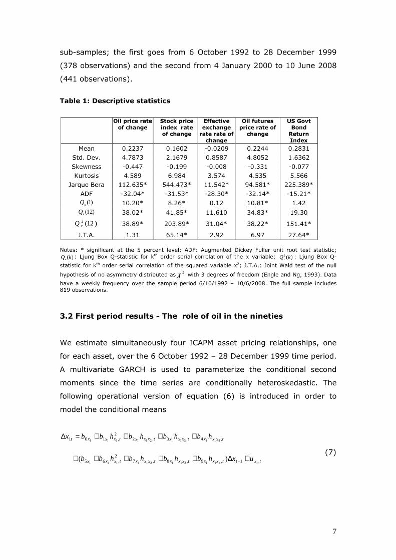
The descriptive statistics are reported in Table 1.4 Over the full sample

period oil returns are higher, on average, than stock returns but smaller

than bond ones. The standard deviation of the oil price rate of change is

significantly greater than that of the returns of the remaining assets. All

the series are mildly skewed and leptokurtic, and the Jarque Bera test

statistics reject the normality of distribution hypothesis. Their stationarity,

tested with the ADF procedure, stands out clearly. Inter-temporal

dependency of weekly returns (with the exception of the rate of change of

the effective exchange rate and of US bond index return) and squared

weekly returns is confirmed by the Ljung Box Q-statistics. Volatility

clustering affects all the time series while asymmetries are present only in

the case of the equity and bond returns.

According to the Andrews (1993) Wald tests (for parameter stability) with

unknown switch point, the time series do not show any sign of regime

shifts. The null hypothesis of no break point - with the usual trimming of

15% of the data at the endpoints – cannot be rejected.5

On the contrary the correlation between the time series does not seem to

be constant over the whole sample. A standard Jenrich (1970) 2χ stability

test detects unequivocally a structural break in the correlation matrix of

returns at the end of the year 1999.6 We split therefore the data in two

4 Percentage rates of return are used in the empirical analysis, computed multiplying by

100 the first logarithmic differences of the original series. The US All Lives Government

Bond Total Return index time series too is multiplied by 100. 5 The tests are based on a first order autoregression with a constant in the case of oil and

equity returns and on a regression on a constant term for the remaining time series. The

statistics are available from the authors upon request. 6 The maximum value of test is 86.72 under the alternative of a breakpoint on 28

December 1999. It strongly rejects the null hypothesis (that two 4-variate normal

populations have correlation matrices that have a common non-singular value), the )6(2χ

5% critical value being 12.6. In order to deal with potential distortions due to non-

normality, we repeated the test using the standardized residuals of a full sample

estimation of our CCC-GARCH behavioral ICAPM system and obtained qualitatively similar

results.

7

sub-samples; the first goes from 6 October 1992 to 28 December 1999

(378 observations) and the second from 4 January 2000 to 10 June 2008

(441 observations).

Table 1: Descriptive statistics

Oil price rate of change

Stock price index rate of change

Effective exchange rate rate of change

Oil futures price rate of

change

US Govt Bond Return Index

Mean 0.2237 0.1602 -0.0209 0.2244 0.2831

Std. Dev. 4.7873 2.1679 0.8587 4.8052 1.6362

Skewness -0.447 -0.199 -0.008 -0.331 -0.077

Kurtosis 4.589 6.984 3.574 4.535 5.566

Jarque Bera 112.635* 544.473* 11.542* 94.581* 225.389*

ADF -32.04* -31.53* -28.30* -32.14* -15.21*

)1(xQ 10.20* 8.26* 0.12 10.81* 1.42

)12(xQ 38.02* 41.85* 11.610 34.83* 19.30

)12(2xQ 38.89* 203.89* 31.04* 38.22* 151.41*

J.T.A. 1.31 65.14* 2.92 6.97 27.64*

Notes: * significant at the 5 percent level; ADF: Augmented Dickey Fuller unit root test statistic;

)(kQx: Ljung Box Q-statistic for kth order serial correlation of the x variable; )(2 kQx

: Ljung Box Q-

statistic for kth order serial correlation of the squared variable x2; J.T.A.: Joint Wald test of the null

hypothesis of no asymmetry distributed as2χ with 3 degrees of freedom (Engle and Ng, 1993). Data

have a weekly frequency over the sample period 6/10/1992 – 10/6/2008. The full sample includes 819 observations.

3.2 First period results - The role of oil in the nineties

We estimate simultaneously four ICAPM asset pricing relationships, one

for each asset, over the 6 October 1992 – 28 December 1999 time period.

A multivariate GARCH is used to parameterize the conditional second

moments since the time series are conditionally heteroskedastic. The

following operational version of equation (6) is introduced in order to

model the conditional means

txxxtxxxtxxxtxxxt hbhbhbhbbx ,4,3,22

,101 411311211111++++=∆

(7)

txttxxxtxxxtxxxtxxx uxhbhbhbhbb ,1,9,8,72

,65 1411311211111)( +∆+++++ −

8

where tt xx 41 ,...,∆∆ are the rates of return of the four assets analyzed in the

paper and 2,1 txh and txx i

h ,1, i=2,3,4, are, respectively, the conditional

variance and covariances obtained with the GARCH model.

txxxtxxxtxxxtxx hbhbhbhb ,4,3,22

,1 41131121111+++ corresponds to

)()()()( ,4,3,22

,1 321 tMFtMFtMFtM σσσσ Φ+Φ+Φ+Φ in equation (6), while

txxxtxxxtxxxtxxx hbhbhbhbb ,9,8,72

,65 411311211111++++ corresponds to

)].()()()([ ,4,3,22

,1 321 tMFtMFtMFtM σσσσγ Φ+Φ+Φ+Φ

The relevance of the feedback trading component and the number of

factors affecting the pricing of each asset are determined empirically. If,

as is the case for the bond return and the rate of change of the exchange

rate time series, no evidence is found of serial correlation, the feedback

trading component is dropped from the corresponding conditional mean

parameterization. In the same way we remove the variables with

insignificant coefficients at the standard 5 percent level or that correspond

to insignificant conditional covariances.7 The conditional second moments

are parameterized using a CCC-GARCH(1,1) model. The behavior of the

rate of change of the spot oil prices ( ts∆ ), the Dow Jones sock index ( tj∆ ),

the US dollar effective exchange rate ( tz∆ ), and of the US Government

bond index total return )( tk∆ are then modelled using the system (A).

tktjkktkkkt

tztjzztzzzt

tjttjkjtjzjtsjjtjjj

tjkjtjzjtsjjtjjjt

tsttsjstsstsjstssst

uhbhbbk

uhbhbbz

ujhbhbhbhbb

hbhbhbhbbj

ushbhbhbhbbs

,,32,10

,,32,10

,1,9,8,72,65

,4,3,22,10

,1,72,6,2

2,10

)(

)(

+++=∆

+++=∆

+∆+++++

++++=∆

+∆++++=∆

−

−

7 This parsimonious approach is motivated by need to reduce the large number of

parameters entering our nonlinear system.

9

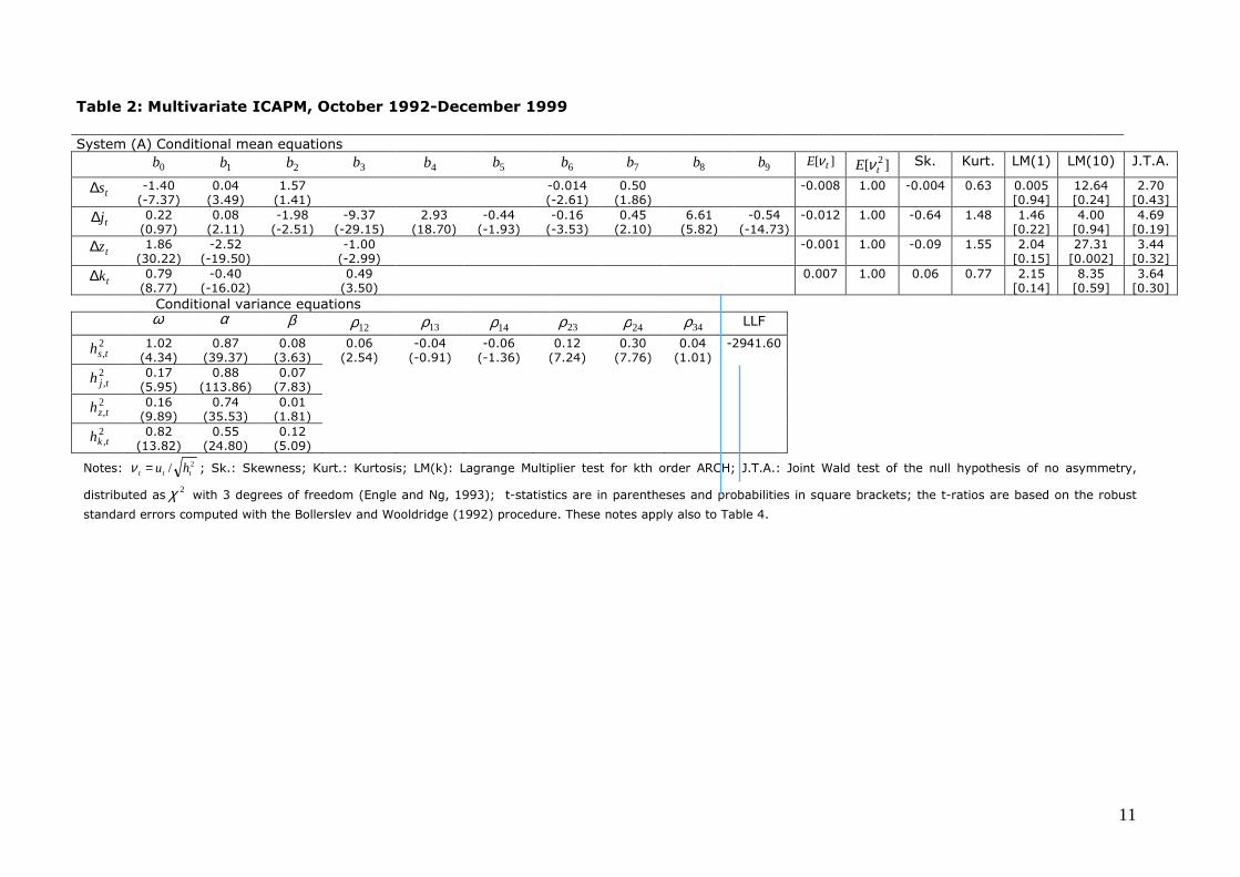
The QML estimates are set out in Table 2. The conditional mean

determinants that are associated with the conditional covariances between

oil returns and exchange rate changes, tszh , , between oil and US bond

returns, tskh , , and between exchange rate changes and bond returns, tzkh , ,

are removed since the corresponding conditional correlation coefficients

estimates 341413 ,, ρρρ do not significantly differ from zero.

The quality of fit is satisfactory. Almost all coefficients are statistically

significant and the usual tests for misspecification suggest that the

standardized residuals tν are well behaved. For each equation we find that

0][ =tE ν and 1][ 2 =tE ν , and that both tν and 2tν are serially uncorrelated.

The sign bias tests by Engle and Ng (1993) support the choice of a

symmetric conditional variance model. Asymmetry, a stylized

characteristic of stock return volatility, is filtered out by the feedback

trading conditional mean parameterization.

For the sake of notational simplicity let iλ , where kzjsi ,,,= , be the CAPM

component - i.e. tsjstssts hbhb ,22,1, +=λ , tjkjtjzjtsjjtjjtj hbhbhbhb ,4,3,2

2,1, +++=λ ,

tjzztzztz hbhb ,32,1, +=λ , and tjkktkktk hbhb ,3

2,1, +=λ - and iφ be the feedback

( )

21,

21,

2,

21,

21,

2,

21,

21,

2,

21,

21,

2,

,

,

,

,

434241

343231

242321

141312

1

,

,

,

,

; ;

000

000

000

000

1

1

1

1

(A) ,0

−−

−−−−−−

−

++=

++=++=++=

=∆

=

∆∆=Ω

=

tkktkkktk

tzztzzztztjjtjjjtjtsstsssts

tk

tz

tj

ts

t

ttt

ttt

tk

tz

tj

ts

t

huh

huhhuhhuh

h

h

h

h

R

RH

HNu

u

u

u

u

u

βαϖ

βαϖβαϖβαϖ

ρρρρρρρρρρρρ

10

trading coefficient - i.e. tsjstsss hbhb ,72,6 +=φ , and

tjkjtjzjtsjjtjjjj hbhbhbhbb ,9,8,72,65 ++++=φ .

In both the oil and stock returns conditional mean equations the overall

CAPM component λ and the feedback trading coefficient φ – computed

with historical simulations which use the values of the conditional second

moments - turn out to be, respectively, positive and negative on average.

(Their behavior over time is set out in Graph 1 and their unconditional

average values can be found in Table 3). The negative

sign of the feedback trading coefficient is due to the presence of

destabilizing speculation, which tends to raise the volatility of the returns

of the asset.

As for the rate of change of the US dollar effective exchange rate and the

US bond returns, the overall CAPM component is negative. The negative

sign of tz,λ implies that an increase in the conditional variance of the rate

of change of the effective exchange rate 2,tzh and of its conditional

covariance with the stock returns tjzh , , brings about a depreciation of the

US effective exchange rate as traders sell dollars (see Graph 1). Similarly

the negative value of tk ,λ means that an increase in the bond return

conditional variance 2,tkh , possibly due to a rise in inflation risk and/or in

general economic uncertainty, will lead to a decline in bond returns as

traders sell bonds which are losing their safe asset characteristics.8

8 Viceira (2007) finds that bond return volatility is positively related to the level and the

slope of the yield curve, factors that proxy for inflation risk and overall economic

uncertainty.

11

Notes: 2/ ttt hu=ν ; Sk.: Skewness; Kurt.: Kurtosis; LM(k): Lagrange Multiplier test for kth order ARCH; J.T.A.: Joint Wald test of the null hypothesis of no asymmetry,

distributed as2χ with 3 degrees of freedom (Engle and Ng, 1993); t-statistics are in parentheses and probabilities in square brackets; the t-ratios are based on the robust

standard errors computed with the Bollerslev and Wooldridge (1992) procedure. These notes apply also to Table 4.

Table 2: Multivariate ICAPM, October 1992-December 1999

System (A) Conditional mean equations

0b 1b 2b 3b 4b 5b 6b 7b 8b 9b ][ tE ν ][ 2tE ν Sk. Kurt. LM(1) LM(10) J.T.A.

ts∆ -1.40 (-7.37)

0.04 (3.49)

1.57 (1.41)

-0.014 (-2.61)

0.50 (1.86)

-0.008 1.00 -0.004 0.63 0.005 [0.94]

12.64 [0.24]

2.70 [0.43]

tj∆ 0.22 (0.97)

0.08 (2.11)

-1.98 (-2.51)

-9.37 (-29.15)

2.93 (18.70)

-0.44 (-1.93)

-0.16 (-3.53)

0.45 (2.10)

6.61 (5.82)

-0.54 (-14.73)

-0.012 1.00 -0.64 1.48 1.46 [0.22]

4.00 [0.94]

4.69 [0.19]

tz∆ 1.86 (30.22)

-2.52 (-19.50)

-1.00 (-2.99)

-0.001 1.00 -0.09 1.55 2.04 [0.15]

27.31 [0.002]

3.44 [0.32]

tk∆ 0.79 (8.77)

-0.40 (-16.02)

0.49 (3.50)

0.007 1.00 0.06 0.77 2.15 [0.14]

8.35 [0.59]

3.64 [0.30]

Conditional variance equations

ϖ α β 12ρ 13ρ 14ρ 23ρ 24ρ 34ρ LLF

2,tsh 1.02

(4.34) 0.87

(39.37) 0.08 (3.63)

2,tjh 0.17

(5.95) 0.88

(113.86) 0.07 (7.83)

2,tzh 0.16

(9.89) 0.74

(35.53) 0.01 (1.81)

0.06 (2.54)

-0.04 (-0.91)

-0.06 (-1.36)

0.12 (7.24)

0.30 (7.76)

0.04 (1.01)

-2941.60

2,tkh 0.82

(13.82) 0.55

(24.80) 0.12 (5.09)

12

Graph 1. First period CAPM components and feedback trading coefficients

Oil return equation CAPM component Oil return equation Feedback trading coef.

0.0

0.5

1.0

1.5

2.0

2.5

3.0

3.5

4.0

1993 1994 1995 1996 1997 1998 1999

lambda oil

-.4

-.3

-.2

-.1

.0

.1

.2

1993 1994 1995 1996 1997 1998 1999

zero phi oil

US stock return equation CAPM component US stock return equation Feedback trading coef.

-1

0

1

2

3

4

5

1993 1994 1995 1996 1997 1998 1999

zero lambda US stock index

-1.2

-1.0

-0.8

-0.6

-0.4

-0.2

0.0

0.2

1993 1994 1995 1996 1997 1998 1999

zero phi US stock index

US dollar equation CAPM component US bond return index equation CAPM component

-2.4

-2.0

-1.6

-1.2

-0.8

-0.4

1993 1994 1995 1996 1997 1998 1999

lambda US dollar effective exchange rate

-3.5

-3.0

-2.5

-2.0

-1.5

-1.0

-0.5

0.0

1993 1994 1995 1996 1997 1998 1999

lambda US bond index

13

Table 3: Average values of the conditional mean CAPM components

(CAPM comp.) and feedback trading coefficients (Fbt coef.)

Oil returns US dollar changes

CAPM comp. 1.52 (52.57)* CAPM comp. -1.83 (-256.51)*

Fbt coef. -0.043 (-12.62)*

US stock returns US bond returns

CAPM comp. 0.16 (6.30)* CAPM comp. -0.58 (-44.85)*

Fbt coef. -0.035 (-6.23)*

Notes. t-statistics (Ho: average = 0) are in parentheses; *: significant at the 5% level.

During the nineties, the link between oil prices and the other assets

investigated in the paper is limited to a positive interaction between oil

and stock returns, which can be attributed to a real (macroeconomic)

channel. A rise in stock returns during the expansionary phase of the

business cycle is associated with an increase in the demand for oil and a

corresponding upward pressure on oil returns. The latter are responding

moreover to a rationale that could connect the convenience yield to

volatility along the lines of the model of Pindyck (2001, 2003) where

volatility and other variables enter the equation of spot returns as proxies

of the convenience yield. As is the case for call options, the greater the

volatility of the cash commodity price, the greater the chance it will

exceed the corresponding futures price and, as a consequence, the

greater the convenience yield. By affecting the size of convenience yields,

cash price volatility is expected to affect positively oil price returns.9

The two spikes that can be detected in the graphs of the CAPM component

and of the feedback trading coefficient of the oil price rate of change

equation (see Graph 1) are caused by sharp increases in oil price

variability. The first price shock in 1996 is idiosyncratic and can be

attributed to a mismatch between actual and expected oil demand. It

affects only the oil return equation by raising the pricing risk premium and

9 On this topic, see also Milonas and Henker (2001).

14

magnifying the feedback trading effects as the traders’ uncertainty rises.10

The second shock is mainly connected to the Asian crisis and affects all of

the remaining assets conditional mean equations by increasing the risk

premium that is required to price both the oil and stock rates of return. As

expected, since they are negatively related to volatility shifts of the CAPM

component, the oil shock has a negative impact (via stocks) on the US

bond returns and on the rate of change of the effective exchange rate.11

3.3 Second period results - Oil as a financial asset

A preliminary analysis of the data in the second time period reveals that

the rates of change of the spot oil prices and of the US effective exchange

rate are homoskedastic, the remaining time series being heteroskedastic,

as in the first time period.12

The exchange rate and oil return variabilities are thus measured as the

unconditional variances of their respective conditional mean residuals. The

variance covariance matrix of system (B) combines the unconditional

variances of the homoskedastic time series with the conditional variances

of the heteroskedastic ones in a modified CCC-GARCH framework.

10 A few historical details are of interest here. Despite the ban on Iraqi exports (a

consequence of the first Gulf war), low levels of production in Iran, Libya, and especially

Russia, following the collapse of the Soviet Union, world oil supply exceeds demand in the

first half of the nineties and brings about a reduction in prices. Towards the end of 1996,

however, oil prices increase unexpectedly, because of a rebound in US consumption and of

an upsurge of demand by the Asian Tigers. 11 At the beginning of 1998, in the aftermath of the financial turmoil, South Korea’s

refiners cut output below maximum capacity. The OPEC, in the same year, reduces twice

its production target level in order to boost oil prices, which tend to subside because of a

reduction in demand from Asia. For more details on this confusing period, see Maugeri

(2006, chapter 14, pp. 169-181). 12 These findings are obtained with the help of Ljung Box Q-tests for kth order serial

correlation (k=1,…,24). With the squared rates of change of oil price and effective

exchange rate, these statistics are never significant at the 5% level. They are strongly

significant in the case of the remaining squared return time series.

15

tktzkktjkktskktkkkt

tztzkztjzztszztzzzt

tjttjzjtsjjtjjjtjkjtjzjtsjjtjjjt

tstss

ttskstszstsjstsstskstszstsjstssst

uhbhbhbhbbk

uhbhbhbhbbz

ujhbhbhbbhbhbhbhbbj

ufbDb

shbhbhbhbhbhbhbhbbs

,,4,3,22,10

,,4,3,22,10

,1,8,72,65,4,3,2

2,10

,111110

1,9,8,72,6,4,3,2

2,10

)(

)(

+++++=∆

+++++=∆

+∆++++++++=∆

+∆++

∆++++++++=∆

−

−

−

( )ttt

ttt

tk

tz

tj

ts

t

RH

HNu

u

u

u

u

u

∆∆=Ω

=

− ,01

,

,

,

,

(B)

1D is a dummy accounting for the steep price rise in the years 2007-2008.

The estimates of system (B) are set out in Table 4. The second period

variance covariance matrix points to a very intricate interrelation pattern.

The conditional correlation coefficients are significant and negative and

suggest that all the assets can be used for portfolio risk diversification. As

for the final specification of the model, all the cross covariances are kept

in the parameterization of the feedback trading coefficients even if,

following our parsimonious approach, the regressors with coefficients that

are not significantly different from zero are dropped from the estimation.

No feedback trading component appears in the conditional means of the

rate of change of the US effective exchange rate and of the US bond

returns, as these time series turn out to be serially uncorrelated.

The shifts over time of the CAPM component and feedback trading

coefficient time series, computed using historical simulations, are set forth

in Graph 2. Their respective unconditional means are collected in Table 5.

21,

21,

2,

22,

21,

21,

2,

22,

,

,

,

,

434241

343231

242321

141312

ˆ ; ;ˆ

000

000

000

000

1

1

1

1

−−

−−

++=

=++==

=∆

=

tkktkkktk

ztztjjtjjjtjsts

tk

tz

tj

ts

t

huh

hhuhh

h

h

h

h

R

βαϖ

σβαϖσ

ρρρρρρρρρρρρ

16

The graphical analysis detects two major shocks to oil prices. The first is

associated with the financial turmoil caused by the military operations

against Iraqi oil infrastructures of 2001 and the second is a direct

consequence of the stock market collapse of 2002.13

The CAPM component of the oil conditional mean equations is mostly

negative from 2000 to 2002. The weighted sum of the variance of oil

returns and of the covariance between oil and bond returns and between

oil returns and the rate of change of the US effective exchange rate is

overcompensated by the negative covariance between oil and stock

market returns.

Indeed, shifts in portfolio composition between stock and oil tend to

reduce risk. The oil risk premium in Graph 2 declines and becomes

negative as investors sell oil and buy stocks, whose CAPM component, in

turn, rises as uncertainty increases. This behavior corroborates our

hypothesis that oil is now a truly financial asset, as suggested by the

significance of all the conditional covariance coefficients in its conditional

mean estimates.

From 2003 onwards the variability of stock returns declines and the oil

CAPM component is mostly positive. The feedback trading coefficient, on

the contrary, is always strongly negative since the loadings of the

covariances between oil returns and the returns of the other assets of the

model are all positive. An inspection of Tables 3 and 5 shows that positive

feedback trading is, on average, more relevant in the second than in the

first time period. Destabilizing speculation becomes a major driver of oil

price movements.

In the US dollar effective exchange rate conditional mean, zb1 is negative;

an increase in volatility brings about a depreciation of the US effective

exchange rate as traders sell dollars. The average negativeness of the

overall CAPM coefficient tz ,λ , however, is mitigated by the impact of the

covariance between the oil prices and the US dollar.

13 Having recovered from the lows which followed September 11 2001, the US stock

indices started to slide from March 2002 onwards. The dramatic declines in July and

September led to lows last reached in 1997 and/or 1998.

17

The sign of the CAPM component of the conditional mean equation of the

US bond index return can be mainly attributed to the influence of two

major factors. The oil channel, tskkhb ,2 , which identifies a joint nature of

bonds and oil as safe assets, and the exchange rate channel, tzkkhb ,4 , which

accounts for the foreign demand of US Treasuries. When the USD

depreciates US bonds become cheaper and their demand rises. Indeed,

the large purchases of Treasuries by foreigners such as the Central Bank

of the Peoples’ Republic of China, or analogous institutions of emerging

market economies, bring about a substantial flattening of the yield curve

and invalidate at least temporarily, the standard relationship between risk

and returns.

18

Table 4: Multivariate ICAPM, January 2000-June 2008

System (B) Conditional mean equations

0b 1b 2b 3b 4b 5b 6b 7b 8b 9b 10b 11b ][ tE ν ][ 2tE ν

Sk. Kurt. LM(1) LM(10) J.T.A.

ts∆

0.50

(2.43)

0.04

(3.00)

2.64

(2.98)

-1.74

(-1.67)

-1.88

(-2.06)

-0.006

(-3.33)

0.17

(2.81)

0.29

(2.40)

0.34

(1.94)

0.86

(2.53)

0.26

(3.76)

0.00 1.36 -0.70 11.05 2.48

[0.11]

16.22

[0.09]

4.25

[0.23]

tj∆

-1.45 (-8.27)

-0.12 (-3.49)

-3.58 (-11.88)

-11.43 (-1.75)

0.42 (2.39)

-0.54 (-4.97)

-0.04 (-4.41)

-0.46 (-10.5)

-9.31 (-9.63)

-0.12 1.00 -0.60 2.21 0.18 [0.66]

4.75 [0.90]

9.46 [0.02]

tz∆

-0.13 (-4.28)

-0.31 (-4.48)

-0.09 (-0.51)

-3.99 (-1.23)

-0.24 (-1.76)

-0.00 1.36 0.10 0.02 1.42 [0.23]

13.59 [0.19]

3.15 [0.36]

tk∆

-1.10 (-5.78)

-0.42 (-6.57)

-9.74 (-24.51)

-0.02 (-0.12)

4.01 (5.20)

0.05 1.01 0.02 0.69 3.21 [0.07]

22.62 [0.01]

4.76 [0.19]

Conditional variance equations

ϖ α β 12ρ 13ρ 14ρ 23ρ 24ρ 34ρ LLF

2,tsh

2,tjh

0.77 (2.41)

0.59 (5.68)

0.28 (3.48)

2,tzh

-0.09 (-7.30)

-0.08 (-2.82)

-0.06 (-41.89)

-0.02 (-3.55)

-0.31 (-5.93)

-0.19 (-6.82)

-3718.17

2,tkh

0.11 (3.46)

0.81 (30.89)

0.14 (6.80)

Graph 2. Second period CAPM components and feedback trading coefficients

Oil return equation CAPM component Oil return equation Feedback trading coef.

-5

-4

-3

-2

-1

0

1

2

00 01 02 03 04 05 06 07 08

zero lambda oil

-.7

-.6

-.5

-.4

-.3

-.2

00 01 02 03 04 05 06 07 08

phi oil

US stock return equation CAPM component US stock return equation Feedback trading coef.

0.8

1.2

1.6

2.0

2.4

2.8

00 01 02 03 04 05 06 07 08

lambda US stock index

-.8

-.7

-.6

-.5

-.4

-.3

-.2

-.1

.0

00 01 02 03 04 05 06 07 08

phi US stock index

US dollar equation CAPM component US bond return index equation CAPM component

-.14

-.12

-.10

-.08

-.06

-.04

-.02

00 01 02 03 04 05 06 07 08

lambda US dollar effective exchange rate

0.0

0.2

0.4

0.6

0.8

1.0

1.2

1.4

1.6

00 01 02 03 04 05 06 07 08

lambda US bond index

20

Table 5: Average values of the conditional mean CAPM components

(CAPM comp.) and feedback trading coefficients (Fbt coef.) Oil returns US dollar changes

CAPM comp. -0.31 (-8.94)* CAPM comp. -0.09 (-114.51)*

Fbt coef. -0.37 (-111.68)*

US stock returns US bond returns

CAPM comp. 1.77 (119.30)* CAPM comp. 1.34 (146.94)*

Fbt coef. -0.15 (-48.40)*

Notes. t-statistics (Ho: average = 0) are in parenteses; *: significant at the 5% level.

4. Portfolio analysis

The paper focuses on the important issue of a change in WTI oil spot

pricing in the last decade. If the hypothesis that in recent years oil

behaved more and more as a financial asset is correct, its inclusion in a

portfolio, given the signs of the correlation coefficients computed in the

previous section, should have a beneficial effect on the corresponding

risk/return trade-off.

We assess this proposition using a straightforward Markowitz procedure,

with no short-selling restrictions, no borrowing and no lending, and base

the portfolio composition on risk minimization criteria.

If '1 ),......,( Nwww = is a Nx1 vector of portfolio weights and Σ is the NxN

variance-covariance matrix of the returns, the portfolio variance is then

ww Σ' . The global minimum variance portfolio is the solution of the

minimization problem minw 11'..' =Σ wtsww , where 1 is a Nx1 column

vector of ones. The weights ',1, ),......,( NMVMVMV www = of the global minimum

variance portfolio take the value .111 1'1 −− ΣΣ=MVw

The expected return MVµ and the variance 2MVσ of the global minimum

variance portfolio read as

11

1'1'

1'

−

−

ΣΣ== µµµ MVMV w (8)

and

21

11

11'

'2−Σ

=Σ= MVMVMV wwσ (9)

where µ is a Nx1 column vector of asset returns. The corresponding

expected return per unit of risk index is then computed as

2

MVMV σµ .

The lower variance bound (9) can be attained only if the variance-

covariance matrix of the asset returns is known. Typically, historical

return observations are used for this estimation. We construct the

portfolios either keeping the weights constant over each sub-sample or

rebalancing them every week, mimicking a tactical asset allocation

behavior. (Weekly portfolio rebalancing is also meant to account for the

volatility clustering of the time series.) Every week the constrained

variance minimization described above is performed over a predetermined

data interval j and the corresponding global minimum variance weights,

(expected) portfolio returns jMV ,µ , portfolio return variance 2, jMVσ and

(expected) return per unit of risk index

2

,, jMVjMV σµ are computed.

The following week the same procedure is repeated over a sample interval

shifted forward by one time period (i.e. one week). This iterative process

continues until the end of the sub-period. A set of three time series for

each portfolio holding period is obtained in this way. We selected here a

12 month and a 6 month holding period. In Table 6 are set out the

unconditional means and the average return per unit of risk, over the two

sub-samples, of these time series.

The entries suggest that, over the last decade, the introduction of oil into

a multi asset-class portfolio improves the risk/return performance.

In the first sub-period the three asset portfolio (without oil) outperforms

the four asset one, which includes oil. This result holds considering both

the unconditional mean returns and the average return per unit of risk,

with and without portfolio rebalancing.

22

Table 6: Portfolio analysis

Holding period

Unconditional mean Unconditional variance Average return per unit of risk

(Mean/Standard error)

First sub-sample

6/10/1992 12/28/1999

Second sub-

sample 4/1/2000 10/6/2008

First sub-sample

6/10/1992 12/28/1999

Second sub-

sample 4/1/2000 10/6/2008

First sub-sample

6/10/1992 12/28/1999

Second sub-

sample 4/1/2000 10/6/2008

No portfolio rebalancing

Without

oil Sub-

sample*

0.0937 0.0491 0.5270 0.3815 0.1292 0.0796

With oil spot price

Sub-sample

0.0909 0.0618 0.5016 0.3440 0.1283 0.1053

With oil futures price

Sub-sample

0.0908 0.0627 0.5037 0.3440 0.1279 0.1068

Weekly portfolio rebalancing

Without oil

Twelve months*

0.1010 0.0619 0.4953 0.2683 0.1496+ 0.1249+

With oil spot price

Twelve months

0.0924 0.0712 0.4631 0.2438 0.1410+ 0.1505+

With oil futures price

Twelve months

0.0940 0.0714 0.4679 0.2437 0.1432+ 0.1499+

Without oil

Six months*

0.1050 0.0760 0.4440 0.2469 0.1699+ 0.1585+

With oil spot price

Six months

0.0966 0.0897 0.4042 0.2147 0.1629+ 0.1968+

With oil futures price

Six months

0.0978 0.0901 0.4082 0.2152 0.1640+ 0.1959+

Notes. *: The optimal weights are computed minimizing the variance of a three asset portfolio, which does not include oil; +: approximation to the exact index according to Jobson and Korkie (1981, page

893).

In the second period, when oil progressively acquires financial

characteristics, we obtain the opposite results. The unconditional portfolio

mean and variance and the average return per unit of risk detect a clear-

cut dominance of the four asset portfolio, independently of the presence of

a rebalancing mechanism and of the length of the holding period. The

analysis is then repeated replacing WTI spot prices with the corresponding

one month to expiration (contract 1) futures prices and provides similar

23

results, a finding which further corroborates the hypothesis on oil spot

pricing mentioned above.14

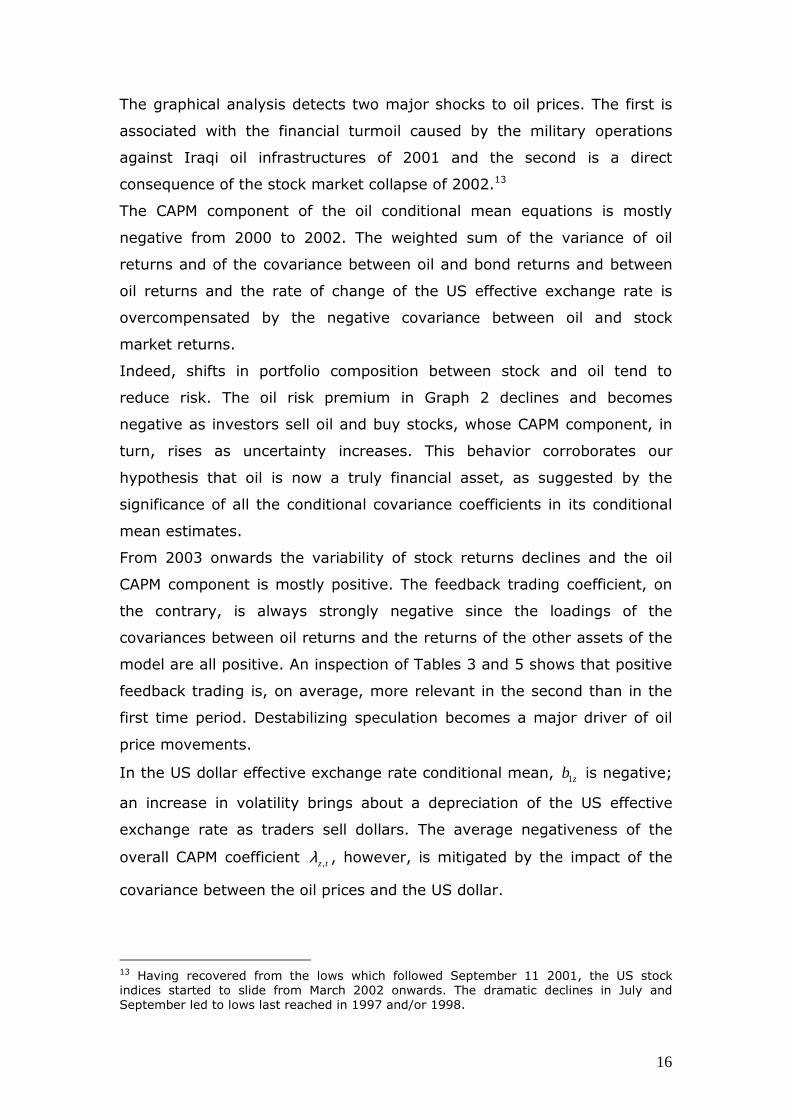
In the same way, the visual inspection of Graph 3, which depicts the

behavior over time of the first and second sub-sample variances of the

global minimum variance four asset portfolio with annual and semi-annual

holding periods, shows that in the second period oil reduces significantly

portfolio risk. In both panels the graphs identify the same volatility peaks

and point to a dominance of the second period portfolio. Differences in

volatility size are due to “ghost features” in the sense of Alexander

(2001), since extreme events are averaged over fewer observations in the

case of the six month holding period.

Graph 3. Variance of the global minimum variance portfolio with weekly

rebalancing and semi-annual and annual holding periods

Six month holding period Twelve month holding period

5. Conclusion

At the beginning of the year 2000 a regime shift is detected within a

highly nonlinear behavioral ICAPM assumed to describe the

interconnection between crude oil contracts, US stocks, bonds and

effective dollar exchange rate. Indeed, the parsimonious estimates of the

model over the 1992-1999 and 2000-2008 time periods differ

14 Also Geman and Kharoubi (2008) find that WTI crude oil futures contracts can be used to

efficiently diversify equity portfolios.

0.0

0.2

0.4

0.6

0.8

1.0

1.2

First Period Variance of the Global Minimum Variance PortfolioSecond Period Variance of the Global Minimum Variance Portfolio

.0

.1

.2

.3

.4

.5

.6

.7

.8

First Period Variance of the Global Minimum Variance PortfolioSecond Period Variance of the Global Minimum Variance Portfolio

24

considerably. The conditional correlations change in sign, absolute value,

and statistical significance. The oil return conditional mean acquires a

complex feedback trading component in the second sub-period and

becomes similar in structure to the conditional mean of the stock returns.

Oil contracts seem to behave as financial assets, which interact with

stocks, bonds, and exchange rates.

In order to further investigate this hypothesis we construct global

minimum variance portfolios containing standard financial assets along

with WTI crude oil contracts. It stands out clearly – comparing return per

unit of risk measures – that the introduction of oil has been of help in

diversifying away the unpriced risk of the portfolios.

The paper thus suggests that, in the second sub-period, traders hedge

their portfolios considering oil as a component of their wealth allocation.

References

Alexander, C., 2001, Market Models. A Guide to Financial Data Analysis,

Chichester: Wiley.

Andrews, D.W.K., 1993, Tests for Parameter Instability and Structural

Change with Unknown Change Point, Econometrica, 61: 821-856.

Bhar, R. and B. Nikolova, 2009, Oil prices and Equity Returns in BRIC

Countries, The World Economy, 32: 1036-1054.

Bollerslev, T. and J.M. Wooldridge, 1992, Quasi-Maximum Likelihood

Estimation and Dynamic Models with Time-Varying Covariances,

Econometric Reviews, 11: 143-172.

Cutler, D.M., Poterba, J.M., and L.H. Summers, 1991, Speculative

Dynamics and the Role of Feedback Traders, American Economic Review,

80: 63-68.

Dean, W.G. and R. Faff, 2008, Feedback Trading and the Behavioural

CAPM: Multivariate Evidence across International Equity and Bond

Markets. Mimeo Monash University, Australia.

25

Engle, R.F. and V.K. Ng, 1993, Measuring and Testing the Impact of News

on Volatility, Journal of Finance, 48: 1749-1778.

Geman, H. and C. Kharoubi, 2008, WTI Crude Oil Futures in Portfolio

Diversification: the Time to Maturity Effect, Journal of Banking and

Finance, 32: 2553-2559.

Jenrich, R.I., 1970, Asymptotic χ2 Test for the Equality of Two Correlation

Matrices, Journal of the American Statistical Association, 65: 904–912.

Jobson, J.D. and B.M. Korkie, 1981, Performance Hypothesis Testing with

the Sharpe and Treynor Measures, Journal of Finance, 36: 889-908.

Koutmos, G., 1997, Feedback Trading and the Autocorrelation Pattern of

Stock Returns: Further Empirical Evidence, Journal of International Money

and Finance, 16, 625-636.

Koutmos, G. and R. Saidi, 2001, Positive Feedback Trading in Emerging

Capital Markets, Applied Financial Economics, 11, 291-297.

Lakonishok, J., Shleifer A., and R.W. Vishny, 1992, The Impact of

Institutional Investors on Stock Prices. Journal of Financial Economics, 32:

23-43.

Maugeri, L., 2006, The Age of Oil, London: Praeger.

Merton, R., 1973, An Intertemporal Asset Pricing Model, Econometrica,

41, 867-888.

Milonas, N.T. and T. Henker, 2001, Price Spread and Convenience Yield

Behaviour in the International Oil Market, Applied Financial Economics,

11: 23-36.

Nofsinger, J.R. and R.W. Sias, 1999, Herding and Feedback Trading by

Institutional and Individual Investors. Journal of Finance, 54: 2263-2295.

Pindyck, R.S., 2001, Dynamics of Commodity Spot and Futures Markets: a

Primer, Energy Journal, 22: 2-29.

26

Pindyck, R.S., 2003, Volatility in Natural Gas and Oil, MIT, Center for

Energy and Environmental Policy Research, Working Paper 03-012.

Roache, S.K., 2008, Commodities and the Market Price of Risk, IMF

Working Paper wp/08/221.

Scruggs, J.T., 1998, Resolving the Puzzling Intertemporal Relation

between the Market Risk Premium and Conditional Market Covariance: a

Two Factor Approach, Journal of Finance, 53: 575-603.

Sentana, E., and S. Wadhwani, 1992, Feedback Trading and Stock Return

Autocorrelations: Evidence from a Century of Daily Data, Economic

Journal, 102: 415-425.

Sadorsky, P., 1999, Oil Price Shocks and Stock Market Activity, Energy

Economics, 21: 449-469.

Shiller, R.J., 1984, Stock Prices and Social Dynamics. Brookings Papers on

Economic Activity 2: 457-498.

Viceira, L.M., 2007, Bond Risk, Bond Return Volatility, and the Term

Structure of Interest Rates, Harvard Business School Working Papers 07-

082.