Irreducible decomposition of products of 10D chiral sigma matrices

arX

iv:h

ep-t

h/00

0420

2v1

28

Apr

200

0

Irreducible Decomposition of Products of 10D Chiral Sigma Matrices ∗

S. James Gates, Jr.† and B. Radak‡

Department of Physics, University of Maryland

College Park, MD 20742-4111 USA

and

V.G.J. Rodgers§

Department of Physics and Astronomy, University of Iowa

Iowa City, Iowa 52242–1479 USA

ABSTRACT

We review the enveloping algebra of the 10 dimensional chiral sigma matrices. To

facilitate the computation of the product of several chiral sigma matrices we have de-

veloped a symbolic program. Using this program one can reduce the multiplication of

the sigma matrices down to linear combinations of irreducilbe elements. We are able to

quickly derive several identities that are not restricted to traces. A copy of the program

written in the Mathematica language is provided for the community.

∗Supported in part by National Science Foundation Grant PHY-98-02551.†[email protected]‡[email protected]§[email protected]

http://arXiv.org/abs/hep-th/0004202v1

I. SPINORS AND SIGMA MATRICES IN 10 D

Several problems in 10 D Physics require the ability to reduce products of the 10 D chiral sigma

matrices into a linear combination of the irreducible matrices [1-4]. In general such calculations

can quickly become intractable. For some problems, many approximation schemes are applied such

as linearization and perturbation theory. However when one is discussing properties of algebras,

such as the closing of the Jacobi identity or commutation relations, exact results are mandatory

[5]. Computations such as computing the equations of motion in some supergravity theories, could

literally take several weeks. These types of calculations could be reduced to a few hours work

using today’s powerful symbolic manipulators, such as Mathematica and Maple, in conjuction with

high speed computers. In this note we provide the community with an example of such a program

along with several identities that we have derived using this tool. We begin by outlining the formal

construction of the enveloping algebra of the 10 dimensional chiral sigma matrices.

It is well known that in D-dimensional space-time Dirac spinor has 2D

2 complex components if D

is even and in that case all the representations of the Dirac algebra are equivalent, while in odd

dimensional space-time the number of components is 2D−1

2 with two inequivalent representations.

This result is valid for any signature of the flat space-time metric. However, this kind of spinor is

not, for any D, the smallest irreducible representation. When D is even we can always impose the

Weyl condition which separates the spinor into its left and right handed components which transform

independently under the Lorentz group. Each of these Weyl spinors thus has only half degrees of

freedom of the original Dirac spinor. One more condition can be imposed to reduce further the

number of independent components. This is so called Majorana condition which relates the charge-

conjugate Dirac spinor to the original one. If after the charge conjugation the spinor is not changed,

the number of independent components is reduced again by a factor of two. In that case the left

and right Weyl spinors are related. The resulting spinor is necessarily real. This type of reduction

can be done in 2 (mod 8) dimensional space-time. It then follows that for D = 10 we can impose

both conditions and have for the basic spinor a 16-dimensional real object. Consequently, instead of

using the Dirac gamma matrices we use the Pauli matrices, of dimension 16×16 with real elements.

We can then use small Greek index to denote 16 component left-handed Majorana-Weyl spinor and

dotted index for a right-handed one:

(ψα)∗ = (ψα), (χα̇)∗ = (χα̇). (1)

The indices can be raised and lowered by the use of the charge conjugation matrix which has mixed

indices: Cαβ̇ and Cαβ̇ ,

ψβ̇ = ψαCαβ̇ , χα = χβ̇Cαβ̇ , (2)

Cαγ̇Cαβ̇ = δβ̇

γ̇, Cαβ̇Cγβ̇ = δα

γ . (3)

As we can see, raising and lowering the indices also changes the handedness of a spinor. The Dirac

algebra (of the Pauli matrices) is defined through the usual anticommutation relation:

(σa)αβ(σb)βγ + (σb)αβ(σa)βγ = −2ηabδ

γα . (4)

The sigma matrices can be regarded as bispinors. There are three types of them: purely left-handed,

purely right-handed and mixed ones. The purely left-handed ones are

2

(σa)αβ , (σabc)αβ , (σa1a2a3a4a5)αβ , (5)

where lower case Latin indices are vector indices denoting space-time directions. Purely right-handed

bispinors have only dotted indices, but due to the existence of the charge conjugation matrix we

have

(σa)αβ = Cαα̇Cββ̇(σa)α̇β̇ . (6)

The mixed bispinors are

Cαβ̇ , (σab)αβ̇ , (σabcd)αβ̇ . (7)

They are, of course, related to

δ βα , (σab) β

α , (σabcd) βα . (8)

The sigma matrices with more vector indices are defined through the following multiplication table:

(σa)αβ(σb)βγ = −ηabδ

γα − (σab)

γα ,

(σa)αβ(σbc)β

γ = −ηa[b(σc])αγ − (σabc)αγ ,

(σa)αβ(σbcd)βγ = −

1

2!ηa[b(σcd])

γα − (σabcd)

γα , (9)

(σa)αβ(σbcde)β

γ =1

3!ηa[b(σcde])αγ + (σabcde)αγ ,

(σa)αβ(σbcdef )βγ = −1

4!ηa[b(σcdef ])

γα −

1

4!ǫabcdef [4](σ

[4]) γα .

(σa)αβ(σb)βγ = −ηabδ

γα − (σab)

γα ,

(σbc)α

β (σa)βγ = +ηa[b(σc])αγ − (σabc)

αγ ,

(σbcd)αβ(σa)βγ = −1

2!ηa[b(σcd])

γα + (σabcd)

γα , (10)

(σbcde)α

β (σa)βγ = −1

3!ηa[b(σcde])

αγ + (σabcde)αγ ,

(σbcdef )αβ(σa)βγ = −1

4!ηa[b(σcdef ])

γα +

1

4!ǫabcdef [4](σ

[4]) γα .

All of the sigma matrices are totally antisymmetric in their vector indices. The sigma matrices with

one or five vector indices are symmetric with respect to spinor indices, while the matrix with three

vector indices is antisymmetric in spinor indices. The symmetrization and antisymmetrization is

denoted in the following way:

A(αBβ) = AαBβ + AβBα,

A[αBβ] = AαBβ − AβBα. (11)

The sigma matrices with five vector indices satisfy the identities:

(σ[5])αβ =1

5!ǫ[5] ¯[5](σ

¯[5])αβ ,

(σ[5])αβ = −

1

5!ǫ[5] ¯[5](σ

¯[5])αβ . (12)

3

It is also useful to define matrices with more than five indices

(σ[6])β

α =1

4!ǫ[6] ¯[4](σ

¯[4]) βα ,

(σ[7])αβ = −1

3!ǫ[7] ¯[3](σ

¯[3])αβ ,

(σ[7])αβ = −

1

3!ǫ[7] ¯[3](σ

¯[3])αβ ,

(σ[8])β

α = −1

2!ǫ[8] ¯[2](σ

¯[2]) βα , (13)

(σ[9])αβ = ǫ[9]a(σa)αβ ,

(σ[9])αβ = ǫ[9]a(σ

a)αβ .

The trace identities are:

(σa)αβ(σc)αβ = −16 δca ,

(σab)β

α (σcd) αβ = −16 δ

c

[aδ

d

b],

(σabc)αβ(σdef )αβ = −16 δd

[aδ

e

bδ

f

c], (14)

(σabcd)β

α (σefgh) αβ = 16 δ

e

[aδ

f

bδ

g

c δh

d],

(σabcde)αβ(σfghij)αβ = −16 [δf

[aδ

g

bδ

hc δ

i

dδ

j

e]+ ǫ

fghij

abcde].

In terms of ordinary matrices, our notation can be regarded as follows. We can introduce a bar-

notation to distinguish the altitude of the indices on the bi-spinors in Eq(5). In otherwords we define

the matrices

σa ≡ (σa)αβ , σ̄a ≡ (σa)αβ , (15)

and similarly for the third and fifth rank space-time tensors.We further use a Northwest-Southeast

convention with respect to the contraction of hidden spinor indices. This is simplest to understand

via the following examples

σaσ̄b ≡ −(σa)αβ(σb)βγ , σ̄bσa ≡ (σb)

γβ(σa)βα . (16)

So when the contraction is up-to-down there is a plus sign when writing out the explicit indices, but

when the contraction is down-to-up there is a minus sign.

The sigma matrices with more vector indices follow from the multiplication table:

σaσ̄b = ηab + σab ,

σ̄aσb = −ηab + σab ,

σaσbc = ηa[bσc] + σabc ,

σbcσa = −ηa[bσc] + σabc ,

σaσ̄bcd =1

2!ηa[bσcd] + σabcd ,

σ̄bcdσa =1

2!ηa[bσcd] + σabcd , (17)

σaσbcde = −1

3!ηa[bσcde] − σabcde ,

4

σbcdeσa = −1

3!ηa[bσcde] + σabcde ,

σaσ̄bcdef =1

4!ηa[bσcdef ] +

1

4!ǫabcdef[4]σ

[4] ,

σ̄bcdefσa = −1

4!ηa[bσcdef ] −

1

4!ǫabcdef [4]σ

[4] .

σ̄aσbc = ηa[bσ̄c] + σ̄abc ,

σbcσ̄a = −ηa[bσ̄c] + σ̄abc ,

σ̄aσbcd =1

2!ηa[bσcd] − σabcd ,

σbcdσ̄a =1

2!ηa[bσcd] − σabcd ,

σ̄aσbcde =1

3!ηa[bσ̄cde] + σ̄abcde , (18)

σbcdeσ̄a =1

3!ηa[bσ̄cde] − σ̄abcde ,

σ̄aσbcdef = −1

4!ηa[bσcdef ] +

1

4!ǫabcdef [4]σ

[4] ,

σbcdef σ̄a =1

4!ηa[bσcdef ] −

1

4!ǫabcdef [4]σ

[4] .

This establishes the enveloping algebra of the 10 D chiral matrices. It is easy to see that one can

use these rules to reduce any product of such matrices down to a linear combination of irreducible

elements. However the presence of the two copies of five forms down to one forms renders many

of the calculatons intractable. In what follows we will introduce a program using the Mathematica

language that can facilitate such computations. We will first give an example worksheet that shows

how to use the program then present results that have exploited the routine. In the last section we

present the program verbatim. We will call the program SigmaVector10D.m.

II. INSTRUCTIONS FOR USING SIGMAVECTOR10D.M

Here is an example run of the Mathematica package SigmaVector10D.m. First one must copy the

program over to a Mathematica notebook and save the file as SigmaVector10D.m. Then open

another notebook and bring in this file by typing, “<< SigmaVector.m”. Below is a transcript of

a typical run.

In[1]:= <<SigmaVector10D.m

Out[1]=

This is SigmaVector program. It reduces the product of sigma matrices. Spinor indices of the

chiral sigma matrices analyzed here are supressed. Sigma matrices with spinor indices down are

denoted by S, as well as those matrices which have one spinor index down and other up. If

both spinor indices are up, the letter SB is used. The program handles all contraction possi-

bilities of spinor indices, except when two sigma matrices, both with even number of vector in-

dices are multiplied in such a way that the lower index of the first sigma matrix is summed with

the upper index of the second matrix. In this case the order of sigma matrices should be re-

versed. Here is an example: (σef )βα ∗ (σabc)

αγ ∗ (σef )δγ should be represented in the symbolic form

as: ExpandAll[ExpandAll[S[e, f ] ∗ ∗SB[a,b, c]] ∗ ∗S[e, f ]//.Rule1], where Rule1 is a rule which

5

transforms sigma matrices with 6 or more vector indices in appropriate sigma matrices with 4 or

less vector indices and contracts corresponding epsilon symbols.

In[2]:= Here is the first example:

In[3]:= Expand[S[a, b] * *S[a, b, c]]

Out[3]= −2 S[c] + 3 Ten S[c] − Ten2 S[c]

In[4]:= The output tells you something about the Kroneker

delta symbols. In most cases you are not interested in

that, so you type:

In[5]:= Ten = 10

Out[5]= 10

In[6]:= The previous example now becomes:

In[7]:= Expand[S[a, b] * *S[a, b, c]]

Out[7]= −72 S[c]

In[8]:= ExpandAll[

ExpandAll[S[e, f] * *S[a]] * *S[e, f]]

Out[8]= 54 S[a]

In[9]:=

In[10]:= Note that we have grouped the products of sigma matrices.

This reduces the run time by a factor of three! When you

have more than 10 vector indices, this is very important.

In this simple example we could have used the following

command:

In[11]:= S[e, f] * *S[a] * *S[e, f]

Out[11]= 54 S[a]

In[12]:= Here comes a nontrivial example:

In[13]:= ExpandAll[

ExpandAll[SB[e, f, g] * *S[a, b, c]] * *

SB[e, f, g]]

Out[13]= 258 SB[a, b, c] + 124 Epsilon[a, b, c, e,

f, g, $1[1], $2[1], $3[1], $4[1]]

SB[e, f, g, $1[1], $2[1], $3[1], $4[1]]

In[14]:= We have obtained a sigma matrix with 7 vector indices!

The introduction of such matrices is important - the run

time is much shorter. We now want to transform this

7-index matrix into a product of epsilon symbol and a

matrix with 3 indices by the use of "Rule1". Two epsilon

symbols will be automatically contracted.

In[15]:= %//. Rule1

6

Out[15]= 258 SB[a, b, c] −

1144 ( −5040 Id[a, $3[6]] Id[b, $2[6]]

Id[c, $1[6]] + 5040 Id[a, $2[6]]

Id[b, $3[6]] Id[c, $1[6]]+

5040 Id[a, $3[6]]

Id[b, $1[6]] Id[c, $2[6]] −

5040 Id[a, $1[6]] Id[b, $3[6]]

Id[c, $2[6]] − 5040 Id[a, $2[6]]

Id[b, $1[6]] Id[c, $3[6]]+

5040 Id[a, $1[6]]

Id[b, $2[6]] Id[c, $3[6]])

SB[ $1[6], $2[6], $3[6]]

In[16]:= In the previous input command line the % symbol stands

for "the last output". Similarly, %% stands for the

output before the last one. Better way is to use the

output name directly, like in Out[17]//.Rule1.

The command //.Rule1 means: apply Rule1 as many times

as it is applicable. If you want to apply it only once,

the appropriate command is /.Rule1.

What we have obtained in the last output is the correct

answer in an unwanted form. To get the final answer we

type:

In[17]:= ExpandAll[%]

Out[17]= 48 SB[a, b, c]

In[18]:= When we put all this together, we see that the optimal

command should have been:

In[19]:= ExpandAll[

ExpandAll[SB[e, f, g] * *S[a, b, c]] * *

SB[e, f, g]//.

Rule1]

Out[19]= 48 SB[a, b, c]

In[20]:= It is always better to use ExpandAll then Expand.

Note also that Rule1 has been used only once and at the

end of the calculation! If you use it more than once in

the same command line you will get wrong answer!

Sometimes, you want to use only a portion of the intermediate

result and multiply it with another sigma matrix - to check

the result, for example.

In[21]:= ExpandAll[SB[e, f, g] * *S[a, b, c]]

7

https://www.researchgate.net/publication/234171786_Type_2_superstrings_in_curved_D_10_space-time_Dynamics_of_their_massless_fields_and_covariant_quantization?el=1_x_8&enrichId=rgreq-11a34f7530fc1404663af53d1cf4e2d3-XXX&enrichSource=Y292ZXJQYWdlOzI0MjMyNDM3MztBUzoxNzQ3MDk4NDA4MTgxNzdAMTQxODY2NTQ4MDc2NQ==




Out[21]= −(Eta[a, g] Eta[b, f] Eta[c, e])+

Eta[a, f] Eta[b, g] Eta[c, e]+

Eta[a, g] Eta[b, e] Eta[c, f] −

Eta[a, e] Eta[b, g] Eta[c, f] −

Eta[a, f] Eta[b, e] Eta[c, g]+

Eta[a, e] Eta[b, f] Eta[c, g] −

Eta[b, g] Eta[c, f] S[a, e]+

Eta[b, f] Eta[c, g] S[a, e]+

Eta[b, g] Eta[c, e] S[a, f] −

Eta[b, e] Eta[c, g] S[a, f] −

Eta[b, f] Eta[c, e] S[a, g]+

Eta[b, e] Eta[c, f] S[a, g]+

Eta[a, g] Eta[c, f] S[b, e] −

Eta[a, f] Eta[c, g] S[b, e] −

Eta[a, g] Eta[c, e] S[b, f]+

Eta[a, e] Eta[c, g] S[b, f]+

Eta[a, f] Eta[c, e] S[b, g] −

Eta[a, e] Eta[c, f] S[b, g] −

Eta[a, g] Eta[b, f] S[c, e]+

Eta[a, f] Eta[b, g] S[c, e]+

Eta[a, g] Eta[b, e] S[c, f] −

Eta[a, e] Eta[b, g] S[c, f] −

Eta[a, f] Eta[b, e] S[c, g]+

Eta[a, e] Eta[b, f] S[c, g] −

Eta[c, g] S[a, b, e, f]+

Eta[c, f] S[a, b, e, g] −

Eta[c, e] S[a, b, f, g]+

Eta[b, g] S[a, c, e, f] −

Eta[b, f] S[a, c, e, g]+

Eta[b, e] S[a, c, f, g] −

Eta[a, g] S[b, c, e, f]+

Eta[a, f] S[b, c, e, g] −

Eta[a, e] S[b, c, f, g] −

S[a, b, c, e, f, g]

In[22]:= Eta symbol is the same as Id - depending whether both

vector indices are down or up or not. Suppose now that

you want to extract the last term S[a,b,c,e,f,g] and

to multiply it with SB[e,f,g]. You first click the mouse

on the last output and press "Command-x", i.e. the

Command key followed by x. This cuts the output. Put it

back by pressing "Command-v". This will paste it back.

Move the cursor beneath the last cell and press again

"Command-v".

8

Out[22]= −(Eta[a, g] Eta[b, f] Eta[c, e])+


Eta[a, g] Eta[b, e] Eta[c, f] −

Eta[a, e] Eta[b, g] Eta[c, f] −


Eta[a, e] Eta[b, f] Eta[c, g] −



Eta[b, g] Eta[c, e] S[a, f] −

Eta[b, e] Eta[c, g] S[a, f] −



Eta[a, g] Eta[c, f] S[b, e] −

Eta[a, f] Eta[c, g] S[b, e] −



Eta[a, f] Eta[c, e] S[b, g] −

Eta[a, e] Eta[c, f] S[b, g] −



Eta[a, g] Eta[b, e] S[c, f] −

Eta[a, e] Eta[b, g] S[c, f] −


Eta[a, e] Eta[b, f] S[c, g] −


Eta[c, f] S[a, b, e, g] −


Eta[b, g] S[a, c, e, f] −


Eta[b, e] S[a, c, f, g] −


Eta[a, f] S[b, c, e, g] −

Eta[a, e] S[b, c, f, g] −

S[a, b, c, e, f, g]

In[23]:= Now you want this output to be turned into an input -

bold face. Click again on it and press "Command 9". This

will turn it into a bold-faced form:

9

In[24]:= −(Eta[a, g] Eta[b, f] Eta[c, e])+


Eta[a, g] Eta[b, e] Eta[c, f]−

Eta[a, e] Eta[b, g] Eta[c, f]−


Eta[a, e] Eta[b, f] Eta[c, g]−



Eta[b, g] Eta[c, e] S[a, f]−

Eta[b, e] Eta[c, g] S[a, f]−



Eta[a, g] Eta[c, f] S[b, e]−

Eta[a, f] Eta[c, g] S[b, e]−



Eta[a, f] Eta[c, e] S[b, g]−

Eta[a, e] Eta[c, f] S[b, g]−



Eta[a, g] Eta[b, e] S[c, f]−

Eta[a, e] Eta[b, g] S[c, f]−


Eta[a, e] Eta[b, f] S[c, g]−


Eta[c, f] S[a, b, e, g]−


Eta[b, g] S[a, c, e, f]−


Eta[b, e] S[a, c, f, g]−


Eta[a, f] S[b, c, e, g]−

Eta[a, e] S[b, c, f, g]−

S[a, b, c, e, f, g]

In[25]:= You can now darken the part which you want to throw out:

Click the mouse at the beginning of the last input and

drag it until the last term. Cut the darkened piece

by "Command x". What is left is S[a,b,c,e,f,g].

In[26]:= Below are two examples that correct Eqs(40) and (43) in the

appendix of [6]:

In[27]:= ExpandAll[SB[f, a, b] * *S[f, c, d]]

10

Out[27]= −8 Eta[a, d] Eta[b, c]+

8 Eta[a, c] Eta[b, d] − 7 Eta[b, d] S[a, c]+

7 Eta[b, c] S[a, d] + 7 Eta[a, d] S[b, c] −

7 Eta[a, c] S[b, d] − 6 S[a, b, c, d]

In[28]:= ExpandAll[SB[a, b, c, d, e] * *S[a, f, g]]

Out[28]= 6 Eta[d, g] Eta[e, f] S[b, c] −

6 Eta[d, f] Eta[e, g] S[b, c] −

6 Eta[c, g] Eta[e, f] S[b, d]+

6 Eta[c, f] Eta[e, g] S[b, d]+

6 Eta[c, g] Eta[d, f] S[b, e] −

6 Eta[c, f] Eta[d, g] S[b, e]+

6 Eta[b, g] Eta[e, f] S[c, d] −

6 Eta[b, f] Eta[e, g] S[c, d] −

6 Eta[b, g] Eta[d, f] S[c, e]+

6 Eta[b, f] Eta[d, g] S[c, e]+

6 Eta[b, g] Eta[c, f] S[d, e] −

6 Eta[b, f] Eta[c, g] S[d, e]+

5 Eta[e, g] S[b, c, d, f] −

5 Eta[e, f] S[b, c, d, g] −

5 Eta[d, g] S[b, c, e, f]+

5 Eta[d, f] S[b, c, e, g]+

5 Eta[c, g] S[b, d, e, f] −

5 Eta[c, f] S[b, d, e, g] −

5 Eta[b, g] S[c, d, e, f]+

5 Eta[b, f] S[c, d, e, g]+

4 S[b, c, d, e, f, g]

III. IDENTITIES AND CALCULATED RESULTS

Before using the program to find new identities we use the definitions from the first section to

construct the following Fiertz identities. Note that our program will not derive these identities since

they are not products of the elements via matrix multiplication.

(σa)(αβ(σa)γ)δ = 0, (19)

(σa)α(β(σa)γ)δ = −(σa)βγ(σa)αδ, (20)

(σa)α(β(σa)γ)δ = −(σa)βγ(σa)αδ, (21)

(σ[5])αβ(σ[5])γδ = 0, (22)

(σabc)αβ(σabc)γδ = −8 · 3! δγ

[αδδβ], (23)

(σabc)αβ(σabc)γδ = −2 · 3! (σa)α[γ(σa)δ]β , (24)

(σabc)αβ(σabc)γδ = −2 · 3! (σa)α[γ(σa)δ]β , (25)

(σ[4]) γα (σ[4])

δβ = 4!{−2 δγ

αδδβ + 12 δγ

βδδα − 2 (σa)αβ(σa)γδ}, (26)

11

(σ[5])αβ(σ[5])γδ = 5!{−16 δγ

(αδδβ) − 2 (σa)αβ(σa)γδ}, (27)

(σab) γα (σab)

δβ = 2 {−δγ

αδδβ − 4 δγ

βδδα − 2 (σa)αβ(σa)γδ}, (28)

(σab) γ

[α(σab)

δβ] = 6 δγ

[αδδβ], (29)

(σab) γ

(α(σab)

δβ) = −10 δγ

(αδδβ) − 8 (σa)αβ(σa)γδ, (30)

[2 δγ

(αδδβ + (σb)(αβ|(σb)

γδ](σa)ǫ)δ = 0, (31)

{(σ[a)(α|γ(σefg)γδ +1

2(σefg)(α|γ(σ[a)γδ}(σbcd])β)δ = 48 (σ[a)αβ δ

e

bδ

f

c δg

d], (32)

(σabc)(α(β(σc)γ)δ) = −2 (σ[a)αδ(σb])βγ , (33)

(σa)(αβ(σab)δ

γ) = −(σb)(αβδδγ), (34)

(σa)(αβ(σab)γ)

δ= (σb)

(αβδγ)δ, (35)

(σc)(αβ(σab)δ

γ)(σc)δǫ = −2(σ[a)(αβ(σb])γ)ǫ. (36)

There is also an interesting identity for which it is convenient to first introduce two arbitrary three-

forms in order to write the identity in a simple manner,

(σ[3]kl)(αβ|(σ[3′]

kl)|γδ)A[3]B[3′] = (σa)(αβ| (σb)|γδ)AacdBbcd

− 6(σa)(αβ|(σbcdef )|γδ)(AabcBdef +BabcAdef ) , (37)

valid for the arbitrary A[3] ≡ Aabc and B[3′] ≡ Bdef .

Finally, the following identities for manipulating the σ-matrices are consequence of our definitions

and are a direct test of the reduction program, SigmaVector10D.m.

(σbcd)αβ(σabc)βγ = 72 δa

dδγα + 56(σ

a

d) γα , (38)

(σabcd) βα (σbcd)βγ = −7 · 8 · 9 (σa)αγ , (39)

(σabc)αβ(σc)βγ = 8 (σab) αγ , (40)

(σabc)αβ(σc)βγ = −8 (σab) γ

α , (41)

(σa)αβ(σab) βγ = −9 (σb)αγ , (42)

(σa)αβ(σab) γ

β= 9 (σb)αγ , (43)

(σabcd) βα (σa)βγ = −7 (σbcd)αγ , (44)

(σabcd) αβ (σa)βγ = −7 (σbcd)αγ , (45)

(σab)β

α (σcd) γ

β= − δ

c

[aδ

d

b]δγα − δ

[c

[a(σ

d]

b]) γα + (σ

cd

ab) γα , (46)

(σabc)αβ(σdef )βγ = δd

[aδ

e

bδ

f

c]δγα +

1

2δ[d

[aδ

e

b(σ

f ]

c]) γα −

1

4δ[d

[a(σ

ef ]

bc]) γα − (σ

def

abc) γα , (47)

(σab) βα (σabc)βγ = −72 (σc)αγ , (48)

(σabc)αβ(σab) γ

β= −72 (σc)

αγ , (49)

(σabcde)αβ(σab)γ

β= −6 · 7 (σcde)αγ , (50)

(σabcde)αβ(σab)β

γ = 6 · 7 (σcde)αγ , (51)

(σab) βα (σ

cd

ab) γβ

= −7 · 8 (σcd) γα , (52)

(σab) αβ (σ

cd

ab) βγ = −7 · 8 (σcd) α

γ , (53)

(σabcde)αβ(σabc)βγ = −6 · 7 · 8 (σde) αγ , (54)

(σabcde)αβ(σbcde)γ

β= 6 · 7 · 8 · 9 (σa)αγ , (55)

12

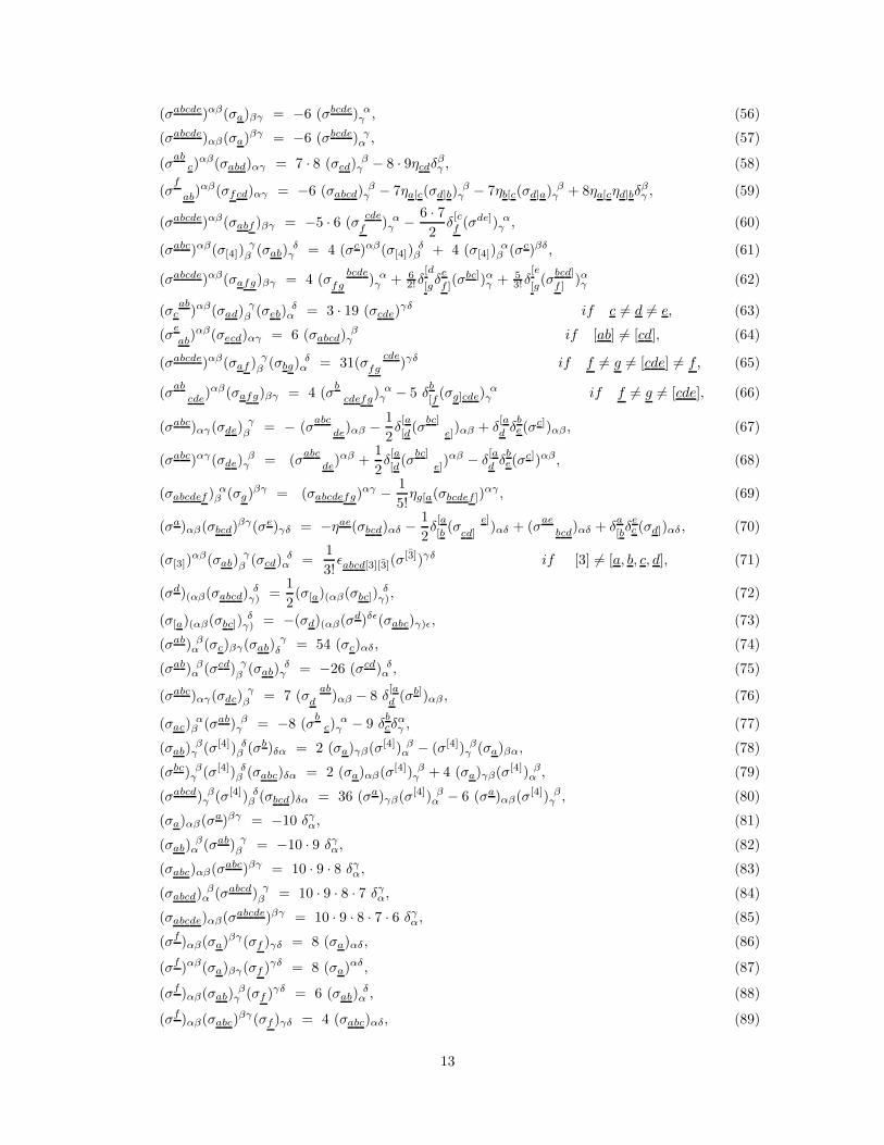
(σabcde)αβ(σa)βγ = −6 (σbcde) αγ , (56)

(σabcde)αβ(σa)βγ = −6 (σbcde) γα , (57)

(σab

c)αβ(σabd)αγ = 7 · 8 (σcd)

βγ − 8 · 9ηcdδ

βγ , (58)

(σf

ab)αβ(σfcd)αγ = −6 (σabcd)

βγ − 7ηa[c(σd]b)

βγ − 7ηb[c(σd]a) β

γ + 8ηa[cηd]bδβγ , (59)

(σabcde)αβ(σabf )βγ = −5 · 6 (σcde

f) αγ −

6 · 7

2δ[cf

(σde]) αγ , (60)

(σabc)αβ(σ[4])γ

β(σab)

δγ = 4 (σc)αβ(σ[4])

δβ + 4 (σ[4])

αβ (σc)βδ, (61)

(σabcde)αβ(σafg)βγ = 4 (σbcde

fg) αγ + 6

2!δ[d

[gδ

e

f ](σbc])α

γ + 53!δ

[e

[g(σ

bcd]

f ])αγ (62)

(σab

c )αβ(σad)γ

β(σeb)

δα = 3 · 19 (σcde)

γδ if c 6= d 6= e, (63)

(σe

ab)αβ(σecd)αγ = 6 (σabcd)

βγ if [ab] 6= [cd], (64)

(σabcde)αβ(σaf ) γ

β(σbg)

δα = 31(σ

cde

fg)γδ if f 6= g 6= [cde] 6= f, (65)

(σab

cde)αβ(σafg)βγ = 4 (σ

b

cdefg) αγ − 5 δ

b

[f(σg]cde)

αγ if f 6= g 6= [cde], (66)

(σabc)αγ(σde)γ

β= − (σ

abc

de)αβ −

1

2δ[a

[d(σ

bc]

e])αβ + δ

[a

dδ

be(σ

c])αβ , (67)

(σabc)αγ(σde)β

γ = (σabc

de)αβ +

1

2δ[a

[d(σ

bc]

e])αβ − δ

[a

dδ

be(σ

c])αβ , (68)

(σabcdef ) αβ (σg)βγ = (σabcdefg)

αγ −1

5!ηg[a(σbcdef])

αγ , (69)

(σa)αβ(σbcd)βγ(σe)γδ = −ηae(σbcd)αδ −

1

2δ[a

[b(σ

e]

cd])αδ + (σ

ae

bcd)αδ + δ

a

[bδ

ec(σd])αδ, (70)

(σ[3])αβ(σab)

γ

β(σcd)

δα =

1

3!ǫabcd[3] ¯[3](σ

¯[3])γδ if [3] 6= [a, b, c, d], (71)

(σd)(αβ(σabcd)δ

γ) =1

2(σ[a)(αβ(σbc])

δγ), (72)

(σ[a)(αβ(σbc])δ

γ) = −(σd)(αβ(σd)δǫ(σabc)γ)ǫ, (73)

(σab) βα (σc)βγ(σab)

γδ

= 54 (σc)αδ, (74)

(σab) βα (σcd) γ

β(σab)

δγ = −26 (σcd) δ

α , (75)

(σabc)αγ(σdc)γ

β= 7 (σ

ab

d)αβ − 8 δ

[a

d(σb])αβ , (76)

(σac)α

β (σab) βγ = −8 (σ

bc)

αγ − 9 δ

bcδ

αγ , (77)

(σab)β

γ (σ[4]) δβ (σb)δα = 2 (σa)γβ(σ[4]) β

α − (σ[4]) βγ (σa)βα, (78)

(σbc) βγ (σ[4]) δ

β (σabc)δα = 2 (σa)αβ(σ[4]) βγ + 4 (σa)γβ(σ[4]) β

α , (79)

(σabcd) βγ (σ[4]) δ

β (σbcd)δα = 36 (σa)γβ(σ[4]) βα − 6 (σa)αβ(σ[4]) β

γ , (80)

(σa)αβ(σa)βγ = −10 δγα, (81)

(σab)β

α (σab) γβ

= −10 · 9 δγα, (82)

(σabc)αβ(σabc)βγ = 10 · 9 · 8 δγα, (83)

(σabcd)β

α (σabcd) γβ

= 10 · 9 · 8 · 7 δγα, (84)

(σabcde)αβ(σabcde)βγ = 10 · 9 · 8 · 7 · 6 δγα, (85)

(σf )αβ(σa)βγ(σf )γδ = 8 (σa)αδ, (86)

(σf )αβ(σa)βγ(σf )γδ = 8 (σa)αδ, (87)

(σf )αβ(σab)β

γ (σf )γδ = 6 (σab)δ

α , (88)

(σf )αβ(σabc)βγ(σf )γδ = 4 (σabc)αδ, (89)

13

(σf )αβ(σabc)βγ(σf )γδ = 4 (σabc)αδ, (90)

(σf )αβ(σabcd)β

γ (σf )γδ = −2 (σabcd)δ

α , (91)

(σf )αβ(σ[5])βγ(σf )γδ = 0, (92)

(σf

1f2) β

α (σa)βγ(σf1f2

) γδ

= 54 (σa)αδ, (93)

(σf

1f2) β

α (σa)αγ(σf1f2

) δγ = 54 (σa)βδ, (94)

(σf

1f2) β

α (σab)α

γ (σf1f2

) γ

δ= −26 (σab)

β

δ, (95)

(σf

1f2) β

α (σabc)βγ(σf1f2

) γδ

= 6 (σabc)αδ, (96)

(σf

1f2) β

α (σabc)αγ(σf

1f2

) δγ = 6 (σabc)

βδ, (97)

(σf

1f2) β

α (σabcd)α

γ (σf1f2

) γδ

= 6 (σabcd)β

δ, (98)

(σf

1f2) β

α (σabcde)βγ(σf1f2

) γ

δ= −10 (σabcde)αδ, (99)

(σf

1f2) β

α (σabcde)αδ(σf

1f2

) γ

δ= −10 (σabcde)

βγ , (100)

(σf

1f2f3)αβ(σa)βγ(σf

1f2f3

)γδ = −8 · 36 (σa)αδ, (101)

(σf

1f2f3)αβ(σa)βγ(σf

1f2f3

)γδ = −8 · 36 (σa)αδ, (102)

(σf

1f2f3)αβ(σab)

βγ (σf

1f2f3

)γδ = −48 (σab)δ

α , (103)

(σf

1f2f3)αβ(σabc)

βγ(σf1f2f3

)γδ = 48 (σabc)αδ, (104)

(σf

1f2f3)αβ(σabc)βγ(σf

1f2f3

)γδ = 48 (σabc)αδ, (105)

(σf

1f2f3)αβ(σabcd)

βγ (σf

1f2f3

)γδ = −48 (σabcd)δ

α , (106)

(σf

1f2f3)αβ(σ[5])

βγ(σf1f2f3

)γδ = 0, (107)

(σf

1f2f3f4) β

α (σa)βγ(σf1f2f3f4

) γδ

= 24 · 42 (σa)αδ, (108)

(σf

1f2f3f4) β

α (σa)αγ(σf1f2f3f4

) γ

δ= 24 · 42 (σa)βδ, (109)

(σf

1f2f3f4) β

α (σab)α

γ (σf1f2f3f4

) γ

δ= −24 · 14 (σab)

β

δ, (110)

(σf

1f2f3f4) β

α (σabc)βγ(σf1f2f3f4

) γδ

= −24 · 14 (σabc)αδ, (111)

(σf

1f2f3f4) β

α (σabc)αγ(σf

1f2f3f4

) δγ = −24 · 14 (σabc)

βδ, (112)

(σf

1f2f3f4) β

α (σabcd)α

γ (σf1f2f3f4

) γδ

= 48 (σabcd)β

δ, (113)

(σf

1f2f3f4) β

α (σabcde)βγ(σf1f2f3f4

) γ

δ= 240 (σabcde)αδ, (114)

(σf

1f2f3f4) β

α (σabcde)αδ(σf

1f2f3f4

) γδ

= 240 (σabcde)βγ . (115)

IV. THE PROGRAM

(*BeginPackage[”SigmaVector‘”]*)

Print[”This is SigmaVector program. It reduces the product of sigma matrices.

Spinor indices of the chiral sigma matrices analyzed here are supressed.

Sigma matrices with spinor indices down are denoted by S, as well as those

matrices which have one spinor index down and other up. If both spinor indices

14

are up, the letter SB is used.

The program handles all contraction possibilities of spinor indices, except when

two sigma matrices, both with even number of vector indices are multiplied in such

a way that the lower index of the first sigma matrix is summed with the upper index

of the second matrix. In this case the order of sigma matrices should be reversed.

Here is an example:

(\sˆ{e, f}) {\a}ˆ{\b} ∗ (\s {a, b, c})ˆ{\a\g} ∗ (\s {e, f}) {\g}ˆ{\d}

should be represented in the symbolic form as:

ExpandAll[ExpandAll[S[e, f ] ∗ ∗SB[a, b, c]] ∗ ∗S[e, f ]//.Rule1],

where Rule1 is a rule which transforms sigma matrices with 6 or more vector indices

in appropriate sigma matrices with 4 or less vector indices and contracts corresponding

epsilon symbols.”]

(* These next rules assumed repeated indices for implied sum *)

SetAttributes[Id,Orderless]

Ten=10

SetAttributes[Eta,Orderless]

Eta/: Eta[a ,b ]ˆ2:= Ten (* 10 for our purposes *)

Eta/: Eta[a ,a ]:= Ten

Eta/: Eta[a , b ]*S[d ,a , c ] := S[d,b, c]

Eta/: S[d ,a , c ]*Eta[a , b ] := S[d,b, c]

Eta/: Eta[a , b ]*SB[d ,a , c ] := SB[d,b, c]

Eta/: SB[d ,a , c ]*Eta[a , b ] := SB[d,b, c]

Eta/: Eta[a , b ]*Epsilon[d ,a , c ] := Epsilon[d,b, c]

Eta/: Epsilon[d ,a , c ]*Eta[a , b ] := Epsilon[d,b, c]

Eta/: Eta[a , b ]*Eta[a , c ] := Eta[b, c]

Eta/: Eta[a , c ]*Eta[a , b ] := Eta[b, c]

Eta/: NumberQ[Eta[x ]] := True

(* These rules define Ten as the dimension so that its

dependence in the

calculations can be followed. *)

Unprotect[NumberQ]

NumberQ[Tenˆn Integer]:=True

NumberQ[Ten] :=True

15

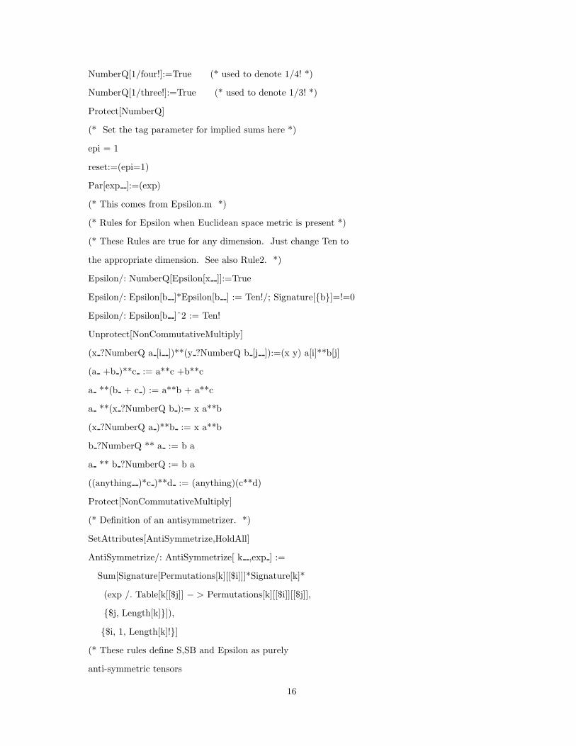
NumberQ[1/four!]:=True (* used to denote 1/4! *)

NumberQ[1/three!]:=True (* used to denote 1/3! *)

Protect[NumberQ]

(* Set the tag parameter for implied sums here *)

epi = 1

reset:=(epi=1)

Par[exp ]:=(exp)

(* This comes from Epsilon.m *)

(* Rules for Epsilon when Euclidean space metric is present *)

(* These Rules are true for any dimension. Just change Ten to

the appropriate dimension. See also Rule2. *)

Epsilon/: NumberQ[Epsilon[x ]]:=True

Epsilon/: Epsilon[b ]*Epsilon[b ] := Ten!/; Signature[{b}]=!=0

Epsilon/: Epsilon[b ]ˆ2 := Ten!

Unprotect[NonCommutativeMultiply]

(x ?NumberQ a [i ])**(y ?NumberQ b [j ]):=(x y) a[i]**b[j]

(a +b )**c := a**c +b**c

a **(b + c ) := a**b + a**c

a **(x ?NumberQ b ):= x a**b

(x ?NumberQ a )**b := x a**b

b ?NumberQ ** a := b a

a ** b ?NumberQ := b a

((anything )*c )**d := (anything)(c**d)

Protect[NonCommutativeMultiply]

(* Definition of an antisymmetrizer. *)

SetAttributes[AntiSymmetrize,HoldAll]

AntiSymmetrize/: AntiSymmetrize[ k ,exp ] :=

Sum[Signature[Permutations[k][[$i]]]*Signature[k]*

(exp /. Table[k[[$j]] − > Permutations[k][[$i]][[$j]],

{$j, Length[k]}]),

{$i, 1, Length[k]!}]

(* These rules define S,SB and Epsilon as purely

anti-symmetric tensors

16

for any rank. *)

S[x ] := Signature[{x}] S@@Sort[{x}] /; Not[OrderedQ[{x}]]

SB[x ] := Signature[{x}] SB@@Sort[{x}] /; Not[OrderedQ[{x}]]

Epsilon[x ] := Signature[{x}] Epsilon@@Sort[{x}] /;

Not[OrderedQ[{x}]]

S[x ]:=0 /; Signature[{x}]==0

SB[x ]:=0 /; Signature[{x}]==0

Epsilon[x ]:=0 /; Signature[{x}]==0

(* Epsilon[1,2,3,4,5,6,7,8,9,10] = 1 *)

(* This rule replaces 6,7,8,9, and 10 forms with their duals *)

Rule1 = {

S[a ,b ,c ,d ,e ,f ] :>

( Epsilon[a,b,c,d,e,f,$1[epi],$2[epi],$3[epi],$4[epi]]*

S[$1[epi],$2[epi],$3[epi],$4[epi++]])/24,

S[d[1],d[2],d[3],d[4],d[5],d[6]]:>

(Epsilon[d[1],d[2],d[3],d[4],d[5],d[6],$1[epi],$2[epi],$3[epi],$4[epi]]*

S[$1[epi],$2[epi],$3[epi],$4[epi++]])/24,

SB[a ,b ,c ,d ,e ,f ,g ] :>

(- Epsilon[a,b,c,d,e,f,g,$1[epi],$2[epi],$3[epi]]*

SB[$1[epi],$2[epi],$3[epi++]])/6,

SB[d[1],d[2],d[3],d[4],d[5],d[6],d[7]]:>

(-Epsilon[d[1],d[2],d[3],d[4],d[5],d[6],d[7],1[epi],$2[epi],$3[epi]]*

SB[$1[epi],$2[epi],$3[epi++]])/6,

S[a ,b ,c ,d ,e ,f ,g ] :>

(- Epsilon[a,b,c,d,e,f,g,$1[epi],$2[epi],$3[epi]]*

S[$1[epi],$2[epi],$3[epi++]])/6,

S[d[1],d[2],d[3],d[4],d[5],d[6],d[7]]:>

(-Epsilon[d[1],d[2],d[3],d[4],d[5],d[6],d[7],$1[epi],$2[epi],$3[epi]]*

S[$1[epi],$2[epi],$3[epi++]])/6,

S[a ,b ,c ,d ,e ,f ,g ,h ] :>

(-Epsilon[a,b,c,d,e,f,g,h,$1[epi],$2[epi]]*

S[$1[epi],$2[epi++]])/2,

17

S[d[1],d[2],d[3],d[4],d[5],d[6],d[7],d[8]] :>

(-Epsilon[d[1],d[2],d[3],d[4],d[5],d[6],d[7],d[8],$1[epi],$2[epi]]*

S[$1[epi],$2[epi++]])/2,

SB[a ,b ,c ,d ,e ,f ,g ,h ,i ] :>

(Epsilon[a,b,c,d,e,f,g,h,i,$1[epi]]*

SB[$1[epi++]]),

SB[d[1],d[2],d[3],d[4],d[5],d[6],d[7],d[8],d[9]] :>

(Epsilon[d[1],d[2],d[3],d[4],d[5],d[6],d[7],d[8],d[9],$1[epi]]*

SB[$1[epi++]]),

S[a ,b ,c ,d ,e ,f ,g ,h ,i ] :>

(Epsilon[a,b,c,d,e,f,g,h,i,$1[epi]]*

S[$1[epi++]])

}

(* This rule pulls out the coefficients of chiral matrices. *)

SetAttributes[Eta2,Orderless]

Eta2/: NumberQ[Eta2[x ]] := True

Rule2 = {

S[a ] :> S[d[1]] * Eta2[d[1],a],

S[a ,b ] :> S[d[1],d[2]] * Eta2[d[1],a] Eta2[d[2],b],

S[a ,b ,c ] :> S[d[1],d[2],d[3]]*Eta2[d[1],a]* Eta2[d[2],b] Eta2[d[3],c],

S[a ,b ,c ,d1 ] :> S[d[1],d[2],d[3],d[4]] *

Eta2[d[1],a]* Eta2[d[2],b] Eta2[d[3],c] Eta2[d[4],d1],

S[a ,b ,c ,d1 ,e ] :>S[d[1],d[2],d[3],d[4],d[5]] *

Eta2[d[1],a]* Eta2[d[2],b] Eta2[d[3],c] Eta2[d[4],d1] Eta2[d[5],e],

S[a ,b ,c ,d1 ,e ,f ] :>S[d[1],d[2],d[3],d[4],d[5],d[6]] *

Eta2[d[1],a]* Eta2[d[2],b] Eta2[d[3],c] Eta2[d[4],d1] Eta2[d[5],e] *

Eta2[f,d[6]],

S[a ,b ,c ,d1 ,e ,f ,g ] :>S[d[1],d[2],d[3],d[4],d[5],d[6],d[7]] *


Eta2[f,d[6]] Eta2[g,d[7]],

S[a ,b ,c ,d1 ,e ,f ,g ,h ] :>S[d[1],d[2],d[3],d[4],d[5],d[6],d[7],d[8]] *


Eta2[f,d[6]] Eta2[g,d[7]] Eta2[h,d[8]],

18

S[a ,b ,c ,d1 ,e ,f ,g ,h ,i ] :>S[d[1],d[2],d[3],d[4],d[5],d[6],d[7],d[8],d[9]] *


Eta2[f,d[6]] Eta2[g,d[7]] Eta2[h,d[8]] Eta2[i,d[9]],

S[a ,b ,c ,d1 ,e ,f ,g ,h ,i ,j ] :>S[d[1],d[2],d[3],d[4],d[5],d[6],d[7],d[8],d[9],d[10]] *


Eta2[f,d[6]] Eta2[g,d[7]] Eta2[h,d[8]] Eta2[i,d[9]] Eta2[j,d[10]],

SB[a ] :> SB[d[1]] * Eta2[d[1],a],

SB[a ,b ,c ] :> SB[d[1],d[2],d[3]]*Eta2[d[1],a]* Eta2[d[2],b] Eta2[d[3],c],

SB[a ,b ,c ,d1 ,e ] :>SB[d[1],d[2],d[3],d[4],d[5]] *

Eta2[d[1],a]* Eta2[d[2],b] Eta2[d[3],c] Eta2[d[4],d1] Eta2[d[5],e],

SB[a ,b ,c ,d1 ,e ,f ,g ] :>SB[d[1],d[2],d[3],d[4],d[5],d[6],d[7]] *


Eta2[f,d[6]] Eta2[g,d[7]],

SB[a ,b ,c ,d1 ,e ,f ,g ,h ,i ] :>SB[d[1],d[2],d[3],d[4],d[5],d[6],d[7],d[8],d[9]] *


Eta2[f,d[6]] Eta2[g,d[7]] Eta2[h,d[8]] Eta2[i,d[9]]

}

(* Use Recover to factor out the S’s and SB’s *)

Recover[exp ] := Collect[exp/.Rule2,{ S[d[1]], S[d[1],d[2]],S[d[1],d[2],d[3]],

S[d[1],d[2],d[3],d[4]], S[d[1],d[2],d[3],d[4],d[5]],

S[d[1],d[2],d[3],d[4],d[5],d[6]],

S[d[1],d[2],d[3],d[4],d[5],d[6],d[7]],

S[d[1],d[2],d[3],d[4],d[5],d[6],d[7],d[8]],

S[d[1],d[2],d[3],d[4],d[5],d[6],d[7],d[8],d[9]],

S[d[1],d[2],d[3],d[4],d[5],d[6],d[7],d[8],d[9],d[10]],

SB[d[1]], SB[d[1],d[2],d[3]], SB[d[1],d[2],d[3],d[4],d[5]],

SB[d[1],d[2],d[3],d[4],d[5],d[6],d[7]],

SB[d[1],d[2],d[3],d[4],d[5],d[6],d[7],d[8],d[9]]} ]/.Rule3

Rule3={Eta2[f ]:> Eta[f]}

(* This rule is time consuming. *)

Epsilon/: Epsilon[b ]*Epsilon[c ] :=

-Par[ Signature[ Join[Complement[{b},

19

Intersection[{b},{c}]],

Intersection[{b},{c}]]]*

Signature[ Join[Complement[{c},Intersection[{b},{c}]],

Intersection[{b},{c}]]]*ReleaseHold[ (

AntiSymmetrize[Complement[{c}, Intersection[{b}, {c}]],

Product[Eta[Complement[{b}, Intersection[{b}, {c}]][[$i]],

Complement[{c}, Intersection[{b}, {c}]][[$i]]],

{$i, Length[Complement[{c}, Intersection[{b},

{c}]]]}]])]*(Length[

Intersection[{b}, {c}]]!)] /; {b}=!={c} && Length[{b}]==Length[{c}]

S/: S[i ]**SB[j ] := - Eta[i, j] - S[i, j]

S/: S[i ]**S[j ,k ] := -S[k] Eta[i, j] + S[j] Eta[i, k] -

S[i, j, k]

S/: S[j ,k ]**S[i ] := -S[k] Eta[i, j] + S[j] Eta[i, k] +

S[i, j, k]

S/: S[j ,k ]**SB[i ] := Eta[i,j] SB[k] - Eta[i,k] SB[j] -

SB[i,j,k]

S/: S[i ] ** SB[j , k , l ] :=

-S[k, l] Eta[i, j] - S[l,j] Eta[i, k] - S[j, k] Eta[i, l] -

S[i, j, k, l]

S/: S[j ,k ,l ]**SB[i ] := -Eta[i,j] S[k,l] - Eta[i,k] S[l,j] -

Eta[i,l] S[j,k] + S[i,j,k,l]

S/: S[i ]**S[j ,k ,l ,m ] := Eta[i,j] S[k,l,m] -

Eta[i,k] S[l,m,j] + Eta[i,l] S[j,k,m] -

Eta[i,m] S[j,k,l] + S[i,j,k,l,m]

S/: S[j ,k ,l ,m ]**S[i ] := -Eta[i,j] S[k,l,m] +

Eta[i,k] S[l,m,j] - Eta[i,l] S[j,k,m] +

Eta[i,m] S[j,k,l] + S[i,j,k,l,m]

S/: S[j ,k ,l ,m ]**SB[i ] := -Eta[i,j] SB[k,l,m] +

Eta[i,k] SB[l,m,j] - Eta[i,l] SB[j,k,m] +

Eta[i,m] SB[j,k,l] + SB[i,j,k,l,m]

S/: S[i ]**SB[j ,k ,l ,m ,n ] := -Eta[i,j] S[k,l,m,n] -

Eta[i,k] S[l,m,n,j] - Eta[i,l] S[m,n,j,k] -

20

Eta[i,m] S[n,j,k,l] - Eta[i,n] S[j,k,l,m] - S[i,j,k,l,m,n]

S/: S[j ,k ,l ,m ,n ]**SB[i ] := -Eta[i,j] S[k,l,m,n] -


Eta[i,m] S[n,j,k,l] - Eta[i,n] S[j,k,l,m] + S[i,j,k,l,m,n]

S/: S[i ]**S[j ,k ,l ,m ,n ,p ] := - S[i,j,k,l,m,n,p] +

(Epsilon[j,k,l,m,n,p,$1[epi], $2[epi], $3[epi], $4[epi]]*

S[i,$1[epi], $2[epi], $3[epi], $4[epi++]])/24

S/: S[j ,k ,l ,m ,n ,p ]**SB[i ] := SB[i,j,k,l,m,n,p] +


SB[i,$1[epi], $2[epi], $3[epi], $4[epi++]])/24

S/: S[j ,k ,l ,m ,n ,p ]**S[i ] := S[i,j,k,l,m,n,p] +


S[i,$1[epi], $2[epi], $3[epi], $4[epi++]])/24

S/: S[i ]**SB[j ,k ,l ,m ,n ,p ,q ] := S[i,j,k,l,m,n,p,q] +

(Epsilon[j,k,l,m,n,p,q,$1[epi], $2[epi], $3[epi]]*

S[i,$1[epi], $2[epi], $3[epi++]])/6

S/: S[j ,k ,l ,m ,n ,p ,q ]**SB[i ] := S[i,j,k,l,m,n,p,q] -


S[i,$1[epi], $2[epi], $3[epi++]])/6

S/: S[i ]**S[j ,k ,l ,m ,n ,o ,p ,q ] :=

S[i,j,k,l,m,n,o,p,q]+

(Epsilon[j,k,l,m,n,o,p,q,$1[epi], $2[epi]]*

S[i,$1[epi], $2[epi++]])/2

S/: S[j ,k ,l ,m ,n ,o ,p ,q ]**S[i ] :=

S[i,j,k,l,m,n,o,p,q]-


S[i,$1[epi], $2[epi++]])/2

S/: S[j ,k ,l ,m ,n ,o ,p ,q ]**SB[i ] :=

- SB[i,j,k,l,m,n,o,p,q]+


SB[i,$1[epi], $2[epi++]])/2

S/: S[i ]**SB[j ,k ,l ,m ,n ,o ,p ,q ,r ] :=

Epsilon[i,j,k,l,m,n,o,p,q,r] -

21

Epsilon[j,k,l,m,n,o,p,q,r,$1[epi]]*S[i,$1[epi++]]

S/: S[j ,k ,l ,m ,n ,o ,p ,q ,r ]**SB[i ] :=

Epsilon[i,j,k,l,m,n,o,p,q,r] +


SB/: SB[i ] ** S[j ] := -Eta[i, j] + S[i, j]

SB/: SB[i ]**S[j ,k ] := Eta[i,j] SB[k] - Eta[i,k] SB[j] +

SB[i,j,k]

SB/: SB[i ]**S[j ,k ,l ] := Eta[i,j] S[k,l] +

Eta[i,k] S[l,j] + Eta[i,l] S[j,k] - S[i,j,k,l]

SB/: SB[j , k , l ] ** S[i ] :=

S[k, l] Eta[i, j] + S[l,j] Eta[i, k] + S[j, k] Eta[i, l] +

S[i, j, k, l]

SB/: SB[i ]**S[j ,k ,l ,m ] := Eta[i,j] SB[k,l,m] -

Eta[i,k] SB[l,m,j] + Eta[i,l] SB[j,k,m] -

Eta[i,m] SB[j,k,l] + SB[i,j,k,l,m]

SB/: SB[i ]**S[j ,k ,l ,m ,n ] := -Eta[i,j] S[k,l,m,n] -


Eta[i,m] S[n,j,k,l] - Eta[i,n] S[j,k,l,m] + S[i,j,k,l,m,n]

SB/: SB[j ,k ,l ,m ,n ]**S[i ] := -Eta[i,j] S[k,l,m,n] -


Eta[i,m] S[n,j,k,l] - Eta[i,n] S[j,k,l,m] - S[i,j,k,l,m,n]

SB/: SB[i ]**S[j ,k ,l ,m ,n ,p ] := - SB[i,j,k,l,m,n,p] +


SB[i,$1[epi], $2[epi], $3[epi], $4[epi++]])/24

SB/: SB[j ,k ,l ,m ,n ,p ,q ]**S[i ] := -S[i,j,k,l,m,n,p,q]-


S[i,$1[epi], $2[epi], $3[epi++]])/6

SB/: SB[i ]**S[j ,k ,l ,m ,n ,p ,q ] := -S[i,j,k,l,m,n,p,q]+


S[i,$1[epi], $2[epi], $3[epi++]])/6

SB/: SB[i ]**S[j ,k ,l ,m ,n ,o ,p ,q ] :=

- SB[i,j,k,l,m,n,o,p,q]-


22

SB[i,$1[epi], $2[epi++]])/2

SB/: SB[j ,k ,l ,m ,n ,o ,p ,q ,r ]**S[i ] :=

Epsilon[i,j,k,l,m,n,o,p,q,r] -


SB/: SB[i ]**S[j ,k ,l ,m ,n ,o ,p ,q ,r ] :=

Epsilon[i,j,k,l,m,n,o,p,q,r] +


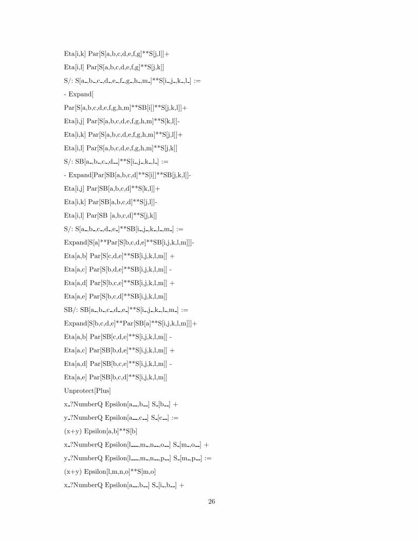
S/: S[i ,j ]**S[k ,l ] := -Eta[k,l] S[i,j] -

Expand[ Par[S[i,j]**S[k]]**SB[l]]

S/: S[a ,b ,c ,d ]**S[k ,l ] :=

-Eta[k,l] S[a,b,c,d] -

Expand[ Par[S[a,b,c,d]**S[k]]**SB[l]]

S/: S[a ,b ,c ,d ,e ,f ]**S[k ,l ] :=

-Eta[k,l] S[a,b,c,d,e,f] -

Expand[ Par[S[a,b,c,d,e,f]**S[k]]**SB[l]]

S/: S[a ,b ,c ,d ,e ,f ,g ,h ]**S[k ,l ] :=

-Eta[k,l] S[a,b,c,d,e,f,g,h] -

Expand[ Par[S[a,b,c,d,e,f,g,h]**S[k]]**SB[l]]

S/: S[a ,b ,c ]**S[k ,l ] :=

Eta[k,l] S[a,b,c] +

Expand[ Par[S[a,b,c]**SB[k]]**S[l]]

S/: S[a ,b ,c ,d ,e ]**S[k ,l ] :=

Eta[k,l] S[a,b,c,d,e] +

Expand[ Par[S[a,b,c,d,e]**SB[k]]**S[l]]

S/: S[a ,b ,c ,d ,e ,f ,g ]**S[k ,l ] :=

Eta[k,l] S[a,b,c,d,e,f,g] +

Expand[ Par[S[a,b,c,d,e,f,g]**SB[k]]**S[l]]

S/: S[a ,b ,c ,d ,e ,f ,g ,h ,m ]**S[k ,l ] :=

Eta[k,l] S[a,b,c,d,e,f,g,h,m] +

Expand[ Par[S[a,b,c,d,e,f,g,h,m]**SB[k]]**S[l]]

S/: S[i ,j ]**S[k ,l ] := -Eta[i,j] S[k,l] -

Expand[ S[i]**Par[SB[j]**S[k,l]]]

S/: S[i ,j ]**SB[k ,l ] := Eta[i,j] SB[k,l] +

23

Expand[ SB[i]**Par[S[j]**SB[k,l]]]

SB/: SB[i ,j ]**S[k ,l ] := - Eta[k,l] SB[i,j] -

Expand[Par[SB[i,j]**S[k]]**SB[l]]

S/: S[i ,j ,k ]**S[l ,m ,n ] :=

- Expand[S[i]**Par[SB[j]**Par[S[k]**S[l,m,n]]]] -

Eta[i,j] S[k]**S[l,m,n] + Eta[i,k] S[j]**S[l,m,n]-

Eta[j,k] S[i]**S[l,m,n]

S/: S[i ,j ,k ]**SB[l ,m ,n ] :=

- Expand[S[i]**Par[SB[j]**

Par[S[k]**SB[l,m,n]]]] -

Eta[i,j] S[k]**SB[l,m,n] + Eta[i,k] S[j]**SB[l,m,n] -

Eta[j,k] S[i]**SB[l,m,n]

S/: S[i ,j ,k ]**S[l ,m ,n ] :=

- Expand[Par[Par[S[i,j,k]**S[l]]**SB[m]]**

S[n]] -

Eta[l,m] S[i,j,k]**S[n] + Eta[l,n] S[i,j,k]**S[m] -

Eta[m,n] S[i,j,k]**S[l]

S/: S[a ,b ,c ]**SB[i ,j ,k ] :=

- Expand[Par[Par[S[a,b,c]**SB[j]]**S[k]]**

SB[i]] -

Eta[j,k] S[a,b,c]**SB[i] + Eta[i,j] S[a,b,c]**SB[k] -

Eta[i,k] S[a,b,c]**SB[j]

S/: SB[a ,b ,c ]**S[i ,j ,k ] :=

- Expand[Par[Par[SB[a,b,c]**S[i]]**SB[j]]**S[k]] -

Eta[j,k] SB[a,b,c]**S[i] - Eta[i,j] SB[a,b,c]**S[k] +

Eta[i,k] SB[a,b,c]**S[j]

SB/: SB[i ,j ,k ]**S[l ,m ,n ] :=

- Expand[SB[j]**Par[S[k]**

Par[SB[i]**S[l,m,n]]]] +

Eta[i,j] SB[k]**S[l,m,n] - Eta[i,k] SB[j]**S[l,m,n] -

Eta[j,k] SB[i]**S[l,m,n]

S/: S[a ,b ,c ,d ]**S[i ,j ,k ,l ] :=

Expand[S[b,c,d]**Par[SB[a]**S[i,j,k,l]]]+

24

Eta[a,b] Par[S[c,d]**S[i,j,k,l]]-

Eta[a,c] Par[S[b,d]**S[i,j,k,l]]+

Eta[a,d] Par[S[b,c]**S[i,j,k,l]]

S/: S[a ,b ,c ,d ]**SB[i ,j ,k ,l ] :=

- Expand[SB[a]**Par[S[b,c,d]**SB[i,j,k,l]]]+

Eta[a,b] Par[S[c,d]**SB[i,j,k,l]]-

Eta[a,c] Par[S[b,d]**SB[i,j,k,l]]+

Eta[a,d] Par[S[b,c]**SB[i,j,k,l]]

S/: S[a ,b ,c ,d ]**S[i ,j ,k ,l ] :=

- Expand[Par[S[a,b,c,d]**S[i]]**SB[j,k,l]]-

Eta[i,j] Par[S[a,b,c,d]**S[k,l]]+

Eta[i,k] Par[S[a,b,c,d]**S[j,l]]-

Eta[i,l] Par[S[a,b,c,d]**S[j,k]]

S/: S[a ,b ,c ,d ,e ,f ]**S[i ,j ,k ,l ] :=

- Expand[Par[S[a,b,c,d,e,f]**S[i]]**SB[j,k,l]]-

Eta[i,j] Par[S[a,b,c,d,e,f]**S[k,l]]+

Eta[i,k] Par[S[a,b,c,d,e,f]**S[j,l]]-

Eta[i,l] Par[S[a,b,c,d,e,f]**S[j,k]]

S/: S[a ,b ,c ,d ,e ,f ,g ,h ]**S[i ,j ,k ,l ] :=

- Expand[Par[S[a,b,c,d,e,f,g,h]**S[i]]**SB[j,k,l]]-

Eta[i,j] Par[S[a,b,c,d,e,f,g,h]**S[k,l]]+

Eta[i,k] Par[S[a,b,c,d,e,f,g,h]**S[j,l]]-

Eta[i,l] Par[S[a,b,c,d,e,f,g,h]**S[j,k]]

S/: S[a ,b ,c ,d ,e ]**S[i ,j ,k ,l ] :=

- Expand[

Par[S[a,b,c,d,e]**SB[i]]**S[j,k,l]]+

Eta[i,j] Par[S[a,b,c,d,e]**S[k,l]]-

Eta[i,k] Par[S[a,b,c,d,e]**S[j,l]]+

Eta[i,l] Par[S[a,b,c,d,e]**S[j,k]]

S/: S[a ,b ,c ,d ,e ,f ,g ]**S[i ,j ,k ,l ] :=

- Expand[

Par[S[a,b,c,d,e,f,g]**SB[i]]**S[j,k,l]]+

Eta[i,j] Par[S[a,b,c,d,e,f,g]**S[k,l]]-

25

Eta[i,k] Par[S[a,b,c,d,e,f,g]**S[j,l]]+

Eta[i,l] Par[S[a,b,c,d,e,f,g]**S[j,k]]

S/: S[a ,b ,c ,d ,e ,f ,g ,h ,m ]**S[i ,j ,k ,l ] :=

- Expand[

Par[S[a,b,c,d,e,f,g,h,m]**SB[i]]**S[j,k,l]]+

Eta[i,j] Par[S[a,b,c,d,e,f,g,h,m]**S[k,l]]-

Eta[i,k] Par[S[a,b,c,d,e,f,g,h,m]**S[j,l]]+

Eta[i,l] Par[S[a,b,c,d,e,f,g,h,m]**S[j,k]]

S/: SB[a ,b ,c ,d ]**S[i ,j ,k ,l ] :=

- Expand[Par[SB[a,b,c,d]**S[i]]**SB[j,k,l]]-

Eta[i,j] Par[SB[a,b,c,d]**S[k,l]]+

Eta[i,k] Par[SB[a,b,c,d]**S[j,l]]-

Eta[i,l] Par[SB [a,b,c,d]**S[j,k]]

S/: S[a ,b ,c ,d ,e ]**SB[i ,j ,k ,l ,m ] :=

Expand[S[a]**Par[S[b,c,d,e]**SB[i,j,k,l,m]]]-

Eta[a,b] Par[S[c,d,e]**SB[i,j,k,l,m]] +

Eta[a,c] Par[S[b,d,e]**SB[i,j,k,l,m]] -

Eta[a,d] Par[S[b,c,e]**SB[i,j,k,l,m]] +

Eta[a,e] Par[S[b,c,d]**SB[i,j,k,l,m]]

SB/: SB[a ,b ,c ,d ,e ]**S[i ,j ,k ,l ,m ] :=

Expand[S[b,c,d,e]**Par[SB[a]**S[i,j,k,l,m]]]+

Eta[a,b] Par[SB[c,d,e]**S[i,j,k,l,m]] -

Eta[a,c] Par[SB[b,d,e]**S[i,j,k,l,m]] +

Eta[a,d] Par[SB[b,c,e]**S[i,j,k,l,m]] -

Eta[a,e] Par[SB[b,c,d]**S[i,j,k,l,m]]

Unprotect[Plus]

x ?NumberQ Epsilon[a ,b ] S [b ] +

y ?NumberQ Epsilon[a ,c ] S [c ] :=

(x+y) Epsilon[a,b]**S[b]

x ?NumberQ Epsilon[l ,m ,n ,o ] S [m ,o ] +

y ?NumberQ Epsilon[l ,m ,n ,p ] S [m ,p ] :=

(x+y) Epsilon[l,m,n,o]**S[m,o]

x ?NumberQ Epsilon[a ,b ] S [i ,b ] +

26

y ?NumberQ Epsilon[a ,c ] S [i ,c ] :=

(x+y) Epsilon[a,b] S[i,b]

x ?NumberQ Epsilon[l ,m ,n ,o ] S [j ,m ,o ] +

y ?NumberQ Epsilon[l ,m ,n ,p ] S [j ,m ,p ] :=

(x+y) Epsilon[l,m,n,o] S[j,m,o]

x ?NumberQ Epsilon[l ,m ,n ,o ] S [m ,j ,o ] +

y ?NumberQ Epsilon[l ,m ,n ,p ] S [m ,j ,p ] :=

(x+y) Epsilon[l,m,n,o] S[m,j,o]

Protect[Plus]

(* EndPackage[] *)

ACKNOWLEDGEMENTS

The authors thanks Eric Sachs, John Veson, and Rachel Williams for their efforts in the University

of Iowa’s Summer Science Training Program.

REFERENCES

[1] S.J. Gates and Nishino, Phys. Lett. 178 (1986) 46,52

[2] Nilsson, Nucl. Phys.B 188 (1981) 176

[3] M. Henneaux amd Mezincescu, Phys. Lett.B 152 (1985) 340

[4] Atick, Dhar, and Ratra, Phys. Rev. Lett. 33 (1986) 2824

[5] S.J. Gates and V.G.J.Rodgers, Phys. Lett.B357, 552 (1995), Phys.Lett.B405, 71 (1997)

[6] B. Radak, Ph.D. Thesis, “Type-II Superstrings in Curved 10-D Spacetime - Dynamics of Their Massless

Fields and Covariant Quantization,” Department of Physics, University of Maryand (1992)

27



Irreducible decomposition of products of 10D chiral sigma matrices

Documents

Transcript of Irreducible decomposition of products of 10D chiral sigma matrices