A&A 610, A4 (2018)DOI: 10.1051/0004-6361/201731619c© ESO 2018

Astronomy&Astrophysics

IRC +10 216 in 3D: morphology of a TP-AGB star envelope?

M. Guélin1, 2, N. A. Patel3, M. Bremer1, J. Cernicharo4, A. Castro-Carrizo1, J. Pety1, J. P. Fonfría4, M. Agúndez4,M. Santander-García4, G. Quintana-Lacaci4, L. Velilla Prieto4, R. Blundell3, and P. Thaddeus3

1 Institut de Radioastronomie Millimétrique, 300 rue de la Piscine, 38406 Saint Martin d’Hères, Francee-mail: guelin@iram.fr

2 LERMA, Observatoire de Paris, PSL Research University, CNRS, UMR 8112, 75014 Paris, France3 Center for Astrophysics, 60 Garden street, Cambridge, MA, USA4 ICMM, CSIC, Group of Molecular Astrophysics, C/ Sor Juana Inés de la Cruz 3, Cantoblanco, 28049 Madrid, Spain

Received 21 July 2017 / Accepted 10 September 2017

ABSTRACT

During their late pulsating phase, AGB stars expel most of their mass in the form of massive dusty envelopes, an event that largelycontrols the composition of interstellar matter. The envelopes, however, are distant and opaque to visible and NIR radiation: theirstructure remains poorly known and the mass-loss process poorly understood. Millimeter-wave interferometry, which combines theadvantages of longer wavelength, high angular resolution and very high spectral resolution is the optimal investigative tool for thispurpose. Mm waves pass through dust with almost no attenuation. Their spectrum is rich in molecular lines and hosts the fundamentallines of the ubiquitous CO molecule, allowing a tomographic reconstruction of the envelope structure. The circumstellar envelopeIRC +10 216 and its central star, the C-rich TP-AGB star closest to the Sun, are the best objects for such an investigation. Two yearsago, we reported the first detailed study of the CO(2–1) line emission in that envelope, made with the IRAM 30-m telescope. Itrevealed a series of dense gas shells, expanding at a uniform radial velocity. The limited resolution of the telescope (HPBW 11′′) didnot allow us to resolve the shell structure. We now report much higher angular resolution observations of CO(2–1), CO(1–0), CN(2–1)and C4H(24–23) made with the SMA, PdB and ALMA interferometers (with synthesized half-power beamwidths of 3′′, 1′′ and 0.3′′,respectively). Although the envelope appears much more intricate at high resolution than with an 11′′ beam, its prevailing structureremains a pattern of thin, nearly concentric shells. The average separation between the brightest CO shells is 16′′ in the outer envelope,where it appears remarkably constant. Closer to the star (<40′′), the shell pattern is denser and less regular, showing intermediary arcs.Outside the small (r < 0.3′′) dust formation zone, the gas appears to expand radially at a constant velocity, 14.5 km s−1, with smallturbulent motions. Based on that property, we have reconstructed the 3D structure of the outer envelope and have derived the gastemperature and density radial profiles in the inner (r < 25′′) envelope. The shell-intershell density contrast is found to be typically 3.The over-dense shells have spherical or slightly oblate shapes and typically extend over a few steradians, implying isotropic mass loss.The regular spacing of shells in the outer envelope supports the model of a binary star system with a period of 700 yr and a near face-on elliptical orbit. The companion fly-by triggers enhanced episodes of mass loss near periastron. The densification of the shell patternobserved in the central part of the envelope suggests a more complex scenario for the last few thousand years.

Key words. ISM: molecules – stars: AGB and post-AGB – astrochemistry – circumstellar matter – stars: individual: IRC +10 216 –stars: mass-loss

1. Introduction

Three-quarters of the matter returned to the interstellar medium(ISM) comes from AGB stars in their late thermally pulsat-ing (TP) phase. The mass loss rate may then reach 10−5 to10−4 M� yr−1 and the stars become enshrouded by a thick, dusty? This work was based on observations carried out with the

IRAM, SMA and ALMA telescopes. IRAM is supported byINSU/CNRS (France), MPG (Germany) and IGN (Spain). The Sub-millimeter Array is a joint project between the Smithsonian As-trophysical Observatory (USA) and the Academia Sinica Insti-tute of Astronomy and Astrophysics (Taiwan) and is funded bythe Smithsonian Institution and the Academia Sinica. This papermakes use of the ALMA data: ADS/JAO.ALMA#2013.1.01215.S &ADS/JAO.ALMA#2013.1.00432.S. ALMA is a partnership of ESO(representing its member states), NSF (USA) and NINS (Japan), to-gether with NRC (Canada), NSC and ASIAA (Taiwan) and KASI (Re-public of Korea), in cooperation with the Republic of Chile. The JointALMA Observatory is operated by ESO, AUI/NRAO and NAOJ.

envelope opaque to visible and near IR radiation. Given that theTP phase is short-lived, the closest AGB-TP stars are fairly dis-tant. High visual opacity and distance conspire to make the massloss mechanism and the envelope structure poorly understood,despite their importance for galactic evolution.

The advent of powerful millimeter/sub-mm interferometersthat combine longer wavelengths with high angular and spectralresolution provides a unique opportunity to investigate these ob-jects. Mm/sub-mm waves freely traverse the thickest dust layers,and the mm spectrum, rich in molecular lines, yields detailedinformation on the gas physical conditions, its chemical con-tent and, mostly, on the velocity field. The latter often reducesto uniform radial expansion, allowing the 3-dimensional enve-lope structure to be recovered. We present in this paper the firsthigh resolution study of the entire IRC +10 216 envelope, thearchetype of TP-AGB star envelopes, carried out in the J = 2–1line of CO, the best single tracer of the molecular gas in this typeof object (Ramstedt et al. 2008).

Article published by EDP Sciences A4, page 1 of 20

A&A 610, A4 (2018)

The envelope IRC +10 2161 (CW Leonis), which sur-rounds the closest C-rich TP-AGB star to the Sun (hereafterdenoted CW Leo?), is of particular interest. Located at a dis-tance of ∼130 pc (Menten et al. 2012), it appears on opticalimages as a dark spherical cloud that extends over several ar-cmin. Some 80 molecular species, half of all known interstellarmolecules, have been detected in this envelope through thou-sands of millimeter-wave lines (Cernicharo et al. 2000). Re-markably, all line profiles but those arising from the tiny dust-acceleration region have the same width in the direction of thestar: 29 km s−1. Since the molecular lines arise at different dis-tances from the central star – e.g. SiO and SiS are restricted tothe central region, whereas the CO is distributed over the wholeenvelope – the constant line width implies a steady expansion ve-locity along the line of sight, 14.5 km s−1, and a small turbulentvelocity. The systemic velocity of the envelope is –26.5 km s−1

relative to the local standard of rest (LSR).IRC +10 216 has been the object of numerous studies in

so far as dust and molecular content are concerned. Of par-ticular relevance to this work are a) the CFHT, Hubble andVLT V-light images of the scattered IS light (Mauron & Huggins2000, 2006; Leão et al. 2006), which revealed the presence ofa ringed dust structure (Fig. 13); b) the detection of UV emis-sion from a termination shock (or astrosphere) that marks theimpact of the outflowing gas on the surrounding ISM at 15′('2 pc) NE of CW Leo? (Sahai & Chronopoulos 2010); andc) the FIR emission map made with the PACS instrument onHerschel (Decin et al. 2011). The 100 µm map, like the visiblelight images, shows a succession of rings that mark the rims ofdense spherical shells. Finally; d) interferometric images of themm line emission of a score of reactive molecules, such as CN,CCH and HC5N, show that these species are mostly confined in-side a thin spherical shell of radius 15′′ whose center, curiously,is offset by 2′′ from CW Leo? (Guélin et al. 1993a).

We have previously reported a detailed study of IRC+10 216 made in the 12CO(2–1) and 12CO(1–0) lines (hereafterdenoted CO(2–1) and CO(1–0)) and in the 13CO(1–0) line withthe IRAM 30-m telescope (Cernicharo et al. 2015). The CO(2–1) line emission was mapped throughout the entire envelope ata resolution of 11′′ (HPBW) and the line was continuously de-tected up to the photodissociation radius rphot ' 180′′, insidewhich CO efficiently self-shields from interstellar UV radiation.The CO envelope fits well inside the large bow-shock traced bythe UV emission, which suggests it expands freely inside thecavity cleared up by the shock (both the 12CO and the 13CO lineprofiles have the canonical full width of 29 km s−1). It consistsof a bright central peak, a broad, slowly decreasing pedestal and,superimposed on the pedestal, a series of over-dense gas shells.

The limited angular resolution of the 30-m telescope did notallow us to resolve the shell structure. So, we turned to the SMA,PdB and ALMA interferometers for much higher resolution ob-servations. The envelope was fully mapped in CO(2–1) with theSMA at 3′′ resolution, and partly with PdBI at 1′′ resolution. Thecentral 1-arcmin region was mapped in the CO(1–0), 13CO(1–0), CN(2–1) and C4H(24–23) lines with the ALMA 12-m anten-nas and, for the short spacings, with the IRAM 30 m-diametersingle-dish (SD) telescope. In Sect. 2, we describe the observa-tions and data reduction procedures, and in Sects. 3 and 4 de-rive the envelope morphology, velocity field and gas physical

1 Designation from the two-micron sky survey (Neugebauer &Leighton 1969), composed of the survey declination strip and a serialnumber. The name IRC +10 216, was condensed into IRC +10216 byBecklin et al. (1969).

Fig. 1. Main beam-averaged 12CO(2–1) line brightness temperatureobserved in IRC +10 216 with the IRAM 30-m telescope (HPBW11′′) at the star velocity (V∗ = −26.5 km s−1, ∆v = 2 km s−1; seeCernicharo et al. (2015). Dotted contours range from 1 to 50 K. On this,as on the other velocity-channel maps, the brightness scale is linear.

Fig. 2. Observed visibilities in the central 100 m of the UV-planefor the SMA (left) and ALMA (middle) observations. Thanks to thesubcompact configuration, the shortest spacings for the SMA are assmall as 6-m. Right: visibility amplitudes versus radius for the mergedALMA+single dish observations. The 30-m telescope amplitudes (bluedots) have been scaled by a factor of 0.8 to match the ALMA ones (reddots) in the overlap region.

properties. Finally, in Sect. 5, we interpret the results in terms ofmass-loss by a binary star system.

2. Observations and data reduction2.1. SMA observations

The SMA observations were made between Dec. 2011 and May2013 in the Compact configuration and in May 2013 in the Sub-compact configuration. Depending on the observing period, thearray consisted of 7 or 8 × 6-m diameter antennas. The antennaHPBW at the frequency of the CO(2–1) line (230.53797 GHz) is54.6′′. The observations were made during Winter and Spring,mostly during night time. The precipitable water vapor was<4 mm and the sky zenith opacity at 220 GHz between 0.1 and0.3. The receivers were tuned so that the CO(J = 2–1) line was inthe LSB, centred on unit s16 of the 4 GHz bandwidth ASIC spec-tral correlator. The spacing between adjacent frequency channelswas originally 812 kHz, but the data in Fig. 3 were binned to1625 kHz (2.1 km s−1 at the CO(2–1) line frequency) to reducethe channel noise and suppress the overlap between adjacentchannels.

We used the mosaic mode through a series of observing loopsof typically 50 pointings, spaced by 25′′ (0.45 HPBW) in RA and

A4, page 2 of 20

M. Guélin et al.: IRC +10 216 in 3D

Fig. 3. Velocity-channel maps of the CO(2–1) line emission in the central 400′′ × 400′′ area of the IRC +10 216 envelope, observed with theSMA at a spatial resolution of 3.7′′ × 3.0′′ (HPBW, PA = –51). The spectra have been binned to a resolution of 2.1 km s−1; velocities are relativeto the LSR; the star systemic velocity is V∗ = −26.5 km s−1; velocities more positive or more negative correspond to the rear and front parts of theenvelope, respectively. The lack of visibilities <6 m carves a negative bowl and black areas at the center of the maps (see text).

Dec. Two such loops were observed during a typical 10 h track.A total of 157 pointings were observed covering a nearly circulararea of diameter '400′′. The signal phase and amplitude werecalibrated by observing the quasars 0854+2006 and 0927+390every 20 min. The antenna pointing was checked prior to eachobserving loop and the flux scale calibrated by observing Titanand/or Callisto on every track, as is standard in SMA observa-tions. The receiver bandpass was also calibrated by observing3C279 on every track.

The SMA data were calibrated using the MIRIAD calibra-tion package (Sault et al. 1995). Calibrated uvfits files were con-verted into GILDAS format and further data processing andanalysis was made with the GILDAS/MAPPING/MOSAIC datareduction software2. The continuum signal was derived for eachpointing by averaging the line emission-free channels of the4 GHz-wide correlator and was subtracted from the original datato yield the CO(2–1) line data. The latter were first processed

2 http://www.iram.fr/IRAMFR/GILDAS

alone to produce a first position-velocity datacube, then repro-cessed after completing the SMA visibilities with short spac-ing pseudo-visibilities from the 30-m SD telescope, to producea second position-velocity datacube. The steps in the secondreduction were: (a) processing the SD data to derive pseudo-visibilities compatible with the SMA visibilities of each mosaicfield; (b) checking the relative calibration of both instruments;(c) adding for each field the single-dish pseudo-visibilities withspatial frequencies between 0 and 20 m to the SMA visibilities;(d) Fourier transform the so-merged visibilities to derive theCO(2–1) dirty map of each field; (e) correct these maps forprimary beam attenuation after truncating them at the 20%attenuation level and combine them into a single dirty image; fi-nally (f) deconvolve the dirty map by the dirty beam to producethe final clean images, using a modified Hogböm algorithm thatproceeds iteratively by order of decreasing signal-to-noise ratio.

The whole (a) to (f) procedure is as described in the GILDASMAPPING Documentation. Step (b) was made by comparingthe amplitudes of the azimuthally averaged pseudo-visibilities

A4, page 3 of 20

A&A 610, A4 (2018)

Fig. 4. Velocity-channel maps of the CO(2–1) line emission after combining the SMA data and the 30-m SD telescope data (see text). The spatialresolution is 3.8′′×3.1′′ (HPBW, PA = –51◦). The spectra have been binned to a resolution of 2.1 km s−1; marked velocities are expressed in km s−1

and relative to the LSR. The star velocity is V∗ = −26.5 km s−1.

of both instruments in the uv-plane region where they overlap.Thanks to the Subcompact configuration, the SMA visibilitiesextended down to the physical size of the antennas, providing acomfortable range of overlap: from 6 m to 24 m. This allowed usin step (c) to discard the single-dish pseudo-visibilities with radiilarger than 20 m, which critically depend on the beam pointingand shape, and are therefore less reliable. The amplitudes ofthe single-dish pseudo-visibilities were scaled by a factor 1.7 tomatch the azimuthally-averaged SMA amplitudes in the over-lap region. No apodisation was applied during step (e), i.e. theSMA visibilities were processed with their natural weights; theweights of the single-dish pseudo-visibilities, on the other hand,were lowered to a constant value to avoid an undue widening ofthe synthesized beam.

The uv-plane coverage with the SMA and with ALMA isillustrated in Fig. 2. The mosaicing observing mode allows, inprinciple, for recovery of part of the visibilities for spacings<6 m. However, since these have a low weight, the reconstruc-tion of the SMA images remains problematic, particularly nearthe extended central source.

The final SMA and SMA+SD image datacubes are shown inFigs. 3 and 4 in the form of velocity-channel maps of velocityresolution 2.1 km s−1. The angular resolution (synthesized beamHPW) is 3.7′′ × 3.0′′ (PA = –51◦) for the SMA maps and 3.8′′ ×3.1′′ (PA = –51◦) for the SMA+SD maps. The rms noise in themaps varies from 0.25 mJy beam−1, in the region within ±50′′ inDec and ±120′′ in RA from CW Leo?, to 0.35 mJy beam−1 at themap edges. The CO line emission shows a very strong source atthe position of CW Leo?. This source is so bright that it causesstrong negative lobes in the dirty map at radii r ≤ 30′′, lobes thatturned out impossible to clean despite the mosaicing observingmode, in view of the limited dynamic range of the SMA data.To obtain reliable images of this region, we have re-observed thecentral 1 arcmin with ALMA.

2.2. ALMA observations

The 1-mm ALMA observations (project code 2013.1.01215.S)were made with the 12-m array in the Compact configuration(Dec. 2014 and Jan. 2015, 32 antennas) and in the Extended

A4, page 4 of 20

M. Guélin et al.: IRC +10 216 in 3D

Fig. 5. Velocity-channel maps of the CO(2–1) line emission in the central 80′′ × 80′′ area of the IRC +10 216 envelope, observed with ALMA+SDat a spatial resolution of 0.35′′ × 0.33′′ (HPBW, PA = 38◦). The spectra have been binned to a resolution of 1.9 km s−1; marked velocities areexpressed in km s−1 and relative to the LSR. The star velocity is V∗ = −26.5 km s−1.

configuration (June 2015, 39 antennas). Ganymede and thequasars 0854+2006 and J1008+0621 were observed on everytrack for flux and phase calibration. The baselines ranged from12.7 m to 1569.4 m. The observing mode consisted of a 27-fieldmosaic with adjacent pointings spaced by 11.2′′ in RA and 12.9′′in Dec, i.e. spaced by 0.42 and 0.48 times the 12-m antenna pri-mary beam (HPBW 26.8′′ at the CO(2–1) line frequency). Themosaic covered a square area of 60′′ × 60′′ at full sensitivity,extending to 90′′ × 80′′ at 1/5th sensitivity. Besides CO(2–1),the usable band of the ALMA Band 6 receiver covered sev-eral molecular lines of interest, the most conspicuous being thethree upper CN(N = 2–1) fine structure (fs) components (around226.9 GHz), both C4H (N = 24–23) fs components (228.3486and 228.3870 GHz) and, in the receiver upper-sideband, theCS(J = 5–4) line (244.9350 GHz). Those were simultaneouslyobserved with CO using several spectral correlator windows withdifferent spectral resolutions. The channel separation for the CO,CN, C4H and CS lines was 0.2 km s−1, 0.3 km s−1 0.4 km s−1 and0.6 km s−1, respectively; most of the data presented here werebinned to resolutions of 1 or 2 km s−1.

One subband of the correlator was tuned to fully cover the244.2–246.1 GHz sky frequency interval from the receiver up-per sideband. The only truly strong line in this interval is the244.935 GHz line of CS(5–4). After discarding the channelswith CS emission, we used this subband to derive the continuumemission.

The data were calibrated through the ALMA/CASA pipeline.The resulting uvfits files were converted into the GILDASuvt format and further processing was made with theGILDAS/MAPPING/MOSAIC software package. The processwas similar to that just described for the SMA data: two CO(2–1) image datacubes were produced, one for ALMA data, theother for the merged ALMA plus SD data. The channel-velocitymaps, binned to velocity resolutions of 1.9 km s−1 are shownin Fig. 5 for ALMA+SD CO and in Fig. 6 for ALMA C4H.The synthesized HPBW is 0.34′′ × 0.31′′ (PA = +36◦) for theALMA maps and 0.35′′×0.33′′ (PA = +38◦) for the ALMA+SDmaps. The rms noise is 3 mJy beam−1 per 2 km s−1 channel and50 µJy beam−1 in the continuum 1.9 GHz subband. A compar-ison of the ALMA+SD map, smoothed to the resolution of the

A4, page 5 of 20

A&A 610, A4 (2018)

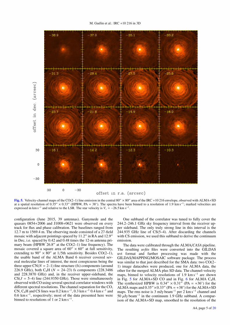
Fig. 6. Velocity-channel maps of the C4H(N = 24–23) line emission in the central 60′′ × 60′′ area of the IRC +10 216 envelope, observedwith ALMA. The spectra have been binned to a resolution of 1.9 km s−1; marked velocities are relative to the LSR. The star velocity is V∗ =−26.5 km s−1; velocities more positive or more negative correspond to the rear and front parts of the envelope, respectively.

SMA+SD map, shows the same bright structures than the latter,outside the innermost region (r > 20′′).

The 3-mm ALMA observations (project code2013.1.00432.S) were obtained in 2015 with the 12-m ar-ray in the Compact and Extended configurations. They consistedin a single pointing, centered on the position of the star in2012.4 (see Table 1), and were part of a spectral survey coveringthe 3-mm atmospheric window. The field of view (half-powerprimary beam width) of the 12-m ALMA antennas at 115.5 GHzis 54′′. The 3-mm data were processed like the 1-mm data andsimilarly combined with 30-m SD data. The synthesized HPBWwas 0.48′′ × 0.45′′ for the CO(1–0) line. A thorough descriptionof the spectral survey will be presented elsewhere (Cernicharoet al., in prep.).

2.3. IRAM 30-m single-dish telescope and PdBI observations

The CO(2–1) 30-m SD observations were reported inCernicharo et al. (2015). They mainly consisted of a fully sam-pled square map of size 480′′ × 480′′, plus 4 additional 240′′ ×240′′ maps centred at the corners of this square. All maps were

observed on-the-fly and a low order baseline was subtractedfrom each of the dumped spectra. The baseline subtraction re-moved the receiver instabilities, but also the continuum signal.The telescope radiation pattern mainly consists of a Gaussianmain beam, of half-power width (HPBW) 11′′, plus a muchwider error beam containing 25% of the total power. The con-tribution of the error beam was subtracted in the maps and anal-ysis presented here. Figure 1 shows the emission seen by the30-m SD telescope at the velocity of the star CW Leo?. Theseobservations have been used as short spacings for the SMA andALMA CO J = 2–1 line data presented here.

Additional CO(1–0) and 13CO(1–0) observations, consistingof a fully sampled map of size 120′′ × 120′′, centred on the star,were made in the Fall 2015 with the 30-m telescope, as partof a spectral survey (Agúndez et al. 2017; Quintana-Lacaci et al.2016).

Finally, fully sampled 120′′×120′′ maps of the C4H(24−23),CN(2−1) and CS(5−4) line emissions were carried out inDecember 2016 with the 30 m IRAM telescope. They providethe total flux and short spacings for the ALMA maps.

A4, page 6 of 20

M. Guélin et al.: IRC +10 216 in 3D

Fig. 7. Maps of the CO(2–1) line emission at the star velocity (–26.5 km s−1) viewed by the SMA before (left) and after (right inclusion of the30-m single-dish short spacings. The yellow curve shows the intensity profile along an EW strip passing through the central star. Most of the brightCO arcs have circular shapes and denote the intersection of the meridional plane with thin spherical shells. The latter typically extend over severalsteradians, as illustrated by the arc at r = 118′′ in the western half of the envelope (dashed yellow circle). The dense gas shell associated with thisarc can be followed over π radians along the line of sight in Fig. 19.

Prior to the SMA and ALMA observations, we made prelim-inary CO(2–1) interferometric observations with the PdBI 6 an-tenna array. They consisted in a mosaic covering one quarter ofa 60′′-wide annulus of inner radius 50′′. The synthesized HPBWwas 1.4′′ × 1.2′′ and the noise 30 mJy beam−1 in 3 km s−1-widechannels. Since the same region was re-observed with the SMAwith a higher sensitivity and denser uv plane coverage, the PdBIdata will be used only in Sect. 3.1, when we compare the innerto the outer arc pattern.

3. Results

3.1. Gas distribution in the meridional plane

3.1.1. Outer envelope

As pointed out above, the outer envelope appears to be expand-ing with a constant velocity of 14.5 km s−1 and has a small(<1 km s−1) turbulence velocity, judging from the remarkablyconstant width of the molecular lines (we further discuss thispoint below in Sect. 4.1, when dealing with the 3D structureof the envelope). Each velocity-channel map (of e.g. Figs. 4and 5) shows the emission from a conical sector (of opening θand thickness δθ), with its axis aligned to the line of sight to thestar CW Leo? (see Fig. A.1). The extreme velocities –40 km s−1

and –12 km s−1 correspond to the approaching and receding po-lar cones and caps, while the central velocity V∗ = −26.5 km s−1

corresponds to a cut through the envelope at the star position;the CO envelope being roughly spherical, the V∗ = −26.5 km s−1

map appears more extended.Figure 7 shows an enlargement of the CO V = −26.7 km s−1

map before (left panel) and after (right panel) addition of theSD short spacings. Thanks to the filtering of the extended emis-sion component by the interferometer, the left map shows moreclearly the bright ringed structure noted in previous observations.The bright arcs, which trace dense shells of molecular gas inthe outer envelope (see Cernicharo et al. 2015), appear far more

Fig. 8. Fourier transform of the azimuthally averaged CO(2–1) linebrightness distribution for the W half of the envelope. Abcissa is spatialfrequency in arcsec−1.

clearly at the 3′′ resolution of the SMA than at the 11′′ resolutionof the 30-m SD (Fig. 1). Surprisingly, they look almost circularand seem regularly spaced, except for three nearly straight seg-ments in the SE quadrant. In contrast, the pattern in the inner 30′′radius region appears confused in Fig. 7, due to artefacts in theimage restoration process. We discuss the central region below.

We have analyzed the ring pattern in the outer envelope byazimuthally averaging the SMA map of Fig. 7 in the NW, NE,SE and SW quarters and by Fourier transforming the resulting 4radial profiles from r = 20′′ to r = 150′′. Except for the SE quad-rant, the FT shows a marked peak that corresponds to a period of16′′ (Fig. 8), i.e. to a time lag of 700 yr for an expansion velocityof 14.5 km s−1 and a distance of 130 pc. Most of bright rings ofthe outer envelope can be fairly well fitted in each quadrant bycircular arcs.

A4, page 7 of 20

A&A 610, A4 (2018)

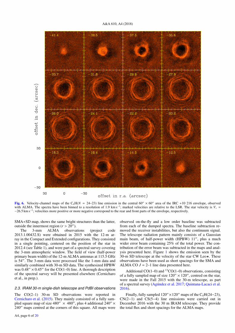
Fig. 9. CO(2–1) brightness distribution of Fig. 7 in polar coordinatesand logarithmic scale. The yellow sinusoids traced over the bright-est features correspond to slightly off-centred circles in the meridionalplane.

The circular arcs are centred close to CW Leo?, albeit notexactly on. This was first noted by Guélin et al. (1993a), whostudied the shape of the inner bright ring at r ' 15′′ appearingon the C4H maps and found that it was centred a couple of arcsecNE of the star. They interpreted the offset as a drift of the denseshell, caused by an orbital motion of CW Leo?. The brightestarcs in Fig. 7 may be similarly fitted by circular arcs slightlyoffset; the offsets range between 2′′ and 10′′.

We note that the fits become poorer when replacing the circu-lar arcs by segments of spirals with significant pitch angles. Thisis illustrated in Fig. 9, which shows the CO V = −26.7 km s−1

emission in polar coordinates. In that representation, anArchimedean spiral would appear as a tilted straight line. We ob-serve instead 100–150◦-long segments almost parallel the x-axis,bending up or down near their edges by up to 10′′, i.e. the signa-ture of slightly off-centred circular arcs. The bending of severalbright segments (e.g. at r = 100′′ and 130′′) occur around anglesof 170◦ ± 180◦, implying an off-centering along the E-W axis.Globally, the offset appears to increase with radius.

3.1.2. Central region

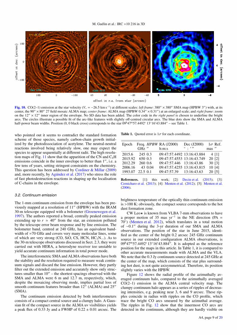
The CO emission at the star velocity in the central part of theenvelope is shown at different scales in the 3 panels of Fig. 10:left frame 380′′ × 380′′ SMA map with at its center the 90′′ × 80′′27 field mosaic ALMA map; center frame the ALMA map at anenlarged scale; right frame a zoom into the central 12′′ × 12′′region of the ALMA map. No SD data has been added in thisfigure.

The remarkable periodicity of the bright arcs in the outer en-velope appears to break down within an arcmin of the star. Thisis not just an effect of the tenfold increase in angular resolu-tion and sensitivity. Indeed, closer than 50′′ from the star, theSMA map shows the same contracted arc pattern as the ALMAdata, smoothed to the 3′′ SMA resolution; similarly the arc pat-tern observed between 50′′ and 110′′ E of CW Leo? with PdBI,smoothed to 3′′, is the same as that in (Fig. 7).

Between r = 10′′ and r = 40′′, the spacing between thebrightest arcs is '10′′ in the NW quadrant and further decreasesto '2′′ closer to the star. The spacing is even smaller in theopposite (SE) quadrant, possibly the effect of a NW drift of thearc centers. We note that the innermost arcs in Fig. 10 seem toform a series of off-centred rings, rather than a single regularspiral. This is illustrated on the right frame by the fit to the innerarc pattern of 3 circles with radii 2.3′′, 3.3′′ and 5′′, respectively

centred at (0.35′′, 0.45′′), (–0.6′′, 0.3′′) and (–0.8′′, 0.5′′) fromthe star. We note that the arc centres seem to drift to the W withincreasing radius, i.e. with the arc age. The arcs are fully re-solved with the 0.3′′ ALMA beam. They appear as tangled fila-ments, some of which are kinked or show bridging branches.

The appearance of the dense shells in the CO(2–1) line, par-ticularly in Fig. 4, is confused by the bright CO source aroundthe star and by the CO emission in the intershell region. In or-der to have a clearer view of the inner shells, we have turned totwo radicals, namely C4H and CN, known to form far from thestar. The C4H(N = 24–23) and CN(N = 2–1) line frequenciesare close enough to that of the CO(2–1) line, and were observedsimultaneously with the ALMA receiver.

Figure 6 shows the velocity-channel maps of the upper fre-quency component of the C4H (N = 24–23) line doublet, ob-served with ALMA. The continuum emission has been removed.As expected, no emission is detected near the star, except forforeground and background emission at terminal velocities (near–12 km s−1 and –40 km s−1). We also note a point-like sourcenear –38 km s−1 of width '6 km s−1 characteristic of vibra-tionally excited lines, that can be assigned to Si34S ν = 1 J = 13–12 at ν = 228 399.382 MHz. Lines from SiS and its isotopo-logues involving vibrationally excited states from ν = 1 up toν = 10 have been detected with ALMA by Cernicharo et al.(2013) and in the infrared by Fonfría et al. (2015).

It was previously noted by Guélin et al. (1993a) that the C4Hemission is essentially confined to a thick shell extending fromr = 10′′ to r = 25′′; the brightest contours at the star velocity(V∗ = −26.5 km s−1) trace a thick circular ring centred 2′′ NEof the star. With the 0.3′′ ALMA beam, each shell is resolvedinto '1′′-thick arcs with different radii and different centers ofcurvature. The outermost arc to the SW, which on the –26 km s−1

map may be interpreted as the onset of a spiral, rather appears asa circle centred at (0.6′′, –2.6′′) on the adjacent –24 km s−1 and–22 km s−1 velocity-channel maps (see Fig. 6).

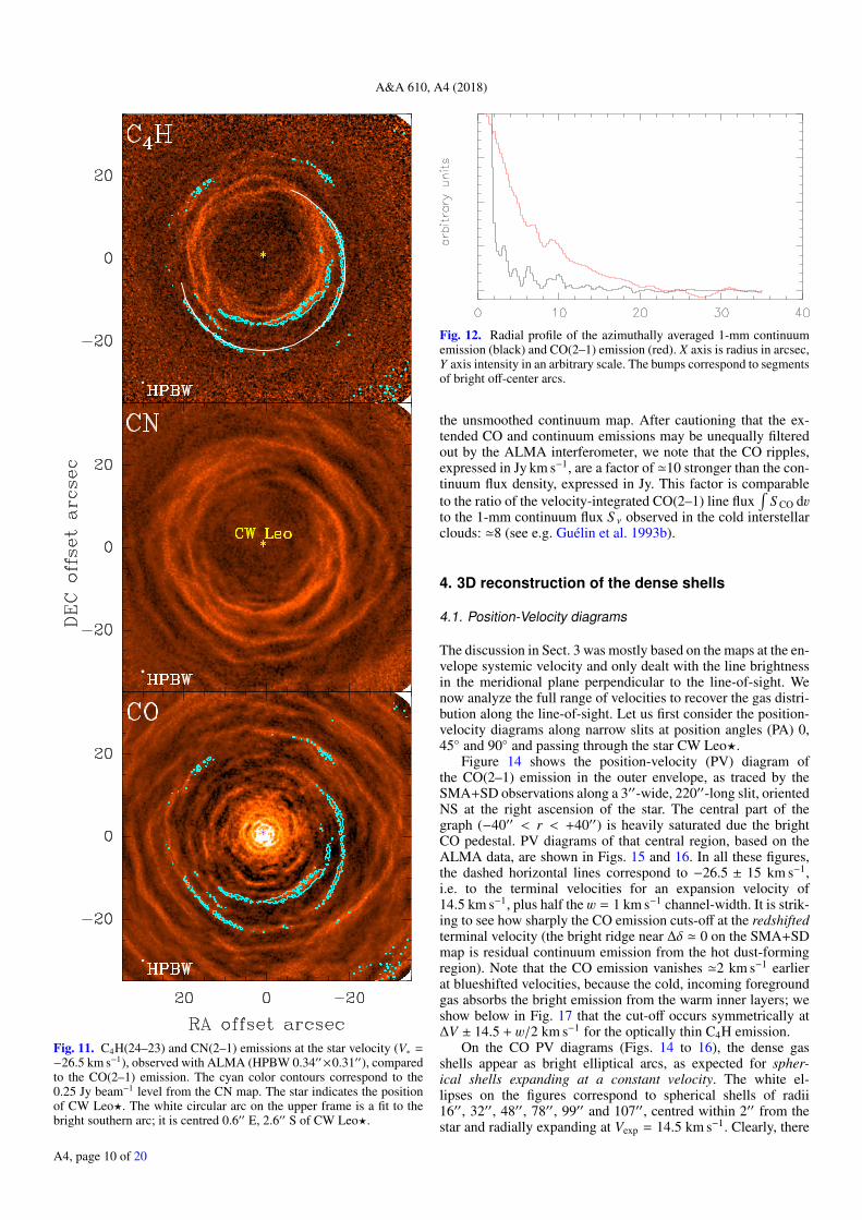
This arc structure is not specific to C4H, but also foundfor the CN(2–1) line emission. Figure 11 shows the C4H(N =24–23) and CN(N = 2–1) channel-velocity maps at V∗ =−26.5 km s−1. CN emission extends further out than the C4Hemission, but, although much stronger, is not observed at smallerradii, hence does not appear earlier than C4H. Within the ra-dius range where all three species are detected, the correla-tion between the CN,C4H and CO bright arcs is striking: thisis illustrated in the figure by the superimposition of the CN0.025 Jy beam−1 brightness contour (cyan color contour) on theC4H and CO maps. As noted above, the bright central arcs maybe fitted by circular arcs whose centers of curvature are offset bya few arcsec from the star.

Figure 13 shows the CO and CN (2–1) line brightness con-tours at the star velocity superimposed on the VLT image of theinterstellar light (V band) scattered by the dense shell dust grains(Leão et al. 2006). Again, the 3 tracers show very similar inten-sity profiles along the arcs (it should be noted that the imprint ofa number of stars has been removed from the VLT image so thatsome areas are artificially dim – see Leão ibid.). The agreementbetween CO and dust is not surprising, as the scattered light isenhanced where the line-of-sight is tangent to the dense shells,i.e. near the meridional plane. As expected, the optical arcs aresomewhat broader and, at places, lie slightly inside the CO arcs.

The similarity between the C4H and CN line brightnessdistributions, as well as the line brightness distributions ofmany other C-chain molecules and radicals (C2H, C6H, HC5N,MgNC,...), was already noticed in lower resolution interferomet-ric maps by Guélin et al. (1993a) and Lucas & Guélin (1999),

A4, page 8 of 20

M. Guélin et al.: IRC +10 216 in 3D

Fig. 10. CO(2–1) emission at the star velocity (V∗ = −26.5 km s−1) at different scales: left frame: 380′′ × 380′′ SMA map (HPBW 3′′) with, at itscenter, the 90′′ × 80′′ 27 field mosaic ALMA map; center frame: ALMA map (HPBW 0.34′′ × 0.31′′) at an enlarged scale; and right frame: zoomon the 12′′ × 12′′ inner region of the envelope. No SD data has been added. The color code in the right panel is chosen to underline the brightarcs. The circles illustrate a possible fit of the arc-like features with slightly off-centred circular arcs. The blue dots show the SMA and ALMAhalf-power beam widths. Position (0, 0 black cross) corresponds to the star 09h47m57.4492s 13◦16′43.884′′ – see Table 1.

who pointed out it seems to contradict the standard formationscheme of those species, namely carbon-chain growth initial-ized by the photodissociation of acetylene. The neutral-neutralreactions involved being relatively slow, one may expect thespecies to appear sequentially at different radii. The high resolu-tion maps of Fig. 11 show that the apparition of the CN and C4Hemissions coincide in the inner envelope to better than 1′′, i.e. afew tens of years, setting stringent constraints on the chemistry.This question has been addressed by Cordiner & Millar (2009)and, more recently, by Agúndez et al. (2017) who stress the roleof fast photodestruction reactions in shaping up the localisationof C-chains in the envelope.

3.2. Continuum emission

The 1-mm continuum emission from the envelope has been pre-viously mapped at a resolution of 11′′ (HPBW) with the IRAM30-m telescope equipped with a bolometer (Groenewegen et al.1997). The authors reported a broad, centrally peaked emissionextending up to r ' 40′′ from the star, an extension pollutedby the telescope error beam response and by line emission. Thebolometer band, centred at 240 GHz, has an equivalent band-width of '70 GHz and covers very many molecular lines, someof which are very strong (CO, SiO, CS, HCN, HC3N...). As tothe 30-m telescope observations discussed in Sect. 2.3, they werecarried out with HERA, a heterodyne receiver too unstable toyield accurate continuum information in total power mode.

The interferometric SMA and ALMA observations have boththe stability and the resolution required to measure weak contin-uum signals and discard the line emission. However, they partlyfilter out the extended emission and accurately show only struc-tures smaller than 10′′ – the shortest spacings observed with theSMA and ALMA were 6 m and 12.7 m, respectively, which,despite the mosaicing observing mode, implies partial loss ofsmooth continuum features broader than 12′′ (ALMA) and 25′′(SMA).

The continuum emission detected by both interferometersconsists of a compact central source and a clumpy halo. A Gaus-sian fit of the compact source in the ALMA uv visibilities yieldsa peak flux of 0.33 Jy and a FWHP of 0.22 ± 0.01 arcsec. The

Table 1. Quoted error is 1σ for each coordinate.

Epoch Freq. HPBW RA (J2000) Dec (J2000) 1σ Ref.GHz ′′ h:m:s ◦ : ′ ′′ mas ′′

2015.6 245 0.3 09:47:57.4492 13:16:43.884 4 [1]2015.92 650 0.3 09:47:57.4553 13:16:43.749 20 [2]2012.29 260 0.6 09:47:57.446 13:16:43.86 30 [3]2006.16 43 0.04 09:47:57.4255 13:16:43.815 10 [4]1993.07 22.5 0.1 09:47:57.39 13:16:43.63 20 [5]

References. [1]: this work; [2]: Decin et al. (2015); [3]:Cernicharo et al. (2013); [4]: Menten et al. (2012); [5]: Menten et al.(2006).

brightness temperature of the optically thin continuum emissionis >100 K: obviously, the compact source corresponds to the hotdust formation zone.

CW Leo? is known from VLBA 7-mm observations to havea proper motion of 35 mas yr−1 in the NE direction (PA =70◦) (Menten et al. 2012), which translates in a total motionof ∼0.1′′ during the 3-yr duration of our SMA and ALMAobservations. The position of the star in June 2015, identi-fied as the center of the bright 0.2 arcsec 245 GHz continuumsource in our extended configuration ALMA observations, is09h47m57.4492s 13◦16′43.884′′. It is adopted as the referenceposition for the maps in this article. In Table 1, it is compared toother accurate measurements made with ALMA and the VLA.We note that the 0.3 Jy continuum source detected at 245 GHz atthe center of the map, which consists of the star plus surround-ing hot dust, is not quite axisymmetrical. Therefore, its positionslightly varies with the HPBW.

Figure 12 shows the radial profile of the azimuthally av-eraged continuum halo, compared to the azimuthally averagedCO(2–1) emission in the ALMA central velocity map. Theclumpy continuum halo appears as a series of ripples of decreas-ing intensities, e.g. peaking near 3, 6 and 9 arcsec. These rip-ples coincide in radius with ripples on the CO profile, whichtrace the bright CO arcs smeared by the azimuthal average.The ripples in Fig. 12 show that the innermost CO arcs aredetected in the continuum, although they are hardly visible on

A4, page 9 of 20

A&A 610, A4 (2018)

Fig. 11. C4H(24–23) and CN(2–1) emissions at the star velocity (V∗ =−26.5 km s−1), observed with ALMA (HPBW 0.34′′×0.31′′), comparedto the CO(2–1) emission. The cyan color contours correspond to the0.25 Jy beam−1 level from the CN map. The star indicates the positionof CW Leo?. The white circular arc on the upper frame is a fit to thebright southern arc; it is centred 0.6′′ E, 2.6′′ S of CW Leo?.

Fig. 12. Radial profile of the azimuthally averaged 1-mm continuumemission (black) and CO(2–1) emission (red). X axis is radius in arcsec,Y axis intensity in an arbitrary scale. The bumps correspond to segmentsof bright off-center arcs.

the unsmoothed continuum map. After cautioning that the ex-tended CO and continuum emissions may be unequally filteredout by the ALMA interferometer, we note that the CO ripples,expressed in Jy km s−1, are a factor of '10 stronger than the con-tinuum flux density, expressed in Jy. This factor is comparableto the ratio of the velocity-integrated CO(2–1) line flux

∫S CO dv

to the 1-mm continuum flux S ν observed in the cold interstellarclouds: '8 (see e.g. Guélin et al. 1993b).

4. 3D reconstruction of the dense shells

4.1. Position-Velocity diagrams

The discussion in Sect. 3 was mostly based on the maps at the en-velope systemic velocity and only dealt with the line brightnessin the meridional plane perpendicular to the line-of-sight. Wenow analyze the full range of velocities to recover the gas distri-bution along the line-of-sight. Let us first consider the position-velocity diagrams along narrow slits at position angles (PA) 0,45◦ and 90◦ and passing through the star CW Leo?.

Figure 14 shows the position-velocity (PV) diagram ofthe CO(2–1) emission in the outer envelope, as traced by theSMA+SD observations along a 3′′-wide, 220′′-long slit, orientedNS at the right ascension of the star. The central part of thegraph (−40′′ < r < +40′′) is heavily saturated due the brightCO pedestal. PV diagrams of that central region, based on theALMA data, are shown in Figs. 15 and 16. In all these figures,the dashed horizontal lines correspond to −26.5 ± 15 km s−1,i.e. to the terminal velocities for an expansion velocity of14.5 km s−1, plus half the w = 1 km s−1 channel-width. It is strik-ing to see how sharply the CO emission cuts-off at the redshiftedterminal velocity (the bright ridge near ∆δ ' 0 on the SMA+SDmap is residual continuum emission from the hot dust-formingregion). Note that the CO emission vanishes '2 km s−1 earlierat blueshifted velocities, because the cold, incoming foregroundgas absorbs the bright emission from the warm inner layers; weshow below in Fig. 17 that the cut-off occurs symmetrically at∆V ± 14.5 + w/2 km s−1 for the optically thin C4H emission.

On the CO PV diagrams (Figs. 14 to 16), the dense gasshells appear as bright elliptical arcs, as expected for spher-ical shells expanding at a constant velocity. The white el-lipses on the figures correspond to spherical shells of radii16′′, 32′′, 48′′, 78′′, 99′′ and 107′′, centred within 2′′ from thestar and radially expanding at Vexp = 14.5 km s−1. Clearly, there

A4, page 10 of 20

M. Guélin et al.: IRC +10 216 in 3D

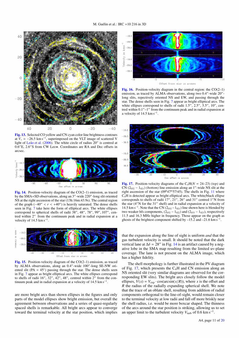
Fig. 13. Selected CO yellow and CN cyan color line brightness contoursat V∗ = −26.5 km s−1, superimposed on the VLT image of scattered Vlight of Leão et al. (2006). The white circle of radius 20′′ is centred at0.6′′E, 2.6′′S from CW Leo?. Coordinates are RA and Dec offsets inarcsec.

Fig. 14. Position-velocity diagram of the CO(2–1) emission, as tracedby the SMA+SD observations, along an 3′′-wide 220′′-long slit orientedNS at the right ascension of the star (13h:16m:43.9s). The central regionof the graph (−40′′ < r < +40′′) is heavily saturated. The dense shellsseen in Fig. 7 take here the form of elliptical arcs. The white ellipsescorrespond to spherical shells of radii 38′′, 48′′, 78′′, 99′′, 107′′, cen-tred within 2′′ from the continuum peak and in radial expansion at avelocity of 14.5 km s−1.

Fig. 15. Position-velocity diagram of the CO(2–1) emission, as tracedby ALMA observations, along an 0.4′′-wide 100′′-long SE-NW ori-ented slit (PA = 45◦) passing through the star. The dense shells seenin Fig. 7 appear as bright elliptical arcs. The white ellipses correspondto shells of radii 16′′, 32′′, 42′′, 48′′, centred within 2′′ from the con-tinuum peak and in radial expansion at a velocity of 14.5 km s−1.

are more bright arcs than shown ellipses in the figures and onlyparts of the model ellipses show bright emission, but overall theagreement between observations and a series of quasi-regularlyspaced shells is remarkable. All bright arcs appear to convergetoward the terminal velocity at the star position, which implies

Fig. 16. Position-velocity diagram in the central region: the CO(2–1)emission, as traced by ALMA observations, along two 0.4′′-wide 20′′-long slits, repectively oriented NS and EW, and passing through thestar. The dense shells seen in Fig. 7 appear as bright elliptical arcs. Thewhite ellipses correspond to shells of radii 1.5′′, 2.5′′, 5.5′′, 10′′, cen-tred within 0.1′′–1′′ from the continuum peak and in radial expansion ata velocity of 14.5 km s−1.

Fig. 17. Position-velocity diagrams of the C4H(N = 24–23) (top) andCN (2032 − 1021) (bottom) line emission along an 1′′-wide NS slit at theright ascension of the star (09h47m57s.45). The shells in Fig. 11 whereC4H is detected appear as bright elliptical arcs. The white/black ellipsecorresponds to shells of radii 17′′, 21′′, 26′′ and 31′′ centred 1′′N fromthe star (4′′N for the 31′′ shell) and in radial expansion at a velocity of14.5 km s−1. Note that the CN (2032−1021) line shown here is blended bytwo weaker hfs components, (2032 − 1022) and (2033 − 1023), respectively11.5 and 16.3 MHz higher in frequency. Those appear on the graph asghosts of the brightest component shifted by –15.2 and –21.6 km s−1.

that the expansion along the line of sight is uniform and that thegas turbulent velocity is small. It should be noted that the darkvertical lane at ∆δ = 28′′ in Fig. 14 is an artifact caused by a neg-ative lobe in the SMA map resulting from the limited uv-planecoverage. The lane is not present on the ALMA image, whichhas a higher fidelity.

The shell morphology is further illustrated in the PV diagramof Fig. 17, which presents the C4H and CN emission along anNS oriented slit (very similar diagrams are observed for the cor-responding EW slits). The bright arcs closely follow the modelellipses, V(x) = Vexp · cos(arcsin(x/R)), where x is the offset andR the radius of the radially expanding spherical shell. We notethat the trace of an oblate shell, resulting from addition of radialcomponents orthogonal to the line-of-sight, would remain closerto the terminal velocity at low radii and fall off more briskly nearthe shell radius, i.e. would be more boxcar shaped. The thinnessof the arcs around the star position is striking, allowing us to setan upper limit to the turbulent velocity Vturb of 0.6 km s−1.

A4, page 11 of 20

A&A 610, A4 (2018)

4.2. Spherical deprojection of the outer envelope

We thus adopt in the following a uniform expansion velocity ofVexp = 14.5 km s−1 and neglect turbulent motions. This enablesus to extract from the position-velocity CO datacubes, XYV, a3-dimensional (3D) spatial representation of the envelope andits dense shells, XYZ. Two different approaches, respectivelydubbed Non-iterative and Iterative, were used for this 3D re-construction. They are described in Appendix A together withcomparative tests on envelope models. Both yield very similarresults, though the iterative method images are less noisy andtrace the arcs closer to the star, at the expense of degraded an-gular resolution and of tight spherical boundaries. For directionsclose to the center of expansion, i.e. CW Leo?, the line of sightvelocity component comes to be degenerated. This, and the re-sulting increase of the CO(2–1) line opacity, prevents us fromlocalizing the gas cells along the line of sight in the approachingand receding polar caps.

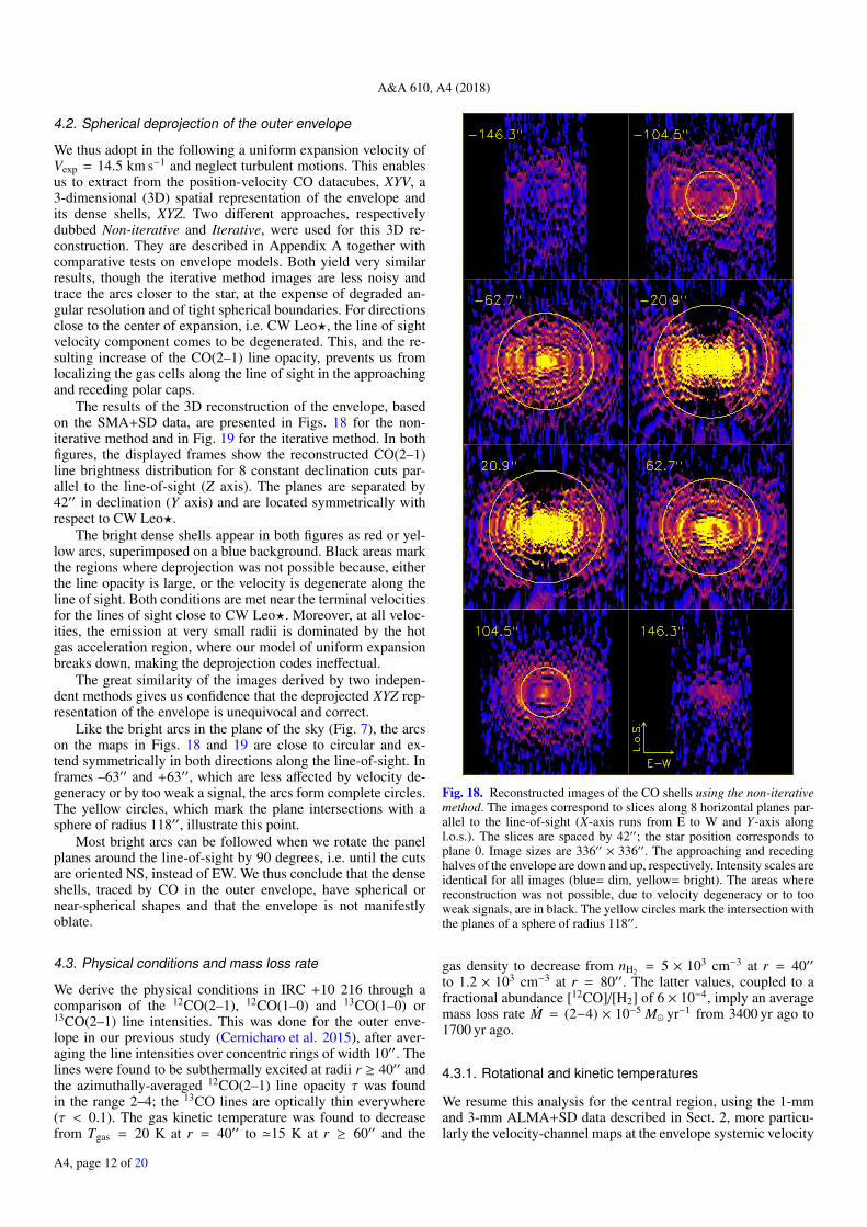
The results of the 3D reconstruction of the envelope, basedon the SMA+SD data, are presented in Figs. 18 for the non-iterative method and in Fig. 19 for the iterative method. In bothfigures, the displayed frames show the reconstructed CO(2–1)line brightness distribution for 8 constant declination cuts par-allel to the line-of-sight (Z axis). The planes are separated by42′′ in declination (Y axis) and are located symmetrically withrespect to CW Leo?.

The bright dense shells appear in both figures as red or yel-low arcs, superimposed on a blue background. Black areas markthe regions where deprojection was not possible because, eitherthe line opacity is large, or the velocity is degenerate along theline of sight. Both conditions are met near the terminal velocitiesfor the lines of sight close to CW Leo?. Moreover, at all veloc-ities, the emission at very small radii is dominated by the hotgas acceleration region, where our model of uniform expansionbreaks down, making the deprojection codes ineffectual.

The great similarity of the images derived by two indepen-dent methods gives us confidence that the deprojected XYZ rep-resentation of the envelope is unequivocal and correct.

Like the bright arcs in the plane of the sky (Fig. 7), the arcson the maps in Figs. 18 and 19 are close to circular and ex-tend symmetrically in both directions along the line-of-sight. Inframes –63′′ and +63′′, which are less affected by velocity de-generacy or by too weak a signal, the arcs form complete circles.The yellow circles, which mark the plane intersections with asphere of radius 118′′, illustrate this point.

Most bright arcs can be followed when we rotate the panelplanes around the line-of-sight by 90 degrees, i.e. until the cutsare oriented NS, instead of EW. We thus conclude that the denseshells, traced by CO in the outer envelope, have spherical ornear-spherical shapes and that the envelope is not manifestlyoblate.

4.3. Physical conditions and mass loss rate

We derive the physical conditions in IRC +10 216 through acomparison of the 12CO(2–1), 12CO(1–0) and 13CO(1–0) or13CO(2–1) line intensities. This was done for the outer enve-lope in our previous study (Cernicharo et al. 2015), after aver-aging the line intensities over concentric rings of width 10′′. Thelines were found to be subthermally excited at radii r ≥ 40′′ andthe azimuthally-averaged 12CO(2–1) line opacity τ was foundin the range 2–4; the 13CO lines are optically thin everywhere(τ < 0.1). The gas kinetic temperature was found to decreasefrom Tgas = 20 K at r = 40′′ to '15 K at r ≥ 60′′ and the

Fig. 18. Reconstructed images of the CO shells using the non-iterativemethod. The images correspond to slices along 8 horizontal planes par-allel to the line-of-sight (X-axis runs from E to W and Y-axis alongl.o.s.). The slices are spaced by 42′′; the star position corresponds toplane 0. Image sizes are 336′′ × 336′′. The approaching and recedinghalves of the envelope are down and up, respectively. Intensity scales areidentical for all images (blue= dim, yellow= bright). The areas wherereconstruction was not possible, due to velocity degeneracy or to tooweak signals, are in black. The yellow circles mark the intersection withthe planes of a sphere of radius 118′′.

gas density to decrease from nH2 = 5 × 103 cm−3 at r = 40′′to 1.2 × 103 cm−3 at r = 80′′. The latter values, coupled to afractional abundance [12CO]/[H2] of 6 × 10−4, imply an averagemass loss rate M = (2−4) × 10−5 M� yr−1 from 3400 yr ago to1700 yr ago.

4.3.1. Rotational and kinetic temperatures

We resume this analysis for the central region, using the 1-mmand 3-mm ALMA+SD data described in Sect. 2, more particu-larly the velocity-channel maps at the envelope systemic velocity

A4, page 12 of 20

M. Guélin et al.: IRC +10 216 in 3D

Fig. 19. Same as Fig. 18 for the iterative method (see text).

V∗ = −26.5 km s−1. The latter provide direct information on thephysical conditions throughout the meridional XY plane.

The 12CO(2–1) ALMA+SD velocity-channel cube(1.9 km s−1-wide channels) was first smoothed to the an-gular resolution of the 12CO(1–0) cube (0′′.48 × 0′′.45 – seeupper frame of Fig. 20). Then, the central (V∗ = −26.5 km s−1)velocity-channel maps of 12CO(2–1) and 12CO(1–0) wereazimuthally averaged over 0′′.53-thick concentric rings centredon CW Leo?. This allowed us to derive the radial profiles of the

Fig. 20. 12CO(1–0) (upper frame) and 13CO(1–0) (lower frame) linebrightness distributions at the envelope systemic velocity (V∗ =−26.5 km s−1) for the ALMA+SD data. The synthesized beam half-power width, (0′′.48 × 0′′.45) in the upper frame, has been degraded to(0′′.86 × 0′′.76) for the rare isotopomer line.

12CO(2–1) peak line intensity, as well as of the R21 =12CO(2–1)/12CO(1–0) line brightness temperature ratio, throughout the'50′′ central region Fig. 20).

From the R21 radial profiles, we derive the rotation temper-ature profile Trot , which represents the kinetic temperature Tkunder the assumption that the low J 12CO levels are at LTE. InFig. 21, the 12CO data set was completed in the inner r ≤ 1′′region using the rotational temperatures derived by Fonfría et al.(2015, 2017) from ro-vibrational SiS and C2H4 lines.

The Trot plot shows at r ' 15′′ ('750 R∗ or 2.8 × 1016 cm)a change in dependence on the distance from the star. Atlower radii, Trot closely follows a power-law Trot = (256.9 ±1.5) (r/0.8)−(0.675±0.003) K, where r is expressed in arcsec. Be-yond r = 15′′, Trot remains around 35 K.

A4, page 13 of 20

A&A 610, A4 (2018)

Fig. 21. Rotational temperature and mass-loss rate throughout the in-ner 50′′ of the CSE. The rotational temperature (black dots) was de-rived from the 12CO(2–1)/12CO(1–0) ratio averaged in concentric ringscentred on the star. The green curve is the kinetic temperature closeto the star calculated from results of previous works. The grey regionaccounts for the 1σ error interval of the rotational temperature. Thevertical dashed grey line indicates the distance from the star where therotational temperature changes its behaviour ('15′′). The black contin-uous lines are the fits to the data set up to 15′′ (Trot ∝ r−0.68) and beyond(Trot ' 35 K). The thin colored lines represent the mass loss rate (rightaxis scale) calculated on the 13CO map by averaging 5◦-wide sectorsoriented N, S, E and W (continuous and dashed red, and continuousand dashed blue curves, respectively) . The magenta line is the averagemass-loss rate and the hatched region depicts the typical deviation (seetext).

The change of the Trot behaviour around r = 15′′ does notresult from a departure from the 12CO levels from LTE: mod-elling the J = 1–0 and 2–1 lines and the 13CO(1–0) line withthe MADEX statistical equilibrium code (Cernicharo 2012), wefind that Trot deviates from Tk by .10% in the range of radiiconsidered here (0′′ ≤ r ≤ 25′′).

Although the critical densities for the low-J CO transitions('1.9 × 103 cm−3 and 1.1 × 104 cm−3, for J = 1–0 and 2–1lines at '35 K) are not much lower than the average gas densityat r = 15′′ ('2.0 × 104 cm−3 – see below), the 12CO(2–1) lineopacity (τ ' 4 for r = 15′′) prevents a significant departure fromthermalization. This is no more the case for the lines of the rareisotopomer 13CO, which, due to a much lower column density,are out of LTE beyond '8′′.

Our law of the dependence of Tk on distance r from the star isthe first directly derived from very high angular resolution obser-vations. It significantly differs from the lower resolution worksof e.g. Doty & Leung (1997) or De Beck et al. (2012), who findbeyond r = 2′′ an exponent q between –1 and –1.2.

Our exponent −0.68 is significantly shallower than that ex-pected for the adiabatic expansion of a diatomic gas in the vibra-tional ground state, '−1.2. This means that the expanding gas isefficiently heated, most likely by dust grains close to the star andby interstellar radiation outside 15′′ (e.g., Huggins et al. 1988).

Indeed, we know that interstellar UV radiation penetrates theenvelope as deep as r = 15′′, since the CCH and CN radicals,which form from the photodissociation of HCCH and HCN (e.g.,Millar & Herbst 1994; Glassgold 1996), are first observed nearthat radius (see Fig. 11). As a matter of fact, a plethora of rad-icals, such as C4H, C3N or MgCCH that are direct or indirectproducts of photodissociation, are found to peak in abundance atr = 14−16′′ (Guélin et al. 1993a; Agúndez et al. 2017).

Fig. 22. Ratio of the brightness temperatures of 12CO(1–0) and 13CO(1–0), 12C/13C isotopic ratio, and optical depth of line 12CO(1–0) againstthe distance to the star (blue squares, red triangles and black circles,respectively). The continuous blue curve is the brightness temperatureratio calculated with MADEX and the kinetic temperature derived inSect. 4.3.1. The 1σ uncertainties have been plotted as vertical bars, agrey region, or a hatched rectangle.

Our present observations do not have the angular resolu-tion required to explore the innermost envelope layers (r .1′′). The modelling of high energy lines arising in those layerspoint to a temperature dependence to r with an exponent q '−0.5 Fonfría et al. (2008), Agúndez et al. (2012), De Beck et al.(2012), Fonfría et al. (2015). This close to the star, molecules arestrongly excited by the radiation from the hot dust cocoon; theircollisional deexcitation is a powerful source of heat for the gasthat adds up to gas-grain collisions. Further out, the infrared ra-diation gets diluted and the gas density falls off. We then expectthe exponent to steepen from q ' −0.5 to q = −0.7 somewherebetween r = 0.5′′ and 1′′.

4.3.2. 12CO/13CO abundance ratio

In order to directly compare the 13CO and 12CO data, we de-graded the spatial resolution of the 12CO(1–0) central velocity-channel maps to (0.86′′ × 0.76′′).

From the resulting 12CO(1–0) and 13CO(1–0) line bright-nesses and the temperature profile derived in Sect. 4.3.1, wethen derived the J = 1–0 line opacity τ and the R12C/13C =

[12CO]/[13CO] abundance ratio throughout the meridional planewith the MADEX code. The radial profiles obtained by aver-aging those quantities in azimuth are displayed in Fig. 22. Theisotopic ratio and the mass-loss rate (see Sect. 4.3.3) have beendetermined at the same time following a self-consistent iterativeprocedure that can be assumed to converge after '10 iterations,when the variation between consecutive iterations was .0.1%.We note that, contrary to 12CO, the low J 13CO levels are foundto depart significantly from LTE, with a rotation temperature atr ' 15′′ 20 to 30% higher than Tk. MADEX indicates that thedifference is above 50% beyond 20′′ from the star.

Within the errors, the ratio R12C/13C plotted in Fig. 22 appearsroughly constant from r = 1.5′′ to r = 20′′ (the error bars on thegraph only denote the 1σ uncertainty on the line brightnesses).Its value up to the r = 15′′ shell, 42, agrees well with thosedetermined from the optically thin mm-wave lines of a numberof C-bearing molecules (C4H, HC3N, SiCC,...) in that very shell(40–43, see e.g. Cernicharo et al. 2000).

A4, page 14 of 20

M. Guélin et al.: IRC +10 216 in 3D

Beyond 20′′, the ratio R12C/13C derived with MADEX underthe assumption that the 12CO rotation temperature equals Tk, ap-pears to decrease with distance from the star. It seems improba-ble that the 12C/13C isotopic ratio has varied in just a few hun-dred years, because of a dredge-up or of chemical fractionation.Also, selective photodissociation of CO by interstellar UV radia-tion would increase, not decrease this ratio. Therefore, it is likelythat the 12CO levels start to depart from LTE for r > 20′′, or thatthe rotation temperature of 13CO is underestimated in our sim-ple model; for example, radiative cascades from higher-J levelspumped by external radiation may overpopulate the J = 1 13COlevel. On the other hand, the value of R12C/13C found for radiismaller than 20′′ and its near constancy supports our analysisand imply that the derived line opacities and CO column den-sities are accurate. Assuming the [CO]/[H2] abundance ratio isknown, we can then accurately derive the mass loss rate duringthe last 2000 yr.

4.3.3. Mass-loss rate

The maps in Fig. 20 show evident arcs formed as a consequenceof the matter ejection process. The very complex structure no-ticeable in these maps depicts a set of higher density shellsthat are expected to be roughly spherically symmetric. Thus, itis possible to estimate the mass-loss rate for every shell alongthe line-of-sight by using the geometrical information extractedfrom the map of the optically thin line 13CO(1–0) and its ro-tational temperature calculated with MADEX from the kinetictemperature derived in Sect. 4.3.1.

The mass-loss rate has been calculated from the brightnesstemperature averaged over the position angle in four 5◦-widesectors oriented along the N, S, E and W directions (Fig. 21).The mean rate derived after weighting the r ≤ 15′′ data withtheir uncertainties is 〈M〉 = (2.7 ± 0.5) × 10−5 M� yr−1. Thisvalue was calculated assuming the 12CO abundance with respectto H2 of 6 × 10−4 estimated by Agúndez et al. (2012). The esti-mates beyond r = 20′′, which seem to show a 30% decrease ofthe mass loss rate, are not reliable in view of the uncertainties onthe large departures to LTE.

The derived average mass-loss rate agrees quite well withmost of the values commonly derived or adopted in the litera-ture '(1.5−4.0) × 10−5 M� yr−1; see e.g. Keady et al. (1988),Teyssier et al. (2006), Decin et al. (2010), Agúndez et al. (2012),Cernicharo et al. (2015). The mass-loss rate radial profiles forthe 5◦-wide sectors show variations by factors of up to 3 overscales of a few arcsec (i.e. timescales of '102 yr). This reflectsthe CO column density variation observed between the brightestarcs and the inter-arc region in Fig. 20, typically a factor of 3.

5. Discussion

The ∼700 yr time delay between the outer arcs corresponds nei-ther to Mira-type oscillations (the IR light period of CW Leo? is1.8 yr), nor to the delay between two thermal pulses (>104 yr fora 2 M� TP-AGB star). In previous articles (Guélin et al. 1993a;Cernicharo et al. 2015) we tentatively explained the off-centringof the arcs and their regular spacing by the presence of a com-panion star on an elliptical orbit in the plane of the sky. Thedistortion of the Roche lobe during the companion fly-by booststhe mass loss rate at regular intervals close to the binary period.The shells of gas emitted at this stage drift away from the bi-nary system in directions that depends on the system phase atthe time of their emission. Numerical simulations – see Fig. 11

of Cernicharo et al. (2015) – show the formation of a pattern ofcircular arcs fairly similar to that observed with the IRAM 30-mtelescope.

The binary star hypothesis may be supported by the detec-tion with the HST of a bright red spot 0.5′′ E of CW Leo?that Kim et al. (2015) tentatively identify with a companion star.The slight curvature of CW Leo?’s trajectory between 1995 and2001, recently reported by Sozetti et al (2017) from an analysisof archival data, may be further evidence for a companion.

Analyzing 13CO(6–5) ALMA observations of a 6′′-widefield around CW Leo?, Decin et al. (2015) revisited this hypoth-esis and argued the inner 13CO position-velocity diagrams arebetter reproduced by a spiral structure viewed edge-on than bya circular structure viewed face-on. In their model, that stemsfrom Mastrodemos & Morris (1999), the spiral structure resultsfrom continuous mass loss in binary star system of period 55 yr,with an orbit viewed edge-on at PA ' 15◦.

Although the Cernicharo et al. (2015) and Decin et al.(2015) models seem contradictory, they try to explain datarelevant to different spatial scales, hence to different epochs.Besides, the Cycle 0 ALMA 13CO(6–5) data, analyzed byDecin et al. (2015), result from a short observing time slot (17min on-source) and are affected by relatively poor signal-to-noise ratio and uv-plane coverage.

The data presented here have a higher sensitivity and reso-lution than the previous molecular line studies and a denser uv-plane coverage, allowing us to further investigate the origin ofthe CO-bright shells. We have seen (e.g. Fig. 11) that the brightring pattern is strikingly similar for the CO, CN and C4H linesat radii where all 3 species are present. Given that the CO andC4H formation paths are quite different and that these speciesabundances are poorly correlated elsewhere in the envelope,the regions with high line brightness must have large H2 col-umn densities and the arcs/filaments must trace high mass-lossevents. This is corroborated by the excellent positional agree-ment between the molecular arcs in the meridional plane and thedusty arcs traced by diffused IS light (Fig. 13). The arc/inter-arc contrast is typically 3 for the V-band brightness intensities(Mauron & Huggins 2000) and 2–3 for CO, which, as we haveseen, implies gas and dust density contrasts close to 3.

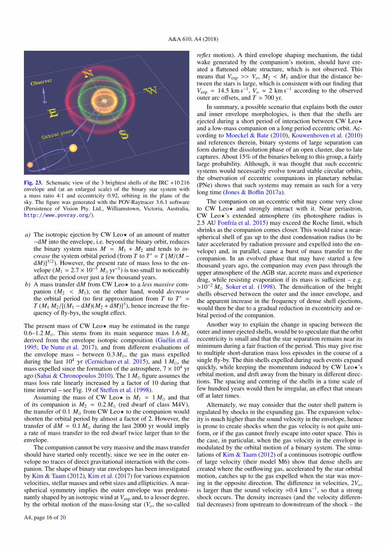
We have shown in Sect. 4 that the bright arcs in the outerenvelope are not narrow structures confined to the plane of thesky, but parts of dense spherical shells pertaining to a sphericalor near-spherical envelope. The thinness of the shells and theirfairly regular spacing set stringent constraints on the mass lossprocess and the binary star hypothesis. We have repeated the nu-merical simulations of Cernicharo et al. (2015; based on the pe-riodic ejection near periastron of spherical shells, consisting offree-moving particles, superimposed on a lower intensity con-tinuous mass loss). Within the simple frame of isotropic massloss, constant expansion velocity and binary orbit orthogonal tothe line-of-sight, we found a set of parameters that reproduce thegross features of the observed outer shell pattern Fig. 23).

The '16′′ spacing (700 yr time delay) between the brightestouter arcs is found to decrease in the central and youngest partof the envelope (with radius r < 40′′ and age <1800 yr – seeFig. 10). It is 10′′ (460 yr) in the NW quadrant between r =10′′ and r = 40′′ (5′′ in the inner SE quadrant) and only '2′′(90 yr) within 10′′ from CW Leo?. Are those different patternsgenerated by a single binary star system and could they denotea rapid change of orbital period during the last 2000 yr? SinceCW Leo? is in a phase of rapid mass loss, let us consider theeffect of mass transfer a to the envelope and b to the companion.

A4, page 15 of 20

A&A 610, A4 (2018)

Fig. 23. Schematic view of the 3 brightest shells of the IRC +10 216envelope and (at an enlarged scale) of the binary star system witha mass ratio 4:1 and eccentricity 0.92, orbiting in the plane of thesky. The figure was generated with the POV-Raytracer 3.6.1 software(Persistence of Vision Pty. Ltd., Williamstown, Victoria, Australia,http://www.povray.org/).

a) The isotropic ejection by CW Leo? of an amount of matter−dM into the envelope, i.e. beyond the binary orbit, reducesthe binary system mass M = M1 + M2 and tends to in-crease the system orbital period (from T to T ′ = T [M/(M −dM)]3/2). However, the present rate of mass loss to the en-velope (M1 = 2.7 × 10−5 M� yr−1) is too small to noticeablyaffect the period over just a few thousand years.

b) A mass transfer dM from CW Leo? to a less massive com-panion (M2 < M1), on the other hand, would decreasethe orbital period (to first approximation from T to T ′ =T (M1 M2/[(M1 − dM)(M2 + dM)]3), hence increase the fre-quency of fly-bys, the sought effect.

The present mass of CW Leo? may be estimated in the range0.6–1.2 M�. This stems from its main sequence mass 1.6 M�derived from the envelope isotopic composition (Guélin et al.1995; De Nutte et al. 2017), and from different evaluations ofthe envelope mass – between 0.3 M�, the gas mass expelledduring the last 104 yr (Cernicharo et al. 2015), and 1 M�, themass expelled since the formation of the astrosphere, 7 × 104 yrago (Sahai & Chronopoulos 2010). The 1 M� figure assumes themass loss rate linearly increased by a factor of 10 during thattime interval – see Fig. 19 of Steffen et al. (1998).

Assuming the mass of CW Leo? is M1 = 1 M� and thatof its companion is M2 = 0.2 M� (red dwarf of class M4V),the transfer of 0.1 M� from CW Leo? to the companion wouldshorten the orbital period by almost a factor of 2. However, thetransfer of dM = 0.1 M� during the last 2000 yr would implya rate of mass transfer to the red dwarf twice larger than to theenvelope.

The companion cannot be very massive and the mass transfershould have started only recently, since we see in the outer en-velope no traces of direct gravitational interaction with the com-panion. The shape of binary star envelopes has been investigatedby Kim & Taam (2012), Kim et al. (2017) for various expansionvelocities, stellar masses and orbit sizes and ellipticities. A near-spherical symmetry implies the outer envelope was predomi-nantly shaped by an isotropic wind at Vexp and, to a lesser degree,by the orbital motion of the mass-losing star (Vo, the so-called

reflex motion). A third envelope shaping mechanism, the tidalwake generated by the companion’s motion, should have cre-ated a flattened oblate structure, which is not observed. Thismeans that Vexp >> Vo, M2 < M1 and/or that the distance be-tween the stars is large, which is consistent with our finding thatVexp = 14.5 km s−1, Vo ' 2 km s−1 according to the observedouter arc offsets, and T ' 700 yr.

In summary, a possible scenario that explains both the outerand inner envelope morphologies, is then that the shells areejected during a short period of interaction between CW Leo?and a low-mass companion on a long period eccentric orbit. Ac-cording to Moeckel & Bate (2010), Kouwenhoven et al. (2010)and references therein, binary systems of large separation canform during the dissolution phase of an open cluster, due to latecaptures. About 15% of the binaries belong to this group, a fairlylarge probability. Although, it was thought that such eccentricsystems would necessarily evolve toward stable circular orbits,the observation of eccentric companions in planetary nebulae(PNe) shows that such systems may remain as such for a verylong time (Jones & Boffin 2017a).

The companion on an eccentric orbit may come very closeto CW Leo? and strongly interact with it. Near periastron,CW Leo?’s extended atmosphere (its photosphere radius is2.5 AU Fonfría et al. 2015) may exceed the Roche limit, whichshrinks as the companion comes closer. This would raise a near-spherical shell of gas up to the dust condensation radius (to belater accelerated by radiation pressure and expelled into the en-velope) and, in parallel, cause a burst of mass transfer to thecompanion. In an evolved phase that may have started a fewthousand years ago, the companion may even pass through theupper atmosphere of the AGB star, accrete mass and experiencedrag, while resisting evaporation if its mass is sufficient – e.g.>10−2 M� Soker et al. (1998). The densification of the brightshells observed between the outer and the inner envelope, andthe apparent increase in the frequency of dense shell ejections,would then be due to a gradual reduction in excentricity and or-bital period of the companion.

Another way to explain the change in spacing between theouter and inner ejected shells, would be to speculate that the orbiteccentricity is small and that the star separation remains near itsminimum during a fair fraction of the period. This may give riseto multiple short-duration mass loss episodes in the course of asingle fly-by. The thin shells expelled during such events expandquickly, while keeping the momentum induced by CW Leo?’sorbital motion, and drift away from the binary in different direc-tions. The spacing and centring of the shells in a time scale offew hundred years would then be irregular, an effect that smearsoff at later times.

Alternately, we may consider that the outer shell pattern isregulated by shocks in the expanding gas. The expansion veloc-ity is much higher than the sound velocity in the envelope, henceis prone to create shocks when the gas velocity is not quite uni-form, or if the gas cannot freely escape into outer space. This isthe case, in particular, when the gas velocity in the envelope ismodulated by the orbital motion of a binary system. The simu-lations of Kim & Taam (2012) of a continuous isotropic outflowof large velocity (their model M6) show that dense shells arecreated where the outflowing gas, accelerated by the star orbitalmotion, catches up to the gas expelled when the star was mov-ing in the opposite direction. The difference in velocities, 2Vo,is larger than the sound velocity '0.4 km s−1, so that a strongshock occurs. The density increases (and the velocity differen-tial decreases) from upstream to downstream of the shock – the

A4, page 16 of 20

M. Guélin et al.: IRC +10 216 in 3D

predicted increase (decrease) is a factor of '4 at large radii, sim-ilar to the observed gas density contrast (see Sect. 4.3.3).

We have searched for signatures of shocks in the velocityfield near the arcs. From the CO, CN and C4H PV diagrams (e.g.Fig. 17) we see no traces of a 2 km s−1 spread in the line-of-sight velocity component, but, of course, have no kinematicalinformation for the perpendicular directions. If the eccentricityof the shells is caused by a binary star system, the orbital planeshould be almost perpendicular to the line-of-sight.

Finally, a third possibility would be that the star system isnot binary, but triple, allowing multiple periods and differentinteraction configurations. Whereas triple stars are common inearly stellar phases, the two closest stars tend with time to forma common-envelope and to merge. Yet, Soker (2016) argue thattriple star systems may survive up to the AGB stage: from theimages of hundreds of PNe they find that one in six seems tohost such a system. However, as pointed up by Jones & Boffin(2017b), so far only one PN has been actually demonstrated tohost 3 stars at its center, on the basis of velocity variations.

6. Summary and conclusion

The main findings of our IRC +10 216 observations can be sum-marized as follows:

1) The star CW Leo? and its hot dust cocoon appear in the1.2 mm continuum as a 0.33 Jy Gaussian source of diameter0.21′′.

2) In the CO(2–1) line, the envelope consists of a strong, fairlycompact source, centred on the star, plus a slowly decreasingcomponent, extending up to r = 3′ from CW Leo? and aseries of bright shells that modulate the extended component.

3) Outside the dust acceleration region, the envelope expandsradially at a remarkably constant velocity, 14.5 km s−1, witha small turbulent velocity (≤0.6 km s−1).

4) At the star velocity, i.e. in the plane of the sky passingthrough the star, the bright shells trace a pattern of circulararcs as thin as the 3′′ SMA beam. Outside radius r = 40′′,the brightest arcs are nearly concentric and regularly spaced,with an average separation of 16′′, or 700 yr in expan-sion time. They are centred a few arcsec on either side ofCW Leo?.

5) Inside radius r = 40′′, ALMA reveals a denser, less regulararc pattern. The typical separation between the brightest arcsdecreases, a change that can hardly be attributed to the ten-fold higher resolution, since smoothed to 3′′, the ALMA arcsfollow the SMA inner arcs. ALMA resolves the bright arcsinto thin circular filaments off-centred from CW Leo? by afraction of an arcsec for the smallest arcs, up to a couple ofarcsec for the largest (20–30′′). Some filaments west of thestar appear kinked.

6) The pattern of bright CO arcs is accurately replicated in theCN and C4H line emissions, wherever theses radicals arepresent, as well as in the dust structures traced by scatteredlight. They must trace gas shells '3 times denser than theintershell regions.

7) The gas kinetic temperature in the central region followsfrom r = 0.5′′ to r = 15′′ the power law Trot = (256.9 ±1.5) (r/0.8)−(0.675±0.003) K, and settles around 35 K until atleast r = 25′′. The mass loss rate during the last 103 yr was〈M〉 = (2.7± 0.5)× 10−5 M� yr−1 on the average, with peak-to-peak variations of a factor of 3. The 12CO/13CO abun-dance ratio is found equal to 42 in the central region.

8) A 3D reconstruction of the outer envelope shows the denseshells have nearly spherical shapes, extending typically overone or more steradians. The envelope shows little or no signsof flatness.

The outer envelope structure (the spherical shape of the shellsand their small eccentring) may be explained by continuous massloss plus short mass-loss episodes triggered by the fly-by of acompanion star with a 700 yr period and orbit nearly perpendic-ular to the line-of-sight. The orbital velocity of the AGB star istypically 1–2 km s−1 during the episodes of high mass loss.

The structure observed in the central region of the envelope,where the shells are denser, less regular and show no obvioussignature of a spiral, is more difficult to explain. It may havebeen shaped by the companion star described above, if its massis much lower (e.g. 1/5th) than the mass the AGB star, and ifa large transfer of mass to the companion has developed duringthe last 2000 yr. Alternately, the central system may consist ofmore than two massive bodies.

Long term very high angular resolution monitoring of thecompact central source in the visible, IR or the sub-mm con-tinuum may allow us to further investigate its nature. The dimsource spotted by Kim et al. (2015) on HST images, and theslight curvature of the CW Leo? track on the sky could be firstevidence for a multiple system.

Acknowledgements. We thank S. Guilloteau and S. Bardeau for their helpon the GILDAS software and J. M. Winters for helpful comments. This pa-per makes use of data from the following instruments: The SubmillimeterArray (SMA project number 2011B-S052, 2012B-S004, and 2012B-S101),IRAM single dish telescope and interferometer (projects t020, v018), ALMA(ADS/JAO.ALMA#2013.1.01215.S). The work was partly supported by theCNRS program “Physique et Chimie du Milieu Interstellaire” (PCMI). M.G.also acknowledges support for travel by the SMA. We thank Spanish MICINNfor funding support through grants AYA2006-14876, AYA2009-07304 andthe CONSOLIDER program “ASTROMOL” CSD2009-00038, and the Euro-pean Research Counil for funding support through the European Union’s Sev-enth Framework Program (FP/2007-2013)/ ERC Grant Agreement No. 610256NANOCOSMOS.

ReferencesAgúndez, M., Fonfría, J. P., Cernicharo, J., et al. 2012, A&A, 543, A48Agúndez, M., Cernicharo, J., Quintana-Lacaci, G., et al. 2017, A&A, 601, A4Becklin, E. E., Frogel, J. A., Hyland, A. R., Kristian, J., & Neugebauer, G. 1969,

ApJ, 158, L133Bremer, M. 1995, A&AS, 112, 551Cernicharo, J. 2012, in EAS Pub. Ser. 58, eds. C. Stehlé, C. Joblin, &

L. d’Hendecourt, 251Cernicharo, J., Guélin, M., & Kahane, C. 2000, A&AS, 142, 181Cernicharo, J., Daniel, F., Castro-Carrizo, A., et al. 2013, ApJ, 778, L25Cernicharo, J., Marcelino, N., Agúndez, M., & Guélin, M. 2015, A&A, 575,

A91Cordiner, M. A., & Millar, T. J. 2009, ApJ, 697, 68De Beck, E., Lombaert, R., Agúndez, M., et al. 2012, A&A, 539, A108De Nutte, R., Decin, L., Olofsson, H., et al. 2017, A&A, 600, A71Decin, L., Agúndez, M., Barlow, M. J., et al. 2010, Nature, 467, 64Decin, L., Royer, P., Cox, N. L. J., et al. 2011, A&A, 534, A1Decin, L., Richards, A. M. S., Neufeld, D., et al. 2015, A&A, 574, A5Doty, S. D., & Leung, C. M. 1997, MNRAS, 286, 1003Fonfría, J. P., Cernicharo, J., Richter, M. J., & Lacy, J. H. 2008, ApJ, 673, 445Fonfría, J. P., Cernicharo, J., Richter, M. J., et al. 2015, MNRAS, 453, 439Fonfría, J. P., Hinkle, K. H., Cernicharo, J., et al. 2017, ApJ, 835, 196Gerhard, O. E., & Binney, J. J. 1996, MNRAS, 279, 993Glassgold, A. E. 1996, ARA&A, 34, 241Groenewegen, M. A. T., van der Veen, W. E. C. J., Lefloch, B., & Omont, A.

1997, A&A, 322, L21Guélin, M., Lucas, R., & Cernicharo, J. 1993a, A&A, 280, L19Guélin, M., Zylka, R., Mezger, P. G., et al. 1993b, A&A, 279, L37Guélin, M., Forestini, M., Valiron, P., et al. 1995, A&A, 297, 183Hubert, B., Opitom, C., Hutsemékers, D., et al. 2016, Icarus, 277, 237Huggins, P. J., Olofsson, H., & Johansson, L. E. B. 1988, ApJ, 332, 1009

A4, page 17 of 20

A&A 610, A4 (2018)

Jones, D., & Boffin, H. M. J. 2017a, Nat. Astron., 1, 0117Jones, D., & Boffin, H. M. J. 2017b, MNRAS, 466, 2034Kaastra, J. S. 1989, A&A, 224, 338Keady, J. J., Hall, D. N. B., & Ridgway, S. T. 1988, ApJ, 326, 832Kim, H., & Taam, R. E. 2012, ApJ, 759, 59Kim, H., Lee, H.-G., Mauron, N., & Chu, Y.-H. 2015, ApJ, 804, L10Kim, H., Trejo, A., Liu, S.-Y., et al. 2017, Nat. Astron., 1, 0060Kouwenhoven, M. B. N., Goodwin, S. P., Parker, R. J., et al. 2010, MNRAS,

404, 1835Leão, I. C., de Laverny, P., Mékarnia, D., de Medeiros, J. R., & Vandame, B.

2006, A&A, 455, 187Lucas, R., & Guélin, M. 1999, in Asymptotic Giant Branch Stars, eds.

T. Le Bertre, A. Lebre, & C. Waelkens, IAU Symp., 191, 305Mastrodemos, N., & Morris, M. 1999, ApJ, 523, 357Mauron, N., & Huggins, P. J. 2000, A&A, 359, 707Mauron, N., & Huggins, P. J. 2006, A&A, 452, 257Menten, K. M., Reid, M. J., Krügel, E., Claussen, M. J., & Sahai, R. 2006, A&A,

453, 301Menten, K. M., Reid, M. J., Kaminski, T., & Claussen, M. J. 2012, A&A, 543,

A73

Millar, T. J., & Herbst, E. 1994, A&A, 288, 561Moeckel, N., & Bate, M. R. 2010, MNRAS, 404, 721Neugebauer, G., & Leighton, R. B. 1969, NASA Spec. Publ., 3047Palmer, P. L. 1994, MNRAS, 266, 697Quintana-Lacaci, G., Cernicharo, J., Agúndez, M., et al. 2016, ApJ, 818, 192Ramstedt, S., Schöier, F. L., Olofsson, H., & Lundgren, A. A. 2008, A&A, 487,

645Rybicki, G. B. 1987, in Structure and Dynamics of Elliptical Galaxies, ed. P. T.

de Zeeuw, IAU Symp., 127, 397Sahai, R., & Chronopoulos, C. K. 2010, ApJ, 711, L53Sault, R. J., Teuben, P. J., & Wright, M. C. H. 1995, in Astronomical Data

Analysis Software and Systems IV, eds. R. A. Shaw, H. E. Payne, & J. J. E.Hayes, ASP Conf. Ser., 77, 433

Soker, N. 2016, MNRAS, 455, 1584Soker, N., Rappaport, S., & Harpaz, A. 1998, ApJ, 496, 842Steffen, M., Szczerba, R., & Schoenberner, D. 1998, A&A, 337, 149Teyssier, D., Hernandez, R., Bujarrabal, V., Yoshida, H., & Phillips, T. G. 2006,

A&A, 450, 167Von Zeipel, H. 1908, Annales de l’Observatoire de Paris, 25, F.1

A4, page 18 of 20

M. Guélin et al.: IRC +10 216 in 3D

Appendix A: Spherical deprojection of the X, Y, VCO datacubes

A number of techniques have been elaborated to take accountof the projection effects that are a daily problem in astronomy.Other than model fitting, deprojection recovers a spatial emissiv-ity structure based on ad hoc symmetry assumptions. Comparedto a typical model fit, it allows the recovery of more detailedstructures at the cost of purely geometrical rather than physicalconstraints; it is well adapted to objects that by nature exhibit aprominent symmetry.

Spherical deprojections based on the Abel transform wereused by Von Zeipel (1908) on globular clusters. Kaastra (1989)extended the method to cylindrical symmetry for a recon-struction of Tycho’s supernova remnant. Hubert et al. (2016)combined the Abel transform with least-squares fits to triangularprofiles to reconstruct cometary atmospheres. However, goingfurther than spherical symmetry makes the results ambiguous.

The principal difference between deprojection and a tomo-graphic 3D reconstruction resides in the uniqueness of the ob-server’s viewing angle for deprojection, uniqueness that maylead to fallacious representations. Rybicki (1987) argued thatthe Fourier slice theorem made it impossible to recover infor-mation from inside a “cone of ignorance” of half-opening an-gle θ for an object whose symmetry axis is tilted by θ relativeto the plane of the sky; Palmer (1994) constructed a Legendre-polynomial based expansion for density distributions that metthe condition that each single term must not be based exclu-sively on terms within the cone of ignorance, requiring an ab-sence of abrupt changes in the density distribution. An itera-tive deprojection algorithm was presented by Bremer (1995),but although the method was stable enough to support noisy im-ages and deconvolution it found its limits at the cone of igno-rance. Gerhard & Binney (1996) demonstrate how axisymmet-ric density distributions can be constructed that are invisiblewhen observed under a range of inclination angles; such distribu-tions may be added and subtracted arbitrarily from a deprojectedcylindrical density distribution without changing the projection.The infinite variety of those functions showed that the absence ofabrupt density changes was not enough to call a distribution suf-ficiently “well behaved” to justify its deprojection. Only whenthe symmetry axis is in the plane of the sky is the cylindricalsymmetry deprojection unique.

For our deprojection analysis of the IRC +10 216, we placethe symmetry constraints on the velocity field, assuming a con-stant spherical expansion velocity. As seen in Sect. 4.1, thisassumption is justified by the shape of the bright arcs in theposition-velocity diagrams and the similarity of the line widthsfor the various tracer molecules of the envelope, both of whichpoint to a constant expansion velocity of 14.5 km s−1.

From the position-velocity datacube (spatially resolved in xand y and binned in the line of sight velocity component, V ,with steps of ∆V = 1 km s−1) we first generate a set of velocity-channel maps, each corresponding to the integral along the lineof sight of the signals emitted within its velocity bin. We notethat for a spherical volume and a uniform expansion velocity,Vexp, the 1 km s−1-wide bins define spherical sectors of equalvolume (see Fig. A.1). Close to the line of sight towards theobserver, we have to expect a final cone of half-opening anglealpha = arccos(1−2/nc) ' 21◦, where nc = 2Vexp/∆V is thenumber of spectral channels required to sample the sphere.

Starting from the (x, y, V) datacube, we follow two differ-ent approaches for the reconstruction of the spatial 3D enve-lope morphology. Both assume a constant expansion velocity,

Fig. A.1. Volumes sampled in the velocity image of a sphere expandingat constant velocity. A total of nc = 30 velocity channels was assumedhere; light and dark grey represent volumes projected into the fourthand seventh channel, respectively.

discarding additional motions in the plane of the sky that are un-observable. Both also assume that the observed CO signals areproportional to the gas column density.

– A: Non-iterative code. The code works with Cartesian co-ordinates. It starts from the central velocity-channel map(V = V∗ bin) and moves alternately towards the adjacent ex-ternal velocity bins. For every pixel x, y in the sky plane, itidentifies from the pre-defined velocity field the coordinaterange along the line of sight (z direction) that correspondsto each velocity bin. For the first bin (V = V∗ ± ∆V/2), itevenly distributes the emission observed toward each x, ypixel over all cells in the allowed z segment. Turning to thenext velocity bin, it first sets the emissivity in each x, y, zcell of that velocity range by taking the average value of itsclosest known neighbours. Then, it calculates for every x, ythe integral of this first guess over z and compares it to theobserved signal in the velocity-channel map. The differenceguessed-observed, weighted by the square of the distance tothe closest neighbours, is subtracted from the guessed val-ues, starting from the most distant (highest weight) cell tothe closest cell; if the subtraction yields a negative value, thelatter is set to zero and the value to be subtracted carried overto the next z cell. The main time consuming feature of thiscode is the distance weighting and the sorting.

– B: Iterative code. This code switches back and forth fromCartesian to spherical coordinates. It first uniformly spreadsthe emissivity observed in every velocity-channel map foreach x, y pixel over all z cells allowed for that bin. Next,it resamples by linear interpolation the so derived emissionmodel onto a spherical coordinate grid (r, φ, θ). Then it per-forms in spherical coordinates a series of smoothing stepsalong the polar (θ) angle with a weighting that tends to dif-fuse the signal toward the polar regions. Finally, it interpo-lates back the emission into the Cartesian 3D grid, calcu-lates the resulting velocity-channel image and normalizes theresult to match the input image. The interpolation/diffusionsteps are repeated until a stable solution is obtained.

A4, page 19 of 20

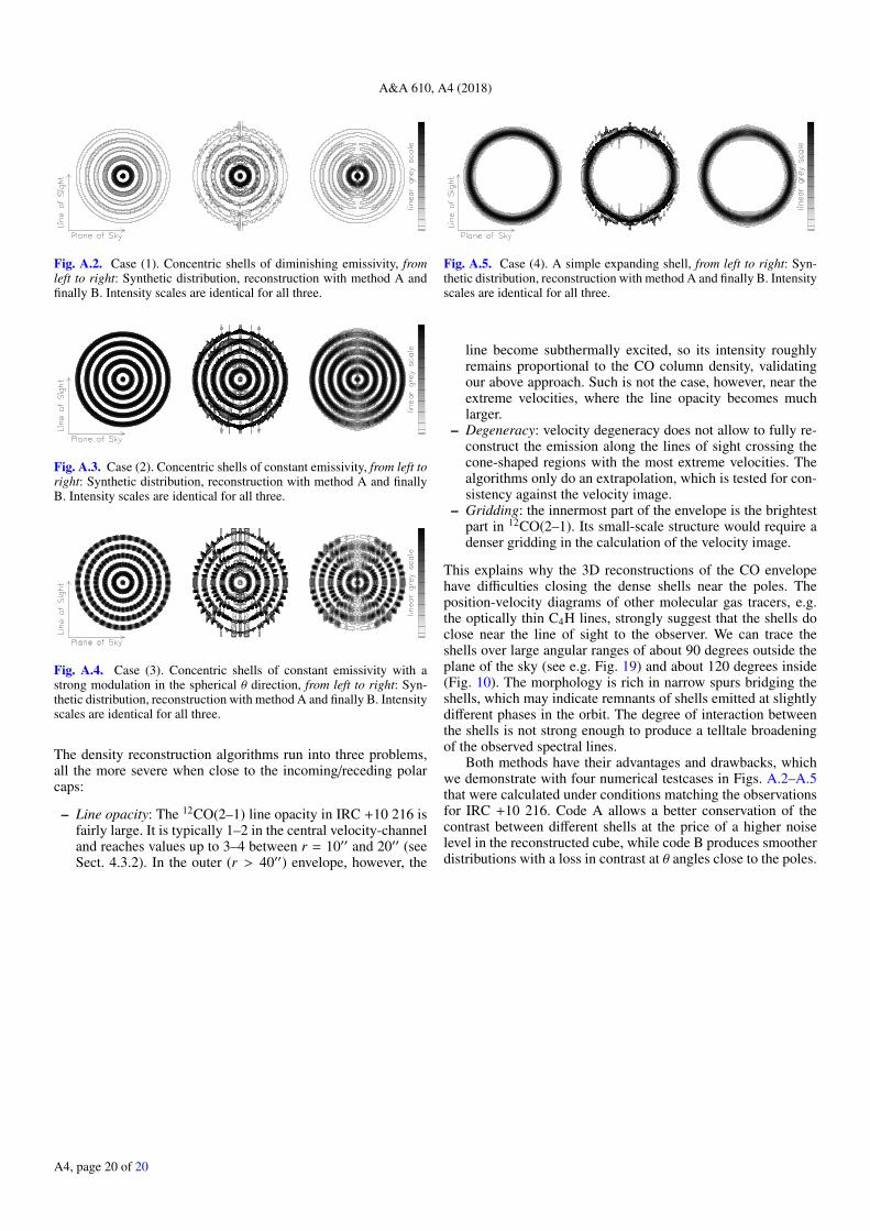
A&A 610, A4 (2018)

Fig. A.2. Case (1). Concentric shells of diminishing emissivity, fromleft to right: Synthetic distribution, reconstruction with method A andfinally B. Intensity scales are identical for all three.

Fig. A.3. Case (2). Concentric shells of constant emissivity, from left toright: Synthetic distribution, reconstruction with method A and finallyB. Intensity scales are identical for all three.

Fig. A.4. Case (3). Concentric shells of constant emissivity with astrong modulation in the spherical θ direction, from left to right: Syn-thetic distribution, reconstruction with method A and finally B. Intensityscales are identical for all three.

The density reconstruction algorithms run into three problems,all the more severe when close to the incoming/receding polarcaps:

– Line opacity: The 12CO(2–1) line opacity in IRC +10 216 isfairly large. It is typically 1–2 in the central velocity-channeland reaches values up to 3–4 between r = 10′′ and 20′′ (seeSect. 4.3.2). In the outer (r > 40′′) envelope, however, the

Fig. A.5. Case (4). A simple expanding shell, from left to right: Syn-thetic distribution, reconstruction with method A and finally B. Intensityscales are identical for all three.

line become subthermally excited, so its intensity roughlyremains proportional to the CO column density, validatingour above approach. Such is not the case, however, near theextreme velocities, where the line opacity becomes muchlarger.

– Degeneracy: velocity degeneracy does not allow to fully re-construct the emission along the lines of sight crossing thecone-shaped regions with the most extreme velocities. Thealgorithms only do an extrapolation, which is tested for con-sistency against the velocity image.

– Gridding: the innermost part of the envelope is the brightestpart in 12CO(2–1). Its small-scale structure would require adenser gridding in the calculation of the velocity image.

This explains why the 3D reconstructions of the CO envelopehave difficulties closing the dense shells near the poles. Theposition-velocity diagrams of other molecular gas tracers, e.g.the optically thin C4H lines, strongly suggest that the shells doclose near the line of sight to the observer. We can trace theshells over large angular ranges of about 90 degrees outside theplane of the sky (see e.g. Fig. 19) and about 120 degrees inside(Fig. 10). The morphology is rich in narrow spurs bridging theshells, which may indicate remnants of shells emitted at slightlydifferent phases in the orbit. The degree of interaction betweenthe shells is not strong enough to produce a telltale broadeningof the observed spectral lines.

Both methods have their advantages and drawbacks, whichwe demonstrate with four numerical testcases in Figs. A.2–A.5that were calculated under conditions matching the observationsfor IRC +10 216. Code A allows a better conservation of thecontrast between different shells at the price of a higher noiselevel in the reconstructed cube, while code B produces smootherdistributions with a loss in contrast at θ angles close to the poles.

A4, page 20 of 20