Ionomer Morphology, Solution to Film Thermodynamics ...

University of ConnecticutOpenCommons@UConn

Doctoral Dissertations University of Connecticut Graduate School

7-25-2014

Ionomer Morphology, Solution to FilmThermodynamics, Molecule Transport, PhysicalProperties, and Water Desalination viaElectrodialysisDonghui [email protected]

Follow this and additional works at: https://opencommons.uconn.edu/dissertations

Recommended CitationWang, Donghui, "Ionomer Morphology, Solution to Film Thermodynamics, Molecule Transport, Physical Properties, and WaterDesalination via Electrodialysis" (2014). Doctoral Dissertations. 496.https://opencommons.uconn.edu/dissertations/496

http://lib.uconn.edu/?utm_source=opencommons.uconn.edu%2Fdissertations%2F496&utm_medium=PDF&utm_campaign=PDFCoverPages

http://lib.uconn.edu/?utm_source=opencommons.uconn.edu%2Fdissertations%2F496&utm_medium=PDF&utm_campaign=PDFCoverPages

https://opencommons.uconn.edu?utm_source=opencommons.uconn.edu%2Fdissertations%2F496&utm_medium=PDF&utm_campaign=PDFCoverPages

https://opencommons.uconn.edu/dissertations?utm_source=opencommons.uconn.edu%2Fdissertations%2F496&utm_medium=PDF&utm_campaign=PDFCoverPages

https://opencommons.uconn.edu/gs?utm_source=opencommons.uconn.edu%2Fdissertations%2F496&utm_medium=PDF&utm_campaign=PDFCoverPages

https://opencommons.uconn.edu/dissertations?utm_source=opencommons.uconn.edu%2Fdissertations%2F496&utm_medium=PDF&utm_campaign=PDFCoverPages

https://opencommons.uconn.edu/dissertations/496?utm_source=opencommons.uconn.edu%2Fdissertations%2F496&utm_medium=PDF&utm_campaign=PDFCoverPages

1

Ionomer Morphology, Solution to Film Thermodynamics, Molecule

Transport, Physical Properties, and Water Desalination via Electrodialysis

Donghui Wang, PhD

University of Connecticut, [2014]

ABSTRACT

Of the different classes of separation polymers, ionomers are considered one of the most

advanced and versatile. They have been successfully utilized in various industrial fields,

including electrodialysis, electrolysis, diffusion dialysis, solid polymer electrolyte batteries,

sensing materials, medical use, and analytical chemistry.

In this study, an ionomer film series of penta block copolymer (PBC, poly(t-butyl styrene-b-

hydrogenated isoprene-b-sulfonated styrene-b-hydrogenated isoprene-b-t-butyl styrene) (tBS-

HI-S-HI-tBS)), sPP (sulfonated polyphenylene), aminated PPSU-TMPS block copolymer

(polyphenyl sulfone-tetramethyl polysulfone), and Nafion were investigated with respect to

thermodynamics, morphology, mechanical and transport properties.

First, the thermodynamic interrelationships between wettability, surface energy, solubility, and

swelling were studied in order to probe ionomer relationships between microscopic interactions

and macroscopic physical properties. Choosing an appropriate surface energy model and an

optimal solubility prediction method is an important role in the study of intrinsic and extrinsic

2

ionomer properties. Second, with the aim of improving ionomer film characteristics, various

casting solvents (tetrahydrofuran, chloroform, cyclohexane:heptane (C:H 1:1 wt%)),

temperature, and processing methodology were utilized. Material solubility parameters and

subsequent interactions between ionomer chains and solvent molecules define its

morphological growth and ultimate microstructures. This morphology has a great impact on the

distribution of functional groups, and transport properties of water and ions. As an example,

the proton conductivity of THF-cast PBC1.0 membrane (15.88 mS/cm) is significantly improved

over that of C:H-cast PBC1.0 membrane (1.09 mS/cm). Third, various ionomer pairs were used

to improve the water desalination via electrodialysis. Finally, my fourth area and future work is

mainly focused on the synthesis and characterization of aminated PPSU-TMPS block copolymers

in order to form a systematic understanding of the material’s properties that is critical for

industrial application and chemical engineering fields.

In conclusion, a comprehensive ionomer system has been set up to manufacture better

performance films with higher proton conductivity used in the fuel-cell industry, designed

materials with appropriate swelling properties that are vital to the electrodialysis desalination

process, neutralized cations for battery research, and other engineering applications.

3

Ionomer Morphology, Solution to Film

Thermodynamics, Molecule Transport, Physical

Properties, and Water Desalination via Electrodialysis

Donghui Wang

B.A., Dalian University of Technology, China [2010]

A Dissertation

Submitted in Partial Fulfillment of the

Requirements for the Degree of

Doctor of Philosophy

at the

University of Connecticut

[2014]

4

Copyright by

Donghui Wang

[2014]

5

APPROVAL PAGE

Doctor of Philosophy Dissertation

Ionomer Morphology, Solution to Film Thermodynamics,

Molecule Transport, Physical Properties, and Water Desalination via Electrodialysis

Presented by

Donghui Wang, B.A.

Major Advisor__________________________________________________________________

Chris J. Cornelius

Associate Advisor________________________________________________________________

Steven Suib


Yu Lei


Mu-Ping Nieh


William Mustain

University of Connecticut

[2014]

6

ACKNOWLEDGMENT

I would like to express my sincere gratitude to my advisor Prof. Cornelius for the continuous

support of my PhD study and research. He gave me the inspiration for instrument setup,

synthesis methodology, and project ideas. From ionomer properties investigation, novel anion

exchange membrane synthesis to various ionomer application, he provided me with a great

amount of opportunity to improve my abilities and enrich my experiences. Thank you from my

deep heart!

I would like to express thanks to my committee members as well. Prof. Suib and Prof. Nieh gave

me a lot of advice on polymer morphology related measurement and orientation influences on

polymer properties. Prof. Lei and Prof. Mustain helped a lot on transport properties of

membranes. Meanwhile, I would like to thank all of the professor and technicians of Chemical

Engineering Department at University of Connecticut and University of Nebraska-Lincoln, who

taught me skills and knowledge to help me complement my research.

I want to extend my thanks to Dr. Carl Willis at Kraton Polymer to provide us Pentablock

ionomers. Without his support of materials, I cannot fulfill my research work. Meanwhile, Prof.

Perahia at Clemson University helped us run SAXS measurement.

7

Additionally, I must thank my fellow group members and others who helped me complete my

research work in this dissertation. My labmate Yanfang Fan (Georgia Tech) helped my on

fundamental ionomer properties characterization. Fei Huang and Tim Largier helped me a lot

organized the lab and gave me support for my research.

Last but not the least, I would like to thank my family: my parents. They always gave me best

education opportunities and supported me to pursue my PhD abroad. Thank them for spiritual

support and encouragement for my studies. All of the loves and happiness from my family made

my doctorate process a success.

8

Table of Contents

Chapter 1 Introduction ........................................................ 14

1.1 Introduction .................................................................................................................... 14

1.2 Definition of Ionomer ..................................................................................................... 14

1.3 Development of Ionomers .............................................................................................. 15

1.4 Characteristics and Application of Ionomers .................................................................. 16

1.5 Research Objectives ........................................................................................................ 19

1.6 Significance and Originality ............................................................................................. 22

Chapter 2 Literature Review: Surface Energy, Solubility, and Water

Transport ............................................................................ 24

2.1 Wettability and Surface Energy of Ionomers .................................................................. 24

2.1.1 Contact Angle, Young’s Equation, and Surface Energy ........................................ 24

2.1.2 Ionomer Surface Energy Calculation Method ...................................................... 28

2.1.3 Roughness ............................................................................................................ 43

2.1.4 Interrelationship within Wettability, Surface Energy and Other Properties, and

Their Application and Development ............................................................................. 49

2.2 Solubility Properties and Swelling & Deswelling Phenomenon ...................................... 52

2.2.1 Swelling and Dissolving Phenomenon ................................................................. 52

2.2.2 Solubility Parameter ............................................................................................. 53

2.2.3 Solubility Parameter Indirect Calculation Method .............................................. 57

2.2.4 Water Self-Diffusion ............................................................................................. 65

2.2.5 Relationship between Solubility and Other Properties ....................................... 70

2.2.6 Development of Swelling Process and Transport Property ................................. 73

2.3 Summary ......................................................................................................................... 75

Chapter 3 Literature Review: Ionomer Morphology ............. 78

3.1 Dense, Porous, and Asymmetric Membranes ................................................................. 79

3.2 Crystalline and Amorphous Structure ............................................................................. 83

3.3 Factors Affecting the Formation of Microstructure ........................................................ 86

3.4 Phase Behavior ................................................................................................................ 88

3.5 Phase Separation of Ion Exchange Groups in Ionomers ................................................. 93

3.6 Development of Ionomer Morphology ........................................................................... 98

3.7 Summary ......................................................................................................................... 99

Chapter 4 Literature Review: Ionomer Transport Property .. 101

9

4.1 Ion Exchange Capacity and Water Content ................................................................... 101

4.2 Diffusion Coefficient of Liquid Molecule Transport and Activation Energy .................. 104

4.2.1 Fick’s Law ............................................................................................................ 104

4.2.2 Solution–diffusion Model .................................................................................. 105

4.2.3 Diffusion Coefficient Calculation ........................................................................ 106

4.2.4 Arrhenius Equation ............................................................................................ 106

4.3 Diffusion Coefficient of Ion Transport and Activation Energy ...................................... 107

4.3.1 Nernst-Einstein Relation .................................................................................... 107

4.3.2 Diffusion Coefficient Calculation ........................................................................ 107

4.3.3 Arrhenius Equation ............................................................................................ 108

4.4 Development of Molecules and Ions Transport ............................................................ 109

4.5 Summary ....................................................................................................................... 112

Chapter 5 Literature Review: Ionomer Mechanical Properties and

Degradation ....................................................................... 114

5.1 Glass Transition Temperature and Melting Temperature ............................................. 114

5.2 Temperature Dependence of the Moduli ..................................................................... 120

5.3 Elastic Quantities and Viscosity .................................................................................... 124

5.3.1 Rubber Elasticity ................................................................................................ 124

5.3.2 Viscoelasticity ..................................................................................................... 125

5.4 Deformation Properties ................................................................................................ 127

5.5 Thermal Degradation .................................................................................................... 132

5.6 Development of Mechanical Properties and Degradation ........................................... 135

5.7 Summary ....................................................................................................................... 136

Chapter 6 Literature Review: Anion Exchange Membranes .. 138

6.1 Cation and Anion Exchange Membranes ...................................................................... 138

6.2 Preparation of Anion Exchange Membranes ................................................................ 140

6.3 Characterization of Anion Exchange Membranes ......................................................... 142

6.3.1 Molecular Weight ............................................................................................... 142

6.3.2 Functional Groups .............................................................................................. 145

6.3.3 Ion Exchange Capacity and Hydroxyl Group Conductivity ................................. 146

6.3.4 Glass Transition Temperature ............................................................................ 147

6.3.5 Thermal Degradation Temperature ................................................................... 147

6.4 Development of Anion Exchange Membranes ............................................................. 148

6.5 Summary ....................................................................................................................... 150

Chapter 7 Literature Review: Electrodialysis ....................... 151

10

7.1 Electrodialysis Definition ............................................................................................... 151

7.2 Characteristics, Advantages and Limitations of Electrodialysis .................................... 151

7.3 Application of Electrodialysis Process ........................................................................... 157

7.4 Theory of ED Process .................................................................................................... 159

7.5 Limiting Current Density (LCD) ...................................................................................... 162

7.6 Nernst-Planck Equation ................................................................................................. 165

7.7 Two Methods to Calculate the Flux of Ions .................................................................. 166

7.8 Summary ....................................................................................................................... 168

Chapter 8 Materials and Methods ...................................... 169

8.1 Materials ....................................................................................................................... 169

8.1.1 Liquid and Other Material .................................................................................. 169

8.1.2 Polymers ............................................................................................................. 169

8.2 Experimental Method ................................................................................................... 175

8.2.1 Membrane Preparation ..................................................................................... 175

8.2.2 Contact Angle Measurement ............................................................................. 175

8.2.3 Water Diffusion Measurement .......................................................................... 177

8.2.4 Solubility Measurement ..................................................................................... 179

8.2.5 Morphology ........................................................................................................ 179

8.2.5.1 Transmission Electron Microscopy (TEM) ....................................................... 179

8.2.5.2 Small Angle X-ray Scattering (SAXS) ................................................................ 185

8.2.6 Fourier Transform Infrared Spectroscopy (FTIR) ................................................ 189

8.2.7 Ion Conductivity Measurement ......................................................................... 191

8.2.8 Molecules Diffusion Measurement.................................................................... 196

8.2.9 Dynamic Mechanical Analysis (DMA) ................................................................ 197

8.2.10 Thermal Gravimetric Analysis (TGA) ................................................................ 203

8.2.11 Electrodialysis (ED) ........................................................................................... 206

8.3 Summary ....................................................................................................................... 210

Chapter 9 Thermodynamic Interrelationship within Wettability,

Surface Energy, and Water Transport of Ionomers .............. 211

9.1 Introduction .................................................................................................................. 211

9.2 Experimental ................................................................................................................. 216

9.2.1 Material .............................................................................................................. 216

9.2.2 Membrane Preparation ..................................................................................... 216

9.2.3 Contact Angle Measurement ............................................................................. 217

9.2.4 Water Diffusion Measurement .......................................................................... 218

9.3 Results and Discussion .................................................................................................. 219

11

9.3.1 Wettability and Surface Energy of Ionomers ..................................................... 219

9.3.1.1 Contact Angle Measurement .......................................................................... 219

9.3.1.2 Optimal Surface Energy Calculation Method .................................................. 220

9.3.1.3 Relationship between Surface Energy and IEC ............................................... 223

9.3.1.4 Roughness ....................................................................................................... 226

9.3.1.5 Wetting Envelope ............................................................................................ 228

9.3.2 Water Transport in Ionomers ............................................................................. 230

9.3.2.1 Swelling and Deswelling Phenomenon ........................................................... 230

9.3.2.2 Swelling and Deswelling Ratios ....................................................................... 232

9.3.2.3 Water Diffusivity of Ionomers ......................................................................... 233

9.4 Conclusion ..................................................................................................................... 238

Chapter 10 Thermodynamic Interrelationship within Solubility,

Swelling, and Crosslink of Ionomers ................................... 239

10.1 Introduction ................................................................................................................ 239

10.2 Experimental ............................................................................................................... 243

10.2.1 Material ............................................................................................................ 243

10.2.2 Membrane Preparation ................................................................................... 243

10.2.3 Solubility Measurement ................................................................................... 244

10.2.4 Swelling Measurement .................................................................................... 244

10.3 Results and Discussion ................................................................................................ 245

10.3.1 Solubility Properties of Ionomers .................................................................... 245

10.3.1.1 Solubility Parameter from Direct Measurement .......................................... 245

10.3.1.2 Solubility Parameter Calculation Methods ................................................... 249

10.3.2 Solubility Parameters and Crosslink Number Achieved by Swelling Property . 261

10.3.2.1 Number of Crosslink Determined by Ionomer Swelling ............................... 261

10.3.2.2 Comparison between Chi Parameters from Hildebrand’s Theory and

Flory-Rehner Equation ................................................................................................ 262

10.3.2.3 Chemical Potential of Ionomer Swelling ....................................................... 265

10.3.2.4 Solubility Parameter and Dielectric Constant of PBCs .................................. 267

10.4 Conclusion ................................................................................................................... 272

Chapter 11 Morphology, Ion Transport, and Solution Thermodynamics

of a Penta Block Copolymer Ionomer .................................. 274

11.1 Introduction ................................................................................................................ 274

11.2 Experimental ............................................................................................................... 279

11.2.1 Material ............................................................................................................ 279

12


11.2.3 Transmission Electron Microscopy (TEM) ........................................................ 279

11.2.4 Small Angle X-ray Scattering (SAXS) ................................................................. 280

11.2.5 Conductivity Measurement ............................................................................. 280

11.2.6 Diffusivity Measurement ................................................................................. 281


11.3.1 Morphology of Ionomers ................................................................................. 282

11.3.2 Proton Conductivity Measurement ................................................................. 287

11.3.3 Diffusivity of Ionomers ..................................................................................... 295

11.3.3.1 Ion Diffusivity of PBCs and Nafion 117 ......................................................... 295

11.3.3.2 Fructose and ethanol liquid molecule diffusion through PBCs and Nafion 117

..................................................................................................................................... 300

11.4 Conclusion ................................................................................................................... 304

Chapter 12 Mechanical, Transport Properties and Degradation of

Solution-cast Penta Block Copolymers ................................ 306

12.1 Introduction ................................................................................................................ 306

12.2 Experimental ............................................................................................................... 309

12.2.1 Material ............................................................................................................ 309


12.2.3 Fourier Transform Infrared Spectroscopy (FTIR) .............................................. 310

12.2.4 Dynamic Mechanical Analysis (DMA) .............................................................. 310



12.3.1 Functional Groups of Ionomers ....................................................................... 311

12.3.2 Mechanical Properties ..................................................................................... 314

12.3.3 Thermal Degradation of Ionomers ................................................................... 322

12.4 Conclusion ................................................................................................................... 326

Chapter 13 Performances of electrodialysis process in desalination of

sodium chloride solution with various ionomer pairs .......... 328

13.1 Introduction ................................................................................................................ 328

13.2 Experimental ............................................................................................................... 330

13.2.1 Material ............................................................................................................ 330

13.2.2 Electrodialysis .................................................................................................. 330


13.3.1 Limiting Current Density .................................................................................. 331

13

13.3.2 Ion Flux ............................................................................................................. 333

13.3.3 Power Consumption and System Resistance ................................................... 336

13.3.4 Desalination Time ............................................................................................ 340

13.4 Conclusion ................................................................................................................... 341

Chapter 14 Further Work: Synthesis and Characterization of Aminated

PolyPhenylSulfone-TetraMethylPolySulfone (PPSU-TMPS) Block

Copolymer ......................................................................... 343

14.1 Introduction ................................................................................................................ 343

14.2 Experimental ............................................................................................................... 345

14.2.1 Material ............................................................................................................ 345

14.2.2 Anion Exchange Membrane Synthesis ............................................................. 345

14.2.3 Fourier Transform Infrared Spectroscopy (FTIR) .............................................. 346

14.2.4 Conductivity Measurement ............................................................................. 347

14.2.5 Dynamic Mechanical Analysis (DMA) .............................................................. 347



14.3.1 Self-Synthetic Anion Exchange Membrane ...................................................... 348

14.3.2 Functional Groups ............................................................................................ 354

14.3.3 Ion Conductivity ............................................................................................... 356

14.3.4 Glass Transition Temperature .......................................................................... 358

14.3.5 Thermal Degradation ....................................................................................... 360

14.4 Conclusion ................................................................................................................... 362

Chapter 15 Conclusion and Future Work ............................. 364

15.1 Wettability ................................................................................................................... 364

15.2 Solubility and Swelling Phenomenon ......................................................................... 364

15.3 Ion Transport ............................................................................................................... 364

15.4 Mechanical Properties ................................................................................................ 365

15.6 Electrodialysis Transport Phenomenon ...................................................................... 365

15.5 Anion Exchange Membrane ........................................................................................ 365

Chapter 16 Reference ......................................................... 366

Table of Figures .................................................................. 383

List of Tables ...................................................................... 394

14

Chapter 1 Introduction

1.1 Introduction

The utilization of different membrane classes to separate substances has grown into a wide

range of applications in industry and human life, including waste treatment, oil separation and

pharmaceutical industries, water treatment[1], fuel cell industry[2], gas separations[3] and

biofuels[4]. Compared with the traditional separation processes, membrane processes (like

pervaporation, membrane distillation, gas separation, facilitated transport, and microfiltration,

nanofiltration, ultrafiltration and reverse osmosis) save a great amount of energy and cost, and

require a smaller footprint. Of the different separation polymers, ionomer is considered the

most advanced and versatile. They have been successfully utilized in various industrial fields,

including electrodialysis, electrolysis, diffusion dialysis, solid polymer electrolyte of batteries,

sensing materials, medical use, and analytical chemistry.[5]

1.2 Definition of Ionomer

An ionomer is a polymer with electrically neutral repeating groups with a fraction of ionizable

units (usually no more than 15 percent).[5-6] Some commercial ionomer applications are golf ball

15

covers, semipermeable membranes, sealing tapes, and thermoplastic elastomers as showed in

Figure 1-1.

Figure 1-1 Some commercial products for ionomers.

1.3 Development of Ionomers

In 1850, H.P. Thompson[7] and J.T. Way[8] found the ion-exchange phenomenon of adsorption of

ammonium sulfate on soil (Ca-Soil + (NH4)2SO4 = 2NH4-Soil + CaSO4), which enlightened and

aroused interest in the study of ion exchange compositions and polymers. Afterwards, a study

by L. Michaelis[9] using a collodion (nitrocellulose) material as an ion permeable membranes

revealed that its charge affected ion permeation through it.

16

In 1943, the first charged membrane was prepared by I. Abrams and K. Sollner.[10] They prepared

modified collodion membranes by the adsorption of protamine (salmine) on porous collodion

films. Subsequently, Adams and Holmes[11] synthesized organic cation and anion exchange resins

by a condensation reaction using phenolic compounds having ionic groups and formaldehyde.

Afterward, D’ Alelio[12] developed poly-vinyl aryl ion-exchange resins, which were synthetic

polymer with sulfonated and aminated segments. Their findings and contribution laid the basis

of studies on electrochemical properties of the ion exchange membranes and resins.

Around 1950, numerous scientists Wyllie[13], and Juda and McRae[14] began to synthesize and

cast cation and anion exchange membranes. After these works, more active studies were mainly

focused on ion exchanging phenomena, synthetic methods, theory, and trials for industrial

application. Afterward, various applications emerged; predominately electrolysis[15],

desalination and electrodialysis[16]. In recent decades, Nafion® and XUS® (produced by DuPont

and Dow, respectively) diversify new and practical applications of ionomers, which are based on

the development of perfluorocarbon ionomers, and hydrocarbon block copolymers.

1.4 Characteristics and Application of Ionomers

The three main characteristics of ionomer membranes are ion conductivity, hydrophilicity, and

fixed carriers. Ion conductivity plays an important role in the electrodialysis (concentration and

17

desalination of electrolytes, separation between electrolyte and non-electrolyte, bipolar ion

exchange membrane process to produce acid and alkali, ion-exchange reaction across the

membrane, electro-deionization)[17], electrolysis (chlor-alkali production, organic synthesis)[18],

diffusion dialysis (acid or alkali recovery from waste), neutralization dialysis(desalination of

water)[19], Donnan dialysis (recovery of precious metals, softening of hard water,

preconcentration of a trace amount of metal ions for analysis)[20], up-hill transport (separation

and recovery of ions)[21], piezodialysis and thermo-dialysis (desalination or concentration)[22],

battery (alkali battery, redox-flow battery, concentration cell)[23], fuel cell (hydrogen-oxygen,

methanol-oxygen)[24], and actuator (catheter for medical use)[25]. Hydrophilicity is applied in the

field of pervaporation (dehydration of water miscible organic solvent), dehumidification

(dehumidification of air and gases), and sensor (gas sensor-humidity of CO, NO, O2, medical like

enzyme immobilization). Fixed carriers are focused on facilitated transport (removal of acidic

gas, separation of olefins form alkanes, separations of sugars) and modified electrodes[5, 26].

Figure 1-2 shows some commercial applications for ionomers.

18

Figure 1-2 Some commercial applications for ionomers.

Cylindrical lithium-ion battery

Ionomer Actuator

Neutralization Electrolysis (chlor-alkali production)

Diffusion Dialysis

Donnan Dialysis (ΔC is the driving force)

Up-hill transport

Pervaporation membrane

Sensor (pH sensitive membrane)

(Proton Exchange Membrane) PEM Fuel Cell

19

1.5 Research Objectives

Here are several questions that can be answered in our research work.

(1) Thermodynamic Interrelationship within Wettability, Surface Energy, and Water Transport

of Ionomers:

What are the interrelationships between ionomer wettability (hydrophobicity and

hydrophilicity), chemical structure, and ion-exchange capacity? How are water transport

phenomena described with respect to the relationship between microscopic interaction

(sulfuric acid groups and water molecules) and its macroscopic physical properties? What is

the optimal water diffusion model that can significantly define water self-diffusivity through

ionomer membranes?

(2) Thermodynamic Interrelationship within Solubility, Swelling, and Crosslink of Ionomers:

Ionomer’s solubility parameters can be obtained by direct measurement or indirect

calculation methods such as Hildebrand’s and Hansen’s theory. Which is the ideal one in

modeling ionomers’ solubility properties? How does the swelling process define the

relationship between microscopic interactions (number of cross-links within the network of

polymers and chemical potential of the mixing process) and macroscopic physical properties

of ionomers such as ion-exchange capacity, swelling ratio, and water uptake?

20

(3) Morphology, Ion Transport, and Solution Thermodynamics of a Penta Block Copolymer

Ionomer:

How do materials’ solubility parameters and subsequent interactions between ionomer

chains and solvent molecules define its morphology and the growth of different

microstructures? What is the impact of ionomer morphology on the distribution of

functional groups, and transport properties of water and ions? What are the optimal

conditions for solution-casting based upon solvent, temperature, and processing

methodology that will enhance morphology, and ion transport?

(4) Mechanical, Transport Properties and Degradation of Solution-cast Penta Block

Copolymers:

What are the interrelationships between glass transition temperature, ion-exchange

capacity, and casting solvents? Why does an ionomer present multiple glass transition

temperatures due to the variety of block segments? In the Dynamic Mechanical Analysis,

what is the effect of morphology and cross-link density (depend on casting solvents and

acid-form or salt-form ionomer) on the storage, loss modulus and phase angle of ionomers?

Based on the Thermal Gravimetric Analysis, what factors will affect an ionomer’s

degradation behavior?

21

(5) Synthesis and Characterization of Aminated PolyPhenylSulfone -TetraMethylPolySulfone

(PPSU-TMPS) Block Copolymer and Its Electrodialysis Application:

What are the advantage and innovation of synthetic anion exchange membranes

(quaternary ammonium) PPSU-TMPS (polyphenylsulfone-b-tetramethylpolysulfone) block

copolymer? Which parameters are significant to the synthesis of aminated PPSU-TMPS block?

What are the relationships between the molecular weight, block length, ion-exchange

capacity (intrinsic property), and ion conductivity (extrinsic or apparent property)? What

factors affect mechanical properties and thermal degradation?

(6) Performances of Electrodialysis Process in Desalination of Sodium Chloride Solution with

Various Ionomer Pairs:

How does flow rate, ionomer type (cation exchange membranes and anion exchange

membranes), driving force (current and voltage), and stream concentration (dilute and

concentrated) effect electrodialysis? What is the description of electrodialysis phenomena

using the Nernst-Planck equation? Compared with commercial sulfonate and aminated

polystyrene, how does solution-cast penta-block copolymer (PBC); aminated PPSU-TMPS

block copolymer, and sulfonated polyphenylene (sPP) enhance ion transport and improve

electrodialysis performance? These variables impact water desalination time, power usage,

and current efficiency.

22

1.6 Significance and Originality

This proposed research provides a deeper understanding of ionomer properties. These

properties are: wettability, swelling and dissolving properties, morphological microstructure,

and mechanical properties associated with chemical structure, ion exchange capacity, and the

molecule transport and diffusion through a series of ionomers. Moreover, synthesis and

characterization of aminated PPSU-TMPS will give a better understanding of morphology

development and its interrelation with intrinsic and extrinsic properties. Finally, the ionomer

performance of Nafion, PPSU-TMPS, sPP and PBC are studies within the electrodialysis process

and as a function of composition, flow rate, concentration of solution, electrical current, and

applied voltage.

The success of this project would result in several broad scientific impacts. Firstly, it will guide

scientists with the manufacture of novel materials with desirable properties. As an example,

advanced materials are designed with suitable hydrophilicity or hydrophobicity, morphology,

and transport properties by changing chemical structures and composition. Second, the data

and results will enrich the current knowledge of ionomer design and functional group

aggregation. Third, this research will influence the development of more than one research area

such as drug delivery, the fuel-cell industry, electrodialysis, biocompatible materials’ separation,

and desalination.

23

Distinctly different from other works, the ionomer wettability study describes the complex

relationship between wettability and factors such as ion-exchange capacity, chemical structure,

surface energy, and interfacial surface tension. Moreover, this research links swelling and

dissolving behavior with diffusivity and its solubility parameter. This study lists numerous

affecting parameters and describes them from a more comprehensive perspective. Except that,

a systematic understanding of ionomer materials’ transport, diffusion characteristics, and

mechanical properties associated with chemical structure, and ion-exchange capacity based

upon ionomer composition is still needed. More importantly, the synthesis and characterization

of aminated PPSU-TMPS membranes will contribute to research questions in this interesting

field. Last but not the least, controlling electrodialysis via engineered material will open new

avenues for understanding transport phenomenon, assisting in improving the industrial

electrodialysis, and optimizing the control parameters.

24

Chapter 2 Literature Review: Surface Energy, Solubility, and

Water Transport

2.1 Wettability and Surface Energy of Ionomers

Wettability is the ability of a liquid to keep contact with a solid surface due to intermolecular

interactions. Wetting exists within three phases: gas (usually air), liquid and solid. The degree of

wettability is determined by a force balance between adhesive forces (adhesion work between

liquid and solid surface) and cohesive forces (surface tension or surface energy of solid

material).

2.1.1 Contact Angle, Young’s Equation, and Surface Energy

Adhesive force exist between a kind of liquid and solid. It drags a liquid drop to spread across

this solid surface. Cohesive forces within the liquid maintain the drop to ball up and avoid

contact with the surface. The resultant between adhesive and cohesive forces determines the

contact angle, which is the angle at which the liquid-vapor interface meets the solid-liquid

interface. As the tendency of a drop spreading out over a flat, solid surface increases, the

contact angle decreases. Therefore, the contact angle provides an inverse measure of

wettability.

25

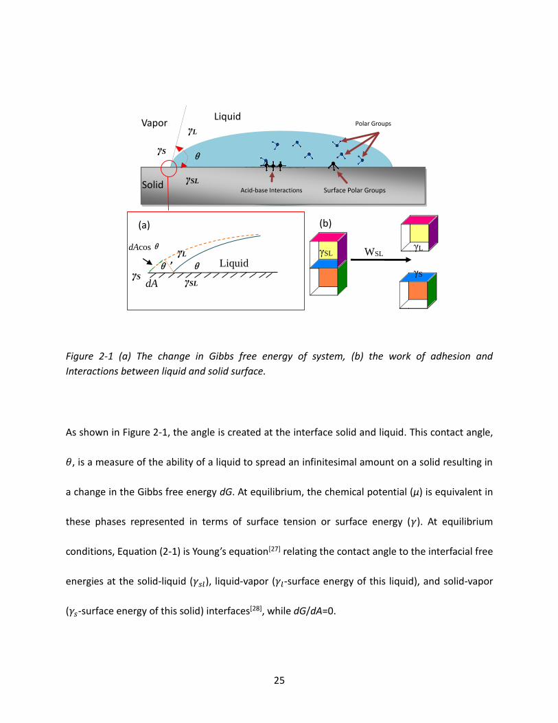
Figure 2-1 (a) The change in Gibbs free energy of system, (b) the work of adhesion and

Interactions between liquid and solid surface.

As shown in Figure 2-1, the angle is created at the interface solid and liquid. This contact angle,

𝜃, is a measure of the ability of a liquid to spread an infinitesimal amount on a solid resulting in

a change in the Gibbs free energy dG. At equilibrium, the chemical potential (μ) is equivalent in

these phases represented in terms of surface tension or surface energy (𝛾). At equilibrium

conditions, Equation (2-1) is Young’s equation[27] relating the contact angle to the interfacial free

energies at the solid-liquid (𝛾𝑠𝑙), liquid-vapor (𝛾𝑙-surface energy of this liquid), and solid-vapor

(𝛾𝑠-surface energy of this solid) interfaces[28], while dG/dA=0.

Vapor Liquid

Solid

θ

γSL

γL

γS

Liquid θ θ'

γL

γS γSL

dAcosθ

dA

γSL

γS

γL WSL

Polar Groups

Acid-base Interactions Surface Polar Groups

(a) (b)

26

𝑑𝐺

𝑑𝐴= 𝛾𝑠𝑙 − 𝛾𝑠 + 𝛾𝑙𝑐𝑜𝑠𝜃 = 0 (2-1)

Hydrophilic materials are characterized by a liquid (usually water) spreading over its surface and

forming an angle less than or equal to 90o. It indicates that wetting of the surface is very

favorable, and the fluid can spread over a large area of the surface. A material is considered

hydrophobic when its contact angle is between 90o and 180o. In other words, the wetting of this

surface is unfavorable so the fluid will minimize contact with the surface to form a compact

liquid droplet. Low surface energy materials such as polytetrafluoroethylene (PTFE, Teflon)

result in highly hydrophobic surfaces possessing water contact angles as high as 120°. Super

hydrophobic materials have contact angles greater than 150o, typically created from highly

rough or textured materials, showing almost no contact between the liquid drop and the

surface. This indicates the weak strength of solid/liquid interaction and strong strength of

liquid/liquid interaction as described in Table 2-1, referred to as the “lotus effect”.

27

Table 2-1 Relationship between various contact angles and their corresponding solid/liquid and

liquid/liquid interactions

Contact angle Degree of wetting Strength of

Solid/liquid

interactions

Liquid/liquid

interactions

𝜽 = 𝟎 Perfect wetting strong weak

𝟎 < 𝜽 < 𝟗𝟎𝒐 High wettability strong/weak strong/weak

𝟗𝟎𝒐 ≤ 𝜽 < 𝟏𝟖𝟎𝒐 Low wettability weak strong

𝜽 = 𝟏𝟖𝟎𝒐 Perfectly non-wetting weak strong

There are two main types of solid surfaces, dividing into the high-energy and low-energy solid

surface with which liquids can interact. The relative energy of a solid is close related to the bulk

nature of the solid itself. Traditionally, solids like metals, glasses, and ceramics are known as

‘hard solids’ because the chemical bonds that hold them together such as covalent, ionic, or

metallic chemical bonds are very strong. Thus, it takes a large input of energy to break these

solids so they are termed “high energy”. Most molecular liquids achieve complete wetting with

high-energy surfaces. The other type of solids is weak molecular crystals (e.g., fluorocarbons,

hydrocarbons, etc.) where the molecules are held together essentially by physical forces (e.g.,

van der Waals and hydrogen bonds). Since these solids are held together by weak forces it

would take a very low input of energy to break them, and thus, they are termed “low energy”.

28

Depending on the type of liquid chosen, low-energy surfaces can permit either complete or

partial wetting.

2.1.2 Ionomer Surface Energy Calculation Method

There are three methods of obtaining surface energy of materials. The first method is to

correlate Young’s Equation with different interfacial interaction models, such as Girifalco and

Good’s method[29], Fowkes’ method[30], Kwok and Neumann (Equation of State, EOS)[31], Owens

and Wendt[32], and Wu’s method[33]. Another way of achieving surface energy is based on the

assumption that the critical surface tension 𝛾𝑐𝑟 is equal to the surface tension 𝛾𝑠, as put forth

by Zisman (1964)[34]. The last method of extrapolating surface tension data is achieved when

polymer melts and is cooled down from high temperature to room temperature (a method for

the rapid measurement of the surface tension of very viscous liquids) according to Roe and

Wu[33]. And there is no direct way available to measure surface tension of solid polymer.

The first method implemented in the DSA (Drop Shape Analysis) program allows the

determination of the surface energy of solids from contact angle data. They are mainly based on

combining various 𝛾𝑠𝑙 starting equations with the Young’s Equation. In order to obtain

equations of state in which 𝑐𝑜𝑠𝜃 represents a function of the phase surface tensions, the polar

and disperse tension components are introduced. As in liquid surface tension data, polar and

29

disperse fractions are constants, it is possible to calculate the polar and disperse tension

components of solids from these equations. All methods assume that the interactions between

the solid and the gas phase (or the liquid vapor phase) are so small as to be negligible. The

methods are described in the following section.

Girifalco and Good’s method

The work of adhesion between two incompatible substances shown in Figure 2-1 (b) is

described as the following Equation (2-2).

𝑊𝑎 = 𝑊12 = 𝛾1 + 𝛾2 − 𝛾12 (2-2)

The work of adhesion can also be expressed by the geometric mean of the surface tensions

(Equation (2-5)) proposed by Girifalco and Good[29].

𝑊𝑎 = 2𝜙(𝛾𝑠𝛾𝑙)1

2 (2-3)

where 𝜙 is the Interaction parameter, as a complex function of molecular quantities, and

initially could only be determined empirically.

30

Combining Equation (2-2) and (2-3), Girifalco and Good method’s[29] Equation (2-4) can be

accomplished. However, it is only valid for substances with additive disperse forces and without

considering hydrogen bonds.

𝛾𝑠𝑙 = 𝛾𝑠 + 𝛾𝑙 − 2𝜙(𝛾𝑠𝛾𝑙)1

2 (2-4)

where the interaction parameter is empirically equal to 4（𝑉𝑠𝑉𝑙）

13

(𝑉𝑠

13+𝑉𝑙

13)2

, (𝑉𝑠 is the molar volume of

solid, 𝑉𝑙 is the molar volume of liquid), 0.5 < 𝜙 < 1.15. Since 𝜙 ≈ 1 for most polymers,

𝛾𝑠𝑙 ≈ (𝛾𝑙

1

2 − 𝛾𝑠1

2)2.

Fowkes’ method

Soon afterwards, Fowkes[30] put forward two fundamental assumptions, that surface tension of

solid can be described as the addition and the geometric mean form. It is to suggest that total

free energy at a surface is the sum of contributions from the different intermolecular forces at

the surface as represented in Equation (2-5).

𝛾 = 𝛾𝑑 + 𝛾𝑝 + 𝛾ℎ + 𝛾𝑖 + 𝛾𝑎𝑏 + ⋯ (2-5)

where d = dispersion force, p = polar force, h = hydrogen bonding force, i = induction force, ab =

acid/base force and etc.

31

Interactions between liquid and solid surface are shown in Figure 2-1. Surface energy is mainly

composed of dispersion (non-polar) and polar energy. The dispersion part of surface energy

results from non-polar interaction of molecules while the polar component is caused by the

interactions between polar groups. Coulomb interactions of polar groups include dipole-dipole

interaction, dipole-induced dipole interaction, and acid-base interactions (including hydrogen

bonding). The dispersion energy exists between all molecules, but the polar part is only

presented with polar groups.

According to the Fowkes’ method, the polar and disperse fractions of the surface free energy of

a solid are illustrated in Equation (2-6).

𝛾𝑠𝑙 = 𝛾𝑠 + 𝛾𝑙 − 2(𝛾𝑠𝑑𝛾𝑙

𝑑)1

2 (2-6)

where γsd and γl

d represent the disperse fraction of surface energy of a solid and a kind of

liquid, respectively.

In the Fowkes’ model, the polar and disperse fractions are determined in succession, i.e. in two

step. In the first step the disperse fraction of the surface energy of the solid is calculated by

making contact angle measurement with at least on purely disperse liquid. By combination of

32

Fowkes’ Equation (Equation (2-6)) with Young’ Equation (Equation (2-1)), the following Equation

(2-7) for the contact angle is obtained after transposition:

𝑐𝑜𝑠𝜃 = 2√𝛾𝑠𝑑 ×

1

√𝛾𝑙𝑑− 1 (2-7)

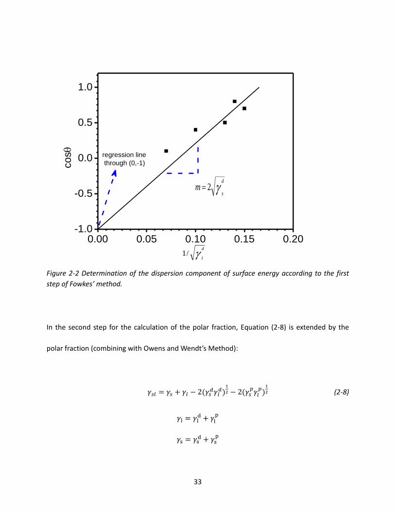
Based upon the general equation for a straight line (𝑦 = 𝑚𝑥 + 𝑏), 𝑐𝑜𝑠𝜃 is then plotted against

the term 1

√𝛾𝑙𝑑 , and 2√𝛾𝑠

𝑑 can be determined from the slope m as demonstrated in Figure 2-2.

The straight line must intercept the ordinate at the point defined as (0,-1). As this point has

been defined, it is possible to determine the disperse fraction from a single contact angle. And a

linear regression with several purely disperse liquids is more accurate.

33

0.00 0.05 0.10 0.15 0.20-1.0

-0.5

0.0

0.5

1.0

d

sm 2

co

s

d

l/1

regression line

through (0,-1)

Figure 2-2 Determination of the dispersion component of surface energy according to the first

step of Fowkes’ method.

In the second step for the calculation of the polar fraction, Equation (2-8) is extended by the

polar fraction (combining with Owens and Wendt’s Method):


𝑑)1

2 − 2(𝛾𝑠𝑝𝛾𝑙

𝑝)1

2 (2-8)

𝛾l = 𝛾ld + 𝛾l

p

𝛾s = 𝛾sd + 𝛾s

p

34

In this case, a single liquid with polar and disperse fractions would be sufficient, although the

results would again be less reliable.

It is assumed that the work of adhesion can also be described by the addition of the polar and

disperse fractions as Equation (2-9).

𝑊𝑠𝑙 = 𝑊𝑠𝑙𝑑 + 𝑊𝑠𝑙

𝑝 (2-9)

Combining Equation (2-1), (2-2) and (2-8),

𝑊𝑠𝑙 = 𝛾𝑠 + 𝛾𝑙 − 𝛾𝑠𝑙 = 𝛾𝑙(𝑐𝑜𝑠𝜃 + 1) = 2(𝛾𝑠𝑑𝛾𝑙

𝑑)1

2 + 2(𝛾𝑠𝑝𝛾𝑙

𝑝)1

2 (2-10)

Therefore, the polar fraction of the adhesion work is defined by the geometric mean of the

polar fractions of the particular surface tensions as Equation (2-11).

𝑊𝑠𝑙𝑝 = 2(𝛾𝑠

𝑝𝛾𝑙𝑝)

1

2 = 𝛾𝑙(𝑐𝑜𝑠𝜃 + 1) − 2(𝛾𝑠𝑑𝛾𝑙

𝑑)1

2 = √𝛾𝑠𝑝 × 2√𝛾𝑙

𝑝 (2-11)

35

Then, by plotting 𝛾l(𝑐𝑜𝑠𝜃 + 1) − 2(𝛾𝑠𝑑𝛾𝑙

𝑑)1

2 against 2√𝛾𝑙𝑝 and following this with a linear

regression, the polar fraction of the solid’s surface energy can be determined from the slope. As

in this case the ordinate intercept b is 0, the regression curve must pass through the origin (0,0).

0 5 100

5

10

15

20

p

sm 2

W p sl

p

l2

regression line

through origin

Figure 2-3 Determination of the polar surface energy according to the second step of Fowkes’

method.

36

Kwok and Neumann’s method

Kwok and Neumann (K&N)[31] argue for using an analytical expression (𝜙 in Equation (2-4)).

Their expression is as the following Equation (2-12).

𝜙 = 𝑒𝑥𝑝[−𝛽(𝛾𝑠 − 𝛾𝑙)2] (2-12)

It is easily seen that if 𝛾𝑠 = 𝛾𝑙, and then 𝜙 = 1. The magnitude of 𝛽 is therefore crucial in

giving a universally correct work of adhesion, if such an expression is possible. K&N have

determined this experimentally from an extensive amount of measurements of low energy

polymer surfaces. They found 𝛽 = 0.0001247(𝑚2/𝑚𝐽)2 giving the best all-over results,

although it varied up to a certain extent.

Therefore, by using an enormous volume of contact angle data the required equation of state

was determined as following Equation (2-13).

𝛾𝑠𝑙 = 𝛾𝑠 + 𝛾𝑙 − 2(𝛾𝑠𝛾𝑙)1

2 × 𝑒𝑥𝑝[−0.0001247(𝛾𝑠 − 𝛾𝑙)2] (2-13)

If the equation of state is inserted in Young’s Equation (2-1) then the new Equation (2-14) is

obtained, allowing the calculation of the surface tension of the solid 𝛾𝑠 from a single contact

angle if the surface tension of liquid 𝛾𝑙 is known.

37

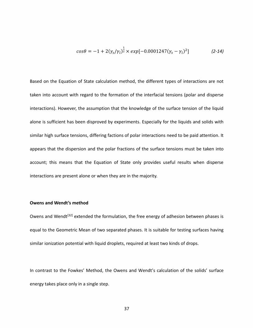
𝑐𝑜𝑠𝜃 = −1 + 2(𝛾𝑠/𝛾𝑙)1

2 × 𝑒𝑥𝑝[−0.0001247(𝛾𝑠 − 𝛾𝑙)2] (2-14)

Based on the Equation of State calculation method, the different types of interactions are not

taken into account with regard to the formation of the interfacial tensions (polar and disperse

interactions). However, the assumption that the knowledge of the surface tension of the liquid

alone is sufficient has been disproved by experiments. Especially for the liquids and solids with

similar high surface tensions, differing factions of polar interactions need to be paid attention. It

appears that the dispersion and the polar fractions of the surface tensions must be taken into

account; this means that the Equation of State only provides useful results when disperse

interactions are present alone or when they are in the majority.

Owens and Wendt’s method

Owens and Wendt[32] extended the formulation, the free energy of adhesion between phases is

equal to the Geometric Mean of two separated phases. It is suitable for testing surfaces having

similar ionization potential with liquid droplets, required at least two kinds of drops.

In contrast to the Fowkes’ Method, the Owens and Wendt’s calculation of the solids’ surface

energy takes place only in a single step.

38

Owens and Wendt took Equation (2-8) for the surface tension as their base and combined it

with Young’s Equation (2-1).


𝑑)1

2 − 2(𝛾𝑠𝑝𝛾𝑙

𝑝)1

2 (2-8)

𝛾l = 𝛾ld + 𝛾l

p


p

These two authors solved the equation system by substituting the contact angle of two liquids

with known disperse and polar fractions of the surface tension into. Moreover, Kaelble[35]

solved the equation for combinations of two liquids and calculated the mean values of the

resulting values for the surface energy. Rabel[36] made it possible to calculate the polar and

dispersion fractions of the surface energy with the aid of a single linear regression from the

contact angle data of various liquids. He combined Equation (2-1) and (2-8) and adapted the

resulting equation by transposition to the general equation for a straight line (𝑦 = 𝑚𝑥 + 𝑏).

This equation is shown as Equation (2-15).

(1+𝑐𝑜𝑠𝜃)𝛾𝑙

2√𝛾𝑙𝑑

= √𝛾𝑠𝑝√

𝛾𝑙𝑝

𝛾𝑙𝑑 + √𝛾𝑠

𝑑 (2-15)

39

In a linear regression of the plot of y against x, 𝛾𝑠𝑝 is obtained from the square of the slope of

the curve m and 𝛾𝑠𝑑 from the square of the ordinate intercept b as illustrated in Figure 2-4.

0 2 4 6 80

5

10

15

d

l

p

l /

d

sb

p

sm 2

Figure 2-4 Determination of the dispersion and the polar fractions of the surface tension of a

solid according to Rabel’s calculation.

Wu’s method

Wu’s Method [33] requires at least two kinds of drops with different surface tensions, and at

least one of the liquids must have a polar fraction larger than 0. Free energy of adhesion

40

between phases is equal to the Harmonic Mean of two separated phases. In this way, he

achieved more accurate results for high-energy systems.

Wu’s initial equation for the interfacial tension between a liquid and a solid phase is as

following Equation (2-16), i represents the number of test liquid in sequence.

𝛾𝑠𝑙 = 𝛾𝑠 + 𝛾𝑖 − 4 [𝛾𝑖𝑑𝛾𝑠

𝑑

𝛾𝑖𝑑+𝛾𝑠

𝑑 +𝛾𝑖𝑝𝛾𝑠𝑝

𝛾𝑖𝑝+𝛾𝑠

𝑝] , 𝑖 = 1,2 (2-16)

𝛾i = 𝛾id + 𝛾i

p


p

If Young’ Equation (2-1) is inserted into Equation (2-16), then the following Equation (2-17) is

available.

(1 + 𝑐𝑜𝑠𝜃)𝛾𝑖 − 4 [𝛾𝑖𝑑𝛾𝑠

𝑑

𝛾𝑖𝑑+𝛾𝑠

𝑑 +𝛾𝑖𝑝𝛾𝑠𝑝

𝛾𝑖𝑝+𝛾𝑠

𝑝] = 0, 𝑖 = 1,2 (2-17)

In order to achieve the two required quantities 𝛾𝑠𝑑 and 𝛾𝑠

𝑝, Wu determined the contact angles

for each of two liquids on the solid surface and drew up an equation for each liquid based on

Equation (2-17). After the factor analysis the resulting Equation (2-18) was as follows.

41

(𝑏𝑖 + 𝑐𝑖 − 𝑎𝑖)𝛾𝑠𝑑𝛾𝑠

𝑝 + 𝑐𝑖(𝑏𝑖 − 𝑎𝑖)𝛾𝑠𝑑 + 𝑏𝑖(𝑐𝑖 − 𝑎𝑖)𝛾𝑠

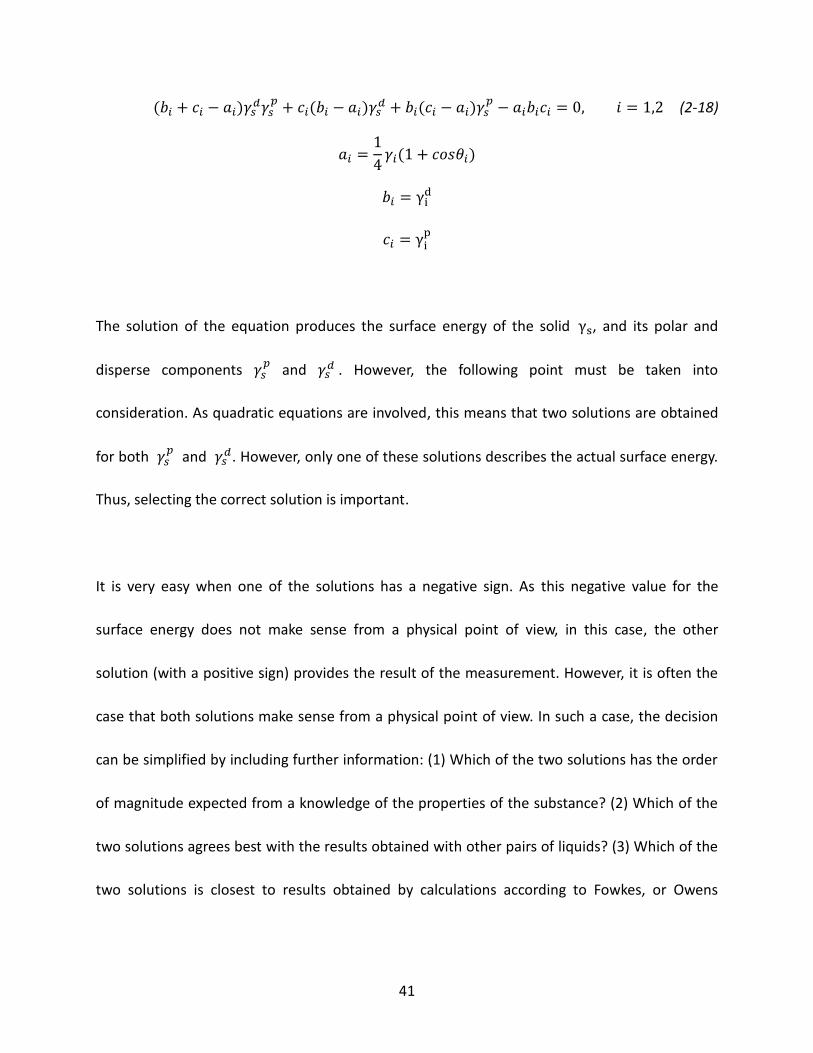
𝑝 − 𝑎𝑖𝑏𝑖𝑐𝑖 = 0, 𝑖 = 1,2 (2-18)

𝑎𝑖 =1

4𝛾𝑖(1 + 𝑐𝑜𝑠𝜃𝑖)

𝑏𝑖 = γid

𝑐𝑖 = γip

The solution of the equation produces the surface energy of the solid γs, and its polar and

disperse components 𝛾𝑠𝑝 and 𝛾𝑠

𝑑 . However, the following point must be taken into

consideration. As quadratic equations are involved, this means that two solutions are obtained

for both 𝛾𝑠𝑝 and 𝛾𝑠

𝑑. However, only one of these solutions describes the actual surface energy.

Thus, selecting the correct solution is important.

It is very easy when one of the solutions has a negative sign. As this negative value for the

surface energy does not make sense from a physical point of view, in this case, the other

solution (with a positive sign) provides the result of the measurement. However, it is often the

case that both solutions make sense from a physical point of view. In such a case, the decision

can be simplified by including further information: (1) Which of the two solutions has the order

of magnitude expected from a knowledge of the properties of the substance? (2) Which of the

two solutions agrees best with the results obtained with other pairs of liquids? (3) Which of the

two solutions is closest to results obtained by calculations according to Fowkes, or Owens

42

&Wendt’s method? In the measurement with more than two liquids, the final determination of

the surface energy is the arithmetic mean of the selected parts.

Zisman’s method

According to Zisman’s assumption[34], the critical surface tension 𝛾𝑐𝑟 is equal to the surface

tension 𝛾𝑠. Free energy of adhesion is equal to the projection of surface tension of drop at a

testing surface. It assumes that the interaction between the liquid drop and the testing surface

is greater than the internal force of drop (low contact angle, i.e. less than 75o). Additionally, the

energy of the interaction is negligible as compared to testing surface energy. Hence, it is

suitable for low contact angle surfaces. Nevertheless, two problems arise in Zisman Plot. One is

that the data line is not really straight, and the other is that the critical surface tension 𝛾𝑐𝑟 is

not exactly same as the surface tension 𝛾𝑠 (only if 𝛾𝑠𝑙 = 0 when 𝜙 = 1) .

43

Figure 2-5 The combination of three different methods with Young’s Equation used in this study

in order to investigate surface energy of solid.

Within all these different combinations mentioned above, three calculation methods are

selected to achieve the polymers’ surface energy in this paper. They are Kwok and Neumann’s

equation, Owens and Wendt’s method, and Wu’s calculation as details shown in Figure 2-5.

2.1.3 Roughness

Unlike ideal surfaces, real surfaces do not have perfect smoothness, rigidity, or chemical

homogeneity, resulting in phenomena called contact-angle hysteresis. It is defined as the

Kwok and Neumann’s

method (K&N)

(𝜙 = exp[−𝛽(𝛾𝑠 − 𝛾𝑙)2])

Low energy polymer

surfaces without polar

part.

Owens and Wendt’s method

(O&W)

(geometric mean)

The combination of

dispersion and polar part.

Wu’s method

(harmonic mean)

The combination of

dispersion and polar part.

High energy surface.

𝛾𝑠𝑙 = 𝛾𝑠 + 𝛾𝑙 − 2𝜙(𝛾𝑠𝛾𝑙)12


𝑑)12 − 2(𝛾𝑠

𝑝𝛾𝑙

𝑝)12

𝛾𝑠𝑙 = 𝛾𝑠 + 𝛾𝑙 − 4 𝛾i

d𝛾sd

𝛾id + 𝛾s

d+

𝛾ip𝛾s

p

𝛾ip+ 𝛾s

p

Young’s Equation:

𝛾𝑠𝑙 − 𝛾𝑠 + 𝛾𝑙𝑐𝑜𝑠𝜃 = 0

44

difference between the advancing (𝜃𝑎) and receding (𝜃𝑟) contact angles[37] as presented in

Equation (2-19).

𝐻 = 𝜃𝑎 − 𝜃𝑟 (2-19)

Contact angle hysteresis is essentially the displacement of a contact line by either expansion or

retraction of the droplet as depicted in Figure 2-6 (a). The advancing and receding contact angle

can also be measured through tilting base method, representing the maximum and the

minimum stable angle as demonstrated in Figure 2-6 (b).

Figure 2-6 Schematic of two methods capturing advancing and receding contact angles.

𝜃𝑎 𝜃𝑟

advancing angle receding angle

(a)

𝜃𝑎 𝜃𝑟

t

(b)

tilting base method

45

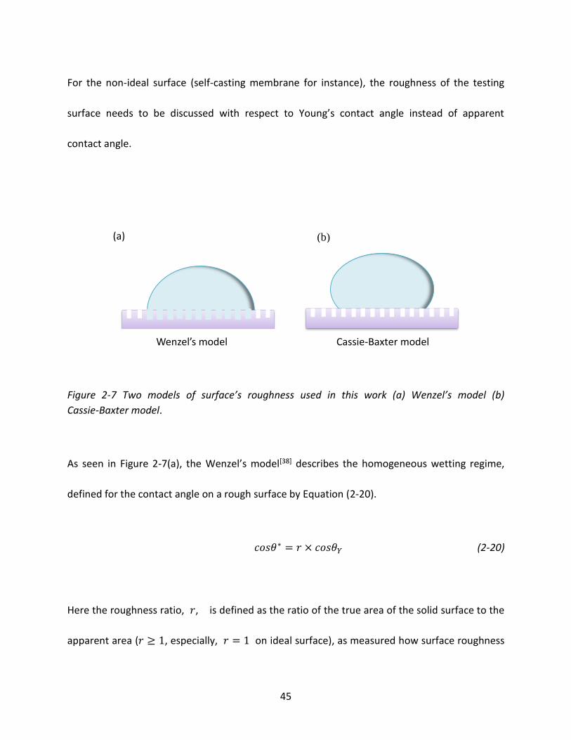
For the non-ideal surface (self-casting membrane for instance), the roughness of the testing

surface needs to be discussed with respect to Young’s contact angle instead of apparent

contact angle.

Figure 2-7 Two models of surface’s roughness used in this work (a) Wenzel’s model (b)

Cassie-Baxter model.

As seen in Figure 2-7(a), the Wenzel’s model[38] describes the homogeneous wetting regime,

defined for the contact angle on a rough surface by Equation (2-20).

𝑐𝑜𝑠𝜃∗ = 𝑟 × 𝑐𝑜𝑠𝜃𝑌 (2-20)

Here the roughness ratio, 𝑟, is defined as the ratio of the true area of the solid surface to the

apparent area (𝑟 ≥ 1, especially, 𝑟 = 1 on ideal surface), as measured how surface roughness

(a) (b)

Cassie-Baxter model Wenzel’s model

46

affects a homogeneous surface. While the apparent contact angle 𝜃∗ is corresponding to the

stable equilibrium state (i.e. minimum free energy for the non-ideal system), 𝜃𝑌 is Young

contact angle as defined for an ideal surface. Although Wenzel’s equation demonstrates that

the contact angle formed on a rough surface is different from the intrinsic contact angle

(Young’s contact angle), it does not describe the phenomena of contact angle hysteresis.

When handling with a heterogeneous surface, a more complex model is introduced to take

place of Wenzel’s one. In the case of the Cassie-Baxter model[39], the drop sits on top of the

textured surface with trapped air underneath, as depicted in Figure 2-7 (b). In order to measure

how the apparent contact angle changes when various materials are involved, the Cassie-Baxter

model is utilized to explain the heterogeneous surface as Equation (2-21).

𝑐𝑜𝑠𝜃∗ = 𝑟𝑓 × 𝑓 × 𝑐𝑜𝑠𝜃𝑌 + 𝑓 − 1 (2-21)

Here rf is the roughness ratio of the wet surface area and f is the fraction of solid surface area

wet by the liquid (𝑓 ≤ 1, special case is 𝑓 = 1 when rf = 𝑟, the Cassie–Baxter equations

becomes the Wenzel equation), θ∗ is apparent contact angle (measured) and θY is Young’s

contact angle (ideal surface).

47

Figure 2-8 Two states during the wetting transition from the Cassie state to Wenzel state (a)

mushroom state, (b) penetration front spreads beyond drop.

During the wetting transition from the Cassie state to Wenzel state, the air pockets are no

longer thermodynamically stable and liquid begins to nucleate from the middle of the drop,

creating a “mushroom state” as seen in Figure 2-8 (a). The penetration condition is given by the

following Equation (2-22).

𝑐𝑜𝑠𝜃𝑐 =𝑓−1

𝑟−𝑓 (2-22)

where θc is the critical contact angle, f is the fraction of solid/liquid interface where is in

contact with surface (𝑓 ≤ 1), and r is solid roughness (𝑟 ≥ 1).

The penetration front propagates to minimize the surface energy until it reaches the edges of

the drop, thus arriving at the Wenzel state. If the solid can be considered an absorptive material,

the phenomenon of spreading and imbibition occurs when the contact angles are in the range

Mushroom state

(a) (b)

Surface film state

48

0 ≤ 𝜃 < 90𝑜. Thus, the Wenzel model is only valid between 𝜃𝑐 < 𝜃 < 90𝑜. If the contact angle

is less than the critical contact angle, the penetration front spreads beyond the drop and a

liquid from forms over the surface as illustrated in Figure 2-8 (b). In this surface film state, the

equilibrium condition and Young’s relation yield the following Equation (2-23).

𝑐𝑜𝑠𝜃∗ = 𝑓𝑐𝑜𝑠𝜃𝑐 + (1 − 𝑓) (2-23)

By fine-tuning the surface roughness, it is possible to achieve a transition between both super

hydrophobic and super hydrophilic regions. Generally, the rougher the surface, the more

hydrophobic it is.

Wettability of various solid polymembranes is a function of polymer composition, surface

topology, surface roughness and chemical structure. The focus of this work is to probe these

material complexities in order to gain scientific insight associated with the surface wettability of

different polymers. Insight gained by this area may contribute to the usage of polymers in

different areas with controlled wetting and improved mass transferring.

49

2.1.4 Interrelationship within Wettability, Surface Energy and Other

Properties, and Their Application and Development

Nature’s self-cleaning properties of the lotus leaf are due to super hydrophobic properties

created from its complex surface features and compositions. These intriguing properties have

inspired the science and engineering of structured surfaces and materials in order to control

hydrophobicity and hydrophilicity.

Due to the absence of surface mobility, solid surface tension is very difficult to measure directly

compared with liquid surface tension.[40] Thus, as an important factor influencing wettability,

solid surface tensions can be estimated through several independent approaches, including

direct force measurements[41], contact angles[29-31, 33-34, 42], capillary penetration into columns of

particle powder[43], sedimentation of particles[44], solidification front interactions with

particles[45], film flotation[46], gradient theory[47], the Lifshitz theory of van der Waals’ forces[48],

and the theory of molecular interactions[49]. Among the available techniques of studying

polymer interfaces, contact angle measurement by probing liquid drop on the testing surface is

an easy method to obtain solid surface energy with the smallest fingerprint 0.1 nm depth and

1000 nm width.[50]

50

An overview of the relevant and important theories was provided by Gennes[51] in 1985

including contact angle, wetting transition, and the dynamics of spreading. Subsequently,

combining Young’s Equation, Shimizu[52] examined several surface energy calculation models,

including Neumann’s equation, Fowkes’ equation, the geometric mean equation, and the

harmonic mean equation. He measured contact angles formed by drops of several kinds of

testing liquid on a polypropylene film, on polystyrene plates, and on a liquid crystalline polymer

plate at 20oC. In addition, Geoghegan[53] reviewed the research progresses in the past few years,

including the influence of a boundary in polymer blends and the growth of wetting layers. He

summarized work over the same period concerning the dewetting of polymer films, along with

a discussion of the role of pattern formation caused by dewetting and topographically and

chemically patterned substrates.

There are several factors influencing the wettability of polymer. From the morphology and

application point of view, Fasolka and Mayes[54] emphasized the role of film thickness and

surface energetics on the morphology of compositionally symmetric, amorphous diblock

copolymer films, considering boundary condition symmetry and surface chemical expression.

Except that, in the second section, they discussed technological applications of block copolymer

films, for example, lithographic masks and photonic materials. Moreover, the surface

topography and chemical compositions of polymers influence surface energy from the

perspective of macro- and microstructures, respectively.[55] Andruzzi[56] evaluated the effect of

51

the chemical structures and compositions on wetting properties of anionically formed

polystyrene-block-polyisoprene block copolymers. These polymers are achieved by

2,2,6,6-tetramethylpiperidin-1-yloxy radical (TEMPO)-mediated controlled radical

polymerization of fluorinated styrene monomers and a sequence of polymer modification

reactions. Afterwards, more works were focused on the polymer design in order to optimize

polymer properties. Tsibouklis[57] met the molecular design requirements to fabricate accessible

film structures with ultra-low surface energy characteristics. Apart from that, Wang[58] showed

that patterned poly(dimethylsiloxane) PDMS stamp was capable of modifying the wettability of

poly(3,4-ethylenedi-oxythiophene)-poly(styrenesulfonate) (PEDOT-PSS) and polyelectrolyte

poly(sodium 4-styrenesulfonate) (NaPSS) surface. Furthermore, more characteristics of polymer

are involved in the network of wettability and surface energy. For instance, Kanakasabai[59]

recently studied the ion exchange capacity, the proton conductivity, and the water sorption

characteristics of crosslinked polyvinyl alcohol (PVA-SSA) and sulfonated poly(ether ether

ketone) (SPEEK). He further linked them with the surface energy and wettability characteristics

of these membranes.

The knowledge of these fundamental surface properties provides researchers with the scientific

guidelines of controlling a material’s surface wetting properties for biological, electronic,

mechanical, and chemical applications[60]. Furthermore, materials’ surfaces and compositions

can be selectively tailored to control hydrophobicity for inhibiting metal corrosion. Except that,

52

such practices provide surface protection from chemical agents, minimize biological fouling of

marine vehicle surfaces, and optimize the wetting of gas diffusion layers in fuel cells.

2.2 Solubility Properties and Swelling & Deswelling

Phenomenon

2.2.1 Swelling and Dissolving Phenomenon

When a polymer is immerged in a certain solvent, the solvent molecules slowly diffuse into the

polymer. Thus, the swelling of the polymer can take place. And the crosslinked networks,

including ionic, covalent and physical crosslinks (hydrogen bonding), and crystallinity enhance

the polymer–polymer intermolecular forces as formed a swollen gel. If the strong polymer–

solvent interactions can balance and overcome these forces, chains of the polymer disentangle

after time has passed (an induction time). Hence, as a second stage, the dissolving behavior of

the polymer by solvent can be demonstrated[61]. The structures of the surface layers of glassy

polymers during dissolution from the pure polymer to the pure solvent are as follows: the

infiltration layer, the solid swollen layer, the gel layer, and the liquid layer[62] as showed in Figure

2-9.

53

Figure 2-9 Schematic picture of the composition of the surface layer.

In the point view of energy balance, the process of swelling is actually led by the repulsive and

attractive forces. These driving forces come from the thermodynamic mixing interactions

between the polymer and the solvent, the interactions between fixed charged groups and free

ions in ionomers, the elastic force of the polymer, and also the inter-chain attractive forces. The

expansion of the polymer takes place due to the entropic diffusion of its constituent chains and

their counterions[63]. Above all, polymer–solvent systems tend to reach the minimum of the

Gibbs energy of mixing, Gmix, which is the driving force of the process.[64]

2.2.2 Solubility Parameter

The solubility parameter of a material is not only a measure of the intermolecular forces in a

given substance (solvent), but also a fundamental property of all ionomers. Knowledge of

intermolecular forces in polymers would enable a better understanding of their physical and

Pure

Polymer Infiltration

Layer

Solid

Swollen

Layer

Gel

Layer

Liquid

Layer

Pure

Solvent

54

chemical properties on a molecular basis. The consideration of the solubility parameter

facilitated meaningful interpretation of phenomena, such as the miscibility of solvents with

polymers, the diffusion of solvents into polymers, the effects of intermolecular forces on the

glass transition temperature, and interfacial interactions within copolymer materials.[6a]

According to Equation (2-26), the solubility parameter, δ, is defined as the square root of the

cohesive energy density which is used considerably in the field of polymer science[65]. As

presented in Equation (2-27), the cohesive energy density is equal to the ratio of the work of

expansion on vaporization (the molar energy of vaporization minus RT) to the molar volume.[66]

𝐶𝑜ℎ𝑒𝑠𝑖𝑣𝑒 𝑒𝑛𝑒𝑟𝑔𝑦 ≡ 𝐸𝑐𝑜ℎ = ∆𝑈 (dimension: J/mol) (2-24)

Cohesive energy density: 𝑒𝑐𝑜ℎ ≡𝐸𝑐𝑜ℎ

𝑉(𝑎𝑡 298𝐾) (dimension: J/cm3) (2-25)

Solubility parameter: 𝛿 = (𝐸𝑐𝑜ℎ

𝑉)1

2 ≡ 𝑒𝑐𝑜ℎ

1

2(at 298K) (dimension: J1/2/cm3/2) (2-26)

𝐸𝑐𝑜ℎ = ∆𝑈𝑣𝑎𝑝 = ∆𝐻𝑣𝑎𝑝 − 𝑝∆𝑉 ≈ ∆𝐻𝑣𝑎𝑝 − 𝑅𝑇 (2-27)

55

It is not defined in this manner for polymers, which cannot be vaporized. However, for various

theoretical reasons, the cohesive energy density of materials which cannot be vaporized equals

to that of vaporizable solvents in which they dissolve thermally.

One-component Hildebrand Solubility Parameter

(based on atomic group contribution methods)

The cohesive energy Ecoh of a substance in a condensed state is defined as the increase in

internal energy U per mole of substance if all the intermolecular forces are eliminated[66].

𝐸𝑐𝑜ℎ = ∆𝑈 ≈ ∆𝐻𝑣𝑎𝑝 − 𝑅𝑇 (2-27)

where ΔHvap is the latent heat of vaporization, R is the universal gas constant, and T is the

absolute temperature.

Directly related to the cohesive energy are the quantities of cohesive energy density and

solubility parameter, known as Hildebrand’s theory [65a].

𝛿 = (𝐸𝑐𝑜ℎ

𝑉)1 2⁄ ≡ 𝑒𝑐𝑜ℎ

1 2⁄ (at 298K) (2-26)

where 𝑒𝑐𝑜ℎ is cohesive energy density, 𝛿 is Hildebrand solubility parameter, and V is the

molar volume of the liquid involved.

56

As an important quantity for characterizing the physical state of a given polymer, the cohesive

energy especially plays a significant role in the interactions between polymers and solvents. For

this purpose, the solubility parameter is generally calculated or measured for polymer

characterization.

Three-component Hansen solubility parameters (HSP)

Hansen[67] assumed that dispersive, polar and H-bonding components of solubility parameters

were valid simultaneously, and proposed an empirical Equation (2-28) predicting the solubility

of a polymer in an organic liquid.

𝑅𝑎 = √4(𝛿𝑑2 − 𝛿𝑑1)2 + (𝛿𝑝2 − 𝛿𝑝1)2 + (𝛿ℎ2 − 𝛿ℎ1)2 (2-28)

where subscripts 1 and 2 denote the solvent and the polymer, and Ra is the distance between

Hansen parameters in Hansen’s space. The 𝛿𝑑, 𝛿𝑝, and 𝛿ℎ present the energy from dispersion

forces, dipolar intermolecular force, and hydrogen bonds between molecules, respectively.

To determine if the parameters of two molecules (usually a solvent and a polymer) are within a

specific range, a value called the interaction radius (𝑅0) is given to the substance being dissolved.

R0 gives the maximum difference in affinity allowed for a good interaction between solvent

57

and polymer. This value determines the radius of the sphere in Hansen’s space and its sphere

center is the coordinate of this three-component Hansen parameter. Combining this with the

actual interaction radius Ra, the relative energy difference (RED) of the system is illustrated as

Equation (2-29).

𝑅𝐸𝐷 = 𝑅𝑎/𝑅0 (2-29)

RED < 1 the molecules are alike and will dissolve.

RED = 1 the system will partially dissolve.

RED > 1 the system will not dissolve.

2.2.3 Solubility Parameter Indirect Calculation Method

The techniques of solubility parameter determination for polymers have been widely described

in literature, including solvency testing (screening procedure), osmotic pressure, swelling values,

turbidimetric titration, specific volume, intrinsic viscosity, inverse gas chromatography and

Matrix Assisted Laser Desorption Ionization, MALDI.[68]

Swelling values calculation method

(based on Flory-Huggins and Flory-Rehner Theory)

58

Flory-Huggins Solution Theory

As a mathematical model of the thermodynamics of polymer solutions, the Flory-Huggins

Solution Theory[69] takes account of the great dissimilarity in molecular sizes in adapting the

usual expression for the entropy of mixing. In other words, polymers truly dissolve in solvents

with similar solubility parameters.

Flory and Huggins proposed the Gibbs free energy and the entropy change associated with

mixing process, as described in Equation (2-30) and (2-31).

𝛥𝐺𝑚 = 𝑅𝑇[𝑛1𝑙𝑛𝜙1 + 𝑛2𝑙𝑛𝜙2 + 𝑛1𝜙2𝜒12] (2-30)

𝛥𝑆𝑚 = −𝑅[𝑛1𝑙𝑛𝜙1 + 𝑛2𝑙𝑛𝜙2] (2-31)

where the number of moles n1 and the volume fraction 𝜙1 of solvent (component 1), the

number of moles n2 and the volume fraction 𝜙2 of polymer (component 2), and a parameter

chi χ is introduced to take account of the energy of interdispersing polymer and solvent

molecules. R is the gas constant and T is the absolute temperature.

The thermodynamic equation for the Gibbs free energy change of mixing a polymer with a

solvent at constant temperature associated with the enthalpy and entropy increment can be

59

shown as following Equation (2-32).

𝛥𝐺𝑚 = 𝛥𝐻𝑚 − 𝑇𝛥𝑆𝑚 (2-32)

Combining Equation (2-30), (2-31), with (2-32), the derivative change of enthalpy can be

displayed in Equation (2-33).

𝛥𝐻𝑚 = 𝑅𝑇𝑛1𝜙2𝜒12 (2-33)

Moreover, the enthalpy change in this mixing process is as well equal to the produce of the

energy change per polymer monomer-solvent interaction and the number of such

interactions, as demonstrated in Equation (2-34).

𝛥𝐻𝑚 = 𝑛1𝜙2𝑧𝛥𝑤 (2-34)

Combining Equation (2-33) with Equation (2-34),

𝜒12 = 𝑧𝛥𝑤/𝑅𝑇 (2-35)

60

where z is the coordination number, described by Vs. Δw is the energy increment per

monomer-solvent contact, represented as (𝛿𝑎 − 𝛿𝑏)2. Equation (2-35) can be derived as the

following Equation (2-36).

𝜒12 = 𝑉𝑠(𝛿𝑎 − 𝛿𝑏)2/𝑅𝑇 (2-36)

where Vs is the molar volume of solvent and 𝜒12 is defined as the polymer-solvent

interaction parameter chi. The value of the interaction parameter can be estimated from the

Hildebrand solubility parameter 𝛿𝑎 (polymer) and 𝛿𝑏 (solvent).

Flory–Rehner Equation

In polymer area, Flory–Rehner equation[70] is to describe the mixing of polymer and liquid

molecules as predicted by the Flory and Rehner equilibrium swelling theory[70b]. They reported

the situation of equilibrium swelling of a lightly cross-linked polymer in terms of crosslink

density, and the quality of the solvent and interaction between polymer and solvent molecules.

The theory considers forces arising from three sources[71]:

(1) The entropy change caused by mixing of polymer and solvent which is positive and

favors swelling.

(2) The entropy change led by reduction in numbers of possible chain conformations on

swelling which is negative and discourages swelling.

61

(3) The heat of mixing of polymer and solvent, which usually, but not always, slightly

positive, and it opposes mixing.

Flory-Rehner theory is based on two particular properties of polymer, which distinguishes them

from other typical solids. They absorb large amounts of solvent without dissolving, and they

undergo large deformations with correspondingly small stresses. The major hypothesis of Flory

and Rehner is that the Gibbs free energy change on swelling a polymer consists of two

contributions, which they assumed to be separable and additive. These are the free energy of

mixing, ΔGmix, and the free energy of elastic deformation, ΔGelastic, as shown in Equation

(2-37).

𝛥𝐺 = 𝛥𝐺𝑚𝑖𝑥 + 𝛥𝐺𝑒𝑙𝑎𝑠𝑡𝑖𝑐 (2-37)

In thermodynamics, chemical potential, also known as partial molar free energy, is a form

of potential energy that can be absorbed or released during a chemical process. The chemical

potential of a species in a mixture can be defined as the slope of the free energy of the system

with respect to a change in the number of molecules of just that species.

At equilibrium, the chemical potential change is equal to zero as shown in Equation (2-38).

∆𝜇 =𝜕∆𝐺

𝜕𝑁=

𝜕∆𝐺𝑚𝑖𝑥

𝜕𝑁+

𝜕∆𝐺𝑒𝑙𝑎𝑠𝑡𝑖𝑐

𝜕𝑁= 0 (2-38)

62

According to Equation (2-32), the free energy of mixing is close relative to the enthalpy and the

entropy change in the process of mixing. Furthermore, the enthalpy of mixing is calculated by

the number of polymer-solvent contacts, and the entropy of mixing by the number of different

configurations possible for the polymer-solvent system. The chemical potential change of

mixing is equal to the slope of the free energy with respect to the number of molecules of that

species, as illustrated in Equation (2-39).

𝛥𝜇𝑚𝑖𝑥 =𝜕∆𝐺𝑚𝑖𝑥

𝜕𝑁= 𝑅𝑇[𝑙𝑛(1 − 𝑣2) + 𝑣2 + 𝜒12𝑣2

2] (2-39)

where v2 is the volume fraction of polymer in the swollen mass, and 𝜒1 is the Flory

solvent-polymer interaction term.

For the free energy of elastic deformation, Flory and Rehner treated the polymer as an

assembly of randomly coiled chains linked together into a coherent network by chemical bonds.

The chemical potential change of elastic part is demonstrated in Equation (2-40).

𝛥𝜇𝑒𝑙𝑎𝑠𝑡𝑖𝑐 =𝜕∆𝐺𝑒𝑙𝑎𝑠𝑡𝑖𝑐

𝜕𝑁= 𝑅𝑇𝑉1𝑛(𝑣2

1

3 −𝑣2

2) (2-40)

where V1 the molar volume of the solvent, and n is the number of network chain segments

bounded on both ends by crosslinks.

63

Combining Equation (2-38), (2-39), and (2-40), the equation is written as Equation (2-41).

−[𝑙𝑛(1 − 𝑣2) + 𝑣2 + 𝜒12𝑣22] = 𝑉1𝑛[𝑣2

1

3 −𝑣2

2] (2-41)

In its full form, the following Equation (2-42) reveals the phenomena of polymers’ swelling in

liquid more in details.

−[𝑙𝑛(1 − 𝑣2) + 𝑣2 + 𝜒1𝑣22] =

𝑉1

�̅�𝑀𝑐(1 −

2𝑀𝑐

𝑀)(𝑣2

1

3 −𝑣2

2) (2-42)

where n =1

v̅Mc(1 −

2Mc

M), v̅ is the specific volume of the polymer, M is the primary molecular

mass, and Mc is the average molecular mass between the crosslink or the network parameter.[71]

Subsequently, equations for the equilibrium swelling of ionomers were developed by equating

four contributions to the free energy by Peppas[72] in 1988. These contributions are due to

mixing of the polymer and water, network elasticity, ionic contributions, and electrostatic

interactions. The general equation is given as Equation (2-43).

𝛥𝐺 = 𝛥𝐺𝑚𝑖𝑥 + 𝛥𝐺𝑒𝑙𝑎𝑠𝑡𝑖𝑐 + 𝛥𝐺𝑖𝑜𝑛𝑖𝑐 + 𝛥𝐺𝑒𝑙𝑒𝑐 (2-43)

64

The 𝛥𝐺𝑚𝑖𝑥 describes the tendency of the polymer dissolving into the solvent, while the

𝛥𝐺𝑒𝑙𝑎𝑠𝑡𝑖𝑐 is caused by the elastic response of the network due to crosslinking. The 𝛥𝐺𝑖𝑜𝑛𝑖𝑐 is

contributed by the osmotic pressure due to differences in ion concentrations between the

ionomer and the water. The 𝛥𝐺𝑒𝑙𝑒𝑐 is the electrostatic interactions of charges on the polymer

chains. Typically, the negligible component 𝛥𝐺𝑒𝑙𝑒𝑐 is very small in comparison to the 𝛥𝐺𝑖𝑜𝑛𝑖𝑐.

The ΔGelastic term is primarily governed by the elastic restraining forces of the crosslinked

polymer chains and is a limiting parameter on extent of swelling. These elastic restraining forces

are entropic in nature because stretching of the polymer matrix reduced the number of

available chain conformation. The elastic contribution to the chemical potential is determined

from the statistical theory of rubber elasticity. The elastic free energy depends on the number

of polymer chains in the network and the linear expansion factor. For ionomers that are

cross-linked in the presence of water, the elastic contribution to the chemical potential is

written as Equation (2-40).

The ionic term is strongly dependent on the ionic strength and nature of the ions, as

demonstrated in Equation (2-44).

𝛥𝜇𝑖𝑜𝑛𝑖𝑐 = 𝑅𝑇𝑉1∆𝐶 (2-44)

where ∆𝐶 is the difference in the total concentration of mobile ions with the ionomer gel.

65

2.2.4 Water Self-Diffusion

Flory Huggins solution theory is to describe the thermodynamics of polymer solutions,

meanwhile Flory Rehner equilibrium swelling theory is to define the mixing of polymer and

liquid molecules. To find out the mechanism of ionomers swelling, liquid self-diffusion models

are introduced in this part.

Method one of water diffusion calculation:

The diffusion data of a kind of liquid into polymer is fitted into the empirical equation (Equation

(2-47))[73] derived from Power Law equation in the transport phenomena (Equation (2-45))[74]. In

this equation, the dMt/dt term is a function of time.

𝑑𝑀𝑡

𝑑𝑡= 𝑛𝑘𝑀∞𝑡𝑛−1 (2-45)

The integration of Equation (2-45) leads to Equation (2-46).

𝑀𝑡

𝑀∞

= 𝑘𝑡𝑛 (2-46)

66

The derivative format is illustrated as Equation (2-47).

𝑙𝑛 (𝑀𝑡

𝑀∞

) = 𝑙𝑛𝑘 + 𝑛𝑙𝑛𝑡 (2-47)

where Mt and M∞ are the mole percent uptake of solvent at time ‘t’ and time ‘infinity’ at

equilibrium. ‘k’ is a constant, which depends upon both on the solvent-polymer interaction and

the structure of polymer as well. The value of ‘n’ gives an idea of the swelling mechanism[75] as

shown in Table 2-2.

Table 2-2 Number n related to mechanism of swelling[75]

n Mechanism of swelling Comment

<0.5 Non-Fickian transport diffusion > polymer relaxation rate

0.5 Fickian transport rate of diffusion of solvent < that of polymer segmental mobility

0.5-1 Anomalous transport diffusion > polymer relaxation rate

1 ‘Case II’transport diffusion > polymer relaxation rate

Method two of water diffusion calculation:

Subsequently, Peppas et al.[76] reported the limitations of Equation (2-47). The previously

discussed Power Law Equation, even though effectively describes the major portion of the

swelling behavior, fails to give a precise analysis above Mt/M∞= 0.60[77]. To develop a better

model beyond 60% swelling ratio, the Berens-Hopfenberg[78] proposed the following differential

Equation (2-48), considering both the sorption process in glassy polymers (adsorption) and a

slower relaxation of the polymeric network (swelling). The Berens-Hopfenberg model is a linear

67

superposition of independent contributions of a rapid Fickian diffusion into pre-existing holes or

vacancies. Thus, the polymer weight change is a function of Mt.

𝑑𝑀𝑡

𝑑𝑡= 𝑘2(𝑀∞ − 𝑀𝑡) (2-48)

where k2 (min-1) is the relaxation rate constant.

The integration of Equation (2-48) leads to Equation (2-49).

𝑀∞

𝑀𝑡= 1 − 𝐴𝑒−𝑘2𝑡 (2-49)

The derivative format of Equation (2-49) leads to Equation (2-50).

𝑙𝑛 (1 −𝑀𝑡

𝑀∞

) = −𝑘2𝑡 + 𝑙𝑛𝐴 (2-50)

Here, the constants A and k2 are calculated from the slopes and intercepts of the plot of

ln(1-Mt/M∞) versus time t (at time when Mt/M∞ > 0.60).

68

Fundamental assumption used in this work:

In this work, it is assumed that the mole swelling ratio is equal to the volume ratio in the

process of liquid molecules diffusion into ionomers, which will be statistically proven in the next

chapter.

𝑀𝑡

𝑀∞

=𝑉𝑡

𝑉∞

(2-51)

where Mt and M∞ are the mole percent uptake of solvent at time ‘t’ and at infinity or

equilibrium, and Vt and V∞ are the volume percent of solvent uptake at time ‘t’ and at infinity

or equilibrium.

Adsorption

The swelling process is composed of two sessions, short time (Method one) and long time

(Method two), and the limitation of the first method is that the value of Vt/V∞ should be smaller

than 0.60.

Method one is based on Power Law Equation in which the values of number n depends on the

polymer properties (see Equation (2-52)). As an example, the rate of diffusion of solvent is less

than that of polymer segmental mobility while n is equal to 0.5 in Fickian transport.

69

𝑉𝑡

𝑉∞

=4

𝑙(𝐷

𝜋)0.5𝑡𝑛 (2-52)

The derivative format of Equation (2-52) leads to Equation (2-53).

ln (Vt

V∞

) = ln [4 (D

π)0.5

] + ln(tn

l) (2-53)

where D and l are the diffusivity of liquid and the thickness of the polymer at time ‘t’,

respectively.

Method two is based on the long-time diffusivity measurement according to time. The more

accurate exponential equations are shown as follows Equation (2-54).

𝑉𝑡

𝑉∞= 1 −

8

𝜋2 [𝑒𝑥𝑝 (−𝜋2𝐷𝑡

𝑙2) +

1

9𝑒𝑥𝑝 (−

9𝜋2𝐷𝑡

𝑙2)] (2-54)

where D and l are the diffusivity of liquid and the thickness of the polymer at time ‘t’,

respectively.

Desorption

Two methods are proposed in the deswelling process as well, short time (Method one) and long

time (Method two), and the limitation of the first method is that the value of Vt/V∞ should be

smaller than 0.60.

70

Method one of the desorption process is similar with that of the adsorption.

1 −𝑉𝑡

𝑉∞=

4

𝑙(𝐷

𝜋)0.5𝑡𝑛 (2-55)

𝑙𝑛 (1 −𝑉𝑡

𝑉∞) = 𝑙𝑛 [4 (

𝐷

𝜋)0.5

] + 𝑙𝑛(𝑡𝑛

𝑙) (2-56)

Method two is based on the long-time deswelling measurement according to time. The more

accurate exponential equations are shown as follows Equation (2-57).

𝑉𝑡

𝑉∞=

8

𝜋2 [𝑒𝑥𝑝 (−𝜋2𝐷𝑡

𝑙2) +

1

9𝑒𝑥𝑝 (−

9𝜋2𝐷𝑡

𝑙2)] (2-57)

2.2.5 Relationship between Solubility and Other Properties

Numerous experiments on the solubility parameter of polymers have been performed to

explain the interrelationship between solubility parameters, physical and chemical properties.

From the Hildebrand solubility parameter (1950)[65a] to the Hansen solubility parameters (HSP)

(1967)[67], these developments provide a direct calculation method to acquire polymers’

solubility parameters according to the chemical structure of a material. In addition, an indirect

method is put forward by combining swelling values with Flory-Huggins model[69] and

71

Flory-Rehner Theory[70]. However, the optimal solubility parameter calculation method is

needed to understanding the thermodynamic, transport, rheological and optical properties

(such as intrinsic viscosity, surface tension, dielectric constant, crosslink density and

concentration of sulfonic groups).

For many years, several methods were proposed by various investigators (Hildebrand, 1916;

Small, 1953; Van Krevelen, 1965; Hoy, 1970; Fedors, 1974; Hoftyzer and Van Krevelen, 1976)[66]

to estimate the solubility parameter by group contribution methods (GCM). Subsequently,

Hansen[67] introduced individual contributions of solubility parameters such as dispersive, polar

component, and hydrogen bonding to investigate the interaction between polymers and

solvents further. Nevertheless, deviations of GCM-determined solubility parameters were

observed when compared with experimental or physical methods. Moreover, more techniques

have been widely described in the literature to determine solubility parameters of polymers,

swelling measurement associated with different combinations of solvents[79], turbidimetric

titration[80], specific volume[81], intrinsic viscosity[79], and inverse gas chromatography[82].

It is generally accepted that there is a kind of intrinsic relationship between solubility

parameters and other properties of materials. Experimental and theoretical permselectivities of

filled elastomeric membranes were examined to correlate Hildebrand solubility parameters in a

solution-diffusion model by LaPack.[83] Shortly after, Ravindra[84] calculated the chitin and

72

chitosan’s solubility parameters by GCM and compared with solubility parameters determined

from the maximum intrinsic viscosity with regard to the surface tension, the Flory-Huggins

interaction parameter and dielectric constant values. Furthermore, Lindvig[85] introduced

Hansen solubility parameter into his work, in which methodology was based on the Hansen

solubility parameters incorporating with the Flory-Huggins model. He presented predictive and

accurate results without requiring knowledge of molecular structures. Jung[86] found that

dissimilar chemical structures led to large solubility parameter differences between liquid

crystals and resins. Moreover, he observed that higher crosslink density enhanced fast grating,

the formation of larger droplet size and high diffraction efficiency of crystals and resins, though

they had similar solubility parameters. Shortly after that, Guan[87] found that interesting effects

of casting solvents on the surface morphologies of sulfonated polyethersulfone (SPES)

membranes are caused by the polymer-solvent interaction. It was anticipated the grain size is

more uniform and the degree of irregularity of polymer membranes surface should decrease

with the stronger polymer-solvent interaction (SPES-DMAc compared with -DMF and -NMP).

After that, Lu[88] experimentally demonstrated that the actuation of thermally responsive

shape-memory polymer (SMP) can be achieved using interactive solvent. More importantly, he

investigated the effect of the solubility parameter of the interactive solvent on the shape

recovery behavior and glass transition temperature of polystyrene SMP.

73

2.2.6 Development of Swelling Process and Transport Property

At the end of the last century, the polymer adsorption has drawn much attention, especially for

ionomers with cation or anion functional groups. Based on the experiments, theory, computer

simulations, and models, more researchers began to investigate the relationships between

chemical and physical properties and the swelling or adsorption phenomenon of polymers

(including homopolymers and block copolymers)[89]. Moreover, the adsorption and diffusion of

solutes and solvents into polymers are characterized by the balanced interaction of all species

molecules within the polymer network, which can significantly modify the membrane

properties.[64, 90] As a result, polymer dissolution plays an important role in industrial

applications of a wide range of areas such as the microlithography process used to fabricate

microchips[91], polymer film casting[92], recycling plastics[93], tissue regeneration[94]. A better

understanding of the polymer dissolution can optimize the molecular design and the processing

conditions of polymer manufacturing, as well as the selection of a suitable solvent.

Another important related characteristic is transport property of ionomers which many

researchers have focused upon. During transport across the membrane, two mutual effects are

considered[90a]. Firstly, a free volume effect for the same molecule species generally leads to the

increase of the diffusivity, like a kind of dragging force due to the concentration difference of

solution. Secondly, a coupling effect results from interactions between different molecule

74

species within the polymer that may increase or decrease their diffusivity within the membrane

(i.e., retarded or accelerated diffusion due to interaction effects). A careful and suitable choice

of the solvent, solute and membrane material is therefore, essential for a successful and

efficient transport process. There are two methods for quantitative determination of membrane

swelling, macroscopic swelling (bulk swelling) and microscopic swelling. The former is defined as

a large-scale expansion of polymer membranes measured over an area of at least 1mm2 while

the latter focuses on the change in microscopic dimension inferred from small-angle X-ray

scattering (SAXS) data.[95] The latter microscopic swelling ratio is then defined as the increase in

the equivalent Bragg spacing as a result of solvation. The gravimetrically measured macroscopic

swelling is not very accurate for volatile (methanol and toluene) or viscous (room temperature

ionic liquids RTILs) solvents so that the volumetrically measured bulk swelling was introduced[38].

It allows for the continuous quantitative determination of macroscopic swelling kinetics and the

in situ equilibrium of thin films.

While these examples do not encompass all material efforts, it is appreciated that complex

liquid molecule-polymer surface interactions are dependent upon chemical compositions and

structures of polymer that impact hydrophobicity. In this work, basic relationships between

surface energy, wetting properties, and water transport are being discussed with respect to the

composition and structure of ionomers.

file:///F:/paper/3.%20wettability%20surface%20energy%20water%20transport%20of%20ionomer.docx%23_ENREF_38

75

2.3 Summary

A number of previous researches have provided an understanding of wettability, surface energy,

and water transport. In our study, the bridge between the characteristics of ionomers and

water diffusion is built to investigate the great impact of wettability from the perspective of

polymeric macro- and micro-properties. In detail, an appropriate model was selected for

combination with Young’s Equation to calculate the surface energy of different polymers.

Furthermore, from the aspect of water transport properties, our study provides insight into the

swelling properties and water self-diffusivity with respect to IEC, thickness, and casting method.

Eventually, our study provided the framework for future studies to assess roughness[96] for

self-casting membranes, humidity, temperature, electrowetting[97], hysteresis phenomenon[98],

and H-bond and acid-base parts[99] of surface energy. Furthermore, the relationships and

interactions between different solutions such as methanol, ethanol and ethylene glycol, and the

chemical structures, physical properties and morphology, like hydrophobic and hydrophilic

domains of ionomers, need to be better and more deeply understood. This study also provides

the reference for manufacturing industrially utilized ionomers.

Although a lot of experiments and literature have covered the relationship between solubility

and other properties of polymer, there are no complete and conclusive rules of choosing the

appropriate calculation method for ionomers’ solubility parameter. This work explored the

76

optimal combination of three calculation methods. Moreover, we establish a new way to

calculate the solubility parameter of a sulfonic acid group by swelling phenomenon, suitable for

sulfonated polymers. Finally, the interrelationship between the chemical potential, the crosslink

density, and the solubility parameter of different polymers is built to investigate the effect of

solubility parameters on the properties.

In our work, three calculation methods for the ionomers’ solubility parameter are reported.

Firstly, Hildebrand’s method is presented by the GCM and Fedor data. However, deviation was

proven to exist for some polymers. Secondly, a new way of calculating HSP uses the empirical

equation modeled by data from 46 common polymers. Finally, the combination of the swelling

values, the Flory-Huggins, and Flory-Rehner Equation is an innovative way of obtaining the

solubility parameter of polymer.

It was observed that among the different methods, except for the direct measurement of

solubility parameter, Fedor provided the widest range of data, but the result is not always

accurate, while the simulating relationship between the Hansen Solubility Parameter (HSP) and

the surface energy (SE) of a polymer is proven to be comprehensive and feasible. However,

these two calculation methods are only applicable in the knowledge of molecular structures or

surface energy. Moreover, the combination of Flory-Huggins and Flory-Rehner Equation is

established to present the number of crosslinks, the Chi parameter, and the solubility

77

parameter of ionic side chains. In other words, the interrelationship between the solubility

parameter, the chemical structure, the number of crosslinks, and the concentration of sulfonic

acid groups can be significantly depicted. Moreover, the chemical potentials of the swelling

process remarkably reflect microscopic interactions between the polymer matrix and liquid

molecules and macroscopic properties.

78

Chapter 3 Literature Review: Ionomer Morphology

Polymer morphology generally describes the arrangement and the micro-scale ordering of

polymer chains in space. Especially, polymeric molecular shapes and the ways of functional

groups arranging in the polymer matrix are important in determining ionomer properties. From

polymers that crumble to the touch to those used in bullet-proof vests, its microscopic

properties (molecular structure, conformation, and chain orientation) can have a major effect

on the macroscopic properties of the material (i.e., transport properties, mechanical properties,

and thermal decomposition).

Ionomers have an interesting microstructure because hydrophilic functional groups exist in a

hydrophobic polymer matrix, which may permit hydrated ions and water to permeate through it.

To improve their characteristics and performances, ionomer membranes are examined to

explore the relationship between properties and function with respect to their microstructures.

Analysis of the membrane structure is mainly classified as follows:

(1) To estimate the pore size of the membranes because ions permeate through the

membrane pores.

(2) To analyze the morphology of ionomers and the distribution of ion exchange groups in

the membrane because the membrane is mainly composed of more than two different

79

polymer blocks wherein polar groups and ion exchange groups disperse in non-polar

polymer.

(3) To clarify the distribution of the fixed ion concentration in the membrane, which

determines the performance of the membrane, and more importantly, ion exchange

groups and water molecules do not always exist homogeneously in the membrane.

3.1 Dense, Porous, and Asymmetric Membranes

Synthetic polymer membranes can be categorized based on their micro-structure or

morphology. In separation industry, three types of polymer membranes are commonly utilized:

dense membranes, porous membranes, and asymmetric membranes.

Dense and porous membranes are distinct from each other based on the size of separated

molecules. Dense membranes as thin layers of dense materials are used in the separation of

small molecules (usually in gas or liquid phase). Porous membranes are intended to separate

larger molecules such as solid colloidal particles, large biomolecules (proteins, DNA, RNA), and

cells from the filtering media. The thicker porous membranes sometimes provide support for

the thin dense membrane layers, forming the asymmetric membrane structures, as presented in

Figure 3-1. These asymmetric membranes are usually produced by a lamination of dense and

porous membranes.

80

Figure 3-1 Cross-section illustration of (a) an integrally skinned asymmetric membrane, (b) SEM

cross sections of dense-skinned polyacrylonitrile and (c) polysulfone membranes manufactured

by GE-Osmonics Inc.

(from http://what-when-how.com/nanoscience-and-nanotechnology/nanofiltration-separations

-part-1-nanotechnology/)

Polymeric dense membranes can be synthesized as amorphous or heterogeneous structures,

such as polytetrafluoroethylene (PTFE) and cellulose esters. These dense membranes are

http://what-when-how.com/nanoscience-and-nanotechnology/nanofiltration-separations

81

usually cast by several methods, including compression molding, solvent casting, and spraying

of a polymer solution. The micro-structure of a dense membrane can be in a rubbery or a glassy

state at a given temperature depending on its glass transition temperature. Dense membranes

are commonly used in industry for gas separations and reverse osmosis applications. Porous

membranes are utilized for microfiltration, ultrafiltration, and dialysis of solution purification

industrial areas.

There is some controversy in defining a “membrane pore”. The most commonly used theory

assumes that a cylindrical pore has the shape of parallel, nonintersecting cylindrical capillaries

for simplicity. But in reality a typical pore is a random network of unevenly shaped structures of

different sizes, induced by the dissolution of a "better" solvent into a "poorer" solvent in a

polymer solution or stretching of crystalline structure polymers, as displayed in Figure 3-2.

82

Figure 3-2 Ideal cylindrical pores and random network of unevenly shaped structures.

The structure of the porous membrane is closely related to the characteristics of the interacting

polymer and solvent, components concentration, molecular weight, temperature, and storing

time in solution. Phase inversion is the most versatile technique with which to prepare porous

polymeric membranes. A variety of morphologies define ionomers in different applications,

from microfiltration membranes with very porous structures, to more dense reverse osmosis

membranes, to gas separation and pervaporation membranes, with a complete defect-free

structure. Table 3-1 provides an overview of the techniques that are commonly applied in the

preparation of synthetic porous polymeric membranes.

83

Table 3-1 Techniques frequently used for the preparation of synthetic polymeric membranes

Process Techniques

Microfiltration Phase inversion, stretching, track-etching

Ultrafiltration Phase inversion

Nanofiltration Phase inversion, interfacial polymerization

Reverse osmosis Phase inversion, interfacial polymerization

Pervaporation Dipcoating, plasma polymerization

Gas separation Phase inversion, dipcoating, plasma polymerization

Vapor permeation Dipcoating

3.2 Crystalline and Amorphous Structure

Crystalline and amorphous materials show crystalline and amorphous microstructure,

respectively. Considering a comparison between glass (amorphous material) and ice which is

crystalline, they commonly appear as hard and clear materials capable of being melted.

However, a difference is apparent when viewing them as crossed polarizers with black

background. The highly ordered crystalline structure of ice changes the apparent properties of

the polarized light, hence, the ice appears bright. Glass and water, lacking that highly ordered

structure, both appear dark, as shown in Figure 3-3.

84

Figure 3-3 Highly ordered crystalline structure of ice and amorphous glass and water.

Amorphous morphology of glass presents very different properties from crystalline solids. The

application of heat turns the glass from a brittle solid-like material to a viscous liquid over a

narrow temperature range, however, the application of heat to the ice turns it from solid to

liquid, leading to striking changes in optical properties during the melting process.

These different phase behaviors are resulted from the micro-structure of the solids. Crystalline

materials have their molecules arranged in well-ordered repeating patterns, for instance;

crystalline polymer materials show a high degree of order formed by folding and stacking of the

polymer chains as shown in Figure 3-4 (a). The common salt, sodium chloride, presents the

simple atomic structures with its component atoms, Na+ and Cl-, arranged in alternating rows in

dark

dark

bright

85

the structure of a small cube. All crystalline materials tend to have highly ordered and regular

structures, such as salt, sugar, ice and most metals.

Amorphous materials, by contrast, have their molecules arranged randomly with long chains

twisting and curving around one-another, like the entanglement of polymer chains as illustrated

in Figure 3-4 (b). An amorphous solid is formed when the chains have little orientation

throughout the bulk polymer. The glass transition temperature is the temperature point at

which the amorphous material goes from a hard and relatively brittle state into a molten or

rubber-like state.

Figure 3-4 Two kinds of micro-structures in the area of polymer morphology, (a) crystalline

structure, (b) amorphous structure.

The morphology of a semi-crystalline polymer is a mixture of crystalline and amorphous

domains that melt over a range of temperature rather than at a definite melting point. Although

(a) crystalline structure (b) amorphous structure

86

some polymers are completely amorphous, most of them are a combination with the tangled

and disordered regions surrounding the crystalline areas as displayed in Figure 3-5. For most

polymers, the combination of crystalline and amorphous structures forms a material with

advantageous properties of strength and stiffness.

Figure 3-5 Semi-crystalline micro-structures in the area of polymer morphology.

3.3 Factors Affecting the Formation of Microstructure

In the crystallization process, it has been observed that relatively short chains organize

themselves into crystalline structures more readily than longer polymer molecules. Therefore,

the Degree of Polymerization (DP) is an important factor in determining the crystallinity of a

polymer. It is defined as the number of monomeric units in a macromolecule, polymer or

oligomer molecule. Polymers with a high degree of polymerization have difficulty in organizing

into layers because they are more likely to become tangled.

87

The cooling rate also impacts the ratio of crystallinity over an amorphous structure. Slow

cooling provides enough time for greater amounts of crystallization to occur, on the other hand,

fast cooling, such as rapid quenches, lead to a relatively high degree of amorphous materials.

Subsequent annealing is the process of heating and holding at an appropriate temperature

below the crystalline melting point and above the glass transition temperature, followed by

slow cooling, producing a significant increase in crystallinity in most polymers, as well as

relieving stresses.

Low molecular weight polymers with relatively short polymer chains are typically weaker in

strength due to the lack of entanglements. Although they are crystalline, only weak Van der

Waals forces hold the lattice together, allowing the crystalline layers to slip past one another

causing a break in the material. On the contrary, high-degree polymerized materials (more

amorphous) have greater strength and mechanical properties because the molecules become

tangled between layers within the polymer matrix.

Moreover, the size and shape of the monomers' substituent groups influence the polymer

morphology. If these groups are large and irregular, it is difficult for the polymer chains to

arrange themselves in a well-ordered manner, resulting in a more amorphous solid. In contrast,

88

smaller monomers, and monomers that have a very regular structure will form more crystalline

polymers.

3.4 Phase Behavior

The morphological microstructure of the ion exchange membrane is very interesting because

hydrophilic domains exist in a hydrophobic polymer matrix while hydroniums, water and other

corresponding ions (positive charged ions passing though cation exchange membranes, and

negative charged ions transporting through anion exchange membranes) can permeate through

the ionomer films.

The phase behavior of block copolymers is determined by three experimentally controllable

factors: the overall degree of polymerization N, the composition f (overall volume fraction of the

A component (as shown in Equation (3-1)), and the Flory-Huggins segment-segment interaction

parameter 𝜒.[100]

𝑓𝐴 =𝑁𝐴

𝑁 (3-1)

Microphase separation is driven by chemical incompatibilities between the different blocks with

different solubility parameters. At equilibrium, a dense collection of block copolymer chains will

89

be aggregated in minimum Gibbs free energy configurations. By assuming that the chains are all

uniformly stretched, the following expression (as seen Equation (3-2))[100] is for describing the

sum of the interaction and the elastic energies per copolymer chain of a lamellar phase.

𝐹𝑙𝑎𝑚𝑒𝑙𝑙𝑎𝑟

𝑘𝐵𝑇=

3(𝜆

2)2

2𝑁𝑎2 + (𝛾𝐴𝐵

𝑘𝐵𝑇)𝐴 (3-2)

The first term on the right side of Equation (3-2) is the stretching energy for a chain of N

segment polymer to extend a half-extended distance, 𝜆

2, in the lamellar phase. The second term

describes that interactions are confined to the narrow interfacial regions between block A and B

microdomains, expressed as a product of the A-B interfacial tension, 𝛾𝐴𝐵 = 𝑘𝐵𝑇 𝑎2⁄ √𝜒𝐴𝐵 6⁄ ,

wherein the interfacial area per chain is 𝐴 =𝑁𝑎3

𝜆 2⁄ (constant a is a monomer size). Inserting

these results into Equation (3-2) and minimizing Flamellar with respect to extended distance, 𝜆,

the following Equation (3-3) is produced.

𝐹𝑙𝑎𝑚𝑒𝑙𝑙𝑎𝑟 ≈ 1.19(𝜒𝐴𝐵𝑁)1 3⁄ 𝑤ℎ𝑒𝑛 𝜆 ≈ 1.03𝑎𝜒𝐴𝐵1 6⁄ 𝑁2 3⁄ (3-3)

In a disordered phase where the A and B blocks are homogeneously mixed, the free energy per

chain can be approximated by the A-B contact energy alone, as demonstrated in Equation

(3-4)[100].

90

𝐹𝑑𝑖𝑠𝑜𝑟𝑑𝑒𝑟

𝑘𝐵𝑇≈ 𝜒𝐴𝐵𝑓𝐴𝑓𝐵𝑁 = (𝜒𝐴𝐵𝑁)/4 (3-4)

The order-disorder phase boundary can be located by equating 𝐹𝑙𝑎𝑚𝑒𝑙𝑙𝑎𝑟 to 𝐹𝑑𝑖𝑠𝑜𝑟𝑑𝑒𝑟, leading

to Equation (3-5) as the location of the order-disorder transition.

𝜒𝐴𝐵𝑁 ≈ 10.5 (3-5)

Thus, high molecular-weight symmetric diblock copolymers with strongly incompatible blocks

(𝜒𝐴𝐵N > 10.5) are predicted to be microphase-separated into lamellae, whereas smaller

copolymers with more compatible blocks (𝜒𝐴𝐵N < 10.5 ) tend to show no microphase

separation.

Matsen and Schick[101] proposed phase diagram for AB diblock copolymers and remarkably

compared it with experimental phase diagrams on model diblock materials, as illustrated in

Figure 3-6.

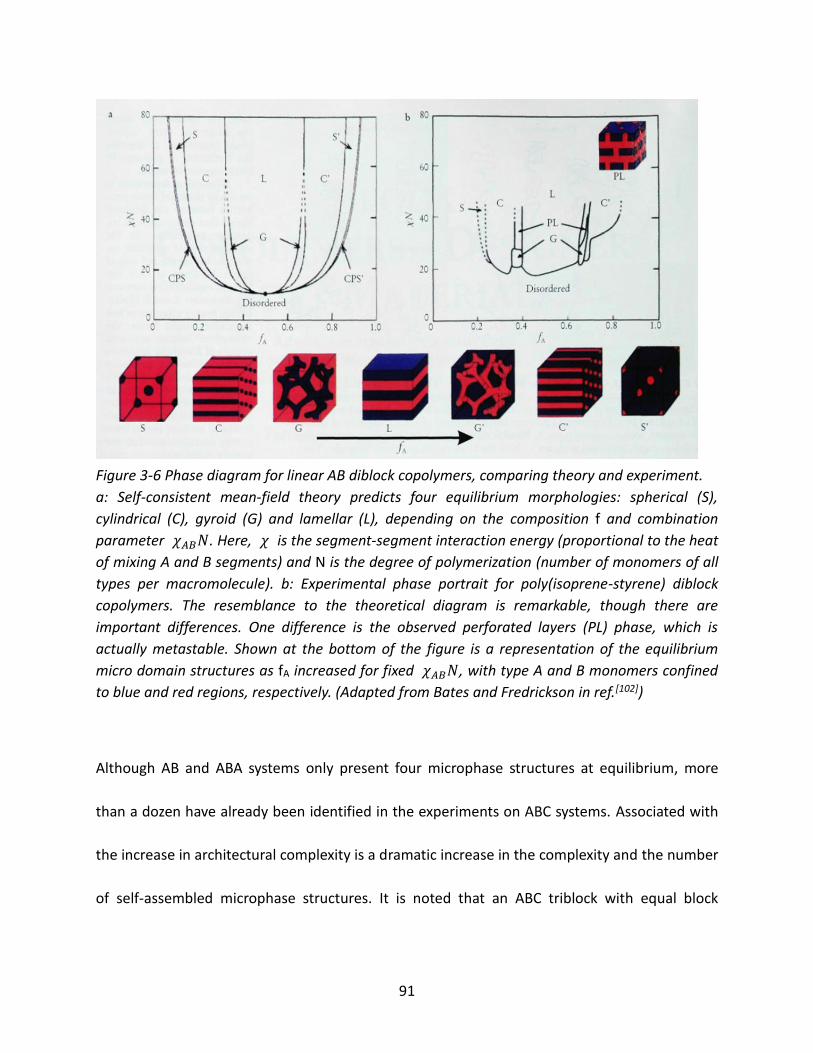
91

Figure 3-6 Phase diagram for linear AB diblock copolymers, comparing theory and experiment.

a: Self-consistent mean-field theory predicts four equilibrium morphologies: spherical (S),

cylindrical (C), gyroid (G) and lamellar (L), depending on the composition f and combination

parameter 𝜒𝐴𝐵𝑁. Here, 𝜒 is the segment-segment interaction energy (proportional to the heat

of mixing A and B segments) and N is the degree of polymerization (number of monomers of all

types per macromolecule). b: Experimental phase portrait for poly(isoprene-styrene) diblock

copolymers. The resemblance to the theoretical diagram is remarkable, though there are

important differences. One difference is the observed perforated layers (PL) phase, which is

actually metastable. Shown at the bottom of the figure is a representation of the equilibrium

micro domain structures as fA increased for fixed 𝜒𝐴𝐵𝑁, with type A and B monomers confined

to blue and red regions, respectively. (Adapted from Bates and Fredrickson in ref.[102])

Although AB and ABA systems only present four microphase structures at equilibrium, more

than a dozen have already been identified in the experiments on ABC systems. Associated with

the increase in architectural complexity is a dramatic increase in the complexity and the number

of self-assembled microphase structures. It is noted that an ABC triblock with equal block

92

lengths (𝑓𝐴 = 𝑓𝐵 = 𝑓𝐶 = 1/3), and nearly equal interaction parameters (𝑥𝐴𝐵 ≈ 𝑥𝐴𝐶 ≈ 𝑥𝐵𝐶) will

self-assemble into a three-color lamellar phase as depicted in Figure 3-7 (a).

Figure 3-7 Morphologies for linear ABC triblock copolymers.

A combination of block sequence (ABC, ACB, BAC), composition and block molecular weights

provides an enormous parameter space for the creation of new morphologies. Micro domains

are colored as shown by the copolymer strand at the top, with monomer types A, B and C

confined to regions colored blue, red and green, respectively. (a) Lamellar phase; (b) coaxial

cylinder phase; (c) lamella-cylinder phase; (d) lamella-sphere phase; (e) cylinder-ring phase; (f)

cylindrical domains in a square lattice structure; (g) spherical domains in the CsCI-type structure;

(h) lamella-cylinder-II; (i) lamella-sphere- II; (J) cylinder-sphere; (k) concentric spherical domain

in bbc structure; (l) tricontinuous G morphology. (Adapted from Bates and Fredrickson in ref.[102])

93

Since the phase behavior of block copolymers is determined by three experimentally

controllable factors: the overall degree of polymerization N, the composition f, and the

Flory-Huggins segment-segment interaction parameter 𝜒. If 𝑓𝐴 ≠ 𝑓𝐵 ≠ 𝑓𝐶 ≠ 1/3, or, 𝑥𝐴𝐵 ≠

𝑥𝐴𝐶 ≠ 𝑥𝐵𝐶, structural transitions of ABC systems can be driven by interaction asymmetries, and

ABC triblock copolymer will reveal other phase behaviors as displayed in Figure 3-4 (b)-(l).

3.5 Phase Separation of Ion Exchange Groups in Ionomers

Most commercially available ion exchange crosslinked copolymer membranes have sulfonated

groups or quaternary ammonium groups. In order to introduce ionic groups into the copolymer

membrane, meanwhile, maintain the mechanical strength of the membrane, inert polymers and

other additives like inert reinforcing fabric are added.

94

Figure 3-8 Transmission electron micrograph and scanning electron micrograph of NEOSEPTA

CL-25L. (a) TEM of the cross-section of cation exchange membrane prepared from styrene and

divinylbenzene in the presence of poly(vinyl chloride), (b) SEM of the porous membrane (Fe3+

from) treated with H2O2, and the ferric ion form membrane was immersed in aqueous 3% H2O2

solution at room temperature for 1h.

It is generally known that two different polymers are difficult to make homogeneously miscible,

and thus, phase separation occurs. Mizutani[103] first found that ion exchange groups did not

disperse well in ion exchange membranes homogeneously, but formed microdomains. Through

experiments, he reported that when a salt-form cation-exchange membrane (ferric ion) is

immersed in hydrogen peroxide solution the sulfonated copolymer of styrene and

divinylbenzene decomposes. As a result, a porous poly(vinyl chloride) membrane is

developed.[104] Hence, the cation exchange membrane (NEOSEPTA CL-25T) is prepared by

copolymerization of styrene and divinylbenzene in the presence of finely powdered spherical

inert polymer poly(vinyl chloride). Owing to the low compatibility of the inert polymer and the

(a) (b)

95

copolymer of styrene and divinylbenzene, phase separation occurs. The small and large black

spots of styrene-divinylbenzene resin components are finely dispersed in the poly(vinyl chloride)

gel phase in the transmission electron micrograph (Figure 3-8 (a)). Moreover, the surface of the

porous membrane is similar to that of the cross-section of the cation exchange membrane. This

clearly shows that the pore size seems to be the same as the large black spots of the

styrene-divinylbenzene resin component as demonstrated in Figure 3-8 (b).[104] Similarly, the

anion-exchange membrane is prepared by copolymerization of chloromethylstyrene and

divinylbenzene in the presence of an inert polymer, acrylonitrile-butadiene rubber, stained with

osmium tetraoxide.[5] Large and tiny white particles of chloromethylstyrene and divinylbenzene

are distributed in the inactive acrylonitrile-butadiene rubber polymer matrix, as presented in

Figure 3-9. This indicated that the polystyrene-divinylbenzene and acrylonitrile-butadiene

system has a two-phase nature: polystyrene-divinylbenzene as dispersed phases,

acrylonitrile-butadiene as a continuous phase. In fact, all ion exchange membranes prepared by

various methods show a similar phase separation phenomenon.

96

Figure 3-9 Scanning transmission electron micrograph of an anion exchange membrane

(cross-link: 20%): a mixture of chloromethylstyrene and divinylbenzene was copolymerized in the

presence of acrylonitrile-butadiene rubber (inert polymer); ratio of divinylbenzene to total vinyl

monomers: 20%.

Cluster network model of ion clustering was proposed by Gierke[105] that was related to cation

exchange groups in perfluorocarbon cation exchange membrane. The size of the ion cluster

depends on the ion-exchange capacity (equivalent weight) of the membrane. In Figure 3-10,

ion-exchange groups and the adsorbed electrolyte phase separate from the fluorocarbon

backbone into approximately spherical clusters (diameter: approximately 3-5 nm). They are

connected by short, narrow channels (diameter; approximately 1 nm), which are barriers to the

transport of counterions through the perfluorocarbon cation exchange membranes.[6a] The

cluster model of Nafion membrane is supported by measurements of the fixed ion

97

concentration and other methods such as transmission electron micrograph of the membrane

stained by Ag+ and Sn2+ ions across the membrane.[6a]

Figure 3-10 Cluster-network model for Nafion perfluorinated membranes.

The ion and ionomer domains phase separate from the fluorocarbon backbone into

approximately spherical clusters connected by narrow ion channels. The polymeric charges are

most likely embedded in the solution near the interface between the electrolyte and

fluorocarbon backbone. This configuration minimizes both the hydrophobic interaction of water

with the backbone and the electrostatic repulsion of sulfonated groups. The dimensions shown

were deduced from experiments. The shaded areas around the interface and inside a channel

are the double layer regions from which the hydroxyl ions are excluded electrostatically.[6a]

SO3

-

SO3

-

SO3

-

SO3

- SO3

-

SO3

-

SO3

-

SO3

-

SO3

-

SO3

- SO3

-

SO3

- SO3

-

SO3

-

SO3

-

SO3

-

SO3

-

SO3

-

SO3

-

SO3

-

SO3

-

SO3

-

1 nm

4 nm

5 nm

98

3.6 Development of Ionomer Morphology

Ionomer properties are dependent upon chain spatial arrangement, which may give rise to

lamellar, cylindrical, or spherical morphology[71]. For example, Zhao[106] and Lee[107] showed that

sulfonated poly(ether ether ketone) (SPEEK) and poly(arylene ether sulfone)-b-polyimide

copolymers containing longer hydrophilic domains triggered phase separation, which led to

more organized ion conductive domains. The resultant morphology had a remarkable increase

in proton conductivity as compared to random copolymers. In addition to block arrangements,

processing methodology is incredibly important to properties. Solvent type and casting

temperature of SPEEK[108] and Nafion[109] led to considerable discrepancies in proton

conductivity and chemical stability. Bebin and Galiano[110] demonstrated that the proton

conductivity of solvent-cast sulfonated polysulfone (sPSU) films was twice as compared to that

of melt-extruded sPSU. Weiss[111] showed that ion aggregation occurred at lower temperatures

in sulfonated block copolymers poly(b-styrene-b-(r-ethylene-so-r-butylene)-b-styrene) (S-SEBS)

as compared to similar homopolymers with different microstructures. Solution-casting and

block length effects related to morphology, physical properties, and proton conductivities were

studied by Lee et al.[112] using sulfonated poly(arylene ether sulfone) multiblock copolymer. Fan

et al.[113] explored viscoelastic and gas transport properties of a series of multiblock copolymer

ionomers sulfonated poly(arylene ether sulfone) (BPSH-BPS) as a function of block length,

99

relaxation time, and temperature. These research efforts illustrate that it is critical to evaluate

solution casting effects in order to create desirable film properties.

3.7 Summary

Several previous researchers have reported on the effect of processing conditions on modifying

morphology, mechanical, physical properties, transport properties, and thermal degradation of

ionomers. However, the importance of the casting method, solvents, and processing

methodology has not drawn much attention. Meanwhile, the comprehensive

membrane-casting operating system has not been set up to improve the characteristics of

ionomers. In our study, the bridge between the casting process and the properties of ionomers

is established, and the network within micro and macro-scale properties is configured to

investigate the wide-ranging influence of the casting process. In particular, appropriate casting

solvent (THF) and higher casting temperature dramatically facilitate proton and other ions

transport through Penta Block Copolymer (PBC) with the same ion exchange capacity. It

provides insight into stable morphological microstructures of PBCs cast by solution evaporation

method, even maintaining under continuous electric field and comparably high temperature for

long times. Finally, our research provides a framework for future studies to assess performance

characteristics such as ion conductivity and to improve chemical and physical properties from

external factors. Subsequent chapters will focus on the mechanical properties, diffusion

100

properties of ions and water, and the degradation of ionomers; also, further work will highlight

the interrelationship between the casting process and industrially utilized ionomers.

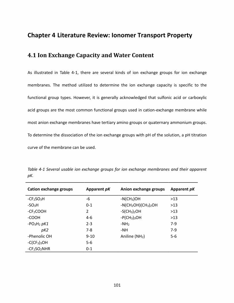
101

Chapter 4 Literature Review: Ionomer Transport Property

4.1 Ion Exchange Capacity and Water Content

As illustrated in Table 4-1, there are several kinds of ion exchange groups for ion exchange

membranes. The method utilized to determine the ion exchange capacity is specific to the

functional group types. However, it is generally acknowledged that sulfonic acid or carboxylic

acid groups are the most common functional groups used in cation-exchange membrane while

most anion exchange membranes have tertiary amino groups or quaternary ammonium groups.

To determine the dissociation of the ion exchange groups with pH of the solution, a pH titration

curve of the membrane can be used.

Table 4-1 Several usable ion exchange groups for ion exchange membranes and their apparent

pK.

Cation exchange groups Apparent pK Anion exchange groups Apparent pK

-CF2SO3H -6 -N(CH3)OH >13

-SO3H 0-1 -N(CH2OH)(CH3)2OH >13

-CF2COOH 2 -S(CH3)2OH >13

-COOH 4-6 -P(CH3)3OH >13

-PO3H2 pK1 2-3 -NH2 7-9

pK2 7-8 -NH 7-9

-Phenolic OH 9-10 Aniline (NH2) 5-6

-C(CF3)3OH 5-6

-CF2SO2NHR 0-1

102

The ion exchange capacity of the membrane is a key property of ionomer because the amount

and species of ion exchange groups determine the properties of the ion exchange membrane.

The capacity is expressed as milligram equivalent per gram of membrane (meq./g ionic-form dry

or wet membrane: dry or wet must be specified). The ion exchange capacity of ion exchange

membrane is generally expressed by equivalent weight (EW, the gram weight of acid-form

membrane, needed to neutralized 1 mol of sodium hydroxide (Equation (4-1) or hydrogen

chloride (Equation (4-2)), which is as well 1000 times the reciprocal of the ion exchange capacity

in milligram equivalents per gram dry membrane as shown in Equation (4-3).

𝐸𝑊 =𝑔 𝑑𝑟𝑦 𝑝𝑜𝑙𝑦𝑚𝑒𝑟

1 𝑚𝑜𝑙𝑒 𝑜𝑓 𝑠𝑢𝑙𝑓𝑜𝑛𝑖𝑐 𝑎𝑐𝑖𝑑 𝑖𝑛 𝑡ℎ𝑒 𝑎𝑐𝑖𝑑 𝑓𝑜𝑟𝑚 𝑜𝑓 𝐶𝐸𝑀 (4-1)

𝐸𝑊 =𝑔 𝑑𝑟𝑦 𝑝𝑜𝑙𝑦𝑚𝑒𝑟

1 𝑚𝑜𝑙𝑒 𝑜𝑓 𝑞𝑢𝑎𝑡𝑒𝑟𝑛𝑎𝑟𝑦 𝑎𝑚𝑚𝑜𝑛𝑖𝑢𝑚 𝑖𝑛 𝑡ℎ𝑒 𝑏𝑎𝑠𝑒 𝑓𝑜𝑟𝑚 𝑜𝑓 𝐴𝐸𝑀 (4-2)

𝐸𝑊 =1000

𝐼𝐸𝐶 (4-3)

Combining Equation (4-1) or Equation (4-2) with Equation (4-3), ion exchange capacity is equal

to the mole of sulfonic acid in the acid form of CEM or the mole of quaternary ammonium

groups in the base form of AEM per 1000g polymer as presented in Equation (4-4) or (4-5).

103

𝐼𝐸𝐶 =𝑚𝑜𝑙 𝑜𝑓 𝑠𝑢𝑙𝑓𝑜𝑛𝑖𝑐 𝑎𝑐𝑖𝑑

1000𝑔 𝑝𝑜𝑙𝑦𝑚𝑒𝑟 𝑖𝑛 𝑡ℎ𝑒 𝑎𝑐𝑖𝑑 𝑓𝑜𝑟𝑚 𝑜𝑓 𝐶𝐸𝑀 (4-4)

𝐼𝐸𝐶 =𝑚𝑜𝑙 𝑜𝑓 𝑞𝑢𝑎𝑡𝑒𝑟𝑛𝑎𝑟𝑦 𝑎𝑚𝑚𝑜𝑛𝑖𝑢𝑚

1000𝑔 𝑝𝑜𝑙𝑦𝑚𝑒𝑟 𝑖𝑛 𝑡ℎ𝑒 𝑏𝑎𝑠𝑒 𝑓𝑜𝑟𝑚 𝑜𝑓 𝐴𝐸𝑀 (4-5)

Ion exchange capacity is determined by measuring the amount of specified counter-ions in the

membrane by titration after ion exchange with other ions or elution, using a suitable indicator.

Water content changes with the concentration of electrolyte solution while the membranes are

equilibrated with the species of counter-ions. The water content of an ion exchange membrane

is expressed as the ratio of the amount of adsorption water over one gram of sodium or

potassium ion-form cation exchange membrane or of chloride ion-form anion exchange

membrane (g-H2O/g specific ion-form wet or dry membrane).

After measuring the ion exchange capacity and water content of the ion exchange membrane,

the fixed ion concentration of the membrane can be calculated according to Equation (4-6).

𝐶𝑅̅̅ ̅ =

𝐼𝐸𝐶

𝑊 (4-6)

where IEC is the milligram equivalent/g dry membrane, and W presents water content (g H2O/g

dry membrane).

104

Permselectivity of counter-ions through the ion exchange membrane depends on the fixed ion

concentration of the membrane. Many efforts have been made to increase the fixed ion

concentration of the membrane: to increase the ion exchange capacity and to decrease the

water content of the membrane, namely, to increase the fixed ion concentration without

increasing the electrical resistant of the membrane.

4.2 Diffusion Coefficient of Liquid Molecule Transport and

Activation Energy

4.2.1 Fick’s Law

Diffusivity or diffusion coefficient is proportionality constant between the molar flux (due to

molecular diffusion) and the concentration gradient of the diffusing species (the driving force

for diffusion), as indicated in Equation (4-7). Diffusivity is encountered in Fick's law[114] and

numerous other equations of physical chemistry as well.

𝐽𝑖 = −𝐷𝑖𝑑𝐶𝑖

𝑑𝑥 (4-7)

105

The higher the diffusivity (of one substance with respect to another), the faster they diffuse into

each other. This coefficient has an SI unit of m2/s (length2/time).

4.2.2 Solution–diffusion Model

Solution–diffusion model is widely used to describe the transport of small molecules in polymer

membranes. The concentration driving forces leads to the overall pushing movement of a

penetrant. Then the flux, Ji , can be expressed as Equation (4-8) using Fick’s law[114b].

𝐽𝑖 =𝐷𝑖

𝑙(𝐶𝑖,𝑥=0 − 𝐶𝑖,𝑥=𝑙) ≈

𝐷𝑖

𝑙𝐶𝑖,𝑥=0 (4-8)

where 𝐶𝑖,𝑥=0 and 𝐶𝑖,𝑥=𝑙 are the concentration in the upstream and downstream surfaces of

the membrane, respectively. Di is the diffusion coefficient and l is the thickness of polymer

film.

The flux of diffusion molecules, Ji, is expressed either in number of molecules per unit area and

unit time, or in terms of mass flux as Equation (4-9).

𝐽𝑖 =𝑑𝐶𝑖,𝑥=𝑙

𝑑𝑡

𝑉0

𝐴= 𝑠𝑙𝑜𝑝

𝑉0

𝐴 (4-9)

where Vo is the volume of one diffusion cell and A is the effective area of membrane film.

106

4.2.3 Diffusion Coefficient Calculation

Combining Equation (4-8) and (4-9), the diffusion coefficient can be calculated as Equation

(4-10).

𝐷𝑖 =𝑑𝐶𝑖,𝑥=𝑙

𝑑𝑡

𝑉0𝑙

𝐶𝑖,𝑥=0𝐴 (4-10)

where 𝑑𝐶𝑖,𝑥=𝑙

𝑑𝑡 can be calculated with the data of the liquid molecule transport experiment. The

other parameters in this equation are constant, such as Vo is the volume of one diffusion cell

and 𝑙 is the thickness of polymer film, 𝐶𝑖,𝑥=0 is the concentration in the upstream surface of

the membrane, and A is the effective area of membrane.

4.2.4 Arrhenius Equation

According to the Arrhenius Equation, the activation energy of liquid molecule diffusion can be

expressed as Equation (4-11).

𝑙𝑛(𝐷) = −𝐸𝑑

𝑅×

1

𝑇+ 𝑙𝑛(𝐷𝑜) (4-11)

107

where D is the ion conductivity, Do is the pre-exponential factor, R presents the gas constant, T is

the temperature, and Ed is the activation energy of ion transport.

4.3 Diffusion Coefficient of Ion Transport and Activation Energy

4.3.1 Nernst-Einstein Relation

The classical Nernst-Einstein relation is valid in aqueous solution, as presented in Equation

(4-12).

𝐷𝑖𝑐 = 𝑢𝑖̇ 𝑅𝑇 (4-12)

where Dic is the self-diffusion coefficient from diffusion measurements, ui̇ is the absolute

mobility and R is the gas constant.

4.3.2 Diffusion Coefficient Calculation

The apparent specific conductivity 𝜎 is given by Equation (4-13).

𝜎 = ∑ 𝑧𝑖𝐶𝑖𝑢𝑖𝐹𝑖 (4-13)

where ui is the conventional mobility, F is the Faraday constant, zi is the valence of the ion i,

and 𝐶𝑖 is the ionic concentration within the membrane.

108

Equation (4-14) describes the correlation between the absolute and the conventional mobility

of one kind of ion.

𝑢𝑖̇ =𝑢𝑖

𝑧𝑖𝐹 (4-14)

The diffusion coefficient of ion though ionomer membrane is derived from Equation (4-12),

(4-13), and (4-14).

𝐷𝑖𝑐 =

𝜎𝑅𝑇

𝑧𝑖2𝐹2𝐶𝑖

(4-15)

Equation (4-15) links the diffusion coefficient of one kind of ion directly with the ion

conductivity in the ionomer membrane[115].

4.3.3 Arrhenius Equation

Based on the Arrhenius Equation, the activation energy can be expressed as Equation (4-16).

𝜎 =𝐴

𝑇𝑒𝑥𝑝(−

𝐸𝑎

𝑅𝑇) (4-16)

109

where 𝜎 is the ion conductivity, A is the pre-exponential factor, R presents the gas constant, T

is the temperature, and Ea is the activation energy of ion transport.

The derivative format is illustrated as Equation (4-17).

𝑙𝑛(𝜎𝑇) = −𝐸𝑎

𝑅×

1

𝑇+ 𝑙𝑛𝐴 (4-17)

The activation energy can be calculated according to the slope of the plot 𝑙𝑛(𝜎𝑇) vs. 1/T.

4.4 Development of Molecules and Ions Transport

One of the most advanced separation polymers, ionomers, has three striking features, ion

conductivity, hydrophilicity, and fixed charge carriers, due to its blocks of both electrically

neutral repeating units and a fraction of ionizable branched units.[5-6] It is generally known that

ionomers have recently attracted widespread interest in the fields of proton exchange

membrane (PEM) fuel cells (FC)[2]. However, these three remarkable characteristics of ionomers

qualify ionomers for use in other processes such as electrodialysis, electrolysis, diffusion dialysis,

batteries, sensing materials, biomedical and analytical chemistry[5], which have not been

appreciably paid enough attention. Hence, the diffusion of different ion such as Na+, Li+, and

Ca2+ and liquid molecules through membranes is equally important as the proton transport in

110

ionomers. For more than 60 years, researchers have been observing the synthesis and

characterization of different kinds of ion-exchange membranes[109, 116]. Subsequently, more

attempts have focused on possible factors improving morphology, transport properties,

mechanical properties, phase behaviors and the degradation of ionomers. However, compared

with intrinsic properties, such as polymer structure, chain end group, and molecular weight of

the polymer, extrinsic casting methods can also affect various characteristics of ionomers

significantly. The casting methodology includes types of solvents used[112], methods of sample

preparation[109-110, 117], and ionic neutralization[118].

In several previous studies, it has been reported that the casting and processing conditions and

technique also substantially influenced the microstructure and transport properties of ionomers.

It is illustrated that different casting solvents and processing methods could lead to large

discrepancies in proton conductivity of block copolymers, such as sulfonated poly(ether ether

ketone) (SPEEK)[108], Nafion[109], sulfonated polysulfone (sPSU)[110], and sulfonated poly(arylene

ether sulfone) multiblock copolymer[112]. Nevertheless, the importance and significance of

ionomer casting conditions and methods have not been paid close attention to so far.

Furthermore, it is claimed that the use of ionic functional groups can modify morphology,

mechanical properties, physical properties, transport properties, and the degradation of

ionomers. In 1990, the introduction of different counter-ions (Na+, K+, Cs+, and Ca2+) contributed

to better fatigue performance and shear deformation caused by more effective ionic crosslinks

111

was discovered by Hara.[118] Before long, Weiss pointed out that the critical temperature for

ionic aggregation and dissociation in the block copolymer ionomer was lower than that for

similar homopolymer ionomers due to perturbation by the block microstructure.[111] Later on,

some researchers proposed that metal ionic neutralized ionomers improved their stability, as

well as, physical and mechanical properties.[119] Moreover, Winey probed the importance of the

cast preparation method and thermal treatment in determining the nanoscale morphology of

the salt-form ionomers Cu-neutralized poly(styrene-ran-methacrylic acid) (SMAA) and

Cu-neutralized poly(3-methylstyrene-ran-methacrylic acid) (3-MeSMAA).[120] However, few

attempts have focused on the relationship between the ionic neutralization of different solvent

cast ionomers and the ion transport properties within ionomers.

In addition to ion transport, numerous investigations have also focused on the diffusion of liquid

molecules through the ionomer as another important transport property. In 1992, Koval

presented that the substitution of silver ions for sodium ions in hydrated ionomer membranes

causes the trans-membrane fluxes of styrene (STY) and ethylbenzene (EBZ) to increase by 2-3

orders of magnitude by facilitated transport.[121] After that, people began to pay close attention

to liquid molecules transport, such as methanol and water. In 2002, Dimitrova illustrated that

Nafion-recast membranes filled with 4.3% silicon dioxide exhibited increased water uptake,

conductance and methanol permeation rate compared with commercial Nafion.[122] Later on,

from a morphological aspect, Elabd[123] put forward that ordered structure sulfonated

112

poly(styrene-isobutylene-styrene) (S-SIBS) caused by higher ion exchange capacity (IEC) greatly

affected the methanol transport properties. Shortly after that, the water transport properties of

salt-form perfluorosulfonated ionomer membranes[124] and the mechanism of methanol,

ethanol, and 2-propanol diffusion through ionomers[125] were demonstrated by Saito, noting

that Li+ and Na+ ionomers have lower water transference coefficients and water permeability

compared with H+ ionomers due to the strong interaction between salt ions and water

molecules. Nevertheless, few efforts have focused on the relationship between different casting

solvents and liquid molecule transport properties within ionomers.

4.5 Summary

A number of previous studies have offered an understanding of the modification of the

morphology, mechanical and physical properties, transport properties, and degradation of

ionomers from the intrinsic properties of ionomers; however, the importance of the casting

method, solvents, and processing conditions has not drawn much attention, and the

comprehensive membrane-casting operating system has not been established to improve

characteristics of ionomers. In our study, the bridge between the casting process and the

characteristics of ionomers is built to investigate the great impact of membrane processing

method from the perspective of polymeric macro- and micro-properties. In more detail,

113

appropriate casting solvent (THF) and comparably high casting temperatures dramatically

facilitate ions and liquid molecules transport through PBCs at a specific IEC. Finally, our research

provides the framework for future studies to assess and improve performance characteristics of

different ionomers such as ion and liquid molecule transport by changing external factors,

whilst also giving a reference for the manufacture of industrially utilized ionomers.

114

Chapter 5 Literature Review: Ionomer Mechanical Properties

and Degradation

5.1 Glass Transition Temperature and Melting Temperature

The glass-liquid transition, or the glass transition for short, is the reversible transition process

from a hard and relatively brittle state into a molten or rubber-like state for amorphous material

or amorphous regions within semi-crystalline materials. An amorphous solid that exhibits a

glass transition is called a glass. Supercooling a viscous liquid into the glass state is called

vitrification.

Figure 5-1 Measurement of Tg by differential scanning calorimetry.

115

The most frequently used definition of Tg uses the energy release on heating in differential

scanning calorimetry. Referring to Figure 5-1 plotting heat capacity as a function of temperature,

glass transition temperature, Tg, is the temperature corresponding to point A on the curve. The

glass transition temperatures of polymers are only mean values, as the glass transition

temperature depends on the cooling rate, molecular weight distribution and could be

influenced by additives as well.

116

Figure 5-2 Temperature-Molecular weight diagram for polymers. (a) Amorphous polymers, (b)

semi-crystalline polymers.[126]

Temperature versus molecular weight diagram for two different kinds of polymers is illustrated

in Figure 5-2, amorphous polymers and semi-crystalline polymers.

Molecular weight

Tem

per

atu

re

Amorphous polymers

③Thermal decomposition

②Diffuse transition zone

①Glass transition

①

②

③

(a)

Molecular weight

Tem

per

atu

re

Semi-crystalline polymers

④Thermal decomposition

③Diffuse transition zone

②Melting point

①Glass transition

①

②

③

(b) ④

Glassy

Rubbery

Viscous

liquid

Rigid semi-crystalline

Leathery

Rubbery

Viscous

liquid

117

Amorphous polymer

If an amorphous polymer is heated, it will begin to soften at the glass transition temperature

and become quite rubbery as shown in Figure 5-2 (a). On further heating, the elastic behavior

diminishes, a shear stress will cause viscous flow to predominate over elastic deformation but it

is only in diffusion transition zone at a temperature range above the glass-rubber transition

temperature. Finally, it enters into thermal decomposition zone. If the molecular weight is

sufficiently high, the glass-rubber transition temperature is almost independent of the

molecular weight and viscous flow zone will disappear. Otherwise, the rubbery-liquid transition

heavily depends on the molecular weight. Furthermore, the decomposition temperature tends

to decrease slightly with increasing molecular weight.

As is well known, the glass-rubber transition is of considerable importance technologically. The

glass transition temperature determines the lower use-limit temperature of a rubber and the

upper use-limit temperature of an amorphous thermoplastic material.

While the main glass transition occurs as soon as large segments of the polymer backbone chain

are free to move, secondary transition occurs at temperature where sub-groups, side chain etc.,

can freely move or oscillate. Though the effects of secondary transition are smaller and often

less obvious, they are important to the mechanical behavior (to diminish brittleness). Secondary

transition below the glass-rubber transition temperature can be detected by studies of

118

mechanical damping, by nuclear magnetic resonance or by electric loss measurements over a

range of temperatures.

Semi-crystalline polymer

Semi-crystalline polymers show four regions of higher order as compared with that of

amorphous polymer, three regions. The major factor determining whether a polymer can

crystallize is the occurrence of successive units in the chain in a configuration of high

geometrical regularity. If the chain elements are small, simple and equal, as in linear

polyethylene, crystallinity is highly developed. If, however, the chain elements are complex,

containing bulky side groups, as in polystyrene, the material can also crystallize only if these

substituent groups are arranged in an ordered configuration.

In Figure 5-2 (b), above the melting temperature which is theoretically the highest temperature

at which polymer crystallites can exist, the semi-crystalline polymer may be liquid, viscoelastic

or rubbery according to its molecular weight. And below it, the polymer will tend to be leathery

and tough down to the glass transition temperature in the high molecular weight range, and

tend to be brittle waxes in the lower molecular weight range. Secondary crystalline transitions

below the melting temperature occur if the material transforms from one type of crystal to

another.

119

Though for semi-crystalline polymers Tm rather than Tg determines the upper service

temperature of plastics and the lower service temperature of rubbers, the glass transition

temperature is still very important. The reason is that between Tm and Tg the polymer is likely to

be tough, and the best used region of the polymer may therefore be expected at the lower end

of the leathery range as illustrated in Figure 5-2 (b). Below the glass transition temperature,

many polymers tend to be brittle, especially if the molecular weight is not very high. Secondary

transitions may be responsible if a rigid material is tough rather than brittle.

Non-thermoplastic polymers

Some polymers, such as cellulose, although linear in structure, have such a strong molecular

interaction, mostly due to hydrogen bridges and polar groups that they do not soften or melt.

Consequently, the transition temperatures as such are less important to this class of polymers.

Normally they are highly crystalline, with a crystalline melting point far above the

decomposition temperature.

Their physical behavior, except for the melting, is that of crystalline polymers. Therefore, they

are suitable raw materials for fibers via solution spinning. Many of these polymers are

plasticized by water, due to the strong influence of water on the molecular interaction. The

polymer can therefore be called hydro-plastics in contradistinction to thermoplastics.

120

Cross-linked polymers

If an amorphous polymer is crosslinked, the basic properties are fundamentally changed. In

some respects, the behavior of the polymer with a high degree of crosslinking is similar to that

with a high degree of crystallinity, because crystallization can be considered as a physical form

of crosslinking. The influence of the melting temperature becomes less and less pronounced as

crosslinking progresses.

5.2 Temperature Dependence of the Moduli

The most important characteristic mechanical properties are called moduli. A modulus is the

ratio between the applied stress and the corresponding deformation.

121

Figure 5-3 Behaviors of some polymer properties at the transition temperature.[126]

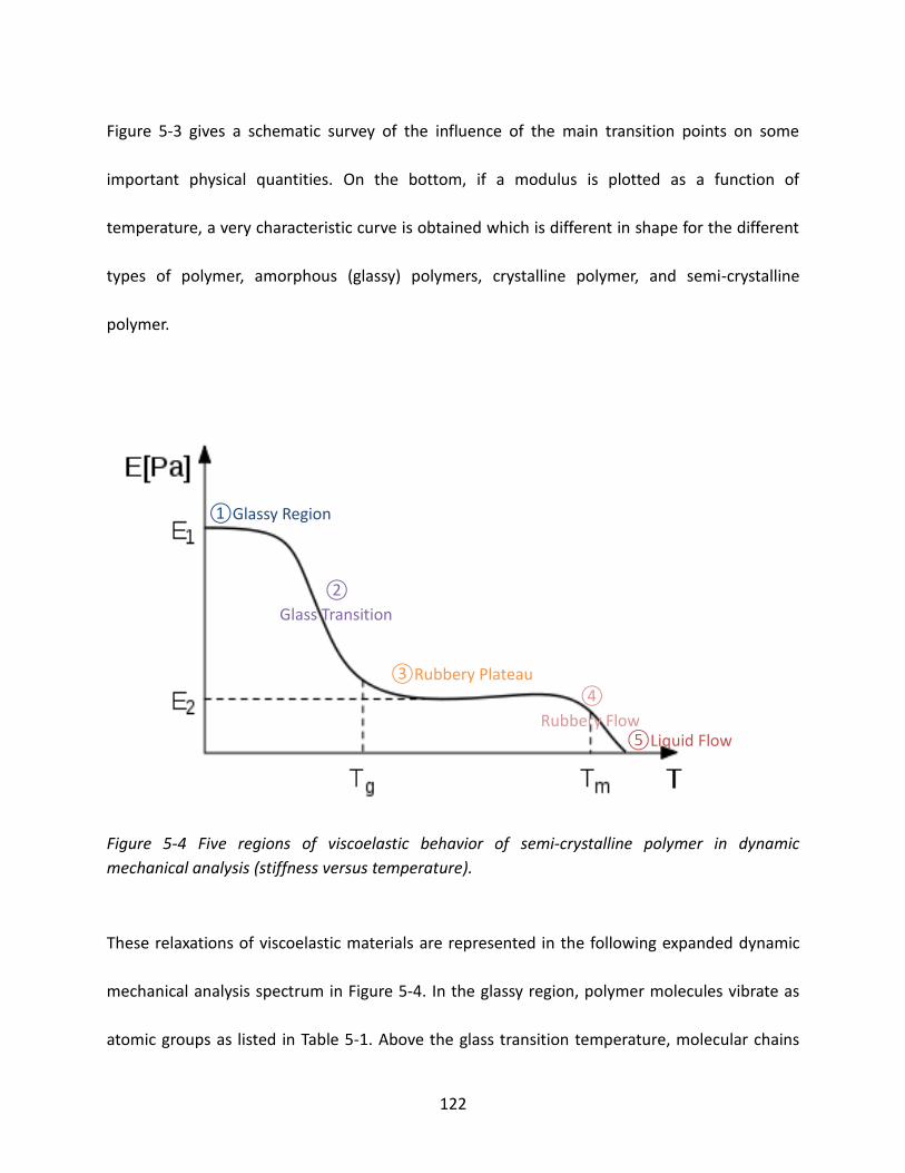
122

Figure 5-3 gives a schematic survey of the influence of the main transition points on some

important physical quantities. On the bottom, if a modulus is plotted as a function of

temperature, a very characteristic curve is obtained which is different in shape for the different

types of polymer, amorphous (glassy) polymers, crystalline polymer, and semi-crystalline

polymer.

Figure 5-4 Five regions of viscoelastic behavior of semi-crystalline polymer in dynamic

mechanical analysis (stiffness versus temperature).

These relaxations of viscoelastic materials are represented in the following expanded dynamic

mechanical analysis spectrum in Figure 5-4. In the glassy region, polymer molecules vibrate as

atomic groups as listed in Table 5-1. Above the glass transition temperature, molecular chains

①Glassy Region

②

Glass Transition

③Rubbery Plateau ④

Rubbery Flow ⑤Liquid Flow

123

slide past each other when a force is applied, in other words, storage modulus (stiffness)

decreases dramatically from E1 to E2, in which chain segments move in a short-range diffusional

mode. And the introduction of relatively stiff chemical groups like phenyl groups will interfere

and increase the glass transition temperature. When the glass transition temperature has been

reached, the stiffness will stay the same for a while near E2 which is rubber plateau (rapid

short-range diffusional motions and retarded long-range motions), until the temperature

exceeds the melting temperature, and the material melts transits from rubber flow (slippage of

long-range entanglements) to liquid flow (long-range configurational changes (whole

molecules)).

Table 5-1 The regions of viscoelastic behavior of semi-crystalline polymers.

Mechanical Behavior Molecular Behavior

Glassy Only vibrations of atomic groups

Leathery Short-range diffusional motion (chain segments)

Rubbery-elastic Rapid short-range diffusional motions, Retarded long-range motions

Rubbery Flow Slippage of long-range entanglements

Liquid Flow Long-range configurational changes (whole molecules)

124

5.3 Elastic Quantities and Viscosity

5.3.1 Rubber Elasticity

Rubber elasticity, a well-known example of hyper-elasticity, describes the mechanical behavior

of many polymers, especially cross-linked polymers. Due to the cross-links, this kind of polymer

hardly shows any flow behavior as presented in Figure 5-5 (without rubbery flow and liquid flow

regions).

Figure 5-5 Three regions of elastic behavior of cross-linked polymer in dynamic mechanical

analysis (stiffness versus temperature).

①Glassy Region

②

Glass Transition

③Rubbery Plateau

125

Temperature affects the elasticity of cross-linked polymer in an unusual way. Heating causes

them to contract, and cooling causes expansion. Stretching a rubber band will cause it to

release heat. In other words, elastic polymers do not store any potential energy in stretched

chemical bonds or elastic work done in stretching molecules, when work is done upon them.

Instead, all work done on the rubber is "released" (not stored) and appears immediately in the

polymer as thermal energy. If we stretch slowly in air at room temperature, we have a reversible,

isothermal process with heat lost to the surroundings (Q < 0). Then ΔSstretch = Qrev/T < 0 in the

stretching process. Since entropy is a state function, ΔScontract = Qrev/T > 0 for the reverse process

of slowly allowing the rubber band to contract. The rubber band has lower entropy, which is

more ordered when stretched. Under tension, the molecules in a rubber band line up and the

arrangement becomes much more ordered, lowering the entropy.

5.3.2 Viscoelasticity

Viscoelasticity is the property of materials that exhibit both viscous and elastic characteristics

when undergoing deformation. Elastic materials strain when stretched and quickly return to

their original state once the stress is removed, as displayed in Figure 5-6 (a). Viscoelastic

materials have elements of both of these two properties and, as such, exhibit time-dependent

strain. Whereas elasticity is generally the result of bond stretching along crystallographic planes

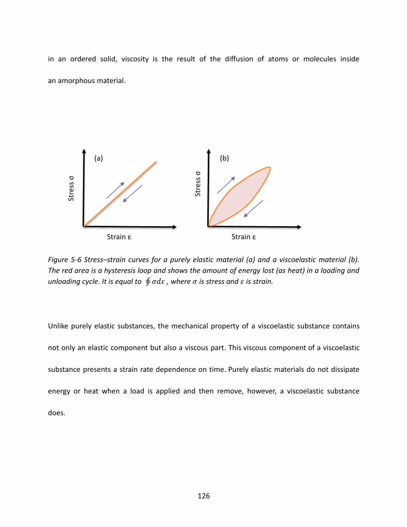
126

in an ordered solid, viscosity is the result of the diffusion of atoms or molecules inside

an amorphous material.

Figure 5-6 Stress–strain curves for a purely elastic material (a) and a viscoelastic material (b).

The red area is a hysteresis loop and shows the amount of energy lost (as heat) in a loading and

unloading cycle. It is equal to ∮𝜎𝑑휀 , where 𝜎 is stress and 휀 is strain.

Unlike purely elastic substances, the mechanical property of a viscoelastic substance contains

not only an elastic component but also a viscous part. This viscous component of a viscoelastic

substance presents a strain rate dependence on time. Purely elastic materials do not dissipate

energy or heat when a load is applied and then remove, however, a viscoelastic substance

does.

Stre

ss σ

Strain ε

Stre

ss σ

Strain ε

(a) (b)

127

Hysteresis is observed in the stress–strain curve as presented in Figure 5-6 (b), with the area of

the loop being equal to the energy lost during the loading cycle. Viscoelasticity is a molecular

rearrangement. When a stress is applied to a viscoelastic polymer, parts of the long polymer

chain rearrange and change positions (this phenomenon is called creep), however, still remains

a solid material. In order to accompany the applied stress, viscoelastic polymer creates a back

stress in the material. When the back stress is the same magnitude as the applied stress, the

material no longer creeps. When the original stress is taken away, the accumulated back

stresses will cause the polymer to return to its original form. The material creeps, which gives

the prefix visco-, and the material fully recovers, which gives the suffix -elasticity.

5.4 Deformation Properties

Polymer engineering applications are governed by strain considerations to a greater extent.

Hence, designers of polymeric materials should understand their mechanical behavior with

respect to the maximum permissible strains to avoid failure. As for most polymeric materials, a

simple tensile stress-strain curve provides a good start towards understanding the mechanical

behavior of a particular polymer.

128

Figure 5-7 Generalized tensile stress-strain curve for polymeric materials.

The strength properties of polymers are most simply expressed by the stress-strain diagram

(Figure 5-7), which is established by continuously measuring the force developed as the sample

is elongated at a constant rate of extension until it breaks. This diagram describes the behavior

of a homogeneous specimen of uniform cross section subjected to uniaxial tension.

Stre

ss σ

Strain ε

Elastic

Region

Plastic

Region

Yield

Elongation

Ultimate

Elongation

Yield Point

Ultimate Strength

Rupture Point

Toughness Resilience

129

Within the linear region the strain is proportional to the stress and the deformation is reversible.

This initial slope gives the value for Young’s modulus or the modulus of elasticity, which is a

measure of stiffness. The area under the curve or work to break is a rough indication of the

toughness of the polymeric material. The stress at the knee in the curve, known as the yield

point, is a measure of the strength of the material and its resistance to permanent deformation.

The stress at the breaking point, commonly known as the ultimate strength, is a measure of the

force required to fracture the material completely. If the material fails and ruptures at a certain

tension and a certain small elongation it is called brittle. If permanent or plastic deformation

sets in after elastic deformation at some critical stress, the material is called ductile.

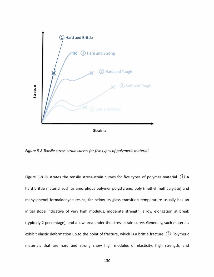
130

Figure 5-8 Tensile stress-strain curves for five types of polymeric material.

Figure 5-8 illustrates the tensile stress-strain curves for five types of polymer material. ① A

hard brittle material such as amorphous polymer polystyrene, poly (methyl methacrylate) and

many phenol formaldehyde resins, far below its glass transition temperature usually has an

initial slope indicative of very high modulus, moderate strength, a low elongation at break

(typically 2 percentage), and a low area under the stress-strain curve. Generally, such materials

exhibit elastic deformation up to the point of fracture, which is a brittle fracture. ② Polymeric

materials that are hard and strong show high modulus of elasticity, high strength, and

Stre

ss σ

Strain ε

131

elongation at break of approximately 5 percentage. This type of the curve often suggests that

the material has broken where a yield point might be expected to show up, with representative

examples of some rigid poly(vinyl chloride) formulations and polystyrene polyblends. ③ Hard,

tough polymers have high yield points and high modulus, high strengths and large elongations.

This type of curve is characteristic of cellulose acetate, cellulose nitrate and nylons ④ Soft and

tough behavior is presented by plasticized PVC and rubbers or elastomers with low modulus and

yield values, moderate strength at break, and very high elongation ranging from 20 to 1000

percentage ⑤ Soft and weak polymeric materials show low modulus, low yield stress, low

ultimate strength and moderate elongation at break.

Strain energy is defined as area under stress-strain curve, which is the total mechanical energy

per unit volume consumed by the material in straining is to that value. In the absence of

molecular slop and other mechanisms for energy dissipation, this mechanical energy is stored

reversibly within the material as strain energy. When the stresses are low enough that the

material remains in the elastic range, the strain energy is just the triangular area in Figure 5-7.

The area up to the yield point is termed the modulus of resilience, and the total area up to

fracture is termed the modulus of toughness. Up to the point of yielding, the material is

unaffected by the applied stress and upon unloading will return to its original shape. But when

the strain exceeds to the yield point, the material is deformed irreversibly, so that some residual

strain will persist even after unloading. The modulus of resilience is then the quantity of energy

132

the material can absorb without suffering damage. Similarly, the modulus of toughness is the

energy needed to completely fracture the material. Materials showing good impact resistance

are generally those with high moduli of toughness.

5.5 Thermal Degradation

Thermal degradation of polymers is the phenomenon of molecular deterioration as a result of

overheating. When it reaches the thermal degradation temperature, the long chain backbone of

the polymer begins to break, which is determined by bond-dissociation energy. Thermal

degradation can show an upper limit to the service temperature of polymers as much as the

possibility of mechanical property loss. And the chemical reactions are involved in thermal

degradation, leading to physical and optical property changes relative to the initially specified

properties.

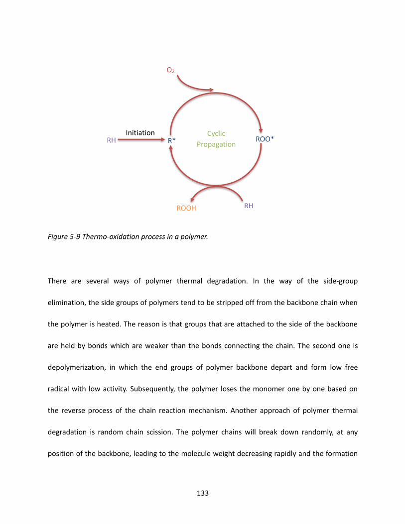
133

Figure 5-9 Thermo-oxidation process in a polymer.

There are several ways of polymer thermal degradation. In the way of the side-group

elimination, the side groups of polymers tend to be stripped off from the backbone chain when

the polymer is heated. The reason is that groups that are attached to the side of the backbone

are held by bonds which are weaker than the bonds connecting the chain. The second one is

depolymerization, in which the end groups of polymer backbone depart and form low free

radical with low activity. Subsequently, the polymer loses the monomer one by one based on

the reverse process of the chain reaction mechanism. Another approach of polymer thermal

degradation is random chain scission. The polymer chains will break down randomly, at any

position of the backbone, leading to the molecule weight decreasing rapidly and the formation

O2

RH Initiation

R* ROO*

RH ROOH

Cyclic

Propagation

134

of new free radicals with high reactivity. In this process, intermolecular chain transfer and

disproportion termination reactions can occur. The last one, oxidation of the polymers is

defined as their thermally initiated reaction with the molecular oxygen. The general scheme

(Figure 5-9) of the polymer thermo-oxidation indicates the radical character of the process.

Figure 5-10 Thermal degradation of ionomers.

In the process of thermal degradation of ionomers as plotted in Figure 5-10, water removal

occurs initially below 100oC. On further heating, from 100oC to the thermal degradation

temperature, functional groups are eliminated from polymer backbones due to the less stability

of functional groups such as sulfuric acid, ammonium groups compared with that of polymer

Wei

ght

frac

tio

n (

%)

Temperature (oC)

Functional group elimination

Water

removal

Depolymerization

or Random chain

scission

135

hydrocarbon backbones. Above the thermal degradation temperature, polymer backbones

begin to break down following the mechanism of depolymerization or the random chain

scission.

5.6 Development of Mechanical Properties and Degradation

For the glass transition properties of ionomers, it was proposed by Tsagaropoulos and

Eisenberg[127] that with the increase of ion content, the number of regions of restricted mobility

grows and starts to overlap which means that at some specific ion content, the aggregates

become large enough to exhibit their own glass transition; above that point, they form clusters

to form a second glass transition temperature peak. Shortly after that, Woo[128] presented that

after heating-induced interchange reactions (-OH and carbonate), randomly linked

homopolymer chain in a classical blend system of a poly(hydroxyl ether bisphenol-A) (phenoxy)

with bisphenol-A polycarbonate (PC) might form and also be forced to relax in coordinated

motion modes, thus showing a single glass transition temperature. Furthermore, Serrano[129]

demonstrated that two phase polymer blends of poly(cyclohexylmethacrylate), PChMA, with

poly(vinylacetate), PVAc, (20/80 and 50/50) were prepared by casting tetrahydrofuran (THF) or

chloroform (CHCl3) solution while a growth in intermolecular interaction of phase-separated

polymer led to a growth in glass transition temperature of the rigid polymer (PChMA) in the

presence of the flexible one (PVAc). Later on, Jara[130] illustrated that different numbers of glass

136

transition temperatures were exhibited according to the degree of phase separation by using

protein/polysaccharide co-dried mixtures. Although the concentration of polymer blends and

the ion contents of ionomers are observed to have a great influence on the glass transition

properties, few researchers cover the interrelation within casting solvents and glass transition

temperatures.

In 1999, Wilkie[131] reviewed the investigations carried out by comparing the thermal stability of

polystyrene, crosslinked styrene and polybutadiene. It presented that a crosslinked polymer was

inherently more thermally stable than the correspondingly thermoplastic polymer. And Jiang[132]

studied the thermal degradation of poly(vinyl sulfonic acid) and its sodium salt, poly(4-styrene

sulfonic acid) and its sodium salt, and poly(vinylphosphonic acid) by using TGA and Fourier

Transform Infrared Spectroscopy (FTIR), and proposed a mechanism in the process of

identification of the volatile products and the analysis of the residues during the degradation.

However, no research is focused on the effect of casting solvent and processing condition on the

polymer degradation.

5.7 Summary



137


method, solvents, and processing conditions has not drawn much attention and the

comprehensive membrane-casting operating system has not been found to improve




appropriate casting solvent (THF) and comparably high casting temperatures dramatically

facilitate ions and liquid molecules transport through PBCs at a specific IEC. Furthermore, from

the aspect of glass transition properties, our study provides insight into more cross-linked

morphological microstructures of acid form and salt form PBCs cast by the THF solution

evaporation method with respect to CHCl3 and C:H. Finally, our research provides the

framework for future studies to assess and improve performance characteristics of different

ionomers such as ion and liquid molecule transport from changing external factors, whilst also

giving reference for the manufacture of industrially utilized ionomers.

138

Chapter 6 Literature Review: Anion Exchange Membranes

6.1 Cation and Anion Exchange Membranes

Today, there are various types of charged membranes include dense, porous, non-porous, or

anisotropic. The ion-exchange membrane is generally recognized as a dense, non-porous,

charged membrane, which has anionic and/or cationic fixed charges, and best suited in the

areas of ion transport and separation processes. Ion-exchange membranes can be classified in

several ways, based on function, chemistry (material constituting the membrane), structure and

microstructure of the membrane, etc. However, classification based on a material’s group is

clear because the function of the ion exchange membrane is determined by the species and

charge of the ion-exchange groups fixed in the membranes, and their distribution in the

membrane.

Cation-exchange membranes have various cation exchange groups (sulfonic acid, carboxylic acid,

phosphonic acid, monosulfate ester groups, mono- and diphosphate ester groups, phenolic

hydroxyl group, thiol groups, perfluoro tertiary alcohol groups, sulfonamide groups, and N-oxide

groups as shown in Figure 6-1), providing a negative fixed charge in aqueous or mixed water and

organic solvent solution, and cations selectively permeate through the membranes. Anion

exchange membranes have various anion exchange groups (primary, secondary, and tertiary

amino groups, quaternary ammonium groups, tertiary sulfonium groups, quaternary

139

phosphonium groups, and cobalticinium groups as presented in Figure 6-2), providing a positive

fixed charge in aqueous or mixed water and organic solvent solution, and anions selectively

permeate through the membranes.

Figure 6-1 Anion charged groups in cation exchange membrane.

Sulfonic acid

R S

O

O

OH

Carboxylic acid

R C

O

OH

Phosphonic acid

R P

O

OH

OH

monosulfate ester

O S

O

O

OHR

monophosphate ester

O P

O

OH

OH

R

diphosphate ester

O P

O

OH

OH

O P

O

OH

R

OHR

phenolic hydroxyl group thiol group

R SH R C

CF3

CF3

OH

perfluoro tertiary alcohol group

sulfonamide group

R N

R1

R2

O

N-oxide group

C S

O

O

N

F

F

R

H

R1

H

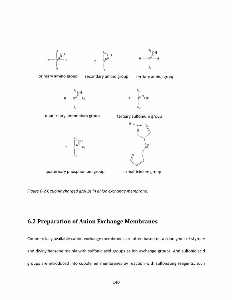
140

Figure 6-2 Cationic charged groups in anion exchange membrane.

6.2 Preparation of Anion Exchange Membranes

Commercially available cation exchange membranes are often based on a copolymer of styrene

and divinylbenzene mainly with sulfonic acid groups as ion exchange groups. And sulfonic acid

groups are introduced into copolymer membranes by reaction with sulfonating reagents, such

R N

H

H

H

OH

primary amino group secondary amino group tertiary amino group

R N

R1

H

H

OHR N

R1

H

R2

OH

R N

R1

R3

R2

OH

quaternary ammonium group

R S

R1

R2

OH

tertiary sulfonium group

quaternary phosphonium group

R P

R1

R3

R2

OH

cobalticinium group

Co

R

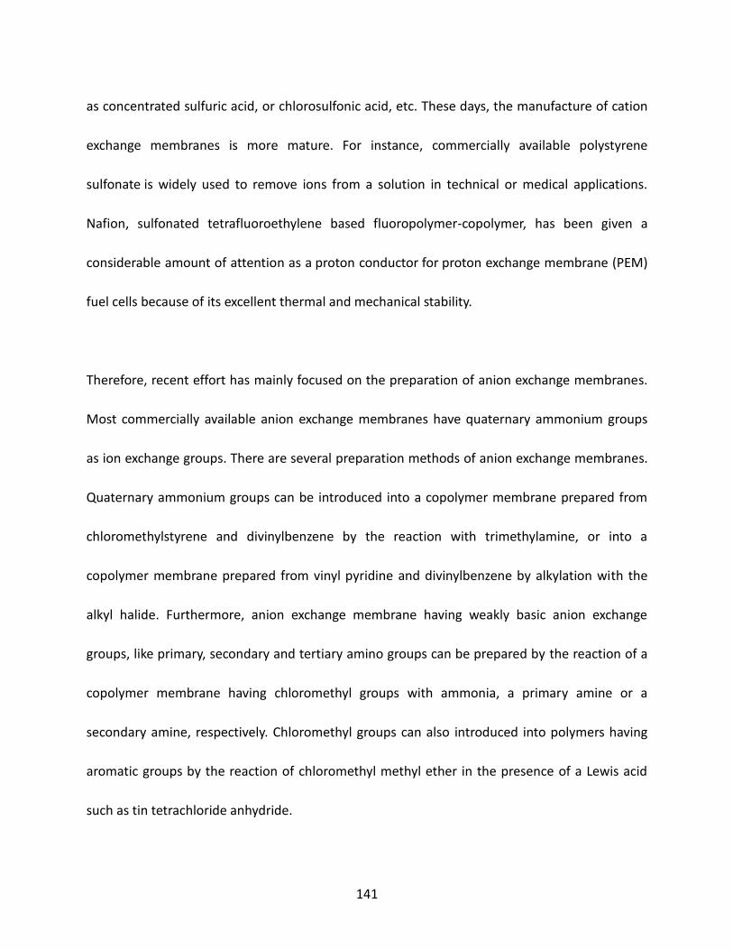
141

as concentrated sulfuric acid, or chlorosulfonic acid, etc. These days, the manufacture of cation

exchange membranes is more mature. For instance, commercially available polystyrene

sulfonate is widely used to remove ions from a solution in technical or medical applications.

Nafion, sulfonated tetrafluoroethylene based fluoropolymer-copolymer, has been given a

considerable amount of attention as a proton conductor for proton exchange membrane (PEM)

fuel cells because of its excellent thermal and mechanical stability.

Therefore, recent effort has mainly focused on the preparation of anion exchange membranes.

Most commercially available anion exchange membranes have quaternary ammonium groups

as ion exchange groups. There are several preparation methods of anion exchange membranes.

Quaternary ammonium groups can be introduced into a copolymer membrane prepared from

chloromethylstyrene and divinylbenzene by the reaction with trimethylamine, or into a

copolymer membrane prepared from vinyl pyridine and divinylbenzene by alkylation with the

alkyl halide. Furthermore, anion exchange membrane having weakly basic anion exchange

groups, like primary, secondary and tertiary amino groups can be prepared by the reaction of a

copolymer membrane having chloromethyl groups with ammonia, a primary amine or a

secondary amine, respectively. Chloromethyl groups can also introduced into polymers having

aromatic groups by the reaction of chloromethyl methyl ether in the presence of a Lewis acid

such as tin tetrachloride anhydride.

142

After the polymer has been chloromethylated by an ordinary method, various amino

compounds, such as trimethylamine (to introduce quaternary ammonium groups) and

polyamines (to form cross-linkages) can be prepared to aminate it. Moreover, multi-layer

membranes, which have different ion exchange capacities, and bipolar membranes can be

prepared by different casting methods. In order to enhance mechanical properties, a

non-woven fabric within a polymer matrix or a block copolymer of styrene and olefin can

reinforce its mechanical strength. In addition, not only dense membranes but also porous and

asymmetric anion exchange membranes can be produced by the phase inversion method.

6.3 Characterization of Anion Exchange Membranes

6.3.1 Molecular Weight

In linear polymers the individual polymer chains rarely have exactly the same degree of

polymerization and molar mass, and there is always a distribution around an average value of

these large molecules. Therefore, one must resort to averages to describe molecular weight.

Among many possible ways of reporting averages, three are commonly used: the number

average (Mn), weight average (Mw), and z-average molecular weights (Mz), are shown in

Equation (6-1), Equation (6-2), and Equation (6-3), respectively. In a typical distribution curve,

the average values are related to each other as follows: Mn < Mw < Mz.

143

𝑁𝑢𝑚𝑏𝑒𝑟 𝑎𝑣𝑒𝑟𝑎𝑔𝑒 𝑀𝑊, �̅�𝑛 =∑(𝑀𝑖𝑁𝑖)

∑(𝑁𝑖) (6-1)

𝑊𝑒𝑖𝑔ℎ𝑡 𝑎𝑣𝑒𝑟𝑎𝑔𝑒 𝑀𝑊, �̅�𝑤 =∑(𝑀𝑖

2𝑁𝑖)

∑(𝑀𝑖𝑁𝑖) (6-2)

𝑍 𝑎𝑣𝑒𝑟𝑎𝑔𝑒 𝑀𝑊, �̅�𝑧 =∑(𝑀𝑖

3𝑁𝑖)

∑(𝑀𝑖2𝑁𝑖)

(6-3)

The ratio of weight average MW to number average MW is known as the polydispersity index

(PDI), and provides a rough indication of the breadth of the distribution. It involves forcing a

polymer solution through a matrix of cross-linked polymer particles at a pressure of up to

several hundred bars. The limited accessibility of stationary phase pore volume for the polymer

molecules results in shorter elution times for high-molecular-mass species. The PDI

approaches 1.0 (the lower limit) for special polymer with very narrow MW distribution, but for

typical commercial polymers, is typically greater than 2. Here is a typical MW distribution curve,

measured by Gel Permeation Chromatography, as presented in Figure 6-3.

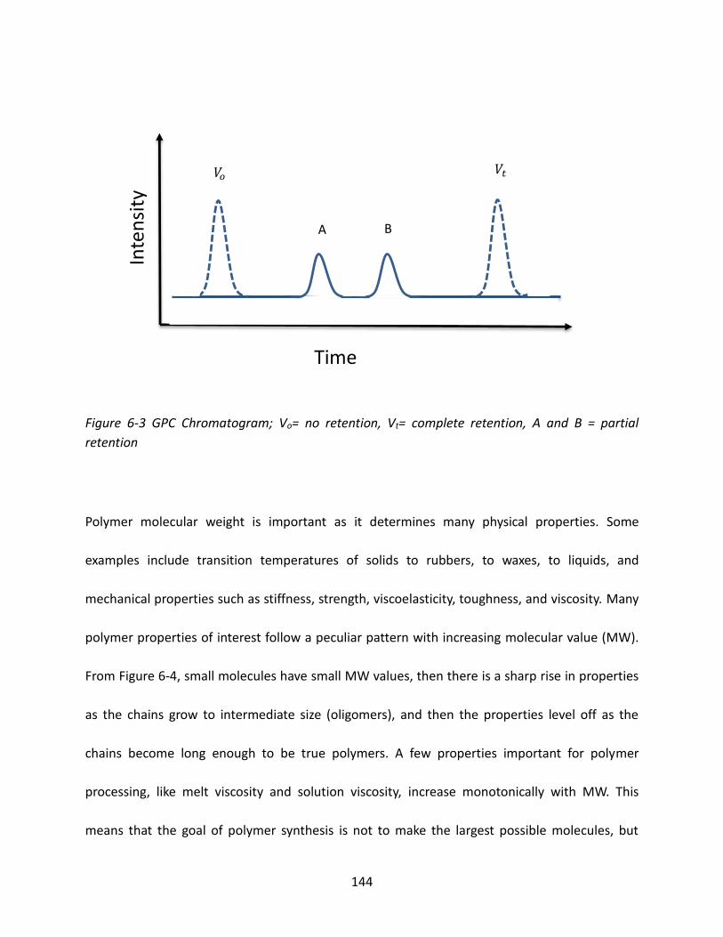
144

Figure 6-3 GPC Chromatogram; Vo= no retention, Vt= complete retention, A and B = partial

retention

Polymer molecular weight is important as it determines many physical properties. Some

examples include transition temperatures of solids to rubbers, to waxes, to liquids, and

mechanical properties such as stiffness, strength, viscoelasticity, toughness, and viscosity. Many

polymer properties of interest follow a peculiar pattern with increasing molecular value (MW).

From Figure 6-4, small molecules have small MW values, then there is a sharp rise in properties

as the chains grow to intermediate size (oligomers), and then the properties level off as the

chains become long enough to be true polymers. A few properties important for polymer

processing, like melt viscosity and solution viscosity, increase monotonically with MW. This

means that the goal of polymer synthesis is not to make the largest possible molecules, but

𝑉𝑜 𝑉𝑡

A B

Time

Inte

nsi

ty

145

rather, to make molecules large enough to get onto the plateau region. Increasing the MW

beyond this does not improve the physical properties much, but makes processing more

difficult.

Figure 6-4 Plot of physical property vs. molecular size for small molecules, oligomers, and

polymers. Examples of physical properties, modulus, strength, and glass transition temperature.

6.3.2 Functional Groups

In organic chemistry, functional groups are specific groups of atoms or bonds within molecules

that are responsible for the characteristic chemical reactions of those molecules. In anion

exchange membrane, vibration of functional groups such as quaternary ammonium groups,

Small

molecules Oligomers Polymers

Molecular Size

Ph

ysic

al P

rop

erty

146

primary, secondary, and tertiary amino groups can be detected by Fourier Transform Infrared

Spectroscopy (FTIR). An infrared spectrum represents a fingerprint of a sample with absorption

peaks which correspond to the frequencies of vibrations between the chemical bonds.

Therefore, it can result in a positive identification (qualitative analysis) of every different kind of

material. In addition, the size of the peaks in the spectrum is a direct indication of the amount

of material present. The peak of 1637cm-1 in IR suggested the existence of quaternary

ammonium group.[133]

6.3.3 Ion Exchange Capacity and Hydroxyl Group Conductivity

The ion exchange capacity of a membrane is an important property because the amount and

species of ion groups determine the properties of the membrane. The ion exchange capacity of

an ionomer is an intrinsic property. However, the hydroxyl group conductivity of anion exchange

membrane is better related to the apparent functional groups within the polymer matrix. Hence,

ion exchange capacity and hydroxyl group conductivity are two important characteristics of the

anion exchange membranes, which can be measured by titration and conductivity

measurement, respectively.

147

6.3.4 Glass Transition Temperature

Many other properties of polymers such as thermal expansion, heat capacity, and shear

modulus show a relatively sudden change at the glass transition temperature. The optimal

temperature range where polymers can be utilized is very important. For anion exchange

membranes, based on different charged functional groups and different polymer blocks, the

glass transition temperatures are more than one if the solubility parameters of polymer blocks

are far away from each other, which leads to phase separation.

6.3.5 Thermal Degradation Temperature

Thermal degradation temperature is an essential property of ionomer, especially for anion

exchange membranes. It can show an upper limit to the service temperature of polymers where

there exists the possibility of mechanical property loss. Positively charged functional groups

within anion exchange membranes such as quaternary ammonium groups are not stable if the

environmental temperature is above a certain point. Hence, service temperature ranges of

anion exchange membranes play a significant role in the industrial application.

148

6.4 Development of Anion Exchange Membranes

Recently, anion exchange membranes have been applied in a variety of industrial fields,

including the separation of environmental polluting metal ions from hard water[134], alkaline

direct methanol fuel cells[135], current and potential applications as ion-exchanger[136],

biomaterials[137], and electrodialysis[138]. However, unlike cation exchange membranes, which

have highly chemical stability such as DuPont’s Nafion and Asahi Glass’ Flemion, commercially

available anion exchange membranes are typically based on cross-linked polystyrene and are

not stable in alkaline and electrochemical environment. Additionally, they are often blended

with other inert polymers and fabric supports that limit ionic conductivity and decrease the

chemical stability of the membranes.[139]

A series of anion exchange membranes, (such as polybenzimidazole[140],

poly(2,6-dimethyl-1,4-phenylene oxide)[141], poly(ether ketone)[142], and poly(ethylene-co-

tetrafluoroethylene) (ETFE)[143], poly(tetrafluoroethylene-co-hexafluoropropylene) (FEP)[144], and

poly(vinylidene fluoride) (PVDF)[145]), have been produce for utilization in alkaline fuel cell

testing. Anion exchange membranes based on polysulfone were prepared by a

chloromethylation reaction on the parent polysulfone and the following conversion of the

chloromethyl groups into tetraalkylammonium cation exposing to trimethylamine.[146] Syntheses

149

of anion exchange membranes based on poly(vinyl alcohol)[147], poly(ether-imide)[148], and

imidazolium-type ionic liquid functionalized polymer[149] have also been reported.

Though polysulfone is most widely used in the manufacture of synthetic polymer membranes

due to its excellent mechanical, thermal and chemical stability, the chloromethylation reaction

for aminated polysulfone requires long reaction times, involves imprecise control over reactant

ratios and grafting locations, and has a large excess of toxic reagents. Moreover, the stability of

the fixed cationic site in alkaline conditions is a concern due to nucleophilic attack by anions.

To avoid these problems, a novel approach to the formation of halomethyl groups by preparing

polymers with benzylic methyl groups has been reported. Poly(2,6-dimethyl-1,4-phenylene

oxide) (PPO)[150] was treated with bromine to convert the methyl groups into bromomethyl

groups and then trimethylamine was used to convert bromomethyl groups in to quaternary

ammonia groups in the same manner as chloromethyl groups. The combination of high pH and

elevated temperature can lead to chemical attack on the quaternary ammonium groups, most

commonly by either an E2 Hofmann degradation mechanism or an SN2 substitution reaction.

The elimination reaction pathway can be avoided by using quaternary ammonium groups that

do not have beta hydrogens such as the benzyltrimethylammonium group.[151] If fluorenyl

groups are introduced into the polymer backbone, the anion exchange membrane may retain its

ionic conductivity and durability in alkaline fuel cell applications.[152]

150

6.5 Summary

In this work, we will start from the synthesis of an anion exchange membrane of

polyphenylsulfone-b-tetramethyl polysulfone (PPSU-TMPS block copolymer) by using

N-bromosuccinimide (NBS) as a source of bromine and benzoyl peroxide as an initiator, to avoid

the problems of chloromethylation reaction and instability of quaternary ammonium groups.

Subsequently, characterization of aminated PPSU-TMPS will be carried out with respect to

molecular weight, functional group, ion exchange capacity, hydroxyl group conductivity, glass

transition temperature, and thermal degradation temperature.

151

Chapter 7 Literature Review: Electrodialysis

7.1 Electrodialysis Definition

Electrodialysis is a process by which ionic substances with molecular weight below several

hundred permeate through a membrane in the presence of an electrochemical potential: to

concentrate salt from dilute solution, to desalinate electrolytic solutions, to separate ionic from

non-ionic substances, to ion exchange ions across a membrane, etc.[5]

7.2 Characteristics, Advantages and Limitations of

Electrodialysis

In the process of electrodialysis, salt ions are transported from one solution through ion

exchange membranes to another solution under the influence of an applied electric potential

difference. This is done in a configuration called an electrodialysis cell, consisting of a dilute

compartment and a concentrated compartment formed by a cation exchange membrane and an

anion exchange membrane placed between two electrodes.

Electrodialysis is generally carried out using a multi-compartment electrodialyzer (called

electrodialysis stack), in which alternating cation and anion exchange membranes (CEM and

AEM) are installed, with the anode and cathode located at each end of the electrodialyzer.

152

Bipolar ion-exchange membranes (the combination of CEM and AEM)[153], while used in the

concentration or desalination of electrolytes and separation between electrolyte and

non-electrolytes, can also be used to generate hydrogen ions and hydroxide ions by splitting

water to produce acid and alkali from neutral salt in the presence of electrical potential.

Meanwhile, the same mechanism can be applied to an ion-exchange reaction[154].

Electrodialysis processes are different compared to distillation techniques and other membrane

based processes (i.e. reverse osmosis), in that dissolved species are moved away from the feed

stream rather than the reverse as shown in Figure 7-1. Because the quantity of dissolved species

in the feed stream is far less than that of the fluid, electrodialysis offers the practical advantage

of much higher feed recovery in many applications.

153

Figure 7-1 Mechanism of reverse osmosis.

The energy-saving and small “carbon footprint” application of electrodialysis also fits to

separate thermally unstable materials such as biomaterials, products in the food industry and

similar materials from salts, acids, and alkalis (by ion-exchange reaction). This is possible as

electrodialysis is a separation process that is not accompanied by phase separation, unlike the

traditional separation process like evaporation and crystallization processes.

Direction of Water Flow

Salt

Water

Fresh

Water

Semi-permeable

Membrane

Applied

Pressure

Pure

Water

154

0.1 1 10 1001

10

100

1000

M

in E

nerg

y C

on

su

mp

tio

n (

J/g

)

Concentration of Feedwater (g/L)

Electrodialysis (ED)

Reverse Osmosis (RO)

Multi-Stage Flash Distillation (MSF)

Potable Water

Brackish Water

Sea Water

PW BW SW

Figure 7-2 Estimated minimum energy consumption per volume of product water and typical

energy consumption for common desalination including multi-stage flash distillation (MSF),

reverse osmosis (RO), and electrodialysis (ED).[155]

The major application of electrodialysis has historically been the desalination of brackish water

or seawater as an alternative to reverse osmosis for potable water production and seawater

concentration for salt production (primarily in Japan, especially in low sodium chloride

concentration), while multi-stage flash distillation requires higher energy consumption

compared with reverse osmosis, as presented in Figure 7-2.

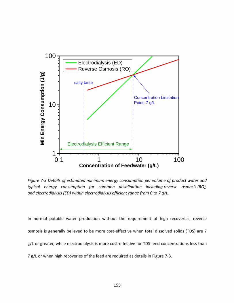
155

0.1 1 10 1001

10

100

salty taste

Min

En

erg

y C

on

su

mp

tio

n (

J/g

)

Concentration of Feedwater (g/L)

Electrodialysis (ED)

Reverse Osmosis (RO)

Concentration Limitation

Point: 7 g/L

Electrodialysis Efficient Range

Figure 7-3 Details of estimated minimum energy consumption per volume of product water and

typical energy consumption for common desalination including reverse osmosis (RO),

and electrodialysis (ED) within electrodialysis efficient range from 0 to 7 g/L.

In normal potable water production without the requirement of high recoveries, reverse

osmosis is generally believed to be more cost-effective when total dissolved solids (TDS) are 7

g/L or greater, while electrodialysis is more cost-effective for TDS feed concentrations less than

7 g/L or when high recoveries of the feed are required as details in Figure 7-3.

156

Another important application for electrodialysis is the production of pure water and ultrapure

water by the process of electrodeionization (EDI), in which the purified compartments and the

concentrated compartments of the electrodialysis stack are filled with an ion exchange resin.

When fed with low TDS feed (e.g., feed purified by RO), the product can reach very high purity

levels. The ion exchange resins act to retain the ions, allowing water molecules diffusing across

the ion exchange membranes. The principal applications of EDI systems are mainly motivated in

the areas of electronics, pharmaceutical, power generation, and cooling tower.

Electrodialysis has inherent limitations, working best at removing low molecular weight ionic

components from a feed stream. Non-charged, higher molecular weight, and less mobile ionic

species will not typically be significantly removed. Also, in contrast to reverse osmosis, the

minimum energy consumption of electrodialysis process increases dramatically above 7 g/L

freed concentration. In this way, it becomes less economical when high salt concentrations in

the feed are present. Moreover, as the feed salt solution concentration becomes lower, the

current density becomes limited and current utilization efficiency typically decreases with fewer

ions in solution to carry current, and both the ion transport and the energy efficiency greatly

decline. Consequently, in order to shorten the electrodialysis process and improve the current

efficiency and the transport number of ionomers, comparatively large membrane areas are

required to satisfy capacity requirements. Innovative systems overcoming the inherent

limitations of electrodialysis (and RO) are available; these integrated systems work

157

synergistically, with each sub-system operating in its optimal range, providing the least overall

operating and capital costs for a particular application.

As with RO, electrodialysis systems require feed pretreatment to remove species that

coat, precipitate onto, or otherwise "foul" the surface of the ion exchange membranes. This

fouling decreases the efficiency of the electrodialysis system. Species of concern

include calcium and magnesium hardness, suspended solids, silica, and organic compounds.

Water softening can be used to remove hardness, and micrometer or multimedia filtration can

be used to remove suspended solids. Hardness in particular is a matter of concern since scaling

can build up on the membranes. Numerous chemicals are also available to help prevent scaling.

Also, electrodialysis reversal systems aim to minimize scaling by periodically reversing the flows

of dilute and concentrate and polarity of the electrodes.

7.3 Application of Electrodialysis Process

In application, electrodialysis systems can be operated as continuous production or batch

production processes. In a continuous process, feed is passed through a sufficient number of

stacks placed in series to produce the final desired product quality. In batch processes, the

dilute and concentrate streams are re-circulated through the electrodialysis systems until the

final product or purifying quality is achieved.

158

Electrodialysis is a separation technique for ionic solutions through an electrochemical

membrane that has served in the industry for several decades. The first application of

electrodialysis in the educational literature appeared in 1931 by Kendall A. I.[156]. Commercial

equipment using the ED Tech was first developed in the 1950s[14, 157]. Since then, ED has

advanced rapidly because of improved ion-exchange membrane properties, better materials of

construction and advances in technology. It can be employed in the separation and

concentration of salts, acids and bases from aqueous solutions, the separation of monovalent

ions from multivalent ions and the separation of ionic compounds from uncharged molecules. It

can be utilized for either electrolyte reduction in feed streams or recovery of ions from dilute

streams[158]. Industrial applications hitherto encompass several industries and include the

production of potable water from brackish water, removal of metals from wastewater,

demineralization of whey, deacidification of fruit juices and the removal of organic acids from

fermentation broth, as shown in Table 7-1.

159

Table 7-1 Application of Electrodialysis

Industrial Application of Electrodialysis Electrolyte recovery

Electrolyte reduction

Potable water from brackish water

Nitrate removal for drinking water

Boiler water, cooling tower water, effluent

steam desalting

Cheese whey demineralization

Fruit juice deacidification

Sugar and molasses desalting

Potassium tartrate removal from wine

Blood plasma protein recovery

Demineralization of amino acid solution in

the food industry

Edible salt production from seawater

Ag(I) salts from photographic waste

Zn(II) from galvanizing rinse water

Organic salts from fermentation broth

Amino acids from protein hydrolysates

Salts, acids, and alkali from industrial

rinse waters

Conversion of organic salts into acid

and base (bipolar membrane ED)

Salt splitting

7.4 Theory of ED Process

ED is an electrochemical separation process in which ions are transferred through ion exchange

membranes by a direct current (DC) voltage. The process uses a driving force to transfer ionic

species from the source water through cathode (positively charged ions) and anode (negatively

charged ions) to a concentrate wastewater stream, creating a more dilute stream and a more

concentrated stream as schemed in Figure 7-4.

160

Figure 7-4 Principles of electrodialysis.

ED selectively removes dissolved solids, based on their electric charge, by transferring the

brackish water ions through a semipermeable ion-exchange membrane charged with an

electrical potential. It points out that the feed water becomes separated into the following

three types of water:

Cathode (-) CEM AEM CEM AEM CEM AEM CEM AEM CEM AEM CEM Anode(+)

Dilute Cylinder

Electrolyte Cylinder

Concentrated Cylinder

CEM AEM

Direct Current Voltage

161

1. Dilute cylinder, which has an acceptably low conductivity and total dissolved solid level;

2. Concentrated cylinder, which is the water that receives the brackish water ions;

3. Electrolyte cylinder, electrode feed water, which is the water that passes directly over the

electrodes that create the electric potential.

Within an electrodialysis stack, the dilute, concentrated streams, and electrolyte are allowed to

flow through the appropriate cell compartments formed by the alternating ion exchange

membranes. Figure 7-4 shows in detail that under the influence of an electrical potential

difference, the negatively charged chloride ions in the dilute stream migrate toward the

positively charged anode through positively charged anion exchange membrane. However,

negatively charged ions are prevented from further migration toward the anode by the

negatively charged cation exchange membrane. Consequently, they stay in the concentrated

stream, which becomes concentrated with the anions. The positively charged sodium species in

the dilute stream migrate toward the negatively charged cathode and pass through the

negatively charged cation exchange membrane. These cations also stay in the concentrated

stream, prevented from further migration toward the cathode by the positively charged anion

exchange membrane. As a result of the anion and cation migration, electric current flows

between the cathode and anode. Only an equal number of anion and cation charge equivalents

are transferred from the dilute stream into the concentrate stream and so the charge balance is

162

maintained in each stream. The overall result of the electrodialysis process is an ion

concentration increase in the concentrate stream with a depletion of ions in the dilute solution

feed stream.

The electrolyte stream is the electrode stream that flows past each electrode in the stack. This

stream may consist of the same composition as the feed stream (e.g., sodium chloride) or may

be a separate solution containing a different species (e.g. sodium sulfate). Depending on the

stack configuration, anions and cations from the electrode stream may be transported into the

concentrated stream, or anions and cations from the dilute stream may be transported into the

electrolyte stream. In each case, this transport is necessary in order to carry current across the

stack and maintain electrically neutral stack solutions.

7.5 Limiting Current Density (LCD)

Reactions take place at each electrode. At the cathode,

2𝑒− + 2𝐻2𝑂 → 𝐻2(𝑔) + 2𝑂𝐻−

while at the anode,

163

𝐻2𝑂 → 2𝐻+ +1

2𝑂2(𝑔) + 2𝑒−

or

2𝐶𝑙− → 𝐶𝑙2(𝑔) + 2𝑒−

Small amounts of hydrogen gas are generated at the cathode and small amounts of either

oxygen or chlorine gas (depending on the compositions of the electrolyte stream and end ion

exchange membrane arrangement) at the anode. These gases are typically dissipated as the

electrolyte stream effluent from each electrode compartment is combined to maintain a neutral

pH and re-circulated in this separate electrolyte tank. Moreover, it is proposed that the

collection of hydrogen gas can be introduced in energy production.

164

Figure 7-5 Model concentration profile at the membrane-solution interface during

electrodialysis (cation exchange membrane).

In the electrodialysis process as given in Figure 7-5, limiting current density of the

electrodialyzer is an important parameter as illustrated in Equation (7-1) which determines the

electrical resistance and the current utilization.

𝑖𝑙𝑖𝑚 =𝐹𝐷𝐶1

𝛿1(�̅�+−𝑡+) (7-1)

where δ1 is the thickness of the diffusion boundary layer at the desalting side depending on

the structure of the electrodialyzer and its operating conditions, t̅+ and t+ are the transport

numbers of the cation in the membrane phase and in the solution, C1 is the concentration of the

𝑖𝑡+

𝐹

𝑖𝑡̅+

𝐹

𝐶1

𝐶2

𝐶3

𝐶4

𝛿1 𝛿𝑚 𝛿2

𝐷(𝐶1 − 𝐶2)

𝛿1

𝐷𝑚(𝐶3 − 𝐶2)

𝛿𝑚

165

desalting solution, D is the diffusion coefficients of the electrolyte in the solution, and F is

Faraday’s constant. The limiting current density of the electrodialyzer is generally determined by

measuring the current-voltage relation of the electrodialyzer.[5]

At a higher current density than the limiting current density, water is split at the

membrane-solution interface of the desalting side. The solution pH changes due to selective

permeation of proton or hydroxide ions through the cation or anion exchange membrane

compared with other ions in low concentration. Moreover, if the solution contains metal ions

that form compounds with low solubility, such as metal hydroxides and carbonates at high pH,

they might precipitate on the membrane, and thus electrodialysis cannot be continuously

performed. Meanwhile, the current efficiency decreases due to permeation of proton or

hydroxide ions through the membranes.

7.6 Nernst-Planck Equation

The Nernst-Planck equation is a conservation of mass equation referring to the motion of

chemical species in a fluid medium. It describes the fluxes of ions under the influence of both an

ionic concentration gradient and an electric field.

166

The Nernst-Planck flux equation has been broadly applied to explain transport phenomena in

ion-exchange membranes and solution systems. The flux of ion i flowing through the ionomer

can be expressed as Equation (7-2)[159].

𝐽𝑖 = 𝐽𝑖(𝑑) + 𝐽𝑖(𝑒)+𝐽𝑖(𝑐𝑜𝑛𝑣) = −𝐷𝑖(𝑑𝐶𝑖

𝑑𝑥+

𝑧𝑖𝐹𝐶𝑖

𝑅𝑇

𝑑𝜓

𝑑𝑥+ 𝐶𝑖

𝑑𝑙𝑛𝛾𝑖

𝑑𝑥) + 𝐶𝑖𝑣 (7-2)

where Ji(d), Ji(e) and Ji(conv) are fluxes caused by diffusion potential, electrical potential and

convection, 𝐷𝑖 is the diffusion coefficient of i in the membrane, 𝐶𝑖 is the concentration of i in

the membrane, v is the flow velocity of the solvent, 𝛾𝑖 is the activity coefficient of i in the

membrane, zi is the valence of ion i, 𝑑𝜓

𝑑𝑥 is the gradient of the electric potential and R the gas

constant and T the absolute temperature.

7.7 Two Methods to Calculate the Flux of Ions

Method One

Through combination of two Equation (7-3) and (7-4) correlating with transport number, ion flux

of species i, Ji, can be determined.[5]

𝑡𝑖 =𝐹𝐽𝑖

𝐼 (7-3)

where 𝐼 is the electric current, 𝑡𝑖 is the transport number of species i in the membrane, and F

is Faraday constant.

167

𝑡𝑖 =𝐹𝑉(𝑑𝐶𝑖/𝑑𝑡)

𝐼𝐴 (7-4)

where V is the overall processing volume of batch ED, I is the electric current in the presence

of an electric potential gradient and 𝑡𝑖 is the transport number of i in the membrane, A is the

effective area of ionomers.

Combining Equation (7-3) with Equation (7-4), Equation (7-5) correlating with the ion flux is

approached.

𝐽𝑖 =𝑉(𝑑𝐶𝑖/𝑑𝑡)

𝐴 (7-5)

Method Two

The Nernst-Planck flux equation can be applied to explain transport phenomena in ion exchange

membranes and solution systems.


𝑑𝑥+


𝑅𝑇

𝑑𝜓

𝑑𝑥+ 𝐶𝑖


𝑑𝑥) + 𝐶𝑖𝑣 (7-2)


convection, 𝐷𝑖 is the diffusion coefficient of i in the membrane, 𝐶𝑖 is the concentration of i in

168

the membrane, v is the flow velocity of the solvent, 𝛾𝑖 is the activity coefficient of i in the

membrane, zi is the valence of ion i, 𝑑𝜓

𝑑𝑥 is the gradient of the electric potential (κ = −[

Idψ

dx

],

where 𝜅 is the specific conductivity of species i in the membrane) and R the gas constant and T

the absolute temperature.

7.8 Summary

In this work, a series of ionomer involving cation exchange membrane (Nafion, sulfonated

polystyrene, penta block copolymer, poly[t-butyl styrene-b-hydrogenated isoprene-b-sulfonated

styrene-b-hydrogenated isoprene-b-t-butyl styrene) (tBS-HI-S-HI-tBS), and sulfonated

polyphenylene) and anion exchange membranes (aminated polystyrene, aminated

polyphenylsulfone-b-tetramethyl polysulfone (PPSU-TMPS block copolymer) will be studied in

the electrodialysis process. The performance parameters of the electrodialyzer, such as the

limiting current density, ion flux, concentration change and resistance change within

electrodialysis cells, energy consumption, transport number, and current efficiency will be

determined in order to explore the optimal ion exchange membranes which can be utilized in

the process of electrodialysis.

169

Chapter 8 Materials and Methods

8.1 Materials

8.1.1 Liquid and Other Material

Ethyl alcohol (200 proof absolute anhydrous ACS/USP grade) is from PharmcoAaper. Ethylene

glycol (EG) 99+% 1L comes from Sigma Aldrich. Microslides, plain, pre-cleaned 75×50 mm,

thickness from 0.96 to 1.06 mm are from Corning Incorporated. Scotch Permanent

Double-Sided Tape is coated with photo-safe, permanent adhesive on both sides with a

no-mess alternative to glue for light-duty attaching and mounting tasks.

8.1.2 Polymers

Polytetrafluoroethylene (PTFE) is a synthetic fluoropolymer of tetrafluoroethylene, as shown in

Figure 8-1 (a), most well-known by the DuPont brand name Teflon. PTFE is hydrophobic with a

high-molecular-weight compound consisting of carbon-fluorine bonds, which are highly

non-reactive at room temperature, with a density of about 2.2 g/cm3. Teflon plate (PTFE) used

in the experiment is flat-form dishes (50 mL 60 ×20 mm) whose supplier is VWR International,

LLC..

170

Perfluorosulfonic acid (PFSA) is a sulfonated tetrafluoroethylene based fluoropolymer

-copolymer as displayed in Figure 8-1 (c), discovered in the late 1960s by Walther Grot of

DuPont as Nafion. As the first of a class of synthetic polymers with ionic properties (called

ionomers), Nafion has unique ionic properties due to its incorporating perfluorovinyl ether

groups terminated with sulfonate groups onto a tetrafluoroethylene (Teflon) backbone. Nafion

membrane NF115 (5mil thick, IEC=0.9), NF117 (7mil thick, typical thickness 183 microns,

IEC=0.9, and basis weight 360 g/m2), and NF212 (2mil thick, IEC=0.9) comes from Ion Power,

Inc., as illustrated in Table 8-1. Nafion ionomer series are cast by different methods, as shown

in Figure 8-2.

Sulfonated poly(phenylene) (sPP) is prepared by the Diels-Alder polymerization[160] which

makes these materials readily soluble in organic solvents and easily processed into thin films.

Six pendant phenyl groups per repeat unit are the maximum amount of sulfonic acid groups.

The sPP3 polymer with 3 sulfonic acid groups is used in the experiment. The sPP3 chemical

structure is shown in Figure 8-1 (b) while the details of synthesis have been documented in the

reference[160] and listed in Table 8-2.

171

Figure 8-1 Chemical structures of polymers utilized in this study.

(d) PBC: poly[t-butyl styrene-b-hydrogenated isoprene-b-sulfonated

styrene-b-hydrogenated isoprene-b-t-butyl styrene) (tBS-HI-S-HI-tBS)

(c) Perfluorosulonic acid (PFSA)

CH3

A B Cx C(1-x)

SO3H

AB

C(CH3)3

CH3

C(CH3)3

CF2

xCF

CF2

OCF2

CF

O

CF2

CF2

S

OH

O

O

y

z

CF3

CF2

(b) sPP3 (NO. of –SO3H group =3)

(a) Polytetrafluoroethylene (PTFE)

*

*

SO3H SO3H

SO3H

CF2

nCF2

O O S

O

O

FS

O

O

OOH

xy

N(CH3)3

N(CH3)3

(H3C)3N

(H3C)3N

OH

OH

OH

OH

(e) aminated PPSU-TMPS: polyphenyl sulfone-tetramethyl polysulfone

172

PBC ionomers were supplied by Kraton Polymers LLC, Houston, TX[161]. This poly[t-butyl

styrene-b-hydrogenated isoprene-b-sulfonated styrene-b-hydrogenated isoprene-b-t-butyl

styrene) (tBS-HI-S-HI-tBS) is produced by anionic polymerization. The chemical structure is given

in Figure 8-1[161a].

After polymerization, the styrene block is selectively sulfonated to a desired IEC in terms of

milliequivalents of sulfonic acid per gram of polymer (mequiv/g)[161a]. The PBC degree of

sulfonation (DS) is the mole fraction of polystyrene blocks PS that are sulfonated (sPS). The

complete synthetic details have been documented elsewhere[161a]. The basic PBC properties are

summarized in Table 8-2.

Table 8-1 Characteristics of Nafions and sPP used in the experiment

IEC EW Mw(g/mol) Thickness(mm) Casting method

NF117 0.91 1100 105-106 0.175 Melting extrusion

NF115 0.91 1100 105-106 0.123 Melting extrusion

NF212 0.98 1020 105-106 0.049 Solution dispersion

sPP3 1.8 1000 1.72×105 0.039 Scrolling casting

Equivalent weight (EW) is the number of grams of dry polymer per mole of sulfonic acid groups

when the material is in the acid form. The sPP3 has 3 sulfonic acid groups per monomer. The

unit of IEC is mol-SO3H/1000g polymer while EW=1000/IEC.

173

Figure 8-2 Casting methods of NF117&115, NF212, and sPP3.

(a) Melting Extrusion

(b) Solution Dispersion

(c) Scrolling Casting

174

Table 8-2 PBC ionomer properties with different IEC [161b]

Copolymers IEC

(mequiv/g)

DS

(mol%)

Density of sS

(g/ cm3)

Volumeratio[tBS-HI-S)]

PBC-0.0 0.0 0 1.05 0.33:0.29:0.38

PBC-0.4 0.4 10 1.09 0.32:0.28:0.40

PBC-0.7 0.7 18 1.13 0.31:0.28:0.41

PBC-1.0 1.0 26 1.16 0.31:0.27:0.42

PBC-1.5 1.5 39 1.21 0.30:0.27:0.43

PBC-2.0 2.0 52 1.27 0.30:0.26:0.44

Aminated PPSU-TMPS block copolymer is prepared by the parent polyphenyl sulfone, PPSU,

(which is prepared by the condensation of 4,4’-difluorophenyl sulfone with biphenol) and the

parent tetramethyl polysulfone, TMPS, (which is prepared by the condensation of

4,4’-difluorophenyl sulfone with tetramethyl bisphenol A, TMBPA). The benzylic methyl groups

on TMPS could be brominated using N-bromosuccinimide (NBS) as a source of bromine and

benzoyl peroxide (BPO) as an initiator. The fraction of methyl groups converted to bromomethyl

groups was controlled by adjusting the amount of NBS used. The quaternary ammonium groups

could be produced using trimethylamine by mixing brominated PPSU-TMPS DMF solution.

175

8.2 Experimental Method

8.2.1 Membrane Preparation

Commercial PBC films were created from a C:H solution that was cast using a Doctor Blade[161].

Experimental PBC films were made by dissolving in either THF, CHCl3, or C:H (1:1 wt%) followed

by solution casting in a Teflon dish.

8.2.2 Contact Angle Measurement

The apparent water contact angle, θ, was measured with a Kruss DSA (Drop Shape Analysis) 100

surface analyzer as shown in Figure 8-3, while the contact angle between NF115 and water was

95.9o consistent with reference [162]. The volume of testing liquid droplet, 15μL, was the optimal

volume for producing reproducible contact angle measurements with a maximum error of +/- 3

degrees (error 3%). All measurements were performed at room temperature and repeated

more than five times in order to determine reproducibility. Different percentages of ethanol, EG,

and water solutions were prepared as testing liquid. Contact angles of different polymer were

measured with the help of DSA 100. According to the different methods, the surface energy of

solid polymers was calculated while optimal calculation methods were investigated with data

analysis.

176

The contact angles were determined on substrates of different polarities. Both on the polar and

the non-polar substrates, the maximum and minimum surface tensions of liquids lead,

respectively, to the highest and the lowest contact angles.[163] The contact angle measurements

give several kinds of information about solid polymers. The affinity between a liquid droplet and

a solid surface, if using water to evaluate the contact angle, can deduce the hydrophobic

(0o~30o) or hydrophilic (greater than 90o) character of the surface. If several reference liquids

are chosen to probe the solid surface energy, the discrimination between polar and dispersive

components can be examined. The measurement of the hysteresis between advancing angle

and recessing angle provides information on non-homogeneity of the surface (e.g., roughness,

rugosity, contamination).

Figure 8-3 The contact angles are formed between different polymers (PTFE, NF115, and sPP3)

and testing liquid water.

The contact angle of PTFE (IEC=0)

107.6o

0.5mm 0.5mm

95.9o 86.6o

The contact angle of sPP3 (IEC=1.8)

0.5mm

The contact angle of NF115 (IEC=0.9)

177

8.2.3 Water Diffusion Measurement

Weight uptake

Different kinds of polymers were pretreated in 1M sulfuric acid, afterwards, DI water and then

dried in the vacuum oven overnight. The polymers were weighted before and after treatments

to calculate water weight uptake.

Volumetric swelling

For swelling measurement, dried sheet-shaped polymer samples were inserted in the gap of

two glass slides. After that, DI water was poured into the gap. In the process of deswelling,

samples were withdrawn from DI water and measured after removing water by lightly blotting

sample surface with a filter paper. Videos of swelling phenomenon for membranes (cut by 2cm

×2cm) are recorded by DSA100 and measured by MB-Ruler.

178

Figure 8-4 Swelling phenomenon of NF117 in accordance with time.

5mm

5mm 5mm 5mm

5mm 5mm 5mm

5mm 5mm 5mm

2 s 3 s 4 s

7 s

10 s

5 s

8 s 9 s

6 s

179

In the first several seconds, volume ratio dramatically increases with time. Measuring with

MB-Ruler software, the data of three-dimensional swelling ratio versus time can be obtained, as

demonstrated in Figure 8-4.

8.2.4 Solubility Measurement

Different kinds of polymers were pretreated in 1M sulfuric acid and DI water, and then dried in

the vacuum oven overnight. Afterwards, membranes were processed in solutions with different

solubility parameters. The polymer was weighted as dry or wet bases in order to calculate

solvent weight uptake.

8.2.5 Morphology

8.2.5.1 Transmission Electron Microscopy (TEM)

Instrumental apparatus

FEI Tecnai Biotwin G2 Spirit Transmission Microscope at 80 kV was utilized to acquire images.

All PBC samples were treated in a BaCl2 solution to convert the acid form to barium form in

order to enhance contrast using electron density. Membrane strips with 0.5-1.0 mm width and

5.0-10.0 mm length were embedded in epoxy. Testing sections were cut using a Diatome

diamond knife, and collected onto 400 mesh copper-ruthenium grids.

180

Introduction

Transmission electron microscopy (TEM) is a microscopy technique in which a beam of

electrons is transmitted through an ultra-thin specimen, interacting with the specimen as it

passes through. An image is formed from the interaction of the electrons transmitted through

the specimen; the image is magnified and focused onto an imaging device, such as a fluorescent

screen, on a layer of photographic film, or to be detected by a sensor such as a CCD camera.

TEMs are capable of imaging at a significantly higher resolution than light microscopes, owing

to the small de Broglie wavelength of electrons. This enables the instrument’s user to examine

a single column of atoms, which is thousands of times smaller than the smallest resolvable

object in a light microscope. TEM forms a major analytical method in the scientific fields,

including both physical and biological sciences. TEMs find application in cancer research,

virology, material science as well as pollution, nanotechnology, and semiconductor research.

For small magnifications, TEM image contrast is due to absorption of electrons in the material,

due to the thickness and composition of the material. At higher magnifications, complex wave

interactions modulate the intensity of the image, requiring expert analysis of observed images.

Alternate modes allow for the TEM to observe modulations in chemical identity, crystal

orientation, electronic structure, and sample induced electron phase shift as well as the regular

absorption based imaging. The first TEM was built by Max Knoll and Ernst Ruska in 1931. With

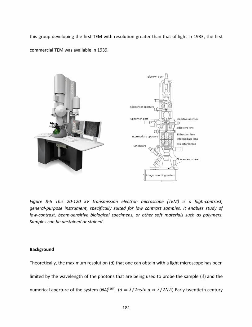
181

this group developing the first TEM with resolution greater than that of light in 1933, the first

commercial TEM was available in 1939.

Figure 8-5 This 20-120 kV transmission electron microscope (TEM) is a high-contrast,

general-purpose instrument, specifically suited for low contrast samples. It enables study of

low-contrast, beam-sensitive biological specimens, or other soft materials such as polymers.

Samples can be unstained or stained.

Background

Theoretically, the maximum resolution (d) that one can obtain with a light microscope has been

limited by the wavelength of the photons that are being used to probe the sample ()and the

numerical aperture of the system (NA)[164]. (𝑑 = 𝜆 2𝑛𝑠𝑖𝑛⁄ 𝛼 ≈ 𝜆 2𝑁𝐴⁄ ) Early twentieth century

182

scientists theorized the limitations of the relatively of visible light (wavelengths of 400-700

nanometers) by using electrons. Like all matter, electrons have both wave and particle

properties (as theorized by Louis-Victor de Broglie), and their wave-like properties mean that a

beam of electrons can be made to behave like a beam of electromagnetic radiation. The

wavelength of electrons is related to their kinetic energy via the de Broglie Equation. An

additional correction must be made to account for relativistic effects, as an electron’s velocity

in a TEM approaches the speed of light, c.[165] 𝜆𝑒 ≈ ℎ √2𝑚0𝐸(1 + 𝐸 2𝑚0𝑐2)⁄⁄ where, h is

Planck’s constant, m0 is the rest mass of an electron and E is the energy of the accelerated

electron. Electrons are usually generated in an electron microscope by a process known as

thermionic emission from a filament, usually tungsten, in the same manner as a light bulb, or

alternatively by field electron emission.[166] The electrons are then accelerated by an electric

potential (measured in volts) and focused by electrostatic and electromagnetic lenses onto the

sample. The transmitted beam contains information about the electron density, phase and

periodicity; this beam is used to form an image.

Components

A TEM is composed of several components, which include a vacuum system in which the

electrons travel, an electron emission source for generation of the electron stream (electron

gun), a series of electromagnetic lenses (electron lens), as well as electrostatic plates, specimen

stage, and apertures. The electron lens and apertures allow the operator to guide and

183

manipulate the beam as required. Another small device is needed as well to allow the insertion

into, motion within, and removal of specimens from the beam path. Imaging devices are

subsequently used to create an image from the electrons that exit the system.

Imaging methods

Imaging methods in TEMs utilize the information contained in the electron waves exiting from

the sample to form an image. The projector lenses allow for the correct positioning of this

electron wave distribution onto the viewing system. The observed intensity of the image, I,

assuming sufficiently high quality of the imaging device, can be approximated as proportional

to the time-average amplitude of the electron wavefunctions, denoted by 𝐼(𝑥) =

𝑘 (𝑡1 − 𝑡0)⁄ ∫ 𝜓𝜓∗𝑑𝑡𝑡1

𝑡0. Different imaging methods therefore attempt to modify the form of

electron waves exiting the sample. From the previous equation, it can be deduced that the

observed image depends not only on the amplitude of the beam, but also on the phase of the

electrons. Therefore, the sample can no longer be considered to be absorbing electrons. The

sample can be modelled as an object that does not change the amplitude of the incoming

electron wavefunction. This model is known as a pure phase object, for sufficiently thin

specimens, phase effects dominate the image, complicating analysis of the observed

intensities.[167] Contrast formation in the TEM depends greatly on the mode of operation.

Complex imaging techniques, which utilize the unique ability to change lens strength or to

deactivate a lens, allow for many operating modes. These modes may be utilized to discern

184

information that is of particular interest to the investigator. The most common mode of

operation for a TEM is the bright field imaging mode. In this mode, the contrast formation,

when considered classically, is formed directly by occlusion and absorption of electrons in the

sample. Thicker regions of the sample, or regions with a higher atomic number will appear dark,

while regions with no sample in the beam path will appear bright. The image is in effect

assumed to be a simple two-dimensional projection of the sample down the optic axis, and to a

first approximation may be modelled via Beer’s law, more complex analyses require the

modelling of the sample to include phase information.

Sample preparation

Sample preparation in TEM can be a complex procedure. TEM specimens are mostly required to

be hundreds of nanometers thick. High quality samples will have a thickness that is comparable

to the mean free path of the electrons that travel through the samples, which may be only a

few tens of nanometers. Preparation of TEM specimens is specific to the material under

analysis and the desired information of the specimen. Hence, many techniques have been used

for the preparation of the required thin sections. Materials that have dimensions small enough

to be electron transparent, such as powders or nanotubes, can be quickly prepared by the

deposition of a dilute sample containing the specimen onto support grids or films. In the

material and metallurgy science, the specimens tend to be naturally resistant to vacuum, but

still must be prepared as a thin foil, or etched, so some a portion of the specimen is thin enough

185

for the beam to penetrate. Constraints on the thickness of the material may be limited by the

scattering cross-section of the atoms from which the material is comprised.

8.2.5.2 Small Angle X-ray Scattering (SAXS)


Small-angle X-ray scattering was carried with a Rigaku Ultima IV using CuK (wavelength =

0.154 Å) at 60 kV and 20 mA. In this study, membranes were probed by adjusting the incident

beam angle from 0.03o to 1.76o using a 0.005o step size. This covered the total momentum

transfer vector q = 4sinfrom 0.0042 Å-1 to 0.25 Å-1.

Figure 8-6 Small-Angle X-ray Scattering (SAXS) device and Method.

186

The scattering vector is closely related to intensity, as shown in Equation (8-1).

𝑞 =4𝜋𝑠𝑖𝑛𝜃

𝜆 (8-1)

where q is scattering vector with intensity I, 2𝜃 is scattering angle, 𝜆 is the wavelength.

According to Bragg’s law[168], the Bragg distance is close related scattering vector q, as presented

in Equation (8-2).

dBragg = 2qmax (8-2)

Introduction

X-ray scattering techniques are a family of non-destructive analytic techniques which reveal

information about the crystal structure, chemical composition, and physical properties of

materials or thin films. These techniques are based on observing the scattered intensity of an

X-ray beam hitting a sample, as a junction of the incident and scattered angle, polarization, and

wavelength or energy.

Small-angle X-ray scattering (SAXS) is a small-angle scattering (SAS) technique where the elastic

scattering of X-rays occurs on a sample which has inhomogeneities in the nanometer-range, is

187

recorded at very low angles (typically 0.1-10o). This angular range contains information about

the shape and size of macromolecules, the characteristic distances of partially ordered

materials, pore sizes, and other data. SAXS is capable of delivering structural information of

macromolecules between 5 and 25nm and partially ordered systems of up to 150nm.[169]

Ultra-Small Angle X-ray Scattering (USAXS) can resolve even larger dimensions. SAXS and USAXS

belong to a family of X-ray scattering techniques that are used in the characterization of

materials. In the case of biological macromolecules such as proteins, the advantage of SAXS

over crystallography is that a crystalline sample is not needed. Nuclear magnetic resonance

spectroscopy methods encounter problems with macromolecules of higher molecular mass

(>30-40 kDa). However, owing to the random orientation of dissolved or partially ordered

molecules, the spatial averaging leads to a loss of information in SAXS compared to

crystallography.

Applications

SAXS is used for the determination of the microscale or nanoscale structure of particle systems

in terms of such parameters as averaged particle sizes, shapes distribution, and

surface-to-volume ratio. The materials can be solid or liquid and they can contain solid, liquid or

gaseous domains of the same or another material in any combination. Not only particles, but

also the structure of ordered systems like lamellae, and fractal-like materials can be studies.

The method is accurate, non-destructive and usually requires only a minimum of sample

188

preparation. Applications broadly include colloids of all types, metals, cement, oil, polymers,

plastics, proteins, food and pharmaceuticals and can be found in research as well as in quality

control. The X-ray source can be a laboratory source or synchrotron light which provides a

higher X-ray flux.

Materials-based studies

Block copolymer can be studied by the SAXS technique either in the solid state or in solution.

The intricate structure and the complex morphologies of block copolymers usually show a

dimension in the range of 1-100nm that is ideal to be studied by SAXS. A block copolymer can

exhibit multiple SAXS peaks due to its periodic microdomain structure having a long-range

order. Information on the microdomain morphology can be obtained from the relative

positions of these peaks which exhibit specific spatial relationships depending on the shape of

the microdomain structure. For example, the ratio of the q values at the scattering maxima

should be 1, 2, 3, 4, ... for lamellae; 1, √3, √4, √7, √9, … for cylinders in a hexagonal array;

1, √2, √3, √4,√5, … for spheres in a body-centered cubic array, etc. Moreover, the unique

class of ion-containing polymers (ionomers) consists of clusters or domains that are generated

by ionic interactions of the charged segments in the polymer chains. These clusters usually have

a dimension in the range of 1-4 nm that can be characterized by the SAXS technique.[170]

189

8.2.6 Fourier Transform Infrared Spectroscopy (FTIR)

Instrument

FTIR was collected with a Nicolet iS10 spectrophotometer with a wavenumber resolution of 4

cm-1. A spectrum was conducted in the attenuated total reflectance (ATR) mode with a single

bounce ZnSe crystal using a scan rate of 16. The entire instrument was continuously purged

with dry air during data collection.

Figure 8-7 Fourier Transform Infrared Spectroscopy (FTIR).

190

Introduction

Fourier transform infrared spectroscopy (FTIR) is a technique which is used to obtain an

infrared spectrum of absorption, emission, photoconductivity or Raman scattering of a solid,

liquid or gas. An FTIR spectrometer simultaneously collects spectral data in a wide spectral

range. This confers a significant advantage over a dispersive spectrometer which measures the

intensity over a narrow range of wavelengths at a time. FTIR has made dispersive infrared

spectrometers all but obsolete (except sometimes in the near infrared), opening up new

applications of infrared spectroscopy.

The goal of any absorption spectroscopy (FTIR, ultraviolet-visible (‘UV-Vis’) spectroscopy, etc.) is

to measure how well a sample absorbs light at each wavelength. The most straightforward way

to do this, the ‘dispersive spectroscopy’ technique, is to shine a monochromatic light beam at a

sample, measure how much of the light is absorbed, and repeat for each different wavelength.

Fourier transform spectroscopy is a less intuitive way to obtain the same information. Rather

than shining a monochromatic beam of light at the sample, this technique shines a beam

containing many frequencies of light at once, and measures how much of that beam is

absorbed by the sample. Next, the beam is modified to contain a different combination of

frequencies, giving a second data point. This process is repeated many times. Afterwards, a

computer takes all these data and works backwards to infer what the absorption is at each

wavelength. The beam described above is generated by starting with a broadband light source

191

which contains the full spectrum of wavelengths to be measured. The light shines into a

Michelson interferometer (a certain configuration of mirrors, one of which is moved by a

motor). As this mirror moves, each wavelength of light in the beam is periodically blocked,

transmitted, blocked, transmitted, by the interferometer, due to wave interference. Different

wavelengths are modulated at different rates, so that at each moment, the beam coming out of

the interferometer has a different spectrum. As mentioned, computer processing is required to

turn the raw data (light absorption for each mirror position) into the desired result (light

absorption for each wavelength). The processing required turns out to be a common algorithm

called the Fourier transform (hence the name, ‘Fourier transform spectroscopy’). The raw data

is sometimes called an ‘interferogram’.

8.2.7 Ion Conductivity Measurement

The 2-probe method is restrictively applicable to the measurement of resistivity in materials

with high resistance (above106 ohm). In this study, proton conductivity of ionomer membranes

under fully hydrated condition was evaluated in liquid DI water. The temperature was controlled

and monitored by isothermal water bath (Thermo Scientific Inc.). Samples with the width of 0.5

cm were measured in the plane of the membrane within the proton conductivity cell (BekkTech.

LLC) as shown in Figure 8-8. The distance between two platinum electrodes is 0.5 cm. Swollen

membrane thickness was measured prior to impedance measurements. Nyquist impedance plot

192

was collected from an Autolab impedance analyzer (Metrohm USA Inc.) over the frequency

range of 0.1 Hz to 1 MHz. The ohmic resistance of the membrane can be obtained by simply

interpolating the low-frequency arc to the x-axis, as illustrated in Figure 8-9, with assumption

that Re is comparably smaller than Rm, and can be neglected.

Now consider a resistance, R, and a capacitance, C, (XC is the capacitive reactance) in series. A

voltage, �̇�, is applied across them, and at all times it must equal the sum of the individual

voltage drops across the resistor and the capacitor.

�̇� = �̇�𝑅 + �̇�𝐶 = 𝐼(̇𝑅 − 𝑗𝑋𝐶) = 𝐼�̇� (8-3)

In this way we find that the voltage is linked to the current through a vector Z called the

impedance, where 𝑍𝑟′ and 𝑍𝑖

′′ are the real and imaginary parts of the impedance.

𝑍(𝜔) = 𝑍𝑟′ − 𝑗𝑍𝑖

′′ = 𝑅 − 𝑗𝑋𝐶 (8-4)

193

Figure 8-8 Impedance response of membrane in-plane 2-probe method at different T. RE:

reference electrode, CE: counter electrode, WE: working electrode, S: sensor electrode

This ion conductivity measurement system can be simulated as equivalent circuit displayed in

Figure 8-8. The imaginary component to the impedance comes solely form Cd. Its contribution

falls to zero at high frequencies, because it offers no impedance. All of the current is charging

current, and the only impedance is sees is the ohmic resistance Re. As the frequency drops, the

finite impedance of Cd manifests itself as a significant 𝑍𝑖′′. At very low frequencies, the

Ion exchange

membrane

Potentiost

at

Temperature controlling

bath

cell

Cell

194

capacitance Cd offers a high impedance, hence, current flow passes mostly though Re and Rm.

Thus the imaginary impedance component falls off again, from Figure 8-9.

Figure 8-9 Nyquist impedance plot with the real (Zr’) and imaginary (Zi’’) parts of the impedance.

ω ∞

sinusoidal Voltage & Current

t

195

Figure 8-10 Impedance response of membrane through-plane 2-probe method. RE: reference

electrode, CE: counter electrode, WE: working electrode, S: sensor electrode

Another way of obtaining the ion conductivity is referred to as the through-plane 2-probe

method. Ions transport through the membranes instead of in the plane of the membrane.

Impedance response of membranes was collected by Autolab as well, as presented in Figure

8-10. Two solution baths at each side of the exchange membrane (CEM) in the cell are fully

filled the solution with a certain concentration (sodium chloride). Concentrations of solutions

have to be controlled to match the ion exchange capacity of ionomers. The other conditions are

the same with the in-plane 2-probe method.

Anode

(WE,S)

CEM

M+

M+

Solution baths

Potentiost

at

cell

Cathode

(RE,CE)

196

8.2.8 Molecules Diffusion Measurement

The liquid permeability was measured using a side-by-side diffusion cell with water jacket made

by Permegear Inc. as shown in Figure 8-11. The permeation area is 3.106 cm2. Each film

separated 20 ml water and 20 ml solutions. A water pump 510 was used to circulate the water

side at 10 ml min-1 through a Waters 2410 refractive index detector (RID 2410) to monitor the

solution concentration changes with time. Both compartments were well stirred using

submersible magnetic stirrers to decrease the concentration difference. Measurements were

taken at 30-60oC controlled by water circulator to go through the water jacket of this diffusion

cell.

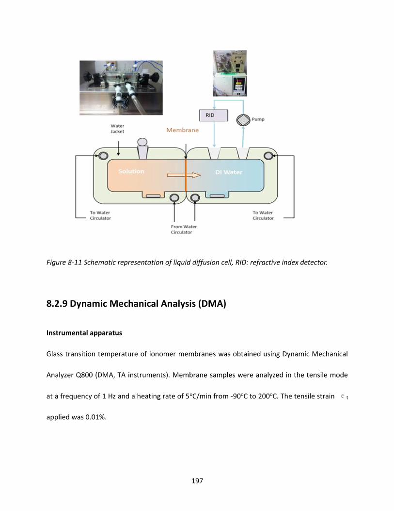
197

Figure 8-11 Schematic representation of liquid diffusion cell, RID: refractive index detector.

8.2.9 Dynamic Mechanical Analysis (DMA)


Glass transition temperature of ionomer membranes was obtained using Dynamic Mechanical

Analyzer Q800 (DMA, TA instruments). Membrane samples were analyzed in the tensile mode

at a frequency of 1 Hz and a heating rate of 5oC/min from -90oC to 200oC. The tensile strain εt

applied was 0.01%.

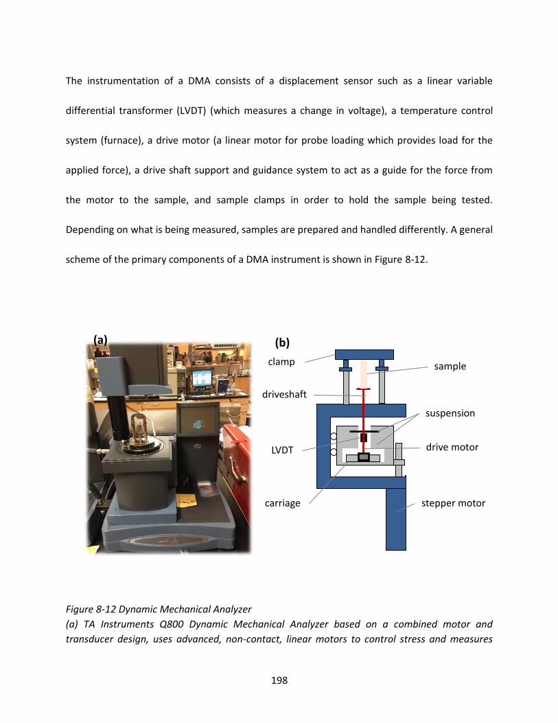
198

The instrumentation of a DMA consists of a displacement sensor such as a linear variable

differential transformer (LVDT) (which measures a change in voltage), a temperature control

system (furnace), a drive motor (a linear motor for probe loading which provides load for the

applied force), a drive shaft support and guidance system to act as a guide for the force from

the motor to the sample, and sample clamps in order to hold the sample being tested.

Depending on what is being measured, samples are prepared and handled differently. A general

scheme of the primary components of a DMA instrument is shown in Figure 8-12.

Figure 8-12 Dynamic Mechanical Analyzer

(a) TA Instruments Q800 Dynamic Mechanical Analyzer based on a combined motor and

transducer design, uses advanced, non-contact, linear motors to control stress and measures

clamp

driveshaft

LVDT

carriage stepper motor

drive motor

suspension

sample

(a) (b)

199

strain with a highly sensitive optical encoder. Unit has ability to provide tension, compression,

3-point bend, dual cantilever, single cantilever, and shear sandwich modes of deformation. In

addition, it can accommodate submersion clamps (tension and 3-pint bend) with fluid reservoirs

that eliminate the need to invert the instrument to perform submersion studies. (b) General

schematic of a DMA instrument in details.

Introduction

DMA, also known as dynamic mechanical spectroscopy, is a useful technique to study and

characterize materials, especially for the viscoelastic behaviors of different polymers. A

sinusoidal stress is applied and the corresponding strain in the material can be measured,

allowing to calculate the complex modulus. Meanwhile, the temperature of the sample and the

frequency of the stress can be changed, leading to variations in the complex modulus. The DMA

approach can be used to locate the glass transition temperature of the material, as well as to

identify transitions corresponding to other molecular motions.

Theory

Polymers with long molecular chains have viscoelastic properties, combing the characteristics

of elastic solids and Newtonian fluids. As demonstrated in the classical theory of elasticity, the

mechanical properties of elastic solid can be described that stress is proportional to strain in

small deformations. At the same time, the classical theory of hydrodynamics describes the

properties of viscous fluid, for which the response of stress is dependent on strain rate.[171] This

solid-like and liquid-like behaviors of polymers can be modeled mechanically with combinations

200

of springs and dashpots.[172] The viscoelastic property of a polymer is studied by DMA where a

sinusoidal-wave force (stress) is applied to a material and the resulting displacement (strain) is

measured. For an ideally elastic solid, the corresponding strain and the applied stress will be

perfectly in phase. However, there will be a 90 degree phase lag of strain with respect to stress

for a purely viscous fluid. Viscoelastic polymers have the characteristics in between where some

phase lag will occur during DMA tests.[173] Stress: 𝜎 = 𝜎0sin (𝑡𝜔 + 𝛿), strain: 휀 = 휀0sin (𝑡𝜔)

where 𝜔 is frequency of strain oscillation, t is time, and 𝛿 is phase lag between stress and

strain. The storage modulus measures the stored energy, representing the elastic portion, while

the loss modulus measures the energy dissipated as heat, representing the viscous portion.

Storage modulus: 𝐸′ = 𝜎0𝑐𝑜𝑠𝛿/휀0 , loss modulus: 𝐸′′ = 𝜎0𝑠𝑖𝑛𝛿/휀0 and phase angle: 𝛿 =

arctan (𝐸′′/𝐸′). Similarly we also define shear storage and loss moduli, G’ and G’’. Complex

variables can be used to express the moduli E* and G* as follows: 𝐸∗ = 𝐸′ + 𝑖𝐸′′ and 𝐺∗ =

𝐺′ + 𝑖𝐺′′ where 𝑖2 = −1.

Test modes

Two major kinds of test modes can be utilized to probe the viscoelastic properties of polymers:

temperature sweep and frequency sweep tests. A third, less commonly studied test mode is

dynamic stress-strain testing. Temperature sweep is a common test method involving

measuring the complex modulus at low constant frequency while varying the environmental

temperature. A prominent peak in 𝑡𝑎𝑛𝛿 appears at the glass transition temperature of the

201

polymer. Secondary transition can also be observed, which can be attributed to the

temperature-dependent activation of a wide variety of chain motions.[174] In semi-crystalline

polymers, separate transitions can be observed for the crystalline and amorphous sections.

Similarly, multiple transitions are often found in polymer blends. In the frequency sweep test

mode, a sample can be held at a fixed temperature and can be tested at varying frequency.

Peaks in 𝑡𝑎𝑛𝛿 and in 𝐸′′ with respect to frequency can be associated with the glass transition,

which corresponds to the ability of chains to move past each other. This implies that the glass

transition is dependent on strain rate in addition to temperature. Secondary transitions may be

observed as well. The Maxwell model provides a convenient description of viscoelastic

materials. Applying a sinusoidal stress to a Maxwell model gives: 𝐸′′ = 𝐸𝜏0𝜔/(𝜏02𝜔2 + 1),

where 𝜏0 = 𝜂/𝐸 is the Maxwell relaxation time. Thus, a peak in 𝐸′′ is observed at the

frequency 1/𝜏0. [174] A real polymer may have several different relaxation times associated

with different molecular motions. In the dynamic stress-strain studies, by gradually increasing

the amplitude of oscillations, one can perform a dynamic stress-strain measurement. Variations

of storage and loss moduli with increasing stress can be used for materials characterization, and

to determine the upper bound of the material’s linear stress-strain regime.[175] Because glass

transitions and secondary transition are seen in both frequency studies and temperature

studies, an interest in multidimensional studies is developed, where temperature sweeps are

conducted at a variety of frequencies or frequency sweeps are conducted at a variety of

202

temperatures. This sort of study provides a rich characterization of the material, and

information about the nature of the molecular motion responsible for the transition.

Application

One important application of DMA is the measurement of the glass transition temperature of

polymers. Amorphous polymers have different glass transition temperatures, above which the

material will have rubbery properties instead of glassy behavior and the stiffness of the

material will drop dramatically with an increase in viscosity. At the glass transition, the storage

modulus decrease dramatically and the loss modulus reaches a maximum.

Temperature-sweeping DMA is often used to characterize the glass transition temperature of a

material. Besides that, varying the composition of monomers and cross-linking can add or

change the functionality of a polymer that can alter the results obtained from DMA. Due to

intermolecular and intramolecular interactions, different compositions of blends can alter the

physical state of the polymer. DMA can also be used to effectively evaluate the miscibility of

polymers. The polymer has a much broader transition with a shoulder instead of a steep

drop-off in a storage modulus plot, indicating that there are areas that are cross-linked or

heterogeneous. Moreover, stress relaxation and toughness can be tested by applying different

models.

203

8.2.10 Thermal Gravimetric Analysis (TGA)


Thermal gravimetric analysis (TGA) was performed using a TGA Q500 (TA Instruments),

requiring a precision balance with a pan loaded with the sample, and a programmable furnace.

Samples are pretreated to remove residual water by vacuum pump overnight. All samples are

heated and kept in an inert N2 atmosphere from 30oC to 700oC or 1000oC using a heating rate of

10oC/min.

Figure 8-13 Thermogravimetric Analysis

(a) Instrumentation for conducting a thermogravimetric analysis. The balance sits on the top of

the instrument with the sample suspended below. A gas line supplies an inert gas that sweeps

the volatile decomposition products out of the furnace. The heat exchanger dissipates the heat

from the furnace to a reservoir of water. (b) Close-up showing the balance pan, which sits on a

moving platform, the thermocouple for monitoring temperature, a hook for lowering the sample

pan into the furnace, and the opening to the furnace. After placing a small portion of the sample

on the balance pan, the platform rotates over the furnace and transfers the balance pan to a

(a) (b)

balance

furnace

gas line

204

hook that is suspended from the balance. Once the balance pan is in place, the platform rotates

back to its initial position. The balance pan and the thermocouple are then lowered into the

furnace.

Introduction

Thermal gravimetric analysis (TGA) is a method of thermal analysis in which changes in physical

and chemical properties of materials are measured as a function of increasing temperature

(with constant heating rate), or as a function of time (with constant temperature and/or

constant mass loss).[176] TGA can give us knowledge about physical phenomena, such as

second-order phase transitions, including vaporization, sublimation, absorption, adsorption,

and desorption. Meanwhile, TGA can provide information about chemical phenomena including

chemisorption, desolvation (especially dehydration), decomposition, oxidative degradation and

solid-gas reaction (e.g., oxidation or reduction). [176] The TGA results can be presented by (1) the

weight versus temperature curve, referred to as the thermo gravimetric analysis (TA) curve, or

(2) the rate of loss of weight versus temperature curve, referred to as the differential thermo

gravimetric analysis (DTA) curve.

TGA is commonly used to determine selected characteristics of materials that exhibit either

mass loss or gain due to decomposition, oxidation, or loss of volatiles (such as moisture).

Common applications of TGA are materials’ decomposition patterns, degradation mechanisms

and reaction kinetics, characterization of organic content in a sample, and analysis of inorganic

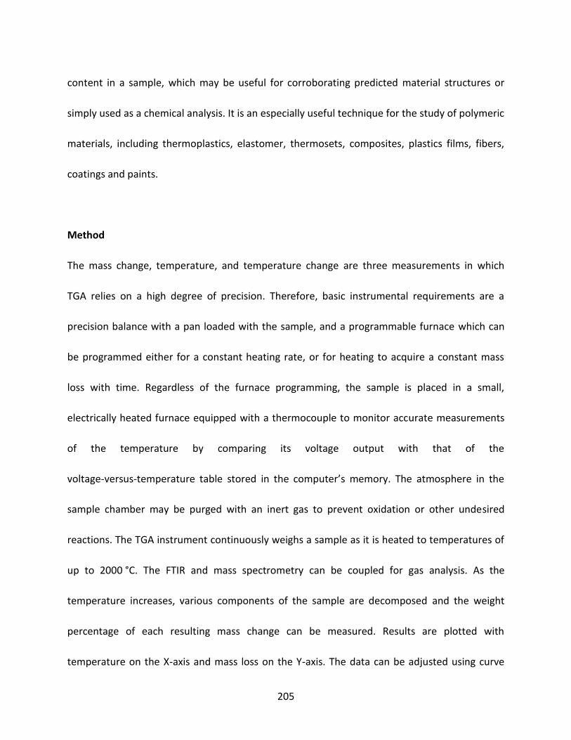
205

content in a sample, which may be useful for corroborating predicted material structures or

simply used as a chemical analysis. It is an especially useful technique for the study of polymeric

materials, including thermoplastics, elastomer, thermosets, composites, plastics films, fibers,

coatings and paints.

Method

The mass change, temperature, and temperature change are three measurements in which

TGA relies on a high degree of precision. Therefore, basic instrumental requirements are a

precision balance with a pan loaded with the sample, and a programmable furnace which can

be programmed either for a constant heating rate, or for heating to acquire a constant mass

loss with time. Regardless of the furnace programming, the sample is placed in a small,

electrically heated furnace equipped with a thermocouple to monitor accurate measurements

of the temperature by comparing its voltage output with that of the

voltage-versus-temperature table stored in the computer’s memory. The atmosphere in the

sample chamber may be purged with an inert gas to prevent oxidation or other undesired

reactions. The TGA instrument continuously weighs a sample as it is heated to temperatures of

up to 2000 °C. The FTIR and mass spectrometry can be coupled for gas analysis. As the

temperature increases, various components of the sample are decomposed and the weight

percentage of each resulting mass change can be measured. Results are plotted with

temperature on the X-axis and mass loss on the Y-axis. The data can be adjusted using curve

206

smoothing and first derivatives are often also plotted to determine points of inflection for more

in-depth interpretations. Thermal stability of a material can be evaluated using TGA. In a certain

temperature range, many species can be thermally stable with no observed mass change while

negligible mass loss corresponds to little or no slope in the TGA trace. TGA also provides the

upper use temperature of a material and beyond this temperature the material will begin to

degrade.

8.2.11 Electrodialysis (ED)

The bench electrodialysis pump unites PCCell BED1-4 provides 4 electrolytic circuits with

flow-through meters (10-100 l/h). It is designed to work in combination with an ED cell to set up

a variety of experiments like desalination.

An ED cell like the PCCell ED 64 can be used to run a standard ED. The ED stack provides n cell

pairs (typically n=5, 10, 50 or even 100), which are formed by n+1 cation exchange membranes,

n anion exchange membranes and 2n spacers. One of the cell systems is the dilute (where the

ions are removed) and the other one is the concentrate in which the ions are collected. If the

polarity is changed, the function of the cell system changes accordingly. A complete ED system is

set up by the ED cell in combination with the ED pump unit and the external solvent tanks, as

illustrated in Figure 8-14.

207

For the connectors of the ED cells, the four liquid systems of the cell (catholyte, anolyte,

concentrate and dilute) require one inlet and outlet. And their direction can be changed, but

inlet and outlet of both, dilute and concentrate, should be at the same cell face to reduce

transmembrane pressure. The connectors for dilute and concentrate are situated diagonally

opposite of each other, and those of electrode chambers in the interior at the same sides

respectively.

For the connection of the dilute and concentrate to the system, the concentrate tank is

connected to the circulating pump inlet, the pump outlet to the inlet of the concentrate

chambers of the cell, and the outlet of the concentrate is taken back to the concentrate tank.

Afterwards, the concentrate tank is filled up with the liquid flowing into the pump. All the

connections are firmly fixed and leak proof.

The electrolyte container has to be filled with about 1 l of the electrolyte solution. Generally, 1

0.1-1molar solution can be used. The pumps and the flow meters have to be degassed by the

electrolyte solution. The anolyte chamber and the catholyte chamber may be connected in one

circuit: the pump outlet is connected to the inlet of the anolyte chamber, the anolyte outlet is

connected to the catholyte inlet, and the catholyte outlet tube goes back to the tank.

208

At startup, the flow of the chemicals should be first started. A pressure difference over the

membranes has to be strictly avoided. A soft start of the pumps is recommended. After all the

electrolytes flow correctly, the height of liquids within the external cylinders should be

monitored. As there should not be any hydraulic leakage, the filling level of the liquids should

achieve a constant level as long as no current is flowing. The current can be applied after all air

bubbles within pump, tubing and stack are removed and an air-free stream of liquid is observed.

Hydrogen will evolved in the electrolyte container. It should be vented properly to hold the

hydrogen concentration below the explosion limit.

Anion exchange membrane, 5 pieces (PC-SA) and cation exchange membrane, 4 pieces (PC-SK)

and are provided by PCCellCorp.

209

Figure 8-14 Bench Electrodialysis Pump Unit PCCell BED 1-4 and ED 64-002, ED 64-4.

210

8.3 Summary

Based on a system of the synthesis, characterization, and application of ionomers, all the

materials and experimental methods mentioned above are used to figure out properties of ion

exchange membranes.

211

Chapter 9 Thermodynamic Interrelationship within

Wettability, Surface Energy, and Water Transport of Ionomers

9.1 Introduction

Nature’s self-cleaning properties of the Lotus leaf are due to super-hydrophobic properties

created from its complex surface features and composition. These intriguing properties have

inspired the science and engineering of structured surfaces and materials in order to control

hydrophobicity and hydrophilicity.

Due to the absence of surface mobility, solid surface tension, as an important factor influencing

wettability, is very difficult to measure directly when compared with liquid surface tension.[40]

Thus, several independent approaches have been utilized to estimate solid surface tensions,

including direct force measurements[41], contact angles measurements[29-31, 33-34, 42], capillary

penetration into columns of particle powder[43], sedimentation of particles[44], solidification

front interactions with particles[45], film flotation[46], gradient theory[47], the Lifshitz theory of

van der Waals’ forces[48], and the theory of molecular interactions[49]. Among available

techniques for ionomer interfaces study, contact angle measurement is an easy method by

probing a liquid drop on the testing surface, in order to determine the solid surface energy with

the smallest area of 0.1 nm depth and 1000 nm width.[50] Combining Young’s Equation,

212

Shimizu[52] examined several surface energy models, including Neumann’s Equation, Fowkes’

Equation, the geometric mean equation, and the harmonic mean equation. He basically

measured contact angles formed by several testing liquid drops on a film of polypropylene, on

plates of polystyrene, and a liquid crystalline polymer at 20oC. An overview of the relevant and

important theory including contact angle, wetting transition, and the dynamics of spreading was

provided by Gennes in 1985.[51] Then, Geoghegan[53] reviewed progress in research correlating

with the influence of polymer blends’ boundary and the growth of wetting layers. Moreover, he

summarized work over the same period concerning the dewetting of polymer films, along with

a discussion of the role of pattern formation caused by topographically and chemically

patterned substrates and dewetting.

There are several factors impacting the wettability of polymer. In the aspect of morphology and

application, Fasolka and Mayes emphasized the influence of film thickness and surface

energetics on the morphology of compositionally symmetric, amorphous diblock copolymer

films, with respect to the boundary condition symmetry and surface chemical expression.

Furthermore, in the second section they discussed technological applications of block

copolymer films (e.g., as lithographic masks and photonic materials).[54] Moreover, the chemical

composition of the polymer and surface topography make a great impact on surface energy

with regards to the micro- and macro-structure of membranes. [15] Andruzzi[56] evaluated the

effect of the chemical structure on the wetting properties, such as

213

2,2,6,6-tetramethylpiperidin-1-yloxy radical (TEMPO)-mediated controlled radical

polymerization of fluorinated styrene monomers, and a sequence of polymer modification

reactions on anionically formed polystyrene-block-polyisoprene block copolymers. Afterwards,

Tsibouklis[57] relied on the molecular design requirements to fabricate accessible film structures

with ultra-low surface energy characteristics. Subsequently, Wang[58] showed that the patterned

poly(dimethylsiloxane) (PDMS) stamp was capable of modifying the wettability of

poly(3,4-ethylenedi-oxythiophene)-poly(styrenesulfonate) (PEDOT-PSS) and polyelectrolyte

poly(sodium 4-styrenesulfonate) (NaPSS) surface. Furthermore, Kanakasabai[59] recently studied

the ion-exchange capacity, proton conductivity and water sorption characteristics of crosslinked

polyvinyl alcohol (PVA-SSA) and sulfonated poly(ether ether ketone) (SPEEK) and correlated

them with the surface energy and wettability characteristics of the membranes.

A better understanding of these fundamental surface properties provides researchers with the

scientific guidelines to control a material’s surface wetting properties for biological, electronic,

mechanical, and chemical systems and applications[60]. Furthermore, selective tailoring of a

material’s surface and composition can be utilized to control hydrophobicity for inhibiting metal

corrosion, providing surface protection from chemical and biological agents, minimizing the

biological fouling of marine vehicle surfaces, and optimizing the wetting of gas diffusion layers

in the fuel cell.

214

At the end of the last century, the adsorption of polymers has drawn considerable attention.

The relationships and implication between chemical, physical properties, and the swelling or

adsorption phenomenon of polymers (including homopolymers and block copolymers) were

illustrated by the experiments, theory, computer simulations, and models[89]. Moreover, the

process of adsorption and diffusion of solutes and solvents into polymers is characterized by the

balanced interaction of all species of molecules within polymer network, which can significantly

influence the membrane properties[64, 90]. As a result, polymer dissolution plays an important

role in the wide-range industrial application. Moreover, a better understanding of the

dissolution procedure can optimize the design and processing conditions of polymer

manufacturing, as well as the selection of a suitable solvent. For instance, the microlithography

process are used to fabricate microchips[91], polymer film casting[92], recycling plastics[93], and

tissue regeneration[94] based on the research of polymer dissolution.

During molecules transport across the membrane, two mutual effects may be considered[90a].

Firstly, a free volume effect occurs for the same molecule species, which generally leads to an

increase in the diffusivity of components (i.e., macroscopically perceived as a plasticizing effect),

like a kind of dragging force due to the concentration difference of solutions. Secondly, there is

a coupling effect, which results from interactions between different molecule species within the

polymer that may increase or decrease their diffusivity within the membrane (i.e., retarded or

accelerated diffusion due to interaction effects). A careful and suitable choice of solvent, solute

215

and membrane material is therefore essential for a successful and efficient transport process.

Two methods are utilized for the quantitative determination of membrane swelling, which are

macroscopic swelling (bulk swelling) and microscopic swelling. The former is defined as a

large-scale expansion of polymer membranes measured over an area of at least 1mm2 while

microscopic swelling is meant to be the change in dimension, usually inferred from small-angle

X-ray scattering (SAXS) data[95] (microscopic swelling observation is then defined as the increase

in the equivalent Bragg spacing as a result of solvation). However, gravimetrically measured

macroscopic swelling is not very accurate for volatile solvents (methanol and toluene) or viscous

liquid (room temperature ionic liquids—RTILs); therefore, volumetrically measured bulk swelling

was developed[38], which allows for the continuous quantitative determination of macroscopic

swelling kinetics and equilibrium within thin films.

While these examples do not encompass all material efforts, it is appreciated that complex

liquid-polymer interactions are dependent upon the chemical composition and structure of

ionomers. In this paper, basic relationships between surface energy, wetting properties, and

water transport will be discussed with respect to ionomer composition and chemical structure.

216

9.2 Experimental

9.2.1 Material

Ethyl alcohol, Ethylene glycol (EG), DI water, micro-slides, double-sided tape for contact angle

measurement.

Polymer: Polytetrafluoroethylene (PTFE), Perfluorosulfonic acid (PFSA), (NF115&117, and

NF212), sulfonated poly(phenylene) (sPP), and PBC ionomer, poly[t-butyl


styrene) (tBS-HI-S-HI-tBS). The detailed information was shown in Chapter 8.


Commercial PBC films (IEC = 0.0, 0.4, 0.7, 1.0, 1.5, and 2.0) were created from a C:H solution

that was cast using a Doctor Blade[161]. Experimental PBC films were made by dissolving in

either THF, CHCl3, or C:H (1:1 wt%) followed by solution casting methodology in a Teflon dish.

217

9.2.3 Contact Angle Measurement

The apparent water contact angle θ was measured with a Kruss DSA (Drop Shape Analysis) 100

surface analyzer, as shown in Figure 9-1, wherein the contact angle between NF115 and water

was 95.9o, which is consistent with reference[162]. 15μL was the optimal testing liquid droplet

volume for producing reproducible contact angle measurements with a maximum error of +/- 3

degrees (error 3%). All measurements were performed at room temperature and repeated

more than five times in order to determine reproducibility. Ethanol, EG and water mixture with

different percentages were produced as testing solutions. Through analyzing different surface

energy methods, optimal calculation methods were determined.

Figure 9-1 Contact angle measurement with Kruss DSA (Drop Shape Analysis) 100 surface

analyzer.

218

9.2.4 Water Diffusion Measurement

In the swelling measurements, dried sheet-shaped polymer samples were inserted in the gap of

two glass slides and DI water was poured into the gap. In the process of deswelling, samples

were withdrawn from the DI water and measured after the removal of surface water by lightly

blotting with filter paper. Videos of swelling phenomenon for membranes (cut into 2cm×2cm)

were recorded using a DSA100 (as illustrated in Figure 9-2) and measured by an MB-Ruler

software.

Figure 9-2 Water diffusion measurement device.

Video camera

2cm×2cm membrane

219

9.3 Results and Discussion

9.3.1 Wettability and Surface Energy of Ionomers

9.3.1.1 Contact Angle Measurement

Contact angles were determined on substrates of different polarities. Liquid droplets with

maximum surface tensions lead to the highest contact angles.[163] The contact angle

measurements give some information of solid polymer, such as wettability, surface energy, and

molecular interactions. The affinity of a liquid to a solid surface, if water is used to measure the

contact angle, one can deduce the hydrophobic (0o~30o) or hydrophilic (greater than 90o)

character of the surface, as shown in Figure 9-3. If several reference liquids are used, the surface

energy of the solid can be calculated, discriminating between polar and dispersive components.

The measurements of the hysteresis between advancing angle and recessing angle give

information on non-homogeneity of the surface (roughness, rugosity, contamination,...).

Figure 9-3 Contact angles of polymers using testing liquid water.

The contact angle of PTFE (IEC=0)

107.6

0.5mm 0.5mm

95.86 86.58

The contact angle of SPP3 (IEC=1.8)

0.5mm

The contact angle of Nafion115 (IEC=0.9)

220

9.3.1.2 Optimal Surface Energy Calculation Method

In order to assess the polymer wettability and their interactions with liquid, contact angle

measurement were carried out with several wetting liquid (water, ethanol, and EG) in order to

determine polymer surface energy. Concentrations of sulfonic acid groups within ionomers play

an important role in the solid surface energy determination with respect to chemical structures,

functional groups, and microstructures.

Figure 9-4 Surface energy and subparts (dispersion ‘d’ and polar ‘p’) of PTFE, NF115 and sPP3

calculated by K&N, O&W, and Wu’s method.

221

It can be seen from Figure 9-4 that the total surface energy calculated by three methods (K&N,

O&W, and Wu) for PTFE is in reasonably statistical agreement with that published in the

literature[66]. However, some deviations of surface energy subparts were observed for PTFE in

details. Surface energy is the main combination of dispersion (non-polar) and polar energy.

Dispersion energy is the surface energy that results from non-polar interaction of molecules

while polar energy is the surface energy that lied in interactions of polar groups. Due to the

fluorocarbon backbone of PTFE, superhydrophobic wetting property leads to very low polar

component (around 1.5 mJ/m2) of surface energy, as calculated by O&W instead of Wu’s

method (in Figure 9-4), corroborated by the literatures[66, 177]. Although the overall surface

energy of NF115 and sPP3 obtained by O&W and Wu is identical, dispersion and polar

components are different. Therefore, PTFE and NF115 with the same polymer backbones

present similar dispersion components (as indicated in O&W’s method) while the larger

contents of sulfonic acid groups in polymer matrix lead to an increase in polar components due

to the formation of hydrogen bonding (pink data points as displayed in Figure 9-4). As a result,

O&W’s model can be chosen convincingly to calculate both overall and sub-components surface

energy, combining with Young’ s Equation.

222

0 1 2 30

10

20

30

K&N

O&W

Wu

d(O&W)

p(O&W)

d(Wu)

p(Wu)

SE

(m

J/m

2)

IEC (mequiv/g)

Figure 9-5 Surface energy and sub-components (dispersion ‘d’ and polar ‘p’) of PBCs calculated

by K&N, O&W, and Wu’s method.

Larger variation exists in the dispersion components of the PBCs’ surface energy from Wu’s

method compared with O&W method. However, it can be seen from Figure 9-5 that the pink

data points (represent the dispersion components of the PBCs’ surface energy) gather densely

in the case of O&W. Moreover, PBCs’ O&W data presents the remarkably upward trend of the

polar component versus IEC, which is as expected rather than Wu’s method. This good

correlation between the surface energy polar part and IEC provided by O&W implies that the

interaction of the hydrogen bonding, which is mainly responsible for polar components, is

223

enhanced by the concentration of sulfonic acid groups within ionomer. Thus, O&W’s method is

ultimately utilized to determine the polymer surface energy in this study.

In summary, K&N’s method is perfectly suitable for low surface energy polymer, especially for

surface without polar component while Wu’s method is suitable for the overall surface energy

calculation (especially good for high surface energy material). However, the latter one presents

large variation of surface energy sub-parts, which is identical with the reference[52]. As discussed

above, as the most favorable method, O&W’s model provides the reliable values of surface

energy and sub-components.

9.3.1.3 Relationship between Surface Energy and IEC

In addition to the influence of polymer chemical structures (which can be predicted from

literature[66]), the concentration of sulfonic acid groups in the membrane has a great impact on

ionomer surface energy as well.

224

0.0 0.5 1.0 1.5 2.0 2.514

16

18

20

22

24

26

PTFE

NF115

PP

sPP3

PBC0.0

PBC0.4

PBC0.7

PBC1.0

PBC1.5

PBC2.0

SE

(m

J/m

2)

IEC (mequiv/g)

Figure 9-6 Relationships between surface energy and IEC within different polymers.

Given that the IEC correlates well with the surface energy for different membrane[59], it is

interesting to observe that the paralleling lines of PPs and PBCs with various IEC (the blue and

pink lines as reported in Figure 9-6), though the black line composed of PTFE and NF115’s data

has small deviations due to the oxygen bonding of NF115 side chains. In details, PTFE and NF115

aren’t constituted of the same basic chemical structure (including backbones and side chains),

though they have the same fluorocarbon backbone. As observed in Figure 9-6, PBC with IEC=2.0

displays the highest surface energy within the PBC ionomer series, which is contributed from

the strong interaction within sulfonic acid groups. Previous studies[66] presented polymer

225

(without functional groups) surface energy based on chemical structure. This study further

establishes a more general correlation between surface energy and IEC.

0.0 0.5 1.0 1.5 2.0 2.5 3.00

5

10

15

20 PTFE d

NF115 d

PP d

sPP3 d

PBC0.0 d

PBC0.4 d

PBC0.7 d

PBC1.0 d

PBC1.5 d

PBC2.0 d

PTFE p

NF115 p

PP p

sPP3 p

PBC0.0 p

PBC0.4 p

PBC0.7 p

PBC1.0 p

PBC1.5 p

PBC2.0 p

SE

(m

J/m

2)

IEC (mequiv/g)

Figure 9-7 Relationship between surface energy (with disperse and polar components) and IEC

within different polymers.

Figure 9-7 shows relationships between surface energy and IEC within various polymers, PTFE,

NF115, sPP and PBC ionomer series. First, the PBCs and sPP3 dispersion parts are around 14.2

mJ/m2 and 12.3 mJ/m2, respectively, while the polar-part change is consistent with IEC.

Moreover, the similarity of PTFE and Nafion115’s disperse components is attributed to the same

polymer backbones (fluorocarbon structures), while the increase of the polar parts correlates

226

with IEC. Last but not the least, surface energy of ionomers can be predicted precisely based on

chemical structure and ion exchange capacity. More in details, the polar component of PBC1.8

can be predicated around 7.8 mJ/m2 (according to the pink line). Furthermore, it can be divided

into two parts, 5.4 mJ/m2 (IEC contribution) and 2.4 mJ/m2 (chemical structure impact). The IEC

contribution is determined by subtracting the polar part of PBC0.0 from that of PBC1.8, as

shown in Figure 9-7. And polar part of sPP3 is 12.2 mJ/m2 which is equal to 4.9 mJ/m2 (IEC = 1.8)

plus 7.3 mJ/m2 (PP chemical structure). The IEC contributions of PBC and sPP3 are almost

identical (5.4 mJ/m2 and 4.9 mJ/m2) due to the same IEC. Therefore, the interrelationships

between surface energy, IEC, and chemical structure can be established, moreover, ionomer

surface energy can be predicted according to a certain trend.

9.3.1.4 Roughness

Surface roughness will be considered and discussed in this part with respect to contact angle.

The roughness ratio of a teflon dish is around 2, determined from contact angle measurement

of solution-cast PBC. Self-cast PBC membranes have a heterogeneous and comparably

hydrophilic surface, while the commercial membrane is assumed to be ideally flat, cast by

Doctoral Blade Die. Cassie-Baxter model and Wenzel transition model[178] were introduced to

determine the fraction of solid/liquid interface ‘f’. As demonstrated in Figure 9-8, the contact

angles formed between water and PBCs (IEC = 1.0, 1.5, and 2.0) decrease with the increasing

227

concentrations of sulfonic acid groups due to the increasing hydrophilicity of ionomers, while

the ‘f’ value (presenting the fraction of solid surface area wet by the liquid) increases with IEC,

caused by the strong interaction between sulfonic acid groups and water molecules. Moreover,

contact angles between water and solution-cast PBCs are larger than those on an ideal flat

surface due to the roughness factor; the ideal contact angles need to be obtained before

calculating the surface energy of polymer membranes. Hence, for various casting methods, the

roughness of casting surfaces should be taken into account.

1.0 1.5 2.080

85

90

95

100

105

commercial

solution-cast

solution-cast

commercial

IEC (mequiv/g)

co

nta

ct

an

gle

(o)

0.4

0.6

0.8

1.0

f

Figure 9-8 Comparison between contact angles and ‘f’ (the fraction of solid surface area wet by

the liquid) of commercial and solution-cast PBCs with different IECs on the Teflon dish.

228

9.3.1.5 Wetting Envelope

Knowledge of a surface's polar and disperse surface energy components allows the

determination of wetting envelope of this surface. First, the polar and disperse fractions of the

liquid for which the contact angle is 0° (cosθ = 1) are calculated with the combination of Young’s

equations and O&W’s model. When this polar fraction is plotted against the disperse fraction, a

closed contour for cosθ = 1 is obtained, which is called the wetting envelope.[179] Use the

Equation (9-1) to calculate the polar and disperse fractions of the liquid to form the wetting

envelope.

𝛾𝑙 = 𝛾𝑙𝑑+𝛾𝑙

𝑝 = (𝛾𝑠𝑑𝛾𝑙

𝑑)1

2 + (𝛾𝑠𝑝𝛾𝑙

𝑝)1

2 (9-1)

Table 9-1 Surface tensions of different testing liquid.

Testing liquid Surface tension

(mJ/m2)

Disperse part

(mJ/m2)

Polar part

(mJ/m2)

Water 72.8 21.8 51

Ethanol 22.1 17.5 4.6

EG 48.2 18.9 29.3

229

0 5 10 15 20 25

0

5

10

15

20

25

30

35

Po

lar

Part

(m

J/m

2)

Disperse Part (mJ/m2)

PTFE

NF115

sPP3

PBC1.5

ethanol

EG

Figure 9-9 Wetting envelope.

Wetting envelops in Figure 9-9 shows the wettability of polymers, and determines the optimal

testing liquid applied on a solid surface. Ethanol is not suitable testing liquid for sPP3 and NF115

due to the complete wettability of ethanol on their surfaces, as shown that the red data point of

ethanol is in the circles of NF115 and sPP3. Therefore, ethanol is utilized as one of Nafion

solvents based on similar solubility parameter (which will be discussed in Chapter 10). Although

ethanol cannot wet PTFE completely because of its high hydrophobicity, pure ethanol is not a

kind of good testing liquid as a result of its high volatility. Hence, different concentrations of

ethanol/water solution can be utilized in the contact angle measurement, wherein 20

percentage is the maximum ethanol weight ratio. Additionally, other factors like solubility

230

parameter should also be taken into account. Although water and EG meet the requirement of

wetting envelope, the solubility parameter of EG and SPP3 are so close (Chi parameter is only

0.09 as displayed in Chapter 10) that EG molecules can diffuse into the sPP3 membranes and

change the original conformation of polymer chain network. In a word, it is important to choose

the testing solution with disperse and polar components which are out of wetting envelope

circle of polymer and also with appropriate solubility parameters and low volatility. Otherwise

the contact angle measurement will result a lot of errors.

9.3.2 Water Transport in Ionomers

9.3.2.1 Swelling and Deswelling Phenomenon

In the swelling and deswelling plots, the swelling ratio is defined as (Vt-V0)/V0, where V0 is the

initial volume of the dried membranes, and Vt is the volume after a swelling time t. And volume

could be replaced of weight or x, y, and z axis swelling length.

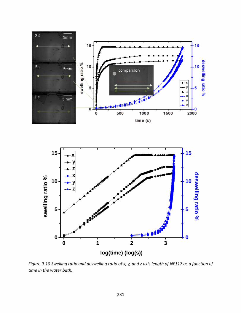
231

0 1 2 30

5

10

15

x

y

z

x

y

z

log(time) (log(s))

sw

ell

ing

rati

o %

0

5

10

15

desw

ellin

g ra

tio %

Figure 9-10 Swelling ratio and deswelling ratio of x, y, and z axis length of NF117 as a function of

time in the water bath.

232

Before swelling experiments, the NF117 membranes were vacuum dried in the oven overnight

to remove residual water and then immerged in the water to observe swelling phenomena.

Initially, three-dimension swelling ratios dramatically increase with time, as shown in Figure

9-10. After around 180s, the values of swelling ratios reach to a high level and keep on this

plateau until balanced.

9.3.2.2 Swelling and Deswelling Ratios

Comparing swelling ratios of NF117 and NF115, the ratios of x swelling direction are the same

while the y axis (film casting direction) and the z axis (thickness direction) swelling ratios relate

to the thickness of the membranes which is the only difference between NF117 and NF115, as

revealed in Figure 9-11. The melt-extrusion membrane-casting method allows NF117 and NF115

polymer chains only stretching in the y axis (film casting direction) and the z axis (thickness

direction), which are proportional to the thickness. However, the NF212 membrane has

identical three-dimensional swelling ratios based on its solution-dispersion membrane-casting

method, which makes NF212 membrane expand in all these three dimensions. Additionally,

sPP3 cast by scrolling method shows the extremely different swelling ratios of x, y and z

compared with Nafion ionomer series. The polymer relaxation direction, the z axis presents

233

large swelling ratio rather than the x or y axis. The reason is that solvents evaporate extremely

fast in the z direction, without any time left for chain movements in the x and y axis.

NF117 NF115 NF212 sPP35

10

15

20

25

x

y

z

sw

ell

ing

rati

o(%

)

ionomers

Figure 9-11 Swelling ratios of x, y and z axis for different ionomers.

9.3.2.3 Water Diffusivity of Ionomers

Assumption that molar swelling ratio is equal to the volume swelling ratio is made in the section

of water diffusion through ionomers. The weight of polymer (including water adsorbed) can be

determined according to the Archimedes' Principle, using weight balance to measure the weight

234

of polymer in the water. Figure 9-12 proves that the weight ratio Mt/M(inf) is equal to the volume

ratio Vt/V(inf) in the ionomer swelling experiments.

0 100 200 300 4000.00

0.25

0.50

0.75

1.00

Weig

ht

or

Vo

lum

e r

ati

o (

Xt/X

(in

f))

time (s)

NF117 Volume ratio

NF117 Weight ratio

sPP3 Volume ratio

sPP3 Weight ratio

Figure 9-12 Weight and Volume ratio vs. time for polymer NF117 and sPP3.

Considering the thickness of ionomers, initial volume and swelling volumetric ratio, Equation

(2-53) is introduced in order to determine the diffusivity. Wherein the y axis is equal to ln (Vt

V∞),

x asix is ln(tn

l), and slope k is keep as 1. Afterwards, diffusivity can be determined from the

intercept, however with the requirement of Vt/V∞< 0.60. As for swelling ratio larger than 60%,

Equation (2-54) is more accurate to determine the molecule diffusivity through ionomers,

235

wherein diffusivity ‘D’, as the only unknown parameter, can be achieved through Goal-Seek

method in Excel.

0 500 1000 1500 2000

0.0

5.0x10-11

1.0x10-10

1.5x10-10

2.0x10-10

0 5 10 15 20 25 30

0.0

5.0x10-11

1.0x10-10

1.5x10-10

2.0x10-10

dif

fus

ivit

y (

m2/s

)

time (s)

method1

method2

dif

fusiv

ity (

m2/s

)

time (s)

method1

method2

Figure 9-13 Diffusivity of NF117 calculated by method 2 (long time method) and method 1 (short

time method) vs. time.

Water diffusivity through NF117 films increases dramatically with time, afterwards, decreases to

a certain small value at infinite time (long enough). The largest diffusivity shows up at t = 9 s

when drag force of diffusion reaches to the highest point, as shown in Figure 9-13.

236

Table 9-2 Diffusivity of different ionomers calculated by different two methods.

Polymer Thickness(mm) Method 1 Method 2

Time(s) n Diffusivity(m2/s) Time(s) Diffusivity(m2/s)

NF117 0.175 3-9 0.4997 1.45×10-10 9 1.34×10-10

NF115 0.123 2-6 0.4997 1.12×10-10 6 1.05×10-10

NF212 0.049 1-4 0.2843 8.72×10-11 1 8.17×10-11

sPP3 0.039 4-11 0.5299 7.60×10-12 11 8.59×10-12

Figure 9-14 Diffusivity calculated by two methods vs thickness of different ionomers.

As illustrated in Figure 9-14, it is clear that the diffusivities of NF115 and NF117 are going up

with the increase of thickness. NF115 and 117 polymer chains are in the similar configuration

237

within the micro-polymer network. Based on the melt-extrusion membrane-casting method,

solvent molecules evaporate so fast that no sufficient time is left for polymer chains aggregating.

Hence, the polymer network is not in the lowest Gibbs-free-energy level. Based on Fickian

transport presented by n = 0.4997 ≈ 0.5 in Table 9-2, the water diffusion rate is smaller than

Nafion115 and 117 segmental mobility. Due to the concentration difference of water within

ionomers, NF117 has the largest thickness value so the water diffusion rate is the highest.

Although NF212 has the same chemical structure with the NF117&115 (only small difference in

IEC), casting methods are totally different. The solution-dispersion membrane-casting method

lets solvent evaporate from solute for a long period of time, and therefore, ionomer chains have

enough time to move around and achieve the optimal and lowest Gibbs-free-energy positions.

So the polymer relaxation rate is smaller than water diffusion rate, which proves to be right that

the calculated ‘n’ result 0.2843, is less than 0.5.

Although sPP3 displays the highest IEC = 1.8, the clusters of water around ionic sites prevent

water diffusing into the membrane in a certain degree. Due to the comparably rigid chemical

structure, the water transporting channels within sPP3 membranes are narrow and volume

swelling ratio is less compared with NF117 and NF115. Overall, the water diffusivity through the

sPP3 films is the least. If another casting method is utilized on sPP3, the water diffusivity will be

238

totally different. Therefore, membrane-casting methods greatly affect the diffusivity of liquid

molecules in the films.

9.4 Conclusion

A number of previous researches have provided an understanding of wettability, surface energy,

and water transport. In our study, the relationship between ionomer characteristics and water

diffusion is achieved to investigate the great impact of wettability from the perspective of

polymeric macro- and micro-properties. In detail, an appropriate model was selected for

combination with Young’s Equation to determine ionomer surface energy. Furthermore, from

the aspect of water transport properties, our study provides insight into the swelling properties

and water self-diffusivity with respect to IEC, thickness, and casting methods. Eventually, our

study provides the framework for future studies to assess roughness[96] (for self-casting

membranes), humidity, temperature, electrowetting[97], the hysteresis phenomenon[98] and

H-bond and acid-base parts[99] of surface energy. For future work, a systematic understanding

of the relationships between different solutions including methanol, ethanol and ethylene

glycol, and chemical structures, physical properties and morphology, (hydrophobic and

hydrophilic domains of ionomers) is needed to provide references for manufacturing

industrially utilized ionomers.

239

Chapter 10 Thermodynamic Interrelationship within Solubility,

Swelling, and Crosslink of Ionomers

10.1 Introduction

Numerous experiments on the polymer solubility parameter have been performed to explain

the interrelationship between solubility parameters and physical and chemical properties. The

developments from the Hildebrand solubility parameter (1950)[65a] to the Hansen solubility

parameters (HSP) (1967)[67] provide a direct calculation method to determine solubility

parameters according to chemical structure or surface energy of a material. In addition, based

on swelling values, solubility parameter can be determined by an indirect method combining

Flory-Huggins model[69] and Flory-Rehner Theory[70]. However, a comprehensive network

between the optimal solubility parameter calculation method, thermodynamic, transport,

rheological and optical properties needs to be significantly established, including intrinsic

viscosity, surface tension, dielectric constant, crosslink density and concentration of sulfonic

groups.

Various investigators proposed several solubility parameter calculation methods based on group

contribution methods (GCM) (Hildebrand, 1916; Small, 1953; Van Krevelen, 1965; Hoy, 1970;

Fedors, 1974; Hoftyzer and Van Krevelen, 1976).[66] Nevertheless, deviations were observed for

240

solubility parameter values determined by GCM when compared with experimental or physical

methods. Therefore, individual contributions such as dispersive, polar force, and hydrogen

bonding to solubility parameters were introduced by Hansen[67] to further investigate the

interaction between polymers and solvents. Moreover, techniques for the solubility

determination have been widely described in the literature, with swelling values being

associated with different combinations of solvents[79], turbidimetric titration[80], specific

volume[81], intrinsic viscosity[79], and inverse gas chromatography[82].

It is generally accepted that there is an intrinsic relationship between solubility parameters and

other properties of a material. LaPack[83] examined correlation between permselectivities and

Hildebrand solubility parameters of filled elastomeric membranes. Ravindra[84] determined the

solubility parameter of chitin and chitosan by GCM and compared it with the values determined

from maximum intrinsic viscosity, surface tension, the Flory-Huggins interaction parameter and

dielectric constant values. Lindvig’s work[85] is based on the correlation between Hansen

solubility parameters and Flory-Huggins model, presenting predictive and accurate solubility

parameter results, without any prior knowledge of molecular structures. Jung[86] found that

dissimilar chemical structures lead to large differences in solubility parameters of liquid crystal

and resin. Moreover, he pointed out that high crosslinking density contributes to the fast

formation of grating, large droplet size and high diffraction efficiency. In 2006, Guan[87] found

that interesting effects of casting solvents on the surface morphologies of sulfonated

241

polyethersulfone (SPES) membranes are caused by polymer-solvent interactions. It is

anticipated the grain size is more uniform and the degree of irregularity of polymer membranes

surface should decrease with an increase in the polymer-solvent interaction (SPES-DMAc

compared with DMF and NMP). Following this, Lu[88] experimentally demonstrated that the

actuation of thermally responsive shape-memory polymer (SMP) can be achieved using

interactive solvent, while the effect of the solubility parameter of the interactive solvent on the

shape recovery behavior and glass transition temperature of polystyrene SMP was also

investigated experimentally.

Although a lot of experiments and literatures have covered the relationship between polymer

solubility and other properties, there are no complete and conclusive rules for choosing the

optimal solubility parameter calculation method. Moreover, a systematic understanding of

interrelationship within solubility parameters and polymer properties is remarkably needed. In

this chapter, three kinds of solubility parameter calculation methods are presented and an

optimal calculation combination is analyzed and selected, which is in statistical agreement with

literatures. Moreover, we create a new way of determining the sulfonic acid group’ solubility

parameter by swelling phenomenon. Finally, the interrelationship between chemical potential,

crosslink density, and solubility parameters of different polymers was established to investigate

the effect of solubility parameter on the polymer properties.

242

In our work, three methods are utilized to calculate the solubility parameter. First, Hildebrand’s

method is presented by group contribution method based on Fedor data. However, deviations

are proven to exist for some polymers. Secondly, Hansen solubility parameter is achieved by

the empirical equation modeled by 46 common polymers’ data. Finally, the combination of

swelling values, Flory-Huggins and Flory-Rehner Equation is an innovative way of determining

polymer solubility parameters.

It is observed that among these different methods, Fedor provides the widest data range,

however, not always accurate. The simulating relationship between Hansen Solubility

Parameter (HSP) and polymer surface energy is proven to be comprehensive and feasible,

further presenting the polymer-solvent interaction. However, these two calculation methods

are only applicable in the knowledge of molecular structures or surface energy. Moreover, the

combination of Flory-Huggins and Flory-Rehner Equation is established to obtain the number of

crosslinks, Chi parameter, and the solubility parameter of ionic side chains. Meanwhile, the

interrelationship between solubility parameter, chemical structure, number of crosslinks and

the concentration of sulfonic acid groups are achieved. As a result, the chemical potential of the

swelling process significantly reflects macroscopic properties and microscopic interactions

between polymer matrix and liquid molecules.

243

10.2 Experimental

10.2.1 Material

Ethyl alcohol, Ethylene glycol (EG), DI water, micro-slides, double-sided tape for contact angle

measurement.

Polymer: Polytetrafluoroethylene (PTFE), Perfluorosulfonic acid (PFSA), (NF115&117, and

NF212), Sulfonated poly(phenylene) (sPP), and PBC ionomer, poly[t-butyl


styrene) (tBS-HI-S-HI-tBS). The detailed information was shown in Chapter 8.


Commercial PBC films (IEC = 0.0, 0.4, 0.7, 1.0, 1.5, and 2.0) were created from a C:H solution

that was cast using a Doctor Blade[161]. Experimental PBC films were made by dissolving in

either THF, CHCl3, or C:H (1:1 wt%) followed by solution casting methodology in a Teflon dish.

244

10.2.3 Solubility Measurement

Polymer was pretreated in 1M sulfuric acid and rinsed in DI water before dried in the vacuum

oven overnight. Afterwards, membranes were treated in solutions with different solubility

parameters. The weight of the polymer was assessed before and after treatment in order to

determine solvent weight uptake.

10.2.4 Swelling Measurement

Weight uptake

Polymer was pretreated in 1M sulfuric acid and DI water before dried in the vacuum oven

overnight. Afterwards, membranes were treated in water. The polymer was weighted before

and after treatment.

Volumetric swelling

For swelling measurements, dried sheet shaped polymer samples were inserted in the gap of

two glass slides and DI water was poured into the gap. Videos of swelling phenomenon for

membranes (cut by 2cm×2cm) were recorded by a DSA100 and measured using an MB-Ruler

software.

245


As outlined in the introduction, various investigators presented several GCM methods to

estimate solubility parameters while other techniques also have been widely described. In this

study, results are divided into three parts as follows: the solubility parameter direct

measurement (by liquid weight uptake), direct calculation methods proposed by Hildebrand

and Hansen, and indirect calculation methods (the combination of swelling values with

Flory-Huggins and Flory-Rehner Equation).

10.3.1 Solubility Properties of Ionomers

10.3.1.1 Solubility Parameter from Direct Measurement

As shown in Figure 10-1, solubility parameters of ethanol/EG and EG/water solutions are

plotted with liquid weight uptake of sPP3 with respect to different solution concentrations. The

experimental results of sPP3 solubility parameter display in the red dot window which is in the

range of 27.5-30.5 J1/2 cm-3/2 while the simulation result demonstrates the most likely sPP3

solubility parameter should be 29.3 J1/2 cm-3/2. Hence, sPP3’s solubility parameter 29.3 J1/2 cm-3/2

is so close to that of EG 31.3 J1/2 cm-3/2 that huge liquid weight uptake of sPP3 372.6% presents

in the pure EG liquid (see Table 10-1). The phenomenon that sPP3 partially dissolves in the EG

testing liquid can be observed according to the “like dissolve like” theory.

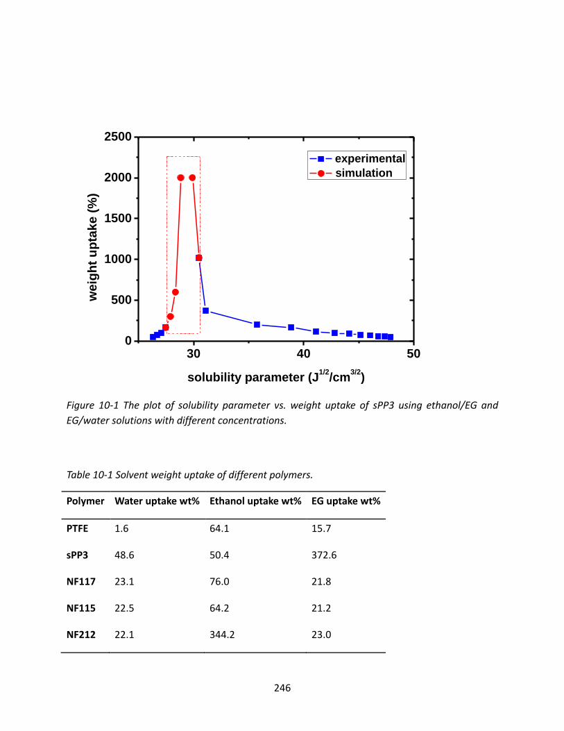
246

30 40 500

500

1000

1500

2000

2500

we

igh

t u

pta

ke

(%

)

solubility parameter (J1/2

/cm3/2

)

experimental

simulation

Figure 10-1 The plot of solubility parameter vs. weight uptake of sPP3 using ethanol/EG and

EG/water solutions with different concentrations.

Table 10-1 Solvent weight uptake of different polymers.

Polymer Water uptake wt% Ethanol uptake wt% EG uptake wt%

PTFE 1.6 64.1 15.7

sPP3 48.6 50.4 372.6

NF117 23.1 76.0 21.8

NF115 22.5 64.2 21.2

NF212 22.1 344.2 23.0

247

4000 3500 3000 2500 2000 1500 1000 500

0

2

4

6

8

882

1084

1432 12072939 2872

3310

ad

so

rban

ce

wavenumber (cm-1)

sPP3

sPP3(EG treated)

Figure 10-2 FTIR spectra of sPP3 before and after EG treatment.

FTIR spectra were produced to identify and characterize the functional groups of sPP3 before

and after EG treatment. These two infrared spectra were normalized according to the obvious

sharp peaks 700 and 764 cm-1 which present the vibrations of phenyl group substitution, as

illustrated in Figure 10-2. Comparing the sPP3 selected infrared absorption bands before and

after EG treatment, the differences of band location assignment appear at 3310cm-1 (O-H

vibration), 1207 cm-1 (C-O vibration), 2939, 2872 cm-1 (-CH2 stretching), 1432 cm-1 (-CH2

bending), and 882 cm-1 (-CH2 rocking) which fit with the EG absorbance peaks (see Table 10-2).

In other words, EG molecules diffuse into sPP3 films and disperse in the polymer matrix,

248

affecting interactions between polymer chains and solvent molecules. Moreover, appropriate

solvents significantly influence not only the macro-scale quantity but also the formation of

ionomer microstructures based on the identification of functional groups due to the identical

fingerprints of FTIR.

Table 10-2 Absorption peaks of sPP3 and sPP3 treated in EG.

Polymer Phenyl Group -SO3- C-S O-H C-O -CH2

C=C C-C conjugation substitution =C-H

sPP

(theoretical)

1500

1450

1000-

1500

1580 1600 710-800

(o m p)

3000-3100

650-900(3b)

1182(S=Oasym)

1041(S=Ostm)

1150(S-O)

1014

1004

3200-3400

EG

3200-3550

1000-1260 2850-3000(stretch)

882 (rocking)

Water 3651(sym)

1595(bend)

1350-1480(bend)

sPP3(EG) 1486

1454

1384 1633 1599 861 764 700 3047 3018

881

1182

1034

1128

1014

1005

3310 1207 1084 2939 2872 886

1432

sPP3 1492

1435

1387 1625 1594 843 757 697 3047 3018

897

1182

1033

1128

1014

1005

3645

1594

3b demonstrates three bands.

249

10.3.1.2 Solubility Parameter Calculation Methods

Two solubility parameter calculation methods are demonstrated in this section.

Hildebrand Theory based on Cohesive Energy

Hildebrand correlated solubility with the cohesive properties of solvents. In this work, the

cohesive energy contributions to a great number of structural groups are presented using Fedor

data.

Table 10-3 Comparison between calculated and empirical solubility parameters of different

polymers and solvents.

Polymer Solubility parameter(J1/2 cm-3/2)

Calculated (Fedor Data)[66]

Solubility parameter(J1/2 cm-3/2)

literature[180]

Total Backbone Ionic side chain Total Backbone Ionic side chain

PTFE 12.7 / / 12.7-14.0 / /

sPP3 29.6, 26.9 32.6 29.3(exp) / /

NF117&115 17.6, 13.6 22.8 21.9 19.8 35.4

NF212 17.9, 13.6 22.8 22.1 19.8 35.4

Water 47.9 47.9

Ethanol 26.3 26.3

EG 31.3 31.3

exp means experiment.

250

Fedor data[66] widely covers the cohesive energy and molar volume of low Mw polymer but is

less accurate for some functional groups. The difference between calculated and empirical

(from literature[180]) Nafion solubility parameters is obvious (as shown in Table 10-3) because

Nafion has medium molecular weight. Additionally, the interactions between backbones and

ionic side chains within polymer network play an import role. Chi parameter, as a reflection of

interactions between polymer chains and solvent molecules, has a great influence on dissolving

and swelling phenomena. The larger Chi parameter is, the weaker interaction between polymers

and solvents exists. If Chi parameter is smaller than 0.5, ionomers can dissolve in this solvent[181].

PTFE, as a kind of superhydrophobic polymer, presents a small water uptake 1.6% (see Table

10-1) due to the weak interaction between PTFE polymer chains and water molecules, as

illustrated as the large Chi parameter 9.02 in Table 10-4. Among these three solvents (water,

ethanol, and EG), ethanol (26.3 J1/2 cm-3/2) presents similar solubility with Nafion (around 22.0

J1/2 cm-3/2), resulting in the ethanol uptake of NF115&117 and NF212 as large as 64.2%, 76%,

and 344.2%, as displayed in Table 10-1. Moreover, huge EG uptake of sPP3 is indicative of small

Chi parameter between sPP3 and EG meanwhile Fedor Data reveals very accurate value of

solubility 29.6 J1/2 cm-3/2, which is proved by experimental result 29.3 J1/2 cm-3/2 as well.

251

Table 10-4 Chi parameters reflecting the interaction between polymer and liquid.

Polymer water Ethanol EG

PTFE 9.02 11.53 20.62

sPP3 2.45 0.66 0.09

Nafion115 & 117 4.92 0.46 1.99

Nafion212 4.84 0.41 1.89

ionomers and solvents

water ethanol EG -SO3H PTFE sPP3 NF115&117 NF212

10

20

30

40

50

60

solubility parameter

fluorocarbon backbone

phenyl backbone

ionic side chain

so

lub

ilit

y p

ara

me

ter

(J1

/2/c

m3

/2)

Figure 10-3 Solubility parameters of polymers (PTFE, SPP3 and Nafion), solvents (water, ethanol

and EG), and sulfonic acid functional group (-SO3H).

252

As shown in Figure 10-3, PTFE presents pure fluorocarbon backbone solubility parameter is 12.7

J1/2 cm-3/2, while the influence of Nafion ionic side chains on carbonfluoro-backbone leads to an

increases in Nafion backbone solubility parameter (two red data points on the right side display

19.8 J1/2 cm-3/2). Based on Fedor data, sulfonic acid group solubility parameter (-SO3H) is 43.3 J1/2

cm-3/2. From the perspective of ionomer chemical structures, the sPP3 ionic side chain is

composed of phenyl (substituted) and sulfonic acid group while the ionizable side chain of

Nafion is the combination of fluorocarbon-oxygen bond and sulfonic acid group. The

comparably non-polar chemical structures of phenyl (substituted) group and the

fluorocarbon-oxygen bond lead to decreases in ionic side chain solubility parameters of

ionomers sPP3 and Nafion, 32.6 J1/2 cm-3/2 and 35.4 J1/2 cm-3/2, respectively.

Therefore, Hildebrand theory can determine the overall ionomer solubility parameter,

combining the backbone and ionic side chain sub-parts from the aspect of molecular structure

in details.

Hansen Solubility Parameter Calculated from Surface Energy

Both surface energy and solubility parameter are determined by molecular interactions with

several following empirical equations describing their connection.

253

𝛿𝑑

2

𝑛 = 𝐴(1

𝑉𝑚)1

3𝛾𝑑 (10-1)

γd is dispersive component of surface energy, δd is dispersive part of solubility parameter, Vm

is average molar volume based on mole fraction of polymer, and A and n are constants.

𝛿𝑝

2

𝑛 = 𝐵(1

𝑉𝑚)1

3𝛾𝑝 (10-2)

γp is polar component of surface energy, δp is polar part of solubility parameter, and B is a

constant.

𝛿ℎ = √𝐸ℎ

𝑉𝑚 (10-3)

Eh is enthalpy of an H-bonding, δh is H-bonding part of solubility parameter.

These aforementioned equations’ limitation is that the molar volume of polymer should be

known. In order to find a new connection between surface energy and solubility parameter

fitting polymers without using the molar volume parameter, a better relationship between

dispersive (or polar) surface tension and dispersive (or polar, H-bonding) solubility parameter is

provided to estimate the accuracy of reported surface energy data and solubility parameters of

polymers.

254

The dispersive force is the main molecular force for most neutral molecules while polar part of

surface energy is composed of interaction within dipole moment and hydrogen bonding.

Different from 37 kinds of solvents and 22 kinds of common polymers used in reference[182], we

present 46 common polymers with dispersive and polar surface energy data and solubility

parameters (from literatures[126]) to achieve Equation (10-4) and (10-5). A good linear

relationship between the dispersive surface energy γd and the calculated parameter γd δd

2

3⁄ is

displayed in Figure 10-4 while a remarkable linear plot of the polar surface energy γp versus

the calculated parameter γp

(δp2+δh

2)13

is reported in Figure 10-5.

𝛾𝑑

𝛿𝑑

23

= 0.1322𝛾𝑑 + 0.5231 R=0.9577 (10-4)

γd is dispersive component of surface energy, δdis dispersive part of solubility parameter.

𝛾𝑝

(𝛿𝑝2+𝛿ℎ

2)13

= 0.142𝛾𝑝 + 0.1913 R=0.9459 (10-5)

γp is polar component of surface energy, δp, δh is polar and H-bonding part of solubility

parameter.

255

0 10 20 30 40 500

2

4

6

8

d /

d2

/3

d

Figure 10-4 Plot of 𝛾𝑑 𝛿𝑑

2

3⁄ vs. 𝛾𝑑.

0 5 10 15 20 25 300

1

2

3

4

5

p /

(p

2+

h2)1

/3

p

Figure 10-5 Plot of 𝛾𝑝 (𝛿𝑝2 + 𝛿ℎ

2⁄ )1/3 vs. 𝛾𝑝.

256

PTFE NF115&117 PBC1.0 PBC1.5 PBC2.0 sPP3

0

5

10

15

dispersive

polar

H-bonding

so

lub

ilit

y p

ara

mete

r (J

1/2 c

m-3

/2)

polymer

Figure 10-6 Dispersive, polar, and H-bonding component of ionomers HSP calculated from

surface energy.

Dispersive, polar and H-bonding parts of solubility parameter of polymers are indicated in

Figure 10-6. Dispersive components of all these polymers are around 14.5 J1/2 cm-3/2 (shown as

black data points). Polar and H-bonding parts of NF115&117 and sPP3 solubility parameter are

9.0 and 11.0 J1/2 cm-3/2, respectively. Moreover, all three components of PBC solubility

parameter increase gradually with IEC because higher concentration of sulfonic acid groups

leads to larger polarity, H-bonding energy and interaction within polymer networks.

257

PTFE NF115&117 PBC1.0 PBC1.5 PBC2.0 sPP30

10

20

30

40

HSP from surface energy

literature & experiment

so

lub

ilit

y p

ara

me

ter

(J1/2 c

m-3

/2)

polymer

Figure 10-7 Solubility parameter of different polymers calculated from surface energy and

obtained from literature and experiment.

As show in Figure 10-7, the overall solubility parameters determined by HSP and literature &

experiment are proved to be very identical, especially for NF115&117 and PBCs. Only little

deviations exist in PTFE and sPP3 solubility parameter compared HSP results with literature &

experiment data.

258

0 5 10 15 20 25 300

5

10

15

20

25

30

0

10

20

30

NF115&117

soluble

insolubleH

-bo

nd

ing

po

lar

dispersive

Figure 10-8 HSP of NF115&117 calculated from surface energy and solvents obtained from

literature.

The 3-D structures of HSP are necessary for a graphical representation of the interaction

between polymers and solvents, while dispersion, polar and H-bonding components of HSP

could be plotted on three mutually perpendicular axes. Figure 10-8 shows a three-dimensional

plot of HSP correlating with NF115&117. The center of sphere is the coordinated of three HSP

components and the radius R0 is equal to 9 J1/2cm-3/2, which is determined by dispersion, polar

259

and H-bonding components of HSP. The tested solvents are marked with green and grey dots.

According to the “like dissovles like” concept of solubility, all the compatible solvents (green) are

almost inside or at the edge and all the incompatible ones (grey) are outside. Two-dimensional

projections on the 𝛿𝑑 versus 𝛿𝑝, 𝛿𝑑 versus 𝛿ℎ, and 𝛿𝑝 versus 𝛿ℎ planes are presented to

help for better visualization, as displayed in Figure 10-8 as well. HSP data points of solvents NO.

5, 7, 11, 12, and 13 (ethanol, methanol, DMAc, DMF, and 2-propanol) are in the Nafion sphere,

illustrating that they can dissolve Nafion polymer completely. Literatures[183] confirm that Nafion

polymer can dissolve in these solvents or the combination of these solvents.

Table 10-5 HSP of solvents.

No. solvent solubility (J1/2 cm-3/2)

dispersion polar H-bonding

1 benzene 9.0 0.0 1.0

2 chloromethane 7.5 3.0 1.9

3 cyclohexane 8.2 0.0 0.1

4 dichloromethane 8.9 3.1 3.0

5 ethanol 7.7 4.3 9.5

6 heptane 7.5 0.0 0.0

7 methanol 7.4 6.0 10.9

8 tetrahydrofuran 8.2 2.8 3.9

9 toluene 8.8 0.7 1.0

10 water 7.6 7.8 20.7

11 N,N-dimethylacetamide 8.2 5.6 5.0

12 N,N-dimethylformamide 8.5 6.7 5.5

13 2-propanol 7.7 3.0 8.0

260

Figure 10-9 shows a two-dimensional projection plot of the HSP found with PBCs correlation

and the radius R0 is equal to 7.5 J1/2 cm-3/2. Compare R0 with Ra, the tested solvent 4, 8, 9, 11, 12

(dichloromethane, tetrahydrofuran, toluene, DMAc, and DMF presented by green dots) are

located in the PBC HSP sphere. Thus, these solvents have good interaction with PBC ionomers.

However, grey solvents dots do not meet this requirement, such as water.

0 5 10 15 20 25 300

5

10

15

20

25

30

0.0

7.5

15.0

22.530.0

PBC1.0

PBC1.5

PBC2.0

soluble

insoluble

H-b

on

din

g

po

lar

dispersive

Figure 10-9 HSP of PBCs calculated from surface energy and solvents obtained from literature.

261

10.3.2 Solubility Parameters and Crosslink Number Achieved by

Swelling Property

10.3.2.1 Number of Crosslink Determined by Ionomer Swelling

Table 10-6 Data utilized to calculate the number of crosslink (water swelling).

ionomers swelling

mass %

n (mol/cm3)

Number of Crosslink

Volume

Fraction v2

Chi

(ionic side chain)

N

NF117 23.1 0.00029 0.69 1.06 6.06

NF115 22.5 0.00039 0.73 1.08 4.52

NF212 22.1 0.00051 0.75 1.13 3.74

sPP3 48.6 0.00120 0.72 1.05 2.76

N is the number of sulfuric acid group forming one bond.

NF117 NF115 NF212 sPP30.0000

0.0005

0.0010

0.0015

0.0020

NO. of Crosslink

Flory-Rehner Eq

ionomer

n (

mo

l/cm

3)

0.0

0.5

1.0

1.5

ch

i (ion

ic s

ide c

hain

)

Figure 10-10 Different ionomers’ number of crosslink and chi parameter (polymer-water).

262

Based on volumetric swelling data, molecular mass between crosslinks (Mc) can be determined.

Afterwards, the number of crosslink n =1

v̅Mc(1 −

2Mc

M) can be achieved. The number of crosslink

is influenced by various factors such as thickness, IEC, and temperature. The number of

crosslink of NF117, 115, 212 and sPP3 is 0.00029, 0.00039, 0.00051, and 0.00120 mol/cm3,

respectively, as displayed in Table 10-6. However, chi parameter (the ionic side chains-water

interaction) is similar for different ionomers, as presented in Figure 10-10. According to

Flory-Rehner Equation, chi parameter, as a reflection of interaction between polymer chains

and liquid molecules can be determined by the number of crosslink. Moreover, the number of

sulfuric acid group forming one bond can be determined to further predict IEC.

10.3.2.2 Comparison between Chi Parameters from Hildebrand’s

Theory and Flory-Rehner Equation

Table 10-7 Solubility parameters of ionic side chains of different ionomers based on Hildebrand’s

Theory, literature and Flory-Rehner Equation (Unit: J1/2 cm-3/2)

ionomers Solubility Parameter

Hildebrand’s Theory

Solubility Parameter

literature

Solubility Parameter

Flory-Rehner Equation

NF117 22.8 35.4 36.1

NF115 22.8 35.4 35.7

NF212 22.8 35.4 35.4

sPP3 32.6 / 35.9

263

According to Flory-Huggins and Flory-Rehner Equations, the solubility parameter of ionic side

group can be determined by swelling data. Conversely, if polymer solubility parameter is known,

chi parameter and number of crosslink can be achieved as well. In Table 10-7, the solubility

parameters of Nafion 117, 115, and 212 ionic side chains are 36.1, 35.7, and 35.4 J1/2 cm-3/2,

respectively, which fit well with the literature[180] 35.4 J1/2 cm-3/2 as shown in Table 10-3.

The Nafion solubility parameters listed in the literature are identical with that determined by

the indirect calculation method, as show in Table 10-7. The interactions within the polymer

chains have a great influence on the solubility parameter of the ionic side chain. The solubility

parameter of Nafion series calculated by the Hildebrand’s Theory has great difference with that

from literature and Flory-Rehner Equation. For some ionomers, it is not a good way of using

Hildebrand’s Theory to calculate the solubility parameter.

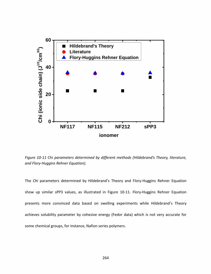
264

NF117 NF115 NF212 sPP30

20

40

60

Hildebrand's Theory

Literature

Flory-Huggins Rehner Equation

Ch

i (i

on

ic s

ide

ch

ain

) (J

1/2/c

m3/2)

ionomer

Figure 10-11 Chi parameters determined by different methods (Hildebrand’s Theory, literature,

and Flory-Huggins Rehner Equation).

The Chi parameters determined by Hildebrand’s Theory and Flory-Huggins Rehner Equation

show up similar sPP3 values, as illustrated in Figure 10-11. Flory-Huggins Rehner Equation

presents more convinced data based on swelling experiments while Hildebrand’s Theory

achieves solubility parameter by cohesive energy (Fedor data) which is not very accurate for

some chemical groups, for instance, Nafion series polymers.

265

10.3.2.3 Chemical Potential of Ionomer Swelling

The chemical potential change of ionomer swelling has great physical significance because it

relates micro-properties with macroscopic phenomena. Water molecules diffuse into ionomers

from high to low chemical potential locations, accompanied with a release of free energy for

the polymer chain movement, is defined as the process of ionomer swelling. In the process of

deswelling, polymer chains coil up and membranes shrink. The chemical potential change of

mixing is related to Chi parameter. For instance, sPP3 presents the smallest mixing chemical

potential change within water, 0.714 J/mol as illustrated in Table 10-8. In other words, sPP3 is

easy to mix with water compared with other ionomers. Moreover, the interactions between

sPP3 polymer chains and water molecules are so strong that sPP3 can easily swell. Therefore,

higher IEC value requires less mixing chemical potential change. Secondly, the number of

crosslink has a great influence on the elastic component of chemical potential. Thirdly, the ionic

part chemical potential change within swelling process is affected by IEC as well. Finally, for the

immiscible polymer-liquid system, the overall chemical potential change is mainly determined

by the mixing component of chemical potential change.

266

Table 10-8 The chemical potential changes in the process of swelling within water for different

ionomers. (Unit: J/mol)

ionomers Δμmix/RT Δμelastic/RT Δμion/RT Δμ/RT

NF117 1.884 0.00286 0.00837 1.896

NF115 2.037 0.00381 0.00837 2.048

NF212 2.093 0.00487 0.00917 2.107

sPP3 0.714 0.01158 0.04922 0.775

0 2 4 6

2600

3900

5200 (a)NF115NF117

NF212

sPP3

mix

m

ix (

J/m

ol)

Chi0.0000 0.0005 0.0010 0.0015 0.00200

10

20

30

40

(b)

NF117

NF115

NF212

sPP3

elastic

e

las

tic (

J/m

ol)

n (NO. of Crosslink) (mol/cm3)

0.0 0.5 1.0 1.5 2.00

50

100

150

(c)

NF115 &117

NF212

sPP3

ion

io

n (

J/m

ol)

IECNF115 NF117 NF212 sPP3

0

1500

3000

4500

6000

(d)

mix

ion

elastic

(

J/m

ol)

ionomer

Figure 10-12 The change of chemical potential in the swelling process for different ionomers.

(a) the mixing chemical potential vs. Chi parameter, (b) the elastic chemical potential vs. NO of

crosslink, (c) the ionic chemical potential vs. IEC, and (d) the overall chemical potentials and the

sub-chemical potentials of different ionomers.

267

The solution dispersion casting membrane method leads to the largest change of chemical

potential mixing component for NF212, stabilizing polymer chains. Hence, if water molecules

want to diffuse into the NF212 membranes, a great amount of energy needs to be provided.

The elastic chemical potential change is primarily governed by the elastic restraining forces of

the cross-linked polymer chains, which is a limiting parameter on extent of swelling. These

elastic restraining forces are entropic in nature because the polymer matrix stretching reduces

the number of available chain conformation. The largest number of crosslink of sPP leads to the

strongest elastic restraining forces with the highest elastic chemical potential change, as shown

in Figure 10-12 (b). The ionic chemical potential is close related to IEC, as presented in Figure

10-12 (c). At last, the mixing chemical potential is the main factor of calculating the overall

chemical potential compared the order of values, as seen from Figure 10-12 (d).

10.3.2.4 Solubility Parameter and Dielectric Constant of PBCs

In order to explore the interaction between ionomer chains and solvent molecules, solubility

parameter and dielectric constant are determined to investigate the correlation between

electrostatic interaction and morphology. As known Hildebrand’s Theory, solubility parameter

δ (dimension: J1/2/cm2/3) is the square root of cohesive energy density ecoh (dimension:

J/cm3), which is defined as cohesive energy Ecoh (dimension: J/mol) divided by molar volume of

a substance at 298K. The cohesive energy of a substance in a condensed state is defined as the

268

increase in internal energy U per mole of substance if all the intermolecular forces are

eliminated.[66] According to Fedor data of cohesive energy and molar volume[66], the group

contribution method (GCM) determines the PBC solubility parameters with different IECs, as

shown in Table 10-9, which is substantially in a good agreement with literatures.

From the polymer handbook[184], it can be found that the solubility parameter of polystyrene is

around 15.6-21.1 J1/2 cm-3/2. Furthermore, Lu and Weiss[185] reported that the solubility

parameter of ionomer can vary between the values for polystyrene and fully sulfonated

polystyrene, i.e., 18.6-33.9 J1/2 cm-3/2, by varying the degree of sulfonation. According to Fedor

Data[66] and GCM, we can verify that S = 21.9 J1/2 cm-3/2 and sS = 31.4 J1/2 cm-3/2, which are

satisfactorily consistent with the data above. Meanwhile, the calculated HI 16.9 J1/2 cm-3/2 is

appreciably in range of 16.2-17.4 J1/2 cm-3/2 from the solubility parameter of ethylene propylene

rubber in the reference[186]. The value of tBS calculated as 19.4 J1/2 cm-3/2 is sufficiently reliable,

though it is a little bit different from 16.6 J1/2 cm-3/2 (combination of molar attraction constant)

and 18.9 J1/2 cm-3/2 (atomic contribution), respectively, by Small and Hoftyzer & Van Krevelen’s

scheme[66]. No experimental value of tBS solubility parameter is reported and the Small and

Hoftyzer & Van Krevelen methods predict the cohesive energy with a mean accuracy of about

10%. At last, the overall solubility parameter of PBCs is the combination of the solubility

parameters of these four blocks in accordance with the degree of polymerization percentage of

each block. Additionally, Darby et al.[187] suggested a correlation between dielectric constant

269

and solubility parameter for polymers, 𝛿 ≈ 7.0𝜖, which has been validated by D. W. Van

Krevelen [66].

Table 10-9 Solubility parameters and dielectric constants of PBCs.

polymer (J1/2

cm-3/2)

ntBS% n HI% nS% nsS%

tBS = 19.4 J1/2 cm-3/2 HI = 16.9 J1/2 cm-3/2 S = 21.9 J1/2 cm-3/2 sS = 31.4 J1/2 cm-3/2

PBC1.0 20.9 0.252 0.385 0.240 0.123 2.93

PBC1.5 21.7 0.252 0.385 0.173 0.190 3.02

PBC2.0 22.5 0.252 0.385 0.104 0.259 3.12

nx% is the degree of polymerization percentage of different blocks. (δ = (∑(𝑛𝑥%×𝐸𝑐𝑜ℎ)

∑(𝑛𝑥%×𝑉𝑥))1

2)

Table 10-10 Basic properties of solvents used.[66]

solvent (J1/2

cm-3/2)

d p h d(g/ml) Tb (oC) Vs

(cm3/mol)

THF 19.5 16.8 5.7 8.0 0.889 63 81.2 7.58

CHCl3 18.8 17.6 3.1 5.7 1.483 61 79.7 4.81

C:H 15.9 15.9 0 0 0.729 81-98 127 1.97

d, d, and h are dispersion, polar, and hydrogen bonding component of solubility parameter,

respectively. d presents density of solvents while Tb is boiling point. Vs demonstrates molar

volume.

According to the Flory-Huggins Solution Theory[69] which is a mathematical model of the

thermodynamics of polymer solutions, taking account of the great dissimilarity in molecular

sizes in adapting the usual expression for the entropy of mixing, polymers truly dissolve in

solvents with similar solubility parameters. Considering Gibbs Free Energy change for mixing a

polymer with a solvent Δ𝐺m = Δ𝐻m − TΔSm, the entropy of mixing R𝑇𝑛1𝜙2𝜒12 = 𝑛1𝜙2zΔw

270

(𝜒12 = 𝑉𝑠(𝛿𝑎 − 𝛿𝑏)2/R𝑇) where the number of moles n1 and volume fraction 𝜙1 of solvent

(component 1), the number of moles n2 and volume fraction 𝜙2 of polymer (component 2),

with the introduction of a parameter 𝜒12 is defined as the polymer-solvent interaction

parameter chi. R is the gas constant and T is the absolute temperature. z is the coordination

number, described by Vs, the molar volume of solvent. Δw is the energy increment per

monomer-solvent contact, represented as (𝛿𝑎 − 𝛿𝑏)2. Charles M. Hansen in 1966[66] divided

the total Hildebrand value into three parts: a dispersion force component, a hydrogen-bonding

part, and a polar component, which is most widely accepted as Hansen Solubility Parameter

(HSP), as illustrated in Table 10-10. Based on Flory-Huggins Solution Theory, Chi parameter (see

Figure 10-13), as a reflection of interaction between ionomer chains and solvent molecules, can

be determined by solubility parameter ionomer and a kind of solvent (combining the data in

Table 10-9 and 10-10). The smaller Chi parameter between the solubility parameters of

ionomers and solvents is, the stronger polymer-solvent interaction presents. As solvents

evaporation, this strong interaction leads to the ionomer chains aggregating as a way of micro

phase separation to minimize interfacial energy in a relatively polar solvent such as THF, while

Chi parameter between PBC and THF is smaller than 0.3.

271

0.5 1.0 1.5 2.0 2.50.0

0.5

1.0

1.5

2.0

2.5

THF

CHCl3

C:H

Ch

i p

ara

me

ter

IEC (mequiv/g)

Figure 10-13 Correlation between Chi parameter and IEC of PBCs cast with different solvents.

Considering the concentration of sulfuric acid within PBC, hydrogen bonds play a significant role

in the formation of microphase-separated structures as well. Due to the scarcity of hydrogen

bond component within solvent C:H solubility parameter, the weaker hydrogen-bonding

interaction between PBC and C:H solvent prevents C:H molecules from getting into PBC

sulfonated domains compared with the other two solvents CHCl3 and THF. Hence, with solvent

C:H evaporation, sulfonated domains are well dispersed in the ionomer matrix to form a

homogeneous microstructure.

272

From another perspective, ionomer solutions can be treated as weak ionic liquid if dielectric

constant of solution is smaller than 30[126]. The electrostatic interaction Uelectr between two ions

is directly proportional to the dielectric constant of solvent if the polymer concentration

remains the same.[188] THF with larger dielectric constant enhances the electrostatic

interactions within ionomer solutions, resulting in the stretching of polyelectrolyte chains and

the prevention of ionomer clustering with solvent evaporating. Finally, THF solvent tends to

induce PBC phase separation rather than C:H. Therefore, it is evident from the results and

discussion above that the option of casting solvents has a great influence on the microscopic

interaction between ionomer chains and solvent molecules and the macroscopic dissolving

properties.

10.4 Conclusion

A number of previous researches have provided an understanding of solubility parameters and

chemical and physical properties. In our study, the bridge between the characteristics of

ionomers and the swelling process has been built to investigate the great impact of solubility

from the perspective of polymeric macro- and micro-properties. In detail, an appropriate

method was selected to calculate the solubility parameter of different polymers, as Fedor data

require the knowledge of molecular structure and surface energy is essential for HSP simulation.

Furthermore, our work represents a new approach to calculating the solubility parameter of

273

ionic side chains of sulfonated polymers by combining Flory-Huggins and Flory-Rehner Equation

with the process of swelling. Therefore, our study provides insight into solubility parameters

with respect to IEC, thickness, number of crosslinks, chemical structure, and chemical potential

changes during swelling. Finally, our study provides the framework for future studies to explore

the membrane casting method and liquid transport in the microscopic and macroscopic

aspects.

274

Chapter 11 Morphology, Ion Transport, and Solution

Thermodynamics of a Penta Block Copolymer Ionomer

11.1 Introduction

Ionomers are one of the most advanced separation polymer utilized in diverse fields such as

electrodialysis, electrolysis, diffusion-dialysis, batteries, sensing materials, medical use,

analytical chemistry, and proton exchange membrane (PEM) fuel cells[5]. An ionomer has three

main characteristics: ion conductivity, hydrophilicity, and fixed charge carriers due to electrically

neutral repeating units and ionizable blocks[5-6]. For more than 60 years, researchers have been

synthesizing new ionomers to improve physical properties[2, 109, 116, 189]. This work has been

focused on optimizing ionomer composition and structure to improve morphology, physical and

transport properties, and thermochemical degradation resistance.

Ionomer properties are dependent upon chain spatial arrangement, which may give rise to

lamellar, cylindrical, or spherical morphology[71]. For example, Zhao[106] and Lee[107] showed that

sulfonated poly(ether ether ketone) (SPEEK) and poly(arylene ether sulfone)-b-polyimide

copolymers containing longer hydrophilic domains triggered microphase separation, which led

to the formation of more organized ion conductive domains. This resultant morphology led to a

remarkable increase in proton conductivity as compared to random copolymers. In addition to

275

block sequences and arrangements, processing methodology is incredibly important to ionomer

properties. Solvent type and casting temperature of SPEEK[108] and Nafion[109] had

considerable effects on proton conductivity and chemical stability. Bebin and Galiano[110]

demonstrated that the proton conductivity of solvent-cast sulfonated polysulfone (sPSU) films

was twice as that of melt-extruded sPSU. Moreover, Weiss[111] showed that ion aggregation

occurred at lower temperatures in sulfonated block copolymers

poly(b-styrene-b-(r-ethylene-so-r- butylene)-b-styrene) (S-SEBS) as compared to similar

homopolymers with different microstructures. Effects of solution-casting and block length on

morphology, physical properties, and proton conductivities were studied by Lee et al.[112] using

sulfonated poly(arylene ether sulfone) multiblock copolymer. Fan et al.[113] explored viscoelastic

and gas transport properties of a series of multiblock copolymer ionomers sulfonated

poly(arylene ether sulfone) (BPSH-BPS) as a function of block length, relaxation time, and

temperature. These research efforts illustrate that it is critical to evaluate solution casting

effects in order to obtain desirable film properties.

It is well known that ionomers have recently attracted widespread interest in the field of proton

exchange membrane (PEM) fuel cells (FC)[2]. Three remarkable characteristics of ionomers

mentioned above qualify ionomers for use in other processes such as electrodialysis,

electrolysis, diffusion dialysis, batteries, sensing materials, medical use, and analytical

chemistry[5]. However, applications in these fields have not appreciably gained enough attention.

276

For more than 60 years, researchers have been reporting the synthesis and characterization of

different kinds of ion-exchange membranes[109, 116]. Subsequently, more attempts have focused

on possible factors improving morphology, transport properties, mechanical properties, phase

behaviors and degradation of ionomers. However, besides intrinsic properties (polymer

structure, chain end group, and molecular weight of the polymer), extrinsic casting methods

also affect various performances of ionomers significantly. The casting methodology includes

types of solvents used[112], methods of sample preparation[109-110, 117], and ionic

neutralization[118]. Because the diffusion of different ion such as Na+, Li+, and Ca2+ and liquid

molecules through membranes is equally important as the proton transport in ionomers.

In several previous studies, it has been reported that the casting and processing conditions and

technique substantially influenced the ionomer microstructures and transport properties. It is

reported that different casting solvents and processing methods could lead to large

discrepancies in proton conductivity of block copolymer such as sulfonated poly(ether ether

ketone) (SPEEK)[108], Nafion[109], sulfonated polysulfone (sPSU)[110], and sulfonated poly(arylene

ether sulfone) multiblock copolymer[112]. Nevertheless, the importance and significance of

ionomer casting methodology has not been paid close attention to so far. Furthermore, it is

claimed that the use of ionic functional groups can modify morphology, mechanical properties,

physical properties, transport properties, and the degradation of ionomers. In 1990, the

introduction of different counter-ions (Na+, K+, Cs+, and Ca2+) contributed to better fatigue

277

performance and shear deformation caused by more effective ionic crosslinks was discovered

by Hara.[118] Before long, Weiss pointed out that the critical temperature for ionic aggregation

and dissociation in the block copolymer ionomer was lower than that of similar homopolymer

ionomers due to perturbation by the block microstructure.[111] Later on, some researchers

proposed that metal ionic neutralized ionomers improved their stability, as well as, physical and

mechanical properties.[119] Moreover, Winey probed the importance of the cast preparation

method and thermal treatment in determining the nanoscale morphology of the salt-form

ionomers Cu-neutralized poly(styrene-ran-methacrylic acid) (SMAA) and Cu-neutralized

poly(3-methylstyrene-ran-methacrylic acid) (3-MeSMAA).[120] However, few attempts have

focused on the relationship between the ionic neutralization of solvent-cast ionomers and the

ion transport properties.

In addition to ion transport, numerous investigations have also focused on the diffusion of liquid

molecules through ionomer films as another important transport property. In 1992, Koval

presented that the substitution of silver ions for sodium ions in hydrated ionomer membranes

causes the trans-membrane fluxes of styrene (STY) and ethylbenzene (EBZ) to increase by 2-3

orders of magnitude by facilitated transport.[121] After that, people began to pay close attention

to liquid molecules transport, such as methanol and water. In 2002, Dimitrova[122] illustrated

that Nafion-recast membranes filled with 4.3% silicon dioxide exhibited increased water uptake,

conductance and methanol permeation rate compared with commercial ones. Later on, from a

278

morphological aspect, Elabd[123] put forward that ordered structure sulfonated

poly(styrene-isobutylene-styrene) (S-SIBS) caused by higher ion exchange capacity (IEC) greatly

affected the methanol transport properties. Shortly after that, the water transport properties of

salt-form perfluorosulfonated ionomer membranes[124] and the mechanism of methanol,

ethanol, and 2-propanol diffusion through ionomers[125] were demonstrated by Saito, noting

that Li+ and Na+ ionomers have lower water transference coefficients and water permeability

compared with H+ ionomers due to the strong interaction between salt ions and water

molecules. Nevertheless, few efforts have focused on the relationship between different

ionomer casting solvents and liquid molecule transport properties.

In this study, a series of solvent-cast penta-block copolymer (PBC) ionomers were cast from

tetrahydrofuran (THF), chloroform and a cyclohexane:heptane (C:H) solution (1:1 wt%). Their

properties were studied as a function of ion-exchange capacity (IEC) using TEM, SAXS, FTIR, and

impedance spectroscopy to measure proton conductivity. It was found that an appropriate

solvent dramatically enhanced proton conductivity and transport properties at the same IEC.

Furthermore, solvent-cast PBCs produced more stable properties compared to commercial PBCs,

illustrating the importance of casting solvent to morphology, functional group distribution, and

transport properties.

279

11.2 Experimental

11.2.1 Material

Penta Block Copolymer (PBC) ionomers were provided by Kraton Polymers LLC, Houston, TX[161].

Its block compostition is poly[t-butyl styrene-b-hydrogenated isoprene-b-sulfonated

styrene-b-hydrogenated isoprene-b-t-butyl styrene) (tBS-HI-S-HI-tBS). The detailed information

was shown in Chapter 8.




by solution casting methodology in a Teflon dish.

11.2.3 Transmission Electron Microscopy (TEM)

The FEI Tecnai Biotwin G2 Spirit Transmission Microscope at 80 kV was used to acquire images.

All PBC samples were treated in a BaCl2 solution to convert the acid-form to barium-form in

order to enhance contrast based on electron density. Membrane strips with 0.5-1.0 mm width

280

and 5.0-10.0 mm length were embedded in epoxy. Testing sections were cut using a Diatome

diamond knife, and collected onto 400 mesh copper ruthenium grids.

11.2.4 Small Angle X-ray Scattering (SAXS)

Small-angle X-ray scattering was carried with a Rigaku Ultima IV using CuK (wavelength =

0.154 Å) at 60 kV and 20 mA. In this study, membranes were probed by adjusting the incident

beam angle from 0.03o to 1.76o using a 0.005o step size. This covered the total momentum

transfer vector q = 4 sin from 0.0042 Å-1 to 0.25 Å-1.

11.2.5 Conductivity Measurement

In this study, ionomer proton conductivity was measured under fully hydrated conditions in

deionized water. The temperature was monitored and controlled by an isothermal water bath

(Thermo Scientific Inc.). A 2-probe method was used to measure resistance in the plane or

though the plane of the film with a BekkTech LLC test cell. The distance between the two

platinum electrodes was 0.5 cm. Film thickness was measured in its swollen state prior to and

after an impedance test. The Nyquist impedance plots were collected using a Metrohm Autolab

PGSTAT302N from 0.1 Hz to 1 MHz.

281

11.2.6 Diffusivity Measurement

The liquid permeability was measured using a side-by-side diffusion cell with water jacket made

by Permegear Inc., as shown in Figure 8-9 (Chapter 8). The permeation area was 3.106 cm2.

Each film was used to separate 20 ml water and 20 ml solutions. A water pump 510 was used to

circulate the water side at 10 ml min-1 through a refractive index detector 2410 (RID 2410) to

monitor the solution concentration changes with time. Both compartments were well stirred

using submersible magnetic stirrers to decrease the concentration difference. The temperature

was maintained at 30-60oC by a water circulator going through the water jacket of the diffusion

cell.

282


11.3.1 Morphology of Ionomers

Figure 11-1 TEM micrographs of PBC1.5 films cast with different solvent and dried at 20oC, (a)

C:H, (b) CHCl3, and (c) THF. Length of scale bar = 100 nm.

Since the effect of processing conditions is critical, a morphological study was investigated

using TEM and SAXS to display the microstructures of PBC1.5 cast with different solvent and to

observe the influence of casting conditions on the final morphology. The TEM samples of

PBC1.5 were prepared using solvent-cast method and the TEM micrographs are illustrated by

Figure 11-1. The unsulfonated block (tBS, HI, and S) domains show brighter in TEM micrographs,

while the sulfonated block (sS) domains appear darker because of the presence of electro-rich

283

ion-pairs stained by heavy metal barium neutralization. According to Figure 11-1 (a), a relatively

homogeneous distribution of lighter and darker domains indicates the absence of well-ordered

ionic domains within the polymer matrix. Moreover, this poorly ordered microstructure of

PBC1.5 is in good agreement with the solubility parameter data as detailed in Figure 10-13. In

contrast to Figure 11-1 (a), Figure 11-1 (b) and (c) display relatively microstructure-ordered

PBC1.5 films cast with CHCl3 and THF. Especially, the TEM micrograph of THF-cast block

copolymer reveals large-scale phase separation between the sulfonated and unsulfonated

blocks. As the Chi parameter decreases from 1.71, 0.26 to 0.16 (C:H, CHCl3, and THF

sequentially) as listed in Figure 10-13 (Chapter 10), the formation of more continuous and

wider spaced domain would be presented. The morphological consideration will be further

discussed with transport properties and physical properties (Chapter 12).

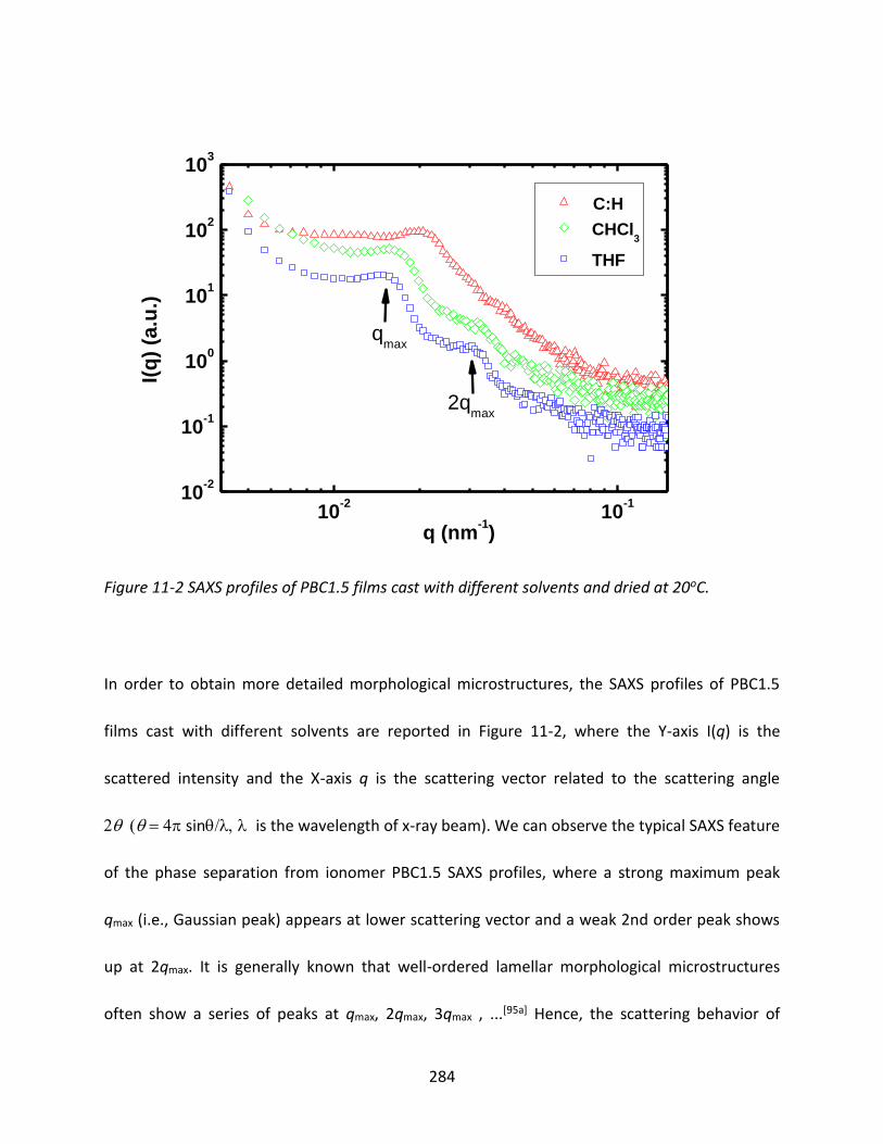
284

10-2

10-1

10-2

10-1

100

101

102

103

I

(q)

(a.u

.)

qmax

2qmax

C:H

CHCl3

THF

q (nm-1)

Figure 11-2 SAXS profiles of PBC1.5 films cast with different solvents and dried at 20oC.

In order to obtain more detailed morphological microstructures, the SAXS profiles of PBC1.5

films cast with different solvents are reported in Figure 11-2, where the Y-axis I(q) is the

scattered intensity and the X-axis q is the scattering vector related to the scattering angle

sin is the wavelength of x-ray beam). We can observe the typical SAXS feature

of the phase separation from ionomer PBC1.5 SAXS profiles, where a strong maximum peak

qmax (i.e., Gaussian peak) appears at lower scattering vector and a weak 2nd order peak shows

up at 2qmax. It is generally known that well-ordered lamellar morphological microstructures

often show a series of peaks at qmax, 2qmax, 3qmax , ...[95a] Hence, the scattering behavior of

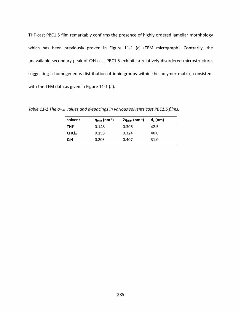
285

THF-cast PBC1.5 film remarkably confirms the presence of highly ordered lamellar morphology

which has been previously proven in Figure 11-1 (c) (TEM micrograph). Contrarily, the

unavailable secondary peak of C:H-cast PBC1.5 exhibits a relatively disordered microstructure,

suggesting a homogeneous distribution of ionic groups within the polymer matrix, consistent

with the TEM data as given in Figure 11-1 (a).

Table 11-1 The qmax values and d-spacings in various solvents cast PBC1.5 films.

solvent qmax (nm-1) 2qmax (nm-1) d1 (nm)

THF 0.148 0.306 42.5

CHCl3 0.158 0.324 40.0

C:H 0.203 0.407 31.0

286

THF CHCl3

C:H25

30

35

40

45

50

SAXS Bragg's law

TEM image analysis

IID

D (

nm

)

solvent

Figure 11-3 Comparison of the center-to-center inter-ionic-domain distance (IIDD) estimated

from the SAXS profiles (calculated) and TEM images (manually measured) of the PBC1.5

membranes cast with different solvent at 20oC.

As the polarity of casting solvent is increased (from C:H, CHCl3 to THF), the maximum peak

becomes stronger and sharper, and simultaneously shifts to lower scattering vector value.

According to Bragg’s law, dBragg is equal to 2qmax, assuming the first order maximum peaks are

due to inter-domain interference between the distance of ionic domains dBragg.[113] Therefore,

the nominal d-spacing between domains calculated by Bragg’s law is 42.5, 40.0, and 31.0 nm as

a function of solvent (see Table 11-1). The sulfonated domains tend to expand with the

increasing polarity of solvents, induced by inherent properties of solvents and polymer-solvent

287

interactions. Moreover, the polar solvent-cast PBC1.5 ionomer could develop a more ordered

and stable morphology and low entropy configuration as discussed previously (Chapter 10). In

addition, comparing the globally dimensional values of the inter-ionic-domain distance (IIDD)

calculated from the SAXS profiles with the local d-spacing values estimated from TEM images,

the significant statistical agreement between these two morphological techniques is reached as

shown in Figure 11-3.

11.3.2 Proton Conductivity Measurement

As outlined in the introduction, differences in transport properties of solution-cast films are

considered to arise from the impact of processing conditions on the surface and bulk structure

of the membranes. In this section, we evaluate the correlation between casting methodology

and proton conductivity of ionomer PBC1.0 films. The experimental result that proton

conductivity of commercial PBC1.0 decreasing from 12 to 1 mS/cm is attributed to the variation

of micro-structure of the polymer when voltage applied to the system, as can be seen from

Figure 11-4 (a). Under electric force, ionomer chains of commercial PBC1.0 membranes tend to

form a more stable microstructure, resulting in proton conductivity decrease to only 1 mS/cm

which is equal to that of C:H-cast PBC1.0. Though commercial PBC1.0 is cast by C:H as well,

processing methods are totally different. The first Doctor Blade Die casting method makes

solvent evaporate so fast that there is not sufficient time for commercial PBC1.0 ionomer

288

chain-relaxation. In contrast, solution-cast methodology enables polymer chain to relax in a

comparably longer evaporation period of time, resulting in more stable proton conductivities.

The latter one leads to a relatively low-Gibbs-free-energy final state comparing with that of

commercial PBC1.0. In Figure 11-4, THF-cast membranes present the highest proton

conductivities compared with other solvent-cast films, due to the influence of morphological

lamellar microstructure on transport properties, as investigated in the previous morphology

part.

289

Figure 11-4 Proton conductivity (a) and swelling ratio (b) of commercial PBC1.0 films and

solution-cast PBC1.0 membranes.

290

According to Figure 11-4 (b), swelling ratio is directly proportional to proton conductivity

influenced by the width of hydrophilic micro-channel (Figure 11-1) which is related to casting

solvent and temperature. The phenomenon of extremely large swelling of THF-cast PBC1.0 at

40oC is ascribed to the formation of wider micro-channel at higher casting temperature,

allowing more water molecules passing through films. Although optimal solvent and casting

temperature can enhance the micro-ordered morphological change, moderate mechanical

properties are derived from excessive large-scale phase separation which will be illustrated in

Chapter 12.

291

10 20 30 40 50 60

0

10

20

30

2nd

cycle

final

initial

final state

initial

final

initial state

(a)

Commercial PBC1.0

THF cast H+ form

THF cast Na+ form

co

nd

ucti

vit

y (

ms c

m-1)

T (oC)

0 1 2 3 4 5

0

10

20

30

final

initial

(b)

co

nd

ucti

vit

y (

ms c

m-1)

cycle

Commercial PBC1.0

THF cast H+ form

THF cast Na+ form

Figure 11-5 Conductivity of PBC1.0 changing with temperature and time (a), and variation of

conductivity with testing cycles at 25oC (b).

292

Details of the experimental procedure can be observed in Figure 11-5, as impedance

measurements were processed with increasing temperature from 25oC to 60oC and then cooling

down to form a round experiment cycle. The proton conductivity of PBC1.0 increases with

temperature (from 25oC to 60oC) due to the change of proton mobility and transport property.

According to Figure 11-5 (a), solution-cast PBC1.0 membranes display very small change of

proton conductivities with testing cycles, no matter for the acid-form or salt-form (Na+) PBC1.0

films. However, proton conductivity of commercial PBC1.0 decreases dramatically at the very

beginning of the experimental cycle to a very low value only 3 mS/cm. Figure 11-5 (b)

demonstrates that the proton conductivity decrease of commercial PBC1.0 is striking with

testing cycles at 25oC. The reason is that commercial PBC1.0 cast by Doctor Blade Die initially is

in a less stable state, and subsequently the electric drag force applied from impedance

experimental system induces the polymer chains moving to a lower Gibbs-free-energy state

which represents a more homogeneous and stable phase. Lastly, conductivity of THF

solution-cast salt-form PBC1.0 is relatively lower than that of acid form due to low mobility and

large molecular size of sodium ions compared with protons.

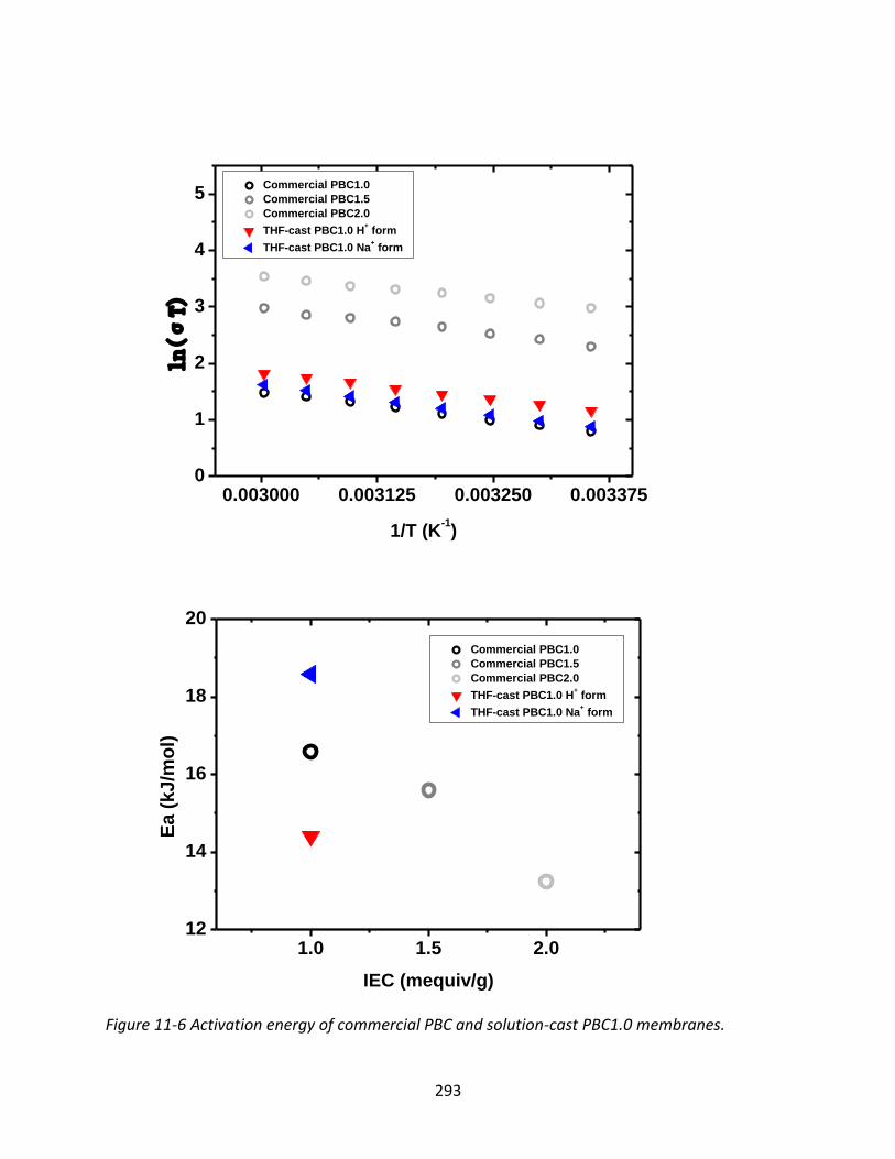
293

0.003000 0.003125 0.003250 0.0033750

1

2

3

4

5

Commercial PBC1.0

Commercial PBC1.5

Commercial PBC2.0

THF-cast PBC1.0 H+ form

THF-cast PBC1.0 Na+ form

ln(σT)

1/T (K-1)

1.0 1.5 2.012

14

16

18

20

Commercial PBC1.0

Commercial PBC1.5

Commercial PBC2.0

THF-cast PBC1.0 H+ form

THF-cast PBC1.0 Na+ form

Ea (

kJ/m

ol)

IEC (mequiv/g)

Figure 11-6 Activation energy of commercial PBC and solution-cast PBC1.0 membranes.

294

The activation energy of ion transport through ionomer films obeys to Arrhenius law[190],

following with an Arrhenius plot displaying the logarithm of kinetic constant (ln(T), Y-axis)

plotted against inverse temperature (1/T, X-axis). 𝑙𝑛(𝜎𝑇) = −𝐸𝑎

𝑅×

1

𝑇+ 𝑙𝑛𝐴, where 𝜎 presents

conductivity, A is pre-exponential factor, and Ea is activation energy of ion transport. The

activation energy of ion transport through ionomer films is obtained from the slope of the

corresponding line. The activation energies for ion transports Ea(ion) are plotted in Figure 11-6

against the IEC values according to Arrhenius plot ln(T) vs. 1/T. Obviously, PBC2.0 displays the

lowest activation energy for proton transport, caused by stronger interactions between sulfonic

acid groups and protons from perspective of quantity. Moreover, ionic conductivity of ionomers

is closely related to the size and the number of ionic cluster regions within the membranes.[124]

It is generally known that protons in aqueous solution are transported by the hopping

mechanism (Grotthus mechanism)[191] and can move faster than the other cations species

transported by the vehicle mechanism.[192] Therefore, the activation energy of H+ transport is

lower than that of Na+ if IEC of ionomers is identical. And H+ ions attract more water molecules

to form larger ionic cluster regions between sulfonic acid mircrochannels compared with the

counter-cation Na+. Comparing the slopes of red and black linear trend lines (Figure 11-6), it can

be found that THF-cast PBC1.0 has lower proton transport activation energy than C:H-cast

PBC1.0, implying that the lamellar morphological microstructure of THF-cast PBC with wider ion

295

transport channel, as investigated in the previous part, significantly improves ion transport

properties.

11.3.3 Diffusivity of Ionomers

11.3.3.1 Ion Diffusivity of PBCs and Nafion 117

As investigated in the previous part, differences of transport properties between commercial

and solution-cast PBC membranes are considered to come from the impact of casting methods

and processing conditions on the morphology of the membranes. In this section, we evaluate

the correlation between casting methods, processing conditions and ion conductivity of

different ionomers. In the aforementioned methodology part, two ways are listed to measure

the proton conductivity and ion conductivity of ionomers, in-plane and through-plane testing

method. The similarity of data is obvious as illustrated in Table 11-2. However, in the

through-plane method, the concentrations of solution baths need to be controlled equal to the

ion concentrations of ionomers. Besides that, acid and base solutions are hard to handle with.

Hence, the in-plane method of testing ion conductivity in DI water was employed in this work

instead of the complicated through-plane method.

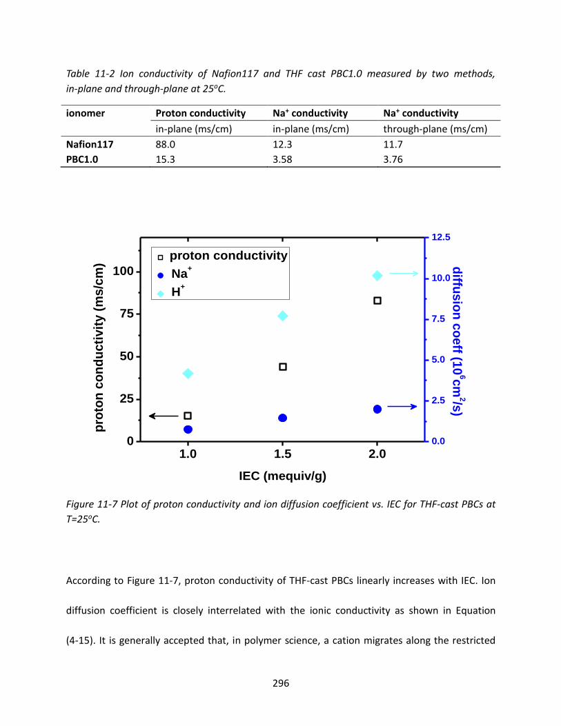
296

Table 11-2 Ion conductivity of Nafion117 and THF cast PBC1.0 measured by two methods,

in-plane and through-plane at 25oC.

ionomer Proton conductivity Na+ conductivity Na+ conductivity

in-plane (ms/cm) in-plane (ms/cm) through-plane (ms/cm)

Nafion117 88.0 12.3 11.7

PBC1.0 15.3 3.58 3.76

1.0 1.5 2.00

25

50

75

100

proton conductivity

Na+

H+

IEC (mequiv/g)

pro

ton

co

nd

ucti

vit

y (

ms/c

m)

0.0

2.5

5.0

7.5

10.0

12.5

diffu

sio

n c

oeff (1

06c

m2/s

)

Figure 11-7 Plot of proton conductivity and ion diffusion coefficient vs. IEC for THF-cast PBCs at

T=25oC.

According to Figure 11-7, proton conductivity of THF-cast PBCs linearly increases with IEC. Ion

diffusion coefficient is closely interrelated with the ionic conductivity as shown in Equation

(4-15). It is generally accepted that, in polymer science, a cation migrates along the restricted

297

path through channels of hydrophilic domains while in solution it moves with larger freedom

against the viscous force of the surrounding medium.[193] Therefore, high concentration of

sulfonic acid groups within ionomers greatly increases the ionic site density and widens the

hydrophilic domains such as PBC2.0, leading to the improvement of ion transport. The H+

diffusion coefficient increases from 4.18×10-6 to 10.2×10-6 cm2/s and the Na+ diffusion

coefficient from 0.75×10-6 to 1.99×10-6 cm2/s. Moreover, due to the smaller size and larger

mobility of H+, the diffusion coefficient of proton is about 4-6 times greater than that of sodium

ion.

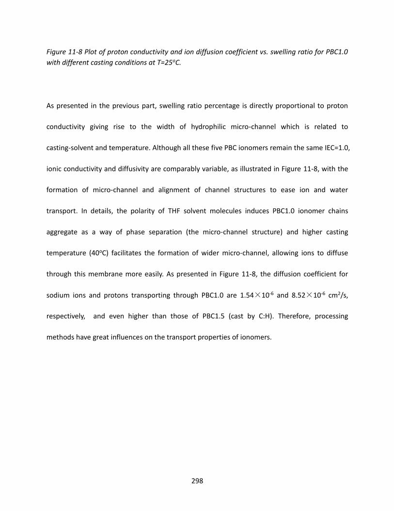
298

Figure 11-8 Plot of proton conductivity and ion diffusion coefficient vs. swelling ratio for PBC1.0

with different casting conditions at T=25oC.

As presented in the previous part, swelling ratio percentage is directly proportional to proton

conductivity giving rise to the width of hydrophilic micro-channel which is related to

casting-solvent and temperature. Although all these five PBC ionomers remain the same IEC=1.0,

ionic conductivity and diffusivity are comparably variable, as illustrated in Figure 11-8, with the

formation of micro-channel and alignment of channel structures to ease ion and water

transport. In details, the polarity of THF solvent molecules induces PBC1.0 ionomer chains

aggregate as a way of phase separation (the micro-channel structure) and higher casting

temperature (40oC) facilitates the formation of wider micro-channel, allowing ions to diffuse

through this membrane more easily. As presented in Figure 11-8, the diffusion coefficient for

sodium ions and protons transporting through PBC1.0 are 1.54×10-6 and 8.52×10-6 cm2/s,

respectively, and even higher than those of PBC1.5 (cast by C:H). Therefore, processing

methods have great influences on the transport properties of ionomers.

299

commercial THF cast 20oC THF cast 40

oC Nafion 117

0

25

50

75

100

125

proton conductivity

Na+

H+

ionomer

pro

ton

co

nd

ucti

vit

y (

ms/c

m)

0

5

10

15d

iffusio

n c

oeff (1

06c

m2/s

)

Figure 11-9 Plot of proton conductivity and ion diffusion coefficient for commercial, solution-cast

PBC1.0, and Nafion 117 at T=25oC.

To compare the ionic conductivity improvement by using different processing conditions,

transport properties of commercial, THF solution-cast PBC1.0, and Nafion 117 are listed and

compared in Figure 11-9. The proton and sodium ion conductivity of Nafion 117 are measured

as 88.0 and 12.3 ms/cm, respectively. According to Equation (4-15), the proton and Na+

diffusion coefficient can be calculated as 1.29×10-5 and 1.75×10-6 cm2/s. In order to confirm

the accuracy and feasibility of this testing and calculating method, several papers[194] are

provided to present the sodium ion conductivity of Nafion 117 (7-13 ms/cm at 5-25oC).

300

Furthermore, the optimal casting solvent enables the ionic diffusion coefficient increase 14

times, and then higher casting temperature will further improve it 2 times more (overall 28

times). Although optimal solvents and casting temperatures enhance the micro-ordered

morphology and transport properties, moderate mechanical properties are derived from

excessive large-scale phase separation which will be illustrated in Chapter 12.

11.3.3.2 Fructose and ethanol liquid molecule diffusion through PBCs

and Nafion 117

Different from other papers mentioned in the introduction part, the diffusions of ethanol and

fructose were investigate to further understand the influence of liquid molecular sizes and

chemical structures, instead of methanol and water which have numerous studies focused on.

According to Equation (4-10), the diffusion coefficient is directly proportional to the slope of the

plot concentration versus time. In the liquid molecule diffusion measurement, fructose

molecules transport through the Nafion 117 membrane, as presented in Figure 11-10

(concentration changing with time). And the slope of the linear part, as the first term of

Equation (4-10) right side, is obtained to calculate the fructose diffusion coefficient through

Nafion 117. And the second term of Equation (4-10) right side combines the volume of one

diffusion cell, the effective area of the membrane, and the concentration of the solution in the

301

upstream surfaces of the membrane which is assumed as a constant compared with the lower

concentration in the downstream surfaces of the membrane.

0 5 10 150.00

0.01

0.02

0.03

0.04

co

ncen

trati

on

(m

ol/

L)

time (min)

concentration

Figure 11-10 Concentration of fructose in the diffusion cell changing with time (Nafion 117 as

the testing membrane).

302

Figure 11-11 Proton conductivity and liquid molecule diffusivity coefficient of commercial,

solution-cast PBC1.0, and Nafion 117 at T=30oC.

As displayed in Figure 11-11, the wider microchannel of THF-cast PBC1.0 improves the diffusion

of protons, ethanol and fructose molecules, compared with commercial ones (the ethanol

diffusion coefficient increase 3.6 times, and 2.8 times for fructose). Fructose molecules diffuse

through PBC1.0 fast due to their similar chemical structure and solubility (fructose and PBC). On

the contrary, Nafion 117 with carbonfluoro-backbone presents a comparably low diffusion

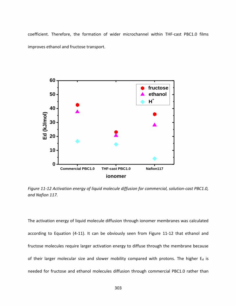
303

coefficient. Therefore, the formation of wider microchannel within THF-cast PBC1.0 films

improves ethanol and fructose transport.

Commercial PBC1.0 THF-cast PBC1.0 Nafion1170

10

20

30

40

50

60

fructose

ethanol

H+

Ed

(kJ/m

ol)

ionomer

Figure 11-12 Activation energy of liquid molecule diffusion for commercial, solution-cast PBC1.0,

and Nafion 117.

The activation energy of liquid molecule diffusion through ionomer membranes was calculated

according to Equation (4-11). It can be obviously seen from Figure 11-12 that ethanol and

fructose molecules require larger activation energy to diffuse through the membrane because

of their larger molecular size and slower mobility compared with protons. The higher Ed is

needed for fructose and ethanol molecules diffusion through commercial PBC1.0 rather than

304

Nafion 117. However, the wider microchannel of THF-cast PBC1.0 dramatically facilitates

ethanol and fructose transport and decreases the activation energy.

11.4 Conclusion

Several previous researchers have reported on the effect of processing conditions on modifying

morphology, mechanical, physical properties, transport properties, and thermal degradation of

ionomers. However, the importance of the casting method, solvents, and processing

methodology has not drawn much attention. Meanwhile, the comprehensive

membrane-casting operating system has not been set up to improve ionomer characteristics. In

our study, the relationship between casting processes and properties of ionomers, and the

network within micro and macro-scale properties are configured to investigate the wide-ranging

influence of the casting process. Results show that appropriate casting solvent (THF) and higher

casting temperature dramatically facilitate proton and other ions transport through Penta Block

Copolymer (PBC) at the same ion exchange capacity (IEC) level. It provides insight into stable

morphological microstructures of PBCs cast by solution evaporation method, even maintaining

under continuous electric field and at comparably high temperature. Moreover, our research

provides a framework for future studies to assess ionomer performance and to improve

chemical and physical properties by adjusting external factors. Subsequent chapters will focus

on the ionomer functional groups, mechanical properties, and thermal degradation of ionomers;

305

also, further work will highlight the interrelationship between casting methodology and

performances of industrially utilized ionomers.

306

Chapter 12 Mechanical, Transport Properties and Degradation

of Solution-cast Penta Block Copolymers

12.1 Introduction

One of the most advanced separation polymers, ionomers, has three striking features, ion

conductivity, hydrophilicity, and fixed carriers, due to electrically neutral repeating groups and

ionizable branched units.[5-6] It is generally known that ionomers have recently attracted

widespread interest in the fields of proton exchange membrane (PEM) fuel cells (FC)[2]. However,

these three remarkable characteristics of ionomers qualify ionomers for use in other processes

such as electrodialysis, electrolysis, diffusion dialysis, batteries, sensing materials, medical use,

and analytical chemistry[5], which have not been appreciably paid enough attention to. For more

than 60 years, researchers have been reporting the synthesis and characterization of different

kinds of ion-exchange membranes[109, 116]. Subsequently, more attempts have focused on

possible factors improving morphology, transport properties, mechanical properties, phase

behaviors and the degradation of ionomers. However, besides intrinsic properties, such as

polymer structure, chain end group, and molecular weight of the polymer, extrinsic casting

methods can also affect various characteristics of ionomers significantly. The casting

methodology includes types of solvents used[112], methods of sample preparation[109-110, 117], and

307

ionic neutralization[118]. Because the diffusion of different ion such as Na+, Li+, and Ca2+ and

liquid molecules through membranes is equally important as the proton transport in ionomers.

For ionomer glass transition properties, it was proposed by Tsagaropoulos and Eisenberg[127]

that, with the increase in ion content, the number of regions of restricted mobility grew and

started to overlap, which meant that at some specific ion content, the aggregates became large

enough to exhibit their own glass transition; above that point, they clustered to form a second

glass transition temperature peak. Shortly after that, Woo presented that, after heating-induced

interchange reactions (-OH and carbonate), randomly linked homopolymer chains might form in

a classical blend system of a poly(hydroxyl ether bisphenol-A) (phenoxy) with bisphenol-A

polycarbonate (PC) and might also be forced to relax in coordinated motion modes, thus

showing a single glass transition temperature.[128] Furthermore, Serrano demonstrated that two

phase polymer blends of poly(cyclohexylmethacrylate), PChMA, with poly(vinylacetate), PVAc,

(20/80 and 50/50) were prepared by casting tetrahydrofuran (THF) or chloroform (CHCl3)

solutions. And a growth in the intermolecular interactions of phase-separated polymers led to a

growth in the glass transition temperature of the rigid polymer (PChMA) in the presence of the

flexible one (PVAc).[129] Later on, Jara illustrated that different glass transition temperatures

were exhibited according to the degree of phase separation by using protein/polysaccharide

co-dried mixtures.[130] Although the concentration of polymer blends and ion contents of

ionomers were observed to have a great influence on glass transition properties, few

308

researchers have covered the interrelation between casting solvent and glass transition

temperature.

In 1999, Wilkie reviewed the investigations carried out by comparing the thermal stability of

polystyrene and cross-linked styrene and polybutadiene relative to the theory that a

cross-linked polymer was inherently more thermally stable than the corresponding

thermoplastic polymer.[131] Also, Jiang studied the thermal degradation of poly(vinyl sulfonic

acid) and its sodium salt, poly(4-styrene sulfonic acid) and its sodium salt, and

poly(vinylphosphonic acid) using TGA and Fourier Transform Infrared Spectroscopy (FTIR), and

proposed a mechanism in the process of identification of the volatile products which were

evolved, as well as analysis of the residues which were obtained during the degradation.[132]

However, no research focused on the effect of casting solvent and processing conditions on

polymer degradation.

In this study, we analyze the impact of casting methodology on distribution of functional groups,

mechanical properties, and degradation of ionomers. Other fundamental characteristics such as

morphology, proton transport properties, and ions and liquid molecule transport properties,

have been discussed in the previous chapter. Three series of PBCs with different IECs, ionic

groups and casting solvents were tested by FTIR, DMA, and TGA. We can observe that high

casting temperature and moisture increase the absorbance intensity of PBC ionomer functional

309

groups, despite the similar IECs of the ionomers; furthermore, the solvent-cast method and

ionic neutralization helps PBCs form larger micro-domains, increase crosslink density, and reveal

stable chemical properties.

12.2 Experimental

12.2.1 Material

Perfluorosulfonic acid (PFSA), (NF115&117, and NF212) comes from Ion Power, Inc.. The

poly[t-butyl styrene-b-hydrogenated isoprene-b-sulfonated styrene-b-hydrogenated

isoprene-b-t-butyl styrene) (tBS-HI-S-HI-tBS), Penta Block Copolymer (PBC) was provided by

Kraton Polymers LLC, Houston, TX[161]. The detailed information was shown in Chapter 8.




by solution casting in a Teflon dish.

310







The glass transition temperature of ionomer membranes was obtained using a Dynamic

Mechanical Analyzer Q800 (DMA, TA instruments). Membrane samples were analyzed in the

tensile mode at a frequency of 1 Hz and a heating rate of 5oC/min from -90oC to 200oC. The

tensile strain εt applied was 0.01%.


Thermal gravimetric analysis (TGA) was performed using a TGA Q500 (TA Instruments). Samples

were pretreated to remove residual water by vacuum pump overnight. Pretreated samples

were heated in an inert N2 atmosphere from 30oC to 700oC using a heating rate of 10oC/min.

311


12.3.1 Functional Groups of Ionomers

FTIR spectra were produced to identify and characterize the functional groups of PBCs. The

full-scale infrared spectrum of a THF-cast PBC1.0 film is shown in Figure 12-1, meanwhile the

absorbance of remarked functional groups of PBC is presented in the enlarged figure. All of

infrared spectra were normalized according to the obvious sharp peaks in the range of

1300-1600 cm-1 which present the vibrations of the phenyl group.[195] The vibrational bands

associating with –SO3H and –SO3- group mainly appear at wavenumber 1000-1200 cm-1, and

more in details, peaks at 1200 cm-1 is assigned as the S=O asymmetric stretching while the S=O

symmetric stretching bands are clearly visible at 1033 and 1005 cm-1, in agreement with the

reference[195-196]. The S-O vibration occurs at 1154 and 1125 nm-1. However, the 1100-1250 cm-1

broad band caused by weak vibration of aromatic ring (according to NICODOM IR Polymers All

Package of polystyrene and poly(t-butyl styrene) provided by NICODOM Ltd.) overlaps with

those of the S=O asymmetric stretching and the S-O vibration, as a result of poorer

distinguishability of –SO3- group compared with the sharp and clear S=O symmetric stretching

peaks. As mentioned earlier, various casting solvents significantly influence the formation of

ionomer microstructures rather than the macro-scale quantity and identification of functional

groups due to the identical fingerprints of FTIR, displayed in Figure 12-1.

312

1500 1400 1300 1200 1100 1000 900 800

0.0

0.4

0.8

1.2

1.6

2.0

4000 3500 3000 2500 2000 1500 1000 500

0.0

0.5

1.0

1.5

2.0

2.5

3.0

ab

so

rba

nce

wavenumber (cm-1)

THF dry

CHCl3 dry

C:H dry

Figure 12-1 FTIR spectra of PBC1.0 membranes cast with different solvent.

In order to test the effect of relative humidity (RH), two sharp and clear S=O symmetric

stretching peaks were used to present the functional –SO3- group, as detailed in Figure 12-2. As

the water content increases, S=O symmetric stretching peaks are shifted to higher wavenumber

from 1031 to 1035 cm-1. With the increase of relative humidity, more -SO3- groups are

hydrogen-bonded to hydronium. Since a stronger hydrogen bonding acceptor property leads to

stronger bridges[195], the stronger O-H bonds within H3O+ ions weaken SO3-H bond. Meanwhile,

more S=O bonds present in the –C6H4-SO3- conjugated system to minimize the overall Gibbs

313

free energy which is consistent with the increase of absorbance intensity in Figure 12-2 (a).

Hence, as the hydration process occurs, the number of -SO3- groups present increases and

consequently the -SO3- band is shifted to higher frequencies due to weak hydrogen bridges.

1040 1000 960

0.0

0.5

1.0 (b)

(a)

THF air

THF cast at 40o

C

THF Na+

form

ab

so

rban

ce

wavenumber (cm-1)

1040

1040 1000 960

0.0

0.5

1.0

THF dry

THF air

THF wet

ab

so

rban

ce

1031

1035

Figure 12-2 FTIR of THF cast PBC1.0 in various relative humidity (RH) (a) and in different

processing conditions and salt form (b).

Casting temperature has a great influence on the presence of functional groups rather than

casting solvent. Heat was added to the solution system to keep it at 40oC while membranes

314

were cast. Data in Figure 12-2 (b) suggests that the absorbance intensity of –SO3- groups

increases for higher temperature cast membrane under the same condition that all samples

were tested in the 20% relative humidity (RH) air. As casting temperature is increased, ionomer

chains will be more flexible, and the distance between them is wider, resulting in the weak

interaction between two –SO3- groups. Hence, like the mechanism of the water-sulfuric acid

group interaction discussed above, weak SO3-H bonds remarkably enhance S=O vibration. On

the other hand, the counter ions Na+ imposes a strong electrostatic field on the SO3- ion which

polarizes the S-O dipole and shifts the symmetric vibration to higher frequencies 1040 cm-1, as

shown in Figure 12-2 (b). In general, although the choice of casting solvents does not affect the

identification and characterization of ionomer from aspect of FTIR, the influence of testing RH,

processing temperatures, and counter ion neutralization is noticeable.

12.3.2 Mechanical Properties

PBCs are composed of four kinds of blocks, which are flexible hydrogenated isoprene, rigid

t-butyl styrene, polystyrene, and sulfonated polystyrene (glass transition temperatures listed in

Table 12-1).

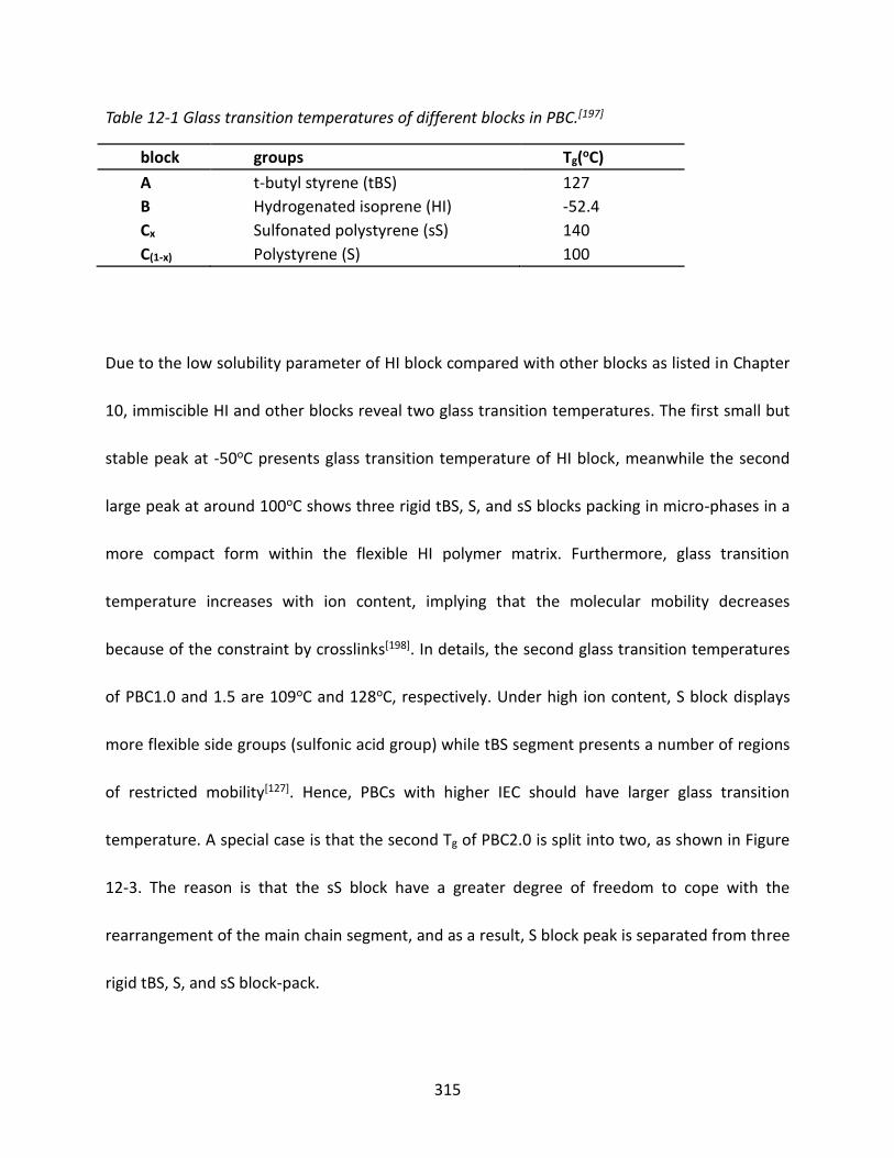
315

Table 12-1 Glass transition temperatures of different blocks in PBC.[197]

block groups Tg(oC)

A t-butyl styrene (tBS) 127

B Hydrogenated isoprene (HI) -52.4

Cx Sulfonated polystyrene (sS) 140

C(1-x) Polystyrene (S) 100

Due to the low solubility parameter of HI block compared with other blocks as listed in Chapter

10, immiscible HI and other blocks reveal two glass transition temperatures. The first small but

stable peak at -50oC presents glass transition temperature of HI block, meanwhile the second

large peak at around 100oC shows three rigid tBS, S, and sS blocks packing in micro-phases in a

more compact form within the flexible HI polymer matrix. Furthermore, glass transition

temperature increases with ion content, implying that the molecular mobility decreases

because of the constraint by crosslinks[198]. In details, the second glass transition temperatures

of PBC1.0 and 1.5 are 109oC and 128oC, respectively. Under high ion content, S block displays

more flexible side groups (sulfonic acid group) while tBS segment presents a number of regions

of restricted mobility[127]. Hence, PBCs with higher IEC should have larger glass transition

temperature. A special case is that the second Tg of PBC2.0 is split into two, as shown in Figure

12-3. The reason is that the sS block have a greater degree of freedom to cope with the

rearrangement of the main chain segment, and as a result, S block peak is separated from three

rigid tBS, S, and sS block-pack.

316

-100 0 100 2000.00

0.25

0.50

0.75

1.00

T

an

Delt

a

T (oC)

PBC1.0 THF

PBC1.5 THF

PBC2.0 THF

Figure 12-3 Plot of Tan Delta vs. temperature for THF-cast PBCs with different IEC.

317

-100 0 100 200

0.0

0.5

1.0

1.5

(a)

THF

CHCl3

THF

CHCl3

T (oC)

Ta

n D

elt

a

10

100

1000 Sto

rag

e M

od

ulu

s (M

Pa

)

-100 0 100 200

0.0

0.5

1.0

1.5

(b)

THF

CHCl3

THF

CHCl3

T (oC)

Ta

n D

elt

a

0

50

100

150

Lo

ss

Mo

du

lus

(MP

a)

Figure 12-4 Plot of Tan Delta and (a) storage modulus and (b) loss modulus vs. temperature for

PBC1.0 cast by THF and CHCl3.

318

At a specific IEC = 1.0, optimal casting solvent can be chosen to increase the crosslink density of

PBCs. As explained in the previous chapter, THF molecules help PBC to form micro-ordered

lamella morphology and to widen the microchannel structure, implying that more sulfuric acid

groups participate to crosslink within ionomer matrix. In the part of ionomer glass transition

(Figure 12-4), loss tangent peak of THF cast PBC1.0 shifts to higher temperature because

samples with higher crosslink densities have higher glass transition temperatures as illustrated

in the previous paragraph. And Table 12-2 displays the glass transition temperatures of PBCs

with respect to different IEC and casting solvent. Second, the value of Tan Delta for THF-cast

PBC1.0 is smaller than that of CHCl3-cast PBC1.0, resulting from higher cross-linked ionomer

having larger elastic moduli (storage modulus as shown red curves in Figure 12-4 (a)) relative to

their viscous moduli (loss modulus as shown green curves in Figure 12-4 (b)). Thirdly, the

broader loss tangent peak of THF-cast PBC1.0 is attributed to an increase in the distribution of

molecular weights between crosslinks or an increase in the heterogeneity of the network

structure.[199]

319

Table 12-2 Glass transition temperature of PBCs cast with different solvents obtained by Tan

Delta and (loss modulus).

IEC of PBC (mequiv/g) Tg (oC)

THF CHCl3 C/H

1.0 109, (82) 103, (78) /, (72)

1.5 128, (83) 108, (81) 94, (72)

2.0 100, 200e, (79) 111, (82) 102, (75)

e presents estimated value.

-100 0 100 2000.0

0.3

0.6

0.9

1.2

Tan

Delt

a

T (oC)

THF H+ form

CHCl3 H

+ form

THF Na+ form

CHCl3 Na

+ form

Figure 12-5 Plot of Tan Delta vs. temperature for acid form and salt form PBC1.0 cast by THF and

CHCl3.

The salt-form PBC1.0 still exhibits ionic aggregation, however, with larger characteristic

dimensions of the ionic domains compared with that of the acid-form PBC1.0. According to

320

Figure 12-5, DMA results indicate that there is nearly no shift of glass transition temperature for

ion neutralization at a specific IEC = 1.0. Moreover, data in Figure 12-6 suggest that the

difference between glass transition temperature of acid-form and salt-form PBC1.0 is less than

3oC though their swelling ratios are very different, caused by ionic interaction (data for H+ form

C:H cast PBC1.0 cannot be obtained due to HI block flowing above 92oC). However, the

magnitudes of Tan Delta of Na+ form PBC1.0 decreases dramatically caused by the increase of

crosslink density. Larger size of sodium ions provides a great opportunity for ionomer to form

more electrostatic crosslinks.

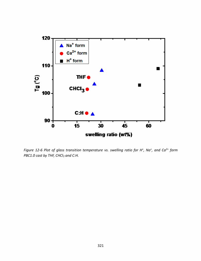
321

Figure 12-6 Plot of glass transition temperature vs. swelling ratio for H+, Na+, and Ca2+ form

PBC1.0 cast by THF, CHCl3 and C:H.

322

12.3.3 Thermal Degradation of Ionomers

0 100 200 300 400 500 600 7000

20

40

60

80

100

PBC1.0

PBC1.5

PBC2.0

T (oC)

weig

ht

fracti

on

(%

)

0.0

0.2

0.4

0.6

0.8

1.0

1.2

De

riv. W

eig

ht (%

/oC

)

Figure 12-7 Plot of weight fraction percentage and derivative weight versus temperature for

PBCs with different IEC.

The thermal stabilities of acid-form and salt-form PBCs were investigated by thermal gravimetric

analysis (TGA) under N2. The derivative thermogravimetry (DTG) curves were gotten from the

derivation of the TGA curves. All membranes were dried in the vacuum oven overnight to

remove water and solvent in the membranes before measuring. The TGA curves of PBCs with

IEC = 1.0, 1.5, and 2.0 are observed in Figure 12-7. All the PBC thin films exhibit a three-step

323

degradation pattern. The first weight loss step observed around 100oC is ascribed to the loss of

water molecules initially absorbed by highly hygroscopic -SO3- groups, especially obvious for

PBC2.0. The second step of thermal degradation was observed around 200-350oC due to the

decomposition of sulfonyl groups, leading to the expulsion of sulfur monoxide and sulfur

dioxide gases.[200] Furthermore, the percentage of weight loss in this step increases with IEC

corresponding to the elimination of -SO3- groups. The third step indicates the decomposition of

the polymer backbones. As an example, PBC2.0 with comparably higher concentration of the

aromatic ring promotes the increase of the degradation temperature.

0 200 400 6000

40

80

120

THF

CHCl3

THF

CHCl3

T (oC)

weig

ht

fracti

on

(%

)

0.0

0.5

1.0

1.5

Deriv

. We

igh

t (%/ oC

)

324

Figure 12-8 Plot of weight fraction percentage and derivative weight vs. temperature for PBC1.0

cast by THF and CHCl3.

THF-cast and CHCl3-cast PBC1.0 present similar onset degradation temperature, as indicated in

Figure 12-8, resulting from the same first degradation step of water loss and the identical

second step of decomposition of sulfonic acid groups, leading to expulsion of sulfur monoxide

and sulfur dioxide gases. However, the plot of derivative weight versus temperature reveals the

different peak temperatures for THF and CHCl3-cast PBC1.0 (408oC and 422oC). A kinetic model

of polymer degradation with volatile product evolution is presented, considering the effects of

diffusion and vaporization of fragments with temperature increasing.[201] The wider

microchannel structure of THF-cast PBC1.0 with better transport properties helps volatile

product diffuse out of the membrane, leading to a lower thermal degradation temperature

compared with that of CHCl3-cast PBC1.0 films.

325

0 100 200 300 400 500 600 7000

20

40

60

80

100

H+ form

Na+ form

Ca2+

form

T (oC)

weig

ht

fracti

on

(%

)

0.0

0.5

1.0

1.5

2.0

2.5D

eriv

. We

igh

t (%/ oC

)

Figure 12-9 Plot of weight fraction percentage and deriv. weight vs. temperature for H+ form,

Na+ form, and Ca2+ form PBC1.0.

As displayed in Figure 12-9, the acid-form PBC is less stable than the salt-form. The mass loss of

acid-form PBC1.0 is 19% at 350oC while the sodium and calcium salt-form PBC1.0s only have 5%

loss at 350oC. Moreover, Na+ and Ca2+ form PBC have higher degradation temperature Td =

423oC and 425oC, respectively, compared with 408oC for H+ form. The differences between the

degradation of the acid-form and salt-form PBC are the temperatures at which the various

gaseous products appear, the amount of non-volatile residue, and the volume expansion which

occurs upon heating.[132] The overall mechanism of the acid-form PBC degradation should be

326

virtually identical with that of the sodium salt-form except for the absence of sulfite ion. In the

second degradation step of the salt-form PBC, sodium or calcium sulfite as a non-volatile

residue arises. However, in the case of the acid-form, sulfurous acid is formed by hydrogen

abstraction from the polymer by the SO3H radical; this will directly generate SO2 and H2O at a

lower temperature. The interaction within Na+, Ca2+ and ionomers makes ionomer network

more stable.

12.4 Conclusion




method, solvents, and processing conditions has not drawn much attention and the

comprehensive membrane-casting operating system has not been found to improve




although the choice of casting solvents does not affect the identification and characterization of

ionomer from aspect of FTIR, the influence of testing RH, processing temperatures, and counter

ion neutralization is noticeable. Furthermore, from the aspect of glass transition properties, our

327

study provides insight into more cross-linked morphological microstructures of acid-form and

salt-form PBCs cast by THF solution evaporation method with respect to CHCl3 and C:H.

Furthermore, this research highlights the framework for future studies to assess and improve

performance and characteristics of different ionomers such as ion and liquid molecule transport

by adjusting external factors, whilst also giving reference for the manufacture of industrially

utilized ionomers.

328

Chapter 13 Performances of electrodialysis process in

desalination of sodium chloride solution with various ionomer

pairs

13.1 Introduction

According to the World Water Council, by 2020, the world will be about 17% short of the fresh

water needed to sustain the world population. Moreover, nowadays about three billion people

in the world have no access to clean drinking water, with about 1.76 billion people that live in

areas already facing a high degree of lacking water. Therefore, the need for fresh water is at the

top of the international agenda of critical problems, considered as important as climate change.

As a consequence of the growing scarcity of freshwater, the implementation of desalination

plants is increasing on a large scale.[202]

It is generally known that desalination processes can be categorized into two major types, one is

phase change based on thermal energy (multi-stage flash distillation (MSF)), and the other is

membrane process separation (reverse osmosis (RO), and electrodialysis (ED)). Compared with

RO and ED desalination processes, MSF require far more energy. The turning point of energy

consumption of RO and ED is at the total dissolved solid 3g/L sodium chloride solution. In other

words, electrodialysis only outperform other processes below total dissolved solid 3g/L

efficiently. Other obstacles include the limited choice and high cost of membranes, extremely

329

high equipment cost of electrodialyzer, and limited efficiency of electrodialysis process due to

the membrane-related problems, such as concentration polarization, water splitting, and scaling.

Therefore, much work is needed to reduce the cost of membranes and electrodes and enhance

cell configurations.

Fortunately, in some applications, eletrodialysis-based processes are preferable in spite of the

cost disadvantage because they can provide products of high quality or are more

environmentally friendly. The increase in environmental awareness and the raw material cost

has accelerated the application of ED-based integrations, especially in highly industrialized and

densely populated countries. In the long-term, ED-based integrations will replace single mass

separations or some other integrated separations. Accordingly, researchers should give

attention to interdisciplinary knowledge and solve some touchy problems, such as materials

design, apparatus design, process control, systematic integration, processes simulation, and

operation optimization in ED-based separation processes.

In this study, novel self-synthetic PPSU-TMPS 2.5, sPP 1.0 and THF solvent-cast PBC1.0 are

introduced in the electrodialysis process in order to compare the performance of commercial

polystyrene. More attention is paid on the materials design (novel self-synthetic ionomers),

process control (flow rate and solution concentration), processes simulation (based on the

Nernst-Planck Equation), and operation optimization in ED-based separation processes.

330

13.2 Experimental

13.2.1 Material

Polymer: Perfluorosulfonic acid (PFSA), (NF115&117, and NF212), sulfonated poly(phenylene)

(sPP), and PBC ionomers (poly[t-butyl styrene-b-hydrogenated isoprene-b-sulfonated styrene-b-

hydrogenated isoprene-b-t-butyl styrene] (tBS-HI-S-HI-tBS)) , sulfonated polystyrene, aminated

polystyrene, aminated PolyPhenylSulfone- TetraMethylPolySulfone (PPSU-TMPS).

13.2.2 Electrodialysis

AEM, anion exchange membrane, 5 pieces, PC-SA and CEM, cation exchange membrane, 4

pieces as PC-SK and 2 end pieces as PC-SC are provided by PCCellCorp..

Bench Electrodialysis Pump Unit PCCell BED 1-4 comes from PCCellCorp.. More details were

provided in Chapter 8.

331


13.3.1 Limiting Current Density

The limiting current density, i𝑙𝑖𝑚, of the electrodialyzer is generally determined by measuring

the current-voltage relation of the electrodialyzer.

Based on the current-voltage plot data, limiting current density, (LCD) (with the combination of

one anion exchange membrane and two cation exchange membranes) can be simulated by

Equation (13-1) with respect to flow rates and concentrations of dilute and concentrated

streams.

𝑖𝑙𝑖𝑚 = 𝑎 × 𝑢𝑏 × 𝐶𝑐 (13-1)

where constant a = 1.400, b = 0.5377, c = 0.1883, and the i𝑙𝑖𝑚 in mA/cm2, flow rate (u) in L/h

and concentration (C) in mol/L.

332

Figure 13-1 The interrelationship within limiting current density, concentration, and flow rate of

dilute and concentrated streams.

Based on the simulation Equation (13-1) of limiting current density, a three-dimensional plot

can be drawn corresponding to concentration and flow rate of dilute and concentrated streams,

as illustrated in Figure 13-1. With increasing concentration and flow rate, limiting current

density also shows an upward trend. Compared with low limiting current density 3.24 mA/cm2

at flow rate 15 L/h and concentration 0.038 mol/L, the data point shows comparably higher

value 7.50 mA/cm2 LCD at flow rate 40 L/h and concentration 0.198 mol/L. Therefore, based on

333

these simulation curves limiting current density can be determined as a reference of current

and voltage used in the electrodialysis process before ED experiments are carried out.

13.3.2 Ion Flux

The ion flux is closely related to the transport number and current efficiency which are very

important properties of ionomers in the electrodialysis process. There are two ways of

simulating the ion flux in the electrodialyzer cell, as mentioned in Chapter Seven. The first one is

calculated by the concentration changing with time as illustrated in Equation (13-2).

𝐽𝑖 =𝑉(𝑑𝐶𝑖/𝑑𝑡)

𝐴 (13-2)

where V is the overall processing volume of batch ED, A is the effective area of ionomers.

According to Nernst-Planck flux equation (Equation (13-3)), the second method is widely

applied to explain transport phenomena in ion-exchange membranes and solution systems.


𝑑𝑥+


𝑅𝑇

𝑑𝜓

𝑑𝑥+ 𝐶𝑖


𝑑𝑥) + 𝐶𝑖𝑣 (13-3)


convection, Di is the diffusion coefficient of i in the membrane, Ci is the concentration of i in

334

the membrane, v is the flow velocity of the solvent, γi is the activity coefficient of i in the

membrane, zi is the valence of ion i, dψ

dxis the gradient of the electric potential and R the gas

constant and T the absolute temperature.

0 50 100 150 2000.0000

0.0002

0.0004

0.0006

J (

mo

l/m

2/s

)

time (min)

commercial polystyrene method 1

commercial polystyrene method 2

THF-cast PBC1.0 method 1

THF-cast PBC1.0 method 2

Figure 13-2 The ion flux of commercial polystyrene and THF-cast PBC1.0 calculated by method

one and two versus time.

In order to explain the transport phenomenon of electrodialysis process, the ion fluxes through

commercial polystyrene and THF-cast PBC1.0 in the electrodialyzer based on these two

335

simulation methods mentioned above are reported as presented in Figure 13-2. In the first 40

min, ion flux through membranes slightly increases until reaches to the maximum value at

which the system also presents the highest transport number and current efficiency. After that,

ion flux decreases to a very low value due to the sodium and chloride ions lacking in dilute

stream. Although the mechanism of these two calculation methods are different, the data of ion

flux simulated by method one and two are in statistical agreement. Hence, each simulation

method can be used to calculate ion flux through membranes in the electrodialyzer.

0 20 40 60 800.0

1.0x10-4

2.0x10-4

3.0x10-4

4.0x10-4

5.0x10-4

Ion F

lux (

mol/m

2/s

)

time (min)

commercial polystyrene

PPSU-TMPS 2.5

THF-cast PBC1.0

NF117

sPP 1.0

Figure 13-3 The ion flux versus time simulated by method one based on commercial polystyrene,

PPSU-TMPS 2.5, THE-cast PBC1.0, NF117, and sPP 1.0.

336

The first simulation method was utilized to calculate the ion flux in the electrodialyzer based on

commercial polystyrene, PPSU-TMPS 2.5, THE-cast PBC1.0, NF117, and sPP1.0 as demonstrated

in Figure 13-3. It can clearly tell that PPSU-TMPS 2.5 (red), THF-cast PBC1.0 (green), and sPP 1.0

(cyan) present a comparably higher ion fluxes while the ion flux of NF117 (blue) is lower

compared with the industrial standard commercial polystyrene (black). Therefore, optimal

solvent-cast PBC1.0 shows satisfactory transport property in the electrodialysis process.

Furthermore, self-synthetic PPSU-TMPS 2.5 and sPP 1.0 also improve ion transport through the

membranes due to steric polymer backbones distribution and stable functional groups

compared with polystyrene.

13.3.3 Power Consumption and System Resistance

In the process of ED, commercial polystyrene, PPSU-TMPS 2.5, sPP 1.0, THF-cast PBC1.0, and

NF117 are used to compare experimental power consumption and system resistance results.

The basic properties of different ionomers, PPSU-TMPS 2.5, sPP 1.0, THF-cast PBC1.0, and

NF117 are illustrated in Table 13-1.

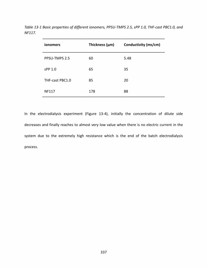
337

Table 13-1 Basic properties of different ionomers, PPSU-TMPS 2.5, sPP 1.0, THF-cast PBC1.0, and

NF117.

ionomers Thickness (μm) Conductivity (ms/cm)

PPSU-TMPS 2.5 60 5.48

sPP 1.0 65 35

THF-cast PBC1.0 85 20

NF117 178 88

In the electrodialysis experiment (Figure 13-4), initially the concentration of dilute side

decreases and finally reaches to almost very low value when there is no electric current in the

system due to the extremely high resistance which is the end of the batch electrodialysis

process.

338

0 50 100 150

0.000

0.005

0.010

0.015

0.020

commercial polystyrene D

PPSU-TMPS 2.5 D

THF-cast PBC1.0 D

NF117 D

sPP 1.0 D

time (min)

Co

nc

en

tra

tio

n (

mo

l/L

)

0

20

40

60

80

100

R (

oh

m)

Figure 13-4 The concentration of dilute stream ‘D’ and system resistance versus time of batch

electrodialysis experiment.

The power usage of the eletrodialyzer cell at a specific time point can be calculated according to

voltage applied on and direct electric current through the ED cell as shown in Figure 13-5. The

total power usage of batch electrodialysis process can be determined by the integral over

desalination time.

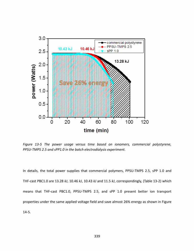
339

Figure 13-5 The power usage versus time based on ionomers, commercial polystyrene,

PPSU-TMPS 2.5 and sPP1.0 in the batch electrodialysis experiment.

In details, the total power supplies that commercial polymers, PPSU-TMPS 2.5, sPP 1.0 and

THF-cast PBC1.0 are 13.28 kJ, 10.46 kJ, 10.43 kJ and 11.5 kJ, correspondingly, (Table 13-2) which

means that THF-cast PBC1.0, PPSU-TMPS 2.5, and sPP 1.0 present better ion transport

properties under the same applied voltage field and save almost 26% energy as shown in Figure

14-5.

340

Overall, self-synthetic PPSU-TMPS 2.5, sPP 1.0, and THF solution-cast PBC1.0 increase the ion

flux and decrease the total power usage compared with commercial polystyrene and NF117.

Table 13-2 The power usage and desalination time of different ionomers, commercial

polystyrene, PPSU-TMPS 2.5, THF-cast PBC1.0, NF117, and sPP1.0.

ionomer Commercial polystyrene PPSU-TMPS 2.5 THF-cast PBC1.0 NF117 sPP 1.0

time(min) 101 76 84 145 79

Power(kJ) 13.28 10.43 11.5 17.15 10.46

13.3.4 Desalination Time

In the process of batch electrodialysis, THF-cast PBC1.0, and sPP1.0 only take around 80 min

while commercial polystyrene consumes 101 min to meet the requirement of 97% desalination

though they have the same ion exchange capacity, as illustrated in Figure 13-6.

The desalination time can be determined by the final concentration of dilute stream that people

need. For instance, if water without a salty taste is required, (the concentration of sodium

chloride is 0.0065 mol/L or 60% desalination percentage for initial concentration 0.016 mol/L),

THF-cast PBC1.0, PPSU-TMPS 2.5and sPP1.0 take 35 min while commercial polystyrene

consumes 40 min to meet the requirement of 60% desalination as demonstrated in Figure 14-6.

341

0 20 40 60 80 100 120 140

0

20

40

60

80

100

portable water

no salty taste

de

sa

linatio

n%

time (min)

commercial polystyrene

PPSU-TMPS 2.5

THF-cast PBC1.0

NF117

sPP 1.0

80 min

101 min 145 min

Figure 13-6 The desalination percentage versus time based on commercial polystyrene,

PPSU-TMPS 2.5, THE-cast PBC1.0, NF117, and sPP 1.0.

13.4 Conclusion

In conclusion, novel self-synthetic PPSU-TMPS 2.5, sPP 1.0 and THF solvent-cast PBC1.0 are

introduced in the electrodialysis process in order to compare the performance of commercial

polystyrene. Firstly, ion flux is simulated by two calculation methods based on the concentration

change with time and Nernst-Planck Flux Equation after limiting current density is determined.

342

Furthermore, electrodialysis performances of different ionomers are explored with respect to

power consumption, system resistance, desalination time, ion flux, and current efficiency.

Hence, novel self-synthetic PPSU-TMPS 2.5, sPP 1.0 and THF solvent-cast PBC1.0 present better

ion transport properties and improve the electrodialysis performance.

343

Chapter 14 Further Work: Synthesis and Characterization of

Aminated PolyPhenylSulfone-TetraMethylPolySulfone

(PPSU-TMPS) Block Copolymer

14.1 Introduction

Recently, anion exchange membranes have been applied in a various industrial fields including

the separation of environmental polluting metal ions from hard water[134], alkaline direct

methanol fuel cells[135], and also current and potential application as ion-exchanger[136],

biomaterials[137], and electrodialysis[138]. However, unlike cation exchange membranes which

have high chemical stability, such as DuPont’s Nafion and Asahi Glass’ Flemion, commercially

available anion exchange membranes are typically based on cross-linked polystyrene and are

not stable in alkaline and electrochemical environment. To overcome this limitation, they are

often blended with other inert polymers and fabric supports that limit ionic conductivity and

decrease the chemical stability of the membrane.[139]

A series of anion exchange membranes, (such as polybenzimidazole[140],

poly(2,6-dimethyl-1,4-phenylene oxide)[141], poly(ether ketone)[142], and poly(ethylene-co-

tetrafluoroethylene) (ETFE)[143], poly(tetrafluoroethylene-co-hexafluoropropylene) (FEP)[144], and

poly(vinylidene fluoride) (PVDF)[145] by radiation grafting of benzyl chloride onto partially or

344

completely fluorinated polymers), have been used to produce and perform for application in

alkaline fuel cell testing. Anion exchange membranes based on polysulfone were prepared by a

chloromethylation reaction on the parent polysulfone and the following conversion of the

chloromethyl groups into tetraalkylammonium cation exposing to trimethylammine.[146]

Synthesis of anion exchange membranes based on poly(vinyl alcohol)[147], poly(ether-imide)[148],

and imidazolium-type ionic liquid functionalized polymer[149] have also been reported.

Though polysulfone is most widely used in the manufacture of synthetic polymer membranes

due to its excellent mechanical, thermal and chemical stability, the chloromethylation reaction

for aminated polysulfone is sluggish, involves long reaction time,s imprecise control of reactant

amount and grafting location, and a large excess of toxic reagents. Moreover, the stability of the

fixed cationic site in alkaline conditions is a concern due to nucleophilic attack by anions.

To avoid these problems, a novel approach to the formation of halomethyl groups by preparing

polymers with benzylic methyl groups has been reported. Poly(2,6-dimethyl-1,4-phenylene

oxide) (PPO)[150] was treated with bromine to convert the methyl groups into bromomethyl

groups and then trimethylamine was used to convert bromomethyl groups in to quaternary

ammonia groups in the same manner as chloromethyl groups. The combination of high pH and

elevated temperature can lead to chemical attack on the quaternary ammonium groups, most

commonly by either an E2 Hofmann degradation mechanism or an SN2 substitution reaction.

345

The elimination reaction pathway can be avoided by using quaternary ammonium groups that

do not have beta hydrogens such as the benzyltrimethylammonium group.[151] If fluorenyl

groups are introduced into the polymer backbone, the anion exchange membrane may retain its

ionic conductivity and durability in alkaline fuel cell applications.[152]

14.2 Experimental

14.2.1 Material

4,4’-difluorophenyl sulfone, biphenol, potassium carbonate, N-bromosuccinimide (NBS),

benzoyl peroxide (BPO), trimethylamine, sodium hydroxide were purchased form Sigma-Aldrich.

Tetramethyl bisphenol A was from TCI America.

N,N-Dimethylacetamide (DMAc), N,N-Dimethylformamide (DMF), toluene, 1,1,2,2-

Tetrachloroethane (TCE), ethanol, methanol were purchased from Sigma-Aldrich.

14.2.2 Anion Exchange Membrane Synthesis

The parent polyphenyl sulfone, PPSU, is prepared by the condensation of 4,4’-difluorophenyl

sulfone with biphenol. The weight average molecular weight of PPSU with a polydispersity of 2

was different for a series of batches in this study.

346

The parent tetramethyl polysulfone, TMPS, is prepared by the condensation of

4,4’-difluorophenyl sulfone with tetramethyl bisphenol A, TMBPA. In order to drive the reaction

to high molecular weights, the product water was removed by azeotropic distillation with

toluene.

The benzylic methyl groups on TMPS could be brominated using N-bromosuccinimide (NBS) as a

source of bromine and benzoyl peroxide (BPO) as an initiator. The fraction of methyl groups

converted to bromomethyl groups was controlled by adjusting the amount of NBS used.

The quaternary ammonium groups could be produced using trimethylamine by mixing

PPSU-TMPS DMF solution.






347

14.2.4 Conductivity Measurement

The 2-probe method is restrictively applicable to the measurement of resistivity in materials

with high resistance (above 106 ohm). In this study, the ion conductivity of ionomer membranes

under fully hydrated conditions was evaluated in liquid DI water. The temperature was

controlled by isothermal water bath (Thermo Scientific Inc.). Samples with a width of 0.5 cm

were measured in the plane of the membrane within the proton conductivity cell (BekkTech.

LLC). The distance between two platinum electrodes was 0.5 cm. Swollen membrane thickness

was measured prior to impedance measurements. The Nyquist impedance plot was collected

from an Autolab impedance analyzer (Metrohm USA, Inc.) over the frequency range of 0.1 Hz to

1 MHz. The ohmic resistance of the membrane was obtained by simply interpolating the

high-frequency arc to the x-axis.


The glass transition temperature of ionomer membranes was obtained using a Dynamic

Mechanical Analyzer Q800 (DMA, TA instruments). Membrane samples were analyzed in the

tensile mode at a frequency of 1 Hz and a heating rate of 5oC/min from -90oC to 200oC. The

tensile strain εt applied was 0.01%.

348


Thermal gravimetric analysis (TGA) was performed using a TGA Q500 (TA Instruments). Samples

were heated in an inert N2 atmosphere from 30oC to 1000oC using a heating rate of 10oC/min.


14.3.1 Self-Synthetic Anion Exchange Membrane

Purification of Monomers and Other Reactants

4,4’-difluorophenyl sulfone, biphenol, and Tetramethyl bisphenol A were recrystallized using

toluene, ethanol, and water:methanol (45:55 volume%), respectively. Benzoyl peroxide (BPO)

was submerged in methanol, filtered and dried in the hood at 50oC. All other reagents were

obtained from commercial sources and used as received.

Synthesis of Parent Polymer PPSU-TMPS (targeting IEC=2.5)

For block PPSU, a flame-dried 250 ml three-necked flask equipped with an argon inlet and

overhead stirrer was charged with biphenol (0.0317 mol, 5.9006 g), 4,4’-difluorophenyl sulfone

(0.0275 mol, 6.9913 g), potassium carbonate (0.0475 mol. 6.5694 g), toluene (48.75 ml), and

DMAc (121.88 ml). The gas outlet was plugged into 1M calcium hydroxide solution to get rid of

hydrogen fluoride gas. The mixture was stirred and heated at reflux 137oC for 5h in order to

349

remove water. The solution was further heated to 157oC and kept for 16h. The PPSU polymer

solution was cooled to room temperature with inert gas protection and sealed with glass caps.

For block TMPS, a flame-dried 500 ml three-necked flask equipped with an argon inlet and

overhead stirrer was charged with tetramethyl bisphenol A (0.0125 mol, 3.5549 g),

4,4’-difluorophenyl sulfone (0.0175 mol, 4.4452 g), potassium carbonate (0.0188 mol. 2.5914 g),

toluene (59.3 ml), and DMAc (148.24 ml). The gas outlet was plugged into 1M calcium

hydroxide solution to get rid of hydrogen fluoride gas. The mixture was stirred and heated at

reflux 137oC for 5h in order to remove water. The solution was further heated to 157oC and kept

for 16h. The TMPS polymer solution was cooled to room temperature with inert gas protection

and sealed with glass caps.

PPSU solution was added into a 500 ml three-necked flask equipped with an argon inlet and

overhead stirrer was charged with TMPS solution. The solution was heated to 157oC and kept

for 16h. After cooling to room temperature with argon flow, the PPSU-TMPS solution was

centrifuged to get rid of potassium carbonate solid. After pouring the solution into stirred 700

ml methanol, the fiber-like or noodle-like precipitate (depending on molecular weight) was

filtered off and washed with methanol three times prior to being dried under vacuum 80oC. The

synthesis procedure is shown in Figure 14-1.

350

Figure 14-1 Synthesis procedure of parent polymer PolyPhenylSulfone-TetraMethylPolySulfone

(PPSU-TMPS) Block Copolymer

Bromination

20g PPSU-TMPS polymer was dissolved in 301.9 ml 1,1,2,2-Tetrachloroethane within

three-necked flask equipped with an argon inlet and an overhead stirrer. When the parent

polymer was well dissolved in TCE, N-bromosuccinimide (NBS) as a source of bromine and

benzoyl peroxide (BPO) as an initiator were added into the polymer solution. The mixture was

kept at room temperature for a few minutes for NBS and BPO well dispersing in the solution and

K2CO3 DMAc 157oC 16h

Toluene (Relux 137oC) 5h


Toluene (Relux 137oC)

5h


OHHO S

O

O

FF S

O

O

FFHO OH

S

O

O

FOOH

x

O O S

O

O

FH

y

O O S

O

O

FS

O

O

OOH

xy

n

351

then slowly heated to 80oC with the heating rate 20oC/h. The solution was kept at 80oC for 3h

before cooling to room temperature. Finally, the solution was dropped into 700 ml ethanol with

only a small amount of deionized water. The fiber-like precipitate was filtered off and washed

with ethanol three times prior to being dried under vacuum 50oC. The bromination procedure is

demonstrated in Figure 14-2.

Quaternization

There are two ways of introducing quaternary ammonium group onto the parent polymer

backbones.

Brominated PPSU-TMPS polymer was dissolved in N,N-Dimethylformamide (DMF) and cast

membranes. These membranes were submerged into trimethylamine ethanol solution at room

temperature for 48h.

Another way is using the solution reaction, in which trimethylamine THF solution was added

into brominated PPSU-TMPS DMF solution and stirred for 12h. The membranes were cast at

optimal temperature. This quaternization procedure is presented in Figure 14-2.

Ion Exchange

352

Quaternized PPSU-TMPS membranes were treated in 1M sodium hydroxide solution at 55oC for

12h and treated in deionized water at room temperature for 12h. The ion exchange procedure is

illustrated in Figure 14-2.

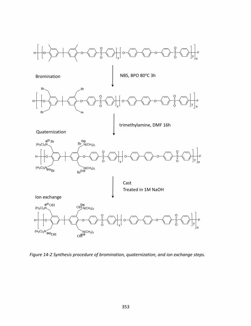
353

Figure 14-2 Synthesis procedure of bromination, quaternization, and ion exchange steps.

NBS, BPO 80oC 3h Bromination

Quaternization

trimethylamine, DMF 16h

Cast

Treated in 1M NaOH

Ion exchange

O O S

O

O

FS

O

O

OOH

xy

n

O O S

O

O

FS

O

O

OOH

xy

Br

Br

Br

Br

n

O O S

O

O

FS

O

O

OOH

xy

N(CH3)3

N(CH3)3

(H3C)3N

(H3C)3N

Br

Br

Br

Br

n

O O S

O

O

FS

O

O

OOH

xy

N(CH3)3

N(CH3)3

(H3C)3N

(H3C)3N

OH

OH

OH

OH

n

354

14.3.2 Functional Groups

FTIR spectra were produced to identify and characterize the functional groups of aminated

PPSU-TMPS polymer with different IECs. The infrared spectra were normalized according to the

obvious sharp peak at 1480 cm-1, which presents the vibrations of carbon-carbon bond within

phenyl group substitutions, as illustrated in Figure 14-3, meanwhile the relatively sharp peak at

1670 cm-1 presents quaternary ammonium group[203].

4000 3500 3000 2500 2000 1500 1000

0.0

0.2

0.4

0.6

0.8

1.0

1.2

2000 1800 1600 1400 1200

0.0

0.5

1.0

ab

sorb

an

ce

wavenumber (cm-1)

ab

so

rba

nce

wavenumber (cm-1)

IEC 3.5

1480cm-1

1670cm-1

Figure 14-3 The infrared spectra of aminated PPSU-TMPS polymer with IEC 3.5.

355

Comparing the selected infrared absorption bands of aminated PPSU-TMPS with IEC 0.0, 1.0,

and 3.5 (from 1400 cm-1 to 1800 cm-1) in Figure 14-4, the differences in band location

assignment appear at 1670 cm-1. In other words, the magnitude of infrared absorption peak at

1670 cm-1 changes with ion exchange capacity of aminated PPSU-TMPS. Therefore, quaternary

ammonium groups can be targeted according to identical fingerprints of FTIR.

1800 1700 1600 1500

0.0

0.2

0.4

0.6

0.8

1.0

1.2

ab

so

rba

nce

wavenumber (cm-1)

IEC 3.5

IEC1.0

IEC 0.0

normalization

-N(CH3)3

+

Figure 14-4 The selected infrared absorption bands of aminated PPSU-TMPS with IEC 0.0, 1.0,

and 3.5 (from 1400 cm-1 to 1800 cm-1).

356

14.3.3 Ion Conductivity

In this section, we evaluate the correlation between IEC, block length, ion conductivity and

swelling ratio of aminated PPSU-TMPS. With increasing ion exchange capacity, ion conductivity

and swelling ratio have an obvious increasing trend, as indicated in Figure 14-5.

Figure 14-5 Hydroxide conductivity and swelling ratio versus aminated PPSU-TMPS with

different IEC and segment block length.

357

Except that, the trend lines of ion conductivity and swelling ratio versus ion exchange capacity

are achieved by connecting (0,0) with data points. When block lengths of PPSU and TMBS are 3k

and 5.6k, respectively, the swelling ratio is relatively small, 9.6%, while the hydroxide

conductivity is comparably large, 5.06 ms/cm (Table 14-1), due to the difference of the

micro-structure of PPSU-TMPS with various block length segments. Therefore, at the same IEC

level, the shorter block length polymer presents, the smaller swelling ratio and higher ion

conductivity are. In other words, the well dispersed microchannel of aminated PPSU-TMPS

helps polymer aggregate as a way of micro-phase separation. The formation of continuous

micro-channel allows more hydroxide ions pass through the membranes. Although ion exchange

capacity can improve ion conductivity, the block length of polymer segments enhances

micro-phase separation which promotes hydroxide ions transport to a great extent.

Table 14-1 Specific data of IEC, block length, ion conductivity and swelling ratio of aminated

PPSU-TMPS.

IEC Block length Ion conductivity (OH-) ms/cm Swelling ratio %

1.0 6k-14k 1.85 4.7

2.5 3k-5.6k 5.06 9.6

3.5 10k-20k 5.48 38.7

358

14.3.4 Glass Transition Temperature

Animated PPSU-TMPS is composed of three different blocks: polyphenyl sulfone (PPSU),

tetramethyl polysulfone (TMPS), animated tetramethyl polysulfone (aminated TMPS). (glass

transition temperatures listed in Table 14-2).

Table 14-2 Glass transition temperature of different blocks of aminated PPSU-TMPS polymer.

block Glass transition temperature (oC)

PPSU 220[204]

TMPS 231[205]

Aminated TMPS 241-256[206]

Due to the similar solubility parameter of these three blocks, miscible PPSU, TMPS, and

aminated TMPS reveal only one glass transition temperature as presented in Figure 14-6. The

large peak at around 237oC shows three block microphase packing in a more compact form

within the polymer matrix. Furthermore, the glass transition temperature increases with TMPS

block length ratio rather than ion exchange capacity, implying that the block length ratio also

plays a more important role than IEC. In detail, the Tg of aminated PPSU-TMPS with block length

ratio PPSU-TMPS (0.22:0.78) is 231oC though IEC is the highest as illustrated in Table 14-3.

359

0 50 100 150 200 250

10

100

1000

10000

Storage Modulus (MPa)

Loss Modulus (MPa)

Tan Delta

Temperature (oC)

0

100

200

300

0.0

0.5

1.0

1.5

Figure 14-6 Storage modulus, loss modulus, and tan delta versus temperature of animated

PPSU-TMPS IEC2.5.

Table 14-3 Glass transition temperature of aminated PPSU-TMPS polymer with different IEC and

block length.

IEC Block length

(TMBS-PPSU)

Block length ratio

(TMBS:PPSU)

Predicated Tg (oC) Experimental Tg (oC)

1.0 16k-26.6k 0.38:0.62 234 241

2.5 3k-5.6k 0.35:0.65 233 239

3.0 6k-21k 0.22:0.78 228 231

360

14.3.5 Thermal Degradation

The thermal stabilities of aminated PPSU-TMPS were investigated by TGA under N2. The

derivative thermogravimetry (DTG) curves were determined from the derivation of the TGA

curves. The thermal degradation temperature of aminated PPSU-TMPS with IEC = 1.0, 2.5, and

3.0 are observed in Table 14-5.

Table 14-4 Thermal degradation temperature of different blocks and functional groups of

aminated PPSU-TMPS polymer.

block Thermal degradation temperature (oC)

PPSU 558[207]

TMPS 400[208]

Quaternary ammonium group 270-290[209]

All the composites exhibited distinct two-stage decomposition as presented in Table 14-4.

Aminated PPSU-TMPS with IEC 2.5, for instance, the first stage degradation occurred around

286oC, causing 7.5% weight loss profiles as shown in Figure 14-7. This was mainly due to the loss

of the quaternary ammonium groups and some low molecular weight components. These

361

materials degrade slowly with increase in temperature until it reached about 500oC, at which

point the PPSU-TMBS backbones start to decompose quickly as the second stage.

0 200 400 600 800 10000

20

40

60

80

100

weight percentage

Deriv. Weight

temperature (oC)

we

igh

t p

erc

en

tag

e (

%)

0.00

0.05

0.10

0.15

0.20

0.25

De

riv

. W

eig

ht

(%/°

C)

Figure 14-7 Weight percentage and derivative weight versus temperature of animated

PPSU-TMPS IEC2.5.

362

Table 14-5 Thermal degradation temperature of aminated PPSU-TMPS polymer with different

IEC and block length.

IEC Block length

(TMBS-PPSU)

Block length ratio

(TMBS:PPSU)

Td1 (oC) Td2 (oC) Predicated Td2 (oC)

1.0 16k-26.6k 0.38:0.62 287 522 498

2.5 3k-5.6k 0.35:0.65 286 501 503

3.0 6k-21k 0.22:0.78 276 551 523

The first thermal decomposition temperature is closed related to the ion exchange capacity

because the loss of the quaternary ammonium group occurs in the first degradation step. With

the increase of IEC, the Td1 decreases from 287oC to 276oC as presented in Table 14-5 while the

second degradation step is influenced by the PPSU and TMPS backbone ratio. Therefore, ion

exchange capacity and block length play an important role in the thermal degradation of

aminated PPSU-TMPS block copolymer.

14.4 Conclusion

In summary, an unconventional approach was used to prepare polyphenyl sulfone-tetramethyl

polysulfone block copolymer (PPSU-TMPS) containing quaternary ammonium groups based on a

novel monomer. Compared with the traditional approach, this new route avoided the use of

363

chloromethyl methyl ether, thus it was more environmentally friendly. The obtained quaternized

ionomers exhibited excellent solubility and formed flexible and tough membranes of varying

ionic content by casting from DMF solution. Through controlling ion exchange capacity and

block length of each segment, aminated PPSU-TMPS block copolymer with different hydroxide

conductivities, mechanical properties, and thermal degradation temperatures can be achieved.

These preliminary properties have demonstrated the potential availability as an anion exchange

membrane in the electrodialysis process. These results will aid in designing better membranes,

such as the block copolymers for improved membrane performance.

364

Chapter 15 Conclusion and Future Work

15.1 Wettability

For future work, more factors such as roughness[96], humidity, temperature, electrowetting[97],

the hysteresis phenomenon[98] and H-bond and acid-base parts of surface energy[99] need to be

taken into account.

15.2 Solubility and Swelling Phenomenon

More solution systems should be taken into account when testing the swelling and dissolving

properties of various kinds of ionomers. The relationships between different liquid molecules

(methanol, ethanol and ethylene glycol) interactions, ionomer chemical structures, physical

properties and morphology (hydrophobic and hydrophilic domains) need a better and deep

understanding. It is also important to explore the mechanism of molecules and ions

transporting phenomenon through different ion-form ionomers.

15.3 Ion Transport

Besides sodium and chloride ions, more kinds of positively charged and negatively charged ions

such as Ca2+, Ba2+, Mg2+ and SO32- should be introduced in the ion transport session. Molecular

interactions within ionomers and different ions will be investigated in the future study.

365

15.4 Mechanical Properties

In this study, storage modulus and loss modulus of ionomers have been reported based on

different temperature. More mechanical properties of ionomers like deformation properties

(stress versus strain) should be taken into consideration as well.

15.6 Electrodialysis Transport Phenomenon

Firstly, the mechanism of electrodialysis process (including concentration polarization) should

be investigated from a deeper level. Secondly, optimal operational condition of ED desalination

should be determined with respect to flow rate, solution concentration, direct electric current,

voltage applied on the system, and membrane properties. Finally, it is significant to find an

approach to establish an industrial-scaled electrodialysis system.

15.5 Anion Exchange Membrane

Although an obvious interrelationship within block length, ion exchange capacity, ion

conductivity, and swelling ratio is reported in this study, more data points are needed to prove

these trends convincingly.

366

Chapter 16 Reference

[1] M. Cheryan and N. Rajagopalan, Journal of Membrane Science 1998, 151, 13-28.

[2] K. D. Kreuer, J. Membr. Sci. 2001, 185, 29-39.

[3] W. J. Koros and G. K. Fleming, Journal of Membrane Science 1993, 83, 1-80.

[4] L. Y. Jiang, Y. Wang, T. S. Chung, X. Y. Qiao and J. Y. Lai, Progress in Polymer Science (Oxford)

2009, 34, 1135-1160.

[5] T. Sata, Ion Exchange Membrane, Preparation, characterization, Modification and

Application 2002, 1-307.

[6] a) A. Eisenberg and H. L. Yeager, Perfluorinated Ionomer Membranes 1982; b) A. Eisenberg

and J.-S. Kim, Introduction to Ionomers, New York: Wiley, 1998.

[7] H. S. Thompson, J. Roy. Agr. Soc. Engl. 1850, 11, 68-74.

[8] J. T. Way, J. Roy. Agr. Soc. Engl. 1850, 11, 313-379.

[9] L. Michaelis, Naturwissenschaften 1926, 14, 33-42.

[10] I. Abrams and K. Sollner, J. Gen. Physiol 1943, 26, 369-379.

[11] B. A. Adams and E. L. Holmes, J. Soc. Chem. Ind. 1935, 54, 1T-9T.

[12] G. F. D. Alelio, US Patent 1944, 2,366,007.

[13] J. R. Wyllie and H. W. Patnode, J. Phys.Chem. 1950, 54, 204.

[14] W. Juda and W. A. McRae, J. Am. Chem. Soc. 1950, 72, 1044.

367

[15] R. A. Rozendal, H. V. M. Hamelers, R. J. Molenkamp and C. J. N. Buisman, Water Research

2007, 41, 1984-1994.

[16] H. Li, Y. Gao, L. Pan, Y. Zhang, Y. Chen and Z. Sun, Water Research 2008, 42, 4923-4928.

[17] a) T. Sata, Journal of Physical Chemistry 1993, 97, 6920-6923; b) Y. Tanaka, Industrial and

Engineering Chemistry Research 2011, 50, 7494-7503.

[18] a) P. Millet, M. Pineri and R. Durand, Journal of Applied Electrochemistry 1989, 19, 162-166;

b) E. Rasten, G. Hagen and R. Tunold, Electrochimica Acta 2003, 48, 3945-3952.

[19] a) M. Igawa, K. Mikami and H. Okochi, Bulletin of the Chemical Society of Japan 2003, 76,

437-441; b) G. Wang, H. Tanabe and M. Igawa, Journal of Membrane Science 1995, 106,

207-211.

[20] a) M. Hichour, F. Persin, J. Molénat, J. Sandeaux and C. Gavach, Desalination 1999, 122,

53-62; b) A. L. Nolan, M. J. McLaughlin and S. D. Mason, Environmental Science and Technology

2003, 37, 90-98.

[21] a) E. Lachowicz, M. E. Páez-Hernández and M. Valiente, Analytica Chimica Acta 1996, 327,

175-181; b) M. Uto, H. Yoshida, M. Sugawara and Y. Umezawa, Analytical Chemistry 1986, 58,

1798-1803.

[22] a) B. Bolto, M. Hoang and T. Tran, Desalination 2010, 254, 1-5; b) K. Saito, S. Ishizuka, M.

Higa and A. Tanioka, Polymer 1996, 37, 2493-2498; c) R. Spohr, N. Reber, A. Wolf, G. M. Alder, V.

Ang, C. L. Bashford, C. A. Pasternak, O. Hideki and M. Yoshida, Journal of Controlled Release

1998, 50, 1-11.

368

[23] T. Fujinami, A. Tokimune, M. A. Mehta, D. F. Shriver and G. C. Rawsky, Chemistry of

Materials 1997, 9, 2236-2239.

[24] J. Ding, C. Chuy and S. Holdcroft, Chemistry of Materials 2001, 13, 2231-2233.

[25] a) M. Shahinpoor, Y. Bar-Cohen, J. O. Simpson and J. Smith, Smart Materials and Structures

1998, 7, R15-R30; b) E. Smela, Advanced Materials 2003, 15, 481-494.

[26] S. A. Schmidt, Thesis and Dissertation: mathematical models of ion transport through

nafion membranes in modified electrodes and fuel cells without electroneutrality 2010.

[27] T. Young, Philos. Trans. R. Soc. London 1805, 95, 65-87.

[28] Y. T. Cheng and D. E. Rodak, Appl. Phys. Lett. 2005, 86, 144101.

[29] R. G. Good and L. A. Girifalco, J. Phys. Chem. 1960, 64, 561-565.

[30] F. M. Fowkes, Ind. Eng. Chem. 1964, 56, 40-52.

[31] D. Y. Kwok and A. W. Neumann, Adv. Colloid Interface Sci. 1999, 81, 167-249.

[32] D. K. Owens and R. C. Wendt, J. Appl. Polym. Sci. 1969, 13, 1741-1747.

[33] S. Wu, J. Adhesion 1973, 5, 39-55.

[34] W. A. Zisman, Adv. Chem. 1964, 43, 1-51.

[35] D. H. Kaelble, Journal of Adhesion 1970, 2, 66-81.

[36] W. Rabel, Farbe und Lack 1971, 77, 997-1005.

[37] R. J. Good, J. Adhesion Sci. Technol. 1992, 6, 1269-1302.

[38] R. N. Wenzel, Ind. Eng. Chem. 1936, 28, 988-994.

369

[39] a) A. B. D. Cassie, Discussions of the Faraday Society 1948, 3, 11-16; b) A. B. D. Cassie and S.

Baxter, Transactions of the Faraday Society 1944, 40, 546-551.

[40] D. Y. Kwok and A. W. Neumann, J. Adhes. Sci. Technol. 2000, 14, 719-743.

[41] a) K. L. Johnson, K. Kendall and A. D. Roberts, Proc. R. Soc. London, Ser. A 1971, 324,

301-313; b) V. M. Muller, V. S. Yushchenko and B. V. Derjaguin, J. Colloid Interface Sci. 1983, 92,

92-101; c) R. M. Pashley, P. M. McGuiggan, B. W. Ninham and D. F. Evans, Science 1985, 229,

1088-1089.

[42] C. J. v. Oss, R. J. Good and M. K. Chaudhury, Adv. Colloid Interface Sci. 1987, 28, 35-64.

[43] a) H. W. Kilau and J. E. Pahlman, Colloids Surf. 1987, 26, 217-242; b) K. Grundke, T. Bogumil,

T. Gietzelt, H. J. Jacobasch, D. Y. Kwok and A. W. Neumann, Prog. Colloid Polym. Sci. 1996, 101,

58-68.

[44] a) E. I. Vargha-Butler, E. Moy and A. W. Neumann, Colloids Surf. 1987, 24, 315-324; b) Y. Zuo,

D. Li and A. W. Neumann, Applied Surface Thermodynamics 1996, 509-556.

[45] a) D. Li, Y. Zuo and A. W. Neumann, Applied Surface Thermodynamics 1996, 557-628; b) J.

Cissé and G. F. Bolling, J. Cryst. Growth 1971, 11, 25-28.

[46] D. W. Fuerstenau and M. C. Williams, Colloids Surf. 1987, 22, 87-91.

[47] E. Moy, R. David and A. W. Neumann, Applied Surface Thermodynamics 1996, 333-378.

[48] A. E. V. Giessen, D. J. Bukman and B. Widom, J. Colloid Interface Sci. 1997, 192, 257-265.

[49] D. V. Matyushov and R. Schmid, J. Chem. Phys. 1996, 104, 8627-8638.

[50] M. Stamm, Polymer Surfaces and Interfaces 2008.

370

[51] P. G. d. Gennes, Reviews of Modern Physics 1985, 57, 827-861.

[52] R. N. Shimizu and N. R. Demarquette, J. Appl. Polym. Sci. 2000, 76, 1831-1845.

[53] M. Geoghegana and G. Krausch, Prog. Polym. Sci. 2003, 25, 261-302.

[54] M. J. Fasolka and A. M. Mayes, Annu. Rev. Mater. Res. 2001, 31, 323-355.

[55] T. Darmanin, M. Nicolas and F. Guittard, Langmuir 2008, 24, 9739-9746.

[56] L. Andruzzi, E. Chiellini and G. Galli, J. Mater. Chem. 2002, 12, 1684-1692.

[57] J. Tsibouklis and T. G. Nevell, Adv. Mater. 2003, 15, 647-650.

[58] X. Wang, M. Ostblom, T. Johansson and O. Inganas, Thin Solid Films 2004, 449, 125-132.

[59] P. Kanakasabai, P. Vijay, A. P. Deshpande and S. Varughese, J. Power Sources 2011, 196,

946-955.

[60] W. Abdallah, J. S. Buckley, A. Carnegie, J. Edwards, B. Herold, E. Fordham, A. Graue, T.

Habashy, N. Seleznev, C. Signer, H. Hussain, B. Montaron and M. Ziauddin, Fundamentals of

Wettability. Oilfield Review 2007.

[61] F. W. J. Billmeyer, 1984.

[62] K. Ueberreiter, 1968, 219-257.

[63] D. J. F. T. Tanaka, J. Chem. Phys. 1979, 70, 1214.

[64] P. Izák, S. Hovorka, T. Bartovský, L. Bartovská and J. G. Crespo, J. Membr. Sci. 2007, 296,

131-138.

[65] a) J. H. Hildebrand and R. L. Scott, the Solubility of Non-Electrolytes, 3rd Ed., Dover, New

York, 1949; b) H.Burrell, 1975, IV-337-359.

371

[66] D. W. V. Krevelen and P. J. Hoftyzer, Properties of Polymers, Their Estimation and Correlation

with Chemical Structure 1976.

[67] C. M. Hansen, Ind. Eng. Chem. Prod. Res. Dev. 1969, 8, 2-11.

[68] C. O. zdemir and A. Guner, Eur. Polym. J. 2007, 43, 3086-3093.

[69] a) P. J. Flory, J. Chem. Phys. 1941, 9, 660-661; b) M. L. Huggins, J. Chem. Phys. 1941, 9, 440.

[70] a) P. J. Flory and J. Rehner, J. Chem. Phys. 1943, 11, 512-520; b) P. J. Flory and J. Rehner,

Statistical Mechanics of Cross-Linked Polymer Networks II. Swelling, AIP, 1943, p. 521-526.

[71] L. H. Sperling, Introduction to Physical Polymer Science (4th ed.). Bethlehem, PA: [3] John

Wiley & Sons. ISBN Alger, Mark (1997). Polymer Science Dictionary (2nd ed.). London: Chapman

& Hall. ISBN 0-412-60870-7. 2006.

[72] a) L. Brannon-Peppas and N. A. Peppas, Polym. Bull. 1988, 20, 285-289; b) L.

Brannon-Peppas and N. A. Peppas, J. Controlled Release 1991, 16, 319-329.

[73] S. C. George, M. Knorgen and S. Thomas, J. Membr. Sci. 1999, 163, 1-17.

[74] S. Ajithkumar, N. K. Patel and S. S. Kansara, Polym. Gels Networks 1998, 6, 137-147.

[75] J. Crank, The Mathematics of Diffusion; Chapter 11. 2nd ed. Clarendon Press. Oxford, 1975.

[76] J. Siepmann and N. A. Peppas, Advanced Drug Delivery Reviews 2001.

[77] T. Bartil, M. Bounekhel, C. Cedric and R. Jerome, Acta Pharm. 2007, 57, 301-314.

[78] A. R. Berens and H. B. Hopfenberg, Polymer 1978, 19, 489-496.

[79] L. A. Errede, Macromolecules 1986, 19, 1522-1525.

372

[80] a) K. W. Suh and D. H. Clarke, J. Polym. Sci. A 1967, 5, 1671-1681; b) C. Marco, A. Bello, J. G.

Fatou and J. Garza, Die Makromolekulare Chemie 1986, 187, 177-185.

[81] Z. Liron and S. Cohen, J. Pharm. Sci. 1983, 72, 499-504.

[82] a) G. DiPaola-Baranyi, Macromolecules 1982, 15, 622-624; b) A. J. Ashworth and G. J. Price,

Macromolecules 1986, 19, 362-363.

[83] M. A. LaPack, J. C. Tou, V. L. McGuffin and C. G. Enke, J. Membr. Sci. 1994, 86, 263-280.

[84] R. Ravindra, K. R. Krovvidi and A. A. Khan, Carbohydrate Polymers 1998, 36, 121-127.

[85] T. Lindvig, M. L. Michelsen and G. M. Kontogeorgis, Fluid Phase Equilibria 2002, 203,

247-260.

[86] J. A. Jung and B. K. Kim, Opt. Commun. 2005, 247, 125-132.

[87] R. Guan, H. Dai, C. Li, J. Liu and J. Xua, J. Membr. Sci. 2006, 277, 148-156.

[88] H. Lu, Y. Liu, J. Leng and S. Du, Smart Mater. Struct. 2009, 18, 1-5.

[89] a) M. A. C. Stuart, T. Cosgrove and B. Vincent, Adv. Coll. Int. Sci. 1986, 24, 143-239; b) S. T.

Milner, T. A. Witten and M. E. Cates, Macromolecules 1988, 21, 2610-2619; c) J. L. Barrat and J. F.

Joanny, Adv. Chem. Phys. 1996, 94, 1-66.

[90] a) R. Y. M. Huang, Pervaporation Membrane Separation Processes. Elsevier, Amsterdam

1990; b) J. G. Crespo and K. W. Boddeker, Membrane Processes in Separation and Purification.

Kluwer Academic Publisher, Dordrecht 1994.

[91] M. Kufner and S. Kufner, Micro-optics and lithography. Brussels: VUB Press; 1997.

373

[92] B. Narasimhan and S. K. Mallapragada, Recent Res. Develop. Macromol. Res. 1998, 3,

311-324.

[93] A. P.Srivastava and B. E. Nauman, Polym. Mater. Sci. Engng. Proc. 1993, 69, 307-308.

[94] N. A. Peppas and R. Langer, Science 1994, 263, 1715-1720.

[95] a) G. Gebel, Polymer 2000, 41, 5829-5838; b) M. Fujimura, T. Hashimoto and H. Kawai,

Macromolecules 1982, 15, 136.

[96] a) S. Wijnans, B.-J. d. Gans, F. Wiesbrock, R. Hoogenboom and U. S. Schubert, Macromol.

Rapid Commun. 2004, 25, 1958-1962; b) A. Lafuma and D. Quere, Nat. Mater. 2003, 2, 457-460.

[97] V. Peykov, A. Quinn and J. Ralston, Colloid Polym. Sci. 2000, 278, 789-793.

[98] E. Chibowski, Adv. Coll. Int. Sci. 2003, 103, 149-172.

[99] D. Janssen, R. D. Palma, S. Verlaak, P. Heremans and W. Dehaen, Thin Solid Films 2006, 515,

1433-1438.

[100] F. S. Bates and G. H. Fredrickson, Annu. Rev. Phys. Chem. 1990, 41, 525-557.

[101] M. W. Matsen and M. Schick, Physical Review Letters 1994, 72, 2660-2663.

[102] F. S. Bates and G. H. Fredrickson, Block Copolymers-Designer Soft Materials, AIP, 1999, p.

32-38.

[103] Y. Mizutani, Bull. Chem. Soc. Jpn. 1970, 43.

[104] Y. Hori, T. Nakatani and Y. Mizutani, J. Electron Microsc. 1986, 35, 220-226.

[105] T. D. Gierke, G. E. Munn and F. C. Wilson, Journal of Polymer Science: Polymer Physics

Edition 1981, 19, 1687-1704.

374

[106] C. Zhao, H. Lin, K. Shao, X. Li, H. Ni, Z. Wang and H. Na, J. Power Sources 2006, 162, 1003–

1009.

[107] H.-S. Lee, A. S. Badami, A. Roy and J. E. McGrath, J. Polym. Sci. A 2007, 45, 4879-4890.

[108] G. P. Robertson and S. D. Mikhailenko, J. Membr. Sci. 2003, 219, 113-121.

[109] R. F. Silva, M. D. Francesco and A. Pozio, Electrochim. Acta 2004, 49 3211–3219.

[110] a) P. Bebin and H. Galiano, Adv. Polym. Sci. 2006, 25, 121-126; b) P. Bebin and H. Galiano,

Adv. Polym. Sci. 2006, 25, 127-133.

[111] X. Lu, W. P. Steckle and R. A. Weiss, Macromolecules 1993, 26, 6525-6530.

[112] M. Lee, R. B. Moore and J. E. McGrath, Polymer 2009, 50, 6129-6138.

[113] Y. Fan, M. Zhang, R. B. Moore, H.-S. Lee, J. E. McGrath and C. J. Cornelius, Polymer 2011,

52, 3963-3969.

[114] a) A. Fick, Ann. der. Physik (in German) 1855, 94, 59; b) A. Fick, Phil. Mag. (in English) 1855,

10, 30.

[115] P. Choi, N. H. Jalani and R. Datta, Journal of The Electrochemical Society 2005, 152, 84-89.

[116] D. Nguyen, C. E. Williams and A. Eisenberg, Macromolecules 1994, 27, 5090-5093.

[117] E. B. Gutoff and E. D. Cohen, Coating and drying defects- troubleshooting operating

problems. John Wiley & Sons, Inc., New York 1995.

[118] M. Hara, P. Jar and J. A. Sauer, Macromolecules 1990, 23, 4465-4469.

375

[119] a) S. Kutsumizu, M. Goto, S. Yano and S. Schlick, Macromolecules 2002, 35, 6298-6305; b) I.

Capek, Adv. Coll. Int. Sci. 2004, 112, 1-29; c) I. Capek, Adv. Coll. Int. Sci. 2005, 118, 73-112; d) X.

Zhu, Y. Song and Q. Zheng, J. Appl. Polym. Sci. 2012, 126, 980-986.

[120] N. M. Benetatos and K. I. Winey, Macromolecules 2007, 40, 3223-3228.

[121] C. A. Koval, T. Spontarelli, P. Thoen and R. D. Noble, Ind. Eng. Chem. 1992, 31, 1116-1122.

[122] P. Dimitrova, K. A. Friedrich, B. Vogt and U. Stimming, J. Electroanal. Chem. 2002, 532,

75-83.

[123] Y. A. Elabd, E. Napadensky, J. M. Sloan, D. M. Crawford and C. W. Walker, J. Membr. Sci.

2003, 217, 227-242.

[124] M. Saito, N. Arimura, K. Hayamizu and T. Okada, J. Phys. Chem. B 2004, 108, 16064-16070.

[125] M. Saito, S. Tsuzuki, K. Hayamizu and T. Okada, J. Phys. Chem. B 2006, 110, 24410-24417.

[126] D. W. v. Krevelen and P. J. Hoftyzer, Properties of polymers, their estimation and correlation

with chemical structure, Elsevier Scientific Pub. Co., Amsterdam ; New York, 1976, p. xxxiii, 620

p.

[127] G. Tsagaropoulos and A. Eisenberg, Macromolecules 1996, 28, 396-398.

[128] E. M. Woo and S. N. Yau, J. Polym. Sci. A 1997, 35, 97-103.

[129] B. Serranoa, I. F. Pierola, J. Bravo and J. Baselga, J. Mater. Proc. Tech. 2003, 141, 123-126.

[130] F. L. Jara and A. M. R. Pilosof, Thermochim. Acta 2009, 487, 65-73.

[131] C. A. Wilkie, Polym. Degrad. Stabil. 1999, 66, 301-306.

376

[132] D. D. Jiang, Q. Yao, M. A. McKinney and C. A. Wilkie, Polym. Degrad. Stabil. 1999, 63,

423-434.

[133] Y. Wang, W. Shi, Y. Yu and X. Chen, Bioinformatics and Biomedical Engineering , 2009.

ICBBE 2009. 3rd International Conference 2009, E-ISBN : 978-1-4244-2902-8, 1-4.

[134] P. Ray, Journal of Applied Polymer Science 2009, 113, 1155-1164.

[135] G. Merle, M. Wessling and K. Nijmeijer, Journal of Membrane Science 2011, 377, 1-35.

[136] E. S. Dragan, E. Avram, D. Axente and C. Marcu, Journal of Polymer Science Part A: Polymer

Chemistry 2004, 42, 2451-2461.

[137] A. K. Salem, F. R. A. J. Rose, R. O. C. Oreffo, X. Yang, M. C. Davies, J. R. Mitchell, C. J.

Roberts, S. Stolnik-Trenkic, S. J. B. Tendler, P. M. Williams and K. M. Shakesheff, Advanced

Materials 2003, 15, 210-213.

[138] a) A. R. Roudman and R. P. Kusy, Polymer 1998, 39, 3641-3649; b) R. C. T. Slade and J. R.

Varcoe, Solid State Ionics 2005, 176, 585-597; c) T. Xu, Z. Liu and W. Yang, Journal of Membrane

Science 2005, 249, 183-191.

[139] K. Kneifel and K. Hattenbach, Desalination 1980, 34, 77-95.

[140] H. Hou, G. Sun, R. He, Z. Wu and B. Sun, Journal of Power Sources 2008, 182, 95-99.

[141] T. Xu, Journal of Membrane Science 2005, 263, 1-29.

[142] J. Fang and P. K. Shen, Journal of Membrane Science 2006, 285, 317-322.

377

[143] a) J. R. Varcoe, Physical Chemistry Chemical Physics 2007, 9, 1479-1486; b) J. R. Varcoe, R.

C. T. Slade, E. Lam How Yee, S. D. Poynton, D. J. Driscoll and D. C. Apperley, Chemistry of

Materials 2007, 19, 2686-2693.

[144] H. Herman, R. C. T. Slade and J. R. Varcoe, Journal of Membrane Science 2003, 218,

147-163.

[145] T. N. Danks, R. C. T. Slade and J. R. Varcoe, journal of materials Chemistry 2003, 13,

712-721.

[146] a) P. Zschocke and D. Quellmalz, Journal of Membrane Science 1985, 22, 325-332; b) B.

Bauer, H. Strathmann and F. Effenberger, Desalination 1990, 79, 125-144; c) T. Sata, M.

Tsujimoto, T. Yamaguchi and K. Matsusaki, Journal of Membrane Science 1996, 112, 161-170; d)

G.-J. Hwang and H. Ohya, Journal of Membrane Science 1998, 140, 195-203; e) G.-J. Hwang and

H. Ohya, Journal of Membrane Science 1998, 149, 163-169; f) J. H. Hao, C. Chen, L. Li, L. Yu and

W. Jiang, Desalination 2000, 129, 15-22; g) E. N. Komkova, D. F. Stamatialis, H. Strathmann and

M. Wessling, Journal of Membrane Science 2004, 244, 25-34; h) L. Li and Y. Wang, Journal of

Membrane Science 2005, 262, 1-4; i) M. R. Hibbs, M. A. Hickner, T. M. Alam, S. K. McIntyre, C. H.

Fujimoto and C. J. Cornelius, Chemistry of Materials 2008, 20, 2566-2573.

[147] Y. Xiong, J. Fang, Q. H. Zeng and Q. L. Liu, Journal of Membrane Science 2008, 311,

319-325.

[148] G. Wang, Y. Weng, D. Chu, D. Xie and R. Chen, Journal of Membrane Science 2009, 326,

4-8.

378

[149] B. Qiu, B. Lin, L. Qiu and F. Yan, journal of materials Chemistry 2012, 22, 1040-1045.

[150] a) X. Tongwen and Y. Weihua, Journal of Membrane Science 2001, 190, 159-166; b) X.

Tongwen and F. F. Zha, Journal of Membrane Science 2002, 199, 203-210.

[151] M. R. Hibbs, C. H. Fujimoto and C. J. Cornelius, Macromolecules 2009, 42, 8316-8321.

[152] D. S. Kim, Y. S. Kim, M. D. Guiver, J. Ding and B. S. Pivovar, Journal of Power Sources 2008,

182, 100-105.

[153] S. Mafé and P. Ramfaz, Acta Polymerica 1997, 48, 234-250.

[154] D. Schweich and M. Sardin, Journal of Hydrology 1981, 50, 1-33.

[155] V. Shkolnikov, S. S. Bahga and J. G. Santiago, Phys. Chem. Chem. Phys 2012, 14,

11534-11545.

[156] A. I. Kendall and e. Gebauer-Fuelnegg, J. Chem. Ed, 1931, 8, 1634.

[157] A.G. Winger, G.W. Bodamer and R. Kunin, J. Electrochem. Soc. 1953, 100, 178.

[158] a) H. Strathmann, 1986; b) T. A. Davis, 1990.

[159] B. Kirby, Micro- and Nanoscale Fluid Mechanics: Transport in Microfluidic Devices: Chapter

11: Species and Charge Transport 2010.

[160] C. H. Fujimoto, M. A. Hickner, C. J. Cornelius and D. A. Loy, Macromolecules 2005, 38,

5010-5016.

[161] a) C. L. Willis in sulfonated block copolymers, method for making same,and various uses

for such block copolymers, Vol. (Ed. USA), Kraton Polymers Y U.S. L.L.C. Houston, TX, USA, 2007;

b) J.-H. Choi, A. Kota and K. I. Winey, Ind. Eng. Chem. Res. 2010, 49, 12093-12097.

379

[162] D. E. Curtin, R. D. Lousenberg and T. J. Henry, J. Power Sources 2004, 131, 41-48.

[163] J. Restolho, J. L. Mata and B. Saramago, J. Colloid Interface Sci. 2009, 340, 82-86.

[164] B. Fultz and J. Howe, Springer 2007.

[165] P. E. Champness, Garland Science 2001.

[166] A. Hubbard, CRC Press 1995.

[167] J. M. Cowley, Elsevier Science B. V. 1995.

[168] W. L. Bragg and W. H. Bragg, 1913.

[169] O. Glatter and O. Kratky, Academic Press 1982.

[170] B. Chu and B. S. Hsiao, Chem. Rev. 2001, 101, 1727-1761.

[171] J. D. Ferry, 1980.

[172] J. D. Ferry, Macromolecules 1991, 24, 5237-5245.

[173] M. A. Meyers and C. K.K., 1999.

[174] R. J. Young and P. A. Lovell, Taylor & Francis 1991.

[175] K. P. Menard, CRC Press 2008.

[176] A. W. Coats and J. P. Redfern, Analyst 1963, 88, 906-924.

[177] D. H. Kaelble and E. H. Cirlin, J. Polym. Sci. A 1971, 9, 363-368.

[178] C. Ishino and K. Okumura, The European Physical Journal E 2008, 25, 415-424.

[179] D. Janssen, R. De Palma, S. Verlaak, P. Heremans and W. Dehaen, Thin Solid Films 2006,

515, 1433-1438.

380

[180] C.-H. Ma, T. L. Yu, H.-L. Lin, Y.-T. Huang, Y.-L. Chen, U. S. Jeng, Y.-H. Lai and Y.-S. Sun,

Polymer 2009, 50, 1764-1777.

[181] M. Okabe, R. Wada, M. Tazaki and T. Homma, Polymer Journal 2003, 35, 798-803.

[182] L. Jia and B. Shi, J. Macromol. Sci., Phys. 2011, 50, 1042-1046.

[183] a) R. F. Silva, S. Passerini and A. Pozio, Electrochim. Acta 2005, 50, 2639-2645; b) R. Jiang,

H. R. Kunz and J. M. Fenton, J. Membr. Sci. 2006, 272, 116-124.

[184] L. M. Robeson, Polymer blend: a comprehensive review. Hanser Gardner Publications, Inc.

2007.

[185] X. Lu and R. A. Weiss, Macromolecules 1996, 29, 1216-1221.

[186] M. J. Forrest, Rubber Analysis: Polymers, Compounds and Products. iSmithers Rapra

Publishing 2001.

[187] J. R. Darby, N. W. Rouchette and K. Sears, Polym. Eng. Sci. 1967, 7, 295-309.

[188] A. V. Dobrynina and M. Rubinstein, Prog. Polym. Sci. 2005, 30, 1049-1118.

[189] C. Heitner-Wirguin, J. Membr. Sci. 1996, 120 1-33.

[190] M. Cappadonia, J. W. Erning, S. M. S. Niaki and U. Stimming, Solid State Ionics 1995, 77,

65-69.

[191] a) T. Thampan, S. Malhotra, H. Tang and R. Datta, J. Electrochem. Soc. 2000, 147,

3242-3250; b) S. J. Paddison and R. Paul, Phys. Chem. Chem. Phys. 2002, 4, 1158-1163.

[192] M. Saito, K. Hayamizu and T. Okada, J. Phys. Chem. B 2005, 109, 3112-3119.

381

[193] T. Okada, G. Xie, O. Gorseth, S. Kjelstrup, N. Nakamura and T. Arimura, Electrochim. Acta

1998, 43, 3741-3747.

[194] a) A. Lehmani, P. Turq and M. Perie, J. Electroanal. Chem. 1997, 428, 81-89; b) G. Pourcelly,

P. Sistat, A. Chapotot, C. Gavach and V. Nikonenko, J. Membr. Sci. 1996, 110, 69-78; c) I.

A.Stenina, P. Sistat, A. I. Rebrov, G. Pourcelly and A. B. Yaroslavtsev, Desalination 2004, 170,

49-57; d) T. K. a. I. Shigemoto, 14th International Conference on the Properties of Water and

Steam in Kyoto 2004.

[195] M. R. Pereira and J. Yarwood, J. Chem. Soc., Faraday Trans. 1996, 92, 2731-2735.

[196] M. Ludvigsson, J. Lindgren and J. Tegenfeldt, Electrochim. Acta 2000, 45, 2267-2271.

[197] a) R. Hagen, L. Salmen and B. Stenberg, J. Polym. Sci. B 1996, 34, 1997-2006; b) C. R.

Martins, G. Ruggeri and M.-A. D. Paoli, J. Braz. Chem. Soc. 2003, 14, 797-802; c) S. Aldrich,

Thermal Transitions of Homopolymers: Glass Transition & Melting Point.

[198] T. Sasaki, T. Uchida and K. Sakurai, J. Polym. Sci. B 2006, 44, 1958-1966.

[199] B.-S. Chiou and P. E. Schoen, J. Appl. Polym. Sci. 2002, 83, 212-223.

[200] W. Jang, C. Lee, S. Sundar, Y. G. Shul and H. Han, Polym. Degrad. Stabil. 2005, 90, 430-440.

[201] H. W. Moeller, Progress in Polymer Degradation and Stability Research. NOVA Publishers

2008.

[202] C. Charcosset, Desalination 2009, 245, 214-231.

[203] W. Yawei, S. Wenjian, Y. Yun and C. Xiaoyun, Bioinformatics and Biomedical Engineering ,

2009. ICBBE 2009. 3rd International Conference on 2009, pp. 1-4.

382

[204] S. Misra, Thermally conductive interface layers, Patent 2000.

[205] K. J. Lee, J. Y. Jho, Y. S. Kang, J. Won, Y. Dai, G. P. Robertson and M. D. Guiver, Journal of

Membrane Science 2003, 223, 1-10.

[206] A. Paul, Dissertation of Doctor of Philosophy July, 2012.

[207] Radel A Polyether sulfone and Radel R Polyphenylsulfone Design Guide, Solvay Advanced

Polymers.

[208] B. X. Zhou, Y. J. Huang, X. H. Zhang, Z. S. Fu and G. R. Qi, Polymer Engineering & Science

2009, 49, 1525-1532.

[209] H.-Q. Xie, Y. Gao, X.-G. Zhan and D. Xie, Journal of Applied Polymer Science 2004, 91,

2914-2922.

383

Table of Figures

Figure 1-1 Some commercial products for ionomers. ......................................................................... 15

Figure 1-2 Some commercial applications for ionomers. ................................................................... 18

Figure 2-1 (a) The change in Gibbs free energy of system, (b) the work of adhesion and

Interactions between liquid and solid surface. ....................................................................................... 25

Figure 2-2 Determination of the dispersion component of surface energy according to the

first step of Fowkes’ method. ......................................................................................................................... 33

Figure 2-3 Determination of the polar surface energy according to the second step of

Fowkes’ method. ................................................................................................................................................. 35

Figure 2-4 Determination of the dispersion and the polar fractions of the surface tension of

a solid according to Rabel’s calculation. .................................................................................................... 39

Figure 2-5 The combination of three different methods with Young’s Equation used in this

study in order to investigate surface energy of solid. .......................................................................... 43

Figure 2-6 Schematic of two methods capturing advancing and receding contact angles. ... 44

Figure 2-7 Two models of surface’s roughness used in this work (a) Wenzel’s model (b)

Cassie-Baxter model. .......................................................................................................................................... 45

Figure 2-8 Two states during the wetting transition from the Cassie state to Wenzel state (a)

mushroom state, (b) penetration front spreads beyond drop. ......................................................... 47

Figure 2-9 Schematic picture of the composition of the surface layer. ......................................... 53

384

Figure 3-1 Cross-section illustration of (a) an integrally skinned asymmetric membrane, (b)

SEM cross sections of dense-skinned polyacrylonitrile and (c) polysulfone membranes

manufactured by GE-Osmonics Inc. ............................................................................................................ 80

Figure 3-2 Ideal cylindrical pores and random network of unevenly shaped structures. ..... 82

Figure 3-3 Highly ordered crystalline structure of ice and amorphous glass and water. ...... 84

Figure 3-4 Two kinds of micro-structures in the area of polymer morphology, (a) crystalline

structure, (b) amorphous structure. ........................................................................................................... 85

Figure 3-5 Semi-crystalline micro-structures in the area of polymer morphology. ................. 86

Figure 3-6 Phase diagram for linear AB diblock copolymers, comparing theory and

experiment............................................................................................................................................................ 91

Figure 3-7 Morphologies for linear ABC triblock copolymers. ......................................................... 92

Figure 3-8 Transmission electron micrograph and scanning electron micrograph of

NEOSEPTA CL-25L. (a) TEM of the cross-section of cation exchange membrane prepared

from styrene and divinylbenzene in the presence of poly(vinyl chloride), (b) SEM of the

porous membrane (Fe3+ from) treated with H2O2, and the ferric ion form membrane was

immersed in aqueous 3% H2O2 solution at room temperature for 1h. ......................................... 94

Figure 3-9 Scanning transmission electron micrograph of an anion exchange membrane

(cross-link: 20%): a mixture of chloromethylstyrene and divinylbenzene was

copolymerized in the presence of acrylonitrile-butadiene rubber (inert polymer); ratio of

divinylbenzene to total vinyl monomers: 20%. ...................................................................................... 96

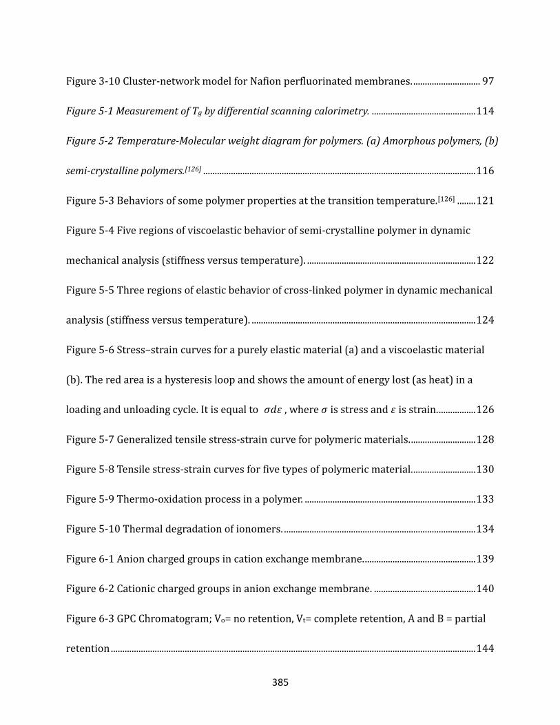
385

Figure 3-10 Cluster-network model for Nafion perfluorinated membranes. ............................. 97

Figure 5-1 Measurement of Tg by differential scanning calorimetry. ............................................. 114

Figure 5-2 Temperature-Molecular weight diagram for polymers. (a) Amorphous polymers, (b)

semi-crystalline polymers.[126] ...................................................................................................................... 116

Figure 5-3 Behaviors of some polymer properties at the transition temperature.[126] ........ 121

Figure 5-4 Five regions of viscoelastic behavior of semi-crystalline polymer in dynamic

mechanical analysis (stiffness versus temperature). ......................................................................... 122

Figure 5-5 Three regions of elastic behavior of cross-linked polymer in dynamic mechanical

analysis (stiffness versus temperature). ................................................................................................. 124

Figure 5-6 Stress–strain curves for a purely elastic material (a) and a viscoelastic material

(b). The red area is a hysteresis loop and shows the amount of energy lost (as heat) in a

loading and unloading cycle. It is equal to 𝜎𝑑휀 , where 𝜎 is stress and 휀 is strain. ................ 126

Figure 5-7 Generalized tensile stress-strain curve for polymeric materials. ............................ 128

Figure 5-8 Tensile stress-strain curves for five types of polymeric material. ........................... 130

Figure 5-9 Thermo-oxidation process in a polymer. .......................................................................... 133

Figure 5-10 Thermal degradation of ionomers. ................................................................................... 134

Figure 6-1 Anion charged groups in cation exchange membrane. ................................................ 139

Figure 6-2 Cationic charged groups in anion exchange membrane. ............................................ 140

Figure 6-3 GPC Chromatogram; Vo= no retention, Vt= complete retention, A and B = partial

retention .............................................................................................................................................................. 144

386

Figure 6-4 Plot of physical property vs. molecular size for small molecules, oligomers, and

polymers. Examples of physical properties, modulus, strength, and glass transition

temperature. ...................................................................................................................................................... 145

Figure 7-1 Mechanism of reverse osmosis. ............................................................................................ 153

Figure 7-2 Estimated minimum energy consumption per volume of product water and

typical energy consumption for common desalination including multi-stage

flash distillation (MSF), reverse osmosis (RO), and electrodialysis (ED).[155] .......................... 154

Figure 7-3 Details of estimated minimum energy consumption per volume of product water

and typical energy consumption for common desalination including reverse osmosis (RO),

and electrodialysis (ED) within electrodialysis efficient range from 0 to 7 g/L. ..................... 155

Figure 7-4 Principles of electrodialysis. .................................................................................................. 160

Figure 7-5 Model concentration profile at the membrane-solution interface during

electrodialysis (cation exchange membrane). ...................................................................................... 164

Figure 8-1 Chemical structures of polymers utilized in this study. .............................................. 171

Figure 8-2 Casting methods of NF117&115, NF212, and sPP3. ..................................................... 173

Figure 8-3 The contact angles are formed between different polymers (PTFE, NF115, and

sPP3) and testing liquid water. ................................................................................................................... 176

Figure 8-4 Swelling phenomenon of NF117 in accordance with time. ....................................... 178

Figure 8-5 This 20-120 kV transmission electron microscope (TEM) is a high-contrast,

general-purpose instrument, specifically suited for low contrast samples. It enables study of

387

low-contrast, beam-sensitive biological specimens, or other soft materials such as polymers.

Samples can be unstained or stained. ...................................................................................................... 181

Figure 8-6 Small-Angle X-ray Scattering (SAXS) device and Method. .......................................... 185

Figure 8-7 Fourier Transform Infrared Spectroscopy (FTIR). ........................................................ 189

Figure 8-8 Impedance response of membrane in-plane 2-probe method at different T. RE:

reference electrode, CE: counter electrode, WE: working electrode, S: sensor electrode ... 193

Figure 8-9 Nyquist impedance plot with the real (Zr’) and imaginary (Zi’’) parts of the

impedance. .......................................................................................................................................................... 194

Figure 8-10 Impedance response of membrane through-plane 2-probe method. RE:

reference electrode, CE: counter electrode, WE: working electrode, S: sensor electrode ... 195

Figure 8-11 Schematic representation of liquid diffusion cell, RID: refractive index detector.

................................................................................................................................................................................. 197

Figure 8-12 Dynamic Mechanical Analyzer ........................................................................................... 198

Figure 8-13 Thermogravimetric Analysis ............................................................................................... 203

Figure 8-14 Bench Electrodialysis Pump Unit PCCell BED 1-4 and ED 64-002, ED 64-4..... 209

Figure 9-1 Contact angle measurement with Kruss DSA (Drop Shape Analysis) 100 surface

analyzer. ............................................................................................................................................................... 217

Figure 9-2 Water diffusion measurement device. ............................................................................... 218

Figure 9-3 Contact angles of polymers using testing liquid water. ............................................... 219

388

Figure 9-4 Surface energy and subparts (dispersion ‘d’ and polar ‘p’) of PTFE, NF115 and

sPP3 calculated by K&N, O&W, and Wu’s method. .............................................................................. 220

Figure 9-5 Surface energy and sub-components (dispersion ‘d’ and polar ‘p’) of PBCs

calculated by K&N, O&W, and Wu’s method. ......................................................................................... 222

Figure 9-6 Relationships between surface energy and IEC within different polymers. ....... 224

Figure 9-7 Relationship between surface energy (with disperse and polar components) and

IEC within different polymers. .................................................................................................................... 225

Figure 9-8 Comparison between contact angles and ‘f’ (the fraction of solid surface area wet

by the liquid) of commercial and solution-cast PBCs with different IECs on the Teflon dish.

................................................................................................................................................................................. 227

Figure 9-9 Wetting envelope. ....................................................................................................................... 229

Figure 9-10 Swelling ratio and deswelling ratio of x, y, and z axis length of NF117 as a

function of time in the water bath. ............................................................................................................ 231

Figure 9-11 Swelling ratios of x, y and z axis for different ionomers. .......................................... 233

Figure 9-12 Weight and Volume ratio vs. time for polymer NF117 and sPP3. ......................... 234

Figure 9-13 Diffusivity of NF117 calculated by method 2 (long time method) and method 1

(short time method) vs. time. ...................................................................................................................... 235

Figure 9-14 Diffusivity calculated by two methods vs thickness of different ionomers. ..... 236

Figure 10-1 The plot of solubility parameter vs. weight uptake of sPP3 using ethanol/EG

and EG/water solutions with different concentrations. ................................................................... 246

389

Figure 10-2 FTIR spectra of sPP3 before and after EG treatment. ................................................ 247

Figure 10-3 Solubility parameters of polymers (PTFE, SPP3 and Nafion), solvents (water,

ethanol and EG), and sulfonic acid functional group (-SO3H). ........................................................ 251

Figure 10-4 Plot of 𝛾𝑑𝛿𝑑23 vs. 𝛾𝑑. ........................................................................................................ 255

Figure 10-5 Plot of 𝛾𝑝(𝛿𝑝2 + 𝛿ℎ2)1/3 vs. 𝛾𝑝. .................................................................................. 255

Figure 10-6 Dispersive, polar, and H-bonding component of ionomers HSP calculated from

surface energy. ................................................................................................................................................... 256

Figure 10-7 Solubility parameter of different polymers calculated from surface energy and

obtained from literature and experiment. .............................................................................................. 257

Figure 10-8 HSP of NF115&117 calculated from surface energy and solvents obtained from

literature. ............................................................................................................................................................. 258

Figure 10-9 HSP of PBCs calculated from surface energy and solvents obtained from

literature. ............................................................................................................................................................. 260

Figure 10-10 Different ionomers’ number of crosslink and chi parameter (polymer-water).

................................................................................................................................................................................. 261

Figure 10-11 Chi parameters determined by different methods (Hildebrand’s Theory,

literature, and Flory-Huggins Rehner Equation). ................................................................................ 264

Figure 10-12 The change of chemical potential in the swelling process for different

ionomers. ............................................................................................................................................................. 266

390

Figure 10-13 Correlation between Chi parameter and IEC of PBCs cast with different

solvents. ............................................................................................................................................................... 271

Figure 11-1 TEM micrographs of PBC1.5 films cast with different solvent and dried at 20oC,

(a) C:H, (b) CHCl3, and (c) THF. Length of scale bar = 100 nm. ....................................................... 282

Figure 11-2 SAXS profiles of PBC1.5 films cast with different solvents and dried at 20oC.. 284

Figure 11-3 Comparison of the center-to-center inter-ionic-domain distance (IIDD)

estimated from the SAXS profiles (calculated) and TEM images (manually measured) of the

PBC1.5 membranes cast with different solvent at 20oC. ................................................................... 286

Figure 11-4 Proton conductivity (a) and swelling ratio (b) of commercial PBC1.0 films and

solution-cast PBC1.0 membranes. ............................................................................................................. 289

Figure 11-5 Conductivity of PBC1.0 changing with temperature and time (a), and variation

of conductivity with testing cycles at 25oC (b). .................................................................................... 291

Figure 11-6 Activation energy of commercial PBC and solution-cast PBC1.0 membranes. 293

Figure 11-7 Plot of proton conductivity and ion diffusion coefficient vs. IEC for THF-cast

PBCs at T=25oC.................................................................................................................................................. 296

Figure 11-8 Plot of proton conductivity and ion diffusion coefficient vs. swelling ratio for

PBC1.0 with different casting conditions at T=25oC. ......................................................................... 298

Figure 11-9 Plot of proton conductivity and ion diffusion coefficient for commercial,

solution-cast PBC1.0, and Nafion 117 at T=25oC. ................................................................................ 299

391

Figure 11-10 Concentration of fructose in the diffusion cell changing with time (Nafion 117

as the testing membrane). ............................................................................................................................ 301

Figure 11-11 Proton conductivity and liquid molecule diffusivity coefficient of commercial,

solution-cast PBC1.0, and Nafion 117 at T=30oC. ................................................................................ 302

Figure 11-12 Activation energy of liquid molecule diffusion for commercial, solution-cast

PBC1.0, and Nafion 117. ................................................................................................................................ 303

Figure 12-1 FTIR spectra of PBC1.0 membranes cast with different solvent. .......................... 312

Figure 12-2 FTIR of THF cast PBC1.0 in various relative humidity (RH) (a) and in different

processing conditions and salt form (b). ................................................................................................ 313

Figure 12-3 Plot of Tan Delta vs. temperature for THF-cast PBCs with different IEC. .......... 316

Figure 12-4 Plot of Tan Delta and (a) storage modulus and (b) loss modulus vs. temperature

for PBC1.0 cast by THF and CHCl3. ............................................................................................................ 317

Figure 12-5 Plot of Tan Delta vs. temperature for acid form and salt form PBC1.0 cast by

THF and CHCl3. .................................................................................................................................................. 319

Figure 12-6 Plot of glass transition temperature vs. swelling ratio for H+, Na+, and Ca2+ form

PBC1.0 cast by THF, CHCl3 and C:H. .......................................................................................................... 321

Figure 12-7 Plot of weight fraction percentage and derivative weight versus temperature

for PBCs with different IEC. .......................................................................................................................... 322

Figure 12-8 Plot of weight fraction percentage and derivative weight vs. temperature for

PBC1.0 cast by THF and CHCl3. ................................................................................................................... 324

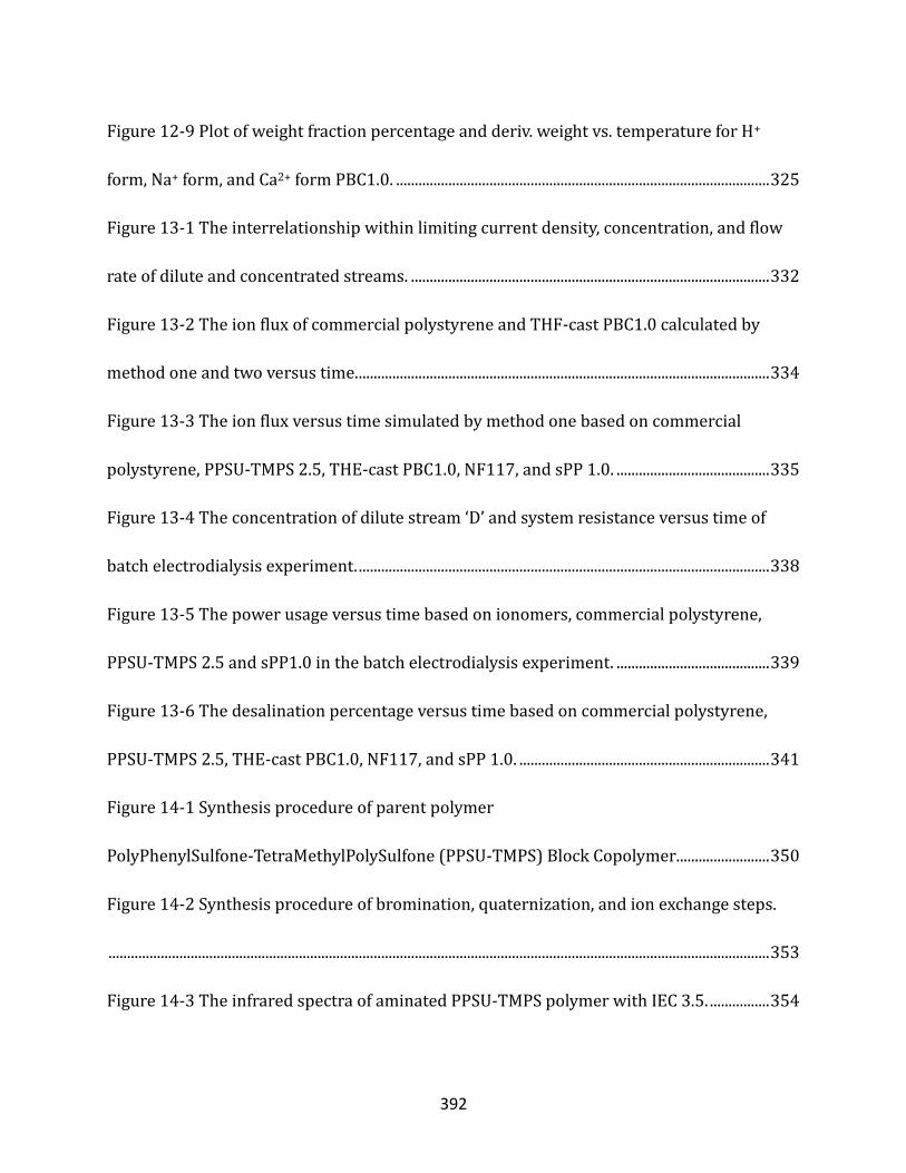
392

Figure 12-9 Plot of weight fraction percentage and deriv. weight vs. temperature for H+

form, Na+ form, and Ca2+ form PBC1.0. .................................................................................................... 325

Figure 13-1 The interrelationship within limiting current density, concentration, and flow

rate of dilute and concentrated streams. ................................................................................................ 332

Figure 13-2 The ion flux of commercial polystyrene and THF-cast PBC1.0 calculated by

method one and two versus time. .............................................................................................................. 334

Figure 13-3 The ion flux versus time simulated by method one based on commercial

polystyrene, PPSU-TMPS 2.5, THE-cast PBC1.0, NF117, and sPP 1.0. ......................................... 335

Figure 13-4 The concentration of dilute stream ‘D’ and system resistance versus time of

batch electrodialysis experiment. .............................................................................................................. 338

Figure 13-5 The power usage versus time based on ionomers, commercial polystyrene,

PPSU-TMPS 2.5 and sPP1.0 in the batch electrodialysis experiment. ......................................... 339

Figure 13-6 The desalination percentage versus time based on commercial polystyrene,

PPSU-TMPS 2.5, THE-cast PBC1.0, NF117, and sPP 1.0. ................................................................... 341

Figure 14-1 Synthesis procedure of parent polymer

PolyPhenylSulfone-TetraMethylPolySulfone (PPSU-TMPS) Block Copolymer......................... 350

Figure 14-2 Synthesis procedure of bromination, quaternization, and ion exchange steps.

................................................................................................................................................................................. 353

Figure 14-3 The infrared spectra of aminated PPSU-TMPS polymer with IEC 3.5. ................ 354

393

Figure 14-4 The selected infrared absorption bands of aminated PPSU-TMPS with IEC 0.0,

1.0, and 3.5 (from 1400 cm-1 to 1800 cm-1). .......................................................................................... 355

Figure 14-5 Hydroxide conductivity and swelling ratio versus aminated PPSU-TMPS with

different IEC and segment block length. ................................................................................................. 356

Figure 14-6 Storage modulus, loss modulus, and tan delta versus temperature of animated

PPSU-TMPS IEC2.5........................................................................................................................................... 359

Figure 14-7 Weight percentage and derivative weight versus temperature of animated

PPSU-TMPS IEC2.5........................................................................................................................................... 361

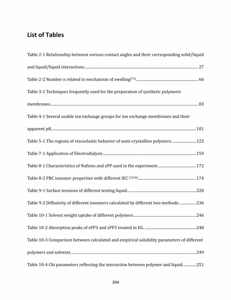
394

List of Tables

Table 2-1 Relationship between various contact angles and their corresponding solid/liquid

and liquid/liquid interactions ....................................................................................................................... 27

Table 2-2 Number n related to mechanism of swelling[75] ................................................................. 66

Table 3-1 Techniques frequently used for the preparation of synthetic polymeric

membranes ........................................................................................................................................................... 83

Table 4-1 Several usable ion exchange groups for ion exchange membranes and their

apparent pK. ....................................................................................................................................................... 101

Table 5-1 The regions of viscoelastic behavior of semi-crystalline polymers. ......................... 123

Table 7-1 Application of Electrodialysis .................................................................................................. 159

Table 8-1 Characteristics of Nafions and sPP used in the experiment ........................................ 172

Table 8-2 PBC ionomer properties with different IEC [161b] ............................................................. 174

Table 9-1 Surface tensions of different testing liquid. ....................................................................... 228

Table 9-2 Diffusivity of different ionomers calculated by different two methods. ................. 236

Table 10-1 Solvent weight uptake of different polymers. ................................................................. 246

Table 10-2 Absorption peaks of sPP3 and sPP3 treated in EG. ...................................................... 248

Table 10-3 Comparison between calculated and empirical solubility parameters of different

polymers and solvents. .................................................................................................................................. 249

Table 10-4 Chi parameters reflecting the interaction between polymer and liquid. ............. 251

395

Table 10-5 HSP of solvents. .......................................................................................................................... 259

Table 10-6 Data utilized to calculate the number of crosslink (water swelling). .................... 261

Table 10-7 Solubility parameters of ionic side chains of different ionomers based on

Hildebrand’s Theory, literature and Flory-Rehner Equation (Unit: J1/2 cm-3/2) ......................... 262

Table 10-8 The chemical potential changes in the process of swelling within water for

different ionomers. (Unit: J/mol) ............................................................................................................... 266

Table 10-9 Solubility parameters and dielectric constants of PBCs. ............................................ 269

Table 10-10 Basic properties of solvents used.[66] .............................................................................. 269

Table 11-1 The qmax values and d-spacings in various solvents cast PBC1.5 films. ................ 285

Table 11-2 Ion conductivity of Nafion117 and THF cast PBC1.0 measured by two methods,

in-plane and through-plane at 25oC. ......................................................................................................... 296

Table 12-1 Glass transition temperatures of different blocks in PBC.[197].................................. 315

Table 12-2 Glass transition temperature of PBCs cast with different solvents obtained by

Tan Delta and (loss modulus). ..................................................................................................................... 319

Table 13-1 Basic properties of different ionomers, PPSU-TMPS 2.5, sPP 1.0, THF-cast

PBC1.0, and NF117. ......................................................................................................................................... 337

Table 13-2 The power usage and desalination time of different ionomers, commercial

polystyrene, PPSU-TMPS 2.5, THF-cast PBC1.0, NF117, and sPP1.0. .......................................... 340

Table 14-1 Specific data of IEC, block length, ion conductivity and swelling ratio of aminated

PPSU-TMPS. ........................................................................................................................................................ 357

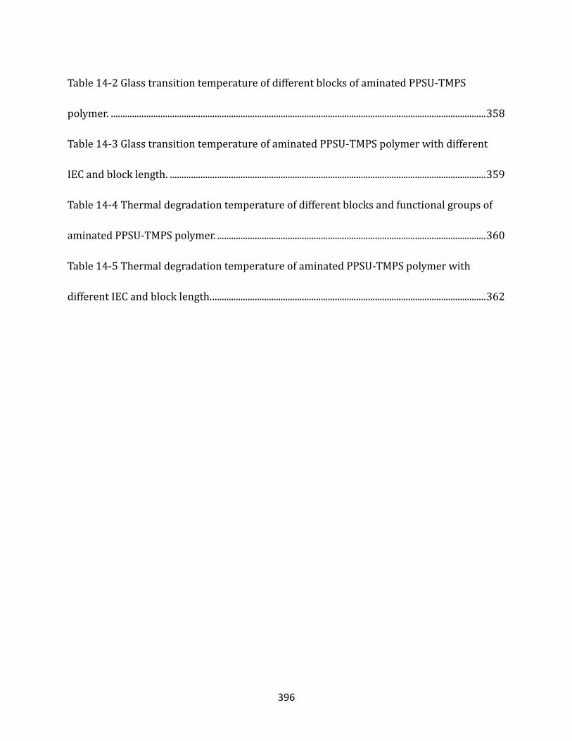
396

Table 14-2 Glass transition temperature of different blocks of aminated PPSU-TMPS

polymer. ............................................................................................................................................................... 358

Table 14-3 Glass transition temperature of aminated PPSU-TMPS polymer with different

IEC and block length. ...................................................................................................................................... 359

Table 14-4 Thermal degradation temperature of different blocks and functional groups of

aminated PPSU-TMPS polymer. .................................................................................................................. 360

Table 14-5 Thermal degradation temperature of aminated PPSU-TMPS polymer with

different IEC and block length. .................................................................................................................... 362

Ionomer Morphology, Solution to Film Thermodynamics ...

Documents

Transcript of Ionomer Morphology, Solution to Film Thermodynamics ...