Analytical Morphology: MathematicalMorphology of Decision TablesAndrzej Skowron�Institute of MathematicsWarsaw UniversityBanacha 2, 02-097 Warsaw, Polande-mail: skowron@mimuw.edu.plLech PolkowskiInstitute of MathematicsWarsaw University of TechnologyPlac Politechniki 1, 00-651 Warsaw, Polande-mail: polk@mimuw.edu.plAbstractWe propose a method called analytical morphology for data �ltering. The method wascreated on the basis of some ideas of rough set theory and mathematical morphology.Mathematical morphology makes an essential use of geometric structure of objects whilethe aim of our method is to provide tools for data �ltering when there is no directlyavailable geometric structure in the data set.1 IntroductionIn many applications there is a need for e�cient methods of data �ltering even ifthere is not any preassumed geometrical (a�ne) structure in the set of attributes(conditions) on the basis of which the decisions should be taken. This situation oftenoccurs when experimental data are recorded in decision tables. The problem arises ofproviding a framework for data �ltering based on tools not relying on a�ne structure.In our proposition we extract from local relations among data some near-to-functionalrelations. From these relations we construct the so called approximation functions. Wepropose a special mechanism for applying of these approximation functions to data inorder to produce their appropriate �ltration; the �rst tests seem to be promising.The paper is structured as follows. In Sections 2 we recall some basic notions fromrough set theory [9]. In particular, we introduce the distribution of objects satisfying agiven formula (built from descriptors) among the decision classes. The data �ltrationproblem for decision tables is formulated in Section 3 in which also a general schemefor data �ltering is discussed. The general scheme involves two main strategies S andH responsible for generating a set of approximation functions and their proper appli-cations to transformed data. One of the possible ideas to build such strategies canbe taken from mathematical morphology [3]. In Section 4 we recall fundamentals ofmathematical morphology trying to present its general scheme. This scheme is takenin Section 5 as a starting point to develop an abstract version of morphology called an-alytical morphology. The di�erent versions of morphological operations, e.g. dilations,erosions, openings and closings, can be obtained by choosing various strategies.The paper sets a proposal for a research project related to data �ltration. In our cur-rent research we are developing some speci�c solutions to presented problems. We are�This work was supported by grant No. 8-S503-019-06 from State Committee for Scienti�c Research(Komitet Bada�n Naukowych)

preparing an implementation of the method to make available a system for automaticdata �ltration.2 Rough Sets PreliminariesInformation systems [8], [9] (sometimes called data tables, attribute-value systems,condition-action tables, knowledge representation systems etc.) are used for represent-ing knowledge.Rough sets have been introduced [9] as a tool to deal with inexact, uncertain orvague knowledge in arti�cial intelligence applications.In this section we recall some basic notions related to information systems and roughsets.An information system is a pair A = (U;A), where U is a non-empty, �nite set calledthe universe and A| a non-empty, �nite set of attributes, i.e. a : U �! Va for a 2 A,where Va is called the value set of a. By V we denote the set [fVa : a 2 Ag.Elements of U are called objects and they are interpreted as, e.g. cases, states,processes, patients, observations. Attributes are interpreted as features, variables,characteristic conditions etc.Every information system A = (U;A) and non-empty set B � A determine a B -information function Inf AB : U �! P B � [a2B Va!de�ned by Inf AB(x) = f(a; a(x)) : a 2 Bg. We write InfB instead of Inf AB when noconfusion arises. The set �InfB(x) : x 2 Uis called the B-information set and it is denoted by INF (A) jB. The set INF (A) jAwill be denoted by INF (A). By INF (A;U; V ) we denote the set of all families offunctions (fa)a2A such that fa is a function from U into V satisfying fa(x) 2 Va forany x 2 U . We write INF (A;V ) instead of INF (A;U; V ), if no confusion arises.We consider a special case of information systems called decision tables. A deci-sion table is an information system of the form A = (U; A [ fdg), where d 62 A is adistinguished attribute called the decision. The elements of A are called conditions.One can interpret a decision attribute as a kind of classi�cation of the universe ofobjects given by an expert, a decision-maker, an operator, a physician, etc. Decisiontables are called training sets of examples in machine learning [6].The cardinality of the image d(U) = fk : d(u) = k for some u 2 Ug is called therank of d and is denoted by r(d).We assume that the set Vd of values of the decision d is equal to f1; :::; r(d)g.Let us observe that the decision d determines the partition fX1; . . . ;Xr(d)g of theuniverse U , where Xk = fu 2 U : d(u) = kg for 1 � k � r(d). The set Xi is called thei-th decision class of A.Let A = (U;A) be an information system. With every subset of attributes B � A, anequivalence relation, denoted by INDA(B) (or IND(B)) called the B-indiscernibilityrelation, is associated and it is de�ned byIND(B) = �(u; u0) 2 U2 : a(u) = a(u0) for any a 2 BObjects u; u0 satisfying relation IND(B) are indiscernible by attributes from B.Let A be an information system with n objects. By M(A) [18] we denote an n� nmatrix [cij], called the discernibility matrix of A such thatcij = �a 2 A : a(ui) 6= a(uj) for i; j = 1; . . . ; n:A discernibility function fA for an information system A is a boolean function of mboolean variables �a1; . . . ; �am corresponding to the attributes a1; . . . ; am respectively,2

and de�ned by fA��a1; . . . ; �am� =^ n_ �cij : 1 � j < i � n; cij 6= ;owhere �cij = ��a : a 2 cij.It can be shown [18] that the set of all prime implicants of fA determines the set ofall reducts of A.If A = (U;A) is an information system, B � A is a set of attributes and X � U isa set of objects, then the sets�u 2 U : [u]B � X and �u 2 U : [u]B \X 6= ;are called the B-lower and the B-upper approximation of X in A, and they are denotedby BX and �BX, respectively, where [u]B = fv 2 U : v IND(B)ug.The set BNB(X) = �BX �BX will be called the B-boundary of X. When B = Awe write also BNA(X) instead of BNA(X).Sets which are unions of some classes of the indiscernibility relation IND(B) arecalled de�nable by B (or B-de�nable). A set X is thus B-de�nable i� �BX = BX.Some subsets (categories) of objects in an information system cannot be expressedexactly by employing available attributes but they can be de�ned roughly.The set BX is the set of all elements of U which can be with certainty classi�edas elements of X, having the knowledge represented by attributes from B; the setBNB(X) is the set of elements which one can classify neither to X nor to �X havingknowledge B.If X1; . . . ;Xr(d) are decision classes of A then the setBX1 [ . . . [ BXr(d)is called the B-positive region of A and is denoted by POSB(d).If A = (U;A [ fdg) is a decision table then we de�ne a function @A : U �!Pf1; . . . ; r(d)g, called the generalized decision in A, by@A(u) = �i : 9u0 2 U u0IND(A)u and d(u0) = i:A decision table A is called consistent (deterministic) if j@A(u)j = 1 for any u 2 U ,otherwise A is inconsistent (non-deterministic). It is easy to see that a decision tableA is consistent i� POSA(d) = U . Moreover, if @B = @B0 then POSB(d) = POSB0(d)for any pair of non-empty sets B;B 0 � A.A subset B of the set A of attributes of decision table A = (U;A[ fdg) is a relativereduct of A i� B is a minimal set with the following property: @B = @A. The set of allrelative reducts in A is denoted by RED(A; d).If B 2 RED(A; d) then the set f(fa = a(u) : a 2 Bg, d = d(u)) : u 2 Ug is calledthe trace of B in A and is denoted by TraceA(B).The rough membership functions (rm-functions) are introduced in [10] as a newtool for reasoning with uncertainty. The de�nition of those functions is based on theobservation that objects are classi�ed by means of available partial information aboutthem. That de�nition allows us to overcome some problems which may be encounteredif we used other approaches (like fuzzy set approach [21]).Let A = (U;A) be an information system and let ; 6= X � U . The rough A-membership function of the set X (or, rm-function, for short) denoted by �AX , is de�nedby: �AX(u) = j[u]A \Xjj[u]Aj ; for u 2 UOne can observe a similarity of the expression on the right hand side of the above def-inition with the expression used to de�ne the conditional probability. Some propertiesof the membership functions are presented in [10].Now we recall the de�nition of decision rules. Let A = (U;A [ fdg) be a decisiontable and let V = S fVa : a 2 Ag [ Vd. 3

The atomic formulas over B � A [ fdg and V are expressions of the form a = v,called descriptors over B and V , where a 2 B and v 2 Va. The set F(B;V ) of formulasover B and V is the least set containing all atomic formulas over B and V and closedwith respect to the classical propositional connectives _ (disjunction), ^ (conjunction).Let � 2 F(B;V ). Then by �A we denote the meaning of � in the decision table A,i.e. the set of all objects in U with property � , de�ned inductively as follows:1. if � is of the form a = v then �A = fu 2 U : a(u) = vg;2. (� ^ � 0)A = �A \ � 0A ; (� _ � 0)A = �A [ � 0A.The set F(A;V ) is called the set of conditional formulas of A and is denoted by C(A;V ).A decision rule of A is any expression of the form� =) d = v where � 2 C(A;V ) and v 2 Vd:The decision rule � =) d = v for A is true in A, symbolically � =)A d = v, i��A � (d = v)A; if �A = (d = v)A then we say that the rule is A-exact .If A = (U;A [ fdg) is a decision table then by A@ we denote the decision table(U;A[ f@g) where @ = @A. Let us observe that any decision rule � =) @A = � where� 2 C(A;V ) and ; 6= � � Vd valid in A@ and having examples in A, i.e. satisfying�A 6= ; determines a distribution of objects satisfying � among elements of �. Thisdistribution is de�ned by�i(A; �; �) = j�A \Xijj�Aj ; for i 2 �:Any decision rule � =) @A = � valid in A@ and having examples in A with j�j > 1 iscalled non-deterministic, otherwise it is deterministic.The number n(A; �; i) = j�A \Xij is called the number of examples supporting � inthe i-th decision class Xi.Let us observe that for any formula � over A and V with �A 6= ; there exists exactlyone subset �� of � such that � =)A @A = �� and �i(A; �; ��) > 0 for any i 2 �� . Inthe sequel we write �i(A; � ) instead of �i(A; �; ��).3 Data �ltrationThe aim of this section is to present some ideas related to data �ltration based onrough set approach. We expect that by developing the ideas presented here and somerelated algorithms e�cient tools for data �ltration can be obtained.3.1 A general searching scheme for decision tables �ltration based onrough set approachThe decision table A0 = (U;A0 [ fdg) is compatible with A = (U;A [ fdg) i� A =fa1; . . . ; amg, A0 = fa01; . . . ; a0mg and Va0i � Vai for i = 1; . . . ;m.Let A = (U;A [ fdg) and A0 = (U;A0 [ fdg) be decision tables and let � 2 (0; 1].We say that A0 is a �-�ltration of A i�(i) A0 is compatible with A(ii) @A = @A0(iii) j f[u]A0 : [u]A0 � Z�g j < �j f[u]A : [u]A � Z�g jfor any � � Vd with ; 6= Z� = @�1A (�).One can also consider another version of this de�nition with condition (ii) replaced bya weaker condition specifying that @A and @A0 should be su�ciently close with respectto some distance function. 4

Let k be a real number from the interval (0; 1]. Let A = (U;A [ fdg) be a decisiontable and let � be a formula over A and V . If � = f(a1; v1); . . . ; (am; vm)g then V�denotes the formula a1 = v1 ^ . . . ^ am = vm. If � is a formula over A and V thenby A� we denote the restriction of A to the set of all objects from U satisfying � , i.e.A� = (�A; A[fdg). By T (A; �; k) we denote the conjunction of the following conditions:(i) �A 6= ;(ii) for any � 2 INF (A�) :(�) there exists exactly one i0 with the following property: �i0(A;V� ^ � ) > k.Condition (�) denotes that exactly one of distribution coe�cients �i(A;V�^� ) (i 2 �)exceeds the threshold k for any � 2 INF (A�).Let A = (U;A [ fdg) be a decision table and let � be a reduction coe�cient. Wepresent a general procedure F of searching for a �ltration of A when �xed the thresholdk and the critical level l are given.Our procedure F has parameters S, G, H, A, � (by assumption l and k are �xed).The proper values for k and l should be chosen by making experiments with A.Now we can formulate a general version of �ltration problems.S, G and H in the procedure F are three �xed strategies. The �rst one S producesfrom an actual decision table A for any a 2 A0 � A a sequence of decision rules of thefollowing form: �1 =) @A�fag = �1; . . . ; �p =) @A�fag = �psatisfying T (Aa; �i; k) for i = 1; . . . ; p.These rules are used next to generate approximation functions by the second strategyH. The strategy H produces from the above sequences a new sequence(s1; . . . ; sr)where si is a set of non-con icting decision rules (see 3.3, below) of the form � =)@A�fag = � for some a 2 A, � � Vd and formula � over A � fag and V . Theapproximation functions corresponding to the decision rules from si are chosen by Hfor simultaneous application at the i-th step of transformation of the actual decisiontable A. The strategy G takes as input a set F of approximation functions and outputsa sequence f1; . . . ; fk over F ; the �ltration is carried out by sequential applications off1; . . . ; fk to the decision table A.PROCEDURE FSTEP 1. For any a 2 A0 � A, where A0 is a randomly chosen sample set of conditionalattributes, apply the methods for decision rules synthesis (see [17], [15], [16]) forthe decision table Aa = (U; fA�A0g)[fag) (in particular apply also for synthesisof rules the so called semi-reducts [16]). The output of this step is a set of decisionrules of the form: � =) @A�A0 = ��where @A�A0 is the generalized decision corresponding to the conditional attributea 2 A0 and � is a formula over A �A0 and V . Now, the strategy S is applied toconstruct from these decision rules a \global" decision rule for a�0 =) @A�fag = �such that T (Aa; �0; k) holds and maxi n(Aa;V�^ �0; i) > l for � 2 INF ((Aa)�0jB)where B is the set of conditional attributes occuring in �0 and (Aa)�0 is the re-striction of Aa to the set of objects satisfying �0.STEP 2. From the global decision rules of STEP 1 for conditional attributes in A theapproximation functions are built by means of the strategy H. In this way weobtain a set F of approximation functions.5

STEP 3. We apply to A approximation functions from F chosen by the strategy Gand in this way we obtain a new decision table A0.STEP 4. If A0 is a �-�ltration of A then stop else go to STEP 1 substituting A0 forA if A0 is a �0-�ltration of A with �0 < 1.There are several problems to be solved when one would like to implement the abovemethod. Among them are:1. Sampling problem: How to choose A0 in STEP 1? The random choice of A0(proposed in STEP 1) may be not su�cient. Some methods for the proper choiceof A0 can be developed basing on properties of reducts [18], [15], [16]. One canapply also some analogies frommathematicalmorphology [14], [3] which have beenused in building the so called analytical morphology (see Section 4.4). Here wewould like only to add, by analogy with the mathematical morphology operationsof erosion and dilation, that one can randomly choose a subset A00 of A � A0 asa new subset of A after entering again STEP 1 where A0 is the previously chosensubset of A. We shall now look for decision rules� =) @A0 = ��where � is over A0 and V and @A0 is the generalized decision corresponding to acondition a 2 A00.2. Generation of approximation functions for decision rules. In Section 3.2we present a de�nition of the approximation functions.3. Con ict problem. This problem (see 3.3, below) arises when one would like toapply the parallel strategy in STEP 3. In particular here arises the compositionof decision rules problem. This problem is related to the synthesis of the globaldecision rule (see STEP 1).4. Application of approximation functions problem. The problem is relatedto the question how to choose a proper subset of approximation functions fromF and in what order to apply them to get the best �ltration of A. To solve thisproblem we would like to apply genetic algorithms.FILTRATION PROBLEM :Input: A, and � 2 [0; 1] \ Q, where Q is the set of rationalnumbersOutput: Strategies S and H such that a �-�tration of Ais returned after calling F with parameters S, H, A and �,if such strategies exist.OPTIMAL FILTRATION PROBLEM :Input: AOutput: inff� 2 Q: there exist strategies S and H such thata �-�tration of A is returned after calling Fwith parameters S, H, A and �gOne can not expect that the solutions S and H for the above �ltration problemsare of polynomial time complexity with respect to the size of A and � because thestrategies S and H are based, e.g. on procedures for decision rules generation andthese procedures are based on the reduct set generation [18]. Nevertheless, one canbuild e�cient heuristics for solving the �ltration problems for practical applications.3.2 Approximation functions for non-deterministic decision rulesFor any decision table A = (U;A [ fdg), formula � over A and V , and a threshold ksatisfying the condition T (A; �; k) one can de�ne a � -approximation function in A withthreshold k F �A; �; k� : INF (A�)jB �! INF �fdg; �A; V �6

by F (A; �; k)(�) = f(u; i0) : u 2 (V� ^ � )Ag for any � 2 INF (A�)jB where�i0(A;V �^ � ) = maxf�i(A;V �^ � ) : i 2 ��g and B is the set of conditions occuringin � . For simplicity of notation we write F (A; �; k)(�) = f instead of F (A; �; k) = ffg.In the sequel we consider F (A; �; k) as a function from INF (A�)jB into INF (fdg; V )assuming additionally that if F (A; �; k) = f then f(�)(u) = d(u) if u 62 �A.We apply the above construction to decision tables derived from a given decisiontable A = (U;A [ fdg). These decision tables are of the form B = (U;B [ fcg) andthey are constructed from information systems B = (U;B [ C), where B;C � A andB \ C = ; by representing C by means of one decision attribute c. We denote bycodeC (or, code, in short) a �xed coding function for information vectors restrictedto C in Vc de�ning c by c(u) = codeC(f(a; a(u)) : a 2 Cg) for any u 2 U . GivenF (A; �; k) : INF (A�)jB �! INF (fcg; V ) where c(u) = codeC(f(a; a(u)) : a 2 Cg)for any u 2 U , we denote, for any a0 2 C and any u 2 U , by F (A; �; k)a0(u) the pair(a0; i(a0)), where F (A; �; k)(�) = f�c and f�c is a constant function taking on elementsfrom (V� ^ � )A the value i0, and code�1C (f(c; i0)g) = f(a; i(a)) : a 2 Cg. For a giventhreshold k we consider decision tables B = (U;B [ fcg) with the property that thereexists a formula � over B and V such that T (B; �; k) holds. These tables correspondto near-to-functional relations of data represented in A by which term we understandthat only one decision is pointed out with the strength exceeding the threshold k. Letus observe that by assumption we have INF (B�)jB = INF (A�)jB.Let l be a positive integer called the critical level of examples. We denote byF(A; k; l) the family of all functions of the form F (B; �; k) such that T (B; �; k) holdsand maxi n(B; �; i) > l. By F(A; l) (or, F(A), in short) we denote the union of thefamily fF(A; k; l) : 0 < k � 1g.Let us observe that the function F (B; �; k) : INF (A�)jB �! INF (fcg; V ) producesfrom the decision table A = (U;A [ fdg) with A = fa1; . . . ; amg a new decision tableA0 = (U;A0 [ fdg) with A0 = fa01; . . . ; a0mg de�ned by f(u; codeCf(a0i; a0i(u)) : ai 2 Cg) :u 2 Ug = F (B; �; k) (Inf AB(u)) and a0i(u) = ai(u) when ai 62 C, for any u 2 �B; ifu 2 U � �B then a0i(u) = ai(u) for any i.In an analogous way can transform (applying codeC function) any approximationfunction F (B; �; k) : INF (A)jB �! INF (fcg; V ) into a function from INF (A)jB intoINF (C; V ), denoted in the sequel also by F (B; �; k).The de�nition of approximation functions presented here can be treated as one ofpossible formalizations of near-to-functional relations between data, e.g. an approxi-mation function could choose the mean value from the set of values exceeding a giventhreshold. We plan to test on various data tables the properties of di�erent notions ofapproximation functions from the point of view of application to data �ltering.3.3 Con ict problemLet us assume that a set F of approximation functions of A is given. Now we wouldlike to transform rows in decision table in parallel, i.e. by simultaneous application offunctions chosen from F on the basis of some strategies. In this case it is necessary tosolve the con ict problem created by functions from F .Let F be a given set of approximation functions and let c 2 A. Let F(c) be the setof all functions from F with co-domains equal to INF (fcg; V ). We say that F(c) iscon icting in A i� there exist u 2 U and f; f 0 2 F(c) such thatf(InfB(u))(u) 6= f 0(InfB0(u))(u)where f : INF (A�)jB �! INF (fcg; V )f 0 : INF (A� 0)jB 0 �! INF (fcg; V ) for some �; � 0:We say that F is con icting in A i� F(c) is con icting in A for some c 2 A.If the value set of c is ordered then one of possibilities to resolve the con ict createdby F(c) is to take as the new value of c for a given u 2 U a randomly chosen valuefrom the interval [min;max], where min and max are the minimum and maximum ofthe values of functions from F(c) at u. This is an analogy to morphological operations7

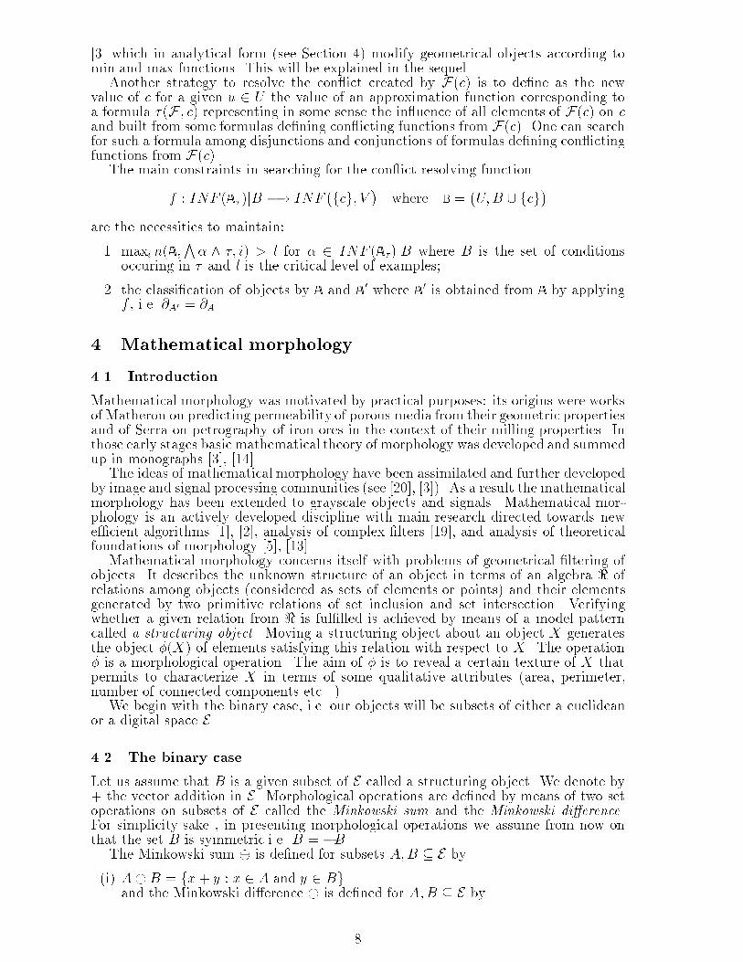
[3] which in analytical form (see Section 4) modify geometrical objects according tomin and max functions. This will be explained in the sequel.Another strategy to resolve the con ict created by F(c) is to de�ne as the newvalue of c for a given u 2 U the value of an approximation function corresponding toa formula � (F ; c) representing in some sense the in uence of all elements of F(c) on cand built from some formulas de�ning con icting functions from F(c). One can searchfor such a formula among disjunctions and conjunctions of formulas de�ning con ictingfunctions from F(c).The main constraints in searching for the con ict resolving functionf : INF (A�)jB �! INF �fcg; V � where B = �U;B [ fcg�are the necessities to maintain:1. maxi n(A;V� ^ �; i) > l for � 2 INF (A�)jB where B is the set of conditionsoccuring in � and l is the critical level of examples;2. the classi�cation of objects by A and A0 where A0 is obtained from A by applyingf , i.e. @A0 = @A.4 Mathematical morphology4.1 IntroductionMathematical morphology was motivated by practical purposes: its origins were worksof Matheron on predicting permeability of porous media from their geometric propertiesand of Serra on petrography of iron ores in the context of their milling properties. Inthose early stages basic mathematical theory of morphology was developed and summedup in monographs [3], [14].The ideas of mathematical morphology have been assimilated and further developedby image and signal processing communities (see [20], [3]). As a result the mathematicalmorphology has been extended to grayscale objects and signals. Mathematical mor-phology is an actively developed discipline with main research directed towards newe�cient algorithms [1], [2], analysis of complex �lters [19], and analysis of theoreticalfoundations of morphology [5], [13].Mathematical morphology concerns itself with problems of geometrical �ltering ofobjects. It describes the unknown structure of an object in terms of an algebra < ofrelations among objects (considered as sets of elements or points) and their elementsgenerated by two primitive relations of set inclusion and set intersection. Verifyingwhether a given relation from < is ful�lled is achieved by means of a model patterncalled a structuring object . Moving a structuring object about an object X generatesthe object �(X) of elements satisfying this relation with respect to X. The operation� is a morphological operation. The aim of � is to reveal a certain texture of X thatpermits to characterize X in terms of some qualitative attributes (area, perimeter,number of connected components etc...).We begin with the binary case, i.e. our objects will be subsets of either a euclideanor a digital space E.4.2 The binary caseLet us assume that B is a given subset of E called a structuring object. We denote by+ the vector addition in E. Morphological operations are de�ned by means of two setoperations on subsets of E called the Minkowski sum and the Minkowski di�erence.For simplicity sake , in presenting morphological operations we assume from now onthat the set B is symmetric i.e B = �B.The Minkowski sum � is de�ned for subsets A;B � E by(i) A�B = fx+ y : x 2 A and y 2 Bgand the Minkowski di�erence is de�ned for A;B � E by8

(ii) AB = fx 2 E : fxg �B � Ag.The Minkowski sum and the Minkowski di�erence operations are employed in thede�nitions of two basic morphological operations viz. the dilation by B and theerosion by B.The dilation of X � E by B, denoted by dB(X) is de�ned by(iii) dB(X) = X �B.The erosion of X by B, denoted by eB(X) is de�ned by(iv) eB(X) = X B.Morphological operations can be composed and new operations can be generated bymeans of set-theoretical operations (see [14]). The body of operations produced fromerosions and dilations is the morphological algebra of operations.In particular, the composition: the erosion by B followed by the dilation by B isthe opening by B, denoted by oB, and the composition: the dilation by B followed bythe erosion by B is the closing by B, denoted by cB.Formally(v) oB(X) = dB � eB(X) and(vi) cB(X) = eB � dB(X) for any X � E.The meaning of the opening by B and the closing by B can be best understoodfrom the following characterizations (see [7] or [14]).Proposition 4.2.1.(a) oB(X) = fx 2 E : 9y(x 2 fyg �B � X)g.(b) cB(X) = fx 2 E : 8y(x 2 fyg �B ) (fyg �B) \X 6= ;)g.Let us observe the parallelism between the description of X provided by the openingof X by B and the closing of X by B and the description of X provided by the B-lowerand the B-upper approximations of X in the rough set theory (see Section 2).The operations in the binary case based on the additive structure of E and settheoretical notions of inclusion and intersection have been extended for needs of imageand signal processing to grayscale, respectively, signal morphology (see [20], [4], [3]).We present below the most essential points of grayscale morphology.4.3 The grayscale caseThe objects of grayscale morphology are functions, representing, e.g. grayscale visualobjects or signals.An object F is a function F : A �! E where A � En for some n. The operations ofmathematicalmorphology are performed on functions indirectly by means of associatedobjects called umbrae.A subset X � En � E is called an umbra if the following holds(i) (x; y) 2 X ^ z � y) (x; z) 2 X.For a function F : A �! E, the umbra of F , denoted by U [F ] is the set f(x; y) 2A� E : y � F (x)g.The objects are recovered from operations on umbrae by means of the envelopeoperation. Suppose that X is an umbra. The envelope of X, denoted by E(X),is de�ned as follows(ii) E(X)(x) = supfy 2 E : (x; y) 2 Xg for x 2 En.Let F : A �! E be an object and K : C �! E (where C � En) be a �xedobject called a structuring object. We denote again by �, , the Minkowski sum,di�erence operators, respectively in the space En+1 induced by the vector addition+. The operations of dilation by K, denoted by dK and of erosion by K, denotedby eK are de�ned on F by(iii) dK(F ) = E(U [F ]� U [K]) 9

(iv) eK(F ) = E(U [F ] U [K]).The morphological algebra is de�ned in the grayscale case in the manner analogousto the case of binary morphology. In particular, the opening by K, denoted byoK, and the closing by K, denoted by cK are de�ned as(v) oK(F ) = E�oU [K](U [F ])�(vi) cK(F ) = E�cU [K](U [F ])�.It will be convenient for our purposes to present the above operations in binary aswell as grayscale case in an analytical form.4.4 Mathematical morphology in analytical formWe will represent morphological operations in an analytical form, i.e. as operations onvector representations of objects.4.4.1 The binary caseWe will represent binary objects X � E as binary vectors of the form v =< vx : x 2E > (vx = 1 i� x 2 X), i.e. X = fx : vx = 1g.The functions D, E, O and C on ZE2 into ZE2 which represent, respectively, thedilation by B, the erosion by B, the opening by B , and the closing by B for anysymmetric structuring object B are de�ned as follows(i) D(v) = v0 where v0x = max�vy : x 2 fyg �B(ii) E(v) = v0 where v0x = min�vy : y 2 fxg �B(iii) O(v) = v0 where v0x = max�minfvz : z 2 fyg �Bg : x 2 fyg �B(iv) C(v) = v0 where v0x = min�maxfvz : y 2 fzg �Bg : y 2 fxg �B.To make our exposition complete, we include a proof that the functions D, E, O,C represent, respectively, dilation, erosion, opening, and closing by the structuringelement B. It su�ces, by virtue of 4.2(v), (vi), to give proofs in cases of D and E. Fora subset X � E, we let vX 2 ZE2 to denote the binary vector de�ned by letting(vX)x = � 1 if x 2 X0 otherwiseand given a binary vector v 2 ZE2 , we denote by suppv, and call the support of v, thesubset fx 2 E : vx = 1g � E. Then we haveProposition 4.4.1. The functions D, E de�ned by (i), (ii) above represent binarymorphological operations of dilation, respetively, erosion, viz.(a) supp(D(vX)) = dB(X),(b) supp(E(vX)) = eB(X) for any subset X 2 E.Proof.For (a), let x 2 dB(X) hence there exists y 2 X with x 2 fyg � B. As vXy = 1, wehave (D(vX))x = 1 i.e. x 2 supp(D(vX)). In case x 2 supp(D(vX)) i.e. (D(vX))x =1 = maxfvXy : x 2 fyg � Bg there exists y 2 fxg � B with vXy = 1 i.e. y 2 X. Hencex 2 dB(X).For (b), let x 2 eB(X) so fxg � B � X i.e. vXy = 1 for any y 2 fxg � B hence(E(vX))x = minfvXy : y 2 fxg � Bg = 1 and thus x 2 supp(E(vX)). Conversely,in case x 2 supp(E(vX)), we have 1 = (E(vX))x = minfvXy : y 2 fxg � Bg hencefxg �B � X i.e. x 2 eB(X).We call x a centre of fxg �B and we call the set fxg � B the in uence set of x.Let us observe the following: 10

a. The operations D and E can be regarded as analytical representations of somestrategies for negotiating among con icting in uences on x of centers of in uencesets containing x and among con icting in uences on x of elements of the in uenceset of x, respectively.b. The operations O and C can be similarly regarded as analytical representationsof some strategies for expressing a common in uence on an element x of in uencesets containing x (�rst we erode fyg�B to y for x 2 fyg�B next we dilate thesey0s to x) and of in uence sets intersecting the in uence set of x, respectively (�rstwe dilate centers of in uence sets fzg�B containing y to y for y 2 fxg�B nextwe erode fxg �B to x). 24.4.2 The grayscale caseGiven x 2 En, we let Vx = E [ f�1g. Selecting vx 2 Vx for each x de�nes a functionF : A �! E where A = fx 2 En : vx 6= �1g and F (x) = vx for x 2 A. We canrepresent therefore morphological grayscale objects by means of vectors v =< vx : x 2E >.Let K : C �! E be a �xed structuring object. The vector representation of K willbe denoted by v� =< v�x : x 2 En >.Analytical operations D, E,O and C which represent grayscale morphological oper-ations of respectively the dilation by K, the erosion by K, the opening by K, and theclosing by K are functions on (E [f�1g)En into (E [f�1g)En given by the following(i) D(v) = v0 where v0x = supfvx�z + v�z : z 2 Cg(ii) E(v) = v0 where v0x = inffvx+z � v�z : z 2 Cg(iii) D(v) = v0 where v0x = supfinffvx�z0+z � v�z : z 2 Cg+ v�z0 : z0 2 Cg(iv) C(v) = v0 where v0x = inffsupfvx�z+z0 + v�z : z 2 Cg � v�z0 : z0 2 CgAs with the binary case, we will include a short proof that the functions D, E, O, Crepresent, respectively, grayscale dilation, erosion, opening, and closing by a structuringelement K : C �! EBy 4.3(v), (vi) it su�ces to give proofs for D, E only.Given a grayscale object F : A �! E where A � En, we denote by vF the vector in(E [ f1g)En de�ned by lettingvFx = � F (x) if x 2 A�1 otherwiseand given a vector v 2 (E [ f�1g)En, we denote by suppv, and call the support ofv, the subset F � En � E de�ned by(x; y) 2 F if and only if vx 6= �1 and y = vx:We denote by v� the vector vK.Then we haveProposition 4.4.2. The functions D, E de�ned by (i), (ii) above represent thegrayscale morphological operations of dilation, respectively, erosion, by the structuringelement K : C �! E viz.(a) supp (D(vF )) = dK(F ),(b) supp(E(vF )) = eK(F ).Proof.For (a), let (x; y) 2 dK(F ), hence y = supfq : (x; q) 2 U(F ) � U(K)g; now (x; q) 2U(F )�U(K) if and only if there exist (u; v) 2 U(F ) and (w; t) 2 U(K) with x = u+wand q = v+ t hence u = x�w and q � F (x�w)+K(w). It follows that q � vFx�w+v�w11

hence y = supfvFx�w + v�w : w 2 Cg and thus y = (D(vF ))x 6= �1 which implies(x; y) 2 supp(D(vF )).Conversely, in case (x; y) 2 supp(D(vF )), we have y = (D(vF ))x 6= �1 hencey = supfvFx�w+v�w : w 2 Cg and by the �rst part of the proof we have that y = supfq :(x; q) 2 U(F )� U(K)g, i.e. y = E(U(F )� U(K)) which implies (x; y) 2 dK(F ).For (b), let (x; y) 2 eK(F ) i.e. y = E(U(F ) U(K))(x) hence y = supfq : (x; q) 2U(F ) U(K)g. Now, (x; q) 2 U(F ) U(K) if and only if(x; q)� U(K) � U(F ) if and only if (x; q) + (u;w) 2 U(F )for any (u;w) 2 U(K) if and only if q � F (x+ u)�K(u) for any u 2 C which impliesy = inffF (x+ u)�K(u) : u 2 Cg= inffvFx+u � v�u : u 2 Cgwhich implies (x; y) 2 supp(E(vF )). Conversely, (x; y) 2 supp(E(vF )) implies y =inffvFx+u � v�u : u 2 Cg which by the �rst part of this proof means y = E(U(F ) U(K))(x) i.e. (x; y) 2 eK(F ). 2Let us recall the remarks of Sections 4.1.a and 4.1.b above and observe that theabove formulas (i) - (iv) can be regarded as analytical representations of strategies fornegotiating among con icting in uences at a point of distinct translates of K.Let us conclude the last two subsections with the following observation that mor-phological operations regarded as strategies of con ict negotiations among disagreeingin uences of elements as well as sets of objects fall into one of the two following cate-goriesa. strategies which negotiate among con icting in uences of elements (dilations, ero-sions...);b. strategies which also delineate the area of in uence (openings, closings ...).In the following Section, we will formulate an abstract version of morphology calledanalytical morphology and apply it to some problems related to data �ltration in deci-sion tables.5 Analytical morphologyLet us stress that the approximation functions chosen by the strategy G are intricatelyoverlapped i.e. some conditional attributes may be in domains of some functions aswell as in co-domains of other functions. We need therefore a guiding principle aboutthe way these functions are applied. We propose analytical morphology as providingsuch principles (of our discussion (pts. a,b) in Section 4.4.1, above).The scheme of mathematical morphology presented in Section 4 has been based ontwo assumptions:a. morphological objects are subsets of a space E with the underlying linear struc-ture; therefore elements of E can be translated one into another by means of thisstructure;b. objects are represented as vectors in a space of states with a given algebraicstructure, e.g. < Z2;max; min > in the binary case and < E;+ > in the grayscalecase over points of an a�ne spaces; therefore a new state at x 2 E can be foundas a function of states at some other elements of E by means of the correspondingalgebraic operations on states over points and a�ne operations on points.Analytical morphology as formulated below can be regarded as an attempt to developa version of mathematical morphology suitable for contexts in which either assumption(a) or (b) may not be ful�lled. We may therefore not presume any linear structure instates or points, and we replace algebraic operations by �ltration of states by meansof approximation functions. 12

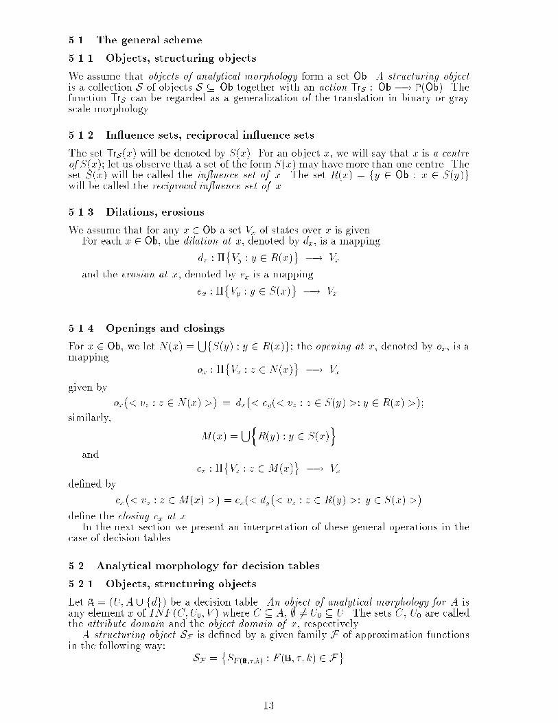
5.1 The general scheme5.1.1 Objects, structuring objectsWe assume that objects of analytical morphology form a set Ob. A structuring objectis a collection S of objects S � Ob together with an action TrS : Ob �! P(Ob). Thefunction TrS can be regarded as a generalization of the translation in binary or grayscale morphology.5.1.2 In uence sets, reciprocal in uence setsThe set TrS(x) will be denoted by S(x). For an object x, we will say that x is a centreof S(x); let us observe that a set of the form S(x) may have more than one centre. Theset S(x) will be called the in uence set of x. The set R(x) = fy 2 Ob : x 2 S(y)gwill be called the reciprocal in uence set of x.5.1.3 Dilations, erosionsWe assume that for any x 2 Ob a set Vx of states over x is given.For each x 2 Ob, the dilation at x, denoted by dx, is a mappingdx : ��Vy : y 2 R(x) �! Vxand the erosion at x, denoted by ex is a mappingex : ��Vy : y 2 S(x) �! Vx.5.1.4 Openings and closingsFor x 2 Ob, we let N(x) = SfS(y) : y 2 R(x)g; the opening at x, denoted by ox, is amapping ox : ��Vz : z 2 N(x) �! Vxgiven by ox�< vz : z 2 N(x) >� = dx�< ey(< vz : z 2 S(y) >: y 2 R(x) >�;similarly, M(x) = SnR(y) : y 2 S(x)oand cx : ��Vz : z 2M(x) �! Vxde�ned bycx�< vz : z 2M(x) >� = ex(< dy�< vz : z 2 R(y) >: y 2 S(x) >�de�ne the closing cx at x.In the next section we present an interpretation of these general operations in thecase of decision tables.5.2 Analytical morphology for decision tables5.2.1 Objects, structuring objectsLet A = (U;A [ fdg) be a decision table. An object of analytical morphology for A isany element x of INF (C;U0; V ) where C � A, ; 6= U0 � U . The sets C, U0 are calledthe attribute domain and the object domain of x, respectively.A structuring object SF is de�ned by a given family F of approximation functionsin the following way: SF = �SF (B;�;k) : F (B; �; k) 2 F13

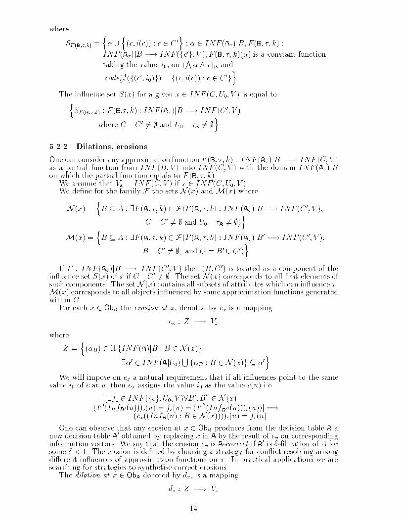
whereSF (B;�;k) = n� [ n(c; i(c)) : c 2 C 0o : � 2 INF (A�)jB;F (B; �; k) :INF (A�)jB �! INF (fc0g; V ); F (B; �; k)(�) is a constant functiontaking the value i0, on (V� ^ � )A andcode�1C0 (f(c0; i0)g) = f(c; i(c)) : c 2 C 0goThe in uence set S(x) for a given x 2 INF (C;U0; V ) is equal tonSF (B;�;k) : F (B:�; k) : INF (A�)jB �! INF (C 0; V )where C \ C 0 6= ; and U0 \ �A 6= ;o5.2.2 Dilations, erosionsOne can consider any approximation function F (B; �; k) : INF (A�)jB �! INF (C; V )as a partial function from INF (B;V ) into INF (C; V ) with the domain INF (A�)jBon which the partial function equals to F (B; �; k).We assume that Vx = INF (C; V ) if x 2 INF (C;U0; V ).We de�ne for the family F the sets N (x) and M(x) whereN (x) = nB � A : 9F (A; �; k) 2 F(F (A; �; k) : INF (A�)jB �! INF (C 0; V );C \ C 0 6= ; and U0 \ �A 6= ;)oM(x) = nB � A : 9F (A; �; k) 2 F(F (A; �; k) : INF (A�)jB 0 �! INF (C 0; V );B \ C 0 6= ;; and C = B 0 [ C 0)oIf F : INF (A�)jB �! INF (C 0; V ) then (B;C 0) is treated as a component of thein uence set S(x) of x if C \C 0 6= ;. The set N (x) corresponds to all �rst elements ofsuch components. The setN (x) contains all subsets of attributes which can in uence x.M(x) corresponds to all objects in uenced by some approximation functions generatedwithin C.For each x 2 ObA the erosion at x, denoted by ex is a mappingex : Z �! VxwhereZ = n(�B) 2 � fINF (A)jB : B 2 N (x)g:9�0 2 INF (AjU0)S f�B : B 2 N (x)g � �0o.We will impose on ex a natural requirement that if all in uences point to the samevalue i0 of c at u, then ex assigns the value i0 as the value c(u) i.e.[9fc 2 INF (fcg; U0; V )8B 0; B 00 2 N (x)(F 0(InfB0(u)))c(u) = fc(u) = (F 00(InfB00(u)))c(u))] =)(ex((InfB(u) : B 2 N (x))))c(u) = fc(u)One can observe that any erosion at x 2 ObA produces from the decision table A anew decision table A0 obtained by replacing x in A by the result of ex on correspondinginformation vectors. We say that the erosion ex is A-correct if A0 is �-�ltration of A forsome � < 1. The erosion is de�ned by choosing a strategy for con ict resolving amongdi�erent in uences of approximation functions on x. In practical applications we aresearching for strategies to synthetise correct erosions.The dilation at x 2 ObA denoted by dx, is a mappingdx : Z �! Vx14

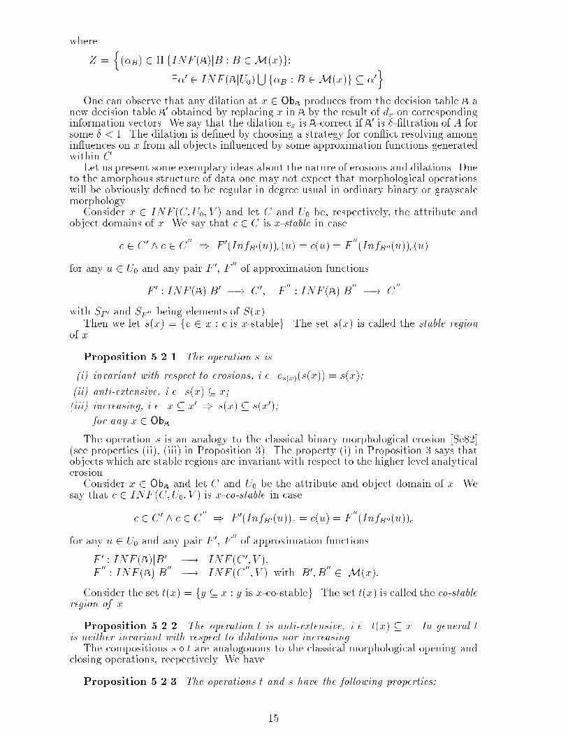
whereZ = n(�B) 2 � fINF (A)jB : B 2 M(x)g:9�0 2 INF (AjU0)S f�B : B 2 M(x)g � �0o.One can observe that any dilation at x 2 ObA produces from the decision table A anew decision table A0 obtained by replacing x in A by the result of dx on correspondinginformation vectors. We say that the dilation ex is A-correct if A0 is �-�ltration of A forsome � < 1. The dilation is de�ned by choosing a strategy for con ict resolving amongin uences on x from all objects in uenced by some approximation functions generatedwithin C.Let us present some exemplary ideas about the nature of erosions and dilations. Dueto the amorphous structure of data one may not expect that morphological operationswill be obviously de�ned to be regular in degree usual in ordinary binary or grayscalemorphology.Consider x 2 INF (C;U0; V ) and let C and U0 be, respectively, the attribute andobject domains of x. We say that c 2 C is x-stable in casec 2 C 0 ^ c 2 C 00 ) F 0(InfB0(u))c(u) = c(u) = F 00(InfB00(u))c(u)for any u 2 U0 and any pair F 0, F 00 of approximation functionsF 0 : INF (A)jB 0 �! C 0; F 00 : INF (A)jB 00 �! C 00with SF 0 and SF 00 being elements of S(x).Then we let s(x) = fc 2 x : c is x-stableg. The set s(x) is called the stable regionof x.Proposition 5.2.1. The operation s is(i) invariant with respect to erosions, i.e. es(x)(s(x)) = s(x);(ii) anti-extensive, i.e. s(x) � x;(iii) increasing, i.e. x � x0 ) s(x) � s(x0);for any x 2 ObA.The operation s is an analogy to the classical binary morphological erosion [Se82](see properties (ii), (iii) in Proposition 3). The property (i) in Proposition 3 says thatobjects which are stable regions are invariant with respect to the higher level analyticalerosion.Consider x 2 ObA and let C and U0 be the attribute and object domain of x. Wesay that c 2 INF (C;U0; V ) is x-co-stable in casec 2 C 0 ^ c 2 C 00 ) F 0(InfB0(u))c = c(u) = F 00(InfB00(u))cfor any u 2 U0 and any pair F 0, F 00 of approximation functionsF 0 : INF (A)jB 0 �! INF (C 0; V );F 00 : INF (A)jB 00 �! INF (C 00; V ) with B 0; B 00 2 M(x):Consider the set t(x) = fy � x : y is x-co-stableg. The set t(x) is called the co-stableregion of x.Proposition 5.2.2. The operation t is anti-extensive, i.e. t(x) � x. In general tis neither invariant with respect to dilations nor increasing.The compositions s � t are analogouous to the classical morphological opening andclosing operations, reepectively. We haveProposition 5.2.3. The operations t and s have the following properties:15

(i) s � s = s;(ii) t � s = s;(iii) t � s � t � s = t � s.In general s � t need not be idempotent. Moreover, the operations d and e generate adynamical system (INF (A;V ); d; e). Strategies searching for correct compositions ofd and e will therefore depend on the ergodic properties of the decision table.In classical mathematical morphology mappings of erosion and dilation may beregarded as negotiation strategies among con icting in uences of points from a neigh-borhood on its center (erosion) or in uences on a point of centers of neighborhoodscontaining this point (dilation). In analytical morphology this mappings negotiateamong con icting in uences of sets of conditions expressed by approximation functionsfrom F . One can also de�ne in analytical morphology opening and closing operationsas respective composition of dilations and erosions according of the general scheme ofSection 5.1.4.It may be convenient to have also some forms of masks for preventing some attributesfrom being modi�ed when their values are already satisfactory.Analytical morphology of decision table A is a system:�S;H;F ; fN (x)gx2ObA; fM(x)gx2ObA; fexgx2ObA; fdxgx2ObA�where S and H are strategies discussed in Section 4.1. The strategy S produces froma given decision table A a sequence of decision rules from which the set F is de�nedby the strategy H. In the case of analytical morphology the strategy H de�nes F andsequences of functions from F applied to decision table A by means of speci�c choicesof erosions, dilations and their compositions.The strategy for erosion and dilation de�nitions can be based on distributions �iand coe�cients ni discussed in Section 2 or on algorithms for decision rules synthesis[16]. In the �rst case the strategy calculates the global distribution from the local �0isand n0is. In the second case the global decision rule is synthetized taking into accountall conditions occurring on the left hand sides of local decision rules.ConclusionsWe presented a new approach to data �ltering. The approach called analytical mor-phology combines the rough set theoretical ideas with the ideas of mathematical mor-phology. We expect that implementations based on ideas of analytical morphology willgive e�ective tools for �ltering of data encoded in decision tables especially when noinherent geometrical structure of the attribute set is assumed.References[1] Bleau, A., deGuise,J., LeBlanc, R.: A new set of fast algorithms for mathemat-ical morphology I; Idempotent geodesic transforms, Computer Vision Graphicsand Image Processing: Image Understanding 56(2) (1992), 178 -209.[2] Bleau, A., deGuise, J., LeBlanc, R.:A new set of fast algorithms for mathemat-ical morphology II; Identi�cation of topographic features on grayscale images,Computer Vision Graphics and Image Processing: Image Understanding 56(2)(1992), 210-229.[3] Giardina, C.R., Dougherty, E.R.: Morphological Methods in Image and SignalProcessing, Prentice Hall, Englewood Cli�s, 1988.[4] Haralick, R.M., Sternberg, S., Zhuong, X.: Image analysis using mathematicalmorphology, IEEE Trans. Pattern Anal. Mach. IntelligencePAMI-9(1987), 532-550. 16

[5] Heijmans, H.J.A.M., Ronse,C.: The algebraic basis of mathematical morphol-ogy I. Dilations and erosions, Computer Vision Graphics and Image Processing50 (1990), 245-295.[6] Kodrato�, Y., Michalski, R.: Machine Learning. An AI Approach, vol. 3,Morgan Kaufmann, Palo Alto, 1993.[7] Matheron, G.: Random Sets and Integral Geometry, Wiley, New York - Lon-don, 1975.[8] Pawlak, Z.: Rough sets, International Journal of Information and ComputerScience, 11 (1982), 344-356.[9] Pawlak, Z.: Rough Sets, Theoretical Aspects of Reasoning about Data, Kluwer,Dordrecht, 1991.[10] Pawlak, Z., Skowron, A.: Rough membership functions, In: Advances in theDempster-Shafer Theory of Evidence, Yager, R.R., Fedrizzi, M., Kacprzyk, J.(eds.), Wiley, New York 1994, 251-271.[11] Pawlak, Z., Skowron, A.: A rough set aproach to decision rules generation,Warsaw University of Technology, ICS Research Report 23/93, Proc. IJCAI'93Workshop: The Management of Uncertainty in AI, 1993.[12] Polkowski, L.T.: Mathematical morphology of rough sets, Bull. Acad. Polon.Sci., Ser. Sci. Math. 41(2) (1993), to appear.[13] Ronse,C., Heijmans, H.J.A.M.: The algebraic basis of mathematical morphol-ogy II. Openings and closings, Computer Vision Graphics and Image Process-ing: Image Understanding 54(1) (1991), 74 - 97.[14] Serra, J.: Image Analysis and Mathematical Morphology, Academic Press, NewYork - London, 1982.[15] Skowron, A.: A synthesis of decision rules: Application of discernibility matrixproperties, Proc. of the Workshop Intelligent Information Systems, August�ow(Poland), 7-11 June, 1993.[16] Skowron ,A.: Extracting laws from decision tables - a rough set approach,Proc. of the International Workshop on Rough Sets and Knowledge DiscoveryRSKD'93, Ban�, Canada 1993, 101-104.[17] Skowron, A.: Boolean reasoning for decision rules generation, Proceedingsof the 7-th International Symposium ISMIS'93, Trondheim, Norway 1993,In: J.Komorowski and Z.Ras (eds.): Lecture Notes in Arti�cial Intelligence,Vol.689. Springer-Verlag 1993, 295-305.[18] Skowron, A., Rauszer, C.: The discernibility matrices and functions in infor-mation systems, In: Intelligent Decision Support. Handbook of Applicationsand Advances of the Rough Sets Theory, R. Slowinski (ed.), Kluwer, Dordrecht,1992, 331-362.[19] Song, J., Delp, E. J.: The analysis of morphological �lters with multiple struc-turing elements, Computer Vision Graphics and Image Processing 50 (1990),308-328.[20] Sternberg, R. S.: Grayscale morphology, Computer Vision Graphics and ImageProcessing 35(3) (1986), 333-355.[21] Zadeh, L.,A.: Fuzzy sets, Information and Control , 8 (965), 338-353.17