CRC Standard Mathematical Tables and Formulae, Thirtieth ...
775
-
Upload
khangminh22 -
Category
Documents
-
view
1 -
download
0
Transcript of CRC Standard Mathematical Tables and Formulae, Thirtieth ...


This book contains information obtained from authentic and highly regarded sources. Reprintedmaterial is quoted with permission, and sources are indicated. A wide variety of references are listed.Reasonable efforts have been made to publish reliable data and information, but the author and the publishercannot assume responsibility for the validity of all materials or for the consequences of their use.
Neither this book nor any part may be reproduced or transmitted in any form or by any means,electronic or mechanical, including photocopying, microfilming, and recording, or by any informationstorage or retrieval system, without prior permission in writing from the publisher.
All rights reserved. Authorization to photocopy items for internal or personal use, or the personal orinternal use of specific clients, may be granted by CRC Press, Inc., provided that $.50 per page photocopiedis paid directly to Copyright Clearance Center, 27 Congress Street, Salem, MA 01970 USA. The fee codefor users of the Transactional Reporting Service is ISBN 0-8493-2479-3/96 $0.0 + $.50. The fee is subjectto change without notice. For organizations that have been granted a photocopy license by CCC, a separatesystem of payment has been arranged.
CRC Press, Inc.’s consent does not extend to copying for general distribution, for promotion, forcreating new works, or for resale. Specific permission must be obtained in writing from CRC Press forsuch copying.
Direct all inquiries to CRC Press, Inc., 2000 Corporate Blvd., N.W., Boca Raton, Florida, 33431.
c© 1996 by CRC Press, Inc.
No claim to original U.S. Government works
International Standard Book Number 0-8493-2479-3
Library of Congress Card Number 30-4052
Printed in the United States of America 1 2 3 4 5 6 7 8 9 0
Printed on acid-free paper
©1996 CRC Press LLC

Editor-in-ChiefDaniel ZwillingerRensselaer Polytechnic InstituteTroy, New York
Associate Editors
Steven G. KrantzWashington UniversitySt. Louis, Missouri
Kenneth H. RosenAT&T Bell LaboratoriesHolmdel, New Jersey
©1996 CRC Press LLC

Editorial Advisory Board
George E. AndrewsPennsylvania State UniversityUniversity Park, Pennsylvania
William H. BeyerThe University of AkronAkron, Ohio
Robert BorrelliHarvey Mudd CollegeClaremont, California
Michael F. BridglandCenter for Computing SciencesBowie, Maryland
Courtney ColemanHarvey Mudd CollegeClaremont, California
J. Douglas FairesYoungstown State UniversityYoungstown, Ohio
Gerald B. FollandUniversity of WashingtonSeattle, Washington
Ben FusaroSalisbury State UniversitySalisbury, Maryland
Alan F. KarrNational Institute Statistical SciencesResearch Triangle Park, North Carolina
Steve LandsburgUniversity of RochesterRochester, New York
Al MardenUniversity of MinnesotaMinneapolis, Minnesota
Cleve MolerThe MathWorksNatick, Massachusetts
William H. PressHarvard UniversityCambridge, Massachusetts
©1996 CRC Press LLC

Preface
It has long been the established policy of CRC Press to publish, in handbook form,the most up-to-date, authoritative, logically arranged, and readily usable referencematerial available. Prior to the preparation of this 30th Edition of the CRC StandardMathematical Tables and Formulae, the content of such a book was reconsidered.Previous editions were carefully reviewed, and input obtained from practitioners inthe many branches of mathematics, engineering, and the physical sciences. The con-tent selected for this Handbook provides the basic mathematical reference materialsrequired for each of these disciplines.
While much material was retained, several topics were completely reworked, andmany new topics were added. New and completely revised topics include: partialdifferential equations, scientific computing, integral equations, group theory, andgraph theory. For each topic, old and new, the contents have been completely rewrittenand retypeset. A more comprehensive index has been added.
The same successful format which has characterized earlier editions of the Hand-book is retained, while its presentation is updated and more consistent from page topage. Material is presented in a multi-sectional format, with each section containinga valuable collection of fundamental reference material—tabular and expository.
In line with the established policy of CRC Press, the Handbook will be kept ascurrent and timely as is possible. Revisions and anticipated uses of newer materialsand tables will be introduced as the need arises. Suggestions for the inclusion ofnew material in subsequent editions and comments concerning the accuracy of statedinformation are welcomed.
No book is created in a vacuum, and this one is no exception. Not only did westart with an excellent previous edition, but our editorial staff was superb, and thecontributors did an amazingly good job. I wholeheartedly thank them all. There werealso many proofreaders, too many to name individually; again, thank you for yourefforts.
Lastly, this book would not have been possible without the support of my lovingwife, Janet Taylor.
Daniel [email protected]
©1996 CRC Press LLC

Contributors
Karen BolingerClarion UniversityClarion, Pennsylvania
Patrick J. DriscollU.S. Military AcademyWest Point, New York
M. Lawrence GlasserClarkson UniversityPotsdam, New York
Jeff GoldbergUniversity of ArizonaTucson, Arizona
Rob GrossBoston CollegeChestnut Hill, Massachusetts
Melvin HausnerCourant Institute (NYU)New York, New York
Christopher HeilGeorgia TechAtlanta, Georgia
Paul JamesonBBNCambridge, Massachusetts
Victor J. KatzMAAWashington, DC
Silvio LevyGeometry CenterUniversity of MinnesotaMinneapolis, Minnesota
Michael MascagniSupercomputing Research CenterBowie, Maryland
Ray McLenaghanUniversity of WaterlooWaterloo, Ontario
John MichaelsSUNY BrockportBrockport, New York
William C. RinamanLeMoyne CollegeSyracuse, New York
Catherine RobertsNorthern Arizona UniversityFlagstaff, Arizona
John S. RobertsonGeorgia CollegeMilledgeville, Georgia
Joseph J. RushananMITRE CorporationBurlington, Massachusetts
Neil J. A. SloaneAT&T Bell LabsMurray Hill, New Jersey
Mike SousaMITRE CorporationBurlington, Massachusetts
Gary L. StanekYoungstown State UniversityYoungstown, Ohio
Michael T. StraussZwillinger & AssociatesNewton, Massachusetts
Nico M. TemmeCWIAmsterdam, The Netherlands
©1996 CRC Press LLC

George K. TzanetopoulosUniversity of Rhode IslandKingston, Rhode Island
Brad WilsonSUNY BrockportBrockport, New York
Ahmed I. ZayedUniversity of Central Florida
Orlando, Florida
©1996 CRC Press LLC
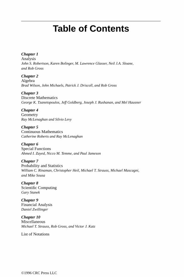
Table of Contents
Chapter 1Analysis John S. Robertson, Karen Bolinger, M. Lawrence Glasser, Neil J.A. Sloane,and Rob Gross
Chapter 2AlgebraBrad Wilson, John Michaels, Patrick J. Driscoll, and Rob Gross
Chapter 3Discrete MathematicsGeorge K. Tzanetopoulos, Jeff Goldberg, Joseph J. Rushanan, and Mel Hausner
Chapter 4GeometryRay McLenaghan and Silvio Levy
Chapter 5Continuous MathematicsCatherine Roberts and Ray McLenaghan
Chapter 6Special FunctionsAhmed I. Zayed, Nicco M. Temme, and Paul Jameson
Chapter 7Probability and StatisticsWilliam C. Rinaman, Christopher Heil, Michael T. Strauss, Michael Mascagni,and Mike Sousa
Chapter 8Scientific ComputingGary Stanek
Chapter 9Financial AnalysisDaniel Zwillinger
Chapter 10MiscellaneousMichael T. Strauss, Rob Gross, and Victor J. Katz
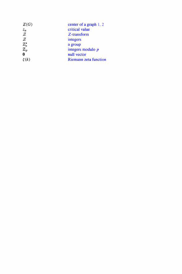
List of Notations
©1996 CRC Press LLC

Chapter 1Analysis
1.1 CONSTANTS1.1.1 Types of numbers1.1.2 Representation of numbers1.1.3 Decimal multiples and prefixes1.1.4 Roman numerals1.1.5 Decimal equivalents of common fractions1.1.6 Hexadecimal addition and subtraction table1.1.7 Hexadecimal multiplication table1.1.8 Hexadecimal–decimal fraction conversion table
1.2 SPECIAL NUMBERS1.2.1 Positive powers of 21.2.2 Negative powers of 21.2.3 Powers of 16 in decimal scale1.2.4 Powers of 10 in hexadecimal scale1.2.5 Special constants 1.2.6 Factorials1.2.7 Important numbers in different bases1.2.8 Bernoulli polynomials and numbers1.2.9 Euler polynomials and numbers1.2.10 Fibonacci numbers1.2.11 Powers of integers 1.2.12 Sums of powers of integers 1.2.13 Negative integer powers1.2.14 Integer sequences1.2.15 de Bruijn sequences
1.3 SERIES AND PRODUCTS 1.3.1 Definitions 1.3.2 General properties1.3.3 Convergence tests1.3.4 Types of series1.3.5 Summation formulae 1.3.6 Improving convergence: Shanks transformation1.3.7 Summability methods1.3.8 Operations with series1.3.9 Miscellaneous sums and series1.3.10 Infinite series1.3.11 Infinite products1.3.12 Infinite products and infinite series
©1996 CRC Press LLC

1.4 FOURIER SERIES1.4.1 Special cases1.4.2 Alternate forms1.4.3 Useful series1.4.4 Expansions of basic periodic functions
1.5 COMPLEX ANALYSIS1.5.1 Definitions1.5.2 Operations on complex numbers1.5.3 Powers and roots of complex numbers1.5.4 Functions of a complex variable1.5.5 Cauchy–Riemann equations1.5.6 Cauchy integral theorem1.5.7 Cauchy integral formula 1.5.8 Taylor series expansions1.5.9 Laurent series expansions1.5.10 Zeros and singularities1.5.11 Residues1.5.12 The argument principle1.5.13 Transformations and mappings1.5.14 Bilinear transformations 1.5.15 Table of transformations 1.5.16 Table of conformal mappings
1.6 REAL ANALYSIS 1.6.1 Relations 1.6.2 Functions (mappings) 1.6.3 Sets of real numbers 1.6.4 Topology 1.6.5 Metric space 1.6.6 Convergence in R 1.6.7 Continuity in R1.6.8 Convergence in Lp1.6.9 Convergence in L2
1.6.10 Asymptotic relationships
1.7 GENERALIZED FUNCTIONS
REFERENCES
©1996 CRC Press LLC

1.1 CONSTANTS
1.1.1 TYPES OF NUMBERS
Natural numbersThe natural numbers are customarily denoted by N. They are the set 0, 1, 2, . . . .Many authors do not consider 0 to be a natural number.
IntegersThe integers are customarily denoted by Z. They are the set 0,±1,±2, . . . .
Rational numbersThe rational numbers are customarily denoted by Q. They are the set p
q| p, q ∈
Z, q = 0. Two fractions p
qand r
sare equal if ps = qr .
Addition of fractions is defined by p
q+ r
s= ps+qr
qs. Multiplication of fractions
is defined by p
q· rs
= pr
qs.
Real numbersThe real numbers are customarily denoted by R. Real numbers are defined to beconverging sequences of rational numbers or as decimals that might or might notrepeat.
Real numbers are often divided into two subsets. One subset, the algebraicnumbers, are real numbers which solve a polynomial equation in one variable withinteger coefficients. For example; 1√
2is an algebraic number because it solves the
polynomial equation 2x2 − 1 = 0, and rational numbers are algebraic. Real numbersthat are not algebraic numbers are called transcendental numbers. Examples oftranscendental numbers include π and e.
Complex numbersThe complex numbers are customarily denoted by C. They are numbers of the forma + bi, where i2 = −1, and a and b are real numbers. See Section 1.5.
The sum of two complex numbers a + bi and c + di is a + c + (b + d)i. Theproduct of two complex numbers a + bi and c + di is ac − bd + (ad + bc)i. Thereciprocal of the complex number a+bi is a
a2+b2 − ba2+b2 i. If z = a+bi, the complex
conjugate of z is z = a − bi. Properties include: z+ w = z+ w and zw = z w.
©1996 CRC Press LLC

1.1.2 REPRESENTATION OF NUMBERS
Numerals as usually written have radix or base 10, because the numeral anan−1 . . .
a2a1a0 represents the number an10n+an−110n−1+· · ·+a2102 +a110+a0. However,other bases can be used, particularly bases 2, 8, and 16 (called binary, octal, andhexadecimal, respectively). When another base is used, it is indicated by a subscript:
5437 = 5 × 72 + 4 × 7 + 3 = 276,
101112 = 1 × 24 + 0 × 23 + 1 × 22 + 1 × 2 + 1 = 23,
A316 = 10 × 16 + 3 = 163.
When writing a number in base b, the digits used can range from 0 to b−1. If b > 10,then the digit A stands for 10, B for 11, etc.
The above algorithm can be used to convert a numeral from base b to base 10. Toconvert a numeral from base 10 to base b, divide the numeral by b, and the remainderwill be the last digit. Then divide the quotient by b, using the remainder as theprevious digit. Continue dividing the quotient by b until a quotient of 0 is arrived at.
For example, to convert 574 to base 12, divide, yielding a remainder of 10 anda quotient of 47. Hence, the last digit of the answer is A. Divide 47 by 12, giving aremainder of 11 again and a quotient of 3. Divide 3 by 12, giving a remainder of 3and a quotient of 0. Therefore, 57510 = 3BA12.
In general, to convert from base b to base r , it is simplest to convert to base 10as an intermediate step. However, it is simple to convert from base b to base ba . Forexample, to convert 1101111012 to base 16, group the digits in fours (because 16is 24), yielding 1 1011 1101, and then convert each group of 4 to base 16 directly,yielding 1BD16.
©1996 CRC Press LLC

1.1.3 DECIMAL MULTIPLES AND PREFIXES
The prefix and symbols below are taken from Conference Generale des Poids etMesures, 1991. The common names are for the U.S.
Multiple Prefix Symbol Common name
10(10100) googolplex10100 googol1024 yotta Y heptillion1021 zetta Z hexillion1018 exa E quintillion1015 peta P quadrillion1012 tera T trillion109 giga G billion106 mega M million103 kilo K thousand102 hecto h hundred101 deca da ten10−1 deci d tenth10−2 centi c hundreth10−3 milli m thousandth10−6 micro µ (Greek mu) millionth10−9 nano n billionth10−12 pico p trillionth10−15 femto f quadrillionth10−18 atto a quintillionth10−21 zepto z hexillionth10−24 yocto y heptillionth
1.1.4 ROMAN NUMERALS
The major symbols in Roman numerals are I = 1, V = 5, X = 10, L = 50, C = 100,D = 500, and M = 1,000. The rules for constructing Roman numerals are
1. A symbol following one of equal or greater value adds its value (for example,II = 2, XI = 11, DV = 505).
2. A symbol following one of lesser value has the lesser value subtracted from thelarger value (for example, IV = 4, IX = 9, VM = 995).
3. When a symbol stands between two of greater value, its value is subtracted fromthe second and the result is added to the first (for example, XIV = 10+(5−1) =14, CIX = 100 + (10 − 1) = 109, DVL = 500 + (50 − 5) = 545).
4. When two ways exist for representing a number, the one in which the symbol oflarger value occurs earlier in the string is preferred (for example, 14 is representedas XIV, not as VIX).
©1996 CRC Press LLC

Decimal number 1 2 3 4 5 6 7 8 9Roman numeral I II III IV V VI VII VIII IX
10 14 50 200 400 500 600 999 1000X XIV L CC CD D DC CMXCIX M
1950 1960 1970 1980 1990MCML MCMLX MCMLXX MCMLXXX MCMXC
1996 1997 1998 1999 2000MCMXCVI MCMXCVII MCMXCVIII MCMXCIX MM
1.1.5 DECIMAL EQUIVALENTS OF COMMON FRACTIONS1/64 0.015625
1/32 2/64 0.031253/64 0.046875
1/16 2/32 4/64 0.06255/64 0.078125
3/32 6/64 0.093757/64 0.109375
1/8 4/32 8/64 0.1259/64 0.140625
5/32 10/64 0.1562511/64 0.171875
3/16 6/32 12/64 0.187513/64 0.203125
7/32 14/64 0.2187515/64 0.234375
1/4 8/32 16/64 0.2517/64 0.265625
9/32 18/64 0.2812519/64 0.296875
5/16 10/32 20/64 0.312521/64 0.328125
11/32 22/64 0.3437523/64 0.359375
3/8 12/32 24/64 0.37525/64 0.390625
13/32 26/64 0.4062527/64 0.421875
7/16 14/32 28/64 0.437529/64 0.453125
15/32 30/64 0.4687531/64 0.484375
1/2 16/32 32/64 0.5
33/64 0.51562517/32 34/64 0.53125
35/64 0.5468759/16 18/32 36/64 0.5625
37/64 0.57812519/32 38/64 0.59375
39/64 0.6093755/8 20/32 40/64 0.625
41/64 0.64062521/32 42/64 0.65625
43/64 0.67187511/16 22/32 44/64 0.6875
45/64 0.70312523/32 46/64 0.71875
47/64 0.7343753/4 24/32 48/64 0.75
49/64 0.76562525/32 50/64 0.78125
51/64 0.79687513/16 26/32 52/64 0.8125
53/64 0.82812527/32 54/64 0.84375
55/64 0.8593757/8 28/32 56/64 0.875
57/64 0.89062529/32 58/64 0.90625
59/64 0.92187515/16 30/32 60/64 0.9375
61/64 0.95312531/32 62/64 0.96875
63/64 0.9843751/1 32/32 64/64 1
©1996 CRC Press LLC

1.1.6 HEXADECIMAL ADDITION AND SUBTRACTION TABLE
A = 10, B = 11, C = 12, D = 13, E = 14, F = 15.Example: 6 + 2 = 8; hence 8 − 6 = 2 and 8 − 2 = 6.Example: 4 + E = 12; hence 12 − 4 = E and 12 − E = 4.
1 2 3 4 5 6 7 8 9 A B C D E F1 02 03 04 05 06 07 08 09 0A 0B 0C 0D 0E 0F 102 03 04 05 06 07 08 09 0A 0B 0C 0D 0E 0F 10 113 04 05 06 07 08 09 0A 0B 0C 0D 0E 0F 10 11 124 05 06 07 08 09 0A 0B 0C 0D 0E 0F 10 11 12 135 06 07 08 09 0A 0B 0C 0D 0E 0F 10 11 12 13 146 07 08 09 0A 0B 0C 0D 0E 0F 10 11 12 13 14 157 08 09 0A 0B 0C 0D 0E 0F 10 11 12 13 14 15 168 09 0A 0B 0C 0D 0E 0F 10 11 12 13 14 15 16 179 0A 0B 0C 0D 0E 0F 10 11 12 13 14 15 16 17 18A 0B 0C 0D 0E 0F 10 11 12 13 14 15 16 17 18 19B 0C 0D 0E 0F 10 11 12 13 14 15 16 17 18 19 1AC 0D 0E 0F 10 11 12 13 14 15 16 17 18 19 1A 1BD 0E 0F 10 11 12 13 14 15 16 17 18 19 1A 1B 1CE 0F 10 11 12 13 14 15 16 17 18 19 1A 1B 1C 1DF 10 11 12 13 14 15 16 17 18 19 1A 1B 1C 1D 1E
1.1.7 HEXADECIMAL MULTIPLICATION TABLE
Example: 2 × 4 = 8.Example: 2 × F = 1E.
1 2 3 4 5 6 7 8 9 A B C D E F1 01 02 03 04 05 06 07 08 09 0A 0B 0C 0D 0E 0F2 02 04 06 08 0A 0C 0E 10 12 14 16 18 1A 1C 1E3 03 06 09 0C 0F 12 15 18 1B 1E 21 24 27 2A 2D4 04 08 0C 10 14 18 1C 20 24 28 2C 30 34 38 3C5 05 0A 0F 14 19 1E 23 28 2D 32 37 3C 41 46 4B6 06 0C 12 18 1E 24 2A 30 36 3C 42 48 4E 54 5A7 07 0E 15 1C 23 2A 31 38 3F 46 4D 54 5B 62 698 08 10 18 20 28 30 38 40 48 50 58 60 68 70 789 09 12 1B 24 2D 36 3F 48 51 5A 63 6C 75 7E 87A 0A 14 1E 28 32 3C 46 50 5A 64 6E 78 82 8C 96B 0B 16 21 2C 37 42 4D 58 63 6E 79 84 8F 9A A5C 0C 18 24 30 3C 48 54 60 6C 78 84 90 9C A8 B4D 0D 1A 27 34 41 4E 5B 68 75 82 8F 9C A9 B6 C3E 0E 1C 2A 38 46 54 62 70 7E 8C 9A A8 B6 C4 D2F 0F 1E 2D 3C 4B 5A 69 78 87 96 A5 B4 C3 D2 E1
©1996 CRC Press LLC

1.1.8 HEXADECIMAL–DECIMAL FRACTION CONVERSIONTABLEHex Decimal Hex Decimal Hex Decimal Hex Decimal
.00 0 .40 0.250000 .80 0.500000 .C0 0.750000
.01 0.003906 .41 0.253906 .81 0.503906 .C1 0.753906
.02 0.007812 .42 0.257812 .82 0.507812 .C2 0.757812
.03 0.011718 .43 0.261718 .83 0.511718 .C3 0.761718
.04 0.015625 .44 0.265625 .84 0.515625 .C4 0.765625
.05 0.019531 .45 0.269531 .85 0.519531 .C5 0.769531
.06 0.023437 .46 0.273437 .86 0.523437 .C6 0.773437
.07 0.027343 .47 0.277343 .87 0.527343 .C7 0.777343
.08 0.031250 .48 0.281250 .88 0.531250 .C8 0.781250
.09 0.035156 .49 0.285156 .89 0.535156 .C9 0.785156
.0A 0.039062 .4A 0.289062 .8A 0.539062 .CA 0.789062
.0B 0.042968 .4B 0.292968 .8B 0.542968 .CB 0.792968
.0C 0.046875 .4C 0.296875 .8C 0.546875 .CC 0.796875
.0D 0.050781 .4D 0.300781 .8D 0.550781 .CD 0.800781
.0E 0.054687 .4E 0.304687 .8E 0.554687 .CE 0.804687
.0F 0.058593 .4F 0.308593 .8F 0.558593 .CF 0.808593
.10 0.062500 .50 0.312500 .90 0.562500 .D0 0.812500
.11 0.066406 .51 0.316406 .91 0.566406 .D1 0.816406
.12 0.070312 .52 0.320312 .92 0.570312 .D2 0.820312
.13 0.074218 .53 0.324218 .93 0.574218 .D3 0.824218
.14 0.078125 .54 0.328125 .94 0.578125 .D4 0.828125
.15 0.082031 .55 0.332031 .95 0.582031 .D5 0.832031
.16 0.085937 .56 0.335937 .96 0.585937 .D6 0.835937
.17 0.089843 .57 0.339843 .97 0.589843 .D7 0.839843
.18 0.093750 .58 0.343750 .98 0.593750 .D8 0.843750
.19 0.097656 .59 0.347656 .99 0.597656 .D9 0.847656
.1A 0.101562 .5A 0.351562 .9A 0.601562 .DA 0.851562
.1B 0.105468 .5B 0.355468 .9B 0.605468 .DB 0.855468
.1C 0.109375 .5C 0.359375 .9C 0.609375 .DC 0.859375
.1D 0.113281 .5D 0.363281 .9D 0.613281 .DD 0.863281
.1E 0.117187 .5E 0.367187 .9E 0.617187 .DE 0.867187
.1F 0.121093 .5F 0.371093 .9F 0.621093 .DF 0.871093
©1996 CRC Press LLC

Hex Decimal Hex Decimal Hex Decimal Hex Decimal.20 0.125000 .60 0.375000 .A0 0.625000 .E0 0.875000.21 0.128906 .61 0.378906 .A1 0.628906 .E1 0.878906.22 0.132812 .62 0.382812 .A2 0.632812 .E2 0.882812.23 0.136718 .63 0.386718 .A3 0.636718 .E3 0.886718.24 0.140625 .64 0.390625 .A4 0.640625 .E4 0.890625.25 0.144531 .65 0.394531 .A5 0.644531 .E5 0.894531.26 0.148437 .66 0.398437 .A6 0.648437 .E6 0.898437.27 0.152343 .67 0.402343 .A7 0.652343 .E7 0.902343.28 0.156250 .68 0.406250 .A8 0.656250 .E8 0.906250.29 0.160156 .69 0.410156 .A9 0.660156 .E9 0.910156.2A 0.164062 .6A 0.414062 .AA 0.664062 .EA 0.914062.2B 0.167968 .6B 0.417968 .AB 0.667968 .EB 0.917968.2C 0.171875 .6C 0.421875 .AC 0.671875 .EC 0.921875.2D 0.175781 .6D 0.425781 .AD 0.675781 .ED 0.925781.2E 0.179687 .6E 0.429687 .AE 0.679687 .EE 0.929687.2F 0.183593 .6F 0.433593 .AF 0.683593 .EF 0.933593
.30 0.187500 .70 0.437500 .B0 0.687500 .F0 0.937500
.31 0.191406 .71 0.441406 .B1 0.691406 .F1 0.941406
.32 0.195312 .72 0.445312 .B2 0.695312 .F2 0.945312
.33 0.199218 .73 0.449218 .B3 0.699218 .F3 0.949218
.34 0.203125 .74 0.453125 .B4 0.703125 .F4 0.953125
.35 0.207031 .75 0.457031 .B5 0.707031 .F5 0.957031
.36 0.210937 .76 0.460937 .B6 0.710937 .F6 0.960937
.37 0.214843 .77 0.464843 .B7 0.714843 .F7 0.964843
.38 0.218750 .78 0.468750 .B8 0.718750 .F8 0.968750
.39 0.222656 .79 0.472656 .B9 0.722656 .F9 0.972656
.3A 0.226562 .7A 0.476562 .BA 0.726562 .FA 0.976562
.3B 0.230468 .7B 0.480468 .BB 0.730468 .FB 0.980468.3C 0.234375 .7C 0.484375 .BC 0.734375 .FC 0.984375.3D 0.238281 .7D 0.488281 .BD 0.738281 .FD 0.988281.3E 0.242187 .7E 0.492187 .BE 0.742187 .FE 0.992187.3F 0.246093 .7F 0.496093 .BF 0.746093 .FF 0.996093
1.2 SPECIAL NUMBERS
1.2.1 POSITIVE POWERS OF 2
n 2n n 2n
1 2 6 642 4 7 1283 8 8 2564 16 9 5125 32 10 1024
©1996 CRC Press LLC

n 2n n 2n
11 204812 409613 819214 1638415 32768
16 6553617 13107218 26214419 52428820 1048576
21 209715222 419430423 838860824 1677721625 33554432
26 6710886427 13421772828 26843545629 53687091230 1073741824
31 214748364832 429496729633 858993459234 1717986918435 34359738368
36 6871947673637 13743895347238 27487790694439 54975581388840 1099511627776
41 219902325555242 439804651110443 879609302330844 1759218604441645 351843720088832
46 7036874417766447 14073748835532848 28147497671065649 56294995342131250 1125899906842624
51 225179981368524852 450359962737049653 900719925474099254 1801439850948198455 36028797018963968
56 7205759403792793657 14411518807585587258 28823037615171174459 57646075230342348860 1152921504606846976
61 230584300921369395262 461168601842738790463 922337203685477580864 1844674407370955161665 36893488147419103232
66 7378697629483820646467 14757395258967641292868 29514790517935282585669 59029581035870565171270 1180591620717411303424
71 236118324143482260684872 472236648286964521369673 944473296573929042739274 1888946593147858085478475 37778931862957161709568
76 7555786372591432341913677 15111572745182864683827278 30223145490365729367654479 60446290980731458735308880 1208925819614629174706176
81 241785163922925834941235282 483570327845851669882470483 967140655691703339764940884 1934281311383406679529881685 38685626227668133590597632
86 7737125245533626718119526487 15474250491067253436239052888 30948500982134506872478105689 61897001964269013744956211290 1237940039285380274899124224
©1996 CRC Press LLC

1.2.2 NEGATIVE POWERS OF 2
n 2−n
1 0.52 0.253 0.1254 0.06255 0.03125
6 0.0156257 0.00781258 0.003906259 0.001953125
10 0.0009765625
11 0.0004882812512 0.00024414062513 0.000122070312514 0.0000610351562515 0.000030517578125
16 0.000015258789062517 0.0000076293945312518 0.00000381469726562519 0.000001907348632812520 0.00000095367431640625
21 0.00000047683715820312522 0.000000238418579101562523 0.0000001192092895507812524 0.00000005960464477539062525 0.0000000298023223876953125
26 0.0000000149011611938476562527 0.00000000745058059692382812528 0.000000003725290298461914062529 0.0000000018626451492309570312530 0.000000000931322574615478515625
31 0.000000000465661287307739257812532 0.0000000002328306436538696289062533 0.00000000011641532182693481445312534 0.000000000058207660913467407226562535 0.00000000002910383045673370361328125
36 0.00000000001455191522836685180664062537 0.000000000007275957614183425903320312538 0.0000000000036379788070917129516601562539 0.00000000000181898940354585647583007812540 0.0000000000009094947017729282379150390625
©1996 CRC Press LLC

1.2.3 POWERS OF 16 IN DECIMAL SCALE
n = 16n = 16−n =0 1 11 16 0.06252 256 0.003906253 4096 0.0002441406254 65536 0.00001525878906255 1048576 0.000000953674316406256 16777216 0.0000000596046447753906257 268435456 0.00000000372529029846191406258 4294967296 0.000000000232830643653869628906259 68719476736 0.000000000014551915228366851806640625
10 1099511627776 0.000000000000909494701772928237915039062511 1759218604441612 28147497671065613 450359962737049614 7205759403792793615 115292150460684697616 1844674407370955161617 29514790517935282585618 472236648286964521369619 7555786372591432341913620 1208925819614629174706176
1.2.4 POWERS OF 10 IN HEXADECIMAL SCALEn = 10n = 10−n =
0 1 11 A 0.19999999999999999999 . . .2 64 0.028F5C28F5C28F5C28F5 . . .3 3E8 0.004189374BC6A7EF9DB2 . . .4 2710 0.00068DB8BAC710CB295E . . .5 186A0 0.0000A7C5AC471B478423 . . .6 F4240 0.000010C6F7A0B5ED8D36 . . .7 989680 0.000001AD7F29ABCAF485 . . .8 5F5E100 0.0000002AF31DC4611873 . . .9 3B9ACA00 0.000000044B82FA09B5A5 . . .
10 2540BE400 0.000000006DF37F675EF6 . . .11 174876E800 0.000000000AFEBFF0BCB2 . . .12 E8D4A51000 0.000000000119799812DE . . .13 9184E72A000 0.00000000001C25C26849 . . .14 5AF3107A4000 0.000000000002D09370D4 . . .15 38D7EA4C68000 0.000000000000480EBE7B . . .
16 2386F26FC10000 0.0000000000000734ACA5 . . .
©1996 CRC Press LLC

1.2.5 SPECIAL CONSTANTS
The constant π
The transcedental number π is defined as the ratio of the circumference of a circle tothe diameter. It is also the ratio of the area of a circle to the square of the radius (r)and appears in several other formulas from elementary geometry (see Section 4.6)
C(circle) = 2πr, V (sphere) = 4
3πr3,
A(circle) = πr2, SA(sphere) = 4πr2.
One method of computing π is to use the infinite series for the function tan−1 x
and one of the identities
π = 4 tan−1 1 = 6 tan−1 1√3
= 2 tan−1 1
2+ 2 tan−1 1
3+ 8 tan−1 1
5− 2 tan−1 1
239
= 24 tan−1 1
8+ 8 tan−1 1
57+ 4 tan−1 1
239
= 48 tan−1 1
18+ 32 tan−1 1
57− 20 tan−1 1
239
There are many other identities involving π . See Section 1.4.3. For example:π3
32 = ∑∞n=0
(−1)n
(2n+1)3 = 1 − 127 + 1
125 − 1343 + . . . .
To 200 decimal places:
π ≈ 3. 14159 26535 89793 23846 26433 83279 50288 41971 69399 3751058209 74944 59230 78164 06286 20899 86280 34825 34211 7067982148 08651 32823 06647 09384 46095 50582 23172 53594 0812848111 74502 84102 70193 85211 05559 64462 29489 54930 38196
©1996 CRC Press LLC

To 50 decimal places:
π/20 ≈ 0.15707 96326 79489 66192 31321 69163 97514 42098 58469 96876π/15 ≈ 0.20943 95102 39319 54923 08428 92218 63352 56131 44626 62501π/12 ≈ 0.26179 93877 99149 43653 85536 15273 29190 70164 30783 28126π/11 ≈ 0.28559 93321 44526 65804 20584 89389 04571 67451 97218 12501π/10 ≈ 0.31415 92653 58979 32384 62643 38327 95028 84197 16939 93751π/9 ≈ 0.34906 58503 98865 91538 47381 53697 72254 26885 74377 70835π/8 ≈ 0.39269 90816 98724 15480 78304 22909 93786 05246 46174 92189π/7 ≈ 0.44879 89505 12827 60549 46633 40468 50041 20281 67057 05359π/6 ≈ 0.52359 87755 98298 87307 71072 30546 58381 40328 61566 56252π/5 ≈ 0.62831 85307 17958 64769 25286 76655 90057 68394 33879 87502π/4 ≈ 0.78539 81633 97448 30961 56608 45819 87572 10492 92349 84378π/3 ≈ 1.04719 75511 96597 74615 42144 61093 16762 80657 23133 12504π/2 ≈ 1.57079 63267 94896 61923 13216 91639 75144 20985 84699 68755
2π/3 ≈ 2.09439 51023 93195 49230 84289 22186 33525 61314 46266 250073π/2 ≈ 4.71238 89803 84689 85769 39650 74919 25432 62957 54099 062665π/2 ≈ 7.85398 16339 74483 09615 66084 58198 75721 04929 23498 43776√
π ≈ 1.77245 38509 05516 02729 81674 83341 14518 27975 49456 12239
The constant e
The transcedental number e is the base of natural logarithms. It is given by
e = limn→∞
(1 + 1
n
)n=
∞∑n=0
1
n!.
To 200 decimal places:
e ≈ 2. 71828 18284 59045 23536 02874 71352 66249 77572 47093 6999595749 66967 62772 40766 30353 54759 45713 82178 52516 6427427466 39193 20030 59921 81741 35966 29043 57290 03342 9526059563 07381 32328 62794 34907 63233 82988 07531 95251 01901
To 50 decimal places:
e/8 ≈ 0.33978 52285 57380 65442 00359 33919 08281 22196 55886 71249e/7 ≈ 0.38832 59754 94149 31933 71839 24478 95178 53938 92441 95714e/6 ≈ 0.45304 69714 09840 87256 00479 11892 11041 62928 74515 61666e/5 ≈ 0.54365 63656 91809 04707 20574 94270 53249 95514 49418 73999e/4 ≈ 0.67957 04571 14761 30884 00718 67838 16562 44393 11773 42499e/3 ≈ 0.90609 39428 19681 74512 00958 23784 22083 25857 49031 23332e/2 ≈ 1.35914 09142 29522 61768 01437 35676 33124 88786 23546 84998
2e/3 ≈ 1.81218 78856 39363 49024 01916 47568 44166 51714 98062 46664
The function ex is defined by ex = ∑∞n=0
xn
n! . The numbers e and π are related by theformula eπi = −1.
©1996 CRC Press LLC

To 50 decimal places:
eπ ≈ 23.14069 26327 79269 00572 90863 67948 54738 02661 06242 60021πe ≈ 22.45915 77183 61045 47342 71522 04543 73502 75893 15133 99669
The constant γ
Euler’s constant γ is defined by
γ = limn→∞
(n∑k=1
1
k− log n
).
To 200 decimal places:
γ ≈ 0. 57721 56649 01532 86060 65120 90082 40243 10421 59335 9399235988 05767 23488 48677 26777 66467 09369 47063 29174 6749514631 44724 98070 82480 96050 40144 86542 83622 41739 9764492353 62535 00333 74293 73377 37673 94279 25952 58247 09492
It is not known whether γ is rational or irrational.
The constant φ
The golden ratio φ is defined as the positive root of the equation φ
1 = 1+φφ
; that is
φ = 1+√5
2 .To 200 decimal places:
φ ≈ 1. 61803 39887 49894 84820 45868 34365 63811 77203 09179 8057628621 35448 62270 52604 62818 90244 97072 07204 18939 1137484754 08807 53868 91752 12663 38622 23536 93179 31800 6076672635 44333 89086 59593 95829 05638 32266 13199 28290 26788
1.2.6 FACTORIALS
The factorial of n, denoted n!, is the product of all integers less than or equal to n.n! = n · (n−1) · (n−2) · · · 2 ·1. The double factorial of n, denoted n!!, is the productof every other integer: n!! = n · (n− 2) · (n− 4) · · · , where the last element in theproduct is either 2 or 1, depending on whether n is even or odd. The generalization ofthe factorial function is the gamma function (see Section 6.11). When n is an integer,(n) = (n− 1)!.
The shifted factorial (also called the falling factorial and Pochhammer’s symbol)is denoted by (a)n (sometimes an) and is defined as
(a)n = a · (a + 1) · (a + 2) · · ·︸ ︷︷ ︸n terms
= (a + n− 1)!
(a − 1)!= (a + n)
(a).
(1.2.1)
©1996 CRC Press LLC

The q-shifted factorial is defined as
(a; q)0 = 1, (a; q)n = (1 − a)(1 − aq) . . . (1 − aqn−1).
(1.2.2)
n n! log10 n! n!! log10 n!!
0 1 0.00000 1 0.000001 1 0.00000 1 0.000002 2 0.30103 2 0.301033 6 0.77815 3 0.477124 24 1.38021 8 0.903095 120 2.07918 15 1.176096 720 2.85733 48 1.681247 5040 3.70243 105 2.021198 40320 4.60552 384 2.584339 3.6288 × 10⁵ 5.55976 945 2.97543
10 3.6288 × 10⁶ 6.55976 3840 3.5843311 3.9917 × 10⁷ 7.60116 10395 4.0168212 4.7900 × 10⁸ 8.68034 46080 4.6635113 6.2270 × 10⁹ 9.79428 1.3514 × 10⁵ 5.1307714 8.7178 × 10¹⁰ 10.94041 6.4512 × 10⁵ 5.8096415 1.3077 × 10¹² 12.11650 2.0270 × 10⁶ 6.3068616 2.0923 × 10¹³ 13.32062 1.0322 × 10⁷ 7.0137617 3.5569 × 10¹⁴ 14.55107 3.4459 × 10⁷ 7.5373118 6.4024 × 10¹⁵ 15.80634 1.8579 × 10⁸ 8.2690319 1.2165 × 10¹⁷ 17.08509 6.5473 × 10⁸ 8.8160620 2.4329 × 10¹⁸ 18.38612 3.7159 × 10⁹ 9.5700621 5.1091 × 10¹⁹ 19.70834 1.3749 × 10¹⁰ 10.1382822 1.1240 × 10²¹ 21.05077 8.1750 × 10¹⁰ 10.9124923 2.5852 × 10²² 22.41249 3.1623 × 10¹¹ 11.5000124 6.2045 × 10²³ 23.79271 1.9620 × 10¹² 12.2927025 1.5511 × 1025 25.19065 7.9059 × 10¹² 12.8979530 2.6525 × 1032 32.42366 4.2850 × 10¹⁶ 16.6319540 8.1592 × 1047 47.91165 2.5511 × 1024 24.4067250 3.0414 × 1064 64.48307 5.2047 × 1032 32.7164060 8.3210 × 1081 81.92017 2.8481 × 1041 41.4545670 1.1979 × 10100 100.07841 3.5504 × 1050 50.5502880 7.1569 × 10118 118.85473 8.9711 × 1059 59.9528490 1.4857 × 10138 138.17194 4.2088 × 1069 69.62416
100 9.3326 × 10157 157.97000 3.4243 × 1079 79.53457110 1.5882 × 10178 178.20092 4.5744 × 1089 89.66033120 6.6895 × 10198 198.82539 9.5934 × 1099 99.98197130 6.4669 × 10219 219.81069 3.0428 × 10110 110.48328140 1.3462 × 10241 241.12911 1.4142 × 10121 121.15050150 5.7134 × 10262 262.75689 9.3726 × 10131 131.97186500 1.2201 × 101134 1134.0864 5.8490 × 10567 567.76709
1000 4.0239 × 102567 2567.6046 3.9940 × 101284 1284.6014
©1996 CRC Press LLC

1.2.7 IMPORTANT NUMBERS IN DIFFERENT BASESBase 2 π = 11.00100100001111110110101010001 . . .
e = 10.10110111111000010101000101100 . . .γ = 0.100100111100010001100111111000 . . .√2 = 1.011010100000100111100110011001 . . .
log 2 = 0.101100010111001000010111111101 . . .
Base 8 π = 3.110375524210264302151423063050 . . .e = 2.557605213050535512465277342542 . . .γ = 0.447421477067666061722321574376 . . .√2 = 1.324047463177167462204262766115 . . .
log 2 = 0.542710277575071736325711707316 . . .
Base 12 π = 3.184809493B918664573A6211BB1515 . . .e = 2.8752360698219BA71971009B388AA8 . . .γ = 0.6B15188A6760B381B754334520434A . . .√2 = 1.4B79170A07B85737704B0854868535 . . .
log 2 = 0.839912483369AB213742A346792537 . . .
Base 16 π = 3.243F6A8885A308D313198A2E037073 . . .e = 2.B7E151628AED2A6ABF7158809CF4F3 . . .γ = 0.93C467E37DB0C7A4D1BE3F810152CB . . .√2 = 1.6A09E667F3BCC908B2FB1366EA957D . . .
log 2 = 0.B17217F7D1CF79ABC9E3B39803F2F6 . . .
1.2.8 BERNOULLI POLYNOMIALS AND NUMBERS
The Bernoulli polynomials Bn(x) are defined by the generating function
text
et − 1=
∞∑n=0
Bn(x)tn
n!. (1.2.3)
These polynomials can also be defined recursively by means of B0(x) = 1, B ′n(x) =
nBn−1(x), and∫ 1
0 Bn(x) dx = 0 for n ≥ 1. The identity Bk+1(x + 1) − Bk+1(x) =(k + 1)xk means that
1k + 2k + · · · + nk = Bk+1(n+ 1)− Bk+1(0)
k + 1. (1.2.4)
n Bn(x)
0 11 (2x − 1)/22 (6x2 − 6x + 1)/63 (2x3 − 3x2 + x)/24 (30x4 − 60x3 + 30x2 − 1)/305 (6x5 − 15x4 + 10x3 − x)/6
The Bernoulli numbers are the Bernoulli polynomials evaluated at 0: Bn =Bn(0). A generating function for the Bernoulli numbers is
©1996 CRC Press LLC

∑∞n=0 Bn
tn
n! = tet−1 . In the following table each Bernoulli number is written as a
fraction of integers: Bn = Nn/Dn. Note that B2m+1 = 0 for m ≥ 1.
n Nn Dn Bn
0 1 1 1.000000000 × 100
1 −1 2 −5.000000000 × 10⁻¹
2 1 6 1.666666667 × 10⁻¹
4 −1 30 −3.333333333 × 10⁻²
6 1 42 2.380952381 × 10⁻²
8 −1 30 −3.333333333 × 10⁻²
10 5 66 7.575757576 × 10⁻²
12 −691 2730 −2.531135531 × 10⁻¹
14 7 6 1.166666667 × 100
16 −3617 510 −7.092156863 × 100
18 43867 798 5.497117794 × 101
20 −174611 330 −5.291242424 × 10²
22 854513 138 6.192123188 × 10³
24 −236364091 2730 −8.658025311 × 10⁴
26 8553103 6 1.425517167 × 10⁶
28 −23749461029 870 −2.729823107 × 10⁷
30 8615841276005 14322 6.015808739 × 10⁸
32 −7709321041217 510 −1.511631577 × 10¹⁰
34 2577687858367 6 4.296146431 × 10¹¹
36 −26315271553053477373 1919190 −1.371165521 × 10¹³
38 2929993913841559 6 4.883323190 × 10¹⁴
40 −261082718496449122051 13530 −1.929657934 × 10¹⁶
1.2.9 EULER POLYNOMIALS AND NUMBERS
The Euler polynomials En(x) are defined by the generating function
2ext
et + 1=
∞∑n=0
En(x)tn
n!. (1.2.5)
n En(x)
0 11 (2x − 1)/22 x2 − x
3 (4x3 − 6x2 + 1)/44 x4 − 2x3 + x
5 (2x5 − 5x4 + 5x2 − 1)/2
©1996 CRC Press LLC

Alternating sums of powers can be computed in terms of Euler polynomials
n∑i=1
(−1)n−i ik = nk − (n− 1)k + · · · ∓ 2k ± 1k = Ek(n+ 1)+ (−1)nEk(0)
2.
(1.2.6)
The Euler numbers are the Euler polynomials evaluated at 1/2, and scaled:En = 2nEn( 1
2 ). A generating function for the Euler numbers is
∞∑n=0
Entn
n!= 2et
n En2 −14 56 −618 1385
10 −5052112 270276514 −19936098116 1939151214518 −240487967544120 37037118823752522 −6934887439313790124 1551453416355708690526 −408707250929312389236128 125225964140362986546828530 −44154389324902310455368282132 17751939157953928943666478966534 −8072329923588789806216824745328136 4122206033951770212234707967125904538 −2348958052704310825201782857619894774140 1485115071811498001787715678140582668442542 −1036462273351961211939795730474518597631020144 794757942259759270360804051008807061951927380546 −666753751668554497743502847477374819752410768466148 6096278645568542158691685742876843153976539044435185
1.2.10 FIBONACCI NUMBERS
The Fibonacci numbers Fn are defined by the recurrence:
F1 = 1, F2 = 1, Fn+2 = Fn + Fn+1.
©1996 CRC Press LLC
e2t+1

An exact formula is available: Fn = 1√5
[(1+√
52
)n−(
1−√5
2
)n]. Note that lim
n→∞Fn+1
Fn=
φ, the golden ratio. Also, Fn ∼ φn/√
5 as n → ∞.
n Fn n Fn n Fn n Fn
1 1 14 377 27 196418 40 1023341552 1 15 610 28 317811 41 1655801413 2 16 987 29 514229 42 2679142964 3 17 1597 30 832040 43 4334944375 5 18 2584 31 1346269 44 7014087336 8 19 4181 32 2178309 45 11349031707 13 20 6765 33 3524578 46 18363119038 21 21 10946 34 5702887 47 29712150739 34 22 17711 35 9227465 48 4807526976
10 55 23 28657 36 14930352 49 777874204911 89 24 46368 37 24157817 50 1258626902512 144 25 75025 38 39088169 51 2036501107413 233 26 121393 39 63245986 52 32951280099
1.2.11 POWERS OF INTEGERS
n n3 n4 n5 n6 n7 n8 n10
1 1 1 1 1 1 1 12 8 16 32 64 128 256 10243 27 81 243 729 2187 6561 590494 64 256 1024 4096 16384 65536 10485765 125 625 3125 15625 78125 390625 97656256 216 1296 7776 46656 279936 1679616 604661767 343 2401 16807 117649 823543 5764801 2824752498 512 4096 32768 262144 2097152 16777216 10737418249 729 6561 59049 531441 4782969 43046721 3486784401
10 1000 10000 100000 1000000 10000000 100000000 1000000000011 1331 14641 161051 1771561 19487171 214358881 2593742460112 1728 20736 248832 2985984 35831808 429981696 61917364224
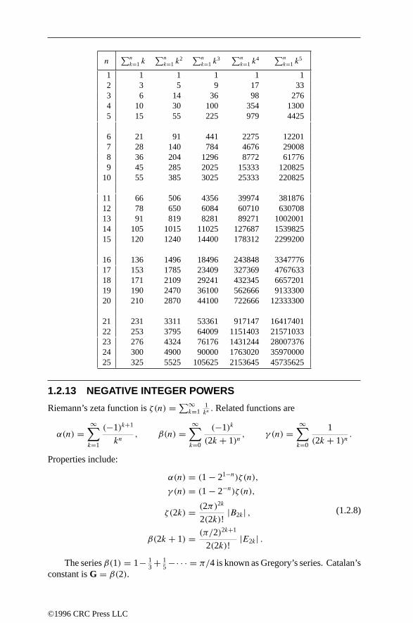
1.2.12 SUMS OF POWERS OF INTEGERS
Define sk(n) = 1k + 2k + · · · + nk = ∑nm=1 m
k. Properties include:
• sk(n) = (k + 1)−1[Bk+1(n+ 1)− Bk+1(0)
](where the Bk are Bernoulli polynomials, see Section 1.2.8).
©1996 CRC Press LLC

• Writing sk(n) as∑k+1
m=1 amnk−m+2 there is the recursion formula:
sk+1(n) =(k + 1
k + 2
)a1n
k+2 + · · · +(k + 1
k
)a3n
k
+ · · · +(k + 1
2
)ak+1n
2 +[
1 − (k + 1)k+1∑m=1
am
k + 3 −m
]n. (1.2.7)
s1(n) = 1 + 2 + 3 + · · · + n = 1
2n(n+ 1).
s2(n) = 12 + 22 + 32 + · · · + n2
= 1
6n(n+ 1)(2n+ 1).
s3(n) = 13 + 23 + 33 + · · · + n3
= 1
4(n2(n+ 1)2) = [s1(n)]
2.
s4(n) = 14 + 24 + 34 + · · · + n4
= 1
5(3n2 + 3n− 1)s2(n).
s5(n) = 15 + 25 + 35 + · · · + n5
= 1
12n2(n+ 1)2(2n2 + 2n− 1).
s6(n) = 16 + 26 + 36 + · · · + n6
= n
42(n+ 1)(2n+ 1)(3n4 + 6n3 − 3n+ 1).
s7(n) = 17 + 27 + 37 + · · · + n7
= n2
24(n+ 1)2(3n4 + 6n3 − n2 − 4n+ 2).
s8(n) = 18 + 28 + 38 + · · · + n8
= n
90(n+ 1)(2n+ 1)(5n6 + 15n5 + 5n4 − 15n3 − n2 + 9n− 3).
s9(n) = 19 + 29 + 39 + · · · + n9
= n2
20(n+ 1)2(2n6 + 6n5 + n4 − 8n3 + n2 + 6n− 3).
s10(n) = 110 + 210 + 310 + · · · + n10
= n
66(n+ 1)(2n+ 1)(3n8 + 12n7 + 8n6 − 18n5
− 10n4 + 24n3 + 2n2 − 15n+ 5).
©1996 CRC Press LLC
n∑n
k=1 k∑n
k=1 k2
∑n
k=1 k3
∑n
k=1 k4
∑n
k=1 k5
1 1 1 1 1 12 3 5 9 17 333 6 14 36 98 2764 10 30 100 354 13005 15 55 225 979 4425
6 21 91 441 2275 122017 28 140 784 4676 290088 36 204 1296 8772 617769 45 285 2025 15333 120825
10 55 385 3025 25333 220825
11 66 506 4356 39974 38187612 78 650 6084 60710 63070813 91 819 8281 89271 100200114 105 1015 11025 127687 153982515 120 1240 14400 178312 2299200
16 136 1496 18496 243848 334777617 153 1785 23409 327369 476763318 171 2109 29241 432345 665720119 190 2470 36100 562666 913330020 210 2870 44100 722666 12333300
21 231 3311 53361 917147 1641740122 253 3795 64009 1151403 2157103323 276 4324 76176 1431244 2800737624 300 4900 90000 1763020 3597000025 325 5525 105625 2153645 45735625
1.2.13 NEGATIVE INTEGER POWERS
Riemann’s zeta function is ζ(n) = ∑∞k=1
1kn. Related functions are
α(n) =∞∑k=1
(−1)k+1
kn, β(n) =
∞∑k=0
(−1)k
(2k + 1)n, γ (n) =
∞∑k=0
1
(2k + 1)n.
Properties include:
α(n) = (1 − 21−n)ζ(n),γ (n) = (1 − 2−n)ζ(n),
ζ(2k) = (2π)2k
2(2k)!|B2k| ,
β(2k + 1) = (π/2)2k+1
2(2k)!|E2k| .
(1.2.8)
The series β(1) = 1− 13 + 1
5 −· · · = π/4 is known as Gregory’s series. Catalan’sconstant is G = β(2).
©1996 CRC Press LLC

ζ(2) = π2/6 β(1) = π/4ζ(4) = π4/90 β(3) = π3/32ζ(6) = π6/945 β(5) = 5π5/1536ζ(8) = π8/9450 β(7) = 61π7/184320ζ(10) = π10/93555 β(9) = 277π9/8257536
n ζ(n) =∞∑k=1
1
kn
∞∑k=1
(−1)k+1
kn
∞∑k=0
1
(2k + 1)n
∞∑k=0
(−1)k
(2k + 1)n
1 ∞ 0.6931471805 ∞ 0.78539816332 1.6449340669 0.8224670334 1.2337005501 0.91596559413 1.2020569032 0.9015426773 1.0517997903 0.96894614634 1.0823232337 0.9470328294 1.0146780316 0.98894455175 1.0369277551 0.9721197705 1.0045237628 0.99615782816 1.0173430620 0.9855510912 1.0014470766 0.99868522227 1.0083492774 0.9925938199 1.0004715487 0.99955450798 1.0040773562 0.9962330018 1.0001551790 0.99984999029 1.0020083928 0.9980942975 1.0000513452 0.9999496842
10 1.0009945752 0.9990395075 1.0000170414 0.999983164011 1.0004941886 0.9995171435 1.0000056661 0.999994374912 1.0002460866 0.9997576851 1.0000018858 0.999998122413 1.0001227133 0.9998785428 1.0000006281 0.999999373614 1.0000612482 0.9999391703 1.0000002092 0.999999791115 1.0000305882 0.9999695512 1.0000000697 0.999999930316 1.0000152823 0.9999847642 1.0000000232 0.999999976817 1.0000076372 0.9999923783 1.0000000077 0.999999992318 1.0000038173 0.9999961879 1.0000000026 0.999999997419 1.0000019082 0.9999980935 1.0000000009 0.999999999120 1.0000009540 0.9999990466 1.0000000003 0.9999999997
1.2.14 INTEGER SEQUENCES
These sequences are arranged in numerical order (disregarding any leading zeros orones). Note that C(n, k) = (
n
k
).
1. 1, −1, −1, 0, −1, 1, −1, 0, 0, 1, −1, 0, −1, 1, 1, 0, −1, 0, −1, 0, 1, 1, −1, 0, 0, 1, 0, 0,−1, −1, −1, 0, 1, 1, 1, 0, −1, 1, 1, 0, −1, −1, −1, 0, 0, 1, −1, 0, 0, 0, 1, 0, −1, 0, 1,0 Mobius functionµ(n), n ≥ 1
2. 1, 1, 0, 1, 1, 0, 0, 1, 1, 1, 0, 0, 1, 0, 0, 1, 1, 1, 0, 1, 0, 0, 0, 0, 2, 1, 0, 0, 1, 0, 0, 1, 0, 1,0, 1, 1, 0, 0, 1, 1, 0, 0, 0, 1, 0, 0, 0, 1, 2, 0, 1, 1, 0, 0, 0, 0, 1, 0, 0, 1, 0, 0, 1, 2, 0, 0, 1,0 Number of ways of writing n as a sum of 2 squares,n ≥ 0
3. 0, 1, 1, 1, 1, 2, 1, 1, 1, 2, 1, 2, 1, 2, 2, 1, 1, 2, 1, 2, 2, 2, 1, 2, 1, 2, 1, 2, 1, 3, 1, 1, 2, 2,2, 2, 1, 2, 2, 2, 1, 3, 1, 2, 2, 2, 1, 2, 1, 2, 2, 2, 1, 2, 2, 2, 2, 2, 1, 3, 1, 2, 2, 1, 2, 3, 1, 2,2 Number of distinct primes dividing n, n ≥ 1
4. 1, 1, 1, 2, 1, 1, 1, 3, 2, 1, 1, 2, 1, 1, 1, 5, 1, 2, 1, 2, 1, 1, 1, 3, 2, 1, 3, 2, 1, 1, 1, 7, 1, 1,1, 4, 1, 1, 1, 3, 1, 1, 1, 2, 2, 1, 1, 5, 2, 2, 1, 2, 1, 3, 1, 3, 1, 1, 1, 2, 1, 1, 2, 11, 1, 1, 1,2 Number of Abelian groups of order n, n ≥ 1
©1996 CRC Press LLC

5. 1, 1, 1, 2, 1, 2, 1, 5, 2, 2, 1, 5, 1, 2, 1, 14, 1, 5, 1, 5, 2, 2, 1, 15, 2, 2, 5, 4, 1, 4, 1, 51,1, 2, 1, 14, 1, 2, 2, 14, 1, 6, 1, 4, 2, 2, 1, 52, 2, 5, 1, 5, 1, 15, 2, 13, 2, 2, 1, 13, 1, 2, 4,267 Number of groups of order n, n ≥ 1
6. 0, 1, 1, 2, 1, 2, 2, 3, 1, 2, 2, 3, 2, 3, 3, 4, 1, 2, 2, 3, 2, 3, 3, 4, 2, 3, 3, 4, 3, 4, 4, 5, 1, 2,2, 3, 2, 3, 3, 4, 2, 3, 3, 4, 3, 4, 4, 5, 2, 3, 3, 4, 3, 4, 4, 5, 3, 4, 4, 5, 4, 5, 5, 6, 1, 2, 2, 3,2 Number of 1’s in binary expansion ofn, n ≥ 0
7. 1, 2, 1, 2, 3, 6, 9, 18, 30, 56, 99, 186, 335, 630, 1161, 2182, 4080, 7710, 14532, 27594,52377, 99858, 190557, 364722, 698870, 1342176, 2580795, 4971008Number of binary irreducible polynomials of degreen, or n-bead necklaces,n ≥ 0
8. 1, 1, 1, 2, 1, 3, 1, 4, 2, 3, 1, 8, 1, 3, 3, 8, 1, 8, 1, 8, 3, 3, 1, 20, 2, 3, 4, 8, 1, 13, 1, 16, 3, 3,3, 26, 1, 3, 3, 20, 1, 13, 1, 8, 8, 3, 1, 48, 2, 8, 3, 8, 1, 20, 3, 20, 3, 3, 1
Number of perfect partitions of n, or ordered factorizations ofn+ 1, n ≥ 0
9. 1, 2, 2, 1, 2, 1, 1, 2, 2, 1, 1, 2, 1, 2, 2, 1, 2, 1, 1, 2, 1, 2, 2, 1, 1, 2, 2, 1, 2, 1, 1, 2, 2, 1,1, 2, 1, 2, 2, 1, 1, 2, 2, 1, 2, 1, 1, 2, 1, 2, 2, 1, 2, 1, 1, 2, 2, 1, 1, 2, 1, 2, 2, 1, 2, 1, 1, 2,1 Thue–Morse nonrepeating sequence
10. 1, 2, 1, 4, 1, 2, 1, 8, 1, 2, 1, 4, 1, 2, 1, 9, 1, 2, 1, 4, 1, 2, 1, 8, 1, 2, 1, 4, 1, 2, 1, 10, 1, 2,1, 4, 1, 2, 1, 8, 1, 2, 1, 4, 1, 2, 1, 9, 1, 2, 1, 4, 1, 2, 1, 8, 1, 2, 1, 4, 1, 2, 1, 12, 1, 2, 1,4 Hurwitz–Radon numbers
11. 1, 2, 2, 3, 2, 4, 2, 4, 3, 4, 2, 6, 2, 4, 4, 5, 2, 6, 2, 6, 4, 4, 2, 8, 3, 4, 4, 6, 2, 8, 2, 6, 4, 4,4, 9, 2, 4, 4, 8, 2, 8, 2, 6, 6, 4, 2, 10, 3, 6, 4, 6, 2, 8, 4, 8, 4, 4, 2, 12, 2, 4, 6, 7, 4, 8, 2,6 d(n), the number of divisors ofn, n ≥ 1
12. 0, 1, 2, 2, 3, 3, 4, 4, 4, 4, 5, 5, 6, 6, 6, 6, 7, 7, 8, 8, 8, 8, 9, 9, 9, 9, 9, 9, 10, 10, 11, 11,11, 11, 11, 11, 12, 12, 12, 12, 13, 13, 14, 14, 14, 14, 15, 15, 15, 15, 15, 15, 16, 16, 16,16 π(n), the number of primes≤ n, for n ≥ 1
13. 1, 1, 2, 2, 3, 4, 5, 6, 8, 10, 12, 15, 18, 22, 27, 32, 38, 46, 54, 64, 76, 89, 104, 122,142, 165, 192, 222, 256, 296, 340, 390, 448, 512, 585, 668, 760, 864, 982, 1113, 1260,1426 Number of partitions of n into distinct parts, n ≥ 1
14. 1, 1, 2, 2, 4, 2, 6, 4, 6, 4, 10, 4, 12, 6, 8, 8, 16, 6, 18, 8, 12, 10, 22, 8, 20, 12, 18, 12, 28,8, 30, 16, 20, 16, 24, 12, 36, 18, 24, 16, 40, 12, 42, 20, 24, 22, 46, 16, 42
Euler totient function φ(n): count numbers≤ n and prime to n, for n ≥ 1
15. 1, 1, 1, 0, 1, 1, 2, 2, 4, 5, 10, 14, 26, 42, 78, 132, 249, 445, 842, 1561, 2988, 5671, 10981,21209, 41472, 81181, 160176, 316749, 629933, 1256070, 2515169, 5049816
Number of series-reduced trees withn unlabeled nodes,n ≥ 0
16. 1, 2, 3, 4, 5, 7, 8, 9, 11, 13, 16, 17, 19, 23, 25, 27, 29, 31, 32, 37, 41, 43, 47, 49, 53,59, 61, 64, 67, 71, 73, 79, 81, 83, 89, 97, 101, 103, 107, 109, 113, 121, 125, 127, 128,131 Prime powers
17. 1, 2, 3, 4, 6, 8, 10, 12, 16, 18, 20, 24, 30, 36, 42, 48, 60, 72, 84, 90, 96, 108, 120, 144,168, 180, 210, 216, 240, 288, 300, 336, 360, 420, 480, 504, 540, 600, 630, 660
Highly abundant numbers: where sum-of-divisors function increases
18. 1, 2, 3, 4, 6, 8, 11, 13, 16, 18, 26, 28, 36, 38, 47, 48, 53, 57, 62, 69, 72, 77, 82, 87,97, 99, 102, 106, 114, 126, 131, 138, 145, 148, 155, 175, 177, 180, 182, 189, 197, 206,209 Ulam numbers: next is uniquely the sum of 2 earlier terms
19. 2, 3, 5, 7, 11, 13, 17, 19, 23, 29, 31, 37, 41, 43, 47, 53, 59, 60, 61, 67, 71, 73, 79,83, 89, 97, 101, 103, 107, 109, 113, 127, 131, 137, 139, 149, 151, 157, 163, 167, 168,173 Orders of simple groups
20. 2, 3, 5, 7, 11, 13, 17, 19, 23, 29, 31, 37, 41, 43, 47, 53, 59, 61, 67, 71, 73, 79, 83, 89,97, 101, 103, 107, 109, 113, 127, 131, 137, 139, 149, 151, 157, 163, 167, 173, 179,181 Prime numbers
©1996 CRC Press LLC
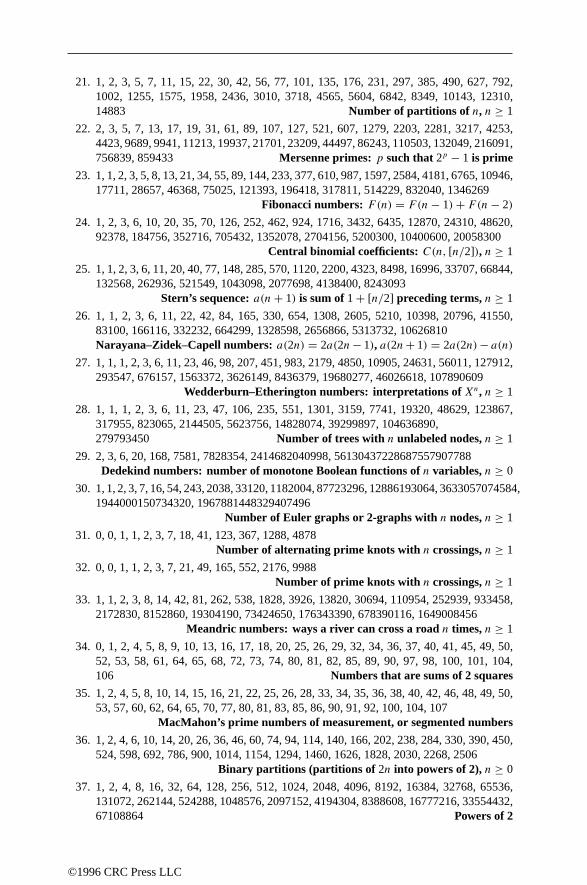
21. 1, 2, 3, 5, 7, 11, 15, 22, 30, 42, 56, 77, 101, 135, 176, 231, 297, 385, 490, 627, 792,1002, 1255, 1575, 1958, 2436, 3010, 3718, 4565, 5604, 6842, 8349, 10143, 12310,14883 Number of partitions of n, n ≥ 1
22. 2, 3, 5, 7, 13, 17, 19, 31, 61, 89, 107, 127, 521, 607, 1279, 2203, 2281, 3217, 4253,4423, 9689, 9941, 11213, 19937, 21701, 23209, 44497, 86243, 110503, 132049, 216091,756839, 859433 Mersenne primes:p such that 2p − 1 is prime
23. 1, 1, 2, 3, 5, 8, 13, 21, 34, 55, 89, 144, 233, 377, 610, 987, 1597, 2584, 4181, 6765, 10946,17711, 28657, 46368, 75025, 121393, 196418, 317811, 514229, 832040, 1346269
Fibonacci numbers: F(n) = F(n− 1)+ F(n− 2)
24. 1, 2, 3, 6, 10, 20, 35, 70, 126, 252, 462, 924, 1716, 3432, 6435, 12870, 24310, 48620,92378, 184756, 352716, 705432, 1352078, 2704156, 5200300, 10400600, 20058300
Central binomial coefficients: C(n, [n/2]), n ≥ 1
25. 1, 1, 2, 3, 6, 11, 20, 40, 77, 148, 285, 570, 1120, 2200, 4323, 8498, 16996, 33707, 66844,132568, 262936, 521549, 1043098, 2077698, 4138400, 8243093
Stern’s sequence:a(n+ 1) is sum of1 + [n/2] preceding terms,n ≥ 1
26. 1, 1, 2, 3, 6, 11, 22, 42, 84, 165, 330, 654, 1308, 2605, 5210, 10398, 20796, 41550,83100, 166116, 332232, 664299, 1328598, 2656866, 5313732, 10626810Narayana–Zidek–Capell numbers:a(2n) = 2a(2n− 1), a(2n+ 1) = 2a(2n)− a(n)
27. 1, 1, 1, 2, 3, 6, 11, 23, 46, 98, 207, 451, 983, 2179, 4850, 10905, 24631, 56011, 127912,293547, 676157, 1563372, 3626149, 8436379, 19680277, 46026618, 107890609
Wedderburn–Etherington numbers: interpretations of Xn, n ≥ 1
28. 1, 1, 1, 2, 3, 6, 11, 23, 47, 106, 235, 551, 1301, 3159, 7741, 19320, 48629, 123867,317955, 823065, 2144505, 5623756, 14828074, 39299897, 104636890,279793450 Number of trees with n unlabeled nodes,n ≥ 1
29. 2, 3, 6, 20, 168, 7581, 7828354, 2414682040998, 56130437228687557907788Dedekind numbers: number of monotone Boolean functions ofn variables,n ≥ 0
30. 1, 1, 2, 3, 7, 16, 54, 243, 2038, 33120, 1182004, 87723296, 12886193064, 3633057074584,1944000150734320, 1967881448329407496
Number of Euler graphs or 2-graphs with n nodes,n ≥ 1
31. 0, 0, 1, 1, 2, 3, 7, 18, 41, 123, 367, 1288, 4878Number of alternating prime knots with n crossings,n ≥ 1
32. 0, 0, 1, 1, 2, 3, 7, 21, 49, 165, 552, 2176, 9988Number of prime knots with n crossings,n ≥ 1
33. 1, 1, 2, 3, 8, 14, 42, 81, 262, 538, 1828, 3926, 13820, 30694, 110954, 252939, 933458,2172830, 8152860, 19304190, 73424650, 176343390, 678390116, 1649008456
Meandric numbers: ways a river can cross a roadn times,n ≥ 1
34. 0, 1, 2, 4, 5, 8, 9, 10, 13, 16, 17, 18, 20, 25, 26, 29, 32, 34, 36, 37, 40, 41, 45, 49, 50,52, 53, 58, 61, 64, 65, 68, 72, 73, 74, 80, 81, 82, 85, 89, 90, 97, 98, 100, 101, 104,106 Numbers that are sums of 2 squares
35. 1, 2, 4, 5, 8, 10, 14, 15, 16, 21, 22, 25, 26, 28, 33, 34, 35, 36, 38, 40, 42, 46, 48, 49, 50,53, 57, 60, 62, 64, 65, 70, 77, 80, 81, 83, 85, 86, 90, 91, 92, 100, 104, 107
MacMahon’s prime numbers of measurement, or segmented numbers
36. 1, 2, 4, 6, 10, 14, 20, 26, 36, 46, 60, 74, 94, 114, 140, 166, 202, 238, 284, 330, 390, 450,524, 598, 692, 786, 900, 1014, 1154, 1294, 1460, 1626, 1828, 2030, 2268, 2506
Binary partitions (partitions of 2n into powers of 2),n ≥ 0
37. 1, 2, 4, 8, 16, 32, 64, 128, 256, 512, 1024, 2048, 4096, 8192, 16384, 32768, 65536,131072, 262144, 524288, 1048576, 2097152, 4194304, 8388608, 16777216, 33554432,67108864 Powers of 2
©1996 CRC Press LLC

38. 1, 1, 2, 4, 9, 20, 48, 115, 286, 719, 1842, 4766, 12486, 32973, 87811, 235381,634847, 1721159, 4688676, 12826228, 35221832, 97055181, 268282855, 743724984,2067174645 Number of rooted trees withn unlabeled nodes,n ≥ 1
39. 1, 1, 2, 4, 9, 21, 51, 127, 323, 835, 2188, 5798, 15511, 41835, 113634, 310572, 853467,2356779, 6536382, 18199284, 50852019, 142547559, 400763223, 1129760415
Motzkin numbers: ways to join n points on a circle by chords
40. 1, 1, 2, 4, 9, 22, 59, 167, 490, 1486, 4639, 14805, 48107, 158808, 531469, 1799659,6157068, 21258104, 73996100, 259451116, 951695102, 3251073303
Number of different scores inn-team round-robin tournament, n ≥ 1
41. 1, 1, 2, 4, 11, 34, 156, 1044, 12346, 274668, 12005168, 1018997864,165091172592, 50502031367952, 29054155657235488, 31426485969804308768
Number of graphs with n unlabeled nodes,n ≥ 0
42. 0, 1, 2, 5, 12, 29, 70, 169, 408, 985, 2378, 5741, 13860, 33461, 80782, 195025, 470832,1136689, 2744210, 6625109, 15994428, 38613965, 93222358, 225058681, 543339720
Pell numbers: a(n) = 2a(n− 1)+ a(n− 2)
43. 1, 1, 2, 5, 12, 35, 108, 369, 1285, 4655, 17073, 63600, 238591, 901971, 3426576,13079255, 50107909, 192622052, 742624232, 2870671950, 11123060678, 43191857688
Polyominoes withn cells,n ≥ 1
44. 1, 1, 2, 4, 12, 56, 456, 6880, 191536, 9733056, 903753248, 154108311168,48542114686912, 28401423719122304, 31021002160355166848
Number of outcomes ofn-team round-robin tournament, n ≥ 1
45. 1, 1, 2, 5, 14, 38, 120, 353, 1148, 3527, 11622, 36627, 121622, 389560, 1301140,4215748, 13976335, 46235800, 155741571, 512559185, 1732007938,5732533570 Number of ways to fold a strip of n blank stamps,n ≥ 1
46. 1, 1, 2, 5, 14, 42, 132, 429, 1430, 4862, 16796, 58786, 208012, 742900, 2674440,9694845, 35357670, 129644790, 477638700, 1767263190, 6564120420, 24466267020
Catalan numbers: C(2n, n)/(n+ 1), n ≥ 0
47. 1, 1, 2, 5, 15, 52, 203, 877, 4140, 21147, 115975, 678570, 4213597, 27644437,190899322, 1382958545, 10480142147, 82864869804, 682076806159,5832742205057 Bell or exponential numbers: expansion ofe(e
x−1)
48. 1, 1, 1, 2, 5, 16, 61, 272, 1385, 7936, 50521, 353792, 2702765, 22368256, 199360981,1903757312, 19391512145, 209865342976, 2404879675441,29088885112832 Euler numbers: expansion ofsec x + tan x
49. 0, 2, 6, 12, 20, 30, 42, 56, 72, 90, 110, 132, 156, 182, 210, 240, 272, 306, 342, 380,420, 462, 506, 552, 600, 650, 702, 756, 812, 870, 930, 992, 1056, 1122, 1190, 1260,1332 Pronic numbers: n(n+ 1), n ≥ 0
50. 1, 2, 6, 20, 70, 252, 924, 3432, 12870, 48620, 184756, 705432, 2704156, 10400600,40116600, 155117520, 601080390, 2333606220, 9075135300,35345263800 Central binomial coefficients: C(2n, n), n ≥ 0
51. 1, 1, 1, 2, 6, 21, 112, 853, 11117, 261080, 11716571, 1006700565,164059830476, 50335907869219, 29003487462848061, 31397381142761241960
Number of connected graphs withn unlabeled nodes,n ≥ 0
52. 1, 2, 6, 22, 101, 573, 3836, 29228, 250749, 2409581, 25598186, 296643390, 3727542188,50626553988, 738680521142
Kendall–Mann numbers: maximal inversions in permutation of n letters, n ≥ 1
53. 1, 1, 2, 6, 24, 120, 720, 5040, 40320, 362880, 3628800, 39916800, 479001600,6227020800, 87178291200, 1307674368000, 20922789888000, 355687428096000,6402373705728000 Factorial numbers: n!, n ≥ 0
©1996 CRC Press LLC
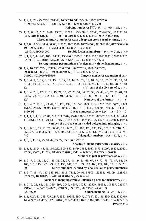
54. 1, 2, 7, 42, 429, 7436, 218348, 10850216, 911835460, 129534272700,31095744852375, 12611311859677500, 8639383518297652500
Robbins numbers:∏n−1
k=0(3k + 1)!/(n+ k)!, n ≥ 1
55. 1, 2, 8, 42, 262, 1828, 13820, 110954, 933458, 8152860, 73424650, 678390116,6405031050, 61606881612, 602188541928, 5969806669034, 59923200729046
Closed meandric numbers: ways a loop can cross a road2n times,n ≥ 1
56. 1, 2, 8, 48, 384, 3840, 46080, 645120, 10321920, 185794560, 3715891200, 81749606400,1961990553600, 51011754393600, 1428329123020800,42849873690624000 Double factorial numbers: (2n)!! = 2nn!, n ≥ 0
57. 0, 1, 2, 9, 44, 265, 1854, 14833, 133496, 1334961, 14684570, 176214841, 2290792932,32071101049, 481066515734, 7697064251745, 130850092279664
Derangements: permutations ofn elements with no fixed points,n ≥ 1
58. 1, 2, 16, 272, 7936, 353792, 22368256, 1903757312, 209865342976,29088885112832, 4951498053124096, 1015423886506852352,246921480190207983616 Tangent numbers: expansion oftan x
59. 1, 3, 4, 7, 6, 12, 8, 15, 13, 18, 12, 28, 14, 24, 24, 31, 18, 39, 20, 42, 32, 36, 24, 60,31, 42, 40, 56, 30, 72, 32, 63, 48, 54, 48, 91, 38, 60, 56, 90, 42, 96, 44, 84, 78, 72, 48,124 σ(n), sum of the divisors ofn, n ≥ 1
60. 1, 3, 4, 7, 9, 12, 13, 16, 19, 21, 25, 27, 28, 31, 36, 37, 39, 43, 48, 49, 52, 57, 61, 63,64, 67, 73, 75, 76, 79, 81, 84, 91, 93, 97, 100, 103, 108, 109, 111, 112, 117, 121, 124,127 Numbers of the form x2 + xy + y2
61. 1, 3, 4, 7, 11, 18, 29, 47, 76, 123, 199, 322, 521, 843, 1364, 2207, 3571, 5778, 9349,15127, 24476, 39603, 64079, 103682, 167761, 271443, 439204, 710647, 1149851,1860498 Lucas numbers:L(n) = L(n− 1)+ L(n− 2)
62. 1, 1, 1, 3, 4, 12, 27, 82, 228, 733, 2282, 7528, 24834, 83898, 285357, 983244, 3412420,11944614, 42080170, 149197152, 531883768, 1905930975, 6861221666, 24806004996
Number of ways to cut ann-sided polygon into triangles,n ≥ 1
63. 1, 3, 6, 10, 15, 21, 28, 36, 45, 55, 66, 78, 91, 105, 120, 136, 153, 171, 190, 210, 231,253, 276, 300, 325, 351, 378, 406, 435, 465, 496, 528, 561, 595, 630, 666, 703, 741,780 Triangular numbers: n(n+ 1)/2, n ≥ 1
64. 1, 3, 6, 11, 17, 25, 34, 44, 55, 72, 85, 106, 127, 151Shortest Golomb ruler with n marks, n ≥ 2
65. 1, 3, 6, 13, 24, 48, 86, 160, 282, 500, 859, 1479, 2485, 4167, 6879, 11297, 18334, 29601,47330, 75278, 118794, 186475, 290783, 451194, 696033, 1068745, 1632658
Number of planar partitions of n, n ≥ 1
66. 1, 3, 7, 9, 13, 15, 21, 25, 31, 33, 37, 43, 49, 51, 63, 67, 69, 73, 75, 79, 87, 93, 99,105, 111, 115, 127, 129, 133, 135, 141, 151, 159, 163, 169, 171, 189, 193, 195, 201,205 Lucky numbers (defined by sieve similar to prime numbers)
67. 1, 3, 7, 19, 47, 130, 343, 951, 2615, 7318, 20491, 57903, 163898, 466199, 1328993,3799624, 10884049, 31241170, 89814958, 258604642
Number of mappings from n unlabeled points to themselves,n ≥ 1
68. 1, 3, 9, 25, 65, 161, 385, 897, 2049, 4609, 10241, 22529, 49153, 106497, 229377,491521, 1048577, 2228225, 4718593, 9961473, 20971521, 44040193,92274689 Cullen numbers: n · 2n + 1, n ≥ 1
69. 1, 3, 9, 27, 81, 243, 729, 2187, 6561, 19683, 59049, 177147, 531441, 1594323, 4782969,14348907, 43046721, 129140163, 387420489, 1162261467, 3486784401, 10460353203
Powers of 3
©1996 CRC Press LLC

70. 1, 3, 9, 33, 139, 718, 4535Number of topologies or transitive-directed graphs withn unlabeled nodes,n ≥ 1
71. 1, 1, 3, 11, 45, 197, 903, 4279, 20793, 103049, 518859, 2646723, 13648869, 71039373,372693519, 1968801519, 10463578353, 55909013009, 300159426963
Schroeder’s second problem: ways to interpretX1X2 . . . Xn, n ≥ 1
72. 1, 3, 11, 50, 274, 1764, 13068, 109584, 1026576, 10628640, 120543840, 1486442880,19802759040, 283465647360, 4339163001600, 70734282393600,1223405590579200 Stirling numbers of first kind:
[n
2
], n ≥ 2.
73. 1, 3, 13, 75, 541, 4683, 47293, 545835, 7087261, 102247563, 1622632573, 28091567595,526858348381, 10641342970443, 230283190977853,5315654681981355 Preferential arrangements ofn things, n ≥ 1
74. 1, 3, 15, 105, 945, 10395, 135135, 2027025, 34459425, 654729075, 13749310575,316234143225, 7905853580625, 213458046676875, 6190283353629375
Double factorial numbers: (2n+ 1)!! = 1 · 3 · 5 · · · (2n+ 1), n ≥ 1
75. 1, 3, 16, 125, 1296, 16807, 262144, 4782969, 100000000, 2357947691,61917364224, 1792160394037, 56693912375296, 1946195068359375,72057594037927936 Number of trees with n labeled nodes:nn−2, n ≥ 2
76. 1, 3, 16, 218, 9608, 1540944, 882033440, 1793359192848, 13027956824399552,341260431952972580352, 32522909385055886111197440
Directed graphs with n unlabeled nodes,n ≥ 1
77. 1, 1, 3, 17, 155, 2073, 38227, 929569, 28820619, 1109652905, 51943281731,2905151042481, 191329672483963, 14655626154768697, 1291885088448017715
Genocchi numbers: expansion oftan(x/2)
78. 0, 1, 4, 5, 16, 17, 20, 21, 64, 65, 68, 69, 80, 81, 84, 85, 256, 257, 260, 261, 272, 273,276, 277, 320, 321, 324, 325, 336, 337, 340, 341, 1024, 1025, 1028, 1029, 1040, 1041
Moser–de Bruijn sequence: sums of distinct powers of 4
79. 4, 7, 8, 9, 10, 11, 12, 12, 13, 13, 14, 15, 15, 16, 16, 16, 17, 17, 18, 18, 19, 19, 19,20, 20, 20, 21, 21, 21, 22, 22, 22, 23, 23, 23, 24, 24, 24, 24, 25, 25, 25, 25, 26, 26,2 Chromatic number of surface of genusn, n ≥ 0
80. 1, 4, 9, 16, 25, 36, 49, 64, 81, 100, 121, 144, 169, 196, 225, 256, 289, 324, 361, 400,441, 484, 529, 576, 625, 676, 729, 784, 841, 900, 961, 1024, 1089, 1156, 1225, 1296
The squares
81. 1, 4, 10, 19, 31, 46, 64, 85, 109, 136, 166, 199, 235, 274, 316, 361, 409, 460, 514,571, 631, 694, 760, 829, 901, 976, 1054, 1135, 1219, 1306, 1396, 1489, 1585, 1684,1786 Centered triangular numbers: (3n2 + 3n+ 2)/2, n ≥ 1
82. 1, 4, 10, 20, 35, 56, 84, 120, 165, 220, 286, 364, 455, 560, 680, 816, 969, 1140, 1330,1540, 1771, 2024, 2300, 2600, 2925, 3276, 3654, 4060, 4495, 4960, 5456, 5984
Tetrahedral numbers: C(n+ 3, 3), n ≥ 0
83. 1, 1, 4, 26, 236, 2752, 39208, 660032, 12818912, 282137824, 6939897856,188666182784, 5617349020544, 181790703209728, 6353726042486272
Schroeder’s fourth problem: families of subsets of ann set,n ≥ 1
84. 1, 4, 29, 355, 6942, 209527, 9535241, 642779354, 63260289423,8977053873043, 1816846038736192, 519355571065774021
Number of transitive-directed graphs with n labeled nodes,n ≥ 1
85. 1, 5, 12, 22, 35, 51, 70, 92, 117, 145, 176, 210, 247, 287, 330, 376, 425, 477, 532,590, 651, 715, 782, 852, 925, 1001, 1080, 1162, 1247, 1335, 1426, 1520, 1617, 1717,1820 Pentagonal numbers:n(3n− 1)/2, n ≥ 1
©1996 CRC Press LLC

86. 1, 5, 13, 25, 41, 61, 85, 113, 145, 181, 221, 265, 313, 365, 421, 481, 545, 613, 685,761, 841, 925, 1013, 1105, 1201, 1301, 1405, 1513, 1625, 1741, 1861, 1985, 2113,2245 Centered square numbers:n2 + (n− 1)2, n ≥ 1
87. 1, 5, 14, 30, 55, 91, 140, 204, 285, 385, 506, 650, 819, 1015, 1240, 1496, 1785, 2109,2470, 2870, 3311, 3795, 4324, 4900, 5525, 6201, 6930, 7714, 8555, 9455, 10416
Square pyramidal numbers: n(n+ 1)(2n+ 1)/6, n ≥ 1
88. 1, 5, 25, 125, 625, 3125, 15625, 78125, 390625, 1953125, 9765625, 48828125,244140625, 1220703125, 6103515625, 30517578125, 152587890625, 762939453125,3814697265625 Powers of 5
89. 1, 5, 52, 1522, 145984, 48464496, 56141454464, 229148550030864,3333310786076963968, 174695272746749919580928
Number of possible relations onn unlabeled points,n ≥ 1
90. 1, 1, 5, 61, 1385, 50521, 2702765, 199360981, 19391512145, 2404879675441,370371188237525, 69348874393137901, 15514534163557086905,4087072509293123892361 Euler numbers: expansion ofsec x
91. 1, 5, 109, 32297, 2147321017, 9223372023970362989,170141183460469231667123699502996689125
Number of ways to cover ann set,n ≥ 1
92. 1, 6, 15, 28, 45, 66, 91, 120, 153, 190, 231, 276, 325, 378, 435, 496, 561, 630, 703,780, 861, 946, 1035, 1128, 1225, 1326, 1431, 1540, 1653, 1770, 1891, 2016, 2145,2278 Hexagonal numbers:n(2n− 1), n ≥ 1
93. 1, 6, 25, 90, 301, 966, 3025, 9330, 28501, 86526, 261625, 788970, 2375101, 7141686,21457825, 64439010, 193448101, 580606446, 1742343625, 5228079450, 15686335501
Stirling numbers of second kind:n
3
, n ≥ 3
94. 6, 28, 496, 8128, 33550336, 8589869056, 137438691328,2305843008139952128, 2658455991569831744654692615953842176
Perfect numbers: equal to the sum of their proper divisors
95. 1, 8, 21, 40, 65, 96, 133, 176, 225, 280, 341, 408, 481, 560, 645, 736, 833, 936, 1045,1160, 1281, 1408, 1541, 1680, 1825, 1976, 2133, 2296, 2465, 2640, 2821, 3008, 3201
Octagonal numbers:n(3n− 2), n ≥ 1
96. 1, 8, 27, 64, 125, 216, 343, 512, 729, 1000, 1331, 1728, 2197, 2744, 3375, 4096, 4913,5832, 6859, 8000, 9261, 10648, 12167, 13824, 15625, 17576, 19683, 21952, 24389
The cubes
97. 1, −24, 252, −1472, 4830, −6048, −16744, 84480, −113643, −115920, 534612,−370944, −577738, 401856, 1217160, 987136, −6905934, 2727432,10661420 Ramanujan τ function
98. 341, 561, 645, 1105, 1387, 1729, 1905, 2047, 2465, 2701, 2821, 3277, 4033, 4369,4371, 4681, 5461, 6601, 7957, 8321, 8481, 8911, 10261, 10585, 11305, 12801, 13741,13747 Sarrus numbers: pseudo-primes to base 2
99. 561, 1105, 1729, 2465, 2821, 6601, 8911, 10585, 15841, 29341, 41041, 46657, 52633,62745, 63973, 75361, 101101, 115921, 126217, 162401, 172081, 188461, 252601,278545 Carmichael numbers
100. 1, 744, 196884, 21493760, 864299970, 20245856256, 333202640600,4252023300096, 44656994071935, 401490886656000, 3176440229784420,22567393309593600 Coefficients of the modular functionj
For more information about all of these sequences including formulae and ref-erences, see N.J.A. Sloane and S. Plouffe, Encyclopedia of Integer Sequences, Aca-demic Press, 1995, where over 5000 other sequences are also described.
©1996 CRC Press LLC

1.2.15 DE BRUIJN SEQUENCES
A sequence of length qn over an alphabet of size q is a de Bruijn sequence if everypossible n-tuple occurs in the sequence (allowing wraparound to the start of thesequence). There are de Bruijn sequences for any q and n. The table below givessome small examples.
q n Length Sequence2 2 4 01102 3 8 011101003 2 9 0012202114 2 16 0011310221203323
1.3 SERIES AND PRODUCTS
1.3.1 DEFINITIONS
If an is a sequence of numbers or functions, then
• SN = ∑Nn=1 an = a1 + a2 + ...+ aN .
• SN is the N th partial sum of S.
• The series is said to converge if the limit exists and diverge if it does not.
• For an infinite series: S = limN→∞ SN = ∑∞n=1 an (when the limit exists).
• If an = bnxn, where bn is independent of x, then S is called a power series.
• If an = (−1)n|an|, then S is called an alternating series.
• If∑ |an| converges, then the series converges absolutely.
• If S converges, but not absolutely, then it converges conditionally.
For example, the harmonic seriesS = 1+ 12 + 1
3+. . . diverges. The correspondingalternating series (called the alternating harmonic series) S = 1 − 1
2 + 13 + · · · +
(−1)n−1 1n
+ . . . converges (conditionally) to log 2.
1.3.2 GENERAL PROPERTIES
1. Adding or removing a finite number of terms does not affect the convergence ordivergence of an infinite series.
2. The terms of an absolutely convergent series may be rearranged in any mannerwithout affecting its value.
©1996 CRC Press LLC

3. A conditionally convergent series can be made to converge to any value bysuitably rearranging its terms.
4. If the component series are convergent, then∑(αan+βbn) = α
∑an+β
∑bn.
5.
( ∞∑n=0
an
)( ∞∑n=0
bn
)=
∞∑n=0
cn where cn = a0bn + a1bn−1 + · · · + anb0.
6. Summation by parts: let∑an and
∑bn converge. Then∑
anbn =∑
Sn(bn − bn+1)
where Sn is the nth partial sum of∑an.
7. A power series may be integrated and differentiated term by term within itsinterval of convergence.
8. Schwarz inequality:
∑|an| |bn| ≤
(∑a2n
)1/2(∑b2n
)1/2
9. Holder’s inequality:
∑ |anbn| ≤ ∑ |an|1/p∑ |bn|1/q
when 1/p + 1/q = 1 and p, q > 1
10. Minkowski’s inequality:
(∑ |an + bn|p)1/p ≤ (∑ |an|p
)1/p + (∑ |bn|p)1/p
when p ≥ 1
For example:
1. Let T be the alternating harmonic series S rearranged so that each positive termis followed by the next two negative terms. By combining each positive termof T with the succeeding negative term, we find that T3N = 1
2S2N . Hence,T = 1
2 log 2.
2. The series 1 + 12 − 1
3 + 14 + 1
5 − 16 + 1
7 + 18 − 1
9 + . . . diverges, whereas
1 + 1
3− 1
2+ 1
5+ 1
7− 1
4+ · · · + 1
4n− 3+ 1
4n− 1− 1
2n+ . . .
converges to log(2√
2).
©1996 CRC Press LLC

1.3.3 CONVERGENCE TESTS
1. Comparison test: If |an| ≤ bn and∑bn converges, then
∑an converges.
2. Limit test: If limn→∞ an = 0, then∑an is divergent.
3. Ratio test: Let ρ = limn→∞ | an+1
an|. If ρ < 1, the series converges absolutely.
If ρ > 1, the series diverges.
4. Cauchy root test: Let σ = limn→∞ |an|1/n. If σ < 1, the series converges. Ifσ > 1, it diverges.
5. Integral test: Let |an| = f (n) with f (x) being monotone decreasing, andlimx→∞ f (x) = 0. Then
∫∞Af (x) dx and
∑an both converge or both diverge
for any A > 0.
6. Gauss’s test: If
∣∣∣∣an+1
an
∣∣∣∣ = 1 − p
n+ An
nqwhere q > 1 and the sequence An is
bounded, then the series is absolutely convergent if and only if p > 1.
7. Alternating series test: If |an| tends monotonically to 0, then∑(−1)n|an|
converges.
For example:
1. For S = ∑∞n=1 n
cxn, ρ = limn→∞(1 + 1n)cx = x. Hence, using the ratio test,
S converges for 0 < x < 1 and any value of c.
2. For S = ∑∞n=1
5n
n20 , σ = limn→∞( 5n
n20 )1/n = 5. Therefore the series diverges.
3. For S = ∑∞n=1 n
−s , let f (x) = x−s . Then∫ ∞
1f (x) dx =
∫ ∞
1
dx
xs= 1
s − 1
for s > 1, and the integral diverges for s ≤ 1. Hence, S converges for s > 1.
4. The sum∑∞
n=21
n(log n)s converges for s > 1 by the integral test.
5. Let an = (c)nn! = c(c+1)...(c+n−1)
n! where c is not 0 or a negative integer. Then|an+1/an| = 1 − (c + 1)/n+ (c + 1)/n2(1 + 1/n). By Gauss’s test, the seriesconverges absolutely if and only if c > 0.
1.3.4 TYPES OF SERIES
Bessel series1. Fourier–Bessel series: ∞∑
n=0
anJν(jν,nz)
2. Neumann series: ∞∑n=0
anJν+n(z)
©1996 CRC Press LLC

3. Kapteyn series:∞∑n=0
anJν+n[(ν + n)z]
4. Schlomilch series:∞∑n=1
anJν(nz)
For example;
• ∑∞n=0
1n!Jν+n(2) = 1
(ν+1)
• ∑∞n=1 Jn(nz) = 1
2z
1−z for 0 < z < 1
• ∑∞n=1(−1)n+1J0(nz) = 1
2 for 0 < z < π
Dirichlet seriesThese are series of the form
∑∞n=1
annx. They converge for x > x0, where x0 is the
abscissa of convergence. Assuming the limits exist:
If∑an diverges, then x0 = lim
n→∞log |a1 + · · · + an|
log n.
If∑an converges, then x0 = lim
n→∞log |an+1 + an+2 + . . . |
log n.
For example:
• Riemann zeta function:
ζ(x) =∞∑n=1
1
nx, x0 = 1
• ∑∞n=1
µ(n)
nx= 1
ζ(x), x0 = 1 (µ(n) denotes the Mobius function)
• ∑∞n=1
d(n)
nx= [ζ(x)]2, x0 = 1 (d(n) is the number of divisors of n)
Fourier seriesIf f (x) satisfies certain properties, then (see page 46 for details)
f (x) = a0
2+
∞∑n=1
(an cos
nπx
L+ bn sin
nπx
L
)(1.3.1)
©1996 CRC Press LLC

• If f (x) has the Laplace transform F(k), then
∞∑k=1
F(k) cos(kt) = 1
2
∫ ∞
0
cos(t)− e−x
cosh(x)− cos(t)f (x) dx,
∞∑k=1
F(k) sin(kt) = 1
2
∫ ∞
0
f (x)
cosh(x)− cos(t)dx. (1.3.2)
• Since the cosine transform of (cosh(x)− cos(t))−1 with respect to x is π csc(t)csch(πy) sinh(π − t)y, we find that
∞∑k=1
k sin(kt)
k2 + y2= π
2
sinh(π − t)y
sinh(πy).
• ∑∞n=1
sin(2nπx)n2k+1 = (−1)k−1
2(2π)2k+1
2k+1 B2k+1(x), for 0 < x < 12
• ∑∞n=1
cos(2nπx)n2k = (−1)k−1
2(2π)2k
(2k)! B2k(x) for 0 < x < 12
• ∑∞n=1
sin((2n+1)πx−πk/2)(2n+1)k+1 = πk+1
4k! Ek(x)
• ∑∞n=1 a
n sin(nx) = a sin(x)1−2a cos(x)+a2 for |a| < 1
• ∑∞n=0 a
n cos(nx) = 1−a cos(x)1−2a cos(x)+a2 for |a| < 1
Hypergeometric seriesThe hypergeometric function is
pFq
(a1 a2 . . . apb1 b2 . . . bq
x
)=
∞∑n=0
(a1)n(a2)n . . . (ap)n
(b1)n(b2)n . . . (bq)n
xn
n!
where (a)n = (a + n)/(a) is the shifted factorial. Any infinite series∑An with
An+1/An a rational function of n is of this type. These include series of products andquotients of binomial coefficients. For example:
2F1
(a, b
c1
)= (c)(c − a − b)
(c − a)(c − b)(Gauss)
3F2
( −n, a, b
c, 1 + a + b − c − n1
)= (c − a)n(c − b)n
(c)n(c − a − b)n(Saalschutz)
4F3
(a, 1 + a/2, b, −na/2, 1 + a − b, 1 + 2b − n
1
)= (a − 2b)n(−b)n(1 + a − b)n(−2b)n
(Bailey)
2n∑m=0
(−1)m(2nm
)(2n+m+1m
)(4n+2m+22m
) (3 + 2√
2)m = (3/4)n(5/4)n(7/8)n(9/8)n
©1996 CRC Press LLC

Power series1. The values of x for which the power series
∑∞n=0 anx
n converges, form aninterval (interval of convergence) which may or may not include one or bothendpoints.
2. A power series may be integrated and differentiated term-by-term within itsinterval of convergence.
3. Note that [1 + ∑∞n=1 anx
n]−1 = 1 − ∑∞n=1 bnx
n, where b1 = a1 and bn =an +∑n−1
k=1 bn−kak for n ≥ 2.
4. Inversion of power series: If s = ∑∞n=1 anx
n, then x = ∑∞n=1 Ans
n, whereA1 = 1/a1, A2 = −a2/a
31 , A3 = (2a2
2 − a1a3)/a51 , A4 = (5a1a2a3 − a2
1a4 −5a3
2)/a71 , A5 = (6a2
1a2a4 + 3a21a
23 + 14a4
2 − a31a5 − 21a1a
22a3)/a
91 .
Taylor series1. Taylor series in 1 variable:
f (a + x) =N∑n=0
xn
n!f (n)(a)+ RN.
2. Lagrange’s form of the remainder:
RN = xN+1
(N + 1)!f (N+1)(θa), for some 0 < θ < 1.
3. Taylor series in 2 variables:
f (a + x, b + y) = f (a, b)+ xfx(a, b)+ yfy(a, b)+1
2!
[x2fxx(a, b)+ 2xyfxy(a, b)+ y2fyy(a, b)
]+ . . . .
4. Taylor series for vectors:
f (a + x) =N∑n=0
[(x · ∇)nf ](a)n!
+ RN(a) = f (a)+ x · ∇f (a)+ . . . .
For example (see also page 40):
• Binomial series:
(x + y)ν =∞∑n=0
(ν + 1)
(ν − n+ 1)
xnyν−n
n!.
When ν is a positive integer, the series terminates at n = ν.
• 1√1−4x
= ∑∞k=0
(2k)!(k!)2 x
k for |x| < 1/4
• xext
ex−1 = ∑∞n=0 Bn(t)
xn
n!
• 2ext
ex+1 = ∑∞n=0 En(t)
xn
n!
©1996 CRC Press LLC

• ∑∞n=1
xn
(n+1)(n+3) = 1x3
∫ x0 u du
∫ u0 dt
∑∞0 tn
= 12x3
[x + 1
2x2 + (1 − x2) log(1 − x)
]for |x| < 1
• ∑∞k=1
xk
kn= Lin(x) (polylogarithm)
Telescoping seriesIf limn→∞ F(n) = 0, then
∑∞n=1[F(n)− F(n+ 1)] = F(1). For example,
∞∑n=1
1
(n+ 1)(n+ 2)=
∞∑n=1
[1
n+ 1− 1
n+ 2
]= 1
2.
The GWZ symbolic computer algorithm expresses a proposed identity in the formof a telescoping series
∑k[F(n+ 1, k)− F(n, k)] = 0, then searches for a G(n, k)
that satisfies F(n + 1, k) − F(n, k) = G(n, k + 1) −G(n, k) and G(n,±∞) = 0.The search assumes that G(n, k) = R(n, k)F (n, k − 1) where R(n, k) is a rationalexpression in n and k. When R is found, the proposed identity is verified. Forexample, the Pfaff–Saalschutz identity has the following proof:
∞∑k=−∞
(a + k)!(b + k)!(c − a − b + n− 1 − k)!
(k + 1)!(n− k)!(c + k)!= (c − a + n)!(c − b + n)!
(n+ 1)!(c + n)!,
R(n, k) = − (b + k)(a + k)
(c − b + n+ 1)(c − a + n+ 1).
Other types of series1. Arithmetic series:
N∑n=1
(a + nd) = Na + 1
2N(N + 1)d.
2. Arithmetic power series:
N∑n=1
(a + nb)xn = a − (a + bN ) xN+1
1 − x+ bx(1 − xN)
(1 − x)2, (x = 1).
3. Geometric series:
1 + x + x2 + x3 + · · · = 1
1 − x, (|x| < 1).
4. Arithmetic–geometric series:
a + (a + b)x + (a + 2b)x2 + (a + 3b)x3 + · · · = a
1 − x+ bx
(1 − x)2,
(|x| < 1).
©1996 CRC Press LLC

5. Combinatorial sums:
• ∑nk=0
(x−kn−k) = (
x+1n
)• ∑m
k=−∞(−1)k(x
k
) = (−1)m(x−1m
)• ∑n
k=0
(k+mk
) = (m+n+1
n
)• ∑m
k=−∞(−1)k(x+mk
) = (−xm
)• ∑∞
k=−∞(x
m+k)(
y
n−k) = (
x+ym+n
)• ∑∞
k=−∞(
l
m+k)(
x
n+k) = (
l+xl−m+n
)• ∑∞
k=−∞(−1)k(
l
m+k)(x+kn
) = (−1)l+m(x−mn−l)
• ∑lk=−∞(−1)k
(l−km
)(x
k−n) = (−1)l+m
(x−m−ll−m−n
)• ∑l
k=0
(l−km
)(q+kn
) = (l+q+1m+n+1
)(m ≥ q)
6. Generating functions:
• Bessel functions:∑∞
k=−∞ Jk(x)zk = exp( 1
2xz2−1z)
• Chebyshev polynomials:∑∞
n=1 Tn(x)zn = z(z+2x)
2xz−z2−1
• Hermite polynomials:∑∞
n=0Hn(x)
n! zn = exp(2xz− z2)
• Laguerre polynomials:∑∞
n=0 L(α)n (x)zn = (1 − z)−α−1 exp[ xz
z−1 ]
• Legendre polynomials:∑∞
n=0 Pn(z)xn = 1√
1−xz+x2 , for |x| < 1
7. Multiple series:
• ∑ (−1)l+m+n√(l+1/6)2+(m+1/6)2+(n+1/6)2
= √3 for −∞ < l,m, n < ∞ not all zero
• ∑ 1(m2+n2)z
= 4β(z)ζ(z) for −∞ < m, n < ∞ not both zero
• ∑∞m,n=0
(−1)n
n!(n+1/2)
(m+n+1/2) zm+n = √
πezerf(√z−z)√
z−z for z > 0
• ∑∞m,n=1
m2−n2
(m2+n2)2= π
4
• ∑ 1k2
1k22 ...k
2n
= π2n
(2n+1)! for 1 ≤ k1 < · · · < kn < ∞
1.3.5 SUMMATION FORMULAE
1. Euler–Maclaurin summation formula: As n → ∞,
n∑k=0
f (k) ∼ 1
2f (n)+
∫ n
0f (x) dx + C +
∞∑j=1
(−1)j+1Bj+1f (j)(n)
(j + 1)!
©1996 CRC Press LLC

where
C = limm→∞
[ m∑j=1
(−1)jBj+1f (j)(0)
(j + 1)!+ 1
2f (0)
+ (−1)m
(m+ 1)!
∫ ∞
0Bm+1(x − [x])f (m+1)(x) dx
].
2. Poisson summation formula: If f is continuous,
1
2f (0)+
∞∑n=1
f (n) =∫ ∞
0f (x) dx + 2
∞∑n=1
[∫ ∞
0f (x) cos(2nπx)dx
].
For example:
• ∑nk=1
1k
∼ log n+ γ + 12n − B2
2n2 − . . . where γ is Euler’s constant.
• 1 + 2∑∞
n=1 e−n2x = √
πx
[1 + 2∑∞
n=1 e−π2n2/x] (Jacobi)
1.3.6 IMPROVING CONVERGENCE: SHANKSTRANSFORMATION
Let sn be the nth partial sum. The sequences S(sn), S(S(sn)), . . . often convergesuccessively more rapidly to the same limit as sn, where
S(sn) = sn+1sn−1 − s2n
sn+1 + sn−1 − 2sn. (1.3.3)
For example, for sn = ∑nk=0(−1)kzk , we find S(sn) = 1
1+z for all n.
1.3.7 SUMMABILITY METHODS
Unique values can be assigned to divergent series in a variety of ways which preservethe values of convergent series.
1. Abel summation:∑∞
n=0 an = limr→1−∑∞
n=0 anrn.
2. Cesaro (C, 1)-summation:∑∞
n=0 an = limN→∞ s0+s1+...sNN+1 where sn = ∑n
m=0 am.
For example:
• 1 − 1 + 1 − 1 + · · · = 12 (in the sense of Abel summation)
• 1 − 1 + 0 + 1 − 1 + 0 + 1 − · · · = 13 (in the sense of Cesaro summation)
©1996 CRC Press LLC

1.3.8 OPERATIONS WITH SERIES
Let y = a1x + a2x2 + a3x
3 + . . . , and let z = z(y) = b1x + b2x2 + b3x
3 + . . . .
z = b0 b1 b2 b3
1
1 − y1 a1 a2
1 + a2 a31 + 2a1a2 + a3
√1 + y 1 1
2a1 − 18a
21 + 1
2a21
16a31 − 1
4a1a2 + 12a3
(1 + y)−1/2 1 − 12a1
38a
21 − 1
2a2 − 516a
31 + 3
4a1a2 − 12a3
ey 1 a112a
21 + a2
16a
31 + a1a2 + a3
log(1 + y) 0 a1 a2 − 12a
21 a3 − a1a2 + 1
3a31
sin y 0 a1 a2 − 16a
31 + a3
cos y 1 0 − 12a
21 −a1a2
tan y 0 a1 a213a
31 + a3
1.3.9 MISCELLANEOUS SUMS AND SERIES
• ∑Nn=1(−1)n+1nk = 1
2 (−1)N+1[Ek(N + 1)+ (−1)NEk]
• ∑nk=1
1k(k+1)(k+2) = 1
4 − 12(n+1)(n+2)
• ∑nk=1
kmk
(k+m)! = 1(m−1)! − mn+1
(m+n)!
• ∑2nk=0(−1)k
(2nk
)−1 = 2n+1n+1
• ∑nk=0
(m
k
)(n
k
)(m+n+km+n
) = (m+nm
)2
• ∑n−1k=0
14k sech2 x
2k = 14n csch2 x
2n − csch2 x
• ∑n−1k=0(−1)k cosn πk
n= n
2n−1 ,∑n
k=0 sec πkn
= 0, (k = n/2)
• ∑∞k=−∞
1(k+a)(k+b) = π
b−a (cot πa − cot πb)
• ∑∞k=0
1k4+a4 = 1
2a4 + π
2a3√
2sinh(aπ
√2)+sin(aπ
√2)
cosh(aπ√
2)−cos(aπ√
2)
• ∑∞k=1
ke2πk−1 = 1
24 − 18π
• The series∞∑n=3
1
n log n(log log n)2converges to 38.43 . . . so slowly that it re-
quires 103.14·1086terms to give two-decimal accuracy
• The series∞∑n=3
1
n log n(log log n)diverges, but the partial sums exceed 10 only
after a googolplex of terms have appeared
©1996 CRC Press LLC

1.3.10 INFINITE SERIES
Algebraic functions
(x + y)n = xn +(n
1
)xn−1y +
(n
2
)xn−2y2 + . . . .
(1 ± x)n = 1 ±(n
1
)x +
(n
2
)x2 ±
(n
3
)x3 + . . . , (x2 < 1).
(1 ± x)−n = 1 ∓(n
1
)x +
(n+ 1
2
)x2 ∓
(n+ 2
3
)x3 + . . . , (x2 < 1).
√1 + x = 1 + 1
2x − 1
8x2 + 1
16x3 − 5
128x4 + . . . , (x2 < 1).
(1 + x)−1/2 = 1 − 1
2x + 3
8x2 − 5
16x3 + 35
128x4 + . . . , (x2 < 1).
(1 ± x)−1 = 1 ∓ x + x2 ∓ x3 + x4 ∓ x5 + . . . , (x2 < 1).
(1 ± x)−2 = 1 ∓ 2x + 3x2 ∓ 4x3 + 5x4 ∓ 6x5 + . . . , (x2 < 1).
Exponential functions
e = 1 + 1
1!+ 1
2!+ · · · + 1
n!+ · · · . (all real values of x)
ex = 1 + x
1!+ x2
2!+ · · · + xn
n!+ · · · ,
= ea[
1 + (x − a)+ (x − a)2
2!+ · · · + (x − a)n
n!+ . . .
].
ax = 1 + x loge a + (x loge a)2
2!+ · · · + (x loge a)
n
n!+ · · · .
©1996 CRC Press LLC

Logarithmic functions
log x = x − 1
x+ 1
2
(x − 1
x
)2
+ · · · + 1
n
(x − 1
x
)n+ · · · , (x > 1/2),
= (x − 1)− 1
2(x − 1)2 + 1
3(x − 1)3 − . . . , (2 ≥ x > 0),
= 2
[x − 1
x + 1+ 1
3
(x − 1
x + 1
)3
+ 1
5
(x − 1
x + 1
)5
+ . . .
], (x > 0).
= log a + (x − a)
a− (x − a)2
2a2+ (x − a)3
3a2− . . . , (0 < x ≤ 2a).
log(1 + x) = x − x2
2+ x3
3− x4
4+ . . . , −1 < x ≤ 1.
log(n+ 1) = log(n− 1)+ 2
[1
n+ 1
3n3+ 1
5n5+ . . .
].
log(a + x) = log a + 2
[x
2a + x+ 1
3
(x
2a + x
)3
+ 1
5
(x
2a + x
)5
+ . . .
],
(a > 0, −a < x).
log1 + x
1 − x= 2
[x + x3
3+ · · · + x2n−1
2n− 1+ . . .
], (−1 < x < 1).
Trigonometric functions
sin x = x − x3
3!+ x5
5!− x7
7!+ . . . . (all real values of x).
cos x = 1 − x2
2!+ x4
4!− x6
6!+ . . . . (all real values of x).
tan x = x + x3
3+ 2x5
15+ . . .+ (−1)n−122n(22n − 1)B2n
(2n)!x2n−1 + . . .
(x2 < π2/4, Bn is the nth Bernoulli number).
cot x = 1
x− x
3− x3
45− 2x5
945− x7
4725− . . .+ (−1)n+122nB2n
(2n)!x2n−1 + . . .
(x2 < π2, Bn is the nth Bernoulli number).
sec x = 1 + x2
2+ 5
24x4 + 61
720x6 + 277
8064x8 + . . .+ (−1)nE2n
(2n)!x2n + . . .
(x2 < π2/4, En is the nth Euler number).
csc x = 1
x+ x
6+ 7x3
360+ 31x5
15120+ . . .+ (−1)n+12(22n−1 − 1)B2n
(2n)!x2n−1 + . . .
©1996 CRC Press LLC

(|x| < π , Bn is the nth Bernoulli number).
log sin x = log x − x2
6− x4
180− x6
2835− . . . (x2 < π2).
log cos x = −x2
2− x4
12− x6
45− 17x6
2520− . . . (x2 < π2/4).
log tan x = log x + x2
3+ 7x4
90+ 62x6
2835+ . . . (x2 < π2/4).
esin x = 1 + x + x2
2!− 3x4
4!− 8x5
5!− 3x6
6!+ 56x7
7!+ . . . .
ecos x = e
(1 − x2
2!+ 4x4
4!− 31x6
6!+ . . .
).
etan x = 1 + x + x2
2!+ 3x3
3!+ 9x4
4!+ 37x5
5!+ . . . (x2 < π2/4).
sin x = sin a + (x − a) cos a − (x − a)2
2!sin a− (x − a)3
3!cos a + . . . .
Inverse trigonometri c functions
sin−1 x = x + 1
2 · 3x3 + 1 · 3
2 · 4 · 5x5 + 1 · 3 · 5
2 · 4 · 6 · 7x7 + . . .
(x2 < 1, −π2 < sin−1 x < π
2 ).
cos−1 x = π
2−(x + 1
2 · 3x3 + 1 · 3
2 · 4 · 5x5 + 1 · 3 · 5
2 · 4 · 6 · 7x7 + . . .
)
(x2 < 1, 0 < cos−1 x < π).
tan−1 x = x − x3
3+ x5
5− x7
7+ . . . (x2 < 1),
= π
2− 1
x+ 1
3x3− 1
5x5+ 1
7x7− . . . (x > 1),
= −π2
− 1
x+ 1
3x3− 1
5x5+ 1
7x7− . . . (x < −1).
cot−1 x = π
2− x + x3
3− x5
5+ x7
7− . . . (x2 < 1).
©1996 CRC Press LLC

Hyperbolic functions
sinh x = x + x3
3!+ x5
5!+ x7
7!+ · · · + x(2n+1)
(2n+ 1)!+ . . . .
sinh ax = 2
πsinh πa
[sin x
a2 + 12− 2 sin 2x
a2 + 22+ 3 sin 3x
a2 + 32+ . . .
](|x| < π).
cosh x = 1 + x2
2!+ x4
4!+ x6
6!+ · · · + x2n
(2n)!+ . . . .
cosh ax = 2a
πsinh πa
[1
2a2− cos x
a2 + 12+ cos 2x
a2 + 22− cos 3x
a2 + 32+ . . .
](|x| < π).
tanh x = x − 1
3x3 + 2
15x5 − · · · + 22n(22n − 1)B2n
(2n)!x2n−1 + . . . (|x| < π/2),
= 1 − 2e−2x + 2e−4x − 2e−6x + . . . (Re x > 0),
= 2x
[1(
π2
)2 + x2+ 1(
3π2
)2 + x2+ 1(
5π2
)2 + x2+ . . .
].
coth x = 1
x+ x
3− x3
45+ 2x5
945+ · · · + 22nB2n
(2n)!x2n−1 + . . . (0 < |x| < π),
= 1 + 2e−2x + 2e−4x + 2e−6x + . . . (Re x > 0),
= 1
x+2x
[+ 1
π2 + x2+ 1
(2π)2 + x2+ 1
(3π)2 + x2+ . . .
](Re x > 0).
sech x = 1 − 1
2!x2 + 5
4!x4 − 61
6!x6 + · · · + E2n
(2n)!x2n + . . .
(|x| < π/2, En is the nth Euler number),
= 2(e−x − e−3x + e−5x − e−7x + . . .
)(Re x > 0),
= 4π
[1
π2 + 4x2− 3
(3π)2 + 4x2+ 5
(5π)2 + 4x2+ . . .
].
csch x = 1
x− x
6+ 7x3
360+ · · · + 2(22n−1 − 1)B2n
(2n)!x2n−1 + . . . (0 < |x| < π),
= 2(e−x + e−3x + e−5x + e−7x + . . .
)(Re x > 0),
= 1
x− 2x
π2 + x2+ 2x
(2π)2 + x2− 2x
(3π)2 + x2+ . . . .
sinh nu = sinh u[(2 cosh u)n−1 − (n− 2)
1!(2 cosh u)n−3
+ (n− 3)(n− 4)
2!(2 cosh u)n−5
− (n− 4)(n− 5)(n− 6)
3!(2 cosh u)n−7 + . . .
].
©1996 CRC Press LLC

cosh nu = 1
2
[(2 cosh u)n − n
1!(2 cosh u)n−2 + n(n− 3)
2!(2 cosh u)n−4
− n(n− 4)(n− 5)
3!(2 cosh u)n−6 + . . .
].
Inverse hyperbolic functions
sinh−1 x = x − 1
2 · 3x3 + 1 · 3
2 · 4 · 5x5 − 1 · 3 · 5
2 · 4 · 6 · 7x7 + . . . (|x| < 1),
= log(2x)+ 1
2· 1
2x2+ 1 · 3
2 · 4· 1
4x4+ 1 · 3 · 5
2 · 4 · 6· 1
6x6+ . . . (|x| > 1).
cosh−1 x = ±[
log(2x)− 1
2· 1
2x2− 1 · 3
2 · 4· 1
4x4+ . . .
](x > 1).
csch−1 x = 1
x− 1
2· 1
3x3− 1 · 3
2 · 4· 1
5x5− 1 · 3 · 5
2 · 4 · 6· 1
7x7+ . . . (|x| > 1),
= log2
x+ 1
2· x
2
2− 1 · 3
2 · 4· x
4
4+ 1 · 3 · 5
2 · 4 · 6· x
6
6− . . . (0 < x < 1).
sech−1 x = log2
x− 1
2· x
2
2− 1 · 3
2 · 4· x
4
4− 1 · 3 · 5
2 · 4 · 6· x
6
6− . . . (0 < x < 1).
tanh−1 x = x + x3
3+ x5
5+ x7
7+ · · · + x2n+1
2n+ 1+ . . . (|x| < 1).
coth−1 x = 1
x+ 1
3x3+ 1
5x5+ 1
7x7+ · · · + 1
(2n+ 1)x2n+1+ . . . (|x| > 1).
gd x = x − 1
6x3 + 1
24x5 + · · · + E2n
(2n+ 1)!x2n+1 + . . . (|x| < 1).
1.3.11 INFINITE PRODUCTS
For the sequence of complex numbers ak, the infinite product is defined as∏∞k=1(1+
ak). A necessary condition for convergence is that limn→∞ an = 0. A necessary andsufficient condition for convergence is that
∑∞k=1 log(1 + ak) converges. Examples:
• z! =∞∏k=1
(1 + 1
k
)z1 + z
k
• sin z = z
∞∏k=1
cosz
2k
• sin πz = πz
∞∏k=1
(1 − z2
k2
)
• cosπz =∞∏k=1
(1 − z2
(k − 12 )
2
)
©1996 CRC Press LLC

• sin(a + z) = (sin a)∞∏
k=0,±1,±2,...
(1 + z
a + kπ
)
• cos(a + z) = (cos a)∞∏
k=±1,±3,±5,...
(1 + 2z
2a + kπ
)
• sinh z = z
∞∏k=1
(1 + z2
k2π2
)
• cosh z =∞∏k=0
(1 + 4z2
(2k + 1)2π2
)
Weierstrass theorem
Define E(w,m) = (1 − w) exp
(w + w2
2+ · · · + wm
m
). For k =
1, 2, . . . let bk be a sequence of complex numbers such that |bk| → ∞.
Then the infinite product P(z) =∞∏k=1
E
(z
bk, k
)is an entire function
with zeros at bk and at these points only. The multiplicity of the root atbn is equal to the number of indices j such that bj = bn.
1.3.12 INFINITE PRODUCTS AND INFINITE SERIES
1. The Rogers–Ramanujan identities (for a = 0 or a = 1) are
1 +∞∑k=1
qk2+ak
(1 − q)(1 − q2) · · · (1 − qk)
=∞∏j=0
1
(1 − q5j+a+1)(1 − q5j−a+4). (1.3.4)
2. Jacobi’s triple product identity is
∞∑k=−∞
q(k
2)xk =∞∏j=1
(1 − qj )(1 + x−1qj )(1 + xqj−1).
(1.3.5)
3. The quintuple product identity is
∞∑k=−∞
(−1)kq(3k2−k)/2x3k(1 + xqk)
=∞∏j=1
(1 − qj )(1 + x−1qj )(1 + xqj−1)(1 + x−2q2j−1)(1 + x2q2j−1).
(1.3.6)
©1996 CRC Press LLC

1.4 FOURIER SERIES
If f (x) is a bounded periodic function of period 2L (that is, f (x + 2L) = f (x)) andsatisfies the Dirichlet conditions,
1. In any period, f (x) is continuous, except possibly for a finite number of jumpdiscontinuities.
2. In any period f (x) has only a finite number of maxima and minima.
Then f (x) may be represented by the Fourier series,
f (x) = a0
2+
∞∑n=1
(an cos
nπx
L+ bn sin
nπx
L
), (1.4.1)
where an and bn are determined as follows:
an = 1
L
∫ α+2L
α
f (x) cosnπx
Ldx for n = 0, 1, 2, . . . ,
= 1
L
∫ 2L
0f (x) cos
nπx
Ldx,
= 1
L
∫ L
−Lf (x) cos
nπx
Ldx;
(1.4.2)
bn = 1
L
∫ α+2L
α
f (x) sinnπx
Ldx for n = 1, 2, 3, . . . ,
= 1
L
∫ 2L
0f (x) sin
nπx
Ldx,
= 1
L
∫ L
−Lf (x) sin
nπx
Ldx,
(1.4.3)
where α is any real number (the second and third lines of each formula representα = 0 and α = L respectively).
The series in Equation (1.4.1) will converge (in the Cesaro sense) to every point
where f (x) is continuous, and tof (x+)+ f (x−)
2(i.e., the average of the left hand
and right hand limits) at every point where f (x) has a jump discontinuity.
1.4.1 SPECIAL CASES
1. If, in addition to the Dirichlet conditions, f (x) is an even function (i.e., f (x) =f (−x)), then the Fourier series becomes
f (x) = a0
2+
∞∑n=1
an cosnπx
L. (1.4.4)
©1996 CRC Press LLC

That is, every bn = 0. In this case, the an may be determined from
an = 2
L
∫ L
0f (x) cos
nπx
Ldx n = 0, 1, 2, . . . . (1.4.5)
If, in addition to the above requirements, f (x) = f (L−x), then an will be zerofor all even values of n. In this case the expansion becomes
f (x) =∞∑m=1
a2m−1 cos(2m− 1)πx
L. (1.4.6)
2. If, in addition to the Dirichlet conditions, f (x) is an odd function (i.e., f (x) =−f (−x)), then the Fourier series becomes
f (x) =∞∑n=1
bn sinnπx
L. (1.4.7)
That is, every an = 0. In this case, the bn may be determined from
bn = 2
L
∫ L
0f (x) sin
nπx
Ldx n = 1, 2, 3, . . . . (1.4.8)
If, in addition to the above requirements, f (x) = f (L−x), then bn will be zerofor all even values of n. In this case the expansion becomes
f (x) =∞∑m=1
b2m−1 sin(2m− 1)πx
L. (1.4.9)
The series in Equation (1.4.6) and Equation (1.4.9) are known as odd harmonicseries, since only the odd harmonics appear. Similar rules may be stated for evenharmonic series, but when a series appears in even harmonic form, it means that 2Lhas not been taken to be the smallest period of f (x). Since any integral multiple ofa period is also a period, series obtained in this way will also work, but, in general,computation is simplified if 2L is taken as the least period.
Writing the trigonometric functions in terms of complex exponentials, we obtainthe complex form of the Fourier series known as the complex Fourier series or as theexponential Fourier series. It is represented by
f (x) =∞∑
n=−∞cne
iωnx (1.4.10)
where ωn = nπ
Lfor n = 0,±1,±2, . . . and the cn are determined from
cn = 1
2L
∫ L
−Lf (x)e−iωnx dx. (1.4.11)
The set of coefficients cn is often referred to as the Fourier spectrum.
©1996 CRC Press LLC

1.4.2 ALTERNATE FORMS
The Fourier series in Equation (1.4.1) may be represented in the alternate forms:
1. When φn = tan −1(−an/bn), an = cn sin φn, bn = −cn cosφn, and cn =√a2n + b2
n, then
f (x) = a0
2+
∞∑n=1
cn sin(nπxL
+ φn
). (1.4.12)
2. When φn = tan−1(an/bn), an = cn sin φn, bn = cn cosφn, and cn = √a2n + b2
n,then
f (x) = a0
2+
∞∑n=1
cn cos(nπxL
+ φn
). (1.4.13)
1.4.3 USEFUL SERIES
1 = 4
π
[sin
πx
k+ 1
3sin
3πx
k+ 1
5sin
5πx
k+ . . .
][0 < x < k].
x = 2k
π
[sin
πx
k− 1
2sin
2πx
k+ 1
3sin
3πx
k+ . . .
][−k < x < k].
x = k
2− 4k
π2
[cos
πx
k+ 1
32cos
3πx
k+ 1
52cos
5πx
k+ . . .
][0 < x < k].
x2 = 2k2
π3
[(π2
1− 4
1
)sin
πx
k− π2
2sin
2πx
k+(π2
3− 4
33
)sin
3πx
k
−π2
4sin
4πx
k+(π2
5− 4
53
)sin
5πx
k. . .
][0 < x < k].
x2 = k2
3− 4k2
π2
[cos
πx
k− 1
22cos
2πx
k+ 1
32cos
3πx
k− 1
42cos
4πx
k+ . . .
][−k < x < k]
1 − 1
3+ 1
5− 1
7+ . . . = π
4.
1 + 1
22+ 1
32+ 1
42+ . . . = π2
6.
1 − 1
22+ 1
32− 1
42+ . . . = π2
12.
1 + 1
32+ 1
52+ 1
72+ . . . = π2
8.
1
22+ 1
42+ 1
62+ 1
82+ . . . = π2
24.
(1.4.14)
©1996 CRC Press LLC

1.4.4 EXPANSIONS OF BASIC PERIODIC FUNCTIONS
• f (x) = 4
π
∑n=1,3,5,...
1
nsin
nπx
L
f(x)
1
0
-1L 2L x
• f (x) = 2
π
∞∑n=1
(−1)n
n
(cos
nπc
L− 1
)sin
nπx
L
f(x)
1
0
-1
c
2L x
c
L
• f (x) = c
L+ 2
π
∞∑n=1
(−1)n
nsin
nπc
Lcos
nπx
L
f(x)
1
0
2c
2L xL
• f (x) = 2
L
∞∑n=1
sinnπ
2
sin(nπc/2L)
nπc/2Lsin
nπx
L
f(x)
1/c
0
1/c2L xL
c
L / 2
c
3L /2
• f (x) = 2
π
∞∑n=1
(−1)n+1
nsin
nπx
L
f(x)
1
0
-1
2L
x
L
• f (x) = 1
2− 4
π2
∑n=1,3,5,...
1
n2cos
nπx
L
f(x)
1
02L xL
• f (x) = 8
π2
∑n=1,3,5,...
(−1)(n−1)/2
n2sin
nπx
L
f(x)
1
0
-12L xLL / 2
3L /2
• f (x) = 1
2− 1
π
∞∑n=1
1
nsin
nπx
L
f(x)
1
02L x
• f (x) = 1 + a
2+ 2
π2(1 − a)
∞∑n=1
1
n2
[(−1)n cos nπa − 1
]cos
nπx
L(a = c
2L)
f(x)
1
02L x
c
L
©1996 CRC Press LLC

• f (x) = 2
π
∞∑n=1
(−1)n−1
n
[1 + sin nπa
nπ(1 − a)
]sin
nπx
L(a = c
2L)
f(x)
1
0
-12L x
c/2
c/2
L
• f (x) = 1
2− 4
π2(1 − 2a)
∑n=1,3,5,...
1
n2cos nπa cos
nπx
L(a = c
2L)
f(x)
1
02L x
c
L 2L - c/2c/2
• f (x) = 2
π
∞∑n=1
(−1)n
n
[1 + 1 + (−1)n
nπ(1 − 2a)sin nπa
]sin
nπx
L(a = c
2L)
f(x)
1
0
-12L x
c/2
c/2 L
c/2
2L - c/2
• f (x) = 4
π
∞∑n=1
1
nsin
nπ
4sin nπa sin
nπx
L(a = c
2L)
f(x)
1
0
-12L x
c
c
LL/4
7L /4
• f (x) = 9
π2
∞∑n=1
1
n2sin
nπa
3sin
nπx
L(a = c
2L)
f(x)
1
0
-1
2L
xLL/3
5L /3
• f (x) = 32
3π2
∞∑n=1
1
n2sin
nπa
4sin
nπx
L(a = c
2L)
f(x)
1
0
-1
2L
xLL/4
7L /4
©1996 CRC Press LLC

• f (x) = 1
π+ 1
2sinωt − 2
π
∑n=2,4,6,...
1
n2 − 1cos nωt
f(x)
1
0tπ/ω
sin ωt T = 2π/ω
2π/ω
1.5 COMPLEX ANALYSIS
1.5.1 DEFINITIONS
A complex number z has the form z = x + iy where x and y are real numbers, andi = √−1; the number i is sometimes called the imaginary unit. We write x = Re zand y = Im z. The number x is called the real part of z and y is called the imaginarypart of z. This form is also called the Cartesian form of the complex number.
Complex numbers can also be written in polar form, z = reiθ , where r , called
the modulus, is given by r = |z| =√x2 + y2, and θ is called the argument: θ =
arg z = tan−1 y
x. The geometric relationship between Cartesian and polar forms is
shown below
x
y r
z = x + iy = reiθ
θ
The complex conjugate of z, denoted z, is defined as z = x − iy = re−iθ . Notethat |z| = |z|, arg z = − arg z, and |z| = √
zz. In addition, ¯z = z, z1 + z2 = z1 + z2,and z1z2 = z1z2.
1.5.2 OPERATIONS ON COMPLEX NUMBERS
Addition and subtraction:
z1 ± z2 = (x1 + iy1)± (x2 + iy2) = (x1 ± x2)+ i(y1 ± y2).
Multiplication:
z1z2 = (x1 + iy1)(x2 + iy2) = (x1x2 − y1y2)+ i(x1y2 + x2y1) = r1r2ei(θ1+θ2).
©1996 CRC Press LLC
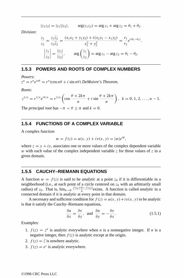
|z1z2| = |z1||z2|, arg(z1z2) = arg z1 + arg z2 = θ1 + θ2.
Division:z1
z2= z1z2
z2z2= (x1x2 + y1y2)+ i(x2y1 − x1y2)
x22 + y2
2
= r1
r2ei(θ1−θ2).
∣∣∣∣z1
z2
∣∣∣∣ = |z1||z2| , arg
(z1
z2
)= arg z1 − arg z2 = θ1 − θ2.
1.5.3 POWERS AND ROOTS OF COMPLEX NUMBERS
Powers:zn = rneinθ = rn(cos nθ + i sin nθ) DeMoivre’s Theorem.
Roots:
z1/n = r1/neiθ/n = r1/n
(cos
θ + 2kπ
n+ i sin
θ + 2kπ
n
), k = 0, 1, 2, . . . , n− 1.
The principal root has −π < θ ≤ π and k = 0.
1.5.4 FUNCTIONS OF A COMPLEX VARIABLE
A complex function
w = f (z) = u(x, y)+ iv(x, y) = |w|eiφ,where z = x + iy, associates one or more values of the complex dependent variablew with each value of the complex independent variable z for those values of z in agiven domain.
1.5.5 CAUCHY–RIEMANN EQUATIONS
A function w = f (z) is said to be analytic at a point z0 if it is differentiable in aneighborhood (i.e., at each point of a circle centered on z0 with an arbitrarily smallradius) of z0. That is, limh→0
f (z0 +h)−f (z0 )h
exists. A function is called analytic in aconnected domain if it is analytic at every point in that domain.
A necessary and sufficient condition for f (z) = u(x, y)+ iv(x, y) to be analyticis that it satisfy the Cauchy–Riemann equations,
∂u
∂x= ∂v
∂y, and
∂u
∂y= −∂v
∂x. (1.5.1)
Examples:
1. f (z) = zn is analytic everywhere when n is a nonnegative integer. If n is anegative integer, then f (z) is analytic except at the origin.
2. f (z) = z is nowhere analytic.
3. f (z) = ez is analytic everywhere.
©1996 CRC Press LLC

1.5.6 CAUCHY INTEGRAL THEOREM
If f (z) is analytic at all points within and on a simple closed curve C, then∫C
f (z) dz = 0. (1.5.2)
1.5.7 CAUCHY INTEGRAL FORMULA
If f (z) is analytic inside and on a simple closed contour C and if z0 is interior to C,then
f (z0) = 1
2πi
∫C
f (z)
z− z0dz. (1.5.3)
Moreover, if the derivatives f ′(z), f ′′(z), . . . of all orders exist, then
f (n)(z0) = n!
2πi
∫C
f (z)
(z− z0)n+1dz. (1.5.4)
1.5.8 TAYLOR SERIES EXPANSIONS
If f (z) is analytic inside of and on a circle C of radius r centered at the point z0, thena unique and uniformly convergent series expansion exists in powers of (z − z0) ofthe form
f (z) =∞∑n=0
an(z− z0)n, |z− z0| < r, z0 = ∞, (1.5.5)
where
an = 1
n!f (n)(z0) = 1
2πi
∫C
f (z)
(z− z0)n+1dz. (1.5.6)
If M(r) is an upper bound of |f (z)| on C, then
|an| = 1
n!|f (n)(z0)| ≤ M(r)
rn(Cauchy’s inequality). (1.5.7)
If the series is truncated with the term an(z− z0)n, the remainder Rn(z) is given by
Rn(z) = (z− z0)n+1
2πi
∫C
f (s)
(s − z)(s − z0)n+1ds, (1.5.8)
and
|Rn(z)| ≤( |z− z0|
r
)nrM(r)
r − |z− z0| . (1.5.9)
©1996 CRC Press LLC

1.5.9 LAURENT SERIES EXPANSIONS
If f (z) is analytic inside the annular domain between the concentric circles C1 andC2 centered at z0 with radii r1 and r2 (r1 < r2), respectively, then a unique seriesexpansion exists in terms of positive and negative powers of z − z0 of the followingform:
f (z) =∞∑n=1
bn(z− z0)−n +
∞∑n=0
an(z− z0)n,
= · · · + b2
(z− z0)2+ b1
z− z0+ a0 + a1(z− z0)+ a2(z− z0)
2 + . . .
(1.5.10)
where
an = 1
2πi
∫C
f (s)
(s − z0)n+1ds, n = 0, 1, 2, . . . , (1.5.11)
and
bn = 12πi
∫Cf (s)(s − z0)
n−1 ds, n = 1, 2, 3, . . . . (1.5.12)
1.5.10 ZEROS AND SINGULARITIES
The points z for which f (z) = 0 are called zeros of f (z). A function f (z) which isanalytic at z0 has a zero of order m there, where m is a positive integer, if and only ifthe first m coefficients a0, a1, . . . , am−1 in the Taylor expansion about z0 vanish.
A singular point or singularity of the function f (z) is any point at which f (z) isnot analytic. An isolated singularity of f (z) at z0 may be classified in one of threeways:
1. A removable singularity if and only if all coefficients bn in the Laurent seriesexpansion of f (z) about z0 vanish.
2. A pole of order m if and only if (z − z0)mf (z), but not (z − z0)
m−1f (z), isanalytic at z0, (i.e., if and only if bm = 0 and 0 = bm+1 = bm+2 = . . . in theLaurent series expansion of f (z) about z0). Equivalently, f (z) has a pole oforder m if 1/f (z) is analytic at z0 and has a zero of order m there.
3. An isolated essential singularity if and only if the Laurent series expansion off (z) about z0 has an infinite number of terms involving negative powers ofz− z0.
©1996 CRC Press LLC
1.5.11 RESIDUES
Given a point z0 where f (z) is either analytic or has an isolated singularity, the residueof f (z) is the coefficient of (z− z0)
−1 in the Laurent series expansion of f (z) aboutz0, or
Res(z0) = b1 = 1
2πi
∫C
f (z) dz. (1.5.13)
If f (z) is either analytic or has a removable singularity at z0, then b1 = 0 there. If z0
is a pole of order m, then
b1 = 1
(m− 1)!
dm−1
dzm−1[(z− z0)
mf (z)]∣∣z=z0
. (1.5.14)
For every simple closed contour C enclosing at most a finite number of singularitiesz1, z2, . . . , zn of an analytic function continuous on C,∫
C
f (z) dz = 2πin∑k=1
Res(zk), (1.5.15)
where Res(zk) is the residue of f (z) at zk .
1.5.12 THE ARGUMENT PRINCIPLE
Let f (z) be analytic on a simple closed curve C with no zeros on C and analyticeverywhere inside C except possibly at a finite number of poles. Let AC arg f (z)denote the change in the argument of f (z) (final value − initial value) as z transversesthe curve once in the positive sense. Then
1
2πAC arg f (z) = N − P, (1.5.16)
whereN is number of zeros of f (z) inside C, and P is the number of poles inside C.The zeros and poles are counted according to their multiplicities.
©1996 CRC Press LLC

1.5.13 TRANSFORMATIONS AND MAPPINGS
A function w = f (z) = u(z)+ iv(z) maps points of the z-plane into correspondingpoints of the w-plane. At every point z such that f (z) is analytic and f ′(z) = 0, themapping is conformal, i.e., the angle between two curves in the z-plane through sucha point is reproduced in magnitude and sense by the angle between the correspondingcurves in thew-plane. A table giving real and imaginary parts, zeros, and singularitiesfor frequently used functions of a complex variable and a table illustrating a numberof special transformations of interest are at the end of this section.
A function is said to be simple in a domain D if it is analytic in D and assumesno value more than once in D. Riemann’s mapping theorem states
IfD is a simply connected domain in the complex z plane, which is neitherthe z plane nor the extended z plane, then there is a simple function f (z)such that w = f (z) maps D onto the disc |w| < 1.
1.5.14 BILINEAR TRANSFORMATIONS
The bilinear transformation is defined by w = az+ b
cz+ d, where a, b, c, and d are
complex numbers and ad = bc. It is also known as the Mobius or linear fractionaltransformation. The bilinear transformation is defined for all z = −d/c. The bilineartransformation is conformal and maps circles and lines into circles and lines.
The inverse transformation is given by z = −dw + b
cw − a, which is also a bilinear
transformation. Note that w = a/c.The cross ratio of four distinct complex numbers zk (for k = 1, 2, 3, 4) is given
by
(z1, z2, z3, z4) = (z1 − z2)(z3 − z4)
(z1 − z4)(z3 − z2).
If any of the zk is complex infinity, the cross ratio is redefined so that the quotient of thetwo terms on the right containing zk is equal to 1. Under the bilinear transformation,the cross ratio of four points is invariant: (w1, w2, w3, w4) = (z1, z2, z3, z4).
©1996 CRC Press LLC

f (z) = w(x, y) u(x, y) = Re w(x, y) v(x, y) = Im w(x, y) Zeros (and order m) Singularities (and order m)z x y z = 0, m = 1 Pole (m = 1) at z = ∞z2 x2 − y2 2xy z = 0, m = 2 Pole (m = 2) at z = ∞1
z
x
x2 + y2
−yx2 + y2
z = ∞, m = 1 Pole (m = 1) at z = 0
1
z2
x2 − y2
(x2 + y2)2
−2xy
(x2 + y2)2z = ∞, m = 2 Pole (m = 2) at z = 0
1
z− (a + ib)
x − a
(x − a)2 + (y − b)2
−(y − b)
(x − a)2 + (y − b)2z = ∞, m = 1 Pole (m = 1) at z = a + ib
a, b real
√z ±
(x +
√x2 + y2
2
)1/2
±(
−x +√x2 + y2
2
)1/2
z = 0, m = 1 Branch point (m = 1) at z = 0Branch point (m = 1) at z = ∞
ez ex cos y ex sin y None Essential singularity at z = ∞sin z sin x cosh y cos x sinh y z = kπ , m = 1
(k = 0,±1,±2, . . . )Essential singularity at z = ∞
cos z cos x sinh y − sin x cosh y z = (k + 1/2)π , m = 1(k = 0,±1,±2, . . . )
Essential singularity at z = ∞
sinh z sinh x cos y cosh x sin y z = kπi, m = 1(k = 0,±1,±2, . . . )
Essential singularity at z = ∞
cosh z cosh x cos y sinh x sin y z = (k + 1/2)πi, m = 1(k = 0,±1,±2, . . . )
Essential singularity at z = ∞
tan zsin 2x
cos 2x + cosh 2y
sinh 2y
cos 2x + cosh 2yz = kπ , m = 1(k = 0,±1,±2, . . . )
Essential singularity at z = ∞Poles (m = 1) at z = (k + 1/2)π(k = 0,±1,±2, . . . )
tanh zsinh 2x
cosh 2x + cos 2y
sin 2y
cosh 2x + cos 2yz = kπi, m = 1(k = 0,±1,±2, . . . )
Essential singularity at z = ∞Poles (m = 1) at z = (k + 1/2)πi(k = 0,±1,±2, . . . )
log z log(x2 + y2)/2 tan−1 x
y+ 2kπ z = 1, m = 1 Branch points at z = 0, z = ∞
(k = 0,±1,±2, . . . )
1.5.15 TABLE OF TRANSFORMATIONS
©1996 CRC Press LLC

1.5.16 TABLE OF CONFORMAL MAPPINGS
In the following functions z = x + iy and w = u+ iv = ρeiφ .
v
uA'B'
C'D'x
y
A
B
C
Dw = z2.
v
ux
y
AB
C D D'
A'B'
C' w = z2.
v
uD'x
y
A
BC
D A'
B'C'k
w = z2; A′, B ′ on the
parabola ρ = 2k2
1 + cosφ.
v
u
D'
x
y
A
B
C
D
A'
B'
C'w = 1/z.
v
ux
y
A B
C
A'
B'
C'
w = 1/z.
v
u
D'
x
y
ABC
D
A'B'C'
E Fπi
1F' E'
w = ez.
©1996 CRC Press LLC

v
u
D'
x
y
A B
C
D
A' B'
Eπi
1
C'
E'
w = ez.
v
u
D'
x
y
A B
C
D
A' B'
Eπi C'
FF'
E'
w = ez.
v
uD'
x
y
A
BCD A'B'C'
E
1−π/2 π/2E'
w = sin z.
v
u
D'
x
y
A
BC
D
A'B'C'
1π/2
w = sin z.
v
u
D'x
y
A
BC
D
A' B'E
π/2
C'
F F'
−π/2 1E'
w = sin z; BCD: y = k, B ′C ′D′
is on the ellipse( u
cosh k
)2+( v
sinh k
)2= 1.
v
u
D'
A
B
CD
A'
B'
E
ι
C'1
y
x
E'
w = z− 1
z+ 1.
v
u
D'
A B C D A'
B'
E1 C'
1
y
x E' w = i − z
i + z.
©1996 CRC Press LLC

v
u
D'
x
y
A
B
C
D
A'
B'
C'E
F
G E'
F'
G'x1x2 R01
1
w = z− a
az− 1; a =
1 + x1x2 +√(1 − x2
1 )(1 − x22 )
x1 + x2;
R0 =1 − x1x2 +
√(1 − x2
1 )(1 − x22 )
x1 − x2(a > 1 and R0 > 1 when −1 <
x2 < x1 < 1).
AAAAAA
v
uD'xA
B
C D A'
B'
C'
y
EF
E'
F'x2R01 1x1
w = z− a
az− 1; a =
1 + x1x2 +√(x2
1 − 1)(x22 − 1)
x1 + x2;
R0 =x1x2 − 1 −
√(x2
1 − 1)(x22 − 1)
x1 − x2(x2 < a < x1 and 0 < R0 < 1
when 1 < x2 < x1).v
uD'x
y
A
B
C
D A'B'
E 1C'
2
E'w = z+ 1/z.
AAAAAAAAAA
v
uD'
x
y
AB
C
D A'B'E1
C'
2
E'
w = z+ 1/z.
v
u
D'
xB
C
DA' B'E
C'
F'
y
A
F
k1
2
E'
w = z+ 1/z; B ′C ′D′ is on theellipse(
ku
k2 + 1
)2
+(
kv
k2 − 1
)2
= 1.
©1996 CRC Press LLC

πi
v
uD'
x
y
A B C D A' B'
C'
E
1
B'D'
E'
w = logz− 1
z+ 1.
v
u
D'
x
y
A
B
C
D
A' B'
1
C'
E F
F' πi
ki
E'
w = logz− 1
z+ 1; ABC is on the
circle x2 + y2 − 2y cot k = 1.
u
D'
xA
BC D
vA'
B'
C'
y
E
F
F'
c1 c21
πi
−πi
E'
w = logz+ 1
z− 1; relationship
between centers and radii: centersof circles at zn = coth cn, radii arecsch cn, n = 1, 2.
πi
v
uG'
x
y
A B C D
A'
F'
C'
E
1
B'
D'
-1
GF
x1
kπi
E'
w = k logk
1 − k+ log 2(1 − k)+
iπ−k log(z+1)−(1−k) log(z−1);x1 = 2k − 1.
v
u
D'
x
y
A B
C
D
A' B'
Eπi
1
C'
E'
w = tan2(z/2).
uD'x
A
BC D
A'
B'
Eπiv
C'
y
F
G
H
H'
G' E'F'w = coth(z/2).
uD'x
A
BC D
A'B'Eπiv
C'
y
F
G
H
H'G'
F'
πi/2
E'w = log coth(z/2).
©1996 CRC Press LLC

v
ux
y
A B C D A'
C'
E
1
B'
D'
1+πi E'
w = πi + z− log z.
v
ux
y
A B C D
A'
C'
E
-1
B'
D'
πi
E'
w = 2(z+ 1)1/2 + log(z+ 1)1/2 − 1
(z+ 1)1/2 + 1.
v
ux
y
A B CD
A'
C'
1
B'
D'
πi
-k2
E F
E'
F'
-π/k
w = i
klog
1 + ikt
1 − ikt+ log
1 + t
1 − t;
t =(z− 1
z+ k2
)1/2
.
v
ux
y
A B C D
A'
C'
1B'
D'
ih
-1w = h
π
[(z2 − 1)1/2 + cosh−1 z
].
v
ux
y
A B C D
A'
C'
B'
D'
πi
k
F'
π/k
1
FE
E'
w = cosh−1
(2z− k − 1
k − 1
)−
1
kcosh−1
[(k + 1)z− 2k
(k − 1)z
].
©1996 CRC Press LLC

1.6 REAL ANALYSIS
1.6.1 RELATIONS
For two sets A and B, the product A× B is the set of all ordered pairs (a, b) wherea is in A and b is in B. Any subset of the product A × B is called a relation. Arelation R on a product A×A is called an equivalence relation if the following threeproperties hold:
1. Reflexive: (a, a) is in R for every a in A.
2. Symmetric: If (a, b) is in R, then (b, a) is in R.
3. Transitive: If (a, b) and (b, c) are in R, then (a, c) is in R.
When R is an equivalence relation then the equivalence class of an element a inA is the set of all b in A such that (a, b) is in R.
Example: The set of rational numbers has an equivalence relation “=” definedby the requirement that an ordered pair ( a
b, cd
) belongs in the relation if and only ifad = bc. The equivalence class of 1
2 is the set 12 ,
24 ,
36 , . . .
−1−2 ,
−2−4 , . . . .
1.6.2 FUNCTIONS (MAPPINGS)
A relation f on a set X × Y is a function (or mapping) from X into Y if (x, y) and(x, z) in the relation implies that y = z, and each x ∈ X has a y ∈ Y such that (x, y)is in the relation. The last condition means that there is a unique pair in f whosefirst element is x. We write f (x) = y to mean that (x, y) is in the relation f , andemphasize the idea of mapping by the notation f : X → Y . The domain of a functionf is the set of all x for which there is a pair (x, y) in the relation. The range of afunction f is a set containing all the y for which there is a pair (x, y) in the relation.The image of a set A in the domain of a function f is the set of y in Y such thaty = f (x) for some x in A. The notation for the image of A under f is f [A]. Theinverse image of a set B in the range of a function f is the set of all x in X such thatf (x) = y for some y in B. The notation is f −1[B].
A function f is one-to-one (or univalent, or injective) if f (x1) = f (x2) impliesx1 = x2. A function f : X → Y is onto (or surjective) if for every y in Y there issome x in X such that f (x) = y. A function is bijective if it is both one-to-one andonto.
Examples:
• f (x) = ex , as a mapping from R to R, is one-to-one because ex1 = ex2 impliesx1 = x2 (by taking the natural logarithm). It is not onto because −1 is not thevalue of ex for any x in R.
©1996 CRC Press LLC

• g(x) = x3 − x, as a mapping from R to R, is onto because every real number isattained as a value of g(x), for some x. It is not one-to-one because g(−1) =g(0) = g(1).
• h(x) = x3, as a mapping from R to R, is bijective.
For an injective function f mapping X into Y , there is an inverse function f −1
mapping the range of f into X which is defined by: f −1(y) = x if and only iff (x) = y. Example: The function f (x) = ex mapping R into R+ (the set of positivereals) is bijective. Its inverse is f −1(x) = ln(x) which maps R+ into R.
For functions f : X → Y and g : Y → Z, with the range of f contained in thedomain of g, the composition (g f ) : X → Z is a function defined by (g f )(x) =g(f (x)) for all x in domain of f .
1. Note that g f may not be the same as f g. For example, for f (x) = x + 1,and g(x) = 2x, we have (g f )(x) = g(f (x)) = 2f (x) = 2(x+ 1) = 2x+ 2.However (f g)(x) = f (g(x)) = g(x)+ 1 = 2x + 1.
2. For every function f and its inverse f −1, we have (f f −1)(x) = x, for all xin the domain of f −1, and (f −1 f )(x) = x for all x in the domain of f . Notethat the inverse function f −1 is not the same as 1
f(unless f (x) = x).
1.6.3 SETS OF REAL NUMBERS
A sequence is the range of a function having the natural numbers as its domain. Itcan be denoted by xn | n is a natural number or simply xn. For a chosen naturalnumber N , a finite sequence is the range of a function having natural numbers lessthan N as its domain. Sets A and B are in a one-to-one correspondence if there isa bijective function from A into B. Two sets A and B have the same cardinality ifthere is a one-to-one correspondence between them. A set which is equivalent to theset of natural numbers is denumerable (or countably infinite). A set which is emptyor is equivalent to a finite sequence is finite (or finite countable).
Examples: The set of letters in the English alphabet is finite. The set of rationalnumbers is denumerable. The set of real numbers is uncountable.
Axioms of order1. There is a subset P (positive numbers) of R for which x + y and xy are in P
for every x and y in P .
2. Exactly one of the following conditions can be satisfied by a number x in R
(trichotomy): x ∈ P , −x ∈ P , or x = 0.
DefinitionsA number b is an upper (lower) bound of a subset S in R if x ≤ b (x ≥ b) for everyx in S. A number c is a least upper bound (lub, supremum, or sup) of a subset S inR if c is an upper bound of S and b ≥ c for every upper bound b of S. A number c is
©1996 CRC Press LLC

a greatest lower bound (glb, infimum, or inf) if c is a lower bound of S and c ≥ b forevery lower bound b of S.
Completeness (or least upper bound) axiomIf a nonempty set of real numbers has an upper bound, then it has a least upper bound.
Characterization of the real numbersThe real numbers are the smallest complete ordered field that contain the rationals.Alternatively, the properties of a field, the order properties, and the least upper boundaxiom characterize the set of real numbers. The least upper bound axiom distinguishesthe set of real numbers from other ordered fields.
Archimedean property of R: For every real number x, there is an integer N suchthat x < N. For every pair of real numbers x and y with x < y, there is a rationalnumber r such that x < r < y. This is sometimes stated: The set of rational numbersis dense in R.
DefinitionsThe extension of R by +∞ is accomplished by including the symbols ∞ and −∞with the following definitions (for all x ∈ R)
• −∞ < x < ∞, for all x in R
• x + ∞ = ∞, for all x in R
• x − ∞ = −∞, for all x in R
• x∞ = x
−∞ = 0, for all x in R
• x · ∞ = ∞, if x > 0
• x · (−∞) = −∞, if x > 0
• ∞ + ∞ = ∞• −∞ − ∞ = −∞• ∞ · ∞ = ∞• −∞ · (−∞) = ∞
1.6.4 TOPOLOGY
A topology on a set X is a collection T of subsets of X (called open sets) having thefollowing properties:
1. The empty set and X are in T .
2. The union of elements in an arbitrary subcollection of T is in T .
3. The intersection of elements in a finite subcollection of T is in T .
©1996 CRC Press LLC

The complement of an open set is a closed set. A set is compact if every opencover has a finite subcover.
Notes1. A subset E of X is closed if and only if E contains all its limit points.
2. The union of finitely many closed sets is closed.
3. The intersection of an arbitrary collection of closed sets is closed.
4. The image of a compact set under a continuous function is compact.
1.6.5 METRIC SPACE
A norm on a vector space E with scalar field R is a function || · || from E into R thatsatisfies the following conditions:
1. Positive definiteness: ||x|| ≥ 0 for all x in E, and ||x|| = 0 if and only if x = 0.
2. Scalar homogeneity: For every x in E and a in R,||ax|| = |a| ||x||.3. Triangle inequality: ||x + y|| ≤ ||x|| + ||y|| for all x, y in E.
A metric (or distance function) on a set E is a function ρ : E ×E → R that satisfiesthe following conditions:
1. Positive definiteness: ρ(x, y) > 0 for all x, y in E, and ρ(x, y) = 0 if and onlyif x = y.
2. Symmetry: ρ(x, y) = ρ(y, x) for all x, y in E.
3. Triangle inequality: ρ(x, y) ≤ ρ(x, z)+ ρ(z, y) for all x, y, z in E.
Every norm || · || gives rise to a metric ρ by defining: ρ(x, y) = ||x−y||. Examples:
1. R with absolute value as norm has metric ρ(x, y) = |x − y|.2. R × R (denoted R2) with Euclidean norm ||(x, y)|| =
√x2 + y2, has metric
ρ((x1, y1), (x2, y2)) =√(x1 − x2)2 + (y1 − y2)2
A δ neighborhood of a point x in a metric space E is the set of all y in E such thatρ(x, y) < δ. For example, a δ neighborhood of x in R is the interval centered at xwith radius δ, (x − δ, x + δ). In a metric space the topology is generated by the δneighborhoods.
1. A subset G of R is open if, for every x in G, there is a δ > 0 such that every yin R with |x−y| < δ is inG also. For example, intervals (a,b), (a,∞), (−∞,b)are open in R.
2. A number x is a limit (or a point of closure, or an accumulation point) of a setF if, for every δ > 0, there is a point y in F such that |x − y| < δ.
©1996 CRC Press LLC

3. A subset F of R is closed if it contains all of its limits. For example, intervals[a,b], (−∞, b], and [a,∞) are closed in R.
4. A subset F is dense in R if every element of R is a limit point of F .
5. A metric space is separable if it contains a denumerable dense set. For example,R is separable because the subset of rationals is a denumerable dense set.
• (Bolzano–Weierstrass theorem) Any bounded infinite set of real numbers has alimit point in R.
• (Heine–Borel theorem) A closed, bounded subset of R is compact.
1.6.6 CONVERGENCE IN R
A number L is a limit point of a sequence xn if, for every ε > 0, there is a naturalnumberN such that |xn−L| < ε for all n > N . If it exists, a limit point of a sequenceis unique. A sequence is said to converge if it has a limit. A number L is a clusterpoint of a sequence xn if, for every ε > 0, there is an indexN such that |xn−L| < ε
for some n > N .Example: The limit of a sequence is a cluster point, as in 1
n,which converges to
0. However, cluster points are not necessarily limits, as in (−1)n, which has clusterpoints +1 and −1 but no limit.
LimitsLet xn be a sequence. A number L is the limit superior (limsup) if, for every ε > 0,there is a natural number N such that xn > L − ε for infinitely many n ≥ N , andxn > L+ε for only finitely many terms. An equivalent definition of the limit superioris given by
lim xn = infN
supk≥N
xk.
The limit inferior (liminf) is defined in a similar way by
lim xn = supN
infk≥N
xk.
For example, the sequence xn with xn = 1 + (−1)n + 12n has lim xn = 2, and
lim xn = 0.(Theorem) Every bounded sequence xn in R has a lim and a lim. In addition,
if lim xn = lim xn, then the sequence converges to their common value.A sequence xn is a Cauchy sequence if, for any ε > 0, there exists a positive integerN such that |xn − xm| < ε for every n > N and m > N .
(Theorem) A sequence xn in R converges if and only if it is a Cauchy sequence.A metric space, in which every Cauchy sequence converges to a point in the space,is called complete. For example, R with the metric ρ(x, y) = |x − y| is complete.
A number L is a limit of a function f as x approaches a number a if, for everyε > 0, there is a δ > 0 such that |f (x) − L| < ε for all x with |x − a| < δ. This
©1996 CRC Press LLC

is represented by the notation limx→a f (x) = L. The symbol ∞ is the limit of afunction f as x approaches a number a if, for every positive number M, there is aδ > 0 such that f (x) > M for all x with |x−a| < δ. Notation is limx→a f (x) = ∞.A number L is a limit of a function f as x approaches ∞ if, for every ε > 0, thereis a positive number M such that |f (x) − L| < ε for all x > M; this is writtenlimx→∞ f (x) = L. The number L is said to be the limit at infinity.
For example, limx→2
3x − 1 = 5, limx→0
1
x2= ∞, and lim
x→∞1
x= 0.
Pointwise and uniform convergenceA sequence of functions fn(x) is said to converge pointwise to the function f (x)on a set E if for every ε > 0 and x ∈ E there is a positive integer N such that|f (x) − fn(x)| < ε for every n ≥ N . A sequence of functions fn(x) is said toconverge uniformly to the function f on a set E if, for every ε > 0, there exists apositive integer N such that |f (x)− fn(x)| < ε for all x in E and n ≥ N .
Note that these formulations of convergence are not equivalent. For example,the functions fn(x) = xn on the interval [0, 1] converge pointwise to the functionf (x) = 0 for 0 ≤ x < 1, f (1) = 1. They do not converge uniformly because, forε = 1/2, there is no N such that |fn(x) − f (x)| < 1/2 for all x in [0, 1] and everyn $ N.
A function f is Lipschitz if there exists k > 0 in R such that |f (x) − f (y)| ≤k|x − y| for all x and y in its domain. The function is a contraction if 0 < k < 1.
(Fixed point or contraction mapping theorem) If the function f : [a, b] → [a, b]is a contraction, then there is a unique point x in [a, b] such that f (x) = x. The pointx is called a fixed point of f .
Example: Newton’s method for finding a zero of f (x) = (x + 1)2 − 2 on theinterval [0, 1] produces xn+1 = g(xn)with the contraction g(x) = x
2 − 12 + 1
x+1 . This
has the unique fixed point√
2 − 1 in [0, 1].
1.6.7 CONTINUITY IN R
A functionf : R → R is continuous at a pointa iff is defined ata and limx→a f (x) =f (a). The function f is continuous on a set E if it is continuous at every point of E.A function f is uniformly continuous on a set E if, for every ε > 0, there exists aδ > 0 such that |f (x)− f (y)| < ε for every x and y in its domain with |x − y| < δ.A sequence fn(x) of continuous functions on the interval [a, b] is equicontinuousif, for every ε > 0, there exists a δ > 0 such that |fn(x) − fn(y)| < ε for every nand for all x and y in [a, b] with |x − y| < δ. Examples:
1. A function can be continuous without being uniformly continuous. The functiong(x) = 1
xis continuous but not uniformly continuous on the open interval (0, 1).
2. A collection of continuous functions can be bounded on a closed interval withouthaving a uniformly convergent sub-sequence. The continuous functionsfn(x) =
x2
x2+(1−nx)2 are each bounded by 1 in the closed interval [0, 1] and for every x
there is the limit: limn→∞ fn(x) = 0. However, fn( 1n) = 1 for every n, so
©1996 CRC Press LLC
that no sub-sequence can converge uniformly to 0 everywhere on [0, 1]. Thissequence is not equicontinuous.
(Theorem) Let fn(x) be a sequence of functions mapping R into R whichconverges uniformly to a function f . If each fn(x) is continuous at a point a, thenf (x) is also continuous at a.
(Theorem) If a function f is continuous on a closed bounded set E, then it isuniformly continuous on E.
(Ascoli–Arzela theorem) Let K be a compact set in R. If fn(x) is uniformlybounded and equicontinuous on K , then fn(x) contains a uniformly convergentsub-sequence on K .
1.6.8 CONVERGENCE IN Lp
In the context of elementary measure theory, two measurable functions f and g areequivalent if they are equal except on a set of measure zero. They are said to be equalalmost everywhere. This is denoted by f = g a.e.
The (vector) space of measurable functions f on [a, b], for which∫ ba
|f (x)|pdx < ∞ with 0 < p < ∞, is denoted by Lp[a, b] or simply Lp. Thespace of bounded measurable functions on [a, b] is denoted by L∞.
The Lp norm for 0 < p < ∞ is defined by ‖f ‖p =(∫ b
a|f (x)|pdx
)1/p. The
L∞ norm is defined by
‖f ‖∞ = ess supa≤x≤b
|f (x)| , (1.6.1)
where
ess supa≤x≤b
|f (x)| = infM|mt : f (t) > M = 0. (1.6.2)
Let fn(x) be a sequence of functions in Lp (1 ≤ p < ∞) and f be some func-tion inLp. We say that fnconverges in the mean of orderp tof if limn→∞ ‖fn − f ‖p =0.
(Riesz–Fischer theorem) The Lp spaces are complete.
Inequalities
1. Minkowski inequality: If f and g are in Lp with 1 ≤ p ≤ ∞, then ‖f + g‖p ≤‖f ‖p + ‖g‖p. That is,
(∫ b
a
|f + g|p)1/p
≤(∫ b
a
|f |p)1/p
+(∫ b
a
|g|p)1/p
for (1 ≤ p < ∞),(1.6.3)
ess sup |f + g| ≤ ess sup |f | + ess sup |g|.
©1996 CRC Press LLC

2. Holder inequality: If p and q are nonnegative extended real numbers such that1/p + 1/q = 1 and f ∈ Lp and g ∈ Lq , then ‖fg‖1 ≤ ‖f ‖p ‖g‖q . That is∫ b
a
|fg| ≤(∫ b
a
|f |p)1/p (∫ b
a
|g|q)1/q
for (1 ≤ p < ∞),(1.6.4)
∫ b
a
|fg| ≤ (ess sup |f |)∫ b
a
|g|. (1.6.5)
3. Schwartz (or Cauchy–Schwartz) inequality: If f and g are in L2, then ‖fg‖1 ≤‖f ‖2 ‖g‖2. This is the special case of Holder’s inequality with p = q = 2.
1.6.9 CONVERGENCE IN L2
Two functions f and g inL2[a, b] are orthogonal if∫ bafg = 0. A set ofL2 functions
φn are orthogonal if∫ baφmφn = 0 for m = n . The set is orthonormal if, in addition,
each member has norm 1. That is, ‖φn‖2 = 1. For example, the functions sin nxare mutually orthogonal on (−π, π). The functions sin nx√
π form an orthonormal set
on (−π, π).Let φn be an orthonormal set inL2 and f be inL2. The numbers cn =
∫ b
a
f φndx
are the generalized Fourier coefficients of f with respect to φn, and the series∑∞n=1 cnφn(x) is called the generalized Fourier series of f with respect to φn.
For a function f in L2, the mean square error of approximating f by the sum∑Nn=1 anφn is 1
b−a∫ ba
|f (x)−∑Nn=1 a n φn(x)|2dx. An orthonormal set φn is complete
if the only measurable function f that is orthogonal to every φn is zero. That is,f = 0 a.e.
(Theorem) The generalized Fourier series of f in L2 converges in the mean (oforder 2) to f.
(Theorem) Parseval’s identity holds:∫ b
a
|f (x)|2dx =∞∑n=1
cn2.
Bessel’s inequality: For a functionf inL2 having generalized Fourier coefficientscn,
∑∞n=1 cn
2 ≤ ∫ ba
|f (x)|2dx.(Theorem) The mean square error of approximating f by the series
∑∞n=1 anφnis
minimum when all coefficients an are the Fourier coefficients off with respect to φn.(Riesz–Fischer theorem) Let φn be an orthonormal set in L2 and let cn be
constants such that∑∞
n=1 cn2 converges. Then a unique function f in L2 exists
such that the cn are the Fourier coefficients of f with respect to φn and∑∞
n=1 cnφnconverges in the mean (or order 2) to f .
Example: suppose that the series ao2 + ∑∞
n=1(a2n + b2
n) converges. Then thetrigonometric series ao
2 +∑∞n=1(an cos nx + bn sin nx) is the Fourier series of some
function in L2.
©1996 CRC Press LLC

1.6.10 ASYMPTOTIC RELATIONSHIPS
Asymptotic relationships are indicated by the symbols O, J, K, o, and ∼.
1. The symbolO (pronounced “big-oh”): f (x) ∈ O(g(x)) as x → x0 if a positiveconstant C exists such that |f (x)| ≤ C |g(x)| for all x sufficiently close to x0.Note that O(g(x)) is a class of functions. Sometimes the statement f (x) ∈O(g(x)) is written (imprecisely) as f = O(g).
2. The symbolJ : f (x) ∈ J(g(x)) as x → x0 if a positive constant C exists suchthat g(x) ≤ Cf (x) for all x sufficiently close to x0.
3. The symbolK : f (x) ∈ K(g(x)) as x → x0 if positive constants c1 and c2 existsuch that c1g(x) ≤ f (x) ≤ c2g(x) for all x sufficiently close to x0. This isequivalent to: f (x) = O(g(x)) and g(x) = O(f (x)). The symbol ≈ is oftenuse for K.
4. The symbol o (pronounced “little-oh”): f (x) ∈ o(g(x)) as x → x0 if, givenany µ > 0, we have |f (x)| < µ|g(x)| for all x sufficiently close to x0.
5. The symbol ∼ (pronounced “asymptotic to”): f (x) ∼ (g(x)) as x → x0 iff (x) = g(x) [1 + o(1)] as x → x0.
6. Two functions, f (x) and g(x), are asymptotically equivalent as x → x0 iff (x)/g(x) ∼ 1 as x → x0.
7. A sequence of functions, gk(x), forms an asymptotic series at x0 if gk+1(x) =o(gk(x)) as x → x0.
8. Given a function f (x) and an asymptotic series gk(x) at x0, the formal series∑`k=0 akgk(x) is an asymptotic expansion of f (x) if f (x) −∑n
k=0 akgk(x) =o(gn(x)) as x → x0 for every n; this is expressed as f (x) ∼ ∑`
k=0 akgk(x).Partial sums of this formal series are called asymptotic approximations to f (x).This formal series need not converge.
Think of O being an upper bound on a function, J being a lower bound, and Kbeing both an upper and lower bound. For example: sin x ∈ O(x) as x → 0, log n ∈o(n) as n → ∞, and n9 ∈ J(n9 + n2) as n → ∞.
1.7 GENERALIZED FUNCTIONS
Dirac’s delta function is defined by δ(x) =
0 x = 0
∞ x = 0, and is normalized so that∫∞
−∞ δ(x) dx = 1. Properties include (assuming that f (x) is continuous):
1.∫∞−∞ f (x)δ(x − a) dx = f (a).
2.∫∞−∞ f (x) d
mδ(x)
dxmdx = (−1)m dmf (0)
dxm.
©1996 CRC Press LLC

3. xδ(x), as a distribution, equals zero
4. δ(ax) = 1|a|δ(x) when a = 0.
5. δ(x2 − a2) = 12a [δ(x + a)+ δ(x − a)].
6. δ(x) = 12L + 1
L
∑∞n=1 cos nπx
L(Fourier series).
7. δ(x) = 2L
∑∞n=1 sin nπξ
Lsin nπx
Lfor 0 < ξ < L (Fourier sine series).
8. δ(x) = 12π
∫∞−∞ eikx dk (Fourier transform).
9. δ(ρ − ρ ′) = ρ∫∞
0 kJm(kρ)Jm(kρ′) dk.
Sequences of functions φn that approximate the delta function as n → ∞ areknown as delta sequences. For example:
• φn(x) = nπ
1a+n2x2
• φn(x) = n√πe−n2x2
• φn(x) = 1nπ
sin2 nxx2
• φn(x) =
0 |x| ≥ 1/n
n/2 |x| < 1/n
The Heaviside function, or step function, is defined as
H(x) = ∫ x−∞ δ(t) dt =
0 x < 0
1 x > 1. Sometimes H(0) is stated to be 1/2. This
function has the representations:
1. H(x) = 12 + 2
π
∑∞n=odd
1n
sin nπxL
2. H(x) = 12πi
∫∞−∞
eikx
kdk
The related signum function gives the sign of its argument:
sgn(x) = 2H(x)− 1 =
−1 if x < 0
1 if x > 0(1.7.1)
The delta function δ(x − x′) = δ(x1 − x ′1)δ(x2 − x ′
2)δ(x3 − x ′3) in terms of the
coordinates (ξ1, ξ2, ξ3), related to (x1, x2, x3), via the Jacobian J (xi, ξj ), is written
δ(x − x′) = 1∣∣J (xi, ξj )∣∣δ(ξ1 − ξ ′1)δ(ξ2 − ξ ′
2)δ(ξ3 − ξ ′3). (1.7.2)
For example, in spherical polar coordinates
δ(x − x′) = 1
r2δ(r − r ′)δ(φ − φ′)δ(cos θ − cos θ ′). (1.7.3)
The solutions to differential equations involving delta functions are called Green’sfunctions (see Sections 5.6.5 and 5.7.4).
©1996 CRC Press LLC

References
1. L. B. W. Jolley, Summation of Series, Dover Publications, New York, 1961.
2. S. G. Krantz, Real Analysis and Foundations, CRC Press, Boca Raton, FL, 1991.
3. S. G. Krantz, The Elements of Advanced Mathematics, CRC Press, Boca Raton,FL, 1995.
4. N. J. A. Sloane and S. Plouffe, Encyclopedia of Integer Sequences, AcademicPress, New York, 1995.
©1996 CRC Press LLC

Chapter 2Algebra
2.1 ELEMENTARY ALGEBRA2.1.1 Basic algebra2.1.2 Progressions2.1.3 DeMoivre’s theorem2.1.4 Partial fractions
2.2 POLYNOMIALS 2.2.1 Quadratic polynomials2.2.2 Cubic polynomials2.2.3 Quartic polynomials2.2.4 Quintic polynomials2.2.5 Tschirnhaus’ transformation2.2.6 Polynomial norms2.2.7 Galoisgroup of a polynomial2.2.8 Other polynomial properties
2.3 NUMBER THEORY 2.3.1 Congruences2.3.2 Chinese remainder theorem2.3.3 Continued fractions2.3.4 Diophantineequations2.3.5 Greatest common divisor2.3.6 Least common multiple2.3.7 Farey sequences2.3.8 Mobius function2.3.9 Primenumbers2.3.10 Primenumbers less than 10,0002.3.11 Primenumbersof special forms2.3.12 Primeperiod lengths2.3.13 Factorization table2.3.14 Factorization of 2m − 12.3.15 Magic squares2.3.16 Totient function
2.4 VECTOR ALGEBRA2.4.1 Notation for vectorsand scalars2.4.2 Physical vectors2.4.3 Fundamental definitions2.4.4 Lawsof vector algebra2.4.5 Vector norms
©1996 CRC Press LLC

2.4.6 Dot, scalar, or inner product2.4.7 Vector or crossproduct2.4.8 Scalar and vector tripleproducts
2.5 LINEAR AND MATRIX ALGEBRA2.5.1 Definitions2.5.2 Typesof matrices2.5.3 Conformability for addition and multiplication2.5.4 Determinantsand permanents2.5.5 Matrix norms2.5.6 Singularity, rank, and inverses2.5.7 Systemsof linear equations2.5.8 Other matrix transformations2.5.9 Linear spacesand linear mappings2.5.10 Traces2.5.11 Generalized inverses2.5.12 Eigenstructure2.5.13 Eigenvaluediagonalization2.5.14 Matrix exponentials2.5.15 Quadratic forms2.5.16 Matrix factorizations2.5.17 Theorems2.5.18 Kronecker productsor tensor products2.5.19 Kronecker sums2.5.20 Thevector operation
2.6 ABSTRACT ALGEBRA 2.6.1 Basic concepts2.6.2 Groups2.6.3 Rings2.6.4 Fields2.6.5 Finitefields2.6.6 Homomorphismsand isomorphisms2.6.7 Matrix classes that aregroups2.6.8 Permutation groups2.6.9 Tables
©1996 CRC Press LLC

2.1 ELEMENTARY ALGEBRA
2.1.1 BASIC ALGEBRA
Algebraic equationsA polynomial equation in one variable is an equation of the form
f (x) = anxn + an−1x
n−1 + · · · + a1x + a0.
The degree of the equation is n (where an = 0).A complex number z is a root of the polynomial f (x) if f (z) = 0. A complex
number z is a root of multiplicity k if f (z) = f ′(z) = f ′′(z) = · · · = f (k−1)(z) = 0,but f (k)(z) = 0. A root of multiplicity 1 is called a simple root. A root of multiplicity2 is called a double root, and a root of multiplicity 3 is called a triple root.
Fundamental theorem of algebraA polynomial equation of degree n has exactly n complex roots, where a double rootis counted twice, a triple root three times, and so on. If the n roots of the polynomialf (x) are z1, z2, . . . , zn (where a double root is listed twice, a triple root three times,and so on), then
f (x) = an(x − z1)(x − z2) · · · (x − zn). (2.1.1)
If the coefficients a0, a1, . . . an are real numbers, then the polynomial will alwayshave an even number of complex roots occurring in pairs. That is, if z is a complexroot, then so is z. If the polynomial has an odd degree and the coefficients are real,then it must have at least one real root.
The coefficients of the polynomial may be expressed as symmetric functions ofthe roots. For example, the elementary symmetric functions are
s1 = z1 + z2 + · · · + zn = −an−1
an,
s2 = z1z2 + z1z3 + z2z3 + · · · =∑i>j
zizj = an−2
an,
...
sn = z1z2z3 · · · zn = (−1)na0
an.
(2.1.2)
where sk is the sum of(n
k
)products, each product combining k factors without
repetition.The discriminant of the polynomial is defined by
∏i>j (zi − zj )
2, where theordering of the roots is irrelevant. The discriminant can always be written as apolynomial combination of a0, a1, . . . , an, divided by an.
©1996 CRC Press LLC

ResultantsLet f (x) = anx
n+an−1xn−1 +· · ·+a1x+a0 and g(x) = bmx
m+bm−1xm−1 +· · ·+
b1x + b0, where an = 0 and bm = 0. The resultant of f and g is the determinant ofthe (m+ n)× (m+ n) matrix
det
an an−1 . . a0 0 . . . 00 an an−1 . a1 a0 0. . . . . . . . . . . . . . . . . . . . . . . . . . . . . . . . . . . . . . . . .
. . 0 an an−1 . a1 a0
bm bm−1 . b0 0 . . . . 00 bm bm−1 . b0 0 . . . 0. . . . . . . . . . . . . . . . . . . . . . . . . . . . . . . . . . . . . . . . .
. . . 0 bm . b1 b0
(2.1.3)
The resultant of f (x) and g(x) is 0 if and only if f (x) and g(x) have a common root.The resultant of f (x) and f ′(x) is zero if and only if f (x) has a multiple root. Forexample:
1. If f (x) = x2 + 2x + 3 and g(x;α) = 4x3 + 5x2 + 6x + (7 + α), then theresultant of f (x) and g(x;α) is
det
1 2 3 0 00 1 2 3 00 0 1 2 34 5 6 7 + α 00 4 5 6 7 + α
= (16 + α)2
Note that g(x,−16) = (4x − 3)(x2 + 2x + 3) = (4x − 3)f (x).
2. The resultant of ax + b and cx + d is da − bc.
3. The resultant of (x + a)5 and (x + b)5 is (b − a)25.
©1996 CRC Press LLC
Algebraic identities
(a ± b)2 = a2 ± 2ab + b2.
(a ± b)3 = a3 ± 3a2b + 3ab2 ± b3.
(a ± b)4 = a4 ± 4a3b + 6a2b2 ± 4ab3 + b4.
(a + b)n =n∑
k=0
(n
k
)akbn−kwhere
(n
k
)= n!
k!(n− k)!.
a2 + b2 = (a + bi)(a − bi).
a4 + b4 = (a2 +√
2ab + b2)(a2 −√
2ab + b2).
a2 − b2 = (a − b)(a + b).
a3 − b3 = (a − b)(a2 + ab + b2).
an − bn = (a − b)(an−1 + an−2b + · · · + abn−2 + bn−1).
(a + b + c)2 = a2 + b2 + c2 + 2ab + 2ac + 2bc.
(a + b + c)3 = a3 + b3 + c3 + 3(a2b + ab2 + a2c + ac2 + b2c + bc2)+ 6abc.
Laws of exponentsAssuming all quantites are real, then
axay = ax+y,ax
ay= ax−y, (ab)x = axbx,
a0 = 1 if a = 0, a−x = 1
ax,
(ab
)x= ax
bx,
(ax)y = axy, a1x = x
√a,
x√ab = x
√a
x√b,
x
√y√a = xy
√a, a
xy = y
√ax = ( y
√a)x, x
√a
b=
x√a
x√b.
ProportionIf a
b= c
d, then a
c= b
d, ad = bc, a+b
b= c+d
d, a−b
b= c−d
d, and a−b
a+b = c−dc+d .
If ab
= cd
, where a, b, c, and d are all positive numbers and a is the largest of thefour numbers, then a + d > b + c.
2.1.2 PROGRESSIONS
Arithmetic progressionAn arithmetic progression is a sequence of numbers such that the difference of any twoconsecutive numbers is constant. If the sequence is a1, a2, . . . an, where ai+1−ai = d,then ak = a1 + (k − 1)d and
a1 + a2 + · · · an = n
2(2a1 + (n− 1)d).
©1996 CRC Press LLC

In particular, the sequence 1, 2, . . . n is an arithmetic progression with sumn(n+1)/2.
Geometric progression
A geometric progression is a sequence of numbers such that the ratio of any twoconsecutive numbers is constant. If the sequence is a1, a2, . . . an, where ai+1/ai = r ,then ak = a1r
k−1.
a1 + a2 + · · · an =a1
1−rn1−r r = 1
na1 r = 1.(2.1.4)
If |r| < 1, then the infinite geometric series a1(1 + r + r2 + r3 + · · · ) converges toa1
1−r . For example, 1 + 12 + 1
4 + 18 + · · · = 2.
Means
The arithmetic mean of a and b is given by a+b2 . More generally, the arithmetic mean
of a1, a2, . . . , an is given by (a1 + a2 + · · · + an)/n.The geometric mean of a and b is given by
√ab. More generally, the geometric
mean of a1, a2, . . . , an is given by n√a1a2 · · · an. The geometric mean of n numbers
is less than the arithmetic mean, unless all of the numbers are equal.The harmonic mean of a and b is given by 2ab
a+b . If A, G, and H represent thearithmetic, geometric, and harmonic means of a and b, then AH = G2.
2.1.3 DEMOIVRE’S THEOREM
A complex number a + bi can be written in the form reiθ , where r2 = a2 + b2 andtan θ = b/a. Because eiθ = cos θ + i sin θ ,
(a + bi)n = rn(cos nθ + i sin nθ),
andn√
1 = cos2kπ
n+ i sin
2kπ
n, k = 0, 1, . . . , n− 1.
2.1.4 PARTIAL FRACTIONS
The technique of partial fractions allows a quotient of two polynomials to be writtenas a sum of simpler terms.
Given the fraction f (x)
g(x), where both f (x) and g(x) are polynomials, begin by
dividing f (x) by g(x) to produce a quotient q(x) and a remainder r(x), where thedegree of r(x) is less than the degree of g(x), so that f (x)
g(x)= q(x)+ r(x)
g(x). Therefore,
assume that the rational function has the form r(x)
g(x), where the degree of the numerator
is less than the degree of the denominator.The techniques used depend on the factorization of g(x).
©1996 CRC Press LLC

Single linear factorSuppose that g(x) = (x − a)h(x), where h(a) = 0. Then
r(x)
g(x)= A
x − a+ s(x)
h(x),
where the number A is given by r(a)/h(a). For example,
2x
x2 − 1= 1
x − 1+ 1
x + 1.
Repeated linear factorSuppose that g(x) = (x − a)kh(x), where h(a) = 0. Then
r(x)
g(x)= A1
x − a+ A2
(x − a)2+ · · · + Ak
(x − a)k+ s(x)
h(x),
where
Ak = r(a)
h(a),
Ak−1 = d
dx
(r(x)
g(x)
)∣∣∣∣x=a
,
Ak−2 = 1
2!
d2
dx2
(r(x)
g(x)
)∣∣∣∣x=a
,
Ak−j = 1
j !
dj
dxj
(r(x)
g(x)
)∣∣∣∣x=a
.
Single quadratic factorSuppose that g(x) = (x2 +bx+ c)h(x), where b2 −4c < 0 (so that x2 +bx+ c doesnot factor into real linear factors) and h(x) is relatively prime to x2 + bx + c. Then
r(x)
g(x)= Ax + B
x2 + bx + c+ s(x)
h(x).
In order to determine A and B, multiply the equation by g(x) so that there are nodenominators remaining, and substitute any two values for x, yielding two equationsfor A and B.
Repeated quadratic factorSuppose that g(x) = (x2 + bx + c)kh(x), where b2 − 4c < 0 (so that x2 + bx + c
does not factor into real linear factors) and h(x) is relatively prime to x2 + bx + c.Then
r(x)
g(x)= A1x + B1
x2 + bx + c+ A2x + B2
(x2 + bx + c)2+ A3x + B3
(x2 + bx + c)3
+ · · · + Akx + Bk
(x2 + bx + c)k+ s(x)
h(x).
©1996 CRC Press LLC

In order to determine Ai and Bi , multiply the equation by g(x) so that there are nodenominators remaining, and substitute any 2k values for x, yielding 2k equationsfor Ai and Bi .
2.2 POLYNOMIALS
2.2.1 QUADRATIC POLYNOMIALS
The solution of the equation ax2 + bx + c = 0, where a = 0, is given by
x = −b ± √b2 − 4ac
2a. (2.2.1)
The discriminant of this equation is b2 − 4ac. Suppose that a, b, and c are all real.If the discriminant is negative, then the two roots are complex numbers which areconjugate. If the discriminant is positive, then the two roots are unequal real numbers.If the discriminant is 0, then the two roots are equal.
2.2.2 CUBIC POLYNOMIALS
To solve the equation ax3 + bx2 + cx + d = 0, where a = 0, begin by making thesubstitution y = x+ b
3a . That gives the equation y3+3py+q = 0, wherep = 3ac−b2
9a2
and q = 2b3−9abc+27a2d27a3 . The discriminant of this polynomial is 4p3 + q2.
The solutions are given by 3√α− 3
√β, e
2πi3 3√α− e
4πi3 3√β, and e
4πi3 3√α− e
2πi3 3√β,
where
α = −q +√q2 + 4p3
2and β = −q −
√q2 + 4p3
2.
Suppose that p and q are real numbers. If the discriminant is positive, then oneroot is real, and two are complex conjugates. If the discriminant is 0, then there arethree real roots, of which at least two are equal. If the discriminant is negative, thenthere are three unequal real roots.
Trigonometric solution of cubic polynomials
In the event that the roots of the polynomial y3 + 3py + q = 0 are all real, meaningthat q2 +4p3 ≤ 0, then the expressions above involve complex numbers. In that caseone can also express the solution in terms of trigonometric functions. Define r and θby
r =√
−p3 and θ = cos−1 −q2r
.
©1996 CRC Press LLC

Then the three roots are given by
2 3√r cos
θ
3, 2 3
√r cos
θ + 2π
3, and 2 3
√r cos
θ + 4π
3
2.2.3 QUARTIC POLYNOMIALS
To solve the equation ax4 + bx3 + cx2 + dx + e = 0, where a = 0, start with thesubstitution y = x + b
4a . That gives y4 + py2 + qy + r = 0, where p = 8ac−3b2
8a2 ,
q = b3−4abc+8a2d8a3 , and r = 16ab2c+256a3e−3b4−64a2bd
256a4 .The cubic resolventof this polynomial is defined as t3−pt2−4rt+(4pr−q2) =
0. If u is a root of the cubic resolvent, then the solutions of the original quartic aregiven by the solutions of
y2 ± √u− p
(y − q
2(u− p)
)+ u
2= 0.
2.2.4 QUINTIC POLYNOMIALS
Some quintic equations are solvable by radicals. If the function f (x) = x5 + ax + b
(with a and b rational) is irreducible, then f (x) = 0 is solvable by radicals if, andonly if, numbers ε, c, and e exist (with ε = ±1, c ≥ 0, and e = 0) such that
a = 5e4(3 − 4εc)
c2 + 1and b = −4e5(11ε + 2c)
c2 + 1.
In this case, the roots are given by x = e(ωju1 + ω2ju2 + ω3ju3 + ω4ju4
)for
j = 0, 1, 2, 3, 4, where ω is a fifth root of unity (ω = exp (2πi/5)) and
u1 =(v2
1v3
D2
), u2 =
(v2
3v4
D2
), u3 =
(v2
2v1
D2
), u4 =
(v2
4v2
D2
),
v1 =√D +
√D − ε
√D, v2 = −
√D −
√D + ε
√D,
v3 = −√D +
√D + ε
√D, v4 =
√D −
√D − ε
√D, and
D = c2 + 1.
EXAMPLE 2.2.1
The quinticf (x) = x5 + 15x + 12 has the valuesε = −1, c = 4/3, ande = 1.Hence the unique real root is given by
x =(
−75 + 21√
10
125
)1/5
+(
−75 − 21√
10
125
)1/5
+(
225 + 72√
10
125
)1/5
+(
225 − 72√
10
125
)1/5
.
©1996 CRC Press LLC

2.2.5 TSCHIRNHAUS’ TRANSFORMATION
The nth degree polynomial equation
anxn + an−1x
n−1 + · · · + a1x + a0 = 0
can be transformed to one with up to three fewer terms,
zn + bn−4zn−4 + · · · + b1z+ b0 = 0
by making a transformation of the form
zj = γ4x4j + γ3x
3j + γ2x
2j + γ1xj + γ0
for j = 1, . . . , n where the γi can be computed, in terms of radicals, from the ai.Hence, the general quintic polynomial can be transformed to the form z5+az+b = 0.
2.2.6 POLYNOMIAL NORMS
The polynomial P(x) =n∑
j=0
ajxj has the norms:
||P ||1 =∫ 2π
0
∣∣P (eiθ)∣∣ dθ
2π|P |1 =
n∑j=0
∣∣aj ∣∣ . (2.2.2)
||P ||2 =(∫ 2π
0
∣∣P (eiθ)∣∣2 dθ
2π
)1/2
|P |2 =(
n∑j=1
∣∣aj ∣∣2)1/2
. (2.2.3)
||P ||∞ = max|z|=1
|P(z)| |P |∞ = maxj
∣∣aj ∣∣ . (2.2.4)
For the double bar norms, P is considered as a function on the unit circle; for thesingle bar norms, P is identified with its coefficients. These norms are comparable:
|P |∞ ≤ ||P ||1 ≤ |P |2 = ||P ||2 ≤ ||P ||∞ ≤ |P |1 ≤ n|P |∞.
(2.2.5)
2.2.7 GALOIS GROUP OF A POLYNOMIAL
Consider the polynomial P(x) = anxn + an−1x
n−1 + · · · + a0 = an(x − z1)(x −z2) . . . (x − zn).
There are certain relations among the roots that do not depend on how the rootsare numbered. For example, this is true of the elementary symmetric functions; seeEquation (2.1.2). The set of permutations that leave all polynomials with rationalcoefficients, H(z1, . . . , zn), invariant is the Galois group of the equation.
©1996 CRC Press LLC

For example, consider the polynomial f (x) = (x2 − 2)(x2 − 3), with rootsz1 = −√
2, z2 = √2, z3 = −√
3, z4 = √3. There are four permutations that leave
all allowable relationships between the roots invariant:
π =(
1 2 3 41 2 3 4
)p1 =
(1 2 3 42 1 3 4
)
p2 =(
1 2 3 41 2 4 3
)p3 =
(1 2 3 42 1 4 3
)
That is, all permutations that switch z1 and z2, or switch z3 and z4, or both, will leaveallowable relations invariant. To demonstrate that neither z1 nor z2 can be switchedwith z3 or z4, consider the expressions H1(zi) = z1z2 + 2 and H2(zi) = z3z4 + 3.
2.2.8 OTHER POLYNOMIAL PROPERTIES
1. For polynomial P(x) =n∑
j=0
ajxj , with a0 = 0, Jensen’s inequality is
∫ 2π
0log
∣∣P (eiθ)∣∣ dθ
2π≥ log |a0|
2. The polynomialP(x1, . . . , xn) =∑|α|=m
aαxα11 x
α22 . . . x
αNN , whereα = (α1, . . . , αN)
can be written in the symmetric form
P(x1, . . . , xn) =N∑
i1,...,im=1
ci1,...,imxi1xi2 . . . xim
with ci1,...,im = ∂mP∂xi1 ...∂xim
. This means that the x1x2 term is written as 12 (x1x2 +
x2x1), the term x1x22 becomes 1
3 (x1x2x2 + x2x1x2 + x2x2x1).
3. A valuation of the polynomial P(x) = anxn + an−1x
n−1 + · · · + a0 = an(x −z1)(x−z2) . . . (x−zn) is given byM(P) = an
∏ni=1 max(1, |zi |). This valuation
satisfies the properties:
• M(P)M(Q) = M(PQ)
• M(P(x)) = M(P(xk)) for k ≥ 1
• M(xnP (x−1)) = M(P(x))
©1996 CRC Press LLC

2.3 NUMBER THEORY
2.3.1 CONGRUENCES
Definitions1. If the integers a and b leave the same remainder when divided by the number n,
then a and b are congruentmodulo n. This is written a ≡ b (mod n).
2. If the congruence x2 ≡ a (mod p) has a solution, then a is a quadratic residueof p. Otherwise, a is a quadratic nonresidueof p.
• Let p be a prime. Legendre’s symbol(ap
)has the value +1 if a is a
quadratic residue of p, and the value −1 if a is a quadratic nonresidue ofp.
• The Jacobi symbolgeneralizes the Legendre symbol to non-prime moduli.If n = ∏k
i=1 pbii then the Jacobi symbol can be written in terms of the
Legendre symbol
(an
)=
k∏i=1
(a
pi
)bi
(2.3.1)
3. Carmichael numbers are composite numbers n that satisfy an−1 ≡ 1 (mod n)
for every a (1 < a < n) relatively prime to n.
Properties1. If a ≡ b (mod n), then b ≡ a (mod n).
2. If a ≡ b (mod n), and b ≡ c (mod n), then a ≡ c (mod n).
3. If a ≡ a′ (mod n), and b ≡ b′ (mod n), then a ± b ≡ a′ ± b′ (mod n).
4. If a ≡ a′ (mod n), then a2 ≡ (a′)2 (mod n), a3 ≡ (a′)3 (mod n), etc.
5. If (k,m) = d, then the congruence kx ≡ n (mod m) is solvable if and only ifd divides n. It then has d solutions.
6. If p is a prime, then ap ≡ a (mod p).
7. If p is a prime, and p does not divide a, then ap−1 ≡ 1 (mod p).
8. If (a,m) = 1 then aφ(m) ≡ 1 (mod m). (See Section 2.3.16 for φ(m).)
9. If p is an odd prime and a is not a multiple of p, then (p−1)! ≡ −(ap
)a(p−1)/2
(mod p).
10. If p and q are odd primes, then the law of quadratic reciprocity states that(p
q
)(q
p
)= (−1)(p−1)(q−1)/4.
©1996 CRC Press LLC

11. The number −1 is a quadratic residue of primes of the form 4k + 1 and anonresidue of primes of the form 4k + 3.
12. The number 2 is a quadratic residue of primes of the form 8k±1 and a nonresidueof primes of the form 8k ± 3.
13. The number −3 is a quadratic residue of primes of the form 6k + 1 and anonresidue of primes of the form 6k + 5.
14. The number 3 is a quadratic residue of primes of the form 12k ± 1 and a non-residue of primes of the form 12k ± 5.
ValuesThere are infinitely many Carmichael numbers. There are 32 Carmichael numbersless than one million; they are 561, 1105, 1729, 2465, 2821, 6601, 8911, 10585,15841, 29341, 41041, 46657, 52633, 62745, 63973, 75361, 101101, 115921, 126217,162401, 172081, 188461, 252601, 278545, 294409, 314821, 334153, 340561, 399001,410041, 449065, and 488881.
2.3.2 CHINESE REMAINDER THEOREM
Let m1,m2, . . . , mr be pairwise relatively prime integers. Then the system ofcongruences
x ≡ a1 (mod m1)
x ≡ a2 (mod m2)
...
x ≡ ar (mod mr)
has a unique solution moduloM = m1m2 · · ·mr . This unique solution can be writtenas
x = a1M1y1 + a2M2y2 + · · · + arMryr (2.3.2)
where Mk = M/mk , and yk is the inverse of Mk (modulo mk).Example: For the system of congruences
x ≡ 1 (mod 3)
x ≡ 2 (mod 5)
x ≡ 3 (mod 7)
we haveM = 3 ·5 ·7 = 105. HenceM1 = 35,M2 = 21, andM3 = 15. The equationfory1 isM1y1 = 35y1 ≡ 1 (mod 3)with solutiony1 ≡ 2 (mod 3). Likewise, y2 ≡ 1(mod 5) and y3 ≡ 1 (mod 7). This results in x = 1 ·35 ·2+2 ·21 ·1+3 ·15 ·1 ≡ 52(mod 105).
©1996 CRC Press LLC

2.3.3 CONTINUED FRACTIONS
The symbol [a0, a1, . . . , aN ] (with N finite or infinite and the ai being positiveintegers) represents the simple continued fraction,
[a0, a1, . . . , aN ] = a0 + 1
a1 + 1
a2 + 1
a3 + 1
a4 + . . .
· · · + 1
aN.
(2.3.3)
Thenth convergent(with 0 < n < N ) of [a0, a1, . . . , aN ] is defined to be [a0, a1, . . . , an].If pn and qn are defined by
p0 = a0, p1 = a1a0 + 1, pn = anpn−1 + pn−2 (2 ≤ n ≤ N)
q0 = 1, q1 = a1, qn = anqn−1 + qn−2 (2 ≤ n ≤ N)
then [a0, a1, . . . , an] = pn/qn. The continued fraction is convergent if and only ifthe infinite series
∑∞ai is divergent.
If the positive rational number x can be represented by a simple continued frac-tion with an odd (even) number of terms, then it is also representable by one withan even (odd) number of terms. (Specifically, if an = 1 then
[a0, a1, . . . , an−1, 1
] =[a0, a1, . . . , an−1 + 1
], and ifan ≥ 2, then [a0, a1, . . . , an] = [a0, a1, . . . , an − 1, 1].)
Aside from this indeterminacy, the simple continued fraction of x is unique. The errorin approximating by a convergent is bounded by∣∣∣∣x − pn
qn
∣∣∣∣ ≤ 1
qnqn+1<
1
q2n
. (2.3.4)
The algorithm for finding a continued fraction expansion of a number is to removethe integer part of the number (this becomes ai), take the reciprocal, and repeat. Forthe number π :
β0 = π ≈ 3.14159 a0 = β0 = 3
β1 = 1/(β0 − a0) ≈ 7.062 a1 = β1 = 7
β2 = 1/(β1 − a1) ≈ 15.997 a2 = β2 = 15
β3 = 1/(β2 − a2) ≈ 1.0034 a3 = β3 = 1
β4 = 1/(β3 − a3) ≈ 292.6 a4 = β4 = 292
Approximations to π and e may be found from π = [3, 7, 15, 1, 292, 1, 1, 1, 2, 1, 3,1, 14, 2, . . . ] and e = [2, 1, 2, 1, 1, 4, 1, 1, 6, . . . , 1, 1, 2n, . . . ]. The convergents forπ are 22
7 ,333106 ,
355113 ,
10399333102 , . . .. The convergents for e are 8
3 ,114 ,
197 ,
8732 , . . ..
©1996 CRC Press LLC

A periodic continued fraction is an infinite continued fraction in which al = al+kfor all l ≥ L. The set of partial quotients aL, aL+1, . . . , aL+k−1 is the period. Aperiodic continued fraction may be written as[
a0, a1, . . . , aL−1, aL, aL+1, . . . , aL+k−1]. (2.3.5)
For example,√
2 = [1, 2],√
3 = [1, 1, 2],√
5 = [2, 4], and√
7 = [2, 1, 1, 1, 4]. If
x = [b, a] then x = 12 (b+
√b2 + 4b
a). For example, [1] = (1+√
5)/2, [2] = 1+√2,
and [2, 1] = 1 + √3.
Functions can be represented as continued fractions. Using the notation
b0 + a1
b1 + a2
b2 + a3
b3 + a4
b4 + . . .
= b0 + a1
b1+a2
b2+a3
b3+a4
b4+ . . .
(2.3.6)
then (allowable values of z may be restricted in the following)
• ln(1 + z) = z1+
z2+
z3+
4z4+
4z5+
9z6+ . . .
• ez = 11−
z1+
z2−
z3+
z2−
z5+
z2− · · · = 1 + z
1−z
2+z
3−z
2+z
5−z
2+z
7− . . .
• tan z = z1−
z2
3−z2
5−z2
7− . . .
• tanh z = z1+
z2
3+z2
5+z2
7+ . . .
2.3.4 DIOPHANTINE EQUATIONS
A diophantine equation is one which requires the solutions to come from the set ofintegers.
Apart from the trivial solutions (with x = y = 0 or x = u), the general solutionto the equation x3 + y3 = u3 + v3 is given by
x = λ[1 − (a − 3b)(a2 + 3b2)
]y = λ
[(a + 3b)(a2 + 3b2)− 1
]u = λ
[(a + 3b)− (a2 + 3b2)2
]v = λ
[(a2 + 3b2)2 − (a − 3b)
](2.3.7)
where λ, a, b are any rational numbers except that λ = 0.A parametric solution to x4 + y4 = u4 + v4 is given by
x = a7 + a5b2 − 2a3b4 + 3a2b5 + ab6
y = a6b − 3a5b2 − 2a4b3 + a2b5 + b7
u = a7 + a5b2 − 2a3b4 − 3a2b5 + ab6
v = a6b + 3a5b2 − 2a4b3 + a2b5 + b7
(2.3.8)
Fermat’s last theorem states that there are no integer solutions to xn + yn = zn,when n > 2. This was proven by Andrew Wiles in 1995.
©1996 CRC Press LLC

Pell’s equationPell’s equation is x2 −My2 = 1. The solutions, integral values of (x, y), arise fromcontinued fraction convergents of
√M (see page 88).
The number√
2 has the continued fraction expansion [1, 2, 2, 2, 2, . . . ]. Hence,the first few convergents are 3
2 ,75 ,
1712 ,
4129 ,
9970 , . . . . In this case, every second conver-
gent represents a solution:
32 − 2 · 22 = 1,
172 − 2 · 122 = 1, and
992 − 2 · 702 = 1.
Pythagorean triplesIf the positive integers A, B, and C satisfy the relationship A2 + B2 = C2, then thetriplet (A,B,C) is a Pythagorean triple. It is possible to construct a right trianglewith sides of length A and B and a hypotenuse of C.
There are infinitely many Pythagorean triples. The most general solution toA2 + B2 = C2, with (A,B) = 1 and A even, is given by
A = 2xy B = x2 − y2 C = x2 + y2, (2.3.9)
where x and y are relatively prime integers of opposite parity with x > y > 0. Thefollowing shows some Pythagorean triples with the associated (x, y) values.
x y A B C
2 1 4 3 54 1 8 15 176 1 12 35 378 1 16 63 65
10 1 20 99 1013 2 12 5 135 2 20 21 297 2 28 45 514 3 24 7 25
Waring’s problemIf each positive integer can be expressed as a sum of n kth powers, then there is aleast value of n for which this is true: this is the number g(k). For all sufficientlylarge numbers, however, a smaller value of n may suffice: this is the number G(k).Lagrange’s theorem states: “Every positive integer is the sum of four squares;” thisis equivalent to the statement g(2) = 4. The following identity shows how a productcan be written as the sum of four squares:
(x21 + x2
2 + x23 + x2
4 )(y21 + y2
2 + y23 + y2
4 ) =(x1y1 + x2y2 + x3y3 + x4y4)
2 + (x1y2 − x2y1 + x3y4 − x4y3)2
+ (x1y3 − x3y1 + x4y2 − x2y4)2 + (x1y4 − x4y1 + x2y3 − x3y2)
2 (2.3.10)
©1996 CRC Press LLC

Consider k = 3; all numbers can be written as the sum of not more than 9 cubes,so that g(3) = 9. However, only the two numbers
23 = 23 + 23 + 13 + 13 + 13 + 13 + 13 + 13 + 13,
239 = 43 + 43 + 33 + 33 + 33 + 33 + 13 + 13 + 13,
require the use of 9 cubes; so G(3) ≤ 8.The current known values of g(k) include: g(3) = 9, g(4) ≥ 19, g(5) = 37 and
g(k) =⌊(
3
2
)k⌋
+ 2k − 2 for 6 ≤ k ≤ 471600000.
The value ofG(k) is only known for two values of k,G(2) = 4 andG(4) = 16. Itis known that: 4 ≤ G(3) ≤ 7,G(5) ≤ 23,G(6) ≤ 36,G(7) ≤ 137, andG(8) ≤ 163.It is also known that
G(k) ≤ 6k log k +(
4 + 3 log
(3 + 2
k
))k + 3. (2.3.11)
2.3.5 GREATEST COMMON DIVISOR
The greatest common divisor (GCD) of the integers n and m is the largest integerthat evenly divides both n and m. The Euclidean algorithm is frequently used forcomputing the GCD of two numbers; it utilizes the fact that a = ⌊
ab
⌋b + c where
0 ≤ c < b. For example, consider 78 and 21. Since 78 = 3 · 21 + 15, the largestinteger that evenly divides both 78 and 21 is also the largest integer that evenly dividesboth 21 and 15. Iterating results in
78 = 3 · 21 + 15
21 = 1 · 15 + 6
15 = 2 · 6 + 3
6 = 2 · 3 + 0
Hence GCD(78,21) = GCD(6,3) = 3. A common notation for GCD(n,m) is (n,m).Two numbers, a and b, are said to be relatively primeif they have no divisors in
common; i.e., if GCD(a, b) = 1. The probability that two integers chosen randomlyare relatively prime is π/6.
2.3.6 LEAST COMMON MULTIPLE
The least common multiple of the integers a and b (denoted LCM(a, b)) is the smallestinteger r that is divisible by both a and b. The simplest way to find the LCM of aand b is via the formula LCM(a, b) = ab/GCD(a, b). For example, LCM(10, 4) =
10·4GCD(10,4) = 10·4
2 = 20.
©1996 CRC Press LLC
2.3.7 FAREY SEQUENCES
The Farey series of ordern, Fn, is the ascending series of irreducible fractions betweenzero and one whose denominators do not exceed n. The fraction k/m belongs to Fn
if 0 ≤ k ≤ m ≤ n and k and m are relatively prime. If k/m and k′/m′ are twosuccessive terms of Fn then mk′ − km′ = 1. Fn−1 can be obtained from Fn bydeleting terms with denominators of n.
F3 =(
0
1,
1
3,
1
2,
2
3,
1
1
),
F5 =(
0
1,
1
5,
1
4,
1
3,
2
5,
1
2,
3
5,
2
3,
3
4,
4
5,
1
1
).
2.3.8 MOBIUS FUNCTION
The Mobius function is defined by
• µ(1) = 1
• µ(n) = 0 if n has a squared factor
• µ(p1p2 . . . pk) = (−1)k if all the primes p1, . . . , pk are distinct
The Mobius inversion formula states that, if g(n) =∑d|n
f (d), then
f (n) =∑d|n
µ(nd
)g(d) =
∑d|n
µ(d)g(nd
).
For example, φ(n) = n∑
d|nµ(d)
d.
The generalized Mobius formula in one dimension is that: ifg(x) = ∑∞n=1 f (nαx) ,
then f (x) = ∑∞n=1 µ(n)g (n
αx), for any real α except 0.The table below can be derived from the table in Section 2.3.13 (For example,
µ(2) = −1, µ(4) = 0, and µ(6) = 1).
©1996 CRC Press LLC

0 1 2 3 4 5 6 7 8 90 1 −1 −1 0 −1 1 −1 0 01 1 −1 0 −1 1 1 0 −1 0 −12 0 1 1 −1 0 0 1 0 0 −13 −1 −1 0 1 1 1 0 −1 1 14 0 −1 −1 −1 0 0 1 −1 0 05 0 1 0 −1 0 1 0 1 1 −16 0 −1 1 0 0 1 −1 −1 0 17 −1 −1 0 −1 1 0 0 1 −1 −18 0 0 1 −1 0 1 1 1 0 −19 0 1 0 1 1 1 0 −1 0 0
10 0 −1 −1 −1 0 −1 1 −1 0 −111 −1 1 0 −1 −1 1 0 0 1 112 0 0 1 1 0 0 0 −1 0 113 −1 −1 0 1 1 0 0 −1 −1 −114 0 1 1 1 0 1 1 0 0 −115 0 −1 0 0 −1 1 0 −1 1 116 0 1 0 −1 0 −1 1 −1 0 017 −1 0 0 −1 −1 0 0 1 1 −118 0 −1 −1 1 0 1 −1 1 0 019 −1 −1 0 −1 1 −1 0 −1 0 −1
2.3.9 PRIME NUMBERS
• A prime numberis a positive integer greater than 1 with no positive, integraldivisors other than 1 and itself. There are infinitely many prime numbers,2, 3, 5, 7, . . . .
• Twin primesare prime numbers that differ by two: (3, 5), (5, 7), (11, 13),(17, 19), . . . . It is not known whether there are infinitely many twin primes.
• For every integer n ≥ 2, the numbers n!+2, n!+3, . . . , n!+n are a sequenceof n− 1 consecutive composite numbers.
The function π(x) represents the number of primes less than x. The primenumber theorem states that π(x) ∼ x/ log x as x → ∞.
x 100 1000 10000 105 106 107
π(x) 25 168 1229 9592 78498 664579
Prime formula
The set of prime numbers is identical with the set of positive values taken on by thepolynomial of degree 25 in the 26 variables a, b, . . . , z:
©1996 CRC Press LLC

(k+2)1− [wz+h+j −q]2 − [(gk+2g+k+1)(h+j)+h−z]2 − [2n+p+q+z−e]2
− [16(k+1)3(k+2)(n+1)2 +1−f 2]2 − [e3(e+2)(a+1)2 +1−o2]2 − [(a2 −1)y2 +1−x2]2
−[16r2y4(a2−1)+1−u2]2−[((a+u2(u2−a))2−1)(n+4dy)2+1−(x+cu)2]2−[n+l+v−y]2
−[(a2−1)l2+1−m2]2−[ai+k+1−l−i]2−[p+l(a−n−1)+b(2an+2a−n2−2n−2)−m]2
−[q+y(a−p−1)+s(2ap+2a−p2−2p−2)−x]2−[z+pl(a−p)+t (2ap−p2−1)−pm]2.(2.3.12)
Although this polynomial appears to factor, the factors are improper, P = P ·1. Notethat this formula will also take on negative values, such as −76.
There also exists a prime representing polynomial which contains 12 variables.Dirichlet’s theorem on primes in arithmetic progressions: Let a and b be rel-
atively prime positive integers. Then the arithmetic progression an + b (for n =1, 2, . . . ) contains infinitely many primes.
Proofs of primality
Lucas–Lehmer primality test: Define the sequence, r1 = 3, rm+1 = r2m − 2. If p is a
prime of the form 4n+3 andMp = 2p−1, thenMp will be prime (called a Mersenneprime) if, and only if, Mp divides rp−1.
This simple test is the reason that the largest known prime numbers are Mersenneprimes. For example, consider p = 7 and M7 = 127. The rn sequence is 3, 7, 47,2207 ≡ 48, 2302 ≡ 16, 254 ≡ 0; hence M7 is prime.
It is also possible to give, for a general number p, a “certificate” that p is prime.It is easy to use the certificate to verify that a given number is prime (easier than it wasto determine that it was prime in the first place). There are several types of certificatesthat can be given. Pratt’s certificate consists of a number a and the factorization ofthe number p − 1. This method is feasible if p − 1 is easy to factor.
The number p will be prime if there exists a primitive root a in the field GF[p].This primitive root must satisfy the conditions ap−1 = 1 (mod p) and a(p−1)/q = 1(mod p) for any prime q that divides p. For example, the number p = 31 hasp − 1 = 30 = 2 · 3 · 5, and a primitive root is given by a = 3. Hence, to verify thatp = 31 is prime, we compute
3(31−1)/2 = 315 ≡ 14348907 ≡ −1 = 1 (mod 31),
3(31−1)/3 = 310 ≡ 59049 ≡ 25 = 1 (mod 31),
3(31−1)/5 = 36 ≡ 719 ≡ 16 = 1 (mod 31),
3(31−1) = (3(31−1)/2
)2 ≡ (−1)2 = 1 (mod 31).
Probabilistic primality test
Let n be a number whose primality is to be determined. Probabilistic primality testscan return one of two results: either a proof that the number n is composite or a
©1996 CRC Press LLC

statement of the form, “The probability that the number n is not prime is less than ε”,where ε can be specified by the user. Typically, we take ε = 2−200 < 10−60.
From Fermat’s theorem, if b = 0, then bn−1 = 1 (mod n) whenever n is prime.If this holds, then n is a probable prime to the baseb. Given a value of n, if a valueof b can be found such that this does not hold, then n cannot be prime. It can happen,however, that a probable prime is not prime.
Let P(x) be the probability that n is composite under the hypotheses:
1. n is an odd integer chosen randomly from the range [2, x];
2. b is an integer chosen randomly from the range [2, n− 2];
3. n is a probable prime to the base b.
Then P(x) ≤ (log x)−197 for x ≥ 1010000.A different test can be obtained from the following theorem. Given the number
n, find s and t with n − 1 = 2s t , with t odd. Then choose a random integer b fromthe range [2, n− 2]. If either
bt = 1 (mod n) or b2i t = −1 (mod n), for some i < s,
then n is a strong probable prime to the baseb. Every odd prime must pass this test.If n > 1 is an odd composite, then the probability that it is a strong probable primeto the base b, when b is chosen randomly, is less than 1/4.
A stronger test can be obtained by choosing k independent values for b in therange [2, n − 2] and checking the above relation for each value of b. Let Pk(x) bethe probability that n is found to be a strong probable prime to each base b. ThenPk(x) ≤ 4−(k−1)P (x)/(1 − P(x)).
2.3.10 PRIME NUMBERS LESS THAN 10,000
The prime number p10n+k is found by looking at the row begining with n and at thecolumn beginning with k.
0 1 2 3 4 5 6 7 8 9
2 3 5 7 11 13 17 19 231 29 31 37 41 43 47 53 59 61 672 71 73 79 83 89 97 101 103 107 1093 113 127 131 137 139 149 151 157 163 1674 173 179 181 191 193 197 199 211 223 2275 229 233 239 241 251 257 263 269 271 277
6 281 283 293 307 311 313 317 331 337 3477 349 353 359 367 373 379 383 389 397 4018 409 419 421 431 433 439 443 449 457 4619 463 467 479 487 491 499 503 509 521 523
10 541 547 557 563 569 571 577 587 593 599
11 601 607 613 617 619 631 641 643 647 65312 659 661 673 677 683 691 701 709 719 72713 733 739 743 751 757 761 769 773 787 79714 809 811 821 823 827 829 839 853 857 85915 863 877 881 883 887 907 911 919 929 937
©1996 CRC Press LLC

0 1 2 3 4 5 6 7 8 9
16 941 947 953 967 971 977 983 991 997 100917 1013 1019 1021 1031 1033 1039 1049 1051 1061 106318 1069 1087 1091 1093 1097 1103 1109 1117 1123 112919 1151 1153 1163 1171 1181 1187 1193 1201 1213 121720 1223 1229 1231 1237 1249 1259 1277 1279 1283 1289
21 1291 1297 1301 1303 1307 1319 1321 1327 1361 136722 1373 1381 1399 1409 1423 1427 1429 1433 1439 144723 1451 1453 1459 1471 1481 1483 1487 1489 1493 149924 1511 1523 1531 1543 1549 1553 1559 1567 1571 157925 1583 1597 1601 1607 1609 1613 1619 1621 1627 1637
26 1657 1663 1667 1669 1693 1697 1699 1709 1721 172327 1733 1741 1747 1753 1759 1777 1783 1787 1789 180128 1811 1823 1831 1847 1861 1867 1871 1873 1877 187929 1889 1901 1907 1913 1931 1933 1949 1951 1973 197930 1987 1993 1997 1999 2003 2011 2017 2027 2029 2039
31 2053 2063 2069 2081 2083 2087 2089 2099 2111 211332 2129 2131 2137 2141 2143 2153 2161 2179 2203 220733 2213 2221 2237 2239 2243 2251 2267 2269 2273 228134 2287 2293 2297 2309 2311 2333 2339 2341 2347 235135 2357 2371 2377 2381 2383 2389 2393 2399 2411 2417
36 2423 2437 2441 2447 2459 2467 2473 2477 2503 252137 2531 2539 2543 2549 2551 2557 2579 2591 2593 260938 2617 2621 2633 2647 2657 2659 2663 2671 2677 268339 2687 2689 2693 2699 2707 2711 2713 2719 2729 273140 2741 2749 2753 2767 2777 2789 2791 2797 2801 2803
41 2819 2833 2837 2843 2851 2857 2861 2879 2887 289742 2903 2909 2917 2927 2939 2953 2957 2963 2969 297143 2999 3001 3011 3019 3023 3037 3041 3049 3061 306744 3079 3083 3089 3109 3119 3121 3137 3163 3167 316945 3181 3187 3191 3203 3209 3217 3221 3229 3251 3253
46 3257 3259 3271 3299 3301 3307 3313 3319 3323 332947 3331 3343 3347 3359 3361 3371 3373 3389 3391 340748 3413 3433 3449 3457 3461 3463 3467 3469 3491 349949 3511 3517 3527 3529 3533 3539 3541 3547 3557 355950 3571 3581 3583 3593 3607 3613 3617 3623 3631 3637
51 3643 3659 3671 3673 3677 3691 3697 3701 3709 371952 3727 3733 3739 3761 3767 3769 3779 3793 3797 380353 3821 3823 3833 3847 3851 3853 3863 3877 3881 388954 3907 3911 3917 3919 3923 3929 3931 3943 3947 396755 3989 4001 4003 4007 4013 4019 4021 4027 4049 4051
56 4057 4073 4079 4091 4093 4099 4111 4127 4129 413357 4139 4153 4157 4159 4177 4201 4211 4217 4219 422958 4231 4241 4243 4253 4259 4261 4271 4273 4283 428959 4297 4327 4337 4339 4349 4357 4363 4373 4391 439760 4409 4421 4423 4441 4447 4451 4457 4463 4481 4483
61 4493 4507 4513 4517 4519 4523 4547 4549 4561 456762 4583 4591 4597 4603 4621 4637 4639 4643 4649 465163 4657 4663 4673 4679 4691 4703 4721 4723 4729 473364 4751 4759 4783 4787 4789 4793 4799 4801 4813 481765 4831 4861 4871 4877 4889 4903 4909 4919 4931 4933
66 4937 4943 4951 4957 4967 4969 4973 4987 4993 4999
©1996 CRC Press LLC

0 1 2 3 4 5 6 7 8 9
67 5003 5009 5011 5021 5023 5039 5051 5059 5077 508168 5087 5099 5101 5107 5113 5119 5147 5153 5167 517169 5179 5189 5197 5209 5227 5231 5233 5237 5261 527370 5279 5281 5297 5303 5309 5323 5333 5347 5351 5381
71 5387 5393 5399 5407 5413 5417 5419 5431 5437 544172 5443 5449 5471 5477 5479 5483 5501 5503 5507 551973 5521 5527 5531 5557 5563 5569 5573 5581 5591 562374 5639 5641 5647 5651 5653 5657 5659 5669 5683 568975 5693 5701 5711 5717 5737 5741 5743 5749 5779 5783
76 5791 5801 5807 5813 5821 5827 5839 5843 5849 585177 5857 5861 5867 5869 5879 5881 5897 5903 5923 592778 5939 5953 5981 5987 6007 6011 6029 6037 6043 604779 6053 6067 6073 6079 6089 6091 6101 6113 6121 613180 6133 6143 6151 6163 6173 6197 6199 6203 6211 6217
81 6221 6229 6247 6257 6263 6269 6271 6277 6287 629982 6301 6311 6317 6323 6329 6337 6343 6353 6359 636183 6367 6373 6379 6389 6397 6421 6427 6449 6451 646984 6473 6481 6491 6521 6529 6547 6551 6553 6563 656985 6571 6577 6581 6599 6607 6619 6637 6653 6659 6661
86 6673 6679 6689 6691 6701 6703 6709 6719 6733 673787 6761 6763 6779 6781 6791 6793 6803 6823 6827 682988 6833 6841 6857 6863 6869 6871 6883 6899 6907 691189 6917 6947 6949 6959 6961 6967 6971 6977 6983 699190 6997 7001 7013 7019 7027 7039 7043 7057 7069 7079
91 7103 7109 7121 7127 7129 7151 7159 7177 7187 719392 7207 7211 7213 7219 7229 7237 7243 7247 7253 728393 7297 7307 7309 7321 7331 7333 7349 7351 7369 739394 7411 7417 7433 7451 7457 7459 7477 7481 7487 748995 7499 7507 7517 7523 7529 7537 7541 7547 7549 7559
96 7561 7573 7577 7583 7589 7591 7603 7607 7621 763997 7643 7649 7669 7673 7681 7687 7691 7699 7703 771798 7723 7727 7741 7753 7757 7759 7789 7793 7817 782399 7829 7841 7853 7867 7873 7877 7879 7883 7901 7907
100 7919 7927 7933 7937 7949 7951 7963 7993 8009 8011
101 8017 8039 8053 8059 8069 8081 8087 8089 8093 8101102 8111 8117 8123 8147 8161 8167 8171 8179 8191 8209103 8219 8221 8231 8233 8237 8243 8263 8269 8273 8287104 8291 8293 8297 8311 8317 8329 8353 8363 8369 8377105 8387 8389 8419 8423 8429 8431 8443 8447 8461 8467
106 8501 8513 8521 8527 8537 8539 8543 8563 8573 8581107 8597 8599 8609 8623 8627 8629 8641 8647 8663 8669108 8677 8681 8689 8693 8699 8707 8713 8719 8731 8737109 8741 8747 8753 8761 8779 8783 8803 8807 8819 8821110 8831 8837 8839 8849 8861 8863 8867 8887 8893 8923
111 8929 8933 8941 8951 8963 8969 8971 8999 9001 9007112 9011 9013 9029 9041 9043 9049 9059 9067 9091 9103113 9109 9127 9133 9137 9151 9157 9161 9173 9181 9187114 9199 9203 9209 9221 9227 9239 9241 9257 9277 9281115 9283 9293 9311 9319 9323 9337 9341 9343 9349 9371
116 9377 9391 9397 9403 9413 9419 9421 9431 9433 9437117 9439 9461 9463 9467 9473 9479 9491 9497 9511 9521
©1996 CRC Press LLC

0 1 2 3 4 5 6 7 8 9
118 9533 9539 9547 9551 9587 9601 9613 9619 9623 9629119 9631 9643 9649 9661 9677 9679 9689 9697 9719 9721120 9733 9739 9743 9749 9767 9769 9781 9787 9791 9803
121 9811 9817 9829 9833 9839 9851 9857 9859 9871 9883122 9887 9901 9907 9923 9929 9931 9941 9949 9967 9973
2.3.11 PRIME NUMBERS OF SPECIAL FORMS
1. As of September 1996, the largest known prime numbers, in descending order,are
Number Number of digits
21257787 − 1 a378,632
2859433 − 1 258,716 2756839 − 1 227,832 391581 · 2216193 − 1 b65,087
2216091 2 1 65,0503 · 2157169 + 1 47,3149 · 2149143 + 1 44,8989 · 2147073 + 1 44,2759 · 2145247 1 1 43,725
2132049 2 1 39,7519 · 2127003 + 1 38,2335 · 2125413 + 1 37,754
9 · 2114854 + 1 34,57613 · 2114296 1 1 34,408
2110503 2 1 33,265
aLargest prime of the form 2n − 1, a Mersenne prime.bLargest non-Mersenne prime.
Other large primes include:
• 134088 · 1015030 + 1 (largest prime of the form k · 10n + 1, has 15,036digits)
• 1011810+1465641·105902+1 (largest palindromic prime, has 11,811 digits)
• 3610! − 1 (largest prime factorial minus 1, has 11,277 digits)
• 2 · 313782 + 1 (largest prime of the form k · 3n + 1, has 6,576 digits)
• 3476!! 2 1 (largest double factorial minus one, has 5,402 digits)
©1996 CRC Press LLC

2. All of the known Mersenne primes of the form 2n − 1 are given by the values(note that n must be prime itself), n = 2, 3, 5, 7, 13, 17, 19, 31, 61, 89, 107,127, 521, 607, 1279, 2203, 2281, 3217, 4253, 4423, 9689, 9941, 11213, 19937,21701, 23209, 44497, 86243, 110503, 132049, 216091, 756839, and 859433.
3. The largest known twin primes are: 242206083· 238880 ± 1 (with 11,713 digits),570918348 · 10 5120
± 1 (with 5,129 digits), and 697053813 · 216352 ± 1 (with4,932 digits).
4. Thenth repunit isRn = (10n−1)/9 = 11 . . . 11. The only known prime repunitscorrespond to n = 2, 19, 23, 317, 1031.
5. Prime numbers of the forms 2n ± a and 10n ± b : Large prime numbers of aspecified size are sometimes needed. In the following table, for a given n, a±and b± are the least values such that 2n + a± and 10n + b± are probably primes(a probabilistic primality test was used). For example, for n = 3, the numbers23 − 1 = 7, 23 + 3 = 11, 103 − 3 = 997, and 103 + 9 = 1009 are all prime.
©1996 CRC Press LLC

2n + a 10n + b
n a− a+ b− b+2 −1 1 −3 13 −1 3 −3 94 −3 1 −27 75 −1 5 −9 36 −3 3 −17 3
7 −1 3 −9 198 −5 1 −11 79 −3 9 −63 7
10 −3 7 −33 1911 −9 5 −23 3
12 −3 3 −11 3913 −1 17 −29 3714 −3 27 −27 3115 −19 3 −11 3716 −15 1 −63 61
17 −1 29 −3 318 −5 3 −11 319 −1 21 −39 5120 −3 7 −11 3950 −27 55 −57 151
100 −15 277 −797 267150 −3 147 −273 67200 −75 235 −189 357300 −153 157 −69 331400 −593 181 −513 69
500 −863 55 −1037 961600 −95 187 −1791 543700 −1113 535 −2313 7800 −105 25 −1007 1537900 −207 693 −773 1873
1000 −1245 297 −1769 453
©1996 CRC Press LLC

6. Define p# to be the product of the prime numbers less than or equal to p.
Form Values of n for which the form is primen! + 1 1, 2, 3, 11, 27, 37, 41, 73, 77, 116, 154, 320, 340, 399, 427,
872, 1477, . . .n! − 1 3, 4, 6, 7, 12, 14, 30, 32, 33, 38, 94, 166, 324, 379, 469,
546, 974, 1963, 3507, 3610, . . .p# + 1 2, 3, 5, 7, 11, 31, 379, 1019, 1021, 2657, 3229, 4547, 4787,
11549, 13649, 18523, 23801, 24029, . . .p# − 1 3, 5, 11, 13, 41, 89, 317, 337, 991, 1873, 2053, 2377, 4093,
4297, 4583, 6569, 13033, 15877, . . .
2.3.12 PRIME PERIOD LENGTHS
When an integer is divided by a prime p, and the result is represented as a dec-imal, the number of digits in the period is called λ(p). For example, 1/7 =0. 142856 142856 . . . so thatλ(7) = 6, and 1/37 = 0. 027 027 . . . so thatλ(37) = 3.The period λ(p) always divides p − 1.
Prime 3 5 7 11 13 17 19 23 29 31 37Period length 1 1 6 2 6 16 18 22 28 15 3
2.3.13 FACTORIZATION TABLE
The following is a list of the factors of numbers up to 1,000. When a number is prime,it is shown in a boldface.
©1996 CRC Press LLC

0 1 2 3 4 5 6 7 8 9
0 1 2 3 22 5 2 · 3 7 23 32
1 2 · 5 11 22 · 3 13 2 · 7 3 · 5 24 17 2 · 32 192 22 · 5 3 · 7 2 · 11 23 23 · 3 52 2 · 13 33 22 · 7 293 2 · 3 · 5 31 25 3 · 11 2 · 17 5 · 7 22 · 32 37 2 · 19 3 · 134 23 · 5 41 2 · 3 · 7 43 22 · 11 32 · 5 2 · 23 47 24 · 3 72
5 2 · 52 3 · 17 22 · 13 53 2 · 33 5 · 11 23 · 7 3 · 19 2 · 29 596 22 · 3 · 5 61 2 · 31 32 · 7 26 5 · 13 2 · 3 · 11 67 22 · 17 3 · 237 2 · 5 · 7 71 23 · 32 73 2 · 37 3 · 52 22 · 19 7 · 11 2 · 3 · 13 798 24 · 5 34 2 · 41 83 22 · 3 · 7 5 · 17 2 · 43 3 · 29 23 · 11 899 2 · 32 · 5 7 · 13 22 · 23 3 · 31 2 · 47 5 · 19 25 · 3 97 2 · 72 32 · 11
10 22 · 52 101 2 · 3 · 17 103 23 · 13 3 · 5 · 7 2 · 53 107 22 · 33 10911 2 · 5 · 11 3 · 37 24 · 7 113 2 · 3 · 19 5 · 23 22 · 29 32 · 13 2 · 59 7 · 1712 23 · 3 · 5 112 2 · 61 3 · 41 22 · 31 53 2 · 32 · 7 127 27 3 · 4313 2 · 5 · 13 131 22 · 3 · 11 7 · 19 2 · 67 33 · 5 23 · 17 137 2 · 3 · 23 13914 22 · 5 · 7 3 · 47 2 · 71 11 · 13 24 · 32 5 · 29 2 · 73 3 · 72 22 · 37 149
15 2 · 3 · 52 151 23 · 19 32 · 17 2 · 7 · 11 5 · 31 22 · 3 · 13 157 2 · 79 3 · 5316 25 · 5 7 · 23 2 · 34 163 22 · 41 3 · 5 · 11 2 · 83 167 23 · 3 · 7 132
17 2 · 5 · 17 32 · 19 22 · 43 173 2 · 3 · 29 52 · 7 24 · 11 3 · 59 2 · 89 17918 22 · 32 · 5 181 2 · 7 · 13 3 · 61 23 · 23 5 · 37 2 · 3 · 31 11 · 17 22 · 47 33 · 719 2 · 5 · 19 191 26 · 3 193 2 · 97 3 · 5 · 13 22 · 72 197 2 · 32 · 11 199
20 23 · 52 3 · 67 2 · 101 7 · 29 22 · 3 · 17 5 · 41 2 · 103 32 · 23 24 · 13 11 · 1921 2 · 3 · 5 · 7 211 22 · 53 3 · 71 2 · 107 5 · 43 23 · 33 7 · 31 2 · 109 3 · 7322 22 · 5 · 11 13 · 17 2 · 3 · 37 223 25 · 7 32 · 52 2 · 113 227 22 · 3 · 19 22923 2 · 5 · 23 3 · 7 · 11 23 · 29 233 2 · 32 · 13 5 · 47 22 · 59 3 · 79 2 · 7 · 17 23924 24 · 3 · 5 241 2 · 112 35 22 · 61 5 · 72 2 · 3 · 41 13 · 19 23 · 31 3 · 83
©1996 C
RC
Press LL
C
©1996 CRC Press LLC

0 1 2 3 4 5 6 7 8 9
25 2 · 53 251 22 · 32 · 7 11 · 23 2 · 127 3 · 5 · 17 28 257 2 · 3 · 43 7 · 3726 22 · 5 · 13 32 · 29 2 · 131 263 23 · 3 · 11 5 · 53 2 · 7 · 19 3 · 89 22 · 67 26927 2 · 33 · 5 271 24 · 17 3 · 7 · 13 2 · 137 52 · 11 22 · 3 · 23 277 2 · 139 32 · 3128 23 · 5 · 7 281 2 · 3 · 47 283 22 · 71 3 · 5 · 19 2 · 11 · 13 7 · 41 25 · 32 172
29 2 · 5 · 29 3 · 97 22 · 73 293 2 · 3 · 72 5 · 59 23 · 37 33 · 11 2 · 149 13 · 23
30 22 · 3 · 52 7 · 43 2 · 151 3 · 101 24 · 19 5 · 61 2 · 32 · 17 307 22 · 7 · 11 3 · 10331 2 · 5 · 31 311 23 · 3 · 13 313 2 · 157 32 · 5 · 7 22 · 79 317 2 · 3 · 53 11 · 2932 26 · 5 3 · 107 2 · 7 · 23 17 · 19 22 · 34 52 · 13 2 · 163 3 · 109 23 · 41 7 · 4733 2 · 3 · 5 · 11 331 22 · 83 32 · 37 2 · 167 5 · 67 24 · 3 · 7 337 2 · 132 3 · 11334 22 · 5 · 17 11 · 31 2 · 32 · 19 73 23 · 43 3 · 5 · 23 2 · 173 347 22 · 3 · 29 349
35 2 · 52 · 7 33 · 13 25 · 11 353 2 · 3 · 59 5 · 71 22 · 89 3 · 7 · 17 2 · 179 35936 23 · 32 · 5 192 2 · 181 3 · 112 22 · 7 · 13 5 · 73 2 · 3 · 61 367 24 · 23 32 · 4137 2 · 5 · 37 7 · 53 22 · 3 · 31 373 2 · 11 · 17 3 · 53 23 · 47 13 · 29 2 · 33 · 7 37938 22 · 5 · 19 3 · 127 2 · 191 383 27 · 3 5 · 7 · 11 2 · 193 32 · 43 22 · 97 38939 2 · 3 · 5 · 13 17 · 23 23 · 72 3 · 131 2 · 197 5 · 79 22 · 32 · 11 397 2 · 199 3 · 7 · 19
40 24 · 52 401 2 · 3 · 67 13 · 31 22 · 101 34 · 5 2 · 7 · 29 11 · 37 23 · 3 · 17 40941 2 · 5 · 41 3 · 137 22 · 103 7 · 59 2 · 32 · 23 5 · 83 25 · 13 3 · 139 2 · 11 · 19 41942 22 · 3 · 5 · 7 421 2 · 211 32 · 47 23 · 53 52 · 17 2 · 3 · 71 7 · 61 22 · 107 3 · 11 · 1343 2 · 5 · 43 431 24 · 33 433 2 · 7 · 31 3 · 5 · 29 22 · 109 19 · 23 2 · 3 · 73 43944 23 · 5 · 11 32 · 72 2 · 13 · 17 443 22 · 3 · 37 5 · 89 2 · 223 3 · 149 26 · 7 44945 2 · 32 · 52 11 · 41 22 · 113 3 · 151 2 · 227 5 · 7 · 13 23 · 3 · 19 457 2 · 229 33 · 17
46 22 · 5 · 23 461 2 · 3 · 7 · 11 463 24 · 29 3 · 5 · 31 2 · 233 467 22 · 32 · 13 7 · 6747 2 · 5 · 47 3 · 157 23 · 59 11 · 43 2 · 3 · 79 52 · 19 22 · 7 · 17 32 · 53 2 · 239 47948 25 · 3 · 5 13 · 37 2 · 241 3 · 7 · 23 22 · 112 5 · 97 2 · 35 487 23 · 61 3 · 16349 2 · 5 · 72 491 22 · 3 · 41 17 · 29 2 · 13 · 19 32 · 5 · 11 24 · 31 7 · 71 2 · 3 · 83 499
©1996 C
RC
Press LL
C
©1996 CRC Press LLC

0 1 2 3 4 5 6 7 8 9
50 22 · 53 3 · 167 2 · 251 503 23 · 32 · 7 5 · 101 2 · 11 · 23 3 · 132 22 · 127 50951 2 · 3 · 5 · 17 7 · 73 29 33 · 19 2 · 257 5 · 103 22 · 3 · 43 11 · 47 2 · 7 · 37 3 · 17352 23 · 5 · 13 521 2 · 32 · 29 523 22 · 131 3 · 52 · 7 2 · 263 17 · 31 24 · 3 · 11 232
53 2 · 5 · 53 32 · 59 22 · 7 · 19 13 · 41 2 · 3 · 89 5 · 107 23 · 67 3 · 179 2 · 269 72 · 1154 22 · 33 · 5 541 2 · 271 3 · 181 25 · 17 5 · 109 2 · 3 · 7 · 13 547 22 · 137 32 · 61
55 2 · 52 · 11 19 · 29 23 · 3 · 23 7 · 79 2 · 277 3 · 5 · 37 22 · 139 557 2 · 32 · 31 13 · 4356 24 · 5 · 7 3 · 11 · 17 2 · 281 563 22 · 3 · 47 5 · 113 2 · 283 34 · 7 23 · 71 56957 2 · 3 · 5 · 19 571 22 · 11 · 13 3 · 191 2 · 7 · 41 52 · 23 26 · 32 577 2 · 172 3 · 19358 22 · 5 · 29 7 · 83 2 · 3 · 97 11 · 53 23 · 73 32 · 5 · 13 2 · 293 587 22 · 3 · 72 19 · 3159 2 · 5 · 59 3 · 197 24 · 37 593 2 · 33 · 11 5 · 7 · 17 22 · 149 3 · 199 2 · 13 · 23 599
60 23 · 3 · 52 601 2 · 7 · 43 32 · 67 22 · 151 5 · 112 2 · 3 · 101 607 25 · 19 3 · 7 · 2961 2 · 5 · 61 13 · 47 22 · 32 · 17 613 2 · 307 3 · 5 · 41 23 · 7 · 11 617 2 · 3 · 103 61962 22 · 5 · 31 33 · 23 2 · 311 7 · 89 24 · 3 · 13 54 2 · 313 3 · 11 · 19 22 · 157 17 · 3763 2 · 32 · 5 · 7 631 23 · 79 3 · 211 2 · 317 5 · 127 22 · 3 · 53 72 · 13 2 · 11 · 29 32 · 7164 27 · 5 641 2 · 3 · 107 643 22 · 7 · 23 3 · 5 · 43 2 · 17 · 19 647 23 · 34 11 · 59
65 2 · 52 · 13 3 · 7 · 31 22 · 163 653 2 · 3 · 109 5 · 131 24 · 41 32 · 73 2 · 7 · 47 65966 22 · 3 · 5 · 11 661 2 · 331 3 · 13 · 17 23 · 83 5 · 7 · 19 2 · 32 · 37 23 · 29 22 · 167 3 · 22367 2 · 5 · 67 11 · 61 25 · 3 · 7 673 2 · 337 33 · 52 22 · 132 677 2 · 3 · 113 7 · 9768 23 · 5 · 17 3 · 227 2 · 11 · 31 683 22 · 32 · 19 5 · 137 2 · 73 3 · 229 24 · 43 13 · 5369 2 · 3 · 5 · 23 691 22 · 173 32 · 7 · 11 2 · 347 5 · 139 23 · 3 · 29 17 · 41 2 · 349 3 · 233
70 22 · 52 · 7 701 2 · 33 · 13 19 · 37 26 · 11 3 · 5 · 47 2 · 353 7 · 101 22 · 3 · 59 70971 2 · 5 · 71 32 · 79 23 · 89 23 · 31 2 · 3 · 7 · 17 5 · 11 · 13 22 · 179 3 · 239 2 · 359 71972 24 · 32 · 5 7 · 103 2 · 192 3 · 241 22 · 181 52 · 29 2 · 3 · 112 727 23 · 7 · 13 36
73 2 · 5 · 73 17 · 43 22 · 3 · 61 733 2 · 367 3 · 5 · 72 25 · 23 11 · 67 2 · 32 · 41 73974 22 · 5 · 37 3 · 13 · 19 2 · 7 · 53 743 23 · 3 · 31 5 · 149 2 · 373 32 · 83 22 · 11 · 17 7 · 107
©1996 C
RC
Press LL
C
©1996 CRC Press LLC
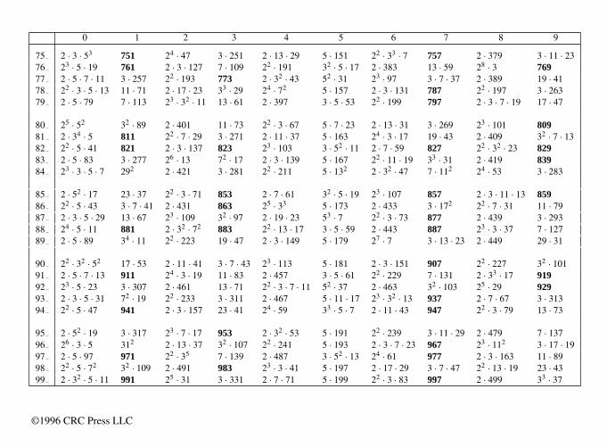
0 1 2 3 4 5 6 7 8 9
75 2 · 3 · 53 751 24 · 47 3 · 251 2 · 13 · 29 5 · 151 22 · 33 · 7 757 2 · 379 3 · 11 · 2376 23 · 5 · 19 761 2 · 3 · 127 7 · 109 22 · 191 32 · 5 · 17 2 · 383 13 · 59 28 · 3 76977 2 · 5 · 7 · 11 3 · 257 22 · 193 773 2 · 32 · 43 52 · 31 23 · 97 3 · 7 · 37 2 · 389 19 · 4178 22 · 3 · 5 · 13 11 · 71 2 · 17 · 23 33 · 29 24 · 72 5 · 157 2 · 3 · 131 787 22 · 197 3 · 26379 2 · 5 · 79 7 · 113 23 · 32 · 11 13 · 61 2 · 397 3 · 5 · 53 22 · 199 797 2 · 3 · 7 · 19 17 · 47
80 25 · 52 32 · 89 2 · 401 11 · 73 22 · 3 · 67 5 · 7 · 23 2 · 13 · 31 3 · 269 23 · 101 80981 2 · 34 · 5 811 22 · 7 · 29 3 · 271 2 · 11 · 37 5 · 163 24 · 3 · 17 19 · 43 2 · 409 32 · 7 · 1382 22 · 5 · 41 821 2 · 3 · 137 823 23 · 103 3 · 52 · 11 2 · 7 · 59 827 22 · 32 · 23 82983 2 · 5 · 83 3 · 277 26 · 13 72 · 17 2 · 3 · 139 5 · 167 22 · 11 · 19 33 · 31 2 · 419 83984 23 · 3 · 5 · 7 292 2 · 421 3 · 281 22 · 211 5 · 132 2 · 32 · 47 7 · 112 24 · 53 3 · 283
85 2 · 52 · 17 23 · 37 22 · 3 · 71 853 2 · 7 · 61 32 · 5 · 19 23 · 107 857 2 · 3 · 11 · 13 85986 22 · 5 · 43 3 · 7 · 41 2 · 431 863 25 · 33 5 · 173 2 · 433 3 · 172 22 · 7 · 31 11 · 7987 2 · 3 · 5 · 29 13 · 67 23 · 109 32 · 97 2 · 19 · 23 53 · 7 22 · 3 · 73 877 2 · 439 3 · 29388 24 · 5 · 11 881 2 · 32 · 72 883 22 · 13 · 17 3 · 5 · 59 2 · 443 887 23 · 3 · 37 7 · 12789 2 · 5 · 89 34 · 11 22 · 223 19 · 47 2 · 3 · 149 5 · 179 27 · 7 3 · 13 · 23 2 · 449 29 · 31
90 22 · 32 · 52 17 · 53 2 · 11 · 41 3 · 7 · 43 23 · 113 5 · 181 2 · 3 · 151 907 22 · 227 32 · 10191 2 · 5 · 7 · 13 911 24 · 3 · 19 11 · 83 2 · 457 3 · 5 · 61 22 · 229 7 · 131 2 · 33 · 17 91992 23 · 5 · 23 3 · 307 2 · 461 13 · 71 22 · 3 · 7 · 11 52 · 37 2 · 463 32 · 103 25 · 29 92993 2 · 3 · 5 · 31 72 · 19 22 · 233 3 · 311 2 · 467 5 · 11 · 17 23 · 32 · 13 937 2 · 7 · 67 3 · 31394 22 · 5 · 47 941 2 · 3 · 157 23 · 41 24 · 59 33 · 5 · 7 2 · 11 · 43 947 22 · 3 · 79 13 · 73
95 2 · 52 · 19 3 · 317 23 · 7 · 17 953 2 · 32 · 53 5 · 191 22 · 239 3 · 11 · 29 2 · 479 7 · 13796 26 · 3 · 5 312 2 · 13 · 37 32 · 107 22 · 241 5 · 193 2 · 3 · 7 · 23 967 23 · 112 3 · 17 · 1997 2 · 5 · 97 971 22 · 35 7 · 139 2 · 487 3 · 52 · 13 24 · 61 977 2 · 3 · 163 11 · 8998 22 · 5 · 72 32 · 109 2 · 491 983 23 · 3 · 41 5 · 197 2 · 17 · 29 3 · 7 · 47 22 · 13 · 19 23 · 4399 2 · 32 · 5 · 11 991 25 · 31 3 · 331 2 · 7 · 71 5 · 199 22 · 3 · 83 997 2 · 499 33 · 37
©1996 C
RC
Press LL
C
©1996 CRC Press LLC

2.3.14 FACTORIZATION OF 2m − 1
23 − 1 = 7 219 − 1 = 52428724 − 1 = 3 × 5 220 − 1 = 3 × 52 × 11 × 31 × 4125 − 1 = 31 221 − 1 = 72 × 127 × 33726 − 1 = 32 × 7 222 − 1 = 3 × 23 × 89 × 68327 − 1 = 127 223 − 1 = 47 × 178481
28 − 1 = 3 × 5 × 17 224 − 1 = 32 × 5 × 7 × 13 × 17 × 24129 − 1 = 7 × 73 225 − 1 = 31 × 601 × 1801210 − 1 = 3 × 11 × 31 226 − 1 = 3 × 2731 × 8191211 − 1 = 23 × 89 227 − 1 = 7 × 73 × 262657212 − 1 = 32 × 5 × 7 × 13 228 − 1 = 3 × 5 × 29 × 43 × 113 × 127
213 − 1 = 8191 229 − 1 = 233 × 1103 × 2089214 − 1 = 3 × 43 × 127 230 − 1 = 32 × 7 × 11 × 31 × 151 × 331215 − 1 = 7 × 31 × 151 231 − 1 = 2147483647216 − 1 = 3 × 5 × 17 × 257 232 − 1 = 3 × 5 × 17 × 257 × 65537217 − 1 = 131071 233 − 1 = 7 × 23 × 89 × 599479
218 − 1 = 33 × 7 × 19 × 73 234 − 1 = 3 × 43691 × 131071
2.3.15 MAGIC SQUARES
A magic square is a square array of integers with the property that the sum of theintegers in each row or column is the same. If (c, n) = (d, n) = (e, n) = (f, n) =(cf − en, n) = 1, then the array A = (aij ) will be magic (and use the n2 numbers 0,1, . . . , n2 − 1) if aij = k with
i ≡ ck + e
⌊k
n
⌋(mod n) and j ≡ dk + f
⌊k
n
⌋(mod n)
For example, with c = 1, d = e = f = 2, and n = 3, a magic square is
6 1 52 3 74 8 0
2.3.16 TOTIENT FUNCTION
Definitions• φ(n) the totient function; is the number of integers not exceeding and
relatively prime to n.
• σ(n) is the sum of the divisors of n.
• τ(n) is the number of divisors of n.
©1996 CRC Press LLC

Define σk(n) to be the kth divisor function, the sum of the kth powers of thedivisors of n. Then φ(n) = σ0(n) and σ(n) = σ1(n).
A perfect number n satisfies σ(n) = 2n.
ExampleThe numbers less than 6 and relatively prime to 6 are 1, 5. Hence φ(6) = 2. Thedivisors of 6 are 1, 2, 3, 6. There are τ(6) = 4 divisors. The sum of these numbersis σ(6) = 1 + 2 + 3 + 6 = 12.
Properties1. φ is a multiplicative function: if (n,m) = 1, then φ(nm) = φ(m)φ(n).
2. Gauss’s theorem states: n = ∑d|n φ(d).
3. When n = ∏i p
αii .
σk(n) =∑d|n
dk =∏i
pk(αi+1)i − 1
pi − 1
4. Generating functions include
∞∑n=0
σk(n)
ns= ζ(s)ζ(s − k)
∞∑n=0
φ(n)
ns= ζ(s − 1)
ζ(s)
5. The positive integern is an even perfect number if, and only if, n = 2m−1(2m−1),where m is a positive integer such that Mm = 2m − 1 is prime (Mm is calleda Mersenne prime). The sequence of perfect numbers is 6, 28, 496, . . . (corresponding to m = 2, 3, 5, . . . ).
©1996 CRC Press LLC
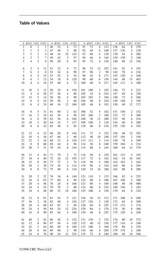
Table of Values
n φ(n) τ(n) σ (n) n φ(n) τ(n) σ (n) n φ(n) τ(n) σ (n) n φ(n) τ(n) σ (n)
1 0 1 1 46 22 4 72 91 72 4 112 136 64 8 2702 1 2 3 47 46 2 48 92 44 6 168 137 136 2 1383 2 2 4 48 16 10 124 93 60 4 128 138 44 8 2884 2 3 7 49 42 3 57 94 46 4 144 139 138 2 1405 4 2 6 50 20 6 93 95 72 4 120 140 48 12 336
6 2 4 12 51 32 4 72 96 32 12 252 141 92 4 1927 6 2 8 52 24 6 98 97 96 2 98 142 70 4 2168 4 4 15 53 52 2 54 98 42 6 171 143 120 4 1689 6 3 13 54 18 8 120 99 60 6 156 144 48 15 403
10 4 4 18 55 40 4 72 100 40 9 217 145 112 4 180
11 10 2 12 56 24 8 120 101 100 2 102 146 72 4 22212 4 6 28 57 36 4 80 102 32 8 216 147 84 6 22813 12 2 14 58 28 4 90 103 102 2 104 148 72 6 26614 6 4 24 59 58 2 60 104 48 8 210 149 148 2 15015 8 4 24 60 16 12 168 105 48 8 192 150 40 12 372
16 8 5 31 61 60 2 62 106 52 4 162 151 150 2 15217 16 2 18 62 30 4 96 107 106 2 108 152 72 8 30018 6 6 39 63 36 6 104 108 36 12 280 153 96 6 23419 18 2 20 64 32 7 127 109 108 2 110 154 60 8 28820 8 6 42 65 48 4 84 110 40 8 216 155 120 4 192
21 12 4 32 66 20 8 144 111 72 4 152 156 48 12 39222 10 4 36 67 66 2 68 112 48 10 248 157 156 2 15823 22 2 24 68 32 6 126 113 112 2 114 158 78 4 24024 8 8 60 69 44 4 96 114 36 8 240 159 104 4 21625 20 3 31 70 24 8 144 115 88 4 144 160 64 12 378
26 12 4 42 71 70 2 72 116 56 6 210 161 132 4 19227 18 4 40 72 24 12 195 117 72 6 182 162 54 10 36328 12 6 56 73 72 2 74 118 58 4 180 163 162 2 16429 28 2 30 74 36 4 114 119 96 4 144 164 80 6 29430 8 8 72 75 40 6 124 120 32 16 360 165 80 8 288
31 30 2 32 76 36 6 140 121 110 3 133 166 82 4 25232 16 6 63 77 60 4 96 122 60 4 186 167 166 2 16833 20 4 48 78 24 8 168 123 80 4 168 168 48 16 48034 16 4 54 79 78 2 80 124 60 6 224 169 156 3 18335 24 4 48 80 32 10 186 125 100 4 156 170 64 8 324
36 12 9 91 81 54 5 121 126 36 12 312 171 108 6 26037 36 2 38 82 40 4 126 127 126 2 128 172 84 6 30838 18 4 60 83 82 2 84 128 64 8 255 173 172 2 17439 24 4 56 84 24 12 224 129 84 4 176 174 56 8 36040 16 8 90 85 64 4 108 130 48 8 252 175 120 6 248
41 40 2 42 86 42 4 132 131 130 2 132 176 80 10 37242 12 8 96 87 56 4 120 132 40 12 336 177 116 4 24043 42 2 44 88 40 8 180 133 108 4 160 178 88 4 27044 20 6 84 89 88 2 90 134 66 4 204 179 178 2 18045 24 6 78 90 24 12 234 135 72 8 240 180 48 18 546
©1996 CRC Press LLC

n φ(n) τ(n) σ (n) n φ(n) τ(n) σ (n) n φ(n) τ(n) σ (n) n φ(n) τ(n) σ (n)
181 180 2 182 226 112 4 342 271 270 2 272 316 156 6 560182 72 8 336 227 226 2 228 272 128 10 558 317 316 2 318183 120 4 248 228 72 12 560 273 144 8 448 318 104 8 648184 88 8 360 229 228 2 230 274 136 4 414 319 280 4 360185 144 4 228 230 88 8 432 275 200 6 372 320 128 14 762
186 60 8 384 231 120 8 384 276 88 12 672 321 212 4 432187 160 4 216 232 112 8 450 277 276 2 278 322 132 8 576188 92 6 336 233 232 2 234 278 138 4 420 323 288 4 360189 108 8 320 234 72 12 546 279 180 6 416 324 108 15 847190 72 8 360 235 184 4 288 280 96 16 720 325 240 6 434
191 190 2 192 236 116 6 420 281 280 2 282 326 162 4 492192 64 14 508 237 156 4 320 282 92 8 576 327 216 4 440193 192 2 194 238 96 8 432 283 282 2 284 328 160 8 630194 96 4 294 239 238 2 240 284 140 6 504 329 276 4 384195 96 8 336 240 64 20 744 285 144 8 480 330 80 16 864
196 84 9 399 241 240 2 242 286 120 8 504 331 330 2 332197 196 2 198 242 110 6 399 287 240 4 336 332 164 6 588198 60 12 468 243 162 6 364 288 96 18 819 333 216 6 494199 198 2 200 244 120 6 434 289 272 3 307 334 166 4 504200 80 12 465 245 168 6 342 290 112 8 540 335 264 4 408
201 132 4 272 246 80 8 504 291 192 4 392 336 96 20 992202 100 4 306 247 216 4 280 292 144 6 518 337 336 2 338203 168 4 240 248 120 8 480 293 292 2 294 338 156 6 549204 64 12 504 249 164 4 336 294 84 12 684 339 224 4 456205 160 4 252 250 100 8 468 295 232 4 360 340 128 12 756
206 102 4 312 251 250 2 252 296 144 8 570 341 300 4 384207 132 6 312 252 72 18 728 297 180 8 480 342 108 12 780208 96 10 434 253 220 4 288 298 148 4 450 343 294 4 400209 180 4 240 254 126 4 384 299 264 4 336 344 168 8 660210 48 16 576 255 128 8 432 300 80 18 868 345 176 8 576
211 210 2 212 256 128 9 511 301 252 4 352 346 172 4 522212 104 6 378 257 256 2 258 302 150 4 456 347 346 2 348213 140 4 288 258 84 8 528 303 200 4 408 348 112 12 840214 106 4 324 259 216 4 304 304 144 10 620 349 348 2 350215 168 4 264 260 96 12 588 305 240 4 372 350 120 12 744
216 72 16 600 261 168 6 390 306 96 12 702 351 216 8 560217 180 4 256 262 130 4 396 307 306 2 308 352 160 12 756218 108 4 330 263 262 2 264 308 120 12 672 353 352 2 354219 144 4 296 264 80 16 720 309 204 4 416 354 116 8 720220 80 12 504 265 208 4 324 310 120 8 576 355 280 4 432
221 192 4 252 266 108 8 480 311 310 2 312 356 176 6 630222 72 8 456 267 176 4 360 312 96 16 840 357 192 8 576223 222 2 224 268 132 6 476 313 312 2 314 358 178 4 540224 96 12 504 269 268 2 270 314 156 4 474 359 358 2 360225 120 9 403 270 72 16 720 315 144 12 624 360 96 24 1170
©1996 CRC Press LLC

n φ(n) τ(n) σ (n) n φ(n) τ(n) σ (n) n φ(n) τ(n) σ (n) n φ(n) τ(n) σ (n)
361 342 3 381 406 168 8 720 451 400 4 504 496 240 10 992362 180 4 546 407 360 4 456 452 224 6 798 497 420 4 576363 220 6 532 408 128 16 1080 453 300 4 608 498 164 8 1008364 144 12 784 409 408 2 410 454 226 4 684 499 498 2 500365 288 4 444 410 160 8 756 455 288 8 672 500 200 12 1092
366 120 8 744 411 272 4 552 456 144 16 1200 501 332 4 672367 366 2 368 412 204 6 728 457 456 2 458 502 250 4 756368 176 10 744 413 348 4 480 458 228 4 690 503 502 2 504369 240 6 546 414 132 12 936 459 288 8 720 504 144 24 1560370 144 8 684 415 328 4 504 460 176 12 1008 505 400 4 612
371 312 4 432 416 192 12 882 461 460 2 462 506 220 8 864372 120 12 896 417 276 4 560 462 120 16 1152 507 312 6 732373 372 2 374 418 180 8 720 463 462 2 464 508 252 6 896374 160 8 648 419 418 2 420 464 224 10 930 509 508 2 510375 200 8 624 420 96 24 1344 465 240 8 768 510 128 16 1296
376 184 8 720 421 420 2 422 466 232 4 702 511 432 4 592377 336 4 420 422 210 4 636 467 466 2 468 512 256 10 1023378 108 16 960 423 276 6 624 468 144 18 1274 513 324 8 800379 378 2 380 424 208 8 810 469 396 4 544 514 256 4 774380 144 12 840 425 320 6 558 470 184 8 864 515 408 4 624
381 252 4 512 426 140 8 864 471 312 4 632 516 168 12 1232382 190 4 576 427 360 4 496 472 232 8 900 517 460 4 576383 382 2 384 428 212 6 756 473 420 4 528 518 216 8 912384 128 16 1020 429 240 8 672 474 156 8 960 519 344 4 696385 240 8 576 430 168 8 792 475 360 6 620 520 192 16 1260
386 192 4 582 431 430 2 432 476 192 12 1008 521 520 2 522387 252 6 572 432 144 20 1240 477 312 6 702 522 168 12 1170388 192 6 686 433 432 2 434 478 238 4 720 523 522 2 524389 388 2 390 434 180 8 768 479 478 2 480 524 260 6 924390 96 16 1008 435 224 8 720 480 128 24 1512 525 240 12 992
391 352 4 432 436 216 6 770 481 432 4 532 526 262 4 792392 168 12 855 437 396 4 480 482 240 4 726 527 480 4 576393 260 4 528 438 144 8 888 483 264 8 768 528 160 20 1488394 196 4 594 439 438 2 440 484 220 9 931 529 506 3 553395 312 4 480 440 160 16 1080 485 384 4 588 530 208 8 972
396 120 18 1092 441 252 9 741 486 162 12 1092 531 348 6 780397 396 2 398 442 192 8 756 487 486 2 488 532 216 12 1120398 198 4 600 443 442 2 444 488 240 8 930 533 480 4 588399 216 8 640 444 144 12 1064 489 324 4 656 534 176 8 1080400 160 15 961 445 352 4 540 490 168 12 1026 535 424 4 648
401 400 2 402 446 222 4 672 491 490 2 492 536 264 8 1020402 132 8 816 447 296 4 600 492 160 12 1176 537 356 4 720403 360 4 448 448 192 14 1016 493 448 4 540 538 268 4 810404 200 6 714 449 448 2 450 494 216 8 840 539 420 6 684405 216 10 726 450 120 18 1209 495 240 12 936 540 144 24 1680
©1996 CRC Press LLC

2.4 VECTOR ALGEBRA
2.4.1 NOTATION FOR VECTORS AND SCALARS
A vectoris an ordered n-tuple of values. A vector is usually represented by a lowercase, bold faced letter, such as v. The individual components of a vector v are typicallydenoted by a lower case letter along with a subscript identifying the relative positionof the component in the vector, such as v = [v1, v2, . . . , vn]. In this case, the vectoris said to be n-dimensional. If the n individual components of the vector are realnumbers, then v ∈ Rn. Likewise, if the n components of v are complex, then v ∈ Cn.
Two vectors, v1 and v2, are said to be equal if they have exactly the same com-ponents. A negative vector, written as −v, is one that acts in direction opposite to v,but is of equal magnitude.
2.4.2 PHYSICAL VECTORS
Any quantity that is completely determined by its magnitude is called a scalar. Forexample, mass, density, and temperature are scalars. Any quantity that is completelydetermined by its magnitude and direction is called, in physics, a vector. We oftenuse a three-dimensional vector to represent a physical vector. Examples of physicalvectors include velocity, acceleration, and force. A physical vector is represented bya directed line segment, the length of which represents the magnitude of the vector.Two vectors are said to be parallel if they have exactly the same direction, i.e., theangle between the two vectors equals zero.
2.4.3 FUNDAMENTAL DEFINITIONS
1. A row vectoris a vector whose components are aligned horizontally. A columnvectorhas its components aligned vertically. The transposeoperator, denotedby the superscript T, switches the orientation of a vector between horizontal andvertical.
EXAMPLE 2.4.1
v = [1, 2, 3, 4], vT =
1234
, (vT)T = [1, 2, 3, 4].
row vector column vector row vector
©1996 CRC Press LLC

Vectors are traditionally written with either rounded braces or with squarebrackets.
2. Two vectors, vi and vj , are said to be orthogonal if vTi · vj = 0, where the
operation “·” denotes an inner product.
3. A set of vectors v1, . . . , vn is said to be orthogonal if vTi · vj = 0 for all i = j .
4. A set of orthogonal vectors v1, . . . , vm is said to be orthonormalif, in additionto possessing the property of orthogonality, the set possesses the property thatvTi · vi = 1 for all 1 ≤ i ≤ m.
2.4.4 LAWS OF VECTOR ALGEBRA
1. The vector sum of v1 and v2, represented by v1 + v2, results in another vector ofthe same dimension, and is calculated by simply adding corresponding vectorcomponents, e.g., if v1, v2 ∈ Rn, then v1 + v2 = [v11 + v21 , . . . , v1n + v2n ].
2. The vector subtraction of v2 from v1, represented by v1 − v2, is equivalent tothe addition of v1 and −v2.
3. If r is a scalar, then rv or vr represents a scaling of the vector v in the samedirection as v, since the multiplicative scalar is distributed to each componentof v.
4. If 0 ≤ r < 1, then the scalar multiplication rv shrinks the length of v, multipli-cation by r = 1 leaves v unchanged, and, if r > 1, then rv stretches the lengthof v. When r < 0, multiplication of v by r has the same effects on the magni-tude, or length of v, but results in a vector oriented in the direction opposite tov.
EXAMPLE 2.4.2
4
1
03
=
4
012
, −4
1
03
=
−4
0−12
.
5. If r and s are scalars, and v1, v2, and v3 are vectors, the following rules of algebraare valid:
v1 + v2 = v2 + v1,
(r + s)v1 = rv1 + sv1 = v1r + v1s = v1(r + s),
r(v1 + v2) = rv1 + rv2, and
v1 + (v2 + v3) = (v1 + v2)+ v3 = v1 + v2 + v3.(2.4.1)
©1996 CRC Press LLC

2.4.5 VECTOR NORMS
1. A norm is the vector analog of absolute value for real scalars. Norms provide adistance measure for a vector space.
2. A vector norm applied to a vector v is denoted by a double bar notation ‖v‖.
3. An n-dimensional real number space Rn together with a norm defines a metricspace.
4. The properties of a vector norm are
• For any vector x = 0, ‖x‖ > 0,
• ‖γ x‖ = |γ | ‖x‖, and
• ‖x + y‖ ≤ ‖x‖ + ‖y‖ (triangle inequality).
5. The three most commonly used vector norms are
• The L1 norm is defined as ‖v‖1 = |v1| + · · · + |vn| = ∑ni=1 |vi |.
• The L2 norm (Euclidean norm) is defined as
‖v‖2 = (|v1|2 + |v2|2 + · · · + |vn|2)1/2 =(
n∑i=1
v2i
)1/2
.
(2.4.2)
• The L∞ norm is defined as ‖v‖∞ = max1≤i≤n
|vi |.
6. In the absence of any subscript, the norm ‖·‖ is usually assumed to be the L2
norm.
7. A unit vectorwith respect to a particular norm ‖·‖ is a vector that satisfies theproperty that ‖v‖ = 1, and is sometimes denoted by v.
2.4.6 DOT, SCALAR, OR INNER PRODUCT
1. The dot, scalar, or inner product of two vectors of the same dimension, rep-resented by v1 · v2 or xTy, has two common definitions, depending upon thecontext in which this product is encountered.
(a) In vector calculus and physics, the dot or scalar product is defined by
v1 · v2 = ‖v1‖2 ‖v2‖2 cos θ, (2.4.3)
where θ represents the angle determined by v1 and v2 (see Figure 2.4.1).
(b) In optimization, linear algebra, and computer science, the inner product oftwo vectors, x and y, is equivalently defined as
xTy =n∑i=1
xiyi = x1y1 + · · · + xnyn. (2.4.4)
©1996 CRC Press LLC

From the first definition, it is apparent that the inner product of two perpendicular,or orthogonal, vectors is zero, since the cosine of 90 is zero.
2. The inner product of two parallel vectors (with v2 = rv1) is given by v1 · v2 =r ‖v1‖2
2. For example, when r > 0,
v1 · v2 = ‖v1‖2 ‖v2‖2 cos 0 = ‖v1‖2 ‖v2‖2 = r ‖v1‖22 .
(2.4.5)
3. The dot, scalar, or inner product is distributive, e.g.,
(v1 + v2) · v3 = v1 · v3 + v2 · v3. (2.4.6)
4. For a,b, c ∈ Rn with n > 1,
aTb = aTc ⇒ b = c. (2.4.7)
However, it is valid to conclude that
aTb = aTc ⇒ aT(b − c) = 0, (2.4.8)
and that the vector a is orthogonal to the vector (b − c).
FIGURE 2.4.1Depiction of right-hand rule.
v1 × v2
v1
v2n
2.4.7 VECTOR OR CROSS PRODUCT
1. The vector or cross product of two nonzero three-dimensional vectors v1 and v2
is defined as
v1 × v2 = n ‖v1‖2 ‖v2‖2 sin θ, (2.4.9)
where n is the unit normalvector perpendicular to both v1 and v2 in the directionadhering to the right-hand rule (see Figure 2.4.1) and θ is the angle between v1
and v2.
©1996 CRC Press LLC

2. If v1 and v2 are parallel, then v1 × v2 = 0.
3. The quantity ‖v1‖2 ‖v2‖2 |sin θ | represents the area of the parallelogram deter-mined by v1 and v2.
4. The following rules apply for vector products:
(γ v1)× (αv2) = (γ α)v1 × v2,
v1 × v2 = −v2 × v1,
v1 × (v2 + v3) = v1 × v2 + v1 × v3,
(v1 + v2)× v3 = v1 × v3 + v2 × v3,
v1 × (v2 × v3) = v2(v3 · v1)− v3(v1 · v2),
(a × b) · (c × d) = (a · c)(b · d)− (a · d)(b · c),
(a × b)× (c × d) = [a · (b × d)]c − [a · (b × c)]d
= [a · (c × d)]b − [b · (c × d)]a.
(2.4.10)
5. The pairwise cross products of the unit vectors i, j, and k, corresponding to thedirections of v = v1 i + v2 j + v3k, are given by
i × j = −(j × i) = k,
j × k = −(k × j) = i,
k × i = −(i × k) = j, and
i × i = j × j = k × k = 0.
(2.4.11)
6. If v1 = a1 i + a2 j + a3k and v2 = b1 i + b2 j + b3k, then
v1 × v2 =∣∣∣∣∣∣
i j ka1 a2 a3
b1 b2 b3
∣∣∣∣∣∣ ,= (a2b3 − b2a3)i + (a3b1 − b3a1)j + (a1b2 − b1a2)k.
(2.4.12)
2.4.8 SCALAR AND VECTOR TRIPLE PRODUCTS
1. The scalar triple productinvolving three three-dimensional vectors a, b, and c,sometimes denoted by [abc] (not to be confused with a matrix containing threecolumns
[a b c
]), can be computed using the determinant
[abc] = a · (b × c) = a ·[ ∣∣∣∣b2 b3
c2 c3
∣∣∣∣ i −∣∣∣∣b1 b3
c1 c3
∣∣∣∣ j +∣∣∣∣b1 b2
c1 c2
∣∣∣∣ k]
= a1
∣∣∣∣b2 b3
c2 c3
∣∣∣∣− a2
∣∣∣∣b1 b3
c1 c3
∣∣∣∣+ a3
∣∣∣∣b1 b2
c1 c2
∣∣∣∣=∣∣∣∣∣∣a1 a2 a3
b1 b2 b3
c1 c2 c3
∣∣∣∣∣∣= ‖a‖ ‖b‖ ‖c‖ cosφ sin θ,
(2.4.13)
©1996 CRC Press LLC

where θ is the angle between b and c, and φ is the angle between a and thenormal to the plane defined by b and c.
2. The absolute value of the triple scalar product calculates the volume of theparallelipiped determined by the three vectors. The answer you get is thereforeindependent of the order in which the triple product is taken.
3. Given three noncoplanar reference vectors v1, v2, and v3, the reciprocal systemis given by v∗
1, v∗2, and v∗
3, where
v∗1 = v2 × v3
[v1v2v3], v∗
2 = v3 × v1
[v1v2v3], v∗
3 = v1 × v2
[v1v2v3].
(2.4.14)
Note that
1 = ‖v1‖∥∥v∗
1
∥∥ = ‖v2‖∥∥v∗
2
∥∥ = ‖v3‖∥∥v∗
3
∥∥and 0 = ‖v1‖
∥∥v∗2
∥∥ = ‖v1‖∥∥v∗
3
∥∥ = ‖v2‖∥∥v∗
1
∥∥ , etc. (2.4.15)
The system i, j, k is its own reciprocal.
4. The vector triple productinvolving three three-dimensional vectors a, b, and c,given by a × (b × c), results in a vector, perpendicular to a, lying in the planeof b and c, and is defined as
a × (b × c) = (a · c)b − (a · b)c,
=
∣∣∣∣∣∣∣∣i j ka1 a2 a3∣∣∣∣b2 b3
c2 c3
∣∣∣∣∣∣∣∣b3 b1
c3 c1
∣∣∣∣∣∣∣∣b1 b2
c1 c2
∣∣∣∣
∣∣∣∣∣∣∣∣ . (2.4.16)
5. (a × b)× (c × d) = [acd]b − [bcd]a = [abd]c − [abc]d
2.5 LINEAR AND MATRIX ALGEBRA
2.5.1 DEFINITIONS
1. Anm×nmatrixis a two-dimensional array of numbers consisting of mrows andn columns. By convention, a matrix is denoted by a capital letter emphasizedwith italics, as in A, B, D, or boldface, A, B, D, along with a subscript denotingthe dimensions of the matrix, e.g., A2×3. If A is a real n × m matrix, then wewrite A ∈ Rn×m.
2. Am×n is called rectangularif m = n.
3. Am×n is called squareif m = n.
©1996 CRC Press LLC
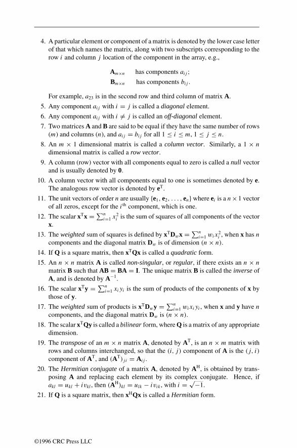
4. A particular element or component of a matrix is denoted by the lower case letterof that which names the matrix, along with two subscripts corresponding to therow i and column j location of the component in the array, e.g.,
Am×n has components aij ;Bm×n has components bij .
For example, a23 is in the second row and third column of matrix A.
5. Any component aij with i = j is called a diagonalelement.
6. Any component aij with i = j is called an off-diagonalelement.
7. Two matrices A and B are said to be equal if they have the same number of rows(m) and columns (n), and aij = bij for all 1 ≤ i ≤ m, 1 ≤ j ≤ n.
8. An m × 1 dimensional matrix is called a column vector. Similarly, a 1 × n
dimensional matrix is called a row vector.
9. A column (row) vector with all components equal to zero is called a null vectorand is usually denoted by 0.
10. A column vector with all components equal to one is sometimes denoted by e.The analogous row vector is denoted by eT.
11. The unit vectors of order n are usually e1, e2, . . . , en where ei is a n×1 vectorof all zeros, except for the i th component, which is one.
12. The scalar xTx = ∑ni=1 x
2i is the sum of squares of all components of the vector
x.
13. The weightedsum of squares is defined by xTDwx = ∑ni=1 wix
2i , when x has n
components and the diagonal matrix Dw is of dimension (n× n).
14. If Q is a square matrix, then xTQx is called a quadraticform.
15. An n × n matrix A is called non-singular, or regular, if there exists an n × n
matrix B such that AB = BA = I. The unique matrix B is called the inverseofA, and is denoted by A−1.
16. The scalar xTy = ∑ni=1 xiyi is the sum of products of the components of x by
those of y.
17. The weightedsum of products is xTDwy = ∑ni=1 wixiyi , when x and y have n
components, and the diagonal matrix Dw is (n× n).
18. The scalar xTQy is called a bilinear form, where Q is a matrix of any appropriatedimension.
19. The transposeof an m × n matrix A, denoted by AT, is an n × m matrix withrows and columns interchanged, so that the (i, j) component of A is the (j, i)component of AT, and (AT)ji = Aij .
20. The Hermitian conjugateof a matrix A, denoted by AH, is obtained by trans-posing A and replacing each element by its complex conjugate. Hence, ifakl = ukl + ivkl , then (AH)kl = ulk − ivik , with i = √−1.
21. If Q is a square matrix, then xHQx is called a Hermitianform.
©1996 CRC Press LLC

2.5.2 TYPES OF MATRICES
1. The diagonal alignment of components in a matrix extending from the upperleft to the lower right is called the principal or maindiagonal.
2. A square matrix with all components off the principal diagonal equal to zerois called a diagonal matrix, typically denoted by the letter D with a subscriptindicating the typical element in the principal diagonal.
EXAMPLE 2.5.1
Da =a11 0 0
0 a22 00 0 a33
, Dλ =
λ11 0 0
0 λ22 00 0 λ33
.
3. The identity matrix, denoted by I, is the diagonal matrix with aij = 1 for alli = j , and aij = 0 for i = j . The n× n identity matrix is denoted In.
4. A matrix that has all main diagonal components equal to one and zeros every-where else except a single nonzero component in location (i, j ) is called anelementarymatrix, denoted by Eij .
EXAMPLE 2.5.2
E31 =
1 0 0 00 1 0 0
−5 0 1 00 0 0 1
.
An elementary matrix can also be expressed as E = I − αuvT, where I is theidentity matrix, α is a scalar, and u and v are vectors of the same dimension. Inthis context, the elementary matrix is referred to as a rank one modificationofan identity matrix.
5. Other elementary matrices are those of the form Eij = eieTj . Note that, using
these matrices, A = ∑i
∑j aijEij .
6. A matrix with all components above the principal diagonal equal to zero is calleda lower triangular matrix.
©1996 CRC Press LLC
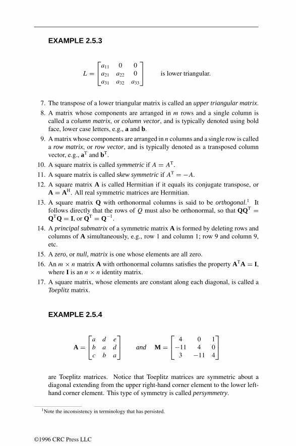
EXAMPLE 2.5.3
L =a11 0 0a21 a22 0a31 a32 a33
is lower triangular.
7. The transpose of a lower triangular matrix is called an upper triangular matrix.
8. A matrix whose components are arranged in m rows and a single column iscalled a column matrix, or column vector, and is typically denoted using boldface, lower case letters, e.g., a and b.
9. A matrix whose components are arranged in n columns and a single row is calleda row matrix, or row vector, and is typically denoted as a transposed columnvector, e.g., aT and bT.
10. A square matrix is called symmetricif A = AT.
11. A square matrix is called skew symmetricif AT = −A.
12. A square matrix A is called Hermitian if it equals its conjugate transpose, orA = AH. All real symmetric matrices are Hermitian.
13. A square matrix Q with orthonormal columns is said to be orthogonal.1 Itfollows directly that the rows of Q must also be orthonormal, so that QQT =QTQ = I, or QT = Q−1.
14. A principal submatrixof a symmetric matrix A is formed by deleting rows andcolumns of A simultaneously, e.g., row 1 and column 1; row 9 and column 9,etc.
15. A zero, or null, matrix is one whose elements are all zero.
16. An m× n matrix A with orthonormal columns satisfies the property ATA = I,where I is an n× n identity matrix.
17. A square matrix, whose elements are constant along each diagonal, is called aToeplitzmatrix.
EXAMPLE 2.5.4
A =a d e
b a d
c b a
and M =
4 0 1−11 4 0
3 −11 4
are Toeplitz matrices. Notice that Toeplitz matrices are symmetric about adiagonal extending from the upper right-hand corner element to the lower left-hand corner element. This type of symmetry is called persymmetry.
1Note the inconsistency in terminology that has persisted.
©1996 CRC Press LLC

18. A Vandermondematrix is a square matrix V ∈ R(n+1)×(n+1) in which eachcolumn contains unit increasing powers of a single matrix value:
V =
1 1 · · · 1v1 v2 · · · v(n+1)
v21 v2
2 · · · v2(n+1)
......
...
vn1 vn2 · · · vn(n+1)
. (2.5.1)
19. A square matrix U is said to be in upper Hessenbergform if uij = 0 wheneveri > j+1. An upper Hessenberg matrix is essentially an upper triangular matrixwith an extra nonzero element immediately below the main diagonal entry ineach column of U. For example,
U =
u11 u12 u13 u14
b21 u22 u23 u24
0 b32 u33 u34
0 0 b43 u44
is upper Hessenberg.
20. If the sum of the components of each column of a matrix A ∈ Rn×n equals one,then A is called a Markovmatrix.
21. A circulant matrix is an n× n matrix of the form
C =
c0 c1 c2 · · · cn−2 cn−1
cn−1 c0 c1 · · · cn−3 cn−2
cn−2 cn−1 c0 · · · cn−4 cn−3...
...
c1 c2 c3 · · · cn−1 c0
, (2.5.2)
where the components cij are such that (j − i) = k mod n have the same valueck . These components comprise the kth stripeof C.
22. A matrix A is called graded across its rowsif aij ≤ ai,j+1, for all i, j ; gradedup its columnsif aij ≤ ai+1,j ; and doubly gradedif both conditions apply.
2.5.3 CONFORMABILITY FOR ADDITION ANDMULTIPLICATION
1. Two matrices A and B can be added (subtracted) if they are of the same dimen-sion. The result is a matrix of the same dimension.
EXAMPLE 2.5.5
A2×3 + B2×3 =[
3 2 −14 0 9
]+[
11 −2 30 1 1
]=[
14 0 24 1 10
].
©1996 CRC Press LLC

2. Multiplication of a matrix or a vector by a scalar is achieved by multiplying eachcomponent by that scalar. If B = αA, then bij = αaij for all components.
3. The matrix multiplication AB is valid if the number of columns of A is equal tothe number of rows of B.
4. The multiplication of two matrices Am×n and Bn×q results in a matrix Cm×qwhose components are defined as
cmq =n∑
k=1
amkbkq . (2.5.3)
Each cmq is the result of the inner (dot) product of the mth row of A with theq th column of B. This rule applies similarly for matrix multiplication involvingmore than two matrices, so that if ABCD = E, then
eij =∑k
∑l
∑m
aikbklclmdmj . (2.5.4)
The second subscript for each matrix component must coincide with the firstsubscript of the next one.
EXAMPLE 2.5.6
[2 −1 3
−4 1 4
] 5 −3 −3
2 2 −1−7 1 5
=
[−13 −5 10−46 18 31
].
5. In general, matrix multiplication is not commutative: AB = BA.
6. Matrix multiplication is associative: A(BC) = (AB)C.
7. The distributive law of multiplication and addition holds: C(A+B) = CA+CBand (A + B)C = AC + BC.
8. Both the transpose operator and the Hermitian operator reverse the order ofmatrix multiplication: (ABC)T = CTBTAT and (ABC)H = CHBHAH.
9. Strassen algorithm: The matrix product
[a11 a12
a21 a22
] [b11 b12
b21 b22
]=[c11 c12
c21 c22
]can be computed in the following way:
m1 = (a12 − a22)(b21 + b22),
m2 = (a11 + a22)(b11 + b22),
m3 = (a11 − a21)(b11 + b12),
m4 = (a11 + a12)b22,
m5 = a11(b12 − b22),
m6 = a22(b21 − b11),
m7 = (a21 + a22)b11,
c11 = m1 +m2 −m4 +m6,
c12 = m4 +m5,
c21 = m6 +m7, and
c22 = m2 −m3 +m5 −m7.(2.5.5)
©1996 CRC Press LLC

This computation uses 7 multiplications and 18 additions and subtractions. Us-ing this formula recursively allows multiplication of two n × n matrices usingO(nlog2 7) = O(n2.807...) scalar multiplications.
10. The order in which matrices are grouped together for multiplication can changethe number of scalar multiplications required. The straightforward number ofscalar multiplications required to multiply matrix Xa×b by matrix Yb×c is abc,without using clever algorithms such as Strassen’s. For example, consider thematrix product P = A10×100B100×5C5×50. The parenthesization P = ((AB)C)
requires (10 × 100 × 5)+ (10 × 5 × 50) = 7, 500 scalar multiplications. Theparenthesization P = (A(BC)) requires (10 × 100 × 50)+ (100 × 5 × 50) =75,000 scalar multiplications.
2.5.4 DETERMINANTS AND PERMANENTS
1. The determinantof a square matrix A, denoted by |A| or det (A), is a scalarfunction of A defined as
det(A) =∑σ
sgn(σ )a1,σ (1) a2,σ (2) · · · an,σ(n) (2.5.6)
where the sum is taken over all permutations σ of 1, 2, . . . , n. The signumfunction sgn(σ ) is the number of successive transpositions required to change thepermutationσ to the identity permutation. Note these properties of determinants:|A| |B| = |AB| and |A| = |AT|.
2. For a 2 × 2 matrix,∣∣ a11 a12a21 a22
∣∣ = a11a22 − a12a21.For a 3 × 3 matrix,∣∣∣∣∣∣
a11 a12 a13
a21 a22 a23
a31 a32 a33
∣∣∣∣∣∣ = a11a22a33 + a12a23a31 + a13a21a32
− a13a22a31 − a11a23a32 − a12a21a33.(2.5.7)
In general, for m = n,∣∣∣∣∣∣∣∣∣a11 a12 · · · a1n
a21 a22 · · · a2n...
......
...
an1 an2 · · · ann
∣∣∣∣∣∣∣∣∣=∑
(−1)δa1i1a2i2 · · · anin (2.5.8)
where the sum is over all permutations i1 = i2 = · · · = in, and δ denotes thenumber of transpositions necessary to bring the sequence (i1, i2, . . . , in) backinto the natural order (1, 2, . . . , n).
3. Interchanging two rows (or columns) of a matrix changes the sign of itsdeterminant.
4. A determinant does not change its value if a linear combination of other rows(or columns) is added to or subtracted from any given row (or column).
©1996 CRC Press LLC

5. Multiplying an entire row (or column) of A by a scalar γ causes the determinantto be multiplied by the same scalar γ .
6. For an n× n matrix A, |γA| = γ n|A|.7. If det (A) = 0, then A is singular; if det (A) = 0, then A is nonsingular or
invertible. The determinant of the identity matrix is one.
8. det (A−1) = 1/ det (A).
9. The size of the determinant of a square matrix A is not related to the conditionnumber of A.
10. When the edges of a parallelepiped P are defined by the rows (or columns) ofA, the absolute value of the determinant of A measures the volume of P . Thus,if any row (or column) of A is dependent upon another row (or column) of A,the determinant of A equals zero.
11. The cofactorof a square matrix A, cofij (A), is the determinant of a submatrixobtained by striking the i th row and the j th column of A and choosing a positive(negative) sign if (i + j ) is even (odd).
EXAMPLE 2.5.7
cof23
2 4 3
6 1 5−2 1 3
= (−1)2+3
∣∣∣∣ 2 4−2 1
∣∣∣∣ = −(2 + 8) = −10.
12. Let aij denote the components of A and aij those of A−1. Then,
aij = cofji(A)/|A|. (2.5.9)
13. Partitioning of determinants: Let A =[
B CD E
]. Assuming all inverses exist,
then
|A| = |E| ∣∣B − CE−1D)∣∣ = |B| ∣∣(E − DB−1C)
∣∣ . (2.5.10)
14. Laplace development: The determinant of A is a combination of row i (column j )and the cofactors of row i (column j ), i.e.,
|A| = ai1cofi1(A)+ ai2cofi2(A)+ · · · + aincofin(A), (2.5.11)
= a1jcof1j (A)+ a2jcof2j (A)+ · · · + anjcofnj (A),
for any row i or any column j .
15. Omitting the signum function in Equation (2.5.6) yields the definition of perma-nentof A, given by per A = ∑
σ a1,σ (1) · · · an,σ(n). Properties of the permanentinclude:
(a) If A is an m× n matrix and B is an n×m matrix, then
|per(AB)|2 ≤ per(AAH) per(BHB). (2.5.12)
©1996 CRC Press LLC

(b) If P and Q are permutation matrices, then per PAQ = per A.
(c) If D and G are diagonal matrices, then per DAG = per D per A per G.
2.5.5 MATRIX NORMS
1. The mapping g : Rm×n ⇒ R is a matrix norm if g satisfies the same threeproperties as a vector norm:
• g(A) ≥ 0 for A = 0 and g(A) = 0 if and only if A ≡ 0, so that (in normnotation) ‖A‖ > 0 for all nonzero A.
• For two matrices A,B ∈ Rm×n, g(A + B) ≤ g(A) + g(B), so that‖A + B‖ ≤ ‖A‖ + ‖B‖.
• g(rA) = |r|g(A), where r ∈ R, so that ‖γA‖ = |γ | ‖A‖.
2. The most common matrix norms are the Lp matrix norm and the Frobeniusnorm. The Lp normof a matrix A is the number defined by
‖A‖p = supx =0
‖Ax‖p‖x‖p
(2.5.13)
where ‖·‖p represents one of the Lp (vector) norms with p = 1, 2, or ∞.
3. The matrix 1-norm of Am×n is defined as ‖A‖1 = max1≤j≤n∑m
i=1 |aij |.4. The matrix 2-norm of A is the square root of the greatest eigenvalue of ATA,
i.e., ‖A‖22 = λmax(ATA), which is the same as the largest singular value of A,
‖A‖2 = σ1(A). When A is symmetric, then ‖A‖ = max |λj |, where λj is thelargest eigenvalue of A.
5. The L∞ norm is defined as ‖A‖∞ = max1≤i≤m∑n
j=1 |aij |.6. The following properties hold:
1√m
‖A‖1 ≤ ‖A‖2 ≤ √n ‖A‖1 ,
maxi,j
|aij | ≤ ‖A‖2 ≤ √mn max
i,j|aij |, and
1√n
‖A‖∞ ≤ ‖A‖2 ≤ √m ‖A‖∞ .
(2.5.14)
7. The matrix p norms satisfy the additional property of consistency, defined as‖AB‖p ≤ ‖A‖p ‖B‖p.
8. The Frobeniusor Hilbert-Schmidt normof a matrix A is a number defined by
‖A‖F =√√√√ m∑
i=1
n∑j=1
|aij |2 (2.5.15)
©1996 CRC Press LLC

which satisfies ‖A‖2F = trace(ATA). Since Rm×n is isomorphic to Rmn, the
Frobenius norm can be interpreted as the L2 norm of an nm× 1 column vectorin which each column of A is appended to the next in succession. See Section2.5.20.
9. The Frobenius norm is compatiblewith the vector 2 norm, i.e., ‖Ax‖F ≤‖A‖F ‖x‖2. Additionally, the Frobenius norm satisfies the condition ‖A‖2 ≤‖A‖F ≤ √
n ‖A‖2.
2.5.6 SINGULARITY, RANK, AND INVERSES
1. An n × n matrix A is called singular if there exists a vector x = 0 such thatAx = 0 or ATx = 0. (Note that x = 0 means that all components of x are zero).If a matrix is not singular, it is called nonsingular.
2. (AB)−1 = B−1A−1, provided all inverses exist.
3. (A−1)T = (AT)−1.
4. (γA)−1 = (1/γ )A−1.
5. If Dw is a diagonal matrix, then D−1w = D1/w.
6. Partitioning: Let A =[
B CD E
]. Assuming that all inverses exist, then A−1 =[
X YZ U
], where
X = (B − CE−1)−1, U = (E − DB−1C)−1, (2.5.16)
Y = −B−1CU, Z = −E−1DX. (2.5.17)
7. If A and B are both invertible, then
(A + B)−1 = B−1(A−1 + B−1
)−1A−1 = A−1 (A−1 + B−1
)−1B−1.
(2.5.18)
8. The row rank of a matrix A is defined as the number of linearly independentrows of A. Likewise, the column rankequals the number of linearly independentcolumns of A.
9. For any matrix, the row rank equals the column rank.
10. If A ∈ Rn×n has rank of n, then A is said to have full rank.
11. A square matrix is invertible if, and only if, it has full rank.
12. Rank(AB) ≤ min [rank(A), rank(B)].
13. Rank(ATA) = rank(AAT) = rank(A).
©1996 CRC Press LLC

2.5.7 SYSTEMS OF LINEAR EQUATIONS
1. Suppose that A is a matrix. Then Ax = b is a system of linear equations. If Ais square and nonsingular, there exists a unique solution x = A−1b.
2. For the linear system of equations involving n variables andm equations, writtenas Ax = c or
a11x1 + a12x2 + · · · + a1nxn = c1,
a21x1 + a22x2 + · · · + a2nxn = c2,
...
am1x1 + am2x2 + · · · + amnxn = cm,
(2.5.19)
three possible outcomes exist for the simultaneous determination of a solution:
• No such solution exists and the system is called inconsistent.
• A unique solution exists, and the system is called consistent.
• Multiple solutions exist, the system has an infinite number of solutions,and the system is called undetermined.
3. For a system of linear equations Ax = b (for which A is nonsingular), thesensitivity of the solution x to pertubations in A and b is given in terms of thecondition numberof A defined by
cond(A) = ∥∥A−1∥∥ ‖A‖ . (2.5.20)
where ‖·‖ is any of the p norms. In all cases, cond(A) ≥ 1. When cond(A)is equal to one, A is said to be perfectly conditioned. Matrices with smallcondition numbers are called well-conditioned. If cond(A) is large, then A iscalled ill-conditioned.
4. The size of the determinant of a square matrix A is not related to the conditionnumber of A.
5. When A is singular, the definition of condition number is modified slightly, incor-porating the generalized, or pseudo inverse, of A, and is defined by cond(A) =∥∥A+∥∥ ‖A‖ , where A+ represents the pseudo inverse of A (see Section 2.5.11).
6. Let A = (aij ) be an n × n matrix. Using the L2 condition number, cond A =maxj
∣∣λj (A)∣∣ /mini |λi(A)|:
©1996 CRC Press LLC

Matrix An×n = (aij ) Condition number
aij = √2/(n+ 1) sin(ijπ/(n+ 1)) cond (A) = 1
aij = nδij + 1 cond (A) = 2
aij = (i + j)/p, n = p − 1, p a prime cond (A) = √n+ 1
The circulant whose first row is (1, 2, . . . , n) cond (A) ∼ n
aij =i/j if i ≤ j
j/i if i > j
cond (A) ∼ cn1+ε ,0 ≤ ε ≤ 1
aij =
−2 if i = j
1 if |i − j | = 1
0 if |i − j | ≥ 2
cond (A) ∼ 4n2/π2
aij = 2 min(i, j)− 1 cond (A) ∼ 16n2/π2
aij = (i + j − 1)−1 (Hilbert matrix)log cond (A) ∼ Kn,K ≈ 3.5
2.5.8 OTHER MATRIX TRANSFORMATIONS
1. A Householder transformation, or Householder reflection, is an n×n matrix Hof the form H = I − (2uuT)/(uTu), where the Householder vectoru ∈ Rn isnonzero.
2. A Givens rotationis defined as a rank two correction to the identity matrix givenby
G(i, k, θ) =
1 · · · 0 · · · 0 · · · 0...
. . ....
......
0 · · · c · · · s · · · 0...
.... . .
......
0 · · · −s · · · c · · · 0...
......
. . ....
0 · · · 0 · · · 0 · · · 1
i
k
,
i k
(2.5.21)
where c = cos θ and s = sin θ for some angle θ . Premultiplication byG(i, k, θ)T induces a counterclockwise rotation of θ radians in the (i, k) plane.For x ∈ Rn and y = G(i, k, θ)Tx, the components of y are given by
yj =
cxi − sxk, for j = i
sxi + cxk, for j = k
xj , for j = i, k.
(2.5.22)
©1996 CRC Press LLC

2.5.9 LINEAR SPACES AND LINEAR MAPPINGS
1. The projection matrix, P, onto a subspace S of the nonzero m × n matrix A,denoted by PS , is the unique m×m matrix possessing the three properties:
(a) PS = PTS ;
(b) P2S = PS (the projection matrix is idempotent);
(c) The vector bS lies in the subspace S if, and only if, bS = PSv for somem-dimensional vector v. In other words, bS can be written as a linearcombination of the columns of PS .
2. Let R(A) and N(A) denote, respectively, the range space and null space of anm× n matrix A. They are defined by
R(A) = y | y = Ax; x ∈ R
n ,and
N(A) = x ∈ Rn | Ax = 0
.
3. When them×nmatrix A has rank n, the projection of A onto the four subspacesof A is given by
PR(A)
= A(ATA)−1AT,
PR(AT
)= I,
PN(A)
= I,
PN(AT
)= I − A(ATA)−1AT.
(2.5.23)
When A is of rank m, the projection of A onto the four subspaces of A is givenby
PR(A)
= I,
PR(AT
)= AT(AAT)−1A,
PN(A)
= I − AT(AAT)−1A,
PN(AT
)= I.
(2.5.24)
4. When A is not of full rank, the matrix AA satisfies the requirements for aprojection matrix. The matrix A is the coefficient matrix of the system ofequations x+ = Ab, generated by the least squaresproblem min ‖b − Ax‖2
2.Thus,
PR(A)
= AA,
PR(AT
)= AA,
PN(A)
= I − AA,
PN(AT
)= I − AA.
(2.5.25)
©1996 CRC Press LLC

5. A matrix B ∈ Rn×n is called similar to a matrix A ∈ Rn×n if B = T−1AT forsome nonsingular matrix T.
6. If B is similar to A, then B has the same eigenvalues as A.
7. If B is similar to A and if x is an eigenvector of A, then y = T−1x is aneigenvector of B corresponding to the same eigenvalue.
2.5.10 TRACES
1. The traceof an n× n matrix A, usually denoted as tr (A), is defined as the sumof the n diagonal components of A.
2. The trace of an n × n matrix A equals the sum of the n eigenvalues of A, i.e.,tr A = a11 + a22 + · · · + ann = λ1 + λ2 + · · · + λn.
3. The trace of a 1 × 1 matrix, a scalar, is itself.
4. If A ∈ Rm×k and B ∈ Rk×m, then tr (AB) = tr (BA).
5. If A ∈ Rm×k , B ∈ Rk×r , and C ∈ Rr×m, then tr (ABC) = tr (BCA) =tr (CAB). For example, if B = b is a column vector and C = cT is a row vector,then tr (AbcT) = tr (bcTA) = tr (cTAb).
6. tr (A + γB) = tr (A)+ γ tr (B), where γ is a scalar.
7. tr (AB) = (Vec AT)T Vec B (see Section 2.5.20).
2.5.11 GENERALIZED INVERSES
1. Every matrix A (singular or nonsingular, rectangular or square) has a generalizedinverse, or pseudoinverse,A+ defined by the Moore–Penroseconditions
AA+A = A,
A+AA+ = A+,
(AA+)T = AA+,
(A+A)T = A+A.
(2.5.26)
2. Only if A is square and nonsingular, A+ will be unique and A+ = A−1. Other-wise, there will exist infinitely many matrices A+ that will satisfy the definingrelations.
3. If A is a rectangular m × n matrix of rank n, with m > n, then A+ is of ordern × m and A+A = I ∈ Rn×n. In this case A+ is called a left inverse, andAA+ = I.
4. If A is a rectangular m × n matrix of rank m, with m < n, then A+ is of ordern × m and AA+ = I ∈ Rm×m. In this case A+ is called a right inverse, andA+A = I.
5. For a square singular matrix A, AA+ = I, and A+A = I.
©1996 CRC Press LLC

6. The least squares problem is to find the x that minimizes ‖y − Ax‖. The x ofleast norm is x = A+y.
7. A square matrix is called idempotentif AA = A2 = A.
8. AA+ and A+A are idempotent.
9. Let A be of rank r; and select r rows and r columns which form a basis ofA. Then, a pseudoinverse of A can be obtained as follows: invert the r × r
matrix, place the inverse (without transposing) into the r rows corresponding tothe column numbers and the r columns corresponding to the row numbers ofthe basis, and place zero into the remaining component positions. Thus, if A isof order 5 × 4 and rank 3, for example, and if rows 1, 2, 4 and columns 2, 3, 4are selected as a basis, A+ of order 4 × 5 will contain the inverse componentsof the basis in rows 2, 3, 4 and column 1, 2, 4, and zeros elsewhere.
10. A pseudoinverse can also be computed for a general matrix Am×n using the sin-gular value decomposition A = UEVT, where Um×m and Vn×n are orthogonalmatrices. When A is of rank r > 0, Em×n will have exactly r positive singularvalues (σi) along the main diagonal extending from the upper left-hand corner.The remaining components of E are zero. The pseudoinverse of A is then givenby A+ = (UEVT)+ = (VT)+E+U+, with (VT)+ = V and U+ = UT becauseof the orthogonality of V and U. The components σ+
i of the pseudoinverse ofE (rectangular, in this case) are given by
σ+i =
1/σi, if σi = 0 ;
0, if σi = 0.(2.5.27)
11. The pseudoinverse is ill-conditioned with respect to rank changing perturbations.For example
([1 −12 −2
]+ ε
[1 00 2
])+= 1
ε2
[−1 12
−1 12
]+ 1
ε
[1 00 1
2
].
2.5.12 EIGENSTRUCTURE
1. If A is a square n × n matrix, then the nth degree polynomial defined bydet (A − λI) = 0 is called the characteristic polynomial, or characteristic equa-tion of A.
2. The n roots (not necessarily distinct) of the characteristic polynomial are calledthe eigenvalues(or characteristic roots) of A. Therefore, the values, λi , i =1, . . . , n, are eigenvalues if, and only if, |A − λiI| = 0.
©1996 CRC Press LLC
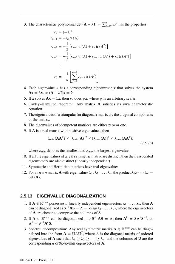
3. The characteristic polynomial det (A − λI) = ∑ni=0 riλ
i has the properties
rn = (−1)n
rn−1 = −rn tr (A)
rn−2 = −1
2
[rn−1 tr (A)+ rn tr (A2)
]rn−3 = −1
3
[rn−2 tr (A)+ rn−1 tr (A2)+ rn tr (A3)
]...
r0 = −1
n
[n−1∑j=1
rn−j tr (Aj )
]
4. Each eigenvalue λ has a corresponding eigenvectorx that solves the systemAx = λx, or (A − λI)x = 0.
5. If x solves Ax = λx, then so does γ x, where γ is an arbitrary scalar.
6. Cayley–Hamilton theorem: Any matrix A satisfies its own characteristicequation.
7. The eigenvalues of a triangular (or diagonal) matrix are the diagonal componentsof the matrix.
8. The eigenvalues of idempotent matrices are either zero or one.
9. If A is a real matrix with positive eigenvalues, then
λmin(AAT) ≤ [λmin(A)]2 ≤ [λmax(A)]2 ≤ λmax(AAT),
(2.5.28)
where λmin denotes the smallest and λmax the largest eigenvalue.
10. If all the eigenvalues of a real symmetric matrix are distinct, then their associatedeigenvectors are also distinct (linearly independent).
11. Symmetric and Hermitian matrices have real eigenvalues.
12. For an n×nmatrix A with eigenvalues λ1, λ2, . . . , λn, the product λ1λ2 · · · λn =det (A).
2.5.13 EIGENVALUE DIAGONALIZATION
1. If A ∈ Rn×n possesses n linearly independent eigenvectors x1, . . . , xn, then Acan be diagonalized as S−1AS = F = diag(λ1, . . . , λn), where the eigenvectorsof A are chosen to comprise the columns of S.
2. If A ∈ Rn×n can be diagonalized into S−1AS = F, then Ak = SFkS−1, orFk = S−1AkS.
3. Spectral decomposition: Any real symmetric matrix A ∈ Rn×n can be diago-nalized into the form A = UFUT, where F is the diagonal matrix of orderedeigenvalues of A such that λ1 ≥ λ2 ≥ · · · ≥ λn, and the columns of U are thecorresponding n orthonormaleigenvectors of A.
©1996 CRC Press LLC

4. The spectral radiusof a real symmetric matrix A, commonly denoted by ρ(A),is defined as ρ(A) = max1≤i≤n |λi(A)|.
5. If A ∈ Rn×n and B ∈ Rn×n are diagonalizable, then they share a commoneigenvector matrix S if and only if AB = BA. (Not every eigenvector of A needbe an eigenvector for B, e.g., A = I.)
6. Schur decomposition: If A ∈ Cn×n, then a unitary matrix Q ∈ Cn×n exists suchthat QHAQ = D + N, where D = diag(λ1, . . . , λn) and N ∈ Cn×n is strictlyupper triangular. The matrix Q can be chosen so that the eigenvalues λi appearin any order along the diagonal.
7. If A ∈ Rn×n and symmetric, then a real orthogonal matrix Q exists such thatQTAQ = diag(λ1, . . . , λn).
8. If A ∈ Rn×n possesses s ≤ n linearly independent eigenvectors, it is similar toa matrix with s Jordan blocks
J = M−1AM =
J1
· 00 ·
Js
,
where each Jordan block Ji is an upper triangular matrix with only a singleeigenvalue λi and a single eigenvector:
Ji =
λi 1 0
· 1· 1
0 λi
(2.5.29)
If Ji has m > 1, then λi repeats m times along the main diagonal, with (m− 1)1’s appearing above the diagonal entries, and all other components are equal tozero.
2.5.14 MATRIX EXPONENTIALS
1. Matrix exponentiation is defined as (the series always converges):
eAt = I + At + (At)2
2!+ (At)3
3!+ · · · .
2. Common properties of matrix exponentials are
(a)(eAs
) (eAt
)= eA(s+t),
(b)(eAt
) (e−At
)= I,
(c) ddteAt = AeAt , and
©1996 CRC Press LLC

(d) when A and B are square matrices, the commutator of A and B is C =[B,A] = BA − AB. Then e(A+B) = eAeBeC/2 provided that [C,A] =[C,B] = 0 (i.e., each of A and B commute with their commutator).
3. For a matrix A ∈ Rn×n, the determinant of eAt is given by
det(eAt
)= eλ1t eλ2t · · · eλnt = etrace(At).
4. The diagonalization of eAt is given by eAt = SeDtS−1 where the columns ofS consist of the eigenvectors of A, and the entries of the diagonal matrix D arethe corresponding eigenvalues of A, that is, A = SDS−1.
5. If A is skew-symmetric, then eAt is an orthogonal matrix.
2.5.15 QUADRATIC FORMS
1. For a symmetric matrix A, the product xTAx is called a pure quadratic form. Ithas the form
xTAx =n∑i=1
n∑j=1
aij xixj = a11x21 + a12x1x2 + a21x2x1 + · · · + annx
2n.
2. For A symmetric, the gradient of xTAx/xTx equals zero if, and only if, x isan eigenvector of A. Thus, the stationary values for this expression are theeigenvalues of A.
3. The ratio of two quadratic forms (B nonsingular) u(x) = (xTAx)/(xTBx) attainsstationary values at the eigenvalues of B−1A. In particular,
umax = λmax(B−1A), and umin = λmin(B−1A).
4. A matrix A is positive definiteif xTAx > 0 for all x = 0.
5. A matrix A is positive semidefiniteif xTAx ≥ 0 for all x.
6. For a real, symmetric matrix A ∈ Rn×n, the following are necessary and suffi-cient conditions to establish the positive definiteness of A:
(a) All eigenvalues, or characteristic roots, of A have λi > 0, for i = 1, . . . , n,and
(b) The upper-left submatrices of A, defined by
A1 = [a11
], A2 =
[a11 a12
a21 a22
], . . . ,
An =
a11 a12 · · · a1n
a21 a22 · · · a2n...
......
an1 an2 · · · ann
,
have det Ak > 0, for all k = 1, . . . , n.
©1996 CRC Press LLC

7. If A is positive definite, then all of the principal submatrices of A are also positivedefinite. Additionally, all diagonal entries of A are positive.
8. For a real, symmetric matrix A ∈ Rn×n, the following are necessary and suffi-cient conditions to establish the positive semidefiniteness of A:
• All eigenvalues, or characteristic roots, of A have λi ≥ 0, for i = 1, . . . , n,and
• The principal submatrices of A have det Ak ≥ 0, for all k = 1, . . . , n.
9. If A is positive definite, then all of the principal submatrices of A are also positivedefinite. Additionally, all diagonal entries of A are nonnegative.
10. If xT denotes the radius vector (running coordinates [x, y, z]), and if a matrixQ is positive definite, then (xT − xT
0 )Q−1(x − x0) = 1 is the equation of an
ellipsoid with its center at [x0, y0, z0] = xT0 and semiaxes equal to the square
roots of the eigenvalues of Q.
2.5.16 MATRIX FACTORIZATIONS
1. Singular value decomposition (SVD): Any m × n matrix A can be written asthe product A = UEVT, where U is an m×m orthogonal matrix, V is an n× n
orthogonal matrix, and E = diag(σ1, σ2, . . . , σp), with p = min (m, n) andσ1 ≥ σ2 ≥ · · · ≥ σp ≥ 0. The values σi , i = 1, . . . , p, are called the singularvaluesof A.
2. When rank(A) = r > 0, A has exactly r positive singular values, and σr+1 =· · · = σp = 0.
3. When A is a symmetric n × n matrix, then σ1 = |λ1|, · · · , σn = |λn|, whereλ1, λ2, . . . , λn are the eigenvalues of A.
4. When A is an m × n matrix, if m ≥ n then the singular values of A are thesquare roots of the eigenvalues of ATA. Otherwise, they are the square roots ofthe eigenvalues of AAT.
5. Any m × n matrix A can be factored as PA = LU, where P is a permutationmatrix, L is lower triangular, and U is an m× n matrix in echelon form.
6. QR factorization: If all the columns of A ∈ Rm×n are linearly independent, thenA can be factored as A = QR, where Q ∈ Rm×n has orthonormal columns andR ∈ Rn×n is upper triangular and nonsingular.
7. If A ∈ Rn×n is symmetric positive definite, then
A = LDLT = LD1/2D1/2LT = (LD1/2
) (LD1/2
)T = GGT
(2.5.30)
where L is a lower triangular matrix and D is a diagonal matrix. The factorizationA = GGT is called the Cholesky factorization, and the matrix G is commonlyreferred to as the Cholesky triangle.
©1996 CRC Press LLC

2.5.17 THEOREMS
1. Frobenius–Perron theorem:If A > 0, then there exists a λ0 > 0 and x0 > 0such that
(a) Ax0 = λ0x0,
(b) if λ is any other eigenvalue of A, λ = λ0, then |λ| < λ0, and
(c) λ0 is an eigenvalue with geometric and algebraic multiplicity equal to one.
2. If A ≥ 0, and Ak > 0 for some positive integer k, then the results of theFrobenius–Perron theorem apply to A.
3. Courant–Fischer minimax theorem:If λi(A) denotes the i th largest eigenvalueof a matrix A = AT ∈ Rn×n, then
λj (A) = maxSj
min0 =x∈Sj
xTAxxTx
j = 1, . . . , n
where x ∈ Rn and Sj is a j -dimensional subspace.
4. Cramer’s rule: The j th component of x = A−1b is given by
xj = det Bj
det A, where Bj =
a11 a12 b1 a1n...
......
...
an1 an2 bn ann
.
(2.5.31)
The vector b = (b1, . . . , bn)T replaces the j th column of the matrix A to formthe matrix Bj .
5. Sylvester’s law of inertia:For a symmetric matrix A ∈ Rn×n, the congruenceA ⇒ CTAC, for C nonsingular, has the same number of positive, negative, andzero eigenvalues.
6. Raleigh’s principle:The quotientR(x) = xTAx/xTx is minimized by the eigen-vector x = x1 corresponding to the smallest eigenvalue λ1 of A. The minimumof R(x) is λ1, that is,
minR(x) = minxTAxxTx
= R(x1) = xT1 Ax1
xT1 x
= xT1λ1x1
xT1 x
= λ1.
(2.5.32)
2.5.18 KRONECKER PRODUCTS OR TENSOR PRODUCTS
If the matrix A = (aij ) has size m × n, and matrix B = (bij ) has size r × s, thenthe Kronecker product of these matrices, denoted A ⊗ B, is defined as the partitionedmatrix
A ⊗ B =
a11B a12B . . . a1nBa21B a22B . . . a2nB...
......
am1B am2B . . . amnB
. (2.5.33)
©1996 CRC Press LLC

Hence, the A ⊗ B matrix has size mr × ns.
For example, if A =[a11 a12
a21 a22
]and B =
[b11 b12
b21 b22
], then
A ⊗ B =[a11B a12Ba21B a22B
]=
a11b11 a11b12... a12b11 a12b12
a11b21 a11b22... a12b21 a12b22
. . . . . . . . . . . . . . . . . . . . . . . . . . . . . . . .
a21b11 a21b12... a22b11 a22b12
a21b21 a21b22... a22b21 a22b22
.
(2.5.34)
The Kronecker product has the following properties:
1. If z and w are vectors of appropriate dimensions, thenAz ⊗ Bw = (A ⊗ B)(z ⊗ w).
2. If α is a scalar, then A ⊗ (αB) = α(A ⊗ B).
3. The Kronecker product is distributive with respect to addition:
• (A + B)⊗ C = A ⊗ C + B ⊗ C, and
• A ⊗ (B + C) = A ⊗ B + A ⊗ C.
4. The Kronecker product is associative: A ⊗ (B ⊗ C) = (A ⊗ B)⊗ C.
5. (A ⊗ B)T = AT ⊗ BT.
6. The mixed product rule: If the dimensions of the matrices are such that theexpressions following exist, then (A ⊗ B)(C ⊗ D) = AC ⊗ BD.
7. If the inverses exist, then (A ⊗ B)−1 = A−1 ⊗ B−1.
8. If λi and xi are the eigenvalues and the corresponding eigenvectors for A,and µj and yj are the eigenvalues and the corresponding eigenvectors for B,then A ⊗ B has eigenvalues λiµj with corresponding eigenvectors xi ⊗ yj .
9. If matrix A has sizen×n and B has sizem×m, then det(A⊗B) = (det A)m(det B)n.
10. If f (z) is an analytic function and A has size n× n, then
• f (In ⊗ A) = In ⊗ f (A), and
• f (A ⊗ In) = f (A)⊗ In.
11. tr (A ⊗ B) = ( tr A)( tr B).
12. If A, B, C, and D are matrices with A similar to C and B similar to D, thenA ⊗ B is similar to C ⊗ D.
13. If C(t) = A(t)⊗ B(t), then dCdt
= dAdt
⊗ B + A ⊗ dBdt
.
©1996 CRC Press LLC
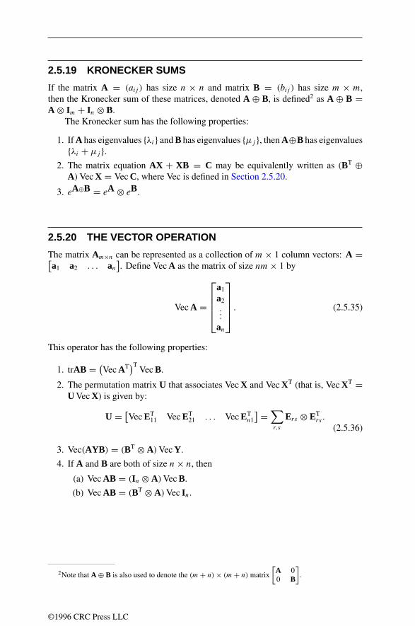
2.5.19 KRONECKER SUMS
If the matrix A = (aij ) has size n × n and matrix B = (bij ) has size m × m,then the Kronecker sum of these matrices, denoted A ⊕ B, is defined2 as A ⊕ B =A ⊗ Im + In ⊗ B.
The Kronecker sum has the following properties:
1. If A has eigenvalues λi and B has eigenvalues µj , then A⊕B has eigenvaluesλi + µj .
2. The matrix equation AX + XB = C may be equivalently written as (BT ⊕A) Vec X = Vec C, where Vec is defined in Section 2.5.20.
3. eA⊕B = eA ⊗ eB.
2.5.20 THE VECTOR OPERATION
The matrix Am×n can be represented as a collection of m × 1 column vectors: A =[a1 a2 . . . an
]. Define Vec A as the matrix of size nm× 1 by
Vec A =
a1
a2...
an
. (2.5.35)
This operator has the following properties:
1. trAB = (Vec AT)T
Vec B.
2. The permutation matrix U that associates Vec X and Vec XT (that is, Vec XT =U Vec X) is given by:
U = [Vec ET
11 Vec ET21 . . . Vec ET
n1
] =∑r,s
Ers ⊗ ETrs .
(2.5.36)
3. Vec(AYB) = (BT ⊗ A)Vec Y.
4. If A and B are both of size n× n, then
(a) Vec AB = (In ⊗ A)Vec B.
(b) Vec AB = (BT ⊗ A)Vec In.
2Note that A ⊕ B is also used to denote the (m+ n)× (m+ n) matrix
[A 00 B
].
©1996 CRC Press LLC

2.6 ABSTRACT ALGEBRA
2.6.1 BASIC CONCEPTS
Definitions
1. A binary operation on a setS is a function H : S × S → S.
2. An algebraic structure(S, H1, . . . , Hn) consists of a nonempty set S with one ormore binary operations Hi defined on S. If the operations are understood, thenthe binary operations need not be mentioned explicitly.
3. The order of an algebraic structure S is the number of elements in S, written|S|.
4. Properties that a binary operation H on an algebraic structure (S, H) may haveare
• Associative: a H (b H c) = (a H b) H c for all a, b, c ∈ S.
• Identity: there exists an element e ∈ S (identity elementof S) such thate H a = a H e = a for all a ∈ S.
• Inverse: a−1 ∈ S is an inverseof a if a H a−1 = a−1 H a = e.
• Commutative(or abelian): if a H b = b H a for all a, b ∈ S.
5. A semigroup(S, H) consists of a nonempty set S and an associative binaryoperation H on S.
6. A monoid(S, H) consists of a nonempty set S with an identity element and anassociative binary operation H.
Examples of semigroups and monoids1. The sets N = 0, 1, 2, 3, . . . (natural numbers), Z = 0,±1,±2, . . . (inte-
gers), Q (rational numbers), R (real numbers), and C (complex numbers) whereH is either addition or multiplication are semigroups and monoids.
2. The set of positive integers under addition is a semigroup but not a monoid.
3. If A is any nonempty set, then the set of all functions f : A → A where H is thecomposition of functions is a semigroup and a monoid.
4. Given a set S, the set of all strings of elements of S, where H is concatenationof strings, is a monoid (the identity is λ, the empty string).
©1996 CRC Press LLC

2.6.2 GROUPS
1. A group(G, H) consists of a set G with a binary operation H defined on G suchthat H satisfies the associative, identity, and inverse laws. Note: The operationH is often written as + (an additive group) or as · or × (a multiplicativegroup).If + is used, the identity is written 0 and the inverse of a is written −a. Ifmultiplicative notation is used, a H b is often written ab and the identity is oftenwritten 1.
2. The order of a ∈ G is the smallest positive integer n such that an = 1 wherean = a · a · · · a (n times) (or a + a + · · · + a = 0 if G is written additively). Ifthere is no such integer, the element has infinite order. In a finite group of ordern, each element has some order k (depending on the particular element) and itmust be that k divides n.
3. (H, H) is a subgroup of (G, H) if H ⊆ G and (H, H) is a group (using the samebinary operation used in (G, H)).
4. The cyclic subgroup〈a〉 generated by a ∈ G is the subgroup an | n ∈ Z =. . . , a−2 = (a−1)2, a−1, a0 = e, a, a2, . . . . The element a is a generatorof〈a〉. A group G is cyclic if there is a ∈ G such that G = 〈a〉.
5. If H is a subgroup of a group G, then a left [right] cosetof H in G is the setaH = ah | h ∈ H [Ha = ha | h ∈ H ] .
6. A normal subgroupof a group G is a subgroup H such that aH = Ha for alla ∈ G.
7. A simple groupis a group G = e with only G and e as normal subgroups.
8. If H is a normal subgroup of G, then the quotient group(or factor group) ofG moduloH is the group G/H = aH | a ∈ G, with binary operationaH · bH = (ab)H .
9. A finite groupG is solvableif there is a sequence of subgroupsG1 = G,G2, . . . ,
Gk−1,Gk = e such that each Gi+1 is a normal subgroup of Gi and Gi/Gi+1
is abelian.
Facts about groups1. The identity element is unique.
2. Each element has exactly one inverse.
3. Each of the equations a H x = b and x H a = b has exactly one solution,x = a−1 H b and x = b H a−1.
4. (a−1)−1 = a.
5. (a H b)−1 = b−1 H a−1.
6. The left [right] cancellation lawholds in all groups: If a H b = a H c then b = c
[if b H a = c H a then b = c].
7. Lagrange’s theorem: If G is a finite group and H is a subgroup of G, then theorder of H divides the order of G.
©1996 CRC Press LLC

8. Every group of prime order is simple.
9. Every abelian group is solvable.
10. Feit–Thompson theorem: All groups of odd order are solvable. Hence, all finitenon-Abelian simple groups have even order.
11. Finite simple groups are of the following types:
• Zp (p prime)
• A group of Lie type
• An (n ≥ 5)
• Sporadic groups (see table)
Examples of groups1. Z, Q, R, and C, with H as addition of numbers, are additive groups.
2. For n a positive integer, nZ = nz | z ∈ Z is an additive group.
3. Q − 0 = Q∗, R − 0 = R∗, C − 0 = C∗, with H as multiplication ofnumbers, are multiplicative groups.
4. Zn = Z/nZ = 0, 1, 2, . . . , n− 1 is a group where H is addition modulo n.
5. Z∗n = k | k ∈ Zn, k has a multiplicative inverse (under multiplication modulo
n) in Zn is a group under multiplication modulo n. If p is prime, Z∗p is cyclic.
If p is prime and a ∈ Z∗p has order (index) p − 1, then a is a primitive root
modulo p. See the tables on pages 78 and 79 for primitive roots and powerresidues.
6. If (G1, H1), (G2, H2), . . . , (Gn, Hn) are groups, the (direct) product group is (G1 × G2 × · · · × Gn, H) = (a1, a2, . . . , an) | ai ∈ Gi, i = 1, 2, . . . , nwhere H is defined by (a1, a2, . . . , an) H (b1, b2, . . . , bn) = (a1 H1 b1, a2 H2
b2, . . . , an Hn bn).
7. All m× n matrices with real entries form a group under addition of matrices.
8. All n × n matrices with real entries and nonzero determinants form a groupunder matrix multiplication.
9. All 1–1, onto functions f : S → S (permutationsof S), where S is anynonempty set, form a group under composition of functions. In particular,if S = 1, 2, 3, . . . , n, the group of permutations of S is called the symmetricgroupSn. Each permutation can be written as a product of cycles. A cycleis apermutation σ = (i1 i2 · · · ik), where σ(i1) = i2, σ (i2) = i3, . . . , σ (ik) = i1.Each cycle of length greater than 1 can be written as a product of transpositions(cycles of length 2). A permutation is even(odd) if it can be written as theproduct of an even (odd) number of transpositions. (Every permutation is eithereven or odd.) The set of all even permutations in Sn is a subgroup An of Sn. Thegroup An is called the alternating group on n letters.
10. Given a regular n-gon, the dihedral groupDn is the group of all symmetries ofthe n-gon, that is, the group generated by the set of all rotations around the center
©1996 CRC Press LLC

of the n-gon through angles of 360k/n degrees (where k = 0, 1, 2, . . . , n− 1),together with all reflections in lines passing through a vertex and the center ofthe n-gon, using composition of functions. Alternately, Dn = aibj | i =0, 1; j = 0, 1, . . . , n− 1; aba−1 = b−1.
11. The group T is of order 12 where T = aibj | i = 0, 1, . . . , 5; j = 0, 1; b2 =a3, ba = a−1b.
12. The quaternion groupQ8 is the set 1,−1, i,−i, j,−j, k,−k where multipli-cation is defined by the following relationships:
i2 = j 2 = k2 = −1, ij = −ji = k, jk = −kj = i, ki = −ik = j
with 1 as the identity. These relations yield the following multiplication table:
× 1 −1 i −i j −j k −k1 1 −1 i −i j −j k −k
−1 −1 1 −i i −j j −k k
i i −i −1 1 k −k −j j
−i −i i 1 −1 −k k j −jj j −j −k k −1 1 i −i
−j −j j k −k 1 −1 −i i
k k −k j −j −i i −1 1−k −k k −j j i −i 1 −1
The quaternion group can also be defined as the following group of 8 matrices:[1 00 1
],
[−1 00 −1
],
[−i 00 i
],
[i 00 −i
],
[0 i
i 0
],
[0 −i−i 0
],
[0 1
−1 0
],
[0 −11 0
]
where i2 = −1 and matrix multiplication is the group operation.
2.6.3 RINGS
Definitions1. A ring (R,+, ·) consists of a nonempty set R and two binary operations, +
and ·, such that (R,+) is an abelian group, the operation · is associative, andthe left distributive lawa(b + c) = (ab) + (ac) and the right distributive law(a + b)c = (ac)+ (bc) hold for all a, b, c ∈ R.
2. A subset S of a ring R is a subringof R if S is a ring using the same operationsused in R.
3. A ring R is a commutativering if the multiplication operation is commutative:ab = ba for all a, b ∈ R.
4. A ring R is a ring with unity if there is an element 1 (called unity) such thata1 = 1a = a for all a ∈ R.
©1996 CRC Press LLC

5. A unit in a ring with unity is an element a with a multiplicative inverse a−1
(aa−1 = a−1a = 1).
6. If a = 0, b = 0, and ab = 0, then a is a left divisor of zeroand b is a rightdivisor of zero.
7. A subset I of a ring (R,+, ·) is an ideal of R if (I,+) is a subgroup of (R,+)and I is closed under left and right multiplication by elements of R (if x ∈ I
and r ∈ R, then rx ∈ I and xr ∈ I ).
8. An ideal I ⊆ R is
• Proper: if I = 0 and I = R
• Maximal: if I is proper there is no proper ideal properly containing I
• Prime: if ab ∈ I implies that a or b ∈ I
• Principal: if there is a ∈ R such that I is the intersection of all idealscontaining a.
9. If I is an ideal in a ring R, then a cosetis a set r + I = r + a | a ∈ I .10. If I is an ideal in a ringR, then the quotient ringis the ringR/I = r+I | r ∈ R,
where (r + I )+ (s + I ) = (r + s)+ I and (r + I )(s + I ) = (rs)+ I .
11. An integral domain(R,+, ·) consists of a nonempty set R and two binaryoperations, + and · , such that (R,+, ·) is a commutative ring with unity, andthe left [right] cancellation laws hold: if ab = ac then b = c [if ba = ca thenb = c] for all a, b, c ∈ R, where a = 0. (Equivalently, an integral domain is acommutative ring with unity that has no divisors of zero.)
12. If R is an integral domain, then a nonzero element r ∈ R that is not a unit isirreducibleif r = ab implies that either a or b is a unit.
13. If R is an integral domain, a nonzero element r ∈ R that is not a unit is a primeif, whenever r|ab, then either r|a or r|b (x|y means that there is an elementz ∈ R such that y = zx.).
14. A unique factorization domain(UFD) is an integral domain such that everynonzero element that is not a unit can be written uniquely as the product ofirreducible elements (except for factors that are units and except for the order inwhich the factor appears).
15. A principal ideal domain(PID) is an integral domain in which every ideal is aprincipal ideal.
16. A division ring is a ring in which every nonzero element has a multiplicativeinverse (that is, every nonzero element is a unit). (Equivalently, a divisionring is a ring in which the nonzero elements form a multiplicative group.) Anoncommutative division ring is called a skew field.
Examples1. Z (integers), Q (rational numbers), R (real numbers), and C (complex numbers)
are rings, with ordinary addition and multiplication of numbers.
©1996 CRC Press LLC

2. Zn is a ring, with addition and multiplication modulo n.
3. If√n is not an integer, then Z[
√n] = a + b
√n | a, b ∈ Z, where (a +
b√n) + (c + d
√n) = (a + c) + (b + d)
√n and (a + b
√n)(c + d
√n) =
(ac + nbd)+ (ad + bc)√n is a ring.
4. The set of Gaussian integersZ[i] = a+ bi | a, b ∈ Z is a ring, with the usualdefinitions of addition and multiplication of complex numbers.
5. The polynomial ringin one variable over a ring R is the ring R[x] = anxn +· · · + a1x + a0 | ai ∈ R; i = 0, 1, . . . , n; n ∈ N (elements of R[x] areadded and multiplied using the usual rules for addition and multiplication ofpolynomials). The degreeof a polynomial anxn + · · · + a1x + a0 with an = 0is n. A polynomial is monicif an = 1. A polynomial f (x) is irreducible overR if f (x) cannot be factored as a product of polynomials in R[x] of degreeless than the degree of f (x). A monic irreducible polynomial f (x) of degreek in Zp[x] (p prime) is primitive if the order of x in Zp[x]/(f (x)) is pk − 1,where (f (x)) = f (x)g(x) | g(x) ∈ Zp[x] (the ideal generated by f (x)). Forexample, the polynomial x2 + 1 is
• Irreducible in R[x] because x2 + 1 has no real root
• Reducible in C[x] because x2 + 1 = (x − i)(x + i)
• Reducible in Z2[x] because x2 + 1 = (x + 1)2
• Reducible in Z5[x] because x2 + 1 = (x + 2)(x + 3)
6. The division ring of quaternionsis the ring (a + bi + cj + dk | a, b, c, d ∈R,+, ·), where operations are carried out using the rules for polynomial addi-tion and multiplication and the defining relations for the quaternion group Q8.
Facts1. The set of all units of a ring is a group under the multiplication defined on the
ring.
2. Every principal ideal domain is a unique factorization domain.
3. If R is a commutative ring with unity, then every maximal ideal is a prime ideal.
4. If R is a commutative ring with unity, then R is a field if and only if the onlyideals of R are R and 0.
5. If R is a commutative ring with unity and I = R is an ideal, then R/I is anintegral domain if and only if I is a prime ideal.
6. If R is a commutative ring with unity, then I is a maximal ideal if and only ifR/I is a field.
7. If f (x) ∈ F [x] (F a field) and the ideal (f (x)) = 0, then the ideal (f (x)) ismaximal if and only if f (x) is irreducible over F .
©1996 CRC Press LLC

2.6.4 FIELDS
Definitions1. A field(F,+, ·) consists of a commutative ring with unity such that each nonzero
element of F has a multiplicative inverse (equivalently, a field is a commutativedivision ring).
2. The characteristicof a field is the smallest positive integer n such that 1 + 1 +· · · + 1 = 0 (n summands). If no such n exists, the field has characteristic 0 (orcharacteristic ∞).
3. Field K is an extension fieldof the field F if F is a subfield of K (i.e., F ⊆ K ,and F is a field using the same operations used in K).
Examples1. The sets Q, R, and C with ordinary addition and multiplication are fields.
2. Zp (p a prime) is a field under addition and multiplication modulo p.
3. F [x]/(f (x)) is a field, provided that F is a field and f (x) is a nonconstantpolynomial irreducible in F [x].
2.6.5 FINITE FIELDS
Facts1. If p is prime, then the ring Zp is a finite field.
2. If p is prime and n is a positive integer, then there is exactly one field (up toisomorphism) with pn elements. This field is denoted GF(pn) or Fpn and iscalled a Galois field. (See the tables beginnning on page 155.)
3. For F a finite field, there is a prime p and a positive integer n such that F haspn elements. The prime number p is the characteristic of F . The field F is afinite extensionof Zp, that is, F is a vector space over Zp.
4. If F is a finite field, then the set of nonzero elements of F under multiplicationis a cyclic group. A generator of this group is a primitive element.
5. There are φ(pn − 1)/n primitive polynomials of degree n (n > 1) over GF(p),where φ is the Euler φ-function. (See table on page 154.)
6. There are (∑
j |k µ(k/j)pnj )/k irreducible polynomials of degree k overGF(pn),
where µ is the Mobius function.
7. If F is a finite field where |F | = k and p(x) is a polynomial of degree n
irreducible over F , then the field F [x]/(p(x)) has order kn. If α is a root ofp(x) ∈ F [x] of degree n ≥ 1, then F [x]/(p(x)) = cn−1α
n−1 +· · ·+c1α+c0 |ci ∈ F for all i.
8. When q is a power of a prime, Fqn can be viewed as a vector space of dimensionn over Fq . A basis of Fqn of the form α, αq , αq
2, . . . , αq
n−1 is called a normal
©1996 CRC Press LLC

basis.If α is a primitive element of Fqn , then the basis is said to be a primitivenormal basis.Such an α satisfies a primitive normal polynomial of degree n
over Fq .
Degree Primitive normal polynomialsn q = 2 q = 3 q = 5
2 x2 + x + 1 x2 + x + 2 x2 + x + 23 x3 + x2 + 1 x3 + 2x2 + 1 x3 + x2 + 24 x4 + x3 + 1 x4 + x3 + 2 x4 + x3 + 4x + 25 x5 + x4 + x2 + x + 1 x5 + 2x4 + 1 x5 + 2x4 + 36 x6 + x5 + 1 x6 + x5 + x3 + 2 x6 + x5 + 27 x7 + x6 + 1 x7 + x6 + x2 + 1 x7 + x6 + 2
2.6.6 HOMOMORPHISMS AND ISOMORPHISMS
Definitions1. A group homomorphismfrom group G1 to group G2 is a function ϕ : G1 → G2
such that ϕ(ab) = ϕ(a)ϕ(b) for all a, b ∈ G1. Note: aϕ is often written insteadof ϕ(a).
2. A characterof a group G is a group homomorphism χ : G → C∗ (nonzerocomplex numbers under multiplication). (See table on page 149.)
3. A ring homomorphismfrom ring R1 to ring R2 is a function ϕ : R1 → R2 suchthat ϕ(a + b) = ϕ(a)+ ϕ(b) and ϕ(ab) = ϕ(a)ϕ(b) for all a, b ∈ R1.
4. An isomorphismfrom group (ring) S1 to group (ring) S2 is a group (ring) homo-morphism ϕ : S1 → S2 that is 1-1 and onto S2. If an isomorphism exists, thenS1 is said to be isomorphicto S2. Write S1
∼= S2. (See the table on page 150for numbers of nonisomorphic groups and the table on page 149 for examplesof groups of orders less than 16.)
5. An automorphismof S is an isomorphism ϕ : S → S.
6. The kernelof a group homomorphism ϕ : G1 → G2 is ϕ−1(e) = g ∈ G1 |ϕ(g) = e. The kernelof a ring homomorphism ϕ : R1 → R2 is ϕ−1(0) = r ∈R1 | ϕ(r) = 0.
Facts1. If ϕ : G1 → G2 is a group homomorphism, then ϕ(G1) is a subgroup of G2.
2. Fundamental homomorphism theorem for groups: If ϕ : G1 → G2 is a grouphomomorphism with kernelK , thenK is a normal subgroup ofG1 andG1/K ∼=ϕ(G1).
3. If G is a cyclic group of infinite order, then G ∼= (Z,+).4. If G is a cyclic group of order n, then G ∼= (Zn,+).5. If p is prime, then there is only one group (up to isomorphism) of order p, the
group (Zp,+).
©1996 CRC Press LLC

6. Cayley’s theorem: IfG is a finite group of order n, thenG is isomorphic to somesubgroup of the group of permutations on n objects.
7. Zm × Zn∼= Zmn if, and only if, m and n are relatively prime.
8. If n = n1 · n2 · . . . · nk where each ni is a power of a different prime, thenZn
∼= Zn1 × Zn2 × · · · × Znk .
9. Fundamental theorem of finite abelian groups: Every finite abelian group G
(order ≥ 2) is isomorphic to a product of cyclic groups where each cyclic grouphas order a power of a prime, that is, there is a unique set n1, . . . , nk whereeach ni is a power of some prime such that G ∼= Zn1 × Zn2 × · · · × Znk .
10. Fundamental theorem of finitely generated abelian groups: If G is a finitelygenerated abelian group, then there is a unique integer n ≥ 0 and a unique setn1, . . . , nk where each ni is a power of some prime such that G ∼= Z
n× Zn1 ×Zn2 × · · · × Znk (G is finitely generated if there are a1, a2, . . . , an ∈ G suchthat every element of G can be written as aε1
k1aε2k2
· · · aεjkj where ki ∈ 1, . . . , n(the ki are not necessarily distinct) and εi ∈ 1,−1).
11. Fundamental homomorphism theorem for rings: If ϕ : R1 → R2 is a ringhomomorphism with kernel K , then K is an ideal in R1 and R1/K ∼= ϕ(R1).
2.6.7 MATRIX CLASSES THAT ARE GROUPS
In the following examples, the group operation is ordinary matrix multiplication:
• GL(n,C) all complex non-singular n× n matrices
• GL(n,R) all real non-singular n× n matrices
• O(n) all n× n matrices A with AAT = I , also called theorthogonal group
• SL(n,C) all complex n × n matrices of determinant 1, also calledthe unimodular groupor the special linear group
• SL(n,R) all real n× n matrices of determinant 1
• SO(2) rotations of the plane: matrices of the form
A(θ) =[
cos θ − sin θsin θ cos θ
]• SO(n) rotations of n-dimensional space
• SU(n) all n× n unitary matrices of determinant 1
• U(n) all n× n unitary matrices with UUH = I
©1996 CRC Press LLC

2.6.8 PERMUTATION GROUPSName Symbol Order Definition
Symmetric group Sp p! All permutations on 1, 2, . . . , pAlternating group Ap p!/2 All even permutations on 1, 2, . . . , pCyclic group Cp p Generated by (12 · · ·p)Dihedral group Dp 2p Generated by (12 · · ·p) and (1p)(2p − 1)Identity group Ep 1 (1)(2) · · · (p) is the only permutation
For example, with p = 3 elements
A3 = (123), (231), (312),C3 = (123), (231), (312),D3 = (231), (213), (132), (321), (312), (123),E3 = (123) and
S3 = (231), (213), (132), (321), (312), (123).
Creating new permutation groupsLet A have permutations Xi, order n, degree d, let B have permutations Yj , orderm, degree e, and let C (a function of A and B) have permutations Wk, order p,degree f .
Name Definition Permutation Order DegreeSum C = A+ B W = X ∪ Y p = mn f = d + e
Product C = A× B W = X × Y p = mn f = de
Composition C = A[B] W = X × Y p = mnd f = de
Power C = BA W = YX p = mn f = ed
Polya theoryDefine Inv (π) to be the number of invariant elements (i.e., mapped to themselves) ofthe permutation π . Define cyc (π) as the number of cycles in π .
1. Burnside’s Lemma: Let G be a group of permutations of a set A, and let S bethe equivalence relation on A induced by G. Then the number of equivalence
classes in A is given by1
|G|∑π∈G
Inv (π).
2. Special case of Polya’s theorem: Let R be an m element set of colors. Let Gbe a group of permutations π1, π2, . . . of the set A. Let C(A,R) be the set ofcolorings of the elements of A using colors in R. Then the number of distinctcolorings in C(A,R) is given by
1
|G|[mcyc (π1) +mcyc (π2) + . . .
].
©1996 CRC Press LLC

3. Polya’s theorem: Let G be a group of permutations on a set A with cycle indexPG(x1, x2, . . . , xk). Let C(A,R) be the collection of all colorings of A usingcolors in R. If w is a weight assignment on R, then the pattern inventory ofcolorings in C(A,R) is given by
PG
(∑r∈R
w(r),∑r∈R
w2(r), · · ·∑r∈R
wk(r)
).
For example, consider necklaces made of 2k beads. Allowing a necklace re-versal results in the permutation group G = π1, π2 with π1 = (1)(2) . . . (2k)and π2 = (
1 2k) (
2 2k − 1) (
3 2k − 2). . .
(k k + 1
). Hence, cyc (π1) = 2k,
cyc (π2) = k, and the cycle index is PG(x1, x2) = (x2k
1 + xk2)/2. Using r colors, the
number of distinct necklaces is (r2k + rk)/2.For a 4 bead necklace (k = 2) using r = 2 colors (say b and g), the (24 +22)/2 =
10 different necklaces are bbbb, bbbg, bbgb, bbgg, bgbg, bggb, gbbg,bggg, gbgg, and gggg. The pattern inventory of colorings, PG(
∑w,
∑w2) =(
(b + g)4 + (b2 + g2)2)/2 = b4 + 2b3g + 4b2g2 + 2bg3 + g4, tells how many
colorings of each type there are.
©1996 CRC Press LLC

2.6.9 TABLES
Groups of Small OrderOrder n Distinct groups of order n
1 e2 Z2
3 Z3
4 Z2 × Z2,Z4
5 Z5
6 Z6,D3
7 Z7
8 Z2 × Z2 × Z2,Z2 × Z4,Z8,Q8,D4
9 Z3 × Z3,Z9
10 Z10,D5
11 Z11
12 Z2 × Z6,Z12, A4,D6, T
13 Z13
14 Z14,D7
15 Z15
Characters for Some Families of GroupsGroup Characters
Zn For m = 0, 1, . . . , n− 1, χm : 1 #→ e2πim/n
G finite G ∼= Zn1 × Zn2 × · · · × Znj with each niAbelian a power of a prime. For mj = 0, 1, . . . , nj − 1
and gj = (0, 0, . . . , 0, 1, 0, . . . , 0)χm1,m2,... ,mn: gj #→ e2πimj /nj
Dn dihedral For x = ±1, y =±1 if n even
1 if n oddχx,y : a #→ x, b #→ y. (See definition of Dn.)
Quaternions For x, y = ±1 or x, y = ±i ,
χx,y :
[0 1
−1 0
]#→ x, χx,y :
[−i 00 i
]#→ y
©1996 CRC Press LLC

Number of Nonisomorphic GroupsOrder No. groups No. Abelian Order No. groups No. Abelian
groups groups
1 1 1 33 1 12 1 1 34 2 13 1 1 35 1 14 2 2 36 14 45 1 1 37 1 1
6 2 1 38 2 17 1 1 39 2 18 5 3 40 14 39 2 2 41 1 1
10 2 1 42 6 1
11 1 1 43 1 112 5 2 44 4 213 1 1 45 2 214 2 1 46 2 115 1 1 47 1 1
16 14 5 48 52 517 1 1 49 2 218 5 2 50 5 219 1 1 51 1 120 5 2 52 5 2
21 2 1 53 1 122 2 1 54 15 323 1 1 55 2 124 15 3 56 13 325 2 2 57 2 1
26 2 1 58 2 127 5 3 59 1 128 4 2 60 13 229 1 1 61 1 130 4 1 62 2 1
31 1 1 63 4 232 51 7 64 267 11
©1996 CRC Press LLC

List of All Sporadic Simple GroupsGroup Order
M11 24 · 32 · 5 · 11M12 26 · 33 · 5 · 11M22 27 · 32 · 5 · 7 · 11M23 27 · 32 · 5 · 7 · 11 · 23M24 210 · 33 · 5 · 7 · 11 · 23
J1 23 · 3 · 5 · 7 · 11 · 19J2 27 · 33 · 52 · 7J3 27 · 35 · 5 · 17 · 19J4 221 · 33 · 5 · 7 · 113 · 23 · 29 · 31 · 37 · 43HS 29 · 32 · 53 · 7 · 11
Mc 27 · 36 · 53 · 11Suz 213 · 37 · 52 · 7 · 11 · 13Ru 214 · 33 · 53 · 7 · 13 · 29He 210 · 33 · 52 · 73 · 17Ly 28 · 37 · 56 · 7 · 11 · 31 · 37 · 67
ON 29 · 34 · 5 · 73 · 11 · 19 · 31.1 221 · 39 · 54 · 72 · 11 · 13 · 23.2 218 · 36 · 53 · 7 · 11 · 23.3 210 · 37 · 53 · 7 · 11 · 23
M(22) 217 · 39 · 52 · 7 · 11 · 13
M(23) 218 · 313 · 52 · 7 · 11 · 13 · 17 · 23M(24)′ 221 · 316 · 52 · 73 · 11 · 13 · 23 · 29F5 215 · 310 · 53 · 72 · 13 · 19 · 31F3 214 · 36 · 56 · 7 · 11 · 19F2 241 · 313 · 56 · 72 · 11 · 13 · 17 · 19 · 23 · 31 · 47
F1 246 · 320 · 59 · 76 · 112 · 133 · 17 · 19 · 23 · 29 · 31 · 41 · 47 · 59 · 71
©1996 CRC Press LLC

Indices and Power Residues
For Z∗n the following table lists the index (order) of a and the power residues
a, a2, . . . , aindex(a) = 1 for each element a, where (a, n) = 1.
Group Element Index Power Group Element Index Powerresidues residues
Z∗2 1 1 1 Z
∗12 1 1 1
Z∗3 1 1 1 5 2 5,1
2 2 2,1 7 2 7,1Z
∗4 1 1 1 11 2 11,1
3 2 3,1 Z∗13 1 1 1
Z∗5 1 1 1 2 12 2,4,8,3,6,12,
2 4 2,4,3,1 11,9,5,10,7,13 4 3,4,2,1 3 3 3,9,14 2 4,1 4 6 4,3,12,9,10,1
Z∗6 1 1 1 5 4 5,12,8,1
5 2 5,1 6 12 6,10,8,9,2,12,Z
∗7 1 1 1 7,3,5,4,11,1
2 3 2,4,1 7 12 7,10,5,9,11,12,3 6 3,2,6,4,5,1 6,3,8,4,2,14 3 4,2,1 8 4 8,12,5,1
5 6 5,4,6,2,3,1 9 3 9,3,16 2 6,1 10 6 10,9,12,3,4,1
Z∗8 1 1 1 11 12 11,4,5,3,7,12,
3 2 3,1 2,9,8,10,6,15 2 5,1 12 2 12,1
7 2 7,1 Z∗14 1 1 1
Z∗9 1 1 1 3 6 3,9,13,11,5,1
2 6 2,4,8,7,5,1 5 6 5,11,13,9,3,14 3 4,7,1 9 3 9,11,15 6 5,7,8,4,2,1 11 3 11,9,1
7 3 7,4,1 13 2 13,18 2 8,1 Z
∗15 1 1 1
Z∗10 1 1 1 2 4 2,4,8,1
3 4 3,9,7,1 4 2 4,17 4 7,9,3,1 7 4 7,4,13,1
9 2 9,1 8 4 8,4,2,1Z
∗11 1 1 1 11 2 11,1
2 10 2,4,8,5,10, 13 4 13,4,7,19,7,3,6,1 14 2 14,1
3 5 3,9,5,4,1 Z∗16 1 1 1
4 5 4,5,9,3,1 3 4 3,9,11,15 5 5,3,4,9,1 5 4 5,9,13,16 10 6,3,7,9,10, 7 2 7,1
5,8,4,2,1 9 2 9,17 10 7,5,2,3,10, 11 4 11,9,3,1
4,6,9,8,1 13 4 13,9,5,18 10 8,9,6,4,10, 15 2 15,1
3,2,5,7,19 5 9,4,3,5,1
10 2 10,1
©1996 CRC Press LLC

Power Residues in Zp
For prime p < 40, the following table lists the minimal primitive root a andthe power residues of a. These can be used to find am (mod p) for any (a, p) = 1.For example, to find 37 (mod 11) (a = 3,m = 7), look in row p = 11 until thepower of a that is equal to 3 is found. In this case 28 ≡ 3 (mod 11). This meansthat 37 ≡ (28)7 ≡ 256 ≡ (210)5 · 26 ≡ 26 ≡ 9 (mod 11).p a Power residues
3 20 1 2 3 4 5 6 7 8 9
0 1 2 1
5 20 1 2 3 4 5 6 7 8 9
0 1 2 4 3 1
7 30 1 2 3 4 5 6 7 8 9
0 1 3 2 6 4 5 1
11 20 1 2 3 4 5 6 7 8 9
0 1 2 4 8 5 10 9 7 3 61 1
13 20 1 2 3 4 5 6 7 8 9
0 1 2 4 8 3 6 12 11 9 51 10 7 1
17 30 1 2 3 4 5 6 7 8 9
0 1 3 9 10 13 5 15 11 16 141 8 7 4 12 2 6 1
19 20 1 2 3 4 5 6 7 8 9
0 1 2 4 8 16 13 7 14 9 181 17 15 11 3 6 12 5 10 1
23 5
0 1 2 3 4 5 6 7 8 90 1 5 2 10 4 20 8 17 16 111 9 22 18 21 13 19 3 15 6 72 12 14 1
29 2
0 1 2 3 4 5 6 7 8 90 1 2 4 8 16 3 6 12 24 191 9 18 7 14 28 27 25 21 13 262 23 17 5 10 20 11 22 15 1
31 3
0 1 2 3 4 5 6 7 8 90 1 3 9 27 19 26 16 17 20 291 25 13 8 24 10 30 28 22 4 122 5 15 14 11 2 6 18 23 7 213 1
37 2
0 1 2 3 4 5 6 7 8 90 1 2 4 8 16 32 27 17 34 311 25 13 26 15 30 23 9 18 36 352 33 29 21 5 10 20 3 6 12 243 11 22 7 14 28 19 1
©1996 CRC Press LLC

Table of Primitive Monic Polynomials
In the table below, the elements in each string are thecoefficients of the polynomial after the highest power of x.(For example, 564 represents x3 + 5x2 + 6x + 4.)
Field Degree Primitive polynomialsF2 1 0 1
2 113 011 1014 0011 10015 00101 01001 01111 10111 11011 111016 000101 011011 100001 100111 101101 110011
F3 1 0 12 12 223 021 121 201 2114 0012 0022 1002 1122 1222 2002
2112 2212
F5 1 0 2 32 12 23 33 423 032 033 042 043 102 113
143 203 213 222 223 242302 312 322 323 343 403412 442
F7 1 0 2 42 13 23 25 35 45 53
55 633 032 052 062 112 124 152
154 214 242 262 264 304314 322 334 352 354 362422 432 434 444 504 524532 534 542 552 564 604612 632 644 654 662 664
Small finite fieldsIn the following, the entries under αi denote the coefficent of powers of α. Forexample, the last entry of the p(x) = x3 + x2 + 1 table is 1 1 0. That is: α6 ≡1α2 + 1α1 + 0α0 modulo p(α), where the coefficients are taken modulo 2.
©1996 CRC Press LLC

q = 4 x2 + x + 1
i αi
0 0 11 1 02 1 1
q = 8 x3 + x + 1
i αi
0 0 0 11 0 1 02 1 0 03 0 1 14 1 1 05 1 1 16 1 0 1
q = 8 x3 + x2 + 1
i αi
0 0 0 11 0 1 02 1 0 03 1 0 14 1 1 15 0 1 16 1 1 0
q = 16 x4 + x + 1
i αi 7 1 0 1 10 0 0 0 1 8 0 1 0 11 0 0 1 0 9 1 0 1 02 0 1 0 0 10 0 1 1 13 1 0 0 0 11 1 1 1 04 0 0 1 1 12 1 1 1 15 0 1 1 0 13 1 1 0 16 1 1 0 0 14 1 0 0 1
q = 16 x4 + x3 + 1
i αi 7 0 1 1 10 0 0 0 1 8 1 1 1 01 0 0 1 0 9 0 1 0 12 0 1 0 0 10 1 0 1 03 1 0 0 0 11 1 1 0 14 1 0 0 1 12 0 0 1 15 1 0 1 1 13 0 1 1 06 1 1 1 1 14 1 1 0 0
Addition and multiplication tables for F2, F3, F4, and F8
F2 addition and multiplication:
+ 0 1 · 0 10 0 1 0 0 01 1 0 1 0 1
F3 addition and multiplication:
+ 0 1 2 · 0 1 20 0 1 2 0 0 0 01 1 2 0 1 0 1 22 2 0 1 2 0 2 1
F4 addition and multiplication (using β = α + 1):
+ 0 1 α β · 0 1 α β
0 0 1 α β 0 0 0 0 01 1 0 β α 1 0 1 α β
α α β 0 1 α 0 α β 1β β α 1 0 β 0 β 1 α
F8 addition and multiplication (using strings of 0s and 1s to represent the poly-nomials: 0 = 000, 1 = 001, α = 010, α + 1 = 011, α2 = 100, α2 + α = 110,α2 + 1 = 101, α2 + α + 1 = 111):
©1996 CRC Press LLC

+ 000 001 010 011 100 101 110 111000 000 001 010 011 100 101 110 111001 001 000 011 010 101 100 111 110010 010 011 000 001 110 111 100 101011 011 010 001 000 111 110 101 100100 100 101 110 111 000 001 010 011101 101 100 111 110 001 000 011 010110 110 111 100 101 010 011 000 001111 111 110 101 100 011 010 001 000
· 000 001 010 011 100 101 110 111000 000 000 000 000 000 000 000 000001 000 001 010 011 100 101 110 111010 000 010 100 110 011 001 111 101011 000 011 110 101 111 100 001 010100 000 100 011 111 110 010 101 001101 000 101 001 100 010 111 011 110110 000 110 111 001 101 011 010 100111 000 111 101 010 001 110 100 011
Table of primitive rootsAs noted on page 106, the number of integers not exceeding and relatively prime toa fixed integer n is represented by φ(n). These integers form a group; the group iscyclic if, and only if, n = 1, 2, 4 or n is of the form pk or 2pk , where p is an oddprime. We refer to g as a primitive root of n if it generates that group, i.e., if g, g2,. . . , gφ(n) are distinct modulo p. There are φ(φ(n)) primitive roots of n. If g is aprimitive root of p and gp−1 ≡ 1 (mod p2), then g is a primitive root of pk for all k.If gp−1 ≡ 1 (mod p2) then g + p is a primitive root of pk for all k.
If g is a primitive root of pk , then either g or g + pk , whichever is odd, is aprimitive root of 2pk .
If g is a primitive root of n, then gk is a primitive root of n if, and only if,k and φ(n) are relatively prime, and each primitive root of n is of this form, i.e.,(φ(n), k) = 1.
In the table below,
• g denotes the least primitive root of p
• G denotes the least negative primitive root of p
• ε denotes whether 10, −10, or both, are primitive roots of p
p p − 1 g G ε p p − 1 g G ε
3 2 2 −1 — 5 22 2 −2 —7 2 · 3 3 −2 10 11 2 · 5 2 −3 —
13 22 · 3 2 −2 — 17 24 3 −3 ±1019 2 · 32 2 −4 10 23 2 · 11 5 −2 1029 22 · 7 2 −2 ±10 31 2 · 3 · 5 3 −7 −10
©1996 CRC Press LLC

p p − 1 g G ε p p − 1 g G ε
37 22 · 32 2 −2 — 41 23 · 5 6 −6 —43 2 · 3 · 7 3 −9 −10 47 2 · 23 5 −2 1053 22 · 13 2 −2 — 59 2 · 29 2 −3 1061 22 · 3 · 5 2 −2 ±10 67 2 · 3 · 11 2 −4 −1071 2 · 5 · 7 7 −2 −10 73 23 · 32 5 −5 —
79 2 · 3 · 13 3 −2 — 83 2 · 41 2 −3 −1089 23 · 11 3 −3 — 97 25 · 3 5 −5 ±10
101 22 · 52 2 −2 — 103 2 · 3 · 17 5 −2 —107 2 · 53 2 −3 −10 109 22 · 33 6 −6 ±10113 24 · 7 3 −3 ±10 127 2 · 32 · 7 3 −9 —
131 2 · 5 · 13 2 −3 10 137 23 · 17 3 −3 —139 2 · 3 · 23 2 −4 — 149 22 · 37 2 −2 ±10151 2 · 3 · 52 6 −5 −10 157 22 · 3 · 13 5 −5 —163 2 · 34 2 −4 −10 167 2 · 83 5 −2 10173 22 · 43 2 −2 — 179 2 · 89 2 −3 10
181 22 · 32 · 5 2 −2 ±10 191 2 · 5 · 19 19 −2 −10193 26 · 3 5 −5 ±10 197 22 · 72 2 −2 —199 2 · 32 · 11 3 −2 −10 211 2 · 3 · 5 · 7 2 −4 —223 2 · 3 · 37 3 −9 10 227 2 · 113 2 −3 −10229 22 · 3 · 19 6 −6 ±10 233 23 · 29 3 −3 ±10
239 2 · 7 · 17 7 −2 — 241 24 · 3 · 5 7 −7 —251 2 · 53 6 −3 — 257 28 3 −3 ±10263 2 · 131 5 −2 10 269 22 · 67 2 −2 ±10271 2 · 33 · 5 6 −2 — 277 22 · 3 · 23 5 −5 —281 23 · 5 · 7 3 −3 — 283 2 · 3 · 47 3 −6 −10
293 22 · 73 2 −2 — 307 2 · 32 · 17 5 −7 −10311 2 · 5 · 31 17 −2 −10 313 23 · 3 · 13 10 −10 ±10317 22 · 79 2 −2 — 331 2 · 3 · 5 · 11 3 −5 —337 24 · 3 · 7 10 −10 ±10 347 2 · 173 2 −3 −10349 22 · 3 · 29 2 −2 — 353 25 · 11 3 −3 —
359 2 · 179 7 −2 −10 367 2 · 3 · 61 6 −2 10373 22 · 3 · 31 2 −2 — 379 2 · 33 · 7 2 −4 10383 2 · 191 5 −2 10 389 22 · 97 2 −2 ±10397 22 · 32 · 11 5 −5 — 401 24 · 52 3 −3 —409 23 · 3 · 17 21 −21 — 419 2 · 11 · 19 2 −3 10
421 22 · 3 · 5 · 7 2 −2 — 431 2 · 5 · 43 7 −5 −10433 24 · 33 5 −5 ±10 439 2 · 3 · 73 15 −5 −10443 2 · 13 · 17 2 −3 −10 449 26 · 7 3 −3 —457 23 · 3 · 19 13 −13 — 461 22 · 5 · 23 2 −2 ±10463 2 · 3 · 7 · 11 3 −2 — 467 2 · 233 2 −3 −10
479 2 · 239 13 −2 −10 487 2 · 35 3 −2 10491 2 · 5 · 72 2 −4 10 499 2 · 3 · 83 7 −5 10503 2 · 251 5 −2 10 509 22 · 127 2 −2 ±10521 23 · 5 · 13 3 −3 — 523 2 · 32 · 29 2 −4 −10
©1996 CRC Press LLC

p p − 1 g G ε p p − 1 g G ε
541 22 · 33 · 5 2 −2 ±10 547 2 · 3 · 7 · 13 2 −4 —
557 22 · 139 2 −2 — 563 2 · 281 2 −3 −10569 23 · 71 3 −3 — 571 2 · 3 · 5 · 19 3 −5 10577 26 · 32 5 −5 ±10 587 2 · 293 2 −3 −10593 24 · 37 3 −3 ±10 599 2 · 13 · 23 7 −2 −10601 23 · 3 · 52 7 −7 — 607 2 · 3 · 101 3 −2 —
613 22 · 32 · 17 2 −2 — 617 23 · 7 · 11 3 −3 —619 2 · 3 · 103 2 −4 10 631 2 · 32 · 5 · 7 3 −9 −10641 27 · 5 3 −3 — 643 2 · 3 · 107 11 −7 —647 2 · 17 · 19 5 −2 10 653 22 · 163 2 −2 —659 2 · 7 · 47 2 −3 10 661 22 · 3 · 5 · 11 2 −2 —
673 25 · 3 · 7 5 −5 — 677 22 · 132 2 −2 —683 2 · 11 · 31 5 −10 −10 691 2 · 3 · 5 · 23 3 −6 —701 22 · 52 · 7 2 −2 ±10 709 22 · 3 · 59 2 −2 ±10719 2 · 359 11 −2 −10 727 2 · 3 · 112 5 −7 10733 22 · 3 · 61 6 −6 — 739 2 · 32 · 41 3 −6 —
743 2 · 7 · 53 5 −2 10 751 2 · 3 · 53 3 −2 —757 22 · 33 · 7 2 −2 — 761 23 · 5 · 19 6 −6 —769 28 · 3 11 −11 — 773 22 · 193 2 −2 —787 2 · 3 · 131 2 −4 −10 797 22 · 199 2 −2 —809 23 · 101 3 −3 — 811 2 · 34 · 5 3 −5 10
821 22 · 5 · 41 2 −2 ±10 823 2 · 3 · 137 3 −2 10827 2 · 7 · 59 2 −3 −10 829 22 · 32 · 23 2 −2 —839 2 · 419 11 −2 −10 853 22 · 3 · 71 2 −2 —857 23 · 107 3 −3 ±10 859 2 · 3 · 11 · 13 2 −4 —863 2 · 431 5 −2 10 877 22 · 3 · 73 2 −2 —
881 24 · 5 · 11 3 −3 — 883 2 · 32 · 72 2 −4 −10887 2 · 443 5 −2 10 907 2 · 3 · 151 2 −4 —911 2 · 5 · 7 · 13 17 −3 −10 919 2 · 33 · 17 7 −5 −10929 25 · 29 3 −3 — 937 23 · 32 · 13 5 −5 ±10941 22 · 5 · 47 2 −2 ±10 947 2 · 11 · 43 2 −3 −10
953 23 · 7 · 17 3 −3 ±10 967 2 · 3 · 7 · 23 5 −2 —971 2 · 5 · 97 6 −3 10 977 24 · 61 3 −3 ±10983 2 · 491 5 −2 10 991 2 · 32 · 5 · 11 6 −2 −10997 22 · 3 · 83 7 −7 — 1009 24 · 32 · 7 11 −11 —
1013 22 · 11 · 23 3 −3 — 1019 2 · 509 2 −3 10
1021 22 · 3 · 5 · 17 10 −10 ±10 1031 2 · 5 · 103 14 −2 —1033 23 · 3 · 43 5 −5 ±10 1039 2 · 3 · 173 3 −2 −101049 23 · 131 3 −3 — 1051 2 · 3 · 52 · 7 7 −5 101061 22 · 5 · 53 2 −2 — 1063 2 · 32 · 59 3 −2 101069 22 · 3 · 89 6 −6 ±10 1087 2 · 3 · 181 3 −2 10
1091 2 · 5 · 109 2 −4 10 1093 22 · 3 · 7 · 13 5 −5 —1097 23 · 137 3 −3 ±10 1103 2 · 19 · 29 5 −3 10
©1996 CRC Press LLC

p p − 1 g G ε p p − 1 g G ε
1109 22 · 277 2 −2 ±10 1117 22 · 32 · 31 2 −2 —1123 2 · 3 · 11 · 17 2 −4 −10 1129 23 · 3 · 47 11 −11 —1151 2 · 52 · 23 17 −2 −10 1153 27 · 32 5 −5 ±10
1163 2 · 7 · 83 5 −3 −10 1171 2 · 32 · 5 · 13 2 −4 101181 22 · 5 · 59 7 −7 ±10 1187 2 · 593 2 −3 −101193 23 · 149 3 −3 ±10 1201 24 · 3 · 52 11 −11 —1213 22 · 3 · 101 2 −2 — 1217 26 · 19 3 −3 ±101223 2 · 13 · 47 5 −2 10 1229 22 · 307 2 −2 ±10
1231 2 · 3 · 5 · 41 3 −2 — 1237 22 · 3 · 103 2 −2 —1249 25 · 3 · 13 7 −7 — 1259 2 · 17 · 37 2 −3 101277 22 · 11 · 29 2 −2 — 1279 2 · 32 · 71 3 −2 −101283 2 · 641 2 −3 −10 1289 23 · 7 · 23 6 −6 —1291 2 · 3 · 5 · 43 2 −4 10 1297 24 · 34 10 −10 ±10
1301 22 · 52 · 13 2 −2 ±10 1303 2 · 3 · 7 · 31 6 −2 101307 2 · 653 2 −3 −10 1319 2 · 659 13 −2 −101321 23 · 3 · 5 · 11 13 −13 — 1327 2 · 3 · 13 · 17 3 −9 101361 24 · 5 · 17 3 −3 — 1367 2 · 683 5 −2 101373 22 · 73 2 −2 — 1381 22 · 3 · 5 · 23 2 −2 ±10
1399 2 · 3 · 233 13 −5 −10 1409 27 · 11 3 −3 —1423 2 · 32 · 79 3 −9 — 1427 2 · 23 · 31 2 −3 −101429 22 · 3 · 7 · 17 6 −6 ±10 1433 23 · 179 3 −3 ±101439 2 · 719 7 −2 −10 1447 2 · 3 · 241 3 −2 101451 2 · 52 · 29 2 −3 — 1453 22 · 3 · 112 2 −2 —
1459 2 · 36 3 −6 — 1471 2 · 3 · 5 · 72 6 −5 −101481 23 · 5 · 37 3 −3 — 1483 2 · 3 · 13 · 19 2 −4 —1487 2 · 743 5 −2 10 1489 24 · 3 · 31 14 −14 —1493 22 · 373 2 −2 — 1499 2 · 7 · 107 2 −3 —1511 2 · 5 · 151 11 −2 −10 1523 2 · 761 2 −3 −10
1531 2 · 32 · 5 · 17 2 −4 10 1543 2 · 3 · 257 5 −2 101549 22 · 32 · 43 2 −2 ±10 1553 24 · 97 3 −3 ±101559 2 · 19 · 41 19 −2 −10 1567 2 · 33 · 29 3 −2 101571 2 · 5 · 157 2 −3 10 1579 2 · 3 · 263 3 −5 101583 2 · 7 · 113 5 −2 10 1597 22 · 3 · 7 · 19 11 −11 —
1601 26 · 52 3 −3 — 1607 2 · 11 · 73 5 −2 101609 23 · 3 · 67 7 −7 — 1613 22 · 13 · 31 3 −3 —1619 2 · 809 2 −3 10 1621 22 · 34 · 5 2 −2 ±101627 2 · 3 · 271 3 −6 — 1637 22 · 409 2 −2 —1657 23 · 32 · 23 11 −11 — 1663 2 · 3 · 277 3 −2 10
1667 2 · 72 · 17 2 −3 −10 1669 22 · 3 · 139 2 −2 —1693 22 · 32 · 47 2 −2 — 1697 25 · 53 3 −3 ±101699 2 · 3 · 283 3 −6 — 1709 22 · 7 · 61 3 −3 ±101721 23 · 5 · 43 3 −3 — 1723 2 · 3 · 7 · 41 3 −6 —1733 22 · 433 2 −2 — 1741 22 · 3 · 5 · 29 2 −2 ±10
©1996 CRC Press LLC

p p − 1 g G ε p p − 1 g G ε
1747 2 · 32 · 97 2 −4 — 1753 23 · 3 · 73 7 −7 —1759 2 · 3 · 293 6 −2 −10 1777 24 · 3 · 37 5 −5 ±101783 2 · 34 · 11 10 −2 10 1787 2 · 19 · 47 2 −3 −101789 22 · 3 · 149 6 −6 ±10 1801 23 · 32 · 52 11 −11 —1811 2 · 5 · 181 6 −3 10 1823 2 · 911 5 −2 10
1831 2 · 3 · 5 · 61 3 −9 — 1847 2 · 13 · 71 5 −2 101861 22 · 3 · 5 · 31 2 −2 ±10 1867 2 · 3 · 311 2 −4 −101871 2 · 5 · 11 · 17 14 −2 −10 1873 24 · 32 · 13 10 −10 ±101877 22 · 7 · 67 2 −2 — 1879 2 · 3 · 313 6 −2 —1889 25 · 59 3 −3 — 1901 22 · 52 · 19 2 −2 —
1907 2 · 953 2 −3 −10 1913 23 · 239 3 −3 ±101931 2 · 5 · 193 2 −3 — 1933 22 · 3 · 7 · 23 5 −5 —1949 22 · 487 2 −2 ±10 1951 2 · 3 · 52 · 13 3 −2 —1973 22 · 17 · 29 2 −2 — 1979 2 · 23 · 43 2 −3 101987 2 · 3 · 331 2 −4 — 1993 23 · 3 · 83 5 −5 —
1997 22 · 499 2 −2 — 1999 2 · 33 · 37 3 −5 −102003 2 · 7 · 11 · 13 5 −3 −10 2011 2 · 3 · 5 · 67 3 −5 —2017 25 · 32 · 7 5 −5 ±10 2027 2 · 1013 2 −3 −102029 22 · 3 · 132 2 −2 ±10 2039 2 · 1019 7 −2 −102053 22 · 33 · 19 2 −2 — 2063 2 · 1031 5 −2 10
2069 22 · 11 · 47 2 −2 ±10 2081 25 · 5 · 13 3 −3 —2083 2 · 3 · 347 2 −4 −10 2087 2 · 7 · 149 5 −2 —2089 23 · 32 · 29 7 −7 — 2099 2 · 1049 2 −3 102111 2 · 5 · 211 7 −2 −10 2113 26 · 3 · 11 5 −5 ±102129 24 · 7 · 19 3 −3 — 2131 2 · 3 · 5 · 71 2 −4 —
2137 23 · 3 · 89 10 −10 ±10 2141 22 · 5 · 107 2 −2 ±102143 2 · 32 · 7 · 17 3 −9 10 2153 23 · 269 3 −3 ±102161 24 · 33 · 5 23 −23 — 2179 2 · 32 · 112 7 −5 102203 2 · 3 · 367 5 −7 −10 2207 2 · 1103 5 −2 102213 22 · 7 · 79 2 −2 — 2221 22 · 3 · 5 · 37 2 −2 ±10
2237 22 · 13 · 43 2 −2 — 2239 2 · 3 · 373 3 −2 −102243 2 · 19 · 59 2 −3 −10 2251 2 · 32 · 53 7 −5 102267 2 · 11 · 103 2 −3 −10 2269 22 · 34 · 7 2 −2 ±102273 25 · 71 3 −3 ±10 2281 23 · 3 · 5 · 19 7 −7 —2287 2 · 32 · 127 19 −7 — 2293 22 · 3 · 191 2 −2 —
©1996 CRC Press LLC

Chapter 3DiscreteMathematics
3.1 SET THEORY3.1.1 Propositional calculus3.1.2 Tautologies3.1.3 Truth tables as functions 3.1.4 Rules of inference3.1.5 Deductions 3.1.6 Sets3.1.7 Set operations and relations3.1.8 Venn diagrams3.1.9 Paradoxes and theorems of set theory3.1.10 Predicate calculus
3.2 COMBINATORICS3.2.1 Sample selection3.2.2 Balls into cells3.2.3 Binomial coefficients3.2.4 Multinomial coefficients 3.2.5 Arrangements and derangements3.2.6 Catalan numbers 3.2.7 Partitions 3.2.8 Stirling numbers3.2.9 Stirling cycle numbers3.2.10 Bell numbers 3.2.11 Tables
3.3 GRAPHS3.3.1 Notation3.3.2 Basic definitions 3.3.3 Constructions 3.3.4 Fundamental results3.3.5 Tree diagrams
3.4 PARTIALLY ORDERED SETS
3.5 COMBINATORIAL DESIGN THEORY 3.5.1 t-Designs3.5.2 Balanced incomplete block designs (BIBDs)
©1996 CRC Press LLC

3.5.3 Difference sets 3.5.4 Finite geometry 3.5.5 Steiner triple systems3.5.6 Hadamard matrices3.5.7 Latin squares 3.5.8 Room squares
3.6 INCLUSION/EXCLUSION
3.7 COMMUNICATION THEORY3.7.1 Information theory3.7.2 Block coding3.7.3 Finite fields 3.7.4 Binary sequences3.7.5 Morse code3.7.6 Source coding for English text 3.7.7 Gray code
3.8 COSTAS ARRAYS
3.9 DIFFERENCE EQUATIONS 3.9.1 The calculus of finite differences3.9.2 Existence and uniqueness3.9.3 Linear independence: general solution3.9.4 Homogeneous equations with constant coefficients 3.9.5 Nonhomogeneous equations with constant coefficients3.9.6 Generating functions and Z transforms3.9.7 Closed form solutions for special equations
3.10 DISCRETE DYNAMICAL SYSTEMS AND CHAOS3.10.1 Chaotic one-dimensional maps 3.10.2 Logistic map3.10.3 Julia sets and the Mandelbrot set
3.11 OPERATIONS RESEARCH3.11.1 Linear programming3.11.2 Duality and complementary slackness 3.11.3 Linear integer programming3.11.4 Branch and bound3.11.5 Network flow methods3.11.6 Assignment problem 3.11.7 Dynamic programming3.11.8 Shortest path problem
REFERENCES
©1996 CRC Press LLC

3.1 SET THEORY
3.1.1 PROPOSITIONAL CALCULUS
Propositional calculus is the study of statements: how they are combined and howto determine their truth. Statements (or propositions) are combined by means ofconnectives such asand (∧) or (∨), not (¬, or sometimes∼), implies (→), andif andonly if (↔). Propositions are assigned lettersp, q, r, . . . . For example, ifp is thestatement “x = 3”, andq the statement “y = 4,” thenp∨¬q would be interpreted as“x = 3 ory = 4.” To determine the truth of a statement,truth tables are used. UsingT (for true) and F (for false), the truth tables for these connectives are as follows:
p q p ∧ q p ∨ q p → q p ↔ q p ¬p
T T T T T T T FT F F T F F F TF T F T T FF F F F T T
The propositionp → q can be read “If p then q” or, less often, “q if p.” Thetable shows that “p ∨ q” is an inclusive or because it is true even whenp andq areboth true. Thus, the statement “I’m watching TV or I’m doing homework” is a truestatement if thenarrator happensto beboth watching TV and doing homework. Notethatp → q is false only whenp is true andq is false. Thus,a false statement impliesany statement anda true statement is implied by any statement.
3.1.2 TAUTOLOGIES
A statement such as (p→(q∧r))∨¬p is a compound statement composed ofthe atomic propositions p, q,and r.The letters P, Q, and R are used to designatecompound statements. A tautology is a compound statement which always is true,
a simple tautology is (¬¬p)↔p. Tautologies are logical truths. Some examplesareas follows:
©1996 CRC Press LLC
regardless of the truth values of the atomic statements used to define it. For example,

Law of the excluded middle p ∨ ¬p,
De Morgan’s laws ¬(p ∨ q) ↔ (¬p ∧ ¬q),
¬(p ∧ q) ↔ (¬p ∨ ¬q),
Modus ponens (p ∧ (p → q)) → q,
Contrapositive law (p → q) ↔ (¬q → ¬p),
Reductio ad absurdum (¬p → p) → p,Elimination of cases ((p ∨ q) ∧ ¬p) → q,Transitivity of implication ((p → q) ∧ (q → r)) → (p → r),
Proof by cases ((p → q) ∧ (¬p → q)) → q,
Idempotent laws p ∧ p ↔ p; p ∨ p ↔ p,
Commutative laws (p ∧ q) ↔ (q ∧ p); (p ∨ q) ↔ (q ∨ p),Associative laws (p ∧ (q ∧ r)) ↔ ((p ∧ q) ∧ r), and
(p ∨ (q ∨ r)) ↔ ((p ∨ q) ∨ r).
3.1.3 TRUTH TABLES AS FUNCTIONS
If we assign the value 1 to T, and 0 to F, then the truth table forp ∧ q is simply thevaluepq. This can be done with all the connectives as follows:
Connective Arithmetic functionp ∧ q pq
p ∨ q p + q − pq
p → q 1 − p + pq
p ↔ q 1 − p − q + 2pq¬p 1 − p
These formulas may be used to verify tautologies, because, from this point of view,a tautology is a function whose value is identically 1. In using them, it is useful toremember thatpp = p2 = p, sincep = 0 orp = 1.
3.1.4 RULES OF INFERENCE
A rule of inference in propositional calculus is a method of arriving at a valid (true)conclusion, given certain statements, assumed to be true, which are called the hy-potheses. For example, suppose that P and Q are compound statements. Then if Pand P
$ Q are true, then Q must necessarily be true. This follows from the modus
P, P → Q ⇒ Q. It isalso classically written
PP → Q
Q.
Some examples of rules of inferences follow, all derived from the above list oftautologies:
©1996 CRC Press LLC
ponens tautology in the above list of tautologies. We write this rule of inference

Modus ponens P, P → Q ⇒ Q
Contrapositive P → Q ⇒ ¬Q → ¬P
Modus tollens P → Q,¬Q ⇒ ¬P
Transitivity P → Q,Q → R ⇒ P → R
Elimination of cases P ∨ Q,¬P ⇒ Q
“And” usage P ∧ Q ⇒ P,P ∧ Q ⇒ Q
3.1.5 DEDUCTIONS
A deduction from hypotheses is a list of statements, each one of which is either one ofthe hypotheses, a tautology, or follows from previous statements in the list by a validrule of inference. It follows that if the hypotheses are true, then the conclusion mustbe true. Suppose for example, that we are givenhypotheses ¬q → p, q → ¬r, r;it is required to deduce theconclusion p. A deduction showing this, with reasons foreach step is as follows:
Statement Reason1. q → ¬r Hypothesis2. r Hypothesis3. ¬q Modus tollens (1,2)4. ¬q → p Hypothesis5. p Modus ponens (3,4)
3.1.6 SETS
A set is a collection of objects. Some examples of sets are
• The population of Cleveland on January 1, 1995
• The real numbers between 0 and 1 inclusive
• The prime numbers 2, 3, 5, 7, 11,. . .
• The numbers 1, 2, 3, and 4
• All of the formulas in this book
3.1.7 SET OPERATIONS AND RELATIONS
If x is an object in a setA, then we writex ∈ A (read “x is in A.”) If x is not inA, we writex ∈ A. When considering sets, a setU , called the universe, is chosen,from which all elements are taken. Thenull set or empty set ∅ is the set containingno elements. Thus,x ∈ ∅ for all x ∈ U . Some relations on sets are as follows:
Relation Read as DefinitionA ⊆ B A is contained inB Any element ofA is also an element ofBA = B A equalsB (A ⊆ B) ∧ (B ⊆ A)
Some basic operations on sets are as follows:
©1996 CRC Press LLC

Operation Read as DefinitionA ∪ B A unionB The elements inA or in B
A ∩ B A intersectionB The elements in bothA andBA − B A minusB The elements inA which are not inBA′ or A Complement ofA The elements inU which are not inAP(A) or 2A Power set ofA The collection of all subsets ofA
3.1.8 VENN DIAGRAMS
The operations and relations on sets can be illustrated byVenn diagrams. The dia-grams below shows a few possibilities.
A B A B A B
A ∪ B A ∩ B A – B
A
A´
A´ A ⊆ B
A B
3.1.9 PARADOXES AND THEOREMS OF SET THEORY
Russell’s paradoxIn about 1900, Bertrand Russell presented a paradox, paraphrased as follows: sincethe elements of sets can be arbitrary, sets can contain sets. Therefore, a set canpossibly be a member of itself. (For example, the set of all sets would be a memberof itself. Another example is the collection of all sets that can be described in fewerthan 50 words.) Now letA be the set of all sets which arenot members of themselves.Then ifA is a member of itself, it is not a member of itself. And ifA is not a memberof itself, then by definition,A is a member of itself. This paradox leads to a muchmore careful evaluation of how sets can be defined.
Infinite sets and the continuum hypothesisGeorg Cantor showed how infinite sets can be counted, much as finite sets. He usedthe symbolℵ0 (read aleph null) for the number of integers and introduced largerinfinite numbers such asℵ1, ℵ2, and so on. Cantor introduced a consistent arithmeticon infinite cardinals and a way of comparing infinite cardinals. A few of his results
©1996 CRC Press LLC

were as follows:
ℵ0 + ℵ0 = ℵ0, (ℵ0)2 = ℵ0, 2ℵ0 = ℵℵ0
0 > ℵ0.
Cantor showed thatc = 2ℵ0 > ℵ0, wherec is the cardinality of real numbers. Thecontinuum hypothesis asked whether or notc = ℵ1, the first infinite cardinal greaterthanℵ0. In 1963, Paul J. Cohen showed that this result is independent of the otheraxioms of set theory. In his words, “. . . the truth or falsity of the continuum hypothesis. . . cannot be determined by set theory as we know it today.”
3.1.10 PREDICATE CALCULUS
Unlike propositional calculus, which may be considered the skeleton of logical dis-course, predicate calculus is the language in which most mathematical reasoningtakes place. It uses the symbols of propositional calculus, with the exception of thepropositional variablesp, q, . . . . Predicate calculus uses theuniversal quantifier ∀,theexistential quantifier ∃, predicatesP(x),Q(x, y), . . . , variables x, y, . . . , and as-sumes auniverse U from which the variables are taken. The quantifiers are illustratedin the following table.
Symbol Read as Usage Interpretation∃ There exists an ∃x(x > 10) There is anx such thatx > 10∀ For all ∀x(x2 + 1 = 0) For allx, x2 + 1 = 0
Predicates are variable statements which may be true or false, depending on the valuesof its variable. In the above table, “x > 10” is a predicate in the one variablex asis “x2 + 1 = 0.” Without a given universe, we have no way of deciding whethera statement is true or false. Thus∀x(x2 + 1 = 0) is true if the universeU is thereal numbers, but false ifU is the complex numbers. A useful rule for manipulatingquantifiers is
¬∀xP (x) ↔ ∃x¬P(x).
For example, it is not true that all people are mortal if, and only if, there is a personwho is immortal. Here the universeU is the set of people, andP(x) is the predicate“x is mortal.” This works with more than one quantifier. Thus,
¬∀x∃yP (x, y) ↔ ∃x∀y¬P(x, y).
For example, if it is not true that every person loves someone, then it follows thatthere is a person who loves no one.
Fermat’s last theorem, stated in terms of the predicate calculus (U = the positiveintegers), is
∀n∀a∀b∀c[(n > 2) → (an + bn = cn)]
It was proven in 1995; its proof is extremely complicated. One does not expect asimple deduction, as in the propositional calculus. In 1931, Godel proved theGodelIncompleteness Theorem. This states that, in any logical system complex enough tocontain arithmetic, it will always be possible to find a true result which is not formally
©1996 CRC Press LLC

provable using predicate logic. This result was especially startling because the notionof truth and provability had been often identified with each other.
3.2 COMBINATORICS
3.2.1 SAMPLE SELECTION
There are four ways in which a sample ofr elements can be obtained from a set ofm
distinguishable objects.
Order Repetitions The sample Number of ways tocounts? allowed? is called an choose the sampleNo No r-combination C(m, r)
Yes No r-permutation P(m, r)
No Yesr-combinationwith replacement
CR(m, r)
Yes Yesr-permutationwith replacement
PR(m, r)
where
C(m, r) =(m
r
)= m!
r! (m − r)!,
P (m, r) = (m)r = mr = m!
(m − r)!,
CR(m, r) = C(m + r − 1, r) = (m + r − 1)!
r!(m − 1)!, and
PR(m, r) = mr.
(3.2.1)
For example, choosing a 2-element sample from the seta, b:
r-combination C(2,2) = 1 ab
r-permutation P(2,2) = 2 ab andbar-combination with replacementCR(2,2) = 3 aa, ab, andbbr-permutation with replacementPR(2,2) = 4 aa, ab, ba, andbb
©1996 CRC Press LLC

3.2.2 BALLS INTO CELLS
There are eight different ways in whichn balls can be placed intok cells:
Distinguish Distinguish Can cells Number of ways tothe balls? the cells? be empty? placen balls intok cellsYes Yes Yes kn
Yes Yes No k!n
k
No Yes Yes C(k + n − 1, n) = (
k+n−1n
)No Yes No C(n − 1, k − 1) = (
n−1k−1
)Yes No Yes
n
1
+ n
2
+ · · · + n
k
Yes No No
n
k
No No Yes p1(n) + p2(n) + · · · + pk(n)
No No No pk(n)
wheren
k
is the Stirling cycle number (see page 174) andpk(n) is the number of
partitions of the numbern into exactlyk integer pieces (see page 173).Givenn distinguishable balls andk distinguishable cells, the number of ways in
which we can placen1 balls into cell 1,n2 balls into cell 2,. . . , nk balls into cellk,is given by the multinomial coefficient
(n
n1,n2,...,nk
)(see page 171).
3.2.3 BINOMIAL COEFFICIENTS
The binomial coefficient(n
m
)is the number of ways of choosingm objects from a
collection ofn distinct objects without regard to order:
1.
(n
m
)= n!
m!(n − m)!= n(n − 1) · · · (n − m + 1)
m!=(
n
n − m
).
2.
(n
0
)=(n
n
)= 1 and
(n
1
)= n.
3.
(2n
n
)= 2n(2n − 1)!!
n!= 2n(2n − 1)(2n − 3) · · · 3 · 1
n!.
4. Example: For the 5 element seta, b, c, d, e there are(5
3
) = 5!3!2! = 10 subsets
containing exactly three elements. They are
(a, b, c) , (a, b, d) , (a, b, e) , (a, c, d) , (a, c, e) ,
(a, d, e) , (b, c, d) , (b, c, e) , (b, d, e) , and (c, d, e) .
©1996 CRC Press LLC

5. The recurrence relation:(n+1m
) = (n
m
)+ (n
m−1
).
6. Two generating functions for binomial coefficients are∑n
m=0
(n
m
)xm = (1+x)n
for n = 1,2, . . . , and∑∞
n=m
(n
m
)xn−m = (1 − x)−m−1.
7. The Vandermonde convolution is
(x + y
n
)=
n∑k=0
(x
k
)(y
n − k
).
8. The Gaussian binomial coefficient[n
r
]q
is defined to be
[nr
]q
=
qn−1q−1
qn−1−1q2−1 · · · qn+1−r−1
qr−1 if 0 < r ≤ n
1 if r = 0
0 if r < 0 or r > n
whereq is a real number. Note that
[nr
]q
=[
n
n − r
]q
and limq→1
[nr
]q
=(n
r
). (3.2.2)
Note also that, treated as polynomials, they are reciprocal.[nr
]q→q−1
= qm(m−n)[nr
]q. (3.2.3)
Pascal’s triangleThe binomial coefficients
(n
k
)can be arranged in a triangle
1
1 2 1
1 3 3 1
1 4 6 4 1
1 5 10 10 5 1
1 6 15 20 15 6 1
in which each number is the sum of the two numbers above it.
©1996 CRC Press LLC

The binomial coefficients satisfy(n
m
)+(
n
m + 1
)=(n + 1
m + 1
),(
n
m
)=(
n
n − m
),(
n
0
)+(n
1
)+ · · · +
(n
n
)= 2n,(
n
0
)−(n
1
)+ · · · + (−1)n
(n
n
)= 0,(
n
n
)+(n + 1
n
)+(n + 2
n
)+ · · · +
(n + m
n
)=(n + m + 1
n + 1
),(
n
0
)+(n
2
)+(n
4
)+ · · · = 2n−1,(
n
1
)+(n
3
)+(n
5
)+ · · · = 2n−1,(
n
0
)2
+(n
1
)2
+ · · · +(n
n
)2
=(
2n
n
),(
m
0
)(n
p
)+(m
1
)(n
p − 1
)+ · · · +
(m
p
)(n
0
)=(m + n
p
),
1
(n
1
)+ 2
(n
2
)+ · · · + n
(n
n
)= n2n−1, and
1
(n
1
)− 2
(n
2
)+ · · · + (−1)n+1n
(n
n
)= 0.
3.2.4 MULTINOMIAL COEFFICIENTS
Themultinomial coefficient(
n
n1,n2,...,nk
)(also writtenC(n; n1, n2, . . . , nk)) isthenum-
ber of ways of choosingn1 objects, thenn2 objects,. . . , thennk objects from a col-lection of n distinct objectswithout regard to order. This requires that
∑kj=1 nj = n.
The multinomial symbol is numerically evaluated as(n
n1, n2, . . . , nk
)= n!
n1! n2! · · · nk!. (3.2.4)
For example, the number of ways to choose 2 objects, then 1 object, then 1 objectfrom the seta, b, c, d is
( 42,1,1
) = 12; they are as follows (vertical bars show theordered selections):
| ab | c | d |, | ab | d | c |, | ac | b | d |, | ac | d | b |,| ad | b | c |, | ad | c | b |, | bc | a | d |, | bc | d | a |,| bd | a | c |, | bd | c | a |, | cd | a | b |, | cd | b | a | .
©1996 CRC Press LLC

3.2.5 ARRANGEMENTS AND DERANGEMENTS
The number of ways to arrangen distinct objects in a row isn!; this is the number ofpermutations ofn objects. For example, for the three objectsa, b, c, the number ofarrangements is 3!= 6. These permutations areabc, bac, cab, acb, bca, andcba.
The number of ways to arrangen objects (assuming that there arek types ofobjects andni copies of each object of typei) is the multinomial coefficient
(n
n1,n2,...,nk
).
For example, for the seta, a, b, c the parameters aren = 4, k = 3,n1 = 2,n2 = 1,andn3 = 1. Hence, there are
( 42,1,1
) = 4!2! 1! 1! = 12 arrangements; they are
aabc, aacb, abac, abca, acab, acba,
baac, baca, bcaa, caab, caba, cbaa.
A derangement is a permutation of objects, in which objecti is not in thei th
location. For example, all of the derangements of1,2,3,4 are
2143, 2341, 2413,3142, 3412, 3421,4123, 4312, 4321.
The number of derangements ofn elements,Dn, satisfies the recursion relation,Dn = (n − 1) (Dn−1 + Dn−2), with the initial valuesD1 = 0 andD2 = 1. Hence,
Dn = n!
(1 − 1
1!+ 1
2!− 1
3!+ · · · + (−1)n
1
n!
).
The numbersDn are also calledsubfactorials or rencontres numbers. For large valuesof n, Dn/n! ∼ e−1 ≈ 0.37. Hence more than one of every three permutations is aderangement.
n 1 2 3 4 5 6 7 8 9 10Dn 0 1 2 9 44 265 1854 14833 133496 1334961
3.2.6 CATALAN NUMBERS
The Catalan number isCn = 1
n − 1
(2n − 2
n − 2
). Given the productA1A2 . . . An, the
number of ways to pair up terms keeping the original order isCn. For example,with n = 4, there are theC4 = 5 ways to group the terms; they are(A1A2)(A3A4),((A1A2)A3)A4, (A1(A2A3))A4, A1((A2A3)A4), andA1(A2(A3A4)).
n 1 2 3 4 5 6 7 8 9 10Cn 1 1 2 5 14 42 132 429 1430 4862
©1996 CRC Press LLC
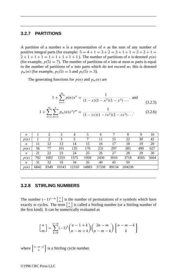
3.2.7 PARTITIONS
A partition of a numbern is a representation ofn as the sum of any number ofpositive integral parts (for example: 5= 4+ 1 = 3+ 2 = 3+ 1+ 1 = 2+ 2+ 1 =2+ 1+ 1+ 1 = 1+ 1+ 1+ 1+ 1 ). The number of partitions ofn is denotedp(n)(for example,p(5) = 7). The number of partitions ofn into at mostm parts is equalto the number of partitions ofn into parts which do not exceedm; this is denotedpm(n) (for example,p3(5) = 5 andp2(5) = 3).
The generating functions forp(n) andpm(n) are
1 +∞∑n=1
p(n)xn = 1
(1 − x)(1 − x2)(1 − x3) · · · , and(3.2.5)
1 +∞∑n=1
n∑m=1
pm(n)xntm = 1
(1 − tx)(1 − tx2)(1 − tx3) · · · . (3.2.6)
n 1 2 3 4 5 6 7 8 9 10p(n) 1 2 3 5 7 11 15 22 30 42n 11 12 13 14 15 16 17 18 19 20
p(n) 56 77 101 135 176 231 297 385 490 627n 21 22 23 24 25 26 27 28 29 30
p(n) 792 1002 1255 1575 1958 2436 3010 3718 4565 5604n 31 32 33 34 35 40 45 50
p(n) 6842 8349 10143 12310 14883 37338 89134 204226
3.2.8 STIRLING NUMBERS
The number(−1)n−m[n
m
]is the number of permutations ofn symbols which have
exactlym cycles. The term[n
m
]is called a Stirling number (or a Stirling number of
the first kind). It can be numerically evaluated as
[ nm
]=
n−m∑k=0
(−1)k(n − 1 + k
n − m + k
)(2n − m
n − m − k
)n − m − k
k
where
n−m−k
k
is a Stirling cycle number.
©1996 CRC Press LLC

• Example: For the 4 element seta, b, c, d, there are[
42
]= 11 permutations
containing exactly 2 cycles. They are
(1
2
2
3
3
1
4
4
)= (123)(4),
(1
3
2
1
3
2
4
4
)= (132)(4),
(1
3
2
2
3
4
4
1
)= (134)(2),(
1
4
2
2
3
1
4
3
)= (143)(2),
(1
2
2
4
3
3
4
1
)= (124)(3),
(1
4
2
1
3
3
4
2
)= (142)(3),(
1
1
2
3
3
4
4
2
)= (234)(1),
(1
1
2
4
3
2
4
3
)= (243)(1),
(1
2
2
1
3
4
4
3
)= (12)(34),(
1
3
2
4
3
1
4
2
)= (13)(24),
(1
4
2
3
3
2
4
1
)= (14)(23).
• There is the recurrence relation:[n+1m
]= [
n
m−1
]− n[n
m
].
• The factorial polynomial is defined asx(n) = x(1 − x) . . . (x − n + 1) withx(0) = 1 by definition. Ifn > 0, then
x(n) =[n
1
]x +
[n2
]x2 + · · · +
[nn
]xn.
For example:x(3) = x(x−1)(x−2) = 2x−3x2+x3 =[
31
]x+
[32
]x2+
[33
]x3.
• Stirling numbers satisfy∑∞
n=m
[n
m
]xn
n! = (log(1+x))m
m! for |x| < 1.
3.2.9 STIRLING CYCLE NUMBERS
The Stirling cycle number,
n
m
, is the number of ways to partition n into m blocks
(this is also called a Stirling number of the second kind). (Equivalently, it is thenumber of ways that n distinguishable balls can be placed into m indistinguishablecells, with no cell empty.) This Stirling number can be numerically evaluated as
n
m
= 1
k!
k∑i=0
(−1)k−i
(k
i
)in.
For example, placing the 4 distinguishable ballsa, b, c, d into 2 indistinguish-
able cells, so that no cell is empty can be done in
42
= 7 ways. These are (vertical
bars delineate the cells)
| ab | cd |, | ad | bc |, | ac | bd |, | a | bcd |,| b | acd |, | c | abd |, | d | abc | .
©1996 CRC Press LLC

• Ordinary powers can be expanded in terms of factorial polynomials. Ifn > 0,then
xn =n
1
x(1) +
n2
x(2) + · · · +
nn
x(n).
For example,x3 =
31
x(1) +
32
x(2) +
33
x(3).
3.2.10 BELL NUMBERS
Thenth Bell number,Bn, denotes the number of partitions of a set withn elements.Computationally, the Bell numbers may be written in terms of the Stirling cyclenumbers,Bn = ∑n
m=1
n
m
.
For example, there areB4 = 15 different ways to partition the 4 element seta, b, c, d:
a, c, b, d, a, d, b, c, b, c, a, d, b, d, a, c, c, d, a, b,a, b, c, d, a, b, c, d, a, c, b, d, a, d, b, c, a, b, c, d,a, b, c, d, b, a, c, d, c, a, b, d, d, a, b, c, a, b, c, d.
n 1 2 3 4 5 6 7 8 9 10Bn 1 2 5 15 52 203 877 4140 21147 115975
• A generating function for Bell numbers is∑∞
n=0 Bnxn = exp(ex − 1)−1. This
results inDobinski’s formula for thenth Bell number,Bn = e−1∑∞m=0 m
n/m!.
• For large values ofn, Bn ∼ n−1/2[λ(n)]n+1/2eλ(n)−n−1 whereλ(n) is defined bythe relation:λ(n) logλ(n) = n.
©1996 CRC Press LLC
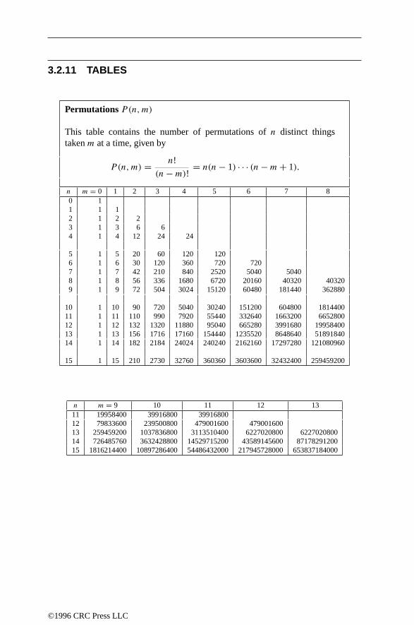
3.2.11 TABLES
Permutations P(n,m)
This table contains the number of permutations ofn distinct thingstakenm at a time, given by
P(n,m) = n!
(n − m)!= n(n − 1) · · · (n − m + 1).
n m = 0 1 2 3 4 5 6 7 80 11 1 12 1 2 23 1 3 6 64 1 4 12 24 24
5 1 5 20 60 120 1206 1 6 30 120 360 720 7207 1 7 42 210 840 2520 5040 50408 1 8 56 336 1680 6720 20160 40320 403209 1 9 72 504 3024 15120 60480 181440 362880
10 1 10 90 720 5040 30240 151200 604800 181440011 1 11 110 990 7920 55440 332640 1663200 665280012 1 12 132 1320 11880 95040 665280 3991680 1995840013 1 13 156 1716 17160 154440 1235520 8648640 5189184014 1 14 182 2184 24024 240240 2162160 17297280 121080960
15 1 15 210 2730 32760 360360 3603600 32432400 259459200
n m = 9 10 11 12 1311 19958400 39916800 3991680012 79833600 239500800 479001600 47900160013 259459200 1037836800 3113510400 6227020800 622702080014 726485760 3632428800 14529715200 43589145600 8717829120015 1816214400 10897286400 54486432000 217945728000 653837184000
©1996 CRC Press LLC

Combinations C(n,m) = (n
m
)This table contains the number of combinations ofn distinct things takenm at a time, given by
C(n,m) =(n
m
)= n!
m!(n − m)!.
n m = 0 1 2 3 4 5 6 71 1 12 1 2 13 1 3 3 14 1 4 6 4 15 1 5 10 10 5 1
6 1 6 15 20 15 6 17 1 7 21 35 35 21 7 18 1 8 28 56 70 56 28 89 1 9 36 84 126 126 84 36
10 1 10 45 120 210 252 210 120
11 1 11 55 165 330 462 462 33012 1 12 66 220 495 792 924 79213 1 13 78 286 715 1287 1716 171614 1 14 91 364 1001 2002 3003 343215 1 15 105 455 1365 3003 5005 6435
16 1 16 120 560 1820 4368 8008 1144017 1 17 136 680 2380 6188 12376 1944818 1 18 153 816 3060 8568 18564 3182419 1 19 171 969 3876 11628 27132 5038820 1 20 190 1140 4845 15504 38760 77520
21 1 21 210 1330 5985 20349 54264 11628022 1 22 231 1540 7315 26334 74613 17054423 1 23 253 1771 8855 33649 100947 24515724 1 24 276 2024 10626 42504 134596 34610425 1 25 300 2300 12650 53130 177100 480700
26 1 26 325 2600 14950 65780 230230 65780027 1 27 351 2925 17550 80730 296010 88803028 1 28 378 3276 20475 98280 376740 118404029 1 29 406 3654 23751 118755 475020 156078030 1 30 435 4060 27405 142506 593775 2035800
©1996 CRC Press LLC

Combinations C(n,m) = (n
m
)This table contains the number of combinations ofn distinct things takenm at a time, given by
C(n,m) =(n
m
)= n!
m!(n − m)!.
n m = 0 1 2 3 4 5 6 731 1 31 465 4495 31465 169911 736281 262957532 1 32 496 4960 35960 201376 906192 336585633 1 33 528 5456 40920 237336 1107568 427204834 1 34 561 5984 46376 278256 1344904 537961635 1 35 595 6545 52360 324632 1623160 6724520
36 1 36 630 7140 58905 376992 1947792 834768037 1 37 666 7770 66045 435897 2324784 1029547238 1 38 703 8436 73815 501942 2760681 1262025639 1 39 741 9139 82251 575757 3262623 1538093740 1 40 780 9880 91390 658008 3838380 18643560
41 1 41 820 10660 101270 749398 4496388 2248194042 1 42 861 11480 111930 850668 5245786 2697832843 1 43 903 12341 123410 962598 6096454 3222411444 1 44 946 13244 135751 1086008 7059052 3832056845 1 45 990 14190 148995 1221759 8145060 45379620
46 1 46 1035 15180 163185 1370754 9366819 5352468047 1 47 1081 16215 178365 1533939 10737573 6289149948 1 48 1128 17296 194580 1712304 12271512 7362907249 1 49 1176 18424 211876 1906884 13983816 8590058450 1 50 1225 19600 230300 2118760 15890700 99884400
©1996 CRC Press LLC

n m = 8 9 10 11 128 19 9 1
10 45 10 111 165 55 11 112 495 220 66 12 1
13 1287 715 286 78 1314 3003 2002 1001 364 9115 6435 5005 3003 1365 45516 12870 11440 8008 4368 182017 24310 24310 19448 12376 6188
18 43758 48620 43758 31824 1856419 75582 92378 92378 75582 5038820 125970 167960 184756 167960 12597021 203490 293930 352716 352716 29393022 319770 497420 646646 705432 646646
23 490314 817190 1144066 1352078 135207824 735471 1307504 1961256 2496144 270415625 1081575 2042975 3268760 4457400 520030026 1562275 3124550 5311735 7726160 965770027 2220075 4686825 8436285 13037895 17383860
28 3108105 6906900 13123110 21474180 3042175529 4292145 10015005 20030010 34597290 5189593530 5852925 14307150 30045015 54627300 8649322531 7888725 20160075 44352165 84672315 14112052532 10518300 28048800 64512240 129024480 225792840
33 13884156 38567100 92561040 193536720 35481732034 18156204 52451256 131128140 286097760 54835404035 23535820 70607460 183579396 417225900 83445180036 30260340 94143280 254186856 600805296 125167770037 38608020 124403620 348330136 854992152 1852482996
38 48903492 163011640 472733756 1203322288 270747514839 61523748 211915132 635745396 1676056044 391079743640 76904685 273438880 847660528 2311801440 558685348041 95548245 350343565 1121099408 3159461968 789865492042 118030185 445891810 1471442973 4280561376 11058116888
43 145008513 563921995 1917334783 5752004349 1533867826444 177232627 708930508 2481256778 7669339132 2109068261345 215553195 886163135 3190187286 10150595910 2876002174546 260932815 1101716330 4076350421 13340783196 3891061765547 314457495 1362649145 5178066751 17417133617 52251400851
48 377348994 1677106640 6540715896 22595200368 6966853446849 450978066 2054455634 8217822536 29135916264 9226373483650 536878650 2505433700 10272278170 37353738800 121399651100
©1996 CRC Press LLC

n m = 13 14 15 16 1713 114 14 115 105 15 116 560 120 16 117 2380 680 136 17 1
18 8568 3060 816 153 1819 27132 11628 3876 969 17120 77520 38760 15504 4845 114021 203490 116280 54264 20349 598522 497420 319770 170544 74613 26334
23 1144066 817190 490314 245157 10094724 2496144 1961256 1307504 735471 34610425 5200300 4457400 3268760 2042975 108157526 10400600 9657700 7726160 5311735 312455027 20058300 20058300 17383860 13037895 8436285
28 37442160 40116600 37442160 30421755 2147418029 67863915 77558760 77558760 67863915 5189593530 119759850 145422675 155117520 145422675 11975985031 206253075 265182525 300540195 300540195 26518252532 347373600 471435600 565722720 601080390 565722720
33 573166440 818809200 1037158320 1166803110 116680311034 927983760 1391975640 1855967520 2203961430 233360622035 1476337800 2319959400 3247943160 4059928950 453756765036 2310789600 3796297200 5567902560 7307872110 859749660037 3562467300 6107086800 9364199760 12875774670 15905368710
38 5414950296 9669554100 15471286560 22239974430 2878114338039 8122425444 15084504396 25140840660 37711260990 5102111781040 12033222880 23206929840 40225345056 62852101650 8873237880041 17620076360 35240152720 63432274896 103077446706 15158448045042 25518731280 52860229080 98672427616 166509721602 254661927156
43 36576848168 78378960360 151532656696 265182149218 42117164875844 51915526432 114955808528 229911617056 416714805914 68635379797645 73006209045 166871334960 344867425584 646626422970 110306860389046 101766230790 239877544005 511738760544 991493848554 174969502686047 140676848445 341643774795 751616304549 1503232609098 2741188875414
48 192928249296 482320623240 1093260079344 2254848913647 424442148451249 262596783764 675248872536 1575580702584 3348108992991 649927039815950 354860518600 937845656300 2250829575120 4923689695575 9847379391150
©1996 CRC Press LLC

Fractional binomial coefficients(a
k
)a k = 0 1 2 3 4 5
1/9 1 1/9 −4/81 68/2187 −442/19683 3094/1771471/8 1 1/8 −7/128 35/1024 −805/32768 4991/2621441/7 1 1/7 −3/49 13/343 −65/2401 351/168071/6 1 1/6 −5/72 55/1296 −935/31104 4301/1866241/5 1 1/5 −2/25 6/125 −21/625 399/15625
2/9 1 2/9 −7/81 112/2187 −700/19683 4760/1771471/4 1 1/4 −3/32 7/128 −77/2048 231/81922/7 1 2/7 −5/49 20/343 −95/2401 494/168071/3 1 1/3 −1/9 5/81 −10/243 22/7293/8 1 3/8 −15/128 65/1024 −1365/32768 7917/262144
2/5 1 2/5 −3/25 8/125 −26/625 468/156253/7 1 3/7 −6/49 22/343 −99/2401 495/168074/9 1 4/9 −10/81 140/2187 −805/19683 5152/1771471/2 1 1/2 −1/8 1/16 −5/128 7/2565/9 1 5/9 −10/81 130/2187 −715/19683 4433/177147
4/7 1 4/7 −6/49 20/343 −85/2401 408/168073/5 1 3/5 −3/25 7/125 −21/625 357/156255/8 1 5/8 −15/128 55/1024 −1045/32768 5643/2621442/3 1 2/3 −1/9 4/81 −7/243 14/7295/7 1 5/7 −5/49 15/343 −60/2401 276/16807
3/4 1 3/4 −3/32 5/128 −45/2048 117/81927/9 1 7/9 −7/81 77/2187 −385/19683 2233/1771474/5 1 4/5 −2/25 4/125 −11/625 176/156255/6 1 5/6 −5/72 35/1296 −455/31104 1729/1866246/7 1 6/7 −3/49 8/343 −30/2401 132/16807
7/8 1 7/8 −7/128 21/1024 −357/32768 1785/2621448/9 1 8/9 −4/81 40/2187 −190/19683 1064/177147
Stirling numbers[n
m
]n m = 1 2 3 4 5 6 71 12 −1 13 2 −3 14 −6 11 −6 15 24 −50 35 −10 16 −120 274 −225 85 −15 17 720 −1764 1624 −735 175 −21 18 −5040 13068 −13132 6769 −1960 322 −289 40320 −109584 118124 −67284 22449 −4536 546
10 −362880 1026576 −1172700 723680 −269325 63273 −9450
©1996 CRC Press LLC
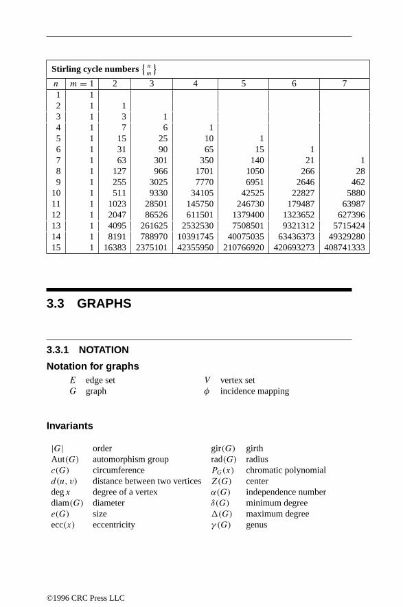
Stirling cycle numbersn
m
n m = 1 2 3 4 5 6 71 12 1 13 1 3 14 1 7 6 15 1 15 25 10 16 1 31 90 65 15 17 1 63 301 350 140 21 18 1 127 966 1701 1050 266 289 1 255 3025 7770 6951 2646 462
10 1 511 9330 34105 42525 22827 588011 1 1023 28501 145750 246730 179487 6398712 1 2047 86526 611501 1379400 1323652 62739613 1 4095 261625 2532530 7508501 9321312 571542414 1 8191 788970 10391745 40075035 63436373 4932928015 1 16383 2375101 42355950 210766920 420693273 408741333
3.3 GRAPHS
3.3.1 NOTATION
Notation for graphsE edge set V vertex setG graph φ incidence mapping
Invariants
|G| order gir(G) girthAut(G) automorphism group rad(G) radiusc(G) circumference PG(x) chromatic polynomiald(u, v) distance between two verticesZ(G) centerdegx degree of a vertex α(G) independence numberdiam(G) diameter δ(G) minimum degreee(G) size (G) maximum degreeecc(x) eccentricity γ (G) genus
©1996 CRC Press LLC

κ(G) vertex connectivity θ(G) thicknessλ(G) edge connectivity χ(G) chromatic numberν(G) crossing number χ ′(G) chromatic indexν(G) rectilinear crossing number ϒ(G) arboricityω(G) clique number
Examples
Cn cycle
Kn empty graph
Kn complete graph
Km,n complete bipartitegraph
K1,n−1 star
K(m)n Kneser graphs
Mn Mobius ladder
On odd graph
Pn path
Qn cube
Tn,k Turan graph
Wn wheel
3.3.2 BASIC DEFINITIONS
There are two standard definitions of graphs, a general definition and a more commonsimplification. Except where otherwise indicated, this book uses the simplified defi-nition, according to which agraph is an ordered pair(V ,E) consisting of an arbitrarysetV and a setE of 2-element subsets ofV . Each element ofV is called avertex(plural vertices). Each element ofE is called anedge.
According to the general definition, agraph is an ordered tripleG = (V ,E, φ)
consisting of arbitrary setsV andE and anincidence mapping φ that assigns to eachelemente ∈ E a nonempty setφ(e) ⊆ V of cardinality at most two. Again, theelements ofV are calledvertices and the elements ofE are callededges. A loop isan edgee for which |φ(e)| = 1. A graph hasmultiple edges if edgese = e′ exist forwhichφ(e) = φ(e′).
A (general) graph is calledsimple if it has neither loops nor multiple edges.Because each edge in a simple graph can be identified with the two-element setφ(e) ⊆V , the simplified definition of graph given above is just an alternative definition of asimple graph.
The wordmultigraph is used to discuss general graphs with multiple edges butno loops. Occasionally the wordpseudograph is used to emphasize that the graphsunder discussion may have both loops and multiple edges. Every graphG = (V ,E)
considered here isfinite, i.e., bothV andE are finite sets.Specialized graph terms include the following:
acyclic: A graph isacyclic if it has no cycles.adjacency: Two distinct verticesv andw in a graph areadjacent if the pairv,w
is an edge. Two distinct edges areadjacent if their intersection is nonempty,i.e., if there is a vertex incident with both of them.
©1996 CRC Press LLC

adjacency matrix: For an orderingv1, v2, . . . , vn of the vertices of a graphG =(V ,E) of order|G| = n, there is a correspondingn×n adjacency matrix A =(aij ) defined as follows:
aij =
1 if vi, vj ∈ E;
0 otherwise.
arboricity: Thearboricity ϒ(G) of a graphG is the minimum number of edge-disjoint spanning forests into whichG can be partitioned.
automorphism: An automorphism of a graph is a permutation of its vertices thatis an isomorphism.
automorphism group: The composition of two automorphisms is again an auto-morphism; with this binary operation, the automorphisms of a graphG form agroup Aut(G) called theautomorphism group of G.
ball: Theball of radiusk about a vertexu in a graph is the set
B(u, k) = v ∈ V | d(u, v) ≤ k.See alsosphere andneighborhood.
block: A block is a graph with no cut vertex. Ablock of a graph is a maximalsubgraph that is a block.
boundary operator: The boundary operator for a graph is the linear mappingfrom 1-chains (elements of the edge space) to 0-chains (elements of the vertexspace) that sends each edge to the indicator mapping the set of two verticesincident with it. See alsovertex space andedge space.
bridge: A bridge is an edge in a connected graph whose removal would disconnectthe graph.
cactus: A cactus is a connected graph, each of whose blocks is a cycle.cage: An (r, n)-cage is a graph of minimal order amongr-regular graphs with girth
n. A (3, n)-cage is also called ann-cage.center: The center Z(G) of a graphG = (V ,E) consists of all vertices whose
eccentricity equals the radius ofG:
Z(G) = v ∈ V (G) | ecc(v) = rad(G).Each vertex in the center ofG is called acentral vertex.
characteristic polynomial: All adjacency matrices of a graphG have the samecharacteristic polynomial, which is called thecharacteristic polynomial ofG.
chromatic index: Thechromatic index χ ′(G) is the leastk for which there existsa properk-coloring of the edges ofG; in other words, it is the least number ofmatchings into which the edge set can be decomposed.
chromatic number: Thechromatic number χ(G) of a graphG is the leastk forwhich there exists a properk-coloring of the vertices ofG; in other words, it isthe leastk for whichG is k-partite. See alsomultipartite.
chromatic polynomial: For a graphG of order|G| = n with exactlyk connectedcomponents, thechromatic polynomial of G is the unique polynomialPG(x)for whichPG(m) is the number of proper colorings ofGwithm colors for eachpositive integerm.
©1996 CRC Press LLC

circuit: A circuit in a graph is a trail whose first and last vertices are identical.circulant graph: A graphG is acirculant graph if its adjacency matrix is a circulant
matrix; that is, the rows are circular shifts of one another.circumference: The circumference of a graph is the length of its longest cycle.clique: A clique is a setS of vertices for which the induced subgraphG[S] is
complete.clique number: Theclique number ω(G) of a graphG is the largest cardinality of
a clique inG.coboundary operator: Thecoboundary operator for a graph is the linear mapping
from 0-chains (elements of the vertex space) to 1-chains (elements of the edgespace) that sends each vertex to the indicator mapping of the set of edgesincident with it.
cocycle vector: A cut vector is sometimes called acocycle vector.coloring: A partition of the vertex set of a graph is called acoloring, and the blocks
of the partition are calledcolor classes. A coloring with k color classes iscalled ak-coloring. A coloring isproper if no two adjacent vertices belong tothe same color class. See alsochromatic number andchromatic polynomial.
complement: The complement G of a graphG = (V ,E) has vertex setV andedge set
(V
2
) \ E; that is, its edges are exactly the pairs of vertices that are notedges ofG.
complete graph: A graph iscomplete if every pair of distinct vertices is an edge;Kn denotes a complete graph withn vertices.
component: A component of a graph is a maximal connected subgraph.connectedness: A graph is said to beconnected if each pair of vertices is joined by
a walk; otherwise, the graph isdisconnected. A graph isk-connected if it hasorder at leastk + 1 and each pair of vertices is joined byk pairwise internallydisjoint paths.
connectivity: The connectivity κ(G) of G is the largestk for which G is k-connected.
contraction: To contract an edgev,w of a graphG is to construct a new graphG′ fromG by removing the edgev,w and identifying the verticesv andw.A graphG is contractible to a graphH if H can be obtained fromG via thecontraction of one or more edges ofG.
cover: A setS ⊆ V is avertex cover if every edge ofG is incident with some vertexin S. A setT ⊆ E is anedge cover of a graphG = (V ,E) if each vertex ofGis incident to at least one edge inT .
crosscap number: Thecrosscap number γ (G) of a graphG is the leastg for whichG has an embedding in a nonorientable surface obtained from the sphere byaddingg crosscaps. See alsogenus.
crossing: A crossing is a point lying in images of two edges of a drawing of a graphon a surface.
crossing number: Thecrossing number ν(G) of a graphG is the minimum numberof crossings among all drawings ofG in the plane. Therectilinear crossingnumber ν(G) of a graphG is the minimum number of crossings among alldrawings ofG in the plane for which the image of each edge is a straight linesegment.
cubic: A graph is acubic graph if it is regular of degree 3.
©1996 CRC Press LLC
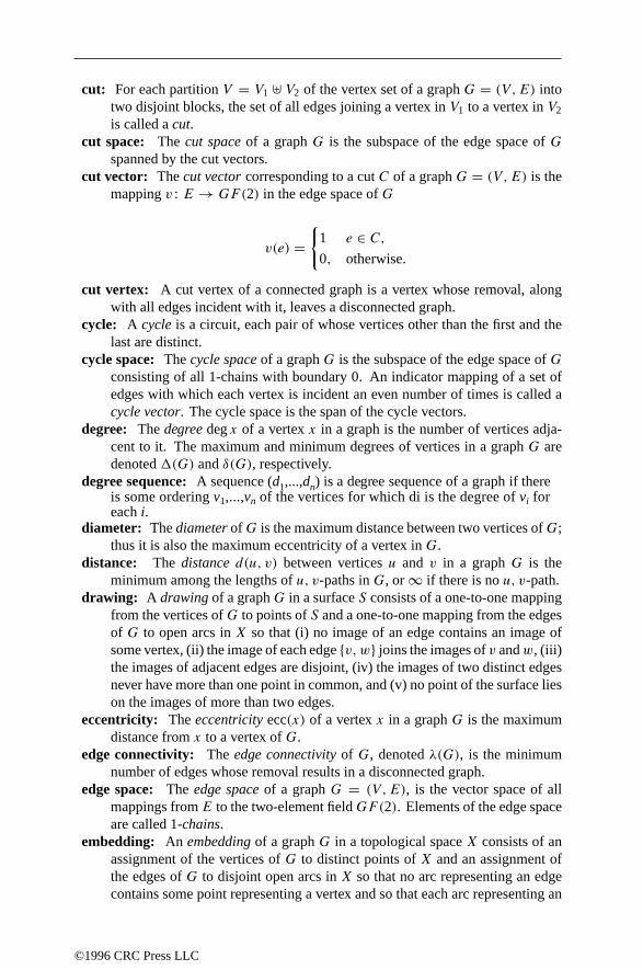
cut: For each partitionV = V1 V2 of the vertex set of a graphG = (V ,E) intotwo disjoint blocks, the set of all edges joining a vertex inV1 to a vertex inV2
is called acut.cut space: The cut space of a graphG is the subspace of the edge space ofG
spanned by the cut vectors.cut vector: Thecut vector corresponding to a cutC of a graphG = (V ,E) is the
mappingv : E→ GF(2) in the edge space ofG
v(e) =
1 e ∈ C,0, otherwise.
cut vertex: A cut vertex of a connected graph is avertex whose removal, alongwith all edges incident with it, leaves adisconnected graph.
cycle: A cycle is acircuit, each pair of whose vertices other than the first and thelast aredistinct.
cycle space: The cycle space of a graphG is the subspace of the edge space of Gconsisting of all 1-chains with boundary 0. An indicator mapping of a set ofedges with which each vertex is incident an even number of times is called acycle vector. Thecyclespace is thespan of thecyclevectors.
degree: The degree degx of a vertex x in agraph is the number of vertices adja-cent to it. The maximum and minimum degrees of vertices in a graph G aredenoted(G) and δ(G), respectively.
degree sequence: A sequence (d1,...,dn) is a degree sequence of a graph if there
each i.diameter: The diameter of G is themaximum distancebetween two verticesof G;
thus it isalso themaximum eccentricity of a vertex inG.distance: The distance d(u, v) between vertices u and v in a graph G is the
minimum among the lengthsof u, v-paths inG, or∞ if there isno u, v-path.drawing: A drawing of a graphG in a surfaceS consists of a one-to-one mapping
from the vertices ofG to points ofS and a one-to-one mapping from the edgesof G to open arcs inX so that (i) no image of an edge contains an image ofsomevertex, (ii ) theimageof eachedgev,w joinstheimagesof v andw, (iii)the imagesof adjacent edgesaredisjoint, (iv) the imagesof two distinct edgesnever have more than one point in common, and (v) no point of the surface lieson the images of more than two edges.
eccentricity: Theeccentricity ecc(x) of a vertexx in a graphG is the maximumdistance fromx to a vertex ofG.
edge connectivity: The edge connectivity of G, denotedλ(G), is the minimumnumber of edges whose removal results in a disconnected graph.
edge space: The edge space of a graphG = (V ,E), is the vector space of allmappings fromE to the two-element fieldGF(2). Elements of the edge spaceare called 1-chains.
embedding: An embedding of a graphG in a topological spaceX consists of anassignment of the vertices ofG to distinct points ofX and an assignment ofthe edges ofG to disjoint open arcs inX so that no arc representing an edgecontains some point representing a vertex and so that each arc representing an
©1996 CRC Press LLC
is some ordering v1,...,vn of the vertices for which di is the degree of vi for

edge joins the points representing the vertices incident with the edge. See alsodrawing.
end vertex: A vertex of degree 1 in a graph is called anend vertex.Eulerian circuits and trails: A trail or circuit that includes every edge of a graph
is said to beEulerian, and a graph isEulerian if it has an Eulerian circuit.even: A graph iseven if the degree of every vertex is even.factor: A factor of a graphG is a spanning subgraph ofG. A factor in which every
vertex has the same degreek is called ak-factor. IfG1, G2, . . . , Gk (k ≥ 2)are edge-disjoint factors of the graphG, and if
⋃ki=1E(Gi) = E(G), thenG is
said to befactored intoG1,G2, . . . ,Gk and we writeG = G1⊕G2⊕· · ·⊕Gk.forest: A forest is an acyclic simple graph; see alsotree.genus: Thegenus γ (G) (plural formgenera) of a graphG is the leastg for which
G has an embedding in an orientable surface of genusg. See alsocrosscapnumber.
girth: Thegirth gir(G) of a graphG is the minimum length of a cycle inG, or∞if G is acyclic.
Hamiltonian cycles and paths: A path or cycle through all the vertices of a graphis said to beHamiltonian. A graph isHamiltonian if it has a Hamiltonian cycle.
homeomorphic graphs: Two graphs arehomeomorphic to one another if there isa third graph of which each is a subdivision.
identification of vertices: To identify verticesv andw of a graphG is to constructa new graphG′ from G by removing the verticesv andw and all the edgesofG incident with them and introducing a new vertexu and new edges joiningu to each vertex that was adjacent tov or tow in G. See alsocontraction.
incidence: A vertexv and an edgee areincident with one another ifv ∈ e.incidence matrix: For an orderingv1, v2, . . . , vn of the vertices and an ordering
e1, e2, . . . , em of the edges of a graphG = (V ,E) with order |G| = n andsizee(G) = m, there is a correspondingn × m incidence matrix B = (bij )
defined as follows:
bij =
1, if vi andej are incident,
0, otherwise.
independence number: The independence number α(G) of a graphG = (V ,E)
is the largest cardinality of an independent subset ofV .independent set: A set S ⊆ V is said to beindependent if the induced sub-
graphG[S] is empty. See alsomatching.internally disjoint paths: Two paths in a graph with the same initial vertexv
and terminal vertexw areinternally disjoint if they have no internal vertex incommon.
isolated vertex: A vertex isisolated if it is adjacent to no other vertex.isomorphism: An isomorphism between graphsG = (VG,EG)andH = (VH ,EH )
is a bijective mappingψ : VG → VH for which x, y ∈ EG if and only ifψ(x), ψ(y) ∈ EH . If there is an isomorphism betweenG andH , thenGand H are said to be isomorphic to one another; this is denoted asG ∼= H .Figure3.3.1 contains threegraphs that are isomorphic.
©1996 CRC Press LLC

FIGURE 3.3.1Three graphs that are isomorphic.
labeled graph: Graph theorists sometimes speak loosely oflabeled graphs ofordern andunlabeled graphs of ordern to distinguish between graphs witha fixed vertex set of cardinalityn and the family of isomorphism classes ofsuch graphs. Thus, one may refer tolabeled graphs to indicate an intentionto distinguish between any two graphs that aredistinct (i.e., have differentvertex sets and/or or different edge sets). One may refer tounlabeled graphsto indicate the intention to view any two distinct but isomorphic graphs as the‘same’ graph, and to distinguish only between nonisomorphic graphs.
matching: A matching in a graph is a set of edges, no two having a vertex incommon. Amaximal matching is a matching that is not a proper subset of anyother matching. Amaximum matching is a matching of greatest cardinality.For a matchingM, anM-alternating path is a path whose every other edgebelongs toM, and anM-augmenting path is anM-alternating path whose firstand last edges do not belong toM. A matchingsaturates a vertex if the vertexbelongs to some edge of the matching.
monotone graph property: A propertyP that a graph may or may not enjoy issaid to bemonotone if, wheneverH is a graph enjoyingP, every supergraphGof H with |G| = |H | also enjoysP.
multipartite graph: A graph isk-partite if its vertex set can be partitioned intokdisjoint sets calledcolor classes in such a way that every edge joins verticesin two different color classes (see alsocoloring). A two-partite graph is calledbipartite.
neighbor: Adjacent verticesv andw in a graph are said to beneighbors of oneanother.
neighborhood: The sphereS(x,1) is called theneighborhood of x, and theballB(x,1) is called theclosed neighborhood of x.
order: The order |G| of a graphG = (V ,E) is the number of vertices inG; inother words,|G| = |V |.
path: A path is a walk whose vertices are distinct.perfect graph: A graph isperfect if χ(H) = ω(H) for all induced subgraphsH
of G.planarity: A graph isplanar if it has a proper embedding in the plane.radius: Theradius rad(G) of a graphG is the minimum vertex eccentricity inG.regularity: A graph isk-regular if each of its vertices has degreek. A graph is
strongly regular with parameters(k, λ, µ) if (i) it is k-regular, (ii) every pair
©1996 CRC Press LLC

of adjacent vertices has exactlyλ common neighbors, and (iii) every pair ofnonadjacent verticeshasexactlyµ commonneighbors. A graphG = (V ,E) oforder |G|ge3 iscalled highly regular if thereexistsan n× nmatrix C = (cij ),where 2 ≤ n < |G|, called a collapsed adjacency matrix, so that, for eachvertexv of G, there is a partition ofV into n subsetsV1 = v, V2, . . . , Vn sothat every vertexy ∈ Vj is adjacent to exactlycij vertices inVi . Every highlyregular graph is also regular.
rooted graph: A rooted graph is an ordered pair(G, v) consisting of a graphGand a distinguished vertexv of G called theroot.
self-complementary: A graph is self-complementary if it is isomorphic to itscomplement.
similarity: Two verticesu andv of a graphG aresimilar (in symbolsu ∼ v) ifthere is an automorphismα of G for which α(u) = v. Similarly, two edges(u, v) and(a, b) in the graphG aresimilar if an automorphismα of G existsfor which α(u), α(v) = a, b.
size: The size e(G) of a graphG = (V ,E) is the number of edges ofG, that is,e(G) = |E|.
spectrum: Thespectrum of a graphG is the spectrum of its characteristic polyno-mial, i.e., the nondecreasing sequence of|G| eigenvalues of the characteristicpolynomial ofG.
sphere: Thesphere of radiusk about a vertexu is the set
S(u, k) = v ∈ V | d(u, v) = k.See alsoball andneighborhood.
subdivision: To subdivide an edgev,w of a graphG is to construct a new graphG′ fromG by removing the edgev,w and introducing new verticesxi andnew edgesv, x1, xk, w andxi, xi+1 for 1 ≤ i < k. A subdivision of agraph is a graph obtained by subdividing one or more edges of the graph.
subgraph: A graphH = (VH ,EH ) is a subgraph of a graphG = (VG,EG) (insymbols,H G), if VH ⊆ VG andEH ⊆ EG. In that case,G is asupergraphofH (in symbols,G H ). If VH = VG, thenH is called aspanning subgraphofG. For each setS ⊆ VG, the subgraphG[S] of G induced byS is the uniquesubgraph ofG with vertex setS for which every edge ofG incident with twovertices inS is also an edge ofG[S].
symmetry: A graph isvertex symmetric if every pair of vertices is similar. A graphis edge symmetric if every pair of edges is similar. A graph issymmetric if it isboth vertex and edge symmetric.
2-switch: For verticesv,w, x, y in agraphG for which v,w and x, y areedges,but v, y and x,w arenot edges, theconstruction of a new graphG′ fromG
via the removal of edges v,w and x, y together with the insertion of theedges v, y and x,w is called a2-switch.
thickness: The thickness θ(G) of a graphG is the leastk for whichG is a unionof k planar graphs.
trail: A trail in a graph is a walk whose edges are distinct.tree: A tree is a connected forest, i.e., a connected acyclic graph. A spanning
subgraph of a graphG that is a tree is called aspanning tree of G.triangle: A 3-cycle is called a triangle.
©1996 CRC Press LLC

trivial graph: A trivial graph is a graph with exactly one vertex and no edges.unicyclic graph: A unicyclic graph is a connected graph that contains exactly one
cycle.vertex space: Thevertex space of a graphG is the vector space of all mappings
from V to the two-element fieldGF(2). The elements of the vertex space arecalled 0-chains.
walk: A walk in a graph is an alternating sequencev0, e1, v1, . . . , ek, vk of ver-ticesvi and edgesei for which ei is incident withvi−1 and withvi for eachi.Such a walk is said to havelength k and tojoin v0 andvk. The verticesv0
andvk are called theinitial vertex andterminal vertex of the walk; the remain-ing vertices are calledinternal vertices of the walk.
3.3.3 CONSTRUCTIONS
Operations on graphsFor graphsG1 = (V1, E1) andG2 = (V2, E2), there are several binary operationsthat yield a new graph fromG1 andG2. The following table gives the names of thoseoperations and the orders and sizes of the resulting graphs.
Operation producingG Order|G| Sizee(G)
Composition G1[G2] |G1| · |G2| |G1|e(G2)+ |G2|2e(G1)
Conjunction G1 ∧G2 |G1| · |G2|Edge suma G1
⊕G2 |G1| = |G2| e(G1)+ e(G2)
Join G1+G2 |G1| + |G2| e(G1)+ e(G2)+ |G1| · |G2|Product G1×G2 |G1| · |G2| |G1|e(G2)+ |G2|e(G1)
Union G1 ∪G2 |G1| + |G2| e(G1)+ e(G2)
aWhen applicable.
composition: For graphsG1 = (V1, E1) andG2 = (V2, E2), the compositionG = G1[G2] is the graph with vertex setV1 × V2 whose edges are the pairs(u, v), (u,w) with u ∈ V1 andv,w ∈ E2 and the pairs(t, u), (v,w) forwhich t, v ∈ E1 andu,w ∈ E2.
conjunction: The conjunctionG1 ∧ G2 of two graphsG1 = (V1, E1) andG2 =(V2, E2) is the graphG3 = (V3, E3) for which V3 = V1 × V2 and for whichverticese1 = (u1, u2) ande2 = (v1, v2) in V3 are adjacent inG3 if, and onlyif, u1 is adjacent tov1 in G1 andu2 is adjacent tov2 in G2.
edge difference: For graphsG1 = (V ,E1) andG2 = (V ,E2)with the same vertexsetV , theedge difference G1−G2 is the graph with vertex setV and edge setE1 \ E2.
edge sum: For graphsG1 = (V ,E1) andG2 = (V ,E2)with the same vertex setV ,theedge sum of G1 andG2 is the graphG1 ⊕G2 with vertex setV and edgesetE1 ∪ E2. Sometimes the edge sum is denotedG1 ∪G2.
join: For graphsG1 = (V1, E1) andG2 = (V2, E2) with V1 ∩ V2 = ∅, the joinG1 + G2 = G2 + G1 is the graph obtained from the union ofG1 andG2 byadding edges joining each vertex inV1 to each vertex inV2.
©1996 CRC Press LLC

power: For a graphG = (V ,E), the kth power Gk is the graph with the samevertex setV whose the edges are the pairsu, v for which d(u, v) ≤ k in G.Thesquare of G isG2.
product: For graphsG1 = (V1, E1) andG2 = (V2, E2), theproduct G1×G2 hasvertex setV1×V2; its edges are all of the pairs(u, v), (u,w) for whichu ∈ V1
andv,w ∈ E2 and all of the pairs(t, v), (u, v) for which t, u ∈ E1 andv ∈ V2.
union: For graphsG1 = (V1, E1) andG2 = (V2, E2) with V1 ∩ V2 = ∅, theunion ofG1 andG2 is the graphG1 ∪G2 = (V1 ∪ V2, E1 ∪E2). The union issometimes called thedisjoint union to distinguish it from theedge sum.
Graphs described by one parametercomplete graph, Kn: A complete graph of ordern is a graph isomorphic to the
graphKn with vertex set1,2, . . . , n whose every pair of vertices is an edge.The graphKn has size
(n
2
)and is Hamiltonian. IfG is a graphg of ordern,
thenKn = G⊕G.
cube, Qn: An n-cube is a graph isomorphic to the graphQn whose vertices arethe 2n binaryn-vectors and whose edges are the pairs of vectors that differ inexactly one place. It is ann-regular bipartite graph of order 2n and sizen2n−1.An equivalent recursive definition,Q1 = K2 andQn = Qn−1×K2.
cycle, Cn: A cycle of ordern is a graph isomorphic to the graphCn with vertexset0,1, . . . , n − 1 whose edges are the pairsvi, vi+1 with 0 ≤ i < n andarithmetic modulon. The cycleCn has sizen and is Hamiltonian.The graphCn is a special case of a circulant graph. The graphC3 is called atriangle, the graphC4 is called asquare.
empty graph: A graph isempty if it has no edges;Kn denotes an empty graph ofordern.
Kneser graphs, K(m)n : Forn ≥ 2m, theKneser graph K(m)
n is the complement ofthe intersection graph of them-subsets of an-set. Theodd graph Om is theKneser graphK(m)
2m+1. ThePetersen graph is the odd graphO2 = K(2)5
ladder: A ladder is a graph of the formPn × P2. TheMobius ladder Mn is thegraph obtained from the ladderPn×P2 by joining the opposite end vertices ofthe two copies ofPn.
path, Pn: A path of ordern is a graph isomorphic to the graphPn whose vertex setis 1, . . . , n and whose edges are the pairsvi, vi+1 with 1 ≤ i < n. A pathof ordern has sizen− 1 and is a tree.
star, Sn: A star of ordern is a graph isomorphic to the graphSn = K1,n−1. It has avertex cover consisting of a single vertex, its size isn− 1, and it is a completebipartite graph and a tree.
wheel, Wn: The wheelWn of ordern ≥ 4 consists of a cycle of ordern − 1and an additional vertex adjacent to every vertex in the cycle. Equivalently,Wn = Cn−1+K1. This graph has size 2(n− 1).
Graphs described by two parameterscomplete bipartite graph,Kn,m: The complete bipartite graphKn,m is the graphKn+
©1996 CRC Press LLC

Km. Its vertex set can be partitioned into two color classes of cardinalitiesn
andm, respectively, so that each vertex in one color class is adjacent to everyvertex in the other color class. The graphKn,m has ordern+m and sizenm.
planar mesh: A graph of the formPn × Pm is called aplanar mesh.prism: A graph of the formCm × Pn is called aprism.Toeplitz graph, TN(w, s): The Toeplitz graph TN(w, s) is defined in terms of its
adjacency matrixA = (aij ), for which
aij =
1, if |i − j | = 1 (modw),
0, otherwise.
The Toeplitz graph is of orderws + 2, size(s + 1)(w − s + 2)/2, and girth 3or 4; it is (s + 1)-regular and Hamiltonian. Moreover, TN(1, s) = Ks+2 andTN(w,1) = Cw+2.
toroidal mesh: A graph of the formCm × Cn with m ≥ 2 andn ≥ 2 is called atoroidal mesh.
Turan graph, Tn,k: TheTuran graph Tn,k is the completek-partite graph in whichthe cardinalities of any two color classes differ by, at most, one. It hasn −k n/k color classes of cardinalityn/k+1 andk−n+k n/k color classesof cardinalityn/k. Note thatω(Tn,k) = k.
Graphs described by three or more parametersCayley graph: For a group: and a setX of generators of:, theCayley graph
of the pair(:,X) is the graph with vertex set: in which α, β is an edge ifeitherα−1β ∈ X or β−1α ∈ X.
complete multipartite graph,Kn1,n2,...,nk : Thecomplete k-partite graphKn1,n2,...,nk
is the graphKn1+· · ·+Knk . It is a ak-partite graph with color classesVi of car-dinalities|Vi | = ni for which every pair of vertices in two distinct color classesis an edge. The graphKn1,n2,...,nk has order
∑ki=1 nk and size
∏1≤i<j≤k ninj .
double loop graph, DLG(n; a, b): The double loop graph DLG(n; a, b) (witha andb between 1 and(n − 1)/2), consists ofn vertices with every vertexi connected by an edge to the verticesi ± a and i ± b (modulo n). Thename comes from the following fact: If gcd(a, b, n) = 1, then DLG(n; a, b)is Hamiltonian and, additionally, DLG(n; a, b) can be decomposed into twoHamiltonian cycles. These graphs are also known as circulant graphs.
intersection graph: For a familyF = S1, . . . , Sn of subsets of a setS, theintersection graph of F is the graph with vertex setF in which Si, Sj is anedge if and only ifSi ∩ Sj = ∅. Each graphG is an intersection graph of somefamily of subsets of a set of cardinality at most
⌊|G|2/4⌋.interval graph: An interval graph is an intersection graph of a family of intervals
on the real line.
Small examplesThe small graphs can be described in terms of the operations on page 190. LetGn,mdenote the family of isomorphism classes of graphs of ordern and sizem. Then
©1996 CRC Press LLC

FIGURE 3.3.2Examples of graphs with 6 vertices.
K6 = P6 =
S6 = W6 =
C6 = K6 =
C6 = K3,3 =
G1,0 = K1,G2,0 = K2,G2,1 = K2,G3,0 = K3,G3,1 = K2 ∪ K1,G3,2 = P3,G3,2 = K3,
G4,0 = K4,G4,1 = P2 ∪K2,G4,2 = P3 ∪K1, P2 ∪ P2,G4,3 = P4,K3 ∪K1,K1,3,G4,4 = C4, ( K2 øK1)+K1,G4,5 = K4 − e, and
G4,6 = K4.
3.3.4 FUNDAMENTAL RESULTS
Walks and connectivity1. Everyx, y walk includes all the edges of somex, y path.
2. Some path inG has lengthδ(G).
3. Connectivity is a monotone graph property. If more edges are added to a
©1996 CRC Press LLC
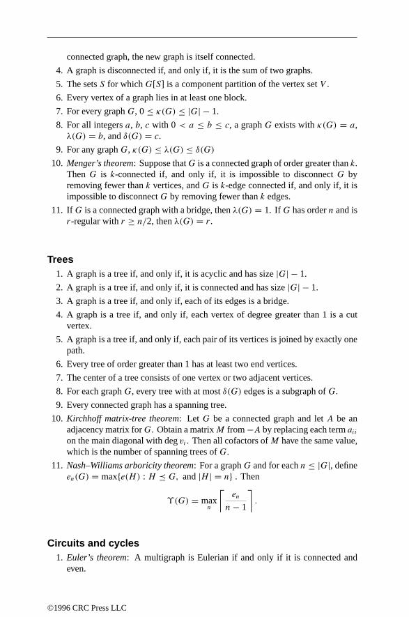
connected graph, the new graph is itself connected.
4. A graph is disconnected if, and only if, it is the sum of two graphs.
5. The setsS for whichG[S] is a component partition of the vertex setV .
6. Every vertex of a graph lies in at least one block.
7. For every graphG, 0≤ κ(G) ≤ |G| − 1.
8. For all integersa, b, c with 0 < a ≤ b ≤ c, a graphG exists withκ(G) = a,λ(G) = b, andδ(G) = c.
9. For any graphG, κ(G) ≤ λ(G) ≤ δ(G)10. Menger’s theorem: Suppose thatG is a connected graph of order greater thank.
ThenG is k-connected if, and only if, it is impossible to disconnectG byremoving fewer thank vertices, andG is k-edge connected if, and only if, it isimpossible to disconnectG by removing fewer thank edges.
11. IfG is a connected graph with a bridge, thenλ(G) = 1. If G has ordern and isr-regular withr ≥ n/2, thenλ(G) = r.
Trees1. A graph is a tree if, and only if, it is acyclic and has size|G| − 1.
2. A graph is a tree if, and only if, it is connected and has size|G| − 1.
3. A graph is a tree if, and only if, each of its edges is a bridge.
4. A graph is a tree if, and only if, each vertex of degree greater than 1 is a cutvertex.
5. A graph is a tree if, and only if, each pair of its vertices is joined by exactly onepath.
6. Every tree of order greater than 1 has at least two end vertices.
7. The center of a tree consists of one vertex or two adjacent vertices.
8. For each graphG, every tree with at mostδ(G) edges is a subgraph ofG.
9. Every connected graph has a spanning tree.
10. Kirchhoff matrix-tree theorem: Let G be a connected graph and letA be anadjacency matrix forG. Obtain a matrixM from−A by replacing each termaiion the main diagonal with degvi . Then all cofactors ofM have the same value,which is the number of spanning trees ofG.
11. Nash–Williams arboricity theorem: For a graphG and for eachn ≤ |G|, defineen(G) = maxe(H) : H G, and|H | = n . Then
ϒ(G) = maxn
⌈en
n− 1
⌉.
Circuits and cycles1. Euler’s theorem: A multigraph is Eulerian if and only if it is connected and
even.
©1996 CRC Press LLC

2. If G is Hamiltonian, and ifG′ is obtained fromG by removing a nonempty setS of vertices, then the number of components ofG′ is at most|S|.
3. Ore’s theorem: If G is a graph for which degv+degw ≥ |G|wheneverv andware nonadjacent vertices, thenG is Hamiltonian.
4. Dirac’s theorem: If G is a graph of order|G| ≥ 3 and degv ≥ |G|/2 for eachvertexv, thenG is Hamiltonian.
5. (Erdos–Chvatal) If α(G) ≤ κ(G), thenG is Hamiltonian.
6. Every 4-connected planar graph is Hamiltonian.
Cliques and independent sets1. A setS ⊆ V is a vertex cover if, and only if,V \ S is an independent set.
2. Turan’s theorem: If |G| = n andω(G) ≤ k, thene(G) ≤ e(Tn,k).3. Ramsey’s theorem: For all positive integersk andl, there is a least integerR(k, l)
for which every graph of order at leastR(k, l) has either a clique of cardinalitykor an independent set of cardinalityl. Fork ≥ 2 andl ≥ 2,R(k, l) ≤ R(k, l −1) + R(k − 1, l). The following table gives the values ofR(k, l) for k ≤ 3andl ≤ 7.
l = 1 2 3 4 5 6 7k = 1 1 1 1 1 1 1 1
2 1 2 3 4 5 6 73 1 3 6 9 14 18 23
Colorings and partitions1. Every graphG is k-partite for somek; in particular,G is |G|-partite.
2. Every graphG has a bipartite subgraphH for which e(H) ≥ e(G)/2.
3. PG(x) = PG−e(x)− PG\e(x).4. Brooks’s theorem: If G is a connected graph that is neither a complete graph
nor a cycle of odd length, thenχ(G) ≤ (G).5. For all positive integersg andc, a graphGexists withχ(G) ≥ c and gir(G) ≥ g.
6. Nordhaus–Gaddum bounds: For every graphG,
2√|G| ≤ χ(G)+ χ(G) ≤ |G| + 1, and
|G| ≤ χ(G)χ(G) ≤( |G| + 1
2
)2
.
7. Szekeres–Wilf theorem: For every graphG = (V ,E),
χ(G) ≤ 1+maxS⊆V
δ(G[S]).
©1996 CRC Press LLC

8. (Konig) If G is bipartite, thenχ ′(G) = (G).
9. Vizing’s theorem: For every graphG,(G) ≤ χ ′(G) ≤ (G)+ 1.
10. The following table gives the chromatic numbers and chromatic polynomials ofvarious graphs:
G χ(G) PG(x)
Kn n x(x − 1) · · · (x − n+ 1)Kn 1 xn
Tn 2 x(x − 1)n−1
Pn 2 x(x − 1)n−1
C4 2 x(x − 1)(x2 − 3x + 3)
11. (Appel-Haken) Four-color theorem: χ(G) ≤ 4 for every planar graphG.
12. For each graphG of order |G| = n and size e(G) = m with exactly k compo-nents, the chromatic polynomial is of the form
PG(x) =n−k∑i=0
(−1)iaixn−i ,
with a0 = 1, a1 = m and everyai positive.
13. Not every polynomial is a chromatic polynomial. For exampleP(x) = x4 −4x3+ 3x2 is not a chromatic polynomial.
14. Sometimes a class of chromatic polynomials can only come from a specific classof graphs. For example:
(a) If PG(x) = xn, thenG = Kn.
(b) If PG(x) = (x)n, thenG = Kn.
(c) If PG(x) = x(x − 1) · · · (x − r + 2)(x − r + 1)2(x − r)n−r−1 for a graphof ordern ≥ r + 1, thenG can be obtained from ar-treeT of ordern bydeleting an edge contained in exactlyr − 1 triangles ofT .
Distance1. A metric space(X, d) is the metric space associated with a connected graph with
vertex setX if , and only if , it satisfiestwo conditions: (i) d(u,v) is anonnegativeinteger for allu, v ∈ X, and (ii) wheneverd(u, v) ≥ 2, some element ofX liesbetweenu andv. The edges of the graph are the pairsu, v ⊆ X for whichd(u, v) = 1. (In an arbitrary metric space(X, d), a pointv ∈ X is said to liebetween distinct points u ∈ X and w ∈ X if it satisfies the triangle equalityd(u,w) = d(u, v)+ d(v,w).)
2. If G = (V ,E) is connected, then distance is always finite, andd is a metriconV . Note that deg(x) = |S(x,1)|.
3. Moore bound: For every connected graphG,
|G| ≤ 1+(G)diam(G)∑i=1
((G)− 1)i .
©1996 CRC Press LLC
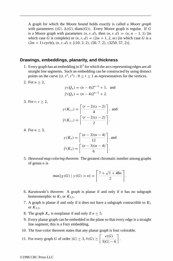
A graph for which the Moore bound holds exactly is called aMoore graphwith parameters(|G|,(G),diam(G)). Every Moore graph is regular. IfGis a Moore graph with parameters(n, r, d), then(n, r, d) = (n, n − 1,1) (inwhich caseG is complete) or(n, r, d) = (2m+ 1,2,m) (in which caseG is a(2m+ 1)-cycle),(n, r, d) ∈ (10,3,2), (50,7,2), (3250,57,2).
Drawings, embeddings, planarity, and thickness
1. Every graph has an embedding inR3 for which the arcs representing edges are allstraight line segments. Such an embedding can be constructed by using distinctpoints on the curve(t, t2, t3) : 0 ≤ t ≤ 1 as representatives for the vertices.
2. Forn ≥ 2,γ (Qn) = (n− 4)2n−3+ 1, and
γ (Qn) = (n− 4)2n−2 + 2.
3. Forr, s ≥ 2,
γ (Kr,s) =⌈(r − 2)(s − 2)
4
⌉, and
γ (Kr,s) =⌈(r − 2)(s − 2)
2
⌉.
4. Forn ≥ 3,
γ (Kn) =⌈(n− 3)(n− 4)
12
⌉,and
γ (Kn) =⌈(n− 3)(n− 4)
6
⌉.
5. Heawood map coloring theorem: The greatest chromatic number among graphsof genusn is
maxχ(G) | γ (G) = n =⌈
7+√1+ 48n
2
⌉.
6. Kuratowski’s theorem: A graph is planar if and only if it has no subgraphhomeomorphic toK5 orK3,3.
7. A graph is planar if and only if it does not have a subgraph contractible toK5
orK3,3.
8. The graphKn is nonplanar if and only ifn ≥ 5.
9. Every planar graph can be embedded in the plane so that every edge is a straightline segment; this is a Fary embedding.
10. The four-color theorem states that any planar graph is four colorable.
11. For every graphG of order|G| ≥ 3, θ(G) ≥⌈
e(G)
3|G| − 6
⌉.
©1996 CRC Press LLC

12. The complete graphsK9 andK10 have thickness 3; forn /∈ 9,10,
θ(Kn) =⌊n+ 7
6
⌋.
13. Then-cube has thicknessθ(Qn) = n/4 + 1.
14. For every planar graphG, ν(G) = ν(G). That equality does not hold for allgraphs:ν(K8) = 18, andν(K8) = 19.
Vertex degrees1. Handshaking lemma: For every graphG,
∑v∈V degv = 2e(G).
2. Every 2-switch preserves the degree sequence.
3. If G andH have the same degree sequence, thenH can be obtained fromG viaa sequence of 2-switches.
4. (Havel–Hakimi) A sequenced1, d2, . . . , dn of nonnegative integers withd1 ≥d2 ≥ · · · ≥ dn (with n ≥ 2 andd1 ≥ 1) is a degree sequence if and only if thesequenced2 − 1, d3− 1, . . . , dd1+1− 1, dd1+2, . . . , dn is a degree sequence.
Algebraic methods1. The bipartite graphsKn,n are circulant graphs.
2. For a graphGwith exactlyk connected components, the cycle space has dimen-sione(G)− |G| + k, and the cut space has dimension|G| − k.
3. In thekth powerAk = (akij ) of the adjacency matrix, each entryakij is the numberof vi, vj walks of lengthk.
4. The incidence matrix of a graphG is totally unimodular if, and only if,G isbipartite.
5. Every odd graph is vertex-transitive.
6. The smallest graph that is vertex symmetric, but is not edge symmetric, is theprismK3 × K2. The smallest graph that is edge symmetric, but is not vertexsymmetric, isS2 = P3 = K1,2.
7. The spectrum of a disconnected graph is the union of the spectra of its compo-nents.
8. The sum of the eigenvalues in the spectrum of a graph is zero.
9. The number of distinct eigenvalues in the spectrum of a graph is greater thanthe diameter of the graph.
10. The largest eigenvalue in the spectrum of a graphG is, at most,(G), withequality if, and only if,G is regular.
11. (Wilf) If G is a connected graph and its largest eigenvalue isλ, thenχ(G) ≤ 1+λ.Moreover, equality holds if, and only if,G is a complete graph or a cycle of oddlength.
©1996 CRC Press LLC

12. (Hoffman) IfG is a connected graph of ordern with spectrumλ1 ≥ · · · ≥ λn,thenχ(G) ≥ 1− λ1/λn.
13. Integrality condition: If G is a strongly regular graph with parameters(k, λ, µ),then the quantities
1
2
(|G| − 1± (|G| − 1)(µ− λ)− 2k√
(µ− λ)2 + 4(k − µ)
)
are nonnegative integers.
14. The following table gives the automorphism groups of various graphs:
G Aut(G)Cn Dn
Kn SnKn SnK1,n E1+ SnPn Cn
15. A graph and its complement have the same group; Aut(G) = Aut(G).
16. Frucht’s theorem: Every finite group is the automorphism group of some graph.
17. IfGandG′ are edge isomorphic, thenGandG′ are not required to be isomorphic.For example, the graphsC3 andS3 are edge isomorphic, but not isomorphic.
18. If the graphG has ordern, then the order of its automorphism group|Aut(G)|is a divisor ofn!. The order of the automorphism group equalsn! if and only ifG Kn orG Kn.
Matchings1. A matchingM is a maximum matching if, and only if, there is noM-augmenting
path.
2. Hall’s theorem: A bipartite graphGwith bipartition(B1, B2)has a matching thatsaturates every vertex inB1 if, and only if, |S(A,1)| ≥ |A| for everyA ⊆ B1.
3. Konig’s theorem: In a bipartite graph, the cardinality of a maximum matchingequals the cardinality of a minimum vertex cover.
Enumeration1. The number of labeled graphs of ordern is 2(
n
2).
2. The number of labeled graphs of ordern and sizem is((n2)m
).
3. The number of different ways in which a graphG of ordern can be labeled isn!/|Aut(G)|.
4. Cayley’s formula: The number of labeled trees of ordern is nn−2.
5. The number of labeled trees of ordern with exactlyt end vertices isn!t !
n−2n−t
for 2≤ t ≤ n− 1.
©1996 CRC Press LLC

Order Graphs Digraphs Trees (tn) Rooted trees (Tn)1 1 1 1 12 2 3 1 13 4 16 1 24 11 218 2 45 34 9608 3 96 156 1540944 6 207 1044 882033440 11 488 12346 1793359192848 23 1159 274668 47 28610 12005168 106 719
Define the generating functionsT (x) = ∑∞n=0 Tnx
n and t (x) = ∑∞n=0 tnx
n.Then T (x) = x exp
(∑∞r=1
1rT (xr)
), and t (x) = T (x)− 1
2
[T 2(x)− T (x2
)].
The following table lists the number of isomorphism classes of graphs of order nand size m.
m n = 1 2 3 4 5 6 7 8 90 1 1 1 1 1 1 1 1 11 1 1 1 1 1 1 1 12 1 2 2 2 2 2 13 1 3 4 5 5 5 54 2 6 9 10 11 11
5 1 6 15 21 24 256 1 6 21 41 56 637 4 24 65 115 1488 2 24 97 221 345
9 1 21 131 402 77110 1 15 148 663 163711 9 148 980 325212 5 131 1312 599513 2 97 1557 10120
14 1 65 1646 1561515 1 41 1557 2193316 21 1312 2798717 10 980 3240318 5 663 34040
©1996 CRC Press LLC

The following table gives the number of labeled graphs of ordern having variousproperties:
n 1 2 3 4 5 6 7 8
All 1 2 8 64 1 024 215 221 228
Connected 1 1 4 38 728 26 704 1 866 256 251 548 592Even 1 1 2 8 64 1 024 215 221
Trees 1 1 3 16 125 1 296 16 807 262 144
The following table gives the numbers of isomorphism classes of graphs of ordern
exhibiting various properties:
n 1 2 3 4 5 6 7 8All 1 2 4 11 34 156 1 044 12 346Connected 1 1 2 6 21 112 853 11 117Even 1 1 2 3 7 16 54 243Eulerian 1 0 1 1 4 8 37 184Blocks 0 1 1 3 10 56 468 7 123Trees 1 1 1 2 3 6 11 23Rooted trees 1 1 2 4 9 20 48 115
3.3.5 TREE DIAGRAMS
Let Tn,m denote themth isomorphism class of trees of order n. Figure 3.3.3 depictstreesof order at most 7. Figure3.3.4 depicts treesof order 8.
3.4 PARTIALLY ORDERED SETS
Consider a setS and a relation on it. Given any two elementsx andy in S, we candetermine whether or notx is “related” toy; if it is, “ x y”. The relation “” willbe apartial orderonS if it satisfies the following three conditions:
reflexive s s for everys ∈ S,
antisymmetric s t andt s imply s = t, and
transitive s t andt u imply s u.
If is a partial order onS, then the pair(S,) is called apartially ordered setor aposet. Given the partial order on the setS, define the relation≺ by
x ≺ y if and only if x y andx = y.
We say that the elementt coversthe elements if s ≺ t and there is no elementu withs ≺ u ≺ t . A Hasse diagram of the poset(S,) is a figure consisting of the elementsof S with a line segment directed generally upward froms to t whenevert coverss.
©1996 CRC Press LLC

FIGURE 3.3.3Trees with 7 or fewer vertices.
T1;1
T2;1
T3;1
T4;1
T4;2
T5;1
T5;2
T5;3
T6;1
T6;2
T6;3
T6;4
T6;5
T6;6
T7;1
T7;2
T7;3
T7;4
T7;5
T7;6
T7;7
T7;8
T7;9
T7;10
T7;11
©1996 CRC Press LLC

FIGURE 3.3.4Trees with 8 vertices.
T8;1
T8;2
T8;3
T8;4
T8;5
T8;6
T8;7
T8;8
T8;9
T8;10
T8;11
T8;12
T8;13
T8;14
T8;15
T8;16
T8;17
T8;18
T8;19
T8;20
T8;21
T8;22
T8;23
©1996 CRC Press LLC
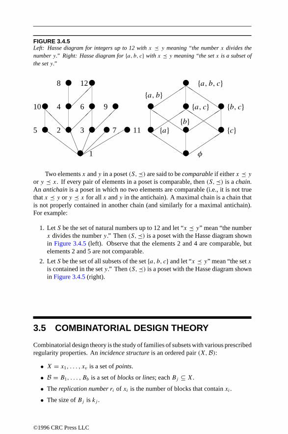
FIGURE 3.4.5Left: Hasse diagram for integers up to 12 withx y meaning “the numberx divides thenumbery.” Right: Hasse diagram fora, b, c with x y meaning “the setx is a subset ofthe sety.”
10 4
8 12
b, ca, c
7 115 2 3
1
6 9
φ
a, b, ca, b
cab
Two elementsx andy in a poset(S,) are said to becomparableif eitherx y
or y x. If every pair of elements in a poset is comparable, then(S,) is achain.An antichainis a poset in which no two elements are comparable (i.e., it is not truethatx y or y x for all x andy in the antichain). A maximal chain is a chain thatis not properly contained in another chain (and similarly for a maximal antichain).For example:
1. LetS be the set of natural numbers up to 12 and let “x y” mean “the numberx divides thenumber y.” Then (S,) isa poset with theHassediagram shownin Figure 3.4.5 (left). Observe that the elements 2 and 4 are comparable, butelements 2 and 5 are not comparable.
2. LetS be the set of all subsets of the seta, b, c and let “x y” mean “the setxiscontained in theset y.” Then (S,) is aposet with theHassediagram shownin Figure3.4.5 (right).
3.5 COMBINATORIAL DESIGN THEORY
Combinatorial design theory is the study of families of subsets with various prescribedregularity properties. Anincidence structureis an ordered pair(X,B):
• X = x1, . . . , xv is a set ofpoints.
• B = B1, . . . , Bb is a set ofblocksor lines; eachBj ⊆ X.
• Thereplication numberri of xi is the number of blocks that containxi .
• The size ofBj is kj .
©1996 CRC Press LLC

Counting the number of pairs(x, B) with x ∈ B yields∑v
i=1 ri = ∑bj=1 kj . The
incidence matrixof an incidence structure is thev × b matrixA = (aij ) with aij = 1if xi ∈ Bj and 0 otherwise.
3.5.1 t-DESIGNS
The incidence structure(X,B) is called at-(v, k, λ) designif
1. For allj , kj = k and 1< k < v, and
2. Any subset oft points lies on exactlyλ blocks.
A 1-design is equivalent to av × b 0-1 matrix with constant row and column sums.Everyt-(v, k, λ) design is also a-(v, k, λ) design (1≤ ≤ t), where
λ = λ
(v −
t −
)/(k −
t −
). (3.5.1)
A necessary condition for the existence of at-(v, k, λ) design is thatλ must be aninteger for all, 1 ≤ ≤ t . Another necessary condition is the generalized Fisher’sinequality whent = 2s: b ≥ (
v
s
).
Related designsA t-(v, k, λ) design also implies the existence of the following designs:
Complementary designLet BC = X\B | B ∈ B. Then the incidence structure(X,BC) is a t-(v, v − k, λ
(v−t
k
) /(v−t
k−t
)) design (providedv ≥ k + t).
Derived designFix x ∈ X and letBD = B\x | B ∈ B with x ∈ B. Then the incidencestructure(X\x,BD) is a(t − 1)-(v − 1, k − 1, λ) design.
Residual designFix x ∈ Xand letBR = B | B ∈ B with x /∈ B. Then the incidence structure(X\x,BR) is a(t − 1)-(v − 1, k − 1, λ
(v−t
k−t+1
) /(v−t
k−t
)) design.
The Mathieu 5-designThe following are the 132 blocks of a 5-(12,6,1) design. The blocks are the supportsof the weight-6 codewords in the ternary Golay code (page 220). Similarly, thesupports of the 759 weight-8 codewords in the binary Golay code form the blocks ofa 5-(24,8,1) design.
0 1 2 3 4 11 0 2 5 7 8 10 1 3 4 7 8 110 1 2 3 5 10 0 2 5 7 9 11 1 3 5 6 7 100 1 2 3 6 8 0 2 6 7 8 9 1 3 5 6 8 110 1 2 3 7 9 0 2 6 8 10 11 1 3 5 8 9 10
©1996 CRC Press LLC

0 1 2 4 5 9 0 3 4 5 6 10 1 3 6 7 8 90 1 2 4 6 10 0 3 4 5 9 11 1 3 7 9 10 110 1 2 4 7 8 0 3 4 6 8 11 1 4 5 6 7 80 1 2 5 6 7 0 3 4 7 8 9 1 4 5 6 9 100 1 2 5 8 11 0 3 4 7 10 11 1 4 5 8 9 110 1 2 6 9 11 0 3 5 6 7 8 1 4 6 7 10 110 1 2 7 10 11 0 3 5 7 9 10 1 4 7 8 9 100 1 2 8 9 10 0 3 5 8 10 11 1 5 6 7 9 110 1 3 4 5 8 0 3 6 7 9 11 1 5 7 8 10 110 1 3 4 6 7 0 3 6 8 9 10 1 6 8 9 10 110 1 3 4 9 10 0 4 5 6 7 9 2 3 4 5 8 110 1 3 5 6 9 0 4 5 7 8 11 2 3 4 5 9 100 1 3 5 7 11 0 4 5 8 9 10 2 3 4 6 7 80 1 3 6 10 11 0 4 6 7 8 10 2 3 4 6 10 110 1 3 7 8 10 0 4 6 9 10 11 2 3 4 7 9 110 1 3 8 9 11 0 5 6 7 10 11 2 3 5 6 7 90 1 4 5 6 11 0 5 6 8 9 11 2 3 5 6 8 100 1 4 5 7 10 0 7 8 9 10 11 2 3 5 7 10 110 1 4 6 8 9 1 2 3 4 5 6 2 3 6 8 9 110 1 4 7 9 11 1 2 3 4 7 10 2 3 7 8 9 100 1 4 8 10 11 1 2 3 4 8 9 2 4 5 6 7 100 1 5 6 8 10 1 2 3 5 7 8 2 4 5 6 9 110 1 5 7 8 9 1 2 3 5 9 11 2 4 5 7 8 90 1 5 9 10 11 1 2 3 6 7 11 2 4 6 8 9 100 1 6 7 8 11 1 2 3 6 9 10 2 4 7 8 10 110 1 6 7 9 10 1 2 3 8 10 11 2 5 6 7 8 110 2 3 4 5 7 1 2 4 5 7 11 2 5 8 9 10 110 2 3 4 6 9 1 2 4 5 8 10 2 6 7 9 10 110 2 3 4 8 10 1 2 4 6 7 9 3 4 5 6 7 110 2 3 5 6 11 1 2 4 6 8 11 3 4 5 6 8 90 2 3 5 8 9 1 2 4 9 10 11 3 4 5 7 8 100 2 3 6 7 10 1 2 5 6 8 9 3 4 6 7 9 100 2 3 7 8 11 1 2 5 6 10 11 3 4 8 9 10 110 2 3 9 10 11 1 2 5 7 9 10 3 5 6 9 10 110 2 4 5 6 8 1 2 6 7 8 10 3 5 7 8 9 110 2 4 5 10 11 1 2 7 8 9 11 3 6 7 8 10 110 2 4 6 7 11 1 3 4 5 7 9 4 5 6 8 10 110 2 4 7 9 10 1 3 4 5 10 11 4 5 7 9 10 110 2 4 8 9 11 1 3 4 6 8 10 4 6 7 8 9 110 2 5 6 9 10 1 3 4 6 9 11 5 6 7 8 9 10
3.5.2 BALANCED INCOMPLETE BLOCK DESIGNS (BIBDS)
Balanced incomplete block designs(BIBDs) aret-designs witht = 2, so that everypair of points is on the same number of blocks. The relevant parameters arev, b, r,k, andλ with
vr = bk and v(v − 1)λ = bk(k − 1). (3.5.2)
©1996 CRC Press LLC

If A is thev×b incidence matrix, thenAAT = (r −λ)Iv +λJv, whereIn is then×n
identity matrix andJn is then × n matrix of all ones.
Symmetric designsFisher’s inequality states thatb ≥ v. If b = v (equivalently,r = k), then the BIBDis called asymmetric design, denoted as a(v, k, λ)-design. The incidence matrix fora symmetric design satisfies
JvA = kJv = AJv and ATA = (k − λ)Iv + λJv, (3.5.3)
that is, any two blocks intersect inλ points. The dualness of symmetric designs canbe summarized by the following:
v points ↔ v blocks,k blocks on a point ↔ k points in a block, andAny two points onλ blocks ↔ Any two blocks shareλ points.
Some necessary conditions for symmetric designs are
1. If v is even, thenk − λ is a square integer.
2. Bruck–Ryser–Chowla theorem: If v is odd, then the following equation hasinteger solutions (not all zero):
x2 = (k − λ)y2 + (−1)(v−1)/2λz2.
Existence table for BIBDsSome of the most fruitful construction methods for BIBD are dealt with in separatesections, difference sets (page 208), finite geometry (page 209), Steiner triple systems(page 211), and Hadamard matrices (page 211). The table below gives all parametersfor which BIBDs exists withk ≤ v/2 andb ≤ 30.
v b r k λ v b r k λ v b r k λ
6 10 5 3 2 10 18 9 5 4 15 30 14 7 66 20 10 3 4 10 30 9 3 2 16 16 6 6 26 30 15 3 6 10 30 12 4 4 16 20 5 4 17 7 3 3 1 11 11 5 5 2 16 24 9 6 37 14 6 3 2 11 22 10 5 4 16 30 15 8 7
7 21 9 3 3 12 22 11 6 5 19 19 9 9 47 28 12 3 4 13 13 4 4 1 21 21 5 5 18 14 7 4 3 13 26 6 3 1 21 30 10 7 38 28 14 4 6 13 26 8 4 2 23 23 11 11 59 12 4 3 1 13 26 12 6 5 25 25 9 9 3
9 18 8 4 3 14 26 13 7 6 25 30 6 5 19 24 8 3 2 15 15 7 7 3 27 27 13 13 6
10 15 6 4 2
©1996 CRC Press LLC

3.5.3 DIFFERENCE SETS
LetG be a finite group of orderv (see page 139). A subsetD of sizek is a(v, k, λ)-difference setin G if every nonidentity element ofG can be writtenλ times as a“difference” d1d
−12 with d1 and d2 in D. If G is the cyclic groupZv, then the
difference set is acyclic difference set. Theorder of a difference set isn = k − λ.
For example,1,2,4 is a(7,3,1) cyclic difference set of order 2.A (v, k, λ)-difference set implies the existence of a(v, k, λ)-design. The points
are the elements ofG and the blocks are the translates ofD: all setsDg = dg : d ∈D for g ∈ G. Note that each translateDg is itself a difference set. Here are the 7blocks for a(7,3,1)-design based onD = 1,2,4:
1 2 4 2 3 5 3 4 6 4 5 0 5 6 1 6 0 2 0 1 3
Example: A(16,6,2)-difference set inG = Z2 ⊕ Z2 ⊕ Z2 ⊕ Z2 is
0000 0001 0010 0100 1000 1111
Example: A(21,5,1)-difference set inG = ⟨a, b : a3 = b7 = 1, a−1ba = a4
⟩is
a, a2, b, b2, b4.
Some families of cyclic difference setsPaley: Let v be a prime congruent to 3 modulo 4. Then the nonzero squares inZv
form a(v, (v−1)/2, (v−3)/4)-difference set. Example:(v, k, λ) = (11,5,2).
Stanton–Sprott: Let v = p(p+2), wherep andp+2 are both primes. Then thereis a(v, (v− 1)/2, (v− 3)/4)-difference set. Example:(v, k, λ) = (35,17,8).
Biquadratic Residues (I): If v = 4a2 + 1 is a prime witha odd, then the nonzerofourth powers modulov form a(v, (v − 1)/4, (v − 5)/16)-difference set. Ex-ample:(v, k, λ) = (37,9,2).
Biquadratic Residues (II): If v = 4a2 + 9 is a prime witha odd, then zero andthe fourth powers modulov form a(v, (v + 3)/4, (v + 3)/16)-difference set.Example:(v, k, λ) = (13,4,1).
Singer: If q is a prime power, then there exists a((qm−1)/(q−1), (qm−1−1)/(q−1), (qm−2 − 1)/(q − 1))-difference set for allm ≥ 3.
Existence table of cyclic difference setsThis table gives all cyclic difference sets fork ≤ v/2 andv ≤ 50 up to equivalenceby translation and multiplication by a number relatively prime tov.
©1996 CRC Press LLC

v k λ n Difference set7 3 1 2 1 2 4
11 5 2 3 1 3 4 5 913 4 1 3 0 1 3 915 7 3 4 0 1 2 4 5 8 1019 9 4 5 1 4 5 6 7 9 11 16 17
21 5 1 4 3 6 7 12 1423 11 5 6 1 2 3 4 6 8 9 12 13 16 1831 6 1 5 1 5 11 24 25 2731 15 7 8 1 2 3 4 6 8 12 15 16 17 23 24 27 29 30
1 2 4 5 7 8 9 10 14 16 18 19 20 25 28
35 17 8 9 0 1 3 4 7 9 11 12 13 14 16 17 21 27 28 29 3337 9 2 7 1 7 9 10 12 16 26 33 3440 13 4 9 1 2 3 5 6 9 14 15 18 20 25 27 3543 21 10 11 1 2 3 4 5 8 11 12 16 19 20 21 22 27 32 33 35 37 39 41 42
1 4 6 9 10 11 13 14 15 16 17 21 23 24 25 31 35 36 38 40 41
47 23 11 12 1 2 3 4 6 7 8 9 12 14 16 17 18 21 24 25 27 28 32 34 36 37 42
3.5.4 FINITE GEOMETRY
Affine planesA finite affine planeis a finite set of points that satisfy the axioms:
• Any two points are on exactly one line.
• (Parallel postulate)Given a pointP and a lineL not containingP , there isexactly one line throughP that does not intersectL.
• There are four points, no three of which are collinear.
These axioms are sufficient to show that a finite affine plane is a BIBD (see page 206)with
v = n2 b = n2 + n r = n + 1 k = n λ = 1
(n is theorder of the plane). The lines of an affine plane can be divided inton + 1parallel classes each containingn lines. A sufficient condition for affine planes toexist is forn to be a prime power.
Below are two views of the affine plane of order 2 showing the parallel classes.
©1996 CRC Press LLC

Below is the affine plane of order 3 showing the parallel classes.
Projective planesA finite projective planeis a finite set of points that satisfy the axioms:
1. Any two points are on exactly one line.
2. Any two lines intersect in exactly one point.
3. There are four points, no three of which are collinear.
These axioms are sufficient to show that a finite affine plane is a symmetric design(see page 207) with
v = n2 + n + 1 k = n + 1 λ = 1
(n is theorder of the plane). A sufficient condition for affine planes to exist is forn
to be a prime power.A projective plane of ordern can be constructed from an affine plane of ordern
by adding aline at infinity. A line of n + 1 new points is added to the affine plane.For each parallel class, one distinct new point is added to each line. The constructionworks in reverse: removing any one line from a projective plane of ordern and itspoints leaves an affine plane of ordern. Below is the projective plane of order 2. Thecenter circle functions as a line at infinity; removing it produces the affine plane oforder 2.
3.5.5 STEINER TRIPLE SYSTEMS
A Steiner triple system(STS) is a 2-(v,3,1) design. In particular, STSs are BIBDs(see page 206). STSs exist if, and only if,v ≡ 1 or 3 (mod 6). The number of blocksin an STS isb = v(v − 1)/6.
©1996 CRC Press LLC
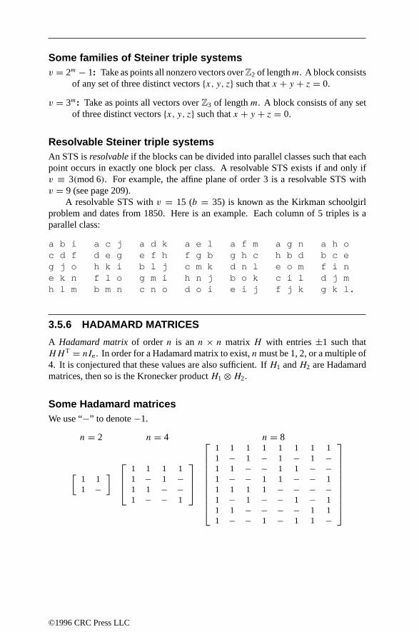
Some families of Steiner triple systemsv = 2m − 1: Take as points all nonzero vectors overZ2 of lengthm. A block consists
of any set of three distinct vectorsx, y, z such thatx + y + z = 0.
v = 3m: Take as points all vectors overZ3 of lengthm. A block consists of any setof three distinct vectorsx, y, z such thatx + y + z = 0.
Resolvable Steiner triple systemsAn STS isresolvableif the blocks can be divided into parallel classes such that eachpoint occurs in exactly one block per class. A resolvable STS exists if and only ifv ≡ 3(mod 6). For example, the affine plane of order 3 is a resolvable STS withv = 9 (see page 209).
A resolvable STS withv = 15 (b = 35) is known as the Kirkman schoolgirlproblem and dates from 1850. Here is an example. Each column of 5 triples is aparallel class:
a b i a c j a d k a e l a f m a g n a h oc d f d e g e f h f g b g h c h b d b c eg j o h k i b l j c m k d n l e o m f i ne k n f l o g m i h n j b o k c i l d j mh l m b m n c n o d o i e i j f j k g k l.
3.5.6 HADAMARD MATRICES
A Hadamard matrixof ordern is ann × n matrix H with entries±1 such thatHH T = nIn. In order for a Hadamard matrix to exist,n must be 1, 2, or a multiple of4. It is conjectured that these values are also sufficient. IfH1 andH2 are Hadamardmatrices, then so is the Kronecker productH1 ⊗ H2.
Some Hadamard matricesWe use “−” to denote−1.
n = 2 n = 4 n = 8
[1 11 −
]
1 1 1 11 − 1 −1 1 − −1 − − 1
1 1 1 1 1 1 1 11 − 1 − 1 − 1 −1 1 − − 1 1 − −1 − − 1 1 − − 11 1 1 1 − − − −1 − 1 − − 1 − 11 1 − − − − 1 11 − − 1 − 1 1 −
©1996 CRC Press LLC

n = 12
1 1 1 1 − − 1 − − 1 − −1 1 1 − 1 − − 1 − − 1 −1 1 1 − − 1 − − 1 − − 1− 1 1 1 1 1 − 1 1 1 − −1 − 1 1 1 1 1 − 1 − 1 −1 1 − 1 1 1 1 1 − − − 1− 1 1 1 − − 1 1 1 − 1 11 − 1 − 1 − 1 1 1 1 − 11 1 − − − 1 1 1 1 1 1 −− 1 1 − 1 1 1 − − 1 1 11 − 1 1 − 1 − 1 − 1 1 11 1 − 1 1 − − − 1 1 1 1
n = 16
1 1 1 1 1 1 1 1 1 1 1 1 1 1 1 11 − 1 − 1 − 1 − 1 − 1 − 1 − 1 −1 1 − − 1 1 − − 1 1 − − 1 1 − −1 − − 1 1 − − 1 1 − − 1 1 − − 11 1 1 1 − − − − 1 1 1 1 − − − −1 − 1 − − 1 − 1 1 − 1 − − 1 − 11 1 − − − − 1 1 1 1 − − − − 1 11 − − 1 − 1 1 − 1 − − 1 − 1 1 −1 1 1 1 1 1 1 1 − − − − − − − −1 − 1 − 1 − 1 − − 1 − 1 − 1 − 11 1 − − 1 1 − − − − 1 1 − − 1 11 − − 1 1 − − 1 − 1 1 − − 1 1 −1 1 1 1 − − − − − − − − 1 1 1 11 − 1 − − 1 − 1 − 1 − 1 1 − 1 −1 1 − − − − 1 1 − − 1 1 1 1 − −1 − − 1 − 1 1 − − 1 1 − 1 − − 1
Designs and Hadamard matrices
Without loss of generality, a Hadamard matrix can be assumed to have a first row andcolumn consisting of all+1s.
BIBDs: Delete the first row and column. The points of the design are the remainingcolumn indices. Each row produces a block of the design, namely those indiceswhere the entry is+1. The resulting design is an(n− 1, (n− 1)/2, (n− 5)/4)symmetric design (see page 211).
3-Designs: The points are the indices of the columns. Each row, except the firstrow, yields two blocks, one block for those indices where the entries are+1and one block for those indices where the entries are−1. The resulting designis a 3-(n, n/2, (n − 5)/4) design.
©1996 CRC Press LLC

3.5.7 LATIN SQUARES
A Latin squareof sizen is ann × n arrayS = [sij ] of n symbols such that everysymbol appears exactly once in each row and column. Two Latin squaresS andTareorthogonalif every pair of symbols occurs exactly once as a pair(sij , tij ). LetM(n) be the maximum size of a set of mutually orthogonal Latin squares (MOLS).
• M(n) ≤ n − 1.
• M(n) = n − 1 if n is a prime power.
• M(n1n2) ≥ min(M(n1),M(n2)).
• M(6) = 1 (i.e., there are no two MOLS of size 6).
• M(n) ≥ 2 for all n ≥ 3 exceptn = 6.
The existence ofn − 1 MOLS of sizen is equivalent to the existence of an affineplane of ordern (see page 209).
Examples of mutually orthogonal Latin squaresThese are complete sets of MOLS forn = 3, 4, and 5.
n = 3 n = 4
0 1 21 2 02 0 1
0 1 22 0 11 2 0
0 1 2 31 0 3 22 3 0 13 2 1 0
0 1 2 32 3 0 13 2 1 01 0 3 2
0 1 2 33 2 1 01 0 3 22 3 0 1
n = 50 1 2 3 41 2 3 4 02 3 4 0 13 4 0 1 24 0 1 2 3
0 1 2 3 42 3 4 0 14 0 1 2 31 2 3 4 03 4 0 1 2
0 1 2 3 43 4 0 1 21 2 3 4 04 0 1 2 32 3 4 0 1
0 1 2 3 44 0 1 2 33 4 0 1 22 3 4 0 11 2 3 4 0
These are two superimposed MOLS forn = 7, 8, 9, and 10.
n = 7 n = 8
00 11 22 33 44 55 6616 20 31 42 53 64 0525 36 40 51 62 03 1434 45 56 60 01 12 2343 54 65 06 10 21 3252 63 04 15 26 30 4161 02 13 24 35 46 50
00 11 22 33 44 55 66 7712 03 30 21 56 47 74 6524 35 06 17 60 71 42 5333 22 11 00 77 66 55 4446 57 64 75 02 13 20 3157 46 75 64 13 02 31 2065 74 47 56 21 30 03 1271 60 53 42 35 24 17 06
©1996 CRC Press LLC

n = 900 11 22 33 44 55 66 77 8812 20 01 45 53 34 78 86 6721 02 10 54 35 43 87 68 7636 47 58 60 71 82 03 14 2548 56 37 72 80 61 15 23 0457 38 46 81 62 70 24 05 1363 74 85 06 17 28 30 41 5275 83 64 18 26 07 42 50 3184 65 73 27 08 16 51 32 40
n = 1000 67 58 49 91 83 75 12 24 3676 11 07 68 59 92 84 23 35 4085 70 22 17 08 69 93 34 46 5194 86 71 33 27 18 09 45 59 6219 95 80 72 44 37 28 56 61 0338 29 96 81 73 55 47 60 02 1457 48 39 90 82 74 66 01 13 2521 32 43 54 65 06 10 77 88 9942 53 64 05 16 20 31 89 97 7863 04 15 26 30 41 52 98 79 87
3.5.8 ROOM SQUARES
A Room squareof siden is ann × n array with entries either empty or consisting ofan unordered pair of symbols from a symbol set of sizen+ 1 with the requirements:
1. Each symbol appears exactly once in each row and column.
2. Every unordered pair occurs exactly once in the array.
Room squares exist if and only ifn is odd andn ≥ 7.
A Room square yields a construction of a round-robin tournament betweenn+1opponents:
1. Rows of the square represent rounds in the tournament.
2. Columns in the square represent locales.
3. Each pair represents one competition.
Then each team plays exactly once in each round, at each locale, and against eachopponent.
For example, this is a Room square of side 7:
©1996 CRC Press LLC

01 26 57 3445 02 37 6172 56 03 41
13 67 04 5263 24 71 05
74 35 12 0615 46 23 07
3.6 INCLUSION/EXCLUSION
Let a1, a2, . . . , ar be properties that the elements of a set may or may not have. Ifthe set hasN objects, then the number of objects having exactlym properties (withm ≤ r), em, is given by
em = sm −(m + 1
1
)sm+1 +
(m + 2
2
)sm+2 −
(m + 3
3
)sm+3
· · · + (−1)p(m + p
p
)sm+p · · · + (−1)r−m
(m + (r − m)
(r − m)
)sr .
Herest = ∑N(ai1ai2 · · · ait ). Whenm = 0, this is the usual inclusion/exclusion
rule:
e0 = s0 − s1 + s2 − · · · + (−1)rsr ,
= N −∑i
N(ai) +∑i,j
i =j
N(aiaj ) −∑i,j,ki =ji =kj =k
N(aiajak) + · · · + (−1)rN(a1a2 . . . ar ).
3.7 COMMUNICATION THEORY
3.7.1 INFORMATION THEORY
DefinitionsLet pX be a probability distribution on the discrete random variableX with Prob(X =x) = px . Theentropyof the distribution is
H(pX) = −∑x
px log2 px. (3.7.1)
WhenX takes only two values,
H(pX) = H(p) = −p log2 p − (1 − p) log2(1 − p). (3.7.2)
©1996 CRC Press LLC

The units for entropy arebits. The range ofH(p) is from 0 to 1 with a maximumatp = 0.5. The maximum ofH(pX) is log2 n and is obtained whenX is a uniformrandom variable takingn values. Entropy measures how much information is gainedfrom learning the value ofX. Below is a plot ofp versusH(p).
0.2 0.4 0.6 0.8 1
0.2
0.4
0.6
0.8
1
Given two discrete random variablesX andY , pX×Y is the joint distribution ofX andY . Themutual informationof X andY is defined by
I (X, Y ) = H(pX) + H(pY ) − H(pX×Y ). (3.7.3)
Note thatI (X, Y ) ≥ 0 and thatI (X, Y ) = 0 if, and only if,X andY are independent.Mutual information gives the amount of information that learning a value ofX saysabout the value ofY (and vice versa).
Channel capacityThe transition probabilitiesare defined bytx,y = Prob(Y = y | X = x). Thedistribution pX determinespY by py = ∑
tx,ypx . The matrixT = (tx,y) is thetransition matrix. The matrixT defines achannelgiven by a transition diagram(input isX, output isY ). For example (hereX andY only take two values),
x1
x0
y1.
y0
tx0,y0
tx1,y1
tx0,y1
tx1,y0
Thecapacityof the channel is defined as
C = maxp
X
I (X, Y ). (3.7.4)
©1996 CRC Press LLC

A channel issymmetricif each row is a permutation of the first row, and thetransition matrix is a symmetric matrix. The capacity of a symmetric channel isC = log2 n − H(p), wherep is the first row. The capacity of a symmetric channelis achieved with equally likely inputs. The channel below on the left is symmetric;both channels achieve capacity with equally likely inputs.
Binary Symmetric Channel Binary Erasure Channel
1
0
1
0
1 − p
1 − p
p
p
1
0
1
?
0
1 − p
1 − p
p
p
C = 1 − H(p). C = 1 − p.
Shannon’s theoremLet bothX andY be discrete random variables with values in an alphabetA. A codeisa set ofn-tuples (codewords) with entries fromA that is in one-to-one correspondencewith M messages. TherateR of the code is defined as1
nlog2 M. Assume that the
codeword is sent via a channel with transition matrixT by sending each vector elementindependently. Define
e = maxall codewords
Prob(codeword incorrectly decoded). (3.7.5)
ThenShannon’s coding theoremstates:
• If R < C, then there is a sequence of codes withn → ∞ such thate → 0.
• If R ≥ C, thene is always bounded away from 0.
3.7.2 BLOCK CODING
DefinitionsA codeC over an alphabetA is a set of vectors of a fixed lengthn with entries fromA. Let A be the finite field GF(q) (see Section 3.7.3). If C is avector space over A,thenC is a linear code; thedimensionk of a linear code is its dimension as a vectorspace.
The Hamming distancedH(u, v) between two vectors,u andv, is the numberof places in which they differ. For a vectoru over GF(q), define theweight,wt(u),as the number of nonzero components. ThendH(u, v) = wt(u − v). The minimumHamming distance between two distinct vectors in a codeC is called theminimumdistanced. A code can detecte errors if e < d. A code can correctt errors if2t + 1 < d.
©1996 CRC Press LLC

Coding diagram for linear codes
x message xG codeword y received word yH syndrome
Encoding Channel Decoding
1. A messagex consists ofk information symbols.
2. The message is encoded asxG ∈ C, whereG is a k × n matrix called thegenerating matrix.
3. After transmission over a channel, a (possibly corrupted) vectory is received.
4. There exists aparity check matrixH such thatc ∈ C if and only if cH = 0.Thus thesyndromez = yH can be used to try to decodey.
5. If G has the form [I A], whereI is thek×k identity matrix, thenH =[ −A
I
].
Cyclic codesA linear codeC of lengthn is cyclic if (a0, a1, . . . , an−1) ∈ C implies(an−1, a0, . . . ,
an−2) ∈ C. To each codeword(a0, a1, . . . , an−1) ∈ C is associated the polynomiala(x) = ∑n−1
i=0 aixi . Every cyclic code has agenerating polynomialg(x) such that
a(x) corresponds to a codeword if, and only if,a(x) ≡ d(x)g(x) (mod xn − 1) forsomed(x). Therootsof a cyclic code are roots ofg(x) under some extension fieldGF(q ′) with primitive elementα.
BCH Bound:If a cyclic codeC has rootsαi, αi+1, . . . , αi+d−2, then the minimumdistance ofC is at leastd.
Binary BCH codes(BCH stands for Bose, Ray-Chaudhuri, and Hocquenghem):Fix m, definen = 2m − 1, and letα be a primitive element in GF(2m). Definefi(x)
as the minimum binary polynomial ofαi . Then
g(x) = LCM (f1(x) · · · f2e(x)) (3.7.6)
defines a generating polynomial for a binary BCH code of lengthn and minimumdistance at leastδ = 2e + 1 (δ is called thedesigned distance). The code dimensionis at leastn − me.
©1996 CRC Press LLC

Table of binary BCH codes
n k d
7 4 3
15 11 37 55 7
31 26 321 516 711 116 15
63 57 351 5
n k d
63 45 739 936 1130 1324 1518 2116 2310 277 31
127 120 3113 5106 799 9
n k d
127 92 1185 1378 1571 1964 2157 2350 2743 3136 3129 ≥ 4322 4715 558 63
Dual code:Given a codeC, the dual code isC⊥ = a | a · x = 0 for all x ∈ C.The codeC⊥ is an(n, n − k) linear code overFq . A code isself-doubtif C = C⊥.
MDS codes:A linear code that meets the Singleton bound,n + 1 = k + d, iscalledMDS (for maximum distance separable). The generating matrix of an MDScode has anyk columns linearly independent.
Reed–Solomon codes:Let α be a primitive element for GF(q) andn = q − 1.The generating polynomialg(x) = (x − α)(x − α2) · · · (x − αd−1) defines a cyclicMDS code with distanced and dimensionk = n − d + 1.
Hexacode:The hexacode is a(6,3,4) self-dual MDS code over GF(4). Letthe finite field of four elements be0,1, a, b with b = a2 = a + 1. The code isgenerated by the vectors(1,0,0,1, a, b), (0,1,0,1, a, b), and(0,0,1,1,1,1). The64 codewords are
000000 1001ba a00a1b b00ba1 0101ab 110011 a10bb0 b10a0a0a0ab1 1a0b0b aa00aa ba0110 0b0b1a 1b0aa0 ab0101 bb00bb001111 1010ab a01b0a b01ab0 0110ba 111100 a11aa1 b11b1b0a1ba0 1a1a1a aa11bb ba1001 0b1a0b 1b1bb1 ab1010 bb11aa00aaaa 10ab10 a0a0b1 b0a10b 01ab01 11aabb a1a11a b1a0a00aa01b 1aa1a1 aaaa00 baabba 0ba1b0 1ba00a ababab bbaa1100bbbb 10ba01 a0b1a0 b0b01a 01ba10 11bbaa a1b00b b1b1b10ab10a 1ab0b0 aabb11 babaab 0bb0a1 1bb11b abbaba bbbb00.
Perfect codes:A linear code isperfectif it satisfies the Hamming bound,qn−k =∑ei=0
(n
i
)(q − 1)i . The binary Hamming codes and Golay codes are perfect.
Binary Hamming codes:Have the parametersn = 2m − 1, k = 2m − 1 − m,d = 3. The parity check matrix is the 2m − 1 × m matrix whose rows are all of thebinarym-tuples in a fixed order. The generating and parity check matrices for the
©1996 CRC Press LLC

(7,4) Hamming code are
G =
1 0 0 0 1 1 00 1 0 0 1 0 10 0 1 0 0 1 10 0 0 1 1 1 1
, H =
1 1 01 0 10 1 11 1 11 0 00 1 00 0 1
. (3.7.7)
Binary Golay code: This has the parametersn = 24, k = 12, d = 8. Thegenerating matrix is
G =
1 0 0 0 0 0 0 0 0 0 0 0 0 1 1 1 1 1 1 1 1 1 1 10 1 0 0 0 0 0 0 0 0 0 0 1 1 1 0 1 1 1 0 0 0 1 00 0 1 0 0 0 0 0 0 0 0 0 1 1 0 1 1 1 0 0 0 1 0 10 0 0 1 0 0 0 0 0 0 0 0 1 0 1 1 1 0 0 0 1 0 1 10 0 0 0 1 0 0 0 0 0 0 0 1 1 1 1 0 0 0 1 0 1 1 00 0 0 0 0 1 0 0 0 0 0 0 1 1 1 0 0 0 1 0 1 1 0 10 0 0 0 0 0 1 0 0 0 0 0 1 1 0 0 0 1 0 1 1 0 1 10 0 0 0 0 0 0 1 0 0 0 0 1 0 0 0 1 0 1 1 0 1 1 10 0 0 0 0 0 0 0 1 0 0 0 1 0 0 1 0 1 1 0 1 1 1 00 0 0 0 0 0 0 0 0 1 0 0 1 0 1 0 1 1 0 1 1 1 0 00 0 0 0 0 0 0 0 0 0 1 0 1 1 0 1 1 0 1 1 1 0 0 00 0 0 0 0 0 0 0 0 0 0 1 1 0 1 1 0 1 1 1 0 0 0 1
. (3.7.8)
Ternary Golay code:This has the parametersn = 12, k = 6, d = 6. Thegenerating matrix is
G =
1 0 0 0 0 0 0 1 1 1 1 10 1 0 0 0 0 1 0 1 2 2 10 0 1 0 0 0 1 1 0 1 2 20 0 0 1 0 0 1 2 1 0 1 20 0 0 0 1 0 1 2 2 1 0 10 0 0 0 0 1 1 1 2 2 1 0
. (3.7.9)
BoundsBounds for block codes investigate the trade-offs between the lengthn, the numberof codewordsM, the minimum distanced, and the alphabet sizeq. The number oferrors that can be corrected ise with 2e+1 ≤ d. If the code is linear, then the boundsconcern the dimensionk with M = qk.
1. Hamming or sphere-packing bound:M ≤ qn/∑e
i=0
(n
i
)(q − 1)i .
2. Plotkin bound: Suppose thatd > n(q − 1)/q. ThenM ≤ qd
qd−n(q−1) .
3. Singleton bound: For any code,M ≤ qn−d+1; if the code is linear, thenk+ d ≤n + 1.
4. Varsharmov–Gilbert bound: There is a block code with minimum distance atleastd andM ≥ qn
/∑d−1i=0
(n
i
)(q − 1)i .
©1996 CRC Press LLC

Table of best binary codesA(n, d) is the number of codewords1 in the largest binary code of lengthn andminimum distanced. Note thatA(n− 1, d − 1) = A(n, d) if d is odd andA(n,2) =2n−1 (given, e.g., by even weight words).
n d = 4 d = 6 d = 8 d = 106 4 2 1 17 8 2 1 18 16 2 2 19 20 4 2 1
10 40 6 2 2
11 72–79 12 2 212 144–158 24 4 213 256 32 4 214 512 64 8 215 1024 128 16 4
16 2048 256 32 417 2720–3276 256–340 36–37 618 5248–6552 512–680 64–74 1019 10496–13104 1024–1288 128–144 2020 20480–26208 2048–2372 256–279 40
21 36864–43690 2560–4096 512 42–4822 73728–87380 4096–6942 1024 68–8823 147456–173784 8192–13774 2048 64–15024 294912–344636 16384–24106 4096 128-280
3.7.3 FINITE FIELDS
Pertinent definitions for finitefieldscan be found in Section 2.6.5.
Irreducible and primitive polynomialsLetNq(n) be the number of monic irreducible polynomials over GF(q). Then
qn =∑d|n
dNq(d) and Nq(n) = 1
n
∑d|n
µ(nd
)qd,
(3.7.10)
whereµ( ) is thenumber theoretic Mobius function (seeSection 2.3.8).
Table of binary irreducible polynomialsThe table lists the nonzero coefficients of the polynomial, e.g., 2 1 0 corresponds tox2 +x1 +x0 = x2 +x+1. Theexponent of an irreducible polynomial is the smallest
1Data fromSphere Packing, Lattices and Groups by J.H. Conway and N.J.A. Sloane, 2nd ed., Springer-Verlag, New York, 1993.
©1996 CRC Press LLC

L such thatf (x) dividesxL−1. AP after the exponent indicates that the polynomialis primitive.
f (x) Exponent f (x) Exponent2 1 0 3 P 7 6 5 3 2 1 0 127 P
3 1 0 7 P 7 6 5 4 0 127 P3 2 0 7 P 7 6 5 4 2 1 0 127 P
4 1 0 15 P 7 6 5 4 3 2 0 127 P4 2 0 15 P 8 4 3 1 0 514 3 2 1 0 5 8 4 3 2 0 255 P
5 2 0 31 P 8 5 3 1 0 255 P5 3 0 31 P 8 5 3 2 0 255 P5 3 2 1 0 31 P 8 5 4 3 0 175 4 2 1 0 31 P 8 5 4 3 2 1 0 855 4 3 1 0 31 P 8 6 3 2 0 255 P5 4 3 2 0 31 P 8 6 4 3 2 1 0 255 P
6 1 0 63 P 8 6 5 1 0 255 P6 3 0 9 8 6 5 2 0 255 P6 4 2 1 0 21 8 6 5 3 0 255 P6 4 3 1 0 63 P 8 6 5 4 0 255 P6 5 0 63 P 8 6 5 4 2 1 0 85
6 5 2 1 0 63 P 8 6 5 4 3 1 0 856 5 3 2 0 63 P 8 7 2 1 0 255 P6 5 4 1 0 63 8 7 3 1 0 856 5 4 2 0 21 P 8 7 3 2 0 255 P
7 1 0 127 P 8 7 4 3 2 1 0 517 3 0 127 P 8 7 5 1 0 857 3 2 1 0 127 P 8 7 5 3 0 255 P7 4 0 127 P 8 7 5 4 0 517 4 3 2 0 127 P 8 7 5 4 3 2 0 85
7 5 2 1 0 127 P 8 7 6 1 0 255 P7 5 3 1 0 127 P 8 7 6 3 2 1 0 255 P7 5 4 3 0 127 P 8 7 6 4 2 1 0 177 5 4 3 2 1 0 127 P 8 7 6 4 3 2 0 857 6 0 127 P 8 7 6 5 2 1 0 255 P
7 6 3 1 0 127 P 8 7 6 5 4 1 0 517 6 4 1 0 127 P 8 7 6 5 4 2 0 255 P7 6 4 2 0 127 P 8 7 6 5 4 3 0 857 6 5 2 0 127 P
Table of binary primitive polynomials2
Listed below are primitive polynomials, with the least number of nonzero terms, ofdegree from 1 to 64. Only the nonzero terms are listed, e.g., 2 1 0 corresponds tox2 + x + 1.
2Taken in part from “Primitive Polynomials (Mod 2)”, E.J. Watson,Math. Comp., 16, 368–369, 1962.
©1996 CRC Press LLC

f (x) f (x) f (x) f (x)
1 0 17 3 0 33 6 4 1 0 49 6 5 4 02 1 0 18 5 2 1 0 34 7 6 5 2 1 0 50 4 3 2 03 1 0 19 5 2 1 0 35 2 0 51 6 3 1 04 1 0 20 3 0 36 6 5 4 2 1 0 52 3 0
5 2 0 21 2 0 37 5 4 3 2 1 0 53 6 2 1 06 1 0 22 1 0 38 6 5 1 0 54 6 5 4 3 2 07 1 0 23 5 0 39 4 0 55 6 2 1 08 4 3 2 0 24 4 3 1 0 40 5 4 3 0 56 7 4 2 0
9 4 0 25 3 0 41 3 0 57 5 3 2 010 3 0 26 6 2 1 0 42 5 4 3 2 1 0 58 6 5 1 011 2 0 27 5 2 1 0 43 6 4 3 0 59 6 5 4 3 1 012 6 4 1 0 28 3 0 44 6 5 2 0 60 1 0
13 4 3 1 0 29 2 0 45 4 3 1 0 61 5 2 1 014 5 3 1 0 30 6 4 1 0 46 8 5 3 2 1 0 62 6 5 3 015 1 0 31 3 0 47 5 0 63 1 016 5 3 2 0 32 7 5 3 2 1 0 48 7 5 4 2 1 0 64 4 3 1 0
3.7.4 BINARY SEQUENCES
Barker sequencesA Barker sequence is a sequence(s1, . . . , sN)with sj = ±1 such that
∑N−ij=1 sj sj+i =
±1 or 0, fori = 1, . . . , N − 1. The following table lists all known Barker sequences(up to reversal, multiplication by−1, and multiplying alternate values by−1).
Length Barker sequence2 +1 +13 +1 +1 −14 +1 +1 +1 −14 +1 +1 −1 +15 +1 +1 +1 −1 +17 +1 +1 +1 −1 −1 +1 −111 +1 +1 +1 −1 −1 −1 +1 −1 −1 +1 −113 +1 +1 +1 +1 +1 −1 −1 +1 +1 −1 +1 −1 +1
Periodic sequencesLet s = (s0, s1, . . . , sN−1) be a periodic sequence with periodN . A (left) shift of s isthe sequence(s1, . . . , sN−1, s0). Forτ relatively prime toN , thedecimation of s is thesequence(s0, sτ , s2τ , . . . ), which also has periodN . Theperiodic autocorrelation isdefined as the vector(a0, . . . , aN−1), with
ai =N−1∑j=0
sj sj+i , subscripts taken moduloN. (3.7.11)
An autocorrelation istwo-valued if all values are equal except possibly for the 0th
term.
©1996 CRC Press LLC

The m-sequencesA binary m-sequence of lengthN = 2r − 1 is the sequence of periodN
(s0, s1, . . . , sN−1), si = Tr(αi),
whereα is a primitive element of GF(2r ) and Tr is the trace function from GF(2r ) toGF(2).
• All m-sequences of a given length are equivalent under decimation.
• Binarym-sequences have a two-valued autocorrelation (with the identificationthat 0↔ +1 and 1↔ −1).
• All m-sequences possess thespan property: all binary r-tuples occur in thesequence except the all-zerosr-tuple.
A binary sequence of length 2n−1 with a two-valued autocorrelation is equivalentto the existence of a cyclic difference set with parameters(2n−1,2n−1−1,2n−2−1).
Shift registersBelow are examples of the two types of shift registers used to generate binarym-sequences. The generating polynomial in each case isx4 + x + 1, the initial registerloading is1 0 0 0, and thegenerated sequence is0, 0, 0, 1, 0, 0, 1, 1, 0, 1, 0, 1, 1, 1,1, . . . .
Additive shift register Multiplicative shift register
1 0 0 0
1 0 0 0
Table of binary sequences with two-valued autocorrelationThe following table lists all binary sequences with two-valued periodic autocorrelationof length 2n −1 forn = 3 to 8 (up to shifts, decimations, and complementation). Thetable indicates the positions of 0; the remaining values are 1. AnS indicates that thatsequence has the span property.
©1996 CRC Press LLC
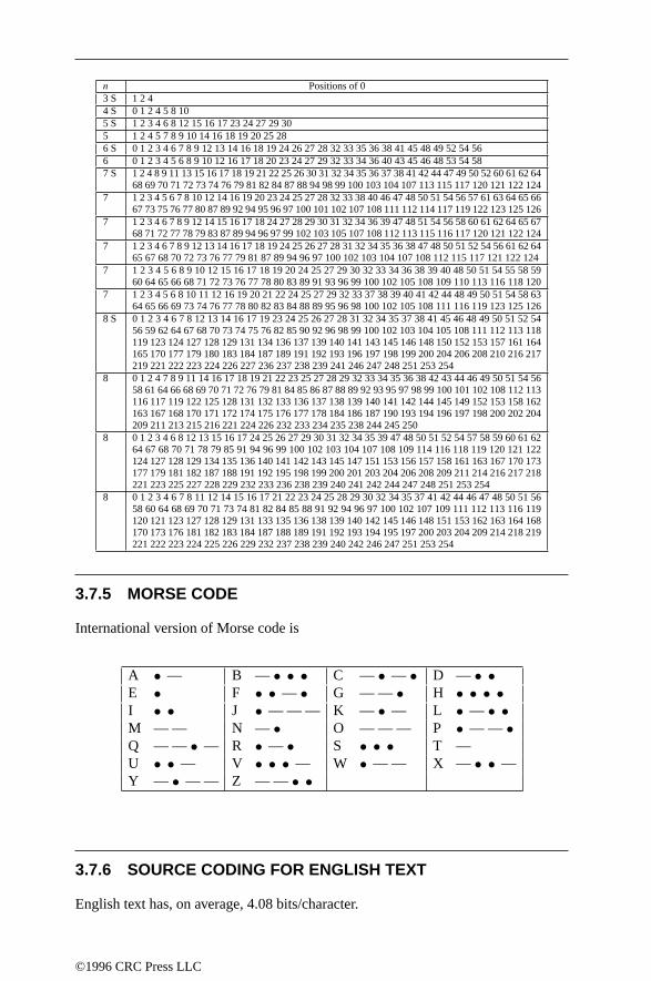
n Positions of 03 S 1 2 44 S 0 1 2 4 5 8 105 S 1 2 3 4 6 8 12 15 16 17 23 24 27 29 305 1 2 4 5 7 8 9 10 14 16 18 19 20 25 286 S 0 1 2 3 4 6 7 8 9 12 13 14 16 18 19 24 26 27 28 32 33 35 36 38 41 45 48 49 52 54 566 0 1 2 3 4 5 6 8 9 10 12 16 17 18 20 23 24 27 29 32 33 34 36 40 43 45 46 48 53 54 587 S 1 2 4 8 9 11 13 15 16 17 18 19 21 22 25 26 30 31 32 34 35 36 37 38 41 42 44 47 49 50 52 60 61 62 64
68 69 70 71 72 73 74 76 79 81 82 84 87 88 94 98 99 100 103 104 107 113 115 117 120 121 122 1247 1 2 3 4 5 6 7 8 10 12 14 16 19 20 23 24 25 27 28 32 33 38 40 46 47 48 50 51 54 56 57 61 63 64 65 66
67 73 75 76 77 80 87 89 92 94 95 96 97 100 101 102 107 108 111 112 114 117 119 122 123 125 1267 1 2 3 4 6 7 8 9 12 14 15 16 17 18 24 27 28 29 30 31 32 34 36 39 47 48 51 54 56 58 60 61 62 64 65 67
68 71 72 77 78 79 83 87 89 94 96 97 99 102 103 105 107 108 112 113 115 116 117 120 121 122 1247 1 2 3 4 6 7 8 9 12 13 14 16 17 18 19 24 25 26 27 28 31 32 34 35 36 38 47 48 50 51 52 54 56 61 62 64
65 67 68 70 72 73 76 77 79 81 87 89 94 96 97 100 102 103 104 107 108 112 115 117 121 122 1247 1 2 3 4 5 6 8 9 10 12 15 16 17 18 19 20 24 25 27 29 30 32 33 34 36 38 39 40 48 50 51 54 55 58 59
60 64 65 66 68 71 72 73 76 77 78 80 83 89 91 93 96 99 100 102 105 108 109 110 113 116 118 1207 1 2 3 4 5 6 8 10 11 12 16 19 20 21 22 24 25 27 29 32 33 37 38 39 40 41 42 44 48 49 50 51 54 58 63
64 65 66 69 73 74 76 77 78 80 82 83 84 88 89 95 96 98 100 102 105 108 111 116 119 123 125 1268 S 0 1 2 3 4 6 7 8 12 13 14 16 17 19 23 24 25 26 27 28 31 32 34 35 37 38 41 45 46 48 49 50 51 52 54
56 59 62 64 67 68 70 73 74 75 76 82 85 90 92 96 98 99 100 102 103 104 105 108 111 112 113 118119 123 124 127 128 129 131 134 136 137 139 140 141 143 145 146 148 150 152 153 157 161 164165 170 177 179 180 183 184 187 189 191 192 193 196 197 198 199 200 204 206 208 210 216 217219 221 222 223 224 226 227 236 237 238 239 241 246 247 248 251 253 254
8 0 1 2 4 7 8 9 11 14 16 17 18 19 21 22 23 25 27 28 29 32 33 34 35 36 38 42 43 44 46 49 50 51 54 5658 61 64 66 68 69 70 71 72 76 79 81 84 85 86 87 88 89 92 93 95 97 98 99 100 101 102 108 112 113116 117 119 122 125 128 131 132 133 136 137 138 139 140 141 142 144 145 149 152 153 158 162163 167 168 170 171 172 174 175 176 177 178 184 186 187 190 193 194 196 197 198 200 202 204209 211 213 215 216 221 224 226 232 233 234 235 238 244 245 250
8 0 1 2 3 4 6 8 12 13 15 16 17 24 25 26 27 29 30 31 32 34 35 39 47 48 50 51 52 54 57 58 59 60 61 6264 67 68 70 71 78 79 85 91 94 96 99 100 102 103 104 107 108 109 114 116 118 119 120 121 122124 127 128 129 134 135 136 140 141 142 143 145 147 151 153 156 157 158 161 163 167 170 173177 179 181 182 187 188 191 192 195 198 199 200 201 203 204 206 208 209 211 214 216 217 218221 223 225 227 228 229 232 233 236 238 239 240 241 242 244 247 248 251 253 254
8 0 1 2 3 4 6 7 8 11 12 14 15 16 17 21 22 23 24 25 28 29 30 32 34 35 37 41 42 44 46 47 48 50 51 5658 60 64 68 69 70 71 73 74 81 82 84 85 88 91 92 94 96 97 100 102 107 109 111 112 113 116 119120 121 123 127 128 129 131 133 135 136 138 139 140 142 145 146 148 151 153 162 163 164 168170 173 176 181 182 183 184 187 188 189 191 192 193 194 195 197 200 203 204 209 214 218 219221 222 223 224 225 226 229 232 237 238 239 240 242 246 247 251 253 254
3.7.5 MORSE CODE
International version of Morse code is
A • — B — • • • C — • — • D — • •E • F • • — • G — — • H • • • •I • • J • — — — K — • — L • — • •M — — N — • O — — — P • — — •Q — — • — R • — • S • • • T —U • • — V • • • — W • — — X — • • —Y — • — — Z — — • •
3.7.6 SOURCE CODING FOR ENGLISH TEXT
English text has, on average, 4.08 bits/character.
©1996 CRC Press LLC

Letter Probability Huffman code Alphabetical codeSpace 0.1859 000 00A 0.0642 0100 0100B 0.0127 011111 010100C 0.0218 11111 010101D 0.0317 01011 01011
E 0.1031 101 0110F 0.0208 001100 011100G 0.0152 011101 011101H 0.0467 1110 01111I 0.0575 1000 1000
J 0.0008 0111001110 1001000K 0.0049 01110010 1001001L 0.0321 01010 100101M 0.0198 001101 10011N 0.0574 1001 1010
O 0.0632 0110 1011P 0.0152 011110 110000Q 0.0008 0111001101 110001R 0.0484 1101 11001S 0.0514 0010 1101
T 0.0796 0010 1110U 0.0228 11110 111100V 0.0083 0111000 111101W 0.0175 001110 111110X 0.0013 0111001100 1111110
Y 0.0164 001111 11111110Z 0.0005 0111001111 11111111Cost 4.0799 4.1195 4.1978
3.7.7 GRAY CODE
A Gray code is a sequence ordering such that a small change in the sequence num-ber results in a small change in the sequence. For example, the 16 4-bit strings0000,0001, . . . ,1111 can be ordered so that adjacent bit strings differ in only 1 bit:
Sequence numberBit string Sequence numberBit string0 0000 8 11001 0001 9 11012 0011 10 11113 0010 11 11104 0110 12 10105 0111 13 10116 0101 14 10017 0100 15 1000
©1996 CRC Press LLC

As another example, the subsets ofa, b, c can be ordered so that adjacentsubsets differ by only the insertion or deletion of a single element:
φ, a, a, b, b, b, c, a, b, c, a, c, c.
3.8 COSTAS ARRAYS
An n×n Costas array is an array of zeros and ones whose autocorrelation function isn at the origin and no more than 1 anywhere else. There areBn basic Costas arrays;there areCn arrays when rotations and flips are allowed. Each array can be interpretedas a permutation.
n 1 2 3 4 5 6 7 8 9 10 11 12Bn 1 1 1 2 6 17 13 17 30 60 555 990Cn 1 2 4 12 40 116 200 444 7602160 4368 7852
n 13 14 15 16 17 18 19 20Bn 1616 2168 2467 2648 2294 1892 1283 810Cn 12828 17252 19612 21104 18276 15096 10240 6464
Bn:
· · ·
C4:
©1996 CRC Press LLC

3.9 DIFFERENCE EQUATIONS
3.9.1 THE CALCULUS OF FINITE DIFFERENCES
1. (f (x)) = f (x + h) − f (x) (forward difference).
2. 2(f (x)) = f (x + 2h) − 2f (x + h) + f (x).
3. n(f (x)) = (n−1(f (x))
) =n∑
k=0
(−1)k(n
k
)f (x + (n − k)h).
4. (cf (x)) = c(f (x)).
5. (f (x) + g(x)) = (f (x)) + (g(x)).
6. (f (x)g(x)) = g(x)(f (x)) + f (x)(g(x)).
7.
(f (x)
g(x)
)= g(x)(f (x))−f (x)(g(x))
g(x)g(x+h),
provided thatg(x)g(x + h) = 0.
8. n(xn) = n !hn, n = 0,1, . . . .
3.9.2 EXISTENCE AND UNIQUENESS
A difference equation of order k has the form
xn+k = f (xn, xn+1, . . . , xn+(k−1), n) (3.9.1)
wheref is a given function andk is a positive integer. Asolution to Equation (3.9.1)is a sequence of numbersxn∞n=0 which satisfies the equation. Any constant solutionof Equation (3.9.1) is called anequilibrium solution.
A linear difference equation of orderk has the form
a(k)n xn+k + a(k−1)n xn+(k−1) + · · · + a(1)n xn−1 + a(0)n xn = gn, (3.9.2)
wherek is a positive integer and the coefficientsa(0)n , . . . , a(k)n along withgn aregiven sequences. If the sequencegn is identically zero, then Equation (3.9.2) is calledhomogeneous; otherwise, it is callednonhomogeneous. If the coefficientsa(0), . . . ,a(k) are constants, Equation (3.9.2) is a difference equation with constant coefficients;otherwise it is a difference equation with variable coefficients.
THEOREM 3.9.1 (Existence and uniqueness)
Consider the initial value problem (IVP)
xn+k + b(k−1)n xn+(k−1) + · · · + b(1)n xn+1 + b(0)n xn = fn, (3.9.3)
xi = αi, i = 0,1, . . . , k − 1, (3.9.4)
©1996 CRC Press LLC

for n = 0,1, . . . , where b(i)n and fn are given sequences with b(0)n = 0 for all nand the αi are given initial conditions. Then the above equations have exactly onesolution.
3.9.3 LINEAR INDEPENDENCE: GENERAL SOLUTION
The sequencesx(1)n , x(2)n , . . . , x(k)n arelinearly dependent if constantsc1, c2, . . . , ck(not all of them zero) exist such that
k∑i=1
cix(i)n = 0 for n = 0,1, . . . . (3.9.5)
Otherwise the sequencesx(1)n , x(2)n , . . . , x(k)n arelinearly independent.TheCasoratian of thek sequencesx(1)n , x(2)n , . . . , x(k)n is thek × k determinant
C(x(1)n , x(2)n , . . . , x(k)n
) =
∣∣∣∣∣∣∣∣x(1)n x(2)n · · · x(k)n
x(1)n+1 x
(2)n+1 · · · x
(k)n+1
. . . . . . . . . . . . . . . . . . . . . . . . . . .
x(1)n+k−1 x
(2)n+k−1 · · · x
(k)n+k−1
∣∣∣∣∣∣∣∣ . (3.9.6)
THEOREM 3.9.2
The solutions x(1)n , x(2)n , . . . , x(k)n of the linear homogeneous difference equation,
xn+k + b(k−1)n xn+(k−1) + · · · + b(1)n xn+1 + b(0)n xn = 0, n = 0,1, . . . ,
(3.9.7)
are linearly independent if, and only if, their Casoratian is different from zero forn = 0.
The setx(1)n , x(2)n , . . . , x(k)n
is a fundamental system of solutions for Equation
(3.9.7) if, and only if, the sequencesx(1)n , x(2)n , . . . , x(k)n are linearly independentsolutions of the homogeneous difference equation (3.9.7).
THEOREM 3.9.3
Consider the nonhomogeneous linear difference equation
xn+k + b(k−1)n xn+(k−1) + · · · + b(1)n xn+1 + b(0)n xn = dn, n = 0,1, . . .
(3.9.8)
where b(i)n and dn are given sequences. Let x(h)n be the general solution of the corre-sponding homogeneous equation
xn+k + b(k−1)n xn+(k−1) + · · · + b(1)n xn+1 + b(0)n xn = 0, n = 0,1, . . . ,
and let x(p)n be a particular solution of Equation (3.9.8). Then x(p)n + x(h)n is the
general solution of Equation (3.9.8).
©1996 CRC Press LLC

THEOREM 3.9.4 (Superposition principle)
Let x(1)n and x(2)n be solutions of the nonhomogeneous linear difference equations
xn+k + b(k−1)n xn+(k−1) + · · · + b(1)n xn+1 + b(0)n xn = αn, n = 0,1, . . . ,
and
xn+k + b(k−1)n xn+(k−1) + · · · + b(1)n xn+1 + b(0)n xn = βn, n = 0,1, . . . ,
respectively, where b(i)n and αn and βn are given sequences. Then x(1)n + x(2)n is asolution of the equation
xn+k + b(k−1)n xn+(k−1) + · · · + b(1)n xn+1 + b(0)n xn = αn + βn, n = 0,1, . . . .
3.9.4 HOMOGENEOUS EQUATIONS WITH CONSTANTCOEFFICIENTS
The results given below for second-order linear difference equations extend naturallyto higher order equations.
Consider the second-order linear homogeneous difference equation,
α2xn+2 + α1xn+1 + α0xn = 0, (3.9.9)
where theαi are real constant coefficients withα2α0 = 0. Thecharacteristic equa-tion corresponding to Equation (3.9.9) is defined as the quadratic equation
α2λ2 + α1λ + α0 = 0. (3.9.10)
The solutionsλ1, λ2 of the characteristic equation are theeigenvalues or thecharac-teristic roots of Equation (3.9.9).
THEOREM 3.9.5
Let λ1 and λ2 be the eigenvalues of Equation (3.9.9). Then the general solution ofEquation (3.9.9) is given as described below with arbitrary constants c1 and c2.
Case 1: λ1 = λ2 with λ1, λ2 ∈ R (real and distinct roots).The general solution is given by xn = c1λ
n1 + c2λ
n2.
Case 2: λ1 = λ2 ∈ R (real and equal roots) .The general solution is given by xn = c1λ
n1 + c2nλ
n1.
Case 3: λ1 = λ2 (complex conjugate roots).Suppose that λ1 = reiφ . The general solution is given by
xn = c1rn cos(nφ) + c2r
n sin(nφ).
©1996 CRC Press LLC

Example: The unique solution of the initial value problem
Fn+2 = Fn+1 + Fn, n = 0,1, . . . ,
F0 = 0, F1 = 1,
is theFibonacci sequence. Using Theorem 3.9.5one can show that
Fn = 1√5
[(1 + √
5
2
)n
−(
1 − √5
2
)n], n = 0,1, . . . .
3.9.5 NONHOMOGENEOUS EQUATIONS WITH CONSTANTCOEFFICIENTS
THEOREM 3.9.6 (Variation of parameters)
Consider the difference equation, xn+2 + αnxn+1 + βnxn = γn, where αn, βn, andγn are given sequences with βn = 0. Let x(1)n and x(2)n be two linearly independentsolutions of the homogeneous equation corresponding to this equation. A particularsolution is given by x(p)n = x(1)n v(1)n +x(2)n v(2)n where the sequences v(1)n and v(2)n satisfythe following system of equations:
x(1)n+1
(v(1)n+1 − v(1)n
)+ x
(2)n+1
(v(2)n+1 − v(2)n
)= 0, and
x(1)n+2
(v(1)n+1 − v(1)n
)+ x
(2)n+2
(v(2)n+1 − v(2)n
)= γn.
(3.9.11)
3.9.6 GENERATING FUNCTIONS AND Z TRANSFORMS
Generating functions can be used to solve initial value problems of difference equa-tions in the same way that Laplace transforms are used to solve initial value problemsof differential equations.
Thegenerating function of the sequencexn, denoted byG[xn], is defined bythe infinite series
G[xn] =∞∑n=0
xnsn (3.9.12)
provided that the series converges for| s | < r, for some positive numberr. Thefollowing are useful properties of the generating function:
1. Linearity: G c1xn + c2yn = c1G xn + c2G yn .
2. Translation invariance: G[xn+k
] = 1
sk
(G [xn] −
k−1∑n=0
xnsn
).
3. Uniqueness: G [xn] = G [yn] ⇔ xn = yn for n = 0,1, . . . ,
©1996 CRC Press LLC

xn G [xn]
11
1 − s
an1
1 − as
nanas
(1 − as)2
npan(sd
ds
)p 1
1 − as
ns
(1 − s)2
n + 11
(1 − s)2
np(sd
ds
)p 1
1 − s
sin(βn)s sinβ
1 − 2s cosβ + s2
cos(βn)1 − s cosβ
1 − 2s cosβ + s2
an sin(βn)as sinβ
1 − 2as cosβ + a2s2
an cos(βn)1 − as cosβ
1 − 2as cosβ + a2s2
xn+11
s(G [xn] − x0)
xn+21
s2(G [xn] − x0 − sx1)
xn+k
1
sk
(G [xn] −
k−1∑n=0
xnsn
)
TheZ-transform of a sequencexn is denoted byZ[xn] and is defined by theinfinite series,
Z[xn] =∞∑n=0
xn
zn, (3.9.13)
provided that the series converges for| z | > r, for some positive numberr.
©1996 CRC Press LLC

Comparing the definitions for the generating function and theZ-tranform one canseethat they areconnected becauseEquation (3.9.13) can beobtained from Equation(3.9.12) by settings = z−1.
3.9.7 CLOSED FORM SOLUTIONS FOR SPECIAL EQUATIONS
In general, it is difficult to find a closed form solution for a difference equation which isnot linear of order one or linear of any order with constant coefficients. A few specialdifference equations which possess closed form solutions are presented below.
THEOREM 3.9.7
The general solution of the first-order linear difference equation with variablecoefficients,
xn+1 − αnxn = βn, n = 0,1, . . . , (3.9.14)
is given by
xn =(n−1∏k=0
αk
)x0 +
n−2∑m=0
(n−1∏
k=m+1
αk
)βm + βn−1, n = 0,1, . . . ,
(3.9.15)
where x0 is an arbitrary constant.
Riccati equationConsider the nonlinear first order equation,
xn+1 = αnxn + βn
γnxn + δn, n = 0,1, . . . , (3.9.16)
whereαn, βn, γn, δn are given sequences of real numbers with
γn = 0 and
∣∣∣∣ αn βnγn δn
∣∣∣∣ = 0, n = 0,1, . . . .(3.9.17)
The following statements are true:
1. The change of variables,un+1
un= γnxn + δn, n = 0,1, . . . ,
u0 = 1,(3.9.18)
reduces Equation (3.9.16) to the linear second order equation,
un+2 = Anun + Bn, n = 0,1, . . . ,
u0 = 1,
u1 = γ0x0 + δ0,
(3.9.19)
whereAn = δn+1 + αnγn+1
γn, andBn = (βnγn − αnδn)
γn+1
γn.
©1996 CRC Press LLC
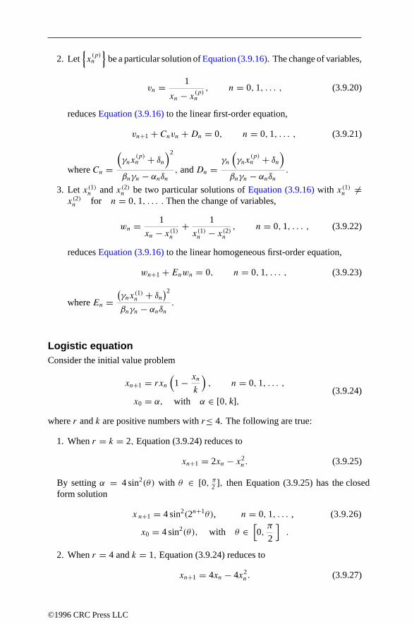
2. Letx(p)n
be aparticular solutionof Equation(3.9.16). Thechangeof variables,
vn = 1
xn − x(p)n
, n = 0,1, . . . , (3.9.20)
reducesEquation (3.9.16) to the linear first-order equation,
vn+1 + Cnvn + Dn = 0, n = 0,1, . . . , (3.9.21)
whereCn =(γnx
(p)n + δn
)2
βnγn − αnδn, andDn =
γn
(γnx
(p)n + δn
)βnγn − αnδn
.
3. Let x(1)n andx(2)n be two particular solutions of Equation (3.9.16) with x(1)n =x(2)n for n = 0,1, . . . . Then the change of variables,
wn = 1
xn − x(1)n
+ 1
x(1)n − x(2)n
, n = 0,1, . . . , (3.9.22)
reducesEquation (3.9.16) to the linear homogeneousfirst-order equation,
wn+1 + Enwn = 0, n = 0,1, . . . , (3.9.23)
whereEn =(γnx
(1)n + δn
)2βnγn − αnδn
.
Logistic equationConsider the initial value problem
xn+1 = rxn
(1 − xn
k
), n = 0,1, . . . ,
x0 = α, with α ∈ [0, k],(3.9.24)
where r and k arepositivenumberswith r≤ 4. The following are true:
1. Whenr = k = 2, Equation (3.9.24) reduces to
xn+1 = 2xn − x2n. (3.9.25)
By setting α = 4 sin2(θ) with θ ∈ [0, π2 ], then Equation (3.9.25) has the closed
form solution
x n+1 = 4 sin2(2n+1θ), n = 0,1, . . . , (3.9.26)
x0 = 4 sin2(θ), with θ ∈[0,
π
2
].
2. Whenr = 4 andk = 1, Equation (3.9.24) reduces to
xn+1 = 4xn − 4x2n. (3.9.27)
©1996 CRC Press LLC

By setting α = sin2(θ) with θ ∈ [0, π2
], then Equation (3.9.27) has the closed
form solution
xn+1 = sin2(2n+1θ), n = 0,1, . . . ,
x0 = sin2(θ), with θ ∈[0,
π
2
].
3.10 DISCRETE DYNAMICAL SYSTEMS ANDCHAOS
Let the distance between successive bifurcations of a process bedk. The limitingratio, δ = limk→∞ dk/dk+1, Feigenbaum’s constant, is constant in many situations;δ ≈ 4.6692016091029.
3.10.1 CHAOTIC ONE-DIMENSIONAL MAPS
1. Logistic map: xn+1 = 4xn(1 − xn).
Solution isxn = 1
2− 1
2cos[2n cos−1(1 − 2x0)].
2. Tent map:xn+1 = 1 − 2∣∣xn − 1
2
∣∣ .Solution isxn = 1
πcos−1[cos(2nπx0)].
3. Baker transformation:xn+1 = 2xn (mod 1).
Solution isxn = 1
πcot−1[cot(2nπx0)].
3.10.2 LOGISTIC MAP
Considerun+1 = f (un) = aun(1 − un). The fixed points satisfyu = f (u) =au(1 − u); they areu = 0 andu = (a − 1)/a.
• If a = 0 thenun = 0.
• If 0 < a ≤ 1 thenun → 0.
• If 1 < a < 3 thenun → (a − 1)/a.
• If 3 < a < 3.449490. . . thenun oscillates between the two roots ofu =f (f (u))which are not roots ofu = f (u), that is,u± = (a+1±√
a2 − 2a − 3)/2a.
©1996 CRC Press LLC

The location of the final state is summarized by the following diagram.
0
0.2
0.4
0.6
0.8
1
0 1 2 3 4
Bifurcation diagram
3.10.3 JULIA SETS AND THE MANDELBROT SET
For the function f (x) = x2 + c consider the iterates of all complex points z, zn+1 =f (zn) with z0 = z. For each z, either the iterates remain bounded (z is in the prisonerset) or they escape to infinity (z is in the escape set). The Julia set Jc is the commonboundary between these two sets. Using lighter colors to indicate a “faster” escapeto infinity, Figure 3.10.6 shows two Julia sets. One of these Julia sets is connected,the other is disconnected. The Mandelbrot set, M , is the set of those complex valuesc for which Jc is a connected set (see Figure 3.10.7). Alternately, the Mandelbrot setconsists of all points c for which the discrete dynamical system, zn+1 = z2
n + c withz0 = 0, converges.
The boundary of the Mandelbrot set is a fractal. There is no universally agreedupon definition of “fractal”. One definition is that it is a set whose fractal dimensiondiffers from its topological dimension.
3.11 OPERATIONS RESEARCH
3.11.1 LINEAR PROGRAMMING
Linear programming (LP) is a technique for modeling problems with linear objectivefunctions and linear constraints. The standard form for an LP model with n decision
©1996 CRC Press LLC

FIGURE 3.10.6Connected Julia set for c = −0.5i (left). Disconnected Julia set for c = − 3
4 (1 + i) (right).
FIGURE 3.10.7The Mandelbrot set. The leftmost point has the coordinates (−2, 0).
variables and m resource constraints is
Minimizen∑
j=1
cjxj (objective function),
Subject to
xj ≥ 0 for j = 1, · · · , n,
n∑j=1
aij xj = bi for i = 1, · · · ,m (constraint functions),(3.11.1)
where xj is the amount of decision variable j used, cj is decision j ′s per unit contribu-tion to the objective, aij is decision j ′s per unit usage of resource i, and bi is the totalamount of resource i available. Let x represent the (n × 1) vector (x1, x2, · · · , xn),c the (1 × n) vector (c1, c2, · · · , cn), b the (m × 1) vector (b1, b2, · · · , bm), A the(m × n) matrix (aij ), and A·j the (n × 1) column of A associated with xj .
©1996 CRC Press LLC

The standard model, written in matrix notation, is “minimize cx subject toAx ≥ band x ≥ 0.” A vector x is called feasible if, and only if, Ax = b and x ≥ 0.
Modeling in LPLP is an appropriate modeling technique if the following four assumptions are satisfiedby the situation:
1. All data coefficients are known with certainty.
2. There is a single objective.
3. The problem relationships are linear functions of the decisions.
4. The decisions can take on continuous values.
Branches of optimization such as stochastic programming, multiobjective pro-gramming, nonlinear programming, and integer programming have developed in op-erations research to allow a richer variety of models and solution techniques forsituations where the assumptions required for LP are inappropriate.
• Product mix problem:Consider a company that has three products to sell. Each product requires fouroperations and the per unit data are given in the following table:
Product Drilling Assembly Finishing Packing ProfitA 2 3 1 2 45B 3 6 2 4 90C 2 1 4 1 55
Hours available 480 960 540 320
Let xA, xB, and xC represent the number of units of A, B, and C manufactureddaily. A model to maximize profit subject to the labor restrictions is
Maximize 45xA + 90xB + 55xC (total profit),
Subject to:
2xA + 3xB + 2xC ≤ 480 (drilling hours),
3xA + 6xB + 1xC ≤ 960 (assembly hours),
1xA + 2xB + 4xC ≤ 540 (finishing hours),
2xA + 4xB + 1xC ≤ 320 (packing hours),
xA ≥ 0, xB ≥ 0, xC ≥ 0.
(3.11.2)
• Maximum flow through a network:Consider the directed network in Figure 3.11.8. Node S denotes the source nodeand node T denotes the terminal node. On each arc shipping material up to thearc capacity Cij is permitted. Material is neither created nor destroyed at nodesother than S and T . The goal is to maximize the amount of material that can beshipped through the network from S to T . Letting xij represent the amount ofmaterial shipped from node i to node j , a model that determines the maximumflow is shown below.
©1996 CRC Press LLC

FIGURE 3.11.8Directed network modeling a flow problem.
Maximize x1T + x3T + x4T ,
Subject to
xS1 = x13 + x14 + x1T (node 1 conservation),
xS2 = x23 + x24 (node 2 conservation),
x13 + x23 = x3T (node 3 conservation),
xS4 + x24 + x14 = x4T (node 4 conservation),
0 ≤ xij ≤ Cij for all (i, j) pairs (arc capacity).
(3.11.3)
Transformation to standard form
Any LP model can be transformed to standard form using the operations in the fol-lowing table:
Original model Standard formmaximize objective minimize objective
multiply cj by −1 (for example: cj = −cj )≤ constraint = constraint
add slack variable(s) ton∑
j=1
aij xj ≤ bi
(for example:n∑
j=1
aij xj + Si = bi.)
≥ constraint = constraint
subtract surplus variable(s) fromn∑
j=1
aij xj ≥ bi
(for example:n∑
j=1
aij xj − Ui = bi)
= constraint = constraintno change required
©1996 CRC Press LLC

LP requires that the slack and surplus variables be nonnegative, therefore, deci-sions are feasible to the new constraint if, and only if, they are feasible to the originalconstraint. All slack and surplus variables have cj = 0.
Assume that there is at least one feasible x vector, and that A has rank m. Geometri-cally, because all constraints are linear, the set of feasible x forms a convex polyhedralset (bounded or unbounded) that must have at least one extreme point. The motivationfor the simplex method for solving LP models is the following:
For any LP model with a bounded optimal solution, an optimal solutionexists at an extreme point of the feasible set.
Given a feasible solution x, let xB be the components of x with xj > 0 and xN
be the components with xj = 0. Associated with xB , define B as the columns of Aassociated with each xj in xB . For example, if x2, x4, and S1 are positive in x, thenxB = (x2, x4, S1), and B is the matrix with columns A·2, A·4, A·S1 . Define N as theremaining columns of A, i.e., those associated with xN . A basic feasible solution(BFS) is a feasible solution where the columns of B are linearly independent. Thefollowing theorem relates a BFS with extreme points:
A feasible solution x is at an extreme point of the feasible region if, andonly if, x is a BFS.
The following simplex method finds an optimal solution to the LP by finding theoptimal partition of x into xB and xN :
1. Find an initial basic feasible solution. Define xB , xN , B, N , cB , and cN as above.
2. Compute the vector c′ = (cN − cBB−1N). If c′j ≥ 0 for all j , then stop; the
solution xB = B−1b is optimal with objective value cBB−1b. Otherwise, selectthe variable xj in xN with the most negative c′
j value, and go to step 3.
3. Compute A′·j = B−1A·j . If A′
ij ≤ 0 for all j , then stop; the problem is un-bounded and the objective can decrease to −∞. Otherwise, compute b′ = B−1b
and find mini|a′
ij>0
b′i
a′ij
. Assume the minimum ratio occurs in row r . Insert xj into
the rth position of xB, take the variable that was in this position, and move itto xN . Update B, N , cB , and cN accordingly. Return to step 2.
Ties in the selections in steps 2 and 3 can be broken arbitrarily. The unbound-edness signal suggests that the model is missing constraints or that there has been adata entry or computational error, because, in real problems, the profit or cost cannotbe unbounded. For maximization problems, only step 2 changes. The solution isoptimal when c′
j ≤ 0 for all j , then choose the variable with the maximum c′j value
to move into xB . Effective methods for updating B−1 in each iteration of step 3 existto ease the computational burden.
To find an initial basic feasible solution define a variable Ai and add this variableto the left hand side of constraint i transforming to
∑nj=1 aij + Ai = bi. The new
©1996 CRC Press LLC

constraint is equivalent to the original constraint if, and only if, Ai = 0. Also, becauseAi appears only in constraint i and there aremAi variables, the columns correspondingto the Ai variables are a rank m linearly independent set. We now solve a “new” LPmodel with the adjusted constraints and the new objective “minimize
∑mi=1 Ai .” If
the optimal solution to this new model is 0, the solution is a basic feasible solutionto the original problem. Otherwise, no basic feasible solution exists for the originalproblem.
Solving LP models: interior point methodAn alternative method to searching extreme points is to cut through the middle of thepolyhedron and go directly towards the optimal solution. Extreme points, however,provide an efficient method of determining movement directions (step 1 of simplexmethod) and movement distances (step 2 of simplex method). There were no effectivemethods on the interior of the feasible set until Karmarkar’s method was developedin 1984. The method assumes that the model has the following form:
Minimizen∑
j=1
cjxj ,
Subject to
n∑j=1
aij xj = 0 for i = 1, · · · ,m,
n∑j=1
xj = 1,
xj ≥ 0, for j = 1, · · · , n.
(3.11.4)
Also, assume that the optimal objective value is 0 and that the xj = 1/n for j =1, · · · , n is feasible. Any model can be transformed so that these assumptions hold.
The following centering transformation, relative to the kth estimate of solutionvector xk , takes any feasible solution vector x and transforms it to y such that the xk is
transformed to the center of the feasible simplex: yj = xj/xkj∑n
r=1(xr/xkr )
. Let Diag(xk)
represent an n × n matrix with off-diagonal entries equal to 0 and the diagonal entryin row j equal to xk
j . The formal algorithm is as follows:
1. Initialize x0j = 1/n and set the iteration count k = 0.
2. Ifn∑
j=1
xkj cj is sufficiently close to 0, then stop. xk is optimal. Otherwise go to
step 3.
3. Move from the center of the transformed space in an improving direction using
yk+1 =[
1
n,
1
n, · · · ,
1
n
]T
− θ(I − PT (PP T )−1P)[Diag(xk)]cT
||Cp||√n(n − 1),
where ||Cp|| is the length of the vector (I − PT (PP T )−1P)[Diag(xk)]cT , P isan (m+1)×n matrix whose first m rows are A[Diag(xk)] and whose last row isa vector of 1′s, and θ is a parameter that must be between 0 and 1. Go to step 4.
©1996 CRC Press LLC

4. Find the new point xk+1 in the original space by applying the inverse transfor-mation of the centering transformation to yk+1. Set k = k + 1 and return tostep 2.
The method is guaranteed to converge to the optimal solution when θ = 14 is
used.
3.11.2 DUALITY AND COMPLEMENTARY SLACKNESS
Define yi as the dual variable (shadow price) representing the purchase price for aunit of resource i. The dual problem to the primal model (maximize objective, all ≤constraints) is
Minimizem∑
i=1
biyi,
Subject to
m∑i=1
aij yi ≥ cj for j = 1, . . . , n,
yi ≥ 0, for i = 1, . . . , m.
(3.11.5)
The objective minimizes the amount of money spent to obtain the resources. Theconstraints ensure that the marginal cost of the resources is greater than or equal tothe marginal profit for each product.
The following results link the dual model (minimization) with its primal model(maximization).
• Weak duality theorem: Assume that x and y are feasible solutions to the respec-tive primal and dual problems. Then
n∑j=1
cjxj ≤m∑
i=1
biyi .
• Strong duality theorem: Assume that the primal has a finite optimal solution x∗.Then the dual has a finite optimal solution y∗, and
n∑j=1
cjx∗j =
m∑i=1
biy∗i .
• Complementary slackness theorem: Assume that x and y are feasible solutionsto the respective primal and dual problems. Then, x is optimal for the primaland y is optimal for the dual if and only if:
yi ·(bi −
n∑j=1
aij xj
)= 0, for i = 1, · · · ,m,
and xj ·(
m∑i=1
aij yi − cj
)= 0, for j = 1, · · · , n. (3.11.6)
©1996 CRC Press LLC

3.11.3 LINEAR INTEGER PROGRAMMING
Linear integer programming models result from restricting the decisions in linearprogramming models to be integer valued. The standard form is
Minimizen∑
j=1
cjxj (objective function),
Subject to
xj ≥ 0, and integer for j = 1, . . . , n,n∑
j=1
aij xj = bi for i = 1, . . . , m (constraint functions).(3.11.7)
As long as the variable values are bounded, then the general model can be trans-formed into a model where all variable values are restricted to either 0 or 1. Therefore,algorithms that can solve 0–1 integer programming models are sufficient for mostapplications.
3.11.4 BRANCH AND BOUND
Branch and bound implicitly enumerates all feasible integer solutions to find theoptimal solution. The main idea is to break the feasible set into subsets (branching)and then evaluate the best solution in each subset or determine that the subset cannotcontain the optimal solution (bounding). When a subset is evaluated, it is said tobe “fathomed”. The following algorithm performs the branching by partitioning onvariables with fractional values and uses a linear programming relaxation to generatea bound on the best solution in a subset:
1. Assume that a feasible integer solution, denoted “the incumbent”, is knownwhose objective function value is z (initially, z may be set to infinity if no feasiblesolution is known). Set p, the subset counter equal to 1. Set the original modelas the first problem in the subset list.
2. If p = 0, then stop. The incumbent solution is the optimal solution. Otherwisego to step 3.
3. Solve the LP relaxation of problem p in the subset list (allow all integer valuedvariables to take on continuous values). Denote the LP objective value by v.If v ≥ z or the LP is infeasible, then set p = p − 1 (fathom by bound orinfeasibility), and return to step 2. If the LP solution is integer valued, thenupdate the incumbent to the LP solution, set z = min(z, v) and p = p − 1, andreturn to step 2. Otherwise, go to step 4.
4. Take any variable xj with fractional value in the LP solution. Replace problemp with two problems created by individually adding the constraints xj ≤ ⌊
xj
⌋and xj ≥ ⌈
xj
⌉to problem p. Add these two problems to the bottom of the
subset list, set p = p + 1, and go to step 2.
©1996 CRC Press LLC

3.11.5 NETWORK FLOW METHODS
A network consists of N, the set of nodes, and A, the set of arcs. Each arc (i, j)
defines a connection from node i to node j . Depending on the application, arc (i, j)
may have an associated cost and upper and lower capacity on flow.Decision problems on networks can often be modeled using linear programming
models, and these models usually have the property that solutions from the simplexmethod are integer valued (the total unimodularity property). Because of the under-lying graphical structure, more efficient algorithms are also available. We presentthe augmenting path algorithm for the maximum flow problem and the Hungarianmethod for the assignment problem.
Maximum flowLet xij represent the flow on arc (i, j), cij the flow capacity of (i, j), S be the sourcenode, and T be the terminal node. The maximum flow problem is to ship as muchflow from S to T without violating the capacity on any arc, and all flow sent intonode i must leave i (for i = S, T ). The following algorithm solves the problem bycontinually adding flow-carrying paths until no path can be found:
1. Initialize xij = 0 for all (i, j).
2. Find a flow-augmenting path from S to T using the following labeling method.Start by labeling S with a∗. From any labeled node i, label node j with the labeli if j is unlabeled and xij < cij (“forward labeling arc”). From any labelednode i, label node j with the label i if j is unlabeled and xji > 0 (“backwardlabeling arc”). Perform labeling until no additional nodes can be labeled. If T
cannot be labeled, then stop. The current xij values are optimal. Otherwise, goto step 3.
3. There is a path from S to T where flow is increased on the forward labeling arcs,decreased on the backward labeling arcs, and gets more flow from S to T . LetF be the minimum of cij − xij over all forward labeling arcs and of xij over allbackward labeling arcs. Set xij = xij +F for the forward arcs and xij = xij −F
for the backward arcs. Return to step 2.
The algorithm terminates with a set of arcs with xij = cij and if these are deleted,then S and T are in two disconnected pieces of the network. The algorithm finds themaximum flow by finding the minimum capacity set of arcs that disconnects S andT (minimum capacity cutset).
3.11.6 ASSIGNMENT PROBLEM
Consider a set J of jobs and a set I of employees. Each employee can do 1 job, andeach job must be done by 1 employee. If job j is assigned to employee i, then thecost to the company is cij . The problem is to assign employees to jobs to minimizethe overall cost.
©1996 CRC Press LLC

This problem can be formulated as an optimization problem on a bipartite graphwhere the jobs are one part and the employees are the other. Let m be the cardinalityof J and I (they must be equal cardinality sets or there is no feasible solution), and letC be the m × m matrix of costs cij . The following algorithm solves for the optimalassignment.
1. Find li = minj
cij for each row i. Let cij = cij − li . Find nj = mini
cij for each
column j . Let cij = cij − nj .
2. Construct a graph with nodes for S, T , and each element of the sets J and I .Construct an arc from S to each node in I, and set its capacity to 1. Constructan arc from each node in J to T , and set its capacity to 1. If cij = 0, thenconstruct an arc from i ∈ I to j ∈ J , and set its capacity to 2. Solve a maximumflow problem on the constructed graph. If m units of flow can go through thenetwork, then stop. The maximum flow solution on the arcs between I and J
represents the optimal assignment. Otherwise, go to step 3.
3. Update C using the following rules based on the labels in the solution to themaximum flow problem: Let LI and LJ be the set of elements of I and J
respectively with labels when the maximum flow algorithm terminates. Letδ = min
i∈LI ,j∈(J−LJ )cij ; note that δ > 0. For i ∈ LI and j ∈ (J − LJ ), set
cij = cij − δ. For i ∈ (I − LI ) and j ∈ LJ , set cij = cij + δ. Leave all othercij values unchanged. Return to step 2.
In step 3, the algorithm creates new arcs, eliminates some unused arcs, andleaves unchanged arcs with xij = 1. When returning to step 2, you can solve the nextmaximum flow problem by adding and deleting the appropriate arcs and starting withthe flows and labels of the preceding execution of the maximum flow algorithm.
3.11.7 DYNAMIC PROGRAMMING
Dynamic programming is a technique for determining a sequence of optimal decisionsfor a system or process that operates over time and requires successive dependentdecisions. The following five properties are required for using dynamic programming:
1. The system can be characterized by a set of parameters called state variables.
2. At each decision point or stage of the process, there is a choice of actions.
3. Given the current state and the decision, it is possible to specify how the stateevolves before the next decision.
4. Only the current state matters, not the path by which the system arrived at thestate (termed “time separability”).
5. An objective function depends on the state and the decisions made.
The separability requirement is necessary to formulate a functional form for thedecision problem. Let f ∗
t (i) denote the optimal objective value to take the system
©1996 CRC Press LLC

from stage t to the end of the process, given that the process is now in state i, At(i)
is the set of decisions possible at stage t and state i, aj is a particular action in At(i),*it (aj ) is the change from state i between stage t and stage t + 1 based on the actiontaken, and cit (aj ) is the immediate impact on the objective of taking action aj at staget and state i.
The principle of optimality states as follows:
An optimal sequence of decisions has the property that, whatever theinitial state and initial decision are, the remaining decisions must be anoptimal policy based on the state resulting from the initial information.
Using the principle, Bellman’s equations are
f ∗t (i) = min
aj∈At (i)cit (aj ) + f ∗
t+1[*it (aj )], for all i.
3.11.8 SHORTEST PATH PROBLEM
Consider a network (N,A) where N is the set of nodes, A the set of arcs, and dij
represents the “distance” of traveling on arc (i, j) (if no arc exists between i and j ,dij = ∞). For any two nodes R and S, the shortest path problem is to find the shortestdistance route through the network from R to S. Let the state space be N and a stagerepresenting travel along one arc. f ∗(i) is the optimal distance from node i to S. Theresultant recursive equations to solve are
f ∗(i) = minj∈N
[dij + f ∗(j)
], for all i.
Dijkstra’s algorithm can be used successively to approximate the solution to theequations when dij > 0 for all (i, j).
1. Set f ∗(S) = 0 and f ∗(i) = diS for all i ∈ N . Let P be the set of permanentlylabeled nodes. P = S. Let T = N − P be the set of temporarily labelednodes.
2. Find i ∈ T with f ∗(i) = minj∈T
f ∗(j). Set T = T − i and P = P + i. If T = ∅(the empty set), then stop; f ∗(R) is the optimal path length. Otherwise, go tostep 3.
3. Set f ∗(j) = min[f ∗(j), f ∗(i) + dij ] for all j ∈ T . Return to step 2.
References
1. B. Bollobas, Graph Theory, Springer–Verlag, Berlin, 1979.
2. J. O’Rourke and J.E. Goodman, Handbook of Discrete and ComputationalGeometry, CRC Press, Boca Raton, FL, to appear.
©1996 CRC Press LLC

3. C. J. Colbourn and J.H. Dinitz, Handbook of Combinatorial Designs, CRC Press,Boca Raton, FL, 1996.
4. J. Gross, Handbook of Graph Theory, CRC Press, Boca Raton, FL, to appear.
5. F. Harary, Graph Theory, Addison–Wesley, Reading, MA, 1972.
6. F.J. MacWilliams and N.J.A. Sloane, The Theory of Error-Correcting Codes,North–Holland, Amsterdam, 1977.
©1996 CRC Press LLC

Chapter 4Geometry
4.1 COORDINATE SYSTEMS IN THE PLANE4.1.1 Substitutions and transformations4.1.2 Cartesian coordinates in the plane4.1.3 Polar coordinates in the plane 4.1.4 Homogeneous coordinates in the plane4.1.5 Oblique coordinates in the plane
4.2 PLANE SYMMETRIES OR ISOMETRIES4.2.1 Formulas for symmetries: Cartesian coordinates4.2.2 Formulas for symmetries: homogeneous coordinates4.2.3 Formulas for symmetries: polar coordinates4.2.4 Crystallographic groups 4.2.5 Classifying the crystallographic groups
4.3 OTHER TRANSFORMATIONS OF THE PLANE 4.3.1 Similarities4.3.2 Affine transformations 4.3.3 Projective transformations
4.4 LINES 4.4.1 Distances4.4.2 Angles4.4.3 Concurrence and collinearity
4.5 POLYGONS4.5.1 Triangles4.5.2 Quadrilaterals4.5.3 Regular polygons
4.6 CIRCLES
4.7 CONICS4.7.1 Alternative characterization 4.7.2 The general quadratic equation4.7.3 Additional properties of ellipses 4.7.4 Additional properties of hyperbolas 4.7.5 Additional properties of parabolas
©1996 CRC Press LLC

4.8 SPECIAL PLANE CURVES4.8.1 Algebraic curves 4.8.2 Roulettes (spirograph curves)4.8.3 Spirals 4.8.4 The Peano curve and fractal curves 4.8.5 Classical constructions
4.9 COORDINATE SYSTEMS IN SPACE 4.9.1 Cartesian coordinates in space4.9.2 Cylindrical coordinates in space4.9.3 Spherical coordinates in space 4.9.4 Relations between Cartesian, cylindrical, and spherical coordinates4.9.5 Homogeneous coordinates in space
4.10 SPACE SYMMETRIES OR ISOMETRIES 4.10.1 Formulas for symmetries: Cartesian coordinates4.10.2 Formulas for symmetries: homogeneous coordinates
4.11 OTHER TRANSFORMATIONS OF SPACE4.11.1 Similarities4.11.2 Affine transformations4.11.3 Projective transformations
4.12 DIRECTION ANGLES AND DIRECTION COSINES
4.13 PLANES
4.14 LINES
4.15 POLYHEDRA4.15.1 Regular polyhedra
4.16 CYLINDERS
4.17 CONES
4.18 SPHERES
4.19 SURFACES OF REVOLUTION: THE TORUS
4.20 QUADRICS
4.21 KNOTS UP TO EIGHT CROSSINGS
4.22 DIFFERENTIAL GEOMETRY4.22.1 Curves 4.22.2 Surfaces
4.23 ANGLE CONVERSION
©1996 CRC Press LLC

REFERENCES
4.1 COORDINATE SYSTEMS IN THE PLANE
ConventionWhen we talk about “the point with coordinates(x, y)” or “the curve with equationy = f (x)”, we always mean Cartesian coordinates. If a formula involves othercoordinates, this fact will be stated explicitly.
4.1.1 SUBSTITUTIONS AND TRANSFORMATIONS
Formulas for changes in coordinate systems can lead to confusion because (for ex-ample) moving the coordinate axesup has the same effect on equations as movingobjectsdown while the axes stay fixed. (To read the next paragraph, you can moveyour eyes down or slide the page up.)
To avoid confusion, we will carefully distinguish between transformations ofthe plane and substitutions, as explained below. Similar considerations will apply totransformationsand substitutions in three dimensions (Section 4.9).
SubstitutionsA substitution, or change of coordinates, relates the coordinates of a point in onecoordinate system to those ofthe same point in a different coordinate system. Usuallyone coordinate system has the superscript′ and the other does not, and we write
x = Fx(x′, y ′),
y = Fy(x′, y ′),
or (x, y) = F(x ′, y ′) (4.1.1)
(where subscripts are not derivatives). This means: given the equation of an objectin the unprimed coordinate system, one obtains the equation of thesame object inthe primed coordinate system by substitutingFx(x ′, y ′) for x andFy(x ′, y ′) for yin the equation. For instance, suppose the primed coordinate system is obtainedfrom the unprimed system by moving the axes up a distanced. Thenx = x ′ andy = y ′ + d. The circle with equationx2 + y2 = 1 in the unprimed system hasequationx ′2 + (y ′ + d)2 = 1 in the primed system. Thus, transforming an implicitequation in(x, y) into one in(x ′, y ′) is immediate.
The pointP = (a, b) in the unprimed system, with equationx = a, y = b,has equationFx(x ′, y ′) = a, Fy(x ′, y ′) = b in the new system. To get the primedcoordinates explicitly, one must solve forx ′ andy ′ (in the example just given we have
©1996 CRC Press LLC

x ′ = a, y ′ + d = b, which yieldsx ′ = a, y ′ = b − d). Therefore, if possible, wegive theinverse equations
x ′ = Gx ′(x, y),
y ′ = Gy ′(x, y)or (x ′, y ′) = G(x, y),
which are equivalent to Equation (4.1.1) if G(F(x, y)) = (x, y) and F(G(x, y)) =(x, y). Then to go from the unprimed to the unprimed system, one merely insertsthe known values ofx andy into these equations. This is also the best strategy whendealing with a curve expressed parametrically, that is,x = x(t), y = y(t).
TransformationsA transformation associates with each point(x, y) a different point in the samecoordinate system; we denote this by
(x, y) → F(x, y), (4.1.2)
whereF is a map from the plane to itself (a two-component function of two variables).For example, translating down by a distanced is accomplished by(x, y) → (x, y−d)(seeSection4.2). Thus, theactionof thetransformation on a point whose coordinatesare known (or on a curve expressed parametrically) can be immediately computed.
If, on the other hand, we have an object (say a curve) definedimplicitly by theequationC(x, y) = 0, finding the equation of the transformed object requires usingtheinverse transformation
(x, y) → G(x, y)
defined byG(F(x, y)) = (x, y) andF(G(x, y)) = (x, y). The equation of thetransformed object isC(G(x, y)) = 0. For instance, ifC is the circle with equationx2 + y2 = 1 and we are translating down by a distanced, the inverse transformationis (x, y) → (x, y + d) (translating up), and the equation of the translated circle isx2 + (y + d)2 = 1. Compare theexample following Equation (4.1.1).
Using transformations to perform changes of coordinatesUsually, we will not give formulas of the form (4.1.1) for changes between twocoordinate systems of the same type, because they can be immediately derived fromthecorrespondingformulas (4.1.2) for transformations, which are given inSection4.2.Wegive two examples for clarity.
Let the two Cartesian coordinate systems(x, y) and(x ′, y ′) be related as follows:They have the same origin, and the positivex ′-axis is obtained from the positivex-axis by a (counterclockwise) rotation through an angle θ (Figure 4.1.1). If a pointhas coordinates(x, y) in the unprimed system, its coordinates(x ′, y ′) in the primedsystem are the same as the coordinates in the unprimed system of a point that undergoesthe inverse rotation, that is, a rotation by an angleα = −θ . According to Equation(4.2.1) (page257), this transformation actsas follows:
(x, y) →[
cosθ sinθ− sinθ cosθ
](x, y) = (x cosθ + y sinθ, −x sinθ + y cosθ).
(4.1.3)
©1996 CRC Press LLC

FIGURE 4.1.1Change of coordinates by a rotation.
x
yx′
y′
θ
Therefore theright-hand sideof Equation (4.1.3) is (x ′, y ′), and thedesired substitu-tion is
x ′ = x cosθ + y sinθ,
y ′ = −x sinθ + y cosθ.
Switching the roles of the primed and unprimed systems we get the equivalentsubstitution
x = x ′ cosθ − y ′ sinθ,
y = x ′ sinθ + y ′ cosθ
(because thex-axis is obtained from thex ′-axis by a rotation through an angle−θ).Similarly, let the two Cartesian coordinate systems(x, y) and(x ′, y ′) differ by a
translation:x is parallel tox ′ andy toy ′, and the origin of the second system coincideswith the point(x0, y0) of the first system. The coordinates(x, y) and(x ′, y ′) of apoint are related by
x = x ′ + x0,
y = y ′ + y0,
x ′ = x − x0,
y ′ = y − y0.(4.1.4)
4.1.2 CARTESIAN COORDINATES IN THE PLANE
In Cartesian coordinates (or rectangular coordinates), the “address” of a pointP isgiven by two real numbers indicating the positions of the perpendicular projectionsfrom the point to two fixed, perpendicular, graduated lines, called theaxes. If onecoordinate is denotedx and the othery, the axes are called thex-axis and they-axis,and we writeP = (x, y). Usually thex-axis is horizontal, withx increasing to theright, and the y-axis is vertical, with y increasing vertically up. The point x = 0,y = 0, where theaxes intersect, is the origin. SeeFigure4.1.2.
4.1.3 POLAR COORDINATES IN THE PLANE
In polar coordinates a pointP is also characterized by two numbers: the distancer ≥ 0 to a fixedpole or originO, and the angleθ that the rayOP makes with a fixed
©1996 CRC Press LLC

FIGURE 4.1.2In Cartesian coordinates, P1 = (4,3), P2 = (−1.3,2.5), P3 = (−1.5,−1.5), P4 = (3.5,−1),and P5 = (4.5,0). The axes divide the plane into four quadrants. P1 is in the first quadrant,P2 in the second, P3 in the third, and P4 in the fourth. P5 is on the positive x-axis.
−2 −1 1 2 3 4 5x
−2
−1
1
2
3
y
P1
P2
P3
P4
P5
ray originating atO, which is generally drawn pointing to the right (this is called theinitial ray). The angleθ is defined only up to a multiple of 360 or 2π radians. Inaddition, it is sometimes convenient to relax the conditionr > 0 and allowr to be asigned distance, so (r, θ) and (−r, θ + 180) represent thesamepoint (Figure4.1.3).
FIGURE 4.1.3Among the possible sets of polar coordinates for P are (10,30), (10,390) and (10, −330).Among the sets of polar coordinates forQ are (2.5, 210) and (−2.5,30).
P
Q
θ = 30
r = 10
r = −2.5
Relations between Cartesian and polar coordinates
Consider a system of polar coordinates and a system of Cartesian coordinates withthe same origin. Assume that the initial ray of the polar coordinate system coincideswith the positivex-axis, and that the rayθ = 90 coincides with the positivey-axis.Then the polar coordinates(r, θ) and the Cartesian coordinates(x, y) of the same
©1996 CRC Press LLC

point are related as follows:
x = r cosθ,
y = r sinθ,
r =
√x2 + y2,
θ = tan−1 y
x,
sinθ = y√x2 + y2
,
cosθ = x√x2 + y2
.
4.1.4 HOMOGENEOUS COORDINATES IN THE PLANE
A triple of real numbers(x : y : t), with t = 0, is a set ofhomogeneous coordinatesfor the pointP with Cartesian coordinates(x/t, y/t). Thus the same point has manysets of homogeneous coordinates:(x : y : t) and(x ′ : y ′ : t ′) represent the samepoint if and only if there is some real numberα such thatx ′ = αx, y ′ = αy, z′ = αz.
When we think of the same triple of numbers as the Cartesian coordinates ofa point in three-dimensional space (page 296), we write it as(x, y, t) instead of(x : y : t). The connection between the point in space with Cartesian coordinates(x, y, t) and the point in the plane with homogeneous coordinates(x : y : t) becomesapparent when we consider the planet = 1 in space, with Cartesian coordinates givenby the first two coordinatesx, y of space (Figure 4.1.4). The point (x, y, t) in spacecan be connected to the origin by a lineL that intersects the planet = 1 in the pointwith Cartesian coordinates(x/t, y/t) or homogeneous coordinates(x : y : t).
FIGURE 4.1.4The point P with spatial coordinates (x, y, t) projects to the pointQ with spatial coordinates(x/t, y/t, 1). The plane Cartesian coordinates ofQ are (x/t, y/t), and (x : y : t) is one setof homogeneous coordinates for Q. Any point on the line L (except for the origin O) wouldalso project to P ′.
x
y
t = 1
tP
Q
O
L
Projective coordinates are useful for several reasons. One the most important isthat they allow one to unify all symmetries of the plane (as well as other transforma-tions) under a single umbrella. All of these transformations can be regarded as linearmaps in the space of triples(x : y : t), and so can be expressed in terms of matrixmultiplications (see page 258).
©1996 CRC Press LLC

If we consider triples(x : y : t) such that at least one ofx, y, t is nonzero, we canname not only the points in the plane but also points “at infinity”. Thus,(x : y : 0)represents the point at infinity in the direction of the line whose slope isy/x.
4.1.5 OBLIQUE COORDINATES IN THE PLANE
The following generalization of Cartesian coordinates is sometimes useful. Considertwo axes (graduated lines), intersecting at theorigin but not necessarily perpendic-ularly. Let the angle between them beω. In this system ofoblique coordinates, apointP is given by two real numbers indicating the positions of the projections fromthe point to each axis, in the direction of the other axis (see Figure 4.1.5). The firstaxis (x-axis) is generally drawn horizontally. The caseω = 90 yields a Cartesiancoordinate system.
FIGURE 4.1.5In oblique coordinates, P1 = (4,3), P2 = (−1.3,2.5), P3 = (−1.5,−1.5), P4 = (3.5,−1),and P5 = (4.5,0). Compare to Figure 4.1.2.
−2 −1 1 2 3 4 5
P1
P2
P3
P4
P5ω
Relations between two oblique coordinate systems
Let the two oblique coordinate systems(x, y) and (x ′, y ′), with anglesω andω′,share the same origin, and suppose thex ′-axis makes an angleθ with thex-axis. Thecoordinates(x, y) and(x ′, y ′) of a point in the two systems are related by
x = x ′ sin(ω − θ)+ y ′ sin(ω − ω′ − θ)sinω
,
y = x ′ sinθ + y ′ sin(ω′ + θ)sinω
.
This formula also covers passing from a Cartesian system to an oblique system andvice versa, by takingω = 90 orω′ = 90.
The relation between two oblique coordinate systems that differ by a translationis thesameas for Cartesian systems. SeeEquation (4.1.4).
©1996 CRC Press LLC
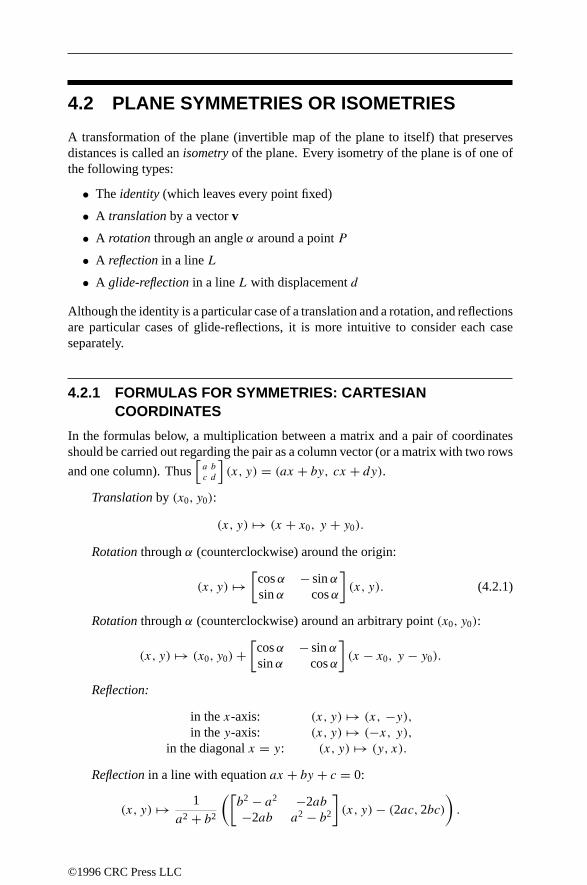
4.2 PLANE SYMMETRIES OR ISOMETRIES
A transformation of the plane (invertible map of the plane to itself) that preservesdistances is called anisometry of the plane. Every isometry of the plane is of one ofthe following types:
• Theidentity (which leaves every point fixed)
• A translation by a vectorv
• A rotation through an angleα around a pointP
• A reflection in a lineL
• A glide-reflection in a lineL with displacementd
Although the identity is a particular case of a translation and a rotation, and reflectionsare particular cases of glide-reflections, it is more intuitive to consider each caseseparately.
4.2.1 FORMULAS FOR SYMMETRIES: CARTESIANCOORDINATES
In the formulas below, a multiplication between a matrix and a pair of coordinatesshould be carried out regarding the pair as a column vector (or a matrix with two rows
and one column). Thus[a
c
b
d
](x, y) = (ax + by, cx + dy).
Translation by (x0, y0):
(x, y) → (x + x0, y + y0).
Rotation throughα (counterclockwise) around the origin:
(x, y) →[cosα − sinαsinα cosα
](x, y). (4.2.1)
Rotation throughα (counterclockwise) around an arbitrary point(x0, y0):
(x, y) → (x0, y0)+[cosα − sinαsinα cosα
](x − x0, y − y0).
Reflection:
in thex-axis: (x, y) → (x, −y),in they-axis: (x, y) → (−x, y),
in the diagonalx = y: (x, y) → (y, x).
Reflection in a line with equationax + by + c = 0:
(x, y) → 1
a2 + b2
([b2 − a2 −2ab−2ab a2 − b2
](x, y)− (2ac,2bc)
).
©1996 CRC Press LLC

Reflection in a line going through(x0, y0) and making an angleα with thex-axis:
(x, y) → (x0, y0)+[cos 2α sin 2αsin 2α − cos 2α
](x − x0, y − y0).
Glide-reflection in a lineL with displacementd: Apply first a reflection inL,then a translation by a vector of lengthd in the direction ofL, that is, by the vector
1
a2 + b2(±ad,∓bd)
if L has equationax + by + c = 0.
4.2.2 FORMULAS FOR SYMMETRIES: HOMOGENEOUSCOORDINATES
All isometries of the plane can be expressed in homogeneous coordinates in terms ofmultiplication by a matrix. This fact is useful in implementing these transformationson a computer. It also means that the successive application of transformations reducesto matrix multiplication. The corresponding matrices are as follows:
Translation by (x0, y0):
T(x0,y0) =1 0 x0
0 1 y0
0 0 1
.
Rotation throughα around the origin:
Rα =cosα − sinα 0
sinα cosα 00 0 1
.
Reflection in a line going through the origin and making an angleα with thex-axis:
Mα =cos 2α sin 2α 0
sin 2α − cos 2α 00 0 1
.
From this one can deduce all other transformations. For example, to find thematrix for a rotation throughα around an arbitrary pointP = (x0, y0), we applya translation by−(x0, y0) to moveP to the origin, a rotation throughα around theorigin, and then a translation by(x0, y0):
T(x0,y0)RαT−(x0,y0) =cosα − sinα x0 − x0 cosα + y0 sinα
sinα cosα y0 − y0 cosα − x0 sinα0 0 1
(notice the order of the multiplication).
©1996 CRC Press LLC

4.2.3 FORMULAS FOR SYMMETRIES: POLAR COORDINATES
Rotation around the origin through an angleα:
(r, θ) → (r, θ + α).Reflection in a line through the origin and making an angleα with the positive
x-axis:(r, θ) → (r, 2α − θ).
4.2.4 CRYSTALLOGRAPHIC GROUPS
A group of symmetries of the plane that is doubly infinite is awallpaper group,or crystallographic group. There are 17 types of such groups, corresponding to 17essentially distinct ways to tile the plane in a doubly periodical pattern. (There arealso 230 three-dimensional crystallographic groups.)
The simplest crystallographic group involves translations only (page 261, topleft). The others involve, in addition to translations, one or more of the other types ofsymmetries (rotations, reflections, glide-reflections). TheConway notation for crys-tallographic groups is based on the types of nontranslational symmetries occurringin the “simplest description” of the group:∗ indicates a reflection (mirror symme-try), × a glide-reflection, and a numbern indicates a rotational symmetry of ordern (rotation by 360/n). In addition, if a numbern comes after the∗, the center ofthe corresponding rotation lies on mirror lines, so that the symmetry there is actuallydihedral of order 2n.
Thus the group∗∗ in the table below (page 261, middle left) has two inequivalentlines of mirror symmetry; the group 333 (page 263, top left) has three inequivalentcenters of order-3 rotation; the group 22∗ (page 261, bottom right) has two inequivalentcenters of order-2 rotation as well as mirror lines; and∗632 (page 263, bottom) haspoints of dihedral symmetry of order 12(= 2 × 6), 6, and 4.
The following table gives the groups in the Conway notation and in the notationtraditional in crystallography. It also gives the quotient space of the plane by theaction of the group. The entry “4,4,2 turnover” means the surface of a triangular puffpastry with corner angles 45(= 180/4), 45 and 90. The entry “4,4,2 turnover slitalong 2,4” means the same surface, slit along the edge joining a 45 vertex to the 90
vertex. Open edges are silvered (mirror lines); such edges occur exactly for thosegroups whose Conway notation includes a∗.
The last column of the table gives the dimension of the space of inequivalentgroups of the given type (equivalent groups are those that can be obtained from oneanother by proportional scaling or rigid motion). For instance, there is a group oftype for every shape parallelogram, and there are two degrees of freedom for thechoice of such a shape (say the ratio and angle between sides). Thus, the group ofpage 261 (top left) is based on a square fundamental domain, while for the groupof page 263 (top left) a fundamental parallelogram would have the shape of twojuxtaposed equilateral triangles. These two groups are inequivalent, although theyare of the same type.
©1996 CRC Press LLC
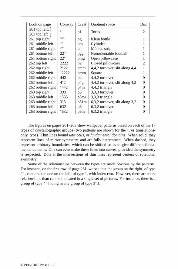
Look on page Conway Cryst Quotient space Dim261 top left;263 top left
p1 Torus 2
261 top right ×× pg Klein bottle 1261 middle left ∗∗ pm Cylinder 1261 middle right ×∗ cm Mobius strip 1261 bottom left 22× pgg Nonorientable football 1261 bottom right 22∗ pmg Open pillowcase 1262 top left 2222 p2 Closed pillowcase 2262 top right 2∗22 cmm 4,4,2 turnover, slit along 4,4 1262 middle left ∗2222 pmm Square 1262 middle right 442 p4 4,4,2 turnover 0262 bottom left 4∗2 p4g 4,4,2 turnover, slit along 4,2 0262 bottom right ∗442 p4m 4,4,2 triangle 0263 top right 333 p3 3,3,3 turnover 0263 middle left ∗333 p3m1 3,3,3 triangle 0263 middle right 3∗3 p31m 6,3,2 turnover, slit along 3,2 0263 bottom left 632 p6 6,3,2 turnover 0263 bottom right ∗632 p6m 6,3,2 triangle 0
The figures on pages 261–263 show wallpaper patterns based on each of the 17types of crystallographic groups (two patterns are shown for the, or translations-only, type). Thin lines boundunit cells, or fundamental domains. When solid, theyrepresent lines of mirror symmetry, and are fully determined. When dashed, theyrepresent arbitrary boundaries, which can be shifted so as to give different funda-mental domains. One can even make these lines into curves, provided the symmetryis respected. Dots at the intersections of thin lines represent centers of rotationalsymmetry.
Some of the relationships between the types are made obvious by the patterns.For instance, on the first row of page 261, we see that the group on the right, of type××, contains the one on the left, of type, with index two. However, there are morerelationships than can be indicated in a single set of pictures. For instance, there is agroup of type×× hiding in any group of type 3∗3.
©1996 CRC Press LLC

p1
××
pg
∗∗
pm
×∗
cm
22×
pgg
22∗
pmg
©1996 CRC Press LLC

2222
p2
2∗22
cmm
∗2222
pmm
442
p4
4∗2
p4g
∗442
p4m
©1996 CRC Press LLC

p1
333
p3
∗333
p3m1
3∗3
p31m
632
p6
∗632
p6m
©1996 CRC Press LLC
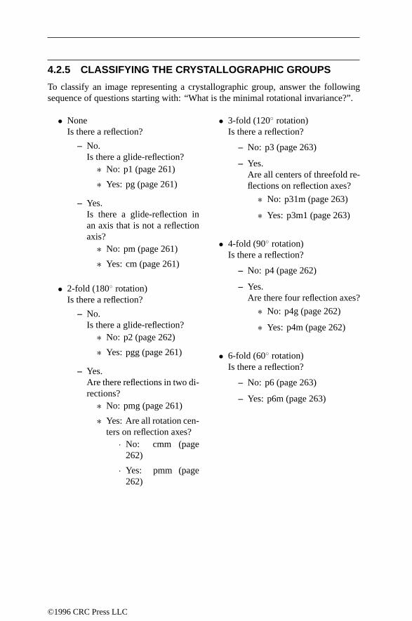
4.2.5 CLASSIFYING THE CRYSTALLOGRAPHIC GROUPS
To classify an image representing a crystallographic group, answer the followingsequence of questions starting with: “What is the minimal rotational invariance?”.
• NoneIs there a reflection?
– No.Is there a glide-reflection?
∗ No: p1 (page 261)
∗ Yes: pg (page 261)
– Yes.Is there a glide-reflection inan axis that is not a reflectionaxis?
∗ No: pm (page 261)
∗ Yes: cm (page 261)
• 2-fold (180 rotation)Is there a reflection?
– No.Is there a glide-reflection?
∗ No: p2 (page 262)
∗ Yes: pgg (page 261)
– Yes.Are there reflections in two di-rections?
∗ No: pmg (page 261)
∗ Yes: Are all rotation cen-ters on reflection axes?
· No: cmm (page262)
· Yes: pmm (page262)
• 3-fold (120 rotation)Is there a reflection?
– No: p3 (page 263)
– Yes.Are all centers of threefold re-flections on reflection axes?
∗ No: p31m (page 263)
∗ Yes: p3m1 (page 263)
• 4-fold (90 rotation)Is there a reflection?
– No: p4 (page 262)
– Yes.Are there four reflection axes?
∗ No: p4g (page 262)
∗ Yes: p4m (page 262)
• 6-fold (60 rotation)Is there a reflection?
– No: p6 (page 263)
– Yes: p6m (page 263)
©1996 CRC Press LLC

4.3 OTHER TRANSFORMATIONS OF THE PLANE
4.3.1 SIMILARITIES
A transformation of the plane that preserves shapes is called asimilarity. Everysimilarity of the plane is obtained by composing aproportional scaling transformation(also known as ahomothety) with an isometry. A proportional scaling transformationcentered at the origin has the form
(x, y) → (ax, ay),
wherea = 0 is the scaling factor (a real number). The corresponding matrix inhomogeneous coordinates is
Ha =a 0 0
0 a 00 0 1
.
In polar coordinates, the transformation is(r, θ) → (ar, θ).
4.3.2 AFFINE TRANSFORMATIONS
A transformation that preserves lines and parallelism (maps parallel lines to parallellines) is anaffine transformation. There are two important particular cases of suchtransformations:
A nonproportional scaling transformation centered at the origin has the form(x, y) →(ax, by), wherea, b = 0 are the scaling factors (real numbers). The correspondingmatrix in homogeneous coordinates is
Ha,b =a 0 0
0 b 00 0 1
.
A shear preserving horizontal lines has the form (x, y) → (x + ry, y), where r isthe shearing factor (see Figure 4.3.6). The corresponding matrix in homogeneouscoordinates is
Sr =1 r 0
0 1 00 0 1
.
Every affine transformation is obtained by composing a scaling transformationwith an isometry, or a shear with a homothety and an isometry.
©1996 CRC Press LLC

FIGURE 4.3.6A shear with factor r = 1
2 .
ry
y
4.3.3 PROJECTIVE TRANSFORMATIONS
A transformation that maps lines to lines (but does not necessarily preserve paral-lelism) is aprojective transformation. Any plane projective transformation can beexpressed by an invertible 3×3 matrix in homogeneous coordinates; conversely, anyinvertible 3× 3 matrix defines a projective transformation of the plane. Projectivetransformations (if not affine) are not defined on all of the plane but only on thecomplement of a line (the missing line is “mapped to infinity”).
A common example of a projective transformation is given by aperspectivetransformation (Figure4.3.7). Strictly speaking thisgives atransformation from oneplaneto another, but, if weidentify thetwo planesby (for example) fixing aCartesiansystem in each, we get a projective transformation from the plane to itself.
FIGURE 4.3.7A perspective transformation with center O, mapping the plane P to the plane Q. The trans-formation is not defined on the line L, where P intersects the plane parallel to Q and goingthrough O.
L
O
P
Q
©1996 CRC Press LLC

4.4 LINES
The (Cartesian) equation of astraight line is linear in the coordinatesx andy:
ax + by + c = 0. (4.4.1)
The slope of this line is−a/b, the intersection with the x-axis (or x-intercept) isx = −c/a, and theintersection with the y-axis (or y-intercept) isy = −c/b. Ifa = 0, the line is parallel to thex-axis, and ifb = 0, then the line is parallel to they-axis.
(In anoblique coordinate system, everything in the preceding paragraph remainstrue, except for the value of the slope.)
Whena2 + b2 = 1 andc ≤ 0 in the equationax + by + c = 0, the equation issaid to be innormal form. In this casec is thedistance of the line to the origin, andω = sin−1 a = cos−1 b is the angle that the perpendicular dropped to the line fromtheorigin makeswith thepositivex-axis (Figure4.4.8).
FIGURE 4.4.8The normal form of the line L is x cosω + y sinω = p.
x
y
ω
L
p
To reduce an arbitrary equationax + by + c = 0 to normal form, divide by±√
a2 + b2, where the sign of the radical is chosen opposite the sign ofc whenc = 0and the same as the sign ofb whenc = 0.
Lines with prescribed properties• Line of slopem intersecting thex-axis atx = x0: y = m(x + x0).
• Line of slopem intersecting they-axis aty = y0: y = mx + y0.
• Line intersecting thex-axis atx = x0 and they-axis aty = y0:
x
x0+ y
y0= 1.
(This formula remains true inoblique coordinates.)
©1996 CRC Press LLC

• Line of slope m passing though (x0, y0): y − y0 = m(x − x0).
• Line passing through points (x0, y0) and (x1, y1):
y − y1
x − x1= y0 − y1
x0 − x1or
∣∣∣∣∣∣x y 1x0 y0 1x1 y1 1
∣∣∣∣∣∣ = 0. (4.4.2)
(These formulas remain true in oblique coordinates.)
• Slopeof line going through points (x0, y0) and (x1, y1):y1 − y0
x1 − x0.
• Line passing through points with polar coordinates(r0, θ0) and (r1, θ1):
r(r0 sin(θ − θ0) − r1 sin(θ − θ1)) = r0r1 sin(θ1 − θ0). (4.4.3)
4.4.1 DISTANCES
The distancebetween two points in the plane is the length of the line segmentjoiningthe two points. If the points have Cartesian coordinates(x0, y0) and (x1, y1), thisdistance is √
(x1 − x0)2 + (y1 − y0)2. (4.4.4)
If the points have polar coordinates(r0, θ0) and (r1, θ1), this distance is√r2
0 + r21 − 2r0r1 cos(θ0 − θ1). (4.4.5)
If the points have oblique coordinates(x0, y0) and (x1, y1), this distance is√(x1 − x0)2 + (y1 − y0)2 + 2(x1 − x0)(y1 − y0) cosω, (4.4.6)
where ω is the angle between the axes (Figure 4.1.5).The point k% of the way from P0 = (x0, y0) to P1 = (x1, y1) is(kx1 + (100 − k)x2
100,ky1 + (100 − k)y2
100
). (4.4.7)
(The same formula also works in oblique coordinates.) This point divides the segmentP0P1 in the ratio k : (100 − k). As a particular case, the midpointof P0P1 is givenby(
12 (x1 + x2),
12 (y1 + y2)
).
The distancefrom the point (x0, y0) to the line ax + by + c = 0 is∣∣∣∣ax0 + by0 + c√a2 + b2
∣∣∣∣ .
©1996 CRC Press LLC

4.4.2 ANGLES
The anglebetween two lines a0x + b0y + c0 = 0 and a1x + b1y + c1 = 0 is
tan−1 b1
a1− tan−1 b0
a0= tan−1 a0b1 − a1b0
a0a1 + b0b1. (4.4.8)
In particular, the two lines are parallel when a0b1 = a1b0, and perpendicularwhena0a1 = −b0b1.
The anglebetween two lines of slopesm0 andm1 is tan−1((m1−m0)/(1+m0m1)).In particular, the two lines are parallel when m0 = m1 and perpendicularwhenm0m1 = −1.
4.4.3 CONCURRENCE AND COLLINEARITY
Three lines a0x + b0y + c0 = 0, a1x + b1y + c1 = 0, and a2x + b2y + c2 = 0 areconcurrentif and only if ∣∣∣∣∣∣
a0 b0 c0
a1 b1 c1
a2 b2 c2
∣∣∣∣∣∣ = 0.
(This remains true in oblique coordinates.)Three points (x0, y0), (x1, y1) and (x2, y2) are collinear if and only if∣∣∣∣∣∣
x0 y0 1x1 y1 1x2 y2 1
∣∣∣∣∣∣ = 0.
(This remains true in oblique coordinates.)Three points with polar coordinates (r0, θ0), (r1, θ1) and (r2, θ2) are collinear if
and only if
r1r2 sin(θ2 − θ1) + r0r1 sin(θ1 − θ0) + r2r0 sin(θ0 − θ2) = 0.
4.5 POLYGONS
Given k ≥ 3 points A1, . . . , Ak in the plane, in a certain order, we obtain a k-sidedpolygonor k-gonby connecting each point to the next, and the last to the first, witha line segment. The points Ai are the verticesand the segments AiAi+1 are the sidesor edgesof the polygon. When k = 3 we have a triangle, when k = 4 we have aquadrangleor quadrilateral, and so on (see page 276). Here we will assume that allpolygons are simple: this means that no consecutive edges are on the same line andno two edges intersect (except that consecutive edges intersect at the common vertex)(see Figure 4.5.9).
©1996 CRC Press LLC

FIGURE 4.5.9Two simple quadrilaterals (left and middle) and one that is not simple (right). We will treatonly simple polygons.
A1
A2A3
A4A1
A2A3
A4
A1
A2
A3
A4
When we refer to the angleat a vertex Ak we have in mind the interior angle (asmarked in the leftmost polygon in Figure 4.5.9). We denote this angle by the samesymbol as the vertex. The complement of Ak is the exterior angleat that vertex;geometrically, it is the angle between one side and the extension of the adjacent side.In anyk-gon, the sum of the angles equals2(k − 2) right angles, or2(k − 2)× 90;for example, the sum of the angles of a triangle is 180.
The areaof a polygon whose verticesAi have coordinates (xi, yi), for 1 ≤ i ≤ k,is the absolute value of
area = 12 (x1y2 − x2y1) + · · · + 1
2 (xk−1yk − xkyk−1) + 12 (xky1 − x1yk),
= 1
2
k∑i=1
(xiyi+1 − xi+1yi), (4.5.1)
where in the summation we take xk+1 = x1 and yk+1 = y1. In particular, for a trianglewe have
area = 12 (x1y2 − x2y1 + x2y3 − x3y2 + x3y1 − x1y3) = 1
2
∣∣∣∣∣∣x1 y1 1x2 y2 1x3 y3 1
∣∣∣∣∣∣ .In oblique coordinateswith angle ω between the axes, the area is as given above,multiplied by sinω.
If the vertices have polar coordinates(ri, θi), for 1 ≤ i ≤ k, the area is theabsolute value of
area = 1
2
k∑i=1
riri+1 sin(θi+1 − θi), (4.5.2)
where we take rk+1 = r1 and θk+1 = θ1.Formulas for specific polygons in terms of side lengths, angles, etc., are given
below.
©1996 CRC Press LLC

4.5.1 TRIANGLES
Because the angles of a triangle add up to 180, at least two of them must be acute(less than 90). In an acute triangleall angles are acute. A right triangle has oneright angle, and an obtuse trianglehas one obtuse angle.
The altitude corresponding to a side is the perpendicular dropped to the linecontaining that side from the opposite vertex. The bisectorof a vertex is the linethat divides the angle at that vertex into two equal parts. The medianis the segmentjoining a vertex to the midpoint of the opposite side. See Figure 4.5.10.
FIGURE 4.5.10Notations for an arbitrary triangle of sidesa, b, c and verticesA, B, C. The altitude corre-sponding toC ishc, the median ismc, the bisector istc. The radius of the circumscribed circleisR, that of the inscribed circle isr.
r
R
C
C2
A B
b
a
hc
mctc
c
Every triangle also has an inscribed circletangent to its sides and interior to thetriangle (in other words, any three nonconcurrent lines determine a circle). The centerof this circle is the point of intersection of the bisectors. We denote the radius of theinscribed circle by r .
Every triangle has a circumscribed circlegoing through its vertices; in otherwords, any three noncollinear points determine a circle. The point of intersection ofthe medians is the center of mass of the triangle (considered as an area in the plane).We denote the radius of the circumscribed circle by R.
Introduce the following notations for an arbitrary triangle of vertices A, B, Cand sides a, b, c (see Figure 4.5.10). Let hc, tc, and mc be the lengths of the altitude,bisector and median originating in vertex C, let r and R be as usual the radii of theinscribed and circumscribed circles, and let s be the semi-perimeter: s = 1
2 (a+b+c).
©1996 CRC Press LLC

Then
c2 = a2 + b2 − 2ab cosC (law of cosines),
a = b cosC + c cosB,
a
sinA= b
sinB= c
sinC(law of sines),
area = 12hcc = 1
2ab sinC = c2 sinA sinB
2 sinC= rs = abc
4R,
=√s(s − a)(s − b)(s − c) (Heron),
r = c sin( 12A) sin( 1
2B) sec( 12C) = ab sinC
2s= (s − c) tan( 1
2C),
=( 1
ha+ 1
hb+ 1
hc
)−1,
R = c
2 sinC= abc
4 area,
hc = a sinB = b sinA = 2 area
c,
tc = 2ab
a + bcos 1
2C =√ab(
1 − c2
(a + b)2
), and
mc =√
12a
2 + 12b
2 − 14c
2.
A triangle is equilateralif all of its sides have the same length, or, equivalently,if all of its angles are the same (and equal to 60). It is isoscelesif two sides are thesame, or, equivalently, if two angles are the same. Otherwise it is scalene.
For an equilateral triangleof side a we have
area = 14a
2√
3, r = 16a
√3, R = 1
3a√
3, h = 12a
√3,
where h is any altitude. The altitude, the bisector, and the median for each vertexcoincide.
For an isosceles triangle, the altitude for the unequal side is also the correspondingbisector and median, but this is not true for the other two altitudes. Many formulasfor an isosceles triangle of sides a, a, c can be immediately derived from those for aright triangle of legs a, 1
2c (see Figure 4.5.11, left).For a right triangle, the hypotenuseis the longest side opposite the right angle;
the legsare the two shorter sides adjacent to the right angle. The altitude for each legequals the other leg. In Figure 4.5.11 (right), h denotes the altitude for the hypotenuse,while m and n denote the segments into which this altitude divides the hypotenuse.
The following formulas apply for a right triangle:
A + B = 90,
r = ab
a + b + c,
a = c sinA = c cosB,
mc = b2,
area = 12ab,
c2 = a2 + b2 (Pythagoras),
R = 12c,
b = c sinB = c cosA,
nc = a2,
hc = ab.
©1996 CRC Press LLC

FIGURE 4.5.11Left: an isosceles triangle can be divided into two congruent right triangles. Right: notationsfor a right triangle.
c
a a
C
A B
b ah
m n
c
FIGURE 4.5.12Left: Ceva’s theorem. Right: Menelaus’s theorem.
C
A
B
E
F
D C
A
B
E
F
D
The hypotenuse is a diameter of the circumscribed circle. The median joining themidpoint of the hypotenuse (the center of the circumscribed circle) to the right anglemakes angles 2A and 2B with the hypotenuse.
Additional facts about triangles:
1. In any triangle, the longest side is opposite the largest angle, and the shortestside is opposite the smallest angle. This follows from the law of sines.
2. Ceva’s theorem (see Figure 4.5.12, left): In a triangle ABC, let D, E, and F bepoints on the linesBC, CA, andAB, respectively. Then the lines AD, BE, andCF are concurrent if, and only if, the signed distances BD, CE, . . . satisfy
BD · CE · AF = DC · EA · FB.This is so in three important particular cases: when the three lines are themedians, when they are the bisectors, and when they are the altitudes.
3. Menelaus’stheorem (see Figure 4.5.12, right): In a triangle ABC, let D, E, andF be points on the lines BC, CA, and AB, respectively. Then D, E, and F arecollinear if, and only if, the signed distances BD, CE, . . . satisfy
BD · CE · AF = −DC · EA · FB.
©1996 CRC Press LLC

4. Each side of a triangle is less than the sum of the other two. For any three lengthssuch that each is less than the sum of the other two, there is a triangle with theseside lengths.
4.5.2 QUADRILATERALS
The following formulas give the area of a general quadrilateral (see Figure 4.5.13,left, for the notation).
area = 12pq sin θ = 1
4 (b2 + d2 − a2 − c2) tan θ
= 14
√4p2q2 − (b2 + d2 − a2 − c2)2
=√(s − a)(s − b)(s − c)(s − d) − abcd cos 1
2 (A + C).(4.5.3)
FIGURE 4.5.13Left: notation for a general quadrilateral; in additions = 1
2 (a + b + c + d). Right: aparallelogram.
DC
B
A
a
b
c
d
p
q
θ
D C
BA
a a
b
b
h
p
q
Often, however, it is easiest to compute the area by dividing the quadrilateral intotriangles. One can also divide the quadrilateral into triangles to compute one sidegiven the other sides and angles, etc.
More formulas can be given for special cases of quadrilaterals. In a parallel-ogram, opposite sides are parallel and the diagonals intersect in the middle (Fig-ure 4.5.13, right). It follows that opposite sides have the same length and that twoconsecutive angles add up to 1808. In the notation of the figure, we have
A = C, B = D,
h = a sinA = a sinB,
p =√a2 + b2 − 2ab cosA,
A + B = 180 ,area = bh,
q =√a2 + b2 − 2ab cosB.
(All this follows from the triangle formulas applied to the triangles ABD and ABC.)Two particular cases of parallelograms are
1. The rectangle , where all angles equal 908. The diagonals of a rectangle havethe same length. The general formulas for parallelograms reduce to
h = a, area = ab, and p = q =√a2 + b2,
©1996 CRC Press LLC

2. The rhombus or diamond♦ , where adjacent sides have the same length (a =b). The diagonals of a rhombus are perpendicular. In addition to the generalformulas for parallelograms, we have area =
12pq and p2 + q2 = 4a2.
The square or regular quadrilateral is both a rectangle and a rhombus. See page 276.A quadrilateral is a trapezoid if two sides are parallel. In
the notation of the figure on the right we haveCD
BA
h
A + D = B + C = 180 , area = 1
2 (AB + CD)h.
The diagonals of a quadrilateral with consecutive sides a, b, c, d are perpendicularif and only if a2 + c2 = b2 + d2.
A quadrilateral is cyclic if it can be inscribed in a circle, that is, if its four verticesbelong to a single, circumscribed, circle. This is possible if and only if the sum ofopposite angles is 180. If R is the radius of the circumscribed circle, we have (in thenotation of Figure 4.5.13, left)
area =√(s − a)(s − b)(s − c)(s − d) = 1
2 (ac + bd) sin θ,
=√(ac + bd)(ad + bc)(ab + cd)
4R(Brahmagupta),
p =√(ac + bd)(ab + cd)
(ad + bc),
R = 1
4
√(ac + bd)(ad + bc)(ab + cd)
(s − a)(s − b)(s − c)(s − d),
sin θ = 2 area
ac + bd,
pq = ac + bd (Ptolemy).
A quadrilateral is circumscribableif it has an inscribed circle (that is, a circletangent to all four sides). Its area is rs, where r is the radius of the inscribed circleand s is as above.
For a quadrilateral that is both cyclic and circumscribable, we have the followingadditional equalities, where m is the distance between the centers of the inscribed andcircumscribed circles:
a + c = b + d,
R = 1
4
√(ac + bd)(ad + bc)(ab + cd)
abcd,
area =√abcd = rs,
1
r2= 1
(R − m)2+ 1
(R + m)2.
©1996 CRC Press LLC

4.5.3 REGULAR POLYGONSA polygon is regular if all of its sides are equal and all its angles are equal. Eithercondition implies the other in the case of a triangle, but not in general. (A rhombus
not neccessarily equal sides ).For a k-sided regular polygon of side a, let θ be the angle at any vertex, and r
and R the radii of the inscribed and circumscribed circles (r is called the apothem).As usual, let s =
1
2 ka be the half-perimeter. Then
RR
r
a
θθ =(k − 2
k
)180 ,
a = 2r tan180
k= 2R sin
180
k,
area = 14ks
2 cot 180
k= kr2 tan
180
k
= 12kR
2 sin360
k,
r = 12 s cot
180
k,
R = 12 s csc
180
k.
Name k Area r R
Equilateral triangle 3 0.43301 a2 0.28868 a 0.57735 aSquare 4 a2 0.50000 a 0.70711 aRegular pentagon 5 1.72048 a2 0.68819 a 0.85065 aRegular hexagon 6 2.59808 a2 0.86603 a a
Regular heptagon 7 3.63391 a2 1.03826 a 1.15238 aRegular octagon 8 4.82843 a2 1.20711 a 1.30656 aRegular nonagon 9 6.18182 a2 1.37374 a 1.46190 aRegular decagon 10 7.69421 a2 1.53884 a 1.61803 aRegular undecagon 11 9.36564 a2 1.70284 a 1.77473 aRegular dodecagon 12 11.19625 a2 1.86603 a 1.93185 a
If ak denotes the side of a k-sided regular polygon inscribed in a circle of radiusR, we have
a2k =√
2R2 − R
√4R2 − a2
k .
If Ak denotes the side of a k-sided regular polygon circumscribed about the samecircle,
A2k = 2RAk
2R +√
4R2 + A2k
.
©1996 CRC Press LLC
has equal sides but not necessarily equal angles, and a rectangle has equal angles but

The areas sk , s2k , Sk and S2k of the same polygons satisfy
s2k =√skSk, S2k = 2s2kSk
s2k + Sk.
4.6 CIRCLES
The set of points whose distance to a fixed point (the center) is a fixed positive number(the radius) is a circle. A circle of radius r and center (x0, y0) is described by theequation
(x − x0)2 + (y − y0)
2 = r2,
or
x2 + y2 − 2xx0 − 2yy0 + x20 + y2
0 − r2 = 0.
Conversely, an equation of the form
x2 + y2 + 2dx + 2ey + f = 0
defines a circle if d2+e2 > f ; the center is (−d, −e) and the radius is√d2 + e2 − f .
Three points not on the same line determine a unique circle. If the points havecoordinates (x1, y1), (x2, y2) and (x3, y3), then the equation of the circle is
∣∣∣∣∣∣∣∣x2 + y2 x y 1x2
1 + y21 x1 y1 1
x22 + y2
2 x2 y2 1x2
3 + y23 x3 y3 1
∣∣∣∣∣∣∣∣ = 0.
A chord of a circle is a line segment between two points (Figure 4.6.14). Adiameteris a chord that goes through the center, or the length of such a chord (thereforethe diameter is twice the radius). Given two points P1 = (x1, y1) and P2 = (x2, y2),there is a unique circle whose diameter is P1P2; its equation is
(x − x1)(x − x2) + (y − y1)(y − y2) = 0.
The lengthor circumferenceof a circle of radius r is 2πr , and the area is πr2.The length of the arc of circle subtended by an angle θ , shown as s in Figure 4.6.14,is rθ . Other relations between the radius, the arc length, the chord, and the areas of
©1996 CRC Press LLC
In particular,
A2k = ak Ak , a2k =! ak A2k
ak + Ak 2.

the corresponding sector and segment are, in the notation of Figure 4.6.14,
d = R cos 12θ = 1
2c cot 12θ = 1
2
√4R2 − c2,
c = 2R sin 12θ = 2d tan 1
2θ = 2√R2 − d2 =
√4h(2R − h),
θ = s
R= 2 cos−1 d
R= 2 tan−1 c
2d= 2 sin−1 c
2R,
area of sector = 12Rs = 1
2R2θ,
area of segment = 12R
2(θ − sin θ) = 12 (Rs − cd) = R2 cos−1 d
R− d
√R2 − d2,
= R2 cos−1 R − h
R− (R − h)
√2Rh− h2.
FIGURE 4.6.14The arc of a circle subtended by the angleθ is s; the chord isc; the sector is the whole sliceof the pie; the segment is the cap bounded by the arc and the chord (that is, the slice minus thetriangle).
R
θ
s
c
h
d
Other properties of circles:
1. If the central angle AOB equals θ , the angle ACB, where C is any point onthe circle, equals 1
2θ or 180 − 12θ (Figure 4.6.15, left). Conversely, given a
segment AB, the set of points that “see” AB under a fixed angle is an arc of acircle (Figure 4.6.15, right). In particular, the set of points that see AB under aright angle is a circle with diameter AB.
2. Let P1, P2, P3, P4 be points in the plane, and let dij , for 1 ≤ i, j ≤ 4, be thedistance between Pi and Pj . A necessary and sufficient condition for all of thepoints to lie on the same circle (or line) is that one of the following equalitiesbe satisfied:
±d12d34 ± d13d24 ± d14d23 = 0.
This is equivalent to Ptolemy’s formula for cyclic quadrilaterals (page 275).
3. In oblique coordinateswith angle ω, a circle of center (x0, y0) and radius r isdescribed by the equation
(x − x0)2 + (y − y0)
2 + 2(x − x0)(y − y0) cosω = r2.
©1996 CRC Press LLC

FIGURE 4.6.15Left: the angleACB equals 1
2 θ for anyC in the long arcAB; ADB equals180 − 12 θ for
anyD in the short arcAB. Right: the locus of points, from which the segmentAB subtends afixed angleθ, is an arc of the circle.
θ
A
B
CD
θ
θ
4. In polar coordinates, the equation for a circle centered at the pole and havingradius a is r = a. The equation for a circle of radius a passing through the poleand with center at the point (r, θ) = (a, θ0) is r = 2a cos(θ − θ0). The equationfor a circle of radius a and with center at the point (r, θ) = (r0, θ0) is
r2 − 2r0r cos(θ − θ0) + r20 − a2 = 0.
5. If a line intersects a circle of center O at points A and B, the segments OA andOB make equal angles with the line. In particular, a tangent line is perpendicularto the radius that goes through the point of tangency.
6. Fix a circle and a point P in the plane, and consider a line through P thatintersects the circle at A and B (with A = B for a tangent). Then the productof the distances PA ·PB is the same for all such lines. It is called the powerofP with respect to the circle.
4.7 CONICS
A conic (or conic section) is a plane curve that can be obtained by intersecting aright circular cone (page 312) with a plane that does not go through the vertex of thecone. There are three possibilities, depending on the relative positions of the coneand the plane (Figure 4.7.16). If no line of the cone is parallel to the plane, then theintersection is a closed curve, called an ellipse. If one line of the cone is parallel to theplane, the intersection is an open curve whose two ends are asymptotically parallel;this is called a parabola. Finally, there may be two lines in the cone parallel to theplane; the curve in this case has two open segments, and is called a hyperbola.
©1996 CRC Press LLC

FIGURE 4.7.16A section of a cone by a plane can yield an ellipse (left), a parabola (middle) or a hyperbola(right).
4.7.1 ALTERNATIVE CHARACTERIZATION
Assume given a point F in the plane, a line d not going through F , and a positivereal number e. The set of points P such that the distance PF is e times the distancefrom P to d (measured along a perpendicular) is a conic. We call F the focus, d thedirectrix, and e the eccentricity of the conic. If e < 1 we have an ellipse, if e = 1 aparabola, and if e > 1 a hyperbola (Figure 4.7.17). This construction gives all conicsexcept the circle, which is a particular case of the ellipse according to the earlierdefinition (we can recover it by taking the limit e → 0).
FIGURE 4.7.17Definition of conics by means of the ratio (eccentricity) between the distance to a point andthe distance to a line. On the left,e = .7; in the middle,e = 1; on the right,e = 2.
P
d
F
P
d
F
P
d
F
For any conic, a line perpendicular to d and passing through F is an axis ofsymmetry. The ellipse and the hyperbola have an additional axis of symmetry, per-pendicular to the first, so that there is an alternate focus and directrix, F ′ and d ′,obtained as the reflection of F and d with respect to this axis. (By contrast, the focusand directrix are uniquely defined for a parabola.)
The simplest analytic form for the ellipse and hyperbola is obtained when thetwo symmetry axes coincide with the coordinate axes. The ellipse in Figure 4.7.18
©1996 CRC Press LLC

has equation
x2
a2+ y2
b2= 1, (4.7.1)
with b < a. The x-axis is the major axis, and the y-axis is the minor axis. Thesenames are also applied to the segments, determined on the axes by the ellipse, andto the lengths of these segments: 2a for the major axis and 2b for the minor. Theverticesare the intersections of the major axis with the ellipse and have coordinates(a, 0) and (−a, 0). The distance from the center to either focusis
√a2 − b2, and the
sum of the distances from a point in the ellipse to the foci is 2a. The latera recta(inthe singular, latus rectum) are the chords perpendicular to the major axis and goingthrough the foci; their length is 2b2/a. The eccentricityis
√a2 − b2/a. All ellipses
of the same eccentricity are similar; in other words, the shape of an ellipse dependsonly on the ratio b/a. The distance from the center to either directrix is a2/
√a2 − b2.
FIGURE 4.7.18Ellipse with major semiaxisa and minor semiaxisb. Hereb/a = 0.6.
x
y
d ′ d
OF ′ F (a, 0)
(0, b)
The hyperbola in Figure 4.7.19 has equation
x2
a2− y2
b2= 1. (4.7.2)
The x-axis is the transverse axis, and the y-axis is the conjugate axis. The verticesarethe intersections of the transverse axis with the ellipse and have coordinates (a, 0) and(−a, 0). The segment thus determined, or its length 2a, is also called the transverseaxis, while the length 2b is also called the conjugate axis. The distance from the centerto either focusis
√a2 + b2, and the difference between the distances from a point in
the hyperbola to the foci is 2a. The latera rectaare the chords perpendicular to thetransverse axis and going through the foci; their length is 2b2/a. The eccentricityis√a2 + b2/a. The distance from the center to either directrix is a2/
√a2 + b2. The
©1996 CRC Press LLC
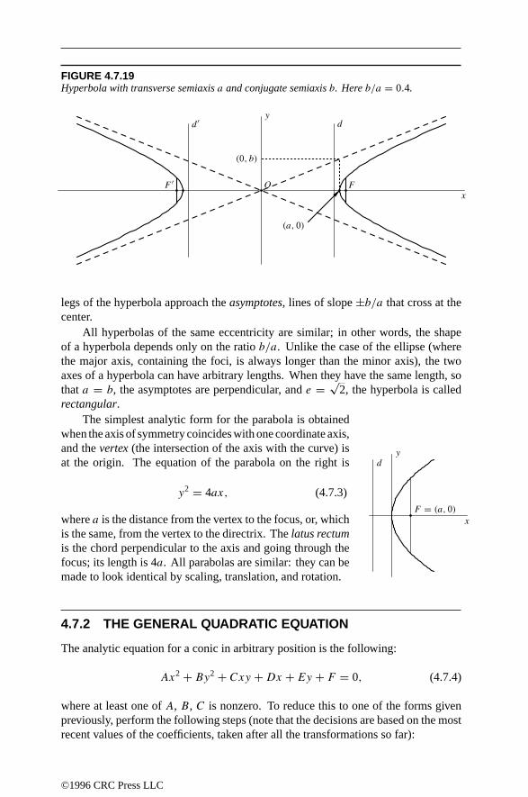
FIGURE 4.7.19Hyperbola with transverse semiaxisa and conjugate semiaxisb. Hereb/a = 0.4.
x
yd ′ d
OF ′ F
(a, 0)
(0, b)
legs of the hyperbola approach the asymptotes, lines of slope ±b/a that cross at thecenter.
All hyperbolas of the same eccentricity are similar; in other words, the shapeof a hyperbola depends only on the ratio b/a. Unlike the case of the ellipse (wherethe major axis, containing the foci, is always longer than the minor axis), the twoaxes of a hyperbola can have arbitrary lengths. When they have the same length, sothat a = b, the asymptotes are perpendicular, and e = √
2, the hyperbola is calledrectangular.
The simplest analytic form for the parabola is obtainedwhen the axis of symmetry coincides with one coordinate axis,and the vertex(the intersection of the axis with the curve) isat the origin. The equation of the parabola on the right is
y2 = 4ax, (4.7.3)
where a is the distance from the vertex to the focus, or, whichis the same, from the vertex to the directrix. The latus rectumis the chord perpendicular to the axis and going through thefocus; its length is 4a. All parabolas are similar: they can bemade to look identical by scaling, translation, and rotation.
x
yd
F = (a, 0)
4.7.2 THE GENERAL QUADRATIC EQUATION
The analytic equation for a conic in arbitrary position is the following:
Ax2 + By2 + Cxy + Dx + Ey + F = 0, (4.7.4)
where at least one of A, B, C is nonzero. To reduce this to one of the forms givenpreviously, perform the following steps (note that the decisions are based on the mostrecent values of the coefficients, taken after all the transformations so far):
©1996 CRC Press LLC

1. IfC = 0, simultaneously perform the substitutions x → qx+y and y → qy−x,where
q =√(B − A
C
)2+ 1 + B − A
C. (4.7.5)
Now C = 0. (This step corresponds to rotating and scaling about the origin.)
2. If B = 0, interchange x and y. Now B = 0.
3. If E = 0, perform the substitution y → y − 12 (E/B). (This corresponds to
translating in the y direction.) Now E = 0.
4. If A = 0:
(a) If D = 0, perform the substitution x → x − (F/D) (translation in the xdirection), and divide the equation by B to get Equation (4.7.3). The conicis a parabola.
(b) If D = 0, the equation gives a degenerate conic. If F = 0, we have theline y = 0 with multiplicity two. If F < 0, we have two parallel linesy = ±√
F/B. If F > 0 we have two imaginary lines; the equation has nosolution within the real numbers.
5. If A = 0:
(a) If D = 0, perform the substitution x → x − 12 (D/A). Now D = 0. (This
corresponds to translating in the x direction.)
(b) If F = 0, divide the equation by F to get a form with F = 1.
i. If A and B have opposite signs, the conic is a hyperbola; to getto Equation (4.7.2), interchange x and y, if necessary, so that A ispositive; then make a = 1/
√A and b = 1/
√B.
ii. If A and B are both positive, the conic is an ellipse; to get to Equation(4.7.1), interchange x and y, if necessary, so that A ≤ B, then makea = 1/
√A and b = 1/
√B. The circle is the particular case a = b.
iii. If A and B are both negative, we have an imaginary ellipse; theequation has no solution in real numbers.
(c) If F = 0, the equation again represents a degenerate conic: when A and Bhave different signs, we have a pair of lines y = ±√−B/Ax, and, whenthey have the same sign, we get a point (the origin).
We work out an example for clarity. Suppose the original equation is
4x2 + y2 − 4xy + 3x − 4y + 1 = 0. (4.7.6)
In step 1 we apply the substitutions x → 2x + y and y → 2y − x. This gives25x2 + 10x − 5y + 1 = 0. Next we interchange x and y (step 2) and get 25y2 +10y− 5x+ 1 = 0. Replacing y by y− 1
5 in step 3, we get 25y2 − 5x = 0. Finally, instep 4a we divide the equation by 25, thus giving it the form of Equation (4.7.3) witha = 1
20 . We have reduced the conic to a parabola with vertex at the origin and focus at
©1996 CRC Press LLC

( 120 , 0). To locate the features of the original curve, we work our way back along the
chain of substitutions (recall the convention about substitutions and transformationsfrom Section 4.1.1):
Substitution y → y − 15
x →y
y →x
x →2x+y
y →2y−x
Vertex (0, 0) (0,− 15 ) (− 1
5 , 0) (− 25 ,− 1
5 )
Focus ( 120 , 0) ( 1
20 ,− 15 ) (− 1
5 ,1
20 ) (− 720 ,
620 )
We conclude that the original curve, Equation (4.7.6), is a parabola with vertex(− 2
5 ,− 15 ) and focus (− 7
20 ,6
20 ).If one just wants to know the type of the conic defined by Equation (4.7.4), an
alternative analysis consists in forming the quantities
( =
∣∣∣∣∣∣∣A 1
2C12D
12C B 1
2E12D
12E F
∣∣∣∣∣∣∣ , J =∣∣∣∣∣ A
12C
12C B
∣∣∣∣∣ , I = A + B,
K =∣∣∣∣∣ A
12D
12D F
∣∣∣∣∣+∣∣∣∣∣ B
12E
12E F
∣∣∣∣∣ ,(4.7.7)
and finding the appropriate case in the following table, where an entry in parenthesesindicates that the equation has no solution in real numbers:
( J (/I K Type of conic
= 0 < 0 Hyperbola= 0 0 Parabola= 0 > 0 < 0 Ellipse= 0 > 0 > 0 (Imaginary ellipse)
0 < 0 Intersecting lines0 > 0 Point0 0 < 0 Distinct parallel lines0 0 > 0 (Imaginary parallel lines)0 0 0 Coincident lines
For the central conics (the ellipse, the point, and the hyperbola), the center (x0, y0)
is the solution of the system of equations
2Ax + Cy + D = 0,
Cx + 2By + E = 0,
and the axes have slope q and −1/q, where q is given by Equation (4.7.5).
©1996 CRC Press LLC

4.7.3 ADDITIONAL PROPERTIES OF ELLIPSES
Let C be the ellipse with equation x2/a2 + y2/b2 = 1, with a > b, and let F,F ′ =(±√
a2 − b2, 0) be its foci (see Figure 4.7.18).
1. A parametric representationfor C is given by(a cos θ, b sin θ). The areaof the shaded sec-tor on the right is 1
2abθ = 12ab cos−1(x/a).
The lengthof the arc from (a, 0) to the point(a cos θ, b sin θ) is given by the elliptic integral
(a cos θ, b sin θ)
b
a
a
∫ θ
0
√1 − e2 cos2 φ dφ = a E(π/2 − θ e),
where e is the eccentricity. (See page 523 for elliptic integrals.) Setting θ = 2πresults in
areaC = πab, perimeter C = 4a E(0, e).
2. A rational parametric representationfor C is given by(a
1 − t2
1 + t2,
2bt
1 + t2
).
3. The polar equationfor C in the usual polar coordinate system is
r = ab√a2 sin2 θ + b2 cos2 θ
.
With respect to a coordinate system with origin at a focus, the equation is
r = l
1 ± e cos θ,
where l = b2/a is half the latus rectum. (Use the + sign for the focus withpositive x-coordinate and the − sign for the focus with negative x-coordinate.)
4. Let P be any point of C. The sum of the distancesPF and PF ′ is constant andequal to 2a.
5. Let P be any point of C. Then the rays PF and PF ′ make the same angle withthe tangent to C at P . Thus any light ray originating at F and reflected in theellipse will also go through F ′.
6. Let T be any line tangent to C. The product of the distances from F and F ′ toT is constant and equals b2.
7. Lahire’s theorem: Let D and D′ be fixed lines in the plane, and consider a thirdmoving line on which three points P , P ′ and P ′′ are marked. If we constrain P
to lie in D and P ′ to lie in D′, then P ′′ describes an ellipse.
©1996 CRC Press LLC

4.7.4 ADDITIONAL PROPERTIES OF HYPERBOLAS
Let C be the hyperbola with equation x2/a2 − y2/b2 = 1, and let
F,F ′ = (±√a2 + b2, 0)
be its foci (see Figure 4.7.19). The conjugatehyperbola of C is the hyperbola C ′
with equation −x2/a2 + y2/b2 = 1. It has the same asymptotes as C, the same axes(transverse and conjugate axes being interchanged), and its eccentricity e′ is relatedto that of C by e′−2 + e−2 = 1.
1. A parametric representationfor C is given
(a cosh θ, b sinh θ)b
a
by (a sec θ, b tan θ). A different paramet-ric representation, which gives one branchonly, is (a cosh θ, b sinh θ). The area ofthe shaded sector on the right is
12abθ = 1
2ab cosh−1(x/a)
= 12ab log
x + √x2 − a2
a.
The lengthof the arc from (a, 0) to the point(a cosh θ, b sinh θ) is given by the ellipticintegral
a
∫ θ
0
√e2 cosh2 φ − 1 dφ = −bi E
(θi,
ea
b
)= a
∫ x
1
√e2ξ 2 − a2
ξ 2 − a2dξ,
where e is the eccentricity, i = √−1, and x = a cosh θ .
2. A rational parametric representationfor C is given by
(a
1 + t2
1 − t2,
2bt
1 − t2
).
3. The polar equationfor C in the usual polar coordinate system is
r = ab√a2 sin2 θ − b2 cos2 θ
.
With respect to a system with origin at a focus, the equation is
r = l
1 ± e cos θ,
where l = b2/a is half the latus rectum. (Use the − sign for the focus withpositive x-coordinate and the + sign for the focus with negative x-coordinate.)
4. Let P be any point of C. The unsigned difference between the distancesPF
and PF ′ is constant and equal to 2a.
©1996 CRC Press LLC

5. Let P be any point of C. Then the rays PF and PF ′ make the same angle withthe tangent to C at P . Thus any light ray originating at F and reflected in thehyperbola will appear to emanate from F ′.
6. Let T be any line tangent to C. The product of the distances from F and F ′ toT is constant and equals b2.
7. LetP be any point ofC. The area of the parallelogram formed by the asymptotesand the parallels to the asymptotes going through P is constant and equals 1
2ab.
8. Let L be any line in the plane. If L intersects C at P and P ′ and intersectsthe asymptotes at Q and Q′, the distances PQ and P ′Q′ are the same. If L istangent to C we have P = P ′, so that the point of tangency bisects the segmentQQ′.
4.7.5 ADDITIONAL PROPERTIES OF PARABOLAS
Let C be the parabola with equation y2 = 4ax, and let F = (a, 0) be its focus.
1. Let P = (x, y) and P ′ = (x ′, y ′) be points on C. The area bounded by thechord PP ′ and the corresponding arc of the parabola is
|y ′ − y|324a
.
It equals four-thirds of the area of the triangle PQP ′, where Q is the point onC whose tangent is parallel to the chord PP ′ (formula due to Archimedes).
2. The lengthof the arc from (0, 0) to the point (x, y) is
y
4
√4 + y2
a2+ a sinh−1
( y
2a
)= y
4
√4 + y2
a2+ a log
y +√y2 + 4a2
2a.
3. The polar equationfor C in the usual polar coordinate system is
r = 4a cos θ
sin2 θ.
With respect to a coordinate system with origin at F, the equation is
r = l
1 − cos θ,
where l = 2a is half the latus rectum.
4. Let P be any point of C. Then the ray PF and the horizontal line through P
make the same angle with the tangent to C at P . Thus light rays parallel to theaxis and reflected in the parabola converge onto F (principle of the parabolicreflector).
©1996 CRC Press LLC

4.8 SPECIAL PLANE CURVES
4.8.1 ALGEBRAIC CURVES
Curves that can be given in implicit form asf (x, y) = 0, wheref is a polynomial,are calledalgebraic. The degree off is called the degree ororder of the curve. Thus,conics (page 279) are algebraic curves of degree two. Curves of degree three alreadyhave a great variety of shapes, and only a few common ones will be given here.
The simplest case is the curve whose graph is of a polynomial of degree three:y = ax3 + bx2 + cx + d, with a = 0. This curve is a (general)cubic parabola(Figure4.8.20), symmetric with respect to thepoint B wherex = −b/3a.
FIGURE 4.8.20The general cubic parabola for a > 0. For a < 0, reflect in a horizontal line.
B B B
b2 > 3ac b2 = 3ac b2 < 3ac
The equation of a semicubic parabola (Figure 4.8.21, left) is y2 = kx3; byproportional scaling one can takek = 1. This curve should not be confused with thecissoid of Diocles (Figure 4.8.21, middle), whose equation is (a − x)y2 = x3 witha = 0.
The latter is asymptotic to the linex = a, whereas the semicubic parabola hasno asymptotes. The cissoid’s points are characterized by the equality OP = AB inFigure4.8.21, right. Onecan takea = 1 by proportional scaling.
More generally, any curve of degree three with equation(x − x0)y2 = f (x),
wheref is a polynomial, is symmetric with respect to thex-axis and asymptotic tothe linex = x0. In addition to the cissoid, the following particular cases are important:
1. The witch of Agnesi has equation xy2 = a2
(a−x), with a=0, and is character-ized by the geometric property shown in Figure 4.8.21, right. The same propertyprovides the parametric representation x = a cos2θ, y = a tan θ. Once more,proportional scaling reduces to thecasea = 1.
2. Thefolium of Descartes (Figure4.8.22, left) isdescribedby equation(x−a)y2 =−x2( 1
3x + a), with a = 0 (reducible toa = 1 by proportional scaling). Byrotating 135 (right) we get the alternative and more familiar equationx3+y3 =cxy, wherec = 1
3
√2a. The folium of Descartes is arational curve, this is, it
©1996 CRC Press LLC

FIGURE 4.8.21The semicubic parabola, the cissoid of Diocles, and the witch of Agnesi.
O diametera
P
A
B
O diametera
P
A
B
is parametrically represented by rational functions. In the tilted position, theequation isx = ct/(1 + t3), y = ct2/(1 + t3) (so thatt = y/x).
3. Thestrophoid’s equation is(x − a)y2 = −x2(x + a), with a = 0 (reducible toa = 1 by proportional scaling). It satisfies the property AP = AP ′ = OA inFigure4.8.22, right; thismeansthatPOP ′ is aright angle. Thestrophoid’spolarrepresentation isr = −a cos 2θ secθ , and the rational parametric representationis x = a(t2 − 1)/(t2 + 1), y = at (t2 − 1)/(t2 + 1) (so thatt = y/x).
FIGURE 4.8.22The folium of Descartes in two positions, and the strophoid.
a3a aaO
P ′
PA
Among the important curves of degree four are the following:
1. A Cassini’s oval is characterized by the following condition: Given twofociF andF ′, a distance 2a apart, a pointP belongs to the curve if the product ofthe distancesPF andPF ′ is a constantk2. If the foci are on thex-axis andequidistant from the origin, the curve’s equation is(x2+y2+a2)2−4a2x2 = k4.Changes ina correspond to rescaling, while the value ofk/a controls the shape:
©1996 CRC Press LLC

the curve has one smooth segment and one with a self-intersection, or twosegments depending on whetherk is greater than, equal to, or smaller thana
(Figure 4.8.23). The case k = a is also known as the lemniscate (of JakobBernoulli); the equation reduces to(x2 + y2)2 = a2(x2 − y2), and upon a 45
rotation to(x2 + y2)2 = 2a2xy. Each Cassini oval is the section of a torus ofrevolution by a plane parallel to the axis of revolution.
FIGURE 4.8.23Cassini’s ovals for k = 0.5a, 0.9, a, 1.1a and 1.5a (from the inside to the outside). The foci(dots) are at x = a and x = −a. The black curve, k = a, is also called Bernoulli’s lemniscate.
2. A conchoid of Nichomedes is the set of points such that the signed distanceAP in Figure 4.8.24, left, equals a fixed real number k (the line L and theorigin O being fixed). IfL is the linex = a, the conchoid’s polar equationis r = a secθ + k. Once more,a is a scaling parameter, and the value ofk/a
controls the shape: whenk > −a the curve is smooth, whenk = −a there isa cusp, and whenk < −a there is a self-intersection. The curves fork and−k
can also be considered two leaves of the same conchoid, with Cartesian equation(x − a)2(x2 + y2) = k2x2.
FIGURE 4.8.24Defining property of the conchoid of Nichomedes (left), and curves for k = ±0.5a, k = ±a,and k = ±1.5a (right).
L
O
PA
a
k
O O O
3. A limacon of Pascal istheset of pointssuchthat thedistanceAP inFigure4.8.25,left, equals a fixed positive numberk measured on either side (the circleC and
©1996 CRC Press LLC

the originO being fixed). IfC has diametera and center at(0, 12a), the limacon’s
polar equation isr = a cosθ + k, and its Cartesian equation is
(x2 + y2 − ax)2 = k2(x2 + y2).
The value ofk/a controls the shape, and there are two particularly interestingcases. Fork = a, we get acardioid (see also page 293). Fora = 1
2k, we geta curve that can be used totrisect an arbitrary angleα. If we draw a lineLthrough the center of the circleC making an angleα with the positivex-axis,and if we callP the intersection ofL with the limacona = 2k, the line fromO
to P makes an angle withL equal to13α.
FIGURE 4.8.25Defining property of the limacon of Pascal (left), and curves for k = 1.5a, k = a, and k = 0.5a(right). The middle curve is the cardioid; the one on the right a trisectrix.
C
O
P
A
diametera
kC
O
C
O
Hypocycloids and epicycloids with rational ratios (see next section) are alsoalgebraic curves, generally of higher degree.
4.8.2 ROULETTES (SPIROGRAPH CURVES)
Suppose given a fixed curveC and a moving curveM, which rolls onC withoutslipping. The curve drawn by a pointP kept fixed with respect toM is called aroulette, of whichP is thepole.
The most important examples of roulettes arise whenM is a circle andC isa straight line or a circle, but an interesting additional example is provided by thecatenary y = a cosh(x/a), which arises by rolling the parabolay = x2/(4a) on thex-axis with pole the focus of the parabola (that is,P = (0, a) in the initial position).The catenary is the shape taken under the action of gravity by a chain or string ofuniform density whose ends are held in the air.
A circle rolling on a straight line gives atrochoid, with thecycloid as a specialcase when the poleP lies on the circle (Figure 4.8.26). If the moving circleM hasradiusa and the distance from the poleP to the center ofM is k, the trochoid’s
©1996 CRC Press LLC

parametric equation is
x = aφ − k sinφ, y = a − k cosφ.
FIGURE 4.8.26Cycloid (top) and trochoids with k = 0.5a and k = 1.5a, where k is the distance PQ from thecenter of the rolling circle to the pole.
a
Q M
P
a
Q M
P
a
Q M
P
The cycloid, therefore, has the parametric equation
x = a(φ − sinφ), y = a(1 − cosφ).
One can eliminateφ to getx as a (multivalued) function ofy, which takes the followingform for the cycloid:
x = cos−1 a − y
a±√
2ay − y2.
The length of one arch of the cycloid is 8a, and the area under the arch is 3πa2.A trochoid is also called acurtate cycloid whenk < a (that is, whenP is inside
the circle) and aprolate cycloid whenk > a.A circle rolling on another circle and exterior to it gives anepitrochoid. If a is
the radius of the fixed circle,b that of the rolling circle, andk is the distance fromPto the center of the rolling circle, the parametric equation of the epitrochoid is
x = (a + b) cosθ − k cos((1+ b/a)θ), y = (a + b) sinθ − k sin((1+ b/a)θ).
These equations assume that, at the start, everything is aligned along the positivex-axis, asin Figure4.8.27, left. Usually oneconsidersthecasewhena/b is arationalnumber, saya/b = p/q wherep andq are relatively prime. Then the rolling circlereturns to its original position after rotatingq times around the fixed circle, andthe epitrochoid is a closed curve—in fact, an algebraic curve. One also usually takesk = b, so that P lieson therollingcircle; thecurvein thiscaseiscalledan epicycloid.ThemiddlediagraminFigure4.8.27showsthecaseb = k = 1
2a, called thenephroid;this curve is the cross section of the caustic of a spherical mirror. The diagram on the
©1996 CRC Press LLC

FIGURE 4.8.27Left: initial configuration for epicycloid (black) and configuration at parameter value θ (gray).Middle: epicycloid with b = 1
2a (nephroid). Right: epicycloid with b = a (cardioid).
P Q
C
M
θ
θa/b
a k b
right shows thecaseb = k = a, which gives thecardioid (compare to Figure4.8.25,middle).
Hypotrochoids andhypocycloids are defined in the same way as epitrochoids andepicycloids, but the rolling circle is inside the fixed one. The parametric equation ofthe hypotrochoid is
x = (a − b) cosθ + k cos((a/b − 1)θ), y = (a − b) sinθ − k sin((a/b − 1)θ),
where the letters have the same meaning as for the epitrochoid. Usually one takesa/b rational andk = b. There are several interesting particular cases:
• b = k = a gives a point.
• b = k = 12a gives a diameter of the circleC.
• b = k = 13a gives the deltoid (Figure4.8.28, left), whose algebraic equation is
(x2 + y2)2 − 8ax3 + 24axy2 + 18a2(x2 + y2) − 27a4 = 0.
• b = k = 14a gives the astroid (Figure 4.8.28, right), an algebraic curve of
degree six whose equation can be reduced tox2/3 + y2/3 = a2/3. The figureillustrates another property of the astroid: its tangent intersects the coordinateaxes at points that are always the same distancea apart. Otherwise said, theastroid is the envelope of a moving segment of fixed length whose endpoints areconstrained to lie on the two coordinate axes.
4.8.3 SPIRALS
A number of interestingcurveshavepolar equationr = f (θ), wheref isamonotonicfunction (always increasing or decreasing). This property leads to a spiral shape. Thelogarithmic spiral or Bernoulli spiral (Figure4.8.29, left) isself-similar: by rotationthecurvecan bemadeto match any scaled copy of itself. Its equation isr = keaθ ; theangle between the radius from the origin and the tangent to the curve is constant and
©1996 CRC Press LLC

FIGURE 4.8.28The hypocycloids with a = 3b (deltoid) and a = 4b (astroid).
a
FIGURE 4.8.29The Bernoulli or logarithmic spiral (left), the Archimedes or linear spiral (middle), and theCornu spiral (right).
φ
φ
2πa
2πa
equal toφ = cot−1 a. A curve parametrized by arc length and such that the curvatureis proportional to the parameter at each point is a Bernoulli spiral.
In the Archimedean spiral or linear spiral (Figure 4.8.29, middle), the spacingbetween intersections along a ray from the origin is constant. The equation of thisspiral isr = aθ ; by scaling one can takea = 1. It has an inner endpoint, in contrastwith the logarithmic spiral, which spirals down to the origin without reaching it. TheCornu spiral or clothoid (Figure 4.8.29, right), important in optics and engineering,has the following parametric representation in Cartesian coordinates:
X = aC(t) = a
∫ t
0cos( 1
2πs2) ds, y = aS(t) = a
∫ t
0sin( 1
2πs2) ds.
(C andS are the so-called Fresnel integrals; see page 498). A curve parametrizedby arclength and such that the curvature is inversely proportional to the parameter ateach point is a Cornu spiral (compare the Bernoulli spiral).
4.8.4 THE PEANO CURVE AND FRACTAL CURVES
There are curves (in the sense of continuous maps from the real line to the plane)that completely cover a two-dimensional region of the plane. We give a construction
©1996 CRC Press LLC

of such aPeano curve, adapted from David Hilbert’s example. The constructionis inductive and is based on replacement rules. We consider building blocks of six
shapes: , the length of the straight segments being twicethe radius of the curved ones. A sequence of these patterns, end-to-end, represents acurve, if we disregard the gray and black half-disks. The replacement rules are thefollowing:
The rules are applied taking into account the way each piece is turned. Here we applythe replacement rules to a particular initial pattern:
(We scale the result so it has the same size as the original.) Applying the processrepeatedly gives, in the limit, the Peano curve. Here are the first five steps:
The same idea of replacement rules leads to many interesting fractal, and oftenself-similar, curves. For example, the substitution leads to theKoch snowflake when applied to an initial equilateral triangle, like this (the first threestages and the sixth are shown):
©1996 CRC Press LLC

4.8.5 CLASSICAL CONSTRUCTIONS
The ancient Greeks used straightedges and compasses to find the solutions to numer-ical problems. For example, they found square roots by constructing the geometricmean of two segments. Three famous problems that have been proved intractable bythis method are
• The trisection of an arbitrary angle
• The squaring of the circle (the construction of a square whose area is equal tothat of a given circle)
• The doubling of the cube (the construction of a cube with double the volume ofa given cube)
A regularn-gon inscribed in the unit circle can be constructed by straightedgeand compass alone if, and only if,n has the formn = 2&p1p2 . . . pk, where& is anonnegative integer andpi are distinct Fermat primes (primes of the form 22m + 1).The only known Fermat primes are form = 1,2,3,4. Thus, regularn-gons can beconstructed forn = 3, 4, 5, 6, 8, 10, 12, 15, 16, 17, 20, 24,. . . , 257,. . . .
4.9 COORDINATE SYSTEMS IN SPACE
ConventionsWhen we talk about “the point with coordinates(x, y, z)” or “the surface with equationf (x, y, z)”, we always mean Cartesian coordinates. If a formula involves anothertype of coordinates, this fact wil l be stated explicitly. Note that Section 4.1.1 hasinformation on substitutions and transformations relevant to the three-dimensionalcase.
4.9.1 CARTESIAN COORDINATES IN SPACE
In Cartesian coordinates (or rectangular coordinates), a pointP is referred to bythree real numbers, indicating the positions of the perpendicular projections from thepoint to three fixed, perpendicular, graduated lines, called theaxes. If the coordinatesare denotedx, y, z, in that order, the axes are called thex-axis, etc., and we writeP = (x, y, z). Often thex-axis is imagined to be horizontal and pointing roughlytoward the viewer (out of the page), they-axis also horizontal and pointing moreor less to the right, and thez-axis vertical, pointing up. The system is calledright-handed if it can berotated so the threeaxesare in thisposition. Figure4.9.30 showsa right-handed system. The pointx = 0, y = 0, z = 0 is theorigin, where the threeaxes intersect.
©1996 CRC Press LLC

FIGURE 4.9.30In Cartesian coordinates, P = (4.2,3.4,2.2).
P
x
y
z
4.9.2 CYLINDRICAL COORDINATES IN SPACE
To definecylindrical coordinates, we take an axis (usually called thez-axis) and aperpendicular plane, on which we choose a ray (theinitial ray) originating at theintersection of the plane and the axis (theorigin). The coordinates of a pointP arethe polar coordinates(r, θ) of the projection ofP on the plane, and the coordinatezof the projection of P on the axis (Figure 4.9.31). See Section 4.1.3 for remarks onthe values ofr andθ .
FIGURE 4.9.31Among the possible sets (r, θ, z) of cylindrical coordinates for P are (10,30,5) and(10,390,5).
P
θ
r
z
4.9.3 SPHERICAL COORDINATES IN SPACE
To definespherical coordinates, we take an axis (thepolar axis) and a perpendicularplane (theequatorial plane), on which we choose a ray (theinitial ray) originating atthe intersection of the plane and the axis (theorigin O). The coordinates of a pointP are the distanceρ from P to the origin, the angleφ (zenith) between the lineOP
©1996 CRC Press LLC

and the positive polar axis, and the angleθ (azimuth) between the initial ray and theprojection of OP to the equatorial plane. See Figure 4.9.32. As in the case of polarand cylindrical coordinates,θ is only defined up to multiples of 360, and likewiseφ.Usuallyφ is assigned a value between 0 and 180, but values ofφ between 180 and360 can also be used; the triples(ρ, φ, θ) and(ρ, 360 − φ, 180 + θ) representthe same point. Similarly, one can extendρ to negative values; the triples(ρ, φ, θ)and(−ρ, 180 − φ, 180 + θ) represent the same point.
FIGURE 4.9.32A set of spherical coordinates for P is (ρ, θ, φ) = (10,60,30).
P
θ
ρ
φ
FIGURE 4.9.33Standard relations between Cartesian, cylindrical, and spherical coordinate systems. Theorigin is the same for all three. The positive z-axes of the Cartesian and cylindrical systemscoincide with the positive polar axis of the spherical system. The initial rays of the cylindricaland spherical systems coincide with the positive x-axis of the Cartesian system, and the raysθ = 90 coincide with the positive y-axis.
P
φ
θ
r
ρ
x
y
z
©1996 CRC Press LLC

4.9.4 RELATIONS BETWEEN CARTESIAN, CYLINDRICAL, ANDSPHERICAL COORDINATES
Consider a Cartesian, a cylindrical, and a spherical coordinate system, related asshown in Figure 4.9.33. The Cartesian coordinates (x, y, z), the cylindrical coordi-nates(r, θ, z), and the spherical coordinates(ρ, φ, θ) of a point are related as follows:
cart↔ cyl
x = r cosθ,
y = r sinθ,
r =
√x2 + y2,
θ = tan−1 y
x,
sinθ = y√x2 + y2
,
cosθ = x√x2 + y2
.
cyl ↔ sph
r = ρ sinφ,
z = ρ cosφ,
ρ =
√r2 + z2,
φ = tan−1 r
z,
sinφ = r√r2 + z2
,
cosφ = z√r2 + z2
.
cart↔ sph
x = ρ cosθ sinφ,
y = ρ sinθ sinφ,
z = ρ cosφ,
ρ =√x2 + y2 + z2,
θ = tan−1 y
x,
φ = tan−1
√x2 + y2
z,
= cos−1 z√x2 + y2 + z2
.
4.9.5 HOMOGENEOUS COORDINATES IN SPACE
A quadruple of real numbers(x : y : z : t), with t = 0, is a set ofhomogeneouscoordinates for the pointP with Cartesian coordinates(x/t, y/t, z/t). Thus thesame point has many sets of homogeneous coordinates:(x : y : z : t) and(x ′ : y ′ :z′ : t ′) represent the same point if, and only if, there is some real numberα such thatx ′ = αx, y ′ = αy, z′ = αz, t ′ = αt . If P has Cartesian coordinates(x0, y0, z0), oneset of homogeneous coordinates forP is (x0, y0, z0,1).
Section 4.1.4 has more information on the relationship between Cartesian andhomogeneouscoordinates. Section 4.10.2 has formulas for space transformations inhomogeneous coordinates.
4.10 SPACE SYMMETRIES OR ISOMETRIES
A transformation of space (invertible map of space to itself) that preserves distancesis called anisometry of space. Every isometry of space is a composition of transfor-mations of the following types:
©1996 CRC Press LLC
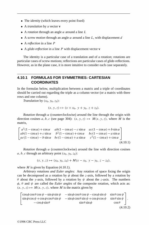
• Theidentity (which leaves every point fixed)
• A translation by a vectorv
• A rotation through an angleα around a lineL
• A screw motion through an angleα around a lineL, with displacementd
• A reflection in a lineP
• A glide-reflection in a lineP with displacement vectorv
The identity is a particular case of a translation and of a rotation; rotations areparticular cases of screw motions; reflections are particular cases of glide-reflections.However, as in the plane case, it is more intuitive to consider each case separately.
4.10.1 FORMULAS FOR SYMMETRIES: CARTESIANCOORDINATES
In the formulas below, multiplication between a matrix and a triple of coordinatesshould be carried out regarding the triple as a column vector (or a matrix with threerows and one column).
Translation by (x0, y0, z0):
(x, y, z) → (x + x0, y + y0, z + z0).
Rotation throughα (counterclockwise) around the line through the origin withdirection cosinesa, b, c (see page 304):(x, y, z) → M(x, y, z), whereM is thematrix, a2(1− cosα)+ cosα ab(1− cosα)− c sinα ac(1− cosα)+ b sinαab(1− cosα)+ c sinα b2(1− cosα)+ cosα bc(1− cosα)− a sinαac(1− cosα)− b sinα bc(1− cosα)+ a sinα c2(1− cosα)+ cosα
(4.10.1)
Rotation throughα (counterclockwise) around the line with direction cosinesa, b, c through an arbitrary point(x0, y0, z0):
(x, y, z) → (x0, y0, z0) + M(x − x0, y − y0, z − z0),
whereM is given by Equation (4.10.1).Arbitrary rotations and Euler angles: Any rotation of space fixing the origin
can be decomposed as a rotation byφ about thez-axis, followed by a rotation byθ about they-axis, followed by a rotation byψ about thez-axis. The numbersφ, θ andψ are called theEuler angles of the composite rotation, which acts as:(x, y, z) → M(x, y, z), whereM is the matrix given bycosφ cosθ cosψ−sinφ sinψ −sinφ cosθ cosψ−cosφ sinψ sinθ cosψ
sinφ cosψ+cosφ cosθ sinψ −sinφ cosθ sinψ+cosφ cosψ sinθ sinψ−cosφ sinθ sinθ sinφ cosθ
.
(4.10.2)
©1996 CRC Press LLC

(An alternative decomposition, more natural if we think of the coordinate system asa rigid trihedron that rotates in space, is the following: a rotation byψ about thez-axis, followed by a rotation byθ about therotated y-axis, followed by a rotationby φ about therotated z-axis. Note that the order is reversed.)
Provided thatθ is not a multiple of 180, the decomposition of a rotation in thisform is unique (apart from the ambiguity arising from the possibility of adding amultiple of 360 to any angle). Figure 4.10.34 shows how the Euler angles can beread off geometrically.
FIGURE 4.10.34The coordinate rays Ox, Oy, Oz, together with their images Oξ , Oη, Oζ under a rotation, fixthe Euler angles associated with that rotation, as follows: θ = zOζ , ψ = xOr = yOs, andφ = sOη. (Here the ray Or is the projection of Oζ to the xy-plane. The ray Os is determinedby the intersection of the xy- and ξη-planes.)
x
y
z
ξ
η
ζ
rs
θ
ψ
ψ
φ
Warning: Some references define Euler angles differently; the most commonvariation is that the second rotation is taken about thex-axis instead of about they-axis.
Screw motion with angleα and displacementd around the line with directioncosinesa, b, c through an arbitrary point(x0, y0, z0):
(x, y, z) → (x0 + ad, y0 + bd, z0 + cd) + M(x − x0, y − y0, z − z0),
whereM is given by (4.10.1).Reflection
in thexy-plane: (x, y, z ) → (x, y, −z).
in thexz-plane: (x, y, z ) → (x, −y, z). (4.10.3)
in theyz-plane: (x, y, z ) → (−x, y, z).
Reflection in a plane with equationax + by + cz + d = 0:
(x, y, z) → 1
a2 + b2 + c2
(M(x0, y0, z0) − (2ad,2bd,2cd)
),
©1996 CRC Press LLC

whereM is the matrix
M =−a2 + b2 + c2 −2ab −2ac
−2ab a2 − b2 + c2 −2bc−2ac −2bc a2 + b2 − c2
. (4.10.4)
Reflection in a plane going through(x0, y0, z0) and whose normal has directioncosinesa, b, c:
(x, y, z ) → (x0 + y0 + z0) + M(x − x0, y − y0, z − z0),
whereM is as in (4.10.4).
Glide-reflection in aplaneP with displacement vector v: Apply first areflectionin P , then a translation by the vectorv.
4.10.2 FORMULAS FOR SYMMETRIES: HOMOGENEOUSCOORDINATES
All isometries of space can be expressed in homogeneous coordinates in terms ofmultiplication by a matrix. As in the case of plane isometries (Section 4.2.2), thismeans that the successive application of transformations reduces to matrix multipli-cation. (In the formulas below,
[M
001
]is the 4×4 projective matrix obtained from the
3 × 3 matrixM by adding a row and a column as stated.)
Translation by (x0, y0, z0):
1 0 0 x0
0 1 0 y0
0 0 1 z0
0 0 0 1
.
Rotation through the origin:
[M 00 1
],
whereM is given in (4.10.1) or (4.10.2), as the case may be.
Reflection in a plane through the origin:
[M 00 1
],
whereM is given in (4.10.4).
From this one can deduce all other transformations, as in the case of plane trans-formations (see page 255).
©1996 CRC Press LLC

4.11 OTHER TRANSFORMATIONS OF SPACE
4.11.1 SIMILARITIES
A transformation of space that preserves shapes is called asimilarity. Every similarityof the plane is obtained by composing aproportional scaling transformation (alsoknown as ahomothety) with an isometry. A proportional scaling transformationcentered at the origin has the form
(x, y, z) → (ax, ay, az),
wherea = 0 is the scaling factor (a real number). The corresponding matrix inhomogeneous coordinates is
Ha =
a 0 0 00 a 0 00 0 a 00 0 0 1
.
In cylindrical coordinates, the transformation is(r, θ, z) → (ar, θ, az). In sphericalcoordinates, it is (r, φ, θ) → (ar, φ, θ).
4.11.2 AFFINE TRANSFORMATIONS
A transformation that preserves lines and parallelism (maps parallel lines to parallellines) is anaffine transformation. There are two important particular cases of suchtransformations:
1. A nonproportional scaling transformation centered at the origin has the form(x, y, z) → (ax, by, cz), wherea, b, c = 0 are the scaling factors (real num-bers). The corresponding matrix inhomogeneous coordinates is
Ha,b,c =
a 0 0 00 b 0 00 0 c 00 0 0 1
.
2. A shear in thex-direction and preserving horizontal planes has the form(x, y, z)
→ (x + rz, y, z), wherer is the shearing factor. The corresponding matrix inhomogeneous coordinates is
Sr =
1 0 r 00 1 0 00 0 1 00 0 0 1
.
Every affine transformation is obtained by composing a scaling transformationwith an isometry, or one or two shears with a homothety and an isometry.
©1996 CRC Press LLC

4.11.3 PROJECTIVE TRANSFORMATIONS
A transformation that maps lines to lines (but does not necessarily preserve paral-lelism) is aprojective transformation. Any spatial projective transformation can beexpressed by an invertible 4×4 matrix in homogeneous coordinates; conversely, anyinvertible 4× 4 matrix defines a projective transformation of space. Projective trans-formations (if not affine) are not defined on all of space, but only on the complementof a plane (the missing plane is “mapped to infinity”).
The following particular case is often useful, especially in computer graphics,in projecting a scene from space to the plane. Suppose an observer is at the pointE = (x0, y0, z0) of space, looking toward the originO = (0,0,0). Let P , thescreen, be the plane throughO and perpendicular to the rayEO. Place a rectangularcoordinate systemξη on P with origin atO so that the positiveη-axis lies in thehalf-plane determined byE and the positivez-axis of space (that is, thez-axis ispointing “up” as seen fromE). Then consider the transformation that associates witha pointX = (x, y, z) the triple(ξ, η, ζ ), where(ξ, η) are the coordinates of the point,where the lineEX intersectsP (the screen coordinates of X as seen fromE), andζ is the inverse of the signed distance fromX to E along the lineEO (this distanceis thedepth of X as seen fromE). This is a projective transformation, given by thematrix
−r2y0 r2x0 0 0−rx0z0 −ry0z0 rρ2 0
0 0 0 rρ
−ρx0 −ρy0 −ρz0 r2ρ
with ρ =√x2
0 + y20 andr =
√x2
0 + y20 + z2
0.
4.12 DIRECTION ANGLES AND DIRECTIONCOSINES
Given a vector(a, b, c) in three-dimensional space, thedirection cosines of this vectorare
cosα = a√a2 + b2 + c2
,
cosβ = b√a2 + b2 + c2
, (4.12.1)
cosγ = c√a2 + b2 + c2
.
Here thedirection angles α, β, γ are the angles that the vector makes with thepositivex-, y- andz-axes, respectively. In formulas, usually the direction cosinesappear, rather than the direction angles. We have
cos2 α + cos2 β + cos2 γ = 1.
©1996 CRC Press LLC
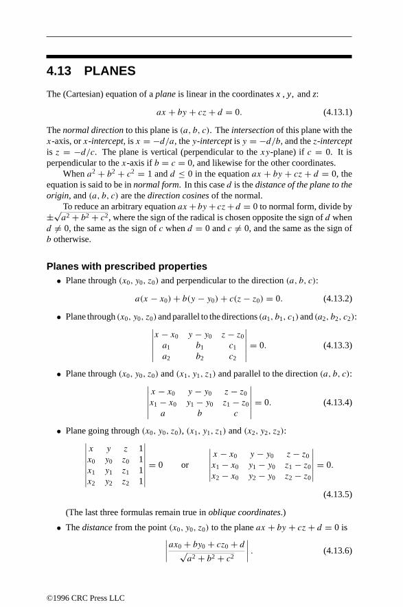
4.13 PLANES
The (Cartesian) equation of a plane is linear in thecoordinates x , y, and z:
ax + by + cz + d = 0. (4.13.1)
Thenormal direction to this plane is(a, b, c). Theintersection of this plane with thex-axis, orx-intercept, isx = −d/a, they-intercept is y = −d/b, and thez-interceptis z = −d/c. The plane is vertical (perpendicular to thexy-plane) if c = 0. It isperpendicular to thex-axis if b = c = 0, and likewise for the other coordinates.
Whena2 + b2 + c2 = 1 andd ≤ 0 in the equationax + by + cz + d = 0, theequation is said to be innormal form. In this cased is thedistance of the plane to theorigin, and(a, b, c) are thedirection cosines of the normal.
To reduce an arbitrary equationax + by + cz+ d = 0 to normal form, divide by±√
a2 + b2 + c2, where the sign of the radical is chosen opposite the sign ofd whend = 0, the same as the sign ofc whend = 0 andc = 0, and the same as the sign ofb otherwise.
Planes with prescribed properties• Plane through(x0, y0, z0) and perpendicular to the direction(a, b, c):
a(x − x0) + b(y − y0) + c(z − z0) = 0. (4.13.2)
• Plane through(x0, y0, z0)and parallel to the directions(a1, b1, c1)and(a2, b2, c2):∣∣∣∣∣∣x − x0 y − y0 z − z0
a1 b1 c1
a2 b2 c2
∣∣∣∣∣∣ = 0. (4.13.3)
• Plane through(x0, y0, z0) and(x1, y1, z1) and parallel to the direction(a, b, c):∣∣∣∣∣∣x − x0 y − y0 z − z0
x1 − x0 y1 − y0 z1 − z0
a b c
∣∣∣∣∣∣ = 0. (4.13.4)
• Plane going through(x0, y0, z0), (x1, y1, z1) and(x2, y2, z2):∣∣∣∣∣∣∣∣x y z 1x0 y0 z0 1x1 y1 z1 1x2 y2 z2 1
∣∣∣∣∣∣∣∣ = 0 or
∣∣∣∣∣∣x − x0 y − y0 z − z0
x1 − x0 y1 − y0 z1 − z0
x2 − x0 y2 − y0 z2 − z0
∣∣∣∣∣∣ = 0.
(4.13.5)
(The last three formulas remain true inoblique coordinates.)
• Thedistance from the point(x0, y0, z0) to the planeax + by + cz + d = 0 is∣∣∣∣ax0 + by0 + cz0 + d√a2 + b2 + c2
∣∣∣∣ . (4.13.6)
©1996 CRC Press LLC

• Theangle between two planesa0x+b0y+c0z+d0 = 0 anda1x+b1y+c1z+d1 =0 is
cos−1 a0a1 + b0b1 + c0c1√a2
0 + b20 + c2
0
√a2
1 + b21 + c2
1
. (4.13.7)
In particular, the two planes areparallel whena0 : b0 : c0 = a1 : b1 : c1, andperpendicular whena0a1 + b0b1 + c0c1 = 0.
Concurrence and coplanarityFour planesa0x + b0y + c0 = 0, a1x + b1y + c1 = 0, a2x + b2y + c2 = 0 anda3x + b3y + c3 = 0 areconcurrent if and only if∣∣∣∣∣∣∣∣
1 a0 b0 c0
1 a1 b1 c1
1 a2 b2 c2
1 a3 b3 c3
∣∣∣∣∣∣∣∣ = 0.
Four points(x0, y0, z0), (x1, y1, z1), (x2, y2, z2) and(x3, y3, z3) arecoplanar if andonly if ∣∣∣∣∣∣∣∣
x0 y0 z0 1x1 y1 z1 1x2 y2 z2 1x3 y3 z3 1
∣∣∣∣∣∣∣∣ = 0.
(Both of these assertions remain true inoblique coordinates.)
4.14 LINES
Two planes that are not parallel or coincident intersect in astraight line, such that onecan express a line by a pair of linear equations
ax + by + cz + d = 0a′x + b′y + c′z + d ′ = 0
such thatbc′ − cb′, ca′ − ac′, andab′ − ba′ are not all zero. The line thus defined isparallel to the vector (bc′ − cb′, ca′ − ac′, ab′ − ba′). The direction cosines of theline are those of this vector. See Equation (4.12.1). (The direction cosines of a lineare only defined up to a simultaneous change in sign, because the opposite vector stillgives the same line.)
The following particular cases are important:
• Line through(x0, y0, z0) parallel to the vector(a, b, c):
x − x0
a= y − y0
b= z − z0
c.
©1996 CRC Press LLC

• Line through(x0, y0, z0) and(x1, y1, z1):
x − x0
x1 − x0= y − y0
y1 − y0= z − z0
z1 − z0.
This line is parallel to the vector(x1 − x0, y1 − y0, z1 − z0).
Distances• Thedistance between two points in space is thelength of the line segment joining
them. The distance between the points(x0, y0, z0) and(x1, y1, z1) is√(x1 − x0)2 + (y1 − y0)2 + (z1 − z0)2.
• The pointk% of the way fromP0 = (x0, y0, z0) to P1 = (x1, y1, z1) is(kx1 + (100− k)x2
100,ky1 + (100− k)y2
100,kz1 + (100− k)z2
100
).
(The same formula also applies in oblique coordinates.) This point divides thesegmentP0P1 in the ratiok : (100− k). As a particular case, themidpoint ofP0P1 is given by (
x1 + x2
2,y1 + y2
2,z1 + z2
2
).
• Thedistance between the point(x0, y0, z0) and the line through(x1, y1, z1) indirection(a, b, c):√√√√√
∣∣∣∣y0 − y1 z0 − z1
b c
∣∣∣∣2 +∣∣∣∣z0 − z1 x0 − x1
c a
∣∣∣∣2 +∣∣∣∣x0 − x1 y0 − y1
a b
∣∣∣∣2a2 + b2 + c2
• Thedistance between the line through(x0, y0, z0) in direction(a0, b0, c0) andthe line through(x1, y1, z1) in direction(a1, b1, c1):∣∣∣∣∣∣∣∣∣∣∣∣
∣∣∣∣∣∣x1 − x0 y1 − y0 z1 − z0
a0 b0 c0
a1 b1 c1
∣∣∣∣∣∣√∣∣∣∣b0 c0
b1 c1
∣∣∣∣2 +∣∣∣∣c0 a0
c1 a1
∣∣∣∣2 +∣∣∣∣a0 b0
a1 b1
∣∣∣∣2
∣∣∣∣∣∣∣∣∣∣∣∣. (4.14.1)
AnglesAngle between lines with directions(x0, y0, z0) and(x1, y1, z1):
cos−1 a0a1 + b0b1 + c0c1√a2
0 + b20 + c2
0
√a2
1 + b21 + c2
1
.
©1996 CRC Press LLC

In particular, the two lines are parallel when a0 : b0 : c0 = a1 : b1 : c1, andperpendicularwhen a0a1 + b0b1 + c0c1 = 0.
Anglebetween lines with direction angles α0, β0, γ0 and α1, β1, γ1:
cos−1(cosα0 cosα1 + cosβ0 cosβ1 + cos γ0 cos γ1).
Concurrence, coplanarity, parallelism
Two lines specified by point and direction are coplanarif, and only if, the determinantin the numerator of Equation (4.14.1) is zero. In this case they are concurrent (if thedenominator is nonzero) or parallel (if the denominator is zero).
Three lines with directions (a0, b0, c0), (a1, b1, c1) and (a2, b2, c2) are parallelto a common planeif and only if∣∣∣∣∣∣
a0 b0 c0
a1 b1 c1
a2 b2 c2
∣∣∣∣∣∣ = 0.
4.15 POLYHEDRA
For any polyhedron topologically equivalent to a sphere—in particular, for any convexpolyhedron—the Euler formulaholds:
v − e + f = 2,
where v is the number of vertices, e is the number of edges, and f is the number offaces.
Many common polyhedra are particular cases of cylinders (Section 4.16) or cones(Section 4.17). A cylinder with a polygonal base (the base is also called a directrix) iscalled a prism. A cone with a polygonal base is called a pyramid. A frustum of a conewith a polygonal base is called a truncated pyramid. Formulas (4.16.1), (4.17.1), and(4.17.2) give the volumes of a general prism, pyramid, and trucated pyramid.
A prism whose base is a parallelogram is a parallelepiped. The volumeofa parallelepiped with one vertex at the origin and adjacent vertices at (x1, y1, z1),(x2, y2, z2), and (x3, y3, z3) is given by∣∣∣∣∣∣
x1 y1 z1
x2 y2 z2
x3 y3 z3
∣∣∣∣∣∣ .The rectangular parallelepipedis a particular case: all of its faces are rectangles. Ifthe side lengths are a, b, c, the volumeis abc, the total areais 2(ab+ ac+ bc), andeach diagonalhas length
√a2 + b2 + c2. When a = b = c we get the cube. See
Section 4.15.1.
©1996 CRC Press LLC

A pyramid whose base is a triangle is a tetrahedron. The volumeof a tetrahedonwith one vertex at the origin and the other vertices at (x1, y1, z1), (x2, y2, z2), and(x3, y3, z3) is given by
1
6
∣∣∣∣∣∣x1 y1 z1
x2 y2 z2
x3 y3 z3
∣∣∣∣∣∣ .In a tetrahedron with vertices P0, P1, P2, P3, let dij be the distance (edge length) fromPi to Pj . Form the determinants
=
∣∣∣∣∣∣∣∣∣∣
0 1 1 1 11 0 d2
01 d202 d2
031 d2
01 0 d212 d2
131 d2
02 d212 0 d2
231 d2
03 d213 d2
23 0
∣∣∣∣∣∣∣∣∣∣and =
∣∣∣∣∣∣∣∣0 d2
01 d202 d2
03d2
01 0 d212 d2
13d2
02 d212 0 d2
23d2
03 d213 d2
23 0
∣∣∣∣∣∣∣∣ .
Then the volumeof the tetrahedron is√||/288, and the radius of the circumscribed
sphereis 12
√|/2|.
4.15.1 REGULAR POLYHEDRA
Figure 4.15.35 shows the five regular polyhedra, or Platonic solids. In the followingtables and formulas, a is the length of an edge, θ the dihedral angle at each edge, Rthe radius of the circumscribed sphere, r the radius of the inscribed sphere, V thevolume, S the total surface area, v the total number of vertices, e the total number ofedges, f the total number of faces, p the number of edges in a face (3 for equilateraltriangles, 4 for squares, 5 for regular pentagons), and q the number of edges meetingat a vertex.
θ = 2 sin−1 cos(180/q)sin(180/p)
,
R
a=
12 sin(180/q)
sin(180/p) cos 12θ,
r
a= a cot
180
ptan
θ
2,
R
r= tan
180
ptan
180
q,
S
a2= fp
4cot
180
p, and
V = 13 rS.
Name v e f p q sin θ θ
Regular tetrahedron 4 6 4 3 3 2√
2/3 7031′44′′
Cube 8 12 6 4 3 1 90
Regular octahedron 6 12 8 3 4 2√
2/3 10928′16′′
Regular dodecahedron 20 30 12 5 3 √
5 11633′54′′
Regular icosahedron 12 30 20 3 5 2/3 13811′23′′
©1996 CRC Press LLC
2/

FIGURE 4.15.35The Platonic solids. Top: the tetrahedron (self-dual). Middle: the cube and the octahedron(dual to one another). Bottom: the dodecahedron and the icosahedron (dual to one another).
©1996 CRC Press LLC

Name R/a r/a
Tetrahedron√
6/4 0.612372√
6/12 0.204124
Cube√
3/2 0.866025 12 0.5
Octahedron√
2/2 0.707107√
6/6 0.408248
Dodecahedron 14 (
√15 + √
3) 1.401259 120
√250 + 110
√5 1.113516
Icosahedron 14
√10 + 2
√5 0.951057 1
12
√42 + 18
√5 0.755761
Name S/a2 V/a3
Tetrahedron√
3 1.73205√
2/12 0.117851
Cube 6 6. 1 1.
Octahedron 2√
3 3.46410√
2/3 0.471405
Dodecahedron 3√
25 + 10√
5 20.64573 14
√15 + 7
√5 7.663119
Icosahedron 5√
3 8.66025 512 (3 + √
5) 2.181695
4.16 CYLINDERS
Given a lineL and a curveC in a plane P , the cylinderwith generatorL and directrixC is the surface obtained by moving L parallel to itself, so that a point of L is alwayson C. If L is parallel to the z-axis, the surface’s implicit equation does not involvethe variable z. Conversely, any implicit equation that does not involve one of thevariables (or that can be brought to that form by a change of coordinates) representsa cylinder.
If C is a simple closed curve, we also apply the word cylinder to the solidenclosed by the surface generated in this way (Figure 4.16.36, left). The volume
FIGURE 4.16.36Left: an oblique cylinder with generatorL and directrixC. Right: a right circular cylinder.
L
P
C
θ
h
r
©1996 CRC Press LLC

contained between P and a plane P ′ parallel to P is
V = Ah = Al sin θ, (4.16.1)
where A is the area in the plane P enclosed by C, h is the distance between P andP ′ (measured perpendicularly), l is the length of the segment of L contained betweenP and P ′, and θ is the angle that L makes with P . When θ = 90 we have a rightcylinder, and h = l. For a right cylinder, the lateral areabetween P and P ′ is hs,where s is the length (circumference) of C.
The most important particular case is the right circular cylinder (often simplycalled a cylinder). If r is the radius of the base and h is the altitude (Figure 4.16.36,right), the lateral area is 2πrh, the total area is 2πr(r + h), and the volumeisπr2h. The implicit equationof this surface can be written x2 + y2 = r2; see alsoSection 4.20.
4.17 CONES
Given a curve C in a plane P and a point O not in P , the conewith vertexOand directrix C is the surface obtained as the union of all lines that join O withpoints of C. If O is the origin and the surface is given implicity by an algebraicequation, that equation is homogeneous (all terms have the same total degree in thevariables). Conversely, any homogeneous implicit equation (or one that can be madehomogeneous by a change of coordinates) represents a cone.
If C is a simple closed curve, we also apply the word coneto the solid enclosedby the surface generated in this way (Figure 4.17.37, top). The volume containedbetween P and the vertex O is
V = 13Ah, (4.17.1)
where A is the area in the plane P enclosed by C and h is the distance from O andP (measured perpendicularly).
The solid contained between P and a plane P ′ parallel to P (on the same side ofthe vertex) is called a frustum. Its volume is
V = 13h(A+ A′ +
√AA′), (4.17.2)
where A and A′ are the areas enclosed by the sections of the cone by P and P ′ (oftencalled the basesof the frustum).
The most important particular case of a cone is the right circular cone(oftensimply called a cone). If r is the radius of the base, h is the altitude, and l is the lengthbetween the vertex and a point on the base circle (Figure 4.17.37, bottom left), the
©1996 CRC Press LLC

FIGURE 4.17.37Top: a cone with vertexO and directrixC. Bottom left: a right circular cone. Bottom right:A frustum of the latter.
O
P
C
h
l
r
h
l
r2
r1
following relationships apply:
l =√r2 + h2,
Lateral area = πrl = πr√r2 + h2,
Total area = πr(l + r) = πr(r +√r2 + h2), and
Volume = 13πr
2h.
The implicit equation of this surface can be written x2 +y2 = z2; see also Section 4.20.For a frustum of a right circular cone (Figure 4.17.37, bottom right),
l =√(r1 − r2)2 + h2,
Lateral area = π(r1 + r2)l,
Total area = π(r21 + r2
2 + (r1 + r2)l), and
Volume = 13πh(r
21 + r2
2 + r1r2).
4.18 SPHERES
The set of points in space whose distance to a fixed point (the center) is a fixed positivenumber (the radius) is a sphere. A circle of radius r and center (x0, y0, z0) is defined
©1996 CRC Press LLC
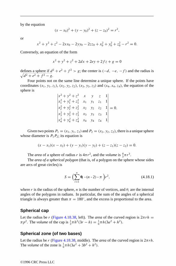
by the equation
(x − x0)2 + (y − y0)
2 + (z− z0)2 = r2,
or
x2 + y2 + z2 − 2xx0 − 2yy0 − 2zz0 + x20 + y2
0 + z20 − r2 = 0.
Conversely, an equation of the form
x2 + y2 + z2 + 2dx + 2ey + 2f z+ g = 0
defines a sphere if d2 + e2 + f 2 > g; the center is (−d, −e, −f ) and the radius is√d2 + e2 + f 2 − g.
Four points not on the same line determine a unique sphere. If the points havecoordinates (x1, y1, z1), (x2, y2, z2), (x3, y3, z3) and (x4, x4, z4), the equation of thesphere is ∣∣∣∣∣∣∣∣∣∣∣∣
x2 + y2 + z2 x y z 1x2
1 + y21 + z2
1 x1 y1 z1 1
x22 + y2
2 + z22 x2 y2 z2 1
x23 + y2
3 + z23 x3 y3 z3 1
x24 + y2
4 + z24 x4 y4 z4 1
∣∣∣∣∣∣∣∣∣∣∣∣= 0.
Given two pointsP1 = (x1, y1, z1) andP2 = (x2, y2, z2), there is a unique spherewhose diameter is P1P2; its equation is
(x − x1)(x − x2)+ (y − y1)(y − y2)+ (z− z1)(z− z2) = 0.
The areaof a sphere of radius r is 4πr2, and the volumeis 43πr
3.The area of a spherical polygon(that is, of a polygon on the sphere whose sides
are arcs of great circles) is
S =( n∑i=1
u i - (n - 2) - π)r2, (4.18.1)
where r is the radius of the sphere, n is the number of vertices, and θi are the internalangles of the polygons in radians. In particular, the sum of the angles of a sphericaltriangle is always greater than π = 180, and the excess is proportional to the area.
Spherical cap
Let the radius be r (Figure 4.18.38, left). The area of the curved region is 2πrh =πp2. The volumeof the cap is 1
3πh2(3r − h) = 1
6πh(3a2 + h2).
Spherical zone (of two bases)
Let the radius be r (Figure 4.18.38, middle). The area of the curved region is 2πrh.The volumeof the zone is 1
6πh(3a2 + 3b2 + h2).
©1996 CRC Press LLC

FIGURE 4.18.38Left: a spherical cap. Middle: a spherical zone (of two bases). Right: a spherical segment.
h
a
p
h
a
b
θ
Spherical segment and luneLet the radius be r (Figure 4.18.38, right). The area of the curved region (lune) is2r2θ , the angle being measured in radians. The volumeof the segment is 2
3 r3θ .
Spheres in arbitrary dimensionsIf the volume of an n-dimensional sphere of radius r is Vn(r) and its surface area isSn(r), then
Vn(r) = 2πr2
nVn−2 = 2πn/2rn
n(n2
) ,Sn(r) = n
rVn = d
dr[Vn(r)].
(4.18.2)
Hence, V2 = πr2, V3 = 43πr
3, . . . , S2 = 2πr , S3 = 4πr2, . . . .
4.19 SURFACES OF REVOLUTION: THE TORUS
A surface of revolutionis formed by the rotation of a planar curve C about an axis inthe plane of the curve and not cutting the curve. The Pappus–Guldinus theoremsaysthat:
• The area of the surface of revolutionon a curve C is equal to the product of thelength of C and the length of the path traced by the centroid of C (which is 2πthe distance from this centroid to the axis of revolution).
• The volume bounded by the surface of revolutionon a simple closed curve C isequal to the product of the area bounded by C and the length of the path tracedby the centroid of the area bounded by C.
When C is a circle, the surface obtained is a circular torusor torus of revolution(Figure 4.19.39). Let r be the radius of the revolving circle and let R be the distance
©1996 CRC Press LLC

from its center to the axis of rotation. The areaof the torus is 4π2Rr , and its volumeis 2π2Rr2.
FIGURE 4.19.39A torus of revolution.
R
r
4.20 QUADRICS
A surface defined by an algebraic equation of degree two is called a quadric. Spheres,circular cylinders, and circular cones are quadrics. By means of a rigid motion, anyquadric can be transformed into a quadric having one of the following equations(where a, b, c = 0):
1. Real ellipsoid: x2/a2 + y2/b2 + z2/c2 = 1.2. Imaginary ellipsoid: x2/a2 + y2/b2 + z2/c2 = −1.3. Hyperboloid of one sheet: x2/a2 + y2/b2 − z2/c2 = 1.4. Hyperboloid of two sheets: x2/a2 + y2/b2 − z2/c2 = −1.5. Real quadric cone: x2/a2 + y2/b2 − z2/c2 = 0.6. Imaginary quadric cone: x2/a2 + y2/b2 + z2/c2 = 0.7. Elliptic paraboloid: x2/a2 + y2/b2 + 2z = 0.8. Hyperbolic paraboloid: x2/a2 − y2/b2 + 2z = 0.9. Real elliptic cylinder: x2/a2 + y2/b2 = 1.
10. Imaginary elliptic cylinder: x2/a2 + y2/b2 = −1.11. Hyperbolic cylinder: x2/a2 − y2/b2 = 1.12. Real intersecting planes: x2/a2 − y2/b2 = 0.13. Imaginary intersecting planes: x2/a2 + y2/b2 = 0.14. Parabolic cylinder: x2 + 2y = 0.15. Real parallel planes: x2 = 1.16. Imaginary parallel planes: x2 = −1.17. Coincident planes: x2 = 0.
Surfaces with Equations 9–17 are cylinders over the plane curves of the sameequation (Section 4.16). Equations 2, 6, 10, and 16 have no real solutions, so that they
©1996 CRC Press LLC

FIGURE 4.20.40The five nondegenerate real quadrics. Top: ellipsoid. Middle left: hyperboloid of one sheet.Middle right: hyperboloid of two sheets. Bottom left: elliptic paraboloid. Bottom right:hyperbolic paraboloid.
©1996 CRC Press LLC

do not describe surfaces in real three-dimensional space. A surface with Equation 5can be regarded as a cone (Section 4.17) over a conic C (any ellipse, parabola orhyperbola can be taken as the directrix; there is a two-parameter family of essentiallydistinct cones over it, determined by the position of the vertex with respect toC). Thesurfaces with Equations 1, 3, 4, 7, and 8 are shown in Figure 4.20.40.
The surfaces with Equations 1–6 are central quadrics; in the form given, thecenter is at the origin. The quantities a, b, c are the semiaxes.
The volume of the ellipsoidwith semiaxes a, b, c is 43πabc. When two of the
semiaxes are the same, we can also write the area of the ellipsoidin closed form.Suppose b = c, so the ellipsoid x2/a2 + (y2 + z2)/b2 = 1 is the surface of revolutionobtained by rotating the ellipse x2/a2 + y2/b2 = 1 around the x-axis. Its area is
2πb2 + 2πa2b√a2 − b2
sin−1
√a2 − b2
a= 2πb2 + πa2b√
b2 − a2log
b + √b2 − a2
b − √b2 − a2
.
The two quantities are equal, but only one avoids complex numbers, depending onwhether a > b or a < b. When a > b, we have a prolate spheroid, that is, an ellipserotated around its major axis; when a < b we have an oblate spheroid, which is anellipse rotated around its minor axis.
Given a general quadratic equation in three variables,
ax2 + by2 + cz2 + 2fyz+ 2gzx + 2hxy + 2px + 2qy + 2rz+ d = 0,(4.20.1)
one can determine the type of conic by consulting the table:
ρ3 ρ4 k signs K signs Type of quadric3 4 < 0 Real ellipsoid3 4 > 0 Same Imaginary ellipsoid3 4 > 0 Opp Hyperboloid of one sheet3 4 < 0 Opp Hyperboloid of two sheets3 3 Opp Real quadric cone3 3 Same Imaginary quadric cone2 4 < 0 Same Elliptic paraboloid2 4 > 0 Opp Hyperbolic paraboloid2 3 Same Opp Real elliptic cylinder2 3 Same Same Imaginary elliptic cylinder2 3 Opp Hyperbolic cylinder2 2 Opp Real intersecting planes2 2 Same Imaginary intersecting planes1 3 Parabolic cylinder1 2 Opp Real parallel planes1 2 Same Imaginary parallel planes1 1 Coincident planes
©1996 CRC Press LLC

The columns have the following meaning. Let
e =a h g
h b f
g f c
and E =
a h g p
h b f q
g f c r
p q r d
.
Let ρ3 and ρ4 be the ranks of e andE, and let be the determinant ofE. The column“k signs” refers to the nonzero eigenvalues of e, that is, the roots of
∣∣∣∣∣∣a − x h g
h b − x f
g f c − x
∣∣∣∣∣∣ = 0;
if all nonzero eigenvalues have the same sign, choose “same”, otherwise “opposite”.Similarly, “K signs” refers to the sign of the nonzero eigenvalues of E.
©1996 CRC Press LLC

4.21 KNOTS UP TO EIGHT CROSSINGSn 3 4 5 6 7 8 9 10 11
Number of knotsWith n crossings
1 1 2 3 7 21 49 165 552
31 41 51 52 61
62 63 71 72 73
74 75 76 77 81
82 83 84 85 86
87 88 89 810 811
812 813 814 815 816
817 818 819 820 821
Image by Charlie Gunn and David Broman. Copyright The Geometry Center, Uni-versity of Minnesota. With permission.
©1996 CRC Press LLC

4.22 DIFFERENTIAL GEOMETRY
4.22.1 CURVES
DefinitionsA regular parametric representation of classCk , k ≥ 1, is a vector valued functionf : I → Rn, where I ⊂ R is an interval that satisfies (i) f is of class Ck , and (ii)f′(t) = 0, for all t ∈ I .
In terms of a standard basis of R3, we write x = f(t) = (f1(t), f2(t), f3(t)),where the real valued functions fi , i = 1, 2, 3 are the component functions of f.
An allowable change of parameter of classCk is any Ck function φ : J → I ,where J is an interval and φ(J ) ⊂ I , that satisfies φ′(τ ) = 0, for all τ ∈ J .
A Ck regular parametric representation f is equivalent to a Ck regular parametricrepresentation g if an only if an allowable change of parameter φ exists so thatf(I g) = If , and g(τ ) = f(f(τ )), for all τ ∈ Ig .
A regular curveC of classCk is an equivalence class of Ck regular parametricrepresentation under the equivalence relation on the set of regular parametric repre-sentations defined in Section 4.22.1.
The arc length of any regular curve C defined by the regular parametric repre-sentation f, with If = [a, b], is defined by
L =∫ b
a
∣∣f′(u)∣∣ du. (4.22.1)
An arc length parameteralong C is defined by
s = α(t) = ±∫ t
c
∣∣f′(u)∣∣ du. (4.22.2)
The choice of sign is arbitrary and c is any number in If .A natural representation of classCk of the regular curve defined by the regular
parametric representation f is defined by g(s) = f(α−1(s)), for all s ∈ [0, L].A propertyof a regular curve C is any property of a regular parametric represen-
tation that defines C as invariant under any allowable change of parameter.Let g be a natural representation of a regular curve C. The following quantities
may be defined at each point x = g(s) of C:
Unit tangent vector t(s) = g(s) with(
g(s) = dgds
)Curvature vector k(s) = t(s)Principal normalunit vector
n(s) = ±k(s)/|k(s)|, for k(s) = 0 defined tobe continuous along C
Unit binormal vector b(s) = t(s)× n(s)Moving trihedron t(s),n(s),b(s)Curvature κ(s) = n(s) · k(s)
©1996 CRC Press LLC
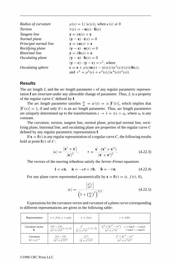
Radius of curvature ρ(s) = 1/ |κ(s)|, when κ(s) = 0Torsion τ(s) = −n(s) · b(s)Tangent line y = λt(s)+ xNormal plane (y − x) · t(s) = 0Principal normal line y = λn(s)+ xRectifying plane (y − x) · n(s) = 0Binormal line y = λb(s)+ xOsculating plane (y − x) · b(s) = 0
Osculating sphere(y − c) · (y − c) = r2, wherec = x + ρ(s)n(s)− (κ(s)/(κ2(s)τ (s)))b(s),and r2 = ρ2(s)+ κ2(s)/(κ4(s)τ 2(s))
ResultsThe arc length L and the arc length parameter s of any regular parametric represen-tation f are invariantunder any allowable change of parameter. Thus, L is a propertyof the regular curve C defined by f.
The arc length parameter satisfies dsdt
= α′(t) = ± ∣∣f ′(t)∣∣, which implies that∣∣f ′(s)
∣∣ = 1, if and only if t is an arc length parameter. Thus, arc length parametersare uniquely determined up to the transformation s → s = ±s + s0, where s0 is anyconstant.
The curvature, torsion, tangent line, normal plane, principal normal line, recti-fying plane, binormal line, and osculating plane are properties of the regular curve Cdefined by any regular parametric representation f.
If x = f(t) is any regular representation of a regular curveC, the following resultshold at point f(t) of C:
|κ| =∣∣x′′ × x′∣∣
|x′|3 , τ = x′ · (x′′ × x′′′)|x′ × x′′|2 . (4.22.3)
The vectors of the moving trihedron satisfy the Serret–Frenet equations
t = κn, n = −κt + τb, b = −τn. (4.22.4)
For any plane curve represented parametrically by x = f(t) = (t, f (t), 0),
|κ| =
∣∣∣ d2xdt2
∣∣∣(1 + (
dxdt
)2)3/2 . (4.22.5)
Expressions for the curvature vector and curvature of a plane curvecorrespondingto different representations are given in the following table:
Representation x = f (t), y = g(t) y = f (x) r = f (θ)
Curvature vectork
(xy − yx)
(x2 + y2)2(−y, x) y ′′
(1 + y ′2)2(−y ′, 1)
(r2 + 2r ′2 − rr ′′)(r2 + r ′2)2
(−r sin θ − r cos θ,r cos θ − r sin θ)
Curvature|κ| = ρ−1
|xy − yx|(x2 + y2)3/2
|y ′′|(1 + y ′2)3/2
r2 + 2r ′2 − rr ′′
(r2 + r ′2)3/2
©1996 CRC Press LLC

The equation of the osculating circle of a plane curve is given by
(y − c) · (y − c) = ρ2,
where c = x + ρ2k is the center of curvature.
THEOREM 4.22.1 (Fundamental existence and uniqueness theorem)
Let κ(s) and τ(s) be any continuous functions defined for all s ∈ [a, b]. Then thereexists, up to a congruence, a unique space curve C for which κ is the curvaturefunction, τ is the torsion function, and s an arc length parameter along C.
Example
A regular parametric representation of the circular helix is given by x = f(t) =(a cos t, a sin t, bt), for all t ∈ R, where a > 0 and b = 0 are constant. By successivedifferentiation,
x′ = (−a sin t, a cos t, b),
x′′ = (−a cos t,−a sin t, 0),
x′′′ = ( a sin t,−a cos t, 0),
so that dsdt
= ∣∣x′∣∣ = √a2 + b2. Hence,
• Arc length parameter: s = α(t) = t (a2 + b2)12
• Unit tangent vector: t = x′|x′| = (a2 + b2)−
12 (−a sin t, a cos t, b)
• Curvature vector: k = dtds
= dtds
dtdt
= (a2 + b2)−1(−a cos t,−a sin t, 0)
• Curvature: κ = |k| = a(a2 + b2)−1
• Principal normal unit vector: n = k/ |k| = (− cos t,− sin t, 0)
• Unit binormal vector:
b = t × n = (a2 + b2)−12 (b sin t, b cos t, a)
b = dt
ds
dbdt
= b(a2 + b2)−1(cos t, sin t, 0)
• Torsion: τ = −n · b = b(a2 + b2)−1
The values of |κ| and τ can be verified using the formulae in (4.22.3). The sign of(the invariant) τ determines whether the helix is right handed, τ > 0, or left handed,τ < 0.
©1996 CRC Press LLC
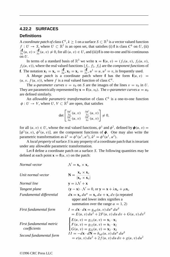
4.22.2 SURFACES
DefinitionsA coordinate patch of classCk , k ≥ 1 on a surface S ⊂ R3 is a vector valued functionf : U → S, where U ⊂ R2 is an open set, that satisfies (i) f is class Ck on U , (ii)∂f∂u(u, v)× ∂f
∂v(u, v) = 0, for all (u, v) ∈ U , and (iii) f is one-to-one and bi-continuous
on U .In terms of a standard basis of R3 we write x = f(u, v) = (f1(u, v), f2(u, v),
f3(u, v)), where the real valued functions f1, f2, f3 are the component functions of
f. The notation x1 = xu = ∂f∂u
, x2 = xv = ∂f∂v
, u1 = u, u2 = v, is frequently used.A Monge patch is a coordinate patch where f has the form f(u, v) =
(u, v, f (u, v)), where f is a real valued function of class Ck .The u-parameter curves v = v0 on S are the images of the lines v = v0 in U .
They are parametrically represented by x = f(u, v0). The v-parameter curves u = u0
are defined similarly.An allowable parametric transformation of class Ck is a one-to-one function
φ : U → V , where U,V ⊂ R2 are open, that satisfies
det
[∂φ1
∂u(u, v)
∂φ1
∂v(u, v)
∂φ2
∂u(u, v)
∂φ2
∂v(u, v)
]= 0,
for all (u, v) ∈ U , whose the real valued functions, φ1 and φ2, defined by φφφ(u, v) =[φ1(u, v), φ2(u, v)], are the component functions of φφφ. One may also write theparametric transformation as u1 = φ1(u1, u2), u2 = φ2(u1, u2).
A local property of surface S is any property of a coordinate patch that is invariantunder any allowable parametric transformation.
Let f define a coordinate patch on a surface S. The following quantities may bedefined at each point x = f(u, v) on the patch:
Normal vector N = xu × xv
Unit normal vector N = xu × xv|xu × xv|
Normal line y = λN + x
Tangent plane (y − x) · N = 0, or y = x + λxu + µxvFundamental differential dx = xα duα = xu du+ xv dv (a repeated
upper and lower index signifies asummation over the range α = 1, 2)
First fundamental form I = dx · dx = gαβ(u, v) duα duβ
= E(u, v) du2 + 2F(u, v) du dv +G(u, v) dv2
First fundamental metriccoefficients
E(u, v) = g11(u, v) = x1 · x1
F(u, v) = g12(u, v) = x1 · x2
G(u, v) = g22(u, v) = x2 · x2
Second fundamental form II = −dx · dN = bαβ(u, v) duα duβ
= e(u, v) du2 + 2f (u, v) du dv + g(u, v) du2
©1996 CRC Press LLC

Second fundamental metriccoefficients
e(u, v) = b11(u, v) = x11 · Nf (u, v) = b12(u, v) = x12 · Ng(u, v) = b22(u, v) = x22 · N
Normal curvature vectorof curve C on S through x
kn = (k · N)N
Normal curvature in thedu : dv direction
κn = k · N = II/I
Dupin’s indicatrix ex21 + 2f x1x2 + gx2
2 = ±1
Elliptic point eg − f 2 > 0
Hyperbolic point eg − f 2 < 0,
Parabolic point eg − f 2 = 0 not all of e, f, g = 0
Planar point e = f = g = 0
Umbilical point κn = constant for all directions du : dv
Principal directions The perpendicular directions du : dv inwhich κn attains its extreme values
Principal curvatures The extreme values κ1 and κ2 of κnLine of curvature A curve on S whose tangent line at each
point coincides with an asymptotic direction
Asymptotic direction A direction du : dv for which κn = 0
Asymptotic line A curve on S whose tangent line at eachpoint coincides with a principal direction
Gaussian curvature K = κ1κ2 = eg − f 2
EG− F 2
Mean curvature H = κ1 + κ2
2= gE + eG− 2fF
2(EG− F 2)
Geodesic curvature vectorof a curve C on Sthrough x
kg = k − (k · N)N = [uα + ' αβγ u
β uγ ]xαwhere 'αβγ denote the Christoffelsymbols of the second kind for the metricgαβ , defined in Section 5.10
Geodesic on S A curve on S which satisfieskg = 0 at each point
ResultsThe tangent plane, normal line, first fundamental form, second fundamental form andall derived quantities thereof are local properties of any surface S.
The transformation laws for the first and second fundamental metric coefficientsand any allowable parametric transformation are given respectively by
gαβ = gγ δ∂uγ
∂uα
∂uδ
∂uβ, and bαβ = bγ δ
∂uγ
∂uα
∂uδ
∂uβ.
Thus gαβ and bαβ are the components of type (0, 2) tensors.I ≥ 0 for all directions du : dv; I = 0 if and only if du = dv = 0.
©1996 CRC Press LLC

The angle θ between two tangent lines toS at x = f(u, v) defined by the directionsdu : dv and δu : δv, is given by
cos θ = gαβ duαδuβ
(gαβ duα duβ)12 (gαβδuαδuβ)
12
.
The angle between the u-parameter curves and the v-parameter curves is givenby cos θ = F(u, v)/(E(u, v)G(u, v))
12 . The u-parameter curves and v-parameter
curves are orthogonal if and only if F(u, v) = 0.The arc length of a curve C on S, defined by x = f(u1(t), u2(t)), a ≤ t ≤ b, is
given by
L =∫ b
a
√gαβ(u1(t), u2(t))uαuβ dt,
=∫ b
a
√E(u(t), v(t))u2 + 2F(u(t), v(t))uv +G(u(t), v(t))v2 dt.
The area of S = f(U) is given by
A =∫∫U
√det(gαβ(u1, u2)) du1 du2,
=∫∫U
√E(u, v)G(u, v)− F 2(u, v) du dv.
The principal curvatures are the roots of the characteristic equation, det(bαβ −λgαβ) = 0, which may be written as λ2 −bαβgαβλ+b/g = 0, where gαβ is the inverseof gαβ , b = det(bαβ), and g = det(gαβ). The expanded form of the characteristicequation is
(EG− F 2)λ2 − (eG− 2fF + gE)λ+ eg − f 2 = 0. (4.22.6)
The principal directions du : dv are obtained by solving the homogeneousequation,
b1αg2β duα duβ − b2αg1β du
α duβ = 0,
or(eF − fE) du2 + (eG− gE) du dv + (fG− gF) dv2 = 0.
Rodrigues formula: du : dv is a principal direction with principal curvature κif, and only if, dN + κ dx = 0.
A point x = f(u, v) on S is an umbilical point if and only if there exists a constantk such that bαβ(u, v) = kgαβ(u, v).
The principal directions at x are orthogonal if x is not an umbilical point.The u- and v-parameter curves at any nonumbilical point x are tangent to the
principal directions if and only if f (u, v) = F(u, v) = 0. If f defines a coordinatepatch without umbilical points, the u- and v-parameter curves are lines of curvatureif and only if f = F = 0.
©1996 CRC Press LLC

If f = F = 0 on a coordinate patch, the principal curvatures are given byκ1 = e/E, κ2 = g/G. It follows that the Gaussian and mean curvatures have theforms
K = eg
EG, and H = 1
2
( eE
+ g
G
). (4.22.7)
The Gauss equation: xαβ = 'γ
αβxγ + bαβN.
The Weingarten equation: Nα = −bαβgβγ xγ .The Gauss–Mainardi–Codazzi equations: bαβbγ δ − bαγ bβδ = Rδαβγ , bαβ,γ −
bαγ,β 1' dbb
dg2 'δαγ bδβ = 0, where Rδαβγ denotes the Riemann curvature tensor
defined in Section 5.10.
THEOREM 4.22.2 (Gauss’s theorema egregium)
The Gaussian curvature K depends only on the components of the first fundamentalmetric gαβ and their derivatives.
THEOREM 4.22.3 (Fundamental theorem of surface theory)
If gαβ and bαβ are sufficiently differentiable functions of u and v which satisfy theGauss–Mainardi–Codazzi equations, det(gαβ) > 0, g11 > 0, and g22 > 0, then asurface exists with I = gαβ du
α duβ and II = bαβ duα duβ as its first and second
fundamental forms. This surface is unique up to a congruence.
Examples
A Monge patch for a paraboloid of revolution is given by x = f(u, v) = (u, v, u2+v2),for all (u, v) ∈ U = R2. By successive differentiation one obtains xu = (1, 0, 2u),xv = (0, 1, 2v), xuu = (0, 0, 2), xuv = (0, 0, 0), and xvv = (0, 0, 2).
• Unit normal vector: N = (1 + 4u2 + 4v2)−12 (−2u,−2v, 1).
• First fundamental coefficients: E(u, v) = g11(u, v) = 1 + 4u2, F(u, v) =g12(u, v) = 4uv, G(u, v) = g22(u, v) = 1 + 4v2.
• First fundamental form: I = (1+4u2) du2 +8uv du dv+ (1+4v2) dv2. SinceF(u, v) = 0 ⇒ u = 0 or v = 0, it follows that the u-parameter curve v = 0,is orthogonal to any v-parameter curve, and the v-parameter curve u = 0 isorthogonal to any u-parameter curve. Otherwise the u- and v-parameter curvesare not orthogonal.
• Second fundamental coefficients: e(u, v) = b11(u, v) = 2(1 + 4u2 + 4v2)−12 ,
f (u, v) = b12(u, v) = 0, g(u, v) = b22(u, v) = 2(1 + 4u2 + 4v2)−12 .
• Second fundamental form: II = 2(1 + 4u2 + 4v2)−12 (du2 + dv2).
• Classification of points: e(u, v)g(u, v) = 4(1 + 4u2 + 4v2) > 0 implies that allpoints on S are elliptic points. The point (0, 0, 0) is the only umbilical point.
©1996 CRC Press LLC
a

• Equation for the principal directions: uv du2 + (v2 − u2) du dv + uv dv2 = 0factors to read (u du+ v dv)(v du− u dv) = 0.
• Lines of curvature: Integrate the differential equations, u dv + v dv = 0, andv du− v du = 0, to obtain, respectively, the equations of the lines of curvature,u2 + v2 = r2, and u/v = cot θ , where r and θ are constant.
• Characteristic equation: (1 + 4u2 + 4v2)λ2 − 4(1 + 2u2 + 2v2) (1 + 4u2 +4v2)−
12 λ+ 4(1 + 4u2 + 4v2)−1 = 0.
• Principal curvatures: κ1 = 2(1 + 4u2 + 4v2)−12 , κ2 = 2(1 + 4u2 + 4v2)−
32 .
The paraboloid of revolution may also be represented by x = f(r, θ) = (r cos θ,r sin θ, r2). In this representation the r- and θ-parameter curves are lines ofcurvature.
• Gaussian curvature: K = 4(1 + 4u2 + 4v2)−2 .
• Mean curvature: H = 2(1 + 2u2 + 2v2)(1 + 4u2 + 4v2)−32 .
4.23 ANGLE CONVERSION
Degrees Radians1 0.01745332 0.03490663 0.05235994 0.06981325 0.0872665
6 0.10471987 0.12217308 0.13962639 0.157079610 0.1745329
Minutes Radians1’ 0.000290892’ 0.000581783’ 0.000872664’ 0.001163555’ 0.00145444
6’ 0.001745337’ 0.002036228’ 0.002327119’ 0.00261799
10’ 0.00290888
Seconds Radians1” 0.00000484812” 0.00000969633” 0.00001454444” 0.00001939255” 0.0000242407
6” 0.00002908887” 0.00003393708” 0.00003878519” 0.000043633210” 0.0000484814
©1996 CRC Press LLC

Radians Deg. Min. Sec. Degrees0.001 0 3’ 26.3” 0.05730.002 0 6’ 52.5” 0.11460.003 0 10’ 18.8” 0.17190.004 0 13’ 45.1” 0.22920.005 0 17’ 11.3” 0.28650.006 0 20’ 37.6” 0.34380.007 0 24’ 3.9” 0.40110.008 0 27’ 30.1” 0.45840.009 0 30’ 56.4” 0.51570.01 0 34’ 22.6” 0.57300.02 1 8’ 45.3” 1.14590.03 1 43’ 7.9” 1.71890.04 2 17’ 30.6” 2.29180.05 2 51’ 53.2” 2.86480.06 3 26’ 15.9” 3.43770.07 4 0’ 38.5” 4.01070.08 4 35’ 1.2” 4.58370.09 5 9’ 23.8” 5.15660.1 5 43’ 46.5” 5.72960.2 11 27’ 33.0” 11.45920.3 17 11’ 19.4” 17.18870.4 22 55’ 5.9” 22.91830.5 28 38’ 52.4” 28.64790.6 34 22’ 38.9” 34.37750.7 40 6’ 25.4” 40.10700.8 45 50’ 11.8” 45.83660.9 51 33’ 58.3” 51.56621 57 17’ 44.8” 57.29582 114 35’ 29.6” 114.59163 171 53’ 14.4” 171.88734 229 10’ 59.2” 229.18315 286 28’ 44.0” 286.47896 343 46’ 28.8” 343.77477 401 4’ 13.6” 401.07058 458 21’ 58.4” 458.36629 515 39’ 43.3” 515.662010 572 57’ 28.1” 572.9578
©1996 CRC Press LLC

References
1. C. Livingston, Knot Theory, The Mathematical Association of America, Wash-ington, D.C., 1993.
2. D. J. Struik, Lectures in Classical Differential Geometry, 2nd ed., Dover, NewYork, 1988.
3. A. Gray, Modern Differential Geometry of Curves and Surfaces, CRC Press,Boca Raton, FL, 1993.
©1996 CRC Press LLC

Chapter 5ContinuousMathematics
5.1 DIFFERENTIAL CALCULUS5.1.1 Maxima and minima of functions5.1.2 Vector calculus 5.1.3 Matrix and vector derivatives
5.2 DIFFERENTIAL FORMS
5.3 INTEGRATION 5.3.1 Definitions 5.3.2 Properties of integration5.3.3 Inequalities5.3.4 Convergence tests5.3.5 Substitution5.3.6 Partial fraction decomposition5.3.7 Integration by parts5.3.8 Special functions defined by integrals5.3.9 Variational principles5.3.10 Line and surface integrals5.3.11 Contour integrals5.3.12 Continuity of integral antiderivatives5.3.13 Asymptotic integral evaluation5.3.14 Moments of inertia for various bodies5.3.15 Table of semi-integrals5.3.16 Tables of integrals
5.4 TABLE OF INDEFINITE INTEGRALS5.4.1 Elementary forms5.4.2 Forms containing a + bx5.4.3 Forms containing c2 ± x2 and x2 − c2
5.4.4 Forms containing a + bx and c + dx5.4.5 Forms containing a + bxn5.4.6 Forms containing c3 ± x3
5.4.7 Forms containing c4 ± x4
5.4.8 Forms containing a + bx + cx2
5.4.9 Forms containing√a + bx
5.4.10 Forms containing√a + bx and
√c + dx
5.4.11 Forms containing√x2 ± a2
©1996 CRC Press LLC

5.4.12 Forms containing√a2 − x2
5.4.13 Forms containing√a + bx + cx2
5.4.14 Forms containing√
2ax − x2
5.4.15 Miscellaneous algebraic forms5.4.16 Forms involving trigonometric functions 5.4.17 Forms involving inverse trigonometric functions5.4.18 Logarithmic forms5.4.19 Exponential forms 5.4.20 Hyperbolic forms5.4.21 Bessel functions
5.5 TABLE OF DEFINITE INTEGRALS
5.6 ORDINARY DIFFERENTIAL EQUATIONS 5.6.1 Linear differential equations5.6.2 Solution techniques5.6.3 Integrating factors 5.6.4 Variation of parameters5.6.5 Green’s functions5.6.6 List of Green’s functions5.6.7 Transform techniques5.6.8 Named ordinary differential equations5.6.9 Liapunov’s direct method5.6.10 Lie groups5.6.11 Types of critical points5.6.12 Stochastic differential equations
5.7 PARTIAL DIFFERENTIAL EQUATIONS5.7.1 Classifications of PDEs5.7.2 Named partial differential equations5.7.3 Well-posedness of PDEs 5.7.4 Green’s functions5.7.5 Quasi-linear equations5.7.6 Exact solutions of Laplace’s equation 5.7.7 Solutions to the wave equation 5.7.8 Separation of variables5.7.9 Transforming partial differential equations
5.8 EIGENVALUES
5.9 INTEGRAL EQUATIONS 5.9.1 Definitions 5.9.2 Connection to differential equations 5.9.3 Fredholm alternative5.9.4 Special equations with solutions
5.10 TENSOR ANALYSIS5.10.1 Definitions5.10.2 Algebraic tensor operations 5.10.3 Differentiation of tensors 5.10.4 Metric tensor 5.10.5 Results 5.10.6 Examples
©1996 CRC Press LLC

5.11 ORTHOGONAL COORDINATE SYSTEMS5.11.1 List of orthogonal coordinate systems
5.12 CONTROL THEORY
REFERENCES
5.1 DIFFERENTIAL CALCULUS
LimitsIf limx→a f (x) = A and limx→a g(x) = B then
• limx→a
(f (x)± g(x)) = A± B• limx→a
f (x)g(x) = AB
• limx→a
f (x)
g(x)= A
B(if B = 0)
• limx→a
[f (x)]g(x) = AB (if A > 0)
• limx→a
h(f (x)) = h(A)(if h continuous)
• if f (x) ≤ g(x), then A ≤ B• if A = B and f (x) ≤ h(x) ≤ g(x), then lim
x→ah(x) = A
Examples:
• limx→∞
(1 + t
x
)x= et
• limx→∞ x1/x = 1
• limx→∞
(log x)p
xq= 0 (if q > 0)
• limx→0
xp |log x|q = 0 (if p > 0)
• limx→0
sin ax
x= a
• limx→0
ax − 1
x= log a
• limx→0
log(1 + x)x
= 1
©1996 CRC Press LLC
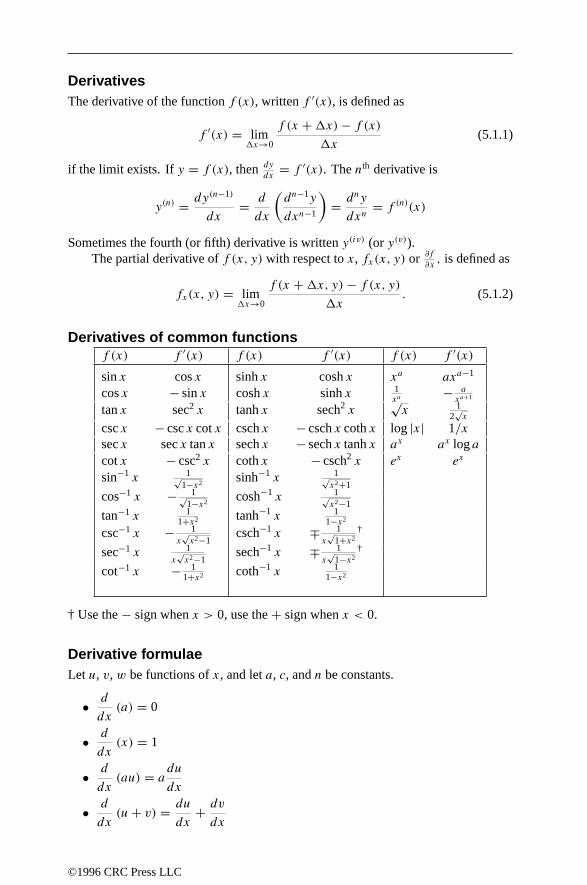
DerivativesThe derivative of the function f (x), written f ′(x), is defined as
f ′(x) = limx→0
f (x +x)− f (x)x
(5.1.1)
if the limit exists. If y = f (x), then dy
dx= f ′(x). The nth derivative is
y(n) = dy(n−1)
dx= d
dx
(dn−1y
dxn−1
)= dny
dxn= f (n)(x)
Sometimes the fourth (or fifth) derivative is written y(iv) (or y(v)).The partial derivative of f (x, y) with respect to x, fx(x, y) or ∂f
∂x, is defined as
fx(x, y) = limx→0
f (x +x, y)− f (x, y)x
. (5.1.2)
Derivatives of common functionsf (x) f ′(x) f (x) f ′(x) f (x) f ′(x)
sin x cos x sinh x cosh x xa axa−1
cos x − sin x cosh x sinh x 1xa
− axa+1
tan x sec2 x tanh x sech2 x√x 1
2√x
csc x − csc x cot x csch x − csch x coth x log |x| 1/xsec x sec x tan x sech x − sech x tanh x ax ax log acot x − csc2 x coth x − csch2 x ex ex
sin−1 x 1√1−x2 sinh−1 x 1√
x2+1cos−1 x − 1√
1−x2 cosh−1 x 1√x2−1
tan−1 x 11+x2 tanh−1 x 1
1−x2
csc−1 x − 1x√x2−1
csch−1 x ∓ 1x√
1+x2†
sec−1 x 1x√x2−1
sech−1 x ∓ 1x√
1−x2†
cot−1 x − 11+x2 coth−1 x 1
1−x2
† Use the − sign when x > 0, use the + sign when x < 0.
Derivative formulaeLet u, v, w be functions of x, and let a, c, and n be constants.
• d
dx(a) = 0
• d
dx(x) = 1
• d
dx(au) = a du
dx
• d
dx(u+ v) = du
dx+ dv
dx
©1996 CRC Press LLC

• d
dx(uv) = v du
dx+ udv
dx
• d
dx(uvw) = uv dw
dx+ uwdv
dx+ vwdu
dx
• d
dx
(uv
)= 1
v
du
dx− u
v2
dv
dx= v(du/dx)− u(dv/dx)
v2
• d
dx
(un) = nun−1 du
dx
• d
dx
(√u) = 1
2√u
du
dx
• d
dx
(1
u
)= − 1
u2
du
dx
• d
dx
(1
un
)= − n
un+1
du
dx
• d
dx
(un
vm
)= un−1
vm+1
(nvdu
dx−mudv
dx
)
• d
dx
(unvm
) = un−1vm−1
(nvdu
dx+mudv
dx
)
• d
dx(f (u)) = df
du(u) · du
dx
• d2
dx2(f (u)) = df
du(u) · ∂
2u
∂x2+ d2f
du2(u) ·
(du
dx
)2
• dn
dxn(uv) =
(n
0
)vdnu
dxn+(n
1
)dv
dx
dn−1u
dxn−1+ · · · +
(n
n
)dnv
dxnu
• d
dx
∫ x
c
f (t) dt = f (x)
• d
dx
∫ c
x
f (t) dt = −f (x)
• dx
dy=(dy
dx
)−1
andd2x
dy2= −d
2y
dx2
/(dy
dx
)3
• If F(x, y) = 0, thendy
dx= −Fx
Fyand
d2y
dx2= −
(FxxF
2y − 2FxyFxFy + FyyF 2
x
)F 3y
• Leibniz’s rule gives the derivative of an integral:
d
dx
(∫ g(x)
f (x)
h(x, t) dt
)= g′(x)h(x, g(x))−f ′(x)h(x, f (x))+
∫ g(x)
f (x)
∂h
∂x(x, t) dt.
• If x = x(t) and y = y(t) then (the dots denote differentiation with respect to t):
dy
dx= y(t)
x(t),
d2y
dx2= xy − xy
(x)2
©1996 CRC Press LLC

Derivative theorems• Fundamental theorem of calculus:
Suppose f is continuous on [a, b].
– If G is defined as G(x) =∫ x
a
f (t) dt for all x in [a, b], then G is an
antiderivative of f on [a, b].
– If F is any antiderivative of f , then∫ b
a
f (t) dt = F(b) − F(a). (Recall
that∫ baf (x) dx is defined as a limit of Riemann sums.)
• Intermediate value theorem:If f (x) is continuous on [a, b] and if f (a) = f (b), then f takes on every valuebetween f (a) and f (b) in the interval (a, b).
• Rolle’s theorem:If f (x) is continuous on [a, b] and differentiable on (a, b), and if f (a) = f (b),then f ′(c) = 0 for at least one number c in (a, b).
• Mean value theorem:If f (x) is continuous on [a, b] and differentiable on (a, b), then a number cexists in (a, b) such that f (b)− f (a) = (b − a)f ′(c).
The chain ruleIf x = x(t), y = y(t), and z = z(x, y), then
dz
dt= ∂z
∂x
dx
dt+ ∂z
∂y
dy
dt, and
d2z
dt2= ∂z
∂x
d2x
dt2+ dx
dt
(∂2z
∂x2
dx
dt+ ∂2z
∂x∂y
dy
dt
)
+ ∂z
∂y
d2y
dt2+ dy
dt
(∂2z
∂y2
dy
dt+ ∂2z
∂x∂y
dx
dt
).
If x = x(u, v), y = y(u, v), and z = z(x, y), then
∂z
∂u= ∂z
∂x
∂x
∂u+ ∂z
∂y
∂y
∂uand
∂z
∂v= ∂z
∂x
∂x
∂v+ ∂z
∂y
∂y
∂v.
If u = u(x, y), v = v(x, y), and f = f (x, y), then the partial derivative of f
with respect to u, holding v constant, written(∂f
∂u
)v, can be expressed as
(∂f
∂u
)v
=(∂f
∂x
)y
(∂x
∂u
)v
+(∂f
∂y
)x
(∂y
∂u
)v
. (5.1.3)
If x, y, and z all depend on one another (say, through f (x, y, z) = 0), then the
©1996 CRC Press LLC

partial derivative of x with respect to y, holding z constant, written(∂x∂y
)z, is
(∂x
∂y
)z
=[(∂y
∂x
)z
]−1
= − (∂f/∂y)x,z(∂f/∂x)y,z
,(∂x
∂y
)z
(∂y
∂z
)x
(∂z
∂x
)y
= −1.
(5.1.4)
l’Hopital’s ruleIf f (x) and g(x) are continuous in the neighborhood of point a, and if f (x) and g(x)both tend to 0 or ∞ as x → a, then
limx→a
f (x)
g(x)= limx→a
f ′(x)g′(x)
(5.1.5)
if the right hand side exists. For example
limx→0
x − sin x
x3= limx→0
1 − cos x
3x2= limx→0
sin x
6x= limx→0
cos x
6= 1
6,
and
limx→∞
xn
ex= limx→∞
nxn−1
ex= limx→∞
n(n− 1)xn−2
ex= · · · = lim
x→∞n!
ex= 0.
5.1.1 MAXIMA AND MINIMA OF FUNCTIONS
• If a function f (x) has a local extremum at a number c, then either f ′(c) = 0 orf ′(c) does not exist.
• If f ′(c) = 0, f (x) is differentiable on an open interval containing c, and
– if f ′′(c) < 0, then f has a local maximum at c;– if f ′′(c) > 0, then f has a local minimum at c.
Lagrange multipliersTo extremize the function f (x1, x2, . . . , xn) = f (x) subject to the n − 1 side con-straints g(x) = 0, introduce an (n − 1)-dimensional vector of Lagrange multipliersλλλ and define F(x,λλλ) = f (x) + λλλTg(x). Then extremize F with respect to all of itsarguments:
∂F
∂xi= ∂f
∂xi+ λλλT ∂g
∂xi= 0, and
∂F
∂λj= gj = 0.
For the simplest case, extremizing f (x, y) subject to g(x, y) = 0,
fx + λgx = 0, fy + λgy = 0, and g = 0.
©1996 CRC Press LLC

For example, finding the points on the unit circle, g(x, y) = (x−1)2+(y−2)2−1 = 0,that are closest and furthest from the origin, the distance squared is f (x, y) = x2+y2,can be determined by solving the three (nonlinear) algebraic equations:
2x + 2λ(x − 1) = 0, 2y + 2λ(y − 2) = 0, (x − 1)2 + (y − 2)2 = 0.
The solutions are x = 1 + 1√
5, y = 2 + 2/√
5, λ = −1 − √5 (furthest), and
x = 1 − 1√
5, y = 2 − 2/√
5, λ = √5 − 1 (closest).
5.1.2 VECTOR CALCULUS
In rectilinear coordinates, ∇ =(∂∂x, ∂∂y, ∂∂z
)= i ∂
∂x+ j ∂
∂y+k ∂
∂z. If u and v are scalars
and F and G are vectors, then
∇(u+ v) = ∇u+ ∇v,∇(uv) = u∇v + v∇u,
∇(F + G) = ∇F + ∇G,
∇(F · G) = (F · ∇)G + (G · ∇)F + F × (∇ × G)+ G × (∇ × F),
∇ · (uF) = u(∇ · F)+ F · ∇u,∇ · (F × G) = G · (∇ × F)− F · (∇ × G),
∇ × (uF) = u(∇ × F)+ (∇u)× F,
∇ × (F × G) = F(∇ · G)− G(∇ · F)+ (G · ∇)F − (F · ∇)G,F · dFdt
= |F| d|F|dt,
∇ × (∇ × F) = ∇(∇ · F)− ∇2F,
∇ × (∇u) = 0,
∇ · (∇ × F) = 0, and
∇2(uv) = u∇2v + 2(∇u) · (∇v)+ v∇2u.
A vector field F is irrotational if ∇ × F = 0. A vector field F is solenoidal if∇ · F = 0.
If r = |r|, a is a constant vector, and n is an integer, then
% ∇% ∇2%
a · r a 0rn nrn−2r n(n+ 1)rn−2
log r r/r2 1/r2
F ∇ · F ∇ × F (G · ∇)Fr 3 0 G
a × r 0 2a a × Garn nrn−2(r · a) nrn−2(r × a) nrn−2(r · G)arrn (n+ 3)rn 0 rnG + nrn−2(r · G)r
a log r r · a/r2 r × a/r2 (G · r)a/r2
©1996 CRC Press LLC

F ∇2F ∇∇ · Fr 0 0
a × r 0 0arn n(n+ 1)rn−2a nrn−2a + n(n− 2)rn−4(r · a)rrrn n(n+ 3)rn−2r n(n+ 3)rn−2r
a log r a/r2 [r2a − 2(r · a)r]/r4
d
dt(F + G) = dF
dt+ dGdt,
d
dt(F · G) = F · dG
dt+ dFdt
· G,
d
dt(F × G) = F × dG
dt+ dFdt
× G,
d
dt[V1V2V3] =
[(dV1
dt
)V2V3
]+[
V1
(dV2
dt
)V3
]+[
V1V2
(dV3
dt
)],
d
dt(V1 × V2 × V3) =
(dV1
dt
)× (V2 × V3)+ V1 ×
((dV2
dt
)× V3
),
+ V1 ×(
V2 ×(dV3
dt
)),
where [V1V2V3] = V1 · (V2 × V3) is the scalar triple product.
5.1.3 MATRIX AND VECTOR DERIVATIVES
Definitions1. The derivative of the row vector y with respect to the scalar x is
∂y∂x
=[∂y1
∂x
∂y2
∂x. . .
∂ym
∂x
].
2. The derivative of a scalar y with respect to the vector x is
∂y
∂x=
∂y
∂x1∂y
∂x2
...∂y
∂xn
.
3. Let x be a n × 1 vector and let y be a m × 1 vector. The derivative of y withrespect to x is the matrix
∂y∂x
=
∂y1
∂x1
∂y2
∂x1. . .
∂ym∂x1
∂y1
∂x2
∂y2
∂x2. . .
∂ym∂x2
......
. . ....
∂y1
∂xn
∂y2
∂xn. . .
∂ym∂xn
.
©1996 CRC Press LLC

In multivariate analysis, if x and y have the same length, then the absolute valueof the determinant of ∂y
∂x is called the Jacobian of the transformation determinedby y = y(x).
4. The derivative of the matrix A(t) = (aij (t)), with respect to the scalar t , is the
matrix dA(t)
dt=(daij (t)
dt
).
5. If X = (xij ) is a n × m matrix and if y is a scalar function of X given byy = f (X), then the derivative of y with respect to X is
∂y
∂X=
∂y
∂x11
∂y
∂x12. . .
∂y
∂x1n∂y
∂x21
∂y
∂x22. . .
∂y
∂x2n
......
. . ....
∂y
∂xm1
∂y
∂xm2. . .
∂y
∂xmn
=
∑ij
Eij∂y
∂xij.
6. If Y = (yij ) is a p× q matrix and X is a m× n matrix, then the derivative of Ywith respect to X is
∂Y
∂X=
∂Y∂x11
∂Y∂x12
. . . ∂Y∂x1n
∂Y∂x21
∂Y∂x22
. . . ∂Y∂x2n
......
. . ....
∂Y∂xm1
∂Y∂xm2
. . . ∂Y∂xmn
=
∑rs
Ers ⊗ ∂Y
∂xrs.
Properties
1.
y (scalar or a vector) ∂y
∂x
Ax AT
xTA A
xTx 2xxTAx Ax + ATx
2. If the matrices A and B can be multiplied, then d(AB)
dt= dA
dtB + AdB
dt.
3. If C = A⊗ B, then dCdt
= dAdt
⊗ B + A⊗ dBdt
.
4. If z = y(x), then ∂z∂y = ∂y
∂x∂z∂y .
5. If y = trX, then ∂y
∂X= In.
6. The derivative of the determinant of a matrix can be written:
• If Yij is the cofactor of element yij in |Y |, then ∂|Y |∂xrs
=∑i
∑j Yij
∂yij∂xrs
.
• If all of the components (xij )ofX are independent, then ∂|X|∂X
= |X| (X−1)T.
• If X is a symmetric matrix, then ∂|X|∂X
= 2X −∑i xii .
7. ∂(AXB)
∂xrs= AErsB where Ers is an elementary matrix of the same size as X.
8. If Y = AXTB, then ∂yij∂X
= BETijA.
©1996 CRC Press LLC

9. If Y = AX−1B, then
• ∂Y∂xrs
= −AX−1ErsX−1B.
• ∂yij∂X
= −(X−1)TATEijBT(X−1)T.
10. If Y = XTAX, then
• ∂Y∂xrs
= ETrsAX +XTAErs.
• ∂yij∂X
= AXETij + ATXEij .
11. Derivatives of powers of matrices are obtained as follows:
• If Y = Xr, then ∂Y∂xrs
=∑r−1k=0X
kErsXn−k−1.
• If Y = X−r , then ∂Y∂xrs
= −X−r(∑r−1
k=0XkErsX
n−k−1)X−r .
12. If y = VecY and x = VecX, then
• If Y = AX, then ∂y∂x = I ⊗ AT.
• If Y = XA, then ∂y∂x = A⊗ I.
• If Y = AX−1B, then ∂y∂x = −(X−1B)⊗ (X−1)TAT.
13. Derivative formulae:
• ∂ log |X|∂X
= (X−1)T.
• ∂ tr (AX)∂X
= AT.
• ∂ tr (XTA)∂X
= A.• ∂ tr (XTAXB)
∂X= AXB + ATXBT.
• If X and Y are matrices, then(∂Y∂X
)T = ∂YT
∂XT .
• If X, Y , and Z are matrices of size m× n, n× v, and p× q, then ∂(XY)
∂Z=
∂X∂Z(Iq ⊗ Y )+ (Ip ⊗ X ) ∂Y
∂Z.
5.2 DIFFERENTIAL FORMS
For the vector a = (a1, . . . , ak, . . . , an), define dxk to be the function that assigns tothe vector a its kth coordinate (that is, dxk(a) = ak). Geometrically, dxk(a) is thelength, with appropriate sign, of the projection of a on the kth coordinate axis. WhenFi are functions, the linear combination of the functions dxk
ωx = F1(x) dx1 + F2(x) dx2 + · · · + Fn(x) dxn (5.2.1)
©1996 CRC Press LLC

produces a new function ωx. This function acts on vectors a as
ωx(a) = F1(x) dx1(a)+ F2(x) dx2(a)+ · · · + Fn(x) dxn(a).
Such a function is a “differential 1-form” or a “1-form”. For example:
1. If a = (−2, 0, 4) then dx1(a) = −2, dx2(a) = 0, and dx3(a) = 4.
2. If in R2, ωx = ω(x,y) = x2 dx + y2 dy, then ω(x,y)(a, b) = ax2 + by2 andω(1,−3)(a, b) = a + 9b.
3. If f (x) is a differentiable function, then ∇xf , the differential of f at x, is a1-form. Note that ∇xf acting on a = (a1, a2, a3) is
∇xf (a) = ∂f
∂x1(x) dx1(a)+ ∂f
∂x2(x) dx2(a)+ ∂f
∂x3(x) dx3(a),
= ∂f
∂x1(x)a1 + ∂f
∂x2(x)a2 + ∂f
∂x3(x)a3.
Products of 1-forms
The basic 1-forms in R3 are dx1, dx2, and dx3. The wedge product dx1 ∧ dx2 isdefined so that it is a function of ordered pairs in R2. Geometrically, dx1 ∧ dx2(a,b)will be the area of the parallelogram spanned by the projections of a and b into the(x1, x2)-plane. The sign of the area is determined so that if the projections of a andb have the same orientation as the positive x1 and x2 axes, then the area is positive;it is negative when these orientations are opposite. Thus, if a = (a1, a2, a3) andb = (b1, b2, b3), then
dx1 ∧ dx2(a,b) = det
[a1 b1
a2 b2
]= a1b2 − a2b1,
and the determinant automatically gives the correct sign. This generalizes to
dxi ∧ dxj (a,b) = det
[dxi(a) dxi(b)dxj (a) dxj (b)
]= det
[ai biaj bj
]. (5.2.2)
• If ω and µ are 1-forms, and f and g are real-valued functions, then fω+ gµ isa 1-form.
• If ω, ν, and µ are 1-forms, then (f ω + gν) ∧ µ = f ω ∧ µ+ g ν ∧ µ.
• dxi ∧ dxj = −dxj ∧ dxi• dxi ∧ dxi = 0
• dxi ∧ dxj (b, a) = −dxi ∧ dxj (a,b)
©1996 CRC Press LLC

Differential 2-formsIn R3, the most general linear combination of the functions dxi ∧ dxj has the formc1 dx2 ∧ dx3 + c2 dx3 ∧ dx1 + c3 dx1 ∧ dx2. If F = (F1, F2, F3) is a vector field,then the function of ordered pairs,
τx(a,b) = F1(x) dx2 ∧ dx3 + F2(x) dx3 ∧ dx1 + F3(x) dx1 ∧ dx2 (5.2.3)
is a “differential 2-form” or “2-form”.
1. For the specific 2-form τx = 2 dx2∧dx3+dx3∧dx1+5 dx1∧dx2, if a = (1, 2, 3)and b = (0, 1, 1), then
τx(a,b) = 2 det
[2 13 1
]+ det
[3 11 0
]+ 5 det
[1 02 1
]= 2 · (−1)+ 1 · (−1)+ 5 · (1) = 2
independent of x. Note that a × b = det
i j k
1 2 30 1 1
= (−1,−1, 1), and so
τx(a,b) = (2, 1, 5) · (a × b).
2. When changing from Cartesian coordinates to polar coordinates, the element ofarea dA can be written
dA = dx ∧ dy= (−r sin θ dθ + cos θ dr) ∧ (r cos θ dθ + sin θ dr)
= −r2 sin θ cos θ dθ ∧ dθ + sin θ cos θ dr ∧ dr− r sin2 θ dθ ∧ dr + r cos2 θ dr ∧ dθ
= r dr ∧ dθ
The 2-forms in Rn
Every 2-form can be written in terms of a set of “basic 2-forms”. For example, in R2
there is only one basic 2-form (which may be taken to be dx1 ∧ dx2) and in R3 thereare 3 basic 2-forms (possibly the set dx1 ∧dx2, dx2 ∧dx3, dx3 ∧dx1). The exteriorproduct of any two 1-forms (in, say, Rn) is found by multiplying the 1-forms as ifthere were ordinary polynomials in the variables dx1, . . . , dxn, and then simplifyingusing the rules for dxi ∧ dxj .
For example, denoting the basic 1-forms in R3 as dx, dy, and dz then
(x dx + y2 dy) ∧ (dx + x dy) = x dx ∧ dx + y2 dy ∧ dx,+ x2 dx ∧ dy + xy2 dy ∧ dy,
= 0 − y2 dx ∧ dy + x2 dx ∧ dy + 0,
= (x2 − y2) dx ∧ dy.
©1996 CRC Press LLC

Higher dimensional forms
The meaning of the basic 3-form dx1 ∧dx2 ∧dx3 is that of a signed volume function.Thus, if a = (a1, a2, a3), b = (b1, b2, b3), and c = (c1, c2, c3) then
dx1 ∧ dx2 ∧ dx3(a,b, c) = det
a1 b1 c1
a2 b2 c2
a3 b3 c3
which is a 3-dimensional oriented volume of the parallepiped defined by the vectorsa, b, and c.
For an ordered p-tuple of vectors in Rn (a1, a2, . . . , ap), where p ≥ 1
dxk1 ∧ dxk2 ∧ · · · ∧ dxkp (a1, . . . ap) = det(dxki (aj )) i=1,...,pj=1,...,p
. (5.2.4)
This equation defines the basicp-forms in Rn, of which the generalp-forms are linearcombinations. Properties include:
1. The interchange of adjacent factors in a basic p-form changes the sign of theform.
2. A basic p-form with a repeated factor is zero.
3. The general p-form can be written ωp = ∑i1<···<ip fi1,...,ip dxi1 ∧ · · · ∧ dxik ,
where 1 ≤ ik ≤ n for k = 1, . . . , p. This sum has(n
p
)distinct nonzero terms in
it.
4. If p > n, then ωp is identically zero.
5. Ifωp is ap-form in Rn andωq is a q-form in Rn, thenωp∧ωq = (−1)pq ωq∧ωp.
The exterior derivative
The exterior differentiation operator is denoted by d. When d is applied to a scalarfunction f (x), the result is the 1-form that is equivalent to the usual “total differential”df = ∂f
∂x1dx1 +· · ·+ ∂f
∂xndxn. For the 1-form ω1 = f1 dx+· · ·+fn dxn the exterior
derivative is dω1 = (df1) ∧ dx1 + · · · + (dfn) ∧ dxn. This generalizes to higherdimensional forms.
1. If f (x1, x2) = x21 + x3
2 , then df = d(x21 + x3
2) = 2x1 dx1 + 3x22 dx2.
2. If ω1(x1,x2)
= x1x2 dx1 + (x21 + x2
2 ) dx2, then dω1 is given by
dω1 = d(x1x2 dx1 + (x21 + x2
2 ) dx2)
= (x2 dx1 + x1 dx2) ∧ dx1 + (2x1 dx1 + 2x2 dx2) ∧ dx2
= x1 dx1 ∧ dx2.
©1996 CRC Press LLC

Properties of the exterior derivative1. If f1(x1, x2) and f2(x1, x2) are differentiable functions, then
df1 ∧ df2 = ∂(f1, f2)
∂(x1, x2)dx1 ∧ dx2.
2. If ωp and ωq represent a p-form and a q-form, then
d(ωp ∧ ωq) = (dωp) ∧ ωq + (−1)pqωp ∧ (dωq).
3. If ωp is a p-form with at least two derivatives, then d(dωp) = 0.
• The relation d(dω0) = 0 is equivalent to curl(grad F) = 0.
• The relation d(dω1) = 0 is equivalent to div(curl f ) = 0.
5.3 INTEGRATION
5.3.1 DEFINITIONS
The following definitions apply to the expression I = ∫ baf (x) dx:
• The integrand is f (x).
• The upper limit is b.
• The lower limit is a.
• I is “the integral of f (x) from a to b”.
It is conventional to indicate the indefinite integral of a function representedby a lowercase letter by the corresponding uppercase letter. For example, F(x) =∫ xaf (t) dt andG(x) = ∫ x
ag(t) dt . Note that all functions that differ from F(x) by a
constant are also indefinite integrals of f (x).
• ∫ f (x) dx indefinite integral of f (x) (also written∫ xf (t) dt)
• ∫ baf (x) dx definite integral of f (x), defined as
limn→∞
(b − an
n∑k=1
f
[a + k
n(b − a)
])
• ∮C f (x) dx definite integral of f (x), taken along the contour C
• ∫∞af (x) dx defined as lim
R→∞
∫ R
a
f (x) dx
©1996 CRC Press LLC

• ∫∞−∞ f (x) dx defined as the limit of
∫ R−S f (x) dx as R and S inde-
pendently go to ∞• ∫ f shorthand for
∫f (x) dx
• Improper integral integral for which the region of integration is notbounded, or the integrand is not bounded
• Cauchy principal value
– The Cauchy principal value of the integral∫ baf (x) dx, denoted −
∫ baf (x) dx,
is defined as limε→0+
(∫ c−ε
a
f (x) dx +∫ b
c+εf (x) dx
), assuming that f is
singular only at c.
– The Cauchy principal value of the integral∫∞−∞ f (x) dx is defined as the
limit of∫ R
−Rf (x) dx as R → ∞.
• If, at the complex point z = a, f (z) is either analytic or has an isolated sin-gularity, then the residue of f (z) at z = a is given by the complex integralResf (a) = 1
2πi
∮C f (ξ) dξ .
5.3.2 PROPERTIES OF INTEGRATION
Indefinite integrals have the properties:
1.∫
[af (x)+ bg(x)] dx = a ∫ f (x) dx + b ∫ g(x) dx (linearity).
2.∫f (x)g(x) dx = F(x)g(x)− ∫ F(x)g′(x) dx (integration by parts).
3.∫f (g(x))g′(x) dx = F(g(x)) (substitution).
4.∫f (ax + b) dx = 1
aF (ax + b).
5. If f (x) is an odd function, then F(x) is an even function.
6. If f (x) is an even function and F(0) = 0, then F(x) is an odd function.
7. If f (x) has a finite number of discontinuities, then the integral∫f (x) dx is the
sum of the integrals over those subintervals where f (x) is continuous (providedthey exist).
8. Fundamental theorem of integral calculus Iff (x) is single-valued, bounded, andintegrable on [a, b], and there exists a function F(x) such that F ′(x) = f (x)
for a ≤ x ≤ b then∫ x
a
f (x) dx = F(x) ∣∣xa
= F(x)− F(a)
for a ≤ x ≤ b.
Definite integrals have the properties:
1.∫ aaf (x) dx = 0.
©1996 CRC Press LLC

2.∫ baf (x) dx = − ∫ a
bf (x) dx.
3.∫ baf (x) dx + ∫ c
bf (x) dx = ∫ c
af (x) dx (additivity).
4.∫ ba [cf (x)+ dg(x)] dx = c
∫ baf (x) dx + d
∫ bag(x) dx (linearity).
5.3.3 INEQUALITIES
1. Schwarz’ inequality:
∫ ba
|fg| ≤√(∫ b
af 2) (∫ b
ag2).
2. Minkowski’s inequality:(∫ ba
|f + g|p)1/p
≤(∫ ba
|f |p)1/p
+(∫ ba
|g|p)1/p
when p ≥ 1.
3. Holder’s inequality:∫ ba
|fg| ≤[∫ ba
|f |p]1/p [∫ b
a|g|q]1/q
when 1p
+ 1q
= 1, p > 1, and q > 1.
4.∣∣∣∫ ba f (x) dx∣∣∣ ≤ ∫ ba |f (x)| dx ≤
(maxx∈[a,b]
|f (x)|)(b − a) assuming a ≤ b.
5. If f (x) ≤ g(x) on the interval [a, b], then∫ baf (x) dx ≤ ∫ b
ag(x) dx.
5.3.4 CONVERGENCE TESTS
1. If∫ ba
|f (x)| dx is convergent, then∫ baf (x) dx is convergent.
2. If 0 ≤ f (x) ≤ g(x) and∫ bag(x) dx is convergent,
then∫ baf (x) dx is convergent.
3. If 0 ≤ g(x) ≤ f (x) and∫ bag(x) dx is divergent,
then∫ baf (x) dx is divergent.
The following integrals may be used, for example, with the above tests:
•∫ ∞
2
dx
x(log x)pand
∫ ∞
1
dx
xpare convergent when p > 1, and divergent when
p ≤ 1.
•∫ 1
0
dx
xpis convergent when p < 1, and divergent when p ≥ 1.
©1996 CRC Press LLC

5.3.5 SUBSTITUTION
Substitution can be used to change integrals to simpler forms. When the transformt = g(x) is chosen, the integral I = ∫
f (t) dt becomes I = ∫f (g(x)) dt =∫
f (g(x))g′(x) dx. Several precautions must be observed when using substitutions:
• Be sure to make the substitution in the dx term, as well as everywhere else inthe integral.
• Be sure that the function substituted is one-to-one and continuous. If this is notthe case, then the integral must be restricted in such a way as to make it true.
• With definite integrals, the limits should also be expressed in terms of the newdependent variables. With indefinite integrals, it is necessary to perform thereverse substitution to obtain the answer in terms of the original independentvariable. This may also be done for definite integrals, but it is usually easier tochange the limits.
ExampleConsider the integral
I =∫
x4
√a2 − x2
dx
Here we choose to make the substitution x = |a| sin θ . From this we find dx =|a| cos θ dθ and√
a2 − x2 =√a2 − a2 sin2 θ = |a|
√1 − sin2 θ = |a| |cos θ |
Note the absolute value signs. It is very important to interpret the square root radicalconsistently as the positive square root. Thus
√x2 = |x|. Failure to observe this is a
common cause of errors in integration.Note that the substitution used above is not a one-to-one function, that is, it does
not have a unique inverse. Thus the range of θ must be restricted in such a way as tomake the function one-to-one. In this case we can solve for θ to obtain
θ = sin−1 x
|a|This will be unique if we restrict the inverse sine to the principal values −π
2 ≤ θ ≤ π2 .
Thus, the integral becomes (with dx = |a| cos θ dθ)
I =∫a4 sin4 θ
|a| |cos θ | |a| cos θ dθ.
Now, however, in the range of values chosen for θ , we find that cos θ is always positive.Thus, we may remove the absolute value signs from cos θ in the denominator. Thenthe cos θ terms cancel and the integral becomes
I = a4∫
sin4 θ dθ.
©1996 CRC Press LLC

By application of the integration formula on page 378 this is integrated to obtain
I = −a4
4sin3 θ cos θ − 3a4
8sin θ cos θ + 3a4
8θ + C. (5.3.1)
To obtain an evaluation of I as a function of x, we must transform variables from θto x. We have
cos θ = ±√
1 − sin2 θ = ±√
1 − x2
a2= ±
√a2 − x2
|a| .
Because of the previously recorded fact that cos θ is positive for our range of θ , wemay omit the ± sign. Using sin θ = x/ |a| and cos θ = √
a2 − x2/ |a| we canevaluate Equation (5.3.1) to obtain the final result,
I =∫
x4
√a2 − x2
= −x3
4
√a2 − x2 − 3a2x
8
√a2 − x2 + 3a4
8sin−1 x
|a| + C.
Useful transformationsThe following transformations may make evaluation of an integral easier:
1.∫f(x,
√x2 + a2
)dx = a ∫ f (a tan u, a sec u) sec2 u du
when u = tan−1 xa
and a > 0.
2.∫f(x,
√x2 − a2
)dx = a ∫ f (a sec u, a tan u) sec u tan u du
when u = sec−1 xa
and a > 0.
3.∫f(x,
√a2 − x2
)dx = a ∫ f (a sin u, a cos u) cos u du
when u = sin−1 xa
and a > 0.
4.∫f (sin x) dx = 2
∫f(
2z1+z2
)dz
1+z2 when z = tan x2 .
5.∫f (cos x) dx = 2
∫f(
1−z2
1+z2
)dz
1+z2 when z = tan x2 .
6.∫f (cos x) dx = − ∫ f (v) dv√
1−v2 when v = cos x.
7.∫f (sin x) dx = ∫ f (u) du√
1−u2 when u = sin x.
8.∫f (sin x, cos x) dx = ∫ f (u,√1 − u2
)du√1−u2 when u = sin x.
9.∫f (sin x, cos x) dx = 2
∫f(
2z1+z2 ,
1−z2
1+z2
)dz
1+z2 when z = tan x2 .
10.∫∞−∞ F(u) dx = ∫∞
−∞ F(x) dx when u = x −n∑j=1
aj
x − cj where ai is any
sequence of positive constants and the cj are any real constants whatsoever.
Several transformations of the integral∫∞
0 f (x) dx, with an infinite integrationrange, to an integral with a finite integration range, are shown:
©1996 CRC Press LLC

t (x) x(t) dxdt
Finite interval integral
e−x − log t − 1t
∫ 10f (− log t)
tdt
x1+x
t1−t
1(1−t)2
∫ 10 f
(t
1−t)
dt(1−t)2
tanh x 12 log 1+t
1−t1
1−t2∫ 1
0 f(
12 log 1+t
1−t)dt
1−t2
5.3.6 PARTIAL FRACTION DECOMPOSITION
Every integral of the form∫R(x) dx, where R is a rational function, can be evalu-
ated (in principle) in terms of elementary functions. The technique is to factor thedenominator of R and create a partial fraction decomposition. Then each resultingsubintegral is elementary.
Example
Consider the integral I =∫
2x3 − 10x2 + 13x − 4
x2 − 5x + 6dx. This can be written as
I =∫ (
2x + x − 4
x2 − 5x + 6
)dx =
∫ (2x + 2
x − 2− 1
x − 3
)dx
which can be readily integrated I = x2 + 2 ln(x − 2)− ln(x − 3).
5.3.7 INTEGRATION BY PARTS
In one dimension, the integration by parts formula is
∫u dv = uv −
∫v du for indefinite integrals, (5.3.2)∫ b
a
u dv = uv ∣∣ba−∫ b
a
v du for definite integrals. (5.3.3)
When evaluating a given integral by this method, u and v must be chosen so that theform
∫u dv becomes identical to the given integral. This is usually accomplished by
specifying u and dv and deriving du and v. Then the integration by parts formulawill produce a boundary term and another integral to be evaluated. If u and v werewell chosen, then this second integral may be easier to evaluate.
ExampleConsider the integral
I =∫x sin x dx.
Two obvious choices for the integration by parts formula are u = x, dv = sin x dxand u = sin x, dv = x dx. We will try each of them in turn.
©1996 CRC Press LLC

• Using u = x, dv = sin x dx, we compute du = dx and v = ∫dv =∫
sin x dx = − cos x. Hence, we can represent I in the alternative form as
I =∫x sin x dx =
∫u dv = uv −
∫v du = −x cos x +
∫cos x dx.
In this representation of I,we must evaluate the last integral. Because we know∫cos x dx = sin x the final result is I = sin x − x cos x.
• Using u = sin x, dv = x dx we compute du = cos x dx and v = ∫dv =∫
x dx = x2/2. Hence, we can represent I in the alternative form as
I =∫x sin x dx =
∫u dv = uv −
∫v du = x2
2cos x −
∫x2
2cos x dx.
In this case, we have actually made the problem “worse” since the remainingintegral appearing in I is “harder” than the one we started with.
ExampleConsider the integral
I =∫ex sin x dx.
We choose to use the integration by parts formula with u = ex and dv = sin x dx.From these we compute du = ex dx and v = ∫
dv = ∫sin x dx = − cos x. Hence,
we can represent I in the alternative form as
I =∫ex sin x dx =
∫u dv = uv −
∫v du = −ex cos x +
∫ex cos x dx
If we write this as
I = −ex cos x + J with J =∫ex cos x dx, (5.3.4)
then we can apply integration by parts to J using u = ex , dv = cos x dx. Fromthese we compute du = ex dx and v = ∫
dv = ∫cos x dx = sin x. Hence, we can
represent J in the alternative form as
J =∫ex cos x dx =
∫u dv = uv −
∫v du = ex sin x −
∫ex sin x dx
If we write this as
J = ex sin x − I, (5.3.5)
then we can solve the linear equations (5.3.4) and (5.3.5) simultaneously to determineboth I and J . We find
I =∫ex sin x dx = 1
2
(ex sin x − ex cos x
), and
J =∫ex cos x dx = 1
2
(ex sin x + ex cos x
).
©1996 CRC Press LLC

Extended integration by parts rule
The following rule is obtained by n+1 successive applications of integration by parts.Let
g1(x) =∫g(x) dx, g2(x) =
∫g1(x) dx,
g3(x) =∫g2(x) dx, . . . , gm(x) =
∫gm−1(x) dx. (5.3.6)
Then
∫f (x)g(x) dx = f (x)g1(x)− f ′(x)g2(x)+ f ′′(x)g3(x)− . . .
+ (−1)nf (n)(x)gn+1(x)+ (−1)n+1∫f (n+1)(x)gn+1(x) dx. (5.3.7)
5.3.8 SPECIAL FUNCTIONS DEFINED BY INTEGRALS
Not all integrals of elementary functions (sines, cosines, rational functions, and others)can be evaluated in terms of elementary functions. For example, the integral
∫e−x
2dx
is represented by the special function “erf(x)” (see page 498). Other useful functionsinclude dilogarithms (see page 506) and elliptic integrals (see page 522).
The dilogarithm function is defined by Li2(x) = − ∫ x0 ln(1 − x)/x dx. Allintegrals of the form
∫ xP (x,
√R) logQ(x,
√R) dx, where P and Q are rational
functions andR = A2 +Bx+Cx2, can be evaluated in terms of elementary functionsand dilogarithms.
All integrals of the form∫xR(x,
√T (x)) dx,whereR is a rational function of its
arguments and T (x) is a third or fourth order polynomial, can be integrated in termsof elementary functions and elliptic functions.
5.3.9 VARIATIONAL PRINCIPLES
If J depends on a function g(x) and its derivatives through an integral of the formJ [g] = ∫
F(g, g′, . . . ) dx, then J will be stationary to small perturbations if Fsatisfies the corresponding Euler–Lagrange equation.
©1996 CRC Press LLC

Function Euler–Lagrange equation∫RF(x, y, y ′) dx ∂F
∂y− ddx
(∂F∂y ′
)= 0
∫RF(x, y, y ′, . . . , y(n)
)dx ∂F
∂y− ddx
(∂F∂y ′
)+ d2
dx2
(∂F∂y ′′
)−
· · · + (−1)n dn
dxn
(∂F∂y(n)
)= 0
∫∫R
[a(∂u∂x
)2 + b ( ∂u∂x
)2 + cu2 + 2f u]dx dy, ∂
∂x
(a ∂u∂x
)+ ∂∂y
(b ∂u∂y
)− cu = f
∫∫R
F(x, y, u, ux, uy, uxx, uxy, uyy) dx dy∂F∂u
− ∂∂x
(∂F∂ux
)− ∂∂y
(∂F∂uy
)+
∂2
∂x2
(∂F∂uxx
)+ ∂2
∂x∂y
(∂F∂uxy
)+
∂2
∂y2
(∂F∂uyy
)= 0
5.3.10 LINE AND SURFACE INTEGRALS
A line integral is a definite integral whose path of integration is along a specified curve;it can be evaluated by reducing it to ordinary integrals. If f (x, y) is continuous onC, and the integration contour C is parameterized by (φ(t), ψ(t)) as t varies from ato b, then ∫
Cf (x, y) dx =
∫ b
a
f
(φ(t), ψ(t)
)φ′(t) dt, (5.3.8)∫
Cf (x, y) dy =
∫ b
a
f
(φ(t), ψ(t)
)ψ ′(t) dt. (5.3.9)
In a simply connected domain, the line integral I = ∫C X dx + Y dy + Z dz
is independent of the path C (beginning and ending at the same place) if, and onlyif, u = (X, Y,Z) is a gradient vector, u = gradF (that is, Fx = X, Fy = Y , andFz = Z).
Green’s theorem: Let D be a domain of the xy plane, and let C be a piecewisesmooth, simple closed curve in D whose interior R is also in D. Let P(x, y) andQ(x, y) be functions defined inD with continuous first partial derivatives inD. Then
∮C(P dx +Qdy) =
∫∫R
(∂Q
∂x− ∂P
∂y
)dx dy. (5.3.10)
The above theorem may be written in the two alternative forms (using u =P(x, y)i +Q(x, y)j and v = Q(x, y)i − P(x, y)j),∮
CuT ds =
∫∫R
curl u dx dy and∮
Cvn ds =
∫∫R
div v dx dy.(5.3.11)
The first equation above is a simplification of Stokes’s theorem, the second equationis the divergence theorem.
©1996 CRC Press LLC

Stokes’s theorem: Let S be a piecewise smooth oriented surface in space, whoseboundary C is a piecewise smooth simple closed curve, directed in accordance withthe given orientation of S. Let u = Li +Mj +Nk be a vector field with continuousand differentiable components in a domainD of space including S. Then,
∫C uT ds =∫∫
S
(curl u) · n dσ, where n is the chosen unit normal vector on S, that is
∫CLdx +M dy +N dz =
∫∫S
(∂N
∂y− ∂M
∂z
)dy dz
+(∂L
∂z− ∂N
∂x
)dz dx +
(∂M
∂x− ∂L
∂y
)dx dy. (5.3.12)
Divergence theorem: Let v = Li +Mj + Nk be a vector field in a domain Dof space. Let L, M , and N be continuous with continuous derivatives in D. Let Sbe a piecewise smooth surface in D that forms the complete boundary of a boundedclosed region R in D. Let n be the outer normal of S with respect to R. Then∫∫S
vn dσ =∫∫∫R
div v dx dy dz, that is
∫∫S
L dy dz+M dz dx +N dx dy
=∫∫∫R
(∂L
∂x+ ∂M
∂y+ ∂N
∂z
)dx dy dz. (5.3.13)
IfD is a three-dimensional domain with boundaryB, let dV represent the volumeelement ofD, let dS represent the surface element of B, and let dS = n dS, where nis the outer normal vector of the surface B. Then Gauss’s formulae are∫∫∫
D
∇ · A dV =∫∫B
dS · A =∫∫B
(n · A) dS, (5.3.14)
∫∫∫D
∇ × A dV =∫∫B
dS × A =∫∫B
(n × A) dS, and(5.3.15)∫∫∫
D
∇φ dV =∫∫B
φ dS, (5.3.16)
where φ is an arbitrary scalar and A is an arbitrary vector.Green’s theorems also relate a volume integral to a surface integral: Let V be
a volume with surface S, which we assume is simple and closed. Define n as theoutward normal to S. Let φ and ψ be scalar functions which, together with ∇2φ and∇2ψ , are defined in V and on S. Then
1. Green’s first theorem states that∫S
φ∂ψ
∂ndS =
∫V
(φ∇2ψ + ∇φ · ∇ψ) dV . (5.3.17)
©1996 CRC Press LLC

2. Green’s second theorem states that∫S
(φ∂ψ
∂n− ψ ∂φ
∂n
)dS =
∫V
(φ∇2ψ − ψ∇2φ
)dV .
(5.3.18)
5.3.11 CONTOUR INTEGRALS
If f (z) is analytic in the region inside of the simple closed curve C (with properorientation), then
1. The Cauchy–Goursat integral theorem is∮C f (ξ) dξ = 0.
2. Cauchy’s integral formula is
f (z) = 1
2πi
∮C
f (ξ)
ξ − z dξ and f ′(z) = 1
2πi
∮C
f (ξ)
(ξ − z)2 dξ.
In general, f (n)(z) = n!2πi
∮C
f (ξ)
(ξ−z)n+1 dξ.
The residue theorem: For every simple closed contour C enclosing at most a finitenumber of (necessarily isolated) singularities z1, z2, . . . , zn of a single-valued func-tion f (z) continuous on C,
1
2πi
∮Cf (ξ) dξ =
n∑k=1
Resf (zk)
5.3.12 CONTINUITY OF INTEGRAL ANTIDERIVATIVES
Consider the following different evaluations of an integral
F(x) =∫f (x) dx =
∫3
5 − 4 cos xdx =
2 tan−1(3 tan(x/2))
2 tan−1(3 sin x/(cos x + 1))
− tan−1(−3 sin x/(5 cos x − 4))
2 tan−1(3 tan x
2
)+ 2π⌊x
2π + 12
⌋where · denotes the floor function. These evaluations are all “correct” becausedifferentiating any of them results in the original integrand. However, if we expectthat
∫ 4π0 f (x) dx = F(4π)−F(0) is correct, then only the last evaluation is correct.
This is true because the other evaluations of F(x) are discontinuous when x is amultiple of π .
In general, if F (x) = ∫ xf (x) dx is a discontinuous evaluation (with F (x)
discontinuous at the single point x = b), then a continuous evaluation on a finiteinterval is given by
∫ caf (x) dx = F(c)− F(a), where
F(x) = F (x)− F (a)+H(x − b)[
limx→b−
F (x)− limx→b+
F (x)
]and where H(·) is the Heaviside function. For functions with an infinite number of
discontinuities, note that∞∑n=1
H(x − pn− q) =⌊x − qp
⌋.
©1996 CRC Press LLC

Applications of integration• Using Green’s theorems, the area bounded by the simple, closed, positively
oriented contour C is
area =∮
Cx dy = −
∮Cy dx. (5.3.19)
• Arc length:
1. s =∫ x2
x1
√1 + y ′2 dx for y = f (x).
2. s =∫ t2
t1
√φ2 + ψ2 dt for x = φ(t), y = ψ(t).
3. s =∫ θ2
θ1
√r2 +
(dr
dφ
)2
dθ =∫ r2
r1
√1 + r2
(dr
dφ
)2
dr for r = f (θ).
• Surface area for surfaces of revolution:
1. A = 2π∫ x2
x1
f (x)√
1 + (f ′(x))2 dx when y = f (x) is rotated about the
x-axis.
2. A = 2π∫ y2
y1
x√
1 + (f ′(x))2 dy when y = f (x) is rotated about the
y-axis.
3. A = 2π∫ t2
t1
ψ
√φ2 + ψ2 dt for x = φ(t), y = ψ(t) rotated about the
x-axis.
4. A = 2π∫ t2
t1
φ
√φ2 + ψ2 dt for x = φ(t), y = ψ(t) rotated about the
y-axis.
5. A = 2π∫ φ2
φ1
r sin φ
√r2 +
(dr
dφ
)2
dφ for r = r(φ) rotated about the
x-axis.
6. A = 2π∫ φ2
φ1
r cosφ
√r2 +
(dr
dφ
)2
dφ for r = r(φ) rotated about the
y-axis.
• Volumes of revolution:
1. V = π∫ x2
x1
f 2(x) dx for y = f (x) rotated about the x-axis.
2. V = π∫ x2
x1
x2f ′(x) dx for y = f (x) rotated about the y-axis.
3. V = π∫ y2
y1
g2(y) dy for x = g(y) rotated about the y-axis.
©1996 CRC Press LLC
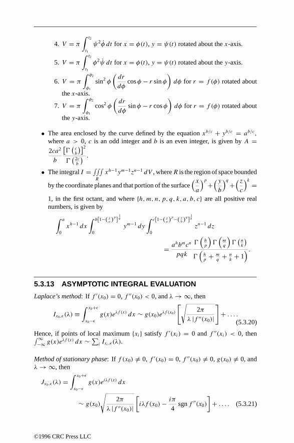
4. V = π∫ t2
t1
ψ2φ dt for x = φ(t), y = ψ(t) rotated about the x-axis.
5. V = π∫ t2
t1
φ2ψ dt for x = φ(t), y = ψ(t) rotated about the y-axis.
6. V = π
∫ φ2
φ1
sin2 φ
(dr
dφcosφ − r sin φ
)dφ for r = f (φ) rotated about
the x-axis.
7. V = π
∫ φ2
φ1
cos2 φ
(dr
dφsin φ − r cosφ
)dφ for r = f (φ) rotated about
the y-axis.
• The area enclosed by the curve defined by the equation xb/c + yb/c = ab/c,
where a > 0, c is an odd integer and b is an even integer, is given by A =2ca2
b
[E(cb
)]2E(
2cb
) .
• The integral I = ∫∫∫R
xh−1ym−1zn−1 dV , whereR is the region of space bounded
by the coordinate planes and that portion of the surface(xa
)p+(yb
)q+(zc
)k=
1, in the first octant, and where h,m, n, p, q, k, a, b, c are all positive realnumbers, is given by∫ a
0xh−1 dx
∫ b[1−( xa )
p] 1q
0ym−1 dy
∫ c[1−( xa )
p−( yb )q ] 1k
0zn−1 dz
= ahbmcn
pqk
E(hp
)E(mq
)E(nk
)E(hp
+ mq
+ nk
+ 1) .
5.3.13 ASYMPTOTIC INTEGRAL EVALUATION
Laplace’s method: If f ′(x0) = 0, f ′′(x0) < 0, and λ→ ∞, then
Ix0,ε(λ) ≡∫ x0+ε
x0−εg(x)eλf (x) dx ∼ g(x0)e
λf (x0)
[√2π
λ |f ′′(x0)|
]+ . . . .
(5.3.20)
Hence, if points of local maximum xi satisfy f ′(xi) = 0 and f ′′(xi) < 0, then∫∞−∞ g(x)e
λf (x) dx ∼∑i Ixi ,ε(λ).
Method of stationary phase: If f (x0) = 0, f ′(x0) = 0, f ′′(x0) = 0, g(x0) = 0, andλ→ ∞, then
Jx0,ε(λ) =∫ x0+ε
x0−εg(x)eiλf (x) dx
∼ g(x0)
√2π
λ |f ′′(x0)|[iλf (x0)− iπ
4sgn f ′′(x0)
]+ . . . . (5.3.21)
©1996 CRC Press LLC

5.3.14 MOMENTS OF INERTIA FOR VARIOUS BODIESBody Axis Moment of inertia
Uniform thin rodNormal to the length, at one
endml2
3
Uniform thin rodNormal to the length, at the
centerm l2
12
Thin rectangular sheet, sides aand b
Through the center parallelto b
ma2
12
Thin rectangular sheet, sides aand b
Through the centerperpendicular to the sheet
ma2+b2
12
Thin circular sheet of radius rNormal to the plate through
the centermr2
2
Thin circular sheet of radius r Along any diameter mr2
4
Thin circular ring, radii r1and r2
Through center normal toplane of ring
mr21 +r2
22
Thin circular ring, radii r1and r2
Along any diameter mr21 +r2
24
Rectangular parallelopiped,edges a, b, and c
Through centerperpendicular to face ab(parallel to edge c)
ma2+b2
12
Sphere, radius r Any diameter m 25 r
2
Spherical shell, external radiusr1, internal radius r2
Any diameter m 25r51 −r5
2r31 −r3
2
Spherical shell, very thin,mean radius r
Any diameter m 23 r
3
Right circular cylinder ofradius r , length l
Longitudinal axis of theslide
mr2
2
Right circular cylinder ofradius r , length l
Transverse diameter m(r2
4 + l2
12
)Hollow circular cylinder, radiir1 and r2, length l
Longitudinal axis of thefigure
mr21 +r2
22
Thin cylindrical shell, length l,mean radius r
Longitudinal axis of thefigure
mr2
Hollow circular cylinder, radiir1 and r2, length l
Transverse diameter m(r21 +r2
24 + l2
12
)Hollow circular cylinder, very
thin, length l, mean radius rTransverse diameter m
(r2
2 + l2
12
)Elliptic cylinder, length l,
transverse semiaxes a and bLongitudinal axis m
(a2+b2
4
)Right cone, altitude h, radius
of base rAxis of the figure m 3
10 r2
Spheroid of revolution,equatorial radius r
Polar axis m 25 r
2
Ellipsoid, axes 2a, 2b, 2c Axis 2a mb2+c2
5
©1996 CRC Press LLC

5.3.15 TABLE OF SEMI-INTEGRALS
fd−1/2f
dx−1/2
0 0
C, a constant 2C√xπ
x−1/2 √π
x 4x2/3
3√π
xn, n = 0, 1, 2, . . . (n!)2(4x)n+1/2
(2n+1)!√π
xp, p > −1 E(p+1)E(p+ 3
2 )xp+1/2
√1 + x √
xπ
+ (1+x) tan−1(√x)√
π
1√1+x
2√π
tan−1(√x)
11+x
2 sinh−1(√x)√
π(1+x)
ex ex erf(√x)
ex erf(√x)
ex − 1sin(√x) √
πxJ1(√x)
cos(√x) √
πxH−1(√x)
sinh(√x) √
πxI1(√x)
cosh(√x) √
πxL−1(√x)
sin(√x)√x
√πH0
(√x)
cos(√x)√x
√πJ0
(√x)
log x 2√xπ
[log(4x)− 2
]log x√x
√π log
(x4
)
5.3.16 TABLES OF INTEGRALS
Many extensive compilations of integrals tables exist. No matter how extensive theintegral table, it is fairly uncommon to find the exact integral desired. Usually someform of transformation will have to be made. The simplest type of transformation issubstitution. Simple forms of substitutions, such as y = ax are employed, almostunconsciously, by experienced users of integral tables. Finding the right substitutionis largely a matter of intuition and experience.
We adopt the following conventions in our integral tables:
• A constant of integration must be included with all indefinite integrals.
©1996 CRC Press LLC
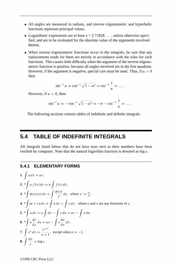
• All angles are measured in radians, and inverse trigonometric and hyperbolicfunctions represent principal values.
• Logarithmic expressions are to base e = 2.71828 . . . , unless otherwise speci-fied, and are to be evaluated for the absolute value of the arguments involvedtherein.
• When inverse trigonometric functions occur in the integrals, be sure that anyreplacements made for them are strictly in accordance with the rules for suchfunctions. This causes little difficulty when the argument of the inverse trigono-metric function is positive, because all angles involved are in the first quadrant.However, if the argument is negative, special care must be used. Thus, if u > 0then
sin−1 u = cos−1√
1 − u2 = csc−1 1
u= . . . .
However, if u < 0, then
sin−1 u = − cos−1√
1 − u2 = −π − csc−1 1
u= . . . .
The following sections contain tables of indefinite and definite integrals.
5.4 TABLE OF INDEFINITE INTEGRALS
All integrals listed below that do not have stars next to their numbers have beenverified by computer. Note that the natural logarithm function is denoted as log x.
5.4.1 ELEMENTARY FORMS
1.∫a dx = ax.
2. *∫a f (x) dx = a
∫f (x) dx.
3. *∫φ(y(x)) dx =
∫φ(y)
y ′ dy, where y ′ = dy
dx.
4. *∫(u+ v) dx =
∫u dx +
∫v dx, where u and v are any functions of x.
5. *∫u dv = u
∫dv −
∫v du = uv −
∫v du.
6. *∫udv
dxdx = uv −
∫vdu
dxdx.
7.∫xn dx = xn+1
n+ 1, except when n = −1.
8.∫dx
x= log x.
©1996 CRC Press LLC

9. *∫f ′(x)f (x)
dx = log f (x), (df (x) = f ′(x) dx).
10. *∫
f ′(x)2√f (x)
dx =√f (x), (df (x) = f ′(x) dx).
11.∫ex dx = ex.
12.∫eax dx = eax
a.
13.∫bax dx = bax
a log b, b > 0.
14.∫
log x dx = x log x − x.
15.∫ax dx = ax
log a, a > 0.
16.∫
dx
a2 + x2= 1
atan−1 x
a.
17.∫
dx
a2 − x2=
1
atanh−1 x
a,
or1
2aloga + xa − x , a2 > x2.
18.∫
dx
x2 − a2=
− 1
acoth−1 x
a,
or1
2alogx − ax + a , x2 > a2.
19.∫
dx√a2 − x2
=
sin−1 x
|a| ,or
− cos−1 x
|a| , a2 > x2.
20.∫
dx√x2 ± a2
= log(x +
√x2 ± a2
).
21.∫
dx
x√x2 − a2
= 1
|a| sec−1 x
a.
22.∫
dx
x√a2 ± x2
= − 1
alog
(a + √
a2 ± x2
x
).
5.4.2 FORMS CONTAINING a + bx
23.∫(a + bx)n dx = (a + bx)n+1
(n+ 1)b, n = −1.
24.∫x(a+ bx)n dx = 1
b2(n+ 2)(a+ bx)n+2 − a
b2(n+ 1)(a+ bx)n+1, n = −1, n = −2.
25.∫x2(a + bx)n dx = 1
b3
[(a + bx)n+3
n+ 3− 2a
(a + bx)n+2
n+ 2+ a2 (a + bx)n+1
n+ 1
], n = −1,
n = −2, n = −3.
©1996 CRC Press LLC

26.∫xm(a + bx)n dx =
xm+1(a + bx)nm+ n+ 1
+ an
m+ n+ 1
∫xm(a + bx)n−1 dx,
or1
a(n+ 1)
[−xm+1(a + bx)n+1 + (m+ n+ 2)
∫xm(a + bx)n+1 dx
],
or1
b(m+ n+ 1)
[xm(a + bx)n+1 −ma
∫xm−1(a + bx)n dx
].
27.∫
dx
a + bx = 1
blog |(a + bx)|.
28.∫
dx
(a + bx)2 = − 1
b(a + bx) .
29.∫
dx
(a + bx)3 = − 1
2b(a + bx)2 .
30.∫
x
a + bx dx =
1
b2
[a + bx − a log (a + bx)] ,
orx
b− a
b2log (a + bx).
31.∫
x
(a + bx)2 dx = 1
b2
[log (a + bx)+ a
a + bx].
32.∫
x
(a + bx)n dx = 1
b2
[ −1
(n− 2)(a + bx)n−2+ a
(n− 1)(a + bx)n−1
], n = 1, n = 2.
33.∫
x2
a + bx dx = 1
b3
(1
2(a + bx)2 − 2a(a + bx)+ a2 log (a + bx)
).
34.∫
x2
(a + bx)2 dx = 1
b3
(a + bx − 2a log (a + bx)− a2
a + bx).
35.∫
x2
(a + bx)3 dx = 1
b3
(log (a + bx)+ 2a
a + bx − a2
2(a + bx)2).
36.∫
x2
(a + bx)n dx = 1
b3
[ −1
(n− 3)(a + bx)n−3+ 2a
(n− 2)(a + bx)n−2
− a2
(n− 1)(a + bx)n−1
], n = 1, n = 2, n = 3.
37.∫
dx
x(a + bx) = − 1
aloga + bxx
.
38.∫
dx
x(a + bx)2 = 1
a(a + bx) − 1
a2loga + bxx
.
39.∫
dx
x(a + bx)3 = 1
a3
[1
2
(2a + bxa + bx
)2
− loga + bxx
].
40.∫
dx
x2(a + bx) = − 1
ax+ b
a2loga + bxx
.
41.∫
dx
x3(a + bx) = 2bx − a2a2x2
+ b2
a3log
x
a + bx .
42.∫
dx
x2(a + bx)2 = − a + 2bx
a2x(a + bx) + 2b
a3loga + bxx
.
©1996 CRC Press LLC

5.4.3 FORMS CONTAINING c2 ± x2 AND x2 − c2
43.∫
dx
c2 + x2= 1
ctan−1 x
c.
44.∫
dx
c2 − x2= 1
2clogc + xc − x , c
2 > x2.
45.∫
dx
x2 − c2= 1
2clogx − cx + c , x
2 > c2.
46.∫
x
c2 ± x2dx = ±1
2log (c2 ± x2).
47.∫
x
(c2 ± x2)n+1dx = ∓ 1
2n(c2 ± x2)n.
48.∫
dx
(c2 ± x2)n= 1
2c2(n− 1)
[x
(c2 ± x2)n−1+ (2n− 3)
∫dx
(c2 ± x2)n−1
].
49.∫
dx
(x2 − c2)n= 1
2c2(n− 1)
[− x
(x2 − c2)n−1− (2n− 3)
∫dx
(x2 − c2)n−1
].
50.∫
x
x2 − c2dx = 1
2log (x2 − c2).
51.∫
x
(x2 − c2)n+1dx = − 1
2n(x2 − c2)n.
5.4.4 FORMS CONTAINING a + bx AND c + dxu = a + bx, v = c + dx, and k = ad − bc. (If k = 0, then v = (c/a)u.)
52.∫dx
uv= 1
klog( vu
).
53.∫x
uvdx = 1
k
(ab
log u− c
dlog v
).
54.∫dx
u2v= 1
k
(1
u+ d
klogv
u
).
55.∫
x
u2vdx = − a
bku− c
k2logv
u.
56.∫x2
u2vdx = a2
b2ku+ 1
k2
(c2
dlog v + a(k − bc)
b2log u
).
57.∫
dx
unvm= 1
k(m− 1)
[ −1
un−1vm−1− b(m+ n− 2)
∫dx
unvm−1
].
58.∫u
vdx = bx
d+ k
d2log v.
59.∫um
vndx =
− 1
k(n− 1)
[um+1
vn−1+ b(n−m− 2)
∫um
vn−1dx
],
or
− 1
d(n−m− 1)
[um
vn−1+mk
∫um−1
vndx
],
or
− 1
d(n− 1)
[um
vn−1−mb
∫um−1
vn−1dx
].
©1996 CRC Press LLC

5.4.5 FORMS CONTAINING a + bxn
60.∫
dx
a + bx2= 1√
abtan−1 x
√ab
a, ab > 0.
61.∫
dx
a + bx2=
1
2√−ab log
a + x√−aba − x√−ab , ab < 0,
or1√−ab tanh−1 x
√−aba
, ab < 0.
62.∫
dx
a2 + b2x2dx = 1
abtan−1 bx
a.
63.∫
x
a + bx2dx = 1
2blog (a + bx2).
64.∫
x2
a + bx2dx = x
b− a
b
∫dx
a + bx2.
65.∫
dx
(a + bx2)2= x
2a(a + bx2)+ 1
2a
∫dx
a + bx2.
66.∫
dx
a2 − b2x2= 1
2abloga + bxa − bx .
67.∫
dx
(a + bx2)m+1=
1
2ma
x(a + bx2
)m + 2m− 1
2ma
∫dx(
a + bx2)m ,
or
(2m)!
(m!)2
[x
2a
m∑r=1
r!(r − 1)!
(4a)m−r (2r)!(a + bx2)r+ 1
(4a)m
∫dx
a + bx2
].
68.∫
x dx
(a + bx2)m+1= − 1
2bm(a + bx2)m.
69.∫
x2 dx
(a + bx2)m+1= − x
2mb(a + bx2)m+ 1
2mb
∫dx
(a + bx2)m.
70.∫
dx
x(a + bx2)= 1
2alog
x2
a + bx2.
71.∫
dx
x2(a + bx2)= − 1
ax− b
a
∫dx
a + bx2.
72.∫
dx
x(a + bx2
)m+1 =
1
2am(a + bx2)m+ 1
a
∫dx
x(a + bx2
)m ,or
1
2am+1
[m∑r=1
ar
r(a + bx2)r+ log
x2
a + bx2
].
73.∫
dx
x2(a + bx2
)m+1 = 1
a
∫dx
x2(a + bx2)m− b
a
∫dx
(a + bx2)m+1.
74.∫
dx
a + bx3= k
3a
[1
2log(k + x)3a + bx3
+√
3 tan−1 2x − kk√
3
], k = 3
√a
b.
75.∫
x dx
a + bx3= 1
3bk
[1
2log
a + bx3
(k + x)3 +√
3 tan−1 2x − kk√
3
], k = 3
√a
b.
©1996 CRC Press LLC

76.∫
x2 dx
a + bx3= 1
3blog a + bx3.
77. *∫
dx
a + bx4=
k
2a
[1
2logx2 + 2kx + 2k2
x2 − 2kx + 2k2+ tan−1 2kx
2k2 − x2
], ab > 0, k =
( a4b
)1/4,
ork
2a
[1
2logx + kx − k + tan−1 x
k
], ab < 0, k =
(−ab
)1/4.
78.∫
x
a + bx4dx = 1
2bktan−1 x
2
k, ab > 0, k = √ a
b.
79.∫
x
a + bx4dx = 1
4bklogx2 − kx2 + k , ab < 0, k = √− a
b.
80.∫
x2
a + bx4dx = 1
4bk
[1
2logx2 − 2kx + 2k2
x2 + 2kx + 2k2+ tan−1 2kx
2k2 − x2
],
ab > 0, k = ( a4b )1/4.
81.∫
x2 dx
a + bx4= 1
4bk
[logx − kx + k + 2 tan−1 x
k
], ab < 0, k = 4
√− a
b.
82.∫
x3 dx
a + bx4= 1
4blog(a + bx4
).
83.∫
dx
x(a + bxn) = 1
anlog
xn
a + bxn .
84.∫
dx
(a + bxn)m+1= 1
a
∫dx
(a + bxn)m − b
a
∫xn dx
(a + bxn)m+1.
85.∫
xm dx
(a + bxn)p+1= 1
b
∫xm−n dx(a + bxn)p − a
b
∫xm−n dx
(a + bxn)p+1.
86.∫
dx
xm(a + bxn)p+1= 1
a
∫dx
xm(a + bxn)p − b
a
∫dx
xm−n(a + bxn)p+1.
87.∫xm(a + bxn)p dx =
1
b(np +m+ 1)
[xm−n+1(a + bxn)p+1 − a(m− n+ 1)
∫xm−n(a + bxn)p dx
],
or1
np +m+ 1
[xm+1(a + bxn)p + anp
∫xm(a + bxn)p−1 dx
],
or1
a(m+ 1)
[xm+1(a + bxn)p+1 − b(m+ 1 + np + n)
∫xm+n(a + bxn)p dx
],
or1
an(p + 1)
[−xm+1(a + bxn)p+1 + (m+ 1 + np + n)
∫xm(a + bxn)p+1 dx
].
5.4.6 FORMS CONTAINING c3 ± x3
88.∫
dx
c3 ± x3= ± 1
6c2log
((c ± x)3c3 ± x3
)+ 1
c2√
3tan−1 2x ∓ c
c√
3.
©1996 CRC Press LLC

89.∫
dx
(c3 ± x3)2= x
3c3(c3 ± x3)+ 2
3c3
∫dx
c3 ± x3.
90.∫
dx
(c3 ± x3)n+1= 1
3nc3
[x
(c3 ± x3)n+ (3n− 1)
∫dx
(c3 ± x3)n
].
91.∫
x dx
c3 ± x3= 1
6clog
c3 ± x3
(c ± x)3 ± 1
c√
3tan−1 2x ∓ c
c√
3.
92.∫
x dx
(c3 ± x3)2= x2
3c3(c3 ± x3)+ 1
3c3
∫x dx
c3 ± x3.
93.∫
x dx
(c3 ± x3)n+1= 1
3nc3
[x2
(c3 ± x3)n+ (3n− 2)
∫x dx
(c3 ± x3)n
].
94.∫
x2 dx
c3 ± x3= ±1
3log (c3 ± x3).
95.∫
x2 dx
(c3 ± x3)n+1= ∓ 1
3n(c3 ± x3)n.
96.∫
dx
x(c3 ± x3)= 1
3c3log
x3
c3 ± x3.
97.∫
dx
x(c3 ± x3)2= 1
3c3(c3 ± x3)+ 1
3c6log
x3
c3 ± x3.
98.∫
dx
x(c3 ± x3)n+1= 1
3nc3(c3 ± x3)n+ 1
c3
∫dx
x(c3 ± x3)n.
99.∫
dx
x2(c3 ± x3)= − 1
c3x∓ 1
c3
∫x dx
(c3 ± x3).
100.∫
dx
x2(c3 ± x3)n+1= 1
c3
∫dx
x2(c3 ± x3)n∓ 1
c3
∫x dx
(c3 ± x3)n+1.
5.4.7 FORMS CONTAINING c4 ± x4
101.∫
dx
c4 + x4= 1
2c3√
2
[1
2log
(x2 + cx√2 + c2
x2 − cx√2 + c2
)+ tan−1 cx
√2
c2 − x2
].
102.∫
dx
c4 − x4= 1
2c3
[1
2logc + xc − x + tan−1 x
c
].
103.∫
x dx
c4 + x4= 1
2c2tan−1 x
2
c2.
104.∫
x dx
c4 − x4= 1
4c2logc2 + x2
c2 − x2.
105.∫
x2 dx
c4 + x4= 1
2c√
2
[1
2log
(x2 − cx√2 + c2
x2 + cx√2 + c2
)+ tan−1 cx
√2
c2 − x2
].
106.∫
x2 dx
c4 − x4= 1
2c
[1
2logc + xc − x − tan−1 x
c
].
107.∫
x3 dx
c4 ± x4= ±1
4log (c4 ± x4).
©1996 CRC Press LLC

5.4.8 FORMS CONTAINING a + bx + cx2
X = a + bx + cx2 and q = 4ac − b2.
If q = 0, then X = c (x + b2c
)2 and other formulae should be used.
108.∫dx
X=
2√q
tan−1 2cx + b√q
, q > 0,
or−2√−q tanh−1 2cx + b√−q , q < 0,
or1√−q log
2cx + b − √−q2cx + b + √−q , q < 0.
109.∫dx
X2= 2cx + b
qX+ 2c
q
∫dx
X.
110.∫dx
X3= 2cx + b
q
(1
2X2+ 3c
qX
)+ 6c2
q2
∫dx
X.
111.∫
dx
Xn+1=
2cx + bnqXn
+ 2(2n− 1)c
qn
∫dx
Xn,
or
(2n)!
(n!)2
(c
q
)n [2cx + bq
n∑r=1
( qcX
)r ( (r − 1)!r!
(2r)!
)+∫dx
X
].
112.∫x dx
X= 1
2clogX − b
2c
∫dx
X.
113.∫x dx
X2= −bx + 2a
qX− b
q
∫dx
X.
114.∫x dx
Xn+1= −2a + bx
nqXn− b(2n− 1)
nq
∫dx
Xn.
115.∫x2 dx
X= x
c− b
2c2logX + b2 − 2ac
2c2
∫dx
X.
116.∫x2 dx
X2= (b2 − 2ac)x + ab
cqX+ 2a
q
∫dx
X.
117.∫xm dx
Xn+1= − xm−1
(2n−m+ 1)cXn− n−m+ 1
2n−m+ 1
b
c
∫xm−1
Xn+1dx
+ m− 1
2n−m+ 1
a
c
∫xm−2
Xn+1dx.
118.∫dx
xX= 1
2alogx2
X− b
2a
∫dx
X.
119.∫dx
x2X= b
2a2log
X
x2− 1
ax+(b2
2a2− c
a
)∫dx
X.
120.∫dx
xXn= 1
2a(n− 1)Xn−1− b
2a
∫dx
Xn+ 1
a
∫dx
xXn−1.
©1996 CRC Press LLC

121.∫
dx
xmXn+1= − 1
(m− 1)axm−1Xn− n+m− 1
m− 1
b
a
∫dx
xm−1Xn+1
−2n+m− 1
m− 1
c
a
∫dx
xm−2Xn+1.
5.4.9 FORMS CONTAINING√a + bx
122.∫ √
a + bx dx = 2
3b
√(a + bx)3.
123.∫x√a + bx dx = −2(2a − 3bx)
15b2
√(a + bx)3.
124.∫x2
√a + bx dx = 2(8a2 − 12abx + 15b2x2)
105b3
√(a + bx)3.
125.∫xm
√a + bx dx =
2
b(2m+ 3)
[xm√(a + bx)3 −ma
∫xm−1
√a + bx dx
],
or2
bm+1
√a + bx
m∑r=0
m!(−a)m−r
r!(m− r)!(2r + 3)(a + bx)r+1.
126.∫ √
a + bxx
dx = 2√a + bx + a
∫dx
x√a + bx .
127.∫ √
a + bxxm
dx = − 1
(m− 1)a
[√(a + bx)3xm−1
+ (2m− 5)b
2
∫ √a + bxxm−1
dx
].
128.∫
dx√a + bx = 2
√a + bxb
.
129.∫
x dx√a + bx = −2(2a − bx)
3b2
√a + bx.
130.∫
x2 dx√a + bx = 2(8a2 − 4abx + 3b2x2)
15b3
√a + bx.
131.∫
xm dx√a + bx =
2
(2m+ 1)b
[xm
√a + bx −ma
∫xm−1
√a + bx dx
],
or2(−a)m√
a + bxbm+1
m∑r=0
(−1)rm!(a + bx)r(2r + 1)r!(m− r)!ar .
132.∫
dx
x√a + bx =
2√−a tan−1
√a + bx
−a , a < 0,
or
1√a
log
(√a + bx − √
a√a + bx + √
a
), a > 0.
133.∫
dx
x2√a + bx = −
√a + bxax
− b
2a
∫dx
x√a + bx .
©1996 CRC Press LLC

134.∫
dx
xn√a + bx =
−√a + bx
(n− 1)axn−1− (2n− 3)b
(2n− 2)a
∫dx
xn−1√a + bx ,
or
(2n− 2)!
[(n− 1)!]2
[−
√a + bxa
n−1∑r=1
r!(r − 1)!
xr(2r)!
(− b
4a
)n−r−1
+(
− b
4a
)n−1 ∫dx
x√a + bx
].
135.∫(a + bx)±n/2 dx = 2(a + bx)(2±n)/2
b(2 ± n) .
136.∫x(a + bx)±n/2 dx = 2
b2
[(a + bx)(4±n)/2
4 ± n − a(a + bx)(2±n)/2
2 ± n].
137.∫
dx
x(a + bx)n/2 = 1
a
∫dx
x(a + bx)(n−2)/2− b
a
∫dx
(a + bx)n/2 .
138.∫(a + bx)n/2
xdx = b
∫(a + bx)(n−2)/2 dx + a
∫(a + bx)(n−2)/2
xdx.
5.4.10 FORMS CONTAINING√a + bx AND
√c + dx
u = a + bx, v = c + dx, k = ad − bc.
If k = 0, then v = cau, and other formulae should be used.
139.∫
dx√uv
=
2√bd
tanh−1
√bduv
bv, bd > 0, k < 0,
2√bd
tanh−1
√bduv
du, bd > 0, k > 0,
1√bd
log(bv + √
bduv)2
v, bd > 0,
2√−bd tan−1
√−bduvbv
, bd < 0,
− 1√−bd sin−1
(2bdx + ad + bc
|k|), bd < 0.
140.∫ √
uv dx = k + 2bv
4bd
√uv − k2
8bd
∫dx√uv.
141.∫
dx
v√u
=
1√kd
logd√u− √
kd
d√u+ √
kd, kd > 0,
or
1√kd
log
(d√u− √
kd)2
v, kd > 0,
or2√−kd tan−1 d
√u√−kd , kd < 0.
142.∫x dx√uv
=√uv
bd− ad + bc
2bd
∫dx√uv.
143.∫
dx
v√uv
= −2√uv
kv.
©1996 CRC Press LLC

144.∫v dx√uv
=√uv
b− k
2b
∫dx√uv.
145.∫ √
v
udx = v
|v|∫v dx√uv.
146.∫vm
√u dx = 1
(2m+ 3)d
(2vm+1√u+ k
∫vm dx√u
).
147.∫
dx
vm√u
= − 1
(m− 1)k
( √u
vm−1+(m− 3
2
)b
∫dx
vm−1√u
).
148.∫vm√udx =
2
b(2m+ 1)
(vm
√u−mk
∫vm−1
√udx
),
or2(m!)2
√u
b(2m+ 1)!
m∑r=0
(−4k
b
)m−r(2r)!
(r!)2vr .
5.4.11 FORMS CONTAINING√x2 ± a2
149.∫ √
x2 ± a2 dx = 1
2
[x√x2 ± a2 ± a2 log x +
√x2 ± a2
].
150.∫
dx√x2 ± a2
= log x +√x2 ± a2.
151.∫
dx
x√x2 − a2
= 1
|a| sec−1 x
a.
152.∫
dx
x√x2 + a2
= − 1
alog
(a + √
x2 + a2
x
).
153.∫ √
x2 + a2
xdx =
√x2 + a2 − a log
(a + √
x2 + a2
x
).
154.∫ √
x2 − a2
xdx =
√x2 − a2 − |a| sec−1 x
a.
155.∫
x√x2 ± a2
dx =√x2 ± a2.
156.∫x√x2 ± a2 dx = 1
3
√(x2 ± a2)3.
157.∫ √
(x2 ± a2)3 dx = 1
4
[x√(x2 ± a2)3 ± 3a2x
2
√x2 ± a2
+3a4
2log(x +
√x2 ± a2
)].
158.∫
dx√(x2 ± a2)3
= ±xa2
√x2 ± a2
.
159.∫
x√(x2 ± a2)3
dx = −1√x2 ± a2
.
160.∫x√(x2 ± a2)3 dx = 1
5
√(x2 ± a2)5.
161.∫x2√x2 ± a2 dx = x
4
√(x2 ± a2)3 ∓ a2
8x√x2 ± a2 − a4
8log x +
√x2 ± a2.
©1996 CRC Press LLC

162.∫x3√x2 + a2 dx = 1
15(3x2 − 2a2)
√(x2 + a2)3.
163.∫x3√x2 − a2 dx = 1
5
√(x2 − a2)5 + a2
3
√(x2 − a2)3.
164.∫
x2
√x2 ± a2
dx = x
2
√x2 ± a2 ∓ a2
2log x +
√x2 ± a2.
165.∫
x3
√x2 ± a2
dx = 1
3
√(x2 ± a2)3 ∓ a2
√x2 ± a2.
166.∫
dx
x2√x2 ± a2
dx = ∓√x2 ± a2
a2x.
167.∫
dx
x3√x2 + a2
dx = −√x2 + a2
2a2x2+ 1
2a3loga + √
x2 + a2
x.
168.∫
dx
x3√x2 − a2
dx =√x2 − a2
2a2x2+ 1
2|a|3 sec−1 x
a.
169.∫x2√(x2 ± a2)3 dx = x
6
√(x2 ± a2)5 ∓ a2x
24
√(x2 ± a2)3 − a4x
16
√x2 ± a2
∓ a6
16log(x +
√x2 ± a2
).
170.∫x3√(x2 ± a2)3 dx = 1
7
√(x2 ± a2)7 ∓ a2
5
√(x2 ± a2)5.
171.∫ √
x2 ± a2
x2dx = −
√x2 ± a2
x+ log
(x +
√x2 ± a2
).
172.∫ √
x2 + a2
x3dx = −
√x2 + a2
2x2− 1
2aloga + √
x2 + a2
x.
173.∫ √
x2 − a2
x3dx = −
√x2 − a2
2x2+ 1
2 |a| sec−1 x
a.
174.∫ √
x2 ± a2
x4dx = ∓
√(x2 ± a2)3
3a2x3.
175.∫
x2 dx√(x2 ± a2)3
= − x√x2 ± a2
+ log(x +
√x2 ± a2
).
176.∫
x3 dx√(x2 ± a2)3
=√x2 ± a2 ± a2
√x2 ± a2
.
177.∫
dx
x√(x2 + a2)3
= 1
a2√x2 + a2
− 1
a3loga + √
x2 + a2
x.
178.∫
dx
x√(x2 − a2)3
= − 1
a2√x2 − a2
− 1∣∣a3∣∣ sec−1 x
a.
179.∫
dx
x2√(x2 ± a2)3
= − 1
a4
[√x2 ± a2
x+ x√
x2 ± a2
].
180.∫
dx
x3√(x2 + a2)3
= − 1
2a2x2√x2 + a2
− 3
2a4√x2 + a2
+ 3
2a5loga + √
x2 + a2
x.
181.∫
dx
x3√(x2 − a2)3
= 1
2a2x2√x2 − a2
− 3
2a4√x2 − a2
− 3
2∣∣a5∣∣ sec−1 x
a.
©1996 CRC Press LLC

182.∫
xm dx√x2 ± a2
= 1
mxm−1
√x2 ± a2 ∓ m− 1
ma2
∫xm−2
√x2 ± a2
dx.
183.∫
x2m dx√x2 ± a2
= (2m)!
22m(m!)2
[√x2 ± a2
m∑r=1
r!(r − 1)!
(2r)!(∓a2)m−r (2x)2r−1
+(∓a2)m log(x +
√x2 ± a2
)].
184.∫x2m+1 dx√x2 ± a2
=√x2 ± a2
m∑r=0
(2r)!(m!)2
(2m+ 1)!(r!)2(∓4a2)m−rx2r .
185.∫
dx
xm√x2 ± a2
= ∓√x2 ± a2
(m− 1)a2xm−1∓ (m− 2)
(m− 1)a2
∫dx
xm−2√x2 ± a2
.
186.∫
dx
x2m√x2 ± a2
=√x2 ± a2
m−1∑r=0
(m− 1)!m!(2r)!22m−2r−1
(r!)2(2m)!(∓a2)m−rx2r+1.
187.∫
dx
x2m+1√x2 + a2
= (2m)!
(m!)2
[√x2 + a2
a2
m∑r=1
(−1)m−r+1 r!(r − 1)!
2(2r)!(4a2)m−rx2r
+ (−1)m+1
22ma2m+1log
√x2 + a2 + a
x
].
188.∫
dx
x2m+1√x2 − a2
= (2m)!
(m!)2
[√x2 − a2
a2
m∑r=1
r!(r − 1)!
2(2r)!(4a2)m−rx2r
+ 1
22m |a|2m+1 sec−1 x
a
].
189.∫
dx
(x − a)√x2 − a2= −
√x2 − a2
a(x − a) .
190.∫
dx
(x + a)√x2 − a2=
√x2 − a2
a(x + a) .
5.4.12 FORMS CONTAINING√a2 − x2
191.∫ √
a2 − x2 dx = 1
2
(x√a2 − x2 + a2 sin−1 x
|a|).
192.∫
dx√a2 − x2
= sin−1 x
|a| = − cos−1 x
|a| .
193.∫
dx
x√a2 − x2
= − 1
alog
(a + √
a2 − x2
x
).
194.∫ √
a2 − x2
xdx =
√a2 − x2 − a log
(a + √
a2 − x2
x
).
195.∫
x√a2 − x2
dx = −√a2 − x2.
196.∫x√a2 − x2 dx = −1
3
√(a2 − x2)3.
197.∫ √
(a2 − x2)3 dx = 1
4
(x√(a2 − x2)3 + 3a2x
2
√a2 − x2 + 3a4
2sin−1 x
|a|).
198.∫
dx√(a2 − x2)3
= x
a2√a2 − x2
.
©1996 CRC Press LLC
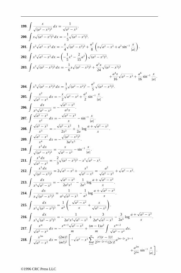
199.∫
x√(a2 − x2)3
dx = 1√a2 − x2
.
200.∫x√(a2 − x2)3 dx = −1
5
√(a2 − x2)5.
201.∫x2√a2 − x2 dx = −x
4
√(a2 − x2)3 + a2
8
(x√a2 − x2 + a2 sin−1 x
|a|).
202.∫x3√a2 − x2 dx =
(−1
5x2 − 2
15a2
)√(a2 − x2)3.
203.∫x2√(a2 − x2)3 dx = −1
6x√(a2 − x2)5 + a2x
24
√(a2 − x2)3
+a4x
16
√a2 − x2 + a6
16sin−1 x
|a| .
204.∫x3√(a2 − x2)3 dx = 1
7
√(a2 − x2)7 − a2
5
√(a2 − x2)5.
205.∫
x2
√a2 − x2
dx = −x2
√a2 − x2 + a2
2sin−1 x
|a| .
206.∫
dx
x2√a2 − x2
= −√a2 − x2
a2x.
207.∫ √
a2 − x2
x2dx = −
√a2 − x2
x− sin−1 x
|a| .
208.∫ √
a2 − x2
x3= −
√a2 − x2
2x2+ 1
2aloga + √
a2 − x2
x.
209.∫ √
a2 − x2
x4dx = −
√(a2 − x2)3
3a2x3.
210.∫
x2 dx√(a2 − x2)3
= x√a2 − x2
− sin−1 x
|a| .
211.∫
x3 dx√a2 − x2
= −2
3
√(a2 − x2)3 − x2
√a2 − x2.
212.∫
x3 dx√(a2 − x2)3
= 2√a2 − x2 + x2
√a2 − x2
= a2
√a2 − x2
+√a2 − x2.
213.∫
dx
x3√a2 − x2
= −√a2 − x2
2a2x2− 1
2a3loga + √
a2 − x2
x.
214.∫
dx
x√(a2 − x2)3
= 1
a2√a2 − x2
− 1
a3loga + √
a2 − x2
x.
215.∫
dx
x2√(a2 − x2)3
= 1
a4
(−
√a2 − x2
x+ x√
a2 − x2
).
216.∫
dx
x3√(a2 − x2)3
= − 1
2a2x2√a2 − x2
+ 3
2a4√a2 − x2
− 3
2a5loga + √
a2 − x2
x.
217.∫
xm√a2 − x2
dx = −xm−1
√a2 − x2
m+ (m− 1)a2
m
∫xm−2
√a2 − x2
dx.
218.∫
x2m
√a2 − x2
dx = (2m)!
(m!)2
[−√a2 − x2
m∑r=1
r!(r − 1)!
22m−2r+1(2r)!a2m−2rx2r−1
+a2m
22msin−1 x
|a|].
©1996 CRC Press LLC
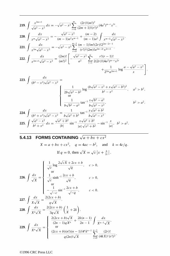
219.∫
x2m+1
√a2 − x2
dx = −√a2 − x2
m∑r=0
(2r)!(m!)2
(2m+ 1)!(r!)2(4a2)m−rx2r .
220.∫
dx
xm√a2 − x2
= −√a2 − x2
(m− 1)a2xm−1+ (m− 2)
(m− 1)a2
∫dx
xm−2√a2 − x2
.
221.∫
dx
x2m√a2 − x2
= −√a2 − x2
m−1∑r=0
(m− 1)!m!(2r)!22m−2r−1
(r!)2(2m)!a2m−2rx2r+1.
222.∫
dx
x2m+1√a2 − x2
= (2m)!
(m!)2
[−
√a2 − x2
a2
m∑r=1
r!(r − 1)!
2(2r)!(4a2)m−rx2r
+ 1
22ma2m+1loga − √
a2 − x2
x
].
223.∫
dx
(b2 − x2)√a2 − x2
=
1
2b√a2 − b2
log(b
√a2 − x2 + x√a2 − b2)2
b2 − x2, a2 > b2,
or1
b√b2 − a2
tan−1 x√b2 − a2
b√a2 − x2
, b2 > a2.
224.∫
dx
(b2 + x2)√a2 − x2
= 1
b√a2 + b2
tan−1 x√a2 + b2
b√a2 − x2
.
225.∫ √
a2 − x2
b2 + x2dx =
√a2 + b2
|b| sin−1 x√a2 + b2
|a| √x2 + b2− sin−1 x
|a| , b2 > a2.
5.4.13 FORMS CONTAINING√a + bx + cx2
X = a + bx + cx2, q = 4ac − b2, and k = 4c/q.
If q = 0, then√X = √
c∣∣x + b
2c
∣∣ .
226.∫dx√X
=
1√c
log2√cX + 2cx + b√
q, c > 0,
or1√c
sinh−1 2cx + b√q
, c > 0,
or
− 1√−c sin−1 2cx + b√−q , c < 0.
227.∫
dx
X√X
= 2(2cx + b)q√X
.
228.∫
dx
X2√X
= 2(2cx + b)3q
√X
(1
X+ 2k
).
229.∫
dx
Xn√X
=
2(2cx + b)√X(2n− 1)qXn
+ 2k(n− 1)
2n− 1
∫dx
Xn−1√X,
or(2cx + b)(n!)(n− 1)!4nkn−1
q(2n)!√X
n−1∑r=0
(2r)!
(4kX)r(r!)2.
©1996 CRC Press LLC

230.∫ √
X dx = (2cx + b)√X4c
+ 1
2k
∫dx√X.
231.∫X
√X dx = (2cx + b)√X
8c
(X + 3
2k
)+ 3
8k2
∫dx√X.
232.∫X2
√X dx = (2cx + b)√X
12c
(X2 + 5X
4k+ 15
8k2
)+ 5
16k3
∫dx√X.
233.∫Xn
√X dx =
(2cx + b)Xn√X4(n+ 1)c
+ 2n+ 1
2(n+ 1)k
∫Xn−1
√X dx,
or
(2n+ 2)!
[(n+ 1)!]2 (4k)n+1
[k(2cx + b)√X
c
n∑r=0
r!(r + 1)!(4kX)r
(2r + 2)!+∫dx√X
].
234.∫x dx√X
=√X
c− b
2c
∫dx√X.
235.∫x dx
X√X
= −2(bx + 2a)
q√X
.
236.∫
x dx
Xn√X
= −√X
(2n− 1)cXn− b
2c
∫dx
Xn√X.
237.∫x2 dx√X
=(x
2c− 3b
4c2
)√X + 3b2 − 4ac
8c2
∫dx√X.
238.∫x2 dx
X√X
= (2b2 − 4ac)x + 2ab
cq√X
+ 1
c
∫dx√X.
239.∫x2 dx
Xn√X
= (2b2 − 4ac)x + 2ab
(2n− 1)cqXn−1√X
+ 4ac + (2n− 3)b2
(2n− 1)cq
∫dx
Xn−1√X.
240.∫x3 dx√X
=(x2
3c− 5bx
12c2+ 5b2
8c3− 2a
3c2
)√X +
(3ab
4c2− 5b3
16c3
)∫dx√X.
241.∫xn dx√X
= 1
ncxn−1
√X − (2n− 1)b
2nc
∫xn−1 dx√X
− (n− 1)a
nc
∫xn−2 dx√X
.
242.∫x√X dx = X
√X
3c− b(2cx + b)
8c2
√X − b
4ck
∫dx√X.
243.∫xX
√X dx = X2
√X
5c− b
2c
∫X
√X dx.
244.∫xXn
√X dx = Xn+1
√X
(2n+ 3)c− b
2c
∫Xn
√X dx.
245.∫x2
√X dx =
(x − 5b
6c
)X
√X
4c+ 5b2 − 4ac
16c2
∫ √X dx.
246.∫
dx
x√X
=
1√−a sin−1
(bx + 2a
|x| √−q), a < 0,
or
−2√X
bx, a = 0,
or
− 1√a
log2√aX + bx + 2a
x, a > 0.
©1996 CRC Press LLC

247.∫
dx
x2√X
= −√X
ax− b
2a
∫dx
x√X.
248.∫ √
X
xdx =
√X + b
2
∫dx√X
+ a∫
dx
x√X.
249.∫ √
X
x2dx = −
√X
x+ b
2
∫dx
x√X
+ c∫dx√X.
5.4.14 FORMS CONTAINING√
2ax − x2
250.∫ √
2ax − x2 dx = 1
2
[(x − a)
√2ax − x2 + a2 sin−1 x − a
|a|].
251.∫
dx√2ax − x2
=
cos−1
(a − x|a|
),
or
sin−1
(x − a|a|
).
252.∫xn√
2ax − x2 dx =
−xn−1√(2ax − x2)3
n+ 2+ (2n+ 1)a
n+ 2
∫xn−1
√2ax − x2 dx,
or√2ax − x2
[xn+1
n+ 2−
n∑r=0
(2n+ 1)!(r!)2an−r+1
2n−r (2r + 1)!(n+ 2)!n!xr
]+ (2n+ 1)!an+2
2nn!(n+ 2)!sin−1
(x − a|a|
).
253.∫ √
2ax − x2
xndx =
√(2ax − x2)3
(3 − 2n)axn+ n− 3
(2n− 3)a
∫ √2ax − x2
xn−1dx.
254.∫
xn dx√2ax − x2
=
−xn−1
√2ax − x2
n+ a(2n− 1)
n
∫xn−1
√2ax − x2
dx,
or
−√
2ax − x2n∑r=1
(2n)!r!(r − 1)!an−r
2n−r (2r)!(n!)2xr−1 + (2n)!an
2n(n!)2sin−1
(x − a|a|
).
255.∫
dx
xn√
2ax − x2=
√2ax − x2
a(1 − 2n)xn+ n− 1
(2n− 1)a
∫dx
xn−1√
2ax − x2,
or
−√
2ax − x2n−1∑r=0
2n−r (n− 1)!n!(2r)!
(2n)!(r!)2an−rxr+1.
256.∫
dx√(2ax − x2)3
= x − aa2
√2ax − x2
.
257.∫
x dx√(2ax − x2)3
= x
a√
2ax − x2.
5.4.15 MISCELLANEOUS ALGEBRAIC FORMS
258.∫
dx√2ax + x2
= log(x + a +
√2ax + x2
).
©1996 CRC Press LLC

259.∫ √
ax2 + c dx =
x
2
√ax2 + c + c
2√−a sin−1
(x
√−ac
), a < 0,
orx
2
√ax2 + c + c
2√a
log(x√a +
√ax2 + c
), a > 0.
260.∫ √
1 + x1 − x dx = sin−1 x −
√1 − x2.
261.∫
dx
x√axn + c =
1
n√c
log
√axn + c − √
c√axn + c + √
c,
or2
n√c
log
√axn + c − √
c√xn
, c > 0,
or2
n√−c sec−1
√−ax
n
c, c < 0.
262.∫
dx√ax2 + c =
1√−a sin−1
(x
√−ac
), a < 0,
or1√a
log(x√a +
√ax2 + c
), a > 0.
263.∫(ax2 + c)m+1/2 dx =
x(ax2 + c)m+1/2
2(m+ 1)+ (2m+ 1)c
2(m+ 1)
∫(ax2 + c)m−1/2 dx,
or
x√ax2 + c
m∑r=0
(2m+ 1)!(r!)2cm−r
22m−2r+1m!(m+ 1)!(2r + 1)!(ax2 + c)r
+ (2m+ 1)!cm+1
22m+1m!(m+ 1)!
∫dx√ax2 + c .
264.∫x(ax2 + c)m+1/2 dx = (ax2 + c)m+3/2
(2m+ 3)a.
265.∫(ax2 + c)m+1/2
xdx =
(ax2 + c)m+1/2
2m+ 1+ c
∫(ax2 + c)m−1/2
xdx,
or√ax2 + c
m∑r=0
cm−r (ax2 + c)r2r + 1
+ cm+1
∫dx
x√ax2 + c .
266.∫
dx
(ax2 + c)m+1/2=
x
(2m− 1)c(ax2 + c)m−1/2+ 2m− 2
(2m− 1)c
∫dx
(ax2 + c)m−1/2,
orx√
ax2 + cm−1∑r=0
22m−2r−1(m− 1)!m!(2r)!
(2m)!(r!)2cm−r (ax2 + c)r .
267.∫
dx
xm√ax2 + c = −
√ax2 + c
(m− 1)cxm−1− (m− 2)a
(m− 1)c
∫dx
xm−2√ax2 + c .
©1996 CRC Press LLC

268.∫
1 + x2
(1 − x2)√
1 + x4dx = 1√
2logx√
2 + √1 + x4
1 − x2.
269.∫
1 − x2
(1 + x2)√
1 + x4dx = 1√
2tan−1 x
√2√
1 + x4.
270.∫
dx
x√xn + a2
= − 2
naloga + √
xn + a2
√xn
.
271.∫
dx
x√xn − a2
= − 2
nasin−1 a√
xn.
272.∫ √
x
a3 − x3dx = 2
3sin−1
(xa
)3/2.
5.4.16 FORMS INVOLVING TRIGONOMETRIC FUNCTIONS
273.∫
sin ax dx = − 1
acos ax.
274.∫
cos ax dx = 1
asin ax.
275.∫
tan ax dx = − 1
alog cos ax = 1
alog sec ax.
276.∫
cot ax dx = 1
alog sin ax = − 1
alog csc ax
277.∫
sec ax dx = 1
alog (sec ax + tan ax) = 1
alog tan
(π4
+ ax
2
)278.
∫csc ax dx = 1
alog (csc ax − cot ax) = 1
alog tan
ax
2
279.∫
sin2 ax dx = x
2− 1
2acos ax sin ax = x
2− 1
4asin 2ax
280.∫
sin3 ax dx = − 1
3a(cos ax)(sin2 ax + 2).
281.∫
sin4 ax dx = 3x
8− sin 2ax
4a+ sin 4ax
32a.
282.∫
sinn ax dx = − sinn−1 ax cos ax
na+ n− 1
n
∫sinn−2 ax dx.
283.∫
sin2m ax dx = − cos ax
a
m−1∑r=0
(2m)!(r!)2
22m−2r (2r + 1)!(m!)2sin2r+1 ax + (2m)!
22m(m!)2x.
284.∫
sin2m+1 ax dx = − cos ax
a
m−1∑r=0
22m−2r (m!)2(2r)!
(2m+ 1)!(r!)2sin2r ax.
285.∫
cos2 ax dx = 1
2x + 1
2asin ax cos ax = 1
2x + 1
4asin 2ax
286.∫
cos3 ax dx = 1
3asin ax(cos2 ax + 2).
287.∫
cos4 ax dx = 3
8x + sin 2ax
4a+ sin 4ax
32a.
288.∫
cosn ax dx = 1
nacosn−1 ax sin ax + n− 1
n
∫cosn−2 ax dx.
©1996 CRC Press LLC

289.∫
cos2m ax dx = sin ax
a
m−1∑r=0
(2m)!(r!)2
22m−2r (2r + 1)!(m!)2cos2r+1 ax + (2m)!
22m(m!)2x.
290.∫
cos2m+1 ax dx = sin ax
a
m∑r=0
22m−2r (m!)2(2r)!
(2m+ 1)!(r!)2cos2r ax.
291.∫
dx
sin2 ax=∫
cosec2 ax dx = − 1
acot ax.
292.∫
dx
sinm ax=∫
cosecm ax dx = − 1
a(m− 1)
cos ax
sinm−1 ax+ m− 2
m− 1
∫dx
sinm−2 ax.
293.∫
dx
sin2m ax=∫
cosec2m ax dx = − 1
acos ax
m−1∑r=0
22m−2r−1(m− 1)!m!(2r)!
(2m)!(r!)2 sin2r+1 ax.
294.∫
dx
sin2m+1 ax=∫
cosec2m+1 ax dx =
− 1
acos ax
m−1∑r=0
(2m)!(r!)2
22m−2r (2r + 1)!(m!)2 sin2r+2 ax+ 1
a
(2m)!
22m(m!)2log tan
ax
2.
295.∫
dx
cos2 ax=∫
sec2 ax dx = 1
atan ax.
296.∫
dx
cosm ax=∫
secm ax dx = 1
a(m− 1)
sin ax
cosm−1 ax+ m− 2
m− 1
∫dx
cosm−2 ax.
297.∫
dx
cos2m ax=∫
sec2m ax dx = 1
asin ax
m−1∑r=0
22m−2r−1(m− 1)!m!(2r)!
(2m)!(r!)2 cos2r+1 ax.
298.∫
dx
cos2m+1 ax=∫
sec2m+1 ax dx = 1
asin ax
m−1∑r=0
(2m)!(r!)2
22m−2r (m!)2(2r + 1)! cos2r+2 ax
+ 1
a
(2m)!
22m(m!)2log (sec ax + tan ax).
299.∫(sinmx)(sin nx) dx = sin (m− n)x
2(m− n) − sin (m+ n)x2(m+ n) , m
2 = n2.
300.∫(cosmx)(cos nx) dx = sin (m− n)x
2(m− n) + sin (m+ n)x2(m+ n) , m
2 = n2.
301.∫(sin ax)(cos ax) dx = 1
2asin2 ax.
302.∫(sinmx)(cos nx) dx = −cos (m− n)x
2(m− n) − cos (m+ n)x2(m+ n) , m2 = n2.
303.∫(sin2 ax)(cos2 ax) dx = − 1
32asin 4ax + x
8.
304.∫(sin ax)(cosm ax) dx = − cosm+1 ax
(m+ 1)a.
305.∫(sinm ax)(cos ax) dx = sinm+1 ax
(m+ 1)a.
306.∫(cosm ax)(sinn ax) dx =
cosm−1 ax sinn+1 ax
(m+ n)a + m− 1
m+ n∫(cosm−2 ax)(sinn ax) dx,
or
−cosm+1 ax sinn−1 ax
(m+ n)a + n− 1
m+ n∫(cosm ax)(sinn−2 ax) dx.
©1996 CRC Press LLC

307.∫
cosm ax
sinn axdx =
− cosm+1 ax
a(n− 1) sinn−1 ax− m− n+ 2
n− 1
∫cosm ax
sinn−2 axdx,
orcosm−1 ax
a(m− n) sinn−1 ax+ m− 1
m− n∫
cosm−2 ax
sinn axdx,
308.∫
sinm ax
cosn axdx =
sinm+1 ax
a(n− 1) cosn−1 ax− m− n+ 2
n− 1
∫sinm ax
cosn−2 axdx,
or
− sinm−1 ax
a(m− n) cosn−1 ax+ m− 1
m− n∫
sinm−2 ax
cosn axdx.
309.∫
sin ax
cos2 axdx = 1
a cos ax= sec ax
a
310.∫
sin2 ax
cos axdx = − 1
asin ax + 1
alog tan
(π4
+ ax
2
).
311.∫
cos ax
sin2 axdx = − csc ax
a= − 1
a sin ax
312.∫
dx
(sin ax)(cos ax)= 1
alog tan ax.
313.∫
dx
(sin ax)(cos2 ax)= 1
a
(sec ax + log tan
ax
2
).
314.∫
dx
(sin ax)(cosn ax)= 1
a(n− 1) cosn−1 ax+∫
dx
(sin ax)(cosn−2 ax).
315.∫
dx
(sin2 ax)(cos ax)= − 1
acsc ax + 1
alog tan
(π4
+ ax
2
).
316.∫
dx
(sin2 ax)(cos2 ax)= − 2
acot 2ax.
317.∫
dx
sinm ax cosn ax=
− 1
a(m− 1) sinm−1 ax cosn−1 ax+ m+ n− 2
m− 1
∫dx
sinm−2 ax cosn ax,
or1
a(n− 1) sinm−1 ax cosn−1 ax+ m+ n− 2
n− 1
∫dx
sinm ax cosn−2 ax.
318.∫
sin (a + bx) dx = −1
bcos (a + bx).
319.∫
cos (a + bx) dx = 1
bsin (a + bx).
320.∫
dx
1 ± sin ax= ∓ 1
atan(π
4∓ ax
2
).
321.∫
dx
1 + cos ax= 1
atanax
2.
322.∫
dx
1 − cos ax= − 1
acotax
2.
323.∫
dx
a + b sin x=
2√a2 − b2
tan−1
(a tan x
2 + b√a2 − b2
),
or
1√b2 − a2
log
(a tan x
2 + b − √b2 − a2
a tan x
2 + b + √b2 − a2
).
©1996 CRC Press LLC

324.∫
dx
a + b cos x=
2√a2 − b2
tan−1
√a2 − b2 tan x
2
a + b ,
or
1√b2 − a2
log
(√b2 − a2 tan x
2 + a + b√b2 − a2 tan x
2 − a − b
).
325.∫
dx
a + b sin x + c cos x=
1√b2 + c2 − a2
logb − √
b2 + c2 − a2 + (a − c) tan x
2
b + √b2 + c2 − a2 + (a − c) tan x
2
, a = c, a2 < b2 + c2,
or2√
a2 − b2 − c2tan−1 b + (a − c) tan x
2√a2 − b2 − c2
, a2 > b2 + c2,
or1
a
[a − (b + c) sin x − (b − c) sin x
a − (b + c) sin x + (b − c) sin x
], a2 = b2 + c2.
326.∫
sin2 x
a + b cos2 xdx = 1
b
√a + ba
tan−1
(√a
a + b tan x
)− x
b, ab > 0, |a| > |b|.
327.∫
dx
a2 cos2 x + b2 sin2 x= 1
abtan−1
(b tan x
a
).
328.∫
cos2 cx
a2 + b2 sin2 cxdx =
√a2 + b2
ab2ctan−1
√a2 + b2 tan cx
a− x
b2.
329.∫
sin cx cos cx
a cos2 cx + b sin2 cxdx = 1
2c(b − a) log(a cos2 cx + b sin2 cx
).
330.∫
cos cx
a cos cx + b sin cxdx =∫
dx
a + b tan cx= 1
c(a2 + b2)
[acx + b log (a cos cx + b sin cx)
]331.
∫sin cx
a cos cx + b sin cxdx =∫
dx
b + a cot cx= 1
c(a2 + b2)
[bcx − a log (a cos cx + b sin cx)
]332.
∫dx
a cos2 x + 2b cos x sin x + c sin2 x=
1
2√b2 − ac log
c tan x + b − √b2 − ac
c tan x + b + √b2 − ac , b2 > ac,
or1√
ac − b2tan−1 c tan x + b√
ac − b2, b2 < ac,
or
− 1
c tan x + b , b2 = ac.
333.∫
sin ax
1 ± sin axdx = ±x + 1
atan(π
4∓ ax
2
).
334.∫
dx
(sin ax)(1 ± sin ax)= 1
atan(π
4∓ ax
2
)+ 1
alog tan
ax
2.
335.∫
dx
(1 + sin ax)2= − 1
2atan(π
4− ax
2
)− 1
6atan3
(π4
− ax
2
).
©1996 CRC Press LLC

336.∫
dx
(1 − sin ax)2= 1
2acot(π
4− ax
2
)+ 1
6acot3
(π4
− ax
2
).
337.∫
sin ax
(1 + sin ax)2dx = − 1
2atan(π
4− ax
2
)+ 1
6atan3
(π4
− ax
2
).
338.∫
sin ax
(1 − sin ax)2dx = − 1
2acot(π
4− ax
2
)+ 1
6acot3
(π4
− ax
2
).
339.∫
sin x
a + b sin xdx = x
b− a
b
∫dx
a + b sin x.
340.∫
dx
(sin x)(a + b sin x)= 1
alog tan
x
2− b
a
∫dx
a + b sin x.
341.∫
dx
(a + b sin x)2=
b cos x
(a2 − b2)(a + b sin x)+ a
a2 − b2
∫dx
a + b sin x,
ora cos x
(b2 − a2)(a + b sin x)+ b
b2 − a2
∫dx
a + b sin x.
342.∫
dx
a2 + b2 sin2 cx= 1
ac√a2 + b2
tan−1
√a2 + b2 tan cx
a.
343.∫
dx
a2 − b2 sin2 cx=
1
ac√a2 − b2
tan−1
√a2 − b2 tan cx
a, a2 > b2,
or1
2ac√b2 − a2
log
√b2 − a2 tan cx + a√b2 − a2 tan cx − a , a2 < b2.
344.∫
cos ax
1 + cos axdx = x − 1
atanax
2.
345.∫
cos ax
1 − cos axdx = −x − 1
acotax
2.
346.∫
dx
(cos ax)(1 + cos ax)= 1
alog tan
(π4
+ ax
2
)− 1
atanax
2.
347.∫
dx
(cos ax)(1 − cos ax)= 1
alog tan
(π4
+ ax
2
)− 1
acotax
2.
348.∫
dx
(1 + cos ax)2= 1
2atanax
2+ 1
6atan3 ax
2.
349.∫
dx
(1 − cos ax)2= − 1
2acotax
2− 1
6acot3 ax
2.
350.∫
cos ax
(1 + cos ax)2dx = 1
2atanax
2− 1
6atan3 ax
2.
351.∫
cos ax
(1 − cos ax)2dx = 1
2acotax
2− 1
6acot3 ax
2.
352.∫
cos x
a + b cos xdx = x
b− a
b
∫dx
a + b cos x.
353.∫
dx
(cos x)(a + b cos x)= 1
alog tan
(x2
+ π
4
)− b
a
∫dx
a + b cos x.
354.∫
dx
(a + b cos x)2= b sin x
(b2 − a2)(a + b cos x)− a
b2 − a2
∫dx
a + b cos x.
355.∫
cos x
(a + b cos x)2dx = a sin x
(a2 − b2)(a + b cos x)− b
a2 − b2
∫dx
a + b cos x.
©1996 CRC Press LLC

356.∫
dx
a2 + b2 − 2ab cos cx= 2
c(a2 − b2)tan−1
(a + ba − b tan
cx
2
).
357.∫
dx
a2 + b2 cos2 cx= 1
ac√a2 + b2
tan−1 a tan cx√a2 + b2
.
358.∫
dx
a2 − b2 cos2 cx=
1
ac√a2 − b2
tan−1 a tan cx√a2 − b2
, a2 > b2,
or1
2ac√b2 − a2
loga tan cx − √
b2 − a2
a tan cx + √b2 − a2
, b2 > a2.
359.∫
sin ax
1 ± cos axdx = ∓ 1
alog (1 ± cos ax).
360.∫
cos ax
1 ± sin axdx = ± 1
alog (1 ± sin ax).
361.∫
dx
(sin ax)(1 ± cos ax)= ± 1
2a(1 ± cos ax)+ 1
2alog tan
ax
2.
362.∫
dx
(cos ax)(1 ± sin ax)= ∓ 1
2a(1 ± sin ax)+ 1
2alog tan
(ax2
+ π
4
).
363.∫
sin ax
(cos ax)(1 ± cos ax)dx = 1
alog (sec ax ± 1).
364.∫
cos ax
(sin ax)(1 ± sin ax)dx = − 1
alog (csc ax ± 1).
365.∫
sin ax
(cos ax)(1 ± sin ax)dx = 1
2a(1 ± sin ax)± 1
2alog tan
(ax2
+ π
4
).
366.∫
cos ax
(sin ax)(1 ± cos ax)dx = − 1
2a(1 ± cos ax)± 1
2alog tan
ax
2.
367.∫
dx
sin ax ± cos ax= 1
a√
2log tan
(ax2
± π
8
).
368.∫
dx
(sin ax ± cos ax)2= 1
2atan(ax ∓ π
4
).
369.∫
dx
1 + cos ax ± sin ax= ± 1
alog(
1 ± tanax
2
).
370.∫
dx
a2 cos2 cx − b2 sin2 cx= 1
2abclogb tan cx + ab tan cx − a .
371.∫x sin ax dx = 1
a2sin ax − x
acos ax.
372.∫x2 sin ax dx = 2x
a2sin ax + 2 − a2x2
a3cos ax.
373.∫x3 sin ax dx = 3a2x2 − 6
a4sin ax + 6x − a2x3
a3cos ax.
374.∫xm sin ax dx =
− 1
axm cos ax + m
a
∫xm−1 cos ax dx,
or
cos ax m2 ∑r=0
(−1)r+1 m!
(m− 2r)!
xm−2r
a2r+1+ sin ax
⌊m−1
2
⌋∑r=0
(−1)rm!
(m− 2r − 1)!
xm−2r−1
a2r+2.
©1996 CRC Press LLC

375.∫x cos ax dx = 1
a2cos ax + x
asin ax.
376.∫x2 cos ax dx = 2x
a2cos ax + a2x2 − 2
a3sin ax.
377.∫x3 cos ax dx = 3a2x2 − 6
a4cos ax + a2x3 − 6x
a3sin ax.
378.∫xm cos ax dx =
xm
asin ax − m
a
∫xm−1 sin ax dx,
or
sin ax m2 ∑r=0
(−1)rm!
(m− 2r)!
xm−2r
a2r+1+ cos ax
⌊m−1
2
⌋∑r=0
(−1)rm!
(m− 2r − 1)!
xm−2r−1
a2r+2.
379.∫
sin ax
xdx =
∞∑n=0
(−1)n(ax)2n+1
(2n+ 1)(2n+ 1)!.
380.∫
cos ax
xdx =
∞∑n=0
(−1)n(ax)2n
(2n)(2n)!.
381.∫x sin2 ax dx = x2
4− x
4asin 2ax − 1
8a2cos 2ax.
382.∫x2 sin2 ax dx = x3
6−(x2
4a− 1
8a3
)sin 2ax − x
4a2cos 2ax.
383.∫x sin3 ax dx = x
12acos 3ax − 1
36a2sin 3ax − 3x
4acos ax + 3
4a2sin ax.
384.∫x cos2 ax dx = x2
4+ x
4asin 2ax + 1
8a2cos 2ax.
385.∫x2 cos2 ax dx = x3
6+(x2
4a− 1
8a3
)sin 2ax + x
4a2cos 2ax.
386.∫x cos3 ax dx = x
12asin 3ax + 1
36a2cos 3ax + 3x
4asin ax + 3
4a2cos ax.
387.∫
sin ax
xmdx = sin ax
(1 −m)xm−1+ a
m− 1
∫cos ax
xm−1dx.
388.∫
cos ax
xmdx = cos ax
(1 −m)xm−1+ a
1 −m∫
sin ax
xm−1dx.
389.∫
x
1 ± sin axdx = ∓ x cos ax
a(1 ± sin ax)+ 1
a2log (1 ± sin ax).
390.∫
x
1 + cos axdx = x
atanax
2+ 2
a2log cos
ax
2.
391.∫
x
1 − cos axdx = −x
acotax
2+ 2
a2log sin
ax
2.
392.∫x + sin x
1 + cos xdx = x tan
x
2.
393.∫x − sin x
1 − cos xdx = −x cot
x
2.
394.∫ √
1 − cos ax dx = − 2 sin ax
a√
1 − cos ax= −2
√2
acos
ax
2
©1996 CRC Press LLC

395.∫ √
1 + cos ax dx = 2 sin ax
a√
1 + cos ax= 2
√2
asinax
2
For the following six integrals, each k represents an integer.
396. *∫ √
1 + sin x dx =
2(
sinx
2− cos
x
2
), (8k − 1) π2 < x ≤ (8k + 3) π2 ,
or
−2(
sinx
2− cos
x
2
), (8k + 3) π2 < x ≤ (8k − 1) π2 .
397. *∫ √
1 − sin x dx =
2(
sinx
2+ cos
x
2
), (8k − 3) π2 < x ≤ (8k + 1) π2 ,
or
−2(
sinx
2+ cos
x
2
), (8k + 1) π2 < x ≤ (8k − 3) π2 .
398. *∫
dx√1 − cos x
=
√2 log tan
x
4, 4kπ < x ≤ (4k + 2)π,
or
−√
2 log tanx
4(4k + 2)π < x ≤ 4kπ .
399. *∫
dx√1 + cos x
=
√2 log tan
(x + π
4
), (4k − 1)π < x ≤ (4k + 1)π,
or
−√
2 log tan
(x + π
4
), (4k + 1)π < x ≤ (4k − 1)π .
400. *∫
dx√1 − sin x
=
√2 log tan
(x4
− π
8
), (8k + 1) π2 < x ≤ (8k + 5) π2 ,
or
−√
2 log tan(x
4− π
8
), (8k + 5) π2 < x ≤ (8k + 1) π2 .
401. *∫
dx√1 + sin x
=
√2 log tan
(x4
+ π
8
), (8k − 1) π2 < x ≤ (8k + 3) π2 ,
or
−√
2 log tan(x
4+ π
8
), (8k + 3) π2 < x ≤ (8k − 1) π2 .
402.∫
tan2 ax dx = 1
atan ax − x.
403.∫
tan3 ax dx = 1
2atan2 ax + 1
alog cos ax.
404.∫
tan4 ax dx = 1
3atan3 ax − 1
atan ax + x.
405.∫
tann ax dx = 1
a(n− 1)tann−1 ax −
∫tann−2 ax dx.
406.∫
cot2 ax dx = − 1
acot ax − x.
407.∫
cot3 ax dx = − 1
2acot2 ax − 1
alog sin ax.
408.∫
cot4 ax dx = − 1
3acot3 ax + 1
acot ax + x.
409.∫
cotn ax dx = − 1
a(n− 1)cotn−1 ax −
∫cotn−2 ax dx.
410.∫
x
sin2 axdx =
∫x csc2 ax dx = −x cot ax
a+ 1
a2log sin ax
©1996 CRC Press LLC

411.∫
x
sinn axdx =
∫x cscn ax dx = − x cos ax
a(n− 1) sinn−1 ax
− 1
a2(n− 1)(n− 2) sinn−2 ax+ n− 2
n− 1
∫x
sinn−2 axdx
412.∫
x
cos2 axdx =
∫x sec2 ax dx = x
atan ax + 1
a2log cos ax
413.∫
x
cosn axdx =
∫x secn ax dx = x sin ax
a(n− 1) cosn−1 ax
− 1
a2(n− 1)(n− 2) cosn−2 ax+ n− 2
n− 1
∫x
cosn−2 axdx
414.∫
sin ax√1 + b2 sin2 ax
dx = − 1
absin−1 b cos ax√
1 + b2.
415.∫
sin ax√1 − b2 sin2 ax
dx = − 1
ablog(b cos ax +
√1 − b2 sin2 ax
).
416.∫(sin ax)
√1 + b2 sin2 ax dx = − cos ax
2a
√1 + b2 sin2 ax − 1 + b2
2absin−1 b cos ax√
1 + b2.
417.∫(sin ax)
√1 − b2 sin2 ax dx = − cos ax
2a
√1 − b2 sin2 ax
−1 − b2
2ablog(b cos ax +
√1 − b2 sin2 ax
).
418.∫
cos ax√1 + b2 sin2 ax
dx = 1
ablog(b sin ax +
√1 + b2 sin2 ax
).
419.∫
cos ax√1 − b2 sin2 ax
dx = 1
absin−1 (b sin ax).
420.∫(cos ax)
√1 + b2 sin2 ax dx = sin ax
2a
√1 + b2 sin2 ax
+ 1
2ablog(b sin ax +
√1 + b2 sin2 ax
).
421.∫(cos ax)
√1 − b2 sin2 ax dx = sin ax
2a
√1 − b2 sin2 ax + 1
2absin−1 (b sin ax).
For the following integral, k represents an integer and a > |b|422. *
∫dx√
a + b tan2 cx=
1
c√a − b sin−1
(√a − ba
sin cx
), (2k − 1) π2 < x ≤ (2k + 1) π2 ,
or
−1
c√a − b sin−1
(√a − ba
sin cx
), (2k + 1) π2 < x ≤ (2k − 1) π2 .
423.∫
cosn x dx = 1
2n−1
n2 −1∑k=0
(n
k
)sin [(n− 2k)x]
(n− 2k)+ 1
2n
(nn
2
)x, n is an even integer.
424.∫
cosn x dx = 1
2n−1
n−12∑k=0
(n
k
)sin [(n− 2k)x]
(n− 2k), n is an odd integer.
425.∫
sinn x dx = 1
2n−1
n2 −1∑k=0
(n
k
)sin([(n− 2k)( π2 − x)])(2k − n) + 1
2n
(nn
2
)x, n is an even integer.
©1996 CRC Press LLC

426.∫
sinn x dx = 1
2n−1
n−12∑k=0
(n
k
)sin([(n− 2k)( π2 − x)])(2k − n) , n is an odd integer.
5.4.17 FORMS INVOLVING INVERSE TRIGONOMETRICFUNCTIONS
427.∫
sin−1 ax dx = x sin−1 ax +√
1 − a2x2
a.
428.∫
cos−1 ax dx = x cos−1 ax −√
1 − a2x2
a.
429.∫
tan−1 ax dx = x tan−1 ax − 1
2alog (1 + a2x2).
430.∫
cot−1 ax dx = x cot−1 ax + 1
2alog (1 + a2x2).
431.∫
sec−1 ax dx = x sec−1 ax − 1
alog(ax +
√a2x2 − 1
).
432.∫
csc−1 ax dx = x csc−1 ax + 1
alog(ax +
√a2x2 − 1
).
433.∫ (
sin−1 x
a
)dx = x sin−1 x
a+√a2 − x2, a > 0.
434.∫ (
cos−1 x
a
)dx = x cos−1 x
a−√a2 − x2, a > 0.
435.∫ (
tan−1 x
a
)dx = x tan−1 x
a− a
2log (a2 + x2).
436.∫ (
cot−1 x
a
)dx = x cot−1 x
a+ a
2log (a2 + x2).
437.∫x sin−1 (ax) dx = 1
4a2
((2a2x2 − 1) sin−1 (ax)+ ax
√1 − a2x2
).
438.∫x cos−1 (ax) dx = 1
4a2
((2a2x2 − 1) cos−1 (ax)− ax
√1 − a2x2
).
439.∫xn sin−1 (ax) dx = xn+1
n+ 1sin−1 (ax)− a
n+ 1
∫xn+1
√1 − a2x2
dx, n = −1.
440.∫xn cos−1 ax dx = xn+1
n+ 1cos−1 (ax)+ a
n+ 1
∫xn+1
√1 − a2x2
dx, n = −1.
441.∫x tan−1 (ax) dx = 1 + a2x2
2a2tan−1 (ax)− x
2a.
442.∫xn tan−1 (ax) dx = xn+1
n+ 1tan−1 (ax)− a
n+ 1
∫xn+1
1 + a2x2dx.
443.∫x cot−1 (ax) dx = 1 + a2x2
2a2cot−1 (ax)+ x
2a.
444.∫xn cot−1 (ax) dx = xn+1
n+ 1cot−1 (ax)+ a
n+ 1
∫xn+1
1 + a2x2dx.
445.∫
sin−1 (ax)
x2dx = a log
(1 − √
1 − a2x2
x
)− sin−1 (ax)
x.
©1996 CRC Press LLC

446.∫
cos−1 (ax)
x2dx = − 1
xcos−1 (ax)+ a log
1 + √1 − a2x2
x.
447.∫
tan−1 (ax)
x2dx = − 1
xtan−1 (ax)− a
2log
1 + a2x2
x2.
448.∫
cot−1 (ax)
x2dx = − 1
xcot−1 (ax)− a
2log
x2
1 + a2x2.
449.∫(sin−1 (ax))2 dx = x(sin−1 (ax))2 − 2x + 2
√1 − a2x2
asin−1 (ax).
450.∫(cos−1 (ax))2 dx = x(cos−1 (ax))2 − 2x − 2
√1 − a2x2
acos−1 (ax).
451.∫(sin−1 (ax))n dx =
x(sin−1 (ax))n + n√
1 − a2x2
a(sin−1 (ax))n−1 − n(n− 1)
∫(sin−1 (ax))n−2 dx,
or
n2 ∑r=0
(−1)rn!
(n− 2r)!x(sin−1 ax)n−2r +
⌊n−1
2
⌋∑r=0
(−1)rn!
√1 − a2x2
(n− 2r − 1)!a(sin−1 ax)n−2r−1.
452.∫(cos−1 (ax))n dx =
x(cos−1 (ax))n − n√
1 − a2x2
a(cos−1 (ax))n−1 − n(n− 1)
∫(cos−1 (ax))n−2 dx,
or
n2 ∑r=0
(−1)rn!
(n− 2r)!x(cos−1 ax)n−2r −
⌊n−1
2
⌋∑r=0
(−1)rn!
√1 − a2x2
(n− 2r − 1)!a(cos−1 ax)n−2r−1.
453.∫
sin−1 ax√1 − a2x2
dx = 1
2a
(sin−1 ax
)2.
454.∫xn sin−1 ax√
1 − a2x2dx = −x
n−1
na2
√1 − a2x2 sin−1 ax + xn
n2a
+n− 1
na2
∫xn−2 sin−1 ax√
1 − a2x2dx.
455.∫
cos−1 ax√1 − a2x2
dx = − 1
2a
(cos−1 ax
)2.
456.∫xn cos−1 ax√
1 − a2x2dx = −x
n−1
na2
√1 − a2x2 cos−1 ax − xn
n2a
+n− 1
na2
∫xn−2 cos−1 ax√
1 − a2x2dx.
457.∫
tan−1 ax
1 + a2x2dx = 1
2a
(tan−1 ax
)2.
458.∫
cot−1 ax
1 + a2x2dx = − 1
2a
(cot−1 ax
)2.
459.∫x sec−1 ax dx = x2
2sec−1 ax − 1
2a2
√a2x2 − 1.
460.∫xn sec−1 ax dx = xn+1
n+ 1sec−1 ax − 1
n+ 1
∫xn√
a2x2 − 1dx.
©1996 CRC Press LLC

461.∫
sec−1 ax
x2dx = − sec−1 ax
x+
√a2x2 − 1
x.
462.∫x csc−1 ax dx = x2
2csc−1 ax + 1
2a2
√a2x2 − 1.
463.∫xn csc−1 ax dx = xn+1
n+ 1csc−1 ax + 1
n+ 1
∫xn√
a2x2 − 1dx.
464.∫
csc−1 ax
x2dx = − csc−1 ax
x−
√a2x2 − 1
x.
5.4.18 LOGARITHMIC FORMS
465.∫
log x dx = x log x − x.
466.∫x log x dx = x2
2log x − x2
4.
467.∫x2 log x dx = x3
3log x − x3
9.
468.∫xn log x dx = xn+1
n+ 1log x − xn+1
(n+ 1)2.
469.∫(log x)2 dx = x(log x)2 − 2x log x + 2x.
470.∫(log x)n dx =
x(log x)n − n
∫(log x)n−1 dx, n = −1,
or
(−1)nn!xn∑r=0
(− log x)r
r!, n = −1.
471.∫(log x)n
xdx = 1
n+ 1(log x)n+1.
472. *∫
dx
log x= log (log x)+ log x + (log x)2
2 · 2!+ (log x)3
3 · 3!+ . . . .
473.∫
dx
x log x= log (log x).
474.∫
dx
x(log x)n= 1
(1 − n)(log x)n−1.
475.∫
xm dx
(log x)n= xm+1
(1 − n)(log x)n−1+ m+ 1
n− 1
∫xm dx
(log x)n−1.
476.∫xm(log x)n dx =
xm+1(log x)n
m+ 1− n
m+ 1
∫xm(log x)n−1 dx,
or
(−1)nn!
m+ 1xm+1
n∑r=0
(− log x)r
r!(m+ 1)n−r.
477.∫xp cos (b log x) dx = xp+1
(p + 1)2 + b2
[b sin (b log x)+ (p + 1) cos (b log x)
].
478.∫xp sin (b log x) dx = xp+1
(p + 1)2 + b2
[(p + 1) sin (b log x)− b cos (b log x)
].
©1996 CRC Press LLC
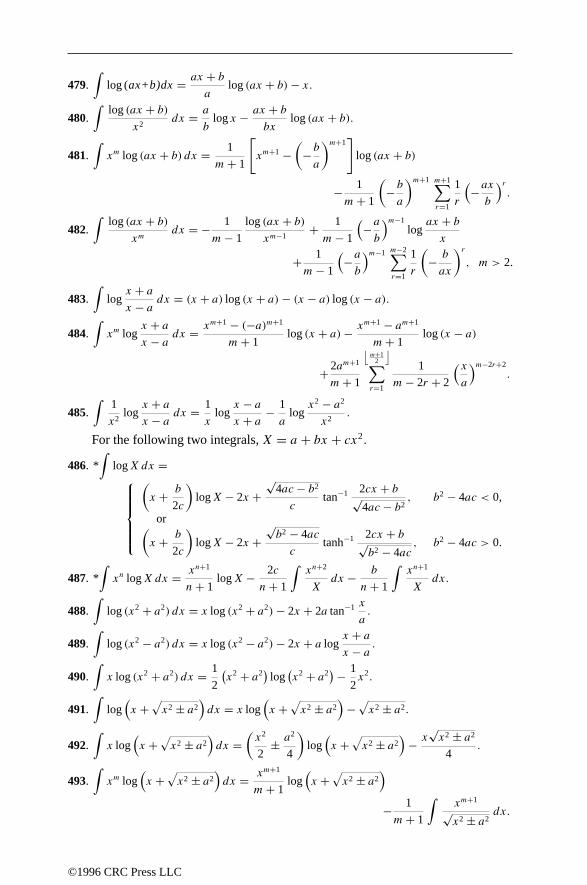
479.∫
log (ax+b)dx = ax + ba
log (ax + b)− x.
480.∫
log (ax + b)x2
dx = a
blog x − ax + b
bxlog (ax + b).
481.∫xm log (ax + b) dx = 1
m+ 1
[xm+1 −
(−ba
)m+1]
log (ax + b)
− 1
m+ 1
(−ba
)m+1 m+1∑r=1
1
r
(−axb
)r.
482.∫
log (ax + b)xm
dx = − 1
m− 1
log (ax + b)xm−1
+ 1
m− 1
(−ab
)m−1logax + bx
+ 1
m− 1
(−ab
)m−1 m−2∑r=1
1
r
(− b
ax
)r, m > 2.
483.∫
logx + ax − a dx = (x + a) log (x + a)− (x − a) log (x − a).
484.∫xm log
x + ax − a dx = xm+1 − (−a)m+1
m+ 1log (x + a)− xm+1 − am+1
m+ 1log (x − a)
+ 2am+1
m+ 1
⌊m+1
2
⌋∑r=1
1
m− 2r + 2
(xa
)m−2r+2.
485.∫
1
x2logx + ax − a dx = 1
xlogx − ax + a − 1
alogx2 − a2
x2.
For the following two integrals, X = a + bx + cx2.
486. *∫
logX dx =
(x + b
2c
)logX − 2x +
√4ac − b2
ctan−1 2cx + b√
4ac − b2, b2 − 4ac < 0,
or(x + b
2c
)logX − 2x +
√b2 − 4ac
ctanh−1 2cx + b√
b2 − 4ac, b2 − 4ac > 0.
487. *∫xn logX dx = xn+1
n+ 1logX − 2c
n+ 1
∫xn+2
Xdx − b
n+ 1
∫xn+1
Xdx.
488.∫
log (x2 + a2) dx = x log (x2 + a2)− 2x + 2a tan−1 x
a.
489.∫
log (x2 − a2) dx = x log (x2 − a2)− 2x + a logx + ax − a .
490.∫x log (x2 + a2) dx = 1
2
(x2 + a2
)log(x2 + a2
)− 1
2x2.
491.∫
log(x +
√x2 ± a2
)dx = x log
(x +
√x2 ± a2
)−√x2 ± a2.
492.∫x log
(x +
√x2 ± a2
)dx =
(x2
2± a2
4
)log(x +
√x2 ± a2
)− x
√x2 ± a2
4.
493.∫xm log
(x +
√x2 ± a2
)dx = xm+1
m+ 1log(x +
√x2 ± a2
)− 1
m+ 1
∫xm+1
√x2 ± a2
dx.
©1996 CRC Press LLC

494.∫ log
(x + √
x2 + a2)
x2dx = −
log(x + √
x2 + a2)
x− 1
aloga + √
x2 + a2
x.
495.∫ log
(x + √
x2 − a2)
x2dx = −
log(x + √
x2 − a2)
x+ 1
|a| sec−1 x
a.
496.∫xn log
(x2 − a2
)dx = 1
n+ 1
[xn+1 log (x2 − a2)− an+1 log (x − a)
−(−a)n+1 log (x + a)− 2 n2 ∑r=0
a2rxn−2r+1
n− 2r + 1
.
5.4.19 EXPONENTIAL FORMS
497.∫ex dx = ex.
498.∫e−x dx = −e−x .
499.∫eax dx = eax
a.
500.∫xeax dx = eax
a2(ax − 1).
501.∫xmeax dx =
xmeax
a− m
a
∫xm−1eax dx,
or
eaxm∑r=0
(−1)rm!xm−r
(m− r)!ar+1.
502. *∫eax
xdx = log x + ax
1!+ a2x2
2 · 2!+ a3x3
3 · 3!+ . . . .
503.∫eax
xmdx = 1
1 −meax
xm−1+ a
m− 1
∫eax
xm−1dx.
504.∫eax log x dx = eax log x
a− 1
a
∫eax
xdx.
505.∫
dx
1 + ex = x − log (1 + ex) = logex
1 + ex
506.∫
dx
a + bepx = x
a− 1
aplog (a + bepx).
507.∫
dx
aemx + be−mx = 1
m√ab
tan−1
(emx√a
b
), a > 0, b > 0.
508.∫
dx
aemx − be−mx =
1
2m√ab
log
√aemx − √
b√aemx + √
b, a > 0, b > 0,
or−1
m√ab
tanh−1
(√a
bemx), a > 0, b > 0.
509.∫ (ax − a−x) dx = ax + a−x
log a.
510.∫
eax
b + ceax dx = 1
aclog (b + ceax).
©1996 CRC Press LLC
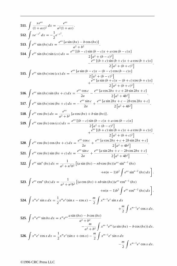
511.∫
xeax
(1 + ax)2 dx = eax
a2(1 + ax) .
512.∫xe−x
2dx = −1
2e−x
2.
513.∫eax sin (bx) dx = eax [a sin (bx)− b cos (bx)]
a2 + b2.
514.∫eax sin (bx) sin (cx) dx = eax [(b − c) sin (b − c)x + a cos (b − c)x]
2[a2 + (b − c)2]
−eax [(b + c) sin (b + c)x + a cos (b + c)x]
2[a2 + (b + c)2] .
515.∫eax sin (bx) cos (cx) dx = eax [a sin (b − c)x − (b − c) cos (b − c)x]
2[a2 + (b − c)2]
+eax [a sin (b + c)x − (b + c) cos (b + c)x]
2[a2 + (b + c)2] .
516.∫eax sin (bx) sin (bx + c) dx = eax cos c
2a− eax [a cos 2bx + c + 2b sin 2bx + c]
2[a2 + 4b2
] .
517.∫eax sin (bx) cos (bx + c) dx = −e
ax sin c
2a+ eax [a sin 2bx + c − 2b cos 2bx + c]
2[a2 + 4b2
] .
518.∫eax cos (bx) dx = eax
a2 + b2[a cos (bx)+ b sin (bx)] .
519.∫eax cos (bx) cos (cx) dx = eax [(b − c) sin (b − c)x + a cos (b − c)x]
2[a2 + (b − c)2]
+eax [(b + c) sin (b + c)x + a cos (b + c)x]
2[a2 + (b + c)2] .
520.∫eax cos (bx) cos (bx + c) dx = eax cos c
2a+ eax [a cos 2bx + c + 2b sin 2bx + c]
2[a2 + 4b2
] .
521.∫eax cos (bx) sin (bx + c) dx = eax sin c
2a+ eax [a sin 2bx + c − 2b cos 2bx + c]
2[a2 + 4b2
] .
522.∫eax sinn (bx) dx = 1
a2 + n2b2
[(a sin (bx)− nb cos (bx))eax sinn−1 (bx)
+n(n− 1)b2
∫eax sinn−2 (bx) dx
].
523.∫eax cosn (bx) dx = 1
a2 + n2b2
[(a cos (bx)+ nb sin (bx))eax cosn−1 (bx)
+n(n− 1)b2
∫eax cosn−2 (bx) dx
].
524.∫xmex sin x dx = 1
2xmex(sin x − cos x)− m
2
∫xm−1ex sin x dx
+m2
∫xm−1ex cos x dx.
525.∫xmeax sin bx dx = xmeax a sin (bx)− b cos (bx)
a2 + b2
− m
a2 + b2
∫xm−1eax(a sin (bx)− b cos (bx)) dx.
526.∫xmex cos x dx = 1
2xmex(sin x + cos x)− m
2
∫xm−1ex sin x dx
−m2
∫xm−1ex cos x dx.
©1996 CRC Press LLC

527.∫xmeax cos bx dx = xmeax a cos (bx)+ b sin (bx)
a2 + b2
− m
a2 + b2
∫xm−1eax(a cos (bx)+ b sin (bx)) dx.
528.∫eax cosm x sinn x dx =
eax(cosm−1 x)(sinn x) [a cos x + (m+ n) sin x]
(m+ n)2 + a2
− na
(m+ n)2 + a2
∫eax(cosm−1 x)(sinn−1 x) dx
+ (m− 1)(m+ n)(m+ n)2 + a2
∫eax(cosm−2 x)(sinn x) dx,
oreax(cosm x)(sinn−1 x) [a sin x − (m+ n) cos x]
(m+ n)2 + a2
+ ma
(m+ n)2 + a2
∫eax(cosm−1 x)(sinn−1 x) dx
+ (n− 1)(m+ n)(m+ n)2 + a2
∫eax(cosm x)(sinn−2 x) dx,
oreax(cosm−1 x)(sinn−1 x)
[a sin x cos x +m sin2 x − n cos2 x
](m+ n)2 + a2
+ m(m− 1)
(m+ n)2 + a2
∫eax(cosm−2 x)(sinn x) dx
+ n(n− 1)
(m+ n)2 + a2
∫eax(cosm x)(sinn−2 x) dx,
oreax(cosm−1 x)(sinn−1 x)
[a sin x cos x +m sin2 x − n cos2 x
](m+ n)2 + a2
+ m(m− 1)
(m+ n)2 + a2
∫eax(cosm−2 x)(sinn−2 x) dx
+ (n−m)(n+m− 1)
(m+ n)2 + a2
∫eax(cosm x)(sinn−2 x) dx.
529.∫xeax sin (bx) dx = xeax
a2 + b2[a sin (bx)− b cos (bx)]
− eax(a2 + b2
)2 [(a2 − b2)
sin bx − 2ab cos (bx)].
530.∫xeax cos (bx) dx = xeax
a2 + b2[a cos (bx)+ b sin (bx)]
− eax(a2 + b2
)2 [(a2 − b2)
cos bx + 2ab sin (bx)].
531.∫
eax
sinn xdx = − e
ax [a sin x + (n− 2) cos x]
(n− 1)(n− 2) sinn−1 x+ a2 + (n− 2)2
(n− 1)(n− 2)
∫eax
sinn−2 xdx.
532.∫
eax
cosn xdx = − e
ax [a cos x − (n− 2) sin x]
(n− 1)(n− 2) cosn−1 x+ a2 + (n− 2)2
(n− 1)(n− 2)
∫eax
cosn−2 xdx.
533.∫eax tann x dx = eax tann−1 x
n− 1− a
n− 1
∫eax tann−1 x dx −
∫eax tann−2 x dx.
©1996 CRC Press LLC

5.4.20 HYPERBOLIC FORMS
534.∫
sinh x dx = cosh x.
535.∫
cosh x dx = sinh x.
536.∫
tanh x dx = log cosh x.
537.∫
coth x dx = log sinh x.
538.∫
sech x dx = tan−1 (sinh x).
539.∫
csch x dx = log tanh(x
2
).
540.∫x sinh x dx = x cosh x − sinh x.
541.∫xn sinh x dx = xn cosh x − n
∫xn−1(cosh x) dx.
542.∫x cosh x dx = x sinh x − cosh x.
543.∫xn cosh x dx = xn sinh x − n
∫xn−1(sinh x) dx.
544.∫
sech x tanh x dx = − sech x.
545.∫
csch x coth x dx = − csch x.
546.∫
sinh2 x dx = sinh 2x
4− x
2.
547.∫
sinhm x coshn x dx =
1
m+ n sinhm+1 x coshn−1 x + n− 1
m+ n∫
sinhm x coshn−2 x dx, m+ n = 0,
or1
m+ n sinhm−1 x coshn+1 x − m− 1
m+ n∫
sinhm−2 x coshn x dx, m+ n = 0.
548.∫
dx
(sinhm x)(coshn x)=
− 1
(m− 1)(sinhm−1 x)(coshn−1 x)− m+ n− 2
m− 1
∫dx
(sinhm−2 x)(coshn x)dx, m = 1,
or1
(n− 1)(sinhm−1 x)(coshn−1 x)+ m+ n− 2
n− 1
∫dx
(sinhm x)(coshn−2 x)dx, n = 1.
549.∫
tanh2 x dx = x − tanh x.
550.∫
tanhn x dx = − tanhn−1 x
n− 1+∫(tanhn−2 x) dx, n = 1.
551.∫
sech2 x dx = tanh x.
©1996 CRC Press LLC

552.∫
cosh2 x dx = sinh 2x
4+ x
2.
553.∫
coth2 x dx = x − coth x.
554.∫
cothn x dx = − cothn−1 x
n− 1+∫
cothn−2 x dx, n = 1.
555.∫
csch2 x dx = − coth x.
556.∫(sinhmx)(sinh nx) dx = sinh (m+ n)x
2(m+ n) − sinh (m− n)x2(m− n) , m2 = n2.
557.∫(coshmx)(cosh nx) dx = sinh (m+ n)x
2(m+ n) + sinh (m− n)x2(m− n) , m2 = n2.
558.∫(sinhmx)(cosh nx) dx = cosh (m+ n)x
2(m+ n) + cosh (m− n)x2(m− n) , m2 = n2.
559.∫ (
sinh−1 x
a
)dx = x sinh−1 x
a−√x2 + a2, a > 0.
560.∫x(
sinh−1 x
a
)dx =
(x2
2+ a2
4
)sinh−1 x
a− x
4
√x2 + a2, a > 0.
561.∫xn sinh−1 x dx = xn+1
n+ 1sinh−1 x − 1
n+ 1
∫xn+1
√1 + x2
dx, n = −1.
562. *∫ z
cosh−1 x
adx =
z cosh−1 z
a−√z2 − a2, cosh−1 z
a> 0,
or
z cosh−1 z
a+√z2 − a2, cosh−1 z
a< 0, a > 0.
563.∫x(
cosh−1 x
a
)dx =
(x2
2− a2
4
)cosh−1 x
a− x
4
√x2 − a2.
564.∫xn cosh−1 x dx = xn+1
n+ 1cosh−1 x − 1
n+ 1
∫xn+1
√x2 − 1
dx, n = −1.
565.∫ (
tanh−1 x
a
)dx = x tanh−1 x
a+ a
2log (a2 − x2),
∣∣ xa
∣∣ < 1.
566.∫ (
coth−1 x
a
)dx = x coth−1 x
a+ a
2log (x2 − a2),
∣∣ xa
∣∣ > 1.
567.∫x(
tanh−1 x
a
)dx = x2 − a2
2tanh−1 x
a+ ax
2,∣∣ xa
∣∣ < 1.
568.∫xn tanh−1 x dx = xn+1
n+ 1tanh−1 x − 1
n+ 1
∫xn+1
1 − x2dx, n = −1.
569.∫x(
coth−1 x
a
)dx = x2 − a2
2coth−1 x
a+ ax
2,∣∣ xa
∣∣ > 1.
570.∫xn coth−1 x dx = xn+1
n+ 1coth−1 x + 1
n+ 1
∫xn+1
x2 − 1dx, n = −1.
571.∫
sech−1 x dx = x sech−1 x + sin−1 x.
572.∫x sech−1 x dx = x2
2sech−1 x − 1
2
√1 − x2.
573.∫xn sech−1 x dx = xn+1
n+ 1sech−1 x + 1
n+ 1
∫xn√
1 − x2dx, n = −1.
©1996 CRC Press LLC

574.∫
csch−1 x dx = x csch−1 x + x
|x| sinh−1 x.
575.∫x csch−1 x dx = x2
2csch−1 x + 1
2
x
|x|√
1 + x2.
576.∫xn csch−1 x dx = xn+1
n+ 1csch−1 x + 1
n+ 1
x
|x|∫
xn√1 + x2
dx, n = −1.
5.4.21 BESSEL FUNCTIONS
Zp(x) represents any of the Bessel functions Jp(x), Yp(x), Kp(x), Ip(x).
577.∫xp+1Zp(x) dx = xp+1Zp+1(x).
578.∫x−p+1Zp(x) dx = −x−p+1Zp−1(x).
579.∫x[Zp(ax)
]2dx = x2
2
[[Zp(ax)
]2 − Zp−1(ax)Zp+1(ax)].
580.∫Z1(x) dx = −Z0(x).
581.∫xZ0(x) dx = xZ1(x).
5.5 TABLE OF DEFINITE INTEGRALS
All integrals listed below that do not have stars next to their numbers have beenautomatically verified by computer.
582.∫ ∞
0xn−1e−x dx = E(n), n is a positive integer.
583.∫ ∞
0xnp−x dx = n!
(logp)n+1, p > 0, n is a non-negative integer.
584.∫ ∞
0xn−1e−(a+1)x dx = E(n)
(a + 1)n, n > 0, a > −1.
585.∫ 1
0xm(
log1
x
)ndx = E(n+ 1)
(m+ 1)n+1, m > −1, n > −1.
586.∫ 1
0xm−1 (1 − x)n−1 dx =
∫ 1
0
xm−1
(1 + x)m+n = E(m)E(n)
E(m+ n) , n > 0, m > 0.
587.∫ b
a
(x−a)m(b−x)n dx = (b−a)m+n+1E(m+ 1) E(n+ 1)
E(m+ n+ 2), m > −1, n > −1, b > a.
588.∫ ∞
1
dx
xm= 1
m− 1, m > 1.
589.∫ ∞
0
dx
(1 + x)xp = π cosecpπ, 0 < p < 1.
©1996 CRC Press LLC

590.∫ ∞
0
dx
(1 − x)xp = −π cot pπ, 0 < p < 1.
591.∫ 1
0
xp
(1 − x)p dx = pπ cosecpπ, |p| < 1.
592.∫ 1
0
xp
(1 − x)p+1dx =
∫ 1
0
(1 − x)pxp+1
dx = −π cosecpπ, −1 < p < 0.
593.∫ ∞
0
xp−1
1 + x dx = π
sinpπ, 0 < p < 1.
594.∫ ∞
0
xm−1
1 + xn dx = π
n sin mπ
n
, 0 < m < n.
595.∫ ∞
0
xa
(m+ xb)c dx = m(a+1−bc)/b
b
E(a+1b
)E(c − a+1
b
)E(c)
, a > −1, b > 0, m > 0,
c > a+1b
.
596.∫ ∞
0
dx
(1 + x)√x = π.
597.∫ ∞
0
a
a2 + x2dx =
π
2, a > 0,
or0, a = 0,or
−π2, a < 0.
598.∫ a
0
(a2 − x2
)n/2dx =
∫ a
0
1
2
(a2 − x2
)n/2dx = n!!
(n+ 1)!!
π
2an+1, a > 0,
n is an odd integer.
599.∫ a
0xm(a2 − x2
)n/2dx = 1
2am+n+1E
(m+1
2
)E(n+2
2
)E(m+n+3
2
) , a > 0, m > −1, n > −2.
600.∫ π/2
0sinn x dx =
∫ π/2
0cosn x dx =
√π
2
E(n+1
2
)E(n+2
2
) , n > −1,
or(n− 1)!!
n!!
π
2, n = 0, n is an even integer,
or(n− 1)!!
n!!, n = 1, n is an odd integer.
601.∫ ∞
0
sin ax
xdx =
π
2, a > 0,
or0, a = 0,
or
−π2, a < 0.
602. *∫ ∞
0
cos x
xdx = ∞.
603.∫ ∞
0
tan x
xdx = π
2.
604.∫ ∞
0
tan ax
xdx = π
2, a > 0.
©1996 CRC Press LLC

605.∫ π
0sin nx · sinmx dx =
∫ π
0cos nx · cosmx dx = 0, n = m, n is an integer,
m is an integer.
606.∫ π/n
0sin nx · cos nx dx =
∫ π/n
0sin nx · cos nx dx = 0, n is an integer.
607. *∫ π
0sin ax cos bx dx =
2a
a2 − b2, a − b is an odd integer.
or0, a − b is an even integer.
608.∫ ∞
0
sin x cos ax
xdx =
0, |a| > 1,or
π
4, |a| = 1,
orπ
2, |a| < 1.
609.∫ ∞
0
sin ax sin bx
x2dx =
πa
2, 0 < a ≤ b,
orπb
2, 0 < b ≤ a.
610.∫ π
0sin2mx dx =
∫ π
0cos2mx dx = π
2, m is an integer.
611.∫ ∞
0
sin2 px
x2dx = π |p|
2.
612.∫ ∞
0
sin x
xpdx = π
2E(p) sin (pπ/2), 0 < p < 1.
613.∫ ∞
0
cos x
xpdx = π
2E(p) cos (pπ/2), 0 < p < 1.
614.∫ ∞
0
1 − cospx
x2dx = π |p|
2.
615.∫ ∞
0
sinpx cos qx
xdx =
0 q > p > 0,or
π
2, p > q > 0,
orπ
4, p = q > 0.
616.∫ ∞
0
cosmx
x2 + a2dx = π
2 |a| e−|ma|.
617. *∫ ∞
0cos x2 dx =
∫ ∞
0sin x2 dx = 1
2
√π
2.
618. *∫ ∞
0sin (axn) dx = 1
na1/nE
(1
n
)sin
π
2n, n > 1.
619. *∫ ∞
0cos (axn) dx = 1
na1/nE
(1
n
)cos
π
2n, n > 1.
620.∫ ∞
0
sin x√xdx =
∫ ∞
0
cos x√xdx =
√π
2.
621.∫ ∞
0
sin3 x
xdx = π
4.
©1996 CRC Press LLC

622.∫ ∞
0
sin3 x
x2dx = 3
4log 3.
623.∫ ∞
0
sin3 x
x3dx = 3π
8.
624.∫ ∞
0
sin4 x
x4dx = π
3.
625.∫ π/2
0
dx
1 + a cos xdx = cos−1 a√
1 − a2, |a| < 1.
626.∫ π
0
dx
a + b cos xdx = π√
a2 − b2, a > b ≥ 0.
627.∫ 2π
0
dx
1 + a cos xdx = 2π√
1 − a2, |a| < 1.
628.∫ ∞
0
cos ax − cos bx
xdx = log
∣∣∣∣ba∣∣∣∣.
629.∫ π/2
0
dx
a2 sin2 x + b2 cos2 xdx = π
2 |ab| .
630.∫ π/2
0
dx
(a2 sin2 x + b2 cos2 x)2dx = π(a2 + b2)
4a3b3, a > 0, b > 0.
631.∫ π/2
0sinn−1 x cosm−1 x dx = 1
2B(n
2
) m2, m is a positive integer, n is a positive integer.
632.∫ π/2
0sin2n+1 x dx = (2n)!!
(2n+ 1)!!, n is a positive integer.
633.∫ π/2
0sin2n x dx = (2n− 1)!!
(2n)!!
π
2, n is a positive integer.
634. *∫ π/2
0
x
sin xdx = 2
(1
12− 1
32+ 1
52− 1
72+ . . .
).
635.∫ π/2
0
dx
1 + tanm xdx = π
4, m is a non-negative integer.
636.∫ π/2
0
√cos x dx = (2π)3/2
(E(1/4))2.
637.∫ π/2
0tanh x dx = π
2 cos(hπ
2
) , 0 < h < 1.
638.∫ π/2
0
tan−1 ax − tan−1 bx
xdx = π
2loga
b, a > 0, b > 0.
639.∫ ∞
0e−ax dx = 1
a, a > 0.
640.∫ ∞
0
e−ax − e−bxx
dx = logb
a, a > 0, b > 0.
641.∫ ∞
0xne−ax dx =
E(n+ 1)
an+1, a > 0, n > −1,
orn!
an+1, a > 0, n is a positive integer.
642.∫ ∞
0xne−ax
p
dx = E((n+ 1)/p)
pa(n+1)/p, a > 0, p > 0, n > −1.
©1996 CRC Press LLC

643.∫ ∞
0e−a
2x2dx = 1
2a
√π, a > 0.
644.∫ b
0e−ax
2dx = 1
2
√π
aerf(b√a), a > 0.
645.∫ ∞
b
e−ax2dx = 1
2
√π
aerfc
(b√a), a > 0.
646.∫ ∞
0xe−x
2dx = 1
2, a > 0.
647.∫ ∞
0x2e−x
2dx =
√π
4.
648.∫ ∞
0xne−ax
2dx = (n− 1)!!
2(2a)n/2
√π
a, a > 0, n > 0.
649.∫ ∞
0x2n+1e−ax
2dx = n!
2an+1, a > 0, n > −1.
650.∫ 1
0xme−ax dx = m!
am+1
[1 − e−a
m∑r=0
ar
r!
].
651.∫ ∞
0e(−x
2−a2/x2) dx = e−2|a|√π2
.
652.∫ ∞
0e(−ax
2−b/x2) dx = 1
2
√π
ae−2
√ab, a > 0, b > 0.
653.∫ ∞
0
√xe−ax dx = 1
2a
√π
a, a > 0.
654.∫ ∞
0
e−ax√xdx =
√π
a, a > 0.
655.∫ ∞
0e−ax cosmx dx = a
a2 +m2, a > 0.
656.∫ ∞
0e−ax cos (bx + c) dx = a cos c − b sin c
a2 + b2, a > 0.
657.∫ ∞
0e−ax sinmx dx = m
a2 +m2, a > 0.
658.∫ ∞
0e−ax sin (bx + c) dx = b cos c + a sin c
a2 + b2, a > 0.
659.∫ ∞
0xe−ax sin bx dx = 2ab
(a2 + b2)2, a > 0.
660.∫ ∞
0xe−ax cos bx dx = a2 − b2
(a2 + b2)2, a > 0.
661.∫ ∞
0xne−ax sin bx dx = n!
[(a + ıb)n+1 − (a − ıb)n+1
]2ı(a2 + b2)n+1
, a > 0.
662.∫ ∞
0xne−ax cos bx dx = n!
[(a − ıb)n+1 + (a + ıb)n+1
]2(a2 + b2)n+1
, a > 0, n > −1.
663.∫ ∞
0
e−ax sin x
xdx = cot−1 a, a > 0.
664.∫ ∞
0e−a
2x2cos bx dx =
√π
2 |a| exp−b2/(4a2), ab > 0.
©1996 CRC Press LLC

665.∫ ∞
0e−x cosφxb−1 sin (x sin φ) dx = E(b) sin (bφ), b > 0, − π
2 < φ <π
2 .
666.∫ ∞
0e−x cosφxb−1 cos (x sin φ) dx = E(b) cos (bφ), b > 0, − π
2 < φ <π
2 .
667.∫ ∞
0xb−1 cos x dx = E(b) cos
(bπ
2
), 0 < b < 1.
668.∫ ∞
0xb−1 sin x dx = E(b) sin
(bπ
2
), 0 < b < 1.
669.∫ 1
0(log x)n dx = (−1)nn!, n < −1.
670.∫ 1
0
√log
1
xdx =
√π
2.
671.∫ 1
0
(log
1
x
)ndx = n!.
672.∫ 1
0x log (1 − x) dx = −3
4.
673.∫ 1
0x log (1 + x) dx = 1
4.
674.∫ 1
0xm(log x)n dx = (−1)nE(n+ 1)
(m+ 1)m+1, m > −1, n is a positive integer.
675.∫ 1
0
log x
1 + x dx = −π2
12.
676.∫ 1
0
log x
1 − x dx = −π2
6.
677.∫ 1
0
log (1 + x)x
dx = π2
12.
678.∫ 1
0
log (1 − x)x
dx = −π2
6.
679.∫ 1
0(log x) log (1 + x) dx = 2 − 2 log 2 − π2
12.
680.∫ 1
0(log x) log (1 − x) dx = 2 − π2
6.
681.∫ 1
0
log x
1 − x2dx = −π
2
8.
682.∫ 1
0log
(1 + x1 − x
)dx
x= π2
4.
683.∫ 1
0
log x√1 − x2
dx = −π2
log 2.
684.∫ 1
0xm[
log
(1
x
)]ndx = E(n+ 1)
(m+ 1)n+1, m > −1, n > −1.
685.∫ 1
0
xp − xqlog x
dx = log
(p + 1
q + 1
), p > −1, q > −1.
686.∫ 1
0
dx√log (− log x)
= √π.
©1996 CRC Press LLC

687.∫ ∞
0log
(ex + 1
ex − 1
)dx = π2
4.
688.∫ π/2
0log sin x dx =
∫ π/2
0log cos x dx = −π
2log 2.
689.∫ π/2
0log sec x dx =
∫ π/2
0log cosec x dx = π
2log 2.
690.∫ π
0x log sin x dx = −π
2
2log 2.
691.∫ π/2
0(sin x) log sin x dx = log 2 − 1.
692.∫ π/2
0log tan x dx = 0.
693.∫ π
0log (a ± b cos x) dx = π log
(a + √
a2 − b2
2
), a ≥ b.
694.∫ π
0log (a2 − 2ab cos x + b2) dx =
2π log a, a ≥ b > 0,or
2π log b, b ≥ a > 0.
695.∫ ∞
0
sin ax
sinh bxdx = π
2btanh
aπ
2 |b| .
696.∫ ∞
0
cos ax
cosh bxdx = π
2bsech
aπ
2b.
697.∫ ∞
0
dx
cosh ax= π
2 |a| .
698.∫ ∞
0
x
sinh axdx = π2
4a2, a ≥ 0.
699.∫ ∞
0e−ax cosh (bx) dx = a
a2 − b2, |b| < a.
700.∫ ∞
0e−ax sinh (bx) dx = b
a2 − b2, |b| < a.
701.∫ ∞
0
sinh ax
ebx + 1dx = π
2bcscaπ
b− 1
2a, b ≥ 0.
702.∫ ∞
0
sinh ax
ebx − 1dx = 1
2a− π
2bcotaπ
b, b ≥ 0.
703. *∫ π/2
0
dx√1 − k2 sin2 x
= π
2
[1 +
(1
2
)2
k2 +(
1 · 3
2 · 4
)2
k4 +(
1 · 3 · 5
2 · 4 · 6
)2
k6 + . . .],
k2 < 1.
704. *∫ π/2
0
dx
(1 − k2 sin2 x)3/2= π
2
[1 +
(1
2
)2
3k2 +(
1 · 3
2 · 4
)2
5k4
+(
1 · 3 · 5
2 · 4 · 6
)2
7k6 + . . .], k2 < 1.
705. *∫ π/2
0
√1 − k2 sin2 x dx = π
2
[1 −
(1
2
)2
k2 −(
1 · 3
2 · 4
)2k4
3
−(
1 · 3 · 5
2 · 4 · 6
)2k6
5− . . .
], k2 < 1.
©1996 CRC Press LLC

706.∫ ∞
0e−x log x dx = −γ.
707.∫ ∞
0e−x
2log x dx = −
√π
4(γ + 2 log 2).
708.∫ ∞
0
(1
1 − e−x − 1
x
)e−x dx = γ.
709.∫ ∞
0
1
x
(1
1 − e−x − 1
x
)dx = γ.
5.6 ORDINARY DIFFERENTIAL EQUATIONS
5.6.1 LINEAR DIFFERENTIAL EQUATIONS
Any linear differential equation can be written in the form
bn(x)y(n) + bn−1(x)y
(n−1) + · · · + b1(x)y′ + b0(x)y = R(x) (5.6.1)
or p(D)y = R(x), where D is the differentiation operator (Dy = dy/dx), p(D) isa polynomial in D with coefficients bi depending on x, and R(x) is an arbitraryfunction. In this notation, a power of D denotes repeated differentiation, that is,Dny = dny/dyn. For such an equation, the general solution has the form
y(x) = yh(x)+ yp(x) (5.6.2)
where yh(x) is the homogeneous solution and yp(x) is the particular solution. Thesefunctions satisfy p(D)yh = 0 and p(D)yp = R(x).
Vector representation
Equation (5.6.1) can be written in the formdydx
= A(x)y + r(x) where
y =
y
y ′
y ′′...
y(n−1)
, A(x) =
0 1 0 . . . 00 0 1 0...
.... . .
0 0 0 1− b0bn
− b1bn
− b2bn
. . . − bn−1
bn
, r(x) =
00...
0Rbn
.
Homogeneous solutionFor the special case of a linear differential equation with constant coefficients (i.e.,the bi in Equation (5.6.1) are constants), the procedure for finding the homogeneoussolution is as follows:
©1996 CRC Press LLC

1. Factor the polynomial p(D) into real and complex linear factors, just as if Dwere a variable instead of an operator.
2. For each nonrepeated linear factor of the form (D − a), where a is real, write aterm of the form ceax , where c is an arbitrary constant.
3. For each repeated real linear factor of the form (D − a)m, write m terms of theform
c1eax + c2xe
ax + c3x2eax + · · · + cmxm−1eax (5.6.3)
where the ci’s are arbitrary constants.
4. For each nonrepeated conjugate complex pair of factors of the form (D − a +ib)(D − a − ib), write two terms of the form
c1eax cos bx + c2e
ax sin bx. (5.6.4)
5. For each repeated conjugate complex pair of factors of the form (D − a +ib)m(D − a − ib)m, write 2m terms of the form
c1eax cos bx + c2e
ax sin bx + c3xeax cos bx + c4xe
ax sin bx + . . .+ c2m−1x
m−1eax cos bx + c2mxm−1eax sin bx. (5.6.5)
6. The sum of all the terms thus written is the homogeneous solution.
ExampleFor the linear equation
y(7) − 14y(6) + 80y(5) − 242y(4) + 419y(3) − 416y ′′ + 220y ′ − 48y = 0,
p(D) factors as p(D) = (D − 1)3(D − 2)2(D − 3)(D − 4). The roots are thus1, 1, 1, 2, 2, 3, 4. Hence, the homogeneous solution has the form
yh(x) = (c0 + c1x + c2x2)ex + (c3 + c4x) e
2x + c5e3x + c6e
4x
where c0, . . . , c6 are arbitrary constants.
©1996 CRC Press LLC
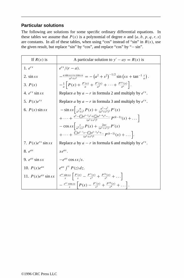
Particular solutionsThe following are solutions for some specific ordinary differential equations. Inthese tables we assume that P(x) is a polynomial of degree n and a, b, p, q, r, sare constants. In all of these tables, when using “cos” instead of “sin” in R(x), usethe given result, but replace “sin” by “cos”, and replace “cos” by “− sin”.
If R(x) is A particular solution to y ′ − ay = R(x) is
1. erx erx/(r − a).2. sin sx − a sin sx+s cos sx
a2+s2 = − (a2 + s2)−1/2
sin(sx + tan−1 s
a
).
3. P(x) − 1a
[P(x)+ P ′(x)
a+ P ′′(x)
a2 + · · · + P (n)(x)
an
].
4. erx sin sx Replace a by a − r in formula 2 and multiply by erx .
5. P(x)erx Replace a by a − r in formula 3 and multiply by erx .
6. P(x) sin sx − sin sx[
aa2+s2P(x)+ a2−s2
(a2+s2)2P ′(x)
+ · · · + ak−(k2)ak−2s2+(k4)ak−4s4−...(a2+s2)k
P (k−1)(x)+ . . .]
− cos sx[
sa2+s2P(x)+ 2as
(a2+s2)2P ′(x)
+ · · · + (k1)ak−1s−(k3)ak−3s3+...(a2+s2)k
P (k−1)(x)+ . . .].
7. P(x)erx sin sx Replace a by a − r in formula 6 and multiply by erx .
8. eax xeax.
9. eax sin sx −eax cos sx/s.
10. P(x)eax eax∫ xP (z) dz.
11. P(x)eax sin sx eax sin sxs
[P ′(x)s
− P ′′′(x)s3 + P (5)(x)
s5 + . . .]
− eax cos sxs
[P(x)− P ′′(x)
s2 + P (4)(x)
s4 + . . .].
©1996 CRC Press LLC

If R(x) is A particular solution to y ′′ − 2ay ′ + a2y = R(x) is
12. erx erx/(r − a)2.13. sin sx (a2−s2) sin sx+2as cos sx
(a2+s2)2= 1
a2+s2 sin(sx + tan−1 2as
a2−s2
).
14. P(x) 1a2
[P(x)+ 2P ′(x)
a+ 3P ′′(x)
a2 + · · · + (n+1)P (n)(x)an
].
15. erx sin sx Replace a by a − r in formula 13 and multiply by erx .
16. P(x)erx Replace a by a − r in formula 14 and multiply by erx .
17. P(x) sin sx sin sx[a2−s2
(a2+s2)2P(x)+ 2 a
2−3as2
(a2+s2)3P ′(x).
+ · · · + (k − 1)ak−(k2)ak−2s2+(k4)ak−4s4−...
(a2+s2)kP (k−2)(x)+ . . .
]+ cos sx
[2as
(a2+s2)2P(x)+ 2 3a2s−s3
(a2+s2)3P ′(x)
+ · · · + (k − 1) (k
1)ak−1s−(k3)ak−3s3+...(a2+s2)k
P (k−2)(x)+ . . .].
18. P(x)erx sin sx Replace a by a − r in formula 17 and multiply by erx .
19. eax x2eax/2.
20. eax sin sx −eax sin sx/s2.
21. P(x)eax eax∫ x ∫ y
P (z) dz dy
22. P(x)eax sin sx − eax sin sxs2
[P(x)− 3P ′′(x)
s2 + 5P (4)(x)s4 + . . .
]− eax cos sx
s2
[2P(x)s
− − 4P ′′′(x)s3 + 6P (5)(x)
s5 + . . .].
©1996 CRC Press LLC

If R(x) is A particular solution to y ′′ + qy = R(x) is
23. erx erx/(r2 + q).24. sin sx sin sx/(q − s2).
25. P(x) 1q
[P(x)− P ′′(x)
q+ P (4)(x)
q2 + · · · + (−1)k P(2k)(x)
qk+ · · ·
].
26. erx sin sx (r2−s2+q)erx sin sx−2rserx cos sx(r2−s2+q)2+(2rs)2 =erx√
(r2−s2+q)2+(2rs)2 sin[sx − tan−1 2rs
r2−s2+q].
27. P(x)erx erx
q+r2
[P(x)− 2r
q+r2P′(x)+ 3r2−q
(q+r2)2P ′′(x)
+ · · · + (−1)k−1 (k
1)rk−1−(k3)rk−3q+...(q+r2)k−1 P (k−1)(x)+ . . .
].
28. P(x) sin sx sin sxq−s2
[P(x)− 3s2+q
(q−s2)2P ′′(x)
+ · · · + (−1)k (2k+1
1 )s2k+(2k+1
3 )s2k−2q+...
(q−s2)2kP (2k)(x)+ . . .
]− s cos sx
q−s2
[2P ′(x)(q−s2)
− 4s2+4q(q−s2)3
P ′′′(x)
+ · · · + (−1)k+1 (2k1 )s
2k−2+(2k3 )s
2k−4q+...(q−s2)2k−1 P (2k−1)(x)+ . . .
].
If R(x) is A particular solution to y ′′ + b2y = R(x) is
29. sin bx −x cos bx/2b.
30. P(x) sin bx sin bx(2b)2
[P(x)− P ′′(x)
(2b)2 + P (4)(x)
(2b)4 + · · ·]
− cos bx2b
∫ [P(x)− P ′′(x)
(2b)2 + · · ·]dx.
©1996 CRC Press LLC
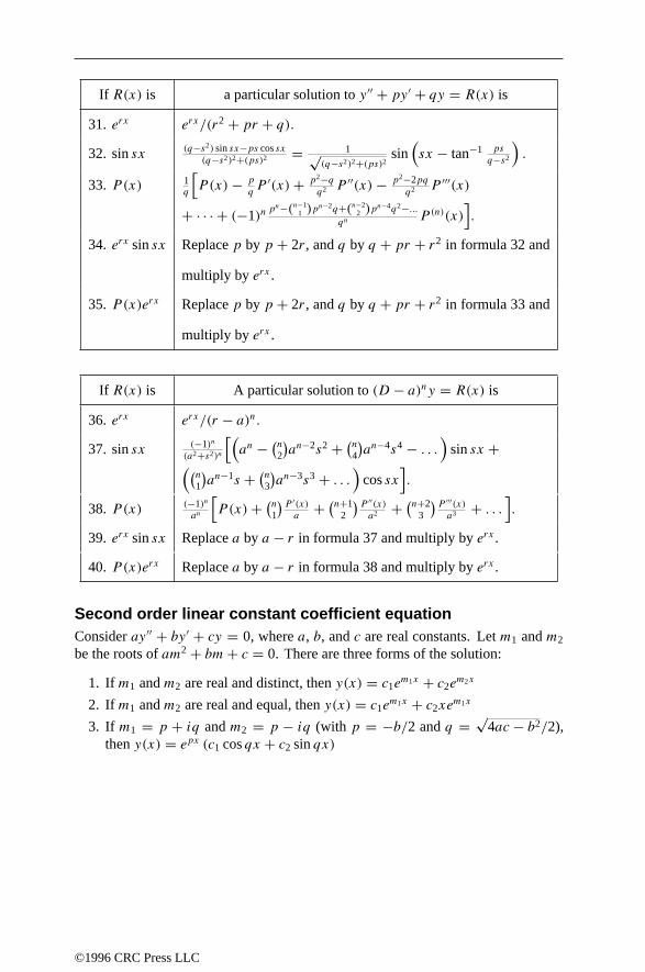
If R(x) is a particular solution to y ′′ + py ′ + qy = R(x) is
31. erx erx/(r2 + pr + q).32. sin sx (q−s2) sin sx−ps cos sx
(q−s2)2+(ps)2 = 1√(q−s2)2+(ps)2 sin
(sx − tan−1 ps
q−s2
).
33. P(x) 1q
[P(x)− p
qP ′(x)+ p2−q
q2 P′′(x)− p2−2pq
q2 P ′′′(x)
+ · · · + (−1)npn−(n−1
1 )pn−2q+(n−2
2 )pn−4q2−...
qnP (n)(x)
].
34. erx sin sx Replace p by p + 2r , and q by q + pr + r2 in formula 32 and
multiply by erx .
35. P(x)erx Replace p by p + 2r , and q by q + pr + r2 in formula 33 and
multiply by erx .
If R(x) is A particular solution to (D − a)ny = R(x) is
36. erx erx/(r − a)n.37. sin sx (−1)n
(a2+s2)n
[(an − (n2)an−2s2 + (n4)an−4s4 − . . .
)sin sx +((
n
1
)an−1s + (n3)an−3s3 + . . .
)cos sx
].
38. P(x) (−1)n
an
[P(x)+ (n1)P ′(x)
a+ (n+1
2
)P ′′(x)a2 + (n+2
3
)P ′′′(x)a3 + . . .
].
39. erx sin sx Replace a by a − r in formula 37 and multiply by erx .
40. P(x)erx Replace a by a − r in formula 38 and multiply by erx .
Second order linear constant coefficient equationConsider ay ′′ + by ′ + cy = 0, where a, b, and c are real constants. Let m1 and m2
be the roots of am2 + bm+ c = 0. There are three forms of the solution:
1. If m1 and m2 are real and distinct, then y(x) = c1em1x + c2e
m2x
2. If m1 and m2 are real and equal, then y(x) = c1em1x + c2xe
m1x
3. If m1 = p + iq and m2 = p − iq (with p = −b/2 and q = √4ac − b2/2),
then y(x) = epx (c1 cos qx + c2 sin qx)
©1996 CRC Press LLC

Consider ay ′′ + by ′ + cy = R(x), where a, b, and c are real constants. Let m1
and m2 be as above.
1. Ifm1 andm2 are real and distinct, then y(x) = C1em1x +C2e
m2x + em1x/(m1 −m2)
∫ xe−m1zR(z) dz+ em2x/(m2 −m1)
∫ xe−m2zR(z) dz.
2. Ifm1 andm2 are real and equal, then y(x) = C1em1x+C2xe
m1x+xem1x∫ xe−m1z
R(z) dz− em1x∫ xze−m1zR(z) dz.
3. If m1 = p + iq and m2 = p − iq, then y(x) = epx (c1 cos qx + c2 sin qx) +epx sin qx/q
∫ xe−pzR(z) cos qz dz− epx cos qx/q
∫ xe−pzR(z) sin qz dz.
Damping: none, under, over, and criticalConsider the linear ordinary differential equation (ODE) x ′′ + µx ′ + x = 0. If thedamping coefficient µ is positive, then all solutions decay to x = 0. If µ = 0, thesystem is undamped and the solution oscillates without decaying. The value of µsuch that the roots of the characteristic equation λ2 + µλ+ 1 = 0 are real and equalis the critical damping coefficient. If µ is less than (greater than) the critical dampingcoefficient, then the system is under (over) damped.
In the following figure all curves have the same initial values: x(0) = 2 andx ′(0) = −2.5. Reading down, at the left-most depression, are the curves
• x ′′ + 3x ′ + x = 0 Overdamped
• x ′′ + 2x ′ + x Critically damped
• x ′′ + 0.2x ′ + x = 0 Underdamped
• x ′′ + x = 0 Undamped
©1996 CRC Press LLC

5.6.2 SOLUTION TECHNIQUES
Differential equation Solution or solution techniqueAutonomous equationf (y(n), y(n−1), . . . , y ′′, y ′, y) = 0
Change dependent variable tou(y) = y ′(x)
Bernoulli’s equationy ′ + f (x)y = g(x)yn
Change dependent variable tov(x) = (y(x))1−n
Clairaut’s equationf (xy ′ − y) = g(y ′) One solution is f (xC − y) = g(C)
Constant coefficient equationa0y
(n) + a1y(n−1) + . . .
+ an−1y91any = 0
There are solutions of the form y = eλx .See Section 5.6.1.
Dependent variablemissingf (y(n), y(n−1), . . . , y ′′, y ′, x) = 0
Change dependent variable tou(x) = y ′(x)
Euler’s equationa0x
ny(n) + a1xn−1y(n−1) + . . .
+ an−1xy + any = 0
Change independent variable to x = et
Exact equationM(x, y) dx +N(x, y) dy = 0with ∂M
∂y= ∂N
∂x
Integrate M(x, y) with respect to xholding y constant, call this m(x, y).
Then m(x, y)+∫ (
N − ∂m
∂y
)dy = C
Homogeneous equation
y ′ = f(yx
) ln x =∫
dv
f (v)− v+ C unless
f (v) = v, in which case y = Cx.
Linear first order equationy ′ + f (x)y = g(x)
y(x) =e− ∫ x f (t) dt [∫ x
e∫ zf (t) dtg(z) dz+ C
]Reducible to homogeneous(a1x + b1y + c1) dx
+ (a2x + b2y + c2) dy = 0with a1/a2 = b1/b2
Change variables to u = a1x + b1y + c
and v = a2x + b2y + c
Reducible to separable(a1x + b1y + c1) dx
+ (a2x + b2y + c2) dy = 0with a1/a2 = b1/b2
Change dependent variable tou(x) = a1x + b1y
Separation of variablesy ′ = f (x)g(y)
∫dy
g(y)=∫f (x) dx + C
5.6.3 INTEGRATING FACTORS
An integrating factor is a multiplicative term that makes a differential equation becomeexact. If the differential equation M(x, y) + dx + N(x, y) = 0 is not exact (i.e.,My = Nx) then it may always be made exact if you can find the integrating factor.
©1996 CRC Press LLC

1. If 1N
(∂M∂y
− ∂N∂x
)= f (x), a function of x alone, then u = exp
(∫ xf (z) dz
)is
an integrating factor.
2. If 1M
(∂M∂y
− ∂N∂x
)= g(y), a function of y alone, then u = exp
(∫ yg(z) dz
)is an
integrating factor.
Example
The equationy
xdx + dy = 0 has M = y/x, N = 1 and f (x) = 1/x. Hence
u = exp(∫ x 1
zdz) = exp (log x) = x is an integrating factor. Multiplying the
original equation by u(x) results in y dx + x dy = 0 or d(xy) = 0.
5.6.4 VARIATION OF PARAMETERS
If the equationL[y] = y ′′ +P(x)y ′ +Q(x)y = R(x) has the homogeneous solutionsy1(x) and y2(x) (i.e., L[yi] = 0), then the solution to the original equation is givenby
y(x) = −y1(x)∫y2(x)R(x)
W(y1,y2)dx + y2(x)
∫y1(x)R(x)
W(y1,y2)dx, (5.6.6)
where W(y1, y2) = y ′1y2 − y1y
′2 is the Wronskian.
ExampleThe homogeneous solutions to y ′′ + y = csc x are clearly y1(x) = sin x and y2(x) =cos x. Here, W(y1, y2) = −1. Hence, y(x) = sin x log(sin x)− x cos x.
5.6.5 GREEN’S FUNCTIONS
Let L[y] = f (x) be a linear differential equation for y(x) with the linear homoge-neous boundary conditions Bi[y] = 0, for i = 1, 2, . . . , n. If there is a Green’sfunction G(x; z) that satisfies
L[G(x; z)] = δ(x − z),
Bi[G(x; z)] = 0,(5.6.7)
where δ is Dirac’s delta function, then the solution of the original system can bewritten as y(x) = ∫ G(x; z)f (z) dz, integrated over an appropriate region.
ExampleTo solve y ′′ = f (x) with y(0) = 0 and y(L) = 0, the appropriate Green’s functionis
G(x; z) =
x(z− L)
Lfor 0 ≤ x ≤ z,
z(x − L)
Lfor z ≤ x ≤ L.
©1996 CRC Press LLC

Hence, the solution is
y(x) =∫ L
0G(x; z) f (z) dz =
∫ x
0
z(x − L)
Lf (z) dz+
∫ L
x
x(z− L)
Lf (z) dz.
5.6.6 LIST OF GREEN’S FUNCTIONS
For the following, the Green’s function is G(x, ξ) when x ≤ ξ and G(ξ, x) whenx ≥ ξ .
1. For the equationd2y
dx2= f (x) with
(a) y(0) = y(1) = 0, G(x, ξ) = −(1 − ξ)x,
(b) y(0) = 0, y ′(1) = 0, G(x, ξ) = −x,(c) y(0) = −y(1), y ′(0) = −y ′(1), G(x, ξ) = − 1
2 (x − ξ)− 14 , and
(d) y(−1) = y(1) = 0, G(x, ξ) = − 12 (x − ξ − xξ + 1).
2. For the equationd2y
dx2− y = f (x) with y finite in (−∞,∞),
G(x, ξ) = − 12ex−ξ .
3. For the equationd2y
dx2+ k2y = f (x) with
(a) y(0) = y(1) = 0, G(x, ξ) = − sin kx sin k(1 − ξ)
k sin k,
(b) y(−1) = y(1), y ′(−1) = y ′(1), and G(x, ξ) = cos k(x − ξ + 1)
2k sin k.
4. For the equationd2y
dx2− k2y = f (x) with
(a) y(0) = y(1) = 0, G(x, ξ) = − sinh kx sinh k(1 − ξ)
k sinh k,
(b) y(−1) = y(1), y ′(−1) = y ′(1), and G(x, ξ) = −cosh k(x − ξ + 1)
2k sinh k.
5. For the equationd
dx
(xdy
dx
)= f (x), with y(0) finite and y(1) = 0,
G(x, ξ) = ln ξ.
6. For the equationd
dx
(xdy
dx
)− m2
xy = f (x), with y(0) finite and y(1) = 0,
G(x, ξ) = − 12m
[(xξ
)m− (xξ)m
], (m = 1, 2, . . . ).
7. For the equationd
dx
((1 − x2)
dy
dx
)− m2
1 − x2y = f (x), with y(−1) and y(1)
finite, G(x, ξ) = − 12m
(1+x1−x
1−ξ1+ξ)m/2
, (m = 1, 2, . . . ).
©1996 CRC Press LLC

8. For the equationd4y
dx4= f (x), with y(0) = y ′(0) = y(1) = y ′(1) = 0,
G(x, ξ) = − x2(ξ−1)2
6 (2xξ + x − 3ξ).
5.6.7 TRANSFORM TECHNIQUES
Transforms can sometimes be used to solve linear differential equations. Laplacetransforms (page 539) are appropriate for initial value problems, while Fourier trans-forms (page 530) are appropriate for boundary value problems.
ExampleConsider the linear second order equation y ′′ + y = p(x), with the initial conditionsy(0) = 0 and y ′(0) = 0. Multiplying this equation by e−sx , and integrating withrespect to x from 0 to ∞, results in∫ ∞
0e−sxy ′′(x) dx +
∫ ∞
0e−sxy(x) dx =
∫ ∞
0e−sxp(x) dx.
Integrating by parts, and recognizing that Y (s) = L[y(x)] = ∫∞0 e−sxy(x) dx is the
Laplace transform of y, this simplifies to
(s2 + 1)Y (s) =∫ ∞
0e−sxp(x) dx = L[p(x)].
If p(x) ≡ 1, then L[p(x)] = s−1. The table of Laplace transforms shows that they(x) corresponding to Y (s) = 1/[s(1 + s2)] is y(x) = L−1[Y (s)] = 1 − cos x.
5.6.8 NAMED ORDINARY DIFFERENTIAL EQUATIONS
1. Airy equation: y ′′ = xy
Solution: y = c1 Ai(x)+ c2 Bi(x)
2. Bernoulli equation: y ′ = a(x)yn + b(x)y
3. Bessel equation: x2y ′′ + xy ′ + (λ2x2 − n2)y = 0Solution: y = c1Jn(λx)+ c2Yn(λx)
4. Bessel equation (transformed): x2y ′′ + (2p + 1)xy ′ + (λ2x2r + β2)y = 0
Solution: y = x−p[c1Jq/r
(λ
rxr)
+ c2Yq/r
(λ
rxr)]
5. Bocher equation: y ′′ + 12
[m1x−a1
+ · · · + mn−1
x−an−1
]y ′
+ 14
[A0+A1x+···+Alxl
(x−a1)m1 (x−a2)
m2 ···(x−an−1)mn−1
]y = 0
6. Duffing’s equation: y ′′ + y + εy3 = 0
7. Emden–Fowler equation: (xpy ′)′ ± xσ yn = 0
©1996 CRC Press LLC
q ; ! p2 2 b2

8. Hypergeometric equation: y ′′ +(
1−α−α′x−a + 1−β−β ′
x−b + 1−γ−γ ′x−c)y ′
−(
αα′(x−a)(b−c) + ββ ′
(x−b)(c−a) + γ γ ′(x−c)(a−b)
)(a−b)(b−c)(c−a)(x−a)(x−b)(x−c)u = 0
Solution: y = P
a b c
α β γ x
α′ β ′ γ ′
(Riemann’s P function)
9. Legendre equation: (1 − x2)y ′′ − 2xy ′ + n(n+ 1)y = 0Solution: y = c1Pn(x)+ c2Qn(x)
10. Mathieu equation: y ′′ + (a − 2q cos 2x)y = 0
11. Painleve transcendent (first equation): y ′′ = 6y2 + x
12. Parabolic cylinder equation: y ′′ + (ax2 + bx + c)y = 0
13. Riccati equation: y ′ = a(x)y2 + b(x)y + c(x)
5.6.9 LIAPUNOV’S DIRECT METHOD
If, as x(t) evolves, the function V depends on x so that V (x) > 0 and dVdt< 0, then
the system is asymptotically stable: V [x(t)] → 0 as x → ∞. For example, for thenonlinear system of differential equations with a > 0
x1 = −ax1 − x1x22 , x2 = −ax2 + x2
1x2,
define V (x) = x21 +x2
2 . Since V = −2a(x21 +x2
2 ) = −2aV , V (t) = V0e−2at . Hence
x1(t) and x2(t) both decay to 0.
5.6.10 LIE GROUPS
An algorithm for integrating second order ordinary differential equations is given by:
1. Determine the admitted Lie algebra Lr , where r is the dimension.
2. If r > 2, determine a subalgebra L2 ⊂ Lr . If r < 2, then Lie groups are notuseful for the given equation.
3. From the commutator and pseudoscalar product, change the basis to obtain oneof the four cases in the table below.
4. Introduce canonical variables specified by the change of basis into the originaldifferential equation. Integrate this new equation.
5. Rewrite the solution in terms of the original variables.
The invertible transformation x = φ(x, y, a), y = ψ(x, y, a) forms a oneparameter group if φ(x, y, b) = φ(x, y, a + b) and ψ(x, y, b) = ψ(x, y, a + b).For small a, these transformations become
x = x + aξ(x, y)+O(a2) y = y + aη(x, y)+O(a2). (5.6.8)
©1996 CRC Press LLC

The infinitesimal generator is X = ξ(x, y) ∂∂x
+ η(x, y) ∂∂y
. If D = ∂∂x
+ y ′ ∂∂y
+y ′′ ∂
∂y ′ + . . ., then the derivatives of the new variables are
y ′ = dy
dx= Dψ
Dφ= ψx + y ′ψyφx + y ′φy
= P(x, y, y ′, a) = y ′ + aζ1 +O(a2), and
y ′′ = dy ′
dx= DP
Dφ= Px + y ′Py + y ′′Py ′
φx + y ′φy= y ′′ + aζ2 +O(a2), (5.6.9)
where
ζ1 = D(η)− y ′D(ξ) = ηx + (ηy − ξx)y′ − y ′2ξy, and
ζ2 = D(ζ1)− y ′′D(ξ) = ηxx + (2ηxy − ξxx)y′ + (ηyy − 2ξxy)y
′2
− y ′3ξyy + (ηy − 2ξx − 3y ′ξy)y ′′.(5.6.10)
The prolongations of X are X(1) = X + ζ1∂∂y ′ and X(2) = X(1) + ζ2
∂∂y ′′ . For a
given differential equation, the different infinitesimal generators will generate an r-dimensional Lie group (Lr )
For the equation F(x, y, y ′, y ′′) = 0 to be invariant under the action of the abovegroup, X(2)F |F=0 = 0. When F = y ′′ − f (x, y, y ′), this determining equationbecomes
ηxx + (2ηxy − ξxx)y′ + (ηyy − 2ξxy)y
′2 − y ′3ξyy
+ (ηy − 2ξx − 3y ′ξy)f −[ηx + (ηy − ξx)y
′ − y ′2]fy ′
− ξfx − ηfy = 0. (5.6.11)
Given the two generators X1 = ξ1∂∂x
+ η1∂∂y
and X2 = ξ2∂∂x
+ η2∂∂y, the pseu-
doscalar product is X1 ∨ X2 = ξ1η2 − ξ2η1, and the commutator is [X1, X2] =X1X2 − X2X1. By a suitable choice of basis, any two-dimensional Lie algebra canbe reduced to one of four types:
No. Commutator Pseudoscalar Typified by
I [X1, X2] = 0 X1 ∨X2 = 0 X1 = ∂∂x
, X2 = ∂∂y
II [X1, X2] = 0 X1 ∨X2 = 0 X1 = ∂
∂y, X2 = x ∂
∂y
III [X1, X2] = X1 X1 ∨X2 = 0 X1 = ∂∂y
, X2 = x ∂∂x
+ y ∂∂y
IV [X1, X2] = X1 X1 ∨X2 = 0 X1 = ∂
∂y, X2 = y ∂
∂y
5.6.11 TYPES OF CRITICAL POINTS
An ODE may have several types of critical points; these include improper node,deficient improper node, proper node, saddle, center, and focus. See Figure 5.6.1.
©1996 CRC Press LLC

FIGURE 5.6.1Types of critical points. Clockwise from upper left: center, improper node, deficient impropernode, spiral, star, saddle.
5.6.12 STOCHASTIC DIFFERENTIAL EQUATIONS
A stochastic differential equation has the form
dX(t) = a(X(t)) dt + b(X(t)) dB(t) (5.6.12)
where B(t) is a random Brownian motion. Brownian motion has a Gaussian proba-bility distribution and independent increments. The probability density function fX(t)for X(t) satisfies the forward Kolmogorov equation
∂∂tfX(t)(x) = 1
2∂2
∂x2
[b2(x)fX(t)(x)
]− ∂∂x
[a(x)fX(t)(x)
]. (5.6.13)
The conditional expectation u(t, x) = E [φ(X(t)) | X(0) = x] satisfies
∂
∂tu(t, x) = 1
2b2(x)
∂2
∂x2u(t, x)+ a(x)
∂
∂xu(t, x) with u(0, x) = φ(x).
(5.6.14)
©1996 CRC Press LLC

5.7 PARTIAL DIFFERENTIAL EQUATIONS
5.7.1 CLASSIFICATIONS OF PDES
Consider second order partial differential equations, with two independent variables,of the form
A(x, y) ∂2u∂x2 + B(x, y) ∂
2u∂x∂y
+ C(x, y) ∂2u∂y2 = =
(u, ∂u
∂x, ∂u∂y, x, y). (5.7.1)
If
B2 − 4AC > 0B2 − 4AC = 0B2 − 4AC < 0
at some point (x, y), then Equation (5.7.1) is
hyperbolic
parabolicelliptic
at
that point. If an equation is of the same type at all points, then the equation is simplyof that type.
5.7.2 NAMED PARTIAL DIFFERENTIAL EQUATIONS
1. Biharmonic equation: ∇4u = 0
2. Burgers’ equation: ut + uux = νuxx
3. Diffusion (or heat) equation: ∇(c(x, t)∇u) = ut
4. Hamilton–Jacobi equation: Vt +H(t, x, Vx1 , . . . , Vxn) = 0
5. Helmholtz equation: ∇2u+ k2u = 0
6. Korteweg de Vries equation: ut + uxxx − 6uux = 0
7. Laplace’s equation: ∇2u = 0
8. Navier–Stokes equations: ut + (u · ∇)u = −∇Pρ
+ ν∇2u
9. Poisson equation: ∇2u = −4πρ(x)
10. Schrodinger equation: − h2
2m∇2u+ V (x)u = ihut
11. Sine–Gordon equation: uxx − uyy ± sin u = 0
12. Tricomi equation: uyy = yuxx
13. Wave equation: c2∇2u = utt
14. Telegraph equation: uxx = autt + but + cu
5.7.3 WELL-POSEDNESS OF PDES
Partial differential equations involvingu(x)usually have the following types of bound-ary conditions:
©1996 CRC Press LLC

1. Dirichlet conditions: u = 0 on the boundary
2. Neumann conditions: ∂u∂n
= 0 on the boundary
3. Cauchy conditions: u and ∂u∂n
specified on the boundary
A well-posed differential equation meets these conditions:
1. The solution exists.
2. The solution is unique.
3. The solution is stable (i.e., the solution depends continuously on the boundaryconditions and initial conditions).
Type of equationType of boundaryconditions
Elliptic Hyperbolic Parabolic
DirichletOpen (spacelike) surface Undetermined Undetermined Unique, stable
solution in onedirection
Closed surface Unique, stablesolution
Undetermined Undetermined
NeumannOpen (spacelike) surface Undetermined Undetermined Unique, stable
solution in onedirection
Closed surface Overdetermined Overdetermined Overdetermined
CauchyOpen (spacelike) surface Not physical results Unique, stable
solutionOverdetermined
Closed surface Overdetermined Overdetermined Overdetermined
5.7.4 GREEN’S FUNCTIONS
In the following, r = (x, y, z), r 0 = (x0, y0, z0),R2 = (x−x0)2+(y−y0)
2+(z−z0)2,
P 2 = (x − x0)2 + (y − y0)
2.
1. For the potential equation ∇2G + k2G = −4πδ(r − r 0), with the radiationcondition (outgoing waves only), the solution is
G =
2πikeik|x−x0| in one dimension,
iπH(1)0 (kP ) in two dimensions, and
eikR
Rin three dimensions,
where H(1)0 (·) is a Hankel function.
©1996 CRC Press LLC

2. For the N-dimensional diffusion equation
∇2G− a2 ∂G
∂t= −4πδ(r − r 0)δ(t − t0),
with the initial condition G = 0 for t < t0, and the boundary condition G = 0at r = ∞, the solution is
G = 4π
a2
(a
2√π(t − t0)
)Nexp
(−a
2|r − r 0|24(t − t0)
).
3. For the wave equation
∇2G− 1
c2
∂2G
∂t2= −4πδ(r − r 0)δ(t − t0),
with the initial conditions G = Gt = 0 for t < t0, and the boundary conditionG = 0 at r = ∞, the solution is
G =
2cπH[(t − t0)− |x−x0|
c
]in one space dimension,
2c√c2(t−t0)2−P 2
H[(t − t0)− P
c
]in two space dimensions, and
1Rδ[Rc
− (t − t0)]
in three space dimensions.
where H(·) is the Heaviside function.
5.7.5 QUASI-LINEAR EQUATIONS
Consider the quasi-linear differential equation for u(x) = u(x1, x2, . . . , xN),
a1(x, u)ux1 + a2(x, u)ux2 + · · · + aN(x, u)uxN = b(x, u).
Defining ∂xk∂s
= ak(x, u), for k = 1, 2, . . . , N , the original equation becomes duds
=b(x, u). To solve the original system, the ordinary differential equations for u(s, t)and the xk(s, t) must be solved. Their initial conditions can often be parameterizedas (with t = (t1, . . . , tN−1))
u(s = 0, t) = v(t),
x1(s = 0, t) = h1(t),
x2(s = 0, t) = h2(t),
...
xN(s = 0, t) = hN(t),
from which the solution follows. This results in an implicit solution.
©1996 CRC Press LLC

ExampleFor the equation ux + x2uy = −yu with u = f (y) when x = 0, the correspondingequations are
∂x
∂s= 1,
∂y
∂s= x2,
du
ds= −yu.
The original initial data can be written parametrically as x(s = 0, t) = 0, y(s =0, t1) = t1, and u(s = 0, t1) = f (t1). Solving for x results in x(s, t1) = s. The equa-tion for y can then be integrated to yield y(s, t1) = s3
3 + t1. Finally, the equation for
u is integrated to obtain u(s, t1) = f (t1) exp(− s4
12 − st1
). These solutions constitute
an implicit solution of the original system.In this case, it is possible to eliminate the s and t1 variables analytically to obtain
the explicit solution: u(x, y) = f
(y − x3
3
)exp
(x4
4− xy
).
5.7.6 EXACT SOLUTIONS OF LAPLACE’S EQUATION
1. If ∇2u = 0 in a circle of radius R and u(R, θ) = f (θ), for 0 ≤ θ < 2π , thenu(r, θ) is
u(r, θ) = 1
2π
∫ 2π
0
R2 − r2
R2 − 2Rr cos(θ − φ)+ r2f (φ) dφ.
2. If ∇2u = 0 in a sphere of radius one and u(1, θ, φ) = f (θ, φ), then
u(r, θ, φ) = 1
4π
∫ π
0
∫ 2π
0f (D,E)
1 − r2
(1 − 2r cos γ + r2)3/2sinDdDdE,
where cos γ = cos θ cosD+ sin θ sinD cos(φ −E).
3. If ∇2u = 0 in the half plane y ≥ 0, and u(x, 0) = f (x), then
u(x, y) = 1
π
∫ ∞
−∞
f (t)y
(x − t)2 + y2dt.
4. If ∇2u = 0 in the half space z ≥ 0, and u(x, y, 0) = f (x, y), then
u(x, y, z) = z
2π
∫ ∞
−∞
∫ ∞
−∞
f (ζ, η)[(x − ζ )2 + (y − η)2 + z2
]3/2 dζ dη.
5.7.7 SOLUTIONS TO THE WAVE EQUATION
Consider the wave equation ∂2u∂t2
= ∇2u = ∂2u∂x1
2 + · · · + ∂2u∂xn2 , with x = (x1, . . . , xn)
and the initial data u(0, x) = f (x) and ut (0, x) = g(x). When n is odd (and n ≥ 3),the solution is
u(t, x) = 1
1 · 3 · · · (n− 2)
∂
∂t
(∂
t ∂t
)(n−3)/2
tn−2ω[f ; x, t]
+(∂
t ∂t
)(n−3)/2
tn−2ω[g; x, t],
(5.7.2)
©1996 CRC Press LLC

whereω[h; x, t] is the average of the functionh(x)over the surface of ann-dimensionalsphere of radius t centered at x; that is, ω[h; x, t] = 1
σn−1(t)
∫h(0, ζζζ ) dG, where
|ζζζ − x|2 = t2, σn−1(t) is the surface area of the n-dimensional sphere of radius t , anddG is an element of area.
When n is even, the solution is given by
u(t, x) = 1
2 · 4 · · · (n− 2)
∂
∂t
(∂
t ∂t
)(n−2)/2∫ t
0ω[f ; x, ρ]
ρn−1 dρ√t2 − ρ2
+(∂
t ∂t
)(n−2)/2∫ t
0ω[g; x, ρ]
ρn−1 dρ√t2 − ρ2
,
(5.7.3)
where ω[h; x, t] is defined as above. Since this expression is integrated over ρ, thevalues of f and g must be known everywhere in the interior of the n-dimensionalsphere.
Using un for the solution in n dimensions, the above simplify to
u1(x, t) = 1
2[f (x − t)+ f (x + t)] + 1
2
∫ x+t
x−tg(ζ ) dζ, (5.7.4)
u2(x, t) = 1
2π
∂
∂t
∫∫R(t)
f (x1 + ζ1, x2 + ζ2)√t2 − ζ 2
1 − ζ 22
dζ1 dζ2
+ 1
2π
∫∫R(t)
g(x1 + ζ1, x2 + ζ2)√t2 − ζ 2
1 − ζ 22
dζ1 dζ2, and(5.7.5)
u3(x, t) = ∂
∂t
(tω[f ; x, t]
)+ tω[g; x, t], (5.7.6)
where R(t) is the region (ζ1, ζ2) | ζ 21 + ζ 2
2 ≤ t2 and
ω[h; x, t] = 1
4π
∫ 2π
0
∫ π
0h(x1 + t sin θ cosφ, x2 + t sin θ sin φ, x3 + t cos θ)
× sin θ dθ dφ.
• The solution of the wave equation
vtt = c2vxx,
v(0, t) = 0, for 0 < t < ∞,
v(x, 0) = f (x), for 0 ≤ x < ∞,
vt (x, 0) = g(x), for 0 ≤ x < ∞,
is
v(x, t) =
12 [f (x + ct)+ f (x − ct)] + 1
2c
∫ x+ctx−ct g(ζ ) dζ, for x ≥ ct ,
12 [f (x + ct)− f (ct − x)] + 1
2c
∫ x+ctct−x g(ζ ) dζ, for x < ct .
• The solution of the inhomogeneous wave equation
∂2u
∂t2− ∂2u
∂x2− ∂2u
∂y2− ∂2u
∂z2= F(t, x, y, z),
©1996 CRC Press LLC
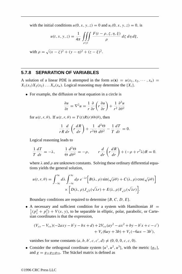
with the initial conditions u(0, x, y, z) = 0 and ut (0, x, y, z) = 0, is
u(t, x, y, z) = 1
4π
∫∫∫ρ≤t
F (t − ρ, ζ, η, ξ)
ρdζ dη dξ,
with ρ =√(x − ζ )2 + (y − η)2 + (z− ξ)2.
5.7.8 SEPARATION OF VARIABLES
A solution of a linear PDE is attempted in the form u(x) = u(x1, x2, · · · , xn) =X1(x1)X2(x2) . . . Xn(xn). Logical reasoning may determine the Xi.
• For example, the diffusion or heat equation in a circle is
∂u
∂t= ∇2u = 1
r
∂
∂r
(r∂u
∂r
)+ 1
r2
∂2u
∂θ2
for u(t, r, θ). If u(t, r, θ) = T (t)R(r)D(θ), then
1
rR
d
dr
(rdR
dr
)+ 1
r2D
d2D
dθ2− 1
T
dT
dt= 0.
Logical reasoning leads to
1
T
dT
dt= −λ, 1
D
d2D
dθ2= −ρ, r
d
dr
(rdR
dr
)+ (−ρ + r2λ)R = 0.
where λ and ρ are unknown constants. Solving these ordinary differential equa-tions yields the general solution,
u(t, r, θ) =∫ ∞
−∞dλ
∫ ∞
−∞dρ e−λt
[B(λ, ρ) sin(
√ρθ)+ C(λ, ρ) cos(
√ρθ)]
×[D(λ, ρ)J√
ρ(√λr)+ E(λ, ρ)Y√
ρ(√λr)].
Boundary conditions are required to determine B,C,D,E.• A necessary and sufficient condition for a system with Hamiltonian H =
12 (p
2x + p2
y) + V (x, y), to be separable in elliptic, polar, parabolic, or Carte-sian coordinates is that the expression,
(Vyy −Vxx)(−2axy− b′y− bx+ d)+ 2Vxy(ay2 − ax2 + by− b′x+ c− c′)
+ Vx(6ay + 3b)+ Vy(−6ax − 3b′),
vanishes for some constants (a, b, b′, c, c′, d) = (0, 0, 0, c, c, 0).
• Consider the orthogonal coordinate system u1, u2, u3, with the metric gii,and g = g11g22g33. The Stackel matrix is defined as
©1996 CRC Press LLC

S =E11(u
1) E12(u1) E13(u
1)
E21(u2) E22(u
2) E23(u2)
E31(u3) E32(u
3) E33(u3)
,
where the Eij are specified. The determinant of S can be written as s =E11M11 +E21M21 +E31M33, where
M11 =∣∣∣∣E22 E23
E32 E33
∣∣∣∣ , M21 = −∣∣∣∣E12 E13
E32 E33
∣∣∣∣ M31 =∣∣∣∣E12 E13
E22 E23
∣∣∣∣ .If gii = s/Mi1 and
√g/s = f1(u
1)f2(u2)f3(u
3) then the Helmholtz equation∇2W +λ2W = 0 separates withW = X1(u
1)X2(u2)X3(u3). Here the Xi are
defined by
1
fi
d
dui
(fidXi
dui
)+Xi
3∑j=1
αjEij = 0,
with α1 = λ2, and α2 and α3 arbitrary. For example, in parabolic coordinatesµ, ν,ψ the metric coefficients are g11 = g22 = µ2 + ν2 and g33 = µ2ν2.Hence,
√g = µν(µ2 + ν2). For the Stackel matrix
S =µ2 −1 1/µ2
ν2 1 1/ν2
0 0 1
(for which s = µ2 +ν2,M11 = M21 = 1, andM21 = µ−2 +ν−2), the separationcondition holds with f1 = µ, f2 = f3 = 1. Hence, the Helmholtz equationseparates in parabolic coordinates. The separated equations are
1
µ
d
dµ
(µdX1
dµ
)+X1
(α1µ
2 − α2 + α1
µ2
)= 0,
1
ν
d
dν
(νdX2
dν
)+X2
(α1ν
2 + α2 + α1
ν2
)= 0, and
d2X3
dψ2+ α3X3 = 0,
where W = X1(µ)X2(ν)X3(ψ).
• Necessary and sufficient conditions for separation of the Laplace equation(∇2W = 0) are
gii
gjj= Mj1
Mi1and
√g
gii= f1(u
1)f2(u2)f3(u
3)Mi1.
Particular solutionsIn these tables, we assume that P(x) is a polynomial of degree n.
©1996 CRC Press LLC

If R(x) is A particular solution to zx +mzy = R(x, y) is
1. eax+by eax+by/(a +mb).
2. f (ax + by)∫f (y) du/(a +mb), u = ax + by.
3. f (y −mx) xf (y −mx).
4. φ(x, y)f (y −mx) f (y − mx)∫φ(x, a + mx) dx; then substitute a =
y −mx.
If R(x) is A particular solution to zx +mzy − kz = R(x, y) is
5. eax+by eax+by/(a +mb − k).
6. sin(ax + by) − (a+bm) cos(ax+by)+k sin(ax+by)(a+bm)2+k2 .
7. eαx+βy sin(ax + by) Replace k by k−α−mβ in formula 6 and multiply by
eαx+βy.
8. exkf (ax + by) ekx∫f (y) du/(a +mb), u = ax + by.
9. f (y −mx) −f (y −mx)/k.
10. P(x)f (y −mx) − 1kf (y −mx)
[P(x)+ P ′(x)
k+ P ′′(x)
k2 + · · · + P (n)(x)
kn
].
11. ekxf (y −mx) xekxf (y −mx).
5.7.9 TRANSFORMING PARTIAL DIFFERENTIAL EQUATIONS
To transform a partial differential equation, construct a new function which dependsupon new variables, and then differentiate with respect to the old variables to see howthe derivatives transform. Consider transforming
fxx + fyy + xfy = 0, (5.7.7)
from the x, y variables to the u, v variables, where u = x, v = x/y. Note thatthe inverse transformation is given by x = u, y = u/v.
First, define g(u, v) as the function f (x, y) when written in the new variables,that is
f (x, y) = g(u, v) = g
(x,x
y
). (5.7.8)
Now create the needed derivative terms, carefully applying the chain rule. For exam-ple, differentiating Equation (5.7.8) with respect to x results in
fx(x, y) = gu∂
∂x(u)+ gv
∂
∂x(v) = g1
∂
∂x(x)+ g2
∂
∂x
(x
y
)
= g1 + g21
y= g1 + v
ug2,
©1996 CRC Press LLC

where a subscript of “1” (“2”) indicates a derivative with respect to the first (sec-ond) argument of the function g(u, v), that is, g1(u, v) = gu(u, v). Use of this“slot notation” tends to minimize errors. In like manner
fy(x, y) = gu∂
∂y(u)+ gv
∂
∂y(v) = g1
∂
∂y(x)+ g2
∂
∂y
(x
y
)
= − x
y2g2 = −v
2
ug2.
The second order derivatives can be calculated similarly:
fxx(x, y) = ∂
∂x(fx(x, y)) = ∂
∂x
(g1 + 1
yg2
),
= g11 + 2v
ug12 + v2
u2g22,
fxy(x, y) = ∂
∂x
(− x
y2g2
)= −u
2
v2g2 − u3
v3g12 − u2
v2g22, and
fyy(x, y) = ∂
∂y
(− x
y2g2
)= 2v3
u2g2 + v4
u2g22.
Finally, Equation (5.7.7) in the new variables has the form,
0 = fxx + fyy + xfy,
=(g11 + 2v
ug12 + v2
u2g22
)+(
2v3
u2g2 + v4
u2g22
)+ (u)
(−v
2
ug2
),
= v2(2v − u2)
u2gv + guu + 2v
uguv + v2(1 + v2)
u2gvv.
5.8 EIGENVALUES
The eigenvalues λi of the differential operator L are the solutions of L[ui] =λiui . Given a geometric shape, the eigenvalues of the Dirichlet problem are calledeigenfrequencies (that is, ∇2u = λu with u = 0 on the boundary).
• You cannot hear the shape of a drum. The following figures have the sameeigenfrequencies.
©1996 CRC Press LLC

• You cannot hear the shape of a two-piece band. The following pairs of figureshave the same eigenfrequencies.
1
1 2
2
√8
2
1
√2
2
√2
5.9 INTEGRAL EQUATIONS
5.9.1 DEFINITIONS
h(x)u(x) = f (x)+ λ
∫ b(x)
a
k(x, t)G[u(t); t] dt. (5.9.1)
• k(x, t) kernel
• u(x) function to be determined
• h(x), f (x) given functions
• λ eigenvalue
Classification of integral equations
Linear G[u(x); x] = u(x).
Volterra b(x) = x.
Fredholm b(x) = b.
First kind h(x) = 0.Second kind h(x) = 1.Third kind h(x) = 0, 1.Homogeneous f (x) = 0.Singular a = −∞, b = ∞.
©1996 CRC Press LLC

Classification of kernelsSymmetric k(x, t) = k(t, x).
Hermitian k(x, t) = k(t, x).
Separable/degenerate k(x, t) =∑ni=1 ai(x)bi(t), n < ∞.
Difference k(x, t) = k(x − t).
Cauchy k(x, t) = 1x−t .
Singular k(x, t) → ∞ as t → x.
Hilbert–Schmidt∫ ba
∫ ba
|k(x, t)|2 dx dt < ∞.
5.9.2 CONNECTION TO DIFFERENTIAL EQUATIONS
The initial value problem
u′′(x)+ A(x)u′(x)+ B(x)u(x) = g(x), x > a,
u(a) = c1, u′(a) = c2,(5.9.2)
is equivalent to the Volterra integral equation,
u(x) = f (x)+∫ x
a
k(x, t)u(t) dt, x ≥ a,
f (x) =∫ x
a
(x − t)g(t) dt + (x − a)[A(a)c1 + c2] + c1,
k(x, t) = (t − x)[B(t)− A′(t)] − A(t).
(5.9.3)
The boundary value problem
u′′(x)+ A(x)u′(x)+ B(x)u(x) = g(x), a < x < b,
u(a) = c1, u(b) = c2,(5.9.4)
is equivalent to the Fredholm integral equation
u(x) = f (x)+∫ b
a
k(x, t)u(t) dt, a ≤ x ≤ b,
f (x) = c1 +∫ x
a
(x − t)g(t) dt + x − a
b − a
[c2 − c1 −
∫ b
a
(b − t)g(t) dt
],
k(x, t) =x−bb−a A(t)− (a − t)[A′(t)− B(t)], x > t,x−ab−a A(t)− (b − t)[A′(t)− B(t)], x < t.
(5.9.5)
5.9.3 FREDHOLM ALTERNATIVE
For u(x) = f (x)+λ ∫ bak(x, t)u(t) dt with λ = 0, consider the solutions to uH (x) =
λ∫ bak(x, t)uH (t) dt .
• If the only solution is uH (x) = 0, then there is a unique solution u(x).
©1996 CRC Press LLC

• If uH (x) = 0, then there is no solution unless∫ bau∗H (t)f (t) dt = 0 for all
u∗H (x) so that u∗
H (x) = λ∫ bak(t, x)u∗
H (t) dt . In this case, there are infinitelymany solutions.
5.9.4 SPECIAL EQUATIONS WITH SOLUTIONS
1. Generalized Abel equation:
∫ x
0
u(t) dt
[h(x)− h(t)]α= f (x),
u(x) = sin(απ)
π
d
dx
∫ x
0
h′(t)f (t) dt[h(x)− h(t)]1−α
(5.9.6)
where 0 ≤ x ≤ 1, 0 ≤ α < 1, 0 ≤ h(x) ≤ 1, h′(x) > 0, and h′(x) iscontinuous.
2. Cauchy equation:
µu(x) = f (x)+ −∫ 1
0
u(t)
t − xdt,
u(x) =xγ sin2
(πγ )
π2ddx
∫ 1x
ds(s−x)γ∫ s
0t−γ f (t)(s−t)1−γ dt, µ < 0,
(1−x)γ sin2(πγ )
π2ddx
∫ x0
ds(x−s)γ∫ 1s
(1−t)−γ f (t)(t−s)1−γ dt, µ > 0,
(5.9.7)
where 0 < x < 1, µ is real, µ = 0, |µ| = π cot(πγ ), 0 < γ < 1/2, and theintegral is a Cauchy principal value integral.
3. Volterra equation with difference kernel:
u(x) = f (x)+ λ
∫ x
0k(x − t)u(t) dt, x ≥ 0
u(x) = L1
[F(s)
1 − λK(s)
],
(5.9.8)
where L [f (x)] = F(s) and L [k(x)] = K(s) (see Section 6.26).
©1996 CRC Press LLC
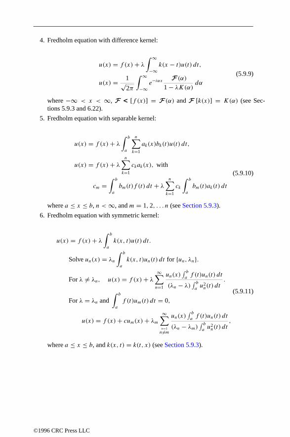
4. Fredholm equation with difference kernel:
u(x) = f (x)+ λ
∫ ∞
−∞k(x − t)u(t) dt,
u(x) = 1√2π
∫ ∞
−∞e−iαx F (α)
1 − λK(α)dα
(5.9.9)
where −∞ < x < ∞, F < [f (x)] = F (α) and F [k(x)] = K(α) (see Sec-tions 5.9.3 and 6.22).
5. Fredholm equation with separable kernel:
u(x) = f (x)+ λ
∫ b
a
n∑k=1
ak(x)bk(t)u(t) dt,
u(x) = f (x)+ λ
n∑k=1
ckak(x), with
cm =∫ b
a
bm(t)f (t) dt + λ
n∑k=1
ck
∫ b
a
bm(t)ak(t) dt
(5.9.10)
where a ≤ x ≤ b, n < ∞, and m = 1, 2, . . . n (see Section 5.9.3).
6. Fredholm equation with symmetric kernel:
u(x) = f (x)+ λ
∫ b
a
k(x, t)u(t) dt.
Solve un(x) = λn
∫ b
a
k(x, t)un(t) dt for un, λn.
For λ = λn, u(x) = f (x)+ λ
∞∑n=1
un(x)∫ baf (t)un(t) dt
(λn − λ)∫ bau2n(t) dt
.
For λ = λn and∫ b
a
f (t)um(t) dt = 0,
u(x) = f (x)+ cum(x)+ λm
∞∑n=1n=m
un(x)∫ baf (t)un(t) dt
(λn − λm)∫ bau2n(t) dt
,
(5.9.11)
where a ≤ x ≤ b, and k(x, t) = k(t, x) (see Section 5.9.3).
©1996 CRC Press LLC

7. Volterra equation of second kind:
u(x) = f (x)+ λ
∫ x
a
k(x, t)u(t) dt,
u(x) = f (x)+ λ
∫ x
a
∞∑n=0
λnkn+1(x, t)f (t) dt,
k1(x, t) = k(x, t),
and kn+1(x, t) =∫ x
t
k(x, s)kn(s, t) ds
(5.9.12)
where k(x, t) and f (x) are continuous, λ = 0, and x ≥ a.
8. Fredholm equation of second kind: resolvent kernel:
u(x) = f (x)+ λ
∫ b
a
k(x, t)u(t) dt,
u(x) = f (x)+ λ
∫ b
a
D(x, t; λ)D(λ)
f (t) dt,
D(λ) =∞∑n=0
(−λ)ncnn!
,
c0 = 1, cn =∫ b
a
An−1(t, t) dt, n = 1, 2, . . . ,
D(x, t; λ) = k(x, t)+∞∑n=1
(−λ)nn!
An(x, t),
A0(x, t) = k(x, t), and An(x, t) = cnk(x, t)
− n
∫ b
a
k(x, s)An−1(s, t) ds
(5.9.13)
where k(x, t) and f (x) are continuous, λ = 0, a ≤ x ≤ b, and D(λ) = 0 (seeSection 5.9.3).
9. Fredholm equation of second kind (Neumann series):
u(x) = f (x)+ λ
∫ b
a
k(x, t)u(t) dt,
u(x) = f (x)+∞∑n=1
λnφn(x),
φn(x) =∫ b
a
kn(x, s)f (s) ds,
k1(x, s) = k(x, s),
and kn(x, s) =∫ b
a
k(x, t)kn−1(t, s) dt, n = 2, 3, . . . ,
(5.9.14)
©1996 CRC Press LLC

where |λ| <(∫ b
a
∫ bak2(x, t) dx dt
)−1/2, λ = 0, and a ≤ x ≤ b (see
Section 5.9.3).
5.10 TENSOR ANALYSIS
5.10.1 DEFINITIONS
1. An n-dimensional coordinate manifold of class Ck , k ≥ 1, is a point set Mtogether with the totality of allowable coordinate systems on M . An allowablecoordinate system (φ,U) onM is a one-to-one mapping φ : U → M , where Uis an open subset of Rn. The n-tuple (x1, . . . , xn) ∈ U give the coordinates ofthe corresponding point φ(x1, . . . , xn) ∈ M . If (φ, U ) is a second coordinatesystem on M , then the one-to-one correspondence φ−1 φ : U → U , called acoordinate transformation onM , is assumed to be of classCk . It may be writtenas
xi = f i(x1, . . . , xn), i = 1, . . . , n, (5.10.1)
where the f are defined by (φ−1 φ)(x1, . . . , xn) = (f 1(x1, . . . , xn), . . . ,
f n(x1, . . . , xn)). The coordinate transformation φ−1 φ has inverse φ−1 φ,expressible in terms of the coordinates as
xi = f i(x1, . . . , xn), i = 1, . . . , n. (5.10.2)
2. The Jacobian matrix ∂xi
∂xjof the transformation satisfies ∂xi
∂xk∂xk
∂xj= δij and ∂xi
∂xk∂xk
∂xj=
δij , where a repeated upper and lower index signifies summation over the range
k = 1, . . . , n (the Einstein summation convention) and δij =
1, i = j
0, i = j
denotes the Kronecker delta. Note also that det(∂xi
∂xj
)= 0.
3. A function F : M → R is called a scalar invariant on M . The coordinaterepresentation of F in any coordinate system (φ,U) is defined by f := F φ.The coordinate representations f ofF with respect to a second coordinate system(φ, U ) is related to f by f (x1, . . . , xn) = f (f 1(x1, . . . , xn), . . . , f n(x1, . . . ,
xn)).
4. A parameterized curve on M is a mapping γ : I → M , where I ⊂ R is someinterval. The coordinate representation of γ in any coordinate system (φ,U)
is a mapping g : I → Rn defined by g = φ−1 γ . The mapping g defines aparameterized curve in Rn. The component functions of g denoted by gi (fori = 1, . . . , n) are defined by g(t) = (g1(t), · · · , gn(t)). The curve γ is Ck if,and only if, the functions gi are Ck for every coordinate system on M . The
©1996 CRC Press LLC

coordinate representation g of γ with respect to a second coordinate system(φ, u) is related to g by gi (t) = f i(g1(t), · · · , gn(t)).
5. A mixed tensor T of contravariant valence r , covariant valence s, and weightw at p ∈ M , called a tensor of type (r, s, w), is an object which, with respect toeach coordinate system onM , is represented by nr+s real numbers whose valuesin any two coordinate systems, φ and φ, are related by
Ti1···irj1···js =
[det
(∂x
∂x
)]wTk1···krQ1···Qs
∂xi1
∂xk1· · · ∂x
ir
∂xkr︸ ︷︷ ︸r factors
∂xQ1
∂xj1· · · ∂x
Qs
∂xjs.︸ ︷︷ ︸
s factors
The superscripts are called contravariant indices and the subscripts covariantindices. If w = 0, then T is said to be a relative tensor. If w = 0, thenT is said to be an absolute tensor or a tensor of type (r, s). In the sequelonly absolute tensors, which will be called tensors, will be considered unlessotherwise indicated. A tensor field T of type (r, s) is an assignment of a tensor oftype (r, s) to each point ofM . A tensor field T is Ck if its component functionsare Ck for every coordinate system on M.
5.10.2 ALGEBRAIC TENSOR OPERATIONS
1. Addition and scalar multiplication: The components of the sum of the tensorsT1 and T2 of type (r, s) are given by
Ti1···ir
3 j1 ···js= T
i1···ir1 j1 ···js
+ Ti1···ir
2 j1 ···js. (5.10.3)
2. Multiplication: The components of the tensor or outer product of a tensor T1 oftype (r, s) and a tensor T2 of type (t, u) are given by
Ti1···ir k1···kt
3 j1···jsQ1···Qu = Ti1···ir
1 j1···js Tk1···kt
2 Q1 ···Qu. (5.10.4)
3. Contraction: The components of the contraction of the t th contravariant indexwith the uth covariant index of a tensor T of type (r, s), with rs ≥ 1, is givenby T i1···it−1kit+1···ir
j1···ju−1kju+1···js .4. Permutation of indices: Let T be any tensor of type (0, r) and Sr the group of
permutations of the set 1, · · · , r. The components of the tensor, obtained bypermuting the indices of T with any σ ∈ Sr, are given by (σT )i1···ir = Tiσ(1)···iσ (r) .The symmetric part of T , denoted by S(T ), is the tensor whose components aregiven by
S(T )i1···ir = T(i1···ir ) = 1
r!
∑σεSr
Tiσ(1)···iσ (r) . (5.10.5)
The tensor T is said to be symmetric if, and only if, Ti1···ir = T(i1···ir ). The skewsymmetric part of T , denoted by A(T ), is the tensor whose components aregiven by
A(T )i1···ir = T[i1···ir ] = 1
r!
∑σ∈Sr
sgn(σ )Tiσ(1)···iσ (1) , (5.10.6)
©1996 CRC Press LLC

where sgn(σ ) = ±1 according to whether σ is an even or odd permutation. Thetensor T is said to be skew symmetric if, and only if, Ti1···ir = T[i1···ir ]. If r = 2,S(T )i1i2 = 1
2 (Ti1i2 + Ti2i1) and A(T )i1i2 = 12 (Ti1i2 − Ti2i1).
5.10.3 DIFFERENTIATION OF TENSORS
1. A linear connection ∇ at p ∈ M is an object which, with respect to eachcoordinate system on M, is represented by n3 real numbers Rijk , called theconnection coefficients, whose values in any two coordinate systems φ and φare related by
Rijk = RQmn∂xi
∂xQ
∂xm
∂xj
∂xn
∂xk+ ∂2xQ
∂xj ∂xk
∂xi
∂xQ(5.10.7)
The quantities Rijk are not the components of a tensor of type (1, 2). A linearconnection ∇ on M is an assignment of a linear connection to each point ofM . A connection ∇ is Ck if its connection coefficients Rijk are Ck in everycoordinate system on M .
2. The components of the covariant derivative of a tensor field T of type (r, s),with respect to a connection ∇, are given by
∇kTi1···irj1···js = ∂kT
i1···irj1···js + R
i1QkT
Qi2···irj1···js + · · ·
· · · + RirQkT
i1 ···ir−1Q
j1···js − RQj1kTi1···irQj2···js · · · − RQjskT
i1···irj1···js−1Q
, (5.10.8)
where
∂kTi1···irji ···js = T
i1···irj1···js ,k = ∂T
i1···irj1 ···js∂xk
. (5.10.9)
This formula has this structure:
• Apart from the partial derivative term, there is a negative affine term foreach covariant index and a positive affine term for each contravariant index.
• The second subscript in the R-symbols is always the differentiated index(k in this case).
3. In tensor analysis, a comma is used to denote partial differentiation.
4. The quantity δAi = dAi − RkijAkdxj is called the covariant differential of Ai .
If Ai is displaced in such a way that δAi = 0, the displacement is said to beparallel with respect to the condition ∇.
5. A vector field Y i(t) is said to be parallel along a parameterized curve γ if thecomponent functions satisfy the differential equation dY i
dt+ Y j dx
k
dtRijk = 0,
where xi denotes the component functions of γ in the coordinate system φ.
©1996 CRC Press LLC
6. A parameterized curve γ in M is said to be an affinely parameterized geodesic ifthe component functions of γ satisfy the differential equation d2xi
dt2 + Rijk
dxj
dtdxk
dt=
0, which is equivalent to the statement that the tangent vector dxidt
to γ is parallelalong γ .
7. The components of the torsion tensor S of ∇ on M are defined by
Sijk = Rijk − Rikj . (5.10.10)
8. The components of the curvature tensor R of ∇ on M are defined by
RijkQ = ∂kRijQ − ∂QR
ijk + RmjQR
imk − RmjkR
imQ. (5.10.11)
In some references R is defined with the opposite sign.
9. The Ricci tensor of ∇ is defined by Rjk = RQjkQ.
5.10.4 METRIC TENSOR
1. A covariant metric tensor field onM is a tensor field gij which satisfies gij = gjiand g = |gij | = 0 on M . The contravariant metric gij satisfies gikgkj = δij .The line element is expressible in terms of the metric tensor as ds2 = gij dx
idxj .
2. Signature of the metric: For each p ∈ M, a coordinate system exists suchthat gij (p) = diag (1, · · · , 1︸ ︷︷ ︸
r
,−1, · · · ,−1)︸ ︷︷ ︸n−r
. The signature of gij is defined by
s = 2r − n. It is independent of the coordinate system in which gij (p) hasthe above diagonal form and is the same at every p ∈ M . A metric is said tobe positive definite if s = n. A manifold, admitting a positive definite metric,is called a Riemannian manifold. A metric is said to be indefinite if s = n
and s = −n. A manifold, admitting an indefinite metric, is called a pseudo-Riemannian manifold. If s = 2 − n or n − 2, the metric is said to Lorentzianand the corresponding manifold is called a Lorentzian manifold.
3. The inner product of a pair of vectorsXi andY j is given by gijXiY j . IfXi = Y i ,then gijXiXj defines the “square” of the length ofXi . If gij is positive definite,then gijXiXj ≥ 0 for all Xi , and gijXiXj = 0 if, and only if, Xi = 0. Inthe positive definite case, the angle θ between two tangent vectors Xi and Y j isdefined by cos θ = gijX
iY j/(gkQXkXQgmnY
mY n)12 . If g is indefinite, gijXiXj
may have a positive, negative, or zero value. A nonzero vector Xi, satisfyinggijX
iXj = 0, is called a null vector. If gij is indefinite, it is not possible ingeneral to define the angle between two tangent vectors.
4. Operation of lowering indices: The components of the tensor resulting fromlowering the t th contravariant index of a tensor T of type (r, s), with r ≥ 1, aregiven by
Ti1···it−1 · it+1···irit j1···js = git kT
i1···it−1kit+1···irj1···js . (5.10.12)
©1996 CRC Press LLC
5. Operation of raising indices: The components of the tensor from raising the t th
covariant index of a tensor T of type (r, s), with s ≥ 1, is given by
Ti1···ir jtji ···jt−1 · jt+1···js = gjt kT
i1···irj1···jt−1kjt+1···js . (5.10.13)
6. The arc length of a parameterized curve γ : I → M , where I = [a, b], and φis any coordinate system, is defined by
L =∫ b
a
√εgij (x1(t), · · · , xn(t))xi xj dt, (5.10.14)
where ε = sgn(gij xi xj ) = ±1 and xi = dxi
dt.
5.10.5 RESULTS
The following results hold on any manifold M admitting any connection ∇:
1. The covariant derivative operator ∇k is linear with respect to tensor addition,satisfies the product rule with respect to tensor multiplication, and commuteswith contractions.
2. If T is any tensor of type (0, r), then
∇[kTi1···ir ] = T[i1···ir ,k] − 1
2
(SQ[ikT|Q|i2 ···ir ] + · · · + SQ[irk Ti1···ir−1]Q
),
(5.10.15)
where | | indicates that the enclosed indices are excluded from the symmetriza-tion. Thus T[i1···ir ,k] defines a tensor of type (0, r + 1), and ∇[kTi1···ir ] = T[i1···ir ,k]
in the torsion free case. If Tj = ∇j f = f,j , where f is any scalar invariant,then ∇[i∇j ]f = 1
2f,kSkij . In the torsion free case, ∇i∇j f = ∇j∇if .
3. If Xi is any vector field on M , then the identity 2∇[j∇k]Xi + ∇QX
iSQjk =XQRiQj k , called the Ricci identity, reduces to 2∇[j∇k]X
i = RiQjkXQ, in the
torsion free case. If Yi is any covariant vector field, the Ricci identity has theform 2∇[i∇j ]Yk + ∇QYiS
Qij = −YQRQkij . The Ricci identity may be extended to
tensor fields of type (r, s). For the tensor field T ijk, it has the form
2∇[i∇i]TkQm + ∇nT
kQmS
nij = T nQmR
knij − T knmR
nkij − T kQnR
nmij .
(5.10.16)
Ifg is any metric tensor field, the above identity implies thatR(ij)kQ = ∇[k∇Q]gij−12∇mgijS
mkQ.
4. The torsion tensor S and curvature tensor R satisfy the following identities:
Si(jk) = 0, 0 = Rij [kl;m] + Rijn[kSnQm], (5.10.17)
Rij (kQ) = 0, Ri[jkQ] = Si[jk;Q] + Sim[j SmkQ]. (5.10.18)
In the torsion free case, these identities reduce to the cyclical identityRi[jkQ] = 0and Bianchi’s identity Rij [kQ;m] = 0.
©1996 CRC Press LLC
The following results hold for any pseudo-Riemannian manifold M with metrictensor field gij :
1. A unique connection ∇ called the Levi–Civita or pseudo-Riemannian connectionwith vanishing torsion (Sijk = 0) exists that satisfies ∇igjk = 0. It follows that∇ig
jk = 0. The connection coefficients of ∇, called the Christoffel symbolsof the second kind, are given by Rijk = giQ[jk, Q], where [jk, Q] = 1
2 (gjQ,k +gkQ,j − gjk,Q) are the Christoffel symbols of the first kind. Rkjk = 1
2∂j (log g) =|g|− 1
2 ∂j |g| 12 and gij,k = [ki, j ] + [kj, i].
2. The operations of raising and lowering indices commute with the covariantderivative. For example if Xi = gijX
j , then ∇kXi = gij∇kXj .
3. The divergence of a vectorXi is given by ∇iXi = |g|− 1
2 ∂i(|g| 12Xi). The Lapla-
cian of a scalar invariant f is given by Sf = gij∇i∇if = ∇i (gij∇j f ) =
|g|− 12 ∂i(|g| 1
2 gij ∂jf ).
4. The equations of an affinely parameterized geodesic may be written as ddt(gij x
j )−12gjk,i x
j xk = 0.
5. Let Xi and Y i be the components of any vector fields which are propagatedin parallel along any parameterized curve γ . Then d
dt(gijX
iY j ) = 0, whichimplies that the inner product gijXiY j is constant along γ . In particular, if xi
are the components of the tangent vector to γ , then gij xi xj is constant along γ .
6. The Riemann tensor, defined by RijkQ = gimRmjkQ, is given by
RijkQ = [jQ, i],k −[jk, i],Q +[iQ,m]Rmjk − [ik,m]RmjQ
= 1
2(giQ,jk + gjk,iQ − gjQ,ik − gik,jQ)
+ gmn([iQ,m][jk, n] − [ik,m][jQ, n]).(5.10.19)
It has the following symmetries:
Rij (kQ) = R(ij)kQ = 0, RijkQ = RkQij , and Ri[jkQ] = 0. (5.10.20)
Consequently it has a maximum of n2(n2 − 1)/12 independent components.
7. The equations RijkQ = 0 are necessary and sufficient conditions for M to bea flat pseudo-Riemannian manifold, that is, a manifold for which a coordinatesystem exists so that the components gij are constant on M .
8. The Ricci tensor is given by
Rij = ∂jRkik − ∂kRkij + RkiQR
Qkj − RkijR
QkQ (5.10.21)
= 1
2∂i∂j (log |g|)− 1
2Rkij ∂k(log |g|)− ∂kR
kij + RkimR
mkj .
It possesses the symmetry Rij = Rji , and thus has a maximum of n(n + 1)/2independent components.
9. The scalar curvature or curvature invariant is defined by R = gijRij .
©1996 CRC Press LLC

10. The Einstein tensor is defined by Gij = Rij − 12Rgij . In view of the Bianchi
identity, it satisfies: gjk∇jGki = 0.
11. A normal coordinate system with origin x0εM is defined by0gij x
j = gij xj ,
where a “0” affixed over a quantity indicates that the quantity is evaluated at x0.
The connection coefficients satisfy0
Ri(j1j2,j3···jr ) = 0 (for r = 2, 3, 4, . . . ) in anynormal coordinate system. The equations of the geodesics through x0 are givenby xi = ski , where s is an affine parameter and ki is any constant vector.
5.10.6 EXAMPLES
1. The components of the gradient of a scalar invariant ∂f
∂xidefine a tensor of type
(0,1), since they transform as ∂f
∂xi= ∂f
∂xj∂xj
∂xi.
2. The components of the tangent vector to a parameterized curve dxi
dtdefine a
tensor of type (1,0), because they transform as dxi
dt= dxj
dt∂xi
∂xj.
3. The determinant of the metric tensor g defines a relative scalar invariant of
weight of w = 2, because it transforms as g =∣∣∣ ∂xi∂xj
∣∣∣2 g.
4. The Kronecker deltas δji are the components of a constant absolute tensor oftype (1, 1), because δij = δkQ
∂xi
∂xk∂xQ
∂xj.
5. The permutation symbol defined by
ei1···in =
1, if i1 · · · in is an even permutation of 1 · · · n,−1, if i1 · · · in is an odd permutation of 1 · · · n, and
0 otherwise, (5.10.22)
satisfies∣∣∣ ∂xi∂xi
∣∣∣ ej1···jn = ei1···in∂xi1
∂xj1· · · ∂xin
∂xjn. Hence it defines a tensor of type
(0, n,−1), that is, it is a relative tensor of weight w = −1. The contravari-ant permutation symbol ei1···in , defined in a similar way, is a relative tensor ofweight w = 1.
6. The Levi–Civita symbol, εi1···in = |g| 12 ei1···in , defines a covarient absolute tensor
of valence n. The contravariant Levi–Civita tensor satisfies
εi1···in = gi1j1 · · · ginjnεj1···jn = (−1)n−s
2 |g|− 12 ei1···in . (5.10.23)
Using this symbol, the dual of a covariant skew-symmetric tensor of valence ris defined by *Ti1···in−r = 1
r!εj1···jri1···in−r Tj1···jr .
7. Cartesian tensors: Let M = E3 (i.e., Euclidean 3 space) with metric tensorgij = δij with respect to Cartesian coordinates. The components of a Cartesiantensor of valence r transform as
Ti1···ir = Tj1···jrOi1jr · · · Oir jr , (5.10.24)
©1996 CRC Press LLC

where Oij are the components of a constant orthogonal matrix which satisfies(O−1)ij = (O′)ij = Oji . For Cartesian tensors, all indices are written ascovariant, because no distinction is required between covariant and contravariantindices.An oriented Cartesian tensor is a Cartesian tensor where the orthogonal matrixin the transformation law is restricted by det(Oij ) = 1. The Levi–Civita symbolεijk is an example of an oriented Cartesian tensor as is the cross product, (X ×Y )i = εijkXjYk, of two vectors. The connection coefficients satisfy Rijk = 0in every Cartesian coordinate system on E3. Thus the partial derivatives ofCartesian tensors are themselves Cartesian tensors, that is, if Ti1···ir is a Cartesiantensor, then so is ∂kTi1···ir . A particular example is the curl of a vector field Xigiven by (curlX)i = εijk∂jXk which defines an oriented Cartesian tensor.
8. Note the useful relations: εijkεklm = δilδjm − δimδjl, εiklεklm = 2δim, andεijkεlmn = δilδjmδkn+ δimδjnδkl + δinδjlδkm− δinδjmδkl − δimδjlδkn− δilδjnδkm.
9. The stress tensor Eij and the strain tensor eij are examples of Cartesian tensors.
10. Orthogonal curvilinear coordinates: Let M be a 3-dimensional Riemannianmanifold admitting a coordinate system [x1, x2, x3] such that the metric tensorhas the form gii = h 2
i (x1, x2, x3) for i = 1, . . . , 3 with gij = gij = 0 for
i = j . The metric tensor on E3 has this form with respect to orthogonalcurvilinear coordinates. The nonzero components of various correspondingquantities corresponding to this metric are as follows:
• Covariant metric tensor,
g11 = h12, g22 = h2
2, g33 = h32.
• Contravariant metric tensor,
g11 = h1−2, g22 = h2
−2, g33 = h3−2.
• Christoffel symbols of the first kind (note that [ij, k] = 0 if i, j , and k areall different),
[11, 1] = h1h1,1 [11, 2] = −h1h1,2 [11, 3] = −h1h1,3
[12, 1] = h1h1,2 [12, 2] = h2h2,1 [13, 1] = h1h1,3
[13, 3] = h3h3,1 [22, 1] = −h2h2,1 [22, 2] = h2h2,2
[22, 3] = −h2h2,3 [23, 2] = h2h2,3 [23, 3] = h3h3,2
[33, 1] = −h3h3,1 [33, 2] = −h3h3,2 [33, 3] = h3h3,3.
• Christoffel symbols of the second kind (note that Rkij = 0 if i, j , and k areall different),
R111 = h1
−1h1,1 R112 = h1
−1h1,2 R113 = h1
−1h1,3
R122 = −h1
−2h2h2,1 R133 = −h1
−2h3h3,1 R211 = −h1h2
−2h1,2
R212 = h2
−1h2,1 R222 = h2
−1h2,2 R223 = h2
−1h2,3
R233 = −h2
−2h3h3,2 R311 = −h1h3
−2h1,3 R313 = h3
−1h3,1
R322 = −h2h3
−2h2,3 R323 = h3
−1h3,2 R333 = h3
−1h3,3.
©1996 CRC Press LLC

• Vanishing Riemann tensor conditions (Lame equations),
h1,2,3 − h2−1h1,2h2,3 − h3
−1h1,3h3,2 = 0,
h2,1,3 − h1−1h1,3h2,1 − h3
−1h3,1h2,3 = 0,
h3,1,2 − h1−1h1,2h3,1 − h2
−1h2,1h3,2 = 0,
h2h2,3,3 + h3h3,2,2 + h1−2h2h3h2,1h3,1 − h2
−1h3h2,2h3,2
− h2h3−1h2,3h3,3 = 0,
h1h1,3,3 + h3h3,1,1 + h1h2−2h3h1,2h3,2 − h1
−1h3h1,1h3,1
− h1h3−1h1,3h3,3 = 0,
h1h1,2,2 + h2h2,1,1 + h1h2h3−2h1,3h2,3 − h1
−1h2h1,1h2,1
− h1h2−1h1,2h2,2 = 0.
11. The 2-sphere: A coordinate system [θ, φ] for the 2-sphere x2 + y2 + z2 + = r2 isgiven by x = r sin θ cosφ, y = r sin θ sin φ, z = r cos θ , where [θ, φ] ∈(0,π)×(0,2π). This is a non-Euclidean space. The nonzero independentcomponents of various quantities defined on the sphere are given below:
• Covariant metric tensor components are g11 = r2, g22 = r2 sin2 θ .
• Contravariant metric tensor components areg11 = r−2, g22 = r−2 csc2 θ .
• Christoffel symbols of the first kind are [12, 2] = r2 sin θ cos θ, [22, 1] =−r2 sin θ cos θ.
• Christoffel symbols of the second kind are R122 = − sin θ cos θ, R2
12 =− cos θ csc θ.
• Covariant Riemann tensor components are R1212 = r2 sin2 θ.
• Covariant Ricci tensor components are R11 = −1, R22 = − sin2 θ.
• Ricci scalar is R = −2r2.
12. The 3-sphere: A coordinate system [ψ, θ, φ] for the 3-sphere x2+y2+z2+w2 =r2 is given by x = r sinψ sin θ cosφ, y = r sinψ sin θ sin φ, z = r sinψ cos θ ,andw = r cosψ , where [ψ, θ, φ] ∈ U = (0, π)×(0, π)×(0, 2π). The nonzerocomponents of various quantities defined on the sphere are given below:
• Covariant metric tensor components,
g11 = r2, g22 = r2 sin2 ψ , g33 = r2 sin2 ψ sin2 θ.
• Contravariant metric tensor components,
g11 = r−2, g22 = r−2 csc2 ψ , g33 = r−2 csc2 ψ csc2 θ.
• Christoffel symbols of the first kind,
[22, 1] = −r2 sinψ cosψ [33, 1] = −r2 sinψ cosψ sin2 θ
[12, 2] = r2 sinψ cosψ [33, 2] = −r2 sin2 ψ sin θ cos θ
[13, 3] = r2 sinψ cosψ sin2 θ [23, 3] = r2 sin2 ψ sin θ cos θ.
©1996 CRC Press LLC
U =

• Christoffel symbols of the second kind,
R122 = − sinψ cosψ R1
33 = − sinψ cosψ sin2 θ
R212 = cotψ R2
33 = − sin θ cos θ
R313 = cotψ R3
23 = cot θ.
• Covariant Riemann tensor components,
R1212 = r2 sin2 ψ , R1313 = r2 sin2 ψ sin2 θ , R2323 = r2 sin4 ψ sin2 θ.
• Covariant Ricci tensor components,R11 = −2, R22 = −2 sin2 ψ , R33 = −2 sin2 ψ sin2 θ . The Ricci
scalar is R = −6r−2.
• Covariant Einstein tensor components,
G11 = 1, G22 = sin2 ψ , G33 = sin2 ψ sin2 θ.
13. Polar coordinates: The line element is given by ds2 = dr2 + r2dθ2. Thus the
metric tensor is gij =(
1 00 r2
), and the nonzero Christoffel symbols are
[21, 2] = [12, 2] = −[22, 1] = r.
5.11 ORTHOGONAL COORDINATE SYSTEMS
In an orthogonal coordinate system, let ai denote the unit vectors in each of thethree coordinate directions, and let ui denote distance along each of these axes.The coordinate system may be designated by the metric coefficients g11, g22, g33,defined by
gii =(∂x1
∂ui
)2
+(∂x2
∂ui
)2
+(∂x3
∂ui
)2
, (5.11.1)
where x1, x2, x3 represent rectangular coordinates. With these, we define g =g11g22g33.
Operations for orthogonal coordinate systems are sometimes written in terms ofhi functions, instead of the gii terms. Here, hi = √
gii , so that√g = h1h2h3.
For example, in cylindrical polar coordinates, x1 = r cos θ , x2 = r sin θ , x3 = z,so that h1 = 1, h2 = r , h3 = 1.
In the following, φ represents a scalar, E = E1a1 + E2a2 + E3a3, and F =F1a1 + F2a2 + F3a3 represent vectors.
©1996 CRC Press LLC
gradφ = ∇φ = a1√g11
∂φ
∂u1+ a2√
g22
∂φ
∂u2+ a3√
g33
∂φ
∂u3, (5.11.2)
div E = ∇ · E
= 1√g
∂
∂u1
(gE1
g11
)+ ∂
∂u2
(gE2
g22
)+ ∂
∂u3
(gE3
g33
),
(5.11.3)
curl E = ∇ × E = a1R1√g11
+ a2R2√g22
+ a3R3√g33
, (5.11.4)
=∣∣∣∣∣∣
a1h2h3
a2h1h3
a3h1h2
∂∂u1
∂∂u2
∂∂u3
h1E1 h2E2 h3E3
∣∣∣∣∣∣ , (5.11.5)
[(F · ∇)E]j =3∑i=1
[Fi
hi
∂Ej
∂ui+ Ei
hihj
(Fj∂hj
∂ui− Fi
∂hi
∂uj
)], (5.11.6)
∇2φ = 1
h1h2h3
∂
∂u1
[h2h3
h1
∂φ
∂u1
]+ ∂
∂u2
[h3h1
h2
∂φ
∂u2
]+ ∂
∂u3
[h1h2
h3
∂φ
∂u3
],
= 1√g
∂
∂u1
[√g
g11
∂φ
∂u1
]+ ∂
∂u2
[√g
g22
∂φ
∂u2
]+ ∂
∂u3
[√g
g33
∂φ
∂u3
], (5.11.7)
grad div E = ∇(∇ · E) = a1√g11
∂ϒ
∂x1+ a2√
g22
∂ϒ
∂x2+ a3√
g33
∂ϒ
∂x3,
(5.11.8)
curl curl E = ∇ × (∇ × E)
= a1
√g11
g
[∂R3
∂x2− ∂R2
∂x3
]+ a2
√g22
g
[∂R1
∂x3− ∂R3
∂x1
]
+ a3
√g33
g
[∂R2
∂x1− ∂R1
∂x2
], (5.11.9)
E = grad div E − curl curl E
= ∇(∇ · E)− ∇ × (∇ × E)
= a1
1√g11
∂ϒ
∂x1+√g11
g
[∂R2
∂x3− ∂R3
∂x2
]
+ a2
1√g22
∂ϒ
∂x2+√g22
g
[∂R3
∂x1− ∂R1
∂x3
]
+ a3
1√g33
∂ϒ
∂x3+√g33
g
[∂R1
∂x2− ∂R2
∂x1
],
(5.11.10)
©1996 CRC Press LLC

where ϒ and RRR = (R1, R2, R3) are defined by
ϒ = 1√g
∂
∂x1
[E1
√g
g11
]+ ∂
∂x2
[E2
√g
g22
]+ ∂
∂x3
[E3
√g
g33
],
R1 = g11√g
∂
∂x2
(√g33E3)− ∂
∂x3
(√g22E2),
R2 = g22√g
∂
∂x3
(√g11E1)− ∂
∂x1
(√g33E3),
R3 = g22√g
∂
∂x1
(√g22E2)− ∂
∂x2
(√g11E1). (5.11.11)
5.11.1 LIST OF ORTHOGONAL COORDINATE SYSTEMS
1. Rectangular coordinates x, y, zRanges: −∞ < x < ∞, −∞ < y < ∞, −∞ < z < ∞.
g11 = g22 = g33 = √g = 1,
h1 = h2 = h3 = 1.
grad f = ax∂f
∂x+ ay
∂f
∂y+ az
∂f
∂z, (5.11.12)
div E = ∂
∂x(Ex)+ ∂
∂y(Ey)+ ∂
∂z(Ez), (5.11.13)
curl E =(∂Ez
∂y− ∂Ey
∂z
)ax +(∂Ex
∂z− ∂Ez
∂x
)ay (5.11.14)
+(∂Ey
∂x− ∂Ex
∂y
)az,
∇2f = ∂2f
∂x2+ ∂2f
∂y2+ ∂2f
∂z2, and (5.11.15)
[(F · ∇)E]x = Fx∂Ex
∂x+ Fy
∂Ex
∂y+ Fz
∂Ex
∂z. (5.11.16)
In this coordinate system the following notation is sometimes used: i = ax ,j = ay , k = az.
©1996 CRC Press LLC

2. Circular cylinder coordinates r, θ, zRelations: x = r cos θ , y = r sin θ , z = z.
Ranges: 0 < r < ∞, 0 < θ < 2π , −∞ < z < ∞.
g11 = g33 = 1, g22 = r2,√g = r ,
h1 = r , h2 = h3 = 1.
grad f = ar∂f
∂r+ aθr
∂f
∂θ+ az
∂f
∂z, (5.11.17)
div E = 1
r
∂
∂r(rEr)+ 1
r
∂Eθ
∂θ+ ∂Ez
∂z, (5.11.18)
(curl E)r = 1
r
∂Ez
∂θ− ∂Eθ
∂z, (5.11.19)
(curl E)θ = ∂Er
∂z− ∂Ez
∂r, (5.11.20)
(curl E)z = 1
r
∂(rEθ)
∂r− 1
r
∂Er
∂θ, and (5.11.21)
∇2f = 1
r
∂
∂r
(r∂f
∂r
)+ 1
r2
∂2f
∂θ2+ ∂2f
∂z2. (5.11.22)
3. Elliptic cylinder coordinates η,ψ, zRelations: x = a cosh η cosψ , y = a sinh η sinψ , z = z.
Ranges: 0 < η < ∞, 0 < ψ < 2π , −∞ < z < ∞.
g11 = g22 = a2(cosh2 η − cos2 ψ), g33 = 1,√g = a2(cosh2 η − cos2 ψ),
h1 = h2 = h3 = 1.
4. Parabolic cylinder coordinates µ, ν, zRelations: x = 1
2 (µ2 − ν2), y = µν, z = z.
Ranges: 0 ≤ µ < ∞, −∞ < ν < 2π , −∞ < z < ∞.
g11 = g22 = µ2 + ν2, g33 = 1,√g = µ2 + ν2,
h1 = h2 = h3 = 1.
5. Spherical coordinates r, θ, ψRelations: x = r sin θ cosφ, y = r sin θ sin φ, z = r cos θ.Ranges: 0 ≤ r < ∞, 0 ≤ θ ≤ π , 0 ≤ ψ < 2π.g11 = 1, g22 = r2, g33 = r2 sin2 θ ,
√g = r2 sin θ,
h1 = r2, h2 = sin θ , h3 = 1.
©1996 CRC Press LLC

grad f = er∂f
∂r+ eθr
∂f
∂θ+ eφr sin θ
∂f
∂φ, (5.11.23)
div E = 1
r2
∂
∂r(r2Er)+ 1
r sin θ
∂
∂θ(Eθ sin θ) (5.11.24)
+ 1
r sin θ
∂Eφ
∂φ
(curl E)r = 1
r sin θ
[∂
∂θ(Eφ sin θ)− ∂Aθ
∂φ
](5.11.25)
(curl E)θ = 1
r sin θ
∂Er
∂φ− 1
r
∂(rEφ)
∂r(5.11.26)
(curl E)φ = 1
r
∂(rEθ)
∂r− 1
r
∂Er
∂θ(5.11.27)
∇2f = 1
r2
∂
∂r
(r2 ∂f
∂r
)+ 1
r2 sin θ
∂
∂θ
(sin θ
∂f
∂θ
)(5.11.28)
+ 1
r2 sin2 θ
∂2f
∂φ2
6. Prolate spheroidal coordinates η, θ, ψRelations: x = a sinh η sin θ cosψ , y = a sinh η sin θ sinψ , z = a cosh η cos θ.Ranges: 0 ≤ η < ∞, 0 ≤ θ ≤ π , 0 ≤ ψ < 2π.g11 = g22 = a2(sinh2 η + sin2 θ) g33 = a2 sinh2 η sin2 θ ,√g = a3(sinh2 η + sin2 θ) sinh η sin θ.
h1 = sinh η, h2 = sin θ , h3 = a.
7. Oblate spheroidal coordinates η, θ, ψRelations: x = a cosh η sin θ cosψ , y = a cosh η sin θ sinψ , z = a sinh η cos θ.Ranges: 0 ≤ η < ∞, 0 ≤ θ ≤ π , 0 ≤ ψ < 2π.g11 = g22 = a2(cosh2 η − sin2 θ) g33 = a2 cosh2 η sin2 θ ,√g = a3(cosh2 η − sin2 θ) cosh η sin θ.
h1 = cosh η, h2 = sin θ , h3 = a.
8. Parabolic coordinates µ, ν,ψRelations: x = µν cosψ , y = µν sinψ , z = 1
2 (µ2 − ν2).
Ranges: 0 ≤ µ < ∞, 0 ≤ ν ≤ ∞, 0 ≤ ψ < 2π.g11 = g22 = µ2 + ν2 g33 = µ2ν2,
√g = µν(µ2 + ν2).
h1 = µ, h2 = ν, h3 = 1.
9. Conical coordinates r, θ, λRelations: x2 = (rθλ/bc)2, y2 = r2(θ2 − b2)(b2 − λ2)/[b2(c2 − b2)], z2 =r2(c2 − θ2)(c2 − λ2)/[c2(c2 − b2)].Ranges: 0 ≤ r < ∞, b2 < θ2 < c2, 0 < λ2 < b2.
g11 = 1, g22 = r2(θ2 − λ2)/((θ2 − b2)(c2 − θ2)),g33 = r2(θ2 − λ2)/((b2 − λ2)(c2 − λ2)),√g = r2(θ2 − λ2)/
√(θ2 − b2)(c2 − θ2)(b2 − λ2)(c2 − λ2).
©1996 CRC Press LLC

h1 = r2, h2 =√(θ2 − b2)(c2 − θ2), h3 =
√(b2 − λ2)(c2 − λ2).
10. Ellipsoidal coordinates η, θ, λRelations: x2 = (ηθλ/bc)2, y2 = (η2 − b2)(θ2 − b2)(b2 − λ2)/[b2(c2 − b2)],z2 = (η2 − c2)(c2 − θ2)(c2 − λ2)/[c2(c2 − b2)].Ranges: c2 ≤ η2 < ∞, b2 < θ2 < c2, 0 < λ2 < b2.
g11 = (η2 − θ2)(η2 − λ2)/((η2 − b2)(η2 − c2)),g22 = (θ2 − λ2)(η2 − θ2)/((θ2 − b2)(c2 − θ2)),g33 = (η2 − λ2)(θ2 − λ2)/((b2 − λ2)(c2 − λ2)),√g = (η2−θ2)(η2−λ2)(θ2−λ2)√
(η2−b2)(η2−c2)(θ2−b2)(c2−θ2)(b2−λ2)(c2−λ2).
h1 =√(η2 − b2)(η2 − c2),h2 =
√(θ2 − b2)(c2 − θ2),h3 =
√(b2 − λ2)(c2 − λ2).
11. Paraboloidal coordinates µ, ν, λRelations: x2 = 4(µ− b)(b − ν)(b − λ)/(b − c),y2 = 4(µ− c)(c − ν)(λ− c)/(b − c), z2 = µ+ ν + λ− b − c.
Ranges: b < µ < ∞, 0 < ν < c, c < λ < b.
g11 = (µ−ν)(µ−λ)/((µ−b)(µ−c)), g22 = (µ−ν)(λ−ν)/((b−ν)(c−ν)),g33 = (λ− ν)(µ− λ)/((b − λ)(λ− c)),
√g = (µ−ν)(µ−λ)(λ−ν)√
(µ−b)(µ−c)(b−ν)(c−ν)(b−λ)(λ−c) .h1 = √
(µ− b)(µ− c), h2 = √(b − ν)(c − ν), h3 = √
(b − λ)(λ− c).
5.12 CONTROL THEORY
Let x be a state vector, let y be an observable vector, and let u be the control. Each ofx, y, and u has n components. If a system evolves as
x = Ax + Bu,
andy = Cx +Du,
then, taking Laplace transforms, y = G(s)u whereG(s) is the transfer function givenby G(s) = C(sI − A)−1B +D.
A system is said to be controllable if, and only if, for any times t0, t1 and anyoutputs y0, y1, a control u(t) exists so that y(t0) = y0 and y(t1) = y1. The systemis not controllable if rank[B AB A2B . . . An−1B] < n.
If, given u(t) and y(t) on some interval t0 < t < t1, the value of x(t) can bededuced on that interval, then the system is said to be observable. Observabilityrequires rank[CT ATCT . . .
(A(n−1))TCT] = n
If the control is bounded (say u−i < ui < u+
i ), then a “bang–bang” control is onefor which ui = u−
i or ui = u+i . A “bang–off–bang” control is one for which ui = 0,
ui = u−i or ui = u+
i .A second frequently studied control problem is x = f (x,u, t), where x(t0) and
x(tf ) are specified, and there is a cost function, J = ∫ tft0φ(x,u, t). The goal is to
©1996 CRC Press LLC

minimize the cost function. Defining the Hamiltonian H(x,u, t) = φ + z · f, theoptimal control satisfies
x = ∂H
∂z, z = −∂H
∂x, 0 = ∂H
∂u.
Example: In the one-dimensional case, with x = −ax+u, x(0) = x0, x(∞) = 0,and J = ∫∞
0 (x2 + u2) dt ; the optimal control is given by u = (a − √1 + a2)x∗(t)
where x∗(t) = x0e−√
1+a2t .
References
1. A. G. Butkovskiy, Green’s Functions and Transfer Functions Handbook,Halstead Press, John Wiley & Sons, New York, 1982.
2. I. S. Gradshteyn and I. M. Rhizik, Tables of Integrals, Series, and Products,A. Jeffrey, Ed., Academic Press, New York, 1994.
3. N. H. Ibragimov, Ed., CRC Handbook of Lie Group Analysis of DifferentialEquations, CRC Press, Boca Raton, FL, 1994, Volume 1.
4. A. J. Jerri, Introduction to Integral Equations with Applications, Marcel Dekker,New York, 1985.
5. A. D. Polyanin and V. F. Zaitsev, Handbook of Exact Solution for OrdinaryDifferential Equations, CRC Press, Boca Raton, FL, 1995.
6. J. A. Schouten, Ricci-Calculus, Springer-Verlag, Berlin, 1954.
7. J. L. Synge and A. Schild, Tensor Calculus, University of Toronto Press, Toronto,1949.
8. D. Zwillinger, Handbook of Differential Equations, 2nd ed., Academic Press,New York, 1992.
9. D. Zwillinger, Handbook of Integration, A. K. Peters, Boston, 1992.
©1996 CRC Press LLC

Chapter 6Special Functions
6.1 TRIGONOMETRIC OR CIRCULAR FUNCTIONS6.1.1 Definition of angles6.1.2 Characterization of angles 6.1.3 Relation between radians and degrees 6.1.4 Circular functions 6.1.5 Periodicity relationships 6.1.6 Symmetry relationships 6.1.7 Signs in the four quadrants6.1.8 Functions in terms of angles in the first quadrant6.1.9 Circular functions of some special angles 6.1.10 One circular function in terms of another6.1.11 Definitions in terms of exponentials 6.1.12 Fundamental identities 6.1.13 Angle sum and difference relationships 6.1.14 Double angle formulae6.1.15 Multiple angle formulae6.1.16 Half angle formulae6.1.17 Powers of circular functions 6.1.18 Products of sine and cosine6.1.19 Sums of circular functions 6.1.20 Evaluating sines and cosines
6.2 CIRCULAR FUNCTIONS AND PLANAR TRIANGLES6.2.1 Right triangles6.2.2 General plane triangles6.2.3 Half angle formulae 6.2.4 Solution of triangles
6.3 INVERSE CIRCULAR FUNCTIONS6.3.1 Definition in terms of an integral6.3.2 Fundamental properties6.3.3 Principal values of the inverse circular functions6.3.4 Fundamental identities 6.3.5 Functions of negative arguments 6.3.6 Relationship to inverse hyperbolic functions 6.3.7 Sum and difference of two inverse trigonometric functions
6.4 SPHERICAL GEOMETRY AND TRIGONOMETRY6.4.1 Right spherical triangles6.4.2 Oblique spherical triangles
©1996 CRC Press LLC

6.4.3 Table of trigonometric functions
6.5 EXPONENTIAL FUNCTION6.5.1 Exponentiation6.5.2 Definition of ez
6.5.3 Derivative and integral of ex
6.5.4 Circular functions in terms of exponentials
6.6 LOGARITHMIC FUNCTIONS 6.6.1 Definition of the natural log 6.6.2 Special values 6.6.3 Logarithms to a base other than e
6.6.4 Relationship of the logarithm to the exponential 6.6.5 Identities 6.6.6 Series expansions for the natural logarithm 6.6.7 Derivative and integration formulae
6.7 HYPERBOLIC FUNCTIONS 6.7.1 Definitions of the hyperbolic functions 6.7.2 Range of values6.7.3 Series expansions6.7.4 Symmetry relationships6.7.5 Interrelationships among the hyperbolic functions6.7.6 Relationship to circular functions6.7.7 Hyperbolic functions in terms of one another 6.7.8 Sum and difference formulae6.7.9 Multiple argument relations6.7.10 Sums of functions 6.7.11 Products of functions6.7.12 Half–argument formulae6.7.13 Differentiation formulae
6.8 INVERSE HYPERBOLIC FUNCTIONS6.8.1 Range of values 6.8.2 Relationships among inverse hyperbolic functions 6.8.3 Relationships with logarithmic functions6.8.4 Relationships with circular functions6.8.5 Sum and difference of functions
6.9 GUDERMANNIAN FUNCTION 6.9.1 Fundamental identities 6.9.2 Derivatives of Gudermannian 6.9.3 Relationship to hyperbolic and circular functions
6.10 ORTHOGONAL POLYNOMIALS 6.10.1 Hermite polynomials6.10.2 Jacobi polynomials 6.10.3 Laguerre polynomials 6.10.4 Generalized Laguerre polynomials6.10.5 Legendre polynomials6.10.6 Tschebysheff polynomials, first kind 6.10.7 Tschebysheff polynomials, second kind 6.10.8 Tables of orthogonal polynomials 6.10.9 Table of Jacobi polynomials
©1996 CRC Press LLC

6.10.10 Spherical harmonics 6.10.11 Table of spherical harmonics
6.11 GAMMA FUNCTION6.11.1 Recursion formula6.11.2 Singular points6.11.3 Special values 6.11.4 Definition by products6.11.5 Other integrals6.11.6 Properties6.11.7 Asymptotic expansion6.11.8 Logarithmic derivative6.11.9 Special values 6.11.10 Asymptotic expansion6.11.11 Numerical values
6.12 BETA FUNCTION 6.12.1 Relation with gamma function 6.12.2 Properties 6.12.3 Other integrals
6.13 ERROR FUNCTIONS AND FRESNEL INTEGRALS 6.13.1 Series expansions 6.13.2 Properties6.13.3 Relationship with normal probability function 6.13.4 Special values 6.13.5 Asymptotic expansion6.13.6 Other functions6.13.7 Properties6.13.8 Numerical values
6.14 SINE, COSINE, AND EXPONENTIAL INTEGRALS 6.14.1 Sine and cosine integrals6.14.2 Alternative definitions 6.14.3 Limits6.14.4 Representations6.14.5 Asymptotic expansion6.14.6 Exponential integrals6.14.7 Special case6.14.8 Logarithmic integral 6.14.9 Representations6.14.10 Numerical values
6.15 POLYLOGARITHMS6.15.1 Alternative definition 6.15.2 Singular points 6.15.3 Integral 6.15.4 Generating function 6.15.5 Special values 6.15.6 Functional equations for dilogarithms
6.16 HYPERGEOMETRIC FUNCTIONS 6.16.1 Definition of the F −function 6.16.2 Polynomial case
©1996 CRC Press LLC

6.16.3 Special cases6.16.4 Special values 6.16.5 Integral6.16.6 Functional relationships6.16.7 Differential equation 6.16.8 Properties6.16.9 Recursion formulae
6.17 LEGENDRE FUNCTIONS6.17.1 Differential equation6.17.2 Definition6.17.3 Polynomial case6.17.4 Singular points 6.17.5 Relationships 6.17.6 Special case 6.17.7 Recursion relationships6.17.8 Integrals6.17.9 Differential equation 6.17.10 Relationships between the associated and ordinary Legendre functions6.17.11 Orthogonality relationship 6.17.12 Recursion relationships
6.18 BESSEL FUNCTIONS6.18.1 Differential equation 6.18.2 Singular points6.18.3 Relationships6.18.4 Series expansions 6.18.5 Recurrence relationships6.18.6 Behavior as z → 0 6.18.7 Integrals6.18.8 Fourier expansion 6.18.9 Auxiliary functions 6.18.10 Inverse relationships 6.18.11 Asymptotic expansions6.18.12 Zeros of Bessel functions 6.18.13 Asymptotics of the zeros 6.18.14 Half order Bessel functions 6.18.15 Modified Bessel functions6.18.16 Numerical values
6.19 ELLIPTIC INTEGRALS 6.19.1 Definitions 6.19.2 Complete elliptic integral of the first and second kind 6.19.3 Complementary integrals6.19.4 Extension of the range of φ6.19.5 Definition 6.19.6 Properties 6.19.7 Periods of the elliptic functions6.19.8 Series expansions
6.20 CLEBSCH–GORDAN COEFFICIENTS
6.21 INTEGRAL TRANSFORMS: PRELIMINARIES
©1996 CRC Press LLC

6.22 FOURIER INTEGRAL TRANSFORM 6.22.1 Existence 6.22.2 Properties 6.22.3 Inversion formula6.22.4 Poisson summation formula6.22.5 Shannon’s sampling theorem 6.22.6 Uncertainty principle6.22.7 Fourier sine and cosine transforms
6.23 DISCRETE FOURIER TRANSFORM (DFT)6.23.1 Properties
6.24 FAST FOURIER TRANSFORM (FFT)
6.25 MULTIDIMENSIONAL FOURIER TRANSFORMS
6.26 LAPLACE TRANSFORM6.26.1 Existence and domain of convergence6.26.2 Properties6.26.3 Inversion formulae6.26.4 Convolution
6.27 Z-TRANSFORM6.27.1 Properties 6.27.2 Inversion formula6.27.3 Convolution and product
6.28 HILBERT TRANSFORM 6.28.1 Existence 6.28.2 Properties 6.28.3 Relationship with the Fourier transform
6.29 HANKEL TRANSFORM 6.29.1 Properties
6.30 TABLES OF TRANSFORMS
REFERENCES
©1996 CRC Press LLC

6.1 TRIGONOMETRIC OR CIRCULAR FUNCTIONS
6.1.1 DEFINITION OF ANGLES
If two lines intersect and one line is rotated about the point of intersection, the angleof rotation is designated positive if the angle of rotation is counterclockwise. Anglesare commonly measured in units of radians or degrees. Degrees are a historical unitrelated to the calendar defined by a complete revolution equalling 360 degrees (theapproximate number of days in a year). Radians are the angular unit usually used formathematics and science. Radians are specified by the arc length traced by the tip ofa rotating line divided by the length of that line. Thus a complete rotation of a lineabout the origin corresponds to 2π radians of rotation. It is a convenient conventionthat a full rotation of 2π radians is divided into four angular segments of π/2 eachand that these are referred to as the four quadrants using Roman numerals I, II, III,and IV to designate them (see Figure 6.1.1).
6.1.2 CHARACTERIZATION OF ANGLES
A “right” angle is the angle between two perpendicular lines. It is equal toπ/2 radiansor 90 degrees. An acute angle is an angle less than π/2 radians. An obtuse angle isone between π/2 and π radians.
6.1.3 RELATION BETWEEN RADIANS AND DEGREES
The angle π radians corresponds to 180 degrees. Therefore,
one radian = 180
π= 57.30 degrees,
one degree = π
180= 0.01745 radians.
(6.1.1)
6.1.4 CIRCULAR FUNCTIONS
Consider the rectangular coordinate system shown in Figure 6.1.1. The coordinate xis positive to the right of the origin and the coordinate y is positive above the origin.The radius vector r shown terminating on the point P(x, y) is shown rotated by theangle α up from the x axis. The radius vector r has component vectors x and y.
The trigonometric or circular functions of the angle α are defined in terms of thesigned coordinates x and y and the length r , always positive. Note that the coordinatex is negative in quadrants II and III and the coordinate y is negative in quadrantsIII and IV. The definitions of the trigonometric functions in terms of the Cartesiancoordinates x and y of the point P(x, y) are shown below. The angle α can bespecified in radians, degrees, or any other unit.
©1996 CRC Press LLC

FIGURE 6.1.1The four quadrants (left) and notation for trigonometric functions (right).
Quadrants
II I
III IV
x
y
O
x
P(x, y)
y α
r
sineα = sin α = y/r,
cosineα = cosα = x/r,
tangentα = tan α = y/x,
cotangentα= cot α = x/y,
cosecantα = cscα = r/y,
secantα = secα = r/x.
There are also the following seldom used functions:
versed sine of A = versine of A = versA = 1 − cosA,coversed sine of A = versed cosine of A = coversA = 1 − sinA,exsecant of A = exsecA = secA − 1,haversine of A = havA = 1
2 versA.
6.1.5 PERIODICITY RELATIONSHIPS
When n is any integer,
sin (α + n2π) = sin α,
cos (α + n2π) = cosα,
tan (α + nπ) = tan α.
(6.1.2)
6.1.6 SYMMETRY RELATIONSHIPS
sin (−α) = − sin α, cos (−α) = + cosα, tan (−α) = − tan α.
©1996 CRC Press LLC

−2
−1.5
−1
−0.5
0
0.5
1
1.5
2
−2π −π 0 π 2π
y
x
Sine, cosine, tangent, and cotangent; angles are in radians
sin xcos xtan xcot x
6.1.7 SIGNS IN THE FOUR QUADRANTS
Quadrant sin cos tan csc sec cotI + + + + + +II + – – + – –III – – + – – +IV – + – – + –
6.1.8 FUNCTIONS IN TERMS OF ANGLES IN THE FIRSTQUADRANT
For 0 ≤ α ≤ π/2, with n any integer
−απ
2± α π ± α
3π
2± α 2nπ ± α
sin − sin α cosα ∓ sin α − cosα ± sin αcos cosα ∓ sin α − cosα ± sin α + cosαtan − tan α ∓ cot α ± tan α ∓ cot α ± tan αcsc − cscα secα ∓ cscα − secα ± cscαsec secα ∓ cscα − secα ± cscα secαcot − cot α ∓ tan α ± cot α ∓ tan α ± cot α
©1996 CRC Press LLC
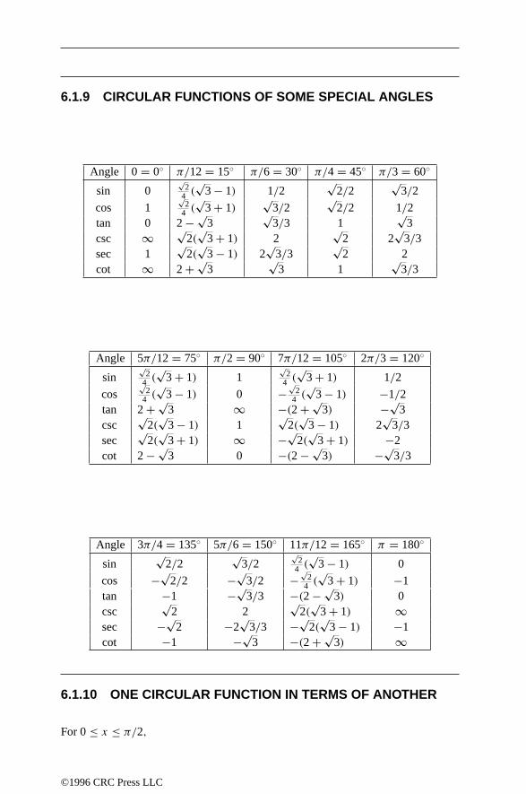
6.1.9 CIRCULAR FUNCTIONS OF SOME SPECIAL ANGLES
Angle 0 = 0 π/12 = 15 π/6 = 30 π/4 = 45 π/3 = 60
sin 0√
24 (
√3 − 1) 1/2
√2/2
√3/2
cos 1√
24 (
√3 + 1)
√3/2
√2/2 1/2
tan 0 2 − √3
√3/3 1
√3
csc ∞ √2(
√3 + 1) 2
√2 2
√3/3
sec 1√
2(√
3 − 1) 2√
3/3√
2 2cot ∞ 2 + √
3√
3 1√
3/3
Angle 5π/12 = 75 π/2 = 90 7π/12 = 105 2π/3 = 120
sin√
24 (
√3 + 1) 1
√2
4 (√
3 + 1) 1/2
cos√
24 (
√3 − 1) 0 −
√2
4 (√
3 − 1) −1/2tan 2 + √
3 ∞ −(2 + √3) −√
3csc
√2(
√3 − 1) 1
√2(
√3 − 1) 2
√3/3
sec√
2(√
3 + 1) ∞ −√2(
√3 + 1) −2
cot 2 − √3 0 −(2 − √
3) −√3/3
Angle 3π/4 = 135 5π/6 = 150 11π/12 = 165 π = 180
sin√
2/2√
3/2√
24 (
√3 − 1) 0
cos −√2/2 −√
3/2 −√
24 (
√3 + 1) −1
tan −1 −√3/3 −(2 − √
3) 0csc
√2 2
√2(
√3 + 1) ∞
sec −√2 −2
√3/3 −√
2(√
3 − 1) −1cot −1 −√
3 −(2 + √3) ∞
6.1.10 ONE CIRCULAR FUNCTION IN TERMS OF ANOTHER
For 0 ≤ x ≤ π/2,
©1996 CRC Press LLC

sin x cos x tan x
sin x = sin x√
1 − cos2 xtan x√
1 + tan2 x
cos x =√
1 − sin2 x cos x1√
1 + tan2 x
tan x = sin x√1 − sin2 x
√1 − cos2 x
cos xtan x
csc x = 1
sin x
1√1 − cos2 x
√1 + tan2 x
tan x
sec x = 1√1 − sin2 x
1
cos x
√1 + tan2 x
cot x =√
1 − sin2 x
sin x
cos x√1 − cos2 x
1
tan x
csc x sec x cotx
sin x = 1
csc x
√sec2 x − 1
sec x
1√1 + cot2 x
cos x =√
csc2 x − 1
csc x
1
sec x
cot x√1 + cot2 x
tan x = 1√csc2 x − 1
√sec2 x − 1
1
cot x
csc x = csc xsec x√
sec2 x − 1
√1 + cot2 x
sec x = csc x√csc2 x − 1
sec x
√1 + cot2 x
cot x
cot x = √csc2 x − 1
1√sec2 x − 1
cot x
6.1.11 DEFINITIONS IN TERMS OF EXPONENTIALS
cos z = eiz + e−iz
2. eiz = cos z + i sin z.
sin z = eiz − e−iz
2i. e−iz = cos z − i sin z.
tan z = sin z
cos z= eiz − e−iz
i(eiz + e−iz).
©1996 CRC Press LLC

6.1.12 FUNDAMENTAL IDENTITIES
Reciprocal relations
sin α = 1
cscα, cosα = 1
secα, tan α = sin α
cosα= 1
cot α,
cscα = 1
sin α, secα = 1
cosα, cot α = cosα
sin α= 1
tan α.
Pythagorean theorem
sin2 z + cos2 z = 1.
sec2 z − tan2 z = 1.
csc2 z − cot2 z = 1.
Product relations
sin α = tan α cosα, cosα = cot α sin α,
tan α = sin α secα, cot α = cosα cscα,
secα = cscα tan α, cscα = secα cot α.
Quotient relations
sin α = tan α
secα, cosα = cot α
cscα, tan α = sin α
cosα,
cscα = secα
tan α, secα = cscα
cot α, cot α = cosα
sin α.
6.1.13 ANGLE SUM AND DIFFERENCE RELATIONSHIPS
sin (α ± β) = sin α cosβ ± cosα sin β.
cos (α ± β) = cosα cosβ ∓ sin α sin β.
tan (α ± β) = tan α ± tan β
1 ∓ tan α tan β.
cot (α ± β) = cot α cot β ∓ 1
cot β ± cot α.
©1996 CRC Press LLC

6.1.14 DOUBLE ANGLE FORMULAE
sin 2α = 2 sin α cosα = 2 tan α
1 + 2 tan2 α.
cos 2α = 2 cos2 α − 1 = 1 − 2 sin2 α = cos2 α − sin2 α = 1 − tan2 α
1 + tan2 α.
tan 2α = 2 tan α
1 − tan2 α.
cot 2α = cot2 α − 1
2 cot α.
6.1.15 MULTIPLE ANGLE FORMULAE
sin 3α = −4 sin3 α + 3 sin α.
sin 4α = −8 sin3 α cosα + 4 sin α cosα.
sin 5α = 16 sin5 α − 20 sin3 α + 5 sin α.
sin 6α = 32 sin α cos5 α − 32 sin α cos3 α + 6 sin α cosα.
sin nα = 2 sin (n − 1)α cosα − sin (n − 2)α.
cos 3α = 4 cos3 α − 3 cosα.
cos 4α = 8 cos4 α − 8 cos2 α + 1.
cos 5α = 16 cos5 α − 20 cos3 α + 5 cosα.
cos 6α = 32 cos6 α − 48 cos4 α + 18 cos2 α − 1.
cos nα = 2 cos (n − 1)α cosα − cos (n − 2)α.
tan 3α = − tan3 α + 3 tan α
−3 tan2 α + 1.
tan 4α = −4 tan3 α + 4 tan α
tan4 α − 6 tan2 α + 1.
tan nα = tan (n − 1)α + tan α
− tan (n − 1)α tan α + 1.
©1996 CRC Press LLC

6.1.16 HALF ANGLE FORMULAE
cosα
2= ±
√1 + cosα
2(positive if α/2 is in quadrant I or IV, negative if in II or III).
sinα
2= ±
√1 − cosα
2(positive if α/2 is in quadrant I or II, negative if in III or IV).
tanα
2= 1 − cosα
sin α= sin α
1 + cosα= ±
√1 − cosα
1 + cosα(positive if α/2 is in quadrant I or III, negative if in II or IV).
cotα
2= 1 + cosα
sin α= sin α
1 − cosα= ±
√1 + cosα
1 − cosα(positive if α/2 is in quadrant I or III, negative if in II or IV).
6.1.17 POWERS OF CIRCULAR FUNCTIONS
sin2 α = 1
2(1 − cos 2α). cos2 α = 1
2(1 + cos 2α).
sin3 α = 1
4(− sin 3α + 3 sin α). cos3 α = 1
4(cos 3α + 3 cosα).
sin4 α = 1
8(3 − 4 cos 2α + cos 4α). cos4 α = 1
8(3 + 4 cos 2α + cos 4α).
tan2 α = 1 − cos 2α
1 + cos 2α.
cot2 α = 1 + cos 2α
1 − cos 2α.
6.1.18 PRODUCTS OF SINE AND COSINE
cosα cosβ = 1
2cos (α − β) + 1
2cos (α + β).
sin α sin β = 1
2cos (α − β) − 1
2cos (α + β).
sin α cosβ = 1
2sin (α − β) + 1
2sin (α + β).
(6.1.3)
©1996 CRC Press LLC
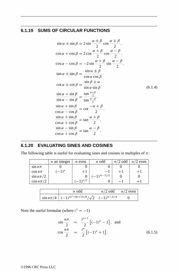
6.1.19 SUMS OF CIRCULAR FUNCTIONS
sin α ± sin β = 2 sinα ± β
2cos
α ∓ β
2.
cosα + cosβ = 2 cosα + β
2cos
α − β
2.
cosα − cosβ = −2 sinα + β
2sin
α − β
2.
tan α ± tan β = sin α ± β
cosα cosβ.
cot α ± cot β = sin β ± α
sin α sin β.
sin α + sin β
sin α − sin β= tan α+β
2
tan α−β
2
.
sin α + sin β
cosα − cosβ= cot
−α + β
2.
sin α + sin β
cosα + cosβ= tan
α + β
2.
sin α − sin β
cosα + cosβ= tan
α − β
2.
(6.1.4)
6.1.20 EVALUATING SINES AND COSINES
The following table is useful for evaluating sines and cosines in multiples of π :
n an integer n even n odd n/2 odd n/2 evensin nπ 0 0 0 0 0cos nπ (−1)n +1 −1 +1 +1sin nπ/2 0 (−1)(n−1)/2 0 0cos nπ/2 (−1)n/2 0 −1 +1
n odd n/2 odd n/2 even
sin nπ/4 (−1)(n2+4n+11)/8/
√2 (−1)(n−2)/4 0
Note the useful formulae (where i2 = −1)
sinnπ
2= in+1
2
[(−1)n − 1
], and
cosnπ
2= in
2
[(−1)n + 1
]. (6.1.5)
©1996 CRC Press LLC

6.2 CIRCULAR FUNCTIONS AND PLANARTRIANGLES
6.2.1 RIGHT TRIANGLES
Let A, B, and C designate the vertices of a right triangle with C the right angle anda, b, and c the lengths of the sides opposite the corresponding vertices:
sinA= a
c= 1
cscA,
cosA= b
c= 1
secA,
tanA= a
b= 1
cot A.
The Pythagorean theorem states that a2 + b2 = c2.The sum of the interior angles equals π , i.e., A + B + C = π .
Right Triangle
a
General Triangle
b
cca
bC
B
A A C
B
6.2.2 GENERAL PLANE TRIANGLES
Let A, B, and C designate the interior angles of a general triangle and let a, b, and c
be the length of the sides opposite those angles.
Radius of the inscribed circle:
r =√(s − a)(s − b)(s − c)
s,
where s = 12 (a + b + c), the semiperimeter.
Radius of the circumscribed circle:
R = a
2 sinA= b
2 sinB= c
2 sinC= abc
4(Area). (6.2.1)
©1996 CRC Press LLC

Law of sines:
a
sinA= b
sinB= c
sinC.
Law of cosines:
a2 = c2 + b2 − 2bc cosA, cosA = c2 + b2 − a2
2bc.
b2 = a2 + c2 − 2ca cosB, cosB = a2 + c2 − b2
2ca.
c2 = b2 + a2 − 2ab cosC, cosC = b2 + a2 − c2
2ab.
Triangle sides in terms of other components:
a = b cosC + c cosB,
c = a cosA + b cosC,
b = c cosB + a cosA.
Law of tangents:
a + b
a − b= tan A+B
2
tan A−B2
,
b + c
b − c= tan B+C
2
tan B−C2
,
a + c
a − c= tan A+C
2
tan A−C2
.
(6.2.2)
Area of general triangle:
Area = bc sinA
2= ac sinB
2= ab sinC
2,
= c2 sinA sinB
2 sinC= b2 sinA sinC
2 sinB= a2 sinB sinC
2 sinA,
=√s(s − a)(s − b)(s − c) = rs = abc
4R(Heron’s formula).
©1996 CRC Press LLC

Mollweide’s formulae:
b − c
a= sin 1
2 (B − C)
cos 12A
,
c − a
b= sin 1
2 (C − A)
cos 12B
,
a − b
c= sin 1
2 (A − B)
cos 12C
.
(6.2.3)
Newton’s formulae:
b + c
a= cos 1
2 (B − C)
sin 12A
,
c + a
b= cos 1
2 (C − A)
sin 12B
,
a + b
c= cos 1
2 (A − B)
sin 12C
.
(6.2.4)
6.2.3 HALF ANGLE FORMULAE
tanA
2= r
s − atan
B
2= r
s − btan
C
2= r
s − c
sinA
2=
√(s − b)(s − c)
bccos
A
2=
√s(s − a)
bc
sinB
2=
√(s − c)(s − a)
cacos
B
2=
√s(s − b)
ca
sinC
2=
√(s − a)(s − b)
abcos
C
2=
√s(s − c)
ab
6.2.4 SOLUTION OF TRIANGLES
A triangle is totally described by specifying any side and two additional parameters:either the remaining two sides, another side and the included angle, or two specifiedangles. Two angles alone specify the shape of a triangle, but not its size, whichrequires specification of a side.
©1996 CRC Press LLC
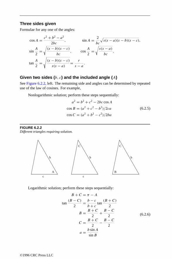
Three sides givenFormulae for any one of the angles:
cosA = c2 + b2 − a2
2bc, sinA = 2
bc
√s(s − a)(s − b)(s − c),
sinA
2=
√(s − b)(s − c)
bc, cos
A
2=
√s(s − a)
bc,
tanA
2=
√(s − b)(s − c)
s(s − a)= r
s − a.
Given two sides (b, c) and the included angle (A)See Figure 6.2.2, left. The remaining side and angles can be determined by repeateduse of the law of cosines. For example,
Nonlogarithmic solution; perform these steps sequentially:
a2 = b2 + c2 − 2bc cosA
cosB = (a2 + c2 − b2)/2ca
cosC = (a2 + b2 − c2)/2ba
(6.2.5)
FIGURE 6.2.2Different triangles requiring solution.
cc
b
C
A B
C
b b
Logarithmic solution; perform these steps sequentially:
B + C = π − A
tan(B − C)
2= b − c
b + ctan
(B + C)
2
B = B + C
2+ B − C
2
C = B + C
2− B − C
2
a = b sinA
sinB
(6.2.6)
©1996 CRC Press LLC

Given two sides (b, c) and an angle (C), not the included angleSee Figure 6.2.2, middle. The remaining angles and side are determined by use ofthe law of sines. and the fact that the sum of the angles is π , A + B + C = π .
sinB = b sinC
c, A = π − B − C, a = b sinA
sinB.
Given one side (b) and two angles (B,C)See Figure 6.2.2, right. The third angle is specified byA = π−B−C. The remainingsides are found by
a = b sinA
sinB, c = b sinC
sinB.
6.3 INVERSE CIRCULAR FUNCTIONS
6.3.1 DEFINITION IN TERMS OF AN INTEGRAL
sin−1 z =∫ z
0
dt√1 − t2
,
cos−1 z =∫ 1
z
dt√1 − t2
= π
2− sin−1 z,
tan−1 z =∫ z
0
dt
1 + t2= π
2− cot−1 z,
where z can be complex. The path of integration must not cross the real axis in the firsttwo cases. In the third case, it must not cross the imaginary axis except possibly insidethe unit circle. If −1 ≤ x ≤ 1, then sin−1 x and cos−1 x are real, −π
2 ≤ sin−1 x ≤ π2 ,
and 0 ≤ cos−1 x ≤ π .
csc−1 z = sin−1(1/z),
sec−1 z = cos−1(1/z),
cot−1 z = tan−1(1/z),
sec−1 z + csc−1 z = π/2.
©1996 CRC Press LLC

6.3.2 FUNDAMENTAL PROPERTIES
The general solutions of the equations sin t = z, cos t = z, tan t = z are, respec-tively, (where k is an arbitrary integer):
t = sin−1 z = (−1)k sin−1 z + kπ,
t = cos−1 z = ± cos−1 z + 2kπ,
t = tan−1 z = tan−1 z + kπ, (z2 = −1).
6.3.3 PRINCIPAL VALUES OF THE INVERSE CIRCULARFUNCTIONS
The notation sin−1 x is used to denote any angle whose sin is x. The function sin−1 x
is usually used to denote the principal value. Similar notation is used for the otherinverse trigonometric functions. The principal values of the inverse trigonometricfunctions are defined as follows:
1. When −1 ≤ x ≤ 1, then −π/2 ≤ sin−1 x ≤ π/2.
2. When −1 ≤ x ≤ 1, then 0 ≤ cos−1 x ≤ π.
3. When −∞ ≤ x ≤ ∞, then −π/2 ≤ tan−1 x ≤ π/2.
4. When 1 ≤ x, then 0 ≤ csc−1 x ≤ π/2.When x ≤ −1, then −π/2 ≤ csc−1 x ≤ 0.
5. When 1 ≤ x, then 0 ≤ sec−1 x ≤ π/2.When x ≤ −1, then π/2 ≤ sec−1 x ≤ π.
6. When −∞ ≤ x ≤ ∞, then 0 ≤ cot−1 x ≤ π.
6.3.4 FUNDAMENTAL IDENTITIES
sin−1 x + cos−1 x = π/2.
tan−1 x + cot−1 x = π/2.(6.3.1)
If α = sin−1 x, then
sin α = x, cosα =√
1 − x2, tan α = x√1 − x2
,
cscα = 1
x, secα = 1√
1 − x2, cot α =
√1 − x2
x.
If α = cos−1 x, then
sin α =√
1 − x2, cosα = x, tan α =√
1 − x2
x,
cscα = 1√1 − x2
, secα = 1
x, cot α = x√
1 − x2.
©1996 CRC Press LLC

If α = tan−1 x, then
sin α = x√1 + x2
, cosα = 1√1 + x2
, tan α = x,
cscα =√
1 + x2
x, secα =
√1 + x2, cot α = 1
x.
6.3.5 FUNCTIONS OF NEGATIVE ARGUMENTS
sin−1 (−z) = − sin−1 z, sec−1 (−z) = π − sec−1 z,
cos−1 (−z) = π − cos−1 z, csc−1 (−z) = − csc−1 z,
tan−1 (−z) = − tan−1 z, cot−1 (−z) = π − cot−1 z.
6.3.6 RELATIONSHIP TO INVERSE HYPERBOLIC FUNCTIONS
sin−1 z = −i sinh−1 (iz), sec−1 z = ±i sech−1 (iz),
cos−1 z = ±i cosh−1 (iz), csc−1 z = i csch−1 (iz),
tan−1 z = −i tanh−1 (iz), cot−1 z = i coth−1 (iz).
6.3.7 SUM AND DIFFERENCE OF TWO INVERSETRIGONOMETRIC FUNCTIONS
sin−1 z1 ± sin−1 z2 = sin−1
(z1
√1 − z2
2 ± z2
√1 − z2
1
).
cos−1 z1 ± cos−1 z2 = cos−1
(z1z2 ∓
√(1 − z2
2)(1 − z21)
).
tan−1 z1 ± tan−1 z2 = tan−1
(z1 ± z2
1 ∓ z1z2
).
sin−1 z1 ± cos−1 z2 = sin−1
(z1z2 ±
√(1 − z2
1)(1 − z22)
),
= cos−1
(z2
√1 − z2
1 ∓ z1
√1 − z2
2
).
tan−1 z1 ± cot−1 z2 = tan−1
(z1z2 ± 1
z2 ∓ z1
)= cot−1
(z2 ∓ z1
z1z2 ± 1
).
©1996 CRC Press LLC

6.4 SPHERICAL GEOMETRY ANDTRIGONOMETRY
6.4.1 RIGHT SPHERICAL TRIANGLES
Let a, b, and c be the sides of a right spherical triangle with opposite angles A, B,and C, respectively, where each side is measured by the angle subtended at the centerof the sphere. Assume that C = π/2 = 90 (see Figure 6.4.3). Then,
sin a = tan b cot B, sin a = sinA sin c,
sin b = tan a cot A, sin b = sinB sin c,
cosA = tan b cot c, cosA = cos a sinB,
cosB = tan a cot c, cosB = cos b sinA,
cos c = cosA cot B, cos c = cos a cos b.
FIGURE 6.4.3Right spherical triangle (left) and diagram for Napier’s rule (right).
c
b
C
co ⋅ C
co ⋅ B
ab
co ⋅ Aa
AB
Napier’s rules of circular partsArrange the five quantities a, b, co-A (complement of A), co-C, co-B of a rightspherical triangle with right angle at C, in cyclic order as pictured in Figure 6.4.3. Ifany one of these quantities is designated a middle part, then two of the other parts areadjacent to it, and the remaining two parts are opposite to it. The formulae above fora right spherical triangle may be recalled by the following two rules:
1. The sine of any middle part is equal to the product of the tangents of the twoadjacent parts.
2. The sine of any middle part is equal to the product of the cosines of the twoopposite parts.
©1996 CRC Press LLC
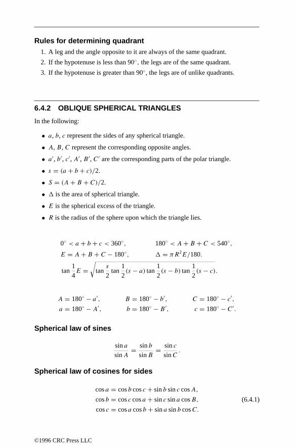
Rules for determining quadrant1. A leg and the angle opposite to it are always of the same quadrant.
2. If the hypotenuse is less than 90, the legs are of the same quadrant.
3. If the hypotenuse is greater than 90, the legs are of unlike quadrants.
6.4.2 OBLIQUE SPHERICAL TRIANGLES
In the following:
• a, b, c represent the sides of any spherical triangle.
• A, B, C represent the corresponding opposite angles.
• a′, b′, c′, A′, B ′, C ′ are the corresponding parts of the polar triangle.
• s = (a + b + c)/2.
• S = (A + B + C)/2.
• ! is the area of spherical triangle.
• E is the spherical excess of the triangle.
• R is the radius of the sphere upon which the triangle lies.
0 < a + b + c < 360, 180 < A + B + C < 540,
E = A + B + C − 180, ! = πR2E/180.
tan1
4E =
√tan
s
2tan
1
2(s − a) tan
1
2(s − b) tan
1
2(s − c).
A = 180 − a′, B = 180 − b′, C = 180 − c′,a = 180 − A′, b = 180 − B ′, c = 180 − C ′.
Spherical law of sines
sin a
sinA= sin b
sinB= sin c
sinC.
Spherical law of cosines for sides
cos a = cos b cos c + sin b sin c cosA,
cos b = cos c cos a + sin c sin a cosB,
cos c = cos a cos b + sin a sin b cosC.
(6.4.1)
©1996 CRC Press LLC

Spherical law of cosines for angles
cosA = − cosB cosC + sinB sinC cos a,
cosB = − cosC cosA + sinC sinA cos b,
cosC = − cosA cosB + sinA sinB cos c.
Spherical law of tangents
tan 12 (B − C)
tan 12 (B + C)
= tan 12 (b − c)
tan 12 (b + c)
,
tan 12 (C − A)
tan 12 (C + A)
= tan 12 (c − a)
tan 12 (c + a)
,
tan 12 (A − B)
tan 12 (A + B)
= tan 12 (a − b)
tan 12 (a + b)
.
(6.4.2)
Spherical half angle formulae
Define k2 = (tan r)2 = sin(s − a) sin(s − b) sin(s − c)
sin s. Then
tan
(A
2
)= k
sin(s − a),
tan
(B
2
)= k
sin(s − b),
tan
(C
2
)= k
sin(s − c).
(6.4.3)
Spherical half side formulae
Define K2 = (tanR)2 = − cos S
cos(S − A) cos(S − B) cos(S − C). Then
tan(a/2) = K cos(S − A),
tan(b/2) = K cos(S − B),
tan(c/2) = K cos(S − C).
(6.4.4)
Gauss’s formulae
sin 12 (a − b)
sin 12c
= sin 12 (A − B)
cos 12C
,cos 1
2 (a − b)
cos 12c
= sin 12 (A + B)
cos 12C
,
sin 12 (a + b)
sin 12c
= cos 12 (A − B)
sin 12C
,cos 1
2 (a + b)
cos 12c
= cos 12 (A + B)
sin 12C
.
©1996 CRC Press LLC

Napier’s analogs
sin 12 (A − B)
sin 12 (A + B)
= tan 12 (a − b)
tan 12c
,sin 1
2 (a − b)
sin 12 (a + b)
= tan 12 (A − B)
cot 12C
,
cos 12 (A − B)
cos 12 (A + B)
= tan 12 (a + b)
tan 12c
,cos 1
2 (a − b)
cos 12 (a + b)
= tan 12 (A + B)
cot 12C
.
Haversine formulae
hav a = hav(b − c) + sin b sin c havA.
havA = sin(s − b) sin(s − c)
sin b sin c,
= hav a − hav(b − c)
sin b sin c,
= hav[180 − (B + C)] + sinB sinC hav a.
(6.4.5)
Rules for determining quadrant
1. If A > B > C, then a > b > c.
2. A side (angle) which differs by more than 90 from another side (angle) is inthe same quadrant as its opposite angle (side).
3. Half the sum of any two sides and half the sum of the opposite angles are in thesame quadrant.
Summary of solution of oblique spherical triangles
Given Solution CheckThree sides Half-angle formulae Law of sinesThree angles Half-side formulae Law of sinesTwo sides andincluded angle
Napier’s analogies (to find sum anddifference of unknown angles); thenlaw of sines (to find remaining side).
Gauss’s formulae
Two angles andincluded side
Napier’s analogies (to find sum anddifference of unknown sides); thenlaw of sines (to find remaining angle).
Gauss’s formulae
Two sides andan oppositeangle
Law of sines (to find an angle); thenNapier’s analogies (to find remainingangle and side). Note number ofsolutions.
Gauss’s formulae
Two angles andan opposite side
Law of sines (to find a side); thenNapier’s analogies (to find remainingside and angle). Note number ofsolutions.
Gauss’s formulae
©1996 CRC Press LLC
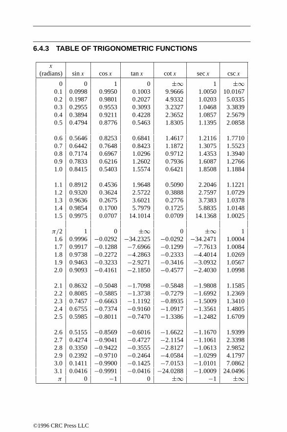
6.4.3 TABLE OF TRIGONOMETRIC FUNCTIONS
x
(radians) sin x cos x tan x cot x sec x csc x
0 0 1 0 ±∞ 1 ±∞0.1 0.0998 0.9950 0.1003 9.9666 1.0050 10.01670.2 0.1987 0.9801 0.2027 4.9332 1.0203 5.03350.3 0.2955 0.9553 0.3093 3.2327 1.0468 3.38390.4 0.3894 0.9211 0.4228 2.3652 1.0857 2.56790.5 0.4794 0.8776 0.5463 1.8305 1.1395 2.0858
0.6 0.5646 0.8253 0.6841 1.4617 1.2116 1.77100.7 0.6442 0.7648 0.8423 1.1872 1.3075 1.55230.8 0.7174 0.6967 1.0296 0.9712 1.4353 1.39400.9 0.7833 0.6216 1.2602 0.7936 1.6087 1.27661.0 0.8415 0.5403 1.5574 0.6421 1.8508 1.1884
1.1 0.8912 0.4536 1.9648 0.5090 2.2046 1.12211.2 0.9320 0.3624 2.5722 0.3888 2.7597 1.07291.3 0.9636 0.2675 3.6021 0.2776 3.7383 1.03781.4 0.9854 0.1700 5.7979 0.1725 5.8835 1.01481.5 0.9975 0.0707 14.1014 0.0709 14.1368 1.0025
π/2 1 0 ±∞ 0 ±∞ 11.6 0.9996 −0.0292 −34.2325 −0.0292 −34.2471 1.00041.7 0.9917 −0.1288 −7.6966 −0.1299 −7.7613 1.00841.8 0.9738 −0.2272 −4.2863 −0.2333 −4.4014 1.02691.9 0.9463 −0.3233 −2.9271 −0.3416 −3.0932 1.05672.0 0.9093 −0.4161 −2.1850 −0.4577 −2.4030 1.0998
2.1 0.8632 −0.5048 −1.7098 −0.5848 −1.9808 1.15852.2 0.8085 −0.5885 −1.3738 −0.7279 −1.6992 1.23692.3 0.7457 −0.6663 −1.1192 −0.8935 −1.5009 1.34102.4 0.6755 −0.7374 −0.9160 −1.0917 −1.3561 1.48052.5 0.5985 −0.8011 −0.7470 −1.3386 −1.2482 1.6709
2.6 0.5155 −0.8569 −0.6016 −1.6622 −1.1670 1.93992.7 0.4274 −0.9041 −0.4727 −2.1154 −1.1061 2.33982.8 0.3350 −0.9422 −0.3555 −2.8127 −1.0613 2.98522.9 0.2392 −0.9710 −0.2464 −4.0584 −1.0299 4.17973.0 0.1411 −0.9900 −0.1425 −7.0153 −1.0101 7.08623.1 0.0416 −0.9991 −0.0416 −24.0288 −1.0009 24.0496π 0 −1 0 ±∞ −1 ±∞
©1996 CRC Press LLC

6.5 EXPONENTIAL FUNCTION
6.5.1 EXPONENTIATION
For a any real number and m a positive integer, the exponential am is defined as
am = a · a · a · · · a︸ ︷︷ ︸m terms
. (6.5.1)
The following three laws of exponents follow:
1. an · am = am+n.
2.am
an=
am−n, if m > n,
1, if m = n,1
an−m , if m < n.
3. (am)n = a(mn).
The nth root function is defined as the inverse of the nth power function:
If bn = a, then b = n√a = a(1/n). (6.5.2)
If n is odd, there will be a unique real number satisfying the above definition ofn√a, for any real value of a. If n is even, for positive values of a there will be two real
values for n√a, one positive and one negative. By convention, the symbol n
√a means
the positive value. If n is even and a is negative, then there are no real values for n√a.
To extend the definition to include at (for t not necessarily an integer), so as tomaintain the laws of exponents, the following definitions are required (where we nowrestrict a to be positive, p to be an odd number, and q to be an even number):
a0 = 1 ap/q = q√ap a−t = 1
at
With these restrictions, the second law of exponents can be written asam
an= am−n.
If a > 1, then the function ax is monotone increasing while, if 0 < a < 1 thenthe function ax is monotone decreasing.
6.5.2 DEFINITION OF ez
exp(z) = ez = limm→∞
(1 + z
m
)m= 1 + z + z2
2!+ z3
3!+ z4
4!+ . . . .
If z = x + iy, then ez = exeiy = ex(cos y + i sin y).
©1996 CRC Press LLC

0
5
10
15
20
−3 −2 −1 0 1 2 3x
ex
e−x
6.5.3 DERIVATIVE AND INTEGRAL OF ex
The derivative of ex is ex . The integral of ex is ex .
6.5.4 CIRCULAR FUNCTIONS IN TERMS OF EXPONENTIALS
cos z = eiz + e−iz
2, eiz = cos z + i sin z.
sin z = eiz − e−iz
2i, e−iz = cos z − i sin z.
6.6 LOGARITHMIC FUNCTIONS
6.6.1 DEFINITION OF THE NATURAL LOG
The natural logarithm (also known as the Napierian logarithm) of z is written as ln zor as loge z. It is sometimes written log z (this is also used to represent a “generic”logarithm, a logarithm to any base). One definition is
ln z =∫ z
1
dt
t,
where the integration path from 1 to z does not cross the origin or the negative realaxis.
©1996 CRC Press LLC

For complex values of z the natural logarithm, as defined above, can be repre-sented in terms of its magnitude and phase. If z = x+iy = reiθ , then ln z = ln r+iθ,
where r =√x2 + y2, x = r cos θ , and y = r sin θ .
6.6.2 SPECIAL VALUES
ln 0 = −∞, ln 1 = 0, ln e = 1,
ln (−1) = iπ + 2πik, ln (±i) = ± iπ
2+ 2πik,
(e is given numerically on page 14).
6.6.3 LOGARITHMS TO A BASE OTHER THAN e
The logarithmic function to the base a, written loga , is defined as
loga z = logb z
logb a= ln z
ln a
Note the properties:
• loga ap = p.
• loga b = 1
logb a.
• log10 z = ln z
ln 10= (log10 e) ln z ≈ (0.4342944819 . . . ) ln z.
• ln z = (ln 10) log10 z ≈ (2.3025850929 . . . ) log10 z.
6.6.4 RELATIONSHIP OF THE LOGARITHM TO THEEXPONENTIAL
For real values of z the logarithm is a monotonic function, as is the exponential. Anymonotonic function has a single-valued inverse function; the natural logarithm is theinverse of the exponential. If x = ey , then y = ln x, and x = eln x . The same inverserelations exist for bases other than e. For example, if u = aw, then w = loga u, andu = aloga u.
©1996 CRC Press LLC

6.6.5 IDENTITIES
loga z1z2 = loga z1 + loga z2, for (−π < arg z1 + arg z2 < π).
logaz1
z2= loga z1 − loga z2, for (−π < arg z1 − arg z2 < π).
loga zn = n loga z, for (−π < n arg z < π), when n is an integer.
6.6.6 SERIES EXPANSIONS FOR THE NATURAL LOGARITHM
ln (1 + z) = z − 1
2z2 + 1
3z3 − . . . , for |z| < 1.
ln z =(z − 1
z
)+ 1
2
(z − 1
z
)2
+ 1
3
(z − 1
z
)3
+ . . . , for Re z ≥ 1
2.
6.6.7 DERIVATIVE AND INTEGRATION FORMULAE
dln z
dz= 1
z,
∫dz
z= ln z,
∫ln z dz = z ln z − z.
6.7 HYPERBOLIC FUNCTIONS
6.7.1 DEFINITIONS OF THE HYPERBOLIC FUNCTIONS
sinh z = ez − e−z
2, csch z = 1
sinh z,
cosh z = ez + e−z
2, sech z = 1
cosh z,
tanh z = ez − e−z
ez + e2z =
sinh z
cosh z, coth z = 1
tanh z.
The curve y = cosh x is called a catenary.
©1996 CRC Press LLC

When z = x + iy,
sinh z = sinh x cos y + i cosh x sin y,
cosh z = cosh x cos y + i sinh x sin y,
tanh z = sinh 2x + i sin 2y
cosh 2x + cos 2y,
coth z = sinh 2x − i sin 2y
cosh 2x − cos 2y.
−20
−10
0
10
20
−4 −2 0 2 4x
sinh xcosh x
−5
0
5
−4 −2 0 2 4x
tanh xcoth x
©1996 CRC Press LLC

6.7.2 RANGE OF VALUES
FunctionDomain
(interval of u)Range
(interval of function)Remarks
sinh u (−∞,+∞) (−∞,+∞)
cosh u (−∞,+∞) [1,+∞)
tanh u (−∞,+∞) (−1,+1)csch u (−∞, 0) (0,−∞) Two branches,
(0,+∞) (+∞, 0) pole at u = 0.sech u (−∞,+∞) (0, 1]coth u (−∞, 0) (−1,−∞) Two branches,
(0,+∞) (+∞, 1) pole at u = 0.
6.7.3 SERIES EXPANSIONS
cosh z = 1 + z2
2!+ z4
4!+ z6
6!+ . . . , |z| < ∞.
sinh z = z + z3
3!+ z5
5!+ z7
7!+ . . . , |z| < ∞.
tanh z = z − z3
3+ 2z5
15+ . . . , |z| < π
2.
6.7.4 SYMMETRY RELATIONSHIPS
cosh (−z) = + cosh z, sinh (−z) = − sinh z, tanh (−z) = − tanh z.
6.7.5 INTERRELATIONSHIPS AMONG THE HYPERBOLICFUNCTIONS
ez = cosh z + sinh z, e−z = cosh z − sinh z,
(cosh z)2 − (sinh z)2 = (tanh z)2 + (sech z)2 = (coth z)2 − (csch z)2 = 1.
6.7.6 RELATIONSHIP TO CIRCULAR FUNCTIONS
cosh z = cos iz, sinh z = −i sin iz, tanh z = −i tan iz.
©1996 CRC Press LLC

6.7.7 HYPERBOLIC FUNCTIONS IN TERMS OF ONE ANOTHER
Function sinh x cosh x tanh x
sinh x = sinh x ±√(cosh x)2 − 1
tanh x√1 − (tanh x)2
cosh x =√
1 + (sinh x)2 cosh x1√
1 − (tanh x)2
tanh x = sinh x√1 + (sinh x)2
±√(cosh x)2 − 1
cosh xtanh x
csch x = 1
sinh x± 1√
(cosh x)2 − 1
√1 − (tanh x)2
tanh x
sech x = 1√1 + (sinh x)2
1
cosh x
√1 − (tanh x)2
coth x =√
1 + (sinh x)2
sinh x± cosh x√
(cosh x)2 − 1
1
tanh x
Function csch x sech x coth x
sinh x = 1
csch x±√
1 − (sech x)2
sech x± 1√
(coth x)2 − 1
cosh x = ±√(csch x)2 + 1
csch x
1
sech x± coth x√
(coth x)2 − 1
tanh x = 1√(csch x)2 + 1
±√
1 − (sech x)21
coth x
csch x = csch x ± sech x√1 − (sech x)2
±√(coth x)2 − 1
sech x = ± csch x√(csch x)2 + 1
sech x ±√(coth x)2 − 1
coth x
coth x =√(csch x)2 + 1 ± 1√
1 − (sech x)2coth x
6.7.8 SUM AND DIFFERENCE FORMULAE
cosh (z1 ± z2) = cosh z1 cosh z2 ± sinh z1 sinh z2,
sinh (z1 ± z2) = sinh z1 cosh z2 ± cosh z1 sinh z2,
tanh (z1 ± z2) = tanh z1 ± tanh z2
1 ± tanh z1 tanh z2= sinh 2z1 ± sinh 2z2
cosh 2z1 ± cosh 2z2,
coth (z1 ± z2) = 1 ± coth z1 coth z2
coth z1 ± coth z2= sinh 2z1 ∓ sinh 2z2
cosh 2z1 − cosh 2z2.
(6.7.1)
©1996 CRC Press LLC

6.7.9 MULTIPLE ARGUMENT RELATIONS
sinh 2α = 2 sinh α cosh α = 2 tanh α
1 − tanh2 α.
sinh 3α = +3 sinh α + 4 sinh3 α = sinh α(4 cosh2 α − 1).
sinh 4α = 4 sinh3 α cosh α + 4 cosh3 α sinh α.
cosh 2α = cosh2 α + sinh2 α = 2 cosh2 α − 1,
= 1 + 2 sinh2 α = 1 + tanh2 α
1 − tanh2 α.
cosh 3α = −3 cosh α + 4 cosh3 α = cosh α(4 sinh2 α + 1).
cosh 4α = cosh4 α + 6 sinh2 α cosh2 α + 6 sinh4 α.
tanh 2α = 2 tanh α
1 + tanh2 α.
tanh 3α = 3 tanh α + tanh3 α
1 + 3 tanh2 α.
coth 2α = 1 + coth2 α
2 coth α.
coth 3α = 3 coth α + coth3 α
1 + 3 coth2 α.
6.7.10 SUMS OF FUNCTIONS
sinh u ± sinhw = 2 sinhu ± w
2cosh
u ∓ w
2,
cosh u + coshw = 2 coshu + w
2cosh
u − w
2,
cosh u − coshw = 2 sinhu + w
2sinh
u − w
2,
tanh u ± tanhw = sinh u ± w
cosh u coshw,
coth u ± cothw = sinh u ± w
sinh u sinhw.
6.7.11 PRODUCTS OF FUNCTIONS
sinh u sinhw = 1
2(cosh(u + w) − cosh(u − w)) ,
sinh u coshw = 1
2(sinh(u + w) + sinh(u − w)) ,
cosh u coshw = 1
2(cosh(u + w) + cosh(u − w)) .
©1996 CRC Press LLC

6.7.12 HALF–ARGUMENT FORMULAE
sinhz
2= ±
√cosh z − 1
2,
coshz
2= +
√cosh z + 1
2,
tanhz
2= ±
√cosh z − 1
cosh z + 1= sinh z
cosh z + 1,
cothz
2= ±
√cosh z + 1
cosh z − 1= sinh z
cosh z − 1.
6.7.13 DIFFERENTIATION FORMULAE
dsinh z
dz= cosh z,
dcosh z
dz= sinh z,
dtanh z
dz= (sech z)2,
dcsch z
dz= − csch z coth z,
dsech z
dz= − sech z tanh z,
dcoth z
dz= −(csch z)2.
6.8 INVERSE HYPERBOLIC FUNCTIONS
When z = x + iy,
cosh−1 z =∫ z
0
dt√t2 − 1
, sinh−1 z =∫ z
0
dt√1 + t2
, tanh−1 z =∫ z
0
dt
1 − t2.
6.8.1 RANGE OF VALUES
Function Domain Range Remarks
sinh−1 u (−∞,+∞) (−∞,+∞) Odd functioncosh−1 u [1,+∞) (−∞,+∞) Even function, double valuedtanh−1 u (−1,+1) (−∞,+∞) Odd functioncsch−1 u (−∞, 0), (0,∞) (0,−∞), (∞, 0) Odd function, two branches,
Pole at u = 0sech−1 u (0, 1] (−∞,+∞) Double valuedcoth−1 u (−∞,−1), (1,∞) (−∞, 0), (∞, 0) Odd function, two branches
©1996 CRC Press LLC

6.8.2 RELATIONSHIPS AMONG INVERSE HYPERBOLICFUNCTIONS
Function sinh−1 x cosh−1 x tanh−1 x
sinh−1 x = sinh−1 x ± cosh−1√x2 + 1 tanh−1 x√
1 + x2
cosh−1 x = ± sinh−1√x2 − 1 cosh−1 x ± tanh−1
√x2 − 1
x
tanh−1 x = sinh−1 x√1 − x2
± cosh−1 1√1 − x2
tanh−1 x
csch−1 x = sinh−1 1
x± cosh−1
√1 + x2
xtanh−1 1√
1 + x2
sech−1 x = ± sinh−1
√1 − x2
xcosh−1 1
x± tanh−1
√1 − x2
coth−1 x = sinh−1 1√x2 − 1
± cosh−1 x√x2 − 1
tanh−1 1
x
Function csch−1 x sech−1 x coth−1 x
sinh−1 x = csch−1 1
x± sech−1 1√
1 + x2coth−1
√1 + x2
x
cosh−1 x = ± csch−1 1√x2 − 1
sech−1 1
x± coth−1 x√
x2 − 1
tanh−1 x = csch−1
√1 − x2
x± sech−1
√1 − x2 coth−1 1
x
csch−1 x = csch−1 x ± sech−1 x√1 + x2
coth−1√
1 + x2
sech−1 x = ± csch−1 x√1 − x2
sech−1 x ± coth−1 1√1 − x2
coth−1 x = csch−1√x2 − 1 sech−1
√x2 − 1
xcoth−1 x
©1996 CRC Press LLC

6.8.3 RELATIONSHIPS WITH LOGARITHMIC FUNCTIONS
sinh−1 x = log(x +
√x2 + 1
), csch−1 x = log
(1 ± √
1 + x2
x
),
cosh−1 x = log(x ±
√x2 − 1
), sech−1 x = log
(1 ± √
1 − x2
x
),
tanh−1 x = 1
2log
(1 + x
1 − x
), coth−1 x = 1
2log
(x + 1
x − 1
).
6.8.4 RELATIONSHIPS WITH CIRCULAR FUNCTIONS
sinh−1 x = −i sin−1 ix, sinh−1 ix = +i sin−1 x,
cosh−1 x = ±i cos−1 ix, cosh−1 ix = ±i cos−1 ix,
tanh−1 x = −i tan−1 ix, tanh−1 ix = +i tan−1 x,
csch−1 x = +i csc−1 ix, csch−1 ix = −i csc−1 x,
sech−1 x = ±i sec−1 ix, sech−1 ix = ±i sec−1 ix,
coth−1 x = +i cot−1 ix, coth−1 ix = −i cot−1 x.
6.8.5 SUM AND DIFFERENCE OF FUNCTIONS
sinh−1 x ± sinh−1 y = sinh−1 x√
1 + y2 ± y√
1 + x2,
cosh−1 x ± cosh−1 y = cosh−1 xy ±√(y2 − 1)(x2 − 1),
tanh−1 x ± tanh−1 y = tanh−1 x ± y
xy ± 1,
sinh−1 x ± cosh−1 y = sinh−1 xy ±√(1 + x2)(y2 − 1),
= cosh−1 y√
1 + x2 ± x√y2 − 1,
tanh−1 x ± coth−1 y = tanh−1
(xy ± 1
y ± x
),
= coth−1
(y ± x
xy ± 1
).
©1996 CRC Press LLC

6.9 GUDERMANNIAN FUNCTION
This function relates circular and hyperbolic functions without the use of functionsof imaginary argument. The Gudermannian is a monotonic odd function which isasymptotic to ∓π
2 at x = ∓∞. It is zero at the origin.
gd x = the Gudermannian of x
=∫ x
0
dt
cosh t= 2 tan−1
(tanh
x
2
)= 2 tan−1 ex − π
2.
gd−1 x = the inverse Gudermannian of x
=∫ x
0
dt
cos t= log
[tan
(π4
+ x
2
)]= log (sec x + tan x).
If gd(x + iy) = α + iβ, then
tan α = sinh x
cos y, tanh β = sin y
cosh x,
tanh x = sin α
cosh β, tan y = sin β
cosh α.
−2
−1
0
1
2
−5 −3 −1 1 3 5x
gd(x)
©1996 CRC Press LLC

6.9.1 FUNDAMENTAL IDENTITIES
tanh(x
2
)= tan
(gd x
2
),
ex = cosh x + sinh x = sec gd x + tan gd x,
= tan
(π
4+ gd x
2
)= 1 + sin (gd x)
cos(gd x),
i gd−1 x = gd−1(ix), where i = √−1.
6.9.2 DERIVATIVES OF GUDERMANNIAN
d(gd x)
dx= sech x
d(gd−1 x)
dx= sec x.
6.9.3 RELATIONSHIP TO HYPERBOLIC AND CIRCULARFUNCTIONS
sinh x = tan (gd x), csch x = cot (gd x),
cosh x = sec (gd x), sech x = cos (gd x),
tanh x = sin (gd x), coth x = cosec (gd x).
x ex log x gd x sinh x cosh x tanh x0 1 −∞ 0 0 1 0
0.1 1.1052 −2.3026 0.0998 0.1002 1.0050 0.09970.2 1.2214 −1.6094 0.1987 0.2013 1.0201 0.19740.3 1.3499 −1.2040 0.2956 0.3045 1.0453 0.29130.4 1.4918 −0.9163 0.3897 0.4108 1.0811 0.37990.5 1.6487 −0.6931 0.4804 0.5211 1.1276 0.4621
©1996 CRC Press LLC

x ex log x gd x sinh x cosh x tanh x0.6 1.8221 −0.5108 0.5669 0.6367 1.1855 0.53700.7 2.0138 −0.3567 0.6490 0.7586 1.2552 0.60440.8 2.2255 −0.2231 0.7262 0.8881 1.3374 0.66400.9 2.4596 −0.1054 0.7985 1.0265 1.4331 0.71631.0 2.7183 −0.0000 0.8658 1.1752 1.5431 0.7616
1.1 3.0042 0.0953 0.9281 1.3356 1.6685 0.80051.2 3.3201 0.1823 0.9857 1.5095 1.8107 0.83371.3 3.6693 0.2624 1.0387 1.6984 1.9709 0.86171.4 4.0552 0.3365 1.0872 1.9043 2.1509 0.88541.5 4.4817 0.4055 1.1317 2.1293 2.3524 0.9051
1.6 4.9530 0.4700 1.1724 2.3756 2.5775 0.92171.7 5.4739 0.5306 1.2094 2.6456 2.8283 0.93541.8 6.0496 0.5878 1.2432 2.9422 3.1075 0.94681.9 6.6859 0.6419 1.2739 3.2682 3.4177 0.95622.0 7.3891 0.6931 1.3018 3.6269 3.7622 0.9640
2.1 8.1662 0.7419 1.3271 4.0219 4.1443 0.97052.2 9.0250 0.7885 1.3501 4.4571 4.5679 0.97572.3 9.9742 0.8329 1.3709 4.9370 5.0372 0.98012.4 11.0232 0.8755 1.3899 5.4662 5.5569 0.98372.5 12.1825 0.9163 1.4070 6.0502 6.1323 0.9866
2.6 13.4637 0.9555 1.4225 6.6947 6.7690 0.98902.7 14.8797 0.9933 1.4366 7.4063 7.4735 0.99102.8 16.4446 1.0296 1.4493 8.1919 8.2527 0.99262.9 18.1741 1.0647 1.4609 9.0596 9.1146 0.99403.0 20.0855 1.0986 1.4713 10.0179 10.0677 0.9951
3.1 22.1980 1.1314 1.4808 11.0765 11.1215 0.99593.2 24.5325 1.1632 1.4893 12.2459 12.2866 0.99673.3 27.1126 1.1939 1.4971 13.5379 13.5748 0.99733.4 29.9641 1.2238 1.5041 14.9654 14.9987 0.99783.5 33.1155 1.2528 1.5104 16.5426 16.5728 0.9982
3.6 36.5982 1.2809 1.5162 18.2855 18.3128 0.99853.7 40.4473 1.3083 1.5214 20.2113 20.2360 0.99883.8 44.7012 1.3350 1.5261 22.3394 22.3618 0.99903.9 49.4024 1.3610 1.5303 24.6911 24.7113 0.99924.0 54.5982 1.3863 1.5342 27.2899 27.3082 0.9993
©1996 CRC Press LLC

6.10 ORTHOGONAL POLYNOMIALS
6.10.1 HERMITE POLYNOMIALS
Symbol: Hn(x).
Interval: [−∞,∞].Differential Equation: y ′′ − 2xy ′ + 2ny = 0.
Explicit Expression: Hn(x) =n/2∑m=0
(−1)mn!(2x)n−2m
m!(n − 2m)!.
Recurrence Relation: Hn+1(x) = 2xHn(x) − 2nHn−1(x).
Weight: e−x2.
Standardization: Hn(x) = 2nxn + . . . .
Norm:∫ ∞
−∞e−x2
[Hn(x)]2 dx = 2nn!
√π.
Rodrigues’ Formula: Hn(x) = (−1)nex2 dn
dxn(e−x2
).
Generating Function:∞∑n=0
Hn(x)zn
n!= e−z2+2zx .
Inequality: |Hn(x)| <√
2nex2n!.
6.10.2 JACOBI POLYNOMIALS
Symbol: P (α,β)n (x).
Interval: [−1, 1].Differential Equation:(1 − x2)y ′′ + [β − α − (α + β + 2)x]y ′ + n(n + α + β + 1)y = 0 .Explicit Expression:
P (α,β)n (x) = 1
2n
n∑m=0
(n + α
m
)(n + β
n − m
)(x − 1)n−m(x + 1)m.
Recurrence Relation: 2(n+ 1)(n+ α + β + 1)(2n+ α + β)P(α,β)
n+1 (x) = (2n+ α +β+1)[(α2 −β2)+ (2n+α+β+2)(2n+α+β)x]P (α,β)
n (x)−2(n+α)(n+β)(2n+α + β + 2)P (α,β)
n−1 (x) .
Weight: (1 − x)α(1 + x)β.
Standardization: P (α,β)n (1) =
(n + α
n
).
Norm:∫ 1
−1(1−x)α(1+x)β
[P (α,β)n (x)
]2dx = 2α+β+1-(n + α + 1)-(n + β + 1)
(2n + α + β + 1)n!-(n + α + β + 1).
©1996 CRC Press LLC

Rodrigues’ Formula:
P (α,β)n (x) = (−1)n
2nn!(1 − x)α(1 + x)β
dn
dxn
[(1 − x)n+α(1 + x)n+β
].
Generating Function:∞∑n=0
P (α,β)n (x)zn = 2α+βR−1(1 − z + R)−α(1 + z + R)−β ,
where R = √1 − 2xz + z2 and |z| < 1.
Inequality: max−1≤x≤1
∣∣P (α,β)n (x)
∣∣ =(
n+q
n
) ∼ nq, if q = max(α, β) ≥ − 12 ,∣∣∣P (α,β)
n (x ′)∣∣∣ ∼ n−1/2, if q = max(α, β) < − 1
2 ,.
where α, β > 1 and x ′ (in the second result) is one of the two maximum points nearest(β − α)/(α + β + 1).
6.10.3 LAGUERRE POLYNOMIALS
Symbol: Ln(x).
Interval: [0,∞].
Ln(x) is the same as L(0)n (x) (see the generalized Laguerre polynomials).
6.10.4 GENERALIZED LAGUERRE POLYNOMIALS
Symbol: L(α)n (x).
Interval: [0,∞].Differential Equation: xy ′′ + (α + 1 − x)y ′ + ny = 0.
Explicit Expression: L(α)n (x) =
n∑m=0
(−1)m
m!
(n + α
n − m
)xm.
Recurrence Relation:(n + 1)L(α)
n+1(x) = [(2n + α + 1) − x]L(α)n (x) − (n + α)L
(α)n−1(x) .
Weight: xαe−x.
Standardization: L(α)n (x) = (−1)n
n!xn + . . . .
Norm:∫ ∞
0xαe−x
[L(α)n (x)
]2dx = -(n + α + 1)
n!.
Rodrigues’ Formula: L(α)n (x) = 1
n!xαe−x
dn
dxn[xn+αe−x].
Generating Function:∞∑n=0
L(α)n (x)zn = (1 − z)−α−1 exp
(xz
z − 1
).
Inequality:∣∣L(α)
n (x)∣∣ ≤
-(n+α+1)n!-(α+1) e
x/2, if x ≥ 0 and α > 0 , [2 − -(n+α+1)
n!-(α+1)
]ex/2, if x ≥ 0 and −1 < α < 0,
.
Note that L(m)n (x) = (−1)m dm
dxm
[Ln+m(x)
].
©1996 CRC Press LLC

6.10.5 LEGENDRE POLYNOMIALS
Symbol: Pn(x).
Interval: [−1, 1].Differential Equation: (1 − x2)y ′′ − 2xy ′ + n(n + 1)y = 0.
Explicit Expression: Pn(x) = 1
2n
n/2∑m=0
(−1)m(n
m
)(2n − 2m
n
)xn−2m.
Recurrence Relation: (n + 1)Pn+1(x) = (2n + 1)xPn(x) − nPn−1(x).
Weight: 1.Standardization: Pn(1) = 1.
Norm:∫ 1
−1[Pn(x)]
2 dx = 2
2n + 1.
Rodrigues’ Formula: Pn(x) = (−1)n
2nn!
dn
dxn[(1 − x2)n].
Generating Function:∞∑n=0
Pn(x)zn = (1 − 2xz+ z2)−1/2, and −1 < x < 1, |z| < 1.
Inequality: |Pn(x)| ≤ 1 for −1 ≤ x ≤ 1.
The Legendre polynomials satisfy∫ 1
−1Pn(x)Pm(x) dx = 2
2m + 1δnm.
The Legendre series representation is
f (x) =∞∑n=0
AnPn(x), An = 2n + 1
2
∫ 1
−1f (x)Pn(x) dx.
(6.10.1)
The associated Legendre functions Pm1 (x) are
Pm1 (x) = (−1)m(1 − x2)m/2 dm
dxmP1(x),
= (−1)m
211!(1 − x2)m/2 d1+m
dx1+m(x2 − 1)1.
(6.10.2)
6.10.6 TSCHEBYSHEFF POLYNOMIALS, FIRST KIND
Symbol: Tn(x).Interval: [−1, 1].Differential Equation: (1 − x2)y ′′ − xy ′ + n2y = 0.Explicit Expression: Tn(x) = cos
(n cos−1 x
),
= n
2
n/2∑m=0
(−1)m(n − m − 1)!
m!(n − 2m)!(2x)n−2m.
Recurrence Relation: Tn+1(x) = 2xTn(x) − Tn−1(x).
Weight: (1 − x2)−1/2.
Standardization: Tn(1) = 1.
©1996 CRC Press LLC

Norm:∫ 1
−1(1 − x2)−1/2 [Tn(x)]
2 dx =π, n = 0,
π/2, n = 0..
Rodrigues’ Formula: Tn(x) =√π(1 − x2)
(−2)n-(n + 12 )
dn
dxn
[(1 − x2)n−1/2
].
Generating Function:∞∑n=0
Tn(x)zn = 1 − xz
1 − 2xz + z2, for −1 < x < 1 and |z| < 1.
Inequality: |Tn(x)| ≤ 1, for −1 ≤ x ≤ 1.
Note that Tn(x) = n!√π
-(n+ 12 )P
(−1/2,−1/2)n (x).
6.10.7 TSCHEBYSHEFF POLYNOMIALS, SECOND KIND
Symbol: Un(x).
Interval: [−1, 1].Differential Equation: (1 − x2)y ′′ − 3xy ′ + n(n + 2)y = 0.
Explicit Expression: Un(x) =n/2∑m=0
(−1)m(m − n)!
m!(n − 2m)!(2x)n−2m
Un(cos θ) = sin[(n + 1)θ ]
sin θ.
Recurrence Relation: Un+1(x) = 2xUn(x) − Un−1(x).
Weight: (1 − x2)1/2.
Standardization: Un(1) = n + 1.
Norm:∫ 1
−1(1 − x2)1/2 [Un(x)]
2 dx = π
2.
Rodrigues’ Formula: Un(x) = (−1)n(n + 1)√π
(1 − x2)1/22n+1-(n + 32 )
dn
dxn[(1 − x2)n+(1/2)].
Generating Function:∞∑n=0
Un(x)zn = 1
1 − 2xz + z2, for −1 < x < 1 and |z| < 1.
Inequality: |Un(x)| ≤ n + 1, for −1 ≤ x ≤ 1.
Note that Un(x) = (n+1)!√π
2-(n+ 32 )P
(1/2,1/2)n (x).
©1996 CRC Press LLC

6.10.8 TABLES OF ORTHOGONAL POLYNOMIALS
H0 = 1 x10 = (30240H0 + 75600H2 + 25200H4 + 2520H6 + 90H8 + H10)/1024H1 = 2x x9 = (15120H1 + 10080H3 + 1512H5 + 72H7 + H9)/512H2 = 4x2 − 2 x8 = (1680H0 + 3360H2 + 840H4 + 56H6 + H8)/256H3 = 8x3 − 12x x7 = (840H1 + 420H3 + 42H5 + H7)/128H4 = 16x4 − 48x2 + 12 x6 = (120H0 + 180H2 + 30H4 + H6)/64H5 = 32x5 − 160x3 + 120x x5 = (60H1 + 20H3 + H5)/32H6 = 64x6 − 480x4 + 720x2 − 120 x4 = (12H0 + 12H2 + H4)/16H7 = 128x7 − 1344x5 + 3360x3 − 1680x x3 = (6H1 + H3)/8H8 = 256x8 − 3584x6 + 13440x4 − 13440x2 + 1680 x2 = (2H0 + H2)/4H9 = 512x9 − 9216x7 + 48384x5 − 80640x3 + 30240x x = (H1)/2H10 = 1024x10 − 23040x8 + 161280x6 − 403200x4 + 302400x2 − 30240 1 = H0
L0 = 1 x6 = 720L0 − 4320L1 + 10800L2 − 14400L3 + 10800L4 − 4320L5 + 720L6L1 = −x + 1 x5 = 120L0 − 600L1 + 1200L2 − 1200L3 + 600L4 − 120L5L2 = (x2 − 4x + 2)/2 x4 = 24L0 − 96L1 + 144L2 − 96L3 + 24L4L3 = (−x3 + 9x2 − 18x + 6)/6 x3 = 6L0 − 18L1 + 18L2 − 6L3L4 = (x4 − 16x3 + 72x2 − 96x + 24)/24 x2 = 2L0 − 4L1 + 2L2L5 = (−x5 + 25x4 − 200x3 + 600x2 − 600x + 120)/120 x = L0 − L1L6 = (x6 − 36x5 + 450x4 − 2400x3 + 5400x2 − 4320x + 720)/720 1 = L0
P0 = 1 x10 = (4199P0 + 16150P2 + 15504P4 + 7904P6 + 2176P8 + 256P10)/46189P1 = x x9 = (3315P1 + 4760P3 + 2992P5 + 960P7 + 128P9)/12155P2 = (3x2 − 1)/2 x8 = (715P0 + 2600P2 + 2160P4 + 832P6 + 128P8)/6435P3 = (5x3 − 3x)/2 x7 = (143P1 + 182P3 + 88P5 + 16P7)/429P4 = (35x4 − 30x2 + 3)/8 x6 = (33P0 + 110P2 + 72P4 + 16P6)/231P5 = (63x5 − 70x3 + 15x)/8 x5 = (27P1 + 28P3 + 8P5)/63P6 = (231x6 − 315x4 + 105x2 − 5)/16 x4 = (7P0 + 20P2 + 8P4)/35P7 = (429x7 − 693x5 + 315x3 − 35x)/16 x3 = (3P1 + 2P3)/5P8 = (6435x8 − 12012x6 + 6930x4 − 1260x2 + 35)/128 x2 = (P0 + 2P2)/3P9 = (12155x9 − 25740x7 + 18018x5 − 4620x3 + 315x)/128 x = P1P10 = (46189x10 − 109395x8 + 90090x6 − 30030x4 + 3465x2 − 63)/256 1 = P0
T0 = 1 x10 = (126T0 + 210T2 + 120T4 + 45T6 + 10T8 + T10)/512T1 = x x9 = (126T1 + 84T3 + 36T5 + 9T7 + T9)/256T2 = 2x2 − 1 x8 = (35T0 + 56T2 + 28T4 + 8T6 + T8)/128T3 = 4x3 − 3x x7 = (35T1 + 21T3 + 7T5 + T7)/64T4 = 8x4 − 8x2 + 1 x6 = (10T0 + 15T2 + 6T4 + T6)/32T5 = 16x5 − 20x3 + 5x x5 = (10T1 + 5T3 + T5)/16T6 = 32x6 − 48x4 + 18x2 − 1 x4 = (3T0 + 4T2 + T4)/8T7 = 64x7 − 112x5 + 56x3 − 7x x3 = (3T1 + T3)/4T8 = 128x8 − 256x6 + 160x4 − 32x2 + 1 x2 = (T0 + T2)/2T9 = 256x9 − 576x7 + 432x5 − 120x3 + 9x x = T1T10 = 512x10 − 1280x8 + 1120x6 − 400x4 + 50x2 − 1 1 = T0
U0 = 1 x10 = (42U0 + 90U2 + 75U4 + 35U6 + 9U8 + U10)/1024U1 = 2x x9 = (42U1 + 48U3 + 27U5 + 8U7 + U9)/512U2 = 4x2 − 1 x8 = (14U0 + 28U2 + 20U4 + 7U6 + U8)/256U3 = 8x3 − 4x x7 = (14U1 + 14U3 + 6U5 + U7)/128U4 = 16x4 − 12x2 + 1 x6 = (5U0 + 9U2 + 5U4 + U6)/64U5 = 32x5 − 32x3 + 6x x5 = (5U1 + 4U3 + U5)/32U6 = 64x6 − 80x4 + 24x2 − 1 x4 = (2U0 + 3U2 + U4)/16U7 = 128x7 − 192x5 + 80x3 − 8x x3 = (2U1 + U3)/8U8 = 256x8 − 448x6 + 240x4 − 40x2 + 1 x2 = (U0 + U2)/4U9 = 512x9 − 1024x7 + 672x5 − 160x3 + 10x x = (U1)/2U10 = 1024x10 − 2304x8 + 1792x6 − 560x4 + 60x2 − 1 1 = U0
©1996 CRC Press LLC

6.10.9 TABLE OF JACOBI POLYNOMIALS
Notation: (m)n = m(m + 1) . . . (m + n − 1).
P0(α, β) (x) = 1.
P1(α, β) (x) =
1
2
(2(α + 1) + (α + β + 2)(x − 1)
).
P2(α, β) (x) =
1
8
(4(α + 1) 2 + 4(α + β + 3)(α + 2)(x − 1) + (α + β + 3)2(x − 1)2
).
P3(α, β) (x) =
1
48
(8(α + 1) 3 + 12(α + β + 4)(α + 2)2(x − 1)
+ 6(α + β + 4)2(α + 3)(x − 1)2 + (α + β + 4)3(x − 1)3).
P4(α, β) (x) =
1
384
(16(α + 1)4 + 32(α + β + 5)(α + 2)3(x − 1)
+ 24(α + β + 5)2(α + 3)2(x − 1)2 + 8(α + β + 5)3(α + 4)(x − 1)3
+ (α + β + 5)4(x − 1)4).
6.10.10 SPHERICAL HARMONICS
The spherical harmonics are defined by
Ylm(θ, φ) =√
2l + 1
4π
(l − m)!
(l + m)!Pml (cos θ)eimφ. (6.10.3)
They satisfy
Yl,−m(θ, φ) = (−1)mY ∗l,m(θ, φ), (6.10.4)
Yl0(θ, φ) =√
2l + 1
4πPl(cos θ), (6.10.5)
Ylm
(π2, φ
)=
√
(2l+1)(l−m)!(l+m)!4π
(−1)(l+m)/2eimφ
2l( l−m2 )!( l+m
2 )!, l+m
2 integral,
0, l+m2 not integral. (6.10.6)
The normalization and orthogonality conditions are∫ 2π
0dφ
∫ π
0sin θ dθ Y ∗
l′m′(θ, φ)Ylm(θ, φ) = δll′δmm′ , (6.10.7)
and∫ 2π
0dφ
∫ π
0sin θ dθ Y ∗
l1m2(θ, φ)Yl2m2(θ, φ)Yl3m3(θ, φ),
=√(2l2 + 1)(2l3 + 1)
4π(2l1 + 1)
(l1 l3m2 m3
l1m1
)(l1 l30 0
l10
), (6.10.8)
©1996 CRC Press LLC

where the terms on the right hand side are Clebsch–Gordan coefficients (see page 527).Because of the (distributional) completeness relation,
∞∑l=0
l∑m=−l
Ylm(θ, φ)Y∗lm(θ
′, φ′) = δ(φ − φ′)δ(cos θ − cos θ ′),(6.10.9)
an arbitrary function g(θ, φ) can be expanded in spherical harmonics as
g(θ, φ) =∞∑l=0
l∑m=−l
AlmYlm(θ, φ), Alm =∫
Y ∗lm(θ, φ)g(θ, φ) d7.
(6.10.10)
In spherical coordinates,
∇2 [f (r)Ylm(θ, φ)] =[
1
r2
d
dr
(r2 df
dr
)− l(l + 1)
f (r)
r2
]Ylm(θ, φ).
(6.10.11)
6.10.11 TABLE OF SPHERICAL HARMONICS
l = 0 Y00 = 1√4π
.
l = 1
Y11 = −
√3
8πsin θ eiφ,
Y10 =√
3
4πcos θ.
l = 2
Y22 = 1
4
√15
2πsin2 θ e2iφ,
Y21 = −√
15
8πsin θ cos θ eiφ,
Y20 = 1
2
√5
4π(3 cos2 θ − 1).
l = 3
Y33 = −1
4
√105
4πsin3 θ e3iφ,
Y32 = 1
4
√105
2πsin2 θ cos θ e2iφ,
Y31 = −1
4
√21
4πsin θ(5 cos2 θ − 1) eiφ,
Y30 = 1
2
√7
4π(5 cos3 θ − 3 cos θ).
©1996 CRC Press LLC

6.11 GAMMA FUNCTION
-(z) =∫ ∞
0t z−1 e−t dt, z = x + iy, x > 0.
2−1
31
2
1
−2
−2 −1
Γ(x) :
1/Γ(x) :
−3
3
−3
Graphs of -(x) and 1/-(x), x real.1
6.11.1 RECURSION FORMULA
-(z + 1) = z -(z).
The relation -(z) = -(z+ 1)/z can be used to define the gamma function in the lefthalf plane, z = 0,−1,−2, . . . .
6.11.2 SINGULAR POINTS
The gamma function has simple poles at z = −n, (for n = 0, 1, 2, . . . ), with therespective residues (−1)n/n!; that is,
limz→−n
(z + n)-(z) = (−1)n
n!.
1From Temme, N.M., Special Functions: An Introduction to the Classical Functions of MathematicalPhysics, John Wiley & Sons, New York, 1996. With permission.
©1996 CRC Press LLC

6.11.3 SPECIAL VALUES
-(n + 1) = n! if n = 0, 1, 2, . . . ,where 0! = 1,
-(1) = 1, -(2) = 1, -(3) = 2, -(1/2) = √π,
-(m + 1/2) = 1 · 3 · 5 · · · (2m − 1)
2m√π, m = 1, 2, 3, . . . ,
-(−m + 1/2) = (−1)m2m
1 · 3 · 5 · · · (2m − 1)
√π, m = 1, 2, 3, . . . .
-( 14 ) = 3.62560 99082, -( 1
3 ) = 2.67893 85347,
-( 12 ) = √
π = 1.77245 38509, -( 23 ) = 1.35411 79394,
-( 34 ) = 1.22541 67024, -( 3
2 ) = √π/2 = 0.88622 69254.
6.11.4 DEFINITION BY PRODUCTS
-(z) = limn→∞
n! nz
z(z + 1) · · · (z + n),
1
-(z)= z eγ z
∞∏n=1
[(1 + z/n) e−z/n
], γ is Euler’s constant.
6.11.5 OTHER INTEGRALS
-(z) cos 1/2πz =∫ ∞
0t z−1 cos t dt, 0 < Re z < 1,
-(z) sin 1/2πz =∫ ∞
0t z−1 sin t dt, −1 < Re z < 1.
6.11.6 PROPERTIES
-′(1) =∫ ∞
0ln t e−t dt = −γ.
Multiplication formula:
-(2z) = π−1/2 22z−1 -(z) -(z + 1/2).
©1996 CRC Press LLC

Reflection formulas:
-(z) -(1 − z) = π
sin πz,
-(1/2 + z) -(1/2 − z) = π
cos πz,
-(z − n) = (−1)n-(z)-(1 − z)
-(n + 1 − z)= (−1)n π
sin πz-(n + 1 − z).
6.11.7 ASYMPTOTIC EXPANSION
For z → ∞, | arg z| < π :
-(z) ∼√
2π/z zz e−z
[1 + 1
12 z+ 1
288 z2− 139
51 840 z3+ . . .
].
ln-(z) ∼ ln(√
2π/zzze−z) +
∞∑n=1
B2n
2n (2n − 1)
1
z2n−1,
∼ ln(√
2π/zzze−z) + 1
12z− 1
360z3+ 1
1 260z5− 1
1 680z7+ . . . ,
where Bn are the Bernoulli numbers. If we let z = n a large positive integer, then auseful approximation for n! is given by Stirling’s formula,
n! ∼√
2πnnn e−n, n → ∞.
6.11.8 LOGARITHMIC DERIVATIVE
Logarithmic derivative of the gamma function
ψ(z) = d
dzln-(z) = −γ +
∞∑n=0
(1
n + 1− 1
z + n
), z = 0,−1,−2, . . . .
6.11.9 SPECIAL VALUES
ψ(1) = −γ, ψ(1/2) = −γ − 2 ln 2.
6.11.10 ASYMPTOTIC EXPANSION
For z → ∞, | arg z| < π :
ψ(z) ∼ ln z − 1
2z−
∞∑n=1
B2n
2nz2n,
∼ ln z − 1
2 z− 1
12 z2+ 1
120 z4− 1
252 z6+ . . . .
©1996 CRC Press LLC

6.11.11 NUMERICAL VALUES
x -(x) ln-(x) ψ(x) ψ ′(x)
1.00 1.00000000 0.00000000 −0.57721566 1.644934071.04 0.97843820 −0.02179765 −0.51327488 1.553711641.08 0.95972531 −0.04110817 −0.45279934 1.471452161.12 0.94359019 −0.05806333 −0.39545533 1.396952221.16 0.92980307 −0.07278247 −0.34095315 1.32920818
1.20 0.91816874 −0.08537409 −0.28903990 1.267377211.24 0.90852106 −0.09593721 −0.23949368 1.210747071.28 0.90071848 −0.10456253 −0.19211890 1.158712301.32 0.89464046 −0.11133336 −0.14674236 1.110755321.36 0.89018453 −0.11632650 −0.10321006 1.06643142
1.40 0.88726382 −0.11961291 −0.06138454 1.025356591.44 0.88580506 −0.12125837 −0.02114267 0.987197731.48 0.88574696 −0.12132396 0.01762627 0.951664661.52 0.88703878 −0.11986657 0.05502211 0.918503531.56 0.88963920 −0.11693929 0.09113519 0.88749142
1.60 0.89351535 −0.11259177 0.12604745 0.858431891.64 0.89864203 −0.10687051 0.15983345 0.831151181.68 0.90500103 −0.09981920 0.19256120 0.805495111.72 0.91258058 −0.09147889 0.22429289 0.781326451.76 0.92137488 −0.08188828 0.25508551 0.75852269
1.80 0.93138377 −0.07108387 0.28499143 0.736974141.84 0.94261236 −0.05910015 0.31405886 0.716582331.88 0.95507085 −0.04596975 0.34233226 0.697258651.92 0.96877431 −0.03172361 0.36985272 0.678923131.96 0.98374254 −0.01639106 0.39665832 0.66150345
2.00 1.00000000 0.00000000 0.42278434 0.64493407
6.12 BETA FUNCTION
B(p, q) =∫ 1
0tp−1(1 − t)q−1 dt, Re p > 0, Re q > 0.
©1996 CRC Press LLC

6.12.1 RELATION WITH GAMMA FUNCTION
B(p, q) = -(p) -(q)
-(p + q).
6.12.2 PROPERTIES
B(p, q) = B(q, p),
B(p, q + 1) = q
pB(p + 1, q) = q
p + qB(p, q),
B(p, q) B(p + q, r) = -(p) -(q) -(r)
-(p + q + r).
6.12.3 OTHER INTEGRALS
(In all cases Re p > 0,Re q > 0.)
B(p, q) = 2∫ π/2
0sin2p−1 θ cos2q−1 θ dθ,
=∫ ∞
0
tp−1
(t + 1)p+qdt,
=∫ ∞
0e−pt
(1 − e−t
)q−1dt,
= rq(r + 1)p∫ 1
0
tp−1(1 − t)q−1
(r + t)p+qdt, r > 0.
6.13 ERROR FUNCTIONS AND FRESNELINTEGRALS
erf x = 2√π
∫ x
0e−t2
dt,
erfc x = 2√π
∫ ∞
x
e−t2dt.
The function erfc x is known as the complementary error function.
©1996 CRC Press LLC

6.13.1 SERIES EXPANSIONS
erf x = 2√π
∞∑n=0
(−1)n x2n+1
(2n + 1) n!= 2√
π
(x − x3
3+ 1
2!
x5
5− 1
3!
x7
7+ . . .
),
= 2√π
∞∑n=0
-(3/2) e−x2
-(n + 3/2)x2n+1 = 2√
πe−x2
(x + 2
3x3 + 4
15x5 . . .
).
6.13.2 PROPERTIES
erf x + erfc x = 1, erf(−x) = −erf x, erfc(−x) = 2 − erfc x.
6.13.3 RELATIONSHIP WITH NORMAL PROBABILITYFUNCTION
∫ x
0f (t) dt = 1/2 erf (x/
√2), f (t) = 1√
2πe− 1
2 t2.
6.13.4 SPECIAL VALUES
erf(±∞) = ±1, erfc(−∞) = 2, erfc ∞ = 0,
erf x0 = erfc x0 = 1/2 if x0 = 0.476936 . . . .
6.13.5 ASYMPTOTIC EXPANSION
For z → ∞, | arg z| < 34π ,
erfc z ∼ 2√π
e−z2
2z
∞∑n=0
(−1)n (2n)!
n!(2z)2n,
∼ 2√π
e−z2
2z
(1 − 1
2z2 1 3
4z42
15
8 z6 1 . . .
).
©1996 CRC Press LLC

6.13.6 OTHER FUNCTIONS
Plasma dispersion function
w(z) = e−z2erfc(−iz),
= 1
πi
∫ ∞
−∞
e−t2
t − zdt, Im z > 0,
= 2 e−z2 − w(−z),
=∞∑n=0
(iz)n
-(n/2 + 1).
Dawson’s integral
F(x) = e−x2∫ x
0et
2dt = −1/2 i
√π e−x2
erf ix.
Fresnel integrals
C(z) =√
2
π
∫ z
0cos t2 dt, S(z) =
√2
π
∫ z
0sin t2 dt.
Relations
C(z) + iS(z) = 1 + i
2erf
(1 − i)z√2
.
Limits
limz→∞C(z) = 1/2, lim
z→∞ S(z) = 1/2.
©1996 CRC Press LLC
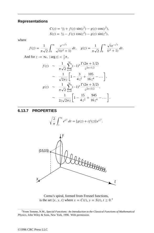
Representations
C(z) = 1/2 + f (z) sin(z2) − g(z) cos(z2),
S(z) = 1/2 − f (z) cos(z2) − g(z) sin(z2),
where
f (z) = 1
π√
2
∫ ∞
0
e−z2t
√t(t2 + 1)
dt, g(z) = 1
π√
2
∫ ∞
0
√te−z2t
(t2 + 1)dt.
And for z → ∞, | arg z| < 12π ,
f (z) ∼ 1
π√
2
∞∑n=0
(−1)n-(2n + 1/2)
z2n+1/2
∼ 1√2πz
[1 − 3
4 z2+ 105
16 z4− . . .
],
g(z) ∼ 1
π√
2
∞∑n=0
(−1)n-(2n + 3/2)
z2n+3/2,
∼ 1
2z√
2πz
[1 − 15
4 z2+ 945
16 z4− . . .
].
6.13.7 PROPERTIES√2
π
∫ ∞
z
eit2dt = [g(z) + if (z)] eiz
2.
x
y
t
(0.5,0.5)
Cornu’s spiral, formed from Fresnel functions,is the set x, y, t where x = C(t), y = S(t), t ≥ 0.2
2From Temme, N.M., Special Functions: An Introduction to the Classical Functions of MathematicalPhysics, John Wiley & Sons, New York, 1996. With permission.
©1996 CRC Press LLC

6.13.8 NUMERICAL VALUES
x erf(x) ex2erfc(x) C(x) S(x)
0.0 0.00000000 1.00000000 0.00000000 0.000000000.2 0.22270259 0.80901952 0.15955138 0.002127450.4 0.42839236 0.67078779 0.31833776 0.016990440.6 0.60385609 0.56780472 0.47256350 0.056918070.8 0.74210096 0.48910059 0.61265370 0.13223984
1.0 0.84270079 0.42758358 0.72170592 0.247558291.2 0.91031398 0.37853742 0.77709532 0.395843131.4 0.95228512 0.33874354 0.75781398 0.552444981.6 0.97634838 0.30595299 0.65866707 0.674427061.8 0.98909050 0.27856010 0.50694827 0.71289443
2.0 0.99532227 0.25539568 0.36819298 0.642118742.2 0.99813715 0.23559296 0.32253723 0.494072862.4 0.99931149 0.21849873 0.40704642 0.365322792.6 0.99976397 0.20361325 0.55998756 0.360738412.8 0.99992499 0.19054888 0.64079292 0.48940140
3.0 0.99997791 0.17900115 0.56080398 0.617213603.2 0.99999397 0.16872810 0.41390216 0.589208473.4 0.99999848 0.15953536 0.39874249 0.441744923.6 0.99999964 0.15126530 0.53845493 0.396487583.8 0.99999992 0.14378884 0.60092662 0.52778933
4.0 0.99999998 0.13699946 0.47431072 0.596126564.2 1.00000000 0.13080849 0.41041217 0.468996974.4 1.00000000 0.12514166 0.54218734 0.419910844.6 1.00000000 0.11993626 0.56533023 0.556858454.8 1.00000000 0.11513908 0.42894668 0.54293254
5.0 1.00000000 0.11070464 0.48787989 0.42121705
©1996 CRC Press LLC
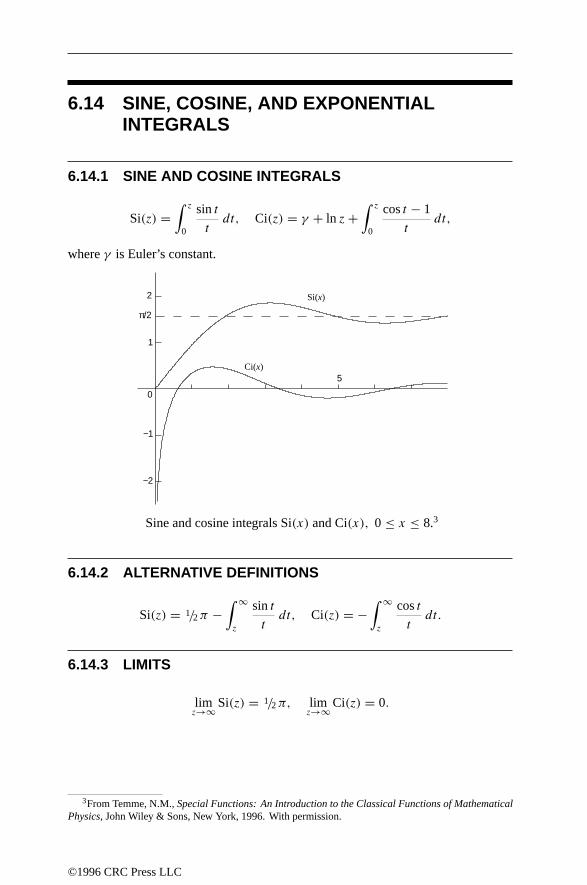
6.14 SINE, COSINE, AND EXPONENTIALINTEGRALS
6.14.1 SINE AND COSINE INTEGRALS
Si(z) =∫ z
0
sin t
tdt, Ci(z) = γ + ln z +
∫ z
0
cos t − 1
tdt,
where γ is Euler’s constant.
π/2
2
1
5
Si(x)
Ci(x)
−1
−2
0
Sine and cosine integrals Si(x) and Ci(x), 0 ≤ x ≤ 8.3
6.14.2 ALTERNATIVE DEFINITIONS
Si(z) = 1/2π −∫ ∞
z
sin t
tdt, Ci(z) = −
∫ ∞
z
cos t
tdt.
6.14.3 LIMITS
limz→∞ Si(z) = 1/2π, lim
z→∞ Ci(z) = 0.
3From Temme, N.M., Special Functions: An Introduction to the Classical Functions of MathematicalPhysics, John Wiley & Sons, New York, 1996. With permission.
©1996 CRC Press LLC

6.14.4 REPRESENTATIONS
Si(z) = −f (z) cos z − g(z) sin z + 1/2π,
Ci(z) = +f (z) sin z − g(z) cos z,
where
f (z) =∫ ∞
0
e−zt
t2 + 1dt, g(z) =
∫ ∞
0
te−zt
t2 + 1dt.
6.14.5 ASYMPTOTIC EXPANSION
For z → ∞, | arg z| < π ,
f (z) ∼ 1
z
∞∑n=0
(−1)n(2n)!
z2n, g(z) ∼ 1
z2
∞∑n=0
(−1)n(2n + 1)!
z2n.
6.14.6 EXPONENTIAL INTEGRALS
En(z) =∫ ∞
1
e−zt
tndt, Re z > 0, n = 1, 2, . . . .
= zn−1e−z
-(n)
∫ ∞
0
e−zt tn−1
t + 1dt, Re z > 0.
6.14.7 SPECIAL CASE
E1(z) =∫ ∞
z
e−t
tdt, | arg z| < π.
This function is also written as − Ei(−z). For real values of z = x,
Ei(x) =∫ x
−∞
et
tdt,
where for x > 0 the integral should be interpreted as a Cauchy principal value integral.
6.14.8 LOGARITHMIC INTEGRAL
li(x) =∫ x
0
dt
ln t= Ei(ln x),
where for x > 1 the integral should be interpreted as a Cauchy principal value integral.
©1996 CRC Press LLC

6.14.9 REPRESENTATIONS
E1(z) = −γ − ln z +∫ z
0
1 − e−t
tdt,
E1
(ze
12πi
)= −γ − ln z − Ci(z) + i [−1/2π + Si(z)] .
6.14.10 NUMERICAL VALUES
Si(x), Ci(x), exE1(x), e−x Ei(x), for 0 ≤ x ≤ 5
x Si(x) Ci(x) exE1(x) e−x Ei(x)
0.0 0.00000000 −∞ ∞ −∞0.2 0.19955609 −1.04220560 1.49334875 −0.672800660.4 0.39646146 −0.37880935 1.04782801 0.070226230.6 0.58812881 −0.02227071 0.82793344 0.422519810.8 0.77209579 0.19827862 0.69124540 0.60542430
1.0 0.94608307 0.33740392 0.59634736 0.697174881.2 1.10804720 0.42045918 0.52593453 0.735544061.4 1.25622673 0.46200659 0.47129255 0.741568231.6 1.38918049 0.47173252 0.42748798 0.727901541.8 1.50581678 0.45681113 0.39149162 0.70249838
2.0 1.60541298 0.42298083 0.36132862 0.670482712.2 1.68762483 0.37507460 0.33565051 0.635191812.4 1.75248550 0.31729162 0.31350201 0.598799302.6 1.80039445 0.25333662 0.29418566 0.562705152.8 1.83209659 0.18648839 0.27717933 0.52778864
3.0 1.84865253 0.11962979 0.26208374 0.494576403.2 1.85140090 0.05525741 0.24858794 0.463356313.4 1.84191398 −0.00451808 0.23644592 0.434255503.6 1.82194812 −0.05797435 0.22546029 0.407294353.8 1.79339035 −0.10377815 0.21547074 0.38242392
4.0 1.75820314 −0.14098170 0.20634565 0.359552014.2 1.71836856 −0.16901316 0.19797586 0.338561154.4 1.67583396 −0.18766029 0.19027005 0.319321014.6 1.63246035 −0.19704708 0.18315120 0.301696804.8 1.58997528 −0.19760361 0.17655390 0.28555486
5.0 1.54993124 −0.19002975 0.17042218 0.27076626
©1996 CRC Press LLC

6.15 POLYLOGARITHMS
Li1(z) =∫ z
0
dt
1 − t= − ln(1 − z), logarithm,
Li2(z) =∫ z
0
Li1(t)
tdt = −
∫ z
0
ln(1 − t)
tdt, dilogarithm,
Lin(z) =∫ z
0
Lin−1(t)
tdt, n ≥ 2, polylogarithm.
6.15.1 ALTERNATIVE DEFINITION
For any complex ν
Liν(z) =∞∑k=1
zk
kν, |z| < 1.
6.15.2 SINGULAR POINTS
z = 1 is a singular point of Liν(z).
6.15.3 INTEGRAL
Liν(z) = z
-(ν)
∫ ∞
0
tν−1
et − zdt, Re ν > 0, z /∈ [1,∞).
6.15.4 GENERATING FUNCTION
∞∑n=2
wn−1 Lin(z) = z
∫ ∞
0
ewt − 1
et − zdt, z /∈ [1,∞).
The series converges for |w| < 1, the integral is defined for Re w < 1.
6.15.5 SPECIAL VALUES
Li2(1) = 1/6π2, Li2(−1) = −1/12π
2, Li2(1/2) = 1/12π2 − 1/2(ln 2)2,
Liν(1) = ζ(ν), Re ν > 1 (Riemann zeta function).
©1996 CRC Press LLC

6.15.6 FUNCTIONAL EQUATIONS FOR DILOGARITHMS
Li2(z) + Li2(1 − z) = 1/6π2 − ln z ln(1 − z),
1/2 Li2(x2) = Li2(x) + Li2(−x),
Li2(−1/x) + Li2(−x) = −1/6π2 − 1/2 (ln x)2,
2Li2(x) + 2Li2(y) + 2Li2(z) =Li2(−xy/z) + Li2(−yz/x) + Li2(−zx/y),
where 1/x + 1/y + 1/z = 1.
6.16 HYPERGEOMETRIC FUNCTIONS
Recall the geometric series and binomial expansion (|z| < 1),
(1 − z)−1 =∞∑n=0
zn, (1 − z)−a =∞∑n=0
(−a
n
)(−z)n =
∞∑n=0
(a)n
n!zn.
where the shifted factorial, (a)n, is defined in Section 1.2.6.
6.16.1 DEFINITION OF THE F−FUNCTION
Gauss hypergeometric function
F (a, b; c; z) =∞∑n=0
(a)n (b)n
(c)n n!zn,
= 1 + ab
cz + a(a + 1) b(b + 1)
c(c + 1) 2!z2 + . . . , |z| < 1,
= F (a, b; c; z) = F (b, a; c; z)
where a, b and c may assume all complex values, c = 0,−1,−2, . . . .
6.16.2 POLYNOMIAL CASE
For m = 0, 1, 2, . . .
F (−m, b; c; z) =m∑n=0
(−m)n (b)n
(c)n n!zn =
m∑n=0
(−1)n(m
n
)(b)n
(c)nzn.
©1996 CRC Press LLC
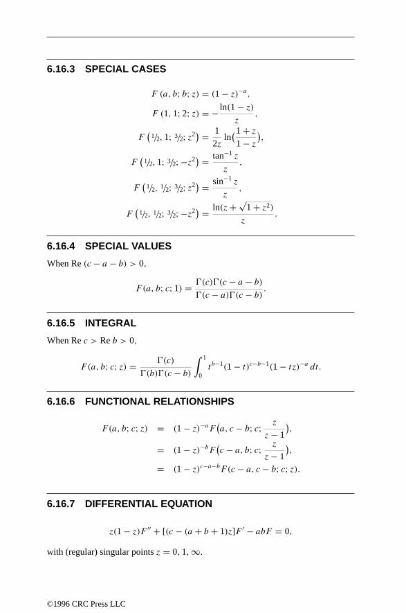
6.16.3 SPECIAL CASES
F (a, b; b; z) = (1 − z)−a,
F (1, 1; 2; z) = − ln(1 − z)
z,
F(
1/2, 1; 3/2; z2) = 1
2zln(1 + z
1 − z
),
F(
1/2, 1; 3/2; −z2) = tan−1 z
z,
F(
1/2, 1/2; 3/2; z2) = sin−1 z
z,
F(
1/2, 1/2; 3/2; −z2) = ln(z + √
1 + z2)
z.
6.16.4 SPECIAL VALUES
When Re (c − a − b) > 0,
F (a, b; c; 1) = -(c)-(c − a − b)
-(c − a)-(c − b).
6.16.5 INTEGRAL
When Re c > Re b > 0,
F (a, b; c; z) = -(c)
-(b)-(c − b)
∫ 1
0tb−1(1 − t)c−b−1(1 − tz)−a dt.
6.16.6 FUNCTIONAL RELATIONSHIPS
F(a, b; c; z) = (1 − z)−aF(a, c − b; c; z
z − 1
),
= (1 − z)−bF(c − a, b; c; z
z − 1
),
= (1 − z)c−a−bF (c − a, c − b; c; z).
6.16.7 DIFFERENTIAL EQUATION
z(1 − z)F ′′ + [(c − (a + b + 1)z]F ′ − abF = 0,
with (regular) singular points z = 0, 1,∞.
©1996 CRC Press LLC

6.16.8 PROPERTIES
d
dzF (a, b; c; z) = ab
cF (a + 1, b + 1; c + 1; z),
dn
dznF (a, b; c; z) = (a)n (b)n
(c)nF (a + n, b + n; c + n; z).
6.16.9 RECURSION FORMULAE
Notation: F is F (a, b; c; z); F(a+), F (a−) are F (a + 1, b; c; z) ,F (a − 1, b; c; z), respectively, etc.
(c − a)F (a−) + (2a − c − az + bz)F + a(z − 1)F (a+) = 0,
c(c − 1)(z − 1)F (c−) + c[c − 1 − (2c − a − b − 1)z]F
+(c − a)(c − b)zF (c+) = 0,
c[a + (b − c)z]F − ac(1 − z)F (a+) + (c − a)(c − b)zF (c+) = 0,
c(1 − z)F − cF (a−) + (c − b)zF (c+) = 0,
(b − a)F + aF(a+) − bF(b+) = 0,
(c − a − b)F + a(1 − z)F (a+) − (c − b)F (b−) = 0,
(c − a − 1)F + aF(a+) − (c − 1)F (c−) = 0,
(b − a)(1 − z)F − (c − a)F (a−) + (c − b)F (b−) = 0,
[a − 1 + (b + 1 − c)z]F + (c − a)F (a−) − (c − 1)(1 − z)F (c−) = 0.
6.17 LEGENDRE FUNCTIONS
6.17.1 DIFFERENTIAL EQUATION
The Legendre differential equation is,
(1 − z2)w′′ − 2zw′ + ν(ν + 1)w = 0.
The solutions Pν(z),Qν(z) can be given in terms of Gaussian hypergeometricfunctions.
©1996 CRC Press LLC

n = 1
n = 3n = 2
n = 0
n = 3n = 1n = 2
1
−1
1
2
−1
−2
3
−3
Legendre functions Pn(x), n = 1, 2, 3 (left) andQn(x), n = 0, 1, 2, 3, on the interval [−1, 1].4
6.17.2 DEFINITION
Pν(z) = F (−ν, ν + 1; 1; 1/2 − 1/2 z) ,
Qν(z) =√π -(ν + 1)
-(ν + 3/2) (2z)ν+1F
(1/2 ν + 1, 1/2 ν + 1/2; ν + 3/2; z−2
).
The Q−function is not defined if ν = −1,−2, . . . .
6.17.3 POLYNOMIAL CASE
Legendre polynomial ν = n = 0, 1, 2, . . . ,
Pn(x) = F (−n, n + 1; 1; 1/2 − 1/2x)
=m∑k=0
(−1)k(2n − 2k)!
2k k! (n − k)! (n − 2k)!xn−2k, m =
12n, if n even,
12 (n − 1), if n odd.
6.17.4 SINGULAR POINTS
Pν(z) has a singular point at z = −1 and is analytic in the remaining part of thecomplex z−plane, with a branch cut along (−∞,−1]. Qν(z) has singular points atz = ±1 and is analytic in the remaining part of the complex z−plane, with a branchcut along (−∞,+1].
4From Temme, N.M., Special Functions: An Introduction to the Classical Functions of MathematicalPhysics, John Wiley & Sons, New York, 1996. With permission.
©1996 CRC Press LLC

6.17.5 RELATIONSHIPS
P−ν−1(z) = Pν(z),
Q−ν−1(z) = Qν(z) − π cot νπPν(z).
6.17.6 SPECIAL CASE
The function Qn(z). We distinguish two cases
Qn(x), x ∈ (−1, 1), Qn(z), z /∈ [−1, 1].
Q0(z) = 1/2 lnz + 1
z − 1, Q1(z) = 1/2 z ln
z + 1
z − 1− 1,
Qn(z) = Pn(z)Q0(z) −n−1∑k=0
(2k + 1)[1 − (−1)n+k]
(n + k + 1)(n − k)Pk(z),
Q0(x) = 1/2 ln1 + x
1 − x, Q1(x) = 1/2 x ln
1 + x
1 − x− 1,
Qn(x) = Pn(x)Q0(x) −n−1∑k=0
(2k + 1)[1 − (−1)n+k]
(n + k + 1)(n − k)Pk(x).
n Pn Qn
0 1 1/2 ln[(1 + x)/(1 − x)]1 x P1(x)Q0(x) − 12 1/2(3x2 − 1) P2(x)Q0(x) − 3/2 x
3 1/2 x(5x2 − 3) P3(x)Q0(x) − 5/2 x2 + 2/3
4 1/8(35x4 − 30x2 + 3) P4(x)Q0(x) − 35/8 x3 + 55/24 x
5 1/8 x(63x4 − 70x2 + 15) P5(x)Q0(x) − 63/8 x4 + 49/8 x
2 − 8/15
Legendre polynomials Pn(x) and functions Qn(x), x ∈ (−1, 1).
6.17.7 RECURSION RELATIONSHIPS
(ν + 1)Pν+1(z) = (2ν + 1)zPν(z) − νPν−1(z),
(2ν + 1)Pν(z) = P ′ν+1(z) − P ′
ν−1(z),
(ν + 1)Pν(z) = P ′ν+1(z) − zP ′
ν(z),
νPν(z) = zP ′ν(z) − P ′
ν−1(z),
(1 − z2)P ′ν(z) = νPν−1(z) − νzPν(z).
The functions Qν(z) satisfy the same relations.
©1996 CRC Press LLC

6.17.8 INTEGRALS
Pν(cosh α) = 2
π
∫ α
0
cosh(ν + 12 )θ√
2 cosh α − 2 cosh θdθ,
= 1
π
∫ α
−α
e−(ν+1/2)θ
√2 cosh α − 2 cosh θ
dθ,
= 1
π
∫ π
0
dψ
(cosh α + sinh α cosψ)ν+1,
= 1
π
∫ π
0(cosh α + sinh α cosψ)ν dψ.
Pν(cosβ) = 2
π
∫ β
0
cos(ν + 12 )θ√
2 cos θ − 2 cosβdθ,
= 1
π
∫ π
0
dψ
(cosβ + i sin β cosψ)ν+1,
= 1
π
∫ π
0(cosβ + i sin β cosψ)ν dψ.
Qν(z) = 2−ν−1∫ 1
−1
(1 − t2)ν
(z − t)ν+1dt, Re ν > −1, | arg z| < π, z /∈ [−1, 1],
=∫ ∞
0
[z +
√z2 − 1 cosh φ
]−ν−1dφ,
=∫ ∞
α
e−(ν+1/2)θ
√2 cosh θ − 2 cosh α
dθ, z = cosh α.
6.17.9 DIFFERENTIAL EQUATION
The associated Legendre differential equation is,
(1 − z2)y ′′ − 2zy ′ +[ν(ν + 1) − µ2
1 − z2
]y = 0.
The solutionsPµν (z),Q
µν (z), the associated Legendre functions, can be given in terms
of Gauss hypergeometric functions. We only consider integer values of µ, ν, andreplace them withm, n, respectively. Then the associated differential equation followsfrom the Legendre differential equation after it has been differentiated m times.
©1996 CRC Press LLC

6.17.10 RELATIONSHIPS BETWEEN THE ASSOCIATED ANDORDINARY LEGENDRE FUNCTIONS
Pmn (z) = (1 − z2)
12m
dm
dzmPn(z), P−m
n (z) = (n − m)!
(n + m)!Pmn (z),
Qmn (z) = (1 − z2)
12m
dm
dzmQn(z), Q−m
n (z) = (n − m)!
(n + m)!Qm
n (z),
P−mn (z) = (1 − z2)−
12m
∫ z
1· · ·
∫ z
1Pn(z) (dz)
m,
Q−mn (z) = (−1)m(1 − z2)−
12m
∫ ∞
z
· · ·∫ ∞
z
Qn(z) (dz)m,
Pm−n−1(z) = Pm
n (z).
6.17.11 ORTHOGONALITY RELATIONSHIP
Let n ≥ m.
∫ 1
−1Pmn (x)P
mk (x) dx =
0, if k = n,
2
2n + 1
(n + m)!
(n − m)!, if k = n.
6.17.12 RECURSION RELATIONSHIPS
Pm+1n (z) + 2mz√
z2 − 1Pmn (z) = (n − m + 1)(n + m)Pm−1
n (z),
(z2 − 1)dPm
n (z)
dz= mzPm
n (z) +√z2 − 1Pm+1
n (z),
(2n + 1)zPmn (z) = (n − m + 1)Pm
n+1(z) + (n + m)Pmn−1(z),
(z2 − 1)dPm
n (z)
dz= (n − m + 1)Pm
n+1(z) − (n + 1)zPmn (z),
Pmn−1(z) − Pm
n+1(z) = −(2n + 1)√z2 − 1Pm−1
n (z).
The functions Qmn (z) satisfy the same relations.
©1996 CRC Press LLC

6.18 BESSEL FUNCTIONS
6.18.1 DIFFERENTIAL EQUATION
The Bessel differential equation,
z2y ′′ + zy ′ + (z2 − ν2)y = 0.
The solutions are denoted with
Jν(z), Yν(z) (the ordinary Bessel functions)
andH(1)
ν (z), H (2)ν (z) (the Hankel functions).
Further solutions are
J−ν(z), Y−ν(z), H(1)−ν (z), H
(2)−ν (z).
When ν is an integer,
J−n(z) = (−1)nJn(z), n = 0, 1, 2, . . . .
J (x)0
1J (x)
1
5 10
−1
0
Y (x)
Y (x)
0
1
Bessel functions J0(x), J1(x), Y0(x), Y1(x), 0 ≤ x ≤ 12.
6.18.2 SINGULAR POINTS
The Bessel differential equation has a regular singularity at z = 0 and an irregularsingularity at z = ∞.
©1996 CRC Press LLC

6.18.3 RELATIONSHIPS
H(1)ν (z) = Jν(z) + iYν(z), H (2)
ν (z) = Jν(z) − iYν(z).
Neumann function: If ν = 0,±1,±2, . . .
Yν(z) = cos νπ Jν(z) − J−ν(z)
sin νπ.
When ν = n (integer) then the limit ν → n should be taken in the right-hand side ofthis equation. Complete solutions to Bessel’s equation may be written as
c1Jν(z) + c2J−ν(z), if ν is not an integer,
c1Jν(z) + c2Yν(z), for any value of ν,
c1H(1)ν (z) + c2H
(2)ν (z), for any value of ν.
6.18.4 SERIES EXPANSIONS
For any complex z,
Jν(z) = (1/2 z)ν
∞∑n=0
(−1)n (1/2 z)2n
-(n + ν + 1) n!.
J0(z) = 1 − (1/2 z)2 + 1
2! 2!(1/2 z)
4 − 1
3! 3!(1/2 z)
6 + . . . ,
J1(z) = 1/2 z
[1 − 1
1! 2!(1/2 z)
2 + 1
2! 3!(1/2 z)
4 − 1
3! 4!(1/2 z)
6 + . . .
],
Yn(z) = 2
πJn(z) ln(1/2 z) − (1/2z)
−n
π
n−1∑k=0
(n − k − 1)!
k!(1/2 z)
2k −
(1/2 z)n
π
∞∑k=0
[ψ(k + 1) + ψ(n + k + 1)](−1)k(1/2 z)
2k
k! (n + k)!,
where ψ is the logarithmic derivative of the gamma function.
6.18.5 RECURRENCE RELATIONSHIPS
Cν−1(z) + Cν+1(z) = 2ν
zCν(z),
Cν−1(z) − Cν+1(z) = 2C ′ν(z),
C ′ν(z) = Cν−1(z) − ν
zCν(z),
C ′ν(z) = −Cν+1(z) + ν
zCν(z),
where Cν(z) denotes one of the functions Jν(z), Yν(z), H (1)ν (z), H (2)
ν (z).
©1996 CRC Press LLC

6.18.6 BEHAVIOR AS z → 0
Let Re ν > 0.
Jν(z) ∼ ( 12z)
ν
-(ν + 1), Yν(z) ∼ − 1
π-(ν)
(2
z
)ν,
H (1)ν (z) ∼ 1
πi-(ν)
(2
z
)ν, H (2)
ν (z) ∼ − 1
πi-(ν)
(2
z
)ν.
The same relations hold as Re ν → ∞, with z fixed.
6.18.7 INTEGRALS
Let Re z > 0 and ν be any complex number.
Jν(z) = 1
π
∫ π
0cos(νθ − z sin θ) dθ − sin νπ
π
∫ ∞
0e−νt − z sinh t dt,
Yν(z) = 1
π
∫ π
0sin(z sin θ − νθ) dθ −
∫ ∞
0
(eνt + e−νt cos νπ
)e−z sinh t dt.
When ν = n (integer), the second integral in the first relation disappears.
6.18.8 FOURIER EXPANSION
For any complex z,
e−iz sin t =∞∑
n=−∞e−intJn(z),
with Parseval relation∞∑
n=−∞J 2n (z) = 1.
6.18.9 AUXILIARY FUNCTIONS
Let χ = z − (1/2 ν + 1/4)π and define
P(ν, z) =√πz/2[ Jν(z) cosχ + Yν(z) sin χ],
Q(ν, z) =√πz/2[−Jν(z) sin χ + Yν(z) cosχ].
©1996 CRC Press LLC

6.18.10 INVERSE RELATIONSHIPS
Jν(z) =√
2/(πz) [P(ν, z) cosχ − Q(ν, z) sin χ],
Yν(z) =√
2/(πz) [P(ν, z) sin χ + Q(ν, z) cosχ]
For the Hankel functions,
H(1)ν (z) =
√2/(πz) [P(ν, z) + iQ(ν, z)]eiχ ,
H (2)ν (z) =
√2/(πz) [P(ν, z) − iQ(ν, z)]e−iχ .
The functions P(ν, z),Q(ν, z) are the slowly varying components in the asymptoticexpansions of the oscillatory Bessel and Hankel functions.
6.18.11 ASYMPTOTIC EXPANSIONS
Let (α, n) be defined by
(α, n) = 2−2n
n!(4α2 − 1)(4α2 − 32) · · · [4α2 − (2n − 1)2],
= -( 12 + α + n)
n!-( 12 + α − n)
, n = 0, 1, 2, . . . ,
= (−1)n cos(πα)
πn!-(1/2 + α + n)-(1/2 − α + n),
with recursion
(α, n + 1) = − (n + 12 )
2 − α2
n + 1(α, n), n = 1, 2, 3, . . . , (α, 0) = 1.
Then, for z → ∞,
P(ν, z) ∼∞∑n=0
(−1)n(ν, 2n)
(2z)2n, Q(ν, z) ∼
∞∑n=0
(−1)n(ν, 2n + 1)
(2z)2n+1.
With µ = 4ν2,
P(ν, z) ∼ 1 − (µ − 1)(µ − 9)
2! (8z)2+ (µ − 1)(µ − 9)(µ − 25)(µ − 49)
4! (8z)4− . . . ,
Q(ν, z) ∼ µ − 1
8z− (µ − 1)(µ − 9)(µ − 25)
3! (8z)3+ . . . .
For large positive values of x,
Jν(x) =√
2/(πx)[cos(x − 1/2 νπ − 1/4π) + O(x−1)
],
Yν(x) =√
2/(πx)[sin(x − 1/2 νπ − 1/4π) + O(x−1)
].
©1996 CRC Press LLC

6.18.12 ZEROS OF BESSEL FUNCTIONS
For ν ≥ 0, the zeros jν,k, yν,k of Jν(x), Yν(x) can be arranged as sequences
0 < jν,1 < jν,2 < · · · < jν,n < · · · , limn→∞ jν,n = ∞,
0 < yν,1 < yν,2 < · · · < yν,n < · · · , limn→∞ yν,n = ∞.
Between two consecutive positive zeros of Jν(x), there is exactly one zero of Jν+1(x).Conversely, between two consecutive positive zeros of Jν+1(x), there is exactly onezero of Jν(x). The same holds for the zeros of Yν(z). Moreover, between each pair ofconsecutive positive zeros of Jν(x), there is exactly one zero of Yν(x), and conversely.
6.18.13 ASYMPTOTICS OF THE ZEROS
When ν is fixed, s ν, and µ = 4ν2,
jν,s ∼ α − µ − 1
8α
[1 − 4(7µ2 − 31)
3(8α)2− 32(83µ2 − 982µ + 3779)
15(8α)4+ . . .
]
where α = (s + 12ν − 1
4 )π ; yν,s has the same asymptotic expansion with α =(s + 1
2ν − 34 )π .
n j0,n j1,n y0,n y1,n
1 2.40483 3.83171 0.89358 2.197142 5.52008 7.01559 3.95768 5.429683 8.65373 10.17347 7.08605 8.596014 11.79153 13.32369 10.22235 11.749155 14.93092 16.47063 13.36110 14.897446 18.07106 19.61586 16.50092 18.043407 21.21164 22.76008 19.64131 21.18807
Positive zeros jν,n, yν,n of Bessel functions Jν(x), Yν(x), ν = 0, 1.
©1996 CRC Press LLC

6.18.14 HALF ORDER BESSEL FUNCTIONS
For integer values of n, let
jn(z) =√π/(2z) Jn+ 1
2(z), yn(z) =
√π/(2z) Yn+ 1
2(z).
Then
j0(z) = y−1(z) = sin z
z, y0(z) = −j−1(z) = −cos z
z,
and, for n = 0, 1, 2, . . . ,
jn(z) = (−z)n[
1
z
d
dz
]n sin z
z, yn(z) = −(−z)n
[1
z
d
dz
]n cos z
z.
Recursion relationshipsThe functions jn(z), yn(z) both satisfy
z[fn−1(z) + fn+1(z)] = (2n + 1)fn(z),
nfn−1(z) − (n + 1)fn+1(z) = (2n + 1)f ′n(z).
Differential equation
z2f ′′ + 2zf ′ + [z2 − n(n + 1)]f = 0.
6.18.15 MODIFIED BESSEL FUNCTIONS
Differential equation
z2y ′′ + zy ′ − (z2 + ν2)y = 0.
With solutions Iν(z),Kν(z),
Iν(z) =( z
2
)ν ∞∑n=0
(z/2)2n
-(n + ν + 1) n!,
Kν(z) = π
2
I−ν(z) − Iν(z)
sin νπ,
where the right-hand side should be determined by a limiting process when ν assumesinteger values. When n = 0, 1, 2, . . . ,
Kn(z) =(−1)n+1In(z) lnz
2+ 1
2
(2
z
)n n−1∑k=0
(n − k − 1)!
k!
(−z2
4
)k
+ (−1)n
2
( z2
)n ∞∑k=0
[ψ(k + 1) + ψ(n + k + 1)](z/2)2k
k! (n + k)!.
©1996 CRC Press LLC
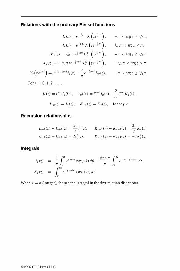
Relations with the ordinary Bessel functions
Iν(z) = e− 12 νπiJν
(ze
12πi
), −π < arg z ≤ 1/2π,
Iν(z) = e32 νπiJν
(ze− 3
2πi), 1/2π < arg z ≤ π,
Kν(z) = 1/2πie12 νπiH (1)
ν
(ze
12πi
), −π < arg z ≤ 1/2π,
Kν(z) = −1/2πie− 1
2 νπiH (2)ν
(ze− 1
2πi), −1/2π < arg z ≤ π,
Yν
(ze
12πi
)= e
12 (ν+1)πiIν(z) − 2
πe− 1
2 νπiKν(z), −π < arg z ≤ 1/2π.
For n = 0, 1, 2, . . . ,
In(z) = i−nJn(iz), Yn(iz) = in+1In(z) − 2
πi−n Kn(z),
I−n(z) = In(z), K−ν(z) = Kν(z), for any ν.
Recursion relationships
Iν−1(z) − Iν+1(z) = 2ν
zIν(z), Kν+1(z) − Kν−1(z) = 2ν
zKν(z)
Iν−1(z) + Iν+1(z) = 2I ′ν(z), Kν−1(z) + Kν+1(z) = −2K ′
ν(z).
Integrals
Iν(z) = 1
π
∫ π
0ez cos θ cos(νθ) dθ − sin νπ
π
∫ ∞
0e−νt − z cosh t dt,
Kν(z) =∫ ∞
0e−z cosh t cosh(νt) dt.
When ν = n (integer), the second integral in the first relation disappears.
©1996 CRC Press LLC

6.18.16 NUMERICAL VALUES
x J0(x) J1(x) Y0(x) Y1(x)
0.0 1.00000000 0.00000000 −∞ −∞0.2 0.99002497 0.09950083 −1.08110532 −3.323824990.4 0.96039823 0.19602658 −0.60602457 −1.780872040.6 0.91200486 0.28670099 −0.30850987 −1.260391350.8 0.84628735 0.36884205 −0.08680228 −0.97814418
1.0 0.76519769 0.44005059 0.08825696 −0.781212821.2 0.67113274 0.49828906 0.22808350 −0.621136381.4 0.56685512 0.54194771 0.33789513 −0.479146971.6 0.45540217 0.56989594 0.42042690 −0.347578011.8 0.33998641 0.58151695 0.47743171 −0.22366487
2.0 0.22389078 0.57672481 0.51037567 −0.107032432.2 0.11036227 0.55596305 0.52078429 0.001487792.4 0.00250768 0.52018527 0.51041475 0.100488942.6 −0.09680495 0.47081827 0.48133059 0.188363542.8 −0.18503603 0.40970925 0.43591599 0.26354539
3.0 −0.26005195 0.33905896 0.37685001 0.324674423.2 −0.32018817 0.26134325 0.30705325 0.370711343.4 −0.36429560 0.17922585 0.22961534 0.401015293.6 −0.39176898 0.09546555 0.14771001 0.415391763.8 −0.40255641 0.01282100 0.06450325 0.41411469
4.0 −0.39714981 −0.06604333 −0.01694074 0.397925714.2 −0.37655705 −0.13864694 −0.09375120 0.368012814.4 −0.34225679 −0.20277552 −0.16333646 0.325970674.6 −0.29613782 −0.25655284 −0.22345995 0.273745244.8 −0.24042533 −0.29849986 −0.27230379 0.21356517
5.0 −0.17759677 −0.32757914 −0.30851763 0.14786314
©1996 CRC Press LLC

x e−xI0(x) e−xI1(x) exK0(x) exK1(x)
0.0 1.00000000 0.00000000 ∞ ∞0.2 0.82693855 0.08228312 2.14075732 5.833386030.4 0.69740217 0.13676322 1.66268209 3.258673880.6 0.59932720 0.17216442 1.41673762 2.373920040.8 0.52414894 0.19449869 1.25820312 1.91793030
1.0 0.46575961 0.20791042 1.14446308 1.636153491.2 0.41978208 0.21525686 1.05748453 1.442897551.4 0.38306252 0.21850759 0.98807000 1.301053741.6 0.35331500 0.21901949 0.93094598 1.191867571.8 0.32887195 0.21772628 0.88283353 1.10480537
2.0 0.30850832 0.21526929 0.84156822 1.033476852.2 0.29131733 0.21208773 0.80565398 0.973770172.4 0.27662232 0.20848109 0.77401814 0.922913672.6 0.26391400 0.20465225 0.74586824 0.878967282.8 0.25280553 0.20073741 0.72060413 0.84053006
3.0 0.24300035 0.19682671 0.69776160 0.806563483.2 0.23426883 0.19297862 0.67697511 0.776280283.4 0.22643140 0.18922985 0.65795227 0.749072063.6 0.21934622 0.18560225 0.64045596 0.724460663.8 0.21290013 0.18210758 0.62429158 0.70206469
4.0 0.20700192 0.17875084 0.60929767 0.681575954.2 0.20157738 0.17553253 0.59533899 0.662742414.4 0.19656556 0.17245023 0.58230127 0.645355874.6 0.19191592 0.16949973 0.57008720 0.629242644.8 0.18758620 0.16667571 0.55861332 0.61425660
5.0 0.18354081 0.16397227 0.54780756 0.60027386
6.19 ELLIPTIC INTEGRALS
6.19.1 DEFINITIONS
Any integral of the type∫R(x, y) dx, where R(x, y) is a rational function of x and
y, with
y2 = a0x4 + a1x
3 + a2x2 + a3x + a4, |a0| + |a1| > 0,
©1996 CRC Press LLC

a polynomial of the third or fourth degree in x, is called an elliptic integral.
F(φ, k) =∫ φ
0
dθ√1 − k2 sin2 θ
,
=∫ x
0
dt√(1 − t2)(1 − k2t2)
, x = sin φ, k2 < 1.
E(φ, k) =∫ φ
0
√1 − k2 sin2 θ dθ,
=∫ x
0
√1 − k2t2
√1 − t2
dt, x = sin φ, k2 < 1.
B(n;φ, k) =∫ φ
0
1
1 + n sin2 θ
dθ√1 − k2 sin2 θ
,
=∫ x
0
1
1 + nt2
dt√(1 − t2)(1 − k2t2)
, x = sin φ, k2 < 1.
If n > 1, this integral should be interpreted as a Cauchy principal value integral.
6.19.2 COMPLETE ELLIPTIC INTEGRAL OF THE FIRST ANDSECOND KIND
In terms of the Gauss hypergeometric function,
K = F(1/2π, k) = 1/2πF(
1/2, 1/2; 1; k2),
E = E(1/2π, k) = 1/2πF(−1/2, 1/2; 1; k2
).
6.19.3 COMPLEMENTARY INTEGRALS
In these expressions, primes do not mean derivatives.
K ′ = F(k′, 1/2π
), E′ = E
(k′, 1/2π
), k′ =
√1 − k2.
k is called the modulus, k′ is called the complementary modulus.The Legendre relation is,
K E′ + EK ′ − K K ′ = 1/2π.
©1996 CRC Press LLC

α K E
0 1.5707963268 1.57079632685 1.5737921309 1.5678090740
10 1.5828428043 1.558887196615 1.5981420021 1.544150496920 1.6200258991 1.5237992053
25 1.6489952185 1.498114928430 1.6857503548 1.467462209335 1.7312451757 1.432290969340 1.7867691349 1.393140248545 1.8540746773 1.3506438810
50 1.9355810960 1.305539094355 2.0347153122 1.258679624860 2.1565156475 1.211056027665 2.3087867982 1.163827964570 2.5045500790 1.1183777380
75 2.7680631454 1.076405113180 3.1533852519 1.040114395785 3.8317419998 1.012663506290 ∞ 1.0000000000
0.5 1.0
1.0
2.0K
E
π/2
0.5
0k →
The complete elliptic integrals E and K , 0 ≤ k ≤ 1.5
5From Temme, N.M., Special Functions: An Introduction to the Classical Functions of MathematicalPhysics, John Wiley & Sons, New York, 1996. With permission.
©1996 CRC Press LLC

6.19.4 EXTENSION OF THE RANGE OF φ
F(π, k) = 2K, E(π, k) = 2E,
and, for m = 0, 1, 2, . . . ,
F (φ + mπ, k) = mF(π, k) + F(φ, k) = 2mK + F(φ, k),
E(φ + mπ, k) = mE(π, k) + E(φ, k) = 2mE + E(φ, k).
6.19.5 DEFINITION
Elliptic functions are the inverses of elliptic integrals. If u = F(φ, k) (the ellipticintegral of the first kind), that is,
u =∫ φ
0
dθ√1 − k2 sin2 θ
=∫ x
0
dt√(1 − t2)(1 − k2t2)
, x = sin φ, k2 < 1,
then x(u), the inverse function, is an elliptic function. The inverse relation is writtenas
x = sin φ = sn(u, k).
φ is called the amplitude of u and denoted by am u. Two other functions are definedby
cn(u, k) = cosφ, dn(u, k) =√
1 − k2 sin2 φ =√
1 − k2 sn2(u, k) = !(φ).
Analogous definitions of these functions are
u =∫ cn(u,k)
1
dt√(1 − t2)(k′2 + k2t2)
,
u =∫ dn(u,k)
1
dt√(1 − t2)(t2 − k′2)
.
6.19.6 PROPERTIES
sn2(u, k) + cn2(u, k) = 1,
dn2(u, k) + k2 sn2(u, k) = 1,
dn2(u, k) − k2 cn2(u, k) = 1 − k2 = k′2.
©1996 CRC Press LLC

6.19.7 PERIODS OF THE ELLIPTIC FUNCTIONS
The elliptic functions are doubly periodic functions with respect to the variable u.The periods of
sn(u, k) are 4K and 2iK ′,cn(u, k) are 4K and 2K + 2iK ′,dn(u, k) are 2K and 4iK ′.
6.19.8 SERIES EXPANSIONS
sn(u, k) = u − (1 + k2)u3
3!+ (1 + 14k2 + k4)
u5
5!
−(1 + 135k2 + 135k4 + k6)u7
7!+ . . . ,
cn(u, k) = 1 − u2
2!+ (1 + 4k2)
u4
4!
−(1 + 44k2 + 16k4)u6
6!+ . . . ,
dn(u, k) = 1 − k2 u2
2!+ k2(4 + k2)
u4
4!
−k2(16 + 44k2 + k4)u6
6!+ . . . .
Let the nome q be defined by q = e−πK/K ′and v = πu/(2K). Then
sn(u, k) = 2π
kK
∞∑n=0
qn+12
1 − q2n+1sin[(2n + 1)v],
cn(u, k) = 2π
kK
∞∑n=0
qn+12
1 + q2n+1cos[(2n + 1)v],
dn(u, k) = π
2K+ 2π
K
∞∑n=1
qn
1 + q2ncos(2nv).
©1996 CRC Press LLC

6.20 CLEBSCH–GORDAN COEFFICIENTS
(j1 j2m1 m2
j
m
)= δm,m1+m2
√(j1 + j2 − j)!(j + j1 − j2)!(j + j2 − j1)!(2j + 1)
(j + j1 + j2 + 1)!
×∑k
(−1)k√(j1 + m1)!(j1 − m1)!(j2 + m2)!(j2 − m2)!(j + m)!(j − m)!
k!(j1 + j2 − j − k)!(j1 − m1 − k)!(j2 + m2 − k)!(j − j2 + m1 + k)!(j − j1 − m2 + k)!.
Conditions:
• Each of j1, j2, j,m1,m2,m may be an integer, or half an integer. Additionally:j > 0, j1 > 0, j2 > 0 and j + j1 + j2 is an integer.
• j1 + j2 − j ≥ 0.
• j1 − j2 + j ≥ 0.
• −j1 + j2 + j ≥ 0.
• |m1| ≤ j1, |m2| ≤ j2, |m| ≤ j.
•(j1 j2
m1 m2
j
m
)= 0 if m1 + m2 = m.
Special values:
•(j1 0m1 0
j
m
)= δj1,j δm1,m.
•(j1 j2
0 0j
0
)= 0 when j1 + j2 + j is an odd integer.
•(j1 j1
m1 m1
j
m
)= 0 when 2j1 + j is an odd integer.
Symmetry relations: all of the following are equal to
(j1 j2
m1 m2
j
m
):
©1996 CRC Press LLC

•(
j2 j1
−m2 −m1
j
−m
),
• (−1)j1+j2−j
(j2 j1
m1 m2
j
m
),
• (−1)j1+j2−j
(j1 j2
−m1 −m2
j
−m
),
•√
2j+12j1+1 (−1)j2+m2
(j j2
−m m2
j1
−m1
),
•√
2j+12j1+1 (−1)j1−m1+j−m
(j j2
m −m2
j1
m1
),
•√
2j+12j1+1 (−1)j−m+j1−m1
(j2 j
m2 −m
j1
−m1
),
•√
2j+12j2+1 (−1)j1−m1
(j1 j
m1 −m
j2
−m2
),
•√
2j+12j2+1 (−1)j1−m1
(j j1
m −m1
j2
m2
).
By use of the symmetry relations, Clebsch–Gordan coefficients may be put inthe standard form j1 ≤ j2 ≤ j and m ≥ 0.
m2 m j1 j
(j1 j2
m1 m2
j
m
)j2 = 1/2
−1/2 0 1/2 1 0.707105√
22
1/2 0 1/2 1 0.707105√
22
0 1/2 1/2 1 0.866025√
32
1/2 1/2 1/2 1 0.866025√
32
1/2 1 1/2 1 1.000000 1
©1996 CRC Press LLC

m2 m j1 j
(j1 j2
m1 m2
j
m
)j2 = 1
−1 0 1 1 0.707105√
22
1 0 1 1 −0.707105 −√
22
−1/2 1/2 1 1 0.750000 3/4
0 1/2 1 1 0.353553√
24
1/2 1/2 1 1 −0.353553 −√
24
1 1/2 1 1 −0.750000 −3/4
0 1 1 1 0.707105√
22
1 1 1 1 −0.707105 −√
22
−1/2 0 1/2 3/2 0.707105√
22
0 0 1/2 3/2 0.866025√
32
1/2 0 1/2 3/2 0.707105√
22
0 1/2 1/2 3/2 0.816496√
63
1 1/2 1/2 3/2 0.577349√
33
1/2 1 1/2 3/2 0.912873√
306
1 1 1/2 3/2 0.790570√
104
1 3/2 1/2 3/2 1.000000 1
−1 0 1 2 0.408249√
66
0 0 1 2 0.816496√
63
1 0 1 2 0.408249√
66
−1/2 1/2 1 2 0.559018√
54
0 1/2 1 2 0.790570√
104
1/2 1/2 1 2 0.790570√
104
1 1/2 1 2 0.559018√
54
0 1 1 2 0.707105√
22
1 1 1 2 0.707105√
22
1/2 3/2 1 2 0.853916√
10512
1 3/2 1 2 0.853916√
10512
1 2 1 2 1.000000 1
©1996 CRC Press LLC

6.21 INTEGRAL TRANSFORMS: PRELIMINARIES
• I = (a, b) is an interval, where −∞ ≤ a < b ≤ ∞.
• L1(I ) is the set of all absolutely integrable functions on I . In particular, L1(R)
is the set of all absolutely integrable functions on the real line R.
• L2(I ) is the set of all square integrable functions on I .
• If f is integrable over every finite closed subinterval of I , but not necessarilyon I itself, we say that f is locally integrable on I . For example, the functionf (x) = 1/x is not integrable on the interval I = (0, 1), yet it is locally integrableon it.
• A function f (x), defined on a closed interval [a, b], is said to be of boundedvariation if there is a positive numberM so that, for any partition a = x0 < x1 <
x2 < · · · , xn = b, the following relation holds:n∑
i=1
|f (xi) − f (xi−1)| ≤ M.
• If f has a derivative f ′ at every point of [a, b], then by the mean value theorem,for any a ≤ x < y ≤ b, we have f (x) − f (y) = f ′(z)(x − y), for somex < z < y. If f ′ is bounded, then f is of bounded variation.
• The left limit of a function f (x) at a point t (if it exists) will be denoted bylimx→t− f (x) = f (t−), and likewise the right limit at t will be denoted bylimx→t+ f (x) = f (t+).
6.22 FOURIER INTEGRAL TRANSFORM
The origin of the Fourier integral transformation can be traced to Fourier’s celebratedwork on the Analytical Theory of Heat, which appeared in 1822. Fourier’s majorfinding was to show that an “arbitrary” function defined on a finite interval couldbe expanded in a trigonometric series (series of sinusoidal functions). In an attemptto extend his results to functions defined on the infinite interval (0,∞), Fourierintroduced what is now known as the Fourier integral transform.
The Fourier integral transform of a function f (t) is defined by
F(f )(ω) = f (ω) = F(ω) = 1√2π
∫ ∞
−∞f (t)eitω dt,
(6.22.1)
whenever the integral exists.There is no universal agreement on the definition of the Fourier integral transform.
Some authors take the kernel of the transformation as e−itω, so that the kernel of the
©1996 CRC Press LLC

inverse transformation is eitω. In either case, if we define the Fourier transform as
f (ω) = a
∫ ∞
−∞f (t)e±itω dt,
then its inverse is f (t) = b
∫ ∞
−∞f (ω)e∓itω dω, (6.22.2)
for some constants a and b, with ab = 1/2π . Again there is no agreement on thechoice of the constants; sometimes one of them is taken as 1 so that the other is1/(2π). For the sake of symmetry, we choose a = b = 1/
√2π . The functions f
and f are called a Fourier transform pair.Another definition that is popular in the engineering literature is the one in which
the kernel of the transform is taken as e2πitω (or e−2πitω) so that the kernel of theinverse transform is e−2πitω (or e2πitω). The main advantage of this definition is thatthe constants a and b disappear and the Fourier transform pair becomes
f (ω) =∫ ∞
−∞f (t)e±2πitω dt and f (t) =
∫ ∞
−∞f (ω)e∓2πitω dω.
(6.22.3)
The Fourier cosine and sine coefficients of f (t) are defined by
a(ω) = 1
π
∫ ∞
−∞f (t) cosωt dt and b(ω) = 1
π
∫ ∞
−∞f (t) sinωt dt.
(6.22.4)
The Fourier cosine and sine coefficients are related to the Fourier cosine and sineintegral transforms. For example, if f is even, then a(ω) = √
2/πFc(ω) and, if f isodd, b(ω) = √
2/πFs(ω) (see Section 6.22.7).Two other integrals related to the Fourier integral transform are Fourier’s repeated
integral and the allied integral. Fourier’s repeated integral, S(f, t), of f (t) is definedby
S(f, t) =∫ ∞
0(a(ω) cos tω + b(ω) sin tω) dω,
= 1
π
∫ ∞
0dω
∫ ∞
−∞f (x) cosω(t − x) dx.
(6.22.5)
The allied Fourier integral, S(f, t), of f is defined by
S(f, t) =∫ ∞
0(b(ω) cos tω − a(ω) sin tω) dω,
= 1
π
∫ ∞
0dω
∫ ∞
−∞f (x) sinω(x − t)dx.
(6.22.6)
6.22.1 EXISTENCE
For the Fourier integral transform to exist, it is sufficient thatf be absolutely integrableon (−∞,∞), i.e., f ∈ L1(R).
©1996 CRC Press LLC

THEOREM 6.22.1 (Riemann–Lebesgue lemma)
If f ∈ L1(R), then its Fourier transform f (ω) is defined everywhere, uniformlycontinuous, and tends to zero as ω → ±∞.
The uniform continuity follows from the relationship
∣∣f (ω + h) − f (ω)∣∣ ≤ 1√
2π
∫ ∞
−∞|f (t)| ∣∣eiht − 1
∣∣ dt,and the tendency toward zero at ±∞ is a consequence of the Riemann–Lebesguelemma.
THEOREM 6.22.2 (Riemann–Lebesgue lemma)
Let f ∈ L1(I ), where I = (a, b) is finite or infinite and let ω be a real variable. Leta ≤ a′ < b′ ≤ b and fω(λ, a′, b′) = ∫ b′
a′ f (t)eiλωt dt . Then limω→±∞ fω(λ, a
′, b′) =0, and the convergence is uniform in a′ and b′. In particular, limω→±∞
∫ ∞−∞ f (t)eiωt
dt = 0.
6.22.2 PROPERTIES
1. Linearity: The Fourier transform is linear,
F [af (t) + bg(t)] (ω) = aF [f (t)] (ω) + bF [g(t)] (ω) = af (ω) + bg(ω),
where a and b are complex numbers.
2. Translation: F [f (t − b)] (ω) = eibωf (ω).
3. Dilation (scaling): F [f (at)] (ω) = 1af ( ω
a), a = 0.
4. Translation and dilation:
F [f (at − b)] (ω) = 1
aeibω/af
(ωa
), a > 0.
5. Complex conjugation: F [f (t)
](ω) = f (−ω).
6. Modulation: F [eiatf (t)
](ω) = f (ω + a), and
F [eiatf (bt)
](ω) = 1
bf
(ω + a
b
), b > 0. (6.22.7)
7. Differentiation: If f (k) ∈ L1(R), for k = 0, 1, 2, · · · , n andlim|t |→∞ f (k)(t) = 0 for k = 0, 1, 2, · · · , n − 1, then
F [f (n)(t)
](ω) = (−iω)nf (ω). (6.22.8)
8. Integration: Let f ∈ L1(R), and define g(x) = ∫ x
−∞ f (t) dt . If g ∈ L1(R),
then g(ω) = −f (ω)/(iω).
©1996 CRC Press LLC

9. Multiplication by polynomials: If tnf (t) ∈ L1(R), then
F [tkf (t)
](ω) = 1
(i)kf (k)(ω), (6.22.9)
and hence,
F[(
n∑k=0
aktk
)f (t)
](ω) =
n∑k=0
ak
(i)kf (k)(ω).
(6.22.10)
10. Convolution: The convolution operation, H, associated with the Fourier trans-form is defined as
h(t) = (f H g)(t) = 1√2π
∫ ∞
−∞f (x)g(t − x)dx,
where f and g are defined over the whole real line.
THEOREM 6.22.3
If f and g belong to L1(R), then so does h. Moreover, h(ω) = f (ω)g(ω). If fand g belong to L1(R), then (f H g)(ω) = (fg)(ω).
11. Parseval’s relation: If F and G are the Fourier transforms of f and g respec-tively, then Parseval’s relation is∫ ∞
−∞F(ω)G(ω) dω =
∫ ∞
−∞f (t)g(−t) dt. (6.22.11)
ReplacingGby G ( so thatg(−t) is replaced by g(t)) results in a more convenientform of Parseval’s relation∫ ∞
−∞F(ω)G(ω) dω =
∫ ∞
−∞f (t)g(t) dt. (6.22.12)
In particular, for f = g,∫ ∞
−∞|F(ω)|2 dω =
∫ ∞
−∞|f (t)|2 dt. (6.22.13)
6.22.3 INVERSION FORMULA
Many of the theorems on the inversion of the Fourier transform are based on Dini’scondition which can be stated as follows:
If f ∈ L1(R), then a necessary and sufficient condition that
S(f, x) = limλ→∞
1
π
∫ ∞
−∞f (t)
sin λ(x − t)
(x − t)dt = a
©1996 CRC Press LLC

is that
limλ→∞
∫ δ
0(f (x + y) + f (x − y) − 2a)
sin λy
ydy = 0,
(6.22.14)
for any fixed δ > 0.By the Riemann–Lebesgue lemma, this condition is satisfied if∫ δ
0
∣∣∣∣f (x + y) + f (x − y) − 2a
y
∣∣∣∣ dy < ∞, (6.22.15)
for some δ > 0. In particular, condition (6.22.15) holds for a = f (x), if f isdifferentiable atx, and fora = [f (x + 0) + f (x − 0)] /2, iff is of bounded variationin a neighborhood of x.
THEOREM 6.22.4 (Inversion theorem)
Let f be a locally integrable function, of bounded variation in a neighborhood of thepoint x. If f satisfies either one of the following conditions:
1. f (t) ∈ L1(R), or
2. f (t)/(1 + |t |) ∈ L1(R), and the integral∫ ∞−∞ f (t)eiωt dt converges uniformly
on every finite interval of ω,
then1√2π
∫ ∞
−∞f (ω)e−ixω dω = lim
λ→∞1√2π
∫ λ
−λ
f (ω)e−ixω dω
is equal to [f (x + 0) + f (x − 0)] /2 whenever the expression has meaning, to f (x)whenever f (x) is continuous at x, and to f (x) almost everywhere. If f is continuousand of bounded variation in the interval (a, b), then the convergence is uniform inany interval interior to (a, b).
6.22.4 POISSON SUMMATION FORMULA
The Poisson summation formula may be written in the form
1√2π
∞∑k=−∞
f
(t + kπ
σ
)= σ
π
∞∑k=−∞
f (2kσ)e−2iktσ , σ > 0,(6.22.16)
provided that the two series converge. A sufficient condition for the validity ofEquation (6.22.16) is that f = O(1 + |t |)−α as |t | → ∞, and f = O
((1 + |ω|)−α
)as |ω| → ∞ for some α > 1.
Another version of the Poisson summation formula is∞∑
k=−∞f (ω + kσ)g(ω + kσ) = 1
σ
∞∑k=−∞
(∫ ∞
−∞f (t)g
(t − 2πk
σ
)dt
)e2πikω/σ .
(6.22.17)
©1996 CRC Press LLC

6.22.5 SHANNON’S SAMPLING THEOREM
If f is a function band-limited to [−σ, σ ], i.e.,
f (t) = 1√2π
∫ σ
−σ
F (ω)eitω dω,
with F ∈ L2(−σ, σ ), then it can be reconstructed from its sample values at the pointstk = (kπ)/σ, k = 0,±1,±2, · · · , via the formula
f (t) =∞∑
k=−∞f (tk)
sin σ(t − tk)
σ (t − tk), (6.22.18)
with the series absolutely and uniformly convergent on compact sets.The series on the right-hand side of Equation (6.22.18) can be written as
sin σ t∞∑
k=−∞f (tk)
(−1)k
(σ t − kπ),which is a special case of a Cardinal series (these series
have the form sin σ t∞∑
k=−∞Ck
(−1)k
(σ t − kπ)).
6.22.6 UNCERTAINTY PRINCIPLE
Let T and W be two real numbers defined by
T 2 = 1
E
∫ ∞
−∞t2|f (t)|2 dt and W 2 = 1
E
∫ ∞
−∞ω2|f (ω)|2 dω,
where
E =∫ ∞
−∞|f (t)|2 dt =
∫ ∞
−∞|f (ω)|2 dω.
Assuming that f is differentiable and lim|t |→∞
tf 2(t) = 0, then 2TW ≥ 1, or
(∫ ∞
−∞t2|f (t)|2 dt
)1/2 (∫ ∞
−∞ω2|f (ω)|2 dω
)1/2
≥ 1
2
∫ ∞
−∞|f (t)|2 dt.
This means that f and f cannot both be very small. Another related property of theFourier transform is that, if either one of the functions f or f vanishes outside somefinite interval, then the other one must trail on to infinity. In other words, they cannot both vanish outside any finite interval.
6.22.7 FOURIER SINE AND COSINE TRANSFORMS
The Fourier cosine transform, Fc(ω), and the Fourier sine transform, Fs(ω), of f (t)are defined as
Fc(ω) =√
2
π
∫ ∞
0f (t) cosωt dt and Fs(ω) =
√2
π
∫ ∞
0f (t) sinωt dt.
(6.22.19)
©1996 CRC Press LLC

The inverse transforms have the same functional form:
f (t) =√
2
π
∫ ∞
0Fc(ω) cosωt dω =
√2
π
∫ ∞
0Fs(ω) sinωt dω.
(6.22.20)
If f is even, i.e., f (t) = f (−t), then F(ω) = Fc(ω), and if f is odd, i.e.,f (t) = −f (−t), then F(ω) = iFs(ω).
6.23 DISCRETE FOURIER TRANSFORM (DFT)
The discrete Fourier transform of the sequence anN−1n=0 , where N ≥ 1, is a sequence
AmN−1m=0 , defined by
Am =N−1∑n=0
an(WN)mn, for m = 0, 1, · · · , N − 1,
(6.23.1)
where WN = e2πi/N . Note that∑N−1
m=0 Wm(k−n)N = Nδkn. For example, the DFT of
the sequence 1, 0, 1, 1 is 3,−i, 1, i.The inversion formula is
an = 1
N
N−1∑m=0
AmW−mnN , n = 0, 1, · · · , N − 1. (6.23.2)
Equations (6.23.1) and (6.23.2) are called a discrete Fourier transform (DFT) pair oforder N . The factor 1/N and the negative sign in the exponent of WN that appear inEquation (6.23.2) are sometimes introduced in Equation (6.23.1) instead. We use thenotation
FN [(an)] = Am F−1N [(Am)] = an,
to indicate that the discrete Fourier transform of order N of the sequence an is Amand that the inverse transform of Am is an.
Because W±(m+N)nN = W±mn
N , Equations (6.23.1) and (6.23.2) can be used toextend the sequences anN−1
n=0 and AmN−1m=0 , as periodic sequences with period N .
This means that Am+N = Am, and an+N = an. Using this, the summation limits, 0and N − 1, can be replaced with n1 and n1 + N − 1, respectively, where n1 is anyinteger. In the special case where n1 = −M and N = 2M + 1, Equations (6.23.1)and (6.23.2) become
Am =M∑
n=−M
anWmnN , for m = −M,−M + 1, · · · ,M − 1,M,
(6.23.3)
and
an = 1
2M + 1
M∑m=−M
AmW−mnN , for n = −M,−M + 1, · · · ,M − 1,M.
(6.23.4)
©1996 CRC Press LLC
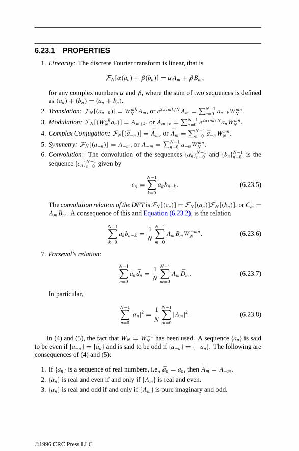
6.23.1 PROPERTIES
1. Linearity: The discrete Fourier transform is linear, that is
FN [α(an) + β(bn)] = αAm + βBm,
for any complex numbers α and β, where the sum of two sequences is definedas (an) + (bn) = (an + bn).
2. Translation: FN [(an−k)] = WmkN Am, or e2πimk/NAm = ∑N−1
n=0 an−kWmnN .
3. Modulation: FN [(WnkN an)] = Am+k , or Am+k = ∑N−1
n=0 e2πink/NanWmnN .
4. Complex Conjugation: FN [(a−n)] = Am, or Am = ∑N−1n=0 a−nW
mnN .
5. Symmetry: FN [(a−n)] = A−m, or A−m = ∑N−1n=0 a−nW
mnN .
6. Convolution: The convolution of the sequences anN−1n=0 and bnN−1
n=0 is thesequence cnN−1
n=0 given by
cn =N−1∑k=0
akbn−k. (6.23.5)
The convolution relation of the DFT is FN [(cn)] = FN [(an)]FN [(bn)], orCm =AmBm. A consequence of this and Equation (6.23.2), is the relation
N−1∑k=0
akbn−k = 1
N
N−1∑m=0
AmBmW−mnN . (6.23.6)
7. Parseval’s relation:
N−1∑n=0
andn = 1
N
N−1∑m=0
AmDm. (6.23.7)
In particular,
N−1∑n=0
|an|2 = 1
N
N−1∑m=0
|Am|2. (6.23.8)
In (4) and (5), the fact that WN = W−1N has been used. A sequence an is said
to be even if a−n = an and is said to be odd if a−n = −an. The following areconsequences of (4) and (5):
1. If an is a sequence of real numbers, i.e., an = an, then Am = A−m.
2. an is real and even if and only if Am is real and even.
3. an is real and odd if and only if Am is pure imaginary and odd.
©1996 CRC Press LLC

6.24 FAST FOURIER TRANSFORM (FFT)
To determine Am for each m = 0, 1, · · · ,M − 1 (using Equation (6.23.1)), M − 1multiplications are required. Hence the total number of multiplications required todetermine all theAm’s is (M−1)2. This number can be reduced by using decimation.
Assuming M is even, we put M = 2N and write
F2N [(an)] = Am. (6.24.1)
Now split an into two sequences, one consisting of terms with even subscripts(bn = a2n) and one with odd subscripts (cn = a2n+1). Then
Am = Bm + Wm2NCm. (6.24.2)
For the evaluation of Bm and Cm, the total number of multiplications required is2(N − 1)2. To determine Am from Equation (6.24.2), we must calculate the productWm
2NCm, for each fixed m. Therefore, the total number of multiplications required todetermine Am from Equation (6.24.2) is 2(N − 1)2 + 2N − 1 = 2N2 − 2N + 1.
But had we determined Am from (6.24.1), we would have performed (2N −1)2 = 4N2 − 4N + 1 multiplications. Thus, splitting the sequence an into twosequences and then applying the discrete Fourier transform, reduces the number ofmultiplications required to evaluate Am approximately by a factor of 2.
IfN is even, this process can be repeated. Split bn and cn into four sequences,each of lengthN/2. ThenBm andCm are determined in terms of four discrete Fouriertransforms, each of order N/2. This process can be continued k− 1 times if M = 2k
for some positive integer k.If we denote the required number of multiplications for the discrete Fourier
transform of order N = 2k by F(N), then F(2N) = 2F(N) + N and F(2) = 1,which leads to F(N) = N
2 log2 N .
6.25 MULTIDIMENSIONAL FOURIERTRANSFORMS
If x = (x1, x2, . . . , xn) and u = (u1, u2, . . . , un), then
1. Fourier transform F(u) = (2π)−n/2∫ ··· ∫
Rn
f (x)e−i(x·u) dx.
2. Inverse Fourier transform f (x) = (2π)−n/2∫ ··· ∫
Rn
F (u)ei(x·u) du.
3. Parseval’s relation ∫ ··· ∫Rn
f (x)g(x) dx = (2π)−n∫ ··· ∫
Rn
F (u)G(u) du.
©1996 CRC Press LLC

6.26 LAPLACE TRANSFORM
The Laplace transformation dates back to the work of the French mathematician,Pierre Simon Marquis de Laplace (1749–1827), who used it in his work on probabilitytheory in the 1780’s.
The Laplace transform of a function f (t) is defined as
F(s) = (Lf ) (s) =∫ ∞
0f (t)e−st dt, (6.26.1)
whenever the integral exists for at least one value of s. The transform variable, s,can be taken as a complex number. We say that f is Laplace transformable or theLaplace transformation is applicable to f if (Lf ) exists for at least one value of s.The integral on the right-hand side of Equation (6.26.1) is called the Laplace integralof f .
6.26.1 EXISTENCE AND DOMAIN OF CONVERGENCE
Sufficient conditions for the existence of the Laplace transform are
1. f is a locally integrable function, i.e.,∫ a
0 |f (t)| dt < ∞, for any a > 0.
2. f is of (real) exponential type, i.e., for some constants M, t0 > 0 and real γ , fsatisfies
|f (t)| ≤ Meγ t , for all t ≥ t0. (6.26.2)
If f is a locally integrable function on [0,∞) and of (real) exponential type γ ,then the Laplace integral of f ,
∫ ∞0 f (t)e−st dt , converges absolutely for Re s > γ
and uniformly for Re s ≥ γ1 > γ . Consequently, F(s) is analytic in the half-plane7 = s ∈ C : Re s > γ . It can be shown that if F(s) exists for some s0, then italso exists for any s for which Re s > Re s0. The actual domain of existence of theLaplace transform may be larger than the one given above. For example, the functionf (t) = cos et is of real exponential type zero, but F(s) exists for Re s > −1.
If f (t) is a locally integrable function on [0,∞), not of exponential type, and∫ ∞
0f (t)e−s0t dt (6.26.3)
converges for some complex number s0, then the Laplace integral∫ ∞
0f (t)e−st dt (6.26.4)
converges in the region Re s > Re s0 and converges uniformly in the region |arg(s − s0)|≤ θ ′ < π
2 . Moreover, if Equation (6.26.3) diverges, then so does Equation (6.26.4)for Re s < Re s0.
©1996 CRC Press LLC

6.26.2 PROPERTIES
1. Linearity: L(αf + βg) = αL(f ) + βL(g) = αF + βG,
for any constants α and β.
2. Dilation: [L (f (at))] (s) = 1
aF
( sa
), for a > 0.
3. Multiplication by Exponential Functions:[L (eatf (t)
)](s) = F(s − a).
4. Translation: [L (f (t − a)H(t − a))] (s) = e−asF (s) for a > 0. This can beput in the form
[L(f (t)H(t − a))] (s) = e−as [L(f (t + a))] (s),
where H is the Heaviside function. Examples:
(a) If
g(t) =
0, 0 ≤ t ≤ a,
(t − a)ν, a ≤ t,
then g(t) = f (t − a)H(t − a) where f (t) = tν(Re ν > −1). Since
L(tν) = -(ν+ 1)/sν+1, it follows that (Lg)(s) = e−as-(ν + 1)/sν+1, forRe s > 0.
(b) If
g(t) =t, 0 ≤ t ≤ a,
0, a < t,
we may write g(t) = t [H(t) − H(t − a)] = tH(t)− (t − a)H(t − a)−aH(t − a). Thus by properties (1) and (4),
G(s) = 1
s2− 1
s2e−as − a
se−as .
5. Differentiation of the transformed function: If f is a differentiable function ofexponential type, limt→0+ f (t) = f (0+) exists, and f ′ is locally integrable on[0,∞), then the Laplace transform of f ′ exists, and(Lf ′) (s) = sF (s) − f (0). (6.26.5)
Note that although f is assumed to be of exponential type, f ′ need not be. Forexample, f (t) = sin et
2, but f ′(t) = 2tet
2cos et
2.
6. Differentiation of higher orders: Letf be ann differentiable function so thatf (k)
(for k = 0, 1, . . . , n−1) are of exponential type with the additional assumptionthat limt→0+ f (k)(t) = f (k)(0+) exists. If f (n) is locally integrable on [0,∞),then its Laplace transform exists, and[L (
f (n))](s) = snF (s) − sn−1f (0) − sn−2f ′(0) − · · · − f (n−1)(0).
(6.26.6)
©1996 CRC Press LLC

7. Integration: If g(t) = ∫ t
0 f (x) dx, then (if the transforms exist)G(s) = F(s)/s.Repeated applications of this rule result in
[L (f (−n)
)](s) = 1
snF (s), (6.26.7)
where f (−n) is the nth antiderivative of f defined by f (−n)(t) = ∫ t
0 dtn∫ tn
0 dtn−1
. . .∫ t2
0 f (t1) dt1. Section 6.26.1 shows that the Laplace transform is an analyticfunction in a half-plane. Hence it has derivatives of all orders at any point inthat half-plane. The next property shows that we can evaluate these derivativesby direct differentiation.
8. Multiplication by powers of t : Let f be a locally integrable function whoseLaplace integral converges absolutely and uniformly for Re s > σ . Then F isanalytic in Re s > σ, and (for n = 0, 1, 2, . . . , with Re s > σ )
[L (tnf (t)
)](s) =
(− d
ds
)n
F (s),[L((
td
dt
)n
f (t)
)](s) =
(− d
dss
)n
F (s),
(6.26.8)
where(t ddt
)nis the operator
(t ddt
)applied n times.
9. Division by powers of t: If f is a locally integrable function of exponential typeso that f (t)/t is a Laplace transformable function, then[
L(f (t)
t
)](s) =
∫ ∞
s
F (u) du, (6.26.9)
or, more generally,
[L(f (t)
tn
)](s) =
∞∫s
· · ·∞∫s
F (s) (ds)n (6.26.10)
is the nth repeated integral. It follows from properties (7) and (9) thatL
t∫
0
f (x)
xdx
(s) = 1
s
∞∫s
F (u)du.
(6.26.11)
10. Periodic functions: Let f be a locally integrable function that is periodic withperiod T . Then
[L(f )] (s) = 1
(1 − e−T s)
T∫0
f (t)e−st dt. (6.26.12)
11. Hardy’s theorem: If f (t) = ∑∞n=0 cnt
n for t ≥ 0 and∑∞
n=0cnn!sn0
converges for
some s0 > 0, then [L(f )] (s) = ∑∞n=0
cnn!sn
for Re s > s0.
©1996 CRC Press LLC
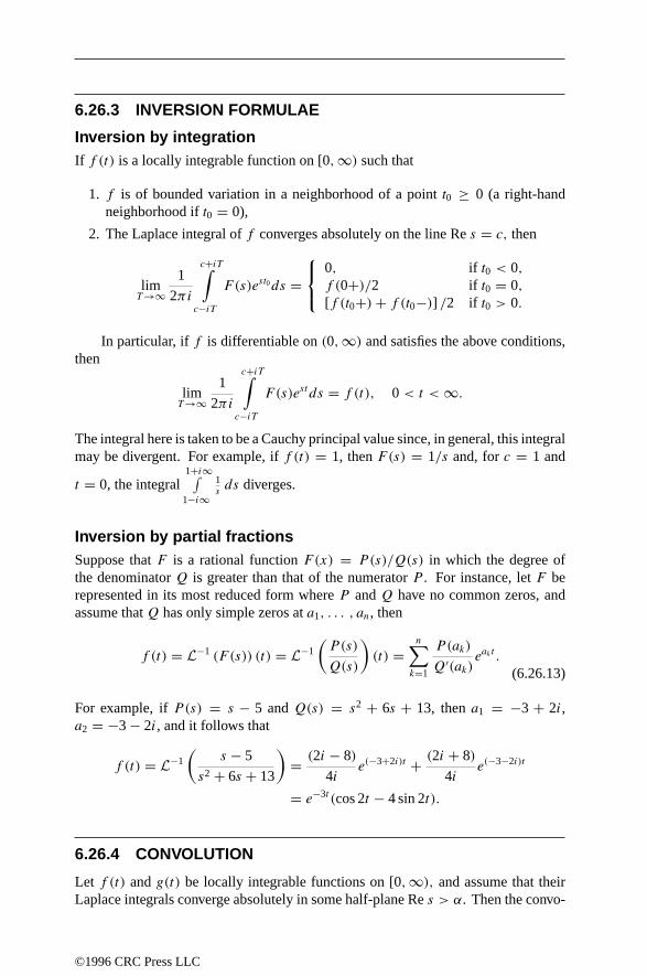
6.26.3 INVERSION FORMULAE
Inversion by integrationIf f (t) is a locally integrable function on [0,∞) such that
1. f is of bounded variation in a neighborhood of a point t0 ≥ 0 (a right-handneighborhood if t0 = 0),
2. The Laplace integral of f converges absolutely on the line Re s = c, then
limT→∞
1
2πi
c+iT∫c−iT
F (s)est0ds =
0, if t0 < 0,f (0+)/2 if t0 = 0,[f (t0+) + f (t0−)] /2 if t0 > 0.
In particular, if f is differentiable on (0,∞) and satisfies the above conditions,then
limT→∞
1
2πi
c+iT∫c−iT
F (s)estds = f (t), 0 < t < ∞.
The integral here is taken to be a Cauchy principal value since, in general, this integralmay be divergent. For example, if f (t) = 1, then F(s) = 1/s and, for c = 1 and
t = 0, the integral1+i∞∫
1−i∞1sds diverges.
Inversion by partial fractionsSuppose that F is a rational function F(x) = P(s)/Q(s) in which the degree ofthe denominator Q is greater than that of the numerator P . For instance, let F berepresented in its most reduced form where P and Q have no common zeros, andassume that Q has only simple zeros at a1, . . . , an, then
f (t) = L−1 (F (s)) (t) = L−1
(P(s)
Q(s)
)(t) =
n∑k=1
P(ak)
Q′(ak)eakt .
(6.26.13)
For example, if P(s) = s − 5 and Q(s) = s2 + 6s + 13, then a1 = −3 + 2i,a2 = −3 − 2i, and it follows that
f (t) = L−1
(s − 5
s2 + 6s + 13
)= (2i − 8)
4ie(−3+2i)t + (2i + 8)
4ie(−3−2i)t
= e−3t (cos 2t − 4 sin 2t).
6.26.4 CONVOLUTION
Let f (t) and g(t) be locally integrable functions on [0,∞), and assume that theirLaplace integrals converge absolutely in some half-plane Re s > α. Then the convo-
©1996 CRC Press LLC

lution operation, H, associated with the Laplace transform, is defined by
h(t) = (f H g)(t) =t∫
0
f (x)g(t − x)dx. (6.26.14)
The convolution off and g is a locally integrable function on [0,∞) that is continuousif either f or g is continuous. Additionally, it has a Laplace transform given by
H(s) = (Lh) (s) = F(s)G(s), (6.26.15)
where (Lf )(s) = F(s) and (Lg)(s) = G(s).
6.27 Z-TRANSFORM
The Z-transform of a sequence f (n)∞−∞ is defined by
Z[f (n)] = F(z) =∞∑
n=−∞f (n)z−n, (6.27.1)
for all complex numbers z for which the series converges.The series converges at least in a ring of the form 0 ≤ r1 < z < r2 ≤ ∞, whose
radii, r1 and r2, depend on the behavior of f (n) at ±∞:
r1 = lim supn→∞
n√
|f (n)|, r2 = lim infn→∞
1n√|f (−n)| . (6.27.2)
If there is more than one sequence involved, we may denote r1 and r2 by r1(f ) andr2(f ) respectively. The function F(z) is analytic in this ring, but it may be possibleto continue it analytically beyond the boundaries of the ring. If f (n) = 0 for n < 0,then r2 = ∞, and if f (n) = 0 for n ≥ 0, then r1 = 0.
Let z = reiθ . Then the Z-transform evaluated at r = 1 is the Fourier transformof the sequence f (n)∞−∞,
∞∑n=−∞
f (n)e−inθ . (6.27.3)
Examples:
1. Let a be a complex number and define f (n) = an, for n ≥ 0, and zero otherwise,then
Z[f (n)] =∞∑n=0
anz−n = z
z − a, |z| > |a|.
(6.27.4)
©1996 CRC Press LLC

2. If f (n) = nan, for n ≥ 0, and zero otherwise, then
Z[f (n)] =∞∑n=0
nanz−n = az
(z − a)2, |z| > |a|.
3. Let u(n) =
1, n ≥ 0,
0, n < 0,then Z[u(n)] = z
z − 1.
4. Let δ(n) =
1, n = 0,
0, otherwise,then Z[δ(n − k)] = z−k for k = 0,±1,±2, · · · .
6.27.1 PROPERTIES
Let the region of convergence of the Z-transform of the sequence f (n) be denotedby Df .
1. Linearity:
Z[af (n)+bg(n)] = aZ[f (n)]+bZ[g(n)] = aF(z)+bG(z), z ∈ Df ∩Dg.
The region Df
⋂Dg contains the ring r1 < |z| < r2, where
r1 = maximum r1(f ), r1(g) and r2 = minimum r2(f ), r2(g).2. Translation: Z[f (n − k)] = z−kF (z).
3. Multiplication by exponentials:Z[(anf (n))] = F(z/a) when ar1 < |z| < ar2.
4. Multiplication by powers of n: For k = 0, 1, 2, · · · and z ∈ Df ,
Z[(nkf (n))] = (−1)k(zd
dz
)k
F (z). (6.27.5)
5. Conjugation: Z[f (−n)] = F
(1
z
).
6. Initial and final values: If f (n) = 0 for n < 0, then limz→∞ F(z) = f (0)and, conversely, if F(z) is defined for r1 < |z| and for some integer m,
limz→∞ zmF(z) = A, then f (m) = A and f (n) = 0, for n < m.
7. Parseval’s relation: Let F(z) and G(z) be the Z-transforms of f (n) andg(n), respectively. Then
∞∑n=−∞
f (n)g(n) = 1
2π
∫ π
−π
F (eiω)G(eiω) dω. (6.27.6)
In particular,
∞∑n=−∞
|f (n)|2 = 1
2π
∫ π
−π
|F(eiω)|2 dω. (6.27.7)
©1996 CRC Press LLC

6.27.2 INVERSION FORMULA
Consider the sequences
f (n) = u(n) =
1, n ≥ 0,
0, n < 0,and g(n) = −u(−n − 1) =
−1, n < 0,
0, n ≥ 0.
Note that F(z) = z
z − 1for |z| > 1, and G(z) = z
z − 1for |z| < 1. Hence, the
inverse Z-transform of the function z/(z − 1) is not unique. In general, the inverseZ-transform is not unique, unless its region of convergence is specified.
1. Inversion by using series representation:If F(z) is given by its series
F(z) =∞∑
n=−∞anz
−n, r1 < z < r2,
then its inverse Z-transform is unique and equals f (n) = an for all n.
2. Inversion by using complex integration:If F(z) is given in a closed form as an algebraic expression and its domain ofanalyticity is known, then its inverse Z-transform can be obtained by using therelationship
f (n) = 1
2πi
∮γ
F (z)zn−1dz, (6.27.8)
where γ is a closed contour surrounding the origin in the domain of analyticityof F(z).
3. Inversion by using Fourier series:If the domain of analyticity of F contains the unit circle, |r| = 1, and if F issingle valued therein, then F(eiθ ) is a periodic function with period 2π , and,consequently, it can be expanded in a Fourier series. The coefficients of theseries form the inverse Z-transform of F and they are given explicitly by
f (n) = 1
2π
∫ π
−π
F (eiθ )einθdθ. (6.27.9)
4. Inversion by using partial fractions:Dividing Equation (6.27.4) by z and differentiating both sides with respect to z,results in
Z−1[(z − a)−k
] =(n − 1
n − k
)an−ku(n − k),
(6.27.10)
for k = 1, 2, · · · and |z| > |a| > 0. Moreover, from the example on page 544,
Z−1[z−k
] = δ(n − k). (6.27.11)
©1996 CRC Press LLC

Let F(z) be a rational function of the form
F(z) = P(z)
Q(z)= aNz
N + · · · + a1z + a0
bMzM + · · · + b1z + b0.
• Consider the caseN < M . The denominatorQ(z) can be factored over thefield of complex numbers asQ(z) = c(z−z1)
k1 · · · (z−zm)km , where c is a
constant and k1 · · · , km are positive integers satisfying k1 +· · ·+km = M .Hence, F can be written in the form
F(z) =m∑i=1
ki∑j=1
Ai,j
(z − zi)j, (6.27.12)
where
Ai,j = 1(ki−j)! limz→zi
dki−j
dzki−j (z − zi)kiF (z). (6.27.13)
The inverseZ-transform of the fractional decomposition Equation (6.27.12)in the region that is exterior to the smallest circle containing all the zerosof Q(z) can be obtained by using Equation (6.27.10).
• Consider the case N ≥ M . We must divide until F can be reduced to theform
F(z) = H(z) + R(z)
Q(z),
where the remainder polynomial, R(z), has degree less than or equal toM −1, and the quotient, H(z), is a polynomial of degree, at most, N −M .The inverse Z-transform of the quotient polynomial can be obtained byusing Equation (6.27.11) and that of R(z)/Q(z) can be obtained as in thecase N < M .
Example: to find the inverse Z-transform of the function,
F(z) = z4 + 5
(z − 1)2(z − 2), |z| > 2,
the partial fraction expansion,
z4 + 5
(z − 1)2(z − 2)= z + 4 − 1
(z − 1)2− 5
(z − 1)+ 16
(z − 2),
is created. With the aid of Equation (6.27.10) and Equation (6.27.11),
Z−1 [F(z)] = δ(n+1)+4δ(n)−(n−1)u(n−2)−5u(n−1)+16·2n−1u(n−1),
or f (n) = −n − 4 + 16 · 2n−1, for n ≥ 2, with the initial values f (−1) = 1,f (0) = 4, and f (1) = 11.
©1996 CRC Press LLC

6.27.3 CONVOLUTION AND PRODUCT
The convolution of two sequences, f (n)∞−∞ and g(n)∞−∞ , is a sequence h(n)∞−∞defined by h(n) = ∑∞
k=−∞ f (k)g(n − k). The Z-transform of the convolution oftwo sequences is the product of their Z-transforms,
Z[h(n)] = Z[f (n)]Z[g(n)],
for z ∈ Df
⋂Dg , or H(z) = F(z)G(z).
The Z-transform of the product of two sequences is given by
Z[f (n)g(n)] = 1
2πi
∮γ
F (ω)G( zω
) dω
ω, (6.27.14)
where γ is a closed contour surrounding the origin in the domain of convergence ofF(ω) and G(z/ω).
6.28 HILBERT TRANSFORM
The Hilbert transform of f is defined as
(Hf )(x) = f (x) = 1
π
∫ ∞
−∞
f (t)
t − xdt = 1
π
∫ ∞
−∞
f (x + t)
tdt
(6.28.1)
where the integral is a Cauchy principal value.Since the definition is given in terms of a singular integral, it is sometimes im-
practical to use. An alternative definition is given below. First, let f be an integrablefunction, and define a(t) and b(t) by
a(t) = 1
π
∫ ∞
−∞f (x) cos txdx, b(t) = 1
π
∫ ∞
−∞f (x) sin tx dx.
(6.28.2)
Consider the function F(z), defined by the Fourier integral
F(z) =∫ ∞
0(a(t) − ib(t))eizt dt = U(z) + iU (z), (6.28.3)
where z = x + iy. The real and imaginary parts of F are
U(z) =∫ ∞
0(a(t) cos xt + b(t) sin xt)e−yt dt, and
U (z) =∫ ∞
0(a(t) sin xt − b(t) cos xt)e−yt dt.
©1996 CRC Press LLC

Formally,
limy→0
U(z) = f (x) =∫ ∞
0(a(t) cos xt + b(t) sin xt) dt,
(6.28.4)
and
limy→0
U (z) = −f (x) =∫ ∞
0(a(t) sin xt − b(t) cos xt) dt,
(6.28.5)
The Hilbert transform of a function f, given by Equation (6.28.4), is defined asthe function f given by Equation (6.28.5).
6.28.1 EXISTENCE
If f ∈ L1(R), then its Hilbert transform (Hf )(x) exists for almost all x. Forf ∈ Lp(R), p > 1, there is the following stronger result:
THEOREM 6.28.1
Let f ∈ Lp(R), p > 1. Then (Hf )(x) exists for almost all x and defines a functionthat also belongs to Lp(R) with∫ ∞
−∞|(Hf )(x)|p dx ≤ Cp
∫ ∞
−∞|f (x)|p dx.
In the special case of p = 2, we have∫ ∞
−∞|(Hf )(x)|2 dx =
∫ ∞
−∞|f (x)|2 dx. (6.28.6)
The theorem is not valid if p = 1 because, although it is true that (Hf )(x)
is defined almost everywhere, it is not necessarily in L1(R). The function f (t) =(t log2 t)−1H(t) provides a counterexample.
6.28.2 PROPERTIES
1. Translation: The Hilbert transformation commutes with the translation operator(Hf )(x + a) = H(f (t + a))(x).
2. Dilation: The Hilbert transformation also commutes with the dilation operator
(Hf )(ax) = H(f (at))(x) a > 0,
but(Hf )(ax) = −H(f (at))(x) for a < 0.
©1996 CRC Press LLC

3. Multiplication by t: H(tf (t))(x) = x(Hf )(x) + 1
π
∫ ∞
−∞f (t) dt.
4. Differentiation: H(f ′(t))(x) = (Hf )′(x), provided that f (t) = O(t) as |t | →∞.
5. Orthogonality: The Hilbert transform of f ∈ L2(R) is orthogonal to f in thesense
∫ ∞−∞ f (x)(Hf )(x)dx = 0.
6. Parity: The Hilbert transform of an even function is odd and that of an oddfunction is even.
7. Inversion formula: If (Hf )(x) = 1
π
∫ ∞
−∞
f (t)
t − xdt, then
f (t) = − 1
π
∫ ∞
−∞
(Hf )(x)
x − tdx or, symbolically,
H (Hf ) (x) = −f (x), (6.28.7)
that is, applying the Hilbert transform twice returns the negative of the originalfunction. Moreover, if f ∈ L1(R) has a bounded derivative, then the alliedintegral (see Equation 6.22.6) equals (Hf )(x).
6.28.3 RELATIONSHIP WITH THE FOURIER TRANSFORM
From Equations (6.28.3)–(6.28.5), we obtain
limy→0
F(z) = F(x) =∫ ∞
0(a(t) − ib(t))eixt dt = f (x) − i(Hf )(x),
where a(t) and b(t) are given by Equation (6.28.2).Let g be a real-valued integrable function and consider its Fourier transform
g(x) = 1√2π
∫ ∞−∞ g(t)eixt dt. If we denote the real and imaginary parts of g by f and
f , respectively, then
f (x) = 1√2π
∫ ∞
−∞g(t) cos xt dt, and
f (x) = 1√2π
∫ ∞
−∞g(t) sin xt dt.
Splitting g into its even and odd parts, ge and go, respectively, we obtain
ge(t) = g(t) + g(−t)
2and go(t) = g(t) − g(−t)
2;
hence
f (x) =√
2
π
∫ ∞
0ge(t) cos xt dt, and f (x) =
√2
π
∫ ∞
0go(t) sin xt dt,
©1996 CRC Press LLC

or
f (x) = 1√2π
∫ ∞
−∞ge(t)e
ixt dt, and f (x) = −i√2π
∫ ∞
−∞go(t)e
ixt dt.
This shows that, if the Fourier transform of the even part of a real-valued functionrepresents a function f (x), then the Fourier transform of the odd part represents theHilbert transform of f (up to multiplication by i).
THEOREM 6.28.2
Let f ∈ L1(R) and assume that Hf is also in L1(R). Then
F(Hf )(ω) = −i sgn(ω)F(f )(ω), (6.28.8)
where F denotes the Fourier transformation. Similarly, if f ∈ L2(R), then (Hf ) ∈L2(R), and Equation (6.28.8) remains valid.
6.29 HANKEL TRANSFORM
The Hankel transform of order ν of a function f (x) is defined as
Hν(f )(y) = Fν(y) =∫ ∞
0f (x)
√xyJν(yx)dx, (6.29.1)
for y > 0 and ν > −1/2, where Jν(z) is the Bessel function of the first kind of orderν.
The Hankel transforms of order 1/2 and −1/2 are equal to the Fourier sine andcosine transforms, respectively, because
J1/2(x) =√
2
πxsin x, J−1/2(x) =
√2
πxcos x.
As with the Fourier transform, there are many variations on the definition of theHankel transform. Some authors define it as
Gν(y) =∫ ∞
0xg(x)Jν(yx)dx; (6.29.2)
however, the two definitions are equivalent; we only need to replace f (x) by√xg(x)
and Fν(y) by√yGν(y).
©1996 CRC Press LLC

6.29.1 PROPERTIES
1. Existence: Since√xJν(x) is bounded on the positive real axis, the Hankel
transform of f exists if f ∈ L1(0,∞).
2. Multiplication by xm:
Hν
(xmf (x)
)(y) = y1/2−ν
(1
y
d
dy
)m [yν+m−1/2Fν+m(y)
].
3. Division by x:
Hν
(2ν
xf (x)
)(y) = y
[Fν−1(y) + Fν+1(y)
],
and also
Hν
(f (x)
x
)(y) = y1/2−ν
∫ y
0tν−1/2Fν−1(t) dt.
4. Differentiation:
Hν
(2νf ′(x)
)(y) = (ν − 1/2)yFν+1(y) − (ν + 1/2)yFν−1(y).
5. Differentiation and multiplication by powers of x:
Hν
[x1/2−ν
(1
x
d
dx
)m (xν+m−1/2f (x)
)](y) = ymFν+m(y).
6. Parseval’s relation: Let Fν and Gν denote the Hankel transforms of order ν off and g, respectively. Then∫ ∞
0Fν(y)Gν(y)dy =
∫ ∞
0f (x)g(x)dx. (6.29.3)
In particular, ∫ ∞
0|Fν(y)|2 dy =
∫ ∞
0|f (x)|2dx. (6.29.4)
7. Inversion formula: If f is absolutely integrable on (0,∞) and of boundedvariation in a neighborhood of point x, then∫ ∞
0Fν(y)
√xyJν(yx)dy = f (x + 0) + f (x − 0)
2,
(6.29.5)
whenever the expression on the right-hand side of the equation has a meaning;the integral converges to f (x) whenever f is continuous at x.
©1996 CRC Press LLC

6.30 TABLES OF TRANSFORMS
Finite sine transforms
fs(n) =∫ π
0F(x) sin nx dx, for n = 1, 2, . . . .
No. fs(n) F (x)
1 (−1)n+1fs(n) F (π − x)
2 1/n π − x/π
3 (−1)n+1/n x/π
4 1 − (−1)n/n 1
52
n2sin
nπ
2
x when 0 < x < π/2
π − x when π/2 < x < π
6 (−1)n+1/n3 x(π2 − x2)/6π
7 1 − (−1)n/n3 x(π − x)/2
8π2(−1)n−1
n− 2[1 − (−1)n]
n3x2
9 π(−1)n(
6
n3− π2
n
)x3
10n
n2 + c2
[1 − (−1)necπ
]ecx
11n
n2 + c2
sinh c(π − x)
sinh cπ
12n
n2 − k2with k = 0, 1, 2, . . .
sin k(π − x)
sin kπ
13
π/2 when n = m
0 when n = m, m = 1, 2, . . .sinmx
14n
n2 − k2[1 − (−1)n cos kπ]
with k = 1, 2, . . .
cos kx
15n
n2 − m2[1 − (−1)n+m]
when n = m = 1, 2, . . .(0 when n = m)
cosmx
16n
(n2 − k2)2with k = 0, 1, 2, . . .
π sin kx
2k sin2 kπ− x cos k(π − x)
2k sin kπ
17 bn/n with |b| ≤ 12
πtan−1 b sin x
1 − b cos x
181 − (−1)n
nbn with |b| ≤ 1
2
πtan−1 2b sin x
1 − b2
©1996 CRC Press LLC

Finite cosine transforms
fc(n) =∫ π
0F(x) cos nx dx, for n = 0, 1, 2, . . . .
No. fc(n) F (x)
1 (−1)nfc(n) F (π − x)
2
π n = 0
0 n = 1, 2, . . .1
3
0 n = 02
nsin
nπ
2n = 1, 2, . . .
1 for 0 < x < π/2
−1 for π/2 < x < π
4
π2
2n = 0
(−1)n − 1/n2 n = 1, 2, . . .x
5
π2
6n = 0
(−1)n/n2 n = 1, 2, . . .
x2
2π
6
0 n = 0
1/n2 n = 1, 2, . . .
(x − π)2
2π− π
6
7
π4
4n = 0
3π2 (−1)n
n2
− 61 − (−1)n
n4
n = 1, 2, . . .x3
8(−1)necπ − 1
n2 + c21cecx
91
n2 + c2
cosh c(π − x)
c sinh cπ
10k
n2 − k2[(−1)n cosπk − 1]
with k = 0, 1, 2, . . .
sin kx
11
0 m = 1, 2, . . .(−1)n+m − 1
n2 − m2m = 1, 2, . . .
1
msinmx
121
n2 − k2
with k = 0, 1, 2, . . .
− cos k(π − x)
k sin kπ
13
π/2 when n = m
0 when n = mcosmx (m = 1, 2, . . . )
©1996 CRC Press LLC

Fourier sine transforms
F(ω) = Fs(f )(ω) =√
2
π
∫ ∞
0f (x) sin(ωx) dx, ω > 0 .
No. f (x) F (ω)
1
1 0 < x < a
0 x > a
√2π
(1−cosωa
ω
)2 xp−1 (0 < p < 1)
√2π
-(p)
ωp sin pπ
2
3
sin x 0 < x < a
0 x > a
1√2π
(sin[a(1−ω)]
1−ω− sin[a(1+ω)]
1+ω
)4 e−x
√2π
ω1+ω2
5 xe−x2/2 ωe−ω2/2
6 cos x2
2
√2[sin ω2
2 C(ω2
2
)− cos ω2
2 S(ω2
2
)]7 sin x2
2
√2[cos ω2
2 C(ω2
2
)+ sin ω2
2 S(ω2
2
)]
Fourier cosine transforms
F(ω) = Fc(f )(ω) =√
2
π
∫ ∞
0f (x) cos(ωx) dx, ω > 0.
No. f (x) F (ω)
1
1 0 < x < a
0 x > a
√2π
sin aωω
2 xp−1 (0 < p < 1)√
2π
-(p)
ωp cos pπ
2
3
cos x 0 < x < a
0 x > a
1√2π
(sin[a(1−ω)]
1−ω+ sin[a(1+ω)]
1+ω
)4 e−x
√2π
11+ω2
5 e−x2/2 e−ω2/2
6 cos x2
2 cos(ω2
2 − π4
)7 sin x2
2 cos(ω2
2 + π4
)
©1996 CRC Press LLC
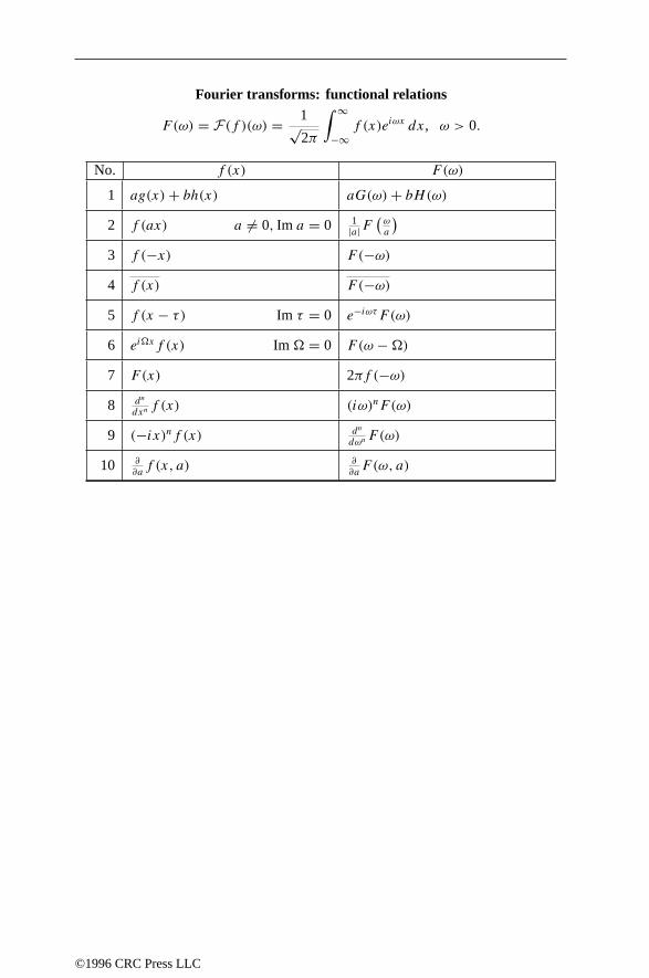
Fourier transforms: functional relations
F(ω) = F(f )(ω) = 1√2π
∫ ∞
−∞f (x)eiωx dx, ω > 0.
No. f (x) F (ω)
1 ag(x) + bh(x) aG(ω) + bH(ω)
2 f (ax) a = 0, Im a = 0 1|a|F
(ωa
)3 f (−x) F (−ω)
4 f (x) F (−ω)
5 f (x − τ) Im τ = 0 e−iωτF (ω)
6 ei7xf (x) Im 7 = 0 F(ω − 7)
7 F(x) 2πf (−ω)
8 dn
dxnf (x) (iω)nF (ω)
9 (−ix)nf (x) dn
dωn F (ω)
10 ∂∂af (x, a) ∂
∂aF (ω, a)
©1996 CRC Press LLC

Fourier transforms
F(ω) = F(f )(ω) = 1√2π
∫ ∞
−∞f (x)eiωx dx, ω > 0.
No. f (x) F (ω)
1 δ(x) 1/√
2π
2 δ(x − τ) eiωτ /√
2π
3 δ(n)(x) (−iω)n/√
2π
4 H(x) =
1 x > 0
0 x < 0− 1
iω√
2π+
√π
2δ(ω)
5 sgn(x) =
1 x > 0
−1 x < 0−√
2
π
1
iω
6
1 |x| < a
0 |x| > a
√2
π
sin aω
ω
7
ei7t |x| < a
0 |x| > a
√2
π
sin a(7 + ω)
7 + ω
8 e−a|x| a > 0 −√
2π
aa2+ω2
9 sin7xx
√π2 [H(7 − ω) − H(−7 − ω)]
©1996 CRC Press LLC

Fourier transforms
F(ω) = F(f )(ω) = 1√2π
∫ ∞
−∞f (x)eiωx dx, ω > 0.
No. f (x) F (ω)
10 sin ax/x
√π2 |ω| < a
0 |ω| > a
11
eiax p < x < q
0 x < p, x > q
i√2π
eip(ω+a) − eiq(ω+a)/ω + a
12
e−cx+iax x > 0
0 x < 0(c > 0)
i√2π(ω + a + ic)
13 e−px2Re p > 0 1√
2pe−ω2/4p
14 cospx2 1√2p
cos(ω2
4p − π4
)15 sinpx2 1√
2pcos
(ω2
4p + π4
)16 |x|−p (0 < p < 1)
√2π
-(1−p) sin pπ
2
|ω|1−p
17 e−a|x|/√|x|
√√a2+ω2+a√ω2+a2
18 cosh axcosh πx (−π < a < π)
√2π
cos a2 cosh ω
2cos a+coshω
19 sinh axsinh πx (−π < a < π) 1√
2πsin a
cos a+coshω
20
1√
a2−x2|x| < a
0 |x| > a
√π2 J0(aω)
21 sin[b√a2+x2]√
a2+x2
0 |ω| > b√
π2 J0(a
√b2 − ω2) |ω| < b
22
Pn(x) |x| < 1
0 |x| > 1in√ωJn+1/2(ω)
23
cos[b
√a2−x2]√
a2−x2|x| < a
0 |x| > a
√π2 J0(a
√ω2 + b2)
24
cosh[b
√a2−x2]√
a2−x2|x| < a
0 |x| > a
√π2 J0(a
√ω2 − b2)
©1996 CRC Press LLC

Multidimensional Fourier transforms
No. f (x) F (u)In n-dimensions
1 f (ax) Im a = 0 |a|−n F (a−1u)
2 f (x − a) e−ia·uF(u)
3 eia·xf (x) F (v − a)
4 F(x) (2π)nf (−u)
Two dimensions: let x = (x, y) and u = (u, v).
5 f (ax, by) 1|ab|F
(u
a, v
b
)6 f (x − a, y − b) ei(au+bv)F (u, v)
7 ei(ax+by)f (x, y) F (u − a, v − b)
8 F(x, y) (2π)2Ff (−u,−v)
9 δ(x − a)δ(y − b) 12π e
−i(au+bv)
10 e−x2/4a−y2/4b a, b > 0 2√ab e−au2−bv2
11
1 |x| < a, |y| < b
0 otherwise (rectangle)2 sin au sin bv
πuv
12
1 |x| < a
0 otherwise (strip)2 sin au
πuvδ(v)
13
1 x2 + y2 < a2
0 otherwise (circle)aJ1(a
√u2 + v2)√
u2 + v2
Three dimensions: let x = (x, y, z) and u = (u, v,w).
14 δ(x − a)δ(y − b)δ(z − c) 1(2π)3/2 e
−i(au+bv+cw)
15 e−x2/4a−y2/4b−z2/4c a, b, c > 0 23/2√abc e−au2−bv2−cw2
16
1 |x| < a, |y| < b, |z| < c
0 otherwise (box)
(2
π
)3/2 sin au sin bv sin cw
uvw
17
1 x2 + y2 + z2 < a2
0 otherwise (ball)sin aρ−aρ cos aρ√
2πρ3 ρ2 = u2 + v2 + w2
©1996 CRC Press LLC

Laplace transforms: functional relations
F(s) = L(f )(s) =∫ ∞
0f (t)e−st dt.
No. f (t) F (s)
1 af (t) + bg(t) aF (s) + bG(s)
2 f ′(t) sF (s) − F(0+)
3 f ′′(t) s2F(s) − sF (0+) − F ′(0+)
4 f (n)(t) snF (s) −n−1∑k=0
sn−1−kF (k)(0+)
5∫ t
0 f (τ) dτ1sF (s)
6∫ t
0
∫ τ
0 f (u) du dτ 1s2 F(s)
7∫ t
0 f1(t − τ)f2(τ ) dτ = f1 ∗ f2 F1(s)F2(s)
8 tf (t) −F ′(s)
9 tnf (t) (−1)nF (n)(s)
10 1tf (t)
∫ ∞s
F (z) dz
11 eatf (t) F (s − a)
12 f (t − b) with f (t) = 0 for t < 0 e−btF (s)
13 1cf(tc
)F(cs)
14 1cebt/cf
(tc
)F(cs − b)
15 f (t + a) = f (t)∫ a
0 e−stf (t) dt/1 − e−as
16 f (t + a) = −f (t)∫ a
0 e−stf (t) dt/1 + e−as
17∑n
k=1p(an)
q ′(an)eant
with q(t) = (t − a1) · · · (t − an)
p(s)
q(s)
18 eatn∑
k=1
φ(n−k)(a)
(n − k)!
tk−1
(k − 1)!φ(s)/(s − a)n
©1996 CRC Press LLC

Laplace transforms
F(s) = L(f )(s) =∫ ∞
0f (t)e−st dt.
No. F (s) f (t)
1 1 δ(t), delta function
2 1/s H(t), unit step function
3 1/s2 t
4 1/sn (n = 1, 2, . . . ) tn−1
(n−1)!
5 1/√
s 1/√π t
6 s−3/2 2√
t/π
7 s−(n+1/2) (n = 1, 2, . . . ) 2ntn−1/2√π(2n−1)!!
8 -(k)
sk (k > 0) tk−1
9 1s−a
eat
10 1(s−a)2 teat
11 1(s−a)n (n = 1, 2, . . . ) 1
(n−1)! tn−1eat
12 -(k)
(s−a)k(k > 0) tk−1eat
13 1(s−a)(s−b)
(a = b) 1a−b
(eat − ebt
)14 s
(s−a)(s−b)(a = b) 1
a−b
(aeat − bebt
)15 1
(s−a)(s−b)(s−c) (a, b, c distinct) − (b−c)eat+(c−a)ebt+(a−b)ect
(a−b)(b−c)(c−a)
16 1s2 +a2
1a
sin at
17 ts2 +a2 cos at
18 1s2 −a2
1a
sinh at
19 ss2 −a2 cosh at
20 1s (s2 +a2)
1a2 (1 − cos at)
21 1s2(s2 +a2)
1a3 (at − sin at)
22 1(s2 +a2)2
12a3 (sin at − at cos at)
23 s(s2 +a2)2
t2a sin at
24 s2
(s2 +a2)21
2a (sin at + at cos at)
©1996 CRC Press LLC

Laplace transforms
F(s) = L(f )(s) =∫ ∞
0f (t)e−st dt.
No. F (s) f (t)
25 s2 −a2
(s2 +a2)2 t cos at
26 s(s2 +a2)(s2 +b2)
(a2 = b2) cos at−cos btb2−a2
27 1(s−a)2 +b2
1beat sin bt
28 s−a(s−a)2 +b2 eat cos bt
291[
(s − a)2 + b2]n − e−at
4n−1b2n
∑nk=1
(2n−k−1n−1
)×(−2t)n−1 dk
dtk [cos bt]
30s[
(s − a)2 + b2]n
e−at
4n−1b2n
∑nk=1
(2n−k−1n−1
)(−2t)k−1
(k−1)!
× dk
dtk [a cos bt + b sin at]
−2b∑n
k=1
(2n−k−2n−1
)(−2t)k−1
(k−1)!
× ∂k
∂tk [sin bt]
313a2
s3 + a3
e−at
−eat/2(
cos at√
32 − √
3 sin at√
32
)32 s
s4 +4a41
2a2 sin at sinh at
33 4a3
s4 +4a4 sin at cosh at − cos at sinh at
34 1s4 −a4
12a3 (sinh at − sin at)
35 ss4 −a4
12a2 (cosh at − cos at)
36 8a3s2
(s2 +a2)3 (1 + a2t2) sin at − at cos at
37 1s
(s−1
s
)nLn(t) = es
n!dn
dtn (tne−t)
38 s(s−a)3/2
1√π teat(1 + 2at)
39√
s − a −√s − b 1
2√π t3
(ebt − eat)
40 1√s+a
1√π t
− aea2t erfc(a
√t)
41√
ss−a2
1√π t
+ aea2t erf(a
√t)
42√
ss+a2
1√π t
− 2a√πe−a2t
∫ a√t
0 eτ2dτ
43 1√s(s−a2)
1aea
2t erf(a√
t)
44 1√s(s+a2)
2a√πe−a2t
∫ a√
t0 eτ
2dτ
©1996 CRC Press LLC

Laplace transforms
F(s) = L(f )(s) =∫ ∞
0f (t)e−st dt.
No. F (s) f (t)
45b2 − a2
(s − a2)(b + √s)
ea2t[b − a erf(a
√t)]
−beb2t erfc(b
√t)
46 1√t(
√s+a)
ea2t erfc(a
√t)
47 1(s+a)
√s+b
1√b−a
e−at erf(√b − a
√t)
48 b2−a2√s(s−a2)(
√s+b)
ea2t[ba
erf(a√
t) − 1]
+eb2t erfc(b
√t)
49 (1−s)n
sn+1/2n!
(2n)!√π tH2n(
√t)
50 (1−s)n
sn+3/2 − n!(2n+1)!
√πH2n+1(
√t)
51√
s+2a√s
− 1 ae−at [I1(at) + I0(at)]
52 1√s+a
√s+b
e−(a+b)t/2I0(a−b
2 t)
53-(k)
(s + a)k(s + b)k(k ≥ 0)
√π(
ta−b
)k−1/2e−(a+b)t/2
×Ik−1/2(a−b
2 t)
541√
s + a(s + b)3/2
te−(a+b)t/2 [I0
(a−b
2 t)
+ I1(a−b
2 t)]
55√
s+2a−√s√
s+2a+√s
1se−atI1(at)
56 1√s2 +a2 J0(at)
57 (√
s2 +a2 −s)k√s2 +a2 (k > −1) akJk(at)
58 1(s2 +a2)k
(k > 0)√π
-(k)
(t
2a
)k−1/2Jk−1/2(at)
59 (√
s2 + a2 − s)k (k > 0) kak
t Jk(at)
60 (s−√s2 −a2)k√
s2 −a2 (k > −1) akIk(at)
61 1(s2 −a2)k
(k > 0)√π
-(k)
(t
2a
)k−1/2Ik−1/2(at)
©1996 CRC Press LLC

Laplace transforms
F(s) = L(f )(s) =∫ ∞
0f (t)e−st dt.
No. F (s) f (t)
62 e−ks
s
0 when 0 < t < k
1 when t > k
63 e−ks
s2
0 when 0 < s < k
t − k when t > k
64 e−ks
sp(p > 0)
0 when 0 < t < k(t−k)p−1
-(p)when t > k
65 1 − e−ks
s
1 when 0 < t < k
0 when t > k
66 as2 +a2 coth πs
2a |sin at |67 1
s e−a/s J0(2
√aT)
68 1√se−a/s 1√
π tcos 2
√at
69 1√sea/s 1√
π tcosh 2
√at
70 1s3/2 e
−a/s 1√πa
sin 2√at
71 1S3/2 e
a/s 1√πa
sinh 2√at
72 1sk e
−a/s (k > 0)(
ta
)(k−1)/2Jk−1(2
√at)
73 1sk e
a/t (k > 0)(ta
)(k−1)/2Ik−1(2
√at)
74 e−a√
s (a > 0) a
2√π te−a2/4t
75 1s e
−a√
s (a ≥ 0) erfc(
a
2√
t
)76 1√
se−a
√s (a ≥ 0) 1√
π te−a2/4t
77 s−3/2e−a√
s (a ≥ 0) t√ t
πe−a2/4t− a erfc
(a
2√
t
)78 e−k
√s√
s(a+√s)
(k ≥ 0) eak+a2t erfc(a√
t + k
2 √
t
)
©1996 CRC Press LLC
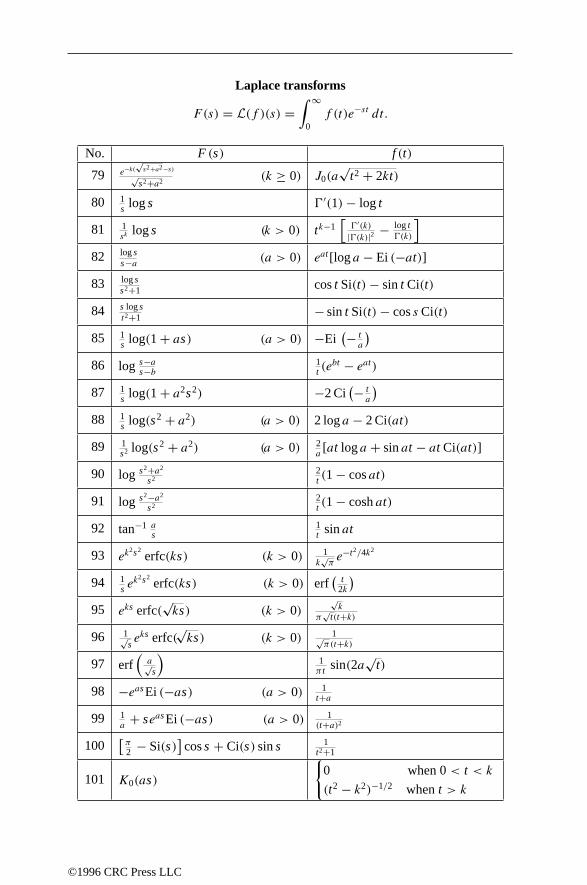
Laplace transforms
F(s) = L(f )(s) =∫ ∞
0f (t)e−st dt.
No. F (s) f (t)
79 e−k(
√s2 +a2 −s)√
s2 +a2 (k ≥ 0) J0(a√
t2 + 2kt)
80 1s log s -′(1) − log t
81 1sk
log s (k > 0) tk−1[
-′(k)|-(k)|2 −
log t-(k)
]82 log s
s−a(a > 0) eat[log a − Ei (−at)]
83 log ss2 +1 cos t Si(t) − sin t Ci(t)
84 s log st2+1 − sin t Si(t) − cos s Ci(t)
85 1s log(1 + as) (a > 0) −Ei
(− ta
)86 log s−a
s−b1t (e
bt − eat)
87 1s log(1 + a2s2) −2 Ci
(− ta
)88 1
s log(s2 + a2) (a > 0) 2 log a − 2 Ci(at)
89 1s2 log(s2 + a2) (a > 0) 2
a [at log a + sin at − at Ci(at)]
90 log s2 +a2
s22t (1 − cos at)
91 log s2 −a2
s22t (1 − cosh at)
92 tan−1 as
1t sin at
93 ek2s2
erfc(ks) (k > 0) 1k√πe−t2/4k2
94 1s e
k2s2 erfc(ks) (k > 0) erf
(t
2k
)95 eks erfc(
√ks) (k > 0)
√k
π√
t(t+k)
96 1√seks erfc(
√ks) (k > 0) 1√
π(t+k)
97 erf(
a√s
)1π t sin(2a
√t)
98 −eas Ei (−as) (a > 0) 1t+a
99 1a
+ seas Ei (−as) (a > 0) 1(t+a)2
100[π2 − Si(s)
] cos s + Ci(s) sin s 1
t2 +1
101 K0(as)
0 when 0 < t < k
(t2 − k2)−1/2 when t > k
©1996 CRC Press LLC

Hankel transforms
Hν(f )(y) = Fν(y) =∫ ∞
0f (x)
√xyJν(yx) dx, y > 0.
No. f (x) Fν(y)
1
xν+1/2, 0 < x < 1
0, 1 < x,
Re ν > −1
y−1/2Jν+1(y)
2
xν+1/2(a2 − x2)µ, 0 < x < a
0, a < x; ,
Re ν, Re µ > −1,
2µ-(µ + 1)aν+µ+1y−µ−1/2
× Jν+µ+1(ay)
3 xν+1/2(x2 + a2)−ν−1/2,
Re a > 0, Re ν > −1/2
√πyν−1/22−νe−ay
× [-(ν + 1/2)]−1
4 xν+1/2e−ax,
Re a > 0, Re ν > −1a(π)−1/22ν+1yν+1/2-(ν + 3/2)× (a2 + y2)−ν−3/2
5 xν+1/2e−ax2,
Re a > 0, Re ν > −1yν+1/2(2a)−ν−1 exp
(−y2/4a)
6 e−ax/√x,
Re a > 0, Re ν > −1y−ν+1/2
[√(a2 + y2) − a
]ν× (a2 + y2)−1/2
7 x−ν−1/2 cos(ax),a > 0, Re ν > −1/2
√π2−νy−ν+1/2[-(ν + 1/2)]−1
× (y2 − a2)ν−1/2H(y − a)
8 x1/2−ν sin(ax),a > 0, Re ν > 1/2
a21−ν√πyν+1/2[-(ν − 1/2)]−1
× (y2 − a2)ν−3/2H(y − a)
9 x−1/2Jν−1(ax),
a > 0, Re ν > −1aν−1y−ν+1/2H(y − a)
10 x−1/2Jν+1(ax),
a > 0, Re ν > −3/2
a−ν−1yν+1/2, 0 < y < a
0, a < y
©1996 CRC Press LLC

Hilbert transforms
H(f )(y) = F(y) = 1
π
∫ ∞
−∞
f (x)
x − ydx.
No. f (x) F (y)
1 1 0
2
0, −∞ < x < a
1, a < x < b
0, b < x < ∞1
πlog
∣∣(b − y)(a − y)−1∣∣
3
0, −∞ < x < a
x−1, a < x < ∞ (πy)−1 log∣∣a(a − y)−1
∣∣ ,0 = y = a, a > 0
4 (x + a)−1 Im a > 0 i(y + a)−1
51
1 + x2−y/1 + y2
61
1 + x4− y(1 + y2)√
2(1 + y4)
7 sin(ax), a > 0 cos(ay)
8 sin(ax)/x, a > 0 [cos(ay) − 1]/y
9 cos(ax), a > 0 − sin(ay)
10 [1 − cos(ax)]/x, a > 0 sin(ay)/y
11 sgn(x) sin(a|x|1/2) a > 0 cos(a|y|1/2) + exp(−a|y|1/2)
12 eiax a > 0 ieiay
©1996 CRC Press LLC

Mellin transforms
f ∗(s) = M[f (x); s] =∫ ∞
0f (x)xs−1 dx.
No. f (x) f ∗(s)
1 ag(x) + bh(x) ag∗(s) + bh∗(s)
2 f (n)(x)† (−1)n -(s)
-(s−n)f ∗(s − n)
3 xnf (n)(x)† (−1)n -(s+n)
-(s)f ∗(s)
4 Inf (x)‡ (−1)n -(s)
-(s+n)f ∗(s + n)
5 e−x -(s) Re s > 0
6 e−x2 12-(
12 s) Re s > 0
7 cos x -(s) cos( 12πs) 0 < Re s < 1
8 sin x -(s) sin( 12πs) 0 < Re s < 1
9 (1 − x)−1 π cot(πs) 0 < Re s < 1
10 (1 + x)−1 π cosec(πs) 0 < Re s < 1
11 (1 + xa)−b -(s/a)-(b−s/a)
a-(b)0 < Re s < ab
12 log(1 + ax) | arg a| < ππs−1a−s cosec(πs)
− 1 < Re s < 0
13 tan−1 x− 1
2πs−1 sec( 1
2πs)
− 1 < Re s < 0
14 cot−1 x 12πs
−1 sec( 12πs) 0 < Re s < 1
15 csch ax Re a > 0 2(1 − 2−s)a−s-(s)ζ(s) Re s > 1
16 sech2 ax Re a > 0 4(2a)−s-(s)ζ(s − 1) Re s > 2
17 csch2 ax Re a > 0 4(2a)−s-(s)ζ(s − 1) Re s > 2
18 Kν(ax)a−s2s−2-((s − ν)/2)
× -((s + ν)/2) Re s > |Re ν|
†Assuming that limx→0 xs−r−1f (r)(x) = 0 for r = 0, 1, . . . , n − 1.
‡Where In denotes the nth repeated integral of f (x): I0f (x) = f (x), Inf (x) =∫ x
0 In−1(t) dt .
©1996 CRC Press LLC

References
1. W. Magnus, F. Oberhettinger, and R.P. Soni, Formulas and Theorems for theSpecial Functions of Mathematical Physics, Springer–Verlag, New York, 1966.
2. Staff of the Bateman Manuscript Project, A. Erdelyi, Ed., Tables of IntegralTransforms, in 3 volumes, McGraw-Hill, New York, 1954.
3. N.I.A. Vilenkin, Special Functions and the Theory of Group Representations,American Mathematical Society, Providence, RI, 1968.
4. I.S. Gradshteyn and I.M. Ryzhik, Tables of Integrals, Series, and Products, 5thed., Academic Press, New York, 1994.
©1996 CRC Press LLC

Chapter 7Probability andStatistics
7.1 PROBABILITY THEORY7.1.1 Introduction7.1.2 Multivariatedistributions7.1.3 Randomsumsof randomvariables7.1.4 Transforming variables7.1.5 Central limit theorem7.1.6 Averagesover vectors7.1.7 Inequalities7.1.8 Geometric probability7.1.9 Classic probability problems
7.2 PROBABILITY DISTRIBUTIONS7.2.1 Discretedistributions7.2.2 Continuousdistributions
7.3 QUEUING THEORY
7.4 MARKOV CHAINS 7.4.1 Transition function7.4.2 Transition matrix7.4.3 Recurrence7.4.4 Stationary distributions7.4.5 Randomwalks7.4.6 Ehrenfest chain
7.5 RANDOM NUMBER GENERATION 7.5.1 Methodsof pseudorandomnumber generation7.5.2 Generating nonuniformrandomvariables
7.6 CONTROL CHARTS
7.7 STATISTICS 7.7.1 Descriptivestatistics7.7.2 Statistical estimators7.7.3 Cramer–Rao bound7.7.4 Order statistics
©1996 CRC Press LLC

7.7.5 Classic statisticsproblems
7.8 CONFIDENCE INTERVALS 7.8.1 Confidence interval: sample fromonepopulation7.8.2 Confidence interval: samples from two populations
7.9 TESTS OF HYPOTHESES7.9.1 Hypothesis tests: parameter fromonepopulation7.9.2 Hypothesis tests: parameters from two populations7.9.3 Hypothesis tests: distribution of a population7.9.4 Hypothesis tests: distributionsof two populations7.9.5 Sequential probability ratio tests
7.10 LINEAR REGRESSION 7.10.1 Linear model y = β0 + β1x + ε
7.10.2 General model y = β0 + β1x1 + β2x2 + · · · + βnxn + ε
7.11 ANALYSIS OF VARIANCE (ANOVA)7.11.1 One-factor ANOVA7.11.2 Unreplicated two-factor ANOVA7.11.3 Replicated two-factor ANOVA
7.12 PROBABILITY TABLES7.12.1 Critical values7.12.2 Tableof thenormal distribution7.12.3 Percentagepoints, Student’s t-distribution7.12.4 Percentagepoints, Chi-squaredistribution7.12.5 Percentagepoints, F -distribution7.12.6 Cumulative terms, binomial distribution7.12.7 Cumulative terms, Poisson distribution7.12.8 Critical values, Kolmogorov–Smirnov test7.12.9 Critical values, two sampleKolmogorov–Smirnov test7.12.10 Critical values, Spearman’s rank correlation
7.13 SIGNAL PROCESSING 7.13.1 Estimation7.13.2 Filters7.13.3 Matched filtering (Weiner filter)7.13.4 Kalman filtering7.13.5 Walsh functions7.13.6 Wavelets
REFERENCES
©1996 CRC Press LLC

7.1 PROBABILITY THEORY
7.1.1 INTRODUCTION
A sample space S associated with an experiment is a set S of elements such that anyoutcome of the experiment corresponds to a unique element of the set. An event E isa subset of a sample space S. An element in a sample space is called a sample pointor a simple event.
Definition of probability
If an experiment can occur in n mutually exclusive and equally likely ways, and ifexactly m of these ways correspond to an event E, then the probability of E is givenby
P(E) = m
n.
If E is a subset of S, and if to each unit subset of S, a nonnegative number, calledthe probability, is assigned, and if E is the union of two or more different simpleevents, then the probability of E, denoted P(E), is the sum of the probabilities ofthose simple events whose union is E.
Marginal and conditional probability
Suppose a sample space S is partitioned into rs disjoint subsets where the generalsubset is denoted Ei ∩ Fj (with i = 1, 2, . . . , r and j = 1, 2, . . . , s). Then themarginal probability of Ei is defined as
P(Ei) =s∑
j=1
P(Ei ∩ Fj ), (7.1.1)
and the marginal probability of Fj is defined as
P(Fj ) =r∑
i=1
P(Ei ∩ Fj ). (7.1.2)
The conditional probability of Ei , given that Fj has occurred, is defined as
P(Ei | Fj ) = P(Ei ∩ Fj )
P (Fj ), when P(Fj ) = 0 (7.1.3)
and that of Fj , given that Ei has occurred, is defined as
P(Fj | Ei) = P(Ei ∩ Fj )
P (Ei), when P(Ei) = 0. (7.1.4)
©1996 CRC Press LLC

Probability theorems1. If ∅ is the null set, then P(∅) = 0.
2. If S is the sample space, then P(S) = 1.
3. If E and F are two events, then
P(E ∪ F) = P(E)+ P(F)− P(E ∩ F). (7.1.5)
4. If E and F are mutually exclusive events, then
P(E ∪ F) = P(E)+ P(F). (7.1.6)
5. If E and E′ are complementary events, then
P(E) = 1− P(E′). (7.1.7)
6. Two events are said to be independent if and only if
P(E ∩ F) = P(E)P (F ). (7.1.8)
The event E is said to be statistically independent of the event F if P(E | F) =P(E) and P(F | E) = P(F).
7. The events E1, . . . , En are called mutually independent for all combinationsif and only if every combination of these events taken any number of times isindependent.
8. Bayes’ rule: If E1, . . . , En are n mutually exclusive events whose union isthe sample space S, and if E is any arbitrary event of S such that P(E) = 0,then
P(Ek | E) = P(Ek) P (E | Ek)
P (E)= P(Ek) P (E | Ek)∑n
j=1 P(Ej ) P (E | Ej).
(7.1.9)
9. For a uniform probability distribution,
P(A) = Number of outcomes in event A
Total number of outcomes
Terminology1. A function whose domain is a sample space S and whose range is some set of real
numbers is called a random variable. This random variable is called discrete if itassumes only a finite or denumerable number of values. It is called continuousif it assumes a continuum of values.
2. “iid” or “i.i.d.” is often used for the phrase “independent and identicallydistributed”.
3. Random variables are usually represented by capital letters.
©1996 CRC Press LLC

4. Many probability distribution have special representations:
(a) χ2n : chi-square random variable with n degrees of freedom
(b) E(λ): exponential distribution with parameter λ
(c) N(µ, σ): normal random variable with mean µ and standard deviation σ
(d) P(λ): Poisson distribution with parameter λ
(e) U [a, b): uniform random variable on the interval [a, b)
Characterizing random variablesWhen X is a discrete random variable, let pk for k = 0, 1, . . . be the probability thatX = xk (with pk ≥ 0 and
∑k pk = 1). For any event E,
P(E) = P(X is in E) =∑xk∈E
pk. (7.1.10)
In the continuous case, f (x) dx is used to denote the probability that X lies inthe region [x, x + dx]; it is called the probability density function(with f (x) ≥ 0and
∫f (x) dx = 1). For any event E,
P(E) = P(X is in E) =∫E
f (x) dx. (7.1.11)
The cumulative distribution function, or simply the distribution function, is de-fined by
F(x) = Probability(X ≤ x) =∑
xk≤x pk, in the discrete case,∫ xf (t) dt, in the continuous case.
(7.1.12)
Note that F(−∞) = 0 and F(∞) = 1. The probability that X is between a and b is
P(a ≤ X ≤ b) = P(X ≤ b)− P(X ≤ a) = F(b)− F(a). (7.1.13)
Let g(X) be a function of X. The expected value of g(X), denoted by E [g(X)],is defined by
E [g(X)] =∑
k pkg(xk), in the discrete case,∫g(t)f (t) dt, in the continuous case.
(7.1.14)
1. E [aX + bY ] = aE [X]+ bE [Y ].
2. E [XY ] = E [X]E [Y ] if X and Y are statistically independent.
The momentsof X are defined by µ′k = E[Xk]. The first moment, µ′1, is called
the meanof X; it is usually denoted by µ = µ′1 = E [X]. The centered momentsof X are defined by µk = E
[(X − µ)k
]. The second centered moment is called
the varianceand is denoted by σ 2 = µ2 = E[(X − µ)2
]. Here, σ is called the
standard deviation. The skewnessis γ1 = µ3/σ3, and the excessor kurtosis is
γ2 = (µ4/σ4)− 3.
©1996 CRC Press LLC

Using σ 2Z to denote the variance for the random variable Z,
1. σ 2cX = c2σ 2
X.
2. σ 2c+X = σ 2
X.
3. σ 2aX+b = a2σ 2
X.
Generating and characteristic functions
In the case of a discrete distribution, the generating functioncorresponding to X
(when it exists) is given by G(s) = GX(s) = E[sX] = ∑∞
k=0 pksxk . From this
function, the moments may be found from
µ′n =(s∂
∂s
)n
G(s)
∣∣∣∣s=1
. (7.1.15)
1. If c is a constant, then the generating function of c +X is scG(s).
2. If c is a constant, then the generating function of cX is G(cs).
3. If Z = X + Y where X and Y are independent discrete random variables, thenGZ(s) = GX(s)GY (s).
4. If Y =∑ni=1 Xi , the Xi are independent, and each Xi has the common gener-
ating function GX(s), then the generating function of Y is [GX(s)]n.
In the case of a continuous distribution, the characteristic functioncorrespondingto X is given by φ(t) = E
[eitX
] = ∫∞−∞ eitxf (x) dx. From this function, the
moments may be found: µ′n = i−nφ(n)(0). If Z = X + Y where X and Y areindependent continuous random variables, then φZ(t) = φX(t)φY (t). The cumulantfunctionis defined as the logarithm of the characteristic function. The nth cumulant,κn, is defined as a certain term in the Taylor series of the cumulant function,
logφ(t) =∞∑n=0
κn(it)n
n!.
Note that κ1 = µ, κ2 = σ 2, κ3 = µ3, and κ4 = µ4 − 3µ22. For a normal probability
distribution, κn = 0 for n ≥ 3. The centered moments in terms of cumulants are
µ2 = κ2,
µ3 = κ3,
µ4 = κ4 + 3κ22 ,
µ5 = κ5 + 10κ3κ2,
µ6 = κ6 + 15κ4κ2 + 10κ23 + 15κ3
2 .
(7.1.16)
©1996 CRC Press LLC

7.1.2 MULTIVARIATE DISTRIBUTIONS
Discrete caseThe k-dimensional random variable (X1, . . . , Xk) is a k-dimensional discrete ran-dom variable if it assumes values only at a finite or denumerable number of points(x1, . . . , xk). Define
P(X1 = x1, X2 = x2, . . . , Xk = xk) = f (x1, x2, . . . , xk) (7.1.17)
for every value that the random variable can assume. The function f (x1, . . . , xk) iscalled the joint density of the k-dimensional random variable. If E is any subset ofthe set of values that the random variable can assume, then
P(E) = P [(X1, . . . , Xk) is in E] =∑E
f (x1, . . . , xk) (7.1.18)
where the sum is over all those points in E. The cumulative distribution function isdefined as
F(x1, x2, . . . , xk) =∑z1≤x1
∑z2≤x2
· · ·∑zk≤xk
f (z1, z2, . . . , zk). (7.1.19)
Continuous caseThe k random variables (X1, . . . , Xk) are said to be jointly distributed if a functionf exists so that f (x1, . . . , xk) ≥ 0 for all −∞ < xi <∞ (i = 1, . . . , k) and so that,for any given event E,
P(E) = P [(X1, X2, . . . , Xk) is in E]
=∫· · ·
∫E
f (x1, x2, . . . , xk) dx1 dx2 · · · dxk. (7.1.20)
The function f (x1, . . . , xk) is called the joint density of the random variables X1, X2,. . . , Xk . The cumulative distribution function is defined as
F(x1, x2, . . . , xk) =∫ x1
−∞
∫ x2
−∞· · ·
∫ xk
−∞f (z1, z2, . . . , zk) dz1 dz2 · · · dzk. (7.1.21)
Given the cumulative distribution function, the probability density may be found from
f (x1, x2, . . . , xk) = ∂
∂x1
∂
∂x2· · · ∂
∂xkF (x1, x2, . . . , xk). (7.1.22)
MomentsThe r th moment of Xi is defined as
E[Xr
i
] =∑
x1· · ·∑xk
xri f (x1, . . . , xk), in the discrete case,∞∫ ··· ∫−∞
xri f (x1, . . . , xk) dx1 · · · dxk in the continuous case.(7.1.23)
©1996 CRC Press LLC

Joint moments about the origin are defined as E[X
r11 X
r22 · · ·Xrk
k
]where r1+ r2+
· · · + rk is the order of the moment. Joint moments about the mean are defined asE [(X1 − µ1)
r1(X2 − µ2)r2 · · · (Xk − µk)
rk ], where µk = E [Xk].
Marginal and conditional distributionsIf the random variablesX1,X2, . . . ,Xk have the joint density functionf (x1, x2, . . . , xk),then the marginal distribution of the subset of the random variables, say, X1, X2, . . . ,Xp (with p < k), is given by
g(x1, x2, . . . , xp) =∑
xp+1
∑xp+2· · ·∑xk
f (x1, x2, . . . , xk), in the discrete case,∞∫ ··· ∫−∞
f (x1, . . . , xk) dxp+1 · · · dxk, in the continuous case.(7.1.24)
The conditional distribution of a certain subset of the random variables is thejoint distribution of this subset under the condition that the remaining variables aregiven certain values. The conditional distribution of X1, X2, . . . , Xp, given Xp+1,Xp+2, . . . , Xk , is
h(x1, . . . , xp | xp+1, . . . , xk) = f (x1, x2, . . . , xk)
g(xp+1, xp+2, . . . , xk) (7.1.25)
if g(xp+1, xp+2, . . . , xk) = 0.The variance σii of Xi and the covariance σij of Xi and Xj are given by
σ 2ii = σ 2
i = E[(Xi − µi)
2],
σ 2ij = ρijσiσj = E
[(Xi − µi)(Xj − µj)
],
(7.1.26)
where ρij is the correlation coefficient, and σi and σj are the standard deviations ofXi and Xj .
7.1.3 RANDOM SUMS OF RANDOM VARIABLES
If T = ∑Ni=1 Xi , N is an integer-valued random variable with generating function
GN(s), and if the Xi are discrete independent and identically distributed randomvariables with generating function GX(s), and the Xi are independent of N , thenthe generating function for T is GT (s) = GN(GX(s)). (If the Xi are continuousrandom variables, then φT (ξ) = GN(φX(ξ)).) Hence,
• µT = µNµX.
• σ 2T = µNσ
2X + µXσ
2N.
©1996 CRC Press LLC

7.1.4 TRANSFORMING VARIABLES
1. Suppose that the random variable X has the probability density function fX(x)
and the random variable Y is defined by Y = g(X). If g is measurable andone-to-one, then
fY (y) = fX(h(y))
∣∣∣∣dhdy∣∣∣∣ (7.1.27)
where h(y) = g−1(y).
2. If the random variables X and Y are independent and if their densities fX andfY , respectively, exist almost everywhere, then the probability density of theirsum, Z = X + Y , is given by the formula,
fZ(z) =∫ ∞−∞
fX(x)fY (z− x) dx. (7.1.28)
3. If the random variables X and Y are independent and if their densities fX andfY , respectively, exist almost everywhere, then the probability density of theirproduct, Z = XY , is given by the formula,
fZ(z) =∫ ∞−∞
1
|x|fX(x)fY( zx
)dx. (7.1.29)
7.1.5 CENTRAL LIMIT THEOREM
If Xi are independent and identically distributed random variables with mean µ andfinite variance σ 2, then the random variable
Z = (X1 +X2 + · · · +Xn)− nµ√nσ
(7.1.30)
tends (as n→∞) to a normal random variable with mean zero and variance one.
7.1.6 AVERAGES OVER VECTORS
Let f (n) denote the average of the function f as the unit vector n varies uniformlyin all directions in three dimensions. If a, b, c, and d are constant vectors, then
|a · n|2 = |a|2 /3,
(a · n)(b · n) = (a · b)/3,
(a · n)n = a/3,
|a× n|2 = 2 |a|2 /3,
(a× n) · (b× n) = 2a · b/3,
(a · n)(b · n)(c · n)(d · n) = [(a · b)(c · d)+ (a · c)(b · d)+ (a · d)(b · c)] /15.
(7.1.31)
©1996 CRC Press LLC

Now let f (n) denote the average of the function f as the unit vector n variesuniformly in all directions in two dimensions. If a and b are constant vectors, then
|a · n|2 = |a|2 /2,
(a · n)(b · n) = (a · b)/2,
(a · n)n = a/2.
(7.1.32)
7.1.7 INEQUALITIES
1. Markov’s Inequality: If X is a random variable which takes only nonnegativevalues, then for any a > 0,
P (X ≥ a) ≤ E [X]
a. (7.1.33)
2. Cauchy–Schwartz Inequality:Let X and Y be random variables for whichE[X2]
and E[Y 2]
exist, then
(E [XY ])2 ≤ E[X2]
E[Y 2]. (7.1.34)
3. One-Sided Chebyshev Inequality:Let X be a random variable with zero mean(i.e., E [X] = 0) and variance σ 2. Then, for any positive a,
P (X > a) ≤ σ 2
σ 2 + a2. (7.1.35)
4. Chebyshev’s Inequality:Let c be any real number and letX be a random variablefor which E
[(X − c)2
]is finite. Then, for every ε > 0 the following holds:
P(|X − c| ≥ ε) ≤ 1
ε2E[(X − c)2
]. (7.1.36)
5. Bienayme–Chebyshev’s Inequality:If E [|X|r ] <∞ for all r > 0 (r not neces-sarily an integer) then, for every a > 0,
P (|X| ≥ a) ≤ E [|X|r ]ar
. (7.1.37)
6. Generalized Bienayme–Chebyshev’s Inequality:Let g(x) be a non-decreasingnonnegative function defined on (0,∞). Then, for a ≥ 0,
P (|X| ≥ a) ≤ E [g(|X|)]g(a)
. (7.1.38)
7. Chernoff bound:This bound is useful for sums of random variables. Let Yn =∑ni=1 Xi where each of the Xi is iid. Let M(t) = Ex[etX] be the common
moment generating function for the Xi, and define g(t) = logM(t). Then,
P(Yn ≥ ng′(t)
) ≤ e−n[tg′(t)−g(t)], if t ≥ 0,
P(Yn ≤ ng′(t)
) ≤ e−n[tg′(t)−g(t)], if t ≤ 0.
©1996 CRC Press LLC

8. Kolmogorov’s Inequality:Let X1, X2, . . . , Xn be n independent random vari-ables such that E [Xi] = 0 and Var(Xi) = σ 2
Xiis finite. Then, for all a > 0,
P
(max
i=1,...,n|X1 +X2 + · · · +Xi | > a
)≤
n∑i=1
σ 2i
a2.
9. Jensen’s Inequality:If E [X] exists, and if f (x) is a convex ∪ (“convex cup”)function, then
E [f (X)] ≥ f (E [X]). (7.1.39)
7.1.8 GEOMETRIC PROBABILITY
1. Points on a finite lineIf A and B are uniformly chosen from the interval [0, 1), and X is the distancebetween A and B (that is, X = |A − B|) then the probability density of X isfX(x) = 2(1− x).
2. Points on a finite lineUniformly and independently choose n− 1 random values in the interval [0, 1).This creates n intervals.
Pk(x) = Probability (exactly k intervals have length larger than x)
=(n
k
)[1− kx]n−1 −
(n− 1
1
)[1− (k + 1)x]n−1 +
· · · + (−1)s(n− k
s
)[1− (k + s)x]n−1
,
where s =⌊
1
x− k
⌋. From this, the probability that the largest interval length
exceeds x is
1− P0(x) =(n
1
)(1− x)n−1 −
(n
2
)(1− 2x)n−1 + . . . .
3. Points in the planeAssume that the number of points in any region A of the plane is a Poissonvariate with mean λA (λ is the “density” of the points). Given a fixed point Pdefine R1, R2, . . . , to be the distance to the point nearest to P , second nearestto P , etc. Then
fRs(r) = 2(λπ)s
(s − 1)!r2s−1e−λπr
2.
4. Buffon’s needle problemA needle of length L is placed at random on a plane on which are ruled parallellines at unit distance apart. Assume that L < 1 so that only one intersection ispossible. The probability P that the needle intersects a line is
P = 2
π
[π2− sin−1 L−1 + L−
√L2 − 1
].
©1996 CRC Press LLC

5. Points in three-dimensional spaceAssume that the number of points in any volume V is a Poisson variate withmean λV (λ is the “density” of the points). Given a fixed point P define R1, R2,. . . , to be the distance to the point nearest to P , second nearest to P , etc. Then
fRs(r) = 3
(43λπ
)s:(s)
r3s−1e−43 λπr
3.
7.1.9 CLASSIC PROBABILITY PROBLEMS
1. Birthday problem: The probability that n people all have different birthdays isqn = 364
365363365 . . .
366−n365 . Let pn = 1 − qn. For 23 people the probability of at
least two people having the same birthday isp23 = 1−q23 > 1/2; more than half.
n 10 20 23 30 40 50pn 0.117 0.411 0.507 0.706 0.891 0.970
2. Raisin cookie problem: A baker creates enough cookie dough for 1000 raisincookies. The number of raisins to be added to the dough, R, is to be determined.
• If you want to be 99% certain that the first cookie will have at least one
raisin, then 1− ( 9991000
)R ≥ 0.99, or R ≥ 4603.
• If you want to be 99% certain that everycookie will have at least one raisin,then P(C,R) ≥ 0.99, where C is the number of cookies and P(C,R) =C−R
∑Ci=0
(C
i
)(−1)i(C − i)R. Hence R ≥ 11508.
7.2 PROBABILITY DISTRIBUTIONS
7.2.1 DISCRETE DISTRIBUTIONS
1. Discrete uniform distribution: If the random variableX has a probability densityfunction given by
P(X = x) = f (x) = 1
n, for x = x1, x2, . . . , xn,
(7.2.1)
then the variable X is said to possess a discrete uniform probability distribution.
©1996 CRC Press LLC

Properties: When xi = i for i = 1, 2, . . . , n then
Mean = µ = n+ 1
2,
Variance = σ 2 = n2 − 1
12,
Standard deviation = σ =√n2 − 1
12,
Moment generating function = G(t) = et (1− ent )
n(1− et ).
(7.2.2)
2. Binomial distribution: If the random variable X has a probability density func-tion given by
P(X = x) = f (x) =(n
x
)θx(1− θ)n−x, for x = 0, 1, . . . , n, (7.2.3)
then the variable X is said to possess a binomial distribution. Note that f (x) isthe general term in the expansion of [θ + (1− θ)]n.Properties:
Mean = µ = nθ,
Variance = σ 2 = nθ(1− θ),
Standard deviation = σ =√nθ(1− θ),
Moment generating function = G(t) = [θet + (1− θ)]n.(7.2.4)
3. Geometric distribution: If the random variable X has a probability densityfunction given by
P(X = x) = f (x) = θ(1− θ)x−1 for x = 1, 2, 3, . . . , (7.2.5)
then the variable X is said to possess a geometric distribution.Properties:
Mean = µ = 1
θ,
Variance = σ 2 = 1− θ
θ2,
Standard deviation = σ =√
1− θ
θ2,
Moment generating function = G(t) = θet
1− et (1− θ).
(7.2.6)
4. Hypergeometric distribution: If the random variable X has a probability densityfunction given by
P(X = x) = f (x) =(k
x
)(N−kn−x
)(N
n
) for x = 1, 2, 3, . . . ,min(n, k) (7.2.7)
©1996 CRC Press LLC
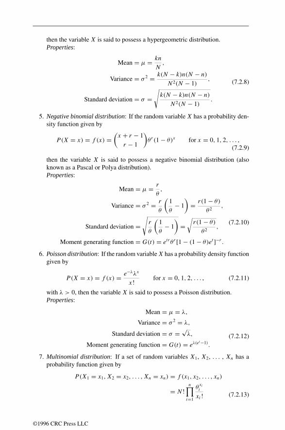
then the variable X is said to possess a hypergeometric distribution.Properties:
Mean = µ = kn
N,
Variance = σ 2 = k(N − k)n(N − n)
N2(N − 1),
Standard deviation = σ =√k(N − k)n(N − n)
N2(N − 1).
(7.2.8)
5. Negative binomial distribution: If the random variable X has a probability den-sity function given by
P(X = x) = f (x) =(x + r − 1
r − 1
)θr(1− θ)x for x = 0, 1, 2, . . . ,
(7.2.9)
then the variable X is said to possess a negative binomial distribution (alsoknown as a Pascal or Polya distribution).Properties:
Mean = µ = r
θ,
Variance = σ 2 = r
θ
(1
θ− 1
)= r(1− θ)
θ2,
Standard deviation =√r
θ
(1
θ− 1
)=√r(1− θ)
θ2,
Moment generating function = G(t) = etrθ r [1− (1− θ)et ]−r .
(7.2.10)
6. Poisson distribution: If the random variableX has a probability density functiongiven by
P(X = x) = f (x) = e−λλx
x!for x = 0, 1, 2, . . . , (7.2.11)
with λ > 0, then the variable X is said to possess a Poisson distribution.Properties:
Mean = µ = λ,
Variance = σ 2 = λ,
Standard deviation = σ =√λ,
Moment generating function = G(t) = eλ(et−1).
(7.2.12)
7. Multinomial distribution: If a set of random variables X1, X2, . . . , Xn has aprobability function given by
P(X1 = x1, X2 = x2, . . . , Xn = xn) = f (x1, x2, . . . , xn)
= N!n∏
i=1
θxii
xi! (7.2.13)
©1996 CRC Press LLC
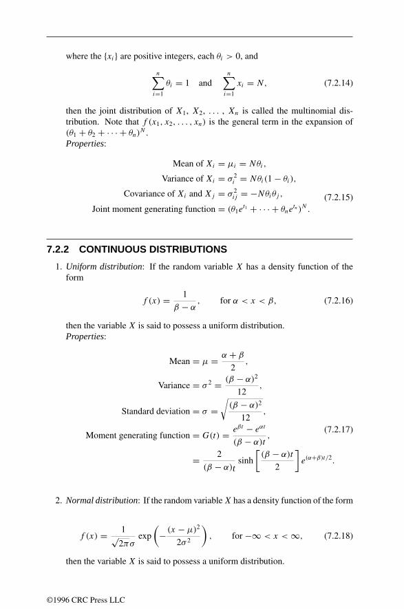
where the xi are positive integers, each θi > 0, and
n∑i=1
θi = 1 andn∑
i=1
xi = N, (7.2.14)
then the joint distribution of X1, X2, . . . , Xn is called the multinomial dis-tribution. Note that f (x1, x2, . . . , xn) is the general term in the expansion of(θ1 + θ2 + · · · + θn)
N .Properties:
Mean of Xi = µi = Nθi,
Variance of Xi = σ 2i = Nθi(1− θi),
Covariance of Xi and Xj = σ 2ij = −Nθiθj ,
Joint moment generating function = (θ1et1 + · · · + θne
tn )N .
(7.2.15)
7.2.2 CONTINUOUS DISTRIBUTIONS
1. Uniform distribution: If the random variable X has a density function of theform
f (x) = 1
β − α, for α < x < β, (7.2.16)
then the variable X is said to possess a uniform distribution.Properties:
Mean = µ = α + β
2,
Variance = σ 2 = (β − α)2
12,
Standard deviation = σ =√(β − α)2
12,
Moment generating function = G(t) = eβt − eαt
(β − α)t,
= 2
(β − α)tsinh
[(β − α)t
2
]e(α+β)t/2.
(7.2.17)
2. Normal distribution: If the random variableX has a density function of the form
f (x) = 1√2πσ
exp
(− (x − µ)2
2σ 2
), for −∞ < x <∞, (7.2.18)
then the variable X is said to possess a uniform distribution.
©1996 CRC Press LLC

Properties:
Mean = µ,
Variance = σ 2,
Standard deviation = σ,
Moment generating function = G(t) = exp
(µt + σ 2t2
2
).
(7.2.19)
• Set y = x−µσ
to obtain a standard normal distribution.
• The cumulative distribution function is
F(x) = ?(x) = 1√2πσ
∫ x
−∞exp
(− (t − µ)2
2σ 2
)dt .
3. Multidimensional normal distribution:The random vector X is said to be multivariate normalif and only if the linearcombination aTX is normal for all vectors a. If the mean of X is µµµ, and if thesecond moment matrix R = E
[(X−µµµ)(X−µµµ)T
]is nonsingular, the density
function of X is
p(x) = 1
(2π)n/2√
detRexp
[−1
2(x−µµµ)TR−1(x−µµµ)
].
(7.2.20)
Sometimes integrals of the form In =∞∫· · ·
∫−∞
(xTMx
)np(x) dx are desired.
Defining ak = tr (MR)k , we find:
I0 = 1,
I1 = a1,
I2 = a21 + 2a2,
I3 = a31 + 6a1a2 + 8a3,
I4 = a41 + 12a2
1a2 + 32a1a3 + 12a22 + 48a4.
(7.2.21)
4. Gamma distribution: If the random variable X has a density function of theform
f (x) = 1
:(1+ α)β1+α xαe−x/β, for 0 < x <∞, (7.2.22)
with α > −1 and β > 0, then the variable X is said to possess a gammadistribution.Properties:
Mean = µ = β(1+ α),
Variance = σ 2 = β2(1+ α),
Standard deviation = σ = β√
1+ α
Moment generating function = G(t) = (1− βt)−1−α, for t < β−1.
(7.2.23)
©1996 CRC Press LLC

5. Exponential distribution: If the random variable X has a density function of theform
f (x) = e−x/θ
θ, for 0 < x <∞, (7.2.24)
where θ > 0, then the variable X is said to possess an exponential distribution.Properties:
Mean = µ = θ,
Variance = σ 2 = θ2,
Standard deviation = σ = θ,
Moment generating function = G(t) = (1− θt)−1.
(7.2.25)
6. Beta distribution: If the random variable X has a density function of the form
f (x) = :(α + β + 2)
:(1+ α):(1+ β)xα(1− x)β, for 0 < x < 1,
(7.2.26)
where α > −1 and β > −1, then the variable X is said to possess a betadistribution.Properties:
Mean = µ = 1+ α
2+ α + β,
Variance = σ 2 = (1+ α)(1+ β)
(2+ α + β)2(3+ α + β),
r th moment about the origin = νr = :(2+ α + β):(1+ α + r)
:(2+ α + β + r):(1+ α).
(7.2.27)
7. Chi-square distribution: If the random variable X has a density function of theform
f (x) = x(n−2)/2e−x/2
2n/2:(n/2)for 0 < x <∞ (7.2.28)
then the variableX is said to possess a chi-square (χ2) distribution withn degreesof freedom.Properties:
Mean = µ = n,
Variance = σ 2 = 2n.(7.2.29)
(a) IfY1, Y2, . . . , Yn are independent and identically distributed normal random
variables with a mean of 0 and a variance of 1, then χ2 =n∑
i=1
Y 2i is
distributed as chi-square with n degrees of freedom.
©1996 CRC Press LLC

(b) If χ21 , χ2
2 , . . . , χ2k , are independent random variables and have chi-square
distributions with n1, n2, . . . , nk degrees of freedom, then∑k
i=1 χ2i has a
chi-squared distribution with n =∑ki=1 ni degrees of freedom.
8. Snedecor’sF -distribution: If the random variable X has a density function ofthe form
f (x) = :(n+m
2
) (mn
)m/2x(m−2)/2
:(m2
):(n2
) (1+ m
nx)(n+m)/2
, for 0 < x <∞, (7.2.30)
then the variable X is said to possess a F -distribution with m and n degrees offreedom.Properties:
Mean = µ = n
n− 2, for n > 2,
Variance = 2n2(m+ n− 2)
m(n− 2)2(n− 4), for n > 4. (7.2.31)
(a) The transformation w = mx/n
1+ mxn
transforms the F -density to the beta
density.
(b) If the random variable X has a χ2-distribution with m degrees of freedom,the random variable Y has a χ2-distribution with n degrees of freedom,
and X and Y are independent, then F = X/m
Y/nis distributed as an F -
distribution with m and n degrees of freedom.
9. Student’st-distribution: If the random variable X has a density function of theform
f (x) = :(n+1
2
)√nπ:
(n2
) (1+ t2
n
)(n+1)/2, for −∞ < x <∞. (7.2.32)
then the variable X is said to possess a t-distribution with n degrees of freedom.
Properties:
Mean = µ = 0,
Variance = σ 2 = n
n− 2, for n > 2.
(7.2.33)
• If the random variable X is normally distributed with mean 0 and varianceσ 2, and if Y 2/σ 2 has a χ2 distribution with n degrees of freedom, and if
X and Y are independent, then t = X√n
Yis distributed as a t-distribution
with n degrees of freedom.
©1996 CRC Press LLC

7.3 QUEUING THEORY
A queue is represented as A/B/c/K/m/Z where
• A and B represent the interarrival times and service times:
GI general independent interarrival time,G general service time distribution,Hk k-stage hyperexponential interarrival or service time distribution,Ek Erlang-k interarrival or service time distribution,M exponential interarrival or service time distribution,D deterministic (constant) interarrival or service time distribution.
• c is the number of identical servers.
• K is the system capacity.
• m is the number in the source.
• Z is the queue discipline:
FCFS first come, first served (also known as FIFO),LIFO last in, first out,RSS random,PRI priority service.
When not all variables are present, the trailing ones have the default values, K = ∞,m = ∞, Z is RSS.
The variable of concern are
1. an: proportion of customers that find n customers already in the system whenthey arrive
2. dn: proportion of customers leaving behind n customers in the system
3. pn: proportion of time the system contains n customers
4. L: average number of customers in the system
5. LQ: average number of customers in the queue
6. W : average time for customer in system
©1996 CRC Press LLC

7. WQ: average time for customer in the queue
8. λ: average arrival rate of customers to the system (number per unit time)
9. µ: average service rate per server (number per unit time)
10. u: traffic intensity, u = λ/µ
11. ρ: server utilization, the probability that any particular server is busy, ρ =u/c = (λ/µ)/c
Theorems:
1. Little’s formula: L = λW and LQ = λWQ .
2. For Poisson arrivals: pn = an.
3. If customers arrive one at a time and are served one at a time: an = dn.
4. For an M/M/1 queue with λ < µ,
• pn = (1− u)un
• L = u/(1− u)
• LQ = L− (1− p0)
• LQ = u2/(1− u)
• W = 1/(µ− λ)
• WQ = λ/µ(µ− λ)
5. For an M/M/c queue (so that µn = nµ for n = 1, 2, . . . , c and µn = cµ forn ≥ c),
• p0 =[
uc
c!(1− ρ)+
c−1∑n=0
un
n!
]−1
• pn = p0un/n! for n = 0, 1, . . . , c
• pn = p0un/c!cn−c for n ≥ c
• LQ = p0ucρ/c!(1− ρ)2
• WQ = LQ/λ
• W = WQ + 1/µ
• L = λW
©1996 CRC Press LLC

7.4 MARKOV CHAINS
A discrete parameter stochastic processis a collection of random variables X(t), t =0,1,2,. . . . The values of X(t) are called the statesof the process. The collection ofstates is called the state space. The values of t usually represent points in time. Thenumber of states is either finite or countably infinite. A discrete parameter stochasticprocess is called a Markov chainif, for any set of n time points t1 < t2 < · · · < tn, theconditional distribution of X(tn) given values for X(t1), X(t2), . . . , X(tn−1) dependsonly on X(tn−1). It is expressed by
P[X(tn) ≤ xn | X(t1) = x1, . . . , X(tn−1) = xn−1
]= P
[X(tn) ≤ xn | X(tn−1) = xn−1
]. (7.4.1)
A Markov chain is said to be stationary if the value of the conditional probabil-ity P
[X(tn+1) = xn+1|X(tn) = xn
]is independent of n. This discussion will be
restricted to stationary Markov chains.
7.4.1 TRANSITION FUNCTION
Let x and y be states and let tn be time points in T = 0, 1, 2, . . . . The transitionfunction, P(x, y), is defined by
P(x, y) = Pn,n+1(x, y) = P[X(tn+1) = y | X(tn) = x
], tn, tn+1 ∈ T .
(7.4.2)
P(x, y) is the probability that a Markov chain in state x at time n will be in state yat time n + 1. Some properties of the transition function are that P(x, y) ≥ 0 and∑
y P (x, y) = 1. The values of P(x, y) are commonly called the one-step transitionprobabilities.
The function π0(x) = P(X(0) = x), with π0(x) ≥ 0 and∑
x π0(x) = 1 iscalled the initial distribution of the Markov chain. It is the probability distributionwhen the chain is started. Thus,
P [X(0) = x0, X(1) = x1, . . . , X(n) = xn]
= π0(x0)P0,1(x0, x1)P1,2(x1, x2) · · ·Pn−1,n(xn−1, xn). (7.4.3)
7.4.2 TRANSITION MATRIX
A convenient way to summarize the transition function of a Markov chain is by usingthe one-step transition matrix. It is defined as
P =
P(0, 0) P (0, 1) . . . P (0, n) . . .
P (1, 0) P (1, 1) . . . P (1, n) . . ....
.... . .
...
P (n, 0) P (n, 1) . . . P (n, n) . . ....
......
.
©1996 CRC Press LLC
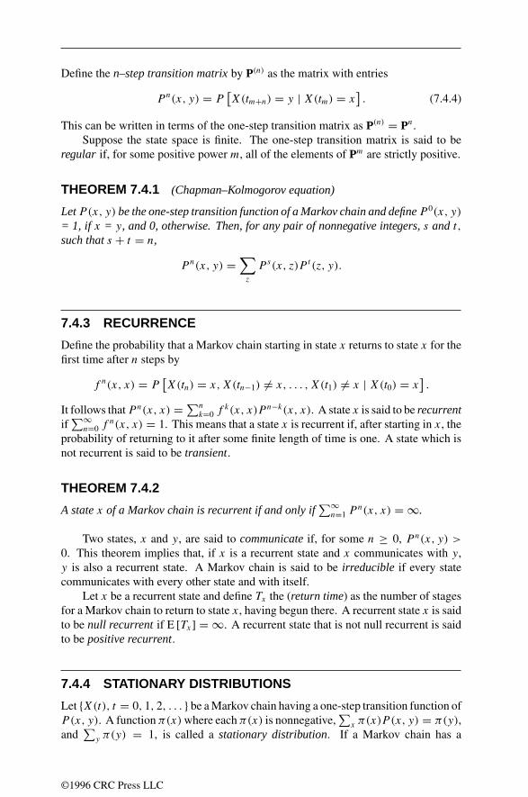
Define the n–step transition matrixby P(n) as the matrix with entries
Pn(x, y) = P[X(tm+n) = y | X(tm) = x
]. (7.4.4)
This can be written in terms of the one-step transition matrix as P(n) = Pn.Suppose the state space is finite. The one-step transition matrix is said to be
regular if, for some positive power m, all of the elements of Pm are strictly positive.
THEOREM 7.4.1 (Chapman–Kolmogorov equation)
LetP(x, y) be the one-step transition function of a Markov chain and defineP 0(x, y)
= 1, if x = y, and 0, otherwise. Then, for any pair of nonnegative integers,s and t,such thats + t = n,
Pn(x, y) =∑z
P s(x, z)P t (z, y).
7.4.3 RECURRENCE
Define the probability that a Markov chain starting in state x returns to state x for thefirst time after n steps by
f n(x, x) = P[X(tn) = x,X(tn−1) = x, . . . , X(t1) = x | X(t0) = x
].
It follows thatPn(x, x) =∑nk=0 f
k(x, x)P n−k(x, x). A state x is said to be recurrentif∑∞
n=0 fn(x, x) = 1. This means that a state x is recurrent if, after starting in x, the
probability of returning to it after some finite length of time is one. A state which isnot recurrent is said to be transient.
THEOREM 7.4.2
A statex of a Markov chain is recurrent if and only if∑∞
n=1 Pn(x, x) = ∞.
Two states, x and y, are said to communicateif, for some n ≥ 0, Pn(x, y) >
0. This theorem implies that, if x is a recurrent state and x communicates with y,y is also a recurrent state. A Markov chain is said to be irreducible if every statecommunicates with every other state and with itself.
Let x be a recurrent state and define Tx the (return time) as the number of stagesfor a Markov chain to return to state x, having begun there. A recurrent state x is saidto be null recurrentif E [Tx] = ∞. A recurrent state that is not null recurrent is saidto be positive recurrent.
7.4.4 STATIONARY DISTRIBUTIONS
Let X(t), t = 0, 1, 2, . . . be a Markov chain having a one-step transition function ofP(x, y). A function π(x)where each π(x) is nonnegative,
∑x π(x)P (x, y) = π(y),
and∑
y π(y) = 1, is called a stationary distribution. If a Markov chain has a
©1996 CRC Press LLC

stationary distribution and limn→∞ Pn(x, y) = π(y), then, regardless of the initialdistribution, π0(x), the distribution of X(tn) approaches π(x) as n becomes infinite.When this happens, π(x) is often referred to as the steady state distribution. Thefollowing categorizes those Markov chains with stationary distributions.
THEOREM 7.4.3
LetXP denote the set of positive recurrent states of a Markov chain.
1. If XP is empty, the chain has no stationary distribution.
2. If XP is a nonempty irreducible set, the chain has a unique stationarydistribution.
3. IfXP is nonempty but not irreducible, the chain has an infinite number of distinctstationary distributions.
The period of a state x is denoted by d(x) and is defined as the greatest commondivisor of all integers, n ≥ 1, for which Pn(x, x) > 0. If Pn(x, x) = 0 for alln ≥ 1, then define d(x) = 0. If each state of a Markov chain has d(x) = 1, thechain is said to be aperiodic. If each state has period d > 1, the chain is said to beperiodicwith period d. The vast majority of Markov chains encountered in practiceare aperiodic. An irreducible, positive recurrent, aperiodic Markov chain alwayspossesses a steady-state distribution. An important special case occurs when the statespace is finite. Suppose that X = 1, 2, . . . , K. Let π0 = π0(1), π0(2), . . . , π0(K).
THEOREM 7.4.4
Let P be a regular one-step transition matrix andπ0 be an arbitrary vector of initialprobabilities. Thenlimn→∞ π0(x) Pn = y, whereyP = y, and
∑Ki=1 π0(ti) = 1.
A simple three-state Markov chain
A Markov chain having three states 0, 1, 2 with a one-step transition matrix of
P = 1
2 0 12
14
34 0
0 34
14
is diagrammed below.
0
1
2
3/4
3/4
1/4
1/21/2
1/4
©1996 CRC Press LLC

The one-step transition matrix gives a two–step transition matrix of
P (2) = P 2 =
14
38
38
516
916
18
316
916
18
The one-step transition matrix is regular. This Markov chain is irreducible, and allthree states are recurrent. In addition, all three states are positive recurrent. Since allstates have period 1, the chain is aperiodic. The steady state distribution is π(0) =3/11, π(1) = 6/11, and π(2) = 2/11.
7.4.5 RANDOM WALKS
Let η(t1), η(t2), . . . be independent random variables having a common density f (x),and let t1, t2, . . . be integers. Let X(t0) be an integer–valued random variable thatis independent of η(t1), η(t2), . . . , and X(tn) = X0 +
∑ni=1 η(ti). The sequence
X(ti), i = 0, 1, . . . is called a random walk. An important special case is a simplerandom walk. It is defined by
P(x, y) =
p, if y = x − 1,
r, if y = x,
q, if y = x + 1,
where p+q+r = 1, and P(0, 0) = p+r.
Here, an object begins at a certain point in a lattice and at each step either stays at thatpoint or moves to a neighboring lattice point. In the case of a one- or two-dimensionallattice, it turns out that, if a random walk begins at a lattice point x, it will return tothat point with probability 1. In the case of a three-dimensional lattice, the probabilitythat it will return to its starting point is only about 0.3405.
7.4.6 EHRENFEST CHAIN
A simple model of gas exchange between two isolated bodies is as follows. Supposethat there are two boxes, Box I and Box II, where Box I contains K moleculesnumbered 1, 2, . . . , K and Box II contains N −K molecules numbered K + 1,K +2, . . . , N . A number is chosen at random from 1, 2, . . . , N, and the molecule withthat number is transferred from its box to the other one. Let X(tn) be the numberof molecules in Box I after n trials. Then the sequence X(tn), n = 0, 1, . . . is aMarkov chain with one-stage transition function of
P(x, y) =
xK, y = x − 1,
1− xK, y = x + 1,
0, otherwise.
©1996 CRC Press LLC

7.5 RANDOM NUMBER GENERATION
7.5.1 METHODS OF PSEUDORANDOM NUMBER GENERATION
Depending on the application, either integers in some range or floating point numbersin [0, 1) are the desired output from a pseudorandom number generator (PRNG). Sincemost PRNGs use integer recursions, a conversion into integers in a desired range orinto a floating point number in [0, 1) is required. If xn is an integer produced by somePRNG in the range 0 ≤ xn ≤ M − 1, then an integer in the range 0 ≤ xn ≤ N − 1,with N ≤ M , is given by yn =
⌊NxnM
⌋. If N M , then yn = xn (mod N) may be
used. Alternately, if a floating point value in [0, 1) is desired, let yn = xn/M .
Linear congruential generatorsPerhaps the oldest generator still in use is the linear congruential generator (LCG).The underlying integer recursion for LCGs is
xn = axn−1 + b (mod M). (7.5.1)
Equation (7.5.1) defines a periodic sequence of integers modulo M starting with x0,the initial seed. The constants of the recursion are referred to as the modulusM ,multiplier a, and additive constantb. If M = 2m, a very efficient implementation ispossible. Alternately, there are theoretical reasons why choosing M prime is optimal.Hence, the only moduli that are used in practical implementations are M = 2m orthe prime M = 2p − 1 (i.e., M is a Mersenne prime). With a Mersenne prime,modular multiplication can be implemented at about twice the computational cost ofmultiplication modulo 2p.
Equation (7.5.1) yields a sequence xn whose period, denoted Per(xn), dependson M , a, and b. The values of the maximal period for the three most common casesused and the conditions required to obtain them are
a b M Per(xn)Primitive root of M Anything Prime M − 1
3 or 5 (mod 8) 0 2m 2m−2
1 (mod 4) 1 (mod 2) 2m 2m
A major shortcoming of LCGs modulo a power-of-two compared with primemodulus LCGs derives from the following theorem for LCGs:
THEOREM 7.5.1
Define the following LCG sequence:xn = axn−1 + b (mod M1). If M2 dividesM1
thenyn = xn (mod M2) satisfiesyn = ayn−1 + b (mod M2).
Theorem 7.5.1 implies that the k least-significant bits of any power-of-two modulusLCG with Per(xn) = 2m = M has Per(yn) = 2k , 0 < k ≤ m. Since a long period is
©1996 CRC Press LLC

crucial in PRNGs, when these types of LCGs are employed in a manner that makesuse of only a few least-significant-bits, their quality may be compromised. When M
is prime, no such problem arises.Since LCGs are in such common usage, here is a list of parameter values men-
tioned in the literature. The Park–Miller LCG is widely considered a minimallyacceptable PRNG.
a b M Source
75 0 231 − 1 Park–Miller131 0 235 Neave
16333 25887 215 Oakenfull3432 6789 9973 Oakenfull171 0 30269 Wichman–Hill
Shift register generatorsAnother popular method of generating pseudorandom numbers is using binary shiftregister sequences to produce pseudorandom bits. A binary shift register sequence(SRS) is defined by a binary recursion of the type,
xn = xn−j1 ⊕ xn−j2 ⊕ · · · ⊕ xn−jk , j1 < j2 < · · · < jk = J, (7.5.2)
where⊕ is the exclusive “or” operation. Note that x⊕y ≡ x+y (mod 2). Thus thenew bit, xn, is produced by adding k previously computed bits together modulo 2. Theimplementation of this recurrence requires keeping the last J bits from the sequencein a shift register, hence the name. The longest possible period is equal to the numberof nonzero J-dimensional binary vectors, namely 2J − 1.
A sufficient condition for achieving Per(xn) = 2J − 1 is that the characteristicpolynomial, corresponding to Equation (7.5.2), be primitive modulo 2. Since prim-itive trinomials of nearly all degrees of interest have been found, SRSs are usuallyimplemented using two-term recursions of the form,
xn = xn−k ⊕ xn−J, 0 < k < J. (7.5.3)
In these two-term recursions, k is the lag and J is the register length. Proper choiceof the pair (J, k) leads to SRSs with Per(xn) = 2J − 1. Here is a list with suitable(J, k) pairs:
Primitive trinomial exponents(5,2) (7,1) (7,3) (17,3) (17,5) (17,6)
(31,3) (31,6) (31,7) (31,13 (127,1) (521,32)
Lagged-Fibonacci generatorsAnother way of producing pseudorandom numbers uses lagged-Fibonacci generators.The term “lagged-Fibonacci” refers to two-term recurrences of the form,
xn = xn−k xn−J, 0 < k < J, (7.5.4)
©1996 CRC Press LLC

where refers to three common methods of combination: (1) addition modulo 2m,(2) multiplication modulo 2m, or (3) bitwise exclusive ‘OR’ing of m-long bit vectors.Combination method (3) can be thought of as a special implementation of a two-termSRS.
Using combination method (1) leads to additive lagged-Fibonacci sequences(ALFSs). If xn satisfies
xn = xn−k + xn−J (mod 2m), 0 < k < J, (7.5.5)
then the maximal period is Per(xn) = (2J − 1)2m−1.ALFS are especially suitable for producing floating point deviates using the real-
valued recursion yn = yn−k + yn−J (mod 1). This circumvents the need to convertfrom integers to floating point values and allows floating point hardware to be used.One caution with ALFS is that Theorem 7.5.1 holds, and so the low-order bits haveperiods that are shorter than the maximal period. However, this is not nearly theproblem as in the LCG case. With ALFSs, the j least-significant bits will have period(2J − 1)2j−1, so, if J is large, there really is no problem. Note that one can use thetable of primitive trinomial exponents to find (J, k) pairs that give maximal periodALF sequences.
7.5.2 GENERATING NONUNIFORM RANDOM VARIABLES
Suppose we want deviates from a distribution with probability density function f (x)and distribution function F(x) = ∫ x
−∞ f (u) du. In the following y is U [0, 1) meansy is uniformly distributed on [0, 1).
Two general techniques for converting uniform random variables into those fromother distributions are as follows:
1. The inverse transform method:If y is U [0, 1), then the random variable F−1(y) will have its density equal tof (x) (since 0 ≤ F(x) ≤ 1).
2. The acceptance-rejection method:Suppose the density can be written as f (x) = Ch(x)g(x) where h(x) is thedensity of a computable random variable, the function 0 < g(x) ≤ 1, andC−1 = ∫∞
−∞ h(u)g(u) du is a normalization constant. If x is U [0, 1), y hasdensity h(x), and if x < g(y), then x has density f (x). Thus one generates x,y pairs, rejecting both if x ≥ g(y) and returning x if x < g(y).
Examples of the inverse transform method:
1. (Exponential distribution) The exponential distribution with rate λ is f (x) =λe−λx (for x ≥ 0) and F(x) = 1 − e−λx . Thus u = F(x) can be solved togive x = F−1(u) = −λ−1 ln(1 − u). If u is U [0, 1), then so is 1 − u. Hencex = −λ−1 ln u is exponentially distributed with rate λ.
2. (Normal distribution) Let zi be normally distributed with f (z) = 1√2πe−z
2/2.If each of the pair (z1, z2) is normally distributed, then the polar transfor-
mation gives random variables r =√z2
1 + z22 (exponentially distributed with
©1996 CRC Press LLC

λ = 2) and θ = tan−1(z2/z1) (uniformly distributed on [0, 2π)). Inverting,z1 =
√−2 ln x1 cos 2πx2 and z2 =√−2 ln x1 sin 2πx2 are normally distributed
when x1 and x2 are U [0, 1).
Examples of the rejection method:
1. (Exponential distribution with λ = 1)
(a) Generate random numbers UiNi=1 uniform on [0, 1]), stopping at N =minn | U1 ≥ U2 ≥ Un−1 < Un.
(b) If N is even, accept that run, and go to step (c). If N is odd reject the run,and return to step (a).
(c) Set X equal to the number of failed runs plus the first random number inthe successful run.
2. (Normal distribution)
(a) Select two random variables (V1, V2) from U [0, 1). Form R = V 21 + V 2
2 .
(b) If R > 1, then reject the (V1, V2) pair, and select another pair.
(c) If R < 1, then x = V1
√−2
lnR
Rhas a N(0, 1) distribution.
3. (Normal distribution)
(a) Select two exponentially distributed random variables with rate 1: (V1, V2).
(b) If V2 ≥ (V1 − 1)2/2, then reject the (V1, V2) pair, and select another pair.
(c) Otherwise, V1 has a N(0, 1) distribution.
4. (Cauchy distribution) To generate values of X from f (x) = 1π(1+x2)
on −∞ <
x <∞,
(a) Generate random numbersU1,U2 (uniform on [0, 1)), and set Y1 = U1− 12 ,
Y2 = U2 − 12 .
(b) If Y 21 + Y 2
2 ≤ 14 , then return X = Y1/Y2. Otherwise return to step (a).
To generate values of X from a Cauchy distribution with parameters β and θ ,
f (x) = β
π[β2 + (x − θ)2
] , for−∞ < x <∞, construct X as above, and then
use βX + θ .
Discrete random variablesIn general, the density function of a discrete random variable can be represented asa vector p = (p0, p1, . . . , pn−1, pn) by defining the probabilities P(x = j) = pj
(for j = 0, . . . , n). The distribution function can be defined by the vector c =(c0, c1, . . . , cn−1, 1), where cj =
∑j
i=0 pi . Given this representation of F(x), wecan apply the inverse transform by computing x to be U [0, 1), and then finding theindex j so that cj ≤ x < cj+1. In this case event j will have occurred. Examples:
©1996 CRC Press LLC
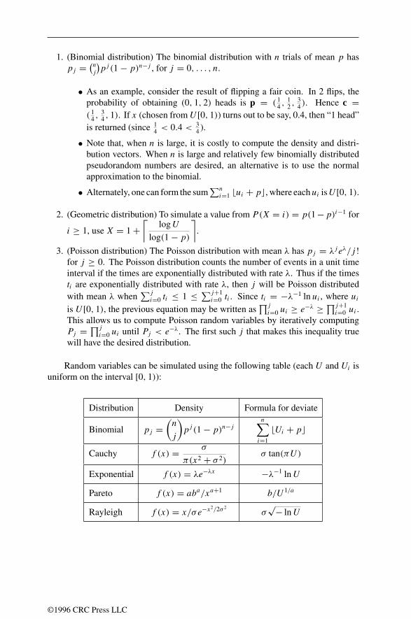
1. (Binomial distribution) The binomial distribution with n trials of mean p haspj =
(n
j
)pj (1− p)n−j , for j = 0, . . . , n.
• As an example, consider the result of flipping a fair coin. In 2 flips, theprobability of obtaining (0, 1, 2) heads is p = ( 1
4 ,12 ,
34 ). Hence c =
( 14 ,
34 , 1). If x (chosen from U [0, 1)) turns out to be say, 0.4, then “1 head”
is returned (since 14 < 0.4 <
34 ).
• Note that, when n is large, it is costly to compute the density and distri-bution vectors. When n is large and relatively few binomially distributedpseudorandom numbers are desired, an alternative is to use the normalapproximation to the binomial.
• Alternately, one can form the sum∑n
i=1 ui + p, where eachui isU [0, 1).
2. (Geometric distribution) To simulate a value from P(X = i) = p(1−p)i−1 for
i ≥ 1, use X = 1+⌈
logU
log(1− p)
⌉.
3. (Poisson distribution) The Poisson distribution with mean λ has pj = λjeλ/j !for j ≥ 0. The Poisson distribution counts the number of events in a unit timeinterval if the times are exponentially distributed with rate λ. Thus if the timesti are exponentially distributed with rate λ, then j will be Poisson distributedwith mean λ when
∑j
i=0 ti ≤ 1 ≤ ∑j+1i=0 ti . Since ti = −λ−1 ln ui , where ui
is U [0, 1), the previous equation may be written as∏j
i=0 ui ≥ e−λ ≥ ∏j+1i=0 ui .
This allows us to compute Poisson random variables by iteratively computingPj =
∏j
i=0 ui until Pj < e−λ. The first such j that makes this inequality truewill have the desired distribution.
Random variables can be simulated using the following table (each U and Ui isuniform on the interval [0, 1)):
Distribution Density Formula for deviate
Binomial pj =(n
j
)pj (1− p)n−j
n∑i=1
Ui + p
Cauchy f (x) = σ
π(x2 + σ 2)σ tan(πU)
Exponential f (x) = λe−λx −λ−1 lnU
Pareto f (x) = aba/xa+1 b/U 1/a
Rayleigh f (x) = x/σe−x2/2σ 2
σ√− lnU
©1996 CRC Press LLC

Testing pseudorandom numbersThe prudent way to check a complicated computation that makes use of pseudorandomnumbers is to run it several times with different types of pseudorandom numbergenerators and see if the results appear consistent across the generators. The factthat this is not always possible or practical has led researchers to develop statisticaltests of randomness that should be passed by general purpose pseudorandom numbergenerators. Some common tests are the spectral test, the equidistribution test, theserial test, the runs test, the coupon collector test, and the birthday spacing test.
7.6 CONTROL CHARTS
Control charts are graphical tools used to assess and maintain the stability of a process.They are used to separate random variation from specific causes. Data measurementsare plotted versus time along with upper and lower control limits and a center line.If the process is in control and the underlying distribution is normal, then the controllimits represent three standard deviations from the center line (mean).
If all of the data points are contained within the control limits, the process isconsidered stable and the mean and standard deviations can be reliably calculated. Thevariations between data points occur from random causes. Data outside the controllimits or forming abnormal patterns point to unstable, out-of-control processes.
In the tables, k denotes the number of samples taken, i is an index for the samples(i = 1 . . . k), n is the sample size (number of elements in each sample), and R is therange of the values in a sample (maximum element value minus minimum elementvalue). The mean is µ and the standard deviation is σ . Control chart upper and lowercontrol limits are denoted UCL and LCL.
©1996 CRC Press LLC

Types of Control Charts, Their Statistics, and UsesChart Statistics Statistical quantity
Applicationsx − R Gaussian Average value and range
Charts continuous measurable quantities. Measurements taken onsmall sample sets.
x − R Gaussian Median value and rangeSimilar to x−R chart but fewer calculations needed for plotting.
x − Rs Gaussian Individual measured valuesSimilar to x − R chart but single measurements are made. Usedwhen measurements are expensive or dispersion of measuredvalues is small. Rs = |xi − xi−1|
pn Binomial Number of defective unitsCharts number of defective units in sets of fixed size.
p Binomial Percent defectiveCharts number of defective units in sets of varying size.
c Poisson Number of defectsCharts number of flaws in a product of fixed size.
u Poisson Defect density (defects per quantity unit)Charts the defect density on a product of varying size.
Types of Control Charts and Limits (“P ” stands for parameter)
Chart(µ, σ )
known?P Centerline UCL LCL
x − R No x ¯x =∑
x
k¯x + A2R ¯x − A2R
x − R No R R =∑
R
kD4R D3R
x − R Yes x ¯x = µ µ+ 3σ√n
µ− 3σ√n
x − R Yes R R = d2σ D2σ D1σ
x − R No x ¯x =∑
x
kx +m3A2 x −m3A2
x − R No R R =∑
R
kD4R D3R
x − Rs No x x =∑
x
kx + 2.66Rs x − 2.66Rs
x − Rs No Rs Rs =∑
Rs
k3.27Rs –
pn No pn pn =∑
pn
kpn+√pn(1− p) pn−√pn(1− p)
p No p p =∑
pn∑n
pn+ 3√
p(1−p)n
pn− 3√
p(1−p)n
c No c c =∑
c
kc + 3
√c c − 3
√c
u No u u =∑
c∑n
u+ 3√u/n u− 3
√u/n
©1996 CRC Press LLC

Sample size n A2 d2 D1 D2 D3 D4 m3 m3A2
2 1.880 1.128 0 3.686 – 3.267 1.000 1.8803 1.023 1.693 0 4.358 – 2.575 1.160 1.1874 0.729 2.059 0 4.698 – 2.282 1.092 0.7965 0.577 2.326 0 4.918 – 2.115 1.198 0.6916 0.483 2.534 0 5.078 – 2.004 1.135 0.5497 0.419 2.704 0.205 5.203 0.076 1.924 1.214 0.5098 0.373 2.847 0.387 5.307 0.136 1.864 1.160 0.4329 0.337 2.970 0.546 5.394 0.184 1.816 1.223 0.412
10 0.308 3.078 0.687 5.469 0.223 1.777 1.176 0.36311 0.285 3.173 0.812 5.534 0.256 1.74412 0.266 3.258 0.924 5.592 0.284 1.71613 0.249 3.336 1.026 5.646 0.308 1.69214 0.235 3.407 1.121 5.693 0.329 1.67115 0.223 3.472 1.207 5.737 0.348 1.65216 0.212 3.532 1.285 5.779 0.364 1.63617 0.203 3.588 1.359 5.817 0.379 1.62118 0.194 3.640 1.426 5.854 0.392 1.60819 0.187 3.689 1.490 5.888 0.404 1.59620 0.180 3.735 1.548 5.922 0.414 1.58621 0.173 3.778 1.605 5.951 0.425 1.57522 0.167 3.819 1.659 5.979 0.434 1.56623 0.162 3.858 1.710 6.006 0.443 1.55724 0.157 3.895 1.759 6.031 0.452 1.54825 0.153 3.931 1.806 6.056 0.459 1.541
Abnormal Distributions of Points in Control ChartsAbnormality DescriptionSequence Seven or more consecutive points on one side of the
center line. Denotes the average value has shifted.Bias Fewer than seven consecutive points on one side of the
center line, but most of the points are on that side.
• 10 of 11 consecutive points
• 12 or more of 14 consecutive points
• 14 or more of 17 consecutive points
• 16 or more of 20 consecutive points
Trend Seven or more consecutive rising or falling points.Approaching the limit Two out of three or three or more out of seven
consecutive points are more than two-thirds thedistance between the center line and a control limit.
Periodicity The data points vary in a regular periodic pattern.
©1996 CRC Press LLC

7.7 STATISTICS
7.7.1 DESCRIPTIVE STATISTICS
1. Sample distribution and density functions
• Sample distribution function:
F (x) = 1
n
n∑i=1
u(x − xi) (7.7.1)
where u(x) be the unit step function defined by u(x) = 0 for x ≤ 0 andu(x) = 1 for x > 0.
• Sample density function or histogram:
f (x) = F (x0 + (i + 1)w)− F (x0 + iw)
w(7.7.2)
for x ∈ [x0+ iw, x0+ (i+ 1)w). The interval [x0+ iw, x0+ (i+ 1)w) iscalled the i th bin,w is the bin width, andfi = F (x0+(i+1)w)−F (x0+iw)is the bin frequency.
2. Order statistics and quantiles
• Order statistics are obtained by arranging the sample values x1, x2, . . . , xnin increasing order, denoted by
x(1) ≤ x(2) ≤ · · · ≤ x(n). (7.7.3)
(a) x(1) and x(n) are the minimum and maximum data values, respectively.
(b) For i = 1, . . . , n, x(i) is called the i th order statistic.
• Quantiles: If 0 < p < 1, then the quantile of order p, ξp, is given bythe p(n + 1)th order statistic. It may be necessary to interpolate betweensuccessive values.
(a) If p = j/4 for j = 1, 2, or 3, then ξ j
4is called the j th quartile.
(b) If p = j/10 for j = 1, 2, . . . , 9, then ξ j
10is called the j th decile.
(c) If p = j/100 for j = 1, 2, . . . , 99, then ξ j
100is called the j th
percentile.
3. Measures of central tendency
• Arithmetic mean:
x = 1
n
n∑i=1
xi = x1 + x2 + · · · + xn
n. (7.7.4)
©1996 CRC Press LLC

• α-trimmed mean:
xα = 1
n(1− 2α)
((1− r)
(x(k+1) + x(n−k)
)+ n−k−1∑i=k+2
x(i)
),
(7.7.5)
where k = αn is the greatest integer less than or equal to αn, andr = αn− k. If α = 0 then xα = x.
• Weighted mean: If to each xi is associated a weight wi ≥ 0 so that
n∑i=1
wi = 1, then xw =n∑
i=1
wixi.
• Geometric mean:
G.M. =(
n∏i=1
xi
) 1n
= (x1x2 · · · xn) 1n . (7.7.6)
• Harmonic mean:
H.M. = n∑ni=1
1xi
= n1x1+ 1
x2+ · · · + 1
xn
. (7.7.7)
• Relationship between arithmetic, geometric, and harmonic means:
H.M. ≤ G.M. ≤ x (7.7.8)
with equality holding only when all sample values are equal.
• The mode is the data value that occurs with the greatest frequency. Notethat the mode may not be unique.
• Median:
(a) If n is odd and n = 2k + 1, then M = x(k+1).
(b) If n is even and n = 2k, then M = (x(k) + x(k+1))/2.
• Midrange:
mid = x(1) + x(n)
2. (7.7.9)
4. Measures of dispersion
• Mean deviation or absolute deviation:
M.D. = 1
n
n∑i=1
|xi −M| , or M.D. = 1
n
n∑i=1
|xi − x| .(7.7.10)
©1996 CRC Press LLC

• Sample standard deviation:
s =√√√√ 1
n− 1
n∑i=1
(xi − x)2 =√∑n
i=1 x2i − nx2
n− 1.
(7.7.11)
• The sample variance is the square of the sample standard deviation.
• Root mean square: R.M.S. =√√√√1
n
n∑i=1
x2i .
• Sample range: x(n) − x(1).
• Interquartile range: ξ 34− ξ 1
4.
• The quartile deviation or semi-interquartile range is one half the interquar-tile range.
5. Higher-order statistics
• Sample moments: mk = 1
n
n∑i=1
xki .
• Sample central moments, or sample moments about the mean:
µk = 1
n
n∑i=1
(xi − x)k . (7.7.12)
7.7.2 STATISTICAL ESTIMATORS
Definitions1. A function of a set of random variables is a statistic. It is a function of observable
random variables that does not contain any unknown parameters. A statistic isitself an observable random variable.
2. Let θ be a parameter appearing in the density function for the random vari-able X. Suppose that we know a formula for computing an approximate valueθ of θ from a given sample x1, . . . , xn (call such a function g). Then θ =g(x1, x2, . . . , xn) can be considered as a single observation of the random vari-able K = g(X1, X2, . . . , Xn). The random variable K is an estimatorfor theparameter θ .
3. A hypothesisis an assumption about the distribution of a random variable X.This may usually be cast into the form θ ∈ K0. We use H0 to denote the nullhypothesisand H1 to denote an alternative hypothesis.
4. In significance testing, a test statisticT = T (X1, . . . , Xn) is used to rejectH0,or to not rejectH0. Generally, if T ∈ C, where C is a critical region, then H0
is rejected.
©1996 CRC Press LLC

5. A type I error, denoted α, is to reject H0 when it should not be rejected. A typeII error , denoted β, is to not reject H0 when it should be rejected.
6. The power of a test is η = 1− β.
Unknown truthH0 H1
Do not reject H0True decision.Probability is 1− α
Type II error.Probability is β
Reject H0Type I error.Probability is α
True decision.Probability is η = 1− β
Consistent estimatorsLet K = g(X1, X2, . . . , Xn) be an estimator for the parameter θ , and supposethat g is defined for arbitrarily large values of n. If the estimator has the prop-
erty, E[(K− θ
)2]→ 0, as n → ∞, then the estimator is called a consistent
estimator.
1. A consistent estimator is not unique.
2. A consistent estimator may be meaningless.
3. A consistent estimator is not necessarily unbiased.
Efficient estimatorsAn unbiased estimator K = g(X1, X2, . . . , Xn) for a parameter θ is said to be efficientif it has finite variance (E
[(K−K)2
]< ∞) and if there does not exist another
estimator K∗ = g∗(X1, X2, . . . , Xn) for θ, whose variance is smaller than that of K.
The efficiencyof an unbiased estimator is the ratio,
Cramer–Rao lower bound
Actual variance.
The relative efficiency of two unbiased estimators is the ratio of their variances.
Maximum likelihood estimators (MLE)Suppose X is a random variable whose density function is f (x;θθθ), where θθθ = (θ1,. . . , θr). If the independent sample values x1, . . . , xn are obtained, then define thelikelihood function as L =∏n
i=1 f (xi;θθθ). The MLE estimate for θθθ is the solution ofthe simultaneous equations, ∂L
∂θi= 0, for i = 1, . . . , r .
1. A MLE need not be consistent.
2. A MLE may not be unbiased.
3. A MLE need not be unique.
4. If a single sufficient statistic T exists for the parameter θ , the MLE of θ mustbe a function of T .
©1996 CRC Press LLC

5. Let K be a MLE of θ . If τ(·) is a function with a single-valued inverse, then aMLE of τ(θ) is τ(K).
Define x =∑ni=1 Xi/n and S2 =∑n
i=1(Xi − x)2/n (note that S = s). Then:
Distribution Estimated MLE estimateparameter of parameter
Exponential E(λ) 1/λ 1/x
Exponential E(λ) λ2 = σ 2 x2
Normal N(µ, σ) µ x
Normal N(µ, σ) σ 2 S2
Poisson P(λ) λ x
Uniform U(0, θ) θ Xmax
Method of moments (MOM)Let Xi be independent and identically distributed random variables with densityf (x;θθθ). Let µ′r (θθθ) = E[Xr ] be the r th population moment (if it exists). Let m′r =1n
∑ni=1 x
ri be the r th sample moment. Form the k equations, µ′r = m′r , and solve to
obtain an estimate of θθθ .
1. MOM estimators are not necessarily uniquely defined.
2. MOM estimators may not be functions of sufficient or complete statistics.
Sufficient statisticsA statistic G = g(X1, . . . , Xn) is defined as a sufficient statisticif, and only if,the conditional distribution of H, given G, does not depend on θ for any statisticH = h(X1, . . . , Xn).
Let Xi be independent and identically distributed random variables, with den-sity f (x; θ). The statistics G1, . . . ,Gr are defined as jointly sufficient statisticsif,and only if, the conditional distribution of X1, X2, . . . , Xn given G1 = g1, G1 = g2,. . . Gr = gr does not depend on θ .
1. A single sufficient statistic may not exist.
Unbiased estimatorsAn estimator g(X1, X2, . . . , Xn) for a parameter θ is said to be unbiasedif
E[g(X1, X2, . . . , Xn)] = θ.
©1996 CRC Press LLC

1. An unbiased estimator may not exist.
2. An unbiased estimator is not unique.
3. An unbiased estimator may be meaningless.
4. An unbiased estimator is not necessarily consistent.
UMVU estimatorsA uniformly minimum variance unbiasedestimator, called a UMVU estimator, isunbiased and has the minimum variance among all unbiased estimators.
Define, as usual, x =∑ni=1 Xi/n and s2 =∑n
i=1(Xi − x)2/(n− 1). Then:
Distribution Estimated UMVU estimate Variance ofparameter of parameter estimator
Exponential E(λ) λn− 1
s
λ2
n− 2
Exponential E(λ)1
λx
1
nλ2
Normal N(µ, σ) µ xσ 2
n
Normal N(µ, σ) σ 2 s2 2σ 4
n− 1
Poisson P(λ) λ xλ2
n
Uniform U(0, θ) θn+ 1
nXmax
θ2
n(n+ 2)
7.7.3 CRAMER–RAO BOUND
The Cramer–Rao bound gives a lower bound on the variance of an unknown unbiasedstatistical parameter, when n samples are taken. When the single unknown parameteris θ ,
σ 2(θ) ≥ 1
−nE[
∂2
∂θ2 log f (x; θ)] = 1
nE[(
∂∂θ
log f (x; θ))2] .
(7.7.13)
Examples
1. For a normal random variable with unknown mean θ and known variance σ 2, thedensity isf (x; θ) = 1√
2πσexp
(− (x−θ)2
2σ 2
). Hence, ∂
∂θlog f (x; θ) = (x−θ)/σ 2.
The computation
E
[(x − θ)2
σ 4
]=∫ ∞−∞
(x − θ)2
σ 4
1√2πσ
e−(x−θ)2/2σ 2
dx = 1
σ 2
results in σ 2(θ) ≥ σ 2
n.
©1996 CRC Press LLC

2. For a normal random variable with known mean µ and unknown variance θ =σ 2, the density is f (x; θ) = 1√
2πθexp
(− (x−µ)2
2θ2
). Hence, ∂
∂θlog f (x; θ) =
((x −µ)2 − 2θ)/(2θ)2. The computation E[(x−µ)2−2θ
(2θ)2
]= 1
2θ2 = 12σ 4 results in
σ 2(θ) ≥ 2σ 4/n.
3. For a Poisson random variable with unknown mean θ , the density is f (x; θ) =θxe−θ /x!. Hence, ∂
∂θlog f (x; θ) = x/θ−1. The computation E
[(xθ− 1
)2]=
∞∑x=0
(xθ− 1
)2 θxe−θ
x!= 1
θresults in σ 2(θ) ≥ θ/n.
7.7.4 ORDER STATISTICS
When Xi are n independent and identically distributed random variables with thecommon distribution function FX(x), let Zm be the mth largest of the values (m =0, 1, . . . , n). Hence Z1 is the maximum of the n values and Zn is the minimum of
the n values. Then FZm(x) =
n∑m=1
(n
i
)[FX(x)]
i [1− FX(x)]n−i . Hence
Fmin(z) = [FX(z)]n , fmin(z) = n [FX(z)]
n−1 fX(z),
Fmax(z) = 1− [1− FX(z)]n , fmax(z) = n [1− FX(z)]
n−1 fX(z).
The expected value of the i th order statistic is given by
E[x(i)
] = n!
(i − 1)!(n− i)!
∫ ∞−∞
xf (x)F i−1(x)[1− F(x)]n−i dx.(7.7.14)
Uniform distribution: If X is uniformly distributed on the interval [0, 1] thenE[x(i)
] = n!(i−1)!(n−i)!
∫ 10 xi(1 − x)n−i dx. The expected value of the largest of n
samples is nn+1 ; the expected value of the least of n samples is 1
n+1 .
Normal distribution: The following table gives values of E[x(i)
]for a standard
normal distribution. Missing values (indicated by a dash) may be obtained fromE[x(i)
] = −E[x(n−i+1)
].
For example, if an average person takes five intelligence tests (each test havinga normal distribution with a mean of 100 and a standard deviation of 20), then theexpected value of the largest score is 100+ (1.1630)(20) ≈ 123.
i n =2 3 4 5 6 7 8 101 0.5642 0.8463 1.0294 1.1630 1.2672 1.3522 1.4236 1.53882 — 0.0000 0.2970 0.4950 0.6418 0.7574 0.8522 1.00143 — — 0.0000 0.2016 0.3527 0.4728 0.65614 — — — 0.0000 0.1522 0.37565 — — — — 0.12266 — — — —7 — — —
©1996 CRC Press LLC

7.7.5 CLASSIC STATISTICS PROBLEMS
Sample size problemSuppose that a Bernoulli random variable is to be estimated from a population. Whatsample size n is required so that, with 99% certainty, the error is no more than e = 5percentage points (i.e., Prob(|p − p| < 0.05) > 0.99)?
If an a priori estimate of p is available, then the minimum sample size is np =z2α/2p(1− p)/e2. If no a priori estimate is available, then nn = z2
α/2/4e2 ≥ np. Forthe numbers above, n ≥ nn = 664.
Large scale testing with infrequent successSuppose that a disease occurs in one person out of every 1000. Suppose that a test forthis disease has a type I and a type II error of 1% (that is, α = β = 0.01). Imaginethat 100,000 people are tested. Of the 100 people who have the disease, 99 will bediagnosed as having it. Of the 99,900 people who do not have the disease, 999 willbe diagnosed as having it. Hence, only 99
1098 ≈ 9% of the people who test positive forthe disease actually have it.
7.8 CONFIDENCE INTERVALS
A probability distribution may have one or more unknown parameters. A confidenceinterval is an assertion that an unknown parameter lies in a computed range, with aspecified probability. Before constructing a confidence interval, first select a confi-dence coefficient, denoted 1− α. Typically, 1− α = 0.95, 0.99, or the like. For thedefinitions of zα, tα, and χ2
α see Section 7.12.1.
7.8.1 CONFIDENCE INTERVAL: SAMPLE FROM ONEPOPULATION
The following confidence intervals assume a random sample of size n, given byx1, x2, . . . , xn.
1. Find mean µ of the normal distribution with known variance σ 2.
• Determine the critical value zα/2 such that ?(zα/2
) = 1 − α/2, where?(z) is the standard normal distribution function.
• Compute the mean x of the sample.
• Compute k = zα/2σ/√n.
• The 100(1−α) percent confidence interval forµ is given by [x − k, x + k].
©1996 CRC Press LLC

2. Find mean µ of the normal distribution with unknown variance σ 2.
• Determine the critical value tα/2 such that F(tα/2
) = 1−α/2, where F (t)
is the t-distribution with n− 1 degrees of freedom.
• Compute the mean x and standard deviation s of the sample.
• Compute k = tα/2s/√n.
• The 100(1−α) percent confidence interval forµ is given by [x − k, x + k].
3. Find the probability of success p for Bernoulli trials with large sample size.
• Determine the critical value zα/2 such that ?(zα/2
) = 1 − α/2, where?(z) is the standard normal distribution function.
• Compute the proportion p of “successes” out of n trials.
• Compute k = zα/2
√p (1− p)
n.
• The 100(1−α) percent confidence interval for p is given by [p − k, p + k].
4. Find variance σ 2 of the normal distribution.
• Determine the critical valuesχ2α/2 andχ2
1−α/2 such thatF(χ2α/2
)= 1−α/2
and F(χ2
1−α/2
)= α/2, where F (z) is the chi-square distribution function
with n− 1 degrees of freedom.
• Compute the standard deviation s.
• Compute k1 = (n− 1)s2
χ2α/2
and k2 = (n− 1)s2
χ21−α/2
.
• The 100(1− α) percent confidence interval for σ 2 is given by [k1, k2].
• The 100(1− α) percent confidence interval for the standard deviation σ isgiven by
[√k1,√k2].
5. Find quantile ξp of order p for large sample sizes.
• Determine the critical value zα/2 such that ?(zα/2
) = 1 − α/2, where?(z) is the standard normal distribution function.
• Compute the order statistics x(1), x(2), . . . , x(n).
• Compute k1 =⌊np − zα/2
√np(1− p)
⌋and
k2 =⌈np + zα/2
√np(1− p)
⌉.
• The 100(1−α) percent confidence interval for ξp is given by[x(k1), x(k2)
].
6. Find median M based on the Wilcoxon one-sample statistic for a large sample.
• Determine the critical value zα/2 such that ?(zα/2
) = 1 − α/2, where?(z) is the standard normal distribution function.
©1996 CRC Press LLC

• Compute the order statistics w(1), w(2), . . . , w(N) of the N = n(n − 1)/2averages
(xi + xj
)/2, for 1 ≤ i < j ≤ n.
• Compute k1 =⌊N
2− zα/2N√
3n
⌋and k2 =
⌈N
2+ zα/2N√
3n
⌉.
• The 100(1−α) percent confidence interval forM is given by[w(k1), w(k2)
].
7.8.2 CONFIDENCE INTERVAL: SAMPLES FROM TWOPOPULATIONS
The following confidence intervals assume random samples from two large popula-tions: one sample of size n, given by x1, x2, . . . , xn, and one sample of size m,given by y1, y2, . . . , ym.
1. Find the difference in population means µx and µy from independent sampleswith known variances σ 2
x and σ 2y .
• Determine the critical value zα/2 such that ?(zα/2
) = 1 − α/2, where?(z) is the standard normal distribution function.
• Compute the means x and y.
• Compute k = zα/2
√σ 2x
n+ σ 2
y
m.
• The 100(1 − α) percent confidence interval for µx − µy is given by[(x − y)− k, (x − y)+ k].
2. Find the difference in population means µx and µy from independent sampleswith unknown variances σ 2
x and σ 2y .
• Determine the critical value zα/2 such that ?(zα/2
) = 1 − α/2, where?(z) is the standard normal distribution function.
• Compute the means x and y, and the standard deviations sx and sy .
• Compute k = zα/2
√s2x
n+ s2
y
m.
• The 100(1 − α) percent confidence interval for µx − µy is given by[(x − y)− k, (x − y)+ k].
3. Find the difference in population means µx and µy from independent sampleswith unknown but equal variances σ 2
x = σ 2y .
• Determine the critical value tα/2 such that F(tα/2
) = 1−α/2, where F (t)
is the t-distribution with n+m− 2 degrees of freedom.
©1996 CRC Press LLC

• Compute the means x and y, the standard deviations sx and sy , and thepooled standard deviation estimate,
s =√(n− 1)s2
x + (m− 1)s2y
n+m− 2. (7.8.1)
• Compute k = tα/2 s
√1
n+ 1
m.
• The 100(1 − α) percent confidence interval for µx − µy is given by[(x − y)− k, (x − y)+ k].
4. Find the difference in population means µx and µy for paired samples withunknown but equal variances σ 2
x = σ 2y .
• Determine the critical value tα/2 such that F(tα/2
) = 1−α/2, where F (t)
is the t-distribution with n− 1 degrees of freedom.
• Compute the mean µd and standard deviation sd of the paired differencesx1 − y1, x2 − y2, . . . , xn − yn.
• Compute k = tα/2 sd/√n.
• The 100(1− α) percent confidence interval for µd = µx −µy is given by[µd − k, µd + k].
5. Find the difference in Bernoulli trial success rates,px−py , for large, independentsamples.
• Determine the critical value zα/2 such that ?(zα/2
) = 1 − α/2, where?(z) is the standard normal distribution function.
• Compute the proportions px and py of “successes” for the samples.
• Compute k = zα/2
√px (1− px)
n+ py
(1− py
)m
.
• The 100(1 − α) percent confidence interval for px − py is given by[(px − py
)− k,(px − py
)+ k].
6. Find the difference in mediansMx−My based on the Mann–Whitney–Wilcoxonprocedure.
• Determine the critical value zα/2 such that ?(zα/2
) = 1 − α/2, where?(z) is the standard normal distribution function.
• Compute the order statistics w(1), w(2), . . . , w(N) of the N = nm differ-ences xi − yj , for 1 ≤ i ≤ n and 1 ≤ j ≤ m.
• Compute
k1 = nm
2+⌊
0.5− zα/2
√nm (n+m+ 1)
12
⌋
©1996 CRC Press LLC

and
k2 =⌈nm
2− 0.5+ zα/2
√nm (n+m+ 1)
12
⌉.
• The 100(1 − α) percent confidence interval for Mx − My is given by[w(k1), w(k2)
].
7. Find the ratio of variances σ 2x /σ
2y , for independent samples.
• Determine the critical valuesFα/2 andF1−α/2 such thatF(Fα/2
) = 1−α/2and F
(F1−α/2
) = α/2, where F (F) is the F -distribution with m− 1 andn− 1 degrees of freedom.
• Compute the standard deviations sx and sy of the samples.
• Compute k1 = F1−α/2 and k2 = Fα/2
• The 100(1 − α) percent confidence interval for σ 2x /σ
2y is given by[
s2x
s2y
k1,s2x
s2y
k2
].
7.9 TESTS OF HYPOTHESES
A statistical hypothesis is a an assumption about the distribution of a random variable.A statistical test of a hypothesis is a procedure in which a sample is used to deter-mine whether we should “reject” or “not reject” the hypothesis. Before employing ahypothesis test, first select a significance level α. Typically, α = 0.05, 0.01, or thelike.
7.9.1 HYPOTHESIS TESTS: PARAMETER FROM ONEPOPULATION
The following hypothesis tests assume a random sample of sizen, given by x1, x2, . . . ,
xn.1. Test of the hypothesis µ = µ0 against the alternative µ = µ0 of the mean of a
normal distribution with known variance σ 2:
• Determine the critical value zα/2 such that ?(zα/2
) = 1 − α/2, where?(z) is the standard normal distribution function.
• Compute the mean x of the sample.
• Compute the test statistic z = (x − µ0)√n
σ.
©1996 CRC Press LLC

• If |z| > zα/2, then reject the hypothesis. If |z| ≤ zα/2, then do not rejectthe hypothesis.
2. Test of the hypothesis µ = µ0 against the alternative µ > µ0 (or µ < µ0) ofthe mean of a normal distribution with known variance σ 2:
• Determine the critical value zα such that ?(zα) = 1 − α, where ?(z) isthe standard normal distribution function.
• Compute the mean x of the sample.
• Compute the test statistic z = (x − µ0)√n
σ. (For the alternative µ < µ0,
multiply z by −1.)
• If z > zα , then reject the hypothesis. If z ≤ zα , then do not reject thehypothesis.
3. Test of the hypothesis µ = µ0 against the alternative µ = µ0 of the mean of anormal distribution with unknown variance σ 2:
• Determine the critical value tα/2 such that F(tα/2
) = 1−α/2, where F (t)
is the t-distribution with n− 1 degrees of freedom.
• Compute the mean x and standard deviation s of the sample.
• Compute the test statistic t = (x − µ0)√n
s.
• If |t | > tα/2, then reject the hypothesis. If |t | ≤ tα/2, then do not reject thehypothesis.
4. Test of the hypothesis µ = µ0 against the alternative µ > µ0 (or µ < µ0) ofthe mean of a normal distribution with unknown variance σ 2:
• Determine the critical value tα such that F (tα) = 1−α, where F (t) is thet-distribution with n− 1 degrees of freedom.
• Compute the mean x and standard deviation s of the sample.
• Compute the test statistic t = (x − µ0)√n
s. (For the alternative µ < µ0,
multiply t by −1.)
• If t > tα , then reject the hypothesis. If t ≤ tα , then do not reject thehypothesis.
5. Test of the hypothesis p = p0 against the alternative p = p0 of the probabilityof success for a binomial distribution, large sample:
• Determine the critical value zα/2 such that ?(zα/2
) = 1 − α/2, where?(z) is the standard normal distribution function.
• Compute the proportion p of “successes” for the sample.
• Compute the test statistic z = p − p0√p0(1−p0)
n
.
©1996 CRC Press LLC

• If |z| > zα/2, then reject the hypothesis. If |z| ≤ zα/2, then do not rejectthe hypothesis.
6. Test of the hypothesis p = p0 against the alternative p > p0 (or p < p0) of theprobability of success for a binomial distribution, large sample:
• Determine the critical value zα such that ?(zα) = 1 − α, where ?(z) isthe standard normal distribution function.
• Compute the proportion p of “successes” for the sample.
• Compute the test statistic z = p − p0√p0(1−p0)
n
. (For the alternative p < p0,
multiply z by −1.)
• If z > zα , then reject the hypothesis. If z ≤ zα , then do not reject thehypothesis.
7. Wilcoxon signed rank test of the hypothesis M = M0 against the alternativeM = M0 of the median of a population, large sample:
• Determine the critical value zα/2 such that ?(zα/2
) = 1 − α/2, where?(z) is the standard normal distribution.
• Compute the quantities |xi −M0|, and keep track of the sign of xi −M0.If |xi −M0| = 0, then remove it from the list and reduce n by one.
• Order the |xi−M0| from smallest to largest, assigning rank 1 to the smallestand rank n to the largest; |xi −M0| has rank ri if it is the r th
i entry in theordered list. If |xi −M0| = |xj −M0|, then assign each the average oftheir ranks.
• Compute the sum of the signed ranks R =n∑
i=1
sign (xi −M0) ri .
• Compute the test statistic z = R√n(n+1)(2n+1)
6
.
• If |z| > zα/2, then reject the hypothesis. If |z| ≤ zα/2, then do not rejectthe hypothesis.
8. Wilcoxon signed rank test of the hypothesis M = M0 against the alternativeM > M0 (or M < M0) of the median of a population, large sample:
• Determine the critical value zα such that ?(zα) = 1 − α, where ?(z) isthe standard normal distribution.
• Compute the quantities |xi −M0|, and keep track of the sign of xi −M0.If |xi −M0| = 0, then remove it from the list and reduce n by one.
• Order the |xi−M0| from smallest to largest, assigning rank 1 to the smallestand rank n to the largest; |xi −M0| has rank ri if it is the r th
i entry in theordered list. If |xi −M0| = |xj −M0|, then assign each the average oftheir ranks.
©1996 CRC Press LLC

• Compute the sum of the signed ranks R =n∑
i=1
sign (xi −M0) ri .
• Compute the test statistic z = R√n(n+1)(2n+1)
6
. (For the alternativeM < M0,
multiply the test statistic by −1.)
• If z > zα , then reject the hypothesis. If z ≤ zα , then do not reject thehypothesis.
9. Test of the hypothesis σ 2 = σ 20 against the alternative σ 2 = σ 2
0 of the varianceof a normal distribution:
• Determine the critical valuesχ2α/2 andχ2
1−α/2 such thatF(χ2α/2
)= 1−α/2
andF(χ2
1−α/2
)= α/2, whereF (x) is the chi-square distribution function
with n− 1 degrees of freedom.
• Compute the standard deviation s of the sample.
• Compute the test statistic χ2 = (n− 1)s2
σ 20
.
• If χ2 < χ21−α/2 or χ2 > χ2
α/2, then reject the hypothesis.
• If χ21−α/2 ≤ χ2 ≤ χ2
α/2, then do not reject the hypothesis.
10. Test of the hypothesis σ 2 = σ 20 against the alternative σ 2 > σ 2
0 (or σ 2 < σ 20 ) of
the variance of a normal distribution:
• Determine the critical value χ2α (χ2
1−α for the alternative σ 2 < σ 20 ) such that
F(χ2α
) = 1−α (F(χ2
1−α) = α), whereF (x) is the chi-square distribution
function with n− 1 degrees of freedom.
• Compute the standard deviation s of the sample.
• Compute the test statistic χ2 = (n− 1)s2
σ 20
.
• If χ2 > χ2α (χ2 < χ2
1−α), then reject the hypothesis.
• If χ2 ≤ χ2α (χ2
1−α ≤ χ2), then do not reject the hypothesis.
7.9.2 HYPOTHESIS TESTS: PARAMETERS FROM TWOPOPULATIONS
The following hypothesis tests assume a random sample of sizen, given by x1, x2, . . . ,
xn, and a random sample of size m, given by y1, y2, . . . , ym.1. Test of the hypothesis µx = µy against the alternative µx = µy of the means of
independent normal distributions with known variances σ 2x and σ 2
y :
©1996 CRC Press LLC

• Determine the critical value zα/2 such that ?(zα/2
) = 1 − α/2, where?(z) is the standard normal distribution function.
• Compute the means, x and y, of the samples.
• Compute the test statistic z = x − y√σ 2x
n+ σ 2
y
m
.
• If |z| > zα/2, then reject the hypothesis. If |z| ≤ zα/2, then do not rejectthe hypothesis.
2. Test of the hypothesis µx = µy against the alternative µx > µy (or µx < µy) ofthe means of independent normal distributions with known variances σ 2
x and σ 2y :
• Determine the critical value zα such that ?(zα) = 1 − α, where ?(z) isthe standard normal distribution function.
• Compute the means x and y of the samples.
• Compute the test statistic z = x − y√σ 2x
n+ σ 2
y
m
. (For the alternative µx < µy ,
multiply z by −1.)
• If z > zα , then reject the hypothesis. If z ≤ zα , then do not reject thehypothesis.
3. Test of the hypothesis µx = µy against the alternative µx = µy of the meansof independent normal distributions with unknown variances σ 2
x and σ 2y , large
sample:
• Determine the critical value zα/2 such that ?(zα/2
) = 1 − α/2, where?(z) is the standard normal distribution.
• Compute the means, x and y, and standard deviations, s2x and s2
y , of thesamples.
• Compute the test statistic z = x − y√s2x
n+ s2
y
m
.
• If |z| > zα/2, then reject the hypothesis. If |z| ≤ zα/2, then do not rejectthe hypothesis.
4. Test of the hypothesis µx = µy against the alternative µx > µy (or µx < µy)of the means of independent normal distributions with unknown variances, σ 2
x
and σ 2y , large sample:
• Determine the critical value zα such that ?(zα) = 1 − α, where ?(z) isthe standard normal distribution function.
• Compute the means, x and y, and standard deviations, s2x and s2
y , of thesamples.
©1996 CRC Press LLC

• Compute the test statistic z = x − y√s2x
n+ s2
y
m
. (For the alternative µx < µy ,
multiply z by −1.)
• If z > zα , then reject the hypothesis. If z ≤ zα , then do not reject thehypothesis.
5. Test of the hypothesis µx = µy against the alternative µx = µy of the means ofindependent normal distributions with unknown variances σ 2
x = σ 2y :
• Determine the critical value tα/2 such that F(tα/2
) = 1−α/2, where F (t)
is the t-distribution with n+m− 2 degrees of freedom.
• Compute the means, x and y, and standard deviations, s2x and s2
y , of thesamples.
• Compute the test statistic t = x − y√(n−1)s2
x+(m−1)s2y
n+m−2
√1n+ 1
m
.
• If |t | > tα/2, then reject the hypothesis. If |t | ≤ tα/2, then do not reject thehypothesis.
6. Test of the hypothesis µx = µy against the alternative µx > µy (or µx < µy)of the means of independent normal distributions with unknown variances σ 2
x =σ 2y :
• Determine the critical value tα such that F (tα) = 1−α, where F (t) is thet-distribution with n+m− 2 degrees of freedom.
• Compute the means, x and y, and standard deviations, s2x and s2
y , of thesamples.
• Compute the test statistic t = x − y√(n−1)s2
x+(m−1)s2y
n+m−2
√1n+ 1
m
. (For the alterna-
tive µx < µy , multiply t by −1.)
• If t > tα , then reject the hypothesis. If t ≤ tα , then do not reject thehypothesis.
7. Test of the hypothesis µx = µy against the alternative µx = µy of the means ofpaired normal samples:
• Determine the critical value tα/2 so that F(tα/2
) = 1 − α/2, where F (t)
is the t-distribution with n− 1 degrees of freedom.
• Compute the mean, µd , and standard deviation, sd, of the differences x1−y1, x2 − y2, . . . , xn − yn.
• Compute the test statistic t = µd
√n
sd.
• If |t | > tα/2, then reject the hypothesis. If |t | ≤ tα/2, then do not reject thehypothesis.
©1996 CRC Press LLC

8. Test of the hypothesis µx = µy against the alternative µx > µy (or µx < µy)of the means of paired normal samples:
• Determine the critical value tα so that F (tα) = 1 − α, where F (t) is thet-distribution with n+m− 2 degrees of freedom.
• Compute the mean, µd , and standard deviation, sd, of the differences x1−y1, x2 − y2, . . . , xn − yn.
• Compute the test statistic t = µd
√n
sd. (For the alternative µx < µy ,
multiply t by −1.)
• If t > tα , then reject the hypothesis. If t ≤ tα , then do not reject thehypothesis.
9. Test of the hypothesispx = py against the alternativepx = py of the probabilityof success for a binomial distribution, large sample:
• Determine the critical value zα/2 such that ?(zα/2
) = 1 − α/2, where?(z) is the standard normal distribution function.
• Compute the proportions, px and py, of “successes” for the samples.
• Compute the test statistic z = px − py√px (1−px)
n+ py(1−py)
m
.
• If |z| > zα/2, then reject the hypothesis. If |z| ≤ zα/2, then do not rejectthe hypothesis.
10. Test of the hypothesis px = py against the alternative px > py (or px < py) ofthe probability of success for a binomial distribution, large sample:
• Determine the critical value zα such that ?(zα) = 1 − α, where ?(z) isthe standard normal distribution function.
• Compute the proportions, px and py, of “successes” for the samples.
• Compute the test statistic z = px − py√px (1−px)
n+ py(1−py)
m
.
• If z > zα , then reject the hypothesis. If z ≤ zα , then do not reject thehypothesis.
11. Mann–Whitney–Wilcoxon test of the hypothesis Mx = My against the alterna-tive Mx = My of the medians of independent samples, large sample:
• Determine the critical value zα/2 such that ?(zα/2
) = 1 − α/2, where?(z) is the standard normal distribution.
• Pool the N = m + n observations, but keep track of which sample theobservation was drawn from.
©1996 CRC Press LLC

• Order the pooled observations from smallest to largest, assigning rank 1to the smallest and rank N to the largest; an observation has rank ri if it isthe r th
i entry in the ordered list. If two observations are equal, then assigneach the average of their ranks.
• Compute the sum of the ranks from the first sample Tx .
• Compute the test statistic z = Tx − m(N+1)2√
mn(N+1)12
.
• If |z| > zα/2, then reject the hypothesis. If |z| ≤ zα/2, then do not rejectthe hypothesis.
12. Mann–Whitney–Wilcoxon test of the hypothesis Mx = My against the alterna-tive Mx > My (or Mx < My) of the medians of independent samples, largesample:
• Determine the critical value zα such that ?(zα) = 1 − α, where ?(z) isthe standard normal distribution.
• Pool the N = m + n observations, but keep track of which sample theobservation was drawn from.
• Order the pooled observations from smallest to largest, assigning rank 1to the smallest and rank N to the largest; an observation has rank ri if it isthe r th
i entry in the ordered list. If two observations are equal, then assigneach the average of their ranks.
• Compute the sum of the ranks from the first sample Tx .
• Compute the test statistic z = Tx − m(N+1)2√
mn(N+1)12
. (For the alternativeMx < My ,
multiply the test statistic by −1.)
• If |z| > zα , then reject the hypothesis. If |z| ≤ zα , then do not reject thehypothesis.
13. Wilcoxon signed rank test of the hypothesis Mx = My against the alternativeMx = My of the medians of paired samples, large sample:
• Determine the critical value zα/2 such that ?(zα/2
) = 1 − α/2, where?(z) is the standard normal distribution.
• Compute the paired differences di = xi − yi , for i = 1, 2, . . . , n.
• Compute the quantities |di | and keep track of the sign of di . If di = 0, thenremove it from the list and reduce n by one.
• Order the |di | from smallest to largest, assigning rank 1 to the smallest andrank n to the largest; |di | has rank ri if it is the r th
i entry in the ordered list.If |di | = |dj |, then assign each the average of their ranks.
• Compute the sum of the signed ranks R =n∑
i=1
sign (di) ri .
©1996 CRC Press LLC

• Compute the test statistic z = R√n(n+1)(2n+1)
6
.
• If |z| > zα/2, then reject the hypothesis. If |z| ≤ zα/2, then do not rejectthe hypothesis.
14. Wilcoxon signed rank test of the hypothesis Mx = My against the alternativeMx > My (or Mx < My) of the medians of paired samples, large sample:
• Determine the critical value zα such that ?(zα) = 1 − α, where ?(z) isthe standard normal distribution.
• Compute the paired differences di = xi − yi , for i = 1, 2, . . . , n.
• Compute the quantities |di | and keep track of the sign of di . If di = 0, thenremove it from the list and reduce n by one.
• Order the |di | from smallest to largest, assigning rank 1 to the smallest andrank n to the largest; |di | has rank ri if it is the r th
i entry in the ordered list.If |di | = |dj |, then assign each the average of their ranks.
• Compute the sum of the signed ranks R =n∑
i=1
sign (di) ri .
• Compute the test statistic z = R√n(n+1)(2n+1)
6
. (For the alternative Mx <
My , multiply the test statistic by −1.)
• If z > zα , then reject the hypothesis. If z ≤ zα , then do not reject thehypothesis.
15. Test of the hypothesis σ 2x = σ 2
y against the alternative σ 2x = σ 2
y (or σ 2x > σ 2
y ) ofthe variances of independent normal samples:
• Determine the critical value Fα/2 (Fα for the alternative σ 2x > σ 2
y ) such thatF(Fα/2
) = 1− α/2 (F (Fα) = 1− α), where F (F) is the F -distributionfunction with n− 1 and m− 1 degrees of freedom.
• Compute the standard deviations sx and sy of the samples.
• Compute the test statistic F = s2x
s2y
. (For the two-sided test, put the larger
value in the numerator.)
• If F > Fα/2 (F > Fα), then reject the hypothesis. If F ≤ Fα/2 (F ≤ Fα),then do not reject the hypothesis.
©1996 CRC Press LLC

7.9.3 HYPOTHESIS TESTS: DISTRIBUTION OF A POPULATION
The following hypothesis tests assume a random sample of size n, given byx1, x2, . . . , xn.
1. Run test for randomness of a sample of binary values, large sample:
• Determine the critical value zα/2 such that ?(zα/2
) = 1 − α/2, where?(z) is the standard normal distribution function.
• Since the data are binary, denote the possible values of xi by 0 and 1. Countthe total number of zeros, and call this n1; count the total number of ones,and call this n2. Group the data into maximal sub-sequences of zeros andones, and call each such sub-sequence a run. Let R be the number of runsin the sample.
• Compute µR = 2n1n2
n1 + n2+ 1, and σ 2
R = (µR−1)(µR−2)n1+n2−1 .
• Compute the test statistic z = R − µR
σR.
• If |z| > zα/2, then reject the hypothesis. If |z| ≤ zα/2, then do not rejectthe hypothesis.
2. Run test for randomness against an alternative that a trend is present in a sampleof binary values, large sample:
• Determine the critical value zα such that ?(zα) = 1 − α, where ?(z) isthe standard normal distribution function.
• Since the data are binary, denote the possible values of xi by 0 and 1. Countthe total number of zeros, and call this n1; count the total number of ones,and call this n2. Group the data into maximal sub-sequences of zeros andones, and call each such sub-sequence a run. Let R be the number of runsin the sample.
• Compute µR = 2n1n2
n1 + n2+ 1, and σ 2
R = (µR−1)(µR−2)n1+n2−1 .
• Compute the test statistic z = R − µR
σR.
• If z < −zα , then reject the hypothesis (this suggests the presence of a trendin the data). If z ≥ −zα , then do not reject the hypothesis.
3. Run test for randomness against an alternative that the data are periodic for asample of binary values, large sample:
• Determine the critical value zα such that ?(zα) = 1 − α, where ?(z) isthe standard normal distribution function.
• Since the data are binary, denote the possible values of xi by 0 and 1. Countthe total number of zeros, and call this n1; count the total number of ones,
©1996 CRC Press LLC

and call this n2. Group the data into maximal sub-sequences of zeros andones, and call each such sub-sequence a run. Let R be the number of runsin the sample.
• Compute µR = 2n1n2
n1 + n2+ 1, and σ 2
R = (µR−1)(µR−2)n1+n2−1 .
• Compute the test statistic z = R − µR
σR.
• If z > zα , then reject the hypothesis (this suggests the data are periodic).If z ≤ zα , then do not reject the hypothesis.
4. Chi-square test that the data are drawn from a specific k-parameter multinomialdistribution, large sample:
• Determine the critical value χ2α such that F
(χ2α
) = 1− α, where F(x) isthe chi-square distribution with k − 1 degrees of freedom.
• The k-parameter multinomial has k possible outcomes A1, A2, . . . , Ak
with probabilities p1, p2, . . . , pk . For i = 1, 2, . . . , k, compute ni , thenumber of xj s corresponding to Ai .
• For i = 1, 2, . . . , k, compute the sample multinomial parameters pi =ni/n.
• Compute the test statistic χ2 =k∑
i=1
(ni − npi)2
npi
.
• If χ2 > χ2α , then reject the hypothesis. If χ2 ≤ χ2
α , then do not reject thehypothesis.
5. Chi-square test for independence of attributesA andB having possible outcomesA1, A2, . . . , Ak and B1, B2, . . . , Bm:
• Determine the critical value χ2α such that F
(χ2α
) = 1− α, where F (x) isthe chi-square distribution with (k − 1)(m− 1) degrees of freedom.
• For i = 1, 2, . . . , k and j = 1, 2, . . . , m, define oij to be the number of
observations having attributes Ai and Bj , and define oi· =m∑j=1
oij and
o·j =∑k
i=1 oij .
• The variables defined above are often collected into a table, called a con-tingency table:
Attribute B1 B2 · · · Bm TotalsA1 o11 o12 · · · o1m o1·A2 o21 o22 · · · o2m o2·...
......
. . ....
...
Ak ok1 ok2 · · · okm ok·Totals o·1 o·2 · · · o·m n
©1996 CRC Press LLC

• For i = 1, 2, . . . , k and j = 1, 2, . . . , m, compute the sample mean num-
ber of observations in the ij th cell of the contingency table eij = oi·o·jn
.
• Compute the test statistic, χ2 =k∑
i=1
m∑j=1
(oij − eij
)2
eij.
• If χ2 > χ2α , then reject the hypothesis (that is, conclude that the attributes
are not independent). If χ2 ≤ χ2α , then do not reject the hypothesis.
6. Kolmogorov–Smirnov test that F0(x) is the distribution of the population fromwhich the sample was drawn:
• Determine the critical value Dα such that Q(Dα) = 1− α, where Q(D)
is the distribution function for the Kolmogorov–Smirnov test statistic D.
• Compute the sample distribution function F (x).
• Compute the test statistic, given the maximum deviation of the sample andtarget distribution functions D = max
∣∣F (x)− F0(x)∣∣.
• If D > Dα , then reject the hypothesis (this suggests the data are periodic).If D ≤ Dα , then do not reject the hypothesis.
7.9.4 HYPOTHESIS TESTS: DISTRIBUTIONS OF TWOPOPULATIONS
The following hypothesis tests assume a random sample of size n, given byx1, x2, . . . , xn, and a random sample of size m, given by y1, y2, . . . , ym.
1. Chi-square test that two k-parameter multinomial distributions are equal, largesample:
• Determine the critical value χ2α such that F
(χ2α
) = 1− α, where F (x) isthe chi-square distribution with k − 1 degrees of freedom.
• The k-parameter multinomials have k possible outcomes A1, A2, . . . , Ak .For i = 1, 2, . . . , k, compute ni , the number of xj s corresponding to Ai ,and compute mi , the number of yj s corresponding to Ai .
• For i = 1, 2, . . . , k, compute the sample multinomial parameters pi =ni +mi
n+m.
• Compute the test statistic,
χ2 =k∑
i=1
(ni − npi)2
npi
+k∑
i=1
(mi −mpi)2
mpi
. (7.9.1)
• If χ2 > χ2α , then reject the hypothesis. If χ2 ≤ χ2
α , then do not reject thehypothesis.
©1996 CRC Press LLC

2. Mann–Whitney–Wilcoxon test for equality of independent continuous distribu-tions, large sample:
• Determine the critical value zα/2 such that ?(zα/2
) = 1− α, where ?(z)
is the normal distribution function.
• For i = 1, 2, . . . , n and j = 1, 2, . . . , m, define Sij = 1 if xi < yj andSij = 0 if xi > yj .
• Compute U =n∑
i=1
m∑j=1
Sij .
• Compute the test statistic z = U − mn2√
mn(m+n+1)12
.
• If |z| > zα/2, then reject the hypothesis. If |z| ≤ zα/2, then do not rejectthe hypothesis.
3. Spearman rank correlation coefficient for independence of paired samples, largesample:
• Determine the critical valueRα/2 such that F(Rα/2
) = 1−α, where F (R)
is the distribution function for the Spearman rank correlation coefficient.
• The samples are ordered, with the smallest xi assigned the rank r1 and thelargest assigned the rank rn; for i = 1, 2, . . . , n, xi is assigned rank ri if itoccupies the i th position in the ordered list. Similarly the yis are assignedranks si . In case of a tie within a sample, the ranks are averaged.
• Compute the test statistic
R = n∑n
i=1 risi −(∑n
i=1 ri) (∑n
i=1 si)√(
n∑n
i=1 r2i −
(∑ni=1 ri
)2) (
n∑n
i=1 s2i −
(∑ni=1 si
)2) .
• If |R| > Rα/2, then reject the hypothesis. If |R| ≤ Rα/2, then do not rejectthe hypothesis.
7.9.5 SEQUENTIAL PROBABILITY RATIO TESTS
Given two simple hypotheses and m observations, compute:
• P0m = Prob (observations | H0).
• P1m = Prob (observations | H1).
• vm = P1m/P0m.
and then make one of the following decisions:
©1996 CRC Press LLC

• If vm ≥ 1− β
αthen reject H0.
• If vm ≤ β
1− αthen reject H1.
• Ifβ
1− α< vm <
1− β
αthen make another observation.
Hence, the number of samples taken is not fixed a priori, but determined as samplingoccurs. For example:
• Let θ denote the fraction of defective items. Two simple hypotheses are H0:θ = θ0 = 0.05 and H1: θ = θ1 = 0.15. Choose α = 5% and β = 10% (i.e.,reject lot with θ = θ0 about 5% of the time; accept lot with θ = θ1 about 10%of the time). If, after m observations, there are d defective items, then
Pim =(m
d
)θdi (1− θi)
m−d and vm =(θ1
θ0
)d (1− θ1
1− θ0
)m−d
or vm = 3d(0.895)m−d , using the above numbers. The critical values are β
1−α =0.105 and 1−β
α= 18. The decision to perform another observation depends on
whether or not0.105 ≤ 3d(0.895)m−d ≤ 18.
Taking logarithms, a (m− d, d) control chart can be drawn with the followinglines: d = 0.101(m− d)− 2.049 and d = 0.101(m− d)+ 2.63. On the figurebelow, a sample path leading to rejection of H0 has been indicated:
Reject H0
Reject H1
m - d (Non-defectives)
d(Defective)
• Let X be normally distributed with unknown mean µ and known standard devi-ation σ . Consider the two simple hypotheses, H0 : µ = µ0 and H1 : µ = µ1.If Y is the sum of the first m observations of X, then a (Y,m) control chart isconstructed with the two lines:
Y = µ0 + µ1
2m+ σ 2
µ1 − µ0log
β
1− α,
Y = µ0 + µ1
2m+ σ 2
µ1 − µ0log
1− β
α.
(7.9.2)
©1996 CRC Press LLC

7.10 LINEAR REGRESSION
1. The general linear statistical model assumes that the observed data valuesy1, y2, . . . , ym are of the form
yi = β0 + β1xi1 + β2xi2 + · · · + βnxin + εi, (7.10.1)
for i = 1, 2, . . . , m.
2. For i = 1, 2, . . . , m and j = 1, 2, . . . , n, the independent variables xij areknown (nonrandom).
3. β0, β1, β2, · · · , βn are unknown parameters.
4. For each i, εi is a zero-mean normal random variable with unknown variance σ 2.
7.10.1 LINEAR MODEL y = β0 + β1x + ε
1. Point estimate of β1:
β1 =m∑m
i=1 xiyi −(∑m
i=1 xi) (∑m
i=1 yi)
m(∑m
i=1 x2i
)− (∑mi=1 xi
)2 . (7.10.2)
2. Point estimate of β0:
β0 = y − β1x. (7.10.3)
3. Point estimate of the correlation coefficient:
r = ρ = m∑m
i=1 xiyi−(∑m
i=1 xi)(∑m
i=1 yi)√m(
∑mi=1 x
2i )−(
∑mi=1 xi)
2√m(
∑mi=1 y
2i )−(
∑mi=1 yi)
2.
(7.10.4)
4. Point estimate of error variance σ 2:
σ 2 =∑m
i=1
(yi − β0 − β1xi
)2
m− 2. (7.10.5)
5. The standard error of the estimate is defined as se =√σ 2.
6. Least-squares regression line: y = β0 + β1x.
7. Confidence interval for β0:
• Determine the critical value tα/2 such that F(tα/2
) = 1−α/2, where F (t)
is the t-distribution with m− 2 degrees of freedom.
• Compute the point estimate β0.
©1996 CRC Press LLC

• Compute k = tα/2se
√1
m+ x2∑m
i=1 (xi − x)2 .
• The 100(1−α)percent confidence interval forβ0 is given by[β0 − k, β0 + k
].
8. Confidence interval for β1:
• Determine the critical value tα/2 such that F(tα/2
) = 1−α/2, where F (t)
is the t-distribution with m− 2 degrees of freedom.
• Compute the point estimate β1.
• Compute k = tα/2se√∑m
i=1 (xi − x)2.
• The 100(1−α)percent confidence interval forβ1 is given by[β1 − k, β1 + k
].
9. Confidence interval for σ 2:
• Determine the critical valuesχ2α/2 andχ2
1−α/2 such thatF(χ2α/2
)= 1−α/2
and F(χ2
1−α/2
)= α/2, where F (z) is the chi-square distribution function
with m− 2 degrees of freedom.
• Compute the point estimate σ 2.
• Compute k1 = (n− 2)σ 2
χ2α/2
and k2 = (n−2)σ 2
χ21−α/2
.
• The 100(1− α) percent confidence interval for σ 2 is given by [k1, k2].
10. Confidence interval (predictive interval) for y, given x0:
• Determine the critical value tα/2 such that F(tα/2
) = 1−α/2, where F (t)
is the t-distribution with m− 2 degrees of freedom.
• Compute the point estimates β0, β1, and se.
• Compute k = tα/2se
√1
m+ (x0 − x)2∑m
i=1 (xi − x)2 and y = β0 + β1x0.
• The 100(1−α)percent confidence interval forβ1 is given by [y − k, y + k].
11. Test of the hypothesis β1 = 0 against the alternative β1 = 0:
• Determine the critical value tα/2 such that F(tα/2
) = 1−α/2, where F (t)
is the t-distribution with m− 2 degrees of freedom.
• Compute the point estimates β1 and se.
• Compute the test statistic t = β1
se
√√√√ m∑i=1
(xi − x)2.
• If |t | > tα/2, then reject the hypothesis. If |t | ≤ tα/2, then do not reject thehypothesis.
©1996 CRC Press LLC

7.10.2 GENERAL MODEL y = β0 + β1x1 + β2x2 + · · · + βnxn + ε
1. The m equations (i = 1, 2, . . . , m)
yi = β0 + β1xi1 + β2xi2 + · · · + βnxin + εi (7.10.6)
can be written in matrix notation as y = Xb + ε where
y =
y1
y2...
ym
, b =
β0
β1...
βn
, ε =
ε1
ε2...
εm
,
(7.10.7)
and
X =
1 x11 x12 · · · x1n
1 x21 x22 · · · x2n...
......
. . ....
1 xm1 xm2 · · · xmn
. (7.10.8)
2. Throughout the remainder of the section, we assume X has full column rank.
3. The least-squares estimate b satisfies the normal equations XTX b = XTy. Thatis, b = (XTX
)−1XTy.
4. Point estimator of σ 2:
σ 2 = 1
m− n− 1
(yTy− bT(XTy)
). (7.10.9)
5. The standard error of the estimate is defined as se =√σ 2.
6. Least-squares regression line: y = XT b.
7. In the following, let cij denote the (i, j)th entry in the matrix(XTX
)−1.
8. Confidence interval for βi :
• Determine the critical value tα/2 such that F(tα/2
) = 1−α/2, where F (t)
is the t-distribution with m− n− 1 degrees of freedom.
• Compute the point estimate βi by solving the normal equations, andcompute se.
• Compute ki = tα/2se√cii .
• The 100(1−α)percent confidence interval forβi is given by[βi − ki, βi + ki
].
9. Confidence interval for σ 2:
• Determine the critical valuesχ2α/2 andχ2
1−α/2 such thatF(χ2α/2
)= 1−α/2
and F(χ2
1−α/2
)= α/2, where F (z) is the chi-square distribution function
with m− n− 1 degrees of freedom.
©1996 CRC Press LLC

• Compute the point estimate σ 2.
• Compute k1 = (m− n− 1)σ 2
χ2α/2
and k2 = (m− n− 1)σ 2
χ21−α/2
.
• The 100(1− α) percent confidence interval for σ 2 is given by [k1, k2].
10. Confidence interval (predictive interval) for y, given x0:
• Determine the critical value tα/2 such that F(tα/2
) = 1−α/2, where F (t)
is the t-distribution with m− 2 degrees of freedom.
• Compute the point estimate βi by solving the normal equations, andcompute se.
• Compute k = tα/2 se
√1+ XT
0
(XTX
)−1 X0 and y = XT
0 b.
• The 100(1−α)percent confidence interval forβ1 is given by [y − k, y + k].
11. Test of the hypothesis βi = 0 against the alternative βi = 0:
• Determine the critical value tα/2 such that F(tα/2
) = 1−α/2, where F (t)
is the t-distribution with m− n− 1 degrees of freedom.
• Compute the point estimates βi and se by solving the normal equations.
• Compute the test statistic t = βi
se√cii
.
• If |t | > tα/2, then reject the hypothesis. If |t | ≤ tα/2, then do not reject thehypothesis.
7.11 ANALYSIS OF VARIANCE (ANOVA)
7.11.1 ONE-FACTOR ANOVA
1. Suppose we have k samples from k populations, with the j th population consist-ing of nj observations,
y11, y21, . . . , yn11
y12, y22, . . . , yn22...
y1k , y2k , . . . , ynkk.
©1996 CRC Press LLC

2. One-factor model:
• The one-factor ANOVA assumes that the i th observation from the j th sam-ple is of the form yij = µ+ τj + eij .
• For j = 1, 2, . . . , k, the parameter µj = µ+ τj is the unknown mean of
the j th population, andk∑
j=1
τj = 0.
• For j = 1, 2, . . . , k and i = 1, 2, . . . , nj , the random variable eij isnormally distributed with mean zero and variance σ 2.
• For j = 1, 2, . . . , k and i = 1, 2, . . . , nj , the random variables eij areindependent.
• The total number of observations is n = n1 + n2 + · · · + nk .
3. Point estimates of means:
• Total sample mean y = 1
n
k∑j=1
nj∑i=1
yij .
• Sample mean of j th sample yj = 1
nj
nj∑i=1
yij .
4. Sums of squares:
• Sum of squares between samples SSb =k∑
j=1
nj(yj − y
)2.
• Sum of squares within samples SSw =k∑
j=1
nj∑i=1
(yij − yj
)2.
• Total sum of squares Total SS =k∑
j=1
nj∑i=1
(yij − y
)2.
• Partition of total sum of squares Total SS = SSb + SSw.
5. Degrees of freedom:
• Between samples, k − 1.
• Within samples, n− k.
• Total, n− 1.
©1996 CRC Press LLC

6. Mean squares:
• Obtained by dividing sums of squares by their respective degrees offreedom.
• Between samples, MSb = SSb
k − 1.
• Within samples (also called the residual mean square),
MSw = SSw
n− k.
7. Test of the hypothesis µ1 = µ2 = · · · = µk against the alternative µi = µj forsome i and j ; equivalently, test the null hypothesis τ1 = τ2 = · · · = τk = 0against the hypothesis τj = 0 for some j :
• Determine the critical value Fα such that F (Fα) = 1− α, where F (F) isthe F -distribution with k − 1 and n− k degrees of freedom.
• Compute the point estimates y and yj for j = 1, 2, . . . , k.
• Compute the sums of squares SSb and SSw.
• Compute the mean squares MSb and MSw.
• Compute the test statistic F = MSb
MSw.
• If F > Fα , then reject the hypothesis. If F ≤ Fα , then do not reject thehypothesis.
• The above computations are often organized into an ANOVA table:
Source SS D.O.F. MS F Ratio
Between samples SSb k − 1 MSb F = MSbMSw
Within samples SSw n− k MSw
Total Total SS n− 1
8. Confidence interval for µi − µj , for i = j :
• Determine the critical value tα/2 such that F(tα/2
) = 1−α/2, where F (t)
is the t-distribution with n− k degrees of freedom.
• Compute the point estimates yi and yj .
• Compute the residual mean square MSw.
• Compute k = tα/2
√MSw
(1
ni+ 1
nj
).
• The 100(1 − α) percent confidence interval for µi − µj is given by[(yi − yj
)− k,(yi − yj
)+ k].
9. Confidence interval for contrast in the means, defined by C = c1µ1 + c2µ2 +· · · + ckµk, where c1 + c2 + · · · + ck = 0 :
©1996 CRC Press LLC

• Determine the critical value Fα such that F (Fα) = 1− α, where F (F) isthe F -distribution with k − 1 and n− k degrees of freedom.
• Compute the point estimates yj for j = 1, 2, . . . , k.
• Compute the residual mean square MSw.
• Compute k =√√√√FαMSw
(k − 1
n
k∑j=1
c2j
).
• The 100(1− α) percent confidence interval for the contrast C is given by[k∑
j=1
cj yj − k,
k∑j=1
cj yj + k
].
7.11.2 UNREPLICATED TWO-FACTOR ANOVA
1. Suppose we have a sample of observations yij indexed by two factors i =1, 2, . . . , m and j = 1, 2, . . . , n.
2. Unreplicated two-factor model:
• The unreplicated two-factor ANOVA assumes that the ij th observation isof the form yij = µ+ βi + τj + eij .
• µ is the overall mean, βi is the i th differential effect of factor one, τj is thej differential effect of factor two, and
m∑i=1
βi =n∑
j=1
τj = 0.
• For i = 1, 2, . . . , m and j = 1, 2, . . . , n, the random variable eij is nor-mally distributed with mean zero and variance σ 2.
• For j = 1, 2, . . . , m and j = 1, 2, . . . , n, the random variables eij areindependent.
• Total number of observations is mn.
3. Point estimates of means:
• Total sample mean y = 1
mn
m∑i=1
n∑j=1
yij .
• i th factor-one sample mean yi· = 1
n
n∑j=1
yij .
• j th factor-two sample mean y·j = 1
m
m∑i=1
yij .
©1996 CRC Press LLC

4. Sums of squares:
• Factor-one sum of squares SS1 = n
m∑i=1
(yi· − y)2.
• Factor-two sum of squares SS2 = m
n∑j=1
(y·j − y
)2.
• Residual sum of squares SSr =m∑i=1
n∑j=1
(yij − yi· − y·j + y
)2.
• Total sum of squares Total SS =k∑
j=1
nj∑i=1
(yij − y
)2.
• Partition of total sum of squares Total SS = SS1 + SS2 + SSr.
5. Degrees of freedom:
• Factor one, m− 1.
• Factor two, n− 1.
• Residual, (m− 1)(n− 1).
• Total, mn− 1.
6. Mean squares:
• Obtained by dividing sums of squares by their respective degrees offreedom.
• Factor-one mean square MS1 = SS1
m− 1.
• Factor-two mean square MS2 = SS2
n− 1.
• Residual mean square MSr = SSr
(m− 1)(n− 1).
7. Test of the null hypothesis β1 = β2 = · · · = βm = 0 (no factor-one effects)against the alternative hypothesis βi = 0 for some i:
• Determine the critical value Fα such that F (Fα) = 1− α, where F (F) isthe F -distribution with m− 1 and (m− 1)(n− 1) degrees of freedom.
• Compute the point estimates y and yi· for i = 1, 2, . . . , m.
• Compute the sums of squares SS1 and SSr.
• Compute the mean squares MS1 and MSr.
• Compute the test statistic F = MS1
MSr.
• If F > Fα , then reject the hypothesis. If F ≤ Fα , then do not reject thehypothesis.
©1996 CRC Press LLC

8. Test of the null hypothesis τ1 = τ2 = · · · = τn = 0 (no factor-two effects)against the alternative hypothesis τj = 0 for some j :
• Determine the critical value Fα such that F (Fα) = 1− α, where F (F) isthe F -distribution with n− 1 and (m− 1)(n− 1) degrees of freedom.
• Compute the point estimates y and y·j for j = 1, 2, . . . , n.
• Compute the sums of squares SS2 and SSr.
• Compute the mean squares MS2 and MSr.
• Compute the test statistic F = MS2
MSr.
• If F > Fα , then reject the hypothesis. If F ≤ Fα , then do not reject thehypothesis.
• The above computations are often organized into an ANOVA table:
Source SS D.O.F. MS F Ratio
Factor one SS1 m− 1 MS1 F = MS1MSr
Factor two SS2 n− 1 MS2 F = MS2MSr
Residual SSr (m− 1)(n− 1) MSr
Total Total SS mn− 1
9. Confidence interval for contrast in the factor-one means, defined byC = c1β1+c2β2 + · · · + cmβm, where c1 + c2 + · · · + cm = 0:
• Determine the critical value Fα such that F (Fα) = 1− α, where F (F) isthe F -distribution with m− 1 and (m− 1)(n− 1) degrees of freedom.
• Compute the point estimates yi· for i = 1, 2, . . . , m.
• Compute the residual mean square MSr.
• Compute k =√√√√FαMSr
(m− 1
n
m∑i=1
c2i
).
• The 100(1− α) percent confidence interval for the contrast C is given by[m∑i=1
ci yi· − k,
m∑i=1
ci yi· + k
].
10. Confidence interval for contrast in the factor-two means, defined by C = c1τ1+c2τ2 + · · · + cnτn, where c1 + c2 + · · · + cn = 0:
• Determine the critical value Fα such that F (Fα) = 1− α, where F (F) isthe F -distribution with n− 1 and (m− 1)(n− 1) degrees of freedom.
• Compute the point estimates y·j for j = 1, 2, . . . , n.
©1996 CRC Press LLC
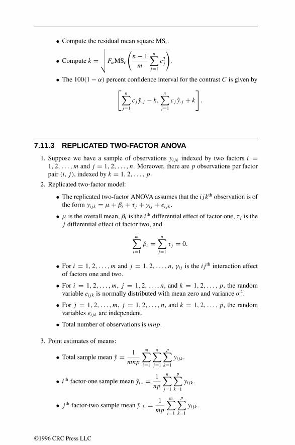
• Compute the residual mean square MSr.
• Compute k =√√√√FαMSr
(n− 1
m
n∑j=1
c2j
).
• The 100(1− α) percent confidence interval for the contrast C is given by[n∑
j=1
cj y·j − k,
n∑j=1
cj y·j + k
].
7.11.3 REPLICATED TWO-FACTOR ANOVA
1. Suppose we have a sample of observations yijk indexed by two factors i =1, 2, . . . , m and j = 1, 2, . . . , n. Moreover, there are p observations per factorpair (i, j), indexed by k = 1, 2, . . . , p.
2. Replicated two-factor model:
• The replicated two-factor ANOVA assumes that the ijkth observation is ofthe form yijk = µ+ βi + τj + γij + eijk .
• µ is the overall mean, βi is the i th differential effect of factor one, τj is thej differential effect of factor two, and
m∑i=1
βi =n∑
j=1
τj = 0.
• For i = 1, 2, . . . , m and j = 1, 2, . . . , n, γij is the ij th interaction effectof factors one and two.
• For i = 1, 2, . . . , m, j = 1, 2, . . . , n, and k = 1, 2, . . . , p, the randomvariable eijk is normally distributed with mean zero and variance σ 2.
• For j = 1, 2, . . . , m, j = 1, 2, . . . , n, and k = 1, 2, . . . , p, the randomvariables eijk are independent.
• Total number of observations is mnp.
3. Point estimates of means:
• Total sample mean y = 1
mnp
m∑i=1
n∑j=1
p∑k=1
yijk .
• i th factor-one sample mean yi·· = 1
np
n∑j=1
p∑k=1
yijk .
• j th factor-two sample mean y·j · = 1
mp
m∑i=1
p∑k=1
yijk .
©1996 CRC Press LLC

• ij th interaction mean yij · = 1
p
p∑k=1
yijk .
4. Sums of squares:
• Factor-one sum of squares SS1 = np
m∑i=1
(yi·· − y)2.
• Factor-two sum of squares SS2 = mp
n∑j=1
(y·j · − y
)2.
• Interaction sum of squares SS12 = p
m∑i=1
n∑j=1
(yij · − y
)2.
• Residual sum of squares SSr =m∑i=1
n∑j=1
p∑k=1
(yijk − yi·· − y·j · + y
)2.
• Total sum of squares Total SS =m∑i=1
n∑j=1
p∑k=1
(yijk − y
)2.
• Partition of total sum of squares Total SS = SS1 + SS2 + SS12 + SSr.
5. Degrees of freedom:
• Factor one, m− 1.
• Factor two, n− 1.
• Interaction, (m− 1)(n− 1).
• Residual, mn(p − 1).
• Total, mnp − 1.
6. Mean squares:
• Obtained by dividing sums of squares by their respective degrees offreedom.
• Factor-one mean square MS1 = SS1
m− 1.
• Factor-two mean square MS2 = SS2
n− 1.
• Interaction mean square MS12 = SS12
(m− 1)(n− 1).
• Residual mean square MSr = SSr
mn(p − 1).
©1996 CRC Press LLC

7. Test of the null hypothesis β1 = β2 = · · · = βm = 0 (no factor-one effects)against the alternative hypothesis βi = 0 for some i:
• Determine the critical value Fα such that F (Fα) = 1− α, where F (F) isthe F -distribution with m− 1 and mn(p − 1) degrees of freedom.
• Compute the point estimates y and yi·· for i = 1, 2, . . . , m.
• Compute the sums of squares SS1 and SSr.
• Compute the mean squares MS1 and MSr.
• Compute the test statistic F = MS1
MSr.
• If F > Fα , then reject the hypothesis. If F ≤ Fα , then do not reject thehypothesis.
8. Test of the null hypothesis τ1 = τ2 = · · · = τn = 0 (no factor-two effects)against the alternative hypothesis τj = 0 for some j :
• Determine the critical value Fα such that F (Fα) = 1− α, where F (F) isthe F -distribution with n− 1 and mn(p − 1) degrees of freedom.
• Compute the point estimates y and y·j · for j = 1, 2, . . . , n.
• Compute the sums of squares SS2 and SSr.
• Compute the mean squares MS2 and MSr.
• Compute the test statistic F = MS2
MSr.
• If F > Fα , then reject the hypothesis. If F ≤ Fα , then do not reject thehypothesis.
9. Test of the null hypothesis γij = 0 for i = 1, 2, . . . , m and j = 1, 2, . . . , n (nofactor-one effects) against the alternative hypothesis γij = 0 for some i and j :
• Determine the critical value Fα such that F (Fα) = 1− α, where F (F) isthe F -distribution with (m−1)(n−1) and mn(p−1) degrees of freedom.
• Compute the point estimates y, yi··, y·j ·, and yij · for i = 1, 2, . . . , m andj = 1, 2, . . . , n.
• Compute the sums of squares SS12 and SSr.
• Compute the mean squares MS12 and MSr.
• Compute the test statistic F = MS12
MSr.
• If F > Fα , then reject the hypothesis. If F ≤ Fα , then do not reject thehypothesis.
©1996 CRC Press LLC

• The above computations are often organized into an ANOVA table:
Source SS D.O.F. MS F Ratio
Factor one SS1 m− 1 MS1 F = MS1/MSr
Factor two SS2 n− 1 MS2 F = MS2/MSr
Interaction SS12 (m− 1)(n− 1) MS12 F = MS12/MSr
Residual SSr mn(p − 1) MSr
Total Total SS mnp − 1
10. Confidence interval for contrast in the factor-one means, defined byC = c1β1+c2β2 + · · · + cmβm, where c1 + c2 + · · · + cm = 0:
• Determine the critical value Fα such that F (Fα) = 1− α, where F (F) isthe F -distribution with m− 1 and mn(p − 1) degrees of freedom.
• Compute the point estimates yi·· for i = 1, 2, . . . , m.
• Compute the residual mean square MSr.
• Compute k =√√√√FαMSr
(m− 1
np
m∑i=1
c2i
).
• The 100(1− α) percent confidence interval for the contrast C is given by
[m∑i=1
ci yi·· − k,
m∑i=1
ci yi·· + k
].
11. Confidence interval for contrast in the factor-two means, defined by C = c1τ1+c2τ2 + · · · + cnτn, where c1 + c2 + · · · + cn = 0:
• Determine the critical value Fα such that F (Fα) = 1− α, where F (F) isthe F -distribution with n− 1 and mn(p − 1) degrees of freedom.
• Compute the point estimates y·j · for j = 1, 2, . . . , n.
• Compute the residual mean square MSr.
• Compute k =√√√√FαMSr
(n− 1
mp
n∑j=1
c2j
).
• The 100(1− α) percent confidence interval for the contrast C is given by
[n∑
j=1
cj y·j · − k,
n∑j=1
cj y·j · + k
].
©1996 CRC Press LLC

7.12 PROBABILITY TABLES
7.12.1 CRITICAL VALUES
The critical value
• zα satisfies ?(zα) = 1 − α (where, as usual, ?(z) is the distribution functionfor the standard normal).
• tα satisfies F(tα) = 1 − α where F(t) is the distribution function for the t-distribution (with some specified number of degrees of freedom).
• χ2α satisfies F(χ2
α) = 1 − α where F(t) is the distribution function for theχ2-distribution (with some specified number of degrees of freedom).
7.12.2 TABLE OF THE NORMAL DISTRIBUTION
For a standard normal random variable:
LimitsProportional of
the total areaRemaining
areaµ− λσ µ+ λσ (%) (%)µ− σ µ+ σ 68.26 31.74µ− 1.65σ µ+ 1.65σ 90 10µ− 1.96σ µ+ 1.96σ 95 5µ− 2σ µ+ 2σ 95.44 4.56µ− 2.58σ µ+ 2.58σ 99 1µ− 3σ µ+ 3σ 99.73 0.27µ− 3.09σ µ+ 3.09σ 99.8 0.2µ− 3.29σ µ+ 3.29σ 99.9 0.1
x 1.282 1.645 1.960 2.326 2.576 3.090
?(x) 0.90 0.95 0.975 0.99 0.995 0.9992[1−?(x)] 0.20 0.10 0.05 0.02 0.01 0.002
x 3.09 3.72 4.26 4.75 5.20 5.61 6.00 6.36
1−?(x) 10−3 10−4 10−5 10−6 10−7 10−8 10−9 10−10
For large values of x:[e−x
2/2
√2π
(1
x− 1
x3
)]< 1−?(x) <
[e−x
2/2
√2π
(1
x
)]
©1996 CRC Press LLC

x F(x) 1− F(x) f (x) x F (x) 1− F(x) f (x)
0.00 0.5000 0.5000 0.3989 0.50 0.6915 0.3085 0.35210.01 0.5040 0.4960 0.3989 0.51 0.6950 0.3050 0.35030.02 0.5080 0.4920 0.3989 0.52 0.6985 0.3015 0.34850.03 0.5120 0.4880 0.3988 0.53 0.7019 0.2981 0.34670.04 0.5160 0.4840 0.3986 0.54 0.7054 0.2946 0.34480.05 0.5199 0.4801 0.3984 0.55 0.7088 0.2912 0.34290.06 0.5239 0.4761 0.3982 0.56 0.7123 0.2877 0.34110.07 0.5279 0.4721 0.3980 0.57 0.7157 0.2843 0.33910.08 0.5319 0.4681 0.3977 0.58 0.7190 0.2810 0.33720.09 0.5359 0.4641 0.3973 0.59 0.7224 0.2776 0.3352
0.10 0.5398 0.4602 0.3970 0.60 0.7258 0.2742 0.33320.11 0.5438 0.4562 0.3965 0.61 0.7291 0.2709 0.33120.12 0.5478 0.4522 0.3961 0.62 0.7324 0.2676 0.32920.13 0.5517 0.4483 0.3956 0.63 0.7357 0.2643 0.32710.14 0.5557 0.4443 0.3951 0.64 0.7389 0.2611 0.32510.15 0.5596 0.4404 0.3945 0.65 0.7421 0.2579 0.32300.16 0.5636 0.4364 0.3939 0.66 0.7454 0.2546 0.32090.17 0.5675 0.4325 0.3932 0.67 0.7486 0.2514 0.31870.18 0.5714 0.4286 0.3925 0.68 0.7518 0.2482 0.31660.19 0.5754 0.4247 0.3918 0.69 0.7549 0.2451 0.3144
0.20 0.5793 0.4207 0.3910 0.70 0.7580 0.2420 0.31230.21 0.5832 0.4168 0.3902 0.71 0.7611 0.2389 0.31010.22 0.5871 0.4129 0.3894 0.72 0.7642 0.2358 0.30790.23 0.5909 0.4091 0.3885 0.73 0.7673 0.2327 0.30560.24 0.5948 0.4052 0.3876 0.74 0.7703 0.2296 0.30340.25 0.5987 0.4013 0.3867 0.75 0.7734 0.2266 0.30110.26 0.6026 0.3974 0.3857 0.76 0.7764 0.2236 0.29890.27 0.6064 0.3936 0.3847 0.77 0.7793 0.2207 0.29660.28 0.6103 0.3897 0.3836 0.78 0.7823 0.2177 0.29430.29 0.6141 0.3859 0.3825 0.79 0.7852 0.2148 0.2920
0.30 0.6179 0.3821 0.3814 0.80 0.7881 0.2119 0.28970.31 0.6217 0.3783 0.3802 0.81 0.7910 0.2090 0.28740.32 0.6255 0.3745 0.3790 0.82 0.7939 0.2061 0.28500.33 0.6293 0.3707 0.3778 0.83 0.7967 0.2033 0.28270.34 0.6331 0.3669 0.3765 0.84 0.7995 0.2004 0.28030.35 0.6368 0.3632 0.3752 0.85 0.8023 0.1977 0.27800.36 0.6406 0.3594 0.3739 0.86 0.8051 0.1949 0.27560.37 0.6443 0.3557 0.3725 0.87 0.8078 0.1921 0.27320.38 0.6480 0.3520 0.3711 0.88 0.8106 0.1894 0.27090.39 0.6517 0.3483 0.3697 0.89 0.8133 0.1867 0.2685
0.40 0.6554 0.3446 0.3683 0.90 0.8159 0.1841 0.26610.41 0.6591 0.3409 0.3668 0.91 0.8186 0.1814 0.26370.42 0.6628 0.3372 0.3653 0.92 0.8212 0.1788 0.26130.43 0.6664 0.3336 0.3637 0.93 0.8238 0.1762 0.25890.44 0.6700 0.3300 0.3621 0.94 0.8264 0.1736 0.25650.45 0.6736 0.3264 0.3605 0.95 0.8289 0.1711 0.25410.46 0.6772 0.3228 0.3589 0.96 0.8315 0.1685 0.25160.47 0.6808 0.3192 0.3572 0.97 0.8340 0.1660 0.24920.48 0.6844 0.3156 0.3555 0.98 0.8365 0.1635 0.24680.49 0.6879 0.3121 0.3538 0.99 0.8389 0.1611 0.2444
0.50 0.6915 0.3085 0.3521 1.00 0.8413 0.1587 0.2420
©1996 CRC Press LLC

x F(x) 1− F(x) f (x) x F (x) 1− F(x) f (x)
1.00 0.8413 0.1587 0.2420 1.50 0.9332 0.0668 0.12951.01 0.8438 0.1562 0.2396 1.51 0.9345 0.0655 0.12761.02 0.8461 0.1539 0.2371 1.52 0.9357 0.0643 0.12571.03 0.8485 0.1515 0.2347 1.53 0.9370 0.0630 0.12381.04 0.8508 0.1492 0.2323 1.54 0.9382 0.0618 0.12191.05 0.8531 0.1469 0.2299 1.55 0.9394 0.0606 0.12001.06 0.8554 0.1446 0.2275 1.56 0.9406 0.0594 0.11821.07 0.8577 0.1423 0.2251 1.57 0.9418 0.0582 0.11631.08 0.8599 0.1401 0.2226 1.58 0.9429 0.0570 0.11451.09 0.8621 0.1379 0.2203 1.59 0.9441 0.0559 0.1127
1.10 0.8643 0.1357 0.2178 1.60 0.9452 0.0548 0.11091.11 0.8665 0.1335 0.2155 1.61 0.9463 0.0537 0.10911.12 0.8686 0.1314 0.2131 1.62 0.9474 0.0526 0.10741.13 0.8708 0.1292 0.2107 1.63 0.9485 0.0515 0.10571.14 0.8729 0.1271 0.2083 1.64 0.9495 0.0505 0.10401.15 0.8749 0.1251 0.2059 1.65 0.9505 0.0495 0.10231.16 0.8770 0.1230 0.2036 1.66 0.9515 0.0485 0.10061.17 0.8790 0.1210 0.2012 1.67 0.9525 0.0475 0.09891.18 0.8810 0.1190 0.1989 1.68 0.9535 0.0465 0.09731.19 0.8830 0.1170 0.1965 1.69 0.9545 0.0455 0.0957
1.20 0.8849 0.1151 0.1942 1.70 0.9554 0.0446 0.09401.21 0.8869 0.1131 0.1919 1.71 0.9564 0.0436 0.09251.22 0.8888 0.1112 0.1895 1.72 0.9573 0.0427 0.09091.23 0.8907 0.1094 0.1872 1.73 0.9582 0.0418 0.08931.24 0.8925 0.1075 0.1849 1.74 0.9591 0.0409 0.08781.25 0.8943 0.1056 0.1827 1.75 0.9599 0.0401 0.08631.26 0.8962 0.1038 0.1804 1.76 0.9608 0.0392 0.08481.27 0.8980 0.1020 0.1781 1.77 0.9616 0.0384 0.08331.28 0.8997 0.1003 0.1759 1.78 0.9625 0.0375 0.08181.29 0.9015 0.0985 0.1736 1.79 0.9633 0.0367 0.0804
1.30 0.9032 0.0968 0.1714 1.80 0.9641 0.0359 0.07901.31 0.9049 0.0951 0.1691 1.81 0.9648 0.0352 0.07751.32 0.9066 0.0934 0.1669 1.82 0.9656 0.0344 0.07611.33 0.9082 0.0918 0.1647 1.83 0.9664 0.0336 0.07481.34 0.9099 0.0901 0.1626 1.84 0.9671 0.0329 0.07341.35 0.9115 0.0885 0.1604 1.85 0.9678 0.0322 0.07211.36 0.9131 0.0869 0.1582 1.86 0.9686 0.0314 0.07071.37 0.9147 0.0853 0.1561 1.87 0.9693 0.0307 0.06941.38 0.9162 0.0838 0.1540 1.88 0.9699 0.0301 0.06811.39 0.9177 0.0823 0.1518 1.89 0.9706 0.0294 0.0669
1.40 0.9192 0.0808 0.1497 1.90 0.9713 0.0287 0.06561.41 0.9207 0.0793 0.1476 1.91 0.9719 0.0281 0.06441.42 0.9222 0.0778 0.1456 1.92 0.9726 0.0274 0.06321.43 0.9236 0.0764 0.1435 1.93 0.9732 0.0268 0.06191.44 0.9251 0.0749 0.1415 1.94 0.9738 0.0262 0.06081.45 0.9265 0.0735 0.1394 1.95 0.9744 0.0256 0.05961.46 0.9278 0.0722 0.1374 1.96 0.9750 0.0250 0.05841.47 0.9292 0.0708 0.1354 1.97 0.9756 0.0244 0.05731.48 0.9306 0.0694 0.1334 1.98 0.9761 0.0238 0.05621.49 0.9319 0.0681 0.1315 1.99 0.9767 0.0233 0.0551
1.50 0.9332 0.0668 0.1295 2.00 0.9772 0.0227 0.0540
©1996 CRC Press LLC

x F(x) 1− F(x) f (x) x F (x) 1− F(x) f (x)
2.00 0.9772 0.0227 0.0540 2.50 0.9938 0.0062 0.01752.01 0.9778 0.0222 0.0529 2.51 0.9940 0.0060 0.01712.02 0.9783 0.0217 0.0519 2.52 0.9941 0.0059 0.01672.03 0.9788 0.0212 0.0508 2.53 0.9943 0.0057 0.01632.04 0.9793 0.0207 0.0498 2.54 0.9945 0.0055 0.01582.05 0.9798 0.0202 0.0488 2.55 0.9946 0.0054 0.01552.06 0.9803 0.0197 0.0478 2.56 0.9948 0.0052 0.01512.07 0.9808 0.0192 0.0468 2.57 0.9949 0.0051 0.01472.08 0.9812 0.0188 0.0459 2.58 0.9951 0.0049 0.01432.09 0.9817 0.0183 0.0449 2.59 0.9952 0.0048 0.0139
2.10 0.9821 0.0179 0.0440 2.60 0.9953 0.0047 0.01362.11 0.9826 0.0174 0.0431 2.61 0.9955 0.0045 0.01322.12 0.9830 0.0170 0.0422 2.62 0.9956 0.0044 0.01292.13 0.9834 0.0166 0.0413 2.63 0.9957 0.0043 0.01262.14 0.9838 0.0162 0.0404 2.64 0.9959 0.0042 0.01222.15 0.9842 0.0158 0.0396 2.65 0.9960 0.0040 0.01192.16 0.9846 0.0154 0.0387 2.66 0.9961 0.0039 0.01162.17 0.9850 0.0150 0.0379 2.67 0.9962 0.0038 0.01132.18 0.9854 0.0146 0.0371 2.68 0.9963 0.0037 0.01102.19 0.9857 0.0143 0.0363 2.69 0.9964 0.0036 0.0107
2.20 0.9861 0.0139 0.0355 2.70 0.9965 0.0035 0.01042.21 0.9865 0.0135 0.0347 2.71 0.9966 0.0034 0.01012.22 0.9868 0.0132 0.0339 2.72 0.9967 0.0033 0.00992.23 0.9871 0.0129 0.0332 2.73 0.9968 0.0032 0.00962.24 0.9875 0.0126 0.0325 2.74 0.9969 0.0031 0.00942.25 0.9878 0.0122 0.0317 2.75 0.9970 0.0030 0.00912.26 0.9881 0.0119 0.0310 2.76 0.9971 0.0029 0.00892.27 0.9884 0.0116 0.0303 2.77 0.9972 0.0028 0.00862.28 0.9887 0.0113 0.0296 2.78 0.9973 0.0027 0.00842.29 0.9890 0.0110 0.0290 2.79 0.9974 0.0026 0.0081
2.30 0.9893 0.0107 0.0283 2.80 0.9974 0.0026 0.00792.31 0.9896 0.0104 0.0277 2.81 0.9975 0.0025 0.00772.32 0.9898 0.0102 0.0271 2.82 0.9976 0.0024 0.00752.33 0.9901 0.0099 0.0264 2.83 0.9977 0.0023 0.00732.34 0.9904 0.0096 0.0258 2.84 0.9977 0.0023 0.00712.35 0.9906 0.0094 0.0252 2.85 0.9978 0.0022 0.00692.36 0.9909 0.0091 0.0246 2.86 0.9979 0.0021 0.00672.37 0.9911 0.0089 0.0241 2.87 0.9980 0.0021 0.00652.38 0.9913 0.0087 0.0235 2.88 0.9980 0.0020 0.00632.39 0.9916 0.0084 0.0229 2.89 0.9981 0.0019 0.0061
2.40 0.9918 0.0082 0.0224 2.90 0.9981 0.0019 0.00602.41 0.9920 0.0080 0.0219 2.91 0.9982 0.0018 0.00582.42 0.9922 0.0078 0.0213 2.92 0.9982 0.0018 0.00562.43 0.9925 0.0076 0.0208 2.93 0.9983 0.0017 0.00542.44 0.9927 0.0073 0.0203 2.94 0.9984 0.0016 0.00532.45 0.9929 0.0071 0.0198 2.95 0.9984 0.0016 0.00512.46 0.9930 0.0069 0.0194 2.96 0.9985 0.0015 0.00502.47 0.9932 0.0068 0.0189 2.97 0.9985 0.0015 0.00492.48 0.9934 0.0066 0.0184 2.98 0.9986 0.0014 0.00472.49 0.9936 0.0064 0.0180 2.99 0.9986 0.0014 0.0046
2.50 0.9938 0.0062 0.0175 3.00 0.9987 0.0014 0.0044
©1996 CRC Press LLC

For a given value of n this table gives the value of t such that
F(t) =∫ t
−∞
:((n+ 1)/2)√nπ:(n/2)
(1+ x2
n
)−(n+1)/2
dx
is a specified number. The t-distribution is symmetrical, so that F(−t) = 1− F(t).
F =n 0.6000 0.7500 0.9000 0.9500 0.9750 0.9900 0.9950 0.9990 0.9995
1 0.325 1.000 3.078 6.314 12.706 31.821 63.657 318.309 636.6192 0.289 0.816 1.886 2.920 4.303 6.965 9.925 22.327 31.5993 0.277 0.765 1.638 2.353 3.182 4.541 5.841 10.215 12.9244 0.271 0.741 1.533 2.132 2.776 3.747 4.604 7.173 8.610
5 0.267 0.727 1.476 2.015 2.571 3.365 4.032 5.893 6.8696 0.265 0.718 1.440 1.943 2.447 3.143 3.707 5.208 5.9597 0.263 0.711 1.415 1.895 2.365 2.998 3.499 4.785 5.4088 0.262 0.706 1.397 1.860 2.306 2.896 3.355 4.501 5.0419 0.261 0.703 1.383 1.833 2.262 2.821 3.250 4.297 4.781
10 0.260 0.700 1.372 1.812 2.228 2.764 3.169 4.144 4.58711 0.260 0.697 1.363 1.796 2.201 2.718 3.106 4.025 4.43712 0.259 0.695 1.356 1.782 2.179 2.681 3.055 3.930 4.31813 0.259 0.694 1.350 1.771 2.160 2.650 3.012 3.852 4.22114 0.258 0.692 1.345 1.761 2.145 2.624 2.977 3.787 4.140
15 0.258 0.691 1.341 1.753 2.131 2.602 2.947 3.733 4.07316 0.258 0.690 1.337 1.746 2.120 2.583 2.921 3.686 4.01517 0.257 0.689 1.333 1.740 2.110 2.567 2.898 3.646 3.96518 0.257 0.688 1.330 1.734 2.101 2.552 2.878 3.610 3.92219 0.257 0.688 1.328 1.729 2.093 2.539 2.861 3.579 3.883
20 0.257 0.687 1.325 1.725 2.086 2.528 2.845 3.552 3.85025 0.256 0.684 1.316 1.708 2.060 2.485 2.787 3.450 3.72550 0.255 0.679 1.299 1.676 2.009 2.403 2.678 3.261 3.496
100 0.254 0.677 1.290 1.660 1.984 2.364 2.626 3.174 3.390∞ 0.253 0.674 1.282 1.645 1.960 2.326 2.576 3.091 3.291
©1996 C
RC
Press LL
C
7.12.3 PERCENTAGE POINTS, STUDENT’St-DISTRIBUTION
©1996 CRC Press LLC

For a given value of n this table gives the value of χ2 such that
F(χ2) =∫ χ2
0
x(n−2)/2e−x/2
2n/2:(n/2)dx
is a specified number.
F =n 0.005 0.010 0.025 0.050 0.100 0.250 0.500 0.750 0.900 0.950 0.975 0.990 0.9951 0.0000393 0.0001571 0.0009821 0.00393 0.0158 0.102 0.455 1.32 2.71 3.84 5.02 6.63 7.882 0.0100 0.0201 0.0506 0.103 0.211 0.575 1.39 2.77 4.61 5.99 7.38 9.21 10.63 0.0717 0.115 0.216 0.352 0.584 1.21 2.37 4.11 6.25 7.81 9.35 11.3 12.84 0.207 0.297 0.484 0.711 1.06 1.92 3.36 5.39 7.78 9.49 11.1 13.3 14.95 0.412 0.554 0.831 1.15 1.61 2.67 4.35 6.63 9.24 11.1 12.8 15.1 16.76 0.676 0.872 1.24 1.64 2.20 3.45 5.35 7.84 10.6 12.6 14.4 16.8 18.57 0.989 1.24 1.69 2.17 2.83 4.25 6.35 9.04 12.0 14.1 16.0 18.5 20.38 1.34 1.65 2.18 2.73 3.49 5.07 7.34 10.2 13.4 15.5 17.5 20.1 22.09 1.73 2.09 2.70 3.33 4.17 5.90 8.34 11.4 14.7 16.9 19.0 21.7 23.6
10 2.16 2.56 3.25 3.94 4.87 6.74 9.34 12.5 16.0 18.3 20.5 23.2 25.211 2.60 3.05 3.82 4.57 5.58 7.58 10.3 13.7 17.3 19.7 21.9 24.7 26.812 3.07 3.57 4.40 5.23 6.30 8.44 11.3 14.8 18.5 21.0 23.3 26.2 28.313 3.57 4.11 5.01 5.89 7.04 9.30 12.3 16.0 19.8 22.4 24.7 27.7 29.814 4.07 4.66 5.63 6.57 7.79 10.2 13.3 17.1 21.1 23.7 26.1 29.1 31.315 4.60 5.23 6.26 7.26 8.55 11.0 14.3 18.2 22.3 25.0 27.5 30.6 32.816 5.14 5.81 6.91 7.96 9.31 11.9 15.3 19.4 23.5 26.3 28.8 32.0 34.317 5.70 6.41 7.56 8.67 10.1 12.8 16.3 20.5 24.8 27.6 30.2 33.4 35.718 6.26 7.01 8.23 9.39 10.9 13.7 17.3 21.6 26.0 28.9 31.5 34.8 37.219 6.84 7.63 8.91 10.1 11.7 14.6 18.3 22.7 27.2 30.1 32.9 36.2 38.620 7.43 8.26 9.59 10.9 12.4 15.5 19.3 23.8 28.4 31.4 34.2 37.6 40.021 8.03 8.90 10.3 11.6 13.2 16.3 20.3 24.9 29.6 32.7 35.5 38.9 41.422 8.64 9.54 11.0 12.3 14.0 17.2 21.3 26.0 30.8 33.9 36.8 40.3 42.823 9.26 10.2 11.7 13.1 14.8 18.1 22.3 27.1 32.0 35.2 38.1 41.6 44.224 9.89 10.9 12.4 13.8 15.7 19.0 23.3 28.2 33.2 36.4 39.4 43.0 45.625 10.5 11.5 13.1 14.6 16.5 19.9 24.3 29.3 34.4 37.7 40.6 44.3 46.930 13.8 15.0 16.8 18.5 20.6 24.5 29.3 34.8 40.3 43.8 47.0 50.9 53.735 17.2 18.5 20.6 22.5 24.8 29.1 34.3 40.2 46.1 49.8 53.2 57.3 60.350 28.0 29.7 32.4 34.8 37.7 42.9 43.9 56.3 63.2 67.5 71.4 76.2 79.5
©1996 C
RC
Press LL
C
7.12.4 PERCENTAGE POINTS, CHI-SQUARE DISTRIBUTION
©1996 CRC Press LLC

Given n and m this gives the value of f such that
F(f ) =∫ f
0
:((n+m)/2)
:(m/2):(n/2)mm/2nn/2xm/2−1(n+mx)−(m+n)/2 dx = 0.9.
m =n 1 2 3 4 5 6 7 8 9 10 50 100 ∞
1 39.86 49.50 53.59 55.83 57.24 58.20 58.91 59.44 59.86 60.19 62.69 63.01 63.332 8.53 9.00 9.16 9.24 9.29 9.33 9.35 9.37 9.38 9.39 9.47 9.48 9.493 5.54 5.46 5.39 5.34 5.31 5.28 5.27 5.25 5.24 5.23 5.15 5.14 5.134 4.54 4.32 4.19 4.11 4.05 4.01 3.98 3.95 3.94 3.92 3.80 3.78 3.76
5 4.06 3.78 3.62 3.52 3.45 3.40 3.37 3.34 3.32 3.30 3.15 3.13 3.106 3.78 3.46 3.29 3.18 3.11 3.05 3.01 2.98 2.96 2.94 2.77 2.75 2.727 3.59 3.26 3.07 2.96 2.88 2.83 2.78 2.75 2.72 2.70 2.52 2.50 2.478 3.46 3.11 2.92 2.81 2.73 2.67 2.62 2.59 2.56 2.54 2.35 2.32 2.299 3.36 3.01 2.81 2.69 2.61 2.55 2.51 2.47 2.44 2.42 2.22 2.19 2.16
10 3.29 2.92 2.73 2.61 2.52 2.46 2.41 2.38 2.35 2.32 2.12 2.09 2.0611 3.23 2.86 2.66 2.54 2.45 2.39 2.34 2.30 2.27 2.25 2.04 2.01 1.9712 3.18 2.81 2.61 2.48 2.39 2.33 2.28 2.24 2.21 2.19 1.97 1.94 1.9013 3.14 2.76 2.56 2.43 2.35 2.28 2.23 2.20 2.16 2.14 1.92 1.88 1.8514 3.10 2.73 2.52 2.39 2.31 2.24 2.19 2.15 2.12 2.10 1.87 1.83 1.80
15 3.07 2.70 2.49 2.36 2.27 2.21 2.16 2.12 2.09 2.06 1.83 1.79 1.7616 3.05 2.67 2.46 2.33 2.24 2.18 2.13 2.09 2.06 2.03 1.79 1.76 1.7217 3.03 2.64 2.44 2.31 2.22 2.15 2.10 2.06 2.03 2.00 1.76 1.73 1.6918 3.01 2.62 2.42 2.29 2.20 2.13 2.08 2.04 2.00 1.98 1.74 1.70 1.6619 2.99 2.61 2.40 2.27 2.18 2.11 2.06 2.02 1.98 1.96 1.71 1.67 1.63
20 2.97 2.59 2.38 2.25 2.16 2.09 2.04 2.00 1.96 1.94 1.69 1.65 1.6125 2.92 2.53 2.32 2.18 2.09 2.02 1.97 1.93 1.89 1.87 1.61 1.56 1.5250 2.81 2.41 2.20 2.06 1.97 1.90 1.84 1.80 1.76 1.73 1.44 1.39 1.34
100 2.76 2.36 2.14 2.00 1.91 1.83 1.78 1.73 1.69 1.66 1.35 1.29 1.20∞ 2.71 2.30 2.08 1.94 1.85 1.77 1.72 1.67 1.63 1.60 1.24 1.17 1.00
©1996 C
RC
Press LL
C
7.12.5 PERCENTAGE POINTS, F-DISTRIBUTION
©1996 CRC Press LLC

Given n and m this gives the value of f such that
F(f ) =∫ f
0
:((n+m)/2)
:(m/2):(n/2)mm/2nn/2xm/2−1(n+mx)−(m+n)/2 dx = 0.95.
m =n 1 2 3 4 5 6 7 8 9 10 50 100 ∞
1 161.4 199.5 215.7 224.6 230.2 234.0 236.8 238.9 240.5 241.9 251.8 253.0 254.32 18.51 19.00 19.16 19.25 19.30 19.33 19.35 19.37 19.38 19.40 19.48 19.49 19.503 10.13 9.55 9.28 9.12 9.01 8.94 8.89 8.85 8.81 8.79 8.58 8.55 8.534 7.71 6.94 6.59 6.39 6.26 6.16 6.09 6.04 6.00 5.96 5.70 5.66 5.63
5 6.61 5.79 5.41 5.19 5.05 4.95 4.88 4.82 4.77 4.74 4.44 4.41 4.366 5.99 5.14 4.76 4.53 4.39 4.28 4.21 4.15 4.10 4.06 3.75 3.71 3.677 5.59 4.74 4.35 4.12 3.97 3.87 3.79 3.73 3.68 3.64 3.32 3.27 3.238 5.32 4.46 4.07 3.84 3.69 3.58 3.50 3.44 3.39 3.35 3.02 2.97 2.939 5.12 4.26 3.86 3.63 3.48 3.37 3.29 3.23 3.18 3.14 2.80 2.76 2.71
10 4.96 4.10 3.71 3.48 3.33 3.22 3.14 3.07 3.02 2.98 2.64 2.59 2.5411 4.84 3.98 3.59 3.36 3.20 3.09 3.01 2.95 2.90 2.85 2.51 2.46 2.4012 4.75 3.89 3.49 3.26 3.11 3.00 2.91 2.85 2.80 2.75 2.40 2.35 2.3013 4.67 3.81 3.41 3.18 3.03 2.92 2.83 2.77 2.71 2.67 2.31 2.26 2.2114 4.60 3.74 3.34 3.11 2.96 2.85 2.76 2.70 2.65 2.60 2.24 2.19 2.13
15 4.54 3.68 3.29 3.06 2.90 2.79 2.71 2.64 2.59 2.54 2.18 2.12 2.0716 4.49 3.63 3.24 3.01 2.85 2.74 2.66 2.59 2.54 2.49 2.12 2.07 2.0117 4.45 3.59 3.20 2.96 2.81 2.70 2.61 2.55 2.49 2.45 2.08 2.02 1.9618 4.41 3.55 3.16 2.93 2.77 2.66 2.58 2.51 2.46 2.41 2.04 1.98 1.9219 4.38 3.52 3.13 2.90 2.74 2.63 2.54 2.48 2.42 2.38 2.00 1.94 1.88
20 4.35 3.49 3.10 2.87 2.71 2.60 2.51 2.45 2.39 2.35 1.97 1.91 1.8425 4.24 3.39 2.99 2.76 2.60 2.49 2.40 2.34 2.28 2.24 1.84 1.78 1.7150 4.03 3.18 2.79 2.56 2.40 2.29 2.20 2.13 2.07 2.03 1.60 1.52 1.45
100 3.94 3.09 2.70 2.46 2.31 2.19 2.10 2.03 1.97 1.93 1.48 1.39 1.28∞ 3.84 3.00 2.60 2.37 2.21 2.10 2.01 1.94 1.88 1.83 1.35 1.25 1.00
©1996 C
RC
Press LL
C
©1996 CRC Press LLC

Given n and m this gives the value of f such that
F(f ) =∫ f
0
:((n+m)/2)
:(m/2):(n/2)mm/2nn/2xm/2−1(n+mx)−(m+n)/2 dx = 0.975.
m =n 1 2 3 4 5 6 7 8 9 10 50 100 ∞
1 647.8 799.5 864.2 899.6 921.8 937.1 948.2 956.7 963.3 968.6 1008 1013 10182 38.51 39.00 39.17 39.25 39.30 39.33 39.36 39.37 39.39 39.40 39.48 39.49 39.503 17.44 16.04 15.44 15.10 14.88 14.73 14.62 14.54 14.47 14.42 14.01 13.96 13.904 12.22 10.65 9.98 9.60 9.36 9.20 9.07 8.98 8.90 8.84 8.38 8.32 8.26
5 10.01 8.43 7.76 7.39 7.15 6.98 6.85 6.76 6.68 6.62 6.14 6.08 6.026 8.81 7.26 6.60 6.23 5.99 5.82 5.70 5.60 5.52 5.46 4.98 4.92 4.857 8.07 6.54 5.89 5.52 5.29 5.12 4.99 4.90 4.82 4.76 4.28 4.21 4.148 7.57 6.06 5.42 5.05 4.82 4.65 4.53 4.43 4.36 4.30 3.81 3.74 3.679 7.21 5.71 5.08 4.72 4.48 4.32 4.20 4.10 4.03 3.96 3.47 3.40 3.33
10 6.94 5.46 4.83 4.47 4.24 4.07 3.95 3.85 3.78 3.72 3.22 3.15 3.0811 6.72 5.26 4.63 4.28 4.04 3.88 3.76 3.66 3.59 3.53 3.03 2.96 2.8812 6.55 5.10 4.47 4.12 3.89 3.73 3.61 3.51 3.44 3.37 2.87 2.80 2.7213 6.41 4.97 4.35 4.00 3.77 3.60 3.48 3.39 3.31 3.25 2.74 2.67 2.6014 6.30 4.86 4.24 3.89 3.66 3.50 3.38 3.29 3.21 3.15 2.64 2.56 2.49
15 6.20 4.77 4.15 3.80 3.58 3.41 3.29 3.20 3.12 3.06 2.55 2.47 2.4016 6.12 4.69 4.08 3.73 3.50 3.34 3.22 3.12 3.05 2.99 2.47 2.40 2.3217 6.04 4.62 4.01 3.66 3.44 3.28 3.16 3.06 2.98 2.92 2.41 2.33 2.2518 5.98 4.56 3.95 3.61 3.38 3.22 3.10 3.01 2.93 2.87 2.35 2.27 2.1919 5.92 4.51 3.90 3.56 3.33 3.17 3.05 2.96 2.88 2.82 2.30 2.22 2.13
20 5.87 4.46 3.86 3.51 3.29 3.13 3.01 2.91 2.84 2.77 2.25 2.17 2.0925 5.69 4.29 3.69 3.35 3.13 2.97 2.85 2.75 2.68 2.61 2.08 2.00 1.9150 5.34 3.97 3.39 3.05 2.83 2.67 2.55 2.46 2.38 2.32 1.75 1.66 1.54
100 5.18 3.83 3.25 2.92 2.70 2.54 2.42 2.32 2.24 2.18 1.59 1.48 1.37∞ 5.02 3.69 3.12 2.79 2.57 2.41 2.29 2.19 2.11 2.05 1.43 1.27 1.00
©1996 C
RC
Press LL
C
©1996 CRC Press LLC

Given n and m this gives the value of f such that
F(f ) =∫ f
0
:((n+m)/2)
:(m/2):(n/2)mm/2nn/2xm/2−1(n+mx)−(m+n)/2 dx = 0.99.
m =n 1 2 3 4 5 6 7 8 9 10 50 100 ∞
1 4052 5000 5403 5625 5764 5859 5928 5981 6022 6056 6303 6334 63362 98.50 99.00 99.17 99.25 99.30 99.33 99.36 99.37 99.39 99.40 99.48 99.49 99.503 34.12 30.82 29.46 28.71 28.24 27.91 27.67 27.49 27.35 27.23 26.35 26.24 26.134 21.20 18.00 16.69 15.98 15.52 15.21 14.98 14.80 14.66 14.55 13.69 13.58 13.46
5 16.26 13.27 12.06 11.39 10.97 10.67 10.46 10.29 10.16 10.05 9.24 9.13 9.026 13.75 10.92 9.78 9.15 8.75 8.47 8.26 8.10 7.98 7.87 7.09 6.99 6.887 12.25 9.55 8.45 7.85 7.46 7.19 6.99 6.84 6.72 6.62 5.86 5.75 5.658 11.26 8.65 7.59 7.01 6.63 6.37 6.18 6.03 5.91 5.81 5.07 4.96 4.869 10.56 8.02 6.99 6.42 6.06 5.80 5.61 5.47 5.35 5.26 4.52 4.41 4.31
10 10.04 7.56 6.55 5.99 5.64 5.39 5.20 5.06 4.94 4.85 4.12 4.01 3.9111 9.65 7.21 6.22 5.67 5.32 5.07 4.89 4.74 4.63 4.54 3.81 3.71 3.6012 9.33 6.93 5.95 5.41 5.06 4.82 4.64 4.50 4.39 4.30 3.57 3.47 3.3613 9.07 6.70 5.74 5.21 4.86 4.62 4.44 4.30 4.19 4.10 3.38 3.27 3.1714 8.86 6.51 5.56 5.04 4.69 4.46 4.28 4.14 4.03 3.94 3.22 3.11 3.00
15 8.68 6.36 5.42 4.89 4.56 4.32 4.14 4.00 3.89 3.80 3.08 2.98 2.8716 8.53 6.23 5.29 4.77 4.44 4.20 4.03 3.89 3.78 3.69 2.97 2.86 2.7517 8.40 6.11 5.18 4.67 4.34 4.10 3.93 3.79 3.68 3.59 2.87 2.76 2.6518 8.29 6.01 5.09 4.58 4.25 4.01 3.84 3.71 3.60 3.51 2.78 2.68 2.5719 8.18 5.93 5.01 4.50 4.17 3.94 3.77 3.63 3.52 3.43 2.71 2.60 2.49
20 8.10 5.85 4.94 4.43 4.10 3.87 3.70 3.56 3.46 3.37 2.64 2.54 2.4225 7.77 5.57 4.68 4.18 3.85 3.63 3.46 3.32 3.22 3.13 2.40 2.29 2.1750 7.17 5.06 4.20 3.72 3.41 3.19 3.02 2.89 2.78 2.70 1.95 1.82 1.70
100 6.90 4.82 3.98 3.51 3.21 2.99 2.82 2.69 2.59 2.50 1.74 1.60 1.45∞ 6.63 4.61 3.78 3.32 3.02 2.80 2.64 2.51 2.41 2.32 1.53 1.32 1.00
©1996 C
RC
Press LL
C
©1996 CRC Press LLC

Given n and m this gives the value of f such that
F(f ) =∫ f
0
:((n+m)/2)
:(m/2):(n/2)mm/2nn/2xm/2−1(n+mx)−(m+n)/2 dx = 0.995.
m =n 1 2 3 4 5 6 7 8 9 10 50 100 ∞
1 16211 20000 21615 22500 23056 23437 23715 23925 24091 24224 25211 25337 254652 198.5 199.0 199.2 199.2 199.3 199.3 199.4 199.4 199.4 199.4 199.5 199.5 199.53 55.55 49.80 47.47 46.19 45.39 44.84 44.43 44.13 43.88 43.69 42.21 42.02 41.834 31.33 26.28 24.26 23.15 22.46 21.97 21.62 21.35 21.14 20.97 19.67 19.50 19.32
5 22.78 18.31 16.53 15.56 14.94 14.51 14.20 13.96 13.77 13.62 12.45 12.30 12.146 18.63 14.54 12.92 12.03 11.46 11.07 10.79 10.57 10.39 10.25 9.17 9.03 8.887 16.24 12.40 10.88 10.05 9.52 9.16 8.89 8.68 8.51 8.38 7.35 7.22 7.088 14.69 11.04 9.60 8.81 8.30 7.95 7.69 7.50 7.34 7.21 6.22 6.09 5.959 13.61 10.11 8.72 7.96 7.47 7.13 6.88 6.69 6.54 6.42 5.45 5.32 5.19
10 12.83 9.43 8.08 7.34 6.87 6.54 6.30 6.12 5.97 5.85 4.90 4.77 4.6411 12.23 8.91 7.60 6.88 6.42 6.10 5.86 5.68 5.54 5.42 4.49 4.36 4.2312 11.75 8.51 7.23 6.52 6.07 5.76 5.52 5.35 5.20 5.09 4.17 4.04 3.9013 11.37 8.19 6.93 6.23 5.79 5.48 5.25 5.08 4.94 4.82 3.91 3.78 3.6514 11.06 7.92 6.68 6.00 5.56 5.26 5.03 4.86 4.72 4.60 3.70 3.57 3.44
15 10.80 7.70 6.48 5.80 5.37 5.07 4.85 4.67 4.54 4.42 3.52 3.39 3.2616 10.58 7.51 6.30 5.64 5.21 4.91 4.69 4.52 4.38 4.27 3.37 3.25 3.1117 10.38 7.35 6.16 5.50 5.07 4.78 4.56 4.39 4.25 4.14 3.25 3.12 2.9818 10.22 7.21 6.03 5.37 4.96 4.66 4.44 4.28 4.14 4.03 3.14 3.01 2.8719 10.07 7.09 5.92 5.27 4.85 4.56 4.34 4.18 4.04 3.93 3.04 2.91 2.78
20 9.94 6.99 5.82 5.17 4.76 4.47 4.26 4.09 3.96 3.85 2.96 2.83 2.6925 9.48 6.60 5.46 4.84 4.43 4.15 3.94 3.78 3.64 3.54 2.65 2.52 2.3850 8.63 5.90 4.83 4.23 3.85 3.58 3.38 3.22 3.09 2.99 2.10 1.95 1.81
100 8.24 5.59 4.54 3.96 3.59 3.33 3.13 2.97 2.85 2.74 1.84 1.68 1.51∞ 7.88 5.30 4.28 3.72 3.35 3.09 2.90 2.74 2.62 2.52 1.60 1.36 1.00
©1996 C
RC
Press LL
C
©1996 CRC Press LLC

Given n and m this gives the value of f such that
F(f ) =∫ f
0
:((n+m)/2)
:(m/2):(n/2)mm/2nn/2xm/2−1(n+mx)−(m+n)/2 dx = 0.999.
m =n 1 2 3 4 5 6 7 8 9 10 50 100 ∞
2 998.5 999.0 999.2 999.2 999.3 999.3 999.4 999.4 999.4 999.4 999.5 999.5 999.53 167.0 148.5 141.1 137.1 134.6 132.8 131.6 130.6 129.9 129.2 124.7 124.1 123.54 74.14 61.25 56.18 53.44 51.71 50.53 49.66 49.00 48.47 48.05 44.88 44.47 44.05
5 47.18 37.12 33.20 31.09 29.75 28.83 28.16 27.65 27.24 26.92 24.44 24.12 23.796 35.51 27.00 23.70 21.92 20.80 20.03 19.46 19.03 18.69 18.41 16.31 16.03 15.757 29.25 21.69 18.77 17.20 16.21 15.52 15.02 14.63 14.33 14.08 12.20 11.95 11.708 25.41 18.49 15.83 14.39 13.48 12.86 12.40 12.05 11.77 11.54 9.80 9.57 9.339 22.86 16.39 13.90 12.56 11.71 11.13 10.70 10.37 10.11 9.89 8.26 8.04 7.81
10 21.04 14.91 12.55 11.28 10.48 9.93 9.52 9.20 8.96 8.75 7.19 6.98 6.7611 19.69 13.81 11.56 10.35 9.58 9.05 8.66 8.35 8.12 7.92 6.42 6.21 6.0012 18.64 12.97 10.80 9.63 8.89 8.38 8.00 7.71 7.48 7.29 5.83 5.63 5.4213 17.82 12.31 10.21 9.07 8.35 7.86 7.49 7.21 6.98 6.80 5.37 5.17 4.9714 17.14 11.78 9.73 8.62 7.92 7.44 7.08 6.80 6.58 6.40 5.00 4.81 4.60
15 16.59 11.34 9.34 8.25 7.57 7.09 6.74 6.47 6.26 6.08 4.70 4.51 4.3116 16.12 10.97 9.01 7.94 7.27 6.80 6.46 6.19 5.98 5.81 4.45 4.26 4.0617 15.72 10.66 8.73 7.68 7.02 6.56 6.22 5.96 5.75 5.58 4.24 4.05 3.8518 15.38 10.39 8.49 7.46 6.81 6.35 6.02 5.76 5.56 5.39 4.06 3.87 3.6719 15.08 10.16 8.28 7.27 6.62 6.18 5.85 5.59 5.39 5.22 3.90 3.71 3.51
20 14.82 9.95 8.10 7.10 6.46 6.02 5.69 5.44 5.24 5.08 3.77 3.58 3.3825 13.88 9.22 7.45 6.49 5.89 5.46 5.15 4.91 4.71 4.56 3.28 3.09 2.8950 12.22 7.96 6.34 5.46 4.90 4.51 4.22 4.00 3.82 3.67 2.44 2.25 2.06
100 11.50 7.41 5.86 5.02 4.48 4.11 3.83 3.61 3.44 3.30 2.08 1.87 1.65∞ 10.83 6.91 5.42 4.62 4.10 3.74 3.47 3.27 3.10 2.96 1.75 1.45 1.00
©1996 C
RC
Press LL
C
©1996 CRC Press LLC

7.12.6 CUMULATIVE TERMS, BINOMIAL DISTRIBUTION
B(n, x; , p) =x∑
k=0
(n
k
)pk(1 2 p)n−k.
Note that B(n, x;p) = B(n, n− x; 1− p).
If p is the probability of success, then B(n, x;p) is the probability of x or fewersuccesses in n independent trials. For example, if a biased coin has a probabilityp = 0.4 of being a head, and the coin is independently flipped 5 times, then there isa 68% chance that there will be 2 or fewer heads (since B(5, 2; 0.4) = 0.6826).
p =n x 0.05 0.10 0.15 0.20 0.25 0.30 0.40 0.502 0 0.9025 0.8100 0.7225 0.6400 0.5625 0.4900 0.3600 0.2500
1 0.9975 0.9900 0.9775 0.9600 0.9375 0.9100 0.8400 0.7500
3 0 0.8574 0.7290 0.6141 0.5120 0.4219 0.3430 0.2160 0.12501 0.9928 0.9720 0.9393 0.8960 0.8438 0.7840 0.6480 0.50002 0.9999 0.9990 0.9966 0.9920 0.9844 0.9730 0.9360 0.8750
4 0 0.8145 0.6561 0.5220 0.4096 0.3164 0.2401 0.1296 0.06251 0.9860 0.9477 0.8905 0.8192 0.7383 0.6517 0.4752 0.31252 0.9995 0.9963 0.9880 0.9728 0.9492 0.9163 0.8208 0.68753 1.0000 0.9999 0.9995 0.9984 0.9961 0.9919 0.9744 0.9375
5 0 0.7738 0.5905 0.4437 0.3277 0.2373 0.1681 0.0778 0.03121 0.9774 0.9185 0.8352 0.7373 0.6328 0.5282 0.3370 0.18752 0.9988 0.9914 0.9734 0.9421 0.8965 0.8369 0.6826 0.50003 1.0000 0.9995 0.9978 0.9933 0.9844 0.9692 0.9130 0.81254 1.0000 1.0000 0.9999 0.9997 0.9990 0.9976 0.9898 0.9688
6 0 0.7351 0.5314 0.3771 0.2621 0.1780 0.1177 0.0467 0.01561 0.9672 0.8857 0.7765 0.6554 0.5339 0.4202 0.2333 0.10942 0.9978 0.9841 0.9527 0.9011 0.8306 0.7443 0.5443 0.34383 0.9999 0.9987 0.9941 0.9830 0.9624 0.9295 0.8208 0.65624 1.0000 1.0000 0.9996 0.9984 0.9954 0.9891 0.9590 0.89065 1.0000 1.0000 1.0000 0.9999 0.9998 0.9993 0.9959 0.9844
7 0 0.6983 0.4783 0.3206 0.2097 0.1335 0.0824 0.0280 0.00781 0.9556 0.8503 0.7166 0.5767 0.4450 0.3294 0.1586 0.06252 0.9962 0.9743 0.9262 0.8520 0.7564 0.6471 0.4199 0.22663 0.9998 0.9973 0.9879 0.9667 0.9294 0.8740 0.7102 0.50004 1.0000 0.9998 0.9988 0.9953 0.9871 0.9712 0.9037 0.77345 1.0000 1.0000 0.9999 0.9996 0.9987 0.9962 0.9812 0.93756 1.0000 1.0000 1.0000 1.0000 0.9999 0.9998 0.9984 0.9922
©1996 CRC Press LLC

p =n x 0.05 0.10 0.15 0.20 0.25 0.30 0.40 0.508 0 0.6634 0.4305 0.2725 0.1678 0.1001 0.0576 0.0168 0.0039
1 0.9428 0.8131 0.6572 0.5033 0.3671 0.2553 0.1064 0.03522 0.9942 0.9619 0.8948 0.7969 0.6785 0.5518 0.3154 0.14453 0.9996 0.9950 0.9787 0.9437 0.8862 0.8059 0.5941 0.36334 1.0000 0.9996 0.9971 0.9896 0.9727 0.9420 0.8263 0.63675 1.0000 1.0000 0.9998 0.9988 0.9958 0.9887 0.9502 0.85556 1.0000 1.0000 1.0000 0.9999 0.9996 0.9987 0.9915 0.96487 1.0000 1.0000 1.0000 1.0000 1.0000 0.9999 0.9993 0.9961
9 0 0.6302 0.3874 0.2316 0.1342 0.0751 0.0403 0.0101 0.00191 0.9288 0.7748 0.5995 0.4362 0.3003 0.1960 0.0705 0.01952 0.9916 0.9470 0.8591 0.7382 0.6007 0.4628 0.2318 0.08983 0.9994 0.9917 0.9661 0.9144 0.8343 0.7297 0.4826 0.25394 1.0000 0.9991 0.9944 0.9804 0.9511 0.9012 0.7334 0.50005 1.0000 0.9999 0.9994 0.9969 0.9900 0.9747 0.9006 0.74616 1.0000 1.0000 1.0000 0.9997 0.9987 0.9957 0.9750 0.91027 1.0000 1.0000 1.0000 1.0000 0.9999 0.9996 0.9962 0.98058 1.0000 1.0000 1.0000 1.0000 1.0000 1.0000 0.9997 0.9980
10 0 0.5987 0.3487 0.1969 0.1074 0.0563 0.0283 0.0060 0.00101 0.9139 0.7361 0.5443 0.3758 0.2440 0.1493 0.0464 0.01072 0.9885 0.9298 0.8202 0.6778 0.5256 0.3828 0.1673 0.05473 0.9990 0.9872 0.9500 0.8791 0.7759 0.6496 0.3823 0.17194 0.9999 0.9984 0.9901 0.9672 0.9219 0.8497 0.6331 0.37705 1.0000 0.9999 0.9986 0.9936 0.9803 0.9526 0.8338 0.62306 1.0000 1.0000 0.9999 0.9991 0.9965 0.9894 0.9452 0.82817 1.0000 1.0000 1.0000 0.9999 0.9996 0.9984 0.9877 0.94538 1.0000 1.0000 1.0000 1.0000 1.0000 0.9999 0.9983 0.98939 1.0000 1.0000 1.0000 1.0000 1.0000 1.0000 0.9999 0.9990
11 0 0.5688 0.3138 0.1673 0.0859 0.0422 0.0198 0.0036 0.00051 0.8981 0.6974 0.4922 0.3221 0.1971 0.1130 0.0302 0.00592 0.9848 0.9104 0.7788 0.6174 0.4552 0.3127 0.1189 0.03273 0.9984 0.9815 0.9306 0.8389 0.7133 0.5696 0.2963 0.11334 0.9999 0.9972 0.9841 0.9496 0.8854 0.7897 0.5328 0.27445 1.0000 0.9997 0.9973 0.9883 0.9657 0.9218 0.7535 0.50006 1.0000 1.0000 0.9997 0.9980 0.9924 0.9784 0.9006 0.72567 1.0000 1.0000 1.0000 0.9998 0.9988 0.9957 0.9707 0.88678 1.0000 1.0000 1.0000 1.0000 0.9999 0.9994 0.9941 0.96739 1.0000 1.0000 1.0000 1.0000 1.0000 1.0000 0.9993 0.9941
10 1.0000 1.0000 1.0000 1.0000 1.0000 1.0000 1.0000 0.9995
©1996 CRC Press LLC

p =n x 0.05 0.10 0.15 0.20 0.25 0.30 0.40 0.50
12 0 0.5404 0.2824 0.1422 0.0687 0.0317 0.0138 0.0022 0.00021 0.8816 0.6590 0.4435 0.2749 0.1584 0.0850 0.0196 0.00322 0.9804 0.8891 0.7358 0.5584 0.3907 0.2528 0.0834 0.01933 0.9978 0.9744 0.9078 0.7946 0.6488 0.4925 0.2253 0.07304 0.9998 0.9957 0.9761 0.9274 0.8424 0.7237 0.4382 0.19385 1.0000 0.9995 0.9954 0.9806 0.9456 0.8821 0.6652 0.38726 1.0000 1.0000 0.9993 0.9961 0.9858 0.9614 0.8418 0.61287 1.0000 1.0000 0.9999 0.9994 0.9972 0.9905 0.9427 0.80628 1.0000 1.0000 1.0000 0.9999 0.9996 0.9983 0.9847 0.92709 1.0000 1.0000 1.0000 1.0000 1.0000 0.9998 0.9972 0.9807
10 1.0000 1.0000 1.0000 1.0000 1.0000 1.0000 0.9997 0.996811 1.0000 1.0000 1.0000 1.0000 1.0000 1.0000 1.0000 0.9998
13 0 0.5133 0.2542 0.1209 0.0550 0.0238 0.0097 0.0013 0.00011 0.8646 0.6213 0.3983 0.2336 0.1267 0.0637 0.0126 0.00172 0.9755 0.8661 0.6920 0.5017 0.3326 0.2025 0.0579 0.01123 0.9969 0.9658 0.8820 0.7473 0.5843 0.4206 0.1686 0.04614 0.9997 0.9935 0.9658 0.9009 0.7940 0.6543 0.3530 0.13345 1.0000 0.9991 0.9925 0.9700 0.9198 0.8346 0.5744 0.29056 1.0000 0.9999 0.9987 0.9930 0.9757 0.9376 0.7712 0.50007 1.0000 1.0000 0.9998 0.9988 0.9943 0.9818 0.9023 0.70958 1.0000 1.0000 1.0000 0.9998 0.9990 0.9960 0.9679 0.86669 1.0000 1.0000 1.0000 1.0000 0.9999 0.9993 0.9922 0.9539
10 1.0000 1.0000 1.0000 1.0000 1.0000 0.9999 0.9987 0.988811 1.0000 1.0000 1.0000 1.0000 1.0000 1.0000 0.9999 0.998312 1.0000 1.0000 1.0000 1.0000 1.0000 1.0000 1.0000 0.9999
7.12.7 CUMULATIVE TERMS, POISSON DISTRIBUTION
F(x; λ) =x∑
k=0
e−λλk
k!.
If λ is the rate of Poisson arrivals, then F(x; λ) is the probability of x or fewerarrivals occurring in a unit of time. For example, if customers arrive at the rate ofλ = 0.5 customers per hour, then the probability of having no customers in anyspecified hour is 0.61 (the probability of one or fewer customers is 0.91).
x =λ 0 1 2 3 4 5 6 7 8 9
0.02 0.980 1.0000.04 0.961 0.999 1.0000.06 0.942 0.998 1.0000.08 0.923 0.997 1.0000.10 0.905 0.995 1.000
0.15 0.861 0.990 1.000 1.0000.20 0.819 0.983 0.999 1.0000.25 0.779 0.974 0.998 1.0000.30 0.741 0.963 0.996 1.0000.35 0.705 0.951 0.995 1.000
0.40 0.670 0.938 0.992 0.999 1.000
©1996 CRC Press LLC

x =λ 0 1 2 3 4 5 6 7 8 9
0.45 0.638 0.925 0.989 0.999 1.0000.50 0.607 0.910 0.986 0.998 1.0000.55 0.577 0.894 0.982 0.998 1.0000.60 0.549 0.878 0.977 0.997 1.000
0.65 0.522 0.861 0.972 0.996 0.999 1.0000.70 0.497 0.844 0.966 0.994 0.999 1.0000.75 0.472 0.827 0.960 0.993 0.999 1.0000.80 0.449 0.809 0.953 0.991 0.999 1.0000.85 0.427 0.791 0.945 0.989 0.998 1.000
0.90 0.407 0.772 0.937 0.987 0.998 1.0000.95 0.387 0.754 0.929 0.984 0.997 1.0001.00 0.368 0.736 0.920 0.981 0.996 0.999 1.0001.1 0.333 0.699 0.900 0.974 0.995 0.999 1.0001.2 0.301 0.663 0.879 0.966 0.992 0.999 1.000
1.3 0.273 0.627 0.857 0.957 0.989 0.998 1.0001.4 0.247 0.592 0.834 0.946 0.986 0.997 0.999 1.0001.5 0.223 0.558 0.809 0.934 0.981 0.996 0.999 1.0001.6 0.202 0.525 0.783 0.921 0.976 0.994 0.999 1.0001.7 0.183 0.493 0.757 0.907 0.970 0.992 0.998 1.000
1.8 0.165 0.463 0.731 0.891 0.964 0.990 0.997 0.999 1.0001.9 0.150 0.434 0.704 0.875 0.956 0.987 0.997 0.999 1.0002.0 0.135 0.406 0.677 0.857 0.947 0.983 0.996 0.999 1.0002.2 0.111 0.355 0.623 0.819 0.927 0.975 0.993 0.998 1.0002.4 0.091 0.308 0.570 0.779 0.904 0.964 0.988 0.997 0.999 1.000
2.6 0.074 0.267 0.518 0.736 0.877 0.951 0.983 0.995 0.999 1.0002.8 0.061 0.231 0.469 0.692 0.848 0.935 0.976 0.992 0.998 0.9993.0 0.050 0.199 0.423 0.647 0.815 0.916 0.967 0.988 0.996 0.9993.2 0.041 0.171 0.380 0.603 0.781 0.895 0.955 0.983 0.994 0.9983.4 0.033 0.147 0.340 0.558 0.744 0.871 0.942 0.977 0.992 0.997
3.6 0.027 0.126 0.303 0.515 0.706 0.844 0.927 0.969 0.988 0.9963.8 0.022 0.107 0.269 0.473 0.668 0.816 0.909 0.960 0.984 0.9944.0 0.018 0.092 0.238 0.433 0.629 0.785 0.889 0.949 0.979 0.9924.2 0.015 0.078 0.210 0.395 0.590 0.753 0.868 0.936 0.972 0.9894.4 0.012 0.066 0.185 0.359 0.551 0.720 0.844 0.921 0.964 0.985
4.6 0.010 0.056 0.163 0.326 0.513 0.686 0.818 0.905 0.955 0.9814.8 0.008 0.048 0.142 0.294 0.476 0.651 0.791 0.887 0.944 0.9755.0 0.007 0.040 0.125 0.265 0.441 0.616 0.762 0.867 0.932 0.9685.2 0.005 0.034 0.109 0.238 0.406 0.581 0.732 0.845 0.918 0.9605.4 0.004 0.029 0.095 0.213 0.373 0.546 0.702 0.822 0.903 0.951
5.6 0.004 0.024 0.082 0.191 0.342 0.512 0.670 0.797 0.886 0.9415.8 0.003 0.021 0.071 0.170 0.313 0.478 0.638 0.771 0.867 0.9296.0 0.003 0.017 0.062 0.151 0.285 0.446 0.606 0.744 0.847 0.9166.2 0.002 0.015 0.054 0.134 0.259 0.414 0.574 0.716 0.826 0.902
©1996 CRC Press LLC

x =λ 0 1 2 3 4 5 6 7 8 9
6.4 0.002 0.012 0.046 0.119 0.235 0.384 0.542 0.687 0.803 0.886
6.6 0.001 0.010 0.040 0.105 0.213 0.355 0.511 0.658 0.780 0.8696.8 0.001 0.009 0.034 0.093 0.192 0.327 0.480 0.628 0.755 0.8507.0 0.001 0.007 0.030 0.082 0.173 0.301 0.450 0.599 0.729 0.8317.2 0.001 0.006 0.025 0.072 0.155 0.276 0.420 0.569 0.703 0.8107.4 0.001 0.005 0.022 0.063 0.140 0.253 0.392 0.539 0.676 0.788
7.6 0.001 0.004 0.019 0.055 0.125 0.231 0.365 0.510 0.648 0.7657.8 0.000 0.004 0.016 0.049 0.112 0.210 0.338 0.481 0.620 0.7418.0 0.000 0.003 0.014 0.042 0.100 0.191 0.313 0.453 0.593 0.7178.5 0.000 0.002 0.009 0.030 0.074 0.150 0.256 0.386 0.523 0.6539.0 0.000 0.001 0.006 0.021 0.055 0.116 0.207 0.324 0.456 0.587
9.5 0.000 0.001 0.004 0.015 0.040 0.088 0.165 0.269 0.392 0.52210.0 0.000 0.001 0.003 0.010 0.029 0.067 0.130 0.220 0.333 0.45810.5 0.000 0.000 0.002 0.007 0.021 0.050 0.102 0.178 0.279 0.39711.0 0.000 0.000 0.001 0.005 0.015 0.037 0.079 0.143 0.232 0.34111.5 0.000 0.000 0.001 0.003 0.011 0.028 0.060 0.114 0.191 0.289
12.0 0.000 0.000 0.001 0.002 0.008 0.020 0.046 0.089 0.155 0.24212.5 0.000 0.000 0.000 0.002 0.005 0.015 0.035 0.070 0.125 0.20113.0 0.000 0.000 0.000 0.001 0.004 0.011 0.026 0.054 0.100 0.16613.5 0.000 0.000 0.000 0.001 0.003 0.008 0.019 0.042 0.079 0.13514.0 0.000 0.000 0.000 0.001 0.002 0.005 0.014 0.032 0.062 0.109
14.5 0.000 0.000 0.000 0.000 0.001 0.004 0.011 0.024 0.048 0.08815.0 0.000 0.000 0.000 0.000 0.001 0.003 0.008 0.018 0.037 0.070
x =λ 10 11 12 13 14 15 16 17 18 19
2.8 1.0003.0 1.0003.2 1.0003.4 0.999 1.0003.6 0.999 1.000
3.8 0.998 0.999 1.0004.0 0.997 0.999 1.0004.2 0.996 0.999 1.0004.4 0.994 0.998 0.999 1.0004.6 0.992 0.997 0.999 1.000
4.8 0.990 0.996 0.999 1.0005.0 0.986 0.995 0.998 0.999 1.0005.2 0.982 0.993 0.997 0.999 1.0005.4 0.978 0.990 0.996 0.999 1.0005.6 0.972 0.988 0.995 0.998 0.999 1.000
5.8 0.965 0.984 0.993 0.997 0.999 1.0006.0 0.957 0.980 0.991 0.996 0.999 1.000 1.0006.2 0.949 0.975 0.989 0.995 0.998 0.999 1.0006.4 0.939 0.969 0.986 0.994 0.997 0.999 1.0006.6 0.927 0.963 0.982 0.992 0.997 0.999 1.000 1.000
©1996 CRC Press LLC

x =λ 10 11 12 13 14 15 16 17 18 19
6.8 0.915 0.955 0.978 0.990 0.996 0.998 0.999 1.0007.0 0.901 0.947 0.973 0.987 0.994 0.998 0.999 1.0007.2 0.887 0.937 0.967 0.984 0.993 0.997 0.999 1.0007.4 0.871 0.926 0.961 0.981 0.991 0.996 0.998 0.999 1.0007.6 0.854 0.915 0.954 0.976 0.989 0.995 0.998 0.999 1.000
7.8 0.835 0.902 0.945 0.971 0.986 0.993 0.997 0.999 1.0008.0 0.816 0.888 0.936 0.966 0.983 0.992 0.996 0.998 0.999 1.0008.5 0.763 0.849 0.909 0.949 0.973 0.986 0.993 0.997 0.999 1.0009.0 0.706 0.803 0.876 0.926 0.959 0.978 0.989 0.995 0.998 0.9999.5 0.645 0.752 0.836 0.898 0.940 0.967 0.982 0.991 0.996 0.998
10.0 0.583 0.697 0.792 0.865 0.916 0.951 0.973 0.986 0.993 0.99710.5 0.521 0.639 0.742 0.825 0.888 0.932 0.960 0.978 0.989 0.99411.0 0.460 0.579 0.689 0.781 0.854 0.907 0.944 0.968 0.982 0.99111.5 0.402 0.520 0.633 0.733 0.815 0.878 0.924 0.954 0.974 0.98612.0 0.347 0.462 0.576 0.681 0.772 0.844 0.899 0.937 0.963 0.979
12.5 0.297 0.406 0.519 0.628 0.725 0.806 0.869 0.916 0.948 0.96913.0 0.252 0.353 0.463 0.573 0.675 0.764 0.836 0.890 0.930 0.95713.5 0.211 0.304 0.409 0.518 0.623 0.718 0.797 0.861 0.908 0.94214.0 0.176 0.260 0.358 0.464 0.570 0.669 0.756 0.827 0.883 0.92314.5 0.145 0.220 0.311 0.412 0.518 0.619 0.711 0.790 0.853 0.901
15.0 0.118 0.185 0.268 0.363 0.466 0.568 0.664 0.749 0.820 0.875
x =λ 20 21 22 23 24 25 26 27 28 29
8.5 1.0009.0 1.0009.5 0.999 1.000
10.0 0.998 0.999 1.00010.5 0.997 0.999 0.999 1.000
11.0 0.995 0.998 0.999 1.00011.5 0.993 0.996 0.998 0.999 1.00012.0 0.988 0.994 0.997 0.999 0.999 1.00012.5 0.983 0.991 0.995 0.998 0.999 0.999 1.00013.0 0.975 0.986 0.992 0.996 0.998 0.999 1.000
13.5 0.965 0.980 0.989 0.994 0.997 0.998 0.999 1.00014.0 0.952 0.971 0.983 0.991 0.995 0.997 0.999 0.999 1.00014.5 0.936 0.960 0.976 0.986 0.992 0.996 0.998 0.999 1.000 1.00015.0 0.917 0.947 0.967 0.981 0.989 0.994 0.997 0.998 0.999 1.000
x =λ 5 6 7 8 9 10 11 12 13 14
16 0.001 0.004 0.010 0.022 0.043 0.077 0.127 0.193 0.275 0.36717 0.001 0.002 0.005 0.013 0.026 0.049 0.085 0.135 0.201 0.28118 0.000 0.001 0.003 0.007 0.015 0.030 0.055 0.092 0.143 0.20819 0.000 0.001 0.002 0.004 0.009 0.018 0.035 0.061 0.098 0.15020 0.000 0.000 0.001 0.002 0.005 0.011 0.021 0.039 0.066 0.105
21 0.000 0.000 0.000 0.001 0.003 0.006 0.013 0.025 0.043 0.07222 0.000 0.000 0.000 0.001 0.002 0.004 0.008 0.015 0.028 0.04823 0.000 0.000 0.000 0.000 0.001 0.002 0.004 0.009 0.017 0.031
©1996 CRC Press LLC

x =λ 5 6 7 8 9 10 11 12 13 14
24 0.000 0.000 0.000 0.000 0.000 0.001 0.003 0.005 0.011 0.02025 0.000 0.000 0.000 0.000 0.000 0.001 0.001 0.003 0.006 0.012
26 0.000 0.000 0.000 0.000 0.000 0.000 0.001 0.002 0.004 0.00827 0.000 0.000 0.000 0.000 0.000 0.000 0.000 0.001 0.002 0.00528 0.000 0.000 0.000 0.000 0.000 0.000 0.000 0.001 0.001 0.00329 0.000 0.000 0.000 0.000 0.000 0.000 0.000 0.000 0.001 0.00230 0.000 0.000 0.000 0.000 0.000 0.000 0.000 0.000 0.000 0.001
x =λ 15 16 17 18 19 20 21 22 23 24
16 0.467 0.566 0.659 0.742 0.812 0.868 0.911 0.942 0.963 0.97817 0.371 0.468 0.564 0.655 0.736 0.805 0.862 0.905 0.937 0.95918 0.287 0.375 0.469 0.562 0.651 0.731 0.799 0.855 0.899 0.93219 0.215 0.292 0.378 0.469 0.561 0.647 0.726 0.793 0.849 0.89320 0.157 0.221 0.297 0.381 0.470 0.559 0.644 0.721 0.787 0.843
21 0.111 0.163 0.227 0.302 0.384 0.471 0.558 0.640 0.716 0.78222 0.077 0.117 0.169 0.233 0.306 0.387 0.472 0.556 0.637 0.71223 0.052 0.082 0.123 0.175 0.238 0.310 0.389 0.472 0.555 0.63524 0.034 0.056 0.087 0.128 0.180 0.243 0.314 0.392 0.473 0.55425 0.022 0.038 0.060 0.092 0.134 0.185 0.247 0.318 0.394 0.473
26 0.014 0.025 0.041 0.065 0.097 0.139 0.191 0.252 0.321 0.39627 0.009 0.016 0.027 0.044 0.069 0.102 0.144 0.195 0.256 0.32428 0.005 0.010 0.018 0.030 0.048 0.073 0.106 0.148 0.200 0.26029 0.003 0.006 0.011 0.020 0.033 0.051 0.077 0.110 0.153 0.20430 0.002 0.004 0.007 0.013 0.022 0.035 0.054 0.081 0.115 0.157
x =λ 25 26 27 28 29 30 31 32 33 34
16 0.987 0.993 0.996 0.998 0.999 0.999 1.00017 0.975 0.985 0.991 0.995 0.997 0.999 0.999 1.00018 0.955 0.972 0.983 0.990 0.994 0.997 0.998 0.999 1.00019 0.927 0.951 0.969 0.981 0.988 0.993 0.996 0.998 0.999 0.99920 0.888 0.922 0.948 0.966 0.978 0.987 0.992 0.995 0.997 0.999
21 0.838 0.883 0.917 0.944 0.963 0.976 0.985 0.991 0.995 0.99722 0.777 0.832 0.877 0.913 0.940 0.960 0.974 0.983 0.990 0.99423 0.708 0.772 0.827 0.873 0.908 0.936 0.956 0.971 0.981 0.98824 0.632 0.704 0.768 0.823 0.868 0.904 0.932 0.953 0.969 0.97925 0.553 0.629 0.700 0.763 0.818 0.863 0.900 0.928 0.950 0.966
26 0.474 0.552 0.627 0.697 0.759 0.813 0.859 0.896 0.925 0.94727 0.398 0.474 0.551 0.625 0.694 0.755 0.809 0.855 0.892 0.92128 0.327 0.400 0.475 0.550 0.623 0.690 0.751 0.805 0.851 0.88829 0.264 0.330 0.401 0.475 0.549 0.621 0.687 0.748 0.801 0.84730 0.208 0.267 0.333 0.403 0.476 0.548 0.619 0.684 0.744 0.797
x =λ 35 36 37 38 39 40 41 42 43 44
16 1.00017 1.00018 1.00019 1.00020 0.999 1.000
©1996 CRC Press LLC
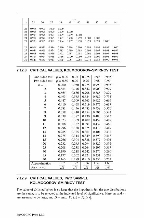
x =λ 35 36 37 38 39 40 41 42 43 44
21 0.998 0.999 1.000 1.00022 0.996 0.998 0.999 0.999 1.00023 0.993 0.996 0.997 0.999 0.999 1.00024 0.987 0.992 0.995 0.997 0.998 0.999 1.000 1.00025 0.978 0.985 0.991 0.994 0.997 0.998 0.999 0.999 1.000
26 0.964 0.976 0.984 0.990 0.994 0.996 0.998 0.999 0.999 1.00027 0.944 0.961 0.974 0.983 0.989 0.993 0.996 0.997 0.998 0.99928 0.918 0.941 0.959 0.972 0.981 0.988 0.992 0.995 0.997 0.99829 0.884 0.914 0.938 0.956 0.970 0.980 0.986 0.991 0.994 0.99730 0.843 0.880 0.911 0.935 0.954 0.968 0.978 0.985 0.990 0.994
7.12.8 CRITICAL VALUES, KOLMOGOROV–SMIRNOV TEST
One-sided test p = 0.90 0.95 0.975 0.99 0.995Two-sided test p = 0.80 0.90 0.95 0.98 0.99
n = 1 0.900 0.950 0.975 0.990 0.9952 0.684 0.776 0.842 0.900 0.9293 0.565 0.636 0.708 0.785 0.8294 0.493 0.565 0.624 0.689 0.7345 0.447 0.509 0.563 0.627 0.6696 0.410 0.468 0.519 0.577 0.6177 0.381 0.436 0.483 0.538 0.5768 0.358 0.410 0.454 0.507 0.5429 0.339 0.387 0.430 0.480 0.513
10 0.323 0.369 0.409 0.457 0.48911 0.308 0.352 0.391 0.437 0.46812 0.296 0.338 0.375 0.419 0.44913 0.285 0.325 0.361 0.404 0.43214 0.275 0.314 0.349 0.390 0.41815 0.266 0.304 0.338 0.377 0.40420 0.232 0.265 0.294 0.329 0.35225 0.208 0.238 0.264 0.295 0.31730 0.190 0.218 0.242 0.270 0.29035 0.177 0.202 0.224 0.251 0.26940 0.165 0.189 0.210 0.235 0.252
Approximationfor n > 40:
1.07√n
1.22√n
1.36√n
1.52√n
1.63√n
7.12.9 CRITICAL VALUES, TWO SAMPLEKOLMOGOROV–SMIRNOV TEST
The value of D listed below is so large that the hypothesis H0, the two distributionsare the same, is to be rejected at the indicated level of significance. Here, n1 and n2
are assumed to be large, and D = max∣∣Fn1(x)− Fn2(x)
∣∣.
©1996 CRC Press LLC

Level of significance Value of D
α = 0.10 1.22√
n1+n2n1n2
α = 0.05 1.36√
n1+n2n1n2
α = 0.025 1.48√
n1+n2n1n2
α = 0.01 1.63√
n1+n2n1n2
α = 0.005 1.73√
n1+n2n1n2
α = 0.001 1.95√
n1+n2n1n2
7.12.10 CRITICAL VALUES, SPEARMAN’S RANKCORRELATION
Spearman’s coefficient of rank correlation, ρs , measures the correspondence betweentwo rankings. Let di be the difference between the ranks of the i th pair of a set of npairs of elements. Then Spearman’s rho is defined as
ρs = 1− 6∑n
i=1 d2i
n3 − n= 1− 6Sr
n3 − n
where Sr =∑n
i=1 d2i . The table below gives critical values for Sr when there is
complete independence.
n p = 0.90 p = 0.95 p = 0.99 p = 0.9994 0.8000 0.8000 − −5 0.7000 0.8000 0.9000 −6 0.6000 0.7714 0.8857 −7 0.5357 0.6786 0.8571 0.96438 0.5000 0.6190 0.8095 0.92869 0.4667 0.5833 0.7667 0.9000
10 0.4424 0.5515 0.7333 0.866711 0.4182 0.5273 0.7000 0.836412 0.3986 0.4965 0.6713 0.818213 0.3791 0.4780 0.6429 0.791214 0.3626 0.4593 0.6220 0.767015 0.3500 0.4429 0.6000 0.746420 0.2977 0.3789 0.5203 0.658625 0.2646 0.3362 0.4654 0.596230 0.2400 0.3059 0.4251 0.5479
©1996 CRC Press LLC

7.13 SIGNAL PROCESSING
7.13.1 ESTIMATION
Let et be a white noise process (so that E [et ] = µ, variance(et ) = σ 2, andcovariance(et , es) = 0 for s = t). Suppose that Xt is a time series. A nonantici-pating linear model presumes that
∑∞u=0 huXt−u = et , where the hu are constants.
This can be written H(z)Xt = et where H(z) = ∑∞u=0 huz
u and znXt = Xt−n.Alternately, Xt = H−1(z)et . In practice, several types of models are used:
• AR(k), autoregressive model of order k: This assumes thatH(z) = 1+ a1z+ · · · + akzk and so
Xt + a1Xt−1 + . . . akXt−k = et . (7.13.1)
• MA(l), moving average of order l: This assumes thatH−1(z) = 1+ b1z+ · · · + bkzk and so
Xt = et + b1et−1 + . . . blet−l . (7.13.2)
• ARMA(k, l), mixed autoregressive/moving average of order (k, l): This as-sumes that H−1(z) = 1+b1z+···+bkzk
1+a1z+···+akzk and so
Xt + a1Xt−1 + . . . akXt−k = et + b1et−1 + . . . blet−l .(7.13.3)
7.13.2 FILTERS
1. Butterworth filter of order n: |Ha(jP)|2 = 1
1+ (jP/jPc)2n.
2. Chebyshev filter of order n: |Ha(jP)|2 = 1
1+ ε2Tn(P/Pc).
7.13.3 MATCHED FILTERING (WEINER FILTER)
Let X(t) represent a signal to be recovered, let N(t) represent noise, and let Y (t) =X(t)+N(t) represent the observable signal. A prediction of the signal is
Xp(t) =∫ ∞
0K(z)Y (t − z) dz,
whereK(z) is a filter. The mean square error is E[(X(t)− Xp(t))
2]; this is minimized
by the optimal (Weiner) filter Kopt(z).
©1996 CRC Press LLC

When X and Y are stationary, define their autocorrelation functions as RXX(t −s) = E [X(t)X(s)] and RYY (t − s) = E [Y (t)Y (s)]. If F represents the Fouriertransform (see page 530), then the optimal filter is given by
F [Kopt(t)
] = 1
2π
F [RXX(t)]
F [RYY (t)]. (7.13.4)
For example, if X and N are uncorrelated, then
F [Kopt(t)
] = 1
2π
F [RXX(t)]
F [RXX(t)]+ F [RNN(t)]. (7.13.5)
In the case of no noise, F [Kopt(t)
] = 12π , Kopt(t) = δ(t), and Sp(t) = Y (t).
7.13.4 KALMAN FILTERING
Kalman filtering is a linear least squares recursive estimator. It is used when thestate space has a higher dimension than the observation space. For example, in someairport radars the distance to aircraft is measured and the velocity of each aircraft isinferred. The general case covered by Kalman filtering is
xn = Fnxn−1 +Gnwn
yn = Hnxn + Jnvn,(7.13.6)
where xn is the state to be estimated and yn is the observable. Here, Fn, Gn, Hn,and Jn are matrices (Fn is required to be non-singular), xn is real-valued withx−1 = 0, and wn and vn are uncorrelated white Gaussian noise processes withE [wn] = E [vn] = 0, E
[wnwT
n
] = σ 2w, and E
[vnvT
n
] = σ 2v .
Consider the simpler system
xn = Fxn−1 +Gwn
yn = xn + vn.(7.13.7)
Here, F and G are constant matrices (F is also nonsingular). If xn,m is the predictorof xn using the values y0, . . . , ym, then the Kalman predictor for xn,n−1 is
xn,n−1 = F[xn−1,n−2 +Kn−1
(yn−1 − xn−1,n−2
)](7.13.8)
and the Kalman predictor for xn,n (called the Kalman filter) is
xn,n = F xn−1,n−1 +Kn
(yn − F xn−1,n−1
)(7.13.9)
with x−1,−1 = 0. Here Kn is the Kalman gain matrix.Define the error xn = xn,n−1−xn and its covariance matrix εn = E
[xnxT
n
]. Then
Kn = εn(εn + σ 2
v
)−1, and εn = Fεn−1
[I −KT
n−1
]F T +Gσ 2
wGT,
which can be solved simultaneously.For example, consider the system xn = 0.9xn−1 + wn, yn = xn + vn with
x−1 = 0, σ 2w = 0.19, and σ 2
v = 1. In this case Kn = εn/(1 + εn), and εn =(0.19+ εn−1)/(1+ εn). In the limit, ε∞ = 0.436 . . . , and K∞ = 0.304 . . . . Hence,for large values of n, xn,n = 0.626xn−1,n−1 + 0.304yn.
©1996 CRC Press LLC
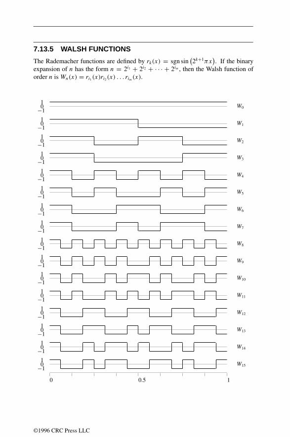
7.13.5 WALSH FUNCTIONS
The Rademacher functions are defined by rk(x) = sgn sin(2k+1πx
). If the binary
expansion of n has the form n = 2i1 + 2i2 + · · · + 2im , then the Walsh function oforder n is Wn(x) = ri1(x)ri2(x) . . . rim(x).
0 0.5 1
10−1
W0
10−1
W1
10−1
W2
10−1
W3
10−1
W4
10−1
W5
10−1
W6
10−1
W710−1
W8
10−1
W9
10−1
W10
10−1
W11
10−1
W12
10−1
W13
10−1
W14
10−1
W15
©1996 CRC Press LLC

7.13.6 WAVELETS
The Haar wavelet is H(x) = 1 if 0 ≤ x < 1/2,−1 if 1/2 ≤ x < 1, and 0 otherwise.Define Hj,k(x) = 2j/2H(2j x − k). Then the Haar system, Hj,k+∞j,k=−∞, forms anorthonormal basis for the Hilbert space, L2(R), consisting of functions f with finiteenergy, i.e.,
∫ +∞−∞ |f (x)|2 dx <∞.
DefinitionsThe construction of other wavelet orthonormal bases ψj,k+∞j,k=−∞ begins by choosingreal coefficients h0, . . . , hn which satisfy the following conditions (we set hk = 0 ifk < 0 or k > n):
• Normalization:∑
k hk =√
2.
• Orthogonality:∑
k hk hk−2j = 1 if j = 0 and 0 if j = 0.
• Accuracy p:∑
k(−1)kkjhk = 0 for j = 0, . . . , p − 1 with p > 0.
• Cohen–Lawton Criterion: A technical condition only rarely violated by coeffi-cients which satisfy the normalization, orthogonality, and accuracyp conditions.
The terms order of approximation or Strang–Fix conditions are often used in placeof “accuracy”. The orthogonality condition implies that n is odd.
The four conditions above imply the existence of a solution ϕ ∈ L2(R), calledthe scaling function, to the following refinement equation:
ϕ(x) =√
2n∑
k=0
hk ϕ(2x − k).
The scaling function has a nonvanishing integral which we normalize to∫ϕ(x) dx =
1. Then ϕ(x) is unique, and it vanishes outside of the interval [0, n]. The maximumpossible accuracy isp = (n+1)/2. Thus, increasing the accuracy requires increasingthe number of coefficients hk . High accuracy is desirable, as it implies that each ofthe polynomials 1, x, . . . , xp−1 can be written as an infinite linear combination of theinteger translates ϕ(x − k). In particular,
∑k ϕ(x − k) = 1. Also, the smoothness
of ϕ is limited by the accuracy; ϕ can have at most n − 2 derivatives, although inpractice it usually has fewer.
For each fixed integer j , let Vj be the closed subspace of L2(R) spanned by thefunctions, ϕj,k+∞k=−∞, where ϕj,k(x) = 2j/2ϕ(2j x − k). The sequence of subspacesVj +∞j=−∞ forms a multiresolution analysis for L2(R), meaning that:
• The subspaces are nested: · · · ⊂ V−1 ⊂ V0 ⊂ V1 · · · .• They are obtained from each other by dilation by 2: v(x) ∈ Vj ⇐⇒ v(2x) ∈Vj+1.
• V0 is integer translation invariant: v(x) ∈ V0 ⇐⇒ v(x + 1) ∈ V0.
• The Vj increase to all of L2(R) and decrease to zero: ∪Vj is dense in L2(R)
and ∩Vj = 0.
©1996 CRC Press LLC

• The set of integer translates ϕ(x− k)+∞k=−∞ forms an orthonormal basis for V0.
The projection of f (x) onto the subspace Vj is an approximation at resolution level2−j . It is given byfj (x) =
∑k cj,k ϕj,k(x)with cj,k = 〈f, ϕj,k〉 =
∫f (x) ϕj,k(x) dx.
The wavelet ψ is derived from the scaling function ϕ by the formula,
ψ(x) =√
2n∑
k=0
gk ϕ(2x − k), where gk = (−1)k hn−k.
The wavelet ψ has the same smoothness as ϕ, and the accuracy p condition impliesvanishing moments for ψ :
∫xjψ(x) dx = 0 for j = 0, . . . , p − 1. The functions
ψj,k(x) = 2j/2ψ(2j x − k) are orthonormal, and the entire collection ψj,k+∞j,k=−∞forms an orthonormal basis for L2(R).
With j fixed, let Wj be the closed subspace of L2(R) spanned by ψ(2j x− k) forinteger k. Then Vj and Wj are orthogonal subspaces whose direct sum is Vj+1. Letf be a function and let pj =
∑k dj,k ϕj,k(x) be its projection onto Wj , where dj,k =
〈f,ψj,k〉. Then the approximation fj+1 with resolution 2−(j+1) is fj+1 = fj + pj ,the sum of the approximation fj at resolution 2−j and the additional fine details pj
needed to give the next higher resolution level.The discrete wavelet transform is an algorithm for computing the coefficients
cj,k and dj,k from the coefficients cj+1,k . It can also be interpreted as an algorithmdealing directly with discrete data, dividing data cj+1,k into a low-pass part cj,k anda high-pass part dj,k . Specifically,
cj,l =∑k
hk−2l cj+1,k and dj,l =∑k
gk−2l cj+1,k.
The inverse transform is
cj+1,k =∑l
hk−2l cj,l +∑l
gk−2l dj,l .
The discrete wavelet transform is closely related to engineering techniques known assub-band coding and quadrature mirror filtering.
Example: the Daubechies family. For each even integer N > 0, there is a uniqueset of coefficients h0, . . . , hN−1 which satisfy the normalization and orthogonalityconditions with maximal accuracy p = N/2. The corresponding ϕ and ψ are theDaubechies scaling function DN and Daubechies wavelet WN . The Haar waveletH is the same as the Daubechies wavelet W2. For the Haar wavelet, the coeffi-cients are h0 = h1 = 1/
√2 and the subspace Vj consists of all functions which are
piecewise constant on each interval [k2−j , (k + 1)2−j ). The coefficients for D4 are:h0 = (1 + √3)/(4
√2), h1 = (3 + √3)/(4
√2), h2 = (3 − √3)/(4
√2), and h3 =
(1−√3)/(4√
2).
GeneralizationsFor a given number of coefficients, the Daubechies wavelet has the highest accu-racy. Other wavelets reduce the accuracy in exchange for other properties. In theCoiflet family the scaling function and the wavelet possesses vanishing moments,
©1996 CRC Press LLC

leading to simple one-point quadrature formulas. The “least asymmetric” waveletsare close to being symmetric or antisymmetric (perfect symmetry is incompatiblewith orthogonality, except for Haar).
Wavelet packets are libraries of basis functions defined recursively from the scal-ing functions φ and ψ . The Walsh functions are wavelet packets based on the Haarwavelet.
Allowing infinitely many coefficients results in wavelets supported on the entirereal line. The Meyer wavelet is band-limited, possesses infinitely many derivatives,and has accuracy p = ∞. The Battle–Lemarie wavelets are piecewise splines andhave exponential decay.
M-band wavelets replace the ubiquitous dilation factor 2 by another integer M .Multiwavelets replace the coefficients hk by r × r matrices and the scaling functionand wavelet by vector-valued functions (ϕ1, . . . , ϕr) and (ψ1, . . . , ψr), resulting inan orthonormal basis for L2(R) generated by the several wavelets ψ1, . . . , ψr .
For higher dimensions, a separable wavelet basis is constructed via a tensorproduct, with scaling function ϕ(x)ϕ(y) and three wavelets ϕ(x)ψ(y), ψ(x)ϕ(y),ψ(x)ψ(y). Nonseparable wavelets replace the dilation factor 2 by a dilation matrix.
Biorthogonal wavelets allow greater flexibility of design by relaxing the require-ment that the wavelet system ψj,k form an orthonormal basis to requiring onlythat it form a Riesz basis. The Cohen–Daubechies–Feauveau wavelets are symmet-ric and their coefficients hk are dyadic rationals. The Chui–Wang–Aldroubi–Unsersemiorthogonal wavelets are splines with explicit analytic formulas.
The basis condition may be further relaxed by allowing ψj,k to be a frame, anovercomplete system with basis-like properties. Introducing further redundancy, thecontinuous wavelet transform uses all possible dilates and translates a1/2ψ(ax+ b).
Wavelet coefficients and figuresCoefficients for Daubechies scaling functions1
D2 : h0: 0.707106781187h1: 0.707106781187
D4 : h0: 0.482962913145h1: 0.836516303738h2: 0.224143868042h3: −0.129409522551
D6 : h0: 0.332670552950h1: 0.806891509311h2: 0.459877502118h3: −0.135011020010h4: −0.085441273882h5: 0.035226291886
D8 : h0: 0.230377813309h1: 0.714846570553h2: 0.630880767930h3: −0.027983769417h4: −0.187034811719h5: 0.030841381836h6: 0.032883011667h7: −0.010597401785
1The tables and figures are taken in part from Table 6.1 and Figure 6.3 of Ingrid Daubechies’ book TenLectures on Wavelets, published by SIAM Press and used with permission.
©1996 CRC Press LLC
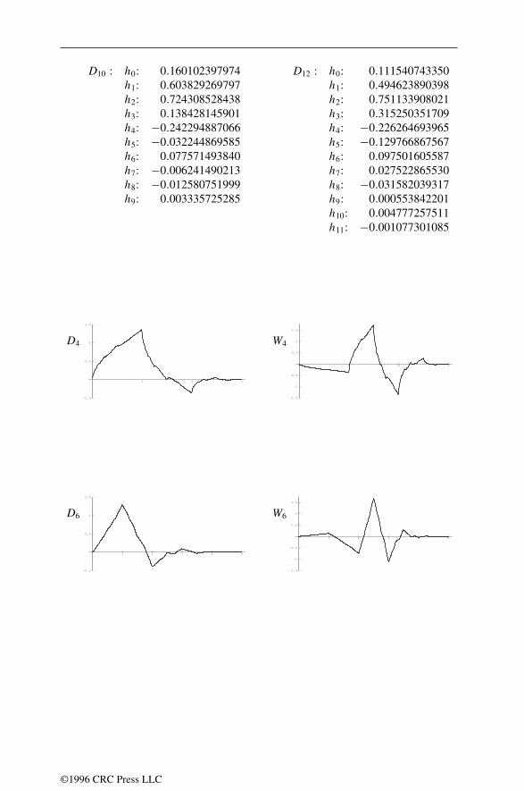
D10 : h0: 0.160102397974h1: 0.603829269797h2: 0.724308528438h3: 0.138428145901h4: −0.242294887066h5: −0.032244869585h6: 0.077571493840h7: −0.006241490213h8: −0.012580751999h9: 0.003335725285
D12 : h0: 0.111540743350h1: 0.494623890398h2: 0.751133908021h3: 0.315250351709h4: −0.226264693965h5: −0.129766867567h6: 0.097501605587h7: 0.027522865530h8: −0.031582039317h9: 0.000553842201h10: 0.004777257511h11: −0.001077301085
D4
1 2 3
-0.5
0.5
1
1.5
W4
1 2 3
-1.5
-1
-0.5
0.5
1
1.5
D6
1 2 3 4 5
-0.5
0.5
1
1.5
W6
1 2 3 4 5
-1.5
-1
-0.5
0.5
1
1.5
©1996 CRC Press LLC

D8
1 2 3 4 5 6 7
-0.5
0.5
1
1.5
W8
1 2 3 4 5 6 7
-1.5
-1
-0.5
0.5
1
1.5
D10
1 2 3 4 5 6 7 8 9
-0.5
0.5
1
1.5
W10
1 2 3 4 5 6 7 8 9
-1.5
-1
-0.5
0.5
1
1.5
References
1. W. H. Beyer, CRC Standard Probability and Statistics: Tables and Formulae,CRC Press, Boca Raton, FL, 1991.
2. I. Daubechies, Ten Lectures on Wavelets, SIAM Press, Philadelphia, 1992.
3. W. Feller, An Introduction to Probability Theory and Its Applications, Volume 1,John Wiley & Sons, New York, 1968.
4. S. K. Park and K. W. Miller, “Random number generators: good ones are hardto find,” Comm. ACM, October 1988, 31, 10, pages 1192–1201.
5. G. Strang and T. Nguyen, Wavelets and Filter Banks, Wellesley–CambridgePress, Wellesley, MA, 1995.
©1996 CRC Press LLC
Chapter 8Scientific Computing
8.1 BASIC NUMERICAL ANALYSIS8.1.1 Approximationsand errors8.1.2 Solution to algebraic equations8.1.3 Interpolation8.1.4 Fitting equations to data
8.2 NUMERICAL LINEAR ALGEBRA 8.2.1 Solving linear systems8.2.2 Gaussian elimination8.2.3 Gaussian elimination algorithm8.2.4 Pivoting8.2.5 Eigenvaluecomputation8.2.6 Householder’smethod8.2.7 QRalgorithm8.2.8 Nonlinear systemsand numerical optimization
8.3 NUMERICAL INTEGRATION AND DIFFERENTIATION 8.3.1 Numerical integration8.3.2 Numerical differentiation8.3.3 Schemes for theODE: y′ = f (x, y)
8.3.4 Explicit schemes for thePDE: aux + ut = 0 8.3.5 Implicit schemes for thePDE: aux + ut = S(x, t)
8.3.6 Schemes for thePDE: F(u)x + ut = 0 8.3.7 Schemes for thePDE: ux
REFERENCES
= utt
8.3.8 Numerical summation
8.4 PROGRAMMING TECHNIQUES
©1996 CRC Press LLC
The text Numerical Analysis, Fifth Edition, Prindle, Weber & Schmidt (Boston) 1993,by R. L. Burden and J. D. Faires, was the primary reference for most of the informationpresented in this chapter.
8.1 BASIC NUMERICAL ANALYSIS
8.1.1 APPROXIMATIONS AND ERRORS
Numerical methods involve finding approximate solutions to mathematical problems.Errors of approximation can result from two sources: error inherent in the method orformula used and round off error. Round off errorresults when a calculator or com-puter is used to perform real-number calculations with a finite number of significantdigits. All but the first specified number of digits are either choppedor roundedtothat number of digits.
If p∗ is an approximation to p, the absolute erroris defined to be |p − p∗| andthe relative erroris |p − p∗|/|p|, provided that p = 0.
Iterative techniques often generate sequences that (ideally) converge to an exactsolution. It is sometimes desirable to describe the rate of convergence.
DEFINITION 8.1.1
Supposelim βn = 0 andlim αn = α. If a positive constantK exists with|αn − α| <K |βn| for largen, thenαn is said to converge toα with arate of convergence O(βn).This is read “big oh ofβn” and written αn = α + O(βn).
DEFINITION 8.1.2
Supposepn is a sequence that converges top. If positive constantsλandα exist with
limn→∞
|pn+1 − p||pn − p|α = λ, thenpn is said toconverge to p of order α, with asymptotic
error constant λ.
In general, a higher order of convergence yields a more rapid rate of convergence.A sequence has linear convergenceif α = 1 and quadratic convergenceif α = 2.
Aitken’s 2 method
DEFINITION 8.1.3
Given the sequencepn∞n=0, define theforward difference pn bypn = pn+1 −pn,
©1996 CRC Press LLC
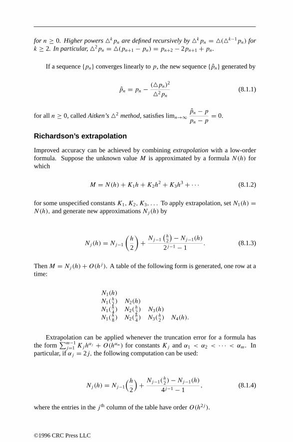
for n ≥ 0. Higher powerskpn are defined recursively bykpn = (k−1pn) fork ≥ 2. In particular,2pn = (pn+1 − pn) = pn+2 − 2pn+1 + pn.
If a sequence pn converges linearly to p, the new sequence pn generated by
pn = pn − (pn)2
2pn
(8.1.1)
for all n ≥ 0, called Aitken’s2 method, satisfies limn→∞pn − p
pn − p= 0.
Richardson’s extrapolation
Improved accuracy can be achieved by combining extrapolationwith a low-orderformula. Suppose the unknown value M is approximated by a formula N(h) forwhich
M = N(h) + K1h + K2h2 + K3h
3 + · · · (8.1.2)
for some unspecified constants K1,K2,K3, . . . To apply extrapolation, set N1(h) =N(h), and generate new approximations Nj(h) by
Nj(h) = Nj−1
(h
2
)+ Nj−1
(h2
)− Nj−1(h)
2j−1 − 1. (8.1.3)
Then M = Nj(h) + O(hj ). A table of the following form is generated, one row at atime:
N1(h)
N1(h2 ) N2(h)
N1(h4 ) N2(
h2 ) N3(h)
N1(h8 ) N2(
h4 ) N3(
h2 ) N4(h).
Extrapolation can be applied whenever the truncation error for a formula hasthe form
∑m−1j=1 Kjh
αj + O(hαm) for constants Kj and α1 < α2 < · · · < αm. Inparticular, if αj = 2j, the following computation can be used:
Nj(h) = Nj−1
(h2
)+ Nj−1(
h2 ) − Nj−1(h)
4j−1 − 1, (8.1.4)
where the entries in the j th column of the table have order O(h2j ).
©1996 CRC Press LLC

8.1.2 SOLUTION TO ALGEBRAIC EQUATIONS
Iterative methods generate sequences pn that converge to a solutionp of an equation.
DEFINITION 8.1.4
A solutionp of f (x) = 0 is a zero of multiplicity m if f (x) can be written asf (x) = (x − p)mq(x), for x = p, wherelimx→p q(x) = 0. A zero is calledsimpleif m = 1.
Fixed point iterationA fixed pointp for a function g satisfies g(p) = p. Given p0, generate pn by
pn+1 = g(pn) for n ≥ 0. (8.1.5)
If pn converges, then it will converge to a fixed point of g and the value pn canbe used as an approximation for p. The following theorem gives conditions thatguarantee convergence.
THEOREM 8.1.1 (Fixed point theorem)
Let g ∈ C[a, b] and suppose thatg(x) ∈ [a, b] for all x in [a, b]. Suppose, inaddition, thatg′ exists on(a, b) with
∣∣g′(x)∣∣ ≤ k < 1, for all x ∈ (a, b). If p0 is
any number in[a, b], then the sequence defined by Equation (8.1.5) converges to the(unique) fixed pointp in [a, b], and|pn − p| ≤ kn
1−k|p0 − p1| for all n ≥ 1.
The iteration sometimes converges even if all the conditions are not satisfied.
THEOREM 8.1.2
Suppose g is a function that satisfies the conditions of Theorem 8.1.1 and g′ is alsocontinuous on (a, b). If g′(p) = 0, then for any numberp0 in [a, b], the sequencegenerated by Equation (8.1.5) converges only linearly to the unique fixed pointp in[a, b].
THEOREM 8.1.3
Let p be a solution of the equationx = g(x). Suppose thatg′(p) = 0 and g′′ iscontinuous and strictly bounded byM on an open intervalI containingp. Then thereexists aδ > 0 such that, forp0 ∈ [p − δ, p + δ], the sequence defined by Equation(8.1.5) converges at least quadratically top.
Steffensen’s methodFor a linearly convergent fixed point iteration, convergence can be accelerated byapplying Aitken’s 2 method. This is called Steffensen’s method. Define p
(0)0 = p0,
©1996 CRC Press LLC

FIGURE 8.1.1Illustration of Newton’s method.1
Slope f´ (p1) y = f(x)
Slope f´ (p0)
(p1, f(p1))
(p0, f(p0))
p0 p2
p1
p
y
x
compute p(0)1 = g(p
(0)0 ) and p
(0)2 = g(p
(0)1 ). Set p(1)
0 = p0 which is computed usingEquation (8.1.1) applied to p(0)
0 , p(0)1 and p
(0)2 . Use fixed point iteration to compute
p(1)1 and p
(1)2 and then Equation (8.1.1) to find p(2)
0 . Continuing, generate p(n)0 .
THEOREM 8.1.4
Suppose that x = g(x) has the solution p with g′(p) = 1. If there exists a δ > 0 suchthat g ∈ C3[p − δ, p + δ], then Steffensen’s method gives quadratic convergence forthe sequence p(n)
0 for any p0 ∈ [p − δ, p + δ].
Newton–Raphson method (Newton’s method)To solve f (x) = 0, given an initial approximation p0, generate pn using
pn+1 = pn − f (pn)
f ′(pn), for n ≥ 0 (8.1.6)
Figure 8.1.1 describes the method geometrically. Each value pn+1 represents thex-intercept of the tangent line to the graph of f (x) at the point [pn, f (pn)].
THEOREM 8.1.5
Let f ∈ C2[a, b]. If p ∈ [a, b] is such that f (p) = 0 and f ′(p) = 0, then thereexists a δ > 0 such that Newton’s method generates a sequence pn converging top for any initial approximation p0 ∈ [p − δ, p + δ].
1From R.L. Burden and J.D. Faires, Numerical Analysis, 5th ed., Prindle, Weber & Schmidt, Boston,1993. With permission.
©1996 CRC Press LLC

Note:
1. Generally the conditions of the theorem cannot be checked. Therefore oneusually generates the sequence pn and observes whether or not it converges.
2. An obvious limitation is that the iteration terminates if f ′(pn) = 0.
3. For simple zeros of f , Theorem 8.1.3 implies that Newton’s method convergesquadratically. Otherwise, the convergence is much slower.
Modified Newton’s method
Newton’s method converges only linearly if p has multiplicity larger that one. How-ever, the function u(x) = f (x)
f ′(x) has a simple zero at p. Hence, the Newton iterationformula applied to u(x) yields quadratic convergence to a root of f (x) = 0. Theiteration simplifies to
pn+1 = pn − f (pn)f′(pn)
[f ′(pn)]2 − f (pn)f ′(pn), for n ≥ 0. (8.1.7)
Secant method
To solve f (x) = 0, the secant method uses the x-intercept of the secant line passingthrough (pn, f (pn)) and (pn−1, f (pn−1)). The derivative of f is not needed. Givenp0 and p1, generate the sequence with
pn+1 = pn − f (pn)(pn − pn−1)
f (pn) − f (pn−1), for n ≥ 1. (8.1.8)
Root bracketing methods
Suppose f (x) is continuous on [a, b] and f (a)f (b) < 0. The intermediate valuetheorem guarantees a number p ∈ [a, b] exists with f (p) = 0. A root bracketingmethod constructs a sequence of nested intervals [an, bn], each containing a solutionof f (x) = 0. At each step, compute pn ∈ [an, bn] and proceed as follows:
If f (pn) = 0, stop the iteration and p = pn.
Else,
if f (an)f (pn) < 0, then set an+1 = an, bn+1 = pn.
Else, set an+1 = pn, bn+1 = bn.
Bisection method
This is a special case of the root bracketing method. The values pn are computed by
pn = an + bn − an
2= an + bn
2, for n ≥ 1. (8.1.9)
©1996 CRC Press LLC

Clearly, |pn − p| ≤ ( b − a)/2n for n ≥ 1. The rate of convergence is O(2 −n). Al-though convergence is slow, the exact number of iterations for a specified accuracy ε
can be determined. To guarantee that |pN − p| < ε, use
N > log2
(b − a
ε
)= ln(b − a) − ln ε
ln 2. (8.1.10)
False position ( regula falsi )
pn = bn − f (bn)bn − an
f (bn) − f (an), for n ≥ 1. (8.1.11)
Both methods converge, provided the initial criteria are satisfied.
Horner’s method with deflationIf Newton’s method is used to solve for roots of the polynomial P(x) = 0, then thepolynomialsP andP ′ are repeatedly evaluated. Horner’s method efficiently evaluatesa polynomial of degree n using only n multiplications and n additions.
Horner’s algorithmTo evaluate P(x) = anx
n + an−1xn−1 + · · · + a0 and its derivative at x0 (y = P(x0),
z = P ′(x0),
INPUT: degree n, coefficients a0, a1, . . . , an; x0,OUTPUT: y = P(x0); z = P ′(x0).Algorithm
1. Set y = an; z = an.
2. For j = n − 1, n − 2, . . . , 1,set y = x0y + aj ; z = x0z + y.
3. Set y = x0y + a0.
4. OUTPUT (y, z). STOP.
When satisfied with the approximation x1 for a root x1 ofP , use synthetic divisionto compute Q1(x) so that P(x) ≈ (x− x1)Q1(x). Estimate a root of Q1(x) and writeP(x) ≈ (x − x1)(x − x2)Q2(x), and so on. Eventually, Qn−2(x) will be a quadratic,and the quadratic formula can be applied. This procedure, finding one root at a time,is called deflation.
Note: Care must be taken since x1 is an approximation for x1. Some inaccuracyoccurs when computing the coefficients of Q1(x), etc. Although the estimate x2 of aroot of Q2(x) can be very accurate, it may not be as accurate when estimating a rootof P(x).
©1996 CRC Press LLC

8.1.3 INTERPOLATION
Interpolation involves fitting a function to a set of data points (x0, y0), (x1, y1), . . . ,(xn, yn). The xi are unique and the yi may be regarded as the values of some functionf (x), that is, yi = f (xi) for i = 0, 1, . . . , n. Polynomial interpolation methods arediscussed below.
Lagrange interpolationThe Lagrange interpolating polynomial, denoted Pn(x), is the unique polynomial ofdegree at most n for which Pn(xk) = f (xk) for k = 0, 1, . . . , n. It is given by
P(x) =n∑
k=0
f (xk)Ln,k(x) (8.1.12)
where x0, . . . , xn are called node points.
Ln,k(x) = (x − x0)(x − x1) · · · (x − xk−1)(x − xk+1) · · · (x − xn)
(xk − x0)(xk − x1) · · · (xk − xk−1)(xk − xk+1) · · · (xk − xn),
=n∏
i=0,i =k
(x − xi)
(xk − xi), for k = 0, 1, . . . , n. (8.1.13)
THEOREM 8.1.6 (Error formula)
If x0, x1, . . . , xn are distinct numbers in [a, b] and f ∈ Cn+1[a, b], then, for each x
in [a, b], a number ξ(x) in (a, b) exists with
f (x) = P(x) + f (n+1)(ξ(x))
(n + 1)!(x − x0)(x − x1) · · · (x − xn),
where P is the interpolating polynomial given in Equation (8.1.12).
Although the Lagrange polynomial is unique, it can be expressed and evaluatedin several ways. Equation (8.1.12) is tedious to evaluate, and including more nodesaffects the entire expression. Neville’s method evaluates the Lagrange polynomialat a single point without explicitly finding the polynomial and adapts easily to theaddition of nodes.
Neville’s methodLetPm1,m2,...,mk
denote the Lagrange polynomial using distinct nodes xm1 , xm2 , . . . , xmk.
If P(x) denotes the Lagrange polynomial using nodes x0, x1, . . . , xk and xi and xj
are two distinct numbers in this set, then
P(x) = (x − xj )P0,1,...,j−1,j+1,...,k(x) − (x − xi)P0,1,...,i−1,i+1,...,k(x)
(xi − xj ). (8.1.14)
©1996 CRC Press LLC

Neville’s algorithmGenerate a table of entriesQi,j for j ≥ 0 and 0 ≤ i ≤ j whereQi,j = Pi−j,i−j+1,...,i−1,i .Calculations use Equation (8.1.14) for a specific value of x as shown:
x0 Q0,0 = P0,
x1 Q1,0 = P1, Q1,1 = P0,1,
x2 Q2,0 = P2, Q2,1 = P1,2, Q2,2 = P0,1,2,
x3 Q3,0 = P3, Q3,1 = P2,3, Q3,2 = P1,2,3, Q3,3 = P0,1,2,3.
Note that Pk = Pk(x) = f (xk) and Qi,i represents successive estimates of f (x)
using Lagrange polynomials. Nodes may be added until∣∣Qi,i − Qi−1,i−1
∣∣ < ε asdesired.
Some interpolation formulae involve divided differences. Given a sequence xiand corresponding function values f (xi), the zeroth divided difference is f [xi] =f (xi). The first divided difference is defined by
f [xi, xi+1] = f (xi+1) − f (xi)
xi+1 − xi
= f [xi+1] − f [xi]
xi+1 − xi
. (8.1.15)
The kth divided difference is defined by
f [xi, xi+1, . . . , xi+k−1, xi+k]
= f [xi+1, xi+2, . . . , xi+k] − f [xi, xi+1, . . . , xi+k−1]
xi+k − xi
. (8.1.16)
Divided differences are usually computed by forming a triangular table.
Divided differencesFirst Second Third
x f (x) divided differences divided differences divided differencesx0 f [x0]
f [x0, x1]x1 f [x1] f [x0, x1, x2]
f [x1, x2] f [x0, x1, x2, x3]x2 f [x2] f [x1, x2, x3]
f [x2, x3]x3 f [x3]
Newton’s interpolatory divided-difference formula(also known as the Newton polynomial)
Pn(x) = f [x0] +n∑
k=1
f [x0, x1, . . . , xk](x − x0) · · · (x − xk−1).
(8.1.17)
Labeling the nodes as xn, xn−1, . . . , x0, a formula similar to Equation (8.1.17)results in Newton’s backward divided-difference formula,
©1996 CRC Press LLC

Pn(x) = f [xn] + f [xn−1, xn](x − xn)
+ f [xn−2, xn−1, xn](x − xn)(x − xn−1)
+ · · · + f [x0, x1, . . . , xn](x − xn) · · · (x − x1). (8.1.18)
If the nodes are equally-spaced (that is, xi −xi−1 = h), define the parameter s bythe equation x = x0 + sh. The following formulae evaluate Pn(x) at a single point:
1. Newton’s interpolatory divided-difference formula,
Pn(x) = Pn(x0 + sh) =n∑
k=0
(s
k
)k!hkf [x0, x1, . . . , xk].
(8.1.19)
2. Newton’s forward-difference formula (Newton–Gregory),
Pn(x) = Pn(x0 + sh) =n∑
k=0
(s
k
)k f (x0). (8.1.20)
3. Newton–Gregory backward formula (fits nodes x−n to x0),
Pn(x) = f (x0) +(s
1
) f (x−1) +
(s + 1
2
)2 f (x−2) +
· · · +(s + n − 1
n
)n f (x−n). (8.1.21)
4. Newton’s backward-difference formula,
Pn(x) =n∑
k=0
(−1)k(−s
k
)k f (xn), (8.1.22)
where kf (xn) is the kth backward difference defined by pn = pn − pn−1
for n ≥ 1. Higher powers are defined recursively by kpn = (k−1pn) fork ≥ 2.
5. Stirling’s formula (for equally-spaced nodes x−m, . . . , x−1, x0, x1, . . . , xm),
Pn(x) = P2m+1(x) = f [x0] + sh
2(f [x−1, x0] + f [x0, x1]) +
s2h2f [x−1, x0, x1] + s(s2 − 1)h3
2(f [x−1, x0, x1, x2] + f [x−2, x−1, x0, x1])
+ · · · + s2(s2 − 1)(s2 − 4) · · · (s2 − (m − 1)2)h2mf [x−m, . . . , xm]
+ s(s2 − 1) · · · (s2 − m2)h2m+1
2(f [x−m, . . . , xm+1] + f [x−m−1, . . . , xm]).
Use the entire formula if n = 2m + 1 is odd, and omit the last term if n = 2mis even. The following table identifies the desired divided differences used inStirling’s formula:
©1996 CRC Press LLC

First divided Second divided Third dividedx f (x) differences differences differences
x−2 f [x−2]f [x−2, x−1]
x−1 f [x−1] f [x−2, x−1, x0]f [x−1, x0] f [x−2, x−1, x0, x1]
x0 f [x0] f [x−1, x0, x1]
f [x0, x1] f [x−1, x0, x1, x2]x1 f [x1] f [x0, x1, x2]
f [x1, x2]x2 f [x2]
Inverse interpolationAny method of interpolation which does not require the nodes to be equally-spacedmay be applied by simply interchanging the nodes (x values) and the function values(y values).
Hermite interpolationGiven node points x0, x1, . . . , xn, the Hermite interpolating polynomial for a func-tion f is the unique polynomial H(x) of degree at most 2n+ 1 that satisfies H(xi) =f (xi) and H ′(xi) = f ′(xi) for each i = 0, 1, . . . , n.
A technique and formula similar to Equation (8.1.17) can be used. For dis-tinct nodes x0, x1, . . . , xn, define z0, z1, . . . , z2n+1 by z2i = z2i+1 = xi fori = 0, 1, . . . , n. Construct a divided difference table for the ordered pairs (zi, f (zi))
using f ′(xi) in place of f [z2i , z2i+1], which would be undefined. Denote the Hermitepolynomial by H2n+1(x).
Hermite interpolating polynomial
H2n+1(x) = f [z0] +2n+1∑k=1
f [z0, z1, . . . , zk](x − z0) · · · (x − zk−1)
= f [z0] + f [z0, z1](x − x0) + f [z0, z1, z2](x − x0)2
+ f [z0, z1, z2, z3](x − x0)2(x − x1)
+ · · · + f [z0, . . . , z2n+1](x − x0)2 · · · (x − xn−1)
2(x − xn).
(8.1.23)
THEOREM 8.1.7 (Error formula)
If f ∈ C(2n+2)[a, b], then
f (x) = H2n+1(x) + f (2n+2)(ξ(x))
(2n + 2)!(x − x0)
2 · · · (x − xn)2
for some ξ ∈ (a, b) and where xi ∈ [a, b] for each i = 0, 1, . . . , n.
©1996 CRC Press LLC
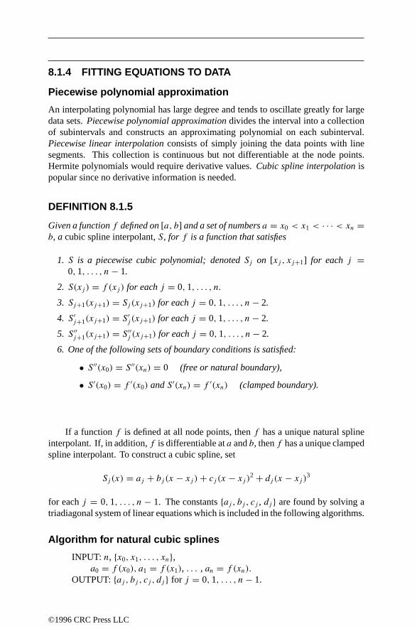
8.1.4 FITTING EQUATIONS TO DATA
Piecewise polynomial approximation
An interpolating polynomial has large degree and tends to oscillate greatly for largedata sets. Piecewise polynomial approximation divides the interval into a collectionof subintervals and constructs an approximating polynomial on each subinterval.Piecewise linear interpolation consists of simply joining the data points with linesegments. This collection is continuous but not differentiable at the node points.Hermite polynomials would require derivative values. Cubic spline interpolation ispopular since no derivative information is needed.
DEFINITION 8.1.5
Given a function f defined on [a, b] and a set of numbers a = x0 < x1 < · · · < xn =b, a cubic spline interpolant, S, for f is a function that satisfies
1. S is a piecewise cubic polynomial; denoted Sj on [xj , xj+1] for each j =0, 1, . . . , n − 1.
2. S(xj ) = f (xj ) for each j = 0, 1, . . . , n.
3. Sj+1(xj+1) = Sj (xj+1) for each j = 0, 1, . . . , n − 2.
4. S ′j+1(xj+1) = S ′
j (xj+1) for each j = 0, 1, . . . , n − 2.
5. S ′′j+1(xj+1) = S ′′
j (xj+1) for each j = 0, 1, . . . , n − 2.
6. One of the following sets of boundary conditions is satisfied:
• S ′′(x0) = S ′′(xn) = 0 (free or natural boundary),
• S ′(x0) = f ′(x0) and S ′(xn) = f ′(xn) (clamped boundary).
If a function f is defined at all node points, then f has a unique natural splineinterpolant. If, in addition, f is differentiable at a and b, then f has a unique clampedspline interpolant. To construct a cubic spline, set
Sj (x) = aj + bj (x − xj ) + cj (x − xj )2 + dj (x − xj )
3
for each j = 0, 1, . . . , n − 1. The constants aj , bj , cj , dj are found by solving atriadiagonal system of linear equations which is included in the following algorithms.
Algorithm for natural cubic splines
INPUT: n, x0, x1, . . . , xn,a0 = f (x0), a1 = f (x1), . . . , an = f (xn).
OUTPUT: aj , bj , cj , dj for j = 0, 1, . . . , n − 1.
©1996 CRC Press LLC
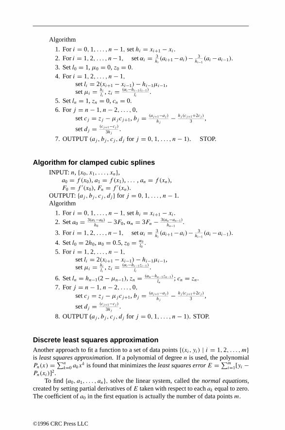
Algorithm
1. For i = 0, 1, . . . , n − 1, set hi = xi+1 − xi .
2. For i = 1, 2, . . . , n−1, set αi = 3hi(ai+1 −ai)− 3
hi−1(ai −ai−1).
3. Set l0 = 1, µ0 = 0, z0 = 0.
4. For i = 1, 2, . . . , n − 1,set li = 2(xi+1 − xi−1) − hi−1µi−1,set µi = hi
li, zi = (αi−hi−1zi−1)
li.
5. Set ln = 1, zn = 0, cn = 0.
6. For j = n − 1, n − 2, . . . , 0,set cj = zj − µjcj+1, bj = (aj+1−aj )
hj− hj (cj+1+2cj )
3 ,
set dj = (cj+1−cj )
3hj.
7. OUTPUT (aj , bj , cj , dj for j = 0, 1, . . . , n − 1). STOP.
Algorithm for clamped cubic splinesINPUT: n, x0, x1, . . . , xn,
a0 = f (x0), a1 = f (x1), . . . , an = f (xn),F0 = f ′(x0), Fn = f ′(xn).
OUTPUT: aj , bj , cj , dj for j = 0, 1, . . . , n − 1.Algorithm
1. For i = 0, 1, . . . , n − 1, set hi = xi+1 − xi .
2. Set a0 = 3(a1−a0)
h0− 3F0, an = 3Fn −
3(an−an−1)
hn−1.
3. For i = 1, 2, . . . , n−1, set αi = 3hi(ai+1 −ai)− 3
hi−1(ai −ai−1).
4. Set l0 = 2h0, u0 = 0.5, z0 = α0l0.
5. For i = 1, 2, . . . , n − 1,set li = 2(xi+1 − xi−1) − hi−1µi−1,set µi = hi
li, zi = (αi−hi−1zi−1)
li.
6. Set ln = hn−1(2 − µn−1), zn = (αn−hn−1zn−1)
ln; cn = zn.
7. For j = n − 1, n − 2, . . . , 0,set cj = zj − µjcj+1, bj = (aj+1−aj )
hj− hj (cj+1+2cj )
3 ,
set dj = (cj+1−cj )
3hj.
8. OUTPUT (aj , bj , cj , dj for j = 0, 1, . . . , n − 1). STOP.
Discrete least squares approximationAnother approach to fit a function to a set of data points (xi, yi) | i = 1, 2, . . . , mis least squares approximation. If a polynomial of degree n is used, the polynomialPn(x) = ∑n
k=0 akxk is found that minimizes the least squares error E = ∑m
i=1[yi −Pn(xi)]2.
To find a0, a1, . . . , an, solve the linear system, called the normal equations,created by setting partial derivatives of E taken with respect to each ak equal to zero.The coefficient of a0 in the first equation is actually the number of data points m.
©1996 CRC Press LLC

Normal equations
a0
m∑i=1
x0i + a1
m∑i=1
x1i + a2
m∑i=1
x2i + · · · + an
m∑i=1
xni =
m∑i=1
yix0i ,
a0
m∑i=1
x1i + a1
m∑i=1
x2i + a2
m∑i=1
x3i + · · · + an
m∑i=1
xn+1i =
m∑i=1
yix1i ,
...
a0
m∑i=1
xni + a1
m∑i=1
xn+1i + a2
m∑i=1
xn+2i + · · · + an
m∑i=1
x2ni =
m∑i=1
yixni .
Note: Pn(x) can be replaced by a function f of specified form. Unfortunately, tominimize E, the resulting system is generally not linear. Although these systems canbe solved, one technique is to “linearize” the data. For example, if y = f (x) = beax ,then ln y = ln b + ax. The least squares method applied to the data points (xi, ln yi)
produces a linear system. Note that this technique does not find the least squaresapproximation for the original problem but, instead, approximates the “linearized”data.
Best fit lineGiven the points P1(x1, y1), P2(x1, y1), . . . Pn(x1, y1) the line of best fit is given byy − y = m(x − x) where
x = 1
n
n∑i=1
xi = (x1 + x2 + · · · + xn)
n,
y = 1
n
n∑i=1
yi = (y1 + y2 + · · · + yn)
n,
m = (x1y1 + x2y2 + · · · + xnyn) − nx y
(x21 + x2
2 + · · · + x2n) − nx2
= xy − x y
x2 − x2.
8.2 NUMERICAL LINEAR ALGEBRA
8.2.1 SOLVING LINEAR SYSTEMS
The solution of systems of linear equations using Gaussian elimination with backwardsubstitution is described in Section 8.2.2. The algorithm is highly sensitive to roundoff error. Pivoting strategies can reduce round off error when solving an n×n system.
©1996 CRC Press LLC

For a linear system Ax = b, assume that the equivalent matrix equation A(k)x = b(k)
has been constructed. Call the entry, a(k)k,k, the pivot element.
8.2.2 GAUSSIAN ELIMINATION
To solve the system Ax = b, Gaussian elimination creates the augmented matrix
A′ = [A... b] =
a11 . . . a1n b1...
......
an1 . . . ann bn
.
This matrix is turned into an upper triangular matrix by a sequence of (1) row permu-tations, and (2) subtracting a multiple of one row from another. The result is a matrixof the form (the primes denote that the quantities have been modified)
a′
11 a′12 . . . a′
1n b′1
0 a′22 . . . a′
2n b′2
.... . .
. . ....
...
0 . . . 0 a′nn b′
n
.
This matrix represents a system of linear equations (just as A′ did), equivalentto the original system. Back substitution can be used to determine, successively,xn, xn−1, . . . .
8.2.3 GAUSSIAN ELIMINATION ALGORITHM
INPUT: number of unknowns and equations n, matrix A, and vector b.OUTPUT: solution to linear system x = (x1, . . . , xn) = A−1b,
or message that system does not have a unique solution.Algorithm
1. Construct the augmented matrix A′ = [A... b] = (a′
ij )
2. For i = 1, 2, . . . , n − 1 do the following: (Elimination process)
(a) Let p be the least integer with i ≤ p ≤ n and a′pi = 0
If no integer can be found, thenOUTPUT(“no unique solution exists”). STOP.
(b) If p = i interchange rows p and i in A′. Call the new matrixA′.
(c) For j = i + 1, . . . , n do the following:
i. Set mij = a′ji/a
′ii .
ii. Subtract from row j the quantity (mij times row i).
3. If a′nn = 0 then OUTPUT (“no unique solution exists”). STOP.
4. Set xn = a′n,n+1/a
′nn. (Start backward substitution)
©1996 CRC Press LLC

5. For i = n − 1, . . . , 2, 1 set xi =[a′i,n+1 −∑n
j=i+1 a′ij xj
]/a′
ii .
6. OUTPUT (x1, . . . , xn), (Procedure completed successfully). STOP.
8.2.4 PIVOTING
Maximal column pivoting
Maximal column pivoting (often called partial pivoting) finds, at each step, the ele-ment in the same column as the pivot element that lies on or below the main diagonalhaving the largest magnitude and moves it to the pivot position. Determine the least
p ≥ k such that∣∣∣a(k)
p,k
∣∣∣ = maxk≤i≤n
∣∣∣a(k)i,k
∣∣∣ and interchange the kth equation with the
pth equation before performing the elimination step.
Scaled-column pivoting
Scaled-column pivoting sometimes produces better results, especially when the ele-ments of A differ greatly in magnitude. The desired pivot element is chosen to havethe largest magnitude relative to the other values in its row. For each row define ascale factor si by si = max1≤j≤n
∣∣ai,j
∣∣. The desired pivot element at the kth step is
determined by choosing the smallest integer p with
∣∣∣a(k)p,k
∣∣∣sp
= maxk≤j≤n
∣∣∣a(k)j,k
∣∣∣Sj
.
Maximal (or complete) pivoting
The desired pivot element at the kth step is the entry of largest magnitude amongai,j with i = k, k + 1, . . . , n and j = k, k + 1, . . . , n. Both row and column inter-changes are necessary and additional comparisons are required, resulting in additionalexecution time.
8.2.5 EIGENVALUE COMPUTATION
Power method
Assume that the n× n matrix A has n eigenvalues λ1, λ2, . . . , λn with independenteigenvectors v(1), v(2), . . . , v(n). Assume further that A has a unique dominanteigenvector λ1, where |λ1| > |λ2| ≥ |λ3| ≥ · · · ≥ |λn|. For any x ∈ Rn, x =∑n
j=1 αjv(j).
The algorithm is called the power method because powers of the input matrix aretaken: limk→∞ Akx = limk→∞ λk
1α1v(1). However, this sequence converges to zero,if |λ1| < 1, and diverges, if |λ1| ≥ 1, provided α1 = 0. Appropriate scaling of Akx isnecessary to obtain a meaningful limit. Begin by choosing a unit vector x(0) havinga component x(0)
p0so that x(0)
p0= 1 = ∥∥x(0)
∥∥∞.
©1996 CRC Press LLC

The algorithm inductively constructs sequences of vectors x(m)∞m=0 and y(m)∞m=0and a sequence of scalars µ(m)∞m=1 by
y(m) = Ax(m−1), µ(m) = y(m)pm
, x(m) = y(m)
y(m)pm
, (8.2.1)
where, at each step, pm represents the least integer for which∣∣y(m)
pm
∣∣ = ∥∥y(m)∥∥
∞.
The sequence of scalars satisfies limm→∞ µ(m) = λ1, provided α1 = 0, and thesequence of vectors x(m)∞m=0 converges to an eigenvector of L∞ associated with λ1.
Power method algorithmINPUT: dimension n, matrix A, vector x, tolerance TOL, and
maximum iterations N .OUTPUT: approximate eigenvalue µ,
approximate eigenvector x (with ‖x‖∞ = 1),or a message that the maximum number of iterations was exceeded.
Algorithm
1. Set k=1.
2. Find an integer p with 1 ≤ p ≤ n and∣∣xp
∣∣ = ‖x‖∞ .
3. Set x= 1xp
x.
4. While (k ≤ N) do the following:
(a) Set y = Ax.
(b) Set µ = yp.
(c) Find an integer p with 1 ≤ p ≤ n and∣∣yp
∣∣ = ‖y‖∞ .
(d) If yp = 0 then OUTPUT (“Eigenvector”, x );OUTPUT (“corresponds to eigenvalue 0;select a new vector x and restart”). STOP.
(e) Set ERR =∥∥∥x − 1
ypy∥∥∥
∞; x = 1
ypy.
(f) If ERR < TOL then OUTPUT (µ, x)(procedure successful). STOP.
(g) Set k = k + 1.
5. OUTPUT (“Maximum number of iterations exceeded”). STOP.
Notes:
1. The method does not really require that λ1 be unique. If the multiplicity isgreater than one, the eigenvector obtained depends on the choice of x(0).
2. The sequence constructed converges linearly, so that Aitken’s 2 method (Equa-tion (8.1.1)) can be applied to accelerate convergence.
©1996 CRC Press LLC

Inverse power methodThe inverse power method modifies the power method to yield faster convergenceby finding the eigenvalue of A that is closest to a specified number q. Assume thatA satisfies the conditions as before. If q = λi , for i = 1, 2, . . . , n, the eigenvaluesof (A − qI)−1 are 1
λ1−q, 1
λ2−q, . . . , 1
λn−qwith the same eigenvectors v(1), . . . , v(n).
Apply the power method to (A − qI)−1. At each step, y(m) = (A − qI)−1x(m−1).Generally, y(m) is found by solving (A−qI)y(m) = x(m−1) using Gaussian eliminationwith pivoting. Choose the value q from an initial approximation to the eigenvectorx(0) by q = x(0)T
Ax(0)/x(0)Tx(0).
The only changes in the algorithm for the power method (see page 685) are insetting an initial value q as described (do this prior to step 1), determining y by solvingthe linear system (A−qI)y(m) = x(m−1) in step (4a), deleting step (4d), and replacingstep (4f) with
if ERR < TOL then set µ = 1
µ+ q; OUTPUT(µ, x); STOP.
Wielandt deflationOnce the dominant eigenvalue has been found, remaining eigenvalues can be found byusing deflation techniques. A new matrix B is formed having the same eigenvalues asA, except that the dominant eigenvalue of A is replaced by 0. One method is Wielandtdeflation which defines x = 1
λ1v(1)i
[ai1 ai2 . . . ain]T, where v(1)i is a coordinate of v(1)
that is nonzero, and the values ai1, ai2, . . . , ain are the entries in the i th row of A.Then the matrix B = A− λ1v(1)xT has eigenvalues 0, λ2, λ3, . . . , λn with associatedeigenvectors v(1), w(2), w(3), . . . , w(n), where
v(i) = (λi − λ1)w(i) + λ1(xTw(i))v(1)
for i = 2, 3, . . . , n. The i th row of B consists entirely of zero entries and B may bereplaced with an (n − 1) × (n − 1) matrix B ′ obtained by deleting the i th row and i th
column of B. The power method can be applied to B ′ to find its dominant eigenvalueand so on.
8.2.6 HOUSEHOLDER’S METHOD
DEFINITION 8.2.1
Two n × n matrices A and B are said to be similar if a nonsingular matrix S existswith A = S−1BS.
Householder’s method constructs a symmetric tridiagonal matrixB that is similarto a given symmetric matrix A. After applying this method, the QR algorithm can beused efficiently to approximate the eigenvalues of the resulting symmetric tridiagonalmatrix.
©1996 CRC Press LLC
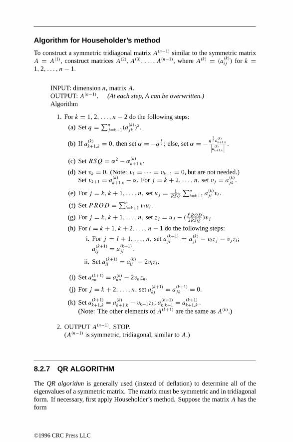
Algorithm for Householder’s method
To construct a symmetric tridiagonal matrix A(n−1) similar to the symmetric matrixA = A(1), construct matrices A(2), A(3), . . . , A(n−1), where A(k) = (a
(k)ij ) for k =
1, 2, . . . , n − 1.
INPUT: dimension n, matrix A.OUTPUT: A(n−1). (At each step, A can be overwritten.)Algorithm
1. For k = 1, 2, . . . , n − 2 do the following steps:
(a) Set q = ∑nj=k+1(a
(k)jk )2.
(b) If a(k)k+1,k = 0, then set α = −q
12 ; else, set α = − q
12 a
(k)k+1,k∣∣∣a(k)
k+1,k
∣∣∣ .
(c) Set RSQ = α2 − α(k)k+1,k .
(d) Set vk = 0. (Note: v1 = · · · = vk−1 = 0, but are not needed.)Set vk+1 = a
(k)k+1,k − α. For j = k + 2, . . . , n, set vj = a
(k)jk .
(e) For j = k, k + 1, . . . , n, set uj = 1RSQ
∑ni=k+1 a
(k)ji vi .
(f) Set PROD = ∑ni=k+1 viui .
(g) For j = k, k + 1, . . . , n, set zj = uj − (PROD2RSQ
)vj .
(h) For l = k + 1, k + 2, . . . , n − 1 do the following steps:
i. For j = l + 1, . . . , n, set a(k+1)j l = a
(k)j l − vlzj − vj zl ;
a(k+1)lj = a
(k+1)j l .
ii. Set a(k+1)ll = a
(k)ll − 2vlzl .
(i) Set a(k+1)nn = a(k)
nn − 2vnzn.
(j) For j = k + 2, . . . , n, set a(k+1)kj = a
(k+1)jk = 0.
(k) Set a(k+1)k+1,k = a
(k)k+1,k − vk+1zk; a(k+1)
k,k+1 = a(k+1)k+1,k .
(Note: The other elements of A(k+1) are the same as A(k).)
2. OUTPUT A(n−1). STOP.(A(n−1) is symmetric, tridiagonal, similar to A.)
8.2.7 QR ALGORITHM
The QR algorithm is generally used (instead of deflation) to determine all of theeigenvalues of a symmetric matrix. The matrix must be symmetric and in tridiagonalform. If necessary, first apply Householder’s method. Suppose the matrix A has theform
©1996 CRC Press LLC

A =
a1 b2 0 · · · 0 0 0b2 a2 b3 0 0 00 b3 a3 0 0 0...
. . ....
0 0 0 an−2 bn−1 00 0 0 bn−1 an−1 bn
0 0 0 · · · 0 bn an
.
If b2 = 0 or bn = 0, then A has the eigenvalue a1 or an, respectively. If bj = 0 forsome j , 2 < j < n, the problem is reduced to considering, instead of A, the smallermatrices,
a1 b2 0 · · · 0b2 a2 b3 00 b3 a3 0...
...
0 0 aj−2 bj−1
0 0 bj−1 aj−1
and
aj bj+1 0 · · · 0bj+1 aj+1 bj+2 0
0 bj+2 aj+2 0...
...
0 0 an−1 bn
0 0 bn an
.
If none of the bj are zero, the QR algorithm forms A(1) = A, A(2), A(3), . . . , as follows:
1. A(1) = A is factored as A(1) = Q(1)R(1), with Q(1) orthogonal and R(1) uppertriangular.
2. A(2) = R(1)Q(1) and is factored as A(2) = Q(2)R(2), with Q(2) orthogonal andR(2) upper triangular.
In general, A(i+1) = R(i)Q(i) = (Q(i)TA(i))Q(i) = Q(i)T
A(i)Q(i). Note thatA(i+1) is symmetric and tridiagonal with the same eigenvalues as A(i) and, hence, hasthe same eigenvalues as A.
Algorithm for QRTo obtain eigenvalues of the symmetric tridiagonal n × n matrix
A ≡ A1 =
a(1)1 b
(1)2 0 · · · 0 0 0
b(1)2 a
(1)2 b
(1)3 0 0 0
0 b(1)3 a
(1)3 0 0 0
.... . .
...
0 0 0 a(1)n−2 b
(1)n−1 0
0 0 0 b(1)n−1 a
(1)n−1 b(1)
n
0 0 0 · · · 0 b(1)n a(1)
n
.
INPUT: n; a(1)1 , . . . , a(1)
n , b(1)2 , . . . , b(1)
n , tolerance TOL, andmaximum iterations M .
©1996 CRC Press LLC

OUTPUT: eigenvalues of A, or recommended splitting of A,or a message that the maximum number of iterations was exceeded.
Algorithm
1. Set k = 1, SHIFT = 0. (Accumulated shift)
2. While k ≤ M, do steps 3–8.
3. Test for success
(a) If∣∣b(k)
n
∣∣ ≤ TOL, then set λ = a(k)n + SHIFT ;
OUTPUT λ; set n = n − 1;
(b) If∣∣∣b(k)
j
∣∣∣ ≤ TOL for 3 ≤ j ≤ n − 1, then
OUTPUT (“split into”, a(k)1 , . . . , a
(k)j−1, b(k)
2 , . . . , b(k)j−1,
and a(k)j , . . . , a(k)
n , b(k)j+1, . . . , b(k)
n , SHIFT ); STOP.
(c) If∣∣∣b(k)
2
∣∣∣ ≤ TOL then, set λ = a(k)1 + SHIFT ;
OUTPUT (λ);Set n = n − 1; a(k)
1 = a(k)2 ;
For j = 2, . . . , n, set a(k)j = a
(k)j+1; b(k)
j = b(k)j+1.
4. Compute shift.
• Set b = −(a(k)n−1 + a(k)
n ), c = a(k)n a
(k)n−1 − [b(k)
n ]2, and
d = (b2 − 4c)12 .
• If b > 0, then set µ1 = −2c(b+d)
, µ2 = −(b+d)
2 .
Else, set µ1 = (d−b)
2 and µ2 = 2c(d−b)
.
• If n = 2, then set λ1 = µ1 + SHIFT .λ2 = µ2 + SHIFT ; OUTPUT (λ1, λ2). STOP.
• Choose s so that∣∣s − a(k)
n
∣∣ = min(∣∣µ1 − a(k)
n
∣∣ , ∣∣µ2 − a(k)n
∣∣).5. Accumulate shift. Set SHIFT = SHIFT + s.
6. Perform shift. For j = 1, . . . , n, set dj = a(k)j − s.
7. Compute R(k).
(a) Set x1 = d1; y1 = b2;
(b) For j = 2, . . . , n,set zj−1 = (x2
j−1 + [b(k)j ]2)
12 , cj = xj−1
zj−1,
set Sj = b(k)j
zj−1, qj−1 = cjyj−1 + Sjdj , and
set xj = −Sjyj−1 + cjdj .
(c) If j = n then, set rj−1 = Sjb(k)j+1, yj = cjb
(k)j+1.
(A(k)j = PjA
(k)j−1 has been computed (Pj is a rotation matrix) and
R(k) = A(k)n .)
8. Compute A(k+1).
(a) Set zn = xn, a(k+1)1 = s2q1 + c2z1, b(k+1)
2 = s2z2.
©1996 CRC Press LLC

(b) For j = 2, 3 . . . , n − 1,set a(k+1)
j = sj+1qj + cj cj+1zj , and
set b(k+1)j+1 = sj+1zj+1.
(c) Set a(k+1)n = cnzn, k = k + 1.
9. OUTPUT (“Maximum iterations exceeded”);(Procedure unsuccessful.) STOP.
8.2.8 NONLINEAR SYSTEMS AND NUMERICAL OPTIMIZATION
Newton’s method
Many iterative methods exist for solving systems of nonlinear equations. Newton’smethod is a natural extension of his method for solving a single equation in one vari-able. Convergence is generally quadratic but usually requires an initial approximationthat is near the true solution. Assume F(x) = 0 where x is an n-dimensional vector,F : Rn → Rn, and 0 is the zero vector, that is,
F(x1, x2, . . . , xn) = (f1(x1, x2, . . . , xn), . . . , fn(x1, x2, . . . , xn))T.
A fixed point iteration is performed on G(x) = x − (J (x))−1F(x) where J(x) isthe Jacobian matrix,
J(x) =
∣∣∣∣∣∣∣∣∣∣
∂f1(x)
∂x1
∂f1(x)
∂x2· · · ∂f1(x)
∂xn∂f2(x)
∂x1
∂f2(x)
∂x2· · · ∂f2(x)
∂xn
......
∂fn(x)
∂x1
∂fn(x)
∂x2· · · ∂fn(x)
∂xn
∣∣∣∣∣∣∣∣∣∣. (8.2.2)
The iteration is given by
x(k) = G(x(k−1)) = x(k−1) − [J(x(k−1))
]−1F(x(k−1)). (8.2.3)
The algorithm avoids calculating J(x)−1 at each step. Instead, it finds a vector yso that J(x(k−1))y = −F(x(k−1)), and then it sets x(k) = x(k−1) + y.
For the special case of a two-dimensional system (the equations f (x, y) = 0 andg(x, y) = 0 are to be satisfied), Newton’s iteration becomes:
xn+1 = xn − fgy − fyg
fxgy − fygx
∣∣∣∣x=xn,y=yn
,
yn+1 = yn − fxg − fgx
fxgy − fygx
∣∣∣∣x=xn,y=yn
.
©1996 CRC Press LLC

Method of steepest descent
The method of steepest descent determines the local minimum for a function of theform g : Rn → R. It can also be used to solve a system fi of nonlinear equations.The system has a solution x = (x1, x2, . . . , xn)
T when the function,
g(x1, x2, . . . , xn) =n∑
i=1
[fi(x1, x2, . . . , xn]2,
has the minimal value zero.This method converges only linearly to the solution but it usually converges even
for poor initial approximations. It can be used to locate initial approximations that areclose enough so that Newton’s method will converge. Intuitively, a local minimumfor a function g : Rn → R can be found as follows:
1. Evaluate g at an initial approximation x(0) = (x(0)1 , . . . , x(0)
n )T.
2. Determine a direction from x(0) that results in a decrease in the value of g.
3. Move an appropriate distance in this direction and call the new vector x(1).
4. Repeat steps 1 through 3 with x(0) replaced by x(1).
The direction of greatest decrease in the value of g at x is the direction given by−∇g(x) where ∇g(x) is the gradient of g.
DEFINITION 8.2.2
If g : Rn → R, the gradient of g at x = (x1, x2, . . . , xn), denoted ∇g(x), is
∇g(x) =(
∂g
∂x1(x),
∂g
∂x2(x), . . . ,
∂g
∂xn
(x))
.
Thus, set x(1) = x(0) − α∇g(x(0)) for some constant α > 0. Ideally the valueof α minimizes the function h(α) = g
(x(0) − α∇g(x(0))
). Instead of tedious direct
calculation, the method interpolates h using a quadratic polynomial P and threenumbers α1, α2, and α3 that are hopefully close to the minimum value of h.
Algorithm for steepest descent
To approximate a solution p to the minimization problem g(p) = minx∈R
ng(x), given
an initial approximation x,
INPUT: number n of variables, initial x = (x1, x2, . . . , xn)T,
tolerance TOL, and maximum iterations N .OUTPUT: approximate solution x = (x1, x2, . . . , xn)
T
or a message of failure.
©1996 CRC Press LLC

Algorithm
1. Set k = 0.
2. While (k ≤ N), do the following steps:
(a) Set: g1 = g(x1, . . . , xn) (Note: g1 = g(x(k)).);z = ∇g(x1, . . . , xn) (Note: z = ∇g(x(k)).);z0 = ‖z‖2 .
(b) If z0 = 0 then OUTPUT (“Zero gradient”);OUTPUT (x1, . . . , xn, g1)(procedure completed, may have a minimum). STOP.
(c) Set z = zz0
. Make z a unit vector.Set α1 = 0, α3 = 1, g3 = g(x − α3z).
(d) While (g3 ≥ g1), do the following steps:
i. Set α3 = α32 , g3 = g(x − α3z).
ii. If α3 < TOL2 , then
OUTPUT (“no likely improvement”);OUTPUT (x1, . . . , xn, g1)
(procedure completed, may not have aminimum). STOP.
(e) Set α2 = α32 , g2 = g(x − α2z).
(f) Set h1 = (g2−g1)
α2, h2 = (g3−g2)
(α3−α2), h3 = (h2−h1)
α3.
(g) Set α0 = 12 (α2 − h1
h3) (critical point occurs at α0).
set g0 = g(x − α0z).
(h) Find α from α0, α3 so that g = g(x − αz) = ming0, g3.(i) Set x = x − αz.
(j) If |g − g1| < TOL then OUTPUT (x1, . . . , xn, g)(procedure completed successfully). STOP.
(k) Set k = k + 1.
3. OUTPUT (“maximum iterations exceeded”);(procedure unsuccessful). STOP.
©1996 CRC Press LLC

8.3 NUMERICAL INTEGRATION ANDDIFFERENTIATION
8.3.1 NUMERICAL INTEGRATION
Numerical quadrature involves estimating∫ b
af (x) dx using a formula of the form
∫ b
a
f (x) dx ≈n∑
i=0
cif (xi). (8.3.1)
Newton–Cotes formulaeA closed Newton–Cotes formula uses nodes xi = x0 + ih for i = 0, 1, . . . , n, whereh = (b − a)/n. Note that x0 = a and xn = b.
An open Newton–Cotes formula uses nodes xi = x0 + ih for i = 0, 1, . . . , n,where h = (b − a)/(n + 2). Here x0 = a + h and xn = b − h. Set x−1 = a andxn+1 = b. The nodes actually used lie in the open interval (a, b).
In all formulae, ξ is a number for which a < ξ < b and fi denotes f (xi).
Closed Newton–Cotes formulae1. (n = 1) trapezoidal rule∫ b
a
f (x) dx = h
2[f (x0) + f (x1)] − h3
12f ′′(ξ).
2. (n = 2) Simpson’s rule∫ b
a
f (x) dx = h
3[f (x0) + 4f (x1) + f (x2)] − h5
90f (4)(ξ).
3. (n = 3) Simpson’s three-eighths rule∫ b
a
f (x) dx = 3h
8[f (x0) + 3f (x1) + 3f (x2) + f (x3) − 3h5
80f (4)(ξ).
4. (n = 4) Milne’s rule∫ b
a
f (x) dx = 2h
45[7f0 + 32f1 + 12f2 + 32f3 + 7f4] − 8h7
945f (6)(ξ).
5. (n = 5)∫ b
a
f (x) dx = 5h
288[19f0+75f1+50f2+50f3+75f4+19f5]− 275h7
12096f (6)(ξ).
©1996 CRC Press LLC

6. (n = 6) Weddle’s rule∫ b
a
f (x) dx = h
140[41f0 + 216f1 + 27f2 + 272f3 + 27f4 + 216f5 + 41f6]
− 9h9
1400f (8)(ξ).
Open Newton–Cotes formulae1. (n = 0) midpoint rule∫ b
a
f (x) dx = 2hf (x0) + h3
3f ′′(ξ).
2. (n = 1) ∫ b
a
f (x) dx = 3h
2[f (x0) + f (x1)] + 3h3
4f ′′(ξ).
3. (n = 2)∫ b
a
f (x) dx = 4h
3[2f (x0) − f (x1) + 2f (x2)] + 14h5
45f (4)(ξ).
4. (n = 3)∫ b
a
f (x) dx = 5h
24[11f (x0) + f (x1) + f (x2) + 11f (x3)] + 95h5
144f (4)(ξ).
Composite rulesSome Newton–Cotes formulae extend to composite formulae. In the following notethat a < µ < b.
1. Composite trapezoidal rule for n subintervals: If f ∈ C2[a, b], h = b−an
, andxj = a + jh, for j = 0, 1, . . . , n, then
∫ b
a
f (x) dx = h
2
[f (a) + 2
n−1∑j=1
f (xj ) + f (b)]
− b − a
12h2f ′′(µ).
2. Composite Simpson’s rule for n subintervals: If f ∈ C4[a, b], n is even, h =b−an
, and xj = a + jh, for j = 0, 1, . . . , n, then
∫ b
a
f (x) dx = h
3
[f (a) + 2
(n/2)−1∑j=1
f (x2j ) + 4n/2∑j=1
f (x2j−1) + f (b)]
− b − a
180h4f (4)(µ).
©1996 CRC Press LLC

3. Composite midpoint rule for ( n2 ) + 1 subintervals: If f ∈ C2[a, b], n is even,
h = b−an+2 , and xj = a + (j + 1)h, for j = −1, 0, 1, . . . , n + 1, then
∫ b
a
f (x) dx = 2hn2∑j=0
f (x2j ) + b − a
6h2f ′′(µ).
Method H.2.1.2 Romberg integrationRomberg integration uses the composite trapezoidal rule beginning with h1 = b −a and hk = b−a
2k−1 , for k = 1, 2, . . . , to give preliminary estimates for∫ b
af (x) dx
and improves the estimates with Richardson’s extrapolation. However, since manyfunction evaluations would be repeated, the first column of the extrapolation table(with entries Ri,j ) can be more efficiently determined by the following recursionformula:
R1,1 = h1
2[f (a) + f (b)] = b − a
2[f (a) + f (b)]
Rk,1 = 1
2
[Rk−1,1 + hk−1
2k−2∑i=1
f (a + (2i − 1)hk)
],
(8.3.2)
for k = 2, 3, . . . . Now apply Equation (8.1.4) to complete the extrapolation table.
Gaussian quadratureA quadrature formula, whose nodes (abscissas) xi and coefficients wi are chosento achieve a maximum order of accuracy, is called a Gaussian quadrature formula.The integrand usually involves a weight function w. An integral in t on an interval(a, b) must be converted into an integral in x over the interval (α, β) specified forthe weight function involved. This can be accomplished by the transformation x =(bα−aβ)
(b−a)+ (β−α)t
(b−a). Gaussian quadrature formulae generally take the form
∫ β
α
w(x)f (x) dx =∑i
wif (xi) + En (8.3.3)
where En = Knf(2n)(ξ) for some α < ξ < β. Many popular weight functions and
their associated intervals are summarized in the following table:
©1996 CRC Press LLC

Formulae for Integration Rules with Various Weight Functions
Interval Abcissasw(x) (α, β) are zeros of xi wi Kn
1 (−1, 1) Pn(x) See table on page 697−2
(n + 1)Pn+1(xi)P ′n(xi)
22n+1(n!)4
(2n + 1)[(2n)!]3
e−x (0,∞) Ln(x) See table on page 698(n!)2xi
(n + 1)2L2n+1(xi)
(n!)2
(2n)!
e−x2(−∞,∞) Hn(x) See table on page 699
2n−1n!√
π
n2H 2n−1(xi)
n!√
π
2n(2n)!
1√1 − x2
(−1, 1) Tn(x) cos(2i − 1)π
2n
π
n
2π
22n(2n)!√1 − x2 (−1, 1) Un(x) cos
(iπ
n + 1
)π
n + 1sin2
(iπ
n + 1
)π
22n+1(2n)!√x
1 − x(0, 1)
T2n+1(√
x)√x
cos2
((2i − 1)π
4n + 2
)2π
2n + 1cos2
((2i − 1)π
4n + 2
)π
24n+1(2n)!√1 − x
1 + x(0, 1) Jn
(x,
1
2,−1
2
)cos
(2iπ
2n + 1
)4π
2n + 1sin2
(iπ
2n + 1
)π
22n(2n)!
1√x
(0, 1) Pn(√
x)(x+i
)22hi
24n+1[(2n)!]3
(4n + 1)[(4n)!]2
√x (0, 1)
P2n+1(√
x)√x
(x+i
)22hi
(x+i
)2 24n+3[(2n + 1)!]4
(4n + 3)[(4n + 2)!]2(2n)!In this table, Pn, Ln, Hn, Tn, Un, and Jn denote the nth Legendre, Laguerre, Hermite, Chebyshev (first kind Tn, second kind Un), andJacobi polynomials, respectively. Also, x+
i denotes the i th positive root of P2n+1(x) and hi denotes the corresponding weight for x+i in the
Gauss–Legendre formula (w(x) = 1).
©1996 CRC Press LLC

The following tables give abscissas and weights for selected formulae. If somexi are specified (such as one or both end points), then the formulae of Radau andLobatto may be used.
Gauss–Legendre quadrature
Weight function is w(x) = 1.∫ 1
−1f (x) dx ≈
n∑i=1
wif (xi).
n Nodes ±xi Weights wi2 0.5773502692 1
3 0 0.88888888890.7745966692 0.5555555556
4 0.3399810436 0.65214515490.8611363116 0.3478548451
5 0 0.56888888890.5384693101 0.47862867050.9061798459 0.2369268851
6 0.2386191861 0.46791393460.6612093865 0.36076157300.9324695142 0.1713244924
7 0 0.41795918370.4058451514 0.38183005050.7415311856 0.27970539150.9491079123 0.1294849662
8 0.1834346425 0.36268378340.5255324099 0.31370664590.7966664774 0.22238103450.9602898565 0.1012285363
n Nodes ±xi Weights wi9 0 0.3302393550
0.3242534234 0.31234707700.6133714327 0.26061069640.8360311073 0.18064816070.9681602395 0.0812743883
10 0.1488743390 0.29552422470.4333953941 0.26926671930.6794095683 0.21908636250.8650633667 0.14945134920.9739065285 0.0666713443
11 0 0.27292508680.2695431560 0.26280454450.5190961292 0.23319376460.7301520056 0.18629021090.8870625998 0.12558036950.9782286581 0.0556685671
12 0.1252334085 0.24914704580.3678314990 0.23349253650.5873179543 0.20316742670.7699026742 0.16007832850.9041172564 0.10693932600.9815606342 0.0471753363
©1996 CRC Press LLC

Gauss–Laguerre quadrature
Weight function is w(x) = e−x .∫ ∞
0e−xf (x) dx ≈
n∑i=1
wif (xi).
n Nodes xi Weights wi2 0.5857864376 0.8535533905
3.4142135623 0.1464466094
3 0.4157745567 0.71109300992.2942803602 0.27851773356.2899450829 0.0103892565
4 0.3225476896 0.60315410431.7457611011 0.35741869244.5366202969 0.03888790859.3950709123 0.0005392947
5 0.2635603197 0.52175561051.4134030591 0.39866681103.5964257710 0.07594244967.0858100058 0.0036117586
12.6408008442 0.0000233699
6 0.2228466041 0.45896467391.1889321016 0.41700083072.9927363260 0.11337338205.7751435691 0.01039919749.8374674183 0.0002610172
15.9828739806 0.0000008985
n Nodes xi Weights wi7 0.1930436765 0.4093189517
1.0266648953 0.42183127782.5678767449 0.14712634864.9003530845 0.02063351448.1821534445 0.0010740101
12.7341802917 0.000015865419.3957278622 0.0000000317
8 0.1702796323 0.36918858930.9037017767 0.41878678082.2510866298 0.17579498664.2667001702 0.03334349227.0459054023 0.0027945362
10.7585160101 0.000090765015.7406786412 0.000000848522.8631317368 0.0000000010
©1996 CRC Press LLC

Gauss–Hermite quadrature
Weight function is w(x) = e−x2.
∫ ∞
−∞e−x2
f (x) dx ≈n∑
i=1
wif (xi).
n Nodes ±xi Weights wi2 0.7071067811 0.8862269254
3 0 1.18163590061.2247448713 0.2954089751
4 0.5246476232 0.80491409001.6506801238 0.0813128354
5 0 0.94530872040.9585724646 0.39361932312.0201828704 0.0199532420
6 0.4360774119 0.72462959521.3358490740 0.15706732032.3506049736 0.0045300099
7 0 0.81026461750.8162878828 0.42560725261.6735516287 0.05451558282.6519613568 0.0009717812
n Nodes ±xi Weights wi8 0.3811869902 0.6611470125
1.1571937124 0.20780232581.9816567566 0.01707798302.9306374202 0.0001996040
9 0 0.72023521560.7235510187 0.43265155901.4685532892 0.08847452732.2665805845 0.00494362423.1909932017 0.0000396069
10 0.3429013272 0.61086263371.0366108297 0.24013861101.7566836492 0.03387439442.5327316742 0.00134364573.4361591188 0.0000076404
©1996 CRC Press LLC

Radau quadrature
∫ 1
−1f (x) dx ≈ 2
n(n − 1)[f (−1) + f (1)]+
n−1∑i=1
wif (xi)+22n−1[n(n − 1)!]4
[(2n − 1)!]3f (2n−1)(ξ),
where xi is the i th root of Pn−1(x)+Pn(x)
x+1 and wi = 1−xi
n2[Pn−1(xi )]2 for i = 1, . . . , n − 1.
n Nodes ±xi Weights wi3 0 1.3333333333
1 0.3333333333
4 0.4472135954 0.83333333331 0.1666666666
5 0 0.71111111110.6546536707 0.54444444441 0.1000000000
6 0.2852315164 0.55485837700.7650553239 0.37847495621 0.0666666666
7 0 0.48761904760.4688487934 0.43174538120.8302238962 0.27682604731 0.0476190476
8 0.2092992179 0.41245879460.5917001814 0.34112269240.8717401485 0.21070422711 0.0357142857
9 0 0.37151927430.3631174638 0.34642851090.6771862795 0.27453871250.8997579954 0.16549536151 0.0277777777
n Nodes ±xi Weights wi10 0.1652789576 0.3275397611
0.4779249498 0.29204268360.7387738651 0.22488934200.9195339081 0.13330599081 0.0222222222
11 0 0.30021759540.2957581355 0.28687912470.5652353269 0.24804810420.7844834736 0.18716988170.9340014304 0.10961227321 0.0181818181
12 0.1365529328 0.27140524090.3995309409 0.25127560310.6328761530 0.21250841770.8192793216 0.15797470550.9448992722 0.09168451741 0.0151515151
13 0 0.25193084930.2492869301 0.24401579030.4829098210 0.22076779350.6861884690 0.18364686520.8463475646 0.13498192660.9533098466 0.07780168671 0.0128205128
©1996 CRC Press LLC

Lobatto quadrature
∫ 1
−1f (x) dx ≈ w1f (−1) + wnf (1)
+n−1∑i=2
wif (xi) − n(n − 1)322n−1[(n − 2)!]4
(2n − 1)[(2n − 2)!]3f (2n−2)(ξ)
where xi is the (i−1)st root of P ′n−1(x) and wi = 2
n(n−1)[Pn−1(xi )]2 for i = 1, . . . , n−2.
Note that w1 = wn = 1n2 .
n Nodes Weights wi3 −0.2898979485 1.0249716523
0.6898979485 0.7528061254
4 −0.5753189235 0.65768863990.1810662711 0.77638693760.8228240809 0.4409244223
5 −0.7204802713 0.4462078021−0.1671808647 0.6236530459
0.4463139727 0.56271203020.8857916077 0.2874271215
6 −0.8029298284 0.3196407532−0.3909285467 0.4853871884
0.1240503795 0.52092678310.6039731642 0.41690133430.9203802858 0.2015883852
7 −0.8538913426 0.2392274892−0.5384677240 0.3809498736−0.1173430375 0.4471098290
0.3260306194 0.42470377900.7038428006 0.31820423140.9413671456 0.1489884711
n Nodes Weights wi8 −0.8874748789 0.1853581548
−0.6395186165 0.3041306206−0.2947505657 0.3765175453
0.0943072526 0.39157216740.4684203544 0.34701479560.7706418936 0.24964790130.9550412271 0.1145088147
9 −0.9107320894 0.1476540190−0.7112674859 0.2471893782−0.4263504857 0.3168437756−0.0903733696 0.3482730027
0.2561356708 0.33769396690.5713830412 0.28638669630.8173527842 0.20055329800.9644401697 0.0907145049
10 −0.9274843742 0.1202966705−0.7638420424 0.2042701318−0.5256460303 0.2681948378−0.2362344693 0.3058592877
0.0760591978 0.31358245720.3806648401 0.29061016480.6477666876 0.23919343170.8512252205 0.16437601270.9711751807 0.0736170054
©1996 CRC Press LLC

Chebyshev quadrature
∫ 1
−1f (x) dx ≈ 2
n
n∑i=1
f (xi).
n Nodes ±xi2 0.5773502691
3 00.7071067811
4 0.18759247400.7946544722
5 00.37454140950.8324974870
6 0.26663540150.42251865370.8662468181
7 00.32391181050.52965677520.8838617007
Monte–Carlo methodsMonte–Carlo methods, in general, involve the generation of random numbers (actuallypseudorandom when computer-generated) to represent independent, uniform randomvariables over [0, 1]. A simulation can provide insight into the solutions of verycomplex problems. Refer to Section 7.5 for terminology and notation.
Monte–Carlo methods are generally not competitive with other numerical meth-ods of this section. However, if the function fails to have continuous derivativesof moderate order, those methods may not be applicable. Monte–Carlo methodscan be extended to multidimensional integrals quite easily although here only a fewtechniques for one-dimensional integrals I = ∫ b
ag(x) dx are given.
Hit or miss methodSuppose 0 ≤ g(x) ≤ c, a ≤ x ≤ b, and > = (x, y) | a ≤ x ≤ b, 0 ≤ y ≤ c. If(X, Y ) is a random vector which is uniformly distributed over >, then the probabilityp that (X, Y ) lies in S (see Figure 8.3.2) is p = I
c(b−a).
If N independent random vectors (Xi, Yi)Ni=1 are generated, the parameterp can be estimated by p = NH
Nwhere NH is the number of times Yi ≤ g(Xi),
i = 1, 2, . . . , N , called the number of “hits.” (Likewise N − NH is the number
©1996 CRC Press LLC

FIGURE 8.3.2Illustration of Monte–Carlo method.2
g(x)
a bx
c
0
MISS
g(x)
HIT
S
Ω
of “misses.”) The value of I is then estimated by the unbiased estimator θ1 =c(b − a)NH/N .
Hit or miss algorithm1. Generate a sequence Uj 2N
j=1 of 2N random numbers, uniformly distributed in[0, 1).
2. Arrange the sequence into N pairs (U1, U′1), (U2, U
′2), . . . , (UN,U ′
N), so thateach Uj is used exactly once.
3. Compute Xi = a + Ui(b − a) and g(Xi) for i = 1, 2, . . . , N .
4. Count the number of cases NH for which g(Xi) > cU ′i .
5. Compute θ1 = c(b − a)NH/N . (Estimate I .)
The number of trials N necessary for P(|θ1 − I | < ε) ≥ α is given by
N ≥ (1 − p)p[c(b − a)]2
(1 − α)ε2. (8.3.4)
Using the usual notation zα for the value of the standard normal random variableZ for which P(Z > zα) = α, a confidence interval for I with confidence level 1 − α
is
θ1 ± z α2
√p(1 − p)(b − a)c√
N. (8.3.5)
The sample-mean Monte–Carlo method
Write the integral I = ∫ b
ag(x) dx as
∫ b
a
g(x)
fX(x)fX(x) dx. Then I = E
[g(X)
fX(X)
]where
the random variable X is distributed according to fX(x). Values from this distribution
2From R.Y. Rubinstein, Simulation and the Monte–Carlo Method, John Wiley & Sons, New York,1981. With permission.
©1996 CRC Press LLC

can be generated by the methods discussed in Section 7.5. For the case where fX(x)
is the uniform distribution on [0, 1], I = (b − a)E[g(X)]. An unbiased estimator ofI is its sample mean
θ2 = (b − a)1
N
N∑i=1
g(Xi). (8.3.6)
It follows that the variance of θ2 is less than or equal to the variance of θ1. Infact,
var θ1 = I
N[c(b − a) − I ], and var θ2 = 1
N
[(b − a)
∫ b
a
g2(x) dx − I 2
].
Note that to estimate I with θ1 or θ2, g(x) is not needed explicity. It is onlynecessary to evaluate g(x) at any point x.
Sample-mean algorithm1. Generate a sequence UiNi=1 of N random numbers, uniformly distributed in
[0, 1)
2. Compute Xi = a + Ui(b − a), for i = 1, 2, . . . , N .
3. Compute g(Xi) for i = 1, 2, . . . , N .
4. Compute θ2 according to Equation (8.3.6) (this is an estimate of I ).
Integration in the presence of noiseSuppose g(x) is measured with some error: g(xi) = g(xi) + εi , for i = 1, 2, . . . , N ,where εi are independent identically distributed random variables with E [εi] = 0,var(ε) = σ 2, and |εi | < k < ∞.
If (X, Y ) is uniformly distributed on the rectangle a ≤ x ≤ b, 0 ≤ y ≤ c1, wherec1 ≥ g(x) + k, set θ1 = c1(b − a)NH/N as in the hit or miss method. Similarly, setθ2 = 1
N(b − a)
∑Ni=1 g(Xi) as in the sample-mean method. Then both θ1 and θ2 are
unbiased and converge almost surely to I . Again, var θ2 ≤ var θ1.
Weighted Monte–Carlo integration
Estimate the integral I = ∫ 10 g(x) dx according to the following algorithm:
1. Generate numbers U1, U2, . . . , UN from the uniform distribution on [0, 1).
2. Arrange U1, U2, . . . , UN in the increasing order U(1), U(2), . . . , U(N).
3. Compute θ3 = 1
2
[N∑i=0
(g(U(i)) + g(U(i+1))(U(i+1) − U(i))
], where U(0) ≡ 0,
U(N+1) ≡ 1. This is an estimate of I .
If g(x) has a continuous second derivative on [0, 1], then the estimator θ3 satifiesvariance θ3 = E(θ3 − I )2 ≤ k/N4, where k is some positive constant.
©1996 CRC Press LLC

8.3.2 NUMERICAL DIFFERENTIATION
Derivative estimatesSelected formulae to estimate the derivative of a function at a single point, with errorterms, are given. Nodes are equally spaced with xi − xi−1 = h; h may be positiveor negative and, in the error formulae, ξ lies between the smallest and largest nodes.To shorten some of the formulae, fj is used to denote f (x0 + jh) and some errorformulae are expressed as O(hk).
1. Two-point formula for f ′(x0)
f ′(x0) = 1
h(f (x0 + h) − f (x0)) − h
2f ′′(ξ). (8.3.7)
This is called a forward-difference formula if h > 0 and a backward-differenceformula if h < 0.
2. Three-point formulae for f ′(x0)
f ′(x0) = 1
2h[−3f (x0) + 4f (x0 + h) − f (x0 + 2h)] + h2
3f (3)(ξ)
= 1
2h[f (x0 + h) − f (x0 − h)] − h2
6f (3)(ξ). (8.3.8)
3. Four-point formulae for f ′(x0)
f ′(x0) = 1
12h[f−2 − 8f−1 + 8f1 − f2] + h4
30f (5)(ξ). (8.3.9)
4. Five-point formulae for f ′(x0)
f ′(x0) = 1
12h[−25f0 + 48f1 − 36f2 + 16f3 − 3f4] + h4
5f (5)(ξ).
(8.3.10)
5. Formulae for the second derivative
f ′′(x0) = 1
h2[f−1 − 2f0 + f1] − h2
12f (4)(ξ),
= 1
h2[f0 − 2f1 + f2] + h2
6f (4)(ξ1) − hf (3)(ξ2). (8.3.11)
6. Formulae for the third derivative
f (3)(x0) = 1
h3[f3 − 3f2 + 3f1 − f0] + O(h),
= 1
2h3[f2 − 2f1 + 2f−1 − f−2] + O(h2). (8.3.12)
©1996 CRC Press LLC

7. Formulae for the fourth derivative
f (4)(x0) = 1
h4[f4 − 4f3 + 6f2 − 4f1 + f0] + O(h),
= 1
h4[f2 − 4f1 + 6f0 − 4f−1 + f−2] + O(h2). (8.3.13)
Richardson’s extrapolation can be applied to improve estimates. The error termof the formula must satisfy Equation (8.1.2) and an extrapolation procedure must bedeveloped. As a special case, however, Equation (8.1.4) may be used when first-column entries are generated by Equation (8.3.8).
Numerica l solution of differential equationsNumerical methods to solve differential equations depend on whether small changesin the statement of the problem cause small changes in the solution.
DEFINITION 8.3.1
The initial value problem ,
dy
dt= f (t, y), a ≤ t ≤ b, y(a) = α, (8.3.14)
is said to be well-posed if
1. A unique solution, y(t), to the problem exists.
2. For any ε > 0, there exists a positive constant k(ε) with the property that,whenever |ε0| < ε and δ(t) is continuous with |δ(t)| < ε on [a, b], a uniquesolution, z(t), to the problem,
dz
dt= f (t, z) + δ(t), a ≤ t ≤ b, z(a) = α + ε0,
exists with |z(t) − y(t)| < k(ε)ε for all a ≤ t ≤ b.
This is called the perturbed problem associated with the original problem. Al-though other criteria exist, the following result gives conditions that are easy to checkto guarantee that a problem is well-posed.
THEOREM 8.3.1 (Well-posed condition)
Suppose that f and fy (its first partial derivative with respect to y) are continuous fort in [a, b]. Then the initial value problem given by Equation (8.3.14) is well-posed.
Using Taylor’s theorem, numerical methods for solving the well-posed, first-order differential equation given by Equation (8.3.14) can be derived. Using equally-spaced mesh points ti = a + ih (for i = 0, 1, 2, . . . , N ) and wi to denote an approxi-mation to yi ≡ y(ti), then the different methods use difference equations of the form
©1996 CRC Press LLC

w0 = α, wi+1 = wi + hφ(ti, wi),
for each i = 0, 1, 2, . . . , N − 1. The difference method has local truncation errorgiven by
τi+1(h) = yi+1 − yi
h− φ(ti, yi),
for each i = 0, 1, 2, . . . , N − 1. The following formulae are called Taylor methods.Each has local truncation error hn
(n+1)!f(n)(ξi, y(ξi)) for each i = 0, 1, 2, . . . , N − 1,
where ξi ∈ (ti , ti+1).
1. Euler’s method (n = 1):
wi+1 = wi + hf (ti, wi). (8.3.15)
2. Taylor method of order n:
wi+1 = wi + hT (n)(ti , wi), (8.3.16)
where T (n)(ti , wi) = f (ti, wi) + h2f
′(ti , wi) + · · · + hn−1
n! f (n−1)(ti , wi).The Runge–Kutta methods below are derived from the nth degree Taylor poly-nomial in two variables.
3. Midpoint method:
wi+1 = wi + h[f(ti + h
2 , wi + h2f (ti, wi)
)]. (8.3.17)
If all second-order partial derivatives of f are bounded, this method has localtruncation error O(h2), as do the following two methods.
4. Modified Euler method:
wi+1 = wi + h2 f (ti, wi) + f [ti+1, wi + hf (ti, wi)] . (8.3.18)
5. Heun’s method:
wi+1 = wi + h4
f (ti, wi) + 3f
[ti + 2
3h,wi + 23hf (ti, wi)
](8.3.19)
6. Runge–Kutta method of order four:
wi+1 = wi + 1
6(k1 + 2k2 + 2k3 + k4), (8.3.20)
wherek1 = hf (ti, wi) ,
k2 = hf
(ti + h
2, wi + 1
2k1
),
k3 = hf
(ti + h
2, wi + 1
2k2
),
k4 = hf (ti+1, wi + k3) .
The local truncation error is O(h4) if the solution y(t) has five continuousderivatives.
©1996 CRC Press LLC

Multistep methods and predictor-corrector methodsA multistep method is a technique whose difference equation to computewi+1 involvesmore prior values than just wi . An explicit method is one in which the computationof wi+1 does not depend on f (ti+1, wi+1) whereas an implicit method does involvef (ti+1, wi+1). For each formula, i = n − 1, n, . . . , N − 1.
Adams–Bashforth n-step (explicit) methods1. (n = 2):
w0 = α, w1 = α1, wi+1 = wi + h2 [3f (ti, wi) − f (ti−1, wi−1)].
The local truncation error is τi+1(h) = 512y
(3)(µi)h2, for some µi ∈ (ti−1, ti+1).
2. (n = 3):w0 = α, w1 = α1, w2 = α2, wi+1 = wi + h
12 [23f (ti, wi) − 16f (ti−1, wi−1) +5f (ti−2, wi−2)].The local truncation error is τi+1(h) = 3
8y(4)(µi)h
3, for some µi ∈ (ti−2, ti+1).
3. (n = 4):w0 = α, w1 = α1, w2 = α2, w3 = α3, wi+1 = wi + h
24 [55f (ti, wi) −59f (ti−1, wi−1) + 37f (ti−2, wi−2) − 9f (ti−3, wi−3)].The local truncation error is τi+1(h) = 251
720y(5)(µi)h
4, for some µi
∫i−3, ti+1).
4. (n = 5):w0 = α,w1 = α1,w2 = α2,w3 = α3,w4 = α4,wi+1 = wi+ h
720 [1901f (ti, wi)−2774f (ti−1, wi−1)+2616f (ti−2, wi−2)−1274f (ti−3, wi−3)+251f (ti−4, wi−4)].The local truncation error is τi+1(h) = 95
288y(6)(µi)h
5, for some µi ∈ (ti−4, ti+1).
Adams–Moulton n-step (implicit) methods1. (n = 2):
w0 = α, w1 = α1, wi+1 = wi+ h12 [5f (ti+1, wi+1)+8f (ti, wi)−f (ti−1, wi−1)].
The local truncation error is τi+1(h) = − 124y
(4)(µi)h3, for someµi ∈ (ti−1, ti+1).
2. (n = 3):w0 = α, w1 = α1, w2 = α2, wi+1 = wi + h
24 [9f (ti+1, wi+1) + 19f (ti, wi) −5f (ti−1, wi−1) + f (ti−2, wi−2)].The local truncation error is τi+1(h) = 19
720y(5)(µi)h
4, for some µi ∈ (ti−2, ti+1).
3. (n = 4):w0 = α, w1 = α1, w2 = α2, w3 = α3, wi+1 = wi + h
720 [251f (ti+1, wi+1) +646f (ti, wi) − 264f (ti−1, wi−1) + 106f (ti−2, wi−2) − 19f (ti−3, wi−3)].The local truncation error is τi+1(h) = − 3
160y(6)(µi)h
5, for someµi ∈ (ti−3, ti+1).
In practice, implicit methods are not used by themselves. They are used toimprove approximations obtained by explicit methods. An explicit method predictsan approximation and the implicit method corrects this prediction. The combinationis called a predictor-corrector method. For example, the Adams–Bashforth methodwith n = 4 might be used with the Adams–Moulton method with n = 3 since bothhave comparable errors. Initial values may be computed, say, by the Runge–Kuttamethod of order four, Equation (8.3.20).
©1996 CRC Press LLC

Higher order differential equations and systems
An mth-order system of first-order initial value problems can be expressed in the form
du1
dt= f1(t, u1, u2, . . . , um),
du2
dt= f2(t, u1, u2, . . . , um),
...
dum
dt= fm(t, u1, u2, . . . , um).
Generalizations of methods for solving first-order equations can be used to solve suchsystems. An example here uses the Runge-Kutta method of order four.
Partition [a, b] as before, and let wi,j denote the approximation to ui(tj ) forj = 0, 1, . . . , N and i = 1, 2, . . . , m. For the initial conditions, set w1,0 = α1,w2,0 = α2, . . . , wm,0 = αm. From the values w1,j , w2,j , . . . , wm,j previouslycomputed, obtain w1,j+1, w2,j+1, . . . , wm,j+1 from
k1,i = hfi
(tj , w1,j , w2,j , . . . , wm,j
),
k2,i = hfi
(tj + h
2, w1,j + 1
2k1,1, w2,j + 1
2k1,2, . . . , wm,j + 1
2k1,m
),
k3,i = hfi
(tj + h
2, w1,j + 1
2k2,1, w2,j + 1
2k2,2, . . . , wm,j + 1
2k2,m
),
k4,i = hfi
(tj + h,w1,j + k3,1, w2,j + k3,2, . . . , wm,j + k3,m
),
wi,j+1 = wi,j + 1
6[k1,i + 2k2,i + 2k3,i + k4,i],
where i = 1, 2, . . . , m for each of the above.
A differential equation of high order can be converted into a system of first-orderequations. Suppose that a single differential equation has the form
y(m) = f (t, y, y ′, y ′′, . . . , y(m−1)), a ≤ t ≤ b
with initial conditions y(a) = α1, y ′(a) = α2, . . . , y(m−1)(a) = αm. All derivativesare with respect to t. That is, y(k) = dky
dtk. Define u1(t) = y(t), u2(t) = y ′(t), . . . ,
um(t) = y(m−1)(t). This yields first-order equations
du1
dt= u2,
du2
dt= u3, . . .
dum−1
dt= um,
dum
dt= f (t, u1, u2, . . . , um),
with initial conditions u1(a) = α1, . . . , um(a) = αm.
©1996 CRC Press LLC

Partial differential equationsTo develop difference equations for partial differential equations, one needs to esti-mate the partial derivatives of a function, say, u(x, y). For example,
∂u
∂x(x, y) = u(x + h, y) − u(x, y)
h− h
2
∂2u(ξ, y)
∂x2for ξ ∈ (x, x + h), (8.3.21)
∂2u
∂x2(x, y) = 1
h2[u(x + h, y) − 2u(x, y) + u(x − h, y)] − h2
12
∂4u(ξ, y)
∂x4, (8.3.22)
for ξ ∈ (x − h, x + h).
Notes:
1. Equation (8.3.21) is simply Equation (8.3.7) applied to estimate the partialderivative. It is given here to emphasize its application for forming differ-ence equations for partial differential equations. A similar formula applies for∂u/∂y, and others could follow from the formulae in Section 8.3.2.
2. An estimate of ∂2u/∂y2 is similar. A formula for ∂2u/∂x∂y could be given.However, in practice, a change of variables is generally used to eliminate thismixed second partial derivative from the problem.
If a partial differential equation involves partials with respect to only one of thevariables, the methods described for ordinary differential equations can be used. If,however, the equation involves partial derivatives with respect to both variables, theapproximation of the partial derivatives require increments in both variables. Thecorresponding difference equations form a system of linear equations that must besolved.
Two specific forms of partial differential equations with popular methods ofsolution are given. The domains are assumed to be rectangular. Otherwise, additionalconsiderations must be made for the boundary conditions.
Poisson equationThis elliptic partial differential equation has the form
∇2u(x, y) = ∂2u
∂x2(x, y) + ∂2u
∂y2(x, y) = f (x, y) (8.3.23)
for (x, y) ∈ R = (x, y) | a < x < b, c < y < d, with u(x, y) = g(x, y) for( x , y ) ∈ S , where S = ∂R.
Partition [a, b] and [c, d] by first choosing integers n and m, define step sizesh = (b − a)/n and k = (d − c)/m, and set xi = a + ih for i = 0, 1, . . . , n andyj = c + jk for j = 0, 1, . . . , m. The lines x = xi , y = yj , are called grid linesand their intersections are called mesh points. Estimates wi,j for u(xi, yj ) can begenerated using Equation (8.3.22) to estimate ∂2u
∂x2 and ∂2u∂y2 .
Central difference methodStart with the values
w0,j = g(x0, yj ), wn,j = g(xn, yj ), wi,0 = g(xi, y0), wi,m = g(xi, ym),
©1996 CRC Press LLC

and then solve the system of linear algebraic equations
2
[(h
k
)2
+ 1
]wi,j − (wi+1,j + wi−1,j ) −
(h
k
)2
(wi,j+1 + wi,j−1) 5 2 h2f (xi, yj ),
for i = 1, 2, . . . , n−1 and j = 1, 2, . . . , m 21. The local truncation error is
If the interior mesh points are relabeled Pl = (xi, yj ) when wl = wi,j wherel = i + (m − 1 − j)(n − 1), i = 1, 2, . . . , n − 1,and j = 1, 2, . . . , m − 1,thenthe two-dimensional array of values is now a one-dimensional array. This results ina banded linear system. The case n = m = 4 yields l = (n − 1)(m − 1) = 9. Usingthe relabeled grid points, f , = f (P,), the equations at the points Pi are
P1: 4w1 − w2 − w4 = w1,4 2 h2f1,P2: 4w2 − w3 − w1 − w5 = w2,42h2f2,P3: 4w3 − w2 − w6 = w4,3 + w3,42h2f3,P4: 4w4 − w5 − w1 − w7 = w0,22h2f4,P5: 4w5 − w6 − w4 − w2 − w8 = 02h2f5,P6: 4w6 − w5 − w3 − w9 = w4,22h2f6,P7: 4w7 − w8 − w4 = w0,1 + w1,02h2f7,P8: 4w8 − w9 − w7 − w5 = w2,02h2f8,P9: 4w9 − w8 − w6 = w3,0 + w4,12h2f9,
where the right-hand sides of the equations are obtained from the boundary conditions.
Heat or diffusion equation
This parabolic partial differential equation has the form
∂u
∂t(x, t) = α2 ∂
2u
∂x2(x, t), 0 < x < F, t > 0. (8.3.24)
One common set of intial and boundary conditions is u(0, t) = 0 and u(F, t) = 0 fort > 0, and u(x, 0) = f (x) for 0 ≤ x ≤ F.
Select mesh constants h and k so that m = F/h is an integer. The differenceequation for the Crank–Nicolson method is
wi,j+1 − wi,j
k
− α2
2
[wi+1,j − 2wi,j + wi−1,j
h2+ wi+1,j+1 − 2wi,j+1 + wi−1,j+1
h2
]= 0.
This has local truncation error O(k2+h2)The difference equations can be representedin the matrix form Aw(j+1) = Bw(j), for each j = 0, 1, 2, . . . , where λ = α2k/h2,w(j) = (w1,j , w2,j , . . . , wm−1,j )
T, and the matrices A and B are given by
©1996 CRC Press LLC
O(h2+k2).

A =
(1 + λ) − λ2 0 0 . . . 0 0
− λ2 (1 + λ) − λ
2 0 . . . 0 00 − λ
2 (1 + λ) − λ2 0 0
0 0 − λ2 (1 + λ) 0 0
......
. . .
0 0 0 0 (1 + λ) − λ2
0 0 0 0 − λ2 (1 + λ)
B =
(1 − λ) λ2 0 0 . . . 0 0
λ2 (1 − λ) λ
2 0 . . . 0 00 λ
2 (1 − λ) λ2 0 0
0 0 λ2 (1 − λ) 0 0
......
. . .
0 0 0 0 (1 − λ) λ2
0 0 0 0 λ2 (1 − λ)
.
8.3.3 SCHEMES FOR THE ODE: y ′ = f (x, y)
Adams–Bashforth, order 2: vn − vn−1 = 12h[3fn−1 − fn−2
]Adams–Bashforth, order 4:
vn − vn−1 = 124h
[55fn−1 − 59fn−2 + 37fn−3 − 9fn−4
]Adams–Moulton, order 4:
vn − vn−1 = 124h
[9fn + 19fn−1 − 5fn−2 + fn−3
]Backward Euler: vn − vn−1 = hfn
Euler’s method: vn − vn−1 = hfn−1
Explicit leapfrog: vn+1 − vn−1 = hfn
Implicit leapfrog: vn − vn−1 = 12h(fn + fn−1)
Simpson’s rule:a vn − vn−2 = 13h(fn + 4fn−1 + fn−2)
Trapezoidal rule:b vn − vn−1 = 12h(fn + fn−1)
aAlso known as Milne’s method.bAlso known as Heun’s method and as the Adams–Moulton method of order 2.
©1996 CRC Press LLC

8.3.4 EXPLICIT SCHEMES FOR THE PDE: aux + ut = 0
Below are explicit difference formulas for the PDE, aux + ut = 0. Here, h is theuniform x spacing, and k is the uniform t spacing. The approximation to u(xn, tj ) =u(x0 + nh, t0 + jk) is represented by un,j .
Forward in time, forward in space (FTFS):
aun+1,j−un,j
h+ un,j+1−un,j
k= 0.
Forward in time, centered in space (FTCS) (unstable):
aun+1,j−un−1,j
2h + un,j+1−un,j
k= 0.
Forward in time, backward in space (FTBS):
aun,j−un−1,j
h+ un,j+1−un,j
k= 0.
Lax–Friedrichs method:
aun+1,j−un−1,j
2h + un,j+1− 12 (un−1,j−un+1,j )
k= 0.
Lax–Wendroff method:
un,j+1 = un,j − ak2h
(un+1,j − un−1,j
)+ a2k2
2h2
(un−1,j − 2un,j + un+1,j
).
8.3.5 IMPLICIT SCHEMES FOR THE PDE: aux + ut = S(x, t)
Below are implicit difference formulas for the PDE, aux + ut = S(x, t). Here,h is the uniform x spacing, and k is the uniform t spacing. The approximation tou(xn, tj ) = u(x0 + nh, t0 + jk) is represented by un,j , and Sn,j is used to representS(xn, tj ).
Backward in time, backward in space (BTBS):
aun+1,j+1−un,j+1
h+ un+1,j+1−un+1,j
k= Sn+1,j+1.
Backward in time, centered in space (BTCS):
aun+1,j+1−un−1,j+1
2h + un,j+1−un,j
k= Sn,j+1.
Crank–Nicolson:12
(a
un+1,j+1−un−1,j+1
2h + aun+1,j−un−1,j
2h
)+ un,j+1−un,j
k= Sn,j+1/2.
Wendroff method:12
(a
un+1,j+1−un,j+1
h+ a
un+1,j−un,j
h
)+ 1
2
(un+1,j+1−un+1,j
k+ un,j+1−un,j
k
)= Sn+1/2,j+1/2.
©1996 CRC Press LLC

8.3.6 SCHEMES FOR THE PDE: F(u)x + ut = 0
Below are difference formulas for the PDE, F(u)x + ut = 0. Here, h is the uniformx spacing, k is the uniform t spacing, and the ratio of these is s = k/h. Theapproximation to u(xn, tj ) = u(x0 + nh, t0 + jk) is represented by un,j and Fm,n =F(um,n
). A star superscript indicates an intermediate result, and F ∗
n = F(u∗n).
Finally, an = F ′n = F ′(un).
Centered in time, centered in space (unstable):
un,j+1 = un,j − 12 s(Fn+1,j − Fn−1,j
).
Lax–Friedrichs method:
un,j+1 = 12
(un+1,j + un−1,j
)− 12 s(Fn+1,j + Fn−1,j
).
Lax–Wendroff method:
un,j+1 = un,j − 12 s(Fn+1,j − Fn−1,j
)+ 1
2 s2[an+1/2,j
(Fn+1,j − Fn,j
)− an−1/2,j(Fn,j − Fn−1,j
)].
Richtmeyer method:
u∗n+1/2 = 1
2
(un+1,j + un,j
)− 12
(Fn+1,j − Fn,j
)un,j+1 = un,j − s
(F ∗
n+1/2 − F ∗n−1
).
MacCormack method:
u∗n = un,j − s
(Fn+1,j − Fn,j
)un,j+1 = 1
2
[un,j + u∗
n − s(F ∗
n − F ∗n−1
)].
FTBS upwind method (use when F ′(u) > 0):
un,j+1 = un,j + s(Fn−1,j − Fn,j
).
FTFS upwind method (use when F ′(u) < 0):
un,j+1 = un,j − s(Fn+1,j − Fn,j
).
8.3.7 SCHEMES FOR THE PDE: ux = utt
Below are difference formulas for the PDE,ux = utt . Here, h is the uniformx spacing,k is the uniform t spacing, and ρ is defined to be ρ = h/k2. The approximation tou(xn, tj ) = u(x0 + nh, t0 + jk) is represented by un,j .
©1996 CRC Press LLC

Classic explicit approximation:
un+1,j = (1 − 2ρ)un,j + ρ(un,j+1 + un,j−1
).
DuFort–Frankel explicit approximation:
(1 + 2ρ)un+1,j = 2ρ(un,j+1 + un,j−1
)+ (1 − 2ρ)un−1,j .
Richardson explicit approximation:
un+1,j − un−1,j − 2ρ(un,j+1 + un,j−1
)+ 4ρun,j = 0.
Backward implicit approximation:
(1 + 2ρ)un+1,j − ρ(un+1,j+1 + un+1,j−1
) = un,j .
Crank–Nicolson implicit approximation:
2(ρ + 1)un+1,j − ρ(un+1,j+1 + un+1,j−1
) = 2(1 − ρ)un,j
+ρ(un,j+1 + un,j−1
).
Variable weighted implicit approximation (with 0 ≤ θ ≤ 1):
(1 + 2ρθ)un+1,j = ρ(1 − θ)(un,j+1 + un,j−1
)+ρθ
(un+1,j+1 + un+1,j−1
)+ [1 − 2ρ(1 − θ)] un,j .
8.3.8 NUMERICAL SUMMATION
A sum of the form∑n
j=0 f (x0 + jh) (n may be infinite) can be approximated by theEuler–Maclaurin sum formula,
n∑j=0
f (x0 + jh) = 1
h
∫ x0+nh
x0
f (y) dy + 1
2[f (x0 + nh) + f (x0)]
+m∑
k=1
B2k
(2k)!h2k−1[f (2k−1)(x0 + nh) − f (2k−1)(x0)] + Em (8.3.25)
where Em = nh2m+2B2m+2
(2m+2)! f (2m+2)(ξ), and x0 < ξ < x0 +nh. The Bn here are Bernoullinumbers (see Section 1.2.8).
The above formula is useful even when n is infinite, although the error can nolonger be expressed in this form. A useful error estimate (which also holds when n
is finite) is that the error is less than the magnitude of the first neglected term in thesummation on the right-hand side of Equation (8.3.25) if f (2m+2)(x) and f (2m+4)(x)
do not change sign and are of the same sign for x0 < x < x0 +nh. If just f (2m+2)(x)
does not change sign in the interval, then the error is less than twice the first neglectedterm.
Quadrature formulae result from Equation (8.3.25) using estimates for thederivatives.
©1996 CRC Press LLC

Gregory’s formulaUsing fj to represent f (x0 + jh),∫ x0+nh
x0
f (y) dy = h(1
2f0 + f1 + · · · + fn−1 + 1
2fn)
+ h
12(f0 − fn−1) − h
24(2f0 + 2fn−2)
+ 19h
720(3f0 − 3fn−3) − 3h
160(4f0 + 4fn−4) + . . . . (8.3.26)
where represents forward differences. The first expression on the right in Equation(8.3.26) is the composite trapezoidal rule, and additional terms provide improvedapproximations. Care must be taken not to carry this process too far because Gregory’sformula is only asymptotically convergent in general and round off error can besignificant when computing higher differences.
8.4 PROGRAMMING TECHNIQUES
Efficiency and accuracy is the ultimate goal when solving any problem. Listed here areseveral suggestions to consider when developing algorithms and computer programs.
1. Every algorithm must have an effective stopping rule. For example, popularstopping rules for iteration methods described in Section 8.1.2 are based on theestimate of the absolute error, relative error, or function value. One might chooseto stop when a combination of the following conditions are satisfied:
|pn − pn−1| < ε1,|pn − pn−1|
|pn| < ε2, |f (pn)| < ε3,
where each εi represents a prescribed tolerance. However, since some iterationsare not guaranteed to converge, or converge very slowly, it is recommended thatan upper bound, say N , is specified for the number of iterations to be performed(see algorithm on page 685). This will avoid infinite loops.
2. Avoid the use of arrays whenever possible. Subscripted values often do notrequire the use of an array. For example, in Newton’s method (see page 673) thecalculations may be performed using p = p0 − f (p0)
f ′(p0). Then check the stopping
rule, say, if |p − p0| < ε, and update the current value by setting p0 = p beforecomputing the next value of the sequence.
3. Limit the use of arrays when forming tables. A two-dimensional array can oftenbe avoided. For example, a divided difference table can be formed and printedas a lower triangular matrix. The entries of any row depend only on the entriesof the preceding row. Thus, one-dimensional arrays may be used to save thepreceding row and the current row being calculated. It is important to note thatusually the entire array need not be saved. For example, only special values inthe table are needed for the coefficients of an interpolating polynomial.
©1996 CRC Press LLC

4. Avoid using formulae that may be highly susceptible to round off error. Exercisecaution when computing quotients of extremely small values as in Equation(8.3.7) with a very small value of h.
5. Alter formulae for iterations to obtain a “small correction” to an approximation.For example, writing a+b
2 as a + b−a2 in the bisection method (see page 674) is
recommended. Many of the iteration formulae in this chapter have this form.
6. Pivoting strategies are recommended when solving linear systems to reduceround off error.
7. Eliminate unnecessary steps that may increase execution time or round off error.
8. Some methods converge very rapidly, when they do converge, but rely on rea-sonably close initial approximations. A weaker, but reliable, method (such asthe bisection method) to obtain such an approximation can be combined with amore powerful method (such as Newton’s method). The weaker method mightconverge slowly and, by itself, is not very efficient. The powerful method mightnot converge at all. The combination, however, might remedy both difficulties.
References
1. R. L. Burden and J. D. Faires, Numerical Analysis, 5th ed., Prindle, Weber &Schmidt, Boston, 1993.
2. G. H. Golub and C. F. Van Loan, Matrix Computations, 2nd ed., The JohnsHopkins Press, Baltimore, 1989.
3. W. H. Press et al., Numerical Recipies: The Art of Scientific Computing, Cam-bridge University Press, New York, 1989.
©1996 CRC Press LLC

Chapter 9Financial Analysis
9.1 FINANCIAL FORMULAE 9.1.1 Definition of financial terms
9.1.2 Formulae connecting financial terms
9.1.3 Examples
9.2 FINANCIAL TABLES
9.3 OPTION PRICING
9.1 FINANCIAL FORMULAE
9.1.1 DEFINITION OF FINANCIAL TERMS
A amount that P is worth, after n time periods, with i percent interest per period
B total amount borrowed
P principal to be invested (equivalently, present value)
a future value multiplier after one time period
i percent interest per time period (expressed as a decimal)
m amount to be paid each time period
n number of time periods
Note that the units of A, B, P , andmmust all be the same, for example, dollars.
©1996 CRC Press LLC

9.1.2 FORMULAE CONNECTING FINANCIAL TERMS
Interest: Let the principal amount P be invested at an interest rate of i% per timeperiod (expressed as a decimal), for n time periods. Let A be the amount that this isworth after n time periods. Then
• Simple interest:
A = P(1 + ni) and P = A
(1 + ni)and i = 1
n
(A
P− 1
)(9.1.1)
• Compound interest (see tables beginning on page 723):
A = P(1 + i)n and P = A
(1 + i)nand i =
(A
P
)1/n
− 1.(9.1.2)
When interest is compounded q times per time period for n time periods, it isequivalent to an interest rate of (i/q)% per time period for nq time periods.
A = P
(1 + i
q
)nq, (9.1.3)
P = A
(1 + i
q
)−nq, (9.1.4)
i = q
[(A
P
)1/nq
− 1
]. (9.1.5)
Continous compounding occurs when the interest is compounded infinitely oftenin each time period (i.e., q → ∞). In this case: A = Pein.
Present value: If A is to be received after n time periods of i% interest per timeperiod, then the present value P of such an investment is given by (from Equation(9.1.2)) P = A(1 + i)−n.
Annuities: Suppose that the amount B (in dollars) is borrowed, at a rate of i% pertime period, to be repaid at a rate of m (in dollars) per time period, for a total of ntime periods. Then (see tables beginning on page 726):
m = Bi(1 + i)n
(1 + i)n − 1, (9.1.6)
B = m
i
(1 − 1
(1 + i)n
). (9.1.7)
Using a = (1 + i), these equations can be written more compactly as
m = Bian
an − 1and B = m
i
(1 − 1
an
). (9.1.8)
©1996 CRC Press LLC

9.1.3 EXAMPLES
1. Question: If $100 is invested at 5% per year, compounded for 10 years, whatis the resulting amount?
• Analysis: Using Equation (9.1.2), we identify
Principal invested, P = 100 (the units are dollars)
Time period, 1 year
Interest rate per time period, i = 5% = 0.05
Number of time periods, n = 10
• Answer: A = P(1 + i)n or A = 100(1 + 0.05)10 = $162.89. (Or, seetables starting on page 726.)
2. Question: If $100 is invested at 5% per year and the interest is compounded 4times a year for 10 years, what is the final amount?
• Analysis: Using Equation (9.1.4) we identify
Principal invested, P = 100 (the units are dollars)
Time period, 1 year
Interest rate per time period, i = 5% = 0.05
Number of time periods, n = 10
Number of compounding time periods, q = 4
• Answer: A = P(
1 + iq
)nqor A = 100(1 + 0.05
4 )4·10 = 100(1.0125)40 =
$164.36.
• Alternate analysis: Using Equation (9.1.2), we identify
Principal invested, P = 100 (the units are dollars)
Time period, quarter of a year
Interest rate per time period, i = 5%4 = 0.05
4 = 0.0125
Number of time periods, n = 10 · 4 = 40
• Alternate answer: A = P(1 + i)n or A = 100(1.0125)40 = $164.36.(Or, see tables starting on page 723.)
3. Question: If $100 is invested now, and we wish to have $200 at the end of 10years, what yearly compound interest rate must we receive?
©1996 CRC Press LLC
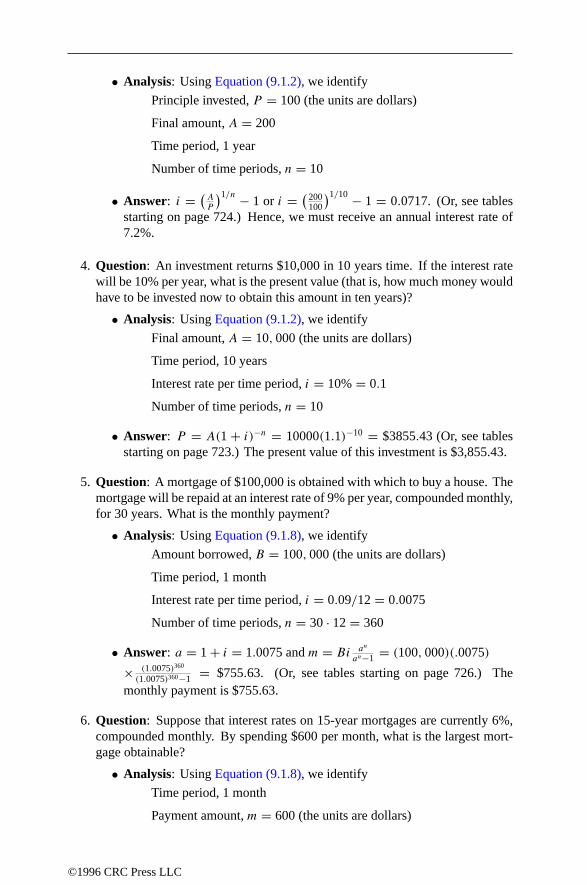
• Analysis: Using Equation (9.1.2), we identify
Principle invested, P = 100 (the units are dollars)
Final amount, A = 200
Time period, 1 year
Number of time periods, n = 10
• Answer: i = (AP
)1/n − 1 or i = (200100
)1/10 − 1 = 0.0717. (Or, see tablesstarting on page 724.) Hence, we must receive an annual interest rate of7.2%.
4. Question: An investment returns $10,000 in 10 years time. If the interest ratewill be 10% per year, what is the present value (that is, how much money wouldhave to be invested now to obtain this amount in ten years)?
• Analysis: Using Equation (9.1.2), we identify
Final amount, A = 10 , 000 (the units are dollars)
Time period, 10 years
Interest rate per time period, i = 10% = 0.1
Number of time periods, n = 10
• Answer: P = A(1 + i)−n = 10000(1.1)−10 = $3855.43 (Or, see tablesstarting on page 723.) The present value of this investment is $3,855.43.
5. Question: A mortgage of $100,000 is obtained with which to buy a house. Themortgage will be repaid at an interest rate of 9% per year, compounded monthly,for 30 years. What is the monthly payment?
• Analysis: Using Equation (9.1.8), we identify
Amount borrowed, B = 100, 000 (the units are dollars)
Time period, 1 month
Interest rate per time period, i = 0.09/12 = 0.0075
Number of time periods, n = 30 · 12 = 360
• Answer: a = 1 + i = 1.0075 and m = Bi an
an−1 = (100, 000)(.0075)
× (1.0075)360
(1.0075)360−1 = $755.63. (Or, see tables starting on page 726.) Themonthly payment is $755.63.
6. Question: Suppose that interest rates on 15-year mortgages are currently 6%,compounded monthly. By spending $600 per month, what is the largest mort-gage obtainable?
• Analysis: Using Equation (9.1.8), we identify
Time period, 1 month
Payment amount, m = 600 (the units are dollars)
©1996 CRC Press LLC

Interest rate per time period, i = 0.06/12 = 0.005
Number of time periods, n = 15 · 12 = 180
• Answer: a = 1+i = 1.005 andB = m(1 − 1/an) /i = 8000.005
(1 − 1
1.005180
)= 94802.81. (Or, see tables starting on page 726.) The largest mortgageamount obtainable is $94,802.81.
9.2 FINANCIAL TABLES
Compound interest: find final valueThese tables use Equation (9.1.2) to determine the final value in dollars ( A) whenone dollar (P = 1) is invested at an interest rate of i per time period, the length ofinvestment time being n time periods. For example, if $1 is invested at a return of3% per time period, for 50 time periods, then the final value would be $4.38 (seefollowing table). Analogously, if $10 had been invested, then the final value wouldbe $43.84.
i =n 1.00% 1.50% 2.00% 2.50% 3.00% 3.50%5 1.0510 1.0773 1.1041 1.1314 1.1593 1.1877
10 1.1046 1.1605 1.2190 1.2801 1.3439 1.410615 1.1610 1.2502 1.3459 1.4483 1.5580 1.675320 1.2202 1.3469 1.4859 1.6386 1.8061 1.989825 1.2824 1.4509 1.6406 1.8539 2.0938 2.363230 1.3478 1.5631 1.8114 2.0976 2.4273 2.806835 1.4166 1.6839 1.9999 2.3732 2.8139 3.333640 1.4889 1.8140 2.2080 2.6851 3.2620 3.959345 1.5648 1.9542 2.4379 3.0379 3.7816 4.702450 1.6446 2.1052 2.6916 3.4371 4.3839 5.5849
i =n 4.00% 4.50% 5.00% 5.50% 6.00% 6.50%5 1.2167 1.2462 1.2763 1.3070 1.3382 1.3701
10 1.4802 1.5530 1.6289 1.7081 1.7908 1.877115 1.8009 1.9353 2.0789 2.2325 2.3966 2.571820 2.1911 2.4117 2.6533 2.9178 3.2071 3.523625 2.6658 3.0054 3.3864 3.8134 4.2919 4.827730 3.2434 3.7453 4.3219 4.9840 5.7435 6.614435 3.9461 4.6673 5.5160 6.5138 7.6861 9.062340 4.8010 5.8164 7.0400 8.5133 10.2857 12.416145 5.8412 7.2482 8.9850 11.1266 13.7646 17.011150 7.1067 9.0326 11.4674 14.5420 18.4202 23.3067
©1996 CRC Press LLC

i =n 7.00% 7.50% 8.00% 8.50% 9.00% 9.50%5 1.4026 1.4356 1.4693 1.5037 1.5386 1.5742
10 1.9672 2.0610 2.1589 2.2610 2.3674 2.478215 2.7590 2.9589 3.1722 3.3997 3.6425 3.901320 3.8697 4.2479 4.6610 5.1120 5.6044 6.141625 5.4274 6.0983 6.8485 7.6868 8.6231 9.668430 7.6123 8.7550 10.0627 11.5583 13.2677 15.220335 10.6766 12.5689 14.7853 17.3796 20.4140 23.960440 14.9745 18.0442 21.7245 26.1330 31.4094 37.719445 21.0025 25.9048 31.9204 39.2951 48.3273 59.379350 29.4570 37.1897 46.9016 59.0863 74.3575 93.4773
i =n 10.00% 10.50% 11.00% 11.50% 12.00% 12.50%5 1.6105 1.6474 1.6851 1.7234 1.7623 1.8020
10 2.5937 2.7141 2.8394 2.9699 3.1058 3.247315 4.1772 4.4713 4.7846 5.1183 5.4736 5.851820 6.7275 7.3662 8.0623 8.8206 9.6463 10.545125 10.8347 12.1355 13.5855 15.2010 17.0001 19.002630 17.4494 19.9926 22.8923 26.1967 29.9599 34.243335 28.1024 32.9367 38.5749 45.1461 52.7996 61.707540 45.2593 54.2614 65.0009 77.8027 93.0510 111.199045 72.8905 89.3928 109.5302 134.0816 163.9876 200.384250 117.3909 147.2699 184.5648 231.0699 289.0022 361.0989
i =n 13.00% 13.50% 14.00% 14.50% 15.00% 15.50%5 1.8424 1.8836 1.9254 1.9680 2.0114 2.0555
10 3.3946 3.5478 3.7072 3.8731 4.0456 4.224915 6.2543 6.6825 7.1379 7.6222 8.1371 8.684220 11.5231 12.5869 13.7435 15.0006 16.3665 17.850125 21.2305 23.7081 26.4619 29.5214 32.9190 36.690230 39.1159 44.6556 50.9502 58.0985 66.2118 75.415335 72.0685 84.1115 98.1002 114.3384 133.1755 155.013540 132.7816 158.4289 188.8835 225.0191 267.8635 318.624645 244.6414 298.4103 363.6791 442.8401 538.7693 654.921650 450.7359 562.0735 700.2330 871.5139 1083.6574 1346.1678
Compound interest: find interest rate
These tables use Equation (9.1.2) to determine the compound interest rate i that mustbe obtained from an investment of one dollar (P = 1) to yield a final value of A (indollars) when the initial amount is invested for n time periods. For example, if $1 isinvested for 50 time periods, and the final amount obtained is $4.00, then the actualinterest rate has been 2.81% per time period (see following table). Analogously, if$100 had been invested, and the final amount was $400, then the interest rate wouldalso be 2.81% per time period.
©1996 CRC Press LLC

A =n 2.0 2.5 3.0 3.5 4.0 4.51 100.00 150.00 200.00 250.00 300.00 350.002 41.42 58.11 73.21 87.08 100.00 112.133 25.99 35.72 44.22 51.83 58.74 65.104 18.92 25.74 31.61 36.78 41.42 45.655 14.87 20.11 24.57 28.47 31.95 35.10
10 7.18 9.60 11.61 13.35 14.87 16.2320 3.53 4.69 5.65 6.46 7.18 7.8130 2.34 3.10 3.73 4.26 4.73 5.1450 1.40 1.85 2.22 2.54 2.81 3.05
A =n 5.0 5.5 6.0 6.5 7.0 7.51 400.00 450.00 500.00 550.00 600.00 650.002 123.61 134.52 144.95 154.95 164.58 173.863 71.00 76.52 81.71 86.63 91.29 95.744 49.53 53.14 56.51 59.67 62.66 65.495 37.97 40.63 43.10 45.41 47.58 49.63
10 17.46 18.59 19.62 20.58 21.48 22.3220 8.38 8.90 9.37 9.81 10.22 10.6030 5.51 5.85 6.15 6.44 6.70 6.9550 3.27 3.47 3.65 3.81 3.97 4.11
A =n 8.0 8.5 9.0 9.5 10.0 10.51 700.00 750.00 800.00 850.00 900.00 950.002 182.84 191.55 200.00 208.22 216.23 224.043 100.00 104.08 108.01 111.79 115.44 118.984 68.18 70.75 73.21 75.56 77.83 80.015 51.57 53.42 55.18 56.87 58.49 60.04
10 23.11 23.86 24.57 25.25 25.89 26.5120 10.96 11.29 11.61 11.91 12.20 12.4830 7.18 7.39 7.60 7.79 7.98 8.1550 4.25 4.37 4.49 4.61 4.71 4.82
A =n 11.0 12.0 13.0 14.0 15.0 16.01 1000.00 1100.00 1200.00 1300.00 1400.00 1500.002 231.66 246.41 260.56 274.17 287.30 300.003 122.40 128.94 135.13 141.01 146.62 151.984 82.12 86.12 89.88 93.43 96.80 100.005 61.54 64.38 67.03 69.52 71.88 74.11
10 27.10 28.21 29.24 30.20 31.10 31.9520 12.74 13.23 13.68 14.11 14.50 14.8730 8.32 8.64 8.93 9.20 9.45 9.6850 4.91 5.10 5.26 5.42 5.57 5.70
©1996 CRC Press LLC

A =n 17.0 18.0 19.0 20.0 25.0 30.01 1600.00 1700.00 1800.00 1900.00 2400.00 2900.002 312.31 324.26 335.89 347.21 400.00 447.723 157.13 162.07 166.84 171.44 192.40 210.724 103.05 105.98 108.78 111.47 123.61 134.035 76.23 78.26 80.20 82.06 90.37 97.44
10 32.75 33.51 34.24 34.93 37.97 40.5120 15.22 15.55 15.86 16.16 17.46 18.5430 9.90 10.11 10.31 10.50 11.33 12.0050 5.83 5.95 6.07 6.17 6.65 7.04
Compound interest: find annuityThese tables use Equation (9.1.6) to determine the annuity (or mortgage) paymentthat must be paid each time period, for n time periods, at an interest rate of i% pertime period, to pay off a loan of one dollar (B = 1). For example, if $1 is borrowed at3% interest per time period, and the amount is to be paid back in equal amounts over10 time periods, then the amount paid back per time period is $0.12 (see followingtable). Analogously, if $100 had been borrowed, then the mortgage amount wouldbe $11.72.
i =n 2.00% 2.25% 2.50% 2.75% 3.00% 3.25%1 1.0200 1.0225 1.0250 1.0275 1.0300 1.03252 0.5150 0.5169 0.5188 0.5207 0.5226 0.52453 0.3468 0.3484 0.3501 0.3518 0.3535 0.35524 0.2626 0.2642 0.2658 0.2674 0.2690 0.27065 0.2122 0.2137 0.2152 0.2168 0.2184 0.21996 0.1785 0.1800 0.1815 0.1831 0.1846 0.18617 0.1545 0.1560 0.1575 0.1590 0.1605 0.16208 0.1365 0.1380 0.1395 0.1410 0.1425 0.14409 0.1225 0.1240 0.1255 0.1269 0.1284 0.1299
10 0.1113 0.1128 0.1143 0.1157 0.1172 0.118715 0.0778 0.0793 0.0808 0.0823 0.0838 0.085320 0.0612 0.0626 0.0641 0.0657 0.0672 0.068830 0.0446 0.0462 0.0478 0.0494 0.0510 0.0527
©1996 CRC Press LLC

i =n 3.50% 3.75% 4.00% 4.25% 4.50% 4.75%1 1.0350 1.0375 1.0400 1.0425 1.0450 1.04752 0.5264 0.5283 0.5302 0.5321 0.5340 0.53593 0.3569 0.3586 0.3603 0.3621 0.3638 0.36554 0.2723 0.2739 0.2755 0.2771 0.2787 0.28045 0.2215 0.2231 0.2246 0.2262 0.2278 0.22946 0.1877 0.1892 0.1908 0.1923 0.1939 0.19547 0.1635 0.1651 0.1666 0.1682 0.1697 0.17138 0.1455 0.1470 0.1485 0.1501 0.1516 0.15329 0.1314 0.1330 0.1345 0.1360 0.1376 0.1391
10 0.1202 0.1218 0.1233 0.1248 0.1264 0.127915 0.0868 0.0884 0.0899 0.0915 0.0931 0.094720 0.0704 0.0720 0.0736 0.0752 0.0769 0.078630 0.0544 0.0561 0.0578 0.0596 0.0614 0.0632
i =n 5.00% 5.25% 5.50% 5.75% 6.00% 6.25%1 1.0500 1.0525 1.0550 1.0575 1.0600 1.06252 0.5378 0.5397 0.5416 0.5435 0.5454 0.54733 0.3672 0.3689 0.3707 0.3724 0.3741 0.37584 0.2820 0.2837 0.2853 0.2869 0.2886 0.29025 0.2310 0.2326 0.2342 0.2358 0.2374 0.23906 0.1970 0.1986 0.2002 0.2018 0.2034 0.20507 0.1728 0.1744 0.1760 0.1775 0.1791 0.18078 0.1547 0.1563 0.1579 0.1594 0.1610 0.16269 0.1407 0.1423 0.1438 0.1454 0.1470 0.1486
10 0.1295 0.1311 0.1327 0.1343 0.1359 0.137515 0.0963 0.0980 0.0996 0.1013 0.1030 0.104720 0.0802 0.0820 0.0837 0.0854 0.0872 0.089030 0.0651 0.0669 0.0688 0.0707 0.0726 0.0746
i =n 6.50% 6.75% 7.00% 7.25% 7.50% 7.75%1 1.0650 1.0675 1.0700 1.0725 1.0750 1.07752 0.5493 0.5512 0.5531 0.5550 0.5569 0.55883 0.3776 0.3793 0.3811 0.3828 0.3845 0.38634 0.2919 0.2936 0.2952 0.2969 0.2986 0.30025 0.2406 0.2423 0.2439 0.2455 0.2472 0.24886 0.2066 0.2082 0.2098 0.2114 0.2130 0.21477 0.1823 0.1839 0.1856 0.1872 0.1888 0.19048 0.1642 0.1658 0.1675 0.1691 0.1707 0.17249 0.1502 0.1519 0.1535 0.1551 0.1568 0.1584
10 0.1391 0.1407 0.1424 0.1440 0.1457 0.147415 0.1064 0.1081 0.1098 0.1115 0.1133 0.115120 0.0908 0.0926 0.0944 0.0962 0.0981 0.100030 0.0766 0.0786 0.0806 0.0826 0.0847 0.0867
©1996 CRC Press LLC
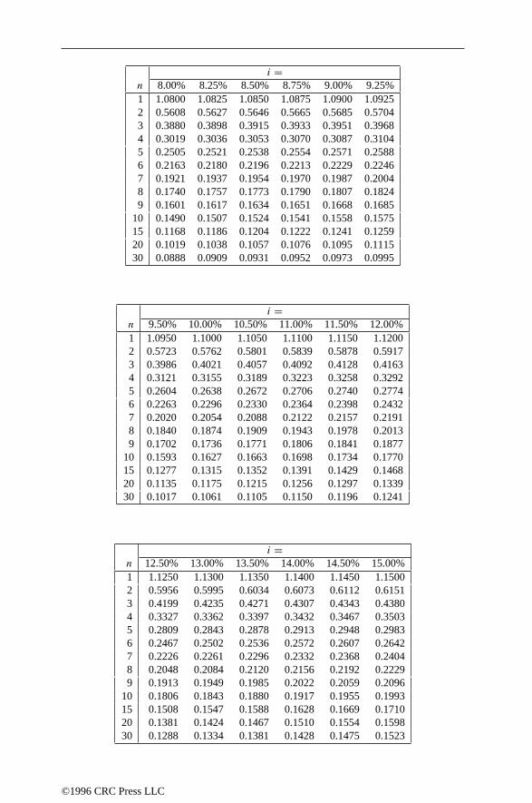
i =n 8.00% 8.25% 8.50% 8.75% 9.00% 9.25%1 1.0800 1.0825 1.0850 1.0875 1.0900 1.09252 0.5608 0.5627 0.5646 0.5665 0.5685 0.57043 0.3880 0.3898 0.3915 0.3933 0.3951 0.39684 0.3019 0.3036 0.3053 0.3070 0.3087 0.31045 0.2505 0.2521 0.2538 0.2554 0.2571 0.25886 0.2163 0.2180 0.2196 0.2213 0.2229 0.22467 0.1921 0.1937 0.1954 0.1970 0.1987 0.20048 0.1740 0.1757 0.1773 0.1790 0.1807 0.18249 0.1601 0.1617 0.1634 0.1651 0.1668 0.1685
10 0.1490 0.1507 0.1524 0.1541 0.1558 0.157515 0.1168 0.1186 0.1204 0.1222 0.1241 0.125920 0.1019 0.1038 0.1057 0.1076 0.1095 0.111530 0.0888 0.0909 0.0931 0.0952 0.0973 0.0995
i =n 9.50% 10.00% 10.50% 11.00% 11.50% 12.00%1 1.0950 1.1000 1.1050 1.1100 1.1150 1.12002 0.5723 0.5762 0.5801 0.5839 0.5878 0.59173 0.3986 0.4021 0.4057 0.4092 0.4128 0.41634 0.3121 0.3155 0.3189 0.3223 0.3258 0.32925 0.2604 0.2638 0.2672 0.2706 0.2740 0.27746 0.2263 0.2296 0.2330 0.2364 0.2398 0.24327 0.2020 0.2054 0.2088 0.2122 0.2157 0.21918 0.1840 0.1874 0.1909 0.1943 0.1978 0.20139 0.1702 0.1736 0.1771 0.1806 0.1841 0.1877
10 0.1593 0.1627 0.1663 0.1698 0.1734 0.177015 0.1277 0.1315 0.1352 0.1391 0.1429 0.146820 0.1135 0.1175 0.1215 0.1256 0.1297 0.133930 0.1017 0.1061 0.1105 0.1150 0.1196 0.1241
i =n 12.50% 13.00% 13.50% 14.00% 14.50% 15.00%1 1.1250 1.1300 1.1350 1.1400 1.1450 1.15002 0.5956 0.5995 0.6034 0.6073 0.6112 0.61513 0.4199 0.4235 0.4271 0.4307 0.4343 0.43804 0.3327 0.3362 0.3397 0.3432 0.3467 0.35035 0.2809 0.2843 0.2878 0.2913 0.2948 0.29836 0.2467 0.2502 0.2536 0.2572 0.2607 0.26427 0.2226 0.2261 0.2296 0.2332 0.2368 0.24048 0.2048 0.2084 0.2120 0.2156 0.2192 0.22299 0.1913 0.1949 0.1985 0.2022 0.2059 0.2096
10 0.1806 0.1843 0.1880 0.1917 0.1955 0.199315 0.1508 0.1547 0.1588 0.1628 0.1669 0.171020 0.1381 0.1424 0.1467 0.1510 0.1554 0.159830 0.1288 0.1334 0.1381 0.1428 0.1475 0.1523
©1996 CRC Press LLC

i =n 15.50% 16.00% 16.50% 17.00% 17.50% 18.00%1 1.1550 1.1600 1.1650 1.1700 1.1750 1.18002 0.6190 0.6230 0.6269 0.6308 0.6348 0.63873 0.4416 0.4453 0.4489 0.4526 0.4562 0.45994 0.3538 0.3574 0.3609 0.3645 0.3681 0.37175 0.3019 0.3054 0.3090 0.3126 0.3162 0.31986 0.2678 0.2714 0.2750 0.2786 0.2823 0.28597 0.2440 0.2476 0.2513 0.2549 0.2586 0.26248 0.2265 0.2302 0.2339 0.2377 0.2415 0.24529 0.2133 0.2171 0.2209 0.2247 0.2285 0.2324
10 0.2031 0.2069 0.2108 0.2147 0.2186 0.222515 0.1752 0.1794 0.1836 0.1878 0.1921 0.196420 0.1642 0.1687 0.1732 0.1777 0.1822 0.186830 0.1571 0.1619 0.1667 0.1715 0.1764 0.1813
9.3 OPTION PRICING
Let S represent the price of a share of stock, and presume that S follows a geometricBrownian motion dS = µS dt + σS dω, where t is time, µ is a constant, and σ is aconstant called the volatility. Let V (S, t) be the value of a derivative security whosepayoff is solely a function of S and t . We construct a portfolio consisting of V andshares of stock. The valueP of this portfolio isP = V+S. The random componentof the portfolio increment (dP ) can be removed by choosing = −∂V/∂S. Theconcept of arbitrage says that dP = rP dt , where r is the (constant) risk-free bankinterest rate. Together this results in the classical Black–Scholes equation for optionpricing (note that no transaction costs are included):
∂V
∂t+ rS
∂V
∂S+ 1
2σ 2S2 ∂
2V
∂S2− rV = 0. (9.3.1)
If the asset pays a continuous dividend ofDS dt (i.e., this is proportional to the assetvalue S during the time period dt) then the modified equation is
∂V
∂t+ (r −D)S
∂V
∂S+ 1
2σ 2S2 ∂
2V
∂S2− rV = 0. (9.3.2)
IfE is the exercise price of the option, and T is the only date on which the option canbe exercised (T is called the expiry date), then the solution of the modified Black–Scholes equation is
V (S, t) = e−D(T−t)S(d1)− Ee−r(T−t)(d2) (9.3.3)
where
d1 = log(S/E)+ (r −D + σ 2/2)(T − t)
σ√T − t
, d2 = d1 − σ√T − t,
and is the cumulative probability distribution for the normal distribution.
©1996 CRC Press LLC

Chapter 10Miscellaneous
10.1 UNITS10.1.1 SI systemof measurement
10.1.2 Dimensional analysis/Buckinghampi
10.1.3 Unitsof physical quantities
10.1.4 Conversion: metric to English
10.1.5 Conversion: English to metric
10.1.6 Temperatureconversion
10.1.7 Miscellaneousconversions
10.1.8 Physical constants
10.2 CALENDAR COMPUTATIONS10.2.1 Leap years
10.2.2 Day of week for any given day
10.2.3 Number of each day of theyear
10.3 AMS CLASSIFICATION SCHEME
10.4 GREEK ALPHABET
10.5 PROFESSIONAL MATHEMATICAL ORGANIZATIONS
10.6 ELECTRONIC MATHEMATICAL RESOURCES
10.7 COMPUTER LANGUAGES 10.7.1 Contact information
10.8 FIELDS’ MEDALS
10.9 BIOGRAPHIES OF MATHEMATICIANS
10.10 ASCII CHARACTER CODES
REFERENCES
©1996 CRC Press LLC

10.1 UNITS
10.1.1 SI SYSTEM OF MEASUREMENT
SI, the abbreviation of the French words “Systeme Internationale d’Unites”, is theaccepted abbreviation for the International Metric System. It has seven base units.
• Base units
Quantity measured Unit SymbolLength Meter mMass Kilogram kgTime Second sElectric current Ampere ATemperature Degrees Kelvin KLuminous intensity Candela cdAmount of substance Mole mol
• Derived units
Quantity SI Name Symbol Combinationof SI units
Absorbed dose Gray Gy J/kgActivity (radiation source) Becquerel Bq 1/sCapacitance Farad F C/VConductance Siemens S A/VElectric charge Coulomb C A-sElectric potential Volt V W/AElectric resistance Ohm V/AEnergy Joule J N-mForce Newton N kg-m/s2
Frequency Hertz Hz 1/sIlluminance Lux lx lm/m2
Inductance Henry H Wb/ALuminous flux Lumen lm cd-srMagnetic flux density Tesla T Wb/m2
Magnetic flux Weber Wb V-sPower Watt W J/sPressure or stress Pascal Pa N/m2
©1996 CRC Press LLC

• Supplementary units
Quantity measured Unit SymbolPlane angle Radian radSolid angle Steradian sr
10.1.2 DIMENSIONAL ANALYSIS/BUCKINGHAM PI
The units of the parameters in a system constrain all the derivable quantities, regard-less of the equations describing the system. In particular, all derived quantities arefunctions of dimensionless combinations of parameters. The number of dimension-less parameters and their forms are given by the Buckingham pi theorem.
In a system, the quantityu = f (W1,W2, . . . ,Wn) is to be determined in terms ofthenmeasurable variables and parametersWi wheref is an unknown function. Letthe quantitiesu,Wi involvem fundamental dimensions labeled byL1, L2, . . . , Lm(such as length, mass, time, or charge). The dimensions of any of theu,Wi is givenby a product of powers of the fundamental dimensions. For example, the dimensionsof Wi areLbi11 L
bi22 L
bi33 · · ·Lbimm where thebij are real and called the dimensional
exponents. A quantity is called dimensionless if all of its dimensional exponentsare zero. Letbi = [
bi1 bi2 . . . bim]T
be the dimension vector ofWi and letB = [
b1 b2 . . . bn]
be them × n dimension matrix of the system. Leta =[a1 a2 . . . am
]Tbe the dimension vector ofu and lety = [
y1 y2 . . . yn]T
represent a solution ofBy = −a. Then,
1. The number of dimensionless quantities isk + 1 = n+ 1 − rank(B), and
2. The measurable quantityu can be expressed in terms of dimensionless param-eters as
u = W−y11 W
−y22 · · ·W−yn
n g(π1, π2, . . . , πk) (10.1.1)
whereg is an unknown function of its parameters and theπi are the dimen-sionless quantities,πi = W
x1i1 W
x2i2 · · ·Wxni
n , andx(i) = [x1i x2i . . . xni
]T(for i = 1,2, . . . , k) represent thek = n− r(B) linearly independent solutionsof the systemBx = 0.
©1996 CRC Press LLC

10.1.3 UNITS OF PHYSICAL QUANTITIES
In the following, read “kilograms” for the massM, “meters” for the lengthL, and“seconds” for the timeT . For example, acceleration is measured in units ofLT −2,or meters per second squared.
Quantity Dimensions
Acceleration LT −2
Angular acceleration T −2
Angular momentum ML2T −1
Angular velocity T −1
Area L2
Displacement L
Energy or work ML2T −2
Force MLT −2
Frequency T −1
Gravitational field strength LT −2
Gravitational potential L2T −2
Length L
Mass M
Momentum MLT −1
Power ML2T −3
Pressure ML−1T −2
Rotational inertia ML2
Time T
Torque ML2T −2
Velocity LT −1
Volume L3
©1996 CRC Press LLC

10.1.4 CONVERSION: METRIC TO ENGLISHMultiply By To obtain
Centimeters 0.3937008 InchesMeters 3.280840 FeetMeters 1.093613 YardsKilometers 0.6213712 MilesGrams 0.03527396 OuncesKilograms 2.204623 PoundsLiters 0.2641721 Gallons (US)Milliliters (cc) 0.03381402 Fluid ouncesSquare centimeters 0.1550003 Square inchesSquare meters 10.76391 Square feetSquare meters 1.195990 Square yardsMilliliters (cc) 0.06102374 Cubic inchesCubic meters 35.31467 Cubic feetCubic meters 1.307951 Cubic yards
10.1.5 CONVERSION: ENGLISH TO METRICMultiply By To obtain
Mils 25.4 MicronsInches 2.540000 CentimetersFeet 0.3048000 MetersYards 0.9144000 MetersMiles 1.609344 KilometersOunces 28.34952 GramsPounds 0.4535924 KilogramsGallons(US) 3.785412 LitersFluid ounces 29.57353 Milliliters (cc)Square inches 6.451600 Square centimetersSquare feet 0.09290304 Square metersSquare yards 0.8361274 Square metersCubic inches 16.38706 Milliliters (cc)Cubic feet 0.02831685 Cubic metersCubic yards 0.7645549 Cubic meters
10.1.6 TEMPERATURE CONVERSION
If TF is the temperature in degrees Fahrenheit andTC is the temperature in degreesCelsius, then
TC = 5
9(TF − 32) and TF = 9
5TC + 32. (10.1.2)
©1996 CRC Press LLC

10.1.7 MISCELLANEOUS CONVERSIONSTo obtain Multiply By
Atmospheres Feet of water at 4C 2.950× 10⁻²
Atmospheres Inches of mercury at 4C 3.342× 10⁻²
Atmospheres Pounds per square inch 6.804× 10⁻²
BTU Foot-pounds 1.285× 10⁻³
BTU Joules 9.480× 10⁻⁴
Cubic feet Cords 128Degree (angle) Radian 57.29578Ergs Foot-pounds 1.356× 10⁷
Feet Miles 5280Feet of water at 4C Atmospheres 33.90Foot-pounds Horsepower-hours 1.98× 10⁶
Foot-pounds Kilowatt-hours 2.655× 10⁶
Foot-pounds per minute Horsepower 3.3 × 10⁴
Horsepower Foot-pounds per second 1.818× 10⁻³
Inches of mercury at 0C Atmospheres 2.036Joules BTU 1.055060× 10³
Joules Foot-pounds 1.35582Kilowatts BTU per minute 1.758× 10⁻²
Kilowatts Foot-pounds per minute 2.26× 10⁻⁵
Kilowatts Horsepower 0.7457Knots Miles per hour 0.8689762Miles Feet 1.893939× 10⁻⁴
Nautical miles Miles 0.8689762Radians Degrees 1.745329× 10⁻²
Square feet Acres 43560Watts BTU per minute 17.5796
©1996 CRC Press LLC

10.1.8 PHYSICAL CONSTANTSEquatorial radius of the earth = 6378.388 km = 3963.34 statute miles.Polar radius of the earth = 6356.912 km = 3949.99 statute miles.1 degree of latitude at 40 = 69 miles.1 international nautical mile = 1.15078 statute miles = 1852 m = 6076.115 ft.Mean density of the earth = 5.522 g/cm3 = 344.7 lb/ft3.G (gravitational constant) =(6.673± 0.003)× 10−8 cm3/g-sec2.Acceleration, sea level, latitude 45 = 980.6194 cm/sec2 = 32.1726 ft/sec2.Length of seconds pendulum, sea level, 45 = 99.3575 cm = 39.1171 in.1 knot (international) = 101.269 ft/min = 1.6878 ft/sec = 1.1508 statute miles/hr.1 micron = 10−4 cm.1 angstrom = 10−8 cm.Mass of hydrogen atom =(1.67339± 0.0031)× 10−24 g.Density of mercury, at 0C = 13.5955 g/ml.Density of water (maximum), at 3.98C = 1.000000 g/ml.Density of water, at 0C = 0.999973 g/ml.Density of dry air, at 0C, 760 mm = 1.2929 g/liter.Velocity of sound, dry air, at 0C = 331.36 m/sec = 1087.1 ft/sec.c (speed of light) = 299,792,458 m/sec (exact).Heat of fusion of water, at 0C = 79.71 cal/g.Heat of vaporization of water, at 100C = 539.55 cal/g.Electrochemical equivalent of silver = 0.001118 g/sec international amp.Absolute wavelength of red cadmium light, air at 15C, 760 mm = 6438.4696 A.Wavelength of orange-red line of krypton 86 = 6057.802 A.e (charge of electron) = 1.602192× 10⁻¹⁹ coul.Avogadro’s number = 6.022169× 1023.1 astronomical unit = 1.495979× 10¹¹ m.
10.2 CALENDAR COMPUTATIONS
10.2.1 LEAP YEARS
If a year is divisible by 4, then it will be a leap year, unless the year is divisible by 100(when it will not be a leap year), unless the year is divisible by 400 (when it will bea leap year). Hence the list of leap years include. . . , 1896, 1904, 1908,. . . , 1992,1996, 2000,. . . and the list of nonleap years includes. . . , 1900,. . . , 1998, 1999,2001,. . . .
©1996 CRC Press LLC

10.2.2 DAY OF WEEK FOR ANY GIVEN DAY
The following formula gives the day of the week for the Gregorian calendar (i.e., forany date after 1582):
W ≡(k + 2.6m− 0.2 − 2C + Y +
⌊Y
4
⌋+⌊C
4
⌋)mod 7
(10.2.1)
where
• The “mod” function returns a nonnegative value.
• · denotes the integer floor function.
• k is the day of the month (1 to 31).
• m is the month (1=March,. . . , 10=December, 11=January, 12=February).(January and February are treated as months of the preceding year).
• C is century (1997 hasC = 19).
• Y is the year (1997 hasY = 97 exceptY = 96 for January and February).
• W is the day of the week (0= Sunday,. . . , 6 = Saturday).
For example, consider the date 16 March 1997 (for whichk = 16, m = 1,C = 19, andY = 97). From Equation (10.2.1), we computeW ≡ 16+2.4 −38+97+ ⌊
974
⌋ + ⌊194
⌋(mod 7) ≡ 2 + 2 − 3 + 6 + 3 + 4 (mod 7) ≡ 0 (mod 7). So
this date will be a Sunday.Because 7 does not divide 400, January 1 occurs more frequently on some days
than others! In a cycle of 400 years, January 1 and March 1 occur on the followingdays with the following frequencies:
Sun Mon Tue Wed Thu Fri SatJanuary 1 58 56 58 57 57 58 56March 1 58 56 58 56 58 57 57
©1996 CRC Press LLC

10.2.3 NUMBER OF EACH DAY OF THE YEARDay Jan Feb Mar Apr May Jun Jul Aug Sep Oct Nov Dec
1 1 32 60 91 121 152 182 213 244 274 305 3352 2 33 61 92 122 153 183 214 245 275 306 3363 3 34 62 93 123 154 184 215 246 276 307 3374 4 35 63 94 124 155 185 216 247 277 308 338
5 5 36 64 95 125 156 186 217 248 278 309 3396 6 37 65 96 126 157 187 218 249 279 310 3407 7 38 66 97 127 158 188 219 250 280 311 3418 8 39 67 98 128 159 189 220 251 281 312 3429 9 40 68 99 129 160 190 221 252 282 313 343
10 10 41 69 100 130 161 191 222 253 283 314 34411 11 42 70 101 131 162 192 223 254 284 315 34512 12 43 71 102 132 163 193 224 255 285 316 34613 13 44 72 103 133 164 194 225 256 286 317 34714 14 45 73 104 134 165 195 226 257 287 318 348
15 15 46 74 105 135 166 196 227 258 288 319 34916 16 47 75 106 136 167 197 228 259 289 320 35017 17 48 76 107 137 168 198 229 260 290 321 35118 18 49 77 108 138 169 199 230 261 291 322 35219 19 50 78 109 139 170 200 231 262 292 323 353
20 20 51 79 110 140 171 201 232 263 293 324 35421 21 52 80 111 141 172 202 233 264 294 325 35522 22 53 81 112 142 173 203 234 265 295 326 35623 23 54 82 113 143 174 204 235 266 296 327 35724 24 55 83 114 144 175 205 236 267 297 328 358
25 25 56 84 115 145 176 206 237 268 298 329 35926 26 57 85 116 146 177 207 238 269 299 330 36027 27 58 86 117 147 178 208 239 270 300 331 36128 28 59 87 118 148 179 209 240 271 301 332 36229 29 * 88 119 149 180 210 241 272 302 333 363
30 30 89 120 150 181 211 242 273 303 334 36431 31 90 151 212 243 304 365
*In leap years, after February 28, add 1 to the tabulated number.
©1996 CRC Press LLC

10.3 AMS CLASSIFICATION SCHEME
00 General01 History and biography03 Mathematical logic and
foundations04 Set theory05 Combinatorics06 Order, lattices, ordered algebraic
structures08 General algebraic systems11 Number theory12 Field theory and polynomials13 Commutative rings and algebras14 Algebraic geometry15 Linear and multilinear algebra;
matrix theory16 Associative rings and algebras17 Nonassociative rings and algebras18 Category theory, homological
algebra19 K-theory20 Group theory and generalizations22 Topological groups, Lie groups26 Real functions28 Measure and integration30 Functions of a complex variable31 Potential theory32 Several complex variables and
analytic spaces33 Special functions34 Ordinary differential equations35 Partial differential equations39 Finite differences and functional
equations40 Sequences, series, summability41 Approximations and expansions42 Fourier analysis43 Abstract harmonic analysis44 Integral transforms, operational
calculus
45 Integral equations46 Functional analysis47 Operator theory49 Calculus of variations and optimal
control; optimization51 Geometry52 Convex and discrete geometry53 Differential geometry54 General topology55 Algebraic topology57 Manifolds and cell complexes58 Global analysis, analysis on
manifolds60 Probability theory and stochastic
processes62 Statistics65 Numerical analysis68 Computer science70 Mechanics of particles and systems73 Mechanics of solids76 Fluid mechanics78 Optics, electromagnetic theory80 Classical thermodynamics, heat
transfer81 Quantum theory82 Statistical mechanics, structure of
matter83 Relativity and gravitational theory85 Astronomy and astrophysics86 Geophysics90 Economics, operations research,
programming, games92 Biology and other natural sciences,
behavioral sciences93 Systems theory; control94 Information and communication,
circuits
©1996 CRC Press LLC

10.4 GREEK ALPHABET
For each Greek letter, we illustrate the form of the capital letter and the form of thelower case letter. In some cases, there is a popular variation of the lower case letter.
Greek Greek English Greek Greek Englishletter name equivalent letter name equivalent
A α Alpha a N ν Nu nB β Beta b % ξ Xi x' γ Gamma g O o Omicron o+ δ Delta d - π . Pi pE ε ε Epsilon e P ρ 4 Rho rZ ζ Zeta z 7 σ ς Sigma sH η Eta e T τ Tau t= θ ϑ Theta th ϒ υ Upsilon uI ι Iota i D φ ϕ Phi phK κ Kappa k X χ Chi chJ λ Lambda l L ψ Psi psM µ Mu m ω Omega o
10.5 PROFESSIONAL MATHEMATICALORGANIZATIONS
• American Mathematical Society (AMS)P.O. Box 6248, Providence, RI 02940-6248Telephone: 401/455-4000, 800/321-4AMSElectronic mail:[email protected]
• American Mathematical Association of Two-Year CollegesNorth Lake College, 5001 MacArthur Blvd, Irving, TX 75038-3899Telephone: 214/659-5328Electronic mail:[email protected]
• American Statistical Association1429 Duke Street, Alexandria, VA 22314-3402Telephone: 703/684-1221
• Association for Symbolic LogicDepartment of Mathematics, University of Illinois,1409 West Green Street, Urbana, IL 61801Telephone: 217/244-7902Electronic mail:[email protected]
©1996 CRC Press LLC

• Association for Women in Mathematics4114 Computer & Space Sciences Building, University of Maryland,College Park, MD 20742-2461Telephone: 301/405-7892Electronic mail:[email protected]
• Canadian Applied Mathematics SocietyDepartment of Mathematics and Statistics, Simon Fraser University,Burnaby, British Columbia, Canada V5A 1S6Telephone: 604/291-3337, 604/291-3332Electronic mail:[email protected]
• Canadian Mathematical Society577 King Edward, Suite 109, P.O. Box 450, Station A,Ottawa, Ontario, Canada K1N 6N5Telephone: 613/564-2223Electronic mail:[email protected]
• Casualty Actuarial Society1100 North Glebe Road, Suite 600, Arlington, VA 22201Telephone: 703/276-3100
• Conference Board of the Mathematical Sciences1529 Eighteenth Street, N.W., Washington, DC 20036Telephone: 202/293-1170Electronic mail:[email protected]
• Consortium for Mathematics and Its Applications (COMAP)57 Bedford Street, Suite 210, Lexington, MA 02173Telephone: 617/862-7878Electronic mail:[email protected]
• Council on Undergraduate Research: Mathematical and ComputerSciences DivisionUniversity of North Carolina at Asheville, One University Heights,Asheville, NC 28804-3299Telephone: 704/251-6006
• Fibonacci AssociationDepartment of Computer Science, Box 2201,South Dakota State University, Brookings, SD 57007-0194Telephone: 605/688-5719
• Industrial Mathematics SocietyP.O. Box 159, Roseville, MI 48066Telephone: 313/771-0403
• Institute for Operations Research and the Management Sciences(INFORMS)940-A Elkridge Landing Road, Linthicum, MD 21090-2909Telephone: 410/850-0300, 800/4IN-FORMSElectronic mail:[email protected]
©1996 CRC Press LLC

• Institute of Mathematical Statistics3401 Investment Boulevard #7, Hayward, CA 94545-3819Telephone: 510/783-8141Electronic mail:[email protected]
• International Mathematics Union (IMPA)Estrada Dona Castorina, 110, Jardim Botanico,Rio de Janeiro – RJ, 22460 BrazilTelephone: 55-21-294 9032, 55-21-5111749Electronic mail:[email protected]
• Joint Policy Board for Mathematics1529 Eighteenth Street, N.W., Washington, DC 20036Telephone: 202/234-9570Electronic mail:[email protected]
• Kappa Mu Epsilon (κµε)National Mathematics Honor Society, Department of Mathematics,Niagara University, Niagara Falls, NY 14109
• Mathematical Association of America (MAA)Dolciani Mathematical Center, 1529 Eighteenth Street, N.W.,Washington, DC 20036Telephone: 202/387-5200Electronic mail:[email protected]
• Mathematical Programming SocietyDepartment of Mathematics and Computer Science, EindhovenUniversity of Technology, 5600 MB Eindhoven, The NetherlandsTelephone: +31-40-474770Electronic mail:[email protected]
• Mu Alpha Theta (µαθ )University of Oklahoma, 610 Elm Avenue, Room 423, Norman, OK 73019-0315Telephone: 405/325-4489Electronic mail:[email protected]
• National Association of MathematiciansBox 959, Elizabeth City State University, Elizabeth City, NC 27909Telephone: 919/335-3326Electronic mail:[email protected]
• National Council of Teachers of Mathematics1906 Association Drive, Reston, VA 22091Telephone: 703/620-9840
• ORSA (seeINFORMS)
©1996 CRC Press LLC

• Pi Mu Epsilon (πµε)National Mathematics Honorary Society, Department of Mathematics,East Carolina University, Greenville, NC 27858Telephone: 919/328-6414
• Rocky Mountain Mathematics ConsortiumArizona State University, Box 871904, Tempe, AZ 85287-1904Telephone: 602/965-3788
• Society of Industrial and Applied Mathematics (SIAM)3600 University City Science Center, Philadelphia, PA 19104-2688Telephone: 215/382-9800Electronic mail:[email protected]
• Society for Mathematical Biology, Inc.P.O. Box 11283, Boulder, CO 80301Telephone: 303/499-0510
• Society of Actuaries475 North Martingale Road, Suite 800, Schaumburg, IL 60173-2226Telephone: 708/706-3500
• Statistical Society of CanadaDepartment of Mathematics and Statistics, University of Victoria,Victoria, British Columbia, Canada V8W 3P4Telephone: 604/721-7470Electronic mail: [email protected]
10.6 ELECTRONIC MATHEMATICAL RESOURCES
The following is a list of Uniform Resource Locators (URL). These are the addressesof Web sites, gopher pages, FTP sites, etc.
http://www.yahoo.com/Science/Mathematics/A very large list of useful sites relating to mathematics. It is perhaps the best place tostart researching an arbitrary mathematical question not covered elsewhere in this list.
http://daisy.uwaterloo.ca/˜alopez-o/math-faq/math-faq.htmlTheFAQ (frequently asked questions) listing from the news groupsci.math.
http://e-math.ams.org/The American Mathematical Society home page, with information about AMS-TEX,the Combined Membership List of the AMS, Math Reviews subject classifications,preprints, etc.
gopher://gopher.maa.org/(old) Now - http://www.maa.org/The Mathematics Association of America, available using gopher.
http://www.siam.org/The Society for Industrial and Applied Mathematics.
©1996 CRC Press LLC

http://netlib2.cs.utk.edu/master/The master listing for Netlib, containing many standard programs, including linpack,eispack, hompack, SPARC packages, and ODEpack.
http://www.netlib.org/liblist.htmlAn alternative site for Netlib.
http://gams.cam.nist.gov/The Guide to Available Mathematical Software.
http://www.nag.co.uk:70/The home page of the Numerical Algorithms Group.
http://www.math.hmc.edu/codee/home.htmlThe Consortium of Ordinary Differential Equation Experiments, maintained by HarveyMudd College.
http://www.ima.umn.edu/The Institute for Mathematics and its Applications at the University of Minnesota.
http://cam.cornell.edu/˜driscoll/research/drums.htmlA famous question posed by mathematical physicist M. Kac is, “Can one hear the shapeof a drum?” In 1991, Gordon, Webb, and Wolpert found two different shaped drums withthe same sequence of eigenvalues. This site contains some details of the calculations.
http://www.utm.edu:80/departments/math/largest.htmlInformation about primes, including largest known primes of various types.
http://www.geom.umn.edu/docs/snell/chance/sources.htmlA listing of interesting sites, primarily related to statistics.
http://aleph0.clarku.edu/˜djoyce/julia/explorer.htmlUseful for exploring the Mandelbrot and Julia sets.
ftp://megrez.math.u-bordeaux.fr/pub/numberfields/The Computational Number Theory group in Bordeaux has announced the availability(by anonymous ftp at the above URL) of extensive tables of number fields (almost550000 number fields). For the number fields belonging to tables of reasonable length,this site contains the signature, the Galois group of the Galois closure of the field, thediscriminant of the number field, the class number, the structure of the class group asa product of cyclic groups, an ideal in the class for each class generating these cyclicgroups, the regulator, the number of roots of unity in the field, a generator of the torsionpart of the unit group, and a system of fundamental units.
http://netlib.bell-labs.com/netlib/master/readme.htmlThe AT&T Bell Laboratories Math Archive.
gopher://ejde.math.unt.eduThe Electronic Journal of Differential Equations. Available via telnet atejde.math.unt.eduwithloginejde,andalsoavailableatejde.math.swt.edu.
http://nyjm.albany.edu:8000/nyjm.htmlThe New York Journal of Mathematics, the first electronic journal devoted to generalmathematics. Alsoavailableviagopher at gopher nyjm.albany.edu 1070 andviaFTPat nyjm.albany.edu in directory /pub/nyjm.
http://www.wavelet.org/wavelet/index.htmlThe Wavelet Digest is an electronic information service on the Internet athttp://www.wavelet.org/wavelet/add.html, containing questions and answersand announcements of papers, books, journals, software, and conferences.
http://www.math.ohio-state.edu/JATThe Journal of Approximation Theory.
http://www.combinatorics.org/The World Combinatorics Exchange and The Electronic Journal of Combinatorics.
©1996 CRC Press LLC

http://www.cs.indiana.edu/cstr/searchUnified Computer Science TR Index.
http://www.c3.lanl.gov/lacesLACES is a database of preprints, papers, abstracts, and related documents in areasinvolving discrete mathematics. This includes combinatorics, graph theory, geometry,algorithms, etc. If you have preprints in any of these areas you are invited to send themto LACES. Submissions are made available to the public immediately. Submissioninstructions and facilities can be found at this site.Features of LACES include full search capabilities, including approximate search andrelevance feedback, comment and reference links, revision, abstract and comment pro-cessing (anyone can add comments to documents in the database), and more. Documentsare permanently archived, and copyrights remain with the authors.
http://rattler.cameron.edu/swjpam/swjpam.htmlThe Southwest Journal of Pure and Applied Mathematics.
http://www.mag-browse.com/Tables of contents of various magazines. As of the summer of 1995, 25 scientificmagazines were included.
Sloane’s sequence identifierTo identify asequence, send electronic mail [email protected],saying (for example) lookup 1 11 21 1211 111221.
10.7 COMPUTER LANGUAGES
The following is a sampling of the computer languages used by scientists and engi-neers:
• Numerical languages
Ada
APL
C
C++
Fortran
Lisp
Matlab
Pascal
• Statistical languages
SPSS
Minitab
• Optimization languages
GAMS(AMPL)
MINOS
MINTO
• Symbolic languages
Axiom
Derive
Macsyma
Maple
Mathematica
Reduce
©1996 CRC Press LLC

10.7.1 CONTACT INFORMATION
1. AXIOM http://www.nag.co.uk/1h/symbolic/AX.html
2. Fortran http://www.nag.co.uk:70/CGI/Forms/Tools/imagemap.cgi/NAG
3. Macsyma http://www.sciencesoftware.com/macsyma.html
4. Maple http://www.maplesoft.com/Maple/index.html
5. MathCad http://www.mathsoft.com/index.html
6. Matlab http://www.mathworks.com
7. Mathematica http://www.wri.com
10.8 FIELDS’ MEDALS
The Fields’ medal is the most prestigious award that can be bestowed upon a math-ematician. It is usually awarded to someone no more than 40 years of age; the agesof the recipients are listed below.
• 1936 Ahlfors, Lars 29 Harvard University
• 1936 Douglas, Jesse 39 MIT
• 1950 Schwartz, Laurent 35 Universite de Nancy
• 1950 Selberg, Atle 33 Princeton/Inst. for Advanced Studies
• 1954 Kodaira, Kunihiko 39 Princeton University
• 1954 Serre, Jean-Pierre 27 College de France
• 1958 Roth, Klaus 32 University of London
• 1958 Thom, Rene 35 University of Strasbourg
• 1962 Hormander, Lars 31 University of Stockholm
• 1962 Milnor, John 31 Princeton University
• 1966 Atiyah, Michael 37 Oxford University
• 1966 Cohen, Paul 32 Stanford University
• 1966 Grothendieck, Alexander 38 University of Paris
• 1966 Smale, Stephen 36 University of California at Berkeley
• 1970 Baker, Alan 31 Cambridge University
• 1970 Hironaka, Heisuke 39 Harvard University
• 1970 Novikov, Serge 32 Moscow University
• 1970 Thompson, John 37 University of Chicago
©1996 CRC Press LLC

• 1974 Bombieri, Enrico 33 Univeristy of Pisa
• 1974 Mumford, David 37 Harvard University
• 1978 Deligne, Pierre 33 IHES
• 1978 Fefferman, Charles 29 Princeton University
• 1978 Margulis, Gregori 32 InstPrblmInfTrans
• 1978 Quillen, Daniel 38 MIT
• 1982 Connes, Alain 35 IHES
• 1982 Thurston, William 35 Princeton University
• 1982 Yau, Shing-Tung 33 IAS
• 1986 Donaldson, Simon 27 Oxford University
• 1986 Faltings, Gerd 32 Princeton University
• 1986 Freedman, Michael 35 University of California at San Diego
• 1990 Drinfeld, Vladimir 36 Phys. Inst. Kharkov
• 1990 Jones, Vaughan 38 University of California at Berkeley
• 1990 Mori, Shigefumi 39 University of Kyoto
• 1990 Witten, Edward 38 Princeton/Inst. for Advanced Studies
• 1994 Lions, Pierre-Louis 38 Universite de Paris-Dauphine
• 1994 Yoccoz, Jean-Chrisophe 36 Universite de Paris-Sud
• 1994 Bourgain, Jean 40 Princeton/Inst. for Advanced Studies
• 1994 Zelmanov, Efim 39 University of Wisconsin
10.9 BIOGRAPHIES OF MATHEMATICIANS
Ah’mose (c. 1650 B.C.E.)was the scribe responsible for copying theRhind Papyrus, themost detailed original document still extant on ancient Egyptian mathematics. Thepapyrus contains some 87 problems with solutions dealing with what we consider first-degree equations, arithmetic progressions, areas and volumes of rectangular and circularregions, proportions, and several other topics. It also contains a table of the results ofthe division of 2 by every odd number from 3 to 101.
Euclid (c. 300 B.C.E.)is responsible for the most famous mathematics text of all time, theElements. Not only does this work deal with the standard results of plane geometry,but it also contains three chapters on number theory, one long chapter on irrationalquantities, and three chapters on solid geometry, culminating with the construction ofthe five regular solids. The axiom-definition-theorem-proof style of Euclid’s work hasbecome the standard for formal mathematical writing up to the present day.
©1996 CRC Press LLC

Archimedes (287–212 B.C.E.)not only wrote several works on mathematical topics moreadvanced than Euclid, but also was the first mathematician to derive quantitative resultsfrom the creation of mathematical models of physical problems on earth. In severalof his books, he described the reasoning process by which he arrived at his results inaddition to giving formal proofs. For example, he showed how to calculate the areas ofa segment of a parabola and the region bounded by one turn of a spiral, and the volumeof a paraboloid of revolution.
Ptolemy(C. 100–178 C.E.)is most famous for theAlmagest, a work in thirteen books, whichcontains a complete mathematical description of the Greek model of the universe withparameters for the various motions of the sun, moon, and planets. The first book providesthe strictly mathematical material detailing the plane and spherical trigonometry, allbased solely on the chord function, necessary for astronomical computations.
Hypatia (c. 370–415), the first woman mathematician on record, lived in Alexandria. She wasgiven a very thorough education in mathematics and philosophy by her father Theon andwas responsible for detailed commentaries on several important Greek works, includingPtolemy’sAlmagest, Apollonius’sConics, and Diophantus’sArithmetica.
Brahmagupta (c. 598–670), from Rajasthan in India, is most famous for hisBrahmas-phutasiddhanta (Correct Astronomical System of Brahma), an astronomical work whichcontains many chapters on mathematics. Among the mathematical problems he con-sidered and gave solution algorithms for were systems of linear congruences, quadraticequations, and special cases of the Pell equationDx2±1 = y2. He also gave the earliestdetailed treatment of rules for operating with positive and negative numbers.
Bhaskara(1114–1185), the most famous of medieval Indian mathematicians, gave a completealgorithmic solution to the Pell equation. In addition, he dealt with techniques of solvingsystems of linear equations with more unknowns than equations and was familiar withthe basic combinatorial formulas, giving many examples, though no proofs, of their use.
Qin Jiushao (1202–1261), born in Sichuan, published a general procedure for solving sys-tems of linear congruences—the Chinese remainder theorem—in hisShushu jiuzhang(Mathematical Treatise in Nine Sections)in 1247, a procedure which makes essentialuse of the Euclidean algorithm. He also gave a complete description of a method forsolving numerically polynomial equations of any degree. Qin’s method was developedin China over a period of a thousand years or more and is very similar to what is nowcalled the Horner method of solution, published by William Horner in 1819.
Muhammad al-Khwarizmi (c. 780–850), originally from Khwarizm in what is now Uzbek-istan, was one of the first scholars called to the House of Wisdom in Baghdad by thecaliph al-Ma’mun. He is best known for his algebra text, in which he gave a carefultreatment of solution methods for quadratic equations. This Arabic text, after beingtranslated into Latin in the twelfth century, provided Europeans with an introductionto algebra, a subject not considered by the ancient Greeks. Al-Khwarizmi’s book onarithmetic provided Europe with one of its earliest looks at the Hindu-Arabic numbersystem.
Abu Ali ibn al-Haytham (965–1039), who spent much of his life in Egypt, is most famousfor his work on optics, a work read and commented on for many centuries in Europe.In pure mathematics, he developed an inductive procedure for calculating formulas forthe sums of integral powers of the firstn integers, and used the formula for fourthpowers to calculate the volume of the solid formed by revolving a parabola about a lineperpendicular to its axis.
©1996 CRC Press LLC

Nasir al-Din al-Tusi (1201–1274)was the head of a large group of astronomers at the ob-servatory in Maragha, in what is now Iran. He computed a new set of very accurateastronomical tables and developed some new ideas on planetary motion which mayhave influenced Copernicus in working out his heliocentric system. In pure mathe-matics, al-Tusi’s attempted proof of the parallel postulate was modified by his son andlater published in Rome, where it influenced European work on non-Euclidean geom-etry. Al-Tusi also wrote the first systematic work on plane and spherical trigonometry,independent of astronomy, and gave the earliest proof of the theorem of sines.
Leonardo of Pisa(1170–1240), often known today as Fibonacci, is most famous for hisLiberAbbaci (Book of Calculation), which contains the earliest publication of the Fibonaccinumbers in the problem of how many pairs of rabbits can be bred in one year from onepair. Many of the sources of the book are in the Islamic world, where Leonardo spentmuch of his early life. The work contains the rules for computing with the new Hindu–Arabic numerals, many practical problems in such topics as calculation of profits andcurrency conversions, and topics now standard in algebra texts such as motion problems,mixture problems, and quadratic equations.
Levi ben Gerson (1288–1344)was a French rabbi and also an astronomer, philosopher,biblical commentator, and mathematician. His most famous mathematical work istheMaasei Hoshev (The Art of the Calculator), which contains detailed proofs of thestandard combinatorial formulas, some of which use the principle of mathematicalinduction.
Gerolamo Cardano(1501–1576), a physician and gambler as well as a mathematician, wroteone of the earliest works containing systematic probability calculations, not all of whichwere correct. He is most famous, however, for hisArs Magna (The Great Art,1545), analgebra text which contained the first publication of the rules for solving cubic equationsalgebraically. Some of the rules had been discovered earlier in the sixteenth century byScipione del Ferro and Niccolo Tartaglia.
Francois Viete (1540–1603), a lawyer and advisor to two kings of France, was one of theearliest cryptanalysts and successfully decoded intercepted messages for his patrons.Although a mathematician only by avocation, he made important contributions to thedevelopment of algebra. In particular, he introduced letters to stand for numericalconstants, thus enabling him to break away from the style of verbal algorithms of hispredecessors and treat general examples by formulas rather than by giving rules forspecific problems.
Simon Stevin(1548–1620)spent much of his life in the service of Maurice of Nassau, theStadhouder of Holland, as a military engineer, advisor in finance and navigation, andquartermaster general of the Dutch army. In his bookDe Thiende (The Art of Tenths),Stevin introduced decimal fractions to Europe, although they had previously been usedin the Islamic world. Stevin’s notation is different from our own, but he had a clearunderstanding of the advantage of decimals and advocated their use in all forms ofmeasurement.
John Napier(1550–1617)was a Scottish laird who worked for years on the idea of producing atable which would enable one to multiply any desired numbers together by performingadditions. These tables of logarithms first appeared in his 1614 bookMirifici Loga-rithmorum Canonis Descriptio (Description of the Wonderful Canon of Logarithms).Napier’s logarithms are different from, but related to, natural logarithms. His ideaswere soon adapted by Henry Briggs, who eventually created the first table of commonlogarithms by 1628.
©1996 CRC Press LLC

Rene Descartes(1596–1650)published theGeometryin 1637 as a supplement to his philo-sophical work, theDiscourse on the Method for Rightly Directing One’s Reason andSearching for Truth in the Sciences. In it, he developed the principles of analytic geom-etry, showing how to derive algebraic equations which represented geometric curves.TheGeometryalso contained methods for solving polynomial equations, including themodern factor theorem and Descartes’ rule of signs.
Pierre de Fermat (1601–1665)was a French lawyer who spent his spare time doing mathe-matics. Not only was he a coinventor of analytic geometry, although his methods weresomewhat different from those of Descartes, but he also was instrumental in the earlydevelopment of probability theory and made many contributions to the theory of num-bers. He is most remembered for the statement of his so-called “last theorem”, that theequationxn + yn = zn has no nontrivial integral solution ifn > 2, a theorem whoseproof was finally completed by Andrew Wiles in 1994.
Blaise Pascal(1623–1662)showed his mathematical precocity with hisEssay on Conicsof1640 in which he stated his theorem that the opposite sides of a hexagon inscribed in aconic section always intersect in three collinear points. Pascal is better known, however,for his detailed study of what is now called Pascal’s triangle of binomial coefficients, thebasic facts of which had been known in the Islamic and Chinese worlds for centuries.He also introduced the differential triangle in hisTreatise on the Sines of a Quadrant ofa Circle, an idea adopted by Leibniz in his calculus.
Isaac Newton(1642–1727), the central figure in the Scientific Revolution, is most famous forhisPhilosophiae Naturalis Principia Mathematica (Mathematical Principles of NaturalPhilosophy,1687), in which he derived his system of the world based on his laws ofmotion and his law of universal gravitation. Over 20 years earlier, however, Newtonhad consolidated and generalized all the material on tangents and areas worked outby his predecessors into the magnificent problem solving tool of the calculus. He alsodeveloped the power series as a method of investigating various transcendental functions,stated the general binomial theorem, and, although never establishing his methods withthe rigor of Greek geometry, did demonstrate an understanding of the concept of limitquite sufficient for him to apply the calculus to solve many important mathematical andphysical problems.
Gottfried Wilhelm Leibniz (1646–1716), born in Leipzig, developed his version of thecalculus some ten years after Isaac Newton, but published it much earlier. Leibnizbased his calculus on the inverse relationship of sums and differences, generalized toinfinitesimal quantities called differentials. By clever manipulation of differentials,based in part on the geometrical model of the differential triangle, Leibniz was able toderive all of the basic rules of the differential and integral calculus and apply them tosolve physical problems expressible in terms of differential equations. Leibniz’sd and∫
notation for differentials and integrals turned out to be much more flexible and usefulthan Newton’s dot notation and remains the notation of calculus to the present day.
Johann Bernoulli (1667–1748), one of a number of prominent mathematicians of his Swissfamily, was one of the earliest proponents of Leibniz’s differential and integral calculus.Bernoulli helped to stimulate the development of the new techniques by proposing chal-lenge problems to mathematicians, the most important probably being that of describingthe brachistochrone, the curve representing the path of descent of a body between twogiven points in the shortest possible time. Many of the problems he posed requiredthe solution of differential equations, and Bernoulli developed many techniques usefultoward this end, including the calculus of the logarithmic and exponential functions.
©1996 CRC Press LLC

Leonhard Euler (1707–1783), a student of Johann Bernoulli in Basel who became one ofthe earliest members of the St. Petersburg Academy of Sciences founded by Peter theGreat of Russia, was the most prolific mathematician of all time. His series of analysistexts,Introduction to Analysis of the Infinite, Methods of the Differential Calculus, andMethods of the Integral Calculus, established many of the notations and methods still inuse today. Among his numerous contributions to every area of mathematics and physicsare his development of the calculus of the trigonometric functions, the establishmentof the theory of surfaces in differential geometry, and the creation of the calculus ofvariations.
Maria Agnesi (1718–1799), the eldest child of a professor of mathematics at the Universityof Bologna, in 1748 published the clearest text on calculus up to that point. Based on thework of Leibniz and his followers, the work explained concepts lucidly and providednumerous examples, including some that have become standard in calculus texts tothis day. Curiously, her name is often attached to a small item in her book not evenoriginal with her, a curve whose equation wasy = a
√a−x√x . This curve was calledla
versiera, derived from the Latin meaning “to turn”; unfortunately the word also was theabbreviation of the Italian word meaning “wife of the devil” and so was translated intoEnglish as “witch” . Thecurvehasever sincebeen known as the “witch of Agnesi.”
Joseph Lagrange(1736–1813), was born in Turin, becoming at age 19 a professor of math-ematics at the Royal Artillery School there. He is most famous for hisAnalyticalMechanics(1788), a work which extended the mechanics of Newton and Euler, anddemonstrated how problems in mechanics can generally be reduced to solutions of or-dinary or partial differential equations. In 1797 he published hisTheory of AnalyticFunctions, which attempted to reduce the ideas of calculus to those of algebraic analy-sis by assuming that every function could be represented as a power series. Althoughhis central idea was incorrect, many of the proofs of basic theorems of calculus in thiswork were subsequently adapted by Cauchy into the forms still in use today.
Benjamin Banneker(1731–1806), the first American black to achieve distinction in science,taught himself sufficient mathematics and astronomy to publish a series of well-regardedalmanacs in the 1790s. He also assisted Andrew Ellicott in the survey of the boundariesof the District of Columbia. He was fond of solving mathematical puzzles and problemsand recorded many of these in his notebooks.
Augustin-Louis Cauchy (1789–1857), the most prolific mathematician of the nineteenthcentury, wrote several textbooks in analysis for use at theEcole Polytechnique, textbookswhich became the model for calculus texts for the next hundred years. In his texts,Cauchy based the calculus on the notion of limit, using, for the first time, a definitionwhich could be applied arithmetically to give proofs of some of the important results.Among numerous other subjects to which he contributed important ideas were complexanalysis, in which he gave the first proof of the Cauchy integral theorem, the theory ofmatrices, in which he demonstrated that every symmetric matrix can be diagonalizedby use of an orthogonal substitution, and the theory of permutations, in which he wasthe earliest to consider these from a functional point of view.
William Rowan Hamilton (1805–1865)became the Astronomer Royal of Ireland in 1827because of his original work in optics accomplished during his undergraduate yearsat Trinity College, Dublin. In 1837, he showed how to introduce complex numbersinto algebra axiomatically by consideringa + ib as a pair(a, b) of real numbers withappropriate computational rules. After many years of seeking an appropriate definitionfor multiplication rules for triples of numbers which could be applied to vector analysisin three-space, he discovered that it was in fact necessary to consider quadruplets of
©1996 CRC Press LLC
numbers. It was out of the natural definition of multiplication of these quaternions thatthe modern notions of dot product and cross product of vectors evolved.
Arthur Cayley (1821–1895), although graduating from Trinity College, Cambridge, as Se-nior Wrangler, became a lawyer because there was no suitable mathematics positionavailable in England. He produced nearly 300 mathematical papers during his 14 yearsas a lawyer, however, and finally secured a professorship at Cambridge in 1863. Amonghis numerous mathematical achievements are the earliest abstract definition of a groupin 1854, out of which he was able to calculate all possible groups of order up to eightand the basic rules for operating with matrices, including a statement (without rigor-ous proof) of the Cayley–Hamilton theorem that every matrix satisfies its characteristicequation.
Richard Dedekind (1831–1916)solved the problem of the lack of unique factorization inrings of algebraic integers by introducing ideals and their arithmetic and demonstratingthat every ideal is either prime or can be expressed uniquely as a product of prime ideals.During his teaching at Zurich in the late 1850s, he realized that, although differentialcalculus deals with continuous magnitudes, there was no satisfactory definition availableof what it means for the set of real numbers to be continuous. He therefore worked outa definition of irrational numbers through his idea of what is now called a Dedekindcut in the set of rational numbers. Somewhat later Dedekind also considered the basicideas of set theory and gave a set theoretic characterization of the natural numbers.
Carl Friedrich Gauss (1777–1855)published his important work on number theory, theDisquisitiones Arithmeticae, when he was only 24, a work containing not only an ex-tensive discussion of the theory of congruences, culminating in the quadratic reciprocitytheorem, but also a detailed treatment of cyclotomic equations in which he showed howto construct regularn-gons by Euclidean techniques whenevern is prime andn− 1 is apower of 2. Gauss also made fundamental contributions to the differential geometry ofsurfaces in hisGeneral Investigations of Curved Surfacesin 1827, as well as to complexanalysis, astronomy, geodesy, and statistics during his long tenure as a professor at theUniversity of Gottingen. Many ideas later published by others, including the basics ofnon-Euclidean geometry, were found in his notebooks after his death.
Karl Weierstrass (1815–1897)taught for many years at German gymnasia before producinga series of brilliant mathematical papers in the 1850s which resulted in his appointmentto a professorship at the University of Berlin. It was in his lectures there that he insistedon defining every concept of analysis arithmetically, including such ideas as uniformconvergence and uniform continuity, thus completing the transformation away from theuse of terms such as “infinitely small”. Since he himself never published many of theseideas, his primary influence was through the work of his numerous students.
Georg Bernhard Riemann (1826–1866), in his 1854 inaugural lecture at the Universityof Gottingen entitled “On the Hypotheses which Lie at the Foundation of Geometry”,discussed the general notion of ann-dimensional manifold, developed the idea of ametric relation on such a manifold, and gave criteria which would determine whether athree-dimensional manifold is Euclidean, or “flat”. This lecture had enormous influenceon the development of geometry, including non-Euclidean geometry, as well as on thedevelopment of a new concept of our physical space ultimately necessary for the theoryof general relativity. Among his other achievements, Riemann’s work on complexfunctions and their associated Riemann surfaces became one of the foundations ofcombinatorial topology.
Sofia Kovalevskaya(1850–1891)was the first European woman since the Renaissance toearn a Ph.D. in mathematics (1874), a degree based on her many new results in the
©1996 CRC Press LLC

theory of partial differential equations. Because women were generally not permittedto study mathematics officially in European universities, Kovalevskaya had been forcedto study privately with Weierstrass. Her mathematical talents eventually earned her aprofessorship at the University of Stockholm, an editorship of the journalActa Math-ematica, and the Prix Bordin of the French Academy of Sciences for her work on therevolution of a solid body about a fixed point. Unfortunately, her career was cut shortby her untimely death from pneumonia at the age of 41.
Henri Poincare (1854–1912), one of the last of the universal mathematicians, contributedto virtually every area of mathematics, including physics and theoretical astronomy.Among his many contributions was the introduction of the idea of homology into topol-ogy, the creation of a model of Lobachevskian geometry which helped to convincemathematicians that this non-Euclidean geometry was as valid as Euclid’s, and a de-tailed study of the nonlinear partial differential equations governing planetary motionaimed at answering questions about the stability of the solar system. Toward the end ofhis life, Poincare wrote several popular books emphasizing the importance of scienceand mathematics.
David Hilbert (1862–1943)is probably most famous for his lecture at the InternationalCongress of Mathematicians in Paris in 1900 in which he presented a list of 23 problemswhich he felt would be of central importance for 20th century mathematics. Most ofthe problems have now been solved, while significant progress has been achieved in theremainder. Hilbert himself made notable contributions to the study of algebraic forms,algebraic number theory, the foundations of geometry, integral equations, theoreticalphysics, and the foundations of mathematics.
Leonard Eugene Dickson(1874–1954)was the first recipient of a doctorate in mathematicsat the University of Chicago, where he ultimately spent most of his mathematical career.Dickson helped to develop the abstract approach to algebra by developing sets of axiomsfor such constructs as groups, fields, and algebras. Among his important books was hismonumental three volumeHistory of the Theory of Numbers, which traced the evolutionof every important concept in that field.
Emmy Noether(1882–1935)received her doctorate from the University of Erlangen in 1908,a few years later moving to Gottingen to assist Hilbert in the study of general relativity.During her 18 years there, she was extremely influential in stimulating a new styleof thinking in algebra by always emphasizing its structural rather than computationalaspects. She is most famous for her work on what are now called Noetherian rings, buther inspiration of others is still evident in today’s textbooks in abstract algebra.
Alan Turing (1912–1954)developed the concept of a “Turing machine” in 1936 to answerthe questions of what a computation is and whether a given computation can in fact becarried out. This notion today lies at the basis of the modern all-purpose computer, amachine which can be programmed to do any desired computation. During World WarII, Turing led the successful effort in England to crack the German “Enigma” code, aneffort central to the defeat of Nazi Germany.
©1996 CRC Press LLC

10.10 ASCII CHARACTER CODES
Left\right American Standard Code for Information Exchangedigits 0 1 2 3 4 5 6 7 8 9
0 nul soh stx etx eot enq ack bel bs ht1 nl vt np cr so si dle dc1 dc2 dc32 dc4 nak syn etb can em sub esc fs gs3 rs us sp ! " # $ % & ’4 ( ) * + , - . / 0 15 2 3 4 5 6 7 8 9 : ;6 < = > ? @ A B C D E7 F G H I J K L M N O8 P Q R S T U V W X Y9 Z [ \ ] ˆ ‘ a b c10 d e f g h i j k l m11 n o p q r s t u v w12 x y z ‖ ˜ del
References
1. C. C. Gillispie, Ed.,Dictionary of Scientific Biography, Scribners, New York,1970–1990.
2. AMS, Mathematical Sciences Professional Directory, American MathematicalSociety, Providence, 1995.
3. H. S. Tropp, “The Origins and History of the Fields Medal”,Historia Mathe-matica, 1976, 3, 167–181.
4. E. T. Bell,Men of Mathematics,Dover, New York, 1945.
©1996 CRC Press LLC