Ion heating and magnetic flux pile-up in a magneticreconnection experiment with super-Alfvénic plasma inflows

The MIT Faculty has made this article openly available. Please share how this access benefits you. Your story matters.

Citation Suttle, L.G., et al., "Ion heating and magnetic flux pile-upin a magnetic reconnection experiment with super-Alfvénicplasma inflows." Physics of Plasmas 25 (2018): no. 042108 doi:10.1063/1.5023664 ©2018 Author(s)

As Published 10.1063/1.5023664

Publisher AIP Publishing

Version Original manuscript

Citable link https://hdl.handle.net/1721.1/124296

Terms of Use Creative Commons Attribution-Noncommercial-Share Alike

Detailed Terms http://creativecommons.org/licenses/by-nc-sa/4.0/

1

Ion heating and magnetic flux pile-up in a magnetic reconnection experiment with super-

Alfvénic plasma inflows

L. G. Suttle,1,a) J. D. Hare,1 S. V. Lebedev,1,b) A. Ciardi,2 N. F. Loureiro,3 G. C. Burdiak,1,c) J. P.

Chittenden,1 T. Clayson,1 J. W. D. Halliday,1 N. Niasse,1,c) D. Russell,1 F. Suzuki-Vidal,1 E.

Tubman,1 T. Lane,4 J. Ma,5 T. Robinson,1 R. A. Smith,1 N. Stuart1

1Blackett Laboratory, Imperial College, London, SW7 2BW, United Kingdom 2Sorbonne Université, Observatoire de Paris, Université PSL, CNRS, LERMA, F-75005, Paris, France 3Plasma Science and Fusion Center, Massachusetts Institute of Technology, Cambridge, Massachusetts,

02139, USA 4West Virginia University, Morgantown, West Virginia 26506, USA 5Northwest Institute of Nuclear Technology, Xi’an 710024, China

(Revised January 26, 2018)

This work presents a magnetic reconnection experiment in which the kinetic, magnetic and thermal properties

of the plasma each play an important role in the overall energy balance and structure of the generated

reconnection layer. Magnetic reconnection occurs during the interaction of continuous and steady flows of

super-Alfvénic, magnetized, aluminum plasma, which collide in a geometry with two-dimensional

symmetry, producing a stable and long-lasting reconnection layer. Optical Thomson scattering measurements

show that when the layer forms, ions inside the layer are more strongly heated than electrons, reaching

temperatures of Ti~Z̅Te ≳ 300 eV – much greater than can be expected from strong shock and viscous

heating alone. Later in time, as the plasma density in the layer increases, the electron and ion temperatures

are found to equilibrate, and a constant plasma temperature is achieved through a balance of the heating

mechanisms and radiative losses of the plasma. Measurements from Faraday rotation polarimetry also

indicate the presence of significant magnetic field pile-up occurring at the boundary of the reconnection

region, which is consistent with the super-Alfvénic velocity of the inflows.

I. INTRODUCTION

The interaction of magnetized plasma flows occurs in

many astrophysical systems (e.g. stellar jets1, supernovae2,

accretion disks3), space environments (e.g. solar flares, solar

wind-magnetosphere interactions)4 and high energy density

laboratory experiments (e.g. laser-plasma interactions5,6, Z-

pinches7 and inertial confinement fusion8,9). For colliding

plasma flows with oppositely-directed, embedded magnetic

fields, the reversal of the field direction across their interface

gives rise to a current sheet. In this layer, the frozen-in flux

condition breaks down and the plasma and magnetic field

decouple, allowing the field lines to break and reconnect,

releasing stored magnetic energy. The spatial scale of the

reconnection layer is controlled by the interplay of the

plasma resistivity, two-fluid and kinetic effects, which drive

this transition from ideal magnetohydrodynamic behavior10–

12. This process depends strongly on the external boundary

conditions, and the structure of the reconnection layer

adjusts to balance the magnetic and material fluxes brought

to the reconnection region, and the rate of magnetic

annihilation and the outflow of energized material13. This is

apparent if the plasma flow into the reconnection region is

strongly driven, such that the ram pressure of the material

a) Email: l.suttle10@imperial.ac.uk b) Email: s.lebedev@imperial.ac.uk c) Current address: First Light Fusion Ltd, Oxfordshire, OX5 1QU, United Kingdom

flux is significant in comparison to the magnetic pressure. A

number of recent laser-driven, high energy density physics

(HEDP) experiments have investigated magnetic

reconnection in conditions where the ram pressure is much

higher than the magnetic pressure14–19. In those experiments,

the interaction of expanding plasma plumes from solid

targets irradiated by 1-2 ns duration laser pulses results in the

transient annihilation of thin sheets of toroidal magnetic

fields.

This paper presents data from experiments carried out on

a recently developed pulsed power reconnection platform20–

23, which applies a 1 MA, ~500 ns current pulse to an array

of thin wires to produce high velocity, counter-streaming

plasma flows with oppositely-directed, embedded magnetic

fields. An important feature of this platform is that the

reconnection layer is long-lasting, as it is continuously

supported by the inflowing magnetized plasma for the

duration of the experiment. This allows sufficient time for

the density and magnetic field structures to form and evolve.

The geometry of the layer displays a two-dimensional

symmetry, which allows for good diagnostic access. The

setup also offers a versatile testbed for studying magnetic

reconnection over a broad range of plasma conditions, as it

2

is possible to control the inflow properties via the choice of

the plasma material. For example, the use of either aluminum

or carbon wires produces flows with a super20 or sub-

Alfvénic velocities21–23 respectively. The reconnection

layers formed in experiments with these two materials have

different Lundquist numbers13 (S=LVA/DM, where L is the

length scale of the plasma, VA is the Alfvén speed of the

upstream plasma and DM is the magnetic diffusivity),

allowing access to different regimes of magnetic

reconnection parameter space (e.g. single vs. multiple x-line

reconnection)24. The work presented in this paper extends

results previously published in Ref. 20, and describes the

detailed characterization of a reconnection layer formed in

an aluminum plasma, with strongly driven inflows

(MA=Vflow/VA≈2). The Lundquist number for the layer is

relatively small (S~10) due to strong radiative cooling of the

aluminum plasma, which limits the electron temperature.

Characterization of the reconnection layer structure is made

via detailed spatially and temporally resolved, quantitative

measurements of the plasma parameters, obtained using a

comprehensive suite of diagnostics.

The paper is organized as follows. Sec. II describes the

setup of the pulsed power magnetic reconnection platform,

which uses a wire array configuration to produce sustained,

counter-streaming, magnetized plasma flows. It also

describes the diagnostic setup of high-speed optical imaging,

laser interferometry, optical Thomson scattering and

Faraday rotation polarimetry, which are used to make non-

perturbative measurements of the plasma. Sec. III presents

the results, showing the conditions of the plasma following

the formation of the reconnection layer, and describes how

the plasma parameters evolve over time. These measured

parameters are summarized in Table I in Sec. IV, and this is

accompanied by a discussion of the main features of the

reconnection layer structure. In this section a brief

comparison is also made to reconnection occurring in

experiments with sub-Alfvénic carbon plasma flows21,22 at a

much larger Lundquist number of S~100 (for a more in

depth comparison see the review article of Ref. 23). The

conclusions of this work are summarized in Sec. V.

II. EXPERIMENTAL SETUP AND DIAGNOSTICS

The experiments were carried out at the MAGPIE pulsed

power facility25, using the setup illustrated in Fig. 1(a). The

supersonic, counter-streaming plasma flows are produced by

the ablation of thin aluminum (Al) wires, driven by a 1 MA,

~500 ns current pulse. These wires are arranged to form two

cylindrical, “inverse” wire arrays26, with the total current

divided equally between the two arrays. The current in each

array runs up the wires and down the central conductor, as

indicated by the (purple) arrows in Fig. 1(a). Plasma is

continuously ablated from the resistively heated wires, and

the J×B force acts on the plasma driving supersonic plasma

flows, which are sustained throughout an entire experiment.

This is similar to the ablation plasma flows produced by

standard (Z-pinch) wire arrays27–29, however, here the J×B

force acts to direct the plasma radially outwards, into a

region initially free of magnetic fields. The ablated plasma is

accelerated away from the wires within the first 1-2 mm, and

thereafter propagates with an almost constant velocity26.

Previous measurements have demonstrated that the plasma

flows generated by a single, inverse Al wire array have a

frozen-in, azimuthal, advected magnetic field (B~2 T), and

the velocity of the flows is super-fast-magnetosonic (i.e.

Vflow > VFMS = [cS2 + VA

2]1 2⁄ , where cS is the ion sound

speed)30–32. The arrays used in the current experiments

consist of 16 Al wires, each 30 µm in diameter and 16 mm

in length, and positioned with uniform spacing on a diameter

of 16 mm, around a 5 mm-diameter central post. The axial,

center-to-center separation of the arrays is 27 mm, such that

FIG.1 (a) Schematic diagram of the experimental setup (with cut-away of the right wire array): current is applied in parallel to two inverse

wire arrays, producing magnetized plasma flows which collide to create a reconnection layer. The directions of the current (purple), plasma

flows (red) and the embedded magnetic fields (blue) are shown. (b-c) Raw interferometry images of the interaction region following the

formation of the reconnection layer, showing (b) the xy-plane and (c) the xz-plane, as defined by the Cartesian coordinate system in (a). The

positions of the wires are indicated.

3

the minimum gap between the wires of the two arrays is 11

mm. The arrays are driven with the same polarity, such that

when the advected magnetic fields meet they are orientated

in opposite directions, and their interaction leads to the

formation of a reconnection layer at the mid-plane.

The reconnection layer is diagnosed using a suite of

complementary plasma diagnostics. These diagnostics can

be fielded simultaneously, allowing the dynamics of the

interaction and the localized plasma parameters of the

system to be determined with a high degree of spatial and

temporal resolution. Due to the highly reproducible nature of

the plasma formation and evolution in this setup, the

diagnostics can be used to acquire data from different times

throughout the development of the interaction across

multiple experiments. The details of the diagnostic setup are

summarized as follows.

To obtain a qualitative overview of the morphology and

structural evolution of the system over the course of a single

experiment, the dynamics of the interaction are captured

using a high-speed, multi-frame, optical camera (Invisible

Vision U2V1224: 12 frames, 5 ns exposure, tuneable

interframe time Δt≥5 ns, with a 600 nm low-pass filter to

block light at laser diagnostic wavelengths). With reference

to the Cartesian coordinate system defined in Fig. 1(a), the

camera images the self-emission from the plasma along the

z-direction, thus producing images of the xy-plane of the

interaction region as demonstrated in Fig. 2.

Several laser-based diagnostics are employed to measure

the quantitative features of the plasma structure.

Measurements of the (line-integrated) electron density

distribution of the interaction region are made using Mach-

Zehnder interferometry imaging31. Interferograms of the xy-

plane (Fig. 1(b)) are obtained by probing along the z-

direction (parallel to the axes of the arrays), using the 2nd

(532 nm) and 3rd (355 nm) harmonics of a pulsed Nd:YAG

laser (EKSPLA SL321P, 0.5 ns, 500 mJ). Both the 532 nm

and 355 nm channels use the same probe path, but have a

time offset to provide two interferograms separated by 20 ns.

A separate interferometer probes the plasma

perpendicularly, along the y-direction, producing

interferograms of the xz-plane (Fig. 1(c)), using an

independent, 1053 nm, 1 ns, 5 J probe beam. The

interferograms are recorded by Canon 350D and 500D

DSLR cameras, with the shutters held open for the duration

of the experiments, such that the time resolution is set by the

pulse duration of the probe laser beams. The interferograms

are processed to produce maps of electron line density

(∫ nedl), using the analysis procedure described in Refs.

31,33.

The magnetic field distribution is measured using a

Faraday rotation polarimetry diagnostic34. The polarimetry is

performed in the y-direction using the same 1053 nm probe

beam as the xz-interferometer. The line-averaged field

strength along the probe direction is calculated from the

rotation of the linear polarization of the probe beam. The

diagnostic consists of two channels, with oppositely offset

linear polarizers, set at 3° either side of extinction, and two

identical Atik 383L+ CCD cameras. For each channel, the

spatial distribution of rotation angle is determined via the

change in intensity recorded on the CCDs due to the rotation

of polarization, either towards or away from extinction. The

combination of the two polarimetry channels allows the

optical self-emission from the plasma to be removed,

reducing systematic errors in determining the polarization of

the laser beam. Further details of the diagnostic are described

in Ref. 31.

An optical Thomson scattering (TS) diagnostic system

(λ=532 nm, 5 ns FWHM, 3 J) records the ion feature of the

collective TS spectra from within the interaction region35. A

focussed laser beam is passed through the xy-plane at the

mid-height (z=0 mm) of the arrays, with a waist diameter of

~200 µm throughout the entire range of interest of the

plasma. The scattered light is collected using single lens

systems to image the path of the laser beam onto the input of

fiber-optic bundles. The bundles contain 14 individual, 100

µm-diameter fibers, each collecting light from a separate

scattering volume on the beam path. In the majority of

experiments two independent imaging systems were used,

observing the TS light from matching spatial positions, but

along different scattering directions in the xy-plane. In other

experiments a single imaging system was used, collecting

scattered light in the out-of-plane, z-direction. Further details

of these scattering geometries are provided in Sec. IIIC. The

coordinates of the scattering volumes are identified within

the xy-plane of interferometry images, to a precision of ≤200

µm, using the procedure described in Ref. 31, allowing the

positions of the TS measurements within the plasma

structure to be determined. The output from the fiber-optic

bundles is recorded using an imaging spectrometer (ANDOR

SR-500i-A, with gated ANDOR iStar ICCD camera). The

spectral resolution of 0.25 Å is set by the combination of the

~50 µm spectrometer slit width and 2400 lines/mm grating,

and the temporal resolution is set by the 4 ns gate time. The

Doppler shift of the TS spectra allow the components of the

bulk plasma flow velocity to be calculated along each of the

scattering vectors defined by the observation directions (see

FIG.2 Time series showing optical self-emission images (false-

color) of the plasma in the xy-plane, from a single experiment.

White dots indicate the wire positions. Video available online

covering the time interval t=160-380 ns (Multimedia view).

4

Sec. IIIC and Fig. 5). Additionally, by fitting theoretical

form-factors to the profiles of the spectra31,35, and utilizing

the electron density values obtained from interferometry

measurements, the local ion temperature (Ti) and the product

of the average ionization and electron temperature (Z̅Te) of

the plasma can be extracted. A non-local thermodynamic

equilibrium (nLTE) model36 is used to decompose Z̅Te into

self-consistent values of Z̅ and Te.

III. EXPERIMENTAL RESULTS

A. Formation of the reconnection layer

The collision of the magnetized flows in the mid-plane

between the two wire arrays leads to the formation of the

reconnection layer. This is seen in the optical, self-emission

image time-series presented in Fig. 2 (video available

online). The images show that the layer becomes detectable

with this diagnostic during the time interval t=160-180 ns

after the start of the ~500ns duration current pulse (the

current start is used as the reference for all times quoted in

this paper). This delay between current start and the

formation of the layer originates from the combination of the

“dwell” time for the first ablated plasma to be formed at the

wires, and the time-of-flight of the plasma to reach the mid-

plane. Measurements from previous wire array experiments

on MAGPIE have typically shown a dwell time of ~50 ns37,

and thus a plasma flow velocity into the reconnection region

can be estimated as Vin ≥ 5.5 mm (120 ± 10 ns)⁄ ≈ 40 −50 km/s. Following the reconnection layer formation, the

intensity of self-emission in the layer increases. The

observable length of the reconnection layer also increases,

rapidly expanding outwards from the center of the images

along the y-direction, reaching the bounds of the field-of-

view (y = ±11.5 mm) by t=240 ns. Throughout the

experiments the layer appears notably straight and maintains

an approximately constant thickness until late in the

experiments (t>300 ns) when the drive current has passed its

peak. Subsequently, the ram pressure of the flows is

expected to start decreasing, which is consistent with the

broadening of the layer as it starts expanding against the

upstream flow at late time.

Interferograms of the interaction region are obtained along

both the y- and z-directions, as demonstrated by the

examples in Figs. 1(b) and 1(c) respectively. These

FIG.3 (a-c) Electron density (ne) distributions calculated from interferograms of the xy-plane of the interaction region, at three times in three

separate experiments. Regions where the interferometry fringes could not be traced are masked in gray. The positions marked a-c in (b)

correspond to the coordinates of TS measurements discussed in Sec. IIIA, whose spectra are presented in Fig. 6. (d) Electron density profiles

of the plasma flow along the radial paths indicated in (b). (e) Electron density profiles along the length of the reconnection layer from the

density maps in (a)-(c) (Data denoted by dashed lines are lower-limits, as ne could not be directly measured at these positions due to sharp

local density gradients obscuring the interferometry fringes.). (f) Electron density vs. time at the positions marked A-D in (c).

5

interferograms reveal the line-integrated electron density

distribution of the plasma by the localized bending of the

initially straight (horizontal) interference fringes, which is

strongest at the mid-distance between the arrays. The

displacement of the fringes is proportional to the integral of

the electron density along the line-of-sight through the

plasma (∫ nedl). Thus, the raw interferograms show that the

reconnection layer has a greater electron density than the

incoming plasma flows, and is uniform in the axial, z-

direction over the height of the arrays. In agreement with the

self-emission images, the layer is first observed in the

interferometry data at t≈180 ns, when the fringe shift reaches

approximately half a fringe spacing, equivalent to ∫ nedl =2 × 1017cm−2.

The electron density distribution in the reconnection plane

is measured using the xy-plane interferometer. The raw

interferograms, similar to that shown in Fig. 1(b), are

processed into maps of electron line density using the

procedure described in Refs. 31,33. These are further

converted to electron density (ne) by dividing by the axial

height of the arrays (Δz=16 mm), utilizing the uniformity of

the plasma structure in this direction (Fig. 1(c)). Figs. 3(a)-

(c) present typical electron density distribution maps

obtained at different times in the experiments, demonstrating

the temporal evolution of the layer. The radially diverging

plasma flows propagating from the arrays can be seen on the

left and right-hand sides of these images. The ablated plasma

density is modulated azimuthally about the arrays due to the

finite number of wires, and the regions of higher density

correlate with the features observed in the self-emission

images.

The flow structure consists of ablation from each of the

wires, as well as regions of enhanced density between the

wires, formed by the collision of plasma expanding from the

adjacent wires. These collision regions are bound by oblique

shock fronts, analogous to the structure observed in the

interior of imploding aluminum wire arrays33, and are

indicative of the supersonic velocity of the flows. The

density within the shock-bound regions is greater than that

of the ambient flow. This is evident from a comparison of

radial profiles at varying azimuthal positions, e.g. profiles 1-

3 in Fig. 3(d), corresponding to the line-outs marked in Fig.

3(b). These profiles also show that at each azimuthal position

the flow density upstream of the layer decreases with radial

distance (Δr) from the array. This is due to the combination

of the time-of-flight of the flow (with lower ablation density

produced earlier in time when the current is smaller) and the

cylindrical divergence of the flow geometry. The plasma

density rises at the position where the flow meets the

boundary of the reconnection layer, just ahead of the mid-

plane. The precise overlap of the profiles 1 and 3 for the

range Δr<5 mm, demonstrates not only that the flows inside

the shock-bound regions are identical, but that the upstream

flow at distances of |x|>1 mm from the layer is not disturbed

by the existence of the layer, which is consistent with the

supersonic nature of the ablation flows. The flows are also

not expected to penetrate through the layer to the opposing

side, as the mean free paths of the plasma particles are

significantly shorter than the layer thickness (see Sec. IV for

more details). Despite the upstream equivalence of the

shock-bound flow regions shown in Fig. 3(d), the density of

the outer stream (3) at the boundary of the layer is lower, due

to the longer path length to the layer and hence greater

cylindrical divergence undergone. Thus, the greatest flux of

plasma into the layer occurs along the central direction y=0

mm.

Inside the layer, the electron density is significantly larger

than in the upstream flow: e.g. at t=215 ns (Fig. 3(d)) the

factor of increase is in the range of 1.5-3. The maximum

density, however, is not located at the central position of the

layer (x,y)=0 mm, despite it receiving the highest density

from the upstream flow. This is demonstrated by the electron

density profiles presented in Fig. 3(e), which show plots

along the layer from the distributions in Figs. 3(a)-(c). The

profiles reveal peaks of density located at symmetric

positions either side of the layer center, with the separation

of these peaks increasing with time. The rate of displacement

of the peaks is consistent with the flow of material outwards

along the layer at a velocity in the range of 30-50 km/s. This

agrees well with direct measurements of the layer outflow

velocity (Vy) using Thomson scattering, which are presented

in Sec. IIIC.

In accordance with the optical, multi-frame images (Fig.

2), the electron density distributions show that for t <300 ns, the layer maintains an approximately uniform

thickness along its entire length (FWHM: 2δ = 0.6 mm),

while the layer expands in the perpendicular y-direction. In

the image of Fig. 3(a), taken at t=195 ns, the layer displays a

length of Δy=13 mm, which rapidly increases to 15 mm by

t=215 ns (Fig. 3(b)), and later extends beyond the bounds of

the field-of-view, i.e. Δy≥16 mm (Fig. 3(c)). The outflow of

material along the layer plays a dominant role in this

expansion process. Evidence of this can be seen in Fig. 3(f),

where the electron density is plotted as a function of time for

positions upstream and inside the layer. The data series are

labelled A-D corresponding to the positions of the

measurements indicated in Fig. 3(c). At the center of the

layer (position B) the density is comparable to that in the

outflow (position D). This is despite a much higher upstream

density flowing into the center of the layer (position A), than

in the corresponding, off-center upstream flow (position C).

Thus, the outflow along the layer must make up a significant

contribution to the density at position D to offset this

difference in the inflows.

B. Measurements of the magnetic field distribution

The distribution of the magnetic field in the xz-plane was

measured using the simultaneous interferometry and

polarimetry diagnostics. Figs. 4(a)-(c) present data obtained

with these diagnostics at a time of t=195 ns, shortly after the

layer formation, and at the same time as the xy-plane density

map shown in Fig. 3(a). These maps depict the xz-plane of

6

the interaction region, with the flows moving horizontally

inwards from the arrays positioned at the left and right-hand

edges of the field of view. The electron line-integrated

density map in Fig. 4(a) shows the density increase in the

reconnection layer in comparison to the flows, with the

thickness 2δ of the layer matching that observed in the xy-

plane. The spatial variation of the rotation angle of the linear

polarization of the probe beam is shown in Fig. 4(b). The

rotation angle is sensitive to the By-component of the

magnetic field, parallel to the direction of the probing beam

through the plasma. The rotation is symmetric with respect

to the midplane (x=0 mm) of the interaction region, with

equal and oppositely directed rotation angles of α = ±0.2°

measured in the plasma on either side of the layer. This is

consistent with the expected magnetic field geometry of the

experimental setup (Fig. 1(a)) of oppositely directed fields

embedded in the flows from each array.

The Faraday rotation angle is determined by both the

magnetic field and electron density of the plasma. The

average By-component of magnetic field can be found by

dividing the rotation angle by the electron line density, using

the formula34

By(x, z) =8π2ε0me

2c3

e3λ2

α(x, z)

∫[ne(x, y, z)dy]∙

The resulting magnetic field distribution is displayed in Fig.

4(c). The distribution exhibits notable uniformity in the z-

direction, despite the presence of some noise on small spatial

scales. To suppress the noise, a horizontal profile is taken

through the field map, averaged vertically over the interval

z=−3 to 3 mm, producing the plot shown in Fig. 4(d). The

field profile shows that upstream of the reconnection layer

the magnetic field has an approximately constant strength,

with By=±1.7 T measured on either side of the layer. Inside

the layer this field drops steeply, passing through 0 at the

mid-point between the arrays. This profile can be well

approximated by a “Harris-sheet” form (By = B0tanh [x δ⁄ ],

red dashed line in Fig. 4(d)), typically used to describe

FIG.4 Faraday rotation polarimetry data. (a) Line-integrated electron density distribution of the xz-plane at t=195 ns. Regions where the

probe beam was obscured are masked in gray. (b) Angular rotation distribution of the probe beam at t=195 ns. Concentric circular features

are artefacts from diffraction of light around dust spots on the optics of the imaging system. (c) Magnetic field distribution calculated from

the combination of data in (a) and (b). (d) Horizontal profile of the magnetic field in (c), averaged vertically over the range z=-3 to 3 mm.

(e) Rotation distribution at t=215 ns, showing enhancements of the Faraday rotation angle at the boundaries of the layer. (f) The

accompanying magnetic field profile for (e). (g) Rotation distribution at t=250 ns, showing further increasing field enhancement at the layer

boundaries. (h) Rotation profile for (g). Data points were not obtained inside the layer at this time as the laser beam could no longer probe

through the layer.

(1)

7

magnetic reconnection current sheets, and the underlying

current density distribution (jz = −1 μ0 ∂By ∂x⁄⁄ ) for this

fitted magnetic field profile corresponds to a peak current

density of 0.5 MA/cm².

At later times in the experiments the increasing density

gradients inside the reconnection layer are large enough to

refract the probe laser beam beyond the acceptance angle of

the imaging system. Consequently, soon after the formation

of the layer, measurements of the magnetic field deep inside

the layer become unreliable, but the field can still be

measured in the flows upstream and at the boundaries of the

layer. Fig. 4(e) displays a map of the Faraday rotation angle

at a time of t=215 ns (corresponding to the time of Fig. 3(b)).

At this time the Faraday rotation angles in the upstream flow

have increased to α = ±0.3°, indicating greater embedded

magnetic field and plasma density. Additionally, even

stronger symmetric rotation angles of α = ±1.0° are

observed over narrow intervals of Δx~0.1 mm at the

boundaries (x=±0.5 mm) of the layer, which are in the same

directions as the rotation in the adjoining upstream flows.

These sharp features at the layer boundaries are not

simultaneously observed by the interferometry diagnostic,

and so it can be concluded that they signify considerable

enhancements of the magnetic field at these locations. The

magnetic field profile calculated from this data (Fig. 4(f))

shows that at t=215 ns the upstream flows possess field

strengths of By=±2 T and the enhanced fields at the edges of

the layer are ±4 T.

Polarimetry data obtained at subsequent times in the

experiments show that the magnetic field brought by the

upstream flow continues to increase, and that the field

enhancements at the boundaries of the layer persist, also with

an increasing strength. This is demonstrated by the Faraday

rotation distribution and accompanying profile in Figs. 4(g)

and 4(h) respectively, which are taken at t=250 ns and

concurrent with Fig. 3(c). The Faraday angles in the

upstream flows (α = ±0.5°) correspond to magnetic fields

of By =±4 T, while the rotations of ±2° at the layer

boundaries correspond to ±8 T.

C. Spatially resolved Thomson scattering measurements

of flow velocities and plasma temperature

• Measurements in the xy-plane

The multipoint Thomson scattering (TS) diagnostic

operated simultaneously with the interferometry and

polarimetry measurements, allowing detailed measurements

of the local flow velocities and thermal properties of the

plasma. The TS measurements presented in this sub-section

were obtained from the geometry illustrated in Fig. 5(a), in

which the probing laser beam passed through the

reconnection layer at an angle of 22.5° to the y-axis. The

scattered light was observed from two opposing directions,

corresponding to scattering angles of 45° and 135°. In both

directions the light was collected from 14 matching, equally-

spaced positions along the linear path of the beam, which

was achieved by imaging the beam path onto the inputs of

fiber-optic bundles. The imaging systems had a

magnification of 0.8, giving collection volumes 125 µm in

diameter, spaced by 0.3mm. The geometry of the input laser

beam and the observation directions defines scattering

vectors (𝐊𝐒 = 𝐊𝐨𝐮𝐭 − 𝐊𝐢𝐧), as depicted in Fig. 5(b). The

detection of the Doppler shifts (∆ω = 𝐕𝐟𝐥𝐨𝐰 ∙ 𝐊𝐒) of the TS

spectra provides measurements of the components of the

bulk velocity of the plasma, along the direction of the

corresponding scattering vectors. The geometry of this TS

setup was selected to obtain separate measurements of the

orthogonal components Vx and Vy of the velocity, which

together reveal the speed and direction of the plasma flow

within the xy-plane.

FIG.5 (a) Schematic diagram of the Thomson scattering geometry

used to make independent measurements of Vx and Vy. TS light is

observed from 14 positions along the path of the probe beam from

two opposing directions. The 14 scattering volumes are imaged

onto the input of individual optical fibers, coupled to an imaging

spectrometer. (b) Geometry of the probe laser, observation and

scattering K-vectors. Equations show the vector relations and

dependence of the Doppler shift (Δω) of the spectra on the local

flow velocity and scattering vector. (c) Examples of raw TS spectra

from the imaging spectrometer CCD. The vertical axis of the

spectrometer corresponds to the position along the probe beam.

8

Fig. 5(c) shows examples of raw TS spectra from the fiber-

optic bundles of each of the two observation directions. The

spectrometer CCD images display the discrete spatial

positions through the plasma (i.e. fibers) on the vertical axes,

against the spectrum of the scattered light along the

horizontal axes. The spectral shape of the TS signal is fitted

with a theoretical spectrum to infer the temperature of both

the electron and ion populations of the plasma. The TS

spectra are processed by integrating vertically across the

CCD pixels for each individual fiber, and fitting is performed

using the non-relativistic, Maxwellian spectral density

function S(ω,K)35. As part of this fitting procedure, the

theoretical spectrum is convolved with the response function

of the spectrometer, which is found from the observed

broadening on the unshifted laser wavelength, recorded

before the experiment.

Figs. 6(a)-(c) present examples of fitted TS spectra,

displayed with their horizontal axes converted from

wavelength to velocity (V = [2πc (λ0 + Δλ)⁄ − ω0]/KS).

The spectra are from 3 key spatial positions in the

reconnection xy-plane, taken around the time of Fig. 3(b)

(t=210-215 ns). The black dots marked a-c on the density

map of Fig. 3(b) denote the coordinates of the collection

volumes for these spectra. The Vx-sensitive spectrum of Fig.

6(a) was obtained in the flow upstream of the layer at

(x,y)=(-1,-1) mm, and shows that the flow here approaches

the layer with a velocity component perpendicular to the

layer of Vx=40 km/s. Inside the layer boundary (x<δ), the Vx

component of the flow is found to rapidly fall to 0 (e.g. Fig.

6(b)), however, for coordinates y≠0 mm the plasma inside

the layer acquires significant outflow motion in the y-

direction (e.g. Fig. 6(c)).

The presence of a significant outflow along the layer is

clearly seen from a comparison of the Vy velocity

components measured in the layer and in the upstream

plasma. Fig. 6(d) contains a full set of measured Vy velocity

components from a single experiment where the laser

crossed the layer at y=1.7 mm. The dataset covers the range

(x,y)=(-1.5,3) mm to (0.5,-2) mm. The profile shows that

non-zero y-velocities are present outside of the layer, but

these follow a strict trend (indicated by the dashed line in

Fig. 6(d)), consistent with the picture of cylindrically

divergent flow emanating from the arrays at a constant radial

speed of |𝐕| = 50 km/s. Inside the layer, however, there is

a significant deviation from the linear profile of Vy velocity

components in the upstream plasma (dashed line), which is

greatest at x=0 mm. The FWHM of the region with high

outflow velocities closely matches the width of the layer

measured in the electron density structure. Similar

measurements, performed in experiments where the TS

probe beam crossed the layer at y=1.0 mm and 3.7 mm,

yielded outflows of Vy=30 km/s and 60 km/s respectively,

indicating an outward acceleration of material along the

layer. The results are consistent with the inferred outflow

velocities across multiple frames of the interferometry data,

described in Sec. IIIA.

In addition to the formation of fast plasma outflows along

the layer, strong ion heating is observed inside the layer

during the early part of the experiments (t=195-225 ns).

Local temperatures obtained from spectral fits for both

scattering directions show good agreement, strongly

suggesting that the shape of spectra from the layer is

determined by thermal motion (i.e. temperature), and not by

variations of the bulk flow velocity within the scattering

volumes. It is noted however that such measurements cannot

fully exclude contributions from small-scale turbulent

motions of the plasma, but this would require motions on

spatial scales smaller than the size of the collection volumes

(i.e. <<125 µm). The widths of the spectra measured inside

the layer at t=215 ns were significantly broader than those

upstream. The upstream plasma was found to be cold

(Ti=22±10 eV, Te<20 eV), while inside the layer the ion

temperature reached Ti~300 eV (Fig. 6(e), corresponding to

the same dataset as Fig. 6(d)).

The electron temperature in the layer is best determined

from the data obtained at the θ=45° observation angle due to

a higher value of the scattering parameter35

α =1

KsλD

∝1

sin(θ 2⁄ ).

For α>1 spectra display ion acoustic peaks (e.g. Fig. 6(b)),

whose separation is sensitive to the product of the electron

temperature and average ionization, Z̅Te. In the case of Fig.

6(b) the data were best fitted with a value of Z̅Te = 320 ±20 eV, corresponding to values of Z̅ = 7.3 and Te = 43 eV

in the nLTE model. It is emphasized that in all TS data

(2)

FIG.6 (a-c) Fitted TS spectra for the three spatial positions in the

interaction region marked in Fig. 3(b). The dashed profile (res.)

indicates the spectrometer response function. (d-e) Profiles of Vy

and Ti measured in a single experiment for scattering volumes

along the TS beam when passing through position c in Fig. 3(b).

The data is plotted as a function of function of x-position, with the

additional scale below indicating the corresponding y-positions of

the volumes.

9

collected during the time interval t=195-225 ns, the

measured ion temperature in the reconnection layer was

found to significantly exceed the electron temperature inside

the layer, and that Ti ≈ Z̅Te.

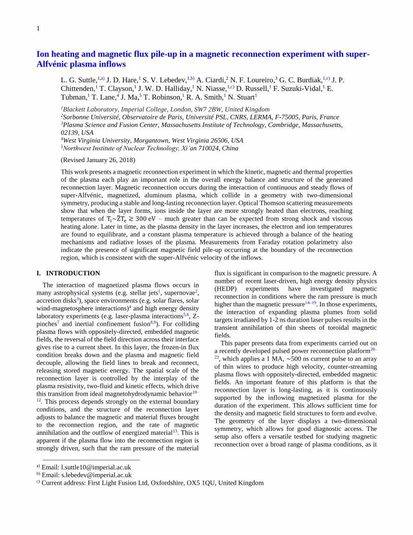
• Measurements in the yz-plane

The TS measurements detailed thus far were made with

the probe laser crossing the layer in the xy-plane, in the

geometry of Fig. 5(a), and the local parameters of the

reconnection layer at different positions along the layer were

obtained by performing multiple experiments and varying

the y-coordinate of the crossing. This method however

restricts the extent of the layer which can be studied, due to

the probe path being obstructed by the array hardware at

large y-crossing values. To overcome this limitation an

alternate TS geometry was employed, where the trajectory

of the probe beam was along the y-direction, at the mid-

height of the arrays (z=0 mm), and the scattered light was

observed at 90° in the out-of-plane z-direction, using a single

fiber-optic bundle. This scattering geometry defined an

alternate 𝐊𝐒 vector, directed at 45° to �̂� and �̂�, such that the

Doppler shift was equally sensitive to Vy and Vz (Δω =

[KS √2⁄ ][Vy + Vz]).

Fig. 7(a) shows the positions of 14, 400 µm-diameter

scattering volumes along the reconnection layer in an

experiment using this TS geometry. The velocities measured

in this experiment are shown in Fig. 7(b), with the data points

in red (circles) calculated directly from the observed Doppler

shifts of the scattered spectra, and thus giving the velocity

component in the direction of the scattering vector. In

agreement with measurements performed in the xy-

geometry, they show the presence of large velocities inside

the layer. However, whilst the shape of the velocity profile

is symmetric about y=0 mm, there is a systematic, positive

offset in the velocities. Since measurements performed in the

layer in the xy-plane demonstrated that Vy=0 km/s at y=0

mm, it can be concluded that the Doppler shift at this position

must be attributed to flow in the positive z-direction, equal

to ~50 km/s. Under the assumption that this Vz component

is constant along the layer, and equal to the value of

Vz(x=0,y=0), the Vy component along the layer can be

calculated as

Vy(y) =VS(y)

sin(45°)− Vz(0,0).

These values are plotted in Fig. 7(b) as the blue data points

(squares). It is seen that this Vy(y) profile is symmetric about

the central position of the layer y=0 mm, and that the

outward flow of plasma reaches velocities of Vy=±100 km/s

by y=±10 mm. It is important to note that measurements

were also performed with the probe beam propagating in the

y-direction, similar to Fig. 7(a), but with the beam path just

outside of the layer, along x=2δ=0.6 mm. In this case there

was little evidence of either vertical motion, or motion

parallel to the layer beyond the standard cylindrical

divergence of the flow, previously discussed in conjunction

with Fig. 6(d). Thus, it can be concluded that the strong

outflow of plasma from the layer, demonstrated in Fig. 7(b),

is due to plasma being accelerated inside the layer.

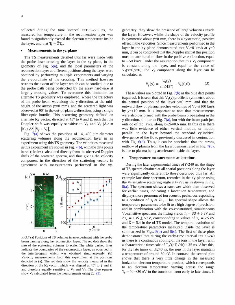
• Temperature measurements at late time

During the later experimental times of t≥240 ns, the shape

of TS spectra obtained at all spatial positions along the layer

were significantly different to those described thus far. An

example late-time spectrum, recorded in the xy-plane using

the Vy sensitive scattering angle at t=295 ns, is shown in Fig.

8(a). The spectrum shows a narrower width than observed

for earlier times, indicating a lower ion temperature, and

displays more pronounced ion acoustic peaks, corresponding

to a condition of Ti ≪ Z̅Te. This spectral shape allows the

temperature parameters to be fit to a high degree of precision,

and in combination with the co-constrained, simultaneous

Vx-sensitive spectrum, the fitting yields Ti = 33 ± 5 eV and

Z̅Te = 135 ± 6 eV, corresponding to values of Te = 25 eV

and Z̅ = 5.4 in the nLTE model. The temporal evolution of

the temperature parameters measured inside the layer is

summarized in Figs. 8(b) and 8(c). The first of these plots

demonstrates that during the early-time interval t=190-240

ns there is a continuous cooling of the ions in the layer, with

a characteristic timescale of Ti (dTi dt⁄ )⁄ ~35 ns. After this,

for the late times of t≥240 ns, the ions in the layer maintain

a temperature of around 30 eV. In contrast, the second plot

shows that there is very little change in the measured

ionization electron temperature product, which corresponds

to an electron temperature varying across the range

Te =40→30 eV in the transition from early to late times. It

(3)

FIG.7 (a) Positions of TS volumes in an experiment with the probe

beam passing along the reconnection layer. The red dots show the

size of the scattering volumes to scale. The white dashed lines

indicate the boundaries of the reconnection layer, as observed in

the interferogram which was obtained simultaneously. (b)

Velocity measurements from this experiment at the positions

depicted in (a). The red dots show the velocity measured in the

direction of the Ks vector, which was aligned at 45° to �̂� and �̂�,

and therefore equally sensitive to Vy and Vz. The blue squares

show Vy calculated from the measurements using Eq. (3).

10

is also important to note that at all times Thomson scattering

measurements showed a Vy profile consistent with that in

Fig. 7(b).

IV. SUMMARY AND DISCUSSION

The experiments reported in this paper utilize counter-

streaming, supersonic, magnetized plasma flows, with anti-

parallel magnetic fields, to produce a reconnection layer in

which the magnetic flux is annihilated. The flow parameters

of the setup provide the boundary conditions for the

magnetic reconnection process, which in this case is

“strongly driven” due to the high ratio of ram to magnetic

pressure in the inflows (characterized by a high dynamic

Beta parameter, βdyn = ρVflow2/[B2/2μ0]~10).

Consequently, the velocity of the inflows is super-Alfvénic

(MA~2).

A notable feature of these pulsed power driven

experiments is the long duration of the reconnection layer. In

contrast to the more transient reconnection phenomenon

occurring in laser-driven reconnection experiments14–19, the

reconnection layer appears to be in a stable and

approximately steady-state, maintained by a continuous

inflow of plasma with embedded magnetic field for a

timescale >100 ns. This is many times greater than the

hydrodynamic time-scale of the system, which can be

estimated as the time taken for the inflow to cross a spatial

scale equal to the layer thickness, i.e. δ Vx⁄ ~5 ns. The

measurements presented in this paper focus on the

characterization of the reconnection layer plasma

parameters, which reveal in detail the structure of the

reconnection layer and its evolution over the observed

timescale. An overview of the measured plasma parameters

at two times in these experiments, representative of the early

and late time properties of the layer, is given in Table I and

the main observations of the study are discussed below.

A. Structural features of the reconnection layer

The geometry of the experiments is quasi-two-

dimensional: the xy-plane of the setup defines the

(reconnection) plane in which the reconnecting magnetic

field lines lie (Figs. 1(b) and 2), and in the perpendicular xz-

plane there is a good, linear symmetry (Fig. 1(c)). The setup

does not contain any guide field. Measurements of the

magnetic field and density distributions of the plasma show

that the magnetic flux advected by the inflows is annihilated

inside the layer, and that there is an accompanying increase

in the plasma density inside the layer (Figs. 3 and 4(a)-(d)).

Following the initial formation of the layer, the magnetic

field distribution is found to closely resemble a Harris sheet

profile (Fig. 4(d)), and the half-thickness δ of the sheet

matches that of the density rise in the layer. At subsequent

times, strong and narrow enhancements in the local magnetic

field strength develop in narrow intervals (Δx≲0.1 mm) at

the boundaries of the layer (Figs. 4(e) and 4(f)), consistent

with the pile-up of magnetic flux, and these features increase

in prominence over time (Figs. 4(g) and 4(h)). It is

interesting that the half-thickness of the layer is equal to the

ion skin depth of the plasma di = c ωpi⁄ calculated from the

layer plasma parameters. This suggests that two fluid

physics, such as the Hall effect10–13, may play an important

role in this system, as the ions decouple from the electrons

on the spatial scale of the flux pile-up. The mean free paths

of both electrons and ions in the plasma are much shorter

than the spatial scales of all observed features of the layer

structure (λii~10−2 mm, λei~10−3 mm), so the plasma is

strongly collisional.

An analysis of the mass flowing into and out of the central

region of the reconnection layer, with the bounds |y| <0.8 mm and |x| < δ, reveals that the rate of plasma inflow

to the layer (ΔyVxni,in) is approximately a factor of 2 greater

than the outflow rate (2δVyni,out). The accumulation of

material in the reconnection layer is indeed seen in the

increasing electron density in Fig. 3(e). Conversion of this

measured ne(t) to ion density, using local TS measurements

of the up- and downstream ionization states of the plasma,

shows a very good agreement with the flux estimate. Despite

the changes in the material density and plasma temperature

in the layer (Fig. 8(b) and 8(c)), the thickness of the layer is

approximately constant throughout the experiments. An

FIG.8 (a) Example of a TS spectrum typical for t≥240 ns, showing narrow and pronounced ion-acoustic peaks recorded at the center of the

layer (x,y)=0 mm, using the Vy-sensitive geometry depicted in Fig. 5. (b-c) Ti and �̅�Te measured inside the reconnection layer at different

times. Each data-point corresponds to the most centrally-located measurement inside the layer from an individual experiment.

11

analysis of the measured plasma parameters (Table I)

indicates that the required pressure balance for this is indeed

accounted for at both the early and late times. During the

early stage of the experiments, when the ion temperature of

the layer is large, the ram pressure of the flow exactly

matches the thermal pressure of the layer. Later in time, the

pressure balance is achieved between the inflow ram

pressure and the magnetic pressure of the field enhancements

at the layer boundary.

The Lundquist number calculated for the system is S =LVA DM⁄ ~10-20, where VA is the upstream Alfvén velocity,

DM the magnetic diffusivity, and the length scale L of the

system is defined as half the radius of curvature (RC) of the

azimuthal magnetic field lines at the mid-plane between the

two wire arrays (Fig. 1(a)). Combining this estimate with the

ratio of the length scale to the ion skin depth (L di⁄ ~20)

leads to the expectation that the system should lie in the

“single x-line collisional reconnection” domain24, where the

reconnection layer is not expected to be unstable to tearing

mode (plasmoid) instabilities38,39. It is important to note

however that this comparison to the known phase-space does

not consider the super-Alfvénic nature of the inflows, which

could have consequences upon this behavior. Nevertheless,

the prediction appears consistent with the observations of the

reconnection layer structure, which show that despite the

presence of density modulations in the inflowing plasma

(Fig. 3(a)-(d)), the layer is highly symmetric about its center,

and displays smoothly varying density and velocity profiles

along its length (Figs. 2, 3 and 7(b)). In contrast, similar

experiments carried out using this pulsed power platform,

but employing a carbon plasma, with a dynamic Beta

parameter βdyn ≈ 1 and sub-Alfvénic inflow velocity,

display a much more unstable reconnection process21–23. The

carbon reconnection layer has a Lundquist number of S≈100

due to a higher electron temperature, caused by the absence

of radiative cooling. This likely places the carbon

experiments in the “semi-collisional” reconnection regime39,

and plasmoids are observed forming and propagating

throughout the layer structure. These observed differences

demonstrate the versatility of the pulsed power setup, as it

can access different regimes of reconnection physics with the

available control over the plasma material. Further details

surrounding the tuneability of the setup and how Lundquist

number parameter space can be explored are discussed in

Ref. 23.

B. Magnetic flux annihilation and plasma outflows from

the reconnection layer

Faraday rotation measurements show evidence of

magnetic field accumulating in pile-up regions at the

reconnection layer boundaries. To determine whether this

could significantly reduce the rate of magnetic flux

annihilation inside the layer, the rate at which magnetic field

builds up at the boundaries is compared to the rate of inflow

TABLE I. Plasma parameters of the inflow and reconnection layer at early and late times in the experiments.

Time: t = 215ns t = 250ns

Parameter Symbol Inflow Layer Inflow Layer

Electron temperature (eV) Te 15 40 15 30

Ion temperature (eV) Ti 20 300 20 30

Ionization Z̅ 3.5 7 3.5 5.7

Electron density (cm-3) ne 5×1017 1.3×1018 8×1017 2.3×1018

Ion density (cm-3) ni 1.4×1017 1.9×1017 2.3×1017 4×1017

Magnetic field (T) By 2 - 4 -

Inflow (outflow) velocity (km/s) Vx (Vy) 50 (100) 50 (100)

Alfvén speed (km/s) VA 22 - 35 -

Ion sound speed (km/s) cS 18 40 18 32

Dynamic Beta βdyn 10 - 4 -

Thermal Beta βth 1.1 - 0.4 -

Lundquist number S - 14 - 18

Layer half-length (mm) i) L = RC/2 - 7 - 7

Layer half-thickness (mm) δ - 0.3 - 0.3

Ion skin depth (mm) di = c/ωpi 0.89 0.37 0.71 0.33

Ion-ion mean free path (mm) λii 10-3 10-2 10-3 10-2

Radiative cooling time (ns) τrad 23 5 15 4

Ion-electron energy exchange time (ns) τeiE 50 40 30 20

i) The length RC is the radius of curvature of the magnetic field lines at the boundary of the reconnection layer.

12

of magnetic flux. The magnetic flux inflow rate is given by

the upstream product ByVx, and the pile-up rate is estimated

as the rate of growth of the field enhancements dBpile dt⁄

(measured from the evolving magnetic field distribution, e.g.

Figs. 4(d), 4(f) and 4(h)) multiplied by the enhancement

thickness Δx. The ratio equates to:

(dBpile

dtΔx) (ByVx)⁄ ~10%.

Within the resolution of the measurements, this suggests

that the majority of the magnetic flux passes through the pile-

up region and is processed inside the layer. However, a

higher magnitude of Bpile at the sharp peaks of the pile-up

region cannot be ruled out due to the line averaged nature of

the magnetic field measurements with the Faraday rotation

diagnostic.

The destruction of magnetic flux in the reconnection layer

leads to plasma heating and the formation of fast, symmetric

outflows of plasma along the layer. This bulk plasma motion

is consistent with the acceleration of material in the direction

of the expected magnetic tension force of the reconnected

field lines. The plasma outflow is measured to reach

velocities of Vy ≳ 100 km/s ~ 4VA, with respect to the

upstream Alfvén speed. This is consistent with the

generalized Sweet-Parker model of Refs. 40,41, as the

outflow is able to acquire this super-Alfvénic velocity from

the additional acceleration of the thermal pressure gradient

in the direction of the open downstream boundary, i.e.

vacuum.

In addition to motion in the xy-plane, results from TS

measurements indicate the presence of a significant ion

motion in the vertical out-of-plane, z-direction (Fig. 7(b)).

This Vz velocity of ~50 km/s, measured in the middle of the

layer, is in the direction of the reconnection electric field

(𝐄𝐳 = 𝐉𝐳 σ⁄ ). It is interesting to compare this unexpectedly

high velocity with the drift velocity between the electrons

and ions required to support the current in the reconnection

layer. A current density of ~0.5-1 MA/cm2 is required to

provide a Harris-like magnetic field profile with the

measured half-thickness δ and upstream field strength.

Combined with the measured electron density, this current

density corresponds to a drift velocity of Ud = Jz ne⁄ =25-

50 km/s. This is comparable to the measured ion velocity,

suggesting that the vertical ion motion could make a

considerable contribution to the current inside the

reconnection layer. This raises the intriguing possibility of

the ions acting as the primary charge carrier responsible for

the current, and therefore merits a future investigation of the

out-of-plane velocity distribution of the reconnection layer.

C. Energy partition

Measurements from TS show that there is a clear evolution

over time of the ion temperature inside the reconnection

layer (Fig. 8(b)). Early in time (t=215 ns) Ti ≫ Te in the

layer, with Ti ≈ Z̅Te~300 eV. It can be demonstrated that

this high ion temperature, which is an order of magnitude

greater than the temperature of the upstream flow, exceeds

what can be expected by both strong-shock heating from the

supersonic entry into the layer, and viscous heating due to

the high velocity shear between the layer and upstream

plasma.

The 50 km/s inflow velocity measured upstream of the

layer boundary, where Ti is small, corresponds to Al ions

with a directed kinetic energy of Ei = miVx2/2 = 350 eV.

Thermalization of this kinetic energy (assuming no energy is

transferred to the electrons) gives a maximum possible ion

temperature of Ti = (2/3)Ei, which is already smaller than

the measured post-interaction Ti at early time. The actual

upper limit of the post-shock plasma temperature is

significantly smaller, and can be estimated using a standard

expression for heating in a strong shock42,

kBTi = Ei

4(γ − 1)

(γ + 1)2

1

(Z̅ + 1),

where γ is the adiabatic index of the plasma. Using γ = 5/3,

and neglecting equilibration with the electrons (i.e. Z̅ = 0),

gives an upper limit for the immediate post-shock ion

temperature of Ti = 120 eV. This reduces to Ti=30-15 eV for

Z̅=3-7, once ion-electron equilibration is established.

The viscous heating rate can be estimated by considering

the viscous damping of the highly sheared velocity profile of

the outflows. Following the treatment of Ref. 43 and

employing Braginskii’s expression for the ion viscosity44:

3

2nikB

∂Ti

∂t= 0.96nikBTiτi (

∂Vy

∂x)

2

,

where τi ∝ Ti3 2⁄

is the ion collisional timescale. Solving this

differential equation using the parameters in Table I and

assuming a maximum velocity shear, where Vy drops from

100 km/s at the center of the layer to zero at |x| = δ, gives a

viscous heating timescale >>500 ns for even a modest

heating to 100 eV from the initial 30 eV of the upstream

flow.

Thus, an additional mechanism for ion heating must be

present inside the layer, which should be expected to draw

from the released magnetic energy. Enhanced heating of ions

has been discussed extensively in the context of magnetic

reconnection, e.g. in Refs. 12,43,45,46, and is often

associated with the development of kinetic plasma

turbulence. The high current density at the boundary of the

current layer corresponds to a drift velocity exceeding the

ion sound speed (Ud cS⁄ ~5). This could lead to the

development of e.g. ion-acoustic or lower hybrid drift

instabilities13, which may be detectable with Thomson

scattering measurements47,48, but additional experiments

would be needed to investigate this further.

At late times in the experiments (t≥240 ns), the thermal

properties of the layer reach an approximately steady state,

with the ion temperature in the layer roughly equal to that of

the electrons, at values comparable to those predicted above

(4)

(5)

13

from Eq. (4) (Ti ≈ Te~30 eV). Calculating the energy

exchange time between these populations (τeiE ∝ 1 ni⁄ )

shows that as the ion density of the layer increases from ni =2 × 1017 cm−3 at t=215 ns, to ni = 4 × 1017 cm−3 at t=250

ns, the exchange time drops over the range τeiE = 40 →

20 ns. In comparison, the time taken for inflowing plasma to

exit the central region of the layer at the measured outflow

velocity is of the order ~50-100 ns. This indicates that as the

experiment progresses the system converges towards a

situation where the ion and electrons have time to equilibrate

before the plasma leaves the layer.

The electron temperature is approximately constant

throughout the experiments, and thus the internal energy Uint

of the electron population should be conserved by a balance

of the in- and outgoing energy fluxes. The incoming energy

can be evaluated as the sum of the contributions from the

ion-electron exchange ((3 2⁄ )nekB(Ti − Te)/τeiE ) and the

resistive heating of the electrons (estimated classically from

the Spitzer resistivity as ηSpJz2). These must counter the

radiative cooling losses of the plasma, which can be

represented as a cooling function Λ(ni, Te). Calculations of

Λ for aluminum, following the approach described in Refs.

49,50, show that the radiative power loss at the relevant

conditions of the layer is significant, and this is reflected by

the relatively short cooling timescales (τrad = Uint neniΛ⁄ )

quoted for the layer in Table I. In comparison to the radiative

power loss, the heating power provided by the ion-electron

exchange and the resistive heating inside the reconnection

current sheet (assuming a Harris-like profile) accounts for

only ~50% of the required energy input to the electrons to

keep an approximately constant temperature at both early

and late times (the ratio however shifts from ~40% of the

required energy input being provided by ion-electron

exchange, and ~10% from resistive heating, at early time, to

the reverse situation at late time). The most plausible

explanation for this apparent shortfall in heating power is

that an additional resistive heating is provided by the current

sheets associated with the magnetic flux pile-up at the

boundaries of the layer. The large spatial gradients of the

magnetic field seen here correspond to current densities

growing from ~3-6 MA/cm2 over the range t=215-250 ns.

Thus, this could potentially provide a short but intense

heating power to the electrons as the plasma passes across

the layer boundary, however higher resolution TS

measurements would be required to verify this hypothesis.

V. CONCLUSIONS

This paper describes the structure and evolution of a long-

lasting reconnection layer formed by colliding magnetized,

aluminum plasma flows in the strongly-driven regime (high

ratio of ram to magnetic pressure, super-Alfvénic inflow

velocity). The reconnection layer is dynamically stable,

highly symmetric and quasi-two-dimensional, allowing ease

of access for diagnosis of the spatially and temporally

resolved plasma parameters of the system. The boundary

conditions set by the driven inflow result in a reconnection

layer which shows evidence of a strong pile-up of the

magnetic flux brought by the inflows at the boundaries of the

layer. Early in time the reconnection layer shows an

unexpectedly large ion temperature, Ti ≈ Z̅Te ≫ Te, which

cannot be explained by considerations of either the

thermalization of the kinetic energy of the inflowing

material, or by classical viscous heating. Later in time the

ions inside the layer cool, via an increased rate of energy

exchange to the electrons. Meanwhile, the electron

population maintains an approximately constant temperature

throughout the lifetime of the reconnection layer, via an

evolving balance between the heating contributions from the

ions and resistive heating, and the strong losses due to

radiative cooling of the aluminum plasma.

A number of significant differences are found between

both the structures and thermal properties of the

reconnection layer observed in these experiments, and in

experiments using a geometrically identical setup but with

sub-Alfvénic, carbon plasma inflows21–23. In both

experiments the reconnection layer forms with a Harris-like

magnetic field profile. However, only in aluminum, with its

much higher dynamic Beta parameter, does this profile later

evolve to show the strong field enhancements associated

with magnetic field pile-up. The strong radiative cooling of

the aluminum plasma also plays a large role in the

differences of these systems. The radiative cooling results in

a much lower electron temperature inside the aluminum

reconnection layer, and consequently the system has a much

smaller Lundquist number (S~10 in aluminum, versus ~100

in carbon). This appears to prevent tearing-mode instabilities

in the aluminum reconnection layer, allowing single-x-line

reconnection layer to operate, without the formation of

plasmoids, such as those observed in the carbon

reconnection experiments21–23. These differences highlight

the suitability of this pulsed power setup for studying

reconnection processes under a range of conditions and

parameter space.

ACKNOWLEDGEMENTS

This work was supported in part by the Engineering and

Physical Sciences Research Council (EPSRC) Grant No.

EP/N013379/1, and by the U.S. Department of Energy

(DOE) Awards No. DE-F03-02NA00057, DE-SC-0001063

and DE-NA-0003764. A.C. and N.F.L. were supported by

LABEX Plas@Par with French state funds managed by the

ANR within the Investissements d’Avenir programme under

reference ANR-11-IDEX-0004-02. N.F.L. was supported by

the NSF-DOE partnership in Basic Plasma Science and

Engineering, Award No. DE-SC-0016215.

1 P. Hartigan, A. Frank, P. Varniere, and E.G. Blackman, Astrophys.

J. 661, 910 (2007). 2 S.P. Reynolds, B.M. Gaensler, and F. Bocchino, Space Sci. Rev.

166, 231 (2012). 3 M. Camenzind, Magnetized Disk-Winds and the Origin of Bipolar

14

Outflows. In: Klare G. (Eds) Accretion and Winds. Reviews in

Modern Astronomy, Vol 3 (Springer, Berlin, Heidelberg, 1990). 4 M. Kivelson and C. Russell, Introduction to Space Physics

(Cambridge University Press, 1995). 5 R.J. Mason and M. Tabak, Phys. Rev. Lett. 80, 524 (1998). 6 U. Wagner, M. Tatarakis, A. Gopal, F.N. Beg, E.L. Clark, A.E.

Dangor, R.G. Evans, M.G. Haines, S.P.D. Mangles, P.A. Norreys,

M.-S. Wei, M. Zepf, and K. Krushelnick, Phys. Rev. E 70, 26401

(2004). 7 D.D. Ryutov, M.S. Derzon, and M.K. Matzen, Rev. Mod. Phys. 72,

167 (2000). 8 E.L. Lindman, High Energy Density Phys. 6, 227 (2010). 9 J.R. Davies, D.H. Barnak, R. Betti, E.M. Campbell, P.-Y. Chang,

A.B. Sefkow, K.J. Peterson, D.B. Sinars, and M.R. Weis, Phys.

Plasmas 24, 62701 (2017). 10 E.G. Zweibel and M. Yamada, Proc. R. Soc. London A Math. Phys.

Eng. Sci. 472, (2016). 11 E.G. Zweibel and M. Yamada, Annu. Rev. Astron. Astrophys. 47,

291 (2009). 12 M. Yamada, R. Kulsrud, and H. Ji, Rev. Mod. Phys. 82, 603 (2010). 13 D. Biskamp, Magnetic Reconnection in Plasmas (Cambridge

University Press, Cambridge, 2000). 14 G. Fiksel, W. Fox, A. Bhattacharjee, D.H. Barnak, P.-Y. Chang, K.

Germaschewski, S.X. Hu, and P.M. Nilson, Phys. Rev. Lett. 113,

105003 (2014). 15 P.M. Nilson, L. Willingale, M.C. Kaluza, C. Kamperidis, S.

Minardi, M.S. Wei, P. Fernandes, M. Notley, S. Bandyopadhyay,

M. Sherlock, R.J. Kingham, M. Tatarakis, Z. Najmudin, W.

Rozmus, R.G. Evans, M.G. Haines, A.E. Dangor, and K.

Krushelnick, Phys. Rev. Lett. 97, 255001 (2006). 16 M.J. Rosenberg, C.K. Li, W. Fox, A.B. Zylstra, C. Stoeckl, F.H.

Séguin, J.A. Frenje, and R.D. Petrasso, Phys. Rev. Lett. 114,

205004 (2015). 17 W. Fox, A. Bhattacharjee, and K. Germaschewski, Phys. Plasmas

19, 56309 (2012). 18 C.K. Li, F.H. Séguin, J.A. Frenje, J.R. Rygg, R.D. Petrasso, R.P.J.

Town, O.L. Landen, J.P. Knauer, and V.A. Smalyuk, Phys. Rev.

Lett. 99, 55001 (2007). 19 L. Willingale, P.M. Nilson, M.C. Kaluza, A.E. Dangor, R.G.

Evans, P. Fernandes, M.G. Haines, C. Kamperidis, R.J. Kingham,

C.P. Ridgers, M. Sherlock, A.G.R. Thomas, M.S. Wei, Z.

Najmudin, K. Krushelnick, S. Bandyopadhyay, M. Notley, S.

Minardi, M. Tatarakis, and W. Rozmus, Phys. Plasmas 17, 43104

(2010). 20 L.G. Suttle, J.D. Hare, S. V. Lebedev, G.F. Swadling, G.C.

Burdiak, A. Ciardi, J.P. Chittenden, N.F. Loureiro, N. Niasse, F.

Suzuki-Vidal, J. Wu, Q. Yang, T. Clayson, A. Frank, T.S.

Robinson, R.A. Smith, and N. Stuart, Phys. Rev. Lett. 116, 225001

(2016). 21 J.D. Hare, L. Suttle, S. V. Lebedev, N.F. Loureiro, A. Ciardi, G.C.

Burdiak, J.P. Chittenden, T. Clayson, C. Garcia, N. Niasse, T.

Robinson, R.A. Smith, N. Stuart, F. Suzuki-Vidal, G.F. Swadling,

J. Ma, J. Wu, and Q. Yang, Phys. Rev. Lett. 118, 85001 (2017). 22 J.D. Hare, S. V. Lebedev, L.G. Suttle, N.F. Loureiro, A. Ciardi,

G.C. Burdiak, J.P. Chittenden, T. Clayson, S.J. Eardley, C. Garcia,

J.W.D. Halliday, N. Niasse, T. Robinson, R.A. Smith, N. Stuart, F.

Suzuki-Vidal, G.F. Swadling, J. Ma, and J. Wu, Phys. Plasmas 24,

102703 (2017). 23 J.D. Hare, L.G. Suttle, S. V. Lebedev, N.F. Loureiro, A. Ciardi, J.P.

Chittenden, T. Clayson, S.J. Eardley, C. Garcia, J.W.D. Halliday,

T. Robinson, R.A. Smith, N. Stuart, F. Suzuki-Vidal, and E.R.

Tubman, arXiv:1711.06534 (2017).

24 H. Ji and W. Daughton, Phys. Plasmas 18, 111207 (2011). 25 I.H. Mitchell, J.M. Bayley, J.P. Chittenden, J.F. Worley, A.E.

Dangor, M.G. Haines, and P. Choi, Rev. Sci. Instrum. 67, 1533

(1996). 26 A.J. Harvey-Thompson, S. V. Lebedev, S.N. Bland, J.P.

Chittenden, G.N. Hall, A. Marocchino, F. Suzuki-Vidal, S.C. Bott,

J.B.A. Palmer, and C. Ning, Phys. Plasmas 16, 22701 (2009). 27 S. V. Lebedev, F.N. Beg, S.N. Bland, J.P. Chittenden, A.E. Dangor,

M.G. Haines, K.H. Kwek, S.A. Pikuz, and T.A. Shelkovenko, Phys.

Plasmas 8, 3734 (2001). 28 J. Greenly, M. Martin, I. Blesener, D. Chalenski, P. Knapp, and R.

McBride, AIP Conf. Proc. 1088, 53 (2009). 29 V. V. Aleksandrov, V.A. Barsuk, E. V. Grabovski, A.N. Gritsuk,

G.G. Zukakishvili, S.F. Medovshchikov, K.N. Mitrofanov, G.M.

Oleinik, and P. V. Sasorov, Plasma Phys. Reports 35, 200 (2009). 30 S. V. Lebedev, L. Suttle, G.F. Swadling, M. Bennett, S.N. Bland,

G.C. Burdiak, D. Burgess, J.P. Chittenden, A. Ciardi, A. Clemens,

P. de Grouchy, G.N. Hall, J.D. Hare, N. Kalmoni, N. Niasse, S.

Patankar, L. Sheng, R.A. Smith, F. Suzuki-Vidal, J. Yuan, A.

Frank, E.G. Blackman, and R.P. Drake, Phys. Plasmas 21, 56305

(2014). 31 G.F. Swadling, S. V. Lebedev, G.N. Hall, S. Patankar, N.H.

Stewart, R.A. Smith, A.J. Harvey-Thompson, G.C. Burdiak, P. de

Grouchy, J. Skidmore, L. Suttle, F. Suzuki-Vidal, S.N. Bland, K.H.

Kwek, L. Pickworth, M. Bennett, J.D. Hare, W. Rozmus, and J.

Yuan, Rev. Sci. Instrum. 85, 11E502 (2014). 32 G.C. Burdiak, S. V. Lebedev, S.N. Bland, T. Clayson, J. Hare, L.

Suttle, F. Suzuki-Vidal, D.C. Garcia, J.P. Chittenden, S. Bott-

Suzuki, A. Ciardi, A. Frank, and T.S. Lane, Phys. Plasmas 24,

72713 (2017). 33 G.F. Swadling, S. V. Lebedev, N. Niasse, J.P. Chittenden, G.N.

Hall, F. Suzuki-Vidal, G. Burdiak, A.J. Harvey-Thompson, S.N.

Bland, P. De Grouchy, E. Khoory, L. Pickworth, J. Skidmore, and

L. Suttle, Phys. Plasmas 20, 22705 (2013). 34 I. Hutchinson, Principles of Plasma Diagnostics, 2nd Ed.

(Cambridge University Press, 2005). 35 D.H. Froula, S.H. Glenzer, N.C.J. Luhmann, and J. Sheffield,

Plasma Scattering of Electromagnetic Radiation, 2nd Ed. (Elsevier,

2011). 36 J.P. Chittenden, B.D. Appelbe, F. Manke, K. McGlinchey, and

N.P.L. Niasse, Phys. Plasmas 23, 52708 (2016). 37 S. V Lebedev, D.J. Ampleford, S.N. Bland, S.C. Bott, J.P.

Chittenden, J. Goyer, C. Jennings, M.G. Haines, G.N. Hall, D.A.

Hammer, J.B.A. Palmer, S.A. Pikuz, T.A. Shelkovenko, and T.

Christoudias, Plasma Phys. Control. Fusion 47, A91 (2005). 38 N.F. Loureiro, A.A. Schekochihin, and S.C. Cowley, Phys. Plasmas

14, 100703 (2007). 39 N.F. Loureiro and D.A. Uzdensky, Plasma Phys. Control. Fusion

58, 14021 (2016). 40 H. Ji, M. Yamada, S. Hsu, and R. Kulsrud, Phys. Rev. Lett. 80,

3256 (1998). 41 H. Ji, M. Yamada, S. Hsu, R. Kulsrud, T. Carter, and S. Zaharia,

Phys. Plasmas 6, 1743 (1999). 42 R. Drake, High-Energy-Density Physics (Springer Berlin

Heidelberg, 2006). 43 S.C. Hsu, T.A. Carter, G. Fiksel, H. Ji, R.M. Kulsrud, and M.

Yamada, Phys. Plasmas 8, 1916 (2001). 44 S.I. Braginskii, Rev. Plasma Phys. 1, (1965). 45 G. Fiksel, A.F. Almagri, B.E. Chapman, V. V. Mirnov, Y. Ren, J.S.

Sarff, and P.W. Terry, Phys. Rev. Lett. 103, 1 (2009). 46 Y. Ono, M. Yamada, and T. Akao, Phys. Rev. Lett. 76, 3328

(1996).

15

47 D.R. Gray and J.D. Kilkenny, Plasma Phys. 22, 81 (1980). 48 S.H. Glenzer, W. Rozmus, V.Y. Bychenkov, J.D. Moody, J.

Albritton, R.L. Berger, A. Brantov, M.E. Foord, B.J. MacGowan,

R.K. Kirkwood, H.A. Baldis, and E.A. Williams, Phys. Rev. Lett.

88, 235002 (2002). 49 F. Suzuki-Vidal, S. V. Lebedev, A. Ciardi, L.A. Pickworth, R.

Rodriguez, J.M. Gil, G. Espinosa, P. Hartigan, G.F. Swadling, J.

Skidmore, G.N. Hall, M. Bennett, S.N. Bland, G. Burdiak, P. de

Grouchy, J. Music, L. Suttle, E. Hansen, and A. Frank, Astrophys.

J. 815, 96 (2015). 50 G. Espinosa, J.M. Gil, R. Rodriguez, J.G. Rubiano, M.A. Mendoza,

P. Martel, E. Minguez, F. Suzuki-Vidal, S.V. Lebedev, G.F.

Swadling, G. Burdiak, L.A. Pickworth, and J. Skidmore, High

Energy Density Phys. 17, 74 (2015).