arX

iv:a

stro

-ph/

0212

423v

1 1

9 D

ec 2

002

Investigation of the possible third image and

mass models of the gravitational lens PMN J1632–0033

Joshua N. Winn1, David Rusin, Christopher S. Kochanek

Harvard-Smithsonian Center for Astrophysics, 60 Garden St., Cambridge, MA 02138

jwinn@cfa.harvard.edu; drusin@cfa.harvard.edu; ckochanek@cfa.harvard.edu

ABSTRACT

We present multi-frequency VLBA2 observations of PMN J1632–0033, one of

the few gravitationally lensed quasars suspected of having a central “odd” image.

The central component has a different spectral index than the two bright quasar

images. Therefore, either the central component is not a third image, and is

instead the active nucleus of the lens galaxy, or else it is a third image whose

spectrum is inverted by free-free absorption in the lens galaxy. In either case, we

have more constraints on mass models than are usually available for a two-image

lens, especially when combined with the observed orientations of the radio jets of

the two bright quasars. If there is no third quasar image, the simplest permitted

model is a singular isothermal sphere in an external shear field: β = 2.05+0.23−0.10

(2σ), where ρ(r) ∝ r−β. If the central component is a third image, a hypothesis

which can be tested with future high-frequency observations, then the density

distribution is only slightly shallower than isothermal: β = 1.91± 0.02 (2σ). We

also derive limits on the size of a constant-density core, and the break radius and

exponent of an inner density cusp.

Subject headings: gravitational lensing — galaxies: structure — galaxies: nuclei

— quasars: individual (PMN J1632–0033)

1NSF Astronomy & Astrophysics Postdoctoral Fellow

2The Very Long Baseline Array (VLBA) and Very Large Array (VLA) are operated by the National

Radio Astronomy Observatory, a facility of the National Science Foundation operated under cooperative

agreement by Associated Universities for Research in Astromomy, Inc.

– 2 –

1. Introduction

The central density profile ρ(r) of galaxies is poorly known, but is important for un-

derstanding galaxy structure and the nature of dark matter. Theoretical cold-dark-matter

(CDM) models predict a steep central density cusp, ρ ∝ r−β with β ≃ 1–1.5 (see, e.g.,

Navarro, Frenk, & White 1997; Moore 1999). However, measurements of spiral galaxy ro-

tation curves suggest the dark matter has a constant-density core. This has been argued

most strongly for low-surface-brightness galaxies (de Blok et al. 2001) but may hold for all

spiral galaxies (Debattista & Sellwood 2000; Salucci & Burkert 2000), including our own

Galaxy (Binney & Evans 2001). The conflict may be due to observational effects such as

beam smearing, at least in part (van den Bosch & Swaters 2001), but the apparent con-

flict has encouraged some theorists to invent mechanisms that avoid producing cusps (e.g.,

bar-induced evolution, Weinberg & Katz 2002; warm dark matter, Bode, Ostriker, & Turok

2001; self-interacting dark matter, Spergel & Steinhardt 2000).

For elliptical galaxies, where rotation curves cannot be measured, the central density

profile is even less well understood. Observations of early-type galaxies with the Hubble

Space Telescope (HST) show that the light distribution is cuspy, with cusp parameters that

may be correlated with global galaxy properties (Lauer et al. 1995; Faber et al. 1997). But

such studies do not probe mass directly, and are limited to nearby galaxies due to the

requirements on angular resolution.

Multiple-image gravitational lenses can be used to measure the central surface density

of galaxies at significant redshift, by searching for faint central images of the background

object. In most cases, lenses should produce an odd number of images (Dyer & Roeder

1980; Burke 1981), one of which is faint and appears near the center of the lens galaxy.

This “central image” or “odd image” corresponds to the central maximum in the time-

delay surface. However, of the ∼80 known systems in which a galaxy produces multiple

images of a quasar or radio source, almost all consist of either 2 or 4 images. One system,

APM 08279+5255, definitely has three quasar images (Lewis et al. 2002b), but the third

image may be due to a “naked cusp” configuration rather than a central time-delay maximum

(Lewis et al. 2002a).

No central image has been identified definitively, even among the radio lenses, where the

central image could in principle be seen through the light and dust of the lens galaxy. The

absence of central images has been attributed to the demagnification of the image by the

high central surface density of the lens galaxy (see, e.g., Narasimha, Subramanian, & Chitre

1986; Wallington & Narayan 1993; Rusin & Ma 2001; Evans & Hunter 2002; Keeton 2002).

An “extra” radio component has been detected in several radio lenses, and in three of those

cases it is still unclear whether the extra component is an additional quasar image or faint

– 3 –

radio emission from an active galactic nucleus (AGN). Those three systems are 0957+561

(Harvanek et al. 1997), MG J1131+0456 (Chen & Hewitt 1993), and the subject of this

paper: PMN J1632–0033 (Winn et al. 2002).

Radio components A and B of J1632–0033 are two images of a z = 3.42 quasar, but the

third, faint component C is of unknown origin (see Fig 1). In an HST image, the lens galaxy

appears to be a fairly circular early-type galaxy with an optical effective radius of ≈ 0.′′2, but

it is too faint to be characterized in detail. The position of component C is near the optical

lens galaxy position, as expected for either an AGN or a central odd image. If A, B, and

C are all images of the same quasar, then they should have similar radio spectra. However,

Winn et al. (2002) only presented measurements of the flux density of C at one frequency.

A

CB

Fig. 1.— Radio map of J1632–0033 reproduced from Winn et al. (2002), illustrating the con-

figuration of components A, B, and C. The map is based on the 5.0 GHz merlin observation

of 2001 April 13. The restoring beam (88× 44 mas, P.A. 24) is illustrated in the upper left

corner. Contours begin at 3σ and increase by factors of two, where σ = 0.13 mJy beam−1.

Here we present new VLBA data that, in combination with the previous data, allow us

to measure the flux densities of all three components at four widely spaced frequencies. Our

analysis shows that C has a significantly different radio spectrum than A and B. We argue

that there are two alternative explanations for this difference. Either C is not a third quasar

image, and instead is the active nucleus of the lens galaxy; or, C is a third image, but its

spectral index is inverted by free-free absorption in the lens galaxy.

– 4 –

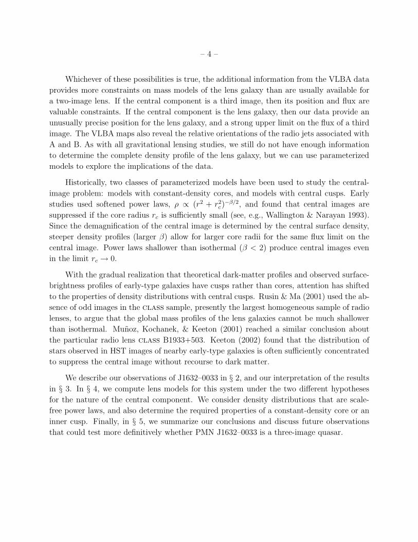
Whichever of these possibilities is true, the additional information from the VLBA data

provides more constraints on mass models of the lens galaxy than are usually available for

a two-image lens. If the central component is a third image, then its position and flux are

valuable constraints. If the central component is the lens galaxy, then our data provide an

unusually precise position for the lens galaxy, and a strong upper limit on the flux of a third

image. The VLBA maps also reveal the relative orientations of the radio jets associated with

A and B. As with all gravitational lensing studies, we still do not have enough information

to determine the complete density profile of the lens galaxy, but we can use parameterized

models to explore the implications of the data.

Historically, two classes of parameterized models have been used to study the central-

image problem: models with constant-density cores, and models with central cusps. Early

studies used softened power laws, ρ ∝ (r2 + r2c )

−β/2, and found that central images are

suppressed if the core radius rc is sufficiently small (see, e.g., Wallington & Narayan 1993).

Since the demagnification of the central image is determined by the central surface density,

steeper density profiles (larger β) allow for larger core radii for the same flux limit on the

central image. Power laws shallower than isothermal (β < 2) produce central images even

in the limit rc → 0.

With the gradual realization that theoretical dark-matter profiles and observed surface-

brightness profiles of early-type galaxies have cusps rather than cores, attention has shifted

to the properties of density distributions with central cusps. Rusin & Ma (2001) used the ab-

sence of odd images in the class sample, presently the largest homogeneous sample of radio

lenses, to argue that the global mass profiles of the lens galaxies cannot be much shallower

than isothermal. Munoz, Kochanek, & Keeton (2001) reached a similar conclusion about

the particular radio lens class B1933+503. Keeton (2002) found that the distribution of

stars observed in HST images of nearby early-type galaxies is often sufficiently concentrated

to suppress the central image without recourse to dark matter.

We describe our observations of J1632–0033 in § 2, and our interpretation of the results

in § 3. In § 4, we compute lens models for this system under the two different hypotheses

for the nature of the central component. We consider density distributions that are scale-

free power laws, and also determine the required properties of a constant-density core or an

inner cusp. Finally, in § 5, we summarize our conclusions and discuss future observations

that could test more definitively whether PMN J1632–0033 is a three-image quasar.

– 5 –

2. Observations

We observed J1632–0033 with the VLBA on 2002 March 14 and 15, for one eight-hour

session each day. On the first day, the array included one VLA antenna in place of the VLBA

antenna at Pie Town, but on the second day, the array consisted of the usual ten antennas.

During both sessions we alternated between observations at the standard 8.4 GHz (3.6 cm)

band and the standard 1.7 GHz (18 cm) band. For both bands, the observing bandwidth

of 32 MHz per polarization was divided into 4 sub-bands. Both senses of polarization were

recorded with 2-bit sampling. The data were correlated in Socorro, New Mexico, producing

16 channels of width 500 kHz from each sub-band, with an integration time of one second.

Calibration was performed with aips5 using standard procedures. We used the obser-

vations of J1632–0033 to solve for residual delays, rates, and phases directly (rather than

using phase-referencing), with a fringe-fitting solution interval of 2 minutes. We used the

multiple-field clean deconvolution algorithm available in aips to deconvolve a field centered

on A and, simultaneously, a field of the same size centered on the mid-point between B and

C. For the 8.4 GHz data, the fields were 1024 × 1024 with a scale of 0.2 mas pixel−1. For

the 1.7 GHz data, the fields were 512 × 512 with a scale of 1.0 mas pixel−1.

At first, the data from each day were analyzed separately. Once we verified that the

results of the two sessions were consistent, we combined the visibility data from each fre-

quency to produce final maps. The data were self-calibrated, based on the clean model

derived from the preliminary maps, with a 15-second solution interval. The final 1.7 GHz

maps are shown in Fig. 2, and the final 8.4 GHz maps are shown in Fig. 3. In the vicinity of

components B and C, the noise level in the maps is close to the theoretical limit. However,

the noise level is three times larger in the vicinity of component A due to large sidelobes.

Further improvement is difficult because of the near-equatorial location of the object, which

results in poor coverage of the visibility plane even for an eight-hour Earth-rotation synthesis

observation.

The flux densities of A, B, and C at each frequency are reported in Table 1. Also

included in this table are results based on the previous data of Winn et al. (2002), for those

cases in which all three components were detected (or could have been detected, given the

angular resolution). These previous data were re-analyzed using natural weighting rather

than uniform weighting, to maximize the sensitivity to the faint component C and to match

the present analysis. The results were consistent with previous results in all cases. Of

5The Astronomical Image Processing System (aips) is developed and distributed by the National Radio

Astronomy Observatory.

– 6 –M

illiA

RC

SE

C

MilliARC SEC1300 1280 1260 1240 1220 1200 1180 1160 1140 1120

-660

-680

-700

-720

-740

-760

-780

-800

-820

-840

Mill

iAR

C S

EC

MilliARC SEC40 20 0 -20 -40

50

40

30

20

10

0

-10

-20

-30

-40

-50

AB

C

Fig. 2.— VLBA maps of J1632–0033 at 1.7 GHz. The restoring beam (14.3 × 6.1 mas,

P.A. 0.4) is illustrated in the lower left corner of each panel. Contours begin at 3σ and

increase by factors of two. The dashed contour is −3σ. In the left panel (components B and

C), σ = 0.045 mJy beam−1. In the right panel (component A), σ = 0.135 mJy beam−1. The

dotted lines are the 1σ limits we adopted for the jet position angles.

Mill

iAR

C S

EC

MilliARC SEC1255 1250 1245 1240 1235 1230

-770

-775

-780

-785

-790

-795

Mill

iAR

C S

EC

MilliARC SEC1175 1170 1165 1160 1155 1150

-715

-720

-725

-730

-735

-740

Mill

iAR

C S

EC

MilliARC SEC10 5 0 -5 -10

10

5

0

-5

-10

AB C

Fig. 3.— VLBA maps of J1632–0033 at 8.4 GHz. The restoring beam (2.8 × 1.2 mas,

P.A. −0.5) is illustrated in the lower left corner of each panel. Contours begin at 3σ and

increase by factors of two. The dashed contour is −3σ. In the left and center panels

(components B and C), σ = 0.040 mJy beam−1. In the right panel (component A), σ =

0.120 mJy beam−1. The dotted lines are the 1σ limits we adopted for the jet position angles.

– 7 –

particular interest was the improved 15 GHz map, in which component C was detected with

flux density 0.84 ± 0.19 mJy. This is consistent with the upper limit of 1.5 mJy given by

Winn et al. (2002), but the positive detection of C in the lower-noise map provides another

valuable point of comparison.

For the VLA and merlin6 data, the flux densities were measured by fitting a model

consisting of 3 point sources to the visibility data, using difmap (Shepherd, Pearson, &

Taylor 1994). The VLBA data sets were too large for model-fitting in visibility space. For

these data, the flux densities were measured in image space with aips, using an aperture

surrounding each component. The quoted uncertainties are the larger of the rms noise and

the spread in values obtained using different choices for the aperture.

With these measurements of the flux densities of all three components at four widely

spaced frequencies, we have the opportunity to test whether C has the same radio continuum

spectrum as A and B. Assuming that the flux density of each component obeys Si(ν) ∝ ναi

(where αi is the spectral index of component i), a linear least-squares fit to the data in Table 1

gives αA = −0.27 ± 0.07, αB = −0.25 ± 0.07, and αC = +0.29 ± 0.18. The uncertainties in

the spectral indices include a contribution from the uncertainties in the absolute flux density

scale, which is at least 5% at all frequencies.

The comparison between αA and αC can be made more precise by examining the

flux density ratios, because the ratios are independent of the uncertainties in the abso-

lute flux density scale. The difference in spectral indices, αC − αA, is the logarithmic

slope of SC(ν)/SA(ν). The flux density ratios SB(ν)/SA(ν) and SC(ν)/SA(ν) are plotted

in Fig. 4. The solid line represents the best-fit power law to SC(ν)/SA(ν), which has a slope

6The Multi-Element Radio Linked Interferometry Network (merlin) is a U.K. national facility operated

by the University of Manchester at Jodrell Bank Observatory on behalf of PPARC.

Table 1. Flux density measurements of J1632–0033

Date Observatory Frequency Flux density (mJy)

(GHz) A B C

2002 Mar 14-15 VLBA 1.67 242 ± 3 16.9 ± 0.1 0.45 ± 0.05

2000 Apr 29 VLBA 4.99 167 ± 2 11.9 ± 0.1 0.60 ± 0.11

2001 Apr 05 merlin 4.99 207 ± 2 14.2 ± 0.3 0.90 ± 0.11

2002 Mar 14-15 VLBA 8.42 167 ± 2 14.0 ± 0.3 0.73 ± 0.04

2000 Nov 11 VLA 14.9 144 ± 2 9.4 ± 0.2 0.84 ± 0.19

2000 Nov 11 VLA 22.5 126 ± 2 8.4 ± 0.6 < 3.2

2000 Nov 11 VLA 42.6 83 ± 1 5.4 ± 0.4 < 1.8

– 8 –

αC − αA = +0.51 ± 0.17, implying the spectral indices of C and A are discrepant at the

3σ level. The dashed line is a fit to the data under the hypothesis that C is a third quasar

image whose spectrum had been modified by free-free absorption (see § 3). Also plotted are

upper limits on SC(ν)/SA(ν) from VLA data at the two highest frequencies.

The position angles of the jets in A and B were measured by fitting elliptical components

to the VLBA maps with aips, using a procedure (JMFIT) that corrects for the ellipticity

of the beam. For modeling purposes, we adopted the average of the 1.7 GHz and 8.4 GHz

results, giving φA = 8 and φB = −69, measured east of north. We estimate the uncertainty

in each position angle to be ±15, an error range that is approximately twice the difference

between the 1.7 GHz and 8.4 GHz results. These ranges of position angle are illustrated by

dotted lines in Figs. 2 and 3, although it is difficult to account for the elliptical beam in a

visual inspection.

3. The nature of component C

The flux density ratio SB(ν)/SA(ν) is nearly independent of observing frequency, as

should be the case for gravitationally lensed images of a single compact source. By contrast,

the flux density ratio SC(ν)/SA(ν) increases significantly with frequency. This immediately

suggests that C is not a third image of the same background source. Given that its position is

consistent with the optical position of the lens galaxy, it would be natural to conclude that C

represents faint radio emission from the lens galaxy, as discussed further in § 3.1. However,

there are several mechanisms that might cause a third quasar image to appear to have a

different spectral index than the two brighter images. These are discussed in § 3.2–§ 3.5.

The only mechanism we cannot rule out is free-free absorption (§ 3.5).

3.1. Lens galaxy emission

How does the flux density of C compare with the flux density expected from a typical

galaxy at the lens redshift? Given the radio flux density and spectral index of component

C that were presented in § 2, and the lens redshift estimate7 of z ≈ 1, the implied 1.4 GHz

luminosity of the lens galaxy is 1.7 × 1024h−2 W Hz−1.

7The lens redshift zl = 1.0 ± 0.1 was estimated by Winn et al. (2002) by requiring the photometric

properties of the lens galaxy to conform to the fundamental plane of elliptical galaxies, a method invented

by Kochanek et al. (2000).

– 9 –

Fig. 4.— Flux density ratios SB(ν)/SA(ν) and SC(ν)/SA(ν), as a function of frequency. To

allow both quantities to be plotted on the same axes, the values of SC(ν)/SA(ν) have been

multiplied by 10. Upper limits on SC(ν)/SA(ν) are plotted at 22.5 GHz and 43 GHz. The

straight line is the best-fitting power law to the SC(ν)/SA(ν) data points at 15 GHz and

below. The dotted line is the best-fitting curve assuming the variation is entirely due to

free-free absorption (see Eq. 1 and § 3.5).

– 10 –

This is significantly more powerful than the radio emission observed from ordinary galax-

ies, which is thought to arise from star formation and is limited to <∼ 1023 W Hz−1. However,

it is within the observed range of luminosities from galaxies harboring active galactic nuclei

(AGN). For example, Sadler et al. (2002) identified a sample of 420 AGN in the 2dF Galaxy

Redshift Survey, of which 24% had a 1.4 GHz radio luminosity at least as large as the implied

luminosity of component C (after correcting for their different choice of cosmology).

We conclude that the identification of component C as the active galactic nucleus of

the lens galaxy is a reasonable one. This would make J1632–0033 unusual among the known

lenses, but not unique; the lens galaxy of B2045+265 has a bright central component that

is almost certainly an active nucleus (Fassnacht et al. 1999).

3.2. Variability

If the source is variable, then the instantaneous flux density ratios between the lensed

images will fluctuate, due to the differential time delays between the images. If, in addition,

the degree of variability depends on frequency, then the flux density ratios will vary with

frequency. However, the differential time delay between components B and C is expected to

be very small (<0.5 day). This is much smaller than typical time scales for quasar variability

(∼months). Indeed, our measurements, which were spaced apart by one day, showed no sign

of variability. We therefore discount the possibility that variability is the reason for the

discrepancy of spectral indices.

3.3. Radio substructure

If the background radio source is extended and has sub-components with different spec-

tral indices, then these sub-components may each be magnified by a different factor (see,

e.g., Patnaik & Porcas 1999). In that case, the sum of flux densities of the sub-components

in a lensed image would not necessarily have the same spectral index as the corresponding

sum in a different image.

However, in the case of J1632–0033, the source is very compact. From Fig. 3 we can

limit the separation of sub-components in image A to <5 mas, corresponding to a change in

magnification of only ∆µ <∼ 0.01 in an isothermal model. Furthermore, the agreement of αA

and αB argues against the presence of a significant effect from frequency-dependent radio

substructure.

– 11 –

3.4. Resolved-out radio structures

If a radio source has structure on large angular scales, with Fourier components corre-

sponding to smaller spatial frequencies than those measured by an interferometer, then that

portion of the radio source is invisible to the interferometer. The invisible radio structure

is said to be “resolved out.” We must consider the possibility that the spectral indices of A

and C are different only because the components are being resolved out by different amounts

at each frequency.

We reject this hypothesis based on three facts. First, there cannot be much resolved-

out structure in components A and B. During a monitoring program, we measured their

flux densities at 8.4 GHz with the VLA on 2002 March 14, simultaneous with the VLBA

measurement described in § 2. The VLBA flux densities were 83 ± 7% of the VLA flux

densities, despite being measured on angular scales ∼200 times smaller. Second, if C is a

third quasar image, it is demagnified by a factor of ∼102 and would have an even smaller

fraction of resolved-out structure than A or B. Third, even if there is resolved-out structure

in A, it would be expected to have a steep radio spectrum, because the extended jets of

quasars generally have steeper spectra than the compact cores. This would only worsen the

discrepancy between the spectral indices of A and C, by causing the true spectral index of

A to be steeper than observed.

3.5. Propagation effects

Propagation effects that are chromatic, and that affect each lensed image by a different

amount, will cause the spectra of the images to differ. For example, reddening by dust

causes the optical colors of lensed images to differ (see, e.g., Motta et al. 2002; Falco et al.

1999). At radio wavelengths, the propagation effects are due to interstellar plasma. The

polarizations of lensed images may differ due to Faraday rotation (see, e.g., Patnaik et al.

1993). Or, in a phenomenon known as “scatter-broadening,” the angular size of a lensed

image may be increased due to scattering by electron-density fluctuations along the line of

sight (see, e.g. Jones et al. 1996). However, these two effects do not alter the spectral indices

of lensed images. A possible exception might arise from scatter-broadening, if it causes a

frequency-dependent amount of flux to be resolved out (see § 3.4 above), but our data do

not show the characteristic ν−2 dependence of angular size due to scatter-broadening.

One propagation effect that would alter the spectral indices of lensed images is free-

free absorption by electrons in the lens galaxy. Free-free absorption decreases strongly with

frequency, which would flatten or invert the spectral index of the central component. We

– 12 –

must therefore consider the possibility that component C is a third quasar image whose

spectral index has been inverted by free-free absorption.

Assuming that C is affected by free-free absorption, and A is not, we would expect the

flux density ratio to obey SC(ν)/SA(ν) = µCA exp(−τν), where µCA is the lensing magnifi-

cation ratio and τν is the optical depth to free-free absorption. Here ν = (1 + z)νobs is the

frequency at the lens redshift. A useful approximation for τν has been given by Altenhoff et

al. (1960) and Mezger & Henderson (1967):

τν = 0.08235 ×

(

Te

K

)−1.35( ν

GHz

)−2.1(

∫

N2e ds

pc · cm−6

)

=

(

ν

νc

)−2.1

, (1)

where Te and Ne are the electron temperature and number density, and νc is defined im-

plicitly. This formula predicts a sharp cut-off at low frequencies, and the asymptotic limit

SC(ν)/SA(ν) = µCA as ν → ∞.

We solved for the values of the two parameters νc and µCA that provide the best fit to

the data. The results were νc = 3.2 GHz (νc,obs = 1.6 GHz) and µCA = 0.0045. The dotted

line in Fig 4 shows the best-fitting curve, which is statistically consistent with the data

(χ2 = 1.1 with 3 degrees of freedom). There are no published cases of free-free absorption

by a lens galaxy for comparison. However, the best-fitting value νc = 3.2 GHz is comparable

to the values of νc = 1–10 GHz that have been inferred for the central regions of some active

galaxies, using multi-frequency VLBI measurements of radio jets (for recent examples, see

Marr, Taylor, & Crawford 2001, Jones et al. 2001, Kameno et al. 2000, Taylor 1996, and

Levinson, Laor, & Vermuelen 1995).

Because the data are quantitatively consistent with both the third-image hypothesis and

the free-free absorption hypothesis, we have only our prior prejudice on the relative likelihood

of these two possibilities to guide us. One might object that the third-image hypothesis

is contrived, because neither a central image nor free-free absorption has previously been

observed in a radio lens. However, we do not consider this “double novelty” as a serious

objection because a central image might be expected to suffer more absorption than other

images, due to the potentially large electron column density near the center of the lens

galaxy. For this reason, we take a neutral position, and consider the consequences of both

hypotheses in the section that follows.

4. Updated lens models

In this section we use information from the VLBA maps to update the lens models

for J1632–0033 that were presented by Winn et al. (2002). The goal of our analysis is to

– 13 –

investigate the improvement that results when two extra pieces of information are available

besides the usual image positions and fluxes: the relative orientations of the radio jets, and

a strong constraint (either a measurement or an upper limit) on the flux of a central image.

In § 4.1, we assume that component C is due to the lens galaxy. In § 4.2, we explore the

consequences if component C is a third quasar image.

4.1. Case 1: Component C is the lens galaxy

In this case, we use the model constraints given in Table 2. The position of C is taken

to be the center of the lens galaxy, which is known more precisely than the lens galaxy

position in most other systems. The upper limit on the flux density of a third quasar im-

age, expressed as the magnification ratio µ3/µA, represents the 5σ limit in the 1.7 GHz

VLBA map. The magnification ratio µBA ≡ µB/µA is the average of the 15 measurements

of SB(ν)/SA(ν) presented in this paper and by Winn et al. (2002), and the uncertainty is

the variance in those measurements. In theory, our error estimates for the positions and

magnification ratio should be enlarged (to ∼1-2 mas and 10-20%, respectively) to account

for possible mass substructure in the lens galaxy (see, e.g., Metcalf & Madau 2001; Dalal

& Kochanek 2002). However, in all the cases described below, the error statistic is domi-

nated by either the third-image flux or the jet orientations, causing the precise values of the

uncertainties on the positions and magnification ratio to be unimportant.

We define the goodness-of-fit parameter as

χ2 =∑

i=A,B

[

(R′

i − Ri)2

(∆Ri)2+

(φ′

i − φi)2

(∆φi)2

]

+(µ′

BA − µBA)2

(∆µBA)2, (2)

in which primed quantities are those determined by the model, and unprimed quantities are

those observed. In addition, we reject models that predict a third image brighter than the

upper limit. This is computationally faster than the more orthodox procedure of adding

another error term to Eq. 2 for the third-image flux, but we have verified that the results

are very nearly equivalent. This is because the flux of the third image depends sensitively

on the parameters in our models, causing χ2 to increase very rapidly across the boundary in

parameter space where the third-image constraint is violated.

Although in principle there could be a complicated angular structure in the lens model,

due to the ellipticity of the lens galaxy and due to external perturbations, we do not have

enough constraints to explore such models. Instead, we use mass models with circular

symmetry, to which we add an external shear field (of strength γ and position angle θγ)

to simulate the combined effect of galaxy ellipticity and tidal fields from neighboring mass

– 14 –

concentrations.

We begin with global power-law models, for which ρ(r) ∝ r−β. The model has 7 free

parameters: β, γ, θγ , the mass normalization, the source location (xs, ys), and the position

angle of the source jet φs. We applied the 8 constraints of Table 2 using a χ2-minimization

code. Because the constraint on the third-image flux is one-sided, and because of the way in

which we have implemented that constraint, the allowed models fit the constraints perfectly

(χ2 = 0). The optimal value is β = 2.05 and the 2σ bounds are 1.95 < β < 2.28. This

range brackets the isothermal value β = 2. The upper bound is enforced by the observed jet

orientations. The lower bound is enforced by the upper limit on the flux of the third image.

The lower bound is robust, even if our upper limit on µ3/µA is too strong due to the

possible extinction of a third image by free-free absorption, or the lowering of its peak flux

density by scatter-broadening. For example, if we weaken the limit on the third-image flux

density by a factor of 10 (µ3/µA < 0.01), the lower bound changes only slightly: 1.91 < β <

2.28.

Interestingly, there is a different (weaker) lower bound on β that results from the relative

positions of A and B with respect to the lens center. For β < 1.83, the radial critical curve is

sufficiently large to encompass B. In such models, the parity of B is reversed, and a brighter

third image is predicted in a location outside the radial critical curve; image B becomes the

central odd image in a three-image system. Such models can be ruled out.

Next, we investigate the possibility of a constant-density core. Given the preceding

results, we assume that the density profile at large radii is isothermal and derive an upper

bound on the size of a hypothetical constant-density core. We adopt a two-dimensional

surface density of the form

κ(R) =b

2√

R2 + R2c

, (3)

where R is the two-dimensional coordinate. The constraint on the third-image flux requires

Rc < 1.6 mas, corresponding to 0.8% of the optical radius of the lens galaxy, or 9h−1 parsecs

at z = 1.2

Finally, we explore models with central cusps. We use the cusped models introduced by

Munoz, Kochanek, & Keeton (2001), in which the mass density is

ρ(r) =ρ0

(r/rb)β[1 + (r/rb)2](η−β)/2. (4)

2Here and elsewhere, we compute angular-diameter distances assuming a flat Ωm = 0.3 cosmology, giving

5.61h−1 kpc per arc second.

– 15 –

The density falls off with a logarithmic slope of η for r ≫ rb, and β for r ≪ rb, where rb is

the “break radius.” This model is convenient because the lensing deflection can be computed

analytically.

First, we assume that the mass distribution at large radii is isothermal (η = 2). We use

the constraints in Table 2 to find the allowed region in the two-dimensional space spanned

by β and rb. As before, the allowed models fit the constraints perfectly (χ2 = 0). The

results are shown in the left panel of Fig. 5. The 1σ allowed region is shaded. For large

rb, the overall mass distribution must be nearly isothermal, as expected from the preceding

results. Shallower inner cusps are allowed only when rb<∼ 0.′′02, corresponding to 10% of the

optical radius, or 100h−1 parsecs at z = 1. As rb approaches zero, the constraint on β widens

rapidly. At rb ≈ 1.6 mas the range of allowed exponents encompasses β = 0, which is the

limit of a constant-density core derived in the previous section.

The allowed region of cusp parameters is qualitatively different if we allow the mass

profile of the galaxy at large radii to be steeper than isothermal. The upper and lower right

panels of Fig. 5 show the results for the cases η = 3 and η = 4. Note that both NFW

(Navarro, Frenk, & White 1997) and Hernquist (1990) profiles, with β = 1 central cusps and

asymptotic slopes of η = 3 and η = 4 respectively, are not permitted as global models of the

mass distribution, because their inner cusps are too shallow. Unlike the case of η = 2, the

range permitted for the central cusp exponent β does not widen as rb shrinks. The central

image and jet orientation constraints instead pinch off the permitted parameter space to set

a minimum break radius: rb > 0.′′12 (rb > 0.′′2) for η = 3 (η = 4). Furthermore, for both

η = 3 and η = 4, the allowed values of β bracket the isothermal value β = 2, regardless

of the break radius. The non-isothermal profile at large radii must be compensated by a

nearly isothermal profile within a fairly large break radius. Again, we see that if the mass

profile obeys a power law over the range of radii between images A and B, then the favored

distribution is close to isothermal.

4.2. Case 2: Component C is a third image

For the three-image scenario, we use the model constraints given in Table 3. In this

case, the lens galaxy position is taken from the optical measurement of Winn et al. (2002),

with error bars enlarged to 23 mas (0.5 pixel) to allow for systematic errors.3 The value

3The smaller error bars of 9 mas quoted by Winn et al. (2002) assume a particular form for the point-

spread function and the galaxy profile. Ordinarily, this would not introduce much additional error, but in

this case component B and the lens galaxy are both faint and merged in the HST image.

– 16 –

η = 3

η = 4η = 2

Fig. 5.— Cuspy lens models, assuming that component C is the lens galaxy. In all cases,

the 1σ allowed region is shaded. The left boundary of the shaded region represents the

third-image constraint. The right boundary of the shaded region is the 1σ boundary due

the jet orientations (the 2σ boundary is also shown). The dashed curve is where image B

flips parity. The horizontal dotted lines mark the observed radii of images A and B, and the

I-band effective radius of the lens galaxy measured by Winn et al. (2002).

– 17 –

adopted for SC(ν)/SA(ν) is based on the fit to the free-free absorption model described in

§ 3.5. We define the goodness-of-fit parameter as

χ2 =∑

i=B,C,Gal

[

(R′

i − Ri)2

(∆Ri)2

]

+∑

i=A,B

[

(φ′

i − φi)2

(∆φi)2

]

+(µ′

BA − µBA)2

(∆µBA)2+

(µ′

CA − µCA)2

(∆µCA)2, (5)

in which primed quantities are those determined by the model, and unprimed quantities are

those observed.

For a scale-free power-law profile in an external shear field, we have three degrees of

freedom. The model does a good job of reproducing the configuration, with χ2 = 2.2. The

logarithmic slope of the density profile in the optimal model is β = 1.91 ± 0.02 (2σ). If we

take the radial density profile to be isothermal with a constant-density core, as in Eq. 3, we

can also achieve a reasonable fit (χ2 = 3.0), with the optimal value rc = 5.5 milliarcseconds,

or 31h−1 parsecs, and a 2σ confidence region of 3.6–7.8 mas.

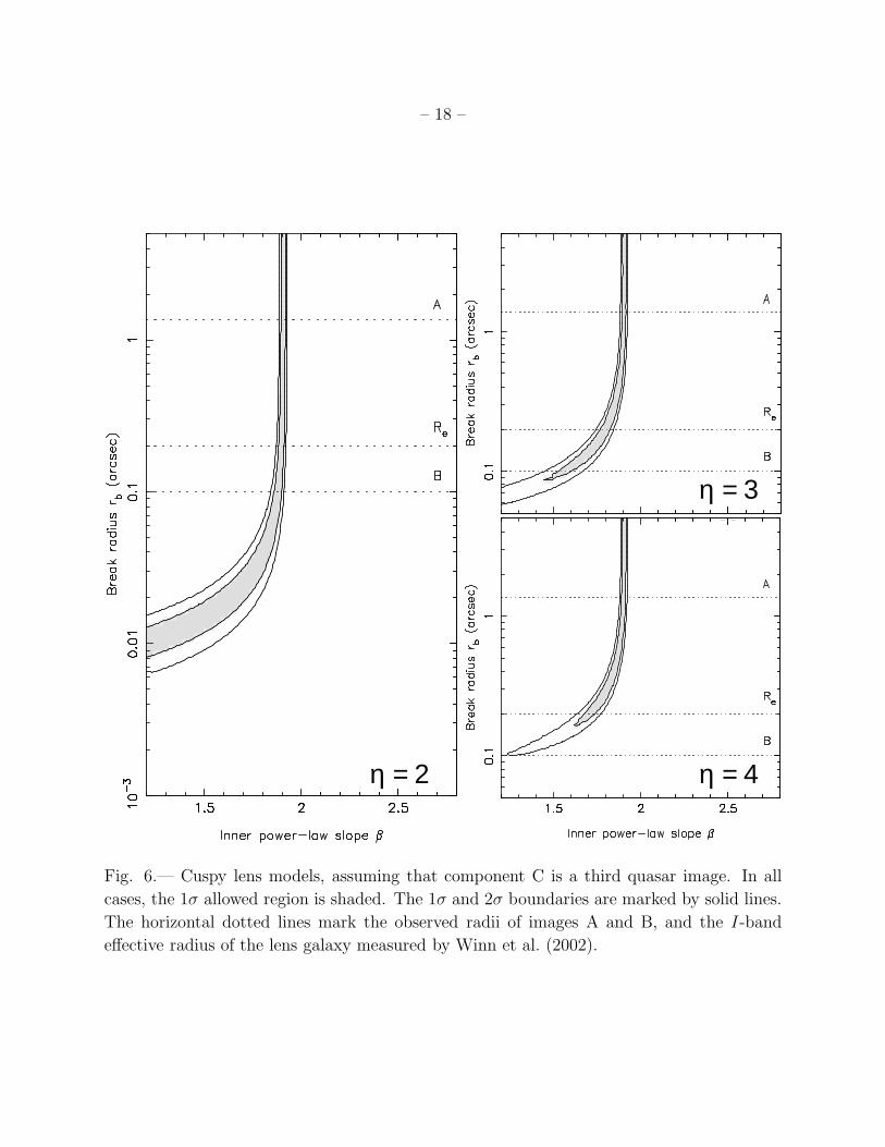
When we apply the cuspy lens model of Eq. 4, we find that the allowed region of cusp

parameters is much more tightly constrained than they are in the two-image lens models.

Figure 6 shows the results for models in which the radial density distribution at large radii

is isothermal (left panel), or obeys a power law with logarithmic slope η = 3 (upper right),

or η = 4 (lower right). Both boundaries of the allowed region (shaded) are enforced by the

constraint on the third-image flux. In particular, for β > 2, no third image is produced.

For large rb, the cusp must conform to the value β = 1.91 derived above. As rb becomes

smaller, the inner mass distribution must become shallower to compensate for the steeper

mass distribution at large radii.

5. Discussion and summary of conclusions

For the purpose of finding central odd images, the best systems are radio-loud two-image

quasars with a large magnification ratio between the two bright images. Radio loudness is

important because the radio components can be observed through the lens galaxy, whereas

optical components are likely to be hidden by the lens galaxy. Free-free absorption is poten-

tially significant but can be overcome by observing at high frequencies. Two-image systems

are better than four-image systems, as emphasized recently by Keeton (2002). This is be-

cause the projected source position in four-image systems is usually closer to the lens center,

where the central image magnification is smallest. In addition, four-image systems are sub-

ject to a larger magnification bias than two-image systems (Wallington & Narayan 1993;

King & Browne 1996; Keeton, Kochanek, & Seljak 1997; Rusin & Tegmark 2001; Finch et

– 18 –

η = 3

η = 4η = 2

Fig. 6.— Cuspy lens models, assuming that component C is a third quasar image. In all

cases, the 1σ allowed region is shaded. The 1σ and 2σ boundaries are marked by solid lines.

The horizontal dotted lines mark the observed radii of images A and B, and the I-band

effective radius of the lens galaxy measured by Winn et al. (2002).

– 19 –

al. 2002), leading to a smaller intrinsic source flux and a fainter odd image. Among two-image

systems, the asymmetric doubles are favorable because the source position is close to the

radial caustic, producing the brightest possible central image for a given mass distribution.

The subject of this paper, PMN J1632–0033, is exactly this type of system: an asym-

metric two-image radio lens. For this reason, it seemed reasonable that the third component

found by Winn et al. (2002) could be an example of the elusive and long-sought central odd

images. However, we have shown that the third component has a spectral index that differs

by 3σ from those of the two bright quasar images.

We have argued that the two most plausible interpretations are that the central com-

ponent is emission from the lens galaxy, or else that it is a third image with the extra

complication that its spectral index has been modified by free-free absorption. The data are

quantitatively consistent with either scenario. Lens galaxies are rarely radio-loud, but the

flux density of the component is consistent with typical radio powers of active galactic nuclei.

No central image has ever been securely identified for a radio lens, nor has free-free absorp-

tion by a lens galaxy ever been reported (with one possible exception, class B0128+437;

I. Browne 2002, private communication), but one might expect the two phenomena to be

related due to the hot and dense conditions near galaxy centers.

Given the new VLBI data, we have investigated models for the mass distribution of the

lens galaxy under various assumptions. Whether or not component C is a third image, we

showed that if the mass distribution obeys a power law ρ ∝ r−β, then it must be nearly

isothermal. If C is the lens galaxy then 1.95 < β < 2.28. If C is a third image then the

profile is tightly constrained to be only slightly shallower: 1.89 < β < 1.93. We also derived

limits on a constant-density core radius, or on the break radius and inner exponent of a

central cusp.

These results can be added to the growing collection of evidence that early-type galaxies

have nearly isothermal mass profiles. In the few other gravitational lens systems where it is

possible to measure the radial density profile, the results favor isothermal profiles (Kochanek

1995; Cohn et al. 2001; Munoz, Kochanek, & Keeton 2001; Rusin et al. 2002; Koopmans

& Treu 2002), although there are some possible counter-examples (Treu & Koopmans 2002;

Chen, Kochanek, & Hewitt 1995). Moreover, the findings are consistent with studies of

early-type galaxies based on stellar dynamics (see, e.g., Gerhard et al. 2001; Rix et al. 1997)

and X-ray halos (see, e.g., Fabbiano et al. 1989).

To further elucidate the nature of the central component and the central density profile

of the lens galaxy, it would help to have a better optical image of the lens galaxy. The

current HST image provides only a weak detection of the lens galaxy. A better image could

– 20 –

be used to test more precisely whether radio component C is coincident with the center of

the lens galaxy, and to study its surface brightness profile in detail. For example, with a

better measurement of the galaxy light profile, one might be able to explore the balance

between the luminous and dark matter in this system.

Even more helpful would be sensitive observations at high radio frequencies ( >∼ 30 GHz).

As shown in Fig. 4, the power-law and the free-free absorption fits diverge significantly at

high frequencies, where free-free absorption becomes negligible. For free-free absorption,

the ratio SC(ν)/SA(ν) must converge to a constant value. For lens galaxy emission, the

spectrum need not follow a power law at the high frequencies, but it would require an

unlikely coincidence for the intrinsic radio spectrum of the lens galaxy to turn over at high

frequencies and become identical to the radio spectra of A and B. Observations at low radio

frequencies ( <∼ 1 GHz) could also distinguish the hypotheses, in principle, but it would be

harder to achieve the necessary angular resolution and signal-to-noise ratio. High frequency

observations present their own challenges, including high noise levels and susceptibility to

poor atmospheric conditions, but the reward would be a definitive discovery of one of the

long-sought but never-seen central images of a gravitational lens.

We thank the anonymous referee for constructive criticism. We also thank I. Browne and

L. Koopmans for interesting discussions about radio propagation effects. J.N.W. is supported

by an Astronomy & Astrophysics Postdoctoral Fellowship, under NSF grant AST-0104347.

C.S.K. is supported by NASA ATP grant NAG5-9265.

REFERENCES

Altenhoff, W., et al. 1960, Veroff. Stenwarte, Bonn, No 59, 48

Binney, J.J. & Evans, N.W. 2001, MNRAS, 327, L27

Bode, P., Ostriker, J.P., & Turok, N. 2001, ApJ, 556, 93

Burke, W.L. 1981, ApJ, 244, L1

Chen, G.H. & Hewitt, J.N. 1993, AJ, 106, 1719

Chen, G.H., Kochanek, C.S., & Hewitt, J.N. 1995, ApJ, 447, 62

Cohn, J.D., et al. 2001, ApJ, 554, 1216

Dalal, N. & Kochanek, C.S. 2002, ApJ, 572, 25

– 21 –

de Blok, W.J.G., et al. 2001, 552, L23

Debattista, V.P. & Sellwood, J.A. 2000, ApJ, 543, 704

Dyer, C.C. & Roeder, R.C. 1980, ApJ, 238, L67

Evans, N.W. & Hunter, C. 2002, ApJ, 575, 68

Fabbiano, G. 1989, ARA&A, 27, 87

Faber, S., et al. 1997, AJ, 114, 1771

Falco, E.E., et al. 1999, ApJ, 523, 617

Fassnacht, C.D., et al. 1999, AJ, 117, 658

Finch, T., Carlivati, L., Winn, J.N., & Schechter, P.L. 2002, ApJ, 577, 51

Gerhard, O., et al. 2001, AJ, 121, 1936

Harvanek, M., et al. 1997, AJ, 114, 2240

Hernquist, L. 1990, ApJ, 356, 359

Jones, D.L., et al. 1996, ApJ, 470, 23

Jones, D.L., et al. 2001, ApJ, 553, 968

Kameno, S., et al. 2000, PASJ, 52, 209

Keeton, C.R. 2002, preprint (astro-ph/0206243)

Keeton, C.R., Kochanek, C.S., & Seljak, U. 1997, ApJ, 482, 604

King, L. & Browne, I.W.A. 1996, MNRAS, 282, 67

Kochanek, C.S. 1995, ApJ, 445, 559

Kochanek, C.S., et al. 2000, ApJ, 543, 131

Koopmans, L.V.E. & Treu, T. 2002, preprint (astro-ph/0205281)

Lauer, T., et al. 1995, ApJ, 292, 104

Levinson, A., Laor, A., & Vermuelen, R.C. 1995, ApJ, 448, 589

Lewis, G., et al. 2002, MNRAS, 330, L15

– 22 –

Lewis, G., et al. 2002, MNRAS, 334, L7

Marr, J.M., Taylor, G.B., & Crawford, F., III 2001, ApJ, 550, 160

Metcalf, R.B. & Madau, P. 2001, ApJ, 563, 9

Mezger, P.G. & Henderson, A.P. 1967, ApJ, 147, 471

Moore, B. 1999, MNRAS, 310, 1147

Motta, V., et al. 2002, ApJ, 574, 719

Munoz, J.A., Kochanek, C.S., & Keeton, C.R. 2001, ApJ, 558, 657

Narasimha, D., Subramanian, K., & Chitre, S. 1986, Nature, 321, 45

Navarro, J.F., Frenk, C.S., & White, S.D.M. 1997, ApJ, 490, 493

Patnaik, A.R., et al. 1993, MNRAS, 261, 435

Patnaik, A.R. & Porcas, R.W. 1999, in ASP Conf. Series 156, Highly Redshifted Radio Lines,

ed. C.L. Carilli, S.J.E. Radford, K.M. Menten, & G.I. Langston (San Francisco: ASP),

247

Rix, H.-W., et al. 1997, ApJ, 488, 702

Rusin, D. & Ma, C.-P. 2001, ApJ, 549, L33

Rusin, D. & Tegmark, M. 2001, ApJ, 553, 709

Rusin, D., et al. 2002, MNRAS, 330, 205

Sadler, E.M., et al. 2002, MNRAS, 329, 227

Salucci, P. & Burkert, A. 2000, ApJ, 537, L9

Shepherd, M.C., Pearson, T.J. & Taylor, G.B. 1994, BAAS, 27, 903

Spergel, D. & Steinhardt, P. 2000, Phys. Rev. Lett., 84, 3760

Taylor, G.B. 1996, ApJ, 470, 394

Treu, T. & Koopmans, L.V.E. 2002, MNRAS, in press [astro-ph/0210002]

van den Bosch, F.C. & Swaters, R.A. 2001, MNRAS, 325, 1017

Wallington, S. & Narayan, R. 1993, ApJ, 403, 517

– 23 –

Weinberg, M.D. & Katz, N. 2002, ApJ, 580, 672

Winn, J.N., et al. 2002, AJ, 123, 10

This preprint was prepared with the AAS LATEX macros v5.0.

– 24 –

Table 2. Constraints on lens models in which C is the lens galaxy

Parameter Value

R.A.(B) – R.A.(A) +1241.90 ± 0.07 mas

Decl.(B) – Decl.(A) −784.00 ± 0.16 mas

R.A.(Gal) – R.A.(A) +1160.61 ± 0.07 mas

Decl.(Gal) – Decl.(A) −726.10 ± 0.16 mas

µBA ≡ µB/µA 0.076 ± 0.008

µ3/µA < 0.00093

φA ≡ P.A. of A-jet 8 ± 15

φB ≡ P.A. of B-jet −69 ± 15

Table 3. Constraints on lens models in which C is a third image

Parameter Value

R.A.(B) – R.A.(A) +1241.90 ± 0.07 mas

Decl.(B) – Decl.(A) −784.00 ± 0.16 mas

R.A.(C) – R.A.(A) +1160.61 ± 0.07 mas

Decl.(C) – Decl.(A) −726.10 ± 0.16 mas

R.A.(Gal) – R.A.(A) +1162 ± 23 mas

Decl.(Gal) – Decl.(A) −738 ± 23 mas

µBA ≡ µB/µA 0.076 ± 0.008

µCA ≡ µC/µA 0.0045 ± 0.0009

φA ≡ P.A. of A-jet 8 ± 15

φB ≡ P.A. of B-jet −69 ± 15