1

Inverse determination of heterotrophic soil respiration response to temperature and

water content under field conditions

J. Bauer1,2*, L. Weihermüller1, J. A. Huisman1, M. Herbst1, A. Graf1, J. M. Séquaris1, H.

Vereecken1

1: Agrosphere Institute, ICG-4, Forschungszentrum Jülich GmbH, Leo Brandt Straße,

52425 Jülich, Germany

2: LOEWE Biodiversity and Climate Research Centre, Frankfurt am Main, Germany

PostPrint for self-archiving. Publication available from:

Bauer, J., L. Weihermüller, J.A. Huisman, M. Herbst, A. Graf, J.M. Sequaris and H.

Vereecken. 2012. Inverse determination of heterotrophic soil respiration response to

temperature and water content under field conditions. Biogeochemistry, 108, 119-134.

2

* Corresponding author: Bauer@iau.uni-frankfurt.de, Tel: +49-(0)69-798-40234, Fax: +49-

(0)69-798-40262

3

Abstract 1

Heterotrophic soil respiration is an important flux within the global carbon cycle. Exact 2

knowledge of the response functions for soil temperature and soil water content is crucial for 3

a reliable prediction of soil carbon turnover. The classical statistical approach for the in situ 4

determination of the temperature response (Q10 or activation energy) of field soil respiration 5

has been criticised for neglecting confounding factors, such as spatial and temporal changes in 6

soil water content and soil organic matter. The aim of this paper is to evaluate an alternative 7

method to estimate the temperature and soil water content response of heterotrophic soil 8

respiration. The new method relies on inverse parameter estimation using a 1-dimensional 9

CO2 transport and carbon turnover model. Inversion results showed that different 10

formulations of the temperature response function resulted in estimated response factors that 11

hardly deviated over the entire range of soil water content and for temperature below 25°C. 12

For higher temperatures, the temperature response was highly uncertain due to the infrequent 13

occurrence of soil temperatures above 25°C. The temperature sensitivity obtained using 14

inverse modelling was within the range of temperature sensitivities estimated from statistical 15

processing of the data. It was concluded that inverse parameter estimation is a promising tool 16

for the determination of the temperature and soil water content response of soil respiration. 17

Future synthetic model studies should investigate to what extent the inverse modelling 18

approach can disentangle confounding factors that typically affect statistical estimates of the 19

sensitivity of soil respiration to temperature and soil water content. 20

21

Keywords: heterotrophic soil respiration; temperature sensitivity; soil water content 22

sensitivity; inverse parameter estimation; SOILCO2/RothC; SCE algorithm, AIC 23

24

25

26

4

1. Introduction 27

Soil respiration is an important flux of CO2 to the atmosphere (Schlesinger & Andrews 2000). 28

Against the background of global climate change, reliable model predictions of soil 29

respiration are highly relevant. Among other factors, accurate knowledge of the response of 30

soil carbon decomposition to changes in soil temperature and water content is essential for 31

reliable predictions (Davidson & Janssens 2006). 32

33

Both laboratory and field experiments have been used to determine the response of 34

heterotrophic soil respiration to changes in soil temperature. Laboratory studies are 35

considered to provide more reliable estimates of temperature responses than field experiments 36

(Kirschbaum 2000, 2006). However, laboratory incubation experiments are typically 37

performed under highly artificial conditions. For example, the natural soil structure is 38

commonly destroyed by sieving and homogenisation. Therefore, the transferability of 39

response equations determined in the laboratory to the field is questionable. 40

41

The direct estimation of the response of heterotrophic soil respiration to temperature from in 42

situ measurements is complicated and often biased by confounding factors. One important 43

confounding factor is the soil water content. High temperatures are often accompanied by low 44

water contents and vice versa (e.g. Davidson et al. 1998). Such a strong interdependency 45

makes it difficult to separate the effects of temperature and soil water content on soil 46

respiration. Furthermore, changes in soil organic matter (SOM) quantity and quality during 47

the course of a field experiment (e.g. fresh litter input, depletion of labile compounds) could 48

strongly influence the direct estimation of response functions (Larionova et al. 2007; Leifeld 49

& Fuhrer 2005; Mahecha et al. 2010). A third confounding factor is that soil respiration 50

originates from two processes: i) the decomposition of soil organic matter (heterotrophic 51

respiration) and ii) root respiration. Both processes probably do not have the same response 52

5

towards changes in temperature (Boone et al. 1998; Lee et al. 2003). In this study, we 53

therefore only consider heterotrophic respiration originating from a managed bare soil. 54

55

Many field studies used a classical regression method to determine the temperature sensitivity 56

of soil respiration. This method does not account for the confounding factors discussed above. 57

Another uncertainty of this method is related to the choice of measurement depth/volume to 58

relate soil temperature and soil respiration. For example, the attenuation and phase shift of the 59

soil temperature amplitude vary with soil depth (Bahn et al. 2008; Pavelka et al. 2007; 60

Reichstein & Beer 2008), which means that different temperature responses will be found for 61

different temperature measurement depths (e.g. Graf et al. 2008; Pavelka et al. 2007; Xu & Qi 62

2001). 63

64

Recently inverse modelling using process-based models has been increasingly used for a more 65

reliable quantification of the response of soil respiration to environmental variables (e.g. 66

Carvalhais et al. 2008; Scharnagl et al. 2010). For example, Weihermüller et al. (2009) 67

presented a laboratory experiment to determine the soil water content response function of 68

soil respiration using inverse modelling. An inverse modelling approach has also been used to 69

determine global scale temperature and soil water content sensitivity of soil respiration by 70

analysis of observed soil organic carbon contents with a mechanistic decomposition model 71

(Ise & Moorcroft 2006). Zhou et al. (2009) inversely estimated the global spatial pattern of 72

temperature sensitivity (Q10 values) from measured soil organic carbon content. A 73

comprehensive overview of parameter estimation within the field of terrestrial carbon flux 74

studies was provided by Wang et al. (2009). The performance of different parameter 75

estimation methods was compared by Fox et al. (2009) and Trudinger et al. (2007). 76

77

6

The aim of this paper is to evaluate a new method to simultaneously estimate the response of 78

soil respiration to changes in temperature and soil water content from field soil respiration 79

measurements. The new method is based on inverse modelling using a detailed CO2 80

production and transport model explicitly accounting for soil temperature and water content 81

variations. The data set used for inverse modelling consisted of measurements of soil 82

respiration, soil temperature, and soil water content at a high temporal resolution and for a 83

comparably long period. The SOILCO2/RothC-model (Herbst et al. 2008) was used for the 84

simulation of water flux, heat flux, CO2 transport, and CO2 production. To investigate whether 85

the choice of functional relationship between temperature and soil respiration affected the 86

inverse modelling results, we tested four common functional approaches in combination with 87

a single soil water content response function. 88

89

2. Materials and Methods 90

2.1 Model description 91

We used the 1-dimensional numerical model SOILCO2/RothC to predict soil water content, 92

soil temperature, CO2 production, and CO2 transport. In the following we provide a brief 93

model description. For detailed information, we refer to Šimůnek and Suarez (1993) and 94

Herbst et al. (2008). 95

96

The water flow is described by the Richards equation: 97

98

Qz

hhK

zt

1

(1)

99

where is the volumetric water content [cm3 cm-3], t is time [h], z is the depth [cm], K is the 100

unsaturated hydraulic conductivity [cm h-1], h is the pressure head [cm], and Q is a 101

7

source/sink term [cm3 cm-3 h-1]. The soil water retention (h) and hydraulic conductivity K(h) 102

functions are described by the Mualem-van Genuchten approach (van Genuchten 1980): 103

104

mn

rsr

hh

1 (2a)

K h KsSe0.5 1 1 Se

1 m m

2

(2b)

with rs

reS

nm 11 1n (2c)

105

where r and s are the residual and saturated water content [cm3 cm-3], is the inverse of the 106

bubbling pressure [cm-1], Ks is the saturated hydraulic conductivity [cm h-1], and m and n are 107

shape parameters [-]. 108

109

The transport of heat is calculated according to Sophocleous (1979) by: 110

111

z

TJC

z

T

zt

TC w

w

(3)

112

where T is the soil temperature [°C], is the thermal conductivity of the soil [kg cm h-3 °C-1], 113

C and Cw are the volumetric heat capacities [kg h-2 cm-1 °C-1] of the porous medium and the 114

liquid phase, and Jw is the water flux density [cm h-1]. It should be noted that water and heat 115

transport are coupled through the dependence of the thermal conductivity on water content 116

and the convective transport of heat with the water flux Jw. 117

118

After the solution of the water and heat transport equations, the transport equation for carbon 119

dioxide is solved considering the CO2 flux caused by diffusion in the gas phase (Jda) [cm h-1], 120

8

the CO2 flux caused by dispersion in the dissolved phase (Jdw) [cm h-1], the CO2 flux caused 121

by convection in the gas phase (Jca) [cm h-1], and the CO2 flux caused by convection in the 122

dissolved phase (Jcw) [cm h-1]: 123

124

SQcJJJJzt

cwcwcadwda

T

(4)

125

where cT is the total volumetric concentration of CO2 [cm3 cm-3], S is the CO2 production/sink 126

term [cm3 cm-3 h-1], cw is the CO2 concentration in the liquid phase [cm3 cm-3], and Q is the 127

root water uptake [cm3 cm-3 h-1]. 128

129

Soil organic matter decomposition (i.e. heterotrophic respiration) is described by the RothC 130

pool concept as sketched in Fig. 1 (Coleman & Jenkinson 2005; Jenkinson 1990). In this 131

concept, fresh plant input entering the soil consists of decomposable plant material (DPM) 132

and resistant plant material (RPM). The proportion of DPM and RPM depends on the plant 133

material, i.e. for agricultural crops and improved grassland the DPM/RPM ratio is 1.44 134

according to Jenkinson (1990). Both pools undergo decomposition, and part of the 135

decomposed carbon fraction is released from the soil as CO2. The remaining fraction of 136

decomposed carbon is used to form microbial biomass (BIO) and humified organic matter 137

(HUM). Both the BIO and HUM pool are decomposed to form further BIO, HUM, and CO2. 138

The proportion of CO2/(BIO+HUM) is a function of the clay content of the soil. Besides these 139

four active pools, one part of SOM is considered to be inert (IOM). Decomposition of the 140

active carbon pools is described by first order kinetics: 141

142

Cp,i

t p,i,o fT fWCp ,i (5)

143

9

where Cp,i is the ith pool concentration [kg C cm-3], andp,i,0 is the decomposition constant of 144

the ith pool, which are 10, 0.3, 0.66, and 0.02 y-1 for the DPM, RPM, BIO, and HUM pool, 145

respectively. The decomposition constants are valid for optimal conditions of soil water, 146

aeration, and a reference temperature fT and fW are response functions [-] for soil temperature 147

and soil water content, respectively. 148

149

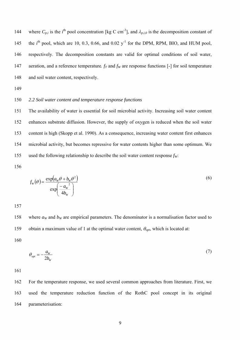
2.2 Soil water content and temperature response functions 150

The availability of water is essential for soil microbial activity. Increasing soil water content 151

enhances substrate diffusion. However, the supply of oxygen is reduced when the soil water 152

content is high (Skopp et al. 1990). As a consequence, increasing water content first enhances 153

microbial activity, but becomes repressive for water contents higher than some optimum. We 154

used the following relationship to describe the soil water content response fW: 155

156

W

W

WWW

b

a

baf

4exp

exp2

2 (6)

157

where aW and bW are empirical parameters. The denominator is a normalisation factor used to 158

obtain a maximum value of 1 at the optimal water content, opt, which is located at: 159

160

W

Wopt b

a

2

(7)

161

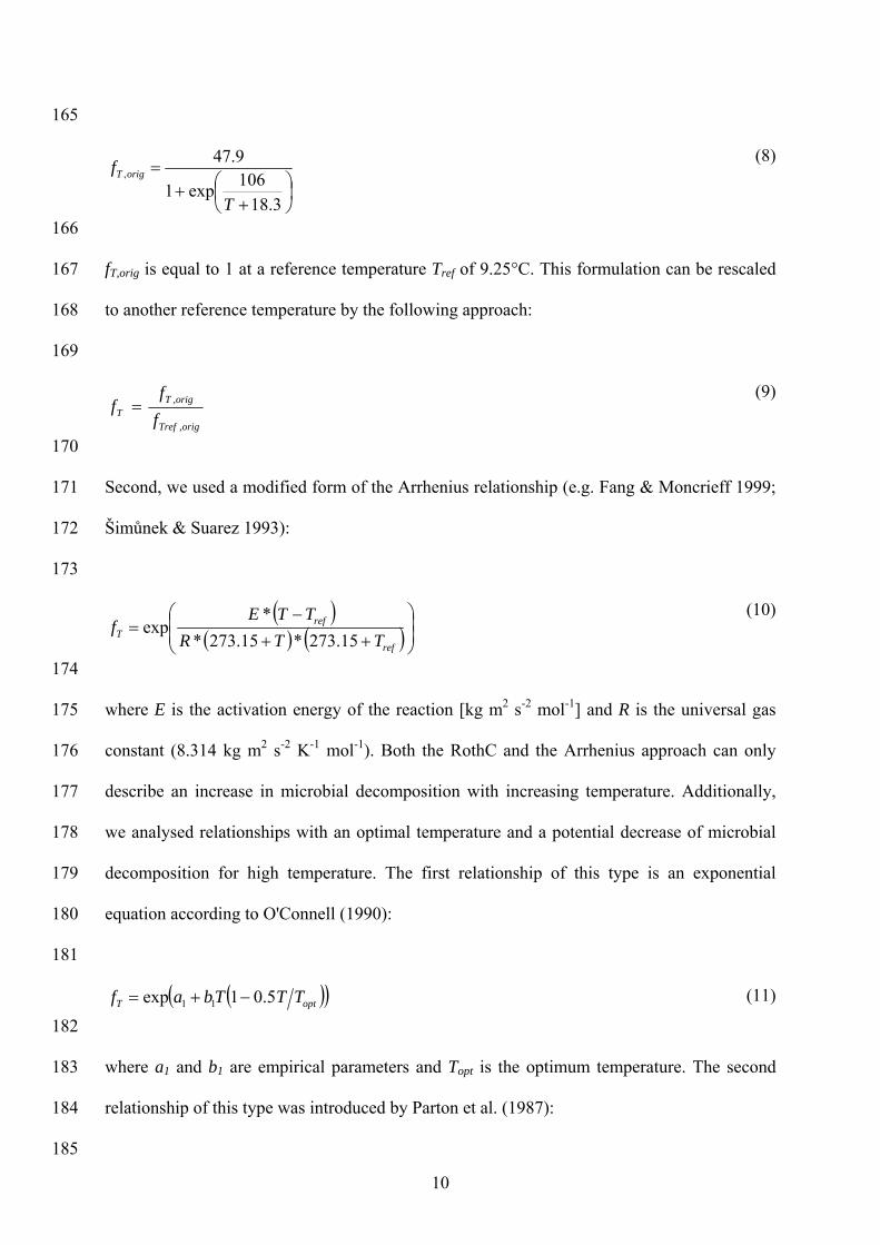
For the temperature response, we used several common approaches from literature. First, we 162

used the temperature reduction function of the RothC pool concept in its original 163

parameterisation: 164

10

165

3.18

106exp1

9.47,

T

f origT (8)

166

fT,orig is equal to 1 at a reference temperature Tref of 9.25°C. This formulation can be rescaled 167

to another reference temperature by the following approach: 168

169

orig,Tref

orig,TT f

ff

(9)

170

Second, we used a modified form of the Arrhenius relationship (e.g. Fang & Moncrieff 1999; 171

Šimůnek & Suarez 1993): 172

173

ref

refT TTR

TTEf

15.273*15.273*

*exp

(10)

174

where E is the activation energy of the reaction [kg m2 s-2 mol-1] and R is the universal gas 175

constant (8.314 kg m2 s-2 K-1 mol-1). Both the RothC and the Arrhenius approach can only 176

describe an increase in microbial decomposition with increasing temperature. Additionally, 177

we analysed relationships with an optimal temperature and a potential decrease of microbial 178

decomposition for high temperature. The first relationship of this type is an exponential 179

equation according to O'Connell (1990): 180

181

optT TTTbaf 5.01exp 11 (11)

182

where a1 and b1 are empirical parameters and Topt is the optimum temperature. The second 183

relationship of this type was introduced by Parton et al. (1987): 184

185

11

22222

edT cTTbaf (12)

186

where a2, b2, c2, d2, and e2 are empirical parameters. Negative values for these temperature 187

response functions were set to 0. 188

189

2.3 Determination of the activation energy from linear regression analysis 190

Conventionally, the activation energy of soil respiration is derived from a linear regression 191

analysis based on the Arrhenius formulation (Johnson & Thornley 1985) according to: 192

193

15.273

expTR

E (13)

194

where [h-1] is a constant. This formulation can be linearised using a log-transform: 195

196

15.273loglog

TR

Eee (14)

197

The activation energy can then be calculated from the slope p1 according to: 198

199

RpE 1 (15)

200

2.4. Field measurements 201

All measurements were made at the FLOWatch test site, which is located in the river Rur 202

catchment (North Rhine-Westphalia, Germany). The soil was classified as Parabraunerde 203

according to World Reference Base for Soil Resources classification (IUSS Working Group 204

WRB, 2006) and consists of three horizons ranging from 0 to 33 cm (Ap), 33 to 57 cm (Al-205

Bv), and 57 to 130+ cm (II-Btv). The soil texture is a silt loam. A detailed description of the 206

12

test site is given by Weihermüller et al. (2007). Our investigation covered the time period 207

from October 2006 until October 2007. CO2 flux measurements were only available until 208

September 2007. During this period, weeds were continuously removed manually and/or by 209

herbicide (glyphosate) application. 210

211

Soil temperature was measured at 0.5, 3, 5, and 10 cm depth by type T thermocouples and at 212

15, 30, 45, 60, 90, and 120 cm depth by pF-meters (Ecotech, Bonn, Germany). Soil water 213

content was measured at 15, 30, 45, 60, 90, and 120 cm depth from April to October 2007 by 214

custom made 3 rod TDR probes with a rod length of 20 cm. All TDR probes were connected 215

to a Campbell multiplexing and data logging system (Campbell Scientific, Logan, UT, USA). 216

The raw waveforms were stored and analysed semi-automatically using the Matlab routine 217

TDRAna developed in the Forschungszentrum Jülich GmbH, which follows the principles 218

suggested by Heimovaara & Bouten (1990). Matric potentials were recorded at 120 cm by pF-219

meters (Ecotech, Bonn, Germany). Climatic data were obtained from the meteorological 220

tower of the Research Centre Jülich GmbH (5.4 km NW from the test site). 221

222

CO2 fluxes were measured by automated soil CO2 flux chambers (Li-8100, Li-Cor Inc., 223

Lincoln, NE, USA) operated with the Li8100 multiplexer system. From October 2006 to April 224

2007, CO2 fluxes were measured twice an hour using a single chamber. In April 2007, we 225

installed a three chamber multiplexer system that measured 4 times per hour. All chambers 226

were placed on a soil collar with a diameter of 20 cm and a height of 7 cm, of which 5 cm 227

were belowground. Each chamber was closed for two minutes and the rise in CO2 228

concentration was measured with an infrared gas analyser. To estimate the CO2 flux, a linear 229

regression was fitted to the measured CO2 concentrations. Finally, hourly mean CO2 fluxes 230

and standard deviations were calculated. In order to remove outliers, we did not consider 231

fluxes with a standard deviation larger than 5 times the mean standard deviation. 232

13

233

In April 2007, the soil collars were temporarily removed and the entire field was power-234

harrowed. Because a large amount of weed was present at the field site surrounding the flux 235

measurement plot, this harrowing caused a significant biomass input at the location of the 236

collars, which were re-installed after harrowing. During summer 2007, a sporadic occurrence 237

of seedlings was observed at the plot. The removing of the weeds by hand ensured a minimal 238

contribution of autotrophic respiration to the measured CO2 flux. 239

240

To characterise the organic carbon within the Ap-horizon, disturbed samples were taken from 241

3 depths (0-10, 10-20, and 20-30 cm) in October 2006. Additionally, mixed soil samples from 242

3 locations were taken from deeper depths (30-40, 40-50, 50-60, 60-100 cm) in June 2007. 243

The organic carbon content of the soil samples was analysed using a Leco CHNS-932 244

analyser (St. Joseph, MI, USA). 245

246

2.5 Model parameterisation and initialisation 247

Since measured data were not available at the beginning of the simulation, the initial soil 248

water content profile was derived from measurements for a comparable period in 2007. An 249

atmospheric boundary condition was used to describe the upper boundary. The reference 250

potential evapotranspiration was estimated according to the FAO guidelines (Allen et al. 251

1998) from measured atmospheric temperature, precipitation, wind speed, atmospheric 252

pressure, relative humidity, and actual duration of sunshine. The potential evaporation of a 253

bare soil was calculated from the reference potential evapotranspiration by multiplication with 254

a factor of 1.15 (Allen et al. 1998). The lower boundary was described by measured matric 255

potentials. Figure 2 shows the precipitation and potential evaporation for the study period. 256

The total precipitation was 831 mm and the total potential evaporation was 757 mm. 257

258

14

The initial conditions and the upper and lower boundary conditions for heat transport were 259

derived from measured soil temperatures. Missing surface temperatures (Tsurf) were estimated 260

from atmospheric temperatures (Tatm) using a linear regression function 261

( 9057.01173.1 atmsurf TT ; R2 = 0.88). Missing temperatures in 120 cm soil depth were 262

estimated by linear interpolation. The parameters for the thermal conductivity of a loamy soil 263

were taken from Chung & Horton (1987), and are summarised in Table 1. 264

265

Initial CO2 concentrations within the soil profile were taken from a forward model run from a 266

comparable period in 2007. CO2 concentration at the soil surface was set to the atmospheric 267

concentration of 0.038%. The lower boundary was defined as a zero flux boundary. All 268

additional CO2 transport parameters are summarised in Table 1. 269

270

The initial carbon pool sizes were determined from measured soil carbon fractions. Therefore, 271

a physical fractionation procedure was used, which is based on wet sieving after chemical 272

dispersion and was proposed by Cambardella & Elliot (1992) and Skjemstad et al. (2004). An 273

amount of 10 g soil (<2 mm) was shaken overnight with 0.05 L of fresh Na-274

hexametaphosphate solution (5 g L−1). Afterwards, the dispersed soil was sieved sequentially 275

using a 200 µm (Retsch GmbH, Haan, Germany) and a 53 µm sieve (Fritsch GmbH, Idar-276

Oberstein, Germany) and rinsed thoroughly with water until the rinsate was clear. The 277

remaining material (200 – 2000 µm, 53 – 200 µm) was freeze-dried and weighed. The 0 – 53 278

µm soil fraction contains the mineral-associated and water-soluble carbon, while the 53 – 279

2000 µm soil fraction contains the particulate organic matter (POM). According to Skjemstad 280

et al. (2004) the RPM fraction CRPM of the SOILCO2/RothC model was set to the measured 281

POM fraction (53 – 2000 m). The size of the IOM pool was set to the MIR-measured black 282

carbon fraction (Bornemann et al. 2008). We assumed that the DPM fraction at the beginning 283

of the simulation was negligible. The fraction of HUM and BIO was calculated as the 284

15

remaining fraction (RF) from the total organic carbon 285

[ RF CHUM CBIO Corg CDPM CRPM CIOM ]. The proportion between BIO and HUM 286

was assumed to be 0.0272 according to Zimmermann et al. (2007). Since no information 287

about SOM composition for soil layers deeper than 30 cm was available at the beginning of 288

the simulation period, we used the SOM composition determined 8 months later and assumed 289

that SOM was not significantly altered in the deeper soil horizons. This assumption was later 290

confirmed by our simulations, which indicate that the mean carbon loss from the RPM pool 291

was only 4% in the 30 to 60 cm depth range for the entire study period. Carbon pool 292

concentrations were linearly interpolated between the measurement depths. 293

294

In Table 2 the measured concentration of SOM, POM (=RPM), and black carbon (=IOM) are 295

summarised. Furthermore, the calculated remaining fraction (RF=HUM+BIO) and 296

percentages of the several fractions are given. As expected, total SOM contents decreased 297

with depth. Both, concentration and percentage of the fast decomposing RPM pool and the 298

slow decomposing HUM pool decreased with depth. Contrarily, the proportion of the inert 299

IOM pool significantly increased with depth. The observed soil carbon distribution 300

characterised by decreasing concentrations and increasing recalcitrance in combination with 301

decreasing soil temperatures in the soil profile cause a strong decrease of CO2 production with 302

soil depth, as is typically observed in field studies (e.g. Köhler et al. 2010; Suarez & Simunek 303

1993). 304

305

Fresh weed material entered the upper 15 cm of the soil after soil harrowing in April 2007. 306

For different crop stands, crop rotations, and fertilization rates various authors proposed 307

annual carbon inputs via roots and crop residuals ranging from 1.5 to more than 3.8 t C ha-1 308

(Coleman & Jenkinson 1996; Coleman et al. 1997; Falloon et al. 1998; Jenkinson & Coleman 309

1994). In many of these cases, large proportions of the plant material were removed by 310

16

harvesting. Due to the way the test site was managed during this experiment (no removal of 311

aboveground weed biomass), rather large amounts of fresh plant material were incorporated 312

into the soil during harrowing. Therefore, we assumed a total input of 3 t C ha-1. 313

314

2.6 Inverse parameter estimation 315

To find the set of model parameters that best describe the measurements, the global 316

optimisation algorithm SCE-UA (shuffled complex evolution method developed at the 317

University of Arizona) was used (Duan et al. 1992; Duan et al. 1994). Optimisation methods 318

are tools to find the minimum of a cost function that expresses the distance between simulated 319

and measured data. Global search methods are more successful in finding the global minimum 320

of a cost function compared to gradient-based methods which can get trapped in local minima 321

(Wang et al. 2009). The SCE-UA algorithm searches the global optimum parameter 322

combination within a feasible parameter space defined by the user using a set of complexes 323

which initially are populated with points randomly distributed in the feasible parameter space. 324

Each complex is made to evolve in the direction of improvement (minimum of the cost 325

function) using the local-search simplex method (Nelder & Mead 1965). At periodic stages in 326

the evolution, the entire population of points is shuffled and points are reassigned to 327

complexes based on their performance to ensure information sharing. A detailed description 328

of the SCE-UA algorithm is provided by Duan et al. (1994). The SCE-UA algorithm has been 329

shown to be a powerful tool for calibration of hydrological models (Madsen et al. 2002) and 330

has been successfully applied in other application areas (e.g. Bauer et al. 2008; Peters & 331

Durner 2008). In this study, the cost function was defined by the sum of squared residuals 332

(SSR): 333

334

k

iisimiobs yySSR

1

2,, (16)

17

335

where yobs and ysim are the observed and simulated data, respectively, and k is the number of 336

data pairs available to compare observation and simulation. 337

338

For a reliable prediction of the water transport, the hydraulic parameters of four soil layers 339

were inversely estimated. To reduce the number of estimated parameters, we assumed that the 340

saturated and residual water contents were constant over the entire soil profile. This 341

assumption is in good agreement with laboratory results for the same location, where the 342

mean saturated water content is 0.39 cm3 cm-3 with a standard deviation of only 0.03 cm3 cm-343

3. In total, we estimated 14 hydraulic parameters (one s and r for the entire profile and , n, 344

and Ks for each layer). Additionally, we imposed a decrease of Ks with depth. We used 3899 345

water content measurements at 15, 30, 45, 60, and 90 cm, respectively and 2247 346

measurements at 120 cm depth in the inversion. In a second step, we inversely estimated the 347

parameters of the soil water content response equation (Eq. [6]) and the temperature response 348

equations (Eqs. [8-12]) from 6269 CO2 flux measurements. For both optimization runs, SCE-349

UA was stopped when the change of the objective function was less than 0.1% in 10 350

consecutive loops, as recommended by previous studies with this optimization algorithm 351

(Mertens et al. 2005). 352

353

2.7 Statistical criteria of model quality 354

Three criteria were used to judge the quality of the model simulations. First, we calculated the 355

coefficient of determination (R2): 356

357

18

2

1

2

,1

2

,

1,,

2

k

isimisim

k

iobsiobs

k

isimisimobsiobs

yyyy

yyyyR (17)

358

where obsy and simy are the arithmetic means of the observed and simulated data, 359

respectively. The model efficiency ME (Nash & Sutcliffe 1970) was used as a second 360

criterion: 361

362

k

iobsiobs

k

iisimiobs

yy

yyME

1

2

,

1

2,,

1 (18)

363

A model efficiency close to 1 indicates that observed and simulated data are closely related 364

and without systematic bias. In contrast, a model efficiency lower than 0 means that the mean 365

is a better predictor of the data than the applied model. In order to identify the best model 366

taking into account both goodness of fit and model complexity, Akaike’s information 367

criterion (AIC, Akaike 1974) was used: 368

369

mLAIC maxe 2log2 (19)

370

where logeLmax is the maximum log-likelihood function and m is the number of model 371

parameters. Assuming normally distributed errors, AIC can be written as: 372

373

19

12log

2

1,,

m

n

yynAIC

n

iisimiobs

e (20)

374

The lowest AIC value identifies the best model. 375

376

3. Results and Discussion 377

3.1. Simulation of soil water content and soil temperature 378

The measured soil water content could not be sufficiently described by the model with one set 379

of hydraulic parameters for the plough horizon Ap (upper 33 cm). Corresponding to the 380

findings of Abbaspour et al. (2000), the Ap horizon had to be divided into two separate layers 381

with different hydraulic properties to obtain an adequate reproduction of the measured soil 382

water content (Fig. 3). The Ap horizon was divided at a depth of 20 cm, which is the 383

maximum penetration depth of the power harrow. The hydraulic properties yielding the best 384

prediction of measured soil water content are summarised in Table 3. The resulting high n 385

value (n = 1.97) of the upper soil layer is not representative for a silt loam soil, which might 386

be due to the large coarse fraction (10 - 15 mass % > 2 mm). In addition, the soil structure of 387

this upper layer was changed due to tillage. However, the water flow of the upper soil layer 388

was predicted well and 87% of the variation in soil water content measured at 15 cm depth 389

was explained (Fig. 3). At 90 cm and 120 cm depth, model efficiency was negative indicating 390

that the mean soil water content at these depths is a better predictor than the model, which is 391

largely the result of the low dynamics in water content (Fig. 3). However, simulated water 392

content was within the uncertainty range of measured values. Furthermore, slight deviations 393

in soil water content of the lower soil layers do not have any significant influence on the 394

estimation of temperature and soil water content response parameters since released CO2 395

mainly originates from soil organic matter decomposition within the upper soil horizons. 396

20

397

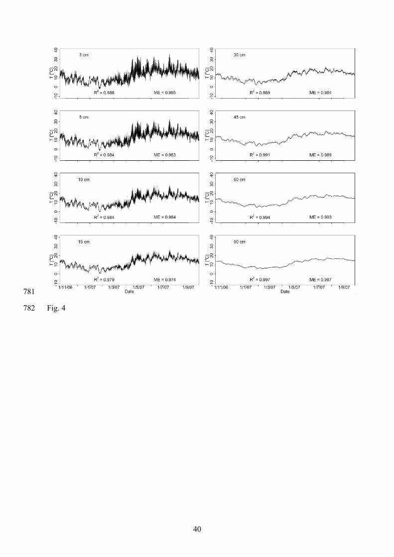
Measured soil temperature was generally predicted well by the model (Fig. 4). However, soil 398

temperature was overestimated by up to 3°C for the first soil layers from mid-November to 399

early January. This is a result of the fact that only few surface temperature measurements 400

were available during this period, and therefore, surface temperatures were estimated from 401

atmospheric temperatures. 402

403

3.2. Simulation of CO2 fluxes 404

To determine the temperature and soil water content response, which are most appropriate to 405

describe the measured CO2 fluxes, the parameters of all possible combinations of the soil 406

water content response function (Eq. 6) and the five different temperature response functions 407

(Eq. 8-12) were inversely estimated by minimizing the difference between measured and 408

modelled CO2 fluxes. For the different combinations of response functions between 2 and 7 409

parameters were estimated. The results are summarised in Table 4. Data and model were not 410

in agreement when the original parameterisation of the RothC temperature response equation 411

was used. Prediction of measured CO2 fluxes was significantly improved when the RothC 412

temperature response equation was scaled to another optimised reference temperature (Sum of 413

Squared Residuals, SSR, decreased from 812 to 632 (kg C ha-1 h-1)2). The data were best 414

described by the approach of Parton et al. (1987) with a SSR value of 538 (kg C ha-1 h-1)2. 415

However, the Arrhenius and O'Connell (1990) equations produced just slightly larger errors 416

(SSR of 542 and 547 (kg C ha-1 h-1)2, respectively). The Parton temperature response function 417

resulted in the smallest value of Akaike’s information criterion, which suggests that this 418

response function provides the best balance between goodness of fit and model complexity. 419

We therefore use this equation to analyze the difference between measured and predicted soil 420

respiration. 421

422

21

In Fig. 5, the measured and simulated CO2 flux is shown for the temperature response 423

equation according to Parton et al. (1987). Furthermore, the distribution of CO2 released 424

during decomposition, soil water content, and soil temperature in the upper soil horizon (0-33 425

cm) are illustrated. Contrary to the continuous distribution of soil temperature, a distinct 426

boundary is visible in 20 cm depth for soil water content due to the different hydraulic 427

properties of the soil layers (Tab. 3). This boundary is also visible in the CO2 distribution 428

since soil organic matter decomposition also depends on the soil water content. The modelled 429

vertical distributions of CO2 concentrations are quite similar to the concentration distributions 430

measured for bare soils under comparable conditions (Suarez & Simunek 1993; Yasuda et al. 431

2008). 432

433

In general, the course of measured CO2 fluxes was well described by the model. In January 434

2007, soil surface temperatures dropped below 0°C resulting in a depression of CO2 435

production. This freezing period was followed by a strong CO2 release up to 1.4 kg C ha-1 h-1. 436

A possible explanation for the observed CO2 flush is the death of microbial biomass due to 437

the low temperature and the subsequent decomposition of this new carbon source with 438

increasing soil temperatures and reactivated microbial activity (e.g. Matzner & Borken 2008). 439

Since the model can currently not describe this process, the measurements of this period were 440

not considered to avoid bias in the inverse parameter estimation procedure. The simulations 441

indicate that 90% of CO2 was produced within the upper soil horizon (0-33 cm) where CO2 442

production was notably high in the upper 15 cm of the soil profile in May and June 2007. In 443

the last half of April and the first half of May 2007, the soil surface layer was almost dry. The 444

low water content obviously hampered SOM decomposition since CO2 fluxes were 445

significantly lower than in the following period despite high temperatures and fresh carbon 446

input in April 2007 due to the harrowing. 447

448

22

High measured CO2 fluxes were systematically underestimated during the first half of June 449

2007. The higher uncertainty in the measured CO2 fluxes during this period expressed by the 450

high standard deviations of up to 1.5 kg C ha-1 cannot completely explain the observed 451

mismatch. Probably, additional CO2 was released by decomposed plant roots, which remained 452

in the soil after the manual weed removal (Herbst et al. 2008). The period of highest soil 453

temperatures in July 2007 was not accompanied by highest CO2 fluxes despite moderate soil 454

water contents. This can be explained by the decrease of the fresh litter input quantity and 455

quality during the course of decomposition, which is supported by the findings of Leifeld & 456

Fuhrer (2005) and Larionova et al. (2007). 457

458

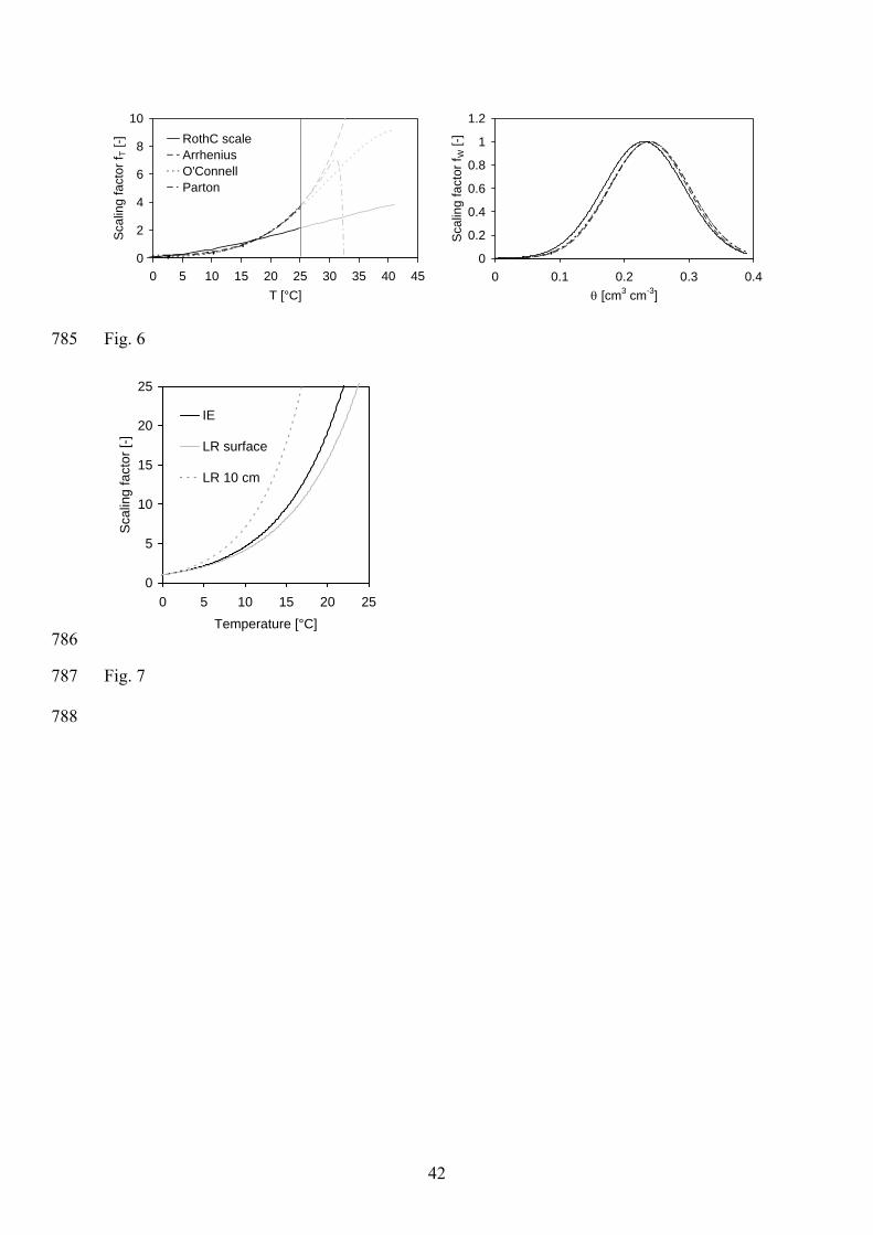
Figure 6 presents the four temperature response functions obtained using inverse modelling. 459

The RothC function clearly deviates from the other three functions. This can be explained by 460

the limited flexibility of the RothC function where only the reference temperature was 461

variable and the curvature was fixed. The other three functions are very similar for 462

temperatures below 25°C. As stated before, the Parton response function is the best approach 463

in regard to both, goodness of data prediction and complexity (number of model parameters) 464

(Tab. 4). For temperatures above 25°C, the three functions highly diverge. The reasons for the 465

uncertainty in the course of the temperature response function for high temperatures are 466

twofold. Temperatures above 25°C only occurred up to a maximum depth of 18 cm, and 467

temperature exceeded 25°C only 1.6 % of the time. It is important to stress here that the 468

scaled temperature functions can be only used in the range of soil temperature used for 469

calibration and to a point where the functions match each other (maximum temperature of 470

25°C). For higher soil temperatures that might occur due to climate change, these temperature 471

functions have to be treated carefully. 472

473

23

The optimized soil water content responses are also shown in Figure 6. The curvatures of the 474

soil water content response equations combined with the temperature response function of 475

Arrhenius, O'Connell (1990), and Parton et al. (1987) are very similar. The calculated optimal 476

water content was 0.24 cm3 cm-3, which corresponds to a water filled pore space of 62 %. 477

This value is in good agreement with many other studies that found optimal aerobic microbial 478

activity between 50 and 80% water filled pore space (e.g. Greaves & Carter 1920; Pal & 479

Broadbent 1975; Rixon & Bridge 1968; Rovira 1953; Seifert 1961; Weihermüller et al. 2009). 480

Overall, the good agreement between the temperature and soil water content response 481

equations despite different functional forms indicates that the inverse modelling approach is a 482

useful tool to obtain reliable estimates of the temperature and soil water content response. 483

484

Measured soil respiration was reasonably described by our optimised model setup. However, 485

there are still differences between simulated and measured soil respiration (Tab. 4). The 486

mismatch between measured and modelled soil respiration is on the one hand caused by 487

measurement errors, on the other hand it is affected by model errors such as missing processes 488

and errors in boundary conditions. Hence, a comprehensive uncertainty analysis is an 489

important future step towards a more complete model-data integration approach (e.g. Wang et 490

al. 2009; Williams et al. 2009). 491

492

Finally, it has to be noted that the inverse modelling analysis presented here leads to an 493

independent estimate of the temperature and water content response function only because 494

water content and temperature are not strongly correlated at our field site (maximum R² of 495

0.13 at the soil surface). Additionally, the response functions obtained by inverse modelling 496

should be treated carefully if they are transferred to other process-based turnover models 497

because any kind of model error is propagated into the estimation of the parameters of the 498

response functions. Both the influence of covariance of the driving variables (soil water 499

24

content and soil temperature) as well as the predictive uncertainty introduced by model errors 500

should be evaluated in future synthetic model studies. 501

502

3.3. Comparison to conventionally determined temperature responses 503

Typically, the temperature response of soil respiration in field studies is quantified by fitting a 504

regression between log-transformed CO2 fluxes and temperatures measured in a certain soil 505

depth (see section 2.3). This practice has been criticised because confounding factors such as 506

correlations with water (Davidson et al. 1998), or the effect of temperature measurement 507

depth (Graf et al. 2008) might strongly affect the temperature sensitivity thus obtained. It is 508

therefore insightful to compare the temperature sensitivity determined using inverse 509

modelling, which simultaneously attempts to consider temperature, water content, and 510

substrate availability effects, to the one that would have been obtained using a linear 511

regression that neglects confounding factors. For reasons of comparability between the two 512

different methods of data analysis, we used simulated instead of measured soil temperatures 513

in the linear regression. This is justified by the excellent model predictions for soil 514

temperature (Fig. 4). As shown before, temperature response derived from the traditional 515

regression analysis highly depends on the depth of the temperature measurement with 516

apparently stronger temperature responses with increasing depth (Bahn et al. 2008; Graf et al. 517

2008; Pavelka et al. 2007). For temperature measurements at the soil surface, the linear 518

regression analysis provided an activation energy of 92 kJ mol-1 and for temperature 519

measurement at 10 cm depth, a much higher value of 126 kJ mol-1 was obtained (Fig. 7). This 520

clearly illustrates the ambiguity of the classical regression method for estimating temperature 521

sensitivity. The inversely estimated activation energy was 98 kJ mol-1 (Tab. 4 and Fig. 7), 522

which is in between the activation energy for soil surface temperature and temperature at 10 523

cm depth, as expected. 524

525

25

4. Summary and conclusions 526

The temperature and soil water content response of soil heterotrophic respiration are crucial 527

for a reliable prediction of soil carbon dynamics. The direct determination of the temperature 528

and soil water content response from field measurements is complicated by the 529

interdependency of soil temperature and water, the quantitative and qualitative change of 530

SOM, and the contribution of root respiration to measured soil respiration. Apparent response 531

equations derived from relating measured CO2 fluxes and temperature or water indicators 532

(e.g. matric potential, water content, precipitation and evapotranspiration) may significantly 533

differ from the intrinsic response. For example, the activation energy of the Arrhenius 534

equation determined using the conventional regression method varied between 92 kJ mol-1 535

and 126 kJ mol-1 for the upper 10 cm of the soil profile. In this study, we determined the 536

temperature and water response of soil heterotrophic respiration by means of inverse 537

parameter estimation using the SOILCO2/RothC model. Due to the implementation of the 538

RothC multi-pool carbon concept into the physically based transport model SOILCO2, 539

temporal changes of temperature, water content, and the concentration and composition of 540

SOM can be described in detail for the entire soil profile. 541

542

The inverse parameter estimation approach considered four widely used temperature response 543

functions. The best prediction of measured CO2 fluxes was obtained by a soil water content 544

reduction function with an optimum at 62% water filled pore space and a temperature 545

response equation according to the formulation of Parton et al. (1987). However, the 546

commonly used Arrhenius equation provided similarly good results. The divergence of the 547

fitted temperature response functions for temperatures above 25°C indicates that the fitted 548

functions might not be reliable in this range. The excellent agreement between the 549

temperature response functions for temperatures below 25°C is encouraging. The activation 550

energy of the Arrhenius equation determined using inverse modelling, was within the range of 551

26

activation energies obtained from the conventional regression approach spanned over the soil 552

profile. It was concluded that inverse parameter estimation is a promising alternative tool for 553

the in situ determination of the temperature and soil water content response of soil respiration. 554

Future synthetic model studies should investigate to what extent the inverse modelling 555

approach can disentangle confounding factors that typically affect statistical estimates of the 556

sensitivity of soil respiration to temperature and soil water content. 557

558

Acknowledgements 559

This research was supported by the German Research Foundation DFG (Transregional 560

Collaborative Research Centre 32 - Patterns in Soil-Vegetation-Atmosphere systems: 561

monitoring, modelling and data assimilation) and by the Hessian initiative for the 562

development of scientific and economic excellence (LOEWE) at the Biodiversity and Climate 563

Research Centre (BiK-F), Frankfurt/Main. We thank Axel Knaps and Rainer Harms for 564

providing the climate data. The organic carbon content of the soil was analysed by the Central 565

Division of Analytical Chemistry at the Forschungszentrum Jülich GmbH. We would like to 566

thank Claudia Walraf and Stefan Masjoshustmann for the physical fractionation of the soil 567

samples and Ludger Bornemann (Institute of Crop Science and Resource Conservation - 568

Division of Soil Science, University of Bonn) for the analysis of black carbon. We are 569

grateful to Horst Hardelauf for modifications of the model source code. Furthermore, we 570

thank three anonymous reviewers for their helpful advices. 571

572

27

References 573

Abbaspour, K, Kasteel, R, et al. (2000). Inverse parameter estimation in a layered unsaturated 574

field soil. Soil Sci 165(2): 109-123. 575

Akaike, H (1974). New look at statistical-model identification. IEEE Trans Autom Control 576

AC19(6): 716-723. 577

Allen, RG, Pereira, LS, et al. (1998). Crop evapotranspiration - Guidelines for computing 578

crop water requirements - FAO Irrigation and drainage paper 56. Rome, FAO - Food and 579

Agriculture Organization of the United Nations. 580

Bahn, M, Rodeghiero, M, et al. (2008). Soil respiration in European grasslands in relation to 581

climate and assimilate supply. Ecosystems 11(8): 1352-1367. 582

Bauer, J, Herbst, M, et al. (2008). Sensitivity of simulated soil heterotrophic respiration to 583

temperature and moisture reduction functions. Geoderma 145(1-2): 17-27. 584

Boone, RD, Nadelhoffer, KJ, et al. (1998). Roots exert a strong influence on the temperature 585

sensitivity of soil respiration. Nature 396(6711): 570-572. 586

Bornemann, L, Welp, G, et al. (2008). Rapid assessment of black carbon in soil organic 587

matter using mid-infrared spectroscopy. Org Geochem 39(11): 1537-1544. 588

Cambardella, CA, Elliott, ET (1992). Particulate soil organic-matter changes across a 589

grassland cultivation sequence. Soil Sci. Soc. Am. J. 56(3): 777-783. 590

Carvalhais, N, Reichstein, M, et al. (2008). Implications of the carbon cycle steady state 591

assumption for biogeochemical modeling performance and inverse parameter retrieval. Glob 592

Biogeochem Cycle 22(2): 16. 593

28

Chung, SO, Horton, R (1987). Soil heat and water-flow with a partial surface mulch. Water 594

Resour Res 23(12): 2175-2186. 595

Coleman, K, Jenkinson, DS (1996). RothC-26.3 - A model for the turnover of carbon in soil. 596

Evaluation of soil organic matter models using existing long-term datasets. Powlson, DS, 597

Smith, P, Smith, JU. Heidelberg, Springer-Verlag. 38: 237-246. 598

Coleman, K, Jenkinson, DS (2005). ROTHC-26.3. A Model for the turnover of carbon in soil. 599

Model description and Windows users guide. Harpenden, IACR - Rothamsted. 600

Coleman, K, Jenkinson, DS, et al. (1997). Simulating trends in soil organic carbon in long-601

term experiments using RothC-26.3. Geoderma 81(1-2): 29-44. 602

Davidson, EA, Belk, E, et al. (1998). Soil water content and temperature as independent or 603

confounded factors controlling soil respiration in a temperate mixed hardwood forest. Glob 604

Change Biol 4(2): 217-227. 605

Davidson, EA, Janssens, IA (2006). Temperature sensitivity of soil carbon decomposition and 606

feedbacks to climate change. Nature 440(7081): 165-173. 607

Duan, QY, Sorooshian, S, et al. (1992). Effective and efficient global optimization for 608

conceptual rainfall-runoff models. Water Resour Res 28(4): 1015-1031. 609

Duan, QY, Sorooshian, S, et al. (1994). Optimal use of the SCE-UA global optimization 610

method for calibrating watershed models. J Hydrol 158(3-4): 265-284. 611

Falloon, P, Smith, P, et al. (1998). Estimating the size of the inert organic matter pool from 612

total soil organic carbon content for use in the Rothamsted carbon model. Soil Biol Biochem 613

30(8-9): 1207-1211. 614

29

Fang, C, Moncrieff, JB (1999). A model for soil CO2 production and transport 1: Model 615

development. Agric For Meteorol 95(4): 225-236. 616

Fox, A, Williams, M, et al. (2009). The REFLEX project: Comparing different algorithms and 617

implementations for the inversion of a terrestrial ecosystem model against eddy covariance 618

data. Agric For Meteorol 149(10): 1597-1615. 619

Graf, A, Weihermüller, L, et al. (2008). Measurement depth effects on the apparent 620

temperature sensitivity of soil respiration in field studies. Biogeosciences 5(4): 1175-1188. 621

Greaves, JE, Carter, EG (1920). Influence of moisture on the bacterial activities of the soil. 622

Soil Sci 10(5): 361-387. 623

Heimovaara, TJ, Bouten, W (1990). A computer-controlled 36-channel Time Domain 624

Reflectometry system for monitoring soil-water contents. Water Resour Res 26(10): 2311-625

2316. 626

Herbst, M, Hellebrand, HJ, et al. (2008). Multiyear heterotrophic soil respiration: Evaluation 627

of a coupled CO2 transport and carbon turnover model. Ecol Model 214(2-4): 271-283. 628

Ise, T, Moorcroft, PR (2006). The global-scale temperature and moisture dependencies of soil 629

organic carbon decomposition: an analysis using a mechanistic decomposition model. 630

Biogeochemistry 80(3): 217-231. 631

IUSS Working Group WRB (2006). World reference base for soil resources – A framework 632

for international classification, correlation and communication. World Soil Resources Reports 633

103. Rome, FAO - Food and Agriculture Organization of the United Nations. 634

Jenkinson, DS (1990). The turnover of organic-carbon and nitrogen in soil. Philos Trans R 635

Soc Lond Ser B-Biol Sci 329(1255): 361-368. 636

30

Jenkinson, DS, Coleman, K (1994). Calculating the annual input of organic-matter to soil 637

from measurements of total organic-carbon and radiocarbon. Eur J Soil Sci 45(2): 167-174. 638

Johnson, IR, Thornley, JHM (1985). Temperature-dependence of plant and crop processes. 639

Ann Bot 55(1): 1-24. 640

Kirschbaum, MUF (2000). Will changes in soil organic carbon act as a positive or negative 641

feedback on global warming? Biogeochemistry 48(1): 21-51. 642

Kirschbaum, MUF (2006). The temperature dependence of organic-matter decomposition - 643

still a topic of debate. Soil Biol Biochem 38(9): 2510-2518. 644

Köhler, B, Zehe, E, et al. (2010). An inverse analysis reveals limitations of the soil-CO2 645

profile method to calculate CO2 production and efflux for well-structured soils. 646

Biogeosciences 7(8): 2311-2325. 647

Larionova, AA, Yevdokimov, IV, et al. (2007). Temperature response of soil respiration is 648

dependent on concentration of readily decomposable C. Biogeosciences 4(6): 1073-1081. 649

Lee, MS, Nakane, K, et al. (2003). Seasonal changes in the contribution of root respiration to 650

total soil respiration in a cool-temperate deciduous forest. Plant Soil 255(1): 311-318. 651

Leifeld, J, Fuhrer, J (2005). The temperature response of CO2 production from bulk soils and 652

soil fractions is related to soil organic matter quality. Biogeochemistry 75(3): 433-453. 653

Madsen, H, Wilson, G, et al. (2002). Comparison of different automated strategies for 654

calibration of rainfall-runoff models. J Hydrol 261(1-4): 48-59. 655

Mahecha, MD, Reichstein, M, et al. (2010). Global Convergence in the Temperature 656

Sensitivity of Respiration at Ecosystem Level. Science 329(5993): 838-840. 657

31

Matzner, E, Borken, W (2008). Do freeze-thaw events enhance C and N losses from soils of 658

different ecosystems? A review. Eur J Soil Sci 59(2): 274-284. 659

Mertens, J, Madsen, H, et al. (2005). Sensitivity of soil parameters in unsaturated zone 660

modelling and the relation between effective, laboratory and in situ estimates. Hydrol. 661

Process. 19(8): 1611-1633. 662

Nash, JE, Sutcliffe, JV (1970). River flow forecasting through conceptual models part I - A 663

discussion of principles. J Hydrol 10(3): 282-290. 664

Nelder, JA, Mead, R (1965). A simplex-method for function minimization. Comput. J. 7(4): 665

308-313. 666

O'Connell, AM (1990). Microbial decomposition (respiration) of litter in eucalypt forests of 667

south-western Australia - an empirical-model based on laboratory incubations. Soil Biol 668

Biochem 22(2): 153-160. 669

Pal, D, Broadbent, FE (1975). Influence of moisture on rice straw decomposition in soils. Soil 670

Sci Soc Am J 39(1): 59-63. 671

Parton, WJ, Schimel, DS, et al. (1987). Analysis of factors controlling soil organic-matter 672

levels in Great-Plains grasslands. Soil Sci Soc Am J 51(5): 1173-1179. 673

Patwardhan, AS, Nieber, JL, et al. (1988). Oxygen, carbon-dioxide, and water transfer in soils 674

- Mechanisms and crop response. Trans ASAE 31(5): 1383-1395. 675

Pavelka, M, Acosta, M, et al. (2007). Dependence of the Q10 values on the depth of the soil 676

temperature measuring point. Plant Soil 292(1-2): 171-179. 677

Peters, A, Durner, W (2008). Simplified evaporation method for determining soil hydraulic 678

properties. J Hydrol 356(1-2): 147-162. 679

32

Reichstein, M, Beer, C (2008). Soil respiration across scales: The importance of a model-data 680

integration framework for data interpretation. J Plant Nutr Soil Sci-Z Pflanzenernahr Bodenkd 681

171(3): 344-354. 682

Rixon, AJ, Bridge, BJ (1968). Respiratory quotient arising from microbial activity in relation 683

to matric suction and air filled pore space of soil. Nature 218(5145): 961-962. 684

Rovira, AD (1953). Use of the Warburg apparatus in soil metabolism studies. Nature 685

172(4366): 29-30. 686

Scharnagl, B, Vrugt, JA, et al. (2010). Information content of incubation experiments for 687

inverse estimation of pools in the Rothamsted carbon model: a Bayesian perspective. 688

Biogeosciences 7(2): 763-776. 689

Schlesinger, WH, Andrews, JA (2000). Soil respiration and the global carbon cycle. 690

Biogeochemistry 48(1): 7-20. 691

Seifert, J (1961). Influence of moisture and temperature on number of bacteria in soil. Folia 692

Microbiol 6(4): 268-272. 693

Šimůnek, J, Suarez, DL (1993). Modeling of carbon dioxide transport and production in soil: 694

1. Model development. Water Resour Res 29(2): 487-497. 695

Skjemstad, JO, Spouncer, LR, et al. (2004). Calibration of the Rothamsted organic carbon 696

turnover model (RothC ver. 26.3), using measurable soil organic carbon pools. Aust J Soil 697

Res 42(1): 79-88. 698

Skopp, J, Jawson, MD, et al. (1990). Steady-state aerobic microbial activity as a function of 699

soil-water content. Soil Sci Soc Am J 54(6): 1619-1625. 700

33

Sophocleous, M (1979). Analysis of water and heat-flow in unsaturated-saturated porous-701

media. Water Resour Res 15(5): 1195-1206. 702

Suarez, DL, Simunek, J (1993). Modeling of carbon-dioxide transport and production in soil 703

2. Parameter selection, sensitivity analysis, and comparison of model predictions to field data. 704

Water Resour. Res. 29(2): 499-513. 705

Trudinger, CM, Raupach, MR, et al. (2007). OptIC project: An intercomparison of 706

optimization techniques for parameter estimation in terrestrial biogeochemical models. J 707

Geophys Res-Biogeosci 112(G2): 17. 708

van Genuchten, MT (1980). A closed form equation for predicting the hydraulic conductivity 709

of unsaturated soils. Soil Sci Soc Am J 44(5): 892-898. 710

Wang, YP, Trudinger, CM, et al. (2009). A review of applications of model-data fusion to 711

studies of terrestrial carbon fluxes at different scales. Agric For Meteorol 149(11): 1829-1842. 712

Weihermüller, L, Huisman, JA, et al. (2009). Multistep outflow experiments to determine soil 713

physical and carbon dioxide production parameters. Vadose Zone J 8(3): 772-782. 714

Weihermüller, L, Huisman, JA, et al. (2007). Mapping the spatial variation of soil water 715

content at the field scale with different ground penetrating radar techniques. J Hydrol 340(3-716

4): 205-216. 717

Williams, M, Richardson, AD, et al. (2009). Improving land surface models with FLUXNET 718

data. Biogeosciences 6(7): 1341-1359. 719

Xu, M, Qi, Y (2001). Spatial and seasonal variations of Q(10) determined by soil respiration 720

measurements at a Sierra Nevadan forest. Glob Biogeochem Cycle 15(3): 687-696. 721

34

Yasuda, Y, Ohtani, Y, et al. (2008). Development of a CO2 gas analyzer for monitoring soil 722

CO2 concentrations. J For Res 13(5): 320-325. 723

Zhou, T, Shi, PJ, et al. (2009). Global pattern of temperature sensitivity of soil heterotrophic 724

respiration (Q(10)) and its implications for carbon-climate feedback. J Geophys Res-725

Biogeosci 114: 9. 726

Zimmermann, M, Leifeld, J, et al. (2007). Measured soil organic matter fractions can be 727

related to pools in the RothC model. Eur J Soil Sci 58(3): 658-667. 728

729

730

731

35

Figure Captions 732

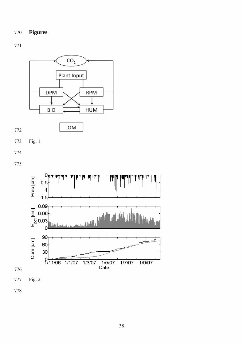
Fig. 1: Schematic overview of the RothC pool concept (modified from Jenkinson 1990). 733

Carbon is exchanged between four active pools: decomposable plant material (DPM), 734

resistant plant material (RPM), microbial biomass (BIO), and humified organic matter 735

(HUM). The fifth pool is inert organic matter (IOM). 736

Fig. 2: Precipitation (Prec), potential evaporation (Epot), cumulative precipitation (black) and 737

potential evaporation (grey) between October 2006 and October 2007. 738

Fig. 3: Measured (grey symbols) and simulated (black lines) water contents at different soil 739

depths. 740

Fig. 4: Measured (grey) and simulated (black) temperature in different soil depths. 741

Fig. 5: Measured and modelled CO2 flux using the soil water content response equation and 742

the temperature response equation according to Parton et al. (1987). Measured CO2 743

fluxes are shown as mean values with standard deviation (grey). Simulated CO2 fluxes 744

are illustrated as black line. Simulated CO2 production, water content, and temperature 745

are plotted for the plough horizon (upper 33 cm). 746

Fig. 6: Optimized temperature and soil water content response functions. Parameters for all 747

functions are listed in Table 4. 748

Fig. 7: Comparison of temperature response determined by inverse parameter estimation (IE) 749

and the conventional linear regression method (LR) for different soil depths.750

36

Tables 751

Tab. 1: Heat (Chung & Horton 1987) and CO2 transport parameters (Patwardhan et al. 752

1988) used in the numerical simulation. 753

Parameter Value Unit Heat transport Thermal dispersivity 1.5 cm Empirical constant b1 of soil thermal conductivity function 1.134E+12 kg cm-1 h-3 °C-1 Empirical constant b2 of soil thermal conductivity function 1.834E+12 kg cm-1 h-3 °C-1 Empirical constant b3 of soil thermal conductivity function 7.157E+12 kg cm-1 h-3 °C-1 CO2 transport Molecular diffusion coefficient of CO2 in air at 20°C 572.4 cm2 h-1 Molecular diffusion coefficient of CO2 in water at 20°C 0.0637 cm2 h-1 Longitudinal dispersivity of CO2 in water 1.5 cm 754

Tab. 2: Measured carbon concentration of total soil organic matter (SOM), particulate 755

organic matter (POM), and black carbon (BC) in the soil profile. RF is the remaining fraction 756

(RF = SOM – POM - BC). In brackets the percentages of POM, BC and RF from SOM are 757

given. 758

Depth SOM POM BC RF [cm] [mg C cm-3] [mg C cm-3] [mg C cm-3] [mg C cm-3] 0-10 18.54 3.30 (17.8%) 2.12 (11.4%) 13.12 (70.8%) 10-20 17.87 2.50 (14.0%) 2.43 (13.6%) 12.94 (72.4%) 20-30 17.21 2.50 (14.5%) 2.52 (14.6%) 12.19 (70.8%) 30-40 7.92 0.51 (6.4%) 1.93 (24.4%) 5.48 (69.2%) 40-50 5.62 0.29 (5.2%) 1.71 (30.4%) 3.62 (64.4%) 50-60 4.72 0.23 (4.9%) 1.42 (30.1%) 3.07 (65.0%) 60-100 4.26 0.21 (4.9%) 1.35 (31.7%) 2.70 (63.4%)

759

37

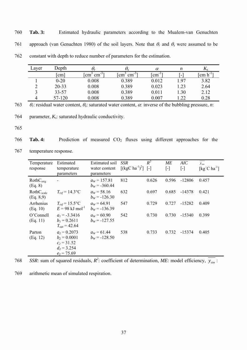
Tab. 3: Estimated hydraulic parameters according to the Mualem-van Genuchten 760

approach (van Genuchten 1980) of the soil layers. Note that r and s were assumed to be 761

constant with depth to reduce number of parameters for the estimation. 762

Layer Depth r s n Ks [cm] [cm3 cm-3] [cm3 cm-3] [cm-1] [-] [cm h-1] 1 0-20 0.008 0.389 0.012 1.97 3.82 2 20-33 0.008 0.389 0.023 1.23 2.64 3 33-57 0.008 0.389 0.011 1.30 2.12 4 57-120 0.008 0.389 0.007 1.22 0.28

r: residual water content, s: saturated water content, inverse of the bubbling pressure, n: 763

parameter, Ks: saturated hydraulic conductivity. 764

765

Tab. 4: Prediction of measured CO2 fluxes using different approaches for the 766

temperature response. 767

Temperature response

Estimated temperature parameters

Estimated soil water content parameters

SSR [(kgC ha-1)2]

R2 [-]

ME [-]

AIC [-]

simy

[kg´C ha-1]

RothCorig (Eq. 8)

- aW = 157.81 bW = -360.44

812 0.626 0.596 -12806 0.457

RothCscale (Eq. 8,9)

Tref = 14.3°C aW = 58.16 bW = -126.30

632 0.697 0.685 -14378 0.421

Arrhenius (Eq. 10)

Tref = 15.5°C E = 98 kJ mol-1

aW = 64.91 bW = -136.39

547 0.729 0.727 -15282 0.409

O’Connell (Eq. 11)

a1 = -3.3416 b1 = 0.2611 Topt = 42.64

aW = 60.90 bW = -127.55

542 0.730 0.730 -15340 0.399

Parton (Eq. 12)

a2 = 0.2073 b2 = 0.0001 c2 = 31.52 d2 = 3.254 e2 = 75.69

aW = 61.44 bW = -128.50

538 0.733 0.732 -15374 0.405

SSR: sum of squared residuals, R2: coefficient of determination, ME: model efficiency, simy : 768

arithmetic mean of simulated respiration. 769

38

Figures 770

771

772

Fig. 1 773

774

775

776

Fig. 2 777

778

39

779

Fig. 3 780

40

781

Fig. 4 782

41

783

Fig. 5 784

42

0

2

4

6

8

10

0 5 10 15 20 25 30 35 40 45

T [°C]

Sca

ling

fact

or f

T [

-] RothC scaleArrheniusO'ConnellParton

0

0.2

0.4

0.6

0.8

1

1.2

0 0.1 0.2 0.3 0.4

[cm3 cm-3]

Sca

ling

fact

or f

W [-

]

Fig. 6 785

0

5

10

15

20

25

0 5 10 15 20 25

Temperature [°C]

Sca

ling

fact

or

[-]

IE

LR surface

LR 10 cm

786

Fig. 7 787

788