Neuroinform (2007) 5:207–222DOI 10.1007/s12021-007-9000-z

Inverse Current-Source Density Method in 3D:Reconstruction Fidelity, Boundary Effects,and Influence of Distant Sources

Szymon Łeski · Daniel K. Wójcik ·Joanna Tereszczuk · Daniel A. Swiejkowski ·Ewa Kublik · Andrzej Wróbel

Published online: 27 November 2007© Humana Press Inc. 2007

Abstract Estimation of the continuous current-sourcedensity in bulk tissue from a finite set of electrodemeasurements is a daunting task. Here we present amethodology which allows such a reconstruction bygeneralizing the one-dimensional inverse CSD method.The idea is to assume a particular plausible form ofCSD within a class described by a number of parame-ters which can be estimated from available data, forexample a set of cubic splines in 3D spanned on afixed grid of the same size as the set of measurements.To avoid specificity of particular choice of reconstruc-tion grid we add random jitter to the points positionsand show that it leads to a correct reconstruction.We propose different ways of improving the qualityof reconstruction which take into account the sources

S. Łeski (B)Center for Theoretical Physics, Polish Academy of Sciences,al. Lotników 32/46, 02-668 Warsaw, Polande-mail: s.leski@nencki.gov.pl

S. Łeski · D. K. Wójcik · D. A. Swiejkowski ·E. Kublik · A. WróbelDepartment of Neurophysiology, Nencki Instituteof Experimental Biology, Polish Academy of Sciences,ul. Pasteura 3, 02-093 Warsaw, Poland

D. K. Wójcike-mail: d.wojcik@nencki.gov.pl

D. K. Wójcik · A. WróbelWarsaw School of Social Psychology,ul. Chodakowska 19/31, 03-815 Warsaw, Poland

J. TereszczukFaculty of Mathematics and Information Science,Warsaw University of Technology,Pl. Politechniki 1, 00-661 Warsaw, Poland

located outside the recording region through appro-priate boundary treatment. The efficiency of the tra-ditional CSD and variants of inverse CSD methods iscompared using several fidelity measures on differenttest data to investigate when one of the methods issuperior to the others. The methods are illustratedwith reconstructions of CSD from potentials evoked bystimulation of a bunch of whiskers recorded in a slab ofthe rat forebrain on a grid of 4 × 5 × 7 positions.

Keywords Current source density ·Local field potentials · Evoked potentials ·Inverse problems · Rat · Thalamus ·Somatosensory system

Introduction

One of the standard methods of analyzing extra-cellularly recorded local field potentials (LFPs) inneural tissue is the estimation of the current-sourcedensity (CSD) which generated them (Freeman andNicholson 1975; Nicholson and Freeman 1975). Theconnection between the electric potential φ and thecurrent-sources of density C is, under assumptionof quasi-static regime (Mitzdorf 1985), given by theequation:

∇(σ∇φ) = −C , (1)

where σ is the electrical conductivity tensor (Plonsey1969). In general, σ not only depends on position but isalso anisotropic (Ueno and Sekino 2005). Since we donot know the properties of σ in the studied tissue in thiswork we assume that it is a constant scalar. This means

208 Neuroinform (2007) 5:207–222

that the electrical conductance of the tissue is assumedhomogeneous and isotropic.

The CSD is usually calculated in one dimension, forexample if a laminar multielectrode is used to recordevoked potentials in the cerebral cortex. In this caseEq. 1 reduces to

σ∂2φ

∂z2= −C(z) . (2)

Let us assume that φ is measured at n equidistantelectrode points with interelectrode distance h. Thetraditional method of estimating C(z) at the interiorpoints zi, i = 2, . . . , n − 1 is to use the numerical secondderivative (Mitzdorf 1985). This leads to

C(zi) = −σφ(zi + h) − 2φ(zi) + φ(zi − h)

h2. (3)

To calculate the CSD at the extreme points one mayfollow the suggestion of Vaknin et al. (1988) which isto assume that the potentials do not vary for z < z1 andz > zn, that is φ(z) = φ(z1) for z < z1 and φ(z) = φ(zn)

for z > zn.Recently, Pettersen et al. (2006) proposed a general

framework called inverse CSD method (iCSD) whichexplicitly takes into account the assumptions madeabout the form of the sources. They observed that giventhe distribution of currents in the tissue it is formallya simple matter to evaluate the potentials measured atany point in space. One has to add up the contributionsfrom every point source I(x0, y0, z0, t) which are ofthe form

φ(x, y, z, t) = I(x0, y0, z0, t)

4πσ√

(x − x0)2 + (y − y0)2 + (z − z0)2.

Taking current-source distribution parameterized withparameters C = [C1, . . . , CM] one gets a functionalrelation

� = [φ(x1) . . . φ(xN)] = F(C)

which can usually be inverted if the number of para-meters, M, is equal to the number of measurementpoints, xi ≡ (xi, yi, zi), i = 1..N. Inverting this relationleads to the values of parameters C for a given set of

measured potentials �. This is particularly convenientfor parameterizations leading to F linear in C.1

The Inverse Current Source Density method isa generalization of the traditional Current SourceDensity method described above. Assume the poten-tials measured at equidistant points zi through the cor-tex, zi+1 − zi = h. Consider current sources distributeduniformly on infinitely extended and infinitely thin par-allel planes passing through the measurement pointsand perpendicular to the electrode. Let Ci be the valueof planar current source density at zi divided by h,which would be the value of volume current-sourcedensity at this point if the current was distributed in theslice of thickness h instead. Then the potentials φ(zi)

are connected with the current-source parameters Ci byEq. 3, see Pettersen et al. (2006).

Once the framework connecting C with φ is estab-lished it is natural to consider other distributions ofcurrent in the brain which would be more plausiblethan infinitely thin, infinitely extended planes of con-stant current-source density. Pettersen et al. consid-ered three different choices of distributions leadingto three variants of iCSD which they called “δ-sourceiCSD”, “step iCSD”, and “spline iCSD” methods. Inthe first case they assumed current sources distributedin infinitely thin discs of radius R passing through zi.“Step iCSD” assumes current distribution in cylindersof radius R and height h centered at measurementpoints. The last method assumes a continuously varyingin z but constant in the x, y plane profile of current-source density. In all these cases the CSD distribution isparameterized by its values at the measurement points.Let us stress that all these methods were developed fora one-dimensional problem of a multielectrode passingthrough the cortex perpendicularly to its surface.

Recently we performed experiments in which LFPswere measured at a three-dimensional array of 4 ×5 × 7 points in order to reveal the dynamics andspecificity of rat diencephalic activation which followsvibrissal stimulation. The simplest approach for exam-ining three-dimensional CSD would be to generalize

1Note that the CSD in the whole tissue needs not be specifiedby its values on the grid, but, for instance, could be specified bythe total current, position of the center and the spread of each ofthe sources. Then the potentials on the grid would be a nonlinearfunction of the parameters of CSD. Such a functional relation,however, would be of smaller practical utility in the applicationconsidered, which is why we restrict ourselves to the linear case.We believe it is useful to stress that the parameterizations canbe more general as there may be other techniques, e.g. based onstatistical learning, where nonlinear parametrization can be morenatural and inverse of F is not required.

Neuroinform (2007) 5:207–222 209

a bFig. 1 The assumed distribution of current-sources (two-dimensional analog). Circles denote the grid points. We usuallyassume that the electrodes are located at, or very close to, the

knots of the grid spanning CSD. a CSD at any point is aninterpolation (linear or spline) of the values at the nodes. b Instep method we assume constant CSD in a box around each node

the numerical second derivative and use an approxima-tion to Laplacian:

C(xi, yi, zi)=− σ

h2

[φ(xi + h, yi, zi) + φ(xi − h, yi, zi)

+ φ(xi, yi + h, zi) + φ(xi, yi − h, zi)

+ φ(xi, yi, zi + h) + φ(xi, yi, zi − h)

− 6φ(zi)]

. (4)

This formula (in two dimensions) was used for exampleby Novak and Wheeler (1989), Shimono et al. (2000)and Lin et al. (2002). However, the traditional approachimplies the exclusion of all the boundary points. Ina typical one-dimensional recording the loss of twopoints out of 15–20 may be acceptable. In our casethe boundary consists of 110 out of 140 measurementpoints. The procedure suggested by Vaknin (to assumethe potentials do not change outside the grid) seemednot well justified in our experiments therefore we de-cided to generalize the inverse CSD method to three-dimensional case. An early attempt to get informationabout the three-dimensional distribution of the field inthe cortex by Sukov and Barth (1998) combined analy-sis of measurements on 8 × 8 epipial electrode grid withlaminar multielectrode depth recordings. The 16-pointmultielectrode was placed in the point which exhibitedhighest surfacial activity. Second order approximationto Laplacian with the Vaknin condition was used toobtain CSD at the measurement points. Other pointsin the bulk tissue were not probed hence the obtainedCSD had a product structure and could not resolve the3D structure of sources and sinks in the studied tissue.

All the figures and all the numerical examples inthe subsequent sections use the grid 4 × 5 × 7 whichwas also used in the experiment. The validity of

the methods, however, is independent of the size ofthe grid.

Methods

The Inverse CSD Method in Three Dimensions

Let us start with a three-dimensional cubic grid ofnx, ny and nz points in respective directions so thateach recording site (x j, y j, z j) is close to one of the gridpoints.2 We assume that the total number of electrodesis the same as the number of grid points and is equalto n = nxnynz. We then consider some class of current-source distributions with n free parameters. Such distri-butions can be parameterized by the n values of CSDat the grid points. One example is a piecewise constant(step) distribution: current-source density is constant incubes of unit edge length centered on the grid points.Next we calculate the potentials at the electrodes lo-cations generated by the assumed CSD distribution.This leads to a linear formula for each φ in terms ofthe n parameters of C of the form � = FC, where Cstands for all the parameters organized in a vector. Wefinally invert this relation to calculate the n unknownparameters C (hence the whole CSD distribution) fromthe measured potentials. The exact form of this linearoperator depends on the assumed form of the currentsources distribution.

We consider a number of different CSD distribu-tions. One is the step distribution described above.Another is based on linear approximation: we assume

2It is convenient to work with unit spacing and to include thetrue edge length h at the very end of the calculations, this is donesimply by dividing the resulting CSD by h2.

210 Neuroinform (2007) 5:207–222

that the CSD is piecewise linear, that is the CSD be-tween the grid points is calculated from the values at thenearest nodes via linear interpolation. The third casewe study is the CSD distribution in the form of three-dimensional cubic splines with knots at grid points (thatmeans the CSD in the whole volume is calculated fromthe values at grid points using spline interpolation).We consider two types of splines, “natural” and “not-a-knot”, differing with a normalization condition (see the“Appendices”). We also considered variants of abovedistributions to deal with boundary effects. They aredescribed in the following sections.

In the case of linear and spline distributions weassumed that the current-sources are localized insidethe grid. In case of the step distribution the CSD isnonzero in a slightly larger cuboid spanned by all theunit-size boxes centered at grid points (see Fig. 1).

The calculation of the linear operator F for stepdistribution is quite simple. Let us denote the positionof the i-th electrode by (xi, yi, zi) and the coordinates ofthe j-th grid node by (x j, y j, z j). In general they neednot be the same. Then the potential at i-th electrodelocation is given by

�i = �(xi, yi, zi) =n∑

j=1

FijC j,

where

C j = C(x j, y j, z j) .

The matrix element Fij is the contribution of theuniform CSD of unit density located at a box centeredat point j to the potential at point i. Thus, for the stepdistribution of CSD, it is given by

Fij = 1

4πσ

∫ x j+1/2

x j−1/2

∫ y j+1/2

y j−1/2

∫ z j+1/2

z j−1/2

dzdydx√

(xi − x)2 + (yi − y)2 + (zi − z)2. (5)

This integral is easy to evaluate numerically, al-though one must be careful because of the singularityof the integrand.3 Once we have the matrix F we canuse its inverse to estimate the CSD at grid points fromknown potentials:

C j =n∑

i=1

(F−1) ji�i .

These values define the whole CSD distribution.The operator F for linear and spline methods is

calculated similarly, although the calculations get muchmore complicated, especially for the cubic splines.For details of the calculations we refer the reader to“Appendices”.

Boundary Effects and Distant Sources

In the linear and spline distributions described in theprevious section it is assumed that CSD is non-zero onlyinside the cuboid enclosing the grid, which was chosento approximate the distribution of electrode locations.In real tissue this assumption is not fulfilled: the arrayof electrodes covers only a small area of the brain andthere are many sources outside that area. If we usedthe Laplacian to calculate CSD, then the influence of

3We dealt with the singularity by simply excising a ball of radiusε = 10−8 or ε = 10−6. The numerical error introduced by such anexcision is smaller than ε2.

the outlying sources could be neglected. For example, ifthere was an additional distant point source then therewould be a 1

r term in observed potentials, but ∇2 1r = 0

which gives no contribution to the calculated CSD.4

The situation is different with the inverse method. Herewe have one-to-one correspondence (via operators Fand F−1) between sources and potentials, hence anyadditional term in the potentials (like 1

r ) will producespurious sources. Nevertheless, it is possible to modifythe inverse method in such a way that we can profitfrom its advantages over traditional CSD and at thesame time limit the impact of the above mentionedeffect.

To accommodate the sources located outside theelectrode grid we extend the grid by one point in eachdirection, therefore an additional layer of non-zeroCSD is created. The CSD at additional grid points iseither zero, which we denote with the letter “B”, or aduplication5 of the boundary layer of the original grid,which is denoted by “D” (see Fig. 2). Therefore we have“linear”, “linear B” and “linear D” methods, similarly

4Except at r = 0, which is not the case here because the source is“distant”.5Note that the larger grid has extra corner points which do notdirectly correspond to points in the original grid. For these cornerpoints duplication means that we take the value at the closest(corner) point in the original grid. In other words, values at thecorner points in the original grid are used at more than one pointin the extended grid. A similar observation applies to the pointson the edges of the grid.

Neuroinform (2007) 5:207–222 211

Fig. 2 Comparison of“standard” vs. B or Ddistribution of sources. Instandard distribution a theCSD is non-zero only insidethe grid of the same size asthe number of electrodes,while in B or D distributionb there is an additional layerof non-zero CSD

a b

for splines. In the context of laminar multielectrodesthe “spline B” method was proposed by Pettersen et al.(2006). At the practical level the difference betweenthese methods is that we use different matrices F.The modified linear operator F is constructed in threesteps. First we act on a vector of n CSD values with amatrix B, which produces a larger vector (of size N =(nx+2)(ny+2)(nz + 2)) of CSD values on a larger grid.There are two different B matrices, BB and BD, forB and D boundary conditions respectively. Then weapply the matrix F calculated for the larger (nx+2)×(ny+2) × (nz + 2) grid. In the final step we discard thevalues of potential at the boundary to get a vectorof size n; this is done by applying a matrix R.Summarizing, we have the following formula for theF B matrix (superscripts indicate the size of the grid forwhich the F matrix is calculated):

Fnx,ny,nz B = RF(nx+2),(ny+2),(nz+2) BB ,

analogously for F D. Note that there is no point inconsidering “step B” method because it is the same as“step”, however, we may consider “step D”.

The B and D boundary conditions are motivatedby the following heuristics. We know that the sourceswe deal with in real-world situations are not restrictedto lie within the space spanned by the grid. Supposetherefore that there is a source outside, for examplenear a corner of the cuboid. This source will affect thepotentials, especially in the corner. The inverse CSDmethod will then generate a current-source distributioninside the grid such that the resulting potential willmatch the one measured at the recording points. Inother words, the method will try to imitate the outlyingsource with sources located inside the grid. This willlead to errors in CSD reconstruction, for example afalse source in the corner may appear. Consider nowthe same potentials processed with a method using Bboundary condition. One expects that the B methodmay also generate a spurious source in the corner, but

the magnitude of the source will be smaller. This isbecause a larger CSD value in the corner means alsolarger CSD in the additional layer and the iCSD Bmethod may place a smaller source in the corner thanstandard iCSD to obtain the same potential. Summariz-ing, we expect the B methods to limit the magnitudesof the spurious sources at the boundary. In case ofD methods this attenuation should be even stronger.We test both B and D variants because it is hard totell a priori which boundary treatment leads to betterreconstructions.

Jittering

The iCSD method allows us to calculate N unknownparameters of CSD distribution from N measuredpo-tentials. So far we assumed that the N unknowns werethe values of CSD at the nodes placed next to theelectrode positions, however, such an assumption isnot the only possible. In fact, it leads to some con-straints on the calculated CSD. For example, in thelinear method the maxima and minima of the obtainedcurrent source density are always located at the nodes.One way to avoid this particular limitation is to use adifferent distribution, such as cubic spline approxima-tion. Another way is to use an approach which we call“spatial jittering”. In this variant we assume that thegrid spanning CSD is slightly displaced with respect tothe distribution of the electrodes (maximally by half ofthe cube size in each direction), see Fig. 3. The CSDobtained in this way is a valid solution of the inverseproblem, that is, it also produces the measured poten-tials. We can now randomly choose many displacedgrids, calculate the CSD and then take the average. Thismethod produces “smoother” CSD distributions, espe-cially for step and linear methods. Due to the linearityof this procedure the average obtained by jittering alsogenerates experimentally obtained potentials and is anequivalent solution of the inverse problem.

212 Neuroinform (2007) 5:207–222

Fig. 3 The idea of spatialjittering. a The CSDdistribution as in B or Dmethod. b Jittering, gridspanning the sources (emptycircles) is displaced withrespect to the array ofelectrodes (the black dots)

a b

The jittering is implemented by altering the Fmatrix. Let �d = (dx, dy, dz) be a displacement vector,that means the CSD grid is shifted by �d with respect

to potentials (electrode) grid. Then the elements of F(in case of “step” distribution) are given by theformula:

Fij = 1

4πσ

∫ x j+ 12

x j− 12

∫ y j+ 12

y j− 12

∫ z j+ 12

z j− 12

dz dy dx√

(xi − dx − x)2 + (yi − dy − y)2 + (zi − dz − z)2.

We always use jittering in combination with either Bor D boundary conditions, which we denote by J andK respectively. The number of displacement vectorsused in the tests varied from 12 to 46. The vectors werechosen from a uniform distribution over the box of edgelength 1 (equal to the distance between the grid points)centered at 0, aligned along the grid axes.

Results

Reconstruction Fidelity for Test Data

To compare quantitatively the different variants ofiCSD method in three dimensions we used the recon-struction error defined as follows. We take an arti-ficial current-source distribution C and calculate thepotentials which would be measured by the three-dimensional array of electrodes. Then we use the po-tentials at the nodes to reconstruct CSD. The totalreconstruction error is then the total square differencebetween the original, C, and the reconstructed, Crec,densities, normalized as follows:

e =∫ nx

1

∫ ny

1

∫ nz

1 (C − Crec)2 dz dy dx

∫ nx

1

∫ ny

1

∫ nz

1 C2dz dy dx. (6)

Other measures of reconstruction error we used are:squared maximal error (max |C − Crec|2), normalizedwith 〈C2〉 (mean of C2), and 0.95/0.99-errors. Wedefine the p-error as the smallest value δ such thatthe probability to find |C−Crec|2

〈C2〉 < δ is p. This is easy

to find from the cumulative distribution function ofsquare errors cdf ( |C−Crec|2

〈C2〉 ). On the graph of cdf onedraws a horizontal line at y = p and reads off the xaxis the value of δ (see Fig. 4b). These measures helpto differentiate between the reconstructions of compa-rable mean square error but with different smoothnessproperties.

The different measures of reconstruction error arepresented in Tables 1 to 4. Each table collects theresults for various reconstruction methods applied togiven sets of test data.6

We compared all the iCSD methods presented in theprevious section, that means all combinations of theassumed distributions (step, linear, natural spline, not-a-knot spline) and the boundary conditions (standard,B, D, jittering J, jittering K). The direct comparisonwith the “traditional” CSD is not possible because thenwe do not have the reconstructed CSD at the boundarynodes. In order to have a “traditional” method for com-parison we generalize the Vaknin procedure to threedimensions, although it does not seem well justified. Weextend the potentials grid by adding one point in eachdirection and duplicating the potential values, then wecalculate the approximate Laplacian, Eq. 4. Hence weobtain the CSD values at all the grid points. To com-pare such reconstructed CSD to the actual sources we

6Even though the reconstruction errors are normalized withrespect to the original sources we think that one should still becareful when comparing the results between different sets.

Neuroinform (2007) 5:207–222 213

0 0.01 0.0310–5

10–4

10–3

10–2

10–1

100Distribution of reconstruction error

Error (C–Crec

)2/<C2>

Vol

ume

(nor

mal

ized

)

step

step (J)

a b0.02 0 0.01 0.02

0.8

0.85

0.9

0.95

0.99

Cumulative distribution of reconstruction error

Error (C–Crec

)2/<C2>

Vol

ume

(nor

mal

ized

)

step

step (J)

Fig. 4 Example of distribution (a) and cumulative distribution(b) of the reconstruction error for step and step J iCSD methods.Vertical lines define 0.95/0.99 errors. Unit normalized volume

corresponds to the volume spanned by the electrodes grid. Herethe step (J) method used 17 jittering vectors drawn from uniformdistribution over [−0.5, 0.5]3 cube

interpolate it between the grid points using splines. Wedenote this approach on figures and in tables by “trad(V) int”.

It appears from our analysis that the relative utilityof the methods depends on the type of the chosen testdata. This is not surprising: if the test distribution wasof the same type as the one assumed in the given iCSDvariant then this (and only this) method would recon-struct the test data exactly. Therefore, an importantquestion is what test data are “natural”, that meansresembling the CSD in actual tissue. We used five typesof test data. The first four types were Gaussian sourceswith CSD given by the formula

C(�r) = A exp

(− (�r − �r0)

2

l

).

There were between 4 and 8 such sources and theparameters A, l, �r0 were chosen randomly. In the firsttype of data we assumed that CSD outside the electrodearray was strictly zero and we truncated the distributionaccordingly. In the second type we assumed that theCSD is non-zero in one additional layer of unit thick-ness, in the third type there were two additional layers.The fourth type was similar to the second but there wasan additional strong point-like source located outsidethe grid. The fifth type of the test data were homo-geneous spherical sources with sharp cut-off. For thetests we assumed the same configuration of electrodelocations as in the motivating experiment which was agrid of size 4 × 5 × 7.

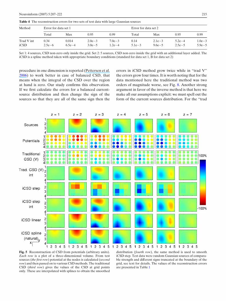
First we compared the reconstruction fidelity of fourdifferent forms of assumed distributions (see Fig. 5 and

Table 1). The test data were of the first type, that is thesources were truncated outside the grid. The results areas expected: the step method is the worst, the linearapproximation of the distribution is an order of mag-nitude better, the natural splines are even better. Thenot-a-knot splines do not work very well on such data,they are worse than natural splines and even slightlyworse than linear approximation (data not shown). Thetraditional method performs here rather poorly.

Note that the data presented in rows 2 and 3 shouldbe interpreted differently than the other rows. Thesedata are plotted with filled circles to emphasize the factthat we only know the values at the grid points. Thefigures for step method (row 5), on the other hand, areshown as squares because that is the assumed form ofthe CSD distribution reconstructed with this method.However, one could do a similar formal trick as we didwith the “trad V” method, that is assume the calculatedvalue at the grid point for the “step” distribution andspline-approximate the CSD between the grid points.

Table 1 The reconstruction errors for test data shown in Fig. 5

Method Reconstruction error

Total Max 0.95 0.99

Trad V int 0.16 8.5e−3 7.4e−4 2.8e−3iCSD step 0.31 7.4e−3 1.4e−3 2.9e−3iCSD step int 0.070 4.2e−3 2.5e−4 9.8e−4iCSD linear 0.013 1.5e−3 6.9e−5 1.7e−4iCSD spline (natural) 4.8e−3 2.5e−4 2.2e−5 4.8e−5

214 Neuroinform (2007) 5:207–222

Table 2 The reconstructionerrors for test data shown inFig. 6

Method Reconstruction error

Total Max 0.95 0.99

Trad V int 0.32 0.048 9.6e−4 7.4e−3iCSD spline 11 26 0.17 0.17iCSD spline B 0.24 0.028 9.3e−4 5.0e−3iCSD spline D 0.25 0.034 6.8e−4 5.2e−3iCSD spline J 0.24 0.028 9.3e−4 4.6e−3iCSD spline K 0.24 0.034 6.8e−4 4.8e−3

This is shown in row 6. Note, however, that proceedingin this way is inconsistent with the assumption of theuniform distribution in the boxes centered on the gridpoints. To obtain smooth CSD estimates one shouldrather assume some other kind of CSD distribution apriori. The smoothed step performs here better than“trad V int”, but still much worse than linear. Weexpect that in all the remaining tests the performanceof the “iCSD step int” method would be somewherebetween the “trad V int” and the more sophisticatediCSD methods such as splines. The only advantageof using the “iCSD step int” would be that it is theeasiest of the iCSD methods to implement. However,the gain in terms of computation time is minimal. Thecalculation of the F matrix is substantially faster than,for example, in spline method; however, the F matrixmay be calculated once and then used for the wholeanalysis. Therefore we do not consider the “iCSD stepint” method in the subsequent analysis and suggest theuse of the spline iCSD.

Next we tested different boundary conditions (seeFig. 6 and Table 2, the splines used here are “not-a-knot”). As the boundary conditions are devised todeal with sources outside the grid, the test data hereare of the second type (non-zero CSD assumed alsoin the additional layer). For such test data the “stan-dard” iCSD method produces spurious sources at theboundary and the reconstruction error is very high. Thequality of the method improves substantially if we useany of the variants pushing the boundary away. We

also considered other forms of distributions but in thecase at hand the appropriate treatment of the boundaryseems much more important than the choice of theinterpolation method. The traditional method is quitegood here, with the error only about thirty percentlarger than the iCSD.

The distortions present in the iCSD spline (secondrow in Fig. 6) form a characteristic pattern. Weobserved very similar patterns in experimental ratdata (when processed without taking into account theboundary effects) and it seems to us that they can beclassified as artifacts resulting from the sources locatedoutside the grid. In the experimental situation these canbe, for example, sources in the neighboring cortex.

It is even more important to choose suitable bound-ary treatment if we add a strong source to our data (thefourth type), see Fig. 7 and Table 3. For such data themethods ignoring the boundary are simply useless (cf.the second row in Fig. 7). The best method here is thetraditional V method, but the iCSD not-a-knot splineK also performs well, although distortions are visible atthe edges of the grid.

Our experience shows that the iCSD method (withappropriate boundary conditions) is usually better andnever much worse than “trad V”. The inverse methodsseem to work comparably to “trad V” in case of com-pact sources, such as shown in Figs. 6 and 7, but areusually an order of magnitude better if we allow thesources to be larger, of the size observed in our experi-mental data, see Table 4 for two examples. The Vaknin

Table 3 The reconstructionerrors for test data shown inFig. 7

Method Reconstruction error

Total Max 0.95 0.99

Trad V int 1.3 0.045 4.5e−3 9.4e−3iCSD spline 5.3e2 1.9e2 1.3 12iCSD spline B 4.3 0.16 0.016 0.049iCSD spline D 2.2 0.057 8.0e−3 0.018iCSD spline J tone 4.1 0.16 0.016 0.045iCSD spline K 2.2 0.056 7.8e−3 0.017

Neuroinform (2007) 5:207–222 215

Table 4 The reconstruction errors for two sets of test data with large Gaussian sources

Method Error for data set 1 Error for data set 2

Total Max 0.95 0.99 Total Max 0.95 0.99

Trad V int 0.34 0.014 2.0e−3 7.0e−3 0.14 2.1e−3 5.2e−4 1.0e−3iCSD 2.5e−6 6.5e−4 3.0e−5 1.2e−4 5.1e−3 9.6e−5 2.5e−5 5.9e−5

Set 1: 4 sources, CSD non-zero only inside the grid. Set 2: 5 sources, CSD non-zero inside the grid with an additional layer added. TheiCSD is a spline method taken with appropriate boundary conditions (standard for data set 1, B for data set 2)

procedure in one dimension is reported (Pettersen et al.2006) to work better in case of balanced CSD, thatmeans when the integral of the CSD over the regionat hand is zero. Our study confirms this observation.If we first calculate the errors for a balanced current-source distribution and then change the sign of thesources so that they are all of the same sign then the

errors in iCSD method grow twice while in “trad V”the errors grow four times. It is worth noting that for thedata mentioned here the traditional method was twoorders of magnitude worse, see Fig. 8. Another strongargument in favor of the inverse method is that here wemake all our assumptions explicit: we must spell out theform of the current sources distribution. For the “trad

Fig. 5 Reconstruction of CSD from potentials (arbitrary units).Each row is a plot of a three-dimensional volume. From testsources (the first row) potential at the nodes is calculated (secondrow) and then passed on to various CSD methods. The traditionalCSD (third row) gives the values of the CSD at grid pointsonly. These are interpolated with splines to obtain the smoothed

distribution (fourth row), the same method is used to smoothiCSD step. Test data were random Gaussian sources of compara-ble strength and different signs truncated at the boundary of thegrid, see text for details. The values of the reconstruction errorsare presented in Table 1

216 Neuroinform (2007) 5:207–222

Fig. 6 Reconstruction of CSD from potentials, comparison ofdifferent treatments of the boundary (arbitrary units). Test datawere random Gaussian sources truncated at the boundary of the

grid extended by one layer in each direction, see text for details.Table 2 contains the values of reconstruction errors for this test

V” method we also make an assumption: potentialsare constant outside the grid, but we do not knowhow that assumption is reflected in the reconstructedCSD. In our opinion it is much more elegant to makeassumptions about the distribution of current-sourcesinstead of the potentials.

The influence of jittering seems to differ strongly forvarious forms of assumed CSD distributions. In case ofstep (see Fig. 4) and linear distributions the jitteringsignificantly improves the quality of the reconstruction,but for splines the improvement is only slight. It canbe easily understood: the “step” reconstruction stronglydepends on the choice of the sources grid, while the“spline” reconstruction does not.

Application to Evoked Potentials in Rat

The method was applied to LFPs recorded from deepstructures of the rat forebrain. An adult male Wistarrat was anesthetized with urethane, placed in a stereo-

taxic apparatus, and a bunch of his left whiskers wasglued to a piezoelectric stimulator. Most of the rightparietal bone was removed and the resulting openingwas covered with agar. A set of five stainless steelmicro-electrodes (FHC, Bowdoin, USA; impedance of1.5 M at 1 kHz) mounted parallely in a sagittal plane(tips in antero-posterior line, spaced by 0.7 mm; themost anterior electrode 1.9 mm posterior to Bregmaand 2.1 mm to the right from the midline) was low-ered vertically through the opening and stopped each0.7 mm at seven depths in the brain tissue, startingat 3.4 mm from the cortical surface. At each stop thebunch of left whiskers was deflected 60 times. LFPswere recorded monopolarly and allowed for extractionof 60 somatosensory evoked potentials (EPs) per eachrecording point. The length of the interelectrode dis-tance was based on the average size of the studiedthalamic nuclei (e.g. POm 1.4 × 1 × 2 mm), and theexpected large-scale activation evoked by the strongmulti-whisker input.

The procedure was repeated at lateral positions2.8, 3.5 and 4.2 mm to the right from midline, at

Neuroinform (2007) 5:207–222 217

Fig. 7 Reconstruction of CSD from potentials. Test data wererandom Gaussian sources truncated at the boundary of the gridextended by one layer in each direction, plus an additional strong

point source outside the grid was added at (x = 6, y = 3, z = 4),see text for details. Table 3 contains the values of reconstructionerrors for this test

corresponding depths. Thus a rectangular grid of 140(4 × 5 × 7) recording points comprising a slab of fore-brain tissue with portions of the thalamus, pretectum,the hippocampus, and cerebral white matter was ob-tained. An exact location of the recording points was

verified histologically after the experiment and anatom-ical structures were identified according to Paxinosand Watson (1996). For details of surgical procedure,stimulation of the vibrissae, signal processing andpost-experimental procedure see Kublik et al. (2003).

Fig. 8 Reconstruction of CSD from potentials for large andnon-balanced current-sources located inside the grid (arbitraryunits). The inverse method gives the total reconstruction error

two orders of magnitude smaller than the traditional method.Note particularly the difference between the reconstructions atz = 3

218 Neuroinform (2007) 5:207–222

Fig. 9 Top row: Currentsource density 3.5 ms afterthe stimulus reconstructedusing the iCSD not-a-knotspline D method. Note thatdifferent plane is shown thanin the previous figures toallow usage of coronal brainsections. Bottom row: splineapproximated potential in thetissue based on the same dataas used for the CSDreconstruction at the sametime. The grid spacing is 0.7mm in each direction. Forabbreviations see“Appendices”

The LFP signal was amplified (1,000 times) and fil-tered (0.1–5 kHz). Epochs (of about 1.4 s) containingEPs were digitized on-line (10 kHz) with 1401plus

interface and Spike-2 software (CED, Cambridge,England). All stored data were examined for integrityand epochs with artifacts were excluded from further

Fig. 10 As in Fig. 9, 15 msafter the stimulus

Neuroinform (2007) 5:207–222 219

analysis. Recordings were stimulus averaged andsmoothed with Savitsky–Golay filter of order 3 withwindow size 9 prior to further analysis.

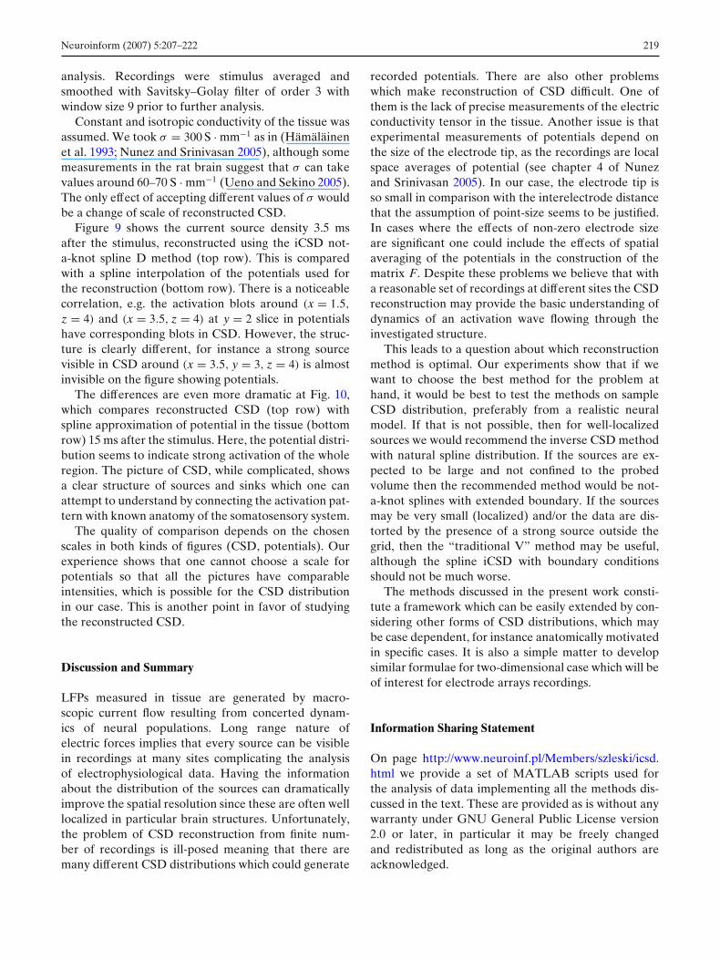
Constant and isotropic conductivity of the tissue wasassumed. We took σ = 300 S · mm−1 as in (Hämäläinenet al. 1993; Nunez and Srinivasan 2005), although somemeasurements in the rat brain suggest that σ can takevalues around 60–70 S · mm−1 (Ueno and Sekino 2005).The only effect of accepting different values of σ wouldbe a change of scale of reconstructed CSD.

Figure 9 shows the current source density 3.5 msafter the stimulus, reconstructed using the iCSD not-a-knot spline D method (top row). This is comparedwith a spline interpolation of the potentials used forthe reconstruction (bottom row). There is a noticeablecorrelation, e.g. the activation blots around (x = 1.5,

z = 4) and (x = 3.5, z = 4) at y = 2 slice in potentialshave corresponding blots in CSD. However, the struc-ture is clearly different, for instance a strong sourcevisible in CSD around (x = 3.5, y = 3, z = 4) is almostinvisible on the figure showing potentials.

The differences are even more dramatic at Fig. 10,which compares reconstructed CSD (top row) withspline approximation of potential in the tissue (bottomrow) 15 ms after the stimulus. Here, the potential distri-bution seems to indicate strong activation of the wholeregion. The picture of CSD, while complicated, showsa clear structure of sources and sinks which one canattempt to understand by connecting the activation pat-tern with known anatomy of the somatosensory system.

The quality of comparison depends on the chosenscales in both kinds of figures (CSD, potentials). Ourexperience shows that one cannot choose a scale forpotentials so that all the pictures have comparableintensities, which is possible for the CSD distributionin our case. This is another point in favor of studyingthe reconstructed CSD.

Discussion and Summary

LFPs measured in tissue are generated by macro-scopic current flow resulting from concerted dynam-ics of neural populations. Long range nature ofelectric forces implies that every source can be visiblein recordings at many sites complicating the analysisof electrophysiological data. Having the informationabout the distribution of the sources can dramaticallyimprove the spatial resolution since these are often welllocalized in particular brain structures. Unfortunately,the problem of CSD reconstruction from finite num-ber of recordings is ill-posed meaning that there aremany different CSD distributions which could generate

recorded potentials. There are also other problemswhich make reconstruction of CSD difficult. One ofthem is the lack of precise measurements of the electricconductivity tensor in the tissue. Another issue is thatexperimental measurements of potentials depend onthe size of the electrode tip, as the recordings are localspace averages of potential (see chapter 4 of Nunezand Srinivasan 2005). In our case, the electrode tip isso small in comparison with the interelectrode distancethat the assumption of point-size seems to be justified.In cases where the effects of non-zero electrode sizeare significant one could include the effects of spatialaveraging of the potentials in the construction of thematrix F. Despite these problems we believe that witha reasonable set of recordings at different sites the CSDreconstruction may provide the basic understanding ofdynamics of an activation wave flowing through theinvestigated structure.

This leads to a question about which reconstructionmethod is optimal. Our experiments show that if wewant to choose the best method for the problem athand, it would be best to test the methods on sampleCSD distribution, preferably from a realistic neuralmodel. If that is not possible, then for well-localizedsources we would recommend the inverse CSD methodwith natural spline distribution. If the sources are ex-pected to be large and not confined to the probedvolume then the recommended method would be not-a-knot splines with extended boundary. If the sourcesmay be very small (localized) and/or the data are dis-torted by the presence of a strong source outside thegrid, then the “traditional V” method may be useful,although the spline iCSD with boundary conditionsshould not be much worse.

The methods discussed in the present work consti-tute a framework which can be easily extended by con-sidering other forms of CSD distributions, which maybe case dependent, for instance anatomically motivatedin specific cases. It is also a simple matter to developsimilar formulae for two-dimensional case which will beof interest for electrode arrays recordings.

Information Sharing Statement

On page http://www.neuroinf.pl/Members/szleski/icsd.html we provide a set of MATLAB scripts used forthe analysis of data implementing all the methods dis-cussed in the text. These are provided as is without anywarranty under GNU General Public License version2.0 or later, in particular it may be freely changedand redistributed as long as the original authors areacknowledged.

220 Neuroinform (2007) 5:207–222

One full set of data for a single rat is providedto allow for the generation of the movies which canalso be found on the above webpage. The data canbe used for research purposes, in particular for testingother methods of data analysis as long as this article isacknowledged in a published account of the results.

Acknowledgements We are grateful to Wit Jakuczun for hissuggestion to investigate spatial jittering as one way to improvethe CSD reconstruction. This work was partly financed from thePolish Ministry of Science and Higher Education research grantsN401 146 31/3239 and 2P04C 046 27.

Appendices

Linear iCSD Method

In this appendix we construct the F matrix for thelinear distribution of CSD. Consider a grid of points(i, j, k), where i = 1..nx, j = 1..ny, k = 1..nz. Let usnumber the points with a multi-index α ≡ (i, j, k) andwrite (i, j, k) ≡ (xα, yα, zα). Let V be the set of 8 vec-tors (v1, v2, v3), vi ∈ {0, 1}. The grid has n = nxnynz

nodes and there are m = (nx − 1)(ny − 1)(nz − 1) boxesspanned by these nodes. We index the boxes so thatthe corners of the box number α are α + v for v ∈V. Let B denote the set of all the allowed indicesα numbering the boxes and G stand for all the gridpoints. Let C denote the vector of CSD values at thenodes, that is Cα = C(xα, yα, zα) for α ∈ G. We assumethat CSD in boxes is given by a linear approximation.

Take a point (x, y, z) in box number α and let δx =x − xα , δy = y − yα , δz = z − zα . The value of CSDat this point obtained with the linear interpolation isgiven by:

C(x, y, z) =∑

v∈V

[1 − v1 + (2v1 − 1)δx]

× [1 − v2 + (2v2 − 1)δy

]

× [1 − v3 + (2v3 − 1)δz] Cα+v.

Therefore the distribution inside the box is a linearcombination of 8 functions fl, l = 1..8: f1 = 1, f2 =δx, f3 = δy, f4 = δz, f5 = δxδy, f6 = δxδz, f7 = δyδz,f8 = δxδyδz, with coefficients depending linearly on thevalues of C at the nodes of the box:

C(x, y, z) =∑

β∈G

8∑

l=1

Elαβ flCβ.

The coefficients Elαβ are non-zero only for β − α ∈ V

and follow from the above formula, e.g. E1α,β = 1 for

β − α = (0, 0, 0), otherwise E1α,β = 0, etc. The poten-

tial generated by such a distribution of current-sourcedensity at some point (x, y, z) is

�(x, y, z) =∑

α∈B

∑

β∈G

8∑

l=1

Flα(x, y, z)El

αβCβ ,

where

Flα(x, y, z) = 1

4πσ

∫ 1

0

∫ 1

0

∫ 1

0

fl(x, y, z) dz dy dx√

(x − xα − x)2 + (y − yα − y)2 + (z − zα − z)2.

If we now take as (x, y, z) one of the grid points γ then

�γ =∑

β∈G

FγβCβ,

where

Fγβ =∑

α∈B

8∑

l=1

Flα(xγ , yγ , zγ )El

αβ.

Thus Fγβ represents the direct and indirect contribu-tions to the total potential at point γ from the CSDassociated with the grid point β.

Spline iCSD Method

The construction of the F matrix for the spline dis-tribution is in principle very similar to the case of

linear distribution, but the level of complication is muchhigher. Similarly as in the previous appendix we have nnodes and m boxes, but now the interpolating functionin each box is the three-dimensional cubic spline. Thatmeans there are 4 × 4 × 4 = 64 base functions. There-fore there will be 64 each of E and F matrices. Themain challenge here is to construct the E matrices, thatmeans to describe how a CSD value associated witha given node influences the interpolating splines in allthe boxes.

First we briefly remind the construction of one-dimensional spline (Press et al. 1992). Suppose we havevalues of a function f at points x = 1..nx. For x suchthat j ≤ x ≤ j + 1 define P1(x) = j + 1 − x, P2(x) =x − j. The formula

f (x) = P1(x) f ( j) + P2(x) f ( j + 1) (7)

Neuroinform (2007) 5:207–222 221

gives a linear approximation, that means an approx-imation with a continuous function. In case of cubicsplines we want more: we want also the first and secondderivatives to be continuous. This can be done if wereplace the right hand side of Eq. 7 with a third-degreepolynomial:

f (x) = P1(x) f ( j) + P2(x) f ( j + 1)

+P3(x) f ′′( j) + P4(x) f ′′( j + 1) , (8)

where P3(x) = 16 (P1(x)3 − P1(x)), P4(x) = 1

6 (P2(x)3 −P2(x)). This formula guarantees that both f and itssecond derivative are continuous. The values of the sec-ond derivative f ′′ of f at nodes are a priori unknown,but can be calculated from the condition that also thefirst derivative is continuous. This condition leads to thefollowing system of equations ( j = 2..nx − 1):

1

6f ′′( j − 1) + 1

3f ′′( j) + 1

6f ′′( j + 1)

= f ( j + 1) − 2 f ( j) + f ( j − 1) .

There are n unknown f ′′( j) and only n − 2 equations,therefore we need two additional conditions. There areseveral commonly used choices for these conditions.One of them is to add equations

f ′′(1) = 0 , f ′′(n) = 0 ,

which leads to so-called “natural splines”. The splinesimplemented in Matlab use a different set of conditions,namely

f ′′(3) − f ′′(2) = f ′′(2) − f ′′(1) ,

f ′′(n) − f ′′(n − 1) = f ′′(n − 1) − f ′′(n − 2) .

These conditions mean that the third derivative is con-tinuous at x = 2 and x = n − 1 and they lead to whatis known as “not-a-knot” splines. The important thingis that in both cases the values of f ′′ at the nodes can

be obtained from f ( j), j = 1..n, by a linear operationwhich we call G:

f ′′(i) =n∑

j=1

Gij f ( j) .

The matrix G is different for “natural” and “not-a-knot” splines.

The three-dimensional spline interpolation is ob-tained simply by performing three one-dimensionalsplines. The complication is that we do not want thevalues of the interpolating function at some points,but the coefficients standing by the base functions. Wefound that it is convenient to choose base functionswhich are products of the polynomials P1, P2, P3, P4

of variables x, y and z, that means P1(x)P1(y)P1(z),P1(x)P1(y)P2(z), . . ., P4(x)P4(y)P4(z). To extract thecoefficients we start with the spline in z direction:

f (x, y, z) =P1(z) f (x, y, j) + P2(z) f (x, y, j + 1)

+ P3(z) fzz(x, y, j) + P4(z) fzz(x, y, j + 1) ,

(9)

where fzz stands for ∂2 f∂z2 and is given by fzz(x, y, j) =

∑nzi=1 Gz

ji f (x, y, i). Therefore we reduce the prob-lem to two-dimensional splines in the xy-plane. Wecontinue with

f (x, y, j ) =P1(y) f (x, i, j ) + P2(y) f (x, i + 1, j)

+ P3(y) fyy(x, i, j ) + P4(z) fyy(x, i + 1, j ) ,

(10)

and so on. In the end we get the coefficients stand-ing by the base functions as combinations of f (i, j, k)

(values of f at the nodes) and the matrices Gx, Gy,Gz. Then we construct the matrices Epqr

αβ , α ∈ B, β ∈G, 1 ≤ p, q, r ≤ 4. The number Epqr

αβ is the coefficientstanding by Pp(x)Pq(y)Pr(z) in box α resulting from aunit CSD at the node β. The construction of 64 F pqr

γα

matrices (each of size n by m), where γ ∈ G and α ∈ B,is simple:

F pqrγα = 1

4πσ

∫ 1

0

∫ 1

0

∫ 1

0

Pp(x)Pq(y)Pr(z)√

(xγ − xα − x)2 + (yγ − yα − y)2 + (zγ − zα − z)2dzdydx ,

and the full matrix F is now

F =4∑

p,q,r=1

F pqr Epqr ,

or

Fγβ =4∑

p,q,r=1

m∑

α=1

F pqrγα Epqr

αβ .

222 Neuroinform (2007) 5:207–222

Anatomical Abbreviations

APT anterior pretectal nucleuscp cerebral peduncle

Hipp hippocampusic internal capsule

MG medial geniculate nucleusml medial lemniscus

PO posterior thalamic nuclear groupRt reticular thalamic nucleusSN substantia nigra

VPm ventral posteromedial thalamic nucleusZI zona incerta

References

Freeman, J. A., & Nicholson, C. (1975). Experimental optimiza-tion of current source-density technique for anuran cerebel-lum. Journal of Neurophysiology, 38, 369–382.

Hämäläinen, M., Hari, R., Ilmoniemi, R. J., Knuutila, J.,& Lounasmaa, O. V. (1993). Magnetoencephalography—theory, instrumentation, and applications to noninvasivestudies of the working human brain. Reviews of ModernPhysics, 65, 413–497.

Kublik, E., Swiejkowski, D. A., & Wróbel, A. (2003). Corticalcontribution to sensory volleys recorded at thalamic nucleiof lemniscal and paralemniscal pathways. Acta Neurobiolo-giae Experimentalis (Wars), 63, 377–382.

Lin, B., Colgin, L. L., Brücher, F. A., Arai, A. C., & Lynch, G.(2002). Interactions between recording technique andAMPA receptor modulators. Brain Research, 955,164–173.

Mitzdorf, U. (1985). Current source-density method and ap-plication in cat cerebral cortex: Investigation of evoked

potentials and eeg phenomena. Physiology Review, 65,37–100.

Nicholson, C., & Freeman, J. A. (1975). Theory of current source-density analysis and determination of conductivity tensorfor anuran cerebellum. Journal of Neurophysiology, 38,356–368.

Novak, J. L., & Wheeler, B. C. (1989). Two-dimensional currentsource density analysis of propagation delays for compo-nents of epileptiform bursts in rat hippocampal slices. BrainResearch, 497, 223–230.

Nunez, P. L., & Srinivasan, R. (2005). Electric fields of the brain:The neurophysics of EEG. Oxford University Press.

Paxinos, G., & Watson, C. (1996). The rat brain in stereotaxiccoordinates, compact third edition Academic.

Pettersen, K. H., Devor, A., Ulbert, I., Dale, A. M., & Einevoll,G. T. (2006). Current-source density estimation based oninversion of electrostatic forward solution: Effects of finiteextent of neuronal activity and conductivity discontinuities.Journal of Neuroscience Methods, 154, 116–133.

Plonsey, R., (1969). Bioelectric phenomena. New York: McGraw-Hill Book Company.

Press, W. H., Teukolsky, S. A., Vetterling, W. T., & Flannery,B. P. (1992). Numerical Recipes in C: The art of scientificcomputing, chapter 3.3 (2nd ed.) (pp. 113–115). CambridgeUniversity Press.

Shimono, K., Brucher, F., Granger, R., Lynch, G., & Taketani, M.(2000). Origins and distribution of cholinergically inducedbeta rhythms in hippocampal slices. Journal of Neuro-science, 20, 8462–8473.

Sukov, W., & Barth, D. S. (1998). Three-dimensional analy-sis of spontaneous and thalamically evoked gamma oscil-lations in auditory cortex. Journal of Neurophysiology, 79,2875–2884.

Ueno, S., & Sekino, M. (2005). Conductivity tensor MRimaging. Proceedings of the XXVIIIth URSI GeneralAssembly in New Delhi.

Vaknin, G., DiScenna, P. G., & Teyler, T. J. (1988). A methodfor calculating current source density (CSD) analysis withoutresorting to recording sites outside the sampling volume.Journal of Neuroscience Methods, 24, 131–135.