Invariant Crease Lines for Topological andStructural Analysis of Tensor Fields

Xavier Tricoche, Member, IEEE, Gordon Kindlmann, and Carl-Fredrik Westin

Abstract—We introduce a versatile framework for characterizing and extracting salient structures in three-dimensional symmetricsecond-order tensor fields. The key insight is that degenerate lines in tensor fields, as defined by the standard topological approach,are exactly crease (ridge and valley) lines of a particular tensor invariant called mode. This reformulation allows us to apply well-studied approaches from scientific visualization or computer vision to the extraction of topological lines in tensor fields. More generally,this main result suggests that other tensor invariants, such as anisotropy measures like fractional anisotropy (FA), can be used in thesame framework in lieu of mode to identify important structural properties in tensor fields. Our implementation addresses the specificchallenge posed by the non-linearity of the considered scalar measures and by the smoothness requirement of the crease manifoldcomputation. We use a combination of smooth reconstruction kernels and adaptive refinement strategy that automatically adjust theresolution of the analysis to the spatial variation of the considered quantities. Together, these improvements allow for the robustapplication of existing ridge line extraction algorithms in the tensor context of our problem. Results are proposed for a diffusion tensorMRI dataset, and for a benchmark stress tensor field used in engineering research.

Index Terms—Tensor fields, tensor invariants, ridge lines, crease extraction, structural analysis, topology.

1 INTRODUCTION

Despite the fundamental importance of tensor fields in the descriptionof a variety of phenomena in science, engineering, and medicine, theanalysis of the corresponding data remains a challenging problem. Inparticular, the ability to effectively represent the information encodedin tensor datasets remains the elusive goal of a significant body ofresearch in the scientific visualization community.

In the variety of tensor visualization techniques proposed in the lit-erature, those that allow for an automatic characterization of impor-tant structural properties are especially useful because they lend them-selves to an offline post-processing of the datasets routinely acquiredthrough measurements or numerical simulations. In applications rang-ing from solid mechanics and fluid dynamics to medical imaging, theability to convey the salient contents of tensor fields to the user withouta time-consuming search is crucial to the task of domain experts.

In recent years, several publications by Zheng and Pang have con-tributed a theoretical and algorithmic topological framework to theanalysis and visual representation of tensor fields [42, 43]. Specifi-cally, their work has clarified the dimensionality of so-called degen-erate tensors, showing that the singularities of the topology typicallyconstitute lines in the tensor setting. Additionally, these authors haveproposed a method that automatically computes the correspondingskeleton, yielding a synthetic and compact representation of the tensordata. While this approach achieves very compelling results in the caseof smooth datasets exhibiting a high degree of symmetry, some authorsrecently showed that the topology is a fragile structure and as such notdirectly relevant to the structural analysis of noisy measurement datalike Diffusion Tensor MRI (DTI) [38].

These observations provide the general context and the motiva-tion of the work presented in this paper. We describe a methodologygrounded on objective principles that inherits the virtue of automaticstructural extraction and abstract representation of the topological ap-

• Xavier Tricoche is with the Computer Science Department, PurdueUniversity, E-mail: xmt@purdue.edu.

• Gordon Kindlmann is with Brigham and Women’s Hospital, HarvardMedical School, E-mail: gk@bwh.harvard.edu.

• Carl-Fredrik Westin is with Brigham and Women’s Hospital, HarvardMedical School, E-mail: westin@bwh.harvard.edu.

Manuscript received 31 March 2008; accepted 1 August 2008; posted online19 October 2008; mailed on 13 October 2008.For information on obtaining reprints of this article, please sende-mailto:tvcg@computer.org.

proach while addressing its practical shortcomings in applications con-fronted to noisy data. In particular, we show that the singularities oftensor topology constitute a special case of a general formalism basedon the notion of crease lines of tensor invariants. An important benefitof this reformulation is that previous work on the extraction of creasemanifolds in image processing and computer vision can be leveragedto facilitate the computation of the corresponding features.

More precisely, we explain in the following how a quantity presentin the continuum mechanics literature called mode exactly character-izes the singular behavior of tensor fields. Hence, if topology is the fo-cus of the data analysis problem, the ridge and valley lines of mode canbe extracted from tensor fields using crease line extraction schemes toyield the desired degenerate lines. More importantly, considering ten-sor topology from this perspective suggests that the crease lines ofother tensor invariants can be substituted to mode in the same versa-tile framework to yield an insightful picture of the important structuralproperties present in the data. One significant example that we con-sider in the following concerns the fractional anisotropy (FA) com-monly used in the analysis of DTI data. Our results show that theridge lines of FA capture certain important white matter tracts. An-other important contribution of this paper, which provides the algo-rithmic foundation of our crease-based approach, is a robust and ac-curate method for the extraction of these feature lines from nonlinearquantities. Indeed, measures like mode and FA are nonlinear invari-ants whose computation from the tensor coefficients requires caution.Since the definition of ridge and valley lines involves the first andsecond-order derivatives of the considered scalar measure, our im-plementation uses smooth reconstruction kernels in the computationof tensor invariants. Additionally, we combine these kernels with anadaptive scheme that automatically adjusts the resolution of the creaseline extraction to the spatial variations of the invariant. As a resultour method permits the application of existing crease line extractionschemes to the structural analysis of tensor fields. Our new frame-work is algorithmically simpler and also theoretically more general,since it allows for the definition of structural saliency in terms of sev-eral invariants that can be naturally adapted to the focus of a particularapplication.

The remainder of this paper is organized as follows. Related work,with emphasis on topological methods for tensor fields and creasemanifolds in image data is discussed in Section 2. Our presentationproceeds by reviewing fundamental theoretical notions relevant to thiswork in Section 3. Implementation considerations, centered aroundthe specific challenges posed by the nonlinearity of tensor invariantsand by their smooth reconstruction, are detailed in Section 4. Results

are proposed in Section 5 for a synthetic dataset of a stress tensor fieldon one hand and for a DTI dataset of the brain white matter on theother hand. We conclude by discussing our findings and mentioninginteresting avenues to extend this work in Section 6.

2 RELATED WORK

The research presented in this paper is closely related to previous workon tensor field topology visualization and crease detection in imagedata.

2.1 Topological Methods

The topological framework was first applied to the visualization ofsecond-order tensor field by Delmarcelle and Hesselink [6]. Lever-aging ideas introduced previously for the topology-based visualiza-tion of vector fields [16, 13], these authors proposed to display a pla-nar tensor field through the topological structure of its two orthogonaleigenvector fields. As discussed in their work, the lack of orientationof eigenvector fields leads to singularities that are not seen in regularvector fields. Those degenerate points correspond namely to locationswhere the tensor field becomes isotropic, i.e. where both eigenvaluesare equal and the eigenvectors are undefined. Yet, this seminal workshows that a similar synthetic representation is obtained in the tensorsetting through topological analysis: degenerate points are connectedin graph structure through curves called separatrices that are every-where tangent to an eigenvector field.

The three-dimensional case was first considered in a subsequent pa-per by Hesselink et al. [17]. Interestingly, their discussion was pri-marily focused on the types of degenerate points that can occur in thissetting. As such it did not explicitly mention that the most typicalsingularities in 3D are lines and not isolated points. In fact, this ba-sic property was first pointed out in the work of Zheng and Pang [42]who also proposed the first algorithm for the extraction of these linefeatures. In a nutshell, their method consists in computing the inter-section of these lines with the faces of a voxel grid, by solving a setof 7 cubic equations. This method was later improved by allowingfor the continuous tracking of intersection points across the voxel in-terior [43]. Additionally, a geometric formulation was proposed as analternative to the system of equations [43]. Most recently, Schultz etal. discussed three-dimensional tensor field topology in the contextof DT-MRI data [38]. Following a systematic approach, their workdemonstrates the shortcomings of this mathematical framework in thestructural analysis of the typically noisy images acquired in practice.As an alternative, they proposed an approach where structure is de-fined with respect to a stochastic assessment of the connectivity alongintegral curves.

2.2 Crease Features in Image Data

The detection of creases, in other words ridges and valleys, in scalarimages is a topic of traditional interest in a variety of disciplines, mostprominently in image processing and computer vision [22]. Amongthe multiple definitions proposed in the literature over the last cen-tury [5, 15, 25], the one introduced by Eberly et al. is widely used inpractice [7]. In essence, this definition generalizes the intuitive height-based definition of ridges and valleys [5] to d-dimensional manifoldsembedded in n-dimensional image space [9].

From an algorithmic standpoint, several methods have been pro-posed that permit the extraction of these manifolds from numericaldata. Many of them apply a principle similar to Marching Cubes [23],effectively interpreting creases as 0-level sets of the dot product be-tween the gradient of the considered scalar image and one or severaleigenvectors of its hessian matrix. The lack of intrinsic orientation ofthose eigenvectors requires the use of heuristics to provide them withan arbitrary but locally consistent orientation. Some authors matchsets of eigenvectors across the faces of a voxel [28, 12] while othersdetermine a local reference by computing the average orientation ofthe eigenvector field over a face [39, 11]. A scale-space approach isdiscussed in [12]. Peikert and Roth introduced the notion of ParallelVector Operator [32] as a computation primitive in flow visualizationand they showed that it could be used to find the intersection of ridge

and valley lines with the faces of a computational mesh [34]. Compu-tationally, the method can be implemented in a variety of ways, includ-ing isocontour intersection, iterative numerical search, and through thesolution of an eigensystem.

It is interesting to observe that several applications of this generalmethodology to Scientific Visualization problems have been presentedin recent years. Sahner et al. extract a skeleton of vortices in three-dimensional flows as valley lines of a galilean invariant called !2 [36].Their algorithm combines ideas developed by Eberly with a FeatureFlow Field approach [40]. In a work most closely related to ours,Kindlmann et al. extract ridge and valley surfaces of the FractionalAnisotropy (FA) in DTI volumes using a modified version of MarchingCubes. In particular, their scheme uses smooth reconstruction kernelsand an orientation tracking scheme along edges to assign a coherentorientation to an eigenvector field on a voxel face. Most recently, Sadloand Peikert applied the scheme proposed by Furst and Pizer [11] toextract Lagrangian Coherent Structures from transient flows as ridgeand valley surfaces of a scalar measure of particle coherence [35].

3 THEORETICAL BACKGROUND

We start our presentation of the theory by summarizing basic defini-tions of tensor topology, which we use to put our work in the perspec-tive of existing techniques. We proceed by discussing the notion oftensor invariants and finally describe how a geometric structure can bederived from those invariants in a practical setting.

3.1 Tensor Field Topology

It is well known that any three-dimensional second-order symmetrictensor (simply called tensor in the following) is equivalently repre-sented by three real eigenvalues and an associated set of three mutu-ally orthogonal eigenvectors. For a tensor field, the ordering of thethree eigenvalues !1 ! !2 ! !3 therefore defines three (so-called ma-jor, medium, and minor) eigenvector fields. In each eigenvector field,curves can be constructed that are everywhere tangent to the field.These curves are generally referred to as hyperstreamlines in the vi-sualization literature [6].

This basic setting allows us to define the topology of a tensor fieldin terms of the connectivity established along hyperstreamlines. Inother words, topology segments the domain into regions where hyper-streamlines share the same end locations. This formalism is directlyrelated to the topological framework used to study vector fields, whereit characterizes regions of similar asymptotic behavior of the corre-sponding flow [37]. In the tensor setting, singularities of the topol-ogy corresponds to locations where the directional information of aneigenvector field is degenerate, which occurs when two or more eigen-values are equal. It follows that three degenerate configurations arepossible in the three-dimensional case, namely !1 = !2 > !3 (some-times called planar anisotropy), !1 > !2 = !3 (referred to as cylindri-cal anisotropy), and !1 = !2 = !3 (spherical isotropy). While the lattercase is in fact numerically instable and typically absent from practicaldatasets, the first two degeneracies are stable features of the tensortopology. In their recent work Zheng and Pang have shown that thesefeatures are in general lines [42, 43], clarifying the picture first offeredby Hesselink et al. in their seminal work on 3D tensor topology [17].

From a visualization standpoint, the method proposed by Zhengand Pang characterizes this one-dimensional skeleton as 0-isolines ofthe tensor discriminant, which is a polynomial invariant defined asD3 = (!1 "!2)

2(!2 "!3)2(!3 "!1)

2. It is straightforward to see thatthis non-negative quantity is 0 if and only if two or more eigenvaluesare equal. While this property implies that the degenerate lines arein fact valley lines of the discriminant D3 (see discussion below), thealgorithm introduced in [42] extracts these lines through a differentapproach that is quite involved. Specifically, it requires to simultane-ously find the roots of 7 constraint functions [42]. These functionscorrespond to a reformulation of a polynomial minimization problemof degree 6 into a 7D cubic root finding problem that can be solved it-eratively on the faces of the 3D grid using a least squares formulationof the Newton-Raphson method [33]. Despite the apparent complexityof this formulation, the authors reported the fast convergence of their

method on the voxel faces of synthetic and simulation datasets [42].In a subsequent paper, Zheng et al. introduced an alternative solu-tion based on the representation of a tensor as the sum of an isotropic(spherical) component and a so-called linear component [43]. In thiscase, the extraction of degenerate points on voxel faces is based onan iterative numerical search that requires the inversion of 5x5 ma-trix at each iteration. Additionally, the efficiency of the initial methodwas improved by tracking intersections points along a degenerate line,based on the computation of its local tangent [43].

Beside its relative computational complexity, another drawback ofthe topological approach lies in its lack of robustness. Indeed, thestructures identified by a topological analysis were shown to be verysensitive to noise and therefore essentially meaningless in the contextof Diffusion Tensor Imaging (DTI), where a low signal-to-noise ratiois typical in clinical practice [38]. This result echoes our observationthat alternative structure definitions are needed to address the visualanalysis needs of a variety of problems. We illustrate this point withour results on FA in DTI in Section 5.

3.2 Tensor Invariants

Invariants of second-order three-dimensional tensors can be intuitivelyunderstood as measurements of tensor shape, which is independent oftensor orientation. Invariants can be functionally defined in terms ofthe tensor eigenvalues, or as functions of the coefficients of the matrixrepresentation of a tensor (in, for example, an orthonormal frame). Ourimplementations use the latter approach to avoid the computationalexpense of eigenvalue determination, and to facilitate the computationof the spatial derivatives (gradient and Hessian) of invariants, althoughsome observations about the properties of invariants can be made moredirectly in terms of eigenvalues.

For tensor field topology, the invariant most connected to lines ofdegeneracy (where two eigenvalues are equal) is mode, which was de-scribed in continuum mechanics by Criscione et al. [4] and in diffusiontensor imaging by Ennis and Kindlmann [10]. The mode of tensor Dis essentially the skewness of the set of three eigenvalues !1 ! !2 ! !3of D

mode(D) =#

2 skewness(!1,!2,!3) =#

2µ3

#µ2

3(1)

µ1 = "i

!i/3 (2)

µ2 = "i

(!i "µ1)2/3 (3)

µ3 = "i

(!i "µ1)3/3. (4)

As can be easily verified, mode is +1 when !1 > !2 = !3 and modeis "1 when !1 = !2 > !3. Also, the skewness of any three numbers is

bounded to ["1/#

2,1/#

2]. Thus, equality of any two tensor eigen-values implies that mode is at an extremum (+1 or "1). Our imple-mentation uses an equivalent definition of mode [10] in terms of the

determinant det(·), norm | · |, and trace tr(·) of the deviatoric [3] !D oftensor D

mode(D) = 3#

6det

"!D|!D|

#

(5)

!D = D" tr(D)I/3 (6)

|!D| =$

tr(!D!DT ). (7)

where I is the identity tensor. We find this direct connection betweentopological degeneracy and a well understood tensor invariant likemode to be intuitive and as such very appealing.

One way to appreciate the natural relationship between the extremaof tensor mode, and the equality of two eigenvalues, is to inspect theformulae for the solution of the sorted eigenvalues !i in terms of their

µ1 !1!2!3

#2µ2

#

# = $3 # = $

4 # = $6 # = $

12 # = 0

m = "1 m = " 1#2

m = 0 m = 1#2

m = 1

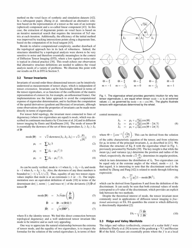
Fig. 1. The eigenvalue wheel provides geometric intuition for why twotensor eigenvalues !i are equal when tensor mode = m is at extremalvalues ±1, as governed by mode = m = cos(3#). The glyphs illustratetensors with eigenvalues determined by the wheel.

central moments µi:

!1 = µ1 +#

2µ2 cos(#)!2 = µ1 +

#2µ2 cos(#"2$/3)

!3 = µ1 +#

2µ2 cos(#+2$/3)(8)

where # = 13 cos"1

%#2µ3#µ2

3

&. This can be derived from the solution

of the cubic characteristic equation of the tensor, and from solutionsfor µi in terms of the principal invariants Ji, as described in [21]. Weillustrate the structure of Eq. 8 with the eigenvalue wheel in Fig. 1,previously presented by Nickalls [29]. The key insight is that while themean (µ1) and variance (µ2) determine the position and radius of the

wheel, respectively, the mode#

2µ3#µ2

3 determines its angular position,

which in turn determines the distribution of !i. Two eigenvalues canbe equal only at the extreme angles of the wheel, mode = ±1. Inthat regard, it is interesting to note that the discriminant used in themethod by Zheng and Pang [42] is related to mode through followingexpression:

D3 =27

2µ3

2 (1"mode(D)2), (9)

which can be derived from Equations 8 and from the definition of thediscriminant. It can easily be seen that both extremal values of modecorrespond to a 0 value of the discriminant, which provides an explicitlink between the two methods.

Despite the theoretical interest of mode, the tensor invariant mostcommonly used in applications of diffusion tensor imaging is frac-tional anisotropy or FA. FA quantifies the extent to which diffusivityis directionally dependent [2]:

FA =

'3

2

|!D||D|

. (10)

3.3 Ridge and Valley Manifolds

The ridges and valleys (collectively, creases) of a scalar field f weredefined by Eberly et al. [9] in terms of the gradient g = % f and HessianH of the field. Creases are essentially points where the f is at a local

extremum, when constrained to the line or plane defined by one ortwo eigenvectors of the Hessian. A function is at extrema where itsgradient is orthogonal to the constraint surface [24], thus ridges andvalleys are where the gradient g is orthogonal to one or two of theunit-length eigenvectors {e1,e2,e3} (with corresponding eigenvalues!1 ! !2 ! !3) of the Hessian H [20]:

Ridge Lineg · e2 = g · e3 = 0

!3,!2 < 0

Valley Lineg · e1 = g · e2 = 0

!1,!2 > 0

To filter out insignificant features, the crease strength is assessed bythe magnitude of the eigenvalues that are required to be negative orpositive for ridges and valleys, respectively [9]. Crease line strength ismeasured by "!2 (for ridges) and !2 (for valleys).

The extraction of crease features of scalar-valued invariants in ten-sor fields is complicated by the non-linearity of the invariants (e.g.,FA(A + B) $= FA(A) + FA(B)). Because differentiation (which is alinear operation) and invariant computation do not commute, one can-not pre-compute the invariants on the regular grid of discrete tensorsamples, and then extract crease features. Our experience has beenthat this has been especially true for mode, which can vary quicklywithin a single voxel. Thus, an important aspect of our approach isanalytically computing the spatial derivatives of invariants. We do thisby evaluating the chain rule for the gradient of invariant J in tensorfield D(x):

%J =dJ

dx=

dJ

dD

dD

dx. (11)

The spatial gradient dDdx of D is a third-order tensor, which is numer-

ically formed by replacing each coefficient Di j (in the matrix repre-sentation of D) by its gradient %Di j . The gradient of J with respectto D is a second-order tensor (like D itself) can be built up formu-

laically with the rules of tensor analysis [18]. For example,d tr(D)

dD = I,d |D|dD = D/|D|, and

d det(D)dD = det(D)D"1, which are sufficient to de-

rive tensor-valued gradients of FA and mode [10]:

d FA(D)

dD=

'3

2

"&(D)

|D|"

|!D|D|D|3

#

(12)

d mode(D)

dD=

3#

6&(D)2 "3mode(D)&(D)"#

6I

|!D|(13)

&(D) = !D/|!D|. (14)

The product dJdD

dDdx in (11) is then computed with tensor contrac-

tion [18].

3.4 Smooth Tensor Field Reconstruction

Following previous work in crease extraction in tensor field [20], weapply a convolution-based method of reconstructing a smooth tensorfield described, similar to previous work [1, 31]. However, as a con-sequence of our algorithmic reliance on the locally-linear property ofnot just the gradient, but also the Hessian eigenvectors, we have foundit useful to have C3-smooth reconstructions, as opposed to the merelyC2 smoothness of cubic B-spline reconstructions. Piecewise polyno-mial reconstruction kernels of tunable smoothness and accuracy havebeen studied extensively by Moller et al., and we have selected the ap-proximating C3 2nd-order accurate filter, which is piece-wise quintickernel with 4-sample support [26]. From this kernel q(x) we define aseparable three-dimensional reconstruction kernel Q(x,y,z)

Q(x,y,z) = q(x)q(y)q(z) (15)

q(x) =

()

*

0 |x|>2

0.1x5 "0.75x4 +2x3 "2x2 +0.8 1< |x|<2

"0.3x5 +0.75x4 " x2 +0.7 0< |x|<1.(16)

The filtering and convolution is computed for each coefficient of thematrix representation of D. We found that extracting the smooth shape

of crease features is improved by additionally smoothing the tensorfield as a pre-process, as described in Section 5. Spatial derivatives ofthe convolution-based reconstructions are measured by convolving thedata with derivatives of the reconstruction kernel [14].

3.5 Crease Lines and Tensor Structure

The contents of this section can be summarized by noting that the ro-bust and accurate numerical computations enabled by smooth recon-struction kernels permit the application of the well established concep-tual framework of crease line extraction to tensor invariants. Further-more the key observation that topological singularities themselves areridge and valley lines of tensor mode underscores the generality of thisframework and its capacity to identify important structures in tensorfields in different contexts. Further evidence is provided in Section 5where we successfully extend this idea to FA in DTI data, an appli-cation domain where topology is not suitable. The following Sectiondescribes the algorithmic solution that allows us to turn this conceptinto a practical tensor analysis tool.

4 IMPLEMENTATION

In this section we describe the algorithmic aspects involved in the ex-traction of ridge and valley lines of a tensor invariant on a voxel grid, inwhich piecewise polynomial kernels provide a smooth reconstructionof the tensor invariant and of its spatial derivatives of first and second-order. Our implementation builds upon a significant body of previouswork in the field of scientific visualization, image analysis, and com-puter vision. Yet, the shortcomings of existing schemes in the specificand challenging case of nonlinear tensor invariants led us to design anew method. For the clarity of the discussion we present in the fol-lowing the basic ideas underlying our method, which we contrast withalternative techniques.

4.1 Isocontour Approach and Limitations

Following the definitions given in Section 3.3 ridge and valleylines can be defined as the one-dimensional intersection of two 0-isosurfaces of the scalar product between the gradient g and one eigen-vector of the Hessian ei. With this approach, each isocontour can becomputed with commonly used isosurface schemes, e.g. MarchingCubes [23]. Yet, this solution requires to assign a consistent orienta-tion to the eigenvector field, which is the basic principle of the methodproposed by Furst and Pizer [11]. In particular, these authors resolvethe orientation ambiguity of eigenvector fields along edges of the voxelby matching their value at both vertices with respect to their averageorientation,which is determined by a Principal Component Analysisfirst proposed by Stetten and Pizer [39].

Unfortunately, we found this approach numerically unstable in ourexperiments, a fact consistent with previous observations [34]. A sim-ple explanation for the rather poor results that we obtained is that thetwo eigenvectorfields involved in that method are quite often ambigu-ous. This situation corresponds to the presence of semi-umbilics –where two eigenvalues of the Hessian are equal – and indicates a localcylindrical symmetry of the scalar measure. Eberly provides a thor-ough analysis of this issue [8]. However the method that he proposesto alleviate this problem requires the computation of the third-orderderivative of the field (the derivative of the Hessian) to define a ridgeflow. This vector field is then used in an iterative search to convergetowards a crease point on a voxel face starting from a nearby location.In contrast, we have chosen to avoid the complexity of a third-orderderivation of our reconstruction kernel in our implementation. A ma-jor motivation for doing so was the significant difficulty involved inderiving analytical expression of the third-order derivative of FA ormode in terms of the coefficients of the tensor and their spatial deriva-tives. We describe in the following our method, in which an efficientand robust adaptive strategy removes the need for third-order deriva-tion.

4.2 Parallel Vector Operator Method

As mentioned in Section 2, the Parallel Vector Operator (PVO) [32]offers an alternative to the intersection of two 0-isosurfaces to com-

pute crease points on triangular faces. Namely, the operator can beapplied to the gradient and the major (resp. minor) eigenvector of theHessian to yield the locations where they are aligned. In its generalform, the PVO takes two vector fields v0 and v1 as input and it deter-mines the locations where v0 and v1 are parallel. Note that this lattercondition is equivalent to v0 % v1 = 0 or, alternatively, &! ' IR, v0 =!v1 or v1 = !v0. From this definition it follows that the PVO alsoidentifies the locations where either vector field is zero. Moreover, ifv0 and v1 are 3D vector fields whose restriction to a triangle is lin-ear, the solution of the PVO on that triangle is obtained through aneigensystem [34]. Indeed, by expressing both vector fields in a localparameterization (u,v) of the triangle as vi(u,v) = Vi(u,v,1)T , wherei ' {0,1} and Vi is a 3%3 matrix, the PVO solution is obtained by

solving V0(u,v,1)T = !V1(u,v,1)T . If V1 is invertible, this is equiv-

alent to V"11 V0(u,v,1)T = ! (u,v,1)T , which is an eigensystem. If

V1 is not invertible but V0 is, the roles of both vector fields can beswapped. If neither matrix is invertible, the system is singular and aninfinite number of solutions exist to the PVO problem [34]. Note thatan alternative computation of the PVO solution which does not assumethe linearity of the vector fields involves an iterative numerical search.Yet, it requires the computation of the Jacobian of the vector fields,which again in our case would necessitate the third-order derivative ofthe considered tensor invariant.

In its linear formulation, the PVO can be applied to the gradientand the major (resp. minor) eigenvector of the Hessian matrix. To doso, the considered eigenvector field must first be oriented consistently.Both vector fields are then linearly interpolated over a triangle, whichyields the eigensystem mentioned previously. It would therefore seemnatural to split the quadrilateral faces of a voxel grid into pairs of tri-angles and to apply this simple method to each of them. The majordrawback of this approach, however, is its assumption of local linear-ity of the vector fields at play. In our case, this assumption is clearlyinvalid at the native resolution of the data [19].

4.3 An Adaptive Method

The solution that we propose follows naturally from the remarks madepreviously. It uses the PVO method in its eigensystem formulationbut it addresses its requirement of local linearity by applying a localrefinement strategy that adjusts the resolution of the analysis to thespatial variations of gradient and eigenvectors of the Hessian. Thedifferent steps of our algorithm are described in the following.

4.3.1 Initial filtering

Our method first applies a simple filtering to the data, which dis-cards the voxel faces in which either the considered invariant has non-interesting values (values under a threshold for ridges, values over athreshold for valleys) or its local crease strength (quantified as !2, re-fer to Section 3.3) has an invalid sign (positive for ridges, negative forvalleys).

4.3.2 Adaptive refinement

For each remaining voxel face, we assign a coherent orientation tothe eigenvectors defined at the four vertices using the PCA method ofStetten [39]. Then we assess the approximation quality of a bilinearinterpolation of the gradient and oriented eigenvector fields. This isdone by comparing interpolated values with the ground truth providedby direct smooth reconstruction from the tensor field, see Figure 3.4,left.

This comparison is done by measuring the angle between thesmooth reconstructed vector and the bilinearly interpolated vector.Note that the vectors are normalized before comparison. A thresholdcontrols the maximal admissible angular discrepancy. This thresholdcan be adjusted to meet the needs of the extraction. In practice, we ini-tially request a maximal angle of $

8 . If interpolation and reconstructiondisagree, the quadrilateral is recursively split in 4 subfaces. Observethat the values at the resulting vertices have already been computed aspart of the approximation quality test. The subdivision stops when theapproximation quality criterion is met or a maximal depth has beenreached. In both cases, we will process the resulting sub-face without

Fig. 2. Left: Need for refinement determined by comparing bilinearinterpolant based on current resolution (gray vertices) with smooth re-construction from tensor data at higher resolution (blue vertices). Right:PVO is applied to both triangular halves by allowing solutions containedin an '-neighborhood around each triangle.

further subdivision. We used a maximum depth of 4 in all our exper-iments, starting from the native resolution of the grid, while in mostcases only 1 or 2 subdivisions were necessary.

4.3.3 PVO method

Once both gradient and eigenvector fields have been found to be prop-erly approximated by low-order interpolation on a given quadrilateralface (or subface), the PVO method can be applied to the correspond-ing pair of triangles. We note that the arbitrary and asymmetric natureof the subdivision in triangles is not problematic in practice since weapply an '-tolerance to include positions lying in the direct vicinityof their common edge (refer to Figure 2, right) and we subsequently”uniquify” potentially redundant crease points.

4.3.4 Verification

The discrepancy between the local piecewise linear interpolation as-sumed by the PVO and the smooth but nonlinear underlying measurecompels us to verify both the validity and the accuracy of the PVOsolutions. To do so we use the smooth reconstruction to obtain bothgradient and eigenvector at the found location. Then, we check that ei-ther the angle between both vectors is small (as measured by 1" | g·e

||g|| |)or that the magnitude of the gradient is converging towards zero. Theformer is checked by imposing a tight error bound (0.005 in our ex-periments). The latter point is controlled by comparing the magnitudeof the gradient at the PVO solution to the average magnitude at thevertices of the processed triangle. If the gradient magnitude is only atiny fraction of the average gradient magnitude in the face, we inter-pret it as a zero value. In practice, a threshold of 5% worked well in allour experiments. Observe that it is important to be able to identify zerogradient values among the solutions of the PVO in cases where the ten-sor invariant reaches its extremum values (e.g. "1/+ 1 for mode). Ifneither criteria are met by the PVO solution, an additional subdivisionis applied around the location of the PVO solution to further refine theapproximation quality of our local linearization. If the refined solutionfails both tests again, the face is discarded.

4.3.5 Connected components

The output of the procedure described above is a point cloud that isfurther organized with respect to the voxels each point belongs to. Wereconstruct connected components from these points by linking pair-wise the points found in the faces of a voxel containing exactly twovertices. If the voxel is associated with more than two crease vertices,we simply select the pair associated with the two highest (resp. low-est) values for a ridge (resp. valley). Note that a more sophisticatedheuristic could be used, in which multiple crease line segments can beidentified by their pairwise signature on the voxel faces and in whichthe ambiguity of the connectivity can be resolved through internal 3Dsubdivision of the voxel. If only one point was found on the side facesof a voxel, two situations are possible. Either the crease line stopsin this voxel (e.g. because the corresponding value of the invariantbecomes non-interesting) or the algorithm described above failed to

converge toward a valid crease point. We rule out false negatives byapplying our adaptive method on the 5 remaining faces of the voxelat a finer resolution, while doubling the approximation accuracy (i.e.dividing the allowed angle discrepancy by 2). The main benefit ofthis search a posteriori is that its higher computational cost is strictlylimited to the relatively few locations where crease lines are alreadyknown to be present. In turn, this feature allows us to work with arather low resolution of the grid and to apply fairly restrictive filteringcriteria in the first stage of the algorithm. Indeed, the only requirementfor a crease line to be completely identified by our algorithm is that atleast one intersected voxel face fulfills the imposed filtering criteria.The remaining points can then be recovered iteratively.

4.3.6 Tracking

Visualization and image processing methods extracting line featuresthrough their pointwise intersection with the faces of a mesh typicallytry to use a tracking strategy to recover a full curve from a single point.When possible, this one-dimensional marching significantly reducesthe computational complexity of the algorithm. Moreover, it permits todisambiguate the connectivity of isolated points on voxel faces. Eberlyproposed such a method [7] that was applied recently by Sahner etal. to extract vortex core lines [36]. This method in fact shares deepsimilarities with the Feature Flow Field [40]. Translated to our setting,however, these methods would require the computation of third-orderderivatives. In contrast, Zheng et al. proposed a method that computesthe tangent of degenerate lines in tensor fields based on the Hessian ofthe tensor discriminant [43]. Therefore it necessitates only the second-order derivatives of the tensor coefficients.

Using mode we can show a very similar result. Indeed, since thedegenerate lines of tensor field topology are ridge and valley lines ofmode associated with global extrema (+1 and "1), the gradient ofmode is uniformly zero along those lines. Moreover, since the minorand medium (resp. medium and major) eigenvalues of the Hessianare by definition both negative (resp. positive) along those lines, itfollows from a simple linear analysis that the tangent of the degenerateline is provided by the major (resp. minor) eigenvector of the Hessianof mode. Furthermore, the associated eigenvalue is zero. Practically,we use this basic result to integrate along ridge and valley lines ofmode corresponding to degenerate lines. Starting from a voxel face,we obtain the next intersection point by integrating along the major(resp. minor) eigenvector of the Hessian. To prevent inaccuracies frombuilding up as we iteratively move across multiple voxels, we use thepoints provided by integration as an approximate location of the creasepoint and apply a PVO computation to a small neighborhood aroundit.

5 RESULTS

5.1 Topology of Stress Tensor Fields

As a first application example of our method, we show how it canbe used to extract the degenerate lines of the tensor field topology.Specifically, we applied our crease line extraction technique to a syn-thetic stress tensor field corresponding to a double point load simu-lation configuration. This tensor field is in fact very similar to theone used by Zheng and Pang in their seminal work on the visualiza-tion of degenerate lines [42, 43]. To generate the data, we samplethe analytic function of two single point loads [41] on a 256 x 256 x128 regular mesh spanning a ["1,1]2x["1,0] volume. The two singleloads are symmetrically positioned with respect to the center of thetop mesh boundary, located at ("0.5,0,0) and (0.5,0,0) respectively.Subsequently, we extract the ridge lines of mode associated with value+1 (corresponding to linear anisotropy, i.e. !1 > !2 = !3) as well asthe valley lines of mode associated with value -1 (planar anisotropy,!1 = !2 > !3). The results are shown in Figure 3.

The structures obtained by our method are remarkably similar tothose previously reported in [42, 43]. Note that to compute the degen-erate lines of a tensor field we only extract a subset of the crease linesof mode, namely those corresponding to its extremal values of +1 and -1. While other crease lines of mode will typically be present, they willnot correspond to degenerate lines and are therefore rejected by our

Fig. 3. Lines of planar and linear anisotropy of the topology extracted asridge (red) and valley (blue) lines of mode with value +1 and -1 respec-tively from a synthetic shear stress tensor field induced by a symmetricdouble point load configuration. The top two images show a gray scalecolormapping of mode on two orthogonal cross sections.

method. Practically, a threshold close to the desired value (+1 or -1)can be applied to determine a small number of voxels that will be in-vestigated. Applying our algorithm to the faces of those voxels yieldsa number of crease points. In voxels where two crease points werefound, their connection provides a local approximation of a degener-ate line. In voxels where only one point was found we simply integratealong the major (resp. minor) eigenvector of the Hessian until we in-tersect the next voxel face. We then iteratively inspect the neighboringvoxel that was reached. This tracking continues until either enteringa voxel that already contained a single crease point, or the integrationalong the eigenvector of the Hessian of mode stops within the voxel,indicating the presence of a spherical degenerate point.

5.2 Analysis of Brain White Matter in DT-MRI

As mentioned previously, an alternative to the topological definitionof tensor structure can be provided by the ridge and valley lines ofanisotropy measures in DT-MRI datasets. In fact, Schultz et al. re-cently showed that topology was unable to reliably characterize struc-tures in DTI data under the presence of noise [38]. On the other hand,previous work on anisotropy crease extraction in DTI suggested thevalue of FA ridges lines, but never demonstrated their geometric ex-traction [20]. We demonstrate here the extraction of FA crease linesto model certain significant white matter tracts. The rationale is that

Fig. 4. Axial view of 425 FA ridge lines (length at least 15mm) withRGB-colored cutting plane (both semi-transparent). Thresholding fur-ther based on average ridge line strength can reduce the set to thestrongest 62 lines (opaque) with more anatomic significance.

Fig. 5. Axial view of main FA ridge lines, with tractography (semi-transparent). CBL, CNR: left and right cingulum bundles; FOR: fornix.

the interior points of regions that remain anisotropic even after somesmoothing must have orientational coherence, and are thus likely tobe fiber bundles. Ridge lines of FA may therefore provide a means ofcapturing the skeleton of certain white matter bundles.

We extracted ridges lines of FA in a human brain DTI scan with res-olution 1.6mm3. Fig. 4 shows the 425 extracted lines with length of atleast 15mm, which includes a number of lines of unclear significance.Further thresholding the lines to select only those with the highest av-erage ridge strength (as defined in Sect 3.3), reveals a smaller subsetof 62 lines that is explored in the following figures.

Figure 5 shows a similar axial view of the main FA ridge lines,including whole-brain tractography seeded at voxels with FA above0.72. The FA ridge lines are shown as thick white tubes amidst thesemi-transparent thin tractography paths. The left (CBL) and right(CBR) cingulum bundles and part of the fornix (FOR) are annotated.These are the main fiber paths that are more tube-like than sheet-like inthe brain white matter [27], so it is fitting that they can be extracted asridge lines of anisotropy. These paths have previously been extractedvia a more involved combination of tractography, clustering, and geo-

Fig. 6. Sagittal view of main FA ridge lines, with sagittal cutting planeand semi-transparent tractography. Inset shows a more coronal andsuperior view of the four ascending paths extracted in the midbrain.

metric processing in recent work by O’Donnell et al. [30]. The CBLand CBR ridge lines, for example, follow the general path of the indi-vidual tractography traces, but the ridge lines succeed in extracting thefiber bundles as single paths through the core of the structure, ratherthan as a cluster of tractography paths. Note also that the fornix, asrepresented by the FA ridge lines, correctly branches into posteriorleft and right tracts. All of these paths complement other white mat-ter structures (such as the corpus callosum) that have been previouslyextracted as ridge surfaces of FA [20].

Figure 6 shows a roughly sagittal view of the same ridge linesshown in Fig. 5, along with a sagittal cutting plane through the leftcingulum bundle (CBL) and semi-transparent tractography. The ex-tracted fornix (FOR) correctly curves inferiorly (towards the bottom ofthe image) closer to the front of the brain (right side of image). Also,both CBL and CBR extend fully inferiorly, showing the full loop ofthe cingulum bundles, which is difficult to capture with conventionaltractography. Also annotated Figure 6 is the right inferior longitudi-nal fasciculus (ILF), which unfortunately was not as cleanly capturedon the left side. The inferior cerebellar peduncles (ICP) were wellcaptured (right ICP shown). In the midbrain four additional pathwayswere captured by FA ridge lines. These are shown in the inset of Fig. 6with a more coronal and superior viewpoint. The extracted FA ridgeslines are mostly centered within the large blue (ascending/descendingdirection) areas of the axial slice, helping identify the paths as the leftand right sides of the medial lemniscus (ML) and cortical spinal tract(CST). While these paths can also be traced with tractography and rep-resented in aggregate by tractograph clustering, our results suggest thatsome major paths may be extracted more directly as a purely structuralproperty of a smooth FA signal, which we feel is simpler from both atheoretical and algorithmic standpoint.

6 CONCLUSION

We have introduced a new versatile framework for the structural analy-sis and the visualization of second-order symmetric tensor fields. Fol-lowing the key observation that the degenerate lines of tensor topol-ogy are equivalently characterized as crease and valley lines of a ten-sor invariant called mode, we have presented an algorithmic solutionthat allows for the robust and accurate extraction of crease lines ofother nonlinear invariants from practical datasets. Our implementationleverages smooth reconstruction kernels and an adaptive refinement

strategy to address the challenge posed by this extraction computationin noisy datasets. Our results show that degenerate lines can be identi-fied by our method in a standard engineering benchmark dataset. Theyalso demonstrate that the ridge lines of FA capture important structuralproperties of the white matter tracts. We find this last point especiallyremarkable and we wish to further study the anatomical relevance ofthis crease-based analysis in future work. Future work will also inves-tigate the stability of the crease lines, subject to noise, to optimize thechoice of invariants and reconstruction kernels used for crease extrac-tion.

ACKNOWLEDGEMENTS

The authors wish to thank Xiaoqiang Zheng and Alex Pang for theirhelp with recreating the shear stress dataset. The implementation ofour method is based on the Teem library (http://teem.sf.net). This workwas made possible in part by the NIH/NCRR Center for IntegrativeBiomedical Computing, P41-RR12553-08, and by NIH grants P41-RR13218 (NAC), R01-MH074794, and U41-RR019703.

REFERENCES

[1] A. Aldroubi and P. Basser. Reconstruction of vector and tensor fields fromsampled discrete data. Contemporary Mathematics, 247:1–15, 1999.

[2] P. J. Basser and C. Pierpaoli. Microstructural and physiological featuresof tissues elucidated by quantitative-diffusion-tensor MRI. Journal ofMagnetic Resonance, Series B, 111:209–219, 1996.

[3] D. E. Bourne and P. C. Kendall. Vector Analysis and Cartesian Tensors.CRC Press, 3rd edition, 1992.

[4] J. C. Criscione, J. D. Humphrey, A. S. Douglas, and W. C. Hunter. Aninvariant basis for natural strain which yields orthogonal stress responseterms in isotropic hyperelasticity. Journal of Mechanics and Physics ofSolids, 48:2445–2465, 2000.

[5] M. de Saint-Venant. Surfaces a plus grande pente constituees sur deslignes courbes. Bulletin de la Societe Philomathematique de Paris, pages24–30, 1852.

[6] T. Delmarcelle and L. Hesselink. The topology of symmetric, second-order tensor fields. In VIS ’94: Proceedings of the conference on Vi-sualization ’94, pages 140–147, Los Alamitos, CA, USA, 1994. IEEEComputer Society Press.

[7] D. Eberly. Ridges in Image and Data Analysis. Kluwer Academic Pub-lishers, 1996.

[8] D. Eberly. Theory of ridges. Inhttp://www.geometrictools.com/Documentation/Ridges.pdf, 2008.

[9] D. Eberly, R. Gardner, B. Morse, and S. Pizer. Ridges for image analysis.Journal of Mathematical Imaging and Vision, 4:351–371, 1994.

[10] D. B. Ennis and G. Kindlmann. Orthogonal tensor invariants and the anal-ysis of diffusion tensor magnetic resonance images. Magnetic Resonancein Medicine, 55(1):136–146, 2006.

[11] J. D. Furst and S. M. Pizer. Marching ridges. In Proceedings of2001 IASTED International Conference on Signal and Image Processing,2001.

[12] J. D. Furst, S. M. Pizer, and D. H. Eberly. Marching cores: A method forextracting cores from 3d medical images. In Proceedings of IEEE Work-shop on Mathematical Methods in Biomedical Image Analysis, pages124–130, 1996.

[13] A. Globus, C. Levit, and T. Lasinski. A tool for visualizing the topologyif three-dimensional vector fields. In IEEE Visualization Proceedings,pages 33 – 40, October 1991.

[14] R. Gonzalez and R. Woods. Digital Image Processing. Addison-WesleyPublishing Company, Reading, MA, 2nd edition, 2002.

[15] R. M. Haralick. Ridges and valleys on digital images. Computer Vision,Graphics, and Image Processing, 22:28–38, 1983.

[16] J. Helman and L. Hesselink. Surface representation of two and three-dimensional fluid flow topology. In Proceedings of IEEE Visualization’90 Conference, pages 6–13, 1990.

[17] L. Hesselink, Y. Levy, and Y. Lavin. The topology of symmetric, second-order 3D tensor fields. IEEE Transactions on Visualization and ComputerGraphics, 3(1):1–11, 1997.

[18] G. A. Holzapfel. Nonlinear Solid Mechanics. John Wiley and Sons, Ltd,England, 2000.

[19] G. Kindlmann, X. Tricoche, and C.-F. Westin. Anisotropy creases delin-eate white matter structure in diffusion tensor MRI. In Proceedings of

Medical Imaging Computing and Computer-Assisted Intervention, MIC-CAI ’06, Lecture Notes in Computer Science 3749, 2006.

[20] G. Kindlmann, X. Tricoche, and C.-F. Westin. Delineating white matterstructure in diffusion tensor MRI with anisotropy creases. Medical ImageAnalysis, 11(5):492–502, October 2007.

[21] G. L. Kindlmann. Visualization and Analysis of Diffusion Ten-sor Fields. PhD thesis, University of Utah, Sept 2004. Chap 2,http://www.cs.utah.edu/research/techreports/2004/UUCS-04-014.pdf.

[22] J. Koenderink and A. van Doorn. Local features of smooth shapes:Ridges and courses. In SPIE, editor, Proc. SPIE Geometric Methods inComputer Vision II, Vol. 2031, pages 2–13, 1993.

[23] W. E. Lorensen and H. E. Cline. Marching cubes: A high resolution3d surface construction algorithm. Computer Graphics, 21(4):163–169,1987.

[24] J. E. Marsden and A. J. Tromba. Vector Calculus. W.H. Freeman andCompany, New York, New York, 1996.

[25] J. Maxwell. On hills and dales. The London, Edinburgh and DublinPhilosophical Magazine and Journal of Science, 40(269):421–425, 1870.

[26] T. Moller, R. Machiraju, K. Mueller, and R. Yagel. Evaluation and designof filters using a taylor series expansion. IEEE Transactions on Visual-ization and Computer Graphics, 3(2):184–199, 1997.

[27] S. Mori, S. Wakana, L. Nagae-Poetscher, and P. V. Zijl. MRI Atlas ofHuman White Matter. Elsevier, 2005.

[28] B. S. Morse. Computation of Object Cores from Grey-Level Images. PhDthesis, University of North Carolina at Chapel Hill, Chapel Hill, NC,1994.

[29] R. W. D. Nickalls. A new approach to solving the cubic: Cardan’s solu-tion revealed. The Mathematical Gazette, 77:354–359, Nov 1993.

[30] L. J. O’Donnell, C.-F. Westin, and A. J. Golby. Tract-based morphome-try. In Tenth International Conference on Medical Image Computing andComputer-Assisted Intervention (MICCAI ’07), volume 4792 of LectureNotes in Computer Science, pages 161–168, Brisbane, Australia, 2007.

[31] S. Pajevic, A. Aldroubi, and P. J. Basser. A continuous tensor field ap-proximation of discrete DT-MRI data for extracting microstructural andarchitectural features of tissue. Journal of Magnetic Resonance, 154:85–100, 2002.

[32] R. Peikert and M. Roth. The Parallel Vectors operator - a vector fieldvisualization primitive. In IEEE Visualization Proceedings ’00, pages263 – 270, 2000.

[33] W. Press, B. Flannery, S. Teukolsky, and W. Vetterling. NumericalRecipes: The Art of Scientific Computing. Cambridge University Press,Cambridge, New York, Melbourne, 1986.

[34] M. Roth. Automatic Extraction of Vortex Core Lines and Other Line-TypeFeatures for Scientific Visualization. PhD thesis, ETH Zurich, 2000.

[35] F. Sadlo and R. Peikert. Efficient visualization of lagrangian coherentstructures by filtered amr ridge extraction. IEEE Transactions on Visual-ization and Computer Graphics, 13(6):1456–1463, 2007.

[36] J. Sahner, T. Weinkauf, and H.-C. Hege. Galilean invariant extraction andiconic representation of vortex core lines. In K. J. K. Brodlie, D. Duke,editor, Proc. Eurographics / IEEE VGTC Symposium on Visualization(EuroVis ’05), pages 151–160, Leeds, UK, June 2005.

[37] G. Scheuermann and X. Tricoche. Topological methods in flow visual-ization. In C. Johnson and C. Hansen, editors, Visualization Handbook,pages 341–356. Academic Press, 2004.

[38] T. Schultz, H. Theisel, and H.-P. Seidel. Topological visualization of braindiffusion MRI data. IEEE Transactions on Visualization and ComputerGraphics, 13(6):1496–1503, 2007.

[39] G. D. Stetten. Medial-node models to identify and measure objects inreal-time 3-D echocardiography. IEEE Transactions on Medical Imaging,18(10):1025–1034, 1999.

[40] H. Theisel and H.-P. Seidel. Feature flow fields. In Proceedings of JointEurographics - IEEE TCVG Symposium on Visualization (VisSym ’03),pages 141–148, 2003.

[41] S. Timoshenko and J. Goodier. Theory of Elasticity. 1970.[42] X. Zheng and A. Pang. Topological lines in 3D tensor fields. In VIS

’04: Proceedings of the conference on Visualization ’04, pages 313–320,Washington, DC, USA, 2004. IEEE Computer Society.

[43] X. Zheng, B. N. Parlett, and A. Pang. Topological lines in 3D tensor fieldsand discriminant hessian factorization. IEEE Transactions on Visualiza-tion and Computer Graphics, 11(4):395–407, 2005.