INTROGRESSION FROM Gossypium mustelinum AND G. tomentosum INTO

UPLAND COTTON, G. hirsutum

A Dissertation

by

BRIAN WAYNE GARDUNIA

Submitted to the Office of Graduate Studies of Texas A&M University

in partial fulfillment of requirements for the degree of

DOCTOR OF PHILOSOPHY

December 2006

Major Subject: Plant Breeding

INTROGRESSION FROM Gossypium mustelinum AND G. tomentosum INTO

UPLAND COTTON, G. hirsutum

A Dissertation

by

BRIAN WAYNE GARDUNIA

Submitted to the Office of Graduate Studies of Texas A&M University

in partial fulfillment of requirements for the degree of

DOCTOR OF PHILOSOPHY

Approved by: Co-Chairs of Committee, David Stelly C. Wayne Smith Committee Members, Rodolfo Aramayo Javier Betran Monica Menz Head of Department, C. Wayne Smith

December 2006

Major Subject: Plant Breeding

iii

ABSTRACT

Introgression from Gossypium mustelinum and G. tomentosum into Upland Cotton, G.

hirusutum. (December 2006)

Brian Wayne Gardunia, B.S., Brigham Young University;

M.S., Brigham Young University

Co-Chairs of Advisory Committee: Dr. David Stelly, Dr. C. Wayne Smith

To increase genetic diversity with elite upland cotton, introgression populations

with wild species of cotton, Gossypium mustelinum and G. tomentosum, were created.

To accomplish this objective, F1, F2, BC1F1, and BC1F2 generations were developed

along with random mating populations (BC1rm1 and BC1rm2) and grown in a

randomized complete block design with four replications in College Station, Texas

during 2003 and 2004, and in Mexico during 2005 for G. mustelinum introgression

populations. These generations were tested with microsatellite markers from

chromosome 11 in order to measure the effects of selection and recombination. Later

generations (BC2F1, BC2rm1, BC2F2, BC3F1, BC3rm1 and BC3F2) and composite

generations were evaluated in a randomized complete block design with four replications

during 2004 and 2005 for agronomic properties.

Introgression barriers for G. mustelinum were found to include daylength

sensitivity and hybrid breakdown, which was only apparent in Mexico. Backcross

generations had improved fiber quality. Random mating populations did not have

increased variance and means differed little from BC1F1 levels. Microsatellite markers

iv

showed decreased frequency of G. mustelinum alleles and decreasing heterozygosity, but

no increase in map distances in random mating populations. Upper-half mean length and

upper quartile length by weight were highly heritable, as measured with parent-offspring

regression. Most other agronomic traits had moderate heritabilities. Composite

generations were found to be favorable for selection and breeding.

For G. tomentosum populations, hybrid breakdown was also a problem with low

yields for F2 and BC1F2 generations, but day length sensitivity was not. Little or no

increase in variance was found in random mating populations when compared to BC1F1

levels. G. tomentosum populations did not show improvements in fiber length as seen in

G. mustelinum populations, but did have increased strength in BC1F1 and F1

generations over TM-1. Mapping distances increased in the random mating populations

for G. tomentosum, and the frequency of alien alleles did not decrease in random mating

populations. Generation means approached recurrent parental values for most traits

within three backcrosses. Composite generations were found to be the most useful for

breeding and selection.

v

DEDICATION

To my family:

Leila, Emily, and Aleah, and to my mother, who made me want to study science and

helped me every time I needed it.

vi

ACKNOWLEDGEMENTS First I would like to recognize the incredible support I have received from Cotton

Incorporated. Cotton Inc. was generous enough to fund my fellowship as well as many

of the research costs related to this study. Without their support, none of this would have

been possible. Cotton Inc. has also enriched my graduate studies in many ways, but most

notably by facilitating attendance at international meetings, the Cotton Breeder’s tour,

fiber testing, molecular markers and supplies, as well as travel and research in Mexico. I

would like to thank Dr. Roy Cantrell, Vice President of Cotton Incorporated, for his

advice and support during my graduate studies. I would also like to thank Lynda Keys

and Dr. Don Jones for their daily support of the CI fellows. I would be remiss if I did not

personally thank Regina Horton and the other technicians in the Fiber Testing

Laboratory. She spent many long hours testing and organizing my samples and all fiber

quality data reported here is the result of their much appreciated help.

Next, I would like to thank all those at the New Beasley lab: Dr. David Stelly,

Wayne Raska, Kelly Biddle, and Nilesh Dighe. Dr. Stelly’s help with my research and

personal support has been constant and essential to my finishing such a large task. You

always encouraged me to have big dreams and ideas. Wayne Raska makes ALL work

possible at the lab and is much more than a technician. I would also like to thank my

fellow graduate students Kelly and Nilesh, who have been my close friends and willingly

endured many hot days chopping weeds and harvesting cotton because of me. I would

also thank the undergraduates who helped with all of the worst jobs: Christian, Kristen,

Katie, Emily, Megan and Ben.

vii

I am also grateful for the training and help given by Dr. Smith and all of the rest

at the Cotton Improvement Laboratory. I always felt welcome and am grateful for the

help with ginning, delinting, seed preparation, field maintenance, planting, spraying, and

advice. I am especially grateful for the help from my fellow graduate students: Chris

Souder, Polly Longenberger, and Chris Braden, as well as Dawn Deno.

The molecular marker analysis would not have been possible without the help of

Dr. Monica Menz, Susan Hall, Andres Guzman, and Arturo Olortegui. Dr. Menz and

Susan were a great help in troubleshooting difficulties with my DNA and procedures.

Arturo, while visiting from Peru, helped do many of the PCR reactions and gels, which

made it possible to finish this work in weeks instead of months.

I would like to thank the entire crew in Técoman, Colima, Mexico for helping

with my experiments there, Cotton Incorporated for funding and travel expenses, and

Wes Malloy, who hosted our visits. I would also like to thank Drs. Osman Gutierrez and

Darryl Bowman for their help making crosses, willingness to give access to their

populations, and daily rides from Manzanillo.

Last, but most of all, I would like to thank my wife, Leila. There were definitely

moments when problems seemed insurmountable and she made sure they were not. I am

grateful for the examples of my two daughters, Emily and Aleah, who look at the world

with such great curiosity and joy. They make me want to learn and achieve great things.

viii

TABLE OF CONTENTS

Page ABSTRACT ............................................................................................................ iii

DEDICATION.......................................................................................................... v

ACKNOWLEDGEMENTS...................................................................................... vi

TABLE OF CONTENTS ....................................................................................... viii

LIST OF TABLES.................................................................................................... x

LIST OF FIGURES ............................................................................................... xiv

CHAPTER

I INTRODUCTION ............................................................................................ 1

Cotton............................................................................................... 1 Interspecific barriers.......................................................................... 4 Structural rearrangements.................................................................. 6 Genetic differences ........................................................................... 9 Selection and linkage drag............................................................... 11 Random mating............................................................................... 13

II Gossypium mustelinum: DAY-LENGTH AND HYBRID BREAKDOWN

AS BARRIERS TO INTROGRESSION OF IMPROVED FIBER QUALITY...................................................................................................... 16

Introduction ..................................................................................... 16 Materials and methods ..................................................................... 17 Results and discussion...................................................................... 25 Conclusions ..................................................................................... 50

III MOLECULAR MARKER ANALYSIS OF CHROMOSOME 11

INTROGRESSION FROM G. mustelinum. .................................................... 56

Introduction ..................................................................................... 56 Materials and methods ..................................................................... 57 Results and discussion...................................................................... 60 Conclusions ..................................................................................... 68

ix

CHAPTER Page

IV ADVANCED BACKCROSS POPULATIONS OF G. mustelinum WITH

UPLAND COTTON: HERITABILITY, SELECTION, AND BREEDING .... 72

Introduction ..................................................................................... 72 Materials and methods ..................................................................... 79 Results and discussion...................................................................... 85 Conclusions ................................................................................... 105

V GENERATION MEANS ANALYSIS OF G. tomentosum:

INTROGRESSION FOR AGRONOMIC PROPERTIES AND INTERSPECIFIC BARRIERS ......................................................................108

Introduction ................................................................................... 108 Early generation means analysis. .................................................... 108 Materials and methods ................................................................... 109 Results and discussion.................................................................... 111 Conclusions ................................................................................... 129

VI MOLECULAR ANALYSIS OF G. tomentosum INTROGRESSION

WITH MICROSATELLITE MARKERS FROM CHROMOSOME 11. ........131

Introduction ................................................................................... 131 Materials and methods ................................................................... 132 Results ........................................................................................... 132 Discussion...................................................................................... 139

VII ADVANCED GENERATION BACKCROSSES AND COMPOSITE

GENERATIONS FROM G. tomentosum: SELECTION, HERITABILITY, AND PERFORMANCE. ..................................................142

Introduction ................................................................................... 142 Materials and methods ................................................................... 144 Results and discussion.................................................................... 146 Conclusions ................................................................................... 165

VIII SUMMARY AND CONCLUSIONS...………………………………….…..168

REFERENCES ......................................................................................................171

VITA…....………………..……...………………………………………………….184

x

LIST OF TABLES TABLE Page

1 Number of plants measured per generation in G. mustelinum early generation mean analysis (GMA) from 2003, 2004, and 2005......................... 20

2 The adjusted marginal means for male sterile, Ms4ms4, and male fertile plants, ms4ms4¸ from 2004 G. mustelinum GMA............................................ 26

3 Significance of fixed and random effects from mixed models for G. mustelinum early GMA plant and yield characteristics.................................... 28

4 Significance of fixed and random effects from mixed models for G. mustelinum early GMA fiber quality measures. .............................................. 29

5 Marginal means by generation for G. mustelinum populations from 2003, 2004, and 2005 yield and plant height............................................................. 31

6 Marginal means by generation for G. mustelinum populations from 2003, 2004, and 2005 for boll weights and NFFB..................................................... 32

7 Marginal means by generation for G. mustelinum populations from 2003 and 2004 for HVI fiber qualities.. ................................................................... 36

8 Marginal means by generation for G. mustelinum populations from 2003 and 2004 for AFIS fiber qualities.................................................................... 37

9 Estimated values for G. mustelinum midpoint (m), additive (a), and dominant (d) genetic effects for yield, height and total number bolls by year. ............................................................................................................... 41

10 Variance by population for G. mustelinum GMA with 95% confidence limits in parentheses. ...................................................................................... 46

11 Pearson's correlations by G. mustelinum BC1F1, BC1rm1, BC1rm2, and BC1F2 generations. ........................................................................................ 48

12 Segregation of chlorophyll deficient mutants in BC1F2 families..................... 50

13 SSR primer sequences used from chromosome 11. ......................................... 59

14 Segregation ratio distortion for SSR markers from G. mustelinum F2, BC1F1, BC1rm1, BC1rm2, and BC1F2 populations. ...................................... 62

xi

TABLE Page

15 Plant numbers measured per generation in G. mustelinum advanced backcross generation testing during 2004 and 2005. ....................................... 81

16 Marginal means for male sterile (Ms4ms4) and male fertile (ms4ms4) plants within generations from 2005 G. mustelinum advanced backcross experiment...................................................................................................... 85

17 Marginal means by male sterile and male fertile plants by population for yield and plant characteristics from G. mustelinum 2005 field experiments..... 87

18 Marginal means by generation for G. mustelinum populations from 2004, and 2005 yield and plant height.. .................................................................... 89

19 Marginal means by generation for G. mustelinum populations from 2004 HVI and AFIS fiber qualities. ......................................................................... 90

20 Variance estimates for plant characteristics by G. mustelinum generations from 2004 and 2005........................................................................................ 93

21 Variance estimates for HVI fiber qualities by G. mustelinum populations from 2004....................................................................................................... 94

22 Variance estimates for AFIS fiber qualities by G. mustelinum populations from 2004....................................................................................................... 95

23 Heritability estimates and standard errors (SE) for G. mustelinum populations from GMA, advanced backcross populations, and parent-offspring regression from 2002 greenhouse BC1F1 populations. .................... 98

24 Performance of descendents in G. mustelinum advanced backcross experimental populations from selected BC1F1 greenhouse parental populations for UHML.. ............................................................................... 102

25 Difference between G. mustelinum top ten percent seed cotton yield plant-1 from 2005 and overall means........................................................................ 103

26 Difference between top ten percent G. mustelinum UHML from 2004 and unselected mean by population.. ................................................................... 103

27 Number of plants evaluated in 2003 and 2004 G. tomentosum GMA experiments. ................................................................................................. 110

xii

TABLE Page

28 Marginal population means for effect of male sterile (Ms4ms4) and male fertile (ms4ms4) plants within G. tomentosum segregating generations from 2004 .................................................................................................... 112

29 Fixed and random effect significance from mixed model analysis for G. tomentosum GMA experiments from 2003 and 2004. ................................... 114

30 Marginal mean yield and plant characteristics for G. tomentosum GMA from 2003 and 2004...................................................................................... 115

31 Marginal mean boll counts and weights for G. tomentosum GMA from 2004.. ........................................................................................................... 116

32 Mean HVI fiber qualities by population from G. tomentosum GMA from 2003 and 2004.............................................................................................. 117

33 Variance estimates by generation and year for G. tomentosum GMA plant and yield characteristics from 2003 and 2004. . ............................................ 120

34 Variance estimates by generation and year for HVI fiber properties from G. tomentosum GMA from 2003 and 2004.. ...................................................... 121

35 Estimates for midpoint (m), additive value (a), dominance (d) from G. tomentosum GMA by year for yield and plant characteristics........................ 123

36 Genetic models for midpoint (m), additive (a), and dominant (d) values for G. tomentosum HVI fiber qualities................................................................ 126

37 Segregation ratios from SSR markers tested on G. tomentosum F2, BC1F1, BC1rm1, BC1rm2, and BC1F2 populations. .................................... 133

38 Plant numbers evaluated in G. tomentosum advanced backcross experiment.................................................................................................... 146

39 The adjusted marginal means for male sterile, Ms4ms4, and male fertile plants, ms4ms4¸ across populations, from the 2005 G. tomentosum advanced backcross experiment. . ................................................................ 147

40 The adjusted marginal means for male sterile, Ms4ms4, and male fertile plants, ms4ms4¸ by population, from the 2005 G. tomentosum advanced backcross experiment. ................................................................................. 148

xiii

TABLE Page

41 Generation means for plant and yield characteristics for G. tomentosum advanced backcross experiments from 2004 and 2005. ................................. 150

42 Generation means for HVI fiber qualities, including both male sterile and male fertile plants, for G. tomentosum advanced backcross experiments from 2004..................................................................................................... 151

43 Variances by generation and year for plant characteristics from G. tomentosum advanced backcross experiments in 2004 and 2005. .................. 154

44 Variances by generation and year for HVI fiber quality from G. tomentosum advanced backcross experiment in 2004.................................... 155

45 Estimated heritabilities from G. tomentosum experiments.............................. 157

46 Difference between selected plants based on pedigree from top greenhouse BC1F1 G. tomentosum and unselected populations from 2004...................... 160

47 Difference for yield between top ten percent of each G. tomentosum introgression popualtion tested from 2004. ................................................... 162

48 Difference between top ten percent UHML G. tomentosum introgression populations and unselected mean values. ...................................................... 165

xiv

LIST OF FIGURES FIGURE Page

1 Scatterplot of observed vs. predicted yield plant-1 for G. mustelinum GMA from 2004 and 2005.. ..................................................................................... 42

2 Scatterplot of observed vs. predicted plant height for G. mustelinum GMA from 2003, 2004, and 2005.. ........................................................................... 43

3 Scatterplot of observed vs. predicted total number of bolls plant-1for G. mustelinum GMA from 2003, 2004, 2005....................................................... 44

4 Boxplots of individual plant heterozygosity by population and scatterplot of allele frequency by population.................................................................... 64

5 Linkage maps for G. hirsutum x G. mustelinum chromosome 11..................... 66

6 Traditional backcross-inbred mating design for breeding with wild species............................................................................................................ 75

7 Backcross-random mating design for breeding with wild species. ................... 76

8 Mating strategy for creation of composite generations. ................................... 77

9. Regression of G. mustelinum BC1F1 midparent UHML (mm) to BC1F2 and BC1RM1 UHML (mm). .......................................................................... 99

10 Observed vs. predicted yields for G. tomentosum GMA from 2003 and 2004. .............................................................................................................124

11 Observed vs. predicted plant heights for G. tomentosum GMA from 2003 and 2004........................................................................................................125

12 Observed vs. predicted UHML for G. tomentosum GMA from 2003 and 2004. .............................................................................................................126

13 Heterozygosity and allele frequency from G. tomentosum F2, BC1F1, BC1rm1, BC1rm2, BC1F2 populations.. .......................................................135

14 Linkage maps from G. hirsutum x G. tomentosum F2, BC1F1, BC1rm1, BC1rm2, and BC1F2 populations showing increase in mapping distance in BC1rm2. .......................................................................................................137

1

CHAPTER I

INTRODUCTION Cotton

The Gossypium genus contains five 52-chromosome species that are widely

regarded as tetraploids due their descent from ancient hybridization between A and D

genome 26 chromosome diploids (Fryxell 1992). These five tetraploid species are:

Gossypium hirsutum L., G. barbadense L., G. darwinii Watt, G. tomentosum Nuttal ex

Seeman and G. mustelinum Meers ex Watt. Only G. hirusutum and G. barbadense are

important textile crops with G. hirsutum dominating the world cultivation due to its

superior yield, but generally lower-quality fiber than G. barbadense. G. darwinii is a

wild relative of G. barbadense found in the Galapagos Islands (Wendel and Percy 1990).

G. tomentosum comes from the Hawaiian and other Pacific islands. It is not cultivated

for fiber, but is occasionally found as an ornamental; it produces a very small amount of

short, reddish-brown lint (Applequist et al. 2001). G. mustelinum is found in a small

area of Brazil. It is the most genetically distant tetraploid species to G. hirsutum

(Wendel et al. 1995).

Four species of Gossypium are grown throughout the world for their fiber:

Gossypium hirsutum L., also known as upland cotton, G. barbadense L., also known as

sea island, pima, egyptian, or american-egyptian cotton, G. arboreum L. and G.

_____________ This dissertation follows the format of Crop Science.

2

herbaceum L. Gossypium herbaceum and G. arboreum are A-genome diploid species

originating from Africa and anciently were cultivated throughout Africa and Asia. In

modern times, they have been largely displaced by higher yielding upland or pima

cottons (Vroh Bi et al. 1999). Upland and pima cottons are AD-genome, 52-chromosome

tetraploids native to Central and South America. Gossypium hirsutum is by far the most

economically important cultivated species, while pima cottons, G. barbadense, are of

higher quality with longer staple lengths, finer fiber, and increased strength but tend to

yield less than upland cultivars. Pima is also more susceptible to the boll weevil which

contributed to decreased acreage in the U.S. and Mexico. (Niles and Feaster 1984)

Lee (1984) reported that genetic yield potential of upland cotton doubled from

the 1930s to 1966 but increased only slightly from the 1960s to about 1980. It has long

been acknowledged that upland cotton has a narrow genetic base and it is generally

accepted by many breeders (Wayne Smith, personal communication) that there is a

critical need for increased diversity in breeding populations. Richmond (1951) noted that

cotton descended from “not more than a dozen introgressions, it is doubtful if future

requirements of special fiber properties, disease, insect, and drought tolerance,

mechanical harvesting, and other specialized uses and properties can be met by the usual

selection methods restricted to present cultivated varieties.” This statement is supported

47 years later by pedigree analysis, as well as, biochemical and genomic DNA markers

(Van Esbroeck and Bowman 1998). In theory, a broad-based germplasm pool allows for

selection of favorable allelic combinations not possible with a narrow base. Although, as

3

Van Esboeck and Bowman (1998) point out, “adaptation” is more important to

increasing yields than genetic distance.

The question then remains, why should breeders use unadapted exotic accessions

instead of predictable elite germplasm? One reason may be to find disease resistance

genes not found in elite germplasm (Ross 1986, Young and Tanksley 1989; Stevens et

al. 1995). Likewise, new alleles from related species can lead to improved quality

(Doganlar et al. 2000) and even yield enhancement (Tanksley and Nelson 1996).

Many G. hirsutum accessions are available that are unadapted, usually day-length

sensitive, and low-yielding, and thus utilized very little in cotton breeding. A subset of

these accessions has been “converted” to day-length insensitivity by backcross

introgression day-length insensitivity alleles (McCarty et al. 1998). These converted

race stocks, CRS, have been an important source of abiotic stress and disease tolerance

(Van Esboeck and Bowman 1998). It was estimated by Jiang (2000) that six percent of

G. hirsutum RFLP markers tested were derived from G. barbadense. Gossypium

barbadense has been seen as a potential source of alleles for improving G. hirusutum

due to its improved fiber quality. G. mustelinum, G. tomentosum, and G. darwinii, the

other AD genome tetraploid species, have been used rarely, probably because they have

shorter fiber, are undomesticated, photoperiodic, and thus difficult to work with in

temperate regions, and produce low yielding progeny when using conventional breeding

programs.

The diploid species have been used though as sources of genes for bacterial

blight (Xanthomonas), cotton rust (Puccinia cacabata Arth. & Holw.), and root knot

4

nematode resistance (Yik and Birchfield 1984). A tri-species hybrid between the two

diploid species G. thurberi, a close relative to the possible D genome progenitor, and G.

arboretum, a close relative to the possible A genome progenitor of tetraploid cotton, and

G. hirsutum, later referred to as triple hybrid, was a source of high fiber strength (Niles

and Feaster 1984).

Although difficult to handle, exotic germplasm may be the key to finding novel

alleles to increase cotton yields, abiotic stress and disease tolerance, and improve fiber

quality. As found in other species, even the wildest germplasm may contain alleles that

will improve elite breeding lines (Tanksley and Nelson 1996). Interestingly, many

QTLs for differences in fiber length and strength between Upland and Pima cotton map

to the D sub-genome, even though this New World (D-genome) diploid species does not

produce appreciable lint (Jiang et al. 2000), which supports the hypothesis that other

species that do not inherently possess desirable agronomic characteristics may harbor

genes that in an adapted background will be beneficial. Recent studies in other crops

have explicitly borne out this principle (Gur and Zamir 2004).

Interspecific barriers

Interspecific breeding efforts are more difficult because the breeder must

overcome some of the genetic isolating barriers in order to introgress the trait of interest

without a large amount of linkage drag. The first barrier that must be overcome is

prezygotic. In natural conditions, species do not hybridize due to temporal, geographic,

or physiological reasons. G. tomentosum for much of its history was isolated in Hawaii,

5

but introduction of cotton plantations to Hawaii resulted in contact with G. hirsutum and

G. barbadense. Hybrid populations have been observed with some intermediate traits,

but on the whole they have remained distinct (DeJoode and Wendel 1992). This may be

due to the ephemeral nature of Gossypium flowers. Upland and pima cotton flowers

open in the morning and are receptive to pollen throughout the day, but by nighttime are

wilting and the stigmas are not receptive to pollen. Gossypium tomentosum flowers on

the other hand last long into the night, and at least according to Fryxell (1979), are not

receptive to pollen until late in the evening and may be moth pollinated, although this

hypothesis has little field evidence to support it. However, observations on petal color,

absence of petal spot, and long style pushing the stigma away from the anthers, as well

as possibly a floral odor, detected by Dr. Fryxell and some others, support this

hypothesis (Fryxell 1979). Gossypium mustelinum populations have existed with native

pima cottons throughout its history as well as introduced upland cultivars, with

apparently little introgression (Pickersgill et al. 1975). It is day-length sensitive and may

have other prezygotic isolating mechanisms that have not been experimentally

determined, in part because there are so few observations of its declining natural

populations (Pickersgill et al. 1975).

Prezygotic barriers to hybridization for these two species can be overcome in

greenhouse conditions, with patience, to handle day length sensitivity and maturity

issues. Although the G. tomentosum stigmas may be unreceptive during the day as

Fryxell (1975) observed, the pollen sheds during daylight hours and can be used to

pollinate G. hirsutum with little difficulty. Crosses with G. tomentosum as female that

6

we attempted almost completely failed, lending support to the possibility that G.

tomentosum normally is pollinated at night.

Besides problems prior to fertilization, other problems may arise in hybrid

populations. There is a wide range of hybrid performance observed in interspecific

populations. Some F1 interspecific F1 hybrids found in plants are sterile, others semi-

sterile, others fertile, and some even have extreme hybrid vigor. Cotton hybrids between

G. hirsutum and G. barbadense have normal pairing, and hybrid vigor for plant height

and yield, but later generations break down (Stephens 1949). The range of hybrid

performance may be due to the combination of isolating mechanisms present in the

species which may include structural rearrangements or genetic effects that result in

hybrid breakdown or sterility.

Structural rearrangements

Structural rearrangements are usually thought of as large chromosomal

differences that accumulate in different species. They include translocations, inversions,

insertions, or deletions. Genomic rearrangements are clear barriers to interspecific

hybridization because they can cause reduced pairing between homologous

chromosomes, the formation of unbalanced gametes, sterility, or semi-sterility.

Structural differences also reduce recombination, especially near the rearrangement

breakpoints, and selection for nonrecombinant genotypes disrupts or inhibits

introgression in these genomic regions. Fishman and Willis (2001) asserted that the

effects of structural differences would be seen as a decrease in F1 hybrid fitness, but an

7

increase in F2 fitness. Sterility in heterozygous translocations comes from creation of

gametes or zygotes deficient for chromosomal segments that make them less fit.

Rieseberg et al. (1995) found that in interspecific Helianthus structural differences

reduced map length and segments with rearrangements were lost, at least for all

individuals tested. Because these areas were not recovered in backcross populations,

Rieseberg et al. (1995) recommended a couple of generations of random sib-mating or

selfing prior to backcrossing to increase the probability of recombination around

breakpoints.

A well documented case study of the effects of translocations in interspecific

populations is found in linkage group 3 of the hexaploid oat map (O’Donoughue et al.

1995). Genomic rearrangements appear to be common in oats, even within Avena sativa

L. (Singh and Kolb 1991). Oats also has a clear karyotype with standard C-banding that

distinguishes many of these differences (Jellen et al. 1993a). Karyotypes of A. byzantina

(C. Koch) and A. sativa show a large terminal translocation between chromosome 7C

and chromosome 17 (Jellen et al. 1993b; Jellen et al. 1997). Using monosomic lines

generated from the two parental species, linkage group 3 was determined to span the

translocated segment and so contained markers from both chromosome 7C and 17 (Fox

et al. 2001). The hypothesized breakpoint is in the middle of an area with little to no

recombination (Fox et al. 2001). Segregation of the quadrivalent in meiosis caused the

formation of duplicate/deficient lines for chromosomes 7C and 17 and significant

segregation ratio distortion.

8

The amenability of cotton to conventional karyotyping is not ideal for diagnosing

genomic reorganization due to small chromosome size and low heterochromatic

polymorphism. FISH-based karyotyping (Henegariu et al., 2001; Islam-Faridi et al.

2002; Kim et al. 2005), while feasible in cotton, has yet to be implemented (personal

communication, David Stelly) and cytologically no karyotypical differences are seen

between these species. Even small structural differences may cause reduced

recombination in those areas and loss of rearranged segments. This is consistent with G.

barbadense introgression efforts of Jiang et al. (2000), although they attribute the

majority of loss of Pima alleles to incompatible epistatic interactions. This is possibly a

barrier, although not a large one since according to Hasenkampf and Menzel (1980)

pairing and recombination between G. hirsutum and both wild species in this study were

close to normal, although there was evidence for a terminal rearrangement in G.

mustelinum that differentiate it from G. hirsutum.

Stephens (1949) theorized that G. hirsutum and G. barbadense may differ for

small regions not detectable with cytological methods. These small differences would

result in small deficiencies and duplications after hybridization and recombination that

would give a selective advantage to non-crossover types, especially in gametophytes

where there is no genetic buffering due to diploidy. They found, supporting this

hypothesis, that genetic ratios were skewed to the recurrent parental type due

presumably to selection against the donor parent (Stephens 1949). This was not the case

for similar intraspecific G. hirsutum populations (Lewis and McFarland 1952).

However, F1 hybrids of G. barbadense and G. hirsutum were fertile and yielded more

9

than F2 populations, which is the opposite of what would be predicted for heterozygous

genomic rearrangements. Molecular markers and sequencing information could be a

powerful tool for finding rearranged genomic regions that are not visible cytologically.

The markers could then be used to distinguish between effects of genomic

rearrangements and gene differences.

Genetic differences

Harland (1939) hypothesized that the hybrid breakdown in Gossypium

interspecific populations was not necessarily due to structural differences, but to

incompatible genetic interactions. Incompatible epistatic or allelic interactions also have

been shown to be an important mechanism for isolating of species, at least in theoretical

models (Orr 1995). In theory, as two populations are separated physically, they

accumulate mutations that are neutral within the population, but are deleterious in hybrid

combination (Orr 1995). These mutations are neutral because they are compensated by

other genes, especially in polyploids. Through time, these mutations build up in isolated

species to be a strong enough barrier to prevent substantial mixing of the two species

once isolation barriers are breached (Harland 1939). Although they do not prevent

formation of hybrids, or reduce initial hybrid vigor, they would increasingly lower

fitness of inbred populations and decrease introgression in regions surrounding the

negative genes. These complexes of genes that prevent introgression and successful

hybridization are sometimes called Dobzhansky-Muller complexes due to their

independent prediction and observation of this barrier to interspecific hybridization

(Dobzhansky 1952 and Muller 1942).

10

Good examples of Dobzhansky-Muller complexes in cotton are the two asynaptic

loci found in G. hirsutum and G. barbadense (Endrizzi et al. 1984). G. hirsutum

genotype is normally As1As1as2as2 and G. barbadense wildtype is as1as1As2As2 and have

normal chromosome synapsis within each species. Hybrids are heterozygous for both

loci and have normal chromosome synapsis. In F2 populations, segregation for these

loci results in one out of sixteen plants that are as1as1as2as2, homozygous recessive for

both asynaptic loci and rendered sterile by asynapsis during meiosis. The hybrid lethality

loci, designated Le1 and Le2, are extreme examples of this type of isolating mechanism.

They are neutral in pima and upland cotton, but lethal in hybrid combination where

either, or both, are combined with a D3-genome of G. klotzchianum or G. davidsonii.

However, double recessive mutants, le1le1le2le2, produce viable hybrids with G.

davidsonii (Endrizzi et al. 1984). Stem tumorigenesis genes, designated G0, Gx, and Gy,

are also found within Gossypium species. The combination GxGy causes the formation

of lethal tumors in incompatible hybrids (Endrizzi et al. 1984).

No nuclear lethality loci have been observed in previous hybridization

experiments with G. tomentosum. Meyer and Meredith (1978) do report that G.

tomentosum carries a gametic incompatibility locus near the H2 locus when crossed with

G. barbadense. They did not find evidence of a complete incompatibility locus for

crosses with G. hirsutum, but they did find skewed segregation ratios consistent with an

incomplete barrier at this position.

It seems likely that most incompatible interactions probably are not lethal, but

would reduce the viability of the hybrid or successive generations. These incompatible

11

interactions could be a mechanism for “breakdown” or even sterility in later generations

of interspecific hybrids, which has been a widely observed problem with G. barbadense

introgression (Stephens 1949), especially as they become inbred. Genetic distances

among the 52-chromosome species are varied but significant in each pairwise

comparison, so it is likely that incompatibilities exist between G. tomentosum and G.

mustelinum relative to G. hirsutum and will have similar breeding ramifications in

hybrid derivatives.

Cytonuclear, i.e., interactions with interspecific nuclear and cytoplasmic genes,

incompatibilities are theorized to accumulate between species and limit introgression

(Cruzan and Arnold 1999). According to their simulations and models recessive lethal

incompatibilities can be maintained in backcross generations, only appearing in selfed

generations. In random-mated populations, they found that the incompatible genes were

not lost, even if they were recessive lethals. Chlorophyll-deficient mutants have been

found in interspecific populations of G. barbadense and G. hirsutum (Endrizzi et al.

1984). An analogous incompatibility arises in G. hirsutum x G. mustelinum F2

populations. Such interlocus interactions are especially important if linked genes affect

agricultural performance or product quality.

Selection and linkage drag

One reason for avoiding the use of exotic germplasm is that productivity and/or

quality of introgression products is unacceptably compromised. “Linkage drag” exists

between the desirable alien gene(s) and one or more undesirable genes. When the

12

breeder selects for a trait of interest in segregating populations and selects for the alien

allele at one or more loci, neutral and deleterious alleles in coupling are selected at rates

proportional to the mapping distances between them and the selected alien alleles. For

negative alleles, like the incompatible alleles discussed previously or even more benign

alleles that are selected against, the opposite is true. Coupled neutral alleles, or

beneficial alleles, are lost because they are linked to the incompatible locus

(Charlesworth et al. 1993). Young and Tanksley (1989) used restriction fragment length

polymorphisms (RFLPs) to quantify the degree of linkage drag in tomato (Lycopersicon

esculentum Mill.) cultivars with the Tm-2 locus introgressed from L. peruvianum. They

found that the linkage drag ranged from 4 to 51 cM of L. peruvianum DNA. One

cultivar retained the entire short arm of the chromosome.

This has been a problem in cotton breeding. With the converted race stocks, it

has taken up to 14 generations of backcrossing to obtain lines with good fiber quality (as

reviewed by Van Esbroeck and Bowman 1998). The difficulty in recovering the

recurrent parent could be attributed to carry-over of deleterious alleles from the donor

parent. Inheritance of beneficial genes linked in coupling with deleterious alleles is made

more difficult and is more likely to be lost during backcrossing. Recovery of the

adapted parent’s high performance level after wide-crosses is rendered difficult when

recombination destroys beneficial multi-locus genotypes. Moreover, the recovery of

desirable performance can be rendered less likely by epistatic interactions, as observed

by Jiang et al. (2000). In order to stack improved alleles into the recurrent parent,

linkages between desirable genes and undesirable epistatic genes must be broken.

13

Random mating

Random mating theoretically would be beneficial to introgression because it

would increase recombination between cultivated and exotic loci which would allow for

novel epistatic combinations of genes. This has been shown in cotton to reduce negative

correlations between traits, for example between the negative correlation yield and fiber

strength (Meredith and Bridge 1971, Miller and Rawlings 1967). Increased

recombination reduces linkage disequilibrium and increases linkage map resolution (Liu

et al. 1996, Lu et al. 2003). Estimates of additivity and dominance are affected by

linkage and so random mating may improve estimates of genetic effects (Dudley 1994).

Silvela et al. (1982) showed that theoretical models predicted that the final response to

selection would be better under random mating, although initial response to selection

was higher under inbreeding. Darvasi and Soller (1995) theorized also that advanced

intercross line populations, developed through cycles of random mating, could “provide

a three- to five-fold reduction in QTL map location as compared with a F2 or BC

population, without increasing in the number of individuals phenotyped or genotyped.”

This would provide increased sensitivity and reliability of marker assisted selection for

quantitative traits, without an increase in population size, a possible limiting factor in

QTL analysis.

For these reasons, random mating has been tested experimentally in a number of

crops, but with mixed results. Meredith and Bridges (1971) and Miller and Rawlings

(1967) showed that random mating was effective in cotton in reducing negative linkages

and increasing variance in breeding populations derived from the Beasley triple-species

14

hybrid. Arbelide and Bernardo (2004) found little to no beneficial effects of random

mating Iowa stiff stalk synthetic (BSSS) backcross generations developed by Syngenta

Seeds on maize testcross performance due to small to no increases in variance for most

traits. Lamkey et al. (1995) used F2-syn8 populations from B73 x B84, two elite corn

inbreds, and found increased testcross variance with random mating, but decrease in

mean yields. They also concluded that the random mated generation was more sensitive

for detecting epistasis and had increased variance compared to the F2 generation without

random mating. Generally, correlations between traits decreased with random mating,

but the authors did not recommend random mating due to decreased means due to

breakage of beneficial linkage blocks (Lamkey et al. 1995).

One of the differences between the cotton random mating experiments such as

Meredith and Bridge (1971) and Miller and Rawlings (1967), and the more recent

experiments in maize by Arbelide and Bernardo (2004) and Lamkey et al. (1995) is that

the maize experiments were performed with elite x elite populations whereas the cotton

experiments were performed with elite x interspecific populations as part of

introgression efforts to extract increased strength while maintaining or increasing yield.

This is a key difference. The effects of breaking up linkage blocks in elite x elite crosses

is expected to decrease mean performance due to formation of less desirable epistatic or

linkage blocks. For this reason, the authors recommend inbreeding and selection which

strengthens the beneficial linkages. In elite x interspecific crosses, less desirable

epistatic blocks already exist and increased recombination forms new and, hopefully,

15

better epistatic combinations, thus random mating may be beneficial. It is for this reason

we would like to test the efficacy of random mating in introgression breeding in cotton.

16

CHAPTER II

Gossypium mustelinum: DAY-LENGTH AND HYBRID BREAKDOWN AS

BARRIERS TO INTROGRESSION OF IMPROVED FIBER QUALITY

Introduction

G. mustelinum is the most distant tetraploid relative to G. hirsutum and is native

to Brazil (Wendel et al. 1994). Genetically it is the most distant from G. hirsutum as

measured with molecular markers (Wendel et al. 1994). G. hirsutum x G. mustelinum

hybrids had slightly reduced numbers of crossovers as measured by chiasmata

frequency, and possibly a terminal rearrangement not found in G. hirsutum from D

genome chromosomes 18, 18, 25 or 26 (Hasenkampf and Menzel 1980). Pickersgill and

Barrett (1975) located three populations of G. mustelinum in Brazil and determined that

phenotypically did not resemble G. hirsutum or G. barbadense populations in the area.

Pickersgill and Barrett (1975) hypothesized that G. mustelinum may be important to

reconstructing the ancient phylogenies of cotton due to its distinct phenotype and

presence in an area thought to be tetraploid Gossypium’s ancestral home.

A key goal of this project has been to increase the genetic diversity within

cultivated G. hirsutum by interspecific hybridization and genetic introgression from G.

mustelinum. We also wanted to evaluate possible barriers to introgression, and test the

efficacy of random mating as a mating scheme for introgression from G. mustelinum in

order to develop effective breeding strategies. A traditional generation means analysis

includes the two parents, F1, F2, BC1F1 to parent 1, and the reciprocal backcross to the

other parent, BC1F1 to parent 2. G. hirsutum cv. “TM-1” was used as the recurrent

17

parent for backcrossing and in creation of the F1 with G. mustelinum. In this study we

did not include backcrosses to G. mustelinum, but included three additional generations

at the BC1 level: BC1F2, BC1rm1 (progeny from intermated BC1F1 parents, rm =

random mating), and BC1rm2 populations. We measured individual plants from each

population for fiber quality as measured by High Volume Instrument (HVI) and

Advance Fiber Information System (AFIS) testing machines, yield per plant (g plant-1),

lint percent (% weight), plant height (cm), and boll number and size (g boll-1) were

evaluated to understand possible economically viable traits from the wild species,

barriers to introgression, and genetic effects. This experiment was grown in College

Station, TX for two years in a long-day environment and also one year in southern

Mexico, a short-day environment. The purpose for the including a long- and a short-day

environment was to evaluate the effect of day-length on performance of introgression

populations. The effect of random mating was tested by looking at mean performance,

variance, and phenotypic correlations.

Materials and methods

Plant material and crossing procedure

TM-1, as noted above, was the G. hirsutum parent in this introgression breeding

study while the G. mustelinum parent was from the breeding stocks of Dr. David Stelly,

originally collected by Dr. Margaret Menzel. The initial hybridization does not require

hormone treatment or embryo rescue, although G. mustelinum is day-length sensitive

and requires a juvenile period before induction of flowering, which complicates timing

18

of crossing. The random mating BC1rm0 population was created by crossing Ms4-TM-1

x (TM-1 x G. mustelinum). Ms4-TM-1 was developed by backcrossing the dominant

male sterile gene, Ms4, into TM-1 for at least 16 backcrosses (R. Kohel, personal

correspondence). Ms4 was found in a single heterozygous plant within a seed increase of

‘Acala 44’ in 1960 (Allison and Fisher 1964). The Ms4-TM-1 is heterozygous for a

dominant nuclear male sterility locus designated Ms4ms4 and segregates 1:1. Because

Ms4-TM-1 had been backcrossed to TM-1 at least sixteen times (R. Kohel, personal

correspondence), and it was considered isogenic and was also used as a recurrent parent

in the crossing scheme. A BC1F1 population segregating for male sterility was

constructed from crosses of the interspecific F1 onto male sterile Ms4-TM-1 plants; this

BC1F1 population served as the base random mating population, or BC1rm0.

Initial BC1F1 populations consisted of 150 plants for backcrossing (TM-1 x

(TM-1 x G. mustelinum)) and 150 plants for random mating (Ms4 x (TM-1 x G.

mustelinum)). Only half of the BC1F1 plants for random mating carried the Ms4 gene

and were male sterile. Each male sterile plant was crossed as female with at least two

different male fertile plants. Pedigree of each cross was maintained, as pollen from

multiple males was not combined. Populations of BC1rm1 were created by planting one

seed from up to four intermatings with each male-sterile female. This was done in order

to maximize the number of different males and females. This increased the random

mating population size to almost 300 plants. In subsequent cycles of intermating, two

progeny from each female plant were included with different male parents to maintain

the population size. All crossing was performed in greenhouse facilities at the Texas

19

Agricultural Experiment Station at College Station. Day-length sensitivity and maturity

issues required crossing through the winter season in order to minimize selection for

early maturing genotypes. All additional backcrossing was made with TM-1 as the

recurrent parent. Open-pollinated seed from the greenhouse, where there was no access

to insect pollinators, was assumed to be self fertilized.

Field evaluation

Field evaluations were performed in 2003 and 2004 at the Agriculture

Experiment Station near College Station, TX. Soils at this site are generally Westwood

silt loams. Entries included two commercial checks, ‘Fibermax 832’ (FM832) and

‘Phytogen 355’ (PSC355), the parents, TM-1 and G. mustelinum, and F1, F2, BC1F1,

BC1F2, BC1rm1, and BC1rm2 generations. The number of plants tested for each

generation is found in Table 1. The experiment was planted as a randomized complete

block with four replications each year. Genotypes and generations were planted in rows

12.2 x 1 m with each row consisting of 25 plants spaced 45 cm apart. Observations were

made on individual plants. Planting occurred between the 10th and 30th of April and

harvest was completed by the 15th of November in both years. In 2003, plants were

established in Jiffy® peat pellets in the greenhouse at the end of March and transplanted

to the field the third week in April. In later years, all plants were direct seeded at three

seeds per hill and thinned to one plant per hill. Pedigree of each plant was recorded. All

cultural practices were consistent with commercial cotton production at College Station,

Texas, including furrow irrigation when needed, chemical and mechanical weed control,

pesticide application, and participation in the boll weevil eradication program, with the

20

exception that plants were not chemically defoliated to reduce the effect of late maturity

of some generations on experimental results.

Table 1. Number of plants measured per generation in G. mustelinum early generation mean analysis (GMA) from 2003, 2004, and 2005. Generation 2003 2004 2005 G. must 11 30 4 F1 80 37 45 F2 74 95 99 BC1F1 95 160 90 BC1rm1 267 142 90 BC1rm2 156 174 90 BC1F2 185 126 88 TM-1 79 95 42 FM832 88 95 42 PSC355 182 98 48

In winter of 2005, an experiment was planted at Técoman, Colima, Mexico at the

United States Department of Agriculture’s (USDA) Cotton Winter Nursery in order to

measure the effect of day-length sensitivity on agronomic performance. This included

the same genotypes and generations as noted above, with plant numbers in Table 1. It

was planted as a randomized complete block field design with three replications. Seeds

were planted in hills and seedlings thinned to one plant per hill. Data were collected

from individual plants and pooled by genotype or generation, i.e., pedigree of each plant

was not maintained as in College Station, Texas. The experiment was planted the last

week in October, 2005, and harvested the first week in April, 2006.

Plant morphology measures included plant height (cm), total number of bolls,

nodes to first fruiting branch (NFFB), total seedcotton weight plant-1 (g), lint weight

21

plant-1 (g), and seed weight plant-1 (g). In 2003, only total boll counts were taken, not

separate counts for harvested and unopened bolls. NFFB was also not measured in

2003. All plants were hand harvested and all years from College Station, TX were

ginned on a laboratory roller gin with no lint cleaners. Samples from Mexico were also

manually harvested, but ginned on two laboratory saw gins with no lint cleaners.

Seedcotton weight, which is the weight of unginned cotton, per plant was used as a

measure of yield. After ginning, weight of lint and seed were used to calculate lint

percent and lint weight boll-1. In 2004 and 2005, it was possible to use the number of

harvested bolls to calculate the weight of seedcotton boll-1 as well as lint and seed weight

boll-1. The weights of seedcotton boll-1, lint boll-1, seed boll-1 were not calculated for

2003 since number of harvested bolls was not recorded.

Fiber properties were determined for the two control cultivars, parents, F1, and

all segregating generations grown at College Station in 2003 and 2004. Fiber collected

from individual plants in the harvest and ginning process described above was evaluated

by Cotton Incorporated at their Cary, NC headquarters. Two different testing methods

were used. The first was High Volume Instrument (HVI) testing using machinery

manufactured by Zellweger Uster international (Switzerland) that measures micronaire,

a measure of resistance of the sample to airflow and is considered to be an estimate of

maturity and/or fiber fineness, fiber length as upper-half mean length (UHML reported

in inches by the Uster HVI), uniformity index as a percentage of the upper-half mean

length to the mean fiber length, fiber bundle strength (g/TEX), elongation (%), and short

fiber content (% of fibers less than 1.26 cm based on fiber length weight classes). Fiber

22

strength (g/TEX) is the gram force required to break a bundle of fibers with a theoretical

length of 1000 m. Elongation (%) is the percent stretch before break in the measurement

of strength. This machine also measures color and trash content, but these were not

performed due to small size of samples and relatively large amounts of trash. This is the

method used by USDA to class all bales of cotton grown in the United States that enters

commercial trade. It is a fast and efficient way to measure fiber quality, but requires 10

g fiber samples for accurate testing of micronaire and strength. A separate micronaire

test was used on samples weighing between three and ten grams using Fiberweigh and

Fibernaire parts from the MCI 3000 (Motion Control Instruments HVI machine). This

micronaire value was manually entered into the HVI machine for more accurate

measurement of fiber strength and elongation.

The Advanced Fiber Information System (AFIS) manufactured by Zellweger

Uster International (Switzerland) also was used to measure fiber quality. AFIS testing

requires much smaller samples because it individualizes the fibers in the sample and

pushes them in a constant airflow past a sensor that can detect the change in electrical

conductivity caused by passage of each fiber. This is used to measure fiber length as

mean (ML) and upper quartile lengths (UQL reported in inches by the AFIS) for the

distribution of fibers per sample by weight and by number. It also calculates span

lengths used in the spinning industry as well as counting the number of fiber

entanglements, called neps, and the amount of small trash per sample. Fiber maturity

and fineness of fibers are determined by the Uster AFIS. The AFIS system measures a

23

number of other fiber characteristics but these were not considered to provide enough

additional information and thus not determined on these samples.

Statistical analysis

In order to calculate mean performance for each generation by year, experiments

from different years were analyzed separately to determine differences in means and

variances across years and then combined after testing for homogeneity of variances

with a modified Levene’s test as described in Neder et al. (2002). Each trait was

analyzed with SAS v8.0 (SAS Institute, Cary, NC) using mixed model analysis with

PROC MIXED and the following model, trait = β0 + β1replication + β3generation + ε for

separate environments. Replications and plants within generation were considered

random. Experimental units were individual plants within an entry, which for

segregating generations could not be replicated. Replication effects were considered

random to account for field variability and differential weathering due to time of harvest.

Generations were fixed effects. Traits with multiple years and locations were modeled

with trait = β0 + β1year + β3location + β4generation + β5rep(year) + β6generation*year +

β7generation*location + ε. Locations, generations, and generation*year were considered

fixed effects. Year, rep(year), and generation*year were considered to be random

effects. Means for generations were calculated using LSMEANS which adjusts means

for other variables in the model. Multiple comparisons were tested for significance with

the Tukey-Kramer adjusted least significant difference (LSD), which is adjusted for

multiple comparisons. SAS output for these comparisons was long and cumbersome;

output was condensed into letter groupings of similar means with a SAS macro written

24

by Saxton (1998). Fixed effects were tested for significance with approximate F-tests

provided by SAS PROC MIXED. Random effects were tested for significance with

likelihood ratio tests as the difference between the full model and model excluding a

random effect.

In order to estimate variances per generation per year, the data set was analyzed

separately by generation with the following model: trait = β0 + β1replication + β2plant +

ε, with replication and individual plants as random effects using PROC MIXED. This

allowed for calculation of the variance per generation on an individual plant basis while

excluding effect of replication as well as computation of confidence limits for each

variance estimate. Variances were considered significantly different if the confidence

limits for different generations did not overlap.

Genetic models were estimated using weighted least squares as described by

Lamkey et al. (1995). Weights were calculated as the inverse of the variance for that

generation so that more weight is given to the generation with lower variance in

estimation of genetic effects. The simple genetic model assumed that all traits were

controlled by only additive and dominant effects with no epistasis and no linkage

disequilibrium. The other included effects of epistasis, but not linkage. Predicted means

were compared to actual values and tested with a Chi-square test. Effects of

recombination were also examined by calculating Pearson’s correlation coefficients for

yield, fiber quality, and plant characteristics on an individual plant basis.

25

Results and discussion

Effects of Ms4 on generation means

One question central to the design of this experiment was whether the use of

Ms4ms4 isoline to facilitate crossing confounded the experimental results. This question

had increased importance due to delayed scoring for male sterility in the 2003 field

because of misconceptions about the magnitude of the difference between fertile and

sterile plant morphology. It was assumed that the differences would be striking, when in

reality, late in the season, unless a plant was still flowering with consistent pollen shed

or absence thereof, no differences in plant morphology or yield could be conclusively

tied to the Ms4ms4 genotype. In 2004, this was corrected by scoring for male sterility as

soon as flowering began and throughout the season. In 2005, plants in Mexico were not

scored for male sterility.

In 2003, the field was near a wooded area with plentiful bees and so would be

expected to have less effect of male sterility due to increased pollinators than more

isolated plots or within larger areas of cotton cultivation. In 2004, the experimental plots

were surrounded by cotton fields farther from apparent bee habitats. Nonetheless, the

male sterile plants and the male fertile plants were not statistically significant for most

measured characteristics, as shown in Table 2 (overlapping confidence limits). The only

significant difference was in plant height (T-test, p-value < 0.05).

26

Table 2. The adjusted marginal means for male sterile, Ms4ms4, and male fertile plants, ms4ms4¸ from 2004 G. mustelinum GMA. Parentheses contain 95% confidence limits. Plant characteristics

Height (cm)

Total bolls†

Harvested bolls

Immature bolls

ms4ms4 136.0 (129, 143) 41.0 (36, 46) 29.0 (25, 33) 10.0 (7, 12) Ms4ms4 152.0 (144, 160) 42.0 (36, 47) 26.0 (21, 31) 14.0 (11, 17) Yield characteristics

Yield

(g plant-1) Lint percent

(%) Boll size (g boll-1)

Lint/boll (g boll-1)

ms4ms4 54.5 (43.2, 65.7) 28 (27, 29) 1.82 (1.65,2.00) 0.514 (0.45, 0.58) Ms4ms4 43.2 (30.9, 55.6) 27 (26, 28) 1.67 (1.47,1.87) 0.465 (0.40, 0.54) Fiber characteristics

UHML (mm)

Strength (g Tex-1)

UQLw (mm)

Fineness index

ms4ms4 29.21 (28.7, 29.7) 32 (31, 33) 31.0 (30.5, 31.5) 162.0 (158, 165) Ms4ms4 29.97 (29.5, 30.5) 33 (32, 34) 32.0 (31.5, 32.5) 161.0 (156, 165)

†Includes empty burrs that were not harvested, but were fully mature.

On average, Ms4ms4 plants were 16 cm taller than fertile plants of the same

generation, but with the same total number of bolls. The male sterile plants also tended

to have more green bolls at harvest time. This suggests that the expected decreased boll

set due to male sterility was compensated by a longer fruiting period. The yields were

decreased by 11 g plant-1, but even this was not a significant difference. The lower

yields were probably due to fewer harvested bolls and smaller boll size. Lint percent

and lint per boll were decreased slightly by the Ms4 allele. The smaller boll size may be

due to fewer first position bolls set on the plant due to the male sterility and

compensation with more second and third position bolls. The later positions tend to be

smaller with slightly lower fiber qualities (Wu et al. 2005, Jenkins and McCarty 1995).

Interestingly, fiber qualities were generally improved slightly in the male sterile plants

27

with increased fiber length (both UHML and UQLw), increased strength, and decreased

fineness, which would not be fully explained by increased second and third position

bolls.

There is little evidence to suggest that these differences may be due to source of

the Ms4 gene. It was found in a field of ‘Acala 44’ in 1960 (Allison and Fisher 1964).

The Acala cultivars of cotton tend to have better fiber qualities than the early DeltaPine

cultivars that were the ancestors of TM-1. Since that time, it was backcrossed sixteen

times to TM-1, the parent used in this study (R. Kohel, personal correspondence). Each

time it was selected for male sterility and the TM-1 phenotype. There is the possibility

of some linkage drag around the Ms4 locus, but it is expected to be small due to the

many generations of backcrossing.

Generation means for yield and plant characteristics

While acknowledging the potential effects of male sterile plants, these plants

could not be removed from the 2003 and 2005 Mexico data and were not removed from

the 2004 College Station, TX data. There was significant genotype x location interaction

for traits measured on experiments in Texas and Mexico (Table 3) (p-value < 0.05, F-

test). There was evidence for the effect of year on plant height, total number of bolls

(Table 3), and fiber qualities: strength, elongation, elongation, maturity, fineness, and

IFC (Table 4, p-values < 0.05, likelihood ratio tests).

28

Table 3. Significance of fixed and random effects from mixed models for G. mustelinum early GMA plant and yield characteristics. Yield§ Height§ Lintperc§ Tboll§ Fixed F† F F F generation 27.78 **** 29.29 **** 259.98 **** 7.43 ** location 5.22 * 7.87 *** 0.33 NS 0.54 NS gen*loc 4.31 **** 3.34 **** 5.9 **** 4.14 **** Random G‡ G G G rep(year) 76.4 **** 0 NS 1 NS 10.2 *** year 2.7 NS 100.3 **** 0 NS 59.8 **** gen*year 80 **** 48.4 **** 0 NS 61.2 **** HBoll§ Wboll§ Lboll§ NFFB§ Fixed F† F F F generation 53.05 **** 592.46 **** 912.78 **** 223.9 **** location 0.51 NS 326.4 **** 249.84 **** . ¶ gen*loc 15.78 **** 18.85 **** 33.19 **** . ¶ Random G‡ G G G rep(env) 45.5 **** 0 1 0.5 NS 17 ****

*, **, ***, **** p-value significant at 0.05, 0.01, 0.001, 0.0001 levels, respectively. NS p-value > 0.05. †F-test ‡ Likelihood ratio test §Yield = Seedcotton plant-1 (g plant-1), Height = plant height (cm), Lintperc = lint percentage (%), Tbolls = total number of bolls (count), Hboll = number of harvested bolls (counts), Wboll = weight boll-1 (g), Lboll = lint weight boll-1 (g), and NFFB = number nodes to first fruiting branch (counts). ¶NFFB not measured in Mexico

29

Tabl

e 4.

Sig

nific

ance

of f

ixed

and

rand

om e

ffect

s fro

m m

ixed

mod

els

for G

. mus

telin

um e

arly

GM

A fi

ber q

ualit

y m

easu

res.

M

IC§

U

HM

L§

UI§

ST

R§

EL

O§

Fi

xed

F†

F

F

F

ge

nera

tion

33.4

**

**

23.6

1 **

**

8.19

**

4.

71

* 9.

58

***

R

ando

m

G‡

G

G

G

G

re

p(ye

ar)

27

****

8.

3 **

98

.1

****

12

**

* 12

.9

***

year

0

NS

1.4

NS

4.1

* 3.

7 *

6.3

**

year

*gen

1.

6 N

S 2.

3 N

S 3.

7 *

29

****

18

.5

****

U

QLw

§

SFC

w§

M

at§

Fi

ne§

IF

C§

Fi

xed

F

F

F

F

F

ge

nera

tion

14.5

1 **

5.

61

* 11

.36

**

39.4

7 **

**

2.95

N

S

Ran

dom

G

G

G

G

re

p(ye

ar)

19.3

**

**

158.

8 **

**

18.6

**

**

14.7

**

**

12

***

year

0

NS

2.7

NS

20.8

**

**

12.1

**

* 16

.9

****

ye

ar*g

en

3.3

NS

6.6

**

10.1

**

5.

7 *

74

****

N

S p-

valu

e >

0.05

. *,

**,

***

, ***

* p-

valu

e si

gnifi

cant

at 0

.05,

0.0

1, 0

.001

, 0.0

001

leve

ls re

spec

tivel

y.

† F-te

st .

‡ Li

kelih

ood

ratio

test

. § M

IC =

mic

rona

ire, U

HM

L =

uppe

r hal

f mea

n le

ngth

(mm

), U

I = u

nifo

rmity

inde

x (%

), ST

R =

stre

ngth

(g te

x-1),

ELO

=

elon

gatio

n (%

), U

QLw

= u

pper

qua

rtile

leng

th b

y w

eigh

t dist

ribut

ion

(mm

), SF

Cw

= sh

ort f

iber

con

tent

(%),

MA

T =

mat

urity

in

dex,

IFC

= im

mat

ure

fiber

con

tent

(%),

FIN

E =

finen

ess

inde

x.

30

The means for plant characteristics are presented in Table 5. They include plant

height, individual plant yield and total number of bolls. This was expanded in 2004 to

include the harvested bolls per plant, the number of immature bolls, the number of nodes

to the first fruiting branch (NNFB), and the boll weight, lint weight boll-1, and seed

weight boll-1. Yields in 2003 were low for experimental populations with yields in the

BC1 generations averaging less than 5 g/plant. Boll numbers were significantly lower

than in 2004 also. This was likely due to adverse conditions in 2003 including early-

season low rainfall, followed by flooding, and herbicide damage. Surprisingly, plant

heights were similar across years at College Station. This suggested that adverse

conditions lowered yields, but given a long enough growing-season these negative

effects could have been ameliorated. As seen in the commercial checks that were able to

compensate within the growing season and had comparable yields to 2004. For this

reason, in 2004, planting was earlier and harvesting later in order to maximize yields of

introgression populations

31

Table 5. Marginal means by generation for G. mustelinum populations from 2003, 2004, and 2005 yield and plant height. Significant differences tested with Tukey-Kramer adjusted LSD. Means with different letter groups are significant at p-value < 0.05. 2003 Yield§ Height§ Lintperc§ Totalboll§ Gmust† -1.5‡ C 164.0 BC -¶ -0.4‡ CDEF F1 0.0 C 215.2 A -¶ 0.0 F F2 0.3 C 140.7 CD 33.3 ABC 0.1 EF BC1F1 4.7 C 164.4 B 26.8 C 14.2 AB BC1F2 1.2 C 130.2 D 29.4 C 6.4 DE BC1rm1 2.1 C 150.7 C 28.4 C 11.9 ABC BC1rm2 2.0 C 146.6 C 27.9 C 12.7 ABC TM-1 74.6 B 93.1 EF 32.9 B 17.0 A FM832 116.7 A 81.5 F 40.0 A 8.6 BCD PSC355 110.5 A 94.9 E 41.3 A 16.1 A 2004 Yield Height Lintperc Totalboll Gmust† 0.5 D 193.9 B -¶ 0.4 F F1 1.3 D 219.2 A 27.2 CD 13.8 EF F2 0.8 D 149.7 D 23.9 D 7.3 F BC1F1 40.6 C 162.1 C 27.1 D 46.4 A BC1F2 30.5 C 127.5 F 27.5 D 29.9 CD BC1rm1 28.1 C 140.2 DE 26.8 D 27.0 D BC1rm2 38.4 C 135.4 EF 27.8 D 41.4 AB TM-1 139.1 A 106.5 G 34.2 C 31.7 CD FM832 112.0 B 102.8 G 39.2 B 25.3 DE PSC355 134.9 A 102.3 G 41.4 A 37.2 BC 2005 Yield Height Lintperc Totalboll Gmust† 4.6 DEF 156.8 ABCD -¶ 1.3 EF F1 85.6 C 166.9 A 24.5 DE 60.8 A F2 3.3 F 138.3 B 20.7 E 10.3 F BC1F1 135.4 B 128.7 BC 28.4 C 45.2 B BC1F2 39.8 E 115.1 DE 26.6 CD 23.1 E BC1rm1 65.8 CD 117.6 CD 27.6 CD 33.6 CD BC1rm2 87.9 C 119.1 CD 26.9 CD 41.9 BC TM-1 185.9 A 113.7 CDE 34.1 B 28.0 DE FM832 137.7 B 101.0 EF 43.6 A 21.9 E PSC355 119.2 B 93.2 F 42.8 A 21.5 E

†Gossypium mustelinum. ‡Negative estimates are result of least squares estimates. Should be considered to be essentially zero. §Yield = Seedcotton plant-1 (g plant-1), Height = plant height (cm), Lintperc = lint percentage (%), and Tbolls = total number of bolls (count). ¶No data because of zero yield.

32

Table 6. Marginal means by generation for G. mustelinum populations from 2003, 2004, and 2005 for boll weights and NFFB. Significant differences tested with Tukey-Kramer adjusted LSD. Means with different letter groups are significant at p-value < 0.05. 2004 Hboll§ Wboll§ Lboll§ NFFB§ Gmust† 0 F -¶ -¶ 47 A F1 14 EF 0.89 CD 0.27 C 29 B F2 7 F 1.00 D 0.22 C 28 B BC1F1 46 A 1.56 CD 0.42 C 11 C BC1F2 30 CD 1.41 CD 0.40 C 10 D BC1rm1 27 D 1.61 CD 0.43 C 11 C BC1rm2 41 AB 1.64 C 0.45 C 9 D TM-1 32 CD 4.62 A 1.58 B 7 E FM832 25 DE 4.82 A 1.89 A 8 E PSC355 37 BC 3.81 B 1.56 B 7 E 2005 Hboll§ Wboll§ Lboll§ NFFB‡§ Gmust† 1 EF -¶ -¶ F1 61 A 1.77 E 0.44 EF F2 10 F 1.21 F 0.30 F BC1F1 45 B 3.40 C 0.99 C BC1F2 23 E 2.17 DE 0.60 DE BC1rm1 34 CD 2.32 D 0.64 D BC1rm2 42 BC 2.46 D 0.66 D FM832 22 E 6.22 A 2.78 A PSC355 22 E 5.37 B 2.31 B TM-1 28 DE 6.71 A 2.30 B

†Gossypium mustelinum. ‡NFFB not measured in Mexico 2005. §Hboll = number of harvested bolls (counts), Wboll = weight boll-1 (g), Lboll = lint weight boll-1 (g), and NFFB = number nodes to first fruiting branch (counts). ¶ No data because of zero yield.

33

Almost no yield or bolls were observed in G. mustelinum, F1, or F2 generations

both years at College Station, TX. This was due to late maturity as seen with the number

of nodes to the first position fruiting branches (NFFB) (Table 5). The first flowers in the

F1 and much of the F2 were observed in late September, which is the end of the

productive flowering period for adapted cultivars. They were also very tall, greater than

2 m for the F1, with very small bolls, at 0.9 g boll-1. Only two plants in the F1 and three

in the F2 yielded enough for fiber testing in 2004. The F2 population was apparently

segregating for maturity factors because the NFFB ranged from 8 to 57, as compared to

the F1 at 29 to 39 nodes. Despite some plants flowering earlier than the F1, the F2

generation still had very low yields both years (Table 6).

The BC1 yields were higher than the F1 and F2 yields in 2004 and 2005 than in

2003 (Table 5). However, the BC1F1 remained lower yielding than the recurrent parent,

TM-1, all years, but yielded equivalent to commercial checks (Table 5) TM-1 outyielded

all backcross generations, whether traditional or random mated backcrosses within all

environments tested. The BC1rm1, BC1rm2, and BC1F2 yields were not different

(p>0.05, Tukey-Kramer adjusted LSD). Estimates of yields excluding male sterile

plants did not change estimates of yields by statistically, or biologically significant

levels; the same relationships existed between BC1 generations as well as the mean

differences. For this reason, male sterile plants were not removed from analysis. Lint

percent remained near 27% for the random mating generations. The decrease in yield in

BC1F2 and BC1rm1 generations apparently was due not only to fewer bolls but to a

34

decrease in boll size as well, for the BC1F2 generation. Some premature boll abscission

was observed in BC1F2 generation.

Although introgression from G. mustelinum requires overcoming low yields due

to late maturity and day-length sensitivity, small boll size, and low lint percent,

introgression populations have improved fiber length (Tables 7 and 8). The few samples

from the F1 and F2 generations from 2004 had average HVI UHMLs of 33.9 and 30.1

mm and AFIS UQLw of 35.6 and 32.8 mm, respectively, which is higher than the

UHML of TM-1 of 28.4 mm. The BC1F1 generation exhibited improved (p<0.05, Tukey

Kramer adjusted LSD) UHML relative TM-1 in at College Station in 2003 and 2004 but

the BC1F2 did not. This may suggest a loss of hybrid vigor for this fiber trait but most

likely represents normal segregation for the fiber length genes that would have been

heterozygous in the BC1F1. While the F1, F2, and BC1F1 data on fiber length are

encouraging relative to introgression of fiber length, the BC1F2 data suggest that large

numbers of plants in segregating generations must be sampled in order to identify

desirable phenotypes that will be fertile after selfing.

Fiber strengths were higher for all introgression populations in 2004 but not in

2003, except for the BC1F1 than TM-1 levels (Table 7). The F1, BC1F1, BC1rm1, and

BC1rm2 generations had finer fiber than the recurrent parent, TM-1, both years, based

on micronaire (Table 7) and AFIS fineness readings (Table 8). However, they also had

increased immature fiber content in both years and decreased maturity indices in 2004

(Table 8). The decrease in fiber maturity probably may have been related to the overall

maturity of the plants. At time of harvest, TM-1 and commercial checks had stopped

35

flowering and most bolls were open. The BC1 generations weren’t as delayed in College

Station as the F1 and F2 generations, but it was obvious that many of the plants, if given

more time would have continued to open and produce more bolls. The plants were not

fully mature and they were maturing fruit during day lengths and temperatures not

conducive to boll and fiber maturation and so it is logical that more of the fiber would be

immature.

Because many plants in BC1 generations were late-maturing, plots were not

defoliated in order to maximize potential yields. All plots were hand harvested and so

harvest lasted three to four weeks for all experiments in College Station due to shortage

of manual labor. In Mexico, the large crew helped to harvest the experiment, which was

somewhat smaller, in a single day. This is preferable, since differential weathering due

to rain and UV degradation of fiber quality probably increased the variance and lowered

estimates of fiber strength, length, and fineness. It is recommended that future

experiments be designed in order to shorten harvest time to less than a week per

experiment to reduce environmental effects.

36

Table 7. Marginal means by generation for G. mustelinum populations from 2003 and 2004 for HVI fiber qualities. Significant differences tested with Tukey-Kramer adjusted LSD. Means with different letter groups are significantly different at p-value < 0.05. 2003 MIC§ UHML UI STR ELO G. must† -‡ -‡ -‡ -‡ -‡ F1 -‡ -‡ -‡ -‡ -‡ F2 -‡ -‡ -‡ -‡ -‡ BC1F1 4.0 C 31.0 AB 84.2 B 36.6 A 4.3 B BC1F2 4.5 ABC 28.3 CDE 84.8 AB 32.6 AB 3.3 BC BC1rm1 4.0 C 29.5 BCDE 84.6 B 35.2 AB 3.8 BC BC1rm2 4.1 C 30.9 ABC 85.2 AB 34.4 AB 4.5 B TM-1 4.7 B 28.4 E 85.1 B 33.4 B 4.4 B FM832 4.4 C 31.2 A 86.5 A 36.9 A 3.3 C PSC355 5.1 A 29.0 D 86.4 A 35.9 A 5.4 A 2004 MIC§ UHML UI STR ELO G. must† -‡ -‡ -‡ -‡ -‡ F1 4.0 ABCD 33.9 AB 85.3 ABC 44.7 A 3.1 BCDE F2 3.5 CD 30.1 ABC 82.3 ABC 36.1 ABC 3.7 CDE BC1F1 3.7 D 30.4 AB 83.6 C 35.0 A 4.7 D BC1F2 4.0 CD 28.2 C 83.2 C 32.4 B 5.2 C BC1rm1 3.8 D 29.8 B 83.2 C 32.8 B 4.9 CD BC1rm2 3.9 CD 30.0 AB 83.8 C 33.5 B 5.0 CD TM-1 4.7 B 28.4 C 83.7 BC 29.3 D 5.8 B FM832 4.2 C 30.6 A 84.4 B 35.1 A 3.7 E PSC355 5.1 A 28.2 C 85.3 A 30.8 C 6.6 A

†Gossypium mustelinum. ‡No plants had fiber samples for HVI testing. §MIC = micronaire, UHML = upper half mean length (mm), UI = uniformity index (%), STR = strength (g tex-1), ELO = elongation (%).

37

Table 8. Marginal means by generation for G. mustelinum populations from 2003 and 2004 for AFIS fiber qualities. Significant differences were tested with Tukey-Kramer adjusted LSD. Means with different letter groups are significantly different at p-value < 0.05. 2003 UQLw§ SFCw FINE MAT IFC G. must† -‡ -‡ -‡ -‡ -‡ F1 -‡ -‡ -‡ -‡ -‡ F2 -‡ -‡ -‡ -‡ -‡ BC1F1 31.2 BC 7.6 ABC 0.96 C 169.7 D 3.4 A BC1F2 28.7 E 8.1 ABC 0.95 C 172.5 CD 3.6 AB BC1rm1 30.9 BC 8.2 AB 0.94 C 164.5 D 3.9 A BC1rm2 31.9 AB 10 A 0.94 C 164.7 D 4.1 A TM-1 29.7 DE 5.9 CD 0.99 B 196.6 B 2.6 C FM832 32.4 A 7 BC 0.99 AB 180.8 C 2.8 BC PSC355 30.3 CD 5.1 D 1.00 A 205.7 A 2.2 D 2004 UQLw§ SFCw FINE MAT IFC G. must† -‡ -‡ -‡ -‡ -‡ F1 35.6 A 11.9 ABCD 0.84 ABC 148.8 CDEF 10.7 ABC F2 32.8 AB 12.7 ABC 0.81 BC 146.8 DEF 11.8 AB BC1F1 32.1 B 12.6 A 0.80 C 150.8 F 12.4 A BC1F2 30.1 C 11.4 AB 0.83 B 159.7 D 11.0 B BC1rm1 31.4 B 11.9 AB 0.81 BC 154.0 EF 11.7 AB BC1rm2 31.6 B 10.8 BC 0.83 B 157.0 DE 11.2 B TM-1 30.0 C 9.4 C 0.88 A 180.4 B 8.0 CD FM832 32.2 B 9.6 C 0.88 A 166.3 C 8.6 C PSC355 29.9 C 7.3 D 0.90 A 186.1 A 7.3 D

†Gossypium mustelinum ‡No plants had fiber samples for HVI testing. §UQLw = upper quartile length by weight distribution (mm), SFCw = short fiber content (%), MAT = maturity index, IFC = immature fiber content (%), FINE = fineness index.

38

Effect of day-length on yield and plant characteristics

Because of maturity and day-length sensitivity seen in College Station, the

experiment was grown in Técoman, Colima, Mexico, during the winter of 2005, in order

to see how the populations performed without the day length effect at College Station.

By planting in Mexico in October, when the F1s were beginning to flower due to

shortening fall days in Texas, the experiment in Mexico was in short days for almost the

entire growing season, and so the introgression populations would have maximum

opportunity for increased yields, especially in the F1. G. mustelinum also was expected

to flower and set bolls under these conditions. Yields in Mexico for most generations

were higher than in College Station (Table 5). The F1 yielded 86 gm/ plant with on

average 49 harvested bolls. The BC1F1, BC1rm1, BC1rm2, and BC1rm2 yields

numerically were improved over performance in College Station, TX, but not as

dramatically. Not only did these generations have a numerically increased number of

bolls, but boll weights were higher. Heights conversely decreased, especially in the F1

generation. It also should be noted that TM-1 yielded more than the commercial checks

in Mexico.

The G. mustelinum parent did not set any bolls nor flower in the Mexico

planting, and at time of harvest, only small flower buds, or squares, were visible.

Unfortunately, most of the G. mustelinum seed did not germinate, possibly due to hard

seed coat. We did not scarify the seed prior to shipping and planting due to concerns

about survival of scarified seeds through fumigation with methyl bromide prior to import

into Mexico. The three plants that grew were all just beginning to produce flower buds,

39

small squares, and thus yielded no bolls. This confirmed our observation from the

greenhouse in Texas that G. mustelinum requires an extended juvenile period in addition

to short days to induce flowering. Apparently short days were not quite enough to

induce flowering in G. mustelinum in time for harvest, though flowering was beginning.

This observation suggested that day-length sensitivity confounded the results of

experiments in College Station, TX. In essence, long days during peak flowering time

limited the sample to those that had inherited the day length insensitivity from G.

hirsutum and was an intense selection pressure.

Removing the effect of day-length, hybrid breakdown was a clear problem in

these crosses. Interestingly, the F2 yields in Mexico were still near zero, on average,

with many plants having no bolls by harvest time (Table 6). The majority of these plants

had flowered along with the other plants in the experiment, but had shed the developing

bolls prior to time of harvest. There was a decrease in yields (p<0.05, Tukey-Kramer

adjusted LSD) between the BC1F1 and BC1F2 from 135 g plant-1 to 40 g plant-1, which

was a reflection of the observed premature boll abscission, and decreased boll weight

(Table 6).

Not only total yield was lower in the inbred populations but also yield

components: lint percent, boll weight, and number of bolls. This suggests that there was

hybrid breakdown between G. hirsutum and G. mustelinum after inbreeding.

The mechanisms for this breakdown require study to know how to better utilize G.

mustelinum in cotton breeding. Although the effect of hybrid breakdown was made

apparent in the short day environment of Técoman Mexico, for some plants poor

40

performance in the F2 was due to maturity issues as the plants were just beginning to

flower at time of harvest. This is not completely unexpected given the performance of

the few G. mustelinum that grew in Mexico. Since this was overcome in the F1 and

BC1F1 it is possibly a recessive trait with relatively simple genetic control.

Genetic models

One of the assumptions made prior to this experiment was that epistasis and

linkage would play a major role in these interspecific populations and so it was expected

that simple models would not fit the results. Genetic models for plant height, individual

plant yield and total number of bolls across all three environments were not estimated as

a result of poor sampling due to low yields in multiple generations and thus low variance

within the populations. These estimates are presented in Table 9. When each

environment was analyzed separately, the deviations from expected were not enough to

reject a simple genetic model containing only additive and dominant gene action without

epistasis or linkage, except in the case of yield. It should be noted that the Chi-square

test used is weighted by the inverse of the variance and so generations with no variance

could not be included in the test. Thus, the predicted mean yield of G. mustelinum, F1,

and F2 populations were not included in tests from 2003 and G. mustelinum was

excluded from tests from 2004 and 2005. The models for yield deviated greatly from

observed values for G. mustelinum and this inadequacy is not reflected in the

significance test. For this reason, the more traditional Chi-square test where the squared

difference between observed and predicted values is weighted by the predicted value is

included.

41

Tabl

e 9.

Est

imat

ed v

alue

s fo

r mid

poin

t (m

), ad

ditiv

e (a

), an

d do

min

ant (

d) g

enet

ic e

ffect

s for

yie

ld, h

eigh

t and

tota

l num

ber

bolls

by

year

.

Yie

ld p

lant

-1 (g

) Pl

ant h

eigh

t (cm

)

Tota

l num

ber b

olls

Gen

etic

effe

cts

2003

20

04

2005

20

03

2004

20

05

2003

2004

20

05

m

9*

5 -7

2*

120*

14

1*

115*

-1

3*

23*

-34*

a

0 71

* 20

2*

-23*

-4

0*

-11

23*

18*

64*

d -1

5*

-10

151*

99

* 63

* 36

* 28

* -1

6*

90*

d.f.

3 3

3 5

5 5

3 4

4 C

hi-s

quar

e A

8.

57*

3.78

2.

44

2.58

1.

98

8.90

1.

851.

95

0.36

C

hi-s

quar

e B

9.

98*

11.3

4*

8.58

*0.

80

0.54

0.

52

5.15

12.1

5*

3.35

*p-v

alue

less

than

0.0

5.

† Chi

-squ

are

A =

∑(o

bser

ved

– pr

edic

ted)

2 Var

ianc

e-1

‡ Chi

-squ

are

B =

∑(o

bser

ved

– pr

edic

ted)

2 pre

dict

ed-1

42

Because Chi-square tests could not include results were not well equipped to

handle negative estimates and 0 values for G. mustelinum, we illustrated the genetic

model in Figs. 1 to 3. In these plots, a perfect model data points would not deviate from

x = y with a slope of 1. The closer that the data clusters around this line shows goodness

of fit of the model. Besides negative predicted values of G. mustelinum for yield and

total number of bolls, the fit is quite good for yield and total number of bolls. The fit of

the genetic model for plant height appears to fit also, as seen with low chi-square values.

Yieldy = x

-300

-200

-100

0

100

200

300

-300 -200 -100 0 100 200 300

Observed

Pre

dict

ed

20042005

Fig. 1. Scatterplot of observed vs. predicted yield plant-1 for G. mustelinum GMA from 2004 and 2005. If predicted and observed values are equal then they should lie on x=y line.

43

Heighty = x

0

50

100

150

200

250

0 50 100 150 200 250

Observed

Pre

dict

ed 200320042005

Fig. 2. Scatterplot of observed vs. predicted plant height for G. mustelinum GMA from 2003, 2004, and 2005. Although a simple genetic model without epistasis or linkage seemed to fit the

mean performance of these generations within each environment, there were differences

between environments (p<0.5, F-test for interaction of environment and genetic effects)

(Table 9). The low yields in 2003 are reflected in the lower estimates of genetic effects

from that year. The higher yields of the F1and BC1F1 generation in Mexico had a

profound effect on the estimated genetic effects; both dominant and additive effects were

significant in 2005, whereas only additive traits were significant in 2004 and only

dominant traits in 2003. For total number of bolls, the direction of dominant gene action

was reversed in the Mexico experiment with an increase in number of bolls expected in

the F1 due to observed hybrid vigor, while in 2003 and 2004 no bolls were present in

this generation and so no dominance was measured. The decrease in plant height of

44

these generations in Mexico also changed the magnitude of estimate of dominant effects.

This suggested that although the traits appeared to be simply genetically controlled

within an environment, they were not. Generation means analysis is hampered in its

ability to estimate genetic effects in that individual gene actions are summed and only

the combined effects can be estimated (Melchinger 1987). For this experiment, the

combined effects were seen to be simply controlled, but the underlying genetic system

may be complex. Genetic control of yield, number of bolls, and plant height appeared to

be affected by the environment, as indicated by the comparison of the short day

environment in Mexico relative to the long day environment in College Station.

Total number of bollsy = x

-110

-60

-10

40

90

-110 -60 -10 40 90

Observed

Pred

icte

d

200320042005

Fig. 3. Scatterplot of observed vs. predicted total number of bolls plant-1 for G. mustelinum GMA from 2003, 2004 and 2005.

45

Random mating effects on means, variances and correlations

The simple genetic models presented above predicted that the means from the

two random mating generations should be equal. The means for most of the traits were

numerically higher for the BC1rm2 generation, but not significantly higher (p-value

>0.05, LSD test). Deviations due to increased recombination might not be extreme

enough to be seen on the macro level of generation means and thus a more sensitive

method may be needed in order to quantify effect of recombination. Molecular markers

testing the segregation of linked markers would be one way to accomplish this increased

sensitivity.

One argument for including random mating as part of a breeding scheme was that

random mating populations would have increased variance due to increased

recombination and allelic combinations not found in the BC1F1 (Arbelide and Bernardo

2004). In this study, the random mating generations had numerically greater variances

compared to the BC1F1 generation in College Station for plant height, but not

statistically different, while the variances for lint percent at College Station were greater

(p-value <0.05) (Table 10). There was evidence from the Mexico environment for

increased variances for random mating generations for yield, total number of bolls,

harvested bolls and lint percent, and plant height (p-value < 0.5). The BC1F2 had

increased variance for many of the traits in Mexico and College Station, TX (Table 10)

(p-value < 0.05). It may be that the profound effect of day length sensitivity on yield

and plant height overshadowed the effects of random mating.

46

Table 10. Variance by population for G. mustelinum GMA with 95% confidence limits in parentheses. 2003 Yield§ Height§ Tbolls§ Lintperc§ G. must† -‡ -‡ 239 (108, 891) -‡ -‡ -‡ -‡ F1 -‡ -‡ 337 (250, 479) -‡ -‡ -‡ -‡ F2 0 (0, 1) 1286 (941, 1862) 1 (1, 2) -‡ -‡ BC1F1 122 (93, 167) 765 (583, 1049) 215 (163, 295) 0 -

BC1F2 22 (18, 28) 1640 (1345, 2045) 121 (99, 152) 27 (14, 83)

BC1rm1 129 (109, 156) 1035 (877, 1240) 233 (197, 279) 31 (18, 64) BC1rm2 29 (23, 37) 984 (794, 1253) 238 (192, 303) 17 (10, 37) TM-1 824 (593, 1222) 334 (245, 482) 496 (367, 709) 0 - FM832 3482 (2501, 5183) 185 (139, 258) 41 (31, 301) 3 (2, 6) PSC355 2744 (2161, 3602) 234¶ (192, 292) 136 (111, 170) 16 (12, 21) 2004 G. must† ‡ ‡ 545 (332, 1057) 0 F1 17 (11, 31) 372 (238, 661) 202 (130, 354) 19 (6, 329) F2 15 (11, 21) 902 (682, 1249) 239 (181, 333) 29 (12, 127) BC1F1 1171 (946, 1486) 689 (557, 873) 904 (728, 1153) 11 (9, 16) BC1F2 1610 (1263, 2123) 840 (656, 1113) 783 (612, 1038) 31 (23, 44) BC1rm1 822 (655, 1060) 839 (669, 1083) 376 (299, 489) 20 (16, 28) BC1rm2 943 (770, 1182) 843 (687, 1058) 556 (453, 699) 31 (24, 41) TM-1 3165 (2401, 4364) 211 (160, 291) 179 (135, 247) 0 . FM832 2065 (1568, 2842) 280 (212, 387) 93 (70, 128) 7 (5, 10) PSC355 3290 (2509, 4509) 156 (118, 215) 248 (188, 341) 8 (6, 12) 2005 G. must† ‡ -‡ 133 (36, 5266) 0 -‡ -‡ -‡ F1 1094 (744, 1768) 463 (314, 749) 532 (361, 860) 2 (1, 4) F2 72 (55, 98) 927 (712, 1258) 144 (111, 196) 130 (70, 327) BC1F1 2051 (1556, 2829) 901 (683, 1243) 275 (208, 379) 13 (9, 20) BC1F2 2302¶ (1746, 3175) 1032¶ (782, 1032) 374 (283, 518) 58 (39, 93) BC1rm1 2481 (1876, 3435) 773 (585, 1071) 454 (343, 629) 38 (27, 56) BC1rm2 3643 (2764, 5025) 628 (476, 867) 481 (364, 665) 26 (18, 39) TM-1 2130 (1429, 3515) 87 (58, 146) 59 (39, 98) 6 (4, 12) FM832 3324 (2230, 5484) 337 (226, 557) 68 (45, 112) 24 (14, 53) PSC355 1332 (917, 2114) 76 (52, 123) 30 (21, 49) 8 (5, 15)

†Gossypium mustelinum ‡Variance not estimated due to poor sampling

§Yield = seedcotton plant-1 (g plant-1), Height = plant height (cm), Tbolls = total number of bolls (counts), and Lintperc = lint percentage (%). ¶Failure of mixed model to estimate variance. Residual variance reported.

47

Meredith and Bridges (1971) and Miller and Rawlings (1967) found that random

mating decreased the negative correlation between yield and fiber strength. We did not

find evidence that random mating decreased correlations between traits (Table 10)

although we did not compute genotypic correlations, only Pearson’s correlation

coefficients. We found that, in most generations, fiber bundle strength was positively

associated with HVI and AFIS measurements of fiber length, and that AFIS fineness

measurements were negatively associated (p<0.05) with all measurements of fiber

length, including SFC (Table 8). Fiber bundle strength has been reported by (1997) to be

associated with HVI micronaire, an estimate of fiber fineness, but no association

between these traits were noted in any generation of this study. AFIS UQLw was

correlated with the corresponding length measure from HVI, as expected. Confidence

limits for estimates of correlations are not reported in Table 11, but 95% confidence

limits overlapped for BC1F1, BC1rm1, BC1rm2, and BC1F2 generations and no

numerical trends were observed that showed that random mating decreased correlations

between traits.

48

Table 11. Pearson's correlations by G. mustelinum BC1F1, BC1rm1, BC1rm2, and BC1F2 generations. Yield Height BC1F1 -0.08 BC1rm1 -0.07 BC1rm2 -0.06 BC1F2 0.03 Height UHML BC1F1 0.00 -0.18 BC1rm1 0.04 0.07 BC1rm2 0.04 0.07 BC1F2 -0.10 -0.17 UHM STR BC1F1 0.01 -0.10 0.28* BC1rm1 -0.09 0.12 0.53* BC1rm2 0.06 0.29* 0.32* BC1F2 -0.10 -0.03 0.23 STR UQLw BC1F1 0.16 -0.02 0.78* 0.27* BC1rm1 0.03 0.00 0.86* 0.45* BC1rm2 0.15 0.09 0.87* 0.38* BC1F2 -0.18 -0.16 0.93* 0.28* UQLw SFCw BC1F1 -0.18 0.46* -0.18 -0.34* -0.25* BC1rm1 -0.18 -0.05 -0.23 -0.30* -0.28* BC1rm2 0.00 0.57* 0.05 0.00 0.00 BC1F2 -0.02 0.07 -0.28* -0.25 -0.30* SFCw Fine BC1F1 -0.08 -0.31 -0.36* 0.15 -0.46* -0.37* BC1rm1 0.05 0.07 -0.45* -0.20 -0.40* -0.33* BC1rm2 0.02 -0.09 -0.32* -0.13 -0.33* -0.42* BC1F2 0.11 0.05 -0.26 -0.12 -0.34* -0.44* Fine TBoll BC1F1 0.74* 0.02 0.00 -0.07 0.27 0.07 -0.28 BC1rm1 0.58* 0.10 0.10 0.02 0.05 -0.05 -0.05 BC1rm2 0.72* 0.05 0.13 0.06 0.14 -0.19 -0.17 BC1F2 0.80* 0.10 -0.22 -0.01 -0.27 0.04 0.11 Yield Height UHM STR UQLw SFCw Fine

§Hboll = number of harvested bolls (counts), Wboll = weight boll-1 (g), Lboll = lint weight boll-1 (g), and NFFB = number nodes to first fruiting branch (counts). * Correlation significantly greater than 0 at alpha = 0.05. Barriers to introgression

The first barrier to introgression from G. mustelinum for breeding with temperate

populations of cotton was day-length sensitivity and maturity. The yields from F1, F2,

49

and BC1F1 plants were low, with many plants not flowering in time for harvest under

normal cultural practices at College Station. Day-length sensitivity could be overcome

by selection in large populations for day length insensitive phenotypes or by selection in

an environment like southern Mexico.

Beyond the F1 and BC1F1 generations, hybrid breakdown would be a greater

barrier to introgression of traits from G. mustelinum. This was not seen clearly in

College Station, TX, due to the response to day length. If the hybrid breakdown was due

to large structural differences, then infertility would have been expected in the F1

generation. Instead, this generation set large numbers of bolls, in Mexico, and had

hybrid vigor for plant height and other plant characteristics, while sterility was seen in

the F2 and BC1F2 populations. This suggests, according to Fishman and Willis (2001)

that the hybrid breakdown was due to epistatic genetic differences, also known as

Dobzhansky-Muller complexes. There is some other evidence to support this. We

observed chlorophyll-deficient seedlings within these populations (Table 12). In

greenhouse screens of BC1F2 families, we saw that these segregated consistently with

possibly a two gene model, like that seen in G. barbadense (Table 12) (Endrizzi et al.

1984). We hypothesize that, like the chlorophyll deficient mutants identified from G.

barbadense, the phenotype is controlled by two genes, presumably on homeologous

chromosomes. From the segregation of BC1F2 seedlings it appears that the genotype of

G. mustelinum parent is Ch1Ch1ch2ch2, the G. hirsutum parent (TM1) is ch1ch1Ch2Ch2,

and the F1 is Ch1ch1Ch2ch2. It is possible that a third locus produces a mottled

phenotype, as seen in Stroman and Mahoney (1925), but more data are needed to

50

identify this locus in G. mustelinum. Further work is needed to determine if these loci

are allelic with the loci already discovered in G. barbadense introgression materials.

Table 12. Segregation of chlorophyll deficient mutants in BC1F2 families. Chi-square values for different segregation ratios are given for each family.

BC1F2 Mutant Normal 1/16 1/4 1/2 7/16 A 5 46 1.10 6.28 32.96** 23.88**

B 4 49 0.15 8.61* 38.21** 28.23**

C 14 54 23.86** 0.71 23.53** 14.82*

D 20 39 76.97*** 2.49 6.12 2.33

*, **, *** p-values less than 0.05, 0.01, and 0.001 respectively. Conclusions

As already noted, generation means analysis can detect large scale genetic effects

caused by summation of contributing gene action (Melchinger 1987). For simply

controlled traits, this becomes an effective tool for understanding gene action and

expression, but for complex traits this may not be so. A good explanation of the effects

of summing polygenic traits in a simple model, as done in generation mean analysis, was

presented by Wade (2001). It examined three-gene epistatic combinations in terms of a

single locus. Under the assumptions in this paper, the genetic architecture of a trait was

affected by its interactions within the genome and the environment. Wade (2001) also

assumed that epistasis is the rule, not the exception at the molecular level. With no

interactions, the summation of gene effects was completely additive in nature (Wade

2001). With epistasis, this may also be true, surprisingly, but the nature of the

interaction can cause the total estimated genetic effects to also be dominant,

51

overdominant, or recessive. These estimates changed with nature of the epistatic or the

environmental interactions (Wade 2001).

This was similar to what we observed in this study. The overall genetic effects

for many traits seemed to be simply controlled, but the magnitude and direction of those

genetic effects changed with the environment, as seen by the performance of the F1 and

F2 generations in the short day environment in Mexico. Sensitivity to day-length loci

obviously interacted with other factors that control boll set and maturity to increase

yields in the F1 and BC1F1 generations in Mexico. This suggested that there was

epistasis underlying these traits, even if a simple model fit within each environment

It was also difficult to estimate genetic effects from G. mustelinum, due to its

poor performance in all environments and unbalanced backcrossing. It seems clear that

G. mustelinum may have alleles that will improve fiber length, bundle strength, and

fineness, but estimates of genetic effects for these traits were not performed due to poor

performance of inbred populations. This effect was exacerbated by poor performance of

G. mustelinum, F1, and F2 generations in College Station, because these generations

have large impacts on the estimates of genetic effects. Difficulty fitting zero F1 yields in

College Station, TX forced a model with large negative yield estimates for G.

mustelinum. Low F2 yields caused by hybrid breakdown also did not fit assumptions in

simple genetic models. Ideally, we would have had equivalent generations that had been

backcrossed to G. mustelinum as well as to G. hirsutum. This was not practical due to

difficulty in making crosses because of day length sensitivity in the G. mustelinum

parent as well as little agronomic gains expected by backcrossing to the wild parent.

52

We had expected that the effects of random mating would be more profound,

because the genetic distance between G. mustelinum and G. hirsutum is the largest of all

the tetraploid species (Wendel et al. 1994) and, although G. mustelinum has improved

fiber quality, it is accompanied with negative traits such as small bolls, low lint

percentage, and day-length sensitivity. Recombinant plants that combine the G.

mustelinum fiber quality with the G. hirsutum agronomic traits would be highly

desirable, and expected to be rare. Thus, increasing recombination was seen as a good

mechanism for increasing the chances of recovering these rare recombinant types. Part

of the problem may be that the generation means analysis was too blunt of an instrument

to detect the underlying changes caused by increased recombination.

The random mating generations generally had equal means equal to the BC1F2

generation for most traits without increased variance, and lower means than the BC1F1

generation. This is similar to that found by Meredith and Bridge (1971) and Miller and

Rawlings (1967) as well as Arbelide and Bernardo (2004). Differences between means

of source populations and intermated populations were attributed by Meredith and

Bridge (1971) to epistasis, seedling vigor, or selection, but the authors favored selection

as the explanation. Arbelide and Bernardo (2004) found no evidence for epistasis or

selection and little difference was seen after one cycle of intermating. Lamkey et al.

(1995) found significant reduction in grain yield in F2-syn8, but few differences were

found for other traits. Lamkey et al. (1995) concluded that recombination of favorable

haplotypes was to blame.

53

In our study, differences between BC1F1 and random mating population means

were not different from that predicted by a simple genetic model containing additive and

dominant traits. This does not mean that epistasis, selection, and linkage disequilibrium

were not present. It is still our expectation that these play a key role in finding high

yielding progeny with improved fiber traits. The low yields of F2 and BC1F2

generations in Mexico, in the absence of confounding day-length effects, suggested that

hybrid breakdown was a strong barrier to natural selection during inbreeding of hybrid

populations. Another uncontrollable selection pressure in a temperate environment was

day-length. These two selection pressures truncate the range of possible phenotypes to

those that do not carry day-length sensitivity and hybrid incompatibility loci.

It is not clear from the results of this study whether the hybrid breakdown was

due to “cryptic structural differentiation” (Stephens 1949 and Stebbins 1945) or to

incompatible genetic interactions (Harland 1939). F1s were fertile, once environmental

conditions were right, but breakdown occurred in F2 and BC1F2 generations, which is

what is predicted with incompatible genetic interactions and not cryptic structural

differences. The premature boll abscission could be compatible with either theory.

F1 and F2 performance could be explained on a molecular level better with

genetic interactions, although not all have to be classic two-gene Dobzhansky-Muller

complexes. The F1 generation in this model carries two complete systems, one from

each species, that work well as long as they do not interact. The F2 generation on the

other hand shuffles these two systems and the G. mustelinum proteins probably would

54

not interact as well with the G. hirsutum proteins that have diverged through time. This

would cause a general decrease in viability in the F2.

Differential response to hormonal and environmental triggers may result as parts

of the pathways are from the different species, which could cause miscommunication as

the species have evolved different ways to react to environmental stimuli. This may

explain premature boll drop as internal miscommunication due interspecific pathway

composition resulted in inability to make physiological changes necessary to shift from

juvenile growth to sexual reproduction. Essentially, it is an internal Tower of Babel

where the different parts of the genome speak different languages. This may act in the

zygote as well as in the gametes, but which is more important cannot be determined

from this study. Further study is needed with molecular markers to track gene

frequencies with reciprocal crosses to test maternal effects versus paternal effects as well

as to test models of selection at the zygotic and gametic levels.

Selection in the BC1F1 generation of interspecific G. mustelinum hybrids would

be hampered by hybrid breakdown effects. The hybrid breakdown in the BC1F2 would

be expected to be a strong selection pressure that is out of the breeder’s control. It may

select for higher yielding genotypes, but probably not for increased fiber length or

quality. Selection of these traits may thus be more difficult because natural selection

may select against G. mustelinum alleles. The random mating generations were less

affected by hybrid breakdown than the BC1F2, and could be increased in size when

created using bee pollinators. Selection for fiber traits could be performed in large

random mating populations, where natural selection would not be as intense as large

55

inbred populations. They could be cycled repeatedly under recurrent selection and

hopefully better maintain the amount of G. mustelinum DNA than inbred populations. If

random mating is utilized, it would be important to balance amount of interspecific

genetic material with the adaptability of the population, which may be achieved with

further backcrossing.

56

CHAPTER III

MOLECULAR MARKER ANALYSIS OF CHROMOSOME 11 INTROGRESSION

FROM G. mustelinum Introduction

SSR markers are 1-6 base pair DNA nucleotide motifs that are repeated between

unique flanking sequences marked by polymerase chain reaction (PCR) primers. The

length of the repeat motif is easily increased or decreased during DNA replication and so

these sequences tend to be highly polymorphic. Because the polymorphisms are

generated by changing the length of the intervening repeat sequence, these markers are

classified as codominant. For molecular marker analysis, this is beneficial because the

heterozygote and both homozygote genotypes can be distinguished after gel

electrophoresis, assuming that there is a length difference between the amplified DNAs.

Because cotton is polyploid, they may also amplify the homologous loci from both

genomes, and potentially other duplications as well, depending on the amount of

divergence of flanking sequences and the fidelity of the primer annealing.

Many research groups currently are involved in increasing the number and utility

of genetic markers in cotton. Molecular maps of interspecific crosses between G.

hirsutum and G. barbadense have been made (Lacape et al. 2004: Rong et al. 2004 and

others), as well as between G. hirsutum and G. tomentosum (Waghmare et al. 2006). To

date, no G. hirsutum x G. mustelinum map has been published. Fewer intraspecific

mapping projects have been attempted due to low number of polymorphisms within

upland cotton germplasm. Possibly as the number of markers increase, intraspecific

57

mapping in cotton will be more feasible. Increased quantity and quality of maps would

be useful for interspecific breeding efforts in order to identify areas that contain genomic

rearrangements as well as to tag genetic combinations that affect hybrid breakdown and

sterility.

Here linkage relationships for chromosome 11 are reported as well as segregation

of these markers in F2, BC1F1, BC1rm1, and BC1rm2 generations. Field experiments

with these populations showed the strong effects of day-length sensitivity and maturity,

hybrid breakdown. Molecular markers have the benefit of being neutral genomic

landmarks. Segregation ratio distortion of the markers may indicate effects of selection.

Inbreeding would be detected by a deficit of heterozygous markers and increased

recombination would result in increased map distances in random mating populations

and smaller linkage blocks of G. mustelinum DNA without, in absence of selection,

decrease in total amount of G. mustelinum genome constitution.

Materials and methods

DNA extraction

Tissue samples were leaves smaller than a 2 cm2 collected from plant meristems

during July of 2004. Tissue samples were placed in 1.5 mL microcentrifuge tubes and

lyophilized for 24 hours. Samples were ground by placing a metal rod bearing inside

each ultracentrifuge tube and shaking 3 minutes with a Genogrinder 2000 (BT&C/OPS

Diagnostics Bridgewater, NJ). DNA extraction procedures followed procedure outlined

by (Chaudhry et al. 1999). Modification included two chloroform washes and

58

elimination of isopropanol precipitation of DNA and replacement with precipitation in

95% ethanol.

DNA samples were all quantified on flourimeter and found to be low quantity

and quality samples. All were diluted to10 ng/ul with distilled water and arrayed in a

96-well plate for PCR amplification. Because of poor quality and low quantity of DNA

samples, standard PCR reaction conditions were modified. Ten microliter reactions

contained 0.06 mg polyvinylpyrrolidine (PVP), 0.2 µg bovine serum albumin (BSA), 1x

PCR buffer from Taq manufacturer, 0.2mM deoxynucleotides (dNTPs), 3.0mM MgCl2,

and 0.375 U of Taq polymerase. PVP and BSA were added to standard the PCR cocktail

following difficulty in amplifying samples following suggestion by Horne et al. (2004).

Taq polymerase and PCR buffer were from Genosys (Cambridge, United Kingdom) or

Promega (Madison, Wisconsin). Primers in Table 13 were ordered from MWG Biotech

(High Point, North Carolina) and diluted to 1 pmol microliter-1. Forward primers were

labeled with 800 or 700 nm fluorescent labels compatible with the LICOR gel system by

MWG Biotech. PCR thermocycler conditions were 95 for 1 min, then 25 cycles of 95

for 30 seconds, 55 for 30 seconds and 72 for 1 minute, and then two holds one at 72

degrees for 5 minutes and then at 4 degrees indefinitely. PCR reactions were stored at

-20 C until time of gel electrophoresis. Primers with different dye labels were combined

and loaded simultaneously. Each gel was loaded, allowed to electrophorese until the

PCR products were approaching the sensor, and then loaded again. Each gel was loaded

2-3 times and then allowed to cool to room temperature and then loaded 2-3 times again.

59

Tabl

e 13

. SSR

prim

er se

quen

ces u

sed

from

chr

omos

ome

11.

BNL

locu

s

LIC

OR

fluor

esce

nt

labe

l Fo

rwar

d se

quen

ce

Reve

rse

sequ

ence

BN

L836

70

0 A

TCTT

GTT

GA

TTTT

CTG

AC

TAC

AG

G

CA

GA

CA

TTCC

CCT

TCC

TTG

A

BNL1

034

800

TTG

CTTT

CA

ATG

GA

AA

AC

CC

CG

TCG

CA

AA

GTT

GA

GA

ATC

A

BNL1

066

800

AC

ATT

TCC

AC

CCA

AG

TCC

AA

A

CTC

TATG

CC

GCC

TCTC

GTA

BN

L115

1 70

0 A

AA

GTA

GC

AG

CG

GTT

CCA

AA

G

AG

CC

GC

TTC

TGTA

GC

TTC

A

BNL1

408

800

AA

GG

GA

GA

GA

AA

CG

GA

GA

GC

C

ATT

TCA

CCT

CTC

CC

ACC

AC

BN

L168

1 80

0 G

TGTG

TGG

GTG

TGC

ATG

TTT

TGG

GG

AG

AC

TTTA

TCA

CG

CT

BNL2

632

800

CG

TGTC

TCC

AG

ACC

AA

CA

AA

G

GG

AG

TTG

AA

GC

CG

AC

ATA

A

BNL2

805

700

AG

TTTG

GA

ATT

AC

AA

TAA

ATG

TAC

TCG

C

CA

AG

GTC

GG

TCG

GTT

AC

TA

BNL2

895

800

CG

ATT

TTA

CTG

CTTC

AG

ACT

TG

TAC

CA

TCTC

AC

GG

ATC

CA

CA

BN

L341

1 70

0 TT

TTA

CA

CTCT

CTC

TCC

TGTC

TCC

G

TTTC

CA

TTTG

CG

ATG

AG

CT

BNL3

431

800

TCA

AC

CA

AG

CA

AC

CA

ATT

CA

A

TGTA

TAG

AG

ATA

GA

TTG

AA

AA

GG

GG

BN

L359

2 80

0 G

TTCT

AG

TCTC

TTTC

TTTT

ATG

GG

C

TTG

ATT

GA

GA

TGCC

AA

TGG

A

BNL3

649

700

AG

GG

ATT

TTG

ATT

GTT

GTG

C

TGA

ATT

CA

AA

AC

AA

ATG

TTA

GC

C

60

Molecular marker analysis

Each marker was tested for segregation ratio distortion within each population.

Deviance from expected was tested with a chi square test of squared difference between

observed and predicted divided by the predicted and summed for each genotypic class.

Homozygous G. hirsutum markers were scored as A, heterozygous markers as H, and

homozygous G. mustelinum as B. Format of datasets is similar to that required by

MapMaker (Green et al. 1987). F2 populations were entered as an F2 intercross

population. BC1F1, BC1rm1, BC1rm2, and BC1F2 were all entered as F2 backcross

populations. Combined datasets were formed sequentially. Maps were made for each

generation using Carthagene (de Givry et al. 2005). Each population was entered

separately intro the program and an initial map was created from 2-point LOD scores,

with a minimum of LOD score of 3 and cM distance of 30 cM. Then a maximum

likelihood map was created by utilization of the simulated annealing algorithm (Liu

1998). Carthagene is unique in that it readily combines datasets from different

population types for a combined analysis. This differs from JoinMap where separate

maps are created and then a consensus map is made (Stam 1993).

Results and discussion

Segregation ratio distortion

Assuming no inbreeding or selection, F2 genotypes are expected to fit a 1:2:1

ratio for homozygous G. mustelinum (GmGm) to heterozygotes (GhGm) to homozygous

G. hirsutum (GhGh). BC1F1 genomic frequencies are expected to be 1:1 homozygous G.

61

hirsutum (GhGh) to heterozygous genotypes (GhGm). BC1rm1 and BC1rm2 genotypes

are expected to fit assumptions of Hardy Weinberg equilibrium (HWE) within a single

generation of random mating for a single gene with genotypic ratios of 1:6:9 for

GmGm:GhGm:GhGh genotypes. HWE assumes no linkage, no mutation, no migration,

no selection, and random mating. Multilocus haplotypes are not expected to fit HWE

expectations due to linkage effects. BC1F2 genotypes are expected to fit 1:2:5 ratio.

Observed frequencies for each marker and population are outlined in Table 14 for

polymorphic SSRs with Chi-square values. Chi-square tests are not as reliable for low

sample sizes, such as seen in G. mustelinum allele frequencies. Thus, the test statistic

reflects mostly deviations from expected frequencies for G. hirsutum and heterozygous

genotypes. For testing segregation ratio distortion the small sample sizes tested with

each population was a limiting factor. More intensive studies would require increased

numbers of individuals

62

Tabl

e 14

. Seg

rega

tion

ratio

dist

ortio

n fo

r SSR

mar

kers

from

G. m

uste

linum

F2,

BC

1F1,

BC

1rm

1, B

C1r

m2,

and

BC

1F2

popu

latio

ns.

F2

BC

1F1

BC1r

m1

BC

1rm

2

BC1F

2

mm

M

h hh

χ2

m

h hh

χ2

mm

m

h hh

χ2

mm

M

h hh

χ2

mm

m

h hh

χ2

bnl1

066

12

23

6 2.

4

23

190.

4

3 21

19

2.6

4

8 25

4.6

2

15

24

4.2

bnl8

36

4 14

9

1.9

20

18

0.1

2

18

240.

4

1 14

20

0.7

4

12

28

0.5

bnl3

6491

8

14

13

2.8

22

17

0.6

1

15

322.

8

1 3

3014

.2*

6

9 28

0.

4 bn

l364

9b

2 24

8

7.9*

19

200.

0

3 20

25

0.4

2

15

170.

6

3 13

27

1.

5 bn

l359

2 12

14

8

2.0

15

24

2.1

2

16

280.

5

2 7

202.

2

6 13

24

0.

9 bn

l140

8a

14

15

11

3.0

25

10

6.4*

2 11

17

0.0

-

- -

-

5 12

22

0.

8 bn

l140

8b

5 23

11

3.

1

21

151.

0

3 12

15

0.9

-

- -

-

5 8

26

0.4

bnl2

895

1 21

8

8.1*

21

160.

7

1 14

28

1.9

2

4 32

12.7

*

1 10

24

3.

0 bn

l280

5 16

13

9

6.4*

24

124.

0*

3

11

313.

3

0 10

27

5.2

7

11

25

0.6

bnl2

632a

14

19

7

2.6

23

12

3.5*

4 10

29

3.9

0

6 30

11.1

*

6 11

24

0.

3 bn

l263

2b

12

19

9 0.

6

31

3 23

.1*

4

9 29

4.8

1

9 25

3.4

3

18

20

8.0*

bn

l168

1 10

18

6

1.1

20

22

0.1

0

14

314.

6

1 10

27

3.5

2

10

32

3.1

bnl3

411

13

23

5 3.

7

17

220.

6

1 20

25

1.7

1

6 32

10.5

*

2 8

31

3.5

bnl1

151a

12

20

8

0.8

19

21

0.1

1

21

203.

3

1 5

3010

.7*

2

10

30

2.6

bnl1

151b

13

22

5

3.6

18

22

0.4

3

19

201.

3

2 14

19

0.1

3

17

20

6.7*

bn

l103

4a

12

18

6 2.

0

17

170.

0

0 21

24

3.9

1

8 26

4.7

4

14

25

1.5

bnl1

034b

6

20

10

1.3

10

26

7.1*

1 23

21

4.1

0

14

212.

3

3 21

19

13

.1*

bnl2

960

6 15

14

4.

4

18

180.

0

1 21

25

2.0

0

11

222.

9

0 12

31

6.

2 ex

pect

ed

1 2

1

1

1

1

6 9

1 6

9

1

2 5

* p-

valu

e <

0.05

, Chi

-squ

are

test

63

Deviation from expected marker frequencies in F2 and BC1F2 was not

unexpected due to populations due to hybrid breakdown observed in field populations.

There was deviation from the expected segregation ratios in F2 populations for bnl

markers 2895, 2805, and 3649b. Bnl3649b had excess numbers of heterozygotes and the

other two had shortage of G. mustelinum markers. Overall fit did not deviate from

expected (Chi square test). The BC1F2 generation showed the significant breakdown in

the field in Mexico and Texas, but bnl2632, 1151b, 1034b had excess heterozygotes

also. This was not due to a loss of homozygous G. mustelinum genotypes, but may

indicate hybrid vigor for heterozygous genotypes and participation from both species in

negative homozygous interactions as predicted by Dobzhansky (1952) and Muller

(1942), although further study would be required for accurate diagnosis. The BC1F1

generation also had three markers (bnl1408a, bnl2805, and bnl2632) with significant

deviations from expected with increased number of heterozygotes. (Table 16)

Instead of an excess of heterozygotes, the random mating populations tended to have

increasing numbers of G. hirsutum homozygous alleles. The BC1rm1 generation did not

deviate from expected for any of the markers tested, but the trend was for slightly higher

number of G. hirsutum markers. The BC1rm2 generation had excess G. hirsutum

homozygous markers for bnl markers 3649a, 2895, 2632a, and 3411. Other markers

were not significantly different, but tended to have higher number than expected G.

hirsutum homozygous markers. Looking at the fingerprint of the plants tested, the

frequency of heterozygous marker genotypes in BC1rm2 plants was lower than that of

the BC1rm1 generation and it more closely resembled the BC1F2 generation (Fig. 4).

64

Fig. 4. Boxplots of individual plant heterozygosity by population and scatterplot of allele frequency by G. mustelinum population. Red circles mark G. mustelinum allele frequency.

Fre

qu

en

cy

65

Maps

We made maps using Carthagene instead of MapMaker (Green et al. 1987)

because Carthagene facilitated combining information from multiple mapping

populations (de Givry 2005) (Fig. 5). Population sizes of 40 to 50 individuals were too

small to have confidence in map order or distances. Cathagene does not pool map

information from different maps as does JoinMap (Stam 1993), but creates a single map

with the combined populations. The F2-BC1F1 map created had three linkage groups:

two from A03, now known as chromosome 11 (Wang et al. 2006), and one from D02.

In the G. hirsutum x G. barbadense map, there is a large cluster of markers from 2632 to

1066. Clustering of the markers was not observed in this region in our maps and the

most likely map order by simulated annealing has inverted marker order for markers

2632A, 2805, 1408A, and 3592. Clustering was found in Lacape et al. (2003), but not

Rong et al. (2004), although Rong et al. (2004) included very few of SSR markers from

this chromosome and no AFLPs. They focused on expressed sequence tag (EST)

derived restriction fragment length polymorphisms (RFLPs), which are predicted to be

high in gene rich regions, not centromeres. This region was hypothesized by Lacape et

al. (2003) to be a centromeric region due to the clustering of SSRs and EcoRI-Mse1

AFLP markers. EcoR1 is a six base cutter that is not affected by methylation and so

these markers cluster in centromeric regions where methylation and repetitive sequences

are high (Lacape et al. 2003). It is possible that this dense region is also due to an

inversion that causes reduced recombination between G. hirsutum and G. barbadense.

This could be more easily diagnosed with Quadmap (Durrant et al. 2005), a program that

66

uses multiple maps of the same region to diagnose segregating structural

rearrangements.

Fig. 5. Linkage maps for G. hirsutum x G. mustelinum chromosome 11. Linkage group A03 from the Lacape et al. (2004) map is presented for reference.

G. mustelinum C11 maps

pAR044b

1066

8363649b3592 14082895b2805a2632a

1681a

341111513431

1034a

Lacape et al. 2003 A03

2632A

2805

1408A

3592

1681

3411

1151A

1034A

2632B

28951408B

BC1F1 and F2 Ch11a

1408 3592

2632 2805

1681

34111151A

1034A

BC1rm1

3592

2805

2632

1681

34111151A

1034A

BC1rm2

2632A2805

1408

3592

1681

3411

1151A

1034A

BC1 combined

0102030405060708090100110120130140150160170180190200210220230240250260270280290300310320330340350360370

D02

67

An increase in recombination was expected in the random mating populations

and thus an increase in map distance between markers. What we observed was a

maintenance or decrease in map length and distance between markers (Fig. 5). In the

BC1rm1 map, there was no overall increase in cM distance and a decrease to 0 cM

between 2805 and 3592 as well as 2632 and 2805. Markers 1151a and 1034a were

linked to the other A03 markers. No linkage was detected for D02 markers. The order

of 2805, 3592, 2632, and 2805 could be inverted with very little decrease in likelihood

estimation, suggesting that the difference in mapping order may not actually be evidence

of a rearrangement, but a statistical anomaly. In the BC1rm2, again there was no large

increase in pairwise distances, with decreased distances between 3411, 1151a, and

1034a. Overall map length decreased in BC1rm2 populations. In the BC1F2 there was

not increased map length either (Fig. 5).

This analysis has weaknesses since the mapping algorithm was not specific for

these population types. In order to form the map we forced the program to recognize

BC1rm1, BC1rm2, and BC1F2 generations as BC1F1 populations. Significant deviation

from expected 1:1 frequencies of genotypes may have affected estimates of map

distance. Also, the map distances were not adjusted for multiple generations of

recombination. Map estimates probably were affected by increasing homozygosity in

the BC1rm1 and BC1rm2 generations. Higher homozygosity may mask increased

recombination since recombination is only effective in heterozygous regions. As length

of a chromosome becomes homozygous, recombination is no longer effective in mixing

the genomes and thus increased recombinational opportunities in random mating

68

populations may be masked by increasing homozygosity. Conclusions based on these

map distances are weakened for these reasons.

For more robust results, future mapping studies will require increased population

sizes and marker coverage. It may be that in large populations, increased sensitivity in

mapping function can be achieved. Increasing marker coverage would also help in

identifying global trends. The small number of markers and genome coverage limits our

ability to determine if the trends observed here are genome-wide or just specific to this

linkage group. Other recommendations would be to adjust mapping algorithm to handle

back cross random mating populations and multiple cycles of recombination.

Conclusions

We observed with molecular markers increased homozygosity in random mated

generations. This suggests population sizes may not have been large enough to

adequately prevent genetic drift and/or crossing selected for G. hirsutum genotypes that

flowered earlier and frequently. We say an increase in heterozygote frequency in

BC1F2 and F2 populations, as would be expected if homozygotes are involved with

Dobzhansky-Muller complexes or small rearrangements. We did not see loss of alleles

that would be expected with microduplication/deficiencies possible with cryptic

structural rearrangements, but that does not rule out their presence within the population.

Overall, there was a high recombination rate between G. hirsutum and G. mustelinum

which suggests that recombination rates will not be a limiting factor to introgression.

69

The mechanism behind possible selection was not clear. Stephens (1949)

hypothesized that the breakdown in G. hirsutum x G. barbadense populations was due to

cryptic structural differences. This theory was in response to Harland’s (1936, and

1939) hypothesis that the breakdown was due mainly to genetic differences between the

species, not structural rearrangements. Markers could be used to identify regions that

have structural differences between the species, but small differences may require high

marker density and even sequence data.

Our data do not show clustering of marker data indicative of structural

differences between G. hirsutum and G. mustelinum, but admittedly it covers only a

portion of the genome and with limited power. Cryptic structural rearrangements would

be consistent with molecular studies in Neurospora that indicate that even very small

unpaired regions are silenced during meiosis in interspecific hybrids (Lee et al. 2004).

From this model, F1 hybrid sterility and possibly F2 hybrid breakdown would be due to

silencing of unpaired regions. For detecting this silencing, molecular markers sensitive

to methylation status of the DNA sequence may be necessary as well as looking at

mRNA composition of F1 and F2 generations. More sensitive techniques like

microarray might be useful for evaluating the role of cryptic structural differences in

hybrid breakdown between these species.

In addition to the change in marker frequencies, we observed chlorophyll

mutants that segregated at 1:15 ratio compatible with a two gene complex. It is not

known if these are the same chlorophyll mutant genes found in G. hirsutum x G.

barbadense populations (Endrizzi et al. 1985). We also did not assay for asynaptic

70

mutants and so it is not known whether they were a factor in hybrid breakdown. More

intensive marker studies are necessary to determine the importance of genetic and

structural differences on interspecific barriers with these species. It would be

interesting, as a case study, to see how introgression is affected by chlorophyll mutant

loci. That would require mapping the mutant loci and then tracking surrounding regions

with molecular markers in breeding populations. Also, quantitative trait loci mapping

may be useful to identify gene regions that contribute to hybrid breakdown as has been

done with monkey flower (Mimulus) ( Fishman and Willis 2001; Fishman et al. 2001;

Fishman and Willis 2005; Sweigart et al. 2006).

For breeding, our results have the following implications: First, increasing

population sizes would be essential for random mating to be effective. If increasing

homozygosity is due to genetic drift, then increasing population sizes should maintain G.

mustelinum allele frequencies. If increasing homozygosity in random mating

populations is not due to genetic drift, but due to selection against negative G.

mustelinum alleles at the gametophytic or sporophytic level, then increasing populations

sizes would help to recover recombinants of beneficial alleles that may flank these

undesirable loci. In order to reduce selection and genetic drift, in addition to increasing

population sizes, we recommend a change to bulk pollinations or bee-mediated

intermating as method of random mating. This would maximize the number of male

parents, while decreasing chance of human error and bias. To overcome effect of day

length on composition of populations, it would be helpful to make early crosses at a

winter nursery near the equator. This may aid molecular studies that rely on

71

assumptions of neutrality and no selection bias of allele frequencies. It may be that

natural selection in random mating populations would be beneficial though for breeding

purposes because natural selection may filter out negative allelic combinations prior to

inbreeding and intensive selection.

72

CHAPTER IV

ADVANCED BACKCROSS POPULATIONS OF G. mustelinum WITH UPLAND

COTTON: HERITABILITY, SELECTION, AND BREEDING Introduction

Backcrossing reduces the non-recurrent parental genomic composition by half

each time, assuming no selection or bias. For alien germplasm introgression,

backcrossing to the cultivated parent, rapidly improves agronomic traits due to rapid

increase in amount of cultivated genome and loss of the wild parental genome. For

simply inherited traits, like dominant disease resistances for example, this is an effective

breeding strategy to approach the phenotype of elite breeding lines as quickly as possible

while bringing only the disease resistance genes from the wild parent. For complex

traits, this is less effective because of the complexity in selecting a multigenic trait while

the amount of the non-recurrent or donor genome is decreasing so quickly. This is

worsened when the non-recurrent genome is at a selective disadvantage.

All of the agronomic traits in this study are quantitative traits with complex

genetic control based upon many different genes and are expected to be difficult to

recover beneficial traits from the wild parent as backcrossing progresses, but increasing

yields and acceptability in an agricultural environment is also necessary. Another level

of complexity comes with interspecific exotic breeding. Because each agronomic trait is

affected by many loci, even if most of the alleles introgressed from the wild species are

negative in a upland cotton background, some exotic alleles, separated from the crowd of

negative alleles, may increase the value of the introgressed individuals or populations as

73

seen in advanced backcross QTL studies with tomato, for example (Tanksley and Nelson

1996). Recovering the positive alleles, while losing the rest, is not a simple task. For

this reason, we wanted to see how quickly backcross populations approached the

recurrent parent, TM-1, yields and fiber quality. Based on the results reported above for

the F1 and BC1 generations, yield was expected to increase while fiber quality was

expected to decrease, as the BC2 and BC3 generations approach the TM-1 parental

phenotype.

Second, how do interspecific barriers affect advanced generation back cross

generations? From the results reported previously, it can be seen that there is significant

hybrid breakdown, which as we define it for this study is seed apparent normal seed

production in F1 plants, but reduced yields and fertility in inbred populations such as the

F2 and BC1F2 generations. We wanted to know whether this was a trend that would

continue beyond a single backcross. G. mustelinum day length sensitivity also reduced

the number of BC1F1 and BC1F2 plants that produced bolls in College Station, TX.

Will later generations also suffer from day length sensitivity or will inadvertent selection

during backcrossing have eliminated alleles that result in late maturity? It was expected

that the number of low yielding plants will decrease as maturity factors from G.

mustelinum are lost.

Finally, which generation is best for selection for yield and fiber traits? The best

population for selection is that with the most variance and the highest mean. This is a

balancing act because as the amount of the wild species in a generation decreases the

population mean increases but the genetic variance decreases. Bernardo (2004)

74

advocates the use of a usefulness criteria that is equal to the mean plus the variance

times the heritability as a statistic to aid in selecting useful populations for selection

because it balances the need for high mean performance with heritability of the trait and

variance. For these populations we propose looking at the difference between the

overall mean and the mean of the top ten percent of the population as an approximation

of the usefulness criteria. The population with the largest difference and the highest

selected mean would be recommended as effective for selection.

In this experiment, we were testing three different mating schemes. The first was

the recurrent backcross with inbreeding at each level of back crossing (Fig. 6). The

second was backcrossing with random mating at each level of backcrossing prior to

selfing (Fig. 7). The third is a composite populations made with a polycross synthetic

made of eleven elite cotton cultivars topcrossed onto the BC2F1 male sterile generation

(Fig. 8). This composite cross differs from random mated generations in that it does not

have a pure line G. hirsutum parent, and so is segregating for upland cotton as well as G.

mustelinum alleles.

75

Fig. 6. Traditional backcross-inbred mating design for breeding with wild species.

TM-1 x G. mustelinum

F1

BC1F1

BC2F1

BC3F1

F2

BC1F2

BC2F2

BC3F2

Further inbreeding and selection

x TM-1

x TM-1

x TM-1

76

Fig. 7. Backcross-random mating design for breeding with wild species.

F1

BC1F1

BC2F1

BC3F1

x Ms4-TM-1

x TM-1

x TM-1

TM-1 x G. mustelinum

rm BC1rm1

rm BC2rm1

rm BC2rm1

Inbreeding and selection

Continued random mating

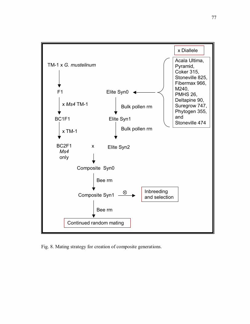
77

Fig. 8. Mating strategy for creation of composite generations.

TM-1 x G. mustelinum

F1

BC1F1

BC2F1 Ms4 only

x Ms4 TM-1

x TM-1

Acala Ultima, Pyramid, Coker 315, Stoneville 825, Fibermax 966, M240, PMHS 26, Deltapine 90, Suregrow 747, Phytogen 355, and Stoneville 474

x Diallele

Elite Syn0

Bulk pollen rm

Elite Syn1

Elite Syn2

Bulk pollen rm

x

Composite Syn0

Composite Syn1

Bee rm

Inbreeding and selection

Continued random mating

Bee rm

78

Using an advanced backcross composite is similar to successful incorporation

breeding from exotic material in barley in Canadian RIPE program (Kannenberg and

Falk 1995) and the California composite-cross populations (Jain and Suneson 1966; also

reviewed by Simmonds 1993). The RIPE program combines backcrossing and

intermating at different levels of elite germplasm, although restricted to exotic entries

with good per se performance. They observed that natural selection seemed to weed out

negative traits in random mating populations (Kannenberg and Falk 1995). Allard

(1992) showed that the California Composites did not collapse to inbred types even after

repeated cycles of intermating and selection. Selection was effective after more than

twenty generations of recombination (Allard 1992). In cotton breeding, advanced

backcross composite populations may be more easily accessed for such diverse

germplasm as G. mustelinum because they already have a base level of adaption that

makes them more useful to other breeders and more likely to be used than going back to

the original species.

Since these populations were relatively small and restricted to a single testing

location, over two years, the results reported here should be considered a preliminary

assessment of these breeding methodologies. Regardless, here we report on population

performance and make recommendations regarding future breeding methods for

handling G. mustelinum in cotton breeding programs.

79

Materials and methods

Plant material

Crossing procedure for BC1 generations was described previously. Day-length

sensitivity and maturity issues required crossing through the winter season in order to

minimize selection for early maturing genotypes. G. hirsutum cv. ‘TM-1’ was the

recurrent male parent. BC1F1’s were used as females; all were hand emasculated, with

the exception of those with Ms4-mediated nuclear male sterility. Intermating was

performed as described for BC1F1 generations, with the exception that some male fertile

plants were used as females to maintain population size. Open-pollinated seed from the

greenhouse, where there was no access to insect pollinators, was assumed to be self

fertilized.

In winter of 2002 and 2003, our BC2F1 introgression populations were crossed

to an elite polycross synthetic from 11 parents created from a diallele with bulked

reciprocals provided by Drs. Clarence Watson, Johnnie Jenkins, Jack McCarty, Osman

Gutierrez, and Darryl Bowman. The parents were diverse elite cultivars that included:

Acala Ultima, Pyramid, Coker 315, Stoneville 825, Fibermax 966, M240, PMHS 26,

Deltapine 90, Suregrow 747, Phytogen 355, and Stoneville 474. In winter of 2003, the

BC2F1 population from G. hirsutum x G. mustelinum was sent to Mexico, where it was

crossed with bulked pollen from the cycle 2 random mating population (Syn2) from the

elite polycross synthetic as described by Bowman et al. (2005). The original plan was to

have the crosses back in time to include the synthetic parent and the composite with G.

mustelinum backcross populations in time to include in field testing at College Station,

80

but unfortunately the late maturity of the population prevented harvest in Mexico until

summer planting in College Station, TX was finished and so was not included. A

greenhouse population was planted and intermated by bulking pollen from male fertile

plants and pollinating male sterile plants to create the random mated composite (Syn1).

All male fertile plants were harvested and selections were made based on visual

impressions of improved yield and morphology. Seed from selected plants were grown

as F2 families for further selection at the Texas Agricultural Experiment Station (TAES)

Research Farm at College Station during 2005. This generation was grown in relative

isolation at the TAES F&B site on Texas A&M University campus where bees are

common for another cycle of random mating during 2005. The next generation of the

composite (Syn2) was formed by bulking 3 bolls from each male sterile plant.

Field testing

Field evaluation was performed in 2004 and 2005 at the TAES Research Farm.

Soils at this site are generally Westwood silt loams. Entries included two commercial

checks: ‘Fibermax 832’ (FM832) and ‘Phytogen 355’ (PSC355), TM-1, BC1F1, BC1F2,

BC1rm1, BC1rm2, BC2F1, BC2rm1, BC3F1 generations both years. Both the Syn0 and

Syn1 composite generations, with no random mating, Syn0, and after one generation of

random mating, Syn1, were only included in 2005. All years, the experiment was planted

as a randomized complete block with four replications. Each entry consisted of 25

plants in a single 12.2 m row. More than one entry was included for all segregating

generations to increase the number of plants sampled to increase the number of

individuals in segregating populations, as seen in Table 15 with final plant numbers per

81

generation. Observations were made on individual plants for all entries. All years,

planting was between the 10 and 30 April and harvest was completed by the 15

November. Plots were direct seeded with three seeds per hill and thinned to one plant

per hill. Pedigree of each plant was maintained. We tried to maintain agronomic

practices consistent with commercial cotton cultivation at the TAES experiment station

including furrow irrigation when needed, chemical and mechanical weed control,

pesticide application, and participation in boll weevil eradication program, with the

exception of defoliation. Because all plots were hand harvested and to maximize yields

of later-maturing generations, plots were not chemically defoliated.

Table 15. Plant numbers measured per generation in G. mustelinum advanced backcross generation testing during 2004 and 2005. Generation 2004 2005 BC1F1 160 93 BC1F2 126 186 BC1rm1 142 100 BC1rm2 174 99 BC2F1 171 101 BC2F2 128 195 BC2rm1 134 188 BC3F1 173 184 FM832 95 100 PSC355 98 100 TM-1 95 99 Comp Syn0 -† 200 Comp Syn1 -† 202 Elite poly Syn2 -† 97

†Not included due to late harvest in winter nursery

82

Fiber testing

Fiber testing for the 2004 advanced backcross field experiments was performed

as described for 2003 and 2004 early generation testing with all samples roller ginned

and sent to Cotton Incorporated HVI and AFIS testing. We also report in this section

parent-offspring regression from parental BC1F1 greenhouse plants. These plants were

grown during 2002 and open pollinated greenhouse samples were ginned with a

laboratory roller gin and sent to Cotton Incorporated for AFIS and HVI testing during

2003. Because only lint from open pollinated bolls was tested, fiber data from male

sterile plants or very low yielding plants was not possible. As 2005 samples have not

been sent at this date for fiber analysis, HVI results are not available.

Statistical analysis

In order to calculate mean performance for each generation across years,

experiments from different years were analyzed separately to determine differences in

means and variances between years and then combined after testing for homogeneity of

variances with a modified Levene’s test as described in Neder et al. (2002). Each trait

was analyzed with SAS v8.0 (SAS Institute, Cary, NC) using mixed model analysis with

PROC MIXED and the following model trait = β0 + β1replication + β2plant(generation)

+ β3generation + ε for separate environments. Replications and plants within generation

were considered random. Generations were fixed effects. Means for generations were

calculated using LSMEANS statement which adjusts means for other variables in the

model. Combined analyses were also analyzed as a mixed model with PROC MIXED

with the following model: trait = β0 + β1environment + β2replication(environment) +

83

β3plant(generation) + β4generation + β5generation x environment + ε. Different years

were considered different environments. Replication within environments and plants

within generations and were considered random effects. Generations and environments

were treated as fixed effects.

In order to estimate variances per generation per year, the data set was analyzed

separately by generation with the following model: trait = β0 + β1replication + β2plant +

ε, with replication and individual plants as random effects using PROC MIXED. This

allowed for calculation of the variance per generation on an individual plant basis while

excluding effect of replication as well as computation of confidence limits for each

variance estimate. The individual plants within a generation were not replicated in this

experiment, due to the fact that most were segregating. The replication effect accounted

for field variation and different harvest dates of the plants and thus their differential

weathering and maturity effects on yield and fiber quality. Variances were considered

significantly different from zero if their confidence limits did not contain zero.

Variances were considered significantly different if the confidence limits for different

generations did not overlap.

Heritability was calculated with SAS codes generously provided by Dr. Jim

Holland and modified to fit this experiment. The model was: trait = β0 + β1genotype +

β2replication(environment) + β3environment + β3genotype x environment + ε , with all

random effects, and variance components were estimated with restricted maximum

likelihood. Heritability was estimated by solving on an entry basis, Vg (Vg + Ve +

Vgxe)-1. Heritability for fiber quality traits was estimated by regressing the midparent

84

value from greenhouse BC1F1 parents to BC1F2 and BC1rm1 offspring grown in 2003

and 2004. Low yields limited this analysis especially to 2004, with only a few progeny

yielding enough for fiber testing. Heritability was estimated as the slope of the

regression line with parents as x and progeny as y divided by two times the coefficient of

parentage. The coefficient of parentage for both random mated and BC1F2 populations

was estimated to be 0.75 (Goffreda and Mutschler 1989). Results from BC1F2 and

BC1rm1 were not combined. Graphs were created using SPSS.

Using Peditree (van Berloo and Hutton 2005), we tracked progeny from the top

15 BC1F1 plants for UHM fiber quality, and then compared the mean performance of

these selected populations to the unselected whole to measure gain from selection. The

predicted gain from selection was calculated according the formula G = csh2(Vp)1/2,

where c is an indicator of pollen control, which in this case is equal to 1 since pollen

sources were controlled. S is the selection index as outlined by Poehlman and Sleper

(1994) that was estimated at 2.056 since the selected number of BC1F1 plants were 5%

of the original 300 of each generation. The phenotypic variance (Vp) from the

greenhouse fiber quality was used and heritability estimates from PROC MIXED were

compared to those from parent-offspring (PO) regression. The mean of the top ten

percent of the original BC1F1 plants for yield, UQLw from AFIS, UHML, and fiber

strength (g/TEX) from HVI were also selected and means from selected BC1F1 progeny

from each generation from 2004 was compared to mean performance with no intentional

selection as a measure of usefulness for breeding.

85

Results and discussion

Ms4

The effect of Ms4 in 2005 was the most pronounced of all years. Male sterile

plants were on average less fit than male fertile plants with increased plant height and

number of immature bolls, but decreased yield and harvested bolls when compared with

male fertile plants within the generation (Table 16). Why was the effect larger than in

previous years? The location was still at the same experiment station, but the field was

moved in 2005 to a more central location where presumably the number of insect

pollinators was lower.

Table 16. Marginal means for male fertile (ms4ms4) and male sterile (Ms4ms4) plants within generations from 2005 G. mustelinum advanced backcross experiment. Parentheses contain 95% confidence limits. Plant characteristics

Plant height (cm)

Total bolls

Harvested bolls

Immature bolls

ms4ms4 162 (153, 171) 27 (19, 34) 19 (13, 24) 7 (4, 9) Ms4ms4 174 (168, 178) 22 (18, 26) 11 (8, 14) 10 (8, 12) Yield characteristics

Yield (g/plant)

Lint percent (%)

Boll size (g boll-1)

Lint/boll (g boll-1)

ms4ms4 57.4 (39, 76) 30.5 (29, 31) 2.66 (1.7, 2.0) 0.60 (0.3, 0.9) Ms4ms4 31.4 (21, 42) 29.5 (28, 30) 2.58 (1.5, 1.9) 0.56 (0.3, 0.9)

86

The means of male sterile and male fertile plants within BC1rm1, BC1rm2,

BC2rm1, Composite Syn0 and composite Syn1 are presented in Table 17. The effect of

Ms4 is more pronounced in the composite generations than in early backcross

generations. Confidence limits for yield, heights and boll counts overlap for the

BC1rm1, BC1rm2 and mostly for the BC2rm1 generations, but not for composites: Syn0

and Syn1. The large plant to plant variation at the early generations as well as the

general low yields overshadowed the effect of male sterility within the early generations.

Apparently, as the yields increased and plant to plant variation decreased in the

composite generations the effect of male sterility is pronounced enough to be

distinguished under normal field conditions.

Because the means for these generations are not being used for estimates of

genetic effects and to remain consistent with values reported in other field experiments

the male sterile plants have not been removed from estimates of general means.

Inclusion of Ms4 plants within each generation does lower the mean and may artificially

increase the variance, over that if we did not have this male sterility effect segregating

within the populations.

87

Table 17. Marginal means by male sterile and male fertile plants by population for yield and plant characteristics from G. mustelinum 2005 field experiments. Parentheses contain 95% confidence limits. Male Fertile ms4ms4 Male Sterile Ms4ms4 Generation Yield† Generation Yield† BC1rm1 14.6 (-4.2, 33.4) BC1rm1 5.9 (-35, 46.8) BC1rm2 25.7 (1.64, 49.7) BC1rm2 14.5 (-8.7, 37.7) BC2rm1 62.0 (46.2, 77.7) BC2rm1 29.9 (8.94, 50.9) Comp Syn0 131.5 (115, 147) Comp Syn0 53.3 (36.7, 69.8) Comp Syn1 120.5 (104, 136) Comp Syn1 52.9 (36.8, 69.0) Height† Height† BC1rm1 175.8 (158, 193) BC1rm1 186.4 (162, 209) BC1rm2 172.3 (154, 190) BC1rm2 175.4 (157, 192) BC2rm1 160.7 (143, 178) BC2rm1 171.6 (154, 189) Comp Syn0 140.6 (122, 158) Comp Syn0 167.4 (149, 184) Comp Syn1 137.1 (119, 154) Comp Syn1 166.9 (149, 184) Hboll† Hboll† BC1rm1 9 (3.99, 13.8) BC1rm1 6 (-6.6, 17.9) BC1rm2 15 (7.90, 21.3) BC1rm2 6 (-0.0, 12.3) BC2rm1 24 (19.7, 27.8) BC2rm1 10 (4.12, 16.1) Comp Syn0 35 (31.3, 39.5) Comp Syn0 17 (12.7, 21.3) Comp Syn1 33 (29.0, 37.4) Comp Syn1 16 (11.9, 20.4) Iboll† Iboll† BC1rm1 8 (4.36, 11.3) BC1rm1 13 (6.66, 19.8) BC1rm2 11 (6.90, 15.0) BC1rm2 12 (7.60, 15.4) BC2rm1 9 (5.70, 12.4) BC2rm1 10 (5.96, 13.6) Comp Syn0 5 (1.57, 8.32) Comp Syn0 8 (4.78, 11.5) Comp Syn1 4 (1.04, 7.80) Comp Syn1 9 (5.20, 11.9) Wboll† Wboll† BC1rm1 1.67 (1.26, 2.07) BC1rm1 1.68 (0.72, 2.62) BC1rm2 1.60 (1.13, 2.06) BC1rm2 2.21 (1.76, 2.65) BC2rm1 2.63 (2.30, 2.95) BC2rm1 2.64 (2.22, 3.06) Comp Syn0 3.69 (3.36, 4.00) Comp Syn0 2.97 (2.64, 3.30) Comp Syn1 3.72 (3.39, 4.04) Comp Syn1 3.37 (3.04, 3.69) Lboll† Lboll† BC1rm1 0.49 (0.23, 0.73) BC1rm1 ‡ ‡ BC1rm2 0.53 (0.26, 0.80) BC1rm2 0.74 (0.50, 0.97) BC2rm1 0.78 (0.65, 0.90) BC2rm1 0.65 (0.38, 0.92) Comp Syn0 1.23 (1.09, 1.37) Comp Syn0 0.84 (0.68, 0.99) Comp Syn1 1.27 (1.11, 1.41) Comp Syn1 1.04 (0.89, 1.18)

†Height = height (cm), Yield = seedcotton plant-1 (g), Hboll = harvested bolls (counts), Iboll = immature bolls not harvested (counts), Wboll = weight boll-1 (g), Lboll = lint boll-1 (g). ‡Not estimated due to poor sampling at time of publication

88

Future experiments for testing of genetic effects or for interfacing with marker

genotypes for quantitative trait loci analysis should be done without the Ms4 trait. But,

for breeding, the male sterility allows for increased number of crosses to be made with

less labor, especially if bee-mediated intermating is utilized, and it is easily removed

from the population, because it is dominant, nuclear and simply controlled.

Means and variances for generations

There was a stepwise approach to recurrent parental values from the BC1 to the

BC3 level (Table 18). Composite generation means were not different from the BC3F1

yields, if male sterile plants are left in the dataset. Considering only male fertile plants,

the composite generations had increased yield over the BC3F1 generation, but still less

than the polycross synthetic parent (Table 17). The increase in yield was due to

increasing weight per boll, lint percentage and number of harvested bolls. As yield

components increased, plant height decreased from 162 cm in BC1F1 population to 128

cm in BC3F1 in 2004 and from 194 to 142 in 2005. The BC3F1 generation was still

taller than TM-1 both years. The composite generations were also taller than TM-1 or

the synthetic parent, suggesting hybrid vigor still present even at this late generation.

89

Table 18. Marginal means by generation for G. mustelinum populations from 2004, and 2005 yield and plant height. Mean differences tested with Tukey-Kramer adjusted LSD. Means with different letter groups are significantly different with p-values < 0.05. 2004 Height† Yield† Hboll† Wboll† lintperc† BC1F1 162.2 A 40.5 D 25.7 CDE 1.6 E 27.2 E BC1F2 127.4 DE 30.5 D 18.5 EF 1.4 E 27.3 E BC1rm1 140.2 BC 28.3 D 16.9 F 1.6 E 26.7 E BC1rm2 135.4 CD 38.4 D 24.5 DE 1.6 E 27.6 E BC1rm3 149.9 B 44.9 D 34.2 ABC 1.3 E 25.6 E BC2F1 136.2 CD 89.3 C 38.4 A 2.4 D 30.3 D BC2F2 121.3 E 88.7 C 34.2 AB 2.6 D 30.0 D BC2rm1 131.3 CDE 73.1 C 30.3 BCD 2.4 D 30.0 D BC3F1 127.8 DE 112.8 B 36.5 AB 3.2 C 32.2 C FM832 102.8 F 112.0 B 23.2 DEF 4.8 A 39.0 A PSC355 102.3 F 134.9 A 33.6 ABC 3.8 B 41.0 A TM-1 106.6 F 139.2 A 29.4 BCD 4.6 A 34.1 B 2005 BC1F1 194.3 A 14.2 D 8.2 G 1.7 F 29.8 DEFG BC1F2 153.2 DE 8.2 D 5.4 G 1.5 F 29.3 DEFG BC1rm1 173.4 B 12.0 D 6.9 G 1.6 F 26.1 FG BC1rm2 171.0 BC 14.1 D 7.6 G 1.8 F 27.1 G BC2F1 158.5 CDE 55.3 C 21.0 DEF 2.5 E 27.9 FG BC2F2 153.0 DE 47.9 C 18.0 F 2.5 E 30.7 CDEF BC2rm1 160.7 CD 48.0 C 18.8 EF 2.6 E 29.2 EFG BC3F1 141.9 F 107.5 B 31.3 BC 3.3 D 31.4 CDE Comp syn0 152.5 DE 94.2 B 26.3 CD 3.5 CD 33.9 B Comp syn1 151.0 EF 88.4 B 24.9 DE 3.4 D 33.4 BC FM832 120.8 G 151.5 A 29.9 BCD 5.0 A 38.6 A PSC355 118.2 G 177.5 A 45.0 A 3.9 C 41.4 A Elite Syn2 113.2 G 164.5 A 35.9 B 4.5 AB 40.9 A TM-1 120.7 G 144.7 A 33.4 BC 4.4 B 33.4 BCD

†Height = height (cm), Yield = seedcotton plant-1 (g), Hboll = harvested bolls (counts), Wboll = weight boll-1, and Lintperc = Lint percentage (%).

Increased yields allowed for better sampling of the population. In 2004, only

56% of BC1F1 and 49% of BC2F2 plants yielded the three grams necessary for HVI

fiber testing. In comparison, 94% of BC2F1 plants and 96 % of BC3F1 plants were

tested for fiber quality with HVI. Only 57% of BC1rm1 plants were tested with HVI,

90

78% of BC1rm2 were large enough for testing. UHM fiber length decreased almost a

millimeter with each generation of backcrossing (Table 19). Strength also decreased,

but was still higher than that of TM-1 at the BC3F1 level. Fineness increased from the

BC1 to the BC3 level, although the BC3F1 was significantly finer than TM-1.

Table 19. Marginal means by generation for G. mustelinum populations from 2004 HVI and AFIS fiber qualities. Mean differences tested with Tukey-Kramer adjusted LSD. Means with different letter groups are significantly different with p-values < 0.05 MIC† UHM† UI† STR† ELO† BC1F1 3.7 GH 30.4 AB 83.6 C 35.0 A 4.7 E BC1F2 4.0 EFG 28.2 E 83.2 C 32.4 BC 5.2 CDE BC1rm1 3.8 GH 29.8 BC 83.2 C 32.8 B 4.9 DE BC1rm2 3.9 FG 30.0 ABC 83.8 BC 33.5 B 5.0 DE BC1rm3 3.6 H 30.6 AB 83.3 C 33.7 AB 4.8 DE BC2F1 4.3 DE 29.4 C 83.9 BC 32.4 B 5.3 CD BC2F2 4.4 CD 28.5 E 83.6 C 30.9 CD 5.6 BC BC2rm1 4.3 DE 29.4 CD 83.9 BC 32.6 B 5.3 CD BC3F1 4.5 BC 28.8 DE 83.9 BC 31.2 CD 5.6 BC FM832 4.2 DEF 30.6 A 84.4 B 35.1 A 3.7 F PSC355 5.1 A 28.2 E 85.3 A 30.8 D 6.6 A TM-1 4.7 B 28.4 E 83.7 BC 29.3 E 5.8 B UQLw† SFCw† FINE† MAT† BC1F1 32.1 AB 12.7 A 150.7 F 0.80 E BC1F2 30.1 EF 11.4 ABC 159.7 D 0.83 D BC1rm1 31.4 BC 11.9 AB 154.0 DEF 0.81 DE BC1rm2 31.6 BC 10.8 BCD 157.0 DE 0.83 D BC1rm3 32.7 A 10.5 BCD 151.4 EF 0.82 DE BC2F1 31.0 CD 10.0 CD 165.8 C 0.85 C BC2F2 30.0 F 10.1 CD 170.1 BC 0.86 C BC2rm1 31.0 CDE 9.9 D 167.9 C 0.85 C BC3F1 30.4 DEF 9.9 D 172.9 B 0.86 BC FM832 32.2 AB 9.6 D 166.3 C 0.88 A PSC355 29.9 F 7.3 E 186.1 A 0.90 A TM-1 30.0 F 9.4 D 180.4 A 0.88 AB

†MIC = micronaire, UHML = upper half mean length, UI = uniformity index, STR = strength, ELO = elongation, UQLw = upper quartile length by weight distribution (mm), SFCw = short fiber content by weight (%), FINE = fineness index, MAT = maturity ratio.

91

In general, the BC3F1 was not equal to TM-1, suggesting continued presence of

G. mustelinum genome. There was evidence both years that BC3F1 yields were lower

than TM-1 (Table 18) (P-value < 0.05, Tukey-Kramer adjusted LSD). Boll weight of the

BC3F1 generation averaged 3.2 in 2004 and 3.4 in 2005; TM-1 averaged 4.5 and 4.6 for

the same years, which decreased plant yields, since the number of bolls harvested was

higher for BC3F1 populations than for TM-1 (Table 18). Fineness and strength were

also improved in the BC3F1 generation over parental levels (Table 19).

Inbreeding depression was a significant barrier to introgression at the BC1F1

level as seen by the drop in yields, boll counts, and boll weight in BC1F2 generation, but

this did not appear to be the case at the BC2 level. The BC2F2 generation tended to be

shorter than the BC1F1 generation (p-value < 0.05, Tukey-Kramer adjusted LSD), but

yield characteristics such as seedcotton per plant, number of bolls, boll weight, and lint

percent were not different from BC2F1 levels (p-value > 0.05) (Table 18). This

suggested that further backcrossing resulted in loss or dilution of factors that caused the

inbreeding depression seen with the BC1F2 and F2 generations.

Another trend seen at the BC1 level was a decrease in means for random mating

generations (Tables 18 and 19) compared to the BC1F1. The BC2rm1 had slightly lower

numerical mean, but not significantly so (p-value > 0.05). This was true for yield in 2004

and 2005 as well as height. The mean level for male fertile plants from the BC2rm1

population in 2005 was higher than BC2F1 means for yield, boll counts, and boll size (p-

value < 0.05, Tukey-Kramer multiple comparison test). The Syn0 composite was

comparable to the BC3F1 generation and the Syn1 was comparable to a BC3rm1

92

generation (p-values > 0.05). The Syn0 and Syn1 means were not significantly different

from eachother for all traits measured (p-values > 0.05). Thus the decrease in means due

to random mating was reduced in later backcross generations.

Variances tended to decrease in more advanced backcross population, as

expected, except for yield and boll count. See Tables 20, 21, and 22. Variances for

height, lint percent and some of the fiber quality traits decreased in BC2 and BC3

populations. See Tables 20 and 21. Variances for yield and boll count increased in later

generations (Table 20) due to low yields in early generations because of strong effects of

maturity and day length that truncated the distribution of phenotypes possible at the

BC1F1 level and limited the range of phenotypes possible. The variance for individual

plant yield was high both years, even in TM-1, which is highly inbred. See Table 20.

High variance in TM-1 and check varieties indicated that environmental variance is high

for individual plant yield, making individual plant selection unreliable.

93

Tabl

e 20

. Var

ianc

e es

timat

es fo

r pla

nt c

hara

cter

istic

s by

G. m

uste

linum

gen

erat

ions

from

200

4 an

d 20

05. P

aren

thes

es c

onta

in

95%

con

fiden

ce li

mits

. 20

04

Hei

ght†

Y

ield

† H

boll†

Lint

perc

† W

boll†

BC1F

1 68

9 (5

57, 8

72)

1171

(9

46, 1

486)

38

7 (3

11, 4

94)

15.5

(1

2.4,

19.

9)

0.00

‡

BC1F

2 84

0 (6

55, 1

113)

16

10

(126

2, 2

122)

41

5 (3

23, 5

50)

32.9

(2

5.0,

45.

2)

0.06

(0

.02,

0.4

6)

BC1r

m1

839

(669

, 108

3)

822

(655

, 106

0)

270

(214

, 350

) 22

.1

(17.

3, 2

9.1)

0.

00‡

BC

1rm

2 84

3 (6

87, 1

058)

94

3 (7

70, 1

182)

30

6 (2

49, 3

85)

27.5

(2

2.1,

34.

9)

0.00

‡

BC2F

1 52

2 (4

24, 6

57)

2705

(2

204,

339

8)

440

(353

, 560

) 15

.9

(12.

8, 2

0.3)

0.

17

(0.0

9, 0

.38)

BC

2F2

513

(403

, 675

) 49

65§

(391

8, 6

498)

55

7 (4

38, 7

31)

21.6

§ (1

7.0,

28.

4)

0.54

(0

.34,

0.9

6)

BC2r

m1

691

(548

, 896

) 19

89

(157

9, 2

584)

33

8 (2

67, 4

42)

12.0

(9

.32,

15.

9)

0.00

‡

BC3F

1 42

6 (3

46, 5

35)

2629

(2

139,

330

9)

255

(206

, 323

) 7.

9 (6

.30,

10.

2)

0.20

(0

.11,

0.4

3)

FM83

2 28

0 (2

12, 3

86)

2065

(1

568,

284

2)

82

(62.

4, 1

13)

7.1

(5.2

3, 1

0.2)

0.

27

(0.1

4, 0

.65)

PS

C35

5 15

6 (1

17, 2

15)

3290

(2

509,

450

2)

232

(175

, 319

) 15

.4

(11.

5, 2

1.4)

0.

09

(0.0

3, 0

.51)

TM

-1

211

(159

, 291

) 31

65

(240

0, 4

364)

14

2 (1

07, 1

96)

15.8

(1

1.8,

22.

1)

0.29

(0

.14,

0.8

0)

2005

H

eigh

t†

Yie

ld†

H

boll†

Li

ntpe

rc†

Wbo

ll†

BC1F

1 46

1 (3

48, 6

39)

448

(341

, 615

) 12

0 (9

1.2,

166

) 37

.9

(22.

4, 7

7.4)

0.

00‡

BC

1F2

1116

(8

89, 1

443)

44

3 (3

50, 5

78)

119

(94.

4, 1

53)

52.3

(2

7.1,

138

.) 0.

12

(0.0

3, 1

.16)

BC

1rm

1 11

23

(829

, 160

7)

383

(277

, 562

) 98

(7

1.9,

140

) 5.

9 (2

.52,

26.

0)

0.00

‡

BC1r

m2

710

(532

, 994

) 45

0 (3

34, 6

36)

144

(107

, 200

) 34

.3

(21.

7, 6

2.0)

0.

87

(0.4

9, 1

.87)

BC

2F1

464

(350

, 644

) 21

01

(157

8, 2

934)

28

0 (2

11, 3

89)

34.8

(2

0.5,

71.

2)

0.24

(0

.12,

0.6

9)

BC2F

2 82

3 (6

68, 1

039)

34

57

(279

9, 4

379)

39

3 (3

19, 4

97)

30.9

(2

0.8,

50.

4)

0.37

(0

.23,

0.6

8)

BC2r

m1

743

(607

, 929

) 22

04

(180

3, 2

755)

36

2 (2

96, 4

53)

17.3

§ (1

2.5,

25.

4)

0.10

(0

.04,

0.6

0)

BC3F

1 51

2 (4

16, 6

43)

4449

(3

632,

557

8)

329

(267

, 413

) 7.

0 (4

.99,

10.

5)

0.22

(0

.13,

0.4

4)

Com

p Sy

n0

814

(665

, 101

8)

4903

(3

997,

615

4)

337

(275

, 422

) 11

.8

(8.3

8, 1

7.8)

0.

35

(0.2

0, 0

.72)

C

omp

Syn1

82

4 (6

77, 1

024)

58

17

(478

2, 7

230)

37

1 (3

04, 4

61)

11.1

(8

.00,

16.

4)

0.41

(0

.26,

0.7

1)

FM83

2 20

9 (1

51, 3

08)

6853

(4

872,

103

5)

199

(143

, 292

) 1.

7 (0

.76,

7.1

4)

0.22

(0

.09,

0.8

7)

PSC

355

330

(246

, 463

) 86

37

(648

0, 1

209)

51

7 (3

86, 7

25)

3.8

(2.3

7, 7

.04)

0.

02

(0.0

0, 3

0.2)

El

ite S

yn2

388

(293

, 537

) 72

30

(549

8, 9

936)

28

1 (2

13, 3

87)

13.1

(8

.31,

23.

7)

0.09

(0

.02,

1.1

6)

TM-1

27

6 (2

06, 3

87)

5401

(4

048,

756

8)

317

(237

, 443

) 0.

3 (0

.07,

63.

8)

0.04

(0

.01,

0.6

1)

† Hei

ght =

hei

ght (

cm),

Yie

ld =

seed

cotto

n pl

ant-1

(g),

Hbo

ll =

harv

este

d bo

lls (c

ount

s), L

intp

erc

= Li

nt p

erce

ntag

e (%

), an

d W

boll

= w

eigh

t bol

l-1.

‡ Con

fiden

ce li

mits

not

com

pute

d by

REM

L fo

r pla

nt(g

en) o

r res

idua

l. V

aria

nce

for g

ener

atio

n eq

ual t

o ze

ro.

§ Var

ianc

e es

timat

ed fr

om re

sidu

al v

aria

nce

due

to fa

ilure

of R

EML

mix

ed m

odel

est

imat

ion

94

Tabl

e 21

. Var

ianc

e es

timat

es fo

r HV

I fib

er q

ualit

ies b

y G

. mus

telin

um p

opul

atio

ns fr

om 2

004.

Par

enth

eses

con

tain

95%

co

nfid

ence

lim

its.

M

IC†

U

HM

L†

UI†

ST

R†

ELO

†

BC1F

1 0.

00‡

1.

77

(1.2

5, 2

.68)

2.

53

(1.8

2, 3

.75)

8.

20

(6.2

0, 1

1.3)

0.

71

(0.4

5, 1

.23)

BC

1F2

0.22

(0

.09,

0.8

6)

3.90

(2

.65,

6.3

2)

1.70

(1

.08,

3.0

7)

14.4

9 (1

0.1,

22.

2)

1.24

(0

.77,

2.3

1)

BC1r

m1

0.14

(0

.06,

0.5

6)

2.56

(1

.70,

4.2

9)

3.72

(2

.78,

5.2

1)

12.1

0 (8

.81,

17.

6)

0.80

(0

.45,

1.7

5)

BC1r

m2

0.00

‡

2.26

(1

.66,

3.2

3)

2.27

(1

.66,

3.2

5)

13.7

4§ (1

0.7,

18.

1)

1.00

(0

.7, 1

.55)

BC

1rm

3 0.

43

(0.3

3, 0

.55)

2.

71

(1.7

0, 4

.97)

4.

14

(2.6

5, 7

.37)

13

.76

(9.3

9, 2

2.0)

0.

48

(0.2

4, 1

.27)

BC

2F1

0.00

‡

1.93

(1

.45,

2.6

7)

1.29

(0

.94,

1.8

8)

8.19

(6

.49,

10.

6)

0.90

(0

.63,

1.3

5)

BC2F

2 0.

07

(0.0

3, 0

.28)

2.

58

(2.0

1, 3

.41)

1.

58

(1.1

1, 2

.41)

7.

66

(5.9

8, 1

0.1)

0.

72

(0.4

7, 1

.21)

BC

2rm

1 0.

20

(0.1

0, 0

.49)

2.

05

(1.4

8, 3

.01)

2.

07

(1.4

9, 3

.06)

8.

31

(6.3

6, 1

1.3)

0.

64

(0.4

1, 1

.10)

BC

3F1

0.14

(0

.06,

0.3

9)

1.15

(0

.84,

1.6

5)

1.09

(0

.78,

1.5

9)

5.16

(4

.06,

6.7

9)

0.54

(0

.35,

0.9

3)

FM83

2 0.

00‡

0.

00‡

1.

44

(0.9

5, 2

.39)

4.

91

(3.5

6, 7

.18)

0.

07

(0.0

2, 0

.67)

PS

C35

5 0.

00‡

0.

07

(0.0

1, 1

839)

1.

01

(0.6

4, 1

.80)

4.

01

(2.9

1, 5

.88)

0.

00‡

TM

-1

0.00

‡

0.00

‡

0.48

(0

.23,

1.5

5)

1.45

(0

.97,

2.3

7)

0.00

‡

† MIC

= m

icro

naire

, UH

ML

= up

per h

alf m

ean

leng

th, U

I = u

nifo

rmity

inde

x, S

TR =

stre

ngth

, ELO

= e

long

atio

n.

‡ Con

fiden

ce li

mits

not

com

pute

d by

REM

L fo

r pla

nt(g

en) o

r res

idua

l. V

aria

nce

for g

ener

atio

n eq

ual t

o ze

ro. V

aria

nce

for g

ener

atio

n ex

plai

ned

with

re

plic

atio

n.

§ Var

ianc

e es

timat

ed fr

om re

sidu

al v

aria

nce

due

to fa

ilure

of R

EML

mix

ed m

odel

est

imat

ion.

95

Tabl

e 22

. Var

ianc

e es

timat

es fo

r AFI

S fib

er q

ualit

ies b

y G

. mus

telin

um p

opul

atio

n fro

m 2

004.

Par

enth

eses

con

tain

con

fiden

ce

limits

.

UQ

Lw†

SF

Cw

†

FIN

E†

Mat

†

BC1F

1 2.

82

(2.1

1, 3

.96)

14

.44

(11.

3, 1

9.1)

10

4.08

(8

2.4,

135

.) 0.

00‡

BC

1F2

8.20

(6

.02,

11.

8)

15.0

9 (1

1.1,

21.

5)

290.

49

(218

., 40

6.)

0.00

‡

BC1r

m1

5.82

§ (4

.58,

7.6

3)

14.5

0 (1

1.2,

19.

4)

168.

05

(131

., 22

1.)

0.00

‡

BC1r

m2

3.34

(2

.57,

4.4

9)

10.9

4 (8

.71,

14.

1)

176.

90

(143

., 22

4.)

0.00

‡

BC1r

m3

4.50

(3

.20,

6.7

7)

14.5

8 (1

0.0,

22.

9)

115.

01

(81.

9, 1

73.)

0.00

‡

BC2F

1 3.

46

(2.6

8, 4

.61)

10

.30

(8.2

3, 1

3.2)

13

5.68

(1

10.,

171.

) 0.

00‡

BC

2F2

3.25

(2

.41,

4.5

9)

7.60

(5

.79,

10.

3)

194.

77

(153

., 25

6.)

0.00

‡

BC2r

m1

3.25

(2

.44,

4.5

3)

12.5

1 (9

.69,

16.

7)

217.

78

(172

., 28

3.)

0.00

‡

BC3F

1 2.

78

(2.1

4, 3

.73)

7.

99

(6.3

7, 1

0.3)

11

4.31

(9

3.2,

143

.) 0.

00‡

FM

832

0.93

(0

.60,

1.6

4)

7.19

(5

.28,

10.

3)

109.

06

(82.

6, 1

50.)

0.00

‡

PSC

355

0.46

(0

.24,

1.1

6)

5.64

(4

.14,

8.1

3)

129.

61

(99.

2, 1

76.)

0.00

‡

TM-1

0.

53

(0.3

1, 1

.06)

5.

95

(4.3

4, 8

.65)

49

.77

(37.

6, 6

8.9)

0.

00‡

† U

QLw

= u

pper

qua

rtile

leng

th b

y w

eigh

t, SF

Cw

= sh

ort f

iber

con

tent

by

wei

ght,

FIN

E =

finen

ess i

ndex

, Mat

= m

atur

ity sc

ore.

‡ C

onfid

ence

lim

its n

ot c

ompu

ted

by R

EML

for p

lant

(gen

) or r

esid

ual.

Var

ianc

e fo

r gen

erat

ion

equa

l to

zero

. Var

ianc

e fo

r gen

erat

ion

expl

aine

d w

ith

repl

icat

ion.

§ V

aria

nce

estim

ated

from

resi

dual

var

ianc

e du

e to

failu

re o

f REM

L m

ixed

mod

el e

stim

atio

n.

96

Heritability

Traditional estimates of heritability are from combinations of generation

variances in a generation means analysis, as correlations of relatives, or variances

estimated in an ANOVA or mixed model (Holland et al. 2003). In this study, we were

not able to take advantage of heritability estimates from generation means analysis since

they rely heavily on variance of F2 and BC1F2 populations. These populations had

artificially low variance due to hybrid breakdown. Variances from ANOVA or mixed

models of entries from the same population in different environments can also be used to

estimate heritability, and thus predicted effectiveness of selection, for that population as

explained by Holland et al. (2003). These experiments have multiple entries with

different amounts of G. mustelinum genomic DNA. If they were all from the same

generation, for example BC1F2 families, then estimates would be easily generated and

interpreted. This was not the situation here, but we wanted to have an estimate of

repeatability as a rough estimate of heritability so we modeled the generations used in

this study as a set of random lines and then calculating heritability according to Holland

et al. (2003) on an individual plant basis as well as narrow sense heritabilities by parent-

offspring regression, as presented in Table 23 and Fig. 9.

97

The broadsense heritability estimates are not made with genetically uniform

entries, but include different generations each with different genomic constitutions.

Thus these heritability estimates are confounded with effects of segregation and

differential levels of upland and exotic genomes, but were considered informative still as

measures of repeatability of the population performance and reliability of different

measurements. For example, it might be of interest to choose plant characteristics for

future selection and improvement, but if the environmental variance is high and

generations have little variance for these traits, then selection is not expected to be

effective.

Heritability was estimated with variance components with early generations from

2003, 2004 and 2005 as well as later generations from 2004 and 2005, which suggested

that most of the fiber properties would be moderately heritable, except uniformity index

and short fiber content. Weight per boll and lint percent were highly heritable, while

individual plant yield was only moderately heritable. The heritability estimates

calculated from early generations were generally higher than those calculated with

advanced generations, probably due to inclusion of advanced backcrosses that are more

genetically uniform. This would increase the amount of the variance due to

environmental effects and decrease the genetic variance, reducing heritabilities.

98

Table 23. Heritability estimates and standard errors (SE) for G. mustelinum populations from GMA, advanced backcross populations, and parent-offspring regression from 2002 greenhouse BC1F1 populations.

Early Generation

Advanced Generation

PO BC1F2 Regression

PO BC1rm1 regression

H2‡ SE H2‡ SE h2§ SE h2§ SE MIC† 0.42 0.14 0.34 0.10 -0.01 0.19 -0.29 0.52 UHM† 0.43 0.16 0.25 0.08 0.41 0.18 0.56 0.28 UI† 0.20 0.10 0.10 0.04 0.15 0.24 -0.39 0.44 STR† 0.32 0.23 0.24 0.08 0.09 0.18 -0.14 0.56 ELO† 0.40 0.16 0.29 0.09 0.39 0.27 0.02 0.54 UQLw† 0.40 0.16 0.19 0.07 0.36 0.11 0.47 0.21 SFCw† 0.16 0.10 0.13 0.05 0.23 0.17 0.09 0.20 Fine† 0.55 0.13 0.44 0.11 0.13 0.14 0.31 0.15 Mat† 0.33 0.13 0.31 0.09 0.01 0.17 0.05 0.31 Height† 0.53 0.13 0.38 0.09 . ¶ . ¶ . ¶ . ¶ Yield† 0.54 0.13 0.39 0.10 . ¶ . ¶ . ¶ . ¶ Hboll† 0.18 0.13 0.11 0.07 . ¶ . ¶ . ¶ . ¶ Wboll† 0.81 0.08 0.70 0.08 . ¶ . ¶ . ¶ . ¶ Lintperc† 0.67 0.11 0.57 0.10 . ¶ . ¶ . ¶ . ¶

†UQLw = upper quartile length by weight, SFCw = short fiber content by weight, FINE = fineness index, Mat = maturity score. ‡Broadsense heritability estimates from variance components estimated according to Holland et al. (2003). §Narrowsense heritability estimates from parent-offspring regression. ¶No data because of zero yield.

99

Fig. 9. Regression of G. mustelinum BC1F1 midparent UHML (mm) to BC1F2 and BC1RM1 UHML (mm).

In 2002, open pollinated fiber from greenhouse grown BC1F1 plants was tested

with AFIS and HVI. These plants were the parents to all of the subsequent generations,

whose pedigrees were maintained in experimental populations. Although adding a level

of complexity to planting and to seed preparation each year, this made it possible to

measure realized heritability of fiber traits by regressing the midparent performance

against their offspring in the BC1F2 and BC1rm1 generations (Fig. 9). Heritability is

100

measured by the slope of the regression line and is a narrow sense estimate of

heritability, the ratio of the additive genetic variance to the total phenotypic variance

(Poehlman and Sleper 1995). This estimate is also affected by the environments of the

parents as well as the offspring. In this case, this statistic measures the heritability of

fiber properties of BC1F1 greenhouse populations to their field grown progenies.

Contrary to broadsense heritability estimates reported in Table 23, there was little to no

heritability for micronaire, uniformity index, strength, fineness, or maturity. UHML as

well as UQLw were highly heritable, as seen in Fig. 9. Micronaire, maturity, and

fineness may have been affected more by the change in the environments from

greenhouse to field. Strength is often cited as a highly heritable trait (Niles and Feaster

1984), which was not the case in this experiment, as measured with parent-offspring

regression in Table 23. This suggested that selection for fiber length would be effective

in these populations as early as the BC1F1 generation, since it was highly heritable, even

from greenhouse populations, but selecting for fiber strength would not be effective.

Selection

Heritability estimates from greenhouse plants were shown to be high from

broadsense heritability estimates as well as PO regression. It was possible trace

pedigrees of experimental plants to reduce the dataset to only the descendents from the

top fifteen fiber length BC1F1 plants in order to measure gain from selection. The

means for this selected dataset and the original dataset are presented in Table 24.

Predicted gain from selection is equal to the selection index times the heritability and the

standard deviation of the trait. In this case, depending which heritability estimate used,

101

gain for selection at the BC1F1 level at 5% intensity was expected to be between 0.9 and

1.9 mm. The observed gain in BC1F2 generation was 1.5 mm over the unselected

generation, which was within the expected range. With the BC1rm1, also consisting of

immediate descendents, the observed gain was only 0.5 mm In each of the subsequent

generations, except the BC1F2, the difference between the selected generation and

unselected generation were lower than that predicted. In fact, the selected generation

mean length erodes each generation, until finally at BC2rm1 and BC3F1 means were not

different from the general population (p-values > 0.05, T-test). This may be due to

natural selection for upland-types that were adapted to cultivated techniques and to day

length insensitivity that have decreased fiber length, although this still exceeds fiber

lengths from TM-1. Fiber length alleles from G. mustelinum may well be linked to other

loci that negatively affect yield. It also may be that there are adjacent loci that have

interactions that affect inbred hybrid breakdown that make it more difficult to recover

the increased fiber length along with an upland-type yield and morphology.

102

Table 24. Performance of descendents in G. mustelinum advanced backcross experimental populations from selected BC1F1 greenhouse parental populations for UHML. Parentheses contain 95% confidence limits.

UHML (mm) Before selection

UHML (mm) After selection

Observed Gain %

BC1F1 30.4 (30, 30) 32.4a (31, 33) 2.0 6.7 BC1F2 28.2 (27, 28) 29.7 (28, 30) 1.5 5.2 BC1rm1 29.8 (29, 30) 30.3 (29, 30) 0.5 1.7 BC1rm2 30.0 (29, 30) 30.2 (29, 30) 0.2 0.7 BC1rm3 30.6 (30, 31) 30.4 (29, 31) -0.2 -0.6 BC2F1 29.4 (29, 29) 29.7 (28, 30) 0.3 0.9 BC2F2 28.5 (28, 28) 29.3 (28, 30) 0.9 3.0 BC2rm1 29.4 (29, 29) 29.4 (28, 30) 0.0 -0.2 BC3F1 28.8 (28, 29) 29.1 (28, 29) 0.3 1.1 Heritability estimates H

Selection intensity s.d.b Expected gain

P-O BC1F2 0.41 5% 1.68 1.4 P-O BC1rm1 0.56 5% 1.68 1.9 Variance components 0.25 5% 1.68 0.9

aMean from greenhouse BC1F1 selected individuals bs.d. = standard deviation of greenhouse plants for UHML

In order to evaluate the usefulness of selection for yield in these populations,

Bernardo (2000) advocates the use of a usefulness criteria. We calculated the difference

between the top ten percent mean and the overall mean for each generation propose its

use as an alternative to the usefulness criteria (Tables 25 and 26). The most useful

population would be one with a high ten percent mean and large difference between the

selected and unselected mean.

103

Table 25. Difference between G. mustelinum top ten percent seed cotton yield plant-1 from 2005 and overall means. Unselected yields are from male fertile plants only. Parentheses contain 95% confidence limits.

Yield (g plant-1) No selection

Yield (g plant-1) 10% selection

Observed gain %

BC1F1 14.2 (1, 27) 57.7 (26, 90) 43.4 305 BC1F2 8.2 (-3, 19) 56.5 (30, 83) 48.3 588 BC1rm1 12.4 (-4, 29) 60.8 (25, 97) 48.4 392 BC1rm2 14.6 (-3, 32) 62.5 (29, 96) 47.9 329 BC2F1 55.3 (42, 69) 153.3 (121, 185) 98.0 177 BC2F2 47.9 (38, 58) 179.9 (156, 204) 132.0 275 BC2rm1 52.9 (42, 64) 152.9 (129, 177) 100.0 189 BC3F1 107.4 (98, 117) 250.7 (227, 274) 143.3 133 Comp Syn0 125.8 (113, 139) 239.8 (216, 263) 114.0 91 Comp Syn1 117.3 (105, 130) 267.1 (244, 290) 149.8 128 FM832 151.5 (135, 168) 314.0 (284, 344) 162.5 107 PSC355 177.4 (164, 191) 374.3 (342, 406) 196.8 111 Syn2 164.5 (151, 178) 366.6 (335, 398) 202.1 123 TM-1 144.8 (131, 159) 293.0 (261, 325) 148.2 103

Table 26. Difference between top ten percent G. mustelinum UHML from 2004 and unselected mean by population. Parentheses contain 95% confidence limits.

UHML (mm) No selection

UHML (mm) 10% selection Observed gain %

BC1F1 30.4 (30, 31) 33.3 (33, 34) 2.9 9.5 BC1F2 28.2 (28, 29) 32.0 (31, 33) 3.8 13.3 BC1rm1 29.8 (29, 30) 33.4 (33, 34) 3.6 12.1 BC1rm2 30.0 (30, 30) 33.0 (33, 33) 3.0 9.9 BC1rm3 30.6 (30, 31) 33.9 (33, 35) 3.4 11.0 BC2F1 29.4 (29, 30) 32.4 (32, 33) 3.0 10.1 BC2F2 28.5 (28, 29) 31.3 (31, 32) 2.8 10.0 BC2rm1 29.4 (29, 30) 32.1 (32, 33) 2.7 9.3 BC3F1 28.8 (28, 29) 31.4 (31, 32) 2.6 9.0 FM832 30.6 (30, 31) 32.6 (32, 33) 2.0 6.5 PSC355 28.2 (28, 29) 29.9 (29, 30) 1.7 6.1 TM-1 28.4 (28, 29) 29.5 (29, 30) 1.0 3.7

104

For individual plants, the high microenvironmental variance complicated the

choice of generation for individual plant selection for yield (Table 25). Selected

population means were higher for all generations, except for BC1F1 (p-values < 0.05, T-

test). For individual plant yield, the observed gain from selection in this case was greater

than 100% for commercial checks and TM-1 that were not segregating. The difference

between segregating populations, as percentage of the mean was even greater. There

was a general trend for observed gain to decrease on a percentage basis from BC1 to

BC2 level in the selected population, while the mean of the selected population

increased. Methods to reduce high variance due to microenvironmental differences

would be beneficial, because with such high environmental variance reliably selecting

high yielding varieties by eye, a common beginning for pedigree breeding, would be

difficult.

For fiber quality, the selected mean was higher than the unselected mean for all

populations except TM-1 and PSC355 (Table 26). The mean UHM fiber length is

highest in the early generations, but the selected population mean remains high until the

BC3F1. The observed gain for UHML in BC2 and BC3 plants was less, but the

population mean was high enough in yield to make better selections. If selection had

been employed in the BC1F1 generation gains from selection for fiber would need to be

balanced with selection for yield in further backcrosses. Fiber data was not available

from 2005 and so variance in composite populations and usefulness for selection for

fiber quality can not be determined at this time.

105

Conclusions

Some of the difficulties we found for breeding with G. mustelinum for

agronomic traits were low yields in early backcrosses due to day-length and maturity

factors, hybrid breakdown in selfed populations, selection for G. hirsutum alleles in

random mating populations, high variance for individual plant yield, and difficulty in

recovering recurrent parental yields. In this experiment we included populations that

could have been part of three different mating schemes, as outlined in the introduction to

this section, and one objective of this research was to decide which would be best in the

face of these difficulties. A traditional backcross-inbred strategy does little to

compensate for selection against the G. mustelinum alleles, or hybrid breakdown. By the

time that parental yields are recovered, probably later than the BC3F1 generation, it may

be difficult to find reliable transgressive segregants due to loss of G. mustelinum alleles.

Selection at the BC1F1 level may be effective for fiber quality, but yields may still be

low and hybrid breakdown is a problem. Little chances for recombination are present

after this level. The backcross-random mate strategy used in this study appears to be

inadequate as seen in the increased frequency of G. hirsutum alleles in the BC1rm2 and

little effect on map length. At least, the inclusion of random mating makes an attempt to

allow for recombination and could be improved by increasing population sizes, increase

of early generations in Mexico, and bulked or bee pollinations instead of plant to plant

intermatings.

Although only preliminary data on performance of the composite populations are

available at this date, they are attempts to overcome the weaknesses of the backcross-

106

random mate strategy. Random mating with these populations was performed with bulk

pollinations or bee-mediated intermating instead of plant to plant intermating. This may

reduce unintentional selection for G. hirsutum alleles. Population sizes were also

increased, although not as much as they could be. Increasing the population size from

hundreds to thousands of plants would be relatively easy since they are bee pollinated

and large numbers of seed are produced. Selection of male fertile lines from the field

generates enough seed that replicated testing of F2 genotypes is possible as well as

recurrent selection of the population. Selections could be spun off into existing cotton

breeding programs to be used as parents in pedigree breeding programs or as entries

themselves. Bulking of the population at each generation also reduces the number of

seed packets and bookkeeping necessary in order to maintain and recreate the

population. This may seem trivial, but a plant to plant intermating of 300 plants with

enough seed for the next generation requires multiple crosses per female plant,

presumably each with a different male. At a minimum that would be 300 to 450 seed

packets, but could be as many as 600 or 1000 if the person performing the crossing is

ambitious. The bulked composite only requires one seed storage container and manual

labor is decreased meaningfully. It may be that the composite generations may be more

useful at an earlier backcrossing level, perhaps at a BC2F1, in order to maximize the

possible variation, but that would mean a drop in mean performance. Further

backcrossing could be performed by crossing male sterile females to bulk pollen from

the parental synthetic or other improved composite.

107

One other justification for using the composite population or a more competitive

cultivar for introgression from G. mustelinum is the relatively mediocre performance of

TM-1 relative to the commercial checks. TM-1 is a highly inbred line ideal for genetic

studies, but is generally considered to be substandard when compared to modern

breeding material and cultivars due to its poor fiber quality and little resistance to

bacterial, fungal, or viral diseases. It yielded less than commercial checks in College

station, although it out yielded both commercial checks in Mexico. The synthetic parent

used in this study includes parents that are resistant to seedling disease, bacterial blight,

as well as root knot nematodes. Moving G. mustelinum genetic material into this

background makes it much more likely to be used by other breeders.

108

CHAPTER V

GENERATION MEANS ANALYSIS OF G. tomentosum INTROGRESSION FOR

AGRONOMIC PROPERTIES AND INTERSPECIFIC BARRIERS

Introduction

The experiments described with crosses with G. mustelinum were performed in

parallel with another wild tetraploid species, G. tomentosum. In the process similar

populations, field testing, and molecular analyses were utilized. F1, BC1F1, and BC1F2

populations as well as random mating generations: BC1rm1 and BC1rm2 populations in

2003 and 2004 were tested for agronomic traits as a generation means analysis. DNA

samples from a subset of these generations were tested with SSR markers, as noted in

Chapter III for G. mustelinum in order to measure segregation ratio distortion and

linkage effects. In 2004 and 2005, later generations were added including BC2F1,

BC2rm1, BC2F2, BC3F1, BC3F2, and BC3rm1 populations, as well as composite Syn0

and Syn1 generations.

Early generation means analysis

This study is focused on introgression efforts from G. tomentosum, which comes

from the Hawaiian and other Pacific islands. It is not cultivated for fiber, but is

occasionally found as an ornamental; it produces a very small amount of short, reddish-

brown lint but has an aesthetically pleasing appearance (Applequist et al. 2001). G.

tomentosum x G. hirsutum hybrids were found to have only very slightly reduced

109

numbers of crossovers as measured by chiasmata frequency by Hasenkampf and Menzel

(1980), which suggests that G. hirsutum and G. tomentosum are closely related.

Allozyme marker analysis by DeJoode and Wendel (1992) also found that G.

tomentosum was closely allied with G. hirsutum and had little internal genetic diversity.

Morphologically, it can be easily distinguished from G. hirsutum due to bright, sulfur-

yellow flower petals, absence of central petal spot, absence of leaf and bracteole

nectaries, long stigma and style, as well as its pilose, but short leaf and stem pubescence

which gives the leaves a slightly grey appearance (Fryxell 1979).

The purpose of this study was to increase genetic diversity within cultivated G.

hirsutum by interspecific hybridization and genetic introgression from G. tomentosum,

evaluate possible barriers to introgression, and test the efficacy of random mating as a

mating scheme for introgression from G. tomentosum. We random mated the BC1F1

generation between G. tomentosum and G. hirsutum cv. ’TM-1’ and looked at generation

mean performance of the parents, F1, F2, BC1F1, BC1rm1, BC1rm2, and BC1F2

populations for individual plant characteristics including: fiber quality as measured by

HVI and AFIS, yield per plant, lint percent, plant height, and boll number and size. The

effect of random mating was tested by looking at mean performance, variance, and

phenotypic correlations between traits.

Materials and methods

Plant material and crossing procedure was the same as described for G.

mustelinum population development. Day-length sensitivity and maturity were not

110

problematic and so greenhouse populations were not maintained for more than one

season. Crossing and field procedures were identical as for G. mustelinum for 2003 and

2004, except that the G. tomentosum introgression populations were not tested in Mexico

during 2005 and the numbers of plants from each generation differed from the G.

mustelinum experiments (Table 27). Seedlings from G. tomentosum in 2003 did not

survive and were replaced with year old greenhouse-grown plants that were blooming at

the time of transplant from the greenhouse. In 2004, G. tomentosum seedlings also died,

but were not replaced with mature plants.

Table 27. Number of plants evaluated in 2003 and 2004 G. tomentosum GMA experiments. Generation 2003 2004 G. tomentosum 8 0 F1 52 43 F2 137 88 BC1F1 303 78 BC1F2 180 134 BC1rm1 291 173 BC1rm2 198 187 TM-1 96 97 FM832 96 102 PSC355 205 99

Data were collected as described for G. mustelinum, with the exception that fiber

testing by Cotton Incorporated did not include AFIS testing of fiber samples and NFFB

was not measured on all plants. Results from field experiments were evaluated by the

same statistical techniques that relied heavily on mixed model estimation of fixed and

random effects due to increased robustness in the face of missing data points. G.

111

tomentosum experiments were only grown in a single location during 2003 and 2004 and

so statistical models did not include locations as a fixed effect, only: generation (fixed

effect), replication within year (random effect), year (random effect), and the generation

by year interaction (random effect).

Results and discussion

Effect of Ms4

Many of the same observations regarding effect of Ms4 gene within the

populations from 2004 from G. mustelinum also applied to G. tomentosum (Table 28).

There was evidence that the male sterile plants had decreased number of harvested bolls

and an increased number of unopened bolls at the time of harvest (p-value < 0.05). There

were no significant differences in total number of bolls, seedcotton yield per plant, lint

percent or boll size. Unlike in the G. mustelinum study, plant height was not

significantly different, although the Ms4ms4 plants tended to be slightly taller. These

differences may have not been as large due to overall shorter generations in the G.

tomentosum experiment. Little difference was found for fiber qualities (Table 28).

Micronaire was slightly increased, but not significantly so, whereas length was not even

numerically different. Uniformity and strength were only slightly different (p-values >

0.05).

Presumably the relatively smaller than expected difference between male sterile

and male fertile plants was due to the presence of insect pollinators in both field

experiments. Because the differences were not profound, the male sterile plants were

112

not removed from the data set prior to analysis, nor was Ms4ms4 used as a variable.

Exclusion of male sterile plants was not possible in 2003 and analysis of 2004 without

the male sterile plants did not change conclusions or relationships among generations,

although means were increased slightly for random mating generations for number of

harvested bolls and individual plant yield.

Table 28. Marginal population means for effect of male sterile (Ms4ms4) and male fertile (ms4ms4) plants within G. tomentosum segregating generations from 2004. Parentheses contain 95%confidence limits. Plant characteristics Plant height (cm) Total number bolls Harvested bolls Immature bolls ms4ms4 128.7 (129, 143) 48.3 (36, 46) 29.3 (27, 32) 16.6 (14, 19) Ms4ms4 132.2 (144, 160) 46.6 (36, 47) 22.5 (20, 25) 22.7 (20, 25) Yield characteristics Yield (g/plant) Lint percent Boll size (g/ boll) Lint/boll (g/boll) ms4ms4 52.7 (36, 60) 30.00 (0.27, 0.29) 1.70 (1.56, 1.84) 0.51 (0.45, 0.57) Ms4ms4 40.9 (33, 48) 30.20 (0.26, 0.28) 1.86 (1.71, 2.0) 0.56 (0.50, 0.62) Fiber traits MIC UHML (mm) UI (%) STR (g/TEX) ms4ms4 4.56 (4.45, 4.67) 26 (25.2, 25.9) 82.10 (81.8, 82.5) 31.2 (158, 165) Ms4ms4 4.80 (4.68, 4.92) 26 (25.2, 25.7) 82.40 (82.0, 82.7) 31.4 (156, 165)

Mean performance of generations

There was not a significant effect of year as separate environments for most traits

and genotype by environment interactions (both experiments were planted at a single

location, years are modeled as different environments) were found for yield, height, total

number of bolls and micronaire (Table 29). Estimated means for plant characteristics

and yield components by generation are outlined in Tables 30 and 31 for 2003 and 2004.

113

G. tomentosum seedlings died in the field in 2003 and were replaced with early

bloom year old plants from the greenhouse. Even though transplants were healthy and

flowered profusely, they did not set seed in the field. In 2004, G. tomentosum seedlings

died and mature plants were not available for transplanting. It is possible that G.

tomentosum is stongly susceptible to a seedling disease pathogen present in these fields.

Decreased seedling viability and vigor was seen in F2 and BC1F2 populations, but not in

F1, BC1F1, BC1rm1 or BC1rm2 generations, which could be explained by a recessive

susceptibility to seedling disease. The few G. tomentosum plants transplanted during

2003 had zero yields, even though the plants did flower. Gossypium tomentosum in the

greenhouse during 2002, 2003 and 2004 set few selfed bolls without assistance due to its

long style that extends the stigma away from shedding pollen. Even with manual

application of the pollen, recovery of selfed bolls was difficult, with many bolls

shedding before maturity. According to Fryxell (1979), G. tomentosum may be

pollinated by nocturnal moths. The flowers remain open well into the night, and

presumably are receptive to pollination then. In the field, available insect pollinators did

not apparently overcome this difficulty.

114

Tabl

e 29

. Fix

ed a

nd ra

ndom

effe

ct s

igni

fican

ce fr

om m

ixed

mod

el a

naly

sis

for G

. tom

ento

sum

GM

A e

xper

imen

ts fr

om 2

003

and

2004

.

Y

ield

†

Tota

lbol

l†

Lint

perc

†

Hei

ght†

H

boll†

W

boll†

Lb

oll†

ge

n‡ F§

12.1

7 **

* 10

.45

**

225.

69

****

20

.96

****

24

.65

****

34

8.32

**

**

318.

72

****

rep(

env)

‡

R§ 22

0.7

****

97

.2

****

7.

8 **

63

.4

****

19

6.9

****

11

.3

****

11

.3

***

env‡

R 0

NS

2 N

S 2.

5 N

S 3.

9 *

¶

¶

¶

gen*

env‡

R 19

6.3

****

38

.5

****

0.

5 N

S 25

.6

****

¶

¶

¶

M

IC†

U

HM

L†

UI†

ST

R†

ELO

†

gen‡

F§ 22

5.69

**

**

150.

54

****

50

.04

****

18

.96

***

58.9

5 **

**

rep(

env)

‡

R§ 11

.8

***

9.7

**

58.9

**

**

17.9

**

**

30.9

**

**

env‡

R 1.

3 N

S 2.

6 N

S 5.

9 *

3.3

NS

7.3

**

gen*

env‡

R 5.

5 *

1.2

NS

1 N

S 1.

9 N

S 1.

3 N

S

*,

**,

***

, ***

*, N

S p-

valu

es le

ss th

an 0

.05,

0.0

1, 0

.001

, and

0.0

001

resp

ectiv

ely.

NS

= no

t sig

nific

ant,

p-va

lue

> 0.

05.

† Yie

ld =

seed

cotto

n pl

ant-1

, Tot

albo

ll =

num

ber o

f bol

ls a

t har

vest

, Lin

tper

c =

lint p

erce

ntag

e (%

), H

boll

= nu

mbe

r of h

arve

sted

bol

ls, W

boll

= w

eigh

t bo

ll-1 (g

), Lb

oll =

wei

ght l

int b

oll-1

(g),

MIC

= m

icro

naire

, UH

ML

= up

per-

half

mea

n le

ngth

(mm

), U

I = u

nifo

rmity

inde

x, S

TR =

stre

ngth

(g/T

EX),

and

ELO

= e

long

atio

n (%

).

‡ gen

= ge

nera

tion,

rep(

env)

= re

plic

atio

n w

ithin

env

ironm

ent,

env

= en

viro

nmen

t, ge

n*en

v =

gene

ratio

n by

env

ironm

ent i

nter

actio

n.

§ F =

fixed

effe

ct, R

= ra

ndom

effe

ct.

¶ Not

mea

sure

d in

200

3.

115

Table 30. Marginal mean yield and plant characteristics for G. tomentosum GMA from 2003 and 2004. Significant differences tested with Tukey-Kramer adjusted LSD. Means with different letter groupings have p-values < 0.05. 2003

Yield † Height† Totalboll† Lintperc† G. tom‡ 0.0 E 115 CD 2.5 DE § F1 8 DE 190 A 50 A 24.6 D F2 1 E 127 C 3 E 27.8 BCD BC1F1 36 C 155 B 38 B 28.9 C BC1F2 19 D 136 C 21 BC 28.9 C BC1rm1 16 D 151 B 26 C 29.3 C BC1rm2 21 D 151 B 34 B 29.0 C TM-1 136 B 107 D 21 CD 32.2 B FM832 170 A 101 D 19 CD 40.0 A PSC355 170 A 106 D 33 B 41.5 A 2004

Yield† Height† Totalboll† Lintperc† F1 40 BCD 156 A 57 A 26.7 E F2 5 E 114 D 22 E 26.0 E BC1F1 67 B 126 BC 52 AB 30.6 D BC1F2 27 D 118 CD 36 CD 30.4 D BC1rm1 43 CD 133 B 48 AB 30.1 D BC1rm2 47 C 129 B 44 BC 30.3 D TM-1 121 A 96 E 27 DE 33.9 C FM832 113 A 97 E 25 E 40.0 B PSC355 127 A 100 E 33 DE 41.7 A

†Yield = seedcotton plant-1, Totalboll = number of bolls at harvest, Lintperc = lint percentage (%). ‡Gossypium tomentosum

116

Table 31. Marginal mean boll counts and weights for G. tomentosum GMA from 2004. Significant differences tested with Tukey-Kramer adjusted LSD. Means with different letter groupings have p-values < 0.05. 2004 Wboll† Lboll† Hboll† F1 1.33 D 0.37 DE 28 ABC F2 0.65 E 0.17 E 3 E BC1F1 1.94 C 0.59 C 35 A BC1F2 1.56 D 0.48 CD 16 D BC1rm1 1.76 CD 0.53 CD 23 C BC1rm2 1.70 CD 0.52 CD 27 BC TM-1 4.64 A 1.57 B 26 C FM832 4.66 A 1.94 A 23 BC PSC355 3.92 B 1.64 B 31 AB

† Wboll = weight boll-1 (g), Lboll = weight lint boll-1 (g), Hboll = number of harvested bolls.

The G. hirsutum parent, ‘TM-1’, yielded generally well both years, with

individual plant yields not measureably different from commercial checks PSC355 and

FM832 in 2004, Table 30, but less in 2003 (p-value < 0.05, Tukey-Kramer adjusted

LSD). For most other traits it was not significantly different from the commercial

checks, except for lint percent (Table 30) fiber qualities: micronaire, and strength (Table

32) (p-value < 0.05, Tukey-Kramer adjusted LSD). TM-1 and commercial check,

PSC355, had decreased UHML, and UI when compared with FM832 (p-value < 0.05,

Tukey-Kramer adjusted LSD). This is not unexpected because TM-1 has not been a

commercial cultivar so has not been selected for improved fiber length, strength, or lint

percent.

117

Table 32. Mean HVI fiber qualities by population from G. tomentosum GMA from 2003 and 2004. Means with different letter designations are statistically different with p-values < 0.05 according to the Tukey-Kramer adjusted LSD. 2003 MIC† UHML† UI† STR† ELO† F1 4.5 ABC 23.7 CD 82.1 CD 30.5 ABC 4.9 ABCD F2 4.2 ABC 25.0 CD 83.5 ABCD 32.6 ABC 4.1 BCD BC1F1 4.4 C 26.3 C 84.1 C 32.5 B 5.5 BC BC1F2 4.5 BC 25.4 D 83.5 CD 31.3 C 5.4 BC BC1rm1 4.6 BC 25.6 D 83.4 D 31.8 BC 5.4 BC BC1rm2 4.5 BC 25.6 D 83.5 D 31.1 C 5.7 B TM-1 4.7 B 28.0 B 84.7 B 30.3 C 5.3 C FM832 4.3 C 30.7 A 85.6 A 34.8 A 3.7 D PSC355 4.9 A 28.6 B 85.8 B 32.3 B 6.1 A 2004 MIC† UHML† UI† STR† ELO† F1 4.9 AB 23.3 E 80.7 E 30.8 BC 5.7 C F2 4.2 BCD 21.5 E 79.0 E 29.6 BC 5.6 ABCD BC1F1 4.7 BC 25.8 C 82.6 BC 31.9 B 6.4 AB BC1F2 4.5 CD 24.9 D 81.5 DE 30.5 BC 6.0 BC BC1rm1 4.7 BC 25.5 CD 82.3 CD 31.4 B 6.2 BC BC1rm2 4.7 BC 25.4 CD 82.1 CD 31.0 B 6.4 AB TM-1 4.7 BC 27.8 B 83.4 B 29.6 C 6.3 BC FM832 4.4 D 30.0 A 84.2 A 34.4 A 4.0 D PSC355 5.2 A 27.8 B 84.9 B 31.4 B 6.8 A

† MIC = micronaire, UHML = upper-half mean length (mm), UI = uniformity index, STR = strength (g/TEX), and ELO = elongation (%).

The F1 generation consisted of large, vigorous plants with plant heights near 2 m

in 2003 (Table 30). They had small bolls weighing only 1.3 g boll-1 (Table 18) with low

lint percentage of 24.6% in 2003 and 26.7% in 2004 (Table 30) and UHML of 23.3 mm

in 2003 and 23.7 in 2004 (Table 32), but relatively strong fiber averaging 31 g/TEX

(Table 32). The fiber color was consistently tan and the leaves were covered in the

characteristic short hairs of G. tomentosum. All flowers were sulfur-yellow with yellow

pollen. F1 plants were yielded 8 g plant-1 in 2003, but averaged 50 bolls plant -1, the

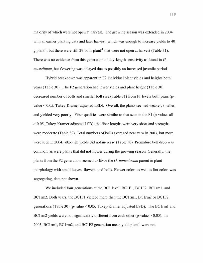
118

majority of which were not open at harvest. The growing season was extended in 2004

with an earlier planting data and later harvest, which was enough to increase yields to 40

g plant-1, but there were still 29 bolls plant-1 that were not open at harvest (Table 31).

There was no evidence from this generation of day-length sensitivity as found in G.

mustelinum, but flowering was delayed due to possibly an increased juvenile period.

Hybrid breakdown was apparent in F2 individual plant yields and heights both

years (Table 30). The F2 generation had lower yields and plant height (Table 30)

decreased number of bolls and smaller boll size (Table 31) from F1 levels both years (p-

value < 0.05, Tukey-Kramer adjusted LSD). Overall, the plants seemed weaker, smaller,

and yielded very poorly. Fiber qualities were similar to that seen in the F1 (p-values all

> 0.05, Tukey-Kramer adjusted LSD); the fiber lengths were very short and strengths

were moderate (Table 32). Total numbers of bolls averaged near zero in 2003, but more

were seen in 2004, although yields did not increase (Table 30). Premature boll drop was

common, as were plants that did not flower during the growing season. Generally, the

plants from the F2 generation seemed to favor the G. tomentosum parent in plant

morphology with small leaves, flowers, and bolls. Flower color, as well as lint color, was

segregating, data not shown.

We included four generations at the BC1 level: BC1F1, BC1F2, BC1rm1, and

BC1rm2. Both years, the BC1F1 yielded more than the BC1rm1, BC1rm2 or BC1F2

generations (Table 30) (p-value < 0.05, Tukey-Kramer adjusted LSD). The BC1rm1 and

BC1rm2 yields were not significantly different from each other (p-value > 0.05). In

2003, BC1rm1, BC1rm2, and BC1F2 generation mean yield plant-1 were not

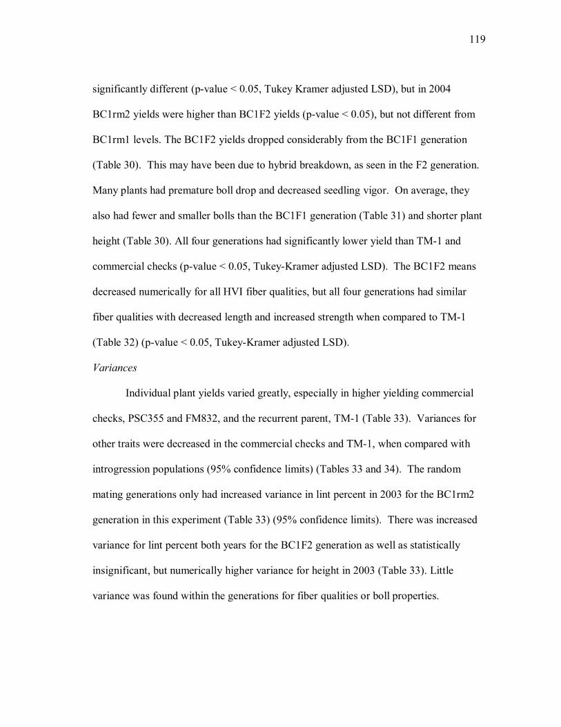
119

significantly different (p-value < 0.05, Tukey Kramer adjusted LSD), but in 2004

BC1rm2 yields were higher than BC1F2 yields (p-value < 0.05), but not different from

BC1rm1 levels. The BC1F2 yields dropped considerably from the BC1F1 generation

(Table 30). This may have been due to hybrid breakdown, as seen in the F2 generation.

Many plants had premature boll drop and decreased seedling vigor. On average, they

also had fewer and smaller bolls than the BC1F1 generation (Table 31) and shorter plant

height (Table 30). All four generations had significantly lower yield than TM-1 and

commercial checks (p-value < 0.05, Tukey-Kramer adjusted LSD). The BC1F2 means

decreased numerically for all HVI fiber qualities, but all four generations had similar

fiber qualities with decreased length and increased strength when compared to TM-1

(Table 32) (p-value < 0.05, Tukey-Kramer adjusted LSD).

Variances

Individual plant yields varied greatly, especially in higher yielding commercial

checks, PSC355 and FM832, and the recurrent parent, TM-1 (Table 33). Variances for

other traits were decreased in the commercial checks and TM-1, when compared with

introgression populations (95% confidence limits) (Tables 33 and 34). The random

mating generations only had increased variance in lint percent in 2003 for the BC1rm2

generation in this experiment (Table 33) (95% confidence limits). There was increased

variance for lint percent both years for the BC1F2 generation as well as statistically

insignificant, but numerically higher variance for height in 2003 (Table 33). Little

variance was found within the generations for fiber qualities or boll properties.

120

Tabl

e 33

. Var

ianc

e es

timat

es b

y ge

nera

tion

and

year

for G

. tom

ento

sum

GM

A p

lant

and

yie

ld c

hara

cter

istic

s. Pa

rent

hese

s en

clos

e 95

% c

onfid

ence

lim

its.

2003

Yie

ld†

H

eigh

t†

Tbol

l†

Lint

perc

†

G. t

om‡

§

127

(96,

174

) §

§

F1

17

5 (1

22, 2

74)

1066

(7

48, 1

640)

81

5 (5

67, 1

273

79

(51,

136

) F2

19

6 (1

56, 2

54)

1055

(8

33, 1

378)

69

(5

5, 9

0)

42

(18,

181

) BC

1F1

1875

(1

605,

222

1)

953

(816

, 112

8)

553

(474

, 655

) 13

(1

1, 1

6)

BC1F

2 11

38

(930

, 142

4)

1350

(1

102,

169

3)

389

(318

, 487

) 48

(3

7, 6

5)

BC1r

m1

541

(460

, 645

) 93

7 (8

00, 1

114)

49

0 (4

18, 5

83)

17

(13,

21)

BC

1rm

2 85

9 (7

08, 1

065)

10

42

(860

, 129

1)

429

(354

, 531

) 30

(2

4, 3

9)

TM-1

23

51

(178

6, 3

236)

33

9 (2

81, 4

17)

66

(50,

93)

2

(1, 3

) FM

832

3640

(2

761,

501

9)

425

(186

, 176

7)

74

(56,

102

) 2

(1, 3

) PS

C35

5 53

42

(437

4, 6

674)

25

4 (1

92, 3

53)

269

(223

, 330

) 5

(4, 6

)

20

04

Y

ield

†

Hei

ght†

Tb

oll†

Li

ntpe

rc†

F1

10

88

(719

, 183

7)

241

(160

, 408

) 43

0 (2

76, 7

62)

4 (2

, 9)

F2

16

(11,

23)

746

(557

, 105

2)

485

(359

, 690

) 15

(8

, 35)

BC

1F1

1285

(9

48, 1

869)

47

1 (3

49, 6

71)

614

(453

, 879

) 11

¶ (8

, 16)

BC

1F2

943

(744

, 123

5)

752

(593

, 984

) 60

5 (4

79, 7

87)

22

(17,

30)

BC

1rm

1 11

09

(902

, 139

8)

728

(592

, 916

) 75

7 (6

14, 9

56)

12

(9, 1

5)

BC1r

m2

1115

(9

10, 1

398)

57

9 (4

73, 7

26)

525

(430

, 656

) 13

(1

0, 1

6)

TM-1

19

18

(145

0, 2

656)

22

3 (1

70, 3

06)

81

(61,

112

) 3

(2, 5

) FM

832

4620

(3

534,

630

0)

330

(252

, 452

) 19

1 (1

45, 2

62)

6 (5

, 9)

PSC

355

2812

(2

110,

393

7)

212

(161

, 294

) 17

0 (1

27, 2

37)

4 (3

, 6)

† Yie

ld =

seed

cotto

n pl

ant-1

, Tbo

ll =

num

ber o

f bol

ls a

t har

vest

, Lin

tper

c =

lint p

erce

ntag

e (%

). ‡

Gos

sypi

um to

men

tosu

m

§ Not

cal

cula

ted

due

to z

ero

yiel

ds.

¶ V

aria

nce

estim

ated

by

resi

dual

var

ianc

e du

e to

failu

re o

f mix

ed m

odel

.

121

Table 34. Variance estimates by generation and year for HVI fiber properties from G. tomentosum GMA from 2003 and 2004. Parentheses contain 95% confidence limits. 2003 MIC† UHML† UI† STR† ELO† F1 0.0 ‡ 0 ‡ 0 ‡ 0 ‡ 0 ‡ F2 0.0 ‡ 0 ‡ 0 ‡ 0 ‡ 0 ‡ BC1F1 0.1 (0.1, 0.3) 2 (2, 3) 1 (1, 2) 14 (10, 21) 0 (0, 1) BC1F2 0.1 (0.0, 0.8) 3 (2, 5) 2 (1, 3) 11 (9, 15) 0 ‡ BC1rm1 0.1 (0.1, 0.4) 3 (2, 4) 2 (1, 2) 11 (8, 16) 1 (0, 1) BC1rm2 0.4 (0.3, 0.5) 3 (2, 4) 2 (1, 2) 4 (3, 6) 1 (1, 2) TM-1 0.0 ‡ 0 (0, 1) 0 (0, 1) 2 (1, 3) 0 ‡ FM832 0.0 ‡ 0 (0, 1) 1 (0, 1) 4 (3, 6) 0 (0, 1) PSC355 0.0 ‡ 0 ‡ 1 (0, 1) 3 (3, 4) 0 ‡ 2004 MIC† UHML† UI† STR† ELO† F1 0.0 ‡ 0 ‡ 0 ‡ 0 ‡ 0 ‡ F2 0.0 ‡ 0 ‡ 0 ‡ 1 (0, 14) 0 ‡ BC1F1 0.0 ‡ 2 (1, 4) 2 (1, 4) 7§ (5, 11) 1 (0, 1) BC1F2 0.0 (0.1, 0.9) 3 (2, 5) 6 (4, 9) 13§ (10, 19) 1 (1, 2) BC1rm1 0.0 (0.0, 1.5) 4§ (3, 5) 3 (2, 4) 8 (6, 10) 0 ‡ BC1rm2 0.1 ‡ 3 (2, 4) 3 (2, 4) 7 (6, 10) 1 (1, 1) TM-1 0.0 ‡ 0 ‡ 0 (0, 1) 1 (1, 2) 0 ‡ FM832 0.0 (0.0, 0.5) 0 (0, 1) 2 (1, 3) 4 (3, 6) 0 ‡ PSC355 0.0 ‡ 0 (0, 1) 1 (1, 2) 3 (2, 5) 0 ‡

†MIC = micronaire, UHML = upper half mean length, UI = uniformity index, STR = strength, ELO = elongation. ‡ Confidence intervals not calculated with REML proc mixed. Zero estimate for variance for generation and residual variance. § Not calculated due to zero yields. ¶ Variance estimated by residual variance due to failure of mixed model. Genetic models

Estimates of genetic effects were complicated by poor performance of G.

tomentosum, large variance for traits on an individual plant basis, and unidirectional

crossing to G. hirsutum. Prediction of means for yield and number of bolls for G.

tomentosum based on a single gene model were negative (Table 35). Rejection of the

model was determined by Lamkey et al. (1995) by a Chi-square test based on the

122

squared difference between observed and expected values for each generation mean

weighted by the inverse of the variance. The variances were so large in this study that

even such large discrepancies between the predicted versus observed values for G.

tomentosum and TM-1 were not statistically significant (Table 35). This can be seen in

Figs. 10 and 11. As described in previous chapters, deviation from x = y in these figures

illustrates model fit. In the case of yield, the there is not a cluster of observations on the

x = y line, showing that a simple model does not fit well the observed data (Fig. 10).

Plant height values, on the other hand, do not deviate from x = y (Fig.11). The more

traditional chi-square test where the squared difference between observed and expected

values is weighted by the inverse of the predicted value seemed more appropriate for this

reason and is also reported here. Using this chi square test the simple model is rejected

for harvested bolls, total number of bolls, and individual plant yield (p-value > 0.05).

Surprisingly, a simple model explained well the performance of generations for all HVI

fiber qualities as well as plant height and lint percent. Estimates may also be biased due

to absence of reciprocal backcrosses to G. tomentosum and only using G. hirsutum

cytoplasms.

123

Tabl

e 35

. Est

imat

es fo

r mid

poin

t (m

), ad

ditiv

e va

lue

(a),

dom

inan

ce (d

) fro

m G

. tom

ento

sum

GM

A b

y ye

ar fo

r yie

ld a

nd p

lant

ch

arac

teris

tics.

Gen

etic

mod

els

Yie

ld†

H

eigh

t† Tb

oll†

Li

ntpe

rc†

H

boll†

Wbo

ll†

2003

20

04

2003

20

04

2003

20

04

2003

20

04

2004

20

04

m‡

-1

1.0*

-1

.8

117.

9**

91.2

**-4

1.0*

*-1

6.9*

* 26

.1**

26.2

**0.

5*

-1.8

* a‡

53.3

**

58.2

**

-3.4

13

.2

61.8

**48

.0**

6.

0**

7.9*

*28

.7**

5.7*

d‡

17.8

* 18

.4*

78.4

**74

.2**

92.1

**89

.0**

-0

.6*

0.3*

10

.6**

2.1*

Chi

-squ

are

A§

3.90

4.

10

1.14

1.

21

0.46

0.

9 0.

12

0.03

2.

52

¶ C

hi-s

quar

e B

§ 20

9.8*

**

142.

7***

7.0

3.9

9.7*

7.

8 0.

2 0.

0 42

.2**

0.2

*,**

,***

p-v

alue

s les

s tha

n 0.

05, 0

.01,

0.0

01 re

spec

tivel

y † Y

ield

= y

ield

pla

nt-1

(g p

lant

-1),

Hei

ght =

hei

ght (

cm),

Tbol

l = to

tal n

umbe

r of b

olls

(cou

nt),

Lint

perc

= L

int p

erce

ntag

e (%

), H

boll

= nu

mbe

r of

harv

este

d bo

lls (c

ount

), W

boll

= w

eigh

t bol

l-1 (g

bol

l-1).

‡ m

= m

idpo

int,

a =

addi

tive

valu

e, d

= d

omin

ance

dev

iatio

n.

§ Chi

-squ

are

A =

(obs

erve

d –

expe

cted

)2 Var

ianc

e-1, C

hi-s

quar

e B

= (o

bser

ved

– ex

pect

ed)2 e

xpec

ted-1

. ¶ N

ot c

alcu

late

d du

e ze

ro v

aria

nce

estim

ates

redu

cing

deg

rees

of f

reed

om to

0.

124

Yieldy = x

-100

-50

0

50

100

150

-10 40 90 140

Observed

Pred

icte

d

20032004

Fig. 10. Observed vs. predicted yields for G. tomentosum GMA from 2003 and 2004.

In the G. mustelinum experiment, different genetic effects were found depending

on the environment (Table 9). With the G. tomentosum introgression populations, this

was not generally true, although the environments in the G. tomentosum experiment

were only different years in the same location and did not include southern Mexico that

had a large effect due to different day-length and climate. A simple genetic model,

without epistasis or linkage, also seemed to fit well for all HVI fiber quality traits (p-

values > 0.05; Chi-square test), as shown in Table 36 and Fig. 12. The model for

strength from 2003 predicted beneficial additive and dominant effects from the recurrent

parent, TM-1, and in 2004 it was reversed, with beneficial additive effects estimated for

the donor parent, G. tomentosum (Table 36). Dominance estimates for micronaire also

125

Heighty = x

0

50

100

150

200

250

0 50 100 150 200 250

Observed

Pre

dict

ed

20032004

Fig. 11. Observed vs. predicted plant heights for G. tomentosum GMA from 2003 and 2004.

changed direction in 2004 from 2003. For the other traits, estimates from the different

years were consistent. Yield was estimated to be mostly controlled by additive genetic

effects from TM-1 with moderate dominance. Height seemed to be a dominant trait, as

seen with heterosis for this trait in the F1 and BC1F1 generations. Moderate additive

and dominance was estimated for UHML, UI, harvested bolls, whereas only additive

genetic effects were important in predicting lint percent. For almost all of these

agronomic traits TM-1 was predicted to be superior to G. tomentosum, except possibly

for lint strength and micronaire (Table 36).

126

Table 36. Genetic models for midpoint (m), additive (a), and dominant (d) values for G. tomentosum HVI fiber qualities. Genetic model MIC† UHML† UI† STR† 2003 2004 2003 2004 2003 2004 2003 2004 m‡ 5.0** 4.0** 20.6** 21.1** 79.8** 76.3** 26.5** 33.3* a‡ -0.3 0.7* 7.5* 6.7* 5.0* 7.3* 4.6* -3.6* d‡ -0.9* 0.9* 3.6* 2.3* 3.3* 5.4* 8.3* -1.6 Chi-square B§ 0.1 0.0 0.3 0.0 0.1 0.0 0.7 0.3

*,**,*** p-values less than 0.05, 0.01, 0.001 respectively. †MIC = micronaire, UHML = upper half mean length (mm), UI = uniformity index (%), STR = strength. ‡ m = midpoint, a = additive value, d = dominance deviation. § Chi-square A = (observed – expected)2 Variance-1 not calculated due to variance estimates equal to zero reducing degrees of freedom to zero, Chi-square B = (observed – expected)2 expected-1.

UHMLy = x

2021222324252627282930

20 22 24 26 28 30

Observed

Pred

icte

d

20032004

Fig. 12. Observed vs. predicted UHML for G. tomentosum GMA from 2003 and 2004.

127

Barriers to introgression from G. tomentosum

The largest barrier to introgression from G. tomentosum was the hybrid

breakdown of inbred populations. The F2 yields were near zero both years and thus the

range of potential phenotypes from the recombining of the two species for agronomic

traits was limited by the low yields (Table 30). Many F2 plants flowered at the normal

time for upland cotton but shed most if not all subsequent bolls. Fruiting nodes were

empty or held dried empty burrs with no seed or lint. Other F2 plants never flowered.

Some of these had abnormal stem and branching patterns. Others had very small leaves,

short internodes, and tiny bolls that when full contained only one or two seeds with very

little lint. Some phenotypes were similar to those associated with monosomes or

duplicate/deficient plants deficient in chromosome segments. The BC1F2 generation

yielded more, but many plants still showed similar symptoms of hybrid breakdown and

no yield. Not reported in this study are BC1F2 family rows grown for selection

purposes where entire families dropped all flowers and were apparently sterile.

Some physiological traits from G. tomentosum may explain in part the

breakdown. G. tomentosum plants in the field during 2003 flowered profusely, but did

not set seed. This may be due to the long style in G. tomentosum that extends the stigma

surface far from the anthers and makes self pollination difficult without insect

pollinators, but as shown with the male sterile, insect pollinators were present

throughout the growing season. It has been hypothesized that G. tomentosum in its

natural environment is pollinated by nocturnal moths and so may be receptive to

pollination at night or twilight (Fryxell 1979). If so, bees and other diurnal insects

128

would be poor pollinators of G. tomentosum and might explain the poor seed set in the

field. If this hypothesized nocturnal habit is passed down in introgression populations,

then generations with G. hirsutum-like pollen that are most potent during early daytime

hours, even if stigma lengths were shorter, would be expected to have decreased seed

set. Long stigma length may also be sufficient by itself to cause sterility.

In the G. tomentosum populations, lethal hybrid mutants, like the chlorophyll

deficient seedlings, were not seen in F2 nor BC1F2 populations. We did find a few

mottled leaf mutants that survived season long. These plants had green veins but

intervening tissue was yellowed and discolored. The yellowed regions in direct sunlight

turned white and almost translucent in the uppermost canopy. These plants produced

seed, but seemed to be stunted and yielded poorly. The most infertile plants from 2003

were transplanted into the greenhouse for the winter to see if we could nurse them into

producing seed. Most did so over the winter and summer of 2004. One plant was found

to be male sterile while four plants had long stigmas and appeared to be effectively self

incompatible. We collected floral buds from the plants that continued to be sterile to see

if there were problems with meiosis or deficiencies for chromosome segments. None

were observed. Plants that in the greenhouse produced seed were grown in 2005 as

family rows from semi-sterile plants to see if the phenotype held. It did. No progeny

produced seed in 2005 fields.

129

Conclusions

As seen with G. mustelinum crosses, it was difficult to estimate genetic effects

from G. tomentosum, due to its poor performance in all environments and unbalanced

backcrossing. Ideally, we would have had equivalent generations that had been

backcrossed to G. tomentosum as well as to G. hirsutum. This was not practical due to

difficulty in making crosses due to poor seed set as well as little agronomic gains

expected by backcrossing to the wild parent. Even still, reciprocal crosses were

attempted during winter of 2003/2004, but discontinued after recovering only a single

boll from weeks of pollinations. This effect was exacerbated by poor performance of G.

tomentosum, F2, and BC1F2 generations. These generations have large effect on

estimates of genetic effects. Together these inadequacies can be seen in the negative

estimates for yield for G. tomentosum.

We found that random mated generations generally had equal or lower means for

most traits without increased variance. This is similar to that found by Meredith and

Bridge (1971) and Miller and Rawlings (1967) as well as Arbelide and Bernardo (2004).

Differences between means of original and intermated populations were attributed by

Meredith and Bridge (1971) to epistasis, seedling vigor, or selection, but the authors

favored selection as the explanation. Arbelide and Bernardo (2004) found no evidence

for epistasis or selection and little difference was seen after one cycle of intermating.

Lamkey et al. (1995) found significant reduction in grain yield in F2-syn8, but little

difference in mean yields were found for other trait. Lamkey et al. (1995) concluded

that recombination of favorable haplotypes was to blame. In our study, differences

130

between BC1F1 and random mating population means were not different from that

predicted by a simple genetic model containing additive and dominant traits, in most

cases. This does not mean than epistasis, selection, and linkage disequilibrium were not

present. It is still our expectation that these play a key role in finding high yielding

progeny with improved fiber traits.

This was especially true when considering hybrid breakdown observed in this

study. The low yields of F2 and BC1F2 generations showed that hybrid breakdown was

a strong force of selection during inbreeding. Selection in the BC1F1 generation would

not be expected to be entirely effective due to inability to replicate genotypes as well as

subsequent hybrid breakdown during inbreeding. Selection of inbred generations would

be difficult due to reduced variance caused by the same hybrid breakdown. The random

mating generations are a compromise between these two alternatives, because of

decreased hybrid breakdown than the BC1F2, but increased recombination. The

increased recombination is still expected to help in finding transgressive segregates and

so for introgression from G. tomentosum random mating may still be recommended if

insect pollinators in isolation are used to minimize time and effort in population

development.

131

CHAPTER VI

MOLECULAR ANALYSIS OF G. tomentosum INTROGRESSION WITH

MICROSATELLITE MARKERS FROM CHROMOSOME 11 Introduction

As explained above for G. mustelinum experiments, the G. tomentosum F2,

BC1F1, BC1F2, BC1rm1 and BC1rm2 populations were tested with microsatellite

markers (Table 13) from cotton linkage group A03 (Lacape et al. 2003; Rong et al.

2004), now classified as chromosome 11 (Wang et al. 2006). Waghmare et al. (2005)

recently completed the first map of G. hirsutum x G. tomentosum. They mapped

locations for the nectariless trait, leaf morphology, and 431 cDNA derived RFLP probes.

Unfortunately, they did not include any SSR markers that can be directly compared with

the results of this study. The map was created with genotypes from 82 F2 plants from a

F1 between a TM-1 derived line and G. tomentosum. They found a terminal inversion in

the G. tomentosum map not present in the G. barbadense map. A few other

inconsistencies were found for chromosomes 10 and 15, but not for A03, now known as

chromosome 11. The Waghmare et al. (2005) A03 linkage group did not coalesce into a

single group, but consisted of four subgroups aligned based on collinearity with G.

hirsutum x G. barbadense map (Rong et al. 2004).

Here we report on linkage relationships for chromosome 11 and segregation of

these markers in F2, BC1F1, BC1F2, BC1rm1, and BC1rm2 generations. Field

experiments showed a strong hybrid breakdown in F2 and BC1F2 populations.

Molecular markers are neutral landmarks in the genome, whose segregation ratio

132

distortion would indicate effects of selection, and a deficit of heterozygous markers

would diagnose inbreeding and increased map distances would suggest increased

recombination.

Materials and methods

DNA extraction, PCR conditions, amplification, gel electrophoresis, and

statistical analysis was identical to that described previously for G. mustelinum

microsatellite testing.

Results

Single marker analysis

The 13 primer combinations amplified a total of 15 loci. Bnl836 was difficult to

score and only one of the two loci was scored in this study. Bnl1681, bnl2895 and

bnl1034 also amplified two segregating loci. All markers were codominant, although

bnl3649 was scored as a dominant band due to chattering in the banding profile making

it difficult to accurately separate homozygous G. tomentosum banding patterns from

heterozygous banding patterns. Observed frequencies for each marker and population

are outlined in Table 37. For testing segregation ratio distortion the small sample sizes

tested with each population was a limiting factor. More intensive studies would require

increased numbers of individuals.

133

Tabl

e 37

. Seg

rega

tion

ratio

s fro

m S

SR m

arke

rs te

sted

on

G. t

omen

tosu

m F

2, B

C1F

1, B

C1r

m1,

BC

1rm

2, a

nd B

C1F

2 po

pula

tions

.

F2

BC

1F1

BC

1rm

1

B

C1r

m2

BC

1F2

G

t H

et

Gh

χ2

Het

Gh

χ2

Gt

Het

Gh

χ2

Gt

Het

Gh

χ2

Gt

Het

Gh

χ2 B

NL1

066

7 15

10

0.

7

28

20

1.3

2

20

24

0.8

5

13

29

3.6

5

16

25

2.3

BN

L364

9 4

14

10

2.6

17

25

1.

5

0 17

28

3.

1

0 13

35

6.

8

1 15

30

4.

9 B

NL3

592

6 18

9

0.8

28

19

1.

7

2 24

21

3.

7

4 16

29

0.

9

5 16

26

1.

9 B

NL2

895A

7

14

12

2.3

23

22

0.

0

2 19

25

0.

4

4 14

26

1.

3

5 7

30

1.7

BN

L280

5 7

17

8 0.

2

24

21

0.2

4

21

22

2.0

4

12

31

3.2

5

16

27

1.7

BN

L263

2 4

19

9 2.

7

24

23

0.0

3

21

22

1.4

0

13

35

6.8

4

11

31

0.5

BN

L341

1 6

11

15

8.2*

22

26

0.3

3

14

30

1.2

1

19

27

1.3

2

13

34

3.0

BN

L343

1 6

10

13

6.2

21

26

0.

5

2 11

27

2.

0

1 24

18

6.

4

4 14

29

0.

8 B

NL1

034a

5

18

8 1.

4

18

29

2.6

3

14

28

0.8

3

12

29

2.0

8

11

28

2.1

BN

L115

1 6

12

15

7.4

22

25

0.

2

. .

. .

1

22

21

3.5

2

18

18

10.4

*B

NL1

681A

6

19

8 1.

0

28

18

2.2

5

24

16

8.9*

5

27

14

13.3

*

6 17

25

3.

0 B

NL2

895B

7

15

10

0.7

22

23

0.

0

1 12

34

5.

2

4 19

22

1.

5

3 10

30

1.

2 B

NL1

681B

3

15

15

9.0*

23

23

0.0

4

12

29

2.8

0

15

31

4.2

3

12

34

1.7

BN

L103

4b

6 15

10

1.

1

29

18

2.6

1

19

26

1.3

2

19

23

0.7

1

23

23

16.1

*B

NL8

36A

.

. .

.

. .

.

3 19

19

1.

7

4 20

20

2.

6

. .

. 0.

4 E

xpec

ted

1 2

1

1

1

1

6 9

1 6

9

1

2 5

*p

-val

ue <

0.0

5

134

We expected deviation from expected marker frequencies in F2 and BC1F2

populations due to hybrid breakdown observed in field populations. What we observed

was significant deviation from expected in F2 populations for only bnl3411, which had

an excess number of G. hirusutum homozygous sequences and a deficiency in G.

tomentosum homozygotes (Table 37). No other marker was statistically different from

predicted ratios, but sample sizes were small and power of Chi-square test is low with

these sample sizes (Neder et al. 1990). The trend was for higher number than expected

of G. hirsutum alleles. Further study is needed to confirm this observation. The BC1F2

generation also showed the significant breakdown in the field, but only bnl1151 and

bnl1034b deviated from expected. Just as in the G. mustelinum population, we observed

a higher number of heterozygotes than expected. The BC1F1 generation had no markers

that deviated from expected. The only marker that deviated from Hardy-Weinberg

frequencies in the BC1rm1 and BC1rm2 was bnl1681A, which also had higher than

expected numbers of heterozygotes.

In the G. mustelinum populations, increased frequency of G. hirsutum alleles in

random mating populations suggested that selection was favoring the cultivated parent.

In the G. tomentosum random mating populations there was not such a trend in the

markers tested (Table 37 and Fig. 13). Overall, they fit well predicted ratios for Hardy

Weinberg equilibrium and the frequency of G. tomentosum alleles did not appear to be

decreasing (Fig. 13), although there was a decrease in heterozygosity from the BC1F1 to

the BC1rm2 population. This suggested that natural selection was not acting the same

on the G. tomentosum introgression populations as it apparently did on G. mustelinum

135

populations. This may be due to absence of day length sensitivity within the wild parent.

Crossing was simplified in G. tomentosum populations because they flowered

consistently in the BC1F1 generation, and thus crossing was simplified and were made

with less difficulty than with the G. mustelinum populations that required maintaining a

large number of plants throughout the winter months in order to accomplish necessary

crossing.

Fig. 13. Heterozygosity and allele frequency from G. tomentosum F2, BC1F1, BC1rm1, BC1rm2, BC1F2 populations. Boxplots illustrate heterozygosity of each population with center line marking median heterozygosity, box edges the first and third quartile. Green circles represent G. tomentosum allele frequency for each population.

Fre

qu

en

cy

136

Maps

We made maps using Carthagene instead of Mapmaker because they facilitated

combining information from multiple mapping populations (Fig. 14). This was

necessary because the individual populations sizes tested ranged from 35 to 50

individuals, which were two small to have high confidence in map order or distances.

Cathagene does not pool map information from different maps as done with JoinMap,

but calculates a single map with the combined populations (de Givry et al. 2005). The

F2-BC1F1 map created had two linkage groups from chromosome 11. The first

contained markers 3952, 2895a, 2805, and 2632, the second contained 1681b, 3411,

3431, 1151, and 1034a. These groups were separated by 55.7 cM in the F2-BC1F1 map,

when linkage was forced. No linkage was found for homoeologous markers from D02.

The map order is consistent with that found in G. barbadense (Lacape et al. 2003). The

potential inversion of 3952, 2895a, 2805, and 2632 found in G. mustelinum was not

present in these maps, suggesting similar marker order to that of G. barbadense,

although very little clustering was observed. In part this may be due to the fact that the

number of markers tested was small and apparently recombination rates were high.

137

Fig. 14. Linkage maps from G. hirsutum x G. tomentosum F2, BC1F1, BC1rm1, BC1rm2, and BC1F2 populations showing increase in mapping distance in BC1rm2.

We had expected an increase in recombination in the random mating populations

and thus an increase in map distance between markers. In the BC1rm1 map, there is a

decrease in map distance between 3592 and 2805 and slight decreases with other

markers (Fig. 14). In the BC1rm2, there is an increase in map distance between 1681b,

3411, 1151, and 3431. The position of 1034a is ambiguous in this population. When

G. mustelinum C11 maps

pAR044b

1066

8363649b3592 14082895b2805a2632a

1681a

341111513431

1034a

Lacape et al. 2003 A03

2632A

2805

1408A

3592

1681

3411

1151A

1034A

2632B

28951408B

BC1F1 and F2 Ch11a

1408 3592

2632 2805

1681

34111151A

1034A

BC1rm1

3592

2805

2632

1681

34111151A

1034A

BC1rm2

2632A2805

1408

3592

1681

3411

1151A

1034A

BC1 combined

0102030405060708090100110120130140150160170180190200210220230240250260270280290300310320330340350360370

G. tomentosum C11 maps

2895A

3592

28052632

1681B341111513431

1034A

BC1F1 and F2

2895A

3592

28052632

1681B34113431

BC1rm1

3592

2895A

2805

2632

3431

1151

3411

1681B

BC1rm2

2895

3592

2805

2632

1681B

3411

3431

1034A

BC1F2

2895A

3592

2805

2632

1681B

3411

3431

1151

1034a

BC1 combined

0

10

20

30

40

50

60

70

80

90

100

110

120

130

140

150

160

170

180

190

138

forced onto the map its position varies from the terminal position in other maps to a

central location by 2805 or 2632. No linkage is detected between 1681b and 2632 when

forced. When the two linkage groups were mapped together, 3431 appeared to be more

tightly linked than 1681b. The map order for 3592 and 2895 also is variable depending

on the stringency of the mapping LOD score cutoffs and the population. In the BC1F2

map, the intervening region between 2632 and 1681b is reduced to 46.4 cM and there is

an increase in distances between 3411, 3431 and 1034a. The combined map for all

markers is consistent with the order found in the G. barbadense maps.

This analysis has weaknesses since the mapping algorithm was not specific for

these population types. In order to form the map we had the program assume they were

BC1F1 populations. Significant deviation from expected 1:1 frequencies of genotypes

may have affected estimates of map distance. Also, the map distances were not adjusted

for multiple generations of recombination. Conclusions based on these map distances

are weakened for these reasons.

For more robust results, future mapping studies require increasing population

sizes and marker coverage. It may be that in large populations increased sensitivity in

mapping function can be achieved. Increasing marker coverage would also help in

identifying global trends. The small number of markers and genome coverage limits our

ability to determine if the trends observed here are genome-wide or just specific to this

linkage group. Other recommendations would be to adjust mapping algorithm to handle

back cross random mating populations and multiple cycles of recombination.

139

Discussion

We observed with molecular markers relatively small deviations from expected

segregation ratios in BC1rm1, BC1rm2, and BC1F2 populations. The unequal

inheritance of G. hirsutum alleles in the F2 population was not significant for many

markers, in part because of small population size. Curiously, Waghmere et al. (2005)

did not discuss possible segregation ratio distortion within their data. Increasing the F2

population size would be quite simple and this population could be key to understanding

the hybrid breakdown in G. tomentosum hybrid populations. Questions that remain

include whether the hybrid breakdown was acting on the zygotic or on the gametophytic

level. In other words, were F2 plants low yielding and dropping bolls because of

problems with the female plant, the pollen, or the egg? The decreased height, smaller

leaf size, and unusual plant morphology of the F2 suggested that there were definitely

zygotic effects that could have reduced fertility. But, were zygotic effects enough to

explain the hybrid breakdown? That was not clear from this experiment. It is doubtful

that decrease in overall plant fertility wouldn’t be seen also at the gametophytic level. It

also remains to be determined exactly what effect or mechanism G. tomentosum’s

potential nocturnal floral habit may have in hybrid populations. The breakdown in F2

plants may well be related to segregation for nocturnal stigmas and diurnal pollen. If

this trait has selected for differential pollen growth or sensitivity to environmental

conditions, this may well be a strong selection factor on haploid gametes that are

segregating for components of this trait. There may be other genetic epistatic

140

interactions that may also be important in causing segregation ratio distortion. Future

mapping and QTL studies would be useful in determining what parts of the genome are

contributing to hybrid breakdown and may help determine the mechanism.

The mechanism behind possible selection was not clear from this study.

Stephens (1949) hypothesized that the breakdown in G. hirsutum x G. barbadense

populations was due to cryptic structural differences. This theory was in response to

Harland’s (1936, and 1939) hypothesis that the breakdown was due mainly to genetic

differences between the species, not of the species. Markers could be used to identify

regions that have structural differences between the species, but small differences may

require high marker density and even sequence data. Our data does not indicate

structural differences between G. hirsutum and G. tomentosum, but admittedly it covers

only a portion of the genome and with limited power. Cryptic structural rearrangements

would be consistent with molecular studies in Neurospora that indicate that even very

small unpaired regions are silenced during meiosis of interspecific hybrids (Lee et al.

2005). From this model, F1 and F2 hybrid breakdown would be due in part to silencing

of unpaired regions, which could manifest itself similar to chromosome deficiencies.

For detecting this silencing, molecular markers sensitive to methylation status of the

DNA sequence may be necessary as well as looking at mRNA composition of F1 and F2

generations. More sensitive techniques like microarray might be useful for evaluating

the role of this mechanism in hybrid breakdown between these species.

As apposed to results seen in G. mustelinum populations, the size of the random

mating populations was sufficient to maintain expected genotypic frequencies. They

141

may not have been large enough though to generate the increased recombination we had

hoped for, but increased cycles of random mating may be necessary in order to see

dramatic results. Although, there was less evidence for genetic drift and selection in

these populations, bulk pollinations are still recommended due to decreased record

keeping, reduced chances for bias and error, and decreased labor. Insect pollinations

would be easier still, although there is more chance of outcrossing and possibly bias due

to pollinating preferences.

142

CHAPTER VII

ADVANCED GENERATION BACKCROSSES AND COMPOSITE GENERATIONS

FROM G. tomentosum: SELECTION, HERITABILITY, AND PERFORMANCE Introduction

Backcrossing reduces the recurrent parental genomic composition by half each

time, assuming no selection or bias. This rapidly increases adaption due to rapid

increase in amount of cultivated genome and loss of the wild parental genome, how

quickly backcross populations approached the recurrent parent yields and fiber quality.

In the case of G. mustelinum, the wild parent had improved fiber quality and so selecting

for yield and fiber quality are in opposite directions. In the case of G. tomentosum, the

wild parent has poor fiber quality and so selection for yield and fiber quality traits are

expected to be more effective than in the case of G. mustelinum. And so the first

question we wanted to answer in this study was how further backcrossing affects means

and variances. At what generations were recurrent parental yields and fiber quality

recovered? We also wanted to evaluate possible effects of interspecific barriers

advanced generation back cross generations. From the results reported previously, it can

be seen that there is significant hybrid breakdown in F2 and BC1F2 generations. We

wanted to know whether this was a trend that would continue beyond a single backcross.

Finally, which generation is best for selection for yield and fiber traits? The best

population for selection is that with the most variance and the highest mean. This is a

balancing act because as the amount of the wild species in a generation decreases so

143

increases the mean, but the genetic variance decreases. Bernardo (2004) advocates the

use of a usefulness criteria that is equal to the mean plus the variance times the

heritability. For these populations we propose looking at the difference between the

overall mean and the mean of the top 10 percent of the population mean. The population

with the largest difference and the highest selected mean would be recommended as

effective for selection.

In this experiment we are testing three different mating schemes. The first is the

recurrent backcross with inbreeding at each level of back crossing. The second is

recurrent backcrossing with random mating at each level of backcrossing prior to selfing.

The third is a composite cross made with a polycross synthetic made of eleven elite

cotton cultivars topcrossed onto the BC2F1 male sterile generation. This composite

cross differs from random mated generations in that it does not have a pure line G.

hirsutum parent, and so is segregating for G. hirsutum as well as G. mustelinum alleles.

Using an advanced backcross composite is similar to successful incorporation

breeding from exotic material in barley such as RIPE from Canada (Kannenberg and

Falk 1995) and the California composites cross populations (Allard 1992). The RIPE

program combined backcrossing and intermating exotic materials, although restricted to

exotic entries with good per se performance. They observed that natural selection

seemed to weed out negative traits in random mating populations (Kannenberg and Falk

1995). Allard (1992) showed that the California composites did not collapse to inbred

types even after repeated cycles of intermating and selection. Selection was effective

even after over twenty generations of recombination (Allard 1992). The RIPE barley

144

introgression project, from Canada, cycles composite populations at different levels of

backcrossing and random mating until reaching levels for competitive selection with

elite materials (Kannenberg and Falk 1995). In cotton breeding, composite populations

may be more easily accessed for such diverse germplasm as G. tomentosum because they

already have a base level of adaption that makes them more useful to other breeders and

more likely to be used than going back to the original species.

Since these populations were relatively small and restricted to a single testing

location, over two years, the results reported here should be considered a preliminary

assessment of these breeding methodologies. Regardless, here we report on population

performance and make recommendations regarding future breeding methods for

handling G. tomentosum in cotton breeding programs.

Materials and methods

Plant material

Crossing procedure was the same as described previously for G. mustelinum

populations. Composite populations were created in 2002 by crossing the cycle 0 bulk

pollen from the elite polycross described previously was used as a male parent with

BC2F1 male sterile plants from G. tomentosum. In summer of 2003, the G. tomentosum

composite Syn0 population was random mated in North Carolina, by Dr. Darryl

Bowman, by allowing bee pollination in isolation and harvesting the male sterile plants

to make the next generation. Another cycle of random mating was performed in Mexico

by bulk pollinating the male sterile plants with the male fertile plants. It was also

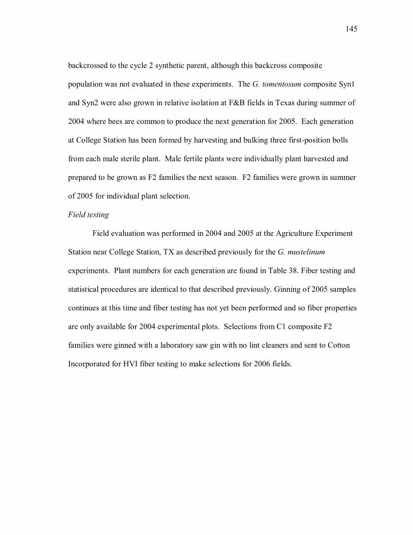
145

backcrossed to the cycle 2 synthetic parent, although this backcross composite

population was not evaluated in these experiments. The G. tomentosum composite Syn1

and Syn2 were also grown in relative isolation at F&B fields in Texas during summer of

2004 where bees are common to produce the next generation for 2005. Each generation

at College Station has been formed by harvesting and bulking three first-position bolls

from each male sterile plant. Male fertile plants were individually plant harvested and

prepared to be grown as F2 families the next season. F2 families were grown in summer

of 2005 for individual plant selection.

Field testing

Field evaluation was performed in 2004 and 2005 at the Agriculture Experiment

Station near College Station, TX as described previously for the G. mustelinum

experiments. Plant numbers for each generation are found in Table 38. Fiber testing and

statistical procedures are identical to that described previously. Ginning of 2005 samples

continues at this time and fiber testing has not yet been performed and so fiber properties

are only available for 2004 experimental plots. Selections from C1 composite F2

families were ginned with a laboratory saw gin with no lint cleaners and sent to Cotton

Incorporated for HVI fiber testing to make selections for 2006 fields.

146

Table 38. Plant numbers evaluated in G. tomentosum advanced backcross experiment. Generation 2004 2005 BC1F1 87 97 BC1F2 158 199 BC1rm1 185 172 BC2F1 202 100 BC2F2 176 177 BC2rm1 197 181 BC3F1 99 101 BC3F2 0 160 BC3rm1 88 88 Comp syn0 202 97 Comp syn1 204 90 FM832 106 98 PSC355 101 100 Elite Syn2 207 100 TM-1 101 100

Results and discussion

Ms4

In 2005, there was evidence for effect of Ms4 male sterile trait on plant height,

total number of bolls, harvested bolls, yield plant-1 (p-values < 0.05, confidence limits)

(Table 39). There was not evidence for a difference between male sterile and male

fertile plants for weight boll-1, lint boll-1, lint percentage, and immature bolls in 2005

(Overlapping confidence limits). When male sterile effect was separated by generation,

unlike in the G. mustelinum populations, there was evidence for the effect of Ms4 at all

levels of backcrossing for G. tomentosum populations (Table 40). Early generation

yields were higher in the G. tomentosum experiment, with less plant to plant variation

than in the G. mustelinum experiment, which may help explain the difference.

147

Table 39. The adjusted marginal means for male sterile, Ms4ms4, and male fertile plants, ms4ms4¸ across populations, from the 2005 G. tomentosum advanced backcross experiment. Parentheses contain 95% confidence limits. Plant characteristics

Plant height (cm) Total bolls Harvested bolls Immature bolls ms4ms4 145.6 (141, 151) 43.0 (39, 47) 31.0 (28, 34) 10.1 (8, 12) Ms4ms4 155.3 (150, 161) 23.3 (19, 27) 12.0 (9, 15) 10.6 (9, 12) Yield characteristics Yield (g/plant) Lint percent Boll size (g) Lint/boll (g) ms4ms4 100.7 (85, 116) 33.0 (29, 36) 2.89 (2.6, 3.2) 1.01 (0.8, 1.3) Ms4ms4 35.9 (25, 47) 33.8 (31, 37) 2.74 (2.5, 3) 1.02 (0.8, 1.2)

148

Table 40. The adjusted marginal means for male sterile, Ms4ms4, and male fertile plants, ms4ms4¸ by population, from the 2005 G. tomentosum advanced backcross experiment Parentheses contain 95% confidence limits. Generation Male fertile (ms4ms4) Generation Male sterile (Ms4ms4) Yield (g) BC1rm1 38 (23, 52) BC1rm1 9 (-6, 25) BC2rm1 77 (64, 91) BC2rm1 19 (4, 33) BC3rm1 114 (99, 129) BC3rm1 44 (19, 68) Comp Syn0 109 (91, 127) Comp Syn0 59 (43, 75) Comp Syn1 116 (98, 134) Comp Syn1 63 (47, 80) Height (cm) BC1rm1 160 (144, 176) BC1rm1 161 (145, 177) BC2rm1 150 (133, 166) BC2rm1 171 (155, 187) BC3rm1 148 (132, 164) BC3rm1 171 (154, 187) Comp Syn0 136 (120, 152) Comp Syn0 165 (149, 180) Comp Syn1 127 (111, 143) Comp Syn1 149 (133, 165) Harvested bolls (counts) BC1rm1 20 (16, 23) BC1rm1 5 (2, 9) BC2rm1 26 (23, 29) BC2rm1 7 (3, 10) BC3rm1 33 (29, 37) BC3rm1 13 (7, 20) Comp Syn0 29 (25, 34) Comp Syn0 19 (15, 22) Comp Syn1 30 (25, 35) Comp Syn1 17 (13, 22) Immature bolls (counts) BC1rm1 17 (13, 21) BC1rm1 14 (9, 18) BC2rm1 10 (5, 14) BC2rm1 9 (5, 13) BC3rm1 8 (4, 12) BC3rm1 12 (7, 17) Comp Syn0 8 (3, 12) Comp Syn0 13 (8, 17) Comp Syn1 3 (-2, 7) Comp Syn1 5 (1, 10) Lint percent (%) BC1rm1 29.4 (28, 31) BC1rm1 31.4 (29, 34) BC2rm1 30.8 (29, 32) BC2rm1 29.5 (28, 31) BC3rm1 31.0 (29, 33) BC3rm1 30.1 (27, 33) Comp Syn0 35.3 (33, 38) Comp Syn0 36.5 (35, 38) Comp Syn1 35.5 (33, 38) Comp Syn1 36.5 (34, 39) Weight boll-1 (g boll-1) BC1rm1 1.83 (1.49, 2.17) BC1rm1 1.80 (1.44, 2.17) BC2rm1 2.78 (2.46, 3.10) BC2rm1 2.86 (2.52, 3.21) BC3rm1 3.37 (3.03, 3.72) BC3rm1 2.96 (2.47, 3.45) Comp Syn0 3.54 (3.16, 3.92) Comp Syn0 3.18 (2.83, 3.53) Comp Syn1 3.64 (3.25, 4.03) Comp Syn1 3.66 (3.29, 4.02) Lint boll-1 (g boll-1) BC1rm1 0.47 (0.30, 0.63) BC1rm1 0.50 (0.32, 0.69) BC2rm1 0.77 (0.61, 0.93) BC2rm1 0.71 (0.54, 0.88) BC3rm1 0.94 (0.77, 1.10) BC3rm1 0.76 (0.55, 0.97) Comp Syn0 1.19 (1.01, 1.37) Comp Syn0 1.10 (0.94, 1.26) Comp Syn1 1.34 (1.15, 1.53) Comp Syn1 1.38 (1.21, 1.56)

149

Because the means for these generations are not being used for estimates of

genetic effects and to remain consistent with values reported in other field experiments,

the male sterile plants were not been removed from estimates of general means.

Inclusion of Ms4 plants within each generation does lower the mean of affected traits

and may artificially increase the variance. Future experiments for testing of genetic

effects or for interfacing with marker genotypes for quantitative trait loci analysis should

be done without the Ms4 trait. But, for breeding, the male sterility allows increased

number of crosses to be made with less labor, and it is easily removed from the

population, because it is dominant, nuclear and simply controlled.

Means and variances for generations

Recovery of the recurrent parent, TM-1, required different levels of backcrossing

for different traits (Tables 41 and 42). There was evidence that the BC1 generations

differed from TM-1 for height, seedcotton yield, boll weight (Table 41), UHML, fiber

strength, and elongation (Table 42), but not for lint percentage (Table 41), micronaire,

and uniformity index (Table 42) (Tukey-Kramer adjusted LSD). BC2 generations

differed from TM-1 for the same traits as the BC2 generations, except strength, in

BC2F2 and BC2rm1 populations, but not BC2F1 which did have increased strength.

There was evidence for increased plant height, decreased weight boll-1 and increased

elongation still in BC3F1 generations compared to recurrent parent TM-1. Thus a single

backcross was sufficient to recover fiver strength and three backcrosses to recover yield

potential and UHML of TM-1. Height, boll weight, and elongation would apparently

require more than three generations of backcrossing to recover recurrent parental values.

150

Table 41. Generation means for plant and yield characteristics for G. tomentosum advanced backcross experiments from 2004 and 2005. Means with different letter designations are significantly different according to the Tukey-Kramer adjusted LSD at p-values < 0.05. 2004 Height† Yield† Lintperc† Hboll† Wboll† BC1F1 126 BC 66 EF 31 FG 35 AB 1.93 A BC1F2 118 C 26 G 30 G 15 F 1.56 A BC1rm1 132 B 43 FG 30 G 23 E 1.77 A BC2F1 121 C 86 DE 33 DE 31 ABC 2.78 B BC2F2 115 C 73 E 32 EFG 27 BCDE 2.51 BC BC2rm1 122 C 68 E 33 DE 27 CDE 2.53 BC BC3F1 116 C 122 B 33 DE 36 A 3.55 BC BC3rm1 117 C 86 CDE 32 DEF 26 BCDE 3.32 BC Comp Syn0 120 C 106 BCD 36 C 30 ABCD 3.45 C Comp Syn0 116 C 115 B 38 B 31 ABC 3.60 D Elite Syn2 104 DE 151 A 41 A 31 ABC 4.85 E TM-1 100 E 121 B 34 D 26 CDE 4.75 E FM832 97 E 113 BC 40 A 23 DEF 4.81 E PSC355 96 E 127 AB 42 A 32 ABC 3.92 D 2005 Height† Yield† Lintperc† Hboll† Wboll† BC1F1 168 A 46 FG 31 E 23 DEF 1.94 G BC1F2 134 DEF 18 G 32 E 10 H 1.76 G BC1rm1 159 AB 21 G 31 E 11 GH 1.84 G BC2F1 145 CD 86 D 32 DE 30 BCD 2.82 DEF BC2F2 152 BC 55 EF 31 E 20 EF 2.55 F BC2rm1 159 AB 48 F 30 E 17 FG 2.85 DF BC3F1 143 CD 127 C 32 E 33 BC 3.82 B BC3F2 128 EF 89 D 30 E 26 CDE 3.22 CE BC3rm1 153 BC 93 D 31 E 27 BCDE 3.26 CD Comp Syn0 152 BC 79 DE 36 BC 23 DEF 3.33 C Comp Syn0 139 DE 83 DE 36 BCD 22 DEF 3.62 BC Elite Syn2 116 G 167 AB 41 A 36 AB 4.65 A TM-1 124 FG 141 BC 34 CDE 30 BCD 4.73 A FM832 112 G 168 AB 39 AB 35 AB 4.82 A PSC355 112 G 175 A 41 A 44 A 4.05 B

† Height = plant height (cm), Yield = seedcotton plant-1, Lintperc = lint percentage (%). Hboll = number of bolls harvested, Wboll = weight boll-1 (g).

151

Table 42. Generation means for HVI fiber qualities, including both male sterile and male fertile plants, for G. tomentosum advanced backcross experiments from 2004. Means with different letter designations are significantly different according to Tukey-Kramer adjusted LSD with p-values less than 0.05. 2004 MIC† UHML† UI† STR† ELO† BC1F1 4.7 BC 25.8 EF 82.6 FGHI 31.8 BCD 6.4 ABC BC1F2 4.5 CD 24.9 F 81.6 JK 30.5 DEFG 6.0 BCD BC1rm1 4.7 C 25.5 F 82.3 HIJ 31.4 DE 6.2 BC BC2F1 4.8 B 26.9 D 83.2 EFG 30.9 DEF 6.3 BC BC2F2 4.7 BC 26.5 DE 82.8 FGHI 30.4 EFG 6.2 BC BC2rm1 4.8 BC 26.9 D 83.2 EFG 30.7 DEFG 6.4 ABC BC3F1 4.8 BC 27.8 C 83.5 CDEF 30.8 DEFG 6.2 BC BC3rm1 4.9 B 27.7 C 83.7 BCDE 31.0 DEFG 6.2 BC Comp Syn0 4.9 B 28.3 BC 84.0 BCD 32.6 BC 5.5 DE Comp Syn1 4.9 B 28.7 B 84.3 AB 32.8 B 5.2 E Syn2 4.8 B 28.7 B 84.2 ABC 31.6 D 6.3 ABC TM-1 4.7 BC 27.8 C 83.4 DEF 29.6 G 4.1 F FM832 4.4 D 30.0 A 84.2 ABCD 34.4 A 6.8 A PSC355 5.2 A 27.8 C 84.9 A 31.4 DEF 5.2 E

† MIC = micronaire, UHML = upper half mean length (mm), UI = uniformity index (%), STR = Strength, ELO = elongation.

Inbreeding depression was a significant barrier to introgression at the BC1F1

level as seen by the drop in yields, plant height, boll counts, and boll weight in BC1F2

generation (Table 41). This effect appeared to decrease in later generations, but was still

present even in BC3F2 generations. The yield decreased from 66 g/plant to 26 g/plant in

2004 and from 46 to 18 g/plant in 2005 for the BC1F1 and BC1F2 generation, which

was due in part to plants with zero yields within the populations. The majority of plants

with zero yields had flowered with the general population, but dropped the developing

bolls before maturity. At two generations of backcrossing the yield drop in 2004 was

not significant from 86 to 73 g/plant, but in 2005 the decrease was higher, from 86 to 55

g plant-1. This was may have been due to slightly shorter season that allowed more of

152

the BC1F2 plants time to catch up to BC1F1 levels. BC3F2 plants were only available

in 2005 for evaluation, but they also decreased in yield from 122 to 89 g/plant. This

suggests that although the BC3F1 yields are similar to the cultivated parent (p-value >

0.05, Tukey-Kramer adjusted LSD), this generation still contains enough G. tomentosum

DNA to show inbreeding depression. The yield differences are due mainly to decreased

number of harvested bolls and decreased boll weight

Another trend seen at the BC1 level was for a decrease in means for random

mating generations. Even considering only male fertile plants this was true for height,

individual plant seedcotton yield, harvested bolls, and weight boll-1 for the BC2 and BC3

generations (Table 41). For example, in 2005, the height of BC1F1 generation was 18

cm taller than the first random mating generation, yields decreased by 8 g plant-1

considering only male fertile lines, but 25 g plant-1 overall, and boll weight decreased by

0.1 g plant even in male fertile plants. The BC2F1 generation and BC2rm1 generation

for this same year decreased in yield per plant from 86 to 48 g plant-1 in the entire

population on average and to 77 g plant-1 in only male sterile lines. The BC3rm1 yields

were significantly lower also (p-value < 0.05, Tukey-Kramer adjusted LSD). The

difference between F1 and random mating generations decreased in later generation

backcrosses, but is still present. This was not the case for fiber quality traits, which were

not significantly different for random mating and F1 generations within the same level of

backcrossing (Table 42).

Variance was predicted to decrease in more advanced backcross populations.

There was not evidence for a difference in variance for height, number of harvested

153

bolls, boll weight (Table 43), upper half mean fiber length, uniformity index, and

elongation (Table 44) for BC1F1 generations as in BC3F1 generations (Overlapping

confidence limits). There was an increase in variance for yield for higher yielding

generations including check varieties. This shows that the individual plant yields are

extremely variable, even in genetically uniform populations. The variation does not

necessarily represent segregation or genetic variance, but is mostly microenvironmental

effects, as can be seen in the difference between first or last plants in a plot. These end

plants have increased access to sunlight and nutrients due to decreased competition from

the other plants in the plot, and thus have increased boll load, height, and individual

plant yields. Besides border effects with the first and last plants, other variables may

greatly effect individual plant yield including access to water, nutrients, sunlight, disease

pressure, insect pressure, and soil variability. Some of these trends will be accounted for

in replication effects, but others will not. This is of key importance in judging yields in

individual plants because sometimes apparent performance is not indicative of genetic

improvements in yield.

154

Tabl

e 43

. Var

ianc

es b

y ge

nera

tion

and

year

for p

lant

cha

ract

erist

ics

from

G. t

omen

tosu

m a

dvan

ced

back

cros

s exp

erim

ents

in

2004

and

200

5. P

aren

thes

es c

onta

in 9

5% c

onfid

ence

lim

its.

20

04

Hei

ght†

Yie

ld†

Li

ntpe

rc†

Hbo

ll†

Wbo

ll† BC

1F1

472

(349

, 671

) 12

84

(937

., 18

68)

11.2

‡ (8

.26,

16.

9)

345.

9 (2

54, 4

98)

0.21

‡ (0

.15,

0.3

1)

BC1F

2 75

2 (5

93, 9

84)

951

(749

., 12

46)

21.9

(1

6.8,

29.

5)

256.

0 (2

02, 3

35)

0.53

‡ (0

.41,

0.7

1)

BC1r

m1

716

(582

, 901

) 11

31

(917

., 14

30)

11.7

(9

.31,

15.

1)

272.

2 (2

20, 3

45)

0.11

(0

.05,

0.3

0)

BC2F

1 46

3 (3

82, 5

73)

2165

(1

781,

268

7)

15.2

(1

2.3,

19.

1)

218.

9 (1

80, 2

72)

0.44

(0

.29,

0.7

1)

BC2F

2 74

6 (6

05, 9

42)

2993

(2

414,

380

9)

10.7

(8

.45,

13.

9)

388.

6 (3

14, 4

94)

0.48

(0

.31,

0.8

2)

BC2r

m1

517

(422

, 645

) 22

64

(184

7, 2

840)

31

.6

(25.

6, 3

9.9)

27

1.6

(221

, 341

) 0.

35

(0.2

2, 0

.62)

BC

3F1

305

(231

, 418

) 23

91

(181

8, 3

285)

2.

9 (2

.06,

4.4

3)

398.

3 (3

01, 5

53)

0.23

(0

.12,

0.6

1)

BC3r

m1

421

(310

, 601

) 16

79

(123

1, 2

426)

6.

7 (4

.72,

10.

1)

99.1

(7

2, 1

45)

0.09

(0

.02,

5.0

0)

Com

p Sy

n0

581

(480

, 716

) 44

00

(345

6, 5

792)

9.

4 (7

.63,

11.

8)

271.

4 (2

21, 3

76)

0.73

(0

.47,

1.2

4)

Com

p Sy

n1

610

(502

, 756

) 47

73

(392

5, 5

928)

7.

4 (5

.95,

9.4

1)

157.

1 (1

19, 2

16)

1.67

(1

.14,

2.6

5)

Syn2

31

2 (2

57, 3

84)

3765

(3

114,

464

2)

16.9

(1

3.8,

21.

1)

75.0

(5

6, 1

05)

0.43

(0

.24,

0.9

4)

TM-1

21

2 (1

60, 2

93)

1918

(1

449,

265

6)

3.1

(2.1

7, 4

.66)

24

5.1

(178

, 359

) 0.

15

(0.0

5, 1

.20)

FM

832

384

(294

, 523

) 45

30

(347

4, 6

156)

6.

0 (4

.47,

8.6

2)

162.

5 (1

22, 2

28)

0.19

(0

.09,

0.6

4)

PSC

355

223

(169

, 306

) 28

12

(211

0, 3

937)

3.

7 (2

.60,

5.5

0)

242.

6 (2

00, 3

00)

0.42

(0

.26,

0.7

3)

20

05

20

05

Hei

ght†

Yie

ld†

Li

ntpe

rc†

H

boll†

W

boll†

BC1F

1 63

5 (4

77, 8

85)

1336

(1

006,

185

9)

69.4

(4

3.3,

128

) 31

8.0

(239

, 444

) 0.

09

(0.0

3, 0

.63)

BC

1F2

1154

(9

27, 1

47)

920

(737

, 118

0)

46.8

(2

9.4,

83.

9)

190.

4 (1

53, 2

44)

0.24

(0

.13,

0.5

8)

BC1r

m1

648

(519

, 830

) 72

5 (5

81, 9

27)

65.8

(4

6.5,

100

) 17

6.1

(141

, 226

) 0.

53‡

(0.4

2, 0

.70)

BC

2F1

540

(408

, 746

) 35

14

(262

4, 4

951)

10

.0

(6.2

4, 1

8.6)

28

1.6

(213

, 390

) 0.

24

(0.1

2, 0

.67)

BC

2F2

630

(508

, 802

) 32

91

(263

3, 4

231)

19

.7

(14.

2, 2

8.9)

35

9 (2

89, 4

57)

0.16

(0

.07,

0.5

2)

BC2r

m1

776

(630

, 979

) 29

58

(239

7, 3

742)

20

.2

(14.

2, 3

0.6)

31

3.4

(255

, 394

) 0.

64

(0.4

3, 1

.02)

BC

3F1

626

(474

, 865

) 57

86

(440

7, 7

931)

2.

9 (1

.81,

5.5

5)

385.

1 (2

92, 5

32)

0.14

(0

.05,

0.5

4)

BC3F

2 59

8 (4

76, 7

73)

4229

(3

394,

541

5)

13.7

(9

.68,

21.

0)

291.

7 (2

33, 3

76)

0.43

(0

.27,

0.7

8)

BC3r

m1

519

(389

, 725

) 41

30

(305

2, 5

902)

8.

2 (5

.18,

14.

7)

314.

2 (2

37, 4

37)

0.41

(0

.30,

0.5

9)

Com

p Sy

n0

663

(504

, 909

) 32

89

(249

1, 4

543)

14

.8

(10.

1, 2

3.6)

22

8.1

(174

, 313

) 0.

71

(0.4

3, 1

.32)

C

omp

Syn1

63

9 (4

81, 8

86)

4485

(3

401,

618

4)

8.0

(5.1

3, 1

3.9)

24

1.8

(183

, 335

) 0.

39

(0.2

2, 0

.87)

155

Tabl

e 43

. con

tinue

d.

20

05

Hei

ght†

Yie

ld†

Li

ntpe

rc†

Hbo

ll†

Wbo

ll† Sy

n2

406

(310

, 555

) 76

53

(585

4, 1

043)

3.

6 (2

.18,

7.0

2)

345.

4 (2

55, 4

94)

0.42

(0

.32,

0.5

7)

TM-1

38

1 (2

90, 5

21)

4667

(3

534,

644

8)

2.4

(1.4

6, 4

.43)

54

1.6

(412

, 745

) 0.

42

(0.2

4, 0

.88)

FM

832

303

(223

, 435

) 94

73

(696

0, 1

364)

1.

8 (1

.00,

3.8

8)

300.

3 (2

29, 4

11)

0.32

(0

.17,

0.8

2)

PSC

355

385

(290

, 534

) 92

38

(694

1, 1

290)

5.

0 (2

.96,

9.9

8)

223.

7 (1

70, 3

07)

0.31

(0

.22,

0.4

2)

† Hei

ght =

hei

ght (

cm),

Yie

ld =

seed

cotto

n pl

ant-1

(g),

Lint

perc

= L

int p

erce

ntag

e (%

), H

boll

= ha

rves

ted

bolls

(cou

nts)

, and

Wbo

ll =

wei

ght b

oll-1

. ‡ V

aria

nce

estim

ated

from

resi

dual

var

ianc

e du

e to

failu

re o

f REM

L m

ixed

mod

el e

stim

atio

n

Tabl

e 44

.Var

ianc

es b

y ge

nera

tion

and

year

for H

VI f

iber

qua

lity

from

G. t

omen

tosu

m a

dvan

ced

back

cros

s exp

erim

ent i

n 20

04.

Pare

nthe

ses c

onta

in 9

5% c

onfid

ence

lim

its.

M

IC†

U

HM

L†

UI†

ST

R†

ELO

†

BC1F

1 0.

0 ‡

2.1

(1.3

9, 3

.52)

0.

5 (0

.29,

1.1

1)

2.2

(1.4

1, 3

.98)

7.

34§

(5.4

0, 1

0.5)

BC

1F2

0.1

(0.0

5, 0

.86)

5.

9 (4

.14,

9.2

2)

1.2

(0.7

4, 2

.20)

3.

2 (2

.15,

5.1

7)

13.3

§ (9

.72,

19.

2)

BC1r

m1

0.0

‡ 3.

0 (2

.22,

4.2

3)

0.0

‡ 2.

7 (2

.03,

3.8

7)

7.6

(5.8

2, 1

0.3)

BC

2F1

0.0

(0.0

1, 1

.04)

2.

5 (1

.95,

3.3

8)

0.6

(0.4

1, 0

.90)

1.

5 (1

.16,

2.1

3)

4.1

(3.2

6, 5

.37)

BC

2F2

0.1

(0.0

5, 0

.32)

3.

3 (2

.49,

4.5

6)

0.7

(0.4

7, 1

.13)

1.

7 (1

.23,

2.5

2)

5.5

(4.2

1, 7

.38)

BC

2rm

1 0.

0 ‡

1.9

(1.4

2, 2

.64)

0.

5 (0

.30,

0.7

7)

1.9

(1.4

5, 2

.70)

4.

1 (3

.19,

5.4

6)

BC3F

1 0.

0 (0

.01,

0.7

3)

1.5

(0.9

6, 2

.46)

0.

0 ‡

0.7

(0.4

1, 1

.33)

3.

7 (2

.62,

5.5

1)

BC3r

m1

0.0

(0.0

0, 9

404)

2.

0 (1

.32,

3.3

4)

0.5

(0.2

8, 1

.12)

1.

5 (0

.96,

2.5

2)

4.9

(3.6

1, 6

.98)

C

omp

Syn0

0.

0 ‡

2.2

(1.7

2, 2

.97)

0.

8 (0

.57,

1.1

5)

1.5

(1.1

4, 2

.06)

5.

7 (4

.56,

7.2

8)

Com

p sy

n1

0.1

(0.0

4, 0

.23)

2.

1 (1

.60,

2.8

2)

0.5

(0.3

1, 0

.84)

1.

8 (1

.34,

2.3

9)

7.2

(5.7

9, 9

.19)

Sy

n2

0.1

(0.0

2, 0

.19)

1.

6 (1

.19,

2.1

3)

0.5

(0.3

0, 0

.78)

1.

2 (0

.90,

1.6

8)

5.6

(4.4

8, 7

.13)

TM

-1

0.0

‡ 0.

4 (0

.18,

1.1

9)

0.0

‡ 0.

5 (0

.40,

0.7

3)

1.4

(0.9

6, 2

.39)

FM

832

0.1

(0.0

3, 0

.44)

1.

8 (1

.20,

2.7

9)

0.0

‡ 0.

3 (0

.18,

0.8

2)

3.9

(2.8

0, 5

.86)

PS

C35

5 0.

0 ‡

1.2

(0.7

9, 2

.08)

0.

0 ‡

0.4

(0.1

9, 1

.01)

3.

0 (2

.09,

4.5

8)

† MIC

= m

icro

naire

, UH

ML

= up

per h

alf m

ean

leng

th, U

I = u

nifo

rmity

inde

x, S

TR =

stre

ngth

, ELO

= e

long

atio

n.

‡ Con

fiden

ce li

mits

not

com

pute

d by

REM

L fo

r pla

nt(g

en) o

r res

idua

l. V

aria

nce

for g

ener

atio

n eq

ual t

o ze

ro. V

aria

nce

for g

ener

atio

n ex

plai

ned

with

re

plic

atio

n.

§ Var

ianc

e es

timat

ed fr

om re

sidu

al v

aria

nce

due

to fa

ilure

of R

EML

mix

ed m

odel

est

imat

ion.

156

Heritability

Traditional estimates of heritability are from combinations of generation

variances in a generation means analysis, as correlations of relatives, or variances

estimated in an ANOVA or mixed model (Holland et al. 2003). In this study, we were

not able to take advantage of heritability estimates from generation means analysis since

they rely heavily on variance of F2 and BC1F2 populations. These populations had

artificially low variance due to hybrid breakdown. Variances from ANOVA or mixed

models of entries from the same population in different environments can also be used to

estimate heritability, and thus predicted effectiveness of selection, for that population as

explained by Holland et al. (2003). These experiments have multiple entries with

different amounts of G. mustelinum genomic DNA. If they were all from the same

generation, for example BC1F2 families, then estimates would be easily generated and

interpreted. This was not the situation here, but we wanted to have an estimate of

repeatability as a rough estimate of heritability so we modeled the generations used in

this study as a set of random lines and then calculating heritability according to Holland

et al. (2003) on an individual plant basis as well as narrow sense heritabilities by parent-

offspring regression, as presented in Table 45. The broadsense heritability estimates are

not made with genetically uniform entries, but include different generations each with

different genomic constitutions. Thus these heritability estimates are confounded with

effects of segregation and differential levels of upland and exotic genomes, but were

considered informative still as measures of repeatability of the population performance

and reliability of different measurements. For example, it might be of interest to choose

157

plant characteristics for future selection and improvement, but if the environmental

variance is high and generations have little variance for these traits, then selection is not

expected to be effective.

Heritability was estimated with variance components with early generations from

2003, 2004 and 2005 as well as later generations from 2004 and 2005, which suggested

that most of the fiber properties would be moderately heritable, except uniformity index

and short fiber content. Weight per boll and lint per boll were highly heritable, while

individual plant yield was only moderately heritable. The heritability estimates

calculated from early generations were generally higher than those calculated with

advanced generations, probably due to inclusion of advanced backcrosses that are more

genetically uniform.

Table 45. Estimated heritabilities from G. tomentosum experiments.

Early generation testing

Advanced backcross testing

PO regression BC1F2

PO regression BC1rm1

H SE H SE h SE h SE MIC 0.12 0.06 0.08 0.03 0.27 0.1 0.12 0.07 UHML 0.69 0.11 0.60 0.08 0.25 0.13 0.15 0.08 UI 0.45 0.13 0.31 0.08 0.29 0.22 0.15 0.11 STR 0.17 0.08 0.15 0.05 0.40 0.16 0.11 0.11 ELO 0.39 0.12 0.27 0.07 0.23 0.17 0.22 0.11 Height 0.41 0.12 0.27 0.08 Yield 0.56 0.13 0.28 0.08 Lintperc 0.65 0.11 0.48 0.10 Harvboll 0.23 0.09 0.07 0.04 Weightboll 0.83 0.07 0.57 0.10 Lintboll 0.81 0.08 0.66 0.09 Totalboll 0.26 0.11 0.00 0.03

158

In 2002, when backcrossing was beginning, we tested the open pollinated fiber

samples from greenhouse BC1F1 plants. These plants were the parents to all of the

subsequent generations. Although adding a level of complexity to planting and to seed

preparation each year, tracking individual plant pedigrees from segregating populations

made it possible to measure heritability of fiber traits through parent-offspring

regression. Heritability is measured by the slope of the regression line of midparent and

progeny performance and is a narrow sense estimate of heritability, the ratio of the

additive genetic variance to the total phenotypic variance (Bernardo 2004). Such

estimates are affected by the environments of the parents as well as the offspring. In this

case it measures the heritability of fiber properties of these particular greenhouse

populations to their field grown progenies.

In the G. mustelinum experiments, we found that contrary to broadsense

heritability estimates, that there was little to no heritability for micronaire, uniformity

index as measured with PO regression (Table 23). In the parallel G. tomentosum

experiments, we found only moderate heritability from PO regression with BC1F2

plants, and lower heritability for PO regression with BC1rm2 plants for all HVI fiber

quality measures (Table 45). Strength estimates especially dropped from 0.595 to 0.17.

UHML was highly heritable in the G. mustelinum populations, but this was not the case

with G. tomentosum, as measured by PO regression. Strength is often cited as a highly

heritable trait (Niles and Feaster 2004), which was not always the case in this

experiment. G. tomentosum does not carry the net beneficial genes that G. mustelinum

has for fiber length and so may explain the decrease in heritability for fiber length

159

Selection

Although heritability estimates from PO regression were shown to be moderate

to low for selecting in BC1F1 plants for upper half mean length, it was of interest to see

if selection for UHML would have similar results in G. tomentosum populations to G.

mustelinum populations. In the case of G. mustelinum, heritability was shown by PO

regression to be high, but progeny in 2004 fields showed less gain from selection than

expected (Table 24). Broadsense heritability estimates for G. tomentosum were

relatively high, but PO regression results were not (Table 45). Because pedigrees of

experimental plants were maintained, the dataset could be reduced to only the

descendents from the top 15 fiber length BC1F1 plants to measure gain from selection.

The UHML means for this hypothetically selected dataset and the original dataset are

presented in Table 46. Predicted gain from selection is equal to the selection index times

the heritability and the standard deviation of the trait (Poehlman and Sleper 1995).

160

Table 46. Difference between selected plants based on pedigree from top greenhouse BC1F1 G. tomentosum and unselected populations from 2004. Parentheses contain confidence limites for estimated means. Unselected UHML Selected UHML Gain Gain % BC1F1-gh 25.8 (25, 26) 28.1 (27, 29) 2.3 9.0 BC1F2 24.9 (24, 25) 26.7 (25, 29) 1.8 7.2 BC1rm1 25.5 (25, 25) 24.0 (23, 25) -1.5 -5.9 BC1rm2 25.4 (25, 25) 26.4 (26, 27) 1.0 3.9 BC2F1 26.9 (26, 27) 28.0 (27, 29) 1.1 4.2 BC2F2 26.5 (26, 26) 28.3 (27, 29) 1.8 6.7 BC2rm1 26.9 (26, 26) 27.9 (27, 29) 1.0 3.7 BC3F1 27.8 (27, 28) 28.3 (27, 29) 0.6 2.0 Heritability estimates Selection intensity s.d. Expected gain P-O BC1F2 0.25 5% 2.18 1.11 P-O BC1rm1 0.15 5% 2.18 0.69 Variance components 0.6 5% 2.18 2.7

Depending which heritability estimate was used from G. tomentosum populations

gain for selection at the BC1F1 was expected to range between 1.7 and 2.7 mm (Table

46). The observed gains in BC1F2 and BC1rm1 random mating generations were 1.8

and 1.5 mm from the unselected generation, which was higher than expected gain for

BC1F2 generation, but BC1rm1 generation selected mean was less than the unselected

BC1rm1. In each of the subsequent generations the gain continued to be near expected

or slightly lower. The selected populations were improved over TM-1 fiber lengths for

BC2F1, BC2F2, BC2rm1, and BC3F1 generations. The mean UHML for BC1F1

populations of G. tomentosum were quite low, reflecting the short fiber from G.

tomentosum. Surprisingly, there was some improvement over recurrent parental lengths

in these later generations. This was also unexpected, because with G. mustelinum

populations selected mean UHML decreased each generation until they were not

161

different from the general population. Because selected in BC1F1 gains persisted after

backcrossing for G. tomentosum populations selection for fiber length at the early

BC1F1 generation appeared to be effective. In the case of G. mustelinum, concurrent

natural selection for G. hirsutum-types and selection for high UHML was not effective

in increasing fiber lengths. In the case of G. tomentosum, if natural selection was still

favoring upland cotton phenotypes, then it may have been selecting at the same time for

longer fiber, which is in upland cotton, but not G. tomentosum, increasing the mean

length of selected populations.

One key question to this experiment was which generation would be most useful

for selection for agronomic traits, like yield and fiber quality. If selection had been

heavy in the BC1F1 for UHML, some gains from selection for fiber would be expected

(Table 46). The possible gains with fiber quality must be balanced in consideration with

hybrid breakdown in selfed populations and low yields in BC1 generations. The

variance for individual plant yield was very high both years, even in TM-1, which is

highly inbred (Table 43). High variance in TM-1 and check varieties indicated that

environmental variance is extremely high for individual plant yield, making individual

plant selection unreliable. This can be seen in the difference between the top ten percent

yielding plants and the overall mean (Table 47).

162

Table 47. Difference for yield between top ten percent of each G. tomentosum introgression population tested from 2004. Parentheses contain 95% confidence limits.

Unselected yield 2004 (g plant-1)

Selected yield 2004 (g plant-1) Gain (g) %

BC1F1 62 (49, 74) 144 (112, 176) 83 134 BC1F2 25 (16, 35) 106 (82, 131) 81 319 BC1rm1 44 (36, 53) 133 (112, 154) 89 202 BC2F1 86 (78, 94) 179 (160, 199) 94 109 BC2F2 74 (66, 83) 200 (178, 222) 126 169 BC2rm1 69 (61, 78) 180 (159, 201) 111 160 BC3F1 122 (111, 134) 198 (178, 218) 76 62 BC3rm1 84 (71, 97) 180 (148, 213) 96 114 Comp Syn0 106 (98, 114) 253 (233, 272) 147 139 Comp Syn1 114 (106, 122) 276 (257, 296) 162 142 FM832 112 (101, 123) 293 (266, 321) 181 161 PSC355 125 (113, 137) 259 (229, 289) 134 108 Syn2 151 (143, 158) 294 (275, 314) 144 95 TM-1 121 (109, 132) 232 (203, 260) 111 92

We wanted to know how effective selection would be within each of the

populations. In order to evaluate the feasibility of individual plant selection for yield we

compared the mean yield plant-1 with the mean of the top ten percent yielding plants. If

the difference is large between these two means it shows that there is variance within the

population. The variance of each population can be partitioned into genetic and

environmental components. The commercial checks and TM-1, the recurrent parent,

were inbred and should have very little genetic variance. The variance from these

generations is from environmental effects. The differences between selected and

unselected mean yield plant-1- for commercial checks and TM-1 were 161% for FM832,

108% for PSC355, and 92% of the unselected mean levels. This means that there was

high variance for individual plant yield for these generations that are genetically

uniform. Variance in commercial checks and TM-1 was mostly due to differences in

163

response to the microenvironments for individual plants, for example seven of ten

selected FM832 plants are from first or last positions in the plot that face large alleys,

data not shown. End plants have decreased competition from cotton plants within the

row.

The differences between mean and top ten percent mean individual plant yields

for segregating generations, as a percentage of the mean, were also greater than 100%.

The largest difference between selected and unselected means in introgression

populations was found in the composite generations, which have higher increase than

even the BC3F1 and BC3rm1 generations that contain similar amounts of the G.

hirsutum genome (Table 47). This may be due to segregation for not only alleles from

G. tomentosum, but also for alleles from the multiple upland cotton parents. There was a

general trend for observed gain to decrease on a percentage basis from BC1 to BC2

level, but an increase in selected population mean levels. At the individual plant level,

the high microenvironmental variance complicates the choice of generation for

individual plant yield selection. If individual plant selection for yield is employed, the

BC1F1 generation would not be ideal because of the low mean population level, and

breakdown in BC1F2 progeny. The inbred BC1F2 population would appear to be better

at this level than the BC1F1, and probably increasing the level of inbreeding before

individual plant selection would increase its effectiveness. The observed gain for BC2

and BC3 plants was less than the BC1, but the population mean was high enough to

make selections. Methods to reduce high variance in individual plant yield due to

microenvironmental differences would be greatly beneficial, because with such high

164

environmental variance reliably picking high yielding varieties by eye, a common

beginning for pedigree breeding, would be expected to be difficult.

For fiber quality, the mean for the top 10% selected plants were higher than the

unselected mean for all populations except TM-1 and PSC355 (Table 48). Unlike for

individual plant yield, large differences were not seen in selected and unselected mean

levels of UHML for commercial checks and TM-1. The mean UHML was lowest in the

early backcross generations, but upper ten percent means are greater than theTM-1

average of 27.8 mm for all generations (Table 48). The composite generations had 9%

higher than UHML in the top ten percent of the populations than the unselected

composite and the top ten percent selections approach fiber quality found in commercial

check rows, exceeding that of TM-1. In order to better combine increased yield and

increased fiber quality, it would be recommend selection for fiber quality in the

composite generations or beyond the second backcross geberatuibs. Balancing fiber

length and yield, the composite generations appear to be better for selection than the

backcross-inbred or backcross-random mated populations.

165

Table 48. Difference between top ten percent UHML G. tomentosum introgression populations and unselected mean values. Unselected UHML 2004 Top 10% UHML 2004

mm 95% C.I. mm 95% C.I. Gain (mm) %

BC1F1 25.8 (25.4, 26.1) 29.4 (28.9, 29.8) 3.6 12.2 BC1F2 24.8 (24.5, 25.2) 28.2 (27.8, 28.7) 3.4 12.1 BC1rm1 25.4 (25.2, 25.7) 28.6 (28.3, 29) 3.2 11.2 BC2F1 26.9 (26.7, 27.1) 29.7 (29.4, 30) 2.8 9.5 BC2F2 26.5 (26.2, 26.7) 29.2 (28.8, 29.5) 2.7 9.3 BC2rm1 26.9 (26.7, 27.2) 29.9 (29.6, 30.2) 3.0 10.1 BC3F1 27.8 (27.4, 28.1) 29.9 (29.5, 30.3) 2.1 7.1 BC3rm1 27.7 (27.4, 28.1) 30.5 (30, 31) 2.8 9.1 Composite Syn0 28.2 (28, 28.5) 31.0 (30.7, 31.3) 2.8 9.0 Composite Syn1 28.7 (28.4, 28.9) 31.6 (31.3, 31.9) 2.9 9.3 FM832 30.0 (29.7, 30.3) 31.6 (31.2, 32.1) 1.6 5.1 PSC355 27.7 (27.4, 28.1) 29.4 (28.9, 29.8) 1.6 5.5 Syn2 28.7 (28.5, 28.9) 31.1 (30.8, 31.4) 2.4 7.7 TM-1 27.8 (27.5, 28.1) 29.1 (28.7, 29.5) 1.3 4.3

Conclusions

Some of the difficulties that we encountered in breeding with G. tomentosum for

agronomic traits were low yields in early backcrosses, hybrid breakdown in selfed

populations, and high variance for individual plant yields. In this experiment, we

included populations that could have been part of three different mating schemes, as

outlined in the introduction to this section, and one objective of this research was to

decide which would be best in the face of these difficulties. A traditional backcross-

inbred strategy does little to compensate for selection against the G. tomentosum alleles,

or hybrid breakdown. By the time that parental yields are recovered, probably at the

BC3F1 generation, it may be difficult to find transgressive segregants due to loss of G.

tomentosum alleles. Selection for individual plant yield is also complicated by high

environmental variance that may mask genetic effects. Selection for yield may be more

166

effective in replicated field trials of advanced inbred generations. Selection at the

BC1F1 level may have some efficacy for fiber quality, but yields would still be very low

and hybrid breakdown was a problem. Little chances for recombination are present after

this level in a traditional backross and inbreed strategy. The backcross-random mate

strategy used in this study appears to be inadequate as judged by its minimal effect on

map length. At least, the inclusion of random mating makes an attempt to allow for

recombination and could be improved by increasing population sizes, and bulked

pollinations instead of plant-to-plant intermatings.

Although only preliminary data on performance of the composite populations is

available at this date, they are an attempt to overcome the weaknesses of the backcross-

random mate strategy. Random mating with composite populations was performed with

bulk pollinations or bee-mediated intermating instead of plant to plant intermating. This

may reduce unintentional selection for G. hirsutum alleles. Population sizes were also

increased, although not as much as they could be. Increasing the population size from

hundreds to thousands of plants would be relatively easy since they are bee pollinated

and large numbers of seed are produced. Selection of male fertile lines from the field

generates enough seed that replicated testing of F2 genotypes is possible as well as

recurrent selection of the population. Selections could be spun off into existing cotton

breeding program to be used as parents in pedigree breeding programs or as entries

themselves. Bulking of the population at each generation also reduces the number of

seed packets and bookkeeping necessary in order to maintain and recreate the

population. It may be that the composite generations may be more useful at an earlier

167

backcrossing level, perhaps at a BC2F1, in order to maximize the possible variation, but

that would mean a drop in mean performance. Further backcrossing could be performed

by crossing male sterile females to bulk pollen from the parental synthetic or other

improved composite.

168

CHAPTER VIII

SUMMARY AND CONCLUSIONS

In order to increase genetic diversity with elite upland cotton, introgression

populations with wild species of cotton, Gossypium mustelinum and G. tomentosum,

were created. Development of these populations would help to determine what

interspecific barriers exist , whether traditional backcross breeding methodology could

be improved by utilization of random mating or composite crosses, and which

populations could be used for further breeding efforts.

To accomplish this objective, F1, F2, BC1F1, BC1F2 generations were

developed along with random mating populations at the BC1 generations, i.e., the

BC1rm1 and BC1rm2 populations. These random mating generations were developed

using the Ms4-TM-1, a isoline heterozygous for Ms4ms4, a dominant nuclear sterile

gene. These generations were grown in a randomized complete block design with four

replications in College Station, Texas during 2003, 2004, and in Mexico during 2005, for

G. mustelinum introgression populations. These generations were tested with

microsatellite markers from chromosome 11 in order to measure effects of selection and

recombination on a molecular level. Later generations (BC2F1, BC2rm1, BC2F2,

BC3F1, BC3rm1, and BC3F2) and composite generations were evaluated in a

randomized complete block design with four replications during 2004 and 2005 for

agronomic properties. Composite generations were made by topcrossing BC2F1 Ms4ms4

male sterile plants with bulked pollen from an elite synthetic created from diallele with

169

parents: Acala Ultima, Pyramid, Coker 315, Stoneville 825, Fibermax 966, M240,

PMHS 26, Deltapine 90, Suregrow 747, Phytogen 355, and Stoneville 474.

It was found for G. mustelinum populations that introgression barriers include

daylength sensitivity and hybrid breakdown in selfed generations and that backcross

generations had improved fiber quality. The effects of hybrid breakdown were not clear

from G. mustelinum populations grown in College Station, because of overall low yields

due to day-length sensitivity, but was made apparent in Mexico where under short days

the F1 yielded on average 82.3 g plant-1 more then the F2 and the BC1F1 yielded 93.6 g

plant-1 more than the BC1F2 population. Random mating populations did not have

increased variance for most traits and means differed little from BC1F1 levels for most

traits. Simple genetic models predicted that the mean for random mating populations

would be equal, which is what was observed. Microsatellite markers showed decreased

frequency of G. mustelinum alleles and decreasing heterozygousity, but no increase in

map distances. For advanced backcross generations, BC3F1 means approached recurrent

parent, TM-1, levels. Fiber quality selection should be performed as early as possible

with G. mustelinum populations due to high heritabilities for upper-half mean length

(UHML) and upper quartile length by weight (UQLw) as measured with parent-

offspring regression. Most other agronomic traits had moderate heritabilities as

estimated with variance components. Composite generations were found to be favorable

for selection and breeding.

For G. tomentosum populations, hybrid breakdown was also a problem with low

yields for F2 and BC1F2 generations, but day length sensitivity was not. Overall yields

170

for introgression populations were higher in 2004 due to earlier planting and delayed

harvest. This increase in the growing season did not help the F2 generation, which

yielded near 0 both years. Little or no increase in variances was found in random mating

populations when compared to BC1F1 levels. G. tomentosum populations did not show

improvements in fiber length as seen in G. mustelinum populations, but did have

increased strength in BC1F1 and F1 generations when compared with TM-1 (p-value

<0.05, Tukey-Kramer LSD). There was an increase in mapping distances measured in

the random mating populations for G. tomentosum, and the frequency of alien alleles did

not vary from expected for most markers. Generation means approached recurrent

parental values for most traits within three backcrosses. Composite generations were

found to be the most useful for breeding and selection.

171

REFERENCES Allard, R. W. 1992. Predictive methods for germplasm identification. In Plant breeding

in the 1990s. Eds. H. T. Stalker and J. P. Murphy, CAB International,

Wallingford, UK.

Allison, D. C. and W. D. Fisher. 1964. A dominant gene for male-sterility in upland

cotton. Crop Sci. 4: 548-549.

Applequist, W. L., R. Cronn, J. F. Wendel. 2001. Comparative development of fiber in

wild and cultivated cotton. Evol. Devel. 3: 3-17.

Arbelide, M. and R. Bernardo. 2004. Random mating before selfing in maize BC1

populations. Crop Sci. 44: 401-404.

Bernardo, R. 2002. Breeding for quantitative traits in plants. Stemma Press, Woodbury,

MN.

Brubaker, C. L and J. F. Wendel. 1994. Reevaluating the origin of domesticated cotton

(Gossypium hirsutum; Malvaceae) using nuclear restriction fragment length

polymorphisms (RFLPs). Am. J. Bot. 81: 1309-1326.

Charlesworth, B., M. T. Morgan, and D. Charlesworth. 1993. The effect of deleterious

mutations on neutral molecular variation. Genetics 134: 1289-1303.

Chaudhry, B., A. Yasmeen, T. Husnain, and S. Riazuddino. 1999.Mini-scale genomic

DNA extraction from cotton. Plant Mol. Biol. Rep. 17: 1–7.

Cruzan, M. B. and M. L. Arnold. 1999. Consequences of cytonuclear epistasis and

assortative mating for genetic structure of hybrid populations. Heredity 82: 36-45

172

Darvasi, A. and M. Soller. 1995. Advanced intercross lines, an experimental population

for fine mapping. Genetics 141: 1199-1207.

de Givry, S., M. Bouchez , P. Chabrier , D. Milan , and T. Schiex . 2005. CARTHA

GENE: Multipopulation integrated genetic and radiation hybrid mapping.

Bioinformatics 21: 1703-1704.

DeJoode, D. R. and J. F. Wendel. 1992. Genetic diversity and the origin of the Hawaiian

Islands cotton, Gossypium tomentosum. Am. J. Bot. 79: 1311-1319.

Dobzhansky, T. H. 1951. Genetics and the origin of species. 3rd ed. Columbia University

Press, New York.

Doganlar, S., A. Frary, and S. D. Tanksley. 2000. The genetic basis of seed-weight

variation: tomato as a model system. Theor. Appl. Genet. 100: 1267-1273.

Dudley, J. W. 1994. Linkage disequilibrium in crosses between Illinois maize strains

divergently selected for protein percentage. Theor. Appl. Genet. 87: 1016-1020

Dudley, J.W. A Dikhuizen, C. Paul, S. T. Coates, and T. R. Rocheford. 2004. Effects of

random mating on marker-QTL associations in the cross of Illinois high protein x

Illinois low protein maize strains. Crop Sci. 44: 1419-1428.

Durrant, J. D., B. W. Gardunia, K. D. Livingstone, M. R. Stevens, and E. N. Jellen.

2006. An algorithm for analyzing linkages affected by heterozygous

translocations: QuadMap. J. Heredity 97:62-66.

Endrizzi, J. E., E. L. Turcotte, R. J. Kohel. 1984. Qualitative genetics, cytology, and

cytogenetics. In: Cotton, R.J. Kohel and C.F. Lewis eds. Agronomy Society of

America. Madison, WI.

173

Fishman, L. and J. H. Willis. 2001. Evidence for Dobzhansky-Muller incompatibilities

contributing to the sterility of hybrids between Mimulus guttatus and M. nasutus.

Evolution 55: 1932-1942

Fishman, L., A. J. Kelly, E. Morgan, and J. H. Willis. 2001. A genetic map in the

Mimulus guttatus species complex reveals transmission ratio distortion due to

heterospecific interactions. Genetics 159: 1701-1716.

Fishman, L. and J. H. Willis. 2005. A novel meiotic drive locus almost completely

distorts segregation in Mimulus (Monkeyflower) hybrids. Genetics 169: 347-

353.

Fox, S. L., E. N. Jellen, S. F. Kianian, H. W. Rines, and R. L. Phillips. 2001. Assignment

of RFLP linkage groups to chromosomes using monosomic F1 analysis in

hexaploid oat. Theor. Appl. Genet. 102: 320-326.

Fryxell, P. A. 1979. A natural history of the cotton tribe. Texas A&M University Press.

College Station, TX.

Fryxell, P. A. 1992. A revised taxonomic interpretation of Gossypium L. (Malvaceae).

Rheeda 2: 108-165.

Gao,W., Z. J. Chen, J. Z. Yu, D. Raska, R. J. Kohel, J. E. Womack and D. M. Stelly.

2004. Wide-cross whole-genome radiation hybrid mapping of cotton

(Gossypium hirsutum L.). Genetics 167: 1317-1329.

Green, E. S. P., J. Abrahamson, A. Barlow, M. J. Daly, S. E. Lincoln, and L. Newburg.

1987. MAPMAKER: An interactive computer package for constructing primary

174

genetic linkage maps of experimental and natural populations. Genomics 1:174-

181.

Gur, A. and D. Zamir. 2004. Unused natural variation can lift yield barriers in plant

breeding. PLoS Biology 2:1610-1615.

Hanson, W. D. 1959. The breakup of initial linkage blocks under selected mating

systems. Genetics 44: 857-868.

Harland, S.C. 1936. The genetical conception of the species. Biol. Rev. 11: 83-112.

Harland, S. C. 1939. Genetical studies in the genus Gossypium and their relationship to

evolutionary and taxonomic problems. Proc. Int. Genet. Congr. Edinburgh 138-

143.

Hasenkampf, C. A. and M. Y. Menzel. 1980. Incipient genome differentiation in

Gossypium. II. Comparison of 12 chromosomes in G. hirsutum, G. mustelinum

and G. tomentosum using herozygous translocations. Genetics 95: 971-983.

Henegariu, O., J. Dunai, X. -N. Chen, J. R. Korenberg, D. C. Ward, J. M. Greally. 2001.

A triple color FISH technique for mouse chromosome identification. Mammalian

Genome 12: 462–465.

Holland, J.B., W. E. Nyquist, and C. T. Cervantes-Martinez. 2003. Estimating and

interpreting heritability for plant breeding. Plant Breed. Rev. 22: 9-112.

Islam-Faridi, M. N., K. L. Childs, P. E. Klein, G. Hodnett, M. A. Menz, R. R. Klein, W.

L. Rooney, J. E. Mullet, D. M. Stelly, and H. J. Price. 2002. A molecular

cytogenetic map of sorghum chromosome 1: Fluorescence in situ hybridization

analysis with mapped bacterial artificial chromosomes. Genetics 161: 345-53.

175

Jain, S. K. and C. A. Suneson. 1966. Increased recombination and selection in barley

populations carrying a male sterility factor. I. Quantitative variability. Genetics

54: 1215-1224.

Jellen, E. N., R. L. Phillips, and H. W. Rhines. 1993a. C-banded karyotypes and

polymorphisms in hexaploid oat accessions (Avena spp.) using Wright’s stain.

Genome 36: 1129-1137.

Jellen, E.N., W. L. Rooney, and R. L. Phillips. 1993b. Characterization of the hexaploid

oat Avena byzantina cv. Kanota monosomic series using C-banding and RFLPs.

Genome 36: 962-970.

Jellen, E.N., B. S. Gill, and T. S. Cox. 1994. Genomic in situ hybridization differentiates

between A/D- and C-genome chromatin and detects intergenomic translocations

in polyploid oat species (genus Avena). Genome 37: 613-618.

Jellen, E. N., H. W. Rines, S. L. Fox, D. W. Davis, R. L. Phillips, and B. S. Gill. 1997.

Characterization of ‘Sun II’ oat monosomics through C-banding and

identifiaction of eight new ‘Sun II’ monosomics. Theor. Appl. Genet. 95: 1190-

1195.

Jenkins, J. N., and J. C. McCarty, Jr. 1995. End of season plant maps. Bull. 1024.

Mississippi Agric. & Forestry Exp. Stn., Mississippi State.

Jiang, C. -X., P. W. Chee, X. Draye, P. L. Morrell, C. W. Smith, and A. H. Paterson.

2000. Multilocus interactions restrict gene introgression in interspecific

populations of polyploid Gossypium (cotton). Evol. 54: 798-814.

176

Kannenberg, L. W. and D. E. Falk. 1995. Models for activation of plant genetic

resources for crop breeding programs. Can. J. Plant Sci. 75: 45-53.

Kim, J.-S., K. L. Childs, M. N. Islam-Faridi, M. A. Menz, R. R. Klein, P. E. Klein, H. J.

Price, J. E. Mullet, and D. M. Stelly. 2002. Integrated karyotyping of sorghum by

in situ hybridization of landed BACs. Genome 45: 402-412.

Kim, J.-S., P. E. Klein, R. R. Klein, H. J. Price, J. E. Mullet, and D. M. Stelly. 2005.

Chromosome identification and nomenclature of Sorghum bicolor. Genetics

169: 1169-1173.

Lacape, J.-M., T.-B. Nguyen, S. Thibivilliers, B. Bojinov, B. Courtois, R. G. Cantrell, B.

Burr, and B. Hau. 2003. A combined RFLP-SSR-AFLP map of teraploid cotton

based on a Gossypium hirsutum x Gossypium barbadense backcross population.

Genome 46: 612-626.

Lamkey, K.R., B. J. Schnicker, and A. E. Melchinger. 1995. Epistasis in an elite maize

hybrid and choice of generation for inbred line development. Crop Sci. 35: 1272-

1281.

Lee, D. W., K.-Y. Seong, R. J. Pratt, K. Baker, and R. Aramayo. 2004. Properties of

unpaired DNA required for efficient silencing in Neurospora crassa. Genetics

167: 131-150.

Lee, J. A. 1984. Cotton as a world crop. In: Cotton, R.J. Kohel and C.F. Lewis eds.

Agronomy Society America. Madison, WI.

Lewis, C. F. and E. F. McFarland. 1952. The transmission of marker genes in

intraspecific backcrosses of Gossypium hirsutum L. Genetics 37: 353-358.

177

Liu, B.-L. 1998. Statistical genomics: Linkage, mapping, and QTL analysis. CRC Press,

New York.

Liu, S., S. Saha, D. Stelly, B. Burr, and R. G. Cantrell. 2000. Chromosomal assignment

of microsatellite loci in cotton. J. Heredity 91: 326-332.

Livingstone, K.D., G. Churchill, and M. K. Jahn. 2000. Linkage mapping in populations

with karyotypic rearrangements. J. Heredity 91: 423-428.

Lu, H., J. Romero-Severson, and R. Bernardo. 2003. Genetic basis of heterosis explored

by simple sequence repeat markers in a random-mated maize population. Theor.

Appl. Genet. 107: 494-502.

McCarty, J. C., Jr., J. N. Jenkins, and J. Zhu. 1998. Introgression of day-neutral genes in

primitive cotton accessions: I. Genetic variances and correlations. Crop Sci. 38:

1425-1428.

Melchinger, A. E. 1987. Expectation of means and variances of testcrosses produced

from F2 and backcross individuals and their selfed progenies. Heredity 59: 105-

115.

Menzel, M.Y., K. L. Richmond, and B. J. Dougherty. 1985. A chromosome translocation

breakpoint map of the Gossypium hirsutum genome. J. Heredity 76: 406-414.

Meredith, W. R. and R. R. Bridge. 1971. Breakup of linkage blocks in cotton,

Gossypium hirsutum L., Crop Sci. 11: 695- 698.

Meyer, V. G. and W. R. Meredith, Jr. 1978. New germplasm from crossing Upland

cotton (Gossypium hirsutum) with G. tomentosum. J. Hered. 69: 183-187.

178

Miller, P. A and J. O. Rawlings. 1967. Breakup of initial linkage blocks through

intermating in a cotton breeding program. Crop Sci. 7: 199-204.

Muller, H. J. 1942. Isolating mechanisms, evolution, and temperature. Biol. Symp. 6: 71-

125.

Neder, J., W. Wassermamn, M. H. Kutner. 1990. Applied linear statistical models. Irwin

Publishing, Homewood, IL.

Niles, G. A. and C. V. Feaster. 1984. Breeding. In: Cotton, R.J. Kohel and C.F. Lewis

eds. Agronomy Society of America. Madison, WI.

O’Donoughue, L.S., S. F. Kianian, P. J. Rayapati, G. A. Penner, M. E. Sorrells, S. D.

Tanksley, R. L. Phillips, H. W. Rines, M. Lee, G. Fedak, S. J. Molnar, D.

Hoffman, C. A. Salas, B. Wu, E. Autrique, and A. Van Deynze. 1995. A

molecular linkage map of cultivated oat. Genome 38: 368-380.

Orr, H. A. 1995. The population genetics of speciation: the evolution of hybrid

incompatibilities. Genetics 139: 1805-1813.

Park, Y.-H., M. S. Alabady, M. Ulloa , B. Sickler, T. A. Wilkins, J. Yu, D. M. Stelly, R.

J. Kohel, O. M. El-Shihy and R. G. Cantrell. 2005. Genetic mapping of new

cotton fiber loci using EST-derived microsatellites in an interspecific

recombinant inbred line cotton population. Mol. Gen. Genet. 274: 428-441.

Pickersgill, B., S.C.H. Barrett, and D. de Andrade-Lima. 1975. Wild cotton in Northeast

Brazil. Biotropica. 7: 42-54.

Poehlman, J. M. and D. A. Sleper. 1995. Breeding field crops, 4th ed. Iowa State

University Press. Ames.

179

Richmond, T.R. 1951. Procedures and methods of cotton breeding with special reference

to American cultivated species. Adv. Genet. 4: 213-245.

Rieseberg, L. H., C. R. Linder, and G. J. Seiler. 1995. Chromosomal and genetic barriers

to introgression in Helianthus. Genetics 141: 1163-1171.

Rieseberg L. H., D. M. Arias, M. C. Ungerer, C.R. Linder, and B. Sinervo. 1996. The

effects of mating design on introgression between chromosomally divergent

sunflower species. Theor. Appl. Genet. 93: 633-644.

Riesberg, L. H. and S. E. Carney. 1998. Tansley review No. 102: Plant hybridization.

New Phytol. 140: 599-624.

Ross, H. 1986. Potato breeding: problems and perspectives. Advances in plant breeding

supplement 13. Paul Parey, Berlin.

Rong, K., C. Abbey, J. E. B owers, C. L. Brubaker, C. Chang, P. W. Chee, T. A.

Delmonte, X. Ding, J. J. Garza, B. S. Marler, C. Park, G. J. Pierce, K. M. Rainey,

V. K. Rastogi, S. R. Schulze, N. L. Trolinder, J. F. Wendel, R. J. Wright, X.

Zhao, L. Zhu, and A. H. Paterson. 2004. A 3347-locus genetic recombination

map of sequence-tagged sites reveals features of genome organization,

transmission, and evolution of cotton (Gossypium). Genetics 166: 389-417.

Saxton, A. M. 1998. A macro for converting mean separation output to letter groupings

in PROC MIXED. Proc. 23rd SAS User’s Group International. p1243-1246.

Silvela, L., I. de la Peña, and R. Gomez-Ruano. 1999. Selection, under negative linkage

disequilibrium. Random mating versus inbreeding. Heredity 82: 598-604.

180

Simmonds, N. W. 1993. Introgression and incorporation. Strategies for the use of crop

genetic resources. Biol. Rev. 68: 539-562.

Singh, R. J. and F. L. Kolb. 1991. Chromosomal interchanges in six hexaploid oat

genotypes. Crop Sci. 31:726-729.

Smith, C. W., and G. G. Coyle. 1997. Association of fiber quality parameters and

within-boll yield components in upland cotton. Crop Sci. 37: 1775–1779.

Stam, P. 1993. Construction of integrated genetic linkage maps by means of a new

computer package: JoinMap. Plant J. 3: 739.

Stebbins, G. L. 1945. The cytological analysis of species hybrids. Bot. Rev. 11: 463-486.

Stephens, S. G. 1949. The cytogenetics of speciation in Gossypium. I. Selective

elimination of the donor parent genotype in interspecific backcrosses. Genetics

34: 626-637.

Stevens, M. R., E. M. Lamb, and D. D. Rhoads. 1995. Mapping the Sw-5 locus for

tomato spotted wilt virus resistance in tomatoes using RAPD and RFLP analyses.

Theor. Appl. Genet. 90: 451-456.

Sweigart, A. L., L. Fishman, and J. H. Willis. 2006. A simple genetic incompatibility

causes hybrid male sterility in Mimulus. Genetics 172: 2465-2479.

Tanksley, S. D. and J. C. Nelson. 1996. Advanced backcross QTL analysis: a method for

the simultaneous discovery and transfer of valuable QTLs from unadapted

germplasm into elite breeding lines. Theor. Appl. Genet. 92: 191-203.

181

Van Becelaer, G., E. L. Lubbers, A. H. Paterson, and P. W. Chee. 2005. Pedigree- vs.

DNA marker-based genetic similarity estimates in cotton. Crop Sci. 45: 2281-

2287.

Van Berloo, R. and R. C. B. Hutten. 2005. Peditree: Software for visualization and

analysis of plant pedigree data. J. Heredity 96: 465-468.

Van der Veen, J. H. 1959. Test of non-allelic interaction and linkage for quantitative

characters in generations derived from two pure diploid lines. Genetica 30: 201-

232.

Van Esbroeck, G. and D. T. Bowman. 1998. Cotton improvement: Cotton germplasm

diversity and its importance to cultivar development. J. Cotton Sci. 2:121-129.

Van Esbroeck, G. A., D. T. Bowman, O.L. May, and D. S. Calhoun. 1999. Genetic

similarity indices for ancestral cotton cultivars and their impact on genetic

diversity estimates of modern cultivars. Crop Sci. 39: 323- 328.

Vroh Bi, I., A. Maquet, J. -P. Baudin, P. du Jardin, J. M. Jacquemin, G. Mergeai. 1999.

Breeding for “low-gossypol seed and high-gossypol plants” in upland cotton.

Analysis of tri-species hybrids and backcross progenies using AFLPs and

mapped RFLPs. Theor. Appl. Genet. 99: 1233-1244.

Wade, M. J. 2001. Epistasis, complex traits, and mapping genes. Genetica 112-113: 59-

69.

Waghmare, V. N., J. Rong, C. J. Rogers, G. J. Pierce, J. F. Wendel, and A. H. Paterson.

2005. Genetic mapping of a cross between Gossypium hirsutum (cotton) and the

Hawaiian endemic, G. tomentosum. Theor. Appl. Genet. 111: 665-676.

182

Wang, G.-L., J.-M. Dong, and A. H. Paterson. 1995. The distribution of Gossypium

hirsutum chromatin in G. barbadense germplasm: Molecular analysis of

introgressive plant breeding. Theor. Appl. Genet. 91: 1153-1161.

Wang, K., X. Song, Z. Han, W. Guo, J. Z. Yu, J. Sun, J. Pan, R. J. Kohel, T. Zhang.

2006. Complete assignment of the chromosomes of Gossypium hirsutum L. by

translocation and fluorescence in situ hybridization mapping. Theor. Appl.

Genet. 113:73-80.

Wendel, J. F. and R. G. Percy. 1990. Allozyme diversity and introgression in the

Galapagos Islands endemic Gossypium darwinii and its relationship to

continental G. barbadense. Biochem. Syst. Ecol. 18: 517-528.

Wendel, J. F., C. L. Brubaker, and A. E. Percival. 1992. Genetic diversity in Gossypium

hirsutum and the origin of Upland Cotton. Am. J. Bot. 79: 1291-1310.

Wendel, J.F., R. Rowley, and J. M. Stewart. 1994. Genetic diversity in and phylogenetic

relationships of the Brazilian endemic cotton, Gossypium mustelinum

(Malvacaeae) Plant Syst. Evol. 192: 49-59.

Wendel, J.F., A. Schnabel, and T. Seelanan. 1995. Bidirectional interlocus concerted

evolution following allopolyploid speciation in cotton (Gossypium). Proc. Nat.

Acad. Sci. USA 92: 280-284.

Wu, J., J. N. Jenkins, J. C. McCarty, Jr. and C. E. Watson. 2005. Comparisons of two

statistical models for evaluating boll retention in cotton. Agron. J. 97:1291-1294.

Yik, C.-P., and W. Birchfield. 1984. Resistant germplasm in Gossypium species and

related plants to Rotylenchulus reniformis. J. Nematol. 16:146-153.

183

Young, N. D. and S. D. Tanksley. 1989. RFLP analysis of the size of chromosomal

segments retained around the Tm-2 locus of tomato during backcross breeding.

Theor. Appl. Genet. 77: 353-359.

Yu, J. and R. Bernardo. 2004. Changes in genetic variance during advanced cycle

breeding in maize. Crop Sci. 44: 405-410.

184

VITA Brian W. Gardunia Agriculture Alumni Seed Improvement Assoc. P.O. Box 158 Romney, IN 47981 1-800-822-7134 765-538-3145 gardunia@agalumniseed.com Education Doctor of Philosophy – 2006, Plant Breeding, Texas A&M University, College Station,

TX Master of Science – 2002, Agronomy, Brigham Young University, Provo, UT Bachelor of Science – 2000, Plant Breeding and Genetics, Brigham Young University,

Provo, UT Awards and honors Cotton Incorporated Research Fellowship (2002 – 2006) First place, graduate student presentation Cotton Beltwide Conference (2003 – 2006) Nominated for Gerald O. Mott Meritorious Graduate Student Award in Crop Science Trustee Scholarship (1995 – 2000) National Merit Scholar (1995) Eagle Scout (1995) Professional Associations Crop Science Society of America Brazos Valley Symphony Orchestra Publications Durrant, J.D., B.W. Gardunia, K.D. Livingstone, M.R. Stevens, and E.N. Jellen. An

algorithm for analyzing linkages affected by heterozygous translocations: QuadMap. J. Heredity 97:62-66.

Maughan, P.J., A. Bonifacio, E.N. Jellen, M.R. Stevens, C.E. Coleman, M. Ricks, S.L. Mason, D.E. Jarvis, B.W. Gardunia, and D.J. Fairbanks. 2004. A genetic linkage map of quinoa (Chenopodium quinoa) based on AFLP, RAPD, and SSR markers. Theoretical and Applied Genetics 109: 1188-1195.