Introductory Statistics, Shafer Zhang-Attributed.pdf - SOL*R |
684
Attributed to Douglas S. Shafer and Zhiyi Zhang Saylor.org Saylor URL: http://www.saylor.org/books/ 1 "This document is attributed to Douglas S. Shafer, and Zhiyi Zhang” About the Authors Douglas S. Shafer Douglas Shafer is Professor of Mathematics at the University of North Carolina at Charlotte. In addition to his position in Charlotte he has held visiting positions at the University of Missouri at Columbia and Montana State University and a Senior Fulbright Fellowship in Belgium. He teaches a range of mathematics courses as well as introductory statistics. In addition to journal articles and this statistics textbook, he has co-authored with V. G. Romanovski (Maribor, Sloveia) a graduate textbook in his research specialty. He earned a PhD in mathematics at the University of North Carolina at Chapel Hill. Zhiyi Zhang Zhiyi Zhang is Professor of Mathematics at the University of North Carolina at Charlotte. In addition to his teaching and research duties at the university, he consults actively to industries and governments on a wide range of statistical issues. His research activities in statistics have been supported by National Science Foundation, U.S. Environmental Protection Agency, Office of Naval Research, and National Institute of Health. He earned a PhD in statistics at Rutgers University in New Jersey. Read License Information Full Legal Code
-
Upload
khangminh22 -
Category
Documents
-
view
0 -
download
0
Transcript of Introductory Statistics, Shafer Zhang-Attributed.pdf - SOL*R |

Attributed to Douglas S. Shafer and Zhiyi Zhang Saylor.org Saylor URL: http://www.saylor.org/books/
1
"This document is attributed to Douglas S. Shafer, and Zhiyi Zhang”
About the Authors
Douglas S. Shafer
Douglas Shafer is Professor of Mathematics at the University of
North Carolina at Charlotte. In addition to his position in Charlotte
he has held visiting positions at the University of Missouri at
Columbia and Montana State University and a Senior Fulbright
Fellowship in Belgium. He teaches a range of mathematics courses
as well as introductory statistics. In addition to journal articles and
this statistics textbook, he has co-authored with V. G. Romanovski (Maribor, Sloveia) a graduate
textbook in his research specialty. He earned a PhD in mathematics at the University of North
Carolina at Chapel Hill.
Zhiyi Zhang
Zhiyi Zhang is Professor of Mathematics at the University of North
Carolina at Charlotte. In addition to his teaching and research duties
at the university, he consults actively to industries and governments
on a wide range of statistical issues. His research activities in statistics
have been supported by National Science Foundation, U.S.
Environmental Protection Agency, Office of Naval Research, and
National Institute of Health. He earned a PhD in statistics at Rutgers University in New Jersey.
Read License Information
Full Legal Code

Attributed to Douglas S. Shafer and Zhiyi Zhang Saylor.org Saylor URL: http://www.saylor.org/books/
2
Acknowledgements We would like to thank the following colleagues whose comprehensive feedback and suggestions for
improving the material helped us make a better text:
Kathy Autrey, Northwestern State University
Kiran Bhutani, The Catholic University of America
Rhonda Buckley, Texas Woman’s University
Susan Cashin, University of Wisconsin-Milwaukee
Kathryn Cerrone, The University of Akron-Summit College
Zhao Chen, Florida Gulf Coast University
Ilhan Izmirli, George Mason University, Department of Statistics
Denise Johansen, University of Cincinnati
Eric Kean, Western Washington University
Yolanda Kumar, Univeristy of Missouri-Columbia
Eileen Stock, Baylor University
Sean Thomas, Emory University
Sara Tomek, University of Alabama
Mildred Vernia, Indiana University Southeast
Gingia Wen, Texas Woman’s University
Jiang Yuan, Baylor University
We also acknowledge the valuable contribution of the publisher’s accuracy checker, Phyllis Barnidge.

Attributed to Douglas S. Shafer and Zhiyi Zhang Saylor.org Saylor URL: http://www.saylor.org/books/
3
Dedication
To our families and teachers.

Attributed to Douglas S. Shafer and Zhiyi Zhang Saylor.org Saylor URL: http://www.saylor.org/books/
4
Preface This book is meant to be a textbook for a standard one-semester introductory statistics course for
general education students. Our motivation for writing it is twofold: 1.) to provide a low-cost
alternative to many existing popular textbooks on the market; and 2.) to provide a quality textbook
on the subject with a focus on the core material of the course in a balanced presentation.
The high cost of textbooks has spiraled out of control in recent years. The high frequency at which
new editions of popular texts appear puts a tremendous burden on students and faculty alike, as well
as the natural environment. Against this background we set out to write a quality textbook with
materials such as examples and exercises that age well with time and that would therefore not
require frequent new editions. Our vision resonates well with the publisher’s business model which
includes free digital access, reduced paper prints, and easy customization by instructors if additional
material is desired.
Over time the core content of this course has developed into a well-defined body of material that is
substantial for a one-semester course. The authors believe that the students in this course are best
served by a focus on the core material and not by an exposure to a plethora of peripheral topics.
Therefore in writing this book we have sought to present material that comprises fully a central body
of knowledge that is defined according to convention, realistic expectation with respect to course
duration and students’ maturity level, and our professional judgment and experience. We believe
that certain topics, among them Poisson and geometric distributions and the normal approximation
to the binomial distribution (particularly with a continuity correction) are distracting in nature.
Other topics, such as nonparametric methods, while important, do not belong in a first course in
statistics. As a result we envision a smaller and less intimidating textbook that trades some extended
and unnecessary topics for a better focused presentation of the central material.
Textbooks for this course cover a wide range in terms of simplicity and complexity. Some popular
textbooks emphasize the simplicity of individual concepts to the point of lacking the coherence of an
overall network of concepts. Other textbooks include overly detailed conceptual and computational
discussions and as a result repel students from reading them. The authors believe that a successful
book must strike a balance between the two extremes, however difficult it may be. As a consequence
the overarching guiding principle of our writing is to seek simplicity but to preserve the coherence of
the whole body of information communicated, both conceptually and computationally. We seek to

Attributed to Douglas S. Shafer and Zhiyi Zhang Saylor.org Saylor URL: http://www.saylor.org/books/
5
remind ourselves (and others) that we teach ideas, not just step-by-step algorithms, but ideas that
can be implemented by straightforward algorithms.
In our experience most students come to an introductory course in statistics with a calculator that
they are familiar with and with which their proficiency is more than adequate for the course material.
If the instructor chooses to use technological aids, either calculators or statistical software such as
Minitab or SPSS, for more than mere arithmetical computations but as a significant component of
the course then effective instruction for their use will require more extensive written instruction than
a mere paragraph or two in the text. Given the plethora of such aids available, to discuss a few of
them would not provide sufficiently wide or detailed coverage and to discuss many would digress
unnecessarily from the conceptual focus of the book. The overarching philosophy of this textbook is
to present the core material of an introductory course in statistics for non-majors in a complete yet
streamlined way. Much room has been intentionally left for instructors to apply their own
instructional styles as they deem appropriate for their classes and educational goals. We believe that
the whole matter of what technological aids to use, and to what extent, is precisely the type of
material best left to the instructor’s discretion.
All figures with the exception of Figure 1.1 "The Grand Picture of Statistics",Figure 2.1 "Stem and
Leaf Diagram", Figure 2.2 "Ordered Stem and Leaf Diagram",Figure 2.13 "The Box Plot", Figure 10.4
"Linear Correlation Coefficient ", Figure 10.5 "The Simple Linear Model Concept", and the
unnumbered figure in Note 2.50 "Example 16" of Chapter 2 "Descriptive Statistics" were generated
using MATLAB, copyright 2010.

Attributed to Douglas S. Shafer and Zhiyi Zhang Saylor.org Saylor URL: http://www.saylor.org/books/
6
Chapter 1
Introduction In this chapter we will introduce some basic terminology and lay the groundwork for the course. We
will explain in general terms what statistics and probability are and the problems that these two
areas of study are designed to solve.
1.1 Basic Definitions and Concepts
LEARNING OBJECT IVE
1. To learn the basic definitions used in statistics and some of its key concepts.
We begin with a simple example. There are millions of passenger automobiles in the United States.
What is their average value? It is obviously impractical to attempt to solve this problem directly by
assessing the value of every single car in the country, adding up all those numbers, and then dividing
by however many numbers there are. Instead, the best we can do would be to estimate the average.
One natural way to do so would be to randomly select some of the cars, say 200 of them, ascertain
the value of each of those cars, and find the average of those 200 numbers. The set of all those
millions of vehicles is called the population of interest, and the number attached to each one, its
value, is a measurement. The average value is a parameter: a number that describes a characteristic
of the population, in this case monetary worth. The set of 200 cars selected from the population is
called a sample, and the 200 numbers, the monetary values of the cars we selected, are the sample
data. The average of the data is called a statistic: a number calculated from the sample data. This
example illustrates the meaning of the following definitions.
Definition A population is any specific collection of objects of interest. A sample is any subset or subcollection of
the population, including the case that the sample consists of the whole population, in which case it is
termed a census.

Attributed to Douglas S. Shafer and Zhiyi Zhang Saylor.org Saylor URL: http://www.saylor.org/books/
7
Definition A measurement is a number or attribute computed for each member of a population or of a sample.
The measurements of sample elements are collectively called the sample data.
Definition A parameter is a number that summarizes some aspect of the population as a whole. A statistic is a
number computed from the sample data.
Continuing with our example, if the average value of the cars in our sample was $8,357, then it seems
reasonable to conclude that the average value of all cars is about $8,357. In reasoning this way we
have drawn an inference about the population based on information obtained from the sample. In
general, statistics is a study of data: describing properties of the data, which is called descriptive
statistics, and drawing conclusions about a population of interest from information extracted from a
sample, which is called inferential statistics. Computing the single number $8,357 to summarize the
data was an operation of descriptive statistics; using it to make a statement about the population was
an operation of inferential statistics.
Definition Statistics is a collection of methods for collecting, displaying, analyzing, and drawing conclusions from
data.
Definition Descriptive statistics is the branch of statistics that involves organizing, displaying, and describing
data.
Definition Inferential statistics is the branch of statistics that involves drawing conclusions about a population
based on information contained in a sample taken from that population.
The measurement made on each element of a sample need not be numerical. Inthe case of
automobiles, what is noted about each car could be its color, its make, its body type, and so on. Such
data are categorical or qualitative, as opposed to numerical or quantitative data such as value or age.
This is a general distinction.

Attributed to Douglas S. Shafer and Zhiyi Zhang Saylor.org Saylor URL: http://www.saylor.org/books/
8
Definition Qualitative data are measurements for which there is no natural numerical scale, but which consist of
attributes, labels, or other nonnumerical characteristics.
Definition Quantitative data are numerical measurements that arise from a natural numerical scale.
Qualitative data can generate numerical sample statistics. In the automobile example, for instance,
we might be interested in the proportion of all cars that are less than six years old. In our same
sample of 200 cars we could note for each car whether it is less than six years old or not, which is a
qualitative measurement. If 172 cars in the sample are less than six years old, which is 0.86 or 86%,
then we would estimate the parameter of interest, the population proportion, to be about the same as
the sample statistic, the sample proportion, that is, about 0.86.
The relationship between a population of interest and a sample drawn from that population is
perhaps the most important concept in statistics, since everything else rests on it. This relationship is
illustrated graphically in Figure 1.1 "The Grand Picture of Statistics". The circles in the large box
represent elements of the population. In the figure there was room for only a small number of them
but in actual situations, like our automobile example, they could very well number in the millions.
The solid black circles represent the elements of the population that are selected at random and that
together form the sample. For each element of the sample there is a measurement of interest,
denoted by a lower case x (which we have indexed as x1,…,xn to tell them apart); these measurements
collectively form the sample data set. From the data we may calculate various statistics. To anticipate
the notation that will be used later, we might compute the sample mean x− and the sample
proportion pˆ, and take them as approximations to the population mean � (this is the lower case
Greek letter mu, the traditional symbol for this parameter) and the population proportion p,
respectively. The other symbols in the figure stand for other parameters and statistics that we will
encounter.

Attributed to Douglas S. Shafer and Zhiyi Zhang Saylor.org Saylor URL: http://www.saylor.org/books/
9
Figure 1.1 The Grand Picture of Statistics
KEY TAKEAWAYS
• Statistics is a study of data: describing properties of data (descriptive statistics) and drawing conclusions
about a population based on information in a sample (inferential statistics).
• The distinction between a population together with its parameters and a sample together with its
statistics is a fundamental concept in inferential statistics.
• Information in a sample is used to make inferences about the population from which the sample was
drawn.
EXERC ISES
1. Explain what is meant by the term population.

Attributed to Douglas S. Shafer and Zhiyi Zhang Saylor.org Saylor URL: http://www.saylor.org/books/
10
2. Explain what is meant by the term sample.
3. Explain how a sample differs from a population.
4. Explain what is meant by the term sample data.
5. Explain what a parameter is.
6. Explain what a statistic is.
7. Give an example of a population and two different characteristics that may be of interest.
8. Describe the difference between descriptive statistics and inferential statistics. Illustrate with an example.
9. Identify each of the following data sets as either a population or a sample:
a. The grade point averages (GPAs) of all students at a college.
b. The GPAs of a randomly selected group of students on a college campus.
c. The ages of the nine Supreme Court Justices of the United States on January 1, 1842.
d. The gender of every second customer who enters a movie theater.
e. The lengths of Atlantic croakers caught on a fishing trip to the beach.
10. Identify the following measures as either quantitative or qualitative:
a. The 30 high-‐temperature readings of the last 30 days.
b. The scores of 40 students on an English test.
c. The blood types of 120 teachers in a middle school.
d. The last four digits of social security numbers of all students in a class.
e. The numbers on the jerseys of 53 football players on a team.
11. Identify the following measures as either quantitative or qualitative:
a. The genders of the first 40 newborns in a hospital one year.
b. The natural hair color of 20 randomly selected fashion models.
c. The ages of 20 randomly selected fashion models.
d. The fuel economy in miles per gallon of 20 new cars purchased last month.
e. The political affiliation of 500 randomly selected voters.
12. A researcher wishes to estimate the average amount spent per person by visitors to a theme park. He takes a
random sample of forty visitors and obtains an average of $28 per person.
a. What is the population of interest?

Attributed to Douglas S. Shafer and Zhiyi Zhang Saylor.org Saylor URL: http://www.saylor.org/books/
11
b. What is the parameter of interest?
c. Based on this sample, do we know the average amount spent per person by visitors to the park?
Explain fully.
13. A researcher wishes to estimate the average weight of newborns in South America in the last five years. He
takes a random sample of 235 newborns and obtains an average of 3.27 kilograms.
a. What is the population of interest?
b. What is the parameter of interest?
c. Based on this sample, do we know the average weight of newborns in South America? Explain
fully.
14. A researcher wishes to estimate the proportion of all adults who own a cell phone. He takes a random
sample of 1,572 adults; 1,298 of them own a cell phone, hence 1298∕1572 ≈ .83 or about 83% own a cell
phone.
a. What is the population of interest?
b. What is the parameter of interest?
c. What is the statistic involved?
d. Based on this sample, do we know the proportion of all adults who own a cell phone? Explain
fully.
15. A sociologist wishes to estimate the proportion of all adults in a certain region who have never married. In a
random sample of 1,320 adults, 145 have never married, hence 145∕1320 ≈ .11 or about 11% have never
married.
a. What is the population of interest?
b. What is the parameter of interest?
c. What is the statistic involved?
d. Based on this sample, do we know the proportion of all adults who have never married? Explain
fully.
16. a. What must be true of a sample if it is to give a reliable estimate of the value of a particular
population parameter?
b. What must be true of a sample if it is to give certain knowledge of the value of a particular

Attributed to Douglas S. Shafer and Zhiyi Zhang Saylor.org Saylor URL: http://www.saylor.org/books/
12
population parameter? ANSWERS
1. A population is the total collection of objects that are of interest in a statistical study.
3. A sample, being a subset, is typically smaller than the population. In a statistical study, all elements of a
sample are available for observation, which is not typically the case for a population.
5. A parameter is a value describing a characteristic of a population. In a statistical study the value of a
parameter is typically unknown.
7. All currently registered students at a particular college form a population. Two population characteristics of
interest could be the average GPA and the proportion of students over 23 years.
9. a. Population.
b. Sample.
c. Population.
d. Sample.
e. Sample.
11. a. Qualitative.
b. Qualitative.
c. Quantitative.
d. Quantitative.
e. Qualitative.
13. a. All newborn babies in South America in the last five years.
b. The average birth weight of all newborn babies in South America in the last five years.
c. No, not exactly, but we know the approximate value of the average.

Attributed to Douglas S. Shafer and Zhiyi Zhang Saylor.org Saylor URL: http://www.saylor.org/books/
13
15. a. All adults in the region.
b. The proportion of the adults in the region who have never married.
c. The proportion computed from the sample, 0.1.
d. No, not exactly, but we know the approximate value of the proportion.
1.2 Overview
LEARNING OBJECT IVE
1. To obtain an overview of the material in the text.
The example we have given in the first section seems fairly simple, but there are some significant
problems that it illustrates. We have supposed that the 200 cars of the sample had an average value
of $8,357 (a number that is precisely known), and concluded that the population has an average of
about the same amount, although its precise value is still unknown. What would happen if someone
were to take another sample of exactly the same size from exactly the same population? Would he get
the same sample average as we did, $8,357? Almost surely not. In fact, if the investigator who took
the second sample were to report precisely the same value, we would immediately become suspicious
of his result. The sample average is an example of what is called a random variable: a number that
varies from trial to trial of an experiment (in this case, from sample to sample), and does so in a way
that cannot be predicted precisely. Random variables will be a central object of study for us,
beginning in Chapter 4 "Discrete Random Variables".
Another issue that arises is that different samples have different levels of reliability. We have
supposed that our sample of size 200 had an average of $8,357. If a sample of size 1,000 yielded an
average value of $7,832, then we would naturally regard this latter number as likely to be a better
estimate of the average value of all cars. How can this be expressed? An important idea that we will
develop in Chapter 7 "Estimation" is that of the confidence interval: from the data we will construct
an interval of values so that the process has a certain chance, say a 95% chance, of generating an
interval that contains the actual population average. Thus instead of reporting a single estimate,

Attributed to Douglas S. Shafer and Zhiyi Zhang Saylor.org Saylor URL: http://www.saylor.org/books/
14
$8,357, for the population mean, we would say that we are 95% certain that the true average is
within $100 of our sample mean, that is, between $8,257 and $8,457, the number $100 having been
computed from the sample data just like the sample mean $8,357 was. This will automatically
indicate the reliability of the sample, since to obtain the same chance of containing the unknown
parameter a large sample will typically produce a shorter interval than a small one will. But unless
we perform a census, we can never be completely sure of the true average value of the population; the
best that we can do is to make statements of probability, an important concept that we will begin to
study formally in Chapter 3 "Basic Concepts of Probability".
Sampling may be done not only to estimate a population parameter, but to test a claim that is made
about that parameter. Suppose a food package asserts that the amount of sugar in one serving of the
product is 14 grams. A consumer group might suspect that it is more. How would they test the
competing claims about the amount of sugar, 14 grams versus more than 14 grams? They might take
a random sample of perhaps 20 food packages, measure the amount of sugar in one serving of each
one, and average those amounts. They are not interested in the true amount of sugar in one serving
in itself; their interest is simply whether the claim about the true amount is accurate. Stated another
way, they are sampling not in order to estimate the average amount of sugar in one serving, but to
see whether that amount, whatever it may be, is larger than 14 grams. Again because one can have
certain knowledge only by taking a census, ideas of probability enter into the analysis. We will
examine tests of hypotheses beginning in Chapter 8 "Testing Hypotheses".
Several times in this introduction we have used the term “random sample.” Generally the value of
our data is only as good as the sample that produced it. For example, suppose we wish to estimate
the proportion of all students at a large university who are females, which we denote by p. If we
select 50 students at random and 27 of them are female, then a natural estimate is p≈pˆ-27/50-0.54 or
54%. How much confidence we can place in this estimate depends not only on the size of the sample,
but on its quality, whether or not it is truly random, or at least truly representative of the whole
population. If all 50 students in our sample were drawn from a College of Nursing, then the
proportion of female students in the sample is likely higher than that of the entire campus. If all 50
students were selected from a College of Engineering Sciences, then the proportion of students in the
entire student body who are females could be underestimated. In either case, the estimate would be
distorted or biased. In statistical practice an unbiased sampling scheme is important but in most
cases not easy to produce. For this introductory course we will assume that all samples are either
random or at least representative.
KEY TAKEAWAY

Attributed to Douglas S. Shafer and Zhiyi Zhang Saylor.org Saylor URL: http://www.saylor.org/books/
15
• Statistics computed from samples vary randomly from sample to sample. Conclusions made about
population parameters are statements of probability.
1.3 Presentation of Data
LEARNING OBJECT IVE
1. To learn two ways that data will be presented in the text.
In this book we will use two formats for presenting data sets. The first is a data list, which is an
explicit listing of all the individual measurements, either as a display with space between the
individual measurements, or in set notation with individual measurements separated by commas.
EXAMPLE 1
The data obtained by measuring the age of 21 randomly selected students enrolled in freshman courses at
a university could be presented as the data list
18 18 19 19 19 18 22 20 18 18 17 19 18 24 18 20 18 21 20 17 19
or in set notation as
{18,18,19,19,19,18,22,20,18,18,17,19,18,24,18,20,18,21,20,17,19}
A data set can also be presented by means of a data frequency table, a table in which
each distinct value x is listed in the first row and its frequency f, which is the number of times the
value x appears in the data set, is listed below it in the second row.
EXAMPLE 2
The data set of the previous example is represented by the data frequency table
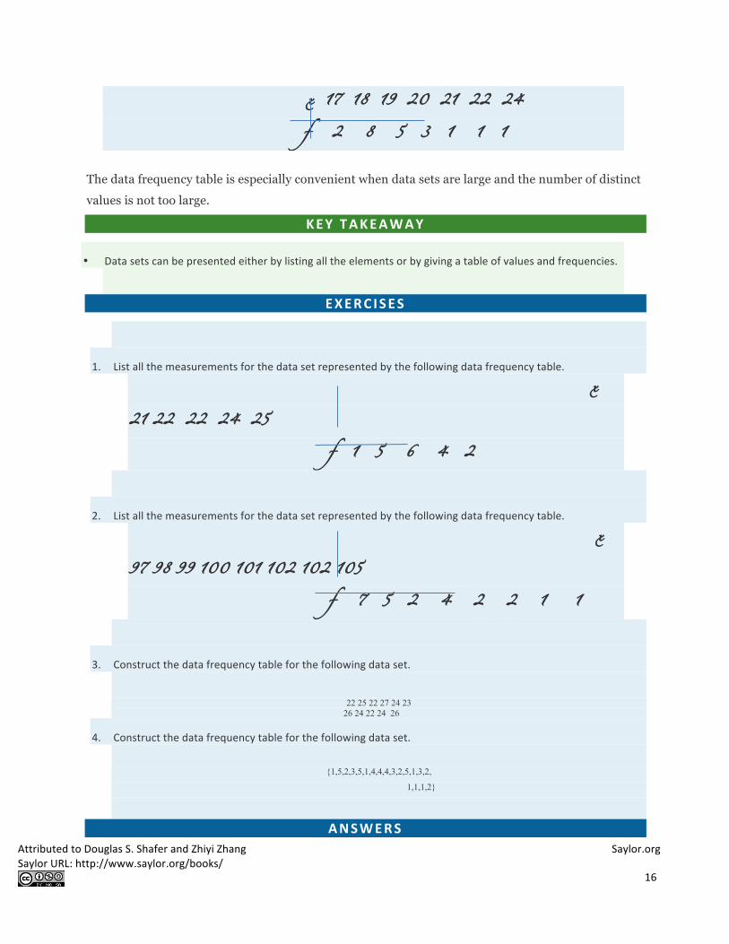
Attributed to Douglas S. Shafer and Zhiyi Zhang Saylor.org Saylor URL: http://www.saylor.org/books/
16
x 17 18 19 20 21 22 24
f 2 8 5 3 1 1 1
The data frequency table is especially convenient when data sets are large and the number of distinct
values is not too large.
KEY TAKEAWAY
• Data sets can be presented either by listing all the elements or by giving a table of values and frequencies.
EXERC ISES
1. List all the measurements for the data set represented by the following data frequency table.
x
21 22 22 24 25
f 1 5 6 4 2
2. List all the measurements for the data set represented by the following data frequency table.
x
97 98 99 100 101 102 102 105
f 7 5 2 4 2 2 1 1
3. Construct the data frequency table for the following data set.
22 25 22 27 24 23
26 24 22 24 26
4. Construct the data frequency table for the following data set.
{1,5,2,3,5,1,4,4,4,3,2,5,1,3,2,
1,1,1,2}
ANSWERS

Attributed to Douglas S. Shafer and Zhiyi Zhang Saylor.org Saylor URL: http://www.saylor.org/books/
17
1. {31,32,32,32,32,32,33,33,33,33,33,33,34,34,34,34,35,35}.
3.
x 22 23 24 25 26 27
f 3 1 3 1 2 1
Chapter 2 Descriptive Statistics
As described in Chapter 1 "Introduction", statistics naturally divides into two branches, descriptive
statistics and inferential statistics. Our main interest is in inferential statistics, as shown in Figure 1.1
"The Grand Picture of Statistics" in Chapter 1 "Introduction". Nevertheless, the starting point for
dealing with a collection of data is to organize, display, and summarize it effectively. These are the
objectives of descriptive statistics, the topic of this chapter.

Attributed to Douglas S. Shafer and Zhiyi Zhang Saylor.org Saylor URL: http://www.saylor.org/books/
18
2.1 Three Popular Data Displays
LEARNING OBJECT IVE
1. To learn to interpret the meaning of three graphical representations of sets of data: stem and leaf
diagrams, frequency histograms, and relative frequency histograms.
A well-known adage is that “a picture is worth a thousand words.” This saying proves true when it
comes to presenting statistical information in a data set. There are many effective ways to present
data graphically. The three graphical tools that are introduced in this section are among the most
commonly used and are relevant to the subsequent presentation of the material in this book.
Stem and Leaf Diagrams
Suppose 30 students in a statistics class took a test and made the following scores:

Attributed to Douglas S. Shafer and Zhiyi Zhang Saylor.org Saylor URL: http://www.saylor.org/books/
19
86 80 25 77 73 76 100 90 69 93 90 83 70 73 73 70 90 83 71 95
40 58 68 69 100 78 87 97 92 74
How did the class do on the test? A quick glance at the set of 30 numbers does not immediately give a
clear answer. However the data set may be reorganized and rewritten to make relevant information more
visible. One way to do so is to construct a stem and leaf diagram as shown in . The numbers in the tens
place, from 2 through 9, and additionally the number 10, are the “stems,” and are arranged in numerical
order from top to bottom to the left of a vertical line. The number in the units place in each measurement
is a “leaf,” and is placed in a row to the right of the corresponding stem, the number in the tens place of
that measurement. Thus the three leaves 9, 8, and 9 in the row headed with the stem 6 correspond to the
three exam scores in the 60s, 69 (in the first row of data), 68 (in the third row), and 69 (also in the third
row). The display is made even more useful for some purposes by rearranging the leaves in numerical
order, as shown in . Either way, with the data reorganized certain information of interest becomes
apparent immediately. There are two perfect scores; three students made scores under 60; most students
scored in the 70s, 80s and 90s; and the overall average is probably in the high 70s or low 80s.
igure 2.1 Stem and Leaf Diagram

Attributed to Douglas S. Shafer and Zhiyi Zhang Saylor.org Saylor URL: http://www.saylor.org/books/
20
Figure 2.2 Ordered Stem and Leaf Diagram
In this example the scores have a natural stem (the tens place) and leaf (the ones place). One could spread
the diagram out by splitting each tens place number into lower and upper categories. For example, all the
scores in the 80s may be represented on two separate stems, lower 80s and upper 80s:
8 0 3 3
8 6 7

Attributed to Douglas S. Shafer and Zhiyi Zhang Saylor.org Saylor URL: http://www.saylor.org/books/
21
The definitions of stems and leaves are flexible in practice. The general purpose of a stem and leaf
diagram is to provide a quick display of how the data are distributed across the range of their values; some
improvisation could be necessary to obtain a diagram that best meets that goal.
Note that all of the original data can be recovered from the stem and leaf diagram. This will not be true in
the next two types of graphical displays.
Frequency Histograms The stem and leaf diagram is not practical for large data sets, so we need a different, purely graphical way
to represent data. A frequency histogram is such a device. We will illustrate it using the same data set
from the previous subsection. For the 30 scores on the exam, it is natural to group the scores on the
standard ten-point scale, and count the number of scores in each group. Thus there are two 100s, seven
scores in the 90s, six in the 80s, and so on. We then construct the diagram shown in by drawing for each
group, or class, a vertical bar whose length is the number of observations in that group. In our example,
the bar labeled 100 is 2 units long, the bar labeled 90 is 7 units long, and so on. While the individual data
values are lost, we know the number in each class. This number is called the frequency of the class,
hence the name frequency histogram.
Figure 2.3 Frequency Histogram
The same procedure can be applied to any collection of numerical data. Observations are grouped into
several classes and the frequency (the number of observations) of each class is noted. These classes are

Attributed to Douglas S. Shafer and Zhiyi Zhang Saylor.org Saylor URL: http://www.saylor.org/books/
22
arranged and indicated in order on the horizontal axis (called the x-axis), and for each group a vertical
bar, whose length is the number of observations in that group, is drawn. The resulting display is a
frequency histogram for the data. The similarity in and is apparent, particularly if you imagine turning the
stem and leaf diagram on its side by rotating it a quarter turn counterclockwise.
In general, the definition of the classes in the frequency histogram is flexible. The general purpose of a
frequency histogram is very much the same as that of a stem and leaf diagram, to provide a graphical
display that gives a sense of data distribution across the range of values that appear. We will not discuss
the process of constructing a histogram from data since in actual practice it is done automatically with
statistical software or even handheld calculators.
Relative Frequency Histograms In our example of the exam scores in a statistics class, five students scored in the 80s. The number 5 is
the frequency of the group labeled “80s.” Since there are 30 students in the entire statistics class, the
proportion who scored in the 80s is 5/30. The number 5/30, which could also be expressed as 0.16≈.1667, or
as 16.67%, is the relative frequency of the group labeled “80s.” Every group (the 70s, the 80s, and so
on) has a relative frequency. We can thus construct a diagram by drawing for each group, or class, a
vertical bar whose length is the relative frequency of that group. For example, the bar for the 80s will have
length 5/30 unit, not 5 units. The diagram is a relative frequency histogram for the data, and is
shown in . It is exactly the same as the frequency histogram except that the vertical axis in the relative
frequency histogram is not frequency but relative frequency.
Figure 2.4 Relative Frequency Histogram

Attributed to Douglas S. Shafer and Zhiyi Zhang Saylor.org Saylor URL: http://www.saylor.org/books/
23
The same procedure can be applied to any collection of numerical data. Classes are selected, the relative
frequency of each class is noted, the classes are arranged and indicated in order on the horizontal axis,
and for each class a vertical bar, whose length is the relative frequency of the class, is drawn. The resulting
display is a relative frequency histogram for the data. A key point is that now if each vertical bar has width
1 unit, then the total area of all the bars is 1 or 100%.
Although the histograms in and have the same appearance, the relative frequency histogram is more
important for us, and it will be relative frequency histograms that will be used repeatedly to
represent data in this text. To see why this is so, reflect on what it is that you are actually seeing in
the diagrams that quickly and effectively communicates information to you about the data. It is
the relative sizes of the bars. The bar labeled “70s” in either figure takes up 1/3 of the total area of all
the bars, and although we may not think of this consciously, we perceive the proportion 1/3 in the
figures, indicating that a third of the grades were in the 70s. The relative frequency histogram is
important because the labeling on the vertical axis reflects what is important visually: the relative
sizes of the bars.
When the size n of a sample is small only a few classes can be used in constructing a relative
frequency histogram. Such a histogram might look something like the one in panel (a) of . If the
sample size n were increased, then more classes could be used in constructing a relative frequency
histogram and the vertical bars of the resulting histogram would be finer, as indicated in panel (b)
of . For a very large sample the relative frequency histogram would look very fine, like the one in (c)
of. If the sample size were to increase indefinitely then the corresponding relative frequency
histogram would be so fine that it would look like a smooth curve, such as the one in panel (d) of .
Figure 2.5 Sample Size and Relative Frequency Histograms

Attributed to Douglas S. Shafer and Zhiyi Zhang Saylor.org Saylor URL: http://www.saylor.org/books/
24
It is common in statistics to represent a population or a very large data set by a smooth curve. It is
good to keep in mind that such a curve is actually just a very fine relative frequency histogram in
which the exceedingly narrow vertical bars have disappeared. Because the area of each such vertical
bar is the proportion of the data that lies in the interval of numbers over which that bar stands, this
means that for any two numbers a and b, the proportion of the data that lies between the two
numbers a and b is the area under the curve that is above the interval (a,b) in the horizontal axis.
This is the area shown in . In particular the total area under the curve is 1, or 100%.
Figure 2.6 A Very Fine Relative Frequency Histogram
KEY TAKEAWAYS
• Graphical representations of large data sets provide a quick overview of the nature of the data.
• A population or a very large data set may be represented by a smooth curve. This curve is a very fine
relative frequency histogram in which the exceedingly narrow vertical bars have been omitted.
• When a curve derived from a relative frequency histogram is used to describe a data set, the proportion of
data with values between two numbers a and b is the area under the curve between a and b, as illustrated
in Figure 2.6 "A Very Fine Relative Frequency Histogram".

Attributed to Douglas S. Shafer and Zhiyi Zhang Saylor.org Saylor URL: http://www.saylor.org/books/
25

Attributed to Douglas S. Shafer and Zhiyi Zhang Saylor.org Saylor URL: http://www.saylor.org/books/
26

Attributed to Douglas S. Shafer and Zhiyi Zhang Saylor.org Saylor URL: http://www.saylor.org/books/
27

Attributed to Douglas S. Shafer and Zhiyi Zhang Saylor.org Saylor URL: http://www.saylor.org/books/
28

Attributed to Douglas S. Shafer and Zhiyi Zhang Saylor.org Saylor URL: http://www.saylor.org/books/
29

Attributed to Douglas S. Shafer and Zhiyi Zhang Saylor.org Saylor URL: http://www.saylor.org/books/
30

Attributed to Douglas S. Shafer and Zhiyi Zhang Saylor.org Saylor URL: http://www.saylor.org/books/
31

Attributed to Douglas S. Shafer and Zhiyi Zhang Saylor.org Saylor URL: http://www.saylor.org/books/
32
2.2 Measures of Central Location
LEARNING OBJECT IVES
1. To learn the concept of the “center” of a data set.
2. To learn the meaning of each of three measures of the center of a data set—the mean, the median, and
the mode—and how to compute each one.
This section could be titled “three kinds of averages of a data set.” Any kind of “average” is meant to
be an answer to the question “Where do the data center?” It is thus a measure of the central location
of the data set. We will see that the nature of the data set, as indicated by a relative frequency

Attributed to Douglas S. Shafer and Zhiyi Zhang Saylor.org Saylor URL: http://www.saylor.org/books/
33
histogram, will determine what constitutes a good answer. Different shapes of the histogram call for
different measures of central location.
The Mean The first measure of central location is the usual “average” that is familiar to everyone. In the formula in
the following definition we introduce the standard summation notation �, where � is the capital Greek
letter sigma. In general, the notation � followed by a second mathematical symbol means to add up all
the values that the second symbol can take in the context of the problem. Here is an example to illustrate
this.
In the definition we follow the convention of using lowercase n to denote the number of
measurements in a sample, which is called the sample size.

Attributed to Douglas S. Shafer and Zhiyi Zhang Saylor.org Saylor URL: http://www.saylor.org/books/
34

Attributed to Douglas S. Shafer and Zhiyi Zhang Saylor.org Saylor URL: http://www.saylor.org/books/
35

Attributed to Douglas S. Shafer and Zhiyi Zhang Saylor.org Saylor URL: http://www.saylor.org/books/
36

Attributed to Douglas S. Shafer and Zhiyi Zhang Saylor.org Saylor URL: http://www.saylor.org/books/
37
In the examples above the data sets were described as samples. Therefore the means were sample means,
denoted by x ̅. If the data come from a census, so that there is a measurement for every element of the
population, then the mean is calculated by exactly the same process of summing all the measurements
and dividing by how many of them there are, but it is now the population mean and is denoted by �, the
lower case Greek letter mu.
The mean of two numbers is the number that is halfway between them. For example, the average of the
numbers 5 and 17 is (5 + 17) � 2 = 11, which is 6 units above 5 and 6 units below 17. In this sense the
average 11 is the “center” of the data set {5,17}. For larger data sets the mean can similarly be regarded as
the “center” of the data.
The Median To see why another concept of average is needed, consider the following situation. Suppose we are
interested in the average yearly income of employees at a large corporation. We take a random sample of
seven employees, obtaining the sample data (rounded to the nearest hundred dollars, and expressed in
thousands of dollars).
24.8 22.8 24.6 192.5 25.2 18.5 23.7
The mean (rounded to one decimal place) is x ̅-47.4, but the statement “the average income of employees
at this corporation is $47,400” is surely misleading. It is approximately twice what six of the seven
employees in the sample make and is nowhere near what any of them makes. It is easy to see what went
wrong: the presence of the one executive in the sample, whose salary is so large compared to everyone
else’s, caused the numerator in the formula for the sample mean to be far too large, pulling the mean far
to the right of where we think that the average “ought” to be, namely around $24,000 or $25,000. The
number 192.5 in our data set is called an outlier, a number that is far removed from most or all of the

Attributed to Douglas S. Shafer and Zhiyi Zhang Saylor.org Saylor URL: http://www.saylor.org/books/
38
remaining measurements. Many times an outlier is the result of some sort of error, but not always, as is
the case here. We would get a better measure of the “center” of the data if we were to arrange the data in
numerical order,
18.5 22.8 23.7 24.6 24.8 25.2 192.5
then select the middle number in the list, in this case 24.6. The result is called the median of the data set,
and has the property that roughly half of the measurements are larger than it is, and roughly half are
smaller. In this sense it locates the center of the data. If there are an even number of measurements in the
data set, then there will be two middle elements when all are lined up in order, so we take the mean of the
middle two as the median. Thus we have the following definition.
Definition The sample median x^~ of a set of sample data for which there are an odd number of measurements is
the middle measurement when the data are arranged in numerical order. The sample median x^~ of a
set of sample data for which there are an even number of measurements is the mean of the two middle
measurements when the data are arranged in numerical order.
The population median is defined in a similar way, but we will not have occasion to refer to it again
in this text.
The median is a value that divides the observations in a data set so that 50% of the data are on its left
and the other 50% on its right. In accordance with , therefore, in the curve that represents the
distribution of the data, a vertical line drawn at the median divides the area in two, area 0.5 (50% of
the total area 1) to the left and area 0.5 (50% of the total area 1) to the right, as shown in . In our
income example the median, $24,600, clearly gave a much better measure of the middle of the data
set than did the mean $47,400. This is typical for situations in which the distribution is skewed.
(Skewness and symmetry of distributions are discussed at the end of this subsection.)

Attributed to Douglas S. Shafer and Zhiyi Zhang Saylor.org Saylor URL: http://www.saylor.org/books/
39
Figure 2.7 The Median

Attributed to Douglas S. Shafer and Zhiyi Zhang Saylor.org Saylor URL: http://www.saylor.org/books/
40

Attributed to Douglas S. Shafer and Zhiyi Zhang Saylor.org Saylor URL: http://www.saylor.org/books/
41
The relationship between the mean and the median for several common shapes of distributions is shown
in . The distributions in panels (a) and (b) are said to be symmetric because of the symmetry that they
exhibit. The distributions in the remaining two panels are said to be skewed. In each distribution we have
drawn a vertical line that divides the area under the curve in half, which in accordance with is located at
the median. The following facts are true in general:
a. When the distribution is symmetric, as in panels (a) and (b) of , the mean and the median are
equal.

Attributed to Douglas S. Shafer and Zhiyi Zhang Saylor.org Saylor URL: http://www.saylor.org/books/
42
b. When the distribution is as shown in panel (c) of , it is said to be skewed right. The mean has
been pulled to the right of the median by the long “right tail” of the distribution, the few relatively large
data values.
c. When the distribution is as shown in panel (d) of , it is said to be skewed left. The mean has been
pulled to the left of the median by the long “left tail” of the distribution, the few relatively small data
values.
Figure 2.8 Skewness of Relative Frequency Histograms
The Mode Perhaps you have heard a statement like “The average number of automobiles owned by households
in the United States is 1.37,” and have been amused at the thought of a fraction of an automobile

Attributed to Douglas S. Shafer and Zhiyi Zhang Saylor.org Saylor URL: http://www.saylor.org/books/
43
sitting in a driveway. In such a context the following measure for central location might make more
sense.
Definition The sample mode of a set of sample data is the most frequently occurring value.
The population mode is defined in a similar way, but we will not have occasion to refer to it again in
this text.
On a relative frequency histogram, the highest point of the histogram corresponds to the mode of the
data set. illustrates the mode.
Figure 2.9 Mode

Attributed to Douglas S. Shafer and Zhiyi Zhang Saylor.org Saylor URL: http://www.saylor.org/books/
44
For any data set there is always exactly one mean and exactly one median. This need not be true of the
mode; several different values could occur with the highest frequency, as we will see. It could even happen
that every value occurs with the same frequency, in which case the concept of the mode does not make
much sense.
EXAMPLE 8
Find the mode of the following data set. −1 0 2 0
Solution:
The value 0 is most frequently observed and therefore the mode is 0.
EXAMPLE 9
Compute the sample mode for the data of .
Solution:
The two most frequently observed values in the data set are 1 and 2. Therefore mode is a set of two
values: {1,2}.
The mode is a measure of central location since most real-life data sets have moreobservations near the
center of the data range and fewer observations on the lower and upper ends. The value with the highest
frequency is often in the middle of the data range.
KEY TAKEAWAY
The mean, the median, and the mode each answer the question “Where is the center of the data set?”
The nature of the data set, as indicated by a relative frequency histogram, determines which one gives the
best answer.

Attributed to Douglas S. Shafer and Zhiyi Zhang Saylor.org Saylor URL: http://www.saylor.org/books/
45

Attributed to Douglas S. Shafer and Zhiyi Zhang Saylor.org Saylor URL: http://www.saylor.org/books/
46

Attributed to Douglas S. Shafer and Zhiyi Zhang Saylor.org Saylor URL: http://www.saylor.org/books/
47

Attributed to Douglas S. Shafer and Zhiyi Zhang Saylor.org Saylor URL: http://www.saylor.org/books/
48

Attributed to Douglas S. Shafer and Zhiyi Zhang Saylor.org Saylor URL: http://www.saylor.org/books/
49

Attributed to Douglas S. Shafer and Zhiyi Zhang Saylor.org Saylor URL: http://www.saylor.org/books/
50

Attributed to Douglas S. Shafer and Zhiyi Zhang Saylor.org Saylor URL: http://www.saylor.org/books/
51
LARGE DATA S E T E X ERC I S E S
28. Large Data Set 1 lists the SAT scores and GPAs of 1,000 students.
http://www.flatworldknowledge.com/sites/all/files/data1.xls
a. Compute the mean and median of the 1,000 SAT scores.
b. Compute the mean and median of the 1,000 GPAs.
29. Large Data Set 1 lists the SAT scores of 1,000 students.
http://www.flatworldknowledge.com/sites/all/files/data1.xls
a. Regard the data as arising from a census of all students at a high school, in which the SAT score of every
student was measured. Compute the population mean μ.
b. Regard the first 25 observations as a random sample drawn from this population. Compute the sample
mean x^− and compare it to μ.
c. Regard the next 25 observations as a random sample drawn from this population. Compute the sample
mean x^− and compare it to μ.
30. Large Data Set 1 lists the GPAs of 1,000 students.
http://www.flatworldknowledge.com/sites/all/files/data1.xls
a. Regard the data as arising from a census of all freshman at a small college at the end of their first academic
year of college study, in which the GPA of every such person was measured. Compute the population
mean μ.
b. Regard the first 25 observations as a random sample drawn from this population. Compute the sample
mean x^− and compare it to μ.
c. Regard the next 25 observations as a random sample drawn from this population. Compute the sample
mean x^− and compare it to μ.
31. Large Data Sets 7, 7A, and 7B list the survival times in days of 140 laboratory mice with thymic leukemia from
onset to death.
http://www.flatworldknowledge.com/sites/all/files/data7.xls
http://www.flatworldknowledge.com/sites/all/files/data7A.xls
http://www.flatworldknowledge.com/sites/all/files/data7B.xls
a. Compute the mean and median survival time for all mice, without regard to gender.
b. Compute the mean and median survival time for the 65 male mice (separately recorded in Large Data Set
7A).
c. Compute the mean and median survival time for the 75 female mice (separately recorded in Large Data Set
7B).

Attributed to Douglas S. Shafer and Zhiyi Zhang Saylor.org Saylor URL: http://www.saylor.org/books/
52

Attributed to Douglas S. Shafer and Zhiyi Zhang Saylor.org Saylor URL: http://www.saylor.org/books/
53
2.3 Measures of Variability LEARNING OBJECT IVES
1. To learn the concept of the variability of a data set.
2. To learn how to compute three measures of the variability of a data set: the range, the variance, and the
standard deviation.
Look at the two data sets in Table 2.1 "Two Data Sets" and the graphical representation of each,
called a dot plot, in Figure 2.10 "Dot Plots of Data Sets".
Table 2.1 Two Data Sets
Data Set I: 40 38 42 40 39 39 43 40 39 40

Attributed to Douglas S. Shafer and Zhiyi Zhang Saylor.org Saylor URL: http://www.saylor.org/books/
54
Data Set II: 46 37 40 33 42 36 40 47 34 45
Figure 2.10 Dot Plots of Data Sets
The two sets of ten measurements each center at the same value: they both have mean, median, and
mode 40. Nevertheless a glance at the figure shows that they are markedly different. In Data Set I the
measurements vary only slightly from the center, while for Data Set II the measurements vary
greatly. Just as we have attached numbers to a data set to locate its center, we now wish to associate
to each data set numbers that measure quantitatively how the data either scatter away from the
center or cluster close to it. These new quantities are called measures of variability, and we will
discuss three of them.
The Range The first measure of variability that we discuss is the simplest.
Definition
The range of a data set is the number R defined by the formula R=xmax−xmin
where xmax is the largest measurement in the data set and xmin is the smallest.
EXAMPLE 10
Find the range of each data set in Table 2.1 "Two Data Sets".
Solution:
For Data Set I the maximum is 43 and the minimum is 38, so the range is R=43−38=5.

Attributed to Douglas S. Shafer and Zhiyi Zhang Saylor.org Saylor URL: http://www.saylor.org/books/
55
For Data Set II the maximum is 47 and the minimum is 33, so the range is R=47−33=14.
The range is a measure of variability because it indicates the size of the interval over which the data
points are distributed. A smaller range indicates less variability (less dispersion) among the data,
whereas a larger range indicates the opposite.
The Variance and the Standard Deviation The other two measures of variability that we will consider are more elaborate and also depend on
whether the data set is just a sample drawn from a much larger population or is the whole population
itself (that is, a census).
Although the first formula in each case looks less complicated than the second, the latter is easier to
use in hand computations, and is called a shortcut formula.

Attributed to Douglas S. Shafer and Zhiyi Zhang Saylor.org Saylor URL: http://www.saylor.org/books/
56
The student is encouraged to compute the ten deviations for Data Set I and verify that their squares
add up to 20, so that the sample variance and standard deviation of Data Set I are the much smaller
numbers s2=20/9=2.2^¯ and s=√20/9≈1.49.

Attributed to Douglas S. Shafer and Zhiyi Zhang Saylor.org Saylor URL: http://www.saylor.org/books/
57
The sample variance has different units from the data. For example, if the units in the data set were
inches, the new units would be inches squared, or square inches. It is thus primarily of theoretical
importance and will not be considered further in this text, except in passing.

Attributed to Douglas S. Shafer and Zhiyi Zhang Saylor.org Saylor URL: http://www.saylor.org/books/
58
If the data set comprises the whole population, then the population standard deviation,
denoted � (the lower case Greek letter sigma), and its square, the population variance �2, are
defined as follows.
Note that the denominator in the fraction is the full number of observations, not that number
reduced by one, as is the case with the sample standard deviation. Since most data sets are samples,
we will always work with the sample standard deviation and variance.
Finally, in many real-life situations the most important statistical issues have to do with comparing
the means and standard deviations of two data sets. Figure 2.11 "Difference between Two Data
Sets" illustrates how a difference in one or both of the sample mean and the sample standard
deviation are reflected in the appearance of the data set as shown by the curves derived from the
relative frequency histograms built using the data.

Attributed to Douglas S. Shafer and Zhiyi Zhang Saylor.org Saylor URL: http://www.saylor.org/books/
59
Figure 2.11 Difference between Two Data Sets
KEY TAKEAWAY
The range, the standard deviation, and the variance each give a quantitative answer to the question “How
variable are the data?”

Attributed to Douglas S. Shafer and Zhiyi Zhang Saylor.org Saylor URL: http://www.saylor.org/books/
60

Attributed to Douglas S. Shafer and Zhiyi Zhang Saylor.org Saylor URL: http://www.saylor.org/books/
61

Attributed to Douglas S. Shafer and Zhiyi Zhang Saylor.org Saylor URL: http://www.saylor.org/books/
62

Attributed to Douglas S. Shafer and Zhiyi Zhang Saylor.org Saylor URL: http://www.saylor.org/books/
63
LARGE DATA S E T E X ERC I S E S
19. Large Data Set 1 lists the SAT scores and GPAs of 1,000 students.
http://www.flatworldknowledge.com/sites/all/files/data1.xls
a. Compute the range and sample standard deviation of the 1,000 SAT scores.
b. Compute the range and sample standard deviation of the 1,000 GPAs.
20. Large Data Set 1 lists the SAT scores of 1,000 students.
http://www.flatworldknowledge.com/sites/all/files/data1.xls
a. Regard the data as arising from a census of all students at a high school, in which the SAT score of every
student was measured. Compute the population range and population standard deviation σ.
b. Regard the first 25 observations as a random sample drawn from this population. Compute the sample range
and sample standard deviation s and compare them to the population range and σ.
c. Regard the next 25 observations as a random sample drawn from this population. Compute the sample range
and sample standard deviation s and compare them to the population range and σ.
21. Large Data Set 1 lists the GPAs of 1,000 students.
http://www.flatworldknowledge.com/sites/all/files/data1.xls
a. Regard the data as arising from a census of all freshman at a small college at the end of their first academic
year of college study, in which the GPA of every such person was measured. Compute the population range
and population standard deviation σ.
b. Regard the first 25 observations as a random sample drawn from this population. Compute the sample range
and sample standard deviation s and compare them to the population range and σ.
c. Regard the next 25 observations as a random sample drawn from this population. Compute the sample range
and sample standard deviation s and compare them to the population range and σ.
22. Large Data Sets 7, 7A, and 7B list the survival times in days of 140 laboratory mice with thymic leukemia from
onset to death.
http://www.flatworldknowledge.com/sites/all/files/data7.xls
http://www.flatworldknowledge.com/sites/all/files/data7A.xls
http://www.flatworldknowledge.com/sites/all/files/data7B.xls
a. Compute the range and sample standard deviation of survival time for all mice, without regard to gender.
b. Compute the range and sample standard deviation of survival time for the 65 male mice (separately recorded
in Large Data Set 7A).

Attributed to Douglas S. Shafer and Zhiyi Zhang Saylor.org Saylor URL: http://www.saylor.org/books/
64
c. Compute the range and sample standard deviation of survival time for the 75 female mice (separately
recorded in Large Data Set 7B). Do you see a difference in the results for male and female mice? Does it
appear to be significant?

Attributed to Douglas S. Shafer and Zhiyi Zhang Saylor.org Saylor URL: http://www.saylor.org/books/
65
2.4 Relative Position of Data
LEARNING OBJECT IVES
1. To learn the concept of the relative position of an element of a data set.
2. To learn the meaning of each of two measures, the percentile rank and the z-‐score, of the relative position
of a measurement and how to compute each one.
3. To learn the meaning of the three quartiles associated to a data set and how to compute them.
4. To learn the meaning of the five-‐number summary of a data set, how to construct the box plot associated
to it, and how to interpret the box plot.
When you take an exam, what is often as important as your actual score on the exam is the way your
score compares to other students’ performance. If you made a 70 but the average score (whether the
mean, median, or mode) was 85, you did relatively poorly. If you made a 70 but the average score
was only 55 then you did relatively well. In general, the significance of one observed value in a data
set strongly depends on how that value compares to the other observed values in a data set.
Therefore we wish to attach to each observed value a number that measures its relative position.
Percentiles and Quartiles Anyone who has taken a national standardized test is familiar with the idea of being given both a score on
the exam and a “percentile ranking” of that score. You may be told that your score was 625 and that it is
the 85th percentile. The first number tells how you actually did on the exam; the second says that 85% of
the scores on the exam were less than or equal to your score, 625.
Definition
Given an observed value x in a data set, x is the Pth percentile of the data if the percentage of the data
that are less than or equal to x is P. The number P is the percentile rank of x.
EXAMPLE 13
What percentile is the value 1.39 in the data set of ten GPAs considered in Note 2.12 "Example
3" in Section 2.2 "Measures of Central Location"? What percentile is the value 3.33?
Solution:
The data written in increasing order are

Attributed to Douglas S. Shafer and Zhiyi Zhang Saylor.org Saylor URL: http://www.saylor.org/books/
66
1.39 1.76 1.90 2.12 2.53 2.71 3.00 3.33 3.71 4.00
The only data value that is less than or equal to 1.39 is 1.39 itself. Since 1 is 1∕10 = .10 or 10% of 10, the
value 1.39 is the 10th percentile. Eight data values are less than or equal to 3.33. Since 8 is 8∕10 = .80 or
80% of 10, the value 3.33 is the 80th percentile.
The Pth percentile cuts the data set in two so that approximately P% of the data lie below it
and (100−P)% of the data lie above it. In particular, the three percentiles that cut the data into fourths,
as shown in Figure 2.12 "Data Division by Quartiles", are called the quartiles. The following simple
computational definition of the three quartiles works well in practice.
Figure 2.12 Data Division by Quartiles
Definition
For any data set:

Attributed to Douglas S. Shafer and Zhiyi Zhang Saylor.org Saylor URL: http://www.saylor.org/books/
67
1. The second quartile Q2 of the data set is its median.
2. Define two subsets:
1. the lower set: all observations that are strictly less than Q2;
2. the upper set: all observations that are strictly greater than Q2.
3. The first quartile Q1 of the data set is the median of the lower set.
4. The third quartile Q3 of the data set is the median of the upper set.
EXAMPLE 14
Find the quartiles of the data set of GPAs of Note 2.12 "Example 3" in Section 2.2 "Measures of Central
Location".
Solution:
As in the previous example we first list the data in numerical order: 1.39 1.76 1.90 2.12 2.53 2.71 3.00 3.33 3.71 4.00
This data set has n = 10 observations. Since 10 is an even number, the median is the mean of the two
middle observations: x˜=(2.53 + 2.71)/2=2.62. Thus the second quartile is Q2=2.62. The lower and upper subsets
are Lower: L={1.39,1.76,1.90,2.12,2.53}
Upper: U={2.71,3.00,3.33,3.71,4.00}
Each has an odd number of elements, so the median of each is its middle observation. Thus the first
quartile is Q1=1.90, the median of L, and the third quartile is Q3=3.33, the median of U. EXAMPLE 15
Adjoin the observation 3.88 to the data set of the previous example and find the quartiles of the new set
of data.
Solution:
As in the previous example we first list the data in numerical order: 1.39 1.76 1.90 2.12 2.53 2.71 3.00 3.33 3.71 3.88 4.00

Attributed to Douglas S. Shafer and Zhiyi Zhang Saylor.org Saylor URL: http://www.saylor.org/books/
68
This data set has 11 observations. The second quartile is its median, the middle value 2.71.
Thus Q2=2.71. The lower and upper subsets are now Lower: L={1.39,1.76,1.90,2.12,2.53}
Upper: U= {3.00,3.33,3.71,3.88,4.00}
The lower set L has median the middle value 1.90, so Q1=1.90. The upper set has median the middle value
3.71, so Q3=3.71. In addition to the three quartiles, the two extreme values, the minimum xmin and the maximum xmax are
also useful in describing the entire data set. Together these five numbers are called the five-
number summary of the data set:
{xmin, Q1, Q2, Q3, xmax}
The five-number summary is used to construct a box plot as in Figure 2.13 "The Box Plot". Each of the
five numbers is represented by a vertical line segment, a box is formed using the line segments
at Q1 and Q3 as its two vertical sides, and two horizontal line segments are extended from the vertical
segments marking Q1 and Q3 to the adjacent extreme values. (The two horizontal line segments are
referred to as “whiskers,” and the diagram is sometimes called a “box and whisker plot.”) We caution the
reader that there are other types of box plots that differ somewhat from the ones we are constructing,
although all are based on the three quartiles.
Figure 2.13 The Box Plot
Note that the distance from Q1 to Q3 is the length of the interval over which the middle half of the
data range. Thus it has the following special name.
Definition
The interquartile range (IQR) is the quantity

Attributed to Douglas S. Shafer and Zhiyi Zhang Saylor.org Saylor URL: http://www.saylor.org/books/
69
IQR=Q3−Q1
EXAMPLE 16
Construct a box plot and find the IQR for the data in Note 2.44 "Example 14".
Solution:
From our work in Note 2.44 "Example 14" we know that the five-‐number summary is xmin=1.39 Q1=1.90 Q2=2.62 Q3=3.33 xmax=4.00
The box plot is
The interquartile range is IQR=3.33−1.90=1.43.
z-‐scores
Another way to locate a particular observation x in a data set is to compute its distance from the mean in
units of standard deviation.

Attributed to Douglas S. Shafer and Zhiyi Zhang Saylor.org Saylor URL: http://www.saylor.org/books/
70
The formulas in the definition allow us to compute the z-score when x is known. If the z-score is
known then x can be recovered using the corresponding inverse formulas
x=(x^−)+sz or x=µ+σz
The z-score indicates how many standard deviations an individual observation x is from the center of
the data set, its mean. If z is negative then x is below average. If z is 0 then x is equal to the average.
If z is positive then x is above average. See Figure 2.14.
Figure 2.14 x-Scale versus z-Score

Attributed to Douglas S. Shafer and Zhiyi Zhang Saylor.org Saylor URL: http://www.saylor.org/books/
71

Attributed to Douglas S. Shafer and Zhiyi Zhang Saylor.org Saylor URL: http://www.saylor.org/books/
72
EXAMPLE 18
Suppose the mean and standard deviation of the GPAs of all currently registered students at a college
are μ = 2.70 and σ = 0.50. The z-‐scores of the GPAs of two students, Antonio and Beatrice,
are z=−0.62 and z = 1.28, respectively. What are their GPAs?
Solution:

Attributed to Douglas S. Shafer and Zhiyi Zhang Saylor.org Saylor URL: http://www.saylor.org/books/
73
Using the second formula right after the definition of z-‐scores we compute the GPAs as Antonio: x=µ+z σ=2.70+(−0.62)(0.50)=2.39 Beatrice: x=µ+z σ=2.70+(1.28)(0.50)=3.34
KEY TAKEAWAYS
• The percentile rank and z-‐score of a measurement indicate its relative position with regard to the other
measurements in a data set.
• The three quartiles divide a data set into fourths.
• The five-‐number summary and its associated box plot summarize the location and distribution of the data.

Attributed to Douglas S. Shafer and Zhiyi Zhang Saylor.org Saylor URL: http://www.saylor.org/books/
74

Attributed to Douglas S. Shafer and Zhiyi Zhang Saylor.org Saylor URL: http://www.saylor.org/books/
75

Attributed to Douglas S. Shafer and Zhiyi Zhang Saylor.org Saylor URL: http://www.saylor.org/books/
76

Attributed to Douglas S. Shafer and Zhiyi Zhang Saylor.org Saylor URL: http://www.saylor.org/books/
77

Attributed to Douglas S. Shafer and Zhiyi Zhang Saylor.org Saylor URL: http://www.saylor.org/books/
78

Attributed to Douglas S. Shafer and Zhiyi Zhang Saylor.org Saylor URL: http://www.saylor.org/books/
79

Attributed to Douglas S. Shafer and Zhiyi Zhang Saylor.org Saylor URL: http://www.saylor.org/books/
80

Attributed to Douglas S. Shafer and Zhiyi Zhang Saylor.org Saylor URL: http://www.saylor.org/books/
81

Attributed to Douglas S. Shafer and Zhiyi Zhang Saylor.org Saylor URL: http://www.saylor.org/books/
82
35.
Emilia and Ferdinand took the same freshman chemistry course, Emilia in the fall, Ferdinand in the spring.
Emilia made an 83 on the common final exam that she took, on which the mean was 76 and the standard
deviation 8. Ferdinand made a 79 on the common final exam that he took, which was more difficult, since
the mean was 65 and the standard deviation 12. The one who has a higher z-‐score did relatively better.
Was it Emilia or Ferdinand?
36. Refer to the previous exercise. On the final exam in the same course the following semester, the mean is 68
and the standard deviation is 9. What grade on the exam matches Emilia’s performance? Ferdinand’s?
37. Rosencrantz and Guildenstern are on a weight-‐reducing diet. Rosencrantz, who weighs 178 lb, belongs to an
age and body-‐type group for which the mean weight is 145 lb and the standard deviation is 15 lb.
Guildenstern, who weighs 204 lb, belongs to an age and body-‐type group for which the mean weight is 165 lb
and the standard deviation is 20 lb. Assuming z-‐scores are good measures for comparison in this context,
who is more overweight for his age and body type? LARGE DATA S E T E X ERC I S E S
38. Large Data Set 1 lists the SAT scores and GPAs of 1,000 students.
http://www.flatworldknowledge.com/sites/all/files/data1.xls
a. Compute the three quartiles and the interquartile range of the 1,000 SAT scores.
b. Compute the three quartiles and the interquartile range of the 1,000 GPAs.
39. Large Data Set 10 records the scores of 72 students on a statistics exam.
http://www.flatworldknowledge.com/sites/all/files/data10.xls
a. Compute the five-‐number summary of the data.
b. Describe in words the performance of the class on the exam in the light of the result in part (a).
40. Large Data Sets 3 and 3A list the heights of 174 customers entering a shoe store.
http://www.flatworldknowledge.com/sites/all/files/data3.xls
http://www.flatworldknowledge.com/sites/all/files/data3A.xls
a. Compute the five-‐number summary of the heights, without regard to gender.
b. Compute the five-‐number summary of the heights of the men in the sample.
c. Compute the five-‐number summary of the heights of the women in the sample.

Attributed to Douglas S. Shafer and Zhiyi Zhang Saylor.org Saylor URL: http://www.saylor.org/books/
83
41. Large Data Sets 7, 7A, and 7B list the survival times in days of 140 laboratory mice with thymic leukemia from
onset to death.
http://www.flatworldknowledge.com/sites/all/files/data7.xls
http://www.flatworldknowledge.com/sites/all/files/data7A.xls
http://www.flatworldknowledge.com/sites/all/files/data7B.xls
a. Compute the three quartiles and the interquartile range of the survival times for all mice, without regard to
gender.
b. Compute the three quartiles and the interquartile range of the survival times for the 65 male mice
(separately recorded in Large Data Set 7A).
c. Compute the three quartiles and the interquartile range of the survival times for the 75 female mice
(separately recorded in Large Data Set 7B).

Attributed to Douglas S. Shafer and Zhiyi Zhang Saylor.org Saylor URL: http://www.saylor.org/books/
84

Attributed to Douglas S. Shafer and Zhiyi Zhang Saylor.org Saylor URL: http://www.saylor.org/books/
85

Attributed to Douglas S. Shafer and Zhiyi Zhang Saylor.org Saylor URL: http://www.saylor.org/books/
86
2.5 The Empirical Rule and Chebyshev’s Theorem
LEARNING OBJECT IVES
1. To learn what the value of the standard deviation of a data set implies about how the data scatter away
from the mean as described by the Empirical Rule and Chebyshev’s Theorem.
2. To use the Empirical Rule and Chebyshev’s Theorem to draw conclusions about a data set.
You probably have a good intuitive grasp of what the average of a data set says about that data set. In
this section we begin to learn what the standard deviation has to tell us about the nature of the data
set.
The Empirical Rule We start by examining a specific set of data. Table 2.2 "Heights of Men" shows the heights in inches of 100
randomly selected adult men. A relative frequency histogram for the data is shown in Figure 2.15 "Heights
of Adult Men". The mean and standard deviation of the data are, rounded to two decimal places, x^−=69.92
and s = 1.70. If we go through the data and count the number of observations that are within one standard
deviation of the mean, that is, that are between 69.92−1.70=68.22 and 69.92+1.70=71.62 inches, there are 69 of
them. If we count the number of observations that are within two standard deviations of the mean, that is,
that are between 69.92−2(1.70)=66.52 and 69.92+2(1.70)=73.32 inches, there are 95 of them. All of the
measurements are within three standard deviations of the mean, that is,
between 69.92−3(1.70)=64.822 and 69.92+3(1.70)=75.02 inches. These tallies are not coincidences, but are in
agreement with the following result that has been found to be widely applicable.
Table 2.2 Heights of Men
68.7 72.3 71.3 72.5 70.6 68.2 70.1 68.4 68.6 70.6
73.7 70.5 71.0 70.9 69.3 69.4 69.7 69.1 71.5 68.6
70.9 70.0 70.4 68.9 69.4 69.4 69.2 70.7 70.5 69.9
69.8 69.8 68.6 69.5 71.6 66.2 72.4 70.7 67.7 69.1
68.8 69.3 68.9 74.8 68.0 71.2 68.3 70.2 71.9 70.4
71.9 72.2 70.0 68.7 67.9 71.1 69.0 70.8 67.3 71.8
70.3 68.8 67.2 73.0 70.4 67.8 70.0 69.5 70.1 72.0
72.2 67.6 67.0 70.3 71.2 65.6 68.1 70.8 71.4 70.2

Attributed to Douglas S. Shafer and Zhiyi Zhang Saylor.org Saylor URL: http://www.saylor.org/books/
87
70.1 67.5 71.3 71.5 71.0 69.1 69.5 71.1 66.8 71.8
69.6 72.7 72.8 69.6 65.9 68.0 69.7 68.7 69.8 69.7
Figure 2.15 Heights of Adult Men
The Empirical Rule If a data set has an approximately bell-shaped relative frequency histogram, then (see Figure 2.16 "The
Empirical Rule")
1. approximately 68% of the data lie within one standard deviation of the mean, that is, in the interval with
endpoints x^−±s for samples and with endpoints µ±σ for populations;
2. approximately 95% of the data lie within two standard deviations of the mean, that is, in the interval with
endpoints x^−±2s for samples and with endpoints µ±2σ for populations; and
3. approximately 99.7% of the data lies within three standard deviations of the mean, that is, in the interval
with endpoints x^−±3s for samples and with endpoints µ±3σ for populations.

Attributed to Douglas S. Shafer and Zhiyi Zhang Saylor.org Saylor URL: http://www.saylor.org/books/
88
Figure 2.16 The Empirical Rule
Two key points in regard to the Empirical Rule are that the data distribution must be approximately bell-
shaped and that the percentages are only approximately true. The Empirical Rule does not apply to data
sets with severely asymmetric distributions, and the actual percentage of observations in any of the
intervals specified by the rule could be either greater or less than those given in the rule. We see this with
the example of the heights of the men: the Empirical Rule suggested 68 observations between 68.22 and
71.62 inches but we counted 69.

Attributed to Douglas S. Shafer and Zhiyi Zhang Saylor.org Saylor URL: http://www.saylor.org/books/
89

Attributed to Douglas S. Shafer and Zhiyi Zhang Saylor.org Saylor URL: http://www.saylor.org/books/
90
Figure 2.17Distribution of Heights
EXAMPLE 20
Scores on IQ tests have a bell-‐shaped distribution with mean μ = 100 and standard deviation σ = 10.
Discuss what the Empirical Rule implies concerning individuals with IQ scores of 110, 120, and 130.
Solution:
A sketch of the IQ distribution is given in Figure 2.18 "Distribution of IQ Scores". The Empirical Rule states
that
1. approximately 68% of the IQ scores in the population lie between 90 and 110,
2. approximately 95% of the IQ scores in the population lie between 80 and 120, and
3. approximately 99.7% of the IQ scores in the population lie between 70 and 130.

Attributed to Douglas S. Shafer and Zhiyi Zhang Saylor.org Saylor URL: http://www.saylor.org/books/
91
Figure 2.18Distribution of IQ Scores
Since 68% of the IQ scores lie within the interval from 90 to 110, it must be the case that 32%
lie outside that interval. By symmetry approximately half of that 32%, or 16% of all IQ scores, will lie above
110. If 16% lie above 110, then 84% lie below. We conclude that the IQ score 110 is the 84th percentile.
The same analysis applies to the score 120. Since approximately 95% of all IQ scores lie within the interval
form 80 to 120, only 5% lie outside it, and half of them, or 2.5% of all scores, are above 120. The IQ score
120 is thus higher than 97.5% of all IQ scores, and is quite a high score.
By a similar argument, only 15/100 of 1% of all adults, or about one or two in every thousand, would have
an IQ score above 130. This fact makes the score 130 extremely high.
Chebyshev’s Theorem
The Empirical Rule does not apply to all data sets, only to those that are bell-shaped, and even then is
stated in terms of approximations. A result that applies to every data set is known as Chebyshev’s
Theorem.
Chebyshev’s Theorem
For any numerical data set,

Attributed to Douglas S. Shafer and Zhiyi Zhang Saylor.org Saylor URL: http://www.saylor.org/books/
92
1. at least 3/4 of the data lie within two standard deviations of the mean, that is, in the interval with
endpoints x^−±2s for samples and with endpoints µ±2σ for populations;
2. at least 8/9 of the data lie within three standard deviations of the mean, that is, in the interval with
endpoints x^−±3s for samples and with endpoints µ±3σ for populations;
3. at least 1−1/k2 of the data lie within k standard deviations of the mean, that is, in the interval with
endpoints x^−±ks for samples and with endpoints µ±kσ for populations, where k is any positive whole
number that is greater than 1.
Figure 2.19 "Chebyshev’s Theorem" gives a visual illustration of Chebyshev’s Theorem.
igure 2.19 Chebyshev’s Theorem
It is important to pay careful attention to the words “at least” at the beginning of each of the three parts.
The theorem gives the minimum proportion of the data which must lie within a given number of standard

Attributed to Douglas S. Shafer and Zhiyi Zhang Saylor.org Saylor URL: http://www.saylor.org/books/
93
deviations of the mean; the true proportions found within the indicated regions could be greater than
what the theorem guarantees.

Attributed to Douglas S. Shafer and Zhiyi Zhang Saylor.org Saylor URL: http://www.saylor.org/books/
94
EXAMPLE 22
The number of vehicles passing through a busy intersection between 8:00 a.m. and 10:00 a.m. was
observed and recorded on every weekday morning of the last year. The data set contains n = 251
numbers. The sample mean is x^−=725 and the sample standard deviation is s = 25. Identify which of
the following statements must be true.
1. On approximately 95% of the weekday mornings last year the number of vehicles passing through the
intersection from 8:00 a.m. to 10:00 a.m. was between 675 and 775.
2. On at least 75% of the weekday mornings last year the number of vehicles passing through the
intersection from 8:00 a.m. to 10:00 a.m. was between 675 and 775.
3. On at least 189 weekday mornings last year the number of vehicles passing through the intersection from
8:00 a.m. to 10:00 a.m. was between 675 and 775.
4. On at most 25% of the weekday mornings last year the number of vehicles passing through the
intersection from 8:00 a.m. to 10:00 a.m. was either less than 675 or greater than 775.
5. On at most 12.5% of the weekday mornings last year the number of vehicles passing through the
intersection from 8:00 a.m. to 10:00 a.m. was less than 675.
6. On at most 25% of the weekday mornings last year the number of vehicles passing through the
intersection from 8:00 a.m. to 10:00 a.m. was less than 675.
Solution:
1. Since it is not stated that the relative frequency histogram of the data is bell-‐shaped, the Empirical Rule
does not apply. Statement (1) is based on the Empirical Rule and therefore it might not be correct.
2. Statement (2) is a direct application of part (1) of Chebyshev’s Theorem because (x^−−2s,x^−+2s)=(675,775). It
must be correct.
3. Statement (3) says the same thing as statement (2) because 75% of 251 is 188.25, so the minimum whole
number of observations in this interval is 189. Thus statement (3) is definitely correct.
4. Statement (4) says the same thing as statement (2) but in different words, and therefore is definitely
correct.
5. Statement (4), which is definitely correct, states that at most 25% of the time either fewer than 675 or
more than 775 vehicles passed through the intersection. Statement (5) says that half of that 25%

Attributed to Douglas S. Shafer and Zhiyi Zhang Saylor.org Saylor URL: http://www.saylor.org/books/
95
corresponds to days of light traffic. This would be correct if the relative frequency histogram of the data
were known to be symmetric. But this is not stated; perhaps all of the observations outside the interval
(675,775) are less than 75. Thus statement (5) might not be correct
6. Statement (4) is definitely correct and statement (4) implies statement (6): even if every measurement
that is outside the interval (675,775) is less than 675 (which is conceivable, since symmetry is not known to
hold), even so at most 25% of all observations are less than 675. Thus statement (6) must definitely be
correct. KEY TAKEAWAYS
• The Empirical Rule is an approximation that applies only to data sets with a bell-‐shaped relative frequency
histogram. It estimates the proportion of the measurements that lie within one, two, and three standard
deviations of the mean.
• Chebyshev’s Theorem is a fact that applies to all possible data sets. It describes the minimum proportion
of the measurements that lie must within one, two, or more standard deviations of the mean.
EXERCISES
BAS I C
1. State the Empirical Rule.
2. Describe the conditions under which the Empirical Rule may be applied.
3. State Chebyshev’s Theorem.
4. Describe the conditions under which Chebyshev’s Theorem may be applied.
5. A sample data set with a bell-‐shaped distribution has mean x^−=6 and standard deviation s = 2. Find the
approximate proportion of observations in the data set that lie:
a. between 4 and 8;
b. between 2 and 10;
c. between 0 and 12.
6. A population data set with a bell-‐shaped distribution has mean μ = 6 and standard deviation σ = 2. Find the
approximate proportion of observations in the data set that lie:
a. between 4 and 8;
b. between 2 and 10;
c. between 0 and 12.
7. A population data set with a bell-‐shaped distribution has mean μ = 2 and standard deviation σ = 1.1. Find the
approximate proportion of observations in the data set that lie:

Attributed to Douglas S. Shafer and Zhiyi Zhang Saylor.org Saylor URL: http://www.saylor.org/books/
96
a. above 2;
b. above 3.1;
c. between 2 and 3.1. 8. A sample data set with a bell-‐shaped distribution has mean x−=2 and standard deviation s = 1.1. Find the
approximate proportion of observations in the data set that lie:
a. below −0.2;
b. below 3.1;
c. between −1.3 and 0.9.
9. A population data set with a bell-‐shaped distribution and size N = 500 has mean μ = 2 and standard
deviation σ = 1.1. Find the approximate number of observations in the data set that lie:
a. above 2;
b. above 3.1;
c. between 2 and 3.1.
10. A sample data set with a bell-‐shaped distribution and size n = 128 has mean x^−=2and standard
deviation s = 1.1. Find the approximate number of observations in the data set that lie:
a. below −0.2;
b. below 3.1;
c. between −1.3 and 0.9.
11. A sample data set has mean x^−=6 and standard deviation s = 2. Find the minimum proportion of
observations in the data set that must lie:
a. between 2 and 10;
b. between 0 and 12;
c. between 4 and 8.
12. A population data set has mean μ = 2 and standard deviation σ = 1.1. Find the minimum proportion of
observations in the data set that must lie:
a. between −0.2 and 4.2;
b. between −1.3 and 5.3.
13. A population data set of size N = 500 has mean μ = 5.2 and standard deviation σ = 1.1. Find the minimum
number of observations in the data set that must lie:
a. between 3 and 7.4;
b. between 1.9 and 8.5.
14. A sample data set of size n = 128 has mean x^−=2 and standard deviation s = 2. Find the minimum number
of observations in the data set that must lie:
a. between −2 and 6 (including −2 and 6);

Attributed to Douglas S. Shafer and Zhiyi Zhang Saylor.org Saylor URL: http://www.saylor.org/books/
97
b. between −4 and 8 (including −4 and 8).
15. A sample data set of size n = 30 has mean x^−=6 and standard deviation s = 2.
a. What is the maximum proportion of observations in the data set that can lie outside the interval
(2,10)?
b. What can be said about the proportion of observations in the data set that are below 2?
c. What can be said about the proportion of observations in the data set that are above 10?
d. What can be said about the number of observations in the data set that are above 10?
16. A population data set has mean μ = 2 and standard deviation σ = 1.1.
a. What is the maximum proportion of observations in the data set that can lie outside the
interval (−1.3,5.3)?
b. What can be said about the proportion of observations in the data set that are below −1.3?
c. What can be said about the proportion of observations in the data set that are above 5.3? APPL I CAT IONS
17. Scores on a final exam taken by 1,200 students have a bell-‐shaped distribution with mean 72 and standard
deviation 9.
a. What is the median score on the exam?
b. About how many students scored between 63 and 81?
c. About how many students scored between 72 and 90?
d. About how many students scored below 54?
18. Lengths of fish caught by a commercial fishing boat have a bell-‐shaped distribution with mean 23 inches and
standard deviation 1.5 inches.
a. About what proportion of all fish caught are between 20 inches and 26 inches long?
b. About what proportion of all fish caught are between 20 inches and 23 inches long?
c. About how long is the longest fish caught (only a small fraction of a percent are longer)?
19. Hockey pucks used in professional hockey games must weigh between 5.5 and 6 ounces. If the weight of
pucks manufactured by a particular process is bell-‐shaped, has mean 5.75 ounces and standard deviation
0.125 ounce, what proportion of the pucks will be usable in professional games?

Attributed to Douglas S. Shafer and Zhiyi Zhang Saylor.org Saylor URL: http://www.saylor.org/books/
98
20. Hockey pucks used in professional hockey games must weigh between 5.5 and 6 ounces. If the weight of
pucks manufactured by a particular process is bell-‐shaped and has mean 5.75 ounces, how large can the
standard deviation be if 99.7% of the pucks are to be usable in professional games?
21. Speeds of vehicles on a section of highway have a bell-‐shaped distribution with mean 60 mph and
standard deviation 2.5 mph.
a. If the speed limit is 55 mph, about what proportion of vehicles are speeding?
b. What is the median speed for vehicles on this highway?
c. What is the percentile rank of the speed 65 mph?
d. What speed corresponds to the 16th percentile?
22. Suppose that, as in the previous exercise, speeds of vehicles on a section of highway have mean 60 mph
and standard deviation 2.5 mph, but now the distribution of speeds is unknown.
a. If the speed limit is 55 mph, at least what proportion of vehicles must speeding?
b. What can be said about the proportion of vehicles going 65 mph or faster?
23. An instructor announces to the class that the scores on a recent exam had a bell-‐shaped distribution with
mean 75 and standard deviation 5.
a. What is the median score?
b. Approximately what proportion of students in the class scored between 70 and 80?
c. Approximately what proportion of students in the class scored above 85?
d. What is the percentile rank of the score 85?
24. The GPAs of all currently registered students at a large university have a bell-‐shaped distribution with
mean 2.7 and standard deviation 0.6. Students with a GPA below 1.5 are placed on academic probation.
Approximately what percentage of currently registered students at the university are on academic
probation?
25. Thirty-‐six students took an exam on which the average was 80 and the standard deviation was 6. A rumor
says that five students had scores 61 or below. Can the rumor be true? Why or why not?

Attributed to Douglas S. Shafer and Zhiyi Zhang Saylor.org Saylor URL: http://www.saylor.org/books/
99

Attributed to Douglas S. Shafer and Zhiyi Zhang Saylor.org Saylor URL: http://www.saylor.org/books/
100

Attributed to Douglas S. Shafer and Zhiyi Zhang Saylor.org Saylor URL: http://www.saylor.org/books/
101

Attributed to Douglas S. Shafer and Zhiyi Zhang Saylor.org Saylor URL: http://www.saylor.org/books/
102

Attributed to Douglas S. Shafer and Zhiyi Zhang Saylor.org Saylor URL: http://www.saylor.org/books/
103
Chapter 3 Basic Concepts of Probability
Suppose a polling organization questions 1,200 voters in order to estimate the proportion of all
voters who favor a particular bond issue. We would expect the proportion of the 1,200 voters in the
survey who are in favor to be close to the proportion of all voters who are in favor, but this need not
be true. There is a degree of randomness associated with the survey result. If the survey result is
highly likely to be close to the true proportion, then we have confidence in the survey result. If it is
not particularly likely to be close to the population proportion, then we would perhaps not take the
survey result too seriously. The likelihood that the survey proportion is close to the population
proportion determines our confidence in the survey result. For that reason, we would like to be able
to compute that likelihood. The task of computing it belongs to the realm of probability, which we
study in this chapter.
3.1 Sample Spaces, Events, and Their Probabilities
LEARNING OBJECT IVES
1. To learn the concept of the sample space associated with a random experiment.
2. To learn the concept of an event associated with a random experiment.
3. To learn the concept of the probability of an event.
Sample Spaces and Events
Rolling an ordinary six-sided die is a familiar example of a random experiment, an action for which all
possible outcomes can be listed, but for which the actual outcome on any given trial of the experiment
cannot be predicted with certainty. In such a situation we wish to assign to each outcome, such as rolling a
two, a number, called the probability of the outcome, that indicates how likely it is that the outcome will
occur. Similarly, we would like to assign a probability to any event, or collection of outcomes, such as
rolling an even number, which indicates how likely it is that the event will occur if the experiment is
performed. This section provides a framework for discussing probability problems, using the terms just
mentioned.

Attributed to Douglas S. Shafer and Zhiyi Zhang Saylor.org Saylor URL: http://www.saylor.org/books/
104
Definition
A random experiment is a mechanism that produces a definite outcome that cannot be predicted
with certainty. The sample space associated with a random experiment is the set of all possible
outcomes. An event is a subset of the sample space.
Definition
An event E is said to occur on a particular trial of the experiment if the outcome observed is an element
of the set E.
EXAMPLE 1
Construct a sample space for the experiment that consists of tossing a single coin.
Solution:
The outcomes could be labeled h for heads and t for tails. Then the sample space is the set S={h,t}.
EXAMPLE 2
Construct a sample space for the experiment that consists of rolling a single die. Find the events that
correspond to the phrases “an even number is rolled” and “a number greater than two is rolled.”
Solution:
The outcomes could be labeled according to the number of dots on the top face of the die. Then the
sample space is the set S={1,2,3,4,5,6}.
The outcomes that are even are 2, 4, and 6, so the event that corresponds to the phrase “an even number
is rolled” is the set {2,4,6}, which it is natural to denote by the letter E. We write E={2,4,6}.
Similarly the event that corresponds to the phrase “a number greater than two is rolled” is the
set T={3,4,5,6}, which we have denoted T.
A graphical representation of a sample space and events is a Venn diagram, as shown in Figure
3.1 "Venn Diagrams for Two Sample Spaces" for Note 3.6 "Example 1" and Note 3.7 "Example 2".
In general the sample space S is represented by a rectangle, outcomes by points within the
rectangle, and events by ovals that enclose the outcomes that compose them.

Attributed to Douglas S. Shafer and Zhiyi Zhang Saylor.org Saylor URL: http://www.saylor.org/books/
105
ure 3.1 Venn Diagrams for Two Sample Spaces
EXAMPLE 3
A random experiment consists of tossing two coins.
a. Construct a sample space for the situation that the coins are indistinguishable, such as two brand
new pennies.
b. Construct a sample space for the situation that the coins are distinguishable, such as one a penny and the
other a nickel.
Solution:
a. After the coins are tossed one sees either two heads, which could be labeled 2h, two tails, which
could be labeled 2t, or coins that differ, which could be labeled d. Thus a sample space is S={2h,2t,d}.
b. Since we can tell the coins apart, there are now two ways for the coins to differ: the penny heads and the
nickel tails, or the penny tails and the nickel heads. We can label each outcome as a pair of letters, the first
of which indicates how the penny landed and the second of which indicates how the nickel landed. A
sample space is then S′={hh,ht,th,tt}.
A device that can be helpful in identifying all possible outcomes of a random experiment, particularly one
that can be viewed as proceeding in stages, is what is called a tree diagram. It is described in the
following example.
EXAMPLE 4
Construct a sample space that describes all three-‐child families according to the genders of the
children with respect to birth order.
Solution:

Attributed to Douglas S. Shafer and Zhiyi Zhang Saylor.org Saylor URL: http://www.saylor.org/books/
106
Two of the outcomes are “two boys then a girl,” which we might denote bbg, and “a girl then two
boys,” which we would denote gbb. Clearly there are many outcomes, and when we try to list all of
them it could be difficult to be sure that we have found them all unless we proceed systematically.
The tree diagram shown inFigure 3.2 "Tree Diagram For Three-‐Child Families", gives a systematic
approach.
Figure 3.2Tree Diagram For Three-‐Child Families
The diagram was constructed as follows. There are two possibilities for the first child, boy or girl, so
we draw two line segments coming out of a starting point, one ending in a b for “boy” and the other
ending in a g for “girl.” For each of these two possibilities for the first child there are two possibilities
for the second child, “boy” or “girl,” so from each of the b and g we draw two line segments, one
segment ending in a b and one in a g. For each of the four ending points now in the diagram there are
two possibilities for the third child, so we repeat the process once more.

Attributed to Douglas S. Shafer and Zhiyi Zhang Saylor.org Saylor URL: http://www.saylor.org/books/
107
The line segments are called branches of the tree. The right ending point of each branch is called
a node. The nodes on the extreme right are the final nodes; to each one there corresponds an
outcome, as shown in the figure.
From the tree it is easy to read off the eight outcomes of the experiment, so the sample space is,
reading from the top to the bottom of the final nodes in the tree, S={bbb,bbg,bgb,bgg,gbb,gbg,ggb,ggg}
Probability
Definition
The probability of an outcome e in a sample space S is a number p between 0 and 1 that measures
the likelihood that e will occur on a single trial of the corresponding random experiment. The value p =
0 corresponds to the outcome e being impossible and the value p = 1 corresponds to the outcome e being
certain.
Definition
The probability of an event A is the sum of the probabilities of the individual outcomes of which it is
composed. It is denoted P(A).
The following formula expresses the content of the definition of the probability of an event:
If an event E is E={e1,e2,…,ek}, then P(E)=P(e1)+P(e2)+ ⋅ ⋅ ⋅ +P(ek)
Figure 3.3 "Sample Spaces and Probability" graphically illustrates the definitions.
Figure 3.3 Sample Spaces and Probability

Attributed to Douglas S. Shafer and Zhiyi Zhang Saylor.org Saylor URL: http://www.saylor.org/books/
108
Since the whole sample space S is an event that is certain to occur, the sum of the probabilities of all
the outcomes must be the number 1.
In ordinary language probabilities are frequently expressed as percentages. For example, we would
say that there is a 70% chance of rain tomorrow, meaning that the probability of rain is 0.70. We will
use this practice here, but in all the computational formulas that follow we will use the form 0.70 and
not 70%.
EXAMPLE 5
A coin is called “balanced” or “fair” if each side is equally likely to land up. Assign a probability to each
outcome in the sample space for the experiment that consists of tossing a single fair coin.
Solution:
With the outcomes labeled h for heads and t for tails, the sample space is the set S={h,t}. Since the
outcomes have the same probabilities, which must add up to 1, each outcome is assigned probability 1/2.
EXAMPLE 6
A die is called “balanced” or “fair” if each side is equally likely to land on top. Assign a probability to each
outcome in the sample space for the experiment that consists of tossing a single fair die. Find the
probabilities of the events E: “an even number is rolled” and T: “a number greater than two is rolled.”
Solution:
With outcomes labeled according to the number of dots on the top face of the die, the sample space is the
set S={1,2,3,4,5,6}. Since there are six equally likely outcomes, which must add up to 1, each is assigned
probability 1/6.

Attributed to Douglas S. Shafer and Zhiyi Zhang Saylor.org Saylor URL: http://www.saylor.org/books/
109
EXAMPLE 7
Two fair coins are tossed. Find the probability that the coins match, i.e., either both land heads or
both land tails.
Solution:
In Note 3.8 "Example 3" we constructed the sample space S={2h,2t,d} for the situation in which the
coins are identical and the sample space S′={hh,ht,th,tt}for the situation in which the two coins can be
told apart.
The theory of probability does not tell us how to assign probabilities to the outcomes, only what to do
with them once they are assigned. Specifically, using sample space S, matching coins is the
event M={2h,2t}, which has probability P(2h)+P(2t). Using sample space S′, matching coins is the
event M′={hh,tt}, which has probability P(hh)+P(tt). In the physical world it should make no difference
whether the coins are identical or not, and so we would like to assign probabilities to the outcomes
so that the numbers P(M) and P(M′) are the same and best match what we observe when actual
physical experiments are performed with coins that seem to be fair. Actual experience suggests that
the outcomes in S′ are equally likely, so we assign to each probability 1∕4, and then P(M′)=P(hh)+P(tt)=1/4+1/4=1/2
Similarly, from experience appropriate choices for the outcomes in S are: P(2h)=1/4 P(2t)=1/4 P(d)=1/2
which give the same final answer P(M)=P(2h)+P(2t)=1/4+1/4=1/2
The previous three examples illustrate how probabilities can be computed simply by counting
when the sample space consists of a finite number of equally likely outcomes. In some situations
the individual outcomes of any sample space that represents the experiment are unavoidably
unequally likely, in which case probabilities cannot be computed merely by counting, but the
computational formula given in the definition of the probability of an event must be used.
EXAMPLE 8
The breakdown of the student body in a local high school according to race and ethnicity is 51%
white, 27% black, 11% Hispanic, 6% Asian, and 5% for all others. A student is randomly selected from

Attributed to Douglas S. Shafer and Zhiyi Zhang Saylor.org Saylor URL: http://www.saylor.org/books/
110
this high school. (To select “randomly” means that every student has the same chance of being
selected.) Find the probabilities of the following events:
a. B: the student is black,
a. M: the student is minority (that is, not white),
b. N: the student is not black.
Solution:
The experiment is the action of randomly selecting a student from the student population of the high
school. An obvious sample space is S={w,b,h,a,o}. Since 51% of the students are white and all students
have the same chance of being selected, P(w)=0.51, and similarly for the other outcomes. This
information is summarized in the following table:
EXAMPLE 9
The student body in the high school considered in Note 3.18 "Example 8" may be broken down into
ten categories as follows: 25% white male, 26% white female, 12% black male, 15% black female, 6%
Hispanic male, 5% Hispanic female, 3% Asian male, 3% Asian female, 1% male of other minorities
combined, and 4% female of other minorities combined. A student is randomly selected from this
high school. Find the probabilities of the following events:
a. B: the student is black,
b. MF: the student is minority female,
c. FN: the student is female and is not black.
Solution:

Attributed to Douglas S. Shafer and Zhiyi Zhang Saylor.org Saylor URL: http://www.saylor.org/books/
111
Now the sample space is S={wm,bm,hm,am,om,wf,bf,hf,af,of}. The information given in the example can be
summarized in the following table, called a two-‐way contingency table:
Gender
Race / Ethnicity
White Black Hispanic Asian Others
Male 0.25 0.12 0.06 0.03 0.01
Female 0.26 0.15 0.05 0.03 0.04
a. Since B={bm,bf}, P(B)=P(bm)+P(bf)=0.12+0.15=0.27.
b. Since MF={bf,hf,af,of},
P(M)=P(bf)+P(hf)+P(af)+P(of)=0.15+0.05+0.03+0.04=0.27
c. Since FN={wf,hf,af,of},
P(FN)=P(wf)+P(hf)+P(af)+P(of)=0.26+0.05+0.03+0.04=0.38 KEY TAKEAWAYS
• The sample space of a random experiment is the collection of all possible outcomes.
• An event associated with a random experiment is a subset of the sample space.
• The probability of any outcome is a number between 0 and 1. The probabilities of all the outcomes add up
to 1.
• The probability of any event A is the sum of the probabilities of the outcomes in A.
EXERCISES
BAS I C
1. A box contains 10 white and 10 black marbles. Construct a sample space for the experiment of randomly
drawing out, with replacement, two marbles in succession and noting the color each time. (To draw “with
replacement” means that the first marble is put back before the second marble is drawn.)
2. A box contains 16 white and 16 black marbles. Construct a sample space for the experiment of randomly
drawing out, with replacement, three marbles in succession and noting the color each time. (To draw “with
replacement” means that each marble is put back before the next marble is drawn.)
3. A box contains 8 red, 8 yellow, and 8 green marbles. Construct a sample space for the experiment of
randomly drawing out, with replacement, two marbles in succession and noting the color each time.

Attributed to Douglas S. Shafer and Zhiyi Zhang Saylor.org Saylor URL: http://www.saylor.org/books/
112
4. A box contains 6 red, 6 yellow, and 6 green marbles. Construct a sample space for the experiment of
randomly drawing out, with replacement, three marbles in succession and noting the color each time.
5. In the situation of Exercise 1, list the outcomes that comprise each of the following events.
a. At least one marble of each color is drawn.
b. No white marble is drawn.
6. In the situation of Exercise 2, list the outcomes that comprise each of the following events.
a. At least one marble of each color is drawn.
b. No white marble is drawn.
c. More black than white marbles are drawn.
7. In the situation of Exercise 3, list the outcomes that comprise each of the following events.
a. No yellow marble is drawn.
b. The two marbles drawn have the same color.
c. At least one marble of each color is drawn.
8. In the situation of Exercise 4, list the outcomes that comprise each of the following events.
a. No yellow marble is drawn.
b. The three marbles drawn have the same color.
c. At least one marble of each color is drawn.
9. Assuming that each outcome is equally likely, find the probability of each event in Exercise 5.
10. Assuming that each outcome is equally likely, find the probability of each event in Exercise 6.
11. Assuming that each outcome is equally likely, find the probability of each event in Exercise 7.
12. Assuming that each outcome is equally likely, find the probability of each event in Exercise 8.
13. A sample space is S={a,b,c,d,e}. Identify two events as U={a,b,d} and V={b,c,d}.Suppose P(a) and P(b) are each 0.2
and P(c) and P(d) are each 0.1.
a. Determine what P(e) must be.
b. Find P(U).

Attributed to Douglas S. Shafer and Zhiyi Zhang Saylor.org Saylor URL: http://www.saylor.org/books/
113
c. Find P(V).
14. A sample space is S={u,v,w,x}. Identify two events as A={v,w} and B={u,w,x}.Suppose P(u)=0.22, P(w)=0.36, and P(x)=0.27.
a. Determine what P(v) must be.
b. Find P(A).
c. Find P(B).
APPL I CAT IONS
17. The sample space that describes all three-‐child families according to the genders of the children with respect
to birth order was constructed in Note 3.9 "Example 4". Identify the outcomes that comprise each of the
following events in the experiment of selecting a three-‐child family at random.
a. At least one child is a girl.
b. At most one child is a girl.
c. All of the children are girls.
d. Exactly two of the children are girls.
e. The first born is a girl.

Attributed to Douglas S. Shafer and Zhiyi Zhang Saylor.org Saylor URL: http://www.saylor.org/books/
114
18. The sample space that describes three tosses of a coin is the same as the one constructed in Note 3.9
"Example 4" with “boy” replaced by “heads” and “girl” replaced by “tails.” Identify the outcomes that
comprise each of the following events in the experiment of tossing a coin three times.
a. The coin lands heads more often than tails.
b. The coin lands heads the same number of times as it lands tails.
c. The coin lands heads at least twice.
d. The coin lands heads on the last toss.
19. Assuming that the outcomes are equally likely, find the probability of each event in Exercise 17.
20. Assuming that the outcomes are equally likely, find the probability of each event in Exercise 18.
ADD IT IONAL EXERC I S E S
21. The following two-‐way contingency table gives the breakdown of the population in a particular locale
according to age and tobacco usage:
Age
Tobacco Use
Smoker Non-smoker
Under 30 0.05 0.20
Over 30 0.20 0.55
A person is selected at random. Find the probability of each of the following events.
a. The person is a smoker.
b. The person is under 30.
c. The person is a smoker who is under 30.
22. The following two-‐way contingency table gives the breakdown of the population in a particular locale
according to party affiliation (A, B, C, or None) and opinion on a bond issue:
Affiliation
Opinion
Favors Opposes Undecided
A 0.12 0.09 0.07
B 0.16 0.12 0.14
C 0.04 0.03 0.06

Attributed to Douglas S. Shafer and Zhiyi Zhang Saylor.org Saylor URL: http://www.saylor.org/books/
115
Affiliation
Opinion
Favors Opposes Undecided
None 0.08 0.06 0.03
A person is selected at random. Find the probability of each of the following events.
a. The person is affiliated with party B.
b. The person is affiliated with some party.
c. The person is in favor of the bond issue.
d. The person has no party affiliation and is undecided about the bond issue.
23. The following two-‐way contingency table gives the breakdown of the population of married or previously
married women beyond child-‐bearing age in a particular locale according to age at first marriage and number
of children:
Age
Number of Children
0 1 or 2 3 or More
Under 20 0.02 0.14 0.08
20–29 0.07 0.37 0.11
30 and above 0.10 0.10 0.01
A woman is selected at random. Find the probability of each of the following events.
a. The woman was in her twenties at her first marriage.
b. The woman was 20 or older at her first marriage.
c. The woman had no children.
d. The woman was in her twenties at her first marriage and had at least three children.
e.
24. The following two-‐way contingency table gives the breakdown of the population of adults in a particular
locale according to highest level of education and whether or not the individual regularly takes dietary
supplements:
Education Use of Supplements

Attributed to Douglas S. Shafer and Zhiyi Zhang Saylor.org Saylor URL: http://www.saylor.org/books/
116
Takes Does Not Take
No High School Diploma 0.04 0.06
High School Diploma 0.06 0.44
Undergraduate Degree 0.09 0.28
Graduate Degree 0.01 0.02
An adult is selected at random. Find the probability of each of the following events.
a. The person has a high school diploma and takes dietary supplements regularly.
b. The person has an undergraduate degree and takes dietary supplements regularly.
c. The person takes dietary supplements regularly.
d. The person does not take dietary supplements regularly.
LARGE DATA S E T E X ERC I S E S
25. Large Data Sets 4 and 4A record the results of 500 tosses of a coin. Find the relative frequency of each
outcome 1, 2, 3, 4, 5, and 6. Does the coin appear to be “balanced” or “fair”?
http://www.flatworldknowledge.com/sites/all/files/data4.xls
http://www.flatworldknowledge.com/sites/all/files/data4A.xls
26. Large Data Sets 6, 6A, and 6B record results of a random survey of 200 voters in each of two regions, in which
they were asked to express whether they prefer Candidate Afor a U.S. Senate seat or prefer some other
candidate.
a. Find the probability that a randomly selected voter among these 400 prefers Candidate A.
b. Find the probability that a randomly selected voter among the 200 who live in Region 1 prefers
Candidate A (separately recorded in Large Data Set 6A).
c. Find the probability that a randomly selected voter among the 200 who live in Region 2 prefers
Candidate A (separately recorded in Large Data Set 6B).
http://www.flatworldknowledge.com/sites/all/files/data6.xls
http://www.flatworldknowledge.com/sites/all/files/data6A.xls
http://www.flatworldknowledge.com/sites/all/files/data6B.xls

Attributed to Douglas S. Shafer and Zhiyi Zhang Saylor.org Saylor URL: http://www.saylor.org/books/
117

Attributed to Douglas S. Shafer and Zhiyi Zhang Saylor.org Saylor URL: http://www.saylor.org/books/
118
3.2 Complements, Intersections, and Unions
LEARNING OBJECT IVES
1. To learn how some events are naturally expressible in terms of other events.
2. To learn how to use special formulas for the probability of an event that is expressed in terms of one or
more other events.
Some events can be naturally expressed in terms of other, sometimes simpler, events.

Attributed to Douglas S. Shafer and Zhiyi Zhang Saylor.org Saylor URL: http://www.saylor.org/books/
119
Complements
Definition The complement of an event A in a sample space S, denoted Ac, is the collection of all outcomes
in S that are not elements of the set A. It corresponds to negating any description in words of the
event A.
EXAMPLE 10
Two events connected with the experiment of rolling a single die are E: “the number rolled is even” and T:
“the number rolled is greater than two.” Find the complement of each.
Solution:
In the sample space S={1,2,3,4,5,6} the corresponding sets of outcomes are E={2,4,6} and T={3,4,5,6}. The
complements are Ec={1,3,5} and Tc={1,2}.
In words the complements are described by “the number rolled is not even” and “the number rolled is not
greater than two.” Of course easier descriptions would be “the number rolled is odd” and “the number
rolled is less than three.”
If there is a 60% chance of rain tomorrow, what is the probability of fair weather? The obvious
answer, 40%, is an instance of the following general rule.
Probability Rule for Complements
P(Ac)=1−P(A)
This formula is particularly useful when finding the probability of an event
EXAMPLE 11
Find the probability that at least one heads will appear in five tosses of a fair coin.
Solution:
Identify outcomes by lists of five hs and ts, such as tthtt and hhttt. Although it is tedious to list them all, it
is not difficult to count them. Think of using a tree diagram to do so. There are two choices for the
first toss. For each of these there are two choices for the second toss, hence 2×2=4 outcomes for two
tosses. For each of these four outcomes, there are two possibilities for the third toss,

Attributed to Douglas S. Shafer and Zhiyi Zhang Saylor.org Saylor URL: http://www.saylor.org/books/
120
hence 4×2=8 outcomes for three tosses. Similarly, there are 8×2=16 outcomes for four tosses and
finally 16×2=32 outcomes for five tosses.
Let O denote the event “at least one heads.” There are many ways to obtain at least one heads, but only
one way to fail to do so: all tails. Thus although it is difficult to list all the outcomes that form O, it is easy
to write Oc={ttttt}. Since there are 32 equally likely outcomes, each has probability 1/32, so P(Oc)=1/32,
hence P(O)=1−1/32≈0.97 or about a 97% chance.
Intersection of Events
Definition The intersection of events A and B, denoted A ∩ B, is the collection of all outcomes that are elements
of both of the sets A and B. It corresponds to combining descriptions of the two events using the word
“and.”
To say that the event A ∩ B occurred means that on a particular trial of the experiment
both A and B occurred. A visual representation of the intersection of events A and B in a sample
space S is given in Figure 3.4 "The Intersection of Events ". The intersection corresponds to the
shaded lens-shaped region that lies within both ovals.
Figure 3.4 The Intersection of Events Aand B

Attributed to Douglas S. Shafer and Zhiyi Zhang Saylor.org Saylor URL: http://www.saylor.org/books/
121

Attributed to Douglas S. Shafer and Zhiyi Zhang Saylor.org Saylor URL: http://www.saylor.org/books/
122
Definition Events A and B are mutually exclusive if they have no elements in common.
For A and B to have no outcomes in common means precisely that it is impossible for both A and B to
occur on a single trial of the random experiment. This gives the following rule.
Probability Rule for Mutually Exclusive Events Events A and B are mutually exclusive if and only if
P(A∩B)=0
Any event A and its complement Ac are mutually exclusive, but A and B can be mutually exclusive without
being complements.
EXAMPLE 14
In the experiment of rolling a single die, find three choices for an event A so that the events A and E: “the
number rolled is even” are mutually exclusive.
Solution:
Since E={2,4,6} and we want A to have no elements in common with E, any event that does not contain any
even number will do. Three choices are {1,3,5} (the complement Ec, the odds), {1,3}, and {5}.

Attributed to Douglas S. Shafer and Zhiyi Zhang Saylor.org Saylor URL: http://www.saylor.org/books/
123
Union of Events Definition The union of events A and B, denoted A ∪ B, is the collection of all outcomes that are elements of one
or the other of the sets A and B, or of both of them. It corresponds to combining descriptions of the two
events using the word “or.”
To say that the event A ∪ B occurred means that on a particular trial of the experiment
either A or B occurred (or both did). A visual representation of the union of events A and B in a sample
space S is given in Figure 3.5 "The Union of Events ". The union corresponds to the shaded region.
Figure 3.5 The Union of Events A and B
EXAMPLE 15
In the experiment of rolling a single die, find the union of the events E: “the number rolled is even” and T:
“the number rolled is greater than two.”
Solution:
Since the outcomes that are in either E={2,4,6} or T={3,4,5,6} (or both) are 2, 3, 4, 5, and 6, E∪T={2,3,4,5,6}. Note
that an outcome such as 4 that is in both sets is still listed only once (although strictly speaking it is not
incorrect to list it twice).
In words the union is described by “the number rolled is even or is greater than two.” Every number
between one and six except the number one is either even or is greater than two, corresponding
to E ∪ T given above.

Attributed to Douglas S. Shafer and Zhiyi Zhang Saylor.org Saylor URL: http://www.saylor.org/books/
124
EXAMPLE 16
A two-‐child family is selected at random. Let B denote the event that at least one child is a boy,
let D denote the event that the genders of the two children differ, and let M denote the event that the
genders of the two children match. Find B ∪ D and B ∪ M.
Solution:
A sample space for this experiment is S={bb,bg,gb,gg}, where the first letter denotes the gender of the
firstborn child and the second letter denotes the gender of the second child. The events B, D,
and M are B={bb,bg,gb} D={bg,gb} M={bb,gg}
Each outcome in D is already in B, so the outcomes that are in at least one or the other of the
sets B and D is just the set B itself: B∪D={bb,bg,gb}=B.
Every outcome in the whole sample space S is in at least one or the other of the sets B and M, so B ∪
M={bb,bg,gb,gg}=S.
The following Additive Rule of Probability is a useful formula for calculating the probability
of A∪B.
Additive Rule of Probability
P(A ∪ B)=P(A)+P(B)−P(A ∩ B)
The next example, in which we compute the probability of a union both by counting and by using the
formula, shows why the last term in the formula is needed.

Attributed to Douglas S. Shafer and Zhiyi Zhang Saylor.org Saylor URL: http://www.saylor.org/books/
125

Attributed to Douglas S. Shafer and Zhiyi Zhang Saylor.org Saylor URL: http://www.saylor.org/books/
126
EXAMPLE 18
A tutoring service specializes in preparing adults for high school equivalence tests. Among all the students
seeking help from the service, 63% need help in mathematics, 34% need help in English, and 27% need
help in both mathematics and English. What is the percentage of students who need help in either
mathematics or English?
Solution:
Imagine selecting a student at random, that is, in such a way that every student has the same chance of
being selected. Let M denote the event “the student needs help in mathematics” and let E denote the
event “the student needs help in English.” The information given is that P(M)=0.63, P(E)=0.34,
and P(M∩E)=0.27.The Additive Rule of Probability gives
P(M ∪ E)=P(M)+P(E)−P(M ∩ E)=0.63+0.34−0.27=0.70

Attributed to Douglas S. Shafer and Zhiyi Zhang Saylor.org Saylor URL: http://www.saylor.org/books/
127
Note how the naïve reasoning that if 63% need help in mathematics and 34% need help in English
then 63 plus 34 or 97% need help in one or the other gives a number that is too large. The percentage
that need help in both subjects must be subtracted off, else the people needing help in both are
counted twice, once for needing help in mathematics and once again for needing help in English. The
simple sum of the probabilities would work if the events in question were mutually exclusive, for
then P(A ∩ B) is zero, and makes no difference.

Attributed to Douglas S. Shafer and Zhiyi Zhang Saylor.org Saylor URL: http://www.saylor.org/books/
128

Attributed to Douglas S. Shafer and Zhiyi Zhang Saylor.org Saylor URL: http://www.saylor.org/books/
129
KEY TAKEAWAY
• The probability of an event that is a complement or union of events of known probability can be computed
using formulas.

Attributed to Douglas S. Shafer and Zhiyi Zhang Saylor.org Saylor URL: http://www.saylor.org/books/
130

Attributed to Douglas S. Shafer and Zhiyi Zhang Saylor.org Saylor URL: http://www.saylor.org/books/
131

Attributed to Douglas S. Shafer and Zhiyi Zhang Saylor.org Saylor URL: http://www.saylor.org/books/
132

Attributed to Douglas S. Shafer and Zhiyi Zhang Saylor.org Saylor URL: http://www.saylor.org/books/
133

Attributed to Douglas S. Shafer and Zhiyi Zhang Saylor.org Saylor URL: http://www.saylor.org/books/
134
R S T
M 0.09 0.25 0.19
N 0.31 0.16 0.00
a. P(R), P(S), P(R∩S).
b. P(M), P(N), P(M∩N).
c. P(R∪S).
d. P(Rc).
e. Determine whether or not the events N and S are mutually exclusive; the events N and T. APPL I CAT IONS
11. Make a statement in ordinary English that describes the complement of each event (do not simply insert the
word “not”).
a. In the roll of a die: “five or more.”
b. In a roll of a die: “an even number.”
c. In two tosses of a coin: “at least one heads.”
d. In the random selection of a college student: “Not a freshman.”
12. Make a statement in ordinary English that describes the complement of each event (do not simply insert the
word “not”).
a. In the roll of a die: “two or less.”
b. In the roll of a die: “one, three, or four.”
c. In two tosses of a coin: “at most one heads.”
d. In the random selection of a college student: “Neither a freshman nor a senior.”
13. The sample space that describes all three-‐child families according to the genders of the children with respect
to birth order is S={bbb,bbg,bgb,bgg,gbb,gbg,ggb,ggg}.
For each of the following events in the experiment of selecting a three-‐child family at random, state the
complement of the event in the simplest possible terms, then find the outcomes that comprise the event and
its complement.
a. At least one child is a girl.
b. At most one child is a girl.

Attributed to Douglas S. Shafer and Zhiyi Zhang Saylor.org Saylor URL: http://www.saylor.org/books/
135
c. All of the children are girls.
d. Exactly two of the children are girls.
e. The first born is a girl.
14. The sample space that describes the two-‐way classification of citizens according to gender and opinion on
a political issue is
S={mf,ma,mn,ff,fa,fn},
where the first letter denotes gender (m: male, f: female) and the second opinion (f: for, a: against, n:
neutral). For each of the following events in the experiment of selecting a citizen at random, state the
complement of the event in the simplest possible terms, then find the outcomes that comprise the event and
its complement.
a. The person is male.
b. The person is not in favor.
c. The person is either male or in favor.
d. The person is female and neutral.
15. A tourist who speaks English and German but no other language visits a region of Slovenia. If 35% of the
residents speak English, 15% speak German, and 3% speak both English and German, what is the probability
that the tourist will be able to talk with a randomly encountered resident of the region?
16. In a certain country 43% of all automobiles have airbags, 27% have anti-‐lock brakes, and 13% have both.
What is the probability that a randomly selected vehicle will have both airbags and anti-‐lock brakes?
17. A manufacturer examines its records over the last year on a component part received from outside
suppliers. The breakdown on source (supplier A, supplier B) and quality (H: high, U: usable, D: defective) is
shown in the two-‐way contingency table.
H U D
A 0.6937 0.0049 0.0014
B 0.2982 0.0009 0.0009
The record of a part is selected at random. Find the probability of each of the following events.
a. The part was defective.

Attributed to Douglas S. Shafer and Zhiyi Zhang Saylor.org Saylor URL: http://www.saylor.org/books/
136
b. The part was either of high quality or was at least usable, in two ways: (i) by adding numbers in the table, and (ii)
using the answer to (a) and the Probability Rule for Complements.
c. The part was defective and came from supplier B.
d. The part was defective or came from supplier B, in two ways: by finding the cells in the table that correspond to
this event and adding their probabilities, and (ii) using the Additive Rule of Probability.
18. Individuals with a particular medical condition were classified according to the presence (T) or absence (N) of a
potential toxin in their blood and the onset of the condition (E: early, M: midrange, L: late). The breakdown
according to this classification is shown in the two-‐way contingency table.
E M L
T 0.012 0.124 0.013
N 0.170 0.638 0.043 One of these individuals is selected at random. Find the probability of each of the following events.
a. The person experienced early onset of the condition.
b. The onset of the condition was either midrange or late, in two ways: (i) by adding numbers in the
table, and (ii) using the answer to (a) and the Probability Rule for Complements.
c. The toxin is present in the person’s blood.
d. The person experienced early onset of the condition and the toxin is present in the person’s
blood.
e. The person experienced early onset of the condition or the toxin is present in the person’s blood,
in two ways: (i) by finding the cells in the table that correspond to this event and adding their
probabilities, and (ii) using the Additive Rule of Probability.
19. The breakdown of the students enrolled in a university course by class (F: freshman, So: sophomore, J:
junior, Se: senior) and academic major (S: science, mathematics, or engineering, L: liberal arts, O: other) is
shown in the two-‐way classification table.
Major
Class
F So J Se
S 92 42 20 13
L 368 167 80 53
O 460 209 100 67

Attributed to Douglas S. Shafer and Zhiyi Zhang Saylor.org Saylor URL: http://www.saylor.org/books/
137
A student enrolled in the course is selected at random. Adjoin the row and column totals to the table and
use the expanded table to find the probability of each of the following events.
a. The student is a freshman.
b. The student is a liberal arts major.
c. The student is a freshman liberal arts major.
d. The student is either a freshman or a liberal arts major.
e. The student is not a liberal arts major.
20. The table relates the response to a fund-‐raising appeal by a college to its alumni to the number of years
since graduation.
Response
Years Since Graduation
0–5 6–20 21–35 Over 35
Positive 120 440 210 90
None 1380 3560 3290 910
An alumnus is selected at random. Adjoin the row and column totals to the table and use the expanded
table to find the probability of each of the following events.
a. The alumnus responded.
b. The alumnus did not respond.
c. The alumnus graduated at least 21 years ago.
d. The alumnus graduated at least 21 years ago and responded.
ADD IT IONAL EXERC I S E S
21. The sample space for tossing three coins is S={hhh,hht,hth,htt,thh,tht,tth,ttt}
a. List the outcomes that correspond to the statement “All the coins are heads.”
b. List the outcomes that correspond to the statement “Not all the coins are heads.”
c. List the outcomes that correspond to the statement “All the coins are not heads.”

Attributed to Douglas S. Shafer and Zhiyi Zhang Saylor.org Saylor URL: http://www.saylor.org/books/
138

Attributed to Douglas S. Shafer and Zhiyi Zhang Saylor.org Saylor URL: http://www.saylor.org/books/
139

Attributed to Douglas S. Shafer and Zhiyi Zhang Saylor.org Saylor URL: http://www.saylor.org/books/
140
3.3 Conditional Probability and Independent Events
LEARNING OBJECT IVES
1. To learn the concept of a conditional probability and how to compute it.
2. To learn the concept of independence of events, and how to apply it.

Attributed to Douglas S. Shafer and Zhiyi Zhang Saylor.org Saylor URL: http://www.saylor.org/books/
141
Conditional Probability Suppose a fair die has been rolled and you are asked to give the probability that it was a five. There are six
equally likely outcomes, so your answer is 1/6. But suppose that before you give your answer you are given
the extra information that the number rolled was odd. Since there are only three odd numbers that are
possible, one of which is five, you would certainly revise your estimate of the likelihood that a five was
rolled from 1/6 to 1/3. In general, the revised probability that an event A has occurred, taking into
account the additional information that another event B has definitely occurred on this trial of the
experiment, is called the conditional probability of A given B and is denoted by P(A|B). The reasoning
employed in this example can be generalized to yield the computational formula in the following
definition.
Definition
The conditional probability of A given B, denoted P(A|B), is the probability that event A has occurred
in a trial of a random experiment for which it is known that event B has definitely occurred. It may be
computed by means of the following formula:
Rule for Conditional Probability
P(A|B)=P(A∩B)/P(B)
EXAMPLE 20
A fair die is rolled.
a. Find the probability that the number rolled is a five, given that it is odd.
b. Find the probability that the number rolled is odd, given that it is a five.
Solution:
The sample space for this experiment is the set S={1,2,3,4,5,6} consisting of six equally likely outcomes.
Let F denote the event “a five is rolled” and let O denote the event “an odd number is rolled,” so that
F={5} and O={1,3,5}

Attributed to Douglas S. Shafer and Zhiyi Zhang Saylor.org Saylor URL: http://www.saylor.org/books/
142

Attributed to Douglas S. Shafer and Zhiyi Zhang Saylor.org Saylor URL: http://www.saylor.org/books/
143
Just as we did not need the computational formula in this example, we do not need it when the
information is presented in a two-way classification table, as in the next example.
EXAMPLE 21
In a sample of 902 individuals under 40 who were or had previously been married, each person was
classified according to gender and age at first marriage. The results are summarized in the following two-‐
way classification table, where the meaning of the labels is:
• M: male
• F: female
• E: a teenager when first married
• W: in one’s twenties when first married
• H: in one’s thirties when first married
E W H Total
M 43 293 114 450
F 82 299 71 452
Total 125 592 185 902
The numbers in the first row mean that 43 people in the sample were men who were first married in their
teens, 293 were men who were first married in their twenties, 114 men who were first married in their
thirties, and a total of 450 people in the sample were men. Similarly for the numbers in the second row.
The numbers in the last row mean that, irrespective of gender, 125 people in the sample were married in
their teens, 592 in their twenties, 185 in their thirties, and that there were 902 people in the sample in all.
Suppose that the proportions in the sample accurately reflect those in the population of all individuals in

Attributed to Douglas S. Shafer and Zhiyi Zhang Saylor.org Saylor URL: http://www.saylor.org/books/
144
the population who are under 40 and who are or have previously been married. Suppose such a person is
selected at random.
a. Find the probability that the individual selected was a teenager at first marriage.
b. Find the probability that the individual selected was a teenager at first marriage, given that the
person is male.
Solution:
It is natural to let E also denote the event that the person selected was a teenager at first marriage and to
let M denote the event that the person selected is male.
a. According to the table the proportion of individuals in the sample who were in their teens at their
first marriage is 125/902. This is the relative frequency of such people in the population,
hence P(E)=125/902≈0.139 or about 14%.
Since it is known that the person selected is male, all the females may be removed from
consideration, so that only the row in the table corresponding to men in the sample applies:
E W H Total
M 43 293 114 450
The proportion of males in the sample who were in their teens at their first marriage is 43/450. This is the
relative frequency of such people in the population of males, hence P(E|M)=43/450≈0.096 or about 10%.
In the next example, the computational formula in the definition must be used.
EXAMPLE 22
Suppose that in an adult population the proportion of people who are both overweight and suffer
hypertension is 0.09; the proportion of people who are not overweight but suffer hypertension is
0.11; the proportion of people who are overweight but do not suffer hypertension is 0.02; and the

Attributed to Douglas S. Shafer and Zhiyi Zhang Saylor.org Saylor URL: http://www.saylor.org/books/
145
proportion of people who are neither overweight nor suffer hypertension is 0.78. An adult is
randomly selected from this population.
a. Find the probability that the person selected suffers hypertension given that he is overweight.
b. Find the probability that the selected person suffers hypertension given that he is not overweight.
c. Compare the two probabilities just found to give an answer to the question as to whether overweight
people tend to suffer from hypertension.
Solution:
Let H denote the event “the person selected suffers hypertension.” Let O denote the event “the
person selected is overweight.” The probability information given in the problem may be organized
into the following contingency table:
O Oc
H 0.09 0.11
Hc 0.02 0.78

Attributed to Douglas S. Shafer and Zhiyi Zhang Saylor.org Saylor URL: http://www.saylor.org/books/
146
Independent Events
Although typically we expect the conditional probability P(A|B) to be different from the
probability P(A) of A, it does not have to be different from P(A). When P(A|B)=P(A), the occurrence
of B has no effect on the likelihood of A. Whether or not the event A has occurred is independent of
the event B.
Using algebra it can be shown that the equality P(A|B)=P(A) holds if and only if the equality P(A ∩
B)=P(A)⋅P(B) holds, which in turn is true if and only if P(B|A)=P(B). This is the basis for the following
definition.
Definition
Events A and B are independent if
P(A∩B)=P(A)⋅P(B)
If A and B are not independent then they are dependent.

Attributed to Douglas S. Shafer and Zhiyi Zhang Saylor.org Saylor URL: http://www.saylor.org/books/
147
The formula in the definition has two practical but exactly opposite uses:
1. In a situation in which we can compute all three probabilities P(A), P(B), and P(A∩B), it is used to check
whether or not the events A and B are independent:
o If P(A∩B)=P(A)⋅P(B), then A and B are independent.
o If P(A∩B)≠P(A)⋅P(B), then A and B are not independent.
2. In a situation in which each of P(A) and P(B) can be computed and it is known that A and B are
independent, then we can compute P(A∩B) by multiplying together P(A) and P(B): P(A∩B)=P(A)⋅P(B).
EXAMPLE 23
A single fair die is rolled. Let A={3} and B={1,3,5}. Are A and B independent?
Solution:
In this example we can compute all three probabilities P(A)=1/6, P(B)=1/2, and P(A ∩ B)=P({3})=1/6. Since the
product P(A)⋅P(B)=(1/6)(1/2)=1/12 is not the same number as P( A ∩ B)=1/6, the events A and B are not
independent.
EXAMPLE 24
The two-‐way classification of married or previously married adults under 40 according to gender and age
at first marriage in Note 3.48 "Example 21" produced the table
E W H Total
M 43 293 114 450
F 82 299 71 452
Total 125 592 185 902
Determine whether or not the events F: “female” and E: “was a teenager at first marriage” are
independent.

Attributed to Douglas S. Shafer and Zhiyi Zhang Saylor.org Saylor URL: http://www.saylor.org/books/
148
EXAMPLE 25
Many diagnostic tests for detecting diseases do not test for the disease directly but for a chemical or
biological product of the disease, hence are not perfectly reliable. The sensitivity of a test is the
probability that the test will be positive when administered to a person who has the disease. The
higher the sensitivity, the greater the detection rate and the lower the false negative rate.
Suppose the sensitivity of a diagnostic procedure to test whether a person has a particular disease is
92%. A person who actually has the disease is tested for it using this procedure by two independent
laboratories.
a. What is the probability that both test results will be positive?
b. What is the probability that at least one of the two test results will be positive?

Attributed to Douglas S. Shafer and Zhiyi Zhang Saylor.org Saylor URL: http://www.saylor.org/books/
149
Solution:
a. Let A1 denote the event “the test by the first laboratory is positive” and let A2 denote the event
“the test by the second laboratory is positive.” Since A1 and A2 are independent,
P(A1 ∩ A2)=P(A1)⋅P(A2)=0.92×0.92=0.8464
b. Using the Additive Rule for Probability and the probability just computed,
P(A1 ∪ A2)=P(A1)+P(A2)−P(A1 ∩ A2)=0.92+0.92−0.8464=0.9936
EXAMPLE 26
The specificity of a diagnostic test for a disease is the probability that the test will be negative when
administered to a person who does not have the disease. The higher the specificity, the lower the false
positive rate.
Suppose the specificity of a diagnostic procedure to test whether a person has a particular disease is 89%.
a. A person who does not have the disease is tested for it using this procedure. What is the probability
that the test result will be positive?
b. A person who does not have the disease is tested for it by two independent laboratories using this
procedure. What is the probability that both test results will be positive?
Solution:
a. Let B denote the event “the test result is positive.” The complement of B is that the test result is
negative, and has probability the specificity of the test, 0.89. Thus
P(B)=1−P(Bc)=1−0.89=0.11.
b. Let B1 denote the event “the test by the first laboratory is positive” and let B2 denote the event
“the test by the second laboratory is positive.” Since B1 and B2 are independent, by part (a) of the example
P(B1 ∩ B2)=P(B1)⋅P(B2)=0.11×0.11=0.0121.
The concept of independence applies to any number of events. For example, three events A, B,
and C are independent if P(A ∩ B∩ C)=P(A)⋅P(B)⋅P(C). Note carefully that, as is the case with just two
events, this is not a formula that is always valid, but holds precisely when the events in question
are independent.

Attributed to Douglas S. Shafer and Zhiyi Zhang Saylor.org Saylor URL: http://www.saylor.org/books/
150

Attributed to Douglas S. Shafer and Zhiyi Zhang Saylor.org Saylor URL: http://www.saylor.org/books/
151
Probabilities on Tree Diagrams Some probability problems are made much simpler when approached using a tree diagram. The next
example illustrates how to place probabilities on a tree diagram and use it to solve a problem.
EXAMPLE 28
A jar contains 10 marbles, 7 black and 3 white. Two marbles are drawn without replacement, which means
that the first one is not put back before the second one is drawn.
a. What is the probability that both marbles are black?
b. What is the probability that exactly one marble is black?
c. What is the probability that at least one marble is black?
Solution:
A tree diagram for the situation of drawing one marble after the other without replacement is shown
in Figure 3.6 "Tree Diagram for Drawing Two Marbles". The circle and rectangle will be explained later, and
should be ignored for now.

Attributed to Douglas S. Shafer and Zhiyi Zhang Saylor.org Saylor URL: http://www.saylor.org/books/
152
Figure 3.6Tree Diagram for Drawing Two Marbles
The numbers on the two leftmost branches are the probabilities of getting either a black marble, 7
out of 10, or a white marble, 3 out of 10, on the first draw. The number on each remaining branch is
the probability of the event corresponding to the node on the right end of the branch occurring,
given that the event corresponding to the node on the left end of the branch has occurred. Thus for
the top branch, connecting the two Bs, it is P(B2|B1), where B1 denotes the event “the first marble
drawn is black” and B2 denotes the event “the second marble drawn is black.” Since after drawing a
black marble out there are 9 marbles left, of which 6 are black, this probability is 6/9.
The number to the right of each final node is computed as shown, using the principle that if the
formula in the Conditional Rule for Probability is multiplied by P(B), then the result is
P(B ∩ A)=P(B)⋅P(A|B)
a. The event “both marbles are black” is B1 ∩ B2 and corresponds to the top right node in the tree, which
has been circled. Thus as indicated there, it is 0.47.
b. The event “exactly one marble is black” corresponds to the two nodes of the tree enclosed by the
rectangle. The events that correspond to these two nodes are mutually exclusive: black followed by white
is incompatible with white followed by black. Thus in accordance with the Additive Rule for Probability we
merely add the two probabilities next to these nodes, since what would be subtracted from the sum is
zero. Thus the probability of drawing exactly one black marble in two tries is 0.23+0.23=0.46.
The event “at least one marble is black” corresponds to the three nodes of the tree enclosed by
either the circle or the rectangle. The events that correspond to these nodes are mutually

Attributed to Douglas S. Shafer and Zhiyi Zhang Saylor.org Saylor URL: http://www.saylor.org/books/
153
exclusive, so as in part (b) we merely add the probabilities next to these nodes. Thus the
probability of drawing at least one black marble in two tries is 0.47+0.23+0.23=0.93.
Of course, this answer could have been found more easily using the Probability Law for
Complements, simply subtracting the probability of the complementary event, “two white
marbles are drawn,” from 1 to obtain 1−0.07=0.93.
As this example shows, finding the probability for each branch is fairly straightforward, since we
compute it knowing everything that has happened in the sequence of steps so far. Two principles that
are true in general emerge from this example:
Probabilities on Tree Diagrams
1. The probability of the event corresponding to any node on a tree is the product of the numbers on the
unique path of branches that leads to that node from the start.
2. If an event corresponds to several final nodes, then its probability is obtained by adding the numbers next
to those nodes.
KEY TAKEAWAYS
• A conditional probability is the probability that an event has occurred, taking into account additional
information about the result of the experiment.
• A conditional probability can always be computed using the formula in the definition. Sometimes it can be
computed by discarding part of the sample space.
• Two events A and B are independent if the probability P(A ∩ B) of their intersection A ∩ B is equal to the
product P(A)⋅P(B) of their individual probabilities.

Attributed to Douglas S. Shafer and Zhiyi Zhang Saylor.org Saylor URL: http://www.saylor.org/books/
154

Attributed to Douglas S. Shafer and Zhiyi Zhang Saylor.org Saylor URL: http://www.saylor.org/books/
155
a. The probability that the card drawn is red.
b. The probability that the card is red, given that it is not green.
c. The probability that the card is red, given that it is neither red nor yellow.
d. The probability that the card is red, given that it is not a four.
10. A special deck of 16 cards has 4 that are blue, 4 yellow, 4 green, and 4 red. The four cards of each color
are numbered from one to four. A single card is drawn at random. Find the following probabilities.
a. The probability that the card drawn is a two or a four.

Attributed to Douglas S. Shafer and Zhiyi Zhang Saylor.org Saylor URL: http://www.saylor.org/books/
156
b. The probability that the card is a two or a four, given that it is not a one.
c. The probability that the card is a two or a four, given that it is either a two or a three.
d. The probability that the card is a two or a four, given that it is red or green.
11. A random experiment gave rise to the two-‐way contingency table shown. Use it to compute the probabilities
indicated.
R S
A 0.12 0.18
B 0.28 0.42
a. P(A), P(R), P(A ∩ R).
b. Based on the answer to (a), determine whether or not the events A and R are independent.
c. Based on the answer to (b), determine whether or not P(A|R) can be predicted without any computation. If so,
make the prediction. In any case, compute P(A|R)using the Rule for Conditional Probability.
12. A random experiment gave rise to the two-‐way contingency table shown. Use it to compute the
probabilities indicated.
R S
A 0.13 0.07
B 0.61 0.19
a. P(A), P(R), P(A ∩ R).
b. Based on the answer to (a), determine whether or not the events A and R are independent.
c. Based on the answer to (b), determine whether or not P(A|R) can be predicted without any
computation. If so, make the prediction. In any case, compute P(A|R)using the Rule for Conditional
Probability.
13. Suppose for events A and B in a random experiment P(A)=0.70 and P(B)=0.30.Compute the indicated
probability, or explain why there is not enough information to do so.
a. P(A ∩ B). b. P(A ∩ B), with the extra information that A and B are independent.
c. P(A ∩ B), with the extra information that A and B are mutually exclusive.
14. Suppose for events A and B connected to some random experiment, P(A)=0.50 and P(B)=0.50. Compute the
indicated probability, or explain why there is not enough information to do so.

Attributed to Douglas S. Shafer and Zhiyi Zhang Saylor.org Saylor URL: http://www.saylor.org/books/
157
a. P(A ∩ B).
b. P(A ∩ B), with the extra information that A and B are independent. c. P(A ∩ B), with the extra information that A and B are mutually exclusive.
15. Suppose for events A, B, and C connected to some random experiment, A, B, and C are independent
and P(A)=0.88, P(B)=0.65, and P(C)=0.44. Compute the indicated probability, or explain why there is not enough
information to do so.
a. P(A ∩B ∩ C) b. P(Ac ∩ B c∩ Cc)
16. Suppose for events A, B, and C connected to some random experiment, A, B, and C are independent
and P(A)=0.95, P(B)=0.73, and P(C)=0.62. Compute the indicated probability, or explain why there is not enough
information to do so.
a. P(A ∩ B ∩ C) b. P(Ac ∩ Bc ∩ Cc)
A PP L I CAT IONS
17. The sample space that describes all three-‐child families according to the genders of the children with respect
to birth order is S={bbb,bbg,bgb,bgg,gbb,gbg,ggb,ggg}
In the experiment of selecting a three-‐child family at random, compute each of the following probabilities,
assuming all outcomes are equally likely.
a. The probability that the family has at least two boys.
b. The probability that the family has at least two boys, given that not all of the children are girls.
c. The probability that at least one child is a boy.
d. The probability that at least one child is a boy, given that the first born is a girl.
18. The following two-‐way contingency table gives the breakdown of the population in a particular locale
according to age and number of vehicular moving violations in the past three years:
Age
Violations
0 1 2+
Under 21 0.04 0.06 0.02
21–40 0.25 0.16 0.01
41–60 0.23 0.10 0.02
60+ 0.08 0.03 0.00

Attributed to Douglas S. Shafer and Zhiyi Zhang Saylor.org Saylor URL: http://www.saylor.org/books/
158
A person is selected at random. Find the following probabilities.
a. The person is under 21.
b. The person has had at least two violations in the past three years.
c. The person has had at least two violations in the past three years, given that he is under 21.
d. The person is under 21, given that he has had at least two violations in the past three years.
e. Determine whether the events “the person is under 21” and “the person has had at least two
violations in the past three years” are independent or not.
19. The following two-‐way contingency table gives the breakdown of the population in a particular locale
according to party affiliation (A, B, C, or None) and opinion on a bond issue:
Affiliation
Opinion
Favors Opposes Undecided
A 0.12 0.09 0.07
B 0.16 0.12 0.14
C 0.04 0.03 0.06
None 0.08 0.06 0.03
A person is selected at random. Find each of the following probabilities.
a. The person is in favor of the bond issue.
b. The person is in favor of the bond issue, given that he is affiliated with party A.
c. The person is in favor of the bond issue, given that he is affiliated with party B.
20. The following two-‐way contingency table gives the breakdown of the population of patrons at a grocery
store according to the number of items purchased and whether or not the patron made an impulse
purchase at the checkout counter:
Number of Items
Impulse Purchase
Made Not Made
Few 0.01 0.19
Many 0.04 0.76
A patron is selected at random. Find each of the following probabilities.
a. The patron made an impulse purchase.

Attributed to Douglas S. Shafer and Zhiyi Zhang Saylor.org Saylor URL: http://www.saylor.org/books/
159
b. The patron made an impulse purchase, given that the total number of items purchased was
many.
c. Determine whether or not the events “few purchases” and “made an impulse purchase at the
checkout counter” are independent.
21. The following two-‐way contingency table gives the breakdown of the population of adults in a particular
locale according to employment type and level of life insurance:
Employment Type
Level of Insurance
Low Medium High
Unskilled 0.07 0.19 0.00
Semi-skilled 0.04 0.28 0.08
Skilled 0.03 0.18 0.05
Professional 0.01 0.05 0.02
An adult is selected at random. Find each of the following probabilities.
a. The person has a high level of life insurance.
b. The person has a high level of life insurance, given that he does not have a professional position.
c. The person has a high level of life insurance, given that he has a professional position.
d. Determine whether or not the events “has a high level of life insurance” and “has a professional
position” are independent.

Attributed to Douglas S. Shafer and Zhiyi Zhang Saylor.org Saylor URL: http://www.saylor.org/books/
160
24. A man has two lights in his well house to keep the pipes from freezing in winter. He checks the lights
daily. Each light has probability 0.002 of burning out before it is checked the next day (independently of
the other light).
a. If the lights are wired in parallel one will continue to shine even if the other burns out. In this
situation, compute the probability that at least one light will continue to shine for the full 24
hours. Note the greatly increased reliability of the system of two bulbs over that of a single bulb.
b. If the lights are wired in series neither one will continue to shine even if only one of them burns
out. In this situation, compute the probability that at least one light will continue to shine for the
full 24 hours. Note the slightly decreased reliability of the system of two bulbs over that of a
single bulb.

Attributed to Douglas S. Shafer and Zhiyi Zhang Saylor.org Saylor URL: http://www.saylor.org/books/
161
25. An accountant has observed that 5% of all copies of a particular two-‐part form have an error in Part I, and
2% have an error in Part II. If the errors occur independently, find the probability that a randomly selected
form will be error-‐free.
26. A box contains 20 screws which are identical in size, but 12 of which are zinc coated and 8 of which are not.
Two screws are selected at random, without replacement.
a. Find the probability that both are zinc coated.
b. Find the probability that at least one is zinc coated.
ADD IT IONAL EXERC I S E S
27. Events A and B are mutually exclusive. Find P(A|B).
28. The city council of a particular city is composed of five members of party A, four members of party B, and
three independents. Two council members are randomly selected to form an investigative committee.
a. Find the probability that both are from party A.
b. Find the probability that at least one is an independent.
c. Find the probability that the two have different party affiliations (that is, not both A, not both B,
and not both independent).
29. A basketball player makes 60% of the free throws that he attempts, except that if he has just tried and
missed a free throw then his chances of making a second one go down to only 30%. Suppose he has just been
awarded two free throws.
a. Find the probability that he makes both.
b. Find the probability that he makes at least one. (A tree diagram could help.)
30. An economist wishes to ascertain the proportion p of the population of individual taxpayers who have
purposely submitted fraudulent information on an income tax return. To truly guarantee anonymity of the
taxpayers in a random survey, taxpayers questioned are given the following instructions.
1. Flip a coin.
2. If the coin lands heads, answer “Yes” to the question “Have you ever submitted
fraudulent information on a tax return?” even if you have not.
3. If the coin lands tails, give a truthful “Yes” or “No” answer to the question “Have you
ever submitted fraudulent information on a tax return?”

Attributed to Douglas S. Shafer and Zhiyi Zhang Saylor.org Saylor URL: http://www.saylor.org/books/
162
The questioner is not told how the coin landed, so he does not know if a “Yes” answer is the truth or is given
only because of the coin toss.
a. Using the Probability Rule for Complements and the independence of the coin toss and the
taxpayers’ status fill in the empty cells in the two-‐way contingency table shown. Assume that the
coin is fair. Each cell except the two in the bottom row will contain the unknown proportion (or
probability) p.
Status
Coin
Probability H T
Fraud
p
No fraud
Probability
1
b. The only information that the economist sees are the entries in the following table:

Attributed to Douglas S. Shafer and Zhiyi Zhang Saylor.org Saylor URL: http://www.saylor.org/books/
163

Attributed to Douglas S. Shafer and Zhiyi Zhang Saylor.org Saylor URL: http://www.saylor.org/books/
164

Attributed to Douglas S. Shafer and Zhiyi Zhang Saylor.org Saylor URL: http://www.saylor.org/books/
165

Attributed to Douglas S. Shafer and Zhiyi Zhang Saylor.org Saylor URL: http://www.saylor.org/books/
166
Chapter 4 Discrete Random Variables
It is often the case that a number is naturally associated to the outcome of a random experiment: the
number of boys in a three-child family, the number of defective light bulbs in a case of 100 bulbs, the
length of time until the next customer arrives at the drive-through window at a bank. Such a number
varies from trial to trial of the corresponding experiment, and does so in a way that cannot be
predicted with certainty; hence, it is called a random variable. In this chapter and the next we study
such variables.
4.1 Random Variables
LEARNING OBJECT IVES
1. To learn the concept of a random variable.
2. To learn the distinction between discrete and continuous random variables.
Definition
A random variable is a numerical quantity that is generated by a random experiment.
We will denote random variables by capital letters, such as X or Z, and the actual values that they can
take by lowercase letters, such as x and z.
Table 4.1 "Four Random Variables" gives four examples of random variables. In the second example, the
three dots indicates that every counting number is a possible value for X. Although it is highly unlikely, for
example, that it would take 50 tosses of the coin to observe heads for the first time, nevertheless it is
conceivable, hence the number 50 is a possible value. The set of possible values is infinite, but is still at
least countable, in the sense that all possible values can be listed one after another. In the last two
examples, by way of contrast, the possible values cannot be individually listed, but take up a whole
interval of numbers. In the fourth example, since the light bulb could conceivably continue to shine
indefinitely, there is no natural greatest value for its lifetime, so we simply place the symbol ∞ for infinity
as the right endpoint of the interval of possible values.

Attributed to Douglas S. Shafer and Zhiyi Zhang Saylor.org Saylor URL: http://www.saylor.org/books/
167
Table 4.1 Four Random Variables
Experiment Number X Possible Values of X
Roll two fair dice Sum of the number of dots on the top faces
2, 3, 4, 5, 6, 7, 8, 9, 10, 11, 12
Flip a fair coin repeatedly Number of tosses until the coin lands heads 1, 2, 3,4, …
Measure the voltage at an electrical outlet Voltage measured 118 ≤ x ≤ 122
Operate a light bulb until it burns out Time until the bulb burns out 0 ≤ x < ∞
Definition A random variable is called discrete if it has either a finite or a countable number of possible values. A
random variable is called continuous if its possible values contain a whole interval of numbers.
The examples in the table are typical in that discrete random variables typically arise from a counting
process, whereas continuous random variables typically arise from a measurement.
KEY TAKEAWAYS
• A random variable is a number generated by a random experiment.
• A random variable is called discrete if its possible values form a finite or countable set.
• A random variable is called continuous if its possible values contain a whole interval of numbers.
EXERCISES
BAS I C
1. Classify each random variable as either discrete or continuous.
a. The number of arrivals at an emergency room between midnight and 6:00 a.m.
b. The weight of a box of cereal labeled “18 ounces.”
c. The duration of the next outgoing telephone call from a business office.
d. The number of kernels of popcorn in a 1-‐pound container.
e. The number of applicants for a job.

Attributed to Douglas S. Shafer and Zhiyi Zhang Saylor.org Saylor URL: http://www.saylor.org/books/
168
2. Classify each random variable as either discrete or continuous.
a. The time between customers entering a checkout lane at a retail store.
b. The weight of refuse on a truck arriving at a landfill.
c. The number of passengers in a passenger vehicle on a highway at rush hour.
d. The number of clerical errors on a medical chart.
e. The number of accident-‐free days in one month at a factory.
3. Classify each random variable as either discrete or continuous.
a. The number of boys in a randomly selected three-‐child family.
b. The temperature of a cup of coffee served at a restaurant.
c. The number of no-‐shows for every 100 reservations made with a commercial airline.
d. The number of vehicles owned by a randomly selected household.
e. The average amount spent on electricity each July by a randomly selected household in a certain
state.
4. Classify each random variable as either discrete or continuous.
a. The number of patrons arriving at a restaurant between 5:00 p.m. and 6:00 p.m.
b. The number of new cases of influenza in a particular county in a coming month.
c. The air pressure of a tire on an automobile.
d. The amount of rain recorded at an airport one day.
e. The number of students who actually register for classes at a university next semester.
5. Identify the set of possible values for each random variable. (Make a reasonable estimate based on
experience, where necessary.)
a. The number of heads in two tosses of a coin.
b. The average weight of newborn babies born in a particular county one month.
c. The amount of liquid in a 12-‐ounce can of soft drink.
d. The number of games in the next World Series (best of up to seven games).
e. The number of coins that match when three coins are tossed at once.
6. Identify the set of possible values for each random variable. (Make a reasonable estimate based on
experience, where necessary.)
a. The number of hearts in a five-‐card hand drawn from a deck of 52 cards that contains 13 hearts in all.

Attributed to Douglas S. Shafer and Zhiyi Zhang Saylor.org Saylor URL: http://www.saylor.org/books/
169
b. The number of pitches made by a starting pitcher in a major league baseball game.
c. The number of breakdowns of city buses in a large city in one week.
d. The distance a rental car rented on a daily rate is driven each day.
e. The amount of rainfall at an airport next month. ANSWERS
1. a. discrete
a. continuous
b. continuous
c. discrete
d. discrete
3.
a. discrete
b. continuous
c. discrete
d. discrete
e. continuous
5.
a. {0.1.2}
b. an interval (a,b) (answers vary)
c. an interval (a,b) (answers vary)
d. {4,5,6,7}
e. {2,3}
4.2 Probability Distributions for Discrete Random Variables
LEARNING OBJECT IVES
1. To learn the concept of the probability distribution of a discrete random variable.
2. To learn the concepts of the mean, variance, and standard deviation of a discrete random variable, and
how to compute them.

Attributed to Douglas S. Shafer and Zhiyi Zhang Saylor.org Saylor URL: http://www.saylor.org/books/
170
Probability Distributions Associated to each possible value x of a discrete random variable X is the probability P(x) that X will take
the value x in one trial of the experiment.
Definition The probability distribution of a discrete random variable X is a list of each possible value
of X together with the probability that X takes that value in one trial of the experiment.
The probabilities in the probability distribution of a random variable X must satisfy the following two
conditions:
1. Each probability P(x) must be between 0 and 1: 0≤P(x)≤1.
2. The sum of all the probabilities is 1: ΣP(x)=1.

Attributed to Douglas S. Shafer and Zhiyi Zhang Saylor.org Saylor URL: http://www.saylor.org/books/
171

Attributed to Douglas S. Shafer and Zhiyi Zhang Saylor.org Saylor URL: http://www.saylor.org/books/
172

Attributed to Douglas S. Shafer and Zhiyi Zhang Saylor.org Saylor URL: http://www.saylor.org/books/
173

Attributed to Douglas S. Shafer and Zhiyi Zhang Saylor.org Saylor URL: http://www.saylor.org/books/
174
Figure 4.2Probability Distribution for Tossing Two Fair Dice

Attributed to Douglas S. Shafer and Zhiyi Zhang Saylor.org Saylor URL: http://www.saylor.org/books/
175
The Mean and Standard Deviation of a Discrete Random Variable
Definition The mean (also called the expected value) of a discrete random variable X is the number
µ=E(X)=Σx P(x)
The mean of a random variable may be interpreted as the average of the values assumed by the random
variable in repeated trials of the experiment.

Attributed to Douglas S. Shafer and Zhiyi Zhang Saylor.org Saylor URL: http://www.saylor.org/books/
176
The concept of expected value is also basic to the insurance industry, as the following simplified
example illustrates.

Attributed to Douglas S. Shafer and Zhiyi Zhang Saylor.org Saylor URL: http://www.saylor.org/books/
177
EXAMPLE 5
A life insurance company will sell a $200,000 one-‐year term life insurance policy to an individual in a
particular risk group for a premium of $195. Find the expected value to the company of a single policy if a
person in this risk group has a 99.97% chance of surviving one year.
Solution:
Let X denote the net gain to the company from the sale of one such policy. There are two possibilities: the
insured person lives the whole year or the insured person dies before the year is up. Applying the “income
minus outgo” principle, in the former case the value of X is 195 − 0; in the latter case it
is 195−200,000=−199,805. Since the probability in the first case is 0.9997 and in the second case is 1−0.9997=0.0003,
the probability distribution for X is:

Attributed to Douglas S. Shafer and Zhiyi Zhang Saylor.org Saylor URL: http://www.saylor.org/books/
178

Attributed to Douglas S. Shafer and Zhiyi Zhang Saylor.org Saylor URL: http://www.saylor.org/books/
179

Attributed to Douglas S. Shafer and Zhiyi Zhang Saylor.org Saylor URL: http://www.saylor.org/books/
180
Compute each of the following quantities.
a. a.
b. P(0).
c. P(X > 0).
d. P(X ≥ 0).
e. P(X≤−2).
f. The mean μ of X.
g. The variance σ2 of X.
h. The standard deviation σ of X.
Solution:
a. Since all probabilities must add up to 1, a=1−(0.2+0.5+0.1)=0.2.
b. Directly from the table, P(0)=0.5.
c. From the table, P(X>0)=P(1)+P(4)=0.2+0.1=0.3.
d. From the table, P(X≥0)=P(0)+P(1)+P(4)=0.5+0.2+0.1=0.8.
e. Since none of the numbers listed as possible values for X is less than or equal to −2, the event X ≤ −2
is impossible, so P(X ≤ −2) = 0.
f. Using the formula in the definition of μ,
µ=Σx P(x)=(−1)⋅0.2+0⋅0.5+1⋅0.2+4⋅0.1=0.4

Attributed to Douglas S. Shafer and Zhiyi Zhang Saylor.org Saylor URL: http://www.saylor.org/books/
181
KEY TAKEAWAYS
• The probability distribution of a discrete random variable X is a listing of each possible value x taken
by X along with the probability P(x) that X takes that value in one trial of the experiment.
• The mean μ of a discrete random variable X is a number that indicates the average value of X over
numerous trials of the experiment. It is computed using the formula µ=Σx P(x).
• The variance σ2 and standard deviation σ of a discrete random variable X are numbers that indicate the
variability of X over numerous trials of the experiment. They may be computed using the
formula σ2=[Σx2 P(x) ]−µ2, taking the square root to obtain σ.

Attributed to Douglas S. Shafer and Zhiyi Zhang Saylor.org Saylor URL: http://www.saylor.org/books/
182

Attributed to Douglas S. Shafer and Zhiyi Zhang Saylor.org Saylor URL: http://www.saylor.org/books/
183

Attributed to Douglas S. Shafer and Zhiyi Zhang Saylor.org Saylor URL: http://www.saylor.org/books/
184

Attributed to Douglas S. Shafer and Zhiyi Zhang Saylor.org Saylor URL: http://www.saylor.org/books/
185
10. Let X denote the number of times a fair coin lands heads in three tosses. Construct the probability
distribution of X.
11. Five thousand lottery tickets are sold for $1 each. One ticket will win $1,000, two tickets will win $500 each,
and ten tickets will win $100 each. Let X denote the net gain from the purchase of a randomly selected ticket.
a. Construct the probability distribution of X.
b. Compute the expected value E(X) of X. Interpret its meaning.

Attributed to Douglas S. Shafer and Zhiyi Zhang Saylor.org Saylor URL: http://www.saylor.org/books/
186
c. Compute the standard deviation σ of X.
12. Seven thousand lottery tickets are sold for $5 each. One ticket will win $2,000, two tickets will win $750 each,
and five tickets will win $100 each. Let X denote the net gain from the purchase of a randomly selected
ticket.
a. Construct the probability distribution of X.
b. Compute the expected value E(X) of X. Interpret its meaning.
c. Compute the standard deviation σ of X.
13. An insurance company will sell a $90,000 one-‐year term life insurance policy to an individual in a particular
risk group for a premium of $478. Find the expected value to the company of a single policy if a person in this
risk group has a 99.62% chance of surviving one year.
14. An insurance company will sell a $10,000 one-‐year term life insurance policy to an individual in a particular
risk group for a premium of $368. Find the expected value to the company of a single policy if a person in this
risk group has a 97.25% chance of surviving one year.
15. An insurance company estimates that the probability that an individual in a particular risk group will survive
one year is 0.9825. Such a person wishes to buy a $150,000 one-‐year term life insurance policy. Let C denote
how much the insurance company charges such a person for such a policy.
a. Construct the probability distribution of X. (Two entries in the table will containC.)
b. Compute the expected value E(X) of X.
c. Determine the value C must have in order for the company to break even on all such policies
(that is, to average a net gain of zero per policy on such policies).
d. Determine the value C must have in order for the company to average a net gain of $250 per
policy on all such policies.
16. An insurance company estimates that the probability that an individual in a particular risk group will survive
one year is 0.99. Such a person wishes to buy a $75,000 one-‐year term life insurance policy. Let C denote how
much the insurance company charges such a person for such a policy.
a. Construct the probability distribution of X. (Two entries in the table will containC.)
b. Compute the expected value E(X) of X.
c. Determine the value C must have in order for the company to break even on all such policies
(that is, to average a net gain of zero per policy on such policies).
d. Determine the value C must have in order for the company to average a net gain of $150 per
policy on all such policies.

Attributed to Douglas S. Shafer and Zhiyi Zhang Saylor.org Saylor URL: http://www.saylor.org/books/
187
17. A roulette wheel has 38 slots. Thirty-‐six slots are numbered from 1 to 36; half of them are red and half are
black. The remaining two slots are numbered 0 and 00 and are green. In a $1 bet on red, the bettor pays $1 to
play. If the ball lands in a red slot, he receives back the dollar he bet plus an additional dollar. If the ball does
not land on red he loses his dollar. Let X denote the net gain to the bettor on one play of the game.
a. Construct the probability distribution of X.
b. Compute the expected value E(X) of X, and interpret its meaning in the context of the problem.
c. Compute the standard deviation of X.
18. A roulette wheel has 38 slots. Thirty-‐six slots are numbered from 1 to 36; the remaining two slots are
numbered 0 and 00. Suppose the “number” 00 is considered not to be even, but the number 0 is still even. In
a $1 bet on even, the bettor pays $1 to play. If the ball lands in an even numbered slot, he receives back the
dollar he bet plus an additional dollar. If the ball does not land on an even numbered slot, he loses his dollar.
Let X denote the net gain to the bettor on one play of the game.
a. Construct the probability distribution of X.
b. Compute the expected value E(X) of X, and explain why this game is not offered in a casino
(where 0 is not considered even).
c. Compute the standard deviation of X.

Attributed to Douglas S. Shafer and Zhiyi Zhang Saylor.org Saylor URL: http://www.saylor.org/books/
188

Attributed to Douglas S. Shafer and Zhiyi Zhang Saylor.org Saylor URL: http://www.saylor.org/books/
189

Attributed to Douglas S. Shafer and Zhiyi Zhang Saylor.org Saylor URL: http://www.saylor.org/books/
190
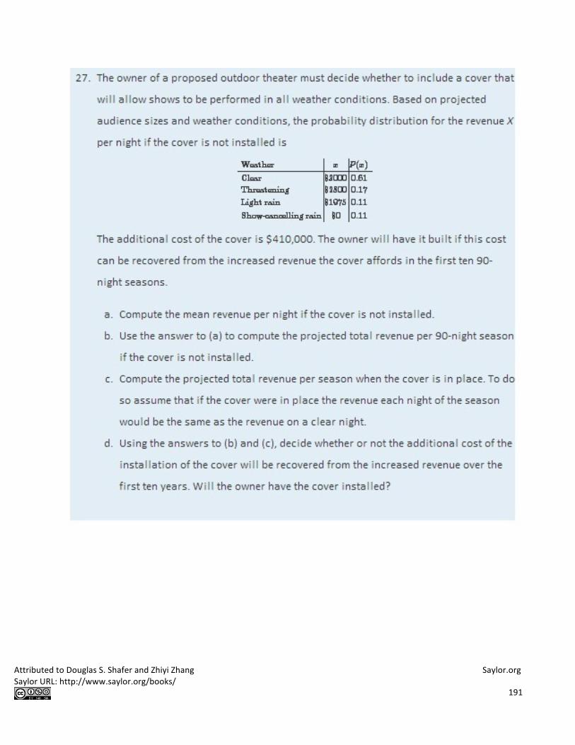
Attributed to Douglas S. Shafer and Zhiyi Zhang Saylor.org Saylor URL: http://www.saylor.org/books/
191

Attributed to Douglas S. Shafer and Zhiyi Zhang Saylor.org Saylor URL: http://www.saylor.org/books/
192

Attributed to Douglas S. Shafer and Zhiyi Zhang Saylor.org Saylor URL: http://www.saylor.org/books/
193

Attributed to Douglas S. Shafer and Zhiyi Zhang Saylor.org Saylor URL: http://www.saylor.org/books/
194
4.3 The Binomial Distribution
LEARNING OBJECT IVES
1. To learn the concept of a binomial random variable.
2. To learn how to recognize a random variable as being a binomial random variable.
The experiment of tossing a fair coin three times and the experiment of observing the genders
according to birth order of the children in a randomly selected three-child family are completely
different, but the random variables that count the number of heads in the coin toss and the number
of boys in the family (assuming the two genders are equally likely) are the same random variable, the
one with probability distribution

Attributed to Douglas S. Shafer and Zhiyi Zhang Saylor.org Saylor URL: http://www.saylor.org/books/
195
A histogram that graphically illustrates this probability distribution is given inFigure 4.4 "Probability
Distribution for Three Coins and Three Children". What is common to the two experiments is that we
perform three identical and independent trials of the same action, each trial has only two outcomes
(heads or tails, boy or girl), and the probability of success is the same number, 0.5, on every trial. The
random variable that is generated is called the binomial random variable with parameters n =
3 and p = 0.5. This is just one case of a general situation.
Figure 4.4 Probability Distribution for Three Coins and Three Children
Definition Suppose a random experiment has the following characteristics.
1. There are n identical and independent trials of a common procedure.
2. There are exactly two possible outcomes for each trial, one termed “success” and the other “failure.”
3. The probability of success on any one trial is the same number p.

Attributed to Douglas S. Shafer and Zhiyi Zhang Saylor.org Saylor URL: http://www.saylor.org/books/
196
Then the discrete random variable X that counts the number of successes in the n trials is the binomial
random variable with parameters nand p. We also say that X has a binomial distribution with
parameters n and p.
The following four examples illustrate the definition. Note how in every case “success” is the outcome
that is counted, not the outcome that we prefer or think is better in some sense.
1. A random sample of 125 students is selected from a large college in which the proportion of students who
are females is 57%. Suppose X denotes the number of female students in the sample. In this situation
there are n = 125 identical and independent trials of a common procedure, selecting a student at random;
there are exactly two possible outcomes for each trial, “success” (what we are counting, that the student be
female) and “failure;” and finally the probability of success on any one trial is the same number p=
0.57. X is a binomial random variable with parameters n = 125 and p = 0.57.
2. A multiple-choice test has 15 questions, each of which has five choices. An unprepared student taking the
test answers each of the questions completely randomly by choosing an arbitrary answer from the five
provided. Suppose X denotes the number of answers that the student gets right. X is a binomial random
variable with parameters n = 15 and p=1/5=0.20.
3. In a survey of 1,000 registered voters each voter is asked if he intends to vote for a candidate Titania
Queen in the upcoming election. Suppose X denotes the number of voters in the survey who intend to vote
for Titania Queen. X is a binomial random variable with n = 1000 and p equal to the true proportion of
voters (surveyed or not) who intend to vote for Titania Queen.
4. An experimental medication was given to 30 patients with a certain medical condition. Suppose X denotes
the number of patients who develop severe side effects. X is a binomial random variable with n = 30
and p equal to the true probability that a patient with the underlying condition will experience severe side
effects if given that medication.
Probability Formula for a Binomial Random Variable
Often the most difficult aspect of working a problem that involves the binomial random variable is
recognizing that the random variable in question has a binomial distribution. Once that is known,
probabilities can be computed using the following formula.

Attributed to Douglas S. Shafer and Zhiyi Zhang Saylor.org Saylor URL: http://www.saylor.org/books/
197

Attributed to Douglas S. Shafer and Zhiyi Zhang Saylor.org Saylor URL: http://www.saylor.org/books/
198

Attributed to Douglas S. Shafer and Zhiyi Zhang Saylor.org Saylor URL: http://www.saylor.org/books/
199
Figure 4.5Probability Distribution of the Binomial Random Variable in Note 4.29 "Example 7"

Attributed to Douglas S. Shafer and Zhiyi Zhang Saylor.org Saylor URL: http://www.saylor.org/books/
200
Special Formulas for the Mean and Standard Deviation of a Binomial Random Variable Since a binomial random variable is a discrete random variable, the formulas for its mean, variance,
and standard deviation given in the previous section apply to it, as we just saw in Note 4.29
"Example 7" in the case of the mean. However, for the binomial random variable there are much
simpler formulas.

Attributed to Douglas S. Shafer and Zhiyi Zhang Saylor.org Saylor URL: http://www.saylor.org/books/
201
The Cumulative Probability Distribution of a Binomial Random Variable
In order to allow a broader range of more realistic problems Chapter 12 "Appendix" contains
probability tables for binomial random variables for various choices of the parameters n and p. These
tables are not the probability distributions that we have seen so far, but are cumulative probability
distributions. In the place of the probability P(x) the table contains the probability
P(X≤x)=P(0)+P(1)+ ⋅ ⋅ ⋅ +P(x)
This is illustrated in Figure 4.6 "Cumulative Probabilities". The probability entered in the table
corresponds to the area of the shaded region. The reason for providing a cumulative table is that in
practical problems that involve a binomial random variable typically the probability that is sought is
of the form P(X≤x) or P(X≥x). The cumulative table is much easier to use for computing P(X≤x) since all
the individual probabilities have already been computed and added. The one table suffices for
both P(X≤x) or P(X≥x) and can be used to readily obtain probabilities of the form P(x), too, because of
the following formulas. The first is just the Probability Rule for Complements.
Figure 4.6 Cumulative Probabilities

Attributed to Douglas S. Shafer and Zhiyi Zhang Saylor.org Saylor URL: http://www.saylor.org/books/
202
If X is a discrete random variable, then
P(X≥x)=1−P(X≤x−1) and P(x)=P(X≤x)−P(X≤x−1)

Attributed to Douglas S. Shafer and Zhiyi Zhang Saylor.org Saylor URL: http://www.saylor.org/books/
203
b. The student must guess correctly on at least 60% of the questions, which
is 0.60⋅10=6 questions. The probability sought is not P(6) (an easy mistake to make), but
P(X≥6)=P(6)+P(7)+P(8)+P(9)+P(10)

Attributed to Douglas S. Shafer and Zhiyi Zhang Saylor.org Saylor URL: http://www.saylor.org/books/
204
Instead of computing each of these five numbers using the formula and adding them we can use the table
to obtain
P(X≥6)=1−P(X≤5)=1−0.6230=0.3770
which is much less work and of sufficient accuracy for the situation at hand. EXAMPLE 10
An appliance repairman services five washing machines on site each day. One-‐third of the service
calls require installation of a particular part.
a. The repairman has only one such part on his truck today. Find the probability that the one part will
be enough today, that is, that at most one washing machine he services will require installation of this
particular part.
b. Find the minimum number of such parts he should take with him each day in order that the probability
that he have enough for the day's service calls is at least 95%.
Solution:
Let X denote the number of service calls today on which the part is required. ThenX is a binomial
random variable with parameters n = 5 and p=1/3=0.3^−.
a. Note that the probability in question is not P(1), but rather P(X ≤ 1). Using the cumulative
distribution table in Chapter 12 "Appendix",
P(X≤1)=0.4609
b. The answer is the smallest number x such that the table entry P(X≤x) is at least 0.9500.
Since P(X≤2)=0.7901 is less than 0.95, two parts are not enough. Since P(X≤3)=0.9547 is as large as 0.95,
three parts will suffice at least 95% of the time. Thus the minimum needed is three.
KEY TAKEAWAYS
• The discrete random variable X that counts the number of successes in n identical, independent trials of a
procedure that always results in either of two outcomes, “success” or “failure,” and in which the
probability of success on each trial is the same number p, is called the binomial random variable with
parameters n and p.
• There is a formula for the probability that the binomial random variable with parameters n and p will take
a particular value x.

Attributed to Douglas S. Shafer and Zhiyi Zhang Saylor.org Saylor URL: http://www.saylor.org/books/
205
• There are special formulas for the mean, variance, and standard deviation of the binomial random variable
with parameters n and p that are much simpler than the general formulas that apply to all discrete
random variables.
• Cumulative probability distribution tables, when available, facilitate computation of probabilities
encountered in typical practical situations.
BAS IC
1. Determine whether or not the random variable X is a binomial random variable. If so, give the values
of n and p. If not, explain why not.
a. X is the number of dots on the top face of fair die that is rolled.
b. X is the number of hearts in a five-‐card hand drawn (without replacement) from a well-‐shuffled
ordinary deck.
c. X is the number of defective parts in a sample of ten randomly selected parts coming from a
manufacturing process in which 0.02% of all parts are defective.
d. X is the number of times the number of dots on the top face of a fair die is even in six rolls of the
die.
e. X is the number of dice that show an even number of dots on the top face when six dice are
rolled at once.
2. Determine whether or not the random variable X is a binomial random variable. If so, give the values
of n and p. If not, explain why not.
a. X is the number of black marbles in a sample of 5 marbles drawn randomly and without
replacement from a box that contains 25 white marbles and 15 black marbles.
b. X is the number of black marbles in a sample of 5 marbles drawn randomly and with replacement
from a box that contains 25 white marbles and 15 black marbles.
c. X is the number of voters in favor of proposed law in a sample 1,200 randomly selected voters
drawn from the entire electorate of a country in which 35% of the voters favor the law.
d. X is the number of fish of a particular species, among the next ten landed by a commercial
fishing boat, that are more than 13 inches in length, when 17% of all such fish exceed 13 inches
in length.
e. X is the number of coins that match at least one other coin when four coins are tossed at once.
3. X is a binomial random variable with parameters n = 12 and p = 0.82. Compute the probability indicated.
a. P(11)
b. P(9)

Attributed to Douglas S. Shafer and Zhiyi Zhang Saylor.org Saylor URL: http://www.saylor.org/books/
206
c. P(0)
d. P(13)
4. X is a binomial random variable with parameters n = 16 and p = 0.74. Compute the probability indicated.
a. P(14)
b. P(4)
c. P(0)
d. P(20)
5. X is a binomial random variable with parameters n = 5, p = 0.5. Use the tables inChapter 12 "Appendix" to
compute the probability indicated.
a. P(X ≤ 3)
b. P(X ≥ 3)
c. P(3)
d. P(0)
e. P(5)
6. X is a binomial random variable with parameters n = 5, p=0.3^−. Use the table inChapter 12 "Appendix" to
compute the probability indicated.
a. P(X ≤ 2)
b. P(X ≥ 2)
c. P(2)
d. P(0)
e. P(5)
7. X is a binomial random variable with the parameters shown. Use the tables inChapter 12 "Appendix" to
compute the probability indicated.
a. n = 10, p = 0.25, P(X ≤ 6)
b. n = 10, p = 0.75, P(X ≤ 6)
c. n = 15, p = 0.75, P(X ≤ 6)
d. n = 15, p = 0.75, P(12)
e. n = 15, p=0.6−, P(10≤X≤12)

Attributed to Douglas S. Shafer and Zhiyi Zhang Saylor.org Saylor URL: http://www.saylor.org/books/
207
8. X is a binomial random variable with the parameters shown. Use the tables in Chapter 12 "Appendix" to
compute the probability indicated.
a. n = 5, p = 0.05, P(X ≤ 1)
b. n = 5, p = 0.5, P(X ≤ 1)
c. n = 10, p = 0.75, P(X ≤ 5)
d. n = 10, p = 0.75, P(12)
e. n = 10, p=0.6−, P(5≤X≤8)
9. X is a binomial random variable with the parameters shown. Use the special formulas to compute its
mean μ and standard deviation σ.
a. n = 8, p = 0.43
b. n = 47, p = 0.82
c. n = 1200, p = 0.44
d. n = 2100, p = 0.62
10. X is a binomial random variable with the parameters shown. Use the special formulas to compute its
mean μ and standard deviation σ.
a. n = 14, p = 0.55
b. n = 83, p = 0.05
c. n = 957, p = 0.35
d. n = 1750, p = 0.79

Attributed to Douglas S. Shafer and Zhiyi Zhang Saylor.org Saylor URL: http://www.saylor.org/books/
208
16. A coin is bent so that the probability that it lands heads up is 2/3. The coin is tossed ten times.
a. Find the probability that it lands heads up at most five times.
b. Find the probability that it lands heads up more times than it lands tails up.

Attributed to Douglas S. Shafer and Zhiyi Zhang Saylor.org Saylor URL: http://www.saylor.org/books/
209
APPL I CAT IONS
17. An English-‐speaking tourist visits a country in which 30% of the population speaks English. He needs to ask
someone directions.
a. Find the probability that the first person he encounters will be able to speak English.
b. The tourist sees four local people standing at a bus stop. Find the probability that at least one of
them will be able to speak English.
18. The probability that an egg in a retail package is cracked or broken is 0.025.
a. Find the probability that a carton of one dozen eggs contains no eggs that are either cracked or
broken.
b. Find the probability that a carton of one dozen eggs has (i) at least one that is either cracked or
broken; (ii) at least two that are cracked or broken.
c. Find the average number of cracked or broken eggs in one dozen cartons.
19. An appliance store sells 20 refrigerators each week. Ten percent of all purchasers of a refrigerator buy an
extended warranty. Let X denote the number of the next 20 purchasers who do so.
a. Verify that X satisfies the conditions for a binomial random variable, and find n and p.
b. Find the probability that X is zero.
c. Find the probability that X is two, three, or four.
d. Find the probability that X is at least five.
20. Adverse growing conditions have caused 5% of grapefruit grown in a certain region to be of inferior quality.
Grapefruit are sold by the dozen.
a. Find the average number of inferior quality grapefruit per box of a dozen.
b. A box that contains two or more grapefruit of inferior quality will cause a strong adverse
customer reaction. Find the probability that a box of one dozen grapefruit will contain two or
more grapefruit of inferior quality.
21. The probability that a 7-‐ounce skein of a discount worsted weight knitting yarn contains a knot is 0.25.
Goneril buys ten skeins to crochet an afghan.
a. Find the probability that (i) none of the ten skeins will contain a knot; (ii) at most one will.
b. Find the expected number of skeins that contain knots.
c. Find the most likely number of skeins that contain knots.
22. One-‐third of all patients who undergo a non-‐invasive but unpleasant medical test require a sedative. A
laboratory performs 20 such tests daily. Let X denote the number of patients on any given day who require a
sedative.
a. Verify that X satisfies the conditions for a binomial random variable, and find n and p.

Attributed to Douglas S. Shafer and Zhiyi Zhang Saylor.org Saylor URL: http://www.saylor.org/books/
210
b. Find the probability that on any given day between five and nine patients will require a sedative
(include five and nine).
c. Find the average number of patients each day who require a sedative.
d. Using the cumulative probability distribution for X in Chapter 12 "Appendix", find the minimum
number x min of doses of the sedative that should be on hand at the start of the day so that there
is a 99% chance that the laboratory will not run out.
23. About 2% of alumni give money upon receiving a solicitation from the college or university from which they
graduated. Find the average number monetary gifts a college can expect from every 2,000 solicitations it
sends.
24. Of all college students who are eligible to give blood, about 18% do so on a regular basis. Each month a local
blood bank sends an appeal to give blood to 250 randomly selected students. Find the average number of
appeals in such mailings that are made to students who already give blood.
25. About 12% of all individuals write with their left hands. A class of 130 students meets in a classroom with 130
individual desks, exactly 14 of which are constructed for people who write with their left hands. Find the
probability that exactly 14 of the students enrolled in the class write with their left hands.
26. A travelling salesman makes a sale on 65% of his calls on regular customers. He makes four sales calls each
day.
a. Construct the probability distribution of X, the number of sales made each day.
b. Find the probability that, on a randomly selected day, the salesman will make a sale.
c. Assuming that the salesman makes 20 sales calls per week, find the mean and standard deviation
of the number of sales made per week.
27. A corporation has advertised heavily to try to insure that over half the adult population recognizes the brand
name of its products. In a random sample of 20 adults, 14 recognized its brand name. What is the probability
that 14 or more people in such a sample would recognize its brand name if the actual proportion p of all
adults who recognize the brand name were only 0.50?
ADD IT IONAL EXERC I S E S
28. When dropped on a hard surface a thumbtack lands with its sharp point touching the surface with probability
2/3; it lands with its sharp point directed up into the air with probability 1/3. The tack is dropped and its
landing position observed 15 times.
a. Find the probability that it lands with its point in the air at least 7 times.
b. If the experiment of dropping the tack 15 times is done repeatedly, what is the average number
of times it lands with its point in the air?
29. A professional proofreader has a 98% chance of detecting an error in a piece of written work (other than
misspellings, double words, and similar errors that are machine detected). A work contains four errors.

Attributed to Douglas S. Shafer and Zhiyi Zhang Saylor.org Saylor URL: http://www.saylor.org/books/
211
a. Find the probability that the proofreader will miss at least one of them.
b. Show that two such proofreaders working independently have a 99.96% chance of detecting an
error in a piece of written work.
c. Find the probability that two such proofreaders working independently will miss at least one
error in a work that contains four errors.
30. A multiple choice exam has 20 questions; there are four choices for each question.
a. A student guesses the answer to every question. Find the chance that he guesses correctly
between four and seven times.
b. Find the minimum score the instructor can set so that the probability that a student will pass just
by guessing is 20% or less.
31. In spite of the requirement that all dogs boarded in a kennel be inoculated, the chance that a healthy dog
boarded in a clean, well-‐ventilated kennel will develop kennel cough from a carrier is 0.008.
a. If a carrier (not known to be such, of course) is boarded with three other dogs, what is the
probability that at least one of the three healthy dogs will develop kennel cough?
b. If a carrier is boarded with four other dogs, what is the probability that at least one of the four
healthy dogs will develop kennel cough?
c. The pattern evident from parts (a) and (b) is that if K+1 dogs are boarded together, one a carrier
and K healthy dogs, then the probability that at least one of the healthy dogs will develop kennel
cough is P(X≥1)=1−(0.992)K, where X is the binomial random variable that counts the number of
healthy dogs that develop the condition. Experiment with different values of K in this formula to
find the maximum number K+1 of dogs that a kennel owner can board together so that if one of
the dogs has the condition, the chance that another dog will be infected is less than 0.05.
32. Investigators need to determine which of 600 adults have a medical condition that affects 2% of the adult
population. A blood sample is taken from each of the individuals.
a. Show that the expected number of diseased individuals in the group of 600 is 12 individuals.
b. Instead of testing all 600 blood samples to find the expected 12 diseased individuals,
investigators group the samples into 60 groups of 10 each, mix a little of the blood from each of
the 10 samples in each group, and test each of the 60 mixtures. Show that the probability that
any such mixture will contain the blood of at least one diseased person, hence test positive, is
about 0.18.

Attributed to Douglas S. Shafer and Zhiyi Zhang Saylor.org Saylor URL: http://www.saylor.org/books/
212
c. Based on the result in (b), show that the expected number of mixtures that test positive is about
11. (Supposing that indeed 11 of the 60 mixtures test positive, then we know that none of the
490 persons whose blood was in the remaining 49 samples that tested negative has the disease.
We have eliminated 490 persons from our search while performing only 60 tests.)

Attributed to Douglas S. Shafer and Zhiyi Zhang Saylor.org Saylor URL: http://www.saylor.org/books/
213

Attributed to Douglas S. Shafer and Zhiyi Zhang Saylor.org Saylor URL: http://www.saylor.org/books/
214
Chapter 5 Continuous Random Variables
As discussed in Section 4.1 "Random Variables" in Chapter 4 "Discrete Random Variables", a random
variable is called continuous if its set of possible values contains a whole interval of decimal numbers.
In this chapter we investigate such random variables.
5.1 Continuous Random Variables
LEARNING OBJECT IVES
1. To learn the concept of the probability distribution of a continuous random variable, and how it is used to
compute probabilities.
2. To learn basic facts about the family of normally distributed random variables.
The Probability Distribution of a Continuous Random Variable For a discrete random variable X the probability that X assumes one of its possible values on a single trial
of the experiment makes good sense. This is not the case for a continuous random variable. For example,
suppose X denotes the length of time a commuter just arriving at a bus stop has to wait for the next bus. If
buses run every 30 minutes without fail, then the set of possible values of X is the interval denoted [0,30],
the set of all decimal numbers between 0 and 30. But although the number 7.211916 is a possible value
of X, there is little or no meaning to the concept of the probability that the commuter will wait precisely
7.211916 minutes for the next bus. If anything the probability should be zero, since if we could
meaningfully measure the waiting time to the nearest millionth of a minute it is practically inconceivable
that we would ever get exactly 7.211916 minutes. More meaningful questions are those of the form: What

Attributed to Douglas S. Shafer and Zhiyi Zhang Saylor.org Saylor URL: http://www.saylor.org/books/
215
is the probability that the commuter's waiting time is less than 10 minutes, or is between 5 and 10
minutes? In other words, with continuous random variables one is concerned not with the event that the
variable assumes a single particular value, but with the event that the random variable assumes a value in
a particular interval.
Definition The probability distribution of a continuous random variable X is an assignment of
probabilities to intervals of decimal numbers using a function f(x), called a density function, in the
following way: the probability that X assumes a value in the interval [a,b] is equal to the area of the
region that is bounded above by the graph of the equation y=f(x),bounded below by the x-axis, and
bounded on the left and right by the vertical lines through a and b, as illustrated in Figure 5.1
"Probability Given as Area of a Region under a Curve".
Figure 5.1Probability Given as Area of a Region under a Curve
This definition can be understood as a natural outgrowth of the discussion inSection 2.1.3 "Relative
Frequency Histograms" in Chapter 2 "Descriptive Statistics". There we saw that if we have in view a
population (or a very large sample) and make measurements with greater and greater precision, then
as the bars in the relative frequency histogram become exceedingly fine their vertical sides merge
and disappear, and what is left is just the curve formed by their tops, as shown in Figure 2.5 "Sample
Size and Relative Frequency Histograms" in Chapter 2 "Descriptive Statistics". Moreover the total

Attributed to Douglas S. Shafer and Zhiyi Zhang Saylor.org Saylor URL: http://www.saylor.org/books/
216
area under the curve is 1, and the proportion of the population with measurements between two
numbersa and b is the area under the curve and between a and b, as shown in Figure 2.6 "A Very
Fine Relative Frequency Histogram" in Chapter 2 "Descriptive Statistics". If we think of X as a
measurement to infinite precision arising from the selection of any one member of the population at
random, then P(a<X<b)is simply the proportion of the population with measurements
between a and b, the curve in the relative frequency histogram is the density function for X, and we
arrive at the definition just above.
Every density function f(x) must satisfy the following two conditions:
1. For all numbers x, f(x)≥0, so that the graph of y=f(x) never drops below the x-axis.
2. The area of the region under the graph of y=f(x) and above the x-axis is 1.
Because the area of a line segment is 0, the definition of the probability distribution of a continuous
random variable implies that for any particular decimal number, say a, the probability
that X assumes the exact value a is 0. This property implies that whether or not the endpoints of an
interval are included makes no difference concerning the probability of the interval.
For any continuous random variable X:
P(a≤X≤b)=P(a<X≤b)=P(a≤X<b)=P(a<X<b)
EXAMPLE 1
A random variable X has the uniform distribution on the interval [0,1]: the density function
is f(x)=1 if x is between 0 and 1 and f(x)=0 for all other values of x, as shown in Figure 5.2 "Uniform
Distribution on ".
Figure 5.2Uniform Distribution on [0,1]

Attributed to Douglas S. Shafer and Zhiyi Zhang Saylor.org Saylor URL: http://www.saylor.org/books/
217
a. Find P(X > 0.75), the probability that X assumes a value greater than 0.75.
b. Find P(X ≤ 0.2), the probability that X assumes a value less than or equal to 0.2.
c. Find P(0.4 < X < 0.7), the probability that X assumes a value between 0.4 and 0.7.
Solution:
a. P(X > 0.75) is the area of the rectangle of height 1 and base length 1−0.75=0.25, hence
is base×height=(0.25)⋅(1)=0.25. See Figure 5.3 "Probabilities from the Uniform Distribution on "(a).
b. P(X ≤ 0.2) is the area of the rectangle of height 1 and base length 0.2−0=0.2, hence
is base×height=(0.2)⋅(1)=0.2. See Figure 5.3 "Probabilities from the Uniform Distribution on "(b).
c. P(0.4 < X < 0.7) is the area of the rectangle of height 1 and length 0.7−0.4=0.3, hence
is base×height=(0.3)⋅(1)=0.3. See Figure 5.3 "Probabilities from the Uniform Distribution on "(c).
Figure 5.3Probabilities from the Uniform Distribution on [0,1]
EXAMPLE 2

Attributed to Douglas S. Shafer and Zhiyi Zhang Saylor.org Saylor URL: http://www.saylor.org/books/
218
A man arrives at a bus stop at a random time (that is, with no regard for the scheduled service) to
catch the next bus. Buses run every 30 minutes without fail, hence the next bus will come any time
during the next 30 minutes with evenly distributed probability (a uniform distribution). Find the
probability that a bus will come within the next 10 minutes.
Solution:
The graph of the density function is a horizontal line above the interval from 0 to 30 and is the x-‐axis
everywhere else. Since the total area under the curve must be 1, the height of the horizontal line is
1/30. See Figure 5.4 "Probability of Waiting At Most 10 Minutes for a Bus". The probability sought
is P(0≤X≤10). By definition, this probability is the area of the rectangular region bounded above by the
horizontal line f(x)=1/30, bounded below by the x-‐axis, bounded on the left by the vertical line at 0
(the y-‐axis), and bounded on the right by the vertical line at 10. This is the shaded region in Figure 5.4
"Probability of Waiting At Most 10 Minutes for a Bus". Its area is the base of the rectangle times its
height, 10⋅(1/30)=1/3. Thus P(0≤X≤10)=1/3.
Figure 5.4Probability of Waiting At Most 10 Minutes for a Bus

Attributed to Douglas S. Shafer and Zhiyi Zhang Saylor.org Saylor URL: http://www.saylor.org/books/
219
Figure 5.5 Bell Curves with � = 0.25 and Different Values of �

Attributed to Douglas S. Shafer and Zhiyi Zhang Saylor.org Saylor URL: http://www.saylor.org/books/
220
The value of � determines whether the bell curve is tall and thin or short and squat, subject always
to the condition that the total area under the curve be equal to 1. This is shown in Figure 5.6 "Bell
Curves with ", where we have arbitrarily chosen to center the curves at � = 6.
Figure 5.6 Bell Curves with � = 6 and Different Values of �
Definition The probability distribution corresponding to the density function for the bell curve with
parameters � and � is called the normal distribution with mean � and standard deviation �.

Attributed to Douglas S. Shafer and Zhiyi Zhang Saylor.org Saylor URL: http://www.saylor.org/books/
221
Definition A continuous random variable whose probabilities are described by the normal distribution with
mean � and standard deviation � is called a normally distributed random variable, or a
normal random variable for short, with mean � and standard deviation �.
Figure 5.7 "Density Function for a Normally Distributed Random Variable with Mean " shows the
density function that determines the normal distribution with mean � and standard deviation �.
We repeat an important fact about this curve:
The density curve for the normal distribution is symmetric about the mean.
Figure 5.7 Density Function for a Normally Distributed Random Variable with Mean � and Standard
Deviation �
EXAMPLE 3
Heights of 25-‐year-‐old men in a certain region have mean 69.75 inches and standard deviation 2.59
inches. These heights are approximately normally distributed. Thus the height X of a randomly
selected 25-‐year-‐old man is a normal random variable with mean μ = 69.75 and standard
deviation σ = 2.59. Sketch a qualitatively accurate graph of the density function for X. Find the
probability that a randomly selected 25-‐year-‐old man is more than 69.75 inches tall.

Attributed to Douglas S. Shafer and Zhiyi Zhang Saylor.org Saylor URL: http://www.saylor.org/books/
222
Solution:
The distribution of heights looks like the bell curve in Figure 5.8 "Density Function for Heights of 25-‐
Year-‐Old Men". The important point is that it is centered at its mean, 69.75, and is symmetric about
the mean.
Figure 5.8Density Function for Heights of 25-‐Year-‐Old Men
Since the total area under the curve is 1, by symmetry the area to the right of 69.75 is half the total,
or 0.5. But this area is precisely the probability P(X > 69.75), the probability that a randomly selected
25-‐year-‐old man is more than 69.75 inches tall.
We will learn how to compute other probabilities in the next two sections.
KEY TAKEAWAYS
• For a continuous random variable X the only probabilities that are computed are those of X taking a value
in a specified interval.
• The probability that X take a value in a particular interval is the same whether or not the endpoints of the
interval are included.

Attributed to Douglas S. Shafer and Zhiyi Zhang Saylor.org Saylor URL: http://www.saylor.org/books/
223
• The probability P(a<X<b), that X take a value in the interval from a to b, is the area of the region between
the vertical lines through a and b, above the x-‐axis, and below the graph of a function f(x) called the
density function.
• A normally distributed random variable is one whose density function is a bell curve.
• Every bell curve is symmetric about its mean and lies everywhere above the x-‐axis, which it approaches
asymptotically (arbitrarily closely without touching).
EXERCISES
BAS I C
1. A continuous random variable X has a uniform distribution on the interval [5,12].Sketch the graph of its density
function.
2. A continuous random variable X has a uniform distribution on the interval [−3,3].Sketch the graph of its density
function.
3. A continuous random variable X has a normal distribution with mean 100 and standard deviation 10. Sketch a
qualitatively accurate graph of its density function.
4. A continuous random variable X has a normal distribution with mean 73 and standard deviation 2.5. Sketch a
qualitatively accurate graph of its density function.
5. A continuous random variable X has a normal distribution with mean 73. The probability that X takes a value
greater than 80 is 0.212. Use this information and the symmetry of the density function to find the
probability that X takes a value less than 66. Sketch the density curve with relevant regions shaded to
illustrate the computation.
6. A continuous random variable X has a normal distribution with mean 169. The probability that X takes a value
greater than 180 is 0.17. Use this information and the symmetry of the density function to find the
probability that X takes a value less than 158. Sketch the density curve with relevant regions shaded to
illustrate the computation.
7. A continuous random variable X has a normal distribution with mean 50.5. The probability that X takes a
value less than 54 is 0.76. Use this information and the symmetry of the density function to find the
probability that X takes a value greater than 47. Sketch the density curve with relevant regions shaded to
illustrate the computation.
8. A continuous random variable X has a normal distribution with mean 12.25. The probability that X takes a
value less than 13 is 0.82. Use this information and the symmetry of the density function to find the
probability that X takes a value greater than 11.50. Sketch the density curve with relevant regions shaded
to illustrate the computation.

Attributed to Douglas S. Shafer and Zhiyi Zhang Saylor.org Saylor URL: http://www.saylor.org/books/
224
9. The figure provided shows the density curves of three normally distributed random variables XA, XB,
and XC. Their standard deviations (in no particular order) are 15, 7, and 20. Use the figure to identify the
values of the means µA, µB, and µC and standard deviations σA, σB, and σC of the three random variables.
10. The figure provided shows the density curves of three normally distributed random variables XA, XB,
and XC. Their standard deviations (in no particular order) are 20, 5, and 10. Use the figure to identify the
values of the means µA, µB, and µC and standard deviations σA, σB, and σC of the three random variables.

Attributed to Douglas S. Shafer and Zhiyi Zhang Saylor.org Saylor URL: http://www.saylor.org/books/
225
APPL I CAT IONS
11. Dogberry's alarm clock is battery operated. The battery could fail with equal probability at any time of the
day or night. Every day Dogberry sets his alarm for 6:30 a.m. and goes to bed at 10:00 p.m. Find the
probability that when the clock battery finally dies, it will do so at the most inconvenient time, between
10:00 p.m. and 6:30 a.m.
12. Buses running a bus line near Desdemona's house run every 15 minutes. Without paying attention to the
schedule she walks to the nearest stop to take the bus to town. Find the probability that she waits more than
10 minutes.
13. The amount X of orange juice in a randomly selected half-‐gallon container varies according to a normal
distribution with mean 64 ounces and standard deviation 0.25 ounce.
a. Sketch the graph of the density function for X.
b. What proportion of all containers contain less than a half gallon (64 ounces)? Explain.
c. What is the median amount of orange juice in such containers? Explain.
14. The weight X of grass seed in bags marked 50 lb varies according to a normal distribution with mean 50 lb
and standard deviation 1 ounce (0.0625 lb).
a. Sketch the graph of the density function for X.
b. What proportion of all bags weigh less than 50 pounds? Explain.
c. What is the median weight of such bags? Explain.

Attributed to Douglas S. Shafer and Zhiyi Zhang Saylor.org Saylor URL: http://www.saylor.org/books/
226
5.2 The Standard Normal Distribution
LEARNING OBJECT IVES
1. To learn what a standard normal random variable is.
2. To learn how to use Figure 12.2 "Cumulative Normal Probability" to compute probabilities related to a
standard normal random variable.
Definition A standard normal random variable is a normally distributed random variable with mean � =
0 and standard deviation � = 1. It will always be denoted by the letter Z.
The density function for a standard normal random variable is shown in Figure 5.9 "Density Curve
for a Standard Normal Random Variable".

Attributed to Douglas S. Shafer and Zhiyi Zhang Saylor.org Saylor URL: http://www.saylor.org/books/
227
Figure 5.9 Density Curve for a Standard Normal Random Variable
To compute probabilities for Z we will not work with its density function directly but instead read
probabilities out of Figure 12.2 "Cumulative Normal Probability" in Chapter 12 "Appendix". The
tables are tables of cumulative probabilities; their entries are probabilities of the form P(Z<z). The use
of the tables will be explained by the following series of examples.
EXAMPLE 4
Find the probabilities indicated, where as always Z denotes a standard normal random variable.
a. P(Z < 1.48).
b. P(Z< −0.25).
Solution:
a. Figure 5.10 "Computing Probabilities Using the Cumulative Table" shows how this probability is read
directly from the table without any computation required. The digits in the ones and tenths places of 1.48,
namely 1.4, are used to select the appropriate row of the table; the hundredths part of 1.48, namely 0.08, is
used to select the appropriate column of the table. The four decimal place number in the interior of the table
that lies in the intersection of the row and column selected, 0.9306, is the probability sought: P(Z<1.48)=0.9306.
Figure 5.10Computing Probabilities Using the Cumulative Table

Attributed to Douglas S. Shafer and Zhiyi Zhang Saylor.org Saylor URL: http://www.saylor.org/books/
228
b. The minus sign in −0.25 makes no difference in the procedure; the table is used in exactly the same
way as in part (a): the probability sought is the number that is in the intersection of the row with heading −0.2
and the column with heading 0.05, the number 0.4013. Thus P(Z < −0.25) = 0.4013. EXAMPLE 5
Find the probabilities indicated.
a. P(Z > 1.60).
b. P(Z > −1.02).
Solution:
a. Because the events Z > 1.60 and Z ≤ 1.60 are complements, the Probability Rule for
Complements implies that P(Z>1.60)=1−P(Z≤1.60)
Since inclusion of the endpoint makes no difference for the continuous random
variable Z, P(Z≤1.60)=P(Z<1.60), which we know how to find from the table. The number in the row
with heading 1.6 and in the column with heading 0.00 is 0.9452. Thus P(Z<1.60)=0.9452 so
P(Z>1.60)=1−P(Z≤1.60)=1−0.9452=0.0548
Figure 5.11 "Computing a Probability for a Right Half-‐Line"illustrates the ideas geometrically. Since
the total area under the curve is 1 and the area of the region to the left of 1.60 is (from the table)
0.9452, the area of the region to the right of 1.60 must be 1−0.9452=0.0548.
Figure 5.11Computing a Probability for a Right Half-‐Line

Attributed to Douglas S. Shafer and Zhiyi Zhang Saylor.org Saylor URL: http://www.saylor.org/books/
229
b. The minus sign in −1.02 makes no difference in the procedure; the table is used in exactly the
same way as in part (a). The number in the intersection of the row with heading −1.0 and the
column with heading 0.02 is 0.1539. This means that P(Z<−1.02)=P(Z≤−1.02)=0.1539, hence
P(Z>−1.02)=1−P(Z≤−1.02)=1−0.1539=0.8461
Figure 5.12 Computing a Probability for an Interval of Finite Length

Attributed to Douglas S. Shafer and Zhiyi Zhang Saylor.org Saylor URL: http://www.saylor.org/books/
230
b. The procedure for finding the probability that Z takes a value in a finite interval whose endpoints
have opposite signs is exactly the same procedure used in part (a), and is illustrated in Figure 5.13
"Computing a Probability for an Interval of Finite Length". In symbols the computation is
P(−2.55<Z<0.09)==P(Z<0.09)−P(Z<−2.55)
=0.5359−0.0054=0.5305
Figure 5.13 Computing a Probability for an Interval of Finite Length

Attributed to Douglas S. Shafer and Zhiyi Zhang Saylor.org Saylor URL: http://www.saylor.org/books/
231
The next example shows what to do if the value of Z that we want to look up in the table is not
present there.
EXAMPLE 7
Find the probabilities indicated.
a. P(1.13<Z<4.16). b. P(−5.22<Z<2.15).
Solution:
a. We attempt to compute the probability exactly as in Note 5.20 "Example 6" by looking up the
numbers 1.13 and 4.16 in the table. We obtain the value 0.8708 for the area of the region under the
density curve to left of 1.13 without any problem, but when we go to look up the number 4.16 in the
table, it is not there. We can see from the last row of numbers in the table that the area to the left of 4.16
must be so close to 1 that to four decimal places it rounds to 1.0000. Therefore P(1.13<Z<4.16)=1.0000−0.8708=0.1292
b. Similarly, here we can read directly from the table that the area under the density curve and
to the left of 2.15 is 0.9842, but −5.22 is too far to the left on the number line to be in the table. We
can see from the first line of the table that the area to the left of −5.22 must be so close to 0 that to
four decimal places it rounds to 0.0000. Therefore
P(−5.22<Z<2.15)=0.9842−0.0000=0.9842
The final example of this section explains the origin of the proportions given in the Empirical Rule.
EXAMPLE 8
Find the probabilities indicated.
a. P(−1<Z<1).
b. P(−2<Z<2).
c. P(−3<Z<3).
Solution:
a. Using the table as was done in Note 5.20 "Example 6"(b) we obtain
P(−1<Z<1)=0.8413−0.1587=0.6826

Attributed to Douglas S. Shafer and Zhiyi Zhang Saylor.org Saylor URL: http://www.saylor.org/books/
232
Since Z has mean 0 and standard deviation 1, for Z to take a value between −1 and 1 means
that Z takes a value that is within one standard deviation of the mean. Our computation shows
that the probability that this happens is about 0.68, the proportion given by the Empirical Rule for
histograms that are mound shaped and symmetrical, like the bell curve.
b. Using the table in the same way,
P(−2<Z<2)=0.9772−0.0228=0.9544
This corresponds to the proportion 0.95 for data within two standard deviations of the mean.
c. Similarly,
P(−3<Z<3)=0.9987−0.0013=0.9974
which corresponds to the proportion 0.997 for data within three standard deviations of the mean.
KEY TAKEAWAYS
• A standard normal random variable Z is a normally distributed random variable with mean μ = 0 and
standard deviation σ = 1.
• Probabilities for a standard normal random variable are computed usingFigure 12.2 "Cumulative Normal
Probability".

Attributed to Douglas S. Shafer and Zhiyi Zhang Saylor.org Saylor URL: http://www.saylor.org/books/
233

Attributed to Douglas S. Shafer and Zhiyi Zhang Saylor.org Saylor URL: http://www.saylor.org/books/
234

Attributed to Douglas S. Shafer and Zhiyi Zhang Saylor.org Saylor URL: http://www.saylor.org/books/
235

Attributed to Douglas S. Shafer and Zhiyi Zhang Saylor.org Saylor URL: http://www.saylor.org/books/
236

Attributed to Douglas S. Shafer and Zhiyi Zhang Saylor.org Saylor URL: http://www.saylor.org/books/
237
5.3 Probability Computations for General Normal Random Variables LEARNING OBJECT IVE
1. To learn how to compute probabilities related to any normal random variable.
If X is any normally distributed normal random variable then Figure 12.2 "Cumulative Normal
Probability" can also be used to compute a probability of the form P(a<X<b) by means of the following
equality.

Attributed to Douglas S. Shafer and Zhiyi Zhang Saylor.org Saylor URL: http://www.saylor.org/books/
238
The new endpoints (a−µ)/σ and (b−µ)/σ are the z-scores of a and b as defined in Section 2.4.2 in Chapter
2 "Descriptive Statistics".
Figure 5.14 "Probability for an Interval of Finite Length" illustrates the meaning of the equality
geometrically: the two shaded regions, one under the density curve for X and the other under the
density curve for Z, have the same area. Instead of drawing both bell curves, though, we will always
draw a single generic bell-shaped curve with both an x-axis and a z-axis below it.
Figure 5.14 Probability for an Interval of Finite Length

Attributed to Douglas S. Shafer and Zhiyi Zhang Saylor.org Saylor URL: http://www.saylor.org/books/
239
EXAMPLE 9
Let X be a normal random variable with mean μ = 10 and standard deviation σ = 2.5. Compute the
following probabilities.
a. P(X < 14).
b. P(8<X<14).
Solution:

Attributed to Douglas S. Shafer and Zhiyi Zhang Saylor.org Saylor URL: http://www.saylor.org/books/
240

Attributed to Douglas S. Shafer and Zhiyi Zhang Saylor.org Saylor URL: http://www.saylor.org/books/
241
EXAMPLE 10
The lifetimes of the tread of a certain automobile tire are normally distributed with mean 37,500
miles and standard deviation 4,500 miles. Find the probability that the tread life of a randomly
selected tire will be between 30,000 and 40,000 miles.
Solution:

Attributed to Douglas S. Shafer and Zhiyi Zhang Saylor.org Saylor URL: http://www.saylor.org/books/
242
Let X denote the tread life of a randomly selected tire. To make the numbers easier to work with we
will choose thousands of miles as the units. Thus μ = 37.5, σ = 4.5, and the problem is to
compute P(30<X<40). Figure 5.17 "Probability Computation for Tire Tread Wear" illustrates the
following computation:

Attributed to Douglas S. Shafer and Zhiyi Zhang Saylor.org Saylor URL: http://www.saylor.org/books/
243
EXAMPLE 11
Scores on a standardized college entrance examination (CEE) are normally distributed with mean 510
and standard deviation 60. A selective university considers for admission only applicants
with CEE scores over 650. Find percentage of all individuals who took the CEE who meet the
university's CEE requirement for consideration for admission.
Solution:
Let X denote the score made on the CEE by a randomly selected individual. Then Xis normally
distributed with mean 510 and standard deviation 60. The probability that X lie in a particular interval
is the same as the proportion of all exam scores that lie in that interval. Thus the solution to the
problem is P(X > 650), expressed as a percentage. Figure 5.18 "Probability Computation for Exam
Scores" illustrates the following computation:

Attributed to Douglas S. Shafer and Zhiyi Zhang Saylor.org Saylor URL: http://www.saylor.org/books/
244
KEY TAKEAWAY
• Probabilities for a general normal random variable are computed usingFigure 12.2 "Cumulative Normal
Probability" after converting x-‐values to z-‐scores.
EXERC ISES
BAS I C
1. X is a normally distributed random variable with mean 57 and standard deviation 6. Find the probability
indicated.
a. P(X < 59.5)
b. P(X < 46.2)
c. P(X > 52.2)
d. P(X > 70)
2. X is a normally distributed random variable with mean −25 and standard deviation 4. Find the probability
indicated.

Attributed to Douglas S. Shafer and Zhiyi Zhang Saylor.org Saylor URL: http://www.saylor.org/books/
245
a. P(X < −27.2)
b. P(X < −14.8)
c. P(X > −33.1)
d. P(X > −16.5)
3. X is a normally distributed random variable with mean 112 and standard deviation 15. Find the probability
indicated.
a. P(100<X<125) b. P(91<X<107) c. P(118<X<160)
4. X is a normally distributed random variable with mean 72 and standard deviation 22. Find the probability
indicated.
a. P(78<X<127) b. P(60<X<90) c. P(49<X<71)
5. X is a normally distributed random variable with mean 500 and standard deviation 25. Find the probability
indicated.
a. P(X < 400)
b. P(466<X<625)
6. X is a normally distributed random variable with mean 0 and standard deviation 0.75. Find the probability
indicated.
a. P(−4.02 < X < 3.82)
b. P(X > 4.11)
7. X is a normally distributed random variable with mean 15 and standard deviation 1. Use Figure 12.2
"Cumulative Normal Probability" to find the first probability listed. Find the second probability using the
symmetry of the density curve. Sketch the density curve with relevant regions shaded to illustrate the
computation.
a. P(X < 12), P(X > 18)
b. P(X < 14), P(X > 16)
c. P(X < 11.25), P(X > 18.75)
d. P(X < 12.67), P(X > 17.33)
8. X is a normally distributed random variable with mean 100 and standard deviation 10. Use Figure 12.2
"Cumulative Normal Probability" to find the first probability listed. Find the second probability using the
symmetry of the density curve. Sketch the density curve with relevant regions shaded to illustrate the
computation.
a. P(X < 80), P(X > 120)

Attributed to Douglas S. Shafer and Zhiyi Zhang Saylor.org Saylor URL: http://www.saylor.org/books/
246
b. P(X < 75), P(X > 125)
c. P(X < 84.55), P(X > 115.45)
d. P(X < 77.42), P(X > 122.58)
9. X is a normally distributed random variable with mean 67 and standard deviation 13. The probability
that X takes a value in the union of intervals (−∞,67−a] ∪ [67+a,∞) will be
denoted P(X≤67−a or X≥67+a). Use Figure 12.2 "Cumulative Normal Probability" to find the following
probabilities of this type. Sketch the density curve with relevant regions shaded to illustrate the
computation. Because of the symmetry of the density curve you need to use Figure 12.2 "Cumulative
Normal Probability" only one time for each part.
a. P(X<57 or X>77) b. P(X<47 or X>87) c. P(X<49 or X>85) d. P(X<37 or X>97)
10. X is a normally distributed random variable with mean 288 and standard deviation 6. The probability
that X takes a value in the union of intervals (−∞,288−a] ∪ [288+a,∞) will be
denoted P(X≤288−a or X≥288+a). Use Figure 12.2 "Cumulative Normal Probability" to find the following
probabilities of this type. Sketch the density curve with relevant regions shaded to illustrate the
computation. Because of the symmetry of the density curve you need to use Figure 12.2 "Cumulative
Normal Probability" only one time for each part.
a. P(X<278 or X>298) b. P(X<268 or X>308) c. P(X<273 or X>303) d. P(X<280 or X>296)
APPL I CAT IONS
11. The amount X of beverage in a can labeled 12 ounces is normally distributed with mean 12.1 ounces and
standard deviation 0.05 ounce. A can is selected at random.
a. Find the probability that the can contains at least 12 ounces.
b. Find the probability that the can contains between 11.9 and 12.1 ounces.
12. The length of gestation for swine is normally distributed with mean 114 days and standard deviation 0.75
day. Find the probability that a litter will be born within one day of the mean of 114.
13. The systolic blood pressure X of adults in a region is normally distributed with mean 112 mm Hg and standard
deviation 15 mm Hg. A person is considered “prehypertensive” if his systolic blood pressure is between 120

Attributed to Douglas S. Shafer and Zhiyi Zhang Saylor.org Saylor URL: http://www.saylor.org/books/
247
and 130 mm Hg. Find the probability that the blood pressure of a randomly selected person is
prehypertensive.
14. Heights X of adult women are normally distributed with mean 63.7 inches and standard deviation 2.71
inches. Romeo, who is 69.25 inches tall, wishes to date only women who are shorter than he but within 4
inches of his height. Find the probability that the next woman he meets will have such a height.
15. Heights X of adult men are normally distributed with mean 69.1 inches and standard deviation 2.92 inches.
Juliet, who is 63.25 inches tall, wishes to date only men who are taller than she but within 6 inches of her
height. Find the probability that the next man she meets will have such a height.
16. A regulation hockey puck must weigh between 5.5 and 6 ounces. The weights X of pucks made by a
particular process are normally distributed with mean 5.75 ounces and standard deviation 0.11 ounce.
Find the probability that a puck made by this process will meet the weight standard.
17. A regulation golf ball may not weigh more than 1.620 ounces. The weights X of golf balls made by a
particular process are normally distributed with mean 1.361 ounces and standard deviation 0.09 ounce.
Find the probability that a golf ball made by this process will meet the weight standard.
18. The length of time that the battery in Hippolyta's cell phone will hold enough charge to operate
acceptably is normally distributed with mean 25.6 hours and standard deviation 0.32 hour. Hippolyta
forgot to charge her phone yesterday, so that at the moment she first wishes to use it today it has been
26 hours 18 minutes since the phone was last fully charged. Find the probability that the phone will
operate properly.
19. The amount of non-‐mortgage debt per household for households in a particular income bracket in one
part of the country is normally distributed with mean $28,350 and standard deviation $3,425. Find the
probability that a randomly selected such household has between $20,000 and $30,000 in non-‐mortgage
debt.
20. Birth weights of full-‐term babies in a certain region are normally distributed with mean 7.125 lb and
standard deviation 1.290 lb. Find the probability that a randomly selected newborn will weigh less than
5.5 lb, the historic definition of prematurity.
21. The distance from the seat back to the front of the knees of seated adult males is normally distributed
with mean 23.8 inches and standard deviation 1.22 inches. The distance from the seat back to the back of
the next seat forward in all seats on aircraft flown by a budget airline is 26 inches. Find the proportion of
adult men flying with this airline whose knees will touch the back of the seat in front of them.

Attributed to Douglas S. Shafer and Zhiyi Zhang Saylor.org Saylor URL: http://www.saylor.org/books/
248
22. The distance from the seat to the top of the head of seated adult males is normally distributed with mean
36.5 inches and standard deviation 1.39 inches. The distance from the seat to the roof of a particular
make and model car is 40.5 inches. Find the proportion of adult men who when sitting in this car will have
at least one inch of headroom (distance from the top of the head to the roof). ADD IT IONAL EXERC I S E S
23. The useful life of a particular make and type of automotive tire is normally distributed with mean 57,500 miles
and standard deviation 950 miles.
a. Find the probability that such a tire will have a useful life of between 57,000 and 58,000 miles.
b. Hamlet buys four such tires. Assuming that their lifetimes are independent, find the probability
that all four will last between 57,000 and 58,000 miles. (If so, the best tire will have no more than
1,000 miles left on it when the first tire fails.) Hint: There is a binomial random variable here,
whose value of p comes from part (a).
24. A machine produces large fasteners whose length must be within 0.5 inch of 22 inches. The lengths are
normally distributed with mean 22.0 inches and standard deviation 0.17 inch.
a. Find the probability that a randomly selected fastener produced by the machine will have an
acceptable length.
b. The machine produces 20 fasteners per hour. The length of each one is inspected. Assuming
lengths of fasteners are independent, find the probability that all 20 will have acceptable length.
Hint: There is a binomial random variable here, whose value of p comes from part (a).
25. The lengths of time taken by students on an algebra proficiency exam (if not forced to stop before completing
it) are normally distributed with mean 28 minutes and standard deviation 1.5 minutes.
a. Find the proportion of students who will finish the exam if a 30-‐minute time limit is set.
b. Six students are taking the exam today. Find the probability that all six will finish the exam within
the 30-‐minute limit, assuming that times taken by students are independent. Hint: There is a
binomial random variable here, whose value of p comes from part (a).
26. Heights of adult men between 18 and 34 years of age are normally distributed with mean 69.1 inches and
standard deviation 2.92 inches. One requirement for enlistment in the military is that men must stand
between 60 and 80 inches tall.
a. Find the probability that a randomly elected man meets the height requirement for military
service.
b. Twenty-‐three men independently contact a recruiter this week. Find the probability that all of
them meet the height requirement. Hint: There is a binomial random variable here, whose value
of p comes from part (a).

Attributed to Douglas S. Shafer and Zhiyi Zhang Saylor.org Saylor URL: http://www.saylor.org/books/
249
27. A regulation hockey puck must weigh between 5.5 and 6 ounces. In an alternative manufacturing process the
mean weight of pucks produced is 5.75 ounce. The weights of pucks have a normal distribution whose
standard deviation can be decreased by increasingly stringent (and expensive) controls on the manufacturing
process. Find the maximum allowable standard deviation so that at most 0.005 of all pucks will fail to meet the
weight standard. (Hint: The distribution is symmetric and is centered at the middle of the interval of
acceptable weights.)
28. The amount of gasoline X delivered by a metered pump when it registers 5 gallons is a normally distributed
random variable. The standard deviation σ of X measures the precision of the pump; the smaller σ is the
smaller the variation from delivery to delivery. A typical standard for pumps is that when they show that 5
gallons of fuel has been delivered the actual amount must be between 4.97 and 5.03 gallons (which
corresponds to being off by at most about half a cup). Supposing that the mean of X is 5, find the largest
that σ can be so that P(4.97 < X < 5.03) is 1.0000 to four decimal places when computed using Figure 12.2
"Cumulative Normal Probability", which means that the pump is sufficiently accurate. (Hint: The z-‐score of 5.03
will be the smallest value of Z so that Figure 12.2 "Cumulative Normal Probability" gives P(Z<z)=1.0000.)

Attributed to Douglas S. Shafer and Zhiyi Zhang Saylor.org Saylor URL: http://www.saylor.org/books/
250

Attributed to Douglas S. Shafer and Zhiyi Zhang Saylor.org Saylor URL: http://www.saylor.org/books/
251
5.4 Areas of Tails of Distributions
LEARNING OBJECT IVE
1. To learn how to find, for a normal random variable X and an area a, the value x* of X so that P(X<x*)=a or
that P(X>x*)=a, whichever is required.
Definition The left tail of a density curve y=f(x) of a continuous random variable Xcut off by a
value x* of X is the region under the curve that is to the left of x*, as shown by the shading
in Figure 5.19 "Right and Left Tails of a Distribution"(a). The right tail cut off by x* is defined
similarly, as indicated by the shading in Figure 5.19 "Right and Left Tails of a Distribution"(b).
Figure 5.19Right and Left Tails of a Distribution

Attributed to Douglas S. Shafer and Zhiyi Zhang Saylor.org Saylor URL: http://www.saylor.org/books/
252
The probabilities tabulated in Figure 12.2 "Cumulative Normal Probability" are areas of left tails in
the standard normal distribution.
Tails of the Standard Normal Distribution At times it is important to be able to solve the kind of problem illustrated by Figure 5.20. We have a
certain specific area in mind, in this case the area 0.0125 of the shaded region in the figure, and we want
to find the value z* of Z that produces it. This is exactly the reverse of the kind of problems encountered so
far. Instead of knowing a value z* of Z and finding a corresponding area, we know the area and want to
find z*. In the case at hand, in the terminology of the definition just above, we wish to find the
value z* that cuts off a left tail of area 0.0125 in the standard normal distribution.
The idea for solving such a problem is fairly simple, although sometimes its implementation can be a bit
complicated. In a nutshell, one reads the cumulative probability table for Z in reverse, looking up the
relevant area in the interior of the table and reading off the value of Z from the margins.
Figure 5.20 Z Value that Produces a Known Area
EXAMPLE 12
Find the value z* of Z as determined by Figure 5.20: the value z* that cuts off a left tail of area 0.0125
in the standard normal distribution. In symbols, find the number z* such that P(Z<z*)=0.0125.
Solution:
The number that is known, 0.0125, is the area of a left tail, and as already mentioned the
probabilities tabulated in Figure 12.2 "Cumulative Normal Probability" are areas of left tails. Thus to
solve this problem we need only search in the interior of Figure 12.2 "Cumulative Normal

Attributed to Douglas S. Shafer and Zhiyi Zhang Saylor.org Saylor URL: http://www.saylor.org/books/
253
Probability" for the number 0.0125. It lies in the row with the heading −2.2 and in the column with
the heading 0.04. This means that P(Z < −2.24) = 0.0125, hence z*=−2.24.
EXAMPLE 13
Find the value z* of Z as determined by Figure 5.21: the value z* that cuts off a right tail of area 0.0250
in the standard normal distribution. In symbols, find the number z* such that P(Z>z*)=0.0250.
Fiigure 5.21Z Value that Produces a Known Area
Solution:
The important distinction between this example and the previous one is that here it is the area of
a right tail that is known. In order to be able to use Figure 12.2 "Cumulative Normal Probability" we
must first find that area of the left tail cut off by the unknown number z*. Since the total area under
the density curve is 1, that area is 1−0.0250=0.9750. This is the number we look for in the interior of Figure
12.2 "Cumulative Normal Probability". It lies in the row with the heading 1.9 and in the column with
the heading 0.06. Therefore z*=1.96.

Attributed to Douglas S. Shafer and Zhiyi Zhang Saylor.org Saylor URL: http://www.saylor.org/books/
254
Definition The value of the standard normal random variable Z that cuts off a right tail of area c is denoted zc. By
symmetry, value of Z that cuts off a left tail of area c is −zc. See Figure 5.22 "The Numbers ".
Figure 5.22The Numbers zc and −zc
EXAMPLE 14
Find z.01 and −z.01, the values of Z that cut off right and left tails of area 0.01 in the standard normal
distribution.
Solution:
Since −z.01 cuts off a left tail of area 0.01 and Figure 12.2 "Cumulative Normal Probability" is a table of
left tails, we look for the number 0.0100 in the interior of the table. It is not there, but falls between
the two numbers 0.0102 and 0.0099 in the row with heading −2.3. The number 0.0099 is closer to
0.0100 than 0.0102 is, so for the hundredths place in −z.01 we use the heading of the column that
contains 0.0099, namely, 0.03, and write −z.01≈−2.33.
The answer to the second half of the problem is automatic: since −z.01=−2.33, we conclude immediately
that z.01=2.33.

Attributed to Douglas S. Shafer and Zhiyi Zhang Saylor.org Saylor URL: http://www.saylor.org/books/
255
We could just as well have solved this problem by looking for z.01 first, and it is instructive to rework
the problem this way. To begin with, we must first subtract 0.01 from 1 to find the
area 1−0.0100=0.9900 of the left tail cut off by the unknown number z.01. See Figure 5.23 "Computation of
the Number ". Then we search for the area 0.9900 in Figure 12.2 "Cumulative Normal Probability". It
is not there, but falls between the numbers 0.9898 and 0.9901 in the row with heading 2.3. Since
0.9901 is closer to 0.9900 than 0.9898 is, we use the column heading above it, 0.03, to obtain the
approximation z.01≈2.33. Then finally −z.01≈−2.33.
Figure 5.23Computation of the Number z.01
Tails of General Normal Distributions The problem of finding the value x* of a general normally distributed random variable X that cuts off
a tail of a specified area also arises. This problem may be solved in two steps.
Suppose X is a normally distributed random variable with mean � and standard deviation �. To find the
value x* of X that cuts off a left or right tail of area c in the distribution of X:
1. find the value z* of Z that cuts off a left or right tail of area c in the standard normal distribution;
2. z* is the z-score of x*; compute x* using the destandardization formula

Attributed to Douglas S. Shafer and Zhiyi Zhang Saylor.org Saylor URL: http://www.saylor.org/books/
256
x*=µ+z*σ
EXAMPLE 15
Find x* such that P(X<x*)=0.9332, where X is a normal random variable with mean μ = 10 and standard
deviation σ = 2.5.
Solution:
All the ideas for the solution are illustrated in Figure 5.24 "Tail of a Normally Distributed Random
Variable". Since 0.9332 is the area of a left tail, we can find z* simply by looking for 0.9332 in the
interior of Figure 12.2 "Cumulative Normal Probability". It is in the row and column with headings 1.5
and 0.00, hence z*=1.50. Thus x* is 1.50 standard deviations above the mean, so
x*=µ+z*σ=10+1.50⋅2.5=13.75.
Figure 5.24Tail of a Normally Distributed Random Variable
EXAMPLE 16

Attributed to Douglas S. Shafer and Zhiyi Zhang Saylor.org Saylor URL: http://www.saylor.org/books/
257
Find x* such that P(X>x*)=0.65, where X is a normal random variable with meanμ = 175 and standard
deviation σ = 12.
Solution:
The situation is illustrated in Figure 5.25 "Tail of a Normally Distributed Random Variable". Since 0.65
is the area of a right tail, we first subtract it from 1 to obtain 1−0.65=0.35, the area of the
complementary left tail. We find z* by looking for 0.3500 in the interior of Figure 12.2 "Cumulative
Normal Probability". It is not present, but lies between table entries 0.3520 and 0.3483. The entry
0.3483 with row and column headings −0.3 and 0.09 is closer to 0.3500 than the other entry is,
so z*≈−0.39. Thus x* is 0.39 standard deviations below the mean, so
x*=µ+z*σ=175+(−0.39)⋅12=170.32
Figure 5.25Tail of a Normally Distributed Random Variable
EXAMPLE 17

Attributed to Douglas S. Shafer and Zhiyi Zhang Saylor.org Saylor URL: http://www.saylor.org/books/
258
Scores on a standardized college entrance examination (CEE) are normally distributed with mean 510
and standard deviation 60. A selective university decides to give serious consideration for admission
to applicants whose CEE scores are in the top 5% of all CEE scores. Find the minimum score that
meets this criterion for serious consideration for admission.
Solution:
Let X denote the score made on the CEE by a randomly selected individual. Then Xis normally
distributed with mean 510 and standard deviation 60. The probability that X lie in a particular interval
is the same as the proportion of all exam scores that lie in that interval. Thus the minimum score that
is in the top 5% of all CEE is the score x* that cuts off a right tail in the distribution of X of area 0.05
(5% expressed as a proportion). See Figure 5.26 "Tail of a Normally Distributed Random Variable".
Figure 5.26Tail of a Normally Distributed Random Variable
Since 0.0500 is the area of a right tail, we first subtract it from 1 to obtain 1−0.0500=0.9500, the area of
the complementary left tail. We find z*=z.05 by looking for 0.9500 in the interior of Figure 12.2
"Cumulative Normal Probability". It is not present, and lies exactly half-‐way between the two nearest
entries that are, 0.9495 and 0.9505. In the case of a tie like this, we will always average the values
of Z corresponding to the two table entries, obtaining here the value z*=1.645. Using this value, we
conclude that x* is 1.645 standard deviations above the mean, so

Attributed to Douglas S. Shafer and Zhiyi Zhang Saylor.org Saylor URL: http://www.saylor.org/books/
259
x*=µ+z*σ=510+1.645⋅60=608.7
EXAMPLE 18
All boys at a military school must run a fixed course as fast as they can as part of a physical
examination. Finishing times are normally distributed with mean 29 minutes and standard deviation 2
minutes. The middle 75% of all finishing times are classified as “average.” Find the range of times that
are average finishing times by this definition.
Solution:
Let X denote the finish time of a randomly selected boy. Then X is normally distributed with mean 29
and standard deviation 2. The probability that X lie in a particular interval is the same as the
proportion of all finish times that lie in that interval. Thus the situation is as shown in Figure 5.27
"Distribution of Times to Run a Course". Because the area in the middle corresponding to “average”
times is 0.75, the areas of the two tails add up to 1 − 0.75 = 0.25 in all. By the symmetry of the density
curve each tail must have half of this total, or area 0.125 each. Thus the fastest time that is “average”
has z-‐score −z.125, which by Figure 12.2 "Cumulative Normal Probability" is −1.15, and the slowest time
that is “average” has z-‐score z.125=1.15. The fastest and slowest times that are still considered average
are
x fast=µ+(−z.125)σ=29+(−1.15)⋅2=26.7
and
x slow=µ+z.125σ=29+(1.15)⋅2=31.3
Figure 5.27Distribution of Times to Run a Course

Attributed to Douglas S. Shafer and Zhiyi Zhang Saylor.org Saylor URL: http://www.saylor.org/books/
260
A boy has an average finishing time if he runs the course with a time between 26.7 and 31.3 minutes,
or equivalently between 26 minutes 42 seconds and 31 minutes 18 seconds.
KEY TAKEAWAYS
• The problem of finding the number z* so that the probability P(Z<z*) is a specified value c is solved by
looking for the number c in the interior of Figure 12.2 "Cumulative Normal Probability" and reading z* from
the margins.
• The problem of finding the number z* so that the probability P(Z>z*) is a specified value c is solved by
looking for the complementary probability 1−cin the interior of Figure 12.2 "Cumulative Normal
Probability" and reading z*from the margins.
• For a normal random variable X with mean μ and standard deviation σ, the problem of finding the
number x* so that P(X<x*) is a specified value c (or so that P(X>x*) is a specified value c) is solved in two
steps: (1) solve the corresponding problem for Z with the same value of c, thereby obtaining the z-‐
score, z*, of x*; (2) find x* using x*=µ+z*⋅σ.
• The value of Z that cuts off a right tail of area c in the standard normal distribution is denoted zc.

Attributed to Douglas S. Shafer and Zhiyi Zhang Saylor.org Saylor URL: http://www.saylor.org/books/
261

Attributed to Douglas S. Shafer and Zhiyi Zhang Saylor.org Saylor URL: http://www.saylor.org/books/
262
9. X is a normally distributed random variable X with mean 15 and standard deviation 0.25. Find the
values xL and xR of X that are symmetrically located with respect to the mean of X and satisfy P(xL < X < xR)
= 0.80. (Hint. First solve the corresponding problem for Z.)
10. X is a normally distributed random variable X with mean 28 and standard deviation 3.7. Find the
values xL and xR of X that are symmetrically located with respect to the mean of X and satisfy P(xL < X < xR) =
0.65. (Hint. First solve the corresponding problem for Z.)
APPL I CAT IONS
11. Scores on a national exam are normally distributed with mean 382 and standard deviation 26.
a. Find the score that is the 50th percentile.
b. Find the score that is the 90th percentile.
12. Heights of women are normally distributed with mean 63.7 inches and standard deviation 2.47 inches.
a. Find the height that is the 10th percentile.
b. Find the height that is the 80th percentile.

Attributed to Douglas S. Shafer and Zhiyi Zhang Saylor.org Saylor URL: http://www.saylor.org/books/
263
13. The monthly amount of water used per household in a small community is normally distributed with mean
7,069 gallons and standard deviation 58 gallons. Find the three quartiles for the amount of water used.
14. The quantity of gasoline purchased in a single sale at a chain of filling stations in a certain region is normally
distributed with mean 11.6 gallons and standard deviation 2.78 gallons. Find the three quartiles for the
quantity of gasoline purchased in a single sale.
15. Scores on the common final exam given in a large enrollment multiple section course were normally
distributed with mean 69.35 and standard deviation 12.93. The department has the rule that in order to
receive an A in the course his score must be in the top 10% of all exam scores. Find the minimum exam score
that meets this requirement.
16. The average finishing time among all high school boys in a particular track event in a certain state is 5 minutes
17 seconds. Times are normally distributed with standard deviation 12 seconds.
a. The qualifying time in this event for participation in the state meet is to be set so that only the
fastest 5% of all runners qualify. Find the qualifying time. (Hint: Convert seconds to minutes.)
b. In the western region of the state the times of all boys running in this event are normally
distributed with standard deviation 12 seconds, but with mean 5 minutes 22 seconds. Find the
proportion of boys from this region who qualify to run in this event in the state meet.
17. Tests of a new tire developed by a tire manufacturer led to an estimated mean tread life of 67,350 miles
and standard deviation of 1,120 miles. The manufacturer will advertise the lifetime of the tire (for
example, a “50,000 mile tire”) using the largest value for which it is expected that 98% of the tires will last
at least that long. Assuming tire life is normally distributed, find that advertised value.
18. Tests of a new light led to an estimated mean life of 1,321 hours and standard deviation of 106 hours. The
manufacturer will advertise the lifetime of the bulb using the largest value for which it is expected that
90% of the bulbs will last at least that long. Assuming bulb life is normally distributed, find that advertised
value.
19. The weights X of eggs produced at a particular farm are normally distributed with mean 1.72 ounces and
standard deviation 0.12 ounce. Eggs whose weights lie in the middle 75% of the distribution of weights of
all eggs are classified as “medium.” Find the maximum and minimum weights of such eggs. (These weights
are endpoints of an interval that is symmetric about the mean and in which the weights of 75% of the
eggs produced at this farm lie.)
20. The lengths X of hardwood flooring strips are normally distributed with mean 28.9 inches and standard
deviation 6.12 inches. Strips whose lengths lie in the middle 80% of the distribution of lengths of all strips
are classified as “average-‐length strips.” Find the maximum and minimum lengths of such strips. (These
lengths are endpoints of an interval that is symmetric about the mean and in which the lengths of 80% of
the hardwood strips lie.)

Attributed to Douglas S. Shafer and Zhiyi Zhang Saylor.org Saylor URL: http://www.saylor.org/books/
264
21. All students in a large enrollment multiple section course take common in-‐class exams and a common
final, and submit common homework assignments. Course grades are assigned based on students' final
overall scores, which are approximately normally distributed. The department assigns a C to students
whose scores constitute the middle 2/3 of all scores. If scores this semester had mean 72.5 and standard
deviation 6.14, find the interval of scores that will be assigned a C.
22. Researchers wish to investigate the overall health of individuals with abnormally high or low levels of
glucose in the blood stream. Suppose glucose levels are normally distributed with mean 96 and standard
deviation 8.5 mg/d ℓ, and that “normal” is defined as the middle 90% of the population. Find the interval
of normal glucose levels, that is, the interval centered at 96 that contains 90% of all glucose levels in the
population.
ADD IT IONAL EXERC I S E S
23. A machine for filling 2-‐liter bottles of soft drink delivers an amount to each bottle that varies from bottle to
bottle according to a normal distribution with standard deviation 0.002 liter and mean whatever amount the
machine is set to deliver.
a. If the machine is set to deliver 2 liters (so the mean amount delivered is 2 liters) what proportion
of the bottles will contain at least 2 liters of soft drink?
b. Find the minimum setting of the mean amount delivered by the machine so that at least 99% of
all bottles will contain at least 2 liters.
24. A nursery has observed that the mean number of days it must darken the environment of a species poinsettia
plant daily in order to have it ready for market is 71 days. Suppose the lengths of such periods of darkening
are normally distributed with standard deviation 2 days. Find the number of days in advance of the projected
delivery dates of the plants to market that the nursery must begin the daily darkening process in order that at
least 95% of the plants will be ready on time. (Poinsettias are so long-‐lived that once ready for market the
plant remains salable indefinitely.)

Attributed to Douglas S. Shafer and Zhiyi Zhang Saylor.org Saylor URL: http://www.saylor.org/books/
265

Attributed to Douglas S. Shafer and Zhiyi Zhang Saylor.org Saylor URL: http://www.saylor.org/books/
266
Chapter 6 Sampling Distributions
A statistic, such as the sample mean or the sample standard deviation, is a number computed from a
sample. Since a sample is random, every statistic is a random variable: it varies from sample to
sample in a way that cannot be predicted with certainty. As a random variable it has a mean, a
standard deviation, and a probability distribution. The probability distribution of a statistic is called
itssampling distribution. Typically sample statistics are not ends in themselves, but are computed in
order to estimate the corresponding population parameters, as illustrated in the grand picture of
statistics presented in Figure 1.1 "The Grand Picture of Statistics" in Chapter 1 "Introduction".
This chapter introduces the concepts of the mean, the standard deviation, and the sampling
distribution of a sample statistic, with an emphasis on the sample mean x^−.
6.1 The Mean and Standard Deviation of the Sample Mean
LEARNING OBJECT IVES
1. To become familiar with the concept of the probability distribution of the sample mean.
2. To understand the meaning of the formulas for the mean and standard deviation of the sample mean.
Suppose we wish to estimate the mean � of a population. In actual practice we would typically take
just one sample. Imagine however that we take sample after sample, all of the same size n, and
compute the sample mean x^− of each one. We will likely get a different value of x^− each time. The
sample mean x^− is a random variable: it varies from sample to sample in a way that cannot be
predicted with certainty. We will write X^−− when the sample mean is thought of as a random variable,
and write x^− for the values that it takes. The random variable X^−− has a mean, denoted µX^−−, and
a standard deviation, denoted σX^−−. Here is an example with such a small population and small
sample size that we can actually write down every single sample.
EXAMPLE 1
A rowing team consists of four rowers who weigh 152, 156, 160, and 164 pounds. Find all possible
random samples with replacement of size two and compute the sample mean for each one. Use
them to find the probability distribution, the mean, and the standard deviation of the sample
mean X^−−.

Attributed to Douglas S. Shafer and Zhiyi Zhang Saylor.org Saylor URL: http://www.saylor.org/books/
267
Solution
The following table shows all possible samples with replacement of size two, along with the mean of
each:
Sample Mean Sample Mean Sample Mean Sample Mean
152, 152 152 156, 152 154 160, 152 156 164, 152 158
152, 156 154 156, 156 156 160, 156 158 164, 156 160
152, 160 156 156, 160 158 160, 160 160 164, 160 162
152, 164 158 156, 164 160 160, 164 162 164, 164 164

Attributed to Douglas S. Shafer and Zhiyi Zhang Saylor.org Saylor URL: http://www.saylor.org/books/
268

Attributed to Douglas S. Shafer and Zhiyi Zhang Saylor.org Saylor URL: http://www.saylor.org/books/
269

Attributed to Douglas S. Shafer and Zhiyi Zhang Saylor.org Saylor URL: http://www.saylor.org/books/
270
KEY TAKEAWAYS
• The sample mean is a random variable; as such it is written X−−, and x− stands for individual values it takes.
• As a random variable the sample mean has a probability distribution, a mean µX−−, and a standard
deviation σX−−.
• There are formulas that relate the mean and standard deviation of the sample mean to the mean and
standard deviation of the population from which the sample is drawn.
EXERC ISES
1. Random samples of size 225 are drawn from a population with mean 100 and standard deviation 20. Find the
mean and standard deviation of the sample mean.
2. Random samples of size 64 are drawn from a population with mean 32 and standard deviation 5. Find the
mean and standard deviation of the sample mean.
3. A population has mean 75 and standard deviation 12.
a. Random samples of size 121 are taken. Find the mean and standard deviation of the sample
mean.
b. How would the answers to part (a) change if the size of the samples were 400 instead of 121?

Attributed to Douglas S. Shafer and Zhiyi Zhang Saylor.org Saylor URL: http://www.saylor.org/books/
271
4. A population has mean 5.75 and standard deviation 1.02.
a. Random samples of size 81 are taken. Find the mean and standard deviation of the sample mean.
b. How would the answers to part (a) change if the size of the samples were 25 instead of 81?
6.2 The Sampling Distribution of the Sample Mean
LEARNING OBJECT IVES
1. To learn what the sampling distribution of X^−− is when the sample size is large. 2. To learn what the sampling distribution of X^−− is when the population is normal.
The Central Limit Theorem In Note 6.5 "Example 1" in Section 6.1 "The Mean and Standard Deviation of the Sample Mean" we
constructed the probability distribution of the sample mean for samples of size two drawn from the
population of four rowers. The probability distribution is:

Attributed to Douglas S. Shafer and Zhiyi Zhang Saylor.org Saylor URL: http://www.saylor.org/books/
272

Attributed to Douglas S. Shafer and Zhiyi Zhang Saylor.org Saylor URL: http://www.saylor.org/books/
273
Histograms illustrating these distributions are shown in Figure 6.2 "Distributions of the Sample
Mean".

Attributed to Douglas S. Shafer and Zhiyi Zhang Saylor.org Saylor URL: http://www.saylor.org/books/
274
Figure 6.2 Distributions of the Sample Mean
As n increases the sampling distribution of X^−− evolves in an interesting way: the probabilities on the
lower and the upper ends shrink and the probabilities in the middle become larger in relation to
them. If we were to continue to increase nthen the shape of the sampling distribution would become
smoother and more bell-shaped.
What we are seeing in these examples does not depend on the particular population distributions
involved. In general, one may start with any distribution and the sampling distribution of the sample
mean will increasingly resemble the bell-shaped normal curve as the sample size increases. This is
the content of the Central Limit Theorem.

Attributed to Douglas S. Shafer and Zhiyi Zhang Saylor.org Saylor URL: http://www.saylor.org/books/
275
The dashed vertical lines in the figures locate the population mean. Regardless of the distribution of
the population, as the sample size is increased the shape of the sampling distribution of the sample
mean becomes increasingly bell-shaped, centered on the population mean. Typically by the time the
sample size is 30 the distribution of the sample mean is practically the same as a normal distribution.

Attributed to Douglas S. Shafer and Zhiyi Zhang Saylor.org Saylor URL: http://www.saylor.org/books/
276
The importance of the Central Limit Theorem is that it allows us to make probability statements
about the sample mean, specifically in relation to its value in comparison to the population mean, as
we will see in the examples. But to use the result properly we must first realize that there are two
separate random variables (and therefore two probability distributions) at play:
1. X, the measurement of a single element selected at random from the population; the distribution of X is
the distribution of the population, with mean the population mean � and standard deviation the
population standard deviation �;
2. X−−, the mean of the measurements in a sample of size n; the distribution of X−−is its sampling
distribution, with mean µX−−=µ and standard deviation σX−−=σ/n√.

Attributed to Douglas S. Shafer and Zhiyi Zhang Saylor.org Saylor URL: http://www.saylor.org/books/
277

Attributed to Douglas S. Shafer and Zhiyi Zhang Saylor.org Saylor URL: http://www.saylor.org/books/
278

Attributed to Douglas S. Shafer and Zhiyi Zhang Saylor.org Saylor URL: http://www.saylor.org/books/
279
Normally Distributed Populations The Central Limit Theorem says that no matter what the distribution of the population is, as long as
the sample is “large,” meaning of size 30 or more, the sample mean is approximately normally
distributed. If the population is normal to begin with then the sample mean also has a normal
distribution, regardless of the sample size.
For samples of any size drawn from a normally distributed population, the sample mean is normally
distributed, with mean µX^−−=µ and standard deviation σX−−=σ/√n, where n is the sample size.
The effect of increasing the sample size is shown in Figure 6.4 "Distribution of Sample Means for a
Normal Population".

Attributed to Douglas S. Shafer and Zhiyi Zhang Saylor.org Saylor URL: http://www.saylor.org/books/
280
Figure 6.4 Distribution of Sample Means for a Normal Population

Attributed to Douglas S. Shafer and Zhiyi Zhang Saylor.org Saylor URL: http://www.saylor.org/books/
281

Attributed to Douglas S. Shafer and Zhiyi Zhang Saylor.org Saylor URL: http://www.saylor.org/books/
282
KEY TAKEAWAYS
• When the sample size is at least 30 the sample mean is normally distributed.
• When the population is normal the sample mean is normally distributed regardless of the sample size.

Attributed to Douglas S. Shafer and Zhiyi Zhang Saylor.org Saylor URL: http://www.saylor.org/books/
283
EXERCISES
BAS I C
1. A population has mean 128 and standard deviation 22.
a. Find the mean and standard deviation of X−− for samples of size 36.
b. Find the probability that the mean of a sample of size 36 will be within 10 units of the population
mean, that is, between 118 and 138.
2. A population has mean 1,542 and standard deviation 246.
a. Find the mean and standard deviation of X−− for samples of size 100.
b. Find the probability that the mean of a sample of size 100 will be within 100 units of the
population mean, that is, between 1,442 and 1,642.
3. A population has mean 73.5 and standard deviation 2.5.
a. Find the mean and standard deviation of X−− for samples of size 30.
b. Find the probability that the mean of a sample of size 30 will be less than 72.
4. A population has mean 48.4 and standard deviation 6.3.
a. Find the mean and standard deviation of X−− for samples of size 64.
b. Find the probability that the mean of a sample of size 64 will be less than 46.7.
5. A normally distributed population has mean 25.6 and standard deviation 3.3.
a. Find the probability that a single randomly selected element X of the population exceeds 30.
b. Find the mean and standard deviation of X−− for samples of size 9.
c. Find the probability that the mean of a sample of size 9 drawn from this population exceeds 30.
6. A normally distributed population has mean 57.7 and standard deviation 12.1.
a. Find the probability that a single randomly selected element X of the population is less than 45.
b. Find the mean and standard deviation of X−− for samples of size 16.
c. Find the probability that the mean of a sample of size 16 drawn from this population is less than
45.
7. A population has mean 557 and standard deviation 35.
a. Find the mean and standard deviation of X−− for samples of size 50.
b. Find the probability that the mean of a sample of size 50 will be more than 570.
8. A population has mean 16 and standard deviation 1.7.
a. Find the mean and standard deviation of X−− for samples of size 80.

Attributed to Douglas S. Shafer and Zhiyi Zhang Saylor.org Saylor URL: http://www.saylor.org/books/
284
b. Find the probability that the mean of a sample of size 80 will be more than 16.4.
9. A normally distributed population has mean 1,214 and standard deviation 122.
a. Find the probability that a single randomly selected element X of the population is between
1,100 and 1,300.
b. Find the mean and standard deviation of X−− for samples of size 25.
c. Find the probability that the mean of a sample of size 25 drawn from this population is between
1,100 and 1,300.
10. A normally distributed population has mean 57,800 and standard deviation 750.
a. Find the probability that a single randomly selected element X of the population is between
57,000 and 58,000.
b. Find the mean and standard deviation of X−− for samples of size 100.
c. Find the probability that the mean of a sample of size 100 drawn from this population is between
57,000 and 58,000.
11. A population has mean 72 and standard deviation 6.
a. Find the mean and standard deviation of X−− for samples of size 45.
b. Find the probability that the mean of a sample of size 45 will differ from the population mean 72
by at least 2 units, that is, is either less than 70 or more than 74. (Hint: One way to solve the
problem is to first find the probability of the complementary event.)
12. A population has mean 12 and standard deviation 1.5.
a. Find the mean and standard deviation of X−− for samples of size 90.
b. Find the probability that the mean of a sample of size 90 will differ from the population mean 12
by at least 0.3 unit, that is, is either less than 11.7 or more than 12.3. (Hint: One way to solve the
problem is to first find the probability of the complementary event.) APPL I CAT IONS
13. Suppose the mean number of days to germination of a variety of seed is 22, with standard deviation 2.3 days.
Find the probability that the mean germination time of a sample of 160 seeds will be within 0.5 day of the
population mean.
14. Suppose the mean length of time that a caller is placed on hold when telephoning a customer service center
is 23.8 seconds, with standard deviation 4.6 seconds. Find the probability that the mean length of time on
hold in a sample of 1,200 calls will be within 0.5 second of the population mean.

Attributed to Douglas S. Shafer and Zhiyi Zhang Saylor.org Saylor URL: http://www.saylor.org/books/
285
15. Suppose the mean amount of cholesterol in eggs labeled “large” is 186 milligrams, with standard deviation 7
milligrams. Find the probability that the mean amount of cholesterol in a sample of 144 eggs will be within 2
milligrams of the population mean.
16. Suppose that in one region of the country the mean amount of credit card debt per household in households
having credit card debt is $15,250, with standard deviation $7,125. Find the probability that the mean
amount of credit card debt in a sample of 1,600 such households will be within $300 of the population mean.
17. Suppose speeds of vehicles on a particular stretch of roadway are normally distributed with mean 36.6 mph
and standard deviation 1.7 mph.
a. Find the probability that the speed X of a randomly selected vehicle is between 35 and 40 mph.
b. Find the probability that the mean speed X−− of 20 randomly selected vehicles is between 35 and
40 mph.
18. Many sharks enter a state of tonic immobility when inverted. Suppose that in a particular species of sharks
the time a shark remains in a state of tonic immobility when inverted is normally distributed with mean 11.2
minutes and standard deviation 1.1 minutes.
a. If a biologist induces a state of tonic immobility in such a shark in order to study it, find the
probability that the shark will remain in this state for between 10 and 13 minutes.
b. When a biologist wishes to estimate the mean time that such sharks stay immobile by inducing
tonic immobility in each of a sample of 12 sharks, find the probability that mean time of
immobility in the sample will be between 10 and 13 minutes.
19. Suppose the mean cost across the country of a 30-‐day supply of a generic drug is $46.58, with standard
deviation $4.84. Find the probability that the mean of a sample of 100 prices of 30-‐day supplies of this drug
will be between $45 and $50.
20. Suppose the mean length of time between submission of a state tax return requesting a refund and the
issuance of the refund is 47 days, with standard deviation 6 days. Find the probability that in a sample of 50
returns requesting a refund, the mean such time will be more than 50 days.
21. Scores on a common final exam in a large enrollment, multiple-‐section freshman course are normally
distributed with mean 72.7 and standard deviation 13.1.
a. Find the probability that the score X on a randomly selected exam paper is between 70 and 80.
b. Find the probability that the mean score X−− of 38 randomly selected exam papers is between 70
and 80.
22. Suppose the mean weight of school children’s bookbags is 17.4 pounds, with standard deviation 2.2 pounds.
Find the probability that the mean weight of a sample of 30 bookbags will exceed 17 pounds.

Attributed to Douglas S. Shafer and Zhiyi Zhang Saylor.org Saylor URL: http://www.saylor.org/books/
286
23. Suppose that in a certain region of the country the mean duration of first marriages that end in divorce is 7.8
years, standard deviation 1.2 years. Find the probability that in a sample of 75 divorces, the mean age of the
marriages is at most 8 years.
24. Borachio eats at the same fast food restaurant every day. Suppose the time Xbetween the moment Borachio
enters the restaurant and the moment he is served his food is normally distributed with mean 4.2 minutes
and standard deviation 1.3 minutes.
a. Find the probability that when he enters the restaurant today it will be at least 5 minutes until he
is served.
b. Find the probability that average time until he is served in eight randomly selected visits to the
restaurant will be at least 5 minutes.
ADD IT IONAL EXERC I S E S
25. A high-‐speed packing machine can be set to deliver between 11 and 13 ounces of a liquid. For any delivery
setting in this range the amount delivered is normally distributed with mean some amount μ and with
standard deviation 0.08 ounce. To calibrate the machine it is set to deliver a particular amount, many
containers are filled, and 25 containers are randomly selected and the amount they contain is measured. Find
the probability that the sample mean will be within 0.05 ounce of the actual mean amount being delivered to
all containers.
26. A tire manufacturer states that a certain type of tire has a mean lifetime of 60,000 miles. Suppose lifetimes
are normally distributed with standard deviation σ= 3,500miles.
a. Find the probability that if you buy one such tire, it will last only 57,000 or fewer miles. If you had
this experience, is it particularly strong evidence that the tire is not as good as claimed?
b. A consumer group buys five such tires and tests them. Find the probability that average lifetime
of the five tires will be 57,000 miles or less. If the mean is so low, is that particularly strong
evidence that the tire is not as good as claimed?

Attributed to Douglas S. Shafer and Zhiyi Zhang Saylor.org Saylor URL: http://www.saylor.org/books/
287

Attributed to Douglas S. Shafer and Zhiyi Zhang Saylor.org Saylor URL: http://www.saylor.org/books/
288
6.3 The Sample Proportion
LEARNING OBJECT IVES
1. To recognize that the sample proportion Pˆ is a random variable.
2. To understand the meaning of the formulas for the mean and standard deviation of the sample
proportion.
3. To learn what the sampling distribution of Pˆ is when the sample size is large.
Often sampling is done in order to estimate the proportion of a population that has a specific
characteristic, such as the proportion of all items coming off an assembly line that are defective or
the proportion of all people entering a retail store who make a purchase before leaving. The
population proportion is denoted p and the sample proportion is denoted pˆ. Thus if in reality 43% of
people entering a store make a purchase before leaving, p = 0.43; if in a sample of 200 people
entering the store, 78 make a purchase, pˆ=78/200=0.39.
The sample proportion is a random variable: it varies from sample to sample in a way that cannot be
predicted with certainty. Viewed as a random variable it will be written Pˆ. It has a mean µPˆ and
a standard deviation σPˆ. Here are formulas for their values.

Attributed to Douglas S. Shafer and Zhiyi Zhang Saylor.org Saylor URL: http://www.saylor.org/books/
289

Attributed to Douglas S. Shafer and Zhiyi Zhang Saylor.org Saylor URL: http://www.saylor.org/books/
290
Figure 6.5 "Distribution of Sample Proportions" shows that when p = 0.1 a sample of size 15 is too
small but a sample of size 100 is acceptable. Figure 6.6 "Distribution of Sample Proportions for
" shows that when p = 0.5 a sample of size 15 is acceptable.

Attributed to Douglas S. Shafer and Zhiyi Zhang Saylor.org Saylor URL: http://www.saylor.org/books/
291
Figure 6.5 Distribution of Sample Proportions
Figure 6.6 Distribution of Sample Proportions for p = 0.5 and n = 15

Attributed to Douglas S. Shafer and Zhiyi Zhang Saylor.org Saylor URL: http://www.saylor.org/books/
292

Attributed to Douglas S. Shafer and Zhiyi Zhang Saylor.org Saylor URL: http://www.saylor.org/books/
293
EXAMPLE 8
An online retailer claims that 90% of all orders are shipped within 12 hours of being received. A
consumer group placed 121 orders of different sizes and at different times of day; 102 orders were
shipped within 12 hours.
a. Compute the sample proportion of items shipped within 12 hours.
b. Confirm that the sample is large enough to assume that the sample proportion is normally
distributed. Use p = 0.90, corresponding to the assumption that the retailer’s claim is valid.
c. Assuming the retailer’s claim is true, find the probability that a sample of size 121 would
produce a sample proportion so low as was observed in this sample.
d. Based on the answer to part (c), draw a conclusion about the retailer’s claim.

Attributed to Douglas S. Shafer and Zhiyi Zhang Saylor.org Saylor URL: http://www.saylor.org/books/
294

Attributed to Douglas S. Shafer and Zhiyi Zhang Saylor.org Saylor URL: http://www.saylor.org/books/
295

Attributed to Douglas S. Shafer and Zhiyi Zhang Saylor.org Saylor URL: http://www.saylor.org/books/
296

Attributed to Douglas S. Shafer and Zhiyi Zhang Saylor.org Saylor URL: http://www.saylor.org/books/
297

Attributed to Douglas S. Shafer and Zhiyi Zhang Saylor.org Saylor URL: http://www.saylor.org/books/
298
APPL I CAT IONS
13. Suppose that 8% of all males suffer some form of color blindness. Find the probability that in a random
sample of 250 men at least 10% will suffer some form of color blindness. First verify that the sample is
sufficiently large to use the normal distribution.
14. Suppose that 29% of all residents of a community favor annexation by a nearby municipality. Find the
probability that in a random sample of 50 residents at least 35% will favor annexation. First verify that the
sample is sufficiently large to use the normal distribution.
15. Suppose that 2% of all cell phone connections by a certain provider are dropped. Find the probability that in a
random sample of 1,500 calls at most 40 will be dropped. First verify that the sample is sufficiently large to
use the normal distribution.
16. Suppose that in 20% of all traffic accidents involving an injury, driver distraction in some form (for example,
changing a radio station or texting) is a factor. Find the probability that in a random sample of 275 such
accidents between 15% and 25% involve driver distraction in some form. First verify that the sample is
sufficiently large to use the normal distribution.
17. An airline claims that 72% of all its flights to a certain region arrive on time. In a random sample of 30 recent
arrivals, 19 were on time. You may assume that the normal distribution applies.
a. Compute the sample proportion.
b. Assuming the airline’s claim is true, find the probability of a sample of size 30 producing a sample
proportion so low as was observed in this sample.
18. A humane society reports that 19% of all pet dogs were adopted from an animal shelter. Assuming the truth
of this assertion, find the probability that in a random sample of 80 pet dogs, between 15% and 20% were
adopted from a shelter. You may assume that the normal distribution applies.

Attributed to Douglas S. Shafer and Zhiyi Zhang Saylor.org Saylor URL: http://www.saylor.org/books/
299
19. In one study it was found that 86% of all homes have a functional smoke detector. Suppose this proportion is
valid for all homes. Find the probability that in a random sample of 600 homes, between 80% and 90% will
have a functional smoke detector. You may assume that the normal distribution applies.
20. A state insurance commission estimates that 13% of all motorists in its state are uninsured. Suppose this
proportion is valid. Find the probability that in a random sample of 50 motorists, at least 5 will be uninsured.
You may assume that the normal distribution applies.
21. An outside financial auditor has observed that about 4% of all documents he examines contain an error of
some sort. Assuming this proportion to be accurate, find the probability that a random sample of 700
documents will contain at least 30 with some sort of error. You may assume that the normal distribution
applies.
22. Suppose 7% of all households have no home telephone but depend completely on cell phones. Find the
probability that in a random sample of 450 households, between 25 and 35 will have no home telephone.
You may assume that the normal distribution applies.
ADD IT IONAL EXERC I S E S
23. Some countries allow individual packages of prepackaged goods to weigh less than what is stated on the
package, subject to certain conditions, such as the average of all packages being the stated weight or greater.
Suppose that one requirement is that at most 4% of all packages marked 500 grams can weigh less than 490
grams. Assuming that a product actually meets this requirement, find the probability that in a random sample
of 150 such packages the proportion weighing less than 490 grams is at least 3%. You may assume that the
normal distribution applies.
24. An economist wishes to investigate whether people are keeping cars longer now than in the past. He knows
that five years ago, 38% of all passenger vehicles in operation were at least ten years old. He commissions a
study in which 325 automobiles are randomly sampled. Of them, 132 are ten years old or older.
a. Find the sample proportion.
b. Find the probability that, when a sample of size 325 is drawn from a population in which the true
proportion is 0.38, the sample proportion will be as large as the value you computed in part (a).
You may assume that the normal distribution applies.
c. Give an interpretation of the result in part (b). Is there strong evidence that people are keeping
their cars longer than was the case five years ago?
25. A state public health department wishes to investigate the effectiveness of a campaign against smoking.
Historically 22% of all adults in the state regularly smoked cigars or cigarettes. In a survey commissioned by the
public health department, 279 of 1,500 randomly selected adults stated that they smoke regularly.
a. Find the sample proportion.

Attributed to Douglas S. Shafer and Zhiyi Zhang Saylor.org Saylor URL: http://www.saylor.org/books/
300
b. Find the probability that, when a sample of size 1,500 is drawn from a population in which the
true proportion is 0.22, the sample proportion will be no larger than the value you computed in
part (a). You may assume that the normal distribution applies.
c. Give an interpretation of the result in part (b). How strong is the evidence that the campaign to
reduce smoking has been effective?
26. In an effort to reduce the population of unwanted cats and dogs, a group of veterinarians set up a low-‐cost
spay/neuter clinic. At the inception of the clinic a survey of pet owners indicated that 78% of all pet dogs and
cats in the community were spayed or neutered. After the low-‐cost clinic had been in operation for three
years, that figure had risen to 86%.
a. What information is missing that you would need to compute the probability that a sample
drawn from a population in which the proportion is 78% (corresponding to the assumption that
the low-‐cost clinic had had no effect) is as high as 86%?
b. Knowing that the size of the original sample three years ago was 150 and that the size of the
recent sample was 125, compute the probability mentioned in part (a). You may assume that the
normal distribution applies.
c. Give an interpretation of the result in part (b). How strong is the evidence that the presence of
the low-‐cost clinic has increased the proportion of pet dogs and cats that have been spayed or
neutered?
27. An ordinary die is “fair” or “balanced” if each face has an equal chance of landing on top when the die is
rolled. Thus the proportion of times a three is observed in a large number of tosses is expected to be close to
1/6 or 0.16−. Suppose a die is rolled 240 times and shows three on top 36 times, for a sample proportion of
0.15.
a. Find the probability that a fair die would produce a proportion of 0.15 or less. You may assume that
the normal distribution applies.
b. Give an interpretation of the result in part (b). How strong is the evidence that the die is not fair?
c. Suppose the sample proportion 0.15 came from rolling the die 2,400 times instead of only 240 times.
Rework part (a) under these circumstances.
d. Give an interpretation of the result in part (c). How strong is the evidence that the die is not fair?

Attributed to Douglas S. Shafer and Zhiyi Zhang Saylor.org Saylor URL: http://www.saylor.org/books/
301

Attributed to Douglas S. Shafer and Zhiyi Zhang Saylor.org Saylor URL: http://www.saylor.org/books/
302

Attributed to Douglas S. Shafer and Zhiyi Zhang Saylor.org Saylor URL: http://www.saylor.org/books/
303
Chapter 7 Estimation
If we wish to estimate the mean � of a population for which a census is impractical, say the average
height of all 18-year-old men in the country, a reasonable strategy is to take a sample, compute its
mean x−, and estimate the unknown number � by the known number x−. For example, if the average
height of 100 randomly selected men aged 18 is 70.6 inches, then we would say that the average
height of all 18-year-old men is (at least approximately) 70.6 inches.
Estimating a population parameter by a single number like this is called point estimation; in the
case at hand the statistic x^− is a point estimate of the parameter �. The terminology arises because
a single number corresponds to a single point on the number line.
A problem with a point estimate is that it gives no indication of how reliable the estimate is. In
contrast, in this chapter we learn about interval estimation. In brief, in the case of estimating a
population mean � we use a formula to compute from the data a number E, called
the margin of error of the estimate, and form the interval [x^−−E,x−+E]. We do this in such a way that
a certain proportion, say 95%, of all the intervals constructed from sample data by means of this
formula contain the unknown parameter �. Such an interval is called
a 95% confidence interval for �.
Continuing with the example of the average height of 18-year-old men, suppose that the sample of
100 men mentioned above for which x^−=70.6 inches also had sample standard deviation s = 1.7
inches. It then turns out that E = 0.33 and we would state that we are 95% confident that the average
height of all 18-year-old men is in the interval formed by 70.6±0.33 inches, that is, the average is
between 70.27 and 70.93 inches. If the sample statistics had come from a smaller sample, say a
sample of 50 men, the lower reliability would show up in the 95% confidence interval being longer,
hence less precise in its estimate. In this example the 95% confidence interval for the same sample
statistics but with n = 50 is 70.6±0.47 inches, or from 70.13 to 71.07 inches.
7.1 Large Sample Estimation of a Population Mean LEARNING OBJECT IVES
1. To become familiar with the concept of an interval estimate of the population mean.
2. To understand how to apply formulas for a confidence interval for a population mean.

Attributed to Douglas S. Shafer and Zhiyi Zhang Saylor.org Saylor URL: http://www.saylor.org/books/
304
Figure 7.2 "Computer Simulation of 40 95% Confidence Intervals for a Mean"shows the intervals
generated by a computer simulation of drawing 40 samples from a normally distributed population
and constructing the 95% confidence interval for each one. We expect that about (0.05)(40)=2 of the
intervals so constructed would fail to contain the population mean �, and in this simulation two of
the intervals, shown in red, do.

Attributed to Douglas S. Shafer and Zhiyi Zhang Saylor.org Saylor URL: http://www.saylor.org/books/
305
Figure 7.2 Computer Simulation of 40 95% Confidence Intervals for a Mean
It is standard practice to identify the level of confidence in terms of the area α in the two tails of the
distribution of X^−− when the middle part specified by the level of confidence is taken out. This is
shown in Figure 7.3, drawn for the general situation, and in Figure 7.4, drawn for 95% confidence.
Remember from Section 5.4.1 "Tails of the Standard Normal Distribution" in Chapter 5 "Continuous
Random Variables" that the z-value that cuts off a right tail of area c is denotedzc. Thus the number
1.960 in the example is z.025, which is zα/2 for α=1−0.95=0.05.
Figure 7.3

Attributed to Douglas S. Shafer and Zhiyi Zhang Saylor.org Saylor URL: http://www.saylor.org/books/
306
100(1−α) α/2.
Figure 7.4
α/2=0.025.

Attributed to Douglas S. Shafer and Zhiyi Zhang Saylor.org Saylor URL: http://www.saylor.org/books/
307

Attributed to Douglas S. Shafer and Zhiyi Zhang Saylor.org Saylor URL: http://www.saylor.org/books/
308
EXAMPLE 2
Use Figure 12.3 "Critical Values of " to find the number zα/2 needed in construction of a confidence
interval:
a. when the level of confidence is 90%;
b. when the level of confidence is 99%.

Attributed to Douglas S. Shafer and Zhiyi Zhang Saylor.org Saylor URL: http://www.saylor.org/books/
309
Solution:
a. In the next section we will learn about a continuous random variable that has a probability
distribution called the Student t-‐distribution. Figure 12.3 "Critical Values of " gives the value tc that cuts off a
right tail of area c for different values of c. The last line of that table, the one whose heading is the
symbol ∞ for infinity and [z], gives the corresponding z-‐value zc that cuts off a right tail of the same area c. In
particular, z0.05 is the number in that row and in the column with the heading t0.05. We read off directly
that z0.05=1.645.
b. In Figure 12.3 "Critical Values of " z0.005 is the number in the last row and in the column headed t0.005, namely
2.576.
Figure 12.3 "Critical Values of " can be used to find zc only for those values of cfor which there is a
column with the heading tc appearing in the table; otherwise we must use Figure 12.2 "Cumulative
Normal Probability" in reverse. But when it can be done it is both faster and more accurate to use the
last line of Figure 12.3 "Critical Values of " to find zc than it is to do so using Figure 12.2 "Cumulative
Normal Probability" in reverse.

Attributed to Douglas S. Shafer and Zhiyi Zhang Saylor.org Saylor URL: http://www.saylor.org/books/
310

Attributed to Douglas S. Shafer and Zhiyi Zhang Saylor.org Saylor URL: http://www.saylor.org/books/
311
EXERCISES
BAS I C
1. A random sample is drawn from a population of known standard deviation 11.3. Construct a 90% confidence
interval for the population mean based on the information given (not all of the information given need be
used).
a. n = 36, x−=105.2, s = 11.2
b. n = 100, x−=105.2, s = 11.2
2. A random sample is drawn from a population of known standard deviation 22.1. Construct a 95% confidence
interval for the population mean based on the information given (not all of the information given need be
used).
a. n = 121, x−=82.4, s = 21.9
b. n = 81, x−=82.4, s = 21.9
3. A random sample is drawn from a population of unknown standard deviation. Construct a 99% confidence
interval for the population mean based on the information given.

Attributed to Douglas S. Shafer and Zhiyi Zhang Saylor.org Saylor URL: http://www.saylor.org/books/
312
a. n = 49, x−=17.1, s = 2.1
b. n = 169, x−=17.1, s = 2.1
4. A random sample is drawn from a population of unknown standard deviation. Construct a 98% confidence
interval for the population mean based on the information given.
a. n = 225, x−=92.0, s = 8.4
b. n = 64, x−=92.0, s = 8.4
5. A random sample of size 144 is drawn from a population whose distribution, mean, and standard
deviation are all unknown. The summary statistics are x−=58.2 and s = 2.6.
a. Construct an 80% confidence interval for the population mean μ.
b. Construct a 90% confidence interval for the population mean μ.
c. Comment on why one interval is longer than the other.
6. A random sample of size 256 is drawn from a population whose distribution, mean, and standard
deviation are all unknown. The summary statistics are x−=1011 and s = 34.
a. Construct a 90% confidence interval for the population mean μ.
b. Construct a 99% confidence interval for the population mean μ.
c. Comment on why one interval is longer than the other.
APPL I CAT IONS
7. A government agency was charged by the legislature with estimating the length of time it takes citizens to fill
out various forms. Two hundred randomly selected adults were timed as they filled out a particular form. The
times required had mean 12.8 minutes with standard deviation 1.7 minutes. Construct a 90% confidence
interval for the mean time taken for all adults to fill out this form.
8. Four hundred randomly selected working adults in a certain state, including those who worked at home,
were asked the distance from their home to their workplace. The average distance was 8.84 miles with
standard deviation 2.70 miles. Construct a 99% confidence interval for the mean distance from home to work
for all residents of this state.
9. On every passenger vehicle that it tests an automotive magazine measures, at true speed 55 mph, the
difference between the true speed of the vehicle and the speed indicated by the speedometer. For 36

Attributed to Douglas S. Shafer and Zhiyi Zhang Saylor.org Saylor URL: http://www.saylor.org/books/
313
vehicles tested the mean difference was −1.2 mph with standard deviation 0.2 mph. Construct a 90%
confidence interval for the mean difference between true speed and indicated speed for all vehicles.
10. A corporation monitors time spent by office workers browsing the web on their computers instead of
working. In a sample of computer records of 50 workers, the average amount of time spent browsing in an
eight-‐hour work day was 27.8 minutes with standard deviation 8.2 minutes. Construct a 99.5% confidence
interval for the mean time spent by all office workers in browsing the web in an eight-‐hour day.
11. A sample of 250 workers aged 16 and older produced an average length of time with the current employer
(“job tenure”) of 4.4 years with standard deviation 3.8 years. Construct a 99.9% confidence interval for the
mean job tenure of all workers aged 16 or older.
12. The amount of a particular biochemical substance related to bone breakdown was measured in 30 healthy
women. The sample mean and standard deviation were 3.3 nanograms per milliliter (ng/mL) and 1.4 ng/mL.
Construct an 80% confidence interval for the mean level of this substance in all healthy women.
13. A corporation that owns apartment complexes wishes to estimate the average length of time residents
remain in the same apartment before moving out. A sample of 150 rental contracts gave a mean length of
occupancy of 3.7 years with standard deviation 1.2 years. Construct a 95% confidence interval for the mean
length of occupancy of apartments owned by this corporation.
14. The designer of a garbage truck that lifts roll-‐out containers must estimate the mean weight the truck will lift
at each collection point. A random sample of 325 containers of garbage on current collection routes
yielded x−=75.3 lb, s = 12.8 lb. Construct a 99.8% confidence interval for the mean weight the trucks must lift
each time.
15. In order to estimate the mean amount of damage sustained by vehicles when a deer is struck, an insurance
company examined the records of 50 such occurrences, and obtained a sample mean of $2,785 with sample
standard deviation $221. Construct a 95% confidence interval for the mean amount of damage in all such
accidents.
16. In order to estimate the mean FICO credit score of its members, a credit union samples the scores of 95
members, and obtains a sample mean of 738.2 with sample standard deviation 64.2. Construct a 99%
confidence interval for the mean FICO score of all of its members.

Attributed to Douglas S. Shafer and Zhiyi Zhang Saylor.org Saylor URL: http://www.saylor.org/books/
314

Attributed to Douglas S. Shafer and Zhiyi Zhang Saylor.org Saylor URL: http://www.saylor.org/books/
315
L ARGE DATA S ET EXERC I S E S
23. Large Data Set 1 records the SAT scores of 1,000 students. Regarding it as a random sample of all high school
students, use it to construct a 99% confidence interval for the mean SAT score of all students.
http://www.flatworldknowledge.com/sites/all/files/data1.xls
24. Large Data Set 1 records the GPAs of 1,000 college students. Regarding it as a random sample of all college
students, use it to construct a 95% confidence interval for the mean GPA of all students.

Attributed to Douglas S. Shafer and Zhiyi Zhang Saylor.org Saylor URL: http://www.saylor.org/books/
316
http://www.flatworldknowledge.com/sites/all/files/data1.xls
25. Large Data Set 1 lists the SAT scores of 1,000 students.
http://www.flatworldknowledge.com/sites/all/files/data1.xls
a. Regard the data as arising from a census of all students at a high school, in which the SAT score
of every student was measured. Compute the population mean μ.
b. Regard the first 36 students as a random sample and use it to construct a 99% confidence for the
mean μ of all 1,000 SAT scores. Does it actually capture the mean μ?
26. Large Data Set 1 lists the GPAs of 1,000 students.
http://www.flatworldknowledge.com/sites/all/files/data1.xls
a. Regard the data as arising from a census of all freshman at a small college at the end of their first
academic year of college study, in which the GPA of every such person was measured. Compute the
population mean μ.
b. Regard the first 36 students as a random sample and use it to construct a 95% confidence for the
mean μ of all 1,000 GPAs. Does it actually capture the meanμ?

Attributed to Douglas S. Shafer and Zhiyi Zhang Saylor.org Saylor URL: http://www.saylor.org/books/
317
7.2 Small Sample Estimation of a Population Mean
LEARNING OBJECT IVES
1. To become familiar with Student’s t-‐distribution.
2. To understand how to apply additional formulas for a confidence interval for a population mean.
The confidence interval formulas in the previous section are based on the Central Limit Theorem, the
statement that for large samples X^−− is normally distributed with mean � and standard
deviation σ/√n. When the population mean � is estimated with a small sample (n < 30), the Central
Limit Theorem does not apply. In order to proceed we assume that the numerical population from
which the sample is taken has a normal distribution to begin with. If this condition is satisfied then
when the population standard deviation � is known the old formula x^−±zα/2(σ/√n) can still be used to
construct a 100(1−α)% confidence interval for �.
If the population standard deviation is unknown and the sample size n is small then when we
substitute the sample standard deviation s for � the normal approximation is no longer valid. The
solution is to use a different distribution, called Student’s t-
distribution with n−1 degrees of freedom. Student’s t-distribution is very much like the standard
normal distribution in that it is centered at 0 and has the same qualitative bell shape, but it has
heavier tails than the standard normal distribution does, as indicated by Figure 7.5 "Student’s ", in
which the curve (in brown) that meets the dashed vertical line at the lowest point is the t-distribution
with two degrees of freedom, the next curve (in blue) is the t-distribution with five degrees of
freedom, and the thin curve (in red) is the standard normal distribution. As also indicated by the
figure, as the sample size n increases, Student’s t-distribution ever more closely resembles the
standard normal distribution. Although there is a different t-distribution for every value of n, once the
sample size is 30 or more it is typically acceptable to use the standard normal distribution instead, as
we will always do in this text.
Figure 7.5 Student’s t-Distribution

Attributed to Douglas S. Shafer and Zhiyi Zhang Saylor.org Saylor URL: http://www.saylor.org/books/
318
Just as the symbol zc stands for the value that cuts off a right tail of area c in the standard normal
distribution, so the symbol tc stands for the value that cuts off a right tail of area c in the standard
normal distribution. This gives us the following confidence interval formulas.

Attributed to Douglas S. Shafer and Zhiyi Zhang Saylor.org Saylor URL: http://www.saylor.org/books/
319

Attributed to Douglas S. Shafer and Zhiyi Zhang Saylor.org Saylor URL: http://www.saylor.org/books/
320
Compare Note 7.9 "Example 4" in Section 7.1 "Large Sample Estimation of a Population
Mean" and Note 7.16 "Example 6". The summary statistics in the two samples are the same, but the
90% confidence interval for the average GPA of all students at the university in Note 7.9 "Example
4" in Section 7.1 "Large Sample Estimation of a Population Mean", (2.63,2.79), is shorter than the 90%
confidence interval (2.45,2.97), in Note 7.16 "Example 6". This is partly because in Note 7.9 "Example

Attributed to Douglas S. Shafer and Zhiyi Zhang Saylor.org Saylor URL: http://www.saylor.org/books/
321
4" the sample size is larger; there is more information pertaining to the true value of � in the large
data set than in the small one.
KEY TAKEAWAYS
• In selecting the correct formula for construction of a confidence interval for a population mean ask two
questions: is the population standard deviation σ known or unknown, and is the sample large or small?
• We can construct confidence intervals with small samples only if the population is normal.

Attributed to Douglas S. Shafer and Zhiyi Zhang Saylor.org Saylor URL: http://www.saylor.org/books/
322

Attributed to Douglas S. Shafer and Zhiyi Zhang Saylor.org Saylor URL: http://www.saylor.org/books/
323

Attributed to Douglas S. Shafer and Zhiyi Zhang Saylor.org Saylor URL: http://www.saylor.org/books/
324

Attributed to Douglas S. Shafer and Zhiyi Zhang Saylor.org Saylor URL: http://www.saylor.org/books/
325

Attributed to Douglas S. Shafer and Zhiyi Zhang Saylor.org Saylor URL: http://www.saylor.org/books/
326

Attributed to Douglas S. Shafer and Zhiyi Zhang Saylor.org Saylor URL: http://www.saylor.org/books/
327

Attributed to Douglas S. Shafer and Zhiyi Zhang Saylor.org Saylor URL: http://www.saylor.org/books/
328

Attributed to Douglas S. Shafer and Zhiyi Zhang Saylor.org Saylor URL: http://www.saylor.org/books/
329

Attributed to Douglas S. Shafer and Zhiyi Zhang Saylor.org Saylor URL: http://www.saylor.org/books/
330
7.3 Large Sample Estimation of a Population Proportion
LEARNING OBJECT IVE
1. To understand how to apply the formula for a confidence interval for a population proportion.
Since from Section 6.3 "The Sample Proportion" in Chapter 6 "Sampling Distributions" we know the
mean, standard deviation, and sampling distribution of the sample proportion pˆ, the ideas of the
previous two sections can be applied to produce a confidence interval for a population proportion.
Here is the formula.

Attributed to Douglas S. Shafer and Zhiyi Zhang Saylor.org Saylor URL: http://www.saylor.org/books/
331
KEY TAKEAWAYS
• We have a single formula for a confidence interval for a population proportion, which is valid when the
sample is large.
• The condition that a sample be large is not that its size n be at least 30, but that the density function fit
inside the interval [0,1].

Attributed to Douglas S. Shafer and Zhiyi Zhang Saylor.org Saylor URL: http://www.saylor.org/books/
332

Attributed to Douglas S. Shafer and Zhiyi Zhang Saylor.org Saylor URL: http://www.saylor.org/books/
333
a. Give a point estimate of the proportion p of all people who could read words disguised in this
way.
b. Show that the sample is not sufficiently large to construct a confidence interval for the
proportion of all people who could read words disguised in this way.
8. In a random sample of 900 adults, 42 defined themselves as vegetarians.
a. Give a point estimate of the proportion of all adults who would define themselves as vegetarians.
b. Verify that the sample is sufficiently large to use it to construct a confidence interval for that
proportion.

Attributed to Douglas S. Shafer and Zhiyi Zhang Saylor.org Saylor URL: http://www.saylor.org/books/
334
c. Construct an 80% confidence interval for the proportion of all adults who would define
themselves as vegetarians.
9. In a random sample of 250 employed people, 61 said that they bring work home with them at least
occasionally.
a. Give a point estimate of the proportion of all employed people who bring work home with them
at least occasionally.
b. Construct a 99% confidence interval for that proportion.
10. In a random sample of 1,250 household moves, 822 were moves to a location within the same county as the
original residence.
a. Give a point estimate of the proportion of all household moves that are to a location within the
same county as the original residence.
b. Construct a 98% confidence interval for that proportion.
11. In a random sample of 12,447 hip replacement or revision surgery procedures nationwide, 162 patients
developed a surgical site infection.
a. Give a point estimate of the proportion of all patients undergoing a hip surgery procedure who
develop a surgical site infection.
b. Verify that the sample is sufficiently large to use it to construct a confidence interval for that
proportion.
c. Construct a 95% confidence interval for the proportion of all patients undergoing a hip surgery
procedure who develop a surgical site infection.
12. In a certain region prepackaged products labeled 500 g must contain on average at least 500 grams of the
product, and at least 90% of all packages must weigh at least 490 grams. In a random sample of 300 packages,
288 weighed at least 490 grams.
a. Give a point estimate of the proportion of all packages that weigh at least 490 grams.
b. Verify that the sample is sufficiently large to use it to construct a confidence interval for that
proportion.
c. Construct a 99.8% confidence interval for the proportion of all packages that weigh at least 490
grams.

Attributed to Douglas S. Shafer and Zhiyi Zhang Saylor.org Saylor URL: http://www.saylor.org/books/
335
15. In order to estimate the proportion of entering students who graduate within six years, the administration at a
state university examined the records of 600 randomly selected students who entered the university six years
ago, and found that 312 had graduated.
a. Give a point estimate of the six-‐year graduation rate, the proportion of entering students who
graduate within six years.
b. Assuming that the sample is sufficiently large, construct a 98% confidence interval for the six-‐year
graduation rate.
16. In a random sample of 2,300 mortgages taken out in a certain region last year, 187 were adjustable-‐rate
mortgages.

Attributed to Douglas S. Shafer and Zhiyi Zhang Saylor.org Saylor URL: http://www.saylor.org/books/
336
a. Give a point estimate of the proportion of all mortgages taken out in this region last year that were
adjustable-‐rate mortgages.
b. Assuming that the sample is sufficiently large, construct a 99.9% confidence interval for the
proportion of all mortgages taken out in this region last year that were adjustable-‐rate mortgages.
17. In a research study in cattle breeding, 159 of 273 cows in several herds that were in estrus were detected by
means of an intensive once a day, one-‐hour observation of the herds in early morning.
a. Give a point estimate of the proportion of all cattle in estrus who are detected by this method.
b. Assuming that the sample is sufficiently large, construct a 90% confidence interval for the proportion
of all cattle in estrus who are detected by this method.
18. A survey of 21,250 households concerning telephone service gave the results shown in the table.
Landline No Landline
Cell phone 12,474 5,844
No cell phone 2,529 403
a. Give a point estimate for the proportion of all households in which there is a cell phone but no
landline.
b. Assuming the sample is sufficiently large, construct a 99.9% confidence interval for the proportion of
all households in which there is a cell phone but no landline.
c. Give a point estimate for the proportion of all households in which there is no telephone service of
either kind.
d. Assuming the sample is sufficiently large, construct a 99.9% confidence interval for the proportion of
all all households in which there is no telephone service of either kind.
ADD IT IONAL EXERC I S E S
19. In a random sample of 900 adults, 42 defined themselves as vegetarians. Of these 42, 29 were women.
a. Give a point estimate of the proportion of all self-‐described vegetarians who are women.
b. Verify that the sample is sufficiently large to use it to construct a confidence interval for that
proportion.
c. Construct a 90% confidence interval for the proportion of all all self-‐described vegetarians who
are women.
20. A random sample of 185 college soccer players who had suffered injuries that resulted in loss of playing time
was made with the results shown in the table. Injuries are classified according to severity of the injury and
the condition under which it was sustained.

Attributed to Douglas S. Shafer and Zhiyi Zhang Saylor.org Saylor URL: http://www.saylor.org/books/
337
Minor Moderate Serious
Practice 48 20 6
Game 62 32 17
a. Give a point estimate for the proportion p of all injuries to college soccer players that are
sustained in practice.
b. Construct a 95% confidence interval for the proportion p of all injuries to college soccer players
that are sustained in practice.
c. Give a point estimate for the proportion p of all injuries to college soccer players that are either
moderate or serious.
21. The body mass index (BMI) was measured in 1,200 randomly selected adults, with the results shown in
the table.
BMI
Under 18.5 18.5–25 Over 25
Men 36 165 315
Women 75 274 335
a. Give a point estimate for the proportion of all men whose BMI is over 25.
b. Assuming the sample is sufficiently large, construct a 99% confidence interval for the proportion of all men whose
BMI is over 25.
c. Give a point estimate for the proportion of all adults, regardless of gender, whose BMI is over 25.
d. Assuming the sample is sufficiently large, construct a 99% confidence interval for the proportion of all adults,
regardless of gender, whose BMI is over 25.

Attributed to Douglas S. Shafer and Zhiyi Zhang Saylor.org Saylor URL: http://www.saylor.org/books/
338

Attributed to Douglas S. Shafer and Zhiyi Zhang Saylor.org Saylor URL: http://www.saylor.org/books/
339

Attributed to Douglas S. Shafer and Zhiyi Zhang Saylor.org Saylor URL: http://www.saylor.org/books/
340

Attributed to Douglas S. Shafer and Zhiyi Zhang Saylor.org Saylor URL: http://www.saylor.org/books/
341
7.4 Sample Size Considerations
LEARNING OBJECT IVE

Attributed to Douglas S. Shafer and Zhiyi Zhang Saylor.org Saylor URL: http://www.saylor.org/books/
342
1. To learn how to apply formulas for estimating the size sample that will be needed in order to construct a
confidence interval for a population mean or proportion that meets given criteria.
Sampling is typically done with a set of clear objectives in mind. For example, an economist might
wish to estimate the mean yearly income of workers in a particular industry at 90% confidence and
to within $500. Since sampling costs time, effort, and money, it would be useful to be able to
estimate the smallest size sample that is likely to meet these criteria.

Attributed to Douglas S. Shafer and Zhiyi Zhang Saylor.org Saylor URL: http://www.saylor.org/books/
343

Attributed to Douglas S. Shafer and Zhiyi Zhang Saylor.org Saylor URL: http://www.saylor.org/books/
344

Attributed to Douglas S. Shafer and Zhiyi Zhang Saylor.org Saylor URL: http://www.saylor.org/books/
345
There is a dilemma here: the formula for estimating how large a sample to take contains the
number pˆ, which we know only after we have taken the sample. There are two ways out of this
dilemma. Typically the researcher will have some idea as to the value of the population proportion p,
hence of what the sample proportion pˆ is likely to be. For example, if last month 37% of all voters
thought that state taxes are too high, then it is likely that the proportion with that opinion this month
will not be dramatically different, and we would use the value 0.37 for pˆ in the formula.
The second approach to resolving the dilemma is simply to replace pˆ in the formula by 0.5. This is
because if pˆ is large then 1−pˆ is small, and vice versa, which limits their product to a maximum value
of 0.25, which occurs when pˆ=0.5. This is called the most conservative estimate, since it gives the
largest possible estimate of n.

Attributed to Douglas S. Shafer and Zhiyi Zhang Saylor.org Saylor URL: http://www.saylor.org/books/
346

Attributed to Douglas S. Shafer and Zhiyi Zhang Saylor.org Saylor URL: http://www.saylor.org/books/
347
KEY TAKEAWAYS
• If the population standard deviation σ is known or can be estimated, then the minimum sample size
needed to obtain a confidence interval for the population mean with a given maximum error of the
estimate and a given level of confidence can be estimated.
• The minimum sample size needed to obtain a confidence interval for a population proportion with a given
maximum error of the estimate and a given level of confidence can always be estimated. If there is prior
knowledge of the population proportion p then the estimate can be sharpened.
EXERCISES
BAS I C
1. Estimate the minimum sample size needed to form a confidence interval for the mean of a population having
the standard deviation shown, meeting the criteria given.
a. σ = 30, 95% confidence, E = 10
b. σ = 30, 99% confidence, E = 10

Attributed to Douglas S. Shafer and Zhiyi Zhang Saylor.org Saylor URL: http://www.saylor.org/books/
348
c. σ = 30, 95% confidence, E = 5
2. Estimate the minimum sample size needed to form a confidence interval for the mean of a population having
the standard deviation shown, meeting the criteria given.
a. σ = 4, 95% confidence, E = 1
b. σ = 4, 99% confidence, E = 1
c. σ = 4, 95% confidence, E = 0.5
3. Estimate the minimum sample size needed to form a confidence interval for the proportion of a population
that has a particular characteristic, meeting the criteria given.
a. p ≈ 0.37, 80% confidence, E = 0.05
b. p ≈ 0.37, 90% confidence, E = 0.05
c. p ≈ 0.37, 80% confidence, E = 0.01
4. Estimate the minimum sample size needed to form a confidence interval for the proportion of a
population that has a particular characteristic, meeting the criteria given.
a. p ≈ 0.81, 95% confidence, E = 0.02
b. p ≈ 0.81, 99% confidence, E = 0.02
c. p ≈ 0.81, 95% confidence, E = 0.01
5. Estimate the minimum sample size needed to form a confidence interval for the proportion of a
population that has a particular characteristic, meeting the criteria given.
a. 80% confidence, E = 0.05
b. 90% confidence, E = 0.05
c. 80% confidence, E = 0.01
6. Estimate the minimum sample size needed to form a confidence interval for the proportion of a
population that has a particular characteristic, meeting the criteria given.
a. 95% confidence, E = 0.02
b. 99% confidence, E = 0.02
c. 95% confidence, E = 0.01
APPL I CAT IONS

Attributed to Douglas S. Shafer and Zhiyi Zhang Saylor.org Saylor URL: http://www.saylor.org/books/
349
7. A software engineer wishes to estimate, to within 5 seconds, the mean time that a new application takes to
start up, with 95% confidence. Estimate the minimum size sample required if the standard deviation of start
up times for similar software is 12 seconds.
8. A real estate agent wishes to estimate, to within $2.50, the mean retail cost per square foot of newly built
homes, with 80% confidence. He estimates the standard deviation of such costs at $5.00. Estimate the
minimum size sample required.
9. An economist wishes to estimate, to within 2 minutes, the mean time that employed persons spend
commuting each day, with 95% confidence. On the assumption that the standard deviation of commuting
times is 8 minutes, estimate the minimum size sample required.
10. A motor club wishes to estimate, to within 1 cent, the mean price of 1 gallon of regular gasoline in a certain
region, with 98% confidence. Historically the variability of prices is measured by σ=$0.03. Estimate the
minimum size sample required.
11. A bank wishes to estimate, to within $25, the mean average monthly balance in its checking accounts, with
99.8% confidence. Assuming σ=$250, estimate the minimum size sample required.
12. A retailer wishes to estimate, to within 15 seconds, the mean duration of telephone orders taken at its call
center, with 99.5% confidence. In the past the standard deviation of call length has been about 1.25 minutes.
Estimate the minimum size sample required. (Be careful to express all the information in the same units.)
13. The administration at a college wishes to estimate, to within two percentage points, the proportion of all its
entering freshmen who graduate within four years, with 90% confidence. Estimate the minimum size sample
required. 14. A chain of automotive repair stores wishes to estimate, to within five percentage points, the proportion of all
passenger vehicles in operation that are at least five years old, with 98% confidence. Estimate the minimum
size sample required.
15. An internet service provider wishes to estimate, to within one percentage point, the current proportion of all
email that is spam, with 99.9% confidence. Last year the proportion that was spam was 71%. Estimate the
minimum size sample required.
16. An agronomist wishes to estimate, to within one percentage point, the proportion of a new variety of seed
that will germinate when planted, with 95% confidence. A typical germination rate is 97%. Estimate the
minimum size sample required.

Attributed to Douglas S. Shafer and Zhiyi Zhang Saylor.org Saylor URL: http://www.saylor.org/books/
350
17. A charitable organization wishes to estimate, to within half a percentage point, the proportion of all
telephone solicitations to its donors that result in a gift, with 90% confidence. Estimate the minimum sample
size required, using the information that in the past the response rate has been about 30%.
18. A government agency wishes to estimate the proportion of drivers aged 16–24 who have been involved in a
traffic accident in the last year. It wishes to make the estimate to within one percentage point and at 90%
confidence. Find the minimum sample size required, using the information that several years ago the
proportion was 0.12. ADD IT IONAL EXERC I S E S
19. An economist wishes to estimate, to within six months, the mean time between sales of existing homes, with
95% confidence. Estimate the minimum size sample required. In his experience virtually all houses are re-‐sold
within 40 months, so using the Empirical Rule he will estimate σ by one-‐sixth the range, or 40/6=6.7.
20. A wildlife manager wishes to estimate the mean length of fish in a large lake, to within one inch, with 80%
confidence. Estimate the minimum size sample required. In his experience virtually no fish caught in the lake
is over 23 inches long, so using the Empirical Rule he will estimate σ by one-‐sixth the range, or 23/6=3.8.
21. You wish to estimate the current mean birth weight of all newborns in a certain region, to within 1 ounce
(1/16 pound) and with 95% confidence. A sample will cost $400 plus $1.50 for every newborn weighed. You
believe the standard deviations of weight to be no more than 1.25 pounds. You have $2,500 to spend on the
study.
a. Can you afford the sample required?
b. If not, what are your options?
22. You wish to estimate a population proportion to within three percentage points, at 95% confidence. A sample
will cost $500 plus 50 cents for every sample element measured. You have $1,000 to spend on the study.
a. Can you afford the sample required?
b. If not, what are your options?

Attributed to Douglas S. Shafer and Zhiyi Zhang Saylor.org Saylor URL: http://www.saylor.org/books/
351

Attributed to Douglas S. Shafer and Zhiyi Zhang Saylor.org Saylor URL: http://www.saylor.org/books/
352
Chapter 8 Testing Hypotheses
A manufacturer of emergency equipment asserts that a respirator that it makes delivers pure air for
75 minutes on average. A government regulatory agency is charged with testing such claims, in this
case to verify that the average time is not less than 75 minutes. To do so it would select a random
sample of respirators, compute the mean time that they deliver pure air, and compare that mean to
the asserted time 75 minutes.
In the sampling that we have studied so far the goal has been to estimate a population parameter.
But the sampling done by the government agency has a somewhat different objective, not so much
to estimate the population mean � as totest an assertion—or a hypothesis—about it, namely, whether
it is as large as 75 or not. The agency is not necessarily interested in the actual value of �, just
whether it is as claimed. Their sampling is done to perform a test of hypotheses, the subject of this
chapter.

Attributed to Douglas S. Shafer and Zhiyi Zhang Saylor.org Saylor URL: http://www.saylor.org/books/
353
8.1 The Elements of Hypothesis Testing LEARNING OBJECT IVES
1. To understand the logical framework of tests of hypotheses.
2. To learn basic terminology connected with hypothesis testing.
3. To learn fundamental facts about hypothesis testing.
Types of Hypotheses
A hypothesis about the value of a population parameter is an assertion about its value. As in the
introductory example we will be concerned with testing the truth of two competing hypotheses, only one
of which can be true.
Definition The null hypothesis, denoted H0, is the statement about the population parameter that is assumed to
be true unless there is convincing evidence to the contrary.
The alternative hypothesis, denoted Ha, is a statement about the population parameter that is
contradictory to the null hypothesis, and is accepted as true only if there is convincing evidence in favor
of it.
Definition Hypothesis testing is a statistical procedure in which a choice is made between a null hypothesis and
an alternative hypothesis based on information in a sample.
The end result of a hypotheses testing procedure is a choice of one of the following two possible
conclusions:
1. Reject H0 (and therefore accept Ha), or
2. Fail to reject H0 (and therefore fail to accept Ha).
The null hypothesis typically represents the status quo, or what has historically been true. In the
example of the respirators, we would believe the claim of the manufacturer unless there is reason not
to do so, so the null hypotheses is H0:µ=75. The alternative hypothesis in the example is the
contradictory statement Ha:µ<75. The null hypothesis will always be an assertion containing an equals

Attributed to Douglas S. Shafer and Zhiyi Zhang Saylor.org Saylor URL: http://www.saylor.org/books/
354
sign, but depending on the situation the alternative hypothesis can have any one of three forms: with
the symbol “<,” as in the example just discussed, with the symbol “>,” or with the symbol “≠” The
following two examples illustrate the latter two cases.
EXAMPLE 1
A publisher of college textbooks claims that the average price of all hardbound college textbooks is
$127.50. A student group believes that the actual mean is higher and wishes to test their belief. State
the relevant null and alternative hypotheses.
Solution:
The default option is to accept the publisher’s claim unless there is compelling evidence to the
contrary. Thus the null hypothesis is H0:µ=127.50. Since the student group thinks that the average
textbook price is greater than the publisher’s figure, the alternative hypothesis in this situation
is Ha:µ>127.50. EXAMPLE 2
The recipe for a bakery item is designed to result in a product that contains 8 grams of fat per serving.
The quality control department samples the product periodically to insure that the production
process is working as designed. State the relevant null and alternative hypotheses.
Solution:
The default option is to assume that the product contains the amount of fat it was formulated to
contain unless there is compelling evidence to the contrary. Thus the null hypothesis is H0:µ=8.0. Since
to contain either more fat than desired or to contain less fat than desired are both an indication of a
faulty production process, the alternative hypothesis in this situation is that the mean is different
from 8.0, so Ha:µ≠8.0. In Note 8.8 "Example 1", the textbook example, it might seem more natural that the publisher’s
claim be that the average price is at most $127.50, not exactly $127.50. If the claim were made this
way, then the null hypothesis would be H0:µ≤127.50, and the value $127.50 given in the example would
be the one that is least favorable to the publisher’s claim, the null hypothesis. It is always true that if
the null hypothesis is retained for its least favorable value, then it is retained for every other value.

Attributed to Douglas S. Shafer and Zhiyi Zhang Saylor.org Saylor URL: http://www.saylor.org/books/
355
Thus in order to make the null and alternative hypotheses easy for the student to distinguish, in
every example and problem in this text we will always present one of the two competing claims about
the value of a parameter with an equality. The claim expressed with an equality is the null
hypothesis. This is the same as always stating the null hypothesis in the least favorable light. So in the
introductory example about the respirators, we stated the manufacturer’s claim as “the average is 75
minutes” instead of the perhaps more natural “the average is at least 75 minutes,” essentially
reducing the presentation of the null hypothesis to its worst case.
The first step in hypothesis testing is to identify the null and alternative hypotheses.
The Logic of Hypothesis Testing Although we will study hypothesis testing in situations other than for a single population mean (for
example, for a population proportion instead of a mean or in comparing the means of two different
populations), in this section the discussion will always be given in terms of a single population
mean �.
The null hypothesis always has the form H0:µ=µ0 for a specific number µ0 (in the respirator
example µ0=75, in the textbook example µ0=127.50, and in the baked goods example µ0=8.0). Since the
null hypothesis is accepted unless there is strong evidence to the contrary, the test procedure is based
on the initial assumption that H0 is true. This point is so important that we will repeat it in a display:
The test procedure is based on the initial assumption that H0 is true.

Attributed to Douglas S. Shafer and Zhiyi Zhang Saylor.org Saylor URL: http://www.saylor.org/books/
356
Figure 8.1 The Density Curve for X−− if H0 Is True
Think of the respirator example, for which the null hypothesis is H0:µ=75, the claim that the average
time air is delivered for all respirators is 75 minutes. If the sample mean is 75 or greater then we
certainly would not reject H0 (since there is no issue with an emergency respirator delivering air even
longer than claimed).

Attributed to Douglas S. Shafer and Zhiyi Zhang Saylor.org Saylor URL: http://www.saylor.org/books/
357
If the sample mean is slightly less than 75 then we would logically attribute the difference to
sampling error and also not reject H0 either.
Values of the sample mean that are smaller and smaller are less and less likely to come from a
population for which the population mean is 75. Thus if the sample mean is far less than 75, say
around 60 minutes or less, then we would certainly reject H0, because we know that it is highly
unlikely that the average of a sample would be so low if the population mean were 75. This is the rare
event criterionfor rejection: what we actually observed (X^−−<60) would be so rare an event if �= 75
were true that we regard it as much more likely that the alternative hypothesis � < 75 holds.
In summary, to decide between H0 and Ha in this example we would select a “rejection region” of
values sufficiently far to the left of 75, based on the rare event criterion, and reject H0 if the sample
mean X−− lies in the rejection region, but not reject H0 if it does not.
The Rejection Region
Each different form of the alternative hypothesis Ha has its own kind of rejection region:
1. if (as in the respirator example) Ha has the form Ha:µ<µ0, we reject H0 if x−is far to the left of µ0, that is, to
the left of some number C, so the rejection region has the form of an interval (�∞,C];
2. if (as in the textbook example) Ha has the form Ha:µ>µ0, we reject H0 if x−is far to the right of µ0, that is, to
the right of some number C, so the rejection region has the form of an interval [C,∞);
3. if (as in the baked good example) Ha has the form Ha:µ≠µ0, we reject H0 if x− is far away from µ0 in either
direction, that is, either to the left of some number C or to the right of some other number C�, so the
rejection region has the form of the union of two intervals (�∞,C]∪[C�,∞).
The key issue in our line of reasoning is the question of how to determine the number C or
numbers C and C�, called the critical value or critical values of the statistic, that determine the
rejection region.
The key issue in our line of reasoning is the question of how to determine the number C or
numbers C and C�, called the critical value or critical values of the statistic, that determine the
rejection region.
Definition

Attributed to Douglas S. Shafer and Zhiyi Zhang Saylor.org Saylor URL: http://www.saylor.org/books/
358
The critical value or critical values of a test of hypotheses are the number or numbers that determine
the rejection region.
Suppose the rejection region is a single interval, so we need to select a single number C. Here is the
procedure for doing so. We select a small probability, denoted α, say 1%, which we take as our
definition of “rare event:” an event is “rare” if its probability of occurrence is less than α. (In all the
examples and problems in this text the value of α will be given already.) The probability
that X^−− takes a value in an interval is the area under its density curve and above that interval, so as
shown in Figure 8.2 (drawn under the assumption that H0 is true, so that the curve centers at µ0) the
critical value C is the value of X^−− that cuts off a tail area α in the probability density curve
of X^−−. When the rejection region is in two pieces, that is, composed of two intervals, the total area
above both of them must be α, so the area above each one is α/2, as also shown in Figure 8.2.
Figure 8.2

Attributed to Douglas S. Shafer and Zhiyi Zhang Saylor.org Saylor URL: http://www.saylor.org/books/
359
Figure 8.3Rejection Region for the Choice α=0.10

Attributed to Douglas S. Shafer and Zhiyi Zhang Saylor.org Saylor URL: http://www.saylor.org/books/
360
The decision procedure is: take a sample of size 5 and compute the sample mean x−. If x− is either 7.89
grams or less or 8.11 grams or more then reject the hypothesis that the average amount of fat
in all servings of the product is 8.0 grams in favor of the alternative that it is different from 8.0 grams.
Otherwise do not reject the hypothesis that the average amount is 8.0 grams.
The reasoning is that if the true average amount of fat per serving were 8.0 grams then there would
be less than a 10% chance that a sample of size 5 would produce a mean of either 7.89 grams or less
or 8.11 grams or more. Hence if that happened it would be more likely that the value 8.0 is incorrect
(always assuming that the population standard deviation is 0.15 gram).
Because the rejection regions are computed based on areas in tails of distributions, as shown
in Figure 8.2, hypothesis tests are classified according to the form of the alternative hypothesis in the
following way.
Definition If Ha has the form µ≠µ0 the test is called a two-tailed test.
If Ha has the form µ<µ0 the test is called a left-tailed test.

Attributed to Douglas S. Shafer and Zhiyi Zhang Saylor.org Saylor URL: http://www.saylor.org/books/
361
If Ha has the form µ>µ0 the test is called a right-tailed test.
Each of the last two forms is also called a one-tailed test.
Two Types of Errors The format of the testing procedure in general terms is to take a sample and use the information it
contains to come to a decision about the two hypotheses. As stated before our decision will always be
either
1. reject the null hypothesis H0 in favor of the alternative Ha presented, or
2. do not reject the null hypothesis H0 in favor of the alternative Ha presented.
There are four possible outcomes of hypothesis testing procedure, as shown in the following table:
True State of Nature
H0 is true H0 is false
Our Decision
Do not reject H0 Correct decision Type II error
Reject H0 Type I error Correct decision
As the table shows, there are two ways to be right and two ways to be wrong. Typically to
reject H0 when it is actually true is a more serious error than to fail to reject it when it is false, so the
former error is labeled “Type I” and the latter error “Type II.”
Definition In a test of hypotheses, a Type I error is the decision to reject H0 when it is in fact true. A Type II error is
the decision not to reject H0 when it is in fact not true.
Unless we perform a census we do not have certain knowledge, so we do not know whether our
decision matches the true state of nature or if we have made an error. We reject H0 if what we observe
would be a “rare” event if H0 were true. But rare events are not impossible: they occur with
probability α. Thus when H0 is true, a rare event will be observed in the proportion α of repeated
similar tests, and H0 will be erroneously rejected in those tests. Thus α is the probability that in
following the testing procedure to decide between H0 and Ha we will make a Type I error.

Attributed to Douglas S. Shafer and Zhiyi Zhang Saylor.org Saylor URL: http://www.saylor.org/books/
362
Definition The number α that is used to determine the rejection region is called the level of significance of the test. It
is the probability that the test procedure will result in a Type I error.
The probability of making a Type II error is too complicated to discuss in a beginning text, so we will say
no more about it than this: for a fixed sample size, choosing α smaller in order to reduce the chance of
making a Type I error has the effect of increasing the chance of making a Type II error. The only way to
simultaneously reduce the chances of making either kind of error is to increase the sample size.
Standardizing the Test Statistic
Hypotheses testing will be considered in a number of contexts, and great unification as well as
simplification results when the relevant sample statistic is standardized by subtracting its mean from it
and then dividing by its standard deviation. The resulting statistic is called a standardized test statistic. In
every situation treated in this and the following two chapters the standardized test statistic will have
either the standard normal distribution or Student’s t-distribution.
Definition A standardized test statistic for a hypothesis test is the statistic that is formed by subtracting from
the statistic of interest its mean and dividing by its standard deviation.

Attributed to Douglas S. Shafer and Zhiyi Zhang Saylor.org Saylor URL: http://www.saylor.org/books/
363

Attributed to Douglas S. Shafer and Zhiyi Zhang Saylor.org Saylor URL: http://www.saylor.org/books/
364
Every instance of hypothesis testing discussed in this and the following two chapters will have a
rejection region like one of the six forms tabulated in the tables above.
No matter what the context a test of hypotheses can always be performed by applying the following
systematic procedure, which will be illustrated in the examples in the succeeding sections.
Systematic Hypothesis Testing Procedure: Critical Value Approach 1. Identify the null and alternative hypotheses.
2. Identify the relevant test statistic and its distribution.
3. Compute from the data the value of the test statistic.
4. Construct the rejection region.
5. Compare the value computed in Step 3 to the rejection region constructed in Step 4 and make a decision.
Formulate the decision in the context of the problem, if applicable.
The procedure that we have outlined in this section is called the “Critical Value Approach” to
hypothesis testing to distinguish it from an alternative but equivalent approach that will be
introduced at the end of Section 8.3 "The Observed Significance of a Test".
KEY TAKEAWAYS
• A test of hypotheses is a statistical process for deciding between two competing assertions about a
population parameter.
• The testing procedure is formalized in a five-‐step procedure.
EXERC ISES
1. State the null and alternative hypotheses for each of the following situations. (That is, identify the correct
number µ0 and write H0:µ=µ0 and the appropriate analogous expression for Ha.)
a. The average July temperature in a region historically has been 74.5°F. Perhaps it is higher now.
b. The average weight of a female airline passenger with luggage was 145 pounds ten years ago.
The FAA believes it to be higher now.
c. The average stipend for doctoral students in a particular discipline at a state university is
$14,756. The department chairman believes that the national average is higher.
d. The average room rate in hotels in a certain region is $82.53. A travel agent believes that the
average in a particular resort area is different.

Attributed to Douglas S. Shafer and Zhiyi Zhang Saylor.org Saylor URL: http://www.saylor.org/books/
365
e. The average farm size in a predominately rural state was 69.4 acres. The secretary of agriculture
of that state asserts that it is less today.
2. State the null and alternative hypotheses for each of the following situations. (That is, identify the correct
number µ0 and write H0:µ=µ0 and the appropriate analogous expression for Ha.)
a. The average time workers spent commuting to work in Verona five years ago was 38.2 minutes.
The Verona Chamber of Commerce asserts that the average is less now.
b. The mean salary for all men in a certain profession is $58,291. A special interest group thinks that
the mean salary for women in the same profession is different.
c. The accepted figure for the caffeine content of an 8-‐ounce cup of coffee is 133 mg. A dietitian
believes that the average for coffee served in a local restaurants is higher.
d. The average yield per acre for all types of corn in a recent year was 161.9 bushels. An economist
believes that the average yield per acre is different this year.
e. An industry association asserts that the average age of all self-‐described fly fishermen is 42.8
years. A sociologist suspects that it is higher.
3. Describe the two types of errors that can be made in a test of hypotheses.
4. Under what circumstance is a test of hypotheses certain to yield a correct decision?

Attributed to Douglas S. Shafer and Zhiyi Zhang Saylor.org Saylor URL: http://www.saylor.org/books/
366
8.2 Large Sample Tests for a Population Mean
LEARNING OBJECT IVES
1. To learn how to apply the five-‐step test procedure for a test of hypotheses concerning a population mean
when the sample size is large.
2. To learn how to interpret the result of a test of hypotheses in the context of the original narrated
situation.

Attributed to Douglas S. Shafer and Zhiyi Zhang Saylor.org Saylor URL: http://www.saylor.org/books/
367
EXAMPLE 4
It is hoped that a newly developed pain reliever will more quickly produce perceptible reduction in
pain to patients after minor surgeries than a standard pain reliever. The standard pain reliever is
known to bring relief in an average of 3.5 minutes with standard deviation 2.1 minutes. To test
whether the new pain reliever works more quickly than the standard one, 50 patients with minor

Attributed to Douglas S. Shafer and Zhiyi Zhang Saylor.org Saylor URL: http://www.saylor.org/books/
368
surgeries were given the new pain reliever and their times to relief were recorded. The experiment
yielded sample mean x^−=3.1 minutes and sample standard deviation s = 1.5 minutes. Is there sufficient
evidence in the sample to indicate, at the 5% level of significance, that the newly developed pain
reliever does deliver perceptible relief more quickly?
Solution:
We perform the test of hypotheses using the five-‐step procedure given at the end of Section 8.1 "The
Elements of Hypothesis Testing".
• Step 1. The natural assumption is that the new drug is no better than the old one, but must be
proved to be better. Thus if μ denotes the average time until all patients who are given the new
drug experience pain relief, the hypothesis test is

Attributed to Douglas S. Shafer and Zhiyi Zhang Saylor.org Saylor URL: http://www.saylor.org/books/
369
perceptible relief from pain using the new pain reliever is smaller than the average time for the
standard pain reliever.
Figure 8.5Rejection Region and Test Statistic forNote 8.27 "Example 4"

Attributed to Douglas S. Shafer and Zhiyi Zhang Saylor.org Saylor URL: http://www.saylor.org/books/
370
EXAMPLE 5
A cosmetics company fills its best-‐selling 8-‐ounce jars of facial cream by an automatic dispensing
machine. The machine is set to dispense a mean of 8.1 ounces per jar. Uncontrollable factors in the
process can shift the mean away from 8.1 and cause either underfill or overfill, both of which are
undesirable. In such a case the dispensing machine is stopped and recalibrated. Regardless of the
mean amount dispensed, the standard deviation of the amount dispensed always has value 0.22
ounce. A quality control engineer routinely selects 30 jars from the assembly line to check the
amounts filled. On one occasion, the sample mean is x−=8.2 ounces and the sample standard deviation
is s = 0.25 ounce. Determine if there is sufficient evidence in the sample to indicate, at the 1% level of
significance, that the machine should be recalibrated.
Solution:
• Step 1. The natural assumption is that the machine is working properly. Thus if μ denotes the
mean amount of facial cream being dispensed, the hypothesis test is H0:µ = 8.1
vs. Ha:µ=≠8.1 @ α=0.01

Attributed to Douglas S. Shafer and Zhiyi Zhang Saylor.org Saylor URL: http://www.saylor.org/books/
371
Figure 8.6Rejection Region and Test Statistic forNote 8.28 "Example 5"

Attributed to Douglas S. Shafer and Zhiyi Zhang Saylor.org Saylor URL: http://www.saylor.org/books/
372
KEY TAKEAWAYS
• There are two formulas for the test statistic in testing hypotheses about a population mean with large
samples. Both test statistics follow the standard normal distribution.
• The population standard deviation is used if it is known, otherwise the sample standard deviation is used.
• The same five-‐step procedure is used with either test statistic.
EXERC ISES
BAS I C
1. Find the rejection region (for the standardized test statistic) for each hypothesis test.
a. H0:µ=27 vs. Ha:µ<27 @ α=0.05.
b. H0:µ=52 vs. Ha:µ≠52 @ α=0.05.
c. H0:µ=−105 vs. Ha:µ>−105 @ α=0.10.
d. H0:µ=78.8 vs. Ha:µ≠78.8 @ α=0.10.
2. Find the rejection region (for the standardized test statistic) for each hypothesis test.
a. H0:µ=17 vs. Ha:µ<17 @ α=0.01.
b. H0:µ=880 vs. Ha:µ≠880 @ α=0.01.
c. H0:µ=−12 vs. Ha:µ>−12 @ α=0.05.
d. H0:µ=21.1 vs. Ha:µ≠21.1@ α=0.05.
3. Find the rejection region (for the standardized test statistic) for each hypothesis test. Identify the test as
left-‐tailed, right-‐tailed, or two-‐tailed.
a. H0:µ=141 vs. Ha:µ<141 @ α=0.20.
b. H0:µ=−54 vs. Ha:µ<−54 @ α=0.05.

Attributed to Douglas S. Shafer and Zhiyi Zhang Saylor.org Saylor URL: http://www.saylor.org/books/
373
c. H0:µ=98.6 vs. Ha:µ≠98.6 @ α=0.05.
d. H0:µ=3.8 vs. Ha:µ>3.8 @ α=0.001.
4. Find the rejection region (for the standardized test statistic) for each hypothesis test. Identify the test as
left-‐tailed, right-‐tailed, or two-‐tailed.
a. H0:µ=−62 vs. Ha:µ≠−62 @ α=0.005.
b. H0:µ=73 vs. Ha:µ>73 @ α=0.001.
c. H0:µ=1124 vs. Ha:µ<1124 @ α=0.001.
d. H0:µ=0.12 vs. Ha:µ≠0.12 @ α=0.001.
5. Compute the value of the test statistic for the indicated test, based on the information given.
a. Testing H0:µ=72.2 vs. Ha:µ>72.2, σ unknown, n = 55, x−=75.1, s = 9.25
b. Testing H0:µ=58 vs. Ha:µ>58, σ = 1.22, n = 40, x−=58.5, s = 1.29
c. Testing H0:µ=−19.5 vs. Ha:µ<−19.5, σ unknown, n = 30, x−=−23.2, s = 9.55
d. Testing H0:µ=805 vs. Ha:µ≠805, σ = 37.5, n = 75, x−=818, s = 36.2
6. Compute the value of the test statistic for the indicated test, based on the information given.
a. Testing H0:µ=342 vs. Ha:µ<342, σ = 11.2, n = 40, x−=339, s = 10.3
b. Testing H0:µ=105 vs. Ha:µ>105, σ = 5.3, n = 80, x−=107, s = 5.1
c. Testing H0:µ=−13.5 vs. Ha:µ≠−13.5, σ unknown, n = 32, x−=−13.8, s = 1.5
d. Testing H0:µ=28 vs. Ha:µ≠28, σ unknown, n = 68, x−=27.8, s = 1.3
7. Perform the indicated test of hypotheses, based on the information given.
a. Test H0:µ=212 vs. Ha:µ<212 @ α=0.10, σ unknown, n = 36, x−=211.2, s = 2.2
b. Test H0:µ=−18 vs. Ha:µ>−18 @ α=0.05, σ = 3.3, n = 44, x−=−17.2, s = 3.1
c. Test H0:µ=24 vs. Ha:µ≠24 @ α=0.02, σ unknown, n = 50, x−=22.8, s = 1.9
8. Perform the indicated test of hypotheses, based on the information given.
a. Test H0:µ=105 vs. Ha:µ>105 @ α=0.05, σ unknown, n = 30, x−=108, s = 7.2
b. Test H0:µ=21.6 vs. Ha:µ<21.6 @ α=0.01, σ unknown, n = 78, x−=20.5, s = 3.9
c. Test H0:µ=−375 vs. Ha:µ≠−375 @ α=0.01, σ = 18.5, n = 31, x−=−388, s = 18.0 APPL I CAT IONS
9. In the past the average length of an outgoing telephone call from a business office has been 143 seconds. A
manager wishes to check whether that average has decreased after the introduction of policy changes. A

Attributed to Douglas S. Shafer and Zhiyi Zhang Saylor.org Saylor URL: http://www.saylor.org/books/
374
sample of 100 telephone calls produced a mean of 133 seconds, with a standard deviation of 35 seconds.
Perform the relevant test at the 1% level of significance.
10. The government of an impoverished country reports the mean age at death among those who have survived
to adulthood as 66.2 years. A relief agency examines 30 randomly selected deaths and obtains a mean of
62.3 years with standard deviation 8.1 years. Test whether the agency’s data support the alternative
hypothesis, at the 1% level of significance, that the population mean is less than 66.2.
11. The average household size in a certain region several years ago was 3.14 persons. A sociologist wishes to
test, at the 5% level of significance, whether it is different now. Perform the test using the information
collected by the sociologist: in a random sample of 75 households, the average size was 2.98 persons, with
sample standard deviation 0.82 person.
12. The recommended daily calorie intake for teenage girls is 2,200 calories/day. A nutritionist at a state
university believes the average daily caloric intake of girls in that state to be lower. Test that hypothesis, at
the 5% level of significance, against the null hypothesis that the population average is 2,200 calories/day
using the following sample data: n = 36, x−= 2,150, s = 203.
13. An automobile manufacturer recommends oil change intervals of 3,000 miles. To compare actual intervals to
the recommendation, the company randomly samples records of 50 oil changes at service facilities and
obtains sample mean 3,752 miles with sample standard deviation 638 miles. Determine whether the data
provide sufficient evidence, at the 5% level of significance, that the population mean interval between oil
changes exceeds 3,000 miles.
14. A medical laboratory claims that the mean turn-‐around time for performance of a battery of tests on blood
samples is 1.88 business days. The manager of a large medical practice believes that the actual mean is
larger. A random sample of 45 blood samples yielded mean 2.09 and sample standard deviation 0.13 day.
Perform the relevant test at the 10% level of significance, using these data.
15. A grocery store chain has as one standard of service that the mean time customers wait in line to begin
checking out not exceed 2 minutes. To verify the performance of a store the company measures the waiting
time in 30 instances, obtaining mean time 2.17 minutes with standard deviation 0.46 minute. Use these data
to test the null hypothesis that the mean waiting time is 2 minutes versus the alternative that it exceeds 2
minutes, at the 10% level of significance.
16. A magazine publisher tells potential advertisers that the mean household income of its regular readership is
$61,500. An advertising agency wishes to test this claim against the alternative that the mean is smaller. A
sample of 40 randomly selected regular readers yields mean income $59,800 with standard deviation $5,850.
Perform the relevant test at the 1% level of significance.
17. Authors of a computer algebra system wish to compare the speed of a new computational algorithm to the
currently implemented algorithm. They apply the new algorithm to 50 standard problems; it averages 8.16

Attributed to Douglas S. Shafer and Zhiyi Zhang Saylor.org Saylor URL: http://www.saylor.org/books/
375
seconds with standard deviation 0.17 second. The current algorithm averages 8.21 seconds on such
problems. Test, at the 1% level of significance, the alternative hypothesis that the new algorithm has a lower
average time than the current algorithm.
18. A random sample of the starting salaries of 35 randomly selected graduates with bachelor’s degrees last year
gave sample mean and standard deviation $41,202 and $7,621, respectively. Test whether the data provide
sufficient evidence, at the 5% level of significance, to conclude that the mean starting salary of all graduates
last year is less than the mean of all graduates two years before, $43,589.
ADD IT IONAL EXERC I S E S
19. The mean household income in a region served by a chain of clothing stores is $48,750. In a sample of 40
customers taken at various stores the mean income of the customers was $51,505 with standard deviation
$6,852.
a. Test at the 10% level of significance the null hypothesis that the mean household income of
customers of the chain is $48,750 against that alternative that it is different from $48,750.
b. The sample mean is greater than $48,750, suggesting that the actual mean of people who
patronize this store is greater than $48,750. Perform this test, also at the 10% level of
significance. (The computation of the test statistic done in part (a) still applies here.)
20. The labor charge for repairs at an automobile service center are based on a standard time specified for each
type of repair. The time specified for replacement of universal joint in a drive shaft is one hour. The manager
reviews a sample of 30 such repairs. The average of the actual repair times is 0.86 hour with standard
deviation 0.32 hour.
a. Test at the 1% level of significance the null hypothesis that the actual mean time for this repair
differs from one hour.
b. The sample mean is less than one hour, suggesting that the mean actual time for this repair is
less than one hour. Perform this test, also at the 1% level of significance. (The computation of the
test statistic done in part (a) still applies here.)
LARGE DATA S ET EXERC I S E S
21. Large Data Set 1 records the SAT scores of 1,000 students. Regarding it as a random sample of all high school
students, use it to test the hypothesis that the population mean exceeds 1,510, at the 1% level of
significance. (The null hypothesis is that μ = 1510.)
http://www.flatworldknowledge.com/sites/all/files/data1.xls
22. Large Data Set 1 records the GPAs of 1,000 college students. Regarding it as a random sample of all college
students, use it to test the hypothesis that the population mean is less than 2.50, at the 10% level of
significance. (The null hypothesis is that μ = 2.50.)

Attributed to Douglas S. Shafer and Zhiyi Zhang Saylor.org Saylor URL: http://www.saylor.org/books/
376
http://www.flatworldknowledge.com/sites/all/files/data1.xls
23. Large Data Set 1 lists the SAT scores of 1,000 students.
http://www.flatworldknowledge.com/sites/all/files/data1.xls
a. Regard the data as arising from a census of all students at a high school, in which the SAT score
of every student was measured. Compute the population mean μ.
b. Regard the first 50 students in the data set as a random sample drawn from the population of
part (a) and use it to test the hypothesis that the population mean exceeds 1,510, at the 10%
level of significance. (The null hypothesis is that μ = 1510.)
c. Is your conclusion in part (b) in agreement with the true state of nature (which by part (a) you
know), or is your decision in error? If your decision is in error, is it a Type I error or a Type II
error?
24. Large Data Set 1 lists the GPAs of 1,000 students.
http://www.flatworldknowledge.com/sites/all/files/data1.xls
a. Regard the data as arising from a census of all freshman at a small college at the end of their first
academic year of college study, in which the GPA of every such person was measured. Compute
the population mean μ.
b. Regard the first 50 students in the data set as a random sample drawn from the population of
part (a) and use it to test the hypothesis that the population mean is less than 2.50, at the 10%
level of significance. (The null hypothesis is that μ= 2.50.)
c. Is your conclusion in part (b) in agreement with the true state of nature (which by part (a) you
know), or is your decision in error? If your decision is in error, is it a Type I error or a Type II
error?

Attributed to Douglas S. Shafer and Zhiyi Zhang Saylor.org Saylor URL: http://www.saylor.org/books/
377

Attributed to Douglas S. Shafer and Zhiyi Zhang Saylor.org Saylor URL: http://www.saylor.org/books/
378
8.3 The Observed Significance of a Test LEARNING OBJECT IVES
1. To learn what the observed significance of a test is.
2. To learn how to compute the observed significance of a test.
3. To learn how to apply the p-‐value approach to hypothesis testing.
The Observed Significance The conceptual basis of our testing procedure is that we reject H0 only if the data that we obtained would
constitute a rare event if H0 were actually true. The level of significance α specifies what is meant by “rare.”
The observed significance of the test is a measure of how rare the value of the test statistic that we have
just observed would be if the null hypothesis were true. That is, the observed significance of the test just
performed is the probability that, if the test were repeated with a new sample, the result of the new test
would be at least as contrary to H0 and in support of Ha as what was observed in the original test.
Definition

Attributed to Douglas S. Shafer and Zhiyi Zhang Saylor.org Saylor URL: http://www.saylor.org/books/
379
The observed significance or p-value of a specific test of hypotheses is the probability, on the
supposition that H0 is true, of obtaining a result at least as contrary to H0 and in favor of Ha as the result
actually observed in the sample data.
Think back to Note 8.27 "Example 4" in Section 8.2 "Large Sample Tests for a Population
Mean" concerning the effectiveness of a new pain reliever. This was a left-tailed test in which the value of
the test statistic was �1.886. To be as contrary to H0 and in support of Ha as the result Z=−1.886 actually
observed means to obtain a value of the test statistic in the interval (−∞,−1.886]. Rounding �1.886 to
�1.89, we can read directly from Figure 12.2 "Cumulative Normal
Probability" that P(Z≤−1.89)=0.0294. Thus the p-value or observed significance of the test in Note 8.27
"Example 4" is 0.0294 or about 3%. Under repeated sampling from this population, if H0 were true then
only about 3% of all samples of size 50 would give a result as contrary to H0 and in favor of Ha as the
sample we observed. Note that the probability 0.0294 is the area of the left tail cut off by the test statistic
in this left-tailed test.
Analogous reasoning applies to a right-tailed or a two-tailed test, except that in the case of a two-tailed
test being as far from 0 as the observed value of the test statistic but on the opposite side of 0 is just as
contrary to H0 as being the same distance away and on the same side of 0, hence the corresponding tail
area is doubled.
Computational Definition of the Observed Significance of a Test of Hypotheses The observed significance of a test of hypotheses is the area of the tail of the distribution cut off by the
test statistic (times two in the case of a two-tailed test).
EXAMPLE 6
Compute the observed significance of the test performed in Note 8.28 "Example 5"in Section 8.2 "Large
Sample Tests for a Population Mean".
Solution:
The value of the test statistic was z = 2.490, which by Figure 12.2 "Cumulative Normal Probability" cuts off
a tail of area 0.0064, as shown in Figure 8.7 "Area of the Tail for ". Since the test was two-‐tailed, the
observed significance is 2×0.0064=0.0128.

Attributed to Douglas S. Shafer and Zhiyi Zhang Saylor.org Saylor URL: http://www.saylor.org/books/
380
Figure 8.7Area of the Tail forNote 8.34 "Example 6"
The p-‐value Approach to Hypothesis Testing In Note 8.27 "Example 4" in Section 8.2 "Large Sample Tests for a Population Mean" the test was
performed at the 5% level of significance: the definition of “rare” event was probability α=0.05 or less.
We saw above that the observed significance of the test was p = 0.0294 or about 3%.
Since p=0.0294<0.05=α (or 3% is less than 5%), the decision turned out to be to reject: what was
observed was sufficiently unlikely to qualify as an event so rare as to be regarded as (practically)
incompatible with H0.
In Note 8.28 "Example 5" in Section 8.2 "Large Sample Tests for a Population Mean" the test was
performed at the 1% level of significance: the definition of “rare” event was probability α=0.01 or less.
The observed significance of the test was computed in Note 8.34 "Example 6" as p = 0.0128 or about
1.3%. Since p=0.0128>0.01=α (or 1.3% is greater than 1%), the decision turned out to be not to reject.
The event observed was unlikely, but not sufficiently unlikely to lead to rejection of the null
hypothesis.

Attributed to Douglas S. Shafer and Zhiyi Zhang Saylor.org Saylor URL: http://www.saylor.org/books/
381
The reasoning just presented is the basis for a slightly different but equivalent formulation of the
hypothesis testing process. The first three steps are the same as before, but instead of using α to
compute critical values and construct a rejection region, one computes the p-value p of the test and
compares it to α, rejecting H0 if p≤α and not rejecting if p>α.
Systematic Hypothesis Testing Procedure: p-‐Value Approach
1. Identify the null and alternative hypotheses.
2. Identify the relevant test statistic and its distribution.
3. Compute from the data the value of the test statistic.
4. Compute the p-value of the test.
5. Compare the value computed in Step 4 to significance level α and make a decision: reject H0 if p≤α and do
not reject H0 if p>α. Formulate the decision in the context of the problem, if applicable.

Attributed to Douglas S. Shafer and Zhiyi Zhang Saylor.org Saylor URL: http://www.saylor.org/books/
382

Attributed to Douglas S. Shafer and Zhiyi Zhang Saylor.org Saylor URL: http://www.saylor.org/books/
383
EXAMPLE 8
Mr. Prospero has been teaching Algebra II from a particular textbook at Remote Isle High School for
many years. Over the years students in his Algebra II classes have consistently scored an average of
67 on the end of course exam (EOC). This year Mr. Prospero used a new textbook in the hope that the
average score on the EOC test would be higher. The average EOC test score of the 64 students who
took Algebra II from Mr. Prospero this year had mean 69.4 and sample standard deviation 6.1.

Attributed to Douglas S. Shafer and Zhiyi Zhang Saylor.org Saylor URL: http://www.saylor.org/books/
384
Determine whether these data provide sufficient evidence, at the 1% level of significance, to
conclude that the average EOC test score is higher with the new textbook.
Solution:
• Step 1. Let μ be the true average score on the EOC exam of all Mr. Prospero’s students who take
the Algebra II course with the new textbook. The natural statement that would be assumed true
unless there were strong evidence to the contrary is that the new book is about the same as the
old one. The alternative, which it takes evidence to establish, is that the new book is better, which
corresponds to a higher value of μ. Thus the relevant test is
H0:µ = 67
vs. Ha:µ >67 @ α=0.01

Attributed to Douglas S. Shafer and Zhiyi Zhang Saylor.org Saylor URL: http://www.saylor.org/books/
385
Figure 8.9Test Statistic forNote 8.37 "Example 8"

Attributed to Douglas S. Shafer and Zhiyi Zhang Saylor.org Saylor URL: http://www.saylor.org/books/
386

Attributed to Douglas S. Shafer and Zhiyi Zhang Saylor.org Saylor URL: http://www.saylor.org/books/
387
Figure 8.10Test Statistic forNote 8.38 "Example 9"
KEY TAKEAWAYS
• The observed significance or p-‐value of a test is a measure of how inconsistent the sample result is
with H0 and in favor of Ha.
• The p-‐value approach to hypothesis testing means that one merely compares the p-‐value to α instead of
constructing a rejection region.
• There is a systematic five-‐step procedure for the p-‐value approach to hypothesis testing.

Attributed to Douglas S. Shafer and Zhiyi Zhang Saylor.org Saylor URL: http://www.saylor.org/books/
388

Attributed to Douglas S. Shafer and Zhiyi Zhang Saylor.org Saylor URL: http://www.saylor.org/books/
389
a. Perform the relevant test of hypotheses at the 20% level of significance using the critical value
approach.
b. Compute the observed significance of the test.
c. Perform the test at the 20% level of significance using the p-‐value approach. You need not repeat
the first three steps, already done in part (a).
9. The mean score on a 25-‐point placement exam in mathematics used for the past two years at a large state
university is 14.3. The placement coordinator wishes to test whether the mean score on a revised version of

Attributed to Douglas S. Shafer and Zhiyi Zhang Saylor.org Saylor URL: http://www.saylor.org/books/
390
the exam differs from 14.3. She gives the revised exam to 30 entering freshmen early in the summer; the
mean score is 14.6 with standard deviation 2.4.
a. Perform the test at the 10% level of significance using the critical value approach.
b. Compute the observed significance of the test.
c. Perform the test at the 10% level of significance using the p-‐value approach. You need not repeat
the first three steps, already done in part (a).
10. The mean increase in word family vocabulary among students in a one-‐year foreign language course is 576
word families. In order to estimate the effect of a new type of class scheduling, an instructor monitors the
progress of 60 students; the sample mean increase in word family vocabulary of these students is 542 word
families with sample standard deviation 18 word families.
a. Test at the 5% level of significance whether the mean increase with the new class scheduling is
different from 576 word families, using the critical value approach.
b. Compute the observed significance of the test.
c. Perform the test at the 5% level of significance using the p-‐value approach. You need not repeat the
first three steps, already done in part (a).
11. The mean yield for hard red winter wheat in a certain state is 44.8 bu/acre. In a pilot program a modified
growing scheme was introduced on 35 independent plots. The result was a sample mean yield of 45.4
bu/acre with sample standard deviation 1.6 bu/acre, an apparent increase in yield.
a. Test at the 5% level of significance whether the mean yield under the new scheme is greater than
44.8 bu/acre, using the critical value approach.
b. Compute the observed significance of the test.
c. Perform the test at the 5% level of significance using the p-‐value approach. You need not repeat the
first three steps, already done in part (a).
12. The average amount of time that visitors spent looking at a retail company’s old home page on the world
wide web was 23.6 seconds. The company commissions a new home page. On its first day in place the mean
time spent at the new page by 7,628 visitors was 23.5 seconds with standard deviation 5.1 seconds.
a. Test at the 5% level of significance whether the mean visit time for the new page is less than the
former mean of 23.6 seconds, using the critical value approach.
b. Compute the observed significance of the test.
c. Perform the test at the 5% level of significance using the p-‐value approach. You need not repeat the
first three steps, already done in part (a).

Attributed to Douglas S. Shafer and Zhiyi Zhang Saylor.org Saylor URL: http://www.saylor.org/books/
391

Attributed to Douglas S. Shafer and Zhiyi Zhang Saylor.org Saylor URL: http://www.saylor.org/books/
392
8.4 Small Sample Tests for a Population Mean LEARNING OBJECT IVE
1. To learn how to apply the five-‐step test procedure for test of hypotheses concerning a population mean
when the sample size is small.
In the previous section hypotheses testing for population means was described in the case of large
samples. The statistical validity of the tests was insured by the Central Limit Theorem, with
essentially no assumptions on the distribution of the population. When sample sizes are small, as is
often the case in practice, the Central Limit Theorem does not apply. One must then impose stricter
assumptions on the population to give statistical validity to the test procedure. One common
assumption is that the population from which the sample is taken has a normal probability
distribution to begin with. Under such circumstances, if the population standard deviation is known,
then the test statistic (x−−µ0)/(σ/√n) still has the standard normal distribution, as in the previous two
sections. If � is unknown and is approximated by the sample standard deviation s, then the resulting
test statistic (x−−µ0)/(s/√n) follows Student’s t-distribution with n−1 degrees of freedom.

Attributed to Douglas S. Shafer and Zhiyi Zhang Saylor.org Saylor URL: http://www.saylor.org/books/
393
Figure 8.11 Distribution of the Standardized Test Statistic and the Rejection Region

Attributed to Douglas S. Shafer and Zhiyi Zhang Saylor.org Saylor URL: http://www.saylor.org/books/
394
The p-value of a test of hypotheses for which the test statistic has Student’s t-distribution can be
computed using statistical software, but it is impractical to do so using tables, since that would
require 30 tables analogous to Figure 12.2 "Cumulative Normal Probability", one for each degree of
freedom from 1 to 30.Figure 12.3 "Critical Values of " can be used to approximate the p-value of such
a test, and this is typically adequate for making a decision using the p-value approach to hypothesis
testing, although not always. For this reason the tests in the two examples in this section will be
made following the critical value approach to hypothesis testing summarized at the end of Section 8.1
"The Elements of Hypothesis Testing", but after each one we will show how the p-value approach
could have been used.
EXAMPLE 10
The price of a popular tennis racket at a national chain store is $179. Portia bought five of the same racket
at an online auction site for the following prices:
155 179 175 175 161
Assuming that the auction prices of rackets are normally distributed, determine whether there is sufficient
evidence in the sample, at the 5% level of significance, to conclude that the average price of the racket is
less than $179 if purchased at an online auction.
Solution:

Attributed to Douglas S. Shafer and Zhiyi Zhang Saylor.org Saylor URL: http://www.saylor.org/books/
395
• Step 1. The assertion for which evidence must be provided is that the average online price μ is less
than the average price in retail stores, so the hypothesis test is
(−∞,−2.132].
• Step 5. As shown in Figure 8.12 "Rejection Region and Test Statistic for " the test statistic falls in
the rejection region. The decision is to reject H0. In the context of the problem our conclusion is:
The data provide sufficient evidence, at the 5% level of significance, to conclude that the average
price of such rackets purchased at online auctions is less than $179.

Attributed to Douglas S. Shafer and Zhiyi Zhang Saylor.org Saylor URL: http://www.saylor.org/books/
396
Figure 8.12Rejection Region and Test Statistic forNote 8.42 "Example 10"
To perform the test in Note 8.42 "Example 10" using the p-value approach, look in the row in Figure 12.3 "Critical Values of " with the heading df=4 and search for the two t-values that bracket the unsigned value 2.152 of the test statistic. They are 2.132 and 2.776, in the columns with headings t0.050 and t0.025. They cut off right tails of area 0.050 and 0.025, so because 2.152 is between them it must cut off a tail of area between 0.050 and 0.025. By symmetry �2.152 cuts off a left tail of area between 0.050 and 0.025, hence the p-value corresponding to t=−2.152 is between 0.025 and 0.05. Although its precise value is unknown, it must be less than α=0.05, so the decision is to reject H0.
EXAMPLE 11
A small component in an electronic device has two small holes where another tiny part is fitted. In
the manufacturing process the average distance between the two holes must be tightly controlled at
0.02 mm, else many units would be defective and wasted. Many times throughout the day quality
control engineers take a small sample of the components from the production line, measure the
distance between the two holes, and make adjustments if needed. Suppose at one time four units are
taken and the distances are measured as
0.021 0.019 0.023 0.020
Determine, at the 1% level of significance, if there is sufficient evidence in the sample to conclude
that an adjustment is needed. Assume the distances of interest are normally distributed.
Solution:

Attributed to Douglas S. Shafer and Zhiyi Zhang Saylor.org Saylor URL: http://www.saylor.org/books/
397
• Step 1. The assumption is that the process is under control unless there is strong evidence to the
contrary. Since a deviation of the average distance to either side is undesirable, the relevant test is
conclusion is:
The data do not provide sufficient evidence, at the 1% level of significance, to conclude that the
mean distance between the holes in the component differs from 0.02 mm.

Attributed to Douglas S. Shafer and Zhiyi Zhang Saylor.org Saylor URL: http://www.saylor.org/books/
398
Figure 8.13Rejection Region and Test Statistic forNote 8.43 "Example 11"
To perform the test in Note 8.43 "Example 11" using the p-value approach, look in the row
in Figure 12.3 "Critical Values of " with the heading df=3 and search for the two t-values that
bracket the value 0.877 of the test statistic. Actually 0.877 is smaller than the smallest number in
the row, which is 0.978, in the column with heading t0.200. The value 0.978 cuts off a right tail of
area 0.200, so because 0.877 is to its left it must cut off a tail of area greater than 0.200. Thus
the p-value, which is the double of the area cut off (since the test is two-tailed), is greater than
0.400. Although its precise value is unknown, it must be greater than α=0.01, so the decision is not
to reject H0.
KEY TAKEAWAYS
• There are two formulas for the test statistic in testing hypotheses about a population mean with small
samples. One test statistic follows the standard normal distribution, the other Student’s t-‐distribution.
• The population standard deviation is used if it is known, otherwise the sample standard deviation is used.
• Either five-‐step procedure, critical value or p-‐value approach, is used with either test statistic.

Attributed to Douglas S. Shafer and Zhiyi Zhang Saylor.org Saylor URL: http://www.saylor.org/books/
399

Attributed to Douglas S. Shafer and Zhiyi Zhang Saylor.org Saylor URL: http://www.saylor.org/books/
400
a. Test H0:µ=250 vs. Ha:µ>250 @ α=0.05.
b. Estimate the observed significance of the test in part (a) and state a decision based on the p-‐value approach to
hypothesis testing.
8. A random sample of size 12 drawn from a normal population yielded the following results: x−=86.2, s = 0.63.
a. Test H0:µ=85.5 vs. Ha:µ≠85.5 @ α=0.01.
b. Estimate the observed significance of the test in part (a) and state a decision based on the p-‐value
approach to hypothesis testing.

Attributed to Douglas S. Shafer and Zhiyi Zhang Saylor.org Saylor URL: http://www.saylor.org/books/
401
APPL I CAT IONS
9. Researchers wish to test the efficacy of a program intended to reduce the length of labor in childbirth. The
accepted mean labor time in the birth of a first child is 15.3 hours. The mean length of the labors of 13 first-‐
time mothers in a pilot program was 8.8 hours with standard deviation 3.1 hours. Assuming a normal
distribution of times of labor, test at the 10% level of significance test whether the mean labor time for all
women following this program is less than 15.3 hours.
10. A dairy farm uses the somatic cell count (SCC) report on the milk it provides to a processor as one way to
monitor the health of its herd. The mean SCC from five samples of raw milk was 250,000 cells per milliliter
with standard deviation 37,500 cell/ml. Test whether these data provide sufficient evidence, at the 10% level
of significance, to conclude that the mean SCC of all milk produced at the dairy exceeds that in the previous
report, 210,250 cell/ml. Assume a normal distribution of SCC.
11. Six coins of the same type are discovered at an archaeological site. If their weights on average are
significantly different from 5.25 grams then it can be assumed that their provenance is not the site itself. The
coins are weighed and have mean 4.73 g with sample standard deviation 0.18 g. Perform the relevant test at
the 0.1% (1/10th of 1%) level of significance, assuming a normal distribution of weights of all such coins.
12. An economist wishes to determine whether people are driving less than in the past. In one region of the
country the number of miles driven per household per year in the past was 18.59 thousand miles. A sample
of 15 households produced a sample mean of 16.23 thousand miles for the last year, with sample standard
deviation 4.06 thousand miles. Assuming a normal distribution of household driving distances per year,
perform the relevant test at the 5% level of significance.
13. The recommended daily allowance of iron for females aged 19–50 is 18 mg/day. A careful measurement of
the daily iron intake of 15 women yielded a mean daily intake of 16.2 mg with sample standard deviation 4.7
mg.
a. Assuming that daily iron intake in women is normally distributed, perform the test that the actual
mean daily intake for all women is different from 18 mg/day, at the 10% level of significance.
b. The sample mean is less than 18, suggesting that the actual population mean is less than 18
mg/day. Perform this test, also at the 10% level of significance. (The computation of the test
statistic done in part (a) still applies here.)

Attributed to Douglas S. Shafer and Zhiyi Zhang Saylor.org Saylor URL: http://www.saylor.org/books/
402
14. The target temperature for a hot beverage the moment it is dispensed from a vending machine is 170°F. A
sample of ten randomly selected servings from a new machine undergoing a pre-‐shipment inspection gave
mean temperature 173°F with sample standard deviation 6.3°F.
a. Assuming that temperature is normally distributed, perform the test that the mean temperature
of dispensed beverages is different from 170°F, at the 10% level of significance.
b. The sample mean is greater than 170, suggesting that the actual population mean is greater than
170°F. Perform this test, also at the 10% level of significance. (The computation of the test
statistic done in part (a) still applies here.)
15. The average number of days to complete recovery from a particular type of knee operation is 123.7 days.
From his experience a physician suspects that use of a topical pain medication might be lengthening the
recovery time. He randomly selects the records of seven knee surgery patients who used the topical
medication. The times to total recovery were:

Attributed to Douglas S. Shafer and Zhiyi Zhang Saylor.org Saylor URL: http://www.saylor.org/books/
403
20,000, at the 10% level of significance. Assume that the SPC follows a normal distribution.
18. One water quality standard for water that is discharged into a particular type of stream or pond is that the
average daily water temperature be at most 18°C. Six samples taken throughout the day gave the data: 16.8 21.5 19.1 12.8 18.0 20.7
The sample mean x^−=18.15 exceeds 18, but perhaps this is only sampling error. Determine whether the data
provide sufficient evidence, at the 10% level of significance, to conclude that the mean temperature for the
entire day exceeds 18°C.
ADD IT IONAL EXERC I S E S
19. A calculator has a built-‐in algorithm for generating a random number according to the standard normal
distribution. Twenty-‐five numbers thus generated have mean 0.15 and sample standard deviation 0.94. Test
the null hypothesis that the mean of all numbers so generated is 0 versus the alternative that it is different
from 0, at the 20% level of significance. Assume that the numbers do follow a normal distribution.
20. At every setting a high-‐speed packing machine delivers a product in amounts that vary from container to
container with a normal distribution of standard deviation 0.12 ounce. To compare the amount delivered at
the current setting to the desired amount 64.1 ounce, a quality inspector randomly selects five containers
and measures the contents of each, obtaining sample mean 63.9 ounces and sample standard deviation 0.10
ounce. Test whether the data provide sufficient evidence, at the 5% level of significance, to conclude that the
mean of all containers at the current setting is less than 64.1 ounces.
21. A manufacturing company receives a shipment of 1,000 bolts of nominal shear strength 4,350 lb. A quality
control inspector selects five bolts at random and measures the shear strength of each. The data are: 4,320 4,290 4,360 4,350 4,320
a. Assuming a normal distribution of shear strengths, test the null hypothesis that the mean shear
strength of all bolts in the shipment is 4,350 lb versus the alternative that it is less than 4,350 lb,
at the 10% level of significance.
b. Estimate the p-‐value (observed significance) of the test of part (a).
c. Compare the p-‐value found in part (b) to α=0.10 and make a decision based on the p-‐value
approach. Explain fully.
22. A literary historian examines a newly discovered document possibly written by Oberon Theseus. The mean
average sentence length of the surviving undisputed works of Oberon Theseus is 48.72 words. The historian
counts words in sentences between five successive 101 periods in the document in question to obtain a
mean average sentence length of 39.46 words with standard deviation 7.45 words. (Thus the sample size is
five.)

Attributed to Douglas S. Shafer and Zhiyi Zhang Saylor.org Saylor URL: http://www.saylor.org/books/
404
a. Determine if these data provide sufficient evidence, at the 1% level of significance, to conclude
that the mean average sentence length in the document is less than 48.72.
b. Estimate the p-‐value of the test.
c. Based on the answers to parts (a) and (b), state whether or not it is likely that the document was
written by Oberon Theseus.

Attributed to Douglas S. Shafer and Zhiyi Zhang Saylor.org Saylor URL: http://www.saylor.org/books/
405
8.5 Large Sample Tests for a Population Proportion
LEARNING OBJECT IVES
1. To learn how to apply the five-‐step critical value test procedure for test of hypotheses concerning a
population proportion.
2. To learn how to apply the five-‐step p-‐value test procedure for test of hypotheses concerning a population
proportion.
Both the critical value approach and the p-value approach can be applied to test hypotheses about a
population proportion p. The null hypothesis will have the form H0:p=p0 for some specific
number p0 between 0 and 1. The alternative hypothesis will be one of the three inequalities p<p0, p>p0,
or p≠p0 for the same number p0 that appears in the null hypothesis.

Attributed to Douglas S. Shafer and Zhiyi Zhang Saylor.org Saylor URL: http://www.saylor.org/books/
406

Attributed to Douglas S. Shafer and Zhiyi Zhang Saylor.org Saylor URL: http://www.saylor.org/books/
407
Figure 8.14 Distribution of the Standardized Test Statistic and the Rejection Region

Attributed to Douglas S. Shafer and Zhiyi Zhang Saylor.org Saylor URL: http://www.saylor.org/books/
408

Attributed to Douglas S. Shafer and Zhiyi Zhang Saylor.org Saylor URL: http://www.saylor.org/books/
409
• Step 5. As shown in Figure 8.15 "Rejection Region and Test Statistic for " the test statistic falls in
the rejection region. The decision is to reject H0. In the context of the problem our conclusion is:
The data provide sufficient evidence, at the 5% level of significance, to conclude that a majority of
adults prefer the company’s beverage to that of their competitor’s.

Attributed to Douglas S. Shafer and Zhiyi Zhang Saylor.org Saylor URL: http://www.saylor.org/books/
410
Figure 8.15Rejection Region and Test Statistic forNote 8.47 "Example 12"

Attributed to Douglas S. Shafer and Zhiyi Zhang Saylor.org Saylor URL: http://www.saylor.org/books/
411

Attributed to Douglas S. Shafer and Zhiyi Zhang Saylor.org Saylor URL: http://www.saylor.org/books/
412
• Step 5. As shown in Figure 8.16 "Rejection Region and Test Statistic for " the test statistic does not
fall in the rejection region. The decision is not to reject H0. In the context of the problem our
conclusion is:
The data do not provide sufficient evidence, at the 10% level of significance, to conclude that the
proportion of newborns who are male differs from the historic proportion in times of economic
recession.

Attributed to Douglas S. Shafer and Zhiyi Zhang Saylor.org Saylor URL: http://www.saylor.org/books/
413
Figure 8.16Rejection Region and Test Statistic forNote 8.48 "Example 13"
EXAMPLE 14
Perform the test of Note 8.47 "Example 12" using the p-‐value approach.
Solution:
We already know that the sample size is sufficiently large to validly perform the test.
• Steps 1–3 of the five-‐step procedure described in Section 8.3.2 "The " have already been done in Note 8.47
"Example 12" so we will not repeat them here, but only say that we know that the test is right-‐tailed and
that value of the test statistic is Z = 1.789.
• Step 4. Since the test is right-‐tailed the p-‐value is the area under the standard normal curve cut off by the
observed test statistic, z = 1.789, as illustrated inFigure 8.17. By Figure 12.2 "Cumulative Normal
Probability" that area and therefore the p-‐value is 1−0.9633=0.0367.
• Step 5. Since the p-‐value is less than α=0.05 the decision is to reject H0.

Attributed to Douglas S. Shafer and Zhiyi Zhang Saylor.org Saylor URL: http://www.saylor.org/books/
414
Figure 8.17P-‐Value for Note 8.49 "Example 14"
EXAMPLE 15
Perform the test of Note 8.48 "Example 13" using the p-‐value approach.
Solution:
We already know that the sample size is sufficiently large to validly perform the test.
• Steps 1–3 of the five-‐step procedure described in Section 8.3.2 "The " have already been done in Note 8.48
"Example 13". They tell us that the test is two-‐tailed and that value of the test statistic is Z = 1.542.
• Step 4. Since the test is two-‐tailed the p-‐value is the double of the area under the standard normal curve
cut off by the observed test statistic, z = 1.542. ByFigure 12.2 "Cumulative Normal Probability" that area
is 1−0.9382=0.0618, as illustrated in Figure 8.18, hence the p-‐value is 2×0.0618=0.1236.
• Step 5. Since the p-‐value is greater than α=0.10 the decision is not to rejectH0.
Figure 8.18P-‐Value for Note 8.50 "Example 15"

Attributed to Douglas S. Shafer and Zhiyi Zhang Saylor.org Saylor URL: http://www.saylor.org/books/
415
KEY TAKEAWAYS
• There is one formula for the test statistic in testing hypotheses about a population proportion. The test
statistic follows the standard normal distribution.
• Either five-‐step procedure, critical value or p-‐value approach, can be used.

Attributed to Douglas S. Shafer and Zhiyi Zhang Saylor.org Saylor URL: http://www.saylor.org/books/
416

Attributed to Douglas S. Shafer and Zhiyi Zhang Saylor.org Saylor URL: http://www.saylor.org/books/
417
A PP L I CAT IONS
11. Five years ago 3.9% of children in a certain region lived with someone other than a parent. A sociologist
wishes to test whether the current proportion is different. Perform the relevant test at the 5% level of
significance using the following data: in a random sample of 2,759 children, 119 lived with someone other
than a parent.
12. The government of a particular country reports its literacy rate as 52%. A nongovernmental organization
believes it to be less. The organization takes a random sample of 600 inhabitants and obtains a literacy rate
of 42%. Perform the relevant test at the 0.5% (one-‐half of 1%) level of significance.
13. Two years ago 72% of household in a certain county regularly participated in recycling household waste. The
county government wishes to investigate whether that proportion has increased after an intensive campaign
promoting recycling. In a survey of 900 households, 674 regularly participate in recycling. Perform the
relevant test at the 10% level of significance.
14. Prior to a special advertising campaign, 23% of all adults recognized a particular company’s logo. At the close
of the campaign the marketing department commissioned a survey in which 311 of 1,200 randomly selected

Attributed to Douglas S. Shafer and Zhiyi Zhang Saylor.org Saylor URL: http://www.saylor.org/books/
418
adults recognized the logo. Determine, at the 1% level of significance, whether the data provide sufficient
evidence to conclude that more than 23% of all adults now recognize the company’s logo.
15. A report five years ago stated that 35.5% of all state-‐owned bridges in a particular state were “deficient.” An
advocacy group took a random sample of 100 state-‐owned bridges in the state and found 33 to be currently
rated as being “deficient.” Test whether the current proportion of bridges in such condition is 35.5% versus
the alternative that it is different from 35.5%, at the 10% level of significance.
16. In the previous year the proportion of deposits in checking accounts at a certain bank that were made
electronically was 45%. The bank wishes to determine if the proportion is higher this year. It examined
20,000 deposit records and found that 9,217 were electronic. Determine, at the 1% level of significance,
whether the data provide sufficient evidence to conclude that more than 45% of all deposits to checking
accounts are now being made electronically.
17. According to the Federal Poverty Measure 12% of the U.S. population lives in poverty. The governor of a
certain state believes that the proportion there is lower. In a sample of size 1,550, 163 were impoverished
according to the federal measure.
a. Test whether the true proportion of the state’s population that is impoverished is less than 12%,
at the 5% level of significance.
1. Compute the observed significance of the test.
18. An insurance company states that it settles 85% of all life insurance claims within 30 days. A consumer group
asks the state insurance commission to investigate. In a sample of 250 life insurance claims, 203 were settled
within 30 days.
a. Test whether the true proportion of all life insurance claims made to this company that are
settled within 30 days is less than 85%, at the 5% level of significance.
b. Compute the observed significance of the test.
19. A special interest group asserts that 90% of all smokers began smoking before age 18. In a sample of 850
smokers, 687 began smoking before age 18.
a. Test whether the true proportion of all smokers who began smoking before age 18 is less than
90%, at the 1% level of significance.
b. Compute the observed significance of the test.
20. In the past, 68% of a garage’s business was with former patrons. The owner of the garage samples 200 repair
invoices and finds that for only 114 of them the patron was a repeat customer.
a. Test whether the true proportion of all current business that is with repeat customers is less than
68%, at the 1% level of significance.
b. Compute the observed significance of the test.

Attributed to Douglas S. Shafer and Zhiyi Zhang Saylor.org Saylor URL: http://www.saylor.org/books/
419
ADD IT IONAL EXERC I S E S
21. A rule of thumb is that for working individuals one-‐quarter of household income should be spent on housing.
A financial advisor believes that the average proportion of income spent on housing is more than 0.25. In a
sample of 30 households, the mean proportion of household income spent on housing was 0.285 with a
standard deviation of 0.063. Perform the relevant test of hypotheses at the 1% level of significance. Hint: This
exercise could have been presented in an earlier section.
22. Ice cream is legally required to contain at least 10% milk fat by weight. The manufacturer of an economy ice
cream wishes to be close to the legal limit, hence produces its ice cream with a target proportion of 0.106
milk fat. A sample of five containers yielded a mean proportion of 0.094 milk fat with standard deviation
0.002. Test the null hypothesis that the mean proportion of milk fat in all containers is 0.106 against the
alternative that it is less than 0.106, at the 10% level of significance. Assume that the proportion of milk fat in
containers is normally distributed. Hint: This exercise could have been presented in an earlier section.
LARGE DATA S ET EXERC I S E S
23. Large Data Sets 4 and 4A list the results of 500 tosses of a die. Let p denote the proportion of all tosses of this
die that would result in a five. Use the sample data to test the hypothesis that p is different from 1/6, at the
20% level of significance.
http://www.flatworldknowledge.com/sites/all/files/data4.xls
http://www.flatworldknowledge.com/sites/all/files/data4A.xls
24. Large Data Set 6 records results of a random survey of 200 voters in each of two regions, in which they were
asked to express whether they prefer Candidate A for a U.S. Senate seat or prefer some other candidate. Use
the full data set (400 observations) to test the hypothesis that the proportion p of all voters who prefer
Candidate A exceeds 0.35. Test at the 10% level of significance.
http://www.flatworldknowledge.com/sites/all/files/data6.xls
25. Lines 2 through 536 in Large Data Set 11 is a sample of 535 real estate sales in a certain region in 2008. Those
that were foreclosure sales are identified with a 1 in the second column. Use these data to test, at the 10%
level of significance, the hypothesis that the proportion p of all real estate sales in this region in 2008 that
were foreclosure sales was less than 25%. (The null hypothesis is H0:p=0.25.)

Attributed to Douglas S. Shafer and Zhiyi Zhang Saylor.org Saylor URL: http://www.saylor.org/books/
420
http://www.flatworldknowledge.com/sites/all/files/data11.xls
26. Lines 537 through 1106 in Large Data Set 11 is a sample of 570 real estate sales in a certain region in 2010.
Those that were foreclosure sales are identified with a 1 in the second column. Use these data to test, at the
5% level of significance, the hypothesis that the proportion p of all real estate sales in this region in 2010 that
were foreclosure sales was greater than 23%. (The null hypothesis is H0:p=0.23.)
http://www.flatworldknowledge.com/sites/all/files/data11.xls

Attributed to Douglas S. Shafer and Zhiyi Zhang Saylor.org Saylor URL: http://www.saylor.org/books/
421

Attributed to Douglas S. Shafer and Zhiyi Zhang Saylor.org Saylor URL: http://www.saylor.org/books/
422

Attributed to Douglas S. Shafer and Zhiyi Zhang Saylor.org Saylor URL: http://www.saylor.org/books/
423
Chapter 9 Two-‐Sample Problems
The previous two chapters treated the questions of estimating and making inferences about a
parameter of a single population. In this chapter we consider a comparison of parameters that
belong to two different populations. For example, we might wish to compare the average income of
all adults in one region of the country with the average income of those in another region, or we
might wish to compare the proportion of all men who are vegetarians with the proportion of all
women who are vegetarians.
We will study construction of confidence intervals and tests of hypotheses in four situations,
depending on the parameter of interest, the sizes of the samples drawn from each of the populations,
and the method of sampling. We also examine sample size considerations.

Attributed to Douglas S. Shafer and Zhiyi Zhang Saylor.org Saylor URL: http://www.saylor.org/books/
424
9.1 Comparison of Two Population Means: Large, Independent Samples
LEARNING OBJECT IVES
1. To understand the logical framework for estimating the difference between the means of two distinct
populations and performing tests of hypotheses concerning those means.
2. To learn how to construct a confidence interval for the difference in the means of two distinct populations
using large, independent samples.
3. To learn how to perform a test of hypotheses concerning the difference between the means of two
distinct populations using large, independent samples.
Suppose we wish to compare the means of two distinct populations. Figure 9.1 "Independent
Sampling from Two Populations" illustrates the conceptual framework of our investigation in this
and the next section. Each population has a mean and a standard deviation. We arbitrarily label one
population as Population 1 and the other as Population 2, and subscript the parameters with the
numbers 1 and 2 to tell them apart. We draw a random sample from Population 1 and label the
sample statistics it yields with the subscript 1. Without reference to the first sample we draw a
sample from Population 2 and label its sample statistics with the subscript 2.
Figure 9.1 Independent Sampling from Two Populations

Attributed to Douglas S. Shafer and Zhiyi Zhang Saylor.org Saylor URL: http://www.saylor.org/books/
425
Definition
Samples from two distinct populations are independent if each one is drawn without reference to the
other, and has no connection with the other.
EXAMPLE 1

Attributed to Douglas S. Shafer and Zhiyi Zhang Saylor.org Saylor URL: http://www.saylor.org/books/
426
To compare customer satisfaction levels of two competing cable television companies, 174 customers
of Company 1 and 355 customers of Company 2 were randomly selected and were asked to rate their
cable companies on a five-‐point scale, with 1 being least satisfied and 5 most satisfied. The survey
results are summarized in the following table:
Company 1 Company 2
n1=174 n2=355
x−1=3.51 x−2=3.24
s1=0.51 s2=0.52
Construct a point estimate and a 99% confidence interval for µ1−µ2, the difference in average
satisfaction levels of customers of the two companies as measured on this five-‐point scale.
Solution:
The point estimate of µ1−µ2 is
x^−1 − x^−2=3.51−3.24=0.27.

Attributed to Douglas S. Shafer and Zhiyi Zhang Saylor.org Saylor URL: http://www.saylor.org/books/
427
Hypothesis Testing
Hypotheses concerning the relative sizes of the means of two populations are tested using the same
critical value and p-value procedures that were used in the case of a single population. All that is
needed is to know how to express the null and alternative hypotheses and to know the formula for
the standardized test statistic and the distribution that it follows.
The null and alternative hypotheses will always be expressed in terms of the difference of the two
population means. Thus the null hypothesis will always be written
H0:µ1−µ2=D0
where D0 is a number that is deduced from the statement of the situation. As was the case with a
single population the alternative hypothesis can take one of the three forms, with the same
terminology:

Attributed to Douglas S. Shafer and Zhiyi Zhang Saylor.org Saylor URL: http://www.saylor.org/books/
428
Form of Ha Terminology
Ha:µ1−µ2<D0 Left-‐tailed
Ha:µ1−µ2>D0 Right-‐tailed
Ha:µ1−µ2≠D0 Two-‐tailed
As long as the samples are independent and both are large the following formula for the standardized
test statistic is valid, and it has the standard normal distribution. (In the relatively rare case that both
population standard deviations σ1 and σ2 are known they would be used instead of the sample
standard deviations.)

Attributed to Douglas S. Shafer and Zhiyi Zhang Saylor.org Saylor URL: http://www.saylor.org/books/
429

Attributed to Douglas S. Shafer and Zhiyi Zhang Saylor.org Saylor URL: http://www.saylor.org/books/
430
reject H0. In the context of the problem our conclusion is:
The data provide sufficient evidence, at the 1% level of significance, to conclude that the mean
customer satisfaction for Company 1 is higher than that for Company 2.
EXAMPLE 3
Perform the test of Note 9.6 "Example 2" using the p-‐value approach.

Attributed to Douglas S. Shafer and Zhiyi Zhang Saylor.org Saylor URL: http://www.saylor.org/books/
431
Solution:
The first three steps are identical to those in Note 9.6 "Example 2".
• Step 4. The observed significance or p-‐value of the test is the area of the right tail of the standard normal
distribution that is cut off by the test statistic Z = 5.684. The number 5.684 is too large to appear in Figure
12.2 "Cumulative Normal Probability", which means that the area of the left tail that it cuts off is 1.0000 to
four decimal places. The area that we seek, the area of the righttail, is therefore 1−1.0000=0.0000 to four
decimal places. See Figure 9.3. That is, p -value=0.0000 to four decimal places. (The actual value is
approximately 0.000 000 007.)
Figure 9.3P-‐Value for Note 9.7 "Example 3"
• Step 5. Since 0.0000 < 0.01, p -value<α so the decision is to reject the null hypothesis:
The data provide sufficient evidence, at the 1% level of significance, to conclude that the mean
customer satisfaction for Company 1 is higher than that for Company 2.
KEY TAKEAWAYS
• A point estimate for the difference in two population means is simply the difference in the corresponding
sample means.
• In the context of estimating or testing hypotheses concerning two population means, “large” samples
means that both samples are large.

Attributed to Douglas S. Shafer and Zhiyi Zhang Saylor.org Saylor URL: http://www.saylor.org/books/
432
• A confidence interval for the difference in two population means is computed using a formula in the same
fashion as was done for a single population mean.
• The same five-‐step procedure used to test hypotheses concerning a single population mean is used to test
hypotheses concerning the difference between two population means. The only difference is in the
formula for the standardized test statistic.

Attributed to Douglas S. Shafer and Zhiyi Zhang Saylor.org Saylor URL: http://www.saylor.org/books/
433

Attributed to Douglas S. Shafer and Zhiyi Zhang Saylor.org Saylor URL: http://www.saylor.org/books/
434

Attributed to Douglas S. Shafer and Zhiyi Zhang Saylor.org Saylor URL: http://www.saylor.org/books/
435

Attributed to Douglas S. Shafer and Zhiyi Zhang Saylor.org Saylor URL: http://www.saylor.org/books/
436

Attributed to Douglas S. Shafer and Zhiyi Zhang Saylor.org Saylor URL: http://www.saylor.org/books/
437
A PP L I CAT IONS
13. In order to investigate the relationship between mean job tenure in years among workers who have a
bachelor’s degree or higher and those who do not, random samples of each type of worker were taken, with
the following results.

Attributed to Douglas S. Shafer and Zhiyi Zhang Saylor.org Saylor URL: http://www.saylor.org/books/
438
n x− s
Bachelor’s degree or higher 155 5.2 1.3
No degree 210 5.0 1.5
a. Construct the 99% confidence interval for the difference in the population means based on these
data.
b. Test, at the 1% level of significance, the claim that mean job tenure among those with higher
education is greater than among those without, against the default that there is no difference in
the means.
c. Compute the observed significance of the test.
14. Records of 40 used passenger cars and 40 used pickup trucks (none used commercially) were randomly
selected to investigate whether there was any difference in the mean time in years that they were kept by
the original owner before being sold. For cars the mean was 5.3 years with standard deviation 2.2 years. For
pickup trucks the mean was 7.1 years with standard deviation 3.0 years.
a. Construct the 95% confidence interval for the difference in the means based on these data.
b. Test the hypothesis that there is a difference in the means against the null hypothesis that there
is no difference. Use the 1% level of significance.
c. Compute the observed significance of the test in part (b).
15. In previous years the average number of patients per hour at a hospital emergency room on weekends
exceeded the average on weekdays by 6.3 visits per hour. A hospital administrator believes that the current
weekend mean exceeds the weekday mean by fewer than 6.3 hours.
a. Construct the 99% confidence interval for the difference in the population means based on the
following data, derived from a study in which 30 weekend and 30 weekday one-‐hour periods
were randomly selected and the number of new patients in each recorded.
n x− s
Weekends 30 13.8 3.1
Weekdays 30 8.6 2.7
b. Test at the 5% level of significance whether the current weekend mean exceeds the weekday
mean by fewer than 6.3 patients per hour.
c. Compute the observed significance of the test.
16. A sociologist surveys 50 randomly selected citizens in each of two countries to compare the mean number
of hours of volunteer work done by adults in each. Among the 50 inhabitants of Lilliput, the mean hours

Attributed to Douglas S. Shafer and Zhiyi Zhang Saylor.org Saylor URL: http://www.saylor.org/books/
439
of volunteer work per year was 52, with standard deviation 11.8. Among the 50 inhabitants of Blefuscu,
the mean number of hours of volunteer work per year was 37, with standard deviation 7.2.
a. Construct the 99% confidence interval for the difference in mean number of hours volunteered
by all residents of Lilliput and the mean number of hours volunteered by all residents of Blefuscu.
b. Test, at the 1% level of significance, the claim that the mean number of hours volunteered by all
residents of Lilliput is more than ten hours greater than the mean number of hours volunteered
by all residents of Blefuscu.
c. Compute the observed significance of the test in part (b).
17. A university administrator asserted that upperclassmen spend more time studying than underclassmen.
a. Test this claim against the default that the average number of hours of study per week by the
two groups is the same, using the following information based on random samples from each
group of students. Test at the 1% level of significance.
n x− s
Upperclassmen 35 15.6 2.9
Underclassmen 35 12.3 4.1
b. Compute the observed significance of the test.
18. An kinesiologist claims that the resting heart rate of men aged 18 to 25 who exercise regularly is more
than five beats per minute less than that of men who do not exercise regularly. Men in each category
were selected at random and their resting heart rates were measured, with the results shown.
n x− s
Regular exercise 40 63 1.0
No regular exercise 30 71 1.2
a. Perform the relevant test of hypotheses at the 1% level of significance.
b. Compute the observed significance of the test.
19. Children in two elementary school classrooms were given two versions of the same test, but with the
order of questions arranged from easier to more difficult in Version A and in reverse order in Version B.
Randomly selected students from each class were given Version A and the rest Version B. The results are
shown in the table.
n x− s

Attributed to Douglas S. Shafer and Zhiyi Zhang Saylor.org Saylor URL: http://www.saylor.org/books/
440
n x− s
Version A 31 83 4.6
Version B 32 78 4.3
a. Construct the 90% confidence interval for the difference in the means of the populations of all
children taking Version A of such a test and of all children taking Version B of such a test.
b. Test at the 1% level of significance the hypothesis that the A version of the test is easier than
the B version (even though the questions are the same).
c. Compute the observed significance of the test.
20. The Municipal Transit Authority wants to know if, on weekdays, more passengers ride the northbound
blue line train towards the city center that departs at 8:15 a.m. or the one that departs at 8:30 a.m. The
following sample statistics are assembled by the Transit Authority.
n x− s
8:15 a.m. train 30 323 41
8:30 a.m. train 45 356 45
a. Construct the 90% confidence interval for the difference in the mean number of daily travellers
on the 8:15 train and the mean number of daily travellers on the 8:30 train.
b. Test at the 5% level of significance whether the data provide sufficient evidence to conclude that
more passengers ride the 8:30 train.
c. Compute the observed significance of the test.
21. In comparing the academic performance of college students who are affiliated with fraternities and those
male students who are unaffiliated, a random sample of students was drawn from each of the two
populations on a university campus. Summary statistics on the student GPAs are given below.
n x− s
Fraternity 645 2.90 0.47
Unaffiliated 450 2.88 0.42
22. Test, at the 5% level of significance, whether the data provide sufficient evidence to conclude that there is
a difference in average GPA between the population of fraternity students and the population of
unaffiliated male students on this university campus.

Attributed to Douglas S. Shafer and Zhiyi Zhang Saylor.org Saylor URL: http://www.saylor.org/books/
441
23. In comparing the academic performance of college students who are affiliated with sororities and those
female students who are unaffiliated, a random sample of students was drawn from each of the two
populations on a university campus. Summary statistics on the student GPAs are given below.
n x− s
Sorority 330 3.18 0.37
Unaffiliated 550 3.12 0.41
24. Test, at the 5% level of significance, whether the data provide sufficient evidence to conclude that there is
a difference in average GPA between the population of sorority students and the population of
unaffiliated female students on this university campus.
25. The owner of a professional football team believes that the league has become more offense oriented
since five years ago. To check his belief, 32 randomly selected games from one year’s schedule were
compared to 32 randomly selected games from the schedule five years later. Since more offense produces
more points per game, the owner analyzed the following information on points per game (ppg).
n x− s
ppg previously 32 20.62 4.17
ppg recently 32 22.05 4.01
26. Test, at the 10% level of significance, whether the data on points per game provide sufficient evidence to
conclude that the game has become more offense oriented.
27. The owner of a professional football team believes that the league has become more offense oriented
since five years ago. To check his belief, 32 randomly selected games from one year’s schedule were
compared to 32 randomly selected games from the schedule five years later. Since more offense produces
more offensive yards per game, the owner analyzed the following information on offensive yards per
game (oypg).
n x− s
oypg previously 32 316 40
oypg recently 32 336 35
28. Test, at the 10% level of significance, whether the data on offensive yards per game provide sufficient
evidence to conclude that the game has become more offense oriented.

Attributed to Douglas S. Shafer and Zhiyi Zhang Saylor.org Saylor URL: http://www.saylor.org/books/
442
LARGE DATA S ET EXERC I S E S
25. Large Data Sets 1A and 1B list the SAT scores for 1,000 randomly selected students. Denote the population of
all male students as Population 1 and the population of all female students as Population 2.
http://www.flatworldknowledge.com/sites/all/files/data1A.xls
http://www.flatworldknowledge.com/sites/all/files/data1B.xls
a. Restricting attention to just the males, find n1, x−1, and s1. Restricting attention to just the
females, find n2, x−2, and s2.
b. Let µ1 denote the mean SAT score for all males and µ2 the mean SAT score for all females. Use the
results of part (a) to construct a 90% confidence interval for the difference µ1−µ2.
c. Test, at the 5% level of significance, the hypothesis that the mean SAT scores among males
exceeds that of females.
26. Large Data Sets 1A and 1B list the GPAs for 1,000 randomly selected students. Denote the population of all
male students as Population 1 and the population of all female students as Population 2.
http://www.flatworldknowledge.com/sites/all/files/data1A.xls
http://www.flatworldknowledge.com/sites/all/files/data1B.xls
a. Restricting attention to just the males, find n1, x−1, and s1. Restricting attention to just the
females, find n2, x−2, and s2.
b. Let µ1 denote the mean GPA for all males and µ2 the mean GPA for all females. Use the results of
part (a) to construct a 95% confidence interval for the difference µ1−µ2.
c. Test, at the 10% level of significance, the hypothesis that the mean GPAs among males and
females differ.
27. Large Data Sets 7A and 7B list the survival times for 65 male and 75 female laboratory mice with thymic
leukemia. Denote the population of all such male mice as Population 1 and the population of all such female
mice as Population 2.
http://www.flatworldknowledge.com/sites/all/files/data7A.xls
http://www.flatworldknowledge.com/sites/all/files/data7B.xls
a. Restricting attention to just the males, find n1, x−1, and s1. Restricting attention to just the
females, find n2, x−2, and s2.

Attributed to Douglas S. Shafer and Zhiyi Zhang Saylor.org Saylor URL: http://www.saylor.org/books/
443
b. Let µ1 denote the mean survival for all males and µ2 the mean survival time for all females. Use
the results of part (a) to construct a 99% confidence interval for the difference µ1−µ2.
c. Test, at the 1% level of significance, the hypothesis that the mean survival time for males exceeds
that for females by more than 182 days (half a year).
d. Compute the observed significance of the test in part (c).

Attributed to Douglas S. Shafer and Zhiyi Zhang Saylor.org Saylor URL: http://www.saylor.org/books/
444

Attributed to Douglas S. Shafer and Zhiyi Zhang Saylor.org Saylor URL: http://www.saylor.org/books/
445
9.2 Comparison of Two Population Means: Small, Independent Samples
LEARNING OBJECT IVES
1. To learn how to construct a confidence interval for the difference in the means of two distinct populations
using small, independent samples.
2. To learn how to perform a test of hypotheses concerning the difference between the means of two
distinct populations using small, independent samples.
When one or the other of the sample sizes is small, as is often the case in practice, the Central Limit
Theorem does not apply. We must then impose conditions on the population to give statistical
validity to the test procedure. We will assume that both populations from which the samples are
taken have a normal probability distribution and that their standard deviations are equal.
Confidence Intervals When the two populations are normally distributed and have equal standard deviations, the following
formula for a confidence interval for µ1−µ2 is valid.

Attributed to Douglas S. Shafer and Zhiyi Zhang Saylor.org Saylor URL: http://www.saylor.org/books/
446
EXAMPLE 4
A software company markets a new computer game with two experimental packaging designs.
Design 1 is sent to 11 stores; their average sales the first month is 52 units with sample standard
deviation 12 units. Design 2 is sent to 6 stores; their average sales the first month is 46 units with
sample standard deviation 10 units. Construct a point estimate and a 95% confidence interval for the
difference in average monthly sales between the two package designs.
Solution:

Attributed to Douglas S. Shafer and Zhiyi Zhang Saylor.org Saylor URL: http://www.saylor.org/books/
447

Attributed to Douglas S. Shafer and Zhiyi Zhang Saylor.org Saylor URL: http://www.saylor.org/books/
448

Attributed to Douglas S. Shafer and Zhiyi Zhang Saylor.org Saylor URL: http://www.saylor.org/books/
449

Attributed to Douglas S. Shafer and Zhiyi Zhang Saylor.org Saylor URL: http://www.saylor.org/books/
450
The data do not provide sufficient evidence, at the 1% level of significance, to conclude that the mean sales
per month of the two designs are different.
EXAMPLE 6
Perform the test of Note 9.13 "Example 5" using the p-‐value approach.
Solution:
The first three steps are identical to those in Note 9.13 "Example 5".

Attributed to Douglas S. Shafer and Zhiyi Zhang Saylor.org Saylor URL: http://www.saylor.org/books/
451
• Step 4. Because the test is two-‐tailed the observed significance or p-‐value of the test is the double
of the area of the right tail of Student’st-‐distribution, with 15 degrees of freedom, that is cut off
by the test statistic T = 1.040. We can only approximate this number. Looking in the row of Figure
12.3 "Critical Values of " headed df=15, the number 1.040 is between the numbers 0.866 and 1.341,
corresponding tot0.200 and t0.100.
The area cut off by t = 0.866 is 0.200 and the area cut off by t = 1.341 is 0.100. Since 1.040 is
between 0.866 and 1.341 the area it cuts off is between 0.200 and 0.100. Thus the p-‐value (since
the area must be doubled) is between 0.400 and 0.200.
• Step 5. Since p>0.200>0.01, p>α, so the decision is not to reject the null hypothesis:
The data do not provide sufficient evidence, at the 1% level of significance, to conclude that the
mean sales per month of the two designs are different.
KEY TAKEAWAYS
• In the context of estimating or testing hypotheses concerning two population means, “small” samples
means that at least one sample is small. In particular, even if one sample is of size 30 or more, if the other
is of size less than 30 the formulas of this section must be used.
• A confidence interval for the difference in two population means is computed using a formula in the same
fashion as was done for a single population mean.

Attributed to Douglas S. Shafer and Zhiyi Zhang Saylor.org Saylor URL: http://www.saylor.org/books/
452

Attributed to Douglas S. Shafer and Zhiyi Zhang Saylor.org Saylor URL: http://www.saylor.org/books/
453

Attributed to Douglas S. Shafer and Zhiyi Zhang Saylor.org Saylor URL: http://www.saylor.org/books/
454

Attributed to Douglas S. Shafer and Zhiyi Zhang Saylor.org Saylor URL: http://www.saylor.org/books/
455

Attributed to Douglas S. Shafer and Zhiyi Zhang Saylor.org Saylor URL: http://www.saylor.org/books/
456

Attributed to Douglas S. Shafer and Zhiyi Zhang Saylor.org Saylor URL: http://www.saylor.org/books/
457

Attributed to Douglas S. Shafer and Zhiyi Zhang Saylor.org Saylor URL: http://www.saylor.org/books/
458

Attributed to Douglas S. Shafer and Zhiyi Zhang Saylor.org Saylor URL: http://www.saylor.org/books/
459

Attributed to Douglas S. Shafer and Zhiyi Zhang Saylor.org Saylor URL: http://www.saylor.org/books/
460

Attributed to Douglas S. Shafer and Zhiyi Zhang Saylor.org Saylor URL: http://www.saylor.org/books/
461

Attributed to Douglas S. Shafer and Zhiyi Zhang Saylor.org Saylor URL: http://www.saylor.org/books/
462
9.3 Comparison of Two Population Means: Paired Samples
LEARNING OBJECT IVES
1. To learn the distinction between independent samples and paired samples.
2. To learn how to construct a confidence interval for the difference in the means of two distinct populations
using paired samples.
3. To learn how to perform a test of hypotheses concerning the difference in the means of two distinct
populations using paired samples.
Suppose chemical engineers wish to compare the fuel economy obtained by two different
formulations of gasoline. Since fuel economy varies widely from car to car, if the mean fuel economy
of two independent samples of vehicles run on the two types of fuel were compared, even if one
formulation were better than the other the large variability from vehicle to vehicle might make any
difference arising from difference in fuel difficult to detect. Just imagine one random sample having
many more large vehicles than the other. Instead of independent random samples, it would make
more sense to select pairs of cars of the same make and model and driven under similar
circumstances, and compare the fuel economy of the two cars in each pair. Thus the data would look
something like Table 9.1 "Fuel Economy of Pairs of Vehicles", where the first car in each pair is

Attributed to Douglas S. Shafer and Zhiyi Zhang Saylor.org Saylor URL: http://www.saylor.org/books/
463
operated on one formulation of the fuel (call it Type 1 gasoline) and the second car is operated on the
second (call it Type 2 gasoline).
Table 9.1 Fuel Economy of Pairs of Vehicles
Make and Model Car 1 Car 2
Buick LaCrosse 17.0 17.0
Dodge Viper 13.2 12.9
Honda CR-Z 35.3 35.4
Hummer H 3 13.6 13.2
Lexus RX 32.7 32.5
Mazda CX-9 18.4 18.1
Saab 9-3 22.5 22.5
Toyota Corolla 26.8 26.7
Volvo XC 90 15.1 15.0
The first column of numbers form a sample from Population 1, the population of all cars operated on
Type 1 gasoline; the second column of numbers form a sample from Population 2, the population of
all cars operated on Type 2 gasoline. It would be incorrect to analyze the data using the formulas
from the previous section, however, since the samples were not drawn independently.
What is correct is to compute the difference in the numbers in each pair (subtracting in the same
order each time) to obtain the third column of numbers as shown in Table 9.2 "Fuel Economy of
Pairs of Vehicles" and treat the differences as the data. At this point, the new sample of
differences d1=0.0,…,d9=0.1 in the third column of Table 9.2 "Fuel Economy of Pairs of Vehicles" may
be considered as a random sample of size n = 9 selected from a population with mean µd=µ1−µ2. This
approach essentially transforms the paired two-sample problem into a one-sample problem as
discussed in the previous two chapters.
Table 9.2 Fuel Economy of Pairs of Vehicles
Make and Model Car 1 Car 2 Difference
Buick LaCrosse 17.0 17.0 0.0
Dodge Viper 13.2 12.9 0.3

Attributed to Douglas S. Shafer and Zhiyi Zhang Saylor.org Saylor URL: http://www.saylor.org/books/
464
Make and Model Car 1 Car 2 Difference
Honda CR-Z 35.3 35.4 −0.1
Hummer H 3 13.6 13.2 0.4
Lexus RX 32.7 32.5 0.2
Mazda CX-9 18.4 18.1 0.3
Saab 9-3 22.5 22.5 0.0
Toyota Corolla 26.8 26.7 0.1
Volvo XC 90 15.1 15.0 0.1
Note carefully that although it does not matter what order the subtraction is done, it must be done in
the same order for all pairs. This is why there are both positive and negative quantities in the third
column of numbers in Table 9.2 "Fuel Economy of Pairs of Vehicles".
Confidence Intervals When the population of differences is normally distributed the following formula for a confidence interval
for µd=µ1−µ2 is valid.

Attributed to Douglas S. Shafer and Zhiyi Zhang Saylor.org Saylor URL: http://www.saylor.org/books/
465
EXAMPLE 7
Using the data in Table 9.1 "Fuel Economy of Pairs of Vehicles" construct a point estimate and a 95%
confidence interval for the difference in average fuel economy between cars operated on Type 1
gasoline and cars operated on Type 2 gasoline.
Solution:
We have referred to the data in Table 9.1 "Fuel Economy of Pairs of Vehicles"because that is the way
that the data are typically presented, but we emphasize that with paired sampling one immediately
computes the differences, as given inTable 9.2 "Fuel Economy of Pairs of Vehicles", and uses the
differences as the data.
The mean and standard deviation of the differences are

Attributed to Douglas S. Shafer and Zhiyi Zhang Saylor.org Saylor URL: http://www.saylor.org/books/
466
Hypothesis Testing Testing hypotheses concerning the difference of two population means using paired difference
samples is done precisely as it is done for independent samples, although now the null and
alternative hypotheses are expressed in terms of µd instead of µ1−µ2. Thus the null hypothesis will
always be written
H0:µd=D0
The three forms of the alternative hypothesis, with the terminology for each case, are:
Form of Ha Terminology
Ha:µd<D0 Left-tailed
Ha:µd>D0 Right-tailed
Ha:µd≠D0 Two-tailed

Attributed to Douglas S. Shafer and Zhiyi Zhang Saylor.org Saylor URL: http://www.saylor.org/books/
467
The same conditions on the population of differences that was required for constructing a confidence
interval for the difference of the means must also be met when hypotheses are tested. Here is the
standardized test statistic that is used in the test.
EXAMPLE 8
Using the data of Table 9.2 "Fuel Economy of Pairs of Vehicles" test the hypothesis that mean fuel
economy for Type 1 gasoline is greater than that for Type 2 gasoline against the null hypothesis that
the two formulations of gasoline yield the same mean fuel economy. Test at the 5% level of
significance using the critical value approach.
Solution:
The only part of the table that we use is the third column, the differences.
• Step 1. Since the differences were computed in the order Type 1 mpg− Type 2 mpg, better fuel
economy with Type 1 fuel corresponds to µd=µ1−µ2>0. Thus the test is
H0:µd = 0
vs. Ha:µd>0 @ α=0.05

Attributed to Douglas S. Shafer and Zhiyi Zhang Saylor.org Saylor URL: http://www.saylor.org/books/
468
(If the differences had been computed in the opposite order then the alternative hypotheses
would have been Ha:µd<0.)
Figure 9.5Rejection Region and Test Statistic for Note 9.20 "Example 8"

Attributed to Douglas S. Shafer and Zhiyi Zhang Saylor.org Saylor URL: http://www.saylor.org/books/
469
The data provide sufficient evidence, at the 5% level of significance, to conclude that the mean fuel
economy provided by Type 1 gasoline is greater than that for Type 2 gasoline.
EXAMPLE 9
Perform the test of Note 9.20 "Example 8" using the p-‐value approach.
Solution:
The first three steps are identical to those in Note 9.20 "Example 8".
• Step 4. Because the test is one-‐tailed the observed significance or p-‐value of the test is just the
area of the right tail of Student’s t-‐distribution, with 8 degrees of freedom, that is cut off by the
test statistic T = 2.600. We can only approximate this number. Looking in the row of Figure 12.3
"Critical Values of " headed df=8, the number 2.600 is between the numbers 2.306 and 2.896,
corresponding tot0.025 and t0.010.
The area cut off by t = 2.306 is 0.025 and the area cut off by t = 2.896 is 0.010. Since 2.600 is
between 2.306 and 2.896 the area it cuts off is between 0.025 and 0.010. Thus the p-‐value is
between 0.025 and 0.010. In particular it is less than 0.025. See Figure 9.6.

Attributed to Douglas S. Shafer and Zhiyi Zhang Saylor.org Saylor URL: http://www.saylor.org/books/
470
Figure 9.6P-‐Value for Note 9.21 "Example 9"
• Step 5. Since 0.025 < 0.05, p<α so the decision is to reject the null hypothesis:
The data provide sufficient evidence, at the 5% level of significance, to conclude that the mean fuel
economy provided by Type 1 gasoline is greater than that for Type 2 gasoline.
The paired two-sample experiment is a very powerful study design. It bypasses many unwanted
sources of “statistical noise” that might otherwise influence the outcome of the experiment, and
focuses on the possible difference that might arise from the one factor of interest.
If the sample is large (meaning that n ≥ 30) then in the formula for the confidence interval we may
replace tα/2 by zα/2. For hypothesis testing when the number of pairs is at least 30, we may use the same
statistic as for small samples for hypothesis testing, except now it follows a standard normal
distribution, so we use the last line of Figure 12.3 "Critical Values of " to compute critical values,
and p-values can be computed exactly with Figure 12.2 "Cumulative Normal Probability", not merely
estimated using Figure 12.3 "Critical Values of ".
KEY TAKEAWAYS
• When the data are collected in pairs, the differences computed for each pair are the data that are used in
the formulas.
• A confidence interval for the difference in two population means using paired sampling is computed using
a formula in the same fashion as was done for a single population mean.
•

Attributed to Douglas S. Shafer and Zhiyi Zhang Saylor.org Saylor URL: http://www.saylor.org/books/
471
• The same five-‐step procedure used to test hypotheses concerning a single population mean is used to test
hypotheses concerning the difference between two population means using pair sampling. The only
difference is in the formula for the standardized test statistic.

Attributed to Douglas S. Shafer and Zhiyi Zhang Saylor.org Saylor URL: http://www.saylor.org/books/
472

Attributed to Douglas S. Shafer and Zhiyi Zhang Saylor.org Saylor URL: http://www.saylor.org/books/
473
House County Government Private Company
1 217 219
2 350 338
3 296 291
4 237 237

Attributed to Douglas S. Shafer and Zhiyi Zhang Saylor.org Saylor URL: http://www.saylor.org/books/
474
House County Government Private Company
5 237 235
6 272 269
7 257 239
8 277 275
9 312 320
10 335 335
a. Give a point estimate for the difference between the mean private appraisal of all such homes
and the government appraisal of all such homes.
b. Construct the 99% confidence interval based on these data for the difference.
c. Test, at the 1% level of significance, the hypothesis that appraised values by the county
government of all such houses is greater than the appraised values by the private appraisal
company.
8. In order to cut costs a wine producer is considering using duo or 1 + 1 corks in place of full natural wood
corks, but is concerned that it could affect buyers’s perception of the quality of the wine. The wine
producer shipped eight pairs of bottles of its best young wines to eight wine experts. Each pair includes
one bottle with a natural wood cork and one with a duo cork. The experts are asked to rate the wines on a
one to ten scale, higher numbers corresponding to higher quality. The results are:
Wine Expert Duo Cork Wood Cork
1 8.5 8.5
2 8.0 8.5
3 6.5 8.0
4 7.5 8.5
5 8.0 7.5
6 8.0 8.0

Attributed to Douglas S. Shafer and Zhiyi Zhang Saylor.org Saylor URL: http://www.saylor.org/books/
475
Wine Expert Duo Cork Wood Cork
7 9.0 9.0
8 7.0 7.5
a. Give a point estimate for the difference between the mean ratings of the wine when bottled are
sealed with different kinds of corks.
b. Construct the 90% confidence interval based on these data for the difference.
c. Test, at the 10% level of significance, the hypothesis that on the average duo corks decrease the
rating of the wine.
9. Engineers at a tire manufacturing corporation wish to test a new tire material for increased durability. To test
the tires under realistic road conditions, new front tires are mounted on each of 11 company cars, one tire
made with a production material and the other with the experimental material. After a fixed period the 11
pairs were measured for wear. The amount of wear for each tire (in mm) is shown in the table:
Car Production Experimental
1 5.1 5.0
2 6.5 6.5
3 3.6 3.1
4 3.5 3.7
5 5.7 4.5
6 5.0 4.1
7 6.4 5.3
8 4.7 2.6
9 3.2 3.0
10 3.5 3.5
11 6.4 5.1
a. Give a point estimate for the difference in mean wear.
b. Construct the 99% confidence interval for the difference based on these data.

Attributed to Douglas S. Shafer and Zhiyi Zhang Saylor.org Saylor URL: http://www.saylor.org/books/
476
c. Test, at the 1% level of significance, the hypothesis that the mean wear with the experimental
material is less than that for the production material.
10. A marriage counselor administered a test designed to measure overall contentment to 30 randomly selected
married couples. The scores for each couple are given below. A higher number corresponds to greater
contentment or happiness.
Couple Husband Wife
1 47 44
2 44 46
3 49 44
4 53 44
5 42 43
6 45 45
7 48 47
8 45 44
9 52 44
10 47 42
11 40 34
12 45 42
13 40 43
14 46 41
15 47 45
16 46 45
17 46 41

Attributed to Douglas S. Shafer and Zhiyi Zhang Saylor.org Saylor URL: http://www.saylor.org/books/
477
Couple Husband Wife
18 46 41
19 44 45
20 45 43
21 48 38
22 42 46
23 50 44
24 46 51
25 43 45
26 50 40
27 46 46
28 42 41
29 51 41
30 46 47
a. Test, at the 1% level of significance, the hypothesis that on average men and women are not
equally happy in marriage.
b. Test, at the 1% level of significance, the hypothesis that on average men are happier than
women in marriage.
LARGE DATA S ET EXERC I S E S
11. Large Data Set 5 lists the scores for 25 randomly selected students on practice SAT reading tests before and
after taking a two-‐week SAT preparation course. Denote the population of all students who have taken the
course as Population 1 and the population of all students who have not taken the course as Population 2.
http://www.flatworldknowledge.com/sites/all/files/data5.xls
a. Compute the 25 differences in the order after− before, their mean d−, and their sample standard
deviation sd.

Attributed to Douglas S. Shafer and Zhiyi Zhang Saylor.org Saylor URL: http://www.saylor.org/books/
478
b. Give a point estimate for µd=µ1−µ2, the difference in the mean score of all students who have taken
the course and the mean score of all who have not.
c. Construct a 98% confidence interval for µd.
d. Test, at the 1% level of significance, the hypothesis that the mean SAT score increases by at least
ten points by taking the two-‐week preparation course.
12. Large Data Set 12 lists the scores on one round for 75 randomly selected members at a golf course, first using
their own original clubs, then two months later after using new clubs with an experimental design. Denote
the population of all golfers using their own original clubs as Population 1 and the population of all golfers
using the new style clubs as Population 2.
http://www.flatworldknowledge.com/sites/all/files/data12.xls
a. Compute the 75 differences in the order original clubs− new clubs, their mean d−, and their sample
standard deviation sd.
b. Give a point estimate for µd=µ1−µ2, the difference in the mean score of all golfers using their
original clubs and the mean score of all golfers using the new kind of clubs.
c. Construct a 90% confidence interval for µd.
d. Test, at the 1% level of significance, the hypothesis that the mean golf score decreases by at least
one stroke by using the new kind of clubs.
13. Consider the previous problem again. Since the data set is so large, it is reasonable to use the standard
normal distribution instead of Student’s t-‐distribution with 74 degrees of freedom.
a. Construct a 90% confidence interval for µd using the standard normal distribution, meaning that
the formula is d−±zα/2sdn−−√. (The computations done in part (a) of the previous problem still apply
and need not be redone.) How does the result obtained here compare to the result obtained in
part (c) of the previous problem?
b. Test, at the 1% level of significance, the hypothesis that the mean golf score decreases by at least
one stroke by using the new kind of clubs, using the standard normal distribution. (All the work
done in part (d) of the previous problem applies, except the critical value is now zα instead
of tα (or the p-‐value can be computed exactly instead of only approximated, if you used the p-‐
value approach).) How does the result obtained here compare to the result obtained in part (c) of
the previous problem?
c. Construct the 99% confidence intervals for µd using both the t- and z-distributions. How much
difference is there in the results now?

Attributed to Douglas S. Shafer and Zhiyi Zhang Saylor.org Saylor URL: http://www.saylor.org/books/
479

Attributed to Douglas S. Shafer and Zhiyi Zhang Saylor.org Saylor URL: http://www.saylor.org/books/
480
9.4 Comparison of Two Population Proportions LEARNING OBJECT IVES
1. To learn how to construct a confidence interval for the difference in the proportions of two distinct
populations that have a particular characteristic of interest.
2. To learn how to perform a test of hypotheses concerning the difference in the proportions of two distinct
populations that have a particular characteristic of interest.
Suppose we wish to compare the proportions of two populations that have a specific characteristic,
such as the proportion of men who are left-handed compared to the proportion of women who are
left-handed. Figure 9.7 "Independent Sampling from Two Populations In Order to Compare
Proportions" illustrates the conceptual framework of our investigation. Each population is divided
into two groups, the group of elements that have the characteristic of interest (for example, being
left-handed) and the group of elements that do not. We arbitrarily label one population as
Population 1 and the other as Population 2, and subscript the proportion of each population that
possesses the characteristic with the number 1 or 2 to tell them apart. We draw a random sample
from Population 1 and label the sample statistic it yields with the subscript 1. Without reference to
the first sample we draw a sample from Population 2 and label its sample statistic with the subscript
2.
Figure 9.7 Independent Sampling from Two Populations In Order to Compare Proportions

Attributed to Douglas S. Shafer and Zhiyi Zhang Saylor.org Saylor URL: http://www.saylor.org/books/
481
Our goal is to use the information in the samples to estimate the difference p1−p2 in the
two population proportions and to make statistically valid inferences about it.
Confidence Intervals
Since the sample proportion pˆ1 computed using the sample drawn from Population 1 is a good estimator
of population proportion p1 of Population 1 and the sample proportion pˆ2 computed using the sample
drawn from Population 2 is a good estimator of population proportion p2 of Population 2, a reasonable
point estimate of the difference p1−p2 is pˆ1−pˆ2. In order to widen this point estimate into a confidence
interval we suppose that both samples are large, as described in Section 7.3 "Large Sample Estimation of a
Population Proportion" in Chapter 7 "Estimation" and repeated below. If so, then the following formula
for a confidence interval for p1−p2 is valid.

Attributed to Douglas S. Shafer and Zhiyi Zhang Saylor.org Saylor URL: http://www.saylor.org/books/
482

Attributed to Douglas S. Shafer and Zhiyi Zhang Saylor.org Saylor URL: http://www.saylor.org/books/
483

Attributed to Douglas S. Shafer and Zhiyi Zhang Saylor.org Saylor URL: http://www.saylor.org/books/
484

Attributed to Douglas S. Shafer and Zhiyi Zhang Saylor.org Saylor URL: http://www.saylor.org/books/
485
The three forms of the alternative hypothesis, with the terminology for each case, are:
Form of Ha Terminology
Ha:p1−p2<D0 Left-tailed
Ha:p1−p2>D0 Right-tailed

Attributed to Douglas S. Shafer and Zhiyi Zhang Saylor.org Saylor URL: http://www.saylor.org/books/
486
Form of Ha Terminology
Ha:p1−p2≠D0 Two-tailed
As long as the samples are independent and both are large the following formula for the standardized
test statistic is valid, and it has the standard normal distribution.
EXAMPLE 11
Using the data of Note 9.25 "Example 10", test whether there is sufficient evidence to conclude that
public web access to the inspection records has increased the proportion of projects that passed on
the first inspection by more than 5 percentage points. Use the critical value approach at the 10% level
of significance.
Solution:

Attributed to Douglas S. Shafer and Zhiyi Zhang Saylor.org Saylor URL: http://www.saylor.org/books/
487
• Step 1. Taking into account the labeling of the populations an increase in passing rate at the first
inspection by more than 5 percentage points after public access on the web may be expressed
as p2>p1+0.05, which by algebra is the same as p1−p2<−0.05. This is the alternative hypothesis. Since the
null hypothesis is always expressed as an equality, with the same number on the right as is in the
alternative hypothesis, the test is
• The data provide sufficient evidence, at the 10% level of significance, to conclude that the rate of
passing on the first inspection has increased by more than 5 percentage points since records were
publicly posted on the web.

Attributed to Douglas S. Shafer and Zhiyi Zhang Saylor.org Saylor URL: http://www.saylor.org/books/
488
Figure 9.8Rejection Region and Test Statistic for Note 9.27 "Example 11"
EXAMPLE 12
Perform the test of Note 9.27 "Example 11" using the p-‐value approach.
Solution:
The first three steps are identical to those in Note 9.27 "Example 11".
• Step 4. Because the test is left-‐tailed the observed significance or p-‐value of the test is just the area of the
left tail of the standard normal distribution that is cut off by the test statistic Z=−1.770. From Figure 12.2
"Cumulative Normal Probability" the area of the left tail determined by −1.77 is 0.0384. The p-‐value is
0.0384.
• Step 5. Since the p-‐value 0.0384 is less than α=0.10, the decision is to reject the null hypothesis: The data
provide sufficient evidence, at the 10% level of significance, to conclude that the rate of passing on the
first inspection has increased by more than 5 percentage points since records were publicly posted on the
web.
Finally a common misuse of the formulas given in this section must be mentioned. Suppose a large
pre-election survey of potential voters is conducted. Each person surveyed is asked to express a
preference between, say, Candidate A and Candidate B. (Perhaps “no preference” or “other” are also
choices, but that is not important.) In such a survey, estimators pˆA and pˆB of pA and pB can be

Attributed to Douglas S. Shafer and Zhiyi Zhang Saylor.org Saylor URL: http://www.saylor.org/books/
489
calculated. It is important to realize, however, that these two estimators were not calculated from two
independent samples. While pˆA−pˆB may be a reasonable estimator of pA−pB, the formulas for
confidence intervals and for the standardized test statistic given in this section are not valid for data
obtained in this manner.
KEY TAKEAWAYS
• A confidence interval for the difference in two population proportions is computed using a formula in the
same fashion as was done for a single population mean.
• The same five-‐step procedure used to test hypotheses concerning a single population proportion is used
to test hypotheses concerning the difference between two population proportions. The only difference is
in the formula for the standardized test statistic.
Attributed to Douglas S. Shafer and Zhiyi Zhang Saylor.org Saylor URL: http://www.saylor.org/books/
490

Attributed to Douglas S. Shafer and Zhiyi Zhang Saylor.org Saylor URL: http://www.saylor.org/books/
491

Attributed to Douglas S. Shafer and Zhiyi Zhang Saylor.org Saylor URL: http://www.saylor.org/books/
492

Attributed to Douglas S. Shafer and Zhiyi Zhang Saylor.org Saylor URL: http://www.saylor.org/books/
493

Attributed to Douglas S. Shafer and Zhiyi Zhang Saylor.org Saylor URL: http://www.saylor.org/books/
494

Attributed to Douglas S. Shafer and Zhiyi Zhang Saylor.org Saylor URL: http://www.saylor.org/books/
495
b. Test H0:p1−p2=0.30 vs. Ha:p1−p2≠0.30 @ α=0.10,
n1=7500, pˆ1=0.664
n2=1000, pˆ2=0.319

Attributed to Douglas S. Shafer and Zhiyi Zhang Saylor.org Saylor URL: http://www.saylor.org/books/
496
A PP L I CAT IONS
In all the remaining exercsises the samples are sufficiently large (so this need not be checked).
13. Voters in a particular city who identify themselves with one or the other of two political parties were
randomly selected and asked if they favor a proposal to allow citizens with proper license to carry a
concealed handgun in city parks. The results are:
Party A Party B
Sample size, n 150 200
Number in favor, x 90 140
a. Give a point estimate for the difference in the proportion of all members of Party A and all
members of Party B who favor the proposal.
b. Construct the 95% confidence interval for the difference, based on these data.
c. Test, at the 5% level of significance, the hypothesis that the proportion of all members of Party A
who favor the proposal is less than the proportion of all members of Party B who do.
d. Compute the p-‐value of the test.
14. To investigate a possible relation between gender and handedness, a random sample of 320 adults was
taken, with the following results:
Men Women
Sample size, n 168 152
Number of left-handed, x 24 9
a. Give a point estimate for the difference in the proportion of all men who are left-‐handed and the
proportion of all women who are left-‐handed.
b. Construct the 95% confidence interval for the difference, based on these data.
c. Test, at the 5% level of significance, the hypothesis that the proportion of men who are left-‐
handed is greater than the proportion of women who are.
d. Compute the p-‐value of the test.
15. A local school board member randomly sampled private and public high school teachers in his district to
compare the proportions of National Board Certified (NBC) teachers in the faculty. The results were:
Private Schools Public Schools

Attributed to Douglas S. Shafer and Zhiyi Zhang Saylor.org Saylor URL: http://www.saylor.org/books/
497
Private Schools Public Schools
Sample size, n 80 520
Proportion of NBC teachers, pˆ 0.175 0.150
a. Give a point estimate for the difference in the proportion of all teachers in area public schools
and the proportion of all teachers in private schools who are National Board Certified.
b. Construct the 90% confidence interval for the difference, based on these data.
c. Test, at the 10% level of significance, the hypothesis that the proportion of all public school
teachers who are National Board Certified is less than the proportion of private school teachers
who are.
d. Compute the p-‐value of the test.
16. In professional basketball games, the fans of the home team always try to distract free throw shooters on the
visiting team. To investigate whether this tactic is actually effective, the free throw statistics of a professional
basketball player with a high free throw percentage were examined. During the entire last season, this player
had 656 free throws, 420 in home games and 236 in away games. The results are summarized below.
Home Away
Sample size, n 420 236
Free throw percent, pˆ 81.5% 78.8%
a. Give a point estimate for the difference in the proportion of free throws made at home and
away.
b. Construct the 90% confidence interval for the difference, based on these data.
c. \Test, at the 10% level of significance, the hypothesis that there exists a home advantage in free
throws.
d. Compute the p-‐value of the test.
17. Randomly selected middle-‐aged people in both China and the United States were asked if they believed that
adults have an obligation to financially support their aged parents. The results are summarized below.
China USA
Sample size, n 1300 150
Number of yes, x 1170 110

Attributed to Douglas S. Shafer and Zhiyi Zhang Saylor.org Saylor URL: http://www.saylor.org/books/
498
Test, at the 1% level of significance, whether the data provide sufficient evidence to conclude that there
exists a cultural difference in attitude regarding this question.
18. A manufacturer of walk-‐behind push mowers receives refurbished small engines from two new
suppliers, A and B. It is not uncommon that some of the refurbished engines need to be lightly serviced
before they can be fitted into mowers. The mower manufacturer recently received 100 engines from each
supplier. In the shipment from A, 13 needed further service. In the shipment from B, 10 needed further
service. Test, at the 10% level of significance, whether the data provide sufficient evidence to conclude that
there exists a difference in the proportions of engines from the two suppliers needing service.
LARGE DATA S ET EXERC I S E S
19. Large Data Sets 6A and 6B record results of a random survey of 200 voters in each of two regions, in which
they were asked to express whether they prefer Candidate Afor a U.S. Senate seat or prefer some other
candidate. Let the population of all voters in region 1 be denoted Population 1 and the population of all
voters in region 2 be denoted Population 2. Let p1 be the proportion of voters in Population 1 who prefer
Candidate A, and p2 the proportion in Population 2 who do.
http://www.flatworldknowledge.com/sites/all/files/data6A.xls
http://www.flatworldknowledge.com/sites/all/files/data6B.xls
a. Find the relevant sample proportions pˆ1 and pˆ2.
b. Construct a point estimate for p1−p2.
c. Construct a 95% confidence interval for p1−p2.
d. Test, at the 5% level of significance, the hypothesis that the same proportion of voters in the two
regions favor Candidate A, against the alternative that a larger proportion in Population 2 do.
20. Large Data Set 11 records the results of samples of real estate sales in a certain region in the year 2008 (lines
2 through 536) and in the year 2010 (lines 537 through 1106). Foreclosure sales are identified with a 1 in the
second column. Let all real estate sales in the region in 2008 be Population 1 and all real estate sales in the
region in 2010 be Population 2.
http://www.flatworldknowledge.com/sites/all/files/data11.xls
a. Use the sample data to construct point estimates pˆ1 and pˆ2 of the proportionsp1 and p2 of all real
estate sales in this region in 2008 and 2010 that were foreclosure sales. Construct a point
estimate of p1−p2.
b. Use the sample data to construct a 90% confidence for p1−p2.
c. Test, at the 10% level of significance, the hypothesis that the proportion of real estate sales in
the region in 2010 that were foreclosure sales was greater than the proportion of real estate

Attributed to Douglas S. Shafer and Zhiyi Zhang Saylor.org Saylor URL: http://www.saylor.org/books/
499
sales in the region in 2008 that were foreclosure sales. (The default is that the proportions were
the same.)

Attributed to Douglas S. Shafer and Zhiyi Zhang Saylor.org Saylor URL: http://www.saylor.org/books/
500
9.5 Sample Size Considerations
LEARNING OBJECT IVE
1. To learn how to apply formulas for estimating the size samples that will be needed in order to construct a
confidence interval for the difference in two population means or proportions that meets given criteria.
As was pointed out at the beginning of Section 7.4 "Sample Size Considerations"in Chapter 7
"Estimation", sampling is typically done with definite objectives in mind. For example, a physician
might wish to estimate the difference in the average amount of sleep gotten by patients suffering a
certain condition with the average amount of sleep got by healthy adults, at 90% confidence and to
within half an hour. Since sampling costs time, effort, and money, it would be useful to be able to
estimate the smallest size samples that are likely to meet these criteria.

Attributed to Douglas S. Shafer and Zhiyi Zhang Saylor.org Saylor URL: http://www.saylor.org/books/
501

Attributed to Douglas S. Shafer and Zhiyi Zhang Saylor.org Saylor URL: http://www.saylor.org/books/
502

Attributed to Douglas S. Shafer and Zhiyi Zhang Saylor.org Saylor URL: http://www.saylor.org/books/
503

Attributed to Douglas S. Shafer and Zhiyi Zhang Saylor.org Saylor URL: http://www.saylor.org/books/
504

Attributed to Douglas S. Shafer and Zhiyi Zhang Saylor.org Saylor URL: http://www.saylor.org/books/
505

Attributed to Douglas S. Shafer and Zhiyi Zhang Saylor.org Saylor URL: http://www.saylor.org/books/
506

Attributed to Douglas S. Shafer and Zhiyi Zhang Saylor.org Saylor URL: http://www.saylor.org/books/
507

Attributed to Douglas S. Shafer and Zhiyi Zhang Saylor.org Saylor URL: http://www.saylor.org/books/
508

Attributed to Douglas S. Shafer and Zhiyi Zhang Saylor.org Saylor URL: http://www.saylor.org/books/
509
KEY TAKEAWAYS
• If the population standard deviations σ1 and σ2 are known or can be estimated, then the minimum equal
sizes of independent samples needed to obtain a confidence interval for the difference µ1−µ2 in two
population means with a given maximum error of the estimate E and a given level of confidence can be
estimated.
• If the standard deviation σd of the population of differences in pairs drawn from two populations is known
or can be estimated, then the minimum number of sample pairs needed under paired difference sampling
to obtain a confidence interval for the difference µd=µ1−µ2 in two population means with a given maximum
error of the estimate E and a given level of confidence can be estimated.
• The minimum equal sample sizes needed to obtain a confidence interval for the difference in two
population proportions with a given maximum error of the estimate and a given level of confidence can
always be estimated. If there is prior knowledge of the population proportions p1 and p2 then the estimate
can be sharpened.
EXERCISES
BAS I C
1. Estimate the common sample size n of equally sized independent samples needed to estimate µ1−µ2 as
specified when the population standard deviations are as shown.
a. 90% confidence, to within 3 units, σ1=10 and σ2=7
b. 99% confidence, to within 4 units, σ1=6.8 and σ2=9.3
c. 95% confidence, to within 5 units, σ1=22.6 and σ2=31.8
2. Estimate the common sample size n of equally sized independent samples needed to estimate µ1−µ2 as
specified when the population standard deviations are as shown.
a. 80% confidence, to within 2 units, σ1=14 and σ2=23
b. 90% confidence, to within 0.3 units, σ1=1.3 and σ2=0.8
c. 99% confidence, to within 11 units, σ1=42 and σ2=37
3. Estimate the number n of pairs that must be sampled in order to estimate µd=µ1−µ2as specified when the
standard deviation sd of the population of differences is as shown.
a. 80% confidence, to within 6 units, σd=26.5
b. 95% confidence, to within 4 units, σd=12

Attributed to Douglas S. Shafer and Zhiyi Zhang Saylor.org Saylor URL: http://www.saylor.org/books/
510
c. 90% confidence, to within 5.2 units, σd=11.3
4. Estimate the number n of pairs that must be sampled in order to estimate µd=µ1−µ2as specified when the
standard deviation sd of the population of differences is as shown.
a. 90% confidence, to within 20 units, σd=75.5
b. 95% confidence, to within 11 units, σd=31.4
c. 99% confidence, to within 1.8 units, σd=4
5. Estimate the minimum equal sample sizes n1=n2 necessary in order to estimate p1−p2 as specified.
a. 80% confidence, to within 0.05 (five percentage points)
1. when no prior knowledge of p1 or p2 is available
2. when prior studies indicate that p1≈0.20 and p2≈0.65
b. 90% confidence, to within 0.02 (two percentage points)
1. when no prior knowledge of p1 or p2 is available
2. when prior studies indicate that p1≈0.75 and p2≈0.63
c. 95% confidence, to within 0.10 (ten percentage points)
1. when no prior knowledge of p1 or p2 is available
2. when prior studies indicate that p1≈0.11 and p2≈0.37
6. Estimate the minimum equal sample sizes n1=n2 necessary in order to estimate p1−p2 as specified.
a. 80% confidence, to within 0.02 (two percentage points)
a. when no prior knowledge of p1 or p2 is available
b. when prior studies indicate that p1≈0.78 and p2≈0.65
b. 90% confidence, to within 0.05 (two percentage points)
a. when no prior knowledge of p1 or p2 is available
b. when prior studies indicate that p1≈0.12 and p2≈0.24
c. 95% confidence, to within 0.10 (ten percentage points)
a. when no prior knowledge of p1 or p2 is available
b. when prior studies indicate that p1≈0.14 and p2≈0.21 APPL I CAT IONS
7. An educational researcher wishes to estimate the difference in average scores of elementary school children
on two versions of a 100-‐point standardized test, at 99% confidence and to within two points. Estimate the
minimum equal sample sizes necessary if it is known that the standard deviation of scores on different
versions of such tests is 4.9.

Attributed to Douglas S. Shafer and Zhiyi Zhang Saylor.org Saylor URL: http://www.saylor.org/books/
511
8. A university administrator wishes to estimate the difference in mean grade point averages among all men
affiliated with fraternities and all unaffiliated men, with 95% confidence and to within 0.15. It is known from
prior studies that the standard deviations of grade point averages in the two groups have common value 0.4.
Estimate the minimum equal sample sizes necessary to meet these criteria.
9. An automotive tire manufacturer wishes to estimate the difference in mean wear of tires manufactured with
an experimental material and ordinary production tire, with 90% confidence and to within 0.5 mm. To
eliminate extraneous factors arising from different driving conditions the tires will be tested in pairs on the
same vehicles. It is known from prior studies that the standard deviations of the differences of wear of tires
constructed with the two kinds of materials is 1.75 mm. Estimate the minimum number of pairs in the sample
necessary to meet these criteria.
10. To assess to the relative happiness of men and women in their marriages, a marriage counselor plans to
administer a test measuring happiness in marriage ton randomly selected married couples, record the their
test scores, find the differences, and then draw inferences on the possible difference. Let µ1 and µ2 be the true
average levels of happiness in marriage for men and women respectively as measured by this test. Suppose it
is desired to find a 90% confidence interval for estimating µd=µ1−µ2 to within two test points. Suppose further
that, from prior studies, it is known that the standard deviation of the differences in test scores is σd≈10. What
is the minimum number of married couples that must be included in this study?
11. A journalist plans to interview an equal number of members of two political parties to compare the
proportions in each party who favor a proposal to allow citizens with a proper license to carry a concealed
handgun in public parks. Let p1 and p2 be the true proportions of members of the two parties who are in
favor of the proposal. Suppose it is desired to find a 95% confidence interval for estimating p1−p2 to within
0.05. Estimate the minimum equal number of members of each party that must be sampled to meet these
criteria.
12. A member of the state board of education wants to compare the proportions of National Board Certified
(NBC) teachers in private high schools and in public high schools in the state. His study plan calls for an equal
number of private school teachers and public school teachers to be included in the study. Let p1 and p2 be
these proportions. Suppose it is desired to find a 99% confidence interval that estimates p1−p2 to within 0.05.
a. Supposing that both proportions are known, from a prior study, to be approximately 0.15,
compute the minimum common sample size needed.
b. Compute the minimum common sample size needed on the supposition that nothing is known
about the values of p1 and p2.

Attributed to Douglas S. Shafer and Zhiyi Zhang Saylor.org Saylor URL: http://www.saylor.org/books/
512

Attributed to Douglas S. Shafer and Zhiyi Zhang Saylor.org Saylor URL: http://www.saylor.org/books/
513
Chapter 10 Correlation and Regression
Our interest in this chapter is in situations in which we can associate to each element of a population
or sample two measurements x and y, particularly in the case that it is of interest to use the value
of x to predict the value of y. For example, the population could be the air in automobile
garages, x could be the electrical current produced by an electrochemical reaction taking place in a
carbon monoxide meter, and y the concentration of carbon monoxide in the air. In this chapter we
will learn statistical methods for analyzing the relationship between variables x and y in this context.
A list of all the formulas that appear anywhere in this chapter are collected in the last section for ease
of reference.

Attributed to Douglas S. Shafer and Zhiyi Zhang Saylor.org Saylor URL: http://www.saylor.org/books/
514
10.1 Linear Relationships Between Variables LEARNING OBJECT IVE
1. To learn what it means for two variables to exhibit a relationship that is close to linear but which contains
an element of randomness.
The following table gives examples of the kinds of pairs of variables which could be of interest from a
statistical point of view.
x y
Predictor or independent variable Response or dependent variable
Temperature in degrees Celsius Temperature in degrees Fahrenheit
Area of a house (sq.ft.) Value of the house
Age of a particular make and model car Resale value of the car
Amount spent by a business on advertising in a year Revenue received that year
Height of a 25-‐year-‐old man Weight of the man
The first line in the table is different from all the rest because in that case and no other the
relationship between the variables is deterministic: once the value of x is known the value of y is
completely determined. In fact there is a formula for y in terms of x: y=95x+32. Choosing several values
for x and computing the corresponding value for y for each one using the formula gives the table

Attributed to Douglas S. Shafer and Zhiyi Zhang Saylor.org Saylor URL: http://www.saylor.org/books/
515

Attributed to Douglas S. Shafer and Zhiyi Zhang Saylor.org Saylor URL: http://www.saylor.org/books/
516
Figure 10.1 Plot of Celsius and Fahrenheit Temperature Pairs
The relationship between x and y in the temperature example is deterministic because once the value
of x is known, the value of y is completely determined. In contrast, all the other relationships listed in
the table above have an element of randomness in them. Consider the relationship described in the
last line of the table, the height x of a man aged 25 and his weight y. If we were to randomly select
several 25-year-old men and measure the height and weight of each one, we might obtain a collection
of (x,y) pairs something like this:
(68,151) (69,146) (70,157) (70,164) (71,171) (72,160)
(72,163)(72,180)(73,170)(73,175)(74,178)(75,188)
A plot of these data is shown in Figure 10.2 "Plot of Height and Weight Pairs". Such a plot is called
a scatter diagram or scatter plot. Looking at the plot it is evident that there exists a linear
relationship between height x and weight y, but not a perfect one. The points appear to be following a
line, but not exactly. There is an element of randomness present.
Figure 10.2 Plot of Height and Weight Pairs

Attributed to Douglas S. Shafer and Zhiyi Zhang Saylor.org Saylor URL: http://www.saylor.org/books/
517
In this chapter we will analyze situations in which variables x and y exhibit such a linear relationship
with randomness. The level of randomness will vary from situation to situation. In the introductory
example connecting an electric current and the level of carbon monoxide in air, the relationship is
almost perfect. In other situations, such as the height and weights of individuals, the connection
between the two variables involves a high degree of randomness. In the next section we will see how
to quantify the strength of the linear relationship between two variables.
KEY TAKEAWAYS
• Two variables x and y have a deterministic linear relationship if points plotted from (x,y) pairs lie exactly
along a single straight line.
• In practice it is common for two variables to exhibit a relationship that is close to linear but which contains
an element, possibly large, of randomness.
EXERCISES

Attributed to Douglas S. Shafer and Zhiyi Zhang Saylor.org Saylor URL: http://www.saylor.org/books/
518
BAS IC
1. A line has equation y=0.5x+2.
a. Pick five distinct x-‐values, use the equation to compute the corresponding y-‐values, and plot the
five points obtained.
b. Give the value of the slope of the line; give the value of the y-‐intercept.
2. A line has equation y=x−0.5.
a. Pick five distinct x-‐values, use the equation to compute the corresponding y-‐values, and plot the
five points obtained.
b. Give the value of the slope of the line; give the value of the y-‐intercept.
3. A line has equation y=−2x+4.
a. Pick five distinct x-‐values, use the equation to compute the corresponding y-‐values, and plot the
five points obtained.
b. Give the value of the slope of the line; give the value of the y-‐intercept.
4. A line has equation y=−1.5x+1.
a. Pick five distinct x-‐values, use the equation to compute the corresponding y-‐values, and plot the
five points obtained.
b. Give the value of the slope of the line; give the value of the y-‐intercept.
5. Based on the information given about a line, determine how y will change (increase, decrease, or stay the
same) when x is increased, and explain. In some cases it might be impossible to tell from the information
given.
a. The slope is positive.
b. The y-‐intercept is positive.
c. The slope is zero.
6. Based on the information given about a line, determine how y will change (increase, decrease, or stay the
same) when x is increased, and explain. In some cases it might be impossible to tell from the information
given.
a. The y-‐intercept is negative.
b. The y-‐intercept is zero.
c. The slope is negative.
7. A data set consists of eight (x,y) pairs of numbers: (0,12)(2,15)(4,16)(5,14)(8,22)(13,24)(15,28)(20,30)
a. Plot the data in a scatter diagram.
b. Based on the plot, explain whether the relationship between x and y appears to be deterministic
or to involve randomness.

Attributed to Douglas S. Shafer and Zhiyi Zhang Saylor.org Saylor URL: http://www.saylor.org/books/
519
c. Based on the plot, explain whether the relationship between x and y appears to be linear or not
linear.
8. A data set consists of ten (x,y) pairs of numbers: (3,20)(5,13)(6,9)(8,4)(11,0)(12,0)(14,1)(17,6)(18,9)(20,16)
a. Plot the data in a scatter diagram.
b. Based on the plot, explain whether the relationship between x and y appears to be deterministic
or to involve randomness.
c. Based on the plot, explain whether the relationship between x and y appears to be linear or not
linear.
9. A data set consists of nine (x,y) pairs of numbers: (8,16)(9,9)(10,4)(11,1)(12,0)(13,1)(14,4)(15,9)(16,16)
a. Plot the data in a scatter diagram.
b. Based on the plot, explain whether the relationship between x and y appears to be deterministic
or to involve randomness.
c. Based on the plot, explain whether the relationship between x and y appears to be linear or not
linear.
10. A data set consists of five (x,y) pairs of numbers: (0,1) (2,5) (3,7) (5,11) (8,17)
a. Plot the data in a scatter diagram.
b. Based on the plot, explain whether the relationship between x and y appears to be deterministic
or to involve randomness.
c. Based on the plot, explain whether the relationship between x and y appears to be linear or not
linear.
APPL I CAT IONS
11. At 60°F a particular blend of automotive gasoline weights 6.17 lb/gal. The weight yof gasoline on a tank truck
that is loaded with x gallons of gasoline is given by the linear equation
y=6.17x
a. Explain whether the relationship between the weight y and the amount x of gasoline is
deterministic or contains an element of randomness.
b. Predict the weight of gasoline on a tank truck that has just been loaded with 6,750 gallons of
gasoline.
12. The rate for renting a motor scooter for one day at a beach resort area is $25 plus 30 cents for each mile the
scooter is driven. The total cost y in dollars for renting a scooter and driving it x miles is

Attributed to Douglas S. Shafer and Zhiyi Zhang Saylor.org Saylor URL: http://www.saylor.org/books/
520
y=0.30x+25
a. Explain whether the relationship between the cost y of renting the scooter for a day and the
distance x that the scooter is driven that day is deterministic or contains an element of
randomness.
b. A person intends to rent a scooter one day for a trip to an attraction 17 miles away. Assuming
that the total distance the scooter is driven is 34 miles, predict the cost of the rental.
13. The pricing schedule for labor on a service call by an elevator repair company is $150 plus $50 per hour on
site.
a. Write down the linear equation that relates the labor cost y to the number of hours x that the
repairman is on site.
b. Calculate the labor cost for a service call that lasts 2.5 hours.
14. The cost of a telephone call made through a leased line service is 2.5 cents per minute.
a. Write down the linear equation that relates the cost y (in cents) of a call to its length x.
b. Calculate the cost of a call that lasts 23 minutes. LARGE DATA S ET EXERC I S E S
15. Large Data Set 1 lists the SAT scores and GPAs of 1,000 students. Plot the scatter diagram with SAT score as
the independent variable (x) and GPA as the dependent variable (y). Comment on the appearance and
strength of any linear trend.
http://www.flatworldknowledge.com/sites/all/files/data1.xls
16. Large Data Set 12 lists the golf scores on one round of golf for 75 golfers first using their own original clubs,
then using clubs of a new, experimental design (after two months of familiarization with the new clubs). Plot
the scatter diagram with golf score using the original clubs as the independent variable (x) and golf score
using the new clubs as the dependent variable (y). Comment on the appearance and strength of any linear
trend.
http://www.flatworldknowledge.com/sites/all/files/data12.xls
17. Large Data Set 13 records the number of bidders and sales price of a particular type of antique grandfather
clock at 60 auctions. Plot the scatter diagram with the number of bidders at the auction as the independent

Attributed to Douglas S. Shafer and Zhiyi Zhang Saylor.org Saylor URL: http://www.saylor.org/books/
521
variable (x) and the sales price as the dependent variable (y). Comment on the appearance and strength of
any linear trend.
http://www.flatworldknowledge.com/sites/all/files/data13.xls

Attributed to Douglas S. Shafer and Zhiyi Zhang Saylor.org Saylor URL: http://www.saylor.org/books/
522
10.2 The Linear Correlation Coefficient
LEARNING OBJECT IVE
1. To learn what the linear correlation coefficient is, how to compute it, and what it tells us about the
relationship between two variables x and y.
Figure 10.3 "Linear Relationships of Varying Strengths" illustrates linear relationships between two
variables x and y of varying strengths. It is visually apparent that in the situation in panel (a), x could
serve as a useful predictor of y, it would be less useful in the situation illustrated in panel (b), and in
the situation of panel (c) the linear relationship is so weak as to be practically nonexistent. The linear
correlation coefficient is a number computed directly from the data that measures the strength of the
linear relationship between the two variables x and y.
Figure 10.3 Linear Relationships of Varying Strengths

Attributed to Douglas S. Shafer and Zhiyi Zhang Saylor.org Saylor URL: http://www.saylor.org/books/
523
2. If |r| is near 0 (that is, if r is near 0 and of either sign) then the linear relationship
between x and y is weak.

Attributed to Douglas S. Shafer and Zhiyi Zhang Saylor.org Saylor URL: http://www.saylor.org/books/
524
Figure 10.4 Linear Correlation Coefficient R
Pay particular attention to panel (f) in Figure 10.4 "Linear Correlation Coefficient ". It shows a
perfectly deterministic relationship between x and y, but r=0 because the relationship is not linear.
(In this particular case the points lie on the top half of a circle.)
EXAMPLE 1
Compute the linear correlation coefficient for the height and weight pairs plotted in Figure 10.2 "Plot
of Height and Weight Pairs".
Solution:
Even for small data sets like this one computations are too long to do completely by hand. In actual
practice the data are entered into a calculator or computer and a statistics program is used. In order
to clarify the meaning of the formulas we will display the data and related quantities in tabular form.
For each (x,y)pair we compute three numbers: x2, xy, and y2, as shown in the table provided. In the last
line of the table we have the sum of the numbers in each column. Using them we compute:

Attributed to Douglas S. Shafer and Zhiyi Zhang Saylor.org Saylor URL: http://www.saylor.org/books/
525
x y x2 xy y2
68 151 4624 10268 22801
69 146 4761 10074 21316
70 157 4900 10990 24649
70 164 4900 11480 26896
71 171 5041 12141 29241
72 160 5184 11520 25600
72 163 5184 11736 26569
72 180 5184 12960 32400
73 170 5329 12410 28900
73 175 5329 12775 30625
74 178 5476 13172 31684
75 188 5625 14100 35344
Σ 859 2003 61537 143626 336025

Attributed to Douglas S. Shafer and Zhiyi Zhang Saylor.org Saylor URL: http://www.saylor.org/books/
526
KEY TAKEAWAYS
• The linear correlation coefficient measures the strength and direction of the linear relationship between
two variables x and y.
• The sign of the linear correlation coefficient indicates the direction of the linear relationship
between x and y.
• When r is near 1 or −1 the linear relationship is strong; when it is near 0 the linear relationship is weak.
EXERC ISES
BAS I C
With the exception of the exercises at the end of Section 10.3 "Modelling Linear Relationships with
Randomness Present", the first Basic exercise in each of the following sections through Section 10.7
"Estimation and Prediction" uses the data from the first exercise here, the second Basic exercise uses the
data from the second exercise here, and so on, and similarly for the Application exercises. Save your
computations done on these exercises so that you do not need to repeat them later.

Attributed to Douglas S. Shafer and Zhiyi Zhang Saylor.org Saylor URL: http://www.saylor.org/books/
527

Attributed to Douglas S. Shafer and Zhiyi Zhang Saylor.org Saylor URL: http://www.saylor.org/books/
528

Attributed to Douglas S. Shafer and Zhiyi Zhang Saylor.org Saylor URL: http://www.saylor.org/books/
529

Attributed to Douglas S. Shafer and Zhiyi Zhang Saylor.org Saylor URL: http://www.saylor.org/books/
530

Attributed to Douglas S. Shafer and Zhiyi Zhang Saylor.org Saylor URL: http://www.saylor.org/books/
531

Attributed to Douglas S. Shafer and Zhiyi Zhang Saylor.org Saylor URL: http://www.saylor.org/books/
532

Attributed to Douglas S. Shafer and Zhiyi Zhang Saylor.org Saylor URL: http://www.saylor.org/books/
533

Attributed to Douglas S. Shafer and Zhiyi Zhang Saylor.org Saylor URL: http://www.saylor.org/books/
534

Attributed to Douglas S. Shafer and Zhiyi Zhang Saylor.org Saylor URL: http://www.saylor.org/books/
535
http://www.flatworldknowledge.com/sites/all/files/data1.xls
30. Large Data Set 12 lists the golf scores on one round of golf for 75 golfers first using their own original
clubs, then using clubs of a new, experimental design (after two months of familiarization with the new
clubs). Compute the linear correlation coefficient r. Compare its value to your comments on the
appearance and strength of any linear trend in the scatter diagram that you constructed in the second
large data set problem for Section 10.1 "Linear Relationships Between Variables".
http://www.flatworldknowledge.com/sites/all/files/data12.xls

Attributed to Douglas S. Shafer and Zhiyi Zhang Saylor.org Saylor URL: http://www.saylor.org/books/
536
31. Large Data Set 13 records the number of bidders and sales price of a particular type of antique
grandfather clock at 60 auctions. Compute the linear correlation coefficient r. Compare its value to your
comments on the appearance and strength of any linear trend in the scatter diagram that you constructed
in the third large data set problem for Section 10.1 "Linear Relationships Between Variables".
http://www.flatworldknowledge.com/sites/all/files/data13.xls

Attributed to Douglas S. Shafer and Zhiyi Zhang Saylor.org Saylor URL: http://www.saylor.org/books/
537
10.3 Modelling Linear Relationships with Randomness Present
LEARNING OBJECT IVE
1. To learn the framework in which the statistical analysis of the linear relationship between two
variables x and y will be done.
In this chapter we are dealing with a population for which we can associate to each element two
measurements, x and y. We are interested in situations in which the value of x can be used to draw
conclusions about the value of y, such as predicting the resale value y of a residential house based on
its size x. Since the relationship between x and y is not deterministic, statistical procedures must be
applied. For any statistical procedures, given in this book or elsewhere, the associated formulas are
valid only under specific assumptions. The set of assumptions in simple linear regression are a
mathematical description of the relationship between x and y. Such a set of assumptions is known as
a model.
For each fixed value of x a sub-population of the full population is determined, such as the collection
of all houses with 2,100 square feet of living space. For each element of that sub-population there is a
measurement y, such as the value of any 2,100-square-foot house. Let E(y) denote the mean of all
the y-values for each particular value of x. E(y) can change from x-value to x-value, such as the mean
value of all 2,100-square-foot houses, the (different) mean value for all 2,500-square foot-houses,
and so on.
Our first assumption is that the relationship between x and the mean of they-values in the sub-
population determined by x is linear. This means that there exist numbers β1 and β0 such that
E(y)=β1x+β0
This linear relationship is the reason for the word “linear” in “simple linear regression” below. (The
word “simple” means that y depends on only one other variable and not two or more.)
Our next assumption is that for each value of x the y-values scatter about the mean E(y) according to
a normal distribution centered at E(y) and with a standard deviation � that is the same for every
value of x. This is the same as saying that there exists a normally distributed random variable � with
mean 0 and standard deviation � so that the relationship between x and y in the whole population is
y=β1x+β0+ε

Attributed to Douglas S. Shafer and Zhiyi Zhang Saylor.org Saylor URL: http://www.saylor.org/books/
538
Our last assumption is that the random deviations associated with different observations are
independent.
In summary, the model is:
Simple Linear Regression Model For each point (x,y) in data set the y-value is an independent observation of
y=β1x+β0+ε
where β1 and β0 are fixed parameters and � is a normally distributed random variable with mean 0 and
an unknown standard deviation �.
The line with equation y=β1x+β0 is called the population regression line.
Figure 10.5 "The Simple Linear Model Concept" illustrates the model. The symbols N(µ,σ2) denote a
normal distribution with mean � and variance σ2, hence standard deviation �.
Figure 10.5 The Simple Linear Model Concept
It is conceptually important to view the model as a sum of two parts:
y=β1x+β0+ε
1. Deterministic Part. The first part β1x+β0 is the equation that describes the trend in y as x increases. The
line that we seem to see when we look at the scatter diagram is an approximation of the
line y=β1x+β0. There is nothing random in this part, and therefore it is called the deterministic part of the
model.

Attributed to Douglas S. Shafer and Zhiyi Zhang Saylor.org Saylor URL: http://www.saylor.org/books/
539
2. Random Part. The second part � is a random variable, often called the error term or the noise. This
part explains why the actual observed values of y are not exactly on but fluctuate near a line. Information
about this term is important since only when one knows how much noise there is in the data can one
know how trustworthy the detected trend is.
There are three parameters in this model: β0, β1, and �. Each has an important interpretation,
particularly β1 and �. The slope parameter β1represents the expected change in y brought about by a
unit increase in x. The standard deviation � represents the magnitude of the noise in the data.
There are procedures for checking the validity of the three assumptions, but for us it will be sufficient
to visually verify the linear trend in the data. If the data set is large then the points in the scatter
diagram will form a band about an apparent straight line. The normality of � with a constant
standard deviation corresponds graphically to the band being of roughly constant width, and with
most points concentrated near the middle of the band.
Fortunately, the three assumptions do not need to hold exactly in order for the procedures and
analysis developed in this chapter to be useful.
KEY TAKEAWAY
• Statistical procedures are valid only when certain assumptions are valid. The assumptions underlying the
analyses done in this chapter are graphically summarized in Figure 10.5 "The Simple Linear Model
Concept".
EXERCISES 1. State the three assumptions that are the basis for the Simple Linear Regression Model.
2. The Simple Linear Regression Model is summarized by the equation
y=β1x+β0+ε
Identify the deterministic part and the random part.
3. Is the number β1 in the equation y=β1x+β0 a statistic or a population parameter? Explain.
4. Is the number σ in the Simple Linear Regression Model a statistic or a population parameter? Explain.
5. Describe what to look for in a scatter diagram in order to check that the assumptions of the Simple Linear
Regression Model are true.
6. True or false: the assumptions of the Simple Linear Regression Model must hold exactly in order for the
procedures and analysis developed in this chapter to be useful.
ANSWERS 1.

Attributed to Douglas S. Shafer and Zhiyi Zhang Saylor.org Saylor URL: http://www.saylor.org/books/
540
a. The mean of y is linearly related to x.
b. For each given x, y is a normal random variable with mean β1x+β0 and standard deviation σ.
c. All the observations of y in the sample are independent.
3. β1 is a population parameter.
5. A linear trend.
10.4 The Least Squares Regression Line LEARNING OBJECT IVES
1. To learn how to measure how well a straight line fits a collection of data.
2. To learn how to construct the least squares regression line, the straight line that best fits a collection of
data.
3. To learn the meaning of the slope of the least squares regression line.
4. To learn how to use the least squares regression line to estimate the response variable y in terms of the
predictor variable x.
Goodness of Fit of a Straight Line to Data Once the scatter diagram of the data has been drawn and the model assumptions described in the
previous sections at least visually verified (and perhaps the correlation coefficient r computed to
quantitatively verify the linear trend), the next step in the analysis is to find the straight line that best fits
the data. We will explain how to measure how well a straight line fits a collection of points by examining
how well the line y=12x−1 fits the data set

Attributed to Douglas S. Shafer and Zhiyi Zhang Saylor.org Saylor URL: http://www.saylor.org/books/
541
To each point in the data set there is associated an “error,” the positive or negative vertical distance
from the point to the line: positive if the point is above the line and negative if it is below the line.
The error can be computed as the actual y-value of the point minus the y-value yˆ that is “predicted”
by inserting the x-value of the data point into the formula for the line:
error at data point (x,y)=(true y)−(predicted y)=y−yˆ
The computation of the error for each of the five points in the data set is shown in Table 10.1 "The
Errors in Fitting Data with a Straight Line".
Table 10.1 The Errors in Fitting Data with a Straight Line

Attributed to Douglas S. Shafer and Zhiyi Zhang Saylor.org Saylor URL: http://www.saylor.org/books/
542
x y yˆ=12x−1 y−yˆ (y−yˆ)2
2 0 0 0 0
2 1 0 1 1
6 2 2 0 0
8 3 3 0 0
10 3 4 −1 1
Σ -‐ -‐ -‐ 0 2
A first thought for a measure of the goodness of fit of the line to the data would be simply to add the
errors at every point, but the example shows that this cannot work well in general. The line does not
fit the data perfectly (no line can), yet because of cancellation of positive and negative errors the sum
of the errors (the fourth column of numbers) is zero. Instead goodness of fit is measured by the sum
of the squares of the errors. Squaring eliminates the minus signs, so no cancellation can occur. For
the data and line in Figure 10.6 "Plot of the Five-Point Data and the Line " the sum of the squared
errors (the last column of numbers) is 2. This number measures the goodness of fit of the line to the
data.
Definition The goodness of fit of a line yˆ=mx+b to a set of n pairs (x,y) of numbers in a sample is the sum of the
squared errors
Σ(y−yˆ)2
(n terms in the sum, one for each data pair).
The Least Squares Regression Line Given any collection of pairs of numbers (except when all the x-values are the same) and the
corresponding scatter diagram, there always exists exactly one straight line that fits the data better
than any other, in the sense of minimizing the sum of the squared errors. It is called the least squares
regression line. Moreover there are formulas for its slope and y-intercept.

Attributed to Douglas S. Shafer and Zhiyi Zhang Saylor.org Saylor URL: http://www.saylor.org/books/
543

Attributed to Douglas S. Shafer and Zhiyi Zhang Saylor.org Saylor URL: http://www.saylor.org/books/
544

Attributed to Douglas S. Shafer and Zhiyi Zhang Saylor.org Saylor URL: http://www.saylor.org/books/
545
TABLE 10 .2 THE ERRORS IN F ITT ING DATA WITH THE LEAST
SQUARES REGRESS ION L INE x y yˆ=0.34375x−0.125 y−yˆ (y−yˆ)2
2 0 0.5625 −0.5625 0.31640625
2 1 0.5625 0.4375 0.19140625
6 2 1.9375 0.0625 0.00390625
8 3 2.6250 0.3750 0.14062500
10 3 3.3125 −0.3125 0.09765625
EXAMPLE 3

Attributed to Douglas S. Shafer and Zhiyi Zhang Saylor.org Saylor URL: http://www.saylor.org/books/
546
Table 10.3 "Data on Age and Value of Used Automobiles of a Specific Make and Model" shows the
age in years and the retail value in thousands of dollars of a random sample of ten automobiles of the
same make and model.
a. Construct the scatter diagram.
b. Compute the linear correlation coefficient r. Interpret its value in the context of the problem.
c. Compute the least squares regression line. Plot it on the scatter diagram.
d. Interpret the meaning of the slope of the least squares regression line in the context of the problem.
e. Suppose a four-‐year-‐old automobile of this make and model is selected at random. Use the regression
equation to predict its retail value.
f. Suppose a 20-‐year-‐old automobile of this make and model is selected at random. Use the regression
equation to predict its retail value. Interpret the result.
g. Comment on the validity of using the regression equation to predict the price of a brand new
automobile of this make and model.
TABLE 10 .3 DATA ON AGE AND VALUE OF USED AUTOMOBILES OF A
SPEC IF IC MAKE AND MODEL
x 2 3 3 3 4 4 5 5 5 6
y 28.7 24.8 26.0 30.5 23.8 24.6 23.8 20.4 21.6 22.1
Solution:
a. The scatter diagram is shown in Figure 10.7 "Scatter Diagram for Age and Value of Used
Automobiles".
Figure 10.7Scatter Diagram for Age and Value of Used Automobiles

Attributed to Douglas S. Shafer and Zhiyi Zhang Saylor.org Saylor URL: http://www.saylor.org/books/
547

Attributed to Douglas S. Shafer and Zhiyi Zhang Saylor.org Saylor URL: http://www.saylor.org/books/
548
d. Since we know nothing about the automobile other than its age, we assume that it is of about
average value and use the average value of all four-‐year-‐old vehicles of this make and model as
our estimate. The average value is simply the value of yˆ obtained when the number 4 is inserted
for x in the least squares regression equation:
e.
yˆ=−2.05(4)+32.83=24.63
which corresponds to $24,630.
f. Now we insert x=20 into the least squares regression equation, to obtain

Attributed to Douglas S. Shafer and Zhiyi Zhang Saylor.org Saylor URL: http://www.saylor.org/books/
549
yˆ=−2.05(20)+32.83=−8.17
which corresponds to −$8,170. Something is wrong here, since a negative makes no sense. The
error arose from applying the regression equation to a value of x not in the range of x-‐values in
the original data, from two to six years.
Applying the regression equation yˆ=βˆ1x+βˆ0 to a value of x outside the range of x-‐values in the data
set is called extrapolation. It is an invalid use of the regression equation and should be avoided.
g. The price of a brand new vehicle of this make and model is the value of the automobile at age 0. If
the value x=0 is inserted into the regression equation the result is always βˆ0, the y-‐intercept, in this
case 32.83, which corresponds to $32,830. But this is a case of extrapolation, just as part (f) was,
hence this result is invalid, although not obviously so. In the context of the problem, since
automobiles tend to lose value much more quickly immediately after they are purchased than they
do after they are several years old, the number $32,830 is probably an underestimate of the price of
a new automobile of this make and model.
For emphasis we highlight the points raised by parts (f) and (g) of the example.
Definition The process of using the least squares regression equation to estimate the value of y at a value of x that
does not lie in the range of the x-values in the data set that was used to form the regression line is
called extrapolation. It is an invalid use of the regression equation that can lead to errors, hence should
be avoided.
The Sum of the Squared Errors SSE In general, in order to measure the goodness of fit of a line to a set of data, we must compute the
predicted y-value yˆ at every point in the data set, compute each error, square it, and then add up all the
squares. In the case of the least squares regression line, however, the line that best fits the data, the sum
of the squared errors can be computed directly from the data using the following formula.
The sum of the squared errors for the least squares regression line is denoted by SSE. It can be computed
using the formula
SSE=SSyy−βˆ1Ssxy

Attributed to Douglas S. Shafer and Zhiyi Zhang Saylor.org Saylor URL: http://www.saylor.org/books/
550

Attributed to Douglas S. Shafer and Zhiyi Zhang Saylor.org Saylor URL: http://www.saylor.org/books/
551
SSE=SSyy−βˆ1SSxy=87.781−(−2.05)(−28.7)=28.946
KEY TAKEAWAYS
• How well a straight line fits a data set is measured by the sum of the squared errors.
• The least squares regression line is the line that best fits the data. Its slope and y-‐intercept are computed
from the data using formulas.
• The slope βˆ1 of the least squares regression line estimates the size and direction of the mean change in the
dependent variable y when the independent variable x is increased by one unit.

Attributed to Douglas S. Shafer and Zhiyi Zhang Saylor.org Saylor URL: http://www.saylor.org/books/
552
• The sum of the squared errors SSE of the least squares regression line can be computed using a formula,
without having to compute all the individual errors.
EXERCISES
BAS I C
For the Basic and Application exercises in this section use the computations that were done for the
exercises with the same number inSection 10.2 "The Linear Correlation Coefficient".
1. Compute the least squares regression line for the data in Exercise 1 ofSection 10.2 "The Linear Correlation
Coefficient".
2. Compute the least squares regression line for the data in Exercise 2 ofSection 10.2 "The Linear Correlation
Coefficient".
3. Compute the least squares regression line for the data in Exercise 3 ofSection 10.2 "The Linear Correlation
Coefficient".
4. Compute the least squares regression line for the data in Exercise 4 ofSection 10.2 "The Linear Correlation
Coefficient".
5. For the data in Exercise 5 of Section 10.2 "The Linear Correlation Coefficient"
a. Compute the least squares regression line.
b. Compute the sum of the squared errors SSE using the definition Σ(y−yˆ)2.
c. Compute the sum of the squared errors SSE using the formula SSE=SSyy−βˆ1SSxy.
6. For the data in Exercise 6 of Section 10.2 "The Linear Correlation Coefficient"
a. Compute the least squares regression line.
b. Compute the sum of the squared errors SSE using the definition Σ(y−yˆ)2.
c. Compute the sum of the squared errors SSE using the formula SSE=SSyy−βˆ1SSxy.
7. Compute the least squares regression line for the data in Exercise 7 ofSection 10.2 "The Linear Correlation
Coefficient".
8. Compute the least squares regression line for the data in Exercise 8 ofSection 10.2 "The Linear Correlation
Coefficient".
9. For the data in Exercise 9 of Section 10.2 "The Linear Correlation Coefficient"
a. Compute the least squares regression line.
b. Can you compute the sum of the squared errors SSE using the definitionΣ(y−yˆ)2? Explain.
c. Compute the sum of the squared errors SSE using the formula SSE=SSyy−βˆ1SSxy.
10. For the data in Exercise 10 of Section 10.2 "The Linear Correlation Coefficient"
a. Compute the least squares regression line.
b. Can you compute the sum of the squared errors SSE using the definition Σ(y−yˆ)2? Explain.
c. Compute the sum of the squared errors SSE using the formula SSE=SSyy−βˆ1SSxy.

Attributed to Douglas S. Shafer and Zhiyi Zhang Saylor.org Saylor URL: http://www.saylor.org/books/
553
APPL I CAT IONS
11. For the data in Exercise 11 of Section 10.2 "The Linear Correlation Coefficient"
a. Compute the least squares regression line.
b. On average, how many new words does a child from 13 to 18 months old learn each month?
Explain.
c. Estimate the average vocabulary of all 16-‐month-‐old children.
12. For the data in Exercise 12 of Section 10.2 "The Linear Correlation Coefficient"
a. Compute the least squares regression line.
b. On average, how many additional feet are added to the braking distance for each additional 100
pounds of weight? Explain.
c. Estimate the average braking distance of all cars weighing 3,000 pounds.
13. For the data in Exercise 13 of Section 10.2 "The Linear Correlation Coefficient"
a. Compute the least squares regression line.
b. Estimate the average resting heart rate of all 40-‐year-‐old men.
c. Estimate the average resting heart rate of all newborn baby boys. Comment on the validity of the
estimate.
14. For the data in Exercise 14 of Section 10.2 "The Linear Correlation Coefficient"
a. Compute the least squares regression line.
b. Estimate the average wave height when the wind is blowing at 10 miles per hour.
c. Estimate the average wave height when there is no wind blowing. Comment on the validity of
the estimate.
15. For the data in Exercise 15 of Section 10.2 "The Linear Correlation Coefficient"
a. Compute the least squares regression line.
b. On average, for each additional thousand dollars spent on advertising, how does revenue
change? Explain.
c. Estimate the revenue if $2,500 is spent on advertising next year.
16. For the data in Exercise 16 of Section 10.2 "The Linear Correlation Coefficient"
a. Compute the least squares regression line.
b. On average, for each additional inch of height of two-‐year-‐old girl, what is the change in the adult
height? Explain.
c. Predict the adult height of a two-‐year-‐old girl who is 33 inches tall.
17. For the data in Exercise 17 of Section 10.2 "The Linear Correlation Coefficient"
a. Compute the least squares regression line.

Attributed to Douglas S. Shafer and Zhiyi Zhang Saylor.org Saylor URL: http://www.saylor.org/books/
554
b. Compute SSE using the formula SSE=SSyy−βˆ1SSxy.
c. Estimate the average final exam score of all students whose course average just before the exam
is 85.
18. For the data in Exercise 18 of Section 10.2 "The Linear Correlation Coefficient"
a. Compute the least squares regression line.
b. Compute SSE using the formula SSE=SSyy−βˆ1SSxy.
c. Estimate the number of acres that would be harvested if 90 million acres of corn were planted.
19. For the data in Exercise 19 of Section 10.2 "The Linear Correlation Coefficient"
a. Compute the least squares regression line.
b. Interpret the value of the slope of the least squares regression line in the context of the problem.
c. Estimate the average concentration of the active ingredient in the blood in men after consuming
1 ounce of the medication.
20. For the data in Exercise 20 of Section 10.2 "The Linear Correlation Coefficient"
a. Compute the least squares regression line.
b. Interpret the value of the slope of the least squares regression line in the context of the problem.
c. Estimate the age of an oak tree whose girth five feet off the ground is 92 inches.
21. For the data in Exercise 21 of Section 10.2 "The Linear Correlation Coefficient"
a. Compute the least squares regression line.
b. The 28-‐day strength of concrete used on a certain job must be at least 3,200 psi. If the 3-‐day
strength is 1,300 psi, would we anticipate that the concrete will be sufficiently strong on the 28th
day? Explain fully.
22. For the data in Exercise 22 of Section 10.2 "The Linear Correlation Coefficient"
a. Compute the least squares regression line.
b. If the power facility is called upon to provide more than 95 million watt-‐hours tomorrow then
energy will have to be purchased from elsewhere at a premium. The forecast is for an average
temperature of 42 degrees. Should the company plan on purchasing power at a premium?

Attributed to Douglas S. Shafer and Zhiyi Zhang Saylor.org Saylor URL: http://www.saylor.org/books/
555
L ARGE DATA S ET EXERC I S E S
25. Large Data Set 1 lists the SAT scores and GPAs of 1,000 students.
http://www.flatworldknowledge.com/sites/all/files/data1.xls
a. Compute the least squares regression line with SAT score as the independent variable (x) and
GPA as the dependent variable (y).
b. Interpret the meaning of the slope βˆ1 of regression line in the context of problem.
c. Compute SSE, the measure of the goodness of fit of the regression line to the sample data.
d. Estimate the GPA of a student whose SAT score is 1350.
26. Large Data Set 12 lists the golf scores on one round of golf for 75 golfers first using their own original clubs,
then using clubs of a new, experimental design (after two months of familiarization with the new clubs).
http://www.flatworldknowledge.com/sites/all/files/data12.xls

Attributed to Douglas S. Shafer and Zhiyi Zhang Saylor.org Saylor URL: http://www.saylor.org/books/
556
a. Compute the least squares regression line with scores using the original clubs as the independent
variable (x) and scores using the new clubs as the dependent variable (y).
b. Interpret the meaning of the slope βˆ1 of regression line in the context of problem.
c. Compute SSE, the measure of the goodness of fit of the regression line to the sample data.
d. Estimate the score with the new clubs of a golfer whose score with the old clubs is 73.
27. Large Data Set 13 records the number of bidders and sales price of a particular type of antique grandfather
clock at 60 auctions.
http://www.flatworldknowledge.com/sites/all/files/data13.xls
a. Compute the least squares regression line with the number of bidders present at the auction as
the independent variable (x) and sales price as the dependent variable (y).
b. Interpret the meaning of the slope βˆ1 of regression line in the context of problem.
c. Compute SSE, the measure of the goodness of fit of the regression line to the sample data.
d. Estimate the sales price of a clock at an auction at which the number of bidders is seven.

Attributed to Douglas S. Shafer and Zhiyi Zhang Saylor.org Saylor URL: http://www.saylor.org/books/
557

Attributed to Douglas S. Shafer and Zhiyi Zhang Saylor.org Saylor URL: http://www.saylor.org/books/
558
10.5 Statistical Inferences About β1 LEARNING OBJECT IVES
1. To learn how to construct a confidence interval for β1, the slope of the population regression line.
2. To learn how to test hypotheses regarding β1.
The parameter β1, the slope of the population regression line, is of primary importance in regression
analysis because it gives the true rate of change in the mean E(y) in response to a unit increase in the
predictor variable x. For every unit increase in x the mean of the response variable y changes
by β1 units, increasing if β1>0 and decreasing if β1<0. We wish to construct confidence intervals
for β1 and test hypotheses about it.
Confidence Intervals for β1 The slope βˆ1 of the least squares regression line is a point estimate of β1. A confidence interval for β1 is
given by the following formula.

Attributed to Douglas S. Shafer and Zhiyi Zhang Saylor.org Saylor URL: http://www.saylor.org/books/
559

Attributed to Douglas S. Shafer and Zhiyi Zhang Saylor.org Saylor URL: http://www.saylor.org/books/
560

Attributed to Douglas S. Shafer and Zhiyi Zhang Saylor.org Saylor URL: http://www.saylor.org/books/
561
years old we are 90% confident that for each additional year of age the average value of such a
vehicle decreases by between $1,100 and $3,000.
Testing Hypotheses About β1 Hypotheses regarding β1 can be tested using the same five-step procedures, either the critical value
approach or the p-value approach, that were introduced in Section 8.1 "The Elements of Hypothesis
Testing" and Section 8.3 "The Observed Significance of a Test" of Chapter 8 "Testing Hypotheses". The

Attributed to Douglas S. Shafer and Zhiyi Zhang Saylor.org Saylor URL: http://www.saylor.org/books/
562
null hypothesis always has the form H0:β1=B0 where B0 is a number determined from the statement of the
problem. The three forms of the alternative hypothesis, with the terminology for each case, are:
Form of Ha Terminology
Ha:β1<B0 Left-‐tailed
Ha:β1>B0 Right-‐tailed
Ha:β1≠B0 Two-‐tailed
The value zero for B0 is of particular importance since in that case the null hypothesis is H0:β1=0, which
corresponds to the situation in which x is not useful for predicting y. For if β1=0 then the population
regression line is horizontal, so the mean E(y) is the same for every value of x and we are just as well off in
ignoring x completely and approximating y by its average value. Given two variables x and y, the burden
of proof is that x is useful for predicting y, not that it is not. Thus the phrase “test whether x is useful for
prediction of y,” or words to that effect, means to perform the test
H0:β1=0 vs. Ha:β1≠0

Attributed to Douglas S. Shafer and Zhiyi Zhang Saylor.org Saylor URL: http://www.saylor.org/books/
563
• Step 5. As shown in Figure 10.9 "Rejection Region and Test Statistic for " the test statistic falls
in the rejection region. The decision is to reject H0. In the context of the problem our
conclusion is:
The data provide sufficient evidence, at the 2% level of significance, to conclude that the
slope of the population regression line is nonzero, so that x is useful as a predictor of y.

Attributed to Douglas S. Shafer and Zhiyi Zhang Saylor.org Saylor URL: http://www.saylor.org/books/
564
Figure 10.9Rejection Region and Test Statistic for Note 10.33 "Example 8"
EXAMPLE 9
A car salesman claims that automobiles between two and six years old of the make and model
discussed in Note 10.19 "Example 3" in Section 10.4 "The Least Squares Regression Line" lose more
than $1,100 in value each year. Test this claim at the 5% level of significance.
Solution:
We will perform the test using the critical value approach.
• Step 1. In terms of the variables x and y, the salesman’s claim is that if x is increased by 1 unit (one
additional year in age), then y decreases by more than 1.1 units (more than $1,100). Thus his
assertion is that the slope of the population regression line is negative, and that it is more
negative than −1.1. In symbols, β1<−1.1.Since it contains an inequality, this has to be the alternative
hypotheses. The null hypothesis has to be an equality and have the same number on the right
hand side, so the relevant test is

Attributed to Douglas S. Shafer and Zhiyi Zhang Saylor.org Saylor URL: http://www.saylor.org/books/
565
The data provide sufficient evidence, at the 5% level of significance, to conclude that vehicles of
this make and model and in this age range lose more than $1,100 per year in value, on average.

Attributed to Douglas S. Shafer and Zhiyi Zhang Saylor.org Saylor URL: http://www.saylor.org/books/
566
Figure 10.10Rejection Region and Test Statistic forNote 10.34 "Example 9"
KEY TAKEAWAYS
• The parameter β1, the slope of the population regression line, is of primary interest because it describes
the average change in y with respect to unit increase in x.
• The statistic βˆ1, the slope of the least squares regression line, is a point estimate of β1. Confidence intervals
for β1 can be computed using a formula.
• Hypotheses regarding β1 are tested using the same five-‐step procedures introduced in Chapter 8 "Testing
Hypotheses".
EXERC ISES
BAS I C
For the Basic and Application exercises in this section use the computations that were done for the
exercises with the same number in Section 10.2 "The Linear Correlation Coefficient" and Section 10.4 "The
Least Squares Regression Line".
1. Construct the 95% confidence interval for the slope β1 of the population regression line based on the sample
data set of Exercise 1 of Section 10.2 "The Linear Correlation Coefficient".
2. Construct the 90% confidence interval for the slope β1 of the population regression line based on the sample
data set of Exercise 2 of Section 10.2 "The Linear Correlation Coefficient".

Attributed to Douglas S. Shafer and Zhiyi Zhang Saylor.org Saylor URL: http://www.saylor.org/books/
567
3. Construct the 90% confidence interval for the slope β1 of the population regression line based on the sample
data set of Exercise 3 of Section 10.2 "The Linear Correlation Coefficient".
4. Construct the 99% confidence interval for the slope β1 of the population regression Exercise 4 of Section 10.2
"The Linear Correlation Coefficient".
5. For the data in Exercise 5 of Section 10.2 "The Linear Correlation Coefficient" test, at the 10% level of
significance, whether x is useful for predicting y (that is, whether β1≠0).
6. For the data in Exercise 6 of Section 10.2 "The Linear Correlation Coefficient" test, at the 5% level of
significance, whether x is useful for predicting y (that is, whether β1≠0).
7. Construct the 90% confidence interval for the slope β1 of the population regression line based on the sample
data set of Exercise 7 of Section 10.2 "The Linear Correlation Coefficient".
8. Construct the 95% confidence interval for the slope β1 of the population regression line based on the sample
data set of Exercise 8 of Section 10.2 "The Linear Correlation Coefficient".
9. For the data in Exercise 9 of Section 10.2 "The Linear Correlation Coefficient" test, at the 1% level of
significance, whether x is useful for predicting y (that is, whether β1≠0).
10. For the data in Exercise 10 of Section 10.2 "The Linear Correlation Coefficient" test, at the 1% level of
significance, whether x is useful for predicting y (that is, whether β1≠0).
APPL I CAT IONS
11. For the data in Exercise 11 of Section 10.2 "The Linear Correlation Coefficient"construct a 90% confidence
interval for the mean number of new words acquired per month by children between 13 and 18 months of
age.
12. For the data in Exercise 12 of Section 10.2 "The Linear Correlation Coefficient"construct a 90% confidence
interval for the mean increased braking distance for each additional 100 pounds of vehicle weight.
13. For the data in Exercise 13 of Section 10.2 "The Linear Correlation Coefficient" test, at the 10% level of
significance, whether age is useful for predicting resting heart rate.
14. For the data in Exercise 14 of Section 10.2 "The Linear Correlation Coefficient" test, at the 10% level of
significance, whether wind speed is useful for predicting wave height.
15. For the situation described in Exercise 15 of Section 10.2 "The Linear Correlation Coefficient"
a. Construct the 95% confidence interval for the mean increase in revenue per additional thousand
dollars spent on advertising.
b. An advertising agency tells the business owner that for every additional thousand dollars spent
on advertising, revenue will increase by over $25,000. Test this claim (which is the alternative
hypothesis) at the 5% level of significance.
c. Perform the test of part (b) at the 10% level of significance.

Attributed to Douglas S. Shafer and Zhiyi Zhang Saylor.org Saylor URL: http://www.saylor.org/books/
568
d. Based on the results in (b) and (c), how believable is the ad agency’s claim? (This is a subjective
judgement.)
16. For the situation described in Exercise 16 of Section 10.2 "The Linear Correlation Coefficient"
a. Construct the 90% confidence interval for the mean increase in height per additional inch of
length at age two.
b. It is claimed that for girls each additional inch of length at age two means more than an
additional inch of height at maturity. Test this claim (which is the alternative hypothesis) at the
10% level of significance.
17. For the data in Exercise 17 of Section 10.2 "The Linear Correlation Coefficient" test, at the 10% level of
significance, whether course average before the final exam is useful for predicting the final exam grade.
18. For the situation described in Exercise 18 of Section 10.2 "The Linear Correlation Coefficient", an agronomist
claims that each additional million acres planted results in more than 750,000 additional acres harvested.
Test this claim at the 1% level of significance.
19. For the data in Exercise 19 of Section 10.2 "The Linear Correlation Coefficient" test, at the 1/10th of 1% level
of significance, whether, ignoring all other facts such as age and body mass, the amount of the medication
consumed is a useful predictor of blood concentration of the active ingredient.
20. For the data in Exercise 20 of Section 10.2 "The Linear Correlation Coefficient" test, at the 1% level of
significance, whether for each additional inch of girth the age of the tree increases by at least two and one-‐
half years.
21. For the data in Exercise 21 of Section 10.2 "The Linear Correlation Coefficient"
a. Construct the 95% confidence interval for the mean increase in strength at 28 days for each
additional hundred psi increase in strength at 3 days.
b. Test, at the 1/10th of 1% level of significance, whether the 3-‐day strength is useful for predicting
28-‐day strength.
22. For the situation described in Exercise 22 of Section 10.2 "The Linear Correlation Coefficient"
a. Construct the 99% confidence interval for the mean decrease in energy demand for each one-‐
degree drop in temperature.
b. An engineer with the power company believes that for each one-‐degree increase in temperature,
daily energy demand will decrease by more than 3.6 million watt-‐hours. Test this claim at the 1%
level of significance.
LARGE DATA S ET EXERC I S E S
23. Large Data Set 1 lists the SAT scores and GPAs of 1,000 students.
http://www.flatworldknowledge.com/sites/all/files/data1.xls

Attributed to Douglas S. Shafer and Zhiyi Zhang Saylor.org Saylor URL: http://www.saylor.org/books/
569
a. Compute the 90% confidence interval for the slope β1 of the population regression line with SAT
score as the independent variable (x) and GPA as the dependent variable (y).
b. Test, at the 10% level of significance, the hypothesis that the slope of the population regression
line is greater than 0.001, against the null hypothesis that it is exactly 0.001.
24. Large Data Set 12 lists the golf scores on one round of golf for 75 golfers first using their own original clubs,
then using clubs of a new, experimental design (after two months of familiarization with the new clubs).
http://www.flatworldknowledge.com/sites/all/files/data12.xls
a. Compute the 95% confidence interval for the slope β1 of the population regression line with
scores using the original clubs as the independent variable (x) and scores using the new clubs as
the dependent variable (y).
b. Test, at the 10% level of significance, the hypothesis that the slope of the population regression
line is different from 1, against the null hypothesis that it is exactly 1.
25. Large Data Set 13 records the number of bidders and sales price of a particular type of antique grandfather
clock at 60 auctions.
http://www.flatworldknowledge.com/sites/all/files/data13.xls
a. Compute the 95% confidence interval for the slope β1 of the population regression line with the
number of bidders present at the auction as the independent variable (x) and sales price as the
dependent variable (y).
b. Test, at the 10% level of significance, the hypothesis that the average sales price increases by
more than $90 for each additional bidder at an auction, against the default that it increases by
exactly $90.

Attributed to Douglas S. Shafer and Zhiyi Zhang Saylor.org Saylor URL: http://www.saylor.org/books/
570

Attributed to Douglas S. Shafer and Zhiyi Zhang Saylor.org Saylor URL: http://www.saylor.org/books/
571
0.6 The Coefficient of Determination
LEARNING OBJECT IVE
1. To learn what the coefficient of determination is, how to compute it, and what it tells us about the
relationship between two variables xand y.
If the scatter diagram of a set of (x,y) pairs shows neither an upward or downward trend, then the
horizontal line yˆ=y− fits it well, as illustrated in Figure 10.11. The lack of any upward or downward
trend means that when an element of the population is selected at random, knowing the value of the
measurement x for that element is not helpful in predicting the value of the measurement y.
Figure 10.11
yˆ=y−
If the scatter diagram shows a linear trend upward or downward then it is useful to compute the least
squares regression line yˆ=βˆ1x+βˆ0 and use it in predicting y. Figure 10.12 "Same Scatter Diagram with
Two Approximating Lines" illustrates this. In each panel we have plotted the height and weight data
of Section 10.1 "Linear Relationships Between Variables". This is the same scatter plot as Figure 10.2
"Plot of Height and Weight Pairs", with the average value line yˆ=y− superimposed on it in the left

Attributed to Douglas S. Shafer and Zhiyi Zhang Saylor.org Saylor URL: http://www.saylor.org/books/
572
panel and the least squares regression line imposed on it in the right panel. The errors are indicated
graphically by the vertical line segments.
Figure 10.12 Same Scatter Diagram with Two Approximating Lines

Attributed to Douglas S. Shafer and Zhiyi Zhang Saylor.org Saylor URL: http://www.saylor.org/books/
573

Attributed to Douglas S. Shafer and Zhiyi Zhang Saylor.org Saylor URL: http://www.saylor.org/books/
574
EXAMPLE 10
The value of used vehicles of the make and model discussed in Note 10.19 "Example 3" in Section 10.4
"The Least Squares Regression Line"varies widely. The most expensive automobile in the sample in Table
10.3 "Data on Age and Value of Used Automobiles of a Specific Make and Model" has value $30,500,
which is nearly half again as much as the least expensive one, which is worth $20,400. Find the proportion
of the variability in value that is accounted for by the linear relationship between age and value.
Solution:
The proportion of the variability in value y that is accounted for by the linear relationship between it and
age x is given by the coefficient of determination, r2. Since the correlation coefficient r was already
computed in Note 10.19 "Example 3" as r=−0.819, r2=(−0.819)2=0.671.About 67% of the variability in the value
of this vehicle can be explained by its age.
EXAMPLE 11
Use each of the three formulas for the coefficient of determination to compute its value for the example
of ages and values of vehicles.
Solution:
In Note 10.19 "Example 3" in Section 10.4 "The Least Squares Regression Line" we computed the exact
values

Attributed to Douglas S. Shafer and Zhiyi Zhang Saylor.org Saylor URL: http://www.saylor.org/books/
575
The coefficient of determination r2 can always be computed by squaring the correlation
coefficient r if it is known. Any one of the defining formulas can also be used. Typically one would
make the choice based on which quantities have already been computed. What should be avoided is
trying to compute rby taking the square root of r2, if it is already known, since it is easy to make a
sign error this way. To see what can go wrong, suppose r2=0.64. Taking the square root of a positive
number with any calculating device will always return a positive result. The square root of 0.64 is
0.8. However, the actual value of r might be the negative number �0.8.
KEY TAKEAWAYS

Attributed to Douglas S. Shafer and Zhiyi Zhang Saylor.org Saylor URL: http://www.saylor.org/books/
576
• The coefficient of determination r2 estimates the proportion of the variability in the variable y that is
explained by the linear relationship between y and the variable x.
• There are several formulas for computing r2. The choice of which one to use can be based on which
quantities have already been computed so far.
EXERCISES
BAS I C
For the Basic and Application exercises in this section use the computations that were done for the
exercises with the same number inSection 10.2 "The Linear Correlation Coefficient", Section 10.4
"The Least Squares Regression Line", and Section 10.5 "Statistical Inferences About ".
1. For the sample data set of Exercise 1 of Section 10.2 "The Linear Correlation Coefficient" find the coefficient
of determination using the formula r2=βˆ1SSxy/SSyy. Confirm your answer by squaring r as computed in that
exercise.
2. For the sample data set of Exercise 2 of Section 10.2 "The Linear Correlation Coefficient" find the coefficient
of determination using the formula r2=βˆ1SSxy/SSyy. Confirm your answer by squaring r as computed in that
exercise.
3. For the sample data set of Exercise 3 of Section 10.2 "The Linear Correlation Coefficient" find the coefficient
of determination using the formula r2=βˆ1SSxy/SSyy. Confirm your answer by squaring r as computed in that
exercise.
4. For the sample data set of Exercise 4 of Section 10.2 "The Linear Correlation Coefficient" find the coefficient
of determination using the formula r2=βˆ1SSxy/SSyy. Confirm your answer by squaring r as computed in that
exercise.
5. For the sample data set of Exercise 5 of Section 10.2 "The Linear Correlation Coefficient" find the coefficient
of determination using the formula r2=βˆ1SSxy/SSyy. Confirm your answer by squaring r as computed in that
exercise.
6. For the sample data set of Exercise 6 of Section 10.2 "The Linear Correlation Coefficient" find the coefficient
of determination using the formula r2=βˆ1SSxy/SSyy. Confirm your answer by squaring r as computed in that
exercise.
7. For the sample data set of Exercise 7 of Section 10.2 "The Linear Correlation Coefficient" find the coefficient
of determination using the formula r2=(SSyy−SSE)/SSyy. Confirm your answer by squaring r as computed in that
exercise.
8. For the sample data set of Exercise 8 of Section 10.2 "The Linear Correlation Coefficient" find the coefficient
of determination using the formula r2=(SSyy−SSE)/SSyy. Confirm your answer by squaring r as computed in that
exercise.

Attributed to Douglas S. Shafer and Zhiyi Zhang Saylor.org Saylor URL: http://www.saylor.org/books/
577
9. For the sample data set of Exercise 9 of Section 10.2 "The Linear Correlation Coefficient" find the coefficient
of determination using the formula r2=(SSyy−SSE)/SSyy. Confirm your answer by squaring r as computed in that
exercise.
10. For the sample data set of Exercise 9 of Section 10.2 "The Linear Correlation Coefficient" find the coefficient
of determination using the formula r2=(SSyy−SSE)/SSyy. Confirm your answer by squaring r as computed in that
exercise.
APPL I CAT IONS
11. For the data in Exercise 11 of Section 10.2 "The Linear Correlation Coefficient" compute the coefficient of
determination and interpret its value in the context of age and vocabulary.
12. For the data in Exercise 12 of Section 10.2 "The Linear Correlation Coefficient" compute the coefficient of
determination and interpret its value in the context of vehicle weight and braking distance.
13. For the data in Exercise 13 of Section 10.2 "The Linear Correlation Coefficient" compute the coefficient of
determination and interpret its value in the context of age and resting heart rate. In the age range of the
data, does age seem to be a very important factor with regard to heart rate?
14. For the data in Exercise 14 of Section 10.2 "The Linear Correlation Coefficient" compute the coefficient of
determination and interpret its value in the context of wind speed and wave height. Does wind speed seem
to be a very important factor with regard to wave height?
15. For the data in Exercise 15 of Section 10.2 "The Linear Correlation Coefficient" find the proportion of the
variability in revenue that is explained by level of advertising.
16. For the data in Exercise 16 of Section 10.2 "The Linear Correlation Coefficient" find the proportion of the
variability in adult height that is explained by the variation in length at age two.
17. For the data in Exercise 17 of Section 10.2 "The Linear Correlation Coefficient" compute the coefficient of
determination and interpret its value in the context of course average before the final exam and score on the
final exam.
18. For the data in Exercise 18 of Section 10.2 "The Linear Correlation Coefficient" compute the coefficient of
determination and interpret its value in the context of acres planted and acres harvested.
19. For the data in Exercise 19 of Section 10.2 "The Linear Correlation Coefficient" compute the coefficient of
determination and interpret its value in the context of the amount of the medication consumed and blood
concentration of the active ingredient.
20. For the data in Exercise 20 of Section 10.2 "The Linear Correlation Coefficient" compute the coefficient of
determination and interpret its value in the context of tree size and age.
21. For the data in Exercise 21 of Section 10.2 "The Linear Correlation Coefficient" find the proportion of the
variability in 28-‐day strength of concrete that is accounted for by variation in 3-‐day strength.

Attributed to Douglas S. Shafer and Zhiyi Zhang Saylor.org Saylor URL: http://www.saylor.org/books/
578
22. For the data in Exercise 22 of Section 10.2 "The Linear Correlation Coefficient" find the proportion of the
variability in energy demand that is accounted for by variation in average temperature.
L ARGE DATA S ET EXERC I S E S
23. Large Data Set 1 lists the SAT scores and GPAs of 1,000 students. Compute the coefficient of determination
and interpret its value in the context of SAT scores and GPAs.
http://www.flatworldknowledge.com/sites/all/files/data1.xls
24. Large Data Set 12 lists the golf scores on one round of golf for 75 golfers first using their own original clubs,
then using clubs of a new, experimental design (after two months of familiarization with the new clubs).
Compute the coefficient of determination and interpret its value in the context of golf scores with the two
kinds of golf clubs.
http://www.flatworldknowledge.com/sites/all/files/data12.xls
25. Large Data Set 13 records the number of bidders and sales price of a particular type of antique grandfather
clock at 60 auctions. Compute the coefficient of determination and interpret its value in the context of the
number of bidders at an auction and the price of this type of antique grandfather clock.
http://www.flatworldknowledge.com/sites/all/files/data13.xls

Attributed to Douglas S. Shafer and Zhiyi Zhang Saylor.org Saylor URL: http://www.saylor.org/books/
579
10.7 Estimation and Prediction LEARNING OBJECT IVES
1. To learn the distinction between estimation and prediction.
2. To learn the distinction between a confidence interval and a prediction interval.
3. To learn how to implement formulas for computing confidence intervals and prediction intervals.

Attributed to Douglas S. Shafer and Zhiyi Zhang Saylor.org Saylor URL: http://www.saylor.org/books/
580
Consider the following pairs of problems, in the context of Note 10.19 "Example 3" in Section 10.4
"The Least Squares Regression Line", the automobile age and value example.
1.
1. Estimate the average value of all four-year-old automobiles of this make and
model.
2. Construct a 95% confidence interval for the average value of all four-year-old
automobiles of this make and model.
2.
1. Shylock intends to buy a four-year-old automobile of this make and model next
week. Predict the value of the first such automobile that he encounters.
2. Construct a 95% confidence interval for the value of the first such automobile
that he encounters.
The method of solution and answer to the first question in each pair, (1a) and (2a), are the
same. When we set x equal to 4 in the least squares regression equation yˆ=−2.05x+32.83 that
was computed in part (c) of Note 10.19 "Example 3" in Section 10.4 "The Least Squares
Regression Line", the number returned,
yˆ=−2.05(4)+32.83=24.63
which corresponds to value $24,630, is an estimate of precisely the number sought in
question (1a): the mean E(y) of all y values when x = 4. Since nothing is known about the first
four-year-old automobile of this make and model that Shylock will encounter, our best guess
as to its value is the mean value E(y) of all such automobiles, the number 24.63 or $24,630,
computed in the same way.
The answers to the second part of each question differ. In question (1b) we are trying to
estimate a population parameter: the mean of the all the y-values in the sub-population
picked out by the value x = 4, that is, the average value of all four-year-old automobiles. In
question (2b), however, we are not trying to capture a fixed parameter, but the value of the
random variable y in one trial of an experiment: examine the first four-year-old car Shylock
encounters. In the first case we seek to construct a confidence interval in the same sense that
we have done before. In the second case the situation is different, and the interval
constructed has a different name, prediction interval. In the second case we are trying to
“predict” where a the value of a random variable will take its value.

Attributed to Douglas S. Shafer and Zhiyi Zhang Saylor.org Saylor URL: http://www.saylor.org/books/
581
a. xp is a particular value of x that lies in the range of x-values in the data set used to construct the
least squares regression line;

Attributed to Douglas S. Shafer and Zhiyi Zhang Saylor.org Saylor URL: http://www.saylor.org/books/
582
b. yˆp is the numerical value obtained when the least square regression equation is evaluated at x=xp;
and
c. the number of degrees of freedom for tα/2 is df=n−2.
The assumptions listed in Section 10.3 "Modelling Linear Relationships with Randomness Present" must
hold.
EXAMPLE 12
Using the sample data of Note 10.19 "Example 3" in Section 10.4 "The Least Squares Regression Line",
recorded in Table 10.3 "Data on Age and Value of Used Automobiles of a Specific Make and Model",
construct a 95% confidence interval for the average value of all three-‐and-‐one-‐half-‐year-‐old automobiles
of this make and model.
Solution:
Solving this problem is merely a matter of finding the values of yˆp, α and tα/2, sε, x−, and SSxx and inserting
them into the confidence interval formula given just above. Most of these quantities are already known.
From Note 10.19 "Example 3" in Section 10.4 "The Least Squares Regression
Line", SSxx=14 and x−=4. From Note 10.31 "Example 7" inSection 10.5 "Statistical Inferences About
", sε=1.902169814.

Attributed to Douglas S. Shafer and Zhiyi Zhang Saylor.org Saylor URL: http://www.saylor.org/books/
583

Attributed to Douglas S. Shafer and Zhiyi Zhang Saylor.org Saylor URL: http://www.saylor.org/books/
584
KEY TAKEAWAYS
• A confidence interval is used to estimate the mean value of y in the sub-‐population determined by the
condition that x have some specific value xp.
• The prediction interval is used to predict the value that the random variable y will take when x has some
specific value xp.
EXERC ISES
BAS I C
For the Basic and Application exercises in this section use the computations that were done for the
exercises with the same number in previous sections.
1. For the sample data set of Exercise 1 of Section 10.2 "The Linear Correlation Coefficient"

Attributed to Douglas S. Shafer and Zhiyi Zhang Saylor.org Saylor URL: http://www.saylor.org/books/
585
a. Give a point estimate for the mean value of y in the sub-‐population determined by the
condition x = 4.
b. Construct the 90% confidence interval for that mean value.
2. For the sample data set of Exercise 2 of Section 10.2 "The Linear Correlation Coefficient"
a. Give a point estimate for the mean value of y in the sub-‐population determined by the
condition x = 4.
b. Construct the 90% confidence interval for that mean value.
3. For the sample data set of Exercise 3 of Section 10.2 "The Linear Correlation Coefficient"
a. Give a point estimate for the mean value of y in the sub-‐population determined by the
condition x = 7.
b. Construct the 95% confidence interval for that mean value.
4. For the sample data set of Exercise 4 of Section 10.2 "The Linear Correlation Coefficient"
a. Give a point estimate for the mean value of y in the sub-‐population determined by the
condition x = 2.
b. Construct the 80% confidence interval for that mean value.
5. For the sample data set of Exercise 5 of Section 10.2 "The Linear Correlation Coefficient"
a. Give a point estimate for the mean value of y in the sub-‐population determined by the
condition x = 1.
b. Construct the 80% confidence interval for that mean value.
6. For the sample data set of Exercise 6 of Section 10.2 "The Linear Correlation Coefficient"
a. Give a point estimate for the mean value of y in the sub-‐population determined by the
condition x = 5.
b. Construct the 95% confidence interval for that mean value.
7. For the sample data set of Exercise 7 of Section 10.2 "The Linear Correlation Coefficient"
a. Give a point estimate for the mean value of y in the sub-‐population determined by the
condition x = 6.
b. Construct the 99% confidence interval for that mean value.
c. Is it valid to make the same estimates for x = 12? Explain.
8. For the sample data set of Exercise 8 of Section 10.2 "The Linear Correlation Coefficient"
a. Give a point estimate for the mean value of y in the sub-‐population determined by the
condition x = 12.
b. Construct the 80% confidence interval for that mean value.
c. Is it valid to make the same estimates for x = 0? Explain.
9. For the sample data set of Exercise 9 of Section 10.2 "The Linear Correlation Coefficient"

Attributed to Douglas S. Shafer and Zhiyi Zhang Saylor.org Saylor URL: http://www.saylor.org/books/
586
a. Give a point estimate for the mean value of y in the sub-‐population determined by the
condition x = 0.
b. Construct the 90% confidence interval for that mean value.
c. Is it valid to make the same estimates for x=−1? Explain.
10. For the sample data set of Exercise 9 of Section 10.2 "The Linear Correlation Coefficient"
a. Give a point estimate for the mean value of y in the sub-‐population determined by the
condition x = 8.
b. Construct the 95% confidence interval for that mean value.
c. Is it valid to make the same estimates for x = 0? Explain.
APPL I CAT IONS
11. For the data in Exercise 11 of Section 10.2 "The Linear Correlation Coefficient"
a. Give a point estimate for the average number of words in the vocabulary of 18-‐month-‐old
children.
b. Construct the 95% confidence interval for that mean value.
c. Is it valid to make the same estimates for two-‐year-‐olds? Explain.
12. For the data in Exercise 12 of Section 10.2 "The Linear Correlation Coefficient"
a. Give a point estimate for the average braking distance of automobiles that weigh 3,250 pounds.
b. Construct the 80% confidence interval for that mean value.
c. Is it valid to make the same estimates for 5,000-‐pound automobiles? Explain.
13. For the data in Exercise 13 of Section 10.2 "The Linear Correlation Coefficient"
a. Give a point estimate for the resting heart rate of a man who is 35 years old.
b. One of the men in the sample is 35 years old, but his resting heart rate is not what you computed
in part (a). Explain why this is not a contradiction.
c. Construct the 90% confidence interval for the mean resting heart rate of all 35-‐year-‐old men.
14. For the data in Exercise 14 of Section 10.2 "The Linear Correlation Coefficient"
a. Give a point estimate for the wave height when the wind speed is 13 miles per hour.
b. One of the wind speeds in the sample is 13 miles per hour, but the height of waves that day is
not what you computed in part (a). Explain why this is not a contradiction.
c. Construct the 90% confidence interval for the mean wave height on days when the wind speed is
13 miles per hour.
15. For the data in Exercise 15 of Section 10.2 "The Linear Correlation Coefficient"
a. The business owner intends to spend $2,500 on advertising next year. Give an estimate of next
year’s revenue based on this fact.

Attributed to Douglas S. Shafer and Zhiyi Zhang Saylor.org Saylor URL: http://www.saylor.org/books/
587
b. Construct the 90% prediction interval for next year’s revenue, based on the intent to spend
$2,500 on advertising.
16. For the data in Exercise 16 of Section 10.2 "The Linear Correlation Coefficient"
a. A two-‐year-‐old girl is 32.3 inches long. Predict her adult height.
b. Construct the 95% prediction interval for the girl’s adult height.
17. For the data in Exercise 17 of Section 10.2 "The Linear Correlation Coefficient"
a. Lodovico has a 78.6 average in his physics class just before the final. Give a point estimate of
what his final exam grade will be.
b. Explain whether an interval estimate for this problem is a confidence interval or a prediction
interval.
c. Based on your answer to (b), construct an interval estimate for Lodovico’s final exam grade at the
90% level of confidence.
18. For the data in Exercise 18 of Section 10.2 "The Linear Correlation Coefficient"
a. This year 86.2 million acres of corn were planted. Give a point estimate of the number of acres
that will be harvested this year.
b. Explain whether an interval estimate for this problem is a confidence interval or a prediction
interval.
c. Based on your answer to (b), construct an interval estimate for the number of acres that will be
harvested this year, at the 99% level of confidence.
19. For the data in Exercise 19 of Section 10.2 "The Linear Correlation Coefficient"
a. Give a point estimate for the blood concentration of the active ingredient of this medication in a
man who has consumed 1.5 ounces of the medication just recently.
b. Gratiano just consumed 1.5 ounces of this medication 30 minutes ago. Construct a 95%
prediction interval for the concentration of the active ingredient in his blood right now.
20. For the data in Exercise 20 of Section 10.2 "The Linear Correlation Coefficient"
a. You measure the girth of a free-‐standing oak tree five feet off the ground and obtain the value
127 inches. How old do you estimate the tree to be?
b. Construct a 90% prediction interval for the age of this tree.
21. For the data in Exercise 21 of Section 10.2 "The Linear Correlation Coefficient"
a. A test cylinder of concrete three days old fails at 1,750 psi. Predict what the 28-‐day strength of
the concrete will be.
b. Construct a 99% prediction interval for the 28-‐day strength of this concrete.
c. Based on your answer to (b), what would be the minimum 28-‐day strength you could expect this
concrete to exhibit?

Attributed to Douglas S. Shafer and Zhiyi Zhang Saylor.org Saylor URL: http://www.saylor.org/books/
588
22. For the data in Exercise 22 of Section 10.2 "The Linear Correlation Coefficient"
a. Tomorrow’s average temperature is forecast to be 53 degrees. Estimate the energy demand
tomorrow.
b. Construct a 99% prediction interval for the energy demand tomorrow.
c. Based on your answer to (b), what would be the minimum demand you could expect?
LARGE DATA S ET EXERC I S E S
23. Large Data Set 1 lists the SAT scores and GPAs of 1,000 students.
http://www.flatworldknowledge.com/sites/all/files/data1.xls
a. Give a point estimate of the mean GPA of all students who score 1350 on the SAT.
b. Construct a 90% confidence interval for the mean GPA of all students who score 1350 on the
SAT.
24. Large Data Set 12 lists the golf scores on one round of golf for 75 golfers first using their own original clubs,
then using clubs of a new, experimental design (after two months of familiarization with the new clubs).
http://www.flatworldknowledge.com/sites/all/files/data12.xls
a. Thurio averages 72 strokes per round with his own clubs. Give a point estimate for his score on
one round if he switches to the new clubs.
b. Explain whether an interval estimate for this problem is a confidence interval or a prediction
interval.
c. Based on your answer to (b), construct an interval estimate for Thurio’s score on one round if he
switches to the new clubs, at 90% confidence.
25. Large Data Set 13 records the number of bidders and sales price of a particular type of antique grandfather
clock at 60 auctions.
http://www.flatworldknowledge.com/sites/all/files/data13.xls
a. There are seven likely bidders at the Verona auction today. Give a point estimate for the price of
such a clock at today’s auction.
b. Explain whether an interval estimate for this problem is a confidence interval or a prediction
interval.
c. Based on your answer to (b), construct an interval estimate for the likely sale price of such a clock
at today’s sale, at 95% confidence.

Attributed to Douglas S. Shafer and Zhiyi Zhang Saylor.org Saylor URL: http://www.saylor.org/books/
589

Attributed to Douglas S. Shafer and Zhiyi Zhang Saylor.org Saylor URL: http://www.saylor.org/books/
590
10.8 A Complete Example LEARNING OBJECT IVE
1. To see a complete linear correlation and regression analysis, in a practical setting, as a cohesive whole.
In the preceding sections numerous concepts were introduced and illustrated, but the analysis was
broken into disjoint pieces by sections. In this section we will go through a complete example of the
use of correlation and regression analysis of data from start to finish, touching on all the topics of
this chapter in sequence.
In general educators are convinced that, all other factors being equal, class attendance has a
significant bearing on course performance. To investigate the relationship between attendance and
performance, an education researcher selects for study a multiple section introductory statistics
course at a large university. Instructors in the course agree to keep an accurate record of attendance
throughout one semester. At the end of the semester 26 students are selected a random. For each
student in the sample two measurements are taken: x, the number of days the student was absent,

Attributed to Douglas S. Shafer and Zhiyi Zhang Saylor.org Saylor URL: http://www.saylor.org/books/
591
andy, the student’s score on the common final exam in the course. The data are summarized in Table
10.4 "Absence and Score Data".
Table 10.4 Absence and Score Data
Absences Score Absences Score
x y x y
2 76 4 41
7 29 5 63
2 96 4 88
7 63 0 98
2 79 1 99
7 71 0 89
0 88 1 96
0 92 3 90
6 55 1 90
6 70 3 68
2 80 1 84
2 75 3 80
1 63 1 78
A scatter plot of the data is given in Figure 10.13 "Plot of the Absence and Exam Score Pairs". There
is a downward trend in the plot which indicates that on average students with more absences tend to
do worse on the final examination.

Attributed to Douglas S. Shafer and Zhiyi Zhang Saylor.org Saylor URL: http://www.saylor.org/books/
592
Figure 10.13 Plot of the Absence and Exam Score Pairs
The trend observed in Figure 10.13 "Plot of the Absence and Exam Score Pairs" as well as the fairly
constant width of the apparent band of points in the plot makes it reasonable to assume a
relationship between x and y of the form
y=β1x+β0+ε
where β1 and β0 are unknown parameters and � is a normal random variable with mean zero and
unknown standard deviation �. Note carefully that this model is being proposed for the population
of all students taking this course, not just those taking it this semester, and certainly not just those in
the sample. The numbers β1, β0, and � are parameters relating to this large population.
First we perform preliminary computations that will be needed later. The data are processed in Table
10.5 "Processed Absence and Score Data".

Attributed to Douglas S. Shafer and Zhiyi Zhang Saylor.org Saylor URL: http://www.saylor.org/books/
593

Attributed to Douglas S. Shafer and Zhiyi Zhang Saylor.org Saylor URL: http://www.saylor.org/books/
594
The statistic sε estimates the standard deviation � of the normal random variable � in the model. Its
meaning is that among all students with the same number of absences, the standard deviation of
their scores on the final exam is about 12.1 points. Such a large value on a 100-point exam means
that the final exam scores of each sub-population of students, based on the number of absences, are
highly variable.

Attributed to Douglas S. Shafer and Zhiyi Zhang Saylor.org Saylor URL: http://www.saylor.org/books/
595
The size and sign of the slope βˆ1=−5.23 indicate that, for every class missed, students tend to score
about 5.23 fewer points lower on the final exam on average. Similarly for every two classes missed
students tend to score on average 2×5.23=10.46 fewer points on the final exam, or about a letter grade
worse on average.
Since 0 is in the range of x-values in the data set, the y-intercept also has meaning in this problem. It
is an estimate of the average grade on the final exam of all students who have perfect attendance. The
predicted average of such students is βˆ0=91.24.
Before we use the regression equation further, or perform other analyses, it would be a good idea to
examine the utility of the linear regression model. We can do this in two ways: 1) by computing the
correlation coefficient r to see how strongly the number of absences x and the score y on the final
exam are correlated, and 2) by testing the null hypothesis H0:β1=0 (the slope of
the population regression line is zero, so x is not a good predictor of y) against the natural
alternative Ha:β1<0 (the slope of the population regression line is negative, so final exam scores y go
down as absences x go up).

Attributed to Douglas S. Shafer and Zhiyi Zhang Saylor.org Saylor URL: http://www.saylor.org/books/
596

Attributed to Douglas S. Shafer and Zhiyi Zhang Saylor.org Saylor URL: http://www.saylor.org/books/
597

Attributed to Douglas S. Shafer and Zhiyi Zhang Saylor.org Saylor URL: http://www.saylor.org/books/
598
or about 49%. Thus although there is a significant correlation between attendance and performance
on the final exam, and we can estimate with fair accuracy the average score of students who miss a
certain number of classes, nevertheless less than half the total variation of the exam scores in the
sample is explained by the number of absences. This should not come as a surprise, since there are
many factors besides attendance that bear on student performance on exams.
KEY TAKEAWAY
• It is a good idea to attend class.

Attributed to Douglas S. Shafer and Zhiyi Zhang Saylor.org Saylor URL: http://www.saylor.org/books/
599
EXERC ISES
The exercises in this section are unrelated to those in previous sections.
1. The data give the amount x of silicofluoride in the water (mg/L) and the amount y of lead in the bloodstream
(μg/dL) of ten children in various communities with and without municipal water. Perform a complete
analysis of the data, in analogy with the discussion in this section (that is, make a scatter plot, do preliminary
computations, find the least squares regression line, find SSE, sε, and r, and so on). In the hypothesis test use
as the alternative hypothesis β1>0, and test at the 5% level of significance. Use confidence level 95% for the
confidence interval for β1. Construct 95% confidence and predictions intervals at xp=2 at the end.

Attributed to Douglas S. Shafer and Zhiyi Zhang Saylor.org Saylor URL: http://www.saylor.org/books/
600
http://www.flatworldknowledge.com/sites/all/files/data3.xls
http://www.flatworldknowledge.com/sites/all/files/data3A.xls
4. Separate out from Large Data Set 3A just the data on men and do a complete analysis, with shoe size as
the independent variable (x) and height as the dependent variable (y). Use α=0.05 and xp=10 whenever
appropriate.
http://www.flatworldknowledge.com/sites/all/files/data3A.xls
5. Separate out from Large Data Set 3A just the data on women and do a complete analysis, with shoe size
as the independent variable (x) and height as the dependent variable (y). Use α=0.05 and xp=10 whenever
appropriate.
http://www.flatworldknowledge.com/sites/all/files/data3A.xls

Attributed to Douglas S. Shafer and Zhiyi Zhang Saylor.org Saylor URL: http://www.saylor.org/books/
601

Attributed to Douglas S. Shafer and Zhiyi Zhang Saylor.org Saylor URL: http://www.saylor.org/books/
602

Attributed to Douglas S. Shafer and Zhiyi Zhang Saylor.org Saylor URL: http://www.saylor.org/books/
603

Attributed to Douglas S. Shafer and Zhiyi Zhang Saylor.org Saylor URL: http://www.saylor.org/books/
604
Chapter 11 Chi-‐Square Tests and F-‐Tests
In previous chapters you saw how to test hypotheses concerning population means and population
proportions. The idea of testing hypotheses can be extended to many other situations that involve
different parameters and use different test statistics. Whereas the standardized test statistics that
appeared in earlier chapters followed either a normal or Student t-distribution, in this chapter the
tests will involve two other very common and useful distributions, the chi-square and the F-
distributions. The chi-square distribution arises in tests of hypotheses concerning the
independence of two random variables and concerning whether a discrete random variable follows a
specified distribution. The F-distribution arises in tests of hypotheses concerning whether or not
two population variances are equal and concerning whether or not three or more population means
are equal.

Attributed to Douglas S. Shafer and Zhiyi Zhang Saylor.org Saylor URL: http://www.saylor.org/books/
605
11.1 Chi-‐Square Tests for Independence LEARNING OBJECT IVES
1. To understand what chi-‐square distributions are.
2. To understand how to use a chi-‐square test to judge whether two factors are independent.
Chi-‐Square Distributions As you know, there is a whole family of t-distributions, each one specified by a parameter called
the degrees of freedom, denoted df. Similarly, all the chi-square distributions form a family, and each of
its members is also specified by a parameter df, the number of degrees of freedom. Chi is a Greek letter
denoted by the symbol χ and chi-square is often denoted by χ2. Figure 11.1 "Many " shows several chi-
square distributions for different degrees of freedom. A chi-square random variable is a random variable
that assumes only positive values and follows a chi-square distribution.
Figure 11.1 Many χ2 Distributions
Definition The value of the chi-square random variable χ2 with df=k that cuts off a right tail of area c is
denoted χ2c and is called a critical value. See Figure 11.2.

Attributed to Douglas S. Shafer and Zhiyi Zhang Saylor.org Saylor URL: http://www.saylor.org/books/
606
Figure 11.2χ2c Illustrated
Figure 12.4 "Critical Values of Chi-Square Distributions" gives values of χ2cfor various values of c and
under several chi-square distributions with various degrees of freedom.
Tests for Independence
Hypotheses tests encountered earlier in the book had to do with how the numerical values of two
population parameters compared. In this subsection we will investigate hypotheses that have to do with
whether or not two random variables take their values independently, or whether the value of one has a
relation to the value of the other. Thus the hypotheses will be expressed in words, not mathematical
symbols. We build the discussion around the following example.
There is a theory that the gender of a baby in the womb is related to the baby’s heart rate: baby girls tend
to have higher heart rates. Suppose we wish to test this theory. We examine the heart rate records of 40
babies taken during their mothers’ last prenatal checkups before delivery, and to each of these 40
randomly selected records we compute the values of two random measures: 1) gender and 2) heart rate. In
this context these two random measures are often called factors. Since the burden of proof is that heart
rate and gender are related, not that they are unrelated, the problem of testing the theory on baby gender
and heart rate can be formulated as a test of the following hypotheses:

Attributed to Douglas S. Shafer and Zhiyi Zhang Saylor.org Saylor URL: http://www.saylor.org/books/
607
HO: Baby gender and baby heart rate are independent
vs. Ha: Baby gender and baby heart rate are not independent
The factor gender has two natural categories or levels: boy and girl. We divide the second factor,
heart rate, into two levels, low and high, by choosing some heart rate, say 145 beats per minute, as
the cutoff between them. A heart rate below 145 beats per minute will be considered low and 145 and
above considered high. The 40 records give rise to a 2 × 2contingency table. By adjoining row totals,
column totals, and a grand total we obtain the table shown as Table 11.1 "Baby Gender and Heart
Rate". The four entries in boldface type are counts of observations from the sample of n= 40. There
were 11 girls with low heart rate, 17 boys with low heart rate, and so on. They form the core of the
expanded table.
Table 11.1 Baby Gender and Heart Rate
Heart Rate
Low High Row Total
Gender
Girl 11 7 18
Boy 17 5 22
Column Total 28 12 Total = 40
In analogy with the fact that the probability of independent events is the product of the probabilities
of each event, if heart rate and gender were independent then we would expect the number in each
core cell to be close to the product of the row total R and column total C of the row and column
containing it, divided by the sample size n. Denoting such an expected number of observations E,
these four expected values are:
• 1st row and 1st column: E=(R×C)/n=18×28/40=12.6
• 1st row and 2nd column: E=(R×C)/n=18×12/40=5.4
• 2nd row and 1st column: E=(R×C)/n=22×28/40=15.4
• 2nd row and 2nd column: E=(R×C)/n=22×12/40=6.6

Attributed to Douglas S. Shafer and Zhiyi Zhang Saylor.org Saylor URL: http://www.saylor.org/books/
608
We update Table 11.1 "Baby Gender and Heart Rate" by placing each expected value in its
corresponding core cell, right under the observed value in the cell. This gives the updated table Table
11.2 "Updated Baby Gender and Heart Rate".
Table 11.2 Updated Baby Gender and Heart Rate
Heart Rate
Low High Row Total
Gender
Girl O=11E=12.6 O=7E=5.4 R = 18
Boy O=17E=15.4 O=5E=6.6 R = 22
Column Total C = 28 C = 12 n = 40
A measure of how much the data deviate from what we would expect to see if the factors really were independent is the sum of the squares of the difference of the numbers in each core cell, or, standardizing by dividing each square by the expected number in the cell, the sum Σ(O−E)2/E. We would reject the null hypothesis that the factors are independent only if this number is large, so the test is right-tailed. In this example the random variable Σ(O−E)2/E has the chi-square distribution with one degree of freedom. If we had decided at the outset to test at the 10% level of significance, the critical value defining the rejection region would be, reading from Figure 12.4 "Critical Values of Chi-Square Distributions", χ2α=χ20.10=2.706, so that the rejection region would be the interval [2.706,∞). When we compute the value of the standardized test statistic we obtain

Attributed to Douglas S. Shafer and Zhiyi Zhang Saylor.org Saylor URL: http://www.saylor.org/books/
609
As in the example each factor is divided into a number of categories or levels. These could arise
naturally, as in the boy-girl division of gender, or somewhat arbitrarily, as in the high-low division of
heart rate. Suppose Factor 1 has I levels and Factor 2 has J levels. Then the information from a
random sample gives rise to a general I × J contingency table, which with row totals, column totals,
and a grand total would appear as shown in Table 11.3 "General Contingency Table". Each cell may
be labeled by a pair of indices (i,j). Oij stands for the observed count of observations in the cell in
row i and column j, Ri for the ith row total and Cj for the jth column total. To simplify the notation we
will drop the indices so Table 11.3 "General Contingency Table" becomes Table 11.4 "Simplified

Attributed to Douglas S. Shafer and Zhiyi Zhang Saylor.org Saylor URL: http://www.saylor.org/books/
610
General Contingency Table". Nevertheless it is important to keep in mind that the Os, the Rs and
the Cs, though denoted by the same symbols, are in fact different numbers.
Table 11.3 General Contingency Table
Factor 2 Levels
1 ⋅ ⋅ ⋅ j ⋅ ⋅ ⋅ J Row Total
Factor 1 Levels
1 O11 ⋅ ⋅ ⋅ O1j ⋅ ⋅ ⋅ O1J R1
⋮ ⋮ ⋮ ⋮ ⋮ ⋮ ⋮
i Oi1 ⋅ ⋅ ⋅ Oij ⋅ ⋅ ⋅ OiJ Ri
⋮ ⋮ ⋮ ⋮ ⋮ ⋮ ⋮
I OI1 ⋅ ⋅ ⋅ OIj ⋅ ⋅ ⋅ OIJ RI
Column Total C1 ⋅ ⋅ ⋅ Cj ⋅ ⋅ ⋅ CJ n
Table 11.4 Simplified General Contingency Table
Factor 2 Levels
1 ⋅ ⋅ ⋅ j ⋅ ⋅ ⋅ J Row Total
Factor 1 Levels
1 O ⋅ ⋅ ⋅ O ⋅ ⋅ ⋅ O R
⋮ ⋮ ⋮ ⋮ ⋮ ⋮ ⋮
i O ⋅ ⋅ ⋅ O ⋅ ⋅ ⋅ O R
⋮ ⋮ ⋮ ⋮ ⋮ ⋮ ⋮
I O ⋅ ⋅ ⋅ O ⋅ ⋅ ⋅ O R

Attributed to Douglas S. Shafer and Zhiyi Zhang Saylor.org Saylor URL: http://www.saylor.org/books/
611
Factor 2 Levels
1 ⋅ ⋅ ⋅ j ⋅ ⋅ ⋅ J Row Total
Column Total C ⋅ ⋅ ⋅ C ⋅ ⋅ ⋅ C n
As in the example, for each core cell in the table we compute what would be the expected number E of
observations if the two factors were independent. E is computed for each core cell (each cell with
an O in it) of Table 11.4 "Simplified General Contingency Table" by the rule applied in the example:

Attributed to Douglas S. Shafer and Zhiyi Zhang Saylor.org Saylor URL: http://www.saylor.org/books/
612
EXAMPLE 1
A researcher wishes to investigate whether students’ scores on a college entrance examination (CEE)
have any indicative power for future college performance as measured by GPA. In other words, he
wishes to investigate whether the factors CEE and GPA are independent or not. He randomly
selects n = 100 students in a college and notes each student’s score on the entrance examination and
his grade point average at the end of the sophomore year. He divides entrance exam scores into two
levels and grade point averages into three levels. Sorting the data according to these divisions, he
forms the contingency table shown as Table 11.6 "CEE versus GPA Contingency Table", in which the
row and column totals have already been computed.

Attributed to Douglas S. Shafer and Zhiyi Zhang Saylor.org Saylor URL: http://www.saylor.org/books/
613
TABLE 11 .6 CEE VERSUS GPA CONT INGENCY TABLE
GPA
<2.7 2.7 to 3.2 >3.2 Row Total
CEE
<1800 35 12 5 52
≥1800 6 24 18 48
Column Total 41 36 23 Total=100
Test, at the 1% level of significance, whether these data provide sufficient evidence to conclude that
CEE scores indicate future performance levels of incoming college freshmen as measured by GPA.
Solution:
We perform the test using the critical value approach, following the usual five-‐step method outlined
at the end of Section 8.1 "The Elements of Hypothesis Testing" in Chapter 8 "Testing Hypotheses".
• Step 1. The hypotheses are
H0: CEE and GPA are independent factors
vs. Ha: CEE and GPA are not independent factors
• Step 2. The distribution is chi-‐square.
• Step 3. To compute the value of the test statistic we must first computed the expected number for
each of the six core cells (the ones whose entries are boldface):
o 1st row and 1st column: E=(R×C)/n=41×52/100=21.32
o 1st row and 2nd column: E=(R×C)/n=36×52/100=18.72
o 1st row and 3rd column: E=(R×C)/n=23×52/100=11.96
o 2nd row and 1st column: E=(R×C)/n=41×48/100=19.68
o 2nd row and 2nd column: E=(R×C)/n=36×48/100=17.28
o 2nd row and 3rd column: E=(R×C)/n=23×48/100=11.04
Table 11.6 "CEE versus GPA Contingency Table" is updated toTable 11.7 "Updated CEE versus GPA
Contingency Table".

Attributed to Douglas S. Shafer and Zhiyi Zhang Saylor.org Saylor URL: http://www.saylor.org/books/
614
• Step 5. Since 31.75 > 9.21 the decision is to reject the null hypothesis. See Figure 11.4. The data provide
sufficient evidence, at the 1% level of significance, to conclude that CEE score and GPA are not
independent: the entrance exam score has predictive power.

Attributed to Douglas S. Shafer and Zhiyi Zhang Saylor.org Saylor URL: http://www.saylor.org/books/
615
Figure 11.4Note 11.9 "Example 1"
KEY TAKEAWAYS
• Critical values of a chi-‐square distribution with degrees of freedom df are found in Figure 12.4 "Critical
Values of Chi-‐Square Distributions".
• A chi-‐square test can be used to evaluate the hypothesis that two random variables or factors are
independent.

Attributed to Douglas S. Shafer and Zhiyi Zhang Saylor.org Saylor URL: http://www.saylor.org/books/
616

Attributed to Douglas S. Shafer and Zhiyi Zhang Saylor.org Saylor URL: http://www.saylor.org/books/
617
Factor 1
Level 1 Level 2 Row Total
Factor 2
Level 1 20 10 R
Level 2 15 5 R
Level 3 10 20 R
Column Total C C n
a. Find the column totals, the row totals, and the grand total, n, of the table.

Attributed to Douglas S. Shafer and Zhiyi Zhang Saylor.org Saylor URL: http://www.saylor.org/books/
618
b. Find the expected number E of observations for each cell based on the assumption that the two factors are
independent (that is, just use the formula E=(R×C)/n).
c. Find the value of the chi-‐square test statistic χ2.
d. Find the number of degrees of freedom of the chi-‐square test statistic. APPL I CAT IONS
9. A child psychologist believes that children perform better on tests when they are given perceived freedom of
choice. To test this belief, the psychologist carried out an experiment in which 200 third graders were
randomly assigned to two groups, A and B. Each child was given the same simple logic test. However in
group B, each child was given the freedom to choose a text booklet from many with various drawings on the
covers. The performance of each child was rated as Very Good, Good, and Fair. The results are summarized in
the table provided. Test, at the 5% level of significance, whether there is sufficient evidence in the data to
support the psychologist’s belief.
Group
A B
Performance
Very Good 32 29
Good 55 61
Fair 10 13 10. In regard to wine tasting competitions, many experts claim that the first glass of wine served sets a reference
taste and that a different reference wine may alter the relative ranking of the other wines in competition. To
test this claim, three wines, A, B and C, were served at a wine tasting event. Each person was served a single
glass of each wine, but in different orders for different guests. At the close, each person was asked to name
the best of the three. One hundred seventy-‐two people were at the event and their top picks are given in the
table provided. Test, at the 1% level of significance, whether there is sufficient evidence in the data to
support the claim that wine experts’ preference is dependent on the first served wine.
Top Pick
A B C
First Glass
A 12 31 27
B 15 40 21

Attributed to Douglas S. Shafer and Zhiyi Zhang Saylor.org Saylor URL: http://www.saylor.org/books/
619
Top Pick
A B C
C 10 9 7
11. Is being left-‐handed hereditary? To answer this question, 250 adults are randomly selected and their
handedness and their parents’ handedness are noted. The results are summarized in the table provided. Test,
at the 1% level of significance, whether there is sufficient evidence in the data to conclude that there is a
hereditary element in handedness.
Number of Parents Left-Handed
0 1 2
Handedness
Left 8 10 12
Right 178 21 21 12. Some geneticists claim that the genes that determine left-‐handedness also govern development of the
language centers of the brain. If this claim is true, then it would be reasonable to expect that left-‐handed
people tend to have stronger language abilities. A study designed to text this claim randomly selected 807
students who took the Graduate Record Examination (GRE). Their scores on the language portion of the
examination were classified into three categories: low, average, and high, and their handedness was also
noted. The results are given in the table provided. Test, at the 5% level of significance, whether there is
sufficient evidence in the data to conclude that left-‐handed people tend to have stronger language abilities.
GRE English Scores
Low Average High
Handedness
Left 18 40 22
Right 201 360 166 13. It is generally believed that children brought up in stable families tend to do well in school. To verify such a
belief, a social scientist examined 290 randomly selected students’ records in a public high school and noted
each student’s family structure and academic status four years after entering high school. The data were
then sorted into a 2 × 3 contingency table with two factors. Factor 1 has two levels: graduated and did not
graduate. Factor 2 has three levels: no parent, one parent, and two parents. The results are given in the table

Attributed to Douglas S. Shafer and Zhiyi Zhang Saylor.org Saylor URL: http://www.saylor.org/books/
620
provided. Test, at the 1% level of significance, whether there is sufficient evidence in the data to conclude
that family structure matters in school performance of the students.
Academic Status
Graduated Did Not Graduate
Family
No parent 18 31
One parent 101 44
Two parents 70 26 14. A large middle school administrator wishes to use celebrity influence to encourage students to make
healthier choices in the school cafeteria. The cafeteria is situated at the center of an open space. Everyday at
lunch time students get their lunch and a drink in three separate lines leading to three separate serving
stations. As an experiment, the school administrator displayed a poster of a popular teen pop star drinking
milk at each of the three areas where drinks are provided, except the milk in the poster is different at each
location: one shows white milk, one shows strawberry-‐flavored pink milk, and one shows chocolate milk.
After the first day of the experiment the administrator noted the students’ milk choices separately for the
three lines. The data are given in the table provided. Test, at the 1% level of significance, whether there is
sufficient evidence in the data to conclude that the posters had some impact on the students’ drink choices.
Student Choice
Regular Strawberry Chocolate
Poster Choice
Regular 38 28 40
Strawberry 18 51 24
Chocolate 32 32 53
LARGE DATA S ET EXERC I S E
15. Large Data Set 8 records the result of a survey of 300 randomly selected adults who go to movie theaters
regularly. For each person the gender and preferred type of movie were recorded. Test, at the 5% level of
significance, whether there is sufficient evidence in the data to conclude that the factors “gender” and
“preferred type of movie” are dependent.

Attributed to Douglas S. Shafer and Zhiyi Zhang Saylor.org Saylor URL: http://www.saylor.org/books/
621
http://www.flatworldknowledge.com/sites/all/files/data8.xls

Attributed to Douglas S. Shafer and Zhiyi Zhang Saylor.org Saylor URL: http://www.saylor.org/books/
622
11.2 Chi-‐Square One-‐Sample Goodness-‐of-‐Fit Tests
LEARNING OBJECT IVE
1. To understand how to use a chi-‐square test to judge whether a sample fits a particular population well. Suppose we wish to determine if an ordinary-looking six-sided die is fair, or balanced, meaning that
every face has probability 1/6 of landing on top when the die is tossed. We could toss the die dozens,
maybe hundreds, of times and compare the actual number of times each face landed on top to the
expected number, which would be 1/6 of the total number of tosses. We wouldn’t expect each
number to be exactly 1/6 of the total, but it should be close. To be specific, suppose the die is
tossed n = 60 times with the results summarized in Table 11.8 "Die Contingency Table". For ease of
reference we add a column of expected frequencies, which in this simple example is simply a column
of 10s. The result is shown as Table 11.9 "Updated Die Contingency Table". In analogy with the
previous section we call this an “updated” table. A measure of how much the data deviate from what
we would expect to see if the die really were fair is the sum of the squares of the differences between
the observed frequency O and the expected frequency Ein each row, or, standardizing by dividing
each square by the expected number, the sum Σ(O−E)2/E. If we formulate the investigation as a test of
hypotheses, the test is
H0: The die is fair
vs. Ha: The die is not fair
Table 11.8 Die Contingency Table
Die Value Assumed Distribution Observed Frequency
1 1/6 9
2 1/6 15
3 1/6 9
4 1/6 8
5 1/6 6
6 1/6 13

Attributed to Douglas S. Shafer and Zhiyi Zhang Saylor.org Saylor URL: http://www.saylor.org/books/
623
Table 11.9 Updated Die Contingency Table
Die Value Assumed Distribution Observed Freq. Expected Freq.
1 1/6 9 10
2 1/6 15 10
3 1/6 9 10
4 1/6 8 10
5 1/6 6 10
6 1/6 13 10
We would reject the null hypothesis that the die is fair only if the number Σ(O−E)2/E is large, so the test is
right-tailed. In this example the random variable Σ(O−E)2/E has the chi-square distribution with five
degrees of freedom. If we had decided at the outset to test at the 10% level of significance, the critical
value defining the rejection region would be, reading from Figure 12.4 "Critical Values of Chi-Square
Distributions", χ2α=χ20.10=9.236, so that the rejection region would be the interval [9.236,∞). When we
compute the value of the standardized test statistic using the numbers in the last two columns of Table
11.9 "Updated Die Contingency Table", we obtain

Attributed to Douglas S. Shafer and Zhiyi Zhang Saylor.org Saylor URL: http://www.saylor.org/books/
624

Attributed to Douglas S. Shafer and Zhiyi Zhang Saylor.org Saylor URL: http://www.saylor.org/books/
625
Table 11.10 General Contingency Table
Factor Levels Assumed Distribution Observed Frequency
1 p1 O1
2 p2 O2
⋮ ⋮ ⋮
I pI OI
Table 11.10 "General Contingency Table" is updated to Table 11.11 "Updated General Contingency
Table" by adding the expected frequency for each value of X. To simplify the notation we drop indices
for the observed and expected frequencies and represent Table 11.11 "Updated General Contingency
Table" by Table 11.12 "Simplified Updated General Contingency Table".

Attributed to Douglas S. Shafer and Zhiyi Zhang Saylor.org Saylor URL: http://www.saylor.org/books/
626
Table 11.11 Updated General Contingency Table
Factor Levels Assumed Distribution Observed Freq. Expected Freq.
1 p1 O1 E1
2 p2 O2 E2
⋮ ⋮ ⋮ ⋮
I pI OI EI
Table 11.12 Simplified Updated General Contingency Table
Factor Levels Assumed Distribution Observed Freq. Expected Freq.
1 p1 O E
2 p2 O E
⋮ ⋮ ⋮ ⋮
I pI O E
Here is the test statistic for the general hypothesis based on Table 11.12 "Simplified Updated General
Contingency Table", together with the conditions that it follow a chi-square distribution.

Attributed to Douglas S. Shafer and Zhiyi Zhang Saylor.org Saylor URL: http://www.saylor.org/books/
627
EXAMPLE 2
Table 11.13 "Ethnic Groups in the Census Year" shows the distribution of various ethnic groups in the
population of a particular state based on a decennial U.S. census. Five years later a random sample of
2,500 residents of the state was taken, with the results given in Table 11.14 "Sample Data Five Years
After the Census Year" (along with the probability distribution from the census year). Test, at the 1%
level of significance, whether there is sufficient evidence in the sample to conclude that the
distribution of ethnic groups in this state five years after the census had changed from that in the
census year.
TABLE 11 .13 ETHNIC GROUPS IN THE CENSUS YEAR Ethnicity White Black Amer.-‐Indian Hispanic Asian Others
Proportion 0.743 0.216 0.012 0.012 0.008 0.009
TABLE 11 .14 SAMPLE DATA F IVE YEARS AFTER THE CENSUS YEAR
Ethnicity Assumed Distribution Observed Frequency

Attributed to Douglas S. Shafer and Zhiyi Zhang Saylor.org Saylor URL: http://www.saylor.org/books/
628
Ethnicity Assumed Distribution Observed Frequency
White 0.743 1732
Black 0.216 538
American-Indian 0.012 32
Hispanic 0.012 42
Asian 0.008 133
Others 0.009 23
Solution:
We test using the critical value approach.
• Step 1. The hypotheses of interest in this case can be expressed as
H0:The distribution of ethnic groups has not changed
vs. Ha: The distribution of ethnic groups has changed
• Step 2. The distribution is chi-‐square.
Step 3. To compute the value of the test statistic we must first compute the expected number for
each row of Table 11.14 "Sample Data Five Years After the Census Year". Since n = 2500, using the
formula Ei=n×pi and the values of pi from either Table 11.13 "Ethnic Groups in the Census
Year" or Table 11.14 "Sample Data Five Years After the Census Year",

Attributed to Douglas S. Shafer and Zhiyi Zhang Saylor.org Saylor URL: http://www.saylor.org/books/
629

Attributed to Douglas S. Shafer and Zhiyi Zhang Saylor.org Saylor URL: http://www.saylor.org/books/
630
KEY TAKEAWAY
• The chi-‐square goodness-‐of-‐fit test can be used to evaluate the hypothesis that a sample is taken from a
population with an assumed specific probability distribution.
EXERCISES
BAS I C
1. A data sample is sorted into five categories with an assumed probability distribution.
Factor Levels Assumed Distribution Observed Frequency

Attributed to Douglas S. Shafer and Zhiyi Zhang Saylor.org Saylor URL: http://www.saylor.org/books/
631
Factor Levels Assumed Distribution Observed Frequency
1 p1=0.1 10
2 p2=0.4 35
3 p3=0.4 45
4 p4=0.1 10
a. Find the size n of the sample.
b. Find the expected number E of observations for each level, if the sampled population has a
probability distribution as assumed (that is, just use the formula Ei=n×pi).
c. Find the chi-‐square test statistic χ2.
d. Find the number of degrees of freedom of the chi-‐square test statistic.
2. A data sample is sorted into five categories with an assumed probability distribution.
Factor Levels Assumed Distribution Observed Frequency
1 p1=0.3 23
2 p2=0.3 30
3 p3=0.2 19
4 p4=0.1 8
5 p5=0.1 10
a. Find the size n of the sample.
b. Find the expected number E of observations for each level, if the sampled population has a
probability distribution as assumed (that is, just use the formula Ei=n×pi).
c. Find the chi-‐square test statistic χ2.
d. Find the number of degrees of freedom of the chi-‐square test statistic.
APPL I CAT IONS
3. Retailers of collectible postage stamps often buy their stamps in large quantities by weight at auctions. The
prices the retailers are willing to pay depend on how old the postage stamps are. Many collectible postage
stamps at auctions are described by the proportions of stamps issued at various periods in the past. Generally
the older the stamps the higher the value. At one particular auction, a lot of collectible stamps is advertised
to have the age distribution given in the table provided. A retail buyer took a sample of 73 stamps from the

Attributed to Douglas S. Shafer and Zhiyi Zhang Saylor.org Saylor URL: http://www.saylor.org/books/
632
lot and sorted them by age. The results are given in the table provided. Test, at the 5% level of significance,
whether there is sufficient evidence in the data to conclude that the age distribution of the lot is different
from what was claimed by the seller.
Year Claimed Distribution Observed Frequency
Before 1940 0.10 6
1940 to 1959 0.25 15
1960 to 1979 0.45 30
After 1979 0.20 22
4. The litter size of Bengal tigers is typically two or three cubs, but it can vary between one and four. Based on
long-‐term observations, the litter size of Bengal tigers in the wild has the distribution given in the table
provided. A zoologist believes that Bengal tigers in captivity tend to have different (possibly smaller) litter
sizes from those in the wild. To verify this belief, the zoologist searched all data sources and found 316 litter
size records of Bengal tigers in captivity. The results are given in the table provided. Test, at the 5% level of
significance, whether there is sufficient evidence in the data to conclude that the distribution of litter sizes in
captivity differs from that in the wild.
Litter Size Wild Litter Distribution Observed Frequency
1 0.11 41
2 0.69 243
3 0.18 27
4 0.02 5
5. An online shoe retailer sells men’s shoes in sizes 8 to 13. In the past orders for the different shoe sizes
have followed the distribution given in the table provided. The management believes that recent
marketing efforts may have expanded their customer base and, as a result, there may be a shift in the size
distribution for future orders. To have a better understanding of its future sales, the shoe seller examined
1,040 sales records of recent orders and noted the sizes of the shoes ordered. The results are given in the
table provided. Test, at the 1% level of significance, whether there is sufficient evidence in the data to
conclude that the shoe size distribution of future sales will differ from the historic one.
Shoe Size Past Size Distribution Recent Size Frequency

Attributed to Douglas S. Shafer and Zhiyi Zhang Saylor.org Saylor URL: http://www.saylor.org/books/
633
Shoe Size Past Size Distribution Recent Size Frequency
8.0 0.03 25
8.5 0.06 43
9.0 0.09 88
9.5 0.19 221
10.0 0.23 272
10.5 0.14 150
11.0 0.10 107
11.5 0.06 51
12.0 0.05 37
12.5 0.03 35
13.0 0.02 11
6. An online shoe retailer sells women’s shoes in sizes 5 to 10. In the past orders for the different shoe sizes
have followed the distribution given in the table provided. The management believes that recent marketing
efforts may have expanded their customer base and, as a result, there may be a shift in the size distribution
for future orders. To have a better understanding of its future sales, the shoe seller examined 1,174 sales
records of recent orders and noted the sizes of the shoes ordered. The results are given in the table provided.
Test, at the 1% level of significance, whether there is sufficient evidence in the data to conclude that the shoe
size distribution of future sales will differ from the historic one.
Shoe Size Past Size Distribution Recent Size Frequency
5.0 0.02 20
5.5 0.03 23
6.0 0.07 88
6.5 0.08 90

Attributed to Douglas S. Shafer and Zhiyi Zhang Saylor.org Saylor URL: http://www.saylor.org/books/
634
Shoe Size Past Size Distribution Recent Size Frequency
7.0 0.20 222
7.5 0.20 258
8.0 0.15 177
8.5 0.11 121
9.0 0.08 91
9.5 0.04 53
10.0 0.02 31
7. A chess opening is a sequence of moves at the beginning of a chess game. There are many well-‐studied
named openings in chess literature. French Defense is one of the most popular openings for black, although it
is considered a relatively weak opening since it gives black probability 0.344 of winning, probability 0.405 of
losing, and probability 0.251 of drawing. A chess master believes that he has discovered a new variation of
French Defense that may alter the probability distribution of the outcome of the game. In his many Internet
chess games in the last two years, he was able to apply the new variation in 77 games. The wins, losses, and
draws in the 77 games are given in the table provided. Test, at the 5% level of significance, whether there is
sufficient evidence in the data to conclude that the newly discovered variation of French Defense alters the
probability distribution of the result of the game.
Result for Black Probability Distribution New Variation Wins
Win 0.344 31
Loss 0.405 25
Draw 0.251 21
8. The Department of Parks and Wildlife stocks a large lake with fish every six years. It is determined that a
healthy diversity of fish in the lake should consist of 10% largemouth bass, 15% smallmouth bass, 10% striped
bass, 10% trout, and 20% catfish. Therefore each time the lake is stocked, the fish population in the lake is
restored to maintain that particular distribution. Every three years, the department conducts a study to see
whether the distribution of the fish in the lake has shifted away from the target proportions. In one particular
year, a research group from the department observed a sample of 292 fish from the lake with the results

Attributed to Douglas S. Shafer and Zhiyi Zhang Saylor.org Saylor URL: http://www.saylor.org/books/
635
given in the table provided. Test, at the 5% level of significance, whether there is sufficient evidence in the
data to conclude that the fish population distribution has shifted since the last stocking.
Fish Target Distribution Fish in Sample
Largemouth Bass 0.10 14
Smallmouth Bass 0.15 49
Striped Bass 0.10 21
Trout 0.10 22
Catfish 0.20 75
Other 0.35 111
LARGE DATA S ET EXERC I S E
9. Large Data Set 4 records the result of 500 tosses of six-‐sided die. Test, at the 10% level of significance,
whether there is sufficient evidence in the data to conclude that the die is not “fair” (or “balanced”), that is,
that the probability distribution differs from probability 1/6 for each of the six faces on the die.
http://www.flatworldknowledge.com/sites/all/files/data4.xls

Attributed to Douglas S. Shafer and Zhiyi Zhang Saylor.org Saylor URL: http://www.saylor.org/books/
636
11.3 F-‐tests for Equality of Two Variances
LEARNING OBJECT IVES
1. To understand what F-‐distributions are.
2. To understand how to use an F-‐test to judge whether two population variances are equal.
F-‐Distributions Another important and useful family of distributions in statistics is the family of F-distributions. Each
member of the F-distribution family is specified by a pair of parameters called degrees of freedom and
denoted df1and df2. Figure 11.7 "Many " shows several F-distributions for different pairs of degrees of
freedom. An F random variable is a random variable that assumes only positive values and follows
an F-distribution.
Figure 11.7 Many F-Distributions
The parameter df1 is often referred to as the numerator degrees of freedom and the parameter df2 as
the denominator degrees of freedom. It is important to keep in mind that they are not interchangeable.
For example, the F-distribution with degrees of freedom df1=3 and df2=8 is a different distribution from
the F-distribution with degrees of freedom df1=8 and df2=3.

Attributed to Douglas S. Shafer and Zhiyi Zhang Saylor.org Saylor URL: http://www.saylor.org/books/
637
Definition The value of the F random variable F with degrees of freedom df1 and df2that cuts off a right tail of
area c is denoted Fc and is called a critical value. See Figure 11.8.
Figure 11.8Fc Illustrated
Tables containing the values of Fc are given in Chapter 11 "Chi-Square Tests and ". Each of the tables
is for a fixed collection of values of c, either 0.900, 0.950, 0.975, 0.990, and 0.995 (yielding what are
called “lower” critical values), or 0.005, 0.010, 0.025, 0.050, and 0.100 (yielding what are called
“upper” critical values). In each table critical values are given for various pairs (df1,df2). We illustrate
the use of the tables with several examples.
EXAMPLE 3
Suppose F is an F random variable with degrees of freedom df1=5 anddf2=4. Use the tables to find
a. F0.10
b. F0.95
Solution:
a. The column headings of all the tables contain df1=5. Look for the table for which 0.10 is one of
the entries on the extreme left (a table of upper critical values) and that has a row heading df2=4 in the

Attributed to Douglas S. Shafer and Zhiyi Zhang Saylor.org Saylor URL: http://www.saylor.org/books/
638
left margin of the table. A portion of the relevant table is provided. The entry in the intersection of the
column with heading df1=5 and the row with the headings 0.10 and df2=4, which is shaded in the table
provided, is the answer, F0.10=4.05.
F Tail Area
df1
1 2 · · · 5 · · · df2
⋮ ⋮ ⋮ ⋮ ⋮ ⋮ ⋮
0.005 4 · · · · · · · · · 22.5 · · ·
0.01 4 · · · · · · · · · 15.5 · · ·
0.025 4 · · · · · · · · · 9.36 · · ·
0.05 4 · · · · · · · · · 6.26 · · ·
0.10 4 · · · · · · · · · 4.05 · · ·
⋮ ⋮ ⋮ ⋮ ⋮ ⋮ ⋮
b. Look for the table for which 0.95 is one of the entries on the extreme left (a table of lower
critical values) and that has a row heading df2=4 in the left margin of the table. A portion of the relevant
table is provided. The entry in the intersection of the column with heading df1=5 and the row with the
headings 0.95 and df2=4, which is shaded in the table provided, is the answer, F0.95=0.19.
F Tail Area
df1
1 2 ·∙ ·∙ ·∙ 5 ·∙ ·∙ ·∙ df2
⋮ ⋮ ⋮ ⋮ ⋮ ⋮ ⋮
0.90 4 ·∙ ·∙ ·∙ ·∙ ·∙ ·∙ ·∙ ·∙ ·∙ 0.28 ·∙ ·∙ ·∙
0.95 4 ·∙ ·∙ ·∙ ·∙ ·∙ ·∙ ·∙ ·∙ ·∙ 0.19 ·∙ ·∙ ·∙
0.975 4 ·∙ ·∙ ·∙ ·∙ ·∙ ·∙ ·∙ ·∙ ·∙ 0.14 ·∙ ·∙ ·∙
0.99 4 ·∙ ·∙ ·∙ ·∙ ·∙ ·∙ ·∙ ·∙ ·∙ 0.09 ·∙ ·∙ ·∙
0.995 4 ·∙ ·∙ ·∙ ·∙ ·∙ ·∙ ·∙ ·∙ ·∙ 0.06 ·∙ ·∙ ·∙
⋮ ⋮ ⋮ ⋮ ⋮ ⋮ ⋮

Attributed to Douglas S. Shafer and Zhiyi Zhang Saylor.org Saylor URL: http://www.saylor.org/books/
639
EXAMPLE 4
Suppose F is an F random variable with degrees of freedom df1=2 anddf2=20. Let α=0.05. Use the
tables to find
a. Fα
b. Fα∕2
c. F1−α
d. F1−α∕2
Solution:
a. The column headings of all the tables contain df1=2. Look for the table for which α=0.05 is one
of the entries on the extreme left (a table of upper critical values) and that has a row heading df2=20 in
the left margin of the table. A portion of the relevant table is provided. The shaded entry, in the
intersection of the column with heading df1=2 and the row with the headings 0.05 and df2=20 is the
answer, F0.05=3.49.
F Tail Area
df1
1 2 · · · df2
⋮ ⋮ ⋮ ⋮ ⋮
0.005 20 · · · 6.99 · · ·
0.01 20 · · · 5.85 · · ·
0.025 20 · · · 4.46 · · ·
0.05 20 · · · 3.49 · · ·
0.10 20 · · · 2.59 · · ·
⋮ ⋮ ⋮ ⋮ ⋮
b. Look for the table for which α∕2=0.025 is one of the entries on the extreme left (a table of upper
critical values) and that has a row heading df2=20 in the left margin of the table. A portion of the relevant
table is provided. The shaded entry, in the intersection of the column with heading df1=2 and the row
with the headings 0.025 and df2=20 is the answer, F0.025=4.46.
F Tail Area df1 1 2 · · ·

Attributed to Douglas S. Shafer and Zhiyi Zhang Saylor.org Saylor URL: http://www.saylor.org/books/
640
df2
⋮ ⋮ ⋮ ⋮ ⋮
0.005 20 · · · 6.99 · · ·
0.01 20 · · · 5.85 · · ·
0.025 20 · · · 4.46 · · ·
0.05 20 · · · 3.49 · · ·
0.10 20 · · · 2.59 · · ·
⋮ ⋮ ⋮ ⋮ ⋮
C. Look for the table for which 1−α=0.95 is one of the entries on the extreme left (a table
of lower critical values) and that has a row heading df2=20 in the left margin of the
table. A portion of the relevant table is provided. The shaded entry, in the intersection
of the column with heading df1=2 and the row with the headings 0.95 and df2=20 is the
answer, F0.95=0.05.
F Tail Area
df1
1 2 · · · df2
⋮ ⋮ ⋮ ⋮ ⋮
0.90 20 · · · 0.11 · · ·
0.95 20 · · · 0.05 · · ·
0.975 20 · · · 0.03 · · ·
0.99 20 · · · 0.01 · · ·
0.995 20 · · · 0.01 · · ·
⋮ ⋮ ⋮ ⋮ ⋮
d. Look for the table for which 1−α∕2=0.975 is one of the entries on the extreme left (a table of
lower critical values) and that has a row heading df2=20 in the left margin of the table. A portion of the
relevant table is provided. The shaded entry, in the intersection of the column with heading df1=2 and
the row with the headings 0.975 and df2=20 is the answer,F0.975=0.03.
F Tail Area
df1
1 2 · · · df2

Attributed to Douglas S. Shafer and Zhiyi Zhang Saylor.org Saylor URL: http://www.saylor.org/books/
641
F Tail Area
df1
1 2 · · · df2
⋮ ⋮ ⋮ ⋮ ⋮
0.90 20 · · · 0.11 · · ·
0.95 20 · · · 0.05 · · ·
0.975 20 · · · 0.03 · · ·
0.99 20 · · · 0.01 · · ·
0.995 20 · · · 0.01 · · ·
⋮ ⋮ ⋮ ⋮ ⋮
A fact that sometimes allows us to find a critical value from a table that we could not read otherwise
is:
If Fu(r,s) denotes the value of the F-distribution with degrees of freedom df1=r and df2=s that cuts off a
right tail of area u, then
Fc(k,ℓ)=1F1−c(ℓ,k)
EXAMPLE 5
Use the tables to find
a. F0.01 for an F random variable with df1=13 and df2=8
b. F0.975 for an F random variable with df1=40 and df2=10
Solution:
a. There is no table with df1=13, but there is one with df1=8.Thus we use the fact that
F0.01(13,8)=1F0.99(8,13)
Using the relevant table we find that F0.99(8,13)=0.18, henceF0.01(13,8)=0.18−1=5.556.
b. There is no table with df1=40, but there is one with df1=10.Thus we use the fact that

Attributed to Douglas S. Shafer and Zhiyi Zhang Saylor.org Saylor URL: http://www.saylor.org/books/
642
F0.975(40,10)=1F0.025(10,40)
Using the relevant table we find that F0.025(10,40)=3.31, henceF0.975(40,10)=3.31−1=0.302.
F-‐Tests for Equality of Two Variances In Chapter 9 "Two-Sample Problems" we saw how to test hypotheses about the difference between
two population means �1 and �2. In some practical situations the difference between the
population standard deviations �1 and�2 is also of interest. Standard deviation measures the
variability of a random variable. For example, if the random variable measures the size of a
machined part in a manufacturing process, the size of standard deviation is one indicator of product
quality. A smaller standard deviation among items produced in the manufacturing process is
desirable since it indicates consistency in product quality.
For theoretical reasons it is easier to compare the squares of the population standard deviations, the
population variances �12 and �22. This is not a problem, since �1=�2 precisely
when �12=�22, �1<�2 precisely when�12<�22, and �1>�2 precisely when �12>�22.
The null hypothesis always has the form H0:�12=�22. The three forms of the alternative
hypothesis, with the terminology for each case, are:
Form of Ha Terminology
Ha:σ12>σ22 Right-‐tailed
Ha:σ12<σ22 Left-‐tailed
Ha:σ12≠σ22 Two-‐tailed
Just as when we test hypotheses concerning two population means, we take a random sample from
each population, of sizes n1 and n2, and compute the sample standard deviations s1 and s2. In this
context the samples are always independent. The populations themselves must be normally
distributed.
Test Statistic for Hypothesis Tests Concerning theDifference Between Two Population Variances

Attributed to Douglas S. Shafer and Zhiyi Zhang Saylor.org Saylor URL: http://www.saylor.org/books/
643
F=s12s22
If the two populations are normally distributed and if H0:�12=�22 is true then under independent
sampling F approximately follows an F-distribution with degrees of freedom df1=n1�1 and df2=n2�1.
A test based on the test statistic F is called an F-test.
A most important point is that while the rejection region for a right-tailed test is exactly as in every
other situation that we have encountered, because of the asymmetry in the F-distribution the critical
value for a left-tailed test and the lower critical value for a two-tailed test have the special forms
shown in the following table:
Terminology Alternative Hypothesis Rejection Region
Right-‐tailed Ha:σ12>σ22 F≥Fα
Left-‐tailed Ha:σ12<σ22 F≤F1−α
Two-‐tailed Ha:σ12≠σ22 F≤F1−α∕2 or F≥Fα∕2
Figure 11.9 "Rejection Regions: (a) Right-Tailed; (b) Left-Tailed; (c) Two-Tailed" illustrates these
rejection regions.
Figure 11.9 Rejection Regions: (a) Right-Tailed; (b) Left-Tailed; (c) Two-Tailed

Attributed to Douglas S. Shafer and Zhiyi Zhang Saylor.org Saylor URL: http://www.saylor.org/books/
644
The test is performed using the usual five-step procedure described at the end of Section 8.1 "The
Elements of Hypothesis Testing" in Chapter 8 "Testing Hypotheses".
EXAMPLE 6
One of the quality measures of blood glucose meter strips is the consistency of the test results on the
same sample of blood. The consistency is measured by the variance of the readings in repeated
testing. Suppose two types of strips, A and B, are compared for their respective consistencies. We
arbitrarily label the population of Type Astrips Population 1 and the population of Type B strips
Population 2. Suppose 15 Type A strips were tested with blood drops from a well-‐shaken vial and 20
Type B strips were tested with the blood from the same vial. The results are summarized in Table
11.16 "Two Types of Test Strips". Assume the glucose readings using Type A strips follow a normal
distribution with variance σ21 and those using Type B strips follow a normal distribution with variance
with σ22. Test, at the 10% level of significance, whether the data provide sufficient evidence to
conclude that the consistencies of the two types of strips are different.

Attributed to Douglas S. Shafer and Zhiyi Zhang Saylor.org Saylor URL: http://www.saylor.org/books/
645

Attributed to Douglas S. Shafer and Zhiyi Zhang Saylor.org Saylor URL: http://www.saylor.org/books/
646

Attributed to Douglas S. Shafer and Zhiyi Zhang Saylor.org Saylor URL: http://www.saylor.org/books/
647
KEY TAKEAWAYS
• Critical values of an F-‐distribution with degrees of freedom df1 and df2 are found in tables in Chapter 12
"Appendix".
• An F-‐test can be used to evaluate the hypothesis of two identical normal population variances.

Attributed to Douglas S. Shafer and Zhiyi Zhang Saylor.org Saylor URL: http://www.saylor.org/books/
648

Attributed to Douglas S. Shafer and Zhiyi Zhang Saylor.org Saylor URL: http://www.saylor.org/books/
649

Attributed to Douglas S. Shafer and Zhiyi Zhang Saylor.org Saylor URL: http://www.saylor.org/books/
650

Attributed to Douglas S. Shafer and Zhiyi Zhang Saylor.org Saylor URL: http://www.saylor.org/books/
651
APPL I CAT IONS
15. Japanese sturgeon is a subspecies of the sturgeon family indigenous to Japan and the Northwest Pacific. In a
particular fish hatchery newly hatched baby Japanese sturgeon are kept in tanks for several weeks before
being transferred to larger ponds. Dissolved oxygen in tank water is very tightly monitored by an electronic
system and rigorously maintained at a target level of 6.5 milligrams per liter (mg/l). The fish hatchery looks to
upgrade their water monitoring systems for tighter control of dissolved oxygen. A new system is evaluated

Attributed to Douglas S. Shafer and Zhiyi Zhang Saylor.org Saylor URL: http://www.saylor.org/books/
652
against the old one currently being used in terms of the variance in measured dissolved oxygen. Thirty-‐one
water samples from a tank operated with the new system were collected and 16 water samples from a tank
operated with the old system were collected, all during the course of a day. The samples yield the following
information:
New Sample 1 :n1=31s21=0.0121
Old Sample 2: n2=16 s22=0.0319
Test, at the 10% level of significance, whether the data provide sufficient evidence to conclude that the new
system will provide a tighter control of dissolved oxygen in the tanks.
16. The risk of investing in a stock is measured by the volatility, or the variance, in changes in the price of that
stock. Mutual funds are baskets of stocks and offer generally lower risk to investors. Different mutual funds
have different focuses and offer different levels of risk. Hippolyta is deciding between two mutual
funds, A and B, with similar expected returns. To make a final decision, she examined the annual returns of
the two funds during the last ten years and obtained the following information:

Attributed to Douglas S. Shafer and Zhiyi Zhang Saylor.org Saylor URL: http://www.saylor.org/books/
653
Test, at the 10% level of significance, whether the data provide sufficient evidence to conclude that the new
playlist has expanded the range of listener ages.
19. A laptop computer maker uses battery packs supplied by two companies, Aand B. While both brands have
the same average battery life between charges (LBC), the computer maker seems to receive more
complaints about shorter LBC than expected for battery packs supplied by company B. The computer
maker suspects that this could be caused by higher variance in LBC for Brand B. To check that, ten new
battery packs from each brand are selected, installed on the same models of laptops, and the laptops are
allowed to run until the battery packs are completely discharged. The following are the observed LBCs in
hours.

Attributed to Douglas S. Shafer and Zhiyi Zhang Saylor.org Saylor URL: http://www.saylor.org/books/
654
LARGE DATA S ET EXERC I S E S
21. Large Data Sets 1A and 1B record SAT scores for 419 male and 581 female students. Test, at the 1% level of
significance, whether the data provide sufficient evidence to conclude that the variances of scores of male
and female students differ.
http://www.flatworldknowledge.com/sites/all/files/data1A.xls
http://www.flatworldknowledge.com/sites/all/files/data1B.xls

Attributed to Douglas S. Shafer and Zhiyi Zhang Saylor.org Saylor URL: http://www.saylor.org/books/
655
22. Large Data Sets 7, 7A, and 7B record the survival times of 140 laboratory mice with thymic leukemia. Test, at
the 10% level of significance, whether the data provide sufficient evidence to conclude that the variances of
survival times of male mice and female mice differ.
http://www.flatworldknowledge.com/sites/all/files/data7.xls
http://www.flatworldknowledge.com/sites/all/files/data7A.xls
http://www.flatworldknowledge.com/sites/all/files/data7B.xls

Attributed to Douglas S. Shafer and Zhiyi Zhang Saylor.org Saylor URL: http://www.saylor.org/books/
656
11.4 F-‐Tests in One-‐Way ANOVA
LEARNING OBJECT IVE
1. To understand how to use an F-‐test to judge whether several population means are all equal.
In Chapter 9 "Two-Sample Problems" we saw how to compare two population means µ1 and µ2. In
this section we will learn to compare three or more population means at the same time, which is
often of interest in practical applications. For example, an administrator at a university may be
interested in knowing whether student grade point averages are the same for different majors. In
another example, an oncologist may be interested in knowing whether patients with the same type of
cancer have the same average survival times under several different competing cancer treatments.
In general, suppose there are K normal populations with possibly different means, µ1,µ2,…,µK, but all
with the same variance σ2. The study question is whether all the K population means are the same.
We formulate this question as the test of hypotheses
H0: µ1=µ2= ⋅ ⋅ ⋅ =µK
vs. Ha: not all K population means are equal
To perform the test K independent random samples are taken from the Knormal populations.
The K sample means, the K sample variances, and the Ksample sizes are summarized in the table:
Population Sample Size Sample Mean Sample Variance
1 n1 x−1 s21
2 n2 x−2 s22
⋮ ⋮ ⋮ ⋮

Attributed to Douglas S. Shafer and Zhiyi Zhang Saylor.org Saylor URL: http://www.saylor.org/books/
657
Population Sample Size Sample Mean Sample Variance
K nK x−K s2K
Define the following quantities:

Attributed to Douglas S. Shafer and Zhiyi Zhang Saylor.org Saylor URL: http://www.saylor.org/books/
658
EXAMPLE 8
The average of grade point averages (GPAs) of college courses in a specific major is a measure of
difficulty of the major. An educator wishes to conduct a study to find out whether the difficulty levels
of different majors are the same. For such a study, a random sample of major grade point averages
(GPA) of 11 graduating seniors at a large university is selected for each of the four majors
mathematics, English, education, and biology. The data are given in Table 11.17 "Difficulty Levels of
College Majors". Test, at the 5% level of significance, whether the data contain sufficient evidence to
conclude that there are differences among the average major GPAs of these four majors.
TABLE 11 .17 D IFF ICULTY LEVELS OF COLLEGE MAJORS
Mathematics English Education Biology
2.59 3.64 4.00 2.78
3.13 3.19 3.59 3.51
2.97 3.15 2.80 2.65
2.50 3.78 2.39 3.16
2.53 3.03 3.47 2.94

Attributed to Douglas S. Shafer and Zhiyi Zhang Saylor.org Saylor URL: http://www.saylor.org/books/
659
Mathematics English Education Biology
3.29 2.61 3.59 2.32
2.53 3.20 3.74 2.58
3.17 3.30 3.77 3.21
2.70 3.54 3.13 3.23
3.88 3.25 3.00 3.57
2.64 4.00 3.47 3.22

Attributed to Douglas S. Shafer and Zhiyi Zhang Saylor.org Saylor URL: http://www.saylor.org/books/
660

Attributed to Douglas S. Shafer and Zhiyi Zhang Saylor.org Saylor URL: http://www.saylor.org/books/
661
EXAMPLE 9
A research laboratory developed two treatments which are believed to have the potential of
prolonging the survival times of patients with an acute form of thymic leukemia. To evaluate the
potential treatment effects 33 laboratory mice with thymic leukemia were randomly divided into
three groups. One group received Treatment 1, one received Treatment 2, and the third was
observed as a control group. The survival times of these mice are given in Table 11.18 "Mice Survival
Times in Days". Test, at the 1% level of significance, whether these data provide sufficient evidence to

Attributed to Douglas S. Shafer and Zhiyi Zhang Saylor.org Saylor URL: http://www.saylor.org/books/
662
confirm the belief that at least one of the two treatments affects the average survival time of mice
with thymic leukemia.
TABLE 11 .18 MICE SURV IVAL T IMES IN DAYS
Treatment 1 Treatment 2 Control
71 75 77 81
72 73 67 79
75 72 79 73
80 65 78 71
60 63 81 75
65 69 72 84
63 64 71 77
78 71 84 67
91

Attributed to Douglas S. Shafer and Zhiyi Zhang Saylor.org Saylor URL: http://www.saylor.org/books/
663

Attributed to Douglas S. Shafer and Zhiyi Zhang Saylor.org Saylor URL: http://www.saylor.org/books/
664
KEY TAKEAWAY
• An F-‐test can be used to evaluate the hypothesis that the means of several normal populations, all with
the same standard deviation, are identical.
EXERC ISES
BAS I C
1. The following three random samples are taken from three normal populations with respective means µ1, µ2,
and µ3, and the same variance σ2.
Sample 1 Sample 2 Sample 3
2 3 0
2 5 1

Attributed to Douglas S. Shafer and Zhiyi Zhang Saylor.org Saylor URL: http://www.saylor.org/books/
665
Sample 1 Sample 2 Sample 3
3 7 2
5
1
3
a. Find the combined sample size n.
b. Find the combined sample mean x−.
c. Find the sample mean for each of the three samples.
d. Find the sample variance for each of the three samples.
e. Find MST.
f. Find MSE.
g. Find F=MST/MSE.
2. The following three random samples are taken from three normal populations with respective
means µ1, µ2, and µ3, and a same variance σ2.
Sample 1 Sample 2 Sample 3
0.0 1.3 0.2
0.1 1.5 0.2
0.2 1.7 0.3
0.1
0.5
0.0
a. Find the combined sample size n.
b. Find the combined sample mean x−.
c. Find the sample mean for each of the three samples.
d. Find the sample variance for each of the three samples.
e. Find MST.
f. Find MSE.
g. Find F=MST/MSE.
3. Refer to Exercise 1.
a. Find the number of populations under consideration K.

Attributed to Douglas S. Shafer and Zhiyi Zhang Saylor.org Saylor URL: http://www.saylor.org/books/
666
b. Find the degrees of freedom df1=K−1 and df2=n−K.
c. For α=0.05, find Fα with the degrees of freedom computed above.
d. At α=0.05, test hypotheses
APPL I CAT IONS
5. The Mozart effect refers to a boost of average performance on tests for elementary school students if the
students listen to Mozart’s chamber music for a period of time immediately before the test. In order to
attempt to test whether the Mozart effect actually exists, an elementary school teacher conducted an
experiment by dividing her third-‐grade class of 15 students into three groups of 5. The first group was given
an end-‐of-‐grade test without music; the second group listened to Mozart’s chamber music for 10 minutes;
and the third groups listened to Mozart’s chamber music for 20 minutes before the test. The scores of the 15
students are given below:
Group 1 Group 2 Group 3
80 79 73
63 73 82
74 74 79
71 77 82
70 81 84

Attributed to Douglas S. Shafer and Zhiyi Zhang Saylor.org Saylor URL: http://www.saylor.org/books/
667
Using the ANOVA F-‐test at α=0.10, is there sufficient evidence in the data to suggest that the Mozart effect
exists?
6. The Mozart effect refers to a boost of average performance on tests for elementary school students if the
students listen to Mozart’s chamber music for a period of time immediately before the test. Many educators
believe that such an effect is not necessarily due to Mozart’s music per se but rather a relaxation period
before the test. To support this belief, an elementary school teacher conducted an experiment by dividing
her third-‐grade class of 15 students into three groups of 5. Students in the first group were asked to give
themselves a self-‐administered facial massage; students in the second group listened to Mozart’s chamber
music for 15 minutes; students in the third group listened to Schubert’s chamber music for 15 minutes before
the test. The scores of the 15 students are given below:
Group 1 Group 2 Group 3
79 82 80
81 84 81
80 86 71
89 91 90
86 82 86
Test, using the ANOVA F-‐test at the 10% level of significance, whether the data provide sufficient evidence to
conclude that any of the three relaxation method does better than the others.
7. Precision weighing devices are sensitive to environmental conditions. Temperature and humidity in a
laboratory room where such a device is installed are tightly controlled to ensure high precision in weighing. A
newly designed weighing device is claimed to be more robust against small variations of temperature and
humidity. To verify such a claim, a laboratory tests the new device under four settings of temperature-‐
humidity conditions. First, two levels of high and low temperature and two levels ofhigh and low humidity
are identified. Let T stand for temperature and H for humidity. The four experimental settings are defined
and noted as (T, H): (high, high), (high, low), (low, high), and (low, low). A pre-‐calibrated standard weight of 1
kg was weighed by the new device four times in each setting. The results in terms of error (in micrograms
mcg) are given below:
(high, high) (high, low) (low, high) (low, low)
−1.50 11.47 −14.29 5.54

Attributed to Douglas S. Shafer and Zhiyi Zhang Saylor.org Saylor URL: http://www.saylor.org/books/
668
(high, high) (high, low) (low, high) (low, low)
−6.73 9.28 −18.11 10.34
11.69 5.58 −11.16 15.23
−5.72 10.80 −10.41 −5.69
Test, using the ANOVA F-‐test at the 1% level of significance, whether the data provide sufficient evidence to
conclude that the mean weight readings by the newly designed device vary among the four settings.
8. To investigate the real cost of owning different makes and models of new automobiles, a consumer
protection agency followed 16 owners of new vehicles of four popular makes and models, call
them TC, HA, NA, and FT, and kept a record of each of the owner’s real cost in dollars for the first five
years. The five-‐year costs of the 16 car owners are given below:
TC HA NA FT
8423 7776 8907 10333
7889 7211 9077 9217
8665 6870 8732 10540
7129 9747
7359 8677
Test, using the ANOVA F-‐test at the 5% level of significance, whether the data provide sufficient evidence to
conclude that there are differences among the mean real costs of ownership for these four models.
9. Helping people to lose weight has become a huge industry in the United States, with annual revenue in
the hundreds of billion dollars. Recently each of the three market-‐leading weight reducing programs
claimed to be the most effective. A consumer research company recruited 33 people who wished to lose
weight and sent them to the three leading programs. After six months their weight losses were recorded.
The results are summarized below:
Statistic Prog. 1 Prog. 2 Prog. 3
Sample Mean x−1=10.65 x−2=8.90 x−3=9.33
Sample Variance s21=27.20 s22=16.86 s23=32.40

Attributed to Douglas S. Shafer and Zhiyi Zhang Saylor.org Saylor URL: http://www.saylor.org/books/
669
Statistic Prog. 1 Prog. 2 Prog. 3
Sample Size n1=11 n2=11 n3=11
The mean weight loss of the combined sample of all 33 people was x−=9.63.Test, using the ANOVA F-‐test at
the 5% level of significance, whether the data provide sufficient evidence to conclude that some program is
more effective than the others.
10. A leading pharmaceutical company in the disposable contact lenses market has always taken for granted that
the sales of certain peripheral products such as contact lens solutions would automatically go with the
established brands. The long-‐standing culture in the company has been that lens solutions would not make a
significant difference in user experience. Recent market research surveys, however, suggest otherwise. To
gain a better understanding of the effects of contact lens solutions on user experience, the company
conducted a comparative study in which 63 contact lens users were randomly divided into three groups, each
of which received one of three top selling lens solutions on the market, including one of the company’s own.
After using the assigned solution for two weeks, each participant was asked to rate the solution on the scale
of 1 to 5 for satisfaction, with 5 being the highest level of satisfaction. The results of the study are
summarized below:
Statistics Sol. 1 Sol. 2 Sol. 3
Sample Mean x−1=3.28 x−2=3.96 x−3=4.10
Sample Variance s21=0.15 s22=0.32 s23=0.36
Sample Size n1=18 n2=23 n3=22
The mean satisfaction level of the combined sample of all 63 participants was x−=3.81. Test, using the
ANOVA F-‐test at the 5% level of significance, whether the data provide sufficient evidence to conclude that
not all three average satisfaction levels are the same.
LARGE DATA S ET EXERC I S E
11. Large Data Set 9 records the costs of materials (textbook, solution manual, laboratory fees, and so on) in each
of ten different courses in each of three different subjects, chemistry, computer science, and mathematics.
Test, at the 1% level of significance, whether the data provide sufficient evidence to conclude that the mean
costs in the three disciplines are not all the same.
http://www.flatworldknowledge.com/sites/all/files/data9.xls

Attributed to Douglas S. Shafer and Zhiyi Zhang Saylor.org Saylor URL: http://www.saylor.org/books/
670

Attributed to Douglas S. Shafer and Zhiyi Zhang Saylor.org Saylor URL: http://www.saylor.org/books/
671
Chapter 12 Appendix
Figure 12.1 Cumulative Binomial Probability

Attributed to Douglas S. Shafer and Zhiyi Zhang Saylor.org Saylor URL: http://www.saylor.org/books/
672

Attributed to Douglas S. Shafer and Zhiyi Zhang Saylor.org Saylor URL: http://www.saylor.org/books/
673
Figure 12.2 Cumulative Normal Probability

Attributed to Douglas S. Shafer and Zhiyi Zhang Saylor.org Saylor URL: http://www.saylor.org/books/
674

Attributed to Douglas S. Shafer and Zhiyi Zhang Saylor.org Saylor URL: http://www.saylor.org/books/
675
Figure 12.3 Critical Values of t

Attributed to Douglas S. Shafer and Zhiyi Zhang Saylor.org Saylor URL: http://www.saylor.org/books/
676

Attributed to Douglas S. Shafer and Zhiyi Zhang Saylor.org Saylor URL: http://www.saylor.org/books/
677

Attributed to Douglas S. Shafer and Zhiyi Zhang Saylor.org Saylor URL: http://www.saylor.org/books/
678
Figure 12.4 Critical Values of Chi-Square Distributions

Attributed to Douglas S. Shafer and Zhiyi Zhang Saylor.org Saylor URL: http://www.saylor.org/books/
679
Figure 12.5 Upper Critical Values of F-Distributions

Attributed to Douglas S. Shafer and Zhiyi Zhang Saylor.org Saylor URL: http://www.saylor.org/books/
680

Attributed to Douglas S. Shafer and Zhiyi Zhang Saylor.org Saylor URL: http://www.saylor.org/books/
681

Attributed to Douglas S. Shafer and Zhiyi Zhang Saylor.org Saylor URL: http://www.saylor.org/books/
682
Figure 12.6 Lower Critical Values of F-Distributions

Attributed to Douglas S. Shafer and Zhiyi Zhang Saylor.org Saylor URL: http://www.saylor.org/books/
683

Attributed to Douglas S. Shafer and Zhiyi Zhang Saylor.org Saylor URL: http://www.saylor.org/books/
684