Zhicai Zhang

CER

N-T

HES

IS-2

020-

173

First observation of the production of three massivevector bosons and search for long-lived particles using

delayed photons in pp collisions at√B = 13 TeV

Thesis byZhicai Zhang

In Partial Fulfillment of the Requirements for theDegree of

Doctor of Philosophy

CALIFORNIA INSTITUTE OF TECHNOLOGYPasadena, California

2020Defended September 22, 2020

ii

© 2020

Zhicai ZhangORCID: 0000-0002-1630-0986

All rights reserved

iii

ACKNOWLEDGEMENTS

This thesis and the work presented here could not have been possible without myadvisor, Professor Harvey Newman. A big thank you, Harvey! It was my privilegeto be your student over the past five years, and I wish I could continue to learnmore from you wherever I go after my graduation. You taught me with tremendouspatience how to think, ask, work, and create like a scientist. Your dedication tophysics, your enthusiasm in work, and your wealth of knowledge about the field andbeyond have been deeply implanted in my soul. You are and will always be my idol,and I wish one day I could be an educator and a physicist like you.

The two and half years at CERN was the core of my learning phase during my PhD,and I cannot imagine how boring it would have been without Dr. Adi Bornheim.Adi, it was great fun being your apprentice and working in labs and on numerous testbeams. And the discussions with you day after day in the office were so precious. Ihope I will still get a seat in that office and have another great discussion with youwhen I come to CERN next time after the COVID is over.

The last year at Fermilab was the most productive period during my PhD journey,and that could not have been possible without the great mentors in the lab: Dr. SergoJindariani, Dr. Artur Apresyan, and Dr. Si Xie. Thank you for all your support andhelp. You made me realize what a great place Fermilab is to do great physics.

Although I only got the chance to stay at the Caltech campus for about one and a halfyears, I am truly grateful for the support of many Caltech colleagues. Thank you tothe Caltech CMS group members: Maria Spiropulu, Si Xie, Cristian Pena, JavierDuarte, Joosep Pata, Nan Lu, Josh Bendavid; Dustin Anderson, Thong Nguyen,Jiajing Mao, Olmo Cerri, Irene Dutta, Christina Wang. For your help, support, anddiscussions both on campus and remotely; for sharing the office with me; and forlunch times, afternoon cake times, morning group meeting bagels.

Special thanks to my friends who never get bored of listening to me and chattingwith me about random things every day: Yongbin Feng, Thong Nguyen, Yu Yang,Christina Wang. You cheered upmy day and made my every day count. I cannotimagine how depressed I would have been without you. I am also grateful for otherfriends who shared a lot of fun times with me over the past years: Miao, Xunwu,Jiajing, Wuming . . .

The triboson observation work presented in this thesis is a result of collaboration

iv

with a great team: Philip, Hannsjorg, Sapta, Sergo, Michael, Si, Karri, Mia, Jonas,Yifan. Thanks to all of you. It was a fantastic journey with you guys.

The delayed photon search presented in this thesis is also a result of a work from agreat team that I am grateful to: Kevin, Si, Livia, Adi. Especially to Kevin: youwere a great teammate, and the times working hard together with you day and night,both remotely and in the Wilson Hall offices, are unforgettable.

The writing of this thesis is also an effort of several people. Thank you Harvey foryour tremendous amount of time spent on polishing the draft and making sure everysentence, every number, table, and plot in the thesis makes sense. Also thanks toChristina for being the first reader of the draft and being the language editor.

This thesis is dedicated to my dad and mom. You are awesome parents. Thank youfor your love, and I love you!

v

ABSTRACT

This thesis presents the first observation of the production of three massive vectorbosons (VVV with V = W,Z) in proton-proton collisions at the LHC at

√B = 13

TeV. The search was performed in final states with two same-sign charged leptons(electrons or muons) plus one or two jets, and three, four, five, or six leptons fromWWW, WWZ, WZZ and ZZZ decays, with a data sample corresponding to anintegrated luminosity of 137 fb−1 collected by the CMS experiment during 2016-2018. The observed (expected) significance of the combined VVV production is5.7 (5.9) standard deviations, and the production cross section is measured to be1010+210

−200 (stat)+150−120 (syst) fb, corresponding to a signal strength of 1.02+0.26

−0.23. We alsofound evidence for WWW and for WWZ production, with observed significancesof 3.3 and 3.4 standard deviations, respectively. The measured production crosssections for individual VVV processes are also reported. The establishment of VVVproduction opens a new program of many standard model studies (such as gauge-gauge and Higgs-gauge couplings), and provides a new tool for many new physicssearches (such as anomalous gauge coupling searches, new resonance searches).This thesis also reports a search for long-lived supersymmetry particles decaying tophotons in proton-proton collisions at the LHC at

√B = 13 TeV, with a data sample

corresponding to an integrated luminosity of 77.4 fb−1 collected by CMS during2016-2017. Results are interpreted with a gauge-mediated supersymmetry breakingmodel, where the long-lived particle is a neutralino and the lightest supersymmetryparticle is a gravitino. For neutralino proper decay lengths of 0.1, 1, 10, and 100m, masses up to 320, 525, 360, and 215 GeV are excluded at 95% confidence level,respectively. This result extends the limits from previous searches by one order ofmagnitude for the neutralino proper decay length and up to 100 GeV more for theneutralino mass. Motivated by the need for precision timing measurements for long-lived particle searches, as well as for improvements in general object reconstructionperformance, the timing performance of two types of sensors are studied in thisthesis: one with a Cerium doped Lutetium Yttrium Orthosilicate (LYSO:Ce) crystalas the scintillator and a silicon photomultiplier (SiPM) as the photodetector, anotherwith a Cadmium-Telluride sensor as the active material for a sampling calorimeter.Both setups have been demonstrated with test beams to be able to provide timingmeasurements of particles with a resolution below 30 ps.

vi

PUBLISHED CONTENT AND CONTRIBUTIONS

[1] CMS Collaboration. Observation of the production of three massive gaugebosons at

√B = 13 TeV. 2020. arXiv: 2006.11191 [hep-ex].

Z.Z. was one of the lead analysts for this search. Z.Z. initiated, developed,and optimized the BDT method for all final states; Z.Z. was in charge ofthe combination of all the final states and the statistical interpretation ofthe results; Z.Z. also participated in other parts of the analysis, such asbackground estimations, trigger and object ID studies, etc.

[2] CMS Collaboration. “Search for long-lived particles using delayed photonsin proton-proton collisions at

√B = 13 TeV.” In: Physical Review D 100.11

(Dec. 2019). issn: 2470-0029. doi: 10.1103/physrevd.100.112003.arXiv: 1909.06166 [hep-ex]. url: http://dx.doi.org/10.1103/PhysRevD.100.112003.Z.Z. was the lead data analyst for the 2016 data in this paper. This paper wasa combination of 2016 data and 2017 data. Z.Z. also lead the combinationof results from two years and participated in preparing the manuscript forpublication.

[3] A. Bornheim et al. “Precision timing detectors with cadmium-telluride sen-sor.” In: NIM-A 867 (2017), pp. 32–39. issn: 0168-9002. doi: https://doi.org/10.1016/j.nima.2017.04.024. url: http://www.sciencedirect.com/science/article/pii/S0168900217304746.Z.Z. participated in the test beam measurements, analyzed the data, andassisted in preparing the manuscript for publication.

[4] CMSCollaboration. “Search for supersymmetry with Higgs boson to dipho-ton decays using the razor variables at

√B = 13 TeV.” In: Physics Letters

B 779 (Apr. 2017), pp. 166–190. issn: 0370-2693. doi: 10.1016/j.physletb.2017.12.069. arXiv: 1709.00384 [hep-ex]. url: http://dx.doi.org/10.1016/j.physletb.2017.12.069.Z.Z. performed the Standard Model background modelling tests and deter-mined the background functions.

https://arxiv.org/abs/2006.11191

https://doi.org/10.1103/physrevd.100.112003


http://dx.doi.org/10.1103/PhysRevD.100.112003


https://doi.org/https://doi.org/10.1016/j.nima.2017.04.024

https://doi.org/https://doi.org/10.1016/j.nima.2017.04.024

http://www.sciencedirect.com/science/article/pii/S0168900217304746

http://www.sciencedirect.com/science/article/pii/S0168900217304746

https://doi.org/10.1016/j.physletb.2017.12.069



http://dx.doi.org/10.1016/j.physletb.2017.12.069


vii

TABLE OF CONTENTS

Acknowledgements . . . . . . . . . . . . . . . . . . . . . . . . . . . . . . . iiiAbstract . . . . . . . . . . . . . . . . . . . . . . . . . . . . . . . . . . . . . vPublished Content and Contributions . . . . . . . . . . . . . . . . . . . . . . viTable of Contents . . . . . . . . . . . . . . . . . . . . . . . . . . . . . . . . viList of Illustrations . . . . . . . . . . . . . . . . . . . . . . . . . . . . . . . ixList of Tables . . . . . . . . . . . . . . . . . . . . . . . . . . . . . . . . . . xxv

I Introduction 1Chapter I: The standard model of particle physics . . . . . . . . . . . . . . . 2Chapter II: Supersymmetry and searches at the LHC . . . . . . . . . . . . . . 10

II The LHC and CMS 19Chapter III: The Large Hadron Collider . . . . . . . . . . . . . . . . . . . . 20Chapter IV: The Compact Muon Solenoid experiment . . . . . . . . . . . . . 29

4.1 Solenoid magnet . . . . . . . . . . . . . . . . . . . . . . . . . . . . 304.2 Tracker . . . . . . . . . . . . . . . . . . . . . . . . . . . . . . . . . 314.3 Calorimeters . . . . . . . . . . . . . . . . . . . . . . . . . . . . . . 334.4 Muon detectors . . . . . . . . . . . . . . . . . . . . . . . . . . . . . 384.5 Triggers . . . . . . . . . . . . . . . . . . . . . . . . . . . . . . . . 444.6 Event reconstruction . . . . . . . . . . . . . . . . . . . . . . . . . . 47

Chapter V: A MIP Timing Detector for the CMS Phase-2 Upgrade . . . . . . 535.1 Test beam study of timing performance for different sizes of LYSO

and SiPM sensors . . . . . . . . . . . . . . . . . . . . . . . . . . . 555.2 Geant4 simulation of light propagation and collection for different

sizes of LYSO and SiPM sensors . . . . . . . . . . . . . . . . . . . 605.3 Conclusion . . . . . . . . . . . . . . . . . . . . . . . . . . . . . . . 64

Chapter VI: ECAL energy calibration with c0 → WW events . . . . . . . . . . 696.1 The c0 trigger stream . . . . . . . . . . . . . . . . . . . . . . . . . 726.2 c0 event reconstruction . . . . . . . . . . . . . . . . . . . . . . . . 756.3 Procedure to derive the inter-calibration constants and results . . . . 816.4 Outlook . . . . . . . . . . . . . . . . . . . . . . . . . . . . . . . . . 83

III Search for triboson production at the LHC 85Chapter VII: First observation of the production of three massive gauge bosons 86

7.1 Analysis strategy . . . . . . . . . . . . . . . . . . . . . . . . . . . . 887.2 Event samples . . . . . . . . . . . . . . . . . . . . . . . . . . . . . 91

viii

7.3 Objects reconstruction and identification . . . . . . . . . . . . . . . 957.4 Event selection . . . . . . . . . . . . . . . . . . . . . . . . . . . . . 102

7.4.1 Same-sign dilepton and three-lepton selections (cut-based) . 1027.4.2 Same-sign dilepton and three-lepton selections (BDT-based) 1107.4.3 Four-lepton selections (cut-based) . . . . . . . . . . . . . . 1177.4.4 Four-lepton selections (BDT-based) . . . . . . . . . . . . . 1207.4.5 Five- and six-lepton selections . . . . . . . . . . . . . . . . 124

7.5 Background estimation . . . . . . . . . . . . . . . . . . . . . . . . . 1267.5.1 Backgrounds in same-sign and three-lepton final states . . . 1267.5.2 Backgrounds in four-lepton final states . . . . . . . . . . . . 1317.5.3 Backgrounds in five- and six-lepton final states . . . . . . . 139

7.6 Systematic uncertainties . . . . . . . . . . . . . . . . . . . . . . . . 1407.7 Results . . . . . . . . . . . . . . . . . . . . . . . . . . . . . . . . . 1507.8 Summary . . . . . . . . . . . . . . . . . . . . . . . . . . . . . . . . 1677.9 Outlook . . . . . . . . . . . . . . . . . . . . . . . . . . . . . . . . . 167

IV Search for long-lived particles using delayed photons inCMS at the LHC 172

Chapter VIII: Search for long-lived particles using delayed photons with 2016data in CMS . . . . . . . . . . . . . . . . . . . . . . . . . . . . . . . . . 1738.1 Event samples . . . . . . . . . . . . . . . . . . . . . . . . . . . . . 1758.2 Object reconstruction and identification . . . . . . . . . . . . . . . . 1778.3 ECAL timing measurement . . . . . . . . . . . . . . . . . . . . . . 1888.4 Event selection . . . . . . . . . . . . . . . . . . . . . . . . . . . . . 1918.5 Background estimation . . . . . . . . . . . . . . . . . . . . . . . . . 1968.6 Systematic uncertainties . . . . . . . . . . . . . . . . . . . . . . . . 1998.7 Results . . . . . . . . . . . . . . . . . . . . . . . . . . . . . . . . . 201

Chapter IX: Results of a combined search with 2016 and 2017 data . . . . . . 212Chapter X: Towards future searches . . . . . . . . . . . . . . . . . . . . . . 218

V Conclusion 221Chapter XI: Conclusion . . . . . . . . . . . . . . . . . . . . . . . . . . . . . 222

VI Appendix 224Appendix A: Precision timing detectors with cadmium-telluride sensors . . . 225Bibliography . . . . . . . . . . . . . . . . . . . . . . . . . . . . . . . . . . 232

ix

LIST OF ILLUSTRATIONS

Number Page1.1 The potential of the Higgs field + (Φ) = −`2Φ†Φ + _(Φ†Φ)2 as a

function of |Φ|. The SM measured value of −`2 = (88.4GeV)2, _ =0.129 are used to make the plot. The minimum of the potential is at|Φ| = ± `2

2_ = ± E√2= ±246√

2GeV. . . . . . . . . . . . . . . . . . . . . 6

1.2 Elementary particles in the standard model: 12 fermions (quarks andleptons), 5 bosons (Higgs boson and gauge bosons). The plot is takenfrom [4]. . . . . . . . . . . . . . . . . . . . . . . . . . . . . . . . . 9

1.3 The direct measurements of Higgs boson mass (horizontal orangeline, whose uncertainty is not visible in the current range) and topquark mass (vertical black lines), as well as the fit results of the Higgsboson mass as a function of top quark mass. The plot is taken from [5]. 9

2.1 Production cross section of SUSY particles at the LHC for proton-proton collisions of

√B = 13 TeV as a function of the mass of SUSY

particles at the next-to-leading logarithmic accuracy (NLL) matchedto next-to-leading order (NLO) predictions for weak production, andnext-to-next-to-leading logarithmic accuracy (NNLL)matched to ap-proximate next-to-next-to-leading order (NNLOapprox) predictions forstrong production. The plot is taken from [26]. . . . . . . . . . . . . 17

3.1 The schematic layout of the LHC; Beam 1 rotates clockwise andBeam 2 rotates anticlockwise [29]. . . . . . . . . . . . . . . . . . . 22

3.2 Upper (bottom) plot: peak luminosity (cumulative luminosity) versusday delivered to CMS for pp collisions during Run 2 [36]. . . . . . . 26

3.3 Pileup (interactions per crossing) distributions for pp collisions dur-ing different years of Run 2 running [36]. . . . . . . . . . . . . . . . 27

4.1 Cutaway diagram of the CMS detector and its subsystems [38]. . . . 304.2 The magnetic field lines (right) and values of magnetic field |� | (left)

at different locations produced by the CMS magnet system. The plotis taken from [42]. . . . . . . . . . . . . . . . . . . . . . . . . . . . 31

x

4.3 The layout of the CMS tracker system (after the Phase I upgrade) inone r-z quadrant. The pixel detector is shown in green; the red andblue segments are the single-sided and double-sided strip modules,respectively. The plot is taken from [44]. . . . . . . . . . . . . . . . 33

4.4 The material budget simulation of various sub-detectors of the CMStracking system as a function of [, measured in units of radiationlength (-0). The left plot is for the detector before February 2017(before Pixel Phase I upgrade). The plot is taken from [47]. . . . . . 34

4.5 ECAL energy resolution measured with electrons from / → 44

events as a function of the supercluster [ for different years duringRun 2. The top plot is for electrons with low bremsstrahlung, andthe bottom plot is for all electrons. The vertical lines indicate theboundaries between modules or boundary between EB and EE. Theplots are from [52]. . . . . . . . . . . . . . . . . . . . . . . . . . . 38

4.6 The overall layout of CMS ECAL in barrel and endcap, along withthe preshower detector in the endcap [49]. . . . . . . . . . . . . . . 39

4.7 The overall layout of subsystems in the CMS HCAL, in one r-zquadrant [54]. . . . . . . . . . . . . . . . . . . . . . . . . . . . . . 40

4.8 Left: transverse view of a drift cell which shows the position ofthe anode wires and the walls of electrode strips and cathode strips.Right: cross-sectional view of the CSC wires and cathode strips andan illustration of how the q information of the hit is obtained, byinterpolating the induced charge distribution on the cathode strips.The plots are taken from [58]. . . . . . . . . . . . . . . . . . . . . . 42

4.9 The layout of CMS subdetectors in the r-z quadrant with muon detec-tors (DT, CSC, RPC) marked and labeled in color. DTs are in orangecolor and labeled as MB1/2/3/4; CSCs are in green color and labeledasMEn/m, with n the index in the z direction and m the index in the Rdirection; RPCs are in blue color and labeled as RB1/2/3/4 for barrelRPCs and REn/m for endcap RPCs, with n the index in the z directionand m the index in the R direction. This plot is taken from [55]. . . . 43

4.10 The architecture and data flow of the CMS Level-1 Trigger duringLHC Run 2 [64]. . . . . . . . . . . . . . . . . . . . . . . . . . . . . 46

xi

4.11 Left (right): L1 trigger efficiency for electron/photon (muon) objectsas a function of the transverse energy (transverse momentum) ofthe object measured with Run 2 data for the single 4/W and singlemuon L1 triggers. The plots are from [68, 70] (see details of themeasurement methods in the references). . . . . . . . . . . . . . . . 48

4.12 A cross sectional view of a sector of the central region of the CMSdetector, together with the interactions of different types of particleswith the detector [72]. . . . . . . . . . . . . . . . . . . . . . . . . . 49

5.1 A schematic view of the MTD layout: the BTL is the grey cylinderand the orange and light violet dics are ETL disks. . . . . . . . . . . 54

5.2 The alignment of the LYSO+SiPM sensors together with the pixeland strip telescope, the trigger and reference timing detectors in theJune 2018 test with FTBF. The four pictures on the upper part showan example of the wrapping of the LYSO+SiPM sensors. . . . . . . 56

5.3 Pulse amplitude (top-left), risetime (top-right), time difference of theLYSO+SiPM signal and MCP signal (bottom-left), and time resolu-tion of the LYSO+SiPM sensor (bottom-right) in 2D bins of the beamimpact point position X and Y coordinates, for a 3 × 3mm2 SiPMattached to a 13 × 13 × 4mm3 LYSO. . . . . . . . . . . . . . . . . . 58

5.4 Time resolution of an LYSO+SiPM sensor as a function of the aspectratio of the SiPM and LYSO sensors (defined as the surface area ofthe SiPM divided by surface area of the LYSO tile). The top plot isthe time resolution for a beam particle hitting the center of the LYSOtile, and the bottom plot is the average time resolution for all impactpoints across the entire LYSO tile. . . . . . . . . . . . . . . . . . . 59

5.5 Pulse amplitude (top plot) and risetime (bottom plot) as a function ofthe aspect ratio of the SiPM and LYSO sensors for a MIP hitting thecenter of the LYSO tile. For the last point (with an aspect ratio = 1.44)in the amplitude plot, the amplitude needs to be scaled up by a factorof about 2.9 as that point was measured with a lower overvoltage onthe SiPM compared to the other points (2.9 is estimated according tothe gain vs. overvoltage relationship of the SiPM being used). . . . . 60

5.6 Fast component spectrum of the LYSO:Ce scintillator used in thesimulation [86]. . . . . . . . . . . . . . . . . . . . . . . . . . . . . 62

xii

5.7 Overviewof the simulated detector system,which contains aLYSO:Cescintillator (blue), a layer of optical grease (purple), and a resin SiPMwindow layer to collect photons (white). An 8×8×4mm3 LYSO:Cecrystal and a 3× 3mm2 SiPM is shown in this sketch, with the SiPMglued to the 8× 8mm2 face of the LYSO:Ce crystal. The direction ofthe entering MIP (the Z direction) is perpendicular to the 8 × 8mm2

face of the LYSO:Ce crystal (which is in the X-Y plane). . . . . . . . 635.8 Some examples of possible paths of an optical photon (green line)

inside the LYSO:Ce crystal: top left: the photon escapes the detector;top right: the photon gets absorbed by the SiPM; bottom left: thephoton goes through multiple bounces and finally reaches the SiPMarea and gets absorbed by the SiPM; bottom right: the photon goesthrough multiple bounces and eventually escapes the detector. . . . . 64

5.9 An example of the photon current pulse for a 1 GeV electron enteringthe center of an 8 × 8 × 4mm3 LYSO:Ce, compared to the case of anelectron entering the edge, where the light is collected by a 3×3mm2

size SiPM, as a function of time. The plot on the bottom only showsthe first 3 ns of the pulse in each case. . . . . . . . . . . . . . . . . . 65

5.10 Amplitude of the photon current pulse as a function of the aspectratio of the SiPM and LYSO:Ce sensor. . . . . . . . . . . . . . . . . 66

5.11 Risetime of the photon current pulse as a function of the aspect ratioof the SiPM and LYSO:Ce sensor. . . . . . . . . . . . . . . . . . . 67

5.12 Time offset (difference of photon arrival time for edge impact andcenter impact) as a function of the aspect ratio of the SiPM andLYSO:Ce sensors. . . . . . . . . . . . . . . . . . . . . . . . . . . . 67

5.13 Time resolution (measured in a test beam) of a CMS BTL LYSOcrystal bar with two SiPMs attached at each end of the bar, measuredas a function of the beam impact position along the bar. The plotshows the time resolution from the individual SiPM measurements(blue and red dots), as well as from the combined measurement ofthe two SiPMs (black dots) based on the average timestamp of thetwo SiPMs [80]. . . . . . . . . . . . . . . . . . . . . . . . . . . . . 68

6.1 (Top) The relative response to laser light measured in bins of |[ | ofthe ECAL crystals for the entire Run 1 and Run 2 data taking periodfrom 2011 through 2018, and (Bottom) the corresponding luminositydelivered to CMS [88]. . . . . . . . . . . . . . . . . . . . . . . . . 71

xiii

6.2 Evolution of the invariant mass of the reconstructed c0 → WW events(normalized by the c0 meson mass 135 MeV) before and after apply-ing the laser correction to the response channel-by-channel during2017 data taking [89]. . . . . . . . . . . . . . . . . . . . . . . . . . 72

6.3 Inter-calibration precision obtained from the various methods dis-cussed in the text and their combination (evaluated by comparing the�8 differences from the different methods), as a function of the [ ofthe crystal, for the data taken during Run 1 (top plot) [90] and Run 2(bottom plot) [91]. . . . . . . . . . . . . . . . . . . . . . . . . . . . 73

6.4 Illustration of two reconstructed photon clusters from a c0 decay.Each cell represents an ECAL channel in this sketch. W1 (the red cells)is the leading photon and gets clustered first, and W2 (the blue cells)is the subleading photon and is clustered from the leftover channels.Figure (a) shows a non-overlapping case and the other three figuresshow overlapping cases. The energy from the overlapping channelsis assigned to W1. . . . . . . . . . . . . . . . . . . . . . . . . . . . 77

6.5 Distribution of the ratio of the reconstructed 3 × 3 photon clusterenergy to the MC true energy before (�raw/�true, purple) and after(�cor/�true, blue) applying the containment correction to the cluster.Also shown in the legend are the feff and the full width at halfmaximum (FWHM), where feff is defined as the smallest x intervalthat contains 68.3% of the distribution. . . . . . . . . . . . . . . . . 78

6.6 2D distribution of the reconstructed photon cluster ?T (Y-axis) andthe MC truth of the generated photon (X-axis) for photons from c0

decay. . . . . . . . . . . . . . . . . . . . . . . . . . . . . . . . . . 796.7 Top plots: distributions of the number of crystals (Nxtal) in a photon

cluster for the leading and sub-leading photons in EB (top-left) andEE (top-right). Bottom plots: the diphoton mass distribution beforeand after applying the Nxtal > 6 cut for each of the photon clustersin EB (bottom-left) and EE (bottom-right). The plots are made fromQCD multijet MC samples. . . . . . . . . . . . . . . . . . . . . . . 80

6.8 2D distribution of the ?T of the reconstructed c0 (Y-axis) and the ?T

of the generated c0 (X-axis). . . . . . . . . . . . . . . . . . . . . . 81

xiv

6.9 Invariant mass of the two photons from a c0 candidate recorded byone particular ECAL crystal (that crystal belongs to one of the twophoton clusters), from 0.1 fb−1 of data taken during 2016. The leftplot is for an EB crystal and the right plot is for an EE crystal. . . . . 82

6.10 Inter-calibration constant precision obtained with the different meth-ods and their combination, as a function of the pseudorapidity |[ |of the crystal for the 2016 data: red, blue, and green are from the/ → 44, �/?, and c0 → WW methods, respectively, and the black isthe precision of the combination from the threemethods (theweightedaverage of the constants obtained by using the three methods) [52]. . 84

7.1 Tree-level Feynman diagrams of di-boson productions (V = W,Z),where the triple gauge-boson coupling, quartic gauge-boson cou-pling, and Higgs-gauge couplings are marked by , , and ,respectively. . . . . . . . . . . . . . . . . . . . . . . . . . . . . . . 86

7.2 Tree-level Feynman diagrams of triple boson productions (V =

W,Z), where the triple gauge-boson coupling, quartic gauge-bosoncoupling, and Higgs-gauge couplings are marked by , , and ,respectively. . . . . . . . . . . . . . . . . . . . . . . . . . . . . . . 87

7.3 Overview of the triboson search strategy: events are categorizedbased on the number of leptons in the final states, and each set offinal states is further divided into different categories to enhance thesignal over background. . . . . . . . . . . . . . . . . . . . . . . . . 91

7.4 Trigger efficiency of the ee trigger for data (left column) and tt MC(right column) in 2016 (top), 2017 (middle), and 2018 (bottom), inbins of the two electrons’ ?T. The x-axis is the ?T of the leadingelectron, ?ℓ1

T . . . . . . . . . . . . . . . . . . . . . . . . . . . . . . . 937.5 Trigger efficiency of the eμ trigger for data (left column) and tt MC

(right column) in 2016 (top), 2017 (middle), and 2018 (bottom), inbins of the electron’s and muon’s ?T. The x-axis is the ?T of theleading electron, ?ℓ1

T . . . . . . . . . . . . . . . . . . . . . . . . . . 947.6 Trigger efficiency of the μμ trigger for data (left column) and tt MC

(right column) in 2016 (top), 2017 (middle), and 2018 (bottom), inbins of the two muons’ ?T. The x-axis is the ?T of the leading muon,?ℓ1T . . . . . . . . . . . . . . . . . . . . . . . . . . . . . . . . . . . 95

xv

7.7 Some discriminant variables for the VVV and VH(VV) signal andthe backgrounds in MC samples for the SS + 2 jets events. Theselection applied in the plots requires two Nominal SS leptons with?T > 25GeV, and two jets. . . . . . . . . . . . . . . . . . . . . . . 106

7.8 Some discriminant variables for the VVV and VH(VV) signal andthe backgrounds in MC samples for the SS + 1 jet events. Theselection applied in the plots requires two Nominal SS leptons with?T > 25GeV, and one jet. . . . . . . . . . . . . . . . . . . . . . . . 107

7.9 Some discriminant variables for the VVV and VH(VV) signal andthe backgrounds in MC samples for the three-lepton events. Theselection applied in the plots requires three Nominal leptons with?T > 25/20/20GeV. . . . . . . . . . . . . . . . . . . . . . . . . . 108

7.10 More discriminant variables for the VVV and VH(VV) signal andthe backgrounds in MC samples for the three-lepton events. Theselection applied in the plots requires three Nominal leptons with?T > 25/20/20GeV. . . . . . . . . . . . . . . . . . . . . . . . . . 109

7.11 ROC curve corresponding to the SS/3ℓ BDT cuts. Left column:prompt BDT; right column: fake BDT. Top: SS2J; middle: SS1J;bottom: 3ℓ. . . . . . . . . . . . . . . . . . . . . . . . . . . . . . . 113

7.12 SS/3ℓ BDT response for signal and backgrounds in training andtesting samples. Left column: prompt BDT; right column: fakeBDT. Top: SS2J; middle: SS1J; bottom: 3ℓ. . . . . . . . . . . . . . 114

7.13 Input variable importance scores (calculated by the number of timesthe feature appears in a tree) for the SS1j, SS2j, and 3ℓ BDT training.Left column: prompt BDT; right column: fake BDT. Top: SS2J;middle: SS1J; bottom: 3ℓ. . . . . . . . . . . . . . . . . . . . . . . . 115

7.14 2D distribution of the prompt BDT (X-axis) and fake BDT (Y-axis).Left: signal events; middle: prompt background events; right: fakebackground events. Top: three-lepton category (selection: threeNominal leptons with ?T > 25/20/20GeV); middle: SS2J category(selection: two Nominal SS leptons with ?T > 25GeV, and two jets);bottom: SS1J category (selection: two Nominal SS leptons with?T > 25GeV, and one jet). . . . . . . . . . . . . . . . . . . . . . . . 116

7.15 Distribution of the invariant mass of the two lepton candidates fromtwo W decays <eμ (left), and the distribution of <T2 (right) in thefour-lepton final state eμ category. . . . . . . . . . . . . . . . . . . 119

xvi

7.16 Distribution of the ?T of the four-lepton system ?4ℓT (left), and the

distribution of ?missT (right) in the four-lepton final state ee/μμ cate-

gory. . . . . . . . . . . . . . . . . . . . . . . . . . . . . . . . . . . 1197.17 Projections of ®?miss

T and leptons ®?T on the Z direction. . . . . . . . . 1207.18 Top: ZZ BDT response in the four-lepton eμ (left) and ee/μμ (right)

categories; bottom: ttZ BDT response in the four-lepton eμ category.The distributions for both the WWZ signal and background MCevents are shown and are split into training and testing sets. . . . . . 122

7.19 The ZZ BDT and ttZ BDT 2D distributions of the signal and back-ground events in the four-lepton eμ category, together with the visu-alized event binning in the 2D plane. . . . . . . . . . . . . . . . . . 123

7.20 Top-left (top-right): distribution of the transverse mass of the W

candidate electron (muon) for five-lepton events; bottom: distributionof scalar sum of the ?T of all leptons for six-lepton events. . . . . . 125

7.21 Data and simulation yields in the lost-lepton/3ℓ (WZ) control regionsfor the cut-based (left) and BDT-based (right) methods. . . . . . . . 128

7.22 Distribution of #b for both data and MC in the ttW± validationregion. . . . . . . . . . . . . . . . . . . . . . . . . . . . . . . . . . 130

7.23 Distribution of<3ℓ after inverting both the<maxT /<3rd

T and ?3ℓT criteria

for 2016 (top-left), 2017 (top-right), and 2018 (bottom) for the cut-based method. . . . . . . . . . . . . . . . . . . . . . . . . . . . . . 132

7.24 Distribution of<3ℓ after inverting both the<maxT /<3rd

T and ?3ℓT criteria

for 2016 (top-left), 2017 (top-right), and 2018 (bottom) for the BDT-based method. . . . . . . . . . . . . . . . . . . . . . . . . . . . . . 133

7.25 <JJ for Δ[JJ > 2.5 (left) and Δ[JJ for <JJ > 500GeV (right) asvalidation of the W±W± VBS background. . . . . . . . . . . . . . . 134

7.26 Distribution of the dielectron invariant mass <ee for events with anSS dielectron pair. . . . . . . . . . . . . . . . . . . . . . . . . . . . 135

7.27 Distributions of<T2 (top-left), ?missT (top-right), and ?4ℓ

T (bottom) forthe data and MC in the four-lepton ZZ CR. . . . . . . . . . . . . . . 137

7.28 Distributions of <T2 (top left), <ℓℓ (top right), ?missT (bottom left),

?4ℓT (bottom right) for the data and MC in the four-lepton b-tag CR. . 138

7.29 The distribution of ?missT in theWZ control region, where one of the

leptons is required to be non-isolated. . . . . . . . . . . . . . . . . . 140

xvii

7.30 The observed events, background, and signal predictions (pre-fit) inall signal regions. The VVV signal is stacked on top of the totalbackground and is based on the SM theoretical cross section. Theyields of the top (bottom) plot are based on the cut-based (BDT-based)method. The middle panel shows the expected signal significanceof each signal region, which is calculated with both the VVV andVH(VV) processes treated as signals from a single bin data. Thebottom panel shows the pulls in each signal region ( #obs−#pred√

f2obs+f2

pred

). . . . 153

7.31 The observed events, background, and signal yields after the fit in allsignal regions. Thefit is performedwith four different signal strengthsfloating at the same time, which corresponds to the WWW, WWZ,WZZ, and ZZZ processes, where the VVV-onshell and VH(VV)signals are not distinguished. The predicted VVV signal is stackedon top of the total background and is from the fit. The yields of the top(bottom) plot are based on the cut-based (BDT-based) method. Themiddle panel shows the expected signal significance of each signalregion, which is calculated with the total VVV+VH taken as signalfrom a single bin fit. The bottom panel shows the pulls in each signalregion ( #obs−#pred√

f2obs+f2

pred

). . . . . . . . . . . . . . . . . . . . . . . . . . . 158

7.32 The observed events, background, and signal yields after the fit in allsignal regions. Thefit is performedwith four different signal strengthsfloating at the same time, which corresponds to the WWW, WWZ,WZZ, and ZZZ processes, where the VVV-onshell and VH(VV)signals are not distinguished. The predicted VVV signal is stackedon top of the total background and is from the fit. The yields of the top(bottom) plot are based on the cut-based (BDT-based) method. Themiddle panel shows the observed signal significance of each signalregion, which is calculated with the total VVV+VH taken as signalfrom a single bin fit. The bottom panel shows the pulls in each signalregion ( #obs−#pred√

f2obs+f2

pred

). . . . . . . . . . . . . . . . . . . . . . . . . . . 159

xviii

7.33 The measured cross sections for the different VVV processeses, to-gether with the corresponding SM predictions, and the ratios betweeneach of the measured cross sections and the corresponding SM pre-dictions. The top plot shows the result from the cut-based method,and the bottom plot shows the result from the BDT-based method.For the ZZZ process, the 95% C.L. upper limits on the cross sectionis shown. . . . . . . . . . . . . . . . . . . . . . . . . . . . . . . . . 164

7.34 2D likelihood contour plots (−2Δ ln ! where ! is the likelihood)as a function of the VVV-onshell and VH(VV) signal strengths`VVV−onshell and `VH(VV) . The plots in the left column (right col-umn) are from the cut-based (BDT-based) method. The top plotsare the likelihood contours versus the signal strength for the WWW-onshell and WH(WW) processes; the middle plots are for the WWZ-onshell and ZH(WW) processes; and the bottom plots are for thecombined VVV-onshell and VH(VV) processes. The point withthe best fit signal strengths `VVV−onshell and `VH(VV) is shown asa diamond in each of the plots together with a star marking the SMprediction at (1.0, 1.0). Each of the plots also shows the curves whichcorrespond to the 68% and 95% C.L. contours. . . . . . . . . . . . . 166

7.35 −2Δ ln ! as a function of the signal strength for different signals:WWW (top-left), WWZ (top-right), WZZ (center-left), ZZZ (center-right), and the combined VVV signal (bottom). The plots are projec-tions of the results expected with 3000 fb−1 of data at the HL-LHC.VH(VV) is included as part of the signal in all plots. . . . . . . . . 170

7.36 Distributions of some useful variables to discriminate the VVV-onshell signal from the VH(VV) signal - top left: subleading jet?T in the SS + 2 jets preselection; top right: Δ'min

ℓj in SS + 1 jetpreselection; bottom left: ?miss

T in the 3ℓ preselection region; bottomright: invariant mass of the two W lepton candidates in the four-lepton eμ final state. . . . . . . . . . . . . . . . . . . . . . . . . . . 171

8.1 Example Feynman diagrams for SUSY processes that result in dipho-ton (left) and single photon (middle and right) final states via squark(upper) and gluino (lower) pair-production at the LHC. . . . . . . . . 174

8.2 Summary of exclusion results in the plane of the proper lifetime of aneutralino NLSP in a GMSB model versus its mass, from searcheswith LHC Run 1 data by both CMS and ATLAS [141]. . . . . . . . . 175

xix

8.3 Distributions of some photon identification variables for GMSB sig-nal photons (GED and OOT photons) from a representative point (Λ= 250 TeV and 2g = 2 m) and fake photons in QCD multijet MCevents. Top row from left to right: (major, (minor; center row from leftto right: '9, H/E; bottom plot is f8[8[. . . . . . . . . . . . . . . . . 182

8.4 Distributions of some photon identification variables for GMSB sig-nal photons (GED and OOT photons) from a representative point(Λ = 250 TeV and 2g = 2 m) and fake photons in QCD multijetMC events. Left column from top to bottom: PhotonPFIso, Neu-tralHadPFIso, ChargedHadPFIso; right column from top to bottom:ECALIso, HCALIso, TrackIso. . . . . . . . . . . . . . . . . . . . . 183

8.5 The GED photon ID signal efficiency as a function of the photon ?T

(top-left), [ (top-right), and arrival time (bottom). The efficienciesare measured using the GMSB Λ = 200 TeV signal samples. Thedenominator is the number of reconstructed (RECO) photons whichare matched to generated (GEN) photons, where a match requires thattheRECOandGENphoton clusters haveΔ' < 0.3, andΔ?T/?GEN

T <

0.3. The numerator is the number of such matched photons that passthe corresponding GED photon ID selection criteria. The efficiencyof the cut-flow in the GED photon ID cut sets are shown in the plots,where the last one (Isolation + f8[8[ + H/E) is the whole set of GEDphoton ID cuts. . . . . . . . . . . . . . . . . . . . . . . . . . . . . 184

8.6 GED photon ID background efficiency as a function of the photon ?T

(top-left), [ (top-right), and arrival time (bottom). The efficienciesare measured using QCD MC signal samples. The denominator isthe number of reconstructed (RECO) photons which have ?T > 70GeV. The numerator is the number of such photons that pass thecorresponding GED photon ID selection. The efficiency of the cut-flow in the GED photon ID cut sets are shown in the plots, where thelast one (Isolation + f8[8[ + H/E) is the whole set of GED photon IDcuts. . . . . . . . . . . . . . . . . . . . . . . . . . . . . . . . . . . 185

xx

8.7 OOT photon ID signal efficiency as a function of the photon ?T

(top-left), [ (top-right), and arrival time (bottom). The efficienciesare measured using the GMSB Λ = 200 TeV signal samples. Thedenominator is the number of reconstructed (RECO) photons whichare matched to generated (GEN) photons, where we require that theRECO and GEN photon clusters are matched within Δ' < 0.3, andΔ?T/?GEN

T < 0.3. The numerator is the number of such matchedphotons that pass the corresponding OOT photon ID selection. Theefficiency of the cut-flow in the OOT photon ID cut sets are shown inthe plots, where the last one (Isolation + f8[8[ + (major) is the wholeset of OOT photon ID cuts. . . . . . . . . . . . . . . . . . . . . . . 186

8.8 OOT photon ID background efficiency as a function of the photon ?T

(top-left), [ (top-right), and arrival time (bottom). The efficienciesare measured using QCD MC signal samples. The denominator isthe number of reconstructed (RECO) photons which have ?T > 70GeV. The numerator is the number of such photons that pass thecorresponding OOT photon ID selection. The efficiency of the cut-flow in the OOT photon ID cut sets are shown in the plots, where thelast one (Isolation + f8[8[ + (major) is the whole set of OOT photonID cuts. . . . . . . . . . . . . . . . . . . . . . . . . . . . . . . . . 187

8.9 The resolution of the time difference (f(ΔC)) of two neighboringECAL crystals as a function of the effective amplitude/noise ratioof the two crystals (�eff/fN). The measurement is performed inthree cases based on whether the two crystals belong to the same ordifferent ECAL readout (RO) units or a mix of the two cases. Thedependence of f(ΔC) on �eff/fN is fitted by the function in Eqn. 8.4,and the results of the fits are shown in the plot. The top ticks on thex-axis show the approximate ECAL energy deposited (in GeV) forthe corresponding �eff/fN, given the average pedestal noise (about62 MeV) in 2016. . . . . . . . . . . . . . . . . . . . . . . . . . . . 190

8.10 The mean (left) and standard deviation (right) of the electron clustertimes in the data and MC of 2016, and the difference between thedata and MC, in bins of the electron cluster energy. . . . . . . . . . 192

8.11 Selection efficiency times acceptance for GMSB SPS8 signal modelsof different 2g and Λ. The x-axis is the Λ of the signal sample, anddifferent curves are for different values of 2g of the signal sample. . 194

xxi

8.12 Illustration of four bins A, B, C and D dividing the CW and ?missT 2D

plane. The boundaries X and Y are optimized for different signalmodels. . . . . . . . . . . . . . . . . . . . . . . . . . . . . . . . . 197

8.13 Distribution of CW for events with different ?missT , from the data in

the control regions W + jets CR (left) and QCD CR (right). Allthe distributions are normalized to have an integral of 1 in order tocompare the shapes of the different curves. . . . . . . . . . . . . . . 198

8.14 CW (left) and ?missT (right) templates derived from the data using the

signal selection: for the CW template, events are selected with ?missT <

100GeV; for the ?missT templates, events are selected with |CW | < 1ns.

Also shown in the plots are the estimates of the ratio of the numberof events in bin B divided by the number in bin A (AB/A) and thecorresponding ratio for bins D and A (AD/A), for different CW and ?

missT

splits. These ratios are used to predict the number of events in binsB, D, and C given the number of events in bin A. . . . . . . . . . . . 200

8.15 The ?missT (left) and CW (right) distributions after the event selection,

shown for the data and for a representative signal benchmark (GMSB:Λ = 200TeV, 2g = 2m). The ?miss

T distribution for data is separatedinto events with CW ≥ 1 ns (blue) and CW < 1 ns (red), scaled to matchthe total number of events with CW ≥ 1 ns. The CW distribution fordata is separated into events with ?miss

T ≥ 100GeV (blue, darker) and?miss

T < 100GeV (red, lighter), scaled to match the total number ofevents with ?miss

T ≥ 100GeV. The signal (black, dotted) is shownin the left plot only for events with CW ≥ 1 ns, and in the right plotonly for events with ?miss

T ≥ 100GeV. The entries in each bin arenormalized by the bin width. The horizontal bars on data indicatethe bin boundaries. The last bin in each plot includes overflow events. 202

8.16 CLs as a function of signal strength A obtained from toy experimentsfor the median expected limit (left plot) and the observed limit (rightplot) for an example signal model (Λ = 350TeV and 2g = 200cm).The 95% confidence level upper limit on the signal strength is takenas the x-axis value where the y-axis is equal to 0.05. . . . . . . . . . 208

xxii

8.17 The observed and expected 95% confidence level upper limits on theGMSB SPS8 signal production cross section, together with the theo-retical signal production cross section, as a function of the neutralinomass, for neutralino signals with different 2g. The corresponding 2gof the signal for each plot are: 10 cm (top-left), 50 cm (top-right),100 cm (bottom-left), and 200 cm (bottom-right). . . . . . . . . . . . 209

8.18 The observed and expected 95% confidence level upper limits onthe GMSB SPS8 signal production cross section, together with thetheoretical signal production cross section, as a function of neutralinomass, for neutralino signals with different 2g. The corresponding 2gof the signal for each plot are: 400 cm (top-left), 600 cm (top-right),800 cm (center-left), 1000 cm (center-right), and 1200 cm (bottom). . 210

8.19 Upper plot: the color map shows the observed 95% confidence levelupper limit on the signal cross section as a function of the Λ (orneutralino mass) and 2g of the signal models; the solid and dashedcurves show the exclusion boundary in the 2g versus Λ 2D plane.Lower plot: the exclusion boundary from this search compared to theexclusion boundaries from the previous ATLAS and CMS searchesin the 2g vs Λ 2D plane. . . . . . . . . . . . . . . . . . . . . . . . . 211

9.1 The observed and expected 95%CL limits on the GMSB SPS8 signalproduction cross section, together with the theoretical signal produc-tion cross section, as a function of neutralino mass, for neutralinosignals with different 2g. The corresponding 2g of the signal for eachplot are: 10 cm (top-left), 50 cm (top-right), 100 cm (bottom-left),and 200 cm (bottom-right). Results from the 2016, 2017 single pho-ton category (W), and the 2017 diphoton category (WW) are shownseparately in each of the plots for comparison. . . . . . . . . . . . . 214

9.2 The observed and expected 95%CL limits on the GMSB SPS8 signalproduction cross section, together with the theoretical signal produc-tion cross section, as a function of neutralino mass, for neutralinosignals with different 2g. The corresponding 2g of the signal foreach plot are: 400 cm (top-left), 600 cm (top-right), 800 cm (center-left), 1000 cm (center-right), and 1200 cm (bottom). Results fromthe 2016, 2017 single photon category (W), and the 2017 diphotoncategory (WW) are shown separately in each of the plots for comparison.215

xxiii

9.3 The exclusion boundary in the Λ and 2g 2D plane from varioussearches: 2016 (diphoton), 2017 single photon category, 2017 dipho-ton category, and the previous ATLAS and CMS searches. . . . . . . 216

9.4 Upper plot: the color map shows the observed 95% confidence levelupper limit on the signal cross section as a function of the Λ (orneutralino mass) and 2g of the signal models; the solid and dashedcurves show the exclusion boundary in the the 2D plane of Λ and 2g.The results are from combined 2016 and 2017 searches. Lower plot:the exclusion boundary from this search compared to the exclusionboundaries from previous ATLAS and CMS searches in the 2g versusΛ 2D plane. . . . . . . . . . . . . . . . . . . . . . . . . . . . . . . 217

10.1 Exclusion region in the 2g versus Λ 2D plane with different detectorupgrade and luminosity scenarios: the dashed black line shows theexpected result with only the ECAL upgrade and 300 fb−1 of data; theorange line shows the expected result with only the ECAL upgradewith 1000 fb−1 of data; the blue line shows the expected result withthe ECAL upgrade and the MTD detector installed, with 1000 fb−1

of data. The plot is taken from Ref. [155]. . . . . . . . . . . . . . . . 220A.1 Experimental test setup for the CdTe sensor at the CERN T9 beam

line. . . . . . . . . . . . . . . . . . . . . . . . . . . . . . . . . . . 226A.2 An example signal pulse from the CdTe sensor for EM showers

produced by a 6-0 tungsten absorber in a 100 GeV electron beam. The left plot is the pulse in the entire 200 ns window from thedigitizer, and the right plot is the zoom in of the early part of the pulse. 227

A.3 Distribution of the total charges collected in the CdTe sensor, for a 2GeV electron beam with a 2-0 lead absorber (left) and for a 100 GeVelectron beam with a 6-0 tungsten and lead absorber (right) placedin front of the sensor. . . . . . . . . . . . . . . . . . . . . . . . . . 228

A.4 The mean collected charge from the CdTe sensor as a function of theelectron beam energy, for 2 - 7 GeV beams with a 2-0 absorber infront of the sensor on the left, and for 50 - 200 GeV beams with a6-0 absorber on the right. The green bars show the resolution of thecharge measurement at each beam energy. . . . . . . . . . . . . . . 228

xxiv

A.5 Distribution of the time difference between the CdTe digitized pulsechannel and the MCP-PMT pulse for a 100 GeV incident electronbeam with a 6-0 absorber. The distribution is fitted with a gaussianfunction. The standard deviation of the fitted gaussian is 45 ps. . . . 229

A.6 The dependence of the timestamp on the amplitude of the pulse for a100 GeV electron beam with a 6-0 absorber. A mild dependence isseen, therefore a correction on the timestamp based on the amplitudeis applied to correct for this dependence. . . . . . . . . . . . . . . . 230

A.7 The dependence of the timestamp on the beam particle position. Theleft plot shows the dependence on the horizontal position and theright plot shows the dependence on the vertical position of the beam. 230

A.8 Distribution of the time difference from CdTe channel and MCP-PMT channel for 100 GeV electron beam with a 6-0 absorber afterthe amplitude correction and beam position correction. A 25 psresolution is achieved. . . . . . . . . . . . . . . . . . . . . . . . . . 231

A.9 The time resolution of the CdTe sensor as a function of the distancefrom the beam position to the wire bond location on the sensor. . . . 231

xxv

LIST OF TABLES

Number Page3.1 Comparison of the design performance of the LHC [29, 32], the actual

performance achieved during Run 2, and the design performance ofthe HL-LHC for pp collisions [37]. . . . . . . . . . . . . . . . . . . 28

7.1 Summary of signal process cross sections (at√B =13 TeV) and the

expected total number of events produced in the Run 2 data set(137 fb−1). . . . . . . . . . . . . . . . . . . . . . . . . . . . . . . . 89

7.2 Electron and Muon Veto ID criteria used in the search and the cor-responding average selection efficiencies for leptons. This commonVeto ID guarantees orthogonality in the event selection among thedifferent lepton bins used in the analyses. . . . . . . . . . . . . . . . 97

7.3 Electron Nominal ID applied for different final states and the cor-responding average selection efficiencies for prompt electrons. Theefficiency is measured after applying the Veto ID. . . . . . . . . . . 99

7.4 Muon Nominal ID applied for different final states and the corre-sponding average selection efficiencies for prompt muons. The effi-ciency is measured after applying the Veto ID. . . . . . . . . . . . . 99

7.5 Jet identification selections for data taken from different years. . . . 1007.6 Definition of an isolated track. . . . . . . . . . . . . . . . . . . . . 1017.7 Event selection for the SS channel: for each category, we define three

signal regions depending on the lepton flavor: e±e±, e±μ±, and μ±μ±.This results in 3 × 3 = 9 signal regions for the SS channel. . . . . . . 103

7.8 Event selection for the three-lepton channels. . . . . . . . . . . . . . 1057.9 List of input variables for SS/3ℓ BDT training. . . . . . . . . . . . . 110

7.10 Selection applied for training events and approximate simulationstatistics used for the SS1j, SS2j, and the 3ℓ BDT training. . . . . . 111

7.11 Event selections for the SS channels using the BDT method: for eachcategory, we define three signal regions depending on the leptonflavor: e±e±, e±μ±, and μ±μ±. This results in 3×3 = 9 signal regionsfor the SS channels. . . . . . . . . . . . . . . . . . . . . . . . . . . 112

7.12 Event selections for the three-lepton channels of BDT method. . . . . 1127.13 Event selections for the four-lepton channels (eμ and ee/μμ). . . . . 1187.14 List of input variables for the four-lepton BDT training. . . . . . . . 121

xxvi

7.15 Event selections for the four-lepton channels (eμ and ee/μμ) of theBDT method. . . . . . . . . . . . . . . . . . . . . . . . . . . . . . 123

7.16 Summary of the typical background systematic uncertainties (in per-cent) for the SS and 3ℓ final states, for the cut-based analysis. . . . . 142

7.17 Summary of the typical background systematic uncertainties (in per-cent) for the SS and 3ℓ final states, for the BDT based analysis. . . . . 142

7.18 Summary of the typical systematic uncertainties (in percent) on thebackground estimates in the eμ SR (denoted by − if not applicable orif the size is smaller than 0.1%). . . . . . . . . . . . . . . . . . . . 143

7.19 Summary of the typical systematic uncertainties (in percent) on thebackground estimates in the ee/μμ SR (denoted by− if not applicableor if the size is smaller than 0.1%). . . . . . . . . . . . . . . . . . . 144

7.20 Summary of the typical systematic uncertainties (in percent) on thebackground estimates in the eμ SR in the BDT approach (denotedwith − if not applicable or if the size is smaller than 0.1%). . . . . . 145

7.21 Summary of the typical systematic uncertainties (in percent) on thebackground estimates in the ee/μμ SR for theBDTapproach (denotedby − if not applicable or if the size is smaller than 0.1%). . . . . . . 146

7.22 Summary of the typical systematic uncertainties (in percent) on thebackground estimates in the five-lepton signal region. . . . . . . . . 146

7.23 Summary of the typical systematic uncertainties (in percent) on thebackground estimates in the six-lepton signal region. . . . . . . . . 147

7.24 Summary of the typical signal systematic uncertainties (in percent)for the SS and 3ℓ final states, for the cut-based analysis. . . . . . . . 147

7.25 Summary of the typical WWW signal systematic uncertainties (inpercent) for the SS and 3ℓ final states, for the BDT based analysis. . . 148

7.26 Summary of the typical systematic uncertainties (in percent) on thenumber of signal events in the four-lepton signal regions (denoted by− if not applicable or if the size is smaller than 0.1%). . . . . . . . . 148

7.27 Summary of the typical systematic uncertainties (in percent) on thesignal events in the four-lepton signal regions in the BDT approach(denoted by − if not applicable or if the size is smaller than 0.1%). . 149

7.28 Summary of the typical systematic uncertainties (in percent) on signalevents in the five and six lepton signal regions (denoted by - if notapplicable or if the size is smaller than 0.1%). . . . . . . . . . . . . 149

xxvii

7.29 The number of expected signal and background events, estimatedby using the background estimation methods (pre-fit) discussed inSection 7.5, for the SS/3ℓ final states corresponding to 137 fb−1 forthe cut-based analysis. The last two rows show the pull and expectedsignificance in each bin (each significance is obtained from a singlebin data). . . . . . . . . . . . . . . . . . . . . . . . . . . . . . . . . 154

7.30 The number of expected signal and background events, estimatedby using the background estimation methods (pre-fit) discussed inSection 7.5, for the SS/3ℓ final states corresponding to 137 fb−1 forthe BDT-based analysis. The last two rows show the pull and expectedsignificance in each bin (each significance is obtained from a singlebin data). . . . . . . . . . . . . . . . . . . . . . . . . . . . . . . . . 155

7.31 The number of expected signal and background events, estimatedby using the background estimation methods (pre-fit) discussed inSection 7.5, for the 4/5/6-lepton final states corresponding to 137 fb−1

for the cut-based analysis. The last two rows show the pull andexpected significance in each bin (each significance is obtained froma single bin data). . . . . . . . . . . . . . . . . . . . . . . . . . . . . 156

7.32 The number of expected signal and background events, estimatedby using the background estimation methods (pre-fit) discussed inSection 7.5, for the 4/5/6-lepton final states corresponding to 137 fb−1

for the BDT-based analysis. The last two rows show the pull andexpected significance in each bin. . . . . . . . . . . . . . . . . . . . 157

7.33 The number of expected signal and background events, estimated byusing the background estimation methods discussed in Section 7.5,after simultaneously fitting the four different VVV signal strengthsWWW, WWZ, WZZ, ZZZ), for the SS/3ℓ final states correspondingto 137 fb−1 for the cut-based analysis. The last two rows show the pulland observed significance in each bin (each significance is obtainedfrom a single bin fit). . . . . . . . . . . . . . . . . . . . . . . . . . . 160

xxviii

7.34 The number of expected signal and background events, estimatedby using the background estimation methods after fitting the fourdifferent VVV signals (in total four signal strengths: WWW, WWZ,WZZ, ZZZ) simultaneously, for the SS/3ℓ final states correspondingto 137 fb−1, for the BDT-based analysis. The last two rows showthe pull and observed significance in each bin (each significance isobtained from a single bin fit). . . . . . . . . . . . . . . . . . . . . . 161

7.35 The number of expected signal and background events, estimated byusing the background estimation methods after fitting simultaneouslythe different VVV signals (in total four signal strengths: WWW,WWZ, WZZ, ZZZ), for the 4/5/6-lepton final states corresponding to137 fb−1, for the cut-based analysis. The last two rows show the pulland observed significance in each bin (each significance is obtainedfrom a single bin fit). . . . . . . . . . . . . . . . . . . . . . . . . . . 162

7.36 The number of expected signal and background events, estimated byusing the background estimation methods after fitting simultaneouslythe different VVV signals (in total four signal strengths: WWW,WWZ, WZZ, ZZZ), for the 4/5/6-lepton final states corresponding to137 fb−1, for the BDT-based analysis. The last two rows show the pulland observed significance in each bin (each significance is obtainedfrom a single bin fit). . . . . . . . . . . . . . . . . . . . . . . . . . . 163

7.37 The measured triboson cross sections f and the corresponding SMpredictions. The uncertainties listed in the brackets are statisticaland systematic respectively. The combined VVV cross section iscalculated from the fit with a single signal strength `VVV, and theindividual cross sections are calculated from a simultaneous fit withfour signal strengths, as discussed in the text. For the ZZZ process,95% confidence level upper limits are reported. . . . . . . . . . . . . 165

7.38 The observed (expected) significance (f) for the different and com-bined triboson processes, for the two different (cut-based, BDT-based) analysis methods, and for the two different fitting strategies(treating VH(VV) as part of the signal or as a background). . . . . . 165

7.39 Expected sensitivity (significance ! (f) and signal strength `) oftriboson measurements for different VVV productions with differentvalues of integrated luminosity (L). . . . . . . . . . . . . . . . . . . 168

xxix

8.1 Table of the generated GMSB SPS8 signal models, and the corre-sponding mass points and cross sections. For each Λ point, a gridof signal models with 2g = 0.1, 0.5, 1, 2, 4, 6, 8, 10, 12, and 100m is generated. The mass of the gravitino "G is proportional tothe square root of 2g (as can be seen in Eq. 2.10 and 2.11, we have"G ∝ 〈�〉, and 2g ∝ 〈�〉2); and the mass of gluino and neutralinoare determined by Λ. . . . . . . . . . . . . . . . . . . . . . . . . . . 176

8.2 Photon identification cuts used in the delayed photon search. All theisolation variables are d corrected as described in the text. . . . . . . 180

8.3 Effective areas used to correct the isolation variables in the GED andOOT photon ID procedures. . . . . . . . . . . . . . . . . . . . . . . 181

8.4 Summary of event selection used in the delayed photon search. . . . . 1938.5 Event selection cut-flow efficiency for GMSB SPS8 signal samples

of cg = 10 cm and varying Λ (unit of efficiency: %; unit of Λ : TeV). 1938.6 Event selection cut-flow efficiency for GMSB SPS8 signal samples

of cg = 100 cm and varying Λ (unit of efficiency: %; unit of Λ : TeV). 1948.7 Event selection cut-flow efficiency for GMSB SPS8 signal samples

of cg = 1000 cm and varying Λ (unit of efficiency: %; unit of Λ : TeV).1958.8 Event selection cut-flow efficiency for GMSB SPS8 signal samples of

cg = 10000 cm and varying Λ (unit of efficiency: %; unit of Λ : TeV). 1958.9 Optimal ABCD binning boundaries for different signal models. . . . 199

8.10 Summary of systematic uncertainties in the delayed photon search.Also included are notes on whether each source affects the signalyields (Sig) or the background (Bkg) estimates, and to which binseach uncertainty applies. . . . . . . . . . . . . . . . . . . . . . . . 201

8.11 Signal yield prediction (pre-fit) in the bins A, B, C, and D esti-mated from signal MC after event selection for the GMSB SPS8Λ = 100TeV models with varying cg. See Table 8.9 for the CW-?

missT

splits for each signal point. . . . . . . . . . . . . . . . . . . . . . . . 2048.12 Signal yield prediction (pre-fit) in bins A, B, C, and D estimated from

signal MC after event selection for GMSB SPS8 Λ = 150TeV andvarying cg. See Table 8.9 for the CW-?

missT splits for each signal point. 204

8.13 Signal yield prediction (pre-fit) in bins A, B, C, and D estimated fromsignal MC after event selection for GMSB SPS8 Λ = 200TeV andvarying cg. See Table 8.9 for the CW-?


xxx









8.18 Observed number of events (#obs) and predicted background yieldsfrom the background-only fit (#post−fit

bkg ) in bins A, B, C, and D in datafor the different CW and ?

missT bin boundaries summarized in Table 8.9.

Uncertainties in the #post−fitbkg values are the postfit uncertainties. The

propagation of the systematic uncertainties is handled during the fit,and therefore they are included in the postfit uncertainties. . . . . . . 207

10.1 Expected 95% confidence level upper limits on the signal strengthA from the 2016 and 2017 analyses, and simple estimates of theexpected upper limits if we add in the 2018 and Run 3 data, assumingthe same event selection efficiency and timing performance as in 2017.218

Part I

Introduction

1

2

C h a p t e r 1

THE STANDARD MODEL OF PARTICLE PHYSICS

The standard model (SM) Lagrangian density is based on the SU(3)2 × SU(2)! ×U(1). (subscript 2 for color, ! for the left-handed fermions, . for the hyperchargeoperator) gauge theory:

L =k8 (8W`) (D`)8 9k 9 −14�0à�

0à − 14,0à,

0à − 14�à�

à

− < 5 k85k 5 8 +

12<2��`�

` + 12<2,,`,

` + 12<2��`�

`, (1.1)

where:

• k is the fermion field;

• �0à,,

0à, �à are the field strength tensors for SU(3)2, SU(2)! , U(1). , re-

spectively.

• Index 0 is the index of the generators, which runs from 1 to 8 for the gluon,and 1 to 3 forW boson;

• < 5 , <� , <, , <� are the masses of the fermion, gluon, W boson, and neutralgauge boson;

• `, a are the Lorentz vector indices.

The first term k8 (8W`) (�`)8 9k 9 is the fermion kinetic term, where the covariantderivative is:

D` = m` − 86′�`. − 86,0`)

0 − 86B�0`C0, (1.2)

and where 6′, 6, 6B are the coupling strengths of the hypercharge interaction, weakinteraction, and strong interaction (62

B = 4cUB); .,)0, C0 are the hypercharge opera-

tor, SU(2) generator, and SU(3) generator, respectively. )0 and C0 are proportionalto the Pauli matrices f0 and Gell-Mann matrices _0, respectively: )0 = f0/2,C0 = _0/2.

f1 =

(0 11 0

), f2 =

(0 −88 0

), f3 =

(1 00 −1

), (1.3)

3

_1 =©«

0 1 01 0 00 0 0

ª®®®¬, _2 =

©«0 −8 08 0 00 0 0

ª®®®¬, _3 =

©«1 0 00 −1 00 0 0

ª®®®¬, _4 =

©«0 0 10 0 01 0 0

ª®®®¬,

_5 =©«

0 0 −80 0 08 0 0

ª®®®¬, _6 =

©«0 0 00 0 10 1 0

ª®®®¬, _7 =

©«0 0 00 0 −80 8 0

ª®®®¬, _8 =

©«

1√3

0 00 −2√

30

0 0 1√3

ª®®®¬,

(1.4)

The field strength tensors in Eq. 1.1 are:

�à = m`�a − ma�`,,0à = m`,

0a − ma,0

` + 6n012,1`,

2a ,

�0à = m`�

0a − ma�0

` + 6B 5 012�1`�

2a, (1.5)

where 5 012 (a,b,c run from 1 to 8) and n012 (a,b,c run from 1 to 3) are the structureconstants of SU(3) and SU(2), and they are related to the generators by:

[C0, C1] = 8 5 012C2, [)0, ) 1] = 8n012) 2 . (1.6)

Expanding the �0à�

0à and ,0à,

0à terms, we can see that there are three-gluon, four-gluon, three-gauge-boson, and four-gauge-boson vertices that involvethe structure constants. The four-body vertices depend on the square of the structureconstants ( 5 012 or n012) and the square of the coupling strengths (6 or 6B), due tothe non-Abelian terms (6n012,1

`,2a and 6B 5

012�1`�

2a) in the field strength tensors

of the gluon and W bosons. Note that the neutral gauge bosons do not self-interact(through three-boson gauge or four-boson gauge couplings of the Z or the photon)in the SM. The experimental study of three- and four-boson gauge couplings is oneof the main topics of this thesis (see Chapter 7).

The second line of Eq. 1.1 gives the mass terms for the fermions, gluons, and gaugebosons. Experimentally, it has been confirmed that gluons and photons are massless,while the fermions, W and Z bosons have precisely determined, nonzero masses.However, as illustrated below, it can be shown that the mass terms in the second lineof Eq. 1.1 are not invariant under local gauge transformations, and thus they mustbe further considered before they can be included in the Lagrangian.

First of all, for the gauge sector, in order to preserve the gauge invariance of the firstline of the Lagrangian in Eq. 1.1, the gauge transformations of the gauge fields need

4

to be written as:

�` → �` +16′m`_. (G)

,0` → ,0

` +16m`_

0! (G) + n012,1

`_2! (G)

�0` → �0

` +16Bm`_

02 (G) + 5 012�1

`_22 (G). (1.7)

Under such gauge transformations, the mass terms 12<

2��`�

`, 12<

2,,`,

`, and12<

2��`�

` are no longer invariant.

For the electroweak interactions of fermions, the fermions are grouped into threefamilies: (a4, 4, D, 3), (a`, `, 2, B), (ag, g, C, 1). For each of the three families, theleft-handed fields are SU(2)! doublets, while the right-handed partners are SU(2)!singlets, and each of them has different hypercharges: 1/6 for &! ≡

(D!3!

), 2/3 for

D', -1/3 for 3', -1/2 for !! ≡(a!4!

), and -1 for 4'. Under gauge transformations,

each of them will be transformed by k → 48_. (G).k, where . is the hypercharge.The mass term of the fermion can be written as:

− < 5 kk = −<k'k! − <k!k' . (1.8)

Under gauge transformation, the sum of the additional phases from transformedk' and k! will not be zero because the hypercharge . for k' and k! is differ-ent, and therefore the mass terms given in Eq. 1.1 are not invariant under gaugetransformations, and are therefore not allowed.

The inclusion of the mass terms without violating gauge invariance is accomplishedthrough the use of spontaneous symmetry breaking, and the so-called “Higgs mech-anism” as outlined below. We start with the Lagrangian density without the massterms:

L = k8 (8W`) (D`)8 9k 9 −14�0à�

0à − 14,0à,

0à − 14�à�

à, (1.9)

and to accommodate the nonzero observed masses of the Z, W, and fermions, wenow introduce a new ingredient: a complex scalar field Φ which is an SU(2)!doublet and color singlet, with hypercharge . = 1/2:

Φ =1√2

(q1

q2

), (1.10)

5

where q1 and q2 are complex scalar fields. The potential of the field Φ is given by:

+ (Φ) = −`2Φ†Φ + _(Φ†Φ)2, (1.11)

where _ needs to be positive so that + (Φ) has minimum value. If −`2 > 0,then + (Φ) will have a minimum of zero when |Φ| = 0, which means the vacuumexpectation value of Φ is zero, and in this case the gauge transformation is stillinvariant and there is still no mass term required for theW, Z and fermions. So −`2

has to be negative, and in that case the potential + (Φ) has a minimum atΦ†Φ = `2

2_ ,and therefore the vacuum expectation value of the field Φ is not zero. Since thegauge transformation of Φ only changes the direction of the four component fieldΦ without changing the potential, we can choose a particular gauge transformationsuch that q1 = 0 and q2 is a real scalar field (denoted as q). In such gauge choice,the potential + (Φ) can be plotted in the real plane of Φ, as shown in Figure 1.1,Under gauge transformation, Φ gets transformed to 48_. (G).Φ (where . = 1/2 is thehypercharge), so the vacuum is not gauge invariant (even though the Lagrangian isstill gauge invariant); in other words the gauge symmetry is spontaneously broken in

the vacuum. Since the potential has a minimum at |Φ| = |q |√2=

√`2

2_ , we can rewrite

the real scalar field q as q = E + ℎ, where E = `2

_ , and ℎ is a real scalar field withzero vacuum expectation value 〈ℎ〉 = 0. With this definition, the Lagrangian fromthe Φ field potential part is then given by:

L+ = −+ (Φ) = `2Φ†Φ − _(Φ†Φ)2 = −_E2ℎ2 − _Eℎ3 − _4ℎ4 + const. (1.12)

where the first term is the mass term of the Higgs, −_E2ℎ2 = −<ℎℎ2/2, and the

second and third terms are the triple Higgs and quartic Higgs interaction vertices.Based on the first term of the equation:

<ℎ =√

2_E (1.13)

where _ is an unknown parameter, and E = 246GeV based on the value of Fermi

coupling constant E = 2<W/6 = 1/√√

2�0� (we will see the relationship between

W boson mass and E, 6 later in this section). Therefore, the mass of the Higgsboson is not predicted by this model and needs to be measured experimentally. TheHiggs boson was first observed by CMS and ATLAS Collaborations in 2012 witha mass around 125 GeV [1, 2], and the latest and most precise measurement of <ℎ

is 125.38 ± 0.14GeV from the CMS Collaboration [3]. From the <ℎ measurement,the value of _ = 0.129 is inferred.

6

300− 200− 100− 0 100 200 300| (GeV)Φ|

100−

50−

0

50

100

150

200

250

300

610×

)4)

(GeV

ΦV

(

Figure 1.1: The potential of the Higgs field + (Φ) = −`2Φ†Φ + _(Φ†Φ)2 as a function of|Φ|. The SM measured value of −`2 = (88.4GeV)2, _ = 0.129 are used to make the plot.The minimum of the potential is at |Φ| = ± `2

2_ = ± E√2= ±246√

2GeV.

Taking into account the Higgs-Higgs, Higgs-gauge and Higgs-fermion interactions,the standard model Lagrangian density now can be written as:

L = − 14�0à�

0à − 14,0à,

0à − 14�à�

à (gauge terms)

+ k8 (8W`) (D`)8 9k 9 (fermion kinetic)

+ `2Φ†Φ − _(Φ†Φ)2 (Higgs-Higgs)

+ (D`Φ)†(D`Φ) (Higgs-gauge)

− H4 !!Φ4' − HD&!ΦD' − H3&!Φ3' + (h.c.) (Higgs-fermion) (1.14)

For the Higgs-gauge term, since the Higgs field Φ is a color singlet and an SU(2)doublet, and has hypercharge . = 1/2, the covariant derivative can be written as:

D` = m` − 86′

2�` − 8

6

2,0`f

0, (1.15)

7

and the Higgs-gauge term can be written as:

(D`Φ)†(D`Φ) =12

(− 826(,1

` − 8,2`) (E + ℎ)

m`ℎ + 82 (6,3

` − 6′�`) (E + ℎ)

)† ( − 826(,1` − 8,2

`) (E + ℎ)m`ℎ + 8

2 (6,3` − 6′�`) (E + ℎ)

)

=12(m`ℎ) (m`ℎ) +

1862(E + ℎ)2(,1

` − 8,2`) (,1` + 8,2`)

+ 18(E + ℎ)2

(−6′�` + 6,3

`

)2, (1.16)

If we define the following four combinations (corresponding to the ,+,,−,Z andphoton fields):

,+` =,1` − 8,2

`√2

,

,−` =,1` + 8,2

`√2

,

/` = cos \,,3` − sin \,�`,

�` = sin \,,3` + cos \,�` (1.17)

where \, is the weak mixing angle (tan \, = 6′

6 ). We can rewrite the Higgs-gaugeterm as the following:

(D`Φ)†(D`Φ) =12(m`ℎ) (m`ℎ) (Higgs kinetic)

+ 62E2

4,+`,

−` +(62 + 6′2)E2

8/`/

` (W and Z mass term)

+ 62E

2ℎ,+`,

−` +

62

2ℎℎ,+`,

−` (hWW and hhWW vertex)

+ (62 + 6′2)E

4ℎ/`/

` + 62 + 6′2

8ℎℎ/`/

` (hZZ and hhZZ vertex)

(1.18)

from which we know that the masses of theW and Z bosons are:

<, =6E

2, </ =

E

2

√62 + 6′2 = <,/cos \, . (1.19)

The experimental study of the Higgs-gauge couplings by the production of threemassive gauge bosons (in which two of them are produced from a Higgs bosondecay) is also one of the main topics of this thesis (see Chapter 7).

8

The Higgs-fermion terms (Yukawa terms) in Eq. 1.14 include the fermion massterms and Higgs-fermion coupling terms:

LYukawa = −(H4E√

2

)44 − H4√

2ℎ44 (lepton)

−(HDE√

2

)DD − HD√

2ℎDD (up-type quark)

−(H3E√

2

)33 − H3√

2ℎ33 (down-type quark) (1.20)

from which we know that the mass of the leptons are:

<4 =H4E√

2, <D =

HDE√2, <3 =

H3E√2. (1.21)

In summary, the standard model (SM) of particle physics defines and classifiesthe elementary particles based on their quantum properties, and describes the weak,strong, and electromagnetic interactions among them. Figure 1.2 summarizes all theelementary particles and their classifications in the SM. So far, all the elementaryparticles in the SM have been experimentally observed and their properties andinteractions have been well-tested and shown to agree within errors with the SMpredictions. Figure 1.3 shows the current SM constraints on the Higgs boson mass("H) from various electroweakmeasurements, together with the directmeasurementof "H. We see that the direct measurement of "H is compatible with the constraintsderived from other electroweak measurements. More precise measurements andtests of the SM are continuously being conducted by particle physics experiments,in the quest for the first hints of the existence and nature of new physics beyond thestandard model.

9

Figure 1.2: Elementary particles in the standard model: 12 fermions (quarks and leptons),5 bosons (Higgs boson and gauge bosons). The plot is taken from [4].

27 10. Electroweak Model and Constraints on New Physics

Table 10.7: Principal SM fit result including mutual correlations.

MZ [GeV] 91.1882± 0.0020 1.00 ≠0.07 0.00 0.00 0.02 0.02‚mt( ‚mt) [GeV] 163.51± 0.55 ≠0.07 1.00 0.00 ≠0.11 ≠0.22 0.04‚mb( ‚mb) [GeV] 4.180± 0.008 0.00 0.00 1.00 0.20 ≠0.02 0.00‚mc( ‚mc) [GeV] 1.275± 0.009 0.00 ≠0.11 0.20 1.00 0.47 0.00–s(MZ) 0.1185± 0.0016 0.02 ≠0.22 ≠0.02 0.47 1.00 ≠0.03∆–

(3)had(2 GeV) 0.00592± 0.00005 0.02 0.04 0.00 0.00 ≠0.03 1.00

160 165 170 175 180

mt [GeV]

10

20

30

50

100

200

300

500

MH [G

eV]

ΓZ, σhad, Rl, Rq (1σ)Z pole asymmetries (1σ)MW (1σ)direct mt (1σ)direct MHall except direct MH (90%)

Figure 10.4: Fit result and one-standard-deviation (39.35% for the closed contours and 68% forthe others) uncertainties in MH as a function of mt for various inputs, and the 90% CL region(∆‰2 = 4.605) allowed by all data. –s(MZ) = 0.1185 is assumed except for the fits including theZ lineshape. The width of the horizontal dashed band is not visible on the scale of the plot.

that at least some of the problem in Ab is due to a statistical fluctuation or other experimentale�ect in one of the asymmetries. Note, however, that the uncertainty in A(0,b)

FB is strongly statisticsdominated. The combined value, Ab = 0.901± 0.013 deviates by 2.6 ‡.

The left-right asymmetry, A0LR = 0.15138± 0.00216 [273], from hadronic decays at SLD, di�ers

by 2.1 ‡ from the SM expectation of 0.1469± 0.0003. The combined value of A¸ = 0.1513± 0.0021from SLD (using lepton-family universality and including correlations) is also 2.1 ‡ above theSM prediction; but there is experimental agreement between this SLD value and the LEP 1 value,A¸ = 0.1481±0.0027, obtained from a fit to A(0,¸)

FB , Ae(P· ), and A· (P· ), again assuming universality.The observables in Table 10.4 and Table 10.5, as well as some other less precise observables,

27th August, 2020 2:40pm

Figure 1.3: The direct measurements of Higgs boson mass (horizontal orange line, whoseuncertainty is not visible in the current range) and top quark mass (vertical black lines), aswell as the fit results of the Higgs boson mass as a function of top quark mass. The plot istaken from [5].

10

C h a p t e r 2

SUPERSYMMETRY AND SEARCHES AT THE LHC

The Higgs boson part of the SM Lagrangian is:

LHiggs = `2Φ†Φ − _(Φ†Φ)2 + (D`Φ)†(D`Φ) + LYukawa. (2.1)

TheHiggs-fermion, Higgs-Higgs andHiggs-gauge interactions induce fermion/Higgs/gaugeloop corrections to the Higgs free field propagatorΦ and this gives radiative correc-tions to the Higgs mass (for the fermion loop, we only consider the top quark loopwhich is dominant):

Φ

f

Φ

f Φ Φ

Φ

Φ Φ

V

X<2ℎ ≈

18c2

(−H2

C + 3_ + 62

4+ 62

4 cos2 \,

)Λ2

UV (2.2)

where ΛUV is the ultraviolet (UV) momentum cutoff of the divergent loop integrals,which is the energy scale above which the SM is no longer valid as an effective fieldtheory. The fact that the measured Higgs boson mass is about 125 GeV and thecoefficients (HC , _, 6) in Eq. 2.2 are on the order of 1 implies that ΛUV ∼ O(1TeV)to make sure that |X<2

ℎ | < <2ℎ. On the other hand, if the ΛUV cutoff for the SM as an

effective theory is on the order of the Planck scale,"% ∼ 1019GeV, then |X<2ℎ |would

be about 1036 times larger than the measured<2ℎ ∼ (125GeV)2. This puzzle, known

as the hierarchy problem, inevitably requires that new physics should exist at theTeV scale to alter the propagators in the loop correction and cut off the loop integral.Note that this problem only exists in the Higgs mass correction, as for the fermionand gauge boson masses, the radiative corrections do not have the direct quadraticdependence on Λ2

UV, but instead they are logarthmic: X<f/W/Z ∝ log( Λ<f/W/Z

).The search for such new physics at the TeV scale is (and will be) one of themain goals/motivations of multi-TeV colliders such as Large Hadron Collider and

11

future colliders with even higher energy. Besides the hierarchy problem, manyother puzzles from experimental observations can only be resolved by consideringtheories beyond the SM; puzzles which include:

• The vacuum instability problem, which is related to the running of the Higgsquartic coupling _ to negative values. Given the current measured values ofthe Higgs mass and top quark mass [6], this occurs at a renormalization groupenergy scale well below the Planck scale "%.

• The nature of dark matter, as observed in galactic rotation curves, the largescale structure of the universe, weak lensing, and other obervations.

• The origin of the neutrino masses observed in long baseline and reactor-basedneutrino oscillation experiments.

• A quantum theory of gravity.

Now, suppose there is a heavy scalar particle S with the Higgs-S coupling term−_S

2 ℎℎ(( in the Lagrangian. Then the sum of the fermion loop and particle S loopcontributions to the Higgs mass correction would be:

Φ

f

Φ

f

2(−iyf√

2)2

Φ Φ

S

−iλS

22

X<2ℎ ≈

116c2

(−2H2

5 + _S

)Λ2

UV. (2.3)

If each of the SM fermions has two companion scalars each with _S = H25 , then the

sum of the Λ2UV term contribution in X<2

ℎ from the fermion and the two scalars willbe exactly zero. And similarly for gauge bosons and Higgs boson, we can cancelout the Λ2

UV term in X<2ℎ by their counterterms from their fermion companions (if

they exist). To make such a theory a success, a new symmetry relating fermions andbosons, called supersymmetry (SUSY) [7], needs to be assumed. A supersymmetry

12

transformation generator & that transforms a bosonic state into a fermionic state,and vice versa, must exist:

& |Boson〉 = |Fermion〉, & |Fermion〉 = |Boson〉. (2.4)

The representations of the supersymmetry algebra are called supermultiplets. Eachsupermultiplet contains both fermion and boson states, which are known as thesuperpartners to each other, and each supermultiplet contains an equal number offermion and boson degrees of freedom (=� = =�). The supermultiplets are classifiedbased on the spin combinations of the fermion and scalar in the supermultiplet: aspin 0 and spin 1/2 combination is called a chiral supermultiplet, and a spin 1/2 andspin 1 combination is called a gauge supermultiplet. The possible supermultipletswhich contain SM particles and their superpartner (called sparticle) are:

• One spin 1/2 fermion (=� = 2), two spin 0 scalars (=� = 1 + 1 = 2) which arecalled sfermions (including squarks, sleptons). This is a chiral supermultiplet.

• One spin 1 vector boson (=� = 2), spin 1/2 fermions (=� = 2) which are calledgauginos. This is a gauge supermultiplet.

• For the Higgs boson, there are two supermultiplets, one with hypercharge. = 1/2 (denoted as �D) and one with hypercharge . = −1/2 (denoted as�3), and the third component of weak isospin )3 = (1/2,−1/2), which makesthe charged and neutral components of �D and �3 (& = )3 + . = −1, 0, 1):�D = (�+D , �0

D), �3 = (�−3 , �03). The physical SM Higgs boson is a linear

combination of �0D and �

03 . And the spin 1/2 superpartners of �D and �3 are

called Higgsinos (�D, �3). They are also chiral supermultiplets.

Among the gauginos, the superpartner of the gluon is called a gluino (6). Themixingof the gauginos ,1, ,2, ,3, � give the mass eigenstates known as winos (,+, ,−),the zino (/) and the photino (�), just like the mixing among their superpartners(the SM particles) as shown in Eq. 1.17. All the supermultiplets mentioned above,which are composed of the SM particles and their superpartners, are the content ofthe most simple extension of the SM, called the Minimal Supersymmetric StandardModel (MSSM).

The MSSM also conserves the R-parity, which is defined based on the baryonnumber B, lepton number L, and spin of the particle:

%' = (−1)3(B−L)+2B . (2.5)

13

With this definition, all SM particles have even R-parity (%' = 1), and all thesuperpartners of the SM particles (sparticles) have odd R-parity (%' = −1). Therequirement of conserving R-parity implies that for any vertex that involves particlesand sparticles, there can only be an even number of sparticles connecting to the vertex(even-in, even-out; or odd-in, odd-out), which means:

• From SM partons in a pp collision, the sparticles are always pair produced,for example pair-produced gluinos or squarks from a gluon.

• The sparticle must be either absolutely stable (no decay) or it must decay toSM particles plus an odd number of sparticles (usually just one).

• The lightest sparticle, called the lightest supersymmetric particle, or LSP,must be absolutely stable (no decay).

Just like electroweak symmetry, which has to be broken in the SM, supersymmetryalso needs to be a broken symmetry in the vacuum state. The reason is that if super-symmetry were unbroken, we would have already easily observed the superpartnersof SM particles which have the same mass as the SM particles, for example 0.511

MeV selectrons 4! and 4' (the superpartners of !! ≡(a!4!

)and 4'), the massless

gluino and photino. The fact that the unbroken supersymmetry already cancelsthe Λ2

UV terms in X<2ℎ through appropriate choices of the dimensionless coupling

parameters (HC , _, 6) requires that the Lagrangian term that violates supersymmetrycan no longer have dimensionless coupling parameters. In other words, the effectiveLagrangian of the MSSM can then be written as:

L = LSUSY + Lsoft (2.6)

where LSUSY contains all the gauge, Yukawa, and dimensionless scalar couplings,and does not break supersymmetry; and Lsoft violates supersymmetry and onlycontains couplings parameters and parameters in mass terms that are dimensionfulwith positive dimensions. This requirement is called soft supersymmetry breaking(for a review see [8]).

Similarly to the SM Lagrangian in Eq. 1.14, the Lagrangian density of a supersym-metric theory can be written as the following terms with all the free supermultiplets

14

and their interactions included:

LSUSY = −14�0à�

0à + 8_†0f`∇`_0 +12�0�0 (gauge term)

− m`q∗8m`q8 + 8k†8f`m`k8 (chiral term)

− 12H8 9 :q8k 9k: −

12H∗8 9 :q

∗8k† 9k†: (chiral interaction)

− 12" 8 9k8k 9 −

12"∗8 9k

†8k† 9 −+ (q, q∗) (chiral interaction)

−√

26(q∗)0k)_0 −√

26_†0 (k†)0q) + 6(q∗)0q)�0 (gauge interaction)(2.7)

where:

• �0à: the field strength tensors for the gauge bosons, as defined in Eq. 1.5.

• _0: the two-component fermion gaugino (superpartners of the gauge bosons).

• �0: the real bosonic auxiliary field for the gauge boson to match the degreeof freedom of the gauge boson and the gaugino.

• q: the scalar field in a chiral supermultiplet, such as Higgs scalars, sleptons.

• k: the fermion field in a chiral supermultiplet, such as Higgsino fermion,leptons. The chiral supermultiplet term (second line) in Eq. 2.7 describes theLagrangian of the free chiral supermultiplets.

• H8 9 : : the Yukawa coupling of a scalar q8 and two fermions k 9k: .

• "8 9 : symmetric mass matrix for the fermions k.

• + (q, q∗): potential of the scalar q,+ (q, q∗) = �∗:�: , where � is an auxiliaryscalar field, �8 = −"∗8 9q∗ 9 − 1

2 H∗8 9 :q

∗ 9q∗: .

• The last line of Eq. 2.7 contains the interaction of scalar, fermion, gaugino,and auxiliary fields between gauge supermultiplet and chiral supermultiplet.

The supersymmetry breaking part of the Lagrangian, Lsoft, in the effective MSSMLagrangian, can be written as:

Lsoft = −(12"0 _

0_0 + 1608 9 :q8q 9q: +

1218 9q8q 9 + C8q8

)+ h.c. − (<2)89q 9∗q8,

(2.8)

where all the parameters have positive dimensions:

15

• "0: the gaugino masses, dimension 1.

• (<2)89 : scalar mass terms, dimension 2.

• 08 9 : : three-scalar couplings, dimension 1.

• 18 9 : two-scalar couplings, dimension 2.

• C8: "tadpole" couplings for scalar1, dimension 3.

Different mechanisms have been proposed to try to explain the spontaneous super-symmetry breaking by constructing non-zero vacuum expectation values from theMSSM supermultiplets, for example the Fayet-Iliopoulos mechanism [10] (whichuses the auxiliary �0 field in the gauge supermultiplet, called a D-term), or theO’Raifeartaigh models [11] (which use the auxiliary �8 field in the chiral supermul-tiplet, called an F-term). However, all of them have proven to be insufficient to beresponsible for the dominant source for supersymmetry breaking [7]. As a result, anextension of the MSSM with a separate supersymmetry breaking sector (called thehidden sector) is needed, in which the spontaneous supersymmetry breaking occursin the hidden sector, and the supersymmetry breaking effects are mediated from thehidden sector to the visible sector (supermultiplets of MSSM) such that the massesof the sparticles in the visible sector are large enough that we still have not observedthem. There are two main models of such mediating interactions, one is gravity-mediated or Planck-scale mediated supersymmetry breaking (PMSB) [12–15], andthe other one is gauge-mediated supersymmetry breaking (GMSB) [16–25].

For PMSB, the supersymmetry breaking is mediated from the hidden sector to theMSSM by new interactions (including gravity) that happen at the Planck scale "%.When taking gravity into account, we get another supermultiplet which has the spin2 graviton and a spin 3/2 fermion called the gravitino (G). If supersymmetry isbroken in the hidden sector by a vacuum expectation value 〈�〉, then the soft termsin MSSM are about:

<soft ∼〈�〉"%

(2.9)

1For a phenomenology of models where the electroweak symmetry breaking is driven by atadpole, and how the Higgs potential can be destabilized by a tadpole, see [9]

16

and in an effective field theory, the parameters in the soft term of the Lagrangian inEq. 2.8 are:

"0 =5 0〈�〉"%

(<2)89 =:98 |〈�〉|2

"2%

08 9 : =U8 9 : 〈�〉"%

18 9 =V8 9 〈�〉"%

(2.10)

where 5 0, : 98 , U8 9 : are dimensionless couplings, and V8 9 has dimension 1. In PMSB,

the gravitino mass (<3/2) is also proportional to 〈�〉"%, so it is comparable to the

masses of the MSSM sparticles (of order 100 GeV or so).

For GMSB, the ordinary gauge interactions are responsible for the origin of super-symmetry breaking in the hidden sector, and another sector called the messengersector is responsible for the coupling to both the hidden sector and the visible sector.The messenger sector has chiral supermultiplets called messengers, which containmessenger fermion quarks (k@, k@), scalar quarks (@, @), fermion leptons (k; , k;),scalar leptons (;, ;), and all of them have very large masses ("mess), at the so-calledmessenger scale. Scalar quark messenger loops and scalar lepton messenger loopsgive masses to the gauginos, which are proportional to 〈�〉/"mess. The masses ofthe scalars in the MSSM are obtained by two-loop corrections from the messen-ger fermions and messenger scalars, and the scalar masses are also proportional to〈�〉/"mess. So the masses of the gauginos and the scalars in the MSSM are closeto each other.

In GMSB, the gravitino mass is much lighter than the sparticles in the MSSM (orderof eV compared to GeV) and it is the LSP in GMSB, and all MSSM sparticleswill eventually decay into a gravitino plus SM particles. The rate of a sparticle -decaying to an SM particle - plus a gravitino is:

Γ( - → -�) =<5-

16c〈�〉2(1 − <2

-/<2-

)4. (2.11)

Depending on the mass spectrum involved in this decay and 〈�〉, the decay ratecould be very small which leads to long-lived sparticles - . The experimental searchfor such long-lived sparticles within the context of a GMSB model is one of themain topics of this thesis (see Chapters 8, 9, and 10).

17

After supersymmetry breaking, the superpartners in the supermultiplets discussedabove might no longer be mass eigenstates. For example, the mixing now canhappen between gauginos and higgsinos that have the same electric charge due toboth electroweak symmetry breaking and supersymmetry breaking effects. The mixof neutral gauginos and neutral higgsinos form the neutralinos (χ01, χ

02, χ

03, χ

04); the

mix of charged gauginos and charged higgsinos form the charginos (χ+1, χ−1 , χ

+2, χ−2 ).

At the Large Hadron Collider, the dominant SUSY production modes are gluino-squark, gluino-gluino, and squark-squark pair productions from gluon-gluon andgluon-quark fusions. The production cross section of different SUSY particle pairsat the LHC can be seen in Figure 2.1. As we can see, the production cross sectionsfor different SUSY particles vary by several orders of magnitude, which makes theproduction of gluinos and squarks the most experimentally sensitive channels at theLHC.

250 500 750 1000 1250 1500 1750 2000particle mass [GeV]

10 6

10 4

10 2

100

102

104

cros

s sec

tion

[pb]

pp, s = 13 TeV, NLO+NLL - NNLOapprox+NNLL

gggq

qq *

tt * , bb *

(higgsino)+1 1 (wino)±1

02 (wino)

L, R L, R

Figure 2.1: Production cross section of SUSY particles at the LHC for proton-protoncollisions of

√B = 13 TeV as a function of the mass of SUSY particles at the next-to-

leading logarithmic accuracy (NLL) matched to next-to-leading order (NLO) predictionsfor weak production, and next-to-next-to-leading logarithmic accuracy (NNLL) matched toapproximate next-to-next-to-leading order (NNLOapprox) predictions for strong production.The plot is taken from [26].

Different models (PMSB, GMSB, etc.) have different predictions for the sparticlemasses and decay modes, depending on the values of the free parameters in such

18

models that have not yet been measured experimentally. When supersymmetrysearches are performed, different searches usually use benchmark points in a specificmodel with some of the free parameters fixed and some free parameters floating tobe constrained experimentally. With the data collected in 2015-2018 by the CMSand ATLAS experiments during the LHC Run2, the mass of the gluino has beenexcluded up to about 2.2 TeV for most decay channels, and the mass of squarks hasbeen excluded up to about 1.7 TeV [27, 28], corresponding to an upper limit in thecross sections on the order of 1 fb, as shown in Figure 2.1.

Part II

The LHC and CMS

19

20

C h a p t e r 3

THE LARGE HADRON COLLIDER

The Large Hadron Collider (LHC) [29] is a machine which accelerates, circulates,and focuses two counter-rotating bunched hadron (proton or heavy ion) beams in a26.659 km circular main tunnel 50 to 150 meters below the ground spanning theborder between Switzerland and France, and collides the bunches at four interactionpoints (IP) where the four major LHC experiments are installed: ATLAS (IP1),ALICE (IP2), CMS (IP5), and LHCb (IP8).

The LHC was built by re-using the Large Electron-Positron Collider (LEP) tunnel,whichwas dug in 1984-88 andwhich has an internal diameter of 3.7meters. TheLEPtunnel was originally foreseen to have a 30 km circumference, but civil engineeringtest borings showed that the tunnel would have to go too deep into the granite belowthe Jura mountains, where there are pockets of water under high pressure. For thisreason, the circumference was reduced, the tunnel was moved to minimize the partof the circumference (less than 2%) in the granite, and it was tilted by 1.5% to fitbetween the foot of the mountains and the Geneva airport.

The main goal of the LHC is to search for new physics beyond the standard model(BSM) with proton-proton (pp) or heavy ion (PbPb, pPb, or XeXe) collisions ofcenter-of-mass energies (

√B) of up to 14 TeV for the proton-proton runs and typical

energies of around 5 TeV during heavy ion runs. A second goal is to preciselymeasure many of the strong and electroweak standard model processes so as todetect signs of BSM processes, or further constrain the yet-to-be-discovered newphysics that may exist. The heavy ion runs have provided new information on statesof nuclear matter including the quark gluon plasma under extreme pressure andtemperature.

Because the two proton beams have the same electric charge (anti-proton beamsare not possible given the LHC’s high beam intensity requirement), separate beampipes and sets of coils are needed in the tunnel in order to produce the magneticfield that bends the two beams in opposite directions. Due to the limited space inthe tunnel, it would have been extremely difficult to install two completely separaterings of dipole magnets to guide the counter-rotating beams. Instead, a twin-boremagnet design [30] was adopted, in which the two beam pipes and two sets of coils

21

are installed within the same mechanical structure and share the same cryostat, andthus the two beam channels are magnetically and mechanically coupled.

There are two main types of magnets in the LHC: 1232 dipole magnets for bendingthe beams and 392 quadrupole magnets for focusing the beams. There are additionalpole windings to correct for higher order multipoles in the magnet lattice andspecialized sextupole and octupole magnets to help control the beam orbit andfocusing. The superconducting magnets are made of Nb-Ti cables, cooled bysuperfluid helium at a temperature of 1.9K, which provides a nominal magneticfield of 8.33 T.

Figure 3.1 shows the schematic layout of the LHC. The LHC tunnel is not a perfectcircle: it has eight 528-m-long straight sections and eight 2.45-km-long arcs. Astraight section plus two transition regions (dispersion suppressors) is defined asone insertion. The region between two insertion points is defined as a sector. Theregion between the middle of the arc to the middle of the next arc is defined asan octant. Insertion points 1, 2, 5, and 8 are where the four main experiments arelocated: ATLAS, ALICE, CMS, and LHCb. The two beams, Beam 1 and Beam2, are injected from insertion point 2 and insertion point 8, with Beam 1 rotatingclockwise and Beam 2 rotating anticlockwise.

The injected 450 GeV-proton beams are produced by stripping the electrons off ofhydrogen gas atoms, and then accelerated in steps in the various accelerator systemsof CERN [31]: Linac2 (50 MeV; after Run 2 Linac2 has been replaced by Linac4,which will accelerate the protons to 160 MeV), the Proton Synchrotron Booster(PSB, 11.4 GeV), the Proton Synchrotron (PS, 25 GeV), and the Super ProtonSynchrotron (SPS, 450 GeV). Finally, the 450 GeV proton beams get injected intothe LHC at the two insertion points. Upon injection into the LHC, the beams arecaptured and accelerated by the superconducting radio-frequency cavity system.

Each proton gains 485 keV energy during one turn through the LHC lattice, whichmeans that 1.35 × 107 turns are needed to ramp up the energy from 450 GeV to 7TeV, corresponding to a typical ramp up time of 20 minutes. The collisions betweenthe bunches in the two beams happen at the four IPs, in which the two beam pipesmerge into one common beam pipe of about 140 m (126 m) long for IP1/5 (IP2/8).To avoid bunch crossings at multiple points in the same beam pipe (in total 37possible crossing points in a 140 m long beam pipe), the two beams are collidedwith each other at the designed point with a small crossing angle (typically a fewhundred `rad). After a certain number of collisions, the two beams are dumped by

22

the beam dump system in insertion point 6.

Figure 3.1: The schematic layout of the LHC; Beam 1 rotates clockwise and Beam 2 rotatesanticlockwise [29].

The event production rate from the collisions depends on the machine luminosityand the production cross section: rate = !fxsec, where fxsec is the production crosssection of the physics process under study, which depends on the center of massenergy

√B. The luminosity ! can be written (approximately) in terms of the main

beam parameters as follows:

! =#21

4cf2C(3.1)

where (from the design reports [29, 32]):

• #1: nominal number of protons per bunch: 1.15 × 1011.

23

• t: time between bunches: 25 ns.

• f: nominal transverse size of the bunch at IP: 16.7 `m.

Using the numbers above, we get ! ≈ 1.5 × 1034 cm−2 s−1.

More precisely, with some corrections and expressed in more general parameters,the luminosity can be also written as:

! =#21=1 5revWA4cn=V

∗ �; � =1√

1 + ( \2fI2f )2(3.2)

where the LHC design values of the parameters in this formula are (from [29, 32]):

• #1: number of protons per bunch: 1.15 × 1011.

• =1: number of bunches per beam: the maximum possible number is de-termined by the length of the LHC tunnel and the distance between twoneighboring bunches: 26.659km/7.5m = 3554; the design number is 2808(allowing for some empty timeslots among the bunches).

• 5rev: revolution frequency: 5rev = 1/) = 299792km/s26.659km =11245Hz (rings/second).

The product of =1 5rev = 31.6MHz is the average bunch crossing rate.

• WA : relativistic gamma factor: 7461 for 7 TeV protons.

• n=: normalized (w.r.t the beam energy) transverse beam emittance: 3.75 `m.

• V∗: beta function at the collision point: 0.55 m.

• �: geometric luminosity reduction factor due to non-zero crossing angle:depends on the crossing angle at the IP, \2 (285`rad), the bunch length, fI(7.55 cm), and the transverse beam size, f (16.7`m). This parameter is about0.836.

Using the numbers above, we get ! = 1.0 × 1034 cm−2 s−1, which is the designluminosity of the LHC.

During actual operation of the LHC in Run 2, several operational parameters havebeen significantly improved relative to the design values, as a result of the largeeffective aperture, quality and remarkable reproducibility of the LHCmagnet lattice,the growing operational experience and expertise of the LHC team, and the discovery

24

of new injection and focusing schemes. This led to greatermaximumbunch intensityin 2016, and smaller emittance and overall a peak luminosity that reached ! = 2 ×1034 cm−2 s−1 repeatedly at the beginning of a fill during 2017 and 2018. Asdiscussed further below, the maximum luminosity is set by the experiments’ abilityto deal with a certain maximum number of “pileup” events accompanying an eventof interest during the same crossing of the proton bunches. A comparison of thenominal LHC design parameters and the typical actual parameters during Run 2operation is given in Table 3.1.

Following the next data taking run, Run 3 scheduled for 2022-24, the LHC ac-celerator and detectors will complete the installation and commissioning of majorupgrades in 2025-26. A new phase of the program called the High-Luminosity LHC(HL-LHC) is scheduled to start in 2028 and continue for approximately 10 years,through 2038. The HL-LHC accelerator has a design luminosity of approximately! = 6.5 × 1034 cm−2 s−1. These upgrades will significantly boost the discoveryreach and rate of scientific progress, and reduce the time needed to reach the ultimateintegrated luminosity goal (about 3000-4000 fb−1). The comparison of the machineparameters in LHC and HL-LHC can also be found in Table 3.1.

The HL-LHC program will enable the study of a wide variety of production anddecay channels, including rare decays of the Higgs boson, vector boson scattering,di-Higgs production to provide key information on the Higgs boson self-coupling,and rare b-meson decays with great precision, enabling both direct and indirectsearches for BSM physics across a vast landscape.

A summary of the operational experience during LHC fills during Run 2 in 2015-18 follows. Once the beams were brought into collision, the luminosity during afill dropped as #1 was reduced due to collisions. The total cross section for ppcollisions is about ftot = 110 mb for

√B = 13 TeV, with small variations for different

center-of-mass energies [33, 34]. This means that the typical reduction rate of thenumber of protons in the beam in the midst of a fill (#1=1) was roughly ftot ! =

110 mb × 1.4 × 1034 cm−2 s−1 = 1.5 × 109 s−1 due to collisions at each IP. The sumof the loss-rates in the two high luminosity experiments CMS and ATLAS was thusabout 3#/3C = 3×109s−1, or 1.1×1013 per hour. This means that the mean lifetimeof the total number of protons #1=1 (or the mean lifetime of the number of protonsin each bunch #1) was about g# = #

3#/3C = 1.25×1011×2556/(1.1×1013 h−1) = 29hours. This gave a typical mean lifetime of the luminosity (g! ≈ g#/2) of about 14hours based on Eq. 3.2.

25

In practice, some of the fills were cut short due to a beam loss. On the other hand,the luminosity lifetime went up at the end of the fill, so long fills were sometimesallowed to last longer, including when any essential component in the LHC injectorchain went down for some hours. In addition, the V∗ was sometimes reduced onthe fly during a fill, and that fill was kept longer. Without the collisions, the typicalbeam lifetimes were above 100 hours.

To achieve the maximum integrated luminosity, the beams were dumped when theluminosity was low enough. The optimal time length of each fill (Cfill) depends onthe turnaround time C) [35]: from the instant data taking is stopped during a fill,to the instant when data taking is resumed at the start of the next fill. C) is thusthe sum of the beam dump time and the preparation time (time that is needed forLHCmagnet cycling and optics setup, injecting the beam, and ramping up the beamenergy) to bring the beams back into collision again at full energy.

Taking an average turnaround time C) of 6 hours and Cfill of 8 hours (as in 2018), theaverage luminosity was about 0.68×1034 cm−2 s−1 (averaged over CT and Cfill, !0E4 =∫Cfill!3C/(CT + Cfill)).Considering that the typical average availability of the LHC

was about 79% (the percentage of time without hardware failures), the integratedluminositywas about 0.46 fb−1 per day. During 2018, therewere 145 days for physicsruns, which yields an integrated luminosity per year in our simplified calculation ofaround 70 fb−1. In reality, the integrated luminosity for pp collisions at

√B = 13 TeV

delivered by the LHC to CMS was about 41.0 fb−1, 49.8 fb−1, and 67.9 fb−1 during2016, 2017 and 2018, respectively.

The integrated luminosity recorded by CMS and good for physics analysis (datacollected by CMS with all essential sub-detectors working) was about 35.9 fb−1 ,41.5 fb−1 , and 59.7 fb−1 during 2016, 2017, and 2018, respectively. The LHCalso delivered and CMS recorded about 4 fb−1 of data during 2015, but this smallpiece of data is not considered in the physics analysis in this thesis, as the cost ofadding in the 2015 data is too high compared to the benefit. We would need separatesimulations for the signal and background events, as well as dedicated calibrations,scale factors, and detector performance measurements. As a result, the computingresources and time required to analyze the 2015 data would be almost the same asfor analyzing the data in other years, while the impact on the overall Run 2 datasample would not be statistically significant.

The actual day by day peak luminosity and the cumulative luminosity delivered toCMS during Run 2 can be seen in Figure 3.2.

26

26

CMS during Run 2 can be seen in Figure 3.2.

1 Aug1 1

ov1 )eb

1 0Dy

1 Aug1 1

ov1 )eb

1 0Dy

1 Aug1 1

ov1 )eb

1 0Dy

1 Aug1 1

ov

DDte (87C)

0

5

10

15

20

25

30

35

40

3eDN D

elLveUe

d L

uP

LnosLt

y (Hz/nb)

DDtD included fUom 2015-06-03 08:41 to 2018-10-26 08:23 8TC

2015, PDx. 5.2 Hz/nb2016, PDx. 15.3 Hz/nb2017, PDx. 20.7 Hz/nb2018, PDx. 21.4 Hz/nb

0

5

10

15

20

25

30

35

40

CMS 3eDk LuPLnoVLty 3er DDy, SS, 0s = 13 TeV

1 Aug1 1

ov1 )eb

1 0Dy

1 Aug1 1

ov1 )eb

1 0Dy

1 Aug1 1

ov1 )eb

1 0Dy

1 Aug1 1

ov

DDte (87C)

0

20

40

60

80

100

120

140

160

180

7otD

l ,n

teg

UDte

d L

um

LnosLt

y (fb�1)

DDtD included fUom 2015-06-03 08:41 to 2018-10-26 08:23 8TC

2015, 4.2 fb�1

2016, 41.0 fb�1

2017, 49.8 fb�1

2018, 67.9 fb�1

0

20

40

60

80

100

120

140

160

180

CMS ,ntegrDted LumLnoVLty DelLvered, SS, 0s = 13 TeV

Figure 3.2: Upper (bottom) plot: peak luminosity (cumulative luminosity) versus daydelivered to CMS for pp collisions during Run 2 [36].

The number of simultaneous pp interactions occurring in the same bunch crossing,defined as the pileup, can be estimated based on the inelastic pp cross sectionfinel, which is 79.5 mb [34] at 13 TeV. With this cross section, the number of ppinteractions per second at each IP for the 2018 peak luminosity (2.1⇥1034 cm�2 s�1)would be about finel ! = 79.5 mb ⇥ 2.1 ⇥ 1034 cm�2 s�1 = 16.7 ⇥ 108 s�1, and theaverage bunch crossing rate would be approximately 28.7 MHz (for 2556 bunchesin 2018), so the number of pp interactions for each crossing would be about

#pileup =finel!

crossing rate=

16.7 ⇥ 108s�1

28.7MHz= 58 (3.3)

which is the estimated peak pileup for the 2018 data taking period.

Alternatively, the number of pp interactions in one crossing can also be calculated

Figure 3.2: Upper (bottom) plot: peak luminosity (cumulative luminosity) versus daydelivered to CMS for pp collisions during Run 2 [36].

The number of simultaneous pp interactions occurring in the same bunch crossing,defined as the pileup, can be estimated based on the inelastic pp cross sectionfinel, which is 79.5 mb [34] at 13 TeV. With this cross section, the number of ppinteractions per second at each IP for the 2018 peak luminosity (2.1×1034 cm−2 s−1)would be about finel ! = 79.5 mb × 2.1 × 1034 cm−2 s−1 = 16.7 × 108 s−1, and theaverage bunch crossing rate would be approximately 28.7 MHz (for 2556 bunches

27

in 2018), so the number of pp interactions for each crossing would be about

#pileup =finel!

crossing rate=

16.7 × 108s−1

28.7MHz= 58, (3.3)

which is the estimated peak pileup for the 2018 data taking period.

Alternatively, the number of pp interactions in one crossing can also be calculatedby the basic formula:

#pileup =#21finel

4cf2beam size

=(1.25 × 1011)2 × 79.5mb

4c × (11`m)2= 82. (3.4)

With a correction by the geometric reduction factor � of about 0.7, we also get about58 peak pileup for the 2018 data taking period.

In reality, the average crossing rate and luminosity changed during the differentyears of Run 2 running, with variations in the bunch intensity and/or the beam sizesat the interaction point, so the peak pileup also changed. The actual crossing rate,peak luminosity and also the peak pileup for different years of LHC Run 2 can befound in Table 3.1. The distribution of the pileup during each year of Run 2 runningmeasured by CMS is shown in Figure 3.3.

0 20 40 60 80100

Mean number of interactions per crossing

0

1000

2000

3000

4000

5000

6000

Record

ed

Lum

inosit

y (pb¡1/1

.00)

¾ ppin (13 TeV)=80:0 mb

Run II: <¹> = 34

2018: <¹> = 37

2017: <¹> = 38

2016: <¹> = 27

2015: <¹> = 13

0

1000

2000

3000

4000

5000

6000

CMS Average Pileup (pp, ps=13 TeV)

Figure 3.3: Pileup (interactions per crossing) distributions for pp collisions during differentyears of Run 2 running [36].

28

Table 3.1: Comparison of the design performance of the LHC [29, 32], the actual per-formance achieved during Run 2, and the design performance of the HL-LHC for ppcollisions [37].

Parameter LHC design 2016 2017/2018 HL-LHCPeak luminosity ! (1034 cm−2 s−1) 1.0 1.4 2.1 6.5Integrated luminosity at IP1/5 ( fb−1/year) 50 41 50/68 ≈ 300Number of bunches =1 2808 2220 2556 2748Average crossing rate (MHz) 31.6 25.0 28.7 30.9Peak pileup 25 45 58 157Average pileup 20 27 38 140Center-of-mass energy

√B (TeV) 14 13 13 14

Number of protons per bunch #1 (1011) 1.15 1.18 1.25 2.2Emittance n= (`m) 3.75 2.2 2.2 2.5V∗ (m) 0.55 0.40 0.33 0.20Crossing angle at IP1/5 f2 (`rad) 285 280 240 590Bunch length fI (cm) 7.55 ≈10 ≈10 7.55Beam size at IP1/5 f (`m) 16.7 ≈12 ≈11 8.2Reduction factor � 0.836 ≈0.7 ≈0.7 0.369Average turnaround time (h) 5 7 6 3Average length of a fill (h) 14 11 8 11Number of physics runs (days) 150 146 140/145 160Machine availability 71% 76% 83/79% 60%

29

C h a p t e r 4

THE COMPACT MUON SOLENOID EXPERIMENT

The Compact Muon Solenoid (CMS) is a general purpose detector whose compacthigh-field design, precision silicon pixel and strip tracker, crystal electromagneticcalorimeter (ECAL), hadron calorimeter (HCAL), and extensive muon system in-terleaved with the steel magnetic flux return are designed to provide a wide rangeof precision electroweak and heavy flavor standard model (SM) measurements, andhigh sensitivity for many beyond standard model (BSM) searches. The high reso-lution of the crystal ECAL, and the combined tracker and muon system have beenoptimized for the discovery of the Higgs boson, with an emphasis on its two photonand four lepton decay modes. CMS also has been shown to provide exceptionaltracking and good energy measurements in high density heavy ion collisions, andhigh sensitivity and excellent measurement capability for rare B meson decays.

CMS features a strong magnetic field (3.8 Tesla) produced by a superconductingsolenoidal magnet coil, inside of which is the silicon-based pixel and strip trackersystem in the innermost layer providing excellent momentum as well as precisevertex measurements for charged particles, followed by a lead tungstate crystal-based electromagnetic calorimeter with excellent energy resolution for photons andelectrons, and a hadronic calorimeter measuring the energy of hadrons. Outside thecoil of the solenoid sit the muon detectors for muon detection and measurements ofmuons with good resolution up to the TeV range.

In general, each sub-detector is composed of cylindrical-shaped layers in the centralregion and circular disks in the forward region. The entire system is 28.7 m long,with a radius of 7.5 m, and weighs 14,000 tonnes. A diagram of the full CMSdetector and each of its main subsystems is shown in Figure 4.1.

CMS has adopted a Cartesian coordinate system following the right-hand rule: theorigin is taken as the nominal interaction point, the x-axis in the horizontal planepoints towards the center of the LHC circle, the y-axis in the vertical plane pointsupwards, and the z-axis is aligned with the beamline with +z pointing towards theJura mountains (which is the same as the direction of Beam 2 at IP5 that travelsanticlockwise in the LHC tunnel, see Figure 3.1). In addition, spherical coordinatesare often used, in which the azimuthal angle q is defined as the angle in the x-y

30

SUPERCONDUCTING SOLENOIDNiobium titanium coil carrying ~18,000 A

PRESHOWERSilicon strips ~16 m2 ~137,000 channels

SILICON TRACKERS

MUON CHAMBERSBarrel: 250 Drift Tube, 480 Resistive Plate ChambersEndcaps: 540 Cathode Strip, 576 Resistive Plate Chambers

FORWARD CALORIMETERSteel + Quartz fibres ~2,000 Channels

STEEL RETURN YOKE12,500 tonnes

HADRON CALORIMETER (HCAL)Brass + Plastic scintillator ~7,000 channels

CRYSTAL ELECTROMAGNETICCALORIMETER (ECAL)~76,000 scintillating PbWO4 crystals

Total weightOverall diameterOverall lengthMagnetic field

: 14,000 tonnes: 15.0 m: 28.7 m: 3.8 T

CMS DETECTOR

Pixel (100x150 μm2) ~1.9 m2 ~124M channelsMicrostrips (80–180 μm) ~200 m2 ~9.6M channels

Figure 4.1: Cutaway diagram of the CMS detector and its subsystems [38].

plane measured from the +x axis, the radius A is defined as the distance from theorigin to the point in the x-y plane, and the polar angle \ is the angle measured fromthe +z axis. To approximate the Lorentz invariant variable rapidity in the < � |p|limit, another coordinate variable called pseudorapidity [ is defined in terms of thepolar angle: [ = − ln

[tan

(\2) ].

The remainder of this chapter is organized as follows: Sections 4.1 to 4.5 describethe details of all the subsystems of the detector (magnets, tracker, calorimeters,muon detectors, and triggers), and Section 4.6 discusses the details of the object andevent reconstruction methods and performance during Run 2.

4.1 Solenoid magnetThe CMSmagnet is widely considered to be themost ambitious large bore supercon-ducting magnet ever built, with a stored energy of 2.3 Gigajoules when in operation.The superconducting magnet coil of 6-m diameter and 12.5-m length [39–41] pro-vides a large, intense, and homogeneous magnetic field in the inner tracking volume.The coil, composed of 2179 turns of superconducting wire braid stabilized with purealuminum, wound in 4 layers, is operated at a current of 18,160 A. Together with

31

the return yoke, the solenoid generates a central magnetic field of 3.8 T along thebeam line inside the solenoid (the yoke only contributes 8% to the central field).The coil is enclosed within three layers of steel flux return yoke in both the barreland endcaps.

The mass of the iron in the return yoke is about 10000 tonnes, contributing about71% of the total mass of the CMS detector. The map of the magnetic field in theentire CMS detector volume measured with the aid of cosmic muon events can beseen in Figure 4.2.

Figure 4.2: The magnetic field lines (right) and values of magnetic field |�| (left) atdifferent locations produced by the CMS magnet system. The plot is taken from [42].

4.2 TrackerMany of the essential tasks of the CMS physics program require fast and preciseposition measurements of particle trajectories, yielding precise measurements ofthe track momenta, primary and secondary vertices, and other characteristics suchas jet flavor tagging in collision events. The CMS tracker detectors which are usedto reconstruct charged particle trajectories consist of an inner pixel detector and anouter strip tracker, both of which are based on solid state silicon detector technology.

The pixel detector uses =+-in-= (=+ pixelated implants on =-bulk) silicon sensors of285 `m thick with a pixel size of 100 × 150`m2 in Aq × AI. Each pixel measuresthe three coordinates of a hit passing through it (A, AI, Aq). When a charged particlepasses through the sensor, it usually generates signals in two or more neighboring

32

pixels. The amplitude of each pixel is then read out and an interpolation of theamplitudes gives a hit resolution of about 10`m (20`m) in Aq (AI), which is muchbetter than the pixel size. In total, there are 48 million pixels in the barrel regionpopulated in three layers at radii of 4.3, 7.3, and 10.4 cm, covering z from -27 cmto 27 cm, and 18 million pixels in the endcap populated in four disks at z of ±35.5and ±46.5 cm, providing [ coverage up to 2.5. During February-March 2017, a newpixel detector (part of the CMS Phase I upgrade [43]) was installed. The new pixeldetector uses the same sensor but an optimized layout design and improved readoutelectronics, in order to cope efficiently with the higher luminosity (above the designvalue) produced by the LHC. The Phase I pixel has four barrel layers at radii of 3.0,6.8, 10.9, and 16.0 cm, and has six endcap disks at z of ±29.1, ±39.6, and ±51.6cm, with a total of 79 (45) million pixels in the barrel (endcaps).

The strip detector uses ?-in-= sensors of 320 to 500 `m thick with distances betweenstrips (pitch) of about 80 to 183 `m. There are 9.3 million strips in total in theCMS strip tracker. All strips run parallel to the beam line in the barrel, which givesa measurement in Aq coordinates for each hit. In addition, there are double-sidedmodules that have two layers of strips, with the additional layer rotated by about 100mrad (5.7◦) with respect to the nominal layer, giving two dimensional measurementsof hits (Aq and AI). There are in total 10 strip layers in the barrel. Layers 1, 2, 5, 6are double-sided and the others are single-sided. The first four layers are called theTracker Inner Barrel (TIB), which spans a radius from 20 cm to 55 cm with a lengthof |I | < 65 cm. The last six layers are called the Tracker Outer Barrel (TOB), whichspans a radius from 55 cm to 110 cm with a length of |I | < 110 cm. The single hitposition resolution from the TIB (TOB) is about 13-38`m (18-47`m).

In addition, in the 20 cm to 55 cm radius and 65 cm < |I | < 110 cm region,disk-shaped detectors (TID) are placed. The sensors in the tracker endcaps (TECs)are trapezoidal with strips running in the radial direction (pointing towards andperpendicular to the beam line), measuring the q coordinate of each hit. There arenine layers of disks in each endcap, covering |I | from 120 cm to 280 cm and radiusfrom 20 cm to 110 cm. A sketch of the CMS pixel and strip tracker layout is shownin Figure 4.3.

Although the silicon sensors in the pixel and strip detectors are very thin and thususually cause almost no energy loss for particles passing through them, the largenumber of pixel/strip channels requires a dedicated mechanical support systemand a large amount of readout electronics and cables to read out the signal, along

33

4.0η

0.0 0.2 0.4 0.6 0.8 1.0 1.2 1.41.6

1.8

2.0

2.22.42.62.83.0

z [mm]0 500 1000 1500 2000 25000

200

400

600

800

1000

1200

r [m

m]

Figure 4.3: The layout of the CMS tracker system (after the Phase I upgrade) in oner-z quadrant. The pixel detector is shown in green; the red and blue segments are thesingle-sided and double-sided strip modules, respectively. The plot is taken from [44].

with services needed to cool the tracker. This results in a significant amount ofmaterial in the detector. These materials lead to energy loss and scattering of thecharged particles and to conversion of neutral particles, and occasionally to nuclearinteractions, before they reach the calorimeter systems designed to measure theirenergy. Prior to the pixel Phase I upgrade, the estimated total amount of material inthe tracker systems as well as the beam pipe and support tube was about 0.4 radiationlengths (-0) in the central region and up to about 1.8-0 at around |[ | = 1.5, as shownin Figure 4.4. After the pixel Phase I upgrade, the amount of material was reducedby about 0.3-0 in the endcap region (1.5 < |[ | < 2.5) due to a reduction in the massof systems such as the cooling system [45].

More details on the CMS tracker system can be found in [46]. Details of the particletrack and momentum reconstruction are discussed in Section 4.6 below.

4.3 CalorimetersThe CMS tracker can only measure charged particles with high resolution overa limited momentum range in a relatively clean environment as a result of thenumber of coordinates along each track and the limited bending of the trajectory ofhigh momentum particles, and in a limited pseudorapidity region due to the partialalignment of the magnetic field direction and particle momentum direction in theforward region. For the momentum (energy) measurement of neutral particles (suchas photons, neutrons, or neutral mesons which do not decay in the tracker volume),or charged particles in the very forward region, calorimeters are the only sourcesof information, and for charged particles in crowded environments (such as high

34

Figure 4.4: The material budget simulation of various sub-detectors of the CMS trackingsystem as a function of [, measured in units of radiation length (-0). The left plot is for thedetector before February 2017 (before Pixel Phase I upgrade). The plot is taken from [47].

energy jets) or charged particles with very high momentum, the calorimeters alsomay provide the most important energy measurement.

To achieve high energy resolution and identification of electrons and photons withhigh efficiency (which has been essential for the discovery and measurements of theHiggs boson in the two-photon decay channel, for example), CMS has adopted asystem with two separate calorimeters: an electromagnetic calorimeter (ECAL) inthe inner layer with enough number of radiation lengths (about 25 -0) to containand measure the energy of electromagnetic showers from high-energy electrons,positrons, photons, or neutral pions, and a hadronic calorimeter (HCAL) in theouter layer which contains and measures the energy of the rest of the hadronicshowers from high-energy hadrons. The ECAL has a small enough thickness ininteraction lengths (about one _� in the case of the CMS) such that the likelihood ofabsorbing all of the energy of a hadronic shower in the ECAL is small, and this aidsin the separation of individual hadrons and jets from electrons and photons.

The basic unit of the CMS ECAL is a lead-tungstate (PbWO4 [48]) crystal with arelatively small size both longitudinally (about 23 cm long) and transversely (about

35

2.2 × 2.2 cm2 at the inner end and 2.5 × 2.5 cm2 at the outer end for the barrelcrystals). The small crystal size is made possible by lead-tungstate’s short radiationlength (-0 = 0.89 cm) and small Molière radius ('M = 2.2 cm), making the ECAL ahomogeneous and hermetic calorimeter with a compact and finely granular design.

The scintillation light produced in the crystals after being excited by particles in anelectromagnetic shower has a spectrum peaked at around 420-430 nm. Avalanchephotodiodes (APDs) and vacuum phototriodes (VPTs) are attached to one end ofthe crystal as photodetectors in the barrel and endcap, respectively. After takinginto account the light transmission in the crystal, the light collection efficiencyby the photodetector, and the quantum efficiency of the photodetectors, about 4.5photoelectrons are produced for 1 MeV energy deposition in the crystal [49]. Thiscorresponds to a stochastic term of about 2.8% in the energy resolution, for the sumof the energymeasured by a group of 3×3 crystals, i.e. f� (GeV) = 2.8%

√� (GeV).

Note that due to radiation damage, the light transmission was progressively reducedduring running (see Chapter 6 for details), so the stochastic term increased accord-ingly. The electronic noise in each readout channel was about 60-80 MeV duringRun 2, corresponding to an uncertainty of about 200 MeV in the sum of energy in agroup of 3 × 3 crystals. In addition, effects such as the non-uniformity of the lightcollection can also contribute about 0.3% to the energy resolution.

In summary, the energy resolution of ECAL can be expressed as the sum of threecontributions (stochastic, noise, and constant terms):

f��=

0√� (GeV)

⊕ 1

� (GeV) ⊕ 2, (4.1)

where for the sum of energy in a group of 3 × 3 crystals during Run 2, the values of0, 1, 2 are measured to be about 2.8%, 20%, and 0.3%, respectively, not counting theeffects of the inter-calibration among crystals which tends to increase the constantterm, and of radiation damage which reduces the light transmission and thereforeincreases the stochastic term.

The crystals in the ECAL barrel (EB) are placed at an inner radius of A = 1.29m,corresponding to a Δ[ × Δq = 0.0174 × 0.0174 coverage for each crystal. A totalof 360 crystals cover the full 2c in the q direction in each ring, and the [ coverageof EB is from -1.479 to 1.479, corresponding to 170 crystals in the [ direction. Thetotal number of crystals in EB is therefore 360 × 170 = 61200. Crystals with thesame value of |[ | have exactly the same size, but crystals at different |[ | positionshave slightly different sizes in order to have all of the crystals pointing near to the

36

interaction point (with a small non-pointing angle of about 3◦ to avoid particlestraveling out from the interaction point along the crack between crystals). In orderto reduce the number of crystal types and ease the construction and assembly, intotal 17 types of crystal sizes are used instead of 85, with every 5 crystals in [grouped together and sharing the same size. A group of 2 × 5 = 10 crystals inq×[ is called a submodule, which are contained in an alveolar supporting structure.The gaps between crystals in the same submodule are about 0.3 mm, and the gapsbetween two submodules are about 0.5mm. Groups of submodules are then groupedtogether and sit in the same supporting basket to form a module, which are calledmodule type 1, 2, 3, and 4 from |[ | = 0 to |[ | = 1.479. Each module consists of20 × 25 (20 × 20) crystals in q × [ for module 1 (2, 3, 4). The crack between twomodules is about 7 mm. Every four modules ranging from [ = 0 to [ = 1.479 arecalled a supermodule, which contains 20 × 85 crystals in q × [; in total, there are18 supermodules in the [ > 0 region and 18 supermodules in the [ < 0 region.

The crystals in the ECAL endcaps (EE) are placed at an inner I = ±3.2m, covering apseudorapidity range from 1.479 to 3.0. Similarly to the crystals in EB, the crystalsin EE are also pointing to the interaction point with a small non-pointing angle inorder to contain a shower in a minimum number of crystals and reduce the effect ofgaps and cracks. A rectilinear grid of 5× 5 crystals in G × H is called a supercrystal.Each endcap is composed of 276 supercrystals and 36 partial supercrystals at theedges (which are each composed of less than 5 × 5 crystals), corresponding toa total of 7324 crystals in each endcap. This rectilinear grid geometry forms anapproximately circular shape for each endcap.

In order to enhance photon identification against photon pairs from neutral piondecay, a sampling calorimeter called a preshower which has a much finer granularityis placed just in front of each ECAL endcap in the region from 1.653 < |[ | < 2.6.The preshower is made of two layers of orthogonal silicon strip planes, each ofwhich is accompanied by a layer of lead absorber in the front. The first layer of leadis about 2-0 thick and the second layer of lead is about 1-0 thick. The silicon stripshave a pitch size of 1.9 mm, which provides much better spatial resolution and wasdesigned in principle to improve the separation of photons against neutral pions.

The reconstruction of the energy of an electromagnetic shower starts from the digi-tized signal pulses converted from the analog output signals of the APDs or VPTs.Each pulse is sampled in 10 consecutive time-samples of 25 ns, corresponding to theinter-bunch spacing of the LHC. As a result, the recorded pulse is an overlap of the

37

signal from the current bunch crossing (BX) with signals from neighboring bunches,referred to as the out-of-time (OOT) pileup. To extract the signal from these OOTpileup contributions, a multifit algorithm [50] is employed that performs a templatefit using a set of in-time and out-of-time predefined pulse shapes. The extractedsignal amplitude in each channel is then calibrated individually and converted fromADC counts into GeV. Signals from different channels are then combined andclustered into basic clusters of 5× 5 crystal matrices in EE (for EB, the basic clusteris a group of 5 × # channels in [ × q, # ranges from 1 to 35) [51]. To collect allthe energy of the photons that converted into electron-positron pairs, or energy ofelectrons that undergo bremsstrahlung before reaching the ECAL, one or multiplebasic clusters in the same [ ring are combined into a supercluster (SC). The energyof the SC is then corrected to account for incomplete shower containment of thetotal electron/photon energy, such as shower losses before reaching the ECAL, gapsbetween ECAL crystals, etc. The details of the energy corrections and calibrationmethods are found in Chapter 6 of this thesis. The typical relative electron/photonenergy resolution (f�/�) has been measured to be approximately 2% in the EB andabout 4% in the EE during Run 2, as shown in Figure 4.5.

The overall layout of EB and EE, together with the preshower detector, is shown inFigure 4.6. More details about the CMS ECAL can be found in [53]. The details ofelectron and photon reconstruction and identification are discussed in Section 4.6.

The CMSHCAL is placed right behind the ECAL, and is divided into 4 subsystems:barrel (HB) for |[ | < 1.4, endcap (HE) for 1.3 < |[ | < 3.0, forward (HF) for 3.0 <|[ | < 5.2, and an additional subsystem in the barrel but outside the solenoid cryostatcalled HO which covers |[ | < 1.2. Both HB and HE are sampling calorimeterswith brass as the absorber and plastic scintillator as the active layers. HO also usesplastic scintillators as the active layers, but uses iron (as well as the solenoidal coilitself) as the absorber. HF uses scintillating quartz fibres as the active materialand steel as the absorber. In HB, HE and HO, the scintillation light is carried bywavelength-shifting fibers to hybrid photodiodes (HPDs) for detection, while thescintillating light in HF is read out by photomultiplier tubes (PMTs). Each segmentof the calorimeter tower covers [ × q of about 0.087 × 0.087 in HB, HE, and HO,and about 0.175 × 0.175 in HF.

Figure 4.7 shows the details of the layout of HB, HE, HO, and HF. Details of thehadron reconstruction are discussed in Section 4.6.

38

0 0.5 1 1.5 2 2.5

|ηSupercluster |

0

0.01

0.02

0.03

0.04

0.05

0.06

/ E

Eσ

Run 2 (13 TeV)CMS Preliminary

Low Bremsstrahlung2016

2017

2018

0 0.5 1 1.5 2 2.5

|ηSupercluster |

0

0.01

0.02

0.03

0.04

0.05

0.06

/ E

Eσ

Run 2 (13 TeV)CMS Preliminary

InclusiveInclusive2016

2017

2018

Figure 4.5: ECAL energy resolution measured with electrons from / → 44 events as afunction of the supercluster [ for different years during Run 2. The top plot is for electronswith low bremsstrahlung, and the bottom plot is for all electrons. The vertical lines indicatethe boundaries between modules or boundary between EB and EE. The plots are from [52].

4.4 Muon detectorsUnlike electrons, muons with an energy in the GeV range predominantly lose energythrough ionization in matter due to their much larger mass. The ionization energyloss (3�/3G) of a minimum ionizing particle (MIP) muon is only about 11 MeV/cmin materials such as iron, so muons can easily penetrate the material inside the

39

Crystals in asupermodule

Preshower

Supercrystals

Modules

Preshower

End-cap crystals

Dee

Figure 4.6: The overall layout of CMS ECAL in barrel and endcap, along with thepreshower detector in the endcap [49].

solenoid magnet coil without losing much energy. This property makes the areaoutside the coil of the solenoid magnet a relatively clean environment to place themuon detectors.

The precise momentummeasurement of muons in CMS is achieved with the combi-nation of the inner tracker and the muon detectors. The measurement in the trackerdominates the precision for muons up to approximately 200 GeV, while the muondetector measurement which is limited by multiple scattering in the iron return yokelayers, dominates the momentum resolution for higher energy muons, and providesa resolution of better than 10% up to the TeV range [55]. The muon detectors arealso essential for the identification and triggering of muon objects in CMS.

The CMS muon system is composed of three types of gas ionization chambers:the drift tubes (DTs) in the barrel (|[ | < 1.2), cathode strip chambers (CSCs) inthe endcaps (0.9 < |[ | < 2.4), and resistive plane chambers in both the barrel andendcap regions (|[ | < 1.9).

The basic unit of a DT chamber is a drift cell, which is a tube of around 2.4 meterslong and with a size of 13 mm × 42 mm in the transverse plane. At the center of thetube is a positively charged wire (anode) of 50 `m diameter made with gold-plated

40

Figure 4.7: The overall layout of subsystems in the CMS HCAL, in one r-z quadrant [54].

stainless-steel, and the tube is filled with an 85% Ar + 15% CO2 gas mixture. Whena muon travels through a tube, it ionizes the gas and generates electrons and ions. A+3600V voltage is applied to the wire (anode); +1800V is applied to the two 42 mmwide walls of the tube (electrode); and -1200V is applied to the two 13 mm widewalls of the tube (cathode). Under such an electric field, electrons travel to the anodewith a drift velocity of about 54 `m/ns (corresponding to about a 390 ns travel timefor the 21 mm distance from the tube wall to the wire), undergo an avalanche closeto the wire, and generate output signals. (Ions, on the other hand, do not have such adirectional movement due to the much larger energy losses resulting from collisionsof the ions with gas atoms).

Figure 4.8 shows the transverse view of the position of the wires, the walls ofthe tube, and the drift lines (the electric field lines) of the electrons. The readoutelectronics measures the time of the signal with a high performance time-to-digitalconverter (TDC). The time measured from the TDC is then converted to the drifttime of the electrons from the ionization cluster to the wire, and then the drift time isconverted to the distance of the muon track in the cell to the wire, and this distancemeasurement (from a single wire) has a resolution of about 260 `m [56].

Four layers of drift cells with staggered centers are fixed together to form a superlayer.EachDT chamber ismade of three superlayers, with thewires of the center superlayerbeing orthogonal to the beam line and providing the I position of the muon track,

41

while the wires of the two outer superlayers are parallel to the beam line and providethe A − q measurement of the track. The combination of 8 track points from the twoouter superlayers provide a global resolution of about 100 `m in A − q and 150 `min I.

A ring of DT chambers with the same value of the radius A makes a DT station.There are four DT stations in total, with the first station (MB1) placed just outsidethe solenoid, the 2nd and 3rd station (MB2, MB3) sitting in between the flux returnyoke layers, and the 4th station (MB4) sitting outside the yoke. Note that in MB4,each DT chamber only has two superlayers, with the wires parallel to the beam line.A DT chamber is about 2.5 m long in the z dimension and about 1.9 m (4.1 m)long in the A − q dimension for the chambers in MB1 (MB4). The layout of the DTstations is shown in Figure 4.9.

The CSC chamber is a multiwire proportional chamber but with two-dimensionalread-out from both the anode and the cathode [57], which provides both the Aposition (from the anode wires) and the q position (from the cathode strips) of amuon hit. A CSC chamber has 6 layers of gold-plated tungsten wires, with each wirerunning in the q direction. The wire layers are embedded within 7 layers of cathodepanels, and each cathode panel has milled copper strips which run perpendicular tothe wires. The distance between two neighboring wires is about 3.1 mm and thedistance between two neighboring strips is about 3 mm at the small A end and 16mm at the large A end. The gas gap, defined as the distance between two cathodepanels, is about 9.5 mm.

The chamber is filled with a 40% Ar + 50% CO2 + 10% CF4 gas mixture, and isoperated at a high voltage of 3600 V, which produces an electric field large enoughto generate an ionization cascade (an avalanche) when a muon passes through thechamber. After the avalanche is formed, the wire collects the electrons and a positivecharge is induced on the cathode strips. The charge on the cathode strips dependson the distance from the strip to where the avalanche occurred. By interpolatingamong the charges on the different strips, one can measure the q position of themuon hit. Figure 4.8 shows the position of the wires and strips and an illustrationof how such an interpolation is done.

There are four CSC stations in each endcap (ME1 to ME4), and each station isa ring of chambers embedded in between two flux return yoke disks. Figure 4.9shows the layout of the CSC stations in one endcap. With offline reconstruction,the spatial resolution measured by one CSC chamber is about 45 to 105 `m for the

42

ME1 chambers and around 130 `m for the other chambers [55].

4. Endcap Chambers

143

The detector technology chosen for the Endcap Muon System is the Cathode StripChamber (CSC), a multiwire proportional chamber in which one cathode plane is segmentedinto strips running across wires. An avalanche developed on a wire induces on the cathodeplane a distributed charge of a well known shape which is defined by electrostatics [4.1]:

( )! ""

"=

#

+K

K

K K1

22

32

2

1

1

tanh

tanh,

where " = x/h (x - coordinate, h - cathode anode spacing), K3 $0.45 for ME1/1 and $0.33 forthe other chambers, where

K K K K K K2 31 2

1 2 31 2

31 2

21

12

14

= #%&'

()* = +

, / / // atan and

Charpak et al. [4.3] showed that by interpolating fractions of charge picked up by thesestrips, one can reconstruct the track position along a wire with a precision of 50 µm or better(for normal track incidence, the precision is almost entirely determined by the ratio of signal toelectronic noise). The principle of operation is shown schematically in Fig. 4.1.4.

muoncathode

cathode

wires

wires

induced charge

cathode with strips

plane cathode

avalanche

3.12 mm

9.5

mm

3 - 16 mm

F i g . 4 . 1 . 4 : Principle of coordinate measurement with a cathode strip chamber: cross-section across wires (top) and across cathode strips (bottom). Close wire spacing allows forfast chamber response, while a track coordinate along the wires can be measured byinterpolating strip charges.

The major advantages of CSCs are:• their intrinsic spatial resolution, being basically defined by signal-to-noise ratio, can

be as good as 50 µm,• closely spaced wires make the CSC a fast detector,

Figure 4.8: Left: transverse view of a drift cell which shows the position of the anodewires and the walls of electrode strips and cathode strips. Right: cross-sectional view ofthe CSC wires and cathode strips and an illustration of how the q information of the hit isobtained, by interpolating the induced charge distribution on the cathode strips. The plotsare taken from [58].

The main purpose of the Resistive Plate Counter (RPC) system is to provide ex-cellent measurements of the times of muon hits together with acceptable positionmeasurements, which are combined with the corresponding position measurementsfrom the DT or CSC chambers in order to trigger on a muon candidate, and assignit to the correct bunch crossing with high efficiency.

A basic RPC module is made up of two gas gaps of 2mm thickness each, and eachgas gap consists of two resistive Bakelite plates. A conductive graphite layer coatedon each of the surfaces of the Bakelite plates facing the gas gaps is used to providea voltage of about 9600V across each gap. The other side of each gap has milledcopper strips at ground, protected with a mylar sheet. The gaps are filled with agas mixture of 95.2% Freon + 4.5% isobutane + 0.3% sulphur hexafluoride (SF6),where the highly electronegative SF6 helps prevent breakdowns in the gas.

When a muon passes through a gas gap, an avalanche occurs and generates inducedcharges on the readout strips, which are located between and are shared by the twogas gaps. The readout electronics then measures the time of the signal with anintrinsic resolution of around 2 ns. Adding the uncertainty of the propagation timeof the signal along the strip, the RPC measures the time of the hit with an overallresolution of better than 3 ns, which is much smaller than the LHC bunch spacing of25 ns, and is precise enough to assign the muon track to the proper bunch crossingwith high efficiency (above 95% during Run 2 [59]).

43

The layout of RPCs is similar to the DTs in the barrel and the CSCs in the endcaps.There are four RPC stations in the barrel: RB1 to RB4. RB1 and RB2 each havetwo layers on both sides of the DT station, while RB3 and RB4 each have only onelayer placed on the inner side of the DT, facing the interaction point. The RPC stripsin the barrel are parallel to the beam line and measure the A − q coordinates of thehit. There are four RPC stations in each endcap (RE1 to RE4), with RE1 and RE3on the outer side of the ME1 and ME3, and RE2 and RE4 on the inner side of ME2and ME4. The RPC strips in the endcap are parallel to the CSC strips and measurethe q coordinate of the hit. The layout of the RPC stations is shown in Figure 4.9.

Further details on the CMS muon detectors can be found in [60]. The details of themuon triggers are discussed in Section 4.5, and details of the muon reconstructionare discussed in Section 4.6.

Figure 4.9: The layout of CMS subdetectors in the r-z quadrant with muon detectors (DT,CSC, RPC) marked and labeled in color. DTs are in orange color and labeled as MB1/2/3/4;CSCs are in green color and labeled as MEn/m, with n the index in the z direction and m theindex in the R direction; RPCs are in blue color and labeled as RB1/2/3/4 for barrel RPCsand REn/m for endcap RPCs, with n the index in the z direction and m the index in the Rdirection. This plot is taken from [55].

44

4.5 TriggersThe storage needed to store the raw digitized signals from all CMS detector com-ponents for one bunch crossing event is about 1 megabyte, and with an averagecrossing rate of about 40 MHz, this means that CMS would have to transfer andstore a few tens of terabytes of data per second if it were to store events from allbunch crossings. Processing and storing data at this rate would require much morecomputing power than is available, and would greatly exceed the CMS budget.

Therefore, an online data filtering system, the CMS Trigger and Data Acquisition(TriDAS) system [61, 62], is needed. As currently designed, the main CMS TriDASoutput stream selects, digitizes, and stores events at a maximum event rate of about1 kHz, which corresponds to processes with a total cross section of 50 nb for! = 2.0 × 10−34 cm−2 s−1. The TriDAS only stores the collision events of greatestinterest, using dozens of trigger lines [62, 63] designed to maximize the coverage ofall of the known and potentially new BSM channels, within the constraints imposedboth by the trigger system itself and the available budgets that limit the ability of theCMS Collaboration to process, distribute and analyze the data.

In addition to the main output stream, there are specialized streams designed toenable various calibrations, including the stream dedicated to calibration of theECAL using c0 decays as described in Section 6.1 of this thesis, and a so-called”data scouting” stream in which only a small subset of the reconstructed eventquantities is stored amounting to a few kilobytes per event. The use of the scoutingstream enables CMS to explore a much larger parameter space and/or kinematicrange, as in the study of a large sample of B-meson decays, for example.

The CMS trigger system is segmented into two levels: the Level-1 (L1) trigger whichmakes decisions to accept or reject every collision event with custom electronicsat an acceptance rate of up to 100 kHz, and the High Level Trigger (HLT) whichprocesses the L1 accepted events with software filters running in commercial CPUsand accepts events with interesting physics content at a rate of up to about 1 kHz.

The digitized output signals from the sub-detectors are continuously stored in thesub-detector front-end pipelined buffers. In addition, some sub-detectors (thecalorimeters and muon detectors) also send their output data to the L1 trigger,which gives an L1 decision about 4 `s later (called the latency time) to the detectorfront-ends via the Timing, Trigger, and Control (TTC) system. Upon arrival of theL1 acceptance decision, the data in the detector front-end buffers are extracted andpushed into the Data Acquisition (DAQ) system by the Front-End Drivers (FEDs).

45

Data fragments from the FEDs are then transported from the electronics room (theUnderground Service Cavern or USC, where the FEDs are located) about 90 me-ters deep underground to the surface building (SCX) by the FED-builder. TheFED-builder also assembles data fragments into super-fragments and stores themin the buffers of the Read-out Units (RU). The RU-builder then assembles all datasuper-fragments that belong to the same event and sends them to a single unit of theHLT filter farm. Accepted events from the filter units are then passed through thecomputing services local area and site networks and are sent to the storage systems.

The CMS L1 trigger [61, 64] is composed of the calorimeter trigger and the muontrigger. A plot which illustrates the architecture and data flow of the L1 calorimetertrigger and L1 muon trigger is shown in Figure 4.10. There are two layers of XilinxVirtex-7 Field ProgrammableGateArray (FPGA)-based processing cards [65] in thecalorimeter trigger. The layer 1 calorimeter trigger receives trigger primitives (TPs)produced by the ECAL and HCAL (HBHE, HF) front-end electronics and calibratesand sorts those TPs. Each TP contains the energy sum in a Δ[×Δq = 0.087×0.087region (corresponding to 5×5ECALcrystals or oneHCAL readout inHB). There are18 cards in layer 1, and there are 72 TPs in the q direction. Each card will process4 out of the 72 TPs in the q direction and for all the [ regions. The calibratedand sorted TPs are then passed to one of the 9 cards in the layer 2 calorimetertrigger with a time multiplexed algorithm [66], in which physics objects such aselectrons/photons, tau leptons, jets, and energy sums (such as scalar sum of ?T

of all jets �T) are reconstructed. Those objects are then passed to a demultiplexer(DeMux) board (also FPGA-based) where events are formatted and sent to the globaltrigger (`GT) for processing.

The global L1 muon trigger is composed of groups of processing cards (also FPGA-based) that are responsible for muons in different [ regions: the barrel (|[ | < 0.83),the endcap (1.24 < |[ | < 2.4), and the overlap region (0.83 < |[ | < 1.24). The drifttube (DT) and cathode strip chambers (CSC) send TPs to L1, while the resistiveplate counter (RPC) system sends its hits (with precise timing information) to theL1 trigger system. The TPs from DT consist of coordinates and quality informationof identified track segments; and the TPs from CSC have the information of a localtrack combined from track segments from the cathode and anode readout. The TPsof DT and the hits of RPC from the same station get merged by a so-called TwinMuxcard, in which the spatial information from DT and timing information from thebarrel RPC get combined into superprimitives. The TwinMux card then sends the

46

superprimitives to the Barrel Muon Track Finder (BMTF) card. The TPs from CSCare collected by the Muon Port Cards, which sort the local tracks and send up tothree candidates to the Endcap Muon Track Finder (EMTF). The EMTF also takesinput from TPs that are reconstructed from endcap RPC hits in adjacent strips in aCPPF (concentrator preprocessor and fan-out) card. In the overlap region, the tracksare built in the Overlap Muon Track Finder (OMTF) card with inputs from the DT,RPC barrel, RPC endcap, RPC endcap, and CSC.

The three track finders (BMTF, EMTF, OMTF) then all run the same algorithmindependently and simultaneously to build muon track candidates, and each of thetrack finders are segmented into several sectors, with each sector responsible forbuilding track candidates in a given range of q (30◦ for BMTF, 60◦ for OMTF andEMTF). All of the three track finders will then send the muon candidates to theGlobal Muon Trigger (`GMT), in which the muons get sorted and duplicate muonsfrom different boards get cleaned, and then the `GMT will send up to eight muonsof the best quality and ?T to the Global Trigger for processing.

Figure 4.10: The architecture and data flow of the CMS Level-1 Trigger during LHC Run2 [64].

47

The processing boards (also FPGA-based) in the Global Muon Trigger take all theobjects from the L1 calorimeter trigger and the L1 muon trigger (electrons/photons,tau leptons, jets, energy sums, and muons), and then make a trigger decision toaccept or reject the event, based on a list of criteria called the trigger "menu." Anevent that passes any criterion (called a Level 1 or L1 seed) in the menu is acceptedby L1 and then passed through to the High Level Trigger (HLT). Each criterion inthe menu is typically a simple requirement of the presence of at least one or moreobjects (of the same type or different types) with ?T or energy greater than somethresholds.

The list of the most used algorithms in the L1 menu during CMS Run 2 runningcan be found in [64]. Among these, the two simplest L1 trigger algorithms are thesingle muon trigger and the single electron/photon trigger. The L1 trigger efficiencyfor a muon object with ?T above the trigger threshold is typically 93%, with slightlysmaller efficiency (around 90%) for muons with very high ?T [67]. The L1 triggerefficiency for electron/photon objects with energy above the trigger threshold islarger, and is very close to 100% [68]. Figure 4.11 shows the efficiency of thesingle 4/W and single muon triggers measured with Run 2 data as a function of thetransverse energy (transverse momentum) of the 4/W (muon) objects. More specificrequirements on higher level variables such as invariant mass or transverse masscan also be executed with the FPGA boards in `GMT. For example a vector bosonfusion Higgs trigger has a cut on the invariant mass of the two jets [69].

The HLT takes the full information from all sub-detectors (including the tracker)of an event that passes the L1 trigger decision, and runs a faster version of theoffline event reconstruction algorithm (including the most time consuming trackreconstruction algorithm). Each filter algorithm in the HLT menu can have multiplerequirements on different objects as well as requirements on high level variables(in principle, an arbitrary software code can be implemented and executed in theHLT CPUs). Different HLT algorithms are usually designed targeting a specificphysics process. The definition of the HLT filters used in this thesis, along withthe efficiency measurements, can be found in the corresponding Chapters for eachphysics analysis.

4.6 Event reconstructionThe reconstruction of physics objects, such as electrons, muons, taus, hadrons, andmissing transverse momentum (?miss

T ) relies on the information from more than one

48

10 210 310 (GeV)

e, offlineT E

0.2

0.4

0.6

0.8

1

Effi

cien

cy

> 30 GeV, L1γe/

T2016, E

> 30 GeV, L1γe/

T2017, E

> 30 GeV, L1γe/

T2018, E

Preliminary

CMS

(2018) (13 TeV)-1 (2017) + 58.8 fb-1 (2016) + 41.3 fb-135.9 fb

| < 2.5e, offlineη|

candidatesγL1 e/

10 20 30 40 50 60 70 80 90 100 (GeV/c)reco

Tp

0

0.2

0.4

0.6

0.8

1

L1 m

uon

effic

ienc

y

data

| < 2.4recoη0 < |

Tight L1 quality

22 GeV≥ L1

Tp

CMS preliminary (13 TeV)-12018 data 5.4 fb

Figure 4.11: Left (right): L1 trigger efficiency for electron/photon (muon) objects as afunction of the transverse energy (transverse momentum) of the object measured with Run 2data for the single 4/W and single muon L1 triggers. The plots are from [68, 70] (see detailsof the measurement methods in the references).

sub-detector in CMS, as many of the objects leave signals in multiple sub-detectors.Figure 4.12 shows an illustration of the interactions of different particles with theCMS detector. To get a complete and non-overlapping list of particles in one event,we start with the basic reconstructed elements from each sub-detector, namely tracksfrom the tracker and muon detectors and clusters in the ECAL and HCAL, and thenwe topologically link those elements across sub-detectors based on the trajectoryprojections for charged and neutral particles. From those links, the list of particlesare extracted based on their characteristic contents in the following order (once aparticle is identified, all the associated elements are removed from the list): muons,electrons, photons, charged hadrons, and neutral hadrons. The properties of eachparticle in the output list are then calculated by combining the measurements fromthe different sub-detectors. The above steps of identifying and reconstructing thefull list of particles in the entire event is called particle-flow (PF) reconstruction [71],which is widely used in CMS.

Tracking is the cornerstone of PF reconstruction, and plays a role in the identificationof all particles: a muon is a link between a tracker track and amuon track; an electronis a link between a track (often a short or bad track due to bremsstrahlung) and ECALcluster(s); a converted photon is a link between a track (without first hits in the firstfew pixel layers) and ECAL clusters; a charged hadron is a link between a trackand calorimeter clusters (ECAL and/or HCAL); an unconverted photon is an ECAL

49

Figure 4.12: A cross sectional view of a sector of the central region of the CMS detector,together with the interactions of different types of particles with the detector [72].

cluster not linked to a track; and a neutral hadron is an HCAL cluster not linked toa track.

Track reconstruction is a process of combining hits in different layers of the tracker ormuon detectors to obtain the momentum and position information of charged parti-cles making those hits. As described in Section 4.2 and 4.4, the local reconstructionof hits can provide local coordinates of the hits with a resolution of 10-50 `m inthe tracker, or 100-150 `m in the muon detectors. The measured local coordinatesare then translated to global coordinates with the mapping of the location of thedetector elements. From the global coordinates of the hits, tracker tracks and muontracks are reconstructed independently using the track finder algorithm based on acombinatorial Kalman filter [73].

Tracker tracks are reconstructed in an iterative procedure, with each iteration tar-geting different kinds of tracks: the first iteration is for high ?T prompt tracks, thesecond iteration is for low ?T prompt tracks, and the third to fifth iterations are fornon-prompt tracks (tracks that originate from outside the beam spot) and for anyremaining tracks not found in the previous iterations. Once one iteration is finished,all the associated hits are removed from consideration for the next iteration. Eachiteration begins with a list of seeds, which are hit pairs or triplets from pixel layersand/or strip layers with the ?T and the distance to the assumed origin compatiblewith the target of that iteration. From each seed, the track finder extrapolates the

50

trajectory of seed hits to the outer layers and searches for hits that are on or close tothe trajectory with the Kalman filter.

A track-fitting procedure is then performed to estimate the parameters of the trajec-tory with a Kalman filter and smoother. The output of this procedure is a collectionof track candidates with some quality variables, such as the number of layers withhits associated to the track, the number of layers in the middle of the track withouthits, and the track’s impact parameters. Requirements on the quality variables arethen applied to the candidates, in order to select good tracks and reject fake tracks(tracks that are not associated with any charged particle). For tracks in the muondetector (called standalone-muon tracks), the reconstruction procedure uses seedsconsisting of groups of DT or CSC segments (a segment is a straight-line track builtfrom all layers in one DT or CSC chamber) and applies the Kalman-filter technique.

After the reconstruction of tracker tracks and standalone-muon tracks, a muon objectcan be reconstructed by combining the two of them. According to the order of thismatching procedure, two types of muons can be reconstructed: tracker muons andglobal muons. For a tracker muon, the matching starts from a tracker track, andthen one extrapolates the tracker track to the muon system and looks for DT or CSCsegments. If one finds at least one matching segment in the projected trajectory,a tracker muon is then considered to be found. The global muon, on the otherhand, is reconstructed by comparing a standalone-muon track with tracker tracksand selecting a tracker track whose parameters match with the standalone-muontrack, and then performing a combined fit with the Kalman filter. The tracker muonshave higher efficiency, since some tracker muons that are not global muons typicallyonly have segments in the innermost muon chamber layers, and the reconstructionof segments in the outer layer chambers are sometimes corrupted by punch-throughhadron showers. The global muons, however, are much cleaner and have a smallermisidentification rate compared to tracker muons.

The momentum of the muon object is measured based on the combined informationfrom both the tracker and muon system, which improves the momentum resolutioncompared to tracker-only measurements, especially for high ?T muons (> 200GeV).Based on the different needs for the balance between efficiency and purity, differentsets of muon identifications can be defined based on the muon properties, such asthe track fit j2 and the number of hits on the track. Muons are used in the searchfor the production of three massive bosons, which is part of this thesis, and thedetails of the selection criteria and efficiency of the muon object used in making

51

that observation are discussed in the corresponding chapter (see Section 7.3).

Electrons are reconstructed by combining the momentum measurement from thetracker and the energy measurement from the ECAL. Due to the material presentin the tracker (see Section 4.2), the electrons traveling through the tracker lose afraction of their energy by bremsstrahlung. When there is little or no bremsstrahlung,the electron deposits nearly all of its energy in a small group of neighboring ECALcrystals; for example, a 120 GeV electron entering the center of the front face of acrystal and traveling along the long crystal axis deposits 97% of its energy on averagein a 5x5 crystal array. When bremsstrahlung occurs and photons are emitted, theelectron and photons will generally end up hitting different locations in the ECALdue to the very strong magnetic field in the tracker and ECAL volume. Because ofthe direction of the magnetic field, which is predominantly parallel to the beam axis,the energy of the initial electron is mainly spread in the q direction. In order to dealwith this effect, the total energy of the initial electron is reconstructed by groupingtogether one or several 5×5 or 5×N crystal arrays in EE or EB (each a “basic cluster”)into a “supercluster” (SC), starting from the seed crystal which has the maximumenergy deposited, and then extending outward along the ±q direction [51].

Once the SC is identified, its position and energy can then be used to find the firstfew hits (seeds) of the electron in the tracker, either by matching the reconstructedtracker hits to the SC, or by matching reconstructed tracks from a general chargedparticle algorithm to the SC.

Once the electron seeds are found, they are then used to initiate the dedicated electrontrack building and fitting procedure, which is based on the Kalman filter method.The dedicated electron track building process takes into account the possibility ofa change of curvature due to bremsstrahlung of the electron by applying a loosematching requirement to the predicted and found hit positions in each layer. Thetrack parameters of the electron are then estimated based on the hits collected in theabove procedure, by using a Gaussian sum filter (GSF) technique which takes intoaccount the energy loss of the track in each layer. The momentum of the electron isdetermined by regression using both the measured track momentum and the energyof the SC. This method greatly improves the momentum resolution, down to about2% for both low and high energy electrons (see Figure 4.5).

Electrons are also used in the search for three massive vector boson production,which is part of this thesis, and the details of the selection criteria and efficiencyof the electron object used in making that observation are also discussed in the

52

corresponding chapter (see Section 7.3).

The reconstruction of photon objects is primarily based on ECAL clusters, withadditional selection requirements that no hits are found in the corresponding pixelarea and no (or very little) energy is deposited in the corresponding HCAL area.To reconstruct all the energy for converted photons, a supercluster is also used. Aphoton is one of the main objects used in the delayed photon search in this thesis,and dedicated identification criteria have been developed for photon objects thatoriginate from a displaced vertex. The details of these criteria are described inSection 8.2.

Once the muons, electrons, and photons are reconstructed in an event, the corre-sponding elements in the tracker, calorimeter, and muon detectors are removed priorto the reconstruction of other particles. The two main remaining types of particlesare charged hadrons and neutral hadrons. Within the tracker coverage (|[ | < 2.5),a link of an ECAL cluster with an HCAL cluster without any matching track isdefined as a neutral hadron, while such a link with a matching track is classified asa charged hadron. Outside of the tracker coverage (|[ | > 2.5), the charged hadronsand neutral hadrons are indistinguishable, and therefore such links are assumed tocome from the same (neutral or charged) hadron shower.

More complicated objects, such as jets and tau leptons decaying to hadrons (gh),can be reconstructed based on the reconstruction of the above PF objects (muons,electrons, photons, charged hadrons, neutral hadrons). Jets are reconstructed withthe anti-:T algorithm [74–76]. The basic elements used for jet clustering canbe either PF candidates (PF jets) or calorimeter clusters (Calo jets). PF jets areused throughout this thesis. For the hadronically decaying tau leptons, the finalstate might include one or several charged hadrons and zero, one, or more neutralpions (c0). Such tau objects are reconstructed from particles inside a jet object bythe hadrons-plus-strips (HPS) algorithm [77–79]. The c0 mesons from gh decaywill decay to photon pairs, which will likely convert to electron-positron pairs,leaving ECAL clusters along the q direction, which are called a "strip" (defined as aΔ[ ×Δq = 0.05× 0.20 window). The energy of a c0 is obtained by summing up allthe energy deposits in that strip. Different hadronic decay modes are then identifiedbased on the set of charges in the charged hadrons and strips contained in a jet aswell as the mass of the system of charged hadrons plus strips.

53

C h a p t e r 5

A MIP TIMING DETECTOR FOR THE CMS PHASE-2UPGRADE

As mentioned in Chapter 3, the LHC will undergo a major upgrade in 2025-2027,after which a new phase of the physics program called the High Luminosity LHC(HL-LHC) will start. The luminosity of the HL-LHC is projected to reach 5 to7.5× 1034 cm−2 s−1, with a corresponding pileup of 140-200 interactions per bunchcrossing. The reconstruction of physics objects in such a high pileup environment isvery challenging, so the CMS detector will also undergo major upgrades (as part ofthe so-called Phase-2 Upgrade) before data taking at the HL-LHC starts. Along withthe upgrades of many existing sub-detectors, CMS will install a new sub-detector,the MIP Timing Detector (MTD), placed in between the tracker and the ECAL [80].

The MTD is designed to measure the time of a minimum ionizing particle (a MIP)or other charged particle passes through an MTD detector layer with a precision of30-40 ps at the beginning of HL-LHC operation, and 50-60 ps at the end of HL-LHCoperation following irradiation over a ten year period.

With the additional requirements on the times of the tracks measured in the MTD,the number of tracks from pileup vertices that are incorrectly assigned to the hardprimary vertex can be significantly reduced. This reduction of pileup tracks asso-ciated to the vertex will effectively clean away much of the pollution from pileup,and enable the particle flow reconstruction to function with significantly improvedefficiency, resolution, and background rejection for many physics objects. A fewexamples of the improvements expected as a result of use of the MTD precise timingmeasurements include: increased identification efficiency for leptons and photonsdue to fewer tracks in the isolation cone, significantly improved resolution and moreaccurate angles in the reconstruction of jets and ?miss

T , and better efficiency andaccuracy in the identification and reconstruction of other objects that heavily relyon primary and secondary vertex reconstruction, such as b-jets.

In addition to the physics object reconstruction improvement, the timing measure-ment of charged particles as well as the vertices will bring new CMS physicscapabilities, as in the search for long-lived particles (LLP), for which the MTD willsignificantly improve the reach in mass and proper lifetime cg for LLPs that decay

54

inside the tracker volume.

The MTD is composed of one layer with a cylindrical barrel layout in the centralbarrel region (BTL) and two disks in each endcap (ETL), as shown in Figure 5.1.The ETL is made with Low Gain Avalanche Detectors (LGAD) sensors 300 `mthick (including a 50 `m thick depletion region) with cell sizes of 1.3 × 1.3mm2.The internal gain (about 10-30) of the LGAD sensors provides a large output signaland thus gives excellent timing resolution. Each endcap has two disks of sensors inorder to provide full coverage of the space occupied by the readout electronics andcables in one layer. In total, 16624 LGAD sensors are used in the two endcaps tocover |[ | from 1.6 to 3.0 at a distance of |I | = 2.98m from the Interaction Point.

Figure 5.1: A schematic view of the MTD layout: the BTL is the grey cylinder and theorange and light violet dics are ETL disks.

In the barrel, the BTL is placed at A = 1.148m with a length of 5 m, with a muchlarger total surface area than that of ETL (about 2.5 times bigger). Therefore a morecost effective sensor choice is made for BTL, with small Cerium doped LutetiumYttrium Orthosilicate (LYSO:Ce) crystal scintillator bars as the sensitive materialelements, each of which is read out by silicon photomultipliers (SiPMs) at the twoends. LYSO crystals have a very large light yield (about 32 scintillation photons perkeV deposited) and a fast rise time, which makes the thin layer BTL design whichfits in the space between the tracker support tube and the ECAL possible, with verygood timing resolution.

Originally, there were two proposals for the size and alignment of a basic BTLsensor. The first proposal, called the tile geometry [81], is based on an LYSO

55

tile with a size of approximately 11 × 11 × 4mm3, with one of the 11 × 11mm2

faces glued to a silicon photomultiplier (SiPM) of 4 × 4mm2 size, where a MIPparticle from the interaction point enters the opposite 11×11mm2 face. The secondproposal, called the bar geometry [80], uses a 57×3×3mm3 LYSO bar as the basicelement, with each of the two 3 × 3mm2 end faces attached to a 3 × 3mm2 SiPM,where a MIP particle from the interaction point enters one of the 57 × 3mm2 facesand generates scintillation light that travels along the bar in both directions and iscollected by the SiPMs at the two ends.

Based on test beam data, it has been found that for the tile geometry, the measuredtimestamp has a strong dependence on the impact point of the MIP particle on theLYSO tile. In order to correct for that, an impact point measurement with a precisionof 1mm or better would be required, which could be achieved from the extrapolationof tracks with ?T > 2GeV, but not for tracks with ?T < 2GeV (which is the ?T

range of many of the pileup tracks). In addition, the measured time resolution isworse when the MIP passes near the edge of the LYSO tile, since less scintillationlight is propagated and collected by the SiPM. In order to minimize the impactpoint dependence of the timestamp as well as the time resolution, it was found thata much larger area SiPM would be needed, to cover a larger fraction of the LYSOtile surface, but such a SiPM would significantly increase the cost of the MTD as awhole.

In the remainder of this chapter, the experimental study (with beam tests) of theimpact point dependence of themeasured timestamp and time resolution for differentsizes of LYSOs and SiPMs of tile geometry is presented, where the results fromthe beam tests have been cross-checked by comparing to simulations of the lightpropagation for different LYSO and SiPM combinations.

5.1 Test beam study of timing performance for different sizes of LYSO andSiPM sensors

In order to study the LYSO+SiPM timing performance for different impact points of aMIP on the sensor and for different sensor sizes of LYSO and SiPM, the sensors havebeen tested with proton beams provided by the Fermilab Test Beam Facility (FTBF).The results presented in this section are based on the test data taken during June2018 at the FTBF. The schematic diagram of the layout of the sensors under test andthe auxiliary devices in the beam line can be seen in Figure 5.2. The test used MIPsfrom the 120 GeV proton beam provided by the FTBF, which go from right to left

56

in Figure 5.2. The LYSO+SiPM sensors under test were placed downstream of thepixel and strip telescope which was used for position measurement of the beam. Thepixel detectors in the telescope were leftover modules from the CMS pixel detectorand the strip detectors were leftover from the D0 tracker, which together gave a veryprecise determination of the extrapolation of the beam position downstream, wherethe sensors under test were placed. The resolution on this extrapolated position wasbetter than 10 `m) [82, 83], which was sufficiently precise for the testbeam study.

120 GeV proton beam

trigger: 20x20mm Crystal + PMT

Reference timing detector: Photek

Different LYSOs & SiPMs

Pixel & strip telescope

Figure 5.2: The alignment of the LYSO+SiPM sensors together with the pixel and striptelescope, the trigger and reference timing detectors in the June 2018 test with FTBF. Thefour pictures on the upper part show an example of the wrapping of the LYSO+SiPM sensors.

In total, 10 different LYSO+SiPM combinations from two types of SiPMs withdifferent sizes (3 × 3mm2 and 6 × 6mm2 of the Hamamatsu S13360 series) and 5types of LYSO crystal tiles with different sizes (5×5mm2, 8×8mm2, 11×11mm2,12 × 12mm2, and 13 × 13mm2; all 4 mm thick) have been tested. The SiPMwas mated to one face of the LYSO crystal with optical silicone grease for lighttransmission from the LYSO tile to the SiPM. The remaining surfaces of the LYSOcrystal were wrapped with Teflon tape, as shown in the upper pictures in Figure 5.2,to reflect back the light that is exiting those surfaces, in order to increase the overalllight collection efficiency.

TheLYSO+SiPMsensorswere then attached to a readout board (with an internal gainof 10), and black tape was used to wrap the entire readout board and LYSO+SiPMsensor in order to shield out light from the environment. A 20 × 20 × 5mm3 LYSO

57

crystal attached to a photomultiplier tube (PMT) was placed downstream of theLYSO+SiPM sensors, to act as the trigger for the readout of the entire setup. Atthe very end of the setup downstream, a Photek 240 Micro Channel Plate-PMT(MCP) was placed as the reference timing detector. The resolution of the timestampprovided by the MCP was measured in situ to be 14 ps (measured by placing anotherMCP of the same type in the beam line), which is well below the time resolution ofthe LYSO+SiPM sensor.

The output signals from the MCP and the different LYSO+SiPM boards were dig-itized by the same VME-based Domino Sampling Chip (DRS) waveform digitizermodule (CAEN V1742 [84]) with a sampling rate of 5 GHz. From the digitizedoutput signal pulse, the timestamp was reconstructed as the time when the pulsereached 10% of the pulse maximum amplitude. This constant ratio timing methodminimized the dependence of the reconstructed timestamp on the amplitude ofthe pulse, and any residual dependence was corrected (with a time-walk correc-tion). From the digitized pulse, we also measured the rise time, which is definedas the time from 10% to 90% of the pulse amplitude. The time resolution of theLYSO+SiPM channel was measured by taking the time difference (ΔC) between theLYSO+SiPM channel and the MCP channel, and by fitting the distribution of the ΔCfrom many events with a Gaussian function and taking the standard deviation as thetime resolution.

For a beam passing the LYSO+SiPM sensor at different locations, the output pulsehad a different amplitude, rise time, mean timestamp, and time resolution. Figure 5.3shows the 2D maps of the measured values and uncertainties in these four variables,in bins of the beam impact point X and Y coordinates measured by the pixel and striptelescope. From these 2D maps, one can clearly see that the time resolution of theLYSO+SiPM is best when the beam hits the center of the sensor, and it gets worse asthe impact point approaches an edge of the sensor. This position dependence is dueto the larger amount of scintillation light collected by the SiPM and the faster risetime when a particle in the beam hits the center, as can be seen from the amplitudeand rise time maps. In addition, the measured mean timestamp also gets larger fora hit at the edge of the sensor (up to 240 ps larger on average for hits in the cornerof the LYSO sensor relative to hits at the center), as it takes longer for the majorityof the scintillation light to reach the SiPM photosensor for the impact points nearerto the edges.

The same measurements have been performed with all combinations of the different

58 58

ampl

itude

[mV]

100

150

200

250

300

350

400

1± 182

1± 188

1± 188

1± 187

1± 186

1± 183

5± 184

1± 187

1± 191

1± 196

1± 198

1± 192

1± 188

3± 189

1± 190

1± 198

1± 216

1± 240

1± 206

1± 193

15± 177

1± 191

1± 201

1± 227

1± 262

1± 214

1± 196

2± 191

1± 189

1± 194

1± 204

1± 210

1± 201

1± 192

4± 189

1± 183

1± 189

1± 193

1± 193

1± 190

1± 186

5± 177

2± 189

8± 188

2± 191

33± 173

2± 185

beam position X [mm]12 14 16 18 20 22 24 26

beam

pos

ition

Y [m

m]

10

12

14

16

18

20

22

24

riset

ime

[ns]

1.4

1.6

1.8

2

2.2

2.4

0.00±2.11

0.00±2.07

0.00±2.06

0.00±2.06

0.00±2.07

0.01±2.09

0.01±2.11

0.00±2.08

0.00±2.05

0.00±2.03

0.00±2.02

0.00±2.05

0.00±2.07

0.01±2.06

0.00±2.05

0.00±2.03

0.00±1.93

0.00±1.87

0.00±2.00

0.00±2.05

0.01±2.07

0.00±2.06

0.00±2.02

0.00±1.90

0.00±1.82

0.00±1.98

0.00±2.04

0.01±2.06

0.00±2.06

0.00±2.04

0.00±2.00

0.00±1.98

0.00±2.02

0.00±2.04

0.01±2.08

0.00±2.08

0.00±2.06

0.00±2.05

0.00±2.05

0.00±2.06

0.00±2.07

0.01±2.08

0.01±2.10

0.01±2.06

0.01±2.07

0.01±2.05

0.01±2.06

0.01±2.07

0.02±2.06


beam

pos

ition

Y [m

m]

10

12

14

16

18

20

22

24

T (c

h1, c

h0) /

ps

Δ

0

50

100

150

200

250

300

2± 232

1± 221

2± 214

2± 215

2± 222

2± 238

8± 233

1± 218

1± 204

1± 168

1± 162

2± 198

2± 229

4± 228

1± 208

1± 169

1± 61

1± 21

2± 131

2± 209

4± 217

1± 217

1± 169

1± 53

1± 0

2± 116

2± 202

3± 209

2± 230

1± 203

1± 148

2± 131

2± 176

2± 217

4± 221

2± 244

1± 240

1± 215

2± 211

2± 223

2± 234

4± 225

5± 243

5± 228

5± 224

4± 218

5± 222

4± 235

14± 231


beam

pos

ition

Y [m

m]

10

12

14

16

18

20

22

24

time

reso

lutio

n [p

s]

20

30

40

50

60

70

80

1± 67

1± 66

1± 68

1± 66

1± 68

2± 66

6± 72

1± 66

1± 68

1± 70

1± 73

1± 67

1± 66

3± 68

1± 66

1± 70

1± 81

1± 71

1± 80

1± 67

3± 72

1± 67

1± 70

1± 77

1± 59

1± 82

1± 66

3± 62

1± 65

1± 69

1± 76

1± 77

1± 71

1± 65

3± 72

1± 68

1± 69

1± 66

1± 68

1± 67

1± 65

3± 67

4± 64

4± 78

4± 73

4± 70

4± 76

3± 65

19± 80


beam

pos

ition

Y [m

m]

10

12

14

16

18

20

22

24 1 ps± = 70 σaverage

Figure 5.3: Pulse amplitude (top-left), risetime (top-right), time di�erence of theLYSO+SiPM signal and MCP signal (bottom-left), and time resolution of the LYSO+SiPMsensor(bottom-right) in 2D bins of the beam impact point position X and Y coordinates, fora 3 ⇥ 3 mm2 SiPM attached to a 13 ⇥ 13 ⇥ 4 mm3 LYSO.

the LYSO tile size, the better the time resolution. Figure 5.4 shows the measuredtime resolution as a function of the SiPM and LYSO sensor aspect ratio, which isdefined as the surface area of the SiPM divided by surface area of the LYSO tile (forexample, a 3 ⇥ 3 mm2 SiPM attached to a 13 ⇥ 13 ⇥ 4 mm3 LYSO tile has an aspectratio of 3 ⇥ 3/(13 ⇥ 13) = 0.053). A clear improvement of the time resolution isseen as the aspect ratio increases.

In order to achieve an average time resolution below 30 ps for a MIP hitting anywhereacross the LYSO tile face, an aspect ratio greater than 0.7 is required, as shown inFigure 5.4. For an LYSO tile of size 11 ⇥ 11 ⇥ 4 mm3 (the size in the tile geometryproposal [81]), that means than a SiPM with an area of at least 9⇥9 mm2 is required.

To better understand the aspect ratio dependence of the time resolution, we measuredthe pulse amplitude and rise time for di�erent aspect ratios, as shown in Figure 5.5.It can be seen that a larger aspect ratio results in a somewhat larger amplitudeand faster rise time, which helps to explain why the time resolution is better forconfigurations with a larger aspect ratio.

Figure 5.3: Pulse amplitude (top-left), risetime (top-right), time difference of theLYSO+SiPM signal and MCP signal (bottom-left), and time resolution of the LYSO+SiPMsensor (bottom-right) in 2D bins of the beam impact point position X and Y coordinates,for a 3 × 3mm2 SiPM attached to a 13 × 13 × 4mm3 LYSO.

SiPM sizes and LYSO sizes. It was found that the bigger the SiPM relative tothe LYSO tile size, the better the time resolution. Figure 5.4 shows the measuredtime resolution as a function of the SiPM and LYSO sensor aspect ratio, which isdefined as the surface area of the SiPM divided by surface area of the LYSO tile (forexample, a 3 × 3mm2 SiPM attached to a 13 × 13 × 4mm3 LYSO tile has an aspectratio of 3 × 3/(13 × 13) = 0.053). A clear improvement of the time resolution isseen as the aspect ratio increases.

In order to achieve an average time resolution below 30 ps for aMIP hitting anywhereacross the LYSO tile face, an aspect ratio greater than 0.7 is required, as shown inFigure 5.4. For an LYSO tile of size 11 × 11 × 4mm3 (the size in the tile geometryproposal [81]), that means that a SiPMwith an area of at least 9×9mm2 is required.

59

To better understand the aspect ratio dependence of the time resolution, wemeasuredthe pulse amplitude and rise time for different aspect ratios, as shown in Figure 5.5.It can be seen that a larger aspect ratio results in a somewhat larger amplitudeand faster rise time, which helps to explain why the time resolution is better forconfigurations with a larger aspect ratio.

aspect ratio2−10×5 1−10 1−10×2 1−10×3 1

time

reso

lutio

n [p

s]

10

20

30

40

50

60

70

80

90

3x3 mm SiPM

6x6 mm SiPM

aspect ratio2−10×5 1−10 1−10×2 1−10×3 1

time

reso

lutio

n [p

s]

10

20

30

40

50

60

70

80

90

3x3 mm SiPM

6x6 mm SiPM

Figure 5.4: Time resolution of an LYSO+SiPM sensor as a function of the aspect ratio ofthe SiPM and LYSO sensors (defined as the surface area of the SiPM divided by surfacearea of the LYSO tile). The top plot is the time resolution for a beam particle hitting thecenter of the LYSO tile, and the bottom plot is the average time resolution for all impactpoints across the entire LYSO tile.

60

aspect ratio2−10×5 1−10 1−10×2 1−10×3 1

ampl

itude

[mV

]

0

200

400

600

800

1000

1200

14003x3 mm SiPM

6x6 mm SiPM

aspect ratio2−10×5 1−10 1−10×2 1−10×3 1

riset

ime

[ns]

1.5

1.55

1.6

1.65

1.7

1.75

1.8

1.85

1.9

1.95

2

3x3 mm SiPM

6x6 mm SiPM

Figure 5.5: Pulse amplitude (top plot) and risetime (bottom plot) as a function of the aspectratio of the SiPM and LYSO sensors for a MIP hitting the center of the LYSO tile. Forthe last point (with an aspect ratio = 1.44) in the amplitude plot, the amplitude needs to bescaled up by a factor of about 2.9 as that point was measured with a lower overvoltage on theSiPM compared to the other points (2.9 is estimated according to the gain vs. overvoltagerelationship of the SiPM being used).

5.2 Geant4 simulation of light propagation and collection for different sizesof LYSO and SiPM sensors

In order to understand the timing performance for the different LYSO and SiPM sizecombinations from the scintillation light propagation point of view, a simulationof MIPs hitting the LYSO+SiPM sensor and of the resulting scintillation light

61

emission, propagation, and collection by the SiPM has been performed using theGeant4 simulation toolkit [85].

In the simulation, the scintillator LYSO:Ce is defined as having a 99.81% massfraction of Lu1.8Y0.2SiO5 and 0.19% of Ce, with a density of 7.4 g/cm3. Therefractive index of the LYSO:Ce is set to be 1.81, and the scintillation light yieldis set to be 32 photons per keV of deposited energy, with the spectrum of the fastcomponent of the scintillation light emission taken from Figure 5.6. The absorptionlength of the crystal is set to be 50 cm (zero) for light with wavelength larger(smaller) than 400 nm. The scintillation decay time of the fast component is set tobe 41 ns. A 0.1 mm thick layer of optical grease is put between the LYSO:Ce andthe SiPM. The grease material is defined as silicone (C2H6SiO), with a refractiveindex of 1.50. The window of the SiPM is simulated by a 1 mm thick layer of epoxyresin (C21H25ClO5), The simulation process ends at the resin layer, and the photonsthat enter that layer, weighted by the quantum efficiency of the SiPM, are countedas photoelectrons (PE), and the corresponding PE current is calculated.

The absorption length of the resin layer is set to be very small such that no light canescape once it enters that layer. The LYSO:Ce surface is modeled to be not perfectlypolished, in which the normal vector at each point ( ®<) is the nominal one (®=, withsize = 1.0 and perpendicular to the macrosurface of the LYSO crystal) plus a smallvector (®A) with size A and a random direction: ®< = ®= + ®A . The value of A is taken tobe a small value (0.01) to simulate the relatively well polished LYSO crystal usedin the test beam.

Figure 5.7 shows a sketch of the simulated system. The MIP particle entering theLYSO:Ce sensor is a 1 GeV electron. Standard electromagnetic processes (scatter-ing, ionisation, bremsstrahlung, Cherenkov radiation) are simulated for the electron.Standard optical photon processes (boundary processes, absorption, Rayleigh scat-tering) are simulated for optical photons generated by scintillation or Cherenkovlight emission. Inside the LYSO:Ce crystal, the generated optical photons bouncearound and eventually arrive at the SiPM area and get absorbed by the SiPM, orescape the detector, or get absorbed by the LYSO:Ce crystal. Figure 5.8 shows thephoton paths from some example simulated events.

The readout electronics chain of the SiPM is not simulated in this study. Instead,the photon current, defined as the number of photons arrived at the SiPM area inevery time interval, is recorded for each event and used to approximate the outputsignal from test beam. In order to mimic the photon detection efficiency of the

62

[nm]λ300 350 400 450 500 550 600 650 700

fast

com

ponn

et [a

.u.]

0

5

10

15

20

25

Figure 5.6: Fast component spectrum of the LYSO:Ce scintillator used in the simula-tion [86].

SiPM, we randomly pick only 20% of the photons arrived at the SiPM in theabove photon current reconstruction procedure (the 20% is tuned such that the totalnumber of photoelectrons obtained in simulation matches the measurement fromthe test beam with the same LYSO and SiPM size). Figure 5.9 shows the photoncurrent pulse (averaged over many pulses) for a 1 GeV electron entering the centerof the 8 × 8 × 4mm3 LYSO:Ce and collected by a 3 × 3mm2 SiPM size. The plotshows two beam impact situations: one when the beam particle goes through thecenter (X = 0, Y = 0) of the LYSO:Ce surface, and the other one when the beamparticle impact point is at the edge (X = 4 mm, Y = 0 mm) of the LYSO:Ce surface.It can be seen that the amplitude of the pulse for edge impact is only about 70% ofthe center impact case, since for the edge impact case, the optical photons need togo through more bounces inside the LYSO:Ce crystal in order to reach the SiPM.Therefore, the chance of the photon being absorbed by the crystal or escaping thedetector is larger in the edge impact case relative to the center impact case.

In order to simulate the timing performance for different aspect ratios of theLYSO:Cecrystal and the SiPM sensor, a scan of a 4 × 4mm2 SiPM with various sizes ofLYSO:Ce (4× 4mm2, 6× 6mm2, 8× 8mm2, 10× 10mm2, 12× 12mm2, all 4 mmthick) has been performed. Figure 5.10 shows the photon current pulse amplitudeas a function of the aspect ratio, which shows a very clear increase of the amplitude

63

Figure 5.7: Overview of the simulated detector system, which contains a LYSO:Ce scin-tillator (blue), a layer of optical grease (purple), and a resin SiPM window layer to collectphotons (white). An 8× 8× 4mm3 LYSO:Ce crystal and a 3× 3mm2 SiPM is shown in thissketch, with the SiPM glued to the 8× 8mm2 face of the LYSO:Ce crystal. The direction ofthe entering MIP (the Z direction) is perpendicular to the 8 × 8mm2 face of the LYSO:Cecrystal (which is in the X-Y plane).

as the aspect ratio increases, similar to the results obtained from the test beam(Figure 5.5).

Figure 5.11 shows the photon current pulse rise time as a function of the aspect ratio,from which we can see that the predicted rise time continues to decrease from about1.8 ns for a 0.1 aspect ratio, to only 0.3 ns as the aspect ratio goes to 1.0. However,from the test beam data as shown in Figure 5.5, when the aspect ratio is large enough,we see that the rise time no longer drops. This difference is due to the fact that thesimulation only includes the rise time due to the scintillation process and photonpropagation time, but in the test beam case, the SiPM itself also contributes to theoutput signal rise time (for example due to the avalanche formation process).

The time offset, defined as the difference between the time the pulse reaches 10%

64

Figure 5.8: Some examples of possible paths of an optical photon (green line) insidethe LYSO:Ce crystal: top left: the photon escapes the detector; top right: the photon getsabsorbed by the SiPM; bottom left: the photon goes through multiple bounces and finallyreaches the SiPM area and gets absorbed by the SiPM; bottom right: the photon goes throughmultiple bounces and eventually escapes the detector.

of its maximum amplitude for a MIP hitting the edge of the sensor, and the corre-sponding time for a MIP hitting the center of the sensor, has also been measured asa function of the aspect ratio, as shown in Figure 5.12. The plot shows that, in thecase of an aspect ratio near 1.0, the time offset is at the 10 ps level, which is wellbelow the time resolution of the sensor.

5.3 ConclusionIn summary, the timing performance of the LYSO tile+SiPM sensor has been studiedwith test beams for different sizes of LYSO and SiPM sensors. The results showthat, in order to get a good time resolution, the size of SiPM needs to be large

65

time [ns]0 20 40 60 80 100

]-1

p.e.

cur

rent

[ns

20

40

60

80

100

120

140

160

180

200 center impact point

edge impact point

time [ns]0 0.5 1 1.5 2 2.5 3

]-1

p.e.

cur

rent

[ns

0

20

40

60

80

100

120

140

160

180

200

220

240

center impact point

edge impact point

Figure 5.9: An example of the photon current pulse for a 1 GeV electron entering thecenter of an 8× 8× 4mm3 LYSO:Ce, compared to the case of an electron entering the edge,where the light is collected by a 3 × 3mm2 size SiPM, as a function of time. The plot onthe bottom only shows the first 3 ns of the pulse in each case.

enough compared to the LYSO size (a large aspect ratio). The reason is that alarge aspect ratio configuration gives a larger amplitude and smaller rise time of theoutput signal. The same trend has also been seen in the light propagation simulationwith Geant4. In addition, in the small aspect ratio case, the time offset betweenedge impact and center impact of the MIP on the LYSO sensor becomes large (ofthe order of a few hundred ps) such that a dedicated impact point correction with aprecision measurement of the MIP position would be required.

66

aspect ratio1−10 1−10×2 1−10×3 1−10×4 1

]-1

ampl

itude

[ns

220

230

240

250

260

270

280

290

Figure 5.10: Amplitude of the photon current pulse as a function of the aspect ratio of theSiPM and LYSO:Ce sensor.

In particular, the aspect ratio in the proposed BTL tile geometry, with an LYSO tilesize of 11 × 11 × 4mm3 and a SiPM size of 4 × 4mm2 [81] has been demonstratedto be too small to achieve the 30 ps resolution required across the entire tile surface.In order to achieve the target resolution, one would have to either reduce the LYSOsize (and thus increase the number of readout channels) or increase the SiPM sizeto an area larger than those which are currently mass produced. As both optionsto modify the tile design have been deemed not to be sufficiently cost effective, thealternate design with the bar geometry has been adopted instead.

As shown in Figure 5.13, the final BTL design, based on the crystal bar option,has since been proven to be able to meet the 30 ps precision specification withoutincreasing the number of channels or increasing the SiPM size, and this designshows no (or very little) dependence on the impact point of the MIP on the bar [80].

67

aspect ratio1−10 1−10×2 1−10×3 1−10×4 1

riset

ime

[ns]

0.2

0.4

0.6

0.8

1

1.2

1.4

1.6

1.8

2

2.2

Figure 5.11: Risetime of the photon current pulse as a function of the aspect ratio of theSiPM and LYSO:Ce sensor.

aspect ratio1−10 1−10×2 1−10×3 1−10×4 1

time

offs

et [p

s]

0

20

40

60

80

100

120

Figure 5.12: Time offset (difference of photon arrival time for edge impact and centerimpact) as a function of the aspect ratio of the SiPM and LYSO:Ce sensors.

68

Figure 5.13: Time resolution (measured in a test beam) of a CMS BTL LYSO crystalbar with two SiPMs attached at each end of the bar, measured as a function of the beamimpact position along the bar. The plot shows the time resolution from the individual SiPMmeasurements (blue and red dots), as well as from the combined measurement of the twoSiPMs (black dots) based on the average timestamp of the two SiPMs [80].

69

C h a p t e r 6

ECAL ENERGY CALIBRATION WITH c0 → WW EVENTS

The energy of an electron or photon supercluster (SC) can be expressed as a sumof the energy deposited in each ECAL channel of the SC and the energy depositedin the preshower detector, with some corrections for each channel and an overallcorrection of the total SC energy:

�4/W = �4/W

[�

∑8

(8 (C)�8�8 + �ES

], (6.1)

where:

• �ES is the estimate of the energy deposited in the preshower (for the endcaponly), which is a weighted sum of the energies in the two preshower planes.

• �8 is the pulse amplitude of channel 8 in the cluster, measured in units of ADCcounts. The pulse amplitude reconstruction is based on the multifit algorithm,as discussed in Section 4.3.

• (8 (C) is the correction for the change in the channel response over time due toradiation effects (such as color center formation [87]) in the crystal that leadsto a drop in the crystal’s transparency, counterbalanced by thermal annealingat room temperature which results in partial recovery. The response changescontinuously as the luminosity during a data taking run evolves, as well asbetween runs. Therefore, the correction is derived continually for all channelsevery 40 minutes with a laser monitoring system which injects light into eachcrystal and measures the response of each channel. Figure 6.1 shows thechange in the response of the crystals over time as the luminosity changes,in several pseudorapidity ranges. For the pseudorapidity range covered bythe tracker (|[ | < 2.5), which is most relevant for 4/W physics in CMS, theradiation damage by the end of Run 2 in the Fall of 2018 had caused theaverage response in a ring of crystals to drop by 12 to 60%, followed by somerecovery due to annealing during the shutdown which is now underway.

The response corrections are then validated with collision data, including afast validation procedure that uses the invariant mass of c0 → WW events (that

70

provides one validation point in just a few minutes), with an example shownin Figure 6.2; and a slower validation (but at higher energy) that uses the ratioof the energy measurement from the ECAL to the momentum measurementfrom the tracker, for electrons fromW or Z bosons.

• � is the ADC-to-GeV conversion factor (absolute energy calibration). Thiscalibration correction is derived in a region where other impacts such asupstream tracker material or crack between ECAL modules are minimal. ForMonte Carlo (MC) events, � is defined such that the reconstructed energyfrom a 5 × 5 crystal matrix is equal to the true energy of an unconvertedphoton. For data, � is defined such that the invariant mass of Z → 44 fromthe data matches the mass from the MC.

• �4/W is the supercluster energy containment correction. This correction isused to account for incomplete 4/W energy containment in the supercluster,including losses due to showering in the material in front of the ECAL,energy leaking from gaps and cracks between crystals, or in-time pileupenergy pollution in the cluster. This correction varies event by event andis evaluated on the fly during the reconstruction of each SC with a BoostedDecision Tree (BDT) regression. The BDT is trained using simulated photonSCs, with the ratio of the true photon energy to the reconstructed SC energyas the target. The input variables to this correction include the position of theSC ([ and q, which is related to the material budget in front of the ECAL),the distance from the SC to the module boundaries (which is related to thegaps and cracks), and the shower shape variables.

• �8 is the inter-calibration constant for channel 8. This set of constants is usedto correct for any residual response differences among the different channelsthat are not already corrected by (8 (C) (which only corrects the short termeffects), such as the aging of photodetectors due to accumulated charges, andthe differences among each channel’s relationship between transparency forscintillation light and transparency for laser light.

Four methods have been developed to derive �8, and the weighted averageof the four sets of �8 are used as the final set of constants: the q-symmetrymethod, which is based on the fact that the energy flux around each q ringshould be uniform, where the �8’s should correct for any non-uniformity; theelectron �/? method, which is based on the fact that the energy measured

71

from the ECAL and the momentum measurement from tracker should beequal, where the �8’s should correct for any discrepancies; the c0 method,which is based on the fact that the measured diphoton invariant mass fromc0 → WW events should equal to the true mass of c0 meson, where the �8should correct for any differences; and finally the / → 44 method, which issimilar to the c0 → WW method but at a higher energy and with much lessstatistics.

Figure 6.1: (Top) The relative response to laser light measured in bins of |[ | of the ECALcrystals for the entire Run 1 and Run 2 data taking period from 2011 through 2018, and(Bottom) the corresponding luminosity delivered to CMS [88].

In order to maintain the constant term of the energy resolution (Eq. 4.1) to a sub-percent level, it is critical to derive a set of inter-calibration constants �8 withsub-percent precision. During Run 1, when there were still not enough statisticsfor inter-calibrations with electrons (using the �/? and / → 44 methods), thec0 method dominated the precision and was the only method which could give aninter-calibration with 0.5% precision (in EB). In Run 2, as the statistics for electronsbecame larger, and the c0 event reconstruction became more challenging for reasonsthat will be discussed later, the precision of the electron methods became similar tothe precision of the c0 method (both at around the 0.5% level in EB), and therefore a

72

Figure 6.2: Evolution of the invariant mass of the reconstructed c0 → WW events (normal-ized by the c0 meson mass 135 MeV) before and after applying the laser correction to theresponse channel-by-channel during 2017 data taking [89].

combination of all methods is used for the determination of the final inter-calibrationconstants. Comparisons of the precision of different inter-calibration methods inthe Run 1 and Run 2 data taking periods can be seen in Figure 6.3.

The remainder of this Chapter focuses on the inter-calibration with the c0 → WW

method, including the details about the data stream used, the event reconstruction,the procedure to derive the constants�8, the resultswithRun 2 data, and the prospectsfor the future of this calibration method.

6.1 The 00 trigger streamThe inter-calibration of the CMS ECAL with c0 → WW decays relies on thereconstruction of a diphoton invariant mass (<WW) peak around the c0 mass for

73

0.0 0.5 1.0 1.5 2.0 2.5 3.0Crystal |η|

0.000

0.005

0.010

0.015

0.020

0.025

Inte

r-cal

ibra

tion

prec

isio

n

58.8 fb−1 (13 TeV)

ECALσIC π0

σIC E/pσIC ZeeσIC combination

CMS Preliminary 2018

Figure 6.3: Inter-calibration precision obtained from the various methods discussed in thetext and their combination (evaluated by comparing the �8 differences from the differentmethods), as a function of the [ of the crystal, for the data taken during Run 1 (top plot) [90]and Run 2 (bottom plot) [91].

each crystal in the ECAL, with enough statistics for each crystal to precisely fit thereconstructed c0 mass. In order to collect such a huge amount of events, a dedicatedHLT stream called the c0 stream is implemented in addition to the main outputstream for physics. The c0 stream uses only about 2% of the total bandwidth of

74

writing to storage (about 40 MB/s out of 2 GB/s) at an event rate about 20 timeshigher than the main output stream (about 20 kHz compared to 1 kHz for the mainstream).

The high trigger rate is achieved by looking for c0 objects from an OR of many L1trigger algorithms (involving jet, 4/W signatures), as the c0 is very often producedfrom the decay chain of hadrons, and it is easy to find a c0 near an L1 jet seed orfrom an event with a high ?T electron or photon which often has associated jets.

In fact the rate was so large in 2016 that only a fraction of the events that passedthe c0 trigger were saved (this is called a trigger pre-scale). During 2016, thepre-scale was about a factor of 5 (which means only 1 out of 5 events passing thetrigger selection were saved). In order to reduce the time between calibration pointswith sufficient statistics for all regions of the ECAL, the total 20 kHz bandwidthallocation was further divided into four trigger paths: two paths for c0 → WW eventsin EB and EE and two paths for [0 → WW events in EB and EE, where the [0 decaypaths have a lower rate but produce photons with a higher energy on average leadingto a mass peak at 549 MeV, compared to the 135 MeV peak for the c0 decays. Theselection criteria for the EB paths were tuned to have a rate of roughly 7 kHz eachfor c0 and [0 decays (with a c0 rate a bit higher than the [0 rate), while the criteriafor the EE paths were tuned to have a rate of about 3 kHz each during 2016.

For the rest of this Chapter only c0 events are discussed, as the [0 events were notused for the actual calibration during Run 2. This was due to the lower rate andmore complicated decay modes of the [0, which led to a mass peak that was not aswell reconstructed as the c0 peak.

Starting from 2017, the selection criteria in the trigger were optimized (as discussedin the next section) with higher selection efficiency but lower rate, so the pre-scalewas removed.

The c0 trigger reconstructs small clusters of 3 × 3 crystals, and then selects pairsof such clusters that have an invariant mass consistent with the c0 meson. Thereconstruction and selection of the clusters as well as the selection of the pairs ofclusters are similar to what is done in the offline reconstruction and selection (tobe discussed in the next section). Events with at least one pair of clusters passingthe selection criteria have the raw digitized pulses for the ECAL and preshowerchannels saved to storage, while information of all other subdetectors is discarded.As a result, the event size in the c0 trigger is only about 1/1000tℎ of the event size

75

in the main HLT stream.

It is also important to note that, due to the limited ECAL readout bandwidth andstorage, there is a data filtering process performedwith a SelectiveReadout Processor(SRP) tomake sure that the amplitude of each ECAL channel’s signal is large enoughto be sent from the on-detector electronics to the upper level stream processing andstorage (L1, HLT, etc.) subsystems in the trigger. As a simple calculation, the pulseof each channel is digitized into 10 time slices and saved in 24 bytes, so that theECAL event size would be about 1.8 MB if all 76,000 ECAL channels were readout. In reality the average ECAL event size gets reduced to less than 2 kB.

The threshold (called the zero-suppression or ZS threshold) was 4.5 (6.5) ADCcounts for all EB (EE) channels in 2016, where one ADC count corresponds to about40 (60) MeV in EB (EE). The zero-suppression could cause incomplete clusters forsome of the 4/W objects that we are interested in, and this would affect the energyreconstruction precision. In order to deal with this issue, a so-called “high interestthreshold” (HTH) was included in the trigger that reads out the entire 15×15 matrixof channels surrounding the 5 × 5 trigger tower of the cluster if the energy sum ofthe 5 × 5 tower is higher than the HTH. If the 5 × 5 energy is smaller than the HTHbut higher than another threshold called the “medium interest threshold“ (MTH),then only the 5 × 5 channels are fully readout and the surrounding channels arezero-suppressed. For an even lower 5 × 5 energy, all channels are zero-suppressed.

During 2016, the HTH and MTH were 2.5 GeV and 1.5 GeV, respectively, and theHTH, MTH as well as the ZS threshold were gradually increased as the data takingprogressed, in order to deal with increasing luminosity. As we will see in the nextsection, the energy of the photon clusters from c0 decay often fell below the HTH orMTH threshold, and as a result the clusters saved for offline reconstruction usuallyhad some channels not read out, and this presented one of the main challenges inthe c0 reconstruction.

6.2 00 event reconstructionThe mass of the c0 meson is rather low (135 MeV), and in order to survive the ZSthreshold from ECAL, the energy of the photons from c0 → WW needs to be at theGeV scale. As a result the two photons from the c0 usually have a very small openingangle. In the meantime the c0 can not be too boosted, since the two photons arecompletely merged in this case, and indistinguishable with the ECAL granularity.As such, a special clustering algorithm is used to reconstruct the photons from c0

76

decay, which is different from the clustering algorithm used for high ?T photons andelectrons.

To minimize the electronic noise contribution to the reconstructed photon energy,and also considering that the two photons from c0 decay have a small opening angle,the reconstruction of c0 photons is based on 3×3 clusters, rather than 5×5 as is usedfor high ?T photon clusters. The clustering begins by sorting all ECAL channelsbased on their energy, and the channel with the highest energy is used as the seedfor the leading photon (W1). A 3×3 matrix of channels centered on the seed channelis then defined as the cluster for W1. Once the cluster for W1 is formed, all of thechannels belonging to it are removed from further consideration. The procedurethen continues with the highest energy channel from among the leftover channelsbeing chosen as the seed for the 2nd (3rd, 4th, ...) 3 × 3 cluster for W2 (W3, W4, ...).The procedure stops when the energy of the seed from the leftover channels fallsbelow 0.5 GeV.

The outcome of this procedure is a list of photon clusters which in principle shouldeach have the size of a 3 × 3 crystal matrix. However, for a photon cluster that getsclustered later (for example W2, W3, ...), some of its 3×3 channels might have alreadybeen claimed by photon clusters that were clustered earlier, and thus the number ofchannels in a photon cluster is not necessarily 9. In an extreme case, a photon clustermight have only one channel when all the 8 channels (except the seed channel) havebeen claimed by four other photon clusters around that cluster. Figure 6.4 showsthe four possible results of clustering when there are two photons in the event. Inaddition, the zero-suppression will also cause zero energy being read out for someof the channels, which further reduces the number of channels in a photon cluster.

Once the list of photon clusters is reconstructed, the energy of each cluster isreconstructed in the same way as in Eq. 6.1, with all the corrections that are availablein the existing database (which are derived from the corresponding calibrations).The two exceptions are the containment correction �4/W and the inter-calibrationconstants �8.

The purpose of c0 reconstruction itself is to update the �8, and this is achieved in aniterative way: for the starting iteration, the process takes the �8 from the database,and after the reconstruction of c0 events, the procedure updates the �8 based on thereconstructed c0 mass, which is then used as the input for the next iteration (furtherdetails of this procedure are discussed in the next section).

77

ɣ1ɣ2

ɣ1

ɣ1ɣ1

ɣ2

ɣ2

a b

c d

ɣ2

Figure 6.4: Illustration of two reconstructed photon clusters from a c0 decay. Each cellrepresents an ECAL channel in this sketch. W1 (the red cells) is the leading photon and getsclustered first, and W2 (the blue cells) is the subleading photon and is clustered from theleftover channels. Figure (a) shows a non-overlapping case and the other three figures showoverlapping cases. The energy from the overlapping channels is assigned to W1.

The cluster containment correction �4/W used for this special 3 × 3 clustering algo-rithm is fundamentally different compared to the containment correction used forhigh ?T photon or electron clusters. The reason is that for this low energy, smallcluster case, the containment correction needs to correct for the additional factorsthat cause incomplete clusters, such as the zero-suppressed energy (which is not aproblem for high ?T clusters), the missing channels being claimed by previouslyclustered clusters, etc.

Therefore, the containment correction gets re-derived specifically for this usage witha similar BDT regression method. In order to take overlapping clusters into account,the containment correction for the leading photon and sub-leading photon are trainedseparately. Furthermore, the number of channels in the photon cluster is also usedas an additional input for the regression training, in order to take into account zero-suppression effects as well as overlapping cluster effects. Figure 6.5 shows the

78

energy response (the ratio of the reconstructed energy to the MC true energy) beforeand after applying the containment correction. We see that after the containmentcorrection, the reconstructed energy gets closer to the true energy and the energyresolution also improves. However, the very low energy tail, which includes someof the extreme cases where many of the channels in the cluster get zero-suppressedor claimed by other clusters, could not be recovered by the containment correctionderived with this regression method.

0 0.2 0.4 0.6 0.8 1 1.2 1.4

Even

ts /

( 0.0

025

)

10000

20000

30000

40000

50000

60000

70000 =0.188, FWHM=0.085effσ, true/EcorE

=0.210, FWHM=0.100effσ, true/ErawE

E/Etrue

Figure 6.5: Distribution of the ratio of the reconstructed 3 × 3 photon cluster energyto the MC true energy before (�raw/�true, purple) and after (�cor/�true, blue) applying thecontainment correction to the cluster. Also shown in the legend are thefeff and the full widthat half maximum (FWHM), where feff is defined as the smallest x interval that contains68.3% of the distribution.

In order to reconstruct a good c0 mass peak, a set of requirements is applied to thephoton clusters before they can be paired to form a c0. Figure 6.6 shows the 2Ddistribution of the reconstructed photon ?T and the true ?T of the generated photonsfrom simulated c0 events. We see that for a large fraction of the photons, thereconstructed ?T is very small (close to zero) regardless of the true ?T. Therefore,a cut of ?T > 0.9 GeV is applied to all photon clusters. A basic shower shapeselection is also applied to the cluster, which requires the highest energy among allpossible 2 × 2 matrices in the cluster (called �4) to be greater than 90% of the totalenergy of the cluster (�9). In addition, a cut on the number of crystals (channels)in the photon cluster is also applied, in order to remove extreme cases of cluster

79

overlap or zero-suppression that cannot be recovered by the containment correction.

Figure 6.7 shows the number of crystals (Nxtal) distribution for the leading andsub-leading photon cluster in EB and EE. We can see that a large fraction of thephoton clusters have less than 9 crystals, and the situation is much worse for EEclusters. A cut of Nxtal > 6 is applied to all reconstructed photon clusters. Alsoshown in Figure 6.7 are the diphoton mass spectrum before and after applying thisNxtal cut. It can be clearly seen that without this Nxtal cut, no c0 peak can even beseen in the endcap. In the barrel, the mass peak resolution as well as the signal overbackground ratio in the spectrum is significantly improved after the Nxtal cut.

One thing to note is that in the c0 trigger stream of 2016, there was no such Nxtalcut applied to the stream. As a result, as shown in Figure 6.7, a large fraction ofevents fail the offline Nxtal > 6 selection, causing the trigger efficiency to be verylow in 2016.

In order to improve the trigger efficiency, the same Nxtal > 6 cut was applied to thetrigger stream starting from 2017 on, and since the rate got reduced significantlyafter applying this cut, the trigger prescale, which was set to about 5 in 2016, wascompletely removed starting from 2017. As a result, the statistics of usable c0

events was significantly increased starting from 2017 without increasing the rate ofthe c0 trigger.

100

200

300

400

500

/ GeVT, gen

p0 0.5 1 1.5 2 2.5 3 3.5 4 4.5 5

/ G

eVT

, rec

p

0

0.1

0.2

0.3

0.4

0.5

0.6

0.7

0.8

0.9

1

Figure 6.6: 2D distribution of the reconstructed photon cluster ?T (Y-axis) and the MCtruth of the generated photon (X-axis) for photons from c0 decay.

80

Nxtal0 1 2 3 4 5 6 7 8 9 10

Eve

nts

5000

10000

15000

20000

250000πleading photon from EB-

0πsub-leading photon from EB-

Nxtal0 1 2 3 4 5 6 7 8 9 10

Eve

nts

2000

4000

6000

8000

100000πleading photon from EE-

0πsub-leading photon from EE-

0.06 0.08 0.1 0.12 0.14 0.16 0.18 0.2 0.22 0.24 (GeV)γγm

0

0.005

0.01

0.015

0.02

0.025

0.03

0.035

0.04

Eve

nts

)0πwith Nxtal>6 cut (EB-

)0πwithout Nxtal cut (EB-

0.06 0.08 0.1 0.12 0.14 0.16 0.18 0.2 0.22 0.24 (GeV)γγm

0

0.005

0.01

0.015

0.02

0.025Eve

nts

)0πwith Nxtal>6 cut (EE-

)0πwithout Nxtal cut (EE-

Figure 6.7: Top plots: distributions of the number of crystals (Nxtal) in a photon clusterfor the leading and sub-leading photons in EB (top-left) and EE (top-right). Bottom plots:the diphoton mass distribution before and after applying the Nxtal > 6 cut for each of thephoton clusters in EB (bottom-left) and EE (bottom-right). The plots are made from QCDmultijet MC samples.

The photon clusters in the list passing the above selection are then paired to formc0 events. First they are sorted based on their seed energy (the same order as W1,W2, ... in the clustering process). Then, the pairing starts with the first photon, bylooking for the next photon that can pair with the first photon which can satisfy someselection to make a c0 event. The process continues until all photons in the list havebeen used and no more diphoton pairs can be formed. The selection applied on thediphoton pair includes a selection on the diphoton mass (<WW), which needs to beinside the c0 mass window: 60MeV < <WW < 250MeV. The c0 object also needsto be well isolated, for which the scalar sum of the ?T of all other clusters inside aΔ' < 0.2 cone centered on the c0 object has to be smaller than 50% of the ?T of thec0 itself. In addition, the ?T of the c0 object has to be greater than 2 GeV in orderto minimize the mis-reconstruction for low ?T objects. This is shown in Figure 6.8

81

which compares the reconstructed ?T of the c0 object to the MC truth.

20

40

60

80

100

120

140

160

/ GeVT, gen

p1 2 3 4 5 6 7 8 9 10

/ G

eVT

, rec

p

0

0.5

1

1.5

2

2.5

3

Figure 6.8: 2D distribution of the ?T of the reconstructed c0 (Y-axis) and the ?T of thegenerated c0 (X-axis).

Once the list of c0 objects has been reconstructed, the invariant mass of the c0 is thenused to derive the inter-calibration constants, for which the procedure is discussedin the next section. As an example, Figure 6.9 shows two example mass spectraof the two photons from the c0 candidate with 0.1 fb−1 of data taken during 2016.The spectrum is fitted with a Gaussian peak (signal) and a second order Chebychevpolynomial (background), and the best fit mass of the c0 is extracted from the fittedvalue of the mean of the Gaussian function.

6.3 Procedure to derive the inter-calibration constants and resultsAs mentioned above, the energies of the photon clusters used to reconstruct the c0

mass are calculated based on Eq. 6.1, which relies on the inter-calibration constants�8, where the reconstructed c0 mass peak is again used to update the constants�8. Therefore, the derivation of the inter-calibration constants �8 is an iterativeprocedure.

For beginning the first iteration, one could in principle just set the �8 to 1.0 for allchannels. However, in order to reduce the number of iterations, we usually take�8 from the database where the values stored usually have been derived during aprevious calibration campaign. Furthermore, to update the�8 for a particular crystal8, we record the diphoton mass spectrum (<WW) of all c

0 events for which one of

82

)2 invariant mass (GeV/cγγ0.08 0.1 0.12 0.14 0.16 0.18 0.2

2 p

airs

/ 0.

004

GeV

/cγγ

0

50

100

150

200

250

300

350

400 Data

Signal + background

Background only

Preliminary CMS (13 TeV)-10.1 fb

ECAL Barrel crystal

)2 invariant mass (GeV/cγγ0.08 0.1 0.12 0.14 0.16 0.18 0.2 0.22 0.24

2 p

airs

/ 0.

004

GeV

/cγγ

0

5

10

15

20

25

30

35 Data

Signal + background

Background only


ECAL Endcap crystal

Figure 6.9: Invariant mass of the two photons from a c0 candidate recorded by oneparticular ECAL crystal (that crystal belongs to one of the two photon clusters), from 0.1fb−1 of data taken during 2016. The left plot is for an EB crystal and the right plot is for anEE crystal.

the photon cluster’s seeds is on that particular crystal. Usually one can get an <WWspectrum with very good statistical precision for every ECAL crystal, with a fewfb−1 of data. For each crystal 8, we then fit the <WW spectrum to obtain the best fitc0 mass (<fit), and the calibration constant �8 for that crystal is then updated as:

�8 =1

1 + A , where A =12

[(<fit<PDG

)2− 1

], (6.2)

where <PDG is the true c0 mass (134.9768 MeV according to the Particle DataGroup (PDG) [5]). After one iteration, the �8 of all crystals are updated, and arethen used as the input for the next iteration.

The process continues until the �8 of two consecutive iterations converge. Theconvergence is evaluated by looking at the distribution of the�8 differences betweentwo consecutive iterations for each of many crystals belonging to the same block inan [ region, and calculating the RMS of the distribution of differences. Once theRMS of the distribution no longer decreases with more iterations, we conclude thatconvergence has been reached, and the �8 from the final iteration are then used asthe output of the c0 calibration. Typically about 10 iterations are needed in order toconverge.

The statistical uncertainty of the �8 derived by using this procedure with about10 fb−1 data is found to be below 0.2%, which is much smaller than the systematic

83

uncertainty. To evaluate the total uncertainty of the �8 with the c0 method, the �8obtained from this method is compared to the �8 from the other methods (in thiscase, the other two methods are the �/? and / → 44 methods as mentioned above).Assuming that the inter-calibration constants obtained from the three methods for aparticular crystal are �1, �2, and �3, with uncertainties (to be derived) f1, f2, andf3, and assuming their uncertainties are uncorrelated, then we have:

f21−2 = f

21 + f2

2

f21−3 = f

21 + f2

3

f22−3 = f

22 + f2

3 (6.3)

where f1−2, f1−3, and f2−3 are the uncertainty of the�1−�2, �1−�3, and�2−�3,respectively, which are obtained by calculating the RMS of the distributions of�1 − �2, �1 − �3, and �2 − �3 in a given [ ring. Solving Eq. 6.3, we get:

f21 =

12(f2

1−2 + f21−3 − f2

2−3)

f22 =

12(f2

1−2 + f22−3 − f2

1−3)

f23 =

12(f2

1−3 + f22−3 − f2

1−2) (6.4)

Figure 6.10 shows the precision of the three methods estimated using the aboveprocedures. As we can see, the three methods give a similar precision in EB (about0.5%), but for EE, the / → 44 method gives the best precision.

6.4 OutlookTo further improve the c0 calibration precision, it will be important to improve thephoton cluster and therefore the c0 event reconstruction. Currently the energy lossfrom zero-suppression is one of the big challenges for this calibration method, andin order to improve that, a more dedicated containment correction will be needed torecover the zero-suppressed energy.

Fortunately for the HL-LHC in the future, the ECAL endcaps will be replaced by ahigh granularity electromagnetic and hadronic calorimeter (HGCAL) [92]. In theECAL barrel crystal calorimeter, the zero-suppression and selective readout willnot be implemented and all ECAL crystal channels in the barrel will be read outusing a faster readout chain that will better-sample the pulse and provide fast timingmeasurements for electrons and photons [93].

84

Figure 6.10: Inter-calibration constant precision obtained with the different methods andtheir combination, as a function of the pseudorapidity |[ | of the crystal for the 2016 data:red, blue, and green are from the / → 44, �/?, and c0 → WW methods, respectively, andthe black is the precision of the combination from the three methods (the weighted averageof the constants obtained by using the three methods) [52].

But in the meantime, the electronic noise will continue to grow as the irradiationof the APD photodetectors [93] will continue, including during LHC Run 3 that isscheduled for 2022-24. The noise subtraction from the small photon clusters willlikely be an increased challenge, for these reasons, during Run 3.

In addition to the zero-suppression challenge, the photon clustering algorithm couldalso be improved such that the energy from the overlapped channels gets sharedbetween two clusters instead of being assigned to the leading photon cluster. Thisfurther development could be important to maintain and possibly improve the sub-percent level precision of the inter-calibration, which is important for the study ofmany SMandBSMphysics processes that require precisemeasurements of electronsand/or photons, such as the measurements of Higgs boson properties and the searchfor deviations from SM predictions using the diphoton and four lepton channels.

Part III

Search for triboson production at theLHC

85

86

C h a p t e r 7

FIRST OBSERVATION OF THE PRODUCTION OF THREEMASSIVE GAUGE BOSONS

In the standard model (SM), the weakly interacting gauge bosonsW and Z interactwith each other through gauge-gauge couplings, the triple gauge coupling (TGC)and quartic gauge coupling (QGC), and they also interact with the Higgs bosonvia a Higgs-gauge coupling (HGC). Together with the direct radiation from quarks,these interactions contribute to the simultaneous production of multiple massivegauge bosons, as shown in Figures 7.1 and 7.2. As a result, the measurement ofmultiboson production is a key tool in probing the TGC, QGC, HGC, and anyanomalous couplings beyond the standard model.

q

q

V

V

q

q

V

V

V

q

V

q

V

q′

V

V

q′

q

V

q

V

H

q′

V

V

q′

Figure 7.1: Tree-level Feynman diagrams of di-boson productions (V =W,Z), where thetriple gauge-boson coupling, quartic gauge-boson coupling, and Higgs-gauge couplings aremarked by , , and , respectively.

The electroweak production of two weakly interacting gauge bosons (VV, V =

W,Z), including W±W± [94, 95], WZ [96, 97], and ZZ [98, 99], have all beenobserved individually at the LHC with Run 2 data. However, the production of

87

q

q

V

V

V

qV

q

V

V

V

q

q

V

V

V

V

q

q

V

H

V

V

V

Figure 7.2: Tree-level Feynman diagrams of triple boson productions (V =W,Z), wherethe triple gauge-boson coupling, quartic gauge-boson coupling, and Higgs-gauge couplingsare marked by , , and , respectively.

three weakly interacting gauge bosons (VVV, V =W,Z) has not been observed sofar (prior to the analysis described in this thesis chapter, that is), due to the muchlower cross section. Previously, ATLAS found the first evidence of combined VVVproduction with 4.0(3.0)f observed (expected) significance by using a data samplecorresponding to an integrated luminosity of 80.0 fb−1 data [100], and CMS alsopublished a WWW search result with a 35.9 fb−1 data sample, which resulted in anobserved (expected) significance of WWW production of 0.60(1.78)f [101].

In this chapter, we report on the first observation of combined VVV production(V = W,Z) with 137 fb−1 of data collected by CMS [102]. The search is per-formed in multiple final states with two same-sign leptons plus one or two jets (forWWW), three leptons (for WWW), four leptons (for WWZ), five leptons (for WZZ),and six leptons (for ZZZ). The observed (expected) significance of the combinedVVV production is 5.7(5.9)f, and the corresponding measured cross section is1010+210

−200 (statistical)+150−120 (systematic) fb, corresponding to 1.02+0.26

−0.23 times the SMprediction. The significance and cross section measurement results for the indi-vidual WWW, WWZ, WZZ, and ZZZ production channels are also reported. TheVVV signals considered in this search include production from both gauge-gaugecoupling (on-shell VVV) and Higgs-gauge couplings (VH(VV)). Fitting results

88

without including VH(VV) as part of the signal (and thus treating it as a back-ground predicted by SM) are also presented. The results of a simultaneous fit of theon-shell VVV and VH(VV) signal strengths are also discussed.

The remaining sections of this chapter are organized as follows: Section 7.1 givesan overview of the analysis and the overall strategy used to perform the search.Section 7.2 lists the data and simulated event samples used in this search and theHigh-Level Triggers (HLT) used to collect the signal events. Section 7.3 discussesthe details of the reconstruction and identification of the related “physics objects”(leptons, jets, ?miss

T ). The details of the event selection are presented in Section 7.4.Background estimates and the systematic uncertainties on the backgrounds and thesignal predictions are presented in Section 7.5 and Section 7.6; Section 7.7 presentsthe interpretation of the search as well as the results. Finally, a summary is given inSection 7.8.

7.1 Analysis strategyTo suppress the enormous QCDmultijet backgrounds, only final states containing atleast one same-sign charged lepton pair resulting from decays of the VVV processare considered, namely: W±W±W∓ → ℓ±ℓ±ν=qq′, W±W±W∓ → ℓ±ℓ±ℓ∓ν=,W±W∓Z → ℓ±ℓ∓ν= ℓ±ℓ∓, W±ZZ → ℓ±ν= 2(ℓ±ℓ∓), and ZZZ → 3(ℓ±ℓ∓)ν=,where ℓ = e or μ and the number of neutrinos = ≥ 0 depending on number ofτ → ℓνν decays in the chain.

The total cross section of VVV production is approximately 1 pb, where WWWhas the largest cross section and ZZZ has the smallest cross section. Table 7.1summarizes the production cross sections for the different VVV processes and thecross section of the corresponding leptonic decay processes, along with the numberof expected signal events produced in the Run 2 dataset (137 fb−1). Signal crosssections are calculated from MadGraph5_aMC@NLO interfaced to Pythia 8,including NNLO QCD + NLO EW corrections [103–111] with the branching ratiostaken from [111]. In general, the VH(VV) contribution is approximately 55% ofthe total VVV production cross section. However, as we will see later in the eventselection and results sections, theVH(VV) contribution to the total event yields afterthe full event selection is less, especially in some of the most sensitive channels,since the selections favor the kinematics of non-VH VVV processes.

To have full coverage of the leptonic channels of VVV decays, as specified above,events are categorized based on the number of leptons in the final state, ranging from

89

Table 7.1: Summary of signal process cross sections (at√B =13 TeV) and the expected

total number of events produced in the Run 2 data set (137 fb−1).

Process (ℓ = e/μ, = ≥ 0) Cross section (fb) Events (137 fb−1)pp→WWWnon-WH 216.0 29592pp→WH→WWW 293.4 40196pp→WWZnon-ZH 165.1 22619pp→ ZH→WWZ 188.9 25879pp→WZZnon-WH 55.7 7631pp→WH→WZZ 36.0 4932pp→ ZZZnon-ZH 14.0 1918pp→ ZH→ ZZZ 23.1 3165sum of pp→ VVVnon-VH 450.8 61759sum of pp→ VH → VVV 541.4 74171pp→WWW→ ℓ±ℓ±ν=qq′ 24.44 3348pp→WWW→ ℓ±ℓ±ℓ∓ν= 8.30 1137pp→WWZ→ ℓ±ℓ∓ν= ℓ±ℓ∓ 1.63 223pp→WZZ→ ℓ±ν= 2(ℓ±ℓ∓) 0.12 16.3pp→ ZZZ→ 3(ℓ±ℓ∓)ν= 0.014 1.9sum of above VVV→ 2/3/4/5/6ℓ + (ν) (q) 34.50 4726

2 to 6, targeting decays fromW±W±W∓ → ℓ±ℓ±ν=qq′ to ZZZ→ 3(ℓ±ℓ∓)ν=. Theselections in each category are then optimized to select one particular VVV decayand to suppress the major backgrounds in that category.

Events in the two lepton category are selected targeting theW±W±W∓ → ℓ±ℓ±ν=qq′

process. As a result, two leptons with the same charge are required in this category,along with additional final state jets. Since the WH(WW) signal is relatively softerand usually has less jets, events with only one jet are also allowed. Therefore,events are then categorized based on the number of jets: one jet or two jets. Fortwo-jet events, the invariant mass of the two jets (<jj) in signal events is usuallyclose to the W mass, so events are further categorized based on whether the <jj isinside or outside a window of ±15 GeV centered on the W mass. There are twomajor backgrounds in the same-sign two leptons final state. The first one is thefully leptonic decay of the WZ process in which one of the three leptons is notreconstructed due to the limited acceptance of the detector and the limited leptonreconstruction efficiency. The second background contains a nonprompt leptonwhich originates from a heavy flavor hadron decay such as a top quark decay, fromlight flavor hadrons such as c±, or from photon conversions. The probability of an

90

electron to be nonprompt is larger than that of a muon. As a result, events in thetwo-lepton category are further divided into three categories based on the flavor ofthe two leptons, to enhance the signal-to-background ratio: e±e±, e±μ±, or μ±μ±.

Events in the three-lepton category are selected to target theW±W±W∓ → ℓ±ℓ±ℓ∓ν=

process. In this final state, the WZ process is the dominant background. To sup-press this background, events are categorized based on the number of same flavorand opposite sign (SFOS) lepton pairs in the event: 0 SFOS (e±e±μ∓, μ±μ±e∓),1 SFOS (e±e∓μ±, μ±μ∓e±), and 2 SFOS (e±e±e∓, μ±μ±μ∓). There are significantlyless background events from WZ in the 0 SFOS category compared to 1 SFOS and2 SFOS, so the 0 SFOS category has much better signal-to-background discrimina-tion.

Events in the four-lepton category are selected to target theW±W∓Z → ℓ±ℓ∓ν= ℓ±ℓ∓

processes. Such events are required to have two SFOS leptons that have an invariantmass inside a Z mass window (±10 GeV around the Z mass). The remaining twoleptons (called W-leptons) are required to have opposite signs of charge. In thiscategory, the ZZ process is the dominant background. To suppress this background,the events are split into two categories based on the flavors of the W-leptons: eμ,ee/μμ. The eμ events have much less background from ZZ, with a small portionfrom Z(ee/μμ)Z(gg) decay. To suppress such events, the invariant mass of theeμ system (<eμ) is used to bin the events, as the <eμ from Z(gg) peaks around50 GeV while the <eμ from WWZ events is distributed over a wider range. Theee/μμ events have enormous backgrounds from the ZZ process. As a result, theinvariant mass of the ee/μμ system (<ℓℓ ) is required to be outside a Z mass window(±10 GeV), and the ?miss

T and ?4ℓT of the event are used to bin the events in order to

enhance the signal-to-background ratio.

Events in the five- and six-lepton categories are selected to target the W±ZZ →ℓ±ν= 2(ℓ±ℓ∓) and ZZZ→ 3(ℓ±ℓ∓)ν= processes, respectively. Such final states havevery low statistics and are very clean in terms of backgrounds. As a result, for thefive-lepton category we simply select 2 pairs of leptons from the Z and require anadditional lepton, and for the six-lepton category we simply require six leptons inthe final state.

For events in the two, three, and four leptons categories, both a sequential cut-basedevent selection method and a Boosted Decision Tree (BDT) based event selectionmethod are used to enhance signal-to-background ratio (see Section 7.4); for eventsin five- and six-lepton categories, only a cut based method is used. A graphical

91

overview of the analysis strategy discussed above can be seen in Figure 7.3.

As we can see from Table 7.1, without considering the reconstruction efficiency,there are a total of 4726 signal events expected in all of the considered categories,which amount to approximately 3.5% of the total number of VVV events produced.The majority of the selected events expected are in the same-sign two-lepton andthree-lepton categories, while only a few events are expected in the six-leptoncategory.

Zhicai Zhang (Caltech) VVV observation

Analysis strategy: VVV full coverage

6

Tag different VVV processes by counting number of leptons (common veto ID)

2

SS (same-sign)Nj=1 Nj≥2

SS1J

- ee

SS1J

- eµ

SS1J

- µµ

MjjI

n - ee

MjjI

n - eµ

MjjI

n - µµ

3 leptons

0SFO

S

1SFO

S

2SFO

S

4 leptons

# of SFOS (same flavor, opposite sign) pair

3 4 5 6

SS1J SS2J

|Mjj - 80| < 15

MjjO

ut - ee

MjjO

ut - eµ

MjjO

ut - µµ

|Mjj - 80| ≥ 15

eµ ee/µµ

W leptons flavors

5 le

pton

s

6 le

pton

s

W±(l⌫)W±(l⌫)W⌥(qq)<latexit sha1_base64="sKPHrdtJ1Cs0dKNdbOToiC7PGck=">AAACFHicbVDLSgMxFM34rPU16tLNYBFahDKjgi6LblxWsA/ojCWTZtrQJJMmGaEM8xFu/BU3LhRx68Kdf2PazkJbD1w4Oedecu8JBSVKu+63tbS8srq2Xtgobm5t7+zae/tNFScS4QaKaSzbIVSYEo4bmmiK20JiyEKKW+HweuK3HrBUJOZ3eixwwGCfk4ggqI3UtU9a96kvWFamPk8qCw8msvLID6FMR1mla5fcqjuFs0i8nJRAjnrX/vJ7MUoY5hpRqFTHc4UOUig1QRRnRT9RWEA0hH3cMZRDhlWQTo/KnGOj9Jwolqa4dqbq74kUMqXGLDSdDOqBmvcm4n9eJ9HRZZASLhKNOZp9FCXU0bEzScjpEYmRpmNDIJLE7OqgAZQQaZNj0YTgzZ+8SJqnVe+s6t2el2pXeRwFcAiOQBl44ALUwA2ogwZA4BE8g1fwZj1ZL9a79TFrXbLymQPwB9bnD/TFnsI=</latexit>

W±(l⌫)W±(l⌫)W⌥(l⌫)<latexit sha1_base64="wr6BTcXkg4VCoqBFmYwl/ipcJxc=">AAACEHicbVC7TsMwFHXKq5RXgJHFokKUpUoACcYKFsYi0YfUhMpxndaq7Vi2g1RF/QQWfoWFAYRYGdn4G9w2A7QcydK559yr63siyag2nvftFJaWV1bXiuuljc2t7R13d6+pk1Rh0sAJS1Q7QpowKkjDUMNIWyqCeMRIKxpeT/zWA1GaJuLOjCQJOeoLGlOMjJW67nHrPgskH1dYINKThYLLvOi6Za/qTQEXiZ+TMshR77pfQS/BKSfCYIa07vieNGGGlKGYkXEpSDWRCA9Rn3QsFYgTHWbTg8bwyCo9GCfKPmHgVP09kSGu9YhHtpMjM9Dz3kT8z+ukJr4MMypkaojAs0VxyqBJ4CQd2KOKYMNGliCsqP0rxAOkEDY2w5INwZ8/eZE0T6v+WdW/PS/XrvI4iuAAHIIK8MEFqIEbUAcNgMEjeAav4M15cl6cd+dj1lpw8pl98AfO5w96SJza</latexit>

WWZ<latexit sha1_base64="0wPPKCk3OwA3ZSS/7WTjzRkgEu4=">AAAB6nicbVBNS8NAEJ3Ur1q/qh69LBbBU0lU0GPRi8eKtim2oWy203bpZhN2N0IJ/QlePCji1V/kzX/jts1BWx8MPN6bYWZemAiujet+O4WV1bX1jeJmaWt7Z3evvH/Q1HGqGDZYLGLVCqlGwSU2DDcCW4lCGoUC/XB0M/X9J1Sax/LBjBMMIjqQvM8ZNVa69/3HbrniVt0ZyDLxclKBHPVu+avTi1kaoTRMUK3bnpuYIKPKcCZwUuqkGhPKRnSAbUsljVAH2ezUCTmxSo/0Y2VLGjJTf09kNNJ6HIW2M6JmqBe9qfif105N/yrIuExSg5LNF/VTQUxMpn+THlfIjBhbQpni9lbChlRRZmw6JRuCt/jyMmmeVb3zqnd3Uald53EU4QiO4RQ8uIQa3EIdGsBgAM/wCm+OcF6cd+dj3lpw8plD+APn8wcMYo2j</latexit>

WZZ<latexit sha1_base64="oNz4lwALkCtp1V0NQFd+SJhNsxk=">AAAB6nicbVBNS8NAEJ3Ur1q/qh69LBbBU0lU0GPRi8eK9oO2oWy2m3bpZhN2J0IJ/QlePCji1V/kzX/jts1Bqw8GHu/NMDMvSKQw6LpfTmFldW19o7hZ2tre2d0r7x80TZxqxhsslrFuB9RwKRRvoEDJ24nmNAokbwXjm5nfeuTaiFg94CThfkSHSoSCUbTSfavT6ZcrbtWdg/wlXk4qkKPeL3/2BjFLI66QSWpM13MT9DOqUTDJp6VeanhC2ZgOeddSRSNu/Gx+6pScWGVAwljbUkjm6s+JjEbGTKLAdkYUR2bZm4n/ed0Uwys/EypJkSu2WBSmkmBMZn+TgdCcoZxYQpkW9lbCRlRThjadkg3BW375L2meVb3zqnd3Uald53EU4QiO4RQ8uIQa3EIdGsBgCE/wAq+OdJ6dN+d90Vpw8plD+AXn4xsQ8Y2m</latexit>

ZZZ<latexit sha1_base64="Ti0bBuAerJW1o/uVzOrofJslAcc=">AAAB6nicbVBNS8NAEJ34WetX1aOXxSJ4KokKeix68VjRftA2lM120i7dbMLuRiihP8GLB0W8+ou8+W/ctjlo64OBx3szzMwLEsG1cd1vZ2V1bX1js7BV3N7Z3dsvHRw2dJwqhnUWi1i1AqpRcIl1w43AVqKQRoHAZjC6nfrNJ1Sax/LRjBP0IzqQPOSMGis9tNvtXqnsVtwZyDLxclKGHLVe6avbj1kaoTRMUK07npsYP6PKcCZwUuymGhPKRnSAHUsljVD72ezUCTm1Sp+EsbIlDZmpvycyGmk9jgLbGVEz1IveVPzP66QmvPYzLpPUoGTzRWEqiInJ9G/S5wqZEWNLKFPc3krYkCrKjE2naEPwFl9eJo3zindR8e4vy9WbPI4CHMMJnIEHV1CFO6hBHRgM4Ble4c0Rzovz7nzMW1ecfOYI/sD5/AEVg42p</latexit>

cut-based & BDT

cut-based & BDT

cut-based & BDT cut-based only

Figure 7.3: Overview of the triboson search strategy: events are categorized based onthe number of leptons in the final states, and each set of final states is further divided intodifferent categories to enhance the signal over background.

7.2 Event samplesThis search uses the pp collision data collected by the CMS detector during the datataking years 2016, 2017, and 2018, corresponding to a total integrated luminosityof 137 fb−1.

The triggers used in this search are the dilepton triggers, which require the presenceof two leptons passing some ?T thresholds. Depending on the flavors of the leptons,there are three different triggers being used: ee, eμ, and μμ triggers. The ee triggerrequires the presence of at least two electrons (or positrons) of ?T > 23 and 12 GeV,

92

and each of them has to pass some electron identification cuts, including cuts onthe shower shapes, isolation, pixel matching, etc. The eμ trigger requires at leastone electron of ?T > 23(8) GeV and at least one muon of ?T > 12(23) GeV, withboth leptons passing the corresponding lepton identification cuts. The μμ triggerrequires at least two isolated muons of ?T > 17 and 8 GeV. An event that passes anyof the above triggers is selected for this search.

In addition to the trigger requirement, the electrons and muons are also required topass much tighter offline identification cuts, which are discussed in Section 7.3. Tostudy the trigger efficiency with respect to the offline selection, and to correct forany mis-modeling of the trigger efficiency in MC, events triggered by orthogonaltriggers (?miss

T triggers) are used. The trigger efficiency is defined as the number ofevents that pass the offline lepton selection and the trigger requirement divided bythe number of events that pass the offline lepton selection. Simulated tt events areused to measure the trigger efficiency in Monte Carlo (MC).

The trigger efficiency of the ee, eμ, and μμ triggers, binned in the ?T of the twoleptons, measured in both data and in tt MC for all three data taking years, areshown in Figures 7.4, 7.5, and 7.6. The ratio of the trigger efficiency in data to thatin MC is used as a scale factor to correct for the MC yields in this search.

On average, the electron triggers have slightly higher efficiency than the muontriggers, mainly due to the inefficiency of the Level 1 (L1) muon triggers, as reportedin [112] and discussed in Section 4.5. For all three triggers, the efficiency in MC isconsistent with the data, with the ratio of efficiency to data consistent with 1.0 withinan uncertainty of about 5%. This small inconsistency is corrected in all MC events,and the uncertainty is taken into account as one of the systematic uncertainties whenwe perform the fit for the result of this search.

The modeling of the standard model (SM) backgrounds and the VVV signal pro-cess rely on Monte Carlo (MC) simulations. The MadGraph5_aMC@NLO v2.2.2(v2.4.2) generator [113] was used in 2016 (2017+2018) to generate the VVV andVH(VV) signal events and the single-top and diboson (VV, VVW) backgroundevents. The next-to-leading order (NLO) powheg 2.0 generator [114–117] wasused to generate VH(VV) signal events and single-top and diboson (VV) back-ground events. The MadGraph5_aMC@NLO generator with the MLM schemefor matrix element and parton shower jet matching [118]wass used to generateSM tt , tt+X (X = W,Z,H), W+jets, Z+jets, Wγ, and W±W± events. TheNNPDF3.0 (3.1) [119, 120] parton distribution functions (PDFs) were used in the

93

0.6

0.7

0.8

0.9

1

1.1

1.2

effic

ienc

y

0.00±0.93

0.00±0.95

0.01±0.95

0.01±0.95

0.01±0.95

0.02±0.93

40 60 80 100 120 140 160 180 200 (GeV)l1

Tp

40

60

80

100

120

140

160

180

200

(G

eV)

l2 Tp

0.6

0.7

0.8

0.9

1

1.1

1.2

effic

ienc

y

0.00±0.93

0.00±0.95

0.00±0.96

0.00±0.96

0.00±0.97

0.00±0.98

40 60 80 100 120 140 160 180 200 (GeV)l1

Tp

40

60

80

100

120

140

160

180

200

(G

eV)

l2 Tp

0.6

0.7

0.8

0.9

1

1.1

1.2

effic

ienc

y

0.00±0.90

0.01±0.90

0.01±0.92

0.01±0.92

0.01±0.95

0.02±0.94

40 60 80 100 120 140 160 180 200 (GeV)l1

Tp

40

60

80

100

120

140

160

180

200

(G

eV)

l2 Tp

0.6

0.7

0.8

0.9

1

1.1

1.2

effic

ienc

y

0.00±0.93

0.00±0.95

0.00±0.96

0.00±0.96

0.00±0.97

0.00±0.98

40 60 80 100 120 140 160 180 200 (GeV)l1

Tp

40

60

80

100

120

140

160

180

200

(G

eV)

l2 Tp

0.6

0.7

0.8

0.9

1

1.1

1.2

effic

ienc

y

0.00±0.93

0.00±0.94

0.00±0.96

0.01±0.95

0.01±0.96

0.02±0.93

40 60 80 100 120 140 160 180 200 (GeV)l1

Tp

40

60

80

100

120

140

160

180

200

(G

eV)

l2 Tp

0.6

0.7

0.8

0.9

1

1.1

1.2

effic

ienc

y

0.00±0.95

0.00±0.96

0.00±0.96

0.00±0.97

0.00±0.98

0.00±0.98

40 60 80 100 120 140 160 180 200 (GeV)l1

Tp

40

60

80

100

120

140

160

180

200

(G

eV)

l2 Tp

Figure 7.4: Trigger efficiency of the ee trigger for data (left column) and tt MC (rightcolumn) in 2016 (top), 2017 (middle), and 2018 (bottom), in bins of the two electrons’ ?T.The x-axis is the ?T of the leading electron, ?ℓ 1

T .

2016 (2017+2018) simulated samples. All MC simulations used pythia 8.205(8.230) [121] in 2016 (2017+2018) to model the parton showering, hadronization,and the underlying event, with parameters set by the CUETP8M1 tune [122] (for2016) or the CP5 tune [123] (for 2017+2018). The interactions of all the particles

94

0.6

0.7

0.8

0.9

1

1.1

1.2

effic

ienc

y

0.00±0.91

0.00±0.92

0.01±0.90

0.00±0.89

0.00±0.90

0.01±0.90

0.01±0.88

0.01±0.90

0.01±0.91

40 60 80 100 120 140 160 180 200 (GeV)l1

Tp

40

60

80

100

120

140

160

180

200

(G

eV)

l2 Tp

0.6

0.7

0.8

0.9

1

1.1

1.2

effic

ienc

y

0.00±0.92

0.00±0.94

0.00±0.95

0.00±0.92

0.00±0.94

0.00±0.94

0.00±0.92

0.00±0.93

0.00±0.94

40 60 80 100 120 140 160 180 200 (GeV)l1

Tp

40

60

80

100

120

140

160

180

200

(G

eV)

l2 Tp

0.6

0.7

0.8

0.9

1

1.1

1.2

effic

ienc

y

0.00±0.88

0.00±0.89

0.01±0.91

0.00±0.87

0.01±0.90

0.01±0.89

0.01±0.86

0.01±0.88

0.01±0.91

40 60 80 100 120 140 160 180 200 (GeV)l1

Tp

40

60

80

100

120

140

160

180

200

(G

eV)

l2 Tp

0.6

0.7

0.8

0.9

1

1.1

1.2

effic

ienc

y

0.00±0.92

0.00±0.94

0.00±0.95

0.00±0.92

0.00±0.94

0.00±0.94

0.00±0.92

0.00±0.93

0.00±0.94

40 60 80 100 120 140 160 180 200 (GeV)l1

Tp

40

60

80

100

120

140

160

180

200

(G

eV)

l2 Tp

0.6

0.7

0.8

0.9

1

1.1

1.2

effic

ienc

y

0.00±0.90

0.00±0.92

0.01±0.92

0.00±0.89

0.00±0.91

0.01±0.91

0.01±0.88

0.01±0.89

0.01±0.92

40 60 80 100 120 140 160 180 200 (GeV)l1

Tp

40

60

80

100

120

140

160

180

200

(G

eV)

l2 Tp

0.6

0.7

0.8

0.9

1

1.1

1.2

effic

ienc

y

0.00±0.92

0.00±0.94

0.00±0.94

0.00±0.92

0.00±0.94

0.00±0.94

0.00±0.92

0.00±0.93

0.00±0.94

40 60 80 100 120 140 160 180 200 (GeV)l1

Tp

40

60

80

100

120

140

160

180

200

(G

eV)

l2 Tp

Figure 7.5: Trigger efficiency of the eμ trigger for data (left column) and tt MC (rightcolumn) in 2016 (top), 2017 (middle), and 2018 (bottom), in bins of the electron’s andmuon’s ?T. The x-axis is the ?T of the leading electron, ?ℓ 1

T .

in the generated events with the CMS detector are simulated with the Geant4 [85]package, and the same reconstruction software used as is for data. Detector readoutinformation from additional pp collisions within one single bunch crossing, referredto as pileup, are also simulated and included in each MC event.

95

0.6

0.7

0.8

0.9

1

1.1

1.2

effic

ienc

y

0.00±0.91

0.00±0.90

0.00±0.89

0.00±0.87

0.00±0.86

0.01±0.84

40 60 80 100 120 140 160 180 200 (GeV)l1

Tp

40

60

80

100

120

140

160

180

200

(G

eV)

l2 Tp

0.6

0.7

0.8

0.9

1

1.1

1.2

effic

ienc

y

0.00±0.92

0.00±0.92

0.00±0.92

0.00±0.92

0.00±0.91

0.00±0.91

40 60 80 100 120 140 160 180 200 (GeV)l1

Tp

40

60

80

100

120

140

160

180

200

(G

eV)

l2 Tp

0.6

0.7

0.8

0.9

1

1.1

1.2

effic

ienc

y

0.00±0.88

0.00±0.87

0.00±0.86

0.00±0.86

0.00±0.85

0.01±0.85

40 60 80 100 120 140 160 180 200 (GeV)l1

Tp

40

60

80

100

120

140

160

180

200

(G

eV)

l2 Tp

0.6

0.7

0.8

0.9

1

1.1

1.2

effic

ienc

y

0.00±0.92

0.00±0.92

0.00±0.92

0.00±0.92

0.00±0.91

0.00±0.91

40 60 80 100 120 140 160 180 200 (GeV)l1

Tp

40

60

80

100

120

140

160

180

200

(G

eV)

l2 Tp

0.6

0.7

0.8

0.9

1

1.1

1.2

effic

ienc

y

0.00±0.89

0.00±0.89

0.00±0.89

0.00±0.88

0.00±0.88

0.01±0.86

40 60 80 100 120 140 160 180 200 (GeV)l1

Tp

40

60

80

100

120

140

160

180

200

(G

eV)

l2 Tp

0.6

0.7

0.8

0.9

1

1.1

1.2

effic

ienc

y

0.00±0.93

0.00±0.93

0.00±0.92

0.00±0.93

0.00±0.92

0.00±0.92

40 60 80 100 120 140 160 180 200 (GeV)l1

Tp

40

60

80

100

120

140

160

180

200

(G

eV)

l2 Tp

Figure 7.6: Trigger efficiency of the μμ trigger for data (left column) and tt MC (rightcolumn) in 2016 (top), 2017 (middle), and 2018 (bottom), in bins of the two muons’ ?T.The x-axis is the ?T of the leading muon, ?ℓ 1

T .

7.3 Objects reconstruction and identificationPhysics objects are reconstructed based on the particle-flow (PF) algorithm [71],with details discussed in Section 4.6.

As electron objects are reconstructed by combining the momentum measurement

96

from the tracker and the energymeasurement from the ECAL, and the tracker systemonly covers the pseudorapidity range up to |[ | < 2.5, electrons in this search are onlyaccepted up to |[ | < 2.5, despite further coverage in [ by ECAL (up to |[ | < 3.0).To select electrons from other objects such as photon conversions and jets, a set ofrequirements is applied to the properties of the electron. This selection includesa multivariate (MVA) electron identification procedure which is trained by usingthe following variables as the main inputs: SC shower shapes (f8[8[, f8q8q, '9), thefraction of the energy radiated as bremsstrahlung, 1/� −1/?, the ratio of the energymeasured in the hadron calorimeter to the energy in the ECAL (H/E), any missinginner track hits, the conversion probability for the photons, Δ[ and Δq betweenthe center of the SC (or the seed cluster) and the track. Apart from the selectionbased on the MVA output, additional selections on the isolation and the vertex ofthe electron are also applied.

The identification (ID) of muons relies on the parameters obtained by the muonreconstruction (such as the number of hits and the track fit j2) and on the matchingbetween tracker tracks and standalone muon tracks. Two sets of muon IDs are usedin this search, referred to as Loose and Medium working points, with the formeraiming to select muons from the primary vertex and from decays of both light andheavy flavors, and the latter aiming to identify muons from the primary vertex andonly heavy flavor decays. Additional requirements on the isolation and vertex of themuon are also implemented in the muon identification.

Two main types of lepton (electron and muon) ID requirements are defined in thissearch. The first one is referred to as Veto IDs, which are used to count the number ofleptons and categorize events. The second type is referred to as Nominal IDs, whichare different in different final states in order to better suppress various backgroundsand maintain high signal efficiencies. Leptons in one specific category which passthe Veto ID but later fail the Nominal ID are discarded (or in some cases, only usedin control regions).

Table 7.2 summarizes the Veto ID requirements for both the electrons and muonsapplied in this search. |3I | (|3GH |) is the longitudinal (transverse) impact parameter,defined as the distance from the center of the beam spot to the electron or muon inthe longitudinal (transverse) plane. �rel,R=0.3,Lep is the relative isolation, calculatedby the ratio of the scalar sum of the ?T’s of all other PF particles (hadrons, photonsand leptons) in a Δ' = 0.3 cone around the lepton to the ?T of the lepton itself. Theelectron and muon are both required to have ?T > 10 GeV to be considered as a

97

Veto lepton. The selection efficiency of this set of Veto ID criteria is about 90-98%for electrons and 93-99% for muons, depending on the ?T of the lepton.

Table 7.2: Electron and Muon Veto ID criteria used in the search and the correspondingaverage selection efficiencies for leptons. This common Veto ID guarantees orthogonalityin the event selection among the different lepton bins used in the analyses.

Electron MuonID MVA Loose Loose|[ | < 2.5 < 2.4|3I | < 0.1 cm < 0.1 cm|3GH | < 0.05 cm < 0.05 cm�rel,R=0.3,Lep < 0.4 < 0.4efficiency (low ?T) 90% 93%efficiency (high ?T) 98% 99%

For the Nominal lepton IDs of same-sign events, tighter selections are applied inaddition to the requirements applied in the Veto lepton IDs, to better reject fakelepton backgrounds. Specifically, the electrons are required to pass a tighter cuton the MVA score (called the 80% working point) and the muons are required topass a tighter cut (called the Medium working point). In addition, we tighten therelative isolation cuts to < 0.05 (0.04) for electrons (muons). We also require the3D impact parameter of the electron (muon) to be smaller than 0.01 (0.015) cmrelative to the primary vertex of the event, and we require the ratio of the 3D impactparameter to its estimated uncertainty for muons to be smaller than 4. The ?T of theelectrons and muons in same-sign final states are both required to be greater than 25GeV. The selection efficiency of the same-sign events’ Nominal lepton ID, which iscalculated after applying the Veto ID, is about 40-70% (20-30%) for an electron inthe barrel (endcap) depending on the ?T of the electron and is about 55-90% for amuon, depending on the ?T of the muon.

For three-lepton events, the Nominal lepton IDs are slightly looser compared to theNominal lepton ID of same-sign events. Specifically, the electrons are required topass a 90% working point and muons are required to pass the Medium workingpoint. The relative isolation cut is < 0.10 (0.15) for electrons (muons). The 3Dimpact parameter is required to be smaller than 0.015 cm for both electrons andmuons. The ratio of the 3D impact parameter to its estimated uncertainty for muonsis required to be smaller than 4. The ?T of the electrons and muons are requiredto be greater than 25/20 GeV depending on the event category (see Section 7.4).

98

The selection efficiency of the Nominal lepton ID for three-lepton events, which iscalculated after applying the Veto ID, is about 60-80% (30-40%) for electrons in thebarrel (endcap) depending on the ?T of the electron, and is about 75-97% for muonsdepending on the ?T of the muon.

For the Nominal lepton ID in four-lepton events, different requirements are appliedbased on whether the lepton is tagged as a lepton from W or Z decay, to optimizethe signal-to-background ratio in these final states. For leptons from W decay,the electrons are required to pass an MVA 90% working point ID, and muons arerequired to pass theMediumworking point ID. The ratio of the 3D impact parameterto its estimated uncertainty for both electrons and muons is required to be smallerthan 4. The relative isolation is required to be smaller than 0.2 (0.15) for electrons(muons). For Z leptons, the electrons are required to pass an MVA Loose workingpoint ID, and muons are required to pass theMediumworking point ID. The ratio ofthe 3D impact parameter to its estimated uncertainty for both electrons and muonsis required to be smaller than 4. The relative isolation is required to be smallerthan 0.20 (0.25) for electrons (muons). The ratio of the 3D impact parameter to itsestimated uncertainty for both electrons and muons is required to be smaller than4. The relative isolation is required to be smaller than 0.20 (0.15) for electrons(muons). The ?T of the two leptons from Z decay are required to be greater than25 (15) GeV for the leading (subleading) lepton; and the ?T of the two chargedleptons from W decay are required to be greater than 25 (15) GeV for the leading(subleading) one as well.

The selection efficiency of the lepton ID for leptons from W decay in four-leptonevents, which is calculated after applying the Veto ID, is about 70-80% for electronsand about 70-97% for muons depending on the ?T of the electron or muon. Theselection efficiency of the lepton ID for leptons from Z decay in four-lepton events,which is calculated after applying the Veto ID, is about 80-90% for electrons andabout 80-97% for muons depending on the ?T of the electron or muon.

For five-lepton events, four of the leptons are required to pair with two Z bosons, andthese leptons are required to pass the Z lepton ID as discussed above for four-leptonevents. The last lepton which is tagged as being from the decay of a W boson, isrequired to pass theW lepton ID as discussed above for four-lepton events. The ?T

of the leading (subleading) leptons associated with the two Z boson candidates isrequired to be greater than 25 (10) GeV. Furthermore, the ?T of the W candidatelepton is required to be greater than 10 GeV.

99

For six-lepton events, only the Veto lepton ID is applied to the six leptons. The ?T

of the two leading leptons are required to be greater than 25 GeV, and the ?T of therest of the four leptons are required to be greater than 10 GeV each.

Tables 7.3 and 7.4 list all the electron and muon cuts applied in the Nominal leptonID for same-sign events, three-lepton events and four-lepton events (W lepton IDand Z lepton ID).

Table 7.3: Electron Nominal ID applied for different final states and the correspondingaverage selection efficiencies for prompt electrons. The efficiency is measured after applyingthe Veto ID.

SS-ID 3ℓ-ID W candidate (WID) Z candidate (ZID)Veto ID Common Veto IDWorking points MVA 80% MVA 90% MVA 90% MVA Loose?T > 25 GeV > 25/20 GeV > 25(15) GeV > 25(15) GeVIP3� < 0.01 cm < 0.015 cm < 4fIP3�

< 4fIP3�

�rel,R=0.3,Lep < 0.05 < 0.10 < 0.20 < 0.20efficiency (low ?T) 20-40% 30-60% 70% 80%efficiency (high ?T) 30-70% 40-80% 80% 90%

Table 7.4: MuonNominal ID applied for different final states and the corresponding averageselection efficiencies for prompt muons. The efficiency is measured after applying the VetoID.

SS-ID 3ℓ-ID W candidate (WID) Z candidate (ZID)Veto ID Common Veto IDWorking points Medium working point?T > 25 GeV > 20 GeV > 25(15) GeV > 25(15) GeVIP3� < 0.015 cm < 0.015 cm < 4fIP3�

< 4fIP3�

�rel,R=0.3,Lep < 0.04 < 0.15 < 0.25 < 0.15efficiency (low ?T) 55% 75% 70% 80%efficiency (high ?T) 90% 97% 97% 97%

For all the Veto and Nominal lepton IDs discussed above, dedicated efficiencies aremeasured in bins of the lepton ?T and [ for both data and MC. The differences ofthe efficiencies between data and MC are used to correct the MC event yields, andthe corresponding uncertainties are also applied.

Jets are reconstructed from PF candidates, clustered with the anti-kt algorithm andwith a cone size of 0.4 [74–76]. Only jets with transverse momentum ?T > 30GeV

100

and |[ | < 2.5 (within the tracker acceptance) are considered in this search. To rejectnoise and mis-measured jets, the selected jets have to fulfill several identificationcriteria, summarized in Table 7.5. The efficiency of this set of identification re-quirements is above 99% for the ?T and [ range we consider in this search [124]. Aseries of corrections is applied to the measured four-momentum of the jet in orderto correct for different effects in the jet measurement (such as pileup subtraction andjet flavor corrections). The corrections for jets reconstructed in data and MC aredifferent. The details of the corrections are discussed further in [125].

Table 7.5: Jet identification selections for data taken from different years.

2016 2017 and 2018neutral hadronic energy fraction < 0.99 < 0.90neutral electromagnetic energy fraction < 0.99 < 0.90number of constituents > 1 > 1charged hadron fraction > 0 > 0charged multiplicity > 0 > 0charged EM fraction < 0.99 -

To avoid double counting due to jets matched geometrically with a lepton, a jet thatis matched to a lepton passing the Veto ID within Δ' < 0.4 is not considered as ajet in the event.

To tag jets originating from b quarks, the loose working point of the deep combinedsecondary-vertex discriminator (DeepCSV) [126] is used. The DeepCSV is a multi-classification discriminator developed using a deep neural network with four hiddenlayers with 100 nodes each. The input variables for the training include the jetvariables (?T, [, number of selected tracks, etc), and the variables of the selectedtracks (up to six selected tracks) as well as variables of the associated secondaryvertex. Each node in the last layer of the neural network is a probability for acertain jet flavor category, for example %(1), %(2), %(D3B6). The b tagging usedin this search requires the output discriminator %(1) of the jet to be greater than0.2217 in 2016, 0.1522 in 2017, and 0.1241 in 2018, which corresponds to about84% efficiency for b jets and about 10% misidentification probability efficiency (forlight-flavor jets). For tagging jets as b-tagged jets, a cut of ?T > 20GeV is used(instead of the > 30 GeV cut which is used to select other jets). To tag b hadronswith even lower ?T more efficiently, a soft b tag object [127] is used, which onlyuses a secondary vertex and does not require the presence of a jet.

101

The missing transverse momentum ?missT is defined as the negative sum of the

transverse momentum of all PF particles reconstructed in an event. The jet energycorrections discussed above are propagated for the correction of the ?miss

T calculation.To avoid anomalous high ?miss

T events from detector noise, a series of filters designedto identify noise in the ECAL, HCAL, and Muon systems is applied to all events.Details of the ?miss

T reconstruction and performance in the CMS detector can befound in [128].

An ”isolated track object” has been designed to reject events containing hadronictau lepton decays. Amajority of hadronic taus are single-prong decays and thereforethe isolated track criterion is efficient in rejecting events containing hadronic taus.An isolated track can be either a PF lepton or a charged PF hadron, with the detailedrequirements summarized in Table 7.6.

Table 7.6: Definition of an isolated track.

If a lepton (e or μ) If a charged PF hadron|3I | < 0.1 cm < 0.1 cm?T > 5 GeV > 10 GeVΔ' with Veto leptons > 0.01 > 0.01?T sum of charged PF

< 8 GeV or 0.2 × ?leptonT < 8 GeV or 0.1 × ?hadron

Tcandidate within Δ' < 0.3

102

7.4 Event selectionThis section discusses the full set of event selections for all the final states used inthe triboson analysis. The selections presented below are optimized in terms of thesignal-to-background ratio in each final state. For the same-sign (SS) dilepton, three-lepton and four-lepton final states, both a sequential cut approach and a multivariateapproach using a Boosted Decision Tree (BDT) are used, and the results for bothmethods are reported in the results section. For the five and six-lepton final states,only a cut-based method is developed, as those two channels are already very clean,and very few events are available for further optimization.

7.4.1 Same-sign dilepton and three-lepton selections (cut-based)As discussed in Section 7.1, events in the SS dilepton final state are first categorizedbased on the number of jets, into 1-jet and 2-jet categories. In the 2-jet category,events are then divided based on the dijet mass: the <jj-in category for events with<jj inside aW mass window, and the <jj-out category for events with <jj outside ofthe W mass window. Additionally, all categories are further divided based on thedilepton flavor (e±e±, e±μ±, μ±μ±).

Different background compositions are present in each of the above categories. Themain backgrounds in the SS categories and the corresponding suppression methodsare:

• WZ backgrounds ("lost-lepton" backgrounds), in which one of the leptonsfrom the Z decay is not reconstructed (or in events of / → gg decay with oneof the g decaying to hadrons). This background is suppressed by requiringthat there is no additional isolated track in the event (to suppress hadronic gobjects), and a maximum transverse mass between the lepton and the ®?miss

T

larger than 90 GeV. A cut on the minimum Δ' between any lepton and the jetpair is also applied: Δ'min

ℓj < 1.5.

• Nonprompt lepton background, which could originate from tt decay wherethe lepton originates from a b-hadron decay. The tt background events arelargely reduced by rejecting events with b jets. We also require that the eventhave a large ?miss

T , as the background events in this category tend to have lessenergy carried away by neutrinos, compared to the signal.

• Irreducible backgrounds, such as those from ttW± andW±W± +jj processes,where one or both leptons originate from W decay. The ttW± events are

103

reduced by rejecting events with a b-jet, and W±W± +jj events are reducedby cuts on the mass and Δ[ of the two leading jets: <JJ < 500 GeV andΔ[JJ < 2.5.

• Other backgrounds, such as events due to lepton charge misreconstruction (asign flip) in lepton pairs from a Z decay, which results in a fake same-signevent. These are suppressed by requiring that the dilepton mass be outsidethe Z mass window (±20 GeV), and also be >20 GeV.

Table 7.7 summarizes all of the selections for the SS dilepton final state. Figures 7.7and 7.8 show the distributions of some example variables that provide good signalto background discrimination for the SS 2-jet and 1-jet events, respectively.

Table 7.7: Event selection for the SS channel: for each category, we define three signalregions depending on the lepton flavor: e±e±, e±μ±, and μ±μ±. This results in 3 × 3 = 9signal regions for the SS channel.

Variable <jj-in and <jj-out 1j target backgroundTriggers Pass the dilepton triggers

-Signal leptons Exactly 2 SS leptons with ?T > 25GeVJets ≥ 2 jets 1 jetAdditional leptons No additional Veto lepton

lost-lepton

Isolated tracks No additional isolated track<max

T >90GeV if not μ±μ± >90GeVΔ'min

ℓj — <1.5

<jj (closest Δ')65 < <jj < 95GeV or —|<jj − 80GeV| ≥ 15GeV

<JJ (leading jets) <500GeV —W±W± +jj

Δ[JJ (leading jets) <2.5 —<ℓℓ |<ℓℓ − <Z | > 20GeV if e±e± charge flip<ℓℓ >20GeVb-tagging no b-tagged jets and soft b-tag objects tt , ttW±

?missT >45GeV tt

Within the three-lepton category, events are further categorized based on the numberof SFOS lepton pairs (0, 1, or 2), since the dominant backgrounds (WZ and ZZ

backgrounds) have one or two SFOS lepton pairs and the VVV signal has 0 SFOSpairs.

Different event selection requirements are then applied to each of these sub-categories,in order to maximize the background discrimination. The main backgrounds in thethree-lepton sub-categories and the corresponding selections to suppress each back-ground are:

104

• WZ backgrounds ("three-lepton" backgrounds) or ZZ backgrounds ("lost-lepton" backgrounds) that are mainly in the 1 SFOS and 2 SFOS categories.To suppress such backgrounds, the mass of the SFOS lepton pair is requiredto be outside the Z mass window (±20 GeV) and the transverse mass of the3rd lepton (for 1 SFOS events) or the maximum transverse mass of all leptons(for 2 SFOS events) is required to be larger than 90 GeV.

• Nonprompt lepton backgrounds, such as those from tt decay where a leptonoriginates from a b hadron decay. The tt events are largely reduced byrejecting events with a b-jet. In addition, for 1 SFOS and 2 SFOS events, werequire that the Δq between the ?T of three-lepton system and the ®?miss

T begreater than 2.5, as the signal peaks at c and the nonprompt background isflat between 0 and c.

• Irreducible backgrounds, such as those from ttW± processes, with leptonsoriginating from W decay. This background is reduced by rejecting eventswith a b-jet; in addition, we reject events with a b-jet in the 1 SFOS and2 SFOS channels.

• Other backgrounds, such as ZW events with the photon misreconstructed asan electron; or misreconstruction of a lepton leading to a charge-sign flip. Tosuppress photon fakes, we cut on the ?T and mass of the three-lepton system,as this kind of background has low ?

3ℓT , and <3ℓ is inside the Z mass window.

To suppress charge-sign flip backgrounds (mainly in 0 SFOS events where twosame-sign electrons get reconstructed from a Z), we require the di-electronmass to be outside the Z mass window.

Table 7.8 summarizes all the selections for the SS dilepton final state. Figures 7.9 and7.10 show the distributions of some example variables which provide good signal-to-background discrimination for the three-lepton events, before any selections areapplied to those distributions.

105

Table 7.8: Event selection for the three-lepton channels.

Variable 0 SFOS 1 and 2 SFOS target backgroundTriggers Pass the dilepton triggers

-Signal leptons Exactly 3 leptons with charge sum = ±1eLepton ?T ?T > 25/25/25 GeV ?T > 25/20/20 GeVJets ≤ 1 jet 0 jetAdditional leptons No additional Veto lepton

three-lepton<3rd

T (1 SFOS) — >90GeV<max

T (2 SFOS) — >90GeV<SFOS <SFOS > 20GeV and |<SFOS − <Z | > 20GeV<SF <SF > 20 GeV —?

3ℓT — >50GeV

W fakes<3ℓ |<3ℓ − <Z | > 10GeVb-tagging no b-tagged jets and soft b-tag objects tt , ttW±

Δq(®? 3ℓ

T , ®?missT

)— >2.5 tt

Dielectron mass |<ee − <Z | > 20GeV — charge flips

106

106

0 50 100 150 200 250 300 (GeV)max

Tm

0

200

400

600

800

1000Ev

ents

Preliminary CMS (13 TeV)-1137 fbl→γ Charge mis-id

Non-prompt (MC) Lost/three lep

Irredu. VVV x 20

VH(VV) x 20

0 50 100 150 200 250 300 (GeV) RΔmin

jjm

0

200

400

600

800

Even

ts



Irredu. VVV x 20

VH(VV) x 20

0 100 200 300 400 500 600 700 (GeV)leading

JJm

0

200

400

600

800

1000

1200

Even

ts



Irredu. VVV x 20

VH(VV) x 20

0 1 2 3 4 5leadingJJη Δ

0

200

400

600

800

1000

Even

ts



Irredu. VVV x 20

VH(VV) x 20

0 1 2 3 4 5num of b jet

0

500

1000

1500

2000Even

ts



Irredu. VVV x 20

VH(VV) x 20

0 20 40 60 80 100120140160180 (GeV)miss

Tp

0

100200300

400500600

700

Even

ts



Irredu. VVV x 20

VH(VV) x 20

Figure 7.7: Some discriminant variables for the VVV and VH(VV) signal, and thebackgrounds in MC samples for the SS + 2 jets events. The selection applied in the plotsrequires two Nominal SS leptons with ?T > 25 GeV, and two jets.

Figure 7.7: Some discriminant variables for the VVV and VH(VV) signal and the back-grounds in MC samples for the SS + 2 jets events. The selection applied in the plots requirestwo Nominal SS leptons with ?T > 25GeV, and two jets.

107

107

0 50 100 150 200 250 300 (GeV)max

Tm

0

200

400

600

800

1000

Even

tsPreliminary CMS (13 TeV)-1137 fb

l→γ Charge mis-id


Irredu. VVV x 20

VH(VV) x 20

0 1 2 3 4 5 6minlj RΔ

0

200

400

600

800

Even

ts



Irredu. VVV x 20

VH(VV) x 20

0 100 200 300 400 500 (GeV)SS

llm

0

200400

600800

100012001400

Even

ts



Irredu. VVV x 20

VH(VV) x 20

0 1 2 3 4 5num of b jet

0

1000

2000

3000

4000

5000

Even

ts



Irredu. VVV x 20

VH(VV) x 20

0 1 2 3 4 5num of soft b quark

0

1000

2000

3000

4000

5000

6000

Even

ts



Irredu. VVV x 20

VH(VV) x 20

0 20 40 60 80 100120140160180 (GeV)miss

Tp

0

200

400

600

800

Even

ts



Irredu. VVV x 20

VH(VV) x 20

Figure 7.8: Some discriminant variables for the VVV and VH(VV) signal, and thebackgrounds in MC samples for the SS + 1 jet events. The selection applied in the plotsrequires two Nominal SS leptons with ?T > 25 GeV, and one jet.

Figure 7.8: Some discriminant variables for the VVV and VH(VV) signal and the back-grounds in MC samples for the SS + 1 jet events. The selection applied in the plots requirestwo Nominal SS leptons with ?T > 25GeV, and one jet.

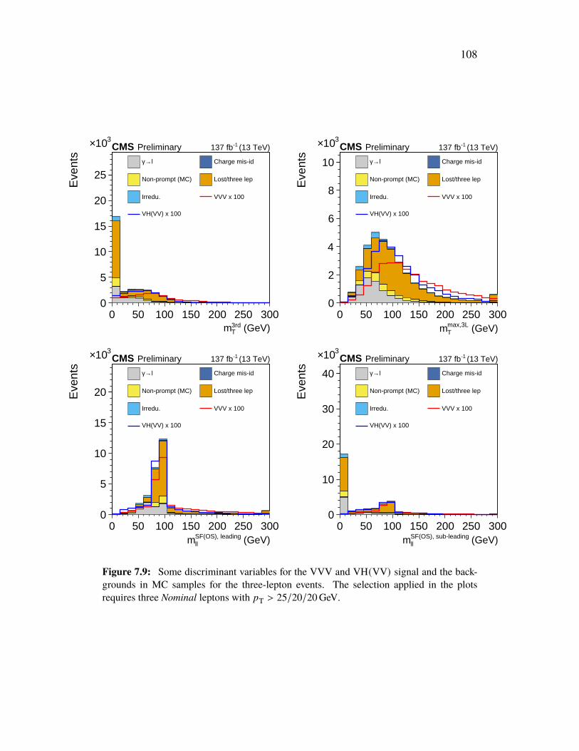
108

0 50 100 150 200 250 300 (GeV)3rd

Tm

0

5

10

15

20

25

310×

Eve

nts

Preliminary CMS (13 TeV)-1137 fb



Irredu. VVV x 100

VH(VV) x 100

0 50 100 150 200 250 300 (GeV)max,3L

Tm

0

2

4

6

8

10

310×

Eve

nts




Irredu. VVV x 100

VH(VV) x 100

0 50 100 150 200 250 300 (GeV)SF(OS), leading

llm

0

5

10

15

20

310×

Eve

nts




Irredu. VVV x 100

VH(VV) x 100

0 50 100 150 200 250 300 (GeV)SF(OS), sub-leading

llm

0

10

20

30

40

310×

Eve

nts




Irredu. VVV x 100

VH(VV) x 100

Figure 7.9: Some discriminant variables for the VVV and VH(VV) signal and the back-grounds in MC samples for the three-lepton events. The selection applied in the plotsrequires three Nominal leptons with ?T > 25/20/20GeV.

109

0 50 100 150 200 250 300 (GeV)3l

Tp

0

2

4

6

8

10

310×

Eve

nts




Irredu. VVV x 100

VH(VV) x 100

0 20 40 60 80 100 120 140 (GeV)3lm

0

10

20

30

40

310×

Eve

nts




Irredu. VVV x 100

VH(VV) x 100

0 1 2 3 4 5num of b jet

0

10

20

30

40

50

310×

Eve

nts




Irredu. VVV x 100

VH(VV) x 100

0 0.5 1 1.5 2 2.5 3)miss

Tp(lll),

Tp(φ ∆

0

1000

2000

3000

4000

5000

6000

7000

Eve

nts




Irredu. VVV x 100

VH(VV) x 100

Figure 7.10: More discriminant variables for the VVV and VH(VV) signal and thebackgrounds in MC samples for the three-lepton events. The selection applied in the plotsrequires three Nominal leptons with ?T > 25/20/20GeV.

110

7.4.2 Same-sign dilepton and three-lepton selections (BDT-based)To better suppress the backgrounds while maintaining high VVV signal efficiency,we trained two sets of Boosted Decision Trees (BDTs), one targeting backgroundsfrom events with prompt leptons (such as WZ, ZZ, W±W±), and another targetingbackgrounds due to nonprompt or fake leptons (such as tt or photonsmisidentified asleptons). The two sets of BDTs are called prompt BDT and fake BDT, respectively.The event categories are kept the same as those used in the cut-based selection, andthe kinematic selections applied in the cut-based method are replaced by cuts on theprompt BDT and fake BDT in each category.

Due to different available kinematic variables in the different categories, the BDTsare trained separately in the different categories: one for SS-2j events, one for SS-1j events, and one for 3ℓ events. The list of input variables used for training thedifferent BDT’s are summarized in Table 7.9.

Table 7.9: List of input variables for SS/3ℓ BDT training.

variables prompt BDT fake BDTSS2J SS1J 3ℓ SS2J SS1J 3ℓ

?missT X X X X X X

leptons-?T X X X X X Xleptons flavor X X X X X Xjets-?T X X X X X X<ℓℓ (SS (SF) pair for SS (3ℓ)) X X X X X X

<maxT X X X X X X

<minT X X X X

?T(ℓℓ) (SS pair) X X X X<jj (closest in Δ') X X<JJ (leading jets) X X<jj (Δ' closest) X XΔ[JJ (leading jets) X XΔ'JJ (leading jets) X XΔ'jj (closest in Δ') X Xnumber of jets X X X X

<3rdT X X

<3ℓ X X

?3ℓT X X

Δq(®? 3ℓ

T , ®?missT

)X X

=SFOS X X

The XGBoost open-source library [129] is used for the BDT training. To have

111

enough training statistics from simulation, events passing very loose preselectioncriteria are used for training. In SS2J, we require two SS leptons and at least twojets, in SS1J, we require two SS leptons and one jet, and for 3ℓ, we require 3 leptonsand |<SFOS − <Z | > 20GeV. Table 7.10 summarizes the selections applied forthe trained events and the approximate MC statistics that were used in the BDTtraining for signal and backgrounds (40% of the events are used for training ineach case). The decision trees have a maximum depth of 3, and in total 400 trees(300 for SS1J training, where the statistics are low) are used and averaged for theBDT output. Some other parameters of the XGBClassifier are: booster = gbtree,learning_rate = 0.1, min_split_loss = 0, reg_lambda = 1, max_leaves = 0 (most ofthese are the default parameter choices in the XGBoost library).

The output of the BDT is the probability of the event to be a signal event (takenfrom the predict_proba function of the XGBClassifier, which is a logarithmic trans-formation of the output of the trees (: 1

1+exp(−() ), which has been constructed toprovide a value ranging from 0 to 1.

Table 7.10: Selection applied for training events and approximate simulation statistics usedfor the SS1j, SS2j, and the 3ℓ BDT training.

SS2J SS1J 3ℓ

selectiontwo SS leptons (?T > 25/25 GeV) 3 leptons (?T > 25/20/20 GeV)

<ℓℓ > 20GeV |<SFOS − <Z | > 20GeV#j ≥ 2 #j = 1

signal MC 42 × 103 32 × 103 48 × 103

prompt background MC 667 × 103 185 × 103 357 × 103

fake background MC 11 × 103 3.7 × 103 28 × 103

Figures 7.11 and 7.12 show the ROC curve (a curve of signal vs. backgroundefficiency obtained with different BDT cuts) and the BDT response of the SS1j,SS2j, and 3ℓ BDTs, respectively. Figure 7.14 shows the 2D distribution of theprompt and fake BDTs for different processes as well as different categories. Fromthis, we can see that signal events are populated in regions with both large promptBDT and large fake BDT score, while background events have either small promptBDT or small fake BDT score. A rectangular cut on the two BDT scores cantherefore be used to remove most of the backgrounds while maintaining high signalefficiency.

The ranking of input variables is given in Figure 7.13.

As mentioned above, we keep the overall classification of the twelve signal regionsas in the cut-based approach, and we replace all selections (including selections on

112

<3rdT /<max

T , ?missT , Δq

(®? 3ℓ

T , ®?missT

), Δ[JJ, <JJ (leading jets), Δ'min

ℓj , and ?3ℓT ) with

selections on the prompt and fake BDT discriminants. Tables 7.11 and Table 7.12summarize all the kinematics selections as well as the BDT cuts for the SS and 3ℓchannels in the BDT-based analysis. The selection cuts on the BDTs are optimizedin each signal region (9 regions in SS, 3 in 3ℓ) individually to optimize the expectedsignificance in each signal region. The final cuts on the prompt and fake BDTs arechosen by scanning both BDT discriminants simultaneously and choosing the cut oneach BDT discriminant for which we get the best combined expected significance.

Table 7.11: Event selections for the SS channels using the BDT method: for each category,we define three signal regions depending on the lepton flavor: e±e±, e±μ±, and μ±μ±. Thisresults in 3 × 3 = 9 signal regions for the SS channels.

Variable <jj-in <jj-out 1je±e± e±μ± μ±μ± e±e± e±μ± μ±μ± e±e± e±μ± μ±μ±

Trigger Pass the dilepton triggersSignal leptons Exactly 2 tight SS leptons with ?T > 25GeVAdditional leptons No additional very loose leptonIsolated tracks No additional isolated tracks<ℓℓ >20GeV<ℓℓ |<ℓℓ − <Z | > 20GeV if e±e±

b-tagging no b-tagged jets and soft b-tag objectsJets ≥ 2 jets ≥ 2 jets 1 jet<jj (closest Δ') 65 < <jj < 95GeV |<jj − 80GeV| ≥ 15GeV —Prompt BDT (>) 0.22 0.32 0.14 0.07 0.19 0.09 0.32 0.26 0.39fake BDT (>) 0.00 0.89 0.77 0.75 0.82 0.73 0.68 0.89 0.64

Table 7.12: Event selections for the three-lepton channels of BDT method.

Variable 0 SFOS 1 SFOS 2 SFOSTrigger Pass dilepton triggers

Signal leptons 3 Nominal leptons with charge sum = ±1e?T > 25/25/25GeV ?T > 25/20/20GeV

Additional leptons No additional very loose lepton<SFOS <SFOS > 20GeV and |<SFOS − <Z | > 20GeV<3ℓ |<3ℓ − <Z | > 10GeVSF lepton mass >20GeV — —Dielectron mass |<ee − <Z | > 20GeV — —Jets ≤ 1 jet 0 jets 0 jetsb-tagging No b-tagged jets and soft b-tag objectsPrompt BDT (>) 0.28 0.60 0.38fake BDT (>) 0.93 0.80 0.78

113

112

Figure 7.11: ROC curve corresponding to the SS/3✓ BDT cuts. Left column: prompt BDT;right column: fake BDT. Top: SS2J; middle: SS1J; bottom: 3✓.

selections on the prompt and fake BDT discriminants. Table 7.11 and tab. 7.12summarize all the kinematics selections as well as the BDT cuts for SS and 3✓channels for the BDT-based analysis. The selection on the BDTs are optimized ineach signal region (9 in SS, 3 in 3✓) individually to optimize the expected significancein each signal region. The final cuts on the prompt and fake BDTs are chosen fromscanning both BDT discriminants simultaneously and choosing the selections oneach BDT discriminant for which we get the best combined expected significance.

Figure 7.11: ROC curve corresponding to the SS/3ℓ BDT cuts. Left column: prompt BDT;right column: fake BDT. Top: SS2J; middle: SS1J; bottom: 3ℓ.

114

113

Figure 7.12: SS/3✓ BDT response for signal and backgrounds in training and testingsamples. Left column: prompt BDT; right column: fake BDT. Top: SS2J; middle: SS1J;bottom: 3✓.

Figure 7.12: SS/3ℓ BDT response for signal and backgrounds in training and testingsamples. Left column: prompt BDT; right column: fake BDT. Top: SS2J; middle: SS1J;bottom: 3ℓ.

115115

Figure 7.13: Input variable importance scorse (calculated by the number of times thefeature appears in a tree) for the SS1j, SS2j and 3✓ BDT training. Left column: promptBDT; right column: fake BDT. Top: SS2J; middle: SS1J; bottom: 3✓.

Figure 7.13: Input variable importance scores (calculated by the number of times thefeature appears in a tree) for the SS1j, SS2j, and 3ℓ BDT training. Left column: promptBDT; right column: fake BDT. Top: SS2J; middle: SS1J; bottom: 3ℓ.

116

115

Figure 7.14: 2D distribution of the prompt BDT (X-axis) and fake BDT (Y-axis). Left:signal events; middle: prompt background events; right: fake background events. Top: 3lepton category (selection: three Nominal leptons with ?T > 25/20/20 GeV); middle: SS2Jcategory (selection: two Nominal SS leptons with ?T > 25 GeV, and two jets); bottom:SS1J category (selection: two Nominal SS leptons with ?T > 25 GeV, and one jet).

Figure 7.14: 2D distribution of the prompt BDT (X-axis) and fake BDT (Y-axis). Left:signal events; middle: prompt background events; right: fake background events. Top:three-lepton category (selection: three Nominal leptons with ?T > 25/20/20GeV); middle:SS2J category (selection: twoNominal SS leptons with ?T > 25GeV, and two jets); bottom:SS1J category (selection: two Nominal SS leptons with ?T > 25GeV, and one jet).

117

7.4.3 Four-lepton selections (cut-based)As discussed in Section 7.1, events in the four-lepton final state are further catego-rized based on the flavor of the two W candidate leptons, into the eμ category andthe ee/μμ category. In both categories, ZZ events are the dominant backgrounds. Inthe eμ category, the main backgrounds are from Z(ℓℓ)Z(gg) decay (where ℓ = e/μ)and in the ee/μμ category, the main backgrounds are from Z(ℓℓ)Z(ℓℓ) decay (whereℓ = e/μ).Several kinematic selections are applied to suppress the ZZ backgrounds. In theeμ category, where the ZZ decays as Z(ℓℓ)Z(gg), the invariant mass of the eμ

pair (<eμ) for ZZ events typically peaks around 50GeV, and there are very fewevents above 100GeV. This is in contrast to the invariant mass distribution of theeμ pair (<eμ) in WWZ events, which is much wider and which has more events inthe high <eμ region. Therefore, we use <eμ as the main discriminating variable tocategorize events in the eμ category. In addition, the <T2 variable [130] is utilizedto suppress the ZZ background process. For our case (where the invisible particlesare neutrinos), <T2 is defined as:

<T2 = min®?ν (1)T + ®?ν (2)T = ®?miss

T

[max

(< (1)T ( ®?

ν (1)T , ®?eT), <

(2)T ( ®?

ν (2)T , ®?μT)

)], (7.1)

In events where two particles are pair-produced and each of the particles decayssemi-invisibly, one cannot simply build <T. The idea behind the definition above isthat for correct transverse masses < (1,2)T , the larger of the two is still smaller than orequal to the parent mass. The minimization over all possible splittings of ?miss

T tothe transverse momenta of the unseen particles, ®?ν (1,2)T , ensures that each transversemass does not exceed the parent mass. The <T2 value tends to be small for the ZZbackground process, since the tau lepton decay products are generally collinear witheach other. Figure 7.15 shows the <eμ and <T2 distributions for both signal andbackground events in the eμ category, from which we can see that a combinationof binning using those two variables can be constructed to give a good signal tobackground ratio.

In the ee/μμ category, the ZZ background decays as Z(ℓℓ)Z(ℓℓ). Compared tothe WWZ signal, such ZZ events will have a much smaller ?miss

T , since more ofthe energy in the signal events is carried away by the neutrinos from W-decay.Therefore, ?miss

T is the main discriminating variable in the ee/μμ category. Inaddition, the transverse momentum of the four-lepton system, ?4ℓ

T , is also used asanother discriminating variable. This variable is similar to ?miss

T , but as ?4ℓT is

118

measured purely from leptons, it is therefore likely to be more precise and well-modelled, and it gives complementary information to ?miss

T . Figure 7.16 showsthe ?4ℓ

T and ?missT distributions for both signal and background events in the ee/μμ

category, and the binning of ee/μμ events is then based on those two variables.

The subdominant background in the four-lepton final states are events from ttZ

decay, where two leptons come from Z and two leptons come from the two t-quarkdecays. To suppress such backgrounds, the events are required to have zero b-taggedjets.

To remove any events stemming from low mass resonances coming from QCDprocesses with large cross sections, we require the invariant mass of any oppositecharged lepton pair to be greater than 12GeV.

Table 7.13 summarizes the event selection and binning for both the eμ and ee/μμcategories in the four-lepton final state. In total, there are four bins in the eμ categoryand three bins in the ee/μμ category.

Table 7.13: Event selections for the four-lepton channels (eμ and ee/μμ).

eμ category ee/μμ categoryTrigger Pass the dilepton triggersZ leptons ZID SFOS pair, ?T > 25/15GeVW leptons WID OS pair, ?T > 25/15GeVW leptons flavor eμ ee/μμb-tagging No b-tagged jets<

Z−tagℓℓ (Z pair) |<Z−tag

ℓℓ − <Z | < 10GeV<ℓℓ (WW pair) — |<ℓℓ − <Z | > 10GeV<OSℓℓ <OS

ℓℓ > 12GeV for any OS dilepton pairBin 1 <eμ < 40GeV —Bin 2 40 < <eμ < 60GeV —Bin 3 60 < <eμ < 100GeV —Bin 4 <eμ > 100GeV, <T2 > 25GeV —Bin A — ?miss

T > 120GeVBin B — 70 < ?miss

T < 120GeV, ?4ℓT > 70GeV

Bin C — 70 < ?missT < 120GeV, 40 < ?4ℓ

T < 70GeV

119

0

10

20

Eve

nts

Data VVV ZZ ZttStat. Uncert. Other tWZ WZ

0 50 100 150 200 250

[GeV]eµm

00.5

11.5

2

Dat

a/P

red.


eµ category

0

10

20

Eve

nts


0 20 40 60 80 100

[GeV]T2m

00.5

11.5

2

Dat

a/P

red.


regionµZ + e

Figure 7.15: Distribution of the invariant mass of the two lepton candidates from twoW decays <eμ (left), and the distribution of <T2 (right) in the four-lepton final state eμcategory.

1−10

1

10

210

310

Eve

nts


0 50 100 150 200 250 300

[GeV]T

p0

0.51

1.52

Dat

a/P

red.


ee/µµ categoty

4l

1−10

1

10

210

310

Eve

nts


0 50 100 150 200 250 300

[GeV]missT

p0

0.51

1.52

Dat

a/P

red.


ee/µµ category

Figure 7.16: Distribution of the ?T of the four-lepton system ?4ℓT (left), and the distribution

of ?missT (right) in the four-lepton final state ee/μμ category.

120

7.4.4 Four-lepton selections (BDT-based)Similarly to the selection used for the same-sign dilepton and three-lepton finalstates, a BDT-based selection is also employed for the four-lepton final states. Twosets of BDTs are trained for the four-lepton events, targeting twomajor backgrounds,ZZ and ttZ. Both the ZZ and ttZ BDTs are trained separately for the eμ and ee/μμevents. Table 7.14 lists all the input variables for the ZZ and ttZ BDT trainings. ForttZ events, the main discriminating power comes from the jet related variables, asthere are two additional b-quark jets in the ttZ decay products. The lepton variablesare used for both the ZZ BDT and ttZ BDT training. For the ZZ BDT, ?miss

T -relatedvariables are also included in the training input.

It has been shown [131] that for Z → ττ events, the angle between the neutrinos andthe e/μ from τ lepton decay is typically small, which results in a large projection of®?miss

T on the e/μ direction; while this is usually not true for the WWZ signal events.Therefore, two variables are defined for the input to the ZZ BDT in this case:

%Z = ( ®?missT + ®?ℓ1T + ®?ℓ2T ) · Z and %vis

Z = ( ®?ℓ1T + ®?ℓ2T ) · Z , (7.2)

where the two leptons ℓ1 and ℓ2 denote the twoW lepton candidates, and Z is a unitvector in the direction of the bisector of ℓ1 and ℓ2, as illustrated in Figure 7.17.

Figure 7.17: Projections of ®?missT and leptons ®?T on the Z direction.

The XGBoost open-source library [129] is used in the BDT training. ZZ, ttZ, andWWZ MC events passing the preselection in Table 7.13 (the selections performedbefore the event binning part) are used in the training. For ttZ MC events, theb-veto selection is not applied to the training events in order to increase the training

121

Table 7.14: List of input variables for the four-lepton BDT training.

variables ttZ BDT ZZ BDT<ℓℓ (WW pair) X X

?ZT X X<T2 X X

?ℓ1T (W lepton) X X

?ℓ2T (W lepton) X X

?4ℓT X X∑48 ?

8T X X

%Z X

%visZ X

?missT X

<ℓ1T (W lepton) X

<ℓ2T (W lepton) X<4ℓ XminΔ'(j, ℓ3) XminΔ'(j, ℓ4) Xleading jet ?T X

statistics. In total, about 300,000 WWZ, 18,000 ZZ, and 25,000 ttZ MC eventsare used in the training for the eμ category, and about 28,000 WWZ and 810,000ZZ MC events are used in the training for the ee/μμ category. The ZZ BDT andttZ BDTs in the eμ category have a maximum depth of 3, and 400 trees are usedand averaged to get the BDT output. For the ZZ BDT in the ee/μμ category,the maximum depth is 5 with 400 trees. Unlike the same-sign and three-leptonanalysis, the four-lepton BDT output distribution is not put through the logarithmictransformation mentioned above. Figure 7.18 shows the ttZ BDT in the eμ categoryand the ZZ BDT in the eμ and ee/μμ categories, for both the signal and backgroundsamples, split into training and testing sets.

With the two BDTs, the <eμ-<T2 (?missT -?4ℓ

T )-based event binning in the cut-basedmethod is replaced by ZZ BDT and ttZ BDT-based binning for eμ (ee/μμ) events,as the signals are enriched in the high ZZ BDT and high ttZ BDT regions. Toachieve optimal signal-to-background discrimination, a series of 2D boundaries oftheZZ BDT and the ttZ BDT have been defined for the eμ category. The boundariesof the 2D binning have been optimized to maximize sensitivity (s/b) in a way similarto creating a decision tree, and the scanning of the boundaries stops when there arenot enough MC events for optimization or the s/b does not increase significantly.

122123

Figure 7.18: Top: ZZ BDT response in four-lepton e� (left) and ee/�� (right) categories;bottom: ttZ BDT response in the four-lepton e� category. The distributions for both WWZsignal and backgrounds MC events are shown and are split into training and testing sets.

significantly. Figure 7.19 shows the 2D distributions of the ZZ and ttZ BDTs forsignal and background events in the e� category, with the optimized binning in the2D plane. For the ee/�� category, only the ZZ BDT is used, and therefore theevents are binned based on the ZZ BDT score.

Table 7.15 summarizes the event binning based on the BDTs, together with all otherselections for the BDT method.

Figure 7.18: Top: ZZ BDT response in the four-lepton eμ (left) and ee/μμ (right)categories; bottom: ttZ BDT response in the four-lepton eμ category. The distributions forboth the WWZ signal and background MC events are shown and are split into training andtesting sets.

Figure 7.19 shows the 2D distributions of the ZZ and ttZ BDTs for signal andbackground events in the eμ category, with the optimized binning in the 2D plane.For the ee/μμ category, only the ZZ BDT is used, and therefore the events arebinned based on the ZZ BDT score.

Table 7.15 summarizes the event binning based on the BDTs, together with all otherselections for the BDT method.

123

Figure 7.19: The ZZ BDT and ttZ BDT 2D distributions of the signal and backgroundevents in the four-lepton eμ category, together with the visualized event binning in the 2Dplane.

Table 7.15: Event selections for the four-lepton channels (eμ and ee/μμ) of the BDTmethod.

eμ category ee/μμ categoryTrigger Pass dilepton triggersZ leptons ZID SFOS pair, ?T > 25/15GeVW leptons WID OS pair, ?T > 25/15GeVW leptons flavor eμ ee/μμb-tagging No b-tagged jets<

Z−tagℓℓ (Z pair) |<Z−tag

ℓℓ − <Z | < 10GeV<ℓℓ (WW pair) — |<ℓℓ − <Z | > 10GeV<OSℓℓ <OS

ℓℓ > 12GeV for any OS dilepton pairBin 1 ZZ BDT < −0.908 —Bin 2 ZZ BDT > −0.908, ttZ BDT < 0.015 —Bin 3 −0.908 < ZZ BDT < 0.733, ttZ BDT > 0.015 —Bin 4 ZZ BDT > −0.733, 0.015 < ttZ BDT < 3.523 —Bin 5 ZZ BDT > −0.733, ttZ BDT > 3.523 —Bin A — 0 < ZZ BDT < 3Bin B — ZZ BDT > 3

124

7.4.5 Five- and six-lepton selectionsEvents in the five- and six-lepton final state categories are relatively clean and havemuch lower statistics, so a minimal set of selections has been applied, and only acut-based selection has been explored for these categories.

For five-lepton events, we require five leptons with four passing the Z and onepassing the W lepton ID criteria, as discussed in Section 7.3, and we require the?T of the leptons from Z decay to be greater than 25/10GeV and the ?T of eachcharged lepton from W decay to be greater than 10GeV. In addition, events withb-tagged jets are vetoed in order to reject backgrounds from t quarks (such as tt ,ttV). To remove nonprompt lepton backgrounds from diboson or tt processes,we also require the transverse mass of the lepton from W decay to be greater than50GeV if the lepton is an electron.

For six-lepton events, we require six Veto-ID leptons as discussed in Section 7.3,with the leading two leptons having ?T greater than 25GeV, and the rest of the fourleptons having ?T greater than 10GeV. In addition, to suppress backgrounds suchas ttH events, we require the scalar sum of the ?T of all leptons to be greater than250GeV.

Figure 7.20 shows the distributions of the two discriminating variables used in thefive and six lepton event selection: <T of theW candidate charged lepton and scalarsum of lepton ?T.

125

126

0 100 200 300 (GeV)e

Tm

0

0.1

0.2

0.3

0.4

0.5

0.6

Even

ts


Other Higgs tWZWZ Ztt ZZWWZ WZZ ZZZ

0 100 200 300 (GeV)µ

Tm

0

0.1

0.2

0.3

0.4

0.5

0.6

Even

ts


Other WZ Higgs

tWZ ZZ Ztt

WWZ WZZ ZZZ

0 200 400 600 800 (GeV)l

TpΣ

0

0.02

0.04

0.06

0.08

Even

ts


WZ Other tWZ

ZZ Ztt Higgs

WWZ WZZ ZZZ

Figure 7.20: Top-left (top-right): distribution of the transverse mass of the W candidateelectron (muon) for five lepton events; bottom: distribution of scalar sum of the ?T of allleptons for six lepton events.

Figure 7.20: Top-left (top-right): distribution of the transverse mass of the W candidateelectron (muon) for five-lepton events; bottom: distribution of scalar sum of the ?T of allleptons for six-lepton events.

126

7.5 Background estimation7.5.1 Backgrounds in same-sign and three-lepton final statesFor same-sign and three-lepton events, we expect the following types of back-grounds:

• Lost/Three-lepton background: This background is the most important inthe SS channel, and stems mostly from WZ production where one leptonfrom the Z boson decay is not reconstructed (“lost”) due to acceptance, ID,or isolation criteria. For the 3ℓ channel, this background comes through anoff-shell Z boson.

• Nonprompt leptonbackground: This background contains one (two) promptleptons and one nonprompt lepton in the SS (3ℓ) channel. The nonprompt lep-ton most often originates from a semileptonic heavy flavor (HF) hadron decay,but can also originate from light flavor (LF) hadron decays, light flavor hadronmisidentification (c±), Dalitz decay of neutral mesons, and conversions fromnon-isolated photons1.

• Irreducible background: This background is very signal-like. In the SSchannel, W±W± can be produced via vector boson scattering (VBS), doubleparton scattering (DPS), or in tt+W associated production. In the 3ℓ channel,WWW can be produced via tt+W.

• Charge misidentification background: This background mostly stems fromevents with a Z boson decay, where one lepton’s charge is misidentified.This type of background is completely negligible for muons and very tiny forelectrons.

• Other backgrounds: Other backgrounds, such as events with misidentifiedprompt photons, where the photons are misidentified as electrons or convertinto an electron-positron pair, are expected to be small.

For the two major backgrounds, the nonprompt lepton background and the lost-lepton/three-lepton background, we have developed data-driven estimation methodsto predict their contributions to the signal regions. For all other backgrounds, westill validate and normalize the backgrounds in dedicated control regions in data,

1Note that prompt isolated photons, e.g. isolated photons identified as an electron or converting toa pair of electrons, are identified using generator information and are part of the “Other backgrounds.”

127

although the splitting of their yields into the signal regions is then performed withsimulation.

The most sensitive regions are the same-sign e±μ±, μ±μ± channels, and the three-lepton 0 SFOS and 1 SFOS channels. In these regions, the background uncertaintiesare dominated by the nonprompt lepton background or by the lost-lepton/three-lepton background (mostly WZ). Another important background is the irreduciblebackground. All other backgrounds are small. In this section, all backgroundestimation techniques are discussed. The final result, including all backgroundpredictions is given in Section 7.7.

To predict the lost-lepton background in the SS channels, we define theWZ controlregion (CR) as follows: In addition to the two signal leptons, we require the presenceof a third lepton. The third lepton needs to pass only the Nominal-3ℓ selectioncriteria. The third lepton has to form a SFOS lepton pair with one of the othertwo leptons and the pair has to be compatible with being from a Z boson, namely|<SFOS −<Z | < 20GeV. For theWZ CR of the cut-based method, we apply all theother selections on the SS channel as in Table 7.7, except that we drop the selection65 < <jj < 95GeV or apply its inverse (|<jj − 80GeV| > 15GeV) for the ≥ 2jet categories, in order to have sufficient statistics in the control region. The <jj

variable will, to first order, have the same distribution in both the signal and controlregions, as both jets should stem from intial state radiation (ISR) for the dominantWZ process, or from the same matrix element process (as in the subdominant ttZbackground). We evaluate the experimental uncertainties on the <jj modeling byvarying the jet energy corrections and validating it in data. For the WZ CR of theBDT-based method, we do not merge the <jj-in and <jj-out categories as the BDTcuts on those two categories are different.

To predict the three-lepton background (from WZ or ZZ) in the three lepton chan-nels, we define theWZ control region (CR) as follows. we keep all the selections forthe 3ℓ channel as in Table 7.8 (Table 7.12) for the cut-based (BDT-based) method.However, we invert the requirement on the <SFOS variable, i.e. instead of vetoingevents where the two leptons are compatible with originating from a Z boson decay,we select such events. By doing so, we have no direct data-driven background es-timation for the 0 SFOS channel. However, since a statistically meaningful controlregion is hard to find (if available at all), we rely on the predictions from the 1 and2 SFOS channels to extrapolate the 3-lepton background to the 0 SFOS channel.

The control regions mentioned above are mutually exclusive to each other (due to

128

the requirement on the number of jets), and also orthogonal to the signal regions.However, two SS signal regions with ≥ 2 jets (for the two <jj bins) have an identicalcontrol region for the cut-basedmethod. Thus, all nuisances between the two regionsfor this background are 100% correlated.

Using those control regions, the estimation of the lost-lepton background (in thesame-sign channels) or the three-lepton background (in the three-lepton channels)is straightforward:

#pred(lost-lepton/3-lepton) = {#CR(data) − #sim.CR (other bkg)} × TFCR→SR, (7.3)

where the transfer factor is obtained from simulation (using WZ MC), but is vali-dated in the control and signal region sidebands.

Figure 7.21 shows the data and MC event yields in theWZ control regions for boththe cut-based and BDT-based methods, and good data/MC agreement is observed.The statistical uncertainty of the events in theCR, aswell as the statistical uncertaintyand systematic uncertainty when measuring the transfer factor, are considered andpropagated to the lost-lepton/3ℓ background prediction.

ee,MjjInem,MjjIn

mm,MjjInee,MjjOut

em,MjjOut

mm,MjjOut

ee1j em1jmm1j

1SFOS2SFOS

0

500

1000

1500

2000

Eve

nts


Data l→γ

Charge mis-id Non-prompt

Lost/three lep Irredu.

VVV

ee,MjjInem,MjjIn

mm,MjjInee,MjjOut

em,MjjOut

mm,MjjOut

ee1j em1jmm1j

1SFOS2SFOS

00.5

11.5

2

Dat

a/M

C ee,MjjInem,MjjIn

mm,MjjInee,MjjOut

em,MjjOut

mm,MjjOut

ee1j em1jmm1j

1SFOS2SFOS

0

50

100

150

200

250

300

Eve

nts


Data l→γ

Charge mis-id Non-prompt


VVV

ee,MjjInem,MjjIn

mm,MjjInee,MjjOut

em,MjjOut

mm,MjjOut

ee1j em1jmm1j

1SFOS2SFOS

00.5

11.5

2

Dat

a/M

C

Figure 7.21: Data and simulation yields in the lost-lepton/3ℓ (WZ) control regions for thecut-based (left) and BDT-based (right) methods.

129

Backgrounds from misidentified leptons are estimated using the tight-to-loose ratiomethod, also known as the fake rate method. The method estimates the number ofmisidentified leptons in the signal region by extrapolating across the lepton isolationvariable. In addition to the Nominal lepton IDs used to define the signal regions(see Tables 7.3 and 7.4), loose lepton IDs are defined by loosening the isolationcriteria of the tight IDs. For both electrons and muons, the relative isolation cuts inthe Loose ID is set to be < 0.4.

The ratio between the number ofmisidentified leptons passing aNominal ID (or to becalled as tight ID) to a Loose ID is called the fake rate. The fake rate is measured byusing separate control data samples collected with a set of appropriately prescaledsingle lepton triggers. The region where the fake rate is measured is called themeasurement region. Taking the same-sign dilepton final state channels as anexample, the fake rate is then used to predict the number of misidentified leptonevents in two tight lepton events (i.e. the signal regions) by extrapolating froma data sample of lepton events with one tight lepton plus one loose-but-not-tightlepton. The latter region where the fake rate is applied to estimate the number ofmisidentified lepton events in the signal region is called the application region. Forthe 3ℓ channels, the application region events contain two tight leptons and oneloose-but-not-tight lepton.

Several effects have to be considered when doing this estimation: when measuringthe fake rate, we need to make sure that the kinematics of the mother parton issimilar in the measurement region and the application region. Residual effects (e.g.due to different flavor composition for the mother parton) are assessed in a closuretest.

All other backgrounds, including events with mismeasured lepton charge or promptphotons misidentified as electrons, and irreducible backgrounds such as W±W± andttW± events, are directly determined from simulation, and validated and correctedby events in the corresponding validation regions.

The ttW± background estimation is validated from a control samplewith at least oneb-tagged jet. We find that the best selection for a reasonably pure sample is to selectevents with two SS leptons, at least four jets, and at least one b-tagged jet. As eventswith ≥2 b-tagged jets have a stronger ability to constrain this background, we use thedistribution of the b-tagged jet multiplicity, #b , to normalize this background. Toachieve the best accuracy for the ttW± estimation, we decided to fit the distributionof tt+X and other backgrounds to the data distribution of #b . Note that since there

130

is a non-negligible contribution of ttH (→WW), we fit the ttW± +ttH processestogether. In the fits, we test if the fit results are stable among the three years, andthe test reveals nothing suspicious. Figure 7.22 shows the #b distribution for bothdata and MC in the validation for the ttW± background. A fit to this distribution(floating tt+X vs. other backgrounds) reveals that the ttW± background estimatedfrom simulation needs to be scaled up by a factor of 1.67 ± 0.18.

0 1 2 3 4 50

200

400

600

800

Eve

nts


Data l→γ

Charge mis-id Non-prompt (MC)

Lost/three lep Other Irredu.

±W±W Wtt

VVV

0 0.5 1 1.5 2 2.5 3 3.5 4 4.5 5 | ttV VRbn

00.5

11.5

2

Dat

a/M

C

Figure 7.22: Distribution of #b for both data and MC in the ttW± validation region.

The fake photon background has multiple sources, however a common feature isa low lepton momentum and/or close proximity to a real lepton. This is why theselection criteria such as the constraints on ?miss

T ,<T, or<ℓℓ reduce this backgrounddramatically. For the 3ℓ signal regions, one frequent background source is Z → ℓℓ

with a radiated photon. Therefore, a large fraction of the background is rejectedby |<3ℓ − <Z | > 10GeV for events with 3ℓ. To validate the background due toprompt photons misidentified as electrons for the cut-based method, we define thevalidation region as follows: select 3ℓ events, apply the signal region selection, butinvert the selection criteria on ?3ℓ

T and <maxT /<3rd

T and drop the <3ℓ criteria, and for

131

the BDT-based method, invert the fake and prompt BDT cuts (requiring the eventsto have prompt BDT < 0.28 and fake BDT < 0.78, motivated by the prompt andfake BDT distributions). After such selections, we find that the photon fakes arevery pure in the region near <3ℓ ≈ <Z , as shown in Figure 7.23 for the cut-basedmethod and Figure 7.24 for the BDT-based method.

A fit to the <3ℓ distribution with photon fake backgrounds against all other back-grounds floating is then performed, and the fit reveals that for the cut-based method,the photon fake backgrounds need to be scaled from MC yields by a factor of0.991± 0.072 for 2016, 0.508± 0.025 for 2017 and 0.551± 0.022 for 2018; and forthe BDT-based method, the photon fake backgrounds need to be scaled from MCyields by a factor of 0.550±0.082, 0.259±0.030, and 0.281±0.026 for 2016, 2017,and 2018 respectively.

The validation region to validate the W±W± background modelling in MC is con-structed by inverting either the <JJ or the Δ[JJ criteria (or both). In Figure 7.25, weshow the <JJ variable for Δ[JJ > 2.5 (left) and Δ[JJ for <JJ > 500GeV. The modelagrees very well with the data in this region, therefore we do not apply any correctionto theWW+jj background. The statistical precision of these two validation regionsis about 10%, and we add this as a systematic uncertainty for this process.

To validate the charge mismeasurement background modeling in MC, we lookat the dielectron invariant mass near the Z mass peak for events having two SSelectrons (and no other selection criteria). As can be appreciated from Figure 7.26,the Z mass peak from charge mismeasurements is well reproduced in simulation,within a precision of about 20%. We therefore take the backgrounds due to chargemismeasurements from simulation without any correction with a 20% systematicuncertainty.

7.5.2 Backgrounds in four-lepton final statesThere are six main background components to the four-lepton final state. They areZZ, ttZ, tWZ,WZ, Higgs, and other rare SM processes.

The largest background contribution to the four-lepton final state comes from theZZ background process, which has a cross section that is three orders of magnitudelarger than that of the signal process. The contribution from this background processin the signal region is estimated from the control region (CR) events that identifytwo Z boson candidates.

The second largest background contribution comes from the ttZ background pro-

132

0 20 40 60 80 100 120 1400

500

1000

1500

2000

2500

Eve

nts


Data l→γ



VVV

0 20 40 60 80 100 120 140 (GeV)3lm

00.5

11.5

2

Dat

a/M

C 0 20 40 60 80 100 120 1400

1000

2000

3000

4000

Eve

nts


Data l→γ



VVV

0 20 40 60 80 100 120 140 (GeV)3lm

00.5

11.5

2

Dat

a/M

C

0 20 40 60 80 100 120 1400

1000

2000

3000

4000

5000

6000

Eve

nts


Data l→γ



VVV

0 20 40 60 80 100 120 140 (GeV)3lm

00.5

11.5

2

Dat

a/M

C

Figure 7.23: Distribution of <3ℓ after inverting both the <maxT /<3rd

T and ?3ℓT criteria for

2016 (top-left), 2017 (top-right), and 2018 (bottom) for the cut-based method.

cess, which has a cross section that is approximately 50 times larger than that ofthe signal process. However, the ttZ background process events are reduced byrequiring that there are no b-tagged jets in each event. The contribution from thettZ background process in the signal region is estimated from the CR events thatrequire the additional presence of b-tagged jets.

The main usage of the CRs is to determine the normalization scale factors to be used

133

0 20 40 60 80 100 120 1400

1000

2000

3000

4000

5000

6000

Eve

nts


Data l→γ



VVV

0 20 40 60 80 100 120 140 (GeV)3lm

00.5

11.5

2

Dat

a/M

C 0 20 40 60 80 100 120 1400

2000

4000

6000

8000

Eve

nts


Data l→γ



VVV

0 20 40 60 80 100 120 140 (GeV)3lm

00.5

11.5

2

Dat

a/M

C

0 20 40 60 80 100 120 1400

2

4

6

8

10

310×

Eve

nts


Data l→γ



VVV

0 20 40 60 80 100 120 140 (GeV)3lm

00.5

11.5

2

Dat

a/M

C

Figure 7.24: Distribution of <3ℓ after inverting both the <maxT /<3rd

T and ?3ℓT criteria for

2016 (top-left), 2017 (top-right), and 2018 (bottom) for the BDT-based method.

in estimating each background’s contribution to one of the signal regions . For eachbackground process and its corresponding control region CRi, the normalizationscale factor NSFBi,CRi

is defined as the ratio of the observed to the expected yieldsin the control region CRi, for the background process Bi being estimated. Theobserved yields in each CRi, #

dataBi,CRi

for each of the background processes underconsideration, are corrected by subtracting the events in this CRi due to all thebackground processes Bj, j ≠ i, other than the one under consideration, where some

134

0 100 200 300 400 500 600 7000

20

40

60

80

Eve

nts


Data l→γ



±W±W Wtt

VVV

0 100 200 300 400 500 600 700 (GeV)JJm

00.5

11.5

2

Dat

a/M

C 0 1 2 3 4 50

10

20

30

40

Eve

nts


Data l→γ



±W±W Wtt

VVV

0 0.5 1 1.5 2 2.5 3 3.5 4 4.5 5 (GeV)

JJη∆

00.5

11.5

2

Dat

a/M

C

Figure 7.25: <JJ for Δ[JJ > 2.5 (left) and Δ[JJ for <JJ > 500GeV (right) as validation ofthe W±W± VBS background.

of the events selected for the other control regions CRj, j ≠ i can, according to thesimulation, end up in the current control region CRi. Once these subtractions aredone, the estimate of the contribution of the background Bi to the signal region canthen be written as

#predSR,Bi

= #MCSR,Bi· #data

Bi,CRi/#MC

Bi,CRi︸︷︷︸Normalization scale factor(NSFBi

)

= #dataBi,CRi

· #MCSR,Bi/#MC

Bi,CRi︸︷︷︸Transfer factor(TFBi ,CRi→SR,Bi

)(7.4)

where #dataBi,CRi

and #MCBi,CRi

are the observed and simulation-estimated yields in thecontrol region CRi due to background process Bi and #

MCSR,Bi

is the yield in thesignal region due background process Bi estimated from the simulation. Once thenormalization scale factor for background process Bi (NSFBi

) is determined, thesimulated events of the background process being estimated are scaled according tothe value of NSFBi

.

Effectively, what is being done is to extrapolate from the observed number of

135

60 70 80 90 100 110 1200

200

400

600

800

1000

1200

1400

1600

Eve

nts


Data l→γ



VVV

60 70 80 90 100 110 120 (GeV)eem

00.5

11.5

2

Dat

a/M

C

Figure 7.26: Distribution of the dielectron invariant mass <ee for events with an SSdielectron pair.

events in the data CR, #dataBi,CRi

, by the transfer factor (TFBi,CRi→SR,Bi) obtained from

the simulation. The various sources of systematic uncertainty associated with theTFBi,CRi→SR,Bi

often cancel out if the effect of the systematic uncertainty is correlatedbetween the signal and the control region. This can lead to a smaller total uncertaintyon important background processes in the signal regions.

In practice, what is being done for the analysis is obtaining the central backgroundestimate yields by taking the #MC

SR,Biand multiplying it by NSFBi

. For the uncertaintyon those estimated yields, the statistical uncertainties from the #data

Bi,CRi’s are taken in

addition to the uncertainties from the TF’s.

The ZZ control region selections are nearly identical to the ones used for the signalregion in the ee/μμ category, except they do not require the ?miss

T cut and have aninverted requirement on the <ℓℓ (i.e. |<ℓℓ − <Z | < 10 GeV). This region willbe referred to as the ZZ control region (ZZ CR). The purity of events from the

136

ZZ background process in the ZZ CR is ≈100%. The normalization scale factorNSF// obtained from the entire Run 2 dataset is 0.99 ± 0.02, which shows a goodconsistency between the simulation and the data. There are slight variations fromyear to year, but the NSF// ’s in each year’s dataset are consistent with unity. TheNSF// factors are applied separately for each year’s simulated dataset.

To ensure proper background estimation, it is important to check that the extrap-olation transfer factors TFZZ CR→eμ SR and TFZZ CR→ee/μμ SR obtained from thesimulation are modeled well. There are several variables to be checked for anypotential mismodeling problem. From the ZZ CR to the signal regions in the eμ

category, there are several key quantities that are being extrapolated, such as thelepton flavors,<ℓℓ, and<T2 distributions. Since the lepton efficiencies are generallywell modeled, within a few percent per lepton, and they are corrected using the scalefactors, the mismodeling in the extrapolation across lepton flavors is expected to benegligible. The modeling of a few key kinematic distributions has been checked, asillustrated in Figure 7.27.

For the BDT-based method, a similar approach is taken to estimate the ZZ back-grounds. In the BDT eμ channel, the ZZ CR is defined in the same way as the ZZCR used in the cut-based method, and a corresponding BDT distribution in the ZZCR is used to assess the individual transfer factor per BDT bin, where each bin inthe control region acts as a control region for each bin in the signal region. In theBDT ee/μμ channel, the ZZ control region is defined from the ee/μμ events with aBDT score of less than 0 (which were discarded and not used in the ee/μμ signalregion).

To estimate the ttZ background contribution in the signal regions, events with morethan one b-tagged jet and theW lepton candidates with eμ flavor are selected. Thisregion will be referred to as the b-tag CR. In this region, the purity of the ttZ

background process is ≈80%. The expected yields of the ttZ background processfrom simulation generally agree well with the observed data. The normalizationscale factor for the ttZ background process NSFttZ has been found to be 1.08±0.17for the Run 2 dataset. For the final estimate, the NSFttZ factors computed for eachyear are applied to their respective data sets. The modeling of key discriminatingvariables is tested in the b-tag CR. Figure 7.28 shows the <T2, <ℓℓ, ?

missT , and ?4ℓ

T

distributions.

Finally, there are the WZ, tWZ, and Higgs background processes. These back-ground processes are subdominant in the signal region (they contribute less than

137

0 50 100 150

[GeV]T2m

0

100

200

300

400

500

600

Eve

nts


Data Higgs tWZOther WZ ZttZZ WWZ WZZZZZ

0 20 40 60 80 100 120 140 160 180 [GeV]T2m

00.5

11.5

2

Dat

a/M

C 0 100 200 300

MET [GeV]

0

100

200

300

400Eve

nts



0 50 100 150 200 250 300MET [GeV]

00.5

11.5

2

Dat

a/M

C

0 100 200 300 [GeV]

T,4lp

0

100

200

300

400

500

Eve

nts



0 50 100 150 200 250 300 [GeV]

T,4lp

00.5

11.5

2

Dat

a/M

C

Figure 7.27: Distributions of<T2 (top-left), ?missT (top-right), and ?4ℓ

T (bottom) for the dataand MC in the four-lepton ZZ CR.

10% to the total background). There are also other rare SM background processesthat haveminor contributions. These background processes are extrapolated directlyfrom the simulation, using appropriate validation regions to check the modeling.For the WZ backgrounds, this process enters the four lepton signal region with amisidentified lepton. To check such modelling in the MC, we checked the leptonisolation variable distribution of events with three Nominal ID leptons and onelepton that passes the Veto ID except for the lepton isolation criteria. No cleardeviation between data and MC is observed, so the distributions generally exhibitgood modeling. We take the statistical uncertainty of those events (about 28%) asthe uncertainty in theWZ background estimation.

To validate the tWZ backgrounds, we define a validation region similar to the ttZ

138

136

from simulation generally agree well with the observed data. The normalizationscale factor for the ttZ background process NSFttZ has been found to be 1.08±0.17for the Run 2 data set. For the final estimate, the NSFttZ factors computed for eachyear are applied to their respective data sets. The modeling of key discriminatingvariables is tested in the b-tag CR. Figure 7.28 shows the <T2, <✓✓, ?

missT and ?4✓

T

distributions.

0 50 100 150 [GeV]T2m

0

5

10

15

20

25Ev

ents


Data WZ OtherHiggs ZZ tWZ

Ztt WWZ WZZZZZ

0 20 40 60 80 100 120 140 160 180 [GeV]T2m

00.5

11.5

2

Dat

a/M

C 0 50 100 150 200 250 [GeV]llm

0

5

10

15

20

Even

ts



Ztt WWZ WZZZZZ

0 50 100 150 200 250 [GeV]llm

00.5

11.5

2

Dat

a/M

C

0 100 200 300MET [GeV]

0

5

10

15

20

25

Even

ts



Ztt WWZ WZZZZZ

0 50 100 150 200 250 300MET [GeV]

00.5

11.5

2

Dat

a/M

C 0 100 200 300 [GeV]

T,4lp

02468

10121416

Even

tsPreliminary CMS (13 TeV)-1137 fb


Ztt WWZ WZZZZZ

0 50 100 150 200 250 300 [GeV]

T,4lp

00.5

11.5

2

Dat

a/M

C

Figure 7.28: Distributions of<T2 (top left), <✓✓ (top right), ?missT (bottom left), ?4✓

T (bottomright) for the data and MC in the four-lepton b-tag CR.

Finally, there are the WZ, tWZ, and Higgs background processes. These back-ground processes are subdominant in the signal region (they contribute less than10% to the total background). There are also other rare SM background processesthat have minor contributions. These background processes are extrapolated directlyfrom the simulation, using appropriate validation regions to check the modeling. ForWZ backgrounds, this process enters the four lepton signal region with a misidenti-

Figure 7.28: Distributions of<T2 (top left),<ℓℓ (top right), ?missT (bottom left), ?4ℓ

T (bottomright) for the data and MC in the four-lepton b-tag CR.

CR, except that only one b-tagged jet is required in this case. By doing so, thetWZ and ttZ events in this region are similar to each other, but the overall tWZ

contribution among the backgrounds is small. When we perform a fit to the numberof jets (# 9 ) distribution in the tWZ CR, the fit reveals that the tWZ componentneeds to be scaled up by a factor of 1.47, with a very large uncertainty on thisnumber (1.47 ± 2.13) due to the smallness of the tWZ contribution to this control

139

region. As a result, we decide to take the MC yield of tWZ directly as the tWZ

background estimation, and assign a 47% uncertainty to this estimate.

7.5.3 Backgrounds in five- and six-lepton final statesFor the five lepton final states, the largest source of background is the ZZ processwhere the additional lepton is often a misidentified jet or is indicative of the presenceof a B-hadron that decayed semileptonically through a cascade to a soft lepton. Toascertain the origin of this lepton, the generator objects that were matched to thislepton within a cone of Δ' < 0.3 were studied. The lepton was found to beassociated with either:

• a heavy flavor B or D hadron decay, which was the dominant source of thefake lepton, or

• π0s decaying to photons with one or more photons converting to lepton pairs;or Dalitz decay of π0 → 4+4−W. This effect is seen to be subdominant.

To further understand this background, we constructed a control region to study theagreement of the data with simulations where one lepton is known to be fake. Inthis context, a fakeable lepton is one that fails the isolation requirements placed onthe leptons in the signal region. Due to the lack of events in a five-lepton selectionwhere one of the leptons is fake (achieved by requiring a non-isolated additionallepton), the analysis was performed using a four-lepton selection. The central ideabehind the construction of this control region is that the exploration of the WZ

process (where the W and Z bosons decay leptonically) in a four lepton selectionis topologically similar to the ZZ process (where both Z bosons decay leptonically)in a five-lepton selection. In order to minimize contamination from Drell-Yan (DY)and ZZ events, we use only the three muon and one electron selection to isolate theWZ signal. The other lepton flavor combinations were explored. Since these eventselections do not produce pure WZ events, they were dropped from consideration.The additional selection requirements applied are the following:

• a b-tagged jet veto

• requiring a Z-boson candidate, where the Z-boson candidate is constructedby combining any two pairs of muons

• the ?T of the electron >15GeV, to reduce the DY background

140

The distributions of ?missT are shown in Figure 7.29. The data and the total simulated

background distributions agree within the statistical uncertainties. As a result,we use the statistical uncertainty in this control region (about 30%) for the ZZbackground uncertainty in the five-lepton final states.

0 100 200 300 (GeV)miss

Tp

0

2

4

6

8

10

12

14E

vent

s


Data Higgs tWZ

Ztt ZZ WZ

Other VVV VH(VV)

0 50 100 150 200 250 300 (GeV)miss

Tp

00.5

11.5

2

Dat

a/M

C

Figure 7.29: The distribution of ?missT in the WZ control region, where one of the leptons

is required to be non-isolated.

In the six-lepton channel, the background processes are determined entirely fromsimulations. The total background contribution in this channel is less than oneevent, and this does not require additional control regions to be constructed in orderto study these minuscule contributions.

7.6 Systematic uncertaintiesThe dominant systematic uncertainties come from the uncertainties related to thebackground estimates, discussed in Section 7.5. The remaining uncertainties are re-lated to instrumental effects and theoretical uncertainties, such as the electron/muonID efficiency scale factor ("eleSF"/"muoSF" in the tables below), the trigger effi-ciency scale factor (triggerSF), the jet energy scale (JES), the luminosity uncertainty,the b tagging scale factor, the statistics of simulated events (Sim. statistics), the nor-malization and factorization scale &2, the PDF uncertainties, and the UB variations.

Tables 7.16 and 7.17 summarize the typical sizes of the systematics on each back-

141

ground process in the same-sign and three-lepton final states from various sources,for the cut-based and BDT-based approach. In general, the contribution from ir-reducible, charge flips, and W → nonprompt ℓ backgrounds are very small, so therelatively large uncertainties in those backgrounds do not matter in the final result.

The typical total uncertainty on the lost/3ℓ (nonprompt ℓ ) backgrounds are about20% (30%) in the most sensitive categories, but they are still small enough such thatthe result is still statistics dominated. Tables 7.18 and 7.19 summarize the typicalsizes of the systematics on each background process in the four-lepton final statesfromvarious sources for the cut-based approach. Tables 7.20 and 7.21 summarize thetypical sizes of the systematics on each background process in the four-lepton finalstates from various sources for the BDT approach. For the dominant backgroundprocesses, ZZ (ttZ) backgrounds, the total systematic uncertainty is about 5-10%(10-20%). Tables 7.22 and 7.23 summarize the systematics on the backgroundprocess for the five and six lepton final states. The dominant systematics in five-and six-lepton final states are the systematics on the ZZ backgrounds where theadditional lepton is a misidentified lepton, for which the uncertainty is estimated tobe 30% in the five-lepton category and 60% in the six-lepton category.

In most final states, the dominant uncertainty on the signal prediction comes fromthe statistics in MC due to the limited number of simulated events that pass theevent selection. This uncertainty is about 5-30% for the same-sign/3ℓ, 3-5% for thefour-lepton, and 0.4-11% for the five- and six-lepton final states.

For the signal predictions, we apply normalization and factorization scale, PDF,and UB variations to obtain the uncertainties on the signal acceptance. Variousexperimental uncertainties (similar to the sources for background uncertainties) arealso evaluated. Table 7.24 summarizes the systematics on the signal process for thecut-based analysis, and Table 7.25 summarizes the systematics on the signal processfor the BDT analysis. Table 7.26 summarizes the systematics on the signal processfor the cut-based approach. Table 7.27 summarizes the systematics on the signalprocess for the BDT approach. Table 7.28 summarizes the systematics on the signalprocess for the five- and six-lepton final states.

All the sources of systematic uncertainties mentioned above are treated carefullyfor correlation among data taken from different years and among different finalstates. For example, all systematics are fully correlated among different years exceptluminosity uncertainty, as most of those systematics are related to measurementsthat are done the same way in different years. All systematics are considered fully

142

correlated among different final states, except the simulation statistics uncertaintyand background estimation method related uncertainties.

Table 7.16: Summary of the typical background systematic uncertainties (in percent) forthe SS and 3ℓ final states, for the cut-based analysis.

Uncertainty Lost/three ℓ Nonprompt ℓ Irreducible Charge flips W → nonprompt ℓSim. statistics 3–15 — 6–26 22–90 30–100Bkg. contam. 0–2 3–20 — — —eleSF 0–2.4 — — — —muoSF 0–1.2 — — — —triggerSF 3 — — — —pileup 0–1 — — — —&2 0–2 — — — —PDF 0–1 — — — —JEC 0–3 — — — —WZ/ttZ fraction <1 — — — —data validation 1–10 — 10–14 20 8–15Fake rate e — 21–44 (SS), 2–3 (3ℓ) — — —Fake rate μ — 3–15 — — —Closure test e — 19–29 (SS), 2–4 (3ℓ) — — —Closure test μ — 7–30 — — —

Table 7.17: Summary of the typical background systematic uncertainties (in percent) forthe SS and 3ℓ final states, for the BDT based analysis.

Uncertainty Lost/three ℓ Nonprompt ℓ Irreducible Charge flips W → nonprompt ℓSim. statistics 5–25 — 5–15 27–100 35–340Bkg. contam. 1–35 10–70 — — —pileup 0–2 — — — —&2 1–13 — — — —PDF 0–2 — — — —JES 0–60 — — — —WZ/ttZ fraction <1 — — — —data validation 1–10 — 10–21 20 7–19Fake rate e — 16–65 (SS), 2–10 (3ℓ) — — —Fake rate μ — 1–20 — — —Closure test e — 20–30 (SS), 2–7 (3ℓ) — — —Closure test μ — 3–30 — — —

143

Table 7.18: Summary of the typical systematic uncertainties (in percent) on the backgroundestimates in the eμ SR (denoted by − if not applicable or if the size is smaller than 0.1%).

Systematics ttZ ZZ tWZ Higgs WZ Otherb-tag CR data statistics 12 - - - - -ZZ CR data statistics - 2.4 - - - -b tagging scale factor (HF) - - 4.9 3.4 - 0.5b tagging scale factor (LF) - - 0.9 0.3 - 0.2JES - - 2.3 12 - 0.1Pileup reweighting - - 1.4 4.3 - 0.5UB - - 0.0 0.1 - 2.0PDF - - 0.4 0.6 - 1.1&2 - - - 15 - 2.9Luminosity 2.5 2.5 2.5 2.5 2.5 2.5Systematics on TFb-tag CR→eμ 10 - - - - -Systematics on TFZZ CR→eμ - 4.5 - - - -Systematics onWZ validation - - - - 30 -triggerSF 3.2 3.2 3.2 3.2 3.2 3.2eleSF - - 3.3 0.1 - 2.1muoSF - - 3.2 4.3 - 3.8Sim. statistics - - 6.2 82 28 43

144

Table 7.19: Summary of the typical systematic uncertainties (in percent) on the backgroundestimates in the ee/μμ SR (denoted by − if not applicable or if the size is smaller than 0.1%).

Systematics ttZ ZZ tWZ Higgs WZ Otherb-tag CR data statistics 12 - - - - -ZZ CR data statistics - 2.4 - - - -b tagging scale factor (HF) - - 4.1 1.5 - 0.0b tagging scale factor (LF) - - 0.8 0.9 - 1.8JES - - 3.9 6.9 - 1.9Pileup reweighting - - 1.3 2.6 - 41UB - - 0.1 0.5 - 0.3PDF - - - 0.9 - 0.1&2 - - 0.2 2.7 - 8.8Luminosity 2.5 2.5 2.5 2.5 2.5 2.5Systematics on TFb-tag CR→eμ 10 - - - - -Systematics on TFZZ CR→eμ - 8.9 - - - -Systematics onWZ validation - - - - 30 -triggerSF 3.2 3.2 3.2 3.2 3.2 3.2eleSF - - 3.2 4.3 - 3.5muoSF - - 3.3 3.0 - 0.7Sim. statistics - - 7.6 26 50 81

145

Table 7.20: Summary of the typical systematic uncertainties (in percent) on the backgroundestimates in the eμ SR in the BDT approach (denoted with − if not applicable or if the sizeis smaller than 0.1%).

Systematics ttZ ZZ tWZ Higgs WZ Otherb-tag CR data statistics 12 - - - - -ZZ CR data statistics - 2.4 - - - -b tagging scale factor (HF) - - 4.9 1.5 - 0.5b tagging scale factor (LF) - - 0.8 0.7 - 0.2JES - - 2.5 0.7 - 0.3Pileup reweighting - - 1.6 4.5 - 1.1UB - - - 0.2 - 1.7PDF - - 0.2 0.9 - 0.9&2 - - - 15 - 1.9Luminosity 2.5 2.5 2.5 2.5 2.5 2.5Systematics on TFb-tag CR→eμ 29 - - - - -Systematics on TFZZ CR→eμ - 2.2 - - - -Systematics onWZ validation - - - - 30 -triggerSF 3.2 3.2 3.2 3.2 3.2 3.2eleSF - - 3.2 2.9 - 2.8muoSF - - 3.2 3.9 - 3.3Sim. statistics - - 5.7 30 22 36

146

Table 7.21: Summary of the typical systematic uncertainties (in percent) on the backgroundestimates in the ee/μμ SR for the BDT approach (denoted by − if not applicable or if thesize is smaller than 0.1%).

Systematics ttZ ZZ tWZ Higgs WZ Otherb-tag CR data statistics 12 - - - - -ZZ CR data statistics - 2.4 - - - -b tagging scale factor (HF) - - 4.2 0.9 - 0.4b tagging scale factor (LF) - - 0.8 1.1 - 1.8JES - - 2.4 1.3 - 0.6Pileup reweighting - - 1.5 3.6 - 41UB - - - 0.5 - 0.4PDF - - 0.3 0.3 - 0.1&2 - - 0.0 0.1 - 8.3Luminosity 2.5 2.5 2.5 2.5 2.5 2.5Systematics on TFb-tag CR→eμ 11 - - - - -Systematics on TFZZ CR→eμ - 3.0 - - - -Systematics onWZ validation - - - - 30 -triggerSF 3.2 3.2 3.2 3.2 3.2 3.2eleSF - - 3.0 4.6 - 3.7muoSF - - 3.4 3.3 - 0.8Sim. statistics - - 6.4 16 19 73

Table 7.22: Summary of the typical systematic uncertainties (in percent) on the backgroundestimates in the five-lepton signal region.

Systematics ttZ ZZ tWZ Otherb tagging scale factor (HF) 4.7 0.00 0.00 0.00b tagging scale factor (LF) 0.01 0.00 0.00 0.00WZ CR uncertainty - 30 - -Luminosity 2.5 2.5 2.5 2.5JES 0.01 0.02 0.00 26.0Pileup reweighting 0.01 0.1 0.00 0.02PDF 1.0 1.0 0.05 0.06&2 0.02 0.01 0.01 0.01UB 0.02 0.01 0.01 0.01eleSF and muoSF 3.6 4.1 5.3 7.4triggerSF 2.0 2.0 2.0 2.0Sim. statistics 22 5.0 34 60

147

Table 7.23: Summary of the typical systematic uncertainties (in percent) on the backgroundestimates in the six-lepton signal region.

Systematics ttZ ZZ ttHb tagging scale factor (HF) 3.13 0.02 0.06b tagging scale factor (LF) 4.16 0.05 0.00WZ CR uncertainty - 60 -Luminosity 2.5 2.5 2.5Pileup reweighting 17 0.01 6.2PDF 7.6 0.05 5.3&2 0.02 0.01 15UB 60 0.01 0.01eleSF and muoSF 18 7.5 6.4triggerSF 2.0 2.0 2.0Sim. statistics 100 28 26

Table 7.24: Summary of the typical signal systematic uncertainties (in percent) for the SSand 3ℓ final states, for the cut-based analysis.

Uncertainty Typical rangeSim. statistics 4–19eleSF 0–5muoSF 0–2triggerSF 1–3pileup 0–2&2 2–14PDF 2–7UB 1JEC 1–5b-tagging HF 0–2b-tagging LF 1–2Luminosity 2.5

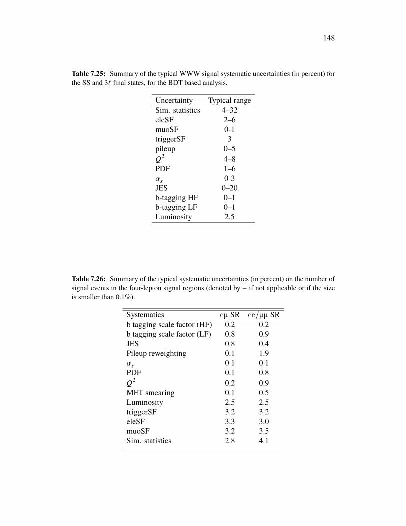
148

Table 7.25: Summary of the typical WWW signal systematic uncertainties (in percent) forthe SS and 3ℓ final states, for the BDT based analysis.

Uncertainty Typical rangeSim. statistics 4–32eleSF 2–6muoSF 0-1triggerSF 3pileup 0–5&2 4–8PDF 1–6UB 0-3JES 0–20b-tagging HF 0–1b-tagging LF 0–1Luminosity 2.5

Table 7.26: Summary of the typical systematic uncertainties (in percent) on the number ofsignal events in the four-lepton signal regions (denoted by − if not applicable or if the sizeis smaller than 0.1%).

Systematics eμ SR ee/μμ SRb tagging scale factor (HF) 0.2 0.2b tagging scale factor (LF) 0.8 0.9JES 0.8 0.4Pileup reweighting 0.1 1.9UB 0.1 0.1PDF 0.1 0.8&2 0.2 0.9MET smearing 0.1 0.5Luminosity 2.5 2.5triggerSF 3.2 3.2eleSF 3.3 3.0muoSF 3.2 3.5Sim. statistics 2.8 4.1

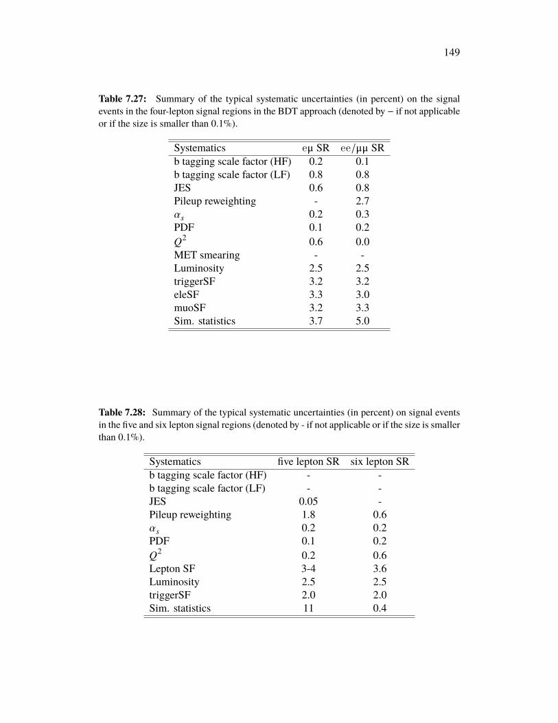
149

Table 7.27: Summary of the typical systematic uncertainties (in percent) on the signalevents in the four-lepton signal regions in the BDT approach (denoted by − if not applicableor if the size is smaller than 0.1%).

Systematics eμ SR ee/μμ SRb tagging scale factor (HF) 0.2 0.1b tagging scale factor (LF) 0.8 0.8JES 0.6 0.8Pileup reweighting - 2.7UB 0.2 0.3PDF 0.1 0.2&2 0.6 0.0MET smearing - -Luminosity 2.5 2.5triggerSF 3.2 3.2eleSF 3.3 3.0muoSF 3.2 3.3Sim. statistics 3.7 5.0

Table 7.28: Summary of the typical systematic uncertainties (in percent) on signal eventsin the five and six lepton signal regions (denoted by - if not applicable or if the size is smallerthan 0.1%).

Systematics five lepton SR six lepton SRb tagging scale factor (HF) - -b tagging scale factor (LF) - -JES 0.05 -Pileup reweighting 1.8 0.6UB 0.2 0.2PDF 0.1 0.2&2 0.2 0.6Lepton SF 3-4 3.6Luminosity 2.5 2.5triggerSF 2.0 2.0Sim. statistics 11 0.4

150

7.7 ResultsThe observed data, together with the signal and background predictions (pre-fit),are shown in Figure 7.30, for both the cut-based and BDT-based methods. Thecorresponding tabulated results are found in Tables 7.29, 7.31, 7.30, and 7.32. Ingeneral, the observed number of events (#obs) agrees well with the sum of the signaland background predictions (#pred) in all channels. The pull, defined as #obs−#pred√

f2obs+f2

pred

,

is less than 1f in most channels.

Several different fitting strategies are employed to interpret the observed data rel-ative to the expected signal and backgrounds. First of all, we have eight differ-ent VVV signals in total: WWW-onshell, WH(WW), WWZ-onshell, ZH(WW),WZZ-onshell, WH(ZZ), ZZZ-onshell, and ZH(ZZ), and each of them may have adifferent signal strength (`, defined as the ratio of the measured production crosssection times branching fraction to the corresponding SM prediction). Differenttreatments of these eight signal strengths are applied during the fit, depending onthe interpretation goals, in several scenarios:

1. A common signal strength is used for all eight signals, `VVV. This scenario isused mainly for the establishment of the first observation of VVV productionregardless of how the three bosons are produced and what combinations ofW and Z they are.

2. A common signal strength is used for all VVV-onshell signals, `VVV−onshell,and all the VH(VV) processes are treated as backgrounds (i.e. their signalstrengths are fixed to 1.0 and they are only allowed to fluctuate within thesystematic uncertainties, by ±1f). This is to measure the VVV-onshellcross section, with the assumption of the VH(VV) process being produced aspredicted by the SM.

3. In total, four different signal strengths are used: `WWW (for WWW-onshelland WH(WW) signals), `WWZ (for WWZ-onshell and ZH(WW) signals),`WZZ (for WZZ-onshell and WH(ZZ) signals), `ZZZ (for ZZZ-onshell andZH(ZZ) signals). In this case, we are measuring the production cross sectionsfor eachVVV process at the same time, where we do not distinguish theVVV-onshell and VH(VV) processes.

4. Same as 3, but treating all theVH(VV) processes as backgrounds. In this case,we are measuring the production cross section for each of the VVV-onshell

151

processes at the same time.

The most straightforward fitting scenario with all eight signal strengths floatingsimultaneously is not among the above scenarios, and this is because the result fromcurrent selection does not have enough distinguishing power between VVV-onshelland VH(VV) signals. However, in the later part of this section, we will show aresult (not optimal) from a fit with all the eight signal strengths floating and presentthe 2D likelihood of the VVV-onshell and VH(VV) signals.

Figure 7.31 and 7.32 show the postfit signal and background yields in each signal re-gion for both the cut-based and the BDT-based methods, using the 3rd fitting strategyabove. The corresponding tabulated results can be found in Tables 7.33, 7.35, 7.34,and 7.36. The result of the fits for the four signal strengths `WWW, `WWZ, `WZZ and`ZZZ are shown in Figure 7.31. As shown, the best fit values for `WWW are `WWZ

are close to 1.0, within the uncertainties. While the central value of `WZZ is largerthan 1 and the value `ZZZ is at 0.0, due to an excess (deficit) of observed events inthe five (six)-lepton final states; the statistics in each of these channels is very smalland the results are consistent with the SM predictions within the uncertainties.

Using the four different fitting strategies mentioned above, we measure the crosssections for the individual VVV signal channels and for the combined VVV signal,for the two cases where the VH(VV) process is taken as part of the signal, and aspart of the background. Figure 7.33 shows the measured cross sections in these twocases, for both the cut-based and BDT-based methods, and in the correspondingtabulated form which is shown in Table 7.37.

We can see that all the measured cross sections agree with the SM predictions,and the uncertainties are mostly statistically dominated. The center values of thecross sections from the BDT-based method agree with the results from the cut-basedmethod within the uncertainties, and the total uncertainty on the VVV cross sectionis 25-26% (23-25%) for the cut-based (BDT-based) method.

The statistical significances ! for the different triboson processes are also computedusing the asymptotic approximation [132]:

! =

{−2 ln_(0) ˆ ≥ 0 ,0 ˆ < 0 ,

(7.5)

where _(0) is the profile likelihood ratio for ` = 0, and ˆ is the best fit value of `.

152

The observed (expected) significance for the combined VVV production is 5.9(5.7)f, and the significances for the individual triboson production processes arefound in Table 7.38.

It is worth noting that in the above fitting strategies, the VH(VV) signal strengthis either fixed to 1.0 (when VH(VV) is treated as background) or the same asthe VVV-onshell signal strength (when VH(VV) is treated as part of the signal).However, the assumptions about VH(VV) in both cases are not necessarily valid,as the VH(VV) process has not been experimentally established yet. In similaranalyses where VH(VV) is the main target process [133, 134], the VVV-onshellprocess is treated as the background and its signal strength is thus fixed to 1.0. A 2Dfit of the two signal strengths is needed to distinguish theVVV-onshell andVH(VV)processes. Figure 7.34 shows such a fit for the WWW, WWZ, and combined VVVsignals, from which one can see that in most cases the observed VVV-onshell signalis smaller than the SM prediction and the VH(VV) signal is larger than SM, butthe deviations are mostly within twice the uncertainty in each case. The likelihoodmaps in Figure 7.34 are also diagonal. Therefore, it is very hard to distinguish thetwo signal processes, since the event selections in this search are designed such thatthe VVV-onshell and VH(VV) signals are similarly distributed in different signalregions. A dedicated event selection is needed to identify VVV-onshell enrichedand VH(VV) enriched signal regions in order to perform a better 2D fit of the twosignals, and this is discussed in Section 7.9.

153

153

020406080

100120140160180200

Even

ts Same-charge/3 lepton 4/5/6 leptonPreliminary CMS (13 TeV)-1137 fb

2468

101214

0 2 4 6 8 10 12 14 16 18 20 220123

L [s

d]

0 1 2 3 4 5 6 7 8 9 10 11 12 13 14 15 16 17 18 19 20 21 22

1−

01

Pulls

[sd]

ee µe µµ ee µe µµ ee µe µµ 2 1 0 A B C 1 2 3 4

1 jet outjjm injjm # SFOS Z + ll µZ + e

Same-charge dilepton 3 lepton 4 lepton

5 lepton6 lepton

Data and prediction stat. uncertainty±Data

systematics±Background

Triboson signalsWWW WWZWZZ ZZZ

Bkg. in same-charge / 3 lep.Lost / three leptonsCharge misassignmentIrreducibleNonprompt leptons

lepton→ γ

Backgrounds in 4/5/6 lep.ZZ tWZ Others

Ztt WZ

0

0

20

40

60

80

100

Even

ts Same-charge/3 lepton 4/5/6 lepton

Bin scaleddow

n by 3x


5

10

15

20

25

30

35

0 2 4 6 8 10 12 14 16 18 20 220123

L [s

d]

0 1 2 3 4 5 6 7 8 9 10 11 12 13 14 15 16 17 18 19 20 21 22

1−

01

Pulls

[sd]

ee µe µµ ee µe µµ ee µe µµ 2 1 0 A B 1 2 3 4 5

1 jet outjjm injjm # SFOS Z + llBDT bins BDT binsµZ + e


5 lepton6 lepton



Triboson signalsWWW WWZWZZ ZZZ


lepton→ γ


Ztt WZ

0

Figure 7.30: The observed events, background, and signal predictions (pre-fit) in all signalregions. The VVV signal is stacked on top of the total background and is based on the SMtheoretical cross section. The yields of the top (bottom) plot are based on the cut-based(BDT-based) method. The middle panel shows the expected signal significance of eachsignal region, which is calculated with both the VVV and VH(VV) processes treated assignals from a single bin data. The bottom panel shows the pulls in each signal region( #obs�#predq

f2obs+f2

pred

).

Figure 7.30: The observed events, background, and signal predictions (pre-fit) in all signalregions. The VVV signal is stacked on top of the total background and is based on the SMtheoretical cross section. The yields of the top (bottom) plot are based on the cut-based(BDT-based) method. The middle panel shows the expected signal significance of eachsignal region, which is calculated with both the VVV and VH(VV) processes treated assignals from a single bin data. The bottom panel shows the pulls in each signal region( #obs−#pred√

f2obs+f2

pred

).

154

Table7.29

:Th

enu

mbero

fexp

ectedsig

nala

ndbackgrou

ndevents,

estim

ated

byusingthebackgrou

ndestim

ationmetho

ds(pre-fit)discussedin

Section7.5,

forthe

SS/3ℓfin

alsta

tesc

orrespon

ding

to13

7fb−

1forthe

cut-b

ased

analysis.

Thelasttworowss

howthepu

llandexpected

signific

ance

ineach

bin(eachsig

nific

ance

isob

tained

from

asin

glebindata).

Sign

alSS

<jj-in

SS<

jj-ou

tSS

1j3ℓ

region

e±e±

e±μ±

μ± μ±

e±e±

e±μ±

μ± μ±

e±e±

e±μ±

μ± μ±

0SFO

S1S

FOS

2SFO

Slost/

3ℓ1.9±

0.5

11.4±2

.38.7±

1.0

9.3±

2.4

48.7±7

.343

.8±4

.48.2±

1.2

42.0±4

.634

.6±2

.74.6±

0.9

15.1±1

.658

.6±2

.7Irredu

cible

2.2±

0.5

11.8±3

.18.7±

1.7

9.9±

1.4

42.0±5

.442

.1±5

.12.6±

0.6

19.9±7

.713

.1±2

.22.4±

0.8

2.1±

1.2

2.5±

0.8

Nonprom

pt1.4±

1.1

6.0±

2.6

7.5±

2.3

2.5±

1.8

12.9±7

.712

.1±4

.01.8±

4.3

2.6±

1.5

3.1±

1.0

3.2±

0.8

5.8±

1.6

6.2±

1.6

Charge

flips

<0.

11.1±

1.0

<0.

12.7±

3.4

1.0±

0.4

<0.

15.0±

4.0

0.2±

0.1

<0.

1<

0.1

1.1±

0.9

0.7±

0.2

W→

nonpromptℓ

1.5±

0.6

2.2±

0.8

<0.

19.5±

4.5

23.4±7

.42.2±

0.8

3.6±

1.2

17.5±5

.414

.4±7

.6<

0.1

0.6±

0.8

0.2±

0.2

Backgrou

ndsum

7.0±

1.4

32.4±4

.824

.9±3

.033

.9±6

.512

8±13

100±

721

.2±6

.282

.1±1

0.6

65.2±8

.410

.2±1

.524

.7±2

.868

.1±3

.2WWW

onshell

1.2±

0.3

3.9±

0.7

4.4±

0.6

1.1±

0.3

4.8±

0.7

5.0±

0.6

0.6±

0.2

2.2±

0.4

2.1±

0.4

7.1±

0.9

4.7±

0.7

3.0±

0.5

WH→

WWW

0.3±

0.3

1.9±

1.4

0.7±

0.3

0.4±

0.4

1.6±

0.6

1.9±

0.7

0.9±

0.4

4.9±

2.0

3.7±

1.3

3.3±

1.5

3.1±

1.0

1.4±

0.6

WWW

total

1.5±

0.4

5.8±

1.5

5.1±

0.7

1.6±

0.4

6.5±

0.9

6.8±

0.9

1.6±

0.5

7.1±

2.1

5.8±

1.4

10.4±1

.87.8±

1.3

4.5±

0.8

WWZon

shell

<0.

10.3±

0.1

0.2±

0.1

<0.

1<

0.1

0.1±

0.0

<0.

1<

0.1

<0.

10.3±

0.2

0.2±

0.2

0.2±

0.2

ZH→

WWZ

<0.

1<

0.1

<0.

1<

0.1

<0.

10.4±

0.3

<0.

1<

0.1

0.5±

0.4

0.2±

0.1

<0.

1<

0.1

WWZtotal

<0.

10.3±

0.1

0.2±

0.1

<0.

1<

0.1

0.5±

0.3

<0.

1<

0.1

0.5±

0.4

0.5±

0.2

0.2±

0.2

0.2±

0.2

WZZ

onshell

<0.

1<

0.1

<0.

1<

0.1

<0.

1<

0.1

<0.

1<

0.1

<0.

1<

0.1

<0.

1<

0.1

WH→

WZZ

<0.

1<

0.1

<0.

1<

0.1

<0.

1<

0.1

<0.

1<

0.1

<0.

1<

0.1

<0.

1<

0.1

WZZ

total

<0.

1<

0.1

<0.

1<

0.1

<0.

1<

0.1

<0.

1<

0.1

<0.

1<

0.1

<0.

1<

0.1

ZZZon

shell

<0.

1<

0.1

<0.

1<

0.1

<0.

1<

0.1

<0.

1<

0.1

<0.

1<

0.1

<0.

1<

0.1

ZH→

ZZZ

<0.

1<

0.1

<0.

1<

0.1

<0.

1<

0.1

<0.

1<

0.1

<0.

1<

0.1

<0.

1<

0.1

ZZZtotal

<0.

1<

0.1

<0.

1<

0.1

<0.

1<

0.1

<0.

1<

0.1

<0.

1<

0.1

<0.

1<

0.1

VVVon

shell

1.2±

0.3

4.2±

0.7

4.6±

0.6

1.1±

0.3

4.8±

0.7

5.1±

0.6

0.6±

0.2

2.2±

0.4

2.1±

0.4

7.4±

0.9

4.9±

0.8

3.2±

0.5

VH→

VVV

0.3±

0.3

1.9±

1.4

0.7±

0.3

0.4±

0.4

1.6±

0.6

2.2±

0.8

0.9±

0.4

4.9±

2.0

4.2±

1.4

3.4±

1.5

3.1±

1.0

1.4±

0.6

VVVtotal

1.5±

0.4

6.1±

1.5

5.3±

0.7

1.6±

0.4

6.5±

0.9

7.3±

1.0

1.6±

0.5

7.1±

2.1

6.3±

1.4

10.9±1

.88.0±

1.3

4.7±

0.8

Total

8.5±

1.5

38.5±5

.030

.2±3

.135

.5±6

.513

4±14

107±

722

.8±6

.289

.2±1

0.8

71.5±8

.521

.1±2

.332

.7±3

.172

.8±3

.3Observed

546

2031

112

118

2910

169

2032

69pu

ll-0.77

0.38

-0.64

-0.06

-0.25

-0.32

0.50

0.23

-0.06

-0.06

-0.04

-0.10

!(exp

ected)

0.54

0.84

0.87

0.20

0.38

0.58

0.29

0.51

0.53

2.66

1.35

0.53

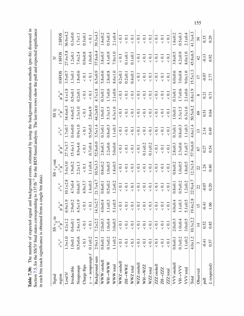
155Ta

ble7.30

:Th

enu

mbero

fexp

ectedsig

nala

ndbackgrou

ndevents,

estim

ated

byusingthebackgrou

ndestim

ationmetho

ds(pre-fit)discussedin

Section7.5,forthe

SS/3ℓfin

alsta

tesc

orrespon

ding

to13

7fb−

1forthe

BDT-basedanalysis.

Thelasttworowsshowthep

ulland

expected

signific

ance

ineach

bin(eachsig

nific

ance

isob

tained

from

asin

glebindata).

Signal

SS<

jj-in

SS<

jj-out

SS1j

3ℓregion

e±e±

e±μ±

μ± μ±

e±e±

e±μ±

μ± μ±

e±e±

e±μ±

μ± μ±

0SFO

S1S

FOS

2SFO

SLo

st/3ℓ

1.3±

1.0

4.2±

1.2

6.9±

1.9

10.1±2

.85.4±

3.0

27.7±3

.71.7±

0.7

34.4±6

.34.1±

1.8

3.5±

0.7

27.4±5

.836.9±4

.2Irreducible

1.0±

0.1

0.6±

0.1

2.9±

0.2

4.7±

0.4

1.9±

0.2

15.4±1

.10.4±

0.0

4.6±

0.2

0.5±

0.1

1.3±

0.1

1.2±

0.1

0.3±

0.0

Nonprom

pt0.5±

0.6

2.4±

1.8

4.5±

1.9

0.6±

0.7

2.2±

1.3

8.9±

4.6

0.9±

1.0

2.3±

1.0

0.2±

0.1

1.8±

0.6

7.4±

2.4

1.7±

1.1

Charge

flips

<0.

1<

0.1

<0.

14.9±

3.7

<0.

1<

0.1

<0.

1<

0.1

<0.

1<

0.1

0.9±

0.8

0.3±

0.1

W→

nonpromptℓ

0.1±

0.2

<0.

1<

0.1

1.4±

0.5

1.1±

0.4

0.7±

0.4

0.5±

0.5

2.8±

4.9

<0.

1<

0.1

1.0±

0.4

<0.

1Ba

ckground

sum

2.9±

1.1

7.2±

2.2

14.3±2

.721.7±4

.710.5±3

.352.8±6

.03.5±

1.4

44.2±8

.04.7±

1.8

6.5±

0.9

37.8±6

.439.3±4

.3WWW

onshell

0.8±

0.1

2.0±

0.3

4.0±

0.4

0.8±

0.1

0.8±

0.2

2.8±

0.3

0.3±

0.1

1.0±

0.1

0.3±

0.1

5.8±

0.6

3.8±

0.5

1.6±

0.2

WH→

WWW

0.3±

0.2

1.0±

0.4

1.1±

0.3

0.5±

0.2

1.0±

0.5

2.2±

0.6

0.8±

0.3

5.3±

1.5

1.7±

0.6

2.8±

0.8

4.1±

0.9

0.5±

0.3

WWW

total

1.1±

0.2

3.0±

0.5

5.1±

0.5

1.2±

0.2

1.8±

0.5

5.0±

0.6

1.1±

0.3

6.3±

1.6

2.1±

0.6

8.6±

1.0

7.9±

1.0

2.1±

0.4

WWZonshell

<0.

1<

0.1

<0.

1<

0.1

<0.

1<

0.1

<0.

1<

0.1

<0.

10.2±

0.1

<0.

1<

0.1

ZH→

WWZ

<0.

1<

0.1

<0.

1<

0.1

<0.

1<

0.1

<0.

1<

0.1

<0.

10.2±

0.1

0.1±

0.1

<0.

1WWZtotal

<0.

1<

0.1

<0.

1<

0.1

<0.

1<

0.1

<0.

1<

0.1

<0.

10.4±

0.1

0.1±

0.1

<0.

1WZZ

onshell

<0.

1<

0.1

<0.

1<

0.1

<0.

1<

0.1

<0.

1<

0.1

<0.

1<

0.1

<0.

1<

0.1

WH→

WZZ

<0.

1<

0.1

<0.

1<

0.1

<0.

10.1±

0.2

<0.

1<

0.1

<0.

1<

0.1

<0.

1<

0.1

WZZ

total

<0.

1<

0.1

<0.

1<

0.1

<0.

10.1±

0.2

<0.

1<

0.1

<0.

1<

0.1

<0.

1<

0.1

ZZZonshell

<0.

1<

0.1

<0.

1<

0.1

<0.

1<

0.1

<0.

1<

0.1

<0.

1<

0.1

<0.

1<

0.1

ZH→

ZZZ

<0.

1<

0.1

<0.

1<

0.1

<0.

1<

0.1

<0.

1<

0.1

<0.

1<

0.1

<0.

1<

0.1

ZZZtotal

<0.

1<

0.1

<0.

1<

0.1

<0.

1<

0.1

<0.

1<

0.1

<0.

1<

0.1

<0.

1<

0.1

VVVonshell

0.8±

0.1

2.0±

0.3

4.0±

0.4

0.8±

0.1

0.8±

0.2

2.8±

0.3

0.3±

0.1

1.0±

0.1

0.3±

0.1

6.0±

0.6

3.8±

0.5

1.6±

0.2

VH→

VVV

0.3±

0.2

1.0±

0.4

1.1±

0.3

0.5±

0.2

1.0±

0.5

2.3±

0.6

0.8±

0.3

5.3±

1.5

1.7±

0.6

3.0±

0.8

4.2±

0.9

0.5±

0.3

VVVtotal

1.1±

0.2

3.0±

0.5

5.1±

0.5

1.2±

0.2

1.8±

0.5

5.1±

0.7

1.1±

0.3

6.3±

1.6

2.1±

0.6

9.0±

1.0

8.0±

1.0

2.1±

0.4

Total

4.0±

1.2

10.3±2

.219.4±2

.822.9±4

.712.3±3

.457.9±6

.04.6±

1.4

50.5±8

.26.8±

1.9

15.5±1

.345.8±6

.541.3±4

.3Observed

314

1522

2267

1369

817

4239

pull

-0.41

0.52

-0.41

-0.07

1.24

0.27

2.14

0.51

0.21

-0.07

-0.13

0.15

!(expected)

0.57

0.85

1.06

0.20

0.40

0.54

0.49

0.64

0.71

2.77

0.92

0.29

156

Table 7.31: The number of expected signal and background events, estimated by using thebackground estimation methods (pre-fit) discussed in Section 7.5, for the 4/5/6-lepton finalstates corresponding to 137 fb−1 for the cut-based analysis. The last two rows show the pulland expected significance in each bin (each significance is obtained from a single bin data).

Signal 4ℓ eμ 4ℓ ee/μμ 5ℓ 6ℓregion bin 1 bin 2 bin 3 bin 4 bin A bin B bin CZZ 0.3±0.0 0.7±0.0 0.7±0.0 0.4±0.0 1.8±0.2 6.1±0.6 5.1±0.5 0.3±0.1 < 0.1ttZ 0.2±0.0 0.3±0.1 0.8±0.1 2.3±0.4 1.4±0.2 1.1±0.2 0.2±0.0 0.1±0.0 < 0.1tWZ 0.1±0.0 0.1±0.0 0.3±0.0 0.8±0.1 0.5±0.1 0.3±0.1 < 0.1 < 0.1 < 0.1WZ 0.2±0.1 < 0.1 0.1±0.1 0.6±0.2 < 0.1 0.2±0.1 < 0.1 < 0.1 < 0.1Higgs < 0.1 0.2±0.1 < 0.1 < 0.1 < 0.1 1.0±0.3 0.1±0.1 < 0.1 < 0.1Other < 0.1 < 0.1 0.5±0.2 0.2±0.1 < 0.1 0.5±0.5 < 0.1 < 0.1 < 0.1Background sum 0.8±0.1 1.3±0.1 2.5±0.3 4.4±0.4 3.7±0.3 9.3±0.8 5.4±0.5 0.4±0.1 0.0±0.0WWW onshell < 0.1 < 0.1 < 0.1 < 0.1 < 0.1 < 0.1 < 0.1 < 0.1 < 0.1WH→WWW < 0.1 < 0.1 < 0.1 < 0.1 < 0.1 < 0.1 < 0.1 < 0.1 < 0.1WWW total < 0.1 < 0.1 < 0.1 < 0.1 < 0.1 < 0.1 < 0.1 < 0.1 < 0.1WWZ onshell 0.5±0.1 0.6±0.1 1.2±0.1 4.5±0.3 2.4±0.3 1.3±0.1 0.7±0.1 < 0.1 < 0.1ZH→WWZ 2.6±0.2 1.2±0.1 0.3±0.0 0.1±0.0 0.9±0.1 1.0±0.1 0.6±0.0 < 0.1 < 0.1WWZ total 3.1±0.2 1.8±0.1 1.5±0.1 4.6±0.4 3.3±0.3 2.4±0.1 1.2±0.1 < 0.1 < 0.1WZZ onshell < 0.1 < 0.1 < 0.1 0.2±0.1 < 0.1 < 0.1 < 0.1 1.2±0.2 < 0.1WH→WZZ < 0.1 0.2±0.2 < 0.1 < 0.1 < 0.1 < 0.1 < 0.1 < 0.1 < 0.1WZZ total < 0.1 0.2±0.2 < 0.1 0.2±0.1 < 0.1 < 0.1 < 0.1 1.2±0.2 < 0.1ZZZ onshell < 0.1 < 0.1 < 0.1 < 0.1 < 0.1 < 0.1 < 0.1 0.4±0.1 0.3±0.0ZH→ZZZ < 0.1 < 0.1 < 0.1 < 0.1 < 0.1 0.2±0.1 < 0.1 < 0.1 < 0.1ZZZ total < 0.1 < 0.1 < 0.1 < 0.1 < 0.1 0.2±0.1 < 0.1 0.4±0.1 0.3±0.0VVV onshell 0.5±0.1 0.6±0.1 1.2±0.1 4.7±0.4 2.4±0.3 1.3±0.1 0.7±0.1 1.5±0.2 0.3±0.0VH→VVV 2.6±0.2 1.5±0.2 0.3±0.0 0.1±0.0 0.9±0.1 1.2±0.1 0.6±0.0 < 0.1 < 0.1VVV total 3.1±0.2 2.1±0.2 1.5±0.1 4.8±0.4 3.3±0.3 2.5±0.2 1.2±0.1 1.5±0.2 0.3±0.0Total 3.9±0.2 3.4±0.3 4.0±0.3 9.2±0.6 7.0±0.4 11.8±0.8 6.7±0.5 2.0±0.2 0.3±0.0Observed 7 1 5 7 6 8 7 3 0pull 0.73 -1.06 0.23 -0.38 -0.28 -0.54 0.01 0.36 -0.74! (expected) 2.47 1.46 0.95 1.96 1.56 0.82 0.53 1.70 1.04

157

Table 7.32: The number of expected signal and background events, estimated by using thebackground estimation methods (pre-fit) discussed in Section 7.5, for the 4/5/6-lepton finalstates corresponding to 137 fb−1 for the BDT-based analysis. The last two rows show thepull and expected significance in each bin.

Signal 4ℓ eμ 4ℓ ee/μμ 5ℓ 6ℓregion bin 1 bin 2 bin 3 bin 4 bin 5 bin A bin BZZ 16.0±1.1 1.6±0.1 0.6±0.1 0.6±0.1 0.2±0.0 78.5±4.7 2.9±0.3 0.3±0.1 < 0.1ttZ 0.3±0.1 0.1±0.1 2.8±0.5 1.5±0.3 < 0.1 1.6±0.2 2.4±0.4 0.1±0.0 < 0.1tWZ < 0.1 < 0.1 0.6±0.1 0.8±0.1 < 0.1 0.5±0.1 0.7±0.1 < 0.1 < 0.1WZ 0.5±0.2 0.2±0.1 0.5±0.2 0.3±0.2 0.1±0.1 1.0±0.3 0.2±0.1 < 0.1 < 0.1Higgs 1.0±0.4 < 0.1 0.3±0.1 0.1±0.1 < 0.1 2.2±0.4 0.5±0.2 < 0.1 < 0.1Other < 0.1 0.4±0.2 0.2±0.1 0.4±0.3 < 0.1 0.5±0.5 < 0.1 < 0.1 < 0.1Background sum 17.7±1.2 2.3±0.3 5.1±0.6 3.7±0.5 0.3±0.1 84.3±4.7 6.6±0.6 0.4±0.1 0.0±0.0WWW onshell < 0.1 < 0.1 < 0.1 < 0.1 < 0.1 < 0.1 < 0.1 < 0.1 < 0.1WH→WWW < 0.1 < 0.1 < 0.1 < 0.1 < 0.1 < 0.1 < 0.1 < 0.1 < 0.1WWW total < 0.1 < 0.1 < 0.1 < 0.1 < 0.1 < 0.1 < 0.1 < 0.1 < 0.1WWZ onshell 0.3±0.1 0.4±0.1 1.6±0.4 4.3±0.5 1.2±0.2 3.1±0.4 3.8±0.5 < 0.1 < 0.1ZH→WWZ 1.2±0.1 1.3±0.1 0.5±0.1 1.5±0.1 2.2±0.1 3.4±0.2 1.7±0.1 < 0.1 < 0.1WWZ total 1.6±0.1 1.7±0.1 2.2±0.4 5.8±0.5 3.4±0.2 6.5±0.5 5.5±0.5 < 0.1 < 0.1WZZ onshell < 0.1 < 0.1 < 0.1 0.2±0.1 < 0.1 0.2±0.1 < 0.1 1.2±0.2 < 0.1WH→WZZ < 0.1 < 0.1 < 0.1 0.2±0.2 < 0.1 < 0.1 < 0.1 < 0.1 < 0.1WZZ total < 0.1 < 0.1 < 0.1 0.4±0.2 < 0.1 0.2±0.1 < 0.1 1.2±0.2 < 0.1ZZZ onshell < 0.1 < 0.1 < 0.1 < 0.1 < 0.1 0.1±0.0 < 0.1 0.4±0.1 0.3±0.0ZH→ZZZ < 0.1 < 0.1 < 0.1 < 0.1 < 0.1 < 0.1 0.1±0.1 < 0.1 < 0.1ZZZ total < 0.1 < 0.1 < 0.1 < 0.1 < 0.1 0.1±0.0 0.1±0.1 0.4±0.1 0.3±0.0VVV onshell 0.3±0.1 0.4±0.1 1.6±0.4 4.5±0.5 1.2±0.2 3.5±0.4 3.8±0.5 1.5±0.2 0.3±0.0VH→VVV 1.2±0.1 1.3±0.1 0.5±0.1 1.7±0.2 2.2±0.1 3.4±0.2 1.8±0.2 < 0.1 < 0.1VVV total 1.6±0.1 1.7±0.1 2.2±0.4 6.2±0.6 3.4±0.2 6.9±0.5 5.6±0.5 1.5±0.2 0.3±0.0Total 19.3±1.2 4.0±0.3 7.3±0.7 9.8±0.7 3.7±0.3 91.2±4.7 12.2±0.8 2.0±0.2 0.3±0.0Observed 22 9 7 8 3 80 11 3 0pull 0.05 1.23 -0.08 -0.32 -0.30 -0.14 -0.22 0.36 -0.74! (expected) 0.14 1.03 0.94 2.58 2.96 0.67 1.93 1.70 1.04

158

158

020406080

100120140160180200

Even


2468

101214

0 2 4 6 8 10 12 14 16 18 20 220123

L [s

d]

0 1 2 3 4 5 6 7 8 9 10 11 12 13 14 15 16 17 18 19 20 21 22

1−

01

Pulls

[sd]




5 lepton6 lepton



Triboson signalsWWWWWZWZZZZZ

)0.34 −0.38 + = 0.82

WWWµ(

)0.36 −0.31 + = 0.90

WWZµ(

)1.09 −1.61 + = 1.85

WZZµ(

)0.00 −1.36 + = 0.0

ZZZµ(


lepton→ γ


Ztt WZ

0

0

20

40

60

80

100

Even


Bin scaleddow

n by 3xPreliminary CMS (13 TeV)-1137 fb

5

10

15

20

25

30

35

0 2 4 6 8 10 12 14 16 18 20 220123

L [s

d]

0 1 2 3 4 5 6 7 8 9 10 11 12 13 14 15 16 17 18 19 20 21 22

1−

01

Pulls

[sd]




5 lepton6 lepton




)0.40 −0.45 + = 1.15

WWWµ(

)0.31 −0.35 + = 0.86

WWZµ(

)1.25 −1.92 + = 2.24

WZZµ(

)0.00 −1.30 + = 0.0

ZZZµ(


lepton→ γ


Ztt WZ

0

Figure 7.31: The observed events, background, and signal yields after the fit in all signalregions. The fit is performed with four di�erent signal strengths floating at the same time,which corresponds to the WWW, WWZ, WZZ, and ZZZ processes, where the VVV-onshelland VH(VV) signals are not distinguished. The predicted VVV signal is stacked on top ofthe total background and is from the fit. The yields of the top (bottom) plot are based on thecut-based (BDT-based) method. The middle panel shows the expected signal significanceof each signal region, which is calculated with the total VVV+VH taken as signal from asingle bin fit. The bottom panel shows the pulls in each signal region ( #obs�#predq

f2obs+f2

pred

).

Figure 7.31: The observed events, background, and signal yields after the fit in all signalregions. The fit is performed with four different signal strengths floating at the same time,which corresponds to the WWW, WWZ, WZZ, and ZZZ processes, where the VVV-onshelland VH(VV) signals are not distinguished. The predicted VVV signal is stacked on top ofthe total background and is from the fit. The yields of the top (bottom) plot are based on thecut-based (BDT-based) method. The middle panel shows the expected signal significanceof each signal region, which is calculated with the total VVV+VH taken as signal from asingle bin fit. The bottom panel shows the pulls in each signal region ( #obs−#pred√

f2obs+f2

pred

).

159

159

020406080

100120140160180200

Even


2468

101214

0 2 4 6 8 10 12 14 16 18 20 220123

L [s

d]

0 1 2 3 4 5 6 7 8 9 10 11 12 13 14 15 16 17 18 19 20 21 22

1−

01

Pulls

[sd]




5 lepton6 lepton




)0.34 −0.38 + = 0.82

WWWµ(

)0.36 −0.31 + = 0.90

WWZµ(

)1.09 −1.61 + = 1.85

WZZµ(

)0.00 −1.36 + = 0.0

ZZZµ(


lepton→ γ


Ztt WZ

0

0

20

40

60

80

100

Even


Bin scaleddow

n by 3xPreliminary CMS (13 TeV)-1137 fb

5

10

15

20

25

30

35

0 2 4 6 8 10 12 14 16 18 20 220123

L [s

d]

0 1 2 3 4 5 6 7 8 9 10 11 12 13 14 15 16 17 18 19 20 21 22

1−

01

Pulls

[sd]




5 lepton6 lepton




)0.40 −0.45 + = 1.15

WWWµ(

)0.31 −0.35 + = 0.86

WWZµ(

)1.25 −1.92 + = 2.24

WZZµ(

)0.00 −1.30 + = 0.0

ZZZµ(


lepton→ γ


Ztt WZ

0

Figure 7.32: The observed events, background, and signal yields after the fit in all signalregions. The fit is performed with four di�erent signal strengths floating at the same time,which corresponds to the WWW, WWZ, WZZ, and ZZZ processes, where the VVV-onshelland VH(VV) signals are not distinguished. The predicted VVV signal is stacked on top ofthe total background and is from the fit. The yields of the top (bottom) plot are based on thecut-based (BDT-based) method. The middle panel shows the observed signal significanceof each signal region, which is calculated with the total VVV+VH taken as signal from asingle bin fit. The bottom panel shows the pulls in each signal region ( #obs�#predq

f2obs+f2

pred

).

Figure 7.32: The observed events, background, and signal yields after the fit in all signalregions. The fit is performed with four different signal strengths floating at the same time,which corresponds to the WWW, WWZ, WZZ, and ZZZ processes, where the VVV-onshelland VH(VV) signals are not distinguished. The predicted VVV signal is stacked on top ofthe total background and is from the fit. The yields of the top (bottom) plot are based on thecut-based (BDT-based) method. The middle panel shows the observed signal significanceof each signal region, which is calculated with the total VVV+VH taken as signal from asingle bin fit. The bottom panel shows the pulls in each signal region ( #obs−#pred√

f2obs+f2

pred

).

160

Table7

.33:

Thenu

mbero

fexp

ectedsig

naland

backgrou

ndevents,

estim

ated

byusingthebackgrou

ndestim

ationmetho

dsdiscussedin

Section7.5,

aftersim

ultaneou

slyfittin

gthefour

diffe

rent

VV

Vsig

nalstre

ngthsW

WW,W

WZ,

WZZ

,ZZZ

),forthe

SS/3ℓfin

alsta

tesc

orrespon

ding

to13

7fb−

1

forthe

cut-b

ased

analysis.

Thelasttworowss

howthepu

llandob

served

signific

ance

ineach

bin(eachsig

nific

ance

isob

tained

from

asin

glebinfit).

Sign

alSS

<jj-in

SS<

jj-ou

tSS

1j3ℓ

region

e±e±

e±μ±

μ± μ±

e±e±

e±μ±

μ± μ±

e±e±

e±μ±

μ± μ±

0SFO

S1S

FOS

2SFO

Slost/

3ℓ1.8±

0.4

10.9±2

.08.7±

1.0

8.8±

1.7

46.0±6

.244

.8±4

.48.4±

1.3

43.5±4

.434

.5±2

.74.6±

0.8

15.1±1

.558

.3±2

.4Irredu

cible

2.1±

0.4

13.0±3

.68.4±

1.4

9.8±

1.4

41.1±4

.542

.8±4

.72.6±

0.6

22.8±8

.613

.2±1

.92.5±

0.9

2.2±

1.2

2.5±

0.8

Nonprom

pt1.3±

0.9

5.8±

2.4

6.8±

2.2

2.3±

1.3

12.0±6

.111

.2±3

.81.8±

2.9

2.4±

1.3

2.8±

1.1

3.0±

0.9

5.7±

1.6

5.9±

1.6

Charge

flips

<0.

11.2±

2.0

<0.

12.6±

1.6

1.0±

0.5

<0.

16.9±

4.7

0.2±

0.1

<0.

1<

0.1

1.1±

1.3

0.7±

0.2

W→

nonpromptℓ

1.4±

0.4

2.3±

0.9

<0.

18.6±

3.1

19.2±5

.12.3±

0.9

3.8±

1.1

19.7±6

.013

.8±7

.0<

0.1

0.6±

0.7

0.2±

0.3

Backgrou

ndsum

6.6±

1.2

33.3±5

.223

.9±2

.832

.1±4

.311

9±11

101±

723

.6±5

.888

.7±1

1.4

64.4±7

.810

.1±1

.524

.7±2

.967

.6±3

.1WWW

onshell

1.0±

0.5

3.3±

1.5

3.5±

1.6

0.9±

0.5

3.9±

1.8

4.1±

1.9

0.5±

0.3

1.8±

0.8

1.7±

0.9

5.9±

2.6

3.8±

1.7

2.5±

1.2

WH→

WWW

0.2±

0.3

1.9±

1.5

0.6±

0.4

0.4±

0.4

1.3±

0.8

1.7±

1.0

0.8±

0.5

4.5±

2.7

3.3±

2.0

3.0±

1.7

2.7±

1.5

1.3±

0.8

WWW

total

1.2±

0.6

5.1±

2.2

4.1±

1.6

1.3±

0.6

5.3±

2.0

5.7±

2.1

1.4±

0.6

6.3±

2.8

5.0±

2.2

8.8±

3.1

6.6±

2.3

3.8±

1.4

WWZon

shell

<0.

10.3±

0.2

0.2±

0.1

<0.

1<

0.1

0.1±

0.1

<0.

1<

0.1

<0.

10.3±

0.2

0.2±

0.2

0.2±

0.1

ZH→

WWZ

<0.

1<

0.1

<0.

1<

0.1

<0.

10.3±

0.3

<0.

1<

0.1

0.4±

0.4

0.2±

0.1

<0.

1<

0.1

WWZtotal

<0.

10.3±

0.2

0.2±

0.1

<0.

1<

0.1

0.4±

0.3

<0.

1<

0.1

0.4±

0.4

0.4±

0.2

0.2±

0.2

0.2±

0.1

WZZ

onshell

<0.

1<

0.1

<0.

1<

0.1

<0.

1<

0.1

<0.

1<

0.1

<0.

1<

0.1

<0.

1<

0.1

WH→

WZZ

<0.

10.2±

0.6

<0.

1<

0.1

0.2±

8.5

0.2±

0.5

0.2±

1.0

<0.

1<

0.1

<0.

1<

0.1

<0.

1WZZ

total

<0.

10.2±

0.6

<0.

1<

0.1

0.2±

8.5

0.2±

0.5

0.2±

1.0

<0.

1<

0.1

<0.

1<

0.1

<0.

1ZZ

Zon

shell

<0.

1<

0.1

<0.

1<

0.1

<0.

1<

0.1

<0.

1<

0.1

<0.

1<

0.1

<0.

1<

0.1

ZH→

ZZZ

<0.

1<

0.1

<0.

1<

0.1

<0.

1<

0.1

<0.

1<

0.1

<0.

1<

0.1

<0.

1<

0.1

ZZZtotal

<0.

1<

0.1

<0.

1<

0.1

<0.

1<

0.1

<0.

1<

0.1

<0.

1<

0.1

<0.

1<

0.1

VVVon

shell

1.0±

0.5

3.5±

1.5

3.7±

1.6

0.9±

0.5

3.9±

1.8

4.2±

1.9

0.5±

0.3

1.8±

0.8

1.7±

0.9

6.1±

2.6

4.0±

1.8

2.7±

1.2

VH→

VVV

0.2±

0.3

2.0±

1.6

0.6±

0.4

0.4±

0.4

1.5±

8.5

2.2±

1.1

1.0±

1.1

4.5±

2.7

3.7±

2.0

3.1±

1.7

2.7±

1.5

1.3±

0.8

VVVtotal

1.2±

0.6

5.5±

2.2

4.2±

1.6

1.3±

0.6

5.4±

8.7

6.3±

2.2

1.5±

1.2

6.3±

2.8

5.4±

2.2

9.3±

3.1

6.8±

2.3

3.9±

1.4

Total

7.8±

1.3

38.8±5

.728

.2±3

.333

.5±4

.412

4±14

107±

725

.1±5

.995

.0±1

1.8

69.8±8

.119

.3±3

.431

.4±3

.771

.5±3

.4Observed

546

2031

112

118

2910

169

2032

69pu

ll-0.66

0.36

-0.54

-0.14

-0.19

0.16

0.28

0.11

-0.02

0.05

0.03

-0.04

!(observed)

0.00

1.74

0.00

0.00

0.00

1.36

1.17

1.30

0.33

2.41

1.24

0.10

161Ta

ble7.34

:Th

enu

mbero

fexp

ectedsig

nala

ndbackgrou

ndevents,

estim

ated

byusingthebackgrou

ndestim

ationmetho

dsafterfi

tting

thefour

diffe

rent

VV

Vsig

nals(in

totalfou

rsignalstre

ngths:

WW

W,W

WZ,

WZZ

,ZZZ

)sim

ultaneou

sly,for

theSS

/3ℓfin

alsta

tesc

orrespon

ding

to13

7fb−

1 ,forthe

BDT-basedanalysis.

Thelasttworowss

howthepu

llandob

served

signific

ance

ineach

bin(eachsig

nific

ance

isob

tained

from

asin

glebinfit).

Signal

SS<

jj-in

SS<

jj-out

SS1j

3ℓregion

e±e±

e±μ±

μ± μ±

e±e±

e±μ±

μ± μ±

e±e±

e±μ±

μ± μ±

0SFO

S1S

FOS

2SFO

Slost/

3ℓ1.4±

0.9

5.5±

1.6

7.0±

1.7

10.7±2

.69.7±

3.6

31.4±3

.82.5±

1.1

41.0±6

.15.8±

1.6

3.5±

0.7

25.6±4

.236.1±3

.1Irreducible

1.0±

0.1

0.6±

0.1

2.9±

0.2

4.7±

0.4

1.9±

0.2

15.5±1

.20.4±

0.0

4.6±

0.2

0.5±

0.1

1.3±

0.1

1.2±

0.1

0.3±

0.0

Nonprom

pt0.6±

0.6

3.6±

2.4

4.2±

1.5

0.8±

1.0

2.8±

1.5

9.1±

4.5

2.5±

5.2

2.9±

1.4

0.2±

0.1

1.8±

0.5

7.5±

2.3

1.8±

1.1

Charge

flips

<0.

1<

0.1

<0.

14.5±

2.5

<0.

1<

0.1

<0.

1<

0.1

<0.

1<

0.1

0.8±

1.2

0.3±

0.1

W→

nonpromptℓ

0.1±

0.2

<0.

1<

0.1

1.4±

0.5

1.1±

0.4

0.7±

0.4

0.6±

1.2

4.8±

8.0

<0.

1<

0.1

1.0±

0.4

<0.

1Ba

ckground

sum

3.1±

1.1

9.7±

2.9

14.2±2

.322.1±3

.815.6±4

.056.8±6

.05.9±

5.4

53.4±1

0.1

6.4±

1.6

6.6±

0.9

36.2±5

.038.6±3

.3WWW

onshell

0.9±

0.4

2.3±

0.9

4.6±

1.7

0.9±

0.4

1.0±

0.6

3.3±

1.3

0.3±

0.2

1.2±

0.4

0.4±

0.2

6.7±

2.4

4.3±

1.6

1.8±

0.7

WH→

WWW

0.4±

0.3

1.3±

0.9

1.2±

0.5

0.5±

0.3

1.3±

1.3

2.7±

1.2

1.1±

0.8

6.5±

3.1

2.2±

1.1

3.4±

1.6

5.0±

2.1

0.6±

0.6

WWW

total

1.3±

0.5

3.7±

1.3

5.8±

1.7

1.5±

0.5

2.3±

1.4

6.0±

1.7

1.4±

0.8

7.7±

3.1

2.5±

1.1

10.1±2

.99.3±

2.6

2.4±

0.9

WWZonshell

<0.

1<

0.1

<0.

1<

0.1

<0.

1<

0.1

<0.

1<

0.1

<0.

10.2±

0.1

<0.

1<

0.1

ZH→

WWZ

<0.

1<

0.1

<0.

1<

0.1

<0.

1<

0.1

<0.

1<

0.1

<0.

10.1±

0.1

<0.

1<

0.1

WWZtotal

<0.

1<

0.1

<0.

1<

0.1

<0.

1<

0.1

<0.

1<

0.1

<0.

10.3±

0.1

<0.

1<

0.1

WZZ

onshell

<0.

1<

0.1

<0.

1<

0.1

<0.

1<

0.1

<0.

1<

0.1

<0.

1<

0.1

<0.

1<

0.1

WH→

WZZ

0.2±

0.3

<0.

1<

0.1

<0.

1<

0.1

0.3±

0.9

<0.

1<

0.1

<0.

1<

0.1

<0.

10.2±

0.9

WZZ

total

0.2±

0.3

<0.

1<

0.1

<0.

1<

0.1

0.3±

0.9

<0.

1<

0.1

<0.

1<

0.1

<0.

10.2±

0.9

ZZZonshell

<0.

1<

0.1

<0.

1<

0.1

<0.

1<

0.1

<0.

1<

0.1

<0.

1<

0.1

<0.

1<

0.1

ZH→

ZZZ

<0.

1<

0.1

<0.

1<

0.1

<0.

1<

0.1

<0.

1<

0.1

<0.

1<

0.1

<0.

1<

0.1

ZZZtotal

<0.

1<

0.1

<0.

1<

0.1

<0.

1<

0.1

<0.

1<

0.1

<0.

1<

0.1

<0.

1<

0.1

VVVonshell

0.9±

0.4

2.3±

0.9

4.6±

1.7

0.9±

0.4

1.0±

0.6

3.3±

1.3

0.3±

0.2

1.2±

0.4

0.4±

0.2

6.9±

2.4

4.3±

1.6

1.8±

0.7

VH→

VVV

0.5±

0.4

1.3±

0.9

1.2±

0.5

0.5±

0.3

1.3±

1.3

3.0±

1.4

1.1±

0.8

6.5±

3.1

2.2±

1.1

3.6±

1.6

5.0±

2.1

0.8±

1.1

VVVtotal

1.5±

0.6

3.7±

1.3

5.8±

1.7

1.5±

0.5

2.3±

1.4

6.3±

1.9

1.4±

0.8

7.7±

3.1

2.5±

1.1

10.4±2

.99.3±

2.6

2.6±

1.3

Total

4.5±

1.2

13.4±3

.120.0±2

.923.6±3

.817.8±4

.263.0±6

.37.4±

5.5

61.1±1

0.6

9.0±

2.0

17.0±3

.045.4±5

.641.2±3

.5Observed

314

1522

2267

1369

817

4239

pull

-0.53

0.06

-0.46

-0.12

0.35

0.11

1.005

0.18

-0.14

0.00

-0.12

-0.06

!(observed)

0.04

1.63

0.15

0.05

1.98

1.45

2.96

2.16

1.07

3.14

0.49

0.00

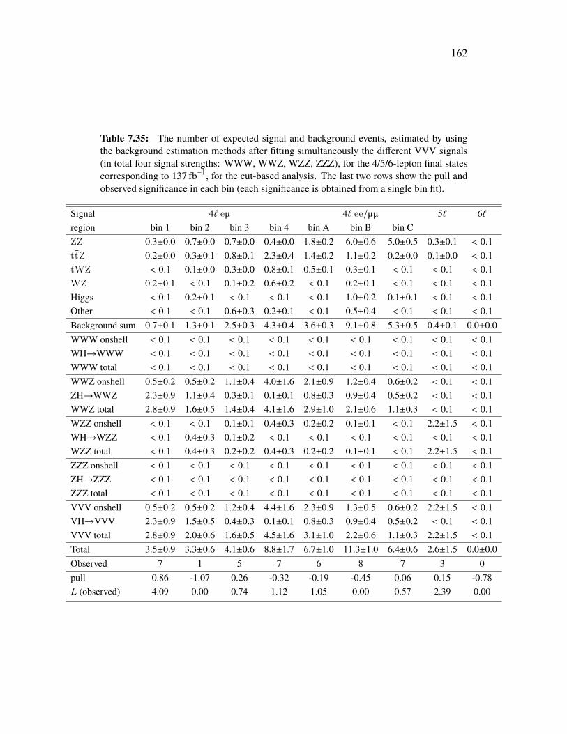
162

Table 7.35: The number of expected signal and background events, estimated by usingthe background estimation methods after fitting simultaneously the different VVV signals(in total four signal strengths: WWW, WWZ, WZZ, ZZZ), for the 4/5/6-lepton final statescorresponding to 137 fb−1, for the cut-based analysis. The last two rows show the pull andobserved significance in each bin (each significance is obtained from a single bin fit).

Signal 4ℓ eμ 4ℓ ee/μμ 5ℓ 6ℓregion bin 1 bin 2 bin 3 bin 4 bin A bin B bin CZZ 0.3±0.0 0.7±0.0 0.7±0.0 0.4±0.0 1.8±0.2 6.0±0.6 5.0±0.5 0.3±0.1 < 0.1ttZ 0.2±0.0 0.3±0.1 0.8±0.1 2.3±0.4 1.4±0.2 1.1±0.2 0.2±0.0 0.1±0.0 < 0.1tWZ < 0.1 0.1±0.0 0.3±0.0 0.8±0.1 0.5±0.1 0.3±0.1 < 0.1 < 0.1 < 0.1WZ 0.2±0.1 < 0.1 0.1±0.2 0.6±0.2 < 0.1 0.2±0.1 < 0.1 < 0.1 < 0.1Higgs < 0.1 0.2±0.1 < 0.1 < 0.1 < 0.1 1.0±0.2 0.1±0.1 < 0.1 < 0.1Other < 0.1 < 0.1 0.6±0.3 0.2±0.1 < 0.1 0.5±0.4 < 0.1 < 0.1 < 0.1Background sum 0.7±0.1 1.3±0.1 2.5±0.3 4.3±0.4 3.6±0.3 9.1±0.8 5.3±0.5 0.4±0.1 0.0±0.0WWW onshell < 0.1 < 0.1 < 0.1 < 0.1 < 0.1 < 0.1 < 0.1 < 0.1 < 0.1WH→WWW < 0.1 < 0.1 < 0.1 < 0.1 < 0.1 < 0.1 < 0.1 < 0.1 < 0.1WWW total < 0.1 < 0.1 < 0.1 < 0.1 < 0.1 < 0.1 < 0.1 < 0.1 < 0.1WWZ onshell 0.5±0.2 0.5±0.2 1.1±0.4 4.0±1.6 2.1±0.9 1.2±0.4 0.6±0.2 < 0.1 < 0.1ZH→WWZ 2.3±0.9 1.1±0.4 0.3±0.1 0.1±0.1 0.8±0.3 0.9±0.4 0.5±0.2 < 0.1 < 0.1WWZ total 2.8±0.9 1.6±0.5 1.4±0.4 4.1±1.6 2.9±1.0 2.1±0.6 1.1±0.3 < 0.1 < 0.1WZZ onshell < 0.1 < 0.1 0.1±0.1 0.4±0.3 0.2±0.2 0.1±0.1 < 0.1 2.2±1.5 < 0.1WH→WZZ < 0.1 0.4±0.3 0.1±0.2 < 0.1 < 0.1 < 0.1 < 0.1 < 0.1 < 0.1WZZ total < 0.1 0.4±0.3 0.2±0.2 0.4±0.3 0.2±0.2 0.1±0.1 < 0.1 2.2±1.5 < 0.1ZZZ onshell < 0.1 < 0.1 < 0.1 < 0.1 < 0.1 < 0.1 < 0.1 < 0.1 < 0.1ZH→ZZZ < 0.1 < 0.1 < 0.1 < 0.1 < 0.1 < 0.1 < 0.1 < 0.1 < 0.1ZZZ total < 0.1 < 0.1 < 0.1 < 0.1 < 0.1 < 0.1 < 0.1 < 0.1 < 0.1VVV onshell 0.5±0.2 0.5±0.2 1.2±0.4 4.4±1.6 2.3±0.9 1.3±0.5 0.6±0.2 2.2±1.5 < 0.1VH→VVV 2.3±0.9 1.5±0.5 0.4±0.3 0.1±0.1 0.8±0.3 0.9±0.4 0.5±0.2 < 0.1 < 0.1VVV total 2.8±0.9 2.0±0.6 1.6±0.5 4.5±1.6 3.1±1.0 2.2±0.6 1.1±0.3 2.2±1.5 < 0.1Total 3.5±0.9 3.3±0.6 4.1±0.6 8.8±1.7 6.7±1.0 11.3±1.0 6.4±0.6 2.6±1.5 0.0±0.0Observed 7 1 5 7 6 8 7 3 0pull 0.86 -1.07 0.26 -0.32 -0.19 -0.45 0.06 0.15 -0.78! (observed) 4.09 0.00 0.74 1.12 1.05 0.00 0.57 2.39 0.00

163

Table 7.36: The number of expected signal and background events, estimated by usingthe background estimation methods after fitting simultaneously the different VVV signals(in total four signal strengths: WWW, WWZ, WZZ, ZZZ), for the 4/5/6-lepton final statescorresponding to 137 fb−1, for the BDT-based analysis. The last two rows show the pull andobserved significance in each bin (each significance is obtained from a single bin fit).

Signal 4ℓ eμ 4ℓ ee/μμ 5ℓ 6ℓregion bin 1 bin 2 bin 3 bin 4 bin 5 bin A bin BZZ 15.9±1.0 1.6±0.1 0.6±0.1 0.6±0.1 0.2±0.0 76.4±4.3 2.9±0.3 0.3±0.1 < 0.1ttZ 0.2±0.1 0.1±0.1 2.8±0.5 1.4±0.2 < 0.1 1.5±0.3 2.3±0.3 0.1±0.0 < 0.1tWZ < 0.1 < 0.1 0.6±0.1 0.7±0.1 < 0.1 0.5±0.1 0.7±0.1 < 0.1 < 0.1WZ 0.5±0.2 0.2±0.2 0.5±0.2 0.3±0.3 0.1±0.1 1.0±0.4 0.2±0.1 < 0.1 < 0.1Higgs 1.0±0.4 0.1±0.4 0.3±0.1 0.1±0.1 < 0.1 2.2±0.4 0.5±0.2 < 0.1 < 0.1Other < 0.1 0.4±0.3 0.2±0.2 0.4±0.2 < 0.1 0.5±0.5 < 0.1 < 0.1 < 0.1Background sum 17.7±1.1 2.4±0.5 5.0±0.6 3.6±0.4 0.3±0.1 82.2±4.3 6.5±0.5 0.4±0.1 0.0±0.0WWW onshell < 0.1 < 0.1 < 0.1 < 0.1 < 0.1 < 0.1 < 0.1 < 0.1 < 0.1WH→WWW < 0.1 < 0.1 < 0.1 < 0.1 < 0.1 < 0.1 < 0.1 < 0.1 < 0.1WWW total < 0.1 < 0.1 < 0.1 < 0.1 < 0.1 < 0.1 < 0.1 < 0.1 < 0.1WWZ onshell 0.3±0.1 0.4±0.2 1.4±0.7 3.6±1.5 1.0±0.5 2.7±1.2 3.2±1.4 < 0.1 < 0.1ZH→WWZ 1.1±0.5 1.1±0.5 0.5±0.2 1.3±0.5 1.8±0.8 2.9±1.2 1.5±0.6 < 0.1 < 0.1WWZ total 1.3±0.5 1.5±0.5 1.9±0.8 4.9±1.6 2.9±0.9 5.6±1.7 4.7±1.5 < 0.1 < 0.1WZZ onshell 0.2±0.2 < 0.1 0.2±0.2 0.4±0.4 < 0.1 0.5±0.4 0.2±0.2 2.6±1.8 < 0.1WH→WZZ 0.2±0.3 0.2±0.3 < 0.1 0.5±0.5 < 0.1 < 0.1 < 0.1 < 0.1 < 0.1WZZ total 0.4±0.3 0.2±0.3 0.2±0.2 0.9±0.7 < 0.1 0.5±0.4 0.2±0.2 2.6±1.8 < 0.1ZZZ onshell < 0.1 < 0.1 < 0.1 < 0.1 < 0.1 < 0.1 < 0.1 < 0.1 < 0.1ZH→ZZZ < 0.1 < 0.1 < 0.1 < 0.1 < 0.1 < 0.1 < 0.1 < 0.1 < 0.1ZZZ total < 0.1 < 0.1 < 0.1 < 0.1 < 0.1 < 0.1 < 0.1 < 0.1 < 0.1VVV onshell 0.5±0.2 0.4±0.2 1.6±0.8 4.0±1.5 1.0±0.5 3.2±1.3 3.4±1.4 2.6±1.8 < 0.1VH→VVV 1.2±0.5 1.3±0.6 0.5±0.2 1.7±0.8 1.8±0.8 2.9±1.2 1.5±0.6 < 0.1 < 0.1VVV total 1.7±0.6 1.7±0.6 2.1±0.8 5.8±1.7 2.9±0.9 6.1±1.8 4.8±1.5 2.6±1.8 < 0.1Total 19.4±1.2 4.1±0.8 7.1±1.0 9.4±1.8 3.2±0.9 88.2±4.7 11.3±1.6 3.0±1.8 0.0±0.0Observed 22 9 7 8 3 80 11 3 0pull 0.05 1.25 -0.02 -0.26 -0.16 -0.11 -0.06 0.02 -0.78! (observed) 0.31 3.12 0.80 1.90 2.33 0.00 1.48 2.39 0.00

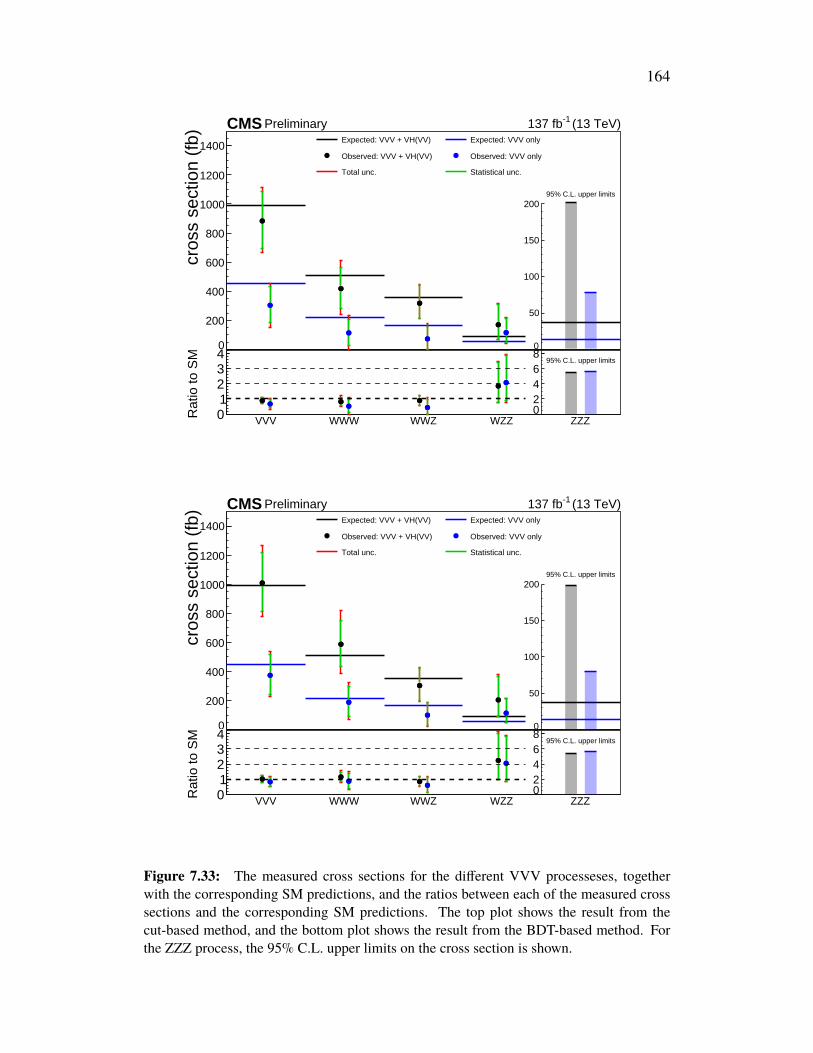
164

VVV WWW WWZ WZZ ZZZ01234

Rat

io to

SM

02468

95% C.L. upper limitsVVV WWW WWZ WZZ ZZZ

0

200

400

600

800

1000

1200

1400

cros

s se

ctio

n (f

b)95% C.L. upper limits

0

50

100

150

200

Expected: VVV + VH(VV) Expected: VVV only

Observed: VVV + VH(VV) Observed: VVV only

Total unc. Statistical unc.

CMS Preliminary (13 TeV)-1137 fb

VVV WWW WWZ WZZ ZZZ01234

Rat

io to

SM

02468

95% C.L. upper limitsVVV WWW WWZ WZZ ZZZ

0

200

400

600

800

1000

1200

1400

cros

s se

ctio

n (f

b)

95% C.L. upper limits

0

50

100

150

200

Expected: VVV + VH(VV) Expected: VVV only

Observed: VVV + VH(VV) Observed: VVV only

Total unc. Statistical unc.

CMS Preliminary (13 TeV)-1137 fb

Figure 7.33: The measured cross sections for the different VVV processeses, togetherwith the corresponding SM predictions, and the ratios between each of the measured crosssections and the corresponding SM predictions. The top plot shows the result from thecut-based method, and the bottom plot shows the result from the BDT-based method. Forthe ZZZ process, the 95% C.L. upper limits on the cross section is shown.

165

Table 7.37: Themeasured triboson cross sectionsf and the corresponding SM predictions.The uncertainties listed in the brackets are statistical and systematic respectively. Thecombined VVV cross section is calculated from the fit with a single signal strength `VVV,and the individual cross sections are calculated from a simultaneous fit with four signalstrengths, as discussed in the text. For the ZZZ process, 95% confidence level upper limitsare reported.

Process fmeasured, BDT (fb) fmeasured, cut (fb) fSM (fb)VH(VV) contributions as signal

VVV 1010+260−230(+210

−200+150−120) 880+230

−220(+200−190

+110−120) 992

WWW 590+230−200(+160

−150+160−130) 420+190

−170(+150−140

+120−110) 509

WWZ 300+120−110(+120

−100+50−40) 320+130

−110(+120−100

+40−30) 354

WZZ 200+180−110(+160

−110+70−20) 170+150

−100(+140−100

+50−20) 92

ZZZ <200 <200 37VH(VV) contributions as background

VVV 370+160−150(+140

−130+80−60) 300+150

−150(+130−120

+70−100) 451

WWW 190+130−120(+110

−100+80−70) 110+120

−120( +90−90

+80−80) 216

WWZ 100 +90−80( +80

−70+30−30) 70+100

−80( +80−70

+60−30) 165

WZZ 110+100−70(+100

−70+30−10) 120+100

−70(+100−70

+30−30) 56

ZZZ <80 <80 14

Table 7.38: The observed (expected) significance (f) for the different and combinedtriboson processes, for the two different (cut-based, BDT-based) analysis methods, and forthe two different fitting strategies (treatingVH(VV) as part of the signal or as a background).

Process VH(VV) as signal VH(VV) as backgroundcut-based BDT-based cut-based BDT-based

WWW 2.54 (2.94) 3.33 (3.09) 0.96 (1.82) 1.63 (1.87)WWZ 3.53 (3.62) 3.35 (4.09) 0.87 (2.17) 1.31 (2.15)WZZ 1.55 (0.70) 1.71 (0.69) 1.68 (0.76) 1.71 (0.76)ZZZ 0.00 (0.90) 0.00 (0.89) 0.00 (0.90) 0.00 (0.90)VVV 5.02 (5.37) 5.67 (5.88) 2.34 (3.52) 2.90 (3.48)

166

164

0

2

4

6

8

10

12

14

16

ln L

Δ- 2

2− 1− 0 1 2 3 4www-onshellµ

0

1

2

3

4

5w

h(w

w)

µCMSPreliminary (13 TeV)-1137 fb

68% C.L.95% C.L.SM

= 4.32wwwhµbest fit

= -1.34wwwµbest fit

0

2

4

6

8

10

12

14

16

ln L

Δ- 2

2− 1− 0 1 2 3 4www-onshellµ

0

1

2

3

4

5

wh(

ww

)µ

CMSPreliminary (13 TeV)-1137 fb68% C.L.95% C.L.SM

= 4.69wwwhµbest fit

= -0.82wwwµbest fit

0

2

4

6

8

10

12

14

16

ln L

Δ- 2

1− 0.5− 0 0.5 1 1.5 2 2.5 3wwz-onshellµ

0

1

2

3

4

5

zh(w

w)

µ


= 1.53wwzhµbest fit

= 0.32wwzµbest fit

0

2

4

6

8

10

12

14

16

ln L

Δ- 2

1− 0 1 2 3 4wwz-onshellµ

0

1

2

3

4

5

zh(w

w)

µ


= 1.44wwzhµbest fit

= -0.17wwzµbest fit

0

2

4

6

8

10

12

14

16

ln L

Δ- 2

0 0.5 1 1.5 2vvv-onshellµ

0

1

2

3

4

5

vh(v

v)µ


= 1.67vhµbest fit

= 0.37vvvµbest fit

0

2

4

6

8

10

12

14

16

ln L

Δ- 2

0 0.5 1 1.5 2 2.5vvv-onshellµ

0

1

2

3

4

5

vh(v

v)µ


= 2.30vhµbest fit

= 0.34vvvµbest fit

Figure 7.33: Likelihood contour plots (�2� ln ! where ! is the likelihood) as a functionof the VVV-onshell and VH(VV) signal strengths `VVV�onshell and `VH(VV) . The plots inthe left column (right column) are from the cut-based (BDT-based) method. The top plotsare the likelihood contours versus the signal strength for the WWW-onshell and WH(WW)processes; the middle plots are for the WWZ-onshell and ZH(WW) processes; and thebottom plots are for the combined VVV-onshell and VH(VV) processes. The point with thebest fit signal strengths `VVV�>=B⌘4;; and `VH(VV) is shown as a cross in each of the plotstogether with a star marking the SM prediction at (1.0, 1.0). Each of the plots also showsthe curves which correspond to the 68% and 95% C.L. contours.

Figure 7.34: 2D likelihood contour plots (−2Δ ln ! where ! is the likelihood) as a functionof the VVV-onshell and VH(VV) signal strengths `VVV−onshell and `VH(VV) . The plots inthe left column (right column) are from the cut-based (BDT-based) method. The top plotsare the likelihood contours versus the signal strength for the WWW-onshell and WH(WW)processes; the middle plots are for the WWZ-onshell and ZH(WW) processes; and thebottom plots are for the combined VVV-onshell and VH(VV) processes. The point withthe best fit signal strengths `VVV−onshell and `VH(VV) is shown as a diamond in each of theplots together with a star marking the SM prediction at (1.0, 1.0). Each of the plots alsoshows the curves which correspond to the 68% and 95% C.L. contours.

167

7.8 SummaryIn summary, we have observed the production of three massive vector bosons forthe first time, with 137 fb−1 of proton-proton collision data collected by the CMSdetector. The observed (expected) significance of the VVV production is 5.9 (5.7)standard deviation. We have also found evidence of WWW production and WWZproduction individually for the first time, with the observed (expected) significanceof 3.3 (3.4)f and 3.1 (4.1)f, respectively. The measured VVV cross section is1.01+0.21

−0.20(stat)+0.15−0.12 (syst) = 1.01+0.26

−0.23 pb, consistent with the SM prediction. Theindividually measured WWW, WWZ, WZZ production cross sections and an upperlimit on the ZZZ production cross section are also reported.

7.9 OutlookAs the current results are still limited by statistics uncertainty, with more integratedluminosity to come in LHC Run 3 and at the HL-LHC, the precision of the tribosonmeasurements reported in this thesis are expected to be further improved, includingthe possible observation of the individual VVV production channels. Makingprojections of the results obtainablewithmore data is not so straightforward, becauseseveral of the systematic uncertainties are not very easy to scale, as some of thebackground estimation-related uncertainties come from the statistical uncertaintiesin the data in the control regions. In addition, a major part of the uncertainties inthe signals come from the simulation statistics which could be improved by usinglarger simulated samples.

Table 7.39 shows a conservative quick projection, in which all the background andsignal systematic uncertainties are kept the same as their current values, and wesimply scale the background and signal yields by the projected luminosity. We cansee from this table that by the end of Run 3 (with a total of 300 fb−1), we expectto observe WWW and WWZ productions (with VH(VV) as signal), and we alsoexpect to observe VVV-onshell production. By the end of HL-LHC (3000 fb−1), weexpect to see evidence for WZZ and ZZZ productions as well. With 3000 fb−1 data,the VVV cross section measurement precision is expected to reach the 10% level,where the uncertaintywill be dominated by systematic errors (including an estimated4% statistical uncertainty and a 9% systematic uncertainty). Figure 7.35 shows thelikelihood (−2Δ ln !) scan over different signal strengths with the uncertaintiesbroken down to the statistical and systematic uncertainties. As we can see in thefigure, this search will be dominated by systematic uncertainty for WWW andWWZ production at the HL-LHC. As discussed above, with improved statistics in

168

the control region data, and more simulated events, the systematic uncertainty canbe further improved relative to the results shown in Table 7.39, raising the prospectof establishing solid evidence (beyond 3f) for WZZ and ZZZ by the end of theHL-LHC program.

Table 7.39: Expected sensitivity (significance ! (f) and signal strength `) of tribosonmeasurements for different VVV productions with different values of integrated luminosity(L).

L( fb−1) quantity VVV WWW WWZ WZZ ZZZ

137

! (f): VH(VV) as signal 5.9 3.1 4.1 0.7 0.9`: VH(VV) as signal 1.00+0.25

−0.22 1.00+0.40−0.36 1.00+0.36

−0.31 1.00+1.67−1.48 1.00+2.88

−0.84! (f): VH(VV) as bkg 3.5 1.8 2.2 0.8 0.9`: VH(VV) as bkg 1.00+0.38

−0.34 1.00+0.62−0.56 1.00+0.59

−0.51 1.00+1.66−1.34 1.00+2.94

−0.84

300


−0.17 1.00+0.31−0.28 1.00+0.26

−0.23 1.00+1.10−0.99 1.00+1.72


−0.25 1.00+0.47−0.43 1.00+0.42

−0.37 1.00+1.08−0.90 1.00+1.74

−0.86

3000


−0.10 1.00+0.19−0.18 1.00+0.13

−0.11 1.00+0.41−0.36 1.00+0.45


−0.14 1.00+0.28−0.27 1.00+0.21

−0.19 1.00+0.40−0.34 1.00+0.45

−0.36

With the first establishment of VVV production, many interesting previously unex-plored areas of physics, both within and beyond the SM, can be studied, using VVVproduction as a tool.

The first area that can be studied concerns the individual gauge-gauge and Higgs-gauge couplings. As stated earlier, these two couplings are still not determinedseparately, because the current event selection is not designed to isolate the VVV-onshell and VH(VV) processes. In order to discriminate between the two processes,several kinematic quantities can be utilized, among which the most significantfeatures of VH(VV) are that the two vector bosons from Higgs boson decay tendto be softer than the 3rd vector boson, and the opening angle of the softest pair ofvector bosons also tends to be smaller, compared to the VVV-onshell case.

As a result, variables such as the jet ?T and minimum jet-lepton opening angle in thesame-sign final state, the ?miss

T in the 3ℓ final state and the invariant mass of the twoW lepton candidates in the four-lepton eμ final state, could be used to bin the eventsinto different signal regions. Figure 7.36 shows the distributions of these variables asexamples. Even without dedicated binning in such variables, once the accumulated

169

luminosity is doubled as projected after LHC Run 3 by 2024, the significances ofthe individual VH(VV) and VVV-onshell signals from a 2D simultaneous fit areeach expected to be around 5f, and this analysis is expected to yield a simultaneousobservation of the two processes.

In addition to the measurement of the SM-predicted gauge-gauge and Higgs-gaugecouplings, VVV production can also be used as a tool to search for many BSMphysics, both directly and indirectly. The four-boson contact interaction in Figure 7.2could be a low-energy approximation of a more precise model with a mediator, andnew physics beyond the SM could thus change this coupling constant. A searchfor anomalous quartic gauge-boson couplings (aQGC) using WWW production(same-sign two-lepton and three-lepton final states) performed by CMS with 2016data [101] has put promising limits on several dimension-8 anomalous coupling termcoefficients [135]. Similar searches could be performed with the full Run 2 dataset and with more hadronic or semi-hadronic final states included, as such searchesrequire a sufficient statistical sample of highly boosted vector bosons. In additionto such indirect BSM searches for aQGC, direct searches for heavy mediators (suchas the radion [136]) modifying the four-boson vertex can also be performed.

170

165

0 0.2 0.4 0.6 0.8 1 1.2 1.4 1.6 1.8 2r_www

0

5

10

15

20

25

30

35

40 ln

LΔ

- 2

0.178−

0.192+r_www = 1.000

(Stat) 0.063−

0.064+(Syst) 0.166−

0.181+r_www = 1.000

CMSPreliminary

ExpectedStatOnly

0.4 0.6 0.8 1 1.2 1.4 1.6r_wwz

0

5

10

15

20

25

30

35

40

ln L

Δ- 2

0.114−

0.125+r_wwz = 1.002

(Stat) 0.065−

0.067+(Syst) 0.094−

0.105+r_wwz = 1.002

CMSPreliminary

ExpectedStatOnly

0 0.5 1 1.5 2r_wzz

0

1

2

3

4

5

6

7

8

ln L

Δ- 2

0.360−

0.407+r_wzz = 1.000

(Stat) 0.300−

0.311+(Syst) 0.198−

0.263+r_wzz = 1.000

CMSPreliminary

ExpectedStatOnly

0.5 1 1.5 2 2.5r_zzz

0

1

2

3

4

5

6

7

8

ln L

Δ- 2

0.361−

0.452+r_zzz = 0.999

(Stat) 0.353−

0.439+(Syst) 0.077−

0.109+r_zzz = 0.999

CMSPreliminary

ExpectedStatOnly

0.6 0.8 1 1.2 1.4r

0

5

10

15

20

25

30

35

40

ln L

Δ- 2

0.096− 0.103+r = 1.001

(Stat) 0.042−

0.043+(Syst) 0.086− 0.094+r = 1.001

CMSPreliminary

ExpectedStatOnly

Figure 7.34: �2� ln ! as a function of the signal strength for di�erent signals: WWW(top-left), WWZ (top-right), WZZ (center-left), ZZZ (center-right), and the combined VVVsignal (bottom). The plots are projections of the results expected with 3000 fb�1 of data atthe HL-LHC. VH(VV) is included as part of the signal in all plots.

Figure 7.35: −2Δ ln ! as a function of the signal strength for different signals: WWW(top-left), WWZ (top-right), WZZ (center-left), ZZZ (center-right), and the combined VVVsignal (bottom). The plots are projections of the results expected with 3000 fb−1 of data atthe HL-LHC. VH(VV) is included as part of the signal in all plots.

171

166

0 20 40 60 80 100 120 140 (GeV)subleading-jet

Tp

0

200

400

600

800

1000

1200

Even

ts




Irredu. VVV x 20

VH(VV) x 20

0 1 2 3 4 5 6minlj RΔ

0

200

400

600

800

Even

ts




Irredu. VVV x 20

VH(VV) x 20

0 20 40 60 80 100120140160180 (GeV)miss

Tp

0

2000

4000

6000

8000Even

ts




Irredu. VVV x 100

VH(VV) x 100

0 50 100 150 200 250 (GeV)µem

0

2

4

6

8

10

Even

ts


Other WZ tWZ

Higgs Ztt ZZ

VVV VH(VV)

Figure 7.35: Distributions of some useful variables to discriminate the VVV-onshell signalfrom the VH(VV) signal - top left: subleading jet ?T in the SS + 2 jets preselection; topright: �'min

✓j in SS + 1 jet preselection; bottom left: ?missT in the 3✓ preselection region;

bottom right: invariant mass of the two W lepton candidates in the four-lepton e� final state.

Figure 7.36: Distributions of some useful variables to discriminate the VVV-onshell signalfrom the VH(VV) signal - top left: subleading jet ?T in the SS + 2 jets preselection; topright: Δ'min

ℓj in SS + 1 jet preselection; bottom left: ?missT in the 3ℓ preselection region;

bottom right: invariant mass of the twoW lepton candidates in the four-lepton eμ final state.

Part IV

Search for long-lived particles usingdelayed photons in CMS at the LHC

172

173

C h a p t e r 8

SEARCH FOR LONG-LIVED PARTICLES USING DELAYEDPHOTONS WITH 2016 DATA IN CMS

There are many SM unstable particles which are long-lived and have proper decaylengths between a few millimeters and a few meters. The decay products of suchlong-lived particles can be detected by CMS, but exhibit different signatures fromprompt particle decays. Such long-lived particles (LLP) are also predicted in manymodels of physics beyond the SM, such as supersymmetry (SUSY) with gauge-mediated SUSY breaking (GMSB) [16–25] or hidden valley models [137].

In this chapter, we present a search for LLPs that decay to a photon and a weaklyinteracting particle, using a benchmark scenario of GMSB, commonly referred toas the "Snowmass Points and Slopes 8" (SPS8) [138]. In this scenario, the LLPswe are interested in are the next-to-lightest SUSY particle (NLSP), the neutralino(χ01), which is produced via cascade decays of pair-produced squarks and gluinosand decays to the lightest SUSY particle (LSP), the gravitino (G), as shown inFigure 8.1. The mass of the neutralino is linearly related to the SUSY scale, Λ,and is also affected by other parameters such as the messenger mass. In the SPS8model, these parameters are fixed and Λ is a free parameter, and the value of Λ alsodetermines the primary production mode and decay rate of the NLSP. The dominantdecay mode of the NLSP in SPS8 is to a photon and gravitino, resulting in a finalstate with one or two photons and missing transverse momentum (?miss

T ).

Previously, a searchwas performed byCMSusing ?missT and the photon arrival time at

the ECAL in single photon plus ?missT events with 4.9 fb−1 of data at

√B = 7TeV [139],

which excluded such a GMSB scenario for neutralino masses below 220 GeV andproper decay length 2g up to 6 m. ATLAS also reported a similar search withthe same GMSB model by using the photon arrival time at their ECAL and thelongitudinal impact parameter of the projected photon trajectory ΔIW relative tothe center of the interaction region, in diphoton events with 4.8 fb−1 data at

√B =

7 TeV [140]. The search excluded such GMSB models for neutralino masses upto 240 GeV and 2g up to 15 m. Followup searches with 8 TeV data have beenperformed by both CMS [141] and ATLAS [142], which excluded such GMSBmodels for a neutralino mass up to 300 GeV and 430 GeV, and 2g up to 25 m and 30

174

p

p q

q

χ0

1

χ0

1

q

γ

G

G

γ

q

p

p q

q

χ0

1

χ±

1

q′

W±

G

G

γ

q

p

p q

q

χ0

1

χ0

1

q

Z

G

G

γ

q

p

pg

g

q χ0

1

q χ0

1

qq

γ

G

G

qq

γ

p

pg

g

q χ0

1

q χ±

1

q q′

W±

G

G

qq

γ

p

pg

g

q χ0

1

q χ0

1

qq

Z

G

G

qq

γ

Figure 8.1: Example Feynman diagrams for SUSY processes that result in diphoton (left)and single photon (middle and right) final states via squark (upper) and gluino (lower)pair-production at the LHC.

m, respectively. Figure 8.2 summarizes the exclusion regions from all the previoussearches by CMS and ATLAS. As we see from the previous results obtained withRun 1 data shown in the figure, the sensitivity for small 2g signal models is greatlyimproved by requiring two photons in the events, as this greatly reduces the promptphoton SM backgrounds.

In this search, we use CMS data taken in 2016 with a diphoton trigger, and selectevents with at least two photons. A dedicated identification is applied to the leadingphoton to ensure high efficiency for time delayed (or vertex displaced) photons, andto suppress prompt photons by cutting on the electromagnetic shower shapes. Thearrival time of the leading photon in the ECAL is then used as a shape variable in thefit to extract the signal yield, together with another variable, the missing transversemomentum (?miss

T ). The results are then combined with a similar search that usesCMS data taken in 2017 with a single photon trigger, that has better sensitivity tosignals with large 2g.

The remaining sections of this chapter are organized as follows: Section 8.1 discussesthe data sample and the triggers used in this analysis. The object reconstruction andidentification, especially the identification details for out-of-time photons, are givenin Section 8.2. Section 8.3 is dedicated to the measurement of the CMS ECALtiming resolution, and the necessary corrections to match MC events with data. Theevent selections are given in Section 8.4. The background estimation as well as thesystematic uncertainties are presented in Sections 8.5 and 8.6, and the final resultsare given in Section 8.7.

175

Figure 8.2: Summary of exclusion results in the plane of the proper lifetime of a neutralinoNLSP in a GMSB model versus its mass, from searches with LHC Run 1 data by both CMSand ATLAS [141].

8.1 Event samplesThe data used in this search corresponds to a total integrated luminosity of 35.9 fb−1

of proton-proton collisions collected by the CMS detector in 2016. The result of acombined search with 2016 and 2017 data will be presented in the next chapter.

The GMSB SPS8 signal model samples are produced by first generating a tabulatedformof the particle spectra in a set of SUSYLesHouchesAccord (SLHA) files [143].The purpose of the SLHAproject is to define a set of conventions for supersymmetricextensions of the Standard Model together with an accord specifying generic filestructures for 1) supersymmetric model specifications and input parameters, 2) EWscale supersymmetric mass and coupling spectra, and 3) decay tables, to providea universal interface between spectrum calculation programs, decay packages, andhigh energy physics event generators using the isasugra toolkit [144] in the isajetv7.87 generator package [145]. isasugra is a subprogram of isajet that calculatesthe mass-spectrum and decay-channels for a number of SUSY models, includingmSUGRA.A grid of samples with different SUSY scaleΛ and neutralino lifetime 2g

176

values is used to construct a set of SLHA tables, where the parameters used togenerate the tables follow the SPS8 recommendations. The resulting SLHA filesare then passed to pythia v8.212 [121] to generate the benchmark signal modelsfor each of the designated Λ and 2g values. Table 8.1 lists all of the GMSB signalsamples used in this search, along with the masses of the gluino, neutralino, andgravitino, and the cross sections for different Λ and 2g values.

Table 8.1: Table of the generated GMSB SPS8 signal models, and the corresponding masspoints and cross sections. For each Λ point, a grid of signal models with 2g = 0.1, 0.5, 1, 2,4, 6, 8, 10, 12, and 100 m is generated. The mass of the gravitino "G is proportional to thesquare root of 2g (as can be seen in Eq. 2.10 and 2.11, we have "G ∝ 〈�〉, and 2g ∝ 〈�〉2);and the mass of gluino and neutralino are determined by Λ.

Λ "g "χ01

"G (10−7 GeV) for different 2g cross section

(TeV) (GeV) (GeV) 0.1, 0.5, 1, 2, 4, 6, 8, 10, 12, 100 m (fb)100 838 139 1.5, 3.4, 4.9, 6.9, 9.7, 12, 14, 15, 17, 49 2160 ± 20150 1207 212 4.7, 10, 15, 21, 30, 36, 42, 47, 51, 148 228 ± 2200 1565 285 10, 22, 32, 45, 64, 78, 90, 100, 110, 318 44.5 ± 0.3250 1915 358 18, 40, 57, 81, 114, 140, 162, 180, 198, 571 12.6 ± 0.1300 2260 430 29, 65, 92, 130, 183, 225, 259, 290, 318, 917 4.45 ± 0.03350 2599 503 43, 96, 136, 193, 273, 334, 386, 430, 473, 1364 1.78 ± 0.01400 2935 576 61, 136, 192, 271, 384, 470, 543, 610, 665, 1920 0.778 ± 0.005

The MadGraph5_aMC@NLO v2.2.2 generator [113] is used to generate the stan-dard model background events, including top quark and tt production at next-to-leading order (NLO) in quantum chromodynamics (QCD), and QCD multijet,W+ jets,W+ jets, and Z+ jets productions at leading order (LO). sherpa v2.2.4 [146,147] is used to generate diphoton events, which include Born processes with upto three additional jets, as well as box-diagram processes at LO precision. TheNNPDF3.0 [119, 120] parton distribution functions (PDFs) are used in the simu-lated samples. All the generated MC samples are processed with Geant4 [85] tosimulate the interactions of particles with the CMS detector. Pileup interactions arealso simulated and included in each MC event.

This search uses an unprescaled diphoton trigger, which requires two isolated photonobjects with transverse energy greater than 42 and 25 GeV for the leading andsubleading photons. Additional requirements, such as cuts on photon shower shapevariables ('9, f8[8[) and ratio of energies in HCAL and ECAL (H/E), are alsoapplied on both photon objects in the trigger. The details of these cuts are discussedin Section 8.2, together with the offline identification criteria for photons.

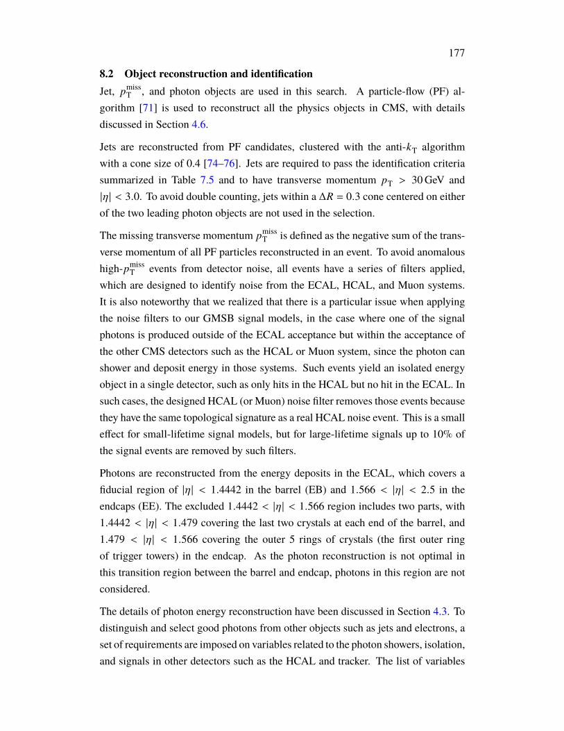
177

8.2 Object reconstruction and identificationJet, ?miss

T , and photon objects are used in this search. A particle-flow (PF) al-gorithm [71] is used to reconstruct all the physics objects in CMS, with detailsdiscussed in Section 4.6.

Jets are reconstructed from PF candidates, clustered with the anti-:T algorithmwith a cone size of 0.4 [74–76]. Jets are required to pass the identification criteriasummarized in Table 7.5 and to have transverse momentum ?T > 30GeV and|[ | < 3.0. To avoid double counting, jets within a Δ' = 0.3 cone centered on eitherof the two leading photon objects are not used in the selection.

The missing transverse momentum ?missT is defined as the negative sum of the trans-

verse momentum of all PF particles reconstructed in an event. To avoid anomaloushigh-?miss

T events from detector noise, all events have a series of filters applied,which are designed to identify noise from the ECAL, HCAL, and Muon systems.It is also noteworthy that we realized that there is a particular issue when applyingthe noise filters to our GMSB signal models, in the case where one of the signalphotons is produced outside of the ECAL acceptance but within the acceptance ofthe other CMS detectors such as the HCAL or Muon system, since the photon canshower and deposit energy in those systems. Such events yield an isolated energyobject in a single detector, such as only hits in the HCAL but no hit in the ECAL. Insuch cases, the designed HCAL (or Muon) noise filter removes those events becausethey have the same topological signature as a real HCAL noise event. This is a smalleffect for small-lifetime signal models, but for large-lifetime signals up to 10% ofthe signal events are removed by such filters.

Photons are reconstructed from the energy deposits in the ECAL, which covers afiducial region of |[ | < 1.4442 in the barrel (EB) and 1.566 < |[ | < 2.5 in theendcaps (EE). The excluded 1.4442 < |[ | < 1.566 region includes two parts, with1.4442 < |[ | < 1.479 covering the last two crystals at each end of the barrel, and1.479 < |[ | < 1.566 covering the outer 5 rings of crystals (the first outer ringof trigger towers) in the endcap. As the photon reconstruction is not optimal inthis transition region between the barrel and endcap, photons in this region are notconsidered.

The details of photon energy reconstruction have been discussed in Section 4.3. Todistinguish and select good photons from other objects such as jets and electrons, aset of requirements are imposed on variables related to the photon showers, isolation,and signals in other detectors such as the HCAL and tracker. The list of variables

178

considered in the photon identification procedure are:

• X9: the energy sum in the 3 × 3 set of crystals centered on the most energeticcrystal in a supercluster (SC), divided by the total energy of the SC. The '9

of good and unconverted photons is very close to 1.0; and the '9 of objectssuch as jets is much smaller. A cut on '9 > 0.9 is applied to all photons inthis search.

• 2i(i(: the width of the seed basic cluster of the photon in the [ direction,computed with weighted crystal [ indices, where the weights are related tothe energy deposited in each crystal, as defined in Eq. 8.1. The distribution off8[8[ for photons peaks below 0.01 and the f8[8[ for jets is usually larger than0.01.

• H/E: the energy deposited in theHCAL in aΔ' = 0.15 cone around the photondirection, divided by the SC energy measured in the ECAL. For photons, thereis generally no significant energy deposited in the cone in the HCAL, and soH/E is in general very small.

• ChargedHadPFIso: the scalar ?T sum of all charged hadron PF candidatesin a Δ' = 0.30 cone around the photon direction.

• TrackIso: the scalar ?T sum of all tracks in a Δ' = 0.30 cone around thephoton direction.

• NeutralHadPFIso: the scalar ?T sum of all neutral hadron PF candidates ina Δ' = 0.30 cone around the photon direction.

• HCALIso: the scalar sum of transverse energy in HCAL deposits in aΔ' = 0.30 cone around the photon direction.

• PhotonPFIso: the scalar ?T sum of all photon PF candidates in a Δ' = 0.30cone around the photon direction.

• ECALIso: the scalar sum of transverse energy in ECAL deposits in aΔ' = 0.30 cone around the photon direction.

• Ymajor: the weighted energy along the semi-major axis of the elliptical photonshower, as defined by the eigenvalues in Eq. 8.1, where (qq, ([[, and ([q arethe second central moments of the spatial distribution of the energy deposits

179

in the ECAL in [-q coordinates, and the logarithmic weight F8 in the equationis the same as the weight used to calculate the cluster position [148].

• Yminor: the weighted energy along the semi-minor axis of the elliptical photonshower, as defined by the eigenvalues in Eq. 8.1.

( majorminor

=(qq + ([[ ±

√((qq − ([[)2 + 4(2

[q

2(8.1)

where ([q =#∑8=1

F8 ([8− < [ >) (q8− < q >)

([[ =#∑8=1

F8 ([8− < [ >) ([8− < [ >)

(qq =#∑8=1

F8 (q8− < q >) (q8− < q >)

< [ > =

∑8 F8[8∑8 F8

, < q >=

∑8 F8q8∑8 F8

F8 = max[4.2 + ln( �8

�cluster); 0

].

The distributions of the above identification variables for signal photons and fakephotons (from jets) are shown in Figures 8.3 and 8.4. For signal photons, two typesof photon collections are shown: the GED photon and OOT photon. The GEDphoton refers to the "general event description" photons, which only collects in-timephotons with a time delay (with respect to a prompt photon from the primary vertex)smaller than 3 ns. To cover our delayed photon signals, a second photon collection,called out-of-time (OOT) photons is designed for this search, which collects photonsthat are not saved in the GED photon collection.

As shown in these figures, the shapes of the photon ID variable distributions are verydifferent for GED and for OOT photons. This is especially true for the shower shapevariables, where the OOT (displaced) photons have a non-zero incident angle withrespect to the long axis of the crystal, and thus the EM shower is non-circular and hasa elliptical shape. In addition, when running the reconstruction for OOT photons,the full particle flow reconstruction is not run on those photons and therefore theHCAL-related information for those photons is not available, including the H/Eand HCALIso values. Due to the differences between GED and OOT photons,

180

different identification criteria are applied to the GED and OOT photons, and theserequirements are optimized separately in order to maximize the signal efficienciesfor in-time and out-of-time signal photons.

Table 8.2 summarizes the full set of photon identification cuts for both GED andOOT photons used in this search. To compensate for the effects of the energydeposited due to pileup, all the isolation variables are corrected event by event, byusing the effective pileup transverse momentum density d (median of the energydensity per unit area in the rapidity-azimuth plane) times an effective area (�eff , thearea of the isolation region), i.e. the isolation variables are subtracted by the pileupcontribution by d�eff [149]. These corrections are measured separately for GEDand OOT photons and have different values for different pseudorapidities of thephotons. Table 8.3 summarizes the corresponding effective areas used in this set ofphoton identification criteria, which are obtained by fitting the isolation dependencyon the d in with W+jet events. The signal efficiency of the GED (OOT) photonID has been measured to be about 65% (80%), while the efficiency for picking upfake GED (OOT) photons from QCD multijet events has been measured to be about5% (10%). Figures 8.5, 8.6, 8.7, and 8.8 show the corresponding efficiencies asa function of the photon ?T, [, and arrival time, from which we can see that theefficiencies are relatively flat for different values of those variables in all cases.

Table 8.2: Photon identification cuts used in the delayed photon search. All the isolationvariables are d corrected as described in the text.

Variable GED photon ID OOT photon IDH/E < 0.0269 —f8[8[ < 0.017 < 0.017ChargedHadPFIso <0.202TrackIso — < 2.0 + 0.005996?WTNeutralHadPFIso < 0.264 + 0.0148?WT + 1.7 × 10−5?

WT

2

PhotonPFIso < 2.362 + 0.0047?WTECALIso — < 3.0 + 0.007132?WT(major — < 1.3

As the GED and OOT photons are reconstructed independently with the samereconstruction algorithm, but just starting from a different seed crystal (GED photonreconstruction only starts with a seed which has a time smaller than 3 ns, while OOTphoton reconstruction starts with a seed which has a time larger than 3 ns), in mostcases the GED and OOT reconstruction will not select the same photon. But in

181

Table 8.3: Effective areas used to correct the isolation variables in the GED and OOTphoton ID procedures.

[ rangeGED photon ID OOT photon ID

ChargedHadPFIso NeutralHadPFIso PhotonPFIso TrackIso NeutralHadPFIso ECALIso|[ | < 1.0 0.0360 0.0597 0.1210 — — —1.0 < |[ | < 1.479 0.0377 0.0807 0.1107 — — —|[ | < 0.8 — — — 0.2304 0.0488 0.15550.8 < |[ | < 1.479 — — — 0.1969 0.0523 0.1362

rare cases (less than 5%), the reconstructed GED and OOT photon clusters mightpartially overlap with each other, i.e. there may be some shared crystals. In suchcases, either one or both of the two clusters is incomplete and is only part of thefull photon cluster. To avoid double counting, a cluster-overlap removal procedureis applied to the two photon collections. To do this, we put all the GED andOOT photons together, and compare every pair of photons with one from the GEDcollection and one from the OOT collection. If the Δ' between the two photons issmaller than 0.3, then we consider that the photons are overlapped and we only keepthe photon with the larger ?T, and remove the photon with smaller ?T from the listof photon objects, before continuing the cluster-overlap procedure.

As mentioned above, the OOT photons are not included in the PF candidate listbecause the full particle flow reconstruction is not run on OOT photons. As a result,if we decide to keep an OOT photon in the above cluster-overlap cleaning procedure,the ®?T of the OOT photon is subtracted from the ®?miss

T . For GED photons, if a GEDphoton is removed during the cleaning procedure, the ®?T of the GED photon isadded back into ®?miss

T since it was included in the ®?missT calculation by default.

When we decide to remove an OOT photon or keep a GED photon in the overlapcleaning, nothing is done to the ®?miss

T . After this correction for ?missT , the resolution

of the ?missT (measured by the standard deviation of the distribution of the difference

between the reconstructed and the generated ?missT in MC) is improved by about

20%.

182 178

0 0.2 0.4 0.6 0.8 1majorS

3−10

2−10

1−10

1Even

ts

, GEDγGMSB , OOTγGMSB γQCD fake

CMS Preliminary (13 TeV)-135.9 fb

0 0.2 0.4 0.6 0.8 1minorS

3−10

2−10

1−10

1

Even

ts



0.5 0.6 0.7 0.8 0.9 19R

3−10

2−10

1−10

1

Even

ts



0 0.005 0.01 0.015 0.02H/E

3−10

2−10

1−10

1

10

Even

ts



0.005 0.01 0.015 0.02 0.025η iηiσ

3−10

2−10

1−10

1

Even

ts



Figure 8.3: Distributions of some photon identification variables for GMSB signal photons(GED and OOT photons) and fake photons in QCD multijet events. Top row from left toright: (major, (minor; center row from left to right: '9, H/E; bottom plot is f8[8[ .

Table 8.2 summarizes the full set of photon identification cuts for both GED andOOT photons used in this search. To compensate for the e�ects of the energydeposited due to pileup, all the isolation variables are corrected event by event, byusing the e�ective pileup transverse momentum density d (median of the energydensity per unit area in the rapidity-azimuth plane) times an e�ective area (�e� , the

Figure 8.3: Distributions of some photon identification variables for GMSB signal photons(GED and OOT photons) from a representative point (Λ = 250 TeV and 2g = 2 m) and fakephotons in QCD multijet MC events. Top row from left to right: (major, (minor; center rowfrom left to right: '9, H/E; bottom plot is f8[8[ .

183

186

0 10 20 30PF photon isolation (GeV)

3−10

2−10

1−10

1

Even

ts



0 5 10ECAL isolation (GeV)

3−10

2−10

1−10

1

Even

ts



0 10 20 30PF neutral hadron isolation (GeV)

3−10

2−10

1−10

1

Even

ts



0 5 10HCAL isolation (GeV)

3−10

2−10

1−10

1Ev

ents



0 10 20 30PF charged hadron isolation (GeV)

3−10

2−10

1−10

1

10

Even

ts



0 5 10Tracker isolation (GeV)

3−10

2−10

1−10

1

Even

ts



Figure 8.4: Distributions of some photon identification variables for GMSB signal photons(GED and OOT photons) and fake photons in QCD multijet events. Left column from topto bottom: PhotonPFIso, NeutralHadPFIso, ChargedHadPFIso; right column from top tobottom: ECALIso, HCALIso, TrackIso.

Figure 8.4: Distributions of some photon identification variables for GMSB signal photons(GED and OOT photons) from a representative point (Λ = 250 TeV and 2g = 2 m) and fakephotons in QCD multijet MC events. Left column from top to bottom: PhotonPFIso, Neu-tralHadPFIso, ChargedHadPFIso; right column from top to bottom: ECALIso, HCALIso,TrackIso.

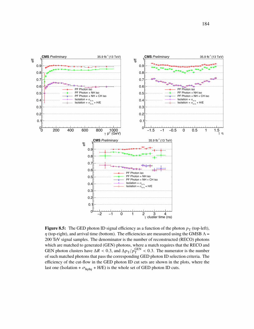
184

187

0 200 400 600 800 1000 (GeV)T pγ

0

0.1

0.2

0.3

0.4

0.5

0.6

0.7

0.8

0.9

1

eff

PF Photon isoPF Photon + NH isoPF Photon + NH + CH iso

η iηiσIsolation + + H/Eη iηiσIsolation +


1.5− 1− 0.5− 0 0.5 1 1.5η γ

0

0.1

0.2

0.3

0.4

0.5

0.6

0.7

0.8

0.9

1

eff




2− 1− 0 1 2 3 4 cluster time (ns)γ

0

0.1

0.2

0.3

0.4

0.5

0.6

0.7

0.8

0.9

1

eff




Figure 8.5: The GED photon ID signal e�ciency as functions of the photon ?T (top-left),[ (top-right), and arrival time (bottom). The e�ciencies are measured using the GMSB ⇤ =200 TeV signal samples. The denominator is the number of reconstructed (RECO) photonswhich are matched to generated (GEN) photons, where a match requires that the RECO andGEN photon clusters have �' < 0.3, and � ?T/?GEN

T < 0.3). The numerator is the numberof such matched photons that pass the corresponding GED photon ID selection criteria. Thee�ciency of the cut-flow in the GED photon ID cut sets are shown in the plots, where thelast one (Isolation + f8[8[ + H/E) is the whole set of GED photon ID cuts.

Figure 8.5: The GED photon ID signal efficiency as a function of the photon ?T (top-left),[ (top-right), and arrival time (bottom). The efficiencies are measured using the GMSB Λ =200 TeV signal samples. The denominator is the number of reconstructed (RECO) photonswhich are matched to generated (GEN) photons, where a match requires that the RECO andGEN photon clusters have Δ' < 0.3, and Δ?T/?GEN

T < 0.3. The numerator is the numberof such matched photons that pass the corresponding GED photon ID selection criteria. Theefficiency of the cut-flow in the GED photon ID cut sets are shown in the plots, where thelast one (Isolation + f8[8[ + H/E) is the whole set of GED photon ID cuts.

185

188

0 200 400 600 800 1000 (GeV)T pγ

0

0.1

0.2

0.3

0.4

0.5

0.6

0.7

0.8

0.9

1

eff




1.5− 1− 0.5− 0 0.5 1 1.5η γ

0

0.1

0.2

0.3

0.4

0.5

0.6

0.7

0.8

0.9

1

eff




2− 0 2 4 6 time (ns)γ

0

0.1

0.2

0.3

0.4

0.5

0.6

0.7

0.8

0.9

1

eff




Figure 8.6: GED photon ID background e�ciency as functions of the photon ?T (top-left),[ (top-right), and arrival time (bottom). The e�ciencies are measured using QCD MCsignal samples. The denominator is the number of reconstructed (RECO) photons whichhave ?T > 70 GeV. The numerator is the number of such photons that pass the correspondingGED photon ID selection. The e�ciency of the cut-flow in the GED photon ID cut sets areshown in the plots, where the last one (Isolation + f8[8[ + H/E) is the whole set of GEDphoton ID cuts.

Figure 8.6: GED photon ID background efficiency as a function of the photon ?T (top-left), [ (top-right), and arrival time (bottom). The efficiencies are measured using QCDMCsignal samples. The denominator is the number of reconstructed (RECO) photons whichhave ?T > 70GeV. The numerator is the number of such photons that pass the correspondingGED photon ID selection. The efficiency of the cut-flow in the GED photon ID cut sets areshown in the plots, where the last one (Isolation + f8[8[ + H/E) is the whole set of GEDphoton ID cuts.

186

189

0 200 400 600 800 1000 (GeV)T pγ

0

0.1

0.2

0.3

0.4

0.5

0.6

0.7

0.8

0.9

1

eff

ECAL isoECAL + PFNH isoECAL + PFNH + tracker iso

η iηiσIsolation + + Smajorη iηiσIsolation +


1.5− 1− 0.5− 0 0.5 1 1.5η γ

0

0.1

0.2

0.3

0.4

0.5

0.6

0.7

0.8

0.9

1

eff




2− 0 2 4 6 cluster time (ns)γ

0

0.1

0.2

0.3

0.4

0.5

0.6

0.7

0.8

0.9

1

eff




Figure 8.7: OOT photon ID signal e�ciency as functions of the photon ?T (top-left), [(top-right), and arrival time (bottom). The e�ciencies are measured using the GMSB ⇤ =200 TeV signal samples. The denominator is the number of reconstructed (RECO) photonswhich are matched to generated (GEN) photons, where we require that the RECO and GENphoton clusters are matched within �' < 0.3, and � ?T/?GEN

T < 0.3. The numerator isthe number of such matched photons that pass the corresponding OOT photon ID selection.The e�ciency of the cut-flow in the OOT photon ID cut sets are shown in the plots, wherethe last one (Isolation + f8[8[ + (major) is the whole set of OOT photon ID cuts.

Figure 8.7: OOT photon ID signal efficiency as a function of the photon ?T (top-left), [(top-right), and arrival time (bottom). The efficiencies are measured using the GMSB Λ =200 TeV signal samples. The denominator is the number of reconstructed (RECO) photonswhich are matched to generated (GEN) photons, where we require that the RECO and GENphoton clusters are matched within Δ' < 0.3, and Δ?T/?GEN

T < 0.3. The numerator is thenumber of such matched photons that pass the corresponding OOT photon ID selection.The efficiency of the cut-flow in the OOT photon ID cut sets are shown in the plots, wherethe last one (Isolation + f8[8[ + (major) is the whole set of OOT photon ID cuts.

187

190

0 200 400 600 800 1000 (GeV)T pγ

0

0.1

0.2

0.3

0.4

0.5

0.6

0.7

0.8

0.9

1

eff




1.5− 1− 0.5− 0 0.5 1 1.5η γ

0

0.1

0.2

0.3

0.4

0.5

0.6

0.7

0.8

0.9

1

eff




2− 0 2 4 6 time (ns)γ

0

0.1

0.2

0.3

0.4

0.5

0.6

0.7

0.8

0.9

1

eff




Figure 8.8: OOT photon ID background e�ciency as functions of the photon ?T (top-left),[ (top-right), and arrival time (bottom). The e�ciencies are measured using QCD MCsignal samples. The denominator is the number of reconstructed (RECO) photons whichhave ?T > 70 GeV. The numerator is the number of such photons that pass the correspondingOOT photon ID selection. The e�ciency of the cut-flow in the OOT photon ID cut sets areshown in the plots, where the last one (Isolation + f8[8[ + (major) is the whole set of OOTphoton ID cuts.

Figure 8.8: OOT photon ID background efficiency as a function of the photon ?T (top-left), [ (top-right), and arrival time (bottom). The efficiencies are measured using QCDMCsignal samples. The denominator is the number of reconstructed (RECO) photons whichhave ?T > 70GeV. The numerator is the number of such photons that pass the correspondingOOT photon ID selection. The efficiency of the cut-flow in the OOT photon ID cut sets areshown in the plots, where the last one (Isolation + f8[8[ + (major) is the whole set of OOTphoton ID cuts.

188

8.3 ECAL timing measurementThis search uses the arrival time of the photon at the ECAL as one of the keydiscriminants to extract delayed photon signals from the SM backgrounds.

As mentioned in Section 4.3, each ECAL crystal’s signal output pulse is digitizedinto 10 consecutive samples spaced 25 ns apart. Our task is to estimate the time atwhich the pulse reaches its maximum amplitude, Cmax. Since the amplitude of eachof the 10 samples depends on the distance from that sample’s time to Cmax as well asthe pulse maximum amplitude, by looking at the ratio of that sample’s amplitude andthe amplitude of its neighboring samples, we can get an estimate of Cmax, which wedenote as Cmax,k ( where the index : denotes the sample bin index in the pulse, whichranges from 0 to 9). And an uncertainty-weighted average of those 10 estimations,is defined as the final estimate of the timestamp of that crystal’s signal pulse, whichwe denote as C8ECAL (index "8" is the crystal index). A detailed description of theECAL timestamp reconstruction, as well as how the Cmax,k is estimated, can be foundin [150].

The timestamp uncertainty for crystal 8 is parameterized as:

f28 =

(#

�8/fN8

)2

+ �2, (8.2)

where �8 is the amplitude of the signal detected by crystal 8, fN8 is the pedestal noisefor crystal 8, and # and � are constants which are determined from a dedicated fitto the data. As shown in Equation 8.2, there are two main sources of uncertaintyin the ECAL timestamp measurement, the noise term and the constant term, whichare added in quadrature. The noise term is proportional to the noise amplitude andinversely proportional to the signal amplitude of the channel. The constant termincludes the systematic uncertainty in the above time estimation method and othereffects such as the variation of the depth of the EM shower starting point in thecrystal.

To measure the values of the constants # and � in the above formula, we comparethe time difference (ΔC) of two neighboring crystals that belong to the same EMshower and have similar energy deposits, specifically by requiring that the ratio ofthe two energies be between 0.8 and 1.2. The EM shower is selected from photonobjects with very basic identification requirements to avoid showers from jets. Inaddition, to avoid noisy channels and gain switch effects in the readout, we requirethe energy deposited in each crystal to be between 1 and 120 GeV. We then fit the

189

ΔC distribution with a Gaussian function, and take the fitted f(ΔC) as the resolution.Different fits are performed in bins of the effective amplitude/noise ratio in the pairof crystals (crystal 1 and 2), defined as:

�eff/fN =(�1/fN1

) (�2/fN2)√

(�1/fN1)2 + (�2/fN2

)2. (8.3)

The f(ΔC) is then the sum (in quadrature) of uncertainties of the two timestampsfrom the two crystals parameterized in Eq. 8.2, and therefore the f(ΔC) can beparameterized as the following:

f2(ΔC) =(

#

�eff/fN

)2+ 2�2, (8.4)

where the uncertainties of the two terms are taken directly from the fit of the f(ΔC)vs. �eff/fN curve.

A detailed study revealed that f(ΔC) depends on whether the two neighboringcrystals belong to the same readout unit (each readout unit consists of a grid of 5×5crystals) or not, as there is clock jitter among the readout units. We refer to thef(ΔC) obtained for pairs of crystals in the same readout unit as the intrinsic timeresolution of the crystals, as the inter-unit clock jitter does not enter.

Figure 8.9 shows the result of the single crystal’s timing resolution measurementobtainedwith the 2016 data. Two additional curves and fitting results are also shown,which are the measurements of f(ΔC) for two neighboring crystals that belong todifferent ECAL readout units, and the combined result that includes both cases: oftwo neighboring crystals that belong to the same or different readout units. We cansee that once the clock jitter is included, the combined resolution gets slightly worse.The constants # and � in Eqn. 8.2 are measured to be # = 31.6 ± 1.2 ns, � =

0.077±0.001 ns for a pair of crystals in the same readout unit, and # = 32.9±1.2 ns,� = 0.085± 0.001 ns for the combined result. As the clock jitter is not simulated inthe MC simulation, we will take this effect into account when we make correctionsto the MC timestamp in a later step.

From the time resolution of each ECAL crystal (parameterized in Eq. 8.2, with thevalues of the constants # and � shown in Figure 8.9), the time resolution of anyECAL crystal hit can then be estimated given the energy deposited and the pedestalnoise for that hit. And based on this estimation, the arrival time of the whole photon

190

210 310Nσ/effA

0.1

0.2

0.3

0.4

0.5

0.60.70.80.9

1

t) (

ns)

∆(σ

CMS Preliminary

10 100E in EB (GeV)

(13 TeV)-135.9 fb

C2 ⊕ N

σ/effANt) = ∆(σ

1.6 ns± = 37.3 diff.N

0.002 ns± = 0.159 diff.C

1.2 ns± = 32.9 incl. N

0.001 ns± = 0.085 incl. C

1.2 ns± = 31.6 sameN

0.001 ns± = 0.077 sameC

Diff. RO unit

Inclusive

Same RO unit

Figure 8.9: The resolution of the time difference (f(ΔC)) of two neighboring ECALcrystals as a function of the effective amplitude/noise ratio of the two crystals (�eff/fN).The measurement is performed in three cases based on whether the two crystals belong tothe same or different ECAL readout (RO) units or a mix of the two cases. The dependence off(ΔC) on �eff/fN is fitted by the function in Eqn. 8.4, and the results of the fits are shown inthe plot. The top ticks on the x-axis show the approximate ECAL energy deposited (in GeV)for the corresponding �eff/fN, given the average pedestal noise (about 62 MeV) in 2016.

cluster can then be estimated as the resolution-weighted average of the times of allthe crystal hits in the cluster:

CECAL =

∑8C8ECALf28∑

81f28

, (8.5)

where C8ECAL is the timestamp of the signal pulse in the crystal andf8 is the resolutionof that timestamp estimated with the method presented above.

For photons from prompt particle decays at the primary vertex, the distribution oftheir arrival times peaks at zero, as they are defined with respect to the collisiontime (which is given by the LHC clock) minus !/2, where ! is the distance from thedetector center to the photon cluster center, and 2 is the speed of light in vacuum.The width of this distribution is about 400 ps, and it has several contributions (inorder of importance):

191

• The collision time with respect to the time given by the LHC clock. As thistime is not measured directly by CMS with the current detector, this time hasa spread of about 200 ps (given by the beam spot time spread).

• The clock jitter of the ECAL readout unit, which contributes about 150 ps.

• The intrinsic time resolution of each ECAL channel, which corresponds toEqn. 8.2 and is typically 100 to 150 ps for high energy hits.

• The fact that the primary vertex position differs from the center of the detector.This is corrected by replacing ! with the distance from the reconstructedprimary vertex position to the photon cluster position in the above definition(a time-of-flight correction).

• The intrinsic jitter of the LHC clock, which is very small (sub-10 ps) [151].

As some factors (such as the clock jitter) which affect the ECAL timing (both themean value and the resolution) are not fully simulated in MC, the timestamps re-constructed with the above method are slightly different for the EM shower clusterin the data and MC. To measure this difference, the mean and standard deviationof the electron cluster timestamp are measured as a function of the electron energy.Figure 8.10 shows the result of this measurement for both data and MC electronclusters. From the plot, we see that the MC timestamp needs to be shifted andsmeared to match the data. The shift and smearing corrections for the MC times-tamps are applied based on the energy of the EM cluster, using the data and MCdifferences shown in Figure 8.10.

8.4 Event selectionEvents with at least two photons with ?T larger than 70 and 40 GeV are selected.Both GED and OOT photons are considered in the selection. The leading photon isrequired to be in the barrel region of the ECAL (|[ | < 1.4442), and it has to passthe ID cuts as listed in Table 8.2. In addition, this photon has to pass '9 > 0.9and (minor < 0.4 cuts to further suppress fake photons from jets. Furthermore, aconversion-safe electron veto cut [149] is also applied on this photon to suppresselectrons that are misidentified as photons. The sub-leading photon can be eitherin the barrel or endcap region, and only very loose ID cuts (a trigger-like selection)are applied. The requirement of the presence of two photons rejects the majorityof background events from pp collisions that have a prompt photon, such as QCDmultijet events or W + jets events.

192

210 310E (GeV)

300−

200−

100−

0

100

200

300

400

500

600

time

(ps)

data MC (data, MC)∆


210 310E (GeV)

100

150

200

250

300

350

400

450

500

(ps

)tσ

data MC (data, MC)∆


Figure 8.10: The mean (left) and standard deviation (right) of the electron cluster timesin the data and MC of 2016, and the difference between the data and MC, in bins of theelectron cluster energy.

In order to suppress non-collisional background events such as hits from beam halomuon-induced photons in the ECAL, events are also required to have at least threejets, with each jet having ?T > 30 GeV, |[ | < 3.0 and to pass the tight jet ID criteria,which is the same jet ID used in the VVV search as described in Section 7.3 andTable 7.5. The non-collisional background events are likely to produce photons withnon-zero arrival times at the ECAL, which is similar to what our delayed photonssignals would look like.

Table 8.4 summarizes the full set of selections used in this search. The selectionefficiency times acceptance for different GMSB SPS8 signal samples are shown inFigure 8.11. As expected, the efficiency times acceptance is high for small 2g andlarge Λ samples. Photons in those samples have larger probability to be producedinside the ECAL and the photons are also more boosted due to the large Λ. Theefficiency times acceptance is about 20% (0.15%) for small (large) 2g samples. Abreakdown of this efficiency into steps of cuts mentioned above can be found inTables 8.5, 8.6, 8.7, and 8.8 for different signal models.

193

Table 8.4: Summary of event selection used in the delayed photon search.

trigger signal trigger as discussed in Section 8.1

leading photon

?T > 70GeV|[ | < 1.4442GED or OOT ID as in Table 8.2(minor < 0.4'9 > 0.9conversion-safe electron veto

sub-leading photon?T > 40GeV|[ | < 1.4442 or 1.566 < |[ | < 2.5very loose ID (trigger like)

jets

nJets ≥ 3?T > 30GeV|[ | < 3.0Jet ID as discussed in Section 8.2

?missT filters as discussed in Section 8.2

Table 8.5: Event selection cut-flow efficiency for GMSBSPS8 signal samples of cg = 10 cmand varying Λ (unit of efficiency: %; unit of Λ : TeV).

selection Λ = 100 Λ = 200 Λ = 300 Λ = 400- 100.00 ± 0.00 100.00 ± 0.00 100.00 ± 0.00 100.00 ± 0.00

+ Signal Trigger 62.46 ± 0.33 61.78 ± 0.31 62.42 ± 0.32 65.13 ± 0.32+ 1st Photon ?T and [ cut 59.32 ± 0.31 61.13 ± 0.31 62.23 ± 0.32 65.05 ± 0.32

+ 1st Photon ID 21.98 ± 0.16 31.22 ± 0.20 38.93 ± 0.23 43.35 ± 0.25+ 1st Photon Electron Veto 20.51 ± 0.16 29.44 ± 0.19 36.80 ± 0.22 40.85 ± 0.24

+ nJets≥ 3 17.75 ± 0.15 22.50 ± 0.16 27.29 ± 0.19 30.15 ± 0.19+ ?miss

T filters 17.61 ± 0.14 22.26 ± 0.16 27.02 ± 0.18 29.82 ± 0.19+ 2nd Photon ?T and [ cut 16.20 ± 0.14 21.04 ± 0.16 25.74 ± 0.18 28.61 ± 0.19

+ 2nd Photon ID 12.23 ± 0.12 17.33 ± 0.14 22.58 ± 0.16 25.29 ± 0.17

194

100 150 200 250 300 350 400 (TeV)Λ

3−10

2−10

1−10

1

effic

ienc

y =10cmτc =50cmτc=100cmτc =200cmτc=400cmτc =600cmτc=800cmτc =1000cmτc=1200cmτc =10000cmτc


Figure 8.11: Selection efficiency times acceptance for GMSB SPS8 signal models ofdifferent 2g and Λ. The x-axis is the Λ of the signal sample, and different curves are fordifferent values of 2g of the signal sample.

Table 8.6: Event selection cut-flow efficiency for GMSB SPS8 signal samples of cg =100 cm and varying Λ (unit of efficiency: %; unit of Λ : TeV).

selection Λ = 100 Λ = 200 Λ = 300 Λ = 400- 100.00 ± 0.00 100.00 ± 0.00 100.00 ± 0.00 100.00 ± 0.00



+ nJets≥ 3 8.10 ± 0.06 12.21 ± 0.09 16.48 ± 0.11 18.67 ± 0.13+ ?miss


+ 2nd Photon ID 5.09 ± 0.05 8.71 ± 0.07 12.75 ± 0.09 14.40 ± 0.11

195


selection Λ = 100 Λ = 200 Λ = 300 Λ = 400- 100.00 ± 0.00 100.00 ± 0.00 100.00 ± 0.00 100.00 ± 0.00



+ nJets≥ 3 0.914 ± 0.036 1.474 ± 0.038 2.044 ± 0.045 2.34 ± 0.05+ ?miss


+ 2nd Photon ID 0.504 ± 0.026 0.928 ± 0.030 1.346 ± 0.036 1.563 ± 0.042


selection Λ = 100 Λ = 200 Λ = 300 Λ = 400- 100.00 ± 0.00 100.00 ± 0.00 100.00 ± 0.00 100.00 ± 0.00



+ nJets≥ 3 0.234 ± 0.012 0.287 ± 0.015 0.301 ± 0.011 0.370 ± 0.013+ ?miss


+ 2nd Photon ID 0.125 ± 0.009 0.162 ± 0.011 0.191 ± 0.009 0.233 ± 0.010

196

8.5 Background estimationThe missing transverse momentum ?miss

T and photon arrival time CW are used asthe final discriminating variables to distinguish signal from background using anABCD method as described below. With the ABCD method, only observed dataand simulated signal samples are needed to estimate the background yield, avoidingissues from the fact that some backgrounds which contribute to events with timedelayed photons are not simulated, such as photons from satellite bunches which arespaced about 2.5 ns apart from the main bunches. Events are first divided into fourbins in the 2D plane of ?miss

T and CW (rectangular binning), which we refer to as bin A,B, C and D, where bin A has low ?miss

T and low CW, bin B has high ?missT and low CW,

bin C has high ?missT and high CW, and bin D has low ?miss

T and high CW, as illustratedin Figure 8.12. As we will demonstrate later, the ?miss

T and CW are uncorrelated forthe backgrounds that pass our selection. As a result, the backgrounds in bin C canbe estimated by BkgB × BkgD/BkgA. The sum of signal and background events inthe four bins (NA, NB, NC, ND) can be expressed as:

NA = BkgA + ` × SigA (8.6)

NB = 21 × BkgA + ` × SigB

NC = 21 × 22 × BkgA + ` × SigC

ND = 22 × BkgA + ` × SigD,

where:

• BkgA is the background yield in bin A (unknown);

• 21 is the ratio between the backgrounds in B and A, and 22 is the ratio betweenthe backgrounds in D and A (unknown);

• ` is the overall signal strength (unknown);

• SigA, SigB, SigC, and SigD are the predicted signal yields in bins A, B, C andD (taken directly from signal MC).

A fit with input from the observed data and expected signal yields in the four binsis then performed to extract the four unknown variables (21, 22, BkgA, `), by

197

tγ

pmissT

A

B C

DX

Y

Figure 8.12: Illustration of four bins A, B, C and D dividing the CW and ?missT 2D plane.

The boundaries X and Y are optimized for different signal models.

maximizing the following likelihood:

! =ABCD∏8

Poisson(Obs8 |#8) ×nuisance∏

9

Constraints(f9 , f9 ) (8.7)

where Obs8 is the observed events in each of the four bins, and f9 are the nui-sance parameters for systematic uncertainties with either Gaussian or log normalconstraints.

An important precondition of using the ABCD method is to make sure that ?missT

and CW are uncorrelated and independent for background events. For non-collisionalbackgrounds, such as from beam halo or cosmic ray muons, the events are usuallyenriched in the large ?miss

T and large CW region, which results in a highly correlated 2Ddistribution of ?miss

T and CW. However, those backgrounds are reduced to a negligiblelevel by the number of jet and number of photons requirements. The dominantbackgrounds come from pp collisions, for which the ?miss

T and CW are uncorrelatedand the CW distributions are the same for low ?miss

T and high ?missT events.

To verify that the ?missT and CW are uncorrelated and independent, two control regions

(CR) are defined, QCD CR and W + jets CR, where each of them is defined in thesame way as the signal region, but with one cut inverted. The W + jets CR is definedby inverting the number of jets required (nJets < 3), and the QCD CR is defined byinverting the photon ID requirement on the leading photon. For the events in the

198

two control regions, we measure the Pearson correlation coefficient between ?missT

and CW (the covariance of the two variables divided by the product of their standarddeviations), and find that the correlation coefficients are below 1% in both cases,even for events in the large time regions. In addition, we also see that the CW shapesare the same for different ?miss

T values, as shown in Figure 8.13.

2− 1− 0 1 2 3 4 5 6 7 8 cluster time (ns)γ

7−10

6−10

5−10

4−10

3−10

2−10

1−10

1

10

210

Eve

nts

< 50miss

T0 < p < 100miss

T50 < p

< 200miss

T100 < p < 300miss

T200 < p

< 500miss

T300 < p < 3000miss

T500 < p


2− 1− 0 1 2 3 4 5 6 7 8 cluster time (ns)γ

7−10

6−10

5−10

4−10

3−10

2−10

1−10

1

10

210

Eve

nts

< 50miss

T0 < p < 100miss

T50 < p

< 200miss

T100 < p < 300miss

T200 < p

< 500miss

T300 < p < 3000miss

T500 < p


Figure 8.13: Distribution of CW for events with different ?missT , from the data in the control

regions W + jets CR (left) and QCD CR (right). All the distributions are normalized to havean integral of 1 in order to compare the shapes of the different curves.

With the four bins A, B, C and D defined above, the delayed photon signals will beenriched in bin C, i.e. the bin with large ?miss

T and large CW. Because different signalmodels with different 2g and Λ have different CW and ?

missT distributions, the optimal

binning to define the four bins (i.e. the time split and ?missT split) are different. The

?missT and CW boundaries that define the four bins A, B, C and D are chosen to yield

the optimal expected sensitivity. For each signal model of a given Λ and 2g, wescan over all the combinations of the following ?miss

T and CW splits:

• ?missT split candidates: 50, 100, 150, 200, 300, 500, 1000 GeV;

• CW split candidates: 0, 0.5, 1.0, 1.5, 2.0, 3.0, 5.0 ns.

For each ?missT and CW split combination candidate, we take the expected signal yields

in bins A, B, C and D from signal MC, and the expected background yield in the four

199

bins from data, in a blinded way. First of all, as bin A is the least sensitive bin andthe signal-to-background ratio in bin A is too small, we directly take the observedevents in bin A, #A, as the predicted background in bin A. The backgrounds in theother three bins (B, C, and D) are then estimated based on #A and the weightedratio AB/A between the high ?miss

T and low ?missT bins, or the ratio AD/A between the

high CW and low CW bins, where the weights are obtained from ?missT and CW template

shapes, respectively. The ?missT and CW template shapes are obtained from the data

in a signal-depleted CW or ?missT region, where the regions are defined respectively as

|CW | < 1 ns or ?missT < 100GeV.

From those templates, we obtain the ratios AB/A (AD/A) by dividing the number ofevents with ?miss

T (CW) larger than the ?missT (CW) split candidate by the number of

events with ?missT (CW) smaller than the ?miss

T (CW) split candidate. Figure 8.14 showsthe CW and ?

missT templates and also the ratios AB/A and AD/A for some representative

?missT and CW split candidates. The background estimates in bins B, C, and D are

then calculated as #AAB/A, #AAB/AAD/A, and #AAD/A, respectively. The expected95% upper limit on the signal strength is then calculated based on the signal andbackground estimates, and the optimal ?miss

T and CW split combination is chosen fromthe one which gives the best expected upper limit on the signal strength for thatsignal model. It turns out that the optimal ABCD binning boundaries for similarsignals with similar 2g or Λ are the same or very close to each other. To simplifythe analysis, we choose the same binning boundary for similar signal models, assummarized in Table 8.9. As we can see from the table, the CW split is small forsmall 2g signal models, as those signals have smaller CW, and the ?

missT split is small

for small Λ signal models, as the ?T of the neutrinos are smaller for those signals.

Table 8.9: Optimal ABCD binning boundaries for different signal models.

2g (m) Λ (TeV) ?missT split ( GeV) CW split (ns)

≤ 0.1 any 250 0.0> 0.1 ≤ 300 100 1.5> 0.1 > 300 150 1.5

8.6 Systematic uncertaintiesThe dominant uncertainty in this search comes from the ABCD fit. The optimizedABCD binnings shown in Table 8.9 yield zero or very few observed events in themost sensitive bin (bin C). Performing a fit with few expected signal events andnear-zero background predictions is very challenging, and leads to a large statistical

200

2− 0 2 4 6 8 10

cluster time (ns)γ

1

10

210

310

Eve

nts

0.013± = 1.171 N(<0.0ns)N(>0.0ns)

0.000066± = 0.000148 N(<1.5ns)N(>1.5ns)


0 100 200 300 400 500 600 700 800 900 1000

(GeV)missT

p

1

10

210

310

410

Eve

nts

0.0011± = 0.0386 N(<100.0GeV)N(>100.0GeV)

0.00063± = 0.01361 N(<150.0GeV)N(>150.0GeV)

0.00029± = 0.00298 N(<250.0GeV)N(>250.0GeV)


Figure 8.14: CW (left) and ?missT (right) templates derived from the data using the signal

selection: for the CW template, events are selected with ?missT < 100GeV; for the ?miss

Ttemplates, events are selected with |CW | < 1ns. Also shown in the plots are the estimates ofthe ratio of the number of events in bin B divided by the number in bin A (AB/A) and thecorresponding ratio for bins D and A (AD/A), for different CW and ?miss

T splits. These ratiosare used to predict the number of events in bins B, D, and C given the number of events inbin A.

uncertainty.

There are several subdominant effects that affect the signal predictions from sim-ulation in each of the four bins A, B, C, and D. The effects include those whichaffect the overall signal normalization in each of the four bins such as the integratedluminosity uncertainty, and those which affect the event migration among the fourbins. The latter category includes effects which might change the ?miss

T or CW shapes,such as the timing correction in MC, the energy scale and resolution of the photonand jet measurements, and the trigger and photon ID efficiencies along with the cor-responding uncertainties. For all cases that affect the ?miss

T or CW shapes, dedicatedmeasurements are performed to evaluate the data and MC differences; the resultingcorrections are then applied to all simulated signal events, and the correspondinguncertainties are propagated to the signal yield predictions as uncertainties in the?miss

T or CW shapes. For example, the photon and jet energy scale and resolutionand the trigger and ID efficiency uncertainties are applied to the ?miss

T shape uncer-tainties, and the MC time correction uncertainties (in the shift correction and the

201

resolution correction) are applied to the CW shape uncertainty.

The background predictionmethod relies on the independence of ?missT and CW, which

has been verified by checking the CW shape for different ?missT values, as shown in

Figure 8.13. An additional systematic uncertainty on the background prediction hasbeen evaluated to account for any additional dependence between the two variables.In order to do this, we look at the number of observed events in bins A, B, C, andD in the QCD and W + jets control regions (CRs): #CR

A , #CRB , #CR

C , and #CRD . If

?missT and CW are independent, we know that the predicted observed events in bin C

should be approximately #CR,predA = #CR

B #CRD /#CR

A . We then compare #CRC with

#CR,predA for all binning options in Table 8.9 in both the QCD and W + jets CRs. It has

been found that for 2g ≤ 0.1 m binning, the difference of #CRC and #CR,pred

A is about2%. But for 2g > 0.1 m binning, the statistics in bin C can be too small, leadingto a difference of nearly 100% (i.e. there are cases where 0 ∼ #CR

C < #CR,predA ).

Because of this observation, we decided to assign a 2% (90%) uncertainty on thebackground prediction in bin C for 2g ≤ 0.1 m (2g > 0.1 m) models.

A summary of the systematic uncertainties for both the signal and backgroundpredictions and the typical values of the uncertainties are shown in Table 8.10.

Table 8.10: Summary of systematic uncertainties in the delayed photon search. Alsoincluded are notes on whether each source affects the signal yields (Sig) or the background(Bkg) estimates, and to which bins each uncertainty applies.

source Sig/Bkg Bins uncertaintyIntegrated luminosity Sig A,B,C,D 2.5%Photon energy scale Sig A,B,C,D 1%Photon energy resolution Sig A,B,C,D 1%Jet energy scale Sig A,B,C,D 1.5%Jet energy resolution Sig A,B,C,D 1.5%Photon time bias Sig A,B,C,D 1.5%Photon time resolution Sig A,B,C,D 0.5%Trigger efficiency Sig A,B,C,D 2%Photon identification Sig A,B,C,D 2%Closure in bin C (2g ≤ 0.1 m) Bkg C 2%Closure in bin C (2g > 0.1 m) Bkg C 90%

8.7 ResultsAs discussed in Section 8.5, the signal and background yields are estimated from afit to the observed data in bins of ?miss

T and CW. Figure 8.15 shows the ?missT and CW

distributions after event selection for both the observed data and the signal MC. The

202

plots show that both the ?missT and CW shapes are very different for the signal versus the

data (which has been proven to consist mainly of backgrounds, as described below),while the ?miss

T (CW) shapes for different CW (?missT ) regions are almost identical in the

data. This further proves that it is valid to use the ABCD method discussed aboveto fit the signal and background yields with these two variables.

0 200 400 600 800 1000

(GeV)missT

p

5−10

4−10

3−10

2−10

1−10

1

10

210

310

Eve

nt /

GeV

0.011)×(Scaled

< 1.0 ns]γ

Data [t

1.0 ns]≥ γ

Data [t

1.0 ns]≥ γ: 2 m [tτc: 200 TeVΛGMSB

(13 TeV)-135.9 fb

2016CMS

0 10 20

(ns)γt

3−10

2−10

1−10

1

10

210

310

410

510

Eve

nt /

ns

0.039)×(Scaled

< 100 GeV]miss

TData [p

100 GeV]≥ miss

T Data [p

100 GeV]≥ miss

T: 2 m [pτc

: 200 TeVΛGMSB

(13 TeV)-135.9 fb

2016CMS

Figure 8.15: The ?missT (left) and CW (right) distributions after the event selection, shown

for the data and for a representative signal benchmark (GMSB: Λ = 200TeV, 2g = 2m).The ?miss

T distribution for data is separated into events with CW ≥ 1 ns (blue) and CW < 1ns (red), scaled to match the total number of events with CW ≥ 1 ns. The CW distributionfor data is separated into events with ?miss

T ≥ 100GeV (blue, darker) and ?missT < 100GeV

(red, lighter), scaled to match the total number of events with ?missT ≥ 100GeV. The signal

(black, dotted) is shown in the left plot only for events with CW ≥ 1 ns, and in the right plotonly for events with ?miss

T ≥ 100GeV. The entries in each bin are normalized by the binwidth. The horizontal bars on data indicate the bin boundaries. The last bin in each plotincludes overflow events.

From these distributions, we count the number of events in bins A, B, C, and D,for each of the signal models, as summarized in Tables 8.11, 8.12, 8.13, 8.14, 8.15,and 8.17 which show the signal yields estimated from the MC simulation (pre-fit).As shown, the expected signal yields in the each of the four bins decrease as the2g of the signal model increases (because of decreasing acceptance) or as the Λof the signal model increases (because of a decreasing production cross section).Table 8.18 shows the observed data compared to the background-only fit yieldsin bins A, B, C and D. No statistically significant excess or deficit relative to thebackground expectation is observed in any of the bins.

203

The observed data is then used to perform the signal+background fit for each signalmodel to obtain the post-fit background and signal yields, and the fit results areinterpreted as the upper limits on the cross sections of signal production for variousΛ and 2g parameter points in the GMSB SPS8 scenario.

Themodified frequentist criterionCLs [152–154]with the profile likelihood ratio teststatistic determined by toy experiments is used to evaluate the observed and expectedupper limits at the 95% confidence level on the signal production cross sections. Inthe toy experiments, we evaluate the confidence level to exclude different injectedsignal strengths A , the ratio of the measured to the predicted signal production crosssection. The exclusion limit on A is taken where the 95% confidence level is reached,which corresponds to CLs = 0.05.

As an example, Figure 8.16 shows the CLs value as a function of the signal strengthA obtained from toy experiments (10000 toys) for the expected and observed limitsfor a representative signal point (Λ = 350 TeV, 2g = 2 m). The corresponding 95%confidence level upper limits are taken from such plots.

Summary plots of the observed and expected 95% confidence level upper limits onthe signal production cross section as a function of the mass of the neutralino (whichis linearly related to Λ) for signal models with different values of 2g are shown inFigures 8.17 and 8.18. Also shown in these plots is the theoretical cross section,which decreases exponentially as a function of the neutralino mass. Signal modelswith an observed upper limit cross section smaller than the theoretical cross sectionare excluded at the 95% confidence level.

Figure 8.19 shows the upper limits on the cross section in the 2D plane of Λ versus2g. Also shown in Figure 8.19 are the exclusion boundaries in the 2D plane of Λversus 2g from this search, and the exclusion boundaries from previous ATLAS andCMS searches. It can be seen that with 35.9 fb−1 data taken from 2016, models withneutralino masses up to 300, 425, 250, and 200 GeV are excluded for neutralino2g of 0.1, 1, 10, and 100 m, respectively. The result is much better than the CMSRun 1 result, and similar to the 20.3 fb−1 result from the ATLAS Run 1 search, withslightly more exclusion power than the ATLAS result in the large 2g region.

204

Table 8.11: Signal yield prediction (pre-fit) in the bins A, B, C, and D estimated from signalMC after event selection for the GMSB SPS8 Λ = 100TeV models with varying cg. SeeTable 8.9 for the CW-?

missT splits for each signal point.

cg ( cm) Yield in Bin A Yield in Bin B Yield in Bin C Yield in Bin D10 2200 ± 43 928 ± 27 1746 ± 38 4590 ± 6350 1600 ± 27 4590 ± 47 141 ± 8 88 ± 6100 1012 ± 21 2638 ± 35 180 ± 9 106 ± 7200 469 ± 19 1416 ± 33 152 ± 11 72 ± 8400 230 ± 13 703 ± 23 86 ± 8 39 ± 6600 130 ± 10 485 ± 19 76 ± 8 20.3 ± 3.9800 83.3 ± 4.6 361 ± 10 47.7 ± 3.5 15.4 ± 1.91000 64 ± 8 286 ± 17 31 ± 6 12.2 ± 3.61200 54 ± 7 248 ± 13 30.8 ± 4.9 18.9 ± 3.810000 14.8 ± 2.8 85 ± 7 1.1 ± 0.8 1.2 ± 0.8

Table 8.12: Signal yield prediction (pre-fit) in bins A, B, C, and D estimated from signalMC after event selection for GMSB SPS8 Λ = 150TeV and varying cg. See Table 8.9 forthe CW-?


cg ( cm) Yield in Bin A Yield in Bin B Yield in Bin C Yield in Bin D10 220.2 ± 4.3 139.8 ± 3.4 293.7 ± 4.9 506 ± 750 164.9 ± 2.9 618.4 ± 5.8 42.2 ± 1.4 14.9 ± 0.8100 100.8 ± 2.2 373.2 ± 4.3 50.7 ± 1.5 19.3 ± 0.9200 52.1 ± 2.0 189.9 ± 4.0 37.0 ± 1.7 15.6 ± 1.1400 20.3 ± 1.3 86.7 ± 2.7 18.9 ± 1.2 7.3 ± 0.8600 13.9 ± 1.0 57.2 ± 2.1 15.3 ± 1.1 5.0 ± 0.6800 8.3 ± 0.8 43.3 ± 1.9 11.1 ± 0.9 2.87 ± 0.481000 5.3 ± 0.6 35.6 ± 1.7 9.7 ± 0.8 3.2 ± 0.51200 4.9 ± 0.7 31.2 ± 1.8 8.2 ± 0.9 2.29 ± 0.4810000 1.33 ± 0.22 9.7 ± 0.6 1.19 ± 0.21 0.19 ± 0.08

205



cg ( cm) Yield in Bin A Yield in Bin B Yield in Bin C Yield in Bin D10 45.4 ± 0.8 37.0 ± 0.7 83.1 ± 1.1 111.3 ± 1.350 30.30 ± 0.47 161.0 ± 1.1 16.10 ± 0.34 3.43 ± 0.15100 20.20 ± 0.42 96.3 ± 0.9 18.10 ± 0.40 4.54 ± 0.20200 10.75 ± 0.41 48.7 ± 0.8 13.93 ± 0.47 3.68 ± 0.24400 4.19 ± 0.27 23.7 ± 0.6 7.87 ± 0.38 1.75 ± 0.18600 2.39 ± 0.19 15.7 ± 0.5 5.42 ± 0.29 1.21 ± 0.13800 1.63 ± 0.16 11.20 ± 0.42 3.98 ± 0.25 0.87 ± 0.111000 1.32 ± 0.14 9.02 ± 0.37 3.45 ± 0.23 0.76 ± 0.101200 1.20 ± 0.14 7.44 ± 0.35 2.76 ± 0.21 0.61 ± 0.1010000 0.23 ± 0.05 2.04 ± 0.17 0.31 ± 0.06 0.049 ± 0.026




206







207




Table 8.18: Observed number of events (#obs) and predicted background yields from thebackground-only fit (#post−fit

bkg ) in bins A, B, C, and D in data for the different CW and ?missT

bin boundaries summarized in Table 8.9. Uncertainties in the #post−fitbkg values are the postfit

uncertainties. The propagation of the systematic uncertainties is handled during the fit, andtherefore they are included in the postfit uncertainties.

Bin boundaryA B C D

[CW (ns), ?missT ( GeV)]

(0, 250)#obs 16 139 41 62 18 826#

post−fitbkg 16 130 ± 110 47.5 ± 4.8 55.6 ± 5.6 18 830 ± 130

(1.5, 100)#obs 33 760 1302 1 5#

post−fitbkg 33 760 ± 160 1303 ± 37 0.29 ± 0.28 5.7 ± 2.2

(1.5, 150)#obs 34 595 467 0 6#

post−fitbkg 34 600 ± 170 467 ± 22 0.08 ± 0.08 5.9 ± 2.3

208

Median expected limit

Target CLs: 0.05 (95%)

CMS preliminary35.9 fb-1 (13TeV)

Observed limit

Target CLs: 0.05 (95%)

CMS preliminary35.9 fb-1 (13TeV)

Figure 8.16: CLs as a function of signal strength A obtained from toy experiments for themedian expected limit (left plot) and the observed limit (right plot) for an example signalmodel (Λ = 350TeV and 2g = 200cm). The 95% confidence level upper limit on the signalstrength is taken as the x-axis value where the y-axis is equal to 0.05.

209

206

100 150 200 250 300 350 400 450 500 550 600 (GeV)

10χ∼

M

4−10

3−10

2−10

1−10

1

10

210

310

410

95%

CL

uppe

r lim

it on

cro

ss s

ectio

n (p

b)

CMSPreliminary

(13 TeV)-135.9 fb

= 10 cm0

1χ∼τ (2016), cγγ

Theoretical cross sectionObserved 95% CL upper limitExpected 95% CL upper limit

Expectedσ 1 ±

Expectedσ 2 ±

100 150 200 250 300 350 400 450 500 550 600 (GeV)

10χ∼

M

4−10

3−10

2−10

1−10

1

10

210

310

410

95%

CL

uppe

r lim

it on

cro

ss s

ectio

n (p

b)

CMSPreliminary

(13 TeV)-135.9 fb

= 50 cm0

1χ∼τ (2016), cγγ


Expectedσ 1 ±

Expectedσ 2 ±

100 150 200 250 300 350 400 450 500 550 600 (GeV)

10χ∼

M

4−10

3−10

2−10

1−10

1

10

210

310

410

95%

CL

uppe

r lim

it on

cro

ss s

ectio

n (p

b)

CMSPreliminary

(13 TeV)-135.9 fb

= 100 cm0

1χ∼τ (2016), cγγ


Expectedσ 1 ±

Expectedσ 2 ±

100 150 200 250 300 350 400 450 500 550 600 (GeV)

10χ∼

M

4−10

3−10

2−10

1−10

1

10

210

310

410

95%

CL

uppe

r lim

it on

cro

ss s

ectio

n (p

b)

CMSPreliminary

(13 TeV)-135.9 fb

= 200 cm0

1χ∼τ (2016), cγγ


Expectedσ 1 ±

Expectedσ 2 ±

Figure 8.16: The observed and expected 95% CL limits on the GMSB SPS8 signal produc-tion cross section, together with the theoretical signal production cross section, as a functionof neutralino mass, for neutralino signals with di�erent 2g. The corresponding 2g of thesignal for each plot are: 10 cm (top-left), 50 cm (top-right), 100 cm (bottom-left), and 200cm (bottom-right).

Figure 8.17: The observed and expected 95% confidence level upper limits on the GMSBSPS8 signal production cross section, together with the theoretical signal production crosssection, as a function of the neutralino mass, for neutralino signals with different 2g. Thecorresponding 2g of the signal for each plot are: 10 cm (top-left), 50 cm (top-right), 100 cm(bottom-left), and 200 cm (bottom-right).

210

207

100 150 200 250 300 350 400 450 500 550 600 (GeV)

10χ∼

M

4−10

3−10

2−10

1−10

1

10

210

310

41095

% C

L up

per l

imit

on c

ross

sec

tion

(pb)

CMSPreliminary

(13 TeV)-135.9 fb

= 400 cm0

1χ∼τ (2016), cγγ


Expectedσ 1 ±

Expectedσ 2 ±

100 150 200 250 300 350 400 450 500 550 600 (GeV)

10χ∼

M

4−10

3−10

2−10

1−10

1

10

210

310

410

95%

CL

uppe

r lim

it on

cro

ss s

ectio

n (p

b)

CMSPreliminary

(13 TeV)-135.9 fb

= 600 cm0

1χ∼τ (2016), cγγ


Expectedσ 1 ±

Expectedσ 2 ±

100 150 200 250 300 350 400 450 500 550 600 (GeV)

10χ∼

M

4−10

3−10

2−10

1−10

1

10

210

310

410

95%

CL

uppe

r lim

it on

cro

ss s

ectio

n (p

b)

CMSPreliminary

(13 TeV)-135.9 fb

= 800 cm0

1χ∼τ (2016), cγγ


Expectedσ 1 ±

Expectedσ 2 ±

100 150 200 250 300 350 400 450 500 550 600 (GeV)

10χ∼

M

4−10

3−10

2−10

1−10

1

10

210

310

410

95%

CL

uppe

r lim

it on

cro

ss s

ectio

n (p

b)

CMSPreliminary

(13 TeV)-135.9 fb

= 1000 cm0

1χ∼τ (2016), cγγ


Expectedσ 1 ±

Expectedσ 2 ±

100 150 200 250 300 350 400 450 500 550 600 (GeV)

10χ∼

M

4−10

3−10

2−10

1−10

1

10

210

310

410

95%

CL

uppe

r lim

it on

cro

ss s

ectio

n (p

b)

CMSPreliminary

(13 TeV)-135.9 fb

= 1200 cm0

1χ∼τ (2016), cγγ


Expectedσ 1 ±

Expectedσ 2 ±

Figure 8.17: The observed and expected 95% CL limits on the GMSB SPS8 signal produc-tion cross section, together with the theoretical signal production cross section, as a functionof neutralino mass, for neutralino signals with di�erent 2g. The corresponding 2g of thesignal for each plot are: 400 cm (top-left), 600 cm (top-right), 800 cm (center-left), 1000cm (center-right), and 1200 cm (bottom).

Figure 8.18: The observed and expected 95% confidence level upper limits on the GMSBSPS8 signal production cross section, together with the theoretical signal production crosssection, as a function of neutralino mass, for neutralino signals with different 2g. Thecorresponding 2g of the signal for each plot are: 400 cm (top-left), 600 cm (top-right), 800cm (center-left), 1000 cm (center-right), and 1200 cm (bottom).

211

3−10

2−10

1−10

1

Obs

erve

d 95

% C

L up

per

limit

on c

ross

sec

tion

(pb)

100 150 200 250 300 350 400 450 500 550 600 (GeV)

1

0χ∼M

1−10

1

10

210

310

(m

)0 1χ∼τc

GMSB SPS8

(2016)γγ) experimentσ 1 ±Expected (

(2016)γγObserved


100 150 200 250 300 350 400 (TeV)Λ

100 150 200 250 300 350 400 450 500 550 600 (GeV)

1

0χ∼M

1−10

1

10

210

310

(m

)0 1χ∼τc

GMSB SPS8γγ (13 TeV), -1) 35.9 fbσ 1 ±CMS expected (

γγ (13 TeV), -1CMS observed 35.9 fb

γγ (8 TeV), -1ATLAS observed 20.3 fb

γ (7 TeV), -1CMS observed 4.9 fb

100 150 200 250 300 350 400 (TeV)Λ

Figure 8.19: Upper plot: the color map shows the observed 95% confidence level upperlimit on the signal cross section as a function of the Λ (or neutralino mass) and 2g of thesignal models; the solid and dashed curves show the exclusion boundary in the 2g versus Λ2D plane. Lower plot: the exclusion boundary from this search compared to the exclusionboundaries from the previous ATLAS and CMS searches in the 2g vs Λ 2D plane.

212

C h a p t e r 9

RESULTS OF A COMBINED SEARCH WITH 2016 AND 2017DATA

A similar searchwith 2017 data was performed using a very similar analysis strategy,event selection, and background estimation methods.

In the search with the 2017 data, a dedicated single photon trigger was developedand used. The dedicated trigger selects one photon with ?T > 60 GeV, and usesrelatively tight cuts on the photon ID in the trigger, including a tighter cut (comparedto the 2016 trigger) on the shower shape f8[8[, and additional cuts on the showershape variables (major and (minor. In addition, the scalar sum of the ?T of all jets(HT) is required to be greater than 350 GeV in the trigger.

Due to the difference in the triggers, slightly different selections are applied to the2016 and 2017 searches. In 2017, events are divided into 2 categories, the singlephoton category and diphoton category. The 2017 diphoton category has the sameselection on photons as the selection used for the 2016 data: requiring the presenceof at least two photons with ?T greater than 70/40 GeV. The 2017 single photoncategory includes events that do not enter the diphoton category, and the event hasto have at least one photon with ?T greater than 70 GeV. In addition, the 2017photon ID is slightly tighter than the 2016 photon ID, due to tighter cuts applied inthe 2017 trigger. In addition, a cut of HT> 400 GeV is also applied to the 2017events to match the cut in the trigger.

For comparison, Figures 9.1 and 9.2 show the upper limits on the cross sectionfrom the different searches and categories: 2016 (diphoton), 2017 single photon,and 2017 diphoton. The corresponding 2D exclusion region from these categoriesare shown in Figure 9.3. As we can see from those plots, the results from the 2016search and the 2017 diphoton category are very similar. They are both much betterthan the 2017 single photon category in the small 2g region, due to the much betterbackground suppression with the two photon selection. In the larger 2g region,the single photon category is better than the diphoton category due to the higheracceptance.

These results (2016, 2017 single photon category, 2017 diphoton category) are thencombined, with most of the systematic uncertainties (except the uncorrelated trigger

213

efficiency uncertainty between 2016 and 2017) fully correlated due to the samemethod being used in the measurements. Figure 9.4 shows the upper limits on thecross section and the exclusion region in the 2g versusΛ 2D plane. The combinationof the 2016 and 2017 searches gives a much better result compared to the previousATLAS and CMS results, at all values of 2g and Λ.

In summary, a search for long-lived particles (neutralinos) decaying to delayedphotons is performed using pp collision data taken during 2016, correspondingto an integrated luminosity of 35.9 fb−1. The search makes use of CMS ECALtiming measurements, which have a typical time precision of about 100-150 ps fora single high energy crystal hit, and a 300 to 400 ps time resolution for an electronor photon cluster as a whole. Backgrounds are estimated by use of a 2D fit of thephoton arrival times at the ECAL CW and the missing transverse momentum ?miss

T ,where the delayed photon signal events are enriched in the region with large CW andlarge ?miss

T . The results are interpreted with a benchmark GMSB SPS8 model, andupper limits on the signal production cross sections are presented. The results arecombined with a similar search using 2017 data (41.5 fb−1), which uses a differentset of triggers but a very similar analysis strategy, event selection, and backgroundestimation methods. Neutralinos with proper decay lengths of 0.1, 1, 10, and 100 mand masses up to 320, 525, 360, and 215GeV are excluded at 95% confidence levelwith the combined result, respectively. We extend the previous best limits in theneutralino proper decay length by up to one order of magnitude, and in the neutralinomass by up to 100GeV.

214

211

100 150 200 250 300 350 400 450 500 550 600 (GeV)

1

0χ∼M

4−10

3−10

2−10

1−10

1

10

210

310

410

x B

R [p

b]σ

95%

CL

limit

on


G~ γ → 10χ∼ = 10.0 cm, 0

1χ∼τc

Theoretical cross-sectionObserved limit, 2016

γObserved limit, 2017 γγObserved limit, 2017

Expected limit, 2016γExpected limit, 2017 γγExpected limit, 2017

100 150 200 250 300 350 400 450 500 550 600 (GeV)

1

0χ∼M

4−10

3−10

2−10

1−10

1

10

210

310

410

x B

R [p

b]σ

95%

CL

limit

on


G~ γ → 10χ∼ = 50 cm, 0

1χ∼τc




100 150 200 250 300 350 400 450 500 550 600 (GeV)

1

0χ∼M

4−10

3−10

2−10

1−10

1

10

210

310

410

x B

R [p

b]σ

95%

CL

limit

on


G~ γ → 10χ∼ = 100 cm, 0

1χ∼τc




100 150 200 250 300 350 400 450 500 550 600 (GeV)

1

0χ∼M

4−10

3−10

2−10

1−10

1

10

210

310

410

x B

R [p

b]σ

95%

CL

limit

on


G~ γ → 10χ∼ = 200 cm, 0

1χ∼τc




Figure 9.1: The observed and expected 95% CL limits on the GMSB SPS8 signal productioncross section, together with the theoretical signal production cross section, as a functionof neutralino mass, for neutralino signals with di�erent 2g. The corresponding 2g of thesignal for each plot are: 10 cm (top-left), 50 cm (top-right), 100 cm (bottom-left), and 200cm (bottom-right). Results from the 2016, 2017 single photon category (W), and the 2017diphoton category (WW) are shown separately in each of the same plots for comparison.

Figure 9.1: The observed and expected 95%CL limits on theGMSBSPS8 signal productioncross section, together with the theoretical signal production cross section, as a functionof neutralino mass, for neutralino signals with different 2g. The corresponding 2g of thesignal for each plot are: 10 cm (top-left), 50 cm (top-right), 100 cm (bottom-left), and 200cm (bottom-right). Results from the 2016, 2017 single photon category (W), and the 2017diphoton category (WW) are shown separately in each of the plots for comparison.

215

212

100 150 200 250 300 350 400 450 500 550 600 (GeV)

1

0χ∼M

4−10

3−10

2−10

1−10

1

10

210

310

410 x

BR

[pb]

σ95

% C

L lim

it on


G~ γ → 10χ∼ = 400 cm, 0

1χ∼τc




100 150 200 250 300 350 400 450 500 550 600 (GeV)

1

0χ∼M

4−10

3−10

2−10

1−10

1

10

210

310

410

x B

R [p

b]σ

95%

CL

limit

on


G~ γ → 10χ∼ = 600 cm, 0

1χ∼τc




100 150 200 250 300 350 400 450 500 550 600 (GeV)

1

0χ∼M

4−10

3−10

2−10

1−10

1

10

210

310

410

x B

R [p

b]σ

95%

CL

limit

on


G~ γ → 10χ∼ = 800 cm, 0

1χ∼τc




100 150 200 250 300 350 400 450 500 550 600 (GeV)

1

0χ∼M

4−10

3−10

2−10

1−10

1

10

210

310

410

x B

R [p

b]σ

95%

CL

limit

on


G~ γ → 10χ∼ = 1000 cm, 0

1χ∼τc




100 150 200 250 300 350 400 450 500 550 600 (GeV)

1

0χ∼M

4−10

3−10

2−10

1−10

1

10

210

310

410

x B

R [p

b]σ

95%

CL

limit

on


G~ γ → 10χ∼ = 1200 cm, 0

1χ∼τc




Figure 9.2: The observed and expected 95% CL limits on the GMSB SPS8 signal productioncross section, together with the theoretical signal production cross section, as a functionof neutralino mass, for neutralino signals with di�erent 2g. The corresponding 2g of thesignal for each plot are: 400 cm (top-left), 600 cm (top-right), 800 cm (center-left), 1000 cm(center-right), and 1200 cm (bottom). Results from the 2016, 2017 single photon category(W), and the 2017 diphoton category (WW) are shown separately in each of the same plots forcomparison.

Figure 9.2: The observed and expected 95%CL limits on theGMSBSPS8 signal productioncross section, together with the theoretical signal production cross section, as a functionof neutralino mass, for neutralino signals with different 2g. The corresponding 2g of thesignal for each plot are: 400 cm (top-left), 600 cm (top-right), 800 cm (center-left), 1000 cm(center-right), and 1200 cm (bottom). Results from the 2016, 2017 single photon category(W), and the 2017 diphoton category (WW) are shown separately in each of the plots forcomparison.

216

100 150 200 250 300 350 400 450 500 550 600

(GeV)1

0χ∼M

1−10

1

10

210

310

410

(m

)0 1χ∼τc

(2016)γγCMS Exp 13TeV (2017)γCMS Exp 13TeV (2017)γγCMS Exp 13TeV (2016)γγCMS Obs 13TeV

(2017)γCMS Obs 13TeV (2017)γγCMS Obs 13TeV γγATLAS Obs 8 TeV

γCMS Obs 7 TeV

CMSPreliminary

(13 TeV)-177.4 fb

100 150 200 250 300 350 400 (TeV)Λ

Figure 9.3: The exclusion boundary in the Λ and 2g 2D plane from various searches: 2016(diphoton), 2017 single photon category, 2017 diphoton category, and the previous ATLASand CMS searches.

217

3−10

2−10

1−10

1

Obs

erve

d 95

% C

L up

per

limit

on c

ross

sec

tion

(pb)

100 150 200 250 300 350 400 450 500 550 600 (GeV)

1

0χ∼M

1−10

1

10

210

310

(m

)0 1χ∼τc

GMSB SPS8

) (2016 + 2017)γ(γ) experimentσ 1 ±Expected (

) (2016 + 2017)γ(γObserved


100 150 200 250 300 350 400 (TeV)Λ

100 150 200 250 300 350 400 450 500 550 600 (GeV)

1

0χ∼M

1−10

1

10

210

310

(m

)0 1χ∼τc

GMSB SPS8γγ, γ (13 TeV), -1) 77.4 fbσ 1 ±CMS expected (

γγ, γ (13 TeV), -1CMS observed 77.4 fb

γγ (8 TeV), -1ATLAS observed 20.3 fb

γ (7 TeV), -1CMS observed 4.9 fb

100 150 200 250 300 350 400 (TeV)Λ

Figure 9.4: Upper plot: the color map shows the observed 95% confidence level upper limiton the signal cross section as a function of the Λ (or neutralino mass) and 2g of the signalmodels; the solid and dashed curves show the exclusion boundary in the the 2D plane of Λand 2g. The results are from combined 2016 and 2017 searches. Lower plot: the exclusionboundary from this search compared to the exclusion boundaries from previous ATLAS andCMS searches in the 2g versus Λ 2D plane.

218

C h a p t e r 10

TOWARDS FUTURE SEARCHES

An on-going analysis with the 2018 data that uses a similar strategy is being per-formed at the time of this thesis writing. As this analysis is completed and whenmore data is taken in CMS at LHC Run3, we can expect forthcoming improvedlimits, especially for models with large 2g.

As a simple estimate of the expected improvement, if we assume the same selectionefficiency and detector performance (i.e. timing resolution, etc.) in 2018 and duringRun 3 as in 2017, and if we simply scale the event yields in different bins A, B, C,and D by the corresponding luminosity, we can get the estimated upper limits on thesignal strength A for different luminosity scenarios, as shown in Table 10.1 for a fewrepresentative signal models.

We can see from the table that with a total of 300 fb−1 from Run 2 and Run 3expected by 2024, for the most sensitive signals with 2g around 2 m, we can expectto exclude signal models with Λ beyond 400 TeV, which corresponds to a limit onthe neutralino mass of 580 GeV. Similar (but a bit smaller) improvements are alsoexpected for signal models with smaller 2g. .

Table 10.1: Expected 95% confidence level upper limits on the signal strength A from the2016 and 2017 analyses, and simple estimates of the expected upper limits if we add in the2018 and Run 3 data, assuming the same event selection efficiency and timing performanceas in 2017.

signal model 2016 2017 2016-17 2018 2016-18 2016-18-Run 3Λ (TeV) 2g (m) 35.9 fb−1 41.5 fb−1 77.4 fb−1 59.7 fb−1 137.1 fb−1 300 fb−1

350 2 1.7 1.2 0.8 0.9 0.5 0.3400 2 3.5 2.3 1.5 1.7 0.9 0.5350 0.1 6.2 3.3 3.0 2.7 2.0 1.2

As the photon arrival time at ECAL CW is the most important discriminant in thissearch, an improved ECAL time measurement is expected to improve the sensitivitysignificantly, especially for small 2g signal models where the CW for signal event isvery small and ismore difficult to be distinguished fromprompt photon backgrounds.

As discussed in Section 8.3, the majority of the uncertainties in the CMSECAL timemeasurement comes from the electronics (including readout unit and clock jitter).

219

The crystals themselves have great potential for improved timing measurements dueto their fast rise time and large amplitude. During the Phase-II upgrade, designedfor the High Luminosity LHC that is scheduled to start running in 2028, all the CMSECAL readout electronics will be replaced by a system that samples the pulse at amuch higher rate (from the current 40 MHz to 160 MHz) [93], which means thatthere will be more samples for each pulse to be used in the timing measurement. TheECAL clock will also be upgraded such that the jitter will be below the 10 ps level.With these upgrades, the intrinsic time resolution for high energy electrons/photonsis expected to be around 30 ps; an order of magnitude better than the ECAL readoutthat was used in this analysis (and which will also continue to be used during theLHC Run 3 in 2022-24).

With the Phase-II ECAL upgrade, we expect to extend our reach to smaller 2gsignal models, and exclude such models for much larger Λ values. Preliminarystudies [155] have shown that the exclusion boundary of Λ is expected to reacharound 500 TeV for 2g down to 0.1 cm with 1000 fb−1 of data with the upgradedECAL, which is much larger than the current reach of approximately 200 TeV.

However, even with the upgraded ECAL, we will still not have a measurement ofthe beam spot timestamp, which has a time spread of about 200 ps as discussedin Section 8.3, and this could dominate the total electron/photon time resolutionmeasurement. Fortunately, as part of the CMS Phase-II upgrade, the new precisionMIP Timing Detector (MTD) which is now under development as discussed inChapter 5, will be installed between the ECAL and tracker, and is expected toprovide timestamps of charged particles with 30 ps resolution [155, 156].

With the timestamps of all (or most) charged particles measured, the primary vertextime can then be reconstructed with a projected resolution at the 30 ps level. Insuch cases, the overall time resolution of electrons/photons will also be at the 30 pslevel, which will make this search sensitive to even smaller 2g models. Preliminarystudies [155] have shown that the exclusion boundary of Λ is expected to be around700 TeV for 2g down to 0.1 cm with 1000 fb−1 data with the MTD, which wouldnot be possible with the upgraded ECAL alone. Figure 10.1, which is taken fromRef. [155], shows a summary of the expected exclusion regions with differentdetector upgrade configurations, as discussed above.

Besides the above discussed improvements for better timing measurements, thesensitivity of this search can also be improved with better analysis techniques. Firstof all, the current photon ID as discussed in Section 8.2 was optimized mainly

220

against fake photons from QCD, and this led to having many prompt photonspassing the photon ID requirement. Several shower shape variables can be used todiscriminate the delayed photon against prompt photons, such as f8[8[, (major, and(minor. Currently the photon ID only applies simple cuts on those variables, whichis not very effective in removing the majority of the prompt photon backgrounds.

A preliminary study of an improved photon ID using machine learning techniqueswith those variables as input for training has shown that the final limit can be im-proved substantially (around a 25% improvement). In addition, further improvementcan be gained with improved triggers. Currently for 2017, the diphoton categoryuses a single photon trigger with relatively tight photon ID cuts, requiring the sametight cuts to be applied offline for the two photon category. If instead the diphotoncategory were to use a diphoton trigger which has no or very loose photon ID cuts inthe trigger to increase the signal yields in the diphoton category, preliminary studieshave shown that about a 30% improvement in the limits on Λ, and therefore on theneutralino mass could be expected.230 Chapter 5. Reconstruction, performance and physics impact

p

p !g

!g

!!01

!!01

qq

"

!G!G

"

qq

[TeV]Λ200 400 600 800 1000

[cm

]τc

2−10

1−10

1

10

210

310

410

510

610) -1no MTD (300 fb)-1no MTD (1000 fb

)-1 MTD (1000 fbG~ + γ → 0

1χGMSB

14 TeVPhase-2 Simulation CMS

Figure 5.27: Left: Diagrams for a SUSY process that results in a diphoton final state throughgluino production at the LHC. Right: Sensitivity to GMSB ec0

1 ! eG + g signals expressed interms of neutralino lifetimes for 180 and 30 ps resolution, corresponding to the Phase-2 detectorwith photon timing without MTD and with MTD, respectively.

a zero background assumption is made in this “signal region”. The signal efficiency of such arequirement is computed and translated, assuming the theoretical cross-sections provided inRef. [122], in an upper limit at 95% CL on the production cross-section of the c0

1 ! G + gprocess. The two simulations provide consistent results, for the same amount of events.

Figure 5.27 (right) shows the analysis sensitivity in terms of the L scale (and therefore of theneutralino mass) and lifetime for three different assumptions on the timing resolution. Thecurves with 180 ps resolution, shown for both 300 and 1000 fb�1 are representative of the TOFresolution of the upgraded CMS detector without the MTD, in which the TOF measurementwill be dominated by the time spread of the luminous region and the photon time will bemeasured by the upgraded ECAL calorimeter with 30 ps precision. The vertex timing providedby the MTD detector will bring the TOF resolution to about 30 ps. As visible in the figure, afull scope upgrade of the CMS detector with photon and track timing will provide a dramaticincrease in sensitivity at short lifetimes and high masses, which could not be otherwise coveredby a simple increase of integrated luminosity.

5.4.2.3 Displaced jets in exotic models involving the Higgs boson

An exotic model in which a Higgs boson mediates the production of two long-lived, scalarbosons (X) decaying into quarks was considered for this topology. Figure 5.28 (left) shows thediagram corresponding to this model where the masses of the Higgs boson and X particles havebeen fixed to 125 GeV and 50 GeV. The X particles generated at the PV travel some distancebefore decaying into pairs of jets. While the X are assumed to be neutral, the jet constituentscan be charged, leaving a signal in the MTD at a time given by the production time at the PVplus the sum of the time of flight of the X particle and the time needed by the constituents toreach the MTD from the decay vertex. In cases where the X particles are very displaced, thistime of arrival would be significantly higher than the time taken by a SM particle travelingfrom the PV to the MTD at the speed at light. This feature can be exploited in order to achievediscrimination of signal events with respect to background events.

Figure 10.1: Exclusion region in the 2g versus Λ 2D plane with different detector upgradeand luminosity scenarios: the dashed black line shows the expected result with only theECAL upgrade and 300 fb−1 of data; the orange line shows the expected result with onlythe ECAL upgrade with 1000 fb−1 of data; the blue line shows the expected result with theECAL upgrade and the MTD detector installed, with 1000 fb−1 of data. The plot is takenfrom Ref. [155].

Part V

Conclusion

221

222

C h a p t e r 11

CONCLUSION

In this thesis, we first presented the power of the standard model of particle physicsin describing the fundamental particles and their interactions (weak, strong, elec-tromagnetic) and predicting the experimental observations. Among the predictions,the production of three massive vector bosons is a good test of the non-Abelianstructure of the gauge field as well as the couplings between the Higgs boson andgauge bosons.

We also presented the motivation for new physics beyond the standard model,in particular a supersymmetric extension of the standard model which solves thehierarchy problem and also includes a good candidate for darkmatter. This extensionpredicts new particles with masses between the GeV and TeV scale and motivates awide range of searches at the LHC.

We then introduced the LHC machine which delivers proton-proton collisions at√B = 13 TeV with high luminosity. We also reviewed the CMS detector which is

designed as a compact high field general purpose detector, with excellent trackingfor charged particles and energy measurements for neutral and charged particles.In particular, we presented details of the energy reconstruction and calibration ofthe electromagnetic calorimeter, with a focus on the inter-calibration of differentchannels with c0 → WW events which is crucial to achieve an energy resolution ofthe calorimeter at about the 2% level.

We then presented in detail the first observation of a rare electroweak process:the production of three massive vector bosons (VVV, with V = W,Z) in proton-proton collisions at

√B = 13 TeV. The analysis presented in this thesis led to

the first observation of a combined VVV production with an observed (expected)significance of 5.7 (5.9) standard deviations. This observation opens a new programof rich physics with VVV processes, including the search for anomalous triple-gauge or quartic-gauge couplings in the context of an effective field theory, and theprospect of constraining the gauge-gauge and Higgs-gauge couplings in the samefinal state, as well as direct searches for new two- or three-boson resonances withheavy mediators.

We also presented a search for long-lived particles that decay to photons inside the

223

CMS ECAL region. The timing measurement of the CMS ECAL is employed todiscriminate the time delayed signal photons from prompt photon backgrounds. Adedicated identification and the timing measurement of such photons are presentedin this thesis. The results are then interpreted with a gauge-mediated supersymmetrybreaking model, where the neutralino is the long-lived particle that decays into aphoton plus a gravitino. The limits on the neutralino’s mass and proper decay lengthpresented in this thesis extend the previous limits by an order of magnitude in theneutralino’s proper decay length, and by about 100 GeV in its mass.

Both of these major physics investigations will continue to advance at CMS asthe LHC physics program continues with Run 3 in 2022-24, and at the HL-LHCscheduled to begin in 2028.

As many long-lived particle searches need a precision timing detector for bothcharged and neutral particles, especially in the challenging high pileup environmentof colliders such as the HL-LHC, and since physics object reconstruction will alsobenefit from additional timing information of the particle, we have reviewed a newdetector for the CMS Phase-2 upgrade of the ECAL, the MIP Timing Detector(MTD), and in particular we have presented the test beam and Geant4 simulationstudies of the timing performance of the barrel layer (LYSO+SiPM) sensors withdifferent sensor sizes, which provided key input for the final design choice for thetiming layer.

In addition, in the appendix, we have presented studies of the timing performance ofa Cadmium-Telluride sensor in electromagnetic showers, which has been shown tobe a good candidate for the active material in a sampling calorimeter for experimentsat a future collider. Overall, it has been demonstrated with test beam data that atime resolution at and below 30 ps is achievable with various sensor choices, whichcan play a key role in opening new chapters of physics investigations both at theHL-LHC and at other future colliders.

Part VI

Appendix

224

225

A p p e n d i x A

PRECISION TIMING DETECTORS WITHCADMIUM-TELLURIDE SENSORS

Calorimeters with excellent timing resolution have been a focal point of recentresearch and development, among which scintillating crystals as well as silicon-based sampling calorimeters have been the design choices of greatest interest.

Silicon-based sensors have very high sensitivity to charged particles in an elec-tromagnetic (EM) shower, but their sensitivity to low energy (keV range) photonswhich compose the majority of the shower is limited. This has motivated the consid-eration of alternative sensors with higher atomic numbers whose higher sensitivityto low energy photons could possibly provide better performance, both for energyand timing measurements.

In this appendix, test beammeasurements of EM showers with a Cadmium-Telluride(CdTe) sensor are presented. As shown, a time resolution of 25 picoseconds (ps)and an energy resolution of 18% have been achieved with a single CdTe sensorplaced near the peak of an EM shower initiated by high energy electrons.

The measurements were performed at two CERN test beam facilities: the East-AreaT9 beam line which provided electrons of energy in the range of 2-7 GeV, and theNorth-Area H2 beam line which provided 50-200 GeV electrons. The beams arecomposed of a mixture of electrons and pions, with an electron fraction of about75% in the H2 beam line and about 10% in the T9 line.

Similar test setups were used in the two beam lines. Figure A.1 shows the setupat the T9 beam line, together with a photo of the CdTe sensor being tested. TheCdTe sensor under test was a 10 × 10 × 1mm3 Schottky type diode purchased fromAcrorad [157]. The CdTe sensor was placed inside a small copper box with 0.3mm thick walls, and was operated at a bias voltage of 700 V. The dark current wasmeasured to be 3 nA to 6nA depending on the environment of the experimentalarea. Wire chambers upstream of the test setup (not shown in the figure) wereused to measure the horizontal and vertical beam position. A micro-channel platephotomultiplier (MCP-PMT) with a time resolution measured in situ of less that10 ps was placed downstream of the wire chamber to serve as a time reference.The time reference detector used at the T9 beamline was a Hamamatsu R3809U

226

MCP-PMT, while in the H2 beamline a Photek 240 MCP-PMT was used. As thePhotek 240 MCP-PMT contains a significant amount of material (about 1.8-0), itwas placed downstream of the CdTe sensor at H2.

The EM shower was produced by a tungsten and lead absorber 6-0 thick in theH2 setup, and by a 2-0 thick absorber in the T9 setup. At T9, since the electronfraction in the beam is relatively low, an LYSO crystal together with an MCP-PMTplaced downstream of the CdTe sensor was used to select electrons. The setup wastriggered by a 1 × 1 cm2 plastic scintillator coupled to a photomultiplier in the T9beamline, and by a 4 × 4 cm2 plastic scintillator at H2.

Zhicai Zhang Precision Timing with CdTe1

electron beam from CERN beam facilities

at T9 (up to 7 GeV) and H2 (up to 200 GeV)

MCP-PMT Reference Time

Detector (resolution < 10ps)

MCP-PMT Optically

Coupled to LYSO Cube

10x10x1 mm CdTe Sensor DRS based fast digitizer as readout

absorber was later installed here (tungsten or lead)

Figure A.1: Experimental test setup for the CdTe sensor at the CERN T9 beam line.

The signal from the CdTe sensor was amplified by a Hamamatsu C5594 amplifierwith a bandwidth of 1.5 GHz and a gain of 36 dB. For the test at H2, where the beamenergy was much higher, a 10 dB attenuator was connected to the output signal ofthe CdTe sensor to fit the signal within the dynamic range of the amplifier. Allsignals were digitized by a CAEN V1742 digitizer [84] at a sampling rate of 5 GHz.The baseline pedestal of each channel of the digitizer was measured by the timesamples outside of the signal window, and was subtracted from the signal pulses.An example pulse from the CdTe sensor from a 100 GeV electron beam is shown inFigure A.2.

The total charge from the CdTe channel was obtained by integrating the pulse overthe entire 200 ns time window recorded by the digitizer. Figure A.3 shows thedistribution of the total charge for a 2 GeV electron beam with a 2-0 absorber (atT9) and a 100 GeV electron beam with a 6-0 absorber (at H2) in front of the CdTe

227

Time [ns]0 20 40 60 80 100 120 140 160 180 200

Am

plitu

de [m

V]

0

5

10

15

20

25

Time [ns]26 28 30 32 34 36 38 40 42 44

Am

plitu

de [m

V]

0

5

10

15

20

25

Figure A.2: An example signal pulse from the CdTe sensor for EM showers produced bya 6-0 tungsten absorber in a 100 GeV electron beam . The left plot is the pulse in the entire200 ns window from the digitizer, and the right plot is the zoom in of the early part of thepulse.

sensor. The two distributions were fitted with a gaussian function. For the 100 GeVelectron beam, the standard deviation from the fit is about 18% of the mean of thetotal charge. Figure A.4 shows the fitted mean charge as a function of the electronbeam energy. We can see that the charge scales up as the beam energy increases.The result of the resolution of the energy measurement is also encouraging as themeasurement is performed using only a single small sensor in one single layer.Further study of the longitudinal shower profile and having more sensors coveringthe transverse area of the shower is expected to give much better energy resolution.

The timestamp of the shower hitting the CdTe sensor was reconstructed as the timeat which the pulse reached 30% of the pulse maximum amplitude. This timestampis compared to the reference time measured by the MCP-PMT. Figure A.5 shows anexample distribution of the time difference between the digitized CdTe output pulseand the MCP-PMT pulse. A resolution of 45 ps is achieved in this case without anycorrections applied.

In order to improve the time resolution, the timestamp from the CdTe channel iscorrected based on the amplitude of the pulse, as illustrated in Figure A.6. Inaddition, we also observed that the timestamp has a strong dependence on theposition of the beam particle, as shown in Figure A.7. The signal from the CdTechannel arrives about 100 ps later when the beam position is far away from theanode wire bond position compared to the case when the beam position is close to

228

Integrated Charge [pC]0 0.05 0.1 0.15 0.2 0.25 0.3 0.35 0.4

Num

ber

of E

vent

s

0

10

20

30

40

50

60

70

80 Mean = 0.08 pC = 0.06 pCσ

Pb Absorber0

2 GeV Electrons, 2 X

Integrated Charge [pC]0 2 4 6 8 10 12

Num

ber

of E

vent

s

0

20

40

60

80

100

120

140Mean = 6.8 pC

= 1.2 pCσ

W-Pb Absorber0


Figure A.3: Distribution of the total charges collected in the CdTe sensor, for a 2 GeVelectron beam with a 2-0 lead absorber (left) and for a 100 GeV electron beam with a 6-0tungsten and lead absorber (right) placed in front of the sensor.

Electron Beam Energy [GeV]0 1 2 3 4 5 6 7

Inte

grat

ed C

harg

e [p

C]

0

0.05

0.1

0.15

0.2

0.25

0.3

0.35

0.4 Lead0Absorber : 2 X

Electron Beam Energy [GeV]40 60 80 100 120 140 160 180 200

Inte

grat

ed C

harg

e [p

C]

0

2

4

6

8

10

12

14

W-Pb0Absorber : 6 X

Figure A.4: The mean collected charge from the CdTe sensor as a function of the electronbeam energy, for 2 - 7 GeV beams with a 2-0 absorber in front of the sensor on the left,and for 50 - 200 GeV beams with a 6-0 absorber on the right. The green bars show theresolution of the charge measurement at each beam energy.

the wire bond. Therefore, a position correction on the timestamp is also appliedbased on Figure A.7.

After the amplitude correction and beam position correction, the time resolutionfor a 100 GeV incident electron is improved from 45 ps to 25 ps, as shown inFigure A.8. Similarly to what has been observed with the LYSO+SiPM sensor, thetime resolution also depends on the position of the beam. In this case it is related

229

t [ns]∆4.3− 4.2− 4.1− 4− 3.9− 3.8−

Num

ber

of E

vent

s / 2

0 ps

0

500

1000

1500

2000

2500

3000

3500

4000

4500

= 45 psσ

W-Pb Absorber0


Figure A.5: Distribution of the time difference between the CdTe digitized pulse channeland the MCP-PMT pulse for a 100 GeV incident electron beam with a 6-0 absorber. Thedistribution is fitted with a gaussian function. The standard deviation of the fitted gaussianis 45 ps.

to the distance of the beam position to the anode wire bond in the CdTe sensor.Figure A.9 shows the resolution dependence on the distance. The best resolution isaround 20 ps for the beam position near the anode wire bond in the sensor.

In summary, the energy and timestamp of an EM shower has been measured witha 10 × 10 × 1mm3 CdTe sensor. An energy resolution of about 18% was achievedwith a single CdTe sensor behind a 6-0 absorber for an incident electron beam of100 GeV. The time resolution has been measured to be 20-33 ps across the entiresensor, where the best case (20 ps) is obtained when the beam position is close tothe anode wire bond of the sensor.

The excellent time and energy resolution obtained with a single sensor in an EMshower in this study indicate that CdTe could be a good choice for the active materialof a sampling calorimeter for future collider experiments.

230

Amplitude [V] 0 0.1 0.2 0.3 0.4 0.5 0.6 0.7

t [n

s]∆

4.6−

4.5−

4.4−

4.3−

4.2−

4.1−

4−

3.9−

3.8−

Num

ber

of E

vent

s

0

20

40

60

80

100

Figure A.6: The dependence of the timestamp on the amplitude of the pulse for a 100 GeVelectron beam with a 6-0 absorber. A mild dependence is seen, therefore a correction onthe timestamp based on the amplitude is applied to correct for this dependence.

Horizontal Beam Position [mm]

10− 8− 6− 4− 2− 0 2 4 6 8 10

t [n

s]∆

4.4−

4.3−

4.2−

4.1−

4−

3.9−

3.8−

3.7−

Num

ber

of E

vent

s

0

10

20

30

40

50

60

70

Vertical Beam Position [mm]

10− 8− 6− 4− 2− 0 2 4 6 8 10

t [n

s]∆

4.4−

4.3−

4.2−

4.1−

4−

3.9−

3.8−

3.7−

Num

ber

of E

vent

s

0

20

40

60

80

100

Figure A.7: The dependence of the timestamp on the beam particle position. The left plotshows the dependence on the horizontal position and the right plot shows the dependenceon the vertical position of the beam.

231

4.35− 4.3− 4.25− 4.2− 4.15− 4.1− 4.05− 4−

t [ns]∆

0

50

100

150

200

250

Num

ber

of E

vent

s

= 25 psσ

, Position Corrected0


Figure A.8: Distribution of the time difference from CdTe channel and MCP-PMT channelfor 100 GeV electron beam with a 6-0 absorber after the amplitude correction and beamposition correction. A 25 ps resolution is achieved.

Distance to anode wire bond [mm]0 1 2 3 4 5 6 7 8

Tim

e R

esol

utio

n [p

s]

0

5

10

15

20

25

30

35

40

45

Figure A.9: The time resolution of the CdTe sensor as a function of the distance from thebeam position to the wire bond location on the sensor.

232

BIBLIOGRAPHY

[1] CMSCollaboration. “Observation of a new boson at a mass of 125 GeVwiththe CMS experiment at the LHC.” In: Physics Letters B 716.1 (Sept. 2012),pp. 30–61. issn: 0370-2693. doi: 10.1016/j.physletb.2012.08.021.arXiv: 1207.7235 [hep-ex]. url: http://dx.doi.org/10.1016/j.physletb.2012.08.021.

[2] ATLAS Collaboration. “Observation of a new particle in the search forthe Standard Model Higgs boson with the ATLAS detector at the LHC.”In: Physics Letters B 716.1 (Sept. 2012), pp. 1–29. issn: 0370-2693. doi:10.1016/j.physletb.2012.08.020. arXiv: 1207.7214 [hep-ex].url: http://dx.doi.org/10.1016/j.physletb.2012.08.020.

[3] CMS Collaboration. “Ameasurement of the Higgs boson mass in the dipho-ton decay channel.” In: Physics Letters B 805 (June 2020), p. 135425.issn: 0370-2693. doi: 10.1016/j.physletb.2020.135425. arXiv:2002.06398 [hep-ex]. url: http://dx.doi.org/10.1016/j.physletb.2020.135425.

[4] The StandardModel of Particle Physics.url:https://www.symmetrymagazine.org/standard-model/ (visited on 08/15/2020).

[5] Particle Data Group. “Review of particle physics.” In: Progress of Theo-retical and Experimental Physics 2020.8 (Aug. 2020). 083C01. issn: 2050-3911. doi: 10.1093/ptep/ptaa104. eprint: https://academic.oup.com/ptep/article-pdf/2020/8/083C01/33653179/ptaa104.pdf.url: https://doi.org/10.1093/ptep/ptaa104.

[6] D. Buttazzo et al. “Investigating the near-criticality of the Higgs boson.”In: Journal of High Energy Physics 2013.12 (Dec. 2013). issn: 1029-8479.doi: 10.1007/jhep12(2013)089. arXiv: 1307.3536 [hep-ph]. url:http://dx.doi.org/10.1007/JHEP12(2013)089.

[7] S. P. Martin. “A Supersymmetry Primer.” In: Advanced Series on Directionsin High Energy Physics (July 1998), pp. 1–98. issn: 1793-1339. doi: 10.1142/9789812839657_0001. arXiv: hep-ph/9709356 [hep-ph]. url:http://dx.doi.org/10.1142/9789812839657_0001.

[8] S. Dimopoulos. “Soft supersymmetry breaking and the supersymmetricstandard model.” In: Nuclear Physics B - Proceedings Supplements 101.1-3 (Aug. 2001), pp. 183–194. issn: 0920-5632. doi: 10.1016/s0920-5632(01)01504-3. arXiv: hep-th/0105034 [hep-th]. url: http://dx.doi.org/10.1016/S0920-5632(01)01504-3.

[9] S. Chang et al. “Phenomenology of induced electroweak symmetry break-ing.” In: Journal of High Energy Physics 2015.3 (Mar. 2015). issn: 1029-








https://doi.org/10.1016/j.physletb.2020.135425


http://dx.doi.org/10.1016/j.physletb.2020.135425


https://www.symmetrymagazine.org/standard-model/

https://www.symmetrymagazine.org/standard-model/

https://doi.org/10.1093/ptep/ptaa104

https://academic.oup.com/ptep/article-pdf/2020/8/083C01/33653179/ptaa104.pdf

https://academic.oup.com/ptep/article-pdf/2020/8/083C01/33653179/ptaa104.pdf

https://doi.org/10.1093/ptep/ptaa104

https://doi.org/10.1007/jhep12(2013)089


http://dx.doi.org/10.1007/JHEP12(2013)089

https://doi.org/10.1142/9789812839657_0001

https://doi.org/10.1142/9789812839657_0001

https://arxiv.org/abs/hep-ph/9709356

http://dx.doi.org/10.1142/9789812839657_0001

https://doi.org/10.1016/s0920-5632(01)01504-3

https://doi.org/10.1016/s0920-5632(01)01504-3

https://arxiv.org/abs/hep-th/0105034

http://dx.doi.org/10.1016/S0920-5632(01)01504-3

http://dx.doi.org/10.1016/S0920-5632(01)01504-3

233

8479. doi: 10.1007/jhep03(2015)017. arXiv: 1411.6023 [hep-ph].url: http://dx.doi.org/10.1007/JHEP03(2015)017.

[10] P. Fayet and J. Iliopoulos. “Spontaneously broken supergauge symmetriesand goldstone spinors.” In:Physics Letters B 51.5 (1974), pp. 461–464. issn:0370-2693. doi: https://doi.org/10.1016/0370-2693(74)90310-4. url: http://www.sciencedirect.com/science/article/pii/0370269374903104.

[11] L. O’Raifeartaigh. “Spontaneous symmetry breaking for chirals scalar su-perfields.” In: Nuclear Physics B 96.2 (1975), pp. 331–352. issn: 0550-3213. doi: https://doi.org/10.1016/0550-3213(75)90585-4.url: http://www.sciencedirect.com/science/article/pii/0550321375905854.

[12] L. Hall, J. Lykken, and S. Weinberg. “Supergravity as the messenger ofsupersymmetry breaking.” In: Phys. Rev. D 27 (10 May 1983), pp. 2359–2378. doi: 10.1103/PhysRevD.27.2359. url: https://link.aps.org/doi/10.1103/PhysRevD.27.2359.

[13] A. H. Chamseddine, R. Arnowitt, and P. Nath. “Locally supersymmetricgrand unification.” In: Phys. Rev. Lett. 49 (14 Oct. 1982), pp. 970–974. doi:10.1103/PhysRevLett.49.970. url: https://link.aps.org/doi/10.1103/PhysRevLett.49.970.

[14] L. Alvarez-Gaumé, J. Polchinski, and M. B. Wise. “Minimal low-energysupergravity.” In:Nuclear Physics B 221.2 (1983), pp. 495–523. issn: 0550-3213. doi: https://doi.org/10.1016/0550-3213(83)90591-6.url: http://www.sciencedirect.com/science/article/pii/0550321383905916.

[15] R. Barbieri, S. Ferrara, and C.A. Savoy. “Gauge models with sponta-neously broken local supersymmetry.” In: Physics Letters B 119.4 (1982),pp. 343–347. issn: 0370-2693. doi: https://doi.org/10.1016/0370-2693(82)90685-2. url: http://www.sciencedirect.com/science/article/pii/0370269382906852.

[16] L. Alvarez-Gaumé, M. Claudson, and M. B. Wise. “Low-energy super-symmetry.” In: Nuclear Physics B 207.1 (1982), pp. 96–110. issn: 0550-3213. doi: https://doi.org/10.1016/0550-3213(82)90138-9.url: http://www.sciencedirect.com/science/article/pii/0550321382901389.

[17] G. F. Giudice and R. Rattazzi. “Theories with gauge mediated supersym-metry breaking.” In: Physics Reports 322.6 (Dec. 1999), pp. 419–499. issn:0370-1573. doi: 10 .1016 /s0370 - 1573(99 ) 00042- 3. arXiv: hep -ph/9801271 [hep-ph]. url: http://dx.doi.org/10.1016/S0370-1573(99)00042-3.




https://doi.org/https://doi.org/10.1016/0370-2693(74)90310-4


http://www.sciencedirect.com/science/article/pii/0370269374903104





https://doi.org/10.1103/PhysRevD.27.2359

https://link.aps.org/doi/10.1103/PhysRevD.27.2359

https://link.aps.org/doi/10.1103/PhysRevD.27.2359

https://doi.org/10.1103/PhysRevLett.49.970

https://link.aps.org/doi/10.1103/PhysRevLett.49.970

https://link.aps.org/doi/10.1103/PhysRevLett.49.970











https://doi.org/10.1016/s0370-1573(99)00042-3



http://dx.doi.org/10.1016/S0370-1573(99)00042-3

http://dx.doi.org/10.1016/S0370-1573(99)00042-3

234

[18] S. Dimopoulos et al. “Experimental signatures of low-energy gauge me-diated supersymmetry breaking.” In: Physical Review Letters 76.19 (May1996), pp. 3494–3497. issn: 1079-7114. doi: 10.1103/physrevlett.76.3494. arXiv: hep-ph/9601367 [hep-ph]. url: http://dx.doi.org/10.1103/PhysRevLett.76.3494.

[19] P. Fayet. “Mixing between gravitational and weak interactions through themassive gravitino.” In: Physics Letters B 70 (1977), p. 461. doi: 10.1016/0370-2693(77)90414-2. url: http://dx.doi.org/10.1016/0370-2693(77)90414-2.

[20] H. Baer et al. “Signals for the minimal gauge-mediated supersymmetrybreaking model at the Fermilab Tevatron collider.” In: Physical ReviewD 55.7 (Apr. 1997), pp. 4463–4474. issn: 1089-4918. doi: 10.1103/physrevd.55.4463. arXiv: hep-ph/9610358 [hep-ph]. url: http://dx.doi.org/10.1103/PhysRevD.55.4463.

[21] H. Baer et al. “Reach of Tevatron upgrades in gauge-mediated supersymme-try breaking models.” In: Physical Review D 60.5 (July 1999). issn: 1089-4918. doi: 10.1103/physrevd.60.055001. arXiv: hep-ph/9903333[hep-ph]. url: http://dx.doi.org/10.1103/PhysRevD.60.055001.

[22] S. Dimopoulos, S. Thomas, and J. D. Wells. “Sparticle spectroscopy andelectroweak symmetry breakingwith gauge-mediated supersymmetry break-ing.” In: Nuclear Physics B 488.1-2 (Mar. 1997), pp. 39–91. issn: 0550-3213. doi: 10 . 1016 / s0550 - 3213(97 ) 00030 - 8. arXiv: hep - ph /9609434 [hep-ph]. url: http://dx.doi.org/10.1016/S0550-3213(97)00030-8.

[23] J. R. Ellis, J. L. Lopez, and D. V. Nanopoulos. “Analysis of LEP constraintson supersymmetric models with a light gravitino.” In: Physics Letters B394.3-4 (Feb. 1997), pp. 354–358. issn: 0370-2693. doi: 10.1016/s0370-2693(97)00019-1. arXiv: hep-ph/9610470 [hep-ph]. url: http://dx.doi.org/10.1016/S0370-2693(97)00019-1.

[24] M. Dine et al. “New tools for low energy dynamical supersymmetry break-ing.” In: Physical Review D 53.5 (Mar. 1996), pp. 2658–2669. issn: 1089-4918. doi: 10.1103/physrevd.53.2658. arXiv: hep- ph/9507378[hep-ph]. url: http://dx.doi.org/10.1103/PhysRevD.53.2658.

[25] G. F. Giudice and R. Rattazzi. “Gauge-mediated supersymmetry break-ing.” In: Perspectives on supersymmetry. World Scientific, Singapore, 1998,p. 355. doi: 10.1142/9789812839657_0015. url: http://dx.doi.org/10.1142/9789812839657_0015.

[26] LHC SUSY Cross Section Working Group. SUSY Cross Sections for 13, 14,33 and 100 TeV pp Collisions. url: https://twiki.cern.ch/twiki/bin/view/LHCPhysics/SUSYCrossSections (visited on 08/20/2020).

https://doi.org/10.1103/physrevlett.76.3494



http://dx.doi.org/10.1103/PhysRevLett.76.3494


https://doi.org/10.1016/0370-2693(77)90414-2

https://doi.org/10.1016/0370-2693(77)90414-2

http://dx.doi.org/10.1016/0370-2693(77)90414-2

http://dx.doi.org/10.1016/0370-2693(77)90414-2










https://doi.org/10.1016/s0550-3213(97)00030-8



http://dx.doi.org/10.1016/S0550-3213(97)00030-8

http://dx.doi.org/10.1016/S0550-3213(97)00030-8

https://doi.org/10.1016/s0370-2693(97)00019-1

https://doi.org/10.1016/s0370-2693(97)00019-1


http://dx.doi.org/10.1016/S0370-2693(97)00019-1

http://dx.doi.org/10.1016/S0370-2693(97)00019-1





https://doi.org/10.1142/9789812839657_0015

http://dx.doi.org/10.1142/9789812839657_0015

http://dx.doi.org/10.1142/9789812839657_0015

https://twiki.cern.ch/twiki/bin/view/LHCPhysics/SUSYCrossSections

https://twiki.cern.ch/twiki/bin/view/LHCPhysics/SUSYCrossSections

235

[27] CMS Collaboration. CMS Supersymmetry Physics Results. url: https://twiki.cern.ch/twiki/bin/view/CMSPublic/PhysicsResultsSUS(visited on 08/20/2020).

[28] SUSY July 2020 Summary Plot Update. Tech. rep. ATL-PHYS-PUB-2020-020. Geneva: CERN, July 2020. url: http://cds.cern.ch/record/2725258.

[29] L. Evans and P. Bryant. “LHCmachine.” In: Journal of Instrumentation 3.08(Aug. 2008), S08001–S08001. doi: 10.1088/1748-0221/3/08/s08001.url: https://doi.org/10.1088/1748-0221/3/08/S08001.

[30] J. P. Blewett. “200 GeV intersecting storage accelerators.” In: Proceedingsof the 8th international conference on high-energy accelerators. Vol. 28.1971. url: https://lss.fnal.gov/conf/C710920/p501.pdf.

[31] E. Mobs. “The CERN accelerator complex - 2019. Complexe des accéléra-teurs du CERN - 2019.” In: (July 2019). General Photo. url: https://cds.cern.ch/record/2684277.

[32] O. S. Brüning et al. LHC Design Report. CERN Yellow Reports: Mono-graphs. Geneva: CERN, 2004. doi: 10.5170/CERN-2004-003-V-1. url:https://cds.cern.ch/record/782076.

[33] ARadi. “Studying total proton–proton cross section collision at large hadroncollider using gene expression programming.” In: 869 (June 2017), p. 012049.doi: 10.1088/1742-6596/869/1/012049. url: https://doi.org/10.1088/1742-6596/869/1/012049.

[34] TOTEM Collaboration. “First measurement of elastic, inelastic and totalcross-section at

√B = 13 TeV by TOTEM and overview of cross-section

data at LHC energies.” In: The European Physical Journal C 79.103 (Feb.2019). issn: 1434-6052. doi: 10.1140/epjc/s10052- 019- 6567- 0.arXiv: 1712.06153 [hep-ex]. url: https://doi.org/10.1140/epjc/s10052-019-6567-0.

[35] M. Benedikt, D. Schulte, and F. Zimmermann. “Optimizing integrated lu-minosity of future hadron colliders.” In: Phys. Rev. ST Accel. Beams 18 (10Oct. 2015), p. 101002. doi: 10.1103/PhysRevSTAB.18.101002. url:https://link.aps.org/doi/10.1103/PhysRevSTAB.18.101002.

[36] CMS Collaboration. CMS Luminosity - Public Results. url: https://twiki.cern.ch/twiki/bin/view/CMSPublic/LumiPublicResults(visited on 08/09/2020).

[37] Apollinari G. et al. High-Luminosity Large Hadron Collider (HL-LHC):TechnicalDesignReport V. 0.1.CERNYellowReports:Monographs.Geneva:CERN, 2017. doi: 10.23731/CYRM-2017-004. url: https://cds.cern.ch/record/2284929.

https://twiki.cern.ch/twiki/bin/view/CMSPublic/PhysicsResultsSUS

https://twiki.cern.ch/twiki/bin/view/CMSPublic/PhysicsResultsSUS

http://cds.cern.ch/record/2725258


https://doi.org/10.1088/1748-0221/3/08/s08001

https://doi.org/10.1088/1748-0221/3/08/S08001

https://lss.fnal.gov/conf/C710920/p501.pdf

https://cds.cern.ch/record/2684277


https://doi.org/10.5170/CERN-2004-003-V-1


https://doi.org/10.1088/1742-6596/869/1/012049

https://doi.org/10.1088/1742-6596/869/1/012049

https://doi.org/10.1088/1742-6596/869/1/012049

https://doi.org/10.1140/epjc/s10052-019-6567-0




https://doi.org/10.1103/PhysRevSTAB.18.101002

https://link.aps.org/doi/10.1103/PhysRevSTAB.18.101002

https://twiki.cern.ch/twiki/bin/view/CMSPublic/LumiPublicResults

https://twiki.cern.ch/twiki/bin/view/CMSPublic/LumiPublicResults

https://doi.org/10.23731/CYRM-2017-004



236

[38] T. Sakuma. “Cutaway diagrams of CMS detector.” In: (May 2019). url:http://cds.cern.ch/record/2665537.

[39] J. C. Lottin et al. “Conceptual design of the CMS 4 Tesla solenoid.” In:Advances in Cryogenic Engineering: Part A. Ed. by Peter Kittel. Boston,MA: Springer US, 1996, pp. 819–826. isbn: 978-1-4613-0373-2. doi: 10.1007/978-1-4613-0373-2_106. url: https://doi.org/10.1007/978-1-4613-0373-2_106.

[40] CMS Collaboration. CMS physics: technical design report volume 1: detec-tor performance and software. Technical Design Report CMS. There is anerror on cover due to a technical problem for some items. Geneva: CERN,2006. url: https://cds.cern.ch/record/922757.

[41] F. Kircher et al. “Final design of the CMS solenoid cold mass.” In: 16thInternational Conference on Magnet Technology (MT-16). Oct. 1999.

[42] CMS Collaboration. “Precise Mapping of the Magnetic Field in the CMSBarrel Yoke using Cosmic Rays.” In: Journal of Instrumentation 5.03 (Mar.2010), T03021–T03021. issn: 1748-0221. doi: 10.1088/1748-0221/5/03/t03021. arXiv: 0910.5530 [physics.ins-det]. url: http://dx.doi.org/10.1088/1748-0221/5/03/T03021.

[43] A. Dominguez et al. CMS technical design report for the Pixel detec-tor upgrade. Tech. rep. CERN-LHCC-2012-016. CMS-TDR-11. Additionalcontacts: Jeffrey Spalding, Fermilab, [email protected] Didier Con-tardo, Universite Claude Bernard-Lyon I, [email protected]. 2012. url: https://cds.cern.ch/record/1481838.

[44] Sketches of the CMS Tracker Detector. url: https://twiki.cern.ch/twiki/bin/view/CMSPublic/DPGResultsTRK (visited on 08/26/2020).

[45] S. Spannagel. Status of the CMS Phase I Pixel detector upgrade. Tech. rep.CMS-CR-2015-272. CMS-CR-2015-272. Geneva: CERN, Oct. 2015. doi:10.1016/j.nima.2016.03.028. url: https://cds.cern.ch/record/2102893.

[46] V. Karimäki et al. The CMS tracker system project: technical design report.Technical Design Report CMS. Geneva: CERN, 1997. url: https://cds.cern.ch/record/368412.

[47] Tracker Material Budget plots. url: https://twiki.cern.ch/twiki/bin/view/CMSPublic/TrackerMaterialBudgetplots (visited on 08/26/2020).

[48] Atomic and nuclear properties of lead tungstate. url: https://pdg.lbl.gov/2017/AtomicNuclearProperties/HTML/lead_tungstate.html(visited on 08/25/2020).


https://doi.org/10.1007/978-1-4613-0373-2_106

https://doi.org/10.1007/978-1-4613-0373-2_106

https://doi.org/10.1007/978-1-4613-0373-2_106

https://doi.org/10.1007/978-1-4613-0373-2_106


https://doi.org/10.1088/1748-0221/5/03/t03021

https://doi.org/10.1088/1748-0221/5/03/t03021


http://dx.doi.org/10.1088/1748-0221/5/03/T03021

http://dx.doi.org/10.1088/1748-0221/5/03/T03021


https://twiki.cern.ch/twiki/bin/view/CMSPublic/DPGResultsTRK

https://twiki.cern.ch/twiki/bin/view/CMSPublic/DPGResultsTRK

https://doi.org/10.1016/j.nima.2016.03.028





https://twiki.cern.ch/twiki/bin/view/CMSPublic/TrackerMaterialBudgetplots

https://twiki.cern.ch/twiki/bin/view/CMSPublic/TrackerMaterialBudgetplots

https://pdg.lbl.gov/2017/AtomicNuclearProperties/HTML/lead_tungstate.html

https://pdg.lbl.gov/2017/AtomicNuclearProperties/HTML/lead_tungstate.html

237

[49] CMS Collaboration. “Energy calibration and resolution of the CMS elec-tromagnetic calorimeter in pp collisions at

√B = 7 TeV.” In: Journal of

Instrumentation 8.09 (Sept. 2013), P09009–P09009. issn: 1748-0221. doi:10.1088/1748-0221/8/09/p09009. arXiv: 1306.2016 [hep-ex]. url:http://dx.doi.org/10.1088/1748-0221/8/09/P09009.

[50] CMS Collaboration. Reconstruction of signal amplitudes in the CMS elec-tromagnetic calorimeter in the presence of overlapping proton-proton inter-actions. 2020. arXiv: 2006.14359 [physics.ins-det].

[51] CMS Collaboration. “Performance of electron reconstruction and selectionwith the CMS detector in proton-proton collisions at

√B = 8 TeV.” In:

Journal of Instrumentation 06 (June 2015), P06005–P06005. issn: 1748-0221. doi: 10.1088/1748-0221/10/06/p06005. arXiv: 1502.02701[physics.ins-det]. url: http://dx.doi.org/10.1088/1748-0221/10/06/P06005.

[52] “ECAL 2016 refined calibration and Run 2 summary plots.” In: (Apr. 2020).url: https://cds.cern.ch/record/2717925.

[53] The CMS electromagnetic calorimeter project: Technical Design Report.Technical Design Report CMS. Geneva: CERN, 1997. url: https://cds.cern.ch/record/349375.

[54] CMS Collaboration. “Performance of the CMS Hadron Calorimeter withcosmic ray muons and LHC beam data.” In: Journal of Instrumentation5.03 (Mar. 2010), T03012–T03012. issn: 1748-0221. doi: 10.1088/1748-0221 / 5 / 03 / t03012. arXiv: 0911 . 4991 [physics.ins-det]. url:http://dx.doi.org/10.1088/1748-0221/5/03/T03012.

[55] CMS Collaboration. “Performance of the CMS muon detector and muonreconstruction with proton-proton collisions at

√B = 13 TeV.” In: Jour-

nal of Instrumentation 13.06 (June 2018), P06015–P06015. issn: 1748-0221. doi: 10.1088/1748-0221/13/06/p06015. arXiv: 1804.04528[physics.ins-det]. url: http://dx.doi.org/10.1088/1748-0221/13/06/P06015.

[56] CMS Collaboration. “Performance of the CMS Drift Tube chambers withcosmic rays.” In: Journal of Instrumentation 5.03 (Mar. 2010), T03015–T03015. issn: 1748-0221. doi: 10.1088/1748-0221/5/03/t03015.arXiv: 0911.4855 [physics.ins-det]. url: http://dx.doi.org/10.1088/1748-0221/5/03/T03015.

[57] G. Charpak and F. Sauli. “High-accuracy, two-dimensional read-out in mul-tiwire proportional chambers.” In: Nuclear Instruments and Methods 113.3(1973), pp. 381–385. issn: 0029-554X. doi: https://doi.org/10.1016/0029-554X(73)90503-X. url: http://www.sciencedirect.com/science/article/pii/0029554X7390503X.

https://doi.org/10.1088/1748-0221/8/09/p09009


http://dx.doi.org/10.1088/1748-0221/8/09/P09009


https://doi.org/10.1088/1748-0221/10/06/p06005



http://dx.doi.org/10.1088/1748-0221/10/06/P06005

http://dx.doi.org/10.1088/1748-0221/10/06/P06005




https://doi.org/10.1088/1748-0221/5/03/t03012

https://doi.org/10.1088/1748-0221/5/03/t03012


http://dx.doi.org/10.1088/1748-0221/5/03/T03012

https://doi.org/10.1088/1748-0221/13/06/p06015



http://dx.doi.org/10.1088/1748-0221/13/06/P06015

http://dx.doi.org/10.1088/1748-0221/13/06/P06015

https://doi.org/10.1088/1748-0221/5/03/t03015


http://dx.doi.org/10.1088/1748-0221/5/03/T03015

http://dx.doi.org/10.1088/1748-0221/5/03/T03015

https://doi.org/https://doi.org/10.1016/0029-554X(73)90503-X

https://doi.org/https://doi.org/10.1016/0029-554X(73)90503-X

http://www.sciencedirect.com/science/article/pii/0029554X7390503X

http://www.sciencedirect.com/science/article/pii/0029554X7390503X

238

[58] The CMS collaboration. “The performance of the CMS muon detectorin proton-proton collisions at sqrt(s) = 7 TeV at the LHC.” In: Jour-nal of Instrumentation 8.11 (Nov. 2013), P11002–P11002. issn: 1748-0221. doi: 10.1088/1748- 0221/8/11/p11002. arXiv: 1306.6905[physics.ins-det]. url: http://dx.doi.org/10.1088/1748-0221/8/11/P11002.

[59] CMSCollaboration. “RPC detector performance results for 2016 and 2017.”In: (Feb. 2018). url: https://cds.cern.ch/record/2305542.

[60] CMS Collaboration. “The CMS experiment at the CERN LHC.” In: Journalof Instrumentation 3.08 (Aug. 2008), S08004–S08004. doi: 10.1088/1748-0221/3/08/s08004. url: https://doi.org/10.1088/1748-0221/3/08/s08004.

[61] CMS Collaboration. CMS TriDAS project: technical design report, volume1: the trigger systems. Technical Design Report CMS. url: https://cds.cern.ch/record/706847.

[62] S. Cittolin, A. Rácz, and P. Sphicas. CMS The TriDAS Project: technicaldesign report, volume 2: data acquisition and High-Level Trigger. CMS trig-ger and data-acquisition project. Technical Design Report CMS. Geneva:CERN, 2002. url: http://cds.cern.ch/record/578006.

[63] CMS Collaboration. “The CMS trigger system.” In: Journal of Instrumen-tation 12.01 (Jan. 2017), P01020–P01020. issn: 1748-0221. doi: 10.1088/1748-0221/12/01/p01020. arXiv: 1609.02366 [physics.ins-det].url: http://dx.doi.org/10.1088/1748-0221/12/01/P01020.

[64] CMS Collaboration. Performance of the CMS Level-1 trigger in proton-proton collisions at

√B = 13 TeV. 2020. arXiv: 2006.10165 [hep-ex].

[65] Virtex-7 FPGA. url: https://www.xilinx.com/products/silicon-devices/fpga/virtex-7.html (visited on 08/21/2020).

[66] R. Frazier et al. “A demonstration of a TimeMultiplexedTrigger for theCMSexperiment.” In: Journal of Instrumentation 7.01 (Jan. 2012), pp. C01060–C01060. doi: 10.1088/1748-0221/7/01/c01060. url: https://doi.org/10.1088/1748-0221/7/01/c01060.

[67] CMS Collaboration. “Performance of the reconstruction and identificationof high-momentum muons in proton-proton collisions at

√B = 13 TeV.” In:

Journal of Instrumentation 15.02 (Feb. 2020), P02027–P02027. issn: 1748-0221. doi: 10.1088/1748-0221/15/02/p02027. arXiv: 1912.03516[physics.ins-det]. url: http://dx.doi.org/10.1088/1748-0221/15/02/P02027.

[68] “Level-1 E/Gamma trigger performance in Run II.” In: (July 2019). url:http://cds.cern.ch/record/2682202.

https://doi.org/10.1088/1748-0221/8/11/p11002



http://dx.doi.org/10.1088/1748-0221/8/11/P11002

http://dx.doi.org/10.1088/1748-0221/8/11/P11002


https://doi.org/10.1088/1748-0221/3/08/s08004

https://doi.org/10.1088/1748-0221/3/08/s08004

https://doi.org/10.1088/1748-0221/3/08/s08004

https://doi.org/10.1088/1748-0221/3/08/s08004




https://doi.org/10.1088/1748-0221/12/01/p01020

https://doi.org/10.1088/1748-0221/12/01/p01020


http://dx.doi.org/10.1088/1748-0221/12/01/P01020


https://www.xilinx.com/products/silicon-devices/fpga/virtex-7.html

https://www.xilinx.com/products/silicon-devices/fpga/virtex-7.html

https://doi.org/10.1088/1748-0221/7/01/c01060

https://doi.org/10.1088/1748-0221/7/01/c01060

https://doi.org/10.1088/1748-0221/7/01/c01060

https://doi.org/10.1088/1748-0221/15/02/p02027



http://dx.doi.org/10.1088/1748-0221/15/02/P02027

http://dx.doi.org/10.1088/1748-0221/15/02/P02027


239

[69] CMS Collaboration. “Selecting VBF Higgs in the Level-1 trigger at CMS.”In: (Feb. 2018). url: https://cds.cern.ch/record/2305546.

[70] “Level-1Muon Trigger Performance.” In: (July 2018). url: https://cds.cern.ch/record/2629852.

[71] CMS Collaboration. “Particle-flow reconstruction and global event descrip-tion with the CMS detector.” In: Journal of Instrumentation 12.10 (Oct.2017), P10003–P10003. issn: 1748-0221. doi: 10.1088/1748- 0221/12/10/p10003. arXiv: 1706.04965 [physics.ins-det]. url: http://dx.doi.org/10.1088/1748-0221/12/10/P10003.

[72] S. R. Davis. “Interactive slice of the CMS detector.” In: (Aug. 2016). url:https://cds.cern.ch/record/2205172.

[73] R. Frühwirth. “Application of Kalman filtering to track and vertex fitting.”In: Nuclear Instruments and Methods in Physics Research Section A: Accel-erators, Spectrometers, Detectors and Associated Equipment 262.2 (1987),pp. 444–450. issn: 0168-9002. doi: https://doi.org/10.1016/0168-9002(87)90887-4. url: http://www.sciencedirect.com/science/article/pii/0168900287908874.

[74] M. Cacciari and G. P. Salam. “Dispelling the #3 myth for the :T jet-finder.” In:Physics Letters B 641.1 (Sept. 2006), pp. 57–61. issn: 0370-2693.doi: 10.1016/j.physletb.2006.08.037. arXiv: hep-ph/0512210[hep-ph]. url: http://dx.doi.org/10.1016/j.physletb.2006.08.037.

[75] M. Cacciari, G. P. Salam, and G. Soyez. “The anti-:T jet clustering algo-rithm.” In: Journal of High Energy Physics 2008.04 (Apr. 2008), pp. 063–063. issn: 1029-8479. doi: 10.1088/1126-6708/2008/04/063. arXiv:0802.1189 [hep-ph]. url: http://dx.doi.org/10.1088/1126-6708/2008/04/063.

[76] M. Cacciari, G. P. Salam, and G. Soyez. “FastJet user manual.” In: TheEuropean Physical Journal C 72.3 (Mar. 2012). issn: 1434-6052. doi:10.1140/epjc/s10052-012-1896-2. arXiv: 1111.6097 [hep-ph].url: http://dx.doi.org/10.1140/epjc/s10052-012-1896-2.

[77] CMS Collaboration. “Performance of tau-lepton reconstruction and identi-fication in CMS.” In: Journal of Instrumentation 7.01 (Jan. 2012), P01001–P01001. issn: 1748-0221. doi: 10.1088/1748-0221/7/01/p01001.arXiv: 1109.6034 [physics.ins-det]. url: http://dx.doi.org/10.1088/1748-0221/7/01/P01001.

[78] CMS Collaboration. “Reconstruction and identification of tau lepton decaysto hadrons and tau neutrino at CMS.” In: Journal of Instrumentation 11.01(Jan. 2016), P01019–P01019. issn: 1748-0221. doi: 10 . 1088 / 1748 -0221/11/01/p01019. arXiv: 1510.07488 [physics.ins-det]. url:http://dx.doi.org/10.1088/1748-0221/11/01/P01019.




https://doi.org/10.1088/1748-0221/12/10/p10003

https://doi.org/10.1088/1748-0221/12/10/p10003


http://dx.doi.org/10.1088/1748-0221/12/10/P10003

http://dx.doi.org/10.1088/1748-0221/12/10/P10003











https://doi.org/10.1088/1126-6708/2008/04/063


http://dx.doi.org/10.1088/1126-6708/2008/04/063

http://dx.doi.org/10.1088/1126-6708/2008/04/063



http://dx.doi.org/10.1140/epjc/s10052-012-1896-2

https://doi.org/10.1088/1748-0221/7/01/p01001


http://dx.doi.org/10.1088/1748-0221/7/01/P01001

http://dx.doi.org/10.1088/1748-0221/7/01/P01001

https://doi.org/10.1088/1748-0221/11/01/p01019

https://doi.org/10.1088/1748-0221/11/01/p01019


http://dx.doi.org/10.1088/1748-0221/11/01/P01019

240

[79] CMS Collaboration. “Performance of reconstruction and identification of gleptons decaying to hadrons and ag in pp collisions at

√B = 13 TeV.” In:

Journal of Instrumentation 13.10 (Oct. 2018), P10005–P10005. issn: 1748-0221. doi: 10.1088/1748-0221/13/10/p10005. arXiv: 1809.02816[hep-ex]. url: http://dx.doi.org/10.1088/1748-0221/13/10/P10005.

[80] CMS Collaboration. A MIP timing detector for the CMS Phase-2 upgrade.Tech. rep. CERN-LHCC-2019-003. CMS-TDR-020. Geneva: CERN, Mar.2019. url: https://cds.cern.ch/record/2667167.

[81] CMS Collaboration. Technical proposal for a MIP timing detector in theCMS experiment Phase 2 upgrade. Tech. rep. CERN-LHCC-2017-027.LHCC-P-009. Geneva: CERN, Dec. 2017. url: https://cds.cern.ch/record/2296612.

[82] S. Kwan et al. “The pixel tracking telescope at the Fermilab test beamfacility.” In: Nucl. Instrum. Methods Phys. Res., A 811.FERMILAB-PUB-14-212-CD (July 2014), 162–169. 8 p. doi: 10.1016/j.nima.2015.12.003. url: https://cds.cern.ch/record/2709555.

[83] FTBF Silicon Telescope. url: https://ftbf.fnal.gov/si-pixel-telescope/ (visited on 08/28/2020).

[84] CAEN V1742. url: https://www.caen.it/products/v1742/ (visitedon 08/28/2020).

[85] S. Agostinelli et al. “Geant4—a simulation toolkit.” In: Nucl. Instrum.Meth. A 506 (2003), p. 250. doi: 10.1016/S0168-9002(03)01368-8.url: http://dx.doi.org/10.1016/S0168-9002(03)01368-8.

[86] LYSO Material Data Sheet. url: https : / / www . crystals . saint -gobain.com/products/prelude-420-LYSO (visited on 08/28/2020).

[87] X. Qu, L. Zhang, and R. Zhu. “Radiation induced color centers and lightmonitoring for lead tungstate crystals.” In: IEEE Transactions on NuclearScience 47.6 (2000), pp. 1741–1747.

[88] CMS Collaboration. “CMS ECAL response to laser light.” In: (Mar. 2019).url: https://cds.cern.ch/record/2668200.

[89] CMS Collaboration. “CMS ECAL with 2017 data.” In: (May 2018). url:https://cds.cern.ch/record/2319285.

[90] “ECAL Detector Performance, 2011 Data.” In: (May 2012). url: http://cds.cern.ch/record/1457922.

[91] “ECAL 2018 refined calibration and Preshower Run 2 performance plots.”In: (Nov. 2019). url: https://cds.cern.ch/record/2701337.

https://doi.org/10.1088/1748-0221/13/10/p10005



http://dx.doi.org/10.1088/1748-0221/13/10/P10005

http://dx.doi.org/10.1088/1748-0221/13/10/P10005







https://ftbf.fnal.gov/si-pixel-telescope/

https://ftbf.fnal.gov/si-pixel-telescope/

https://www.caen.it/products/v1742/

https://doi.org/10.1016/S0168-9002(03)01368-8

http://dx.doi.org/10.1016/S0168-9002(03)01368-8

https://www.crystals.saint-gobain.com/products/prelude-420-LYSO

https://www.crystals.saint-gobain.com/products/prelude-420-LYSO






241

[92] The Phase-2 Upgrade of the CMS Endcap Calorimeter. Tech. rep. CERN-LHCC-2017-023. CMS-TDR-019. Geneva: CERN,Nov. 2017. url: https://cds.cern.ch/record/2293646.

[93] CMS Collaboration. The Phase-2 upgrade of the CMS barrel calorimeters.Tech. rep. CERN-LHCC-2017-011. CMS-TDR-015. Geneva: CERN, Sept.2017. url: https://cds.cern.ch/record/2283187.

[94] CMS Collaboration. “Measurements of production cross sections of WZand same-signWWboson pairs in association with two jets in proton-protoncollisions at

√B = 13 TeV.” In: (2020). arXiv: 2005.01173 [hep-ex].

[95] ATLAS Collaboration. “Observation of electroweak production of a same-sign , boson pair in association with two jets in ?? collisions at

√B =

13 TeV with the ATLAS detector.” In: Physical Review Letters 123.16(Oct. 2019). issn: 1079-7114. doi: 10.1103/physrevlett.123.161801.arXiv: 1906.03203 [hep-ex]. url: http://dx.doi.org/10.1103/PhysRevLett.123.161801.

[96] CMS Collaboration. “Measurements of production cross sections of WZand same-signWWboson pairs in association with two jets in proton-protoncollisions at

√B = 13 TeV.” In: (2020). arXiv: 2005.01173 [hep-ex].

[97] ATLAS Collaboration. “Observation of electroweak ,±/ boson pair pro-duction in association with two jets in ?? collisions at

√B = 13 TeV with

the ATLAS detector.” In: Physics Letters B 793 (June 2019), pp. 469–492.issn: 0370-2693. doi: 10.1016/j.physletb.2019.05.012. arXiv:1812.09740 [hep-ex]. url: http://dx.doi.org/10.1016/j.physletb.2019.05.012.

[98] CMSCollaboration. Evidence for vector boson scattering in events with fourleptons and two jets in proton-proton collisions at

√B = 13 TeV. Tech. rep.

CMS-PAS-SMP-20-001. Geneva: CERN, 2020. url: http://cds.cern.ch/record/2718812.

[99] ATLAS Collaboration. “Observation of electroweak production of two jetsand a /-boson pair with the ATLAS detector at the LHC.” In: (2020). arXiv:2004.10612 [hep-ex].

[100] ATLAS Collaboration. “Evidence for the production of three massive vectorbosons with the ATLAS detector.” In: Physics Letters B 798 (Nov. 2019),p. 134913. issn: 0370-2693. doi: 10.1016/j.physletb.2019.134913.arXiv: 1903.10415 [hep-ex]. url: http://dx.doi.org/10.1016/j.physletb.2019.134913.

[101] CMSCollaboration. “Search for the production ofW±W±W∓ events at√B =

13 TeV.” In: Physical Review D 100.1 (July 2019). issn: 2470-0029. doi:10.1103/physrevd.100.012004. arXiv: 1905.04246 [hep-ex]. url:http://dx.doi.org/10.1103/PhysRevD.100.012004.

















https://doi.org/10.1016/j.physletb.2019.134913







242

[102] CMS Collaboration. Observation of the production of three massive gaugebosons at

√B = 13 TeV. 2020. arXiv: 2006.11191 [hep-ex].

[103] A. Lazopoulos, K. Melnikov, and F. Petriello. “QCD corrections to tribosonproduction.” In: Physical Review D 76.1 (July 2007). issn: 1550-2368. doi:10.1103/physrevd.76.014001. arXiv: hep-ph/0703273 [hep-ph].url: http://dx.doi.org/10.1103/PhysRevD.76.014001.

[104] T. Binoth et al. “NLO QCD corrections to triboson production.” In: Journalof High Energy Physics 2008.06 (June 2008), pp. 082–082. issn: 1029-8479.doi: 10.1088/1126-6708/2008/06/082. arXiv: 0804.0350 [hep-ph].url: http://dx.doi.org/10.1088/1126-6708/2008/06/082.

[105] V. Hankele and D. Zeppenfeld. “QCD corrections to hadronic WWZ pro-duction with leptonic decays.” In: Physics Letters B 661.2-3 (Mar. 2008),pp. 103–108. issn: 0370-2693. doi: 10.1016/j.physletb.2008.02.014. arXiv: 0712.3544 [hep-ph]. url: http://dx.doi.org/10.1016/j.physletb.2008.02.014.

[106] F. Campanario et al. “QCD corrections to charged triple vector boson pro-duction with leptonic decay.” In: Physical Review D 78.9 (Nov. 2008). issn:1550-2368. doi: 10.1103/physrevd.78.094012. arXiv: 0809.0790[hep-ph]. url: http://dx.doi.org/10.1103/PhysRevD.78.094012.

[107] S. Dittmaier, A. Huss, and G. Knippen. “Next-to-leading-order QCD andelectroweak corrections to WWW production at proton-proton colliders.”In: Journal of High Energy Physics 2017.9 (Sept. 2017). issn: 1029-8479.doi: 10.1007/jhep09(2017)034. arXiv: 1705.03722 [hep-ph]. url:http://dx.doi.org/10.1007/JHEP09(2017)034.

[108] T. Han and S. Willenbrock. “QCD correction to the pp→WH and ZH totalcross-sections.” In: Phys. Lett. B273 (1991), pp. 167–172. doi: 10.1016/0370-2693(91)90572-8.

[109] O. Brein, A. Djouadi, and R. Harlander. “NNLO QCD corrections to theHiggs-strahlung processes at hadron colliders.” In: Physics Letters B 579.1-2 (Jan. 2004), pp. 149–156. issn: 0370-2693. doi: 10.1016/j.physletb.2003.10.112. arXiv: hep-ph/0307206 [hep-ph]. url: http://dx.doi.org/10.1016/j.physletb.2003.10.112.

[110] M. L. Ciccolini, S. Dittmaier, and M. Kramer. “Electroweak radiative cor-rections to associated WH and ZH production at hadron colliders.” In:Physical Review D 68.7 (Oct. 2003). issn: 1089-4918. doi: 10.1103/physrevd.68.073003. arXiv: hep-ph/0306234 [hep-ph]. url: http://dx.doi.org/10.1103/PhysRevD.68.073003.

[111] D. de Florian et al. Handbook of LHC Higgs cross sections: 4. Decipheringthe nature of the Higgs sector. CERN Report CERN-2017-002-M. 2016.doi: 10.23731/CYRM-2017-002. arXiv: 1610.07922 [hep-ph].





https://doi.org/10.1088/1126-6708/2008/06/082


http://dx.doi.org/10.1088/1126-6708/2008/06/082













https://doi.org/10.1016/0370-2693(91)90572-8

https://doi.org/10.1016/0370-2693(91)90572-8











https://doi.org/10.23731/CYRM-2017-002


243

[112] Donato, S. “CMS trigger performance.” In: EPJ Web Conf. 182 (2018),p. 02037. doi: 10.1051/epjconf/201818202037. url: https://doi.org/10.1051/epjconf/201818202037.

[113] J. Alwall et al. “The automated computation of tree-level and next-to-leadingorder differential cross sections, and their matching to parton shower simu-lations.” In: Journal of High Energy Physics 2014.7 (July 2014). issn: 1029-8479. doi: 10.1007/jhep07(2014)079. arXiv: 1405.0301 [hep-ph].url: http://dx.doi.org/10.1007/JHEP07(2014)079.

[114] P. Nason. “A new method for combining NLO QCD with shower MonteCarlo algorithms.” In: Journal of High Energy Physics 2004.11 (Nov. 2004),pp. 040–040. issn: 1029-8479. doi: 10.1088/1126-6708/2004/11/040.arXiv: hep-ph/0409146 [hep-ph]. url: http://dx.doi.org/10.1088/1126-6708/2004/11/040.

[115] S. Frixione, P. Nason, and C. Oleari. “Matching NLO QCD computationswith parton shower simulations: the powheg method.” In: Journal of HighEnergy Physics 2007.11 (Nov. 2007), pp. 070–070. issn: 1029-8479. doi:10.1088/1126-6708/2007/11/070. arXiv: 0709.2092 [hep-ph]. url:http://dx.doi.org/10.1088/1126-6708/2007/11/070.

[116] S. Alioli et al. “A general framework for implementing NLO calculations inshower Monte Carlo programs: the powheg BOX.” In: Journal of HighEnergy Physics 2010.6 (June 2010). issn: 1029-8479. doi: 10 . 1007 /jhep06(2010)043. arXiv: 1002.2581 [hep-ph]. url: http://dx.doi.org/10.1007/JHEP06(2010)043.

[117] E. Re. “Single-top Wt-channel production matched with parton showersusing the powheg method.” In: The European Physical Journal C 71.2(Feb. 2011). issn: 1434-6052. doi: 10.1140/epjc/s10052-011-1547-z. arXiv: 1009.2450 [hep-ph]. url: http://dx.doi.org/10.1140/epjc/s10052-011-1547-z.

[118] J. Alwall et al. “Comparative study of various algorithms for the mergingof parton showers and matrix elements in hadronic collisions.” In: TheEuropean Physical Journal C 53.3 (Dec. 2007), pp. 473–500. issn: 1434-6052. doi: 10.1140/epjc/s10052-007-0490-5. arXiv: 0706.2569[hep-ph]. url: http://dx.doi.org/10.1140/epjc/s10052-007-0490-5.

[119] R. D. Ball et al. “Parton distributions for the LHC Run II.” In: Journalof High Energy Physics 2015.4 (Apr. 2015). issn: 1029-8479. doi: 10.1007/jhep04(2015)040. arXiv: 1410.8849 [hep-ph]. url: http://dx.doi.org/10.1007/JHEP04(2015)040.

[120] R. D. Ball et al. “Parton distributions from high-precision collider data.”In: Eur. Phys. J. C 77 (2017), p. 663. doi: 10.1140/epjc/s10052-017-5199-5. arXiv: 1706.00428 [hep-ph].

https://doi.org/10.1051/epjconf/201818202037






https://doi.org/10.1088/1126-6708/2004/11/040


http://dx.doi.org/10.1088/1126-6708/2004/11/040

http://dx.doi.org/10.1088/1126-6708/2004/11/040

https://doi.org/10.1088/1126-6708/2007/11/070


http://dx.doi.org/10.1088/1126-6708/2007/11/070






https://doi.org/10.1140/epjc/s10052-011-1547-z

https://doi.org/10.1140/epjc/s10052-011-1547-z


http://dx.doi.org/10.1140/epjc/s10052-011-1547-z

http://dx.doi.org/10.1140/epjc/s10052-011-1547-z














244

[121] T. Sjöstrand et al. “An introduction to pythia 8.2.” In: Computer PhysicsCommunications 191 (June 2015), pp. 159–177. issn: 0010-4655. doi: 10.1016/j.cpc.2015.01.024. arXiv: 1410.3012 [hep-ph]. url: http://dx.doi.org/10.1016/j.cpc.2015.01.024.

[122] CMS Collaboration. “Event generator tunes obtained from underlying eventandmultiparton scatteringmeasurements.” In: The European Physical Jour-nal C 76.3 (Mar. 2016). issn: 1434-6052. doi: 10.1140/epjc/s10052-016-3988-x. arXiv: 1512.00815 [hep-ex]. url: http://dx.doi.org/10.1140/epjc/s10052-016-3988-x.

[123] CMSCollaboration. “Extraction and validation of a new set ofCMSPYTHIA8tunes from underlying-event measurements.” In: The European PhysicalJournal C 80.1 (Jan. 2020). issn: 1434-6052. doi: 10 . 1140 / epjc /s10052 - 019 - 7499 - 4. arXiv: 1903 . 12179 [hep-ex]. url: http ://dx.doi.org/10.1140/epjc/s10052-019-7499-4.

[124] CMS Collaboration. Jet algorithms performance in 13 TeV data. Tech. rep.CMS-PAS-JME-16-003. Geneva: CERN, 2017. url: http://cds.cern.ch/record/2256875.

[125] CMSCollaboration. “Jet energy scale and resolution in the CMS experimentin pp collisions at 8 TeV.” In: Journal of Instrumentation 12.02 (Feb. 2016),P02014–P02014. issn: 1748-0221. doi: 10.1088/1748-0221/12/02/p02014. arXiv: 1607.03663 [hep-ex]. url: http://dx.doi.org/10.1088/1748-0221/12/02/P02014.

[126] CMS Collaboration. “Identification of heavy-flavour jets with the CMSdetector in pp collisions at 13 TeV.” In: Journal of Instrumentation 13.05(May 2017), P05011–P05011. issn: 1748-0221. doi: 10.1088/1748-0221/13/05/p05011. arXiv: 1712.07158 [physics.ins-det]. url:http://dx.doi.org/10.1088/1748-0221/13/05/P05011.

[127] CMS Collaboration. “Search for direct production of supersymmetric part-ners of the top quark in the all-jets final state in proton-proton collisionsat√B = 13TeV.” In: Journal of High Energy Physics 2017.10 (Oct. 2017).

issn: 1029-8479. doi: 10.1007/jhep10(2017)005. arXiv: 1707.03316[hep-ex]. url: http://dx.doi.org/10.1007/JHEP10(2017)005.

[128] CMSCollaboration.Performance ofmissing energy reconstruction in 13 TeVpp collision data using theCMSdetector.Tech. rep. CMS-PAS-JME-16-004.Geneva: CERN, 2016. url: http://cds.cern.ch/record/2205284.

[129] T. Chen and C. Guestrin. XGBoost: a scalable tree boosting system. Aug.2016. doi: 10.1145/2939672.2939785. arXiv: 1603.02754 [cs.LG].url: http://dx.doi.org/10.1145/2939672.2939785.

[130] C. G. Lester and D. J. Summers. “Measuring masses of semi-invisiblydecaying particles pair produced at hadron colliders.” In: Physics Letters B463.1 (Sept. 1999), pp. 99–103. issn: 0370-2693. doi: 10.1016/s0370-

https://doi.org/10.1016/j.cpc.2015.01.024

https://doi.org/10.1016/j.cpc.2015.01.024


http://dx.doi.org/10.1016/j.cpc.2015.01.024

http://dx.doi.org/10.1016/j.cpc.2015.01.024

https://doi.org/10.1140/epjc/s10052-016-3988-x

https://doi.org/10.1140/epjc/s10052-016-3988-x


http://dx.doi.org/10.1140/epjc/s10052-016-3988-x

http://dx.doi.org/10.1140/epjc/s10052-016-3988-x








https://doi.org/10.1088/1748-0221/12/02/p02014

https://doi.org/10.1088/1748-0221/12/02/p02014


http://dx.doi.org/10.1088/1748-0221/12/02/P02014

http://dx.doi.org/10.1088/1748-0221/12/02/P02014

https://doi.org/10.1088/1748-0221/13/05/p05011

https://doi.org/10.1088/1748-0221/13/05/p05011


http://dx.doi.org/10.1088/1748-0221/13/05/P05011






https://doi.org/10.1145/2939672.2939785


http://dx.doi.org/10.1145/2939672.2939785

https://doi.org/10.1016/s0370-2693(99)00945-4

https://doi.org/10.1016/s0370-2693(99)00945-4

245

2693(99)00945-4. arXiv: hep-ph/9906349 [hep-ph]. url: http://dx.doi.org/10.1016/S0370-2693(99)00945-4.

[131] CMS Collaboration. “Measurement of the ZW∗ → gg cross section in ppcollisions at

√B = 13 TeV and validation of g lepton analysis techniques.” In:

The European Physical Journal C 78.9 (Sept. 2018). issn: 1434-6052. doi:10.1140/epjc/s10052-018-6146-9. arXiv: 1801.03535 [hep-ex].url: http://dx.doi.org/10.1140/epjc/s10052-018-6146-9.

[132] G. Cowan et al. “Asymptotic formulae for likelihood-based tests of newphysics.” In: The European Physical Journal C 71.2 (Feb. 2011). issn: 1434-6052. doi: 10.1140/epjc/s10052-011-1554-0. arXiv: 1007.1727[physics.data-an]. url: http://dx.doi.org/10.1140/epjc/s10052-011-1554-0.

[133] CMS Collaboration. “Measurements of properties of the Higgs boson de-caying to a W boson pair in pp collisions at

√B = 13 TeV.” In: Physics

Letters B 791 (Apr. 2019), pp. 96–129. issn: 0370-2693. doi: 10.1016/j.physletb.2018.12.073. arXiv: 1806.05246 [hep-ex]. url: http://dx.doi.org/10.1016/j.physletb.2018.12.073.

[134] Measurements of properties of the Higgs boson in the four-lepton final statein proton-proton collisions at

√B = 13 TeV. Tech. rep. CMS-PAS-HIG-

19-001. Geneva: CERN, 2019. url: http://cds.cern.ch/record/2668684.

[135] C. Degrande. “A basis of dimension-eight operators for anomalous neu-tral triple gauge boson interactions.” In: Journal of High Energy Physics2014.2 (Feb. 2014). issn: 1029-8479. doi: 10.1007/jhep02(2014)101.arXiv: 1308.6323 [hep-ph]. url: http://dx.doi.org/10.1007/JHEP02(2014)101.

[136] K. Agashe et al. “Flavor universal resonances and warped gravity.” In:Journal of High Energy Physics 2017.1 (Jan. 2017). issn: 1029-8479. doi:10.1007/jhep01(2017)016. arXiv: 1608.00526 [hep-ph]. url: http://dx.doi.org/10.1007/JHEP01(2017)016.

[137] M. J. Strassler and K. M. Zurek. “Echoes of a hidden valley at hadroncolliders.” In: Physics Letters B 651.5-6 (Aug. 2007), pp. 374–379. issn:0370-2693. doi: 10.1016/j.physletb.2007.06.055. arXiv: hep-ph/0604261 [hep-ph]. url: http://dx.doi.org/10.1016/j.physletb.2007.06.055.

[138] B. C. Allanach et al. “The Snowmass Points and Slopes: Benchmarks forSUSY Searches.” In: The European Physical Journal C 25.1 (Sept. 2002),pp. 113–123. issn: 1434-6052. doi: 10.1007/s10052- 002- 0949- 3.arXiv: hep-ph/0202233 [hep-ph]. url: http://dx.doi.org/10.1007/s10052-002-0949-3.

https://doi.org/10.1016/s0370-2693(99)00945-4

https://doi.org/10.1016/s0370-2693(99)00945-4


http://dx.doi.org/10.1016/S0370-2693(99)00945-4

http://dx.doi.org/10.1016/S0370-2693(99)00945-4





























https://doi.org/10.1007/s10052-002-0949-3


http://dx.doi.org/10.1007/s10052-002-0949-3

http://dx.doi.org/10.1007/s10052-002-0949-3

246

[139] CMS Collaboration. “Search for long-lived particles in events with photonsand missing energy in proton-proton collisions at

√B = 7 TeV.” In: Physics

Letters B 722.4-5 (May 2013), pp. 273–294. issn: 0370-2693. doi: 10.1016/j.physletb.2013.04.027. arXiv: 1212.1838 [hep-ex]. url:http://dx.doi.org/10.1016/j.physletb.2013.04.027.

[140] ATLASCollaboration. “Search for non-pointing photons in the diphoton and�miss

T final state in√B = 7 TeV proton-proton collisions using the ATLAS

detector.” In: Physical Review D 88.1 (July 2013). issn: 1550-2368. doi:10.1103/physrevd.88.012001. arXiv: 1304.6310 [hep-ex]. url:http://dx.doi.org/10.1103/PhysRevD.88.012001.

[141] Search for long-lived neutral particles in the final state of delayed photonsand missing energy in proton-proton collisions at

√B = 8 TeV. Tech. rep.

CMS-PAS-EXO-12-035. Geneva: CERN, 2015. url: http://cds.cern.ch/record/2063495.

[142] ATLAS Collaboration. “Search for non-pointing and delayed photons in thediphoton andmissing transversemomentumfinal state in 8TeV ?? collisionsat the LHC using the ATLAS detector.” In: Physical Review D 90.11 (Dec.2014). issn: 1550-2368. doi: 10.1103/physrevd.90.112005. arXiv:1409.5542 [hep-ex]. url: http://dx.doi.org/10.1103/PhysRevD.90.112005.

[143] P. Skands et al. SUSY Les Houches Accord: interfacing SUSY spectrumcalculators, decay packages, and event generators. July 2004. doi: 10.1088/1126-6708/2004/07/036. arXiv: hep-ph/0311123 [hep-ph].url: http://dx.doi.org/10.1088/1126-6708/2004/07/036.

[144] Tools to scan the mSUGRA phasespace. url: https://wiki.nikhef.nl/atlas/Tools_to_scan_the_mSUGRA_phasespace (visited on09/06/2020).

[145] H. Baer et al. ISAJET 7.69: A Monte Carlo Event Generator for pp, ? ?, and4+4− Reactions. 2003. arXiv: hep-ph/0312045 [hep-ph].

[146] E. Bothmann et al. “Event Generation with Sherpa 2.2.” In: SciPost Physics7.3 (Sept. 2019). issn: 2542-4653. doi: 10.21468/scipostphys.7.3.034. arXiv: 1905.09127 [hep-ph]. url: http://dx.doi.org/10.21468/SciPostPhys.7.3.034.

[147] T. Gleisberg et al. “Event generation with SHERPA 1.1.” In: Journal ofHigh Energy Physics 2009.02 (Feb. 2009), pp. 007–007. issn: 1029-8479.doi: 10.1088/1126-6708/2009/02/007. arXiv: 0811.4622 [hep-ph].url: http://dx.doi.org/10.1088/1126-6708/2009/02/007.

[148] T.C. Awes et al. “A simple method of shower localization and identifi-cation in laterally segmented calorimeters.” In: Nuclear Instruments andMethods in Physics Research Section A: Accelerators, Spectrometers, De-tectors and Associated Equipment 311.1 (1992), pp. 130–138. issn: 0168-














https://doi.org/10.1088/1126-6708/2004/07/036

https://doi.org/10.1088/1126-6708/2004/07/036


http://dx.doi.org/10.1088/1126-6708/2004/07/036

https://wiki.nikhef.nl/atlas/Tools_to_scan_the_mSUGRA_phasespace

https://wiki.nikhef.nl/atlas/Tools_to_scan_the_mSUGRA_phasespace


https://doi.org/10.21468/scipostphys.7.3.034

https://doi.org/10.21468/scipostphys.7.3.034


http://dx.doi.org/10.21468/SciPostPhys.7.3.034

http://dx.doi.org/10.21468/SciPostPhys.7.3.034

https://doi.org/10.1088/1126-6708/2009/02/007


http://dx.doi.org/10.1088/1126-6708/2009/02/007

247

9002. doi: https://doi.org/10.1016/0168-9002(92)90858-2.url: http://www.sciencedirect.com/science/article/pii/0168900292908582.

[149] CMS Collaboration. “Performance of photon reconstruction and identifica-tion with the CMS detector in proton-proton collisions at

√B = 8 TeV.” In:

Journal of Instrumentation 10.08 (Aug. 2015), P08010–P08010. issn: 1748-0221. doi: 10.1088/1748-0221/10/08/p08010. arXiv: 1502.02702[physics.ins-det]. url: http://dx.doi.org/10.1088/1748-0221/10/08/P08010.

[150] CMS Collaboration. “Time reconstruction and performance of the CMSElectromagnetic Calorimeter.” In: Journal of Instrumentation 5.03 (Mar.2010), T03011–T03011. issn: 1748-0221. doi: 10.1088/1748-0221/5/03/t03011. arXiv: 0911.4044 [physics.ins-det]. url: http://dx.doi.org/10.1088/1748-0221/5/03/T03011.

[151] S. Baron et al. “Jitter impact on clock distribution in LHC experiments.”In: Journal of Instrumentation 7.12 (Dec. 2012), pp. C12023–C12023. doi:10.1088/1748-0221/7/12/c12023. url: https://doi.org/10.1088/1748-0221/7/12/C12023.

[152] T. Junk. “Confidence level computation for combining searches with smallstatistics.” In:Nuclear Instruments andMethods in Physics Research SectionA: Accelerators, Spectrometers, Detectors and Associated Equipment 434.2-3 (Sept. 1999), pp. 435–443. issn: 0168-9002. doi: 10.1016/s0168-9002(99)00498-2. arXiv: hep-ex/9902006 [hep-ex]. url: http://dx.doi.org/10.1016/S0168-9002(99)00498-2.

[153] A. L. Read. “Presentation of search results: the �!B technique.” In: Journalof Physics G: Nuclear and Particle Physics 28.10 (Sept. 2002), pp. 2693–2704. doi: 10.1088/0954-3899/28/10/313. url: https://doi.org/10.1088/0954-3899/28/10/313.

[154] The ATLAS Collaboration, The CMS Collaboration, and The LHC HiggsCombination Group. Procedure for the LHC Higgs boson search combina-tion in Summer 2011. Tech. rep. CMS-NOTE-2011-005. ATL-PHYS-PUB-2011-11. Geneva: CERN, Aug. 2011. url: https://cds.cern.ch/record/1379837.

[155] CMS Collaboration. A MIP Timing Detector for the CMS Phase-2 upgrade.Tech. rep. CERN-LHCC-2019-003. CMS-TDR-020. Geneva: CERN, Mar.2019. url: https://cds.cern.ch/record/2667167.

[156] Z. Zhang. “Performance of the CMS precision electromagnetic calorimeterat LHC Run II and prospects for High-Luminosity LHC.” In: Journal ofInstrumentation 13.04 (Apr. 2018), pp. C04013–C04013. doi: 10.1088/1748-0221/13/04/c04013. url: https://doi.org/10.1088/1748-0221/13/04/C04013.




https://doi.org/10.1088/1748-0221/10/08/p08010



http://dx.doi.org/10.1088/1748-0221/10/08/P08010

http://dx.doi.org/10.1088/1748-0221/10/08/P08010

https://doi.org/10.1088/1748-0221/5/03/t03011

https://doi.org/10.1088/1748-0221/5/03/t03011


http://dx.doi.org/10.1088/1748-0221/5/03/T03011

http://dx.doi.org/10.1088/1748-0221/5/03/T03011

https://doi.org/10.1088/1748-0221/7/12/c12023

https://doi.org/10.1088/1748-0221/7/12/C12023

https://doi.org/10.1088/1748-0221/7/12/C12023

https://doi.org/10.1016/s0168-9002(99)00498-2

https://doi.org/10.1016/s0168-9002(99)00498-2

https://arxiv.org/abs/hep-ex/9902006

http://dx.doi.org/10.1016/S0168-9002(99)00498-2

http://dx.doi.org/10.1016/S0168-9002(99)00498-2

https://doi.org/10.1088/0954-3899/28/10/313

https://doi.org/10.1088/0954-3899/28/10/313

https://doi.org/10.1088/0954-3899/28/10/313




https://doi.org/10.1088/1748-0221/13/04/c04013

https://doi.org/10.1088/1748-0221/13/04/c04013

https://doi.org/10.1088/1748-0221/13/04/C04013

https://doi.org/10.1088/1748-0221/13/04/C04013

248

[157] Acrorad Co., Ltd. url: https://www.acrorad.co.jp/ (visited on08/31/2020).

https://www.acrorad.co.jp/

Zhicai Zhang

Documents

Transcript of Zhicai Zhang