Application of the Zhang-Gal-Chen Single-Doppler Velocity Retrieval to a Deep Convective Storm

998 VOLUME 58J O U R N A L O F T H E A T M O S P H E R I C S C I E N C E S

q 2001 American Meteorological Society

Application of the Zhang–Gal-Chen Single-Doppler Velocity Retrieval to aDeep Convective Storm

STEVEN LAZARUS

Department of Meteorology, University of Utah, Salt Lake City, Utah

ALAN SHAPIRO AND KELVIN DROEGEMEIER

School of Meteorology and Center for Analysis and Prediction of Storms, University of Oklahoma,Norman, Oklahoma

(Manuscript received 24 June 1999, in final form 7 July 2000)

ABSTRACT

The Zhang–Gal-Chen single-Doppler velocity retrieval (SDVR) technique is applied to a multicell stormobserved by three radars near the Orlando, Florida, airport on 9 August 1991. This dataset is unique in that 3-min volume scans at very high spatial resolution (200 m) are available during a 24-min period. The retrieved(unobserved) wind, determined using only the radial wind and reflectivity from one of the radars, is comparedto the (observed) winds obtained from a hybrid three-dimensional wind synthesis.

Error statistics demonstrate that the retrievals perform best when applied in a reference frame moving withthe storm; however, the results also show that the specification of this frame is problematic. The findings alsoindicate that, in an environment where the mean flow has a critical layer, the moving reference frame is bestdefined as a function of height rather than a volume mean. The benefit of such a reference frame is case dependentand is best realized in regions such as a surface cold pool or upper-level divergence at storm top.

Error statistics demonstrate that the SDVR technique recovers the horizontal wind with greater accuracy thanit does the vertical velocity—suggesting that for deep convection, the absence of dynamical constraints is critical.The kinematic and O’Brien techniques and a new variational technique, in which the solution to a second-orderordinary differential equation for the vertical velocity is expressed in terms of Bessel functions, are tested aspossible alternatives to the SDVR vertical velocity. Results indicate that this new technique yields verticalvelocities significantly better than those using the other three methods.

1. Introduction

The extensive coverage afforded by the nationalWSR-88D Doppler radar network is an important factormotivating storm-scale prediction research (Lilly 1990;Droegemeier 1990, 1997). Despite the potential for highspace and time resolution data, the wind field observedby the WSR-88D is limited to the radial component,with the large distances among radars generally pre-cluding dual-Doppler analysis. These factors, coupledwith a desire to obtain a more complete representationof the storm-scale environment, have prompted researchinto a class of wind retrieval techniques commonly re-ferred to as single-Doppler velocity retrieval (SDVR).Although these techniques apply different methodolo-gies, each of them seeks to obtain the unobserved windcomponents by utilizing a time series of the observed

Corresponding author address: Dr. Steven Lazarus, Department ofMeteorology, University of Utah, 819 William Browning Building,Salt Lake City, UT 84112.E-mail: [email protected]

single-Doppler radial velocity and/or reflectivity fields.SDVR has been applied primarily to boundary-layerphenomena such as the sea breeze and cold-air outflows,and thus its applicability to deep convection has yet tobe thoroughly tested (Crook and Tuttle 1994; Shapiroet al. 1995; Sun and Crook 1994; Tuttle and Foote 1990;Xu et al. 1994a,b; Xu et al. 1995; Zhang and Gal-Chen1996, hereafter ZG96).

The results of Weygandt et al. (1995), where SDVRhas been applied to a deep convective-scale dataset,support the Gal-Chen hypothesis that retrievals per-formed in the moving reference frame are more accuratethan their stationary frame counterparts (Gal-Chen1982). The relatively large temporal rift (upward of 6min) between successive radar scans can, even in thepresence of perfect data, engender errors in estimatingthe reflectivity time derivative (ZG96). By defining amoving frame that minimizes the total reflectivity timederivative, the effects of aliasing can be mitigated. Ad-ditionally, if the scheme in question assumes that thevelocity field is stationary, a moving reference frame isless likely to violate this assumption. It is important to

1 MAY 2001 999L A Z A R U S E T A L .

point out, however, that there exists no unique way todefine the moving reference frame, and thus the designof an ‘‘optimal’’ frame is likely problematic (Hane1993).

Weygandt et al. (1995) tested two techniques for es-timating storm motion: the Gal-Chen least-squaresmethodology (hereafter referred to as ZG), and a secondmethod that calculates a mean horizontal velocity byminimizing departures in the observed radial velocity.Both of these methods, as applied by Weygandt et al.,estimate a single volume-averaged mean wind. The lat-ter technique delivered the best results for his particulardataset—a supercell storm. Its success may be attrib-utable, in part, to the alignment of the principal storm-scale flow with that of the mean wind at most levels.Our results indicate that in cases of near quiescent con-ditions, or in the presence of a critical layer, a referenceframe defined by the volume-averaged mean wind maynot prove to be optimal. Because we seek to obtain aframe that minimizes errors in the retrieved winds, theZG scheme has an advantage over that of other SDVRschemes in that one can easily redefine the movingframe (e.g., from one where the mean flow is determinedfrom a volume average to one where the mean flow isheight dependent). Additionally, the ZG scheme is setup such that it can be evaluated analytically—therebylending itself to quantifiable sensitivity analyses (Laz-arus et al. 1999).

Sun and Crook (1998) applied an adjoint model toretrieve the 3D wind, temperature, and microphysics ofa Florida airmass thunderstorm. They performed ex-periments using one and two radars and compared theirresults to aircraft measurements. They were able to cap-ture the overall structure of the convection; however,the strength of the convection in their single-Dopplerexperiment was reduced over that of their dual-Dopplerassimilation experiment. The Sun and Crook results areencouraging and represent a first attempt to apply ad-joint methodology to retrieve wind and thermodynamicquantities for deep convection.

Most recently, Liou (1999) modified the ZG tech-nique by introducing additional constraints (mass con-servation and vorticity) to the cost function originallyproposed by ZG. This modified technique was then com-pared with the original ZG method using simulated data.Liou shows marked improvement in the retrieved hor-izontal wind components using his modified method;however, the vertical wind component retrieval was lesssuccessful. Liou suggests that his technique applies bestto low-elevation angle scans and does not apply it todeep convection.

These and other studies have yielded valuable infor-mation concerning the capabilities and limitations ofSDVR techniques. Yet despite this work, there remainsa number of unanswered questions surrounding the ap-plication of these techniques to deep precipitating sys-tems, particularly the utility of reflectivity conservationschemes in the presence of nonconservative processes

such as precipitation fallout, evaporation, and conden-sation, as well as the assignment of an appropriate ref-erence frame. We attempt to address these and relatedissues by applying the ZG SDVR technique to a deepconvective dataset. The technique is predicated on theassumptions of reflectivity conservation and velocitystationarity in the moving reference frame and uses aleast squares methodology to recover the unknown windcomponents from volume time series of the single-Doppler radial wind and reflectivity fields.

In section 2 we discuss the dataset while in section3 we briefly address the moving reference frame for-mulation. The results from a number of sensitivity testsare presented in section 4. A benchmark retrieval (basedon the results obtained in section 4), and, for comparisonpurposes, the statistics of two other retrievals composesection 5. The retrieval of the vertical velocity, as wellas alternative methods for obtaining it, is examined insection 6. A summary of the results is presented insection 7.

2. Dataset description

a. Technical aspects

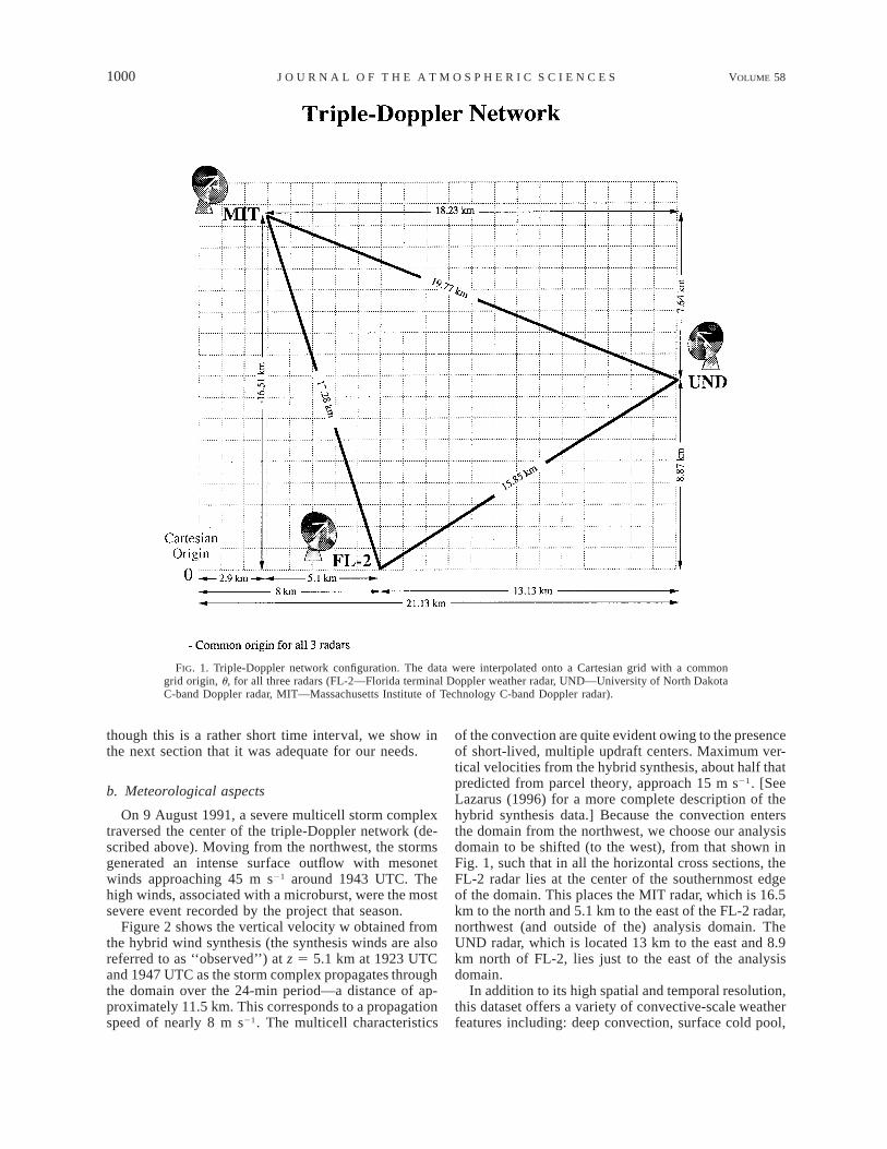
The three-dimensional wind field used in this workwas obtained from MIT/Lincoln Lab in conjunction withthe Federal Aviation Administration’s Terminal DopplerWeather Radar program near the Orlando InternationalAirport (Keohan et al. 1992). The network comprisedthree C-Band Doppler weather radars positioned in atriangular configuration, with baselines ranging from 16to 20 km (Fig. 1). A signal-to-noise ratio of 10 dB waschosen as a threshold for both the reflectivity and radialvelocity. Although this threshold is on the high side, theanalysis was not concerned with low signal events (e.g.,fine lines), it ensured that the data would be relativelynoisefree (M. Wolfson 1999, personal communication).The thresholded data were first interpolated to a 200-mCartesian grid by averaging specified range gates where-in the radials were subdivided by azimuth, range, andheight. The Cartesian-grided data were then hole-filledby both a linear and median filter with the latter beingapplied as a means for dealiasing. A synthetic hybridthree-dimensional wind analysis (DeLaura et al. 1989)was then applied and, within their baselines, the three-dimensional wind field was recovered. DeLaura et al.applied a hybrid methodology to perform this synthe-sis—using both the direct (Armijo 1969) and overde-termined dual-Doppler (Ray et al. 1980) methods toobtain the three-dimensional wind field.

In addition to the hybrid wind synthesis data, single-Doppler radial velocities and reflectivity data wereavailable from each of the three individual radars. Thedata are of very high temporal (3 min between volumescans) and space (200 m) resolution, and are availablefor 24 min (from 1923 to 1947, all times UTC). Al-


FIG. 1. Triple-Doppler network configuration. The data were interpolated onto a Cartesian grid with a commongrid origin, u, for all three radars (FL-2—Florida terminal Doppler weather radar, UND—University of North DakotaC-band Doppler radar, MIT—Massachusetts Institute of Technology C-band Doppler radar).

though this is a rather short time interval, we show inthe next section that it was adequate for our needs.

b. Meteorological aspects

On 9 August 1991, a severe multicell storm complextraversed the center of the triple-Doppler network (de-scribed above). Moving from the northwest, the stormsgenerated an intense surface outflow with mesonetwinds approaching 45 m s21 around 1943 UTC. Thehigh winds, associated with a microburst, were the mostsevere event recorded by the project that season.

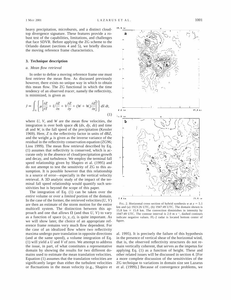
Figure 2 shows the vertical velocity w obtained fromthe hybrid wind synthesis (the synthesis winds are alsoreferred to as ‘‘observed’’) at z 5 5.1 km at 1923 UTCand 1947 UTC as the storm complex propagates throughthe domain over the 24-min period—a distance of ap-proximately 11.5 km. This corresponds to a propagationspeed of nearly 8 m s21. The multicell characteristics

of the convection are quite evident owing to the presenceof short-lived, multiple updraft centers. Maximum ver-tical velocities from the hybrid synthesis, about half thatpredicted from parcel theory, approach 15 m s21. [SeeLazarus (1996) for a more complete description of thehybrid synthesis data.] Because the convection entersthe domain from the northwest, we choose our analysisdomain to be shifted (to the west), from that shown inFig. 1, such that in all the horizontal cross sections, theFL-2 radar lies at the center of the southernmost edgeof the domain. This places the MIT radar, which is 16.5km to the north and 5.1 km to the east of the FL-2 radar,northwest (and outside of the) analysis domain. TheUND radar, which is located 13 km to the east and 8.9km north of FL-2, lies just to the east of the analysisdomain.

In addition to its high spatial and temporal resolution,this dataset offers a variety of convective-scale weatherfeatures including: deep convection, surface cold pool,

1 MAY 2001 1001L A Z A R U S E T A L .

FIG. 2. Horizontal cross section of hybrid synthesis w at z 5 5.1km and (a) 1923:26 UTC, (b) 1947:49 UTC. The domain shown is15.8 km 3 15.8 km. The convection diminishes in intensity by1947:49 UTC. The contour interval is 2.0 m s21 , dashed contoursindicate negative values. FL-2 radar is located bottom center offigure.

heavy precipitation, microbursts, and a distinct cloud-top divergence signature. These features provide a ro-bust test of the capabilities, limitations, and challengesthat face SDVR. Before applying the ZG scheme to theOrlando dataset (sections 4 and 5), we briefly discussthe moving reference frame characteristics.

3. Technique description

a. Mean flow retrieval

In order to define a moving reference frame one mustfirst retrieve the mean flow. As discussed previouslyhowever, there exists no unique way in which to obtainthis mean flow. The ZG functional in which the timetendency of an observed tracer, namely the reflectivity,is minimized, is given as

2]Z ]Z ]Z ]ZJ [ m 1 U 1 V 1 (W 1 W ) dx dt,E t5 6[ ]]T ]x ]y ]z

V

(1)

where U, V, and W are the mean flow velocities, theintegration is over both space dx (dx, dy, dz) and timedt and Wt is the fall speed of the precipitation (Kessler1969). Here, Z is the reflectivity factor in units of dBZ,and the weight m is given as the inverse variance of theresidual in the reflectivity conservation equation (ZG96;Liou 1999). The mean flow retrieval described by Eq.(1) assumes that reflectivity is conserved, which is ac-curate only in the absence of cloud/precipitation growthand decay, and turbulence. We employ the terminal fallspeed relationship given by Shapiro et al. (1995) anddo not attempt to test the sensitivity of ZG to this as-sumption. It is possible however that this relationshipis a source of error—especially in the vertical velocityretrieval. A 3D analytic study of the impact of the ter-minal fall speed relationship would quantify such sen-sitivities but is beyond the scope of this paper.

The integration of Eq. (1) can be taken over theentire volume or over a limited portion of the domain.In the case of the former, the retrieved velocities (U, V )are then an estimate of the storm motion for the entiremulticell system. The distinction between this ap-proach and one that allows V (and thus U, V ) to varyas a function of space (x, y, z), is quite important. Aswe will show later, the choice of an appropriate ref-erence frame remains very much flow dependent. Forthe case of an idealized flow where two reflectivitymaxima undergo pure translation in opposite directions(and at the same speed), a volume integration of Eq.(1) will yield a U and V of zero. We attempt to addressthe issue, in part, of what constitutes a representativedomain by showing the results for two different do-mains used to estimate the mean translation velocities.Equation (1) assumes that the translation velocities aresignificantly larger than either the turbulent velocitiesor fluctuations in the mean velocity (e.g., Shapiro et

al. 1995). It is precisely the failure of this hypothesisin the presence of vertical shear of the horizontal wind,that is, the observed reflectivity structures do not re-main vertically coherent, that serves as the impetus forapplying Eq. (1) as a function of height. These andother related issues will be discussed in section 4. [Fora more complete discussion of the sensitivities of theZG technique to variations in domain size see Lazaruset al. (1999).] Because of convergence problems, we


take m to be a constant, and thus it does not affect theminimum of the cost function in Eq. (1). Experimentswhere V is varied do indicate convergence if a suffi-ciently large number of grid points (on the order of20) are used to estimate m. However, results from theseexperiments are not significantly different from thosewhere m is taken to be constant. To obtain the meanflow velocity from Eq. (1), we proceed as in ZG byminimizing Eq. (1) (assuming W 5 0), which resultsin a 3 3 3 matrix associated with the linear Euler–Lagrange equations.

b. Perturbation flow retrieval

Because the retrieval is best performed in a movingreference frame that minimizes errors in the time de-rivative of the reflectivity field (ZG96), once the meanflow is obtained, one can proceed to transform both thereflectivity and radial wind equations from a fixed frameto a moving frame {see Liou [1999, Eq. (9)] for thetransformation equations}. Similar to the mean flow re-trieval, the minimization of the moving frame (trans-formed) functional,

2 2]Z ]Z ]Z ]Z x9 2 a9 y9 2 b9 z9 2 c9

J [ m9 1 u9 1 y9 1 (w9 1 W ) 1 y9 2 u9 2 y9 2 w9 dx9 dt9, (2)E t r5 1 2 1 2 6]t9 ]x9 ]y9 ]z9 r9 r9 r9x,t

yields a system of three linear equations in three un-knowns (i.e., the moving frame velocities, u9, y9, w9).Here, a9 5 a 2 UDt, b9 5 b 2 VDt, and c9 5 c arethe moving frame radar coordinates with respect to theradar location (x, y, z) 5 (a, b, c), Dt is the differencebetween the observation time and some reference time(i.e., the time the retrieval is valid), dx9 is area of in-tegration in the moving frame, and m9 and r9 are themoving frame weight and radar-to-gridpoint distance,respectively (see GZ96 for details). The total wind field(u, y , w) is then obtained by combining the mean (U, V)and perturbation winds (u9, y9, w9). Estimates of themean vertical velocity, which are nonzero for the re-trievals performed herein, are not used to transform thereflectivity and radial wind equations to a moving ref-erence frame. This will likely contribute to retrievalerror as proper minimization of the reflectivity time de-rivative depends on all three mean wind components.In practice, one might expect W to be small as the large-scale vertical motion is typically two orders of mag-nitude smaller than that of the deep convection. In thispaper, we concentrate our efforts on the moving frameas defined by the mean horizontal components only. Itwould, however, be instructive to examine the impactof this assumption (i.e., W 5 0) on the retrieval.

Because the radial wind conservation equation is em-ployed as a weak constraint, the retrieved radial windsproduced by this will not ‘‘exactly’’ match the observedradial wind. However, because the velocity stationarityassumption is likely violated [e.g., Lazarus et al. (1999,their Fig. 11)], it makes sense to choose a weak con-straint on y r. In the absence of reflectivity error, Lazaruset al. (1999) show that the reflectivity conservation con-straint is essential for the retrieval of the local flowvelocities, that is, radial wind information alone is notsufficient to determine the local flow. This is somewhatintuitive as if the radial wind were sufficient to deter-

mine the local flow, then a simple projection of y r ontothe Cartesian components would suffice. Because of theidealized nature of these results, it is difficult to ascertainwhat the impact would be for imperfect data. Ideally,if the weight in Eq. (1) is an accurate indicator of theamount of radial wind/reflectivity error, the two will beweighted appropriately. Additionally, the reflectivityconservation assumption will, at times, be violated fordeep convection—especially if it is rapidly evolving.Thus, assuming ‘‘perfect’’ reflectivity (i.e., a strong con-straint) may also be a source of retrieval error [see Laz-arus et al. (1999) for a discussion of the impact of re-flectivity errors in the presence of perfect radial winds].

4. Sensitivity tests

The ZG methodology described in sections 3a and 3bis applied to the deep convective storm discussed insection 2. Although single-Doppler radar data wereavailable from all three radars, only data from FL-2radar (see Fig. 1) were used in our retrieval experiments.This choice was purely arbitrary.

a. Statistics

The retrievals are performed on a nonstaggered grid,that is, all variables are collocated with the radial ve-locity and reflectivity. Grid spacings of Dx, Dy 5 400m, and Dz 5 200 m are used in the sensitivity testsdiscussed in this section. The results are quantified bycomparing the retrieved 3D velocity with the hybridwind synthesis via the volume rms error statistic; thatis,

obs ret 2(x 2 x )rms 5 , (3)O ! N

the mean flow statistic:

1 MAY 2001 1003L A Z A R U S E T A L .

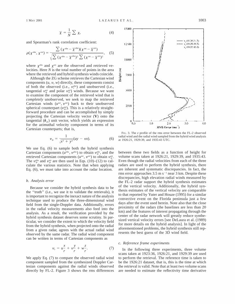
FIG. 3. The z profile of the rms error between the FL-2 observedradial wind and the radial wind sampled from the hybrid wind analysisat 1926:21, 1929:39, and 1935:43 UTC.

1x 5 x, (4)O

N

and Spearman’s rank correlation coefficient:

obs retobs ret(x 2 x )(x 2 x )Oobs retr(x , x ) 5 , (5)

obs retobs 2 ret 2(x 2 x ) (x 2 x )ÎO Owhere xobs and xret are the observed and retrieved ve-locities. Here N is the total number of points in the areawhere the retrieved and hybrid synthesis winds coincide.

Although the ZG scheme retrieves the Cartesian windcomponents (u, y , w) directly, these components consistof both the observed (i.e., ) and unobserved (i.e.,obsy r

tangential and polar ) winds. Because we wantret rety yf u

to examine the component of the retrieved wind that iscompletely unobserved, we seek to map the retrievedCartesian winds (uret , y ret) back to their unobservedspherical counterpart ( ). This is a relatively straight-rety f

forward procedure and can be accomplished by simplyprojecting the Cartesian velocity vector (V) onto thetangential (ef ) unit vector, which yields an expressionfor the azimuthal velocity component in terms of itsCartesian counterparts; that is,

1y 5 (uy 2 yx). (6)f 2 2Îx 1 y

We use Eq. (6) to sample both the hybrid synthesisCartesian components (uobs, y obs) to obtain , and theobsy f

retrieved Cartesian components (uret , y ret) to obtain .rety f

The and are then used in Eqs. (10)–(12) to cal-obs rety yf f

culate the various statistics. Note that when applyingEq. (6), we must take into account the radar location.

b. Analysis error

Because we consider the hybrid synthesis data to bethe ‘‘truth’’ (i.e., we use it to validate the retrievals), itis important to recognize the inexact nature of the analysistechnique used to produce the three-dimensional windfield from the single-Doppler data. Additionally, errorsin the radial velocity measurements also feed into theanalysis. As a result, the verification provided by thehybrid synthesis dataset deserves some scrutiny. In par-ticular, we consider the extent to which the velocity fieldfrom the hybrid synthesis, when projected onto the radialfrom a given radar, agrees with the actual radial windobserved by the same radar. The radial wind componentcan be written in terms of Cartesian components as

x y zy 5 u 1 y 1 w . (7)r r r r

We apply Eq. (7) to compare the observed radial windcomponent sampled from the synthesized Doppler Car-tesian components against the radial winds observeddirectly by FL-2. Figure 3 shows the rms differences

between these two fields as a function of height forvolume scans taken at 1926:21, 1929:39, and 1935:43.Even though the radial velocities from each of the threeradars are used to perform the hybrid synthesis, thereare inherent and systematic discrepancies. In fact, therms error approaches 3.5 m s21 near 3 km. Despite thesediscrepancies, high elevation radial winds measured bythe FL-2 radar support the hybrid synthesis estimatesof the vertical velocity. Additionally, the hybrid syn-thesis estimates of the vertical velocity are comparableto that reported by Yuter and Houze (1995) for a similarconvective event on the Florida peninsula just a fewdays after the event used herein. Note also that the closeproximity of the radars (the baselines are less than 20km) and the features of interest propagating through thecenter of the radar network will greatly reduce synthe-sized vertical velocity errors [see DeLaura et al. (1989)for more details on the hybrid analysis]. In light of theaforementioned problems, the hybrid synthesis still rep-resents the best guess of the 3D wind field.

c. Reference frame experiments

In the following three experiments, three volumescans taken at 1923:36, 1926:21, and 1929:39 are usedto perform the retrieval. The reference time is taken tobe the 1926:21 dataset, that is, this is the time at whichthe retrieval is valid. Note that at least two volume scansare needed to estimate the reflectivity time derivative


TABLE 1. Statistical comparison between the SDVR and hybridwind synthesis data for experiments with varying reference frames.

Exp. yf rms yf(r) y f y r rms y r(r) y r

OBSNMVMVLVL

3.0223.0713.159

0.4520.4960.535

0.7931.0031.4520.879

4.0403.7543.667

0.6190.6980.702

22.1200.7320.3830.330

but the algorithm does not require that the volume scansbe evenly spaced in time. We performed experimentswhere the number of volume scans were varied fromtwo to four. The results of these experiments (not shownhere) are consistent with those of Xu et al. (1994a,b)and Xu et al. (1995) and ZG96—showing an improvedcross-beam wind retrieval with increasing number ofvolume scans. With the exception of experiment LVLin Table 1, the experiments performed in the movingreference frame are performed using a mean flow de-termined by a volume integration of Eq. (1). Note thatwe use the observed radial wind rather than that sampledfrom the hybrid synthesis to calculate the y r rms statis-tics. Consequently, the interpretation of the error sta-tistics for the radial component are somewhat morestraightforward than those for the tangential component.However, if one assumes that the synthesis errors in thecross-beam component obtained from the hybrid tech-nique are comparable to the radial wind errors shownin Fig. 3 (the best-case scenario), then errors in theretrieved tangential component can be interpreted in asimilar manner as its radial wind counterpart. Unfor-tunately, in the latter case, it is impossible to separatethe error contribution from the hybrid synthesis fromthat of the retrieval.

In theory, the perturbation flow can be retrieved usinga single point. Yet because observation errors can leadto matrix ill-conditioning for the linear system of equa-tions, it is necessary to involve neighboring points inthe calculation of the perturbation flow (ZG96). Theaddition of these surrounding points, which define thearea of integration [dx9, Eq. (2)], has a stabilizing effecton the solution but does so at the expense of potentiallyremoving detail from the retrieved wind field. Carboneet al. (1985) have demonstrated that, at close range, oneneeds at least 6–8 radar samples to resolve a completewave. For the following experiments we choose a dx9of 4D (where D 5 400 m represents only the x and ydirections). We performed experiments whereby dx9 wasvaried but for the sake of brevity these results are notpresented here. Our choice of dx9 yields a sufficientnumber of surrounding points such that the solution ofperturbation flow equation is stable, preserves as muchdetail in the retrieved winds as possible, and resolvesthe features of interest.

The results of three experiments are presented in Ta-ble 1. Also shown are the hybrid synthesis mean radialand tangential wind components (OBS). ExperimentNMV is performed in a nonmoving reference frame

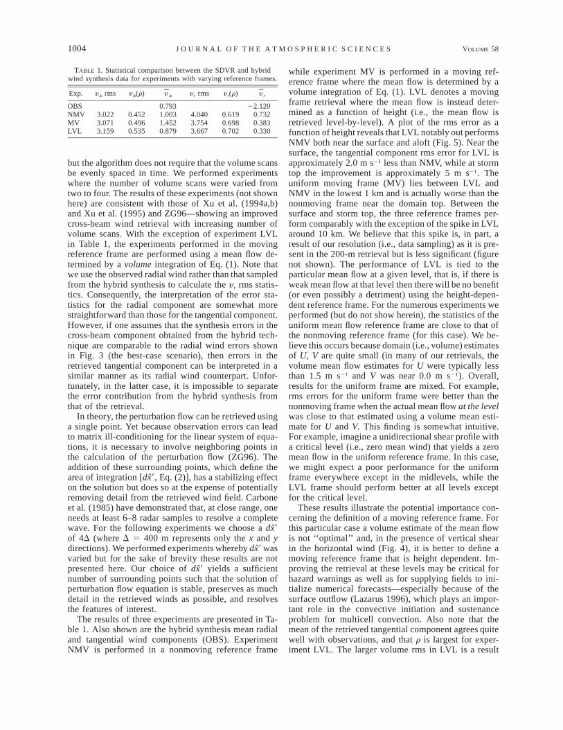
while experiment MV is performed in a moving ref-erence frame where the mean flow is determined by avolume integration of Eq. (1). LVL denotes a movingframe retrieval where the mean flow is instead deter-mined as a function of height (i.e., the mean flow isretrieved level-by-level). A plot of the rms error as afunction of height reveals that LVL notably out performsNMV both near the surface and aloft (Fig. 5). Near thesurface, the tangential component rms error for LVL isapproximately 2.0 m s21 less than NMV, while at stormtop the improvement is approximately 5 m s21. Theuniform moving frame (MV) lies between LVL andNMV in the lowest 1 km and is actually worse than thenonmoving frame near the domain top. Between thesurface and storm top, the three reference frames per-form comparably with the exception of the spike in LVLaround 10 km. We believe that this spike is, in part, aresult of our resolution (i.e., data sampling) as it is pre-sent in the 200-m retrieval but is less significant (figurenot shown). The performance of LVL is tied to theparticular mean flow at a given level, that is, if there isweak mean flow at that level then there will be no benefit(or even possibly a detriment) using the height-depen-dent reference frame. For the numerous experiments weperformed (but do not show herein), the statistics of theuniform mean flow reference frame are close to that ofthe nonmoving reference frame (for this case). We be-lieve this occurs because domain (i.e., volume) estimatesof U, V are quite small (in many of our retrievals, thevolume mean flow estimates for U were typically lessthan 1.5 m s21 and V was near 0.0 m s21). Overall,results for the uniform frame are mixed. For example,rms errors for the uniform frame were better than thenonmoving frame when the actual mean flow at the levelwas close to that estimated using a volume mean esti-mate for U and V. This finding is somewhat intuitive.For example, imagine a unidirectional shear profile witha critical level (i.e., zero mean wind) that yields a zeromean flow in the uniform reference frame. In this case,we might expect a poor performance for the uniformframe everywhere except in the midlevels, while theLVL frame should perform better at all levels exceptfor the critical level.

These results illustrate the potential importance con-cerning the definition of a moving reference frame. Forthis particular case a volume estimate of the mean flowis not ‘‘optimal’’ and, in the presence of vertical shearin the horizontal wind (Fig. 4), it is better to define amoving reference frame that is height dependent. Im-proving the retrieval at these levels may be critical forhazard warnings as well as for supplying fields to ini-tialize numerical forecasts—especially because of thesurface outflow (Lazarus 1996), which plays an impor-tant role in the convective initiation and sustenanceproblem for multicell convection. Also note that themean of the retrieved tangential component agrees quitewell with observations, and that r is largest for exper-iment LVL. The larger volume rms in LVL is a result

1 MAY 2001 1005L A Z A R U S E T A L .

FIG. 4. The z profile of the observed mean wind u component (solidcurve) and y component (dashed curve) at 1926:21 UTC from thehybrid wind synthesis data.

FIG. 6. The z profile of the mean tangential wind component at1926:21 UTC for the observations (long dashed curve), nonmoving(solid curve), uniform moving (dotted), and level-by-level (shortdashed curve) reference frames. Note the improvement above andbelow for the moving reference frame. The profiles are taken fromthe sensitivity tests NMV, MV, and LVL in Table 1.

FIG. 5. The z profile of the rms error in the tangential wind com-ponent for the nonmoving (solid curve), uniform moving (dottedcurve), and level-by-level (dashed curve) reference frames at 1926:21 UTC. The profiles are taken from the sensitivity tests NMV, MV,and LVL in Table 1.

of the ‘‘spike’’ near 10 km (see Fig. 5). Figure 6, whichdepicts the mean profiles for the observed and retrievedtangential velocity, reveals that the LVL overestimates(by approximately 5 m s21) the magnitude of the cross-beam component at this level. A similar ‘‘spike’’ is pre-sent in NMV as well but is closer to that observed.

5. Tangential velocity retrieval

In this section, we focus on the results of one par-ticular retrieval that is valid at reference time 1935:43UTC. For the sake of brevity, we refer only to thisretrieval (R35) while the statistics associated with twocomparable retrievals, valid at reference times 1926:21and 1929:39 (R26 and R29), are displayed for compar-ison purposes in Table 2 and discussed in section 5b.

We choose a dx9 of 6D as we perform these retrievalsusing the radar data at its highest resolution (i.e., anisotropic grid with D 5 200 m). As discussed previ-ously, this choice reflects a compromise between so-lution stability, the filtering of small-scale noise (un-resolvable features, random data errors, etc.), and a suc-cessful retrieval of the resolvable-scale winds. As in thesensitivity tests in section 4, the single-Doppler datawere obtained from the FL-2 radar. However, we usefour volume scans for R35 instead of three as in thesensitivity experiments. Figure 7 shows the reference


TABLE 2. Statistical comparison between the SDVR and hybrid wind synthesis data for all three retrievals.

Retr yf rms yf(r) y f Retr y f Obs y r rms y r(r) y r Retr y r Obs *y r rms *y r Retr

R26R29R35

2.933.102.90

0.5730.5660.773

0.8290.6620.214

0.8390.8170.289

3.823.874.26

0.6860.7230.700

0.470.480.53

22.1121.9622.12

2.783.223.67

21.1921.2120.98

FIG. 7. Schematic diagram indicating the single-Doppler volumescans that are used for the retrievals. The time in bold indicates theretrieval reference time.

times given in bold for all three retrievals. Although asfew as two volume scans would suffice for each retriev-al, we use four volume scans here. The missing data at1932:25 do not pose a logistical problem in that the ZGretrieval can accommodate missing or irregularly spaceddata (in time or space). The use of an increased numberof volume scans yields slightly improved retrievals. Itis important to point out however that this may notalways be the case as an increased number of volumescans increases the likelihood that the reflectivity con-servation constraint will be violated. We feel howeverthat the time resolution of our dataset is sufficient toavoid, for the most part, any significant errors associatedwith the velocity stationarity assumption. Problems as-sociated with sparse data can be overcome, more ap-propriately, by introducing a smoothing function di-rectly into the ZG functional (e.g., Liou 1999).

In section 5a, we present and compare the results ofR35 in both the nonmoving and moving referenceframes (where the mean flow is determined as a functionof height, e.g., LVL). In section 5b we compare thevolume-averaged statistics from R35 with those ob-tained from R26 and R29.

a. R35

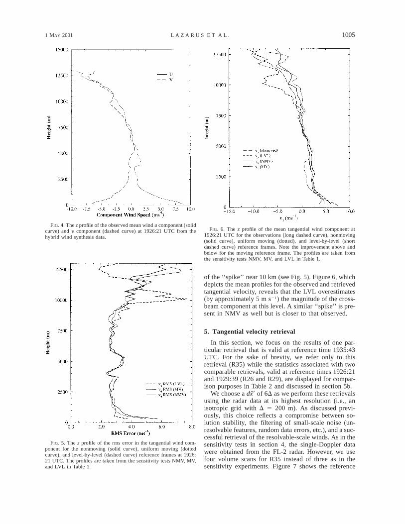
R35 illustrates the importance of the moving refer-ence frame as defined by integrating Eq. (1) as a functionof height. Figure 8 depicts the horizontal cross sectionof the tangential wind component at z 5 0.3 km for thehybrid Doppler observations and nonmoving and mov-ing reference frames, respectively. (This is the lowestlevel for which the retrieval is performed.) The contourinterval is 2.0 m s21 in all cross sections unless other-wise stated. Although data exists as low as 100 m, cen-tered spatial differences preclude the use of the lowestlevel because the reflectivity is not known below thislevel. It is important to point out that the retrieval ofthe tangential component represents a severe test of the

SDVR as this component is completely unobserved. Theretrieved moving frame yf maximum (21.7 m s21) isrelatively close to that observed (25.8 m s21), while thenonmoving frame significantly underestimates the max-imum yf (7.6 m s21). The retrieved maximum is as-sociated with a feature in the eastern portion of thedomain. To the east of this feature, the moving framerecovers another region where the retrieved yf is quiteclose to the maximum. The location of this secondsmaller feature agrees quite nicely with the observedmaximum. Neither the stationary nor moving frame re-trievals recover the region to the west where yf , 0.

Because the convection extends over a depth of 14km, it is important to evaluate the retrieval performanceat higher elevations as well. Figure 9 is the same as Fig.8, except at z 5 8.3 km. This level was selected some-what arbitrarily but is representative of the retrieval per-formance in the midlevels of the multicell convection.At this level, the moving and nonmoving frames per-form equally well—each captures the overall divergencepattern of yf . The mean flow velocities, U and V [asdetermined from (1)], are 0.6 m s21 and 21.0 m s21,respectively, compared to 5.1 m s21 and 21.8 m s21 atz 5 0.3 km. The reduced mean flow at z 5 8.3 kmsuggests that the moving frame does not benefit theretrieval at this level compared to the near-surface re-trieval where the mean winds are stronger (a direct resultof the cold pool). In the case where the mean flow isrelatively small, such as z 5 8.3 km, interpolation errorsencountered as a result of shifting the coordinate systemmay actually overwhelm the error reduction due to min-imization of the reflectivity time derivative.

The retrieved stationary frame minimum (23.6 ms21) is close to the moving frame minimum (23.1 ms21) and both are quite a bit less than observed (212.0m s21). The retrieved stationary frame maximum (3.5m s21) and moving frame maximum (4.6 m s21) aresomewhat less than the observed (6.0 m s21). The yf

couplet in the northeast portion of the domain is re-trieved quite well in both reference frames, and eachrecovers a weak couplet near the southern edge as wellas a region (running southeast to northwest) of relativemaximum yf . Despite some agreement with the obser-vations, the retrieval limitations are obvious, as thesmall-scale features in the observations are not recov-ered in either reference frame retrieval. Time and spaceintegrations stabilize the least squares problem via av-eraging, yet a direct result of this filtering is the removalof both small-scale signal and noise. Liou (1999) hasshown that the addition of mass conservation into the

1 MAY 2001 1007L A Z A R U S E T A L .

FIG. 8. Horizontal cross section of the tangential wind componentat z 5 0.3 km and 1935:43 UTC for the (a) observations, (b) ZGnonmoving frame, and (c) ZG moving frame. The domain shown is15.8 km 3 15.8 km. Note the improvement in both the orientationand the magnitude of yf in the moving reference frame. The contourinterval is 2.0 m s21, dashed contours indicate negative values.

cost function [Eq. (1)] can significantly improve the ZGretrieval at low elevation angles.

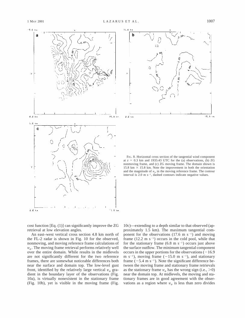
An east–west vertical cross section 4.8 km north ofthe FL-2 radar is shown in Fig. 10 for the observed,nonmoving, and moving reference frame calculations ofyf . The moving frame retrieval performs relatively wellover the entire domain. While results in the midlevelsare not significantly different for the two referenceframes, there are somewhat noticeable differences bothnear the surface and domain top. The low-level gustfront, identified by the relatively large vertical yf gra-dient in the boundary layer of the observations (Fig.10a), is virtually nonexistent in the stationary frame(Fig. 10b), yet is visible in the moving frame (Fig.

10c)—extending to a depth similar to that observed (ap-proximately 1.5 km). The maximum tangential com-ponent for the observations (17.6 m s21) and movingframe (12.2 m s21) occurs in the cold pool, while thatfor the stationary frame (6.8 m s21) occurs just abovethe surface outflow. The minimum tangential componentoccurs in the upper portions for the observations (216.9m s21), moving frame (215.0 m s21), and stationaryframe (25.4 m s21). Note the significant difference be-tween the moving frame and stationary frame retrievalsas the stationary frame yf has the wrong sign (i.e., .0)near the domain top. At midlevels, the moving and sta-tionary frames are in good agreement with the obser-vations as a region where yf is less than zero divides


FIG. 9. Horizontal cross section of the tangential wind componentat z 5 8.3 km and 1935:43 UTC for the (a) observations, (b) ZGnon moving frame, and (c) ZG moving frame. The domain shown is15.8 km 3 15.8 km. Note that at this level, there is no improvementin the yf retrieval in the moving reference frame. The contour intervalis 2.0 m s21, dashed contours indicate negative values.

regions to the east and west where yf is greater thanzero. The moving frame does not retrieve the full mag-nitude of the tangential component in these regions, butdoes exhibit a relative minimum in both areas.

Figure 11 shows the rms errors in yf as functions ofheight for the nonmoving and moving frames are quitesimilar. (We do not show the rms profile for the uniformmoving frame case because it is similar to that of thenonmoving retrieval due to the weak mean flow at thistime.) The rms errors are consistent with vertical profilesof the observed and retrieved mean tangential winds(not shown) which indicate that the moving referenceframe out performs the nonmoving frame in the lowerand upper levels only (from 3.0 to 9.0 km, the retrieved

moving and stationary frame y f were close to zero).Midlevel rms errors for the two reference frames arequite similar. In contrast, in the regions where the meanflow is large, that is, near the surface and the domaintop (z . 11 km), the moving frame significantly im-proves the results. Below 2.5 km, the rms errors for themoving frame retrieval are less than the stationaryframe, with the largest improvement just above the sur-face where the moving frame rms is approximately 2.5m s21 less than the stationary frame. The advantage ofthe moving frame above 9 km is also clearly demon-strated as it yields rms errors that are as much as 4.5m s21 less than the stationary frame. The general in-crease in rms errors in these regions (i.e., above 9 km

1 MAY 2001 1009L A Z A R U S E T A L .

FIG. 10. Vertical x–z cross section of the tangential wind componentat y 5 4.8 km north of FL-2 and 1935:43 UTC for the (a) observations,(b) ZG nonmoving frame, and (c) ZG moving frame. The domainshown is 15.8 km 3 14.6 km. The contour interval is 2.0 m s21,dashed contours indicate negative values.

and below 1.5 km) for both reference frames primarilyreflects the larger velocity magnitudes associated withthe surface outflow and the upper-level divergence sig-natures. It is also possible that errors increase (above 9km) as a result of the large elevation angles. The com-bination of the high elevation angles and the proximityof the convection imply that the radial wind ‘‘sees’’more of the Cartesian vertical component than it doesthe horizontal components. Consequently, it is possiblethat the retrieval has a difficult time gleaning infor-mation (about U and V) from the radial wind constraintin the upper levels of the domain.

The weak constraint on the radial velocity given sug-gests that it might be possible to use the radial windretrieval error as a possible gauge or quality controlmeasure for the tangential component. Because radialwind measurements will be available, error statistics canbe calculated and perhaps used to ‘‘flag’’ those regions,

which have the potential to produce erroneous tangentialwind information. Unfortunately, the results herein in-dicate no correlation between the errors in the retrievedradial component and those of the retrieved tangentialcomponent. To illustrate, Fig. 12 shows a vertical profileof the rms error in yf and y r for R35. The profile, rep-resentative of all three retrievals, indicates little, if anycorrelation between the errors in the radial and tangen-tial winds. Attempts were made to evaluate the utilityof other error measures, none of which indicated theycould be used reliably as a quality control parameter.

b. Comparison of R35, R26, and R29

For comparison purposes we show the volume-av-eraged statistics for the retrieval presented in section 5awith those of R26 and R29 (Table 2). All variables havethe same definitions as in Table 1. The results for all


FIG. 11. The z profile of the rms error in the tangential wind com-ponent for the nonmoving (solid curve) and moving (dashed curve)reference frames at 1935:43 UTC.

FIG. 12. The z profile of the rms error in the retrieved tangential(dashed curve) and radial (solid curve) wind component at 1935:43UTC for the moving frame.

three retrievals are quite similar. R35 yields the bestresults with small tangential component errors and avolume correlation coefficient more than 10.20 betterthan for the other two retrievals. (The improved statisticsmay result from the storm complex entering a relativelysteady period and/or a result of the closer proximity ofthe observations to the radar at this time.) Radial ve-locity statistics are calculated using all three retrievedcomponents in Eq. (8), and calculated using Eq. (8)without the retrieved vertical velocity (denoted by anasterisk). The marked improvement reflected by the lat-ter statistic suggests that the retrieved vertical velocityobtained from ZG has large errors (see section 6).

6. Vertical velocity retrieval

Heretofore the discussion has been limited to the re-trieval of the tangential velocity component. At lowelevation angles, the observed radial component andretrieved tangential component, in tandem, describemost of the observed horizontal flow (provided that theerrors in the retrieved fields are not large). The resultsin section 5 indicate, for the most part, that retrievalerror magnitudes (in the tangential component) are com-parable to the discrepancy between the hybrid synthesisradial winds and those observed directly by the FL-2radar (see Fig. 3). Heretofore, however, there has beenno assessment of the retrieval of the vertical motionfield. In this section we discuss the ZG retrieval of w

for R35. The results for the other two retrievals aresimilar and will not be shown.

For brevity, we compare horizontal cross sections ofthe observed vertical velocity and that obtained fromR35 at z 5 5.1 km only (Figs. 13a,b, respectively). Thislevel is representative of the overall performance of theZG w retrieval. The observations at z 5 5.1 km indicatethat a line of convection running southwest to northeastis recovered by ZG, albeit somewhat crudely. The ob-servations indicate sinking motion over the northern halfof the domain, while the retrieval shows some sinkingmotion or relatively weak upward motion. At this level,r 5 0.38 and the rms error is relatively large (5.7 ms21). The volume-averaged w rms error is 5.6 m s21

(nearly twice that of the horizontal components) and ris 0.27.

The generally poor w retrievals obtained by the ZGscheme are likely a consequence of several factors, oneof which involves the absence of a kinematic constrainton the vertical velocity (e.g., mass conservation; Liou1999). In particular, this may explain the degraded re-sults near the surface where the observed w tends tozero but the retrieved w can be arbitrary as it is not tiedto any lower boundary condition. Errors associated withthe terminal fall speed assumption may also be impor-tant. Another factor may be the moving frame definitionitself—which takes into account the mean horizontalflow but not the vertical. (Results from our experimentssuggest that W is not zero.) Another potential influence

1 MAY 2001 1011L A Z A R U S E T A L .

FIG. 13. Horizontal cross section of w at z 5 5.1 km and 1935:43UTC for (a) observations, and (b) ZG—moving frame. The domainshown is 15.8 km 3 15.8 km. The contour interval is 2.0 m s21,dashed contours indicate negative values.

may be intrinsic to the flow itself whereby the surfaceoutflow and upper-level divergence patterns are persis-tent features in contrast to the more transient nature ofthe updrafts over the 24-minute observation span. In thenext section, we discuss several alternative methods todeduce w and compare these results with those obtainedvia the ZG methodology.

a. Kinematic and O’Brien techniquesVertical velocities obtained using the retrieved hori-

zontal wind field as input to the kinematic technique

were unrealistic (not shown)—an artifact of the un-specified top boundary condition in combination withdivergence estimates contaminated by error. This canbe particularly problematic in the case where the hor-izontal wind field is provided by a retrieval. Because ofthe large errors in estimating w using the kinematictechnique, O’Brien (1970) sought an alternative methodto obtain physically realistic values of the vertical mo-tion field. By taking into account the variation of thedivergence error with height, the variational formulationposed by O’Brien provides an objective adjustment tothe divergence, which yields improved estimates of w.Our estimates of the vertical velocity using the O’Brienmethod were improved over that of the kinematic meth-od. However, we still found the magnitude of the verticalvelocity to be more than twice that of the observations.In contrast with the kinematic method, w is fixed (setto zero) at both top and bottom boundaries in theO’Brien technique. This will likely improve the resultsnear the boundary where the extra condition has beenapplied, provided that the observed w actually ap-proaches zero at that boundary.

b. Modified O’Brien technique

Because of the aforementioned difficulties associatedwith obtaining a realistic vertical velocity we derive analternative method. Note that for the kinematic andO’Brien techniques discussed previously and the fol-lowing technique, the vertical velocity is not estimatedin the data-void regions. Estimates of the divergence onthe periphery of the data region are also rejected. Inaddition, we use a variable elevation for the top of theintegration domain—defined as the level (in that col-umn) above which the reflectivity observations are miss-ing.

The proximity of the convection to the radar suggeststhat the observed radial velocity, especially in the midto upper levels of the storm, might be used to obtainan improved estimate of w. This, along with the resultsof the O’Brien technique, serves as the motivation be-hind the development of what we call the modifiedO’Brien method. In it, we use the divergence of theretrieved winds in the lower portion of the storm, alongwith the radial velocity in the mid-to-upper levels, soas to take advantage of the large correlation betweenthe radial wind and the vertical velocity at high elevationangles.

Assuming that the radial velocity is observed and thatthe velocity retrieval yields estimates of the horizontalwind field, we can adjust the unknown vertical com-ponent subject to two weak constraints: mass conser-vation and a Cartesian coordinate–radial velocity rela-tionship expressed by the following functional:


2r r a]ru ]ry ]rwr r a o 2J 5 a[ru x 1 ry y 1 r(w 1 W )z 2 rry ] 1 1 1 dV, (8)E t r5 6[ ]]x ]y ]zV

where denotes the observed radial velocity; a is aoy r

three-dimensional weight; r is the base-state density(e.g., given by a sounding); ur and y r are the retrievedhorizontal winds from ZG; wa is the adjusted (unknown)vertical velocity; x, y, and z are the Cartesian coordi-nates; r is the radar-to-grid point distance; V representsa 3D volume in Cartesian space; Wt is the raindropterminal velocity defined by Eq. (2); and all other var-iables have their previously defined meanings. Bousquetand Chong (1998) combine elements of Eq. (8) aboveto perform a multiple-Doppler synthesis. Their analysiscouples a least squares formulation of the overdeter-mined dual-Doppler problem (Ray and Sangren 1983)with mass conservation and smoothness constraints.Bousquet and Chong’s technique, designed for multipleradars, simultaneously adjusts all three wind compo-nents (here we adjust the vertical component only). Asan alternative to the modified O’Brien technique pre-sented here, one could apply mass conservation directlyto Eq. (2)—creating a modified ZG technique that di-rectly builds in a dynamical constraint and adjusts allthree wind components similar to the Bousquet andChong. The advantage of the modified O’Brien (or ZG)technique over that of the Bousquet and Chong methodis it requires only single-Doppler winds and reflectivity.Liou (1999) added a mass conservation constraint to theZG method and produced improved retrievals of thehorizontal wind components for a synthetic dataset atlow-elevation angles. Analogous to the modifiedO’Brien technique presented here, Liou suggests thatthe vertical component can be derived from his modifiedZG method if the horizontal components are retrievedwith sufficient accuracy. Ideally, a combination of theLiou approach and that presented herein for the verticalvelocity may produce the best 3D wind retrieval.

Anticipating that a should depend explicitly upon z,we set a(x, y, z) 5 g(x, y) 3 zp, where p is an unde-termined exponent. Minimizing Eq. (8) with respect torwa and setting J equal to zero yields a second-orderinhomogeneous ordinary differential equation:

2d W21p2 gWz 5 F, (9)

2dz

where F is given as

11p r r oF 5 gz [ru x 1 ry y 1 rW z 2 rry ]t r

r r] ]ru ]ry2 1 , (10)[ ]]z ]x ]y

W 5 rwa, and as additional constraints, we require thevertical velocity to vanish at the domain top and bottom.

Applying the method of variation of parameters (e.g.,Kreysig 1983), we can solve Eq. (9) and after sometedious algebra (see appendix for the details), arrive atthe following solution:

HK [h(H )]nW(z) 5 ÏzI (h) 2Ïz*nFI (h) dz*n E n5 I [h(H )]n 0

H

2 2Ïz*nFK (h) dz*E n

0

z

1 2Ïz*nFK (h) dz*E n 60

z

2 ÏzK (h) 2Ïz*nFI (h) dz*, (11)n E n

0

where we have applied the impermeable boundary con-ditions on W. Here In(h) and Kn(h) are modified Besselfunctions of the first and second kind, respectively, n5 1/(4 1 p), h 5 2n gz1/2n, H is the domain depth,Ïand the asterisk denotes a dummy variable.

The weights (g) are determined by the inverse vari-ance of the integrated horizontal divergence and radialvelocity in a vertical column; that is,

2H r r]ru ]ry1 dzE 1 2]x ]y0

g(x, y) 5 . (12)H

o 2 p(rry ) z dzE r

0

We tested other weights, including a single volume-averaged quantity (i.e., horizontally homogeneous),which yielded inferior results to those given by Eq. (12).

A series of experiments were conducted to determinethe optimum value of p. Vertical velocity rms errorswere calculated for a sequence of simulations using theZG retrieved winds from the sensitivity experiment LVLgiven in Table 1. The lowest volume rms errors werefound to occur for values of p ø 1.5 (figure not shown).Thus, as the elevation angle increases, the relative im-portance of the radial velocity also increases. Intuitively,this makes sense because, as a scanning radar samplesat higher elevation angles, it detects a larger fraction ofthe vertical velocity.

As in the kinematic and O’Brien techniques testedabove, the input horizontal winds are those output fromR26. Figure 16 depicts the retrieved vertical velocityfield obtained via the modified O’Brien technique. Themodified O’Brien technique yields magnitudes that are

1 MAY 2001 1013L A Z A R U S E T A L .

FIG. 14. Horizontal cross section of observed w at z 5 7.5 km and1926:21 UTC. The domain shown is 15.8 km 3 15.8 km. The max-imum (minimum) observed w is 10.4 m s21 (211.6 m s21). Thecontour interval is 2.0 m s21, dashed contours indicate negative val-ues.

FIG. 16. Horizontal cross section of retrieved w at z 5 7.5 km and1926:21 UTC for the modified O’Brien method. The domain shownis 15.8 km 3 15.8 km. The maximum (minimum) w is 24.3 m s21

(218.9 m s21). The contour interval is 2.0 m s21, dashed contoursindicate negative values.

FIG. 17. The z profile of the w rms error at 1926:21 UTC for ZG(solid curve), modified O’Brien (thick dashed curve), O’Brien (solidcurve with circles), and kinematic (thin dashed curve) techniques.

FIG. 15. Horizontal cross section of retrieved w at z 5 7.5 km and1926:21 UTC for the ZG method. The domain shown is 15.8 km 315.8 km. The maximum (minimum) w is 17.9 m s21 (24.8 m s21).The contour interval is 2.0 m s21, dashed contours indicate negativevalues.

much closer to that of the observed w (Fig. 14) thanthe ZG method (Fig. 15). Significant improvements areotherwise obvious—especially the highly correlated up-drafts and downdrafts. The rms errors as a function ofheight for the three techniques are shown in Fig. 17.The vertical error profile underscores the significant im-


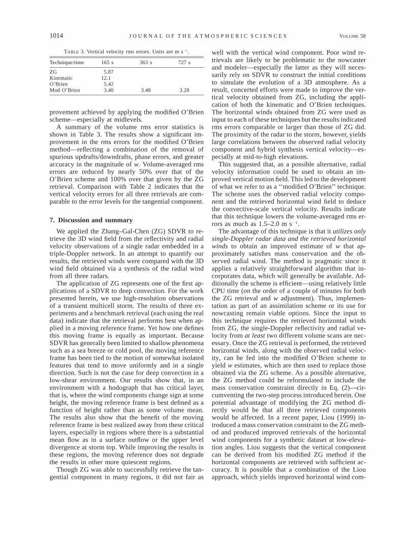
TABLE 3. Vertical velocity rms errors. Units are m s21.

Technique/time 165 s 363 s 727 s

ZGKinematicO’BrienMod O’Brien

5.8712.15.423.40 3.48 3.28

provement achieved by applying the modified O’Brienscheme—especially at midlevels.

A summary of the volume rms error statistics isshown in Table 3. The results show a significant im-provement in the rms errors for the modified O’Brienmethod—reflecting a combination of the removal ofspurious updrafts/downdrafts, phase errors, and greateraccuracy in the magnitude of w. Volume-averaged rmserrors are reduced by nearly 50% over that of theO’Brien scheme and 100% over that given by the ZGretrieval. Comparison with Table 2 indicates that thevertical velocity errors for all three retrievals are com-parable to the error levels for the tangential component.

7. Discussion and summary

We applied the Zhang–Gal-Chen (ZG) SDVR to re-trieve the 3D wind field from the reflectivity and radialvelocity observations of a single radar embedded in atriple-Doppler network. In an attempt to quantify ourresults, the retrieved winds were compared with the 3Dwind field obtained via a synthesis of the radial windfrom all three radars.

The application of ZG represents one of the first ap-plications of a SDVR to deep convection. For the workpresented herein, we use high-resolution observationsof a transient multicell storm. The results of three ex-periments and a benchmark retrieval (each using the realdata) indicate that the retrieval performs best when ap-plied in a moving reference frame. Yet how one definesthis moving frame is equally as important. BecauseSDVR has generally been limited to shallow phenomenasuch as a sea breeze or cold pool, the moving referenceframe has been tied to the motion of somewhat isolatedfeatures that tend to move uniformly and in a singledirection. Such is not the case for deep convection in alow-shear environment. Our results show that, in anenvironment with a hodograph that has critical layer,that is, where the wind components change sign at someheight, the moving reference frame is best defined as afunction of height rather than as some volume mean.The results also show that the benefit of the movingreference frame is best realized away from these criticallayers, especially in regions where there is a substantialmean flow as in a surface outflow or the upper leveldivergence at storm top. While improving the results inthese regions, the moving reference does not degradethe results in other more quiescent regions.

Though ZG was able to successfully retrieve the tan-gential component in many regions, it did not fair as

well with the vertical wind component. Poor wind re-trievals are likely to be problematic to the nowcasterand modeler—especially the latter as they will neces-sarily rely on SDVR to construct the initial conditionsto simulate the evolution of a 3D atmosphere. As aresult, concerted efforts were made to improve the ver-tical velocity obtained from ZG, including the appli-cation of both the kinematic and O’Brien techniques.The horizontal winds obtained from ZG were used asinput to each of these techniques but the results indicatedrms errors comparable or larger than those of ZG did.The proximity of the radar to the storm, however, yieldslarge correlations between the observed radial velocitycomponent and hybrid synthesis vertical velocity—es-pecially at mid-to-high elevations.

This suggested that, as a possible alternative, radialvelocity information could be used to obtain an im-proved vertical motion field. This led to the developmentof what we refer to as a ‘‘modified O’Brien’’ technique.The scheme uses the observed radial velocity compo-nent and the retrieved horizontal wind field to deducethe convective-scale vertical velocity. Results indicatethat this technique lowers the volume-averaged rms er-rors as much as 1.5–2.0 m s21.

The advantage of this technique is that it utilizes onlysingle-Doppler radar data and the retrieved horizontalwinds to obtain an improved estimate of w that ap-proximately satisfies mass conservation and the ob-served radial wind. The method is pragmatic since itapplies a relatively straightforward algorithm that in-corporates data, which will generally be available. Ad-ditionally the scheme is efficient—using relatively littleCPU time (on the order of a couple of minutes for boththe ZG retrieval and w adjustment). Thus, implemen-tation as part of an assimilation scheme or its use fornowcasting remain viable options. Since the input tothis technique requires the retrieved horizontal windsfrom ZG, the single-Doppler reflectivity and radial ve-locity from at least two different volume scans are nec-essary. Once the ZG retrieval is performed, the retrievedhorizontal winds, along with the observed radial veloc-ity, can be fed into the modified O’Brien scheme toyield w estimates, which are then used to replace thoseobtained via the ZG scheme. As a possible alternative,the ZG method could be reformulated to include themass conservation constraint directly in Eq. (2)—cir-cumventing the two-step process introduced herein. Onepotential advantage of modifying the ZG method di-rectly would be that all three retrieved componentswould be affected. In a recent paper, Liou (1999) in-troduced a mass conservation constraint to the ZG meth-od and produced improved retrievals of the horizontalwind components for a synthetic dataset at low-eleva-tion angles. Liou suggests that the vertical componentcan be derived from his modified ZG method if thehorizontal components are retrieved with sufficient ac-curacy. It is possible that a combination of the Liouapproach, which yields improved horizontal wind com-

1 MAY 2001 1015L A Z A R U S E T A L .

ponents, and that presented herein for the vertical ve-locity may produce the best 3D wind retrieval. This doesnot diminish, however, our findings, which demonstratethat the choice of a particular reference frame can beimportant. Unlike some retrieval techniques, the ZGmethod can easily accommodate various referenceframe definitions.

It is important to point out that the retrieved verticalmotion field from the modified O’Brien technique maybe overly optimistic due to the uncharacteristically largeelevation angles and the storm proximity to the radar.Additionally, typical operational WSR-88D scan strat-egies produce volume scans on the order of 5 min—nearly twice that of the data used in this study. As shownhere, even with high temporal resolution, rapidly evolv-ing features may be problematic and the benefits of anincreased number of volume scans to the retrieval maybe somewhat reduced or offset by phase and amplitudeerrors in the retrieved wind field. Further evaluation ofboth the modified technique and the ZG methodologyon other datasets is necessary, especially data obtainedoperationally where the observations are likely to betaken less frequently and at a greater distance from theradar. The question of what constitutes a ‘‘good’’ re-trieval has been relegated to a somewhat simple eval-uation in terms of rms error. While it would certainlybe advantageous to use other indicators to gauge thequality of the retrieval, for example, a model initiali-zation and forecast, we defer this to future work.

Acknowledgments. A special note of appreciation isin order for Dr. Tzvi Gal-Chen, who developed the par-ticular SDVR technique investigated herein. Dr. Gal-Chen passed away 5 years ago, yet the fact that his workcontinues to be of such utility reflects his intellectualpursuits and lasting contributions to the field of mete-orology. We also extend a special thanks to our col-leagues and friends, Sue Weygandt for assisting withthe figures, and Jian Zhang, coauthor of the SDVR tech-nique used herein. Our discussions stimulated manythoughts and ideas related to single-Doppler retrievals.

The hybrid wind synthesis dataset and soundingswere obtained from Lincoln Laboratory with softwaresupport made available through Dr. Marilyn Wolfson ofLincoln Lab/MIT. The computations were performed onthe IBM RISC System 6000 in conjunction with com-puter support from the Center for Analysis and Predic-tion of Storms. This research represents part of the leadauthor’s Ph.D. thesis at the School of Meteorology, Uni-versity of Oklahoma, and was supported by the NationalScience Foundation under Grants ATM91-20009 andATM-92-22576.

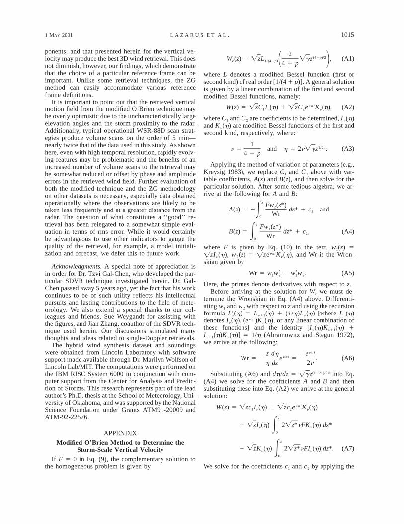
APPENDIX

Modified O’Brien Method to Determine theStorm-Scale Vertical Velocity

If F 5 0 in Eq. (9), the complementary solution tothe homogeneous problem is given by

2(41p)/2W (z) 5 ÏzL Ïgz , (A1)c 1/(41p)1 24 1 p

where L denotes a modified Bessel function (first orsecond kind) of real order [1/(4 1 p)]. A general solutionis given by a linear combination of the first and secondmodified Bessel functions, namely:

np iW(z) 5 ÏzC I (h) 1 ÏzC e K (h), (A2)1 n 2 n

where C1 and C2 are coefficients to be determined, In(h)and Kn(h) are modified Bessel functions of the first andsecond kind, respectively, where:

11/2nn 5 and h 5 2nÏgz . (A3)

4 1 p

Applying the method of variation of parameters (e.g.,Kreysig 1983), we replace C1 and C2 above with var-iable coefficients, A(z) and B(z), and then solve for theparticular solution. After some tedious algebra, we ar-rive at the following for A and B:

z Fw (z*)2A(z) 5 2 dz* 1 c andE 1Wr0

z Fw (z*)1B(z) 5 dz* 1 c , (A4)E 2Wr0

where F is given by Eq. (10) in the text, w1(z) 5zIn(h), w2(z) 5 zenpiKn(h), and Wr is the Wron-Ï Ï

skian given by

Wr 5 w1 2 w2.w9 w92 1 (A5)

Here, the primes denote derivatives with respect to z.Before arriving at the solution for W, we must de-

termine the Wronskian in Eq. (A4) above. Differenti-ating w1 and w2 with respect to z and using the recursionformula (h) 5 Ln11(h) 1 (n/h)Ln(h) [where Ln(h)L9ndenotes In(h), (enpi)Kn(h), or any linear combination ofthese functions] and the identity [In(h)Kn11(h) 1In11(h)Kn(h)] 5 1/h (Abramowitz and Stegun 1972),we arrive at the following:

np iz dh enp iWr 5 2 e 5 2 . (A6)

h dz 2n

Substituting (A6) and dh/dz 5 gz(122y )/2y into Eq.Ï(A4) we solve for the coefficients A and B and thensubstituting these into Eq. (A2) we arrive at the generalsolution:

np iW(z) 5 Ïzc I (h) 1 Ïzc e K (h)1 n 2 n

z

1 ÏzI (h) 2Ïz*nFK (h) dz*n E n

0

z

2 ÏzK (h) 2Ïz*nFI (h) dz*. (A7)n E n

0

We solve for the coefficients c1 and c2 by applying the


impermeable boundary conditions on W. Note that Ky

grows without bound as z approaches zero, and does sofaster than z → 0 (Abramowitz and Stegun 1972);Ïconsequently, we set c2 5 0. On the top boundary (atz 5 H) Eq. (A7) yields:

HK [h(H )]nc 5 2Ïz*nFI (h) dz*1 E nI [h(H )]n 0

H

2 2Ïz*nFK (h) dz*, (A8)E n

0

where h(H) 5 2y gH 1/2y .ÏSubstituting c2 5 0 and Eq. (A8) back into Eq. (A7)

yields the solution [Eq. (11) in the text] to the variationalproblem given by Eq. (8).

REFERENCES

Abromowitz, M., and I. E. Stegun, 1972: Handbook of Mathematicswith Formulas, Graphs, and Mathematical Tables. National Bu-reau of Standards Applied Mathematics Series, Vol. 55, U.S.Dept. of Commerce, 1046 pp.

Armijo, L., 1969: A theory for the determination of wind and pre-cipitation velocities with Doppler radars. J. Atmos. Sci., 26, 570–573.

Bousquet, O., and Michel Chong, 1998: A Multiple-Doppler Syn-thesis and Continuity Adjustment Technique (MUSCAT) to re-cover wind components from Doppler radar measurements. J.Atmos. Oceanic Technol., 15, 343–359.

Carbone, R. E., M. J. Carpenter, and C. D. Burghart, 1985: Dopplerradar sampling limitations in convective storms. J. Atmos. Oce-anic Technol., 2, 357–361.

Crook, A., and J. D. Tuttle, 1994: Numerical simulations initializedwith radar-derived winds. Part II: Forecasts of three gust frontcases. Mon. Wea. Rev., 122, 1204–1217.

DeLaura, R., M. M. Wolfson, and P. S. Ray, 1989: A hybrid Cartesianwindfield synthesis technique using a triple-Doppler radar net-work. Preprints, 25th Int. Conf. on Radar Meteorology, Paris,France, Amer. Meteor. Soc., 240–243.

Droegemeier, K. K., 1990: Toward a science of storm-scale predic-tion. Preprints, 16th Conf. on Severe Local Storms, KananaskisPark, AB, Canada, Amer. Meteor. Soc., 256–262., 1997: The numerical prediction of thunderstorms: Challenges,potential benefits, and results from realtime operational tests.WMO Bull., 46, 324–336.

Gal-Chen, T., 1982: Errors in fixed and moving frame of references:Applications for conventional and Doppler radar analysis. J. At-mos. Sci., 39, 2279–2300.

Hane, C. E., 1993: Storm motion estimates derived from dynamic-retrieval calculations. Mon. Wea. Rev., 121, 431–443.

Keohan, C. F., M. C. Liepins, C. A. Meuse, and M. M. Wolfson,1992: Summary of triple-Doppler data; Orlando 1991. FederalAviation Administration Project Report DOT/FAA/NR-92/2.

Kessler, E., 1969: On the Distribution and Continuity of Water Sub-stance in Atmospheric Circulations. Meteor. Monogr., No. 32,Amer. Meteor. Soc., 84 pp.

Kreysig, E., 1983: Advanced Engineering Mathematics. 5th ed. JohnWiley and Sons, 988 pp.

Lazarus, S. M., 1996: The assimilation and prediction of a Floridamulticell storm using single-Doppler data. Ph.D. dissertation,University of Oklahoma, 345 pp. [Available from School ofMeteorology, 100 East Boyd, Norman, OK 73019.], A. Shapiro, K. Droegemeier, 1999: Analysis of the Gal-Chen–Zhang single-Doppler velocity retrieval. J. Atmos. Oceanic Tech-nol., 16, 5–18.

Lilly, D. K., 1990: Numerical prediction of thunderstorms—Has itstime come? Quart. J. Roy. Meteor. Soc., 116, 779–798.

Liou, Y., 1999: Single radar recovery of cross-beam wind componentsusing a modified moving frame of reference technique. J. Atmos.Oceanic Technol., 16, 1003–1016.

O’Brien, J. J., 1970: Alternative solutions to the classical verticalvelocity problem. J. Appl. Meteor., 9, 197–203.

Ray, P. S., and K. L. Sangren, 1983: Multiple-Doppler radar networkdesign. J. Climate Appl. Meteor., 22, 1444–1454., C. L. Zeigler, W. Bumgarner, and R. J. Serafin, 1980: Singleand multiple-Doppler radar observations of tornadic storms.Mon. Wea. Rev., 108, 129–147.

Shapiro, A., S. Ellis, and J. Shaw, 1995: Single-Doppler velocityretrievals with Pheonix-II data: Clear air and microburst windretrievals in the planetary boundary layer. J. Atmos. Sci., 52,1265–1287.

Sun, J., and A. Crook, 1994: Wind and thermodynamic retrieval fromsingle-Doppler measurements of a gust front observed duringPheonix II. Mon. Wea. Rev., 122, 1075–1091., and , 1998: Dynamical and microphysical retrieval fromDoppler radar observations using a cloud model and its adjoint.Part II: Retrieval experiments of an observed Florida convectivestorm. J. Atmos. Sci., 55, 835–852.

Tuttle, J. D., and G. B. Foote, 1990: Determination of the boundarylayer airflow from a single-Doppler radar. J. Atmos. OceanicTechnol., 7, 218–232.

Weygandt, S., A. Shapiro, and K. K. Droegemeier, 1995: Adaptationof a single-Doppler velocity retrieval on a deep-convectivestorm. Preprints, 27th Conf. on Radar Meteorology, Vail, CO,Amer. Meteor. Soc., 264–266.

Xu, Q., Chong-Jian Qiu, and Jin-Xiang Yu, 1994a: Adjoint methodretrievals of low-altitude wind fields from single-Doppler re-flectivity measured during Pheonix-II. J. Atmos. Oceanic Tech-nol., 11, 275–288., , and , 1994b: Adjoint method retrievals of low-al-titude wind fields from single-Doppler wind data. J. Atmos. Oce-anic Technol., 11, 579–585., , H.-D. Gu, and Jin-Xiang Yu, 1995: Simple adjoint re-trievals of microburst winds from single-Doppler radar data.Mon. Wea. Rev., 123, 1822–1833.

Yuter, S. E., and R. A. Houze 1995: Three-dimensional kinematicand microphysical evolution of Florida cumulonimbus. Part I:Spatial distribution of updrafts, downdrafts, and precipitation.Mon. Wea. Rev., 123, 1921–1940.

Zhang, J., and T. Gal-Chen, 1996: Single-Doppler wind retrieval inthe moving frame of reference. J. Atmos. Sci., 53, 2609–2623.

Application of the Zhang-Gal-Chen Single-Doppler Velocity Retrieval to a Deep Convective Storm

Documents

Transcript of Application of the Zhang-Gal-Chen Single-Doppler Velocity Retrieval to a Deep Convective Storm