Study on Classification of Plant Images using Combined Classifier
*Corresponding author E-mail adress : [email protected], fax : +33 (0)1 45 92 55 01 LTN, Institut National de recherche sur les Transports et leur Sécurité, Le Descartes 2 ‐ 2 rue de la Butte Verte. 93166 Noisy‐le‐Grand Cedex
Fault diagnosis in railway track circuits using Dempster-Shafer
classifier fusion
Latifa Oukhellou a,b*, Alexandra Debiolles c, Thierry Denœux d, Patrice Aknin b
a Certes, Université Paris XII, 61 Av du Gal de Gaulle 94110 Créteil France b LTN, Institut National de recherche sur les Transports et leur Sécurité, 2 Av Malleret Joinville 94114 Arcueil France
c SNCF, ingénierie IG SF 43, 4 et 6 Av François Mitterrand, 93574 La plaine St Denis France d Heudiasyc, Université de Technologie de Compiègne, UMR CNRS 6599, BP 20529, 60205 Compiègne France
xxxxxxxxxxxxxxxx
Abstract
This paper addresses the problem of fault detection and isolation in railway track circuits. A track circuit can be
considered as a large-scale system composed of a series of trimming capacitors located between a transmitter and
a receiver. A defective capacitor affects not only its own inspection data (short circuit current) but also the
measurements related to all capacitors located downstream (between the defective capacitor and the receiver).
Here, the global fault detection and isolation problem is broken down into several local pattern recognition
problems, each dedicated to one capacitor. The outputs from local neural network or decision tree classifiers are
expressed using Dempster-Shafer theory and combined to make a final decision on the detection and localization
of a fault in the system. Experiments with simulated data show that correct detection rates over 99 % and correct
localization rates over 92% can be achieved using this approach, which represents a major improvement over the
state of the art reference method.
Keywords: Classifier Fusion, Belief Functions, Neural Networks, Evidence Theory, Transferable Belief Model, Fault
Detection and Isolation, Pattern Recognition.
hal-0
0467
941,
ver
sion
1 -
29 M
ar 2
010
Author manuscript, published in "Engineering Applications of Artificial Intelligence 23, 1 (2010) 117-128" DOI : 10.1016/j.engappai.2009.06.005
2
1. Introduction
Complex industrial systems need to be monitored continuously to detect dysfunctions and maintain a
good quality of service. In the railway domain, the infrastructure is often inspected by instrumented
vehicles in order to ensure a high level of safety and availability within a predictive maintenance
framework. For some applications, signals recorded during inspection runs are manually analyzed by
maintenance experts and technicians in order to identify anomalies. In this case, there is a need for
automatic fault detection and isolation (FDI) systems, which can reduce the time consumed by the analysis
phase and improve the diagnosis performances. The aim of such systems is to detect the occurrence of a
fault based on recorded measurements and then determine the exact nature and location of the fault.
Maintainers are thus provided with an accurate and systematic analysis of recordings that allows them to
schedule preventive maintenance appropriately.
Various approaches can be adopted in order to build an automatic FDI system, depending on the
available knowledge of the system under study. In the so-called model-based approach, an accurate model
of the system is typically assumed to be available. Several approaches have been proposed to exploit
analytical redundancy, including parity space equations, state observers and process identification [17]
[21] [24] [30] [33]. In contrast, the pattern recognition approach to fault diagnosis uses only a set of
historical data containing representative measurements acquired under various normal and abnormal
conditions [33] [11]. In most cases, an initial pre-processing stage, referred to as feature extraction, maps
data from the measurement space to a reduced feature space relevant to the FDI task. Machine learning
techniques (such as decision trees, neural networks or support vector machines [14][4][23]) then capture
the relationships between feature values and system states, based on learning data. To ensure good
generalization, this approach requires some knowledge of the system to extract relevant features, as well as
a large and exhaustive labelled database covering most of the situations that can be encountered in
practice. A comparison between the model-based and pattern recognition approaches is given in [33], and
an approach to fault diagnosis based on trend analysis is presented in [28].
This paper presents a method for FDI in railway track circuits based on a statistical pattern recognition
approach. Track circuits generally use a scheduled maintenance regime: inspection is carried out on every
track circuit periodically (typically, every 15 days) and inspection recordings are analyzed visually in
order to detect major defects. Recent work on fault detection and diagnosis for railway track circuits has
been published in [3]. The authors proposed a neuro-fuzzy system that makes it possible to detect and
diagnose the most common track circuit failures in a laboratory test rig. The diagnosis system proposed
here differs since it uses a train-based approach and it is dedicated to detect different kind of defects.
A track circuit is composed of a series of trimming capacitors connected between the two rails [1] [18].
Part of the difficulty of FDI task for this system arises from the fact that the presence of a fault in one
subsystem (trimming capacitor) influences the inspection signal of other subsystems located downstream
hal-0
0467
941,
ver
sion
1 -
29 M
ar 2
010

3
(between the defective capacitor and the receiver). This is depicted schematically in Figure 1, where
S1,…,SN represent the N trimming capacitors, and Ii denotes the inspection signal (measurement) for
capacitor Si. A fault in Si influences the inspection signals corresponding to all capacitors between Si and
SN. Consequently, the fault isolation task must take into account the spatial relationship between
subsystems: an abnormal measurement from one subsystem may indicate a fault in that subsystem or in
any of the subsystems located upstream of it.
. . .S1 S2 S3 S4 SN
defectivesubsystem
. . .I1 I2 I3 I4 IN
unchangedsignal modified signal
PhysicalSubsystems
Inspectioninformation
measuringprocess
Upstream Downstream
Fig.1. Spatial relationship between subsystems: a defective subsystem (S3) influences the inspection signals I3, I4,…,IN related to
downstream subsystems.
The approach presented here uses machine learning (neural networks, decision trees) and information
fusion techniques to perform fault detection and isolation. Each capacitor is classified as fault-free or
defective using a neural network or decision tree classifier and the local decisions are combined to make a
final decision regarding the presence and location of a fault.
Training a neural network classifier involves minimizing the discrepancy between the neural network
outputs and target outputs encoding class membership of training patterns. Consequently, an output coding
scheme has to be chosen. Two such schemes will be tested and evaluated. In the first one, only the target
output related to the defective subsystem is set to 1 (the others being set to 0). This scheme may be
referred to as local coding. Alternatively, the target outputs of both the defective subsystem and the
subsystems located downstream of it may be set to 1; in this case, the coding is said to be distributed. Each
classifier thus provides information on the presence of a fault either in a specific subsystem (local coding)
or in any of the subsystems located upstream (distributed coding).
A large number of methods for classifier fusion have been proposed. For many applications, it has been
shown that combining classifiers can yield performance improvements [2] [41] [16] [27]. Depending on
the information provided by the individual classifiers, three categories of fusion methods can be
distinguished [25] [42]:
- When each classifier produces a single class label output (crisp label), the two most representative
approaches are majority voting [26], and the behaviour-knowledge space (BKS) method [20].
hal-0
0467
941,
ver
sion
1 -
29 M
ar 2
010
4
- The second group of fusion methods is of the rank level decision type, i.e., the output of each
classifier is a subset of possible labels ranked by plausibility. The fusion strategies applied on
outputs of this type are based on class set reduction, class set reordering or a combination of both
[19]. The first approach aims at reducing the set of considered classes while the objective of the
second one is to place the true class as close as possible to the top.
- The third and largest group of fusion methods operates on classifiers that produce so-called soft
labels in the range [0,1]. These methods can be based on Bayesian Probability theory [27] [34],
Possibility Theory [31] [13] [44] or the theory of belief functions, also referred to as Dempster-
Shafer or evidence theory [11] [12] [5] [22] [43]. The method investigated here is based on the
latter approach, which provides a flexible framework for handling uncertainty and managing the
conflict between several classifiers.
The rest of the paper is organized as follows. Section 2 describes the application under study and
introduces the diagnosis problem in greater detail. The necessary notions of Dempster-Shafer theory are
then recalled in Section 3. A system for fault detection and isolation in track circuits based on classifier
fusion in the Dempster-Shafer framework is then presented in Section 4. Experimental results are finally
reported in Section 5, and Section 6 concludes the paper.
2. Case study
The application considered in this paper concerns FDI in railway track circuits. This device will first be
described in Section 2.1, and the problem addressed will be exposed in Section 2.2. An overview of the
proposed FDI method will then be presented in Section 2.3.
2.1. Track circuit principle
The track circuit is an essential component of the automatic train control system. Its main function is to
detect the presence or absence of vehicle traffic within a specific section of railway track. The signalling
system uses the occupation of track section to protect trains from coming into conflict. On French high
speed lines, the track circuit is also a fundamental component of the track/vehicle transmission system. It
uses a specific carrier frequency to transmit coded data to the train, for example the maximum authorized
speed on a given section on the basis of safety constraints.
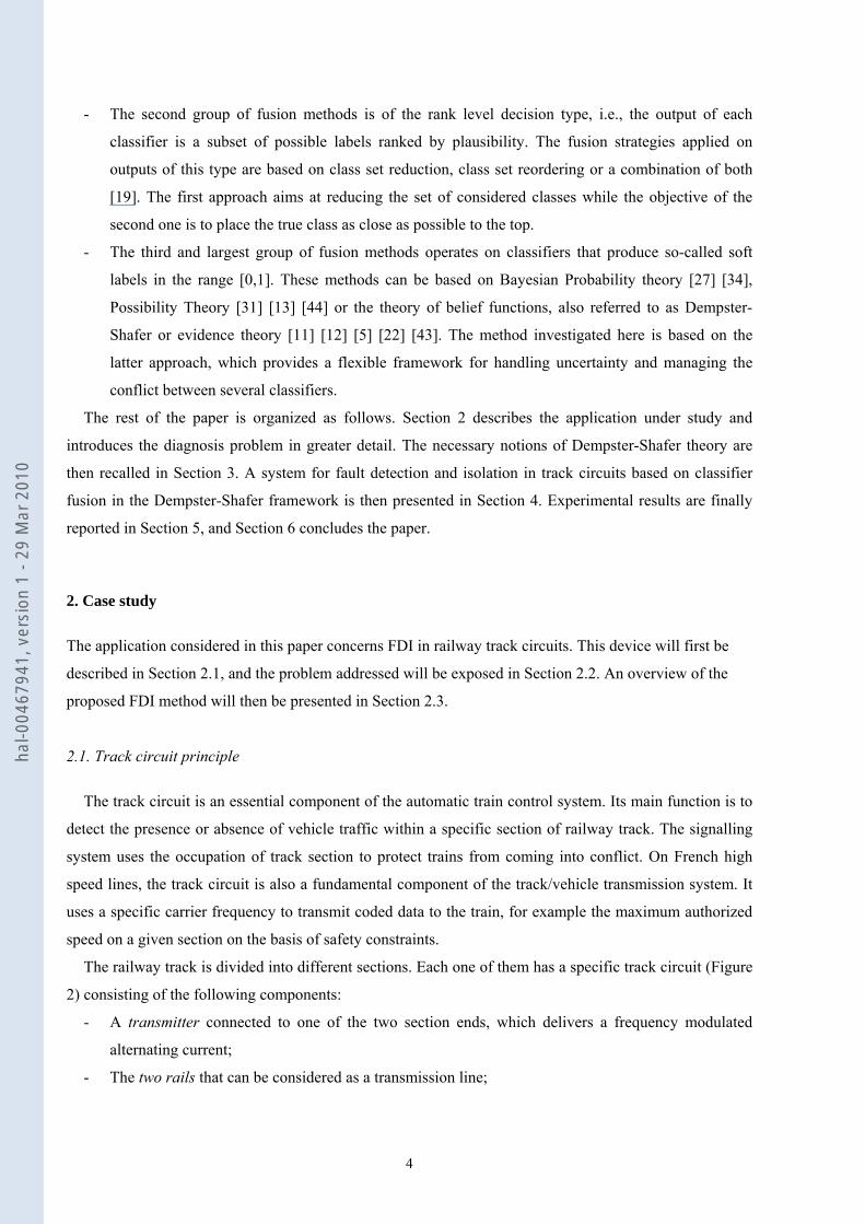
The railway track is divided into different sections. Each one of them has a specific track circuit (Figure
2) consisting of the following components:
- A transmitter connected to one of the two section ends, which delivers a frequency modulated
alternating current;
- The two rails that can be considered as a transmission line;
hal-0
0467
941,
ver
sion
1 -
29 M
ar 2
010
5
- At the other end of the track section, a receiver that essentially consists of a trap circuit used to
avoid the transmission of information to the neighbouring section;
- Trimming capacitors connected between the two rails at constant spacing to compensate for the
inductive behaviour of the track. Electrical tuning is then performed to limit the attenuation of the
transmitted current and improve the transmission level. The number of compensation points
depends on the carrier frequency and the length of the track section.
Icc
transmitter receiverrail
rail
C : trimming capacitors
Icc
trimming cell
track circuit
axle running direction
Experimental signal
C C C CC
Icc
position (meter)
(Ampere)
Fig. 2. Diagram of a track circuit and example of an inspection signal.
The rails themselves are part of the track circuit, and a train is detected when its wheels and axles short-
circuit the track. The presence of a train in a given section induces the loss of track circuit signal due to
shorting by train wheels. The drop of the received signal below a preset threshold indicates that the section
is occupied. In order to make the transmitted information specific to each track section and to minimize the
influence of both longitudinal interference and transverse crosstalk, four frequencies are used for adjacent
and parallel track circuits. Neighbouring track circuits are also isolated electrically by using tuned circuits
(capacitor and inductance) on both the transmitter and the receiver.
2.2. Problem description
The different parts of the track circuit are subject to malfunctions (due to aging, atmospheric conditions
or track maintenance operations) that must be detected as soon as possible in order to maintain the system
at the required safety and availability levels. In the most extreme cases, such malfunctions can cause a
significant attenuation of the transmitted signal which may induce signalling problems. The purpose of
hal-0
0467
941,
ver
sion
1 -
29 M
ar 2
010
6
system diagnosis is to inform maintainers about track circuit failures, thus ensuring that the quality of
transmitted information remains high.
A vehicle-based fault diagnosis system can be developed by equipping an inspection vehicle with a
sensor in front of the first axle. The carrier current level of the short-circuit current (Icc) is picked up by
the sensor coils and recorded at each position of the train, while the track circuit is shunted by the
inspection train itself (Figure 2).
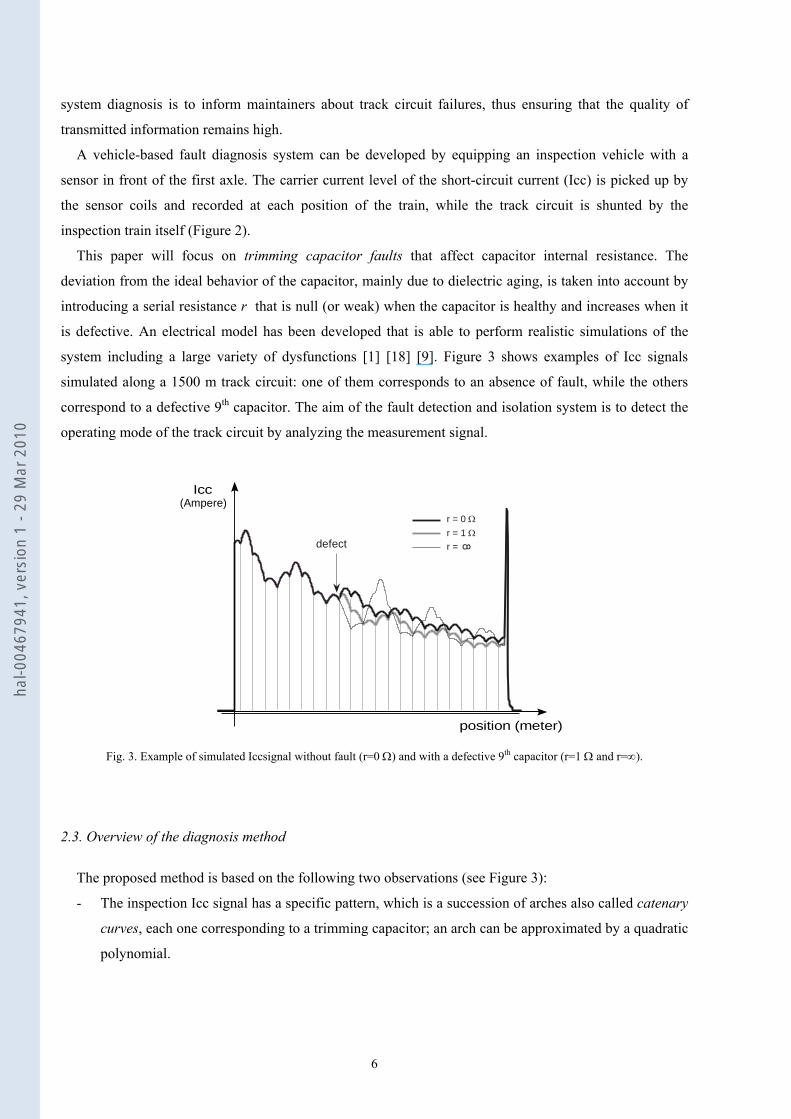
This paper will focus on trimming capacitor faults that affect capacitor internal resistance. The
deviation from the ideal behavior of the capacitor, mainly due to dielectric aging, is taken into account by
introducing a serial resistance r that is null (or weak) when the capacitor is healthy and increases when it
is defective. An electrical model has been developed that is able to perform realistic simulations of the
system including a large variety of dysfunctions [1] [18] [9]. Figure 3 shows examples of Icc signals
simulated along a 1500 m track circuit: one of them corresponds to an absence of fault, while the others
correspond to a defective 9th capacitor. The aim of the fault detection and isolation system is to detect the
operating mode of the track circuit by analyzing the measurement signal.
r = 0 Ωr = 1 Ωr =defect
Icc
position (meter)
(Ampere)
Fig. 3. Example of simulated Iccsignal without fault (r=0 Ω) and with a defective 9th capacitor (r=1 Ω and r=∞).
2.3. Overview of the diagnosis method
The proposed method is based on the following two observations (see Figure 3):
- The inspection Icc signal has a specific pattern, which is a succession of arches also called catenary
curves, each one corresponding to a trimming capacitor; an arch can be approximated by a quadratic
polynomial.
hal-0
0467
941,
ver
sion
1 -
29 M
ar 2
010

7
- The presence of a fault in the system only affects the shape of the arches between the fault and the
receiver leaving the signal upstream (between the transmitter and the fault) unchanged.
The proposed method consists in extracting features from the Icc signal, and training one classifier for
each trimming capacitor. Elementary classifier outputs are then represented using the formalism of belief
functions and combined. Finally, a decision regarding the presence and location of a fault is made.
3. Dempster-Shafer theory
This section will provide a brief account of the fundamental notions of the Dempster-Shafer theory of
belief functions, also referred to as Evidence Theory. This uncertain reasoning framework was initiated by
Dempster [10] and developed by Shafer [35]. It can be seen as an extension of Bayesian Probability
Theory. A particular interpretation of Dempster-Shafer theory has been proposed by Smets [37], under the
name of the Transferable Belief Model (TBM). The TBM has a two-level structure composed of
- a credal level where beliefs are entertained, and
- a pignistic level where decisions are made.
In this section, we shall define only the concepts used in the diagnosis method introduced below. Further
details can be found in [36] [37] [38] [39][32].
3.1. Representation of beliefs: the credal level
Let Θ denote the set of possible answers to a given problem, called the frame of discernment. Here,
Θ will be assumed to be finite:
{ }1 2θ θ θΘ = n, , ..., . (1)
A basic belief assignment (BBA) is a function m from 2Θ to [0,1] that assigns a “mass of belief” to each
subset A of the frame of discernment Θ, such that:
( ) 1.A
m A⊆Θ
=∑ (2)
The basic belief mass m(A) represents a measure of the belief that is assigned to subset A⊆Θ, given the
available evidence, and that cannot be committed to any strict subset of A. Every A⊆Θ such that m(A)>0 is
called a focal set. A BBA such that ( ) 0∅ =m , where ∅ denotes the empty set, is said to be normal. The
quantity ( )∅m can be interpreted as that part of belief that is committed to the assumption that none of the
hypotheses in Θ might be true (open-world assumption). When ( ) 1Θ =m , m is called a vacuous BBA: it
represents total ignorance regarding the question under consideration.
hal-0
0467
941,
ver
sion
1 -
29 M
ar 2
010

8
Example 1: Let Θ={θ1,θ2,θ3} denote the possible states of a system under study, where θ1 is the normal
state, and the other two states are faulty. Assume that we have some evidence that the system is in a faulty
state (but we do not know which one), and we have a degree of confidence of 0.8 in this piece of evidence.
This information can be represented as the following BBA:
{ }( )( )
1 2 3
1
, 0.8
0.2.
m
m
θ θ =
Θ =
We note that the mass 0.8 is attached to {θ2,θ3} because the piece of evidence only tells us that the system
is in a faulty state, without pointing specifically to θ2 or θ3. The remaining mass of 0.2 is not assigned to θ1
as no evidence points to that particular hypothesis. It remains uncommitted and attached to the whole
frame of discernment.
3.2. Combination of several BBAs
To combine several BBAs defined on the same frame of discernment, Smets introduced the conjunctive
rule of combination, also referred to as the unnormalized Dempster’s rule [39]. For this rule to be used, the
different BBAs must be based upon independent pieces of evidence. Let m1 and m2 be two BBAs. The
BBA that results from their conjunctive combination, denoted by 1 2∩m m , is defined for all ⊆ ΘA as:
( ) ( ) ( )1 2 1 2, :
.B C B C A
m m A m B m C⊆Θ ∩ =
∩ = ∑ (3)
This rule is commutative and associative. When combining n BBAs m1,…,mn, we may thus either use
(3) iteratively, or use the following direct formula:
( ) ( ) ( )1
1 1 1 .n
n n nB B A
m m A m B m B∩ ∩ =
∩ ∩ = ∑…
… … (4)
The mass ( )∅m assigned to the empty set may be interpreted as a measure of conflict between the two
sources.
Example 2: Continuing Example 1, assume that we receive another independent piece of evidence telling
us that the system is not in state θ2, with confidence 0.6. This evidence may be represented by the
following BBA:
{ }( )( )
2 1 3
2
, 0.6
0.4.
m
m
θ θ =
Θ =
Combining m1 and m2 using (3) yields the BBA m=m1 ∩m2 defined as follows:
hal-0
0467
941,
ver
sion
1 -
29 M
ar 2
010

9
{ }( ){ }( ){ }( )
( )
3
2 3
1 3
0.8 0.6 0.48
, 0.8 0.4 0.32
, 0.2 0.6 0.12
0.2 0.4 0.08.
m
m
m
m
θ
θ θ
θ θ
= × =
= × =
= × =
Θ = × =
We observe that the masses still sum to one.
3.3. Discounting
The reliability of a source of information can be taken into account by discounting the original BBA m
by a discount rate 1-α, where α is a coefficient between 0 and 1. The smaller the reliability, the larger is
the discount rate. The resulting BBA αm is defined by [35] [40]:
( ) ( )( ) ( )
, ,
1 1 .
m A m A A
m m
α
α
α
α
= ∀ ⊂ Θ
Θ = − − Θ⎡ ⎤⎣ ⎦ (5)
In this way, part of the total mass of belief is transferred to Θ, resulting in a less informative BBA. The
coefficient α represents the degree of belief that the source is reliable [40] [29]. If α = 1, we have full
confidence in the source and the belief function is unchanged. The closer α is to zero, the closer the
resulting BBA is to the vacuous belief function (m(Θ)=1), meaning that the information provided by the
source is discarded. Several methods have been proposed to learn the optimal value of α from data [15]
[29].
Example 3: Assume that we are about to toss a coin, and we represent our belief regarding the outcome on
the frame Θ={Head,Tails}. If the coin is fair, then our belief on Θ can be represented by the following
BBA:
{ }( ){ }( )
0.5
0.5.
m Head
m Tails
=
=
Such a BBA, whose focal sets are singletons, is equivalent to a probability distribution and is called a
Bayesian BBA. Assume now that we are not sure that the coin is fair, and we only have a degree of belief
equal to 0.7 in this hypothesis. Then, the above BBA should be discounted by a rate 1-α=1-0.7=0.3. The
discounted BBA is
{ }( ){ }( )
( )
0.7 0.5 0.35
0.7 0.5 0.35
0.3.
m Head
m Tails
m
α
α
α
= × =
= × =
Θ =
hal-0
0467
941,
ver
sion
1 -
29 M
ar 2
010

10
We observe that part of the mass has been transferred to the frame of discernment, which reflects partial
ignorance of the probabilities.
3.4. Decision-making: the pignistic level
The TBM is based on a two-level structure: the credal level where beliefs are entertained and the
pignistic1 level where BBAs ar converted into probability distributions are used to make decisions
according to the principle of maximal expected utility [36] [37].
When a decision has to be made, the BBAs are transformed into probabilities. For this purpose, we
build a pignistic probability function BetP from the BBA m, using the pignistic transformation defined as
[36]:
( ) ( )( ){ },
1 , ,1B B
m BBetP
B mθ
θ θ⊆Θ ∈
= ∀ ∈Θ− ∅∑ (6)
where B denotes the cardinality of B and it is assumed that m(∅)<1.
This definition is based on the idea that, in the absence of additional information, m(B) should be
equally distributed between the components of B, for all B⊆Θ. The pignistic probability is a classical
probability measure that can be used for decision making using standard Bayesian decision theory. A
detailed discussion on this concept can be found in [36].
Example 4: Let us come back to the BBA m of Example 2. Its pignistic probability function is:
{ }( )
{ }( )
{ }( )
1
2
3
0.12 0.08 0.092 3
0.32 0.08 0.192 3
0.32 0.12 0.080.48 0.73.2 2 3
BetP
BetP
BetP
θ
θ
θ
= +
= +
= + + +
4. The diagnostic system
The whole architecture of the proposed diagnosis system is sketched in Figure 4. In this figure, the
system Σ represents a track circuit, and the N subsystems S1,…,SN are the trimming capacitors. As
explained in Section 2, the objective of the application is to detect a fault in any of these capacitors, and to
determine the position of the defective capacitor if a fault has been detected. It is assumed that there is at
most one defective capacitor. In Figure 4, Ii represents the measurement data corresponding to capacitor Si.
The vector of measurement data I1,…,IN consists in the features extracted from the Icc curve as displayed
1 From the Latin word “pignus” meaning “a bet”.
hal-0
0467
941,
ver
sion
1 -
29 M
ar 2
010

11
in Figure 2. The arrows between S3 and I3,…,IN represent the fact that a fault in capacitor S3 (for instance)
influences the measurement data (i.e., the shape if catenary curves) related to all capacitors downstream.
As shown in Figure 4, the proposed system is composed of N local classifiers D1,…,DN. Two distinct
learning tasks can be assigned a priori to each local classifier Di: it can be trained to predict either if
capacitor Si is faulty, or if any of the upstream capacitors is faulty. These two approaches will be hereafter
referred to as local and distributed coding, respectively. As they both seem reasonable, these two
approaches will be investigated below.
D1 D2 D3 DN
Fusion / Combination
Decision
Position of the defective subsystem
Large-scale system Σ
. . .
. . .I2
SNS1 S2 S3
D4
p1 p2 p3 p4 pN
Defect
. . .
N classifiersD1, D2,......,DN
DN-1
IN-1
SN-1
pN-1 N outputs
N subsystemsS1, S2,......,SN
I1 I3 I4
S4
IN N inspection dataI1, I2,......,IN
Fig. 4. Principle of the fault detection and isolation method.
Each classifier Di receives feature values extracted from raw inspection data, and computes a
probability pi. Depending on the coding chosen, this output is converted into a Dempster-Shafer mass
function mi. The N mass functions are then pooled into a combined mass function m using (3)-(4), and a
decision regarding the presence and location of the fault is made based on pignistic probabilities (6).
In the rest of this section, we will first describe the feature space and the decision space of each local
classifier in Subsections 4.1, and 4.2, respectively. The fusion process will then be described in
Subsections 4.3, and the final decision procedure will be presented in Subsection 4.4. Details regarding the
training of classifiers will be presented with experimental results in Section 5.
4.1 Feature extraction
As explained in Section 2.2, the inspection data take the form of a Icc curve as shown in Figure 3. This
constitutes the measurement space. The Icc curve is composed of arched curve segments. Each of these
hal-0
0467
941,
ver
sion
1 -
29 M
ar 2
010
12
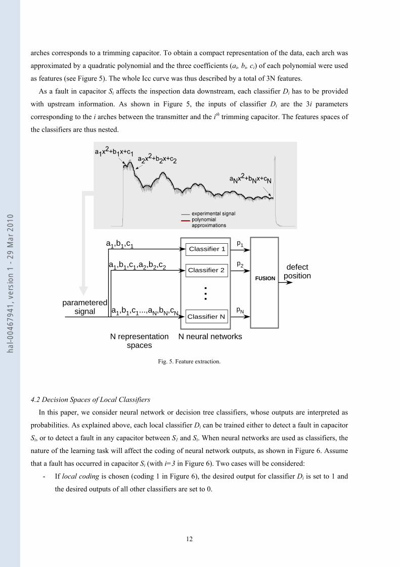
arches corresponds to a trimming capacitor. To obtain a compact representation of the data, each arch was
approximated by a quadratic polynomial and the three coefficients (ai, bi, ci) of each polynomial were used
as features (see Figure 5). The whole Icc curve was thus described by a total of 3N features.
As a fault in capacitor Si affects the inspection data downstream, each classifier Di has to be provided
with upstream information. As shown in Figure 5, the inputs of classifier Di are the 3i parameters
corresponding to the i arches between the transmitter and the ith trimming capacitor. The features spaces of
the classifiers are thus nested.
Classifier 1
..
.
N neural networks
p1
p2
pN
FUSION
defectposition
parameteredsignal
a1,b1,c1
a1,b1,c1,a2,b2,c2
a1,b1,c1...,aN,bN,cN
N representationspaces
Classifier 2
Classifier N
Fig. 5. Feature extraction.
4.2 Decision Spaces of Local Classifiers
In this paper, we consider neural network or decision tree classifiers, whose outputs are interpreted as
probabilities. As explained above, each local classifier Di can be trained either to detect a fault in capacitor
Si, or to detect a fault in any capacitor between S1 and Si. When neural networks are used as classifiers, the
nature of the learning task will affect the coding of neural network outputs, as shown in Figure 6. Assume
that a fault has occurred in capacitor Si (with i=3 in Figure 6). Two cases will be considered:
- If local coding is chosen (coding 1 in Figure 6), the desired output for classifier Di is set to 1 and
the desired outputs of all other classifiers are set to 0.
hal-0
0467
941,
ver
sion
1 -
29 M
ar 2
010

13
- In the case of distributed coding (coding 2 in Figure 6), the desired outputs of classifiers Dj with
j≥ i are set to 1 and the desired outputs of all other classifiers are set to 0.
Distributed coding seems a priori to be more appropriate to account for the spatial relationship between
subsystems. However, both solutions will be studied and experimented in this paper.
. . .I1 I2 I3 I4 IN
unchangedsignal modified signal
Inspectioninformation
0 0 1 0 0Coding 1
Coding 2
. . .
0 0 1 1 1. . .
Fault position
Fig. 6. The two output coding schemes used to train the N classifiers when capacitor S3 is defective. Using local coding (coding 1),
only the desired output of classifier D3 is set to 1.Using distributed coding (coding 2), the desired outputs of all classifiers Dj with
j≥3 are set to 1.
4.3 Classifier Fusion
As classifiers Di (i=1,…,N) process only local information, their outputs have to be combined to reach a
final decision regarding the presence and location of a defective capacitor. Here, the classifier outputs will
are expressed in the Dempster-Shafer framework and combined using Dempster’s rule (3)-(4).
As indicated in Section 3, to build a Dempster-Shafer model we first need to define the frame of
discernment. Here, it will be the set Θ={1,…,N,N+1}, where N is the number of capacitors in the track
circuit. Each singleton {i}, i=1,..,N+1 corresponds to a possible position of the fault. The virtual position
N+1 corresponds to the absence of fault.
The conversion of classifier outputs into mass functions and their combination will be presented below,
first in the case of local coding, and then in the case of distributed coding.
4.3.1. Classifier fusion with local coding
Using local coding, if the output of classifier Di is 1, the fault is considered to be in capacitor Si.
Otherwise, there is either a fault in some capacitor Sj with j≠i or no fault. The output from the classifier Di
can thus be represented as BBA mi with two focal sets: the singleton {i} and its complement Θ \{i}:
{ }({ })( \ ) 1 ,
i i
i i
m i pm i p
=Θ = −
(9)
where pi∈[0,1] is the output of classifier Di.
The combination of the N BBAs m1,…,mN using the unnormalized Dempster’s rule (4) yields a BBA m
with N+1 focal sets: the singletons and the empty set. This BBA has the following expression:
hal-0
0467
941,
ver
sion
1 -
29 M
ar 2
010
14
11
1
({ }) (1 ) 1
({ 1}) (1 )
( ) 1 ({ }).
i jj i
N
ii
N
i
m i p p i N
m N p
m Ø m i
≠
=+
=
= − ∀ = , ,
+ = −
= −
∏
∏
∑
(10)
Let us now assume that we discount each classifier output by a rate 1-αi with 0 1≤ ≤iα (see Section
3.3). As will be explained in Section 5, the discount rate can be determined as function of the classifier
error. The BBA mi representing the output of classifier Di then becomes:
( )({ })( \{ }) 1( ) 1 .
i i i
i i i
i i
m i pm i pm
αα
α
=Θ = −Θ = −
(11)
Combining these N BBAs using the unnormalized Dempster’s rule now gives a BBA m defined as
follows:
1
1
({ }) (1 ) (1 ) , 1
({ 1}) (1 )
( ) (1 ) (1 ), , 1 ,1 ,
( ) (1 ),
i i j j jj i
N
i ii
i i ii A i AN
ii
m i p p i N
m N p
m A p A N A A N
m
α α α
α
α α
α
≠
=
∉ ∈
=
⎡ ⎤= − + − ∀ = , ,⎣ ⎦
+ = −
= − − ∀ ⊂ Θ + ∈ < <
Θ = −
∏
∏∏ ∏
∏
(12)
the rest of the mass being assigned to the empty set. By convention, the products in the above expressions
vanish when the indices of the coefficients are negative or 0.
4.3.2. Classifier fusion with distributed coding
Assume that distributed coding was used, and the output of classifier Di is equal to 0. This means that
no fault was detected between S1 and Si: consequently, there is either a fault between Si+1 and SN, or no
fault. On the contrary, if the output of classifier Di is equal to 1, it means that a fault was detected between
S1 and Si. The information provided by classifier Di can therefore be represented by the following BBA:
[ ]( )[ ]( )1,
1, 1 1 .i i
i i
m i pm i N p
=+ + = −
(13)
where, as before, pi∈[0,1] denotes the output of classifier Di, and [1,i] denotes the set of integers between
1 and i.
The combination of m1,…,mN using Dempster’s rule (4) yields the following BBA:
hal-0
0467
941,
ver
sion
1 -
29 M
ar 2
010

15
1
1
11
1
({ }) (1 ) 1
({ 1}) (1 )
( ) 1 ({ }).
i N
j kj k iN
ii
N
i
m i p p i N
m N p
m Ø m i
−
= =
=+
=
= − , ∀ = , ,
+ = −
= −
∏ ∏
∏
∑
(14)
If, as before, we now discount each BBA representing the output of classifier Di by a rate 1-αi, the BBA
mi given by the ith classifier becomes:
[ ]( )[ ]( )1,
1, 1 (1 )( ) 1 .
i i i
i i i
i i
m i pm i N p
m
αα
α
=+ + = −
Θ = −
(15)
Combining these BBAs using the unnormalized Dempster’s rule now yields:
( )
( ) [ ] [ ]
[ ]( )
1 12
2 2 1 13
2
1 11 1
1
1
1 1
({1}) (1 )
({2}) 1 (1 )
({ }) 1 (1 ) (1 ) (1 ) 3,
({ 1}) (1 ) (1 ) (1 )
, (1 )
N
j j jj
N
j j jj
N i
i i i i j j j k k kj i k
N
N N j j jj
i i
m p p
m p p p
m i p p p p i N
m N p p
m i j p
α α α
α α α α
α α α α α α
α α α
α α
=
=−
− −= + =
−
=
− −
⎡ ⎤= + −⎣ ⎦
⎡ ⎤= − + −⎣ ⎦
⎡ ⎤= − + − − + − ∀ ∈⎣ ⎦
⎡ ⎤+ = − − + −⎣ ⎦
= −
∏
∏
∏ ∏
∏
[ ]1 2
1 1
1
(1 ) [(1 ) ] [ (1 ) (1 )] , ,
( ) (1 ),
j N i
j j m j k k l l lm i k j l
N
ii
p p p i j i j
m
α α α α α
α
− −
= = + =
−
− − + − + − ∀ < ⊂ Θ
Θ = −
∏ ∏ ∏
∏
(16)
the rest of the mass being assigned to the empty set.
Example: Let us consider a hypothetical system composed of N=3 subsystems. The frame of discernment
is then Θ={1,2,3,4}. Without discounting, the different BBAs provided by the classifiers are given by:
Classifier D1: 1 1
1 1
({1})({2,3,4}) 1
m pm p
== −
Classifier D2: 2 2
2 2
({1,2})({3,4}) 1
m pm p
== −
Classifier D3: 3 3
3 3
({1,2,3})({4}) 1
m pm p
== −
The combined BBA is then:
hal-0
0467
941,
ver
sion
1 -
29 M
ar 2
010

16
( )( ) ( )( ) ( ) ( )
1 2 3
1 2 3
1 2 3
1 2 34
1
({1})({2}) 1({3}) 1 1({4}) 1 1 1
( ) 1 ({ }) .i
m p p pm p p pm p p pm p p p
m m i=
== −= − −= − − −
∅ = −∑
We can notice that if, e.g., p1=p3=1 and p2=0, there is a contradiction between classifier 1 and classifier
3. Then, applying the formulas, we obtain
({1}) ({2}) ({3}) 0m m m= = = , ({4}) 0m = ( ) 1m ∅ = ,
which means that there is total conflict between the three classifier outputs.
With discounting, the BBAs given by the classifiers are:
Classifier D1: ( )
1 1 1
1 1 1
1 1
({1})({2,3,4}) 1({1,2,3,4}) 1
m pm pm
αα
α
== −= −
Classifier D2: ( )
2 2 2
2 2 2
2 2
({1,2})({3,4}) 1({1,2,3,4}) 1
m pm pm
αα
α
== −= −
Classifier D3: ( )
3 3
3 3 3
3 3
({1,2,3})({4}) 1({1,2,3,4}) 1
m pm pm
αα
== −= −
The combined BBA is:
( ) ( ) ( ) ( )( ) ( ) ( )( ) ( ) ( ) ( )( ) ( ) ( ) ( ) ( ) ( )
( ) ( ) ( ) ( ) ( )
1 1 2 2 3 3 1 1 2 3 3 1 1 2 2 3 1 1 2 3
1 1 2 2 3 3 1 1 2 2 3
1 1 2 2 3 3 1 2 2 3 3
1 1 2 2 3 3 1 2 2 3 3
1 1 2 3 3 1 2
({1}) 1 1 1 1({2}) 1 1 1({3}) 1 1 1 1({4}) 1 1 1 1 1 1
1 1 1 1 1
m p p p p p p p pm p p p p pm p p p p pm p p p p p
p p
α α α α α α α α α α α αα α α α α αα α α α α αα α α α α α
α α α α α
= + − + − + − −= − + − −= − − + − −= − − − + − − −
+ − − − + − − ( )( ) ( ) ( )
( ) ( )( ) ( ) ( ) ( ) ( ) ( )
( ) ( )( ) ( ) ( )
( ) ( ) ( )
3 3
1 2 2 3 3 1 2 2 3
1 1 2 3 3
1 1 2 2 3 1 2 2 3
1 2 3 3
1 1 2 3
1 2 3
1({1,2}) 1 1 1({2,3}) 1 1({3,4}) 1 1 1 1 1 1({1,2,3}) 1 1({2,3,4}) 1 1 1
( ) 1 1 1 ,
pm p p pm p pm p p pm pm p
m
αα α α α α α
α α αα α α α α α
α α αα α α
α α α
−= − + − −= − −= − − − + − − −= − −= − − −
Θ = − − −
the rest of the mass being assigned to the empty set.
4.4. Decision
To make the final decision, we compute the pignistic probability of each singleton using (6), and the
estimated position θ̂ of the fault is that with the highest pignistic probability:
hal-0
0467
941,
ver
sion
1 -
29 M
ar 2
010

17
( )ˆ max .arg BetPθ
θ θ∈Θ
= (17)
By convention, ˆ 1Nθ = + is interpreted as absence of fault.
5. Experimental results
In this section, the diagnosis system introduced in this paper is assessed using simulated data, and
compared to a simple reference approach. The experimental settings will be described in Subsection 5.1
and the results will be reported and discussed in Subsections 5.2 and 5.3, respectively.
5.1 Experimental settings
To assess the performances of the method, we considered a track circuit of N=19 trimming capacitors
and built a database containing 4256 simulated noised signals obtained for different values of the
resistance of each capacitor. Among these signals, 608 were fault-free and 3648 had one defective
capacitor with a resistance between r=1 Ω and r= ∞ (removed capacitor). The data set was split randomly
into three subsets (training, validation and test) and the performances were estimated on the test set
containing 1064 signals. We have chosen to compare our approach to a basic method using one multilayer
perceptron that directly estimates the position of the defective capacitor (position N+1 is used for fault-free
case). In such way, we are able to quantify the benefits of our method that builds as many classifiers as
trimming capacitors and uses an additional fusion stage to detect and localize a fault in the system.
The following methods were compared:
1. Regression using a multilayer perceptron [4] with one sigmoid hidden layer of 7 neurons and a
linear output layer with one neuron. The inputs were the 19×3=57 parameters (ai,bi,ci),
i=1,…,19 of the Icc curve, and the output was the location of the fault. The virtual location N+1
was used when the system was fault-free. This is considered as the reference method. This
network was trained to minimize the mean square error between the estimated and the true fault
positions on the whole training set. The number of hidden neurons was varied between 3 and
15; the best results on the validation set were obtained with 7 hidden neurons.
2. Fusion with neural networks and decision trees as local classifiers, with the two coding schemes
described in Section 4.3, with and without discounting. Overall, this makes 8 different fusion-
based methods. The neural network classifiers had one tan-sigmoid hidden layer and a sigmoid
output layer with one neuron (Figure 7). Table 1 gives the number of hidden nodes used for
each classifier, which was determined by minimizing the error criterion on the validation set.
hal-0
0467
941,
ver
sion
1 -
29 M
ar 2
010
18
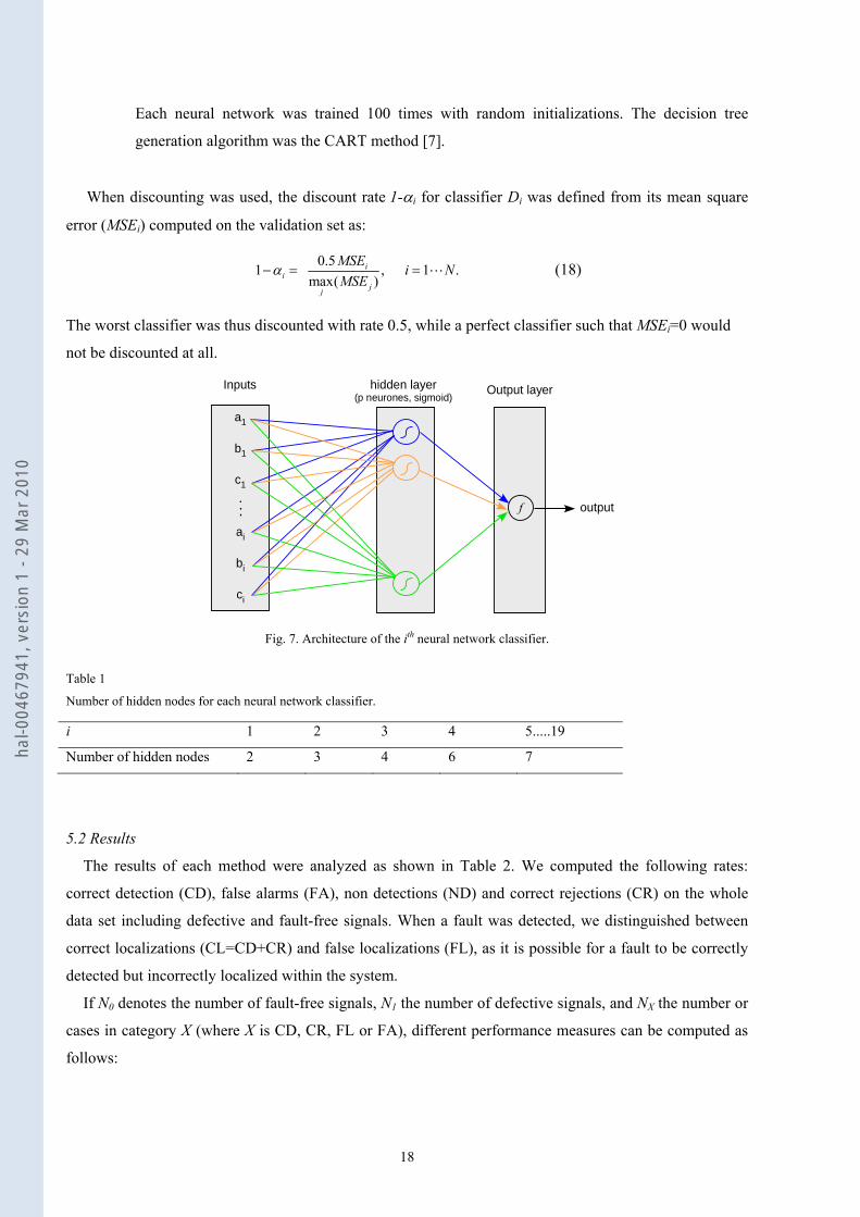
Each neural network was trained 100 times with random initializations. The decision tree
generation algorithm was the CART method [7].
When discounting was used, the discount rate 1-αi for classifier Di was defined from its mean square
error (MSEi) computed on the validation set as:
0.51 , 1 .max( )
ii
jj
MSE i NMSE
α− = = (18)
The worst classifier was thus discounted with rate 0.5, while a perfect classifier such that MSEi=0 would
not be discounted at all.
a1
b1
c1
ai
bi
ci
output
hidden layer(p neurones, sigmoid)
Inputs Output layer
... f
Fig. 7. Architecture of the ith neural network classifier.
Table 1
Number of hidden nodes for each neural network classifier.
i 1 2 3 4 5.....19
Number of hidden nodes 2 3 4 6 7
5.2 Results
The results of each method were analyzed as shown in Table 2. We computed the following rates:
correct detection (CD), false alarms (FA), non detections (ND) and correct rejections (CR) on the whole
data set including defective and fault-free signals. When a fault was detected, we distinguished between
correct localizations (CL=CD+CR) and false localizations (FL), as it is possible for a fault to be correctly
detected but incorrectly localized within the system.
If N0 denotes the number of fault-free signals, N1 the number of defective signals, and NX the number or
cases in category X (where X is CD, CR, FL or FA), different performance measures can be computed as
follows:
hal-0
0467
941,
ver
sion
1 -
29 M
ar 2
010

19
0 1
CD CR FLCD
N N NtN N+ +
=+
, CD CRCL
CD CR FL
N NtN N N
+=
+ +
0
FAFA
NtN
= , 1
.NDND
NtN
=
The results are shown in Table 3. Results obtained using decision tree classifiers (DT) are also reported
to compare them to those of neural networks. The discount rates used to combine the classifier outputs
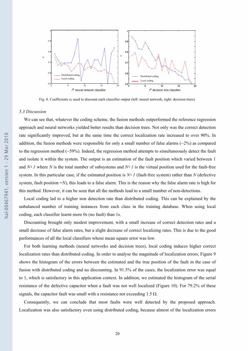
were computed according to (18) and are reported in Figure 8. Except for neural network classifiers using
distributed coding, we can see that coefficients αi tend to decrease with i, which means that classifiers are
more heavily discounted as i increases, the learning task becoming more complex as we get closer to the
receiver.
Table 2
Analysis of the results
Truth
Fault position k No fault
Decision
Fault position k CD
NCD FA
NFA Fault position
j≠k
FL
NFL
No fault ND
NND
CR
NCR
Table 3
Performances of the reference regression method as well as the 8 fusion-based methods using neural networks (NN) and decision
trees (DT), for the two coding schemes, with and without discounting.
Rates NN
Regression
NN
Local coding
NN
Distributed coding
DT
Local coding
DT
Distributed coding
(%) No disc. Disc. No disc. Disc. No disc. Disc. No disc. Disc.
tCD 84.71 94.27 95.18 99.53 99.62 87.97 88.82 93.23 94.92
tCL 56.12 99.8 98.28 92.26 91.89 98.93 98.42 88.61 88.42
tFA 59.2 1.97 1.07 1.32 0.66 2.63 1.58 2.39 1.97
tND 1.17 6.36 6.36 0.33 0.33 6.16 6.36 2.41 2.52
hal-0
0467
941,
ver
sion
1 -
29 M
ar 2
010
20
0 5 10 15 200.5
0.6
0.7
0.8
0.9
1
Local codingDistributed coding
α
ith neural network classifier0 5 10 15 20
0.5
0.6
0.7
0.8
0.9
1
Distributed coding
ith decision tree classifier0 5 10 15 20
0.5
0.6
0.7
0.8
0.9
1
Local coding
α
Fig. 8. Coefficients αi used to discount each classifier output (left: neural network, right: decision trees).
5.3 Discussion
We can see that, whatever the coding scheme, the fusion methods outperformed the reference regression
approach and neural networks yielded better results than decision trees. Not only was the correct detection
rate significantly improved, but at the same time the correct localization rate increased to over 90%. In
addition, the fusion methods were responsible for only a small number of false alarms (~2%) as compared
to the regression method (~59%). Indeed, the regression method attempts to simultaneously detect the fault
and isolate it within the system. The output is an estimation of the fault position which varied between 1
and N+1 where N is the total number of subsystems and N+1 is the virtual position used for the fault-free
system. In this particular case, if the estimated position is N+1 (fault-free system) rather than N (defective
system, fault position =N), this leads to a false alarm. This is the reason why the false alarm rate is high for
this method. However, it can be seen that all the methods lead to a small number of non-detections.
Local coding led to a higher non detection rate than distributed coding. This can be explained by the
unbalanced number of training instances from each class in the training database. When using local
coding, each classifier learnt more 0s (no fault) than 1s.
Discounting brought only modest improvement, with a small increase of correct detection rates and a
small decrease of false alarm rates, but a slight decrease of correct localizing rates. This is due to the good
performances of all the local classifiers whose mean square error was low.
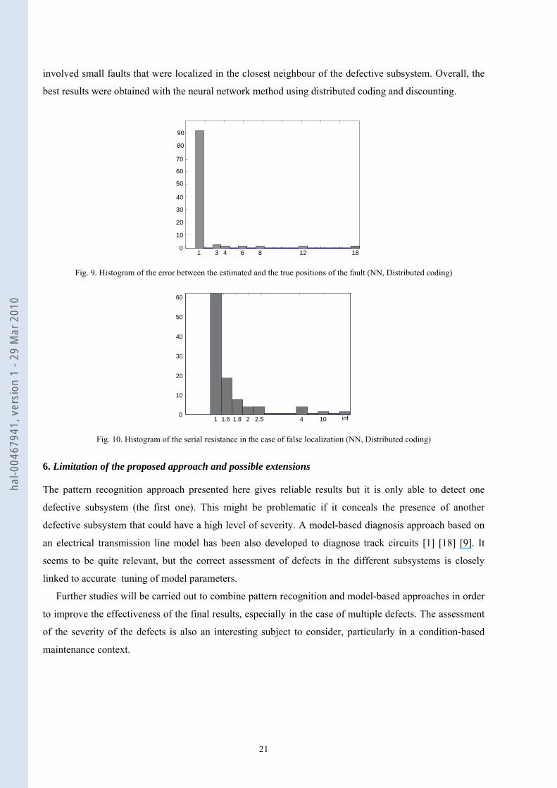
For both learning methods (neural networks and decision trees), local coding induces higher correct
localization rates than distributed coding. In order to analyse the magnitude of localization errors, Figure 9
shows the histogram of the errors between the estimated and the true position of the fault in the case of
fusion with distributed coding and no discounting. In 91.5% of the cases, the localization error was equal
to 1, which is satisfactory in this application context. In addition, we estimated the histogram of the serial
resistance of the defective capacitor when a fault was not well localized (Figure 10). For 79.2% of these
signals, the capacitor fault was small with a resistance not exceeding 1.5 Ω.
Consequently, we can conclude that most faults were well detected by the proposed approach.
Localization was also satisfactory even using distributed coding, because almost of the localization errors
hal-0
0467
941,
ver
sion
1 -
29 M
ar 2
010
21
involved small faults that were localized in the closest neighbour of the defective subsystem. Overall, the
best results were obtained with the neural network method using distributed coding and discounting.
1 4 6 8 12 180
10
20
30
40
50
60
70
80
3
90
Fig. 9. Histogram of the error between the estimated and the true positions of the fault (NN, Distributed coding)
1 1.5 1.8 2 2.5 4 100
10
20
30
40
50
60
inf
Fig. 10. Histogram of the serial resistance in the case of false localization (NN, Distributed coding)
6. Limitation of the proposed approach and possible extensions
The pattern recognition approach presented here gives reliable results but it is only able to detect one
defective subsystem (the first one). This might be problematic if it conceals the presence of another
defective subsystem that could have a high level of severity. A model-based diagnosis approach based on
an electrical transmission line model has been also developed to diagnose track circuits [1] [18] [9]. It
seems to be quite relevant, but the correct assessment of defects in the different subsystems is closely
linked to accurate tuning of model parameters.
Further studies will be carried out to combine pattern recognition and model-based approaches in order
to improve the effectiveness of the final results, especially in the case of multiple defects. The assessment
of the severity of the defects is also an interesting subject to consider, particularly in a condition-based
maintenance context.
hal-0
0467
941,
ver
sion
1 -
29 M
ar 2
010

22
7. Conclusion
This article described an application of pattern recognition and information fusion techniques to fault
detection and isolation in a railway track circuits. This device can be considered as a large-scale system
that comprises several interconnected and spatially related subsystems. This means that a defective
subsystem influences not only its own inspection data but also that of the systems located downstream of
it.
The proposed method is based on a classifier fusion approach that builds as many local classifiers as
subsystems. The local classifier outputs are then combined using Dempster-Shafer theory, which provides
a convenient framework for handling imprecision and uncertainty in decision problems. Two learning
strategies for local classifiers have been implemented, which consist in detecting the presence of a fault
either on a subsystem or between a subsystem and the transmitter. Both neural networks and decision trees
were investigated as local classifiers.
Experiments with simulated data have shown that correct detection rates over 99 % and correct
localization over 92 % could be achieved using this approach, which represents a major improvement over
the reference method that does not use classifier fusion. Additionally, we have shown that localization
errors are small, and incorrectly localized faults generally correspond to a small resistance of the defective
capacitor. Overall, the best results were obtained with neural network local classifiers and distributed
coding. Although no result with real data could be presented because of lack of labelled signals, the results
were judged conclusive enough by the end user to decide the implementation and dissemination of the
method.
Further studies are being carried out to handle multiple faults and assess their severity, which may be
useful in a predictive maintenance context. The functionality of the system will be extended to
discriminate between benign faults, faults that need to be monitored and very serious faults that require
immediate maintenance action.
Although the method has been developed in the context of railway track circuit diagnosis, we believe
that it can be transferred to other application domains involving the diagnosis of large scale systems
composed or linearly organized subsystems, such as other infrastructure networks.
Acknowledgements
This work was supported by the Infrastructure Department and the Engineering Department of the
French National Railway Company (SNCF). The authors thank the anonymous referees for their helpful
comments.
References
hal-0
0467
941,
ver
sion
1 -
29 M
ar 2
010

23
[1] M.L. Berova, Development of software tools for simulation and design of jointless track circuits. Ph.D.
thesis, The university of Bath.
[2] Y. Bi, D. Bell, H. Wang, G. Guo, K. Greer, Combining Multiple Classifiers Using Dempster’s Rule of
Combination for Text Categorization, lecture notes in Computer science,31, pp 127-138, 2004.
[3] J. Chen, C. Roberts, P. Weston, Fault detection and diagnosis for railway track circuits using neuro-
fuzzy systems. Control Engineering Practice, 16, 585-596, 2008.
[4] C.M. Bishop, Neural Networks for Pattern Recognition, Oxford university Press edition, 1995.
[5] I. Bloch, Information combination operator for data fusion: a comparative review with classification.
IEEE Transactions on Systems, Man, and Cybernetics, 26, p.52-67, 1996.
[6] D. Bonnet, A. Grumbach, V. Labouisse, On the parsimony of the multi-layer perceptrons when
processing encoded symbolic variables. Neural Processing Letters, 8(2), p.145-153, 1998.
[7] L. Breiman, J. H. Friedman, R. A. Olshen and C. J. Stone, Classification and Regression Trees,
Wadsworth, Belmont, CA, 1984.
[8] A. Debiolles, L. Oukhellou, T. Denoeux, P. Aknin, Output coding of spatially related subclassifiers in
evidential framework. Application to the diagnosis of railway track-vehicle system, in Proc. Fusion
2006, Firenze, July 2006.
[9] A. Debiolles, L. Oukhellou, P. Aknin, Combined use of Partial Least Squares regression and neural
network for diagnosis tasks, in Proc. Intern. Conf. on Pattern Recognition ICPR’04, Cambridge, 2004.
[10] A. P. Dempster, A generalization of Bayesian inference. Journal of the Royal Statistical Society, 30, p
205-247, 1968.
[11] T. Denœux, M.-H. Masson, B. Dubuisson, Advanced pattern recognition techniques for system
monitoring and diagnosis: a survey. Journal Européen des Systèmes Automatisés (RAIRO-APII-JESA),
31(9-10), p. 1509-1539, 1998.
[12] T. Denoeux, Analysis of evidence-theoretic decision rules for pattern classification. Pattern
recognition, 30(7):1095-1107, 1997.
[13] D. Dubois, H. Prade, Possibility Theory: An Approach to Computerized Processing of Uncertainty.
Plenum Press, New York, November 1988.
[14] R.O. Duda, P.E. Hart, D.G. Stork, Pattern classification, John Wiley and Sons edition, 2001.
[15] Z. Elouedi, K. Mellouli, Ph Smets, Assessing sensor reliability for multi-sensor data fusion within the
Transferable Belief Model. IEEE Transactions on Systems, Man, and Cybernetics B, 34(1), p. 782-787,
2004.
[16] L.R. Galina, Combining the results of several neural network classifiers, Neural Networks, vol. 7(5),
pp. 777–781, 1994.
[17] J. Gertler: Fault Detection and Diagnosis in Engineering Systems. Marcel Dekker, New York (1998).
hal-0
0467
941,
ver
sion
1 -
29 M
ar 2
010
24
[18] R.J. Hill, D.C. Carpenter, Rail track distributed transmission line impedance and admittance:
theoretical modelling and experimental results. IEEE Transactions on Vehicular Technology, 42(4),
225-241, 1993.
[19] T.H. Ho, J.J. Hull, S.N. Srihari, Decision combination in multiple classifier system, IEEE
Transactions on Pattern Analysis and Machine Intelligence, 16(1), pp. 66-75, 1994.
[20] Y.S. Huang, C.Y. Suen, A method of combining multiple experts for the recognition of unconstrained
handwritten numerals. IEEE Transactions on Pattern Analysis and Machine Intelligence, 17, pp. 90-93,
1995.
[21] R. Isermann, Fault-Diagnosis Systems: An Introduction From Fault Detection To Fault Tolerance,
Springer, 2005.
[22] R.W. Jones; A. Lowe; M.J. Harrison, A framework for intelligent medical diagnosis using the theory
of evidence, Knowledge-Based Systems, vol. 15(1), p. 77-84(8), 2002, Elsevier.
[23] J. Kittler, Combining classifiers: a theoretical framework. Pattern Analysis and Applications, 1:p.18-
27, 1998.
[24] J. Korbicz, Advances in fault diagnosis systems, Proc. 10th IEEE Int. Conf. on Methods and Models in
Automation and Robotics MMAR, 725–733 (2004).
[25] L. I. Kuncheva, Combining Pattern Classifiers: Methods and Algorithms, John Wiley and Sons
edition, 2004.
[26] L. Lam and, C.Y. Suen, Application of Majority Voting to Pattern Recognition: An Analysis of Its
Behavior and Performance. IEEE Transactions on Systems, Man, and Cybernetics - Part A: Systems
and Humans, 27, pp.553-568, 1997.
[27] C.A. Le., V.N. Huynh, A. Shimazu, Combining classifiers with multi-representation of context in
word sense disambiguation, PAKDD 2005, T.B. Ho et al. (Eds.), Springer-Verlag, LNAI 3518, pp. 262-
268. 2005.
[28] M. R Maurya, R. Rengaswamy and V. Venkatasubramanian, Fault diagnosis using trend analysis: a
review and recent developments. Engineering Applications of Artificial Intelligence, 20, p. 133-146,
2007.
[29] D. Mercier, B. Quost and T. Denoeux. Refined modeling of sensor reliability in the belief function
framework using contextual discounting, Information Fusion, Vol. 9, p. 246–258, 2008.
[30] R.J. Patton, P. Franck, J. Chen, Fault diagnosis in Dynamic systems: Theory and Applications.
Prentice-Hall, New York, 1989.
[31] W. Pedrycz, J.C. Bezdzk, R.J. Hathaway, G.W. Rogers, Two Nonparametric models for fusing
heterogeneous fuzzy data, IEEE Transactions on Fuzzy Systems, vol.6 (3), pp. 411-425, 1998.
[32] A. Rakar, D. Juricic and P. Ballé. Transferable belief model in fault diagnosis. Engineering
Applications of Artificial Intelligence, 12(5), p. 555-567, 1999.
hal-0
0467
941,
ver
sion
1 -
29 M
ar 2
010
25
[33] R.Rengaswamy, D. Mylaraswamy, Karl-Erik Arzen and V. Venkatasubramanian, A Comparison of
Model-Based and Neural Network-Based Diagnostic Methods, Engineering Applications of Artificial
Intelligence, 14(6), 805-818, 2002.
[34] D. Ruta, B. Gabrys, An overview of classifier fusion methods, Computing and Information Systems,
7, pp.1-10, 2000.
[35] G. Shafer, A mathematical Theory of Evidence, Princeton University Press, 1976.
[36]P. Smets, Decision making in a context where uncertainty is represented by belief functions. In R.P.
Srivastava and T.J. Mock, Editors, Belief Functions in Business Decisions. Physica-Verlag,
Heildelberg, 2002.
[37] P. Smets, R. Kennes, The Transferable Belief Model. Artificial Intelligence, vol.66, p.191-234, 1994.
[38] P. Smets, R. Kruse, The Transferable Belief Model for quantified belief representation. In A. Motro
and Ph. Smets, editors, Uncertainty in Information Systems: From Needs to Solutions, p. 343-368,
Kluwer, Boston, MA, 1997.
[39] P. Smets, The combination of evidence in the Tranferable Belief Model, IEEE transactions on Pattern
Analysis and Machine Intelligence, vol.12(5), p. 447-458, 1990.
[40] P. Smets, Belief functions: the disjunctive rule of combination and the Generalized Bayesian theorem.
International Journal of Approximate Reasoning, 9, p 1-35, 1993.
[41] F. Valente, H. Hermansky, Combination of Acoustic Classifiers based on Dempster-Shafer Theory of
evidence, in Proc. Int. Conf. on Acoustics, Speech, and Signal Processing ICASSP, Honolulu, Hawaï,
2007.
[42] L. Xu, A. Krzyzak, and C.Y. Suen, Methods of combining multiple classifiers and their application to
Handwriting Recognition. IEEE Transactions on Systems, Man Cybernetics, 22(3):418-435, May 1992.
[43] G. Yang, X. Wu, Synthesized Fault Diagnosis Method Based on Fuzzy Logic and D-S Evidence
Theory, Vol. 4682, pp. 1024-1031, Advanced Intelligent Computing Theories and Applications, 2007,
Springer.
[44] L. Zadeh, Fuzzy sets as a basis for a theory of possibility. Fuzzy Sets and Systems, 1(3):3-28, 1978.
hal-0
0467
941,
ver
sion
1 -
29 M
ar 2
010
Copyright © 2022 FDOKUMEN