Introduction to Mathematical Methods for Environmental ...
476
Introduction to Mathematical Methods for Environmental Engineers and Scientists
-
Upload
khangminh22 -
Category
Documents
-
view
1 -
download
0
Transcript of Introduction to Mathematical Methods for Environmental ...

Introduction to Mathematical
Methods for Environmental
Engineers and Scientists

Scrivener Publishing
100 Cummings Center, Suite 541J
Beverly, MA 01915-6106
Publishers at Scrivener
Martin Scrivener ([email protected])
Phillip Carmical ([email protected])

Introduction to Mathematical
Methods for Environmental
Engineers and Scientists
Charles Prochaska Louis Theodore

This edition first published 2018 by John Wiley & Sons, Inc., 111 River Street, Hoboken, NJ 07030, USA
and Scrivener Publishing LLC, 100 Cummings Center, Suite 541J, Beverly, MA 01915, USA
© 2018 Scrivener Publishing LLC
For more information about Scrivener publications please visit www.scrivenerpublishing.com.
All rights reserved. No part of this publication may be reproduced, stored in a retrieval system, or
transmitted, in any form or by any means, electronic, mechanical, photocopying, recording, or other-
wise, except as permitted by law. Advice on how to obtain permission to reuse material from this title
is available at http://www.wiley.com/go/permissions.
Wiley Global Headquarters
111 River Street, Hoboken, NJ 07030, USA
For details of our global editorial offices, customer services, and more information about Wiley prod-
ucts visit us at www.wiley.com.
Limit of Liability/Disclaimer of Warranty
While the publisher and authors have used their best efforts in preparing this work, they make no rep-
resentations or warranties with respect to the accuracy or completeness of the contents of this work and
specifically disclaim all warranties, including without limitation any implied warranties of merchant-
ability or fitness for a particular purpose. No warranty may be created or extended by sales representa-
tives, written sales materials, or promotional statements for this work. The fact that an organization,
website, or product is referred to in this work as a citation and/or potential source of further informa-
tion does not mean that the publisher and authors endorse the information or services the organiza-
tion, website, or product may provide or recommendations it may make. This work is sold with the
understanding that the publisher is not engaged in rendering professional services. The advice and
strategies contained herein may not be suitable for your situation. You should consult with a specialist
where appropriate. Neither the publisher nor authors shall be liable for any loss of profit or any other
commercial damages, including but not limited to special, incidental, consequential, or other damages.
Further, readers should be aware that websites listed in this work may have changed or disappeared
between when this work was written and when it is read.
Library of Congress Cataloging-in-Publication Data
ISBN 978-1-119-36349-1
Cover image: Pixabay.Com
Cover design by Russell Richardson
Set in size of 10pt and Minion Pro by Exeter Premedia Services Private Ltd., Chennai, India
Printed in the USA
10 9 8 7 6 5 4 3 2 1

To
my parents who have provided immeasurable
support in every aspect of my life (CP)
and
Arthur Lovely, a truly great guy and the world’s greatest
sports historian… ever (LT)

vii
Contents
Preface ix
Part I: Introductory Principles 1
1 Fundamentals and Principles of Numbers 3
2 Series Analysis 21
3 Graphical Analysis 29
4 Flow Diagrams 43
5 Dimensional Analysis 53
6 Economics 73
7 Problem Solving 89
Part II: Analytical Analysis 99
8 Analytical Geometry 101
9 Differentiation 115
10 Integration 121
11 Differential Calculus 133
12 Integral Calculus 147
13 Matrix Algebra 161
14 Laplace Transforms 173
Part III: Numerical Analysis 183
15 Trial-and-Error Solutions 185
16 Nonlinear Algebraic Equations 195
17 Simultaneous Linear Algebraic Equations 209
18 Differentiation 219

viii Contents
19 Integration 225
20 Ordinary Differential Equations 235
21 Partial Differential Equations 247
Part IV: Statistical Analysis 259
22 Basic Probability Concepts 261
23 Estimation of Mean and Variance 275
24 Discrete Probability Distributions 287
25 Continuous Probability Distributions 307
26 Fault Tree and Event Tree Analysis 343
27 Monte Carlo Simulation 357
28 Regression Analysis 371
Part V: Optimization 385
29 Introduction to Optimization 387
30 Perturbation Techniques 395
31 Search Methods 405
32 Graphical Approaches 419
33 Analytical Approaches 435
34 Introduction to Linear Programming 449
35 Linear Programming Applications 465
Index 481
ix
Preface
It is no secret that in recent years the number of people entering the environmental
field has increased at a near exponential rate. Some are beginning college students
and others had earlier chosen a non-technical major/career path. A large number
of these individuals are today seeking technical degrees in environmental engi-
neering or in the environmental sciences. These prospective students will require
an understanding and appreciation of the numerous mathematical methods that
are routinely employed in practice. This technical steppingstone to a successful
career is rarely provided at institutions that award technical degrees. This intro-
ductory text on mathematical methods attempts to supplement existing environ-
mental curricula with a sorely needed tool to eliminate this void.
The question often arises as to the educational background required for mean-
ingful analysis capabilities since technology has changed the emphasis that is
placed on certain mathematical subjects. Before computer usage became popular,
instruction in environmental analysis was (and still is in many places) restricted
to simple systems and most of the effort was devoted to solving a few derived
elementary equations. These cases were mostly of academic interest, and because
of their simplicity, were of little practical value. To this end, a considerable amount
of time is now required to acquire skills in mathematics, especially in numerical
methods, statistics, and optimization. In fact, most environmental engineers and
scientists are given courses in classical mathematics, but experience shows that
very little of this knowledge is retained after graduation for the simple reason that
these mathematical methods are not adequate for solving most systems of equa-
tions encountered in industry. In addition, advanced mathematical skills are either
not provided in courses or are forgotten through sheer disuse.
As noted in the above paragraph, the material in this book was prepared pri-
marily for beginning environmental engineering and science students and, to a
lesser extent, for environmental professionals who wish to obtain a better under-
standing of the various mathematical methods that can be employed in solving
technical problems. The content is such that it is suitable both for classroom use
and for individual study. In presenting the text material, the authors have stressed
the pragmatic approach in the application of mathematical tools to assist the
reader in grasping the role of mathematical skills in environmental problem solv-
ing situations.

x Preface
In effect, this book serves two purposes. It may be used as a textbook for begin-
ning environmental students or as a “reference” book for practicing engineers,
scientists, and technicians involved with the environment. The authors have
assumed that the reader has already taken basic courses in physics and chemis-
try, and should have a minimum background in mathematics through elementary
calculus. The authors’ aim is to offer the reader the fundamentals of numerous
mathematical methods with accompanying practical environmental applications.
The reader is encouraged through references to continue his or her own develop-
ment beyond the scope of the presented material.
As is usually the case in preparing any text, the question of what to include and
what to omit has been particularly difficult. The material in this book attempts to
address mathematical calculations common to both the environmental engineer-
ing and science professionals. The book provides the reader with nearly 100 solved
illustrative examples. The interrelationship between both theory and applications
is emphasized in nearly all of the chapters. One key feature of this book is that the
solutions to the problems are presented in a stand-alone manner. Throughout the
book, the illustrative examples are laid out in such a way as to develop the reader’s
technical understanding of the subject in question, with more difficult examples
located at or near the end of each set.
The book is divided up into five (V) parts (see also the Table of Contents):
I. Introduction
II. Analytical Analysis
III. Numerical Analysis
IV. Statistical Analysis
V. Optimization
Most chapters contain a short introduction to the mathematical method in ques-
tion, which is followed by developmental material, which in turn, is followed by
one or more illustrative examples. Thus, this book offers material not only to indi-
viduals with limited technical background but also to those with extensive envi-
ronmental industrial experience. As noted above, this book may be used as a text
in either a general introductory environmental engineering/ science course and
(perhaps) as a training tool in industry for challenged environmental professionals.
Hopefully, the text is simple, clear, to the point, and imparts a basic understand-
ing of the theory and application of many of the mathematical methods employed
in environmental practice. It should also assist the reader in helping master the
difficult task of explaining what was once a very complicated subject matter in a
way that is easily understood. The authors feel that this delineates this text from
the numerous others in this field.
It should also be noted that the authors have long advocated that basic sci-
ence courses ‒ particularly those concerned with mathematics ‒ should be taught
to engineers and applied scientists by an engineer or applied scientist. Also, the
books adopted for use in these courses should be written by an engineer or an

Preface xi
applied scientist. For example, a mathematician will lecture on differentiation ‒ say
dx/dy ‒ not realizing that in a real-world application involving an estuary y could
refer to concentration while x could refer to time. The reader of this book will not
encounter this problem.
The reader should also note that parts of the material in the book were drawn
from one of the author’s notes of yesteryear. In a few instances, the original source
was not available for referencing purposes. Any oversight will be corrected in a
later printing/edition.
The authors wish to express appreciation to those who have contributed
suggestions for material covered in this book. Their comments have been very
helpful in the selection and presentation of the subject matter. Special apprecia-
tion is extended to Megan Menzel for her technical contributions and review, Dan
McCloskey for preparing some of the first draft material in Parts II and III, and
Christopher Testa for his contributions to Chapters 13 and 14. Thanks are also due
to Rita D’Aquino, Mary K. Theodore, and Ronnie Zaglin.
Finally, the authors are especially interested in learning the opinions of those
who read this book concerning its utility and serviceability in meeting the needs
for which it was written. Corrections, improvements and suggestions will be con-
sidered for inclusion in later editions.
Chuck Prochaska
Lou Theodore
April 2018
1
Part I
INTRODUCTORY PRINCIPLES
Webster defines introduction as … “the preliminary section of a book, usually
explaining or defining the subject matter…” And indeed, that is exactly what this
Part I of the book is all about. The chapters contain material that one might view
as a pre-requisite for the specific mathematical methods that are addressed in
Parts II–V.
There are seven chapters in Part I. The chapter numbers and accompanying
titles are listed below.
Chapter 1: Fundamentals and Principles of Numbers
Chapter 2: Series Analysis
Chapter 3: Graphical Analysis
Chapter 4: Flow Diagrams
Chapter 5: Dimensional Analysis
Chapter 6: Economics
Chapter 7: Problem Solving
Introduction to Mathematical Methods for Environmental Engineers and Scientists. Charles Prochaska and Louis Theodore.
© 2018 Scrivener Publishing LLC. Published 2018 by John Wiley & Sons, Inc.

3
The natural numbers, or so-called counting numbers, are the positive integers: 1, 2, 3,
… and the negative integers: 1, 2, 3,… The following applies to real numbers:
a b a b means that is a positive real number (1.1)
If and , then a b b c a c (1.2)
If and 0, then a b c ac bc (1.3)
If and then a b c d a c b d, (1.4)
If and 0, then a b aba b
1 1 (1.5)
a b b a a b b a a b; ( )( ) (1.6)
a b c a b c a bc ab c( ) ( ) ( ) ( ); (1.7)
1Fundamentals and Principles of Numbers
Introduction to Mathematical Methods for Environmental Engineers and Scientists. Charles Prochaska and Louis Theodore.
© 2018 Scrivener Publishing LLC. Published 2018 by John Wiley & Sons, Inc.

4 Introduction to Mathematical Methods
a b c a b a c( ) (1.8)
If | | , where 0, then , or x a a x a x a (1.9)
If | | , then where x c c x c c 0 (1.10)
aa
an
n
1, 0 (1.11)
(ab a bn n n) (1.12)
( )a a a a an m nm n m n m, (1.13)
a a0 1, 0 (1.14)
log log log , ab a b a b, 0 0 (1.15)
log log a n an (1.16)
log log log a
ba b (1.17)
log1
log a an
n (1.18)
ln aa 2 3026. log (1.19)
Based on the above, one may write
(4)(9) ( . )( )3 60 10 1
( ) ( )( )6 2.16 103 2
3375 1 50 103 1( . )( )
( ). ( . )( ).0 916 9 39 103
4 15 1
log 0.389210 ( ).2 45

Fundamentals and Principles of Numbers 5
ln 5.5013( ) ( . )( . )245 2 3892 2 3026
log .( )10 0 245 109.3892 0.6108
Given any quadratic equation of the general form
ax bx c2 0 (1.20)
a number of methods of solution are possible depending on the specific nature
of the equation in question. If the equation can be factored, then the solution is
straightforward. For instance, consider
x x2 3 10 (1.21)
Put into the standard form,
x x2 3 10 0 (1.22)
this equation can be factored as follows:
( )( )x x5 2 0 (1.23)
This condition can be met, however, only when the individual factors are zero, i.e.,
when x 5 and x 2. That these are indeed the solutions to the equation may be
verified by substitution.
If, upon inspection, no obvious means of factoring an equation can be found,
an alternative approach may exist. For example, in the equation
4 12 72x x (1.24)
the expression
4 122x x (1.25)
could be factored as a perfect square if it were
4 12 92x x (1.26)
which equals
( )2 3 2x (1.27)

6 Introduction to Mathematical Methods
This can easily be achieved by adding 9 to the left side of the equation. The same
amount must then, of course, be added to the right side as well, resulting in:
4 12 9 7 9x x2 (1.28)
so that,
( )2 3 2x 16 (1.29)
This can be reduced to
( )2 3 16x (1.30)
or
2 3 4x (1.31)
and
2 3 4x (1.32)
Since 16 above has two solutions, i.e., +4 and –4, the first equation leads to the
solution x 0.5 while the second equation leads to the solution x 7/2, or x 3.5.
If the methods of factoring or completing the square are not possible, any qua-
dratic equation can always be solved by the quadratic formula. This provides a
method for determining the solution of the equation if it is in the form
ax bx c2 0 (1.33)
In all cases, the two solutions of x are given by the formula
xb b ac
a
2 4
2 (1.34)
For example, to find the roots of
x x2 4 3 (1.35)
the equation is first put into the standard form of Equation (1.33)
x x2 4 3 0 (1.36)
As a result, a 1, b 4, and c 3. These terms are then substituted into the
quadratic formula presented in Equation (1.34).

Fundamentals and Principles of Numbers 7
x( ) ( )( )
( )
( )4 4 4 1 3
2 1
4 16 12
2
2
(1.37)
4 4
2
4 2
23 and 1 (1.38)
The practicing environmental engineer and scientist occasionally has to solve
not just a single equation but several at the same time. The problem is to find
the set of all solutions that satisfies both equations. These are called simultane-
ous equations, and specific algebraic techniques may be used to solve them. For
example, a simple solution exists given two linear equations and two unknowns:
3 4 10x y (1.39)
2 5x y (1.40)
The variable y in Equation (1.40) is isolated (y 5 – 2x), and then this value of y is
substituted into Equation (1.39).
3 4 5 2 10x x( ) (1.41)
This reduces the problem to one involving the single unknown x and it follows
that
3 20 8 10x x
or
5 10x (1.42)
so that
x 2 (1.43)
When this value is substituted into either equation above, it follows that
y 1 (1.44)
A faster method of solving simultaneous equations, however, is obtained by
observing that if both sides of Equation (1.40) are multiplied by 4, then
8 4 20x y (1.45)

8 Introduction to Mathematical Methods
If Equation (1.39) is subtracted from Equation (1.45), then 5x 10, or x 2.
This procedure leads to another development in mathematics, i.e., matrices, which
can help to produce solutions for any set of linear equations with a corresponding
number of unknowns (refer also to Chapter 13).
Four sections compliment the presentation of this chapter. Section numbers
and subject titles follow:
1.1: Interpolation and Extrapolation
1.2: Significant Figures and Approximate Numbers
1.3: Errors
1.4: Propagation of Errors
1.1 Interpolation and Extrapolation
Experimental data (and data in general) in environmental engineering and science
may be presented using a table, a graph, or an equation. Tabular presentation per-
mits retention of all significant figures of the original numerical data. Therefore,
it is the most numerically accurate way of reporting data. However, it is often
difficult to interpolate between data points within tables.
Tabular or graphical presentation of data is usually used if no theoretical or
empirical equations can be developed to fit the data. This type of presentation of
data is one method of reporting experimental results. For example, heat capaci-
ties of benzene might be tabulated at various temperatures. This data may also be
presented graphically. One should note that graphs are inherently less accurate
than numerical tabulations. However, they are useful for visualizing variations in
data and for interpolation and extrapolation.
Interpolation is of practical importance to the environmentalist because of the
occasional necessity of referring to sources of information expressed in the form
of a table. Logarithms, trigonometric functions, water properties of steam, liquid
water and ice vapor pressures, and other physical and chemical data are commonly
given in the form of tables in the standard reference works. Although these tables
are sometimes given in sufficient detail so that interpolation may not be necessary,
it is important to be able to interpolate properly when the need arises.
Assume that a series of values of the dependent variable y are provided for cor-
responding tabulated values of the independent variable x. The goal of interpola-
tion is to obtain the correct value of y at any value of x. (Extrapolation refers to a
value of x lying outside the range of tabulated values of x.) Clearly, interpolation
or extrapolation may be accomplished by using data for x and y to develop a linear
relationship between the two variables. The general method would be to fit two
points (y1, x
1), and (y
2, x
2) by means of
y a bx (1.46)

Fundamentals and Principles of Numbers 9
and then employ this equation to calculate y for some value of x lying between x1
and x2. Most practitioners do this mentally when reading values from a table, e.g.,
steam tables. If a number of points are used, a polynomial of a correspondingly
higher degree may be employed. Thus, interpolation may be viewed as the process
of finding the value of a function at some arbitrary point when the function is
not known but is represented over a given range as a table of discrete points. (See
also Table 1.1 where y represents a reservoir’s height as a function of time in days
during a rainy season.) Interpolation is thus necessary to find y when x is some
value not given in the table. For instance, one may be interested in finding y when
x 11. (The process of finding x when y is known is referred to as inverse inter-
polation). Given a table such as Table 1.1, one can draw a picture and write the
equation of the straight line through the points (x1, y
1) and (x
2, y
2) for y.
y yy y
x xx x1
2 1
2 1
1( ) (1.47)
Equation (1.47) can be solved for y in terms of x
y yy y x x
x x1
2 1 1
2 1
( )( ) (1.48)
or
yy x x y y x x
x x0 0 1 0 0
1 0
( ) ( )( ) (1.49)
Illustrative Example 1.1
Refer to Table 1.1. Find y at x 11.
Table 1.1 Reservoir height vs. time in days.
x, height y, days
0 30
3 31
6 33
9 35
12 39
15 46
18 52

10 Introduction to Mathematical Methods
Solution
Proceed as follows. Set up calculations as shown in Table 1.2
Table 1.2 Information for Illustrative Example 1.1.
Data Point i xi
yi
x xi
1 9 35 2
2 12 39 1
Apply Equation (1.48). Therefore,
y 391
335 1 39 2 35
4 2
335
8
3[( )( ) ( )( )]
( )( )
As noted above, inverse interpolation involves estimating x which corresponds
to a given value of y and extrapolation involves estimating values of y outside the
interval in which the data x0, …, x
n fall. It is generally unwise to extrapolate any
empirical relation significantly beyond the first and last data points. If, however, a
certain form of equation is predicted by theory and substantiated by (other) avail-
able data, reasonable extrapolation is ordinarily justified.
1.2 Significant Figures and Approximate Numbers [1]
Significant figures provide an indication of the precision with which a quantity is
measured or known. The last digit represents in a qualitative sense, some degree
of doubt. For example, a measurement of 8.32 nm (nanometers) implies that
the actual quantity is somewhere between 8.315 and 8.325 nm. This applies to
calculated and measured quantities; quantities that are known exactly (e.g., pure
integers) have an infinite number of significant figures. Note, however, that
there is an upper limit to the accuracy with which physical measurements can
be made.
The method for counting the significant digits of a number follows one of
two rules depending on whether there is or is not a decimal point present. The
significant digits of a number always start from the first nonzero digit on the
left to either:
1. the last digit (whether it is nonzero or zero) on the right if there is
a decimal point present, or
2. the last nonzero digit on the right of the number if there is no
decimal point present.
Fundamentals and Principles of Numbers 11
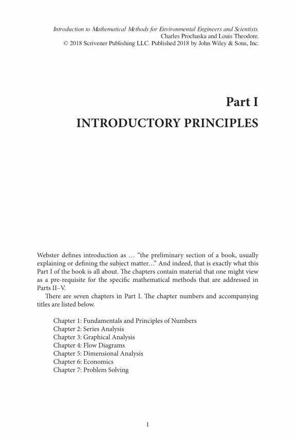
For example:
370 has 2 significant figures
370 has 3 significant figures
370.0 has 4 significant figures
28,070 has 4 significant figures
0.037 has 2 significant figures
0.0370 has 3 significant figures
0.02807 has 4 significant figures
Whenever quantities are combined by multiplication and/or division, the number
of significant figures in the result should equal the lowest number of significant fig-
ures of any of the quantities. In long calculations, the final result should be rounded
off to the correct number of significant figures. When quantities are combined by
addition and/or subtraction, the final result cannot be more precise than any of the
quantities added or subtracted. Therefore, the position (relative to the decimal point)
of the last significant digit in the number that has the lowest degree of precision is the
position of the last permissible significant digit in the result. For example, the sum of
3702, 370, 0.037, 4, and 37 should be reported as 4110 (without a decimal). The least
precise of the five number is 370, which has its last significant digit in the tens posi-
tion. Therefore, the answer should also have its last significant digit in its tens position.
Unfortunately, environmental engineers and scientists rarely concern them-
selves with significant figures in their calculations. However, it is recommended
that the reader attempt to follow the calculational procedure set forth in this section.
In the process of preforming engineering/scientific calculations, very large and
very small number are often encountered. A convenient way to represent these
numbers is to use scientific notation. Generally, a number represented in scientific
notation is the product of a number and 10 raised to an integer power. For example,
28 070 000 000 2 807 10 2 807 10
0 000002807 2 807 1
10 10, , , . ( . )( )
. . 00 6
A positive feature of using scientific notation is that only the significant figures
need appear in the number.
Thus, when approximate numbers are added, or subtracted, the results are pre-
sented in terms of the least precise number. Since this is a relatively simple rule to
master, note that the answer in Equation (1.50) follows the aforementioned rule
of precision.
6 04 2 8 4 173 4 7. . . .L L L L (1.50)

12 Introduction to Mathematical Methods
(The result is 4.667L.) The expressions in Equation (1.50) have two, one, and three
decimal places respectively. The least precise number (least decimal places) in the
problem is 2.8, a value carried only to the tenths position. Therefore, the answer
must be calculated to the tenths position only. Thus, the correct answer is 4.7L.
(The last 6 and the 7 are dropped from the 4.667L, and the first 6 is rounded up to
provide 4.7L.)
In multiplication and division of approximate numbers, finding the number of
significant digits is used to determine how many digits to keep (i.e., where to trun-
cate). One must first understand significant digits in order to determine the correct
number of digits to keep or remove in multiplication and division problems. As
noted earlier in this section, the digits 1 through 9 are considered to be significant.
Thus, the numbers 123, 53, 7492, and 5 contain three, two, four and one significant
digits respectively. The digit zero must be considered separately.
Zeroes are significant when they occur between significant digits. In the follow-
ing example, all zeroes are significant: 10001, 402, 1.1001, 500.09 with five, three,
five, and four significant figures, respectively. Zeroes are not significant when they
are used as place holders. When used as a place holder, a zero simply identifies
where a decimal is located. For example, each of the following numbers has only
one significant digit: 1000, 500, 60, 0.09, 0.0002. In the numbers 1200, 540, and
0.0032 there are two significant digits, and the zeroes are not significant. When
zeroes follow a decimal and are preceded by a significant digit, the zeroes are signifi-
cant. In the following examples, all zeroes are significant: 1.00, 15.0, 4.100, 1.90,
10.002, 10.0400. For 10.002, the zeroes are significant because they fall between
two significant digits. For 10.0400, the first two zeroes are significant because they
fall between two significant digits; the last two zeroes are significant because they
follow a decimal and are preceded by a significant digit. As noted above, when
approximate numbers are multiplied or divided, the result is expressed as a num-
ber having the same number of significant digits as the number in the problem
with the least number of significant digits.
When truncating (removing final, unwanted digits), rounding is normally
applied to the last digit to be kept. Thus, if the value of the first digit to be discarded
is less than 5, one should retain the last retained digit with no change. If the value of
the first digit to be discarded is 5 or greater, one should increase the last kept digit’s
value by one. Assume, for example, only the first two decimal places are to be kept
for 25.0847 (the 4 and 7 are to be dropped). The number is then 25.08. Since the
first digit to be discarded (4) is less than 5, i.e., the 8 is not rounded up. If only
the first two decimal places are to be kept for 25.0867 (the 6 and the 7 are to be
dropped), it should be rounded to 25.09. Since the first digit to be discarded (6) is
5 or more, the 8 is rounded up to 9.
When adding or subtracting approximate numbers, a rule based upon preci-
sion determines how many digits are kept. In general, precision relates to the deci-
mal significance of a number. When a measurement is given as 1.005 cm, one can
say that the number is precise to the thousandth of a centimeter. If the decimal is
removed (1005 cm), the number is precise to thousands of centimeters.
Fundamentals and Principles of Numbers 13
In some water pollution studies, a measurement in gallons or liters may be
required. Although a gallon or liter may represent an exact quantity, the measuring
instruments that are used are only capable of producing approximations. Using a
standard graduated flask in liters as an example, can one determine whether there
is exactly one liter? Not likely. In fact, one would be pressed to verify that there was
a liter to within 1/10 of a liter. Therefore, depending upon the instruments used,
the precision of a given measurement may vary.
If a measurement is given as 16.0L, the zero after the decimal indicates that the
measurement is precise to within 1/10L i.e., 0.1L. A given measurement of 16.00L,
indicates precision to the 1/100L. As noted, the digits following the decimal indi-
cate how precise the measurement is. Thus, precision is used to determine where
to truncate when approximate numbers are added or subtracted.
1.3 Errors
This is the first of two sections devoted to errors. This section introduces the vari-
ous classes of errors while the next section demonstrates the propagation of some
of these errors. As one might suppose, numerous books have been written on the
general subject of “errors.” Different definitions for errors appear in the literature
but what follows is the authors’ attempt to clarify the problem [1].
Any discussion of errors would be incomplete without providing a clear and
concise definition of two terms: the aforementioned precision and accuracy. The
term precision is used to describe a state or system or measurement for which
the word precise implies little to no variation; some refer to this as reliability.
Alternatively, accuracy is used to describe something free from the matter of
errors. The accuracy of a value, which may be represented in either absolute or
relative terms, is the degree of agreement between the measured value and the
true value.
All measurements and calculations are subject to two broad classes of errors:
determinate and indeterminate. The error is known as a “determinate error” if an
error’s magnitude and sign are discovered and accounted for in the form of a cor-
rection. All errors that either cannot be or are not properly allowed for in magni-
tude and sign are known as “indeterminate errors.”
A particularly important class of indeterminate errors is that of accidental errors.
To illustrate the nature of these, consider the very simple and direct measurement of
temperature. Suppose that several independent readings are made and that tempera-
tures are read to 0.1 °F. When the results of the different readings are compared, it may
be found that even though they have been performed very carefully, they may differ
from each other by several tenths of a degree. Experience has shown that such devia-
tions are inevitable in all measurements and that these result from small unavoidable
errors of observation due to the sensitivity of measuring instruments and the keen-
ness of the sense of perception. Such errors are due to the combined effect of a large
number of undetermined causes and they can be defined as “accidental errors.”

14 Introduction to Mathematical Methods
Regarding the words precision and accuracy, it is also important to note that
a result may be extremely precise and at the same time inaccurate. For instance,
the temperature readings just mentioned might all agree within 1 °F. From this it
would not be permissible to conclude that the temperature is accurate to 1 °F until
it can be definitively shown that the combined effects of uncorrected constant
errors and known errors are negligible compared with 1 °F. It is quite conceivable
that the calibration of the thermometer might be grossly incorrect. Errors such
as these are almost always present and can never be detected individually. Such
errors can be detected only by obtaining the readings with several different ther-
mometers and, if possible, several independent methods and observers.
It should also be understood at the onset that most numerical calculations are
by their very nature inexact. The errors are primarily due to one of three sources:
inaccuracies in the original data, lack of precision in carrying out calculations,
or inaccuracies introduced by approximate or incorrect methods of solution. Of
particular significance are the aforementioned errors due to “round-off ” and the
inability to carry more than a certain number of significant figures. The errors
associated with the method of solution are usually the area of greatest concern
[1]. These usually arise as a result of approximations and assumptions made in the
development of an equation used to calculate a desired result and should not be
neglected in any error analysis.
Finally, many list the following three errors associated with a computer
(calculator).
1. Truncation error. With the truncation of a series after only a few
terms, one is committing a generally known error. This error is not
machine-caused but is due to the method.
2. Round-off error. The result of using a finite number of digits to rep-
resent a number. In reality, numbers have an infinite number of
digits extending past the decimal point. For example, the integer 1
is really 1.000…0 and π is 3.14159… but numbers are rounded to
allow for calculation and representation. This rounding is a form of
error known as round-off error.
3. Propagation or inherited error. This is caused by sequential calcu-
lations that include points previously calculated by the computer
which already are erroneous owing to the two errors above. Since
the result is already off the solution curve, one cannot expect any
new values computed to be on the correct solution curve. Adding
the round-off errors and truncation errors into the calculation
causes further errors to propagate, adding more error at each step.
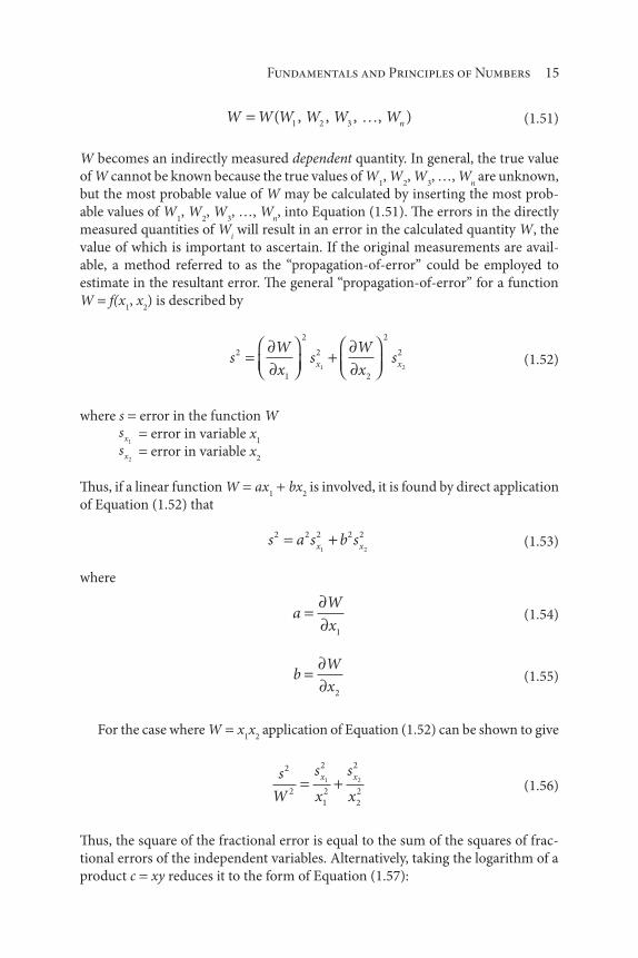
1.4 Propagation of Errors
When a desired quantity W is related to several directly measured independent
quantities W1, W
2, W
3, …, W
n by the equation
Fundamentals and Principles of Numbers 15
W W W W W Wn( )1 2 3, , , , (1.51)
W becomes an indirectly measured dependent quantity. In general, the true value
of W cannot be known because the true values of W1, W
2, W
3, …, W
n are unknown,
but the most probable value of W may be calculated by inserting the most prob-
able values of W1, W
2, W
3, …, W
n, into Equation (1.51). The errors in the directly
measured quantities of Wi will result in an error in the calculated quantity W, the
value of which is important to ascertain. If the original measurements are avail-
able, a method referred to as the “propagation-of-error” could be employed to
estimate in the resultant error. The general “propagation-of-error” for a function
W f(x1, x
2) is described by
sW
xs
W
xsx x
2
1
2
2
2
2
2
1 2 (1.52)
where s error in the function Ws
x1error in variable x
1
sx2
error in variable x2
Thus, if a linear function W ax1
bx2 is involved, it is found by direct application
of Equation (1.52) that
s a s b sx x
2 2 2 2 2
1 2 (1.53)
where
aW
x1
(1.54)
bW
x2
(1.55)
For the case where W x1x
2 application of Equation (1.52) can be shown to give
s
W
s
x
s
x
x x2
2
2
1
2
2
2
2
1 2 (1.56)
Thus, the square of the fractional error is equal to the sum of the squares of frac-
tional errors of the independent variables. Alternatively, taking the logarithm of a
product c xy reduces it to the form of Equation (1.57):

16 Introduction to Mathematical Methods
( ) ( ) ( )logs s sW logx logx
2 2 2
1 2 (1.57)
As would be expected, the greatest variation in the approach of different investiga-
tors lies in the details of how they propose to obtain values of the error measurement.
Basically, these may be obtained by comparing either a series of pairs of estimates and
true values from similar previous readings (i.e., “looking at the record”) or obtaining
a number of independent estimates of the particular value needed.
Illustrative Example 1.2 [2]
Table 1.3 gives basic data on investment and production costs for a unit for coking
a heavy crude to produce gasoline and distillate fuel. It is desired to determine the
standard deviation of the profit and its significance in predicting the uncertainty
involved.
Solution
The standard deviation equation is applied to determine the standard deviation of
the profit (income – cost). This is represented as (refer to Table 1.3)
s2 2 2 2 2480 000 180 900 66 300 1060 9480( , ) ( , ) ( , ) ( ) ( )(3860) +2 22
2 2
11
191 000 24 000
30 47 10
552 000
( , ) ( , )
.
$ ,s
Table 1.3 Investment data.
Item Average value X, $/yr Standard deviation
Investment $5,195,000 $513,000
Direct production cost
Raw materials $2,137,000 $180,900
Labor 215,000 66,300
Utilities 26,000 3,800
Operating Supplies 6,100 1,060
Maintenance 29,300 9,480
Royalties 16,500 0
$2,466,500 –
Indirect production cost 2,383,000 $191,000
Fixed production cost 494,000 24,000
Sales 6,700,000 480,000
Profits 1,356,500 –

Fundamentals and Principles of Numbers 17
Happel also goes on to calculate the percent return of an investment – a calcula-
tion beyond the scope of this introductory book [2].
Illustrative Example 1.3
Consider the data taken from an actual experiment performed by McHugh [3].
One step involves determining the number of moles of benzene, NB, loaded into
a round-bottom flask. Moles of benzene are calculated from two pieces of weight
data that are measured experimentally. Errors in these weight data accumulate to
result in an estimated accumulated error, s.
A Mettler electronic balance was used in an actual gravimetric transfer of ben-
zene, C6H
6, into the round-bottom flask. The following data was obtained:
Weight of volumetric flask benzene before transfer to round-bottom flask,
W1
105.321 0.001 g
Weight of volumetric flask benzene after transfer to round-bottom flask,
W2
85.466 0.001 g
Solution
The molecular weight of C6H
6 (MW
g) may be taken as equal to 78.12 g/g-mol. The
purity of the C6H
6 is 99.99%; this percentage is included as a variable (wt%) in
developing the equation for NB. The equation below is the defining equation for
moles of benzene, NB.
NW W
MWwtB
B
1 2 0 254% .
Taking the partial derivatives of the above equation with MWB as a constant and
the other terms being variables, gives the following values:
aN
W MWwtB
B1
10 0128% .
bN
W MWwtB
B2
10 0128% .

18 Introduction to Mathematical Methods
cN
wt
W W
MWB
B
1 2 0 254.
There are two s terms corresponding to the two weights (W1 and W
2) above.
These two terms are labelled s sW W1 2
and where W1 is the weight before the trans-
fer and the W2 is the weight after. A third s term, corresponding to the percentage
purity (wt%), is labelled swt%
. Substituting into the equations above leads to the
accumulated error equation.
sMW
wt sMW
wt sW W
MWB
W
B
W
B
2
2
2 2
2
2 2 1 21 11 2% %
2
2
2 2 2 2 2 2
10 10
1 2
1 6384 10 1 6384 10
s
a s b s c s
wt
w w wt
%
%
. . 11 6129 10
4 8897 10
10
10
.
.
The values for s sW W1 2
and used in this calculation are both 0.001 g, which is
the manufacturer’s specified “error” for the analytical balance used in this transfer;
this error is often reported as the repeatability or reproducibility of the balance.
The wt% term may be taken as 0.99990 0.00005, so that swt%
equals to 0.00005.
Calculating s yields.
s 2 2112 10 5.
so that
NB 0 254 2 2112 10 5. . gmol
A comparison of the value of s with the value of NB, indicates that the transfer
is accurate to five significant figures. On a percentage basis, s/NB is accurate within
0.009%; clearly this very “good” data.
Illustrative Example 1.4 [4]
In a rotary dryer experiment, samples of partially dried cornmeal are collected
in aluminum weighing pans and weighed (W1). The pans are placed in the oven
overnight to dry the remaining water from the cornmeal and reweighed (W2). The
dry cornmeal is discarded and the empty pan is weighed (W3). Data obtained from
one experiment appear below in Table 1.4.

Fundamentals and Principles of Numbers 19
Table 1.4 Rotary dryer experiment data.
Jill and Joe’s data Analytical balance
Weight of weighing pan
Cornmeal before drying (W1)
4.0 0.1g 4.012 0.001g
Weight of weighing pan
Cornmeal after drying (W2)
3.7 0.1g 3.638 0.001g
Weight of empty pan (W3) 1.3 0.1g 1.394 0.001g
(This example demonstrates a case where very “bad” data is obtained because the
students, Joe Jasper and his partner Jill Joker, decide to use a measuring device
that they liked instead of the best measuring device available. Jill and Joe were
instructed to use an analytical balance accurate to 0.001 g. However, Jill and Joe
didn’t like the analytical balance, so they decided to use a balance that is only
accurate to 0.1 g.)
Compare Jill and Joe’s data with the correct analytical data, and determine
whether using a less accurate balance significantly affects experimental error.
Solution
The weight of water removed from the cornmeal by drying is (W1 W
2). The
weight of the dry cornmeal is (W2 W
3). First, use the student data in Table 1.4
to calculate the weight fraction, W, of water in the partially dried cornmeal, as
defined by the following equation:
WW W
W W1 2
2 3
0 125.g water
g dry solids
Taking the partial derivative of the above equation and following the procedure
in the previous illustrated example yields the following equation for the accumu-
lated error.
sW W
sW W
W Ws
W W
WW W
2
2 3
2
2 1 3
2 3
2
2
2 1 3
2
11 2( ) ( WW
sW
3
2
2
2
3)
The values for s s sW W W1 2 3
, and used in this calculation are all 0.1 g, which is the
manufacturer’s specified “error” for the scale used by the students. Calculating s
from their data yields,
s2 32
2106.1305
g water
g dry solids

20 Introduction to Mathematical Methods
and
s 0.07830g water
g dry solids
so that
W 0 125. 0.07830g water
g dry solids
A comparison of the value of s with the value of W shows that the data obtained
with this balance is very “bad.” On a percentage basis, s/W is accurate to within
50%. This value of W is then used in successive calculations with the accumulated
errors getting even worse.
Much better results would have been obtained if the students used an analytical
balance with 0.001 g accuracy. A value for s of 0.00086 g/g would result in a per-
centage error of only 0.52% on redoing the calculation with the correct weights.
Details are left as an exercise for the reader.
References
1. L. Theodore and F. Taylor, Probability and Statistics, A Theodore Tutorial, Theodore Tutorials, East
Williston, NY, originally published by the USEPA/APTI, RTP, NC, 1995.
2. J. Happel, Chemical Process Economics, John Wiley & Sons, Hoboken, NJ, 1958.
3. M. McHugh, doctoral presentation, Department of Chemical Engineering, University of Delaware,
1981.
4. Author(s) unknown, Unit Operation Experiment, Manhattan College, Bronx, NY, date unknown.
21
An infinite series is an infinite sum of the form
a a an1 2 (2.1)
going on to infinitely many terms. It can further be defined that the terms in some
series are non-ending. Such series are familiar even in the simplest operations. For
example, one may write
2
30 66666. (2.2)
This is equivalent to
2
3
4
6
6
10
6
100
6
1 000
6
10 000, , (2.3)
2 Series Analysis
Introduction to Mathematical Methods for Environmental Engineers and Scientists. Charles Prochaska and Louis Theodore.
© 2018 Scrivener Publishing LLC. Published 2018 by John Wiley & Sons, Inc.

22 Introduction to Mathematical Methods
One might also “truncate,” or cut the infinite series after a certain number of
decimal places and use the resulting rational number
0 66666666
10 000.
, (2.4)
as a sufficiently good approximation to the number 2 3/ . One may also “round off ”
the above number to 0.6667.
The procedure just used applies to the general series a1
a2 +… a
n …. To
evaluate it, one rounds off after m terms and replaces the series by a finite sum.
a a am1 2 (2.5)
However, the rounding off procedure must be justified, i.e., one must be sure that
taking more than m terms would not significantly affect the result. For the series
3 3 3 3 (2.6)
such a justification would be inappropriate, since the first term gives a sum of 3,
two terms give 6, three terms give 9, etc. Truncating is of no help here. This series
is an example of a divergent series. On the other hand, for the series
Sn
11
4
1
9
1
16
12 (2.7)
it seems reasonable to truncate. Thus, one has as sums of the first four of the n
terms:
S 11
4
1
9
1
16
205
144 (2.8)
In addition, for
n S n S n S1 1 2 11
4
5
43 1
1
4
1
5
49
36, , ; , ;
Three sections compliment the presentation of this chapter. Section numbers
and subject titles follow:
2.1: Other Infinite Series
2.2: Tests for Convergence and Divergence
2.3: Infinite Series Equations

Series Analysis 23
2.1 Other Infinite Series
A portion of differential equations (see Part II, Chapter 11) result in solutions that
can be expressed in a closed or analytical form. In such cases, many of these solu-
tions are obtained in terms of functions which actually represent an infinite series.
Logarithmic, trigonometric, and hyperbolic functions are cases in point (see last
section in this chapter). It is not too surprising, then, to find that the solutions to
certain classes of differential equations are obtained in the form of an infinite series
of terms, i.e., an infinite series. Certain equations of this class appear frequently
enough that the particular forms of infinite series which represent their solutions
have been given specific names and symbols and the numerical values of the series
are tabulated in reference books. Bessel functions, Legendre polynomials, etc., are
typical examples [1]. Power series and Taylor series are briefly addressed below.
An expression of the type
a a x x a x xn
n
0 1 0 0( ) ( ) (2.9)
is termed a “power series.” Such a series is said to “converge” if it approaches a
finite value as n approaches infinity. The simplest test for convergence is the ratio
test; if the absolute value of the ratio of the (n 1) term to the nth term in any
infinite series approaches a limit j as n , then the series converges for j < 1,
diverges for j > 1, and fails if j 1.
A “Taylor series” expansion of y as a function of x (in the vicinity of xo) may be
written as
y x y x x x y xx x
y x( ) ( ) ( ) ( )!
( )( )
0 0 00
2
02
(2.10)
where
y ythe first derivative; the second derivative, etc. (2.11)
By setting the interval from the original point of expansion x0 to a general point x
as h, Equation (2.10) can be rewritten as
y x hh
n
d y
dxn
n n
n
x x
( )!
( )0
00
(2.12)
where 0! 1. If the values of the function and its derivatives at the point x0
are given, the solution for other values of x can be determined by simply
adjusting h.

24 Introduction to Mathematical Methods
2.2 Tests for Convergence and Divergence [2]
In general, the problem of determining whether a given series will or will not con-
verge can occasionally require a great deal of ingenuity and resourcefulness. The
convergence or divergence of an infinite series is complicated by the removal of
a finite number of terms. There is no all-inclusive test which can be applied to all
series. As the only alternative, it is necessary to apply one or more of the theorems
below in an attempt to ascertain the convergence or divergence of the series under
study. The following 10 tests are given in relative order of effectiveness.
1. A series will converge if the absolute value of each term (with or
without a finite number of terms) is less than the corresponding
term of a known convergent series.
2. A positive series is divergent if it is term-wise larger than a known
divergent series of positive terms.
3. A series is divergent if the nth term of the series does not approach
zero as n becomes increasingly large.
4. If the absolute ratio of the (n 1) term divided by the nth term as
n becomes unbounded approaches
a. a number less than 1, the series is convergent.
b. a number greater than 1, the series is divergent.
c. a number equal to 1, the test for convergence or divergence is
inconclusive.
5. The series converges if the partial summation of a series converges
as n becomes unbounded.
6. The series diverges if the partial summation of a series diverges as
n becomes unbounded.
7. If the terms of a series are alternately positive and negative and
never increase in numerical value, the series will converge, pro-
vided that the terms tend to zero as a limit.
8. If the nth root of the absolute value of the nth term, as n becomes
unbounded, approaches
a. a number less than 1, the series is convergent.
b. a number greater than 1, the series is divergent.
c. a number equal to 1, the test for convergence or divergence is
inconclusive.
9. If a series has no sum, it is divergent.
10. Multiplying every term of an infinite series by the same quantity
will not affect the convergence or divergence of the series.
2.3 Infinite Series Equations
This section opens with 3 arithmetic series which are expressed in terms of n,
followed by over 30 special cases involving infinite series.

Series Analysis 25
1 2 31
2n
n n( ) (2.13)
1 3 5 2 1 2( )n n (2.14)
( ) ( ) ( )( )( )
1 2 31 2 1
6
2 2 2 2nn n n
(2.15)
Special cases follow.
11
2
1
3
1
4
1
52ln( ) (2.16)
11
3
1
5
1
7
1
9 4 (2.17)
1
1
1
2
1
3
1
4 62 2 2 2
2
(2.18)
1
1
1
2
1
3
1
4 904 4 4 4
4
(2.19)
1
1
1
2
1
3
1
4 122 2 2 2
2
(2.20)
1
1
1
2
1
3
1
4
7
7204 4 4 4
4
(2.21)
1
1
1
3
1
5
1
7 82 2 2 2
2
(2.22)
1
1
1
3
1
5
1
7 964 4 4 4
4
(2.23)
1
1
1
3
1
5
1
7 323 3 3 3
3
(2.24)
1
1 3
1
3 5
1
5 7
1
7 9
1
2 (2.25)
1
1 3
1
2 4
1
3 5
1
4 6
3
4 (2.26)

26 Introduction to Mathematical Methods
1
1 3
1
3 5
1
5 7
1
7 9
8
162 2 2 2 2 2 2 2
2
(2.27)
1
1 2 3
1
2 3 4
1
3 4 5
4 39
162 2 2 2 2 2 2 2 2
2
(2.28)
( )1 1 1 11 2 3 4x x x x x x (2.29)
( )1 1 2 3 4 5 1 12 2 3 4x x x x x x (2.30)
( )1 1 3 6 10 15 1 13 2 3 4x x x x x x (2.31)
( )1 11
2
1 3
2 4
1 3 5
2 4 61 1
1
2 2 3x x x x x (2.32)
( )1 11
2
1
2 4
1 3
2 4 6
1
2 2 3x x x x x (2.33)
e xx x
xx 12 3
2 3
! ! (2.34)
a e x ax a x a
xx x aln lnln
!
ln
!
( ) ( )1
2 3
2 3
(2.35)
ln xx
x
x
x
x
x2
1
1
1
3
1
1
1
5
1
1
3 5
x 0 (2.36)
l n xx
x
x
x
x
xx
1 1
2
1 1
3
1 1
2
2 3
(2.37)
ln( )12 3 4
1 12 3 4
x xx x x
x (2.38)
1
2
1
1 3 5 71 1
3 5 7
ln! !
x
xx
x x xx (2.39)

Series Analysis 27
sin! ! !
x xx x x
x3 5 7
3 5 7 (2.40)
cos! ! !
;xx x x
x12 4 6
2 4 6
(2.41)
References
1. H. Mickley, T. Sherwood, and C. Reed, (adapted from) Applied Mathematics in Chemical
Engineering, McGraw-Hill, New York City, NY, 1957.
2. D. Green and R. Perry, editors, (adapted from) Perry’s Chemical Engineers’ Handbook, 8th ed.,
McGraw-Hill, New York City, NY, 2008.

29
Engineering data are often best understood when presented in the form of graphs or
mathematical equations. The preferred method of obtaining the mathematical rela-
tions between variables is to plot the data as straight lines and use the slope-intercept
method to obtain coefficients and exponents; therefore, it behooves the environmen-
tal engineer and scientist to be aware of the methods of obtaining straight lines on
various types of graph paper, and of determining the equations of such lines (see Part
IV, Chapter 28). One always strives to plot data as straight lines because of the sim-
plicity of the curve, ease of both interpolation and extrapolation. Graphical meth-
ods proved invaluable in the past in the analysis of relatively complex relationships.
Much of the basic physical and chemical data are still best represented graphically,
and graphical methods are often employed in the analytical treatment of processes.
One or more of the many types of graphical representations may be employed
for the following purposes:
1. as an aid in visualizing a process for the representation of qualita-
tive data
2. for the representation of quantitative data
3. for the representation of a theoretical equation
4. for the representation of an empirical equation
3Graphical Analysis
Introduction to Mathematical Methods for Environmental Engineers and Scientists. Charles Prochaska and Louis Theodore.
© 2018 Scrivener Publishing LLC. Published 2018 by John Wiley & Sons, Inc.

30 Introduction to Mathematical Methods
5. for the comparison of experimental data with a theoretical expression
6. for the comparison of experimental data with an empirical expression
The relation between two quantities y ‒ the dependent variable and x ‒ the inde-
pendent variable is commonly obtained as a tabulation of values of y for several
different values of x. The relation between y and x may not be easy to visualize by
studying the tabulated results and is often best seen by plotting y vs. x. If the condi-
tions are such that y is known to be a function of x only, the functional relation will
be indicated by the fact that the points may be represented graphically by a smooth
curve. Deviations of the points from a smooth curve generally indicates unreli-
ability in the data. If y is a function of two variables x1
and x2, a series of results
of y in terms of x1 may be obtained in terms of x
2. When plotted, the data will be
represented by a family of curves, each curve representing the relation between y
and x1 for a definite constant value of x
2. If another variable x
3 is involved, one may
have separate graphs for constant values of x3, each showing a family of curves of
y vs. x1. One may expand this method of representing data to express the relation-
ship between more than four independent variables (This method is explored in
more depth in Chapter 32, Part V).
Graphs can also be used for interpolation and extrapolation. In addition,
graphs may be employed to perform common mathematical manipulations such
as integration and differentiation. The data may be of almost any type encountered
in environmental engineering and science practice. They may be physical property
data, such as the variation in density and viscosity with temperature. They may be
process data, such as the variation in temperature along a tube in a heat exchanger
with respect to the flow rate of the fluid. One of the things that should be kept in
mind whenever working with plotted data is the loss of accuracy arising due to the
use of graphs. In general, the number of significant figures may be only as great as
the size of the divisions on the graph.
Five sections compliment the presentation of this chapter. Section numbers
and subject titles follow:
3.1: Rectangular Coordinates
3.2: Logarithmic-Logarithmic (Log-Log) Coordinates
3.3: Semi- Logarithmic (Semi-Log) Coordinates
3.4: Other Graphical Coordinates
3.5: Methods of Plotting Data
The reader should note that a good part of this material will be revisited in the
Optimization section (Chapter 32, Part V).
3.1 Rectangular Coordinates
Rectangular (sometimes referred to as Cartesian) coordinates on graph paper are
most generally used to represent equations of the form

Graphical Analysis 31
y mx b (3.1)
where y dependent variable represented on the ordinate
x independent variable represented on the abscissa
m slope of the line
b y-intercept at x 0
The bulk of the development in this chapter will be based on rectangular coor-
dinates. For general engineering use, the most common form of graph paper is the
8 ½ 11-inch sheet, having 20 lines per inch, with every fifth line accented, and
every tenth line heavily accented. This type of coordinate graph may be obtained
on drawing or tracing paper, with lines in black, orange, or green, and with or
without accented and heavy lines; it is also available in other sizes.
All graphs are created by drawing a line, or lines, about one or more axes. For
the purpose of this chapter, the presentation will be primarily concerned with
graphs built around two axes ‒ the x axis and the y axis. The graph data may be
presented as coordinates of the x and y axis in the form (x, y), or they may be pre-
sented as the abscissa (distance from the y axis or the x coordinate) and the ordi-
nate (distance from the x axis or the y coordinate). Referring to Figure 3.1, point
L5 has an abscissa (x coordinate) of +60 and an ordinate of +40 (y coordinate).
Using coordinate notation, the point can be described as (60, 40) where the points
are listed as (x, y). Point L2 can be described as (–6.7, 0).
All coordinates are produced as the result of solving an equation by assigning
different values to x or y, and solving for the value of the other. By convention,
problems are usually stated in the following form: y some value(s) of x and other
constant(s) (e.g., y mx +b).
The x and y axes divide a graph into four quadrants. The quadrants are usu-
ally numbered in a counter-clockwise sequence, beginning with the upper right
x
60Quadrant II Quadrant I
Quadrant III Quadrant IV
L1
L2L3
L4
y = 0.6x + 4
(10, 10)
(60, 40)
(0, 4)(–6.7, 0)
(–40, –20)
L5
50
40
y
30
20
10
0
–10
–20
–30
–40–40 –30 –20 –10 0 10 20 30 40 50 60
Figure 3.1 Linear coordinates.
32 Introduction to Mathematical Methods
quadrant (see Figure 3.1). Note that in quadrants I and IV, the x values are positive
while the x values are negative in quadrants II and III. The y values are positive in
quadrants I and II and negative in quadrants III and IV. The quadrant identifica-
tions are only of value when information is provided that a point or result lies in
a certain quadrant. Without knowledge of the precise values of x or y one can still
determine whether the x and y values are positive or negative.
Equations are identified by the type of line (or curve) they produce when plot-
ted on a graph. A linear equation, as the name implies, will result in a plot of a
straight line on a graph. With the linear equation, each incremental change of x
(or y) will result in an incremental change of a fixed ratio in y (or x). The ratio of
change between y and x is known as the slope of the line. A linear equation is also
referred to as a first-degree equation. The line plotted between L1 and L5 in Figure
3.1, is linear. All solutions to the equation describing the line (y 0.6x 4) will fall
somewhere on the line.
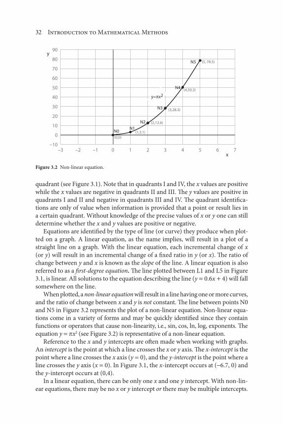
When plotted, a non-linear equation will result in a line having one or more curves,
and the ratio of change between x and y is not constant. The line between points N0
and N5 in Figure 3.2 represents the plot of a non-linear equation. Non-linear equa-
tions come in a variety of forms and may be quickly identified since they contain
functions or operators that cause non-linearity, i.e., sin, cos, ln, log, exponents. The
equation y x2 (see Figure 3.2) is representative of a non-linear equation.
Reference to the x and y intercepts are often made when working with graphs.
An intercept is the point at which a line crosses the x or y axis. The x-intercept is the
point where a line crosses the x axis (y 0), and the y-intercept is the point where a
line crosses the y axis (x 0). In Figure 3.1, the x-intercept occurs at ( 6.7, 0) and
the y-intercept occurs at (0,4).
In a linear equation, there can be only one x and one y intercept. With non-lin-
ear equations, there may be no x or y intercept or there may be multiple intercepts.
(0,0)
(1,3.1)
(2,12.6)
(3,28.3)
(4,50.3)
(5, 78.5)
–10
0
10
20
30
40
50
60
70
80
90
–3 –2 –1 0 1 2 3 4 5 6 7
y= x2
N0
N1
N2
N3
N4
N5
y
x
Figure 3.2 Non-linear equation.

Graphical Analysis 33
Note that in Figure 3.2, an intercept occurs when x 0 or y 0. In Figure 3.3, there
are two x-intercepts [( 2, 0) and (0, 0)] and one y-intercept (0, 0).
The reader should note that a good part of the above material will be revisited
in Part IV, Chapter 32.
3.2 Logarithmic-Logarithmic (Log-Log) Coordinates
A logarithmic scale is easily constructed by plotting (on rectangular paper) num-
bers from one to ten on the ordinate versus the logarithm of the number on the
abscissa. If the points representing the numbers on the ordinate are projected to
the resultant curve and then upward, the scale formed by the vertical lines will
be a logarithmic scale. The construction is illustrated in Figure 3.4. The utility of
the logarithmic scale lies in the fact that one can use actual numbers on the scale
instead of the logarithms. When two logarithmic scales are placed perpendicular
to each other and lines are drawn vertically and horizontally to represent major
divisions, a full logarithmic graph results, i.e., a log-log graph.
The term log-log or full logarithmic referred to above is used to distinguish
between another kind yet to be discussed, e.g., semi-logarithmic (see next sec-
tion). The full logarithmic graphs may be obtained in many types depending on
the scale length, sheet size, and number of cycles desired. The paper is specified
by the number of cycles on the ordinate and abscissa; for example, logarithmic 2
3 cycles means two cycles on the ordinate and three on the abscissa. Cycle lengths
are generally the same on both axes of a particular sheet. In addition, the distance
between numbers differing by a factor of 10 is constant on a logarithmic scale.
When plotting lines on logarithmic paper, equations in the general form
y bxm (3.2)
–4
–2
0
2
4
6
8
10
12
14
16
–10 –8 –6 –4 –2 0 2 4 6 8 10
x
y
y = 2x + x2
(3, 15)
(2,8)
(–5,15)
(–4,8)
(–3,3)
(–2,0)(0,0)
(–1–1)
(1,3)
Figure 3.3 Intercepts analysis.

34 Introduction to Mathematical Methods
where y a dependent variable
x an independent variable
b a constant
m a constant
will plot as straight lines on (full) logarithmic paper. A form of the equation analo-
gous to the slope-intercept equation for a straight line is obtained by plotting the
equation in logarithmic form, i.e.,
log log logy b m x (3.3)
If log y versus log x were plotted on rectangular coordinates, a straight line of slope
m and y-intercept log b would result. An expression for the slope is obtained by
differentiating Equation (3.3).
d y
d xm
(log )
(log ) (3.4)
When x 1, m log x 0, and the equation reduces to
log logy b (3.5)
Hence, log b is the y-intercept.
To illustrate the above, a linear plot of the equation
y x2 1 3. (3.6)
Figure 3.4 Log10
of a number.
0
1
2
3
4
5
6
7
8
9
10
11
0 0.1 0.2 0.3 0.4 0.5 0.6 0.7 0.8 0.9 1
Nu
mb
er
Log10
of a number

Graphical Analysis 35
00
0.5
1
0.5
0.1
0.5
0.6
0.65
1.08
m = = 1.30.65
0.5
0.43
Log10
x
Lo
g1
0 y
1
Figure 3.5 Linear plot of y 2x1.3.
1
10
100
1 10 100
y
x
a
b
Figure 3.6 The equation y 2x1.3 on logarithmic-logarithmic paper.
is given in Figure 3.5 on rectangular coordinate paper. It should be noted that
although the slope was obtained from a ratio of logarithmic differences, the same
result could have been obtained using measured differences if the scale of the ordinate
and abscissa were the same (in this case they were).
Inspection of Figure 3.6 reveals that equal measured distances on the logarith-
mic scale are equivalent to equal logarithmic differences on the abscissa of that
plot. It therefore follows that since the slope of Equation (3.3) is a ratio of loga-
rithmic differences, the slope on full logarithmic paper could be obtained using
measured distances. The plot of Equation (3.6) on 2 2 cycle logarithmic paper
is given in Figure 3.6. The slope using logarithmic differences from Figure 3.5 is
my y
x x2 1
2 1
1 08 0 43
0 60 0 101 3
. .
. .. (3.7)

36 Introduction to Mathematical Methods
and the slope using measured differences in Figure 3.6 is
ma
b1 3. (3.8)
To further illustrate the use of full logarithmic paper, consider the determina-
tion of a mathematical equation to represent data which are known to plot as a
straight line on log-log paper. If data in Table 3.1 are to be plotted, it is evident that
more than one cycle will be needed in both directions. For x, the data covers the
range from
2 10 0 2 10 6 2 100 1 1 (or to . ) . (3.9)
and for y the range is
3 6 10 0 36 10 5 0 100 1 1. ( . ) .or to (3.10)
In both cases two cycles are needed to cover the ranges from 100 to 101 and from
101 to 102. A general rule would be that the number of cycles should be equal to
the number of exponents of ten involved in the range of data – in this case, two for
each coordinate. The data are plotted in Figure 3.7. The slope may be once again
calculated in either of two ways:
mlog log .
log log ..
50 3 6
62 2 00 765 (3.11)
or
mc
d0 765. (3.12)
Table 3.1 Log data.
x y
2.0 3.6
3.9 6.0
7.0 9.4
14.0 16.0
26.5 26.0
62.0 50.0

Graphical Analysis 37
The y-intercept is 2.13; hence, the equation of the line is
log . . logy x2 13 0 765 (3.13)
In those cases where the line x 1 is several cycles removed from the data
range it may be inconvenient to extrapolate; the intercept can then be is deter-
mined by substituting the value of the slope and one data point and solving for b.
3.3 Semilogarithmic (Semi-Log) Coordinates
Graph paper made with one logarithmic scale and one arithmetic scale is termed
semilogarithmic. The logarithmic scale is normally the ordinate and the arithme-
tic scale is the abscissa on semilogarithmic paper. The paper is available in many
styles depending on the sheet size, type of paper, color of lines, number of cycles,
length of cycles, and the divisions on the uniform scale. The designation semilog-
arithmic, 7 5 to the ½ inch refers to semilogarithmic paper whose logarithmic
scale contains seven cycles whose uniform scale contains five divisions to the half
inch. The designation 10 division per inch (70 divisions) by two 5-inch cycles refers
to paper whose arithmetic scale is seven inches long and contains ten division per
inch, and whose logarithmic scale contains two-cycles for each five inches. Thus,
a semilogarithmic graph uses a standard scale for one axis and a logarithmic scale
for the other axis. The reason for this use of scales is that a logarithmic (exponen-
tial) plot would quickly exceed the physical boundaries of the graph.
Semilogarithmic paper can be used to represent equations of the form
y nemx (3.14)
1
10
100
1 10 100
y
x
c
d
Figure 3.7 Determination of a mathematical equation from raw data.

38 Introduction to Mathematical Methods
or
y n mx10 (3.15)
where y dependent variable
x independent variable
n a constant
m a constant
e the natural logarithm
Here again a form of the equation analogous to the slope-intercept equation
can be obtained by placing one of the above equations in logarithmic form. For
example, Equation (3.14) may be written as
log y b mx (3.16)
where b log n
An expression for slope is obtained from the differential form of Equation (3.16):
d y
dxm
(log ) (3.17)
so that the y-intercept is log n or b. Expressions for the slope and intercept of
Equation (3.15) are similar to those of Equation (3.14) except for the fact that
natural logarithms are employed.
One can illustrate the use of semilogarithmic paper by plotting a segment of the
curve representing the equation
log ..
yx
2 246 3
(3.18)
The line may be constructed (see Figure 3.8) by choosing values of x, solving
for y, and plotting the results. Note that values of y and not log y are plotted
on the ordinate. The slope is a logarithmic difference divided by an arithmetic
difference and, in this case, may be calculated from the two indicated points as
follows:
mlog log .
. .
1585 158 5
46 3 0
1
46 3 (3.19)
The slope of a line on semilogarithmic coordinates may be calculated from any
two points, but the simplest method is the one used above in which the slope
is the logarithmic difference on one cycle (equal to log 10 or 1.0) divided by

Graphical Analysis 39
the arithmetic difference cut by one cycle. Note that if the cycle had been taken
between y 300 and y 3000, the slope would be
mlog log
. . .
3000 300
59 1 12 8
1
46 3 (3.20)
It should also be noted that the y-intercept is 2.2, as required by Equation (3.18).
The method of obtaining a mathematical equation from data that are known
to plot as a straight line on semilogarithmic paper may be illustrated by the use of
the following data provided in Table 3.2.
Figure 3.8 The equation log y 2.2 x/46.3 plotted on semilogarithmic paper.
100
1000
0 10 20 30 40 50
y
x
46.3, 1585
0, 158.5
Figure 3.9 The determination of a mathematical equation from raw data.
100
1000
10000
0 1 2 3 4 5
y
x

40 Introduction to Mathematical Methods
The data are plotted in Figure 3.9. Three cycles on the logarithmic scale were
necessary because values of y ranged from
4 32 10 2 7 102 4. . to (3.21)
and three exponents of ten are involved, e.g., 2, 3, and 4. The slope may be calcu-
lated as follows:
mlog(27,000) log(432)
4.5 0.93
1
2 (3.22)
The line is extrapolated to x 0 to give a y-intercept of 2.175; hence the equation
representing the data is
log log logyx
2.1752
(3.23)
or
y 2.175+( /2)x (3.24)
3.4 Other Graphical Coordinates
Triangular (or trilinear) coordinates are used in some mass transfer studies to rep-
resent systems defined by three variables [1]. The graph can be in the form of an
equilateral triangle, each side of which is usually divided into 100 equal parts (see
Figure 3.10).
Table 3.2 Log data.
x y
0.93 432
1.52 886
2.56 2,830
3.20 6,000
3.80 12,000
4.50 27,000

Graphical Analysis 41
In addition to the more common types of graph paper previously discussed,
the practicing environmental engineer and scientist may also have need for prob-
ability versus arithmetic, probability versus logarithmic, logarithmic versus recip-
rocals, and other special types of graphs. Non-standard scales, if desired, may be
constructed in a similar manner to the logarithmic scale shown earlier. For exam-
ple, logarithmic-probability (log-normal) graphics find applications in air pollu-
tion studies to describe particle size distribution [2].
3.5 Methods of Plotting Data
The simplest procedure to employ in plotting equations of various forms is detailed
in Table 3.3 Various additional forms are available in the literature. Details on sta-
tistical methods for calculating the coefficients in the seven equations provided are
reviewed in Part IV, Chapter 28.
xa, mass fraction component a
x b, m
ass
frac
tio
n c
om
po
nen
t bx
c , mass fractio
n co
mp
on
ent c
0
100
90
80
70
60
50
40
30
20
10
0 100
90
80
70
60
50
P40
30
20
10
0
10 20 30 40 50 60 70 80 90 100
Figure 3.10 Equilateral triangular coordinates for a three-component mixture.

42 Introduction to Mathematical Methods
References
1. L. Theodore and F. Ricci, Mass Transfer Operations for the Practicing Engineer, John Wiley & Sons,
Hoboken, NJ, 2010.
2. L. Theodore, Air Pollution Control Equipment Calculations, John Wiley & Sons, Hoboken, NJ, 2008.
Table 3.3 Procedures for plotting equations.
y a bxplot y vs. x
y axn plot log y vs. log x or y vs. x on logarithmic crdinates
y c axn first obtain c as an intercept on a plot of y vs. x; then plot log (y c) vs.
x on logarithmic coordinates
y aebx plot log y vs. x on semilogarithmic coordinates
y abx plot log y vs. x on semilogarithmic coordinates
y ab
xplot y vs 1/x
yx
a bxplot x/y vs. x or 1/y vs. 1/x

43
The complete design specification for a medium-sized chemical process could
cover several hundred pages. It would include diagrams, tables, and discussion of
all aspects of the plant, including chemical, environmental, mechanical, structural,
electrical, metallurgical, and civil engineering considerations. To understand a
complete design, an environmental engineer or scientist must have training and
experience in this area (Note: Computer flow diagrams are not addressed in this
chapter.)
Any manufacturing plant, whether for the production of canned fruit, vacuum
cleaners, sulfuric acid, rubber tires, or any environmental process, may be visual-
ized as a box into which raw materials and energy are fed and from which use-
ful products, waste, and energy emerge. The manufacturing process ordinarily
involves several consecutive operations or steps through which the materials in
the process pass.
Figure 4.1 is a schematic representation of materials passing into and out of an
unidentified process for which there are environmental concerns. In this hypo-
thetical three-step process, raw materials A and B are fed into step 1; material C is
drawn off while material D is passed to step 2 for further processing. One cannot
tell whether C is a useful product or waste. From the sketch in step 2, it is neces-
sary to combine raw material E with D in order to produce F. In step 3, material F
4 Flow Diagrams
Introduction to Mathematical Methods for Environmental Engineers and Scientists. Charles Prochaska and Louis Theodore.
© 2018 Scrivener Publishing LLC. Published 2018 by John Wiley & Sons, Inc.

44 Introduction to Mathematical Methods
is separated into G, H, and J, ending the process. Again, the figure does not show
which of the last three items are useful products. The arrows lettered A, B, C, etc.
represented material streams and the sketch is known as a flow diagram. Although
nothing has been said about the specific nature of the process, this flow diagram
nevertheless conveys a great deal of information; namely, that in this three-step
process, three raw materials A, B, and E are required to produce four products
C, G, H, and J, and that these seven materials enter and leave the manufacturing
process at the points shown on the diagram [1].
As one might expect, a process flow diagram for a chemical or petroleum plant
is usually significantly more complex than that for a simple environmental facility.
For the latter case, the flow sequence and other determinations often reduce to an
approach that employs a “railroad” or sequential type of calculation that does not
require iterative calculations [1].
Five sections compliment the presentation of this chapter. Section numbers and
subject titles follow:
4.1: Process Schematics
4.2: Flow Chart Symbols
4.3: Preparing Flow Diagrams
4.4: Simplified Flow Diagrams
4.5: Hazard Risk Assessment Flow Chart
4.1 Process Schematics
To the environmental engineer, but particularly the chemical engineer, the
process flowchart is the key instrument for defining, refining, and documenting
a chemical process. The process flow diagram is the authorized process blueprint,
the framework for specifications used in equipment designation and design; it is
the single, authoritative document employed to define, construct, and operate a
process [1].
There are several essential constituents to a detailed process flowchart beyond
equipment symbols and process stream flow lines. These include equipment
B
A
C
D
E
F H
J
G
1 2 3
1 = pump
2 = mixer
3 = separator
Figure 4.1 Flow diagram for a three-step manufacturing process.
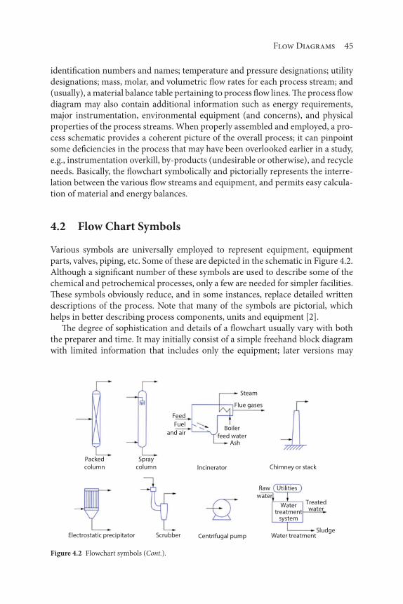
Flow Diagrams 45
identification numbers and names; temperature and pressure designations; utility
designations; mass, molar, and volumetric flow rates for each process stream; and
(usually), a material balance table pertaining to process flow lines. The process flow
diagram may also contain additional information such as energy requirements,
major instrumentation, environmental equipment (and concerns), and physical
properties of the process streams. When properly assembled and employed, a pro-
cess schematic provides a coherent picture of the overall process; it can pinpoint
some deficiencies in the process that may have been overlooked earlier in a study,
e.g., instrumentation overkill, by-products (undesirable or otherwise), and recycle
needs. Basically, the flowchart symbolically and pictorially represents the interre-
lation between the various flow streams and equipment, and permits easy calcula-
tion of material and energy balances.
4.2 Flow Chart Symbols
Various symbols are universally employed to represent equipment, equipment
parts, valves, piping, etc. Some of these are depicted in the schematic in Figure 4.2.
Although a significant number of these symbols are used to describe some of the
chemical and petrochemical processes, only a few are needed for simpler facilities.
These symbols obviously reduce, and in some instances, replace detailed written
descriptions of the process. Note that many of the symbols are pictorial, which
helps in better describing process components, units and equipment [2].
The degree of sophistication and details of a flowchart usually vary with both
the preparer and time. It may initially consist of a simple freehand block diagram
with limited information that includes only the equipment; later versions may
Centrifugal pumpScrubberElectrostatic precipitator
Packed
column
Spray
column Incinerator
Steam
Flue gases
Boiler
feed waterAsh
Chimney or stack
Raw
waterTreatedwater
Watertreatment
system
Water treatmentSludge
Utilities
Feed
Fuel
and air
Figure 4.2 Flowchart symbols (Cont.).

46 Introduction to Mathematical Methods
include line drawings with pertinent process data such as overall and componen-
tial flow rates, utility and energy requirements, environmental equipment, and
instrumentation. During the later stages of a design project, the flowchart will be
a highly-detailed P&I (piping and instrumentation) diagram; this aspect of the
design procedure is beyond the scope of this text. The reader is referred to the
literature for information on P&I diagrams [3].
In a sense, flowcharts are the international language of the engineer, particu-
larly the practicing engineer. Chemical engineers conceptually view a (chemical)
plant as consisting of a series of interrelated building blocks that are defined as
units or unit operations [4–7]. The plant ties together the various pieces of equip-
ment that make up the process. Flow schematics follow the successive steps of a
process by indicating where the pieces of equipment are located and the material
streams entering and leaving each unit [8–9].
4.3 Preparing Flow Diagrams
Before attempting to calculate the material or energy requirements of a process
it is desirable to attain a clear picture of the process. The best way to do this is to
draw the aforementioned flow diagram where the flow diagram is defined as a line
diagram showing the succession of steps in the process. Flow diagrams are very
important for saving time and eliminating mistakes. The beginner should learn
how to draw them properly and cultivate the habit of sketching them on the slight-
est excuse. The following rules should be observed.
1. Show operating units by simple neat rectangles. Do not waste time
in elaborate art work since it is without advantage or even meaning
(see Figure 4.3).
2. Make each material stream line represent an actual stream of mate-
rial passing along a pipe, duct, chute, belt, or other conveying device.
Refer to Figure 4.4(a). Show the gaseous mixture of carbon dioxide,
Counterflow
Condensers
Process fluid on
tube side
Process fluid on
shell side
Process fluid on
tube side
Process fluid on
shell side
Process fluid on
shell side
Parallel flow
Process fluid on
tube side
Figure 4.2 Flowchart symbols (Continued).

Flow Diagrams 47
oxygen, carbon monoxide, nitrogen, and water vapor obtained from
the combustion of a hydrocarbon fuel and exiting from the stack of
a furnace as a single material stream of flue gas, not to be confused
as five separate streams. Figure 4.4(b) shows a sophisticated “device”
that sorts components of the flue gas and delivers them as five sepa-
rate products through five separate pipes.
3. Distinguish between “open” and “closed” material streams. In
Figure 4.5(a), open steam is being blown into the tank, mixing
with the other materials in it. In Figure 4.5(b), steam is passing
through a coil, being kept separate from the tank contents, and
heating them by the transfer of heat through the walls of the coil.
Figure 4.3 Simple flowchart symbols.
WrongRight
WrongRight
Dis
tilla
tio
n c
olu
mn
Stirredmixing
tank
CC
B
A A
B
Figure 4.4 Right-and-wrong representation of a flue gas containing CO2, O
2, CO, N
2, and water
vapor.
Right(a) (b) Wrong
FurnaceFurnace
Liquid
Air
Liquid
Flue gas
CO2
CO
O2
N2
H2O
Air

48 Introduction to Mathematical Methods
4. Distinguish between a continuous operation, in which raw mate-
rial is fed into the equipment in an uninterrupted stream and a
batch operation in which a fixed charge of material is introduced,
processed, and removed, followed by the feeding of a new charge
with repetition of the cycle, etc. Batch operation is indicated con-
veniently by putting a double bar on the material stream lines of
entering materials as shown in Figure 4.6(b).
5. Except for a few unusual situations which will be discussed later,
keep flow diagrams free of data regarding the material streams. An
over-burden of data clutters up the diagram and robs it of its main
function, which is to present a clear picture of the materials as they
move into, through, and out of the process. This is illustrated in
Figure 4.7 with the air and coal entering a furnace.
4.4 Simplified Flow Diagrams
In many cases simplified flow sheets are prepared to illustrate a process. These
are often for a special purpose and do not show all the details of the process.
Figure 4.5 Open and closed material streams.
Steam
A
B
C
A
B
C
Steam out
Steam in
Figure 4.6 Continuous vs. batch operation.
A
B
C
D
A
B
C
D
(a) Continuous (b) Batch

Flow Diagrams 49
A common type of flow sheet shows the major unit operations and chemical reac-
tors with their interconnecting piping and an identification of the materials being
processed. The units are not shown to scale, but the drawing may resemble the
equipment used for the operation. Such a diagram would be called a graphic pro-
cess flow sheet. For a small process of a few units, a pictorial flow sheet with draw-
ings of equipment approximately to scale may be used. Photographs are usually
unsatisfactory because the arrangement and connections are seldom clear. On a
process flow sheet, the equipment is arranged logically to show the flow of mate-
rials through the process, but a photograph shows the final physical arrangement
determined by structural requirements without regard to the process flow. All
tall absorber columns may be grouped together for structural support, and large
heat exchangers may be grouped together for ease of maintenance. The successful
individual must learn to read flow sheets and to relate them to the actual plant
layout.
If sufficient data are available, a quantitative process flowsheet may be prepared
showing the flow rates, compositions, temperatures, and pressures throughout the
process. Such flow sheets may be very complicated. Flow sheets showing instru-
mentation and controls are also occasionally prepared.
4.5 Hazard Risk Assessment Flow Chart
An acceptable risk is a risk whose probability is unlikely to occur during the lifetime
of a plant or process. An acceptable hazard risk can also be defined as an acci-
dent that has a high probability of occurring, but with negligible consequences.
Risks can be ranked qualitatively in categories of high, medium, and low. Risks can
also be ranked quantitatively as the annual number of fatalities per million affect
individuals.
Hazard risk assessment (HZRA) calculations are based on an algorithm pro-
posed over 30 years ago. This algorithm is based on a simple flowchart (see also
Flue gas
Cinder
Furnace
Flue gas
Air
Coal
Cinder
Furnace
Air: 79% N2, 21% O
2,
t=70°F, p=1atm, H=62%
Coal: 3.8% H2O, 8.6% ash,
7.2% volatile matter,
80.4% fixed carbon
(a) Right (b) Wrong
Figure 4.7 Inclusion versus exclusion of experimental data on flow diagrams.

50 Introduction to Mathematical Methods
Figure 4.8). There are several steps in evaluating the risk of an accident; if the
system in question is a chemical plant, the following guidelines apply:
1. A brief description of the equipment and chemicals used in the
plant is needed.
2. Any hazard in the system has to be identified. Hazards that may
occur in a chemical plant include:
a. Corrosion
b. Explosions
c. Fires
d. Rupture of a pressurized vessel
e. Runaway reactions
f. Slippage
g. Unexpected leaks
3. The event or series of events that will initiate an accident must be
identified. An event could be a failure to follow correct safety pro-
cedures, to improperly repair equipment, or the failure of a safely
mechanism.
4. The probability that the accident will occur often has to be deter-
mined. For example, if a nuclear power plant has a 10-year life,
what is the probability that the temperature in a reactor will exceed
System
description
Hazard/event
problemidentification
Accidentprobability
Accidentconsequence
evaluation
Riskdetermination
Is isk/hazard
acceptable?
If YES,operatesystem
If NO,modifysystem
Figure 4.8 HZRA flowchart for a chemical plant.

Flow Diagrams 51
the specified temperature range? The probability can be ranked
qualitatively from low to high. A low probability means that it is
unlikely for the event to occur in the life of the plant. A medium
probability suggests that there is a possibility that the event will
occur. A high probability means that the event will probably occur
during the life of the plant.
5. The severity of the consequence of the accident must be determined.
6. If the probability of the accident and the severity of its conse-
quences are low, then the risk is usually deemed acceptable and the
plant should be allowed to operate. If the probability of occurrence
is too high or the damage to the surroundings is too great, then the
risk is usually unacceptable and the system needs to be modified to
minimize these effects.
The heart of the hazard risk assessment algorithm provided is enclosed in the
dashed-line box in Figure 4.8. This algorithm allows for reevaluation of the process
if the risk is deemed unacceptable (the process is repeated starting with step 1 or 2).
The reader should note that both health risk assessment and hazard risk assess-
ment plus accompanying calculations have received extensive treatment in the
literature [10–11].
References
1. L. Theodore, personal notes, East Williston, NY, 1967.
2. G. Ulrich, A Guide to Chemical Engineering Process Design and Economics, John Wiley & Sons, NY,
1984.
3. T. Shen, Y. Choi, and L. Theodore. Hazardous Waste Incineration Manual, A Theodore Tutorial,
Theodore Tutorials, East Williston, NY, originally published by USEPA/APTI, RTP, NC, 1985.
4. P. Abulencia and L. Theodore, Fluid Flow for the Practicing Chemical Engineer, John Wiley & Sons,
Hoboken, NJ, 2007.
5. L. Theodore, Heat Transfer Applications for the Practicing Engineer, John Wiley & Sons, Hoboken,
NJ, 2011.
6. L. Theodore and F. Ricci, Mass Transfer Operations for the Practicing Engineer, John Wiley & Sons,
Hoboken, NJ, 2010.
7. L. Theodore, R. Dupont, K. Ganesan, Unit Operations in Environmental Engineering, Scrivener-
Wiley, Salem, MA, 2017.
8. R. Perry and D. Green, editors, Perry’s Chemical Engineers’ Handbook, 8th ed., McGraw-Hill, New
York City, NY, 2008.
9. W. McCabe, J. Smith, and P. Harriot, Unit Operations of Chemical Engineering, 5th ed., McGraw-
Hill, New York City, NY, 1993.
10. L. Theodore, J. Reynolds, and K. Morris, Accident and Emergency Management, A Theodore
Tutorial, Theodore Tutorials, East Williston, NY, originally published by USEPA/APTI, RTP,
NC, 1996.
11. L. Theodore and R. Dupont, Environmental Health Risk and Hazard Risk Assessment: Principles
and Calculations, CRC Press/Taylor & Francis Group, Boca Raton, Fla., 2012.

53
A surprising amount of a practicing environmental engineer’s time (and scien-
tist’s as well) is spent in converting data and equations from one set of units to
another. Keep in mind that a unit is defined as a measure of a physical extent while
a dimension is a description of the physical extent. As long as most physicists and
chemist make measurement in grams and centimeters while many engineers in the
United States employ pounds and feet, confusion in terminology will continue to
exist.
Units, unlike physical laws, can be considered as either derived or basic. There
is a certain latitude in choosing the basic units and, unfortunately, this free choice
has resulted in the aforementioned mild form of confusion. Two systems of units
have arisen: metric-the cgs, or centimeters-gram-second system and the English
the fps, or foot-pound-second system of engineering. The metric system has come
to be defined as the System of International Units, or more commonly for some as
the SI system.
Six sections compliment the presentation of this chapter. Section numbers and
subject titles follow:
5.1: The Metric System
5.2: The SI System
5.3: Conversion of Units
5 Dimensional Analysis
Introduction to Mathematical Methods for Environmental Engineers and Scientists. Charles Prochaska and Louis Theodore.
© 2018 Scrivener Publishing LLC. Published 2018 by John Wiley & Sons, Inc.

54 Introduction to Mathematical Methods
5.4: Select Common Abbreviations
5.5: Dimensionless Numbers
5.6: Buckingham Pi ( ) System
5.1 The Metric System [1]
The need for a single worldwide coordinated measurement system was recognized
nearly 350 years ago. In 1670, Gabriel Mouton, Vicar of St. Paul’s Church in Lyon,
France, proposed a comprehensive decimal measurement system based on the
length of one minute of arc of a great circle of the Earth. On 1671, Jean Picard, a
French astronomer, proposed the length of a pendulum arc beating seconds as the
unit of length. (Such a pendulum would be fairly easy to reproduce, thus facili-
tating the widespread distribution of uniform standards.) Other proposals were
made, but over a century elapsed before any action was taken.
In 1790, in the midst of the French Revolution, the National Assembly of France
requested the French Academy of Scientists to “deduce an invariable standard for
all the measures and weights.” The Commission appointed by the Academy cre-
ated a system that was, at once, simple and scientific. The unit of length was to be
a portion of the Earth’s circumference. Measures for capacity (volume) and mass
(weight) were to be derived from the unit of length, thus relating the basic units of
the system to each other and to nature. Furthermore, the larger and smaller ver-
sions of each unit were to be created by multiplying or dividing the basic units by
10 and its multiples. This feature provided a great convenience to users of the sys-
tem by eliminating the need for calculating and dividing by 16 (to convert ounces
to pounds) or by 12 (to convert inches to feet). Similar calculations in the metric
system could be performed simply by shifting the decimal point. Thus, the metric
system is a base-10 or decimal system.
The Commission assigned the name metre (which is now spelled meter) to the
unit of length. This name was derived from the Greek word metron meaning “a
measure.” The physical standard representing the meter was to be constructed
so that it would equal one ten-millionth of the distance from the north pole to
the equator along the meridian of the Earth running near Dunkirk in France and
Barcelona in Spain.
The metric unit of mass, called the gram, was defined as the mass of one cubic
centimeter (a cube that is 1/100 of a meter on each side) of water at its temperature
of maximum density. The cubic decimeter (a cube 1/10 of a meter on each side)
was chosen as the unit of fluid capacity. This measure was given the name liter.
Although the metric system was not accepted with enthusiasm at first, adop-
tion by other nations occurred steadily after France made its use compulsory in
1840. The standardized character and decimal features of the metric system made
it well suited to scientific and engineering work. Consequently, it is not surprising
that the rapid spread of the system coincided with an age of rapid technological
development. In the United States, by Act of Congress in 1866, it was made “lawful

Dimensional Analysis 55
throughout the United States of America to employ the weights and measures of
the metric system in all contracts, dealings, or court proceedings.”
By the late 1860’s, even better metric standards were needed to keep pace with
scientific advances. In 1875, an international treaty, the “Treaty of the Meter,” set
up well-defined metric standards for length and mass, and established permanent
machinery to recommend and adopt further refinements in the metric system.
This treaty, known as the Metric Convention, was signed by 17 countries, including
the United States.
As a result of the treaty, metric standards were constructed and distributed to
each nation that ratified the Convention. The internationally agreed metric stan-
dards have served as the fundamental weights and measures standards of the
United States since 1893.
A total of 35 nations- including the major nations of continental Europe and
most of South America- had officially accepted the metric system by 1900. Today,
with the exception of the United States and a few small countries, the entire world is
predominately using the metric system, or is committed to such use. The Secretary
of Commerce, in transmitting to Congress the results of a 3-year study authorized
by the Metric Study Act of 1968, recommended in 1971 that the US change to the
predominant use of the metric system through a coordinated national program.
The International Bureau of Weights and Measures located at Sevres, France,
serves as a permanent secretariat for the Metric Convention, coordinating the
exchange of information about the use and refinement of the metric system. As
measurement science develops, more precise and easily reproducible ways of defin-
ing the measurement units will emerge. The General Conference of Weights and
Measures- the diplomatic organization made up of adherents to the Convention-
meets periodically to ratify improvements in the system and the standards.
5.2 The SI System
In 1960, the General Conference adopted an extensive revision and simplification
of the system. The name Le Systeme International d’Unites (International System
of Units), with the international abbreviation SI, was adopted for this modernized
metric system. Further improvements in and additions to SI were made by the
General Conference in 1964, 1968, and 1971.
The basic units in the SI system are the kilogram (mass), meter (length), sec-
ond (time), Kelvin (temperature), ampere (electric current), candela (the unit of
luminous intensity), and radian (angular measure), all of which are commonly
used by the practicing environmental engineer and scientist. The Celsius scale of
temperature (0 °C 273.15 K) is commonly used with the absolute Kelvin scale.
The important derived units are the newton (SI unit of force), the joule (SI unit of
energy), the watt (SI unit of power), the pascal (SI unit of pressure), and the hertz
(SI unit of frequency). There are a number of electrical units: coulomb (charge),
farad (capacitance), henry (inductance), volt (potential), and weber (magnetic

56 Introduction to Mathematical Methods
flux). As noted above, one of the major advantages of the metric system is that
larger and smaller units are given in powers of ten. In the SI system, a further sim-
plification is introduced by recommending only the use of units with multipliers
of 103. Thus, for lengths in engineering, the micrometer (previously referred to as
micron), millimeter, and the kilometer are recommended, and the centimeter is gen-
erally avoided. A further simplification is that the decimal point may be substituted
by a comma (as in France, Germany, and South Africa), while the other number,
before and after the comma, is separated by spaces between groups of three.
The aforementioned seven base units have been associated with the SI.
1. Length – meter (m)
2. Mass – kilogram (kg)
3. Time – second (s)
4. Electric current – ampere (A)
5. Temperature – Kelvin (K)
6. Amount of substance – mole (mol) (aka gram mole)
7. Luminous intensity – candela (cd)
Note that two supplementary units are occasionally employed in geometric studies:
1. Phase angle – radian (rad)
2. Solid angle – steradian (sr)
5.3 Conversion of Units
Momentum and rate of momentum come into play in both fluid flow and the con-
servation law in momentum studies. The latter term is defined (in terms of units) as
Rate of Momentumlb ft
s2 (5.1)
The above units can be converted to lbf , if multiplied by an appropriate constant.
A conversion constant is a term that is used to obtain units in a more convenient
form. All conversion constants have magnitude and units in the term, but can also
be shown to be equal to 1.0 (unity) with no units.
A conversion constant used often is
12 in/ft (5.2)
This term is obtained from the following defining equation:
12 1 in ft (5.3)

Dimensional Analysis 57
If both sides of this equation are divided by 1 ft, one obtains:
1 12 in/ft (5.4)
Note that this conversion constant, like all others, is also equal to unity without
any units.
Another defining equation is:
1 32 22
lblb ft
sf . (5.5)
If this equation is divided by lbf, Equation (5.6) results.
1 0 32 22
. .lb ft
lb sf
(5.6)
This serves to define the conversion constant gc. If the rate of momentum is
divided by gc as 32 2 2. lb ft/lb s
f – this operation being equivalent to dividing by
1 – the following units result:
Rate of Momentumlb ft
s
lb s
lb ftlb
2
2
f
f (5.7)
One can conclude from the above dimensional analysis that a force is equivalent
to a rate of momentum.
There are hundreds of conversion constants employed by engineers and scientists.
Some of the more common “conversion constants” are provided in Table 5.1 [1].
Conversion of units can be accomplished by the multiplication of the quan-
tity to be converted by appropriate unit ratios, i.e., the conversion constants. For
example, suppose an energy of 50 Btu must be converted to units of (ft lbf). From
the energy section in Table 5.1 one notes that to convert from Btu to (ft lbf), mul-
tiply by 778. Therefore,
778 1( )ft lb Btuf
(5.8)
and the conversion constant or unit ratio is similarly,
778
11 0
( ).
ft lb
Btu
f (5.9)
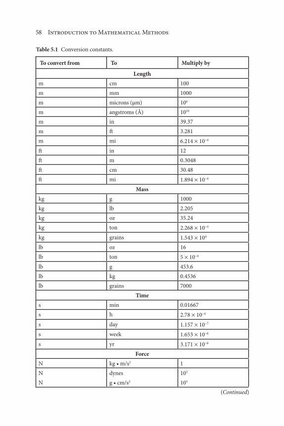
58 Introduction to Mathematical Methods
Table 5.1 Conversion constants.
To convert from To Multiply by
Length
m cm 100
m mm 1000
m microns (μm) 106
m angstroms (Å) 1010
m in 39.37
m ft 3.281
m mi 6.214 10 4
ft in 12
ft m 0.3048
ft cm 30.48
ft mi 1.894 10 4
Mass
kg g 1000
kg lb 2.205
kg oz 35.24
kg ton 2.268 10 4
kg grains 1.543 104
lb oz 16
lb ton 5 10 4
lb g 453.6
lb kg 0.4536
lb grains 7000
Time
s min 0.01667
s h 2.78 10 4
s day 1.157 10 7
s week 1.653 10 6
s yr 3.171 10 8
Force
N 1
N dynes 105
N 105
(Continued)

Dimensional Analysis 59
To convert from To Multiply by
N lbf
0.2248
N 7.233
lbf
N 4.448
lbf
dynes 4.448 105
lbf
4.448 105
lbf
32.17
Pressure
atm N/m2 (Pa) 1.013 105
atm kPa 101.3
atm bars 1.013
atm dynes/cm2 1.013 106
atm lbf /in2 (psi) 14.696
atm mm Hg at 0 oC (torr) 760
atm in Hg at 0 oC 29.92
atm ft H2O at 4 oC 33.9
atm in H2O at 4 oC 406.8
psi atm 6.80 10 2
psi mm Hg at 0 oC (torr) 51.71
psi in H2O at 4 oC 27.70
in H2O at 4 oC atm 2.458 10 3
in H2O at 4 oC psi 0.0361
in H2O at 4 oC mm Hg at 0 oC (torr) 1.868
Volume
m3 L 1000
m3 cm3 (cc, mL) 106
m3 ft3 35.31
m3 gal (U.S.) 264.2
m3 qt 1057
ft3 in3 1728
ft3 gal (U.S.) 7.48
ft3 m3 0.02832
ft3 L 28.32
Table 5.1 Cont.
(Continued)

To convert from To Multiply by
Energy
.
Power
Concentration
Table 5.1
Continued
60 INTRODUCTION TO MATHEMATICAL METHODS
Cont.
J Nom 1
J erg 107
J dyne 0 em 107
J kWh 2.778 x 10⁻⁷
J cal 0.2390
J ft olbf 0.7376
J Btu 9.486 x 10⁻⁴
cal J 4.186
cal Btu 3.974 x 10⁻³
cal ft olbf 3.088
Btu ft olbf 778
Btu hpoh 3.929 x 10⁻⁴
Btu cal 252
Btu kWoh 2.93 x 10⁻⁴
ft olbf cal 0.3239
ft olbf J 1.356
ft olbf Btu 1.285 x 10⁻³
W J/s 1
W calls 0.2390
W ft olb,ts 0.7376
W kW 10-3
kW Btu/s 0.949
kW hp 1.341
hp ft o Ih,ts 550
hp kW 0.7457
hp calls 178.2
hp Btu/s 0.707
llg/m3 Ib/ft3 6.243 x 10⁻¹¹
llg/m3 Ib/gal 8.346 x 10⁻¹²
llg/m3 gr (grain)/ft3 4.370 X 10⁻⁷

Dimensional Analysis
To convert from To Multiply by
Viscosity
Heat Capacity
f
f
Table 5.1
61
Cont.
gr/ft3 Jlg/m3 2.288 X 10⁶
gr/ft3 glm3 2.288
lb/ft3 Jlg/m3 1.602 X 10¹⁰
lb/ft3 Jlg/L 1.602 X 10⁻⁸
lb/ft3 lb/gal 7.48
P (poise) glcm. s 1
P cP (centipoise) 100
P kg/m .h 360
P lb/ft. s 6.72 X 10⁻²
P lb/ft. h 241.9
P lb/m. s 5.6 X 10⁻³
lb/ft. s P 14.88
lb/ft. s glcm. s 14.88
lb/ft. s kg/m .h 5.357 x 10³
lb/ft. s lb/ft. h 3600
callg'oC Btu/lb. OF 1
callg'oC kcallkg.oC 1
callg'oC cal/gmol.oC Molecular weight
callgmol. °C Btu/lbmol of 1
J/g'oC Btu/lb. of 0.2389
Btu/lb. OF cal/g'oC 1
Btu/lb. of J/g'oC 4.186
Btu/lb. of Btu/lbmol of Molecular weight
The 50 Btu may be multiplied by the above conversion constant without changing its value. Therefore,
(778(ft.lb ))
(50 Btu) = 38,900(lb . ft) 1 Btu
(5.10)
with the Btu units canceling, just like numbers.

62 Introduction to Mathematical Methods
Illustrative Example 5.1
Convert:
1. 150 miles/h to yards/h
2. 100.0 m/s2 to ft/min2
3. 0.03 g/m3 to lb/ft3
Solution
Employ Table 5.1.
1. 150 5 280
32 6 105 mile
h
ft
mile
yd
ft yd/h
,.
2. 100 0100
30 48
601 181
2
..
.m/s cm
m
ft
cm
s
min
2 1106 2 ft/min
3. ( . ).
.0 06454
30 482 0
3
3g/cmlb
g
cm
ft lb/ft3
5.4 Select Common Abbreviations [1]
Some typical abbreviations that are employed in environmental engineering and
science practice are provided in Table 5.2.
5.5 Dimensionless Numbers
Problems are frequently encountered in environmental studies and other engineer-
ing work that involve several variables. Engineers and scientists are generally inter-
ested in developing functional relationships (equations) between these variables.
When these variables can be grouped together in such a manner that they can be
used to predict the performance of similar pieces of equipment, independent of
the scale or size of the operation, something very valuable has been accomplished.
Consider, for example, the problem of establishing a method of calculating
power requirements for mixing liquids in an open tank at a water treatment facil-
ity. The obvious variables would be the depth of liquid in the tank, the density and
viscosity of the liquid, the speed of the agitator, the geometry of the agitator, and
the diameter of the tank. There are therefore six variables that affect the power, or
a total of seven terms that must be considered. To generate a general equation to
describe power variation with these variables, a series of tanks having different
diameters would have to be set up in order to gather data for various values of each

Dimensional Analysis
Table 5.2
f
Continued
63
Selected common abbreviations.
A,A angstrom unit oflength
abs absolute
amb ambient
app.MW,M apparent molecular weight, molecular weight
atm atmosphere
at. wt. atomic weight
b.p. boiling point
bbl barrel
Btu British thermal unit
cal calorie
cg centigram
cm centimeter
cgs system centimeter gram second system
conc concentration
cc, cm3 cubic centimeter
cu ft, ft3 cubic feet
cfh cubic feet per hour
cfm cubic feet per minute
cfs cubic feet per second
m3, M3 (rarely) cubic meter
° degree
°C degree Celsius, degree Centigrade
OF degree Fahrenheit
OR degree Rankine, degree Reamur (rarely)
ft foot
ft .lb foot pound mass
ft .lb foot pound force
fpm feet per minute
fps feet per second
fps system foot. pound. second system
f.p. freezing point
gr grain
g,gm gram
h hour

Table 5.2
Continued
64 INTRODUCTION TO MATHEMATICAL METHODS
Cont.
in inch
kcal kilocalorie
kg kilogram
km kilometer
liq liquid
L liter
log logarithm (common)
In logarithm (natural)
m.p. melting point
m, M (rarely) meter
flIl1 micrometer (micron)
mks system meter. kilogram. second system
mph miles per hour
mg milligram
ml milliliter
mm millimeter
mfl millimicron
min minute
molwt,MW,M molecular weight
oz ounce
ppb parts per billion
pphm parts per hundred million
ppm parts per million
lb pound
psi pound force per square inch
psia pound force per square inch absolute
psig pound force per square inch gage
rpm revolutions per minute
s, sec second
spgr specific gravity
spht specific heat
spwt specific weight
sq square
scf standard cubic foot
STP standard temperature and pressure
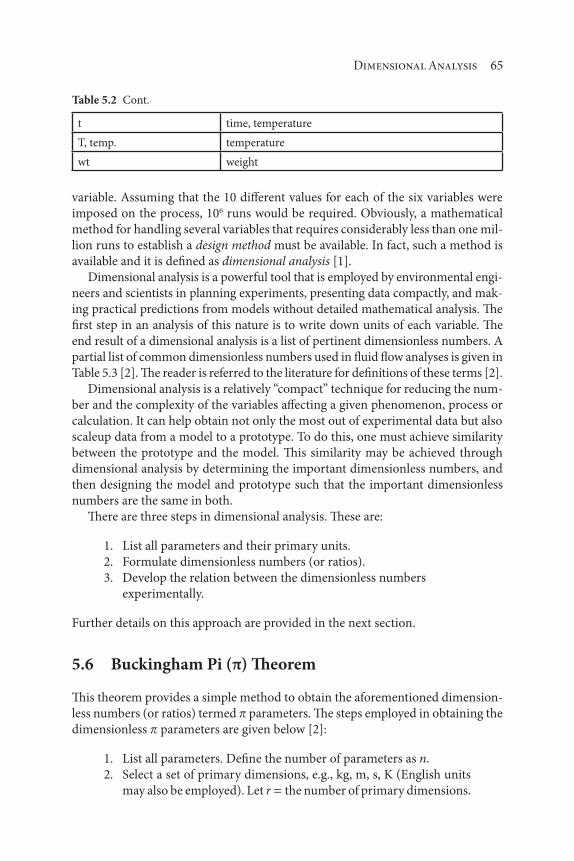
Dimensional Analysis 65
t time, temperature
T, temp. temperature
wt weight
variable. Assuming that the 10 different values for each of the six variables were
imposed on the process, 106 runs would be required. Obviously, a mathematical
method for handling several variables that requires considerably less than one mil-
lion runs to establish a design method must be available. In fact, such a method is
available and it is defined as dimensional analysis [1].
Dimensional analysis is a powerful tool that is employed by environmental engi-
neers and scientists in planning experiments, presenting data compactly, and mak-
ing practical predictions from models without detailed mathematical analysis. The
first step in an analysis of this nature is to write down units of each variable. The
end result of a dimensional analysis is a list of pertinent dimensionless numbers. A
partial list of common dimensionless numbers used in fluid flow analyses is given in
Table 5.3 [2]. The reader is referred to the literature for definitions of these terms [2].
Dimensional analysis is a relatively “compact” technique for reducing the num-
ber and the complexity of the variables affecting a given phenomenon, process or
calculation. It can help obtain not only the most out of experimental data but also
scaleup data from a model to a prototype. To do this, one must achieve similarity
between the prototype and the model. This similarity may be achieved through
dimensional analysis by determining the important dimensionless numbers, and
then designing the model and prototype such that the important dimensionless
numbers are the same in both.
There are three steps in dimensional analysis. These are:
1. List all parameters and their primary units.
2. Formulate dimensionless numbers (or ratios).
3. Develop the relation between the dimensionless numbers
experimentally.
Further details on this approach are provided in the next section.
5.6 Buckingham Pi (π) Theorem
This theorem provides a simple method to obtain the aforementioned dimension-
less numbers (or ratios) termed parameters. The steps employed in obtaining the
dimensionless parameters are given below [2]:
1. List all parameters. Define the number of parameters as n.
2. Select a set of primary dimensions, e.g., kg, m, s, K (English units
may also be employed). Let r the number of primary dimensions.
Table 5.2 Cont.

66 Introduction to Mathematical Methods
Table 5.3 Dimensionless numbers [2].
Parameter Definition Area of importance Qualitative ratio
Cavitation numberCa
P p
v
!
2 2/
Cavitation Pressure
Inertia
Eckert numberEc
v
C Tp
2 Dissipation Kinetic energy
Inertia
Euler numberEu
P
v2 2/
Pressure drop Pressure
Inertia
Froude numberFr
v
gL
2 Free surface flow Inertia
Gravity
Mach numberMa
v
c
Compressible flow Flow speed
Sound speed
Poiseuille numberP
D P
Lv0
2 Laminar flow in pipes Pressure
Viscous forces
Relative roughness k
D
Turbulent flow, rough
wallsWall roughness
Body length
Reynolds numberRe
vD vD
v
Various uses Inertia forces
Viscous forces
Strouhal numberSt
wL
v
Oscillating flow Oscillation speed
Mean speed
Weber numberWe
v L2 Surface forces effect Inertia
Surface tension
3. List the units of all parameters in terms of the primary dimen-
sions, e.g., L [=] m, where “[=]” means “has the units of.” This is
a critical step and often requires some creativity and ingenuity on
the part of the individual performing the analysis.
4. Select a number of variables from the list of parameters (equal
to r). These are called repeating variables. The selected repeating
parameters must include all r independent primary dimensions.
The remaining parameters are called “non-repeating” variables.
5. Set up dimensional equations by combining the repeating param-
eters with each of the non-repeating parameters in turn to form
the dimensionless parameters. . There will be (n – r) dimension-
less groups of ( s).
6. Check that each resulting group is in fact dimensionless.

Dimensional Analysis 67
Note that it is permissible to form a different group from the product or division
of other s, e.g.,
51 2
3
2 6
4
2 1or (5.11)
Note, however, that a dimensional analysis approach will fail if the fundamen-
tal variables are not correctly chosen. The Buckingham Pi theorem approach to
dimensionless numbers is given in the Illustrative Example that follows.
Illustrative Example 5.2
When a fluid flows through a horizontal circular pipe, it undergoes a pressure
drop. P (P2 P
1). For a rough pipe, P will be higher than a smooth pipe. The
extent of non-smoothness of a material is expressed in terms of the roughness,
k [2]. For steady state incompressible Newtonian fluid flow, the pressure drop is
believed to be a function of the fluid average velocity v, viscosity , density , pipe
diameter D, pipe length L, pipe roughness k, and the speed of sound in a fluid (an
important variable if the flow is compressible) c, i.e.,
P f v D L k c( , , , , , , )
Determine the dimensionless numbers of importance for this flow system [1, 2].
Solution
A pictorial representation of the system in question is provided in Figure (5.1). List
all the parameters and find the value of n:
P v D L k c, , , , , , ,
There are 8 parameters therefore, n 8. Choose primary units (employ SI).
m, s, kg, K
21
D
L
v
Figure 5.1 Pipe.

68 Introduction to Mathematical Methods
List the primary units of each parameter:
P [ ] Pa kg m s1 2
v [=] ms 1
[ ] kg m s1 1
D [=] m
L [=] m
kg m[ ] 3
k [=] m
c [=] ms 1
Therefore, r 3 with primary units m, s, kg.
Select three parameters from the list of eight parameters. These are the repeat-
ing variables:
D [=] m
[ ] kg m 3
v [ =] ms 1
The non-repeating parameters are then P, , k, c and L. Determine the number
of s:
n - 3 8 - 3 5
Formulate the first , i.e., 1, employing P as the non-repeating parameter.
1 Pv Da b f
Determine a, b, and f by comparing the units on both sides of the following
equation:
0 1 2 1 3[ ]( )( ) ( ) ( )kg m s m s kg m ma b f

Dimensional Analysis 69
Compare kg:
0 1 1b b. , Therefore
Compare s:
0 2 2a a. ,Therefore
Compare m:
0 1 3 0a b f f. ,Therefore
Substituting back into 1 leads to:
1 2Pv
P
v
a b
This represents the Euler number (see Table 5.3).
Formulate the second , i.e., 2, as
2 v Da b f
Determine a, b, and f by comparing the units on both sides:
0 1 2 1 3[ ]( )( ) ( ) ( )kg m s m s kg m ma b f
Compare kg:
0 1 1b b. ,Therefore
Compare s:
0 1 1a a. Therefore,
Compare m:
0 1 3 1a b f f. Therefore,
Substituting back into 2 yields:
2
1 1 1v Dv D

70 Introduction to Mathematical Methods
Replace 2 by its reciprocal:
2
v DRe
where Re Reynolds number.
Similarly, the remaining non-repeating variables lead to
3 kv Dk
D
a b f
and from
4 cv Da b f
one obtains
4
v
cthe Mach Number
Similarly,
5
L
D
Combine the s into an equation, expressing 1 as a function of
2,
3,
4 and
5.
EuP
vf
k
DMa
L
D2
2
Re the Euler number, , ,
Consider the case of incompressible flow.
EuP
vf
k
D
L
D2
2
Re , ,
The result indicates that to achieve similarity between a model (m) and a proto-
type (p), one must have the following:
Rem
Rep

Dimensional Analysis 71
k
D
k
Dm p
L
D
L
Dm p
Since Eu Re fk
D
L
D, , , then it follows that Eu
mEu
p (see also Table 5.3).
References
1. I. Farag and J. Reynolds, Fluid Flow, A Theodore Tutorial, Theodore Tutorials, East
Williston, NY, originally published by the USEPA/APTI, RTP, NC, 1995.
2. P. Abulencia and L. Theodore, Fluid Flow for the Practicing Chemical Engineer, John
Wiley & Sons, Hoboken, NJ, 2009.

73
Regardless of the type of society or government within which a business is oper-
ated, it must either show a profit or perish. What applies to an individual business
applies equally to a community or an entire economy. Without profit, the structure
is weak; with profit, it may be strong. This conclusion is not debatable.
Because of the necessity for combining economic considerations with environ-
mental fundamentals and principles, the environmental engineer or scientist must
be aware of the many different types of costs involved in environmental processes
and issues. Money must be paid out for different plant expenses such as those for
raw materials, labor, and equipment. In addition, many other indirect expenses are
incurred, and these must be included if a complete analysis of the total cost is to be
obtained. Some examples of these are addressed later in the chapter.
Since this chapter was written primarily for the beginning student it would
be almost impossible at this level to cover all of the various aspects of engineer-
ing economics. This chapter therefore introduces the philosophy of economics in
engineering and shows, by means of a few illustrative examples, the use of eco-
nomics as a tool. It is realized that the broad subject of engineering economics
cannot be fitted to any rigid set of formulas. For the interested reader, there are
many texts available in the literature which provide a much broader treatment of
6Economics
Introduction to Mathematical Methods for Environmental Engineers and Scientists. Charles Prochaska and Louis Theodore.
© 2018 Scrivener Publishing LLC. Published 2018 by John Wiley & Sons, Inc.

74 Introduction to Mathematical Methods
the subject. Both the qualitative and quantitative viewpoints are emphasized in the
material to follow.
Four sections compliment the presentation of this chapter. Section numbers
and subject titles follow:
6.1: Definitions
6.2: The Need for an Economic Analysis
6.3: Capital Investment and Risk
6.4: Applications
6.1 Definitions
Before proceeding to the applications later in the chapter, it would be wise to pro-
vide the reader with certain key definitions used in the field. Fourteen concepts
that often come into play in an economic analysis are given below. The definitions
have been drawn from the literature [1].
Simple Interest
The term interest can be defined as the money paid for the use of money. It is also
referred to as the value or worth of money. Two terms of concern are simple inter-
est and compound interest. Simple interest is always computed on the original
principal. The basic formula to employ in simple interest calculations is:
S P ni( )1 (6.1)
where P original principle
n time in years
i annual interest rate
S sum of interest and principal after n years
Normally, the interest period is one year, in which case i is referred to as the effec-
tive annual interest rate.
Compound Interest
Unlike simple interest, with compound interest, interest is added periodically to
the original principle. The term conversion or compounding of interest simply
refers to the addition of interest to the principal. The interest period or conversion
period in compound interest calculations is the time interval between successive
conversions of interest. The interest rate is the ratio of the stated annual rate to the
number of interest periods in one year. Thus, if the given interest rate is 10% com-
pounded semiannually, the interest period is six months and the interest rate per
interest period is 5%. Alternatively, if the given interest rate is 10% compounded

Economics 75
quarterly, then the interest period is 3 months and the interest rate per interest
period is 2.5%. One should always assume the interest is compounded annually
unless otherwise stated. The basic formula to employ for compound interest is:
S P i n( )1 (6.2)
If interest payments become due m times per year at compound interest, (m)
(n) payments are required in n years. An effective annual interest rate, i , may be
defined by
ii
m
m
1 1 (6.3)
In this case, the new equation for S becomes:
S P in
1 (6.4)
In the limit (as m approaches infinity), such payments may be considered to
be required at infinitesimally short intervals, in which case, the interest is said to
be compounded continuously. Numerically, the difference between compounding
may be significant when applied to vary large sums of money.
Present Worth
The present worth is the current value of a sum of money due at time n and at
interest rate i. The following equation is the compound interest equation solved
for the present worth term P.
P S i n( )1 (6.5)
Evaluation of Sums of Money
The value of a sum of money changes with time because of interest considerations.
$1,000 today, $1,000 ten years from now, and $1,000 ten years ago all have different
meanings when interest is taken into account. $1,000 today would be worth more
than $1,000 ten years from now because of the interest that could be accumulated
in the interim. On the other hand, $1,000 today would have been worth less ten
years ago because a smaller sum of money could have been invested then so as
to yield $1,000 today. Therefore, one must refer to the date as well as the sum of
money when evaluating sums of money.
Summarizing, evaluating single sums of money requires multiplying by (1 i)n
if the required date of evaluation is after the date associated with the obligation or

76 Introduction to Mathematical Methods
multiplying by (1 i) n if the required date of evaluation is before the date associ-
ated with the obligation. The term n is always the time in periods between the date
associated with the obligation and the evaluation date.
The evaluation of sums of money may be applied to the evaluation of a uniform
series of payments. A uniform series is a series of equal payments made at equal
intervals. Suppose R is invested at the end of every interest period for n periods.
The total value of all these payments, S, as of the date of the last payment, may be
calculated from the equation
SR i
i
n[( ) ]1 1 (6.6)
The term S is then called the amount of the uniform series.
Depreciation
The term depreciation refers to the decrease in the value of an asset. Two approaches
that can be employed are the straight line and sinking fund method. In the straight
line method of depreciation, the value of the asset is decreased each year by a con-
stant amount. The annual depreciation amount, D, is given by:
DOriginal cost Salvage value
Estimated life in years (6.7)
In the sinking fund method of depreciation, the value of the asset is determined by
first assuming that a “sinking” fund consisting of uniform annual payments had
been set up for the purpose of replacing the asset at the end of its estimated use-
ful life. The uniform annual payment (UAP) may be calculated from the equation
UAP Original cost Salvage value SFDF( )( ) (6.8)
where SFDF is the sinking fund deposit factor and is given by
SFDFi
i n[ ]( )1 1 (6.9)
The value of the asset at any time is estimated to be the difference between the
original cost and the amount that would have accumulated in the sinking fund.
The amount accumulated in the sinking fund is obtained by multiplying the SFDF
by the compound amount factor (CAF) where
CAFi
i
n[( ) ]1 1 (6.10)

Economics 77
Fabricated Equipment Cost Index
A simple process is available to estimate the equipment cost from past cost data.
The method consists of adjusting the earlier cost data to present values using fac-
tors that correct for inflation. A number of such indices are available; one of the
most commonly used is the fabricated equipment cost index (FECI).
Cost CostFECI
FECIyear B year A
year B
year A
(6.11)
Given the cost and FECI for year A, as well as the FECI for year B, the cost of the
equipment in year B can be estimated by employing Equation (6.11).
Capital Recovery Factor
In comparing alternative processes or different options for a particular process
from an economic point-of-view, one recommended procedure to follow is that
the total capital cost can be converted to an annual basis by distributing it over
the projected lifetime of the facility (or the equivalent). The sum of both the annu-
alized capital cost (ACC), including installation, and the annual operating cost
(AOC), is called the total annualized cost (TAC) for the project or facility. The
economic merit of the proposed facility process, or scheme can be examined once
the total annual cost is available.
The conversion of the total capital cost (TCC) to an ACC requires the determi-
nation of an economic parameter known as the capital recovery factor (CRF). This
parameter can be found in any standard economics textbook or calculated directly
from the following equation:
CRFi i
i
n
n
( )
( )[ ]
1
1 1 (6.12)
where n projected lifetime of the system
i annual interest rate (as a fraction)
The CRF is a positive, fractional number. Once this factor has been determined,
the ACC can be calculated from the following equation:
ACC TCC CRF)( )( (6.13)
The annualized capital cost can be viewed as the cost associated with recovering
the initial capital expenditure over the depreciable life of the system.

78 Introduction to Mathematical Methods
Present Net Worth
There are various approaches that may be employed in the economic selection
of the best of several alternatives. For each alternative in the present net worth
(PNW) method of economic selection, a single sum is calculated that would pro-
vide for all expenditures over a common time period. The alternative having the
least PNW of expenditures is selected as the most economical. The equation to
employ is
PNW CC PN PWD PWS (6.14)
where
CC Capital cost
PN Future renewals
PWD Other disbursements
PWS Salvage value
If the estimate lifetimes differ for the various alternatives, one should employ
a period of time equal to the least common multiple of the different lifetimes for
renewal purposes.
Perpetual Life
Capitalized cost can be viewed as present worth under the assumption of per-
petual life. Computing capitalized cost involves, in a very real sense, finding the
present worth of an infinite series of payments. To obtain the present worth of an
infinite series of payments of $R at the end of each interest period forever, one
needs simply to divide R by i, where i is the interest rate per interest period. Thus,
to determine what sum of money, P, would have to be invested at 8.0% to provide
payments of $100,000 at the end of each year forever, P would have to be such that
the interest on it each period would be $100,000. Withdrawal of the interest at the
end of each period would leave the original sum intact to again draw $100,000
interest at the end of the next period. For this example,
P100 000
0 081 250 000
,
.$ , , (6.15)
The $1,250,00 would be the present worth of an infinite series of payments of
$100,000 at the end of each year forever, assuming money is worth 8%.
To determine the present worth of an infinite series of payments of $R at
the end of each n periods forever, first multiply by the SFDF to convert to an
equivalent single period payment and then divide by i (fractional value) to obtain
the present worth.

Economics 79
Break-Even Point
From an economic point-of-view, the break-even point of a process operation is
defined as that condition when the costs (C) exactly balance the income (I). The
profit (P) is therefore:
P I C (6.16)
At break-even, the profit is zero.
Approximate Rate of Return
Rate of return can be viewed as the interest that will make the present worth of net
receipts equal to the investment. The approximate rate of return (ARR), denoted
by some as p, may be estimated from the equation below:
p ARRAverage annual profit or earnings
Initial total investtment (6.17)
To determine the average annual profit, simply divide the difference between
the total money receipts (income) and the total money disbursements (expenses)
by the number of years in the period of the investment.
Exact Rate of Return
Using the approximate rate of return as a guide, one can generate the exact rate
of return (ERR). This is usually obtained by trial-and-error and interpolation cal-
culations of the rate of interest that makes the present worth of the net receipts
equal to the investments. The approximate rate of return will tend to overestimate
the exact rate of return when all or a large part of the receipts occur at the end
of a period of investment. The approximate rate will tend to underestimate the
exact rate when the salvage value is zero and also when the salvage value is a high
percentage of the investment.
Bonds
A bond is a written promise to pay both a certain sum of money (redemption price)
at a future date (redemption date) and equal interest payments at equal intervals in
the interim. The holder of a $1,000, 5% bond, redeemable at 105 (bond prices are
listed without the last zero) in 10 years, with interest payable semiannually would
be entitled to semiannual payments of ($1,000) (0.025) or $25 for 10 years and
105% of $1,000, that is $1,050, at the end of 10 years when the bond is redeemed.
The interest payment on a bond is found by multiplying the face value of the
bond by the bond interest rate per period. From the above, the face value is $1,000
80 Introduction to Mathematical Methods
and the bond interest rate per period is 0.025. Therefore, the periodic interest pay-
ment is the aforementioned $25. Redeemable at 105 means that the redemption
price is 105% of the face value of the bond.
The purchase price of a bond depends on the yield rate, i.e., the actual rate of
return on the investment represented by the bond purchase. Therefore, the pur-
chase price of a bond is the present worth of the redemption price plus the pres-
ent worth of future interest payments, all computed at the yield rate. The bond
purchase price formula is:
VC i R
i
n( )1 (6.18)
where
V purchase price
C redemption price
R periodic interest payment
n time in periods to maturity
i yield rate
Incremental Cost
By definition, the average unit increment cost is the increase in cost divided by the
increase in production. Only those cost factors which vary with the production
can affect the average unit incremental cost. In problems involving decisions as to
whether to stay in production or (temporarily) shut down, the average unit incre-
ment cost may be compared with the unit increment cost or the unit selling price.
6.2 The Need for an Economic Analysis [1]
Before an environmental engineer or scientist can successfully apply the principles
of economics to operational expenses, he/she must first become familiarized with
the existing economics with which he/she is associated, as well as with the policies,
if applicable, of the company itself. A company or individual hoping to increase its
profitability must carefully assess a range of investment opportunities and select
the most profitable options from those available. Increasing competitiveness also
requires that efforts be expended to reducing costs of existing processes. In order
to accomplish this, environmental engineers and scientists should be fully aware
of not only technical but also economic factors, particularly those that have the
largest effect on profitability.
In earlier years, environmental engineers (and scientists) concentrated on the
technical side of projects and left the financial studies to the economist. In effect,
all those engineers involved in making estimates of the capital and operating costs
Economics 81
had often left the overall economic analysis and investment decision-making to
others. This approach is no longer acceptable.
Some engineers are not equipped to perform a financial and/or economic anal-
ysis. Furthermore, many environmental engineers and scientists already working
for companies have never taken courses in this area. This shortsighted attitude
is surprising in a group of people who normally go to great lengths to get all the
available technical data before making an assessment of a project or study. The
attitude is even more surprising when one notes that data are readily available to
enable an engineer to assess the prospects of both his/her own company and those
of his/her particular industry [2].
Bridging the gap between theory and practice is often a matter of experience
acquired over a number of years. Even then, methods developed from experience
all too often must be re-evaluated in the light of changing economic conditions if
optimum profits are to result. The approach presented here therefore represents an
attempt to provide a consistent and reasonably concise method for the solution of
these problems involving economic alternatives [3].
As noted above, the purpose of this chapter is to provide a working tool to bet-
ter assist the reader in not only understanding economics and finance but also in
applying technical information to the economic design and operation of processes
and plants. The material to follow will often focus on environmental and/or plant
applications. Hopefully, this approach will provide the reader with a better under-
standing of some of the fundamentals and principles.
The term “economic analysis” in engineering problems generally refers to
calculations made to determine the conditions for realizing maximum financial
return for a design or operation. The same general principles apply, whether one
is interested in the choice of alternatives for competing projects, in the design
of plants or projects so that the various components are economically propor-
tioned, or in the optimization for economical operation of existing plants. General
considerations that form the framework on which sound decisions must be made
are often simple. Sometimes their application in the problems encountered in the
development of a commercial enterprise involves too many intangibles to allow
exact analysis, in which case judgments must be intuitive. Often, however, such
calculations may be made with a considerable degree of exactness. This chapter
attempts to develop a relatively concise method for applying these principles.
Finally, concern with the maximum financial returns implies that the crite-
rion for judging projects involves profit. While this is usually true, there are many
important objectives which, though aimed at ultimate profit increase, cannot be
immediately evaluated on quantitative terms. Perhaps the most significant of these
has been the tendency in recent years to regard management of commercial orga-
nizations as a profession with environmental obligations and responsibilities; con-
siderations other than the profit motive may govern business decisions. However,
these additional social objectives are for the most part often consistent with the
economic goal of satisfying human wants with the minimum cost and effort. In

82 Introduction to Mathematical Methods
fact, even in the operation of primarily nonprofit organizations, it is still important
to determine the effect of various policies on profit [1].
6.3 Capital Investment and Risk
A capital investment is required for any process, and the determination of the
necessary investment is an important part of a project. The total investment for
any process consists of the fixed capital investment for the physical equipment
and facilities plus the working capital for money which must be available to pay
salaries, keep raw materials and products on hand, and handle other special items
requiring a direct cash outlay. Thus, in an analysis of costs in industrial processes,
investment costs, factory manufacturing costs, and general expenses that include
income taxes must be taken into consideration.
The following material primarily addresses chemical plants. The following
sequence of steps must be taken before a chemical plant can be put into operation:
1. A process must be planned and evaluated, or even invented.
2. The equipment is designed and the operational procedure worked
out and analyzed.
3. Land is acquired for the site and services made available through
roads, lines for gas, water, and electricity, sewage disposal systems,
etc.
4. Requisite materials are purchased, and the buildings and all equip-
ment erected.
5. Funds must be made constantly available to keep the venture in
operation once the plant has been put “on stream.”
All five of the above steps require money. The total money involved is called the
capital investment. This consists of two parts; that required for steps (1), (2), (3),
and (4), known as fixed capital and that required for step (5) called working capital.
In more graphic terms, the money required to bring the process from the moment
of conception to the moment of when the “button is pushed” and the plant is first
set in operation is fixed capital. Typical items of the fixed capital are salary paid,
e.g., to researchers and engi neers for conception and design. All money required
for the venture thereafter (with the exception of capital improvements or expan-
sions of the plant) is working capital that can include the cost of raw materials;
salaries and wages paid to production engineers, foremen, and plant workers;
packaging and shipping costs; the costs of water, gas, fuel, electricity, etc., and, the
salaries paid to clerical personnel involved with the process [4].
Many a process that looked good in an early stage of research or development
proved to be economically unattractive after closer and more intensive examina-
tion. Often, the process does not go beyond step (2) listed above. Money invested
up to this point is partly lost and may be completely lost. In other cases, the process

Economics 83
gets all the way to the operational stage before proving to be unprofitable, in which
case the loss may be significant.
Certain things should be obvious. All investment of capital in chemical process-
ing involves a risk. Manufacturing profit cannot start unless and until the process
is put into actual operation, and since for every process that proves profitable there
are others that do not, the profitability of the successful processes should be suf-
ficient to absorb the losses incurred by the unsuccessful ventures. What potential
profit level should seem probable before capital is invested in a manufacturing pro-
cess? A partial answer is provided in the next paragraph.
Money put into a savings account or invested in bonds may draw a certain
return without risk, effort, or worry. It follows that the investment of capital in
a manufacturing process that would yield as little as this percent return would
be unsound since this would represent the assumption of business risk with no
profit at all. How far in excess above the potential rate of return should be to jus-
tify the investment of capital depends upon the nature of both the industry and
the individual process. When new frontiers are being broached, a potential profit
of 30 percent or more may be essential to make a plant design attractive. On the
other hand, starting a plant to produce a heavy chemical by a process with a long
record of successful performance for which detailed economic data are available is
another matter and may be attractive at a lower profitability potential.
6.4 Applications
The remainder of the chapter is devoted to illustrative examples, many of which
contain technical development material. A good number of these environmental
applications have been drawn from the National Science Foundation (NSF) litera-
ture [5–8] and one other key source [9].
Illustrative Example 6.1
List the major fixed capital costs for the chemical process industry.
Solution
1. Major process equipment (i.e., reactors, tanks, pumps, filters, dis-
tillation columns, etc.)
2. Installation of major process equipment
3. Process pumping
4. Insulation
5. Instrumentation
6. Auxiliary facilities (i.e., power substations, transformers, boiler
houses, fire-control equipment, etc.)
7. Outside lines (i.e., piping external to the building, supports and posts
for overhead piping, electric feeders from the power substations, etc.)

84 Introduction to Mathematical Methods
8. Land and site improvements
9. Building and structures
10. Consultant fees
11. Engineering and construction (design and engineering fees plus
supervision of plant erection)
12. Contractors’ fees (administrative)
Illustrative Example 6.2
List the major working capital costs for the chemical process industry.
Solution
1. Raw materials for plant startup
2. Raw materials, intermediate and finished product inventories
3. Cost of handling and transportation of materials to and from sites
4. Cost inventory control, warehouses, associated insurance, security
arrangements, etc.
5. Money to carry accounts receivable (i.e., credit extended to cus-
tomers) less accounts payable (i.e., credit extended by suppliers)
6. Money to meet payrolls when starting up
7. Readily available cash for emergencies
8. Any additional cash required to operate the process or business
9. Expenses associated with new hires
10. Startup consultant fees
Illustrative Example 6.3
A fluid is to be transported 4 miles under turbulent fluid flow conditions. An engi-
neer is confronted with two choices in designing the system:
a. Employ a 2-inch ID pipe at a cost of $1/foot.
b. Employ a 4-inch ID pipe at a cost of $6/foot.
Pressure drop costs for the 2-inch ID pipe are $20,000/year. Assume that the only
operating cost is the pressure drop and the only capital cost is the pipe. The capital
recovery factor (CRF) for either pipe system is 0.1. Estimate the operating cost for
the 4-inch ID pipe. Also, determine which is the more economical pipe system?
Solution
The pressure drop is (approximately) proportional to the velocity squared for tur-
bulent flow [10]. The velocity of the fluid is lower for the 4-inch ID pipe. Since the
area ratio is 4 (diameter squared), the 4-inch ID pipe velocity is one quarter of

Economics 85
the velocity of the fluid in the 2-inch ID pipe. Therefore, the pressure drop for the
4-inch ID pipe is approximately one sixteenth of the pressure drop for the 2-inch
ID pipe. The operating cost associated with this pressure drop is equal to:
Operating Costyr
/yr
$ ,
$
20 000
161250
To select the more economic pipe system, calculate the total cost
Total Cost Operating Cost Capital Cost
The operating cost for a 2-inch pipe system and a 4-inch pipe system are given in
the problem statement and calculated above, respectively. The annual capital cost
is calculated as follows:
Capital Cost Distance)(Cost Capital recovery factor( )( )
Capital cost inch miles ft/mile /ft( ) ( )( )($ )( . ) $2 4 5280 1 0 1 22 110,
Capital cost inch miles ft/mile /ft( ) ( )( )($ )( . ) $4 4 5280 6 0 1 112 700,
Annual cost data is summarized in Table 6.1. Obviously, the 4-inch pipe is more
economical.
Illustrative Example 6.4
A process emits 50,000 acfm of gas containing dust (it may be considered metal) at
a loading of 2.0 gr/ft3. A particulate control device is employed for particle capture
and the dust captured from the unit is worth $0.03/lb of dust. Experimental data
have shown that the collection efficiency, E, is related to the system pressure drop,
P, by the formula:
EP
P 15 0.
Table 6.1 Costs results for two different sized pipes.
2-inch 4-inch
Operating cost $20,000 $1,250
Capital cost $2,110 $12,700
Total Cost $22,110 $13,950

86 Introduction to Mathematical Methods
where, E fractional collection efficiency
ΔP pressure drop, lbf/ft2
If the fan is 55% efficient (overall) and electric power costs $0.18/kW h, at
what collection efficiency is the cost of power equal to the value of the recovered
material? What is the pressure drop in inches of water (in H2O) at this condition?
Solution
The value of the recovered material (RV) may be expressed in terms of the
volumetric flowrate q, the inlet dust loading c, the value of the dust (DV), and the
frac tional collection efficiency E:
RV q c DV E( )( )( )( )
Substituting yields
RV50 000 2 0 1
7 000
0 03
3
, .
,
. ft
min
gr
ft
lb
gr
33
0 429
$( )
. $; $ / min
lb
min
E
E
The recovered value can be expressed in terms of pressure drop, i.e., replace E by
P:
RVP
Pmin
( . )( )
.;$
0 429
15 0/
The cost of power (CP) in terms of P, q, the cost of electricity (CE), and the
fan fractional efficiency, Ef, is
CPq P CE
E f
( )( )( )
Substitution yields
CPP f50 000 0 18 13
2
, . $ ft
min
lb
ft kW h
min kWW
ft
h
min
mi
44 200
1
0 55
1
60
0 006
, .
. $
lb
P
f
nn; $ / min

Economics 87
The pressure drop at which the cost of power is equal to the value of the recov-
ered material is found by equating RV with CP:
RV CP
Solving yields
P f66 5 12 82
2. .lb /ft inH O
The collection efficiency corresponding to the above calculated P is
EP
P 15 0
66 5
66 5 15 00 82 82
.
.
. .. %
The reader should note that operating below this efficiency (or the correspond-
ing pressure drop) will produce a profit; operating above this value leads to a loss.
Calculating the maximum profit is left as an exercise for the reader. [Hint: Set
the first derivative of the profit (i.e., RV – CP) with respect to P equal to zero.]
This problem will be revisited several times in Part V – Optimization.
Illustrative Example 6.5
The annual operating cost of an outdated environmental control device is $75,000.
Under a proposed emission reduction plan, the installation of a new fan system
will require an initial cost of $150,000 and an annual operating cost of $15,000 for
the first 5 years. Determine the annualized cost for the new processing system by
assuming the system has only 5 years (n) of operational life. The interest rate (i) is
7%. The capital recovery factor (CRF) or annual payment of a capital investment
can be calculated from Equation (6.12) as follows:
CRFA
P
i
ii n
n
n
,
( )
[( ) ]
1 1
1 1
where A is the annual cost and P is the present worth.
Compare the costs for both the outdated and proposed operations,
Solution
The annualized cost for the new fan is determined based on the following input data:
Capital cost $150,000
Interest, i 7%
Term, n 5 yr
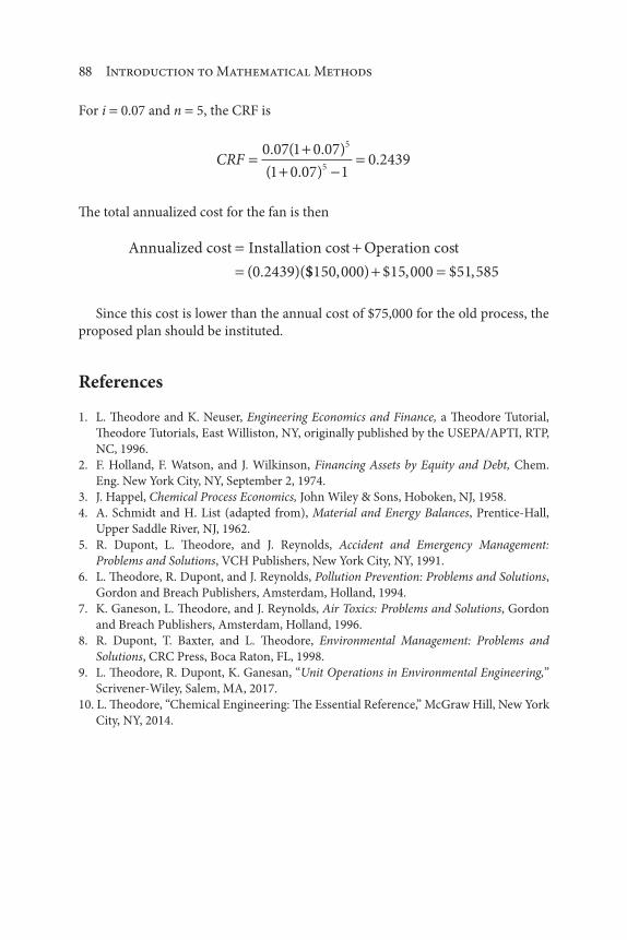
88 Introduction to Mathematical Methods
For i 0.07 and n 5, the CRF is
CRF0 07 1 0 07
1 0 07 10 2439
5
5
. ( . )
( . ).
The total annualized cost for the fan is then
Annualized cost Installation cost Operation cost
( . )(0 2439 $$ , ) $ , $ ,150 000 15 000 51 585
Since this cost is lower than the annual cost of $75,000 for the old process, the
proposed plan should be instituted.
References
1. L. Theodore and K. Neuser, Engineering Economics and Finance, a Theodore Tutorial,
Theodore Tutorials, East Williston, NY, originally published by the USEPA/APTI, RTP,
NC, 1996.
2. F. Holland, F. Watson, and J. Wilkinson, Financing Assets by Equity and Debt, Chem.
Eng. New York City, NY, September 2, 1974.
3. J. Happel, Chemical Process Economics, John Wiley & Sons, Hoboken, NJ, 1958.
4. A. Schmidt and H. List (adapted from), Material and Energy Balances, Prentice-Hall,
Upper Saddle River, NJ, 1962.
5. R. Dupont, L. Theodore, and J. Reynolds, Accident and Emergency Management:
Problems and Solutions, VCH Publishers, New York City, NY, 1991.
6. L. Theodore, R. Dupont, and J. Reynolds, Pollution Prevention: Problems and Solutions,
Gordon and Breach Publishers, Amsterdam, Holland, 1994.
7. K. Ganeson, L. Theodore, and J. Reynolds, Air Toxics: Problems and Solutions, Gordon
and Breach Publishers, Amsterdam, Holland, 1996.
8. R. Dupont, T. Baxter, and L. Theodore, Environmental Management: Problems and
Solutions, CRC Press, Boca Raton, FL, 1998.
9. L. Theodore, R. Dupont, K. Ganesan, “Unit Operations in Environmental Engineering,”
Scrivener-Wiley, Salem, MA, 2017.
10. L. Theodore, “Chemical Engineering: The Essential Reference,” McGraw Hill, New York
City, NY, 2014.

89
The engineer (and to a lesser degree the scientist) is known for his/her problem-
solving ability. It is probably this ability more than any other that has enabled
many engineers to rise to positions of leadership and top management within their
companies.
In problem-solving, both in school and in industry, considerable importance is
attached to a proper analysis of the problem, to a logical recording of the problem
solution, and to the overall professional appearance of the finished produced cal-
culations. Neatness and clarity of presentation should be distinguishing marks of
the work. Environmental engineers and scientists should always strive to practice
professional habits of problem solving analysis and to make a conscious effort to
improve the appearance of each document whether it is submitted for grading or
is included in a notebook.
The value of an environmental engineer or scientist is determined by his/her
ability to apply basic principles, facts, and methods in order to accomplish some
useful purpose. In this modern age of industrial competition, the ultimate defini-
tion of a useful purpose is usually based on a tangible profit of dollars and cents.
It is not sufficient, therefore, to have a knowledge and understanding of phys-
ics, chemistry, mathematics, mechanics, stoichiometry, thermodynamics, the unit
operations, chemical technology, engineering, and other related scientific subjects;
he/she must also have the ability to apply this knowledge to practical situations,
7Problem Solving
Introduction to Mathematical Methods for Environmental Engineers and Scientists. Charles Prochaska and Louis Theodore.
© 2018 Scrivener Publishing LLC. Published 2018 by John Wiley & Sons, Inc.

90 Introduction to Mathematical Methods
and, in making these applications, recognize the importance of the dollar sign (see
also the previous chapter).
Environmental engineers and scientists who have mastered the method of
problem solving are considerably more successful in their work than are people
who have not been trained in this technique. Many engineering problems in the
past were of such a routine nature that a resort to deductive reasoning would suf-
fice, and premises of deduction could be taken from handbooks. However, many
of the engineering problems of today cannot be solved by mere “handbook tech-
niques.” Experimentation, research, and development have indeed become more
significant activities in today’s world.
Four sections compliment the presentation of this chapter. Section numbers and
subject titles follow:
7.1: Sources of Information
7.2: Generic Problem-Solving Techniques
7.3: An Approach
7.4: Some Generic Comments
7.1 Sources of Information [1]
The field of environmental engineering and science encompasses many diverse
fields of activity. It is therefore important that means be available to place widely
scattered information in the hands of the reader. One need only examine the wide
variety of problems seen in practice to appreciate the need for a readily avail-
able source of a wide variety of information. Problems should almost always be
approached by checking on and reviewing all sources of information. Most of this
information can be classified in the following source categories:
Traditional Sources
Engineering and Science Sources
New Sources
Personal Experience
Each topic is discussed below.
Traditional Sources
The library is the major repository of traditional information. To efficiently use
the library, one must become familiar with its classification system. In general,
environmental engineers and scientists use the technical section of a library to
seek information on a certain subject and not material by a particular author or in
a specific book. For this reason, classification systems are based on subject matter.
The question confronting the user then is how to find and/or obtain information
on a particular subject. Two basic subject-matter-related classification systems are

Problem Solving 91
employed in U.S. libraries: the Dewey Decimal System and the Library of Congress
System. (The systems have changed somewhat with the advent of computers and
the internet.) A library (particularly a technical one) usually contains all or some
of the following:
1. General books (nonfiction, etc.)
2. Reference books
3. Handbooks
4. Journals
5. Transactions
6. Encyclopedias
7. Periodicals
8. Dictionaries
9. Trade literature
10. Catalogs
Engineering and Science Sources
Engineering and science technical literature includes textbooks, handbooks, peri-
odicals, magazines, journals, dictionaries, encyclopedias, and industrial catalogs.
There are a host of textbooks, including some of the classic works. The three major
engineering handbooks include those by Perry and Green [2], Kirk and Othmer
[3], and Albright [4]. Journals and magazines abound in the literature.
New Sources
The internet has a variety of resources available within it where information
regarding just about anything, including precise technical information, can be
found. Search engines such as Google, Bing, Yahoo!, and DuckDuckGo allow one
to search public webpages, one of the largest repositories of information in history,
free of charge and in a fraction of a second.
Wikipedia (derived from the phrase “What I Know Is…”) is essentially an
online site that provides free and open information. It is a collaborative encyclo-
pedia where one can obtain or apply information to a host of topics. It is a great
tool for fast reference but information can be provided by users and as such may
contain errors so sources must be checked to confirm their validity. Sources are
listed at the bottom of the Wikipedia pages usually in the form of clickable links.
Virtually every university, business, government (national, state, local) orga-
nization has a website. Individuals can also have one or more websites. Even one
of your humble authors has two websites. One site, www.theodorenewsletter.com,
provides information on education, sports, economics, politics, and a host of other
topics. Try Basketball Coaching 101 if the reader is interested in basketball [5].
Engineering Toolbox (http://www.engineeringtoolbox.com) provides most
of the tables and reference material one would find in engineering handbooks

92 Introduction to Mathematical Methods
organized by category. This site, along with many others, includes imbedded cal-
culators that can perform many different calculations ranging from simple unit
conversion to complex thermodynamic and optimization calculations.
There are also third party computer programs such as Aspen HYSYS and
CHEMCAD that specialize in chemical process simulations. With proper train-
ing, these programs can be used to make extensive and complicated process
related calculations in seconds. This ability is only possible with their vast data-
bases. However, these programs come at great monetary cost, with licenses being
anywhere from the tens to hundreds of thousands of dollars. This high cost limits
access of these programs to large institution’s such as universities, colleges, and
large companies.
Problem solving will usually require a combination of different sources and
websites. It is rare that one source will contain all the information necessary to
complete a problem. Note also that some of the above will almost certainly have
changed between the times when this section was initially written (March 2016)
and when it reaches the reading audience.
Personal Experience
Another information source – and a frequently underrated one – is one’s per-
sonal experience, personal files, and company experience files. Although tradi-
tional engineering and science problem-solving methods and the new sources
previously described are important, other fields can also provide useful informa-
tion. In fact, most equipment designs, process changes, and new-plant designs in
the chemical process industries are based on either prior experience, company
files, or both.
7.2 Generic Problem-Solving Techniques [6]
Certain methods of logic and techniques of calculation are fundamental to the
solution of many problems, and there is a near infinite number of methods. Words
such as creative, ingenuity, original, etc., etc., etc., appear in all these approaches.
What do they all have in common? They usually provide a systematic, logical
approach to solving problems, and what follows is the authors’ definition of a
generic approach.
The methodology of solving problems has been discussed by most mathemati-
cians and logicians since the days of Aristotle. Heuristic (“serving to discover”) is
the term often given to this study of the methods and rules of solving problems.
Nearly always, a stepwise approach to the solution is desirable. The broad
steps are:
1. Understanding the problem
2. Devising a plan
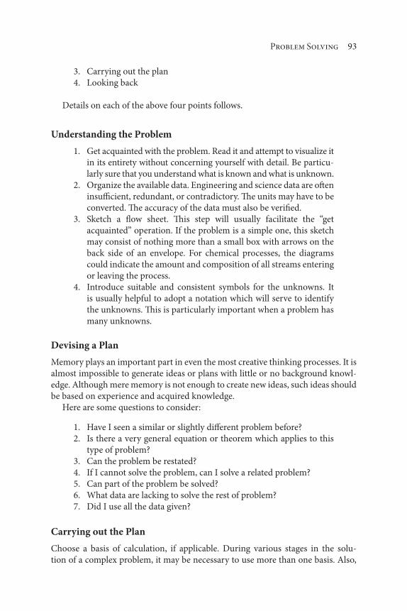
Problem Solving 93
3. Carrying out the plan
4. Looking back
Details on each of the above four points follows.
Understanding the Problem
1. Get acquainted with the problem. Read it and attempt to visualize it
in its entirety without concerning yourself with detail. Be particu-
larly sure that you understand what is known and what is unknown.
2. Organize the available data. Engineering and science data are often
insufficient, redundant, or contradictory. The units may have to be
converted. The accuracy of the data must also be verified.
3. Sketch a flow sheet. This step will usually facilitate the “get
acquainted” operation. If the problem is a simple one, this sketch
may consist of nothing more than a small box with arrows on the
back side of an envelope. For chemical processes, the diagrams
could indicate the amount and composition of all streams entering
or leaving the process.
4. Introduce suitable and consistent symbols for the unknowns. It
is usually helpful to adopt a notation which will serve to identify
the unknowns. This is particularly important when a problem has
many unknowns.
Devising a Plan
Memory plays an important part in even the most creative thinking processes. It is
almost impossible to generate ideas or plans with little or no background knowl-
edge. Although mere memory is not enough to create new ideas, such ideas should
be based on experience and acquired knowledge.
Here are some questions to consider:
1. Have I seen a similar or slightly different problem before?
2. Is there a very general equation or theorem which applies to this
type of problem?
3. Can the problem be restated?
4. If I cannot solve the problem, can I solve a related problem?
5. Can part of the problem be solved?
6. What data are lacking to solve the rest of problem?
7. Did I use all the data given?
Carrying out the Plan
Choose a basis of calculation, if applicable. During various stages in the solu-
tion of a complex problem, it may be necessary to use more than one basis. Also,

94 Introduction to Mathematical Methods
remember that the most brilliant work is useless if it cannot be conveyed clearly to
other persons by written or oral presentation(s).
Looking Back
The amount of time it takes to check a problem (if applicable) is usually only a
small fraction of the time it takes to solve it. Nearly all solutions to physical prob-
lems are amendable to verification. Thus, one should always:
1. Look for order-of-magnitude errors. Can the answer be checked
by an approximate solution? Does the answer make sense?
2. Attempt to solve the problem by an alternate method.
3. Can the results be verified?
7.3 An Approach
Here is an approach drawn from the files of one of the authors [7]. This method
involves six steps (see Figure 7.1).
1. The first step, and perhaps the most important one, is that of prob-
lem definition. It is not possible to establish rules for problem
definition that are sufficiently general to be useful. Environmental
problems are so diverse that it is up to the analyst to clearly state
the nature of the problem. This will establish a definite objective
for the analysis and is invaluable in outlining a path from the prob-
lem to the solution.
2. The next step is a definition of the theory that governs the phenom-
ena of the environmental problem. This theory is usually available
from a variety of sources, both published and unpublished, but for
those isolated cases where there is no theory available, it is worth-
while to postulate one (or several) and to test its validity later by
Definition of problem
Desired solutions
Common sense
Mathematics Solutions
ChecksComputers
Theory Equations Info. flow
Figure 7.1 A problem-solving approach.
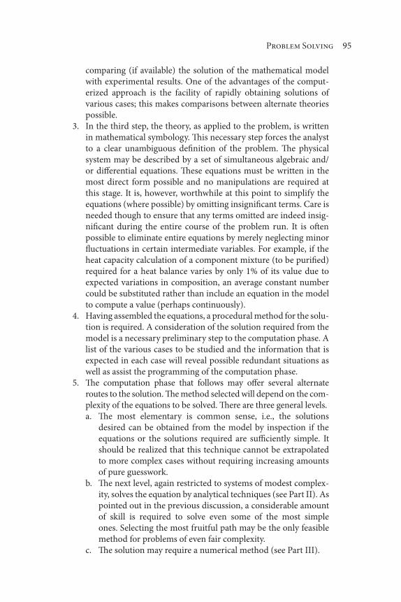
Problem Solving 95
comparing (if available) the solution of the mathematical model
with experimental results. One of the advantages of the comput-
erized approach is the facility of rapidly obtaining solutions of
various cases; this makes comparisons between alternate theories
possible.
3. In the third step, the theory, as applied to the problem, is written
in mathematical symbology. This necessary step forces the analyst
to a clear unambiguous definition of the problem. The physical
system may be described by a set of simultaneous algebraic and/
or differential equations. These equations must be written in the
most direct form possible and no manipulations are required at
this stage. It is, however, worthwhile at this point to simplify the
equations (where possible) by omitting insignificant terms. Care is
needed though to ensure that any terms omitted are indeed insig-
nificant during the entire course of the problem run. It is often
possible to eliminate entire equations by merely neglecting minor
fluctuations in certain intermediate variables. For example, if the
heat capacity calculation of a component mixture (to be purified)
required for a heat balance varies by only 1% of its value due to
expected variations in composition, an average constant number
could be substituted rather than include an equation in the model
to compute a value (perhaps continuously).
4. Having assembled the equations, a procedural method for the solu-
tion is required. A consideration of the solution required from the
model is a necessary preliminary step to the computation phase. A
list of the various cases to be studied and the information that is
expected in each case will reveal possible redundant situations as
well as assist the programming of the computation phase.
5. The computation phase that follows may offer several alternate
routes to the solution. The method selected will depend on the com-
plexity of the equations to be solved. There are three general levels.
a. The most elementary is common sense, i.e., the solutions
desired can be obtained from the model by inspection if the
equations or the solutions required are sufficiently simple. It
should be realized that this technique cannot be extrapolated
to more complex cases without requiring increasing amounts
of pure guesswork.
b. The next level, again restricted to systems of modest complex-
ity, solves the equation by analytical techniques (see Part II). As
pointed out in the previous discussion, a considerable amount
of skill is required to solve even some of the most simple
ones. Selecting the most fruitful path may be the only feasible
method for problems of even fair complexity.
c. The solution may require a numerical method (see Part III).

96 Introduction to Mathematical Methods
6. The sixth and last phase is the study and verification of the
solution(s) obtained from the mathematical model. Any unex-
pected solution(s) should be scrutinized so as to ensure that no
errors have occurred in the computation; also, some of the com-
puter logic should be specifically designed to check the validity of
the mathematical model.
7.4 Some General Concerns
Here is what one of the authors [8] has stressed in terms of developing problem-
solving skills and other creative thinking.
1. Carefully define the problem at hand.
2. Obtain all pertinent data and information.
3. Initially, generate an answer or solution.
4. Examine and evaluate as many alternatives as possible, employing
“what if ” scenarios [9].
5. Reflect on the above over time.
6. Consider returning to step 1 and repeat/expand the process.
As noted earlier, the traditional methodology of solving problems has been
described for decades in the following broad stepwise manner:
1. Understand the problem.
2. Devise a plan.
3. Carry out the plan.
4. Look back and (possibly) revise.
Many now believe creative thinking should be part of every student’s education.
Here are some ways that have proven to nudge the creative process along:
1. Break out of the one-and-only answer rut.
2. Use creative thinking techniques and games.
3. Foster creativity with assignments and projects.
4. Be careful not to punish creativity.
The above-suggested activities will ultimately help develop a critical thinker that:
1. Raises important questions and problems, formulating them
clearly and precisely.
2. Gathers and assesses relevant information, using abstract ideas to
interpret it effectively.

Problem Solving 97
3. Comes to well-rounded conclusions and solutions, testing them
against relevant criteria and standards.
4. Thinks open mindedly with alternative systems of thought, recog-
nizing and assessing, as need be, their assumptions, implications,
and practical consequences.
5. Communicates effectively with others in figuring out solutions to
complex problems.
The analysis aspect of a problem remains. It essentially has not changed. The
analysis of a new problem in environmental engineering and science can still be
divided into four steps.
1. Consideration of the process in question
2. Mathematical description of the process, if applicable
3. Solution of any mathematical relationships to provide a solution
4. Verification of the solution
References
1. L. Theodore, Chemical Engineering: The Essential Reference, McGraw-Hill, New York City, NY,
2014.
2. D. Green and R. Perry (editors), Perry’s Chemical Engineers’ Handbook, 8th ed., McGraw-Hill, New
York City, NY, 2008.
3. R. Kirk and D. Othmer, Encyclopedia of Chemical Technology, 4th ed., John Wiley & Sons, Hoboken,
NJ, 2001.
4. L. Albright, Albright’s Chemical Engineering Handbook, CRC Press/Taylor & Francis Group, Boca
Raton, FL, 2008.
5. L. Theodore, Basketball Coaching 101, Kourtakis – Tonry Publishers, East Williston, NY, (available
from Amazon or Createspace), 2015.
6. L. Theodore, personal notes, original sources unknown, East Williston, NY, 1980-1984.
7. L. Theodore, personal notes, original sources unknown, East Williston, NY, 1962.
8. P. Abulencia and L. Theodore, Open-Ended Problems: A Future Chemical Engineering Education
Approach, Scrivener – Wiley Publishing, Salem, MA, 2015.
9. L. Theodore and R. Dupont, Environmental Health and Hazard Risk Assessment: Principles and
Calculations, CRC/Taylor &Francis Group, Boca Raton, FL, 2014.

99
Perhaps the most important step in many environmental engineering/science
problems is the determination of the numerical value(s) of one or more equations.
These solutions may be obtained analytically (in closed/exact form) or numerically
(by some approximate method). A great number of methods have been developed
for doing this. The purpose of this part is to introduce and provide some of the
more important analytical methods. Part III addresses numerical methods.
There are seven chapters in Part II. The chapter numbers and accompanying
titles are listed below:
Chapter 8: Analytical Geometry
Chapter 9: Differentiation
Chapter 10: Integration
Chapter 11: Differential Calculus
Chapter 12: Integral Calculus
Chapter 13: Matrix Algebra
Chapter 14: Laplace Transforms
Part II
ANALYTICAL ANALYSIS
Introduction to Mathematical Methods for Environmental Engineers and Scientists. Charles Prochaska and Louis Theodore.
© 2018 Scrivener Publishing LLC. Published 2018 by John Wiley & Sons, Inc.

101
A host of subject matter receives treatment in this introductory chapter in Part II.
The key topics will involve the three coordinate systems that the environmental
engineer or scientist encounters in practice – rectangular, cylindrical, and
spherical.
The location of a point or a system in space may be defined in various coordinate
systems. Normally, the presentation keys on rectangular coordinates. However,
many applications involve curvilinear-coordinate systems-thus, the inclusion of
cylindrical and spherical coordinates in this chapter.
Five sections complement the presentation of this chapter. Section numbers
and subject titles follow.
8.1: Rectangular Coordinates
8.2: Cylindrical Coordinates
8.3: Spherical Coordinates
8.4: Key Physical Equations
8.5: Applications
8Analytical Geometry
Introduction to Mathematical Methods for Environmental Engineers and Scientists. Charles Prochaska and Louis Theodore.
© 2018 Scrivener Publishing LLC. Published 2018 by John Wiley & Sons, Inc.

102 Introduction to Mathematical Methods
8.1 Rectangular Coordinates
In rectangular coordinates, the position of a point P(x, y, z) is determined by the
intersection of three mutually perpendicular planes x constant, y constant,
and z constant. The Point P in Figure 8.1 (a) is defined by the rectangular
Figure 8.1 Coordinate systems.
P’
P P’ P”
P
P = P(x, y, z)P = P(r, , z)
P = P(r, , )
yy
x
z
z
P”
P”’P”’1
1
3
2
1
2
Rectangular coordinates(a) (b) Cylindrical coordinates
(c) Spherical coordinates
2
3 3
y
y
x
z
z
z
r
d
P’ P”’
P
r
d
d
x

Analytical Geometry 103
coordinates x, y, and z. The differential lengths in the x, y, and z directions are
given by
ds PP dx1 (8.1)
ds PP dy2 (8.2)
ds PP dz3 (8.3)
Any differential in length ds in this coordinate system is given by
( ) ( ) ( ) ( ) ( ) ( ) ( )ds PP PP PP dx dy dz2 2 2 2 2 2 2 (8.4)
The differential area elements df in the planes of constant x, y, and z take the form
df dy dzx (8.5)
df dx dzy (8.6)
df dx dyz (8.7)
The differential volume element dτ is
d dx dy dz (8.8)
8.2 Cylindrical Coordinates
The same point P in space may also be represented by the cylindrical coordinates r,
ϕ, and z. With reference to Figure 8.1(b) one can easily follow the transformation
of x, y, and z into cylindrical coordinates.
x r cos (8.9)
y r sin (8.10)
z z (8.11)
The right-handed, mutually perpendicular (orthogonal) axes for this coordi-
nate system are 1, 2, and 3. The differential lengths ds1, ds
2, and ds
3 in the r, ϕ, and
z, direction, respectively, are given by
ds PP dr1 (8.12)

104 Introduction to Mathematical Methods
ds PP r d2 (8.13)
ds PP dz3 (8.14)
The differential length ds now takes the form
( ) ( ) ( ) ( )
( ) ( ) ( )
ds PP PP PP
dr r d dz
2 2 2 2
2 2 2 (8.15)
The differential area element df on the curved surface is given by
df PP PP
r d dz
r d dz
( )( )
( )( )
(8.16)
(The differential element on the top or bottom planes that bound the cylinder is
(PP )(PP ) r dr dϕ). The differential volume element dτ is
d PP PP PP
dr r d dz
r dr d dz
( )( )( )
( )( )( )
(8.17)
8.3 Spherical Coordinates
The point P is described by the spherical coordinates r, , and ϕ in Figure 8.1 (c).
One can easily show that
x r sin cos (8.18)
y r sin sin (8.19)
z r cos (8.20)
The right-handed orthogonal axes for this coordinate system are once again 1,
2, and 3. The different lengths ds1, ds
2, and ds
3 in the r, , and ϕ directions, respec-
tively, are given by
ds PP dr1 (8.21)
ds PP r d2 (8.22)

Analytical Geometry 105
ds PP r d3 sin (8.23)
The differential length ds equation takes the form
( ) ( ) ( ) ( )
( ) ( ) ( sin )
ds PP PP PP
dr r d r d
2 2 2 2
2 2 2 (8.24)
The differential area element df on the curved surface is given by
df PP PP
r d r d
r d d
( )( )
( )( sin )
sin
2
(8.25)
while the differential volume element dτ is
d PP PP PP
dr r d r d
r dr d d
( )( )( )
( )( )( sin )
sin
2
(8.26)
8.4 Key Physical Equations
This section provides equations for calculating the area and/or volume and/or
perimeter of a host of objects listed below.
a. Sphere, Cube, Rectangular Parallelepiped, and Cylinder
b. Parallelogram, Triangle, and Trapezoid
c. Polygon
d. Ellipse and Ellipsoid
e. Cone
f. Torus
a. Sphere, Cube, Rectangular Parallelepiped, and Cylinder
Describing equations for the area and volume of the following shaped particles are
provided below.
1. Sphere of radius R
2. Cube of side A
3. Rectangular parallelepiped of sides A and B
4. Cylinder of radius R and height H

106 Introduction to Mathematical Methods
Equations
1. For a sphere of radius R:
Volume4
3
3R (8.27)
Area 4 2R (8.28)
2. For a cube of side A:
Volume A3 (8.29)
Area 6 2A (8.30)
3. For a rectangular parallelepiped of depth C:
Volume ABC (8.31)
Area 2( )AB AC BC (8.32)
4. For a cylinder of radius R and height H:
Volume R H2 (8.33)
Area 2 RH (8.34)
b. Parallelogram, Triangle, and Trapezoid
Describing equations for the area and perimeter of the following shaped particles
are provided below.
1. Parallelogram of height H, side A, and base B
2. Triangle of height H, base B, and left side A; the angle between side
A and base B is ϕ
3. Trapezoid of height H and parallel sides A and B; the lower left
angle is ϕ and the lower right angle is
Equations
1. For the parallelogram:
Area ( )( ) ( )( )sinH B A B (8.35)
Analytical Geometry 107
Perimeter 2 2A B (8.36)
2. For the triangle:
Area1
2
1
2( )( ) ( )( )sinB H A B (8.37)
Perimeter A B C (8.38)
3. For the trapezoid:
Area1
2H A B( ) (8.39)
Perimeter A B H
A B H
1 1
sin sin
(csc csc )
(8.40)
c. Polygon
Describing equations for the area and perimeter of the following shaped particles
are provided below.
1. Regular polygon of N sides, each of length B
2. Regular polygon of N sides inscribed in circle of radius R
Equations
1. For case (1):
Area/
/
1
4
1
4
2 2NBN
NBN
Ncot
cos( )
sin( ) (8.41)
Perimeter ( )( )N B (8.42)
2. For case (2):
Area1
2
2 1
2
3602 2NRN
NRN
sin sin (8.43)
Perimeter 2 2180
( )( )sin ( )( )sinN RN
N RN
(8.44)

108 Introduction to Mathematical Methods
d. Ellipse and Ellipsoid
Describing equations for the area, perimeter, or volume of the following shaped
particles are provided below.
1. Ellipse of semimajor axis A and semiminor axis B
2. Ellipsoid of semi-axes A, B, C
Equations
1. For case (1):
Area ( )( )A B (8.45)
Perimeter 4 1 2 2A k dsin (8.46)
21
2
2 2( ) ( )A B approximate (8.47)
where k A B A( )2 2 /
2. For case (2):
Volume1
2
2B A
e. Cone
Describing equations for the volume and surface area of the following shaped par-
ticles are provided below.
1. Right circular cone of radius R, lateral length L, and height H
2. Frustum of right circular cone of radii A, B, lateral length L, and
height H
Equations
1. For case (1):
Volume1
3
2R H (8.48)
Surface area R R H RL2 2

Analytical Geometry 109
2. For case (2):
Volume1
3
2 2H A AB B( ) (8.50)
Surface area ( ) ( ) ( )A B H B A A B L2 2 (8.51)
f. Torus
Describing equations for the volume and surface area off a torus of inner radius A
and outer radius B are provided below.
Equations
Volume1
4
2 2( )( )A B B A (8.52)
Surface Area 2 2 2( )B A (8.53)
8.5 Applications
Illustrative Example 8.1
Develop the area to volume ratio equations for the shaped particles from
sections 8.4A, 8.4E, and 8.4F.
Solution
For 8.4A:
Area/Volume /3 R
Area/Volume /6 A
Area/Volume / / /2 1 1 1[( ) ( ) ( )]A B C
Area/Volume /2 R
For 8.4E:
Area/Volume /3L RH
Area/Volume /[ ][ ( ) ] ( )3 2 2A B L H A AB B

110 Introduction to Mathematical Methods
For 8.4 F:
Area/Volume /( )4 B A
Illustrative Example 8.2
Calculate the area to volume ratio of shaped particles from sections 8.4A, 8.4E,
and 8.4F given the following data:
A 1, B 2, C 2, L 1, H 1, and R 1
Solution
For 8.4A:
Area/Volume 3
Area/Volume 6
Area/Volume 4
Area/Volume 2
For 8.4E:
Area/Volume 3
Area/Volume /9 7
For 8.4F:
Area/Volume 4
Illustrative Example 8.3 [1]
Consider a sphere with a diameter of 1.0 μm (micrometer or micron). If this same
mass of sphere is converted through a size reduction process to spheres with a
diameter of 1.0 nm (nanometer), calculate the increase in surface area of the
smaller sized spheres [1].
Solution
From 8.4A, the volume of a sphere is given by
V R R D
D
4
32
6
3
3
; /
/
Analytical Geometry 111
The volume of a 1.0 μm sphere is therefore
V( . ) ( . )
. ( ) .
. ( )
1 0 1 0 6
0 5236 1 0 10
0 5236 10
3
3 3
9
m /
m m nm
nm 33
The volume of a 1.0 nm sphere is correspondingly
V( . ) ( . )
. ( )
1 0 1 0 6
0 5236
3
3
nm /
nm
Since the mass – as well as the total volume – remain the same, the number of
smaller particles is
N0 5236 10
0 523610
99.
.
The surface area of the 1.0 μm particle is
SA R D( . )
( . )( )
. ( )
. ( )
1 0 4
3 14
3 14
3 14 10
2 2
2
2
6 2
m
1
m
nm
and
SA( . ) ( . )( )
. ( )
1 0 3 14 1
3 14
2
2
nm
nm
However, there are 109 of the 1.0 nm particles. Therefore, the 109 smaller sized
particles have a total surface area of 3.14 109 (nm)2. This reduction in size has
increased the surface area by a factor of 1000 or 103. The reader should note that
the particle diameter has decreased by the same factor.
Illustrative Example 8.4
Consider a cube with side of 1.0 μm. If the same mass of cube is converted to
cubes with sides of 1.0 nm, calculate the increase in surface area of the smaller
sized cubes.

112 Introduction to Mathematical Methods
Solution
From section 8.4A, the volume of a cube is given by
V A3
Therefore,
V( . ) ( )
. ( )
. ( )
1 0 1
1 0
1 0 10
3
3
9 3
m
m
nm
The volume of the 1.0 nm sided cube is
V( . ) ( )1 0 3 nm 1.0 nm
Since the volume remains the same, the number of smaller cubes is
N 10 1 0 109 9/ .
The surface area of a 1.0 m sided cube is
SA A( . )
( )
( )
1 0 6
6
6 10
2
2
6 2
m
m
nm
and
SA A .0 nm
nm
( )
( )
1 6
6
2
2
Since there are 109 of the 1.0 nm sized cubes, their total surface area is 6 109
(nm)2. Once again, the reduction in size has increased the surface area by a factor
of 1000 due to a similar corresponding decrease in side length of the cube.
Illustrative Example 8.5 [2]
A new baghouse [3–4] is structured as shown in Figure 8.2. (A baghouse contains
multiple filter bags for removing particulate matter from a pollutant/latent gas
stream.) The outside surface of the baghouse is to be covered with a new experi-
mental outer insulating covering. Assume that there will be no waste in the cover-
ing process. The material is ordered to the nearest 0.01 yd2 and the cost is $87.54/

Analytical Geometry 113
yd2. The minimum order that will be shipped is 5 yd2. Your department budget
must bear the cost. What will be the debit to your budget?
Data:
1. Surface E is a square with a measurement of 3 m per side.
2. The top roof angle (B) is 80°, the remaining two angles are equal.
3. The ends of the rounded hoppers (H) are semicircles (half circles)
of equal size.
4. The length of the unit side (S) is 6.6 m.
Note: The problem requires several steps/processes. Therefore, one needs not only
to know and use the appropriate mathematical principles but also needs to orga-
nize their work to avoid “oversight” errors.
Solution
There are two identical surfaces for E, R, S, and T. There are three surfaces of
dimension C, and there are six ends (H). Therefore, the total area (At) to be cov-
ered is calculated as follows:
A X E R S T C Ht 2 3 6( )
Note that the dimensions are provided in metric units and the insulating mate-
rial is provided in English units. In any problem where the units of measure are
mixed, terms must be converted to consistent units. In this problem, each of the
measures provided in meters could be changed to yards, but that would be time
consuming. Since all the linear measures are in meters, one would be better served
by computing the areas in metric units and then converting the final number of
square meters to square yards.
Note also that one square meter (1 m2) is equal to 1.196 yd2. Therefore
X X( ) ( )yds m 1.1962 2
For the interested reader, the solution, left as an exercise, is $14,300.
Figure 8.2 Physical configuration of a new baghouse.
H H H
C
E
T
Angle (B)
S
R

114 Introduction to Mathematical Methods
Illustrative Example 8.6
Determine the total particulate matter that can be collected in the hoppers, i.e.,
how many cubic feet will be occupied by the particulate matter when the three
hoppers are full?
Solution
The calculation essentially requires determining the volume of the free hoppers.
The interested reader is also left the exercise of verifying the solution provided
below.
V 17 1
604
. m
ft
3
3
References
1. L. Theodore, Nanotechnology: Basic Calculations for Engineers and Scientists, John Wiley & Sons,
Hoboken, NJ, 2006.
2. L. Theodore, personal notes (original source unknown), East Williston, NY, 1998.
3. L. Theodore, Air Pollution Control Equipment Calculations, John Wiley & Sons, Hoboken, NJ, 2008.
4. L. Theodore, R. Dupont, K. Ganesan, Unit Operations in Environmental Engineering, Scrivener-
Wiley, Salem, MA, 2017.

115
The terms derivative and differentiation have not only come to mean different
things to different people but have also been used interchangeably. The authors
offer the following definitions. The former term provides information on how one
variable, e.g., a dependent variable, changes with respect to another variable, e.g.,
an independent variable. The derivative dy/dx relates how a dependent variable y
varies with an independent variable x. Differentiation is the operation that enables
one to determine the value of the derivative.
One form of a derivative enables one to determine how fast something is mov-
ing at a given point or instant in time. To use a familiar example, if points A and
B are 60 miles apart and a car travels from point A to point B in 60 minutes, one
may say the car traveled at a rate of 60 mph (miles per hour). However, stating
that the car traveled at 60 mph is an average that assumed the car was moving at a
steady rate of 60 mph from the start to the finish. However, in reality, the car must
accelerate from 0 to 60 mph beginning at point A and it must decelerate from 60 to
0 mph to stop at point B. Obviously the car traveled at varying rates of speed, and
at some point had to be traveling faster than 60 mph. A derivative called velocity
can be used to determine the speed of the car at any point along the route. The car’s
speedometer produces a derivative function – one can look at the speedometer
at any time and determine the velocity (instantaneous speed) of the car. Many
9Differentiation
Introduction to Mathematical Methods for Environmental Engineers and Scientists. Charles Prochaska and Louis Theodore.
© 2018 Scrivener Publishing LLC. Published 2018 by John Wiley & Sons, Inc.

116 Introduction to Mathematical Methods
pollution control equipment and other environmental engineering calculations
involving derivatives relate to velocity.
Two sections complement the presentation of this chapter. Section numbers and
subject titles follow:
9.1: Graphical Methods
9.2: Finite Differencing
9.1 Graphical Methods
The fundamental laws on which engineering and science are based are frequently
expressed in the form of differential equations providing the rate of change of
an important dependent quantity with respect to an independent variable. It is
therefore particularly necessary in the interpretation of experimental data to be
able to carry out the process of differentiation analytically, graphically, or numeri-
cally. This chapter reviews the subject from a graphical perspective. A later chapter
examines differentiation from an analytical point of view, while Part III provides
material on numerical methods of analysis.
Since the derivative of a function y at any particular value of x is the slope of the
curve of y vs. x at that value of x, it follows that any graphical means of measuring
the slope of a curve may be employed to obtain the derivative. One rather obvious
method is to plot the function and obtain the slope with the aid of a straightedge.
The straightedge is swung about the point on the curve until it is judged “by eye” to
best represent the slope of the curve at the point. A straight line is then drawn, and
the slope of the straight line is calculated by any suitable means. In this last step, it
is important to obtain the slope in terms of the variables, taking into account the
scales used for the ordinate and abscissa. Only where these are equal is the geo-
metric slope the correct value.
A better way to obtain the derivative is to place a protractor or triangle on a
fixed straightedge or T square at a definite angle to the x axis and slide it along
until it touches the curve representing the function. This procedure locates the
point on the curve where the slope is equal to the predetermined value. As an aid
in locating the exact point in tangency, several chords, such as AB of Figure 9.1,
may be drawn parallel to the tangent. These are bisected, and a line QP is drawn
through their mid-points to intersect the curve at the desired point P. Although
the principle is quite similar to the direct measurement of the slope at a point, the
results obtained are found to be somewhat better. With a graph of reasonable size,
it is usually possible to obtain the derivative in this way with an error of less than
5 percent, although the accuracy (as one would expect) varies considerably with
the curvature of the line representing the function.
A very convenient device for measuring slopes of curves in past years is a mov-
able protractor fitted with a prism at the center. This is placed over the curve at the
point in question and turned until the two branches of the curve seen through the
two faces of the prism appear to join to form a smooth continuous curve. The slope

Differentiation 117
of the curve with reference to the base of the instrument may then be read. Some of
the instruments of this type employ a protractor of such a small diameter that the
accuracy is no better than, if as good as, that obtainable by the preceding methods.
It is important to note that the first derivative, dy/dx, represents the ratio of two
distinct quantities, dy and dx. Consequently, this ratio may be handled by ordinary
algebraic procedures. For example
dxdy
dxdy (9.1)
dy
dx
dx
dz
dy
dz (9.2)
On the other hand, in general, the higher derivatives cannot be treated in this
manner.
As noted above, one frequently uses graphs to find the derivative of one vari-
able with respect to another. The slope of a curve of distance vs. time (discussed
earlier) would give the velocity at that point. In an another example, the deriva-
tive of the molal volume of a solution with respect to concentration is the partial
molal volume [1, 2]. In cases where the relationship between the variables can
be expressed by an equation, the computation of slopes and derivatives is best
done either analytically or numerically. If empirical equations are not available, the
aforementioned graphical techniques must be brought to bear.
Thus, graphical differentiation may be used to determine the slope of a curve
relating two variables. If the analytical relationship is known, the differentiation
may be performed analytically for a precise answer. If the function is not known,
the data may be plotted and the slope may be determined by drawing a tangent as
described above to the curve at a point. However, the determination of the proper
slope of the tangent is often uncertain, especially if the experimental data are inac-
curate. Graphical differentiation may then be used to obtain values of the slope. If
tabulated data are available, the data are plotted as y as a function of x [1–3].
x
y
AP
BQ
Figure 9.1 Graphical differentiation.
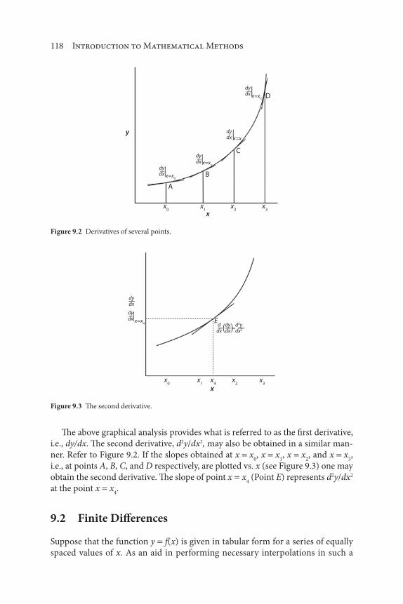
118 Introduction to Mathematical Methods
The above graphical analysis provides what is referred to as the first derivative,
i.e., dy/dx. The second derivative, d2y/dx2, may also be obtained in a similar man-
ner. Refer to Figure 9.2. If the slopes obtained at x x0, x x
1, x x
2, and x x
3,
i.e., at points A, B, C, and D respectively, are plotted vs. x (see Figure 9.3) one may
obtain the second derivative. The slope of point x x4 (Point E) represents d2y/dx2
at the point x x4.
9.2 Finite Differences
Suppose that the function y f(x) is given in tabular form for a series of equally
spaced values of x. As an aid in performing necessary interpolations in such a
x
y
B
A
C
D
dydx
dydx
dydx
dydx
x=x0
x0
x1
x2
x3
x=x1
x=x2
x=x3
Figure 9.2 Derivatives of several points.
Figure 9.3 The second derivative.
x
E
x0
x1
x4
x2
x3
dydx
dydx x=x
4 dydx
d2ydx2
d=dx

Differentiation 119
table one may, and in fact often does, list explicitly the differences between suc-
cessive values of f(x). In the same way, the differences between these differences
may be calculated and listed, and so on indefinitely, unless perhaps at some stage
the differences turn out to be zero. In the field of numerical mathematics these
differences play an important role not only in interpolation, but also in such pro-
cesses as the construction of tables, curve fitting, the differentiation and integra-
tion of tabular functions, and the approximate solution of differential equations.
In this section, the fundamental properties of the differences of a function are
developed, and their use in carrying out the operations just mentioned are
detailed.
Begin by investigating from an elementary point of view the general problem
of interpolation. In its simplest form, interpolation consists of substituting the
chord of a curve for the curve itself, as in Figure 9.4 (a), and subsequently reading
values of the function from the chord rather than from the graph of the func-
tion. Analytically, let h be the interval between successive values of x at which f(x)
is known, and let x x0
rh, where r is some fraction, be a point intermediate
between x0 and x
1x
0h at which the value of f(x) is desired. Then manipulating
the equation with the assumption that x0 = 0, one has for the equation of the chord
joining the points (x0, f
0) [now (0, f
0)] and (x
1, f
1) [now (h, f
1)]
f x y ff f
hx( ) 0
1 0 (9.3)
Since x = x0
+ rh and x0
= 0 in this manipulation, x can be replaced simply with rh.
Substituting rh for x into Equation(9.3) one is left with
y f f f r0 1 0( ) (9.4)
y y
x x
f0f0 f1 f2
x0 x1 = x0+h x1 = x0+h x2 = x0+2h(x = x0+rh) (x0+rh)
y = f(x)
y = f(x)
f1
(a) (b)
Figure 9.4 Approximation of derivatives by finite differences.

120 Introduction to Mathematical Methods
One may also introduce the notation
f f f0 1 0 (9.5)
Finally, reverse the initial manipulation (x0
= its original value and not 0) and one
can write
f x rh f r f( )0 0 0 (9.6)
This derivation was provided for an explanation of Equation(9.6) and is not
required to calculate an interpolated value. One can simply place the original val-
ues into Equation(9.6).
On the other hand, it would be reasonable to attempt to approximate the graph
of y f(x) not by a straight line through two successive points where f(x) is known,
but by a parabola through three such points, as in Figure 9.4 (b). In general,
because of its curvature, a parabola will fit the graph of f(x) more closely than will
a straight line, and hence interpolation based on a parabolic approximating arc will
be more accurate than ordinary linear interpolation.
A host of procedures are available for estimating the derivative in this and other
ways. For example, to develop a formula for parabolic interpolation, one must first
determine the coefficients a, b, c in the equation of the approximating arc
y a bx cx2 (9.7)
This, as well as several other methods, receive treatment in Part III.
Naturally, by approximating f(x) by polynomial functions of higher and higher
order, and proceeding exactly as indicated above, increasingly refined interpola-
tion formulas can be obtained [4]. This topic will be re-visited in Part III, Chapter
28. However, the labor involved in proceeding in this fashion soon becomes pro-
hibitive, and many turn their attention to more efficient operational methods of
deriving such results via numerical analysis.
References
1. H. Mickley, T. Sherwood, and C. Reed, Applied Mathematics in Chemical Engineering, 2nd Ed,
McGraw-Hill, New York City, NY, 1957.
2. L. Theodore, Chemical Engineering: The Essential Reference, McGraw-Hill, New York City, NY,
2014.
3. R. Ketter and S. Prawel, Modern Methods of Engineering Computation, McGraw-Hill, New York
City, NY, 1969.
4. S. Shaefer and L. Theodore, Probability and Statistics for Environmental Science, CRC Press/Taylor
& Francis Group, Boca Raton, FL, 2007.

121
Three words that will appear regularly in this chapter are: integral, integrate, and
integration. Most practicing environmental engineers and scientists use the terms
interchangeably. But is there a difference? Here is what Webster [1] has to say:
1. Integral. “…the result of integrating a function.”
2. Integrate. “…to calculate the integral or integrals of (a function,
equation, etc.).”
3. Integration. “…the process of finding the quantity or function of
which a given quantity or function is the derivative or differential.”
Does this help? Add to this that an integral equation is one which contains the
unknown function behind the integral sign. Its importance for physical problems
lies in the fact that most differential equations together with their boundary condi-
tions may be reformulated to give a single integral equation. If the latter can be
solved, the mathematical difficulties are not appreciably greater even when the
number of independent variables is increased.
As an example, assume that a source emits known quantities of hazardous
particulate matter comprised of various sizes of particles into the atmosphere.
As the particulate is dispersed into the surrounding area, the small particles
travel a greater distance than the large particles, so that several concentric zones
10Integration
Introduction to Mathematical Methods for Environmental Engineers and Scientists. Charles Prochaska and Louis Theodore.
© 2018 Scrivener Publishing LLC. Published 2018 by John Wiley & Sons, Inc.

122 Introduction to Mathematical Methods
surrounding the source contain particles of predictable sizes. This particle size
information can be used in integral calculations to compute the quantity of par-
ticulate matter dispersed to each zone [2].
Five sections complement the presentation of this chapter. Section numbers and
subject titles follow:
10.1: Graphical Integration
10.2: The Rectangle Method
10.3: The Method of Rectangles
10.4: The Method of Trapezoids
10.5: Simple Batch (Differential) Distillation Example
10.1 Graphical Integration
This technique can be applied whenever it is arduous to fit an equation to experi-
mental data, or when it is easier and faster to integrate graphically rather than
analytically. Consider, for example, Figure 10.1. The data depicted are a plot of vol-
umetric flow (f t3/h) readings versus time (sec) as recorded at a small stack emitting
200 30 60
Time t, sec
Vo
lum
etr
ic fl
or
rate
, ft3
/h
90 120
25
30
Q1
Q3
Q2
35
40
Figure 10.1 Flow readings.

Integration 123
a pollutant gas. It is obviously difficult, if not impossible, to describe these data
by means of an equation. However, since the definite integral is simply a number
representing the infinite sum
lim ( )x
x a
x b
f x x0
(10.1)
or
x a
x b
f x dx( ) (10.2)
where a and b are variable limits, the integration can be carried out graphically
without recourse to an equation.
The average flow rate during the first 10 sec, t, is approximately Q1 f t3, in the
next 10 sec the flow rate is Q2 ft3, etc. The total volumetric flow rate for the first two
minutes Qt is thus
Q Q Q Qt 1 2 12
10
3 600
10
3 600
10
3 600, , , (10.3)
Q t Q t dti 0
120 3 600/ ,
( )
Hence, in order to calculate the total volume of gas emitted over a 2 minute period
(120 seconds), one has only to add the entire area under the curve Q versus t. The
total emission obtained in this way is approximately 1.10 ft3.
There are many different methods for obtaining areas graphically. Counting
areas or arbitrary blocks is often the quickest and surest way. A number of other
techniques may be applied, such as:
1. Weighing: If the graph paper is of uniform thickness one can sim-
ply cut the figure out and weigh it. The weight is then compared to
that of a standard rectangle and multiplied by the appropriate ratio
of weights. This method is rarely, if ever, used today.
2. Planometers: Mechanical devices consisting of lever arms and
a wheel which traces the curve are available commercially. This
method is also rarely used today.
3. Analytical approximations: The methods of Simpson, Gauss, etc.,
as described in any appropriate mathematics text [3, 4], and in Part
III of this text.

124 Introduction to Mathematical Methods
It is fair to say that graphical integration is useful when no analytical expression
of the function exists. To evaluate the integral
y I dx I I xx
x
1
2
; ( ) (10.4)
analytically, it is necessary to know how I varies with x. If I is constant, the integral
is
y I x x( )2 1 (10.5)
If I can be expressed as an analytical function of temperature T where x = T
(see also Figure 10.2), for example, where I is the heat capacity cp
I x4 3 10 3 2. (10.6)
the integral could be evaluated analytically:
y x dx
x x
x
x
1
2
4 3
4 3 10
3
2
3
2
3
1
3
.
.( )
10 3
(10.7)
Substitution of numerical values of the limits x1 and x
2 would enable quantita-
tive evaluation of the integral. For example, if x1
200 and x2
600, then
y4 3 10
3600 200 298 10
33 3 3.
( ) (10.8)
However, the above integral can also be evaluated graphically by determining the
area under the curve of I as a function of x. For example, Equation 10.6 is replot-
ted in Figure 10.2. The limits cp1
200, cp2
600 are shown. The area under the
curve and between the limits is equal to the integral. The area may be evaluated by
counting areas and then multiplying by the value of each area. This is an exercise
left for the reader.
There are several methods of counting areas. The three most often employed are:
1. One Rectangle
2. Several Rectangles
3. Several Trapezoids
The next three sections review these approaches to graphically evaluate an integral.
The development is based on calculating the average heat capacity of a substance
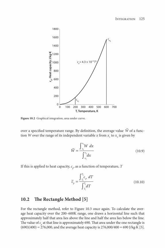
Integration 125
over a specified temperature range. By definition, the average value W of a func-
tion W over the range of its independent variable x from x1 to x
2 is given by
WW dx
dx
x
x
x
x
1
2
1
2
(10.9)
If this is applied to heat capacity, cp, as a function of temperature, T
cc dT
dTp
T
T
p
T
T
1
2
1
2
(10.10)
10.2 The Rectangle Method [5]
For the rectangle method, refer to Figure 10.3 once again. To calculate the aver-
age heat capacity over the 200–600K range, one draws a horizontal line such that
approximately half that area lies above the line and half the area lies below the line.
The value of cp at that line is approximately 690. That area under the one rectangle is
(690)(400) 276,000, and the average heat capacity is 276,000/400 690 J/kg·K [5].
00
200cp1
cp2
cp= 4.3 × 10⁻³ T 2
400
600
800
1000
1200
1400
1600
1800
100 200 300 400
T, Temperature, K
c p, H
ea
t ca
pa
city
J/k
g·K
500 600 700
Figure 10.2 Graphical integration, area under curve.
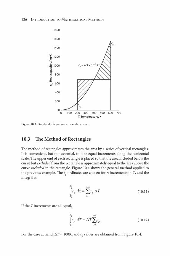
126 Introduction to Mathematical Methods
10.3 The Method of Rectangles
The method of rectangles approximates the area by a series of vertical rectangles.
It is convenient, but not essential, to take equal increments along the horizontal
scale. The upper end of each rectangle is placed so that the area included below the
curve but excluded from the rectangle is approximately equal to the area above the
curve included in the rectangle. Figure 10.4 shows the general method applied to
the previous example. The cp ordinates are chosen for n increments in T, and the
integral is
T
T
p
i
i n
pc dx c T
1
2
1
(10.11)
If the T increments are all equal,
T
T
p
i
i n
pic dT T c
1
2
1
(10.12)
For the case at hand, T 100K, and cp values are obtained from Figure 10.4.
0 100 200 300 400
T, Temperature, K
500 600 7000
200
400
600
800
1000
1200
1400
1600
1800
c p, H
ea
t ca
pa
city
J/k
g·K
cp = 4.3 × 10⁻³ T 2
cp2
cp1
Figure 10.3 Graphical integration; area under curve.

Integration 127
T
T
pc dT
1
2
100 270 510 870 1300
295 000
( )( )
,
(10.13)
The average heat capacity is then
cp
295 000
600 200
295 000
400773 8
, ,. J/kg K (10.14)
10.4 The Method of Trapezoids
The method of trapezoids replaces the smooth curve by a series of straight-line
segments between data points. The area of each trapezoid is evaluated and the
results are summed for the total area. With reference to Figure 10.5, the area of the
first trapezoid A1 is
A c T c c Tc c
Tp p p
p p
1 1 1 11 2 1
2 11
2 2( ) (10.15)
0 100 200 300 400
T, Temperature, K
500 600 7000
200
400
600
800
1000
Equal
Equal
Equal
Equal
T1
T2
T3
T4
1200
1400
1600
1800
c p, H
ea
t ca
pa
city
J/k
g·K
cp1
cp2
cp3
cp4 1,300
870
510
270
Figure 10.4 Graphical integration, method of rectangles.

128 Introduction to Mathematical Methods
The total integral is
T
T
p
i
i np p
ic dTc c
T T K T Ki i
1
2
1
1
1 22
200 600 ; , (10.16)
If all T increments are equal,
T
T
i
i np p
p p ppdT Tc
c c cc
n
i i n
1
2
1
1 2 1
1 2 c (10.17)
For this calculation, Figure 10.5 indicates that with
T c c c c cp p p p p100 172 387 688 1075 15481 2 3 4 5
, , , , ,
Thus,
T
T
pc dT
1
2
100172 1548
2387 688 1075
301 000
( )
,
(10.18)
T1
T2
T3
T40
200
400
600
800
1000
1200
1400
1600
1800
c p, H
ea
t ca
pa
city
J/k
g·K
cp1
cp2
cp3
cp4
cp5
0 100 200 300 400
T, Temperature, K
500 600 700
Figure 10.5 Graphical integrations; method of trapezoids.

Integration 129
The average heat capacity is then
cp
301 000
400752 5
,. J/kg K (10.19)
In this case, the area is somewhat high because each straight-line approximation
includes slightly more area than that provided by the curve.
The method of a rectangle, the method of rectangles, and the method of trap-
ezoids may be applied to a series of data points without plotting the data. Note also
that the three methods produced results that were within reasonable agreement.
The above equations are introductory examples of the general subject of numerical
methods, to be discussed in Part III, and they may be applied to graphs or numeri-
cal data.
10.5 Rayleigh Equation for Simple Batch (Differential) Distillation
In a simple batch distillation (see Figure 10.6), the composition of the evolved
vapors and the composition of the liquid in the still pot are continuously chang-
ing. Therefore, the mathematical analysis of the operation must be based on dif-
ferential changes. Although batch distillations are generally more costly than their
continuous counterparts, there are certain applications in which batch distillation
is the method of choice. Batch distillation is typically chosen when it is not pos-
sible to run a continuous process due to limiting process constraints, the need to
distill other process streams, or because the low frequency use of distillation does
not warrant a unit devoted solely to a specific product [6–9].
A relatively efficient separation of two or more components may be accom-
plished through batch distillation in a pot or tank. Although the purity of the dis-
tilled product varies throughout the course of batch distillation, it still has its use
in industry. As shown in Figure 10.6, a feed is initially charged to a tank, and the
Initially (t = 0)
Steam coil
Batch still Condensate tank
Condenser
D, y
D, xD
W, xW
Distillate
Figure 10.6 Batch distillation diagram.
130 Introduction to Mathematical Methods
vapor generated by boiling the liquid is withdrawn and enters a condenser. The
condensed product is collected as distillate, D, with composition xD, and the liquid
remaining in the pot, W, has composition xW
. Total and componential material
balances around a batch distillation unit are shown below.
F W D (10.20)
Fx Wx DxF W D (10.21)
Note that W, xW
, D, and xD all vary throughout the distillation process.
A convenient method for mathematically representing a binary batch distil-
lation process is known as the Rayleigh equation [6, 7]. This equation relates the
composition and amount of material remaining in the batch to an initial feed
charge, F, and composition, xF
lnW
F
dx
y xx
x
W
F
* (10.22)
where y* mole fraction of vapor in equilibrium with liquid of composition x.
At the desired distillate composition, the distillation is stopped. At this time,
the moles remaining in the still is denoted Wfinal
, with composition xW,final
. As such,
Equation (10.22) may be re-written as shown below
W F expdx
y xfinal
x
x
W final
F
,*
(10.23)
The above equation may be solved numerically by plotting 1/(y* x) vs. x and inte-
grating between the limits xW,final
and xF to determine the area (A) under the curve.
The above can therefore be written as
W F exp Afinal [ ] (10.24)
where A area under the curve [6, 7]. This problem will be revisited in Part III –
Numerical Methods.
References
1. Webster’s New World Dictionary, 2nd ed., Prentice-Hall, Upper Saddle River, NJ, 1971.
2. L. Theodore, Air Pollution Control Equipment Calculations, John Wiley & Sons, Hoboken, NJ, 2008.
3. H. Mickley, T. Sherwood, and C. Reed, Applied Mathematics in Chemical Engineering, 2nd ed.,
McGraw-Hill, New York City, NY, 1957.

Integration 131
4. R. Ketter and S. Prawel, Modern Methods of Engineering Computation, McGraw-Hill, New York
City, NY, 1969.
5. L. Theodore, personal notes, East Williston, NY, 1970.
6. L. Theodore and J. Barden, Mass Transfer Operations, A Theodore Tutorial, Theodore Tutorials,
East Williston, NY, originally published by the USEPA/APTI, RTP, NC, 1996.
7. L. Theodore and F. Ricci, Mass Transfer Operations for the Practicing Engineer, John Wiley & Sons,
Hoboken, NJ, 2010.
8. L. Theodore, Chemical Engineering: The Essential Reference, McGraw-Hill, New York City, NY,
2014.
9. L. Theodore, R. Dupont, K. Ganesan, Unit Operations in Environmental Engineering, Scrivener-
Wiley, Salem, MA, 2017.

133
Once again, let the function f(x) be defined for a<x<b. For each x in this range, the
derivative y f (x) is defined by the equation
f xf x x f x
xx( ) lim
( ) ( )
0 (11.1)
provided this limit exists. It should be noted that the limit cannot exist if f(x) is
discontinuous at the value of x considered; however, continuity alone does not
imply existence of the derivative.
The differential dy of the function y f(x) may be approximated as follows:
y f x x( ) (11.2)
In this equation, Δx can be replaced by dx so that one has
dy f x dx( )
11Differential Calculus
Introduction to Mathematical Methods for Environmental Engineers and Scientists. Charles Prochaska and Louis Theodore.
© 2018 Scrivener Publishing LLC. Published 2018 by John Wiley & Sons, Inc.

134 Introduction to Mathematical Methods
or
dy
dxf x( ) (11.3)
This derivative can be interpreted graphically as the slope of the tangent to the
curve y f(x) at point (x, y). The equation of the tangent at the point (x1, y
1) is then
y y f x x x1 1 1( )( ) (11.4)
Thus dx and dy can be interpreted as changes in x and y at (x, y).
The second derivative f (x) is defined as the derivative of the first derivative,
and higher derivatives are correspondingly defined. The notations
d y
dx
d y
dx
d y
dx
d y
dx
n
n
2
2
3
3
4
4, , , , (11.5)
or
y y y yiv n, , , , ( ) (11.6)
are also used to represent higher derivatives, respectively.
The basic properties of the derivative are summarized in the following theo-
rems where u f(x) and v g(x), are defined for a x b.
( )u v u v (11.7)
( )u v uv vu (11.8)
u
v
vu uv
v2 (11.9)
For example, repeated application of the rule for the derivative of the product xy
gives the rule:
y nxn 1 (11.10)
y xn (11.11)
for any positive integer n. In addition, if y 0, then y c, (c constant)
Four sections complement the presentation of this chapter. Section numbers
and subject titles follow:
11.1: Differential Operations
11.2: Ordinary Differential Equations
11.3: Partial Differential Equations
11.4: Maxima/Minima
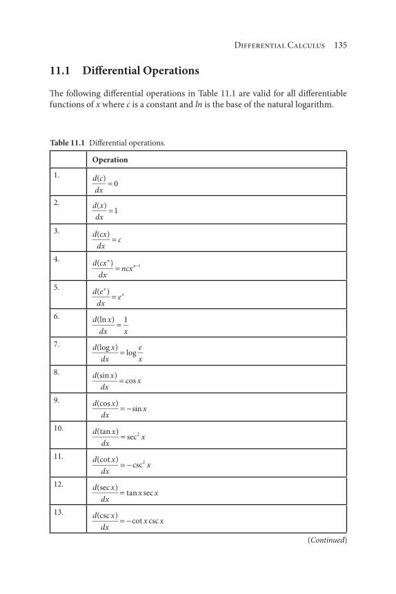
Differential Calculus 135
11.1 Differential Operations
The following differential operations in Table 11.1 are valid for all differentiable
functions of x where c is a constant and ln is the base of the natural logarithm.
Table 11.1 Differential operations.
Operation
1. d c
dx
( )0
2. d x
dx
( )1
3. d cx
dxc
( )
4.d cx
dxncx
nn( ) 1
5.d e
dxe
xx( )
6. d x
dx x
(ln ) 1
7. d x
dx
e
x
(log )log
8. d x
dxx
(sin )cos
9. d x
dxx
(cos )sin
10. d x
dxx
(tan )sec2
11. d x
dxx
(cot )csc2
12. d x
dxx x
(sec )tan sec
13. d x
dxx x
(csc )cot csc
(Continued)

136 Introduction to Mathematical Methods
Table 11.1 Cont.
Operation
14.d x
dxx
(sin )( )
12
1
21
15.d x
dxx
(cos )( )
12
1
21
16.d x
dxx
(tan )( )
12 11
17. d cu
dxc
du
dxu f x
( ); ( )
18. d uv
dxu
dv
dxv
du
dxv f x
( ); ( )
19.d
u
v
dx v
du
dx
u
v
dv
dx
12
20.d u
dxnu
du
dx
nn( ) 1
21.d u
dxu
du
dx
( ) ( / )1 2
1 21
2
/
22.d
u
dx u
du
dx
1
12
23.d
u
dx
n
u
du
dx
n
n
1
1
24. d u
dx u
du
dx
(ln ) 1
25.d c
dxc c
du
dx
uu( )
( )(ln )
26.d e
dxe
du
dx
uu( )

Differential Calculus 137
11.2 Ordinary Differential Equations
The natural laws in any scientific or technological field are not regarded as precise
and definitive until they have been expressed in mathematical form. Such a form,
often an equation, is a relation between the quantity of interest, say pollutant emis-
sions, and independent variables such as concentration or flow rates on which the
emission(s) depend. When it happens that this equation involves one or more of
its derivatives it is called a differential equation.
When a function involved in the equation depends only on one variable, its
derivatives are ordinary derivatives and the differential equation is called an ordi-
nary differential equation. When the function depends on several independent
variables, then the equation is called a partial differential equation. The theories
of ordinary and partial differential equations are quite different. In almost every
respect the latter is more difficult to treat analytically. Ordinary differential equa-
tions arise from those systems in which all the quantities may be taken as a func-
tion of a single independent variable. It is usually easy to test for the presence of
a single independent variable from knowledge of the physical situation at hand.
For example, in a single-pass countercurrent heat exchanger [1] at a water treat-
ment facility operating under fixed terminal conditions, it is necessary only to
specify the position in the exchanger by means of one variable, such as the distance
x from the cold end, and all the other variables at this point are fixed by the physi-
cal laws controlling the system. In a continuously operated absorption tower [2],
liquid and gas compositions vary throughout the tower, but if the input and outlet
conditions are fixed, it suffices (if channeling effects are neglected and concentra-
tions are assumed equal at all points across any cross section) to specify position in
order to calculate the properties of both the liquid and gas streams.
As noted above, ordinary differential equations generally arise from a descrip-
tion of situations involving one independent variable. The most important cases in
practice involve, in addition to the independent variable, one dependent variable,
and the most general differential equation for two variables may be written thusly
f x ydy
dx
d y
dx
d y
dx
d y
dx
n
n, , , , , ,
2
2
3
30 (11.12)
Any value of y which, when substituted into Equation (11.12), reduces the left-
hand side to zero is called a “solution” of the differential equation.
The order of a differential equation is the order of the highest derivative occur-
ring within the equation. The degree of a differential equation is the power to
which the highest derivative is raised when the equation has been rationalized and
cleared of fractions. The differential equation
d y
dxf x
dy
dx
2
2
21
2
1( ) (11.13)

138 Introduction to Mathematical Methods
is of the second order and the second degree, as may be seen by applying the pre-
ceding rules after squaring both sides.
The solution of a differential equation involving the most general possible rela-
tionship among the variables is known as the “general solution” or the “primitive.”
When the constants in the general solution are allowed to take on values correspond-
ing to the conditions in a specific problem, the resulting equation is known as a “par-
ticular solution” of the differential equation because it is now applicable to but one
particular case. The limitations introduced in obtaining a particular solution from a
general solution are known collectively as the “boundary conditions” of the problem.
Whenever a relationship exists between two variables x and y such that for
every value of x there exists at least one value of y, y is said to be a function of x,
and the functional relation may be expressed symbolically as
f x y( , ) 0 (11.14)
Equation (11.14) can be solved for either x in terms of y or y in terms of x.
Solving differential equations analytically is one of the major problems faced
by environmental engineers and scientists as such a wide variety of applications
lead to differential equations, and some cannot be solved analytically. The classical
initial value problem is to find a function y(x) that satisfies the first order differen-
tial equation y f(x, y) and takes on the initial value form of y(x0) y
0. A broad
variety of methods have been devised for the approximate solution to this classical
problem, most of which have then been generalized for treating solutions to these
problems [3–6].
11.3 Partial Differential Equations
Suppose now that the end conditions in the two preceding examples, i.e., the heat
exchanger and absorber, are not steady or constant with time. The rate of flow of
the cold stream to the heat exchanger may vary with time, or the rate of flow of the
solvent liquid to the absorption tower may vary with time, per some known relation.
In order to specify conditions completely at any point in either unit, the values of
two independent variables – position and either time or rate of flow of the variable
stream – must be specified. In this case, the instantaneous behavior of the system will
be expressed by an equation involving the variables and their partial derivatives. The
analytical solution of partial differential equations is available in the literature [3–6].
It is fair to say that the analysis of situations involving two or more indepen-
dent variables frequently results in a partial differential equation. The mathemati-
cal techniques employed to formulate the partial differential equation are similar
to those used to set up an ordinary differential equation. The details of the two
processes and, in particular, the manipulations involved are, however, surprisingly
different. The general function of n independent variables
y f x x xn( , , , )1 2 (11.15)
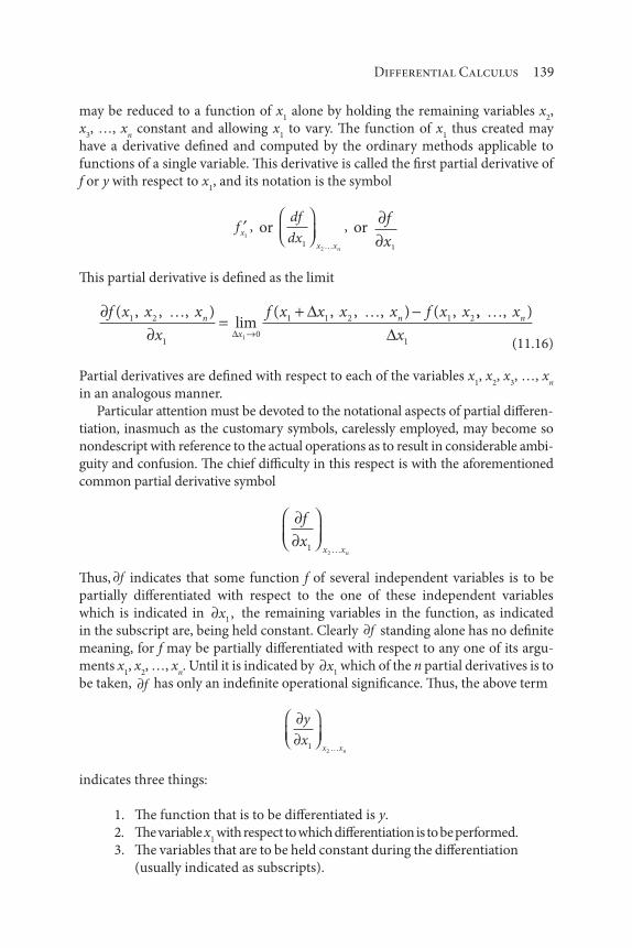
Differential Calculus 139
may be reduced to a function of x1 alone by holding the remaining variables x
2,
x3, …, x
n constant and allowing x
1 to vary. The function of x
1 thus created may
have a derivative defined and computed by the ordinary methods applicable to
functions of a single variable. This derivative is called the first partial derivative of
f or y with respect to x1, and its notation is the symbol
fx1
, or df
dxx xn
12
, or f
x1
This partial derivative is defined as the limit
f x x x
x
f x x x x f x xn
x
n( , , , )lim
( , , , ) ( ,1 2
10
1 1 2 1 2
1
,, , ) x
xn
1 (11.16)
Partial derivatives are defined with respect to each of the variables x1, x
2, x
3, …, x
n
in an analogous manner.
Particular attention must be devoted to the notational aspects of partial differen-
tiation, inasmuch as the customary symbols, carelessly employed, may become so
nondescript with reference to the actual operations as to result in considerable ambi-
guity and confusion. The chief difficulty in this respect is with the aforementioned
common partial derivative symbol
f
xx xn
12
Thus, f indicates that some function f of several independent variables is to be
partially differentiated with respect to the one of these independent variables
which is indicated in x1, the remaining variables in the function, as indicated
in the subscript are, being held constant. Clearly f standing alone has no definite
meaning, for f may be partially differentiated with respect to any one of its argu-
ments x1, x
2, …, x
n. Until it is indicated by x
1which of the n partial derivatives is to
be taken, f has only an indefinite operational significance. Thus, the above term
y
xx xn
12
indicates three things:
1. The function that is to be differentiated is y.
2. The variable x1 with respect to which differentiation is to be performed.
3. The variables that are to be held constant during the differentiation
(usually indicated as subscripts).

140 Introduction to Mathematical Methods
The partial derivative
y
xx1
2
(11.17)
or
y
xx2
1
(11.18)
may be demonstrated graphically (see previous Chapter). Refer to Figure 11.1
which provides a plot of y vs x1. The slope of any point along the curve represents
y
xx1
2
since x2 is constant. The derivative can be generated for various values of x
2 as
pictured in Figure 11.2. If the four slopes calculated keeping x2 constant at A, B,
C, and D, i.e., the partial of y with respect to x1 evaluated at x
1
* , are plotted vs the
complementary four values of x2, i.e., a, b, c, and d – as shown in Figure 11.3 – the
slope at any point along the curve would represent
y x
xx x
/
*
1
21 1
x2 = constant
dydx
1
yx
1
x1
y
x2
Figure 11.1 A plot of x1 vs. y.

Differential Calculus 141
Not surprisingly, an equation involving partial derivatives is defined as a partial
differential equation. The equation
2
0T
x y (11.19)
x2 = d
x2 = c
x2 = b
x2 = a
x1
x1*
y
D
C
B
A
Figure 11.2 Partial derivative of y with respect to x1 keeping x
2 constant at a, b, c, and d.
x1 = x
1*
yx
1
x2
A
a b c d
BCD
Figure 11.3 Partial derivative of y with respect to x1 vs. x
2.
142 Introduction to Mathematical Methods
is a partial differential equation. Such equations are of importance in environmen-
tal engineering and science because the significant independent variables are fre-
quently functions of more than one independent variable, and the basic differential
expressions for the natural laws are, therefore, partial differential equations. The
usual problem is to determine a particular relation between y, x1, and x
2 expressed
as y f(x1, x
2), that satisfies the basic differential equation and also satisfies some
particular condition specified by the practical problem at hand.
The order of a partial differential equation is the order of the highest derivative
appearing in the equation. For example, the equation
4
2 2
2
2
3 0T
x y
T
xT (11.20)
is fourth order. A partial differential equation is said to be linear if no powers or
products of the dependent variable or its partial derivatives are present. If one of
the coefficients in the equation is a function of the dependent variable y, then the
equation would be classified as nonlinear. Homogenous partial differential equa-
tions are ones in which all terms contain derivatives of the same order. The solu-
tion of a partial differential equation must also satisfy both the original differential
equation and its boundary conditions. A discussion of the number and type of
boundary conditions necessary and sufficient to ensure a solution of a partial dif-
ferential equation is beyond the scope of this chapter [1, 3, 4]. However, in most
environmental engineering applications, the physical system enables the necessary
boundary conditions to be established relatively easily.
No general formalized analytical procedure for the solution of an arbitrary par-
tial differential equation is known. Details are articulated in the literature [3–6] but
one should not rule out guessing at a solution [7].
Illustrative Example 11.1
If
y f x u v xuv u v( , , ) 2
evaluate
y
x
y
u, , and
y
v
if both u and v are functions of x.
Solution
y
xuv

Differential Calculus 143
y
uxv 1
y
vxu 2
11.4 Maxima and Minima
Since the derivative dy dx/ , or f (x), represents the rate of change of y with change
in x, it is evident that if the function passes through a maximum or minimum
the derivative will be zero. If the occurrence of such a maximum or minimum is to
be determined and located, the derivative is equated to zero, thus giving the condi-
tion for which the maximum or minimum exists. This procedure is of consider-
able value in environmental engineering calculations, particularly those involving
optimization, since the location of a maximum or minimum is frequently of sig-
nificant importance. This is particularly true in plant design, since the optimum
operating and design variables are to be determined in order that the maximum
profit and/or minimum cost will result.
In Figure 11.4, the curve ABCDE represents the function y f(x). If values of
y in the neighborhood of points A and C are all less than the values of y at A
and C, the function is said to go through a maximum at these points. Similarly,
because the values of y in the neighborhood of B are all greater than the value of
B, the function is said to go through a minimum at B. This curve emphasizes that
the terms “maximum” and “minimum” do not necessarily denote the greatest and
least possible values a function may assume.
A
BDerived curve
y
D
C
E
F0 H
G K
LJ
I
x
Figure 11.4 Maximum and minimum of a function with derived curve.

144 Introduction to Mathematical Methods
As noted above, it is evident geometrically that the slope of the curve is zero at
the maximum and minimum points, and since the slope is given by the derivative
dy dx/ , or f (x), these points may be determined and located through solution of
the equation f (x) 0. The roots of this equation merely locate the maximum and
minimum points and cannot distinguish between them. Furthermore, the condi-
tion locates such points as E. One method of distinguishing between points A, C,
and E is to calculate values of f(x) in their immediate vicinity. These are known as
points of inflection. A convenient rule of these relations is as follows:
Maximum: dy
dx
d y
dx0 0
2
2, (11.21)
Minimum: dy
dx
d y
dx0 0
2
2, (11.22)
Calculations to determine the optimum conditions from the point of view of
costs and monetary return are termed economic balances. The basic criterion of
the true optimum is maximum return on the investment, but the problem can fre-
quently simplify to one of determining the minimum cost, the maximum produc-
tion from a piece of equipment, the minimum power, etc. The quantity considered
is expressed as a function of the design or operating variables. On differentiating
and equating to zero, one obtains the condition which determines the optimum
value of the variable under consideration.
Illustrative Example 11.2 [8]
Consider the two-stage reversible adiabatic compression [8] of a gas from an ini-
tial pressure P1 to a final pressure P
3. If the fixed charges on the compressors are
assumed to be essentially independent of the interstage pressure employed, then
the optimum operation involves the determination of the interstage pressure for
which the total power requirement is a minimum. For a fixed gas flow, this cor-
responds to the minimum work for the two stages. If the gas enters at T1 and is
cooled to T1 between stages, the total work is given by
W NRTk
kP
P
P
P
k
k
k
k
1 22
1
1
3
2
1
; T T1 (11.23)
where (in consistent units)
N pound moles of gas compressed
R molal gas constant
k ratio of heat capacity at constant pressure to heat capacity at constant vol-
ume for the gas compressed

Differential Calculus 145
T1
inlet gas temperature
W total work, ft·lbf
Outline how to determine P2 for minimum power required.
Solution
If the above quantity is to be a minimum, then the derivative must be zero:
dW
dPNRT
k
k
k
kP P
k
kPk k k
2
1
1
2
1
1
1 1( )/ ( / )
33
1
2
1 2 0( )/ ( )/k k k kP
The above equation can now be solved for P2. This example will be revisited several
times in Part V – Optimization.
References
1. L. Theodore, Heat Transfer Applications for the Practicing Engineer, John Wiley & Sons, Hoboken,
NJ, 2012.
2. L. Theodore and F. Ricci, Mass Transfer Operations for the Practicing Engineer, John Wiley & Sons,
Hoboken, NJ, 2010.
3. H. Mickley, T. Sherwood, and C. Reed, Applied Mathematics in Chemical Engineering, 2nd ed.,
McGraw-Hill, New York City, NY, 1957.
4. L. Theodore, Chemical Engineering: The Essential Reference, McGraw-Hill, New York City, NY,
2014.
5. R. Ketter and S. Prawel, Modern Methods of Engineering Computation, McGraw-Hill, New York
City, NY, 1969.
6. L. Lapidus, Digital Computation for Chemical Engineers, McGraw-Hill, New York City, NY, 1962.
7. L. Theodore, personal notes, East Williston, NY, 1970.
8. J. Happel, Chemical Process Economics, John Wiley & Sons, Hoboken, NJ, 1958.

147
The reader is reminded that Chapter 10 primarily keyed on graphical integration.
That material is now extended to include the analytical approach to integration. As
noted earlier, numerical integration receives treatment in Part III.
Four sections complement the presentation of this chapter. Section numbers
and subject titles follow:
12.1: Analytical Integration
12.2: Indefinite Integrals
12.3: Definite Integrals
12.4: Integration Applications
12.1 Analytical integration
The definite integral f x dxa
b
( ) of a function f(x) for a x b, is defined by the
limiting process:
I f x dx f x xa
b
n
xi
n
i i
i
( ) lim ( )
max
*
01
(12.1)
12Integral Calculus
Introduction to Mathematical Methods for Environmental Engineers and Scientists. Charles Prochaska and Louis Theodore.
© 2018 Scrivener Publishing LLC. Published 2018 by John Wiley & Sons, Inc.
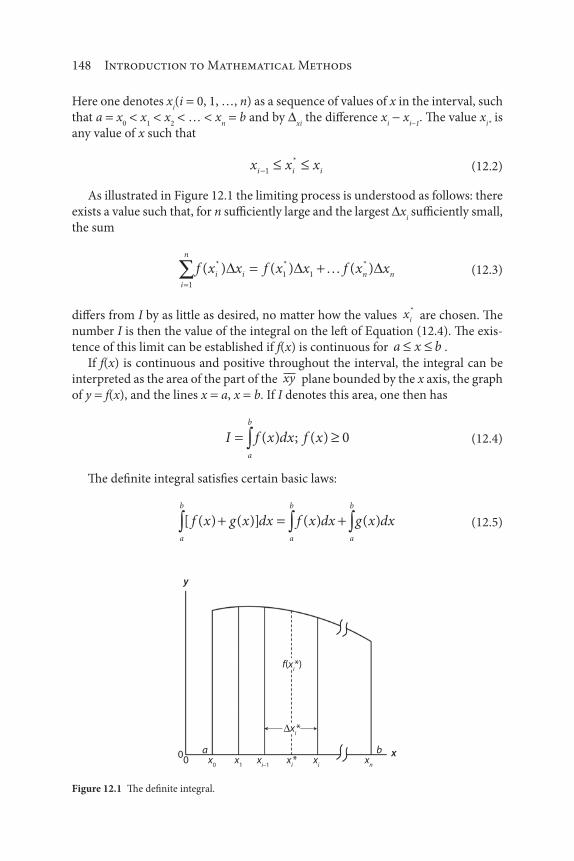
148 Introduction to Mathematical Methods
Here one denotes xi(i 0, 1, …, n) as a sequence of values of x in the interval, such
that a x0
x1
x2
… xn
b and by xi the difference x
i x
i 1. The value x
i* is
any value of x such that
x x xi i i1
* (12.2)
As illustrated in Figure 12.1 the limiting process is understood as follows: there
exists a value such that, for n sufficiently large and the largest xi sufficiently small,
the sum
i
n
i i n nf x x f x x f x x1
1 1( ) ( ) ( )* * * (12.3)
differs from I by as little as desired, no matter how the values xi
* are chosen. The
number I is then the value of the integral on the left of Equation (12.4). The exis-
tence of this limit can be established if f(x) is continuous for a x b .
If f(x) is continuous and positive throughout the interval, the integral can be
interpreted as the area of the part of the xy plane bounded by the x axis, the graph
of y f(x), and the lines x a, x b. If I denotes this area, one then has
I f x dx f xa
b
( ) ; ( ) 0 (12.4)
The definite integral satisfies certain basic laws:
a
b
a
b
a
b
f x g x dx f x dx g x dx[ ( ) ( )] ( ) ( ) (12.5)
x0
00 x
1xi–1
xi*
f(xi*)
xi* xi xn
ba x
y
Figure 12.1 The definite integral.

Integral Calculus 149
a
b
a
b
cf x dx c f x dx c constant( ) ( ) ; (12.6)
a
b
b
c
a
c
f x dx f x dx f x dx( ) ( ) ( ) (12.7)
12.2 Indefinite Integrals
If f (x) is the derivative of f(x), the antiderivative of f (x) is f(x). Symbolically, the
indefinite integral of f (x) is
f x dx f x c( ) ( ) (12.8)
where c is an arbitrary constant to be determined. The following relationships
in Table 12.1 hold (a and b are constants) by virtue of the known formulas for
differentiation.
Table 12.1 Indefinite integrals.
Operation
1.a dx ax
2.af x dx a f x dx( ) ( )
3.( )u v w dx u dx v dx w dx
4.( )du dv dw du dv dw
5.u dv uv v du [integration by parts]
6.u du
u
nnn
n
1
11,
7. du
uu if u u if u
u
ln ln( )
ln | |
or 0 0
8.e du eu u
(Continued)
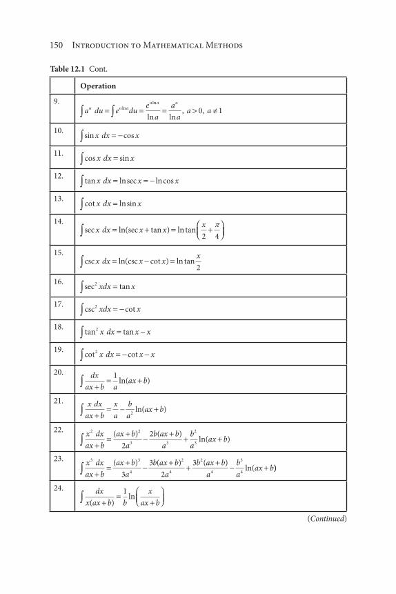
150 Introduction to Mathematical Methods
Table 12.1 Cont.
Operation
9.a du e du
e
a
a
aa au u a
u a u
lnln
ln ln, ,0 1
10.sin cosx dx x
11.cos sinx dx x
12.tan lnsec lncosx dx x x
13.cot lnsinx dx x
14.sec (sec tan ) ln tanx dx x x
x ln
2 4
15.csc (csc cot ) ln tanx dx x x
x ln
2
16.sec tan2 xdx x
17.csc cot2 xdx x
18.tan tan2 x dx x x
19.cot cot2 x dx x x
20. dx
ax b aax b
1ln( )
21. x dx
ax b
x
a
b
aax b
2
ln( )
22.x dx
ax b
ax b
a
b ax b
a
b
aax b
2 2
3 3
2
32
2 ( ) ( )ln( )
23.x dx
ax b
ax b
a
b ax b
a
b ax b
a
b
aax b
3 3
4
2
4
2
4
3
43
3
2
3 ln(
( ) ( )( )))
24. dx
x ax b b
x
ax b( )ln
1
(Continued)

Integral Calculus 151
Table 12.1 Cont.
Operation
25. dx
x ax b bx
a
b
ax b
x2 2
1
( )ln
26.dx
x ax b
ax b
b x
a
b
x
ax b3 2 2
2
3
2
2( )ln
27. dx
ax b a ax b( ) ( )2
1
28. x dx
ax b
b
a ax b aax b
ln( )
( ) ( )2 2 2
1
12.3 Definite Integrals
The concept and derivation of the definite integral are completely different from
those for the indefinite integral. These are by definition different types of opera-
tions. However, the formal operation as it turns out treats the integrand in the
same way for both.
Consider the function f(x) 10 – 10e 2x. Define x1
a and xn
b, and suppose
it is desirable to compute the area between the curve and coordinate axis y 0 and
bounded by x1
a, xn
b. Obviously, this area could be approximated as closely as
desired by a sufficiently large number of rectangles. Thus, the value of the definite
integral depends on the limits a, b and any selected variable coefficients in the
function - but not on x. There are certain restrictions on the integration definition:
“The function f(x) must be continuous on the finite interval (a, b) with at most a
finite number of discontinuities,” which must be observed before integration for-
mulas can be generally applied. Two techniques for determining when integration
is valid under these conditions are available in the literature [1–4].
Some useful analytical integrals in environmental engineering and science are
provided below in Table 12.2; note that the equations are definite integrals, i.e., the
upper and lower limits are specified [5].
Note, once again, that there are limits on the integrals.
Illustrative Example 12.1
Find
0
2
2sin x dx

152 Introduction to Mathematical Methods
Table 12.2 Definite integrals.
Operation
1.
0
x
a dx ax
2.
0
1
1
1
1
x
xdx
xln
3.
0
2
1
1
1
1
x
xdx
x( )
4.
0
2
1
1 1
x
xdx
x
x( )
5.
0
1
1
11
x
xdx xln( )
6.
0
1
11
1
1
xx
xdx
xx( )ln
7.
0
2
1
1
1
1
1
1
xx
xdx
x
x x( )
( )( )ln
8.
0
2
2
221
12 1 1
1
1
xx
xdx x x
x
x
( )
( )
( ) ( )
( )( )ln( )
9.
0
1
1
1
1 11
x
B B
B
B
Bx x
dxx
x( )( )ln
( )( )( )
( ) for
10.
0
2
21 2
2
24
x
ax bx cdx
ax b bb ac
( ) for
11.
0
2
21 14
x
ax bx cdx
a p q
q x p
p x qb a
( )( )ln
( )( )
( )( ) for cc
where p and q are roots of the equation
ax bx c p qb b ac
a
22
1
2
04
2, i.e., ,
( )
12.
0
2
xa bx
c gxdx
bx
g
ag bc
gc gxln | |
(Continued)

Integral Calculus 153
Table 12.2 Cont.
Operation
13.
0
2
xx
ax bdx
x
a
b
aax bln( )
14.
0
2 2
3 2
2
32
2x
x
ax bdx
ax b
a
b
aax b
b
aax b
( )( ) ln( )
15.
0
1 1x
x ax bdx
b
x
ax b( )( )ln
16.
0
2 2
1
2x adx
a
17.
02 2
1
2
a
a x
18.
0
2 22
4
a
a x dxa
Solution
Apply (10) in Table 12.1.
2 2 22
0 20
2
02sin [ ] cos cosx dx x cos
Illustrative Example 12.2
Find
0
4
2
1
2( )xdx
Solution
Direct application of the general integration formula would yield the incorrect
value.
0
4
2
0
41
2
1
21
( )xdx
x

154 Introduction to Mathematical Methods
It should be noted that
f xx
( )( )
1
2 2
becomes unbounded as x 2, i.e., the integral diverges and hence is said not to
exist.
12.4 Integration Applications
Illustrative Example 12.3
Calculate the surface area and volume of the unit cube described in Section 8.4.
Solution
Refer to Chapter 8. There are six surfaces on the cube. The surface in the yz-plane
is given by
f dy dzx
z y0
1
0
1
f x( ) 1
There are two such surfaces – one at x 0 and another at x 1. The remaining four
surfaces can be determined in a similar manner.
f y 1
fz 1
The total surface area is 6 1 6 units of area.
The volume of the cube is given by
z y x
dx dy dz0
1
0
1
0
1
1
unit of volume.
Illustrative Example 12.4
Calculate the volume V of a cylinder of radius a and height h.

Integral Calculus 155
Solution
Refer to Chapter 8.
d r dr d dz
V d
Substituting
V r dr d dz
h r dr d h
z
h
r
a
r
a
r
a
0 0
2
0
0
2
0 0
2
rr dr hr
a h
a
22
2
0
2
Illustrative Example 12.5
Evaluate the surface area A of a sphere of radius a.
Solution
Refer to Chapter 8.
df r d d
A df r d d
2
0
2
0 0
2
0
2
2
sin
sin
0
2 2
0
2
0
2 22 2 2 1 1 4r d r d r r rsin sin cos[ ] [ ]
Therefore, the surface of A a sphere where r a is
A a4 2
Illustrative Example 12.6
The velocity of a fluid in a horizontal cylinder of radius R is represented in cylin-
drical coordinates by the equation
vr
R100 1
2
; ft/s
Calculate the average velocity of the fluid flowing in the cylinder [6].

156 Introduction to Mathematical Methods
Solution
Based on the problem statement
vr
Rz 100 1
2
The velocity vz varies over the cross-sectional area of the cylinder f. A differential
area element in this cross section is given by (see Chapter 8)
df r dr d
By definition,
vv df
dfz
z
Substituting
v
r
Rr dr d
r dr dz
R
R
0
2
0
2
0
2
0
100 100
2
00
3
2
2
24
2
0
2
100 100
2
5025
R
R
rr
Rdr
R
rr
R
R2
50 2550
2 2
2
( )R R
R ft/s
Note that the maximum velocity is located at r 0 and vz
100 ft/s at that
point. Also note that the ratio of the average to the maximum velocity is 1/2 [7].
Illustrative Example 12.7
The temperature T in a solid sphere of radius a is given by T 100r. Compute the
average temperature of the sphere.
Solution
Refer to Chapter 8. By definition
TTd
d
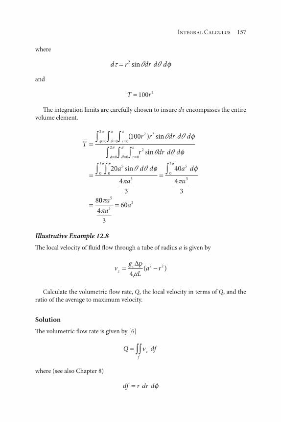
Integral Calculus 157
where
d r dr d d2 sin
and
T r100 2
The integration limits are carefully chosen to insure dτ encompasses the entire
volume element.
Tr r dr d d
r
r
a
r
a
0
2
0 0
2 2
0
2
0 0
2
100( ) sin
s
iin
sin
dr d d
a d d
a
a d
a
0
2
0
5
3
0
25
3
20
4
3
40
4
3
800
4
3
605
3
2a
aa
Illustrative Example 12.8
The local velocity of fluid flow through a tube of radius a is given by
vg
La rz
c p
4
2 2( )
Calculate the volumetric flow rate, Q, the local velocity in terms of Q, and the
ratio of the average to maximum velocity.
Solution
The volumetric flow rate is given by [6]
Q v dfz
f
where (see also Chapter 8)
df r dr d
158 Introduction to Mathematical Methods
Thus,
Qg
La r r dr d
g
La r r dr
r
a
c c
a
0
2
0
2 2
0
2 3
4 2
p p ( ) ( )
gg
L
a r r g
Lc cp pa
2 2 4 8
2 2 4
0
4 4
and
p
L
Q
g ac
84
Substituting the above equation into the equation for the local velocity of the
fluid flow leads to
vQ
a
r
az
21
2
2
The maximum velocity can easily be shown to be located at r 0. Therefore,
vQ
azmax
22
The average velocity is given by
v
Q
a
r
ar dr d
rdrd
Q
a
z
a
a
0
2
0 2
2
0
2
0
21
2
22 0
2
2
4
2 4
2
0
2 1
4
2 4
( )a
a
r
ar dr
a
Q
a
r r
a
Q
a
vQ
a
Q
Az
2
2

Integral Calculus 159
so that
v vr
av
r
az z zmax
2 1 1
2 2
Finally
v
vz
zmax
1
2
This result (as expected) is in agreement with the result of Illustrative Example 12.6.
References
1. H. Mickley, T. Sherwood, and C. Reed, Applied Mathematics in Chemical Engineering, 2nd ed.,
McGraw-Hill, New York City, NY, 1957.
2. L. Theodore, Chemical Engineering: The Essential Reference, McGraw-Hill, New York City, NY,
2014.
3. R. Ketter and S. Prawel, Modern Methods of Engineering Computation, McGraw-Hill, New York
City, NY, 1969.
4. L. Lapidus, Digital Computation for Chemical Engineers, McGraw-Hill, New York City, NY, 1962.
5. L. Theodore, personal notes, East Williston, NY, 1970.
6. L. Theodore, “Transport Phenomena for Engineers,” Theodore Tutorials, East Williston, NY,
originally published by the International Textbook Company, Scranton, PA, 1971.
7. P. Abulencia and L. Theodore, Fluid Flow for the Practicing Chemical Engineer, John Wiley & Sons,
Hoboken, NJ, 2009.

161
The simulation of complex environmental systems, whether they are described by
linear or non-linear systems, will often require the use of computers. Analog com-
puters in the past were quite useful in handling systems that can be modelled in
terms of ordinary differential equations. If the mathematical model contains par-
tial differential equations, a numerical solution will usually be required, and these
can best be handled on a digital computer. Matrix methods efficiently manipulate
the many process variables and large sets of algebraic equations often found in
complex systems.
This chapter covers the basic definitions and theorems concerned with matrix
analysis with simple examples to illustrate their applications. Following a section
on definitions, an introductory review of determinants precedes the discussion of
matrices.
Four sections complement the presentation of this chapter. Section numbers
and subject titles follow:
13.1: Definitions
13.2: Rules for Determinants and Matrices
13.3: Rank and Solution of Linear Equations
13.4: Linear Equations
13Matrix Algebra [1]
Contributing Authors: Megan Menzel and Christopher Testa
Introduction to Mathematical Methods for Environmental Engineers and Scientists. Charles Prochaska and Louis Theodore.
© 2018 Scrivener Publishing LLC. Published 2018 by John Wiley & Sons, Inc.

162 Introduction to Mathematical Methods
13.1 Definitions
A matrix is defined as an array of elements arranged in rows and columns. The
elements may be real or complex, constants or functions. Several examples are
shown below:
1 5 3
2 1 0 (13.1)
1 0
0 2 3
2 1
i
i
i i
(13.2)
cos sin cos sin
cos sin cos sin
cos sin cos
t i t t i t
t i t t i t
t i t
2
2 2 2
3 33 2t i tsin
(13.3)
The order of a matrix is denoted by m x n where m is the number of rows and
n the number of columns. The matrices in equations (13.2) and (13.3) are of the
order 3 2 while the matrix in equation (13.1) is of the order 2 3.
Elements of a matrix are identified by a double subscript, the first denoting row
position and the second denoting column position. Thus, if A is a matrix contain-
ing elements aij, then
A a
a a a a
a a a aij
n
m m m mn
[ ]
11 12 13 1
1 2 3
(13.4)
and a23
is the elements of A in the second row, third column. When a matrix X
contains a single column and is thus of order m x 0, it is called a vector.
X
x
x
xm
1
2 (13.5)
The n columns of an m x n order matrix may also be considered vectors. For
example, the third column of the m x n order matrix A may be considered the vec-
tor A3, in which case
Matrix Algebra 163
A
x
x
xm
3
1
2 (13.6)
Two matrices are equal if they are of the same order and the corresponding ele-
ments are equal. If a matrix is multiplied by a scalar constant k, then each element
within the matrix is multiplied by k. Thus, if
A aij[ ] (13.7)
then
kA kaij[ ]
Matrices may be added provided they are of the same order. If
A a B bij ij[ ] [ ] and (13.8)
then
A B a bij ij[ ]
If all elements of a matrix are zero, the matrix is considered a null matrix.
A square matrix of (order n x n) with zeros for all elements but the diagonal is
called a diagonal matrix.
A
a
a
a
11
22
33
0 0
0 0
0 0
(13.9)
If the elements of a diagonal matrix consist of ones, it is called a unit matrix,
identity matrix, or idem matrix.
A
1 0 0
0 1 0
0 0 1
(13.10)

164 Introduction to Mathematical Methods
The unit matrix can be represented concisely in terms of the kronecher delta
function, defined as
ij
i j
i j
0
1 (13.11)
In terms of ij,
I ij[ ] (13.12)
A general diagonal matrix may be written as
A aij ij[ ] (13.13)
The product of two matrices A and B in the order A B can be found provided
A has as many columns as B has rows. The first factor, A, is labelled the prefactor,
while the second factor, B, is called the postfactor. If the product of B premultiplied
by A is designated by C,
C AB (13.14)
The rule for multiplication is that the element cij is formed by multiplying cor-
responding elements of the ith row of A with the jth column of B and summing.
Consider the example below:
1 1
0 2
1 0
1 1
2 1
1 1 1 2 1 1 1 1
0 1 2
( ) ( ) ( ) ( )
( ) (
x x x x
x x22 0 1 2 1
1 1 0 2 1 1 0 1
) ( ) ( )
( ) ( ) ( ) ( )
x x
x x x x
(13.15)
In effect,
A B C
x x
p x n m x n
x
x
x
x
m x p
3 2 2 2 3 2
( ) ( ) ( ) ( ) ( ) ( )
The elements of C are formed in accordance with the rule
c a bij
k
p
ij ij
1
(13.16)
Matrix multiplication obeys the distributive law,
A B C AB AC( ) (13.17)

Matrix Algebra 165
and the associative law
A BC AB C( ) ( ) (13.18)
However, the reverse rule cannot generally be applied, i.e.,
AB BA (13.19)
In fact, the product may exist in one order, but not the other.
The determinant of a square matrix of order n is denoted
det | | | |A a Aij (13.20)
The determinant of a matrix A is a scalar function of the elements of A. It is the
sum of all the products formed by taking one element from each row and column
(see Equations (13.21) and (13.22) below).
13.2 Rules for Determinants and Matricies
A determinant consists of a certain expression associated with a square array of n2
quantities, where the number n is the order of the determinant [2]. A second order
determinant is equal to the difference between the product of the elements on the
principle diagonal and the product of the elements on the other diagonal:
a b
c dad bc (13.21)
Similarly, a third order determinant has an expansion containing six terms:
a b c
a b c
a b c
ab c
b cba c
a cca b
a b
a b c
1 1 1
2 2 2
3 3 3
12 2
3 31
2 2
3 31
2 2
3 3
1 2 3 a c b b a c b c a c a b c b a1 2 3 1 2 3 1 2 3 1 2 3 1 2 3
(13.22)
A number of rules follow from the definition of a determinant. Some of these
are listed below:
1. Multiplication of a determinant by a scalar k is equivalent to mul-
tiplying every element of a single row or column by k.
2. An interchange of k rows (or columns) results in a multiplication
of the determinant by ( 1)k.
3. If two rows (or columns) are proportional, the determinant must
vanish.

166 Introduction to Mathematical Methods
4. Two determinants may be added if they are identical, except for
one row (or one column). The sum is obtained as shown below
a a a
a a a
a a a
a x a
a x a
a x a
a a11 12 13
21 22 23
31 32 33
11 1 13
21 2 23
31 3 33
11 122 1 13
21 22 2 23
31 32 3 33
x a
a a x a
a a x a
(13.23)
5. The minor of an element aij is defined as the determinant of the
matrix remaining after striking out the ith row and jth column of A.
The cofactor of aij, designated A
ij, is defined as
A aij
i j
ij( ) ( )1 minor of (13.24)
It can be shown from the above rules that
j
n
ij kj ik ija A a1
| | (13.25)
i
n
ij ik jk ija A a1
| | (13.26)
Equation (13.25) is the Laplace expansion of a determinant in terms of cofactors
of elements of the ith row or jth column.
The transpose of a matrix AT is the matrix formed by interchanging rows and
columns. If A [aij], then
A a a aT
ji ij
T
ji[ ] and (13.27)
The transpose of a vector (a column matrix) is a row matrix.
X x x xT
n[ , , , ]1 2 (13.28)
An adjoint matrix can be defined for square matrices in the following manner:
Given the square matrix A [aji], the adjoint matrix of A is
adj A
A A A
A A A
A A A
n
m m mn
11 12 1
21 22 21
1 2
. . .
. . .
. . .
. . .
. . .
. . .
(13.29)

Matrix Algebra 167
where Aij is the cofactor of a
ij.
It should be noted that the adj A is formed from A by replacing each element
by its cofactor and transposing the resulting matrix. An example of an adjoint
matrix is
A
1 0 1
1 2 1
0 1 0
(13.30)
where
A x x
A x x
A
11
1 1
12
1 2
13
1 2 0 1 1 1
1 1 0 0 1 0
( ) ( ) ( )
( ) ( ) ( )
(
( )
( )
1 1 1 0 2 11 3) ( ) ( )( )x x
(13.31)
Similarly,
A
A
A
A
A
A
21
31
22
32
23
33
1
2
0
0
1
2
,
,
,
,
Thus,
adj A
1 1 2
0 0 0
1 1 2
(13.32)
It should also be noted that (adj A)kj
Ajk. Therefore, if C A adj A,
c a adj Aij
k
n
ij kj
1
( ) (13.33)
and
c a Aij
k
n
ij jk
1
(13.34)
However, from Laplace’s expansion, which is provided in equation (13.25), one
may write
c a Aij ij ij ij| | det (13.35)

168 Introduction to Mathematical Methods
In the preceding example, det A 0 and A adj A is the null matrix of order 3.
Since det A is a scalar it may be factored out of the matrix so that
A adj A A
A I
ij det [ ]
(det ) (13.36)
where I is once again the identity matrix.
The operation of division is not defined for matrices. However a reciprocal
or inverse matrix is defined, which is analogous to the reciprocal of a scalar. For
example, in scalar arithmetic the reciprocal of x has the property that
( )( )x xreciprocal of 1 (13.37)
Likewise, in matrix algebra, the inverse of A has the property that
A A I( )inverse (13.38)
The inverse A is denoted symbolically by A 1. Since division is not defined, it
is improper to say that A 1 1/A. If both sides of equation (13.35) are multiplied
by A
( )AA A IA1
A A A A( )1 (13.39)
Therefore,
A A I1 (13.40)
If Equation (13.39) is divided by det A, one obtains
Aadj A
AI
det (13.41)
and it is clear from equation (13.40) that
Aadj A
A
1
det (13.42)
If det A 0, as in the previous example, the matrix is said to be singular and it
cannot possess an inverse. However, it may possess an adjoint as demonstrated.

Matrix Algebra 169
The transpose and inverse matrices follow an interesting reversal rule given in
the equation below. If C AB, one may write
C A BT T T (13.43)
and
C A B1 1 1 (13.44)
13.3 Rank and Solution of Linear Equations
The rank of matrix A of order m x n is equal to the order of the largest square
matrix contained in A whose determinant is non-vanishing, i.e., the maximum
number of independent rows or columns. This square matrix is obtained by strik-
ing out rows and columns of A. As an example of the determination of rank, con-
sider the following matrix.
A
2 1 2 3
1 1 2 3
0 2 4 6
(13.45)
All third order square matrices contained in A have at least two proportional
columns, hence by the above rule, all third order determinants must vanish. The
matrix A has many non-vanishing second order determinants, the elements of one
being a11
, a21
, a14
, and a24
; hence, it is of rank 2.
According to Sylvester’s law of nullity, given two square matrices A and B of
order n and of rank ra and r
b, respectively, then the rank of the product A B, desig-
nated rab
, must satisfy the following two inequalities.
r r r nab a b (13.46)
r r rab a bsmaller of the ranks of and
In order to illustrate Sylvester’s law of nullity consider the following example
A rA
1 0 0
0 2 0
0 0 1
3 of (13.47)

170 Introduction to Mathematical Methods
B rB
1 0 0
0 1 0
0 0 1
2 of (13.48)
AB rAB
1 0 0
0 2 0
0 0 0
2of (13.49)
r rAB AB2 3 2 3 2 2; (13.50)
The above is also valid when A and B are not square; that is, for any two matrices
A and B. Thus,
r r rAB A Bsmaller of rank and (13.51)
It can also be shown that
r rAB B (13.52)
if A is a non-singular square matrix.
13.4 Linear Equations
Consider the following set of linear equations
a x a x a x b c
a x a x a x b c
a x a
n n
n n
m m
11 1 12 2 1 1 1
21 1 22 2 2 2 2
1 1 2xx a x b cmn n m m2
(13.53)
Equation (13.53) may be written in matrix form as
a a a
a a a
a a a
x
x
x
n
n
m m mn n
11 12 1
21 22 2
1 2
1
2
b c
b c
b cm m
1 1
2 2 (13.54)
Or more concisely as
Ax c (13.55)

Matrix Algebra 171
One notes that, in the form of equation (13.55), the matrix A operates on the
unknown vector x to produce vector c. This operation is called a linear transforma-
tion, and A is the coefficient matrix for the transformation.
Another matrix of theoretical importance in determining the solvability of a
linear transformation is the augmented coefficient matrix, denoted aug A.
aug A
a a a b
a a a b
a a a b
n
n
m m mn m
11 12 1 1
21 22 2 2
1 2
(13.56)
References
1. J. Famularo, personal communication to L. Theodore (with permission), Engelwood Cliffs, NJ,
1973.
2. C. Wiley, Advanced Engineering Mathematics, McGraw-Hill, New York City, NY, 1951.
173
The Laplace transform of a function f(t) is denoted by F(s) and is represented by
the following equation:
L f t F s f t e dtst{ ( )} ( ) ( )0
(14.1)
The Laplace transform of a function f(t) is defined for positive values of t as a func-
tion of the new variable s. The transform exists if f(t) satisfies the following three
conditions:
1. f(t) is continuous or piecewise continuous in any interval t t t
1 2, where t
10.
2. tn|f(t)| is bounded near t 0 when approached from positive val-
ues of t for some number n where n 1.
3. e s t*
is bounded for large values of t for some number s*.
The function f(t) is piecewise continuous in the range t t t1 2
. if it is possible to
divide the range into a finite number of intervals in such a way that f(t) is continu-
ous within each interval and approaches finite values as either end of the interval is
14Laplace Transforms
Contributing Author: Megan Menzel
Introduction to Mathematical Methods for Environmental Engineers and Scientists. Charles Prochaska and Louis Theodore.
© 2018 Scrivener Publishing LLC. Published 2018 by John Wiley & Sons, Inc.

174 Introduction to Mathematical Methods
approached from within the interval. Thus, a piecewise continuous function may
have a number of finite discontinuities.
The Laplace transform method can reduce the solution of an ordinary or partial
differential equation to essentially an algebraic procedure. In effect, the two advan-
tages of the Laplace transformation in solving differential equations are the way in
which it reduces the problem to one in algebra and by the automatic way in which
it takes care of initial conditions without the necessity of constructing a general
solution and then specifying the arbitrary constants which it contains. Material is
presented in this chapter that allows one to employ tables of transforms which can
be used, like tables of logarithms, to manipulate functions, and by means of which
one can recover the proper function of t from its Laplace transform.
Five sections complement the presentation of this chapter. Section numbers
and subject titles follow:
14.1: Laplace Transform Theorems
14.2: Laplace Transforms of Special Functions
14.3: Splitting Proper Rational Fractions into Partial Fractions
14.4: Converting an Ordinary Differential Equation into an Algebraic
Equation
14.5: Converting a Partial Ordinary Differential Equation into an
Ordinary Differential Equation
14.1 Laplace Transform Theorems
The utility of the Laplace transform is based primarily upon the following four
theorems.
1. The Laplace transform of a sum is the sum of the transforms of the
individual terms, i.e.,
L f t g t f g e dt
fe dt ge d f g
st
st st
{ } (
( ) ( )
( ) ( ) )0
0 0
(14.2)
2. The Laplace transform of a constant times a function is the con-
stant times the transform of the function, i.e.,
L cf cf e dt
c fe dt c f
st
st
( ) ( )0
0
( )
(14.3)

Laplace Transforms 175
3. If f(t) is a function of exponential order which is continuous and
whose derivative is continuous, the Laplace transform of the deriv-
ative of f(t), i.e. f (t), is given by
L f f e dtst( )0
(14.4)
4. If f(t) is of exponential order and continuous, then the Laplace
transform of a
t
f t dt( ) is given by the formula
L f t dts
L fs
f t dta
t
a
( ) ( ) ( )1 1
0
(14.5)
Theorem 4, like Theorem 3, is also useful in finding the inverses of transforms.
Thus, if
L Fs
s( ) ( )1
(14.6)
and if f(t) is a function such that
L f s( ) ( ) (14.7)
then by Theorem 4
L f t dts
L f
ss L F
t
0
1
1
( )
( ) ( )
( )
(14.8)
Therefore,
F t f t dtt
( ) ( )0
(14.9)
In effect, if one chooses, one may neglect the factor 1/s in a transform, deter-
mine the inverse f(t) of what remains, and then integrate f(t) from 0 to t to find
the required function F(t). In the same way, the factor 1/sk can be neglected in a
transform, provided that the inverse of the remaining portion is integrated k times
from 0 to t.

176 Introduction to Mathematical Methods
14.2 Laplace Transforms of Specific Functions
The most difficult problem in practical environmental engineering and science
applications involving Laplace transforms is the determination of the function
which corresponds to a known transform. A short list of transforms is provided
below in Table 14.1. This material, together with additional techniques to be
described shortly, will handle most analytical problems. When all other methods
of finding the inverse transform fail, numerical integration [1,2] techniques may
be employed. These procedures are described in Part III of this book. Fortunately,
the inversion process is unique; i.e., if one function f(t) corresponding to the
known transform can be found, it is the correct one.
Table 14.1 Special Laplace Transforms.
f(s) F(t)
1. 1
s
1
2. 12s
t
3. 11 2 3
sn
n; , , ,
t
n
n 1
10 1
( )!; !
4. 1
s a
eat
5. 11 2 3
( ), , ,
s an
n;
t e
n
n at1
10 1
( )!!;
6. 12 2s a
sinat
a
7. s
s a2 2
cos at
8. 12 2( )s b a
e at
a
bt sin
9. s b
s b a( )2 2
ebt cos at
10. 12 2s a
sinhat
a
(Continued)

Laplace Transforms 177
Table 14.1 Cont.
f(s) F(t)
11. s
s a2 2
cos h at
12. 12 2( )s b a
e at
a
bt sinh
13. a f1(s) b f
2(s) a f
1(t) b f
2(t)
14. f(s/a) a f(at)
15. f(s a) eat f(t)
16. e as f(s)
u t af t a t a
t a( )
( )
0
17. s f(s) – F(0) f (t)
18. s2f(s) – sF(0) F (0) f (t)
19. f (s) t f(t)
20. f (s) t2 f(t)
21. f(n)(s) ( 1)n tn f(t)
22. f s
s
( )
0
t
f u du( )
23. f s
sn
( )
0 0 0
1
1
t t
n
t n
f u dut u
nf u du
( )
( )!( )
24. f s g s( ) ( )
0
t
f u g t u du( ) ( )
14.3 Splitting Proper Rational Fractions into Partial Fractions
This section presents useful rules for inverting Laplace transforms back to the
time domain. An expression of the form P/Q, where P and Q are polynomials
in s, is called a rational fraction. If P is of a lower degree than Q, P/Q is called a
proper fraction. If P is not of a lower degree than Q, then P/Q is called an improper
fraction. In general, if P and Q are two rational, integral algebraic functions of s,
and the fraction P/Q is expressed as the algebraic sum of a simpler fraction with
denominators containing the factors of Q, the fraction P/Q can be resolved into
partial fractions. The following rules are applicable for splitting a proper rational
fraction into partial fractions.

178 Introduction to Mathematical Methods
1. Corresponding to every non-repeated linear factor as b of the
denominator, there exists a partial fraction
A
as b (14.1)
where A is a constant.
2. Corresponding to every repeated linear factor (as b)p of the
denominator, there exists fractions of the form
A
as b
A
as b
A
as b
p
p
1 2
2( ) ( ) (14.2)
where A1, A
2, …, A
p are constants.
3. Corresponding to every non-repeated irreducible quadratic factor
as2 bs c of the denominator, there exists a fraction of the form
As B
as bs c2 (14.3)
where A and B are constants.
4. Corresponding to every repeated quadratic factor (as2 bs c)p
when as2 bs c has no linear factors, there exist fractions of the
form
A s B
as bs c
A s B
as bs c
A s B
As bs c
p p
p
1 1
2
2 2
2 2 2( ) ( ) (14.4)
Finally, one must express an improper fraction as the sum of an integral function
and a proper fraction, and then split the proper fraction into partial fractions.
Illustrative Example 14.1
Convert
5 3
1 2 12
s
s s( ) ( )
into partial fractions.
Solution
As noted, it is important to resolve partial fractions prior to taking the inverse of
the Laplace transform. Let

Laplace Transforms 179
5 3
1 2 1 1 1 2 12 2
s
s s
A
s
B
s
C
s( ) ( ) ( )
Setting s 1 and s 0.5 in succession, one obtains B C 2. Equating the
known absolute terms on both sides of the above equation leads to
3 1A B C A or
Therefore,
5 3
1 2 1
1
1
2
1
2
2 12 2
s
s s s s s( ) ( ) ( )
14.4 Converting An Ordinary Differential Equation (ODE) Into An Algebraic Equation
As noted earlier, the Laplace transform method of analysis can be employed to
convert an ordinary differential equation into an algebraic equation. The illustra-
tive example that follows, adopted from Mickley et al. [2], illustrates this method.
The next section outlines how a partial differential equation can be “reduced” to
an ordinary differential equation.
Illustrative Example 14.2
Consider the ordinary differential equation
dT
dtT eat
with the boundary condition
T t1 0 at
A solution is desired which is valid for positive values of t.
Solution
The Laplace transform method proceeds by multiplying both sides of the initial
equation by e pt dt (provided that p a) and integrating the result from zero to
infinity:
0 0 0
edT
dtdt e T dt e e dtpt pt pt at
180 Introduction to Mathematical Methods
0 0
1e e dt
e
p a p a
pt atp a t
( )
The first integral above may be integrated by parts:
0
0
0
0
1
edT
dtdt e T p e T dt
p e T dt
pt pt pt
pt
[ ]
This applies provided that e pt T 0 as t , following the introduction of the
boundary condition. When the above equations are combined one obtains
( )p e T dtp a
pt11
10
or
0
1
1e T dt
a p
p p a
pt
( )( )
The problem that remains is to determine the function of T whose Laplace
transform is given by the right hand side (RHS) of the above equation. First,
expand the right-hand side by the method of partial fractions to give
0
1
1
1
1
1
1
e T dta p
p p a
a p a
a
a
pt
( )( )
11
1p
It then follows that
Ta
ea
aeat t1
1 1
This is the solution to the above ordinary differential equation. Direct substitution
and comparison with the initial conditions demonstrates that this is in fact the
solution of this ODE.

Laplace Transforms 181
14.5 Converting a Partial Differential Equation (PDE) into an Ordinary Differential Equation (ODE)
The following partial differential equation describes the temperature profile in an
infinite solid medium [3].
T
t
T
x
2
2 (14.5)
The solution? The separation of variables method [2] is usually applicable to finite-
media systems. However, this technique often produces meaningless results when
used for semi-infinite or infinite media. Equation (14.5) can be solved by using
Laplace transforms (or Fourier integrals) [3]. An outline of the Laplace transform
method of solution is presented below.
Begin by multiplying both sides of Equation (14.5) by e pt and integrating from
0 to .
0 0
2
2e
T
tdt
T
xe dtpt pt
(14.6)
The left-hand side (LHS) of (14.6) is integrated by parts to give
LHS e T p e T dt
T pT T
pt pt
00
0 0( ) ; ( ) initial temperature
(14.7)
where the integral
0
e T dtpt (14.8)
now is represented by T and defined as the Laplace transform of T. One notes that T is a function of p and T. The RHS of equation (14.6) becomes
RHSx
Te dt
T
x
d T
dx
pt2
2
0
2
2
2
2
(14.9)

182 Introduction to Mathematical Methods
The resulting equation is
T pTd T
dx( )0
2
2 (14.10)
Note that this operation has converted the PDE in Equation (14.5) to an ODE and
eliminated time as a variable. It is an order of magnitude easier to integrate. This
ODE can now be solved subject to revised boundary conditions. The remainder of
this solution is not presented, but is available in the literature [3]
References
1. L. Theodore, Chemical Engineering: The Essential Reference, McGraw-Hill, New York City, NY,
2014.
2. H. Mickley, T. Sherwood, and C. Reed, Applied Mathematics in Chemical Engineering, 2nd ed.,
McGraw-Hill, New York City, NY, 1957.
3. L. Theodore, Transport Phenomena for Engineers, Theodore Tutorials, East Williston, NY, originally
published by the International Textbook Company, Scranton, PA, 1971.

183
Early in one’s career, the environmental engineer/scientist learns how to use equa-
tions and mathematical methods to obtain exact analytical answers to a large range
of relatively simple problems. Unfortunately, these techniques are often inadequate
for solving real-world problems, although the reader should note that one rarely
needs exact answers in technical practice. Most real-world applications involving
calculations are usually inexact because they have been generated from data or
parameters that are measured, and hence represent only approximations. What
one is likely to require in a realistic situation is not an exact answer but rather one
having reasonable accuracy from an engineering point of view.
Numerical methods provide a step-by-step procedure that ultimately leads to
an answer and a solution to a particular problem. The method usually requires
a large number of calculations and is therefore ideally suited for digital compu-
tation. The subject of numerical methods was taught in the past as a means of
providing environmental engineers and scientists with ways to solve complicated
mathematical expressions that they could not solve otherwise. However, with the
advent of computers, these solutions have become readily obtainable. Because
of the breadth of the subject matter, the reader should note that only the seven
numerical methods of primary interest to the environmentalist receive treatment
in this part. Details on the remaining methods are available in the literature.
Part III
NUMERICAL ANALYSIS
Introduction to Mathematical Methods for Environmental Engineers and Scientists. Charles Prochaska and Louis Theodore.
© 2018 Scrivener Publishing LLC. Published 2018 by John Wiley & Sons, Inc.
184 Introduction to Mathematical Methods
There are seven chapters in Part III. The chapter numbers and accompanying
titles are listed below:
Chapter 15: Trial and Error Solutions
Chapter 16: Non-linear Algebraic Equations
Chapter 17: Simultaneous Linear Algebraic Equations
Chapter 18: Differentiation
Chapter 19: Integration
Chapter 20: Ordinary Differential Equations
Chapter 21: Partial Differential Equations

185
This introductory (and abbreviated) chapter to Part III is primarily concerned with
trial-and-error solutions. Although most of the material presented was developed
in earlier times, it does serve as an excellent introduction to the more sophisticated
numerical methods employed today.
Five sections complement the presentation of this chapter. Section numbers
and subject titles follow:
15.1: Square Root Calculations
15.2: Quadratic and Cubic Equations
15.3: Two or More Simultaneous Non-Linear Equations
15.4: Higher Order Algebraic Equations
15.5: Other Approaches
15.1 Square Root Calculations
The following iterative procedure can be employed to find the square root of a
positive real number, n. Let x0 be the first guess. First compute n/x
0. If n/x
0x
0,
the calculation is completed since x n0
2 . However, the probability that this will
15Trial-and-Error Solutions
Introduction to Mathematical Methods for Environmental Engineers and Scientists. Charles Prochaska and Louis Theodore.
© 2018 Scrivener Publishing LLC. Published 2018 by John Wiley & Sons, Inc.

186 Introduction to Mathematical Methods
occur is small. If n/x0
x0 so that n x
0
2 , one can conclude that x0 is too large. If
x0 is too large, n x n/
0. Thus,
n
xn x
0
0 (15.1)
Similarly, one can establish that if n/x0
x0 then x n
0 and x n n x
0 0/ , i.e.,
n
xn x
0
0 (15.2)
In either solution ( )x n x n0 0
or the square root of n is between n/x0 and x
0.
Now guess again:
x xn
x1 0
0
1
2 (15.3)
This average at least appears reasonable. This procedure will converge to n as it
is used repetitively employing Equation (15.4).
x xn
xi i
i
1
1
2 (15.4)
Illustrative Example 15.1
Find 90 using x0
1 and Equation (15.4).
Solution
Calculations subsequent to x0
1 are provided below.
x1
1
21
90
145 5.
x2
1
245 5
90
45 523 739.
..
x3
1
223 739
90
23 73913 7651.
..

Trial-and-Error Solutions 187
x4
1
213 7651
90
13 765110 15169.
..
x5
1
210 15169
90
10 151699 508604.
..
x6
1
29 508604
90
9 5086049 4868579.
..
x7
1
29 4868579
90
9 48685799 4868330.
..
x8
1
29 4868330
90
9 48683309 4868329.
..
The last approximation, x8, is accurate to six significant figures.
Another procedure may also be employed. It is based on a starting value for
n of x0
n/2. For 90, n/2 45 x0. This approach produces the following
results.
x1
1
245
90
4523 5.
x2
1
223 5
90
23 513 66.
..
x3
1
213 66
90
13 6610 124.
..
x4
1
210 124
90
10 1249 5069.
..
x5
1
29 5069
90
9 50699 48685.
..
x6
1
29 48685
90
9 486859 486833.
..
x7
1
29 486833
90
9 4868339 4868329.
..

188 Introduction to Mathematical Methods
This produced a result accurate to six figures in seven iterations. This method was
programmed in the past as a subroutine on digital computers.
Useful iterative methods should have the following requirements:
1. A means of making a satisfactory first guess; in many applications,
physical or other considerations may provide this guess
2. A means of systematically improving on the previous approximation
3. A criterion (or choice of several criteria) for stopping the iteration
when sufficient accuracy has been obtained
Brute force trial-and-error procedures are employed and occasionally used in
not only other algebraic equations but also in the solution of ordinary and partial
differential equations, simultaneous linear equations, and simultaneous nonlinear
equations. This chapter will primarily be limited to a discussion of iterative meth-
ods used in the solution of algebraic and transcendental equations.
15.2 Quadratic and Cubic Equations
A problem commonly encountered in environmental engineering and scien-
tific practice is that of determining the root of a non-linear equation of the form
f(x) 0. In this section, two methods of finding the real root of such equations are
considered.
1. The trial-and-error method
2. The linear-interpolation method
The Newton-Raphson method is addressed in the next chapter.
If f(x) is a polynomial with real coefficients, there are several ways to find
both the real and complex roots of the polynomial. One such method for solving
f(x) 0 involves a trial-and-error calculation. In the simplest of the trial- and-
error approaches, one calculates values of f(x) for successive values of x until a sign
change occurs for f(x), i.e., a positive ( ) value to a negative ( ) value, or vice versa.
The sign change indicates that the root solution has been passed. A closer approxi-
mation of the root may then be obtained by reverting to the last x value preced-
ing the sign change and, beginning with this x value, again determining values of
f(x) for successive values of x using a smaller increment than was used initially
until the sign of f(x) changes again. This procedure is repeated with progressively
smaller increments of x until a sufficiently accurate value of the root is obtained.
If additional roots are desired, the incrementation of x can be continued until the
next root is approximately located by another sign change of f(x), etc.
As with many numerical methods, care must be exercised in selecting the initial
value by which x is to be incremented so that a root is not passed by in a situation

Trial-and-Error Solutions 189
when two roots are in close proximity. However, this is usually not troublesome if
fairly small increments are used in the initially selected value.
Consider first the quadratic equation
ax bx c2 0 (15.5)
The above procedures may be employed to find the solution(s), though the equa-
tion can also be solved algebraically to obtain an exact solution.
xb b ac
a
2 4
2 (15.6)
If a, b, c are real, and if D is defined as
D b ac2 4 (15.7)
then the solutions are
1. Real and unequal if D 0
2. Real and equal if D 0
3. Complex conjugate if D 0
In addition, if x1, x
2 are the roots, then
x xb
a1 2 (15.8)
x xc
a1 2 (15.9)
Note also that if b >>> c, one root is approximately b/a.
Consider the second case of a cubic equation
x a x a x a3
1
2
2 3 0 (15.10)
The trial-and-error method suggested above may again be employed. However, an
algebraic (exact) solution exists. The following four terms are first defined:
Qa a3
92 1
2
(15.11)
Ra a a a9 27 2
541 2 3 1
3
(15.12)

190 Introduction to Mathematical Methods
S R Q R3 2 (15.13)
T R Q R3 2 (15.14)
The solution takes the form
x S T a1 1
1
3 (15.15)
x S T a i S T2 1
1
2
1
3
1
23( ) ( ) (15.16)
x S T a i S T3 1
1
2
1
3
1
23( ) ( ) (15.17)
If a1, a
2, a
3 in Equation (15.7) are real and if
D Q R3 2 (15.18)
then:
1. One root is real and two are complex conjugate if D 0
2. All roots are real and at least two are equal if D 0
3. All roots are real and unequal if D 0
If D 0, one obtains
x Q1 21
3cos (15.19)
x Q2 21
3120cos (15.20)
x Q3 21
3240cos (15.21)
where
cosR
Q3 (15.22)
In addition
x x x a1 2 3 1 (15.23)

Trial-and-Error Solutions 191
x x x x x x a1 2 2 3 3 1 2 (15.24)
x x x a1 2 3 3 (15.25)
where x1, x
2, x
3 are the three roots.
Illustrative Example 15.2
Solve the cubic equation
3 4 6 3 02 2x x x
Solution
Here is one approach to solving this equation. Substituting x 0, the left-hand-
side (LHS) of the equation equals 3, while if x 1, it equals +2. Because of the
continuity of polynomial functions, one of the roots lies between 0 and 1. The
graphical interpolation shown in Figure 15.1 can be used to approximate the cor-
rect answer.
The trial-and-error calculation may, of course, be continued until an answer of
the desired accuracy is obtained. Note that only one root of the equation has been
located. More can be found by repeating the procedure. It is often easy to pick out
the proper root in problems involving actual physical phenomena.
15.3 Two or More Simultaneous Non-Linear Equations
Two or more simultaneous equations of the second degree or higher may also
be solved conventionally by trial-and-error techniques. The procedure to be
used varies with each problem, although for second-order equations having two
unknowns, one can always assume values for one unknown and then calculate the
0.1 0.2 0.3 0.4
x = 0.6
x0.5 0.6 0.7 0.8 0.9 1 1.10
2
1
0f(x)
–1
–2
–3
Figure 15.1 Graphical interpolation.
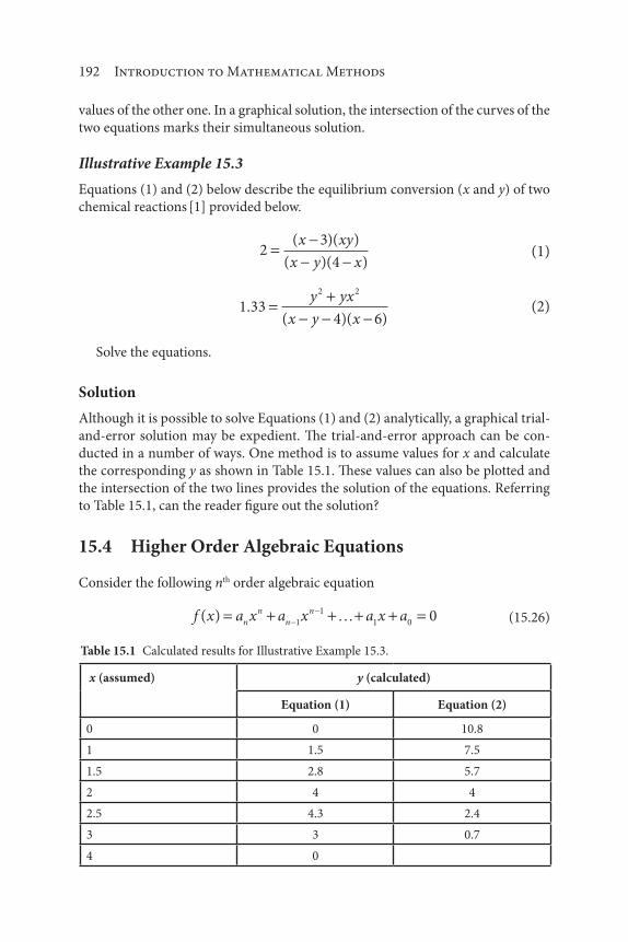
192 Introduction to Mathematical Methods
values of the other one. In a graphical solution, the intersection of the curves of the
two equations marks their simultaneous solution.
Illustrative Example 15.3
Equations (1) and (2) below describe the equilibrium conversion (x and y) of two
chemical reactions [1] provided below.
23
4
( )( )
( )( )
x xy
x y x (1)
1 334 6
2 2
.( )( )
y yx
x y x (2)
Solve the equations.
Solution
Although it is possible to solve Equations (1) and (2) analytically, a graphical trial-
and-error solution may be expedient. The trial-and-error approach can be con-
ducted in a number of ways. One method is to assume values for x and calculate
the corresponding y as shown in Table 15.1. These values can also be plotted and
the intersection of the two lines provides the solution of the equations. Referring
to Table 15.1, can the reader figure out the solution?
15.4 Higher Order Algebraic Equations
Consider the following nth order algebraic equation
f x a x a x a x an
n
n
n( ) 1
1
1 0 0 (15.26)
Table 15.1 Calculated results for Illustrative Example 15.3.
x (assumed) y (calculated)
Equation (1) Equation (2)
0 0 10.8
1 1.5 7.5
1.5 2.8 5.7
2 4 4
2.5 4.3 2.4
3 3 0.7
4 0

Trial-and-Error Solutions 193
The solution to this equation is demonstrated by solving the following 3rd
order equation
f x x x x( ) . . .3 26 6 29 05 22 64 0 (15.27)
Divide through by x, drop 22.64/x, and solve the resulting quadratic equation. This
provides a starting value for the trial-and-error solution.
x x2 6 6 29 05 0. . (15.28)
The solution is
x 9 6. (15.29)
One now notes that
f ( . ) .9 6 22 04 (15.30)
This provides an excellent starting value in an attempt to obtain a solution to
Equation (15.27)
15.5 Other Approaches
Environmental engineers and scientists occasionally solve equations which have
no simple analytical solution. For example, consider the equation [2]
e xx2
14 2. (15.31)
Once again, the most convenient way to solve this equation is to assume values of
x until the left side of the equation equals the right. However, the equation should
be inspected carefully to determine the general effect of a variation in x. Perhaps
one term is substantially smaller than the other so that it may be neglected for a
first estimation of x. In Equation (15.31), x is probably small compared to ex2
. As
a first approximation for x, assume x 0 in Equation (15.31) so that ex2
14 2.
and x 1.63. But
e xx2
14 2 16 3 12 6 14 2. . . . (15.32)
Inspection of Equation (15.31) indicates that a somewhat larger value of x
should be used. For the second trial, set x 1.70. Then

194 Introduction to Mathematical Methods
e1 72
1 7 17 8 1 7 16 1 14 2. . . . . . (15.33)
The second trial assumed an x which is too large. The two points can be plotted
on Figure 15.2. Although the function is highly non-linear, a straight line is drawn
between the fist and second approximations. The third approximation is taken at
the intersection of this line and the line ( )..e xx2
14 2 Applying a third approxi-
mation with x 1.665 gives
e( ). . . . .1 665 2
1 665 15 9 1 665 14 2 (15.34)
The third trial has effectively done the job. In many environmental engineering
calculations it is not necessary to plot the trials for a new estimate. The experi-
enced engineer can often make mental estimates and interpolations.
References
1. L. Theodore, Chemical Reactor Analysis and Applications for the Practicing Engineer, John Wiley &
Sons, Hoboken, NJ, 2011.
2. J. Famularo, personal communication to L. Theodore (with revision), Englewood Cliffs, NJ, 1970.
16.5
16
15.5
15
14.5
14
13.5
13
12.5
121.62 1.63 1.64 1.65 1.66
x
ex2 –
x ex2 – x = 14.2 (desired value)
2nd Approximation
3rd Approximation
1st Approximation
1.67 1.68 1.69 1.7 1.71
Figure 15.2 Graphical estimation in a trial-and-error procedure.

195
Many areas of environmental engineering and scientific analysis require the use of
efficient techniques for determining the roots of algebraic (and/or transcendental)
equations. It is for this reason that the subject of the solution to a nonlinear alge-
braic equation is considered in this chapter. Although several algorithms are avail-
able in the literature, this presentation will focus on the Newton-Raphson (NR)
method of evaluating the root(s) of a nonlinear algebraic equation.
Three sections complement the presentation of this chapter. Section numbers
and subject titles follow:
16.1: The Reguli-Falsi (False Position) Method
16.2: The Newton-Raphson Method
16.3: Newton’s Second Order Method
16.1 The Reguli-Falsi (False Position) Method
The Reguli-Falsi method (referred to by some as the False Position linear-inter-
polation method) involves obtaining values for two roots, i.e., values (x1, y
1) and
(x2, y
2) to the equation f(x) 0 by trial-and-error. From a plot of x vs. y and apply-
ing similar “triangles” to a third root (x3, y
3),
16Nonlinear Algebraic Equations
Introduction to Mathematical Methods for Environmental Engineers and Scientists. Charles Prochaska and Louis Theodore.
© 2018 Scrivener Publishing LLC. Published 2018 by John Wiley & Sons, Inc.

196 Introduction to Mathematical Methods
y y
x x
y y
x x2 1
2 1
3 1
3 1
(16.1)
For y3
0, one obtains
xx y x y
y yx
y x x
y y3
1 2 2 1
2 1
11 2 1
2 1
( ) (16.2)
If y is expressed as y f(x), the above equation becomes
xx f x x f x
f x f xx
f x x x
f x f x3
1 2 2 1
2 1
11 2 1
2 1
( ) ( )
( ) ( )
( )( )
( ) ( ) (16.3)
Theodore [1] also provides the following “algorithm”.
1. Assume a value of x1, (hopefully near to the actual value of the root).
2. Evaluate f(x1).
3. Find an x2 such that the sign of f(x
2) is different from that of f(x
1).
4. Plot f(x) vs x.
5. Draw a straight line between the two points and use the point
where the chord crosses the axis at f(x) 0 as x3.
6. Evaluate f(x3).
7. Use a new chord, f(x3) to f(x
2) to evaluate x
4.
8. The procedure is repeated employing Equation (16.4).
xx f x x f x
f x f xn
n n n n
n n
11
1
( ) ( )
( ) ( ) (16.4)
9. Continue until
| |x xn n1
1 (16.5)
or
f x f xn n( ) ( )1
2 (16.6)
Note: (error tolerance) will be defined later in Equation (16.20)
Thus, if values of f(x) for two relatively close trial values of x are known and that
one of the functional values is positive while the other is negative, at least one root
will be contained within this range of x. This is illustrated in Figure 16.1.
There is also a modification to the False Position method [1]. If
x x1 1 value of st
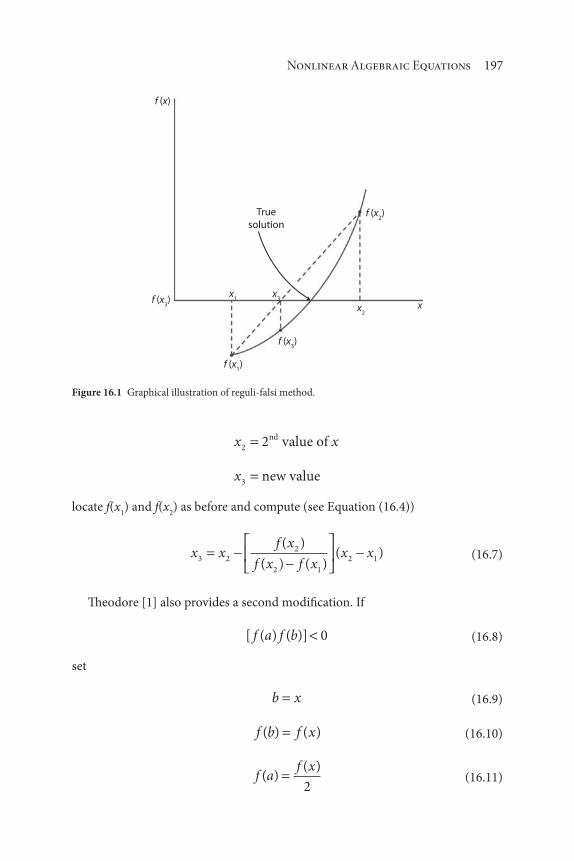
Nonlinear Algebraic Equations 197
x x2 2 value of nd
x3 new value
locate f(x1) and f(x
2) as before and compute (see Equation (16.4))
x xf x
f x f xx x3 2
2
2 1
2 1
( )
( ) ( )( ) (16.7)
Theodore [1] also provides a second modification. If
[ ( ) ( )]f a f b 0 (16.8)
set
b x (16.9)
f b f x( ) ( ) (16.10)
f af x
( )( )
2 (16.11)
x1
x3
x2
f (x3)
f (x2)
f (x)
x
f (x1)
f (x3)
True
solution
Figure 16.1 Graphical illustration of reguli-falsi method.

198 Introduction to Mathematical Methods
and test for convergence. If satisfactory, terminate the calculation; if not satisfac-
tory, return to Equation (16.7). If Equation (16.8) 0, set
a x (16.12)
f a f x( ) ( ) (16.13)
f bf x
( )( )
2 (16.14)
and check as above for convergence.
Illustrative Example 16.1
Solve the following equation
f x x x( ) 2 4 1 0
using the interpolation method. You have been informed that 3 x 4.
Solution
The appropriate equation below is a modified form of Equation (16.4).
x xx x f x
f x f xn n
n n n
n n
11
1
( ) ( )
( ) ( )
Apply the above equation to solve for x3., i.e., n = 2.
x xx x f x
f x f x3 2
2 1 2
2 1
( ) ( )
( ) ( )
Set x1
3 and x2
4.
f x( ) ( )( )1
23 4 3 1 2
f x( ) ( )( )2
24 4 4 1 1
Therefore
x3 41 1
1 24
1
33 667
( )( )
( ) ( ).

Nonlinear Algebraic Equations 199
Once again employ Equation (16.4) for xn+1
x4
x xx x f x
f x f x4 3
3 2 3
3 2
( ) ( )
( ) ( )
For this trial, x3
3.667, x2
4, f(x3) -0.222, f(x
2) 1. Therefore
x4 3 6673 667 4 0 222
0 222 1
3 6670 333 0 222
.( . )( . )
.
.( . )( . )
( 1 2223 667 0 061
3 728
.. .
.
)
Proceeding further is left as an option for the reader. For reference the true
solution for this root is 3 +2 or 3.732 .
16.2 Newton-Raphson Method
Although several algorithms are available for the solution to a nonlinear alge-
braic equation, the presentation in this section will key on the Newton-Raphson
method (or the Newton Method of Tangents) of evaluating the root(s) of a nonlin-
ear algebraic equation. The solution to the equation
f x( ) 0 (16.15)
is obtained by guessing a value for x (xold
) that will satisfy the above equation. This
value is continuously updating (xnew
) using the equation
x xf x
f xfnew old
old
old
( )
( ); derivative (16.16)
until either little or no change in (xnew
xold
) is obtained. One can express this
operation graphically (see Figure 16.2). Noting that
f xdf x
dx
f x
x
f x
x xold
old
old new
( )( ) ( ) ( ) 0
(16.17)
one may rearrange Equation (16.17) to yield Equation (16.18) below. The xnew
then
becomes the xold
in the next calculation.
This method as mentioned above is also referred to as Newton’s Method of
Tangents and is a widely used method for improving a first approximation to a

200 Introduction to Mathematical Methods
root to the aforementioned equation of the form f(x) 0. The above development
can be rewritten in subscripted form to (perhaps) better accommodate a computer
calculation. Thus,
f xf x
x xn
n
n n
( )( )
1
(16.18)
from which
x xf x
f xn n
n
n
1
( )
( )
or
x xf x
f x2 1
1
1
( )
( ) (16.19)
where xn+1
is again the improved estimate of xn, the solution to the equation
f(x) 0. The value of the function and the value of the derivative of the func-
tion are determined at x xn for this procedure and the new approximation to the
root, xn+1
is obtained. The same procedure is repeated with the new approximation
to obtain a better approximation of the root. This continues until successive val-
ues for the approximate root differ by less than a prescribed small value, , which
XXoXnXn+1Xn+2
Exact
solution
Fourth
approximation
F(x)
Figure 16.2 Graphical expression of the Newton-Raphson method.

Nonlinear Algebraic Equations 201
controls the allowable error (or tolerance) in the root. Relative to the previous
estimate, is given by
x x
xn n
n
1 (16.20)
Despite its popularity, the method suffers for two reasons. First, an analytical
expression for the derivative, i.e., f (xn) is required. In addition to the problem
of having to compute an analytical derivative value at each iteration, one would
expect Newton’s method to converge fairly rapidly to a root in the majority of
cases. However, as is common with some numerical methods, it may fail occasion-
ally in certain instances. A possible initial oscillation followed by a displacement
away from a root is illustrated in Figure 16.3. Note, however, that the method
would have converged (in this case) if the initial guess had been somewhat closer
to the exact root. Thus, it can be seen that the initial guess may be critical to the
success of the calculation.
In addition to the aforementioned False-Position and Second Order Newton
methods, one may also employ the Wegstein method and the Half-interval
method.(1, 2)
Illustrative Example 16.2
The vapor pressure, p , for a new synthetic chemical at a given temperature has
been determined to take the form [2]:
p T T T p atm3 2 12 2 ;
where the actual temperature, t (in K), is given by
t T T103 or = 10 t3
Solve the above equation for the actual temperature in K for p 1. Earlier stud-
ies indicate that t is in the 1000–1200K range.
f (x) f (x)
Exact solution
x4
x2
x3
xx
1
Figure 16.3 Failure of the Newton-Raphson method.

202 Introduction to Mathematical Methods
Solution
If p 1, one may then write
f T T T T( ) 3 22 2 1 0
Assume an initial temperature t1. Set t
11100, so that
T1
31100 10 1 1( )( ) .
Obtain the analytical derivative, f (T).
f T T T( ) 3 4 22
Calculate f(T1) and f (T
1).
f T T T( . ) ( . ) ( . ) ( . ) .1 1 2 2 1 1 1 2 1 1 2 1 1 1 0 1113 2 3 2
f T T( . ) ( . ) ( . ) .1 1 3 4 2 3 1 1 4 1 1 2 1 232 2
Use the Newton-Raphson method to estimate T2. Employ Equation (16.19).
T Tf T
f T2 1
1
1
( )
( )
Substituting
T2 1 10 111
1 231 0098.
.
..
Calculate T3.
f T f T T( ) . ; ( ) . ; .2 2 30 0099 1 0198 1 0001
Finally, calculate the best estimate (based on two iterations) of t.
t TK103 ; =1000.1K
Illustrative Example 16.3
It can be shown that the average velocity in a system involving the flow of water at
60°F is given by [3]
v
Re
2180
213 5 10
1
4.

Nonlinear Algebraic Equations 203
For water at 60°F, Re 12,168v.
Calculate the average velocity, v (ft/s), using the Newton-Raphson method of
solution [4].
Solution
Substitute the expression of Reynolds number as a function of velocity into the
velocity equation.
v
Re v
2180
213 5 10
2180
213 5 12 168 10
1
4
1
4. . ( , )
22180
213 5 12 168 101
4. ( , )/ v
Manipulate the above equation into one that is easier to differentiate. Squaring
both sides gives
v
v
v2
1
4
1
42180
213 5 12 168 10
2180 12 168
213 5 10 12 1[ . ( , ) ]
( , )
. ( ,/ 6681
4v)
Cross multiplying leads to
213 5 10 12 168 2180 12 168 021
4 21
4. ( , ) ( , )v v v v
or
f v v v v( ) . . , .. .213 5 105 03 22 896 08 02 2 25 0 25
The analytical derivative of f(v) is
f v v v v( ) . .. .427 236 313 5724 021 25 0 75
Make an initial guess of v 5 ft/s and substitute into the above equations:
f v f1 1 5 24 973 8( ) ( ) , .
f v f1 1 5 2189 97( ) ( ) .
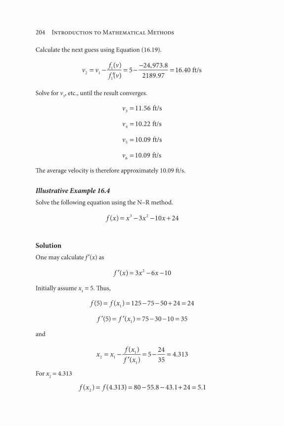
204 Introduction to Mathematical Methods
Calculate the next guess using Equation (16.19).
v vf v
f v2 1
1
1
524 973 8
2189 9716 4
( )
( )
, .
.. 0 ft/s
Solve for v3, etc., until the result converges.
v3 11 56. ft/s
v4 10 22. ft/s
v5 10 09. ft/s
v6 10 09. ft/s
The average velocity is therefore approximately 10.09 ft/s.
Illustrative Example 16.4
Solve the following equation using the N–R method.
f x x x x( ) 3 23 10 24
Solution
One may calculate f (x) as
f x x x( ) 3 6 102
Initially assume x1
5. Thus,
f f x( ) ( )5 125 75 50 24 241
f f x( ) ( )5 75 30 10 351
and
x xf x
f x2 1
1
1
524
354 313
( )
( ).
For x2
4.313
f x f( ) ( . ) . . .2 4 313 80 55 8 43 1 24 5 1

Nonlinear Algebraic Equations 205
f x f( ) ( . ) . . .2 4 313 55 8 25 9 10 19 9
so that
x xf x
f x3 2
2
2
4 3135 1
19 94 057
( )
( ).
.
..
One may choose to continue the iteration.
Illustrative Example 16.5
Solve the equation provided in Illustrative Example 16.1 employing the Newton-
Raphson method.
Solution
Apply the N–R method of solution to the equation x2 – 4x 1 0. Employ
x xf x
f xn n
n
n
1
( )
( )
For this example start with x1
3. Then
f x f x fn( ) ( ) ( )1 3 2
f x f x fn( ) ( ) ( )1 3 2
so that
x2 32
23 1 4
( )
For the second iteration,
f x( )2 1
f x( )2 4
so that
x3 41
43 75.
Proceeding further is left as an exercise for the reader. Again, for reference, the
true solution rounded to three decimal places is 3.732.

206 Introduction to Mathematical Methods
16.3 Newton’s Second Order Method
Newton’s Second Order method requires the determination of the first derivative
of f (x1), for the first assumed value of x
1, and the second derivative, f (x
1). The
algorithm (derivation not presented) is with f y and f y .
x x
y
yy y
y2 1
1
11 1
12
(16.21)
If y is replaced by f(x), the above algorithm becomes
x x
f x
f xf x f x
f x2 1
1
11 1
12
( )
( )( ) ( )
( )
(16.22)
which may be rewritten as
x xf x f x
f x f x f x2 1
1 1
1
2
1 1
2
2
( ) ( )
( ) ( ) ( ) (16.23)
As one might suppose, there are a host of other procedures/methods for solving
nonlinear algebraic equations. It should also be mentioned that brute-force and
trial-and-error approaches have merit, particularly if one has a reasonable idea
of the correct root. However, this method was discussed in the previous chapter.
Illustrative Example 16.6
Solve the equation
f x x x x( ) 3 23 10 24
using Newton’s Second Order method.
Solution
Calculate the first and second derivative of f(x)
f x x x( ) 3 6 102
f x x( ) 6 6

Nonlinear Algebraic Equations 207
Assume an educated value for x1, say x
15. Then
f ( )5 24
f ( )5 35
f ( )5 24
Substitute into Equation (16.23).
x2 2
52 24 35
2 35 24 245
1680
1874
4 104
( )( )
( ) ( )( )
.
Similarly
f x f( ) ( . ) .2 4 104 1 55
f x f( ) ( . ) .2 4 104 15 9
f x f( ) ( . ) .2 4 104 18 6
so that
x3 2
4 1042 1 55 15 9
2 15 9 1 4 18 64 104
49.
( . )( . )
( . ) ( . )( . ).
.229
479 58
4 001
.
.
Proceed or terminate, as desired.
References
1. L. Theodore, personal notes, East Williston, NY, 1970.
2. L. Theodore, F. Ricci, and T. VanVliet, Thermodynamics for the Practicing Engineer, John Wiley &
Sons, Hoboken, NJ, 2009.
3. P. Abulencia and L. Theodore, Fluid Flow for the Practicing Chemical Engineer, John Wiley & Sons,
Hoboken, NJ, 2009.

209
Environmentalists frequently encounter problems involving the solution of sets of
simultaneous linear algebraic equations. Such problems arise in a host of areas that
include electrical-circuit analysis, heat transfer, vibrations, chemical reactions, etc.
The most common methods of solving simultaneous equations involve the elim-
ination of unknowns by combining equations. When three or more simultane-
ous equations are being solved, one must resort to other methods. For example,
the method of determinants with expansion by minors is completely impractical
when large numbers of equations must be solved simultaneously.
Note that in the presentation to follow there are an equal number of unknowns
and equations. If there are more unknowns than equations, the system has an infinite
number of solutions. If there are fewer equations than unknowns, then the system of
equations does not have a solution. Because of the breadth of the subject matter, the
reader should also note that only three numerical methods receive treatment in the
chapter. Information on the remaining methods can be found in the literature [1,2].
Four sections complement the presentation of this chapter. Section numbers
and subject titles follow:
17.1: Notation for Solving Simultaneous Linear Algebraic Equations
17.2: Gauss Elimination Method
17Simultaneous Linear Algebraic Equations
Introduction to Mathematical Methods for Environmental Engineers and Scientists. Charles Prochaska and Louis Theodore.
© 2018 Scrivener Publishing LLC. Published 2018 by John Wiley & Sons, Inc.

210 Introduction to Mathematical Methods
17.3: Gauss-Jordan Reduction Method
17.4: Gauss-Seidel Method
17.1 Notation For Solving Simultaneous Linear Algebraic Equations
The engineer often encounters problems that not only contain more than two or
three simultaneous algebraic equations, but also those that are sometimes nonlin-
ear as well. Therefore, there is an obvious need for providing systematic methods
of solving simultaneous linear and simultaneous nonlinear equations [1]. This sec-
tion will address linear sets of equations. Information on nonlinear sets is available
in the literature [2].
Consider the following set of n equations:
a x a x a x c
a x a x a x c
a x a x
n n
n n
m m
11 1 12 2 1 1
21 1 22 2 2 2
1 1 2 2 a x cmn n n
(17.1)
where a is the coefficient of the variable x and c is a constant. The above set is con-
sidered to be linear as long as none of the x terms are nonlinear, for example, x2
2
or ln x1. Thus, a linear system requires that all terms in x be linear.
The above system of linear equations may be set in matrix form (see Part II):
a a a
a a a
a a a
x
x
x
n
n
m m mn n
11 12 1
21 22 2
1 2
1
2
c
c
cn
1
2 (17.2)
However, it is often more convenient to represent Equation (17.2) in the aug-
mented matrix provided in Equation (17.3).
a a a c
a a a c
a a a c
n
n
m m mn n
11 12 1 1
21 22 2 2
1 2
(17.3)

Simultaneous Linear Algebraic Equations 211
As noted above, only the first three methods are discussed in this chapter.
The coefficient matrix of the set of equations in Equation (17.1) is
a a a
a a
a a
n
n
n
11 12 1
21 2
31 3
(17.4)
If the constants of Equation (17.1) are added to the coefficient matrix as a col-
umn of elements in the position shown in Equation (17.3), the augmented matrix
is formed. A comparison of Equations (17.1) and (17.4) shows that a coefficient
matrix is a matrix whose elements are the coefficients of the unknowns in the set
of the equations.
In many instances in computer programming, it may be found convenient to
express the column of constants c1, c
2, c
3, …, c
n, as simply an additional column of
aij’s. In such an instance the matrix of Equation (17.3) might be expressed as
B
a a a a
a a a a
a a a
n n
n n
m mn m n
11 12 1 1 1
21 22 2 2 2
1 1
,
,
,
(17.5)
If c1, c
2, c
3, …, c
n are not all zero, the set of equations is nonhomogeneous,
and one will find that all the equations must be independent to obtain unique
solutions. If the constants c1, c
2, c
3, …, c
n are all zero, the set of equations is
homogenous, where nontrivial solutions exist only if all the equations are not
independent.
In this chapter, the solution of both homogenous and nonhomogeneous sets
of linear algebraic equations shall be considered since both types appear in envi-
ronmental applications. The sets of equations which are to be addressed will
involve n unknowns in n equations, which have the general form provided in
Equation (17.1).
Methods of solution available for solving these linear sets of equations include:
1. Gauss elimination
2. Gauss-Jordan reduction
3. Gauss-Seidel
4. Cramer’s rule
5. Cholesky’s method

212 Introduction to Mathematical Methods
17.3 Gauss-Jordan Reduction Method
The second method presented for the solution of simultaneous linear algebraic
equations – a variation of the gauss elimination – is one in which the unknowns
are reduced by combining equations. Such a method is known as a reduction
method. It is referred to by some as Gauss’s method or the Gauss-Jordan method
if a particular systematic scheme is used in the reduction process. This method
involves the “reduction” of the simultaneous equations to the solution of one lin-
ear equation with one unknown.
17.2 Gauss Elimination Method
Using Gauss’ elimination method, a set of n equations and n unknowns is reduced
to an equivalent triangular set (an equivalent set is a set having identical solu-
tion values), which is then easily solved by “back substitution,” a simple procedure
which will be illustrated in an illustrative example.
Gauss’ scheme begins by reducing a set of simultaneous equations, such as those
given in Equation (17.1), to an equivalent triangular set such as the following:
a x a x a x a x a x c
a x a x a x
n n11 1 12 2 13 3 14 4 1 1
22 2 23 3 24 4 aa x c
a x a x a x c
a
n n
n n
m n
m
2 2
33 3 34 4 3 3
1 1
.
,
22
1 1
2
1
2
1 1
x a x c
a x c
n m n
m
n n
n
mn
m
n n
n
,
(17.6)
where the prime subscripts indicate new coefficients which are formed in the
reduction process. The following steps accomplish the actual reduction. First, the
lead equation in Equation (17.1) is divided by the coefficient of x1 to obtain
xa
ax
a
ax
a
ax
c
an
n112
11
213
11
31
11
1
11
(17.7)
Next, Equation (17.7) is multiplied by the coefficient of x1 in the second equa-
tion found in Equation (17.1), and the resulting equation is subtracted from the
original second equation in Equation (17.1), which eliminates x1. Equation (17.7)
is then multiplied by the coefficient of x1 in the third equation of Equation (17.1),
and the resulting equation is subtracted from the third equation to eliminate x2.
This process is repeated until one can solve for xn directly. The algorithm for solv-
ing an n x m set of equations is provided in Figure 17.1.

Simultaneous Linear Algebraic Equations 213
Carnahan and Wilkes [1] solved the following two simultaneous equations
using the Gauss-Jordan reduction method:
3 4 291 2x x (17.8)
6 10 681 2x x (17.9)
Application of the aforementioned procedure follows.
1. Divide Equation (17.8) through by the coefficient of x1:
x x1 2
4
3
29
3 (17.10)
2. Subtract a suitable multiple, in this case 6, of equation (17.10) from
Equation (17.9), so that x1 is eliminated. Equation (17.10) remains
untouched, leaving:
x x1 2
4
3
29
3 (17.11)
2 102x (17.12)
3. Divide Equation (17.12) by the coefficient of x2, that is, solve
Equation (17.12)
x2 5 (17.13)
4. Subtract a suitable factor of Equation (17.13) from Equation
(17.11) so that x2 is eliminated. When (4/3)x
2 = 20/3 is subtracted
from Equation (17.11), one obtains
x1 3 (17.14)
The augmented matrix from Equation (17.3) is
3 46 10
2968
1 4 36 10
29 368
1 4 30 2
29 310
/ /
/ /

214 Introduction to Mathematical Methods
2 105
2
2
x
x
10
02
310
x1 3
Illustrative Example 17.1
Solve the following set of linear algebraic equations using Gauss elimination.
3 2 7
4 2 21
2 3 4 9
1 2 3
1 2 3
1 2 3
x x x
x x x
x x x
Solution
First, set up the augmented matrix.
3 2 1 7
1 4 2 21
2 3 4 9
In order to convert the first column of elements below the diagonal to zero, start
by setting the first row as the pivot row. For the remaining rows, multiply each ele-
ment by a11
/an1
and subtract each row from the pivot row. Thus:
Row 2 coefficients:
3 3 1 0( )( )
2 3 4 14( )( )
1 3 2 7( )( )
7 3 21 56( )( )
Row 3 coefficients:
33 2
20
( )( )

Simultaneous Linear Algebraic Equations 215
23 3
22 5
( )( ).
13 4
27
( )( )
73 9
26 5
( )( ).
This procedure calls forcreating an (n × n + 1)matrix where the n + 1
column containsonly constants.
Setup equationsin matrix form
(n × m)
Starting with thesecond row,
multiply eachelement of thatrow by a
11/an1
where n is therow number.
Note that this will make thefirst element of the each row
equal to the first elementof the first row.
Note that this will make thefirst element of the each row
equal to zero.
Subtract eachrow from the first
and place theresult in the
matrix where thesubtracted row
once was.
Is this the lastrow?
Is this the secondto last column?
Yes
Yes
NoNo
Starting with thethird row,
multiply eachelement of thatrow by a
22/an2
where n is therow number
Figure 17.1 Algorithm for Gauss Elimination with back substitution.

216 Introduction to Mathematical Methods
The resulting matrix is:
3 2 1 7
0 14 7 56
0 2 5 7 6 5. .
Now starting with the second column and the second row, perform the same
procedure again, with the second row as the pivot row.
Row 3 coefficients:
1414 2 5
2 50
( )( . )
.
714 7
2 546 2
( )( )
..
5614 6 5
2 592 4
( )( . )
..
Figure 17.1 Algorithm for Gauss Elimination with back substitution (continued).
Yes
No
The last row may
be solved for xn.
Have all the
equations been
solved?
Knowing the
value of xn, the
second to last
row can be
solved for xn–1.
The last row is of the
form, an(m–1) × xn = anm.
The last row is of the form,
an–1(m–2) × xn–1
+an–1(m–1) × xn = a
(n–1)m.
Solving for xn–1,
xn–1 = [a
(n–1)m–an–1(m–1) × xn]/a
(n–1)(m–2).
Solving for xn,
xn = anm/an(m–1).

Simultaneous Linear Algebraic Equations 217
This produces the following matrix:
3 2 1 7
0 14 7 56
0 0 46 2 92 45. .
At this point, back substitution may be employed. The following results are
obtained:
46 2 92 4 23 3. . ;x x
14 2 7 56 32 2x x( ) ;
3 2 3 1 2 7 51 1x x( )( ) ( ) ;
Gauss elimination is useful for systems that contain fewer than 30 equations.
Larger systems become subject to roundoff error where numbers are truncated by
computers performing the calculations.
17.4 Gauss-Seidel Method
Another approach to solving an equation or series/sets of equations is to make an
educated guess. If the first assumed value(s) does not work, the value is updated.
By carefully noting the influence of these guesses on each variable, the answers
or correct set of values for a system of equations can be approached. The reader
should note that when this type of iterative procedure is employed, a poor guess
does not prevent the correct solution from ultimately being obtained.
Ketter and Prawel provide the following example [1]. Consider the equations
below:
4 2 0 21 2 3x x x
2 10 4 61 2 3x xx
0 4 5 51 2 3x x x
The reader may choose to assume as a starting point x1 = x
2 = x
3 = 0, for the non-
bold terms. Solving each equation for the bold terms (found on the diagonal), one
obtains
x x x1 2 30 50 0 60 1 00. ; . ; .

218 Introduction to Mathematical Methods
These computed values can now be used as new guesses to update the initially
assumed x values.
x x x1 1 2 3
2
4
0
40 50
2
40 60 0 20x . ( . ) .
x x x2 2 1 3
2
10
4
100 60
2
100 50
4
101 00 0 90x . ( . ) ( . ) .
x x x3 3 1 2
0
5
4
51 00
0
50 50
4
50 60 1 48x . ( . ) ( . ) .
The right-hand side of these equations may be viewed as residuals. The proce-
dure is repeated until convergence is achieved with the residuals approaching zero.
More rapid convergence techniques are available in the literature [2].
References
1. R. Ketter and S. Prawler, Modern Methods of Engineering Computations, McGraw-Hill, New York
City, NY, 1969.
2. B. Carnahan and J. Wilkes, Digital Computing and Numerical Methods, John Wiley & Sons,
Hoboken, NJ, 1973.

219
Numerical differentiation should be avoided whenever possible, particularly when
data are empirical and subject to appreciable observation errors. Errors in data
can affect numerical derivatives, i.e., differentiation is a significantly “roughen-
ing” process. When such a calculation must be made, it is usually desirable to first
smooth the data to a certain extent (if possible).
Derivatives of a function f(x) may be evaluated numerically by any one of
several methods involving two data points. Three simple formulas that may be
employed to evaluated the derivative, f(x) d[f(x)]/dx, are given below.
f xh
f x h f x( ) [ ) ( )];1
( forward difference (18.1)
f xh
f x h f x h( ) [ ( ) ( )];1
2 central difference (18.2)
f xh
f x f x h( ) [ ( ) ( )];1
backward difference (18.3)
The term h represents an incremental change in x.
18Differentiation
Introduction to Mathematical Methods for Environmental Engineers and Scientists. Charles Prochaska and Louis Theodore.
© 2018 Scrivener Publishing LLC. Published 2018 by John Wiley & Sons, Inc.

220 Introduction to Mathematical Methods
Three sections complement the presentation of this chapter. Section numbers
and subject titles follow:
18.1: Employing Two and Three Point Formulas
18.2: Employing Five Point Formulas
18.3: Method of Least Squares
18.1 Employing Two and Three Point Formulas
Several differentiation methods [1] are available for generating expressions for a
derivative using three data points. Consider the problem of determining the ben-
zene concentration time gradient dC dt/ at t 4.0 s; refer to Table 18.1.
Method 1. This method involves the selection of any three data points and calcu-
lating the slope m of the two extreme points. This slope is approximately equal to
the slope at the point lying in the middle. The value obtained is the equivalent of
the derivative at that point 4. Using data points from 3.0s to 5.0s, one obtains
Slope mC C
t t5 3
5 3
1 63 2 70
5 0 3 00 535
. .
. ..
(18.4)
Method 2. This method involves determining the average of two slopes. Using the
same points chosen above, two slopes can be calculated, one for points 3 and 4 and
the other for points 4 and 5. Adding the two results and dividing them by 2 will
provide an approximation of the derivative at point 4. For the points used in this
method, the results are as follows.
Table 18.1 Concentration-Time data.
Time, s Data point Concentration of benzene, mg/L
0.0 0 7.46
1.0 1 5.41
2.0 2 3.80
3.0 3 2.70
4.0 4 2.01
5.0 5 1.63
6.0 6 1.34
7.0 7 1.17

Differentiation 221
m slopeC C
t t1 1
4 3
4 3
2 01 2 70
4 0 3 00 69
. .
. ..
(18.5)
m slopeC C
t t2 2
5 4
5 4
1 63 2 01
5 0 4 00 38
. .
. ..
(18.6)
m slopeavg avg
0 69 0 38
20 535
. ( . ). (18.7)
Method 3. Method 3 consists of using any three data points (in this case the
same points chosen before) and fitting a curve to it. The equation for the curve is
obtained by employing a second-order equation and solving it with the three data
points. The equation can be quickly provided by Microsoft Excel’s “add trend line”
function. The result is
C t t0 155 1 775 6 632. . . (18.8)
The derivative of the equation is then calculated and evaluated at any point. (Here,
point 4 is used).
dC
dtt0 31 1 775. . (18.9)
Evaluating the derivative at t 4.0 yields
SlopedC
dt0 31 4 1 775 0 535. ( ) . . (18.10)
18.2 Employing Five Point Formulas
There are two methods to employ here and they are very similar to each other.
They are based on five data points used to generate coefficients. For this develop-
ment, represent C and t by f and x (as it appears in the literature [2]), respectively.
The first method uses five data points to generate a five coefficient (fourth
order) model using an equation in the form
f x A Bx Cx Dx Ex( ) 2 3 4 (18.11)

222 Introduction to Mathematical Methods
This method is known as interpolating. A set of equations is used to evaluate
numerical derivatives from the interpolating polynomial. The equations are listed
below.
f xf f f f f
h( )
( )0
0 1 2 3 425 48 36 16 3
12 (18.12)
f xf f f f f
h( )
( )1
0 1 2 3 43 10 18 6
12 (18.13)
f xf f f f
hi
i i i i( )( )2 1 1 28 8
12 (18.14)
f xf f f f f
hn
n n n n n( )( )
14 3 2 16 18 10 3
12 (18.15)
f xf f f f f
hn
n n n n n( )( )3 16 36 48 25
124 3 2 1 (18.16)
where h xi+1
xi, f
ifunction evaluated at i.
For example, the equation obtained for “the five data set” from 1.0 to 5.0 s, i.e.,
t 1.0, 2.0, 3.0, 4.0, and 5.0 s, using the author’s [2] approach gives
f x x x x x( ) . . . . .0 0012 0 002 0 02616 2 34 7 4674 3 2
All these equations can be evaluated for each value of x and f(x). The value for the
derivative for point 4.0 is 0.5448.
The second and last method also uses five data points but only three coefficients
are generated for a second-order polynomial equation of the form
f A Bx Cx2 (18.17)
Another set of equations are used to evaluate the derivative at each point using this
method. The equations are provided below.
f xf f f f f
h( )
( )0
0 1 2 3 454 13 40 27 26
70 (18.18)
f xf f f f f
h( )
( )1
0 1 2 3 434 3 20 17 6
70 (18.19)
f xf f f f
hi
i i i i( )( )2 2
102 1 1 2
(18.20)
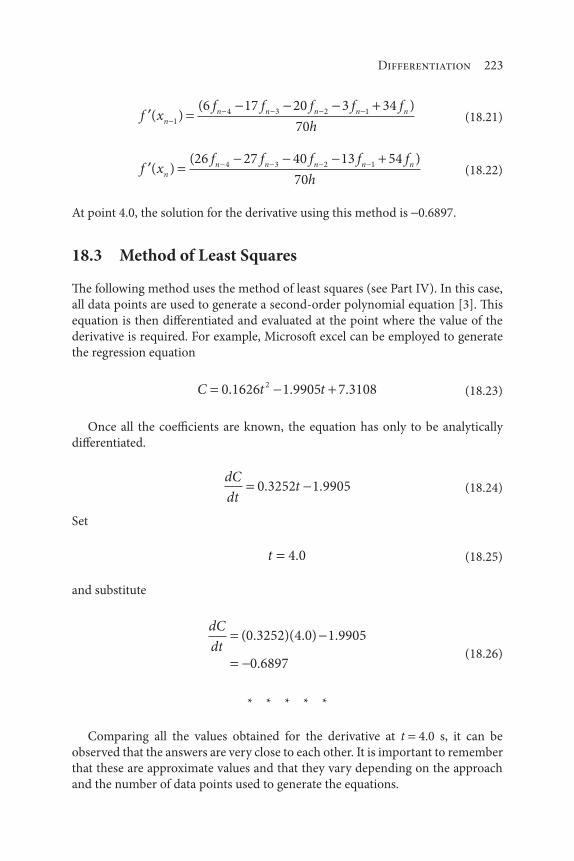
Differentiation 223
f xf f f f f
hn
n n n n n( )( )
14 3 2 16 17 20 3 34
70 (18.21)
f xf f f f f
hn
n n n n n( )( )26 27 40 13 54
704 3 2 1
(18.22)
At point 4.0, the solution for the derivative using this method is 0.6897.
18.3 Method of Least Squares
The following method uses the method of least squares (see Part IV). In this case,
all data points are used to generate a second-order polynomial equation [3]. This
equation is then differentiated and evaluated at the point where the value of the
derivative is required. For example, Microsoft excel can be employed to generate
the regression equation
C t t0 1626 1 9905 7 31082. . . (18.23)
Once all the coefficients are known, the equation has only to be analytically
differentiated.
dC
dtt0 3252 1 9905. . (18.24)
Set
t 4 0. (18.25)
and substitute
dC
dt( . )( . ) .
.
0 3252 4 0 1 9905
0 6897 (18.26)
* * * * *
Comparing all the values obtained for the derivative at t 4.0 s, it can be
observed that the answers are very close to each other. It is important to remember
that these are approximate values and that they vary depending on the approach
and the number of data points used to generate the equations.

224 Introduction to Mathematical Methods
References
1. L. Perez, term project submitted to L. Theodore, Manhattan College, Bronx, NY, 2003.
2. F. Lavery, The Perils of Differentiating Engineering Data Numerically, Chem. Eng., New York City,
NY, 1979.
3. S. Shaefer and L. Theodore, Probability and Statistics for Environmental Science, CRC Press/Taylor &
Francis Group, Boca Raton, FL, 2007.

225
Numerous environmental engineering and science problems require the solution
of integral equations. In a general sense, the problem is to evaluate the function on
the right-hand side (RHS) of Equation (19.1)
I f x dxa
b
( ) (19.1)
where I is the value of the integral. As discussed earlier, there are two key methods
employed in their solution: analytical and numerical. If f(x) is a simple function, it
may be integrated analytically. For example, if f(x) x2, then
I x dx b aa
b
2 3 31
3( ) (19.2)
If, however, f(x) is a function too complex to integrate analytically {e.g., log[ )]tan (h ex3 2
}, one may resort to any of the numerical methods available. Two
simple numerical integration methods that are commonly employed in practice
19Integration
Introduction to Mathematical Methods for Environmental Engineers and Scientists. Charles Prochaska and Louis Theodore.
© 2018 Scrivener Publishing LLC. Published 2018 by John Wiley & Sons, Inc.

226 Introduction to Mathematical Methods
are the trapezoidal rule and Simpson’s rule. These are described below. However,
there are other numerical integration methods, including:
1. Romberg’s method
2. Composite formulas
3. Gregory’s formulas
4. Taylor’s theorem
5. Method of undetermined coefficients
6. Richardson’s extrapolation
Details are available in the literature [1–3].
Finally, the reader should once again realize that analytical approaches yield
closed form and/or exact solutions. Numerical methods provide discrete and/or
inexact answers. Thus, the analytical approach should always be attempted first
even though numerical methods have become the preferred choice.
Three sections complement the presentation of this chapter. Section numbers
and subject titles follow:
19.1:Trapezoidal Rule
19.2: Simpson’s Rule
19.3: Comparing the Trapezoidal Rule with Simpson’s Rule
19.1 Trapezoidal Rule
In order to use the trapezoidal rule to evaluate the integral given by Equation (19.1), as
I f x dxa
b
( ) (19.1)
use the equation
Ih
y y y y yn n2
2 2 20 1 2 1[ ] (19.3)
where h is the incremental change in x. Thus,
h x (19.4)
and
y f x f x ao ( ) ( )0 (19.5)

Integration 227
y f x f x bn n( ) ( ) (19.6)
hb a
n (19.7)
This method is known as the trapezoidal rule because it approximates the area
under the function f(x) – which is generally curved – with a two-point trapezoidal
rule calculation. The error associated with this rule is illustrated in Figure 19.1.
There is an alternative available for improving the accuracy of this calculation.
The interval (a b) can be subdivided into smaller intervals. The trapezoidal rule
can be applied repeatedly in turn over each subdivision.
Illustrative Example 19.1
The volume requirement of a reactor [4, 5] undergoing conversion X for the reac-
tant (the principal component from the bottom of a distillation column) [6] is
described by the following integral:
VX dX
X X6 0 10
1 0 125
10 1 1 0 5
3
0
0 45 3
4 2.
.
.;
( )
( )( )
.
liters
Calculate the volume using the trapezoidal rule method of integration. Discuss
the effect of varying the increment in conversion X (e.g., if X 0.45, 0.09, 0.05,
0.01, 0.005, 0.001).
Solution
Regarding integration, an algorithm for applying the trapezoidal rule is given in
Figure 19.2.
Error =
f(x)
f(x)
f(a) f(b)
xa b
Figure 19.1 Trapezoidal rule error.
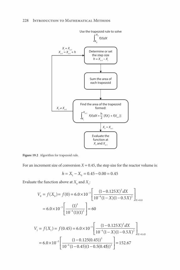
228 Introduction to Mathematical Methods
For an increment size of conversion X 0.45, the step size for the reactor volume is:
h X X1 0 0 45 0 00 0 45. . .
Evaluate the function above at X0 and X
1:
V f XX dX
X X0 0
33
4 26 0 10
1 0 125
10 1 1 0 5( ) .
.
.
( )
( )( )f (0)
X 0 0
33
4 26 0 10
1
10 1 160
.
.( )
( )( )
V f XX dX
X X1 1
33
4 26 0 10
1 0 125
10 1 1 0 5( ) .
( . )
.( )( )f (0.45)
X 0 45
33
46 0 10
1 0 125 0 45
10 1 0 45 1 0 5 0 4
.
.. ( . )
. . ( .
( )
( )( 55152 67
2).
)
f(X)dXxT
x0
Use the trapezoid rule to solve
Determine or setthe step sizeh = Xi+1
– Xi
Sum the area ofeach trapezoid
Find the area of the trapezoidformed:
Evaluate thefunction atXT and Xi+1
Xi = Xi+1
Xi+1 = Xi+1
+ h
XT Xi+1
XT = Xi+1
h
2f(X)dX = [f(Xi) + f(Xi+1
)]xi+1
xi
Figure 19.2 Algorithm for trapezoid rule.

Integration 229
The two point trapezoid rule is given by
X
X
f X dXh
f X f X
1
2
20 1( ) [ ( ) ( )]
Therefore,
Vh
f X f X
hV V
L
2
20 45
260 152 67
47 85
0 1
0 1
[ ( ) ( )]
[ ]
.[ . ]
.
The trapezoid rule is often the quickest but least accurate way to perform a
numerical integration by hand. However, if the step size is decreased the answer
should converge to the analytical solution. Note that for smaller step sizes, the
results of each numerical integration must be added together to obtain the final
answer. The results (to seven significant figures) for various step sizes are listed in
Table 19.1. Can the reader comment on whether convergence has been achieved?
19.2 Simpson’s Rule
A higher-degree interpolating polynomial scheme can be employed for more accu-
rate results. One of the more popular integration approaches is Simpson’s rule. For
Simpson’s 3-point (or one-third) rule, one may use the equation
Ih
y y ya b a b3
4 2[ ]( )/ (19.8)
Table 19.1 Trapezoid rule for various step sizes.
Step size ( X) Volume
0.45 47.85094
0.09 43.13532
0.05 42.98842
0.01 42.92521
0.005 42.92324
0.001 42.92260

230 Introduction to Mathematical Methods
For the general form of Simpson’s rule (where n is an even integer), the equa-
tion is
Ih
y y y y y yn n3
4 2 40 1 2 3 1( )4 + (19.9)
This method also generates an error, although it is usually smaller than that asso-
ciated with the trapezoidal rule. A diagrammatic representation of the error for a
3-point calculation is provided in Figure 19.3.
Illustrative Example 19.2
Evaluate the integral below using Simpson’s 3-point rule. The term I in this appli-
cation represents the volume requirement for a tubular flow reactor.(4, 5)
IX
X X XdX
0
0 468 2
2
1 0 4
1 1 0 4 1 19
.( ).
( )( . ) .
Solution
Write the 3-point rule. See Equation (19.9).
Ih
y y y
hf X a f X b a f X b
a b a b3
4
34 2
2[ ]
[ ( ) ( ( ) ) ( )]
( )/
/
f(x)
f(x)
f(x0) f(x
1) f(x
2)
x2
xx
1
x2 – x
1 = x
1 – x
0
= error
Error
Error
Simpson
x0
Figure 19.3 Simpson’s rule analysis and error.

Integration 231
Evaluate h.
h0 468
20 234
..
Calculate ya, y
(b+a)/2, and y
b. For X a 0,
y x y( ) ( ). ( )
( ( ))( . ( )) . ( )
( )0 0
1 0 4 0
1 0 1 0 4 0 1 19 01
2
2
Similarly,
y X( . )0 234 1.306
y X( . )0 468 3.846
Finally, calculate the integral I.
Ih
y y ya b a b3
4
0 234
31 4
2[ ]
.[ ( ) ]
( )/
1.306 3.846 0.785
19.3 Comparing the Trapezoidal and Simpson’s Rules
Comparing the integrations in the two previous sections is accomplished via a two
part illustrative example.
Illustrative Example 19.3
Given the following integral:
I x dx0
4
21
225( )
1. Calculate I by the trapezoidal rule for 2 and 4 intervals to three
decimal places.
2. Calculate I by Simpson’s one-third rule for 2 and 4 intervals to
three decimal places.
Compare the results.

232 Introduction to Mathematical Methods
Solution
Referring to Table 19.2, tabulate I at 5 points (values of x).
1. By the trapezoidal rule with 2 intervals, i.e., h 2.
I2
20 200 2 0 218 0 333( . ( . ) . )
I 0 969.
For 4 intervals, h 1 so that
I1
20 200 2 0 204 2 0 218 2 0 250 0 333[ . ( . ) ( . ) ( . ) . ]
I 0 939.
2. By Simpson’s rule with 2 intervals, i.e., h 2.
I2
30 200 0 333( . . )4(0.218)
I 0 937.
For 4 intervals, h 1 so that
I1
30 200 4 204 2 0 218 4 0 250 0 333[ . (. ) ( . ) ( . ) . ]
I 0 928.
Which is more accurate? One needs the analytical solution for comparison.
One is left the exercise of determining that (2) is a better approximation.
Table 19.2 Values of I vs x; Illustrative Example 19.3.
x I
0 0.200
1 0.204
2 0.218
3 0.250
4 0.333
Integration 233
In general, comparing the trapezoid rule and Simpson’s one-third rule, one
notes that the trapezoid rule requires n 1 data points for obtaining the area in
n subintervals of width x, whereas Simpson’s one-third rule requires n 1 data
points for obtaining the area in 2n subintervals of width ( x)/2.
References
1. R. L. Ketter and S. P. Prawler, Modern Methods of Engineering Computations, McGraw-Hill, New
York City, NY, 1969.
2. J. Reynolds, class notes (with permission), Manhattan College, Bronx, NY, 2001.
3. J. Famularo, class notes (with permission), Manhattan College, Bronx, NY, 1981.
4. L. Theodore, Chemical Reaction Analysis and Applications for the Practicing Engineer, John Wiley &
Sons, Hoboken, NJ, 2011.
5. L. Theodore, Chemical Reaction Kinetics, A Theodore Tutorial, Theodore Tutorials, East Williston,
NY, originally published by USEPA/APTI, RTP, NC, 1994.
6. L. Theodore and F. Ricci, Mass Transfer Operations for the Practicing Engineer, John Wiley & Sons,
Hoboken, NJ, 2010.

235
The natural laws in environmental engineering and science are not regarded as
precise and definitive until they have been expressed in mathematical form. Such
a form, often an equation, is a relation between the quantity of interest, say, pollut-
ant concentration, and independent variables such as time and position on which
the concentration depends. When it happens that this equation involves, besides
the function itself, one or more of its derivatives it is called a differential equation.
When the aforementioned function involved in the equation depends only on
one variable, its derivatives are ordinary derivatives and the differential equation
is referred to as an ordinary differential equation. When the function depends
on several independent variables, the equation is then called a partial differential
equation (see next chapter). The theories of ordinary and partial differential equa-
tions are different and the latter is more “difficult” in almost every respect.
Of increasing concern to the environmental engineer and scientist is the
description of dynamic or transient staged and/or lumped-parameter processes.
Ordinary differential equations are usually used to represent the behavior of
such processes; when combined with chemical reaction [1] or equilibrium [2]
relationships, the equations are often highly nonlinear.
One often encounters differential equations which cannot be solved by any
analytical methods except that of a solution in terms of a series, and this method
20Ordinary Differential Equations
Introduction to Mathematical Methods for Environmental Engineers and Scientists. Charles Prochaska and Louis Theodore.
© 2018 Scrivener Publishing LLC. Published 2018 by John Wiley & Sons, Inc.

236 Introduction to Mathematical Methods
may be difficult to apply in certain cases. Even when an analytical solution is avail-
able, it is sometimes difficult to find numerical values of corresponding pairs of the
dependent and independent variables. However, a variety of methods have been
devised to solve ordinary differential equations numerically. Several references
contain detailed information [3–6].
Interestingly, a numerical solution of a differential equation can generally
provide a table of values of the dependent variable and its derivatives over only
a limited portion of the range of the independent variable. Also of interest,
every differential equation of order n can be written as n first order equations.
Therefore, the methods given in the early sections of this chapter will be for
first-order equations, and the generalization to simultaneous systems will be
subsequently discussed. The reader might also note that the analytical solution
to an ordinary differential equation was not addressed in any detail in Part II,
Chapter 11.
Five sections complement the presentation of this chapter. Section numbers
and subject titles follow:
20.1: Finite Difference/Lumped Parameter Method
20.2: Runge-Kutta Method
20.3: Runge-Kutta-Gill Method
20.4: Several Ordinary Differential Equations
20.5: Higher Ordinary Differential Equations
20.1 Finite Difference/Lumped Parameter Method
This method is illustrated via a chemical reactor example [7]. The concentra-
tion, C, variation with length, z, in a 3 ft continuous flow tubular reactor (TF) is
described by the equation:
dC
C
k
vdz (20.1)
where k is 50(h) 1, v is 50 ft/h, C is in lbmol/ft3, z is in feet, and C 1.0 lbmol/ft3
at z 0.
It has been proposed to represent the TF with 10 CSTR (continuous stirred tank
reactor) staged units 0.3 ft in length. Solutions to this problem are now developed
using a finite difference method of solving an ordinary differential equation and
lumped parameter model employing a method of solution of simultaneous linear
algebraic equations. The aforementioned CSTR is a perfectly mixed tank reactor
whose discharge concentration is equal to the concentration within the reactor result-
ing in an equation containing finite differences rather than differential values [7].
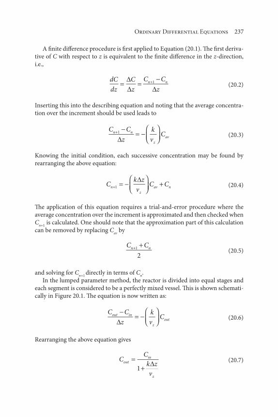
Ordinary Differential Equations 237
A finite difference procedure is first applied to Equation (20.1). The first deriva-
tive of C with respect to z is equivalent to the finite difference in the z-direction,
i.e.,
dC
dz
C
z
C C
zn n1
(20.2)
Inserting this into the describing equation and noting that the average concentra-
tion over the increment should be used leads to
C C
z
k
vCn n
z
av1
(20.3)
Knowing the initial condition, each successive concentration may be found by
rearranging the above equation:
Ck z
vC Cn
z
av n1 (20.4)
The application of this equation requires a trial-and-error procedure where the
average concentration over the increment is approximated and then checked when
Cn+1
is calculated. One should note that the approximation part of this calculation
can be removed by replacing Cav
by
C Cn n1
2 (20.5)
and solving for Cn+1
directly in terms of Cn.
In the lumped parameter method, the reactor is divided into equal stages and
each segment is considered to be a perfectly mixed vessel. This is shown schemati-
cally in Figure 20.1. The equation is now written as:
C C
z
k
vCout in
z
out (20.6)
Rearranging the above equation gives
CC
k z
v
outin
z
1
(20.7)

238 Introduction to Mathematical Methods
If the initial concentration is C0 and the term
1k z
vR
z
(20.8)
then the following set of equations are generated for each stage:
C RC1 0 0 (20.9)
C RC2 1 0 (20.10)
C RCfinal final 1 0 (20.11)
The above represents a series of (simultaneous) linear algebraic equations. These
equations can be solved by a direct step-by-step hand calculation. Alternatively, a
Gauss-Jordan or Gauss-Seidel method can also be used [3–6]. (See also Chapter 17).
The results of the analyses by the two methods are combined and presented in
tabular form for comparison along with the analytical solution (see Table 20.1).
The reader is left the exercise of calculating the values at z 3.0 ft.
20.2 Runge-Kutta Method
The Runge-Kutta (RK) method is one of the most widely used techniques in engi-
neering and science practice for solving first order differential equations. For the
equation
dy
dxf x yn n( , ) (20.12)
the solution takes the form
y yh
D D D Dn n1 1 2 3 46
2 2( ) (20.13)
Figure 20.1 Lumped parameter method.
Section n – 1 Section n + 1Section n
Cin
Cn
Cout Cn
Cout
Cn–1

Ordinary Differential Equations 239
where
D hf x yn n1 ( , ) (20.14)
D hf xh
yD
n n21
2 2, (20.15)
D hf xh
yD
n n32
2 2, (20.16)
D hf x h y Dn n4 3( , ) (20.17)
The term h represents the increment in x, the term yn is the solution to the equa-
tion at xn, and y
n+1 is the solution to the equation at x
n+1 where x
n+1x
nh. Thus,
the RK method provides a straightforward means for developing expressions for
y, namely, yn+1
yn, in terms of the function f(x, y) at various “locations” along
the interval in question.
For a simple equation of the form
dC
dta bC (20.18)
where at t 0, C C0, the RK algorithm given above becomes (for t h)
C Ch
D D D D1 0 1 2 3 46
2 2( ) (20.19)
Table 20.1 Concentration profile via three methods.
z, ft Analytical Finite-difference Lumped-parameter
0.0 1.0000 1.0000 1.0000
0.3 0.8354 0.8358 0.8474
0.6 0.6980 0.7001 0.7181
0.9 0.5830 0.5863 0.6086
1.2 0.4870 0.4910 0.5157
1.5 0.4070 0.4112 0.4371
1.8 0.3400 0.3444 0.3704
2.1 0.2840 0.2884 0.3139
2.4 0.2370 0.2415 0.2660
2.7 0.1980 0.2022 0.2254

240 Introduction to Mathematical Methods
and the coefficients are then given by
D hf x y h a bCn n1 0( , ) ( ) (20.20)
D hf xh
yD
h a b CD
n n21
01
2 2 2, (20.21)
D hf xh
yD
h a b CD
n n32
02
2 2 2, (20.22)
D hf x h y D h a b C Dn n4 3 0 3( , ) [ ( )] (20.23)
The same procedure is repeated to obtain values for C2 at t 2h, C
3 at t 3h, and
so on.
The RK method can also be used if the function in question also contains the
independent variable. Consider the following equation:
dC
dtf t C( , ) (20.24)
For this situation, one obtains
C Ch
D D D D1 0 1 2 3 46
2 2( ) (20.25)
with
D hf t C1 0( ),0 (20.26)
D hf th
CD
2 0 01
2 2, (20.27)
D hf th
CD
3 0 02
2 2, (20.28)
D hf t h C D4 0 0 3( , ) (20.29)
For example, if
dC
dtC e Ct5 (20.30)

Ordinary Differential Equations 241
then
D h CD
eC
Dt
h
20
1 2 25
2
01
0 (20.31)
etc.
Illustrative Example 20.1 [7]
The equation describing the concentration of a reactant in a tubular flow reactor
is given by
dC
dtC0 580 6.
with C0
5.0 gmol/cm3 at t 0 min. Estimate C in gmol/cm3 at 1 and 5 minutes.
Use the Runge-Kutta method analysis [3–6].
Solution
Based on the data provided, evaluate the R–K coefficients for t h 1:
D1 1 0 6 0 2 9 3 1. ( . . ) .
D2 1 0 6 0 0 58 5 03 1
22 2. . . .
..
D3 1 0 6 0 0 58 5 02 2
22 46. . . .
..
D4 1 0 6 0 0 58 5 0 2 46 1 67. [ . . ( . . )] .
Calculate C1:
C Ch
D D D D1 0 1 2 3 46
2 2
5 01
63 1 2 2 2 2 2 46 1 67
7
(
. [ . ( . ) ( . ) . ]
.
)
335 gmol/cm3

242 Introduction to Mathematical Methods
To calculate C2:
D1 1 0 6 0 0 58 7 35 1 74. [ . . ( . )] .
D2 1 24.
D3 1 38.
D4 0 94.
and
C Ch
D D D D2 1 1 2 3 46
2 2
7 341
61 74 2 1 24 2 1 38 0 94
( )
. [ . ( . ) ( . ) . ]
8 66. gmol/cm3
Also calculate C3, C
4, and C
5:
C t3 9 40 3. at min
C t4 9 81 4. at min
C t5 10 04 5. at min
The reader is left the exercise of comparing the numerical solution above (includ-
ing that at t ) with that provided by the analytical solution provided below.
C e
t5
2960 31
29
50
20.3 Runge-Kutta-Gill Method
The RKG method of solving an ordinary differential equation is an extension of,
and is similar to, the RK method. The describing equations are given by
k hf x yn n1 ( , ) (20.32)
k hf xh
yk
n n21
2 2, (20.33)
k hf xh
yv
kv
kn n3
2
1
2
22
1
2
11
1, (20.34)

Ordinary Differential Equations 243
k hf x h yv
kv
kn n4
2
2
2
3
11
1, (20.35)
with
y y k kv
kv
kn n1 1 4
2
2
2
3
1
6
1
31
1 1
31
1( ) (20.36)
Where v2 2 2/
Illustrative Example 20.2
Resolve the previous illustrative example using the RKG method.
Solution
The solution is left as an exercise for the reader , but it can be seen that both meth-
ods only diverge from the analytical solution by ~0.04%.
20.4 Several Ordinary Differential Equations
Situations may arise when there is a need to simultaneously solve more than one
ordinary differential equation (ODE). In a more general case, one could have n
dependent variables y1, y
2, …, y
n with each related to a single independent variable
x by the following system of n simultaneous first-order ODEs:
dy
dxf x y y yn
11 1 2( ), , , , (20.37)
dy
dxf x y y yn
22 1 2( ), , , , (20.38)
dy
dxf x y y yn
n n( ), , , , 1 2 (20.39)
Note that Equations (20.37–20.39) are interrelated, i.e., they are dependent on
each other.
An outline to the solution is illustrated in the following two equations:
dC
dtAe C f C t
E
RT ( , ) (20.40)

244 Introduction to Mathematical Methods
dT
dtkC
H
Cg C t
p
( , ) (20.41)
or in a more general sense
dy
dxf x y z e g xyz( , , ); ( . ., ) (20.42)
dz
dxg x y z e g x y e z( , , ); ( . ., ) 2 2
(20.43)
The RK algorithm for Equations (20.42) and (20.43) is
y y RY RY RY RY1 0 1 2 3 4
1
62 2( ) (20.44)
z z RZ RZ RZ RZ1 0 1 2 3 4
1
62 2( ) (20.45)
where y1 – y
0y, z
1 – z
0z, h x and
RY h f x y z1 0 0 0( , , ) (20.46)
RZ h g x y z1 0 0 0( , , ) (20.47)
RY h f xh
yRY
zRZ
2 0 01
01
2 2 2, , (20.48)
RZ h g xh
yRY
zRZ
2 0 01
01
2 2 2, , (20.49)
RY h f xh
yRY
zRZ
3 0 02
02
2 2 2, , (20.50)
RZ h g xh
yRY
zRZ
3 0 02
02
2 2 2, , (20.51)
RY h f x h y RY z RZ4 0 0 3 0 3( , , ) (20.52)
RZ h g x h y RY z RZ4 0 0 3 0 3( , , ) (20.53)
Ordinary Differential Equations 245
20.5 Higher Order Ordinary Differential Equations
Although the RK approach (and other companion methods) have traditionally
been employed to solve first-order ODEs, it can also treat higher order ODEs. The
procedure requires reducing an nth order ODE to n first-order ODEs. For example,
if the equation is of the form [8]
d y
dxf y x
2
2( , ) (20.54)
set
zdy
dx (20.55)
so that
dz
dx
d y
dx
2
2 (20.56)
The second order equation in Equation (20.54) has now been reduced to the two
first-order ODEs in Equation (20.57):
d y
dx
dz
dxf y x
2
2
( , )
dy
dxz (20.57)
The procedure set forth earlier can now be applied to generate a solution to
Equation (20.54). Note, however, that the first derivative (i.e., dy/dx or its estimate)
is required at the start of the integration. Extending the procedure to higher order
equations is left as an exercise for the reader.
The selection of increment size remains a variable to the practicing engineer.
Most numerical analysis methods provided in the literature are not concerned with
error analysis. In general, roundoff errors appear as demonstrated in Figure 20.2.
In the limit, when the increment approaches 0, one obtains a solution approach-
ing that analytically. Roundoff error then increases exponentially as the increment
approaches 0 as the number of computations correspondingly increases. However,
selecting the increment size that will minimize the error is rarely a problem; in
addition, computing it is also rarely a problem.

246 Introduction to Mathematical Methods
References
1. L. Theodore, Chemical Reaction Analysis and Applications for the Practicing Engineer, John Wiley &
Sons, Hoboken, NJ, 2011.
2. L. Theodore, F. Ricci, and T. VanVliet, Thermodynamics for the Practicing Engineer, John Wiley &
Sons, Hoboken, NJ, 2009.
3. M. Moyle, Introduction to Computers for Engineers, John Wiley & Sons, Hoboken, NJ, 1967.
4. B. Carnahan and J. Wilkes, Digital Computing and Numerical Methods, John Wiley & Sons,
Hoboken, NJ, 1973.
5. R. Ketter and S. Prawler, Modern Methods of Engineering Computations, McGraw-Hill, New York
City, NY, 1969.
6. J. Reynolds, J. Jeris, and L. Theodore, Handbook of Chemical and Environmental Engineering
Calculations, John Wiley & Sons, Hoboken, NJ, 2004.
7. L. Theodore, Chemical Reaction Kinetics, A Theodore Tutorial, Theodore Tutorials, East Williston,
NY, originally published by USEPA/APTI, RTP, NC, 1994.
8. L. Theodore, personal notes, East Williston, NY, 1970.
ERoundoff
Numerical
Increment
Figure 20.2 Error analysis.
247
Many practical problems in environmental engineering and science involve at least
two independent variables i.e., the dependent variable is defined in terms of (or is a
function of) more than one independent variable. The derivatives describing these
independent variables are defined as partial derivatives. Differential equations con-
taining partial derivatives are referred to as partial differential equations (PDEs).
Contrary to a widely accepted myth, an engineer’s mathematical obligations
do not end after formulating a problem, where it may be given to a mathemati-
cian to solve. Even if such an ideal situation should exist, it is still necessary for
engineers – and this includes environmental engineers and scientists – to have a
reasonable understanding of the mathematical methods and their limitations in
order to interpret results.
It has been said that “the solution of a partial differential equation is essentially
a guessing game.” In other words, one cannot expect to be given a formal method
that will yield exact solutions for all partial differential equations [1]. Fortunately,
numerical methods for solving these equations were developed during the middle
and latter part of the 20th century.
Some of the applications in environmental engineering and science fall naturally
into partial differential equations of second order, although there are exceptions
in elasticity, vibration theory, and elsewhere. The solutions of problems involving
21Partial Differential Equations
Technical Consultant: Megan Menzel
Introduction to Mathematical Methods for Environmental Engineers and Scientists. Charles Prochaska and Louis Theodore.
© 2018 Scrivener Publishing LLC. Published 2018 by John Wiley & Sons, Inc.

248 Introduction to Mathematical Methods
partial differential equations often revolve about an attempt to reduce the partial
differential equation to one or more ordinary differential equations. The solutions
of the ordinary differential equations are then combined (if possible) so that the
boundary conditions as well as the original partial differential equation are simul-
taneously satisfied. It should be noted that most of the computational methods for
partial differential equations have evolved from finite-difference approximations
for the partial derivatives. Partial derivatives can be approximated by finite differ-
ences in many ways depending on accuracy requirements.
As noted, this concluding chapter in Part III is concerned with the numerical
solutions of partial differential equations.
Four sections complement the presentation of this chapter. Section numbers
and subject titles follow:
21.1: Partial Differential Equation (PDE) Classification
21.2: Parabolic Partial Differential Equations
21.3: Parabolic PDE with Three Independent Variables
21.4: Elliptic Partial Differential Equations
21.1 Partial Differential Equation (PDE) Classification
This chapter will examine partial differential equations of the general form
aT
xb
T
x yc
T
yf x y T
2
2
2 2
2( , , ) (21.1)
where, in general, the coefficients a, b, and c are functions of x and y, and f is a
function of x, y, and T. Such equations arise in environmental work involving heat
transfer, boundary-layer flow, vibrations, elasticity, and so on. However, the scope
of this chapter is not to present a comprehensive coverage of the various numerical
methods for solving partial differential equations. Rather, the material presented will
provide an introduction to the subject. The various forms of Equation (21.1) may
take are classified as elliptic, parabolic, or hyperbolic. Some details are provided in
this chapter. These three PDEs are briefly introduced below employing T (e.g., the
temperature as the dependent variable) with t (time) and x, y, z (position) as the
independent variables.
The parabolic equation is:
T
t
T
z
2
2 (21.2)
The elliptical equation is:
2
2
2
20
T
x
T
y (21.3)

Partial Differential Equations 249
The hyperbolic equation is:
2
2
2
2
T
t
T
x (21.4)
Regarding the hyperbolic equations, it should be noted that the coefficients a, b,
and c in Equation (21.1) have values such that
b ac2 4 0 (21.5)
The one-dimensional wave equation
2
2
22
2
u
ta
u
x (21.6)
which is frequently encountered in the areas of applied physics, is an example of
a hyperbolic partial differential equation. This equation has been used to describe
the motion of various types of systems.
As noted, the preferred numerical method of solution involves finite differencing.
Only the parabolic and elliptical equations are considered in the next two sections.
21.2 Parabolic Partial Differential Equations
Parabolic differential equations arise in what some refer to as propagation prob-
lems. In this type of system, the solution advances away from specified initial
and boundary conditions. The general partial differential equation, as provided
by Equation (21.1), is defined as parabolic when the coefficients a, b, and c have
values such that
b ac2 4 0 (21.7)
Examples of parabolic PDEs include
T
t
T
x
2
2 (21.8)
and (the two-dimensional)
T
t
T
x
T
y
2
2
2
2 (21.9)
Ketter and Prawler [2], as well as many others, have reviewed the finite differ-
ence approach to solving Equation (21.8). This is detailed below.

250 Introduction to Mathematical Methods
Consider the (t, x) grid provided in Figure 21.1. The partial derivatives may be
approximated by
T
t
T
t
T T
t
T T
kt k4 2 4 2
2 2( ); (21.10)
and
T
x x
T
x
T T T
hx h
2
2
3 0 1
2
2; (21.11)
Substituting Equations (21.10) and (21.11) into Equation (21.8) leads to
T T
k
T T T
h4 2 3 0 1
22
2 (21.12)
Solving for T2:
T T r T T T2 4 3 0 12 2( ) (21.13)
where r = k/h2.
Thus, T2 may be calculated if T
0, T
1, T
3, and T
4 are known. Unfortunately, sta-
bility and error problems arise in employing the above approach. These can be
removed by replacing the central difference term in Equation (21.10) by a forward
difference term, i.e.,
T
t
T
t
T T
t
T T
k0 2 0 2
( ) (21.14)
T2
T3
T0
T4
x = h
t = k t
xT
1
Figure 21.1 Parabolic grid.

Partial Differential Equations 251
With this substitution, Equation (21.13) becomes
T T r T T T2 0 3 0 12( ) (21.15)
It can be shown that the problem associated with the central difference derivative
is removed if r 0.5.
Consider the following application. An unsteady-state heat conduction experi-
ment conducted at Manhattan College’s unit operations laboratory is concerned
with the application of this parabolic equation. In the experiment, a 316 stainless
steel rod is heated at each end with steam at temperature TS. The initial tempera-
ture of the rod is TA. The describing equation and Ba/o IC(s) for this system are
T
t
T
x
2
2 (21.16)
BC T T xS( )1 0: at
BC T T x LS( )2 : at
IC: at , T T t x LA 0 0
The analytical solution to this equation can be shown [3] to be:
T T T Tn
en x
S A S
n
n nt
( ) sin( )
1
122
1 1
2
2
(21.17)
The reader may choose to solve this problem numerically.
21.3 Parabolic PDE with Three Independent Variables
The previous section on parabolic PDEs was limited to systems involving only two
independent variables. Problems involving three or more independent variables
may be handled by analogous methods although the calculations become more
tedious. For example, consider the simple unsteady-state heat-conduction equa-
tion for a solid in two linear dimensions:
T
t
T
x
T
y
2
2
2
2 (21.18)
To generate a solution, divide the solid into a series of rectangles, each of length
x and of width y. Let m x denote the x distance of a point in the solid from
a suitable reference y axis, p y denote the y distance of the same point from a

252 Introduction to Mathematical Methods
suitable reference x axis, and n t denote the elapsed time since the start of the cal-
culational process. The finite difference equivalent of Equation (21.18) is approxi-
mately given by
T T tT T T
x
Tm p n m p n
m p n m p n m p n m p n
, , , ,
, , , , , , , ,
1
1 1
2
12 2TT T
y
m p n m p n, , , ,1
2
(21.19)
One again, the concept of a modulus may be employed:
Rx
t
2
(21.20)
Sy
t
2
(21.21)
The incremental changes in x and y need not be equal, but t must be indepen-
dent of the position in space. Equation (21.19) with the moduli R and S is similar
to the finite difference approximation to the one-distance coordinate case, and the
solution of Equation (21.19) proceeds in a similar manner; however the boundary
conditions are somewhat more troublesome.
21.4 Elliptical Partial Differential Equations
For this equation examine the grid in Figure 21.2 [2]. Using finite differences to
replace the derivatives in Equation (21.3) ultimately leads to
T T T T T x y0 1 2 3 4
1
4( ); (21.22)
In effect, each T value calculated reduces to the average of its four nearest neigh-
bors in the square grid. This difference equation may then be written at each inte-
rior grid point, resulting in a linear system of N equations, where N is the number
of grid points. The system can then be solved by one of several methods provided
in the literature [1,2].
Another solution method involves applying the Monte Carlo approach, requir-
ing the use of random numbers [1,2]. Consider the squares shown in Figure 21.3.
If the describing equation for the variation of T within the grid structure is
2
2
2
20
T
x
T
y (21.23)

Partial Differential Equations 253
with specified boundary conditions (BCs) for T(x, y) of T(0, y), T(a, y), T(x, 0),
and T(x, a), one may employ the following approach to generate a solution
1. Proceed to calculate T at point 1 (i.e., T1).
2. Generate a random number between 00 and 99.
3. If the number is between 00 and 24, move to the left of point 1.
For 25 to 49, 50 to 74, 75 to 99, move upwards, to the right, and
downwards of point 1, respectively.
4. If the move in step 3 results in a new position that is at the outer
surface (boundary), terminate the first calculation for point 1 and
y
T2
T3
T0
T4
T1
x
x
y
Figure 21.2 Partial differential equation elliptical grid.
y=0
y=a
x=0 x=a
1 2 3
6 5 4
7 8 9
x
y
Figure 21.3 Monte Carlo grid approach.

254 Introduction to Mathematical Methods
record the T value of the boundary at that new position. However,
if the move results in a new position that is not at a boundary, and
is still at one of the other eight interval grid points, repeat steps 2
and 3. This process is continued until an outer surface boundary
is reached.
5. Repeat steps 2 to 4 numerous times, for example, 1000 times.
6. After completing step 5, sum all the T values obtained and divide
this value by the number of times steps (2 to 4) have been repeated.
The resulting value provides a reasonable estimate of T1.
7. Return to step 1 and repeat the calculation for the remaining eight
grid points.
This method of solution is not limited to square systems. In addition, one
of the authors [5] has applied this method of solution to numerous real-world
problems.
Illustrative Example 21.1
Consider the system pictured in Figure 21.4. If the system is solid and the vari-
able T is the temperature, the elliptical equation provided in Equation (21.3)
applies. For this system, the temperature at each location is given by the average
temperature of its four neighboring points. Using the Monte Carlo procedure
provided above and in Part IV, Chapter 27, generate the temperature profile in
the solid. The base temperature is maintained at 100°C and the other three sur-
faces at 0°C.
x = 0
y = b
a = b
100°C
0°C
0°C
0°C
0°C
0°C
0°C
0°C0°C0°C0°C0°C
100°C 100°C 100°C 100°Cy = 0
x = a
1 2 3
4 5 6
7 8 9
y
x
Figure 21.4 Temperature grid for a square.

Partial Differential Equations 255
Solution
Using the Monte Carlo algorithm and a random number generator leads to the
following results:
T1 7 07. C
T2 9 80. C
T3 7 16. C
T4 18 67. C
T5 25 12. C
T6 18 77. C
T7 42 93. C
T8 52 57. C
T9 42 80. C
This procedure can be extended to rectangles; it is not limited to squares. If a
rectangle is subjected to the following (somewhat similar) boundary conditions,
T x y T( , )0 0 any
T x b y( , ) any 0
T x y a( , )any 0
T x y a( , )any 0
The analytical solution for the above rectangle (2a by b) [4] is
T Ta
b x
bn
n
n
n
n
21
0
0
( ) ( )sinh[ ]
sinh( )coss( )n y
where
n
n
an
( ); , , , ,
2 1
20 1 2 3

256 Introduction to Mathematical Methods
Illustrative Example 21.2
Solve Illustrative Example 21.1 using the Gauss-Elimination method.
Solution [5]
The familiar finite difference approach will be employed. For example,
T T T T T5 2 4 6 8
1
4[ ]
This form of the equation may be applied to the nine points, which sets each T
equal to the average of temperature of its four neighboring points. This produces
a set of nine equations with nine unknowns. Employing Mathematica, Mathcad,
Excel, or a similar program leads to
T1 7 14. C
T2 9 82. C
T3 7 14. C
T4 18 75. C
T5 25 00. C
T6 18 75. C
T7 42 86. C
T8 52 68. C
T9 42 86. C
Illustrative Example 21.3
Comment on the results of the two previous examples.
Solution
As expected the results are in reasonable agreement with each other. In addition,
T T T T T T8 7 5 4 2 1

Partial Differential Equations 257
with
T T1 3
T T4 6
T T7 9
Illustrative Example 21.4
Outline how to solve the previous example if the face surface is a rectangular solid
(see Figure 21.5).
Solution
The outline of the calculation presented in the previous examples remains the
same. The reader should note that this illustrative example, as well as Illustrative
Example 21.1, will be revisited in Part IV, Chapter 27.
References
1. B. Carnahan and J. Wilkes, Digital Computing and Numerical Methods, John Wiley & Sons,
Hoboken, NJ, 1973.
2. R. L. Ketter and S. P. Prawler, Modern Methods of Engineering Computations, McGraw-Hill,
New York City, NY, 1969.
3. L. Theodore, personal notes, East Williston, NY, 1965.
4. L. Theodore, personal notes, East Williston, NY, 1969.
5. L. Theodore, personal notes, East Williston, NY, 1985.
y
x
20
0°C
100°C
0°C
0°C
11
10
1
19
12
9
2
18
13
8
3
17
14
7
4
16
15
6
5
Figure 21.5 Rectangular grid.

259
It is no secret that the teaching of probability and statistics is now considered
essential in most curricula and is generally accepted as one of the fundamental
branches of mathematics. This course, or its equivalent, is now a required under-
graduate course at most colleges and universities and is slowly and justifiably find-
ing its way into most environmental curricula.
Texts in this field are considered by some to be too advanced for the under-
graduate student. This Part of the text is intended to overcome the difficulties and
sometimes frightening experiences a beginning student encounters on being intro-
duced to this subject. The authors’ aim is to offer the reader the fundamentals of
probability and statistics with appropriate environmental applications and to serve
as an introduction to the specialized and more sophisticated texts in this area.
This Part has primarily evolved from a Theodore Tutorial prepared by Theodore
and Taylor titled “Probability and Statistics.” Material has also been drawn from
notes prepared by one of the authors (many years ago) for a one-semester three-
credit course given to senior students at Manhattan College; the course was also
offered as an elective to other disciplines.
An important point needs to be made, and this applies to other parts of the
book as well. There have been numerous occasions during one of the authors’ ten-
ure as an educator when students solved problems using packaged programs such
Part IV
STATISTICAL ANALYSIS
Introduction to Mathematical Methods for Environmental Engineers and Scientists. Charles Prochaska and Louis Theodore.
© 2018 Scrivener Publishing LLC. Published 2018 by John Wiley & Sons, Inc.

260 Introduction to Mathematical Methods
as Excel, MathCAD, etc. For example, the problem could have involved a solution
to a differential equation or the regression of some data. On being questioned
how the packaged program performed the calculation, the student almost always
responded with something to the effect of, “I don’t know and I don’t care.” For this
reason, the reader should note that no attempt was made to provide details on
applied packaged computer programs that are presently available for this subject.
The author is deeply indebted to the aforementioned Frank Taylor who in a
very real sense allowed this Part of the text to become a reality.
There are seven chapters in Part IV. The chapter numbers and accompanying
titles are listed below.
Chapter 22: Basic Probability Concepts
Chapter 23: Estimation of the Mean and Variance
Chapter 24: Discrete Probability Distributions
Chapter 25: Continuous Probability Distributions
Chapter 26: Fault and Event Trees
Chapter 27: Monte Carlo Simulation
Chapter 28: Regression Analysis

261
Probabilities are nonnegative numbers associated with the outcomes of so-called
random experiments. A random experiment is an experiment whose outcome is
uncertain. Examples include throwing a pair of dice, tossing a coin, counting the
number of defectives in a sample from a lot of manufactured items, and observing
the time to failure of a tube in a heat exchanger or a seal in a pump or a bus section
in an electrostatic precipitator. The set of possible outcomes of a random experi-
ment is called a sample space and is usually designated by S. The term P(A), the
probability of an event A, is the sum of the probabilities assigned to the outcomes
constituting the subset A of the sample space S.
Consider, for example, tossing a coin twice. The sample space can be described as
S HH HT TH TT{ , , , } (22.1)
If probability 1/4 is assigned to each element of S, and A is the event of at least one
head, then
A { , , }HH HT TH (22.2)
22Basic Probability Concepts
Introduction to Mathematical Methods for Environmental Engineers and Scientists. Charles Prochaska and Louis Theodore.
© 2018 Scrivener Publishing LLC. Published 2018 by John Wiley & Sons, Inc.

262 Introduction to Mathematical Methods
the sum of the probabilities assigned to the elements of A is 3/4. Therefore P(A)=
3/4. The description of the sample space is not unique. The sample space S in the
case of tossing a coin twice could be described in terms of the number of heads
obtained. Then
S { , , }0 1 2 (22.3)
Suppose probabilities 1/4, 1/2, and 1/4 are assigned to the outcomes 0, 1, and 2,
respectively. Then A, the event of at least one head, would have for its probability,
P P( ) { , }A 1 23
4 (22.4)
Three sections complement the presentation of this chapter. Section numbers
and subject titles follow:
22.1: Probability Definitions
22.2: Permutations and Combinations
22.3: Series and Parallel Systems
The bulk of the material in this chapter was drawn from the work of Theodore
and Taylor [1].
22.1 Probability Definitions
How the probabilities are assigned to the elements of the sample space depends
on the desired interpretation of the probability of an event. The aforementioned
P(A), can be interpreted as a theoretical relative frequency, i.e., a number about
which the relative frequency of event A tends to cluster as n, the number of times
the random experiment is preformed, increases indefinitely. This is the objective
interpretation of probability. Under this interpretation, to say that P(A) is 3/4 in
the aforementioned example means that if a coin is tossed twice and this trial is
repeated n times, the proportion of times one or more heads occurs clusters about
3/4 as n increases indefinitely.
As another example, consider a single valve that can stick in an open (O) or
closed (C) position. The sample space can be described as follows:
S O C{ , } (22.5)
Suppose that the valve sticks twice as often in the open position as it does in
the closed position. Under the theoretical relative frequency interpretation,
the probability assigned to element O in S would be 2/3, twice the probability
Basic Probability Concepts 263
assigned to element C. If two such valves are observed, the sample space S can be
described as
S OO OC CO CC{ , , , } (22.6)
Assuming that the two valves operate independently, a reasonable assignment of
probabilities to the elements of S, as just listed above, should be 4/9, 2/9, 2/9, and
1/9 respectively. The reason for this assignment will become clear after consider-
ation of the concept of independence. If A is the event of at least one valve sticking
in the closed position, then
A OC CO CC{ , , } (22.7)
the sum of the probabilities assigned to the elements of A is 5/9. Therefore,
P(A) = 5/9.
Probability P(A) can also be interpreted subjectively as a measure of degree of
belief, on a scale from 0 to1, that event A occurs. This interpretation is frequently
used in ordinary conversation. For example, if someone says, “The possibility that
I will go to the casino tonight is 90%,” then 90% is a measure of the person’s belief
that he or she will go to a casino. This interpretation is also used when, in the
absence of concrete data needed to estimate an unknown probability based on an
observed relative frequency, the opinion of an expert is sought. For example, an
expert may be asked to estimate the probability that the seals in a newly designed
pump will leak at high pressures. The estimate would be based on the expert’s
familiarity with pumps of a similar design.
Illustrative Example 22.1
Discuss the difference between a sample and a population.
Solution
When there is a set of n observations, one may wish to use the values of these
observations to estimate certain characteristics of a larger number of observations
that have not yet been made. In other words, the interest is not directly on a par-
ticular set of observations, but rather in using them to estimate something about a
potentially larger set. One refers to the observations as a sample. The larger “sup-
ply,” which one may have, is called a population. From the characteristics of a sam-
ple of observations, one can estimate similar characteristics for the population.
Illustrative Example 22.2
Discuss the difference between a statistic and a parameter.

264 Introduction to Mathematical Methods
Solution
When one calculates some measured value of a sample, it is referred to as a sta-
tistic. A statistic is any characteristic of a set of observations calculated from a
sample. The measurement corresponding to a statistic obtained from a population
is referred to as a parameter. In most cases of interest, the values of the parameters
are unknown and must be estimated by the statistics derived from a sample. Thus,
the sample value is an estimate of the population value.
22.2 Permutations and Combinations
The problem with calculating probabilities of objects or events in a finite group –
defined above as the sample space – in which equal probabilities are assigned to
the elements in the sample space requires counting the elements which make up
the events. The counting of such events is often greatly simplified by employing the
rules for permutations and combinations.
Permutations and combinations deal with the grouping and arrangement of
objects or events. By definition, each different order or arrangement with regard
to order of all or part of the objects is called a permutation. Alternately, each of the
sets which can be made by using all or part of a given collection of objects without
regard to order of the objects in the set is called a combination. Although, per-
mutations or combinations can be obtained with replacement or without replace-
ment, most analyses of permutations and combinations are based on sampling that
is performed without replacement; i.e., each object or element can be used only
once. For each of the two aforementioned with/without pairs (with/without regard
to order and with/without replacement), four subsets if two may be drawn. These
four are provided in Table 22.1 [2].
Each of the four paired subsets in Table 22.1 is considered in the following text
with accompanying examples based on the letters A, B, and C. To personalize this,
the reader could consider the options (games of chance) one of the authors faces
while on a one-day visit to a casino. The only three options normally considered
are dice (often referred to as craps), blackjack (occasionally referred to as 21), and
pari-mutual (horses, trotters, dogs, and jai alai) simulcasting betting. All three of
these may be played during a visit, although playing two or only one is also an
option. In addition, the order may vary and the option may be repeated. Some
possibilities include the following:
Dice, blackjack, and simulcast wagering
Blackjack, wagering, and dice
Wagering, dice, and wagering
Wagering and dice (one of the author’s usual sequence)
Blackjack, blackjack (following a break), and dice
In order to simplify the four examples that follow, dice, blackjack, and wagering
are referred to as objects, represented by the letters A, B, and C, respectively.

Basic Probability Concepts 265
1. Consider a scenario that involves three separate objects, A, B, and C. The
arrangement of these objects is called a permutation. There are six different orders
or permutations of these three objects possible, note that ABC CBA.
ABC BAC CAB
ACB BCA CBA
Thus, BCA would represent blackjack, wagering, and dice.
The number of different permutations of n objects is always equal to n!, where
n! is normally referred to as a factorial n. Factorial n or n! is defined as the product
of the n objects taken n at a time and denoted as P(n, n). Thus,
P n n n( , ) ! (22.8)
With three objects, the number of permutations is 3! 3 2 1 6. Note that 0!
is 1.
The number of different permutations of n objects taken r at a time is given by
P n rn
n r( , )
!
( )! (22.9)
[Note: The permutation term P also appears in the literature as nPr or P(
rn).] For the
three objects A, B, and C, taken two at a time, n 3, and r 2. Thus,
P( , )!
( )!
( )( )( )3 2
3
3 2
3 2 1
16 (22.10)
These possible different orders, noting once again that AB BC, are
AB BC AC
BA CB CA
Consider now a scenario involving n objects in which these can be divided
into j sets with the objects within each set being alike. If r1, r
2, …, r
j represents the
Table 22.1 Subsets of permutations and combinations.
Permutations
(with regard to order)
Combinations
(without regard to order)
Without replacement Without replacement
With replacement With replacement

266 Introduction to Mathematical Methods
number of objects within each of the respective sets, with n r1
r2 … r
j, then
the number of permutations of the n objects is given by
P n r r rn
r r rj
j
( ; , , , )!
! ! !1 2
1 2
(22.11)
This represents the number permutations of n objects of which r1 are alike, r
2 are
alike, and so on. Consider, for example, 2 A’s, 1B, and 1C; the number of permuta-
tions of these 4 objects is
P( ; , , )!
! ! !4 2 1 1
4
2 1 112 (22.12)
The 12 permutations for this scenario are as follows:
AABC ABAC ABCA BAAC BACA BCAA
AACB ACAB ACBA CAAB CABA CBAA
2. Consider the arrangement of the same three objects above, but obtain the num-
ber of permutations (with regard to order) and with replacement, PR [1]. There are
27 different permutations possible.
AAA BBB CCC
AAB BBA CCB
AAC BBC CCA
ABA BAB CBC
ABB BAA CBB
ACA BCB CAC
ACC BCC CAA
ABC BAC CBA
ACB BCA CAB
For this scenario,
PR n n n n( , ) ( ) (22.13)

Basic Probability Concepts 267
so that
PR( , ) ( )3 3 3 273 (22.14)
For n objects taken r at a time,
PR n r n r( , ) ( ) (22.15)
3. The number of different ways in which one can select r objects from a set of n
without regard to order (i.e., the order does not count) and without replacement
is defined as the number of combinations, C, of the n objects taken r at a time. The
number of combinations of n objects taken r at a time is given by
C n rP n r
r
n
r n r( , )
( , )
!
!
!( )! (22.16)
[Note: The combination term C also appears in the literature as Crn or C(
rn).]
For the ABC example taken two letters at a time, one has
C( , )!
! !( )( )( )
( )( )( )
3 23
2 13 2 1
2 1 1
3
The number of combinations becomes
AB AC BC
Note that the combination BA is not included since AB BA for combinations.
4. The arrangement of n objects, taken r at a time without regard to the order and
with replacement is denoted by CR and given by [1]
CR n r C n r n n( , ) ( , ) ( ) 1 (22.17)
with
CR n n C n n n r nn( , ) ( , ) ( ) ;1 (22.18)
For the ABC example above taken two letters at a time, one employs Equation
(22.17).
CR C( , ) ( )3 2 3
3 3 6
2 1 (22.19)
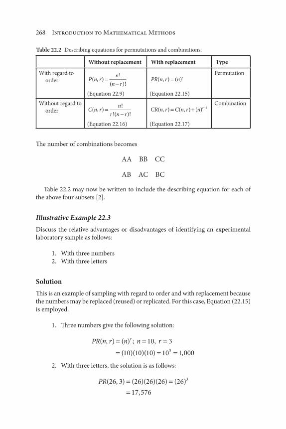
268 Introduction to Mathematical Methods
The number of combinations becomes
AA BB CC
AB AC BC
Table 22.2 may now be written to include the describing equation for each of
the above four subsets [2].
Illustrative Example 22.3
Discuss the relative advantages or disadvantages of identifying an experimental
laboratory sample as follows:
1. With three numbers
2. With three letters
Solution
This is an example of sampling with regard to order and with replacement because
the numbers may be replaced (reused) or replicated. For this case, Equation (22.15)
is employed.
1. Three numbers give the following solution:
PR n r n n rr( , ) ( ) ; ,
( )( )( ) ,
10 3
10 10 10 10 1 0003
2. With three letters, the solution is as follows:
PR( , ) ( )( )( ) ( )
,
26 3 26 26 26 26
17 576
3
Table 22.2 Describing equations for permutations and combinations.
Without replacement With replacement Type
With regard to
order P n rn
n r( , )
!
( )!
(Equation 22.9)
PR n r n r( , ) ( )
(Equation 22.15)
Permutation
Without regard to
order C n rn
r n r( , )
!
!( )!
(Equation 22.16)
CR n r C n r n r( , ) ( , ) ( ) 1
(Equation 22.17)
Combination

Basic Probability Concepts 269
Obviously, the latter choice (three letters) provides greater flexibility because
numerous identification possibilities are available.
Illustrative Example 22.4
Determine the number of 4-element chemical compounds that can theoretically
be generated from a pool of 112 elements. Assume each element counts only once
in the chemical formula and that the order of the elements in the compound mat-
ters. An example of a three-element compound is H2SO
4 (sulfuric acid) or CH
3OH
(methanol). An example of a four-element compound is NaNCO3.
Solution
As discussed earlier, each different ordering or arrangement of all or part of a
number of symbols (or objects) in which the order matters is defined as a permuta-
tion. There are 112 elements to choose from in this application. For this problem,
the describing equation is given by Equation (22.9).
P n rn
n r( , )
!
( )!
Based on the problem statement, n 112 and r 4. Therefore,
P( , )
!
( )!
!
!
( )( )( )( ) .
112 4112
112 4
112
108
112 111 110 109 1 49 1008
This is a large number. This number would be further increased if the number of
a particular element appearing in the chemical formula was greater than one, for
example, HCN (hydrogen cyanide) vs. C3H
3N (acrylonitrile). However, a more
realistic scenario would involve a calculation in which the order does not matter.
This is left as an exercise for the reader.
Two points need to be made, one concerning the calculation and the other
concerning the chemistry of the compound:
1. For calculations involving large factorials, it is often convenient to
use an approximation known as Stirling’s formula:
n nn n! ( ) . .2 0 5 0 5e (22.20)
2. For a real-world “viable” compound, the elements involved in this
application must be capable of bonding.

270 Introduction to Mathematical Methods
Illustrative Example 22.5
Exposure to a nanoagent has four ways in which it can lead to a major health effect
and twelve ways to a minor effect. How many ways may an individual be exposed
to the following?
1. Two major and two minor health effects
2. One major and four minor health effects
Solution
Because the order in which the effects appear or impact on an individual does
not matter, an analysis involving combinations without replacement is required.
Employing Equation (22.16), the number of combined health effects (HE) is thus:
1. For two major and two minor effects:
HE C C( , ) ( , )!
! !
!
! !4 2 12 2
4
2 2
12
10 2
4 3
2
12 111
2396
2. For one major and four minor effects:
HE C C( , ) ( , )!
! !
!
! !
( )
4 1 12 44
3 1
12
8 4
412 11 10 9
4 33 21 980,
22.3 Series and Parallel Systems
Many systems in environmental practice consisting of several components can be
classified as series, parallel, or a combination of both. However, many chemical and
environmental industrial and process plants (units and systems) have a series of
parallel configurations.
A series system is one in which the entire system fails to operate if any one of its
components fails to operate. If such a system consists of n components that func-
tion independently, then the reliability of the system is the product of the reliabili-
ties of the individual components. If Rs denotes the reliability of a series system
and Ri denotes the reliability of the ith component i 1, …, n, then
R R R R Rs n
i
n
i1 2
1
(22.21)
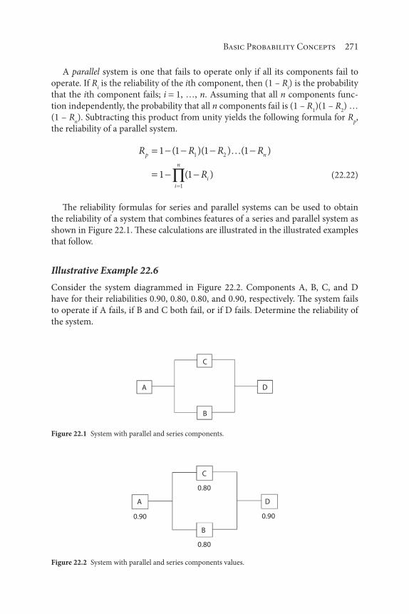
Basic Probability Concepts 271
A parallel system is one that fails to operate only if all its components fail to
operate. If Ri is the reliability of the ith component, then (1 – R
i) is the probability
that the ith component fails; i 1, …, n. Assuming that all n components func-
tion independently, the probability that all n components fail is (1 – R1)(1 – R
2) …
(1 – Rn). Subtracting this product from unity yields the following formula for R
p,
the reliability of a parallel system.
R R R R
R
p n
i
n
i
1 1 1 1
1 1
1 2
1
( )( ) ( )
( ) (22.22)
The reliability formulas for series and parallel systems can be used to obtain
the reliability of a system that combines features of a series and parallel system as
shown in Figure 22.1. These calculations are illustrated in the illustrated examples
that follow.
Illustrative Example 22.6
Consider the system diagrammed in Figure 22.2. Components A, B, C, and D
have for their reliabilities 0.90, 0.80, 0.80, and 0.90, respectively. The system fails
to operate if A fails, if B and C both fail, or if D fails. Determine the reliability of
the system.
A
C
B
D
Figure 22.1 System with parallel and series components.
A
C
B
D
0.80
0.80
0.90 0.90
Figure 22.2 System with parallel and series components values.

272 Introduction to Mathematical Methods
Solution
Components B and C constitute a parallel subsystem connected in series to com-
ponents A and D. The reliability of the parallel subsystem is obtained by applying
Equation (22.22) which yields
Rp 1 1 0 80 1 0 80 0 96( . )( . ) .
The reliability of the system is then obtained by applying Equation (22.21), which
yields
Rs ( . )( . )( . ) .0 90 0 96 0 90 0 78
Illustrative Example 22.7
Determine the reliability of the electrical system shown in Figure 22.3 using the
reliabilities indicated under the various components.
Solution
First identify the components connected in parallel. A and B are connected in par-
allel. D, E, and F are also connected in parallel. Therefore, compute the reliability
of each subsystem of the components connected in parallel. The reliability of the
parallel subsystem consisting of components A and B is
Rp 1 1 0 7 1 0 7 0 91( . )( . ) .
The reliability of the parallel system consisting of components D, E, and F is
Rp 1 1 0 6 1 0 6 1 0 6 0 936( . )( . )( . ) .
Multiply the product of the reliabilities of the parallel subsystems by the product of
the reliabilities of the components to which the parallel subsystems are connected
in series:
A
B
C
D
E
F
G H
0.7
0.7
0.9
0.6
0.6
0.6
0.9 0.9
Figure 22.3 Diagram of electrical system I.

Basic Probability Concepts 273
Rs ( . )( . )( . )( . )( . ) .0 91 0 9 0 936 0 9 0 9 0 621
The reliability of the whole system is therefore 0.621 or 62.1%
Illustrative Example 22.8
Determine the reliability of the components A, D, and G of the electrical system
illustrated in Figure 22.4 using the reliabilities indicated under the various compo-
nents. The overall reliability has been determined to be 0.42.
Solution
The reliability of the parallel subsystem consisting of components A and B is
obtained once again by applying Equation (22.22), which yields
R
A
p 1 1 0 7 1 1 0 3 0 7
0 7 0 3
( . )( ) ( . . )
. .
A A A
The reliability of the parallel subsystem consisting of components D, E, and F is
R
D
p 1 1 1 0 6 1 0 6
1 0 16 1 0 84 0 16
( )( . )( . )
. ( ) . .
D
D
The reliability of the entire system is obtained by applying Equation (22.21),
which yields
Rs 0 42 0 7 0 3 0 9 0 84 0 16 0 9. ( . . )( . )( . . )( )( . )A D G
Since this single equation contains three unknowns, an infinite number of solu-
tions are possible, including, for example,
A D G0 0 0 882; ; .
A
B
C
D
E
F
G H
0.7
0.9
0.6
0.6 0.9
Figure 22.4 Diagram of electrical system II.

274 Introduction to Mathematical Methods
Illustrative Example 22.9
Consider the system shown in Figure 22.5. Determine the reliability, R, if the oper-
ating time for each unit is 5000 hr. Components A and B have exponential failure
rates, λ, of 3 10 6 and 4 10 6 failures per hour, respectively, where R ei
ti ;
t time, hr. The term λ may be viewed as the reciprocal of the average time to
failure. See Chapter 25 for additional details.
Solution
Because this is a series system,
R R Rs A B
As indicated above, for an exponential failure rate
R e t hrt ; time,
so that
R e eA
( )( ) . .3 10 5000 0 0156
0 9851
and
R e eB
( )( ) . .4 10 5000 0 026
0 9802
Therefore,
RS ( . )( . ) .0 9851 0 9802 0 9656 96.56%
References
1. L. Theodore and F. Taylor, Probability and Statistics, A Theodore Tutorial, Theodore Tutorials, East
Williston, NY, originally published by USEPA/APTI, RTP, NC,1996.
2. L. Theodore, personal notes, East Williston, NY, 2006.
A B
Figure 22.5 Exponential failure rate: series system.

275
23Estimation of Mean and Variance
By definition, the mean and the variance σ2 of a random variable are constants
characterizing the random variable’s average value and its dispersion about its
mean, respectively. The mean and variance can also be derived from the probabil-
ity distribution function (pdf) of the random variable – a topic to be discussed in
the next two chapters. If the pdf is unknown, however, the mean and the variance
can be estimated on the basis of a random sample of some, but not all, observa-
tions on the random variable.
Three sections complement the presentation of this chapter. Section numbers
and subject titles follow:
23.1: Estimation of the Mean
23.2: Estimation of the Variance
23.3: Interpretation of the Mean and Variance
Note that the bulk of the material in this chapter was drawn from the work of
Theodore and Taylor [1].
Introduction to Mathematical Methods for Environmental Engineers and Scientists. Charles Prochaska and Louis Theodore.
© 2018 Scrivener Publishing LLC. Published 2018 by John Wiley & Sons, Inc.
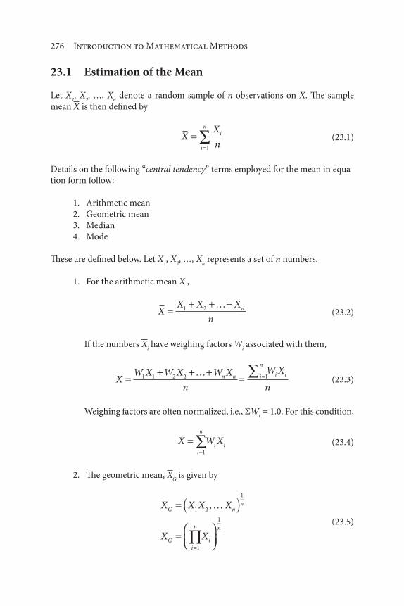
276 Introduction to Mathematical Methods
23.1 Estimation of the Mean
Let X1, X
2, …, X
n denote a random sample of n observations on X. The sample
mean X is then defined by
XX
ni
ni
1
(23.1)
Details on the following “central tendency” terms employed for the mean in equa-
tion form follow:
1. Arithmetic mean
2. Geometric mean
3. Median
4. Mode
These are defined below. Let X1, X
2, …, X
n represents a set of n numbers.
1. For the arithmetic mean X ,
XX X X
nn1 2
(23.2)
If the numbers Xi have weighing factors W
i associated with them,
XW X W X W X
n
W X
nn n i
n
i i1 1 2 2 1 (23.3)
Weighing factors are often normalized, i.e., ΣWi
1.0. For this condition,
X W Xi
n
i i
1
(23.4)
2. The geometric mean, XG is given by
X X X X
X X
G nn
G
i
n
i
n
1 2
1
1
1
,
(23.5)

Estimation of Mean and Variance 277
3. The median is defined as the middle value (or arithmetic mean of
the two middle values) of a set of numbers. Thus, the median of 4,
5, 9, 10, 15 is 9. It is also occasionally defined as the distribution’s
midpoint. Further, the median of a continuous probability distri-
bution function f(x) is that value of c so that
c
f x dx( ) .0 5 (23.6)
4. The mode is the value that occurs with the greatest frequency in
a set of numbers. Thus, it is the typical or most common value in
a set.
Additional details follow. Other definitions also exist in the literature for the afore-
mentioned four terms.
The reader should note that one basic way of summarizing data is by the com-
putation of a central value. The most commonly used central value statistic is the
arithmetic average, or the mean discussed above. This statistic is particularly use-
ful when applied to a set of data having a fairly symmetrical distribution. The mean
is an efficient statistic because it summarizes all the data in the set and each piece
of data is taken into account in the computation. However, the arithmetic mean is
not a perfect measure of the true central value of a given data set because arithme-
tic means can overemphasize the importance of one or two extreme data points.
When a distribution of data is asymmetrical, it is sometimes convenient to
compute a different measure of central value. The second measure, known as the
median, is simply the middle value of a distribution, or the quantity above which
half of the data lie and below which the other half lie. If n data points are listed
in their order of magnitude, the median is the [(n 1)/2]th value. If the number
of data points is even, then the numerical value of the median is the value mid-
way between the two data points nearest the middle. The median, being a posi-
tional value, is less influenced by extreme values in a distribution than the mean.
However, the median alone is usually not a good measure of central tendency. To
obtain the median, the data values provided, i.e., 15, 8, 22, 18, 10, 13 must first be
arranged in order of magnitude, such as
8 10 13 15 18 22, , , , ,
Thus, the median for this data is 14, or the value halfway between 13 and 15
because this data set has an even number of measurements.
Another measure of central tendency used in specialized applications is the
aforementioned geometric mean, XG.
Generally, the mean falls near the “middle” of the distribution. Actually, the
mean may be thought of as the center of gravity of the distribution. The mean has

278 Introduction to Mathematical Methods
another important property. If each measurement is subtracted from the mean,
one obtains n “discrepancies” or differences; some of these are positive and some
are negative, but the algebraic sum of all the differences is equal to zero.
23.2 Estimation of the Variance
Once again, let X1, X
2, …, X
n denote a random sample of n observations on X. Then
the sample variance s2 is defined by
sX X
ni
ni2
1
2
1
( ) (23.7)
where X and s2 are random variables in the sense that their values vary from sample
to sample of the observations on X. It can be shown that the expected value of X is
the population mean and that the expected value of s2 is the population variance
σ2. Because of this, X and s2 are called unbiased estimators of and 2, respectively.
The calculation of s2 can be facilitated by use of the computation formula
sn X X
n n
i
n
i i
n
i2 1
2
1
2
1( ) (23.8)
For example, given the sample 5, 3, 6, 4, 7,
i
iX1
52 135 (23.9)
i
iX1
5
25 (23.10)
and
n 5 (23.11)
Substituting in Equation (23.8) yields
s225 135 25
5 42 5
( )( ) ( )
( )( ). (23.12)
In the case of a random sample of observations of a continuous random vari-
able assumed to have a so-called normal pdf (see also Chapter 25), the graph of
Estimation of Mean and Variance 279
which is a bell-shaped curve, the following statements give a more precise inter-
pretation of the sample standard deviation s as a measure of spread or dispersion.
1. X s includes approximately 68% of the sample observations.
2. X 2s includes approximately 95% of the sample observations.
3. X 3s includes approximately 99.7% of the sample observations.
The source of these percentages is the normal probability distribution, which is
studied in more detail in Chapter 25.
Chebyshev’s theorem provides an interpretation of the sample standard devia-
tion (the positive square root of the sample variance) as a measure of the spread
(dispersion) of sample observations about their mean. Chebyshev’s theorem states
that with k 1, at least (1 1/k2) of the sample observations lie in the interval
(X-ks, X ks). For k 2, for example, this means that at least 75% of the sam-
ple observations lie in the interval (X-2s, X0
2s). The smaller the value of s, the
greater the concentration of observations in the vicinity of X.
The following is provided as a qualitative description of the standard deviation.
The mean of a set of measurements provides some information about the aforemen-
tioned location of the “middle” or “center of gravity” of the set of measurements, but
it gives no information about the scatter (or dispersion or amount of concentration)
of the measurements. For example, the five measurements 14.0, 24.5, 25.0, 25.5, and
36.0 have the same mean as the five measurements 24.0, 24.5, 25.0, 25.5, and 26.0,
but the two sets of measurements have different amounts of scatter.
One simple indication of the scatter of a set of measurements is the range, i.e.,
the largest measurement minus the smallest. In the two sets of measurements
mentioned earlier, the ranges are 22 and 8, respectively. With fairly small sample
sizes one would find the range to be very convenient. It is difficult, however, to
compare a range for one sample size with that for a different sample size. For this
and other reasons, the range, in spite of its simplicity, convenience, and impor-
tance, is used only in rather restricted situations.
One clearly needs a measure of scatter which can be used in samples of any size
and in some sense, make use of all the measurements in the sample. There are sev-
eral measures of scatter that can be used for this purpose, and the most common
of these is the aforementioned standard deviation. The standard deviation may be
thought of as the “natural” measure of scatter.
The two illustrative examples that follow will illustrate the procedure to obtain
these values.
Illustrative Example 23.1
The average weekly wastewater temperatures (°C) for six consecutive weeks are
22 10 8 15 13 18, , , , ,
Find the standard deviation of the temperature T of the water samples.

280 Introduction to Mathematical Methods
Solution
First calculate the arithmetic, T,
T( )
.8 10 13 15 18 22
614 33 C
As noted earlier, the most commonly used measure of dispersion, or variabil-
ity, of sets of data is the standard deviation, s. Its defining formula is given by the
expression in Equation (23.7).
sX X
ni
n
1
1
2
1
( )
The expression (Xi X) shows that the deviation of each piece of data from the
mean is taken into account by the standard deviation. Although the defining for-
mula for the standard deviation gives insight into its meaning, the following alge-
braically equivalent formula (see Equation 23.8) makes computation much easier
(now applied to the temperature, T):
sT T
n
n T T
ni i i( ) ( )2 2 2
1 1
The standard deviation may now be calculated for the data at hand:
Ti
2 2 2 2 2 2 28 10 13 15 18 22 1366( ) ( ) ( ) ( ) ( ) ( )
and
( ) ( )Ti
2 28 10 13 15 18 22 7396
Thus,
s6 1366 7396
6 15 16
( )
( ) ( ). C
Illustrative Example 23.2
The following are SO2 concentrations X ( g/m3) for March, April, and May of 2017
at Floral Park, NY ‒ home of Belmont Park racetrack (another place one of the
authors regularly visits):
29 103 27 14 24 63 24
Calculate the standard deviation and variance.

Estimation of Mean and Variance 281
Solution
Once again, apply Equation (23.8),
sX
X
nn
ii2
2
1
( )
The calculations are performed as follows based on Table 23.1. From the calcula-
tion of Xi determine ( X
i)2:
( ) ( ) ,Xi
2 2284 80 656
Substituting gives
s
17 49680 656
7
6995 62 31 55
,,
. . g/m3
For the variance
s2 2
2 231 55 995
( )
( . ) ( )
standard deviation
g/m3
23.3 Interpretation of Mean and Variance
The mean and variance can be interpreted for both a discrete and continuous ran-
dom variable. The following two illustrative examples review both terms.
Table 23.1 SO2 calculations.
Xi
Xi2
14 196
24 576
24 576
27 729
29 841
63 3969
103 10609
Xi
284 Xi2 17496

282 Introduction to Mathematical Methods
Illustrative Example 23.3
A discrete random variable X assumes the values 49, 50, and 51 each with prob-
ability 1/3. A discrete random variable Y assumes the values 0, 50, and 100 each
with probability 1/3. Compare the means and variances of X and Y, and interpret
the results.
Solution
As indicated earlier, the pdf of a discrete random variable requires the probability
assigned to each of the possible values of the random variable. For this problem,
f x x( ) ; , ,1
349 50 51
g y y( ) ; , ,1
30 50 100
To obtain x, the mean of X, and
y, the mean of Y. Use the formulas [1, 2]:
x E X x f x( ) ( ) (23.13)
y E Y y g y( ) ( ) (23.14)
where E(X) is the expected value of X. Substituting gives,
x
y
491
350
1
351
1
350
01
350
1
3100
1
350
Obtain x
2, the variance of X, and y2, the variance of Y, by applying the follow-
ing equations [1, 2]:
x xE X2 2( ) (23.15)
y yE X2 2( ) (23.16)
The alternative formula for computing the variance of X is
E X E Xx x( ) ( )- -2 2 2 (23.17)

Estimation of Mean and Variance 283
Applying this form of the equation to both X and Y gives
x xx f x x f x2 2 2
2 2
50
49 501
350 50
1
3
( ) ( ) ( ) ( )
( ) ( ) ( ) .51 501
3
2
30 6672
y yy g y y g y2 2 2
2 2
50
0 501
350 50
1
3
( ) ( ) ( ) ( )
( ) ( ) ( )100 501
3
5000
316672
Note that X and Y have the same mean but the variance of Y is greater than the
variance of X, which reflects the greater dispersion (spread or variability) of the val-
ues of Y about its mean in contrast to the dispersion of the values of X about its mean.
Illustrative Example 23.4
Continuous random variables X and Y have pdfs specified by f(x) and g(y), respec-
tively, as follows:
f x x( ) ;1
21 1
g y y( ) ;1
42 2
Compute the mean and variance of X and Y and compare the results.
Solution
Note that for a continuous random variable, integration replaces summation in
the calculation of the mean and variance. Furthermore, the probability that a con-
tinuous random variable lies in a certain interval is obtained by integrating the pdf
over that interval (See Chapter 25).
First compute x, the mean of X, and
y, the mean of Y. Use the following for-
mulas [1, 2]:
x x f x dx( ) (23.18)
y y g y dy( ) (23.19)

284 Introduction to Mathematical Methods
Substituting f(x) and g(y) gives
x x dx1
11
20
y y dy2
21
40
The terms x
2, the variance of X, and y2, the variance of Y, are calculated as
follows (1, 2):
x xE X x dx2 2 2
1
1
2 1
2
1
30 333( ) .
y yE Y y dy2 2 2
2
2
2 1
4
4
31 333( ) .
As with the previous illustrative example, X and Y have the same mean, i.e., 0.
The variance of Y is greater than the variance of X, which reflects the greater dis-
persion of the values of Y about its mean.
Illustrative Example 23.5
A continuous random variable X has a pdf given by
f x x x( ) ;4 0 13
Calculate and 2 for x.
Solution
By definition (See Chapter 25),
x f x dx( ) (23.20)
Substituting gives
0
1
3
0
1
44 4x x dx x dx( )

Estimation of Mean and Variance 285
Integrating gives
45
4
5
5
0
1
x
For 2, apply the methods described earlier.
2 2 2 2 2E X x f x dx( ) ( )
Substituting gives
2
0
1
2 3 24x x dx( )
Integrating,
26 2
4
6
4
5
2
3
16
25
50 48
75
2
750 0267
x.
Reference
1. L. Theodore and F. Taylor, Probability and Statistics, A Theodore Tutorial, Theodore Tutorials, East
Williston, NY, originally published by USEPA/APTI, RTP, NC,1996.
2. S. Shaefer and L. Theodore, Probability and Statistics Applications for Environmental Science, CRC
Press/Taylor & Francis Group, Boca Raton, FL, 2007.

287
The probability distribution of a random variable concerns the distribution of
the probability over the range of the random variable. The distribution of prob-
ability, i.e., the values of the discrete random variable together with their associ-
ated probabilities, is specified by the probability distribution function (pdf). This
chapter is devoted to providing general properties of the pdf in the case of dis-
crete random variables, as well as an introduction to the cumulative distribution
function (cdf).
The pdf of a discrete random variable X is specified by f(x), where f(x) has the
following three essential properties:
1. f x P X x( ) ( ) probability assigned to the outcome
correspondiing to the number in the range of
i.e., is a specifi
x X
X ccally designed value of x
(24.1)
2. f x( ) 0 (24.2)
3. x
f x( ) 1 (24.3)
24Discrete Probability Distributions
Introduction to Mathematical Methods for Environmental Engineers and Scientists. Charles Prochaska and Louis Theodore.
© 2018 Scrivener Publishing LLC. Published 2018 by John Wiley & Sons, Inc.
288 Introduction to Mathematical Methods
Property (24.1) indicates that the pdf of a discrete random variable generates
probability by substitution. Property (24.2) and Property (24.3) restrict the values
of f(x) to nonnegative real numbers and numbers whose sum is 1, respectively.
Consider, for example, a box of 100 transistors containing 5 defectives. Suppose
that a transistor is selected at random is to be classified as defective or nondefec-
tive. Then X is a discrete random variable with pdf specified by
f x x( ) . ;0 05 1 (24.4)
0 95 0. ; x (24.5)
For another example of the pdf of a discrete random variable, let X denote
the number of the throw on which the first failure of an electrical switch occurs.
Suppose the probability that a switch fails on any throw is 0.001 and that succes-
sive throws are independent with respect to failure. If the switch fails for the first
time on throw x, it must have been successful on each of the preceding x 1 trials.
In effect, the switch survives up to x 1 trials and fails at trial x. Therefore, the pdf
of X is given by
f x x nx( ) ( . ) . ; , , , , ,( )0 999 0 001 1 2 31 (24.6)
Note that the range of X consists of a countable infinitude of values.
Another function used to describe the probability distribution of a random
variable X is the aforementioned cdf. If f(x) specifies the pdf of a random variable
X, then F(x) is used to specify the cdf. For both discrete and continuous random
variables, the cdf of X is defined by
F x P X x x( ) ( ); (24.7)
Note that the cdf is defined for all real numbers, not just the values assigned by the
random variable.
To illustrate the derivation of the cdf from the pdf, consider a case of a discrete
random variable X whose pdf is specified by
f x x( ) . ;0 2 2 (24.8)
0 3 5. ; x (24.9)
0 5 7. ; x (24.10)
Applying the definition of the cdf in Equation (24.7), one obtains for the cdf of X
(see also Figure 24.1)

Discrete Probability Distributions 289
F x x
x
x
x
( ) ;
. ;
. ;
;
0 2
0 5 5 7
0 2 2 5
7 7
It is helpful to think of F(x) as an accumulator of probability as x increases
through all real numbers. In the case of a discrete random variable, the cdf is a step
function increasing by finite jumps at the values of x in the range of X. In the above
example, these jumps occur at the values 2, 5, and 7. The magnitude of each jump
is equal to the probability assigned to the value at which the jump occurs. This is
depicted in Figure 24.1.
Illustrative Example 24.1
Provide an example of a discrete random variable and a continuous random variable.
Solution
A random variable may be discrete; i.e., it can take on only a finite or countable
number of distinct values. Alternately, the random variable may be continuous,
with values occurring anywhere in an interval. The outcome of the throw of a die
is a discrete random variable. The exact height of an individual selected from a
particular group is a continuous variable.
Illustrative Example 24.2
Let X denote the number of supply ships reaching a port on a given day. The pdf
for X is given by:
f xx
x( ) ; , , , , ,21
1 2 3 4 5 6
1
0.5
00 5 10
X
F(x
)
Figure 24.1 Graph of the cdf of a discrete random variable X.

290 Introduction to Mathematical Methods
Verify that f(x) is a valid pdf and calculate the probability that at least three
ships but less than six ships will arrive on a given day.
Solution
For f(x) to be valid, the following two conditions must be satisfied:
0 1 6f x x( ) ; between 1 and
and
1
6
1f x( )
Substituting into the second condition yields
1
6
1
6
21
1
21
2
21
3
21
4
21
5
21
6
21
21
211 0
f xx
( )
.
Thus, both conditions are satisfied and f(x) is a valid pdf.
The probability that at least 3 ships but less than 6 ships will arrive on a given
day can be determined by
P X f x f x f x( ) ( ) ( ) ( )
.
3 6 3 4 5
3
21
4
21
5
21
12
210 429
Illustrative Example 24.3
Let X denote the annual number of floods in a certain region. The pdf of X is speci-
fied as
f x x( ) . ;0 25 0
f x x( ) . ;0 35 1
f x x( ) . ;0 24 2
f x x( ) . ;0 11 3
f x x( ) . ;0 04 4

Discrete Probability Distributions 291
f x x( ) . ;0 01 5
1. What is the probability of two or more floods in any year?
2. What is the probability of four or more floods in a year, given that
two floods have already occurred?
3. What is the probability of at least one flood in a year, given that one
has already occurred?
Solution
1. For two or more floods in any year, one may write
P x f x f x
f f f f
( ) ( ) ( )
( ) ( ) ( ) ( )
. . .
2
2 3 4 5
0 24 0 11 0 04
2 2
5
00 01 0 40. .
2. This involves a conditional probability calculation [1]. The describ-
ing equation and solution is
P X XP X X
P X
P X
P X
( / )( )
( )
( )
( )
.
..
4 24 2
2
4
2
0 05
0 400 12
and
55
3. This also involves a conditional probability calculation [1]. For this
case,
P X XP X X
P X
P X
P X
( / )( )
( )
( )
( )
.
. .
2 12 1
1
2
1
0 40
0 40 0 35
and
0 40
0 750 53
.
..
Three sections complement the presentation of this chapter. Section numbers
and subject titles follow:
24.1: The Binomial Distribution
24.2: The Hypergeometric Distribution
24.3: The Poisson Distribution

292 Introduction to Mathematical Methods
Note that the bulk of the material in this chapter was drawn from the work of
Theodore and Taylor [1].
24.1 The Binomial Distribution
Consider n independent performances of a random experiment with mutually
exclusive outcomes that can be classified as success or failure. The words “success”
and “failure” are to be regarded as labels for two mutually exclusive categories of
outcomes of the random experiment and they do not necessarily have the ordinary
connotation of success or failure. Assume that p, the probability of success on any
performance of the random experiment, is constant. Let Q be the probability of
failure, so that
Q p1 (24.11)
The probability distribution of X, the number of successes in n performances of
the random experiment, is the binomial distribution, with a probability distribu-
tion function (pdf) specified by
f xn
x n xp Q x nx n x( )
!
!( )!; , , , 0 1 (24.12)
where f(x) is the probability of x successes in n performances. One can show that
the expected value of the random variable X is np and its variance is npQ [2].
As a simple example of the binomial distribution, consider the probability dis-
tribution of the number of defectives in a sample of 5 items drawn with replace-
ment from a lot of 1000 items, 50 of which are defective. Associate “success” with
drawing a defective item from the lot. The result of each drawing can then be
classified as success (defective item) or failure (nondefective item). The sample
of five items is drawn with replacement (i.e., each item in the sample is returned
before the next is drawn from the lot; therefore, the probability of success remains
constant at 0.05). Substituting the values n 5, p 0.05, and Q 0.95 in Equation
(24.12) yields
f xx x
xx x( )!
!( )!( . ) . ; , , , , ,( )
5
50 05 0 95 0 1 2 3 4 55 (24.13)
as the pdf for X, the number of defectives in the sample. The probability that the
sample contains exactly three defectives is given by
P X( )!
! !( . ) . .( )3
5
3 20 05 0 95 0 00113 2
(24.14)

Discrete Probability Distributions 293
The binomial distribution can be used to calculate the reliability of a redundant
system. A redundant system consisting of n identical components is a system that
fails only if more than r components fail. Familiar examples include single-usage
equipment such as missile engines, short-life batteries, and flash bulbs which are
required to operate for one time period and are not reused. Once again, associ-
ate “success” with the failure of a component. Assume that the n components are
independent with respect to failure, and that the reliability of each is 1 p. Then X,
the number of failures, has the binomial pdf in Equation (24.12) and the reliability
of the redundant system is
P X rn
x n xp Q
x
rx n x( )
!
!( )!0
(24.15)
The binomial distribution has been applied in problems in which samples are
drawn from a large population with specified “success” or “failure” probabilities and
there is a desire to evaluate instances of obtaining a certain number of successes in
the sample. It has applications in quality control, reliability, environmental engi-
neering, environmental management, consumer sampling, and many other cases.
Suppose a trial or event can result in one and only one of mutually exclu-
sive events E1, E
2, …, E
j with probabilities p
1, p
2, …, p
j respectively, where
p1
p2
… pj
1. If n independent trials are made, then one can show that the
probability function of obtaining x1 of E
1s, x
2 of E
2s, …, x
j of E
js is given by
f x xn
x xp pj
j
x
j
x j( , , )!
! !1
1
11 (24.16)
where 0 xj
n, i 1, …, j, and x1
… xj
n. This is the probability func-
tion of the multinominal distribution. Note that if j 2 this function reduces to
the binomial distribution. Hence, the multinominal distribution is essentially an
extension of the binomial distribution for just two possible outcomes ‒ success
and failure.
Illustrative Example 24.4
A sample of five transistors is drawn with replacement from a lot which is 5% defec-
tive. Once again, “with replacement” means that each transistor drawn is returned
to the lot before the next is drawn. What is the probability that the number of
defective transistors and the sample is:
1. Exactly 2
2. At most 2
3. At least 2

294 Introduction to Mathematical Methods
Solution
This random experiment consists of drawing a transistor at random with replace-
ment from a lot. The random experiment is preformed five times because a sample
of five transistors is drawn with replacement from the lot. Therefore, n =5. Also,
note that the performances are independent because each transistor is replaced
before the next is drawn. Therefore, the composition of the lot is exactly the same
before each drawing.
1. For this problem, associate “success” with drawing a defective
transistor. Associate “failure” with drawing a nondefective. Refer
once again to Equation (24.12). Because 5% of the lot is defective,
p 0.05. Therefore, Q 0.95. These values (n, p, and Q) may be
substituted in the binomial pdf.
f xx x
xx x( )!
!( )!( . ) . ; , , ,( )
5
50 05 0 95 0 1 55 (24.13)
2. Substitute the appropriate value of X to obtain the required
probabilities.
3. For this problem,
P P X( ) ( )
!
! !( . ) . .( )
exactly defectives2 2
5
2 30 05 0 95 0 2142 3
P P X
x xx
x
( ) ( )
!
!( )!( . ) .(
at most defectives2 2
5
50 05 0 95
0
2
))
. . . .
5
0 7738 0 2036 0 0214 0 998
x
P X
P X
x xx
( )
( )
!
!( )!
at least defectives P( )2 2
1 1
15
50
1
(( . ) .
( . . ) .
( )0 05 0 95
1 0 7748 0 2036 0 0226
5x x
Note that this problem involved summing the binomial pdf over the appropri-
ate values of X; this procedure applies if the probability of more than a single value
of X is required.

Discrete Probability Distributions 295
Illustrative Example 24.5
The probability that an exposure to a nanocarcinogen will be fatal is 0.80. Find the
probability of the following events for a group of 15 workers:
1. At least 9 will die.
2. From 4 to 8 will die.
Solution
1. For event 1,
P P X p Q m
x
( ) ( ); . , .at least will die , =159 9 0 8 0 2
15
9
15 !!
!( )!( . ) .
. . . . .
( )x x
x x
150 8 0 2
0 0430 0 1032 0 1876 0 2501 0 2
15
3309
0 1319 0 0352
0 982
. .
.
This calculation can be performed by longhand or obtained directly from
binomial tables.
2. For event 2,
P X P X P X( ) . ( ) ( )4 8 1 0 9 0 4
One notes, almost immediately that
P X( )0 4 0
Therefore,
P X( ) . . . .4 8 1 0 0 982 0 0 0 018
Illustrative Example 24.6
A redundant system consisting of three operating pumps can survive two pump
failures. Assume that the pumps are independent with respect to failure and each
has a probability of failure of 0.10. What is the reliability of the system?
Solution
The system consists of three pumps. Therefore, n 3. The system can survive
the failure of two pumps. Equation (24.12) should be employed with r 2. The

296 Introduction to Mathematical Methods
probability of a pump failure is 0.10. Therefore, p 0.10. Substitute these values
for n and p (with Q 0.90) in the binomial pdf:
f xx x
xx x( )!
!( )!( . ) . ; , , ,( )
3
30 10 0 90 0 1 33
Sum the binomial pdf from 0 to r to find the reliability, R:
Rx xx
x x
0
233
30 10 0 90 0 999
!
!( )!( . ) . .( )
Illustrative Example 24.7
The probabilities of hospitals A, B, and C obtaining a particular type of serum are
0.5, 0.3, and 0.2, respectively. Four such serums are to be provided. What is the
probability that a single hospital receives all four serums?
Solution
This involves the use of the multinomial distribution. The desired probability is
(see Equation (24.16))
P
f f f
( )
( , , ) ( , , ) ( ,
one hospital alone getting serum
4 0 0 0 4 0 0 00 4
4
4 0 00 5 0 3 0 2
4
0 4 00 5 0 3 0 24 0 0 0 4
, )
!
! ! !( . ) . .
!
! ! !( . ) . .( ) ( ) ( ) ( )00
0 0 44
0 0 40 5 0 3 0 2
0 0625 0 0081 0 0016 0 0722
!
! ! !( . ) . .
. . . .
( ) ( )
Note that for this calculation a hospital receives all four serum shipments.
24.2 Hypergeometric Distribution
The hypergeometric distribution is applicable to situations in which a random
sample of r items is drawn without replacement from a set of n items. Without
replacement means that an item is not returned to the set after it is drawn. Recall
that the binomial distribution is frequently applicable in cases where the item is
drawn with replacement.
Suppose that it is possible to classify each of the n items as a success or failure.
Again, the words “success” and “failure” do not have the usual connotation. They

Discrete Probability Distributions 297
are merely labels for two mutually exclusive categories into which n items have
been classified. Thus, each element of the population may be dichotomized as
belonging to one of two disjointed classes.
Let a be the number of items in the category labeled success. Then n a will be
the number of items in the category labeled failure. Let X denote the number of
successes in a random sample of r items drawn without replacement from the set
of n items. Then the random variable X has a hypergeometric distribution whose
probability distribution function (pdf) is specified as follows [1]:
f x
a
x a x
n a
r x n a r x
n
r n r
x( )
!
!( )!
( )!
( )!( )!
!
!( )!
; , , , m 0 1 iin( , )a r (24.17)
The term f(x) in Equation (24.17) is the probability of x successes in a random
sample of n items drawn without replacement from a set of n items, a of which
are classified as successes and n a as failures. The term min(a, r) represents the
smaller of the two numbers a and r, i.e., min(a, r) a if a r and min(a, r) r
if r a.
The hypergeometric distribution can also be arrived at through the use of com-
binations. Using this approach, the total number of possible selections of r ele-
ments out of n is C(n, r). Furthermore, x “good” elements may be chosen out of the
total of a good elements in a total of C(a, x) combinations. For each such combi-
nation, it is also possible to select r x of n a “bad” elements in C(a, x) C(n a,
r x). Because each selection possibility is equally likely, the probability of picking
exactly x good elements is
f xC a x C n a r x
C n r( )
( , ) ( , )
( , ) (24.18)
which, upon substitution of C is the expression given in Equation 24.17 for the
probability density function of the hypergeometric distribution. As with the bino-
mial distribution, a tabulation of cumulative and individual terms of the hyper-
geometric distribution is available in the literature [2].
The hypergeometric distribution is applicable in situations similar to those
when the binomial density is used, except that samples are taken from a small
population. Examples arise in the sampling of small numbers of chemical, medi-
cal, and environmental samples, as well as from manufacturing lots. The hyper-
geometric distribution is obviously a special case of the binomial distribution
when applied to finite populations. In particular, the hypergeometric distribution
approaches the binomial distribution when the population size approaches infin-
ity. Note, however, that others have claimed that the binomial distribution is a
special case of a hypergeometric distribution.

298 Introduction to Mathematical Methods
Illustrative Example 24.8
A sample of 5 transistors is drawn at random without replacement from a lot of
1000 transistors, 50 of which are defective. What is the probability that the sample
contains exactly 3 defectives?
Solution
The number of items in the set from which the sample is drawn is the number
of transistors in the lot. Therefore, n 1000. Associate once again “success” with
drawing a defective transistor, and “failure” with drawing a nondefective one.
Determine a, the number of “successes” in the set of n items. Because 50 of the
transistors in the lot are defective, a 50. Also, note that the sample is drawn with-
out replacement and that the size of the sample is r 5.
Substituting the values of n, r, and a in a hypergeometric pdf provided in
Equation (24.17) gives
f xx x x x
x( )
!
!( )!
!
( )!( )!
!
! !
; , , ,
50
50
950
5 945
1000
5 995
0 1 5
Also, substitute the appropriate value of X above to obtain the required probability.
P P X( ) ( )sample contains exactly defectives3 3
Therefore,
P Xx
( )
!
! !
!
!( )!
!
! !
.3
50
47
950
2 945 3
1000
5 995
0 0011
Illustrative Example 24.9
A pillbox contains 24 drug tablets, 3 of which are contaminated. If a sample of six
is chosen at random from the pillbox, what is the probability that:
1. Zero will be contaminated
2. One will be contaminated
3. Two will be contaminated
4. Three will be contaminated

Discrete Probability Distributions 299
Solution
First note that this once again involves sampling without replacement. Employing
the combination equation provided above, Equation (24.18) yields
f xC a x C n a r x
C n ra r n( )
( , ) ( , )
( , ): , , 3 6 24
Therefore,
f xC x C x
Cx( )
( , ) ( , )
( , );
3 21 6
24 60 3
Note that there are only four values X can assume: 0, 1, 2, and 3.
1. Substituting X 0 gives
P XC C
C( )
( , ) ( , )
( , )
!
! !
!
! !
!
03 0 21 6
24 6
3
0 3
21
6 15
24
6!! !
( )( , )
,( ).
18
1 54 264
134 5960 40316
2. For one pill,
P XC C
C( )
( , ) ( , )
( , ).1
3 1 21 5
24 60 45356
3. For two pills,
P XC C
C( )
( , ) ( , )
( , ).2
3 2 21 4
24 60 13340
4. For three pills,
P XC C
C( )
( , ) ( , )
( , ).3
3 3 21 3
24 60 00988
Illustrative Example 24.10
An environmental quality control engineer inspects a random sample of three
vacuum pumps at a water treatment plant drawn without replacement from each

300 Introduction to Mathematical Methods
incoming lot of 25 vacuum pumps. A lot is accepted only if the sample contains
no defectives. If any defectives are found, the entire lot is inspected, at the cost
charged to the vendor. What is the probability of accepting a lot containing 10
defective vacuum pumps?
Solution
Each lot consists of 25 vacuum pumps. Therefore, n 25. Once again, associate
“success” with a defective vacuum pump. Determine, a, the number of “successes”
in the set of n items. For this problem, a = 10. A sample of three vacuum pumps is
drawn without replacement from each lot; therefore, r 3.
Substitute the values of n, r, and a in the pdf of the hypergeometric distribution.
f xx x x x
x( )
!
!( )!
!
( )!( )!
!
! !
; , , ,
10
10
15
3 12
25
3 22
0 1 2 3
Substitute the appropriate values of X to obtain the required probability. The prob-
ability of accepting a lot containing 10 defective vacuum pumps is
P X( )
!
! !
!
( )! !
!
! !
( )( ).0
10
0 10
15
3 0 12
25
3 22
1 455
23000 20
Illustrative Example 24.11
An order was recently received to manufacture a special type of water pollution
monitor. The total order consisted of 25 monitors. Five of these monitors are to be
selected at random and initially life tested. The contract specifies that if not more
than 1 of the 5 monitors fails a specified life test, the remaining 20 will be accepted;
otherwise, the complete lot will be rejected. What is the probability of lot accep-
tance if exactly 4 of the 25 submitted monitors are defective?
Solution
The lot will be accepted if the sample of 5 contains either 0 or 1 of the 4 defective
monitors. The probability of this happening is given by the hypergeometric distri-
bution as
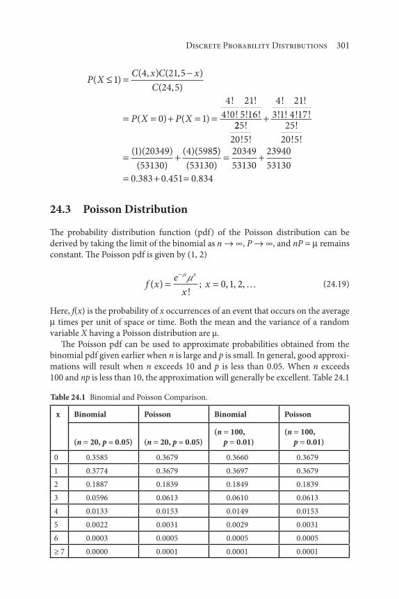
Discrete Probability Distributions 301
P XC x C x
C
P X P X
( )( , ) ( , )
( , )
( ) ( )
!
! !
!
! !
14 21 5
24 5
0 1
4
4 0
21
5 16225
20 5
4
3 1
21
4 1725
20 51 20349
53130
4 598
!
! !
!
! !
!
! !!
! !( )( ) ( )(
( )
55
53130
20349
53130
23940
53130
0 383 0 451 0 834
)
. . .
( )
24.3 Poisson Distribution
The probability distribution function (pdf) of the Poisson distribution can be
derived by taking the limit of the binomial as n ∞, P ∞, and nP remains
constant. The Poisson pdf is given by (1, 2)
f xe
xx
x
( )!
; , , , 0 1 2 (24.19)
Here, f(x) is the probability of x occurrences of an event that occurs on the average
times per unit of space or time. Both the mean and the variance of a random
variable X having a Poisson distribution are μ.
The Poisson pdf can be used to approximate probabilities obtained from the
binomial pdf given earlier when n is large and p is small. In general, good approxi-
mations will result when n exceeds 10 and p is less than 0.05. When n exceeds
100 and np is less than 10, the approximation will generally be excellent. Table 24.1
Table 24.1 Binomial and Poisson Comparison.
x Binomial Poisson Binomial Poisson
(n 20, p = 0.05) (n 20, p = 0.05)
(n 100,
p 0.01)
(n 100,
p 0.01)
0 0.3585 0.3679 0.3660 0.3679
1 0.3774 0.3679 0.3697 0.3679
2 0.1887 0.1839 0.1849 0.1839
3 0.0596 0.0613 0.0610 0.0613
4 0.0133 0.0153 0.0149 0.0153
5 0.0022 0.0031 0.0029 0.0031
6 0.0003 0.0005 0.0005 0.0005
≥ 7 0.0000 0.0001 0.0001 0.0001

302 Introduction to Mathematical Methods
compares binomial and Poisson probabilities for the case of (n 20, p 0.05) and
(n 100, p 0.01).
If is the failure rate (per unit of time) of each component of a system, then λt is
the average number of failures for a given unit of time. The probability of x failures
in the specified unit of time is obtained by substituting t in Equation (24.19)
to obtain
f xe t
xx
t x
( )!
; , , ,( )
0 1 2 (24.20)
Suppose, for example, that in a certain country the average number of airplane
crashes per year is 2.5. What is the probability of 4 or more crashes during the next
year? Substituting λ 2.5 and t 1 in Equation 24.20 yields
f xe
xx
x
( ).
!; , , ,
( ).2 5 2 50 1 2 (24.21)
as the pdf of X, the number of airplane crashes in a year. The probability of 4 or
more airplane crashes next year is then
P Xe
xx
x
( ).
!
( . . . . )
( ).
4 12 5
1 0 0821 0 205 0 257 0 214
1
0
3 2 5
0 76 0 24. .
(24.22)
As another example, suppose that the average number of breakdowns of per-
sonal computers during 1000 h of operation of a computer center is 3. What is
the probability of no breakdowns during a 10-h work period? Note that the given
average is the average number of breakdowns during 1000 h, so the unit of time
associated with the given average is 1000 h. The probability required is the prob-
ability of no breakdowns during a 10-h period, and the unit of time connected with
the required probability is 10 h. If 10 is divided by 1000, the result is 0.01 so that
in a 10-h period there are 0.01 time periods of 1000-h duration. The given aver-
age of breakdown is 3; multiplication by 0.01 yields 0.03, the average number of
occurrences during a 10-h time period . This value of may be substituted in the
Poisson pdf:
f xe
xx
x
( ).
!; , , ,
( ).0 03 0 030 1 2 (24.23)

Discrete Probability Distributions 303
One may now substitute for x, the number of occurrences whose probability is
required. The probability of no breakdowns in a 10-h period is:
P Xe
e( ).
!.
( )..0
0 03
00 97
0 03 00 03
(24.24)
In addition to the applications cited, the Poisson distribution can be used to
obtain the reliability R of a standby redundancy system in which one unit is in the
operating mode and n identical units are in standby mode. Unlike parallel systems,
the standby units are inactive. The reliability of the standby redundancy system may
be calculated by employing the Poisson distribution under the following conditions:
1. all units have the same failure rate in the operating mode
2. unit failures are independent
3. standby units have 0 failure rate in the standby mode
4. there is perfect switch over to a standby when the operating unit fails
The Poisson distribution is a distribution in its own right and arises in many
different situations. For instance, it provides probabilities of specified numbers of
telephone calls per unit interval of time, of environmental sampling procedures, of
given numbers of defects per unit area of glass, textiles, or papers, and of various
numbers of bacterial colonies per unit volume.
Illustrative Example 24.12
Microscopic slides of a certain culture of microorganisms contain on the average
of 20 microorganisms per square centimeter. After treatment by a chemical, one
cm2 is found to contain only 10 such microorganisms. If the treatment had no
effect, what would be the probability of finding 10 or fewer microorganisms in a
given square centimeter?
Solution
Let X denote the number of microorganisms in one cm2. If the chemical treat-
ment had no effect, X has a Poisson pdf with 20. The probability of 10 or fewer
microorganisms in a given square centimeter is
P X e
P X P X P Xx
x( )
( ) ( ) ( )
( )10 20
0 1 100
1020
Longhand calculation leads to
P X( ) .10 0 0128

304 Introduction to Mathematical Methods
Illustrative Example 24.13
The average number of defective welds detected at the final examination of the tail
section of an aircraft is 5. What is the probability of detecting at least one defective
well during the final examination of the tail section?
Solution
The given average is the average number of defective welds detected at the final
inspection of an aircraft tail section. The unit of space connected with the given
average is the space occupied by the tail section of the aircraft. Therefore, the asso-
ciated unit of space is the same as the space occupied by the tail section of the
aircraft. Because both the unit of space connected with the given average and the
unit of space connected with the required area are the same, their quotient is one.
The probability required is the probability of detecting at least one defective weld
at the final inspection of the tail section. The given average number of defectives
is 5; multiplication by 1 yields the value of as 5. This value of μ is to be substituted
in the Poisson pdf.
f xe
xx
x
( )!
; , , ,( )5 5
0 1 2
Substitute for x, the number of occurrences whose probability is required. The
probability of detecting at least one defective weld is therefore
P X P X
e
( ) ( )
!.
( )
0 1 0
15
00 9933
5 0
Illustrative Example 24.14
Over the last 10 years, a local hospital reported that the number of deaths per year
due to temperature inversions (air pollution) was 0.5 [3]. What is the probability
of exactly 3 deaths in a given year?
Solution
For this problem,
P Xe
( ).
!.
( ).
30 5
30 0126
0 5 3

Discrete Probability Distributions 305
Illustrative Example 24.15
The number of hazardous waste trucks arriving daily at a certain hazardous waste
incineration facility has a Poisson distribution with parameter n 2.5. Present
facilities can accommodate 3 trucks a day. If more than 3 trucks arrive in a day, the
trucks in excess of 3 must be sent elsewhere.
1. On a given day, what is the probability of having to send a truck
elsewhere?
2. How much must the present waste facilities be increased to permit
handling of all trucks on about 95% of the days?
Solution
1. Let X denote the number of trucks arriving on a given day. Then
P P X( ) ( )sending trucks elsewhere 4
This may also be written as
P X P X( ) ( )4 1 4
P X P X P X P X P X( ) ( ) ( ) ( ) ( )4 1 0 1 2 3
Employing the Poisson pdf with 2.5 gives
P X e ee e
( ) .. .( ) ( ). .
. .
4 1 2 52 5
2
2 5
6
1
2 5 2 52 2 5 3 2 5
(( . . . . )
.
0 0821 0 2052 0 2565 0 2138
0 2424
2. Note that the number of trucks has not been specified. The general
solution is given by
P P X ii
n
( ) . ( )sending trucks elsewhere 0 05 10
A trial-and-error solution is required because a different equation is obtained
for each value of n. For example, if n 5.
0 05 1 0 1 2 3 4 5. [ ( ) ( ) ( ) ( ) ( ) ( )]P X P X P X P X P X P X

306 Introduction to Mathematical Methods
Substituting gives
0 05 1 1 2 52 5
2
2 5
6
2 5
24
2 5
120
2 52 3 4 5
. .. . . .( ) ( ) ( ) ( ).e
1 0 0821 1 0 2 5 3 125 2 604 1 628 0 814
1 0 958
. [ . . . . . . ]
.
0.05 0.0042
The increase is from 3 to 5; therefore, the facilities must be increased by approx-
imately 67%.
References
1. L. Theodore and F. Taylor, Probability and Statistics, A Theodore Tutorial, Theodore Tutorials, East
Williston, NY, originally published by USEPA/APTI, RTP, NC,1996.
2. S. Shaefer and L. Theodore, Probability and Statistics Applications for Environmental Science, CRC
Press/Taylor & Francis Group, Boca Raton, FL, 2007.
3. Theodore, Air Pollution Control Equipment Calculations, John Wiley & Sons, Hoboken, NJ, 2008.

307
The probability distribution of a continuous random variable concerns the dis-
tribution of probability over the range of the random variable. The distribution
probability, i.e., the values of the variables together with their associated prob-
abilities, is specified by the aforementioned probability distribution function (pdf).
This chapter is devoted to providing general properties of the pdf for the case of
continuous random variables as well as an introduction to the cumulative distribu-
tion function (cdf).
The pdf of a continuous random variable X has the following properties:
a
b
f x dx P a X b( ) ( ) (25.1)
f x( ) 0 (25.2)
f x dx( ) 1 (25.3)
Equation (25.1) indicates that the pdf of a continuous random variable gener-
ates probability by integration of the pdf over the interval whose probability is
25Continuous Probability Distributions
Introduction to Mathematical Methods for Environmental Engineers and Scientists. Charles Prochaska and Louis Theodore.
© 2018 Scrivener Publishing LLC. Published 2018 by John Wiley & Sons, Inc.

308 Introduction to Mathematical Methods
required. When this interval contracts to a single value, the integral over the inter-
val becomes zero. Therefore, the probability associated with any particular value of
a continuous random variable is zero. Consequently, if X is continuous
P a X b P a X b
P a X b
P a X b
( ) ( )
( )
( )
(25.4)
Equation (25.2) restricts the value of f(x) to nonnegative numbers. Equation (25.3)
follows from the fact that
P X( ) 1 (25.5)
As an example of the pdf of a continuous random variable, consider the pdf
of the time X in hours between successive failures of an aircraft air conditioning
system. Suppose the pdf of X is specified by
f x e xx( ) . ;.0 01 00 01 (25.6)
0; elsewhere (25.7)
A plot of f(x) vs. X for positive values of X is provided in Figure 25.1. Inspection of
the graph indicates that intervals in the lower part of the range of X are assigned
greater probabilities than intervals of the same length in the upper part of the range
of X because the areas over the former are greater than the areas over the latter.
The expression P(a X b) provided in Equation (25.1) can be interpreted
geometrically as the area under the pdf curve over the interval (a, b). Integration
0
0.001
0.002
0.003
0.004
0.005
0.006
0.007
0.008
0.009
0.01
0 100 200 300 400 500
f(x
)
x
Figure 25.1 The pdf for a continuous variable.

Continuous Probability Distributions 309
of the pdf over the interval yields the probability assigned to the interval. For
example, the probability that the time in hours between successive failures of the
aforementioned aircraft air conditioning system is greater than 6 but less than 10 is
P X e dx e dx( ) . .
..
. .6 10 0 01 0 01
0 011
0 01
6
10
0 01
6
10
0 01
e
e
e e
x
x
0 01
6
10
0 01
6
10
0 01 10 0 01 6
.
.
( . ) ( . )
|
( )
e e0 1 0 06
0 9048 0 9418 0 037 3 7
. .
. . . . %
(25.8)
Another function used to describe the probability distribution of a random
variable X is the aforementioned cdf. If f(x) specifies the pdf of a random variable
X, then F(x) is used to specify the cdf. For both discrete and continuous random
variables, the cdf of X is defined by
F x P X x x( ) ( ); (25.9)
In the case of a continuous random variable, the cdf is a continuous function.
Suppose, for example, that x is a continuous random variable with a pdf speci-
fied by
f x x x( ) ;2 0 1 (25.10)
0; elsewhere (25.11)
Applying the definition in Equations (25.1)–(25.3), one obtains
F x x( ) 0 0; (25.12)
F x x dx x xx
( ) ;0
22 0 1 (25.13)
F x x( ) ;1 1 (25.14)
Figure 25.2 displays the graph of this cdf, which is simply a plot of F(x) vs. x.
Differentiating the cdf and setting the pdf equal to zero where the derivative of
the cdf does not exist can provide the pdf of a continuous random variable. For

310 Introduction to Mathematical Methods
example, differentiating the cdf of x2 yields the specific pdf of 2x. In this case, the
derivative of the cdf does not exist for x 1.
The following properties of the cdf of a random variable X can be deduced
directly from the definition of F(x).
F b F a P a X b( ) ( ) ( ) (25.15)
F( ) 1 (25.16)
F( ) 0 (25.17)
F x x( ) is a nondecreasing function of (25.18)
Interestingly, these properties apply to the cases of both discrete and continuous
random variables.
Illustrative Example 25.1
The difference between the magnitude of a large earthquake, as measured on the
Richter scale, and the threshold value of 3.25 is a random variable X having the pdf
f x e xx( ) . ;.1 7 01 7
0; elsewhere
Calculate P(2 X 6).
Solution
Applying the definition of cdf leads to
P X f x dx( ) ( )2 62
6
Figure 25.2 Graph of the cdf of a continuous random variable x.
0
0.1
0.2
0.3
0.4
0.5
0.6
0.7
0.8
0.9
1
0 0.2 0.4 0.6 0.8 1 1.2
F(x
)
x

Continuous Probability Distributions 311
Substituting and integrating yields
P X e dx
e e
x( ) .
. .
.
.
.
. .
2 6 1 7
0 0334 0 0
0 0334
3 3
2
6
1 7
3 4 10 2
44%
Illustrative Example 25.2
A random variable X denoting the useful life of a battery in years has the pdf
f x x x( ) ;
;
3
80 2
0
2
elesewhere
Find the cdf of X.
Solution
As before, the cdf of X is given by
f x P X x
f x dx
( ) ( )
( )
Therefore,
F x x( ) ;0 0
And,
F x x dx
xx
( )
;
3
8
80 2
2
3
In addition,
F x x( ) ;1 2

312 Introduction to Mathematical Methods
Illustrative Example 25.3
The probability that a light switch fails is 0.0001. Let X denote the trial number on
which the first failure occurs. Find the probability that X exceeds 1000.
Solution
The probability of no failures on the first x 1 trials and a failure on trial x is
(0.9999)x 1(0.0001). Thus, the pdf of X is
f x x( ) ( . ) .( )0 9999 0 00011
which is a geometric series with the first term equal to
f x( ) ( . ) .( )0 9999 0 00011000
and common ratio equal to 0.9999. This reduces to
P X( )
. .
.. . %
( ) ( )1000
0 9999 0 0001
1 0 99990 9048 90 48
1000
Four sections complement the presentation of this chapter. Section numbers
and subject titles follow.
25.1: Exponential Distribution
25.2: Weibull Distribution
25.3: Normal Distribution
25.4: Log-Normal Distribution
Note: The bulk of the material in this chapter was drawn from the work of
Theodore and Taylor [1].
25.1 Exponential Distribution
The exponential distribution is an important distribution in that it represents
the distribution of the time required for a single event from a Poisson process to
occur [1]. In particular, in sampling from a Poisson distribution with parameter ,
the probability that no event occurs during (0, t) is e t. Consequently, the prob-
ability that an event will occur during (0, t). is
F t e t( ) 1 (25.19)
This represents the cumulative distribution function (cdf) of t. One can therefore
show that the probability distribution function (pdf) is
f t e t( ) (25.20)
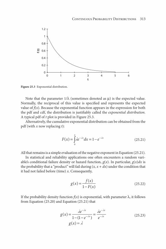
Continuous Probability Distributions 313
Note that the parameter 1/ (sometimes denoted as ) is the expected value.
Normally, the reciprocal of this value is specified and represents the expected
value of f(x). Because the exponential function appears in the expression for both
the pdf and cdf, the distribution is justifiably called the exponential distribution.
A typical pdf of t plot is provided in Figure 25.3.
Alternatively, the cumulative exponential distribution can be obtained from the
pdf (with x now replacing t):
F x e dx ex
x x( )0
1 (25.21)
All that remains is a simple evaluation of the negative exponent in Equation (25.21).
In statistical and reliability applications one often encounters a random vari-
able’s conditional failure density or hazard function, g(x). In particular, g(x)dx is
the probability that a “product” will fail during (x, x dx) under the condition that
it had not failed before (time) x. Consequently,
g xf x
F x( )
( )
( )1 (25.22)
If the probability density function f(x) is exponential, with parameter , it follows
from Equation (25.20) and Equation (25.21) that
g xe
e
e
e
g x
x
x
x
x( )
( )
( )
1 1 (25.23)
0
0.2
0.4
0.6
0.8
1
1.2
0 1 2 3 4 5 6
f (t
)
t
Figure 25.3 Exponential distribution.

314 Introduction to Mathematical Methods
Equation (25.23) indicates that the failure probability is constant, irrespective
of time. It implies that the probability that a component whose time-to-failure dis-
tribution is exponential fails in an instant during the first hour of its life is the same
as its failure probability during an instant in the thousandth hour ‒ presuming it
has survived up to that instant. It is for this reason that the parameter λ is usually
referred to in life-test applications as a failure rate. This definition generally has
meaning only with an exponential distribution.
This natural association with life-testing and the fact that it is very tractable
mathematically makes the exponential distribution attractive as representing the
life distribution of a complex system or several complex systems. In fact, the expo-
nential distribution is as prominent in reliability analysis as the normal distribu-
tion is in other branches of statistics.
Illustrative Example 25.4
Discuss some of the advantages and limitations of the exponential distribution.
Solution
It has been shown theoretically that this distribution provides a reasonable model
for systems designed with a limited degree of redundancy and made up of many
components, none of which has a high probability of failure. This is especially
true when low component failure rates are maintained by periodic inspection and
replacement, or in situations in which failure is a function of outside phenomena
rather than a function of previous conditions. On the other hand, the exponen-
tial distribution often cannot represent individual component life (because of its
“infant mortalities” and wearout patterns), and it is sometimes questionable even
as a system model.
Illustrative Example 25.5
Estimate the probability that a pump at a nuclear power plant will survive at least:
1. 3 times its expected life
2. 5 times its expected life
3. 10 times its expected life
Assume an exponential distribution applies.
Solution
The exponential distribution gives
P T e t timet( ) ;

Continuous Probability Distributions 315
with 1/a where a expected life of the pump. Thus for 3 times its expected
life t 3a,
P T a e eaa
( )
. . %
( )
3
0 0498 4 98
13
3
Therefore, there is a 5% chance that the pump will survive past 3 times its expected
life.
For 5 times its expected life t 5a
P T a e eaa
( )
. . %
( )
5
0 0067 0 67
15
5
and for 10 times its expected life t 10a
P T a e eaa
( )
. . %
( )
10
4 54 10 4 54 10
110
10
5 3
As expected, the probability decreases with increasing survival time.
Illustrative Example 25.6
The time to failure for a battery is presumed to follow an exponential distribution
with 0.1 (per year). What is the probability of a failure within the first year?
Solution
Refer to Equation (25.20)
F x e dx ex x( )0
1
1 (25.21)
For this case (with x representing time),
P X e dx
e e e
e
x
x
( ) ( . )
.
.
( . )
( . ) .
1 0 1
0 1
0 1
1
0
1
0 1
0 1
0
10 1 0
00 1 0 095 9 5. . . %

316 Introduction to Mathematical Methods
Therefore, there is nearly a 10% probability that the battery will fail within the first
year.
Illustrative Example 25.7
An electronic system consists of 3 components (1, 2, 3) connected in parallel. If the
time to failure for each component is exponentially distributed and mean times of
failures for components 1, 2, and 3, are 200, 300, and 600 d, respectively, determine
the system reliability for a year (365 d).
Solution
For this series system, the probability of failure is
P F P
P P P
( ) ( )
( )( )( )
all the components fail
1 1 11 2 3
where Pi is the probability of surviving 365 d. The system reliability is
R P F
P P P
1
1 1 1 11 2 3
( )
( )( )( )
Based on the data provided:
P e1
365
200 0 161.
P e2
365
300 0 296.
P e3
365
600 0 544.
Therefore, the system reliability is
R 1 1 0 161 1 0 296 1 0 544
0 731 73 1
( . )( . )( . )
. . %
Illustrative Example 25.8
A pumping system at a nuclear facility consists of 4 components. 3 are connected
in parallel, which in turn are connected downstream (in series) with the other
component. The arrangement is schematically shown in Figure 25.4.

Continuous Probability Distributions 317
If the pumps have the same exponential failure rate, , of 0.5 (year) 1, estimate
the probability that the system will not survive for more than one year.
Solution
Based on the information provided, the pumping system fails when the 3 parallel
components fail or when the downstream component fails. This is a combination
of a parallel and a series system. The reliability is
R t F t( ) ( )1 (25.24)
where F(t) is the probability of failure between 0 and t. The reliability of the paral-
lel system is
R R R R R R
R
p i1 1 1 1
1 1
1 2 3
3
( )( )( )
( )
;
For a series system
R R R R Rs p p4
where Rs also represents the overall system reliability.
Applying the exponential model gives
R t F t e et t( ) ( ) ( )1 1 1
R R R R R e
R
1 2 3 4
0 5 1
0 6065
( . )( )
.
Thus,
Rp 1 1 0 6065 1 0 0609 0 9391 93 93( . ) . . . %
1
2
3
4
Figure 25.4 Pumping system.

318 Introduction to Mathematical Methods
and
Rs ( . )( . )
. %
0 9391 0 6065
0 57 57
Illustrative Example 25.9
The probability that a thermometer placed in three different locations of a hazard-
ous waste incinerator will not survive for more than 36 months is 0.925, 0.95, and
0.99 respectively. How often should the thermometer be replaced in each one of
these situations? Assume the time to failure is exponentially distributed and that
the replacement time should be based on the thermometer’s expected life.
Solution
This requires the calculation of in the exponential model with units of (month) 1.
Once again,
F t e t( ) 1
Based on the information provided
P T( ) .36 0 925
or
0 925 1 36. ( )( )e
Solving gives
1
361 0 925ln( . ) 0.07195
The expected time (or life), E(T), is [1, 2]
E T( ).
.1 1
0 0719513 9 months
Therefore, for the first location the thermometer should be replaced in approxi-
mately 14 months.
For the second location, the describing equation remains
F t e t( ) 1

Continuous Probability Distributions 319
For F(t) 0.95,
0 95 1 36. ( )( )e
Solving for gives
1
361 0 95 0 0832ln( . ) .
The expected life is then
E T( ).
1 1
0 083212 months
For the third location
1
361 0 99 0 128ln( . ) .
and
E T( ).
.1 1
0 1287 82 months
25.2 Weibull Distribution
Unlike the exponential distribution, the failure rate of equipment frequently
exhibits 3 stages: a break-in stage with a declining failure rate, a useful life stage
characterized by a fairly constant failure rate, and a wear out period characterized
by an increasing failure rate. Many industrial parts and components follow this
behavior. A failure rate curve exhibiting these 3 phases (see Figure 25.5) is called
a bathtub curve.
In the case of the bathtub curve, the failure rate during useful life is constant.
Letting this constant be yields
F t dt t t et
t( ) exp exp( )0
0; (25.25)
as the probability distribution function (pdf) of time to failure during the useful
life stage of the bathtub curve. Equation (25.25) defines an exponential (pdf) that
is a special case of the pdf defining the Weibull distribution.

320 Introduction to Mathematical Methods
Weibull introduced the distribution, which bears his name principally on empir-
ical grounds, to represent certain life-test data. The Weibull distribution provides a
mathematical model of all 3 stages of the bathtub curve. This is now discussed. An
assumption about the failure rate Z(t) that reflects all 3 stages of the bathtub curve is
Z t t t( ) 1 0; (25.26)
where and β are constants. For 1, the failure rate Z(t) decreases with time. For
1, the failure rate is constant and equal to α. For 1, the failure rate increases
with time. Using this equation again to translate the assumption about failure rate
into a corresponding assumption about the pdf of T, time to failure, one obtains
f t t t dt t t t( ) exp exp( ) ,1
0
1
1 1 0 0; ; 0 (25.27)
Equation (25.27) defines the pdf of the Weibull distribution. As noted, the expo-
nential distribution discussed in the preceding section, whose pdf was given in
Equation (25.20) earlier, is a special case of the Weibull distribution with 1.
A variety of assumptions about failure rate and the probability distribution
of time to failure that can be accommodated by the Weibull distribution make it
especially attractive in describing failure time distributions in industrial and pro-
cess plant applications
To illustrate probability calculations involving the exponential and Weibull
distributions introduced in conjunction with the bathtub curve of failure rate,
consider first the case of a transistor having a constant rate of failure of 0.01 per
thousand hours. To find the probability that a transistor will operate for at least
25,000 h, substitute the failure rate
Z t( ) .0 01 (25.28)
Break in Useful life Wear out
Time
Fa
ilu
re r
ate
Figure 25.5 Bathtub curve.

Continuous Probability Distributions 321
which yields
f t dt
e t
t
t
( ) exp .
. .
0
0 01
0 01
0 01 0;
(25.29)
as the pdf of T, the time to failure of the transistor. Because t is measured in thou-
sands of hours, the probability that the transistor will operate for at least 25,000 h
is given by
P T e dt
e e
t( ) .
.
. %
.
. ( )
25 0 01
0 0 78
0 78 78
25
0 01
0 01 25
(25.30)
Now suppose it is desired to determine the 10,000 h reliability of a circuit of
5 such transistors connected in series. The 10,000 h reliability of one transistor is
the probability that it will last at least 10,000 h. This probability can be obtained by
integrating the pdf of T, time to failure, which gives
P T e dt
e e
t10 0 01
0 0 90
10
0 01
0 01 10
.
.
.
.
90%
(25.31)
The 10,000 h reliability of a circuit of 5 transistors connected in series is obtained
by applying the formula for the reliability of series systems to obtain
R Rs [ ( )] ( . )
. %
10 0 9
0 59 59
5 5
(25.32)
As another example of probability calculations, consider a component whose
time to failure T, in hours, has a Weibull pdf with parameters 0.01 and 0.50
in Equation (25.27). This gives
f t t e tt( ) ( . )( . ) . ( . ) .
0 01 0 5 00 5 1 0 01 0 5
; (25.33)

322 Introduction to Mathematical Methods
As the Weibull pdf of the failure time of the component under consideration, the
probability that the component will operate at least 8100 h is then given by
P T f t dt t e dt
e
t( ) ( ) . . ( . )
.
.
8100 0 0058100 8100
0 5 0 01
0
0 5
001
8100
0 01 81000 5 0 5
0 0 41 41t e. .
| . %( . )( )
(25.34)
Illustrative Example 25.10
Discuss some Weibull distribution applications.
Solution
A variety of conditional failure distributions, including wear out patterns, can be
accommodated by the Weibull distribution. Therefore, this distribution has been
frequently recommended – instead of the exponential distribution – as an appro-
priate failure distribution model. Empirically, satisfactory fits have been obtained
for failure data on electron tubes, relays, ball bearings, metal fatigue, and even
business mortality.
Illustrative Example 25.11
The life (time to failure) of a machine component has a Weibull distribution.
Outline how to determine the probability that the component lasts a given period
of time if the failure rate is t 1/2.
Solution
Identify the failure rate, Z(t), from Equation (25.26).
Z t t( )1
2
Also, identify the values of and appearing in the failure rate. If the failure rate is
t 1/2,
11
2
and
1
Therefore, 1/2, and 2.

Continuous Probability Distributions 323
For these values of and obtained above, determine the Weibull pdf
f t t e tt( )1
2 2
1
2
0;
Integration of this pdf will yield the required probability. This is demonstrated
in the next illustrative example.
Illustrative Example 25.12
Refer to Illustrative Example 25.11. Determine the probability that the component
lasts at least 25,000 h if t is measured in thousands of hours.
Solution
For this case,
t 25
Because time is measured in thousands of hours the probability that the compo-
nent lasts at least 25,000 h is
P T t e dt
e
t
t
( )
|
2525
1
2 2
2
25
1
2
This may be integrated to give
P T e( ) ( )
. %
( ) .
25 0
4 5 10 0
2 25
5
0 5
Illustrative Example 25.13
The life of a gasket has a Weibull distribution with failure rate
Z tt
t( ) /1 1 2
where t is measured in years. What is the probability that the gasket will last at
least 4 years?

324 Introduction to Mathematical Methods
Solution
The pdf specified by f(t) in terms of the failure rate, Z(t), is as follows:
f t Z t Z t dtt
( ) ( )exp ( )0
Substituting 1/t1/2 for Z(t) yields
f t t t dt t dt t( ) exp exp1
2
0
1
2
1
2
1
22 0t ;
Once again, employ the integration procedure provided earlier. The probability
that the seal lasts at lasts 4 years is
P T t t dt e
e
t( ) exp [ ]
( ) .
.
4 2
0 0 0183 1
4
1
2
1
2 2
4
4
0 5
.. %83
25.3 Normal Distribution
The initial presentation in this section on normal distributions will focus on failure
rate, but can be simply applied to all other applications involving normal distribu-
tions. When T, time to failure, has a normal distribution, its probability distribu-
tion function (pdf) is given by
f TT
t( ) exp1
2
1
2
2
; (25.35)
where μ is the mean value of T and is its standard deviation. The graph of f(T) is
the familiar bell-shaped curve shown in Figure 25.6.
The reliability function corresponding to the normal distributed failure time is
given by
f TT
dtt
( ) exp1
2
1
2
2
(25.36)
If T is normally distributed with mean and standard deviation σ, then the ran-
dom variable (T )/ is normally distributed with mean 0 and standard devia-
tion 1. The term (T )/ is called a standard normal curve that is represented by

Continuous Probability Distributions 325
Z, not to be confused with the failure rate Z(t). This is discussed in more detail
later in this section.
Table 25.1 is a tabulation of areas under a standard normal curve to the right
of z0 for nonnegative values of z
0. Probabilities about the normal variable Z can be
determined from this table. For example,
P Z( . ) .1 54 0 062 (25.37)
is obtained directly from Table 25.1 as the area to the right of 1.54. As presented
in Figure 25.7, the symmetry of the standard normal curve about zero implies that
the area to the right of zero is 0.5.
Plots demonstrating the effect of and on the bell-shaped curve are provided
in Figure 25.8 and Figure 25.9. Consequently, one can deduct from Table 25.1 and
Figure 25.7 that
P Z( ) . . .0 154 0 5 0 062 0 438 (25.38)
Also, because of symmetry
P Z( . ) .1 54 0 0 438 (25.39)
and
P Z( . ) .1 54 0 062 (25.40)
The following probabilities can also be deduced by noting that the area to the
right of 1.54 is 0.062 in Figure 25.7.
P Z( . . ) .1 54 1 54 0 876 (25.41)
P Z( . ) .1 54 0 938 (25.42)
f(T)
Figure 25.6 Normal pdf of time to failure.

326 Introduction to Mathematical Methods
Table 25.1 Standard normal cumulative probability; right-hand tail.
Second decimal place of z
z .00 .01 .02 .03 .04 .05 .06 .07 .08 .09
0.0 .5000 .4960 .4920 .4880 .4840 .4801 .4761 .4721 .4681 .4641
0.1 .4602 .4562 .4522 .4483 .4443 .4404 .4364 .4325 .4286 .4247
0.2 .4207 .4168 .4129 .4090 .4052 .4013 3971 .3936 .3897 .3859
0.3 .3821 .3783 1745 .3707 .3669 .3632 .3594 .3557 .3520 .3483
0.4 .3446 .3409 .3372 .3336 .3300 .3264 .3228 .3192 .3156 .3121
0.5 .3085 .3050 .3015 .2981 .2946 .2912 .2877 .2843 .2810 .2776
0.6 .2743 .2709 .2676 .2643 .2611 .2578 .2546 .2514 .2483 .2451
0.7 .2420 .2389 .2358 .2327 .2296 2266 .2236 .2206 .2177 .2148
0.8 .2119 .2090 .2061 .2033 .2005 .1977 .1949 .1922 1894 .1867
0.9 .1841 .1814 .1788 .1762 .1736 .1711 .1685 .1660 .1635 .1611
1.0 .1587 .1562 .1539 .1515 .1492 .1469 .1446 .1423 .1401 .1379
1.1 .1357 .1335 .1314 .1292 .1271 .1251 .1230 .1210 .1190 .1170
1.2 .1151 .1131 .1112 .1093 .1075 .1056 .1038 .1020 .1003 .0985
1.3 .0968 .0951 .0934 .0918 .0901 .0885 .0869 .0853 .0838 .0823
1.4 .0808 .0793 .0778 076-1 .0749 .0735 1721 .0708 0694 .0681
1.5 .0668 .0655 .06-13 .0630 .0618 .0606 .0591 .0582 .0571 .0559
1.6 .0548 .0537 .0526 .0516 .0505 .0495 .0485 .0475 .0465 .0455
1.7 .0446 .0436 .0127 .0118 .0109 .0401 .0392 .0384 .0375 .0367
1.8 .0359 .0351 .0344 .0336 .0329 .0322 .0314 .0307 .0301 .0294
1.9 .0287 .0281 .0274 .0268 .0262 .0256 .0250 .0244 .0239 .0233
2.0 .0228 .0222 .0217 .0212 .0207 .0202 .0197 .0192 .0188 .0183
2.1 .0179 .0174 .0170 .0166 .0162 .0158 .0154 .0150 .0146 .0143
2.2 .0139 .0136 .0132 .0129 .0125 .0122 .0119 .0116 .0113 .0110
2.3 .0107 .0104 .0102 .0099 .0096 .0094 .0091 .0089 .0087 .0084
2.4 .0082 .0080 .0078 .0075 .0073 .0071 .0069 .0068 .0066 .0064
2.5 .0062 0060 .0059 .0057 .0055 .0054 .0052 .0051 .0049 .0048
2.6 .0047 .0045 .0044 .0043 .0041 .0040 .0039 .0038 .0037 .0036
2.7 .0035 0034 .0033 .0032 .0031 .0030 .0029 .0028 .0027 .0026
2.8 .0026 .0025 .0024 .0023 .0023 .0022 .0021 .0021 .0020 .0019
2.9 .0019 .0018 .0018 .0017 .0016 .0016 .0015 .0015 .0014 .0014

Continuous Probability Distributions 327
P Z( . ) .1 54 0 938 (25.43)
Table 25.1 can also determine probabilities concerning normal random vari-
ables that are not standard normal variables. The required probability is first con-
verted to an equivalent probability about a standard normal variable. For example,
–1.54
0.062 0.062
0.4380.438
1.540t
f(t)
Figure 25.7 Areas under a standard normal curve.
–2 2
= –2 = +2
= 0
t
f(t)
Figure 25.8 Normal pdf – varying .
–2 2
= 2
= 1
= 0.5
t
f(t)
Figure 25.9 Normal pdf – varying .

328 Introduction to Mathematical Methods
if T, the time to failure, is normally distributed with mean 100 and standard
deviation 2 then (T 100)/2 is a standard normal variable and one may write
P T T T PT T T
( )1 21 2 (25.44)
where
T
Z standard normal variable (22.45)
Therefore, if T1
98 and T2
104 as an example, the describing equation becomes
P TT
PT
( )98 10498 104
98 100
2 2
104 100
2
PT
P Z
1100
22
1 2
0 341 0 477
0 818 81
( )
. .
. .88%
(25.46)
For any random variable X ‒ where X has now replaced T ‒ that is normally dis-
tributed with mean and standard deviation , one may now write the following:
P X P
X
P Z
( )
( ) .
1 1
1 1 0 68
(25.47)
P X P
X
P Z
( )
( ) .
2 2 2 2
2 2 0 95
(25.48)
P X P
X
P Z
( )
( ) .
3 3 3 3
3 3 0 997
(25.49)

Continuous Probability Distributions 329
The probabilities given above are the sources of the percentages cited earlier [2].
These can be used to interpret the standard deviation s of a sample of observations
on a normal random variable as a measure of dispersion about the sample mean X.
The normal distribution can be used to obtain probabilities concerning the
mean X of a sample of n observations on a random variable X if X is normally
distributed with mean μ and standard deviation / n. For example, suppose
X is normally distributed with mean 100 and standard deviation 2. Then X, of
a sample of 16 observations on X, is normally distributed with mean 100 and
standard deviation 0.5. To calculate the probability that X is greater than 101,
one would write
P X PX
( ). .
101100
0 5
101 100
0 5 (25.50)
P X P
XZ
X
P Z
( ). . .
( ) .
101100
0 5
101 100
0 5
100
0 5
2 0 0
;
223 2 3. %
(25.51)
If X is not normally distributed, then X, the mean of a sample of n observations
on X, is approximately normally distributed with mean and standard deviation / n, provided the sample size n is large (>30). This result is based on an impor-
tant theorem and probability called the central limit theorem.
Suppose for example, that the mean and variance for a random variable are 1
and 1/3 respectively. If X is the mean of a random sample of 48 observations on
X, X is approximately normally distributed with mean 1 and standard deviation / n. The latter term is therefore given by
n
1 3
48
1
3 48
1
144
1
12
/
( )( ) (25.52)
The following example is now provided for this case.
P X PX
P Z9
8
1
1
12
9
81
1
12
1 5 0 067( . ) . (25.53)
One of the principal applications of the normal distribution in reliability calcu-
lations and hazard risk analysis is the distribution of time to failure due to “wear
out.” Suppose, for example, that a production lot of thermometers, to be employed
in an incinerator especially designed to withstand high temperatures and intense
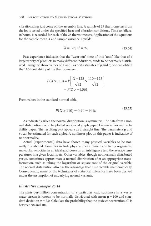
330 Introduction to Mathematical Methods
vibrations, has just come off the assembly line. A sample of 25 thermometers from
the lot is tested under the specified heat and vibration conditions. Time to failure,
in hours, is recorded for each of the 25 thermometers. Application of the equations
for the sample mean X and sample variance s2 yields
X s125 922; (25.54)
Past experience indicates that the “wear out” time of this “unit,” like that of a
large variety of products in many different industries, tends to be normally distrib-
uted. Using the above values of X and s as best estimates of μ and σ, one can obtain
the 110-h reliability of the thermometers.
P X PX
P
( )110125
92
110 125
92
(Z 1.56)
From values in the standard normal table,
P X( ) . %110 0 94 94
(25.55)
As indicated earlier, the normal distribution is symmetric. The data from a nor-
mal distribution could be plotted on special graph paper, known as normal prob-
ability paper. The resulting plot appears as a straight line. The parameters μ and
, can be estimated for such a plot. A nonlinear plot on this paper is indicative of
nonnormality.
Actual (experimental) data have shown many physical variables to be nor-
mally distributed. Examples include physical measurements on living organisms,
molecular velocities in an ideal gas, scores on an intelligence test, the average tem-
peratures in a given locality, etc. Other variables, though not normally distributed
per se, sometimes approximate a normal distribution after an appropriate trans-
formation, such as taking the logarithm or square root of the original variable.
The normal distribution also has the advantage that it is tractable mathematically.
Consequently, many of the techniques of statistical inference have been derived
under the assumption of underlying normal variants.
Illustrative Example 25.14
The parts-per-million concentration of a particular toxic substance in a waste-
water stream is known to be normally distributed with mean 100 and stan-
dard deviation 2.0. Calculate the probability that the toxic concentration, C, is
between 98 and 104.

Continuous Probability Distributions 331
Solution
Because C is normally distributed with 100 and a standard deviation 2.0,
then (C – 100)/2 is a standard normal variable and
P C P
C
P Z
( )
( )
98 104 1100
22
1 2
From the values in the standard normal table,
P C( ) . . . . %98 104 0 341 0 477 0 818 81 8
The reader should note that the calculation for this illustrative example is iden-
tical to one presented earlier for a time to failure application.
Illustrative Example 25.15
Acceptance limits require the plate-to-plate spacing in an electrostatic precipitator
to be between 24 and 25 cm [3]. Spacing from other installations suggests that it is
normally distributed with an average length of 24.6 cm and a standard deviation
of 0.4 cm. What proportion of the plate spacing in a typical unit can be assumed
unacceptable [3]?
Solution
The problem is equivalent to determining the probability that an observation or
sample from a normal distribution with parameters 0 and 1 either exceeds
Z1
25 0 24 6
0 41
. .
.
or falls below
Z2
24 0 24 6
0 41 5
. .
..
These probabilities are 0.159 and 0.067, respectively, from the table of the standard
normal distribution. Consequently, the proportion of unacceptable spacing is
P P Z P Z( ) ( ) ( . )
. .
.
unacceptable spacing 1 1 5
0 159 0 067
0 226 26 6. %

332 Introduction to Mathematical Methods
Illustrative Example 25.16
The temperature of a polluted estuary during the summer months is normally
distributed with mean 56°F and standard deviation 3.0°F. Calculate the probability
that the temperature is between 55 and 62°F.
Solution
Normalizing the temperature T gives
Z1
55 56
3 00 333
..
Z2
62 56
3 02 0
..
Thus,
P Z P Z P Z( . . ) ( . . ) ( . . )
. .
0 333 2 0 0 0 2 0 0 0 0 333
0 4722 0 1293 0.. . %6015 60 15
Illustrative Example 25.17
The regulatory specifications on a toxic substance in a solid waste ash calls for a
concentration level of 1.0 ppm or less [4]. Earlier observations of the concentra-
tion of the ash, C, indicate a normal distribution with a mean of 0.60 ppm and a
standard deviation of 0.20 ppm. Estimate the probability that ash will exceed the
regulatory limit.
Solution
The problem requires the calculation of P(C 1.0). Normalizing the variable C,
PC 0 6
0 2
1 0 0 6
0 2
.
.
. .
.
P Z( . )2 0
From the standard normal table
P Z( . ) . . %2 0 0 0228 2 28
For this situation, the area to the right of the 2.0 is 2.28% of the total area. This
represents the probability that ash will exceed the regulatory limit of 1.0 ppm.

Continuous Probability Distributions 333
Illustrative Example 25.18
The diameter D of wires installed in an electrostatic precipitator (ESP) has a stan-
dard deviation of 0.01 in [3]. At what value should the mean be if the probability
of its exceeding 0.21 in is to be 1%?
Solution
For this example,
PD 0 21
0 010 01
.
..
where
ZD
Therefore,
P Z0 21
0 010 01
.
..
For a one-tailed test at the 1% (0.01) level [1, 2],
Z 2 326.
so that
2 326
0 21
0 010 187
..
.. in
Illustrative Example 25.19
The lifetime, T, of a circuit board employed is normally distributed with a mean of
2500 d. What is the largest lifetime variance the installed circuit boards can have if
95% of them need to last at least 365 d?
Solution
For this application,
P T( ) .365 0 95

334 Introduction to Mathematical Methods
Normalizing gives
PT
P Z
365 25000 95
21351 6
.
. 445
The following equation must apply for this condition:
2135
1 645.
Solving,
1298 d
In addition,
2 6 21 68 10. d
Illustrative Example 25.20
Let X denote the coded quality of bag fabric used in a particular utility baghouse [3].
Assume that X is normally distributed with mean 10 and standard deviation 2.
1. Find c such that P X c(| | ) .10 0 90
2. Find k such that P X k( ) .0 90
Solution
1. Because X is normally distributed with mean 10 and standard
deviation 2, (X 10)/2 is a standard normal variable. For this two-
sided test [1, 2],
P X c P c X c
Pc X c
Pc
Zc
(| | ) ( )10 10
2
10
2 2 2 2
2 02
P Zc
; due to symmetry

Continuous Probability Distributions 335
Because
P X c(| | ) .10 0 90
one may write
2 02
0 90P Zc
.
P Zc
02
0 45.
For this condition to apply,
c
c2
1 645
3 29
.
.
2. Based on the problem statement,
P X k
PX k
P Zk
( ) .
.
.
0 90
10
20 90
10
20 90
For this equation to be valid
k 10
21 28.
Solving for k gives
k 7 44.
25.5 Log-Normal Distribution
A nonnegative random variable X has a log-normal distribution whenever ln X, i.e.,
the natural logarithm of X, has a normal distribution. The probability distribution

336 Introduction to Mathematical Methods
function (pdf) of a random variable X having a log-normal distribution is speci-
fied by
f x x
xx( ) exp ;
;
( )1
2 20
0
12
2
ln
elsewhere
(25.56)
The mean and variance of a random variable X having a log-normal distribution
are given by
e
2
2 (25.57)
2 2 2 2
1e e( ) (25.58)
Figure 25.10 plots the pdf of the log-normal distribution for 0 and 1.
Probabilities concerning random variables having a log-mean distribution can be
calculated from the previously employed tables of the normal distribution. If X
has a log-normal distribution with parameters and β, then the ln X has a nor-
mal distribution with and . Probabilities concerning X can therefore be
converted into equivalent probabilities concerning ln X.
For example, suppose that X has a log-normal distribution with 2 and
0.1. Then
0.7
0.6
0.5
0.4
0.3
0.2
0.1
00 1 2 3 4
x
f(x
)
5 6 7 8
Figure 25.10 Log-normal pdf for 0, 1.

Continuous Probability Distributions 337
P X P X
X
P
( ) ( )
. . .
(
6 8 6 8
6 2
0 1
2
0 1
8 2
0 1
ln ln ln
ln ln
22 08 0 79
0 5 0 019 0 5 0 215
0 481 0 285
0 78
. . )
( . . ) ( . . )
. .
.
Z
(25.59)
Estimates of the parameters and in the pdf of a random variable X having
a log-normal distribution can be obtained from a sample of observations on X
by making use of the aforementioned fact that ln X is normally distributed with a
mean and a standard deviation . Therefore, the mean and standard deviation
of the natural logarithms of the sample observations on X furnish estimates of
and . To illustrate this procedure, suppose the time to failure T, in thousands
of hours, was observed for a sample of five pumps at a water treatment plant.
The observed values of T were 8, 11, 16, 22, and 34. The natural logarithms of
these observations are 2.08, 2.40, 2.77, 3.09, and 3.53. Assuming that T has a
log-normal distribution, the estimates of the parameters and in the pdf are
obtained from the mean and standard deviation of the natural logs of the obser-
vations on T. Applying Equation (23.1) and Equation (23.7) developed earlier
yields 2.77 as the estimate of and 0.57 as the estimate of . See also Illustrative
Example 25.21.
The log-normal distribution has been employed as an appropriate model in
a wide variety of situations from environmental management to biology to eco-
nomics. Additional applications include the distributions of personal incomes,
inheritances, bank deposits as well as the distribution of organism growth sub-
ject to many small impurities. Perhaps the primary application of the log-normal
distribution has been to represent the distribution for particle sizes in gaseous
emissions from many industrial processes, details of which are provided in the
literature [3].
Illustrative Example 25.21
The time to failure, T, in thousands of hours was observed for a sample of 5 electric
motors as follows:
8 11 16 22 34, , , ,
Assuming T has a log-normal distribution estimate the probability that an elec-
tric motor last less than 5000 h.

338 Introduction to Mathematical Methods
Solution
Under the assumption that T has a log-normal distribution, the natural logs of
the observation constitute a sample from; a normal population. First, obtain the
natural logs of the given observations on T, time to failure:
ln ln ln ln ln8 2 08 16 2 77 34 3 53 11 2 40 22 3 09. , . , . , . , .
Compute the mean, , and the standard deviation, σ, of these results.
i
iT
1
5
52 77
ln.
i
iT
1
5 22 77
40 57
[ ]..
ln
Estimate α and β in the pdf of T from μ and σ, respectively.
Estimate of 2 77.
Estimate of 0 57.
Convert the required probability concerning T into a probability about ln T:
P T P T P T( ) (ln ln ) (ln . )5 5 1 61
The required probability using the standard normal table can now be obtained; by
treating ln T as a random variable that is normally distributed with mean α and
standard deviation .
P T PT
P Z
(ln . )ln .
. .
1 611 61
1 61 2 77
00572 04
0 021 2 1
P Z( . )
. . %
Illustrative Example 25.22
Resolve Illustrative Example 25.21 by calculating the probability that an electric
motor lasts more than
1. 5,000 h
2. 10,000 h

Continuous Probability Distributions 339
Solution
1. One can immediately conclude that
P T P T P T( ) (ln . ) ( )
. . . . %
5 1 61 1 5
1 0 0 0021 0 979 97 9
2. The describing equation becomes
P T P T P T( ) (ln ln ) (ln . )10 10 2 303
Converting to a standard normal variable,
P T PT
P Z
(ln . )ln .
.
2 3032 303
2 303 2..
.( . )
. . %
77
0 572 434
0 9926 99 26
P Z
Illustrative Example 25.23
The failure rate per year, Y, of a coolant recycle pump in a wastewater treatment
plant has a log-normal distribution. If ln Y has a mean of 2.0 and variance of 1.5,
find P(0.175 Y 1).
Solution
If Y has a log-normal distribution, ln Y has a normal distribution with mean 2 and
standard deviation 1.51/2 1.22. Therefore,
P Y P Y
PY
( . ) (ln . ln ln )
ln .
.
ln
0 175 1 0 175 1
0 175 2
1 22
2
11 22
1 2
1 22
3 07 1 64 0 1587 0 0011
.
ln
.
( . . ) . .P Z
0 1576 15 76. . %
Illustrative Example 25.24
Normalized biological oxygen demand (BOD) levels in an estuary during the past
10 years are summarized in Table 25.2 [4]. If the BOD levels are assumed to follow
a log-normal distribution, predict the level that would be exceeded only once in
100 years [2].

340 Introduction to Mathematical Methods
Solution
For this case, refer to Table 25.3. Based on the data provided
XX
n
2 38 86
103 886
..
sX X
n
n2
22
2
1
156 7838 86
1010 1
0 64
( )
..
.
( )
and
s 0 80.
Table 25.2 Estuary BOD data.
Year 1 2 3 4 5 6 7 8 9 10
BOD level 23 38 17 210 62 142 43 29 71 31
Note: BOD biological oxygen demand
Table 25.3 BOD calculations.
Year (Y) BOD Level X ln BOD X2
1 23 3.13 9.83
2 38 3.64 13.25
3 17 2.83 8.01
4 210 5.35 28.62
5 62 4.13 17.06
6 142 4.96 24.60
7 43 3.76 14.14
8 29 3.37 11.36
9 71 4.26 18.15
10 31 3.43 11.67
Total – 38.86 156.78

Continuous Probability Distributions 341
For this test, with Z 2.327 for the 99% value,
ZX X
s
2 3273 886
0 80.
.
.
X
Solving for X yields
X 5 748.
For this log-normal distribution,
X ln( )BOD
X 5 748. ln( )BOD
BOD 313
Reference
1. L Theodore and F. Taylor, Probability and Statistics, A Theodore Tutorial, Theodore Tutorials, East
Williston, NY, originally published by USEPA/APTI, RTP, NC, 1997.
2. S. Shaefer and L. Theodore, Probability and Statistics Applications for Environmental Science, CRC
Press/Taylor & Francis Group, Boca Raton, FL, 2007.
3. L. Theodore, Air Pollution Control Equipment Calculations, John Wiley & Sons, Hoboken, NJ, 2008.
4. R. Dupont, K. Ganesan, and L. Theodore, Pollution Prevention: Sustainability, Industrial Ecology,
and Green Engineering, 2nd ed., CRC Press/Taylor & Francis Group, Boca Raton, FL, 2017.

343
Tree analysis has become an integral part of probability analysis for environmen-
tal engineering and science practitioners. There are two tree analyses that are
employed: fault trees and event trees. Fault trees attempt to determine the cause of
failure in a system while event trees attempt to determine the consequences associ-
ated with a system that has failed.
Two sections compliment the presentation of this chapter. Section numbers
and subject titles follow.
26.1: Fault Trees
26.2: Event Trees
26.1 Fault Trees
A fault tree is a graphical technique used to analyze some complex systems. The
objective is to spotlight faulty conditions that have caused a system to fail. Fault
tree analysis attempts to describe how and why an accident or other undesirable
event has occurred. It may also be used to describe how and why an accident or
other undesirable event could take place. A fault tree analysis also finds wide
26Fault Tree and Event Tree Analysis [1]
Introduction to Mathematical Methods for Environmental Engineers and Scientists. Charles Prochaska and Louis Theodore.
© 2018 Scrivener Publishing LLC. Published 2018 by John Wiley & Sons, Inc.

344 Introduction to Mathematical Methods
application in environmental management as it applies to hazard analysis and risk
assessment of process and plant systems.
Fault tree analysis seeks to relate the occurrence of an undesired event, the “top
event,” to one or more antecedent events, called basic events. The top event may be,
and usually is, related to the basic events via certain intermediate events. A fault
tree diagram exhibits the usual chain, linking the basic events to the intermediate
events and the latter to the top event. In this chain, the logical connection between
events is indicated by so-called logic gates. The principal logic gates on the fault
tree are the “AND” gate, symbolized by , and the “OR” gate, symbolized by .
As a simple example of a fault tree, consider a water pumping system consisting
of 2 pumps A and B, where A is the pump ordinarily operating and B is a standby
unit that automatically takes over if A fails. A control valve in both cases regulates
flow of water through the pump. Suppose that the top event is no water flow, result-
ing from the following basic events: failure of pump A and failure of pump B or fail-
ure of the control valve. The full tree diagram for the system is shown in Figure 26.1.
Because one of the purposes of a fault tree analysis is the calculation of the
probability of the top event, let A, B, and C represent the failure of pump A, the
failure of pump B, and the failure of the control valve, respectively. Then, if T rep-
resents the top event of no water flow, one can write
T AB C (26.1)
This equation indicates that T occurs if both A and B occur or if C occurs.
Assume that A, B, and C are independent and P(A) 0.01, P(B) 0.005, and
P(C) 0.02. Then, application of the addition theorem [1] yields
P T P AB P C P ABC( ) ( ) ( ) ( ) (26.2)
No flow
OR
Pump
failureControl
valve
failure
Pump A
failure
Pump B
failure
AND OR
AND
or gate
and gate
Figure 26.1 Fault tree for a water pumping system.

Fault Tree and Event Tree Analysis 345
The independence of A, B, and C implies
P AB P A P B( ) ( ) ( ) (26.3)
and
P ABC P A P B P C( ) ( ) ( ) ( ) (26.4)
Therefore, the proceeding equation can be written as
P T P A P B P C P A P B C( ) ( ) ( ) ( ) ( ) ( )( ) (26.5)
Substituting the proceeding data gives
P T( ) ( . )( . ) . ( . )( . )( . )
.
0 01 0 005 0 02 0 01 0 005 0 02
0 020049 (26.6)
In connection with fault trees, cut sets and minimal cut sets are defined as fol-
lows. A cut set is a basic event or intersection of basic events that will cause the top
event to occur. A minimal cut set is a cut set that is not a subset of any other cut
set. In the example presented above, AB and C are cut sets because if AB occurs
then T occurs, and if C occurs, then T occurs. Also, AB and C are minimal cut sets,
because neither is a subset of the other. The event T describes what can be regarded
as a top event represented as a union of cut sets.
The reader should note the behavior of a fault tree includes the following:
1. A fault tree works backwards from an undesirable event or ulti-
mate consequence to the possible causes and failures.
2. It relates the occurrence of an undesired event to one or more pre-
ceding events.
3. It “chain-links” basic events to intermediate events that are in turn
connected to the top event.
4. It is used in the calculation of the probability of the top event.
5. It is based on the most likely or credible events that lead to a par-
ticular failure or accident.
6. Its analysis includes human error as well as equipment failure.
Illustrative Example 26.1
A runaway chemical reaction can lead to a fire, an explosion, or massive pollutant
emissions. It occurs if coolers fail (A) or there is a bad chemical batch (B). Coolers
fail only if both cooler #1 fails (C) and cooler #2 fails (D). A bad chemical batch
occurs if there is a wrong mix (E) or there is a process upset (F). A wrong mix
occurs only if there is an operator error (G) and instrument failure (H). Construct
a fault tree.

346 Introduction to Mathematical Methods
Solution
Begin with the top event for this problem shown in Figure 26.2. Generate the
first branch of the fault tree (see Figure 26.3), applying the logic gates seen in
Figure 26.1. Then generate the second and third branches using the same process.
The addition of the second and third branches can be seen in Figure 26.4 and
Figure 26.5, respectively.
Runaway chemical
reaction (I)
Figure 26.2 Top event of fault tree.
Runaway chemical
reaction (I)
Cooler fails
(A) Bad batch
(B)
Figure 26.3 Fault tree with first branch.
Runawaychemical
reaction (I)
Badbatch
(B)
Cooler fails(A)
Cooler#1 fails
(C)
Cooler#2 fails
(D)
Wrongmix(E)
Processupset
(F)
Figure 26.4 Fault tree with second branch.
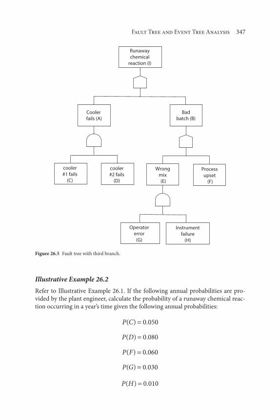
Fault Tree and Event Tree Analysis 347
Illustrative Example 26.2
Refer to Illustrative Example 26.1. If the following annual probabilities are pro-
vided by the plant engineer, calculate the probability of a runaway chemical reac-
tion occurring in a year’s time given the following annual probabilities:
P C( ) .0 050
P D( ) .0 080
P F( ) .0 060
P G( ) .0 030
P H( ) .0 010
Runaway
chemical
reaction (I)
Cooler
fails (A)
Bad
batch (B)
cooler
#1 fails
(C)
cooler
#2 fails
(D)
Wrong
mix
(E)
Process
upset
(F)
Operator
error
(G)
Instrument
failure
(H)
Figure 26.5 Fault tree with third branch.

348 Introduction to Mathematical Methods
Solution
Redraw Figure 26.5 and insert the given probabilities (see Figure 26.6). Calculate
the probability that the runaway reaction will occur
P ( . )( . ) ( . )( . ) .
. . .
.
0 05 0 08 0 01 0 03 0 06
0 0040 0 0003 0 06
0 064
Note that the process upset, F, is the major contributor to the probability. The
reader should also note that if A and B are not mutually exclusive then
P 0 004 0 0603 0 004 0 0603
0 06406
. . ( . )( . )
.
Figure 26.6 Runaway chemical reaction probabilities.
Runawaychemical
reaction (I)
Cooler fails (A)
Badbatch (B)
Cooler#1 fails
(C)
Cooler#2 fails
(D)
Wrongmix(E)
Processupset
(F)
Operatorerror(G)
Instrumentfailure
(H)
0.05 0.08
0.03 0.01
0.06

Fault Tree and Event Tree Analysis 349
Illustrative Example 26.3
A distillation column explosion can occur if the overhead cooler fails (OC) and the
condenser fails (CO) or there is a problem with the reboiler (RB) [2]. The overhead
unit fails (OUC) only if both the cooler fails (OC) and the condenser fails (CO).
Reboiler problems develop if there is a power failure (PF) or there is a failed tube
(FT) [3]. A power failure occurs only if there are both operator error (OE) and
instrument failure (IF). Construct a fault tree with the information below.
P OC( ) .0 02
P CO( ) .0 05
P FT( ) .0 04
P OE( ) .0 60
P IF( ) .0 005
Solution
The fault tree is given in Figure 26.7. Based on the data provided,
P( ) ( . )( . ) ( . )( . ) .
. . .
explosion 0 02 0 05 0 005 0 6 0 04
0 001 0 003 0 004 0 0413.
Note that the major contributor to an explosion is the failed tube (FT), whose
probability is 0.04.
26.2 Event Trees
An event tree provides a diagrammatic representation of event sequences that
begin with a so-called initiating event and terminate in one or more undesirable
consequences. In contrast to a fault tree, which works backwards from an unde-
sirable consequence to possible causes, an event tree looks forward from the ini-
tiating event to possible undesirable consequences. The initiating event may be
equipment failure, human error, power failure, or some other event that has the
potential for adversely affecting an ongoing process or environment.
The following illustration of an event tree analysis is based on one reported in
the classic work by Lees [4]. Consider a situation in which the probability of an
external power outage in any given year is 0.1. A backup generator is available, and
the probability that it will fail to start on any given occasion is 0.02. If the generator
starts, the probability that it will not supply sufficient power for the duration of the

350 Introduction to Mathematical Methods
external power outage is 0.001. An emergency battery power supply is available;
the probability that it will be inadequate is 0.01.
Figure 26.8 shows the event tree with the initiating event-external power out-
age, denoted by I. Labels for the other events on the event tree are also indicated.
The event sequences I S G B and I S B terminate in the failure of emergency power
supply. Applying the multiplication theorem, one obtains
P ISGB( ) ( . )( . )( . )( . ) .0 1 0 98 0 001 0 01 9 8 10 7
P ISB( ) ( . )( . )( . )0 1 0 02 0 01 2 10 5
Therefore, the probability of emergency power supply failure in any given year is
2.098 10 5, the sum of these two probabilities.
Distillationcolumn
explosion
Overheadfails
(OUC)
Reboilerproblem
(RB)
Coolerfails(OC)
Condenserfails(CO)
Powerfailure
(PF)
Failedtube(FT)
Operatorerror (OE)
Instrumentfailure
(IF)
0.02 0.05
0.60 0.005
0.04
Figure 26.7 Distillation column explosion fault tree.

Fault Tree and Event Tree Analysis 351
The reader should note the behavior of an event tree includes the following:
1. An event tree works forward from an initial event, or an event that
has the potential for adversely affecting an ongoing process, and
ends at one or more undesirable consequences.
2. It is used to represent the possible steps leading to a failure or
accident.
3. It uses a series of branches that relate the proper operation and/or
failure of a system with the ultimate consequences.
4. It is a quick identification of the various hazards that could result
from a single initial event.
5. It is beneficial in examining the possibilities and consequences of
a failure.
6. It does not usually quantify (although it can) the potential of the
event occurring.
7. It can be incomplete if all the initial events are not identified.
Thus, the use of event trees is sometimes limited for hazard analysis because
they usually do not quantify the potential of the event occurring. They may also be
incomplete if all the initial occurrences are not identified. Their use is beneficial on
examining, rather than evaluating, the possibilities and consequences of a failure.
For this reason, a fault tree analysis should supplement this model to establish the
probabilities of the event tree branches.
External power outage(I)
Generatorstarts (S)
Generatorfails to start
(S)
Generatorpower
inadequate (G)
Generatorpower
adequate (G)
Battery poweradequate (B)
Battery powerinadequate (B)
Battery poweradequate (B)
Battery powerinadequate (B)
Figure 26.8 Event tree for power outage.

352 Introduction to Mathematical Methods
Illustrative Example 26.4
Construct a decision tree given the following information:
Date: a couple’s anniversary
Decision of husband: buy flowers or do not buy flowers
Consequences (buy flowers): domestic bliss or suspicious wife
Consequences (do not buy flowers): status quo, or wife in tears/ hus-
band in doghouse
Solution
Begin by setting the initial event “tree” format which is the top event in Figure 26.9.
Also note that this is an event tree. Set up the first branch from the initial event.
This is the first decision point (Figure 26.10).
One may now complete the tree. Note that the bottom four events evolve from
what may be defined as resolution of uncertainty points (Figure 26.11).
This is an example of an event tree. As indicated above, in contrast to a fault
tree, which works backwards from a consequence to possible causes, an event tree
works forward from the initiating (or top) event to all possible consequences.
Thus, this type of tree provides a diagrammatic representation of sequences that
Anniversary
Figure 26.9 Top event.
Anniversary
Buyflowers
Don’t buyflowers
Figure 26.10 First decision point.
Anniversary
Buyflowers
Don’t buyflowers
Dom.bliss
Sus.wife
Doghouse
Statusquo
Figure 26.11 Marital bliss event tree.

Fault Tree and Event Tree Analysis 353
begin with a so-called initiating event and terminate in one or more consequences.
It primarily finds application in hazard analysis.
Illustrative Example 26.5
If a plant fire occurs, a smoke alarm sounds with probability 0.9. The sprinkler
system functions with probability 0.7 whether or not the smoke alarm sounds. The
consequences are minor fire damage (alarm sounds, sprinkler works), moderate
fire damage with few injuries (alarm fails, sprinkler works), moderate fire damage
with many injuries (alarm sounds, sprinkler fails), and major fire damage with
many injuries (alarm fails, sprinkler fails). Construct an event tree, and indicate
the probabilities for each of the four consequences.
Solution
The first set of consequences of the plant fire with their probabilities are shown
in Figure 26.12. The second set of consequences of the plant fire and their prob-
abilities are shown in Figure 26.13. The final set of consequences and the prob-
abilities of minor fire damage, moderate fire damage with few injuries, moderate
fire damage with many injuries, and major fire damage with many injuries are
shown in Figure 26.14. Note that for each new branch in an event tree, the sum of
probabilities must equal 1.0.
Plant fire
Smoke alarmsounds
Smoke alarmfails
0.9 0.1
Figure 26.12 Event tree with first set of consequences.
Plant fire
Smoke alarmsounds
Smoke alarmfails
0.9 0.1
Sprinklersystem
functions
Sprinklersystem
fails
Sprinklersystem
functions
Sprinklersystem
fails
0.7 0.3 0.7 0.3
Figure 26.13 Event tree with second set of consequences.

354 Introduction to Mathematical Methods
Illustrative Example 26.6
An explosion followed immediately by an emission occurs in a plant. An alarm
(A) then sounds with probability 0.7. The emission control system (E) functions
with probability 0.9 whether or not the alarm sounds. The consequences are minor
damage (A sounds, E works), moderate damage with few injuries (A sounds,
E fails), moderate damage with many injuries (A fails, E works), and major dam-
age with many injuries (A fails, E fails). Construct an event tree and indicate the
probabilities for each of the four consequences.
Solution
This is a “takeoff ” on illustrative example 26.5. The event tree for this application
is shown in Figure 26.15.
Illustrative Example 26.7
A risk assessment is being conducted at a chemical plant to determine the conse-
quences of two incidents, with the initiating event being an unstable chemical. The
incidents are as follows:
Incident I: an explosion resulting from detonation of an unstable
chemical
Incident II: a release of a flammable toxic gas
Plant fire
Smoke alarmsounds
Smoke alarmfails
0.9 0.1
Sprinklersystem
functions
Sprinklersystem
fails
Sprinklersystem
functions
Sprinklersystem
fails
0.7 0.3 0.7 0.3
Moderatefire damage;
manyinjuries
Moderatefire
damage; fewinjuries
Minor firedamage
Major firedamage;
manyinjuries
(0.9)(0.7) = 0.63 (0.9)(0.3) = 0.27 (0.1)(0.7) = 0.07 (0.1)(0.3) = 0.03
Figure 26.14 Event tree with final set of consequences.

Fault Tree and Event Tree Analysis 355
Incident I has one possible outcome, the explosion, the consequences of which
are assumed to be unaffected by weather conditions. Incident II has several pos-
sible outcomes, which, for purposes of simplification, are reduced to the following:
Outcome IIA: vapor-cloud explosion, caused by ignition of the gas
released, centered at the release point, and unaffected by weather
conditions
Outcome IIB: toxic cloud extending downwind and affected by
weather conditions.
For purposes of further simplification only two weather conditions are envisioned,
a northeast wind and a southwest wind. Associated with these two wind directions
are events IIB1 and IIB2:
Event IIB1: toxic cloud to the southwest
Event IIB2: toxic cloud to the Northeast
Prepare an event tree for incident I and incident II. (Note: this was an actual
analysis conducted at a chemical plant.)
Solution
The event tree is provided in Figure 26.16. Additional details, including numerical
data and calculations, are available in the literature [5].
Plant explosion
ASounds
AFails
EFails
EFunctions
EFunctions
EFails
Minor damageModerate
damage; fewinjuries
Major damage;many injuries
Moderatedamage; many
injuries
0.63 0.27 0.030.07
Figure 26.15 Event tree for plant explosion.

356 Introduction to Mathematical Methods
References
1. L. Theodore and F. Taylor, Probability and Statistics, A Theodore Tutorial, Theodore Tutorials, East
Williston, NY, originally published by USEPA/APTI, RTP, NC,1996.
2. L. Theodore and F. Ricci, Mass Transfer Operations for the Practicing Engineer, John Wiley & Sons,
Hoboken, NJ, 2009.
3. L. Theodore, Heat Transfer Applications for the Practicing Engineer, John Wiley & Sons, Hoboken,
NJ, 2012.
4. Lees, Loss Prevention in the Chemical Industries, Butterworth, Boston, MA, 1980.
5. L. Theodore and R. Dupont, Environmental Health and Hazard Risk Assessment: Principles and
Calculations, CRC Press / Taylor & Francis Group, Boca Raton, FL, 2012.
Unstable chemical
DetonationFlammable
toxic gas
Ignition No ignition
Vapor cloudexplosion
I IIA IIB1 IIB2
Northeastwind
Southwestwind
Toxic cloud tosouthwest
ExplosionToxic cloud to
northeast
Figure 26.16 Event tree showing outcomes of two incidents (I and II) involving an unstable
chemical.

357
Monte Carlo simulation is a procedure for mimicking observations on a random
variable that permits verification of results that would ordinarily require difficult
mathematical calculations and/or extensive experimentation. The method nor-
mally uses computer programs called random number generators. A random num-
ber is a number selected from the interval (0, 1) in such a way that the possibilities
that the number comes from any two subintervals of equal “length” are equal. For
example, the probability that the number is in the subinterval (0.1, 0.3) is the same
as the probability that the number is in the subinterval (0.5, 0.7). Thus, random
numbers are observations on a random variable X having a uniform distribution
on the interval (0, 1). This means that the probability distribution function (pdf)
of x is specified by
f x x( ) 1 0 1; (27.1)
0; elsewhere (27.2)
The above pfd assigns equal probability to subintervals of equal length in the
interval (0, 1). Using random number generators, Monte Carlo simulation can
generate observed values of a random variable having any specified pfd. For
27Monte Carlo Simulation
Introduction to Mathematical Methods for Environmental Engineers and Scientists. Charles Prochaska and Louis Theodore.
© 2018 Scrivener Publishing LLC. Published 2018 by John Wiley & Sons, Inc.

358 Introduction to Mathematical Methods
example, to generate observed values of T, the time to failure, when T is assumed
to have a pdf specified by f(t), one first uses the random number generator to
generate the value of T between 0 and 1. The solution is an observed value of the
random variable T having a pdf specified by f(t).
One of the authors’ first academic introductions to Monte Carlo methods
involved the evaluation of a simple integral [1]. Consider the following integral, I
I I x dx0
99
( ) (27.3)
where I(x) is an integrand which is a function of x. A solution to this integral can
be obtained in the following manner:
1. Generate by any means a random number between 00 and 99.
2. Set x to the value of the random number.
3. Calculate I(x) at that value of x, i.e., the random number.
4. Repeat steps (1) – (3) for N times (a large number of random
numbers).
5. Sum all the N values of I(x).
6. Divide the sum obtained in (5) by N. This represents the average
value Ī (x) for I(x) over the 00 – 99 range of x.
7. Multiply Ī (x) by the range of x, i.e.,
I I x I x( )[ ] ( )00 99 99 (27.4)
Monte Carlo methods find application in a host of applied mathematical and
engineering areas. Most of these involve the solution of problems that cannot be
solved by analytical or ordinary numerical methods. Solving these types of prob-
lems using Monte Carlo methods will be explored in the illustrative examples to
follow.
Three sections compliment the presentation of this chapter. Section numbers
and subject titles follow.
27.1: Exponential Distribution Applications
27.2: Normal Distribution Applications
27.3: Heat Conduction Applications
27.1 Exponential Distribution Applications
Three illustrative examples are provided below for the chapter’s section involving
the exponential distribution.

Monte Carlo Simulation 359
Illustrative Example 27.1
A pump has time to failure, T, measured in years, with an exponential pdf speci-
fied by
f t e t ot( ) ;
; elsewhere0
Generate 15 simulated values of T using a Monte Carlo procedure, i.e., the gen-
eration of random numbers.
Solution
Calculate the cumulative distribution function (cdf), F(t), from the given pdf
specified by f(t).
f t e t
t
t( ) ;
;
0
0 0
From Chapter 25 one may write
F t P T t
f t dt
e dt e t
t
t
t
t t
( ) ( )
( )0
0
1 0
0 0
;
;
Fifteen random numbers are now generated in the interval or range of 0 to 1:
0 93 0 06 0 53 0 56 0 41 0 38 0 78 0 54. . . . . . . ., , , , , , , ,
0 49 0 89 0 77 0 85 0 17 0 34 0 56. . . . . . ., , , , , ,
For each random number generated, solve the equation obtained by setting the
random number equal to F(t). The first random number generated is 0.93. Setting
this equal to the cdf, F(t), produces the equation
0 93 1. e t

360 Introduction to Mathematical Methods
Solving yields
e t 0 07.
t ln . .0 07 2 66
Therefore, the first simulated value of T, time to failure, is 2.66 years. The other
simulated values of T obtained in the same manner are shown in Table 27.1.
Illustrative Example 27.2
Use the results of the previous example to estimate the average life of the pump.
Solution
The average value of T is the sum of all 15 simulated values divided by the number
of simulated values (N). in this case N 15. The average value of T is 1.02 years;
this represents the Monte Carlo estimate of the average life of the pump.
Illustrative Example 27.3
Outline at least two other methods that could be employed to estimate the average
life of the pump in Illustrative Example 27.1.
Table 27.1 Simulated time to failure.
Random number Simulated time to failure (years)
0.93 2.66
0.06 0.06
0.53 0.76
0.41 0.82
0.38 0.48
0.78 1.52
0.54 0.78
0.49 0.67
0.89 2.21
0.77 1.47
0.85 1.90
0.17 0.19
0.34 0.42
0.56 0.82
Monte Carlo Simulation 361
Solution
The exact value of the average life of the pump can be calculated by finding the
expected value of T from its pdf [2].
E T tf t dt
te dtt
( ) ( )
.0
1 0
A more accurate estimate of the true value of the average life of the pump can
be obtained by increasing the number of simulated values on which the estimate
is based. The expected value, or mean, can also be shown to equal the coeffi-
cient associated with the exponential term, i.e., t, for an exponential distribution.
Therefore, the mean for this distribution is 1.0 year.
27.2 Normal Distribution Applications
Two illustrative examples are provided for different applications involving the nor-
mal distribution.
Illustrative Example 27.4
A series system consists of two electrical components, A and B. Component A has
a time to failure, TA, and assumed to be normally distributed with mean ( ) of 100
h and standard deviation ( ) of 20 h. Component B has a time to failure, TB, and
assumed to be normally distributed with mean 90 h and standard deviation 10 h.
The system fails whenever either component A or component B fails. Therefore,
TS, the time to failure of the system is the minimum of the times to failure of com-
ponents A and B.
Estimate the average value of Ts on the basis of the simulated values of 10 simu-
lated values of TA and 10 simulated values of T
B.
Solution
First, generate 20 random numbers in the range 0 to 1:
0 10 0 54 0 42 0 02 0 81 0 07 0 06 0 27 0 57 0 80. . . . . . . . . ., , , , , , , , , ;; A
0 92 0 86 0 45 0 38 0 88 0 21 0 26 0 51 0 73 0 71. . . . . . . . . ., , , , , , , , , ;; B
Use the table of the standard normal distribution (see Table 25.1) and obtain the
simulated value of Z corresponding to each of the above companion random

362 Introduction to Mathematical Methods
numbers for A+B. The first random number is 0.10. the corresponding simulated
value of Z is 1.28 because the area under a standard normal curve to the left of
1.28 is 0.10. The remaining simulated values of Z are obtained in similar fashion.
The 20 simulated values of Z are provided in Table 27.2.
Using the first 10 simulated values of Z, obtain 10 simulated values of TA by
multiplying each simulated value of Z by 20 (the standard deviation ) and adding
100 (the mean, ), i.e.,
T ZA 100
Note that
ZTA 100
Table 27.2 Simulated values of Z
Random number Simulated values of Z
0.10 1.28
0.54 0.10
0.42 0.20
0.02 2.05
0.81 0.88
0.07 1.48
0.06 1.56
0.27 0.61
0.57 0.18
0.80 0.84
0.92 1.41
0.86 1.08
0.45 0.13
0.38 0.31
0.88 1.17
0.21 0.81
0.26 0.64
0.51 0.03
0.73 0.61
0.71 0.56

Monte Carlo Simulation 363
The life time or time to failure of each component, T, is calculated using this
equation. Thus, multiplying each of the first 10 simulated values of Z by 20 and
adding 100 yields the following simulated values of TA:
74 102 96 59 118 70 69 88 104 117, , , , , , , , ,
Multiplying each of the second 10 simulated values of Z by 10 and adding 90 yields
the following simulated values of TB:
104 101 89 87 102 82 84 90 96 96, , , , , , , , ,
Simulated values of TS corresponding to each companion pair of simulated val-
ues of TA
and TB are obtained by recording the minimum of each pair. The values
are shown in Table 27.3.
The average of the 10 simulated values of TS is 84, the estimated time to failure
of the system.
Illustrative Example 27.5
According to state regulations, three thermometers (A, B, C) are positioned near
the outlet of an afterburner. Assume that the individual thermometer component
lifetimes are normally distributed with means and standard deviations given in
Table 27.4.
Using the 10 random numbers from 0 to 1 provided in Table 27.5 for each ther-
mometer, simulate the lifetime (time to thermometer failure) of the temperature
recording system, estimate its mean and standard deviation, and the estimated
Table 27.3 Minimum simulated values.
Simulated time to failure
Component A (TA) Component B (T
B) System (T
S)
74 104 74
102 101 101
96 89 89
59 87 59
118 102 102
70 82 70
69 84 69
88 90 88
104 96 96
117 96 96

364 Introduction to Mathematical Methods
time to failure for this system. The lifetime is defined as the time (in weeks) for one
of the thermometers to “fail.”
Solution
Let TA, T
B, and T
C denote the lifetimes of thermometer components, A, B, and C,
respectively. Let Ts denote the lifetime of the system. The random number gener-
ated in Table 27.5 may be viewed as the cumulative probability, and the cumulative
probability is the area under the standard normal distribution curve. Because the
standard normal distribution curve is symmetrical, the negative values of Z and
the corresponding area are once again found by symmetry. For example,
P Z
P Z
P Z P Z
( . ) .
( . ) .
( . ) . ( . )
1 54 0 062
1 54 0 062
0 1 54 0 5 1 54
0.. . .5 0 062 0 438
Recall that the lifetime or time to failure of each component, T, is calculated
using the equation
T Z
where is the mean, , the standard deviation, and Z, the standard normal vari-
able. First; determine the values of the standard normal variable, Z, for component
A using the 10 random numbers given in the problem statement and the standard
normal table. Then calculate the lifetime of thermometer component, TA, using
Table 27.4 Thermometer data.
Thermometer A B C
Mean (weeks) 100 90 80
Standard deviation (weeks) 30 20 10
Table 27.5 Thermometer random numbers.
For A For B For C
0.52 0.01 0.77 0.67 0.14 0.90
0.80 0.50 0.54 0.31 0.39 0.28
0.45 0.29 0.96 0.34 0.06 0.51
0.68 0.34 0.02 0.00 0.86 0.56
0.59 0.46 0.73 0.48 0.87 0.82

Monte Carlo Simulation 365
the above equation for T. Results are provided in Table 27.6. Next, determine the
values of the standard normal variable and the lifetime of the thermometer com-
ponent of components B and C (see also Table 27.7 and 27.8, respectively)
For each random value of each component, determine the system lifetime, TS.
Since this is system a series, the system lifetime is limited by the component with
the minimum lifetime (see Table 27.9).
The mean value, , of TS, is
635
1063 5. years
Table 27.6 Lifetime of thermometer A (TA).
Random number Z (standard normal table) TA
100 30 Z
0.52 0.05 102
0.80 0.84 125
0.45 0.13 96
0.68 0.47 114
0.59 0.23 107
0.01 2.33 30
0.50 0.00 100
0.29 0.55 84
0.34 0.41 88
0.46 0.10 97
Table 27.7 Lifetime of thermometer B (TB).
Random number Z (standard normal table) TB
90 20 Z
0.77 0.74 105
0.54 0.10 92
0.96 1.75 125
0.02 2.05 49
0.73 0.61 102
0.67 0.44 99
0.31 0.50 80
0.34 0.41 82
0.00 3.90 12
0.48 0.05 89

366 Introduction to Mathematical Methods
Calculate the standard deviation, , of TS using the equation [2]
2 21
nTS( )
where n is 10, the number in the population. Note that this is not a sample, so that
a modified equation applies for 2 (see Table 27.10). Therefore,
5987
1024 5
0 5.
. years
Table 27.8 Lifetime of thermometer C (TC).
Random number Z (standard normal table) TC
80 10 Z
0.14 1.08 69
0.39 0.28 77
0.06 1.56 64
0.86 1.08 91
0.87 1.13 91
0.90 1.28 93
0.28 0.58 74
0.51 0.03 80
0.56 0.15 81
0.82 0.92 89
Table 27.9 Thermometer system lifetime.
TA
TB
TC
TS
102 105 69 69
125 92 77 77
96 125 64 64
114 49 49 49
107 102 91 91
30 99 30 30
100 80 74 74
84 82 80 80
88 12 12 12
97 89 89 89
Total 635

Monte Carlo Simulation 367
Monte Carlo simulation is an extremely powerful tool available to the environ-
mental engineer/scientist that can be used to solve multivariable systems, ordinary
and partial differential equations, numerical integrations, etc. The application to
solving differential equations is provided in the next section.
27.3 Heat Conduction Applications
Three illustrative examples are provided in this section, two of which were intro-
duced in Part III, Chapter 21.
Illustrative Example 27.6
A new radiant heat transfer rod has been proposed for use in the incineration of
hazardous waste. One of the first steps in determining the usefulness of this form
of “hot” rod, is to analytically estimate the temperature profile in the rod.
A recent environmental engineering graduate has proposed to estimate the tem-
perature profile of the square pictured in Figure 27.1. She sets out to outline a calcu-
lational procedure to determine the temperature profile. One of the options available
is to employ the Monte Carlo method. Provide an outline for such a procedure. ( See
also Illustrative Example 21.1 where this example was previously visited.)
Solution
One method of solution involves the use of the Monte Carlo approach, involving
the use of random numbers. Consider the square (it could also be a rectangle)
Table 27.10 Thermometer standard deviation calculation.
System lifetime (TS) (T
S-μ)2
69 30.25
77 182.25
64 0.25
49 210.25
91 756.25
30 1122.25
74 110.25
80 272.25
12 2652.25
89 650.25
Total 5987

368 Introduction to Mathematical Methods
pictured in Figure 27.1. If the describing equation for the variation of T within the
grid structure is
2
2
2
20
T
x
T
y
with specified boundary conditions (BC) for T(x, y) of T(0, y), T(a, y), T(x, 0), and
T(x, b), one may employ the following approach.
1. Proceed to calculate T at point 1, i.e., T1.
2. Generate a random number between 00 and 99.
3. If the number is between 00 and 24, move to the left. For 25 to 49,
50 to 74, and 75 to 99, move upward, to the right, and downward,
respectively.
4. If the move in step 3 results in a new position that is at an outer
surface (boundary), terminate the first calculation for point 1 and
record the T value of the boundary at the new position. However,
if the move results in a new position that is not at a boundary and
is still at one of the nine internal grid points, repeat step 2 and step
3. This process is continued until an outer surface or boundary is
reached.
5. Repeat step 2 to step 4 numerous times e.g., 1000 times.
6. After completing step 5, sum all the T values obtained and divided
that value by the number of times step 2 to step 4 have been
z
x = ax = 0
y = 0
y = b
y
9 8 7
6 5 4
3
z
2 1
x
Figure 27.1 Monte Carlo grid (square surface).

Monte Carlo Simulation 369
repeated e.g., 1000. The resulting value provides a reasonable esti-
mate of T1.
7. Return to step 1 and repeat the calculations for the remaining 8
grid points.
Much of this material was presented earlier. As mentioned, this method of
solution is not limited to square systems. Calculation details were provided in
Illustrative Example 21.1.
Illustrative Example 27.7
Outline how to solve the problem in Illustrative Example 27.6 if the face surface is
a rectangle as seen in Figure 27.2.
Solution
Consider the grid for the face surface in Figure 27.2. The outline of the calculation
presented in the previous illustrative example applies. Some additional informa-
tion is available in Part III, Chapter 21.
Illustrative Example 27.8
Consider the system provided in Figure 27.3. Outline a procedure to estimate the
corresponding profile.
Solution
A “grid” of several annular circles must be set at points that produce equal annu-
lar areas. Unlike the previous two examples, this involves a one-dimensional
z
x = 0
y = 0
y = b
y
9 8 7
6 5 4
3 2 1
x = a x
Figure 27.2 Rectangular grid.
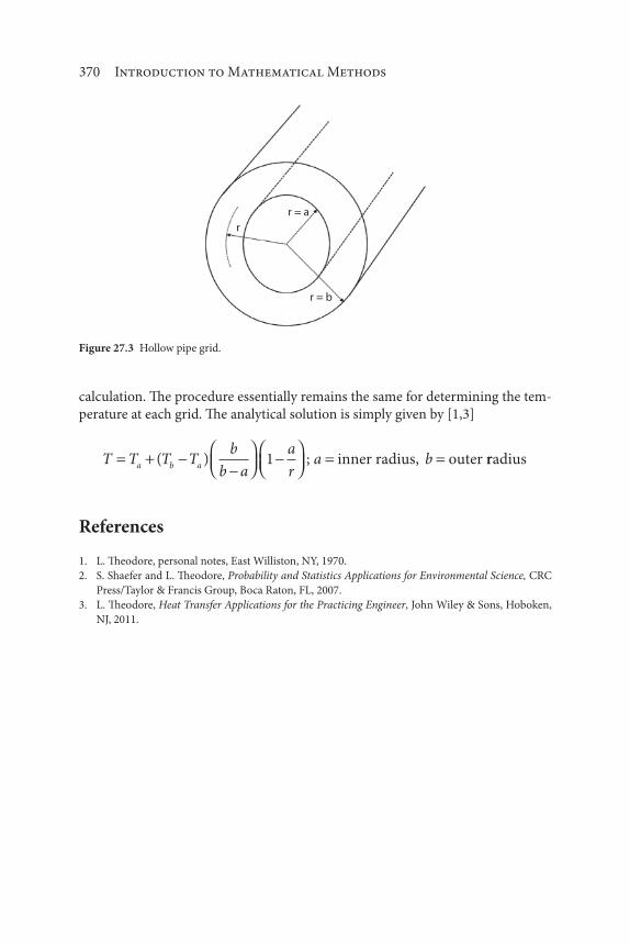
370 Introduction to Mathematical Methods
calculation. The procedure essentially remains the same for determining the tem-
perature at each grid. The analytical solution is simply given by [1,3]
T T T Tb
b a
a
ra ba b a( ) ,1 ; inner radius outer rradius
References
1. L. Theodore, personal notes, East Williston, NY, 1970.
2. S. Shaefer and L. Theodore, Probability and Statistics Applications for Environmental Science, CRC
Press/Taylor & Francis Group, Boca Raton, FL, 2007.
3. L. Theodore, Heat Transfer Applications for the Practicing Engineer, John Wiley & Sons, Hoboken,
NJ, 2011.
Figure 27.3 Hollow pipe grid.
r
r = a
r = b

371
It is not secret that statistical calculations are now performed with spreadsheets or
packaged programs. This statement is particularly true with regression analysis.
Microsoft Excel possesses an “add trend line” function that will fit scatter plot data
to a function. The result of this has often been the reduction or elimination of one’s
fundamental understanding of this subject. Without a fundamental understand-
ing, the user can easily become confused as to what type of function to use or how
to interpret the data. This chapter attempts to correct this shortcoming.
Engineers and scientist often encounter applications that require the need
to develop a mathematical relationship between data for two or more variables. For
example, if Y (a dependent variable) is a function of or depends on X (an independent
variable), i.e.,
Y f X( ) (28.1)
one may be required to express this (X, Y) data in equation form. This process is
referred to as regression analysis, and the regression method most often employed
is the method of least squares.
28Regression Analysis [1, 2]
Introduction to Mathematical Methods for Environmental Engineers and Scientists. Charles Prochaska and Louis Theodore.
© 2018 Scrivener Publishing LLC. Published 2018 by John Wiley & Sons, Inc.

372 Introduction to Mathematical Methods
Three sections compliment the presentation of this chapter. Section numbers
and subject titles follow.
27.1: Scatter Diagrams
27.2: Method of Least Squares
27.3: The Correlation Coefficient
28.1 Scatter Diagrams
An important step in a regression analysis procedure – which is often omitted – is
to prepare a plot of Y vs. X. The result, referred to as a scatter diagram, could take
on any form. Three such plots are provided in Figure 28.1 (A to C). The first plot
(A) suggests a linear relationship between X and Y, i.e.,
Y a a X0 1 (28.2)
The second graph (B) appears to be represented by a second order (or parabolic)
relationship, i.e.,
Y a a X a X0 1 2
2 (28.3)
The third plot suggests a linear model that applies over two different ranges, i.e., it
could represent the data
Y a a X X X XM0 1 0; (28.4)
and
Y a a X X X XM L0 1 ; (28.5)
This multiequation model finds application in representing adsorption equilibria,
multiparticle size distributions, quantum energy relationships, etc. In any event, a
scatter diagram and individual judgment can suggest an appropriate model at an
early stage in the analysis [1, 2].
Some of the models often employed by technical individuals are as follows:
Linear: Y a a X0 1 (28.6)
Parabolic: Y a a X a X0 1 2
2 (28.7)
Cubic: Y a a X a X a X0 1 2
2
3
3 (28.8)
Quadratic: Y a a X a X a X a X0 1 2
2
3
3
4
4 (28.9)

Regression Analysis 373
28.2 Method of Least Squares
Procedures to evaluate the regression coefficients a0, a
1, a
2, etc. referred to in
the previous section are provided below. The reader should note that the analy-
sis is based on the method of least squares. This technique provides numerical
values for the regression coefficients ai such that the sum of the square of the
Figure 28.1 Scatter diagrams: (a) linear relationship, (b) parabolic relationship, and (c) dual-linear
relationship.
(c)
(b)
(a)
Y
X
YY
X
XL
Xm
Xm
X0
X

374 Introduction to Mathematical Methods
difference (error) between actual Y and the Ye predicted by the equation or
model is minimized.
Two sets of data are shown in Figure 28.2. In Figure 28.2, the solid dots (experi-
mental value of Y) and open dots (equation or model value of Y, i.e., Ye) represent
the data and model values, respectively. On examining the two figures, one can
immediately conclude that the error (Y Ye) squared and summed for the eight
points is more for the first figure on the left. Note that a dashed line represents the
error. The line that ultimately produces a minimum of the sum of the individual
error squared, i.e., has the smallest possible value, is the regression model (based
on the method of least squares). The proof is left as an exercise.
To evaluate a0 and a
1 for a linear model (see Equation 28.6), one employs the
following least squares algorithm for n data points of Y and X.
a n a X Y0 1 (28.10)
a X a X XY0 1
2 (28.11)
All the quantities given, except a0 and a
1, can be easily calculated for the data. Since
there are two equations and two unknowns, the set of equations can be solved for
a0 and a
1. For this case,
an XY X Y
n X X1 2 2( )
(28.12)
Dividing numerator and denominator by n, and defining X X/n and Y Y/n,
leads to
aXY
X Y
n
XX
n
XY nXY
X nX1
22 2 2( )
(28.13)
Figure 28.2 Error difference: actual and predicted values.
Y
XActual / data Model value
Y
XActual / data Model value
Regression Analysis 375
Using this value of a1 produces the following equation for a
0:
a Y a X0 1 (28.14)
If the model (or line of regression) is forced to fit through the origin, then the
calculated value of Ye
0 at X 0. For this case, the line of regression takes the
form
Y a X ae 1 0 0; (28.15)
with
aXY
X1 2 (28.16)
A cubic model takes the form (see Equation 28.8):
Y a a X a X a X0 1 2
2
3
3 (28.8)
For n pairs for X Y values, the constants a0, a
1, a
2, and a
3 can be obtained by the
method of least squares so that (Y Ye)2 again has the smallest possible value,
i.e., is minimized. The coefficients a0, a
1, a
2, and a
3 are the solution of the following
system of four linear equations (1, 2):
a n a X a X a X Y0 1 2
2
3
3
a X a X a X a X YX0 1
2
2
3
3
4
a X a X a X a X YX0
2
1
3
2
4
3
5 2 (28.17)
a X a X a X a X YX0
3
1
4
2
5
3
6 3
This set of equations can be solved for a0, a
1, a
2, and a
3 since there are four equa-
tions and four unknowns. This development can be extended to other regression
equations, e.g., exponential, hyperbola, higher order models, etc.
28.3 The Correlation Coefficient
The correlation coefficient provides information on how well the model, or line of
regression, fits the data. It is denoted by r and is given by
rXY
X Y
n
XX
nY
Y
n2
22
2( ) ( )
(28.18)

376 Introduction to Mathematical Methods
or
rn XY X Y
n X X n Y Y[ ( ) ][ ( ) ]2 2 2 2 (28.19)
or
rXY nXY
X nX Y nY( )( )2 2 2 2 (28.20)
This equation can also be shown to take the from
rY Y
Y Ye( )
( )
2
2 (28.21)
The correlation coefficient satisfies the following six properties:
1. If all points of a scatter diagram lie on a line, then r 1 or 1. In
addition, r2 1. The square of the correlation coefficient is defined
as the coefficient of determination.
2. If no linear relationship exists between the X’s and Y’s then r 0.
Furthermore, r2 0. It can be concluded that r is always between
1 and 1, and r2 is always between 0 and 1.
3. Values of r close to 1 and 1 are indicative of a strong, or positive
linear relationship.
4. Values of r close to 0 are indicative of a weak linear relationship.
5. The correlation coefficient is positive or negative, depending on
whether the linear relationship has a positive or negative slope.
Thus, positive values or r indicate that Y increases as X increases;
negative values indicate that Y decreases as X increases.
6. A value of r 0 only indicates the lack of a linear correlation; X
and Y might be strongly correlated by some nonlinear relation,
as discussed earlier. Thus, r can only measure the strength of lin-
ear correlations; if the data are nonlinear, one should attempt to
linearize before computing r.
Another measure of the model’s fit to the data is the standard error of the estimate,
or se. It is given as
sY Y
ne
e( ).
20 5
(28.22)
Regression Analysis 377
Finally, the equation of the least-squares line of best fit for the given observa-
tions on X and Y can be written in terms of the correlation coefficient as follows:
Y Y rs
sX X
y
x
( ) (28.23)
where X, Y, sx, s
y, and r are the two sample means, the two sample standard devia-
tions, and sample correlation coefficient obtained from the n pairs of observations
on X and Y, respectively. It should be noted once again that the correlation coef-
ficient only provides information on how well the model fits the data. It is empha-
sized that r provides no information on how good the model is, or whether this is
the correct or best model to describe the functional relationship of the data.
Illustrative Example 28.1
Table 28.1 shows eight pairs of observations on X and Y where Y is the observed
percentage yield of a biological reaction at various centigrade temperatures, X.
Obtain the least-squares line of regression of Y on X.
Solution
The observed values of Y against the associated values of X are plotted in
Figure 28.3. The scatter diagram appears to exhibit a linear pattern. Equation 28.1
is assumed to apply. The values of X, Y, XY, X2, Y2, ( X)2, ( Y)2 and n are
now calculated:
X
Y
XY
1900
700
169 547 5, .
Table 28.1 Temperature – biological yield data.
% Yield (Y) Temperature, °C (X)
75.4 150
79.4 175
82.1 200
86.6 225
90.9 250
93.3 275
95.9 300
96.1 325

378 Introduction to Mathematical Methods
X
X
Y
Y
n
2
2
2
2
477 500
3 610 000
490 000
61 676 94
8
,
, ,
,
, .
( )
( )
The least-squares estimates, a0 and a
1, are calculated using the equations pro-
vided above. Appling Equation (28.12),
an XY X Y
n X X1 2 2
8 169547 5 1900 700
8 477500
( )
( )( . ) ( )( )
( )( )) ( )
.
3610000
0 126
(28.12)
The coefficient a0 is calculated employing Equation (28.14).
a Y a X
a
0 1
0
700
80 126
1900
8
57 5
.
.
(28.13)
Thus, the describing equation is
Y X57 5 0 126. . ; consistent units
Figure 28.3 Scatter diagram of yield vs. temperature for a biological reaction; Illustrative
Example 28.1.
70125 175 225 275 325
75
80
85
90
95
100
Pe
rce
nt
yie
ld (
Y)
Temperature (X)

Regression Analysis 379
The reader should note that if more temperature-yield data become available,
thus increasing the number of points, then the calculated line may not be the best
representation of all the data; the least-squares solution should then be recom-
puted using all the data. In addition, the assumed model, e.g., linear, may not be
the “best” model.
Illustrative Example 28.2
Use the results from the previous illustrative example to estimate the “average”
percentage yield of the biological reaction at 260 °C.
Solution
The result of
Y X0 126 57 575. .
is employed to calculate the value of Y when X 260. For X 260,
Y 0 126 260 57 575
90 3
. ( ) .
. %
Therefore, the estimated average percentage yield at 260 °C is 90.3%.
Illustrative Example 28.3
Pollutant A is undergoing a reaction in a specially controlled laboratory experi-
ment. The data in Table 28.2 have been obtained for the reaction rate, rA, vs.
concentration, CA. Using the data, estimate the coefficient k
A and in the equation
below [3]:
r k CA A A
Solution
As discussed in the introduction, given experimental data for Y measured at
known values of X, an often-encountered problem is to identify the functional
Table 28.2 Reaction rate data.
Reaction rate, rA (lbmol/ft3 · sec) Concentration, C
A (lbmol/ft3)
48 8
27 6
12 4
3 2
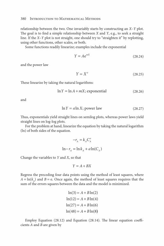
380 Introduction to Mathematical Methods
relationship between the two. One invariably starts by constructing an X–Y plot.
The goal is to find a simple relationship between X and Y, e.g., to seek a straight
line. If the X–Y plot is not straight, one should try to “straighten it” by replotting,
using other functions, other scales, or both.
Some functions readily linearize; examples include the exponential
Y A mXe (28.24)
and the power law
Y X (28.25)
These linearize by taking the natural logarithms:
ln lnY A mX; exponential (28.26)
and
ln lnY X; power law (28.27)
Thus, exponentials yield straight lines on semilog plots, whereas power laws yield
straight lines on log-log plots.
For the problem at hand, linearize the equation by taking the natural logarithm
(ln) of both sides of the equation.
r k CA A A
ln ln ln( )r k CA A A
Change the variables to Y and X, so that
Y A BX
Regress the preceding four data points using the method of least squares, where
A ln(kA) and B . Once again, the method of least squares requires that the
sum of the errors squares between the data and the model is minimized.
ln( ) ln( )
ln( ) ln( )
ln( ) ln( )
ln( ) ln(
3 2
12 4
27 6
48 8
A B
A B
A B
A B ))
Employ Equation (28.12) and Equation (28.14). The linear equation coeffi-
cients A and B are given by

Regression Analysis 381
A
B
0 2878
2 0
.
.
These may be obtained through longhand calculation. However, they are more
often obtained with the aid of computer software.
Take the inverse natural logarithm of A to obtain kA.
A k
B
Aln .
.
0 75
2 0
The equation for the rate of reaction is therefore
r CA A0 75 2 0. .
Illustrative Example 28.4
The resistance in ohms and failure time in minutes of a random sample of 20 tran-
sistors were recorded as shown in Table 28.3.
Calculate the linear correlation coefficient, r.
Solution
Calculate X, Y, XY, X2, Y2, and n for an assumed linear model.
X
Y
752
692
Table 28.3 Transistor resistance – failure time data.
Resistance (X) Failure time (Y) Resistance (X) Failure time (Y)
43 32 36 31
36 36 44 37
29 20 29 24
44 45 39 46
32 34 46 43
48 47 42 33
35 29 30 25
30 25 30 25
33 32 35 35
46 47 45 46

382 Introduction to Mathematical Methods
XY
X
Y
n
26 952
29 104
25 360
20
2
2
,
,
,
Obtain r using Equation (28.19):
rn XY X Y
n X X n Y Y[ ( ) ][ ( ) ]2 2 2 2 (28.19)
Substituting,
r20 26952 752 692
20 29104 752 20 25360 6920 86
2 2
( ) ( )
( ( ) )( ( ) ).
Illustrative Example 28.5 [4]
A solution containing 50 moles of benzene and 50 moles of toluene is batch dis-
tilled at a constant pressure until such a time that only 50 moles of liquid is left.
Determine the composition of the liquid residue at the conclusion of the distilla-
tion process. Benzene / toluene equilibrium data (x, y*) is provided in Table 28.4.
(Note that, as is common practice in batch distillation, all mole fractions refer to
the lighter component, which in this case is benzene.)
Table 28.4 Benzene / toluene equilibrium data.
x y* y* x 1/(y* x)
0.000 0.000 0.000 –
0.116 0.240 0.124 8.06
0.228 0.418 0.190 5.26
0.336 0.533 0.217 4.61
0.440 0.660 0.221 4.52
0.541 0.747 0.205 4.88
0.639 0.817 0.178 5.62
0.734 0.875 0.142 7.04
0.825 0.924 0.098 10.2
0.914 0.965 0.051 19.6
1.000 1.000 0.000 –

Regression Analysis 383
Solution
Write the Rayleigh equation for a simple batch distillation [4].
ln
,
*
W
F
dx
y x
final
x
x
W final
F
The initial concentration of benzene (mole fraction) is:
xF
50
50 500 50.
In addition,
ln ln ln( . ) .W
F
final 50
50 500 5 0 693
A trial-and-error solution is now required to determine the benzene mole
fraction in the liquid. All values are known in the above integral except for the
integral itself, i.e., the value when xW
xW, final
. The area under the curve is deter-
mined by guessing values of xW, final
until the right-hand side of the integral is equal
to 0.693. If a numerical package is not available, one may plot 1/(y* x) vs x as
in Figure 28.4.
The equation appearing in Figure 28.4 is a polynomial regression fit to the data
points, which can facilitate analytical, as opposed to numerical, integration. Upon
integration of f(x) at varying lower bounds, it can be shown that when xW, final
0.35,
Figure 28.4 Benzene / toluene equilibrium Rayleigh diagram.
y = 1910x6 – 5395x5 + 6192x4 – 3685x3 + 1219x2 – 218.8x + 21.78
00 0.2 0.4 0.6 0.8 1
5
10
15
20
25
f (x)
= 1
/(y*
– x
)
x

384 Introduction to Mathematical Methods
the area under the curve is approximately equal to 0.693, which satisfies the inte-
gral. (This calculation is left as an exercise for the reader.) Therefore,
xW final, benzene0 35. ( )
1 0 65xW final, toluene. ( )
References
1. L. Theodore and F. Taylor, Probability and Statistics, A Theodore Tutorial, Theodore Tutorials, East
Williston, NY, originally published by USEPA/APTI, RTP, NC,1996.
2. S. Shaefer and L. Theodore, Probability and Statistics Applications for Environmental Science, CRC
Press/Taylor & Francis Group, Boca Raton, FL, 2007.
3. L. Theodore, Chemical Reactor Analysis and Applications for the Practicing Engineer, John Wiley &
Sons, Hoboken, NJ, 2012.
4. L. Theodore and F. Ricci, Mass Transfer Operations for the Practicing Engineer, John Wiley & Sons,
Hoboken, NJ, 2010.

385
As one might suspect, the term optimization has come to mean different things
to different people. It has also come to mean different things for different appli-
cations, i.e., it could involve a simple two step calculation or one that requires
the use of a detailed numerical method. To take this a step further, the authors
were undecided to how to include optimization in this text, i.e., should it be a
chapter – and in which Part, or does it deserve its own Part (in this case, Part V).
After much deliberation and meditation, it was decided to present the material
in the last Part (V) of the book, as opposed to preparing a chapter for Part III in
Numerical Methods. The decision was primarily influenced by the desire that this
be a book not only on the introduction to mathematical methods but also one
that addresses a topic that is emerging as an important topic for environmental
engineers and scientists.
There are seven chapters in Part V. The chapter numbers and accompanying
titles are listed below.
Chapter 29: Introduction to Optimization
Chapter 30: Perturbation Techniques
Chapter 31: Search Methods
Chapter 32: Graphical Analysis
Part V
OPTIMIZATION
Introduction to Mathematical Methods for Environmental Engineers and Scientists. Charles Prochaska and Louis Theodore.
© 2018 Scrivener Publishing LLC. Published 2018 by John Wiley & Sons, Inc.

386 Introduction to Mathematical Methods
Chapter 33: Analytical Analysis
Chapter 34: Linear Programming
Chapter 35: Linear Programming Applications
The reader should note that some of the material in Chapter 32 - Graphical
Analysis - appeared earlier in part I, Chapter 3.

387
The optimization problem has been described succinctly by Aris as “getting the
best you can out of a given situation” [1]. Problems amenable to solution by
mathematical optimization techniques generally have one or more independent
variables whose values must be chosen to yield a viable solution and measure of
“goodness” available to distinguish between the many viable solutions generated
by different choices of these variables. Mathematical optimization techniques are
also used for guiding the problem solver to the choice of variables that maximizes
the aforementioned “goodness” measure (e.g., profit) or that minimizes some
“badness” measure (e.g., cost).
One of the most important areas for the application of mathematical optimi-
zation techniques is in chemical engineering (the authors’ supposed expertise)
design. Applications include:
1. Generation of best functional representations (e.g., curve fitting)
2. Design of optimal control systems
3. Determining the optimal height (or length) of a mass (pollutant)
transfer control (or recovery) unit
4. Determining the optimal diameter of a unit
5. Finding the best equipment material of construction
29Introduction to Optimization
Introduction to Mathematical Methods for Environmental Engineers and Scientists. Charles Prochaska and Louis Theodore.
© 2018 Scrivener Publishing LLC. Published 2018 by John Wiley & Sons, Inc.

388 Introduction to Mathematical Methods
6. Generating operating schedules
7. Selecting operating conditions
In addition to the optimization definition presented above by Aris, one
might offer the following generic definition for many environmental engineers:
“Optimization is concerned with determining the ‘best’ solution to a given
problem” [2]. Alternatively, a dictionary would offer something to the effect: “to
make the most of… develop or realize to the utmost extent… often the most effi-
cient or optimum use of.” The process of optimization in environmental practice
is required in the solution of many problems and often involves the maximization
or minimization of a mathematical function. As one might suppose many of the
applications involve economic consideration.
Three sections complement the presentation of this chapter. Section numbers
and subject titles follow:
29.1: History of Optimization
29.2: The Computer Age
29.3: The Scope of Optimization
Illustrative Example 29.1
Qualitatively discuss optimization.
Solution
Optimization is viewed by many as a tool in decision-making. It often aids in the
selection of values that allow the practicing environmental engineer to better solve
a problem. This brief answer provides a qualitative look at optimization.
As noted above, in its most elementary and basic form, one may say that opti-
mization is concerned with the determination of the “best” solution to a given
problem. This process is required in the solution of many general problems in
environmental engineering and applied science in the maximization (or minimi-
zation) of a given function(s), in the selection of a control variable to facilitate the
realization of a desired condition, in the scheduling of a series of operations or
events to control completion dates of a given project, in the development of opti-
mal layouts of organizational units within a given design space, etc.
One of the most important areas for the application of mathematical optimization
techniques is in engineering design. In engineering design, once a particular subject
or process scheme has been selected for study, it is common practice to optimize
the process from a capital cost and O&M (operation and maintenance) standpoint.
There are many optimization procedures available, most of them too detailed
for meaningful application in a text of this nature. These sophisticated optimization
techniques, some of which are routinely used in the design of conventional chemi-
cal and petrochemical plants, invariably involve computer calculations. Although

Introduction to Optimization 389
the use of these techniques in the majority of environmental applications was not
warranted in the past, more and more real-world problems are requiring the use
of optimization techniques.
29.1 The History of Optimization
The subject of mathematics encompasses the study of relationships among quanti-
ties, magnitudes, and properties of logical operations by which unknown quanti-
ties, magnitudes, and properties may be deduced. In the past, mathematics was
regarded as a science involving geometry, numbers, and/or algebra. Toward the
middle of the 19th century, however, mathematics came to be regarded increas-
ingly as the science of relations, or as the science that draws necessary conclusions.
This latter view encompasses mathematical or symbolic logic, the science of using
symbols to provide an exact theory of logical deduction and reference based on
definitions, axioms, postulates, and rules for combining and transforming primi-
tive elements into more complex relations and theorems. Enter optimization.
This brief survey of the history of optimization traces the evolution of mathe-
matical ideas and concepts, beginning in prehistory. Indeed, mathematics is nearly
as old as humanity itself; evidence of a sense of geometry and interest in geo-
metrical patterns has been found in the designs of prehistoric pottery and textiles,
and in cave paintings. Primitive counting systems were almost certainly based on
using the fingers of both hands, as evidenced by the predominance of the number
10 as the base for many number systems employed today.
Interestingly, the mathematics of the late 19th and the 20th centuries is charac-
terized by an interest in unifying elements across numerous fields of mathematical
endeavor, especially in logic. For example, group theory has proven a particularly
effective unifier. The amount of new math and the particular topics arising at that
time were numerous and varied as the unified set theory, intuitive geometry, the
development of the number systems, including methods of numeration, binary
and other bases of notation, and modular arithmetic and measurement, with
attention to accuracy, precision, and error study. It also included studies of alge-
braic systems, linear algebra, modern algebra, vectors, matrices, logic, truth tables,
the nature of proofs, Venn and Euler diagrams, relations, functions, probability
and statistics, linear programming, and computer programming.
As to the origin of optimization, it depends on who provides the response,
because there are so many aspects of optimization of interest to the practitioner.
For example, some claim it was Thomas Edison, when he developed a long-lasting,
high-quality light bulb in the 1870s. His success was primarily the result of an
extensive trial-and-error search for the optimum filament material. A few now
refer to it as the Edisonian approach. One of the authors refers to it as the pertur-
bation approach; on occasion, he has modestly termed it the Theodore approach.
Advances in computer calculation have not only reduced the cost and time
required to perform each iteration but also provides a better understanding of how
390 Introduction to Mathematical Methods
this method works. However, the success of this approach still relies heavily on the
limitations of the user’s intuition and experience, since one often cannot predict or
even comprehend the effects of changing numerous variables in a complex system.
Despite this barrier, the computer has expanded and improved the employment of
the classical methods of optimization.
With the promise of reducing design time and cost while improving product
quality, automated design optimization held tremendous potential. Starting with
a sub-optimal design, a numerical optimization algorithm could be used to itera-
tively adjust a set of pre-selected design parameters in an attempt to achieve a
set of design targets. This new class of optimization technology enables broader,
more comprehensive and faster searches for innovative designs than was possible
using previous generations of tools. Moreover, it requires no expertise in opti-
mization theory, so it is easier to use for non-experts and experts alike. By lever-
aging an engineer’s potential to discover new design concepts, this new class of
optimization technology overcomes the limits of human intuition and extends the
designer’s professional capability to achieve break-through designs and accelerated
innovation.
As noted earlier, today’s computers now allow optimization (or mathematics,
computer science, operations research, mathematical optimization of mathemati-
cal programming) to more easily select the best element (with regard to some cri-
teria) from some set of available alternatives. In the simplest case, an optimization
problem consists of maximizing (or minimizing) a real function by systematically
choosing input values from within an allowed set of variables in order to compute
the value of the function. Mathematically speaking, optimization allows one to
find the best available value(s) of some objective function given a defined domain
(or a set of constraints), including a variety of different types of objective functions
and different types of domains. These various options are discussed in the last sec-
tion of this chapter.
29.2 The Computer Age
Although digital computers are often viewed as fast calculators or special slide
rulers, they are, in fact, rather general devices for manipulating symbolic informa-
tion. As noted, the symbols being manipulated are numbers or digits (hence the
name digital computer), and the operations being performed on the symbols are
the standard arithmetical operations such as addition and subtraction. Famularo
offered the following thoughts in the late 1960s: “The digital computer can be
viewed as a high-speed calculator, which, with the availability of subroutines and
a compiling language, is able to perform many mathematical operations such as
add, multiply, generate analytic functions, logic decisions, etc.” [3]. Although the
details of coding are not in the scope of this text, there is an intermediate step
between the equations and the coding program, and that is to arrange the comput-
ing procedure in block diagram or information flow form. The operation of each

Introduction to Optimization 391
block is described inside the block, and the computer will perform the instruc-
tions around the loop until the condition in the decision block is satisfied, at which
time the most recently computed values were then punched out on tape or card.
For a large computer, this entire sequence, including a half dozen cycles around
the loop, would be accomplished within a millisecond or so. Of course, as the
number of equations to be solved increases, the time required to obtain a solution
increases. For cases where the solution time becomes excessive, mathematics or
other more sophisticated programming is used to accelerate the convergence and
decrease the total computation time required.
High-speed computing equipment (today’s computers) has had a tremendous
impact on engineering design, scientific computation, and data processing. The
ability of computers to handle large quantities of data and to perform the math-
ematical operations described above at tremendous speeds permits the analysis of
many more applications and more engineering variables than could possibly be
handled on the aforementioned slide ruler – the trademark of engineers of yester-
year. Scientific calculations previously estimated in lifetimes of computation time
are currently generated in seconds and, on many occasions, microseconds, and in
some rare instances, nanoseconds [4].
Increased growth is expected in the microcomputer field as inexpensive infor-
mation-processing devices continue to be explored. The cost will continue to
decrease, while the cost of the associated software will probably tend to increase;
computerized processes will, therefore, be quite inexpensive unless customized
programs must be written.
29.3 The Scope Of Optimization
One can conclude from the above that the theory and application of optimization
is mathematical in nature, and it typically involves the maximization or minimiza-
tion of a function (usually known), which represents the “performance” of some
“system.” This is carried out by the finding of values for those variables, which
cause the function to yield an optimal value.
Perhaps the most important tool employed in optimization by environmental-
ists is linear programming. Linear programming consists of a linear, multivari-
able function, which is to be optimized (maximized or minimized), subject to a
particular number of constraints. The constraints are normally expressed in linear
form. Integer linear programming refers to optimization problems in which at
least some of the variables must assume integer values. The reader should note that
the terms linear programming and nonlinear programming are essentially similar
from an application perspective. There were problems around the middle of the
last century because of some difficulties that arose in attempting to solve nonlin-
ear programming problems. However, the arrival of the modern-day computer
and sophisticated software (e.g., EXCEL) have removed these problems. Unless
a solution is presented graphically in this Part, it will be obtained directly from

392 Introduction to Mathematical Methods
EXCEL so that the reader need not be concerned with whether a system’s perti-
nent describing equations and constraints are linear or nonlinear. Thus, details
regarding the solution methodology for both linear programming and nonlinear
programming problems plus the accompanying illustrative examples will not be
presented later. They are simply not necessary and beyond the scope of this text.
One of the major responsibilities in optimization is to construct the correct
objective function to be maximized. In a simple environmental problem, the
objective function might be the profit associated with the operation of a land-
fill that treats two categories of waste: “inert” and “non-inert.” One optimization
problem could be to maximize the profit (from handling the waste) by employing
an operating treatment schedule subject to the landfill’s capacity and environmen-
tal regulatory requirements, or the problem might be rephrased in the following
manner: what combination of the quantities of the two wastes will produce the
maximum profit subject to the constraints connected with the landfill’s process-
ing capabilities and the different regulation requirements imposed on each waste.
The objective function may be quite simple and easy to calculate in some envi-
ronmental applications, or it may be complicated and difficult to not only calculate
but also specify and/or describe. The objective function may also be very illu-
sive due to the presence of conflicting or dimensionally incompatible objectives;
for example, one might be asked to optimize the profit for the aforementioned
landfill that not only minimizes air and water contamination but also is aestheti-
cally appealing. Thus, it may not be always possible to quantify an objective func-
tion and hence be able to use any of the mathematical optimization procedures
available.
There are a large number of mathematical optimization methods available in
practice. Some of the simple ones are listed below:
1. A function of one variable with no constraints
2. A function of two variables with no constraints
3. A function of more than two variables with no constraints
4. Simple perturbation schemes
5. A function of one variable with constraints
6. A function of two variables with constraints
7. A function of more than two variables with constraints
Several of the above methods will be reviewed in the chapters to follow.
Some optimization problems can be divided into parts, where each part is then
optimized. In some instances, it is possible to attain the optimum for the original
problem by simply realizing how to optimize these constituent parts. This pro-
cess is very powerful, as it allows one to solve a series of smaller, easier problems
rather than one large one. One of the best-known techniques to attack such prob-
lems is dynamic programming; this approach is characterized by a process which
is performed in stages, such as manufacturing processes. Rather than solving the
problem as a whole, dynamic programming thus optimizes one stage at a time to

Introduction to Optimization 393
produce an optimal set of decisions for the whole process. Although dynamic pro-
gramming has applicability in some systems/processes, it is not reviewed in this
book. If the assumption of linearity cannot be made, as it was in the case of linear
programming, there do exist some general procedures for nonlinear problems.
The collection of techniques developed for these problems is called nonlinear pro-
gramming. This too is addressed in this book.
Finally, most engineering optimization applications involve economics: maxi-
mizing profit, minimizing cost, or both. Environmental applications can involve
minimizing toxic emissions, maximizing energy usage and conservation, mini-
mizing health and safety risks, standard economic concerns, etc. The reader
should not lose sight that most real-world industry applications involving optimi-
zation usually require simple solutions. Here is a comment from a retired engineer
[4]: “Generally, the consumer goods industry where I worked does not rely on
sophisticated models. Basically, optimization was conducted to determine overall
consumer preference, or liking, to determine how to use minimum resources and
lastly to determine how to minimize costs subject to constraints. In the determi-
nation of consumer preference, we typically used design of experiments to exam-
ine the broad range of attributes that led to maximum product liking or decision
to purchase. Occasionally, we modeled processes and used regression models. In
that case, we could search or compute the desired maximum. The last set of tech-
niques used is what the business world calls Operations Research. Typically, linear
or dynamic programming was used to evaluate an objective function subject to
constraints. For example, we used linear programming in hot dog manufacturing.
The goal was to come up with a mixture of meat cuts that minimized costs while
meeting governmental requirements for protein, fat, and water content”.
References
1. R. Aris, Discrete Dynamic Programming, Blaisdell, Boston, MA, 1964.
2. L. Theodore, personal notes, East Williston, NY, 2011.
3. J. Famularo, personal communication to L. Theodore (with permission), Englewood Cliffs, NJ,
1973.
4. R. Altomare, communication to L. Theodore, Bronx, NY, 2016.

395
A significant number of optimization problems face the environmental engineer.
The optimal design of industrial processes as well as process equipment has
long been of concern to the practicing engineer, and indeed, for some, might be
regarded as a definition of the function and goal of applied engineering. The prac-
tical attainment of an optimum design is generally a result of factors that include
mathematical analysis, empirical information, and both the subjective and objec-
tive experience of the engineer and/or scientist.
One simple approach for solving optimization problems that is recommended
by the authors is a trial-and-error scheme that includes perturbation calculations.
This involves a systematic change of variables, one by one, in an attempt to locate
an optimum. To be practical, this can mean that one must limit the number of
variables by assuming values to those (process) variables that are known before-
hand to play an insignificant role. Reasonable guesses or simple or shortcut math-
ematical methods can further simplify the procedure. Much information can be
gathered from this type of study since it usually identifies those variables that sig-
nificantly impact the solution, such as on the overall performance of equipment
or a process, and helps identify the major contributors effecting the optimization
calculations.
30Perturbation Techniques
Introduction to Mathematical Methods for Environmental Engineers and Scientists. Charles Prochaska and Louis Theodore.
© 2018 Scrivener Publishing LLC. Published 2018 by John Wiley & Sons, Inc.

396 Introduction to Mathematical Methods
Four sections complement the presentation of this chapter. Section numbers
and subject titles follow:
30.1: One Independent Variable
30.2: Two Independent Variables
30.3: Three Independent Variables
30.4: The Heat Exchange Network Dilemma
30.1 One Independent Variable
Two illustrative examples highlight this section. These examples have a depen-
dent variable that depends on one independent variable. One example involves a
cyclone and air pollution recovery/control. The second example is concerned with
minimizing the work requirement for a two-stage compressor.
Illustrative Example 30.1
A process emits 50,000 acfm of gas containing a dust (it may be considered ash
and/or metal) at a loading of 2.0 gr/ft3. A cyclone [1, 2] is employed for particle
capture and the dust captured from the unit is worth $0.03/lb of dust. Experimental
data have shown that the collection efficiency, E, is related to the system pressure
drop, ΔP, by the formula:
EP
P 15 0.
where E fractional collection efficiency
ΔP pressure drop, lbf /ft2 (psf)
If the fan is 55% efficient (overall) and electric power costs $0.18/kWh at what
pressure drop and corresponding collection efficiency should the cyclone operate
to maximize profits? Earlier studies suggest that the optimum pressure drop is in
the 5–35 psf range.
Solution
The value of the recovered material (RV) may be expressed in term of the frac-
tional collection efficiency E, the volumetric flowrate q, the inlet dust loading w,
and the value of the dust (DV):
RV (q)(w)(DV)(E)
Substituting yields

Perturbation Techniques 397
RV50,000 ft
min
2.0 gr
ft
1 lb
7000 gr
0.033
3
$$
lb$/minE E0 429. ;
The recovered value can be expressed in terms of pressure drop, i.e., replace E
by ΔP:
RV /min( . )( )
.$
0 429
15 0
P
P
The cost of power (CP) in terms of ΔP, q, the cost of electricity (CE) and the fan
efficiency, Ef , is
CP q P CE E f( )( )( )/( )
Substitution yields
CP
50,000 ft
min
lb
ft kWh
kW3
f
2
P 0 18 1. $ min
444 200
1
0 55
1
0 006
, .
.
ft lb 60 min
$/min
f
P
h
The describing equation for the profit P is given by:
P RV CP
Substitution gives
Px
xx x P
0 429
15 00 006
.
.. ;
Table 30.1 Calculations for Illustrative Example 30.1.
x, psf P, $/min
5.0 0.0773
10.0 0.1116
15.0 0.1245
20.0 0.1251
25.0 0.1181
30.0 0.1060
35.0 0.0903

398 Introduction to Mathematical Methods
Since the pressure drop is believed to exist between 5 and 35 psf, employ incre-
ments of 5 psf over the range and calculate the profit P in $/min. The results for P
to four significant figures are recorded in Table 30.1. Using the above perturbation
analysis, the results indicate that the profit achieves a maximum value of approxi-
mately 0.1251 $/min at an operating pressure drop of approximately 20 psf. The
reader may choose to resolve Illustrative Example 6.4.
Illustrative Example 30.2
Consider the two-stage reversible adiabatic compression of a gas from an initial
pressure P1 to a final pressure P
3. If the gas enters at T and is cooled to T between
stages, the total work E is given by [3,4]
E NRTk
kP
P
P
P
k
k
k
k
122
1
1
3
2
1
where E total work ft lbf
R molal gas constant
T inlet absolute temperature
k 1.4, the ratio of heat capacity at constant pressure to heat capacity at
constant volume for the compressed gas
Determine the intermediate stage pressure if E is to be minimized and
P1
1 atm and P3
10 atm.
Solution
The intermediate stage pressure of P2 exists in the range 1 P
210. To apply
the perturbation method, select increments of 2 atm between the range of
2 and 8, i.e. 2, 4, 6, 8. Calculated values of E at these intervals are presented in
Table 30.2 assuming NRT 1 and k 1.4. The results in Table 30.2 indicate
that for E to be minimized the intermediate pressure P2 value is 4 atm with E
at 2.748 ft lbf. The results further suggest that the minimum energy expen-
diture occurs between 2 and 6 atm. Selecting the midpoint between 2
Table 30.2 Illustrative Example 30.2 calculation.
P2, atm E, ft lb
f
2 2.810
4 2.748
6 2.890
8 3.070

Perturbation Techniques 399
and 4 atm and 4 and 6 atm could provide an improved answer for the
minimum E. The reader may choose to resolve Illustrative Example 11.2.
30.2 Two Independent Variables
This section presents two examples that illustrate the method solution when
there are two independent variables. These examples introduce the reader to the
concept of constraints.
Illustrative Example 30.3
Obtain the maximum and minimum for the following function describing the
emission E from a stack.
E x x3 51 2
There are two constraints:
0 3 0 41 2x x,
Solution
Proceed as illustrated below. The function E can be calculated at the 20 points
shown in parenthesis.
( ) ( ) ( ) ( )
) ( ) ( ) ( )
( )
( )
( )
(
, , , ,
, , , ,
,
,
,
,
0 0 1 0 2 0 3 0
0 1 1 1 2 1 3 1
0 2
0 3
0 4
1
(
22
1 3
1 4
2 2
2 3
2 4
3 2
3 3
3 4
)
( )
( )
( )
( )
( )
( )
( )
( )
,
,
,
,
,
,
,
,
The value of the function for each point is shown immediately to the right of the
point in parenthesis.
( , ) ( , ) ( , ) ( , )
( , ) ( , ) ( , ) ( , )
( , )
(
0 0 0 1 0 3 2 0 6 3 0 9
0 1 5 1 1 8 2 1 11 3 1 14
0 2 10
00 3 15
0 4 20
1 2 13
1 3 18
1 4 23
2 2 16
2 3 21
2 4 26
3
, )
( , )
( , )
( , )
( , )
( , )
( , )
( , )
( ,, )
( , )
( , )
2 19
3 3 24
3 4 29
As can be seen from the above results, the maximum (emission) E is 29 and
occurs at x1
3 and x2
4, and the minimum E is located at x1
0 and x2
0 with
a minimum value of 0 for E.
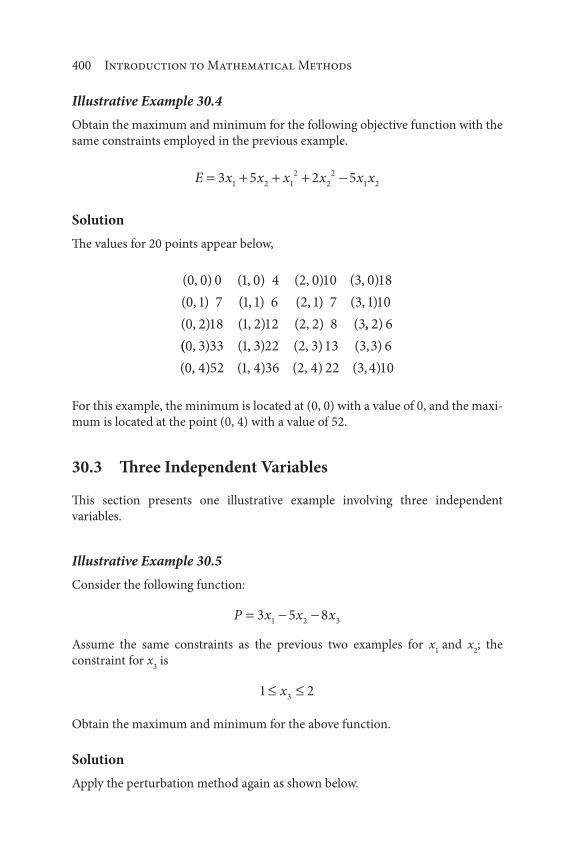
400 Introduction to Mathematical Methods
Illustrative Example 30.4
Obtain the maximum and minimum for the following objective function with the
same constraints employed in the previous example.
E x x x x x x3 5 2 51 2 1
2
2
2
1 2
Solution
The values for 20 points appear below,
( , ) ( , ) ( , ) ( , )
( , ) ( , ) ( , ) ( , )
( , )
0 0 0 1 0 4 2 0 10 3 0 18
0 1 7 1 1 6 2 1 7 3 1 10
0 2 18
(( , )
( , )
( , )
( , )
( , )
( , )
( , )
( , )
(
0 3 33
0 4 52
1 2 12
1 3 22
1 4 36
2 2 8
2 3 13
2 4 22
3,, )
( , )
( , )
2 6
3 3 6
3 4 10
For this example, the minimum is located at (0, 0) with a value of 0, and the maxi-
mum is located at the point (0, 4) with a value of 52.
30.3 Three Independent Variables
This section presents one illustrative example involving three independent
variables.
Illustrative Example 30.5
Consider the following function:
P x x x3 5 81 2 3
Assume the same constraints as the previous two examples for x1
and x2; the
constraint for x3 is
1 23x
Obtain the maximum and minimum for the above function.
Solution
Apply the perturbation method again as shown below.

Perturbation Techniques 401
For x3
1:
( , ) ( , ) ( , ) ( , )
( , ) ( , ) ( , ) ,
(
( )
0 0 8 1 0 5 2 0 2 3 0 1
0 1 13 1 1 10 2 1 7 3 1 4
00 2 18
0 3 23
0 4 28
1 2 15
1 3 20
1 4 25
2 2 12
2
, )
( , )
( , )
( , )
( , )
( , )
( , )
( ,, )
( , )
( , )
( , )
( , )
3 17
2 4 22
3 2 9
3 3 14
3 4 19
For x3
2:
( , ) ( , ) ( , ) ( , )
( , ) ( , ) ( , ) ,(
0 0 16 1 0 13 2 0 10 3 0 1
0 1 21 1 1 18 2 1 15 3 11 6
0 2 26
0 3 31
0 4 36
1 2 23
1 3 28
1 4 33
2 2
)
( , )
( , )
( , )
( , )
( , )
( , )
( , ) 20
2 3 25
2 4 30
3 2 11
3 3 16
3 4 21
( , )
( , )
( , )
( , )
( , )
Based on the above two trials for x3, the maximum is located at (3, 0, 1) and
the minimum value is located at (0,4,2) with corresponding P values of 1 and 36,
respectively. However, additional perturbation calculations should be performed
for values of x3 between 1 and 2.
30.4 The Heat Exchange Network Dilemma
This last section involves a heat exchange design project that is concerned with
not only energy recovery but also energy conservation. The design is based
on a network of heat exchangers at a refinery and the purpose of the project
is to arrange a network consisting of an unknown (and unspecified in terms
of area) number of exchangers in order to satisfy certain specified design
conditions [5].
The remainder of this last section of the “Perturbation” chapter consists of two
illustrative examples. The first example introduces the heat transfer system under
study [6]. The last example requests the design of a heat exchanger network sys-
tem to satisfy a specified requirement. This project demonstrates that despite the
advances in analytical numerical methods, a perturbation method of solution may
be the only viable option for the designer. For the second example, one out of a
near infinite amount of possible solutions is presented. Theodore [7] provides two
additional examples that ratchet up the complexity of other possible requirements
by increasing the difficulty in obtaining the “best” solution. These examples present
evidence of how difficult it may be to solve some real-word optimization problems.

402 Introduction to Mathematical Methods
Illustrative Example 30.6
A refinery has three streams to be heated (see Table 30.3) and three streams to
be cooled (see Table 30.4). Cooling water (90 °F supply, 115 °F return) and steam
(saturated at 250 psi) are available. Note that the saturated steam at 250 psi has a
temperature of 401 °F. Calculate the heating and cooling duties and indicate what
utility (or utilities) should be employed.
Solution
The sensible heating duties for all streams are first calculated. The total heating and
cooling duties can now be computed and compared. The results are shown below.
Heating: 7,475,000 6,612,000 9,984,000 24,071,000 Btu/h
Cooling: 12,600,000 4,160,000 3,150,000 19,910,000 Btu/h
Heating – Cooling: 24,071,000 – 19,910,000 4,161,000 Btu/h
As a minimum, 4,161,000 Btu/h will have to be supplied by steam or another hot
medium.
Illustrative Example 30.7
Refer to the previous Illustrative Example. Devise a network of heat exchanges that
will make full use of heating and cooling streams against each other, using utilities
only if necessary [5].
Table 30.3 Streams to be heated.
Stream
Flowrate,
lb/hr CP, Btu/lb °F T
in, °F T
out, °F
1 50,000 0.65 70 300
2 60,000 0.58 120 310
3 80,000 0.78 90 250
Table 30.4 Streams to be cooled.
Stream
Flowrate,
lb/hr CP, Btu/lb °F T
in, °F T
out, °F
1 60,000 0.70 420 120
2 40,000 0.52 300 100
3 35,000 0.60 240 90

Perturbation Techniques 403
Solution
Figure 30.1 represents a system of heat exchanges that will transfer heat from the
hot streams to the cold ones in the amounts desired. It is important to note that this
is but one of many possible schemes. The optimum system would require a trial-
and-error procedure that would examine a host of different networks. Obviously,
the economics would also come also into play.
It should also be noted that in many chemical and petrochemical plants there
are cold streams that must be heated and hot streams that must be cooled. Rather
than use steam to do all the heating and cooling water to do all the cooling, it is
often advantageous, as demonstrated in this problem, to have some of the hot
streams heat the cold ones. The problem of optimum heat exchanger networks to
accomplish this has been extensively studied and is available in the literature. This
example provides one simple illustration.
Finally, highly interconnected networks of exchangers can save a great deal of
“quality” energy [3, 6, 8] in a refinery or chemical plant. This issue is also addressed
by Theodore [7]. The more interconnected they are, however, the harder the refin-
ery is to control, start-up, and shut down [5]. In addition, an economic analysis
should be included in any study [5, 7]. Often auxiliary heat sources and cooling
sources must be included in the plant design in order to ensure that the plant can
operate smoothly [5].
References
1. L. Theodore, Air Pollution Control Equipment Calculations, John Wiley & Sons, Hoboken, NJ,
2008.
Figure 30.1 Heat exchanger network flow diagram.
2
6,612,000
1,600,000 4,388,000 1,496,000
2,500,000
650,000 2,665,000
4,160,00
4
3
6
1
5100°F
70°F
90°F
90°F
120°F
90°F 218°F
121°F
115.6°F
158°F
120°F
250°F
240°F
300°F
300°F
Steam
Steam
310°F2
4
3
6
3
3
420°F

404 Introduction to Mathematical Methods
2. L. Theodore, Chemical Engineering: The Essential Reference, McGraw- Hill, New York City, NY,
2014.
3. L. Theodore, F. Ricci, and T. VanVliet, Thermodynamics for the Practicing Engineer, John Wiley &
Sons, Hoboken, NJ, 2009.
4. P. Abulencia and L. Theodore, (adapted from) Fluid Flow for the Practicing Chemical Engineer, John
Wiley & Sons, Hoboken, NJ, 2009.
5. D. Kauffman, Process Synthesis and Design, A Theodore Tutorial, Theodore Tutorials, East Williston,
NY, originally published by the USEPA/APTI, RTP, NC, 1992.
6. A.M. Flynn and L. Theodore, “Kern’s Process Heat Transfer,” 2nd ed., Scrivener-Wiley, Salem, MA,
(forthcoming) 2018.
7. L. Theodore, Heat Transfer Applications for the Practicing Engineer, John Wiley & Sons, Hoboken,
NJ, 2011.
8. L. Theodore, R. Dupont, K. Ganesan, Unit Operations in Environmental Engineering, Scrivener-
Wiley, Salem, MA, 2017.

405
The mathematicians’ literature abounds with search methods, i.e., methods that
allow one to search for a solution to an equation. There are both indirect and direct
approaches, with indirect search methods generally defined as indirect methods.
However, direct methods – those that produce an exact answer – are generally pre-
ferred by environmental engineers and scientists. These methods have also been
defined in the literature as seek methods, and usually apply to single-independent
variable unimodal equations; they provide results in intervals (or limits) of uncer-
tainty for the variable in a (minimum) number of trials during the search process.
Two such procedures that are available include the interval halving (or bisection)
and golden section search methods [1]. The unimodal function referred to above
for single-independent variable equations contains a single optimization (maxi-
mum or minimum) point over a specified interval. Some applications can arise for
multi-independent variable equations; perhaps the most popular approach to these
equations is the steepest ascent/descent method [2]. It should also be noted that non-
linear algebraic equations are often solved using the Newton-Rhapson method [3];
however, this latter method requires that the derivative of the function is available.
When an initial interval has been established around the optimum, interval
reduction schemes may be applied to obtain an improved estimate of the location
of the optimum point. The amount of subinterval eliminated at each step depends
on both the initial interval and the location of the initial trial points within the
31Search Methods
Introduction to Mathematical Methods for Environmental Engineers and Scientists. Charles Prochaska and Louis Theodore.
© 2018 Scrivener Publishing LLC. Published 2018 by John Wiley & Sons, Inc.
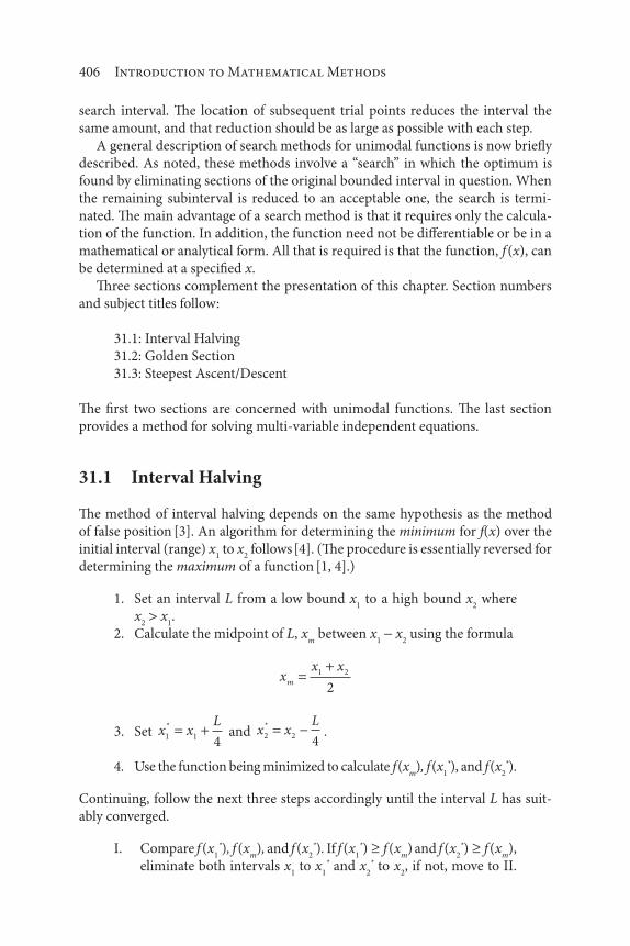
406 Introduction to Mathematical Methods
search interval. The location of subsequent trial points reduces the interval the
same amount, and that reduction should be as large as possible with each step.
A general description of search methods for unimodal functions is now briefly
described. As noted, these methods involve a “search” in which the optimum is
found by eliminating sections of the original bounded interval in question. When
the remaining subinterval is reduced to an acceptable one, the search is termi-
nated. The main advantage of a search method is that it requires only the calcula-
tion of the function. In addition, the function need not be differentiable or be in a
mathematical or analytical form. All that is required is that the function, f (x), can
be determined at a specified x.
Three sections complement the presentation of this chapter. Section numbers
and subject titles follow:
31.1: Interval Halving
31.2: Golden Section
31.3: Steepest Ascent/Descent
The first two sections are concerned with unimodal functions. The last section
provides a method for solving multi-variable independent equations.
31.1 Interval Halving
The method of interval halving depends on the same hypothesis as the method
of false position [3]. An algorithm for determining the minimum for f(x) over the
initial interval (range) x1 to x
2 follows [4]. (The procedure is essentially reversed for
determining the maximum of a function [1, 4].)
1. Set an interval L from a low bound x1 to a high bound x
2 where
x2
x1.
2. Calculate the midpoint of L, xm
between x1 x
2 using the formula
xx x
m
1 2
2
3. Set x xL
1 14
* and x x
L2 2
4
*.
4. Use the function being minimized to calculate f (xm), f (x
1*), and f (x
2*).
Continuing, follow the next three steps accordingly until the interval L has suit-
ably converged.
I. Compare f (x1
*), f (xm
), and f (x2
*). If f (x1
*) f (xm
) and f (x2
*) f (xm
),
eliminate both intervals x1 to x
1* and x
2* to x
2, if not, move to II.
Search Methods 407
The new range L, (x1 to x
2) is the original x
1* to x
2* while x
m remains
unchanged. The optimum is now known to be between the new x1
and x2. If the interval L has been reduced to a satisfactory level the
calculation is stopped. If it is not, begin again at step 1 calculating
new values based on the new interval L.
II. Compare f (x1
*) and f (xm
). If f (x1
*) f (xm
), eliminate the interval
from xm
to x2 and set a new high interval x
2 to the old midpoint x
m.
In addition, set the new midpoint xm
equal to x1
*. The new range
L is therefore x1 to x
2 where x
2 is the old x
m. The optimum is now
known to be between the new x1 and x
2. If L has been reduced to
a satisfactory level, the calculation is stopped. If the interval is
not yet small enough, proceed to start again at step 1 calculating
new values based on the new interval L. If, however f (x1
*) f (xm
),
proceed to III.
III. Compare f (x2
*) and f (xm
). If f (x2
*) f (xm
), eliminate the interval
x1 to x
m and set a new low interval x
1 equal to the old midpoint x
m.
In addition, set the new midpoint xm
equal to x2
*. The new range
L is therefore x1 to x
2 where x
1 is now the old x
m. The optimum is
now known to be between the new x1 and x
2. If L has been reduced
to a satisfactory level, the calculation is stopped. If the interval is
not small enough, proceed to start again at step 1, calculating new
values based on the new interval L.
Illustrative Example 31.1
Refer to Illustrative Example 30.1. Solve the problem using the interval halving
method.
Solution
Once again, the describing equations (functions) for the profit P in $/min is:
Px
xx
0 429
15 00 006
.
..
where x pressure drop in psf. Employ the interval halving method over the range
of 5 to 35 for x1
5 and x2
35 to obtain the maximum profit. Proceed as sug-
gested above.
L x x( )2 1 35 5 30
xx x
m
( )2 1
2
35 5
220

408 Introduction to Mathematical Methods
x xL
1 14
530
412 5* .
x xL
2 24
3530
427 5* .
P x( *, ) .lower 0 1150
P x( *, ) .upper 0 1126
P x Pm( ) ( ) .20 0 1251
Since both P (12.5) P (20), and P (27.5) P (20) eliminate the intervals x1
* to x1,
i.e. 5 to 12.5 and x2
* to x2, i.e., 27.5 to 35. The remaining interval is therefore 12.5
to 27.5.
Calculate an updated L, x1
*, and x2
*.
L 27 5 12 5 15. .
x1 12 515
416 25* . .
x2 27 515
423 75* . .
Repeat the above calculations noting that xm
remains at 20.
P( . ) .16 25 0 1256
P( . ) .23 75 0 1204
Since P (23.75) P (20), eliminate the interval xm
to x2, i.e., 20 to 27.5. The remain-
ing interval is therefore 12.5 to 20. The calculation may be further updated (for L
and xm
).
L 20 12 5 7 5. .
xm
20 12 5
216 25
..
P( . ) .16 25 0 1256 $/min
Further calculations are optional. If one were to stop here, the maximum profit
would approximately be 0.1256 $/min at a pressure drop of 16.25 psf.
Search Methods 409
Illustrative Example 31.2
Refer to Illustrative Example 30.2. Solve the problem employing the interval halv-
ing method.
Solution
Employing the interval halving approach between an initial range of P1
1 atm
and P3
10 atm would proceed as follows.
L P P3 1 9
Pm
1 10
25 5.
P lower1 19
41 2 25 3 25* ( ) . .
P upper3 109
410 2 25 7 75* ( ) . .
E P Pm( ) ( . ) .5 5 2 848
Evaluate E at P1
* and P2
*,
E( . ) .3 25 2 727
E( . ) .7 75 3 047
Since E (3.25) E (5.5), the correct P must therefore lie in the range 3.25 P 5.5.
Repeat the above calculations.
L 5 5 1 4 5. .
Pm
1 5 5
23 25
..
P lower1 14 5
41 1 125 2 125* ( )
.. .
P upper3 5 54 5
45 5 1 125 4 375* ( ) .
.. . .
E P Em( ) ( . ) .3 25 2 727

410 Introduction to Mathematical Methods
E P E( ) ( . ) .*
1 2 125 2 789
E P E( ) ( . ) .*
3 4 375 2 768
Since P (2.125) and P (4.375) are P (3.25), eliminate the outer intervals, P1 to P
1*
and P2 to P
2*. It appears the correct P is in the range 2.125 P 4.375. The cor-
responding E at Pm
3.25
E( . ) .3 25 2 727
The reader may choose to refine the calculation further for the optimum P
and E.
31.2 Golden Section
An improvement on the interval halving method can be had by employing the
golden section method. Consider the two trial points located between the initial
interval x1 and x
2 as pictured in Figure 31.1. Assume the initial interval, x
1 to x
2, has
arbitrarily been set equal to 1.0 units and the minimum of f (x) in the range (x1, x
2)
is desired. If the right side of the interval, i.e., 1 (where is a fractional quan-
tity) is discarded based on the calculations for f (x1), f (x
2), f (x
3), and f (x
4), then
the new interval that would remain is with x3 located from x
1; this is pictured
in Figure 31.2. The question that arises is: what value of should be selected? The
golden selection method is based on 0.618. The basis of this choice is provided
in the literature [5].
1
1– = 2 2 –1 = 3 1–
1–
x4
x1 = 0 x
2 = 1 x
3
Figure 31.1 Golden section initial search.

Search Methods 411
1
1–
1– = 2 2 –1 = 3 1–
x4
x1 = 0 x
3x
2 = 0
4 =2– 3
= 2–3
1– = 2
2 –1 = 3 2 –1
1– = 2
x5
Figure 31.2 Golden Section; remaining interval.
1
1–
1– = 2 2 –1 = 3 1–
x4
x1 = 0 x
3x
2 = 0
4 =2– 3
= 2–3
2 –1
1– = 2
x5
{First interval
reduction}
{Second interval
reduction}
x6
4 = ( 2)2
2 –1 = 3
1– = 2
1– = 2
4 5
Figure 31.3 Golden Selection; Subsequent Interval.

412 Introduction to Mathematical Methods
The result of the first calculation has reduced the first (original) interval from
1 to . In effect is now the new interval. This may be viewed as a fraction of
the original interval, often given as the product of the first interval and . Refer
once again to Figure 31.2. The next trial point would then be located at x5 which
is 2 1 from x, the same distance from x4 to x
5. [Note: It can be shown that in
the golden section method 2 1 . The solution of this quadratic equation 2 1= 0 is simply
( ) ( )( ) ( )( )( )1 1 1 4 1 1
2
the positive solution of which is 0.618.] Following the second trial with x5 results in
a further reduction of the interval by 2 1 which can be shown to equal (1 ).
The interval has thus been reduced by the product of the interval ( ) and ( 1).
Further, the new or remining interval is once again the product of the previous
interval ( ) and ( ) i.e., ( )( ) 2. Each successive trial would result in an inter-
val reduction given by multiplying the interval by . For n trials, the final interval
would be ( )n. If n 5, the final interval would be (0.618)5 0.0901; the interval is
therefore reduced by more than 90% after 5 trials.
Illustrative Example 31.3
Refer to Illustrative Example 31.1. Solve this maximization problem employing
the golden section search method.
Solution
The function to be maximized is
Px
xx
0 429
15 00 006
.
..
Once again, assume an initial range of (5,35 with an interval of 30). Based on the
material provided above obtain P at the following values of x.
P( )5
P( )35
Noting that (0.618)(30) 18.54 and (0.382)(30) 11.46,
P P( . ) ( . )11 46 5 16 46
P P( . ) ( . )18 54 5 23 54

Search Methods 413
The calculated results are:
P( ) .5 0 03025
P( ) .35 0 0903
P( . ) .16 46 0 2302
P( . ) .23 54 0 1208
Since the function is to be maximized, eliminate the interval (23.54, 35). The
interval has therefore been reduced from (5,35) to (5, 23.45). Calculate P at the
location of the next trial, i.e., at – 2. However, and as shown in Figure 31.3,
2 2 31 0 236( ) ( ) .
the new location then becomes 5 (0.236)(30) 5 7.08 12.08. Continuing, the
interval (5, 12.08) may be eliminated, narrowing the interval where the maximum
is located to (12.08, 23.54). The calculation may be continued as demonstrated
above… or simply assume an average over the new interval x and calculate the
corresponding P
xm
12 08 23 54
217 81
. ..
P( . ) .12 08 0 1189
P( . ) .17 81 0 1260
P( . ) .23 54 0 1208
This represents an estimate of the solution of the example.
31.4 Steepest Ascent/Descent
The method of steepest ascent/descent involves calculations where a step size is
selected to achieve the maximum amount of increase/decrease of the function at
each succeeding step. Thus, the step size gradient varies as the calculation continues,
settling on zero as the maximum/minimum point is approached. Perhaps Happel
[2] provided a satisfactory explanation and illustrative example involving steepest
ascent/descent calculations from an engineering perspective. His description follows.
“There are many situations, especially where experimentation is involved, in
which neither an analytical nor graphical representation is available for the
function to be optimized for the entire range of the variables involved. The
question then arises as to what course the experimenter should follow, be it

414 Introduction to Mathematical Methods
in the research laboratory or full-scale commercial plant. He may employ any
of the several trial-and-error procedures previously discussed. However, if
results are known only for a small area, some efficient method of extrapolation
will help to minimize the amount of trial and error necessary. Such a scheme
is the method of steepest ascents. The concept behind the idea of predicting
a path of steepest ascent is simply that a plane does a good job of approxi-
mating a curved surface over a limited area. Thus, for a situation involving
the maximizing of a function of two independent variables, a contour map
with the variables as horizontal co-ordinates and the (profit) function as the
vertical coordinate will illustrate the plan. The best-fitting plane is obtained
in a small area under investigation. Then, from the tilt of the fitted plane, the
direction of further experimentation is established as the direction of steepest
ascent. Experiments are performed along this path until a decline in response
is noted. Additional observations/ calculations are taken around this point
to confirm whether a maximum has indeed been reached or whether a new
path of steepest ascent should be predicted. The method, of course, does not
eliminate the possibility that more than one optimum may exist in the area
of interest.
In practice, the method of steepest ascents is generally applied to calcula-
tion involving more than two variables. It is difficult, but the mechanics is
entirely similar to the two-dimensional approach. More specifically, the par-
tial derivatives of the response f(x) will indicate its rate of change with respect
to a series of variables, x1, x
2, x
3, …. From these derivatives the gradient [6]
[ ( )]f x is computed
[ ( )]( ) ( ) ( )
f x if x
xi
f x
xi
f x
x1
1
2
2
3
3
(31.1)
where i1, i
2, i
3, … are unit vectors in the directions of coordinate axes repre-
senting the variables, each variable being associated with one dimension in
a multidimensional space. The gradient [ ( )]f x is a vector which has the
property of being directed along the path on which f(x) increases most rapidly
(i.e. the path of “steepest ascent”). The direction is along a path proportional
to the rate of increase for a unit change of each variable.”
The following example, similar to the two stage compressor problem of
Illustrative Example 30.2, illustrates the way the procedure works. By applying
it in a case where the result is known, it is possible to readily note its limitations.
Technically, it is correct only at the base chosen for each ascent. As exploration
moves from this point, the shape of the response surface must change.
Illustrative Example 31.4
Consider the case of a three-stage compressor. It is desired to demonstrate the
method of steepest ascents for P1
1 and P4
10 atm. Since the procedure implies

Search Methods 415
knowledge of the work expended corresponding to only a limited area, rather than
the complete range, the arbitrary assumption will be made that the intermediate
pressures are taken at the start as P2
4 and P3
7 atm.
Solution
In this example, the optimum will be reached by the steepest descent to minimum
total work, which corresponds to maximum profit for the operation employing
such a compressor. The describing equation for the work E is [2]
E NRTk
kP
P
P
P
P
P
k
k
k
k
12
1
1
3
2
1
4
3
( ) ( ) ( )k
k
1
3
Once again, NRT is set equal to 1, k 1.4, P1
1, and P4
10. It will be shown in
Chapter 33 that the minimum work is
E f2 575. ft lb
and the corresponding optimum values of P2 and P
3 are
P2 2 154. atm
P3 4 642. atm
The direction of steepest ascent at P2
4, P3
7 is obtained by differentiating
the describing equation for E (differentiation and substitution steps have been
omitted for simplicity),
E
P2
1
1 4
1 4 1
1 4
1 2 8
1 44 7 4
0 079
( ) ( ) ( )
.
( ) ( ) ( )
.
.
.
.
.
Similarly,
E
P3
0 009.
To obtain the path of steepest descent, increments of pressure must be taken
proportional to these rates of change; thus
P
P2
3
0 079
0 0098 8
.
..

416 Introduction to Mathematical Methods
If increments of P3 are taken equal to 0.05, then the increments of ΔP
2
(0.05 8.8) 0.44. In this way the first descent is established starting at P2
4 and
P3
7:
Using the same procedure following the first decent, a second derivative is
made starting at P2
2.68 and P3
6.85. This results in establishing the condi-
tion P2
2.50 and P3
4.45 with E 2.587 as the minimum point. A third descent
from this point establishes P2
2.14 and P3
4.60 with E 2.576. These condi-
tions are shown on Figure 31.4. Three descents are sufficient to establish the opti-
mum condition.
It should be noted that considerable accuracy in computation is required to
establish the optimum. This frequently occurs in applying the method so that it
is finally necessary to use an analytical expression to establish the optimum accu-
rately. Numerical results are provided in Table 31.1. Another limitation in the
procedure, using the method of steepest ascents and the general differentiation
procedure previously discussed is that they do not take into account constraints
imposed on the system. The gradient may lead into an area in which operations
are not possible.”
First interstage, P2 atm
Se
con
d in
ters
tag
e, P
3 a
tm
02
3
4
5
6
7
82.65
2.60
2.59
2.58
2
E = 2.70
9
10
1 2 3 4 5
Figure 31.4 Contours of constant work Note: Path of steepest descent shown dotted.

Search Methods 417
References
1. R. Ketter and S. Prawel, Modern Methods of Engineering Computation, McGraw-Hill, New York
City, NY, 1969.
2. J. Happel, Chemical Process Economics, John Wiley & Sons, Hoboken, NJ, 1958.
3. L. Theodore, Chemical Engineering: The Essential Reference, McGraw-Hill, New York City, NY,
2014.
4. L. Theodore, personal notes, East Williston, NY, 2010.
5. G. Reklaitis, A. Ravindran, and K. Ragsdell, Engineering Optimization, John Wiley & Sons,
Hoboken, NJ, 1983.
6. L. Theodore, Transport Phenomena for Engineers, Theodore Tutorials, East Williston, NY, originally
published by the International Textbook Company, Scranton, PA, 1971.
Table 31.1 Results of Illustrative Example 31.4.
P2, atm P
3, atm E, ft · lb
f
4.00 7.00 2.681
3.56 6.95 2.653
3.12 6.90 2.629
2.68 6.85 2.615 (min)
2.24 6.80 2.622

419
The general subject of graphical analysis serves as an excellent starting point
before proceeding to analytical analysis, the subject title for the next chapter. The
overlap between these two topics will become apparent in the both the develop-
mental material and illustrative examples to follow. Most of the early presentations
in this chapter will involve the repetition and extension of some of the mathemati-
cal methods reviewed earlier in Parts I, II, and III; hopefully, this duplication will
assist the reader during his/her review of this material as it relates to optimization.
Engineering data are often best understood when presented in the form of
graphs or mathematical equations. The earlier preferred method of obtaining the
graphical relations between variables was to plot the data as straight lines and
use the slope-intercept method to obtain coefficients and exponents; therefore, it
behooves the environmental engineer and scientist to be aware of the methods of
obtaining straight lines on the various types of graph paper, and of determining
the equations of such lines [1]. One always strives to plot data as straight lines
because of the simplicity of the curve, ease of interpolation, and ease of extrapola-
tion. Graphical methods proved invaluable in the past in the analysis of the rela-
tively complex processes of that era. Much of the basic physical and chemical data
are still best represented graphically.
32Graphical Approaches
Introduction to Mathematical Methods for Environmental Engineers and Scientists. Charles Prochaska and Louis Theodore.
© 2018 Scrivener Publishing LLC. Published 2018 by John Wiley & Sons, Inc.

420 Introduction to Mathematical Methods
One or more of the many types of graphical representations may be employed
for the following purposes:
1. as an aid in visualizing a process for the representation of quantita-
tive data
2. for the representation of quantitative data
3. for the representation of a theoretical equation
4. for the representation of an empirical equation
5. for the comparison of experimental data with a theoretical expression
6. for the comparison of experimental data with an empirical expression
7. for solving some optimization problems
The relation between two quantities, y-the dependent variable and x-the inde-
pendent variable, is commonly obtained as a tabulation of values of y for a number
of different values of x. The relation between y and x may not be easy to visualize
by studying tabulated results and is often best seen by plotting y vs. x. If the condi-
tions are such that y is known to be a function of x only, the functional relation
will be indicated by the fact that the points may be represented graphically by a
smooth curve. Deviations of the points from a smooth curve can indicate the reli-
ability of the data. If y is a function of two variables, x1 and x
2, a series of results
of y in terms of x1 may be obtained for a (definite) constant x
2. When plotted, the
data will be represented by a family of curves, each curve representing the rela-
tion between x1 and y for a constant value of x
2. If another variable x
3 is involved,
one may have separate graphs for constant values of x3, each showing a family
of curves of y vs. x1. One may expand this method of representing data to more
than three independent variables, although this rarely occurs in practice. In addi-
tion, graphs may be employed to perform common mathematical manipulations
such as integration and differentiation, operations that usually arises in analytical
analyses.
Data may be of almost any type encountered in environmental engineering
and science practice. They may be physical property data, such as the variation
in density and viscosity with temperature along a tube in a heat exchanger. One
of the things that should be kept in mind is the loss of accuracy arising due to
the use of graphs whenever one works with plotted data. In general, the num-
ber of significant figures may be only as great as the size of the divisions on the
graph.
Five sections complement the presentation of this chapter. Section numbers
and subject titles follow:
32.1: Rectangular Coordinates
32.2: Logarithmic-Logarithmic (Log-Log) Coordinates
32.3: Semi- Logarithmic (Semi-Log) Coordinates
32.4: Methods of Plotting Data
32.5: Optimization Illustrative Examples

Graphical Approaches 421
32.1 Rectangular Coordinates
Rectangular (sometimes referred to as Cartesian) coordinates graph paper is most
generally used to represent equations of the form
y mx b (32.1)
where
y variable represented on the ordinate
x variable represented on the abscissa
m slope of the line
b y-intercept at x 0
The most common form of graph paper for engineering use is the 8 12 11-inch
sheet, having 20 lines per inch, with every fifth line accented, and every tenth line
heavily accented. This type of coordinate graph may be obtained on drawing or
tracing paper, with lines in black, orange, or green, and with or without accented
and heavy lines; it is also available in other sizes. Also note that the bulk of the
development in the last section of this chapter will key on rectangular coordinates.
All graphs are created by drawing a line, or lines, about one or more axes. For
the purposes of this chapter the presentation will be primarily concerned with
graphs built around two axes, the x axis and the y axis. The graph data may be
presented as coordinates of the x and y axis in the form (x, y), or they may be pre-
sented as the abscissa (distance from the y axis or the x coordinate) and the ordi-
nate (distance from the x axis or the y coordinate). Referring to Figure 32.1, point
L5 has an abscissa (x coordinate) of 60 and an ordinate of 40 (y coordinate).
Using coordinate notation, the point can be described as (60, 40) where the points
are listed as (x, y). Point L2 can be described as ( 6.7,0).
All coordinates are produced as the result of solving an equation by assigning
different values to x or y, and solving for the value of the other. By convention,
equations are usually stated in the following form: y equals some value(s) of x and
other constants, e.g., y mx b.
Equations are identified by the type of line (or curve) they produce when plot-
ted on a graph. A linear equation, as the name implies, will result in a plot of a
straight line on a graph. With the linear equation, each incremental change of
x (or y) will result in an incremental change of a fixed ratio in y (or x). The ratio
of change between y and x is known as the slope of the line. A linear equation is
also referred to as a first-degree equation. The remainder of this section provides
methods briefly introduced in Chapter 2.
In Figure 32.1, the line plotted between L1 and L5 is linear. A non-linear equa-
tion, when plotted, will result in a line having one or more curves, and the ratio
of change between x and y is not constant. The line between points N0 and N5 in
Figure 32.2 represents a plot of a non-linear equation. Non-linear equations come
in a variety of forms and may be quickly identified since they have at least one term

422 Introduction to Mathematical Methods
–3–10
0
10
20
30
40
50
60
70
80
90
–2 –1 0 1 2 3 4 5 6 7
N0N1
N2
N3
N4
N5(5, 78.5)
(4, 50.3)
(3, 28.3)
(2, 12.6)
(1, 3.1)
(0, 0)
y axis
x axis
Figure 32.2 Non-linear equation.
Quadrant III Quadrant IV
Quadrant I
y axis
x axis
Quadrant II
(–40, –20)
–40–40
–30
–20
–10
0
10
20
30
40
50
60
–30 –20 –10 0 10 20 30 40 50 60
(–6.7, 0)
(0, 4)
(10, 10)
(60, 40)
y = 0.6x + 4
L5
L4
L3
L2
L1
Figure 32.1 Linear coordinates.
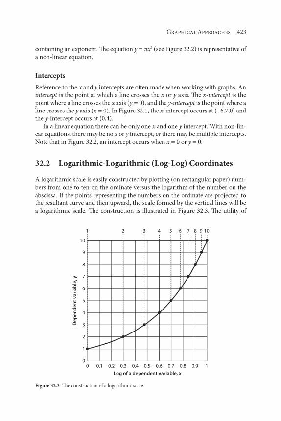
Graphical Approaches 423
containing an exponent. The equation y πx2 (see Figure 32.2) is representative of
a non-linear equation.
Intercepts
Reference to the x and y intercepts are often made when working with graphs. An
intercept is the point at which a line crosses the x or y axis. The x-intercept is the
point where a line crosses the x axis (y 0), and the y-intercept is the point where a
line crosses the y axis (x 0). In Figure 32.1, the x-intercept occurs at ( 6.7,0) and
the y-intercept occurs at (0,4).
In a linear equation there can be only one x and one y intercept. With non-lin-
ear equations, there may be no x or y intercept, or there may be multiple intercepts.
Note that in Figure 32.2, an intercept occurs when x 0 or y 0.
32.2 Logarithmic-Logarithmic (Log-Log) Coordinates
A logarithmic scale is easily constructed by plotting (on rectangular paper) num-
bers from one to ten on the ordinate versus the logarithm of the number on the
abscissa. If the points representing the numbers on the ordinate are projected to
the resultant curve and then upward, the scale formed by the vertical lines will be
a logarithmic scale. The construction is illustrated in Figure 32.3. The utility of
0
1
2
3
4
5
6
7
8
9
10
1 2 3 4 5 6 7 8 9 10
0.10 0.2 0.3 0.4 0.5
Log of a dependent variable, x
De
pe
nd
en
t v
ari
ab
le, y
0.6 0.7 0.8 0.9 1
Figure 32.3 The construction of a logarithmic scale.

424 Introduction to Mathematical Methods
the logarithmic scale lies in the fact that one can use actual numbers on the scale
instead of the logarithms. When two logarithmic scales are placed perpendicular
to each other and lines are drawn vertically and horizontally to represent major
divisions, full logarithmic graph paper results, i.e., a log-log graph.
The term log-log or full logarithmic is used to distinguish between another
kind of graph or relationship yet to be discussed, i.e., semi-logarithmic (see next
section). The full logarithmic may be obtained in many types depending on the
scale length, sheet size, and number of cycles desired. The paper is specified by
the number of cycles of the ordinate and abscissa; for example, logarithmic 2 3
cycles means two cycles on the ordinate and three on the abscissa. Cycle lengths
are generally the same on both axes of a particular graph. In addition, the distance
between numbers differing by a factor of 10 is constant on a logarithmic scale.
Equations of the general form
y bxm (32.2)
where
y a variable
x a variable
b a constant
m a constant
will plot as straight lines on (full) logarithmic paper. A form of the equation analo-
gous to the slope-intercept equation for a straight line is obtained by writing and
then subsequently plotting the equation in logarithmic form.
log log logy b m x (32.3)
If log y versus log x were plotted on rectangular coordinates, a straight line of
slope m and y-intercept log b would be obtained. An expression for the slope is
obtained by differentiating Equation (32.3).
d y
d xm
(log )
(log ) (32.4)
When x 1, m log x 0, Equation (32.3) reduces to
log logy b (32.5)
Hence, log b is the y-intercept.
To illustrate the above, a linear plot of the equation
y x2 1 3. (32.6)

Graphical Approaches 425
Figure 32.4 A linear plot of y 2x1.3 on rectilinear graph paper.
0
0.302
1.0
1.08
0.43
0.43
m = = 1.30.650.5
0.5
0.6
0.6
0.1
0.1log
10 x
log10
y
on rectangular coordinate paper is given in Figure 32.4. It should be noted that
although the slope was obtained from a ratio of logarithmic differences, the same
result could have been obtained using measured differences if the scale of ordinate
and abscissa were the same (in this case they were).
Inspection of Figure 32.5 reveals that equal measured distances on the loga-
rithmic scale are equivalent to equal logarithmic differences on the abscissa of
that plot. It therefore follows that since the slope of Equation (32.3) is a ratio of
coordinate differences, the slope on full logarithmic paper could be obtained using
measured distances. The plot of Equation (32.6) on 2 2 cycle logarithmic paper is
given in Figure 32.5. The slope using logarithmic differences is
m1 08 0 43
0 60 0 101 3
. .
. .. (32.7)
and the slope using measured differences is also
ma
b1 3. (32.8)
32.3 Semilogarithmic (Semi-Log) Coordinates
This section is a review on Semi-Log coordinates visited earlier in Chapter 3,
section 3.3 and includes their application with regard to optimization. Graph

426 Introduction to Mathematical Methods
paper made with one logarithmic scale and one arithmetic scale is termed semilog-
arithmic. The logarithmic scale is normally the ordinate and the arithmetic scale
is the abscissa on semilogarithmic paper. The paper is available in many styles
depending on the sheet size, type of paper, color of lines, number of cycles, length
of cycles, and the divisions on the uniform scale. The designation semilogarithmic,
7 5 to the ½ inch refers to semilogarithmic paper whose logarithmic scale con-
tains seven cycles whose uniform scale contains five divisions to the half inch. The
designation 10 division per inch (70 divisions) by two 5-inch cycles refers to paper
whose arithmetic scale is seven inches long and contains ten division per inch, and
whose logarithmic scale contains two-cycles for each five inches. Thus, a semi-
logarithmic graph uses a standard scale for one axis and a logarithmic scale for the
other axis, i.e., the graph uses scales of different mathematical proportions. The
reason for this use of scales is that a logarithmic (exponential) plot would quickly
exceed the physical boundaries of the graph if one were to plot values of some base
having exponents of 2, 3, 4, 5, 6, 7 and 8 against an ordinary numeric scale.
Semilogarithmic paper can be used to represent as straight lines equation of
the form
y nemx (32.9)
or
y n mx10 (32.10)
100
80
60
40
20
10
ab
y
x
8
6
4
2
11 2 4 6 8 10 20 40 60 80 100
Figure 32.5 The Equation y 2x1.3 Plotted on Logarithmic Graph Paper.

Graphical Approaches 427
where
y dependent variable
x independent variable
n a constant
m a constant
e the natural logarithm base
Here again a form of the equation analogous to the slope-intercept equation
can be obtained by placing the above equation in logarithmic form. For example,
Equation (32.9) may be written as
log y b mx (32.11)
where b log n
An expression for slope is obtained from the differential form of Equation (32.11):
d y
dxm
(log ) (32.12)
so that the y-intercept is log n or b.
One can illustrate the use of semilogarithmic paper by plotting a segment of the
curve representing the equation
log ..
yx
2 246 3
(32.13)
The line may be constructed (see also Figure 32.6) by choosing values of x, solving
for y, and plotting the results. Note that values of y and not log y are plotted on the
ordinate. The slope is a logarithmic difference divided by an arithmetic difference
and in this case may be calculated from the two indicated points (see Figure 32.6)
as follows:
mlog( ) log( . )
. .
1587 158 7
43 6 0
1
46 3 (32.14)
The slope of a line on semilogarithmic coordinates may be calculated from any
two points, but the simplest method is the one used above in which the slope is the
logarithmic difference on one cycle (equal to log 10 or 1.0) divided by the arithme-
tic difference of one cycle. Note that if the cycle had been taken between y 300
and y 3000, the slope would be
mlog( ) log( )
. .
3000 300
59 12 7
1
46 3 (32.15)

428 Introduction to Mathematical Methods
It should also be noted that the y-intercept is 2.2, as required by Equation (32.13).
In addition to the more common types of paper previously discussed, the prac-
ticing environmental engineer and scientist may also have need for probability
versus arithmetic, probability versus logarithmic, logarithmic versus reciprocals,
and other special type of graphs. Non-standard scales, if desired, may be con-
structed in a similar manner to the logarithmic scale shown earlier. For example,
logarithmic-probability (log-normal) graphics find applications in air pollution
studies [1] to describe particle size distribution.
32.4 Methods of Plotting Data
The simplest procedure to employ in plotting equations of various forms is pro-
vided below in Table 32.1. Various additional forms are available in the literature.
Details on statistical methods for calculating the coefficients in the 7 equations are
provided in the literature [2].
32.5 Optimization Illustrative Examples
This last section contains five illustrative examples. Some are extensions of prob-
lems discussed earlier with the material keying on solutions employing graphical
approaches.
5000
1000
500
1000 10 20 30 40
x
y
50 60 70 80
Figure 32.6 The equation log y 2.2 x 46 3. plotted on semi-logarithmic paper.

Graphical Approaches 429
Illustrative Example 32.1
Some optimization problems require the solution to a problem where the depen-
dent variable is a function of two independent variables, e.g.,
y f x f x x( ) ( , )1 2
Outline a simple graphical procedure that one can employ to obtain the mini-
mum (or maximum) of this type of function.
Solution
The optimum values of x1 and x
2 can be found graphically on a two-dimensional
plot by employing the following method. See Figure 32.7. In this figure, y is plotted
against one of the independent variables (x1) with the second variable (x
2) held at a
constant value. A series of such plots can be made with each dashed curve represent-
ing a different constant value of the second variable. As shown in Figure 32.7, each
of the curves (a, b, c, d, and e) gives one value of the variable x1 at the point where
f (x) is a minimum. The curve AB represents the locus of all these minimum points,
and the optimum value of x1 and x
2 occurs at the minimum point on the AB curve.
The reader should also note once again that similar graphical procedures can
be used when there are more than two independent variables, e.g., x1, x
2, and x
3.
The first step would be to make a plot similar to Figure 32.7 at one constant value
of x3. Each plot would give an optimum value of x
1, x
2, and f (x) for a particular
x3. Finally, the overall optimum value of x
1, x
2, x
3, and f (x) could be obtained by
plotting x3 versus the individual optimum values of f (x). This procedure is rarely
employed by the practicing environmental engineer.
Table 32.1 Plotting procedure.
y a bx Plot y vs. x.
y axn Plot log y vs. log x or y vs. x on logarithmic coordinates.
y c axn First obtain c as the intercept on a plot of y vs. x; then plot log (y – c)
vs. x on logarithmic coordinates.
y abex Plot log y vs. x or y vs. x on semilogarithmic coordinates.
y abx Plot log y vs. x or y vs. x on semilogarithmic coordinates.
y ab
xPlot y vs.
1
x.
yx
a bxPlot
x
y vs. x or
1
y vs.
1
x.
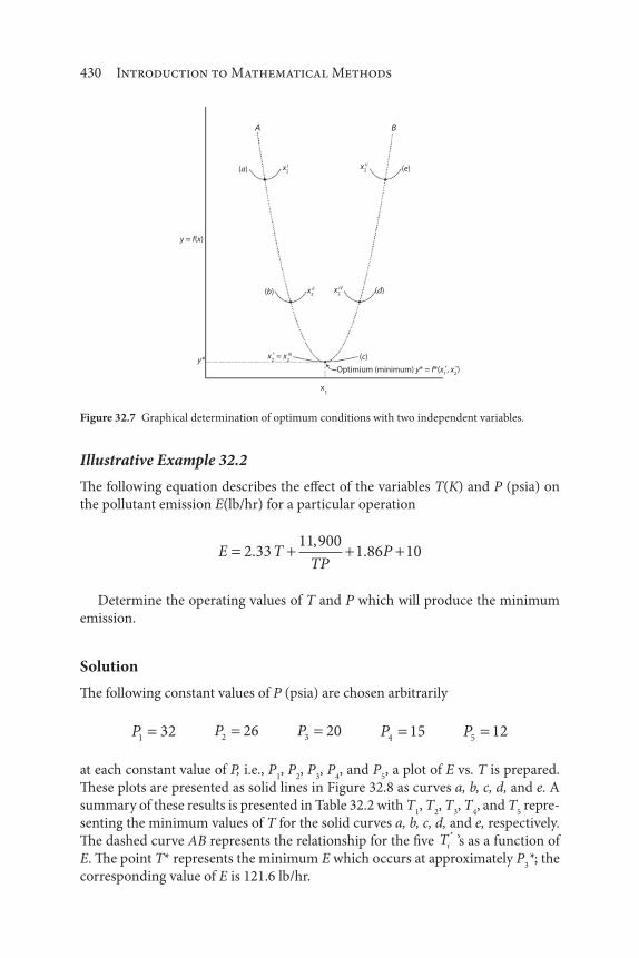
430 Introduction to Mathematical Methods
Illustrative Example 32.2
The following equation describes the effect of the variables T(K) and P (psia) on
the pollutant emission E(lb/hr) for a particular operation
E TTP
P2 3311 900
1 86 10.,
.
Determine the operating values of T and P which will produce the minimum
emission.
Solution
The following constant values of P (psia) are chosen arbitrarily
P1 32 P2 26 P3 20 P4 15 P5 12
at each constant value of P, i.e., P1, P
2, P
3, P
4, and P
5, a plot of E vs. T is prepared.
These plots are presented as solid lines in Figure 32.8 as curves a, b, c, d, and e. A
summary of these results is presented in Table 32.2 with T1, T
2, T
3, T
4, and T
5 repre-
senting the minimum values of T for the solid curves a, b, c, d, and e, respectively.
The dashed curve AB represents the relationship for the five Ti
*’s as a function of
E. The point T* represents the minimum E which occurs at approximately P3*; the
corresponding value of E is 121.6 lb/hr.
Optimium (minimum) y* = f*(x1*, x
2*)
A B
(e)(a)
(b)
y*
y = f(x)
(d)
(c)
x1
x2II
x2* = x
2III
x2IV
x2Vx
2I
Figure 32.7 Graphical determination of optimum conditions with two independent variables.

Graphical Approaches 431
The curve AB in Figure 32.8 passing through the various optimum points
shows that the overall minimum emission occurs at approximately
T 16 K
with corresponding
P 20 pisa
and
E 121.6 lb/hr
Illustrative Example 32.3
Refer to Illustrative Example 30.1. Solve the problem using a graphical approach.
Table 32.2 Optimal T and P results
P, psia Optimum T, K Minimum E, lb/hr
P1
32 T1 12 7* . 128.3
P2
26 T2 14 1* . 123.6
P3
20 T3 16 0* . 121.6
P4
15 T4 18 5* . 123.9
P5
12 T5 20 7* . 128.5
Figure 32.8 Graphical determination of emission with two independent variables (T, P).
130
E(T, R)
129
128
127
126
125
124
123
122121.6
12112 14 T* = 16
P* = P3 = 20psia
P2 = 26psia
P1 = 32psia P
5 = 12psia
P4 = 15psia
Optimium (minimum) E* = E*(T*, P*)
(c)
(d)(b)
(a) (e)
BA
18 20 22T, K
E, lb/hr

432 Introduction to Mathematical Methods
Solution
To solve the program graphically, plot P versus x on arithmetic graph paper.
The calculated values are shown in Figure 32.9. The maximum profit appears
approximately at 0.125 $/min of a pressure drop of 20 psf.
Illustrative Example 32.4
Refer to Illustrative Example 30.2. Solve the problem employing a graphical
approach.
Solution
Figure 32.10 provides a graphical plot of the four E vs P calculations from
Illustrative Example 30.2 The results indicate that for minimum work expenditure
0.14
0.12
0.1
0.08
0.06
0.04
0.02
00 5 10 15 20 25 30 35 40
Pro
fit
($/m
in)
Pressure drop, psf
Figure 32.9 P vs. x for Illustrative Example 32.3.
2.70 1 2 3 4 5 6 7 8 9
2.8
2.9
3
3.1
E, ft
lbf
P, atm
Figure 32.10 E vs x for Illustrative Example 32.4.

Graphical Approaches 433
the intermediate stage pressure appears to be in the neighborhood of 4 atm with a
corresponding work load of 2.75 ft·lbf.
References
1. L. Theodore, Air Pollution Control Equipment Calculations, John Wiley & Sons, Hoboken, NJ, 2008.
2. S. Shaefer and L. Theodore, Probability and Statistics Applications for Environmental Science, CRC
Press/Taylor & Francis Group, Boca Raton, FL, 2007.

435
The subject of analytical analysis serves as an excellent starting point before pre-
ceding to the last subject of optimization in this Part – linear programming. In
terms of introduction, once again consider the following. Since the derivative
dy dx/ or f (x), represents the rate of change of y with respect to the change in
x, it is evident that the derivative will be zero if the function passes through a
maximum or minimum. If the occurrence of such a maximum or minimum is to
be determined and located, the derivative must be equated to zero, thus providing
the condition for which the maximum or minimum exists. This analytical proce-
dure is of considerable value in environmental engineering calculations since the
location of a maximum or minimum is frequently of practical importance. As one
might suppose, many of the applications are related to economics, e.g., maximiz-
ing profit and/or minimizing cost (see also the first section in this chapter).
Five sections complement the presentation of this chapter. Section numbers
and titles follow:
33.1: Breakeven Considerations
33.2: One Independent Variable
33.3: General Analytical Formulation of the Optimum
33.4: Two Independent Variables
33.5: Three Independent Variables
33Analytical Approaches
Introduction to Mathematical Methods for Environmental Engineers and Scientists. Charles Prochaska and Louis Theodore.
© 2018 Scrivener Publishing LLC. Published 2018 by John Wiley & Sons, Inc.

436 Introduction to Mathematical Methods
33.1 Breakeven Considerations
In solving many environmental optimization problems, one often selects optimum
conditions from the standpoint of economics. Consider, a simple case in which
there is only one independent variable affecting profit P, i.e., income I minus
cost C. Refer to Figure 33.1. The term y is the dependent variable that will later
be referred to as the objective function and x is the independent variable. The for-
mer term could represent the aforementioned profit and x could be the operating
temperature. As can be seen from Figure 33.1, the “system” operates at a loss when
operating below x* and operates at a profit when above x*. The term x* is located
at the breakeven point, i.e. where the profit is zero.
The above breakeven problem can be solved by three methods.
1. Solve the problem analytically as follows. Assume I and C can be
represented in equation form, i.e.,
I I(x) (33.1)
C C(x) (33.2)
Since
P I C (33.3)
the solution for x when P 0 provides the breakeven point (of the
operation).
2. Select various values of x and calculate both the income and cost,
and profit. The breakeven point arises when the profit is zero.
3. Graph the results. A typical solution is presented in Figure 33.1.
See also the previous chapter.
Profit, P
x*
x*
x
Cost, C
y
Income, I
(I, x)
(P, x)
(C, x)
Figure 33.1 Breakeven figure.

Analytical Approaches 437
Economic studies often reveal that certain cost factors increase while others
decrease relative to an independent variable. For example, as the thickness of
the insulation (x) on a steam pipe increases, the cost of the insulation increases
but correspondingly the heat loss (and steam-generating cost) decreases [1–3].
Here the thickness of the insulation serves as the independent variable and if the
installed cost of the insulation and the steam-generating cost (the independent
variable) could both be determined as functions of the independent variable,
a condition would exist for which the total cost is a minimum. This solution is
pictured in Figure 33.2 and the optimum income is located at the point, x*. Here,
the total cost is plotted against the insulation thickness.
33.2 One Independent Variable
The case of a dependent variable and a single (one) independent variable was
reviewed in the thee previous chapters. Here
y f (x) (33.4)
Insulation thickness, x
Tota
l co
st
Heatloss cost
Economicoptimum
Fixed charges
x*
Figure 33.2 Total cost vs insulation thickness.

438 Introduction to Mathematical Methods
As noted above, the optimization of y can be generated by setting
dy
dx0 (33.5)
The optimum y is obtained by substituting the value of x from Equation (33.5) into
Equation (33.4) and, y is a maximum if
dy
dx0 (33.6)
When x from Equation (33.5) is substituted into Equation (33.4) the calculated
y is a minimum if
d y
dx
2
20 (33.7)
To summarize, a maximum occurs when dy dx/ 0 and d y dx2 2 0/ ; a mini-
mum occurs when dy dx/ 0 and d y dx2 2 0/ ; this development will be revisited
later in this chapter in section 33.3.
Illustrative Example 33.1
Consider the following function
y xx
162 2.3311 900,
Determine the maximum (or minimum) of the above function by analytical
means.
Solution
Apply Equation (33.5).
dy
dx x2.33
11 9000
2
,
Solution for x,
x2 11 900
2 335 107
,
.,
x 71.5

Analytical Approaches 439
The second derivative dy dx2 2/ is negative since
dy
dx x
2
2 3
23800
The calculated value of y at x 71.5 is therefore a maximum with a value of
y 162 2 33 71 5
11 900
71 5162 166 6 166 4 161 8
( . )( . ),
.. . .
Illustrative Example 33.2
Refer to Illustrative Example 30.1. Solve the problem analytically.
Solution
Once again, the describing equation is
Px
xx
0 429
15 00 006
.
..
To proceed analytically, calculate dP dx/ and set it equal to zero.
dP
dx x
x
x
0 429
15 0
0 429
15 00 006 0
2
.
.
.
( . ).
Solve for x by any suitable method.
0 4290 429
15 00 006 15 0 0.
.
.. ( . )
x
xx
x 17.5 psf
The corresponding maximum profit is then
P( . )( . )
. .( . )( . )
. . . ;
0 429 17 5
17 5 15 00 006 17 5
0 231 0 105 0 126 $$/min
The above analytical result compares formally with the results provided earlier
in Illustrative Examples 30.1, 31.1, 31.3 and 32.3.

440 Introduction to Mathematical Methods
Illustrative Example 33.3
Refer to Illustrative Example 30.2. Solve the problem employing an analytical
approach.
Solution
As noted in Illustrative Example 31.2 the total work is given by
E NRTk
k
P
P
P
P
k
k
k
k
122
1
1
3
2
1
If this quantity is to be a optimized, then the derivative must be zero(s), i.e.,
dE
dP
k
k
k
kP P
k
k
k
k k
2
1
1
2
1
1
1 1P P
k
k
k
k
3
1
2
1 2
0
NRT has once again been arbitrarily set equal to unity. Solving for P2 yields
P2
(k – 1)/k P1
(k – 1)/kP3
(k – 1 )/k
Rearranging yields
P P P2 1 3
1 2 10( ) 3.162 atm/
The corresponding minimum value of E is then
E P( . ) .2 3 162 2 726 ft lbf
This result compares favorably with the answers provided earlier in Illustrative
Examples, 31.2, and 32.2.
Interestingly, Happel [3] addresses the problem of maximizing the work
requirement for a three-stage compressor operating between 1 and 10 atm. This
problem was solved using an analytical approach along with the method of steep-
est ascent [3] (See also the previous development in Illustrative Example 3.4).
Applying the analytical method for the two intermediate pressures P2 and P
3 yields
the equations (see Illustrative Example 31.4 for details)
P2
(P1
2P4)1/3
P3
(P4
2P1)

Analytical Approaches 441
With P1
1 and P2
10 atm,
P2
101/3 2.154 atm
P3
102/3
4.642 atm
and
E 2.575 ft ∙ lbf
Happel [3] also noted that the location of a maximum or minimum becomes
obvious if the function is plotted, and this graphical procedure may be followed
in economic-balance calculations. The analytical method has the advantage of
directness and simplicity in many cases. The formal method involves the calcula-
tion of the function at a number of points and requires more time to obtain the
result. When the curve is obtained, however, its shape indicates the importance
of operating at the exact optimum. If the curve is flat, a considerable variation in
operating conditions will not appreciably affect the costs or profits. If the maxi-
mum or minimum is not flat, it may be quite important to operate at the optimum
point. This problem will be visited later for the case of optimizing a four-stage
compressor [3]. In some situations, the dependent variable may be a function of
several independent variables. The determination of a maximum or minimum
value under such circumstances is reviewed later in this chapter.
33.3 General Analytical Formulation of the Optimum
When more than one independent variable is involved in determining a func-
tion, e.g., profitability, a more elaborate treatment is necessary than was employed
above. Thus, for a system of x1, x
2, x
3, …, x
n independent variables, the function y
will depend on these variables.
y f x x x xn( ) ( , , , , )profit 1 2 3 (33.8)
Instead of profit, y may naturally be expressed in other convenient and equivalent
forms. The problem is to specify x1, x
2, x
3, …, x
n so that y will be a maximum (or
minimum). In general, this will involve some type of trial-and-error calculation.
It is possible in some cases to set up an explicit function which will relate the
objective function y to the independent variables. Differentiation will then result
in a series of partial derivations
y
x
y
x1 2
, , etc.
Setting these partial derivatives equal to zero will result in the same number of
simultaneous equations as the variables involved. These equations, subject to

442 Introduction to Mathematical Methods
limitations, can be solved for the corresponding optimum values of these vari-
ables. The necessary conditions for a maximum at a point where the first deriva-
tives become zero include restrictions on the second derivatives, continuity of the
function involved throughout the range of independent variables, and absence of
optimum conditions at limiting values of one or more of the variables. These con-
ditions can on occasion restrict the applicability of this approach [3].
Thus, for the case of a two-variable function, y f (x1, x
2) a point x
1a, x
2b
will have a maximum value y f (x1, x
2) if the following conditions hold:
y
x
y
x1 2
0 (33.9)
with
2
1
2
2
2
20 0
y
x
y
x; (33.10)
and
2
1
2
2
2
2
2
1 2
2
y
x
y
x
y
x x (33.11)
Similarly, if 2
1
2y x/ and 2
2
2y x/ are positive and Equation (33.11) holds,
there will be a minimum. But, if
2
1
2
2
2
2
2
1 2
2
y
x
y
x
y
x x (33.12)
then the point concerned will be a saddle point. The case where
2
1
2
2
2
2
2
1 2
2
y
x
y
x
y
x x (33.13)
is open and the value may be a maximum, a minimum, or neither. Happel also
provided the following three general comments on the above as they relate to both
economics and engineering practices [3].
1. For a process with a fixed output, involving a number of pieces of
equipment (for example, an absorber, a heat exchanger, a preheater,
a stripper, a cooler, ect. (4)), there are a number of design variables,
some which affect the cost of several of the operations. For the
moment assume that there are two major independent variables -x1

Analytical Approaches 443
and x2. For a given value of x
2 the total costs are tabulated for various
values of x1, and the minimum total cost, C, is noted; this procedure
is repeated for other values of x2 and that combination of values of
x1 and x
2 is selected which gives the minimum of the minima. If the
values of x1 and x
2 can be varied by differential increments, the same
result can be obtained by first setting the partial derivatives C x/1
and C x/2 equal to zero, and solving simultaneously for the opti-
mum values of x1 and x
2 (these procedures where discussed earlier).
Similar procedures could be used where there are more than two
design variables. Careful study of the particular process may show
that certain design variables affect costs of several but not all parts of
the process. In such cases, the problem is thereby simplified.
2. In the important problem of estimating the optimum production
of a plant, similar methods of attack may be followed, although in
this case maximum annual profit (or minimum annual loss) are
the criteria, since here the output can be varied, whereas in the
cases consided in [1], the output was fixed. Hence, the minimum
sum of variable costs could be used. In case of operating at a loss,
the plant should not be shut down until the out-of-pocket income
would fall below the out-of-pocket expenses, excluding fixed
charges. If continuity of supply is stipulated in a contract, the plant
may be operated at a loss on an out-of-pocket basis.
3. In the case of a proposed expenditure that is not essential to the
success of an environmental process, the decision is often based
on whether or not the pay-off time is attractive. The pay-off time
is defined as that period in which the actual savings due to the
proposed change would equal the original investment. The nov-
ice sometimes credits more towards savings than actually would
be realized. For example, the total cost of 1,000 lb of steam might
be 35 cts. If the bare steam mains were insulated, the required
steam load on the power plant might be reduced by 1,000 lb/h. At
first inspection, the insulation is credited with a saving of 35 c/h.
Further analysis of the steam costs might show that the 35 c/1,000
lb consisted of 10 cts for fuel and 25 cts for fixed charges. Since the
latter would not be changed by insulating the steam lines, the true
saving is only the cost of fuel based on the value of the fuel saved.
33.4 Two Independent Variables
Illustrative Example 33.4
An objective function is specified as:
f x x x x x x x( , )1 2 1
2
1 2
2
1 22 1

444 Introduction to Mathematical Methods
Determine if the function has a maximum or a minimum. Also, calculate that
value.
Solution
For the above equation
f
xx x
1
1 22 2 0
f
xx x
2
2 12 0
The following solution results, when the above two equations are set equal to
zero
x1
4
3
x2
2
3
Since
2
1
22
f
x
2
2
22
f
x
the solution provided for x1 and x
2 represents a minimum with
y f x x( , )1 2 8
Illustrative Example 33.5
A profit equation is given by:
P xx x
162 2 3311 900
01
1
2
2
.,
Calculate values of x1 and x
2 that would either maximize or minimize P.

Analytical Approaches 445
Solution
Begin by generating the first derivative and setting them equal to zero.
P
x x x1 1
2
2
2 3311 900
0.,
P
x x x2 1 2
1 8611 900
0.,
Solving simultaneously yields
x1 16
x2 20
The corresponding P(16,20) is a maximum since both second partial deriva-
tives can be shown to be negative. Thus,
P P 16 20 50 3, .
The reader may choose to revisit Illustrative Example 32.2.
Illustrative Example 33.6
Obtain values for T and P which will yield the minimum emissions in the equation
below by employing an analytical method of analysis.
E TTP
P2 3311 900
1 86 10.,
.
Solution
Begin once again by generating the first derivatives and setting them equal to 0.
E
T T P2 33
11 9002
.,
E
P TP1 86
11 9002
.,
The simultaneous solution to the above two equations yields
T 16
T 20
Furthermore,
E E (16,20) 121.6
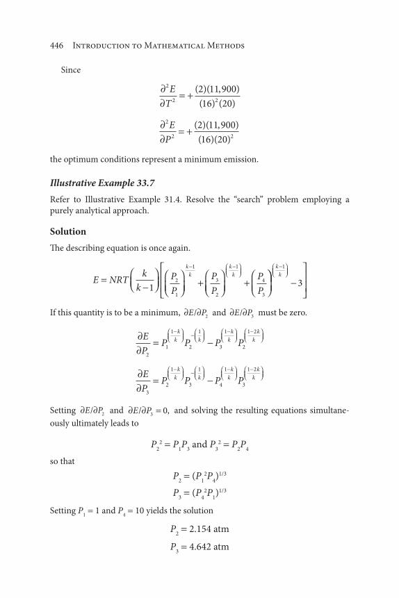
446 Introduction to Mathematical Methods
Since
2
2 2
2 11 900
16 20
E
T
( )( , )
( ) ( )
2
2 2
2 11 900
16 20
E
P
( )( , )
( )( )
the optimum conditions represent a minimum emission.
Illustrative Example 33.7
Refer to Illustrative Example 31.4. Resolve the “search” problem employing a
purely analytical approach.
Solution
The describing equation is once again.
E NRTk
kP
P
P
P
P
P
k
k
k
k
12
1
1
3
2
1
4
3
k
k
1
3
If this quantity is to be a minimum, E P/2 and E P/
3 must be zero.
E
PP P P P
k
k k
k
k
k
k
2
1
1
2
1
3
1
2
1 2
E
PP P P P
k
k k
k
k
k
k
3
2
1
3
1
4
1
3
1 2
Setting E P/2 and E P/
30, and solving the resulting equations simultane-
ously ultimately leads to
P2
2 P1P
3 and P
32 P
2P
4
so that
P2
(P1
2P4)1/3
P3
(P4
2P1)1/3
Setting P1
1 and P4
10 yields the solution
P2
2.154 atm
P3
4.642 atm
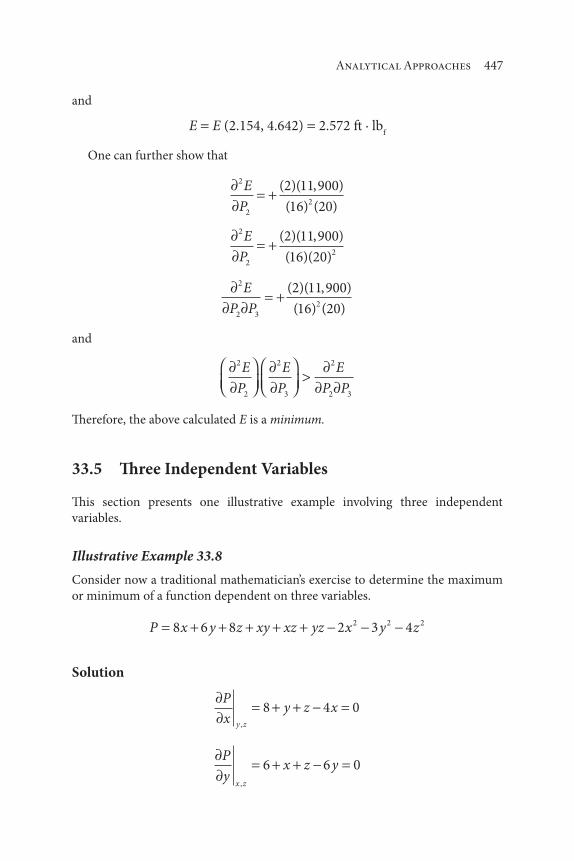
Analytical Approaches 447
and
E E (2.154, 4.642) 2.572 ft ∙ lbf
One can further show that
2
2
2
2 11 900
16 20
E
P
( )( , )
( ) ( )
2
2
2
2 11 900
16 20
E
P
( )( , )
( )( )
2
2 3
2
2 11 900
16 20
E
P P
( )( , )
( ) ( )
and
2
2
2
3
2
2 3
E
P
E
P
E
P P
Therefore, the above calculated E is a minimum.
33.5 Three Independent Variables
This section presents one illustrative example involving three independent
variables.
Illustrative Example 33.8
Consider now a traditional mathematician’s exercise to determine the maximum
or minimum of a function dependent on three variables.
P x y z xy xz yz x y z8 6 8 2 3 42 2 2
Solution
P
xy z x
y z,
8 4 0
P
yx z y
x z,
6 6 0

448 Introduction to Mathematical Methods
P
zy x z
x y,
8 8 0
The solution to the above three linear simultaneous equations is
x y z = 2.8256; = 1.7326; = 1.5698
for which
P 22 78.
To determine whether the above P is a maximum or minimum, calculate the
three second order partial derivatives.
2
24
P
x
2
26
P
y
P
z28
Since the three derivatives are negative, the value of P above (22.78) is a maximum,
i.e., any other calculated P for a different x, y, and z would produce a value of P
less than 22.78. The “proof ” is left as an exercise for the reader. However, if one
were to select values of x, y, and z straddling the maximum set of values, P should
be below 22.78. For example, the value of P for x 2, y 2, and z 2 is 20. For
x y z 10, the value of P is -380.
References
1. L. Theodore, Heat Transfer Applications for the Practicing Engineer, John Wiley & Sons, Hoboken,
NJ, 2011
2. A.M. Flynn, T. Akashige L. Theodore, Kern’s Process Heat Transfer, 2nd ed., Scrivener-Wiley, Salem,
MA, (forthcoming) 2018.
3. J. Happel, Chemical Process Economics, John Wiley & Sons, Hoboken, NJ, 1958.

449
Linear programming is one of several techniques for optimization which has
increased in usefulness because of the availability of digital computers. The title
results from the assumptions in the method that linear relationships describe the
problem/system/relationship under consideration. For example, each production
element per day increase in a process could produce a corresponding linear profit
increase per day. However, there are many instances where a linear model does
not accurately describe the totality of the problem/system/relationship. It may
then be necessary to resort to other procedures such as nonlinear programming;
some brief details will be presented for handling the nonlinear section in the next
paragraph.
The reader should note that the terms linear programming and nonlinear pro-
gramming are essentially similar from an applications perspective. There were
problems around the middle of the last century because of some difficulties that
arose in attempting to solve nonlinear programming problems. However, the
arrival of the modern day computer (see Chapter 29) and sophisticated software
(e.g., EXCEL) have removed these problems. Unless a solution is presented graph-
ically in this and the next chapter, it will be obtained directly from EXCEL so
that the reader need not be concerned with whether a system’s pertinent describ-
ing equations and constraints are linear or nonlinear. Thus, details regarding the
34Introduction to Linear Programming
Introduction to Mathematical Methods for Environmental Engineers and Scientists. Charles Prochaska and Louis Theodore.
© 2018 Scrivener Publishing LLC. Published 2018 by John Wiley & Sons, Inc.

450 Introduction to Mathematical Methods
solution methodology for both linear programming and nonlinear programming
problems and illustrative examples will not be presented. They are simply not nec-
essary and beyond the scope of this introductory optimization Part.
Other than linear programming, dynamic programming is probably the more
often used optimization method by the practicing environmental engineer and
scientist. As described earlier, it is a process involving decisions made at multiple
stages. Just as an optimization model is defined by its variables, constraints, and
objective function, a multistage decision process is defined by its stages and deci-
sions. At any stage, there is enough information about decisions made at preceding
stages to make informed decisions at the present stage. Thus, some optimization
problems can be reformulated as multistage decision process problems. One then
proceeds through subsequent stages until the final stage of the process is reached.
Some additional details are provided in the next section.
As one might suppose, there are numerous other optimization methods avail-
able to the practicing environmental engineer and scientist. Several of these are
detailed in Perry’s Handbook [1].
1. Mixed Integer
2. Mixed Integer Nonlinear Programming
3. Mixed Integer Linear Programming
4. Quadrative Programming
5. Differential/Nondifferentiable Systems
6. Convex/Nonconvex
The above topics are not reviewed in this text. The reader is referred to the optimi-
zation literature [2–6] for details.
Regarding contents, Section 34.1 provides definitions as they apply to opti-
mization and, in particular, to linear programming – the title of this chapter.
Section 34.2 examines linear programming from an elementary principles per-
spective while Section 34.3 addresses the topic from a mathematician’s viewpoint.
Section 34.4 is concerned with an engineer’s approach to linear programming.
Linear programming examples that are not applications-related highlight the last
section (34.5).
34.1 Definitions
Seven key definitions – as they apply to optimization and linear programming are
provided below (in alphabetical order).
1. Algebra: A branch of mathematics in which letters are used to
represent basic arithmetic relations. As in arithmetic, the basic
operations of algebra are addition, subtraction, multiplica-
tion, and division. Arithmetic, however, cannot generalize such

Introduction to Linear Programming 451
mathematical relations as the Pythagorean theorem (which states
that the sum of the squares of the sides of any right triangle is also a
square). Arithmetic can produce specific instances of this relations
(for example 3, 4, and 5, where 32 42 52). Algebra can make a
purely general statement that fulfills the conditions of the theo-
rem, i.e., a2 b2 c2. Any number multiplied by itself is termed
squared and is indicated by a superscript number 2. For example,
3 3 is notated as 32 and is termed three squared; similarly, a a is
equivalent to a2. Classical algebra, which is concerned with solving
equations, uses symbols instead of specific numbers and employs
arithmetic operations to establish procedures for manipulating
symbols while modern algebra has evolved from classical algebra
by placing more attention to the structures within mathematics.
2. Constraint: “A constraining or being constrained… confinement
or restrictions… forced… something that constrains.” The term
constraints is defined as “to bond together, draw together… to
force into or hold in, close bounds, confine… restrain.”
3. Dynamic Programming: The dimesionality of a particular opera-
tion is reduced from (m)(n) variables to m repeated n times. As
noted above, if it is not practical or possible to solve a large com-
plex system of equations, the system is reduced in complexity in a
manner that requires the solution of a smaller subset of the origi-
nal problem, noting that for each n (for example, each stage in a
mass transfer operation) [7] only m variables are involved in the
optimization process. One can then work backwards and combine
the solutions generated at each n.
4. Linear Algebra: A branch of mathematics that is concerned with
systems of linear equations, linear transformations, vectors, vec-
tor spaces, and related topics. The major interest is with linear
equations.
5. Linear Programming: A mathematical and operations research
technique used in engineering, science, administrative engineer-
ing, and economic planning to maximize the linear function(s) of
a large number of variable(s) subject to certain constraint(s). It is
basically used to find a set of values, chosen from a prescribed set
of numbers, that will maximize or minimize, i.e. optimize, a given
equation.
6. Operations Research: A confusing term that most often has been
used to describe linear programming.
7. Optimization: As noted earlier in this Part, optimization has
come to mean different things to different people. Its definition
has also varied in the literature. In its most elementary and basic
form, optimization is concerned with the determination of the
optimum solution to a given problem. This process is required in

452 Introduction to Mathematical Methods
the solution of many problems in environmental engineering that
involve the maximization or minimization of a given function(s).
Some specific examples include:
a. environmental engineering research
b. applied environmental science
c. in the selection of control variables to accomplish a desired
operation
d. in the scheduling of a series of operations or events to control
dates of a given project
e. the development of optimal layouts of organizational units
within a given design space, etc.
34.2 Basic Concepts of Optimization
The term linear programming defines a particular class of optimization problems
in which the constraints of the system can be expressed as linear equations or
inequalities and the function is linear with respect to the independent design vari-
able. These techniques are widely used to solve a number of engineering, envi-
ronmental, chemical, structural, economic, and societal problems. The primary
reasons for its wide use today are the availability of a host of commercial software
to solve complex problems and the ease with which any data variation that could
involve sensitivity analysis can be handled.
As noted in the earlier chapters in this Part, the optimization problem in which
the performance measure is a function of one variable is the most elementary type
of optimization problem since it is a type of problem that the environmental engi-
neer commonly encounters in practice. It also allows single-variable optimization
to be employed as a sub-problem within iterative procedures for solving multivari-
able optimization problems.
Constraints, constraints, constraints. Constraints continue to be imposed on
individuals, organizations, groups, governments, religions, relatives, friends, etc. It
seems to be getting worse each year. And, one of the hallmarks of linear program-
ming is the inclusion of constraints in the problem description, i.e., the objective
function. Linear programming involves linear constraints. For example, the function
f (x) x4 3x2 2x 5; all values of x (34.1)
is an unconstrained function. However, the function
f (x) x6 4x 6; 3 x 6 (34.2)
is a constrained function. When constraints are present, the function being opti-
mized is usually referred to as the objective function to distinguish it from any other
functions that may be used to define the constraints or the problem. Although
Introduction to Linear Programming 453
the emphasis to follow in this and the next chapter is on linear constraints, many
real-world applications also involve non-linear constraints and nonlinear objec-
tive functions.
From a basic perspective, the problem is to optimize the objective function
y f (x1, x
2) (34.3)
The constraints can include
g x x( , )1 2 0 (34.4)
x1 0 (33.5)
x2 0 (34.6)
This is a simple yet typical problem in optimization – the maximization or mini-
mization of a real-value function of a number of real variables (occasionally just
a single variable) subject to a number of constraints (occasionally the number
is zero). However, the mathematical model normally contains several (n, for
example) variables known as the independent design variables denoted as x1, x
2,
x3, …, x
n. This set of variables has been described by some as a vector, X. One may
view each x as one dimension in the set (space) of variables, and any particular set
of variables, and any particular set of values for these variables in this system as a
solution.
One of the more important recent areas for the application of mathematical
optimization techniques is in environmental engineering and science. Many envi-
ronmental problems require an iterative and/or trial-and-error solution and the
problem of concern is often stated in an ambiguous and open-ended way. The first
task is to decide what the problem is and to identify the requirements or specifi-
cations for any proposed and/or feasible solution. One then generates a concept,
perhaps in the form of a rough configuration, for the object, system, or process
to be optimized. This phase of the problem is usually the most difficult and can
require the greatest ingenuity and engineering judgement.
The next step attempts to model the object, system, or process. This model may
assume a wide variety of forms, but the usually preferred ones are mathematical in
nature. One may then use many mathematical, scientific, and engineering tools.
These can involve not only the most empirical of data correlations but also the
most rigorous mathematical procedures to the least formal cut-and-try methods
for assisting in the analysis of this aspect of the solution.
It may happen that certain functional equality constraints also apply.
f x x x x
f x x x x
n
k n
1 1 2 3
1 2 3
0
0
( )
( )
, , , ,
, , , ,
(34.7)

454 Introduction to Mathematical Methods
There may also be certain inequality constraints such as
g x x x x
g x x x x
n
m n
1 1 2 3
1 2 3
0
0
( )
( )
, , , ,
, , , ,
(34.8)
that are specified on the space so that only points in a portion of the total space
may be considered as acceptable values for the solution of the problem. This region
is defined as the feasible space and points in the region are defined as feasible
solutions.
The above equality constraints – Equation (34.7) – come from functional rela-
tionships that must be satisfied among the aforementioned n variables. If there is
to be a choice in the values for which at least some of the variables may assume,
then k must be smaller than n. The inequality constraints in Equation (34.8) usu-
ally arise from some specified limitations (maximum permissible stress, minimum
emissions, minimum allowable temperatures, etc.). Note that there is no upper
limit on the value of m.
Finally, the following comments are provided on the objective function. It may
be quite simple and easy to determine, or complicated and difficult to calculate.
The objective function may also be very illusive due to the presence of conflicting
or dimensionally incompatible sub-objectives; for example, one might be asked to
design an absorber [7] at minimum cost and make it aesthetically appealing. In some
cases, it may not be possible to find a quantitative objective function. In this case,
one can assume that a suitable qualitative objective function can be formulated.
34.3 Applied Mathematics Concepts on Linear Programming
As noted earlier, linear programming deals with the determination of an optimum
solution of a problem expressed in linear relationships where there are a large
number of possible solutions. In general, the methods of solution employed are of
a trial-and-error nature, where the procedure systemically follows a mathematical
treatment which minimizes one’s labor and insures that a correct result has been
obtained. The following graphical approach to a linear programming problem
illustrates some of the mathematics employed in the solution.
Consider now an example that involves minimizing an objective variable E
(e.g., expenditure or emission)
E a x a x1 1 2 2 (34.9)
subject to two constraints
B b x b x1 1 2 2 (34.10)

Introduction to Linear Programming 455
C c x c x1 1 2 2 (34.11)
In addition,
x1 0 (34.12)
x2 0 (34.13)
In terms of a solution, first examine the above system of equations analyti-
cally. The problem can be viewed in Figure 34.1 and 34.2. First note that only the
first quadrant need be considered since Equations (34.12) and (34.13) must hold.
Equations (34.10) and (34.11) are rewritten in the following form
xB
b
b
bx2
2
1
2
1 (34.14)
Equation(34.14)
(a) (b)
(c)
Equation(34.15)
x1
x2
x1
x2
x
x2
x2
x2
Figure 34.1 Two variable minimization problems.
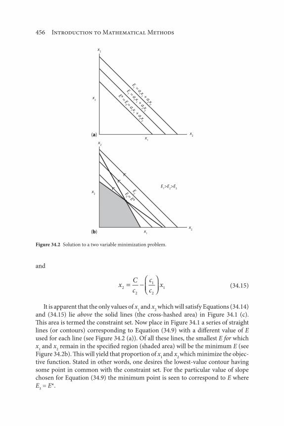
456 Introduction to Mathematical Methods
and
xC
c
c
cx2
2
1
2
1 (34.15)
It is apparent that the only values of x1 and x
2 which will satisfy Equations (34.14)
and (34.15) lie above the solid lines (the cross-hashed area) in Figure 34.1 (c).
This area is termed the constraint set. Now place in Figure 34.1 a series of straight
lines (or contours) corresponding to Equation (34.9) with a different value of E
used for each line (see Figure 34.2 (a)). Of all these lines, the smallest E for which
x1 and x
2 remain in the specified region (shaded area) will be the minimum E (see
Figure 34.2b). This will yield that proportion of x1 and x
2 which minimize the objec-
tive function. Stated in other words, one desires the lowest-value contour having
some point in common with the constraint set. For the particular value of slope
chosen for Equation (34.9) the minimum point is seen to correspond to E where
E3 = E*.
x2
x2
x2
x2
x2
x2x
1
x1
E1 = a
1 x1 + a
2 x2
E2
E1 = a
1 x1 + a
2 x2
E* = E3 = a
1 x1 + a
2 x2
E3 = E*
(a)
(b)
E1>E
2>E
3
Figure 34.2 Solution to a two variable minimization problem.

Introduction to Linear Programming 457
The point which represents the minimum is therefore determined by con-
straints a1
and a2
of the problem. Further, if the constants c1
and c2
in Equation
(34.11) are changed, it is possible that the minimum point would occur elsewhere.
The situation is essentially reversed for a maximization problem, i.e., for a profit P.
This is demonstrated in Figure 34.3.
It should be pointed out that if the objective function – Equation (34.7) – was
nonlinear the contour lines would be curved and if the constraint equations were
nonlinear the constraint lines would not be straight. It should be intuitively obvi-
ous that locating the minimum point graphically is more complicated in this case.
The above methodology can be extended to more than two variables and two
constraints. The following would apply for three variables and four constraints.
y f x x x a x a x a x( , , )1 2 3 1 1 2 2 3 3 (34.16)
and
B b x b x b x1 1 2 2 3 3 (34.17)
C c x c x c x1 1 2 2 3 3 (34.18)
D d x d x d x1 1 2 2 3 3 (34.19)
E e x e x e x1 1 2 2 3 3 (34.20)
and
x1 0 (34.21)
x2 0 (34.22)
x2
x2
x1x
1
P1
P2
P3 = P*
P3<P
2<P
1
Figure 34.3 Possible solution to a two variable maximization problem.

458 Introduction to Mathematical Methods
x3 0 (34.23)
Naturally, the above can be rewritten for n objective functions and m constraints.
34.4 Applied Engineering Concepts in Linear Programming
An engineer’s first task in problem solving is to decide what the problem is and to
identify the requirements or specifications for any proposed and/or feasible solu-
tion. One then generates a concept, perhaps in the form of a rough configuration,
for the object, or process to be optimized. As noted above, this phase of the prob-
lem is often the most difficult and requires the greatest ingenuity and engineering
judgement.
Perhaps Happel [8] best described linear programming from a practicing engi-
neer’s perspective (the reader should note the overlap with some of the material in
section 34.5). His edited write up follows.
“The general problem of finding a maximum usually assumes that some par-
tial derivative of the function y f (x1, x
2, x
3) vanishes within the range of
interest of the variables. In practical problems it often happens, however, that
the optimum solutions will be obtained at the boundary or limiting values
of the variables. This is, of course, always true where the function to be opti-
mized is linear. In such cases, explicit analytical solution is not possible and
the optimum must be obtained by some other method or iteration.
In general, even the simplest type of formulations may require a great deal
of computation in practical applications which is facilitated by the availabil-
ity of high-speed computers. Linear programming, discussed in greater detail
below, is beginning to be used to a substantial extent by practicing engineers.
In order to apply linear programming to a problem, the relationships
between variables must be expressed as a set of linear equations or inequali-
ties. The variables must be otherwise independent and must exceed the num-
ber of equations. Mathematically expressed,
i
ij i ia X b i m J n n m( , , , ; , , ; )1 2 1 (34.24)
where the sum of the coefficient aij times the value of each variable X
i equals
a requirement bi in the ith equation. The number of variables must exceed
the number of equations, so that an infinite number of solutions is pos-
sible. The “best” one is selected. Often the relationships in equation (34.24)
are expressed as inequalities. “Dummy” additional variables are introduced
in order to convert these inequalities into appropriate equations. Another
requirement is that no quantity can be negative. Thus, mathematically

Introduction to Linear Programming 459
x bi i0 0 and (34.25)
This requirement will insure that only useful answers are obtained.
The solution of a problem by linear programming also requires a profit
function or objective function to be maximized (or minimized). This require-
ment is stated
P c Xi
i i maximum (or minimum) (34.26)
where ci is the profit (or cost) per unit of X
i used. The solution is carried out
by an iterative process, which at each stage of calculation assigns either zero
or positive values to all Xi variables. As the calculation proceeds, the values
selected, while meeting the constraints imposed, will tend to increase the
summation to be maximized at each stage. If a solution exists, a maximum
profit case will finally be realized.”
Figure 34.4 illustrates a simple situation involving the operation of an
absorber[7, 9, 10] with temperature and pressure limits for which each depends
on the magnitude of the other. The former might come from limitations due to
equilibrium consideration, since “the higher the temperature in the absorber the
lower the absorptive capacity of the absorbing liquid while the higher the pressure
in the absorber increases the absorption” [11]. The region of feasible solutions for
the absorber problem is the region enclosed by the constraints. The optimization
problem is to find the one set of variables or point in the feasible solution space
Lowerconstraint
on T Feasiblesolutions
Upper constraint onboth T and P
Lower constraint on P
Temperature, T
Pre
ssu
re, P
Figure 34.4 Feasible solution for operation of an absorber.

460 Introduction to Mathematical Methods
that corresponds to the so-called best solution - in this case, minimizing the gas-
eous pollutant emission.
In order to locate the best feasible solution of the potentially infinite number
of feasible solutions using a mathematical optimization technique it is essential
that a meaningful objective function f(x) of the independent design variables be
specified for an operation concerned with - for example - the control and/or recov-
ery of a particular component of gaseous emission. For simplicity, assume that
for the aforementioned application, one must choose two independent variables
– temperature T and pressure P. The space is, therefore, two dimensional, with
temperature and pressure as the coordinates. In practice, there usually are certain
inequality constraints placed upon the range on both T and P. As shown in Figure
34.4 there could be lower limits for the temperature and pressure, and an upper
limit for each that depends on the magnitude of the other.
Once again, the optimization problem is to find the one set of variables or point,
X, in the feasible solution space that corresponds to the best solution. In order to
locate the best feasible of the potentially infinite number of feasible solutions using
a mathematical optimization technique, it is essential that a meaningful objective
function f (x) of the design variables be specified to provide for a comparison of
alternative solutions.
34.5 Applied Engineering Concepts in Linear Programming
This last section attempts to clarify the ideas presented above via three illustrative
examples. An attempt will also be to relate the variables to real-world quantitative
factors. That will occur in the next and last chapter. In fact, the first illustrative
example will be revisited as it applies to pollutant emission concerns from a coal-
fired boiler.
Illustrative Example 34.1
You have been requested to obtain the maximum value of P subject to the follow-
ing conditions.
Objective function:
P x x0 3 51 2. (1)
Constraints:
x x2 10 5 3. (2)
x x2 13 6 (3)

Introduction to Linear Programming 461
x1 3 (4)
x2 4 (5)
Once again, the solution is provided in graphical form. Refer to Figure (34.5).
Conditions (4) and (5) require that the solutions, i.e., the values x1 and x
2 that will
maximize P lie within the rectangle provided in Figure (34.5). Conditions (2) and
(3) require that the solution be within the area ABCD in Figure 34.5 (b). When
the objective function equation is superimposed on Figure 34.5 (b), Figure 34.5
(c) results. The maximum P is located at x1
1.2 and x2
2.4 for which P 15.6.
EXCEL provides the same solution.
Illustrative Example 34.2
A company manufactures two products, A and B, with an accompanying unit profit
of PA and P
B, respectively. A minimum number of N products can be produced on
a daily basis. The daily production rates of A and B is xA
and xB, respectively. In
1.0
2.0
3.0
4.0(5)
(4) (2)
(4)(3)
(5)
(a) (b)
(c)
1.0 3.0
5.00
4.80
3.12
5.2
Objective function
6.7 8.2
P = 25P = 20P = P* = 15.6
P*
x1
x2 = 2.4
x1 = 1.2
x2
x2
x1DA
B
Figure 34.5 Graphical solution for Illustrative Example 34.1.

462 Introduction to Mathematical Methods
addition, the fractional defective rate of producing A and B are a and b respec-
tively. Each defective product reduces the profit associated with product A and B
by c and d, respectively. Determine the describing equations (the model for the
production rate of A and B) that will maximize daily profits P.
Solution
As noted, xA and x
B are the daily production rates of A and B, respectively. The
function P is then
P x P x P x ac x bdA A B B A B
The constraints are
xA
xB
N
xA, x
B0
This problem will be evaluated again in the next chapter.
Illustrative Example 34.3
A batch chemical reactor [12] can produce either product A, B, or C. The daily pro-
duction levels of each are represented by xA, x
B, and x
C with an accompanying unit
profit of PA, P
B, and P
C, respectively. The two unit expressions of concern for each
product are manpower (M) and energy costs (E), neither of which can exceed Y
and Z, respectively. Develop the linear programming model to optimize the profit
P for this system.
Solution
Based on the problem statement one concludes:
P P x P x P xA A B B C C
with
MAxA MBxB MCxC Y
EAx
AE
Bx
BE
Cx
CZ
xA, x
B, x
C0
Numerical problems of this nature will also be revisited in the next/last
chapter.

Introduction to Linear Programming 463
References
1. D. Green and R. Perry (editors), Perry’s Chemical Engineers’ Handbook, 8th ed., McGraw-Hill, New
York City, NY, 2007.
2. R. Ketter and S. Prawel, Modern Methods of Engineering Computation, (adapted from), McGraw-
Hill, New York City, NY, 1969.
3. L. Lapidus, Digital Computations for Chemical Engineers, (adapted from) McGraw-Hill, New York
City, NY, 1962.
4. G. Reklaitis, A. Ravindran, and K. Ragsdell, Engineering Optimization: Methods and Applications,
John Wiley & Sons, Hoboken, NJ, 1983.
5. E. Chong and S. Zak, An Introduction to Optimization, 4th ed., John Wiley & Sons, Hoboken, NJ,
2013.
6. H. Mickley, T. Sherwood, and C. Reed, Applied Mathematics in Chemical Engineering, McGraw-
Hill, New York City, NY, 1957.
7. L.Theodore, F. Ricci, and T. VanVliet, Thermodynamics for the Practicing Engineer, John Wiley &
Sons, NJ, 2009.
8. J. Happel, Chemical Process Economics, John Wiley & Sons, Hoboken, NJ, 1958.
9. L. Theodore, Air Pollution Control Equipment Calculations, John Wiley & Sons, Hoboken, NJ,
2008.
10. L. Theodore, Chemical Engineering: The Essential Reference, McGraw-Hill, New York City, NY
2014.
11. J. Reynolds, J. Jeris, and L. Theodore, Handbook of Chemical and Environmental Engineering
Calculations, John Wiley & Sons, Hoboken, NJ, 2004.
12. L. Theodore, Chemical Reactor Analysis and Applications for the Practicing Engineer, John Wiley &
Sons, Hoboken, NJ.

465
This is the last chapter of not only this Part (V) but also of the book. Part V is
devoted to optimization, but the emphasis is on linear programming – a subject
that the authors view as a subset of optimization. Since the earlier material in the
previous five chapters has – for the most part – relied on optimization methods,
it is appropriate that this last chapter compliment the presentation with applica-
tions-oriented illustrative examples.
It should be noted once again that formal optimization techniques have as their
goal the development of procedures for the attainment of an optimum in a system
which can be characterized mathematically. The mathematical characterization
may be:
1. partial or complete,
2. approximate or exact, and/or
3. empirical or theoretical.
The resulting optimum may be a final implementable solution or a guide to a
practical solution and a criterion by which practical solutions are to be judged. In
either case, the applications of these optimization techniques should serve as an
important part of the effort in the solution of some environmental problems [1].
35Linear Programming Applications
Introduction to Mathematical Methods for Environmental Engineers and Scientists. Charles Prochaska and Louis Theodore.
© 2018 Scrivener Publishing LLC. Published 2018 by John Wiley & Sons, Inc.

466 Introduction to Mathematical Methods
Nine illustrative examples follow. Three are concerned with environmental
matters, five deal with the chemical process industries, and one involves a Monte
Carlo exercise. The order of presentation and the accompanying titles are:
Illustrative Example 35.1: Vitamin Caloric Requirement
Illustrative Example 35.2: Operation of a Natural Gas Boiler
Illustrative Example 35.3: Maximizing Coal Usage Profits
Illustrative Example 35.4: Maximizing Crude Oil Profits
Illustrative Example 35.5: Tube-and-Bundle/Finned Heat Exchangers
Illustrative Example 35.6: Minimizing Gaseous Pollution Emissions
from an Oil-Fired Burner
Illustrative Example 35.7: Pharmaceutical Cancer Drug
Illustrative Example 35.8: Optimum Operation of a Butane Plant
Illustrative Example 35.9: Monte Carlo Application
Illustrative Example 35.1: Vitamin Caloric Requirement
Vitamin (1) costs $0.20 per mg and contains 50 cal/mg and 20 mg protein/mg.
Vitamin (2) costs $0.15 per mg and contains 40 cal/mg and 10 mg protein/mg.
What amounts of vitamins x1 and x
2 would meet the minimum regulatory require-
ment while minimizing production cost, C. The USDA provided the following
objective function for C:
C x x20 151 2
along with the constraints
50 40 3001 2x x
20 10 1201 2x x
and
x1 6
x2 6
Solution
EXCEL provides the following solution:
x1
6
x2
0

Linear Programming Applications 467
and
C 120
The reader should note before leaving this problem that this illustrative exam-
ple is similar to that presented in Section 34.3 of the last chapter, only this time
with numbers specified for the variables and with the problem related to a real-
world situation.
Illustrative Example 35.2: Operation of a Natural Gas Boiler
The cost associated with the operation of a gas-fired boiler R has been found to be
linearly related to both the operating temperature T and operating pressure P. That
relationship (in consistent absolute units) is given by
R T P0 18 0 05. . ; consistent units, $/hr
However, for ignition to occur, the following constraints must be satisfied
a T b P I1 1
along with the energy component of the gaseous fuel
a T b P E2 2
If
a b1 10 2 0 05. , .
a b2 20 4 0 02. , .
and
I 600
E 450
T1 0
P1 0
calculate the operating temperature and pressure that minimizes the cost
of operation and satisfy the constraints associated with ignition and energy
content.

468 Introduction to Mathematical Methods
Solution
This is a typical linear programming problem. For this example,
R T P0 18 0 05. .
The constraints are
0 2 0 05 450. .T P
and
0 4 0 02 600. .T P
with
T 0
P 0
EXCEL provides the following solution
T 2250
P 0
and
R 40.5 $/hr 972$/day
Illustrative Example 35.3: Maximizing Coal Usage Profits
A coal manufacturer mines two grades of coal – (1) and (2). Coal 1 emits 25 mg
NO2 per ton combusted, 6 mg SO
4 per ton combusted, and 68 mg particulate per
ton combusted. Each ton of Coal 1 sold yields a $30 profit. Coal 2 emits 75 mg
NO2, 60 mg SO
4, and 34 mg particulate per ton combusted. Each ton of Coal 2 sold
yields a profit pf $40. Due to stringent state air pollution regulatory requirements
no more than 450 mg NO2, 480 mg SO
4, and 374 mg particulate may be potentially
emitted from the coal sold by the manufacturer. How many tons of Coal (x1) and
(x2) should be mined daily to maximize profits and satisfy regulatory rules? What
is the corresponding maximum daily profit?
Solution
The objective function for the coal operation is
P x x30 401 2

Linear Programming Applications 469
subject to the constraints
a x a x E1 1 2 2 1
b x b x E1 1 2 2 2
c x c x E1 1 2 2 2
where (in consistent units)
a a1 225 75,
b b1 260 60,
c c1 268 34,
E E E1 2 3450 480 374, ,
and
x1 0
x2 0
Solution
EXCEL provides the following solution.
x1
3
x2
5
and
P $290
The low value of P suggests that the coal manufacturer is operating at or near
breakeven economics.
Illustrative Example 35.4: Maximizing Crude Oil Profits [2,3]
A refinery has two catcrackers that can produce various grades of hydrocarbon
products. Due to consumer fuel demand, the production of gasoline, home heat-
ing oil, and diesel must be limited. This information is provided in Table 35.1. The
profit on processing U.S. crude oil is $2.00/gal and on Venezuelan crude is $1.60/
gal. Find the approximate daily processing rate of the two crudes in order to maxi-
mize profits.

470 Introduction to Mathematical Methods
Solution
Set
x1
gallons of U.S. crude
x2
gallons of Venezuelan crude
The objective function for the daily profit, P, that is to be maximized is:
P x x2 0 1 61 2. .
The constraints are:
0 08 0 11 15001 2. .x x
0 29 0 54 55001 2. .x x
0 63 0 35 110001 2. .x x
with
x1 0
x2 0
The solution to the above from EXCEL is: 16,820 gal of U.S. crude per day
should be processed and 1152 gal per day should be derived from Venezuelan
crude. This results in a total daily profit of $35,484 [1, 2]. Thus,
x1 16 820, gal U.S. crude per day
x2 1152 gal Venezuelan crude per day
P $ ,35 484
Table 35.1 Catcracker information
Product grades U.S. Crude (%
distribution)
Venezuelan crude
(% distribution)
Max. production
rate (gal/day)
Gasoline 8 11 1,500
Home Heating Oil 29 54 5,500
Diesel Oil 63 35 11,000

Linear Programming Applications 471
Illustrative Example 35.5: Tube-and-Bundle/Finned Heat Exchangers
Ricci Consultants were requested to develop a mathematical model involving heat
exchangers at the Bayway Refinery in Linden, NJ. The purpose of the assignment
was to develop a heat exchanger network (see Illustrative Examples 30.6 and 30.7
in Chapter 30) that maximizes both the profit associated with the recovery of both
energy and the “quality” energy [3] by employing a number of only tube-and-bun-
dle (x1) and finned (x
2) exchangers. The proposed model for the objective function
takes the form:
RC e x x xx x( ).1 20 25
1 2 1
2 ; $
The constraints specified were
x x1
2
2 200
x x1 24 50
x1 0
x2 0
Determine RC, x1, and x
2,
Solution
Note that his is a “nonlinear” programming problem. EXCEL provides the follow-
ing solution:
x1 13
x2 9
RC $ .4 2 106
Thirteen tube-and-bundle and 9 finned heat exchangers are recommended.
Illustrative Example 35.6: Minimizing Gaseous Pollutant Emissions from an Oil- Fired Utility Boiler
A state-wide utility has proposed to convert some of its coal-fired boilers to oil-
fired. DuPont Associates was hired to generate a model (objective function) that
would minimize the cost of the replacement relative to the quantity of oil to be
combusted. Two oils – (1) and (2) – are available to supply the necessary energy for
all the new boilers. The project also recognized that an attempt be made to salvage

472 Introduction to Mathematical Methods
as many of the old boilers currently burning coal [3]. The cost associated with each
oil varies with its content, regulatory requirements, heating value, etc. The engi-
neers at DuPont Associates proposed the following cost model, DA.
DA x x x3 4 101 2 3
4; $
(Salvaging the existing boilers resulted in a credit.) The constraints, primarily due
to emission rules for NOX, SOX, and ROX were
x x2 3 100 (nitrous oxide, NOX)
x x1 3 50 (sulfur dioxide, SOX)
x x x x1 2 3 3
2 1000 (particulate, ROX)
with
x x x1 2 3 50
Solution
EXCEL provides the following solution:
x1 4
x2 10
x3 26
with
DA $ $ ,26 10 260 0004
Thus, the solution requires the purchase of 4 new boilers that burn Oil (1), 10
new boilers that will burn Oil (2), and the reassignment of 26 of the old coal-fired
boilers (3).
Illustrative Example 35.7: Pharmaceutical Cancer Drug
A new consortium of drug laboratories has combined their resources to produce
four variations of the same drug. Initial estimates of the predicted hourly profit
from the production of drugs A, B, C, and D were $100, $150, $200, and $250,
respectively. Table 35.2 below shows how much time is required in each of the
three research labs to make one unit of each of the four products.
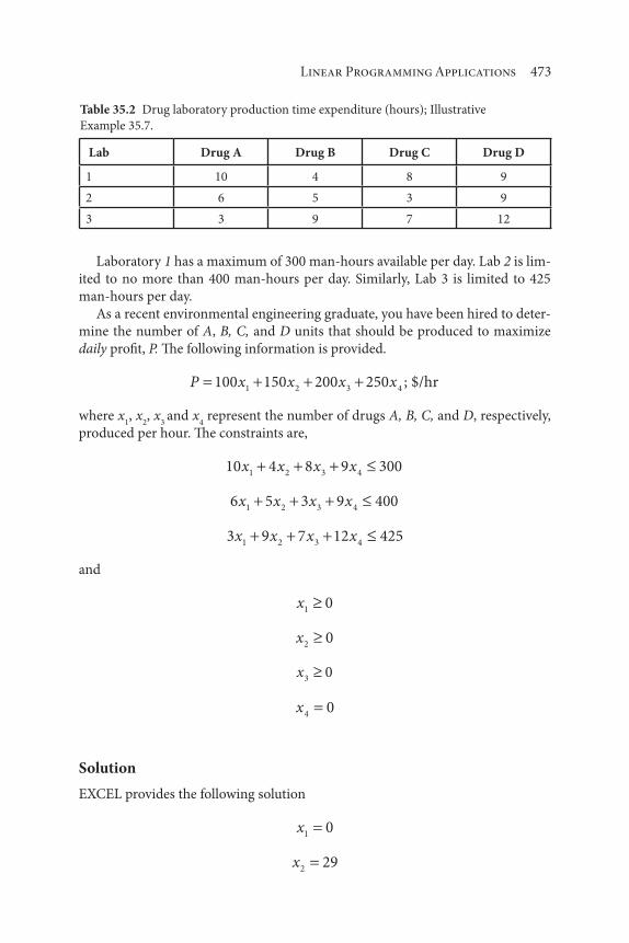
Linear Programming Applications 473
Laboratory 1 has a maximum of 300 man-hours available per day. Lab 2 is lim-
ited to no more than 400 man-hours per day. Similarly, Lab 3 is limited to 425
man-hours per day.
As a recent environmental engineering graduate, you have been hired to deter-
mine the number of A, B, C, and D units that should be produced to maximize
daily profit, P. The following information is provided.
P x x x x100 150 200 2501 2 3 4 ; $/hr
where x1, x
2, x
3 and x
4 represent the number of drugs A, B, C, and D, respectively,
produced per hour. The constraints are,
10 4 8 9 3001 2 3 4x x x x
6 5 3 9 4001 2 3 4x x x x
3 9 7 12 4251 2 3 4x x x x
and
x1 0
x2 0
x3 0
x4 0
Solution
EXCEL provides the following solution
x1 0
x2 29
Table 35.2 Drug laboratory production time expenditure (hours); Illustrative
Example 35.7.
Lab Drug A Drug B Drug C Drug D
1 10 4 8 9
2 6 5 3 9
3 3 9 7 12

474 Introduction to Mathematical Methods
x3 23
x4 0
with a profit of
P $8950/hr $214,900/day (around-the-clock operation)
Illustrative Example 35.8: Optimum Operation of Butadiene Plant [1]
Note: Illustrative Example 35.8 was drawn (with permission) from the classic work
of Happel titled “Chemical Process Economics” [1].
It is desired to be determined the optimum operation of a plant for the produc-
tion of butadiene by catalytic dehydrogenation of butylene. The steps involved are
shown schematically in Figure 35.1.
It is assumed that such items as labor, steam, and fuel consumption will remain
relatively constant so that the profitability of one system of operation as compared
with another will be a function of the feed required (at $8.40/bbl), the fuel gas pro-
duced (equivalent to $0.90 of butane degraded), the recycle from the purification
unit (at $6.32/bbl), and the butadiene product (at $32.80/bbl). The profit function,
Z, to be maximized is therefore
Z D C B A32 8 6 32 0 90 8 40. . . .
The operation of the plant is assumed to involve only two variables subject
to independent selection; namely, the per cent conversion of butylenes per pass
through the catalytic dehydrogenation system, and the per cent of normal butane
(which is assumed to be inert) allowed to build in the total feed to the dehydro-
genation unit (i.e., fresh feed plus recycle). Additional restrictions due to process
limitations are that the fresh feed A cannot exceed 9000 bbl/day, that the buildup
F of n-butane in the recycle stream must not exceed 17% and that the conversion
Dehydrogenation
unit
Recovery
unit
Purification
unit
Product
butadiene, DFuel gas, B
Recycle, C
Fresh feed,
A
Figure 35.1 Butadiene plant; Illustrative Example 35.8.

Linear Programming Applications 475
E of n-butylenes per pass will be at least 25%. Calculations based on plants tests
gave the results in Table 35.3.
If it is assumed that over the range of interest, variation in the dependent vari-
ables A, B, C, and D will be linear with respect to changes in the independent
variables E and F, the following four equations results:
AE F
7880 7880 674030
512900 7880
15
4( ) ( )
BE F
1300 1300 90030
51380 1300
15
4( ) ( )
CE F
3500 3500 312030
58460 3500
15
4( ) ( )
DE F
2960 2960 263030
53034 2960
15
4( ) ( )
with the additional restrictions
A 9000
F 17
E 25
Since the problem involves only two independent variables, it can readily be
solved without elaborate mathematical tools. The values of A, B, C, and D above are
inserted into the relationship defining the profit function to be maximized, obtaining
Profit W E F1024 800 2080
Table 35.3 Process data for butadiene plant; Illustrative Example 35.8.
A Feed,
bbl/day
B Fuel,
bbl/day
C Recycle,
bbl/day
D Butadiene,
bbl/day
E Percent
Conversion
Of C4
F Percent
n-C4 in
Total
Feed
7,88 1300 3500 2960 30 15
6,740 900 3120 2630 25 15
12,900 1380 8460 3034 20 11

476 Introduction to Mathematical Methods
Thus, it is clear that E and F should be selected as large as possible without
violating the restriction A 9000. The equation for A shows that, in fact increas-
ing F decreases A, so it is immediately clear that F 17 is the optimum. The value
of E corresponding to A 9000 is then determined from the same equation: i.e.,
F 46.0.
Another way of visualizing the problem is to estimate the variable A from the
restrictions by making use of the value of A in terms of E and F to obtain
288 1255 10 865E F ,
The above equation, together with F 17 and E 25, constitutes a statement
of the constraints in terms of the independent variables E and F. These relation-
ships are plotted on Figure 35.2 and indicate the area, which is shaded, in which
the desired solution must be located. The locus of the profit function on this
figure consists of straight lines parallel to each other, shown as a dashed line on
Figure 35.2. The maximum occurs where the profits function intersects one of the
extreme points (vertices of the triangle in Figure 35.2): i.e., E 46.0.
If more than two independent variables were involved, it would not be pos-
sible to employ a geometrical construction, and more elaborate mathemati-
cal techniques would be required which in effect accomplish the same thing
analytically.
70
60
50
40E
F
30
20
105 10
E = 25
W + 1024800
2080800
E = F–
F = 17
Optim
um
228E – 1255F= –10,865
15 20 25 30
Figure 35.2 Illustration of solution by geometry of Illustrative Example 35.8.

Linear Programming Applications 477
To solve this problem by linear programming the constraints must be changed to
equalities by the use of slack [1] variables S1, S
2, and S
3 to obtain the following form:
228 1255 10 8651E F S ,
E S2 25
F S3 17
A base-case matrix table is set up, showing these equations and the profit func-
tion in Table 35.4. It will be noted that this matrix table consists of the coefficients
in the preceding equations under the appropriate column for each variable. The
columns S1, S
2, S
3, and Z are “identity columns,” since the only element in each is
a single +1. The row corresponding to each of these unity coefficients is known
by the same designation as the column, and the quantity Q is the actual value
assigned to this variable. The variables S1, S
2, S
3, and Z are said to be “in the basis,”
and the variables E and F are not in the basis and have zero values. The problem is
to establish variables of E and F that will maximize W.
Variable F has the largest negative value in the W row and therefore has the
greatest profit associated with it. Table 35.5 shows how it is brought into the basis
to replace S1.
Now F has been put into the basis, and column F is an identity column. The equa-
tions represented by the matrix still satisfy the necessary restrictions. The profit can
be further increased by putting E into the basis. Table 35.6 shows this transforma-
tion, replacing S3. Table 35.6 represents the solution to the problem. The values of
the variables required are shown in the Q column, in agreement with results by
other methods. The profit function shows that $71,073/day is the optimum.
Illustrative Example 35.9: Monte Carlo Approach
Maximize the following objective function utilizing a Monte Carlo approach
[4, 5]. This model was recently developed by Kourtakis Engineering via a regres-
sion analysis to describe the profit MC generated from operating 6 different pro-
duction plants producing a new product x. Outline how to calculate the profit
product x from each of the pilot processes.
Table 35.4 Profit function table; Illustrative Example 35.8.
Z E F S1
S2
S3
Q
S1
– 228 1255 1 – – 10,865
S2
– 1 – – 1 – 25
S3
– – 1 – – 1 17
Z 1 800 2080 – – – 1,024
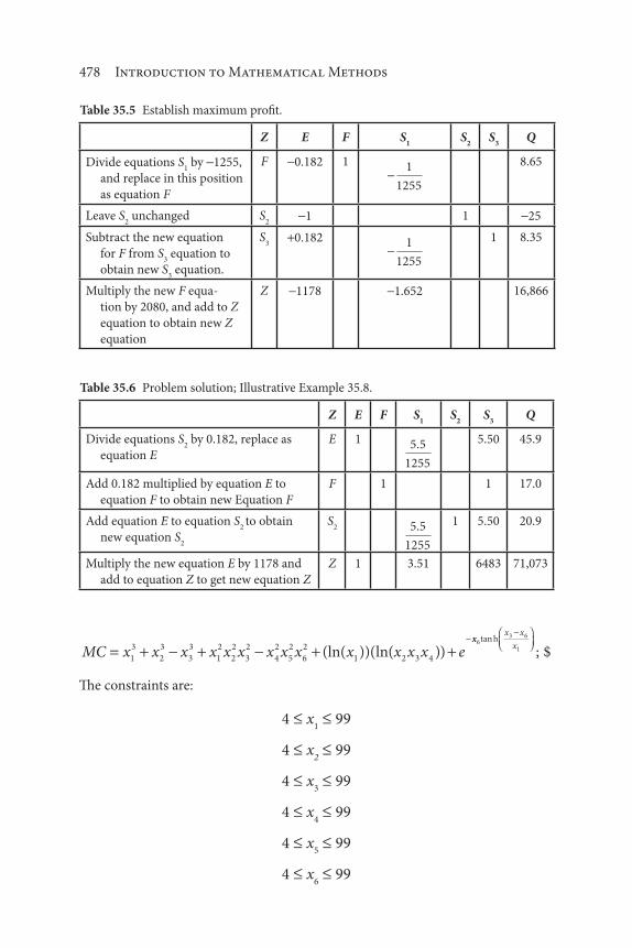
478 Introduction to Mathematical Methods
MC x x x x x x x x x x x x x e1
3
2
3
3
3
1
2
2
2
3
2
4
2
5
2
6
2
1 2 3 4(ln( ))( )ln( )xx
x x
x6
3 6
1
tan h
; $
The constraints are:
4 x1
99
4 x2
99
4 x3
99
4 x4
99
4 x5
99
4 x6
99
Table 35.5 Establish maximum profit.
Z E F S1
S2
S3
Q
Divide equations S1 by 1255,
and replace in this position
as equation F
F 0.182 1 1
1255
8.65
Leave S2 unchanged S
21 1 25
Subtract the new equation
for F from S3 equation to
obtain new S3 equation.
S3
0.182 1
1255
1 8.35
Multiply the new F equa-
tion by 2080, and add to Z
equation to obtain new Z
equation
Z 1178 1.652 16,866
Table 35.6 Problem solution; Illustrative Example 35.8.
Z E F S1
S2
S3
Q
Divide equations S2 by 0.182, replace as
equation E
E 1 5 5
1255
. 5.50 45.9
Add 0.182 multiplied by equation E to
equation F to obtain new Equation F
F 1 1 17.0
Add equation E to equation S2 to obtain
new equation S2
S2 5 5
1255
. 1 5.50 20.9
Multiply the new equation E by 1178 and
add to equation Z to get new equation Z
Z 1 3.51 6483 71,073

Linear Programming Applications 479
Note that there are (96)6 MC integer values to be checked. Outline a method of
solution. (The reader to referred to Ch. 24, Part IV – Monte Carlo Methods).
Solution
Apply the Monte Carlo method in the solution to the problem. Here is one of the
author’s approaches [6]. It involves the reading/sampling of 10,000 (it could be
more or less) possible solutions and selecting the maximum value derived from
the objective function. First set MC = 0.
1. Generate a random 2-digit number from 4 – 99 and assign it to x1.
2. Generate a random 2-digit number from 4 – 99 and assign it to x2.
3. Generate a random 2-digit number from 4 – 99 and assign it to x3.
4. Generate a random 2-digit number from 4 – 99 and assign it to x4.
5. Generate a random 2-digit number from 4 – 99 and assign it to x5.
6. Generate a random 2-digit number from 4 – 99 and assign it to x6.
7. Substitute the above x1, x
2, x
3, x
4, x
5, and x
6 values into the objective
function MC and calculate MC.
8. Store (retain) this MC value.
9. Compare this new value of MC with the previous value of MC.
Store or retain the larger of the two.
10. Repeat steps (1–9) 9,999 times.
11. The last man (or is it person) standing, i.e., the last retained MC is
the maximum value of MC.
The answer in (11) represents the maximum value of the sample of the 10,000
solutions totaled. The “actual” or “true” maximum of the entire population of (96)6
MC’s is probably slightly higher than the value in (11).
The reader should consider what other approaches could be employed to
improve on the accuracy of the answer provided by the Monte Carlo method.
References
1. J. Happel, Chemical Process Economics, John Wiley & Sons, Hoboken, NJ, 1958.
2. L. Theodore, personal notes, East Williston, NY, 2011.
3. L. Theodore, Heat Transfer Applications for the Practicing Engineer, John Wiley & Sons, Hoboken,
NJ, 2011.
4. L. Theodore, personal notes, East Williston, NY, 2016.
5. S. Shaefer and L. Theodore, Probability and Statistics Applications for Environmental Science, CRC
Press/Taylor & Francis Group, Boca Raton, FL, 2007.
6. Lou Theodore, personal notes, East Williston, NY, 2017.

481
Index
Actual maximum, 479
Adjoint matrix, 166
Adsorption equilibria, 372
Afterburner, 363
Algorithm for Gauss-Jordan reduction,
215–216
Algorithm for trapezoid rule, 228
Analytical analysis, 99–218
Analytical approaches, 435–448
Analytical geometry, 101–114
Cylindrical coordinates, 103–104
Rectangular coordinates, 29–34,
102–103, 421, 424
Spherical coordinates, 104–105
Analytical integrals, 151
Analytical integration, 147–149
AND gate, 344
Annual payment, 87
Approximate rate of return, 79
Arithmetic mean, 276–277
Associative law, 165
Augmented matrix, 210–211
Average velocity, 158–159
Backward difference, 219
Bag fabric, 334
Baghouse, 112–113
Baghouse, 334
Batch distillation, 129–130, 382–383
Batch operation, 48
Bathtub curve, 319–320
Bell-Shaped curve, 279, 324–325
Bessel function, 23
Binomial distribution, 292–296
Biological oxygen demand, 339
Bonds, 79–80
Boundary conditions, 121, 138, 142,
182, 248–255, 368
Breakeven considerations, 436–437
Break-Even curve, 79
Breakeven point, 436–437, 469
Break-In stage, 319
Buckingham Pi (π) theorem, 65–71
Capital investment, 82–83
Capital recovery factor, 77
Central difference, 219
Central limit theorem, 329
Central tendency, 276–277
Chain-Links, 345
Chebyshev’s theorem, 279
Cholesky’s method, 211
Coefficient matrix, 171, 211
Coefficient of determination, 376
Cofactor, 166–167
Combinations, 264–270
Complex conjugates, 190
Complex roots, 188
Composite formulas, 226
Compound interest, 74–76
Computer age, 390–391
Computer programming, 211, 389
Cone, 106, 108
Constant failure rate, 319
Constraints, 129, 390–393, 399–400,
416, 449–454, 457–460,
466–478
Continuous operation, 48
Continuous probability distribution,
307–341
Introduction to Mathematical Methods for Environmental Engineers and Scientists. Charles Prochaska and Louis Theodore.
© 2018 Scrivener Publishing LLC. Published 2018 by John Wiley & Sons, Inc.

482 Index
Continuous random variable, 278,
281–284, 288–289, 307–310
Convergence, 24
Conversion constants, 56–61
Conversion of units, 56
Convex/Nonconvex, 450
Coolant recycle pump, 339
Correlation coefficient, 375–384
Counting numbers, 3
Cramer’s Rule, 211
Cube, 54, 105–105, 111–112, 154
Cubic equation, 189–191
Cubic equations, 188–191
Cubic model, 375
Cumulative distribution function
(CDF) 287–289, 307, 309,
312–313, 326, 359
Cut set, 345
Cyclone, 396
Cylinder, 104–106, 154–156
Declining failure rate, 319
Definite integral, 151–153
Degree of differential equation, 137
Depreciation, 76
Determinant, 165–169
Diagonal matrix, 163
Differential calculus, 133–145
Differential equations, 121, 137–142,
174, 235–257, 367
Differential operations, 135–136
Differential/Nondifferential systems,
450
Differentiation, 115–120, 220–223,
416, 420, 441
Finite differences, 118
Five point formula, 221–223
Graphical methods, 116–118
Two point formula, 220–221
Dimensional analysis, 53–71
Dimensionless numbers, 62–71
Cavitation number, 66
Eckert number, 66
Euler number, 66
Froude number, 66
Mach number, 66
Poiseuille number, 66
Relative roughness, 66
Reynolds number, 66
Strouhal number, 66
Weber number, 66
Discrete probability distributions,
287–306
Discrete random variable, 282,
287–289
Distillation column, 47, 83, 227,
349–350
Distributive law, 164–163
Divergence, 24
Dynamic programming, 392
Dynamic programming, 392–393,
450–451
Economic analysis, 81
Economic balances, 144
Economics, 73–88, 91, 393, 403,
435–436, 442, 469, 474
Electrostatic precipitator, 45, 331, 261,
333
Ellipse, 108–109
Ellipsoid, 108–109
Elliptical partial differential equation,
252
Energy quality, 403
Equipment failure, 345
Error, 13–14, 17–20, 116, 201
Accidental error, 13
Accumulated error, 17–20
Determinate error, 13
Error tolerance, 196, 201
Estimation of mean, 276–278
Estimation of the variance, 278–281
Euler diagrams, 389
Evaluation of sums of money, 75
Event tree analysis, 349–356
Event trees, 349
Exact rate of return, 79
Expected value, 278, 282, 292, 313, 361

Index 483
Exponential distribution, 312–320,
322, 358-361
Extrapolation, 8–10, 30, 226, 414, 419
Fabricated equipment cost, 77
Factorial, 265–270
Failure rate, 274, 303, 314, 317–320,
322–325
Fault tree analysis, 343–349
Fault trees, 343–345,
Feasible space, 454
Finite difference method, 236–238
First-Degree equation, 32, 421
Fixed capital, 82
Flow chart symbols, 45–46
Flow diagrams, 43–51
Forward difference, 219
Gauss elimination method, 212,
256–257
Gauss-Jordan reduction method,
212–218, 238
Gauss-Seidel method, 217–218, 238
General analytical formulation,
441–443
Generic problem-solving techniques,
92–93
Geometric mean, 276–277
Golden section, 410–413
Graphical analysis, 29–42
Rectangular coordinates, 31–33,
421–423
Quadrant, 31–32, 422, 455
Slope, 32, 220–221, 376, 421,
424–427
Intercept, 32–42, 419, 423–429
Graphical approaches, 419–433
Graphical coordinates, 30–42
Equilateral triangular coordinates,
41
Triangular (trilinear) coordinates,
40
Graphical integration, 122–130
Gregory’s formulas, 226
Hazard risk analysis, 329
Hazard risk assessment, 49–51
Acceptable risk, 49
Corrosion, 50
Explosion, 50
Fire, 50
Hazard risk assessment algorithm,
51
Leaks, 50
Runaway reaction, 50
Rupture of pressure vessel, 50
Severity, 51
Slippage, 50
Hazardous waste incinerator, 318
Heat exchanger, 30, 49, 137–138, 261,
401, 442, 471
Heat exchanger network diagram, 403
Higher order algebraic equations,
192–193
Higher order ordinary differential
equations, 245–246
Hollow pipe, 370
Hoppers, 114
Human error, 345, 349
Hypergeometric distribution,
296–301
Idem matrix, 163
Identity matrix, 163
Improper fraction, 178
Incremental cost, 80
Indefinite integral, 149–151
Inequality constraints, 454
Inflection, 144
Integral calculus, 147–159
Integration, 121–131, 147–159, 176,
225–233, 245, 283, 307–308,
323–324, 420
Intercepts, 32–33, 423
International system, 55
Interpolation, 8–10, 30, 119, 191,
194–195, 198, 419
Interpolation method, 198
Interval halving, 406–410

484 Index
Laplace transform theorems, 174–175
Laplace transforms, 173–182
Legendre polynomials, 23
Linear algebra, 209–218, 389, 405, 451
Linear programming, 389, 391–392
Linear programming, 449–463
Linear relationship, 8, 372–376,
449, 454
Linear transformation, 171
Linear-Interpolation method, 188,
195–199
Local velocity, 157–159
Log coordinates, 33–42
Full logarithmic, 33 424
Log-Log, 33 423–425
Semi-Log, 37–40
Semilogarithmic coordinates, 37
425–428
Logic, 389
Logic gate, 344, 346
Log-Normal distribution, 41,
335–341, 428
Lumped parameter method, 236
Material stream, 44, 46–48
Matrices, 161–171, 389
Matrix algebra, 161–171
Maxima, 143–145
Maximizing coal usage, 468–469
Maximizing crude oil profits,
469–470
Maximum velocity, 158–159
Mean, 275–285, 301, 316, 324,
328–330, 332–339, 361–365
Measure of scatter, 279
Median, 276–277
Method of least squares, 223, 373–375
Method of rectangles, 126–128
Method of trapezoids, 127–129
Method of undetermined coefficients,
226
Methods of plotting data, 428
Metric convention, 55
Minima, 143–145
Minimal cut, 345
Minimizing gaseous pollutant
Emissions, 471–472
Minor of an element, 166
Mixed integer, 450
Mixed integer linear programming,
450
Mixed integer nonlinear
programming, 450
Mode, 276–277
Monte carlo approach, 477–479
Monte carlo simulation, 357–370
Multinomial distribution, 293
Multiple size distributions, 372
Natural numbers, 3
Newton method of tangents, 199–205
Newton-Raphson method, 188,
199–205, 405
Nonhomogeneous, 211
Nonlinear algebraic equations,
195–207, 405
Normal distribution, 324, 329–331,
339, 341, 361–364
Nuclear power plant, 50, 314
Null matrix, 163
Numerical analysis, 183–258
One-Dimensional wave equation, 249
Operation of a natural gas boiler,
447–448
Operations research, 451
Optimization, 385–479
Optimization history, 389–390
OR gate, 344
Order of differential equation, 137
Ordinary differential equations,
137–138
Ordinary differential equations,
235–246
P&I (piping and instrumentation)
diagram, 46
Parabolic interpolation, 120

Index 485
Parabolic partial differential equations,
249–251
Parabolic PDE with three independent
variables, 251–252
Parallel systems, 270–274, 303, 317
Partial derivative, 139–140
Partial differential equation
classification, 248–249
Partial differential equations,
137–141, 247–258
Permutations, 264–270
Perpetual life, 78
Perturbation techniques, 395–404
Pharmaceutical cancer drug, 472–474
Planometers, 123
Poisson distribution, 301–306
Polluted estuary, 332
Polygon, 107
Polynomial regression, 383
Positive linear relationship, 376
Postfactor, 164
Present net worth, 78
Present worth, 75
Probability concepts, 261–274
Probability density function, 297, 313
Probability distribution function
(PDF) 275, 279, 282–283, 287,
307–313, 319–325, 327, 336–338,
357–358, 361
Problem solving, 89–97
Process schematics, 44–45
Propagation-of-error, 16–20
Proper fraction, 177
Quadratic equation, 5–7, 189–190,
193, 412
Quadrative programming, 450
Quality constraints, 453, 460
Quantum energy relationships, 372
Radiant heat transfer, 367
Random number generators, 357
Rank of linear equations, 169–170
Rayleigh equation, 129, 383
Rectangle method, 125–126
Rectangular grid, 257
Rectangular parallelepipe, 105
Regression analysis, 317–384
Reguli-Falsi (false position) method,
195–199
Reliability, 13, 30, 270–274, 293–296,
303, 313–317, 324, 329,
330, 420
Reliability formulas, 271
Repeatability, 18
Reproducibility, 18
Reversible two-stage adiabatic
compression, 398
Richardson’s extrapolation, 226
Romberg’s method, 226
Runaway chemical reaction, 347
Runge-Kutta method, 238–242
error analysis, 246
Saddle point, 442
Sample population, 263
Sample space, 261–264
Scatter diagrams, 372–373
Scientific notation, 11–12
Scope of optimization, 390–393
Search methods, 405–417
Second order newton methods,
201–207
Series analysis, 21–28
Divergent series, 22
Infinite series, 21–22, 24–27
Power series, 23
Taylor series, 23
Series systems, 270–274, 316–317,
321, 361
Several ordinary differential equations,
243–244
Significant figures, 10–14
Simple interest, 74–75
Simplified flow diagrams, 48–49
Simpson’s rule, 229–231
Simpson’s rule analysis and error,
230–233

486 Index
Simultaneous linear algebraic
equations, 209–218
Single integral equations, 121
Solid waste, 332
Solution of linear equations,
169–170
Solving simultaneous linear algebraic
equations, 210–211
Sources of information, 90–92
engineering and science sources,
91–92
Personal experience, 92
Sphere, 105–106, 110–111, 156
Splitting proper rational fractions,
177–179
Square matrix, 166
Square root calculations, 185–188
Standard deviation, 16, 279–281,
328–334, 337–339, 361–364,
366–367, 377
Standard normal cumulative
probability, 326
Standard normal curve, 324–325, 327,
362
Statistic, 259, 263–264, 277, 313–314,
389, 428
Statistical analysis, 259–384
Steepest ascent/Decent, 413–417
Stirling’s formula, 269
Sylvester’s law, 169–170
Taylor’s theorem, 226
The metric system, 54–55
The SI system, 55–56
Theodore approach, 389
Theoretical relative frequency, 262
Torus, 109–110
Toxic substance, 330, 332
Transpose, 166
Trapezoidal rule, 226–229
Trapezoidal rule error, 227
Trial-and-Error solutions, 185–194
True maximum, 479
Truth tables, 389
Tube-and-Bundle/finned heat
exchangers, 471
Two-Stage reversible adiabatic
compression, 144
Unit matrix, 163
Unit operations, 46–48, 89, 251
Useful life, 76, 311, 319–320
Vacuum pumps, 299
Variance, 275–285, 292, 301, 329–330,
333, 336, 339
Vectors, 162, 389, 414, 451
Venn diagrams, 389
Vitamin caloric requirement, 466–447
Volumetric flow rate, 157–159
Water treatment plant, 299
Wear out, 319–320, 322, 329–330
Weibull distribution, 319–324
Weighing factors, 276
What if scenarios, 96
With replacement, 264–270
Without replacement, 264–270
Working capital, 82


![Frontiers in Mathematical Sciences: 3rd conference [Vector Optimization: An Introduction and Some Recent Problems]](https://static.fdokumen.com/doc/165x107/632230b661d7e169b00c82f7/frontiers-in-mathematical-sciences-3rd-conference-vector-optimization-an-introduction.jpg)